flow modeling and control through deep reinforcement learning
TRANSCRIPT

ETH Library
Flow modeling and control throughdeep reinforcement learning
Doctoral Thesis
Author(s):Novati, Guido
Publication date:2020
Permanent link:https://doi.org/10.3929/ethz-b-000476304
Rights / license:In Copyright - Non-Commercial Use Permitted
This page was generated automatically upon download from the ETH Zurich Research Collection.For more information, please consult the Terms of use.
diss . eth no. 27023
F L O W M O D E L I N G A N D C O N T R O L T H R O U G HD E E P R E I N F O R C E M E N T L E A R N I N G
A dissertation submitted to attain the degree of
doctor of sciences of eth zurich
(Dr. sc. ETH Zurich)
presented by
guido novati
M.Sc., Delft University of Technology
born on May 10th 1989
citizen of Italy
accepted on the recommendation of
Prof. Dr. P. Koumoutsakos, examinerProf. Dr. C. Uhler, co-examiner
Prof. Dr. L. Mahadevan, co-examiner
2020

Guido Novati: Flow modeling and control through deep reinforcement learning, ©2020
doi: 10.3929/ethz-b-000476304
A B S T R A C T
This thesis discusses the development and application of deep reinforcementlearning (RL) to augment the existing methodologies for fluid dynamicsresearch. RL finds control strategies for sequential decision problems byoptimizing high-level objectives, allowing the practitioner to specify “whatto do” rather than “how to do it”. We combine RL and high-fidelity fluiddynamics to achieve unprecedented simulations ranging from collectiveswimming to turbulence modeling.
The first part of the thesis is focused on the development of a novelmethod to make RL more stable, sample-efficient and precise, especiallywhen combined with deep neural networks. We propose Remember andForget Experience Replay (ReF-ER), which applies and adapts the insight de-veloped by prior research into policy gradient-based methods to off-policyalgorithms. We show that ReF-ER substantially increases the performanceof many existing RL methods and is competitive with the state-of-the-art.
Then, we employ RL to reverse-engineer patterns of biolocomotion influids. For example, we focus on fish schooling, one of the archetypalmanifestations of collective behavior in nature. In this case, the scientificand engineering challenge of reproducing collective biological behaviors iscompounded with the computational cost of conducting accurate numericalsimulations and by the partial observability of the fluid mechanics. Weshow that schooling emerges as the optimal strategy with respect to the ob-jective of propulsive efficiency and we present world-first three-dimensionalsimulations of sustained schooling.
Finally, we propose RL as a general framework to find closure modelsfor non-linear partial differential equations. We showcase this approach onlarge-eddy simulations of turbulence, a necessary tool to perform accuratesimulations of many phenomena at scales relevant to science and engineer-ing. Turbulence modeling is cast as a cooperative control problem, withagents dispersed throughout the simulation domain and exerting localizedactuation to account for the sub-grid scale terms. We show that RL agentslearn to reproduce time-averaged quantities of interest from reference data,without the need for instantaneous objectives.
iii


Z U S A M M E N FA S S U N G
In dieser Arbeit wird die Anwendung und Weiterentwicklung von DeepReinforcement Learning (RL) auf den Bereich der Fluiddynamik vorgestellt.RL findet Kontrollstrategien für sequentielle Entscheidungsprozesse indemübergeordnete Ziele verfolgt werden. Es erlaubt dem Anwender anzugeben“was” zu tun ist, anstatt “wie” es zu tun ist. Wir kombinieren RL mitFluiddynamik um neuartige Simulationen von kollektivem Schwimmen biszu Modellierung von Turbulenzen zu ermöglichen.
Der erste Teil der Arbeit beschreibt die Entwicklung einer stabileren, effi-zienteren und präziseren Methode zur Kombination von RL mit künstlichenneuronalen Netzen. Remember and Forget Experience Replay (ReF-ER) ba-siert auf bestehender Forschung für policy-gradient Methoden und wendetdiese auf off-policy Algorithmen an. Wir können zeigen, dass ReF-ER dieLeistung von bestehenden RL Methoden verbessert und die Resultate mitden neusten Algorithmen konkurrenzieren kann.
Anschliessend verwenden wir RL um Schwimmverhalten in Flüssigkeitennachzuvollziehen. Eine Anwendung ist das Schwarmverhalten von Fischen,eine der archetypischen Formen von kollektivem Verhalten in der Natur.Die wissenschaftliche und technische Herausforderung dieses Verhalten zureproduzieren wird durch den Umstand erschwert, dass genaue Simula-tionen sehr rechenintensiv sind und der Zustand des Fluides nur teilweisebeobachtet werden kann. Wir zeigen, dass Schwarmverhalten eine optimaleStrategie bezüglich der Schwimmeffizienz darstellt und präsentieren dieersten dreidimensionalen Simulation dieses Phänomens.
Im letzten Teil der Arbeit präsentieren wir RL als allgemeinen Rahmenum closure-models für nichtlineare partielle Differentialgleichungen zufinden. Wir führen diesen Ansatz anhand von Large Eddy Simulationenvon turbulenter Strömung vor. Diese Art von Simulation ist für viele Phä-nomene von grosser wissenschaftlicher und technischer Relevanz. Wirformulieren die zugrundeliegende Modellierung der Turbulenz als ko-operatives Kontrollproblem. Das Fluid wird an verschiedenen Stellen imSimulationsbereich beeinflusst um damit die nötigen Modellterme in derGleichung zu ersetzten. Unsere Resultate zeigen, dass diese neue Methode
v

die statistischen Grössen von Referenzdaten reproduziert ohne Anwendungvon unmittelbaren Feedback Methoden.
vi

A C K N O W L E D G E M E N T S
All of the work described in this thesis was done in collaboration with myadvisor, Petros Koumoutsakos. I am very grateful to Petros for invitingme to his research group, for setting me off to work on an ambitious andinterdisciplinary research topic, and for pushing and advising me towardsresults that I can be proud of.
I wish to thank L. Mahadevan for supporting my studies, by hostingme in his research group in Harvard, by offering so much of his time toinsightful and inspiring discussion, and finally by serving in my doctoralcommittee.
I am also indebted to Caroline Uhler for many instructive discussions oncausality and reinforcement learning, as well as for serving in my doctoralcommittee.
I am not sure whether this thesis would have been possible without thehelp of Siddhartha Verma. Sid was my safety net during the first yearsof my doctoral studies, he fundamentally taught me to keep calm whilesolving big problems by splitting them into smaller, manageable, ones. Ilearned a lot from him and I wish him a brilliant academic career.
I am also very grateful for and to all past and current members of theCSE-lab. I am making an explicit effort here to mention only the profes-sional acknowledgements, rather than thanking people for their friendship.Therefore, I will specifically thank Panos Hadjidoukas, Dmitry Alexeev,Fabian Wermelinger, Ivica Kicic, and Lucas Amoudruz for helping me learnthe fundamentals of computational engineering and programming, formanifesting how much I have yet to learn, and for being always availableto discuss and talk through problems, best practices and bugs.
On the other side of the path towards a doctoral degree, my growth as ascientist was helped tremendously by learning from and discussing withall lab members. Beyond those mentioned above, I am especially grateful toJens Walther, Georgios Arampatzis, Stephen Wu, Wonmin Byeon, ThomasGillis, Pantelis Vlachas, Pascal Weber, Jacopo Canton, Martin Boden, andDaniel Wälchli.
vii

I am extremely grateful to Susanne Lewis, for being an arbiter of peaceand for allowing me to procrastinate any organizational and bureaucraticmatter with full confidence that she would have my back.
I would also like to thank the many BSc and MSc students who let mewear the hat of academic advisor. I fear I have learned more from themthan they did from me.
viii
C O N T E N T S
1 introduction 1
1.1 Structure and summary of contributions . . . . . . . . . . . . 3
2 off-policy deep reinforcement learning 7
2.1 Preliminary definitions . . . . . . . . . . . . . . . . . . . . . . . 8
2.1.1 Off-policy algorithms . . . . . . . . . . . . . . . . . . . 15
2.2 Remember and Forget Experience Replay . . . . . . . . . . . . 17
2.3 Related work . . . . . . . . . . . . . . . . . . . . . . . . . . . . . 19
2.4 Implementation . . . . . . . . . . . . . . . . . . . . . . . . . . . 20
2.4.1 State, action and reward preprocessing . . . . . . . . . 22
2.4.2 Pseudo-codes . . . . . . . . . . . . . . . . . . . . . . . . 23
2.5 Results . . . . . . . . . . . . . . . . . . . . . . . . . . . . . . . . 26
2.5.1 Results for DDPG . . . . . . . . . . . . . . . . . . . . . . 27
2.5.2 Results for NAF . . . . . . . . . . . . . . . . . . . . . . . 29
2.5.3 Results for V-RACER . . . . . . . . . . . . . . . . . . . . 30
2.5.4 Results for a partially-observable flow control task . . 32
2.5.5 Sensitivity to hyper-parameters . . . . . . . . . . . . . 34
2.6 Conclusion . . . . . . . . . . . . . . . . . . . . . . . . . . . . . . 39
3 optimal controlled gliding and perching 41
3.1 Model . . . . . . . . . . . . . . . . . . . . . . . . . . . . . . . . . 43
3.2 Reinforcement Learning for landing and perching . . . . . . . 45
3.2.1 Off-policy actor-critic . . . . . . . . . . . . . . . . . . . 46
3.2.2 Reward formulation . . . . . . . . . . . . . . . . . . . . 48
3.3 Results . . . . . . . . . . . . . . . . . . . . . . . . . . . . . . . . 49
3.4 Comparison with Optimal Control . . . . . . . . . . . . . . . . 55
3.5 Analysis of the learning methods . . . . . . . . . . . . . . . . . 56
3.6 Conclusion . . . . . . . . . . . . . . . . . . . . . . . . . . . . . . 59
4 equations and methods for fluid-structure interac-tion 61
4.1 Background . . . . . . . . . . . . . . . . . . . . . . . . . . . . . 63
4.1.1 Body discretization and kinematics . . . . . . . . . . . 66
4.1.2 Flow-induced forces, and energetics variables . . . . . 67
4.2 Conservative Brinkman penalization . . . . . . . . . . . . . . . 68
4.3 Iterative penalization scheme . . . . . . . . . . . . . . . . . . . 72
4.4 Validation . . . . . . . . . . . . . . . . . . . . . . . . . . . . . . 73
4.5 Conclusion . . . . . . . . . . . . . . . . . . . . . . . . . . . . . . 75
ix
x contents
5 efficient collective swimming by harnessing vortices 77
5.1 Simulation details . . . . . . . . . . . . . . . . . . . . . . . . . . 80
5.1.1 Swimmer shape and kinematics . . . . . . . . . . . . . 81
5.1.2 Proportional-Integral (PI) feedback controller . . . . . 82
5.2 Reinforcement Learning . . . . . . . . . . . . . . . . . . . . . . 83
5.3 Rigid objects with pre-specified motion . . . . . . . . . . . . . 88
5.4 Two-self propelled swimmers without active control . . . . . 90
5.5 Learning to intercept vortices for efficient swimming . . . . . 92
5.6 Harnessing vortices in three–dimensional flows . . . . . . . . 106
5.7 Conclusion . . . . . . . . . . . . . . . . . . . . . . . . . . . . . . 111
6 turbulence modeling as multi-agent flow control 113
6.1 Forced Homogeneous and Isotropic Turbulence . . . . . . . . 115
6.1.1 Turbulent Kinetic Energy . . . . . . . . . . . . . . . . . 116
6.1.2 The Characteristic Scales of Turbulence . . . . . . . . . 117
6.1.3 Direct Numerical Simulations (DNS) . . . . . . . . . . 118
6.1.4 Large-Eddy Simulations (LES) . . . . . . . . . . . . . . 120
6.2 Multi-agent Reinforcement Learning for SGS Modeling . . . . 122
6.2.1 Multi-agent problem formulation . . . . . . . . . . . . 124
6.2.2 Reinforcement Learning framework . . . . . . . . . . . 126
6.2.3 Overview of the training set-up . . . . . . . . . . . . . 130
6.2.4 Hyper-parameter analysis . . . . . . . . . . . . . . . . . 136
7 conclusions and perspectives 141
7.1 Conclusions . . . . . . . . . . . . . . . . . . . . . . . . . . . . . 141
7.2 Perspectives . . . . . . . . . . . . . . . . . . . . . . . . . . . . . 144
bibliography 147
1I N T R O D U C T I O N
The application of machine learning methods to realistic physics simulationsholds the way to breakthroughs that will ripple through the branches ofapplied science and engineering. For example, machine learning carriesthe tools to revisit empirical physical laws, extend linear approaches tothe nonlinear regime (Brunton et al., 2020), develop surrogate modelsfrom large-scale biological and biomedical dataset (Alber et al., 2019), andsimulate environments to train robotic controllers for driverless cars (Aminiet al., 2020).
This thesis concerns the development and application of reinforcementlearning methods to augment the existing methodologies for fluid dynamicsresearch. Deep reinforcement learning algorithms have produced manyof the seminal results of machine learning, achieving success in classicgames (Silver et al., 2016), videogames (Mnih et al., 2015; Vinyals et al.,2019), and robotic control (Andrychowicz et al., 2020b; Levine et al., 2016).These results required extraordinary feats in terms of algorithmic andmodeling advances, as well as high-performance computing to produce thelarge amounts of data required for training. However, recent works haveshown that the results obtained by deep reinforcement learning rely, inunintuitive ways, on code-level optimizations (Engstrom et al., 2019) andhyper-parameter tuning (Henderson et al., 2018). This evidence suggeststhat reinforcement learning techniques are not robust enough to be appliedexpensive problems without expert tuning. Nevertheless, reinforcementlearning techniques are starting to be applied to real world problemsincluding health-care (Chakraborty et al., 2014; Kosorok et al., 2015), trafficcontrol (Mannion et al., 2016; Van der Pol et al., 2016), electric powergrids (Glavic et al., 2017; Wen et al., 2015), and finance (Deng et al., 2016; Liet al., 2009).
Fluid dynamics seems to occupy the other end of the scientific spectrum.Fluid dynamics provides a mature toolbox routinely used for countlessapplications: in engineering it enables optimal design of products rangingfrom cars to nuclear reactors, in science it provides insight across scalesfrom biomedical research to astrophysics, and it informs policy through cli-
1
2 introduction
mate modeling and weather forecasting. In many cases, flow simulators areemployed by practitioners without extensive knowledge of fluid mechanicsor of numerical methods. Given a set of initial conditions, flow field proper-ties and geometry, there exists innumerable techniques and algorithms thatdescribe the fluid dynamics with varying degree of approximation.
However, it is not yet possible, with the established techniques providedby fluid dynamics research, to simulate qualitative behaviors. In fact, manyfascinating biological phenomena, like fish schooling or exploiting vorticalflows to swim efficiently, birds using thermal winds to soar and glide (Cone,1962; Reddy et al., 2016), involve complex adaptive behaviors. Experimentalinvestigations into these behaviors are often frustrated by the challengeof reproducing them in controlled environements. For example, so farthe simulation of schooling behavior has been mainly attempted withbottom-up approaches: preset interaction rules are specified a priori and theemerging collective behaviors are observed a posteriori (Couzin et al., 2003;Reynolds, 1987; Vicsek et al., 1995). The natural alternative is the top-downapproach: to cast the simulation of behavior as an optimization problem,where we specify high-level objectives and let algorithms systematicallyfind the optimal solution by interacting with a physics simulation. Werecognize schooling when we see it, we know that it is the result of millionsof years of evolution, and we can hypothesize the optimality criteria andconstrains that it addresses, but we do not know how fish use local flowinformation to self-organize into complex behaviors.
Optimization techniques have enabled new modes of fluid dynamicresearch and have been employed to reverse engineer biological functions.For example, stochastic algorithms (e.g. CMA-ES, Hansen et al., 2003, 2001)have been used to find optimal parameters of handcrafted functions thatdescribe undulatory swimming gaits (Gazzola et al., 2012; Kern et al., 2006;Tokic et al., 2012), the shape of streamlined bodies (Gazzola et al., 2011b;Rees et al., 2013), and the placement of sensors to gather information fromthe surrounding flow (Verma et al., 2020). However, these methods requireexpert design of the parametric model in order to limit the dimensionalityof the optimization space. As a consequence, they have not been appliedto control problems that require reaction to perturbations or that dependon the long-term evolution of the flow. Alternatively, the physical insightmay be invested in the development of linearized models which describethe most relevant flow dynamics (Kim et al., 2007) in order to developfeedback controllers (Cattafesta III et al., 2008; Ma et al., 2011) or optimalcontrol (Paoletti et al., 2011). However, the complexity and nonlinearities
1.1 structure and summary of contributions 3
inherent to many biological and unsteady problems make it especiallydifficult to formulate simplified models.
The reinforcement learning framework overcomes the need for low-dimensional models. Like stochastic optimization, reinforcement learningimproves a parametric model directly from trial-and-error interaction witha “black-box” environment (Sutton et al., 1998). Additionally, like optimalcontrol theory, reinforcement learning describes the control problems asoccurring over discrete time intervals (Bertsekas et al., 1995). As we willelaborate in the following chapters, this temporal decomposition is crucialto solve high-dimensional problems. Classic reinforcement learning furtherdiscretizes the control problem into a tabular representation, and has beenrecently used to great effect in simulation studies of swimming and flyingbehavior (Colabrese et al., 2017; Gazzola et al., 2014; Reddy et al., 2016).
Deep reinforcement learning trains policies parameterized by multi-layerneural networks, leveraging their well-known property of being universalfunction approximators (Hornik et al., 1989). Therefore, these methodseliminate any arbitrary limitation on the control strategy which may becaused by discretization or handcrafted functions. Deep reinforcementlearning have been demonstrated capable of solving complex problems,for example with non-linear and partially-observable dynamics or withlong-term consequences and dependencies. However, as already mentioned,deep reinforcement learning is brittle, as it may require careful tuning, andrequires large amount of data, which in case of flow control problems maybe expensive to collect.
1.1 structure and summary of contributions
In this work, we develop an interdisciplinary computational framework tosolve flow control problems which combines high-fidelity simulations andstate-of-the-art deep reinforcement learning techniques. We then apply thisframework to perform unprecedented three-dimensional simulations of fishschooling and turbulent flows.
Chapter 2: Off-Policy Deep Reinforcement Learning
In Chapter 2 we introduce the reinforcement learning framework and dis-cuss key concepts and definitions of the problem statement. We then review
4 introduction
three prominent paradigms of off-policy deep reinforcement learning. Thecommon feature among these methods is that they leverage experiencereplay: data collected by interacting with the environment is reused overmultiple training iterations. Experience replay has been crucial to increasethe sample-efficiency of deep reinforcement learning. Then, we analyze thekey contribution of the chapter: Remember and Forget Experience Replay(ReF-ER). ReF-ER applies to off-policy algorithms the insight developedfor on-policy methods since the work of Kakade et al., 2002: that updatesfor the control policy should be constrained to the training experiencesto ensure stability and accuracy. ReF-ER consists of a simple modifica-tion of the optimization objective that can be applied to any method withparameterized policies. We demonstrate its efficacy by applying ReF-ERto multiple algorithms and in so doing we achieve training performancethat are, at time of writing, competitive with the state-of-the-art. Finally,we examine the methods on a partially-observable flow control problemdemonstrating that ReF-ER can be readily applied to new tasks withoutnecessity for hyper-parameter tuning.
Chapter 3: Optimal controlled gliding and perching
In Chapter 3 we illustrate the capability of the reinforcement learningframework to discover precise and adaptive behaviors in flow controlproblems. We analyze controlled gliding dynamics of blunt-shaped bodies,lacking any specialized feature for generating lift. We employ a finite-dim-ensional model of the planar flow, which has been shown to capture thequalitative behavior of the true dynamics and is capable of producingfluttering, tumbling as well as chaotic motions. We show that reinforcementlearning agents develop a variety of optimal flight patterns that minimizeeither time-to-target or energy cost. We characterize the phase space of themodel.
Chapter 4: Equations and methods for fluid-structure interaction
In Chapter 4 we present the numerical methods for three-dimensional simu-lations of fluid-solid interaction. The incompressible flows are described bythe Navier-Stokes equations, a set of partial differential equations represent-ing the spatio-temporal evolution of fluid momentum. In order to handlecomplex shapes and arbitrary deformations, we model solid bodies with
1.1 structure and summary of contributions 5
a penalization technique which extends the fluid equations into the solidsand imposes boundary conditions through forcing terms. This approachwas first used by Coquerelle et al., 2008. Here we propose a novel, uncondi-tionally stable, time-integration and projection technique. We show that theconventional techniques do not conserve momenta and that our methodsproduce uniform results regardless of penalization coefficients. Finally, weintroduce a novel iterative scheme that ensures consistency between theelliptic pressure equations and the local penalization forces.
Chapter 5: Efficient collective swimming by harnessing vortices
In Chapter 5 we combine deep reinforcement learning and high-fidelity flowsimulations to explore the question “why do fish swim together?”. Further-more, the flow field induced by the motion of each self-propelled swimmerimplies non-linear hydrodynamic interactions among the members of agroup. How do swimmers compensate for such hydrodynamic interactionsin coordinated patterns? We present answers to this riddles though a seriesof two and three dimensional simulations of swimmers interacting withunsteady wakes. We find that swimming in vortical flows is not alwaysassociated with energetic benefits, but require adaptive actuation to harnessvortices and extract energy. We show that swimmers trained via reinforce-ment learning to maximize energy efficiency autonomously choose to swimin tandem and, correspondingly, swimmers trained to swim in tandemmaximize efficiency. We reverse engineer and distill the control policy intothe fundamental intuition of the fluid dynamics, and use this knowledgeto extend the schooling behavior to three-dimensional simulations. Finally,we show unprecedented simulations of sustained, energetically efficient,schooling in three dimensions.
Chapter 6: Turbulence modeling as multi-agent flow control
So far, reinforcement learning has been used to model embodied agentscapable of sensing and actuation. In Chapter 6 we propose reinforcementlearning as a general tool for the automated discovery of closure modelsfor non-linear conservation laws. Previous data-driven approaches haveleveraged supervised deep learning, which requires gradients of the mod-eling error with respect to the parameters and either end-to-end trainingor one-step ahead targets. Reinforcement learning maximizes high-level

6 introduction
objectives computed from direct interaction of the learned model with thesimulation. Therefore it allows integrating partial-differential equationsmodels and neural networks, is stable under perturbation and resistant tocompounding errors. The proposed methods are applied to sub-grid scalemodeling for large-eddy simulations of turbulent flows. Reinforcementlearning is incorporated into a flow solver and the sub-grid scale model isobtained as localized actuation by dispersed agents. We empirically quan-tified and explored the ability of multi-agent reinforcement learning toconverge to accurate models and to generalize to unseen flow conditionsand grid resolutions and compare its accuracy to established methods.
2O F F - P O L I C Y D E E P R E I N F O R C E M E N T L E A R N I N G
Deep reinforcement learning (RL) has an ever increasing number of successstories ranging from realistic simulated environments (Mnih et al., 2016;Schulman et al., 2015a), robotics (Levine et al., 2016; Reddy et al., 2018)and games (Mnih et al., 2015; Silver et al., 2016). Experience Replay (ER)(Lin, 1992) enhances RL algorithms by using information collected in pastpolicy iterations (usually termed “behaviors” β) to compute updates forthe current policy (π). ER-based approaches are closely related to batch RLalgorithms (Lange et al., 2012), where learning is performed from a finitedataset (here the training behaviors β may be random exploration or expertdemonstrations) without having the possibility to further interact with theenvironment.
ER has become one of the mainstay techniques to improve the sample-efficiency of off-policy deep RL. Sampling from a dataset (often termed“replay memory”, RM) stabilizes stochastic gradient descent (SGD) by dis-rupting temporal correlations and extracts information from useful expe-riences over multiple updates (Schaul et al., 2015b). However, when πis parameterized by a neural network (NN), SGD updates may result insignificant changes to the policy, thereby shifting the distribution of statesobserved from the environment. In this case sampling the RM for furtherupdates may lead to incorrect gradient estimates, therefore deep RL meth-ods must account for and limit the dissimilarity between π and trainingbehaviors in the RM. Previous works employed trust region methods tobound policy updates (Schulman et al., 2015a; Wang et al., 2016). Despiteseveral successes, deep RL algorithms are known to suffer from instabilitiesand exhibit high-variance of outcomes (Henderson et al., 2018; Islam et al.,2017), especially continuous-action methods employing the stochastic (Sut-ton et al., 2000) or deterministic (Silver et al., 2014) policy gradients (PG orDPG).
In this chapter we redesign ER in order to control the similarity be-tween the behaviors β used to compute the update and the policy π. Morespecifically, we classify experiences either as “near-policy" or “far-policy",depending on the importance weight ρ between the probability of selecting
7
8 off-policy deep reinforcement learning
the associated action with π and that with β. The weight ρ appears in manyestimators that are used with ER such as the off-policy policy gradients(off-PG) (Degris et al., 2012) and the off-policy return-based evaluationalgorithm Retrace (Munos et al., 2016). Here we propose and analyze Re-member and Forget Experience Replay (ReF-ER), an ER method that canbe applied to any off-policy RL algorithm with parameterized policies.ReF-ER limits the fraction of far-policy samples in the RM, and computesgradient estimates only from near-policy experiences. Furthermore, thesehyper-parameters can be gradually annealed during training to obtain in-creasingly accurate updates from nearly on-policy experiences. We showthat ReF-ER allows better stability and performance than conventional ER inall three main classes of continuous-actions off-policy deep RL algorithms:methods based on the DPG (ie. DDPG (Lillicrap et al., 2016)), methodsbased on Q-learning (ie. NAF (Gu et al., 2016)), and with off-PG (Degriset al., 2012; Wang et al., 2016).
In recent years, there is a growing interest in coupling RL with high-fidelity physics simulations (Colabrese et al., 2017; Gazzola et al., 2014;Reddy et al., 2016). The computational cost of these simulations calls forreliable and data-efficient RL methods that do not require problem-specifictweaks to the hyper-parameters (HP). Moreover, while on-policy trainingof simple architectures has been shown to be sufficient in some bench-marks (Rajeswaran et al., 2017), agents aiming to solve complex problemswith partially observable dynamics might require deep or recurrent modelsthat can be trained more efficiently with off-policy methods. We analyze ReF-ER on the OpenAI Gym (Brockman et al., 2016) as well as fluid-dynamicssimulations to show that it reliably obtains competitive results withoutrequiring extensive HP optimization.
acknowledgments This chapter is based on the paper “Rememberand forget for Experience Replay” (Novati et al., 2019a). The computa-tional resources were provided by a grant from the Swiss National Super-computing Centre (CSCS) under project s658.
2.1 preliminary definitions
We consider the Reinforcement Learning (RL) discrete-time sequentialdecision process of an agent trying to optimize the interaction with its envi-ronment. At each time step t, the agent observes its state st and performs
2.1 preliminary definitions 9
an action at. In response, the environment advances in time for ∆t, allowingthe agent to observe a new state st+1 with reward rt+1. We assume thatthe environment transitions according to unknown Markovian dynamicsst+1 ∼ D(·|at, st). The agent selects actions according to a control policy,either stochastic (at ∼ πw(·|st)) or deterministic (at = πw(st)). The objectiveis to find the optimal parameters w of the policy πw such that it maximizesthe expectation of rewards from the environment:
J(w) = E
[∞
∑t=1
rt
∣∣∣ at∼πw(·|st)st+1 ∼D(·|at ,st)
](2.1)
Once the optimal policy has been inferred the agent can interact autono-mously with the environment without further learning. We now describewith more detail each key concept of RL.
state In general terms, the state st is an observation of quantities thatcharacterize the environment and agent at time t. The RL theory assumesa Markov Decision Process (MDP), which means that observing st shouldfully describe the current state of the environment, independently of thepast trajectory. The state can either be a vector of continuous variables (i.e.st ∈ RdS ) or an enumerable label (i.e. st ∈ [0, nS]). Examples of the first caseare control problems involving sensors or visual inputs, an example of thesecond case is finite-state machines.
reward The reward rt ∈ R is a scalar value that quantifies the agent’sperformance. Rewards can be seen as being intrinsic to the environment (e.g.in the game of chess the agent may receive a positive or negative rewarddepending on the outcome of each match), or being purposefully engineeredin order to guide the agent towards solving some task or satisfying someconstraint. One source of confusion regarding rewards has to do with thenotation for time. We follow the convention that performing the action atadvances the simulation to time t+1 and allows the agent to observe st+1and rt+1. However, some authors denote by rt the reward that follows at.
action Actions allow the agent to control the environment’s dynamics.Like states, actions can either be vectors of continuous variables (i.e. at ∈RdA ) or enumerable labels (i.e. at ∈ [0, nA]). Continuous-states do not implycontinuous-actions. For example, video-games often involve continuousvalued visual feeds as states and discrete options as actions. While we will
10 off-policy deep reinforcement learning
consider discrete action spaces in Chapter 5, the rest of this Chapter focuseson continuous action spaces.
policy The policy πw(a|st) is typically parameterized by a NN whichoutputs, given a state, the statistics of a probability distribution. For exam-ple, for continuous action spaces, the policy is a (multivariate) Gaussiandistribution and the NN outputs the mean vector µw(s) and covariance ma-trix Σw(s). For discrete action spaces, the policy is a categorical distributionand the NN outputs the probability of selecting each option.
episodes While the compact RL notation presupposes a continuous feedof states and actions, the experiences of a RL agent usually form distincttime-series (termed “episodes”). We retain the notion of time-step from theRL notation of continuous interaction with the environment where t = 0 isthe first time-step ever experienced by the agent. However, we assume thatsome conditions exist that cause the environment to terminate and reset toa distribution of initial conditions. The behavior would be described as:
. . .
st−1, rt−1 ∼D(·|st−2, at−2)
at−1 ∼ πw(a|st)(·|st−1)
stermt , rterm
t ∼ D(·|st−1, at−1)
sinitt+1 = D0(s)
at+1 ∼ πw(a|st)(·|sinitt+1)
. . .
Here we introduced the distribution D0(s) of initial conditions. By defini-tion, the reward of an initial state (before having performed an action) is 0.We will note wherever the RL notation of continuous interaction hides de-tails about the presence of distinct time-series. The sum of rewards obtainedduring an episode is called “return”.
value functions The on-policy state-action value (also known as Q-function) measures the expected future rewards starting from (s, a) andfollowing the policy πw(a|s):
Qπw(s, a) = E
[∞
∑t=0
γtrt+1
∣∣∣ s0=s, at∼πw(·| st)a0=a, st+1, rt+1∼D(·| st ,at)
](2.2)
2.1 preliminary definitions 11
Here γ ∈ [0, 1] is a discount factor. Exact estimates of Qπ(s, a) are com-puted by observing multiple interactions of the policy πw(a|s) with theenvironment. The value of state s is the on-policy expectation:
Vπw(s) = E
[Qπw
(s, a) | a ∼ πw(·| s)]
(2.3)
and the action-advantage function (or just “advantage”) is Aπ(s, a) =Qπ(s, a)−Vπ(s), such that
E
[Aπw
(s, a) | a = πw(·| s)]= 0.
The summation of Eq. 2.2 is truncated if the agent encounters a terminalstate. Also, the value functions of a terminal state sterm
t are by definitionzero. This is because no rewards will be earned after having reached aterminal state.
The action-value function Qπ(s, a) satisfying the Bellman equation (Bell-man, 1952) can be written as:
Qπ(s, a) = Eπ
[∞
∑k=0
γkrk+1 | s0 = s, a0 = a
](2.4)
The Bellman equation and value functions are also inherent to Dynamic Pro-gramming (DP) (Bertsekas et al., 1995). The key difference between RL anddynamic programming is that RL treats the environment as a black box andinfers the optimal policy by trial-and-error interaction. Moreover RL can beapplied to non-MDPs. As such RL is in general more computationally inten-sive than DP and optimal control but at the same time can handle black-boxproblems and is robust to noisy and stochastic environments. With theadvancement of computational capabilities, RL is becoming a valid com-plement to optimal control and other machine learning strategies (Duriezet al., 2017) for fluid mechanics problems.
approximators Most RL methods optimize the parameters of somefunction approximator. For example, the function πw(a|s) approximatesthe optimal policy, or qw(s, a) and vw(s) approximate, respectively, theon-policy state-action Qπw
(s, a) or state value function Vπw(s). Tabular
approximators, which reflect discrete sets of states and actions, have beenused with success in fluid mechanics applications (Colabrese et al., 2017;Gazzola et al., 2014; Reddy et al., 2018) by discretizing the state-action
12 off-policy deep reinforcement learning
variables. However, flow environments are often characterized by non-linear and complex dynamics which may not be amenable to binning intabular approximations. Conversely, neural networks (NN), with iterativelyupdated parameters w, allow continuous approximations, which have beenshown to lead to robust and efficient learning policies (Novati et al., 2017;Verma et al., 2018).
Moreover, in many cases the same network approximates both the policyand value. For example, Q-learning (Watkins et al., 1992) based methodsusually train a NN to output one approximate Q-value per action. In thiscase, the policy is often derived directly from the Q-values (e.g. performthe action with the highest Q), without introducing a separate network.Furthermore, even if the policy-network and the value-networks are definedseparately, it’s common practice to share most parameters w between them.For example, a network may encode the state into a feature-space (e.g. withdeep, convolutional, and/or recurrent layers), and only the final layersseparate the output into πw(a|s), qw(s, a), or vw(s). For this reason, we willoften denote with w the parameters of all approximators, overlooking thespecific details of the NN architecture.
Many RL algorithms alternate between updating w and interacting withthe environment to gather data. In this case, we can define a sequence ofparameters w1, w2, . . . , wk, where k is the counter of optimization steps. Theindex k is distinct from the counter t of total time steps performed in theenvironment (disregarding any notion of “episode”) since the beginningof training. In fact, RL algorithms typically prescribe a fixed ratio betweenenvironment steps and optimization steps (e.g. “advance the environmentfor F steps and perform one update step”). Because many algorithms setF = 1, we introduce a small abuse of the notation and we denote by, forexample, πwt(a|st) the agent’s best estimate of the optimal control policy attime step t, which should actually be denoted as πwt/F (a|st).
experience replay Off-policy RL methods are often trained by Ex-perience Replay (ER). ER allows the agent to use over multiple learning-iterations the information collected during prior time steps. The experiencesare stored in a Replay Memory (RM), which constitutes the data used byoff-policy RL to optimize the parameters of the approximators. Here weencapsulate in the experience xt all the information available to or produced
2.1 preliminary definitions 13
by the agent at time-step t. For example, for continuous action spaces wemay have
xt = st, rt, µt, Σt, at,where µt and Σt store the mean and covariance matrix that define theGaussian policy that was used to sample action at. In the off-policy RLliterature, this stored policy is often referred to as “behavior” β, e.g.
βt(· | st) ≡ P(· | µt, Σt)
This behavior may or may not coincide with the agent’s best estimateof an optimal control policy πwt(·|st) at time t. There are many possi-ble reasons why the policy and the behavior may differ, for example theexploration-exploitation dilemma. The RL algorithm may search for opti-mal deterministic policies (e.g. DDPG (Lillicrap et al., 2016) or DQN (Mnihet al., 2015) respectively in the continuous- and discrete-action settings).In this case, in order to explore the environment’s dynamics, exploratorynoise must be added to the deterministic policy (e.g. Gaussian noise forcontinuous actions).
The importance weight ρwt = πw(at|st)/βt(at|st) is the ratio between theprobability of selecting at with the current πw and with the behavior βt,which gradually becomes dissimilar from πw as the latter is trained.
estimators Value approximators may be trained to minimize the dis-crepancy with an estimator of the on-policy values. For example, the Q-learning (Watkins et al., 1992) estimator for the state-action value is:
Qt = rt+1 + γ maxa′
[qw(st+1, a′)
](2.5)
Note that estimators generally combine experienced rewards (denotedby their time-step t) and approximations (denoted by their parametersw). Return-based estimators extend the Q-learning target with correctionsbased on multiple future steps of off-policy rewards and value approxi-mators, with the objective of speeding-up the propagation of informationabout future rewards. These estimators require a Replay Memory of experi-ences, and may attempt to correct for the discrepancy between the trainingbehaviors βt and πw. The general form of a return estimator is computedstarting from some time-step t in the RM and using the experiences thatfollowed t until the end of the episode (Munos et al., 2016):
Qt = qw(st, at) +∞
∑s≥t
γs−t
(s
∏j=t+1
cj
)δs (2.6)
14 off-policy deep reinforcement learning
Here we defined ∏ij=t+1 cj ≡ 1 if i = t, regardless of the choice of cj, and
the estimator δi
δt = rt+1 + γEa′∼πw
[qw(st+1, a′)
]− qw(st, at) (2.7)
is the Temporal Difference (TD) residual. If in Eq. 2.6 cj = 0, we only useone off-policy step and we recover the Q-learning target. Eq. 2.6 can beseen as an extension of the Eligibility Traces proposed by Sutton et al., 1998.Importance-weighted off-policy estimators use cj = ρwj = πw(aj|sj)/β j(aj|sj)
(Precup et al., 2001), which corrects for the mismatch between the on-policy probability of selectin at and the on-behavior β j probability. Thekey drawback of importance-weighted estimators is the possibly of infinitevariance due to the unbounded ρwj . Retrace (Munos et al., 2016) reduces thisvariance by using cj = min1, ρwj with the same convergence guarantees(in the tabular setting) for any πw and β j. The Retrace estimator is oftenwritten in its recursive form:
Qrett = rt + γvw(st+1) + γ min1, ρwt
[Qret
t+1 − qw(st+1, at+1)]
(2.8)
surrogate optimization objective The policy optimization ob-jective (Eq. 2.1) is known to suffer from high variance and requires manyon-policy experiences to accurately estimate. In fact, it accounts for all pos-sible outcomes from the interaction with the environment with the policy.Because of this, policy updates are often cautious (i.e. πw(a|s) changes littlebetween iterations) and it is desirable to use off-policy data to improve thesample-efficiency of the optimization. The importance-weighted policy opti-mization objective accounts for the fact that actions are sampled accordingto the replayed behaviors and not the policy (Jie et al., 2010; Meuleau et al.,2000):
Jimp(w) = E
[∑t=0
(t
∏j=0
ρwj
)rt+1
∣∣∣∣∣ st, at, βt, Qt∼ RM
](2.9)
Here we introduced notation to describe that experiences are sampled fromthe empirical distribution contained in the RM. The alternative descriptionconsiders the state-visitation frequency given by the training behaviorsβ: ηβ(s) ∝ limt′→∞ ∑t′
t=0 P(st = s|β), however this definition does notaccurately represent practical ER-based approaches, where the behaviors βtmay vary over time and the training samples are finite.
2.1 preliminary definitions 15
Equation 2.9 suffers from two sources of high variance: the exponentialdimensionality of all possible environment trajectories and the unboundedimportance weights. A surrogate optimization objective can be derivedby assuming that the state-visitation frequency is not affected by policychanges and that the on-policy returns can be approximated with someestimator Q (Degris et al., 2012; Espeholt et al., 2018; Wang et al., 2016):
Jmarg(w) = E[
ρwt Qt∣∣ st, at, βt, Qt
∼ RM
](2.10)
Despite the fact that Eq. 2.10 makes very strong assumption (seldom met inpractice), this surrogate objective has lead to many state-of-the-art results.For example PPO (Schulman et al., 2017), where Q is the GeneralizedAdvantage Estimator (Schulman et al., 2015b), and IMPALA where returnsare approximated with V-trace (Espeholt et al., 2018).
2.1.1 Off-policy algorithms
In this Chapter we analyze three deep-RL algorithms, each representingone class of off-policy continuous action RL methods.
ddpg (Lillicrap et al., 2016) DDPG is an actor-critic method based ondeterministic PG which trains two networks by ER. The value-network(critic) outputs qw
′(s, a) and is trained to minimize the L2 distance from the
temporal difference (TD) target Qt = rt+1 + γEa′∼πw
[qw′(st+1, a′)
]:
LQ(w′) = E
[12
(qw′(st, at)− Qt
)2∣∣∣∣ st, at, Qt
∼ RM
](2.11)
The policy-network (actor) is trained to output the deterministic policy µw
that maximizes the returns predicted by the critic (Silver et al., 2014):
LDPG(w) = E[−qw
′(sk, µw(sk))
∣∣∣ st ∼ RM]
(2.12)
Differentiating the loss function defined by Eq. 2.12 derives the deterministicpolicy gradient (DPG) (Silver et al., 2014).
naf (Gu et al., 2016) NAF is the state-of-the-art of Q-learning basedalgorithms for continuous-action problems. It employs a quadratic-formapproximation of the advantage qw:
qwNAF(s, a) = vw(s)− [a−µw(s)]T Lw(s) [Lw(s)]T [a−µw(s)] (2.13)
16 off-policy deep reinforcement learning
Given a state s, a single network estimates its value vw(s), the optimal action-vector µw(s), and the lower-triangular matrix Lw(s) which parameterizes theadvantage. Due to the properties of lower-triangular matrices, Lw(s) [Lw(s)]T
is a positive-definite symmetric matrix. Moreover, to ensure bijection, thediagonal entries of Lw(s) are mapped onto R+ (here we use a SoftPlusnon-linearity). Therefore, the action that maximizes qwNAF(s, a) correspondsby construction to µw(s), and µw(s) can be interpreted as a deterministicpolicy.
Like in DDPG, qwNAF(s, a) is trained to minimize the error with respectto a target Q-value by ER (Eq. 2.11), in this case the Q-learning target(Eq. 2.5). Furthermore, when sampling the environment the agent followsthe stochastic policy πw(·|s) = µw(s) +N (0, σ2I).
v-racer V-RACER is the method we propose to analyze off-policy policygradients (off-PG) and ER. Given s, a single NN outputs the value vw, themean µw and diagonal covariance Σw of the Gaussian policy πw(a|s). Thepolicy is updated with the off-policy objective (Degris et al., 2012):
Loff-PG(w) = E[
ρwt(Qt − vw(st)
)∣∣ st, at, βt, Qt∼ RM
](2.14)
On-policy returns are estimated with Retrace (Eq. 2.8), which takes intoaccount rewards obtained by training behaviors (Munos et al., 2016). V-RACER avoids training a NN for the action advantage by approximatingqw(s, a) = vw(s) (i.e. it assumes that any individual action has a small effecton returns (Tucker et al., 2018)). The on-policy state value is estimated withthe “variance truncation and bias correction trick” (TBC) (Wang et al., 2016):
Vtbct = vw(st) + min1, ρwt [Qret
t − qw(st, at)] (2.15)
From Eq. 2.8 and 2.15 we obtain Qrett =rt+1+γVtbc
t+1. From this, Eq. 2.15 andqw(s, a) = vw(s), we obtain a recursive estimator for the on-policy statevalue that depends on vw(s) alone:
Vtbct = vw(st) + min1, ρwt
[rt+1 + γVtbc
t+1 − vw(st)]
(2.16)
This target is equivalent to the recently proposed V-trace estimator (Espeholtet al., 2018) when all importance weights are clipped at 1, which wasempirically found by the authors to be the best-performing solution. Finally,the value estimate is trained to minimize the loss:
Lret(w) = E
[12
(vw(st)− Vtbc
t
)2∣∣∣∣ st, Vtbc
t
∼ RM
](2.17)
2.2 remember and forget experience replay 17
In order to estimate Vtbct for a sampled time step t, Eq. 2.16 requires vw
and ρwt for all following steps in sample t’s episode. These are naturallycomputed when training from batches of episodes (as in ACER (Wanget al., 2016)) rather than time steps (as in DDPG and NAF). However,the information contained in consecutive steps is correlated, worseningthe quality of the gradient estimate, and episodes may be composed ofthousands of time steps, increasing the computational cost. To efficientlytrain from uncorrelated time steps, V-RACER stores for each sample themost recently computed estimates of Vw(sk), ρwk and Vtbc
k . When a time stepis sampled, the stored Vtbc
k is used to compute the gradients. At the sametime, the current NN outputs are used to update vw(sk), ρwk and to correctVtbc for all prior time-steps in the episode with Eq. 2.16.
Each algorithm and the remaining implementation details are describedin Sec. 2.4.
2.2 remember and forget experience replay
In off-policy RL it is common to maximize on-policy returns estimatedover the distribution of states contained in a RM. In fact, each methodintroduced in Sec. 2.1 relies on computing estimates over the distributionof states observed by the agent following behaviors βk over prior steps k.However, as πw gradually shifts away from previous behaviors, the empir-ical distribution of experiences in the RM is increasingly dissimilar fromthe on-policy distribution, and trying to increase an off-policy performancemetric may not improve on-policy outcomes. This issue can be compoundedwith algorithm-specific concerns. For example, the dissimilarity between βkand πw may cause vanishing or diverging importance weights ρwk , therebyincreasing the variance of the off-PG and deteriorating the convergencespeed of Retrace (and V-trace) by inducing “trace-cutting” (Munos et al.,2016). Multiple remedies have been proposed to address these issues. For ex-ample, ACER tunes the learning rate and uses a target-network (Mnih et al.,2015), updated as a delayed copy of the policy-network, to constrain policyupdates. Target-networks are also employed in DDPG to slow down thefeedback loop between value-network and policy-network optimizations.This feedback loop causes overestimated action values that can only be cor-rected by acquiring new on-policy samples. Recent works (Henderson et al.,2018) have shown the opaque variability of outcomes of continuous-actiondeep RL algorithms depending on hyper-parameters. Target-networks may
18 off-policy deep reinforcement learning
be one of the sources of this unpredictability. In fact, when using deep ap-proximators, there is no guarantee that the small weight changes imposedby target-networks correspond to small changes in the network’s output.
This work explores the benefits of actively managing the “off-policyness”of the experiences used by ER. We propose a set of simple techniques,collectively referred to as Remember and Forget ER (ReF-ER), that can beapplied to any off-policy RL method with parameterized policies.
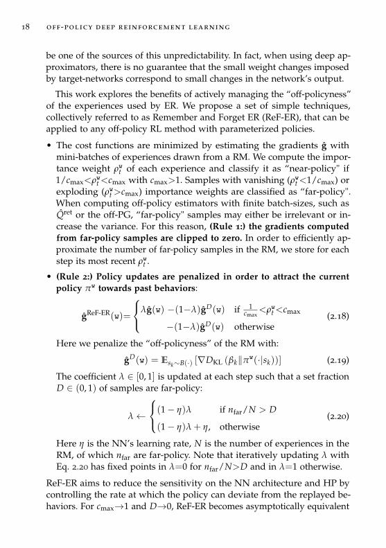
• The cost functions are minimized by estimating the gradients g withmini-batches of experiences drawn from a RM. We compute the impor-tance weight ρwt of each experience and classify it as “near-policy" if1/cmax<ρwt <cmax with cmax>1. Samples with vanishing (ρwt <1/cmax) orexploding (ρwt >cmax) importance weights are classified as “far-policy".When computing off-policy estimators with finite batch-sizes, such asQret or the off-PG, “far-policy" samples may either be irrelevant or in-crease the variance. For this reason, (Rule 1:) the gradients computedfrom far-policy samples are clipped to zero. In order to efficiently ap-proximate the number of far-policy samples in the RM, we store for eachstep its most recent ρwt .
• (Rule 2:) Policy updates are penalized in order to attract the currentpolicy πw towards past behaviors:
gReF-ER(w)=
λg(w) −(1−λ)gD(w) if 1cmax
<ρwt <cmax
−(1−λ)gD(w) otherwise(2.18)
Here we penalize the “off-policyness” of the RM with:
gD(w) = Esk∼B(·) [∇DKL (βk‖πw(·|sk))] (2.19)
The coefficient λ ∈ [0, 1] is updated at each step such that a set fractionD ∈ (0, 1) of samples are far-policy:
λ←
(1− η)λ if nfar/N > D
(1− η)λ + η, otherwise(2.20)
Here η is the NN’s learning rate, N is the number of experiences in theRM, of which nfar are far-policy. Note that iteratively updating λ withEq. 2.20 has fixed points in λ=0 for nfar/N>D and in λ=1 otherwise.
ReF-ER aims to reduce the sensitivity on the NN architecture and HP bycontrolling the rate at which the policy can deviate from the replayed be-haviors. For cmax→1 and D→0, ReF-ER becomes asymptotically equivalent
2.3 related work 19
to computing updates from on-policy data. Therefore, we anneal ReF-ER’scmax and the NN’s learning rate according to:
cmax(t) = 1+C/(1 + A · t), η(t) = η/(1 + A · t) (2.21)
Here t is the time step index, A regulates annealing, and η is the initiallearning rate. cmax determines how much πw is allowed to differ from thereplayed behaviors. By annealing cmax we allow fast improvements at thebeginning of training, when inaccurate policy gradients might be sufficientto estimate a good direction for the update. Conversely, during the laterstages of training, precise updates can be computed from almost on-policysamples. For all results with ReF-ER, we use A=5·10−7, C=4, D=0.1, andN=218.
2.3 related work
The rules that determine which samples are kept in the RM and how theyare used for training can be designed to address specific objectives. For ex-ample, it may be necessary to properly plan ER to prevent lifelong learningagents from forgetting previously mastered tasks (Isele et al., 2018). ER canbe used to train transition models in planning-based RL (Pan et al., 2018),or to help shape NN features by training off-policy learners on auxiliarytasks (Jaderberg et al., 2017; Schaul et al., 2015a). When rewards are sparse,RL agents can be trained to repeat previous outcomes (Andrychowicz et al.,2017) or to reproduce successful states or episodes (Goyal et al., 2018; Ohet al., 2018).
In the next section we compare ReF-ER to conventional ER and PrioritizedExperience Replay (Schaul et al., 2015b) (PER). PER improves the performanceof DQN (Mnih et al., 2015) by biasing sampling in favor of experiencesthat cause large temporal-difference (TD) errors. TD errors may signalrare events that would convey useful information to the learner. Bruinet al. (2015) proposes a modification to ER that increases the diversity ofbehaviors contained in the RM, which is the opposite of what ReF-ERachieves. Because the ideas proposed by Bruin et al. (2015) cannot readilybe applied to complex tasks (the authors state that their method is notsuitable when the policy is advanced for many iterations), we compareReF-ER only to PER and conventional ER. We assume that if increasing thediversity of experiences in the RM were beneficial to off-policy RL theneither PER or ER would outperform ReF-ER.
20 off-policy deep reinforcement learning
ReF-ER is inspired by the techniques developed for on-policy RL to boundpolicy changes in PPO (Schulman et al., 2017). Rule 1 of ReF-ER is similar tothe clipped objective function of PPO (gradients are zero if the importanceweight ρ is outside of some range). However, Rule 1 is not affected by thesign of the advantage estimate and clips both policy and value gradients.Another variant of PPO penalizes DKL(βt||πw) in a similar manner to Rule2 (also Schulman et al. (2015a) and Wang et al. (2016) employ trust-regionschemes in the on- and off-policy setting respectively). PPO picks one of thetwo techniques, and the authors find that gradient-clipping performs betterthan penalization. Conversely, in ReF-ER Rules 1 and 2 complement eachother and can be applied to most off-policy RL methods with parametricpolicies.
V-RACER shares many similarities with ACER (Wang et al., 2016) andIMPALA (Espeholt et al., 2018) and is a secondary contribution of this work.The improvements introduced by V-RACER have the purpose of aidingour analysis of ReF-ER: (1) V-RACER employs a single NN; not requiringexpensive architectures eases reproducibility and exploration of the HP(e.g. continuous-ACER uses 9 NN evaluations per gradient). (2) V-RACERsamples time steps rather than episodes (like DDPG and NAF and unlikeACER and IMPALA), further reducing its cost (episodes may consist ofthousands of steps). (3) V-RACER does not introduce techniques that wouldinterfere with ReF-ER and affect its analysis. Specifically, ACER uses theTBC (Sec. 2.1) to clip policy gradients, employs a target-network to boundpolicy updates with a trust-region scheme, and modifies Retrace to use
dA√
ρ instead of ρ. Lacking these techniques, we expect V-RACER to requireReF-ER to deal with unbounded importance weights. Because of points (1)and (2), V-RACER is expected to be two orders of magnitude faster thanACER.
2.4 implementation
We implemented all presented learning algorithms within smarties,1 ouropen source C++ RL framework, and optimized for high CPU-level effi-ciency through fine-grained multi-threading, strict control of cache-locality,and computation-communication overlap. On every step, we asynchro-nously obtain on-policy data by sampling the environment with π, whichadvances the index t of observed time steps, and we compute updates by
1 https://github.com/cselab/smarties
2.4 implementation 21
sampling from the Replay Memory (RM), which advances the index k ofgradient steps. The ratio of time and update steps is equal to a constantF = t/k, usually set to 1. This parameter affects the data efficiency of thealgorithm; by lowering F each sample is used more times to improve thepolicy before being replaced by newer samples (Hasselt et al., 2019). Uponcompletion of all tasks, we apply the gradient update and proceed to thenext step. The pseudo-codes in Sec. 2.4.2 neglect parallelization details asthey do not affect execution.
In order to evaluate all algorithms on equal footing, we use the samebaseline network architecture for V-RACER, DDPG and NAF, consisting ofan MLP with two hidden layers of 128 units each. For the sake of computa-tional efficiency, we employed Softsign activation functions. The weights ofthe hidden layers are initialized according to U
[−6/
√fi + fo, 6/
√fi + fo
],
where fi and fo are respectively the layer’s fan-in and fan-out (Glorot et al.,2010). The weights of the linear output layer are initialized from the distri-bution U
[−0.1/
√fi, 0.1/
√fi], such that the MLP has near-zero outputs
at the beginning of training. When sampling the components of the actionvectors, the policies are treated as truncated normal distributions withsymmetric bounds at three standard deviations from the mean. Finally, weoptimize the network weights with the Adam algorithm (Kingma et al.,2014).
v-racer We note that the values of the diagonal covariance matrix areshared among all states and initialized to Σ=0.2I. To ensure that Σ ispositive definite, the respective NN outputs are mapped onto R+ by aSoftplus rectifier. We set the discount factor γ=0.995, ReF-ER parametersC=4, A=5·10−7 and D=0.1, and the RM contains 218 samples. We performone gradient step per environment time step, with mini-batch size B=256and learning rate η=10−4.
ddpg We use the common MLP architecture for each network. The out-put of the policy-network is mapped onto the bounded interval [−1, 1]dA
with an hyperbolic tangent function. We set the learning rate for the policy-network to 1 · 10−5 and that of the value-network to 1 · 10−4 with L2 weightdecay coefficient of 1 · 10−4. The RM is set to contain N=218 observationsand we follow Henderson et al. (2018) for the remaining hyper-parameters:mini-batches of B=128 samples, γ=0.995, soft target-network update coeffi-cient 0.01. We note that while DDPG is the only algorithm employing two
22 off-policy deep reinforcement learning
networks, choosing half the batch-size as V-RACER and NAF makes thecompute cost roughly equal among the three methods. Finally, when usingReF-ER we add exploratory Gaussian noise to the deterministic policy:πw=µw+N (0, σ2I) with σ=0.2. When performing regular ER or PER wesample the exploratory noise from an Ornstein–Uhlenbeck process withσ=0.2 and θ=0.15.
naf We use the same baseline MLP architecture and learning rate η =10−4, batch-size B = 256, discount γ = 0.995, RM size N = 218, andsoft target-network update coefficient 0.01. Gaussian noise is added to thedeterministic policy πw′=µw′+N (0, σ2I) with σ=0.2.
ppo We tuned the hyper-parameters as Henderson et al. (2018): γ=0.995,GAE (Schulman et al., 2015b) with λGAE=0.97, the gradient clipping thresh-old if the importance weight deviates from 1 is ερ = 0.2, and we alternateperforming 2048 environment steps and 10 optimizer epochs with batch-size 64 on the obtained data. Both the policy- and the value-network are2-layer MLPs with 64 units per layer. We further improved results by havingseparate learning rates (10−4 for the policy and 3 · 10−4 for the critic) withthe same annealing as used in the other experiments.
acer We kept most hyper-parameters as described in the original pa-per (Wang et al., 2016): the TBC clipping parameter is c = 5, the trust-regionupdate parameter is δ = 1, and five samples of the advantage-network areused to compute action-advantage estimates under π. We use a RM of 1e5samples, each gradient is computed from 24 uniformly sampled episodes,and we perform one gradient step per environment step. Because herelearning is not from pixels, each network (value, advantage, and policy) isan MLP with 2 layers and 128 units per layer. Accordingly, we reduced thesoft target-network update coefficient (α = 0.001) and the learning ratesfor the advantage-network (η=10−4), value-network (η=10−4) and for thepolicy-network (η=10−5).
2.4.1 State, action and reward preprocessing
Several authors have employed state (Henderson et al., 2018) and reward(Duan et al., 2016; Gu et al., 2017) rescaling to improve the learning results.
2.4 implementation 23
For example, the stability of DDPG is affected by the L2 weight decay ofthe value-network. Depending on the numerical values of the distributionof rewards provided by the environment and the choice of weight decaycoefficient, the L2 penalization can be either negligible or dominate theBellman error. Similarly, the distribution of values describing the statevariables can increase the challenge of learning by gradient descent.
We partially address these issues by rescaling both rewards and statevectors depending on the the experiences contained in the RM. At thebeginning of training we prepare the RM by collecting Nstart observationsand then we compute:
βs =1
nobs∑nobs
t=0 st (2.22)
σs =√
1nobs
∑nobst=0 (st − βs)
2 (2.23)
Throughout training, βs and σs are used to standardize all state vectorsst = (st − βs)/(σs + ε) before feeding them to the NN approximators.Moreover, every 1000 steps, chosen as the smallest power of 10 that doesn’taffect the run time, we loop over the nobs samples stored in the RM tocompute:
σr ←
√√√√ 1nobs
nobs
∑t=0
(rt+1)2 (2.24)
This value is used to scale the rewards rt = rt/(σr + ε) used by the Q-learning target and the Retrace algorithm. We use ε = 10−7 to ensurenumerical stability.
The actions sampled by the learner may need to be rescaled or boundedto some interval depending on the environment. For the OpenAI Gymtasks this amounts to a linear scaling a′=a (upper_value− lower_value)/2,where the values specified by the Gym library are ±0.4 for Humanoid tasks,±8 for Pendulum tasks, and ±1 for all others.
2.4.2 Pseudo-codes
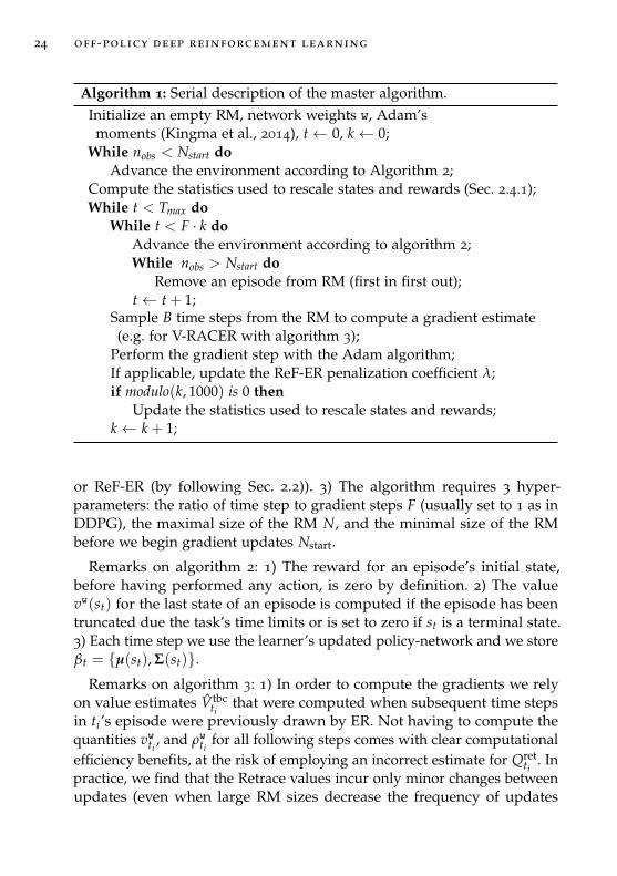
Remarks on algorithm 1: 1) It describes the general structure of the ER-basedoff-policy RL algorithms implemented for this work (i.e. V-RACER, DDPG,and NAF). 2) This algorithm can be adapted to conventional ER, PER (bymodifying the sampling algorithm to compute the gradient estimates),
24 off-policy deep reinforcement learning
Algorithm 1: Serial description of the master algorithm.Initialize an empty RM, network weights w, Adam’smoments (Kingma et al., 2014), t← 0, k← 0;
While nobs < Nstart doAdvance the environment according to Algorithm 2;
Compute the statistics used to rescale states and rewards (Sec. 2.4.1);While t < Tmax do
While t < F · k doAdvance the environment according to algorithm 2;While nobs > Nstart do
Remove an episode from RM (first in first out);t← t + 1;
Sample B time steps from the RM to compute a gradient estimate(e.g. for V-RACER with algorithm 3);
Perform the gradient step with the Adam algorithm;If applicable, update the ReF-ER penalization coefficient λ;if modulo(k, 1000) is 0 then
Update the statistics used to rescale states and rewards;k← k + 1;
or ReF-ER (by following Sec. 2.2)). 3) The algorithm requires 3 hyper-parameters: the ratio of time step to gradient steps F (usually set to 1 as inDDPG), the maximal size of the RM N, and the minimal size of the RMbefore we begin gradient updates Nstart.
Remarks on algorithm 2: 1) The reward for an episode’s initial state,before having performed any action, is zero by definition. 2) The valuevw(st) for the last state of an episode is computed if the episode has beentruncated due the task’s time limits or is set to zero if st is a terminal state.3) Each time step we use the learner’s updated policy-network and we storeβt = µ(st), Σ(st).
Remarks on algorithm 3: 1) In order to compute the gradients we relyon value estimates Vtbc
tithat were computed when subsequent time steps
in ti’s episode were previously drawn by ER. Not having to compute thequantities vwti
, and ρwtifor all following steps comes with clear computational
efficiency benefits, at the risk of employing an incorrect estimate for Qretti
. Inpractice, we find that the Retrace values incur only minor changes betweenupdates (even when large RM sizes decrease the frequency of updates
2.4 implementation 25
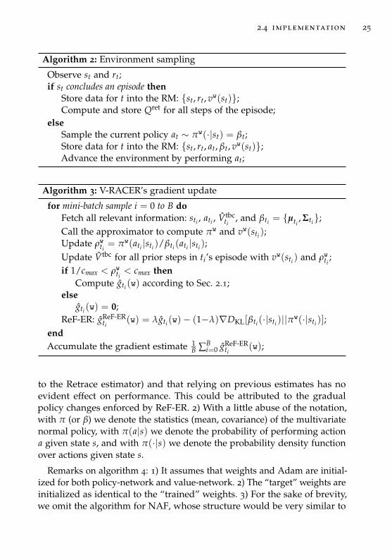
Algorithm 2: Environment sampling
Observe st and rt;if st concludes an episode then
Store data for t into the RM: st, rt, vw(st);Compute and store Qret for all steps of the episode;
elseSample the current policy at ∼ πw(·|st) = βt;Store data for t into the RM: st, rt, at, βt, vw(st);Advance the environment by performing at;
Algorithm 3: V-RACER’s gradient update
for mini-batch sample i = 0 to B doFetch all relevant information: sti , ati , Vtbc
ti, and βti = µti
, Σti;Call the approximator to compute πw and vw(sti );Update ρwti
= πw(ati |sti )/βti (ati |sti );Update Vtbc for all prior steps in ti’s episode with vw(sti ) and ρwti
;if 1/cmax < ρwti
< cmax thenCompute gti (w) according to Sec. 2.1;
elsegti (w) = 0;
ReF-ER: gReF-ERti
(w) = λgti (w)− (1−λ)∇DKL[βti (·|sti )||πw(·|sti )];endAccumulate the gradient estimate 1
B ∑Bi=0 gReF-ER
ti(w);
to the Retrace estimator) and that relying on previous estimates has noevident effect on performance. This could be attributed to the gradualpolicy changes enforced by ReF-ER. 2) With a little abuse of the notation,with π (or β) we denote the statistics (mean, covariance) of the multivariatenormal policy, with π(a|s) we denote the probability of performing actiona given state s, and with π(·|s) we denote the probability density functionover actions given state s.
Remarks on algorithm 4: 1) It assumes that weights and Adam are initial-ized for both policy-network and value-network. 2) The “target” weights areinitialized as identical to the “trained” weights. 3) For the sake of brevity,we omit the algorithm for NAF, whose structure would be very similar to
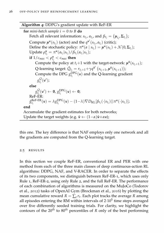
26 off-policy deep reinforcement learning
Algorithm 4: DDPG’s gradient update with ReF-ER
for mini-batch sample i = 0 to B doFetch all relevant information: sti , ati , and βti = µti
, Σti;Compute µw(sti ) (actor) and the qw
′(sti , ati ) (critic);
Define the stochastic policy: πw(a | sti ) = µw(sti ) +N (0, Σti );Update ρwti
= πw(ati |sti )/βti (ati |sti );if 1/cmax < ρwti
< cmax thenCompute the policy at ti+1 with the target-network: µw(sti+1);Q-learning target: Qti = rti+1+γqw
′ (sti+1, µw(sti+1)
);
Compute the DPG gDPGti
(w) and the Q-learning gradient
gQti(w′);
elsegQ
ti(w′)← 0, gDPG
ti(w)← 0;
ReF-ER:gReF-ER
ti(w) = λgDPG
ti(w)− (1−λ)∇DKL[βti (·|sti )||πw(·|sti )];
endAccumulate the gradient estimates for both networks;Update the target weights (e.g. w← (1−α)w+αw);
this one. The key difference is that NAF employs only one network and allthe gradients are computed from the Q-learning target.
2.5 results
In this section we couple ReF-ER, conventional ER and PER with onemethod from each of the three main classes of deep continuous-action RLalgorithms: DDPG, NAF, and V-RACER. In order to separate the effectsof its two components, we distinguish between ReF-ER-1, which uses onlyRule 1, ReF-ER-2, using only Rule 2, and the full ReF-ER. The performanceof each combination of algorithms is measured on the MuJoCo (Todorovet al., 2012) tasks of OpenAI Gym (Brockman et al., 2016) by plotting themean cumulative reward R = ∑t rt. Each plot tracks the average R amongall episodes entering the RM within intervals of 2·105 time steps averagedover five differently seeded training trials. For clarity, we highlight thecontours of the 20th to 80th percentiles of R only of the best performing
2.5 results 27
HumanoidStandup-v2
1
1.5
2
2.5
3
cum
ulat
ive
rew
ard
105 Humanoid-v2
0
1000
2000
3000
4000
5000Ant-v2
0
1000
2000
3000
4000
HalfCheetah-v2
2 4 6 8 10106 time steps
3000
4000
5000
6000
7000
8000
9000
cum
ulat
ive
rew
ard
Hopper-v2
2 4 6 8 10106 time steps
0
1000
2000
3000
Swimmer-v2
2 4 6 8 10106 time steps
150
200
250
300
350 Reacher-v2
2 4 6 8 10106 time steps
-25
-20
-15
-10
Walker2d-v2
0
1000
2000
3000
4000
(a)
10
100
101
102
< D
KL(
||
) >
2 4 6 8 10
Humanoid-v2
2 4 6 8 10
Ant-v2
2 4 6 8 10
Walker2d-v2
2 4 6 8 10
HalfCheetah-v2
2 4 6 8 10
Swimmer-v2
106 time steps 106 time steps 106 time steps 106 time steps 106 time steps
(b)
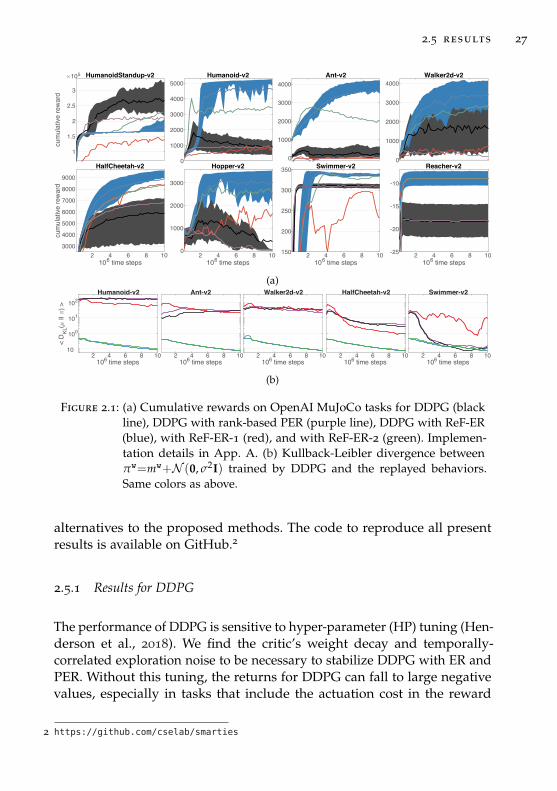
Figure 2.1: (a) Cumulative rewards on OpenAI MuJoCo tasks for DDPG (blackline), DDPG with rank-based PER (purple line), DDPG with ReF-ER(blue), with ReF-ER-1 (red), and with ReF-ER-2 (green). Implemen-tation details in App. A. (b) Kullback-Leibler divergence betweenπw=mw+N (0, σ2I) trained by DDPG and the replayed behaviors.Same colors as above.
alternatives to the proposed methods. The code to reproduce all presentresults is available on GitHub.2
2.5.1 Results for DDPG
The performance of DDPG is sensitive to hyper-parameter (HP) tuning (Hen-derson et al., 2018). We find the critic’s weight decay and temporally-correlated exploration noise to be necessary to stabilize DDPG with ER andPER. Without this tuning, the returns for DDPG can fall to large negativevalues, especially in tasks that include the actuation cost in the reward
2 https://github.com/cselab/smarties
28 off-policy deep reinforcement learning
0.6
0.8
1
1.2
1.4
1.6
cum
ulat
ive
rew
ard
105 HumanoidStandup-v2
1000
2000
3000
4000
Humanoid-v2
-1000
0
1000
2000
3000 Ant-v2
0
500
1000
1500
2000
Walker2d-v2
2 4 6 8 10106 time steps
-1000
0
1000
2000
3000
cum
ulat
ive
rew
ard
HalfCheetah-v2
2 4 6 8 10106 time steps
0
500
1000
1500
2000
Hopper-v2
2 4 6 8 10106 time steps
0
100
200
300
Swimmer-v2
2 4 6 8 10106 time steps
-20
-15
-10
Reacher-v2
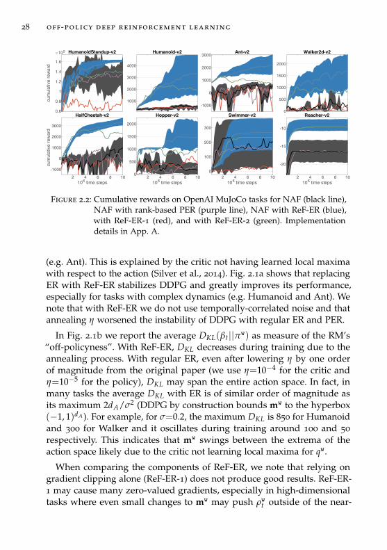
Figure 2.2: Cumulative rewards on OpenAI MuJoCo tasks for NAF (black line),NAF with rank-based PER (purple line), NAF with ReF-ER (blue),with ReF-ER-1 (red), and with ReF-ER-2 (green). Implementationdetails in App. A.
(e.g. Ant). This is explained by the critic not having learned local maximawith respect to the action (Silver et al., 2014). Fig. 2.1a shows that replacingER with ReF-ER stabilizes DDPG and greatly improves its performance,especially for tasks with complex dynamics (e.g. Humanoid and Ant). Wenote that with ReF-ER we do not use temporally-correlated noise and thatannealing η worsened the instability of DDPG with regular ER and PER.
In Fig. 2.1b we report the average DKL(βt||πw) as measure of the RM’s“off-policyness”. With ReF-ER, DKL decreases during training due to theannealing process. With regular ER, even after lowering η by one orderof magnitude from the original paper (we use η=10−4 for the critic andη=10−5 for the policy), DKL may span the entire action space. In fact, inmany tasks the average DKL with ER is of similar order of magnitude asits maximum 2dA/σ2 (DDPG by construction bounds mw to the hyperbox(−1, 1)dA ). For example, for σ=0.2, the maximum DKL is 850 for Humanoidand 300 for Walker and it oscillates during training around 100 and 50
respectively. This indicates that mw swings between the extrema of theaction space likely due to the critic not learning local maxima for qw.
When comparing the components of ReF-ER, we note that relying ongradient clipping alone (ReF-ER-1) does not produce good results. ReF-ER-1 may cause many zero-valued gradients, especially in high-dimensionaltasks where even small changes to mw may push ρwt outside of the near-
2.5 results 29
policy region. However, it’s on these tasks that combining the two rulesbrings a measurable improvement in performance over ReF-ER-2. Trainingfrom only near-policy samples, provides the critic with multiple examplesof trajectories that are possible with the current policy. This focuses therepresentation capacity of the critic, enabling it to extrapolate the effectof a marginal change of action on the expected returns, and thereforeincreasing the accuracy of the DPG. Any misstep of the DPG is weightedwith a penalization term that attracts the policy towards past behaviors.This allows time for the learner to gather experiences with the new policy,improve the value-network, and correct the misstep. This reasoning isalmost diametrically opposed to that behind PER, which generally obtainsworse outcomes than regular ER. In PER observations associated withlarger TD errors are sampled more frequently. In the continuous-actionsetting, however, TD errors may be caused by actions that are fartherfrom mw. Therefore, precisely estimating their value might not help thecritic in yielding an accurate estimate of the DPG. The Swimmer andHumanoidStandup tasks highlight that ER is faster than ReF-ER in findingbang–bang policies. The bounds imposed by DDPG on mw allow learningthese behaviors without numerical instability and without finding localmaxima of qw. The methods we consider next learn unbounded policies.These methods do not require prior knowledge of optimal action bounds,but may not enjoy the same stability guarantees.
2.5.2 Results for NAF
Figure 2.2 shows how NAF is affected by the choice of ER algorithm. WhileQ-learning based methods are thought to be less sensitive than PG-basedmethods to the dissimilarity between policy and stored behaviors owing tothe bootstrapped Q-learning target, NAF benefits from both rules of REF-ER. Like for DDPG, Rule 2 provides NAF with more near-policy samplesto compute the off-policy estimators. Moreover, the performance of NAFis more distinctly improved by combining Rule 1 and 2 of REF-ER overusing REF-ER-2. This is because Qπ is likely to be approximated well by thequadratic qwNAF in a small neighborhood near its local maxima. When qwNAFlearns a poor fit of Qπ (e.g. when the return landscape is multi-modal),NAF may fail to choose good actions. Rule 1 clips the gradients from actionsoutside of this neighborhood and prevents large TD errors from disruptingthe locally-accurate approximation qwNAF. This intuition is supported byobserving that rank-based PER (the better performing variant of PER also
30 off-policy deep reinforcement learning
HumanoidStandup-v2
0.5
1
1.5
2
2.5
cum
ulat
ive
rew
ard
105 Humanoid-v2
1000
2000
3000
4000
5000
6000
Ant-v2
0
1000
2000
3000
4000
5000
6000
Walker2d-v2
1000
2000
3000
4000
5000
6000
HalfCheetah-v2
2 4 6 8 10106 time steps
2000
4000
6000
8000
10000
cum
ulat
ive
rew
ard
Hopper-v2
2 4 6 8 10106 time steps
0
1000
2000
3000
Swimmer-v2
2 4 6 8 10106 time steps
50
100
150
200
250
300
350Reacher-v2
2 4 6 8 10106 time steps
-14
-12
-10
-8
-6
-4
-2
(a)
2 4 6 8 1010-2
100
102
104
< D KL
( ||
) >
Humanoid-v2
2 4 6 8 10
Ant-v2
2 4 6 8 10
Walker2d-v2
2 4 6 8 10
HalfCheetah-v2
2 4 6 8 10
Swimmer-v2
106 time steps 106 time steps 106 time steps 106 time steps 106 time steps
(b)
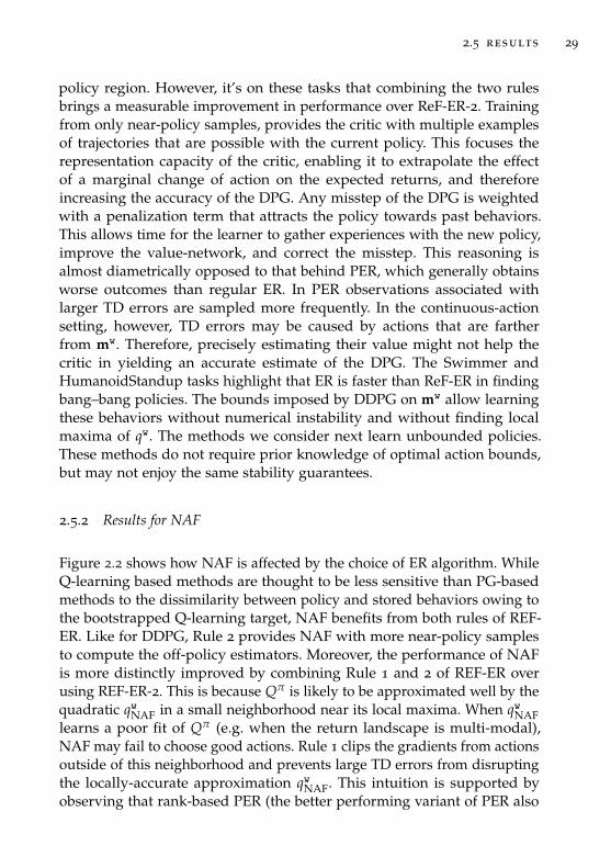
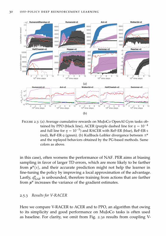
Figure 2.3: (a) Average cumulative rewards on MuJoCo OpenAI Gym tasks ob-tained by PPO (black line), ACER (purple dashed line for η = 10−4
and full line for η = 10−5) and RACER with ReF-ER (blue), ReF-ER-1(red), ReF-ER-2 (green). (b) Kullback-Leibler divergence between πw
and the replayed behaviors obtained by the PG-based methods. Samecolors as above.
in this case), often worsens the performance of NAF. PER aims at biasingsampling in favor of larger TD errors, which are more likely to be fartherfrom µw(s), and their accurate prediction might not help the learner infine-tuning the policy by improving a local approximation of the advantage.Lastly, qwNAF is unbounded, therefore training from actions that are fartherfrom µw increases the variance of the gradient estimates.
2.5.3 Results for V-RACER
Here we compare V-RACER to ACER and to PPO, an algorithm that owingto its simplicity and good performance on MuJoCo tasks is often usedas baseline. For clarity, we omit from Fig. 2.3a results from coupling V-
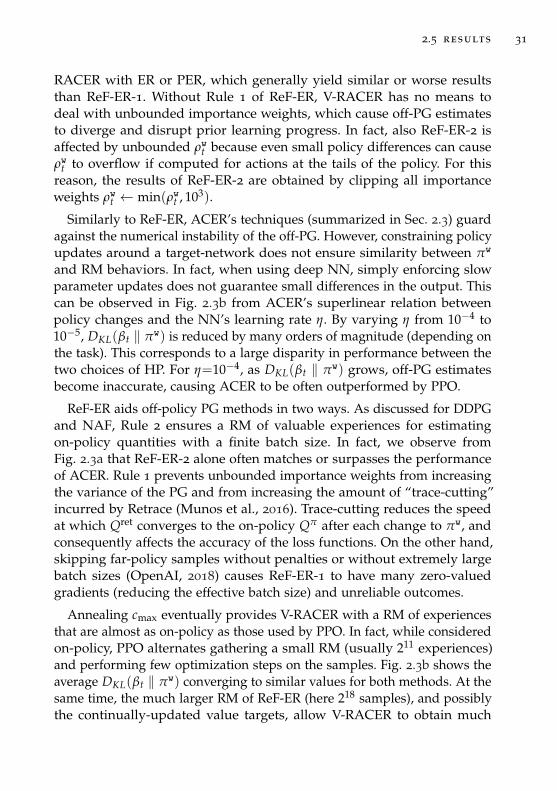
2.5 results 31
RACER with ER or PER, which generally yield similar or worse resultsthan ReF-ER-1. Without Rule 1 of ReF-ER, V-RACER has no means todeal with unbounded importance weights, which cause off-PG estimatesto diverge and disrupt prior learning progress. In fact, also ReF-ER-2 isaffected by unbounded ρwt because even small policy differences can causeρwt to overflow if computed for actions at the tails of the policy. For thisreason, the results of ReF-ER-2 are obtained by clipping all importanceweights ρwt ← min(ρwt , 103).
Similarly to ReF-ER, ACER’s techniques (summarized in Sec. 2.3) guardagainst the numerical instability of the off-PG. However, constraining policyupdates around a target-network does not ensure similarity between πw
and RM behaviors. In fact, when using deep NN, simply enforcing slowparameter updates does not guarantee small differences in the output. Thiscan be observed in Fig. 2.3b from ACER’s superlinear relation betweenpolicy changes and the NN’s learning rate η. By varying η from 10−4 to10−5, DKL(βt ‖ πw) is reduced by many orders of magnitude (depending onthe task). This corresponds to a large disparity in performance between thetwo choices of HP. For η=10−4, as DKL(βt ‖ πw) grows, off-PG estimatesbecome inaccurate, causing ACER to be often outperformed by PPO.
ReF-ER aids off-policy PG methods in two ways. As discussed for DDPGand NAF, Rule 2 ensures a RM of valuable experiences for estimatingon-policy quantities with a finite batch size. In fact, we observe fromFig. 2.3a that ReF-ER-2 alone often matches or surpasses the performanceof ACER. Rule 1 prevents unbounded importance weights from increasingthe variance of the PG and from increasing the amount of “trace-cutting”incurred by Retrace (Munos et al., 2016). Trace-cutting reduces the speedat which Qret converges to the on-policy Qπ after each change to πw, andconsequently affects the accuracy of the loss functions. On the other hand,skipping far-policy samples without penalties or without extremely largebatch sizes (OpenAI, 2018) causes ReF-ER-1 to have many zero-valuedgradients (reducing the effective batch size) and unreliable outcomes.
Annealing cmax eventually provides V-RACER with a RM of experiencesthat are almost as on-policy as those used by PPO. In fact, while consideredon-policy, PPO alternates gathering a small RM (usually 211 experiences)and performing few optimization steps on the samples. Fig. 2.3b shows theaverage DKL(βt ‖ πw) converging to similar values for both methods. At thesame time, the much larger RM of ReF-ER (here 218 samples), and possiblythe continually-updated value targets, allow V-RACER to obtain much
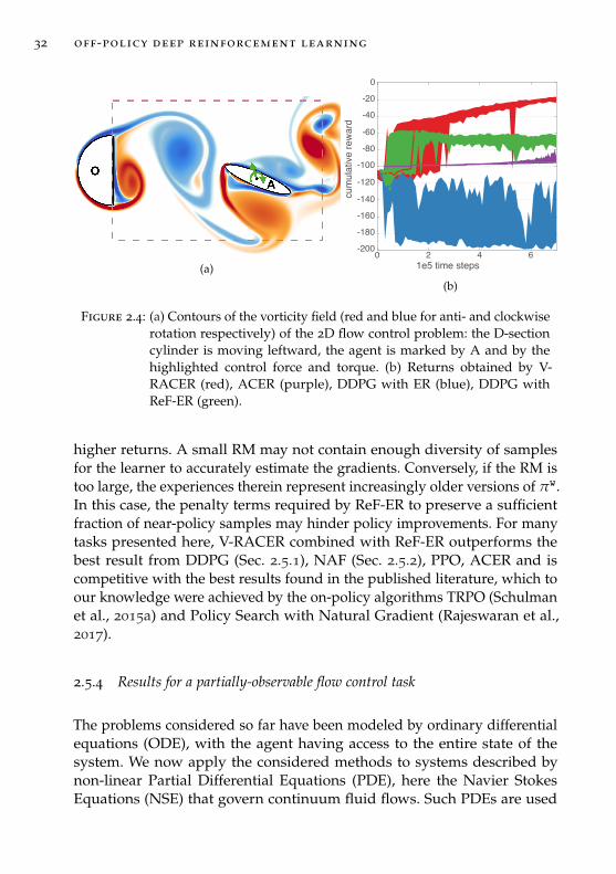
32 off-policy deep reinforcement learning
(a)
cum
ulat
ive
rew
ard
1e5 time steps
0
-200
-180
-160
-140
-120
-100
-80
-60
-40
-20
0 2 4 6
(b)
Figure 2.4: (a) Contours of the vorticity field (red and blue for anti- and clockwiserotation respectively) of the 2D flow control problem: the D-sectioncylinder is moving leftward, the agent is marked by A and by thehighlighted control force and torque. (b) Returns obtained by V-RACER (red), ACER (purple), DDPG with ER (blue), DDPG withReF-ER (green).
higher returns. A small RM may not contain enough diversity of samplesfor the learner to accurately estimate the gradients. Conversely, if the RM istoo large, the experiences therein represent increasingly older versions of πw.In this case, the penalty terms required by ReF-ER to preserve a sufficientfraction of near-policy samples may hinder policy improvements. For manytasks presented here, V-RACER combined with ReF-ER outperforms thebest result from DDPG (Sec. 2.5.1), NAF (Sec. 2.5.2), PPO, ACER and iscompetitive with the best results found in the published literature, which toour knowledge were achieved by the on-policy algorithms TRPO (Schulmanet al., 2015a) and Policy Search with Natural Gradient (Rajeswaran et al.,2017).
2.5.4 Results for a partially-observable flow control task
The problems considered so far have been modeled by ordinary differentialequations (ODE), with the agent having access to the entire state of thesystem. We now apply the considered methods to systems described bynon-linear Partial Differential Equations (PDE), here the Navier StokesEquations (NSE) that govern continuum fluid flows. Such PDEs are used
2.5 results 33
to describe many problems of scientific (e.g. turbulence, fish swimming)and industrial interests (e.g. wind farms, combustion engines). These prob-lems pose two challenges: First, accurate simulations of PDEs may entailsignificant computational costs and large scale computing resources whichexceed by several orders of magnitude what is required by ODEs. Sec-ond, the NSE are usually solved on spatial grids with millions or eventrillions of degrees of freedom. It would be excessive to provide all thatinformation to the agent, and therefore the state is generally measured bya finite number of sensors. Consequently, the assumption of Markoviandynamics at the core of most RL methods is voided. This may be remediedby using recurrent NN (RNN) for function approximation. In turn, RNNsadd to the challenges of RL the increased complexity of properly trainingthem. Here we consider the small 2D flow control problem of agent A, anelliptical body of major-axis D and aspect ratio 0.2, interacting with anunsteady wake. The wake is created by a D-section cylinder of diameter D(O in Fig. 2.4a) moving at constant speed (one length D per time-unit T )at Reynolds number D2/(νT )=400. Agent A performs one action per unitT by imposing a force and a torque on the flow at:= fX , fY, τ. The statest∈R14 contains A’s position, orientation and velocity relative to O and has4 flow-speed sensors located at A’s 4 vertices. The reward is rt+1=− ‖at‖2.If A exits the area denoted by a dashed line in Fig. 2.4a, the terminal re-ward is −100 and the simulation restarts with random initial conditions.Otherwise, the maximum duration of the simulation is 400 actions. Weattempt this problem with three differently-seeded runs of each methodconsidered so far. Instead of maximizing the performances by HP tuning,we only substitute the MLPs used for function approximation with LSTMnetworks (2 layers of 32 cells with back-propagation window of 16 steps).
If correctly navigated, drafting in the momentum released into the flowby the motion of O allows A to maintain its position with minimal actuationcost. Fig. 2.4b shows that the optimal HP found for ACER (small η) in theODE tasks, together with the lack of feature-sharing between policy andvalue-networks and with the variance of the off-PG, cause the method tomake little progress during training. DDPG with ER incurs large actuationcosts, while DDPG with ReF-ER is the fastest at learning to avoid thedistance limits sketched in Fig. 2.4a. In fact the critic quickly learns thatA needs to accelerate leftward to avoid being left behind, and the policyadopts the behavior rapidly due to the lower variance of the DPG (Silveret al., 2014). Eventually, the best performance is reached by V-RACER withReF-ER (an animation of a trained policy is provided in the Supplementary
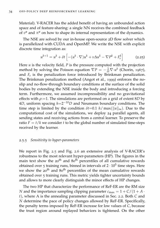
34 off-policy deep reinforcement learning
Material). V-RACER has the added benefit of having an unbounded actionspace and of feature-sharing: a single NN receives the combined feedbackof vw and πw on how to shape its internal representation of the dynamics.
The NSE are solved by our in-house open-source 2D flow solver whichis parallelized with CUDA and OpenMP. We write the NSE with explicitdiscrete time integration as:
uk+1 = uk + δt[−(uk · ∇)uk + ν∆uk −∇Pk + Fk
s
](2.25)
Here u is the velocity field, P is the pressure computed with the projectionmethod by solving the Poisson equation ∇P = − 1
δt∇·uk (Chorin, 1967),and Fs is the penalization force introduced by Brinkman penalization.The Brinkman penalization method (Angot et al., 1999) enforces the no-slip and no-flow-through boundary conditions at the surface of the solidbodies by extending the NSE inside the body and introducing a forcingterm. Furthermore, we assumed incompressibility and no gravitationaleffects with ρ:=1. The simulations are performed on a grid of extent 8D by4D, uniform spacing h=2−10D and Neumann boundary conditions. Thetime step is limited by the condition δt=0.1 h/ max(‖u‖∞). Due to thecomputational cost of the simulations, we deploy 24 parallel agents, allsending states and receiving actions from a central learner. To preserve theratio F = t/k we consider t to be the global number of simulated time-stepsreceived by the learner.
2.5.5 Sensitivity to hyper-parameters
We report in Fig. 2.5 and Fig. 2.6 an extensive analysis of V-RACER’srobustness to the most relevant hyper-parameters (HP). The figures in themain text show the 20
th and 80th percentiles of all cumulative rewards
obtained over 5 training runs, binned in intervals of 2 · 105 time steps. Herewe show the 20
th and 80th percentiles of the mean cumulative rewards
obtained over 5 training runs. This metric yields tighter uncertainty boundsand allows to more clearly distinguish the minor effects of HP changes.
The two HP that characterize the performance of ReF-ER are the RM sizeN and the importance sampling clipping parameter cmax = 1 + C/(1 + A ·t), where A is the annealing parameter discussed in Sec. 2.2. Both C andN determine the pace of policy changes allowed by ReF-ER. Specifically,the penalty terms imposed by ReF-ER increase for low values of C, becausethe trust region around replayed behaviors is tightened. On the other
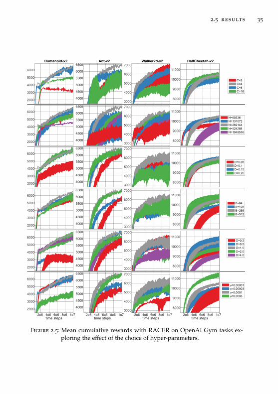
2.5 results 35
2000
3000
4000
5000
6000
2000
3000
4000
5000
6000
2000
3000
4000
5000
6000
2000
3000
4000
5000
6000
2000
3000
4000
5000
6000
2000
3000
4000
5000
6000
2e6 4e6 6e6 8e6 1e7time steps
4000
4500
5000
5500
6000
6500
4000
4500
5000
5500
6000
6500
4000
4500
5000
5500
6000
6500
4000
4500
5000
5500
6000
6500
4000
4500
5000
5500
6000
6500
4000
4500
5000
5500
6000
6500
2e6 4e6 6e6 8e6 1e7time steps
3000
4000
5000
6000
7000
3000
4000
5000
6000
7000
3000
4000
5000
6000
7000
3000
4000
5000
6000
7000
3000
4000
5000
6000
7000
3000
4000
5000
6000
7000
2e6 4e6 6e6 8e6 1e7time steps
8000
9000
10000
11000
8000
9000
10000
11000
8000
9000
10000
11000
8000
9000
10000
11000
8000
9000
10000
11000
8000
9000
10000
11000
2e6 4e6 6e6 8e6 1e7time steps
Figure 2.5: Mean cumulative rewards with RACER on OpenAI Gym tasks ex-ploring the effect of the choice of hyper-parameters.
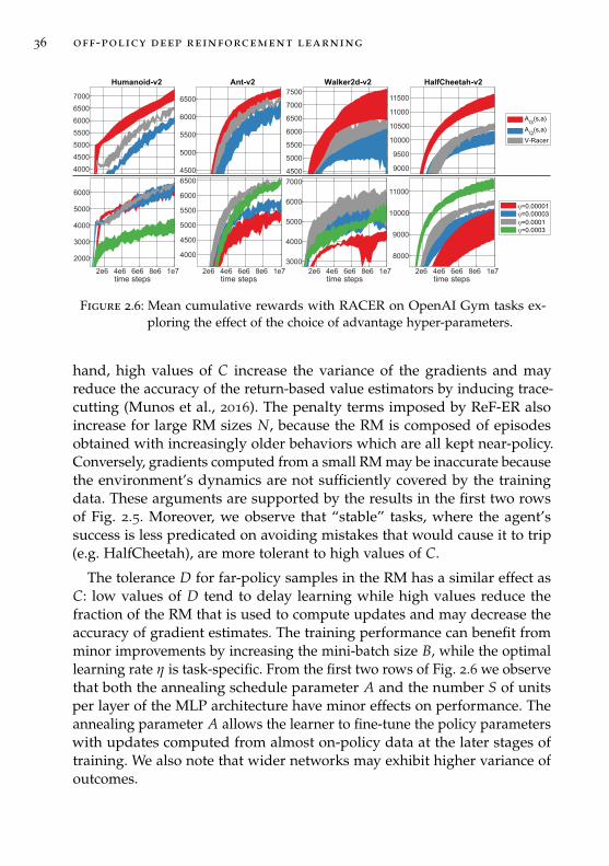
36 off-policy deep reinforcement learning
2000
3000
4000
5000
6000
2e6 4e6 6e6 8e6 1e7time steps
4000
4500
5000
5500
6000
6500
2e6 4e6 6e6 8e6 1e7time steps
3000
4000
5000
6000
7000
2e6 4e6 6e6 8e6 1e7time steps
8000
9000
10000
11000
2e6 4e6 6e6 8e6 1e7time steps
4000
4500
5000
5500
6000
6500
7000
4500
5000
5500
6000
6500
4500
5000
5500
6000
6500
7000
7500
9000
9500
10000
10500
11000
11500
Figure 2.6: Mean cumulative rewards with RACER on OpenAI Gym tasks ex-ploring the effect of the choice of advantage hyper-parameters.
hand, high values of C increase the variance of the gradients and mayreduce the accuracy of the return-based value estimators by inducing trace-cutting (Munos et al., 2016). The penalty terms imposed by ReF-ER alsoincrease for large RM sizes N, because the RM is composed of episodesobtained with increasingly older behaviors which are all kept near-policy.Conversely, gradients computed from a small RM may be inaccurate becausethe environment’s dynamics are not sufficiently covered by the trainingdata. These arguments are supported by the results in the first two rowsof Fig. 2.5. Moreover, we observe that “stable” tasks, where the agent’ssuccess is less predicated on avoiding mistakes that would cause it to trip(e.g. HalfCheetah), are more tolerant to high values of C.
The tolerance D for far-policy samples in the RM has a similar effect asC: low values of D tend to delay learning while high values reduce thefraction of the RM that is used to compute updates and may decrease theaccuracy of gradient estimates. The training performance can benefit fromminor improvements by increasing the mini-batch size B, while the optimallearning rate η is task-specific. From the first two rows of Fig. 2.6 we observethat both the annealing schedule parameter A and the number S of unitsper layer of the MLP architecture have minor effects on performance. Theannealing parameter A allows the learner to fine-tune the policy parameterswith updates computed from almost on-policy data at the later stages oftraining. We also note that wider networks may exhibit higher variance ofoutcomes.
2.5 results 37
More uncertain is the effect of the number F of environment time stepsper learner’s gradient step. Intuitively, increasing F could either cause arightward shift of the expected returns curve, because the learner computesfewer updates for the same budget of observations, or it could improvereturns by providing more on-policy samples, which decreases ReF-ER’spenalty terms and may increase the accuracy of the estimators. In practicethe effect of F is task-dependent. Problems with more complex dynamics,or higher dimensionality (e.g. Humanoid), seem to benefit from refreshingthe RM more frequently with newer experiences (higher F), while simplertasks can be learned more rapidly by performing more gradient steps pertime step.
We considered extending V-RACER’s architecture by adding a closed-form parameterization for the action advantage. Rather than having aseparate MLP with inputs (s, a) to parameterize qw (as in ACER or DDPG),whose expected value under the policy would be computationally demand-ing to compute, we employ closed-form equations for the action advantageinspired by NAF (Gu et al., 2016). The network outputs the coefficients of aconcave function f w(s, a) which is chosen such that its maximum coincideswith the mean of the policy µ(s), and such that it is possible to deriveanalytical expectations for a ∼ πw(·|s):
qw(s, a) = vw(s) + f w(s, a)− Ea′∼πw(·|s)
[f w(s, a′)
](2.26)
Therefore, like the exact on-policy Aπ , the parametric advantage has bydesign expectation zero under the policy. Here we consider two optionsfor the parameterized advantage. First, the quadratic form employed byNAF (Gu et al., 2016):
f wQ(s, a) = −12[a−µ(s)]T LQ(s)LT
Q(s) [a−µ(s)] (2.27)
From f wQ, the action-advantage is uniquely defined for any action a. Theexpectation can be computed as (Petersen et al., 2008):
Ea′∼π
[f wQ(s, a′)
]= Tr
[LQ(s)LT
Q(s)Σ(s)]
(2.28)
Here Tr denotes the trace of a matrix. Second we consider the asymmetricGaussian parameterization:
f wG(s, a) = K(s) exp[−1
2aT+ L−1
+ (s) a+ −12
aT− L−1
− (s) a−
](2.29)
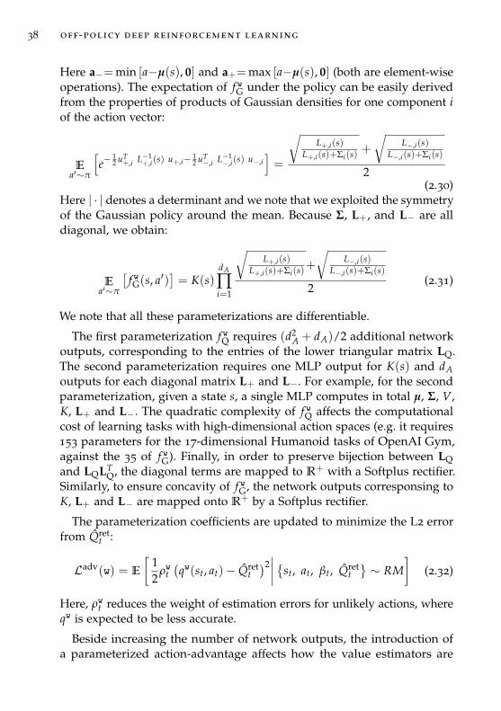
38 off-policy deep reinforcement learning
Here a−=min [a−µ(s), 0] and a+=max [a−µ(s), 0] (both are element-wiseoperations). The expectation of f wG under the policy can be easily derivedfrom the properties of products of Gaussian densities for one component iof the action vector:
Ea′∼π
[e−
12 uT
+,i L−1+,i(s) u+,i− 1
2 uT−,i L−1
−,i(s) u−,i]=
√L+,i(s)
L+,i(s)+Σi(s)+
√L−,i(s)
L−,i(s)+Σi(s)
2(2.30)
Here | · | denotes a determinant and we note that we exploited the symmetryof the Gaussian policy around the mean. Because Σ, L+, and L− are alldiagonal, we obtain:
Ea′∼π
[f wG(s, a′)
]= K(s)
dA
∏i=1
√L+,i(s)
L+,i(s)+Σi(s)+
√L−,i(s)
L−,i(s)+Σi(s)
2(2.31)
We note that all these parameterizations are differentiable.
The first parameterization f wQ requires (d2A + dA)/2 additional network
outputs, corresponding to the entries of the lower triangular matrix LQ.The second parameterization requires one MLP output for K(s) and dAoutputs for each diagonal matrix L+ and L−. For example, for the secondparameterization, given a state s, a single MLP computes in total µ, Σ, V,K, L+ and L−. The quadratic complexity of f wQ affects the computationalcost of learning tasks with high-dimensional action spaces (e.g. it requires153 parameters for the 17-dimensional Humanoid tasks of OpenAI Gym,against the 35 of f wG). Finally, in order to preserve bijection between LQand LQLT
Q, the diagonal terms are mapped to R+ with a Softplus rectifier.Similarly, to ensure concavity of f wG, the network outputs corresponsing toK, L+ and L− are mapped onto R+ by a Softplus rectifier.
The parameterization coefficients are updated to minimize the L2 errorfrom Qret
t :
Ladv(w) = E
[12
ρwt(qw(st, at)− Qret
t)2∣∣∣∣ st, at, βt, Qret
t∼ RM
](2.32)
Here, ρwt reduces the weight of estimation errors for unlikely actions, whereqw is expected to be less accurate.
Beside increasing the number of network outputs, the introduction ofa parameterized action-advantage affects how the value estimators are
2.6 conclusion 39
computed (i.e. we do not approximate qw = vw when updating Retrace asdiscussed in Sec. 2.1). This change may decrease the variance of the valueestimators, but its observed benefits are negligible when compared to otherHP changes. The minor performance improvements allowed by the intro-duction of a closed-form advantage parameterization are outweighed inmost cases by the increased simplicity of the original V-RACER architecture.
2.6 conclusion
Many RL algorithms update a policy πw from experiences collected with off-policy behaviors β. We present evidence that off-policy continuous-actiondeep RL methods benefit from actively maintaining similarity betweenpolicy and replay behaviors. We propose a novel ER algorithm (ReF-ER)which consists of: (1) Characterizing past behaviors either as “near-policy"or “far-policy" by the deviation from one of the importance weight ρw =πw(a|s)/β(a|s) and computing gradients only from near-policy experiences.(2) Regulating the pace at which πw is allowed to deviate from β throughpenalty terms that reduce DKL(β||πw). This allows time for the learnerto gather experiences with the new policy, improve the value estimators,and increase the accuracy of the next steps. We have analyzed the twocomponents of ReF-ER and show their effects on continuous-action RLalgorithms employing off-policy PG, deterministic PG (DDPG) and Q-learning (NAF). Moreover, we introduced V-RACER, a novel algorithmbased on the off-policy PG which emphasizes simplicity and computationalefficiency. The combination of ReF-ER with V-RACER reliably obtainsperformance that is competitive with the state-of-the-art.

3O P T I M A L C O N T R O L L E D G L I D I N G A N D P E R C H I N G
Gliding is an intrinsically efficient motion that relies on the body shape toextract momentum from the air flow, while performing minimal mechanicalwork to control attitude. The sheer diversity of animal and plant speciesthat have independently evolved the ability to glide is a testament to theefficiency and usefulness of this mode of transport. Well known examplesinclude birds that soar with thermal winds, fish that employ burst and coastswimming mechanisms and plant seeds, such as the samara, that spreadby gliding. Furthermore, arboreal animals that live in forest canopies oftenemploy gliding to avoid earth-bound predators, forage across long distances,chase prey, and safely recover from falls. Characteristic of gliding mammalsis the membrane (patagium) that develops between legs and arms. Whenextended, the patagium transforms the entire body into a wing, allowingthe mammal to stay airborne for extended periods of time (Jackson, 2000).Analogous body adaptations have developed in species of lizards (Moriet al., 1994) and frogs (McCay, 2001).
Most surprisingly, gliding has developed in animal species character-ized by blunt bodies lacking specialized lift-generating appendages. TheChrysopelea genus of snakes have learned to launch themselves from trees,flatten and camber their bodies to form a concave cross-section, and performsustained aerial undulations to generate enough lift to match the glidingperformance of mammalian gliders (Socha, 2002). Wingless insects suchas tropical arboreal ants (Yanoviak et al., 2005) and bristletails (Yanoviaket al., 2009) are able to glide when falling from the canopy in order to avoidthe possibly flooded or otherwise hazardous forest understory. Duringdescent these canopy-dwelling insects identify the target tree trunk usingvisual cues (Yanoviak et al., 2006) and orient their horizontal trajectoryappropriately.
Most bird species alternate active flapping with gliding, in order to reducephysical effort during long-range flight (Rayner, 1985). Similarly, gliding isan attractive solution to extend the range of micro air vehicles (MAVs). MAVdesigns often rely on arrays of rotors (ie. quadcoptors) due to their simplestructure and due to the existence of simplified models that capture the
41
42 optimal controlled gliding and perching
main aspects of the underlying fluid dynamics. The combination of thesetwo features allows finding precise control techniques (Gurdan et al., 2007;Lupashin et al., 2010) to perform complex flight maneuvres (Mellinger et al.,2013; Müller et al., 2011). However, the main drawback of rotor-propelledMAVs is their limited flight-times, which restricts real-world applications.Several solutions for extending the range of MAVs have been proposed,including techniques involving precise perching manouvres (Thomas et al.,2016), mimicking flying animals by designing a flier (Abas et al., 2016)capable of gliding, and exploiting the upward momentum of thermal windsto soar with minimal energy expense (Reddy et al., 2016; Reddy et al., 2018).
Here we study the ability of falling blunt-shaped bodies, lacking anyspecialized feature for generating lift, to learn gliding strategies throughReinforcement Learning (Bertsekas et al., 1995; Kaelbling et al., 1996; Suttonet al., 1998). The goal of the RL agent is to control its descent towards aset target landing position and perching angle. The agent is modeled bya simple dynamical system describing the passive planar gravity-drivendescent of a cylindrical object in a quiescent fluid. The simplicity of thesystem is due to a parameterized model for the fluid forces which hasbeen developed through simulations and experimental studies (Andersenet al., 2005a,b; Wang et al., 2004). Following the work of Paoletti et al., 2011,we augment the original, passive dynamical system with active control.We identify optimal control policies through Reinforcement Learning, asemi-supervised learning framework, that has been employed successfullyin a number of flow control problems (Colabrese et al., 2017; Gazzola etal., 2014, 2016; Novati et al., 2017; Reddy et al., 2016). We employ recentadvances in coupling RL with deep neural networks (Mnih et al., 2015).These so called Deep Reinforcement Learning algorithms have been shownin several problems to match and even surpass the performance of classicalcontrol algorithms. For example, in Waldock et al., 2017 it was shown thatD-RL outperforms an interior point method for constraint optimization,using pre-computed actions from a simulation to land unmanned aerialvehicles in an experimental setting. Indeed D-RL appears to be a verypromising control strategy for perching in UAVs, a critical energy savingprocess (Hang et al., 2019).
The chapter is organised as follows: we describe the model of an active,falling body in section 3.1 and frame the problems in terms of ReinforcementLearning in section 3.2. In section 3.2.1 we present a high-level descrip-tion of the RL algorithm and describe the reward shaping combining thetime/energy cost with kinematic constraints as described in section 3.2.2.
3.1 model 43
We explore the effects of the weight and shape of the agent’s body onthe optimal gliding strategies in section 3.3. In sections 3.4 and 3.5 weanalyze the RL methods by comparing RL policies to the trajectories foundwith optimal control (OC) (Paoletti et al., 2011), by varying the problemformulation, and by comparing RL algorithms.
acknowledgments This chapter is based on the paper “Controlledgliding and perching through deep-reinforcement-learning” (Novati et al.,2019b). The computational resources were provided by a grant from theSwiss National Super-computing Centre (CSCS) under project s658.
3.1 model
The motion of falling slender elliptical bodies involves rich hydrodynamicswhich have inspired intense research (Andersen et al., 2005a,b; Belmonteet al., 1998; Mahadevan et al., 1999; Mittal et al., 2004; Pesavento et al.,2004). Depending on its size, shape, density and initial orientation, theellipse’s descent follows motion patterns classified as steady-fall, flutter-ing (side-to-side oscillation of the horizontal motion), tumbling (repeatedrotation around the out-of-plane direction), or transitional patterns. Theaforementioned studies show that these descent patterns can be quali-tatively described by a simple model consisting of ordinary differentialequations (ODEs) for the ellipse’s translational and rotational degrees offreedom (see figure 3.1). This ODE based model relies on the assumptionthat the descent is essentially planar (i.e. the axis of rotation of the ellipticalbody is orthogonal to its velocity) and it has been derived on the basis ofinviscid fluid dynamics (Lamb, 1932) with a corrective parametric model toaccount for viscous effects. We employ here the dimensionless form of theODEs as originally proposed by Andersen et al., 2005a for the gravity-drivendescent of a cylindrical ellipse of density ρs with semi-axes a and b in aquiescent fluid of density ρ f . The non-dimensionalization is performed with
the length scale a and the velocity scale√(ρs/ρ f − 1)gb, obtained from
the balance between gravitational force and quadratic drag (Mahadevanet al., 1999). The resulting set of equations depends on the dimensionlessparameters β = b/a and I = βρ∗, which represents the non-dimensionalmoment of inertia with ρ∗ = ρs/ρ f :
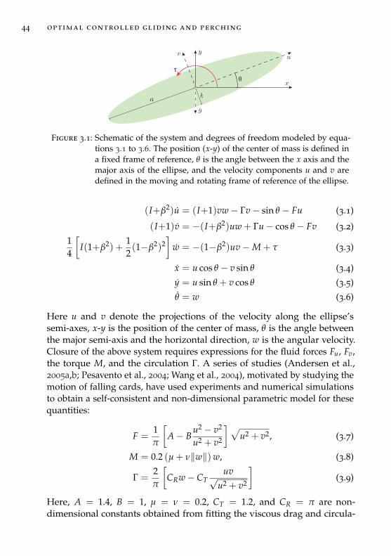
44 optimal controlled gliding and perching
θ
τ
Figure 3.1: Schematic of the system and degrees of freedom modeled by equa-tions 3.1 to 3.6. The position (x-y) of the center of mass is defined ina fixed frame of reference, θ is the angle between the x axis and themajor axis of the ellipse, and the velocity components u and v aredefined in the moving and rotating frame of reference of the ellipse.
(I+β2)u = (I+1)vw− Γv− sin θ − Fu (3.1)
(I+1)v = −(I+β2)uw + Γu− cos θ − Fv (3.2)
14
[I(1+β2) +
12(1−β2)2
]w = −(1−β2)uv−M + τ (3.3)
x = u cos θ − v sin θ (3.4)
y = u sin θ + v cos θ (3.5)
θ = w (3.6)
Here u and v denote the projections of the velocity along the ellipse’ssemi-axes, x-y is the position of the center of mass, θ is the angle betweenthe major semi-axis and the horizontal direction, w is the angular velocity.Closure of the above system requires expressions for the fluid forces Fu, Fv,the torque M, and the circulation Γ. A series of studies (Andersen et al.,2005a,b; Pesavento et al., 2004; Wang et al., 2004), motivated by studying themotion of falling cards, have used experiments and numerical simulationsto obtain a self-consistent and non-dimensional parametric model for thesequantities:
F =1π
[A− B
u2 − v2
u2 + v2
]√u2 + v2, (3.7)
M = 0.2 (µ + ν‖w‖)w, (3.8)
Γ =2π
[CRw− CT
uv√u2 + v2
](3.9)
Here, A = 1.4, B = 1, µ = ν = 0.2, CT = 1.2, and CR = π are non-dimensional constants obtained from fitting the viscous drag and circula-
3.2 reinforcement learning for landing and perching 45
tion to those measured from numerical simulations. Wang and co-authorsshow that such parameterization, while it may not be sufficient to preciselyquantify the viscous fluid forces, enables the ODE model to qualitativelydescribe the regular and irregular motion patters, such as fluttering andtumbling, associated with falling elliptical bodies. The values chosen forthis study were obtained (by Wang and co-authors) to approximate thefluid forces at intermediate Reynolds numbers O(103) (Paoletti et al., 2011),consistent with that of gliding ants (Yanoviak et al., 2005). Given the closurefor the fluid forces and torques, the dynamics of the system are charac-terized by the dimensionless parameters β = b/a, and I = βρ∗. Paolettiet al., 2011 focus their optimal control study to β = 0.1 and I = 20, whichrepresents the inertia of both the ant’s body and the fluid contained insidethe body-fitted ellipse. However, independently from β and I, the parame-terized model for the viscous fluid forces will be consistent with Reynoldsnumbers Re ≈ O(103).
In active gliding, we assume that the gravity-driven trajectory can be mod-ified by the agent modulating the dimensionless torque τ in equation 3.3,introduced by Paoletti et al., 2011 as a minimal representation of the abilityof gliding ants to guide their fall by rotating their hind legs (Yanoviak et al.,2010). Alternatively, the control torque could be obtained by the gliderdeforming its body in order to displace the center of mass, or by extendingits limbs to deflect the incoming flow. This leads to a natural question:how should the active torque be varied in time for the ant to achieve aparticular task such as landing and perching at a particular location witha particular orientation, subject to some constraints, e.g. optimizing time,minimizing power consumption, maximizing accuracy etc., a problem con-sidered by Paoletti et al., 2011 in an optimal control framework. Here weconsider an alternative approach inspired by how organisms might learn,that of reinforcement learning (Sutton et al., 1998).
3.2 reinforcement learning for landing and perching
The tasks of landing and perching are achieved by the falling body byemploying a reinforcement learning (RL) framework (Bertsekas et al., 1995;Kaelbling et al., 1996; Sutton et al., 1998) to identify their control actions.We follow the problem definition of a glider attempting to land at a targetlocation as described by Paoletti et al., 2011. We consider an agent, initiallylocated at x0 = y0 = θ0 = 0, that has the objective of landing at a target
46 optimal controlled gliding and perching
location xG = 100, yG = −50 (expressed in units of the ellipse major semi-axis (a)) with perching angle θG = π
4 . For most results we consider anelliptical glider with non-dimensional moment of inertia I 1, so thatthe amplitude of the fluttering motion is much smaller than the distancefrom the target (Andersen et al., 2005a). In such cases the spread of landinglocations for the uncontrolled ellipse is of order O(1), much smaller thanthe distance ‖xG − x0‖.
By describing the trajectory with the model outlined in section 3.1, thestate of the agent is completely defined at every time step by the state vectors := x, y, θ, u, v, w. With a finite time interval ∆t = 0.5, the agent is ableto observe its state st and, based on the state, samples a stochastic controlpolicy π to select an action at ∼ π(a|st). The actuation period ∆t is of thesame order of magnitude as the tumbling frequency for an ellipse withI ≈ O(1) (Andersen et al., 2005b) and is analyzed in more detail in Sec. 3.5.We consider continuous-valued controls defined by Gaussian policies whichallows for fine-grained corrections (in contrast to the usually employeddiscretized controls). The action determines the constant control torqueτt = tanh(at) ∈ −1, 1 exerted by the agent between time t and t + ∆t. Inorder to provide enough diversity of initial conditions to the RL method, weinitialize x(0) ∼ U [−5, 5] and θ(0) ∼ U [−π/2, π/2]. In the case of perchingand landing, each episode is terminated when at some terminal time T theagent touches the ground yT = −50. Because the gravitational force actingon the glider ensures that each trajectory will last a finite number of stepswe can avoid the discount factor and set γ = 1.
Since the dynamics of the system are described by a small numberof ODEs that can be solved at each instant to determine the full stateof the system, in contrast with the need to solve the full Navier-Stokesequations (as in Chapter 5), the present control problem satisfies the Markovassumption. Therefore, we can use a feedforward network (NN) rather thanrecurrent neural networks (RNN) as policy approximators Sutton et al.,2000. The use of RNN to solve partially-observable problems (non-MDPs)is explored in Sec. 3.5.
3.2.1 Off-policy actor-critic
We solve the RL problem with the off-policy actor-critic algorithm RACER, avariant of the V-RACER algorithm described in Chapter 2. RACER relies ontraining a neural network (NN), defined by weights w, to obtain a continuous
3.2 reinforcement learning for landing and perching 47
approximation of the policy πw(a|s), the state value vw(s) and the state-action value qw(s, a). The network receives as input s = x, y, θ, u, v, w ∈ R6
and produces as output the set µw, σw, vw, lw ∈ R4 which we now explain.The policy πw(a|s) for each state is approximated with a Gaussian having amean µw(s) and a standard deviation σw(s):
πw(a|s) = 1√2πσw(s)
exp
[−1
2
(a− µw(s)
σw(s)
)2]
(3.10)
The standard deviation is initially wide enough to adequately explore thedynamics of the system. Where RACER differs from V-RACER is in itsparametric estimate of the state-action value function Qπ(s, a). Rather thanhaving a specialized network, which includes in its input the action a, wepropose computing the estimate qw(s, a) by combining the network’s statevalue estimate vw(s) with a quadratic term with vertex at the mean µw(s) ofthe policy:
qw(s, a) = vw(s)− 12
lw(s)2 [a−µw(s)]2 + Ea′∼π
[12
lw(s)2 [a′−µw(s)]2]
= vw(s)− 12
lw(s)2[[a−µw(s)]2 − [σw(s)]2
](3.11)
This definition ensures that vw(s) = Ea∼π [vw(s, a)]. Here lw(s) is an outputof the network describing the rate at which the action value decreasesfor actions farther away from µw(s). This parameterization relies on theassumption that for any given state vw(s, a) is maximal at the mean of thepolicy.
RACER is trained with Experience Replay, specifically with the ReF-ERmethod described in Chapter 2. For each sampled action which advancesthe environment simulation, a number B of experiences are sampled fromthe Replay Memory (RM). These experienced are used to update networkweights via back-propagation of the policy (gπ) and value function gradients(gQ). The policy statistics µw(s) and σw(s) are improved through the off-policy policy gradient estimator (Degris et al., 2012):
gπ(w)=E
[πw(at|st)
P(at|µt, σt)
[Qret
t −vw(st)]∇w log πw(at|st)
∣∣∣∣ st , at , µt ,σt , Qret
t
∼RM
](3.12)
Here, P(at|µt, σt) is the probability of action at given the mean and stan-dard deviation used at the time step t corresponding to the sampled experi-ence, and Qret
t is the Retrace estimator (Eq. 2.8) for the state-action value
48 optimal controlled gliding and perching
Qπ(st, at). A key insight from policy-gradient based algorithms is that theparameterized qw(st, at) cannot safely be used to approximate on-policyreturns, due to its inaccuracy during training (Sutton et al., 2000). On theother hand, obtaining Qπ(st, at) through Monte Carlo sampling is oftencomputationally prohibitive. Therefore, we estimate Qret
t with the Retracealgorithm (Munos et al., 2016).
The state value vw(s) and action value coefficient lw(s) are trained withthe importance-sampled gradient of the L2 distance from Qret:
gQ(w)=E
[πw(at|st)
P(at|µt, σt)
[Qret
t −qw(st, at)]∇wqw(st, at)
∣∣∣∣ st , at , µt ,σt , Qret
t
∼RM
](3.13)
In all cases, we use NN models with three layers of 128 units each. This sizewas chosen to disregard any issue with the representational capacity of thenetwork. In fact, we found that even removing one layer and halving thenumber of units does not prevent the RL method from achieving similarresults to those shown in Sec. 3.3. Further implementation details of thealgorithm can be found in Chapter 2.
3.2.2 Reward formulation
We wish to identify energy-optimal and time-optimal control policies byvarying the aspect and density ratios that define the system of ODEs.Optimal policies minimize the control cost ∑T
t=1 ct with ct = ∆t for time-optimal policies and ct =
∫ tt−1 τ(t)2dt = τ2
t−1∆t for energy-optimal policies.The actuation cost τ2 is used as a proxy for the energy cost for consistencywith Paoletti et al., 2011. Due to the quadratic drag on the angular velocity(Eq. 3.3), consistent with Re ≈ O(103), the average angular velocity scalesas w2 ≈ τ. The input power is wτ and should scale as τ3/2. Therefore, thequadratic actuation cost imposes on average a stricter penalty than theinput power.
In the optimal control setting, boundary conditions, such as the initialand terminal positions of the glider, and constraints, such as bounds on theinput power or torque, can be included directly in the problem formulation,as described for the present system in Paoletti et al., 2011. In RL boundaryconditions can only be included in the functional form of the reward. Theagent is discouraged from violating optimization constraints by introducinga condition for termination of a simulation, accompanied by negative
3.3 results 49
terminal rewards. For example, here we inform the agent about the landingtarget by composing the reward as:
rt = −ct + ‖xG − xt−1‖ − ‖xG − xt‖ (3.14)
Note that for a trajectory monotonically approaching xG (which was alwaysthe case in Paoletti et al., 2011) the difference between the cumulativerewards computed by RL and optimal control cost function is ∑T
t=1 rt +ct = ‖xG − x0‖ − ‖xG − xT‖. If the exact target location xG is reached atthe terminal state, the discrepancy between the two formulations wouldbe a constant baseline ‖xG − x0‖, which can be proved to not affect thepolicy (Ng et al., 1999). Therefore, a RL agent that maximizes cumulativerewards computed with Eq. 3.14 also minimizes either the time or the energycost. We remark that τ, ∆t and distances are consistent with the ODE modeldescribed in Sec. 3.1 and therefore all control costs are dimensionless.
The episodes are terminated if the ellipse touches the ground at yG = −50.In order to allow the agent to explore diverse perching maneuvers, such asphugoid motions, the ground is recessed between x = 50 and x = 100 and islocated at yG = −50− 0.4 min(x− 50, 100− x). For both time optimal andenergy optimal optimizations, the desired landing position and perchingangle can be favored through a termination bonus:
rT = −cT + K(
e−(xG−xT)2+ e−10(θG−θT)
2)
(3.15)
The parameter K of the terminal reward is selected such that the terminationbonus is of the same order of magnitude as the cumulative control cost.Because the gravity-driven descent requires O(100) RL turns and the timecost is ∆t = 0.5, we use K=KT=50 when training time-optimal policies.Similarly, due to the lower numerical values of the energy-cost, we useK=KE=20 when training for energy-optimal policies. The second expo-nential term of Eq. 3.15 is added only if 95 < xT < 105. This avoids thepossibility of locally-optimal policies where the agent lands with the correctangle θG, but far away from the target xG with minimal time/energy costs.
3.3 results
We explore the gliding strategies of the RL agents that aim to minimizeeither time-to-target or energy expenditure, by varying the aspect ratio βand density ratio ρ∗ of the falling ellipse. These two optimization objectives
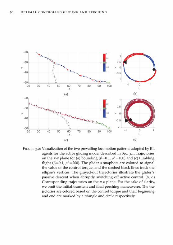
50 optimal controlled gliding and perching
20 30 40 50 60 70 80 90 100x
-50
-40
-30
-20
y
-1
-0.5
0
0.5
1
(a)
-1 0 1u
-1
-0.5
0
0.5
1
v
(b)
20 30 40 50 60 70 80 90 100x
-50
-40
-30
-20
y
-1
-0.5
0
0.5
1
(c)
-1 0 1u
-1
-0.5
0
0.5
1
v
(d)
Figure 3.2: Visualization of the two prevailing locomotion patterns adopted by RLagents for the active gliding model described in Sec. 3.1. Trajectorieson the x-y plane for (a) bounding (β=0.1, ρ∗=100) and (c) tumblingflight (β=0.1, ρ∗=200). The glider’s snaphots are colored to signalthe value of the control torque, and the dashed black lines track theellipse’s vertices. The grayed-out trajectories illustrate the glider’spassive descent when abruptly switching off active control. (b, d)Corresponding trajectories on the u-v plane. For the sake of clarity,we omit the initial transient and final perching maneuverer. The tra-jectories are colored based on the control torque and their beginningand end are marked by a triangle and circle respectively.
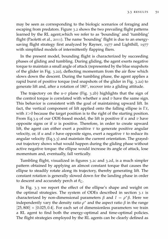
3.3 results 51
may be seen as corresponding to the biologic scenarios of foraging andescaping from predators. Figure 3.2 shows the two prevailing flight patternslearned by the RL agent,which we refer to as ‘bounding’ and ‘tumbling’flight (Paoletti et al., 2011). The name ‘bounding’ flight is due to an energy-saving flight strategy first analyzed by Rayner, 1977 and Lighthill, 1977
with simplified models of intermittently flapping fliers.
In the present model, bounding flight is characterized by succeedingphases of gliding and tumbling. During gliding, the agent exerts negativetorque to maintain a small angle of attack (represented by the blue snapshotsof the glider in Fig. 3.2a), deflecting momentum from the air flow whichslows down the descent. During the tumbling phase, the agent applies arapid burst of positive torque (red snapshots of the glider in Fig. 3.2a) togenerate lift and, after a rotation of 180, recover into a gliding attitude.
The trajectory on the u-v plane (Fig. 3.2b) highlights that the sign ofthe control torque is correlated with whether u and v have the same sign.This behavior is consistent with the goal of maintaining upward lift. Infact, the vertical component of lift applied onto the falling ellipse is Γx,with x>0 because the target position is to the right of the starting position.From Eq.3.9 of our ODE-based model, the lift is positive if u and v haveopposite signs or if w is positive. Therefore, in order to create upwardlift, the agent can either exert a positive τ to generate positive angularvelocity, or, if u and v have opposite signs, exert a negative τ to reduce itsangular velocity (Eq.3.3) and maintain the current orientation. The grayed-out trajectory shows what would happen during the gliding phase withoutactive negative torque: the ellipse would increase its angle of attack, losemomentum and, eventually, fall vertically.
Tumbling flight, visualized in figures 3.2c and 3.2d, is a much simplerpattern obtained by applying an almost constant torque that causes theellipse to steadily rotate along its trajectory, thereby generating lift. Theconstant rotation is generally slowed down for the landing phase in orderto descent and accurately perch at θG.
In Fig. 3.3 we report the effect of the ellipse’s shape and weight onthe optimal strategies. The system of ODEs described in section 3.1 ischaracterized by non-dimensional parameters β and I = ρ∗β. Here weindependently vary the density ratio ρ∗ and the aspect ratio β in the range[25, 800]× [0.025, 0.4]. For each set of dimensionless parameters we traina RL agent to find both the energy-optimal and time-optimal policies.The flight strategies employed by the RL agents can be clearly defined as
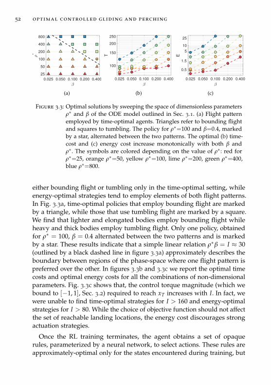
52 optimal controlled gliding and perching
0.025 0.050 0.100 0.200 0.400
25
50
100
200
400
800*
(a)
0.025 0.050 0.100 0.200 0.400
100
150
200
250
T
(b)
0.025 0.050 0.100 0.200 0.400
0.5
1.5
5
10
25
E
(c)
Figure 3.3: Optimal solutions by sweeping the space of dimensionless parametersρ∗ and β of the ODE model outlined in Sec. 3.1. (a) Flight patternemployed by time-optimal agents. Triangles refer to bounding flightand squares to tumbling. The policy for ρ∗=100 and β=0.4, markedby a star, alternated between the two patterns. The optimal (b) time-cost and (c) energy cost increase monotonically with both β andρ∗. The symbols are colored depending on the value of ρ∗: red forρ∗=25, orange ρ∗=50, yellow ρ∗=100, lime ρ∗=200, green ρ∗=400,blue ρ∗=800.
either bounding flight or tumbling only in the time-optimal setting, whileenergy-optimal strategies tend to employ elements of both flight patterns.In Fig. 3.3a, time-optimal policies that employ bounding flight are markedby a triangle, while those that use tumbling flight are marked by a square.We find that lighter and elongated bodies employ bounding flight whileheavy and thick bodies employ tumbling flight. Only one policy, obtainedfor ρ∗ = 100, β = 0.4 alternated between the two patterns and is markedby a star. These results indicate that a simple linear relation ρ∗β = I ≈ 30(outlined by a black dashed line in figure 3.3a) approximately describes theboundary between regions of the phase-space where one flight pattern ispreferred over the other. In figures 3.3b and 3.3c we report the optimal timecosts and optimal energy costs for all the combinations of non-dimensionalparameters. Fig. 3.3c shows that, the control torque magnitude (which webound to [−1, 1], Sec. 3.2) required to reach xT increases with I. In fact, wewere unable to find time-optimal strategies for I > 160 and energy-optimalstrategies for I > 80. While the choice of objective function should not affectthe set of reachable landing locations, the energy cost discourages strongactuation strategies.
Once the RL training terminates, the agent obtains a set of opaquerules, parameterized by a neural network, to select actions. These rules areapproximately-optimal only for the states encountered during training, but
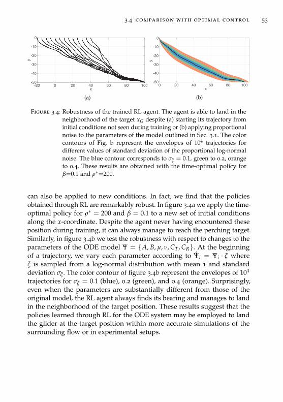
3.4 comparison with optimal control 53
-20 0 20 40 60 80 100x
-50
-40
-30
-20
-10
0
y
(a)
0 20 40 60 80 100x
-50
-40
-30
-20
-10
0
y
(b)
Figure 3.4: Robustness of the trained RL agent. The agent is able to land in theneighborhood of the target xG despite (a) starting its trajectory frominitial conditions not seen during training or (b) applying proportionalnoise to the parameters of the model outlined in Sec. 3.1. The colorcontours of Fig. b represent the envelopes of 104 trajectories fordifferent values of standard deviation of the proportional log-normalnoise. The blue contour corresponds to σξ = 0.1, green to 0.2, orangeto 0.4. These results are obtained with the time-optimal policy forβ=0.1 and ρ∗=200.
can also be applied to new conditions. In fact, we find that the policiesobtained through RL are remarkably robust. In figure 3.4a we apply the time-optimal policy for ρ∗ = 200 and β = 0.1 to a new set of initial conditionsalong the x-coordinate. Despite the agent never having encountered theseposition during training, it can always manage to reach the perching target.Similarly, in figure 3.4b we test the robustness with respect to changes to theparameters of the ODE model Ψ = A, B, µ, ν, CT , CR. At the beginningof a trajectory, we vary each parameter according to Ψi = Ψi · ξ whereξ is sampled from a log-normal distribution with mean 1 and standarddeviation σξ . The color contour of figure 3.4b represent the envelopes of 104
trajectories for σξ = 0.1 (blue), 0.2 (green), and 0.4 (orange). Surprisingly,even when the parameters are substantially different from those of theoriginal model, the RL agent always finds its bearing and manages to landin the neighborhood of the target position. These results suggest that thepolicies learned through RL for the ODE system may be employed to landthe glider at the target position within more accurate simulations of thesurrounding flow or in experimental setups.
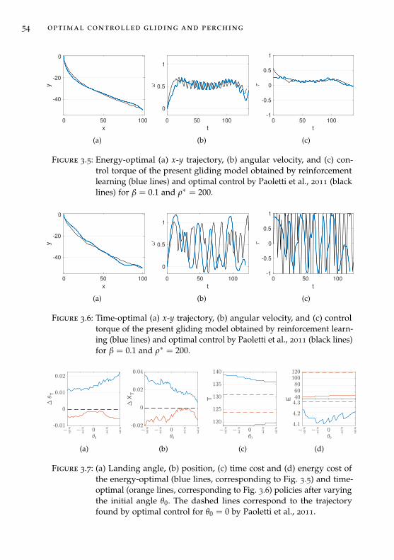
54 optimal controlled gliding and perching
0 50 100
x
-40
-20
0
y
(a)
0 50 100
t
0
0.5
1
(b)
0 50 100
t
-1
-0.5
0
0.5
1
(c)
Figure 3.5: Energy-optimal (a) x-y trajectory, (b) angular velocity, and (c) con-trol torque of the present gliding model obtained by reinforcementlearning (blue lines) and optimal control by Paoletti et al., 2011 (blacklines) for β = 0.1 and ρ∗ = 200.
0 50 100
x
-40
-20
0
y
(a)
0 50 100
t
0
0.5
1
(b)
0 50 100
t
-1
-0.5
0
0.5
1
(c)
Figure 3.6: Time-optimal (a) x-y trajectory, (b) angular velocity, and (c) controltorque of the present gliding model obtained by reinforcement learn-ing (blue lines) and optimal control by Paoletti et al., 2011 (black lines)for β = 0.1 and ρ∗ = 200.
T
(a)
XT
(b)
T
(c)
E
(d)
Figure 3.7: (a) Landing angle, (b) position, (c) time cost and (d) energy cost ofthe energy-optimal (blue lines, corresponding to Fig. 3.5) and time-optimal (orange lines, corresponding to Fig. 3.6) policies after varyingthe initial angle θ0. The dashed lines correspond to the trajectoryfound by optimal control for θ0 = 0 by Paoletti et al., 2011.
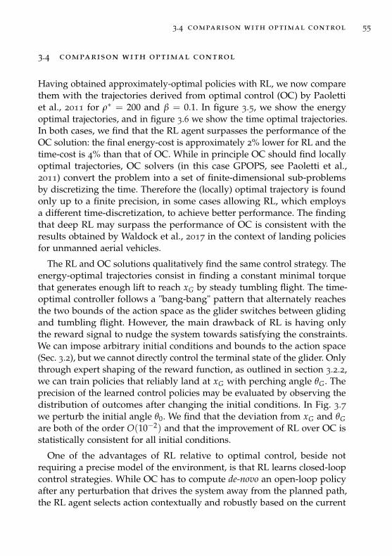
3.4 comparison with optimal control 55
3.4 comparison with optimal control
Having obtained approximately-optimal policies with RL, we now comparethem with the trajectories derived from optimal control (OC) by Paolettiet al., 2011 for ρ∗ = 200 and β = 0.1. In figure 3.5, we show the energyoptimal trajectories, and in figure 3.6 we show the time optimal trajectories.In both cases, we find that the RL agent surpasses the performance of theOC solution: the final energy-cost is approximately 2% lower for RL and thetime-cost is 4% than that of OC. While in principle OC should find locallyoptimal trajectories, OC solvers (in this case GPOPS, see Paoletti et al.,2011) convert the problem into a set of finite-dimensional sub-problemsby discretizing the time. Therefore the (locally) optimal trajectory is foundonly up to a finite precision, in some cases allowing RL, which employsa different time-discretization, to achieve better performance. The findingthat deep RL may surpass the performance of OC is consistent with theresults obtained by Waldock et al., 2017 in the context of landing policiesfor unmanned aerial vehicles.
The RL and OC solutions qualitatively find the same control strategy. Theenergy-optimal trajectories consist in finding a constant minimal torquethat generates enough lift to reach xG by steady tumbling flight. The time-optimal controller follows a "bang-bang" pattern that alternately reachesthe two bounds of the action space as the glider switches between glidingand tumbling flight. However, the main drawback of RL is having onlythe reward signal to nudge the system towards satisfying the constraints.We can impose arbitrary initial conditions and bounds to the action space(Sec. 3.2), but we cannot directly control the terminal state of the glider. Onlythrough expert shaping of the reward function, as outlined in section 3.2.2,we can train policies that reliably land at xG with perching angle θG. Theprecision of the learned control policies may be evaluated by observing thedistribution of outcomes after changing the initial conditions. In Fig. 3.7we perturb the initial angle θ0. We find that the deviation from xG and θGare both of the order O(10−2) and that the improvement of RL over OC isstatistically consistent for all initial conditions.
One of the advantages of RL relative to optimal control, beside notrequiring a precise model of the environment, is that RL learns closed-loopcontrol strategies. While OC has to compute de-novo an open-loop policyafter any perturbation that drives the system away from the planned path,the RL agent selects action contextually and robustly based on the current
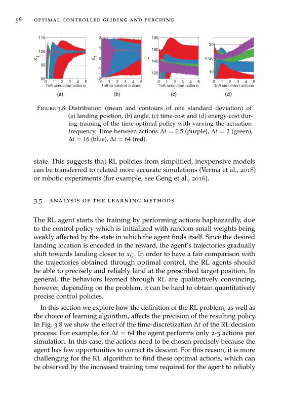
56 optimal controlled gliding and perching
(a) (b) (c) (d)
Figure 3.8: Distribution (mean and contours of one standard deviation) of(a) landing position, (b) angle, (c) time-cost and (d) energy-cost dur-ing training of the time-optimal policy with varying the actuationfrequency. Time between actions ∆t = 0.5 (purple), ∆t = 2 (green),∆t = 16 (blue), ∆t = 64 (red).
state. This suggests that RL policies from simplified, inexpensive modelscan be transferred to related more accurate simulations (Verma et al., 2018)or robotic experiments (for example, see Geng et al., 2016).
3.5 analysis of the learning methods
The RL agent starts the training by performing actions haphazardly, dueto the control policy which is initialized with random small weights beingweakly affected by the state in which the agent finds itself. Since the desiredlanding location is encoded in the reward, the agent’s trajectories graduallyshift towards landing closer to xG. In order to have a fair comparison withthe trajectories obtained through optimal control, the RL agents shouldbe able to precisely and reliably land at the prescribed target position. Ingeneral, the behaviors learned through RL are qualitatively convincing,however, depending on the problem, it can be hard to obtain quantitativelyprecise control policies.
In this section we explore how the definition of the RL problem, as well asthe choice of learning algorithm, affects the precision of the resulting policy.In Fig. 3.8 we show the effect of the time-discretization ∆t of the RL decisionprocess. For example, for ∆t = 64 the agent performs only 2-3 actions persimulation. In this case, the actions need to be chosen precisely because theagent has few opportunities to correct its descent. For this reason, it is morechallenging for the RL algorithm to find these optimal actions, which canbe observed by the increased training time required for the agent to reliably
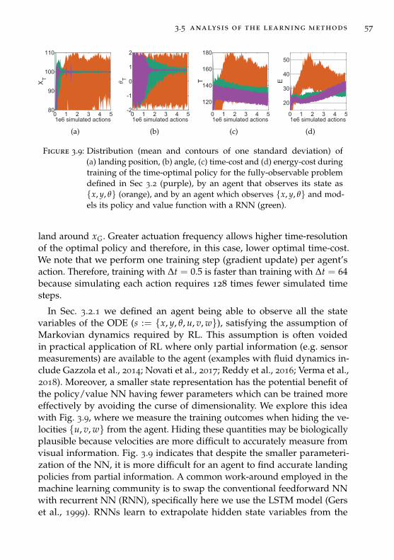
3.5 analysis of the learning methods 57
(a) (b) (c) (d)
Figure 3.9: Distribution (mean and contours of one standard deviation) of(a) landing position, (b) angle, (c) time-cost and (d) energy-cost duringtraining of the time-optimal policy for the fully-observable problemdefined in Sec 3.2 (purple), by an agent that observes its state asx, y, θ (orange), and by an agent which observes x, y, θ and mod-els its policy and value function with a RNN (green).
land around xG. Greater actuation frequency allows higher time-resolutionof the optimal policy and therefore, in this case, lower optimal time-cost.We note that we perform one training step (gradient update) per agent’saction. Therefore, training with ∆t = 0.5 is faster than training with ∆t = 64because simulating each action requires 128 times fewer simulated timesteps.
In Sec. 3.2.1 we defined an agent being able to observe all the statevariables of the ODE (s := x, y, θ, u, v, w), satisfying the assumption ofMarkovian dynamics required by RL. This assumption is often voidedin practical application of RL where only partial information (e.g. sensormeasurements) are available to the agent (examples with fluid dynamics in-clude Gazzola et al., 2014; Novati et al., 2017; Reddy et al., 2016; Verma et al.,2018). Moreover, a smaller state representation has the potential benefit ofthe policy/value NN having fewer parameters which can be trained moreeffectively by avoiding the curse of dimensionality. We explore this ideawith Fig. 3.9, where we measure the training outcomes when hiding the ve-locities u, v, w from the agent. Hiding these quantities may be biologicallyplausible because velocities are more difficult to accurately measure fromvisual information. Fig. 3.9 indicates that despite the smaller parameteri-zation of the NN, it is more difficult for an agent to find accurate landingpolicies from partial information. A common work-around employed in themachine learning community is to swap the conventional feedforward NNwith recurrent NN (RNN), specifically here we use the LSTM model (Gerset al., 1999). RNNs learn to extrapolate hidden state variables from the
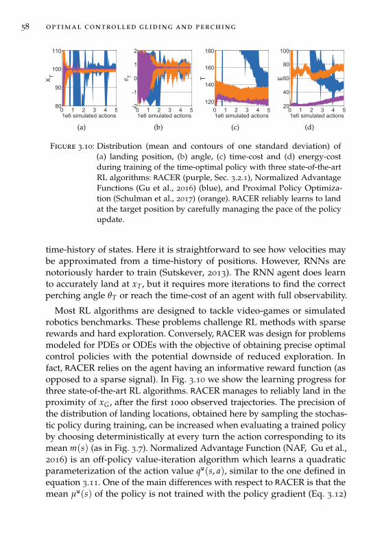
58 optimal controlled gliding and perching
(a) (b) (c) (d)
Figure 3.10: Distribution (mean and contours of one standard deviation) of(a) landing position, (b) angle, (c) time-cost and (d) energy-costduring training of the time-optimal policy with three state-of-the-artRL algorithms: RACER (purple, Sec. 3.2.1), Normalized AdvantageFunctions (Gu et al., 2016) (blue), and Proximal Policy Optimiza-tion (Schulman et al., 2017) (orange). RACER reliably learns to landat the target position by carefully managing the pace of the policyupdate.
time-history of states. Here it is straightforward to see how velocities maybe approximated from a time-history of positions. However, RNNs arenotoriously harder to train (Sutskever, 2013). The RNN agent does learnto accurately land at xT , but it requires more iterations to find the correctperching angle θT or reach the time-cost of an agent with full observability.
Most RL algorithms are designed to tackle video-games or simulatedrobotics benchmarks. These problems challenge RL methods with sparserewards and hard exploration. Conversely, RACER was design for problemsmodeled for PDEs or ODEs with the objective of obtaining precise optimalcontrol policies with the potential downside of reduced exploration. Infact, RACER relies on the agent having an informative reward function (asopposed to a sparse signal). In Fig. 3.10 we show the learning progress forthree state-of-the-art RL algorithms. RACER manages to reliably land in theproximity of xG, after the first 1000 observed trajectories. The precision ofthe distribution of landing locations, obtained here by sampling the stochas-tic policy during training, can be increased when evaluating a trained policyby choosing deterministically at every turn the action corresponding to itsmean m(s) (as in Fig. 3.7). Normalized Advantage Function (NAF, Gu et al.,2016) is an off-policy value-iteration algorithm which learns a quadraticparameterization of the action value qw(s, a), similar to the one defined inequation 3.11. One of the main differences with respect to RACER is that themean µw(s) of the policy is not trained with the policy gradient (Eq. 3.12)
3.6 conclusion 59
but with the critic gradient (Eq. 3.13). While the accuracy of the parame-terized qw(s, a) might increase during training, µw(s) does not necessarilycorrespond to better action, leading to the erratic distribution of landingpositions in figure 3.10. Proximal Policy Optimization (PPO, Schulman et al.,2017) is an on-policy actor-critic algorithm. This algorithm’s main differencewith respect to RACER is that only the most recent (on-policy) trajectoriesare used to update the policy. This allows estimating Qπ(s, a) directly fromon-policy rewards (Schulman et al., 2015b) rather than with an off-policyestimator (here we used Retrace 2.8), and it bypasses the need for learninga parametric qw(s, a). While PPO has led to many state-of-the-art results inbenchmark test cases, here it does not succeed to center the distribution oflanding positions around xG. This could be attributed to the high varianceof the on-policy estimator for Qπ(s, a).
3.6 conclusion
We have demonstrated that Reinforcement Learning can be used to developgliding agents that execute complex and precise control patterns usinga simple model of the controlled gravity-driven descent of an ellipticalobject. We show that RL agents learn a variety of optimal flight patternsand perching maneuvers that minimize either time-to-target or energy cost.The RL agents were able to match and even surpass the performance oftrajectories found through Optimal Control. We also show that the theRL agents can generalize their behavior, allowing them to select adequateactions even after perturbing the system. Finally, we examined the effects ofthe ellipse’s density and aspect ratio to find that the optimal policies lead toeither bounding flight or tumbling flight. Bounding flight is characterizedas alternating phases of gliding with a small angle of attack and rapidrotation to generate lift. Tumbling flight is characterized by continual rota-tion, propelled by a minimal almost constant torque. Ongoing work aimsto extend the present algorithms to three dimensional Direct NumericalSimulations of gliders and using lessons learned from these simulations forthe perching and gliding of UAVs.

4E Q UAT I O N S A N D M E T H O D S F O R F L U I D - S T R U C T U R EI N T E R A C T I O N
One of the most challenging tasks in computational physics involves sim-ulating interactions between deforming solids and fluid flow. This is acommonly occurring scenario both in nature and in engineering applica-tions, where moving or deforming surfaces manipulate the surroundingfluid either for energy extraction, or to modify reaction forces acting on abody. Some important examples include wind and water turbines, controlsurfaces on ships and airplanes, and the locomotory organs of birds andaquatic animals. Detailed studies of fluid-solid interactions can not onlycomplement our understanding of the way animals interact with their fluidenvironment, but can be invaluable for improving the design of a varietyof engineering devices. For instance, physical insights gained from experi-mental and computational studies can lead to technological advances in thefield of bioinspired propulsion, by enabling fine-tuned optimization of bodygeometry and kinematics, or by exploring energy-harvesting mechanismsin unsteady flows.
While experimental diagnostic techniques, such as Particle Image Ve-locimetry (PIV), have contributed immensely to our understanding ofphysical mechanisms governing animal locomotion (Katija et al., 2008; Liaoet al., 2003a; Spedding et al., 2003; Warrick et al., 2005), limited spatial andtemporal resolution pose certain limitations when detailed quantitativeflow data are required. Moreover, these techniques may encounter diffi-culties when considering hydrodynamic interactions of multiple objectspresent in the flow field. Such scenarios are crucial when investigating thephysical mechanisms governing collective locomotion (Ashraf et al., 2017;Bialek et al., 2012), and interactions of animals with objects present in theirenvironment (Beal et al., 2006; Liao et al., 2003a). At moderate Reynoldsnumbers, simulations can serve as immensely powerful tools to complementexperiments, by providing detailed spatial and temporal measurementsin the flow. Computational studies also allow rapid evaluation of designiterations (Gazzola et al., 2012; Rees et al., 2013, 2015; Verma et al., 2017b),which may not be feasible to do experimentally owing to both time and
61
62 equations and methods for fluid-structure interaction
cost constraints. Another notable advantage of adopting computations fordesign optimization is the emergence of novel morphology and behaviour,which may not occur in nature owing to restrictive biological constraints.Recently, high-fidelity simulations have been coupled with machine learn-ing algorithms to accomplish high-level tasks in extremely demandingsituations involving highly unsteady flow fields. These studies incorporateautonomous control techniques that are robust to perturbations, and couldeventually be repurposed for use in coordinated motion of robotic swarmsfor navigation through unfamiliar terrain, for search and rescue operations,or for energy-efficient formation swimming. Apart from advancing noveldesigns and control mechanisms, simulations provide invaluable physicalinsight into the principles governing locomotion, which in turn can helpexplain the evolution of certain biological traits and behaviour in animals.Various numerical studies have discovered optimal traits that closely mimicthose found in nature, such as specific morphology (Rees et al., 2013, 2015),certain locomotion gaits (Gazzola et al., 2012; Verma et al., 2017b), andeven peculiar interactions of animals with their environment (Reddy etal., 2016) and with other animals. Such studies have the potential to sup-port design advancements for micro aerial vehicles (MAVs) (Pines et al.,2006), autonomous underwater vehicles (AUVs) (Paull et al., 2014), andeven robotic swimmers that mimic undulatory motion used by fish forlocomotion (Barrett et al., 1999).
Most of the computational studies mentioned above usually rely onexpansive in-house codes, requiring several person-years of development toreach a certain level of maturity. Commercially available software suites offera viable alternative to code development, however, their ability to handlemultiple shapes that evolve in time remains limited. This capability isinvaluable when investigating hydrodynamic interactions of self-propelledanimals with their environment, such as with rocks and boulders presentin streams, or when examining collective interactions among animals, asin small schools of fish. To address this need, we developed CubismUP,which is a general purpose incompressible Navier-Stokes solver capable ofhandling multiple solid and deforming objects simultaneously. The codeovercomes a majority of the challenges described here via a combinationof pressure-projection (Chorin, 1968) and Brinkman penalization (Angotet al., 1999; Coquerelle et al., 2008). The backend is based on the ‘CUBISM’framework (Rossinelli et al., 2013), which discretizes the computationaldomain using cubic ‘blocks’ for increasing parallelism and better cachelocality. This allows for efficient utilization of high core count CPUs, where
4.1 background 63
each MPI rank associated with a distinct CPU is assigned a certain numberof blocks, and each block is processed by a single thread. The Poissonequation for the pressure field may be solved either on CPUs or, if available,GPUs. This Chapter presents the numerical methods used in the code.
acknowledgments Part of this Chapter is based on unpublished workperformed with Siddhartha Verma. The computational resources wereprovided by a grant from the Swiss National Super-computing Centre(CSCS) under project s929.
4.1 background
The Brinkman penalization method (Angot et al., 1999) enforces the no-slipand no-through boundary conditions at the surface of a solid by extendingthe Navier–Stokes Equations (NSE) inside the body and introducing aforcing term. We write the penalized NSE with discrete time integration as:
∇ · u(k) = 0 (4.1)
u(k+1) − u(k)
δt= −(u(k) · ∇)u(k) + ν∆u(k) − ∇P(k)
ρ+F
(k)s (4.2)
Here u(k) is the velocity field at time step k, P(k) is the pressure field, F (k)s is
the penalization force introduced by Brinkman method, ρ and ν correspondto the fluid density and viscosity. Due to the extension of the fluid equationsto the solid domain, the penalized NSE are solved over Ω = ΩS ∪ΩF, withΩS and ΩF the solid and fluid domains respectively.
For simplicity, the notation of Eq. 4.2 implies that time-stepping is per-formed via first–order explicit Euler integration. In practice, for all resultspresented hereafter, we advance the momentum equation via Godunovoperator splitting, whereby the penalty, advection-diffusion, Brinkman pe-nalization and pressure–projection steps are followed sequentially. Theadvection and diffusion step is performed with the second–order explicitRunge–Kutta scheme. Unless otherwise stated, we constrain the advectiveCFL (Courant-Friedrichs-Lewy) and diffusive Fourier numbers to be lessthan 0.1 (CFLadv = ‖u‖δt/h, Fourierdiff = νδt/h2), where h is the uniformgrid resolution. Finally, spatial derivatives are discretized using secondorder accurate centered finite differences, except for the advection termwhich is discretized with third-order upwind.
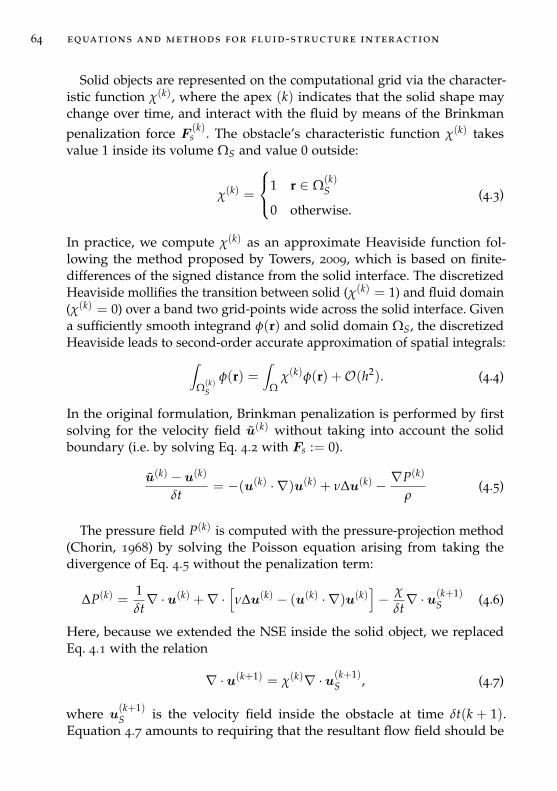
64 equations and methods for fluid-structure interaction
Solid objects are represented on the computational grid via the character-istic function χ(k), where the apex (k) indicates that the solid shape maychange over time, and interact with the fluid by means of the Brinkmanpenalization force F
(k)s . The obstacle’s characteristic function χ(k) takes
value 1 inside its volume ΩS and value 0 outside:
χ(k) =
1 r ∈ Ω(k)S
0 otherwise.(4.3)
In practice, we compute χ(k) as an approximate Heaviside function fol-lowing the method proposed by Towers, 2009, which is based on finite-differences of the signed distance from the solid interface. The discretizedHeaviside mollifies the transition between solid (χ(k) = 1) and fluid domain(χ(k) = 0) over a band two grid-points wide across the solid interface. Givena sufficiently smooth integrand φ(r) and solid domain ΩS, the discretizedHeaviside leads to second-order accurate approximation of spatial integrals:∫
Ω(k)S
φ(r) =∫
Ωχ(k)φ(r) +O(h2). (4.4)
In the original formulation, Brinkman penalization is performed by firstsolving for the velocity field u(k) without taking into account the solidboundary (i.e. by solving Eq. 4.2 with Fs := 0).
u(k) − u(k)
δt= −(u(k) · ∇)u(k) + ν∆u(k) − ∇P(k)
ρ(4.5)
The pressure field P(k) is computed with the pressure-projection method(Chorin, 1968) by solving the Poisson equation arising from taking thedivergence of Eq. 4.5 without the penalization term:
∆P(k) =1δt∇ · u(k) +∇ ·
[ν∆u(k) − (u(k) · ∇)u(k)
]− χ
δt∇ · u(k+1)
S (4.6)
Here, because we extended the NSE inside the solid object, we replacedEq. 4.1 with the relation
∇ · u(k+1) = χ(k)∇ · u(k+1)S , (4.7)
where u(k+1)S is the velocity field inside the obstacle at time δt(k + 1).
Equation 4.7 amounts to requiring that the resultant flow field should be
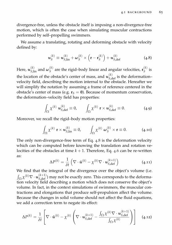
4.1 background 65
divergence-free, unless the obstacle itself is imposing a non-divergence-freemotion, which is often the case when simulating muscular contractionsperformed by self–propelling swimmers.
We assume a translating, rotating and deforming obstacle with velocitydefined by:
u(k)S ≡ u
(k)S,lin + ω
(k)S ×
(r− r(k)S
)+ u
(k)S,def (4.8)
Here, u(k)S,lin and ω
(k)S are the rigid–body linear and angular velocities, r(k)S is
the location of the obstacle’s center of mass, and u(k)S,def is the deformation–
velocity field, describing the motion internal to the obstacle. Hereafter wewill simplify the notation by assuming a frame of reference centered in theobstacle’s center of mass (e.g. rS = 0). Because of momentum conservation,the deformation–velocity field has properties:∫
Ωχ(k) u
(k)S,def ≡ 0,
∫Ω
χ(k) r× u(k)S,def ≡ 0. (4.9)
Moreover, we recall the rigid–body motion properties:∫Ω
χ(k) r× u(k)S,lin ≡ 0,
∫Ω
χ(k) ω(k)S × r ≡ 0. (4.10)
The only non-divergence-free term of Eq. 4.8 is the deformation velocitywhich can be computed before knowing the translation and rotation ve-locities of the obstacles at time k + 1. Therefore, Eq. 4.6 can be re-writtenas:
∆P(k) =1δt
(∇ · u(k) − χ(k)∇ · u(k+1)
S,def
)(4.11)
We find that the integral of the divergence over the object’s volume (i.e.∫Ω χ(k)∇ ·u(k+1)
S,def ) may not be exactly zero. This corresponds to the deforma-tion velocity field describing a motion which does not conserve the object’svolume. In fact, in the context simulations of swimmers, the muscular con-tractions and elongations that produce self-propulsion affect the volume.Because the changes in solid volume should not affect the fluid equations,we add a correction term to negate its effect:
∆P(k) =1δt
∇ · u(k) − χ(k)
∇ · u(k+1)S,def −
∫Ω χ(k)∇ · u(k+1)
S,def∫Ω χ(k)
(4.12)
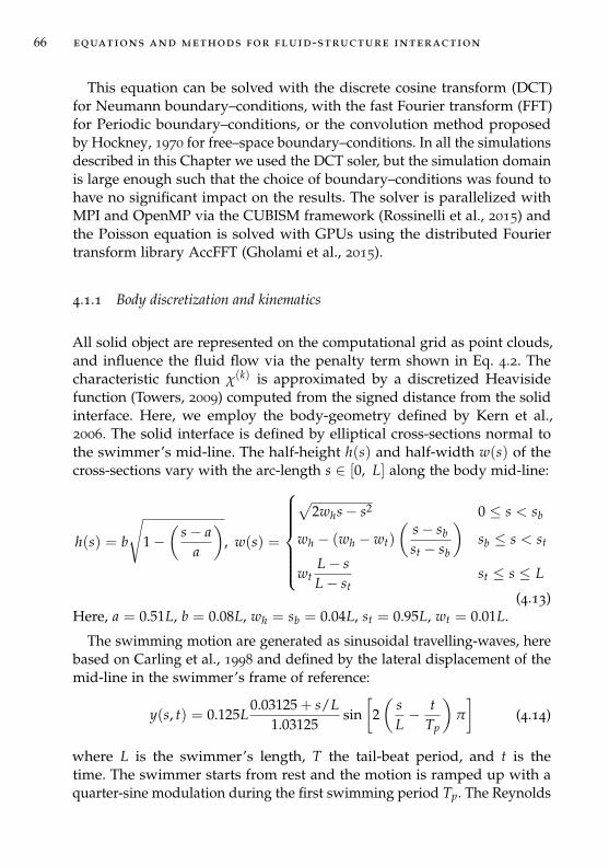
66 equations and methods for fluid-structure interaction
This equation can be solved with the discrete cosine transform (DCT)for Neumann boundary–conditions, with the fast Fourier transform (FFT)for Periodic boundary–conditions, or the convolution method proposedby Hockney, 1970 for free–space boundary–conditions. In all the simulationsdescribed in this Chapter we used the DCT soler, but the simulation domainis large enough such that the choice of boundary–conditions was found tohave no significant impact on the results. The solver is parallelized withMPI and OpenMP via the CUBISM framework (Rossinelli et al., 2015) andthe Poisson equation is solved with GPUs using the distributed Fouriertransform library AccFFT (Gholami et al., 2015).
4.1.1 Body discretization and kinematics
All solid object are represented on the computational grid as point clouds,and influence the fluid flow via the penalty term shown in Eq. 4.2. Thecharacteristic function χ(k) is approximated by a discretized Heavisidefunction (Towers, 2009) computed from the signed distance from the solidinterface. Here, we employ the body-geometry defined by Kern et al.,2006. The solid interface is defined by elliptical cross-sections normal tothe swimmer’s mid-line. The half-height h(s) and half-width w(s) of thecross-sections vary with the arc-length s ∈ [0, L] along the body mid-line:
h(s) = b
√1−
(s− a
a
), w(s) =
√2whs− s2 0 ≤ s < sb
wh − (wh − wt)
(s− sbst − sb
)sb ≤ s < st
wtL− sL− st
st ≤ s ≤ L
(4.13)Here, a = 0.51L, b = 0.08L, wh = sb = 0.04L, st = 0.95L, wt = 0.01L.
The swimming motion are generated as sinusoidal travelling-waves, herebased on Carling et al., 1998 and defined by the lateral displacement of themid-line in the swimmer’s frame of reference:
y(s, t) = 0.125L0.03125 + s/L
1.03125sin[
2(
sL− t
Tp
)π
](4.14)
where L is the swimmer’s length, T the tail-beat period, and t is thetime. The swimmer starts from rest and the motion is ramped up with aquarter-sine modulation during the first swimming period Tp. The Reynolds
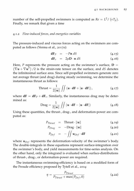
4.1 background 67
number of the self-propelled swimmers is computed as Re = L2/(νTp
).
Finally, we remark that given a time
4.1.2 Flow-induced forces, and energetics variables
The pressure-induced and viscous forces acting on the swimmers are com-puted as follows (Verma et al., 2017a):
dFP = −Pn dS (4.15)
dFν = 2µD · n dS (4.16)
Here, P represents the pressure acting on the swimmer’s surface, D =(∇u +∇uT) /2 is the strain-rate tensor on the surface, and dS denotes
the infinitesimal surface area. Since self-propelled swimmers generate zeronet average thrust (and drag) during steady swimming, we determine theinstantaneous thrust as follows:
Thrust =1
2‖u‖∫∫
(u · dF + |u · dF|) , (4.17)
where dF = dFP + dFν. Similarly, the instantaneous drag may be deter-mined as:
Drag =1
2‖u‖∫∫
(u · dF− |u · dF|) (4.18)
Using these quantities, the thrust-, drag-, and deformation-power are com-puted as:
PThrust = Thrust · ‖u‖ (4.19)
PDrag = −Drag · ‖u‖ (4.20)
PDe f = −∫∫
uDe f · dF (4.21)
where uDe f represents the deformation-velocity of the swimmer’s body.The double-integrals in these equations represent surface-integration overthe swimmer’s body, and yield measurements for time-series analysis. Onthe other hand, only the integrand is evaluated when surface-distributionsof thrust-, drag-, or deformation-power are required.
The instantaneous swimming-efficiency is based on a modified form ofthe Froude efficiency proposed by Tytell et al., 2004:
η =PThrust
PThrust + max(PDe f , 0)(4.22)
68 equations and methods for fluid-structure interaction
To compute both η and the Cost of Transport (CoT), we neglect negativevalues of PDe f :
CoT(t) =
∫ tt−Tp
max(PDe f , 0)dt∫ tt−Tp‖u‖dt
. (4.23)
This restriction accounts for the fact that the elastically rigid swimmer maynot store mechanical energy furnished by the flow, and yields a conservativeestimate of potential savings in the CoT.
4.2 conservative brinkman penalization
The interpretation of the Brinkman penalization force in Eq. 4.2 dependson the kind of fluid–structure interaction being simulated. In the case ofsolid obstacles which are externally forced to move with a set velocity, orfixed in place, the role of the penalization coefficient is that of a Lagrangianmultiplier. In the case of self-propelled object, the penalization force isakin to an elastic response: it compels the fluid contained inside ΩS tobehave as if it were the solid (or deforming) obstacle. In this case, Brinkmanpenalization is performed by first updating the momenta of the solidobstacle to be equal to the momenta of the flow contained in the domainΩS (Coquerelle et al., 2008):
u(k)S,lin = M−1
∫Ω
χ(k) u(k), ω(k)S = J−1
∫Ω
χ(k) r× u(k) (4.24)
with the mass M and moment of inertia J:
M =∫
Ωχ(k), J =
∫Ω
χ(k)
y2 + z2 −xy −xz
−xy x2 + z2 −yz
−xz −yz y2 + x2
(4.25)
Then, the velocity field is updated either with explicit–Euler integration,
u(k+1) = u(k) + δt λ χ(k) (u(k+1)S − u(k)), (4.26)
or with implicit–Euler integration,
u(k+1) = u(k) + δt λ χ(k) (u(k+1)S − u(k+1)) =
u(k) + δt λ χ(k) u(k+1)S
1 + δt λ χ(k),
(4.27)
4.2 conservative brinkman penalization 69
Here, λ is the penalization coefficient. While implicit–Euler integration isunconditionally stable, when using explicit–Euler integration the relationλδt ≤ 1 must be satisfied for stability (Coquerelle et al., 2008). We remarkthat, when using explicit–Euler integration and λδt = 1, Brinkman penal-ization can be seen to directly replace the flow velocity inside ΩS with apatch of velocity which satisfies the solid–body motion of the obstacle:
u(k+1) =
u(k+1)S r ∈ Ω(k)
S
u(k) otherwise.(4.28)
Moreover, explicit–Euler integration of the penalization steps is a momenta–conserving operation, that is:
0 =∫
Ωu(k+1) − u(k), 0 =
∫Ω
r×(u(k+1) − u(k)
)This property can be easily derived by rewriting the integrand with Eq. 4.26
(with λδt = 1) and by leveraging the properties defined by Eq. 4.9 andEq. 4.10.
Coquerelle et al., 2008 propose using large penalization coefficientsλδt 1 and implicit–Euler integration to strictly enforce the boundaryconditions. The same approach was followed by our prior implementa-tions, including the PPM-based solver (Gazzola et al., 2011a), MRAG-I2D(Rossinelli et al., 2015), and MRAG3D (Rees, 2014). This technique is validfor solid obstacles which are externally forced to move with a set velocity.However, in the case of self–propelled obstacles we find that results arestrongly affected by the penalization coefficient λ, as shown by Fig. 4.1a.Therein, the black lines refer to simulations performed in Rees, 2014 withnon-momenta conserving implicit penalization with λ = 104 and a vortex-method based solver. We attribute the discrepancy in forward velocitybetween Rees, 2014 and our simulations with implicit penalization andλ = 104 to the different δt of the numerical methods. In fact, the rate ofmomentum injection due to implicit Brinkman penalization is dependenton λδt.
We recall that Brinkman–penalization extends the NSE inside the soliddomain and that the penalization term introduces an elastic response whichforces the fluid contained inside ΩS to behave as if it were the solid. It
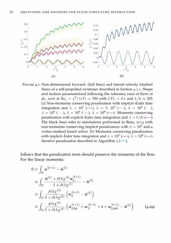
70 equations and methods for fluid-structure interaction
0 1 2 3 4 5 6
t / Tp
0
0.1
0.2
0.3
0.4
0.5
u
Tp /
L
(a)
0 1 2 3 4 5 6
t / Tp
-0.02
0
0.02
0.04
0.06
0.08
0.1
0.12
0.14
u
Tp /
L
(b)
Figure 4.1: Non-dimensional forward- (full lines) and lateral-velocity (dashedlines) of a self-propelled swimmer described in Section 4.1.1. Shapeand motion parameterized following the reference runs of Kern etal., 2006 at ReL = L2/(νT) = 550 with CFL = 0.1 and L/h ≈ 205.(a) Non-momenta conserving penalization with implicit–Euler timeintegration and λ = 103 ( ), λ = 5 · 103 ( ), λ = 104 ( ),λ = 105 ( ), λ = 106 ( ), λ = 108 ( ). Momenta conservingpenalization with explicit–Euler time integration and λ = 1/δt ( ).The black lines refer to simulations performed in Rees, 2014 withnon-momenta conserving implicit penalization with λ = 104 and avortex-method based solver. (b) Momenta conserving penalizationwith implicit–Euler time integration and λ = 103 ( ), λ = 108 ( ).Iterative penalization described in Algorithm 5 ( ).
follows that the penalization term should preserve the momenta of the flow.For the linear momenta:
0 ≡∫
Ωu(k+1) − u(k)
≡∫
Ω
u(k) + δtλχ(k)u(k+1)S
1 + δtλχ(k)− u(k)
≡∫
Ω
δtλχ(k)
1 + δtλχ(k)
(u(k+1)S − u(k)
)≡∫
Ω
δtλχ(k)
1 + δtλχ(k)
(u(k+1)S,lin + ω
(k+1)S × r + u
(k+1)S,def − u(k)
)(4.29)
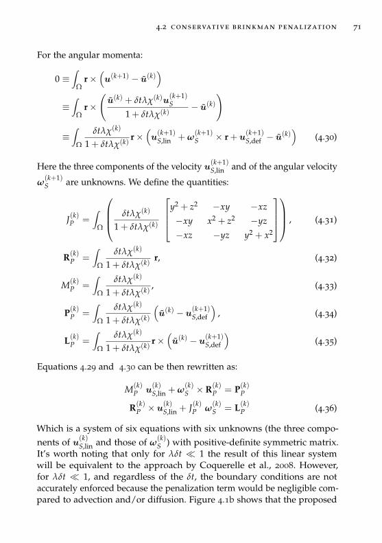
4.2 conservative brinkman penalization 71
For the angular momenta:
0 ≡∫
Ωr×
(u(k+1) − u(k)
)≡∫
Ωr×
(u(k) + δtλχ(k)u
(k+1)S
1 + δtλχ(k)− u(k)
)
≡∫
Ω
δtλχ(k)
1 + δtλχ(k)r×
(u(k+1)S,lin + ω
(k+1)S × r + u
(k+1)S,def − u(k)
)(4.30)
Here the three components of the velocity u(k+1)S,lin and of the angular velocity
ω(k+1)S are unknowns. We define the quantities:
J(k)P =∫
Ω
δtλχ(k)
1 + δtλχ(k)
y2 + z2 −xy −xz
−xy x2 + z2 −yz
−xz −yz y2 + x2
, (4.31)
R(k)P =
∫Ω
δtλχ(k)
1 + δtλχ(k)r, (4.32)
M(k)P =
∫Ω
δtλχ(k)
1 + δtλχ(k), (4.33)
P(k)P =
∫Ω
δtλχ(k)
1 + δtλχ(k)
(u(k) − u
(k+1)S,def
), (4.34)
L(k)P =
∫Ω
δtλχ(k)
1 + δtλχ(k)r×
(u(k) − u
(k+1)S,def
)(4.35)
Equations 4.29 and 4.30 can be then rewritten as:
M(k)P u
(k)S,lin + ω
(k)S × R(k)
P = P(k)P
R(k)P × u
(k)S,lin + J(k)P ω
(k)S = L(k)
P (4.36)
Which is a system of six equations with six unknowns (the three compo-nents of u(k)
S,lin and those of ω(k)S ) with positive-definite symmetric matrix.
It’s worth noting that only for λδt 1 the result of this linear systemwill be equivalent to the approach by Coquerelle et al., 2008. However,for λδt 1, and regardless of the δt, the boundary conditions are notaccurately enforced because the penalization term would be negligible com-pared to advection and/or diffusion. Figure 4.1b shows that the proposed
72 equations and methods for fluid-structure interaction
penalization method for implicit–Euler time integration produces resultsthat are almost independently of the choice of λ. Moreover, these results areconsistent with those obtained by explicit–Euler integration of the Brinkmanpenalization, which we have shown to naturally conserve momenta.
4.3 iterative penalization scheme
The time-step splitting employed by Brinkman penalization is known tointroduce an inconsistency in flow kinematics (Hejlesen et al., 2015). Ateach step we compute u(k) and the pressure field by solving the ellipticPoisson equation without taking into account the no-slip and no-throughflow boundary conditions. However, the Brinkman penalization corrects thevelocity field to satisfy the boundary conditions only through local relations.Here we adapt for the (u, P) formulation of the NSE the iterative penal-ization method proposed by Hejlesen et al., 2015 for vortex-method basedsolvers, and extend it to three-dimensional flows. The iterative Brinkmanpenalization technique involves solving the Poisson equation multiple timesper time step in a way to achieve the following objectives: First, the infor-mation of the boundary conditions are propagated into the flow beyond thearea immediately surrounding the body (as in the classic approach, whichlimits the allowable time step sizes). Second, the no-slip and no-throughboundary conditions are satisfied (almost) exactly at each step. Third, andcrucially, the iterations propagate the information related to the boundaryconditions throughout the domain by including the penalization terms inthe Poisson equation.
The proposed iterative method is defined in Algorithm 5. We remarkthat, like u
(k+1)S , the penalization force F(k)
s is a field quantity and the con-vergence check between iterations is computed with spatial–integrals ofthe L2 norms. We set the tolerance ε = 10−4 which, for the simulationspresented in Fig. 4.1b, corresponds to performing on average 8 iterationsper step, except for the initial time–steps which require up to 40 iterations.Furthermore, we note that the advection-diffusion step is performed withsecond-order explicit Runge-Kutta and 3rd order upwind spatial discretiza-tion, in identical manner to that of the non-iterative solver.
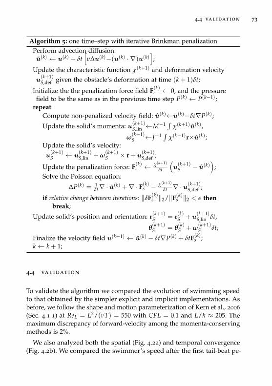
4.4 validation 73
Algorithm 5: one time–step with iterative Brinkman penalizationPerform advection-diffusion:u(k) ← u(k) + δt
[ν∆u(k)−(u(k) · ∇)u(k)
];
Update the characteristic function χ(k+1) and deformation velocityu(k+1)S,def given the obstacle’s deformation at time (k + 1)δt;
Initialize the the penalization force field F(k)s ← 0, and the pressure
field to be the same as in the previous time step P(k) ← P(k−1);repeat
Compute non-penalized velocity field: u(k)←u(k)−δt∇P(k);
Update the solid’s momenta: u(k+1)S,lin ←M−1
∫χ(k+1)u(k),
ω(k+1)S ←J−1
∫χ(k+1)r×u(k);
Update the solid’s velocity:u(k+1)S ← u
(k+1)S,lin + ω
(k+1)S × r + u
(k+1)S,def ;
Update the penalization force: F(k)s ← χ(k+1)
δt
(u(k+1)S − u(k)
);
Solve the Poisson equation:
∆P(k) = 1δt∇ · u(k) +∇ · F(k)
s − χ(k+1)
δt ∇ · u(k+1)S,def ;
if relative change between iterations: ‖δF(k)s ‖2/‖F(k)
s ‖2 < ε thenbreak;
Update solid’s position and orientation: r(k+1)S = r(k)S + u
(k+1)S,lin δt,
θ(k+1)S = θ
(k)S + ω
(k+1)S δt;
Finalize the velocity field u(k+1) ← u(k) − δt∇P(k) + δtF(k)s ;
k← k + 1;
4.4 validation
To validate the algorithm we compared the evolution of swimming speedto that obtained by the simpler explicit and implicit implementations. Asbefore, we follow the shape and motion parameterization of Kern et al., 2006
(Sec. 4.1.1) at ReL = L2/(νT) = 550 with CFL = 0.1 and L/h ≈ 205. Themaximum discrepancy of forward-velocity among the momenta-conservingmethods is 2%.
We also analyzed both the spatial (Fig. 4.2a) and temporal convergence(Fig. 4.2b). We compared the swimmer’s speed after the first tail-beat pe-
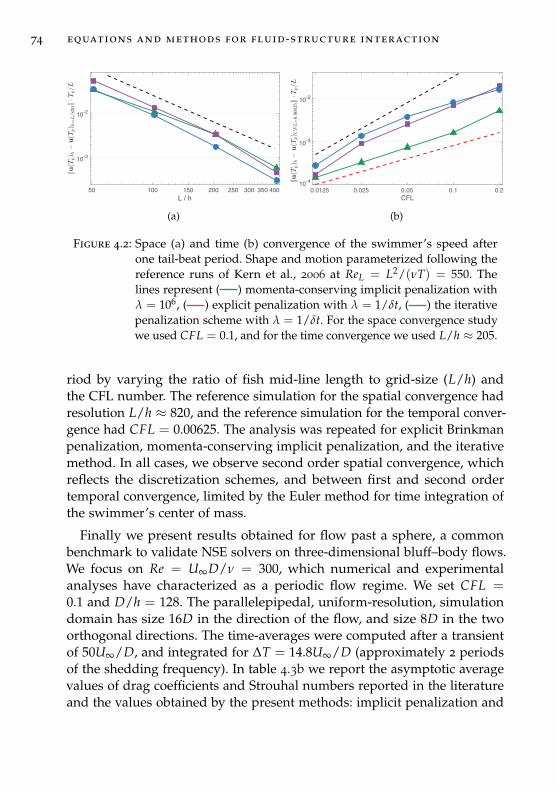
74 equations and methods for fluid-structure interaction
50 100 150 200 250 300 350 400L / h
10-3
10-2
(a)
0.0125 0.025 0.05 0.1 0.2CFL
10-4
10-3
10-2
(b)
Figure 4.2: Space (a) and time (b) convergence of the swimmer’s speed afterone tail-beat period. Shape and motion parameterized following thereference runs of Kern et al., 2006 at ReL = L2/(νT) = 550. Thelines represent ( ) momenta-conserving implicit penalization withλ = 106, ( ) explicit penalization with λ = 1/δt, ( ) the iterativepenalization scheme with λ = 1/δt. For the space convergence studywe used CFL = 0.1, and for the time convergence we used L/h ≈ 205.
riod by varying the ratio of fish mid-line length to grid-size (L/h) andthe CFL number. The reference simulation for the spatial convergence hadresolution L/h ≈ 820, and the reference simulation for the temporal conver-gence had CFL = 0.00625. The analysis was repeated for explicit Brinkmanpenalization, momenta-conserving implicit penalization, and the iterativemethod. In all cases, we observe second order spatial convergence, whichreflects the discretization schemes, and between first and second ordertemporal convergence, limited by the Euler method for time integration ofthe swimmer’s center of mass.
Finally we present results obtained for flow past a sphere, a commonbenchmark to validate NSE solvers on three-dimensional bluff–body flows.We focus on Re = U∞D/ν = 300, which numerical and experimentalanalyses have characterized as a periodic flow regime. We set CFL =0.1 and D/h = 128. The parallelepipedal, uniform-resolution, simulationdomain has size 16D in the direction of the flow, and size 8D in the twoorthogonal directions. The time-averages were computed after a transientof 50U∞/D, and integrated for ∆T = 14.8U∞/D (approximately 2 periodsof the shedding frequency). In table 4.3b we report the asymptotic averagevalues of drag coefficients and Strouhal numbers reported in the literatureand the values obtained by the present methods: implicit penalization and
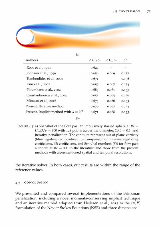
4.5 conclusion 75
(a)
Authors < CD > < CL > St
Roos et al., 1971 0.629 - -
Johnson et al., 1999 0.656 0.069 0.137
Tomboulides et al., 2000 0.671 - 0.136
Kim et al., 2002 0.657 0.067 0.134
Ploumhans et al., 2002 0.683 0.061 0.135
Constantinescu et al., 2004 0.655 0.065 0.136
Mimeau et al., 2016 0.673 0.066 0.133
Present, Iterative method 0.670 0.067 0.135
Present, Implicit method with λ = 1060.671 0.068 0.135
(b)
Figure 4.3: a) Snapshot of the flow past an impulsively started sphere at Re =U∞D/ν = 300 with 128 points across the diameter, CFL = 0.1, anditerative penalization. The contours represent out-of-plane vorticity(blue negative, red positive). (b) Comparison of time-averaged dragcoefficients, lift coefficients, and Strouhal numbers (St) for flow pasta sphere at Re = 300 in the literature and those from the presentmethods with aforementioned spatial and temporal resolutions.
the iterative solver. In both cases, our results are within the range of thereference values.
4.5 conclusion
We presented and compared several implementations of the Brinkmanpenalization, including a novel momenta-conserving implicit techniqueand an iterative method adapted from Hejlesen et al., 2015 to the (u, P)formulation of the Navier-Stokes Equations (NSE) and three dimensions.

76 equations and methods for fluid-structure interaction
We demonstrated that the momenta-conserving implicit technique largelyremoves the dependency of the fluid-structure interaction on the penal-ization coefficient λ. We argue that it is the correct approach to performimplicit time integration of the Brinkman penalization.
In analyzing the iterative technique, we did not observe accuracy benefitsthat would justify the large increase in computational cost (approximately8-times, as we did not introduce any obstacle-sub domains) compared tothe non-iterative implementations. However, we only considered globalvariables (swimming speed, drag coefficients) rather than flow features (asdone in Hejlesen et al., 2015), which could be more visibly affected by thestrict enforcement of boundary conditions allowed by the iterative method.
5E F F I C I E N T C O L L E C T I V E S W I M M I N G B Y H A R N E S S I N GV O RT I C E S
There is a long-standing interest for understanding and exploiting thephysical mechanisms employed by active swimmers in nature (Aleyev, 1977;Lang et al., 1966; Schmidt, 1923; Triantafyllou et al., 2016). Fish schoolingin particular, one of the most striking patterns of collective behaviourand complex decision making in nature, has been the subject of intenseinvestigation (Breder, 1965; Burgerhout et al., 2013; Pavlov et al., 2000; Shaw,1978; Weihs, 1973). Fish sense and navigate in complex flow-fields full ofmechanical energy that is distributed across multiple scales by vorticesgenerated by obstacles and other swimming organisms (Chapman et al.,2011; Montgomery et al., 1997). There is evidence that their swimmingbehaviour adapts to flow gradients (rheotaxis) and, in certain cases, itreflects energy-harvesting from such environments (Liao et al., 2003a; Oteizaet al., 2017).
The fish schooling patterns that form when individual swimmers adapttheir motion to that of their peers is thought to provide an energetic advan-tage to individuals, as well as to their group, in terms of increased swim-ming range, endurance and chances of survival. Schooling has also beencredited with serving diverse biological functions including defence frompredators (Brock et al., 1960; Cushing et al., 1968), enhanced feeding andreproductive opportunities (Pitcher et al., 1982). At present, there is no con-sensus regarding the evolutionary purpose of schooling behaviour (Pavlovet al., 2000). However, there is growing evidence supporting the hypothesisthat fluid dynamics affects swimming patterns in fish schools (Triantafyllouet al., 2016) and related experimental model configurations (Becker et al.,2015) as well as flying patterns of birds (Portugal et al., 2014).
Experiments that have investigated swimming of fish groups indicatea reduction in energy expenditure, based on respirometer readings andreduced tail-beat frequency (Abrahams et al., 1985; Herskin et al., 1998;Jr., 1973; Killen et al., 2012; Svendsen et al., 2003). Importantly, there isevidence to suggest that reduction in energy expenditure is not distributeduniformly throughout a schooling group. Several studies (Herskin et al.,
77
78 efficient collective swimming by harnessing vortices
1998; Killen et al., 2012; Svendsen et al., 2003) have observed that the tail-beatfrequency of trailing fish was lower than that of fish at the front of the school.Moreover, Killen et al., 2012 note that fish with inherently lower aerobicscope prefer to stay towards the rear of a group. Studies investigating theresponse of solitary fish to unsteady flow (Liao et al., 2003a) found that troutswimming behind obstacles exerted reduced effort for station-keeping. Thetrout adopted a gait which allowed them to ‘slalom’ through the oncomingvortex street. The ensuing reduction in muscle activity was confirmedusing neuromuscular measurements (Liao et al., 2003a) and respirometerreadings (Taguchi et al., 2011). These experimental studies suggest that fishcan detect and exploit vortices present in their surroundings (Triantafyllouet al., 2016).
There is a well documented hypothesis (Breder, 1965; Weihs, 1973, 1975)that flow patterns which emerge as a consequence of schooling, can beexploited by individual swimmers. Understanding the role of the flow envi-ronment of fish schooling behaviour has the potential for engineering appli-cations (Whittlesey et al., 2010). This hypothesis was first quantified (Weihs,1973, 1975) using inviscid point-vortices as models of the fish wake-vortices.It was postulated that large groups of fish could gain a propulsive advan-tage by swimming in a ‘diamond’ configuration, with opposing tail-beatphase. The energetic gain was attributed to two distinct mechanisms: drag-reduction resulting from decreased relative velocity in the vicinity of specificvortices; and a forward ‘push’ originating from a ‘channelling effect’ be-tween lateral neighbors. Weihs noted that a rigid geometrical arrangement,and perfectly synchronized anti-phase swimming among lateral neighbours,were unlikely to occur in nature. Nonetheless, he postulated that given theimmense potential for energy savings, even intermittent utilization of theproposed arrangement could lead to a tangible benefit (Weihs, 1975). Suchsimplified models of hydrodynamics in fish schools have even inspired theoptimal design of wind turbine farms (Whittlesey et al., 2010). We notealso that synchronised motion has been obtained for viscous simulationsof two cylinders performing rotary oscillations (Rees et al., 2015). Therole of hydrodynamics in fish-schooling was later questioned (Partridgeet al., 1979), based on empirical observations of fish-schools which rarelydisplayed diamond formations. However, a later study based on aerial pho-tographs of hunting tuna schools (Partridge et al., 1983) provided evidencefor such diamond-like formations. We believe that these studies highlightthe difficulties of maintaining fixed patterns in the dynamically evolvingenvironment of schooling fish. These difficulties are also reflected in simula-
efficient collective swimming by harnessing vortices 79
tions studies. Bergmann et al., 2011 presented short-time simulation of twoand three self-propelled swimmers with prescribed kinematics that mayeventually lead to the collision or divergence of the swimmers. Long-timesimulations of multiple swimmers, have either pre-specified their spatialdistribution and kinematics (Daghooghi et al., 2015; Hemelrijk et al., 2015;Maertens et al., 2017) or they have employed potential flow models (Gazzolaet al., 2016; Tsang et al., 2013). We note that simulations of single swimmersperforming optimised swimming motions have been performed over thelast ten years (Borazjani et al., 2008; Daghooghi et al., 2016; Gilmanov et al.,2005; Kern et al., 2006).
Here, we present two- and three-dimensional simulations of viscous,incompressible flows of self-propelled swimmers in coordinated swim-ming patterns that can dynamically discover their swimming strategies viaReinforcement Learning (RL). To the best of our knowledge, no viscoussimulations have ever been presented for multiple self-propelled swimmerswith sustained synchronised motions. We focus on two swimmers in asustained leader-follower configuration, a biologically relevant schoolingpattern characterized by the follower interacting with the unsteady flowin the leader’s wake. We investigate the hydrodynamic interactions of theswimmers in various scenarios including pre-specified coordinated motionsand initial distances, as well as the dynamic adaptation of the follower’smotion using a reinforcement learning algorithm, so as to remain withina specific region in the leader’s wake. We investigate the impact of theleader’s wake on the follower’s motion and identify the mechanisms thatlead to energy savings. The chapter is organised as follows: we outlinethe numerical methods for the simulations of self-propelled swimmersin Section 5.1, and the reinforcement learning algorithm is discussed inSection 5.2.
We distinguish externally imposed motions on the swimmers to those thatare achieved by the deformation of the body of self-propelled swimmers.In section we discuss two rigid airfoils executing pre-specified motion, twoself-propelled swimmers interacting without control, and a ‘smart’ followerutilizing adaptive control to interact with the leader’s wake.
acknowledgments This chapter is based on the papers “Synchronisa-tion through learning for two self-propelled swimmers” (Novati et al., 2017)and “Efficient collective swimming by harnessing vortices through deepreinforcement learning” (Verma et al., 2018). The computational resources
80 efficient collective swimming by harnessing vortices
were provided by a grant from the Swiss National Super-computing Centre(CSCS) under project s658.
5.1 simulation details
The simulations presented here are based on the incompressible Navier-Stokes (NS) equations:
∇ · u = 0∂u∂t
+ u · ∇u = −∇Pρ f
+ ν∇2u + λχ(us − u)
Each swimmer is represented on the computational grid via the character-istic function χ, and interacts with the fluid by means of the penalty (Co-querelle et al., 2008) term λχ (us − u) .Here, us denotes the swimmer’scombined translational, rotational, and deformation velocity, whereas u andν correspond to the fluid velocity and viscosity, respectively. P representsthe pressure, and the fluid density is denoted by ρ f .
The vorticity form of the NS equations was used for the two-dimensionalsimulations, with λ = 1e6. A wavelet adaptive grid (Rossinelli et al., 2015)with an effective resolution of 40962 points was used to discretize a unitsquare domain. A lower effective resolution of 10242 points was used forthe training-simulations to minimize computational cost. We have deter-mined in previous tests that this resolution provides a reasonable balancebetween speed and accuracy (Verma et al., 2017a). The pressure-Poissonequation (∇2P = −ρ f
(∇uT : ∇u
)+ ρ f λ∇ · (χ (us − u))), necessary for
estimating the distribution of flow-induced forces on the swimmers’ bodies,was solved using the Fast Multipole Method with free-space boundaryconditions (Verma et al., 2017a). The Lagrangian CFL number was set to0.1, with the resulting time-step size ranging from 1e-4 to 1e-3.
The three-dimensional simulations were performed with the pressure-projection method for solving the NS equations (Chorin, 1968) described inthe previous chapter. The simulations were carried out on a uniform gridconsisting of 2048× 1024× 256 points in a domain of size 1× 0.5× 0.125,with penalty parameter λ = 1e5. Further grid-refinement by 1.5× in allthree directions, and increasing the penalty parameter to 1e6 resulted in nodiscernible change in the swimmer’s speed. Thus, the lower grid resolutionwas selected to keep computational cost manageable. The CFL (Courant-Friedrichs-Lewy) number was constrained to be less than 0.1, resulting in
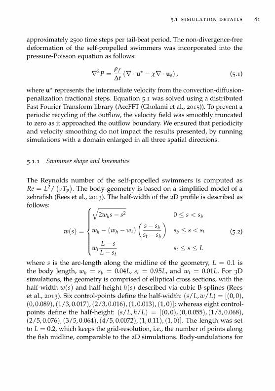
5.1 simulation details 81
approximately 2500 time steps per tail-beat period. The non-divergence-freedeformation of the self-propelled swimmers was incorporated into thepressure-Poisson equation as follows:
∇2P =ρ f
∆t(∇ · u? − χ∇ · us) , (5.1)
where u? represents the intermediate velocity from the convection-diffusion-penalization fractional steps. Equation 5.1 was solved using a distributedFast Fourier Transform library (AccFFT (Gholami et al., 2015)). To prevent aperiodic recycling of the outflow, the velocity field was smoothly truncatedto zero as it approached the outflow boundary. We ensured that periodicityand velocity smoothing do not impact the results presented, by runningsimulations with a domain enlarged in all three spatial directions.
5.1.1 Swimmer shape and kinematics
The Reynolds number of the self-propelled swimmers is computed asRe = L2/
(νTp
). The body-geometry is based on a simplified model of a
zebrafish (Rees et al., 2013). The half-width of the 2D profile is described asfollows:
w(s) =
√2whs− s2 0 ≤ s < sb
wh − (wh − wt)
(s− sbst − sb
)sb ≤ s < st
wtL− sL− st
st ≤ s ≤ L
(5.2)
where s is the arc-length along the midline of the geometry, L = 0.1 isthe body length, wh = sb = 0.04L, st = 0.95L, and wt = 0.01L. For 3Dsimulations, the geometry is comprised of elliptical cross sections, with thehalf-width w(s) and half-height h(s) described via cubic B-splines (Reeset al., 2013). Six control-points define the half-width: (s/L, w/L) = [(0, 0),(0, 0.089), (1/3, 0.017), (2/3, 0.016), (1, 0.013), (1, 0)]; whereas eight control-points define the half-height: (s/L, h/L) = [(0, 0), (0, 0.055), (1/5, 0.068),(2/5, 0.076), (3/5, 0.064), (4/5, 0.0072), (1, 0.11), (1, 0)]. The length was setto L = 0.2, which keeps the grid-resolution, i.e., the number of points alongthe fish midline, comparable to the 2D simulations. Body-undulations for
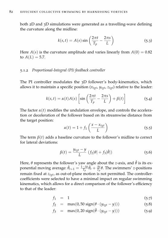
82 efficient collective swimming by harnessing vortices
both 2D and 3D simulations were generated as a travelling-wave definingthe curvature along the midline:
k(s, t) = A(s) sin(
2πtTp− 2πs
L
)(5.3)
Here A(s) is the curvature amplitude and varies linearly from A(0) = 0.82to A(L) = 5.7.
5.1.2 Proportional-Integral (PI) feedback controller
The PI controller modulates the 3D follower’s body-kinematics, whichallows it to maintain a specific position (xtgt, ytgt, ztgt) relative to the leader:
k(s, t) = α(t)A(s)[
sin(
2πtTp− 2πs
L
)+ β(t)
](5.4)
The factor α(t) modifies the undulation envelope, and controls the accelera-tion or deceleration of the follower based on its streamwise distance fromthe target position:
α(t) = 1 + f1
(x− xtgt
L
)(5.5)
The term β(t) adds a baseline curvature to the follower’s midline to correctfor lateral deviations:
β(t) =ytgt − y
L( f2|θ|+ f3|θ|) (5.6)
Here, θ represents the follower’s yaw angle about the z-axis, and θ is its ex-ponential moving average: θt+1 = 1−∆t
Tpθt +
∆tTp
θ. The swimmers’ z-positionsremain fixed at ztgt, as out-of-plane motion is not permitted. The controller-coefficients were selected to have a minimal impact on regular swimmingkinematics, which allows for a direct comparison of the follower’s efficiencyto that of the leader:
f1 = 1 (5.7)
f2 = max(0, 50 sign(θ · (ytgt − y))) (5.8)
f3 = max(0, 20 sign(θ · (ytgt − y))) (5.9)
5.2 reinforcement learning 83
5.2 reinforcement learning
Reinforcement Learning (RL) (Sutton et al., 1998) has been introduced toidentify navigation policies in several model systems of vortex dipoles, soar-ing birds and micro-swimmers (Colabrese et al., 2017; Gazzola et al., 2016;Reddy et al., 2016). These studies often rely on simplified representationsof organisms interacting with their environment, which allows them tomodel animal-locomotion with reduced physical complexity, and manage-able computational cost. However, the simplifying assumptions inherentin such models often do not account for feedback of the animals’ motionon the environment. High-fidelity numerical simulations, although signifi-cantly more computationally demanding, can account for such importantconsiderations to a greater extent, for instance by allowing flapping orswimming motions that closely mimic the interaction of real animals withtheir environment. This makes them invaluable for investigating conceptsthat may be carried over readily to bioinspired robotic applications, withminimal modification. This consideration has motivated our present studyon combining Reinforcement Learning with Direct Numerical Simulationsof the Navier–Stokes equations for self-propelled autonomous swimmers.
RL is a process by which an agent (in this case, a swimmer) learnsto earn rewards through trial-and-error interaction with its environmentover discrete time steps. At each turn, the agent observes the state ofthe environment sn ∈ RdimS and performs an action an, which influencesboth the transition to the next state sn+1 ∈ RdimS and the reward receivedrn+1 ∈ R. RL is well suited to flow control problems as it searches foractuation policies that maximize the reward signal without requiring anymodel or prior knowledge about the underlying dynamics. In this case,the scalar reward signal measures specific high-level objectives, such asdeviation from a target schooling formation or swimming efficiency andwill be discussed in more detail in Section 5.5.
In this chapter we consider a RL problem with a discrete action space,i.e. at each turn the agent may select one out of NA options and an ∈1, 2, · · · , NA. Therefore, we employ RL algorithms based on Q-learning(Watkins et al., 1992). The agent’s goal is to learn the optimal control policya ∼ π∗(·|s) which maximises the action value Qπ(s, a), defined as the sumof discounted future rewards:
Qπ(s, a) = E
[r1 + γr2 + γ2r3 + · · ·
∣∣∣s0=sa0=a
an∼π(·| sn),sn+1,rn+1∼D(·| sn ,an)
](5.10)
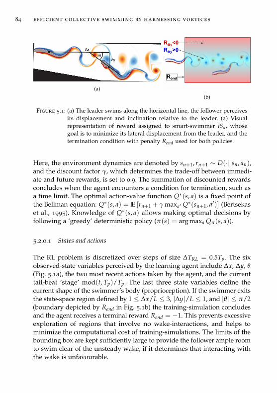
84 efficient collective swimming by harnessing vortices
∆x
∆y
(a)
(b)
Figure 5.1: (a) The leader swims along the horizontal line, the follower perceivesits displacement and inclination relative to the leader. (a) Visualrepresentation of reward assigned to smart-swimmer ISd, whosegoal is to minimize its lateral displacement from the leader, and thetermination condition with penalty Rend used for both policies.
Here, the environment dynamics are denoted by sn+1, rn+1 ∼ D(·| sn, an),and the discount factor γ, which determines the trade-off between immedi-ate and future rewards, is set to 0.9. The summation of discounted rewardsconcludes when the agent encounters a condition for termination, such asa time limit. The optimal action-value function Q∗(s, a) is a fixed point ofthe Bellman equation: Q∗(s, a) = E [rn+1 + γ maxa′ Q∗(sn+1, a′)] (Bertsekaset al., 1995). Knowledge of Q∗(s, a) allows making optimal decisions byfollowing a ‘greedy’ deterministic policy (π(s) = arg maxa Qπ(s, a)).
5.2.0.1 States and actions
The RL problem is discretized over steps of size ∆TRL = 0.5Tp. The sixobserved-state variables perceived by the learning agent include ∆x, ∆y, θ(Fig. 5.1a), the two most recent actions taken by the agent, and the currenttail-beat ‘stage’ mod(t, Tp)/Tp. The last three state variables define thecurrent shape of the swimmer’s body (proprioception). If the swimmer exitsthe state-space region defined by 1 ≤ ∆x/L ≤ 3, |∆y|/L ≤ 1, and |θ| ≤ π/2(boundary depicted by Rend in Fig. 5.1b) the training-simulation concludesand the agent receives a terminal reward Rend = −1. This prevents excessiveexploration of regions that involve no wake-interactions, and helps tominimize the computational cost of training-simulations. The limits of thebounding box are kept sufficiently large to provide the follower ample roomto swim clear of the unsteady wake, if it determines that interacting withthe wake is unfavourable.
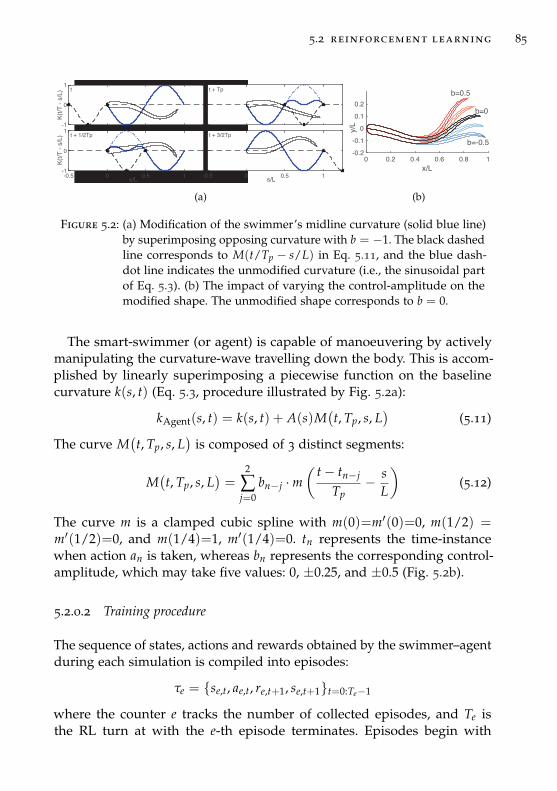
5.2 reinforcement learning 85
K(t/T
- s/
L)
-1
0
1
-1
0
1
-0.5 0 0.5 1s/L
K(t/T
- s/
L) t + 3/2Tp
t + Tpt
t + 1/2Tp
-0.5 0 0.5 1s/L
(a)
x/L0 0.2 0.4 0.6 0.8 1
y/L
-0.2
-0.1
0
0.1
0.2
b=-0.5
b=0
b=0.5
(b)
Figure 5.2: (a) Modification of the swimmer’s midline curvature (solid blue line)by superimposing opposing curvature with b = −1. The black dashedline corresponds to M(t/Tp − s/L) in Eq. 5.11, and the blue dash-dot line indicates the unmodified curvature (i.e., the sinusoidal partof Eq. 5.3). (b) The impact of varying the control-amplitude on themodified shape. The unmodified shape corresponds to b = 0.
The smart-swimmer (or agent) is capable of manoeuvering by activelymanipulating the curvature-wave travelling down the body. This is accom-plished by linearly superimposing a piecewise function on the baselinecurvature k(s, t) (Eq. 5.3, procedure illustrated by Fig. 5.2a):
kAgent(s, t) = k(s, t) + A(s)M(t, Tp, s, L
)(5.11)
The curve M(t, Tp, s, L
)is composed of 3 distinct segments:
M(t, Tp, s, L
)=
2
∑j=0
bn−j ·m( t− tn−j
Tp− s
L
)(5.12)
The curve m is a clamped cubic spline with m(0)=m′(0)=0, m(1/2) =m′(1/2)=0, and m(1/4)=1, m′(1/4)=0. tn represents the time-instancewhen action an is taken, whereas bn represents the corresponding control-amplitude, which may take five values: 0, ±0.25, and ±0.5 (Fig. 5.2b).
5.2.0.2 Training procedure
The sequence of states, actions and rewards obtained by the swimmer–agentduring each simulation is compiled into episodes:
τe = se,t, ae,t, re,t+1, se,t+1t=0:Te−1
where the counter e tracks the number of collected episodes, and Te isthe RL turn at with the e-th episode terminates. Episodes begin with
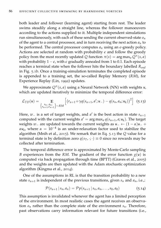
86 efficient collective swimming by harnessing vortices
both leader and follower (learning agent) starting from rest. The leaderswims steadily along a straight line, whereas the follower manoeuversaccording to the actions supplied to it. Multiple independent simulationsrun simultaneously, with each of these sending the current observed-state onof the agent to a central processor, and in turn receiving the next action an tobe performed. The central processor computes an using an ε-greedy policy.Actions are selected at random with probability ε and follow the greedypolicy from the most recently updated Q function π(s) = arg maxa Qπ(s, a)with probability 1− ε, with ε gradually annealed from 1 to 0.1. Each episodereaches a terminal state when the follower hits the boundary labelled Rendin Fig. 5.1b. Once a training-simulation terminates the completed episodeis appended to a training set, the so-called Replay Memory (RM), forExperience Replay (Lin, 1992) updates.
We approximate Qπ(s, a) using a Neural Network (NN) with weights w,which are updated iteratively to minimize the temporal difference error:
LTD(w) = E sn , an ,sn+1,rn+1
∼RM
[(rn+1+γq(sn+1, a′; w−)− q(sn, an; wk)
)2]
(5.13)
Here, w− is a set of target weights, and a′ is the best action in state sn+1computed with the current weights a′ = arg maxa q(sn+1, a; wk). The targetweights w− are updated towards the current weights as w− ← (1− α)w− +αwk, where α = 10−4 is an under-relaxation factor used to stabilize thealgorithm (Mnih et al., 2015). We remark that in Eq. 5.13 the Q value for aterminal state is by definition zero q(sT , ·; ·) ≡ 0 since no rewards may becollected after termination.
The temporal difference error is approximated by Monte-Carlo samplingB experiences from the RM. The gradient of the error function g(w) iscomputed via back propagation through time (BPTT) (Graves et al., 2005)and the weights are then updated with the Adam stochastic optimizationalgorithm (Kingma et al., 2014).
One of the assumptions in RL is that the transition probability to a newstate sn+1 is independent of the previous transitions, given sn and an, i.e.,:
P(sn+1 | sn, an) = P p(sn+1 | sn, an, . . . , s0, a0) (5.14)
This assumption is invalidated whenever the agent has a limited perceptionof the environment. In most realistic cases the agent receives an observa-tion on rather than the complete state of the environment sn. Therefore,past observations carry information relevant for future transitions (i.e.,
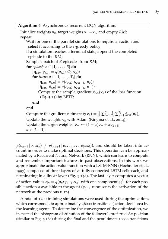
5.2 reinforcement learning 87
Algorithm 6: Asynchronous recurrent DQN algorithm.
Initialize weights w0, target weights w−=w0, and empty RM;repeat
Wait for one of the parallel simulations to require an action andselect it according to the ε-greedy policy;
If a simulation reaches a terminal state, append the completedepisode to the RM;
Sample a batch of B episodes from RM;for episode e ∈ [1, . . . , B] do
[qe,0, ye,0] = q(oe,0; ∅, wk);for turns n ∈ [1, . . . , Te] do
[qe,n, ye,n] = q(oe,n; ye,n−1, wk);[qe,n, ye,n] = q(oe,n; ye,n−1, w−);Compute the sample gradient ge,n(wk) of the loss function(Eq. 5.13) by BPTT;
endendCompute the gradient estimate g(wk) =
1B ∑B
e=11Te
∑Ten=1 ge,n(wk);
Update the weights wk with Adam (Kingma et al., 2014);Update the target weights: w− ← (1− α)w− + αwk+1;k← k + 1;
p(on+1 | on, an) 6= p(on+1 | on, an, . . . , o0, a0)), and should be taken into ac-count in order to make optimal decisions. This operation can be approxi-mated by a Recurrent Neural Network (RNN), which can learn to computeand remember important features in past observations. In this work weapproximate the action-value function with a LSTM-RNN (Hochreiter et al.,1997) composed of three layers of 24 fully connected LSTM cells each, andterminating in a linear layer (Fig. 5.14a). The last layer computes a vectorof action-values qn = q(on; yn−1, wk) with one component q(a)
n for each pos-sible action a available to the agent (yn−1 represents the activation of thenetwork at the previous turn).
A total of 1200 training simulations were used during the optimization,which corresponds to approximately 46000 transitions (action decisions) bythe learning agents. To determine the convergence of the optimization, weinspected the histogram distribution of the follower’s preferred ∆x position(similar to Fig. 5.16a) during the final and the penultimate 10000 transitions.
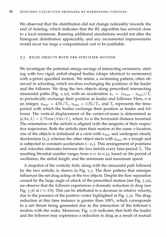
88 efficient collective swimming by harnessing vortices
We observed that the distribution did not change noticeably towards theend of training, which indicates that the RL algorithm has arrived closeto a local minimum. Running additional simulations would not alter thehistogram distribution appreciably, and any incremental improvementswould incur too large a computational cost to be justifiable.
5.3 rigid objects with pre-specified motion
We investigate the potential energy-savings of interacting swimmers, start-ing with two rigid, airfoil-shaped bodies (shape identical to swimmers)with a-priori specified motion. We mimic a swimming pattern, often ob-served in schooling, which involves exchanging the positions of the leaderand the follower. We drag the two objects along prescribed intersectingsinusoidal paths (Fig. 5.3a), with an acceleration ax = (umax − umin)/Tsto periodically exchange their position as leader and follower. Here, n isan integer, umax = 4.5L/Ts, umin = 1.5L/Ts, and Ts represents the time-period with which the bodies exchange their position as leader and fol-lower. The vertical displacement of the center-of-mass is determined asy(∆x, L) = L/5 cos (π∆x/L), where ∆x is the horizontal distance traversed.The orientation of the airfoils is aligned with the tangents of their respec-tive trajectories. Both the airfoils start their motion at the same x-location;one of the objects is initialized at a crest with umax and undergoes steadydeceleration (ax), whereas the other object starts with umin on a trough andis subjected to constant acceleration (−ax). This arrangement of positionsand velocities alternates between the two airfoils every time-period Ts. Theresulting Strouhal number ranges from 0.11 to 0.33, based on the period ofoscillation, the airfoil length, and the minimum and maximum speed.
A snapshot of the vorticity field, along with the sinusoidal path followedby the two airfoils, is shown in Fig. 5.3. The flow pattern that emergesinfluences the net drag acting on the two objects. Despite the flow separationcaused by the large angle of attack of the prescribed motion (see Fig. 5.3a),we observe that the follower experiences a dramatic reduction in drag (seeFig. 5.3b at t ≈ 3.9). This can be attributed to a decrease in relative velocity,due to the presence of the positive vortex highlighted in Fig. 5.3a. The drag-reduction at this time instance is greater than 100%, which correspondsto a net thrust being generated due to the interaction of the follower’smotion with the wake. Moreover, Fig. 5.3b indicates that both the leaderand the follower may experience a reduction in drag as a result of mutual
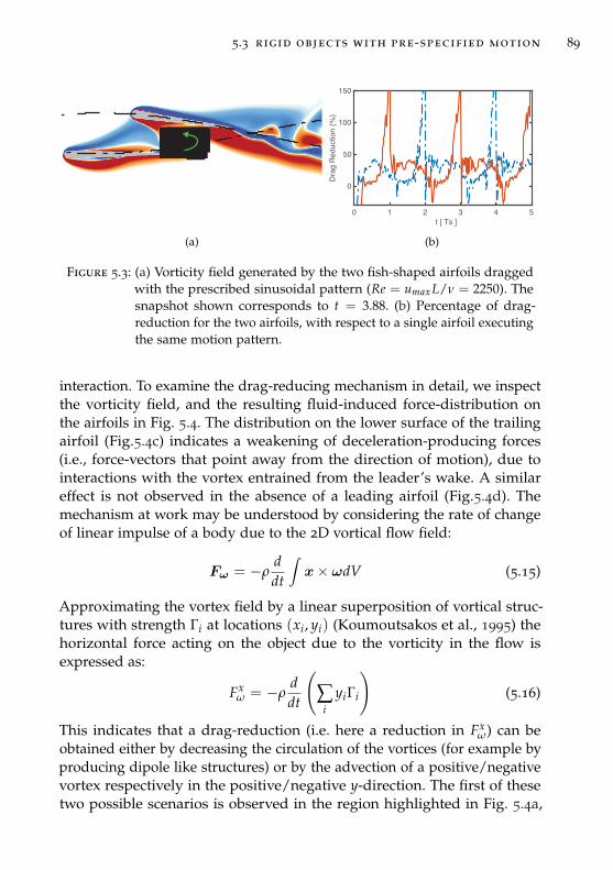
5.3 rigid objects with pre-specified motion 89
(a)
t [ Ts ]0 1 2 3 4 5
Dra
g R
educ
tion
(%)
0
50
100
150
(b)
Figure 5.3: (a) Vorticity field generated by the two fish-shaped airfoils draggedwith the prescribed sinusoidal pattern (Re = umax L/ν = 2250). Thesnapshot shown corresponds to t = 3.88. (b) Percentage of drag-reduction for the two airfoils, with respect to a single airfoil executingthe same motion pattern.
interaction. To examine the drag-reducing mechanism in detail, we inspectthe vorticity field, and the resulting fluid-induced force-distribution onthe airfoils in Fig. 5.4. The distribution on the lower surface of the trailingairfoil (Fig.5.4c) indicates a weakening of deceleration-producing forces(i.e., force-vectors that point away from the direction of motion), due tointeractions with the vortex entrained from the leader’s wake. A similareffect is not observed in the absence of a leading airfoil (Fig.5.4d). Themechanism at work may be understood by considering the rate of changeof linear impulse of a body due to the 2D vortical flow field:
Fω = −ρddt
∫x×ωdV (5.15)
Approximating the vortex field by a linear superposition of vortical struc-tures with strength Γi at locations (xi, yi) (Koumoutsakos et al., 1995) thehorizontal force acting on the object due to the vorticity in the flow isexpressed as:
Fxω = −ρ
ddt
(∑
iyiΓi
)(5.16)
This indicates that a drag-reduction (i.e. here a reduction in Fxω) can be
obtained either by decreasing the circulation of the vortices (for example byproducing dipole like structures) or by the advection of a positive/negativevortex respectively in the positive/negative y-direction. The first of thesetwo possible scenarios is observed in the region highlighted in Fig. 5.4a,
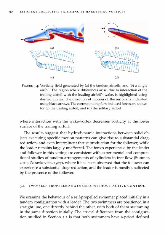
90 efficient collective swimming by harnessing vortices
(a) (b)
(c) (d)
Figure 5.4: Vorticity field generated by (a) the tandem airfoils, and (b) a singleairfoil. The region where differences arise, due to interaction of thetrailing airfoil with the leading airfoil’s wake, is highlighted usingdashed circles. The direction of motion of the airfoils is indicatedusing black arrows. The corresponding flow-induced forces are shownfor (c) the trailing airfoil, and (d) the solitary airfoil.
where interaction with the wake-vortex decreases vorticity at the lowersurface of the trailing airfoil.
The results suggest that hydrodynamic interactions between solid ob-jects executing specific motion patterns can give rise to substantial drag-reduction, and even intermittent thrust production for the follower, whilethe leader remains largely unaffected. The forces experienced by the leaderand follower in this setting are consistent with experimental and computa-tional studies of tandem arrangements of cylinders in free flow (Sumner,2010; Zdravkovich, 1977), where it has been observed that the follower canexperience a substantial drag-reduction, and the leader is mostly unaffectedby the presence of the follower.
5.4 two-self propelled swimmers without active control
We examine the behaviour of a self-propelled swimmer placed initially in atandem configuration with a leader. The two swimmers are positioned in astraight line, one directly behind the other, with both of them swimmingin the same direction initially. The crucial difference from the configura-tion studied in Section 5.3 is that both swimmers have a-priori defined
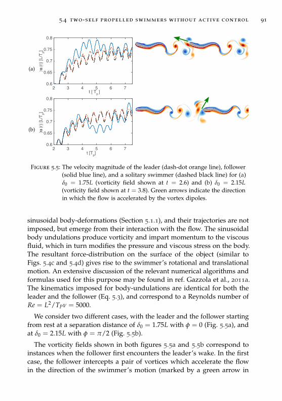
5.4 two-self propelled swimmers without active control 91
(a)
t [ Tp ]2 3 4 5 6 7
|u (t)|
[L/T
p]
0.6
0.65
0.7
0.75
0.8
(b)
2 3 4 5 6 7
|u (t)| [
L/T p]
0.6
0.65
0.7
0.75
0.8
t [Tp]
Figure 5.5: The velocity magnitude of the leader (dash-dot orange line), follower(solid blue line), and a solitary swimmer (dashed black line) for (a)δ0 = 1.75L (vorticity field shown at t = 2.6) and (b) δ0 = 2.15L(vorticity field shown at t = 3.8). Green arrows indicate the directionin which the flow is accelerated by the vortex dipoles.
sinusoidal body-deformations (Section 5.1.1), and their trajectories are notimposed, but emerge from their interaction with the flow. The sinusoidalbody undulations produce vorticity and impart momentum to the viscousfluid, which in turn modifies the pressure and viscous stress on the body.The resultant force-distribution on the surface of the object (similar toFigs. 5.4c and 5.4d) gives rise to the swimmer’s rotational and translationalmotion. An extensive discussion of the relevant numerical algorithms andformulas used for this purpose may be found in ref. Gazzola et al., 2011a.The kinematics imposed for body-undulations are identical for both theleader and the follower (Eq. 5.3), and correspond to a Reynolds number ofRe = L2/TPν = 5000.
We consider two different cases, with the leader and the follower startingfrom rest at a separation distance of δ0 = 1.75L with φ = 0 (Fig. 5.5a), andat δ0 = 2.15L with φ = π/2 (Fig. 5.5b).
The vorticity fields shown in both figures 5.5a and 5.5b correspond toinstances when the follower first encounters the leader’s wake. In the firstcase, the follower intercepts a pair of vortices which accelerate the flowin the direction of the swimmer’s motion (marked by a green arrow in
92 efficient collective swimming by harnessing vortices
Fig. 5.5a). The reduction in relative velocity of the flow provides a drag-reduction resulting in a 9.5% increase of the follower’s maximum speed(Fig. 5.5a, t ≈ 4.4). In the second case, the follower intercepts a pair ofvortices which increases the relative velocity of the flow, and causes a largelateral deviation of the follower, with a subsequent speed-change of up to−9% (Fig. 5.5b, t ≈ 4.9). This vortex-induced acceleration or deceleration isequivalent, in a self-propelled setting, to the reduction in drag discussedin the previous section for the prescribed motion (please see Fig. 5.4). TheStrouhal number for the fast follower is 0.23, and that for the slow followeris 0.31, based on the tail-beat period, maximum tail-beat amplitude, andthe maximum/minimum speeds.
These results suggest that unsteady vortical structures in a leader’s wakecan have both a beneficial, as well as a detrimental impact on the perfor-mance of a follower. Furthermore, in both cases, the follower’s trajectorystarts deviating laterally as soon as it encounters the wake, and the followeris completely clear of the wake after approximately 4 to 6 tail-beat periods.This suggests the need for active modulation of the trailing swimmer’sactions when navigating a leader’s wake, in order to maintain a tandemconfiguration.
5.5 learning to intercept vortices for efficient swimming
We now examine configurations of two self-propelled swimmers in a leader-follower arrangement, and investigate the physical mechanisms that lead toenergetically beneficial interactions by considering four distinct scenarios.Two of these involve Active Followers (AF) navigating a leader’s wakeaccording to the control policy trained by RL (e.g., the follower in Fig. 5.1a).Additionally, we consider two distinct Solitary Swimmers (SS) that swim inisolation in an unbounded domain. These Active Followers take decisionsby virtue of deep RL (see Section 5.2), using visual cues from their environ-ment (see Fig. 5.1a). AFη denotes swimmers that learns the most efficientway of swimming in the leader’s wake by finding the policy πw
η whichmaximizes rn = η(n · ∆TRL) (without any positional constraints). We recallfrom Section 5.2.0.1 that RL select actions over discrete turns n spaced bysimulation–time intervals ∆TRL = Tp/2. In turn, swimmer AF∆y attemptsto minimize lateral deviations from the leader’s path by training the policyπw
d . The reward function for AF∆y penalizes the follower when it deviateslaterally from the path of the leader; i.e. rn = 1− |∆y(n · ∆TRL)|/L.
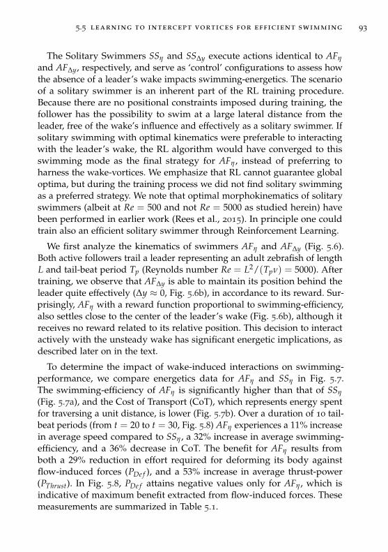
5.5 learning to intercept vortices for efficient swimming 93
The Solitary Swimmers SSη and SS∆y execute actions identical to AFη
and AF∆y, respectively, and serve as ‘control’ configurations to assess howthe absence of a leader’s wake impacts swimming-energetics. The scenarioof a solitary swimmer is an inherent part of the RL training procedure.Because there are no positional constraints imposed during training, thefollower has the possibility to swim at a large lateral distance from theleader, free of the wake’s influence and effectively as a solitary swimmer. Ifsolitary swimming with optimal kinematics were preferable to interactingwith the leader’s wake, the RL algorithm would have converged to thisswimming mode as the final strategy for AFη , instead of preferring toharness the wake-vortices. We emphasize that RL cannot guarantee globaloptima, but during the training process we did not find solitary swimmingas a preferred strategy. We note that optimal morphokinematics of solitaryswimmers (albeit at Re = 500 and not Re = 5000 as studied herein) havebeen performed in earlier work (Rees et al., 2015). In principle one couldtrain also an efficient solitary swimmer through Reinforcement Learning.
We first analyze the kinematics of swimmers AFη and AF∆y (Fig. 5.6).Both active followers trail a leader representing an adult zebrafish of lengthL and tail-beat period Tp (Reynolds number Re = L2/(Tpν) = 5000). Aftertraining, we observe that AF∆y is able to maintain its position behind theleader quite effectively (∆y ≈ 0, Fig. 5.6b), in accordance to its reward. Sur-prisingly, AFη with a reward function proportional to swimming-efficiency,also settles close to the center of the leader’s wake (Fig. 5.6b), although itreceives no reward related to its relative position. This decision to interactactively with the unsteady wake has significant energetic implications, asdescribed later on in the text.
To determine the impact of wake-induced interactions on swimming-performance, we compare energetics data for AFη and SSη in Fig. 5.7.The swimming-efficiency of AFη is significantly higher than that of SSη
(Fig. 5.7a), and the Cost of Transport (CoT), which represents energy spentfor traversing a unit distance, is lower (Fig. 5.7b). Over a duration of 10 tail-beat periods (from t = 20 to t = 30, Fig. 5.8) AFη experiences a 11% increasein average speed compared to SSη , a 32% increase in average swimming-efficiency, and a 36% decrease in CoT. The benefit for AFη results fromboth a 29% reduction in effort required for deforming its body againstflow-induced forces (PDe f ), and a 53% increase in average thrust-power(PThrust). In Fig. 5.8, PDe f attains negative values only for AFη , which isindicative of maximum benefit extracted from flow-induced forces. Thesemeasurements are summarized in Table 5.1.
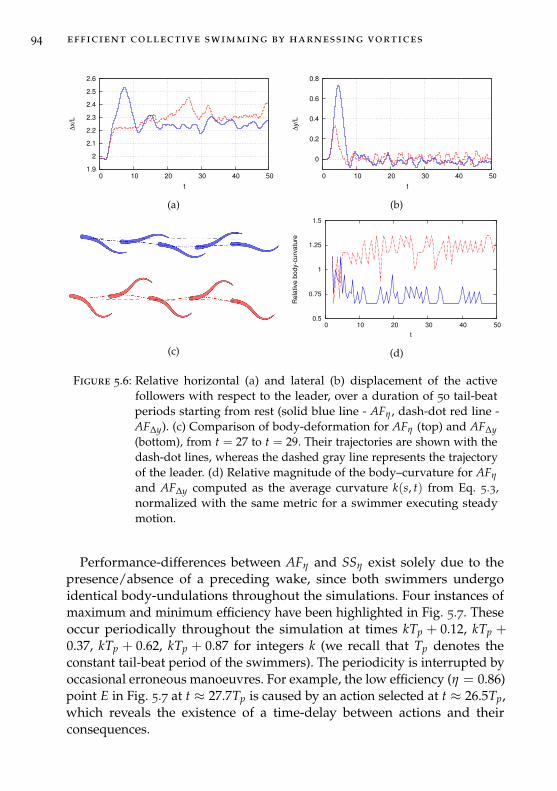
94 efficient collective swimming by harnessing vortices
1.9
2
2.1
2.2
2.3
2.4
2.5
2.6
0 10 20 30 40 50
∆x/L
t
(a)
0
0.2
0.4
0.6
0.8
0 10 20 30 40 50
∆y/L
t
(b)
(c)
0.5
0.75
1
1.25
1.5
0 10 20 30 40 50
Rela
tive b
ody-c
urv
atu
re
t
(d)
Figure 5.6: Relative horizontal (a) and lateral (b) displacement of the activefollowers with respect to the leader, over a duration of 50 tail-beatperiods starting from rest (solid blue line - AFη , dash-dot red line -AF∆y). (c) Comparison of body-deformation for AFη (top) and AF∆y(bottom), from t = 27 to t = 29. Their trajectories are shown with thedash-dot lines, whereas the dashed gray line represents the trajectoryof the leader. (d) Relative magnitude of the body–curvature for AFη
and AF∆y computed as the average curvature k(s, t) from Eq. 5.3,normalized with the same metric for a swimmer executing steadymotion.
Performance-differences between AFη and SSη exist solely due to thepresence/absence of a preceding wake, since both swimmers undergoidentical body-undulations throughout the simulations. Four instances ofmaximum and minimum efficiency have been highlighted in Fig. 5.7. Theseoccur periodically throughout the simulation at times kTp + 0.12, kTp +0.37, kTp + 0.62, kTp + 0.87 for integers k (we recall that Tp denotes theconstant tail-beat period of the swimmers). The periodicity is interrupted byoccasional erroneous manoeuvres. For example, the low efficiency (η = 0.86)point E in Fig. 5.7 at t ≈ 27.7Tp is caused by an action selected at t ≈ 26.5Tp,which reveals the existence of a time-delay between actions and theirconsequences.
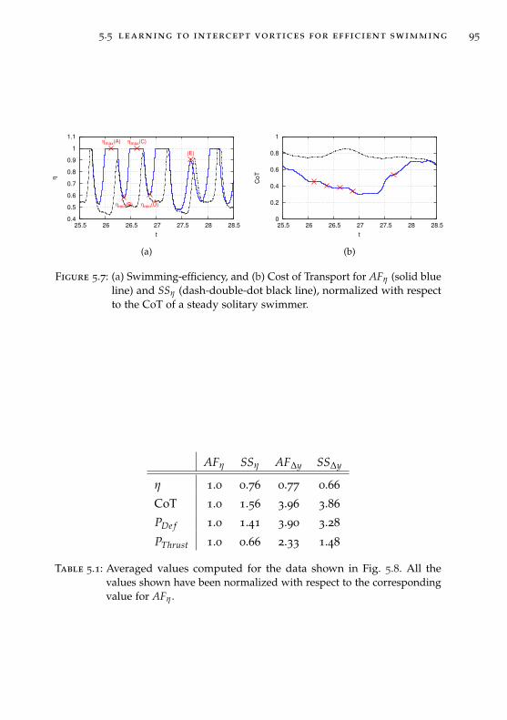
5.5 learning to intercept vortices for efficient swimming 95
0.4
0.5
0.6
0.7
0.8
0.9
1
1.1
25.5 26 26.5 27 27.5 28 28.5
η
t
ηmax(A)
ηmin(B)
ηmax(C)
ηmin(D)
(E)
(a)
0
0.2
0.4
0.6
0.8
1
25.5 26 26.5 27 27.5 28 28.5
Co
T
t
(b)
Figure 5.7: (a) Swimming-efficiency, and (b) Cost of Transport for AFη (solid blueline) and SSη (dash-double-dot black line), normalized with respectto the CoT of a steady solitary swimmer.
AFη SSη AF∆y SS∆y
η 1.0 0.76 0.77 0.66
CoT 1.0 1.56 3.96 3.86
PDe f 1.0 1.41 3.90 3.28
PThrust 1.0 0.66 2.33 1.48
Table 5.1: Averaged values computed for the data shown in Fig. 5.8. All thevalues shown have been normalized with respect to the correspondingvalue for AFη .
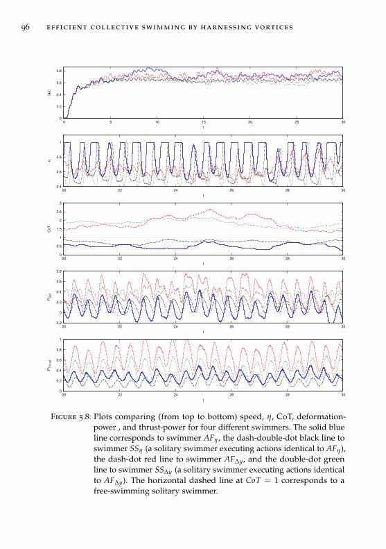
96 efficient collective swimming by harnessing vortices
0
0.2
0.4
0.6
0.8
0 5 10 15 20 25 30
||u
||
t
0.4
0.6
0.8
1
20 22 24 26 28 30
η
t
0
0.5
1
1.5
2
2.5
3
20 22 24 26 28 30
CoT
t
-0.2
0
0.2
0.4
0.6
0.8
20 22 24 26 28 30
PD
ef
t
0
0.2
0.4
0.6
0.8
1
20 22 24 26 28 30
PT
hru
st
t
Figure 5.8: Plots comparing (from top to bottom) speed, η, CoT, deformation-power , and thrust-power for four different swimmers. The solid blueline corresponds to swimmer AFη , the dash-double-dot black line toswimmer SSη (a solitary swimmer executing actions identical to AFη),the dash-dot red line to swimmer AF∆y, and the double-dot greenline to swimmer SS∆y (a solitary swimmer executing actions identicalto AF∆y). The horizontal dashed line at CoT = 1 corresponds to afree-swimming solitary swimmer.
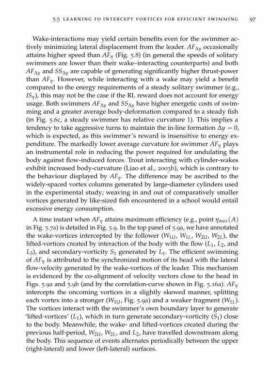
5.5 learning to intercept vortices for efficient swimming 97
Wake-interactions may yield certain benefits even for the swimmer ac-tively minimizing lateral displacement from the leader. AF∆y occasionallyattains higher speed than AFη (Fig. 5.8) (in general the speeds of solitaryswimmers are lower than their wake–interacting counterparts) and bothAF∆y and SS∆y are capable of generating significantly higher thrust-powerthan AFη . However, while interacting with a wake may yield a benefitcompared to the energy requirements of a steady solitary swimmer (e.g.,ISη), this may not be the case if the RL reward does not account for energyusage. Both swimmers AF∆y and SS∆y have higher energetic costs of swim-ming and a greater average body-deformation compared to a steady fish(in Fig. 5.6c, a steady swimmer has relative curvature 1). This implies atendency to take aggressive turns to maintain the in-line formation ∆y = 0,which is expected, as this swimmer’s reward is insensitive to energy ex-penditure. The markedly lower average curvature for swimmer AFη playsan instrumental role in reducing the power required for undulating thebody against flow-induced forces. Trout interacting with cylinder-wakesexhibit increased body-curvature (Liao et al., 2003b), which is contrary tothe behaviour displayed by AFη . The difference may be ascribed to thewidely-spaced vortex columns generated by large-diameter cylinders usedin the experimental study; weaving in and out of comparatively smallervortices generated by like-sized fish encountered in a school would entailexcessive energy consumption.
A time instant when AFη attains maximum efficiency (e.g., point ηmax(A)in Fig. 5.7a) is detailed in Fig. 5.9. In the top panel of 5.9a, we have annotatedthe wake-vortices intercepted by the follower (W1U , W1L, W2U , W2L), thelifted-vortices created by interaction of the body with the flow (L1, L2, andL3), and secondary-vorticity S1 generated by L1. The efficient swimmingof AFη is attributed to the synchronized motion of its head with the lateralflow-velocity generated by the wake-vortices of the leader. This mechanismis evidenced by the co-alignment of velocity vectors close to the head inFigs. 5.9a and 5.9b (and by the correlation-curve shown in Fig. 5.16a). AFη
intercepts the oncoming vortices in a slightly skewed manner, splittingeach vortex into a stronger (W1U , Fig. 5.9a) and a weaker fragment (W1L).The vortices interact with the swimmer’s own boundary layer to generate‘lifted-vortices’ (L1), which in turn generate secondary-vorticity (S1) closeto the body. Meanwhile, the wake- and lifted-vortices created during theprevious half-period, W2U , W2L, and L2, have travelled downstream alongthe body. This sequence of events alternates periodically between the upper(right-lateral) and lower (left-lateral) surfaces.
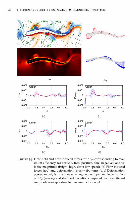
98 efficient collective swimming by harnessing vortices
L1
L2
W1U
L3
W1L
W2U
W2L
S1
(a) (b)
-0.002
-0.001
0
0.001
0.002
0.0 0.2 0.4 0.6 0.8 1.0
Upper
PD
ef
s/L
(c)
-0.002
-0.001
0
0.001
0.002
0.0 0.2 0.4 0.6 0.8 1.0
Upper
PT
hru
st
s/L
(d)
-0.002
-0.001
0
0.001
0.002
0.0 0.2 0.4 0.6 0.8 1.0
Lower
PD
ef
s/L
(e)
-0.002
-0.001
0
0.001
0.002
0.0 0.2 0.4 0.6 0.8 1.0
Lower
PT
hru
st
s/L
(f)
Figure 5.9: Flow-field and flow-induced forces for AFη , corresponding to max-imum efficiency. (a) Vorticity (red: positive, blue: negative), and ve-locity magnitude (bright: high, dark: low speed). (b) Flow-inducedforces (top) and deformation velocity (bottom). (c, e) Deformation-power, and (d, f) thrust-power acting on the upper and lower surfaceof AFη (average and standard deviation computed over 10 differentsnapshots corresponding to maximum efficiency).
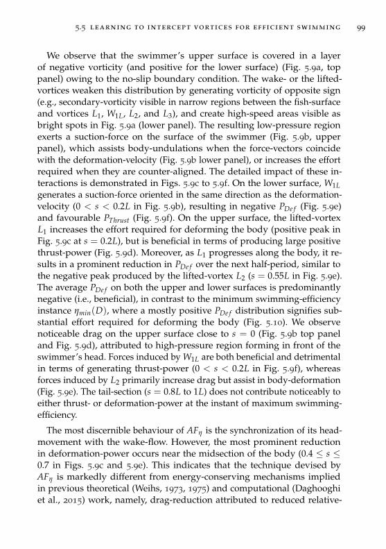
5.5 learning to intercept vortices for efficient swimming 99
We observe that the swimmer’s upper surface is covered in a layerof negative vorticity (and positive for the lower surface) (Fig. 5.9a, toppanel) owing to the no-slip boundary condition. The wake- or the lifted-vortices weaken this distribution by generating vorticity of opposite sign(e.g., secondary-vorticity visible in narrow regions between the fish-surfaceand vortices L1, W1L, L2, and L3), and create high-speed areas visible asbright spots in Fig. 5.9a (lower panel). The resulting low-pressure regionexerts a suction-force on the surface of the swimmer (Fig. 5.9b, upperpanel), which assists body-undulations when the force-vectors coincidewith the deformation-velocity (Fig. 5.9b lower panel), or increases the effortrequired when they are counter-aligned. The detailed impact of these in-teractions is demonstrated in Figs. 5.9c to 5.9f. On the lower surface, W1Lgenerates a suction-force oriented in the same direction as the deformation-velocity (0 < s < 0.2L in Fig. 5.9b), resulting in negative PDe f (Fig. 5.9e)and favourable PThrust (Fig. 5.9f). On the upper surface, the lifted-vortexL1 increases the effort required for deforming the body (positive peak inFig. 5.9c at s = 0.2L), but is beneficial in terms of producing large positivethrust-power (Fig. 5.9d). Moreover, as L1 progresses along the body, it re-sults in a prominent reduction in PDe f over the next half-period, similar tothe negative peak produced by the lifted-vortex L2 (s = 0.55L in Fig. 5.9e).The average PDe f on both the upper and lower surfaces is predominantlynegative (i.e., beneficial), in contrast to the minimum swimming-efficiencyinstance ηmin(D), where a mostly positive PDe f distribution signifies sub-stantial effort required for deforming the body (Fig. 5.10). We observenoticeable drag on the upper surface close to s = 0 (Fig. 5.9b top paneland Fig. 5.9d), attributed to high-pressure region forming in front of theswimmer’s head. Forces induced by W1L are both beneficial and detrimentalin terms of generating thrust-power (0 < s < 0.2L in Fig. 5.9f), whereasforces induced by L2 primarily increase drag but assist in body-deformation(Fig. 5.9e). The tail-section (s = 0.8L to 1L) does not contribute noticeably toeither thrust- or deformation-power at the instant of maximum swimming-efficiency.
The most discernible behaviour of AFη is the synchronization of its head-movement with the wake-flow. However, the most prominent reductionin deformation-power occurs near the midsection of the body (0.4 ≤ s ≤0.7 in Figs. 5.9c and 5.9e). This indicates that the technique devised byAFη is markedly different from energy-conserving mechanisms impliedin previous theoretical (Weihs, 1973, 1975) and computational (Daghooghiet al., 2015) work, namely, drag-reduction attributed to reduced relative-
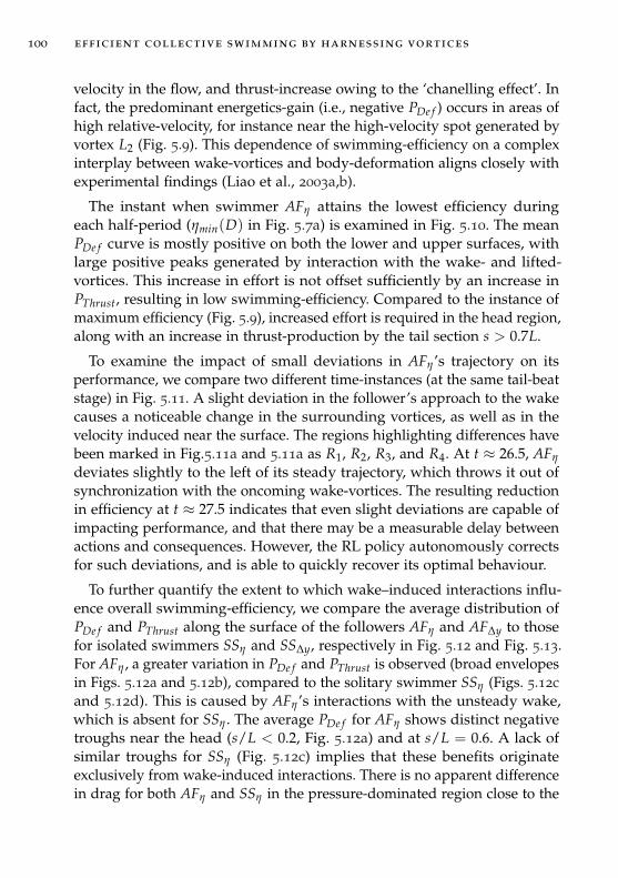
100 efficient collective swimming by harnessing vortices
velocity in the flow, and thrust-increase owing to the ‘chanelling effect’. Infact, the predominant energetics-gain (i.e., negative PDe f ) occurs in areas ofhigh relative-velocity, for instance near the high-velocity spot generated byvortex L2 (Fig. 5.9). This dependence of swimming-efficiency on a complexinterplay between wake-vortices and body-deformation aligns closely withexperimental findings (Liao et al., 2003a,b).
The instant when swimmer AFη attains the lowest efficiency duringeach half-period (ηmin(D) in Fig. 5.7a) is examined in Fig. 5.10. The meanPDe f curve is mostly positive on both the lower and upper surfaces, withlarge positive peaks generated by interaction with the wake- and lifted-vortices. This increase in effort is not offset sufficiently by an increase inPThrust, resulting in low swimming-efficiency. Compared to the instance ofmaximum efficiency (Fig. 5.9), increased effort is required in the head region,along with an increase in thrust-production by the tail section s > 0.7L.
To examine the impact of small deviations in AFη’s trajectory on itsperformance, we compare two different time-instances (at the same tail-beatstage) in Fig. 5.11. A slight deviation in the follower’s approach to the wakecauses a noticeable change in the surrounding vortices, as well as in thevelocity induced near the surface. The regions highlighting differences havebeen marked in Fig.5.11a and 5.11a as R1, R2, R3, and R4. At t ≈ 26.5, AFη
deviates slightly to the left of its steady trajectory, which throws it out ofsynchronization with the oncoming wake-vortices. The resulting reductionin efficiency at t ≈ 27.5 indicates that even slight deviations are capable ofimpacting performance, and that there may be a measurable delay betweenactions and consequences. However, the RL policy autonomously correctsfor such deviations, and is able to quickly recover its optimal behaviour.
To further quantify the extent to which wake–induced interactions influ-ence overall swimming-efficiency, we compare the average distribution ofPDe f and PThrust along the surface of the followers AFη and AF∆y to thosefor isolated swimmers SSη and SS∆y, respectively in Fig. 5.12 and Fig. 5.13.For AFη , a greater variation in PDe f and PThrust is observed (broad envelopesin Figs. 5.12a and 5.12b), compared to the solitary swimmer SSη (Figs. 5.12cand 5.12d). This is caused by AFη’s interactions with the unsteady wake,which is absent for SSη . The average PDe f for AFη shows distinct negativetroughs near the head (s/L < 0.2, Fig. 5.12a) and at s/L = 0.6. A lack ofsimilar troughs for SSη (Fig. 5.12c) implies that these benefits originateexclusively from wake-induced interactions. There is no apparent differencein drag for both AFη and SSη in the pressure-dominated region close to the
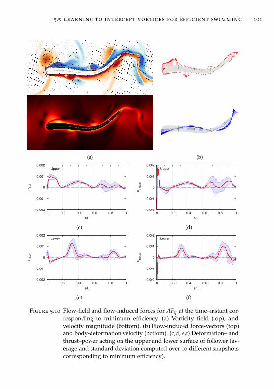
5.5 learning to intercept vortices for efficient swimming 101
(a) (b)
-0.002
-0.001
0
0.001
0.002
0 0.2 0.4 0.6 0.8 1
PD
ef
s/L
Upper
(c)
-0.002
-0.001
0
0.001
0.002
0 0.2 0.4 0.6 0.8 1
PT
hru
st
s/L
Upper
(d)
-0.002
-0.001
0
0.001
0.002
0 0.2 0.4 0.6 0.8 1
PD
ef
s/L
Lower
(e)
-0.002
-0.001
0
0.001
0.002
0 0.2 0.4 0.6 0.8 1
PT
hru
st
s/L
Lower
(f)
Figure 5.10: Flow-field and flow-induced forces for AFη at the time–instant cor-responding to minimum efficiency. (a) Vorticity field (top), andvelocity magnitude (bottom). (b) Flow-induced force-vectors (top)and body-deformation velocity (bottom). (c,d, e,f) Deformation– andthrust–power acting on the upper and lower surface of follower (av-erage and standard deviation computed over 10 different snapshotscorresponding to minimum efficiency).
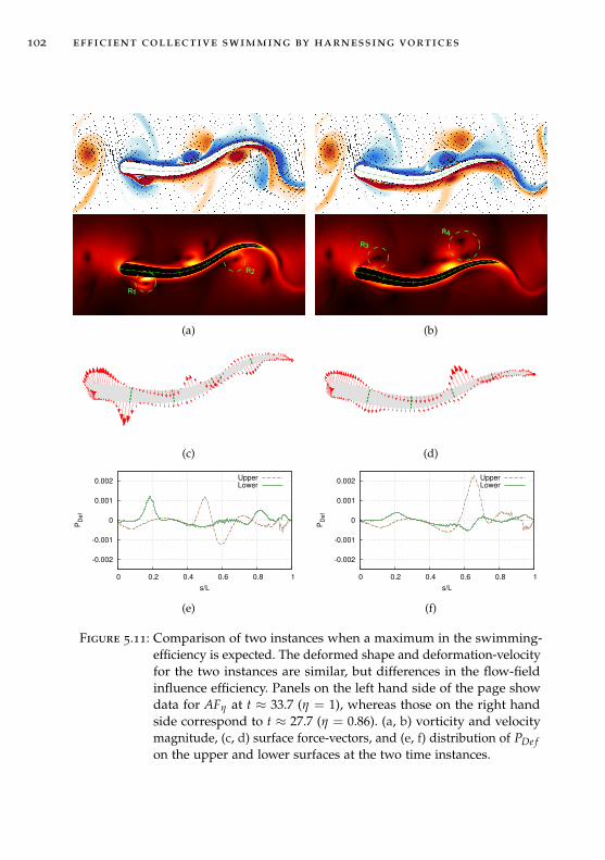
102 efficient collective swimming by harnessing vortices
R1
R2
(a)
R3
R4
(b)
(c) (d)
-0.002
-0.001
0
0.001
0.002
0 0.2 0.4 0.6 0.8 1
PD
ef
s/L
UpperLower
(e)
-0.002
-0.001
0
0.001
0.002
0 0.2 0.4 0.6 0.8 1
PD
ef
s/L
UpperLower
(f)
Figure 5.11: Comparison of two instances when a maximum in the swimming-efficiency is expected. The deformed shape and deformation-velocityfor the two instances are similar, but differences in the flow-fieldinfluence efficiency. Panels on the left hand side of the page showdata for AFη at t ≈ 33.7 (η = 1), whereas those on the right handside correspond to t ≈ 27.7 (η = 0.86). (a, b) vorticity and velocitymagnitude, (c, d) surface force-vectors, and (e, f) distribution of PDe fon the upper and lower surfaces at the two time instances.
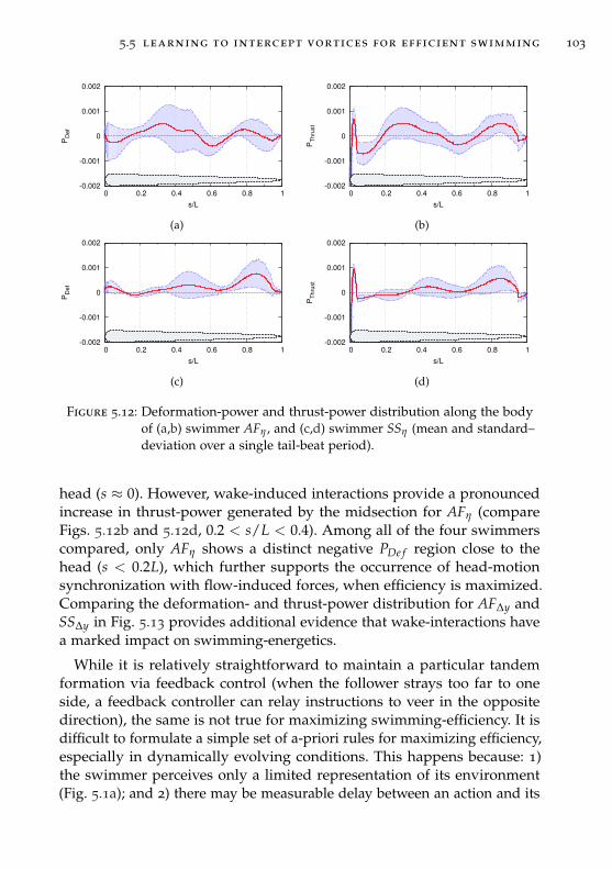
5.5 learning to intercept vortices for efficient swimming 103
-0.002
-0.001
0
0.001
0.002
0 0.2 0.4 0.6 0.8 1
PD
ef
s/L
(a)
-0.002
-0.001
0
0.001
0.002
0 0.2 0.4 0.6 0.8 1
PT
hru
st
s/L
(b)
-0.002
-0.001
0
0.001
0.002
0 0.2 0.4 0.6 0.8 1
PD
ef
s/L
(c)
-0.002
-0.001
0
0.001
0.002
0 0.2 0.4 0.6 0.8 1
PT
hru
st
s/L
(d)
Figure 5.12: Deformation-power and thrust-power distribution along the bodyof (a,b) swimmer AFη , and (c,d) swimmer SSη (mean and standard–deviation over a single tail-beat period).
head (s ≈ 0). However, wake-induced interactions provide a pronouncedincrease in thrust-power generated by the midsection for AFη (compareFigs. 5.12b and 5.12d, 0.2 < s/L < 0.4). Among all of the four swimmerscompared, only AFη shows a distinct negative PDe f region close to thehead (s < 0.2L), which further supports the occurrence of head-motionsynchronization with flow-induced forces, when efficiency is maximized.Comparing the deformation- and thrust-power distribution for AF∆y andSS∆y in Fig. 5.13 provides additional evidence that wake-interactions havea marked impact on swimming-energetics.
While it is relatively straightforward to maintain a particular tandemformation via feedback control (when the follower strays too far to oneside, a feedback controller can relay instructions to veer in the oppositedirection), the same is not true for maximizing swimming-efficiency. It isdifficult to formulate a simple set of a-priori rules for maximizing efficiency,especially in dynamically evolving conditions. This happens because: 1)the swimmer perceives only a limited representation of its environment(Fig. 5.1a); and 2) there may be measurable delay between an action and its
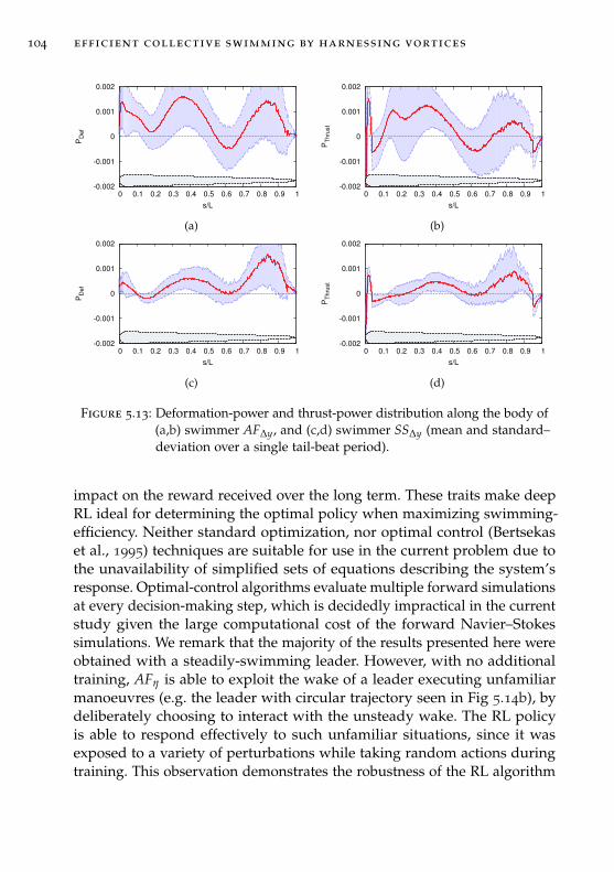
104 efficient collective swimming by harnessing vortices
-0.002
-0.001
0
0.001
0.002
0 0.1 0.2 0.3 0.4 0.5 0.6 0.7 0.8 0.9 1
PD
ef
s/L
(a)
-0.002
-0.001
0
0.001
0.002
0 0.1 0.2 0.3 0.4 0.5 0.6 0.7 0.8 0.9 1
PT
hru
st
s/L
(b)
-0.002
-0.001
0
0.001
0.002
0 0.1 0.2 0.3 0.4 0.5 0.6 0.7 0.8 0.9 1
PD
ef
s/L
(c)
-0.002
-0.001
0
0.001
0.002
0 0.1 0.2 0.3 0.4 0.5 0.6 0.7 0.8 0.9 1
PT
hru
st
s/L
(d)
Figure 5.13: Deformation-power and thrust-power distribution along the body of(a,b) swimmer AF∆y, and (c,d) swimmer SS∆y (mean and standard–deviation over a single tail-beat period).
impact on the reward received over the long term. These traits make deepRL ideal for determining the optimal policy when maximizing swimming-efficiency. Neither standard optimization, nor optimal control (Bertsekaset al., 1995) techniques are suitable for use in the current problem due tothe unavailability of simplified sets of equations describing the system’sresponse. Optimal-control algorithms evaluate multiple forward simulationsat every decision-making step, which is decidedly impractical in the currentstudy given the large computational cost of the forward Navier–Stokessimulations. We remark that the majority of the results presented here wereobtained with a steadily-swimming leader. However, with no additionaltraining, AFη is able to exploit the wake of a leader executing unfamiliarmanoeuvres (e.g. the leader with circular trajectory seen in Fig 5.14b), bydeliberately choosing to interact with the unsteady wake. The RL policyis able to respond effectively to such unfamiliar situations, since it wasexposed to a variety of perturbations while taking random actions duringtraining. This observation demonstrates the robustness of the RL algorithm
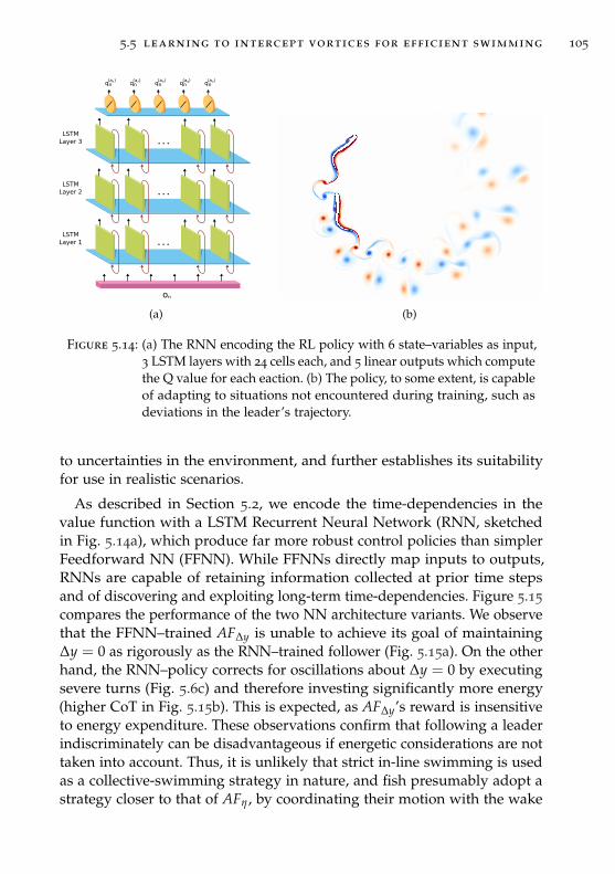
5.5 learning to intercept vortices for efficient swimming 105
LSTMLayer 2
LSTMLayer 1
LSTMLayer 3
on
(a3)qn(a1)qn
(a2)qn(a4)qn
(a5)qn
(a) (b)
Figure 5.14: (a) The RNN encoding the RL policy with 6 state–variables as input,3 LSTM layers with 24 cells each, and 5 linear outputs which computethe Q value for each eaction. (b) The policy, to some extent, is capableof adapting to situations not encountered during training, such asdeviations in the leader’s trajectory.
to uncertainties in the environment, and further establishes its suitabilityfor use in realistic scenarios.
As described in Section 5.2, we encode the time-dependencies in thevalue function with a LSTM Recurrent Neural Network (RNN, sketchedin Fig. 5.14a), which produce far more robust control policies than simplerFeedforward NN (FFNN). While FFNNs directly map inputs to outputs,RNNs are capable of retaining information collected at prior time stepsand of discovering and exploiting long-term time-dependencies. Figure 5.15
compares the performance of the two NN architecture variants. We observethat the FFNN–trained AF∆y is unable to achieve its goal of maintaining∆y = 0 as rigorously as the RNN–trained follower (Fig. 5.15a). On the otherhand, the RNN–policy corrects for oscillations about ∆y = 0 by executingsevere turns (Fig. 5.6c) and therefore investing significantly more energy(higher CoT in Fig. 5.15b). This is expected, as AF∆y’s reward is insensitiveto energy expenditure. These observations confirm that following a leaderindiscriminately can be disadvantageous if energetic considerations are nottaken into account. Thus, it is unlikely that strict in-line swimming is usedas a collective-swimming strategy in nature, and fish presumably adopt astrategy closer to that of AFη , by coordinating their motion with the wake
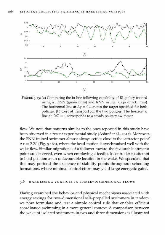
106 efficient collective swimming by harnessing vortices
-0.02
-0.015
-0.01
-0.005
0
0.005
15 20 25 30 35 40 45
∆y
t
(a)
0
0.5
1
1.5
2
2.5
15 20 25 30 35 40 45
CoT
t
(b)
Figure 5.15: (a) Comparing the in-line following capability of RL policy trainedusing a FFNN (green lines) and RNN in Fig. 5.14a (black lines).The horizontal line at ∆y = 0 denotes the target specified for bothpolicies. (b) Cost of transport for the two policies. The horizontalline at CoT = 1 corresponds to a steady solitary swimmer.
flow. We note that patterns similar to the ones reported in this study havebeen observed in a recent experimental study (Ashraf et al., 2017). Moreover,the FNN-trained swimmer almost always settles close to the ‘attractor point’∆x = 2.2L (Fig. 5.16a), where the head-motion is synchronised well with thewake flow. Similar migrations of a follower toward the favourable attractorpoint are observed, even when employing a feedback controller to attemptto hold position at an unfavourable location in the wake. We speculate thatthis may portend the existence of stability points throughout schoolingformations, where minimal control-effort may yield large energetic gains.
5.6 harnessing vortices in three–dimensional flows
Having examined the behavior and physical mechanisms associated withenergy savings for two–dimensional self–propelled swimmers in tandem,we now formulate and test a simple control rule that enables efficientcoordinated swimming in a more general context. A comparison betweenthe wake of isolated swimmers in two and three dimensions is illustrated
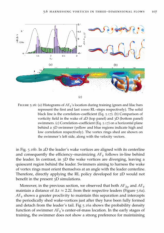
5.6 harnessing vortices in three–dimensional flows 107
(a) (b)
(c)
Figure 5.16: (a) Histograms of AFη ’s location during training (green and lilac barsrepresent the first and last 10000 RL–steps respectively). The solidblack line is the correlation–coefficient (Eq. 5.17). (b) Comparison ofvorticity field in the wake of 2D (top panel) and 3D (bottom panel)swimmers. (c) Correlation–coefficient (Eq. 5.17) on a horizontal planebehind a 3D swimmer (yellow and blue regions indicate high andlow correlation respectively). The vortex rings shed are shown onthe swimmer’s left side, along with the velocity vectors.
in Fig. 5.16b. In 2D the leader’s wake vortices are aligned with its centerlineand consequently the efficiency–maximizing AFη follows in-line behindthe leader. In contrast, in 3D the wake vortices are diverging, leaving aquiescent region behind the leader. Swimmers aiming to harness the wakeof vortex rings must orient themselves at an angle with the leader centerline.Therefore, directly applying the RL policy developed for 2D would notbenefit in the present 3D simulations.
Moreover, in the previous section, we observed that both AF∆y and AFη
maintain a distance of ∆x ≈ 2.2L from their respective leaders (Figure 5.6a).AFη shows a greater proclivity to maintain this separation and interceptsthe periodically shed wake-vortices just after they have been fully formedand detach from the leader’s tail. Fig 5.16a shows the probability densityfunction of swimmer AFη’s center-of-mass location. In the early stages oftraining, the swimmer does not show a strong preference for maintaining
108 efficient collective swimming by harnessing vortices
any particular separation distance. Towards the end of training, the swim-mer displays a strong preference for maintaining a separation-distance ofeither ∆x = 1.5L or 2.2L. These are locations where the follower’s head-movement is synchronized with the flow-velocity of the leader’s wake (e.g.the maximum efficiency condition described in Fig. 5.9). The difference 0.7Lmatches the distance between vortices in the wake of the leader. In bothpositions the lateral motion of the follower’s head is synchronized withthe flow-velocity in the leader’s wake, thus inducing minimal disturbanceon the oncoming flow-field. We note that a similar synchronization withthe flow velocity has been observed when trout minimize muscle usage byinteracting with vortex-columns in a cylinder’s wake (Liao et al., 2003a).
Given that the most discernible behaviour of AFη is the synchronization ofits head-movement with the wake-flow, we first identify suitable locationsbehind a 3D leader where the flow velocity would match a follower’shead motion (Fig. 5.16c). The Proportional-Integral (PI) feedback controllerdescribed in Section 5.1.2 is then used to regulate the undulations of twofollowers to maintain these target coordinates on either branch of thediverging wake, as shown in Fig. 5.17b. The correlation-coefficient curveshown in Fig. 5.16a, and the correlation map shown in Fig. 5.16c, werecomputed as follows:
ρ(u, uhead) =cov (u(x, y), uhead)
σu(x,y) σuhead
=∑t u(x, y, t) · uhead(t)√
∑t ‖u(x, y, t)‖2√
∑t ‖uhead(t)‖2
(5.17)Here, u(x, y, t) was recorded in the wake of a solitary swimmer, whereasuhead(t) was recorded at the swimmer’s head. Maxima in ρ(u, uhead) pro-vide an estimate for the coordinates where a follower’s head-movementswould exhibit long-term synchronization with an undisturbed wake.
The correlation–coefficient between follower’s head movement and anundisturbed three–dimensional wake is visualized in Fig. 5.16c. We remarkthat the plot extends only on a plane on the right side of the swimmerbecause the correlation is symmetric around the wake’s centerline. Themaxima are located at ∆x ≈ 1.15L and |∆y|≈ 0.225L. These relative posi-tions identify three optimal schooling arrangements: 1) The leader–followerarrangement with the latter increasing its efficiency by swimming at thelocation of maximal correlation with one row of the vortex rings shed bythe leader (illustrated in Fig. 5.17a). 2) A leader–two–followers arrange-ment with the two swimmers placed at the two symmetric optima, eachharnessing one row of vortex rings (illustrated in Fig. 5.17b). 3) A two–
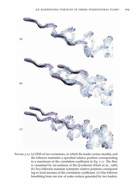
5.6 harnessing vortices in three–dimensional flows 109
(a)
(b)
(c)
Figure 5.17: (a) DNS of two swimmers, in which the leader swims steadily, andthe follower maintains a specified relative position correspondingto a maximum of the correlation–coefficient in Eq. 5.17. The flowis visualised by iso-surfaces of the Q-criterion (Hunt et al., 1988).(b) Two followers maintain symmetric relative positions correspond-ing to local maxima of the correlation–coefficient. (c) One followerbenefitting from one row of wake-vortices generated by two leaders.
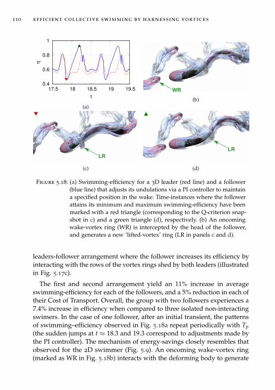
110 efficient collective swimming by harnessing vortices
0.4
0.6
0.8
1
17.5 18 18.5 19 19.5
η
t
(a)
WR
(b)
LR
(c)
LR
(d)
Figure 5.18: (a) Swimming-efficiency for a 3D leader (red line) and a follower(blue line) that adjusts its undulations via a PI controller to maintaina specified position in the wake. Time-instances where the followerattains its minimum and maximum swimming-efficiency have beenmarked with a red triangle (corresponding to the Q-criterion snap-shot in c) and a green triangle (d), respectively. (b) An oncomingwake-vortex ring (WR) is intercepted by the head of the follower,and generates a new ‘lifted-vortex’ ring (LR in panels c and d).
leaders-follower arrangement where the follower increases its efficiency byinteracting with the rows of the vortex rings shed by both leaders (illustratedin Fig. 5.17c).
The first and second arrangement yield an 11% increase in averageswimming-efficiency for each of the followers, and a 5% reduction in each oftheir Cost of Transport. Overall, the group with two followers experiences a7.4% increase in efficiency when compared to three isolated non-interactingswimers. In the case of one follower, after an initial transient, the patternsof swimming–efficiency observed in Fig. 5.18a repeat periodically with Tp(the sudden jumps at t ≈ 18.3 and 19.3 correspond to adjustments made bythe PI controller). The mechanism of energy-savings closely resembles thatobserved for the 2D swimmer (Fig. 5.9). An oncoming wake-vortex ring(marked as WR in Fig. 5.18b) interacts with the deforming body to generate
5.7 conclusion 111
a ‘lifted-vortex’ ring (LR - Fig. 5.18c). As this new ring proceeds alongthe length of the body, it modulates the follower’s swimming-efficiency asobserved in Fig. 5.18. Remarkably, the positioning of the lifted-ring at theinstants of minimum and maximum swimming-efficiency resembles thecorresponding positioning of lifted-vortices in the 2D case. The swimming-efficiency is initially lowered as the lifted-vortices interacts with the anteriorsection of the body. This situation repeats in the 3D case for t ≈ (k + 0.8)Tp(Fig. 5.18a) and is illustrated by the Q–criterion snapshot in Fig. 5.18c),while in the 2D case is illustrated by Fig. 5.10. The initial dip in efficiencyis outweighed by the downstream energy benefit when the lifted-vorticesinteract with the followers’ midsection (Fig. 5.18d and Fig. 5.9). The mech-anism by which the follower in a two–leaders arrangement benefits fromthe wake is analogous, but with spikes of swimming efficiency on bothhalves of the period Tp (Fig. 5.18a), as it interacts with twice the number ofvortex–rings. As a consequence, the single follower in the third schoolingarrangement (Fig. 5.17c) benefits from an almost doubled (19%) increase inaverage swimming–efficiency.
5.7 conclusion
In this chapter, we demonstrated the energetic benefits of coordinatedswimming for two and three swimmers in leader-follower configurations,through a series of simulations. First, an arrangement of rigid airfoil-shapedswimmers, executing pre–specified motion, is observed to give rise tosubstantial drag-reduction. This simplified scenario demonstrates that in-teracting swimmers may see a benefit arising from vortices present in theflow even in the presence of large flow separation. Following this, weinvestigate self-propelled fish shapes, with both the leader and the fol-lower employing identical kinematics. Without any active adaptation, thefollower’s interactions with the leader’s wake can be either energeticallybeneficial or detrimental, depending on the initial condition. Furthermore,the follower tends to diverge from the leader’s wake, which points to theneed for active modulation of the follower’s actions to maintain a stabletandem configuration. Finally, we examine the case where the leader swimswith a steady gait and the follower adapts its behaviour dynamically toaccount for the effects of the wake encountered. The actions of the fol-lower are selected autonomously from an optimal policy determined viaReinforcement Learning, and allow the swimmer to maximize a specifiedlong-term reward. The results indicate that swimming in tandem can lead
112 efficient collective swimming by harnessing vortices
to measurable energy savings for the follower. These results showcase thecapability of machine learning, and deep RL in particular, for discover-ing effective solutions to complex physical problems with inherent spatialand temporal non-linearities, in a completely data-driven and model-freemanner. Deep RL is especially useful in scenarios where decisions must betaken adaptively in response to a dynamically evolving environment, andthe best control-strategy may not be evident a-priori due to unpredictabletime-delay between actions and their effect. This necessitates the use ofrecurrent networks capable of encoding time-dependencies, which can havea demonstrable impact on the physical outcome, as shown in Fig. 5.15.
We note that the training process of Reinforcement Learning is compu-tationally expensive thus requiring large scale computational resources.Under this constraint, we performed a novel reverse-engineering analysis ofRL in order to extend the knowledge obtained from two-dimensional simu-lations to the context of three-dimensional Direct Numerical Simulations(DNS), where: (i) we have utilized the capability of RL to discern usefulpatterns from a large cache of simulation data; (ii) we have analysed thephysical aspects of the resulting optimal strategy, to identify the behaviourand mechanisms that lead to energetic-benefits, and finally; (iii) we usethis understanding to devise a rule-based control algorithm for sustainedenergy-efficient synchronized swimming, in a notably more complex three-dimensional setting. We find that expert use of two-dimensional simulationsand low order models allows gaining insight into three-dimensional flows.To the best of our knowledge, there is no work available in the literaturethat investigates the flow-physics governing interactions among multiple in-dependent swimmers, using high-fidelity simulations of three-dimensionalNavier-Stokes equations. We demonstrate that RL can produce efficientnavigation algorithms for use in complex flow-fields which in turn canbe used to formulate control-rules that are effective in decidedly morecomplex settings, and thus have promising implications for energy savingsin engineering applications with strong hydrodynamic interactions.
6T U R B U L E N C E M O D E L I N G A S M U LT I - A G E N T F L O WC O N T R O L
The prediction of turbulent flows is critical for engineering (cars to nuclearreactors), science (ocean dynamics to astrophysics) and policy (climatemodeling and weather forecasting). Over the last sixty years we have in-creasingly relied for such predictions on simulations based on the numericalintegration of the Navier-Stokes equations. Today we can perform simula-tions using trillions of computational elements and resolve flow phenomenaat unprecedented detail. However, despite the ever increasing availabilityof computing resources, most simulations of turbulent flows require theadoption of models to account for the spatio-temporal scales that cannotbe resolved. Over the last few decades, the development of TurbulenceModels (TM) has been the subject of intense investigations that have reliedon physical insight and engineering intuition. Recent advances in machinelearning and in the availability of data have offered new perspectives (andhope) in developing data-driven TM. Interestingly, turbulence and statisticallearning theories have common roots in the seminal works of Kolmogorovon the analysis of homogeneous and isotropic turbulent flows (see Kol-mogorov, 1941; Li et al., 1997. These flows are characterized by vorticalstructures and their interactions exhibiting a broad spectrum of spatio-temporal scales (Cardesa et al., 2017; Pope, 2001; Taylor, 1935) At one end ofthe spectrum we encounter the integral scales, which depend on the specificforcing, flow geometry, or boundary conditions. At the other end we findthe Kolmogorov scales at which turbulent kinetic energy is dissipated. Thehandling of these turbulent scales provides a classification of turbulencesimulations: Direct Numerical Simulations (DNS), which use a sufficientnumber of computational elements to resolve all scales of the flow field, andsimulations using TM where the equations are solved in relatively few com-putational elements and the non-resolved terms are described by closuremodels. In DNS (Moin et al., 1998) most of the computational effort is spentin fully resolving the Kolmogorov scales despite them being statisticallyhomogeneous and largely unaffected by large scale effects. RemarkableDNS (Moser et al., 1999) have provided us with unique insight into thephysics of turbulence that can lead in turn to effective TM. However, it is
113
114 turbulence modeling as multi-agent flow control
well understood that in the foreseeable future DNS will not be feasible atresolutions necessary for engineering applications. In TM (Durbin, 2018)two techniques have been dominant: Reynolds Averaged Navier-Stokes(RANS) and Large-eddy Simulations (LES) in which only the large scaleunsteady physics are explicitly computed whereas the sub grid-scale (SGS),unresolved, physics are modeled. In the context of LES (Leonard et al.,1974), classic approaches to the explicit modeling of SGS stresses includethe standard (Smagorinsky, 1963) and the dynamic Smagorinsky model(Germano, 1992; Germano et al., 1991; Lilly, 1992). SGS models have beenconstructed using physical insight, numerical approximations and oftenproblem-specific intuition. While efforts to develop models for turbulentflows using machine learning and neural networks (NN) in particular dateback decades (Lee et al., 1997; Milano et al., 2002), recent advances in hard-ware and algorithms have made their use feasible for the development ofdata-driven turbulence closure models (Duraisamy et al., 2019).
To date, to the best of our knowledge, all data-driven turbulence closuremodels are based on supervised learning (SL). In LES, early approaches(Sarghini et al., 2003) trained a NN to emulate and speed-up a conventional,but computationally expensive, SGS model. More recently, data-drivenSGS models have been trained by SL to predict the “perfect” SGS termscomputed from filtered DNS data (Gamahara et al., 2017; Xie et al., 2019).Variants include deriving the target SGS term from optimal estimatortheory (Vollant et al., 2017) and reconstructing the SGS velocity field as adeconvolution operation, or inverse filtering (Fukami et al., 2019; Hickel etal., 2004; Maulik et al., 2017). In SL the parameters of the NN are commonlyderived via a gradient descent algorithm to minimize the model predictionerror. As the error is required to be differentiable with respect to the modelparameters, and due to the computational challenge of obtaining chain-derivatives through a flow solver, SL approaches often define one-steptarget values for the model (e.g. reference SGS stresses computed fromfiltered DNS). Therefore it is necessary to differentiate between a prioriand a posteriori testing. The first measures the accuracy of the SL modelin predicting the target values on a database of reference simulations,typically obtained via DNS. A posteriori testing is performed after training,by integrating in time the NSE along with trained SL closure and comparingthe obtained statistical quantities to that of DNS or other references. Dueto the single-step cost function, the resultant NN model is not trained tocompensate for the systematic discrepancies between DNS and LES andthe compounding errors. The issue of ill-conditioning of data-driven SGS
6.1 forced homogeneous and isotropic turbulence 115
models has been exposed by studies that perform a posteriori testing (Wuet al., 2018). For example, in the work by Gamahara et al., 2017, while theSGS stresses are accurately recovered, the mean flow velocities are not.Moreover, Nadiga et al., 2007 shows that in many cases the perfect SGSmodel is structurally unstable and diverges from the original trajectoryunder perturbation. Likewise, Beck et al., 2019 shows that a deep NNtrained by SL, while closely matching the perfect SGS model for any singlestep, accumulates high-spatial frequency errors which cause instability.
We introduce Reinforcement Learning (RL) as a framework for the auto-mated discovery of closure models of non-linear conservation laws, hereapplied to the construction of SGS models for LES. The key distinctionbetween RL and SL is that RL optimizes a parametric model by directexploration-exploitation of the underlying task specification. Moreover, theperformance of a RL strategy is not measured by a differentiable objectivefunction but by a cumulative reward. These features are especially beneficialin the case of TM as they permit avoiding the distinction between a prioriand a posteriori evaluation. RL training is not performed on a database ofreference data, but is performed by integrating in time the model and itsconsequences. In the case of LES, the performance of the RL strategy may bemeasured by comparing the statistical properties of the simulation to thoseof reference data. Indeed, rather than perfectly recovering SGS computedfrom filtered simulations, which may produce numerically unstable LES(Nadiga et al., 2007), RL can develop novel models which are optimized toaccurately reproduce the quantities of interest.
acknowledgments This chapter is based on the paper “AutomatingTurbulence Modelingby Multi-Agent Reinforcement Learning” written withHugues Lascombes de Laroussilhea, and Petros Koumoutsakos, which iscurrently under review. The computational resources were provided bya grant from the Swiss National Super-computing Centre (CSCS) underproject s929.
6.1 forced homogeneous and isotropic turbulence
We use as a benchmark problem the simulations of Forced HomogeneousIsotropic Turbulence (F-HIT) with a linear, low-wavenumber forcing term.These methods have been implemented in the three-dimensional incom-pressible Navier-Stokes solver CubismUP.
116 turbulence modeling as multi-agent flow control
6.1.1 Turbulent Kinetic Energy
A turbulent flow is homogeneous and isotropic when the averaged quantitiesof the flow are invariant under arbitrary translations and rotations. Theflow statistics are independent of space and the mean velocity of the flowis zero. Forced, homogeneous, isotropic turbulence is governed by theincompressible Navier-Stokes equations, ∂u
∂t + (u · ∇)u = −∇p +∇ · (2νS) + f
∇ · u = 0(6.1)
where S = 12 (∇u+∇uT) is the rate-of-strain tensor. The the turbulent
kinetic energy (second order statistics of the velocity field) is expressed as :
e(x, t) ≡ 12u · u, K(t) ≡ 1
2〈u · u〉 , (6.2)
where the angle brackets 〈·〉 ≡ 1V∫D · denote an ensemble average over the
domain D with volume V . For a flow with periodic boundary conditions theevolution of the kinetic energy is described as:
dKdt
= −ν∫D‖∇u‖2 +
∫Duf (6.3)
= −2ν 〈Z〉 + 〈u · f 〉 (6.4)
where the energy dissipation due to viscosity, is expressed in term ofthe norm of the vorticity ω ≡ ∇ × u and the enstrophy Z = 1
2ω2. This
equation clarifies that the vorticity of the flow field is responsible for energydissipation that can only be conserved if there is a source of energy.
We investigate the behaviour of homogeneous isotropic turbulence in astatistically stationary state by injecting energy through forcing. In genericflow configurations the role of this forcing is taken up by the large-scalestructures and it is assumed that it does not influence smaller scale statistics,which are driven by viscous dissipation. The injected energy is transferredfrom large-scale motion to smaller scales due to the non-linearity of Navier-Stokes equations. We implement a classic low-wavenumber (low-k) forcingterm (Ghosal et al., 1995) for homogeneous isotropic turbulence that isproportional to the local fluid velocity as filtered from its large wave numbercomponents:
f (k, t) ≡ α G(k, k f ) u(k, t) = α u<(k, t), (6.5)
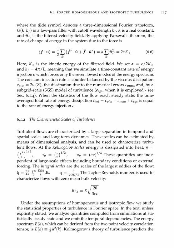
6.1 forced homogeneous and isotropic turbulence 117
where the tilde symbol denotes a three-dimensional Fourier transform,G(k, k f ) is a low-pass filter with cutoff wavelength k f , α is a real constant,and u< is the filtered velocity field. By applying Parseval’s theorem, therate-of-change of energy in the system due to the force is
〈f · u〉 = 12 ∑
k
(f ∗ · u+ f · u∗
)= α ∑
k
u2< = 2αK<. (6.6)
Here, K< is the kinetic energy of the filtered field. We set α = ε/2K<
and k f = 4π/L, meaning that we simulate a time-constant rate of energyinjection ε which forces only the seven lowest modes of the energy spectrum.The constant injection rate is counter-balanced by the viscous dissipationεvisc = 2ν 〈Z〉, the dissipation due to the numerical errors εnum, and, by asubgrid-scale (SGS) model of turbulence (εsgs, when it is employed - seeSec. 6.1.4). When the statistics of the flow reach steady state, the time-averaged total rate of energy dissipation εtot = εvisc + εnum + εsgs is equalto the rate of energy injection ε.
6.1.2 The Characteristic Scales of Turbulence
Turbulent flows are characterized by a large separation in temporal andspatial scales and long-term dynamics. These scales can be estimated bymeans of dimensional analysis, and can be used to characterize turbu-lent flows. At the Kolmogorov scales energy is dissipated into heat: η =(
ν3
ε
)1/4, τη =
(νε
)1/2 , uη = (εν)1/4 These quantities are inde-pendent of large-scale effects including boundary conditions or externalforcing. The integral scales are the scales of the largest eddies of the flow:
lI = 3π4K∫ ∞
0E(k)
k dk, τI =lI√
2K/3The Taylor-Reynolds number is used to
characterize flows with zero mean bulk velocity:
Reλ = K
√20
3νε
Under the assumptions of homogeneous and isotropic flow we studythe statistical properties of turbulence in Fourier space. In the text, unlessexplicitly stated, we analyze quantities computed from simulations at sta-tistically steady state and we omit the temporal dependencies. The energyspectrum E(k), which can be derived from the two point velocity correlationtensor, is E(k) ≡ 1
2 u2(k). Kolmogorov’s theory of turbulence predicts the
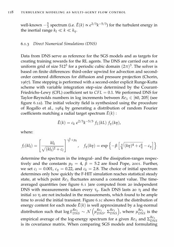
118 turbulence modeling as multi-agent flow control
well-known − 53 spectrum (i.e. E(k) ∝ ε2/3k−5/3) for the turbulent energy in
the inertial range kI k kη .
6.1.3 Direct Numerical Simulations (DNS)
Data from DNS serve as reference for the SGS models and as targets forcreating training rewards for the RL agents. The DNS are carried out on auniform grid of size 5123 for a periodic cubic domain (2π)3. The solver isbased on finite differences: third-order upwind for advection and second-order centered differences for diffusion and pressure projection (Chorin,1967). Time stepping is performed with a second-order explicit Runge-Kuttascheme with variable integration step-size determined by the Courant-Friedrichs–Lewy (CFL) coefficient set to CFL = 0.1. We performed DNS forTaylor-Reynolds numbers in log increments between Reλ ∈ [60, 205] (seefigure 6.1a). The initial velocity field is synthesized using the procedureof Rogallo et al., 1984 by generating a distribution of random Fouriercoefficients matching a radial target spectrum E(k) :
E(k) = ck ε2/3k−5/3 fL(kL) fη(kη),
where:
fl(klI) =
[klI√
(klI)2 + cl
]−53 +p0
, fη(kη) = exp−β
[4√(kη)4 + c4
η − cη
]determine the spectrum in the integral- and the dissipation-ranges respec-tively and the constants p0 = 4, β = 5.2 are fixed Pope, 2001. Further,we set cl = 0.001, cη = 0.22, and ck = 2.8. The choice of initial spectrumdetermines only how quickly the F-HIT simulation reaches statistical steadystate, at which point Reλ fluctuates around a constant value. The time-averaged quantities (see figure 6.1 )are computed from 20 independentDNS with measurements taken every τη . Each DNS lasts 20 τI and theinitial 10 τI are not included in the measurements, which found to be ampletime to avoid the initial transient. Figure 6.1c shows that the distribution ofenergy content for each mode E(k) is well approximated by a log-normaldistribution such that log EReλ
DNS ∼ N(
µReλDNS, ΣReλ
DNS
), where µ
ReλDNS is the
empirical average of the log-energy spectrum for a given Reλ and ΣReλDNS
is its covariance matrix. When comparing SGS models and formulating
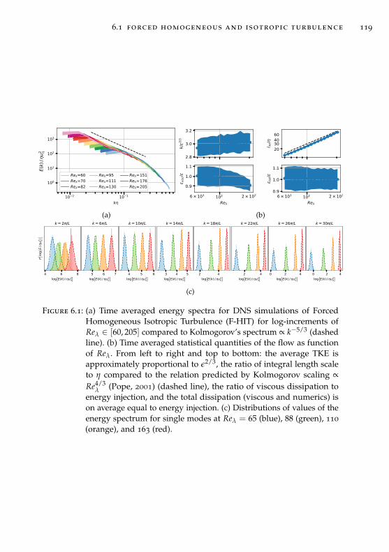
6.1 forced homogeneous and isotropic turbulence 119
(a) (b)
(c)
Figure 6.1: (a) Time averaged energy spectra for DNS simulations of ForcedHomogeneous Isotropic Turbulence (F-HIT) for log-increments ofReλ ∈ [60, 205] compared to Kolmogorov’s spectrum ∝ k−5/3 (dashedline). (b) Time averaged statistical quantities of the flow as functionof Reλ. From left to right and top to bottom: the average TKE isapproximately proportional to ε2/3, the ratio of integral length scaleto η compared to the relation predicted by Kolmogorov scaling ∝Re4/3
λ (Pope, 2001) (dashed line), the ratio of viscous dissipation toenergy injection, and the total dissipation (viscous and numerics) ison average equal to energy injection. (c) Distributions of values of theenergy spectrum for single modes at Reλ = 65 (blue), 88 (green), 110
(orange), and 163 (red).
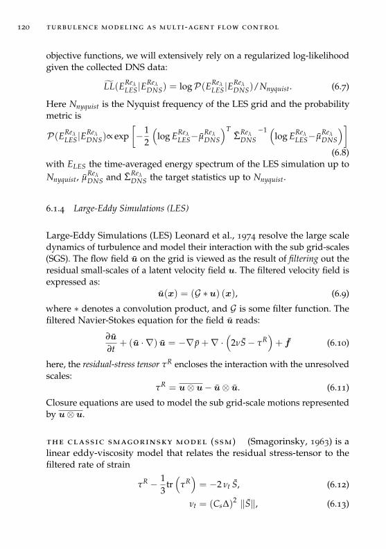
120 turbulence modeling as multi-agent flow control
objective functions, we will extensively rely on a regularized log-likelihoodgiven the collected DNS data:
LL(EReλLES|E
ReλDNS) = logP(EReλ
LES|EReλDNS)/Nnyquist. (6.7)
Here Nnyquist is the Nyquist frequency of the LES grid and the probabilitymetric is
P(EReλLES|E
ReλDNS)∝ exp
[−1
2
(log EReλ
LES−µReλDNS
)TΣReλ
DNS−1 (
log EReλLES−µ
ReλDNS
)](6.8)
with ELES the time-averaged energy spectrum of the LES simulation up toNnyquist, µ
ReλDNS and ΣReλ
DNS the target statistics up to Nnyquist.
6.1.4 Large-Eddy Simulations (LES)
Large-Eddy Simulations (LES) Leonard et al., 1974 resolve the large scaledynamics of turbulence and model their interaction with the sub grid-scales(SGS). The flow field u on the grid is viewed as the result of filtering out theresidual small-scales of a latent velocity field u. The filtered velocity field isexpressed as:
u(x) = (G ∗ u) (x), (6.9)
where ∗ denotes a convolution product, and G is some filter function. Thefiltered Navier-Stokes equation for the field u reads:
∂u
∂t+ (u · ∇) u = −∇ p +∇ ·
(2νS− τR
)+ f (6.10)
here, the residual-stress tensor τR encloses the interaction with the unresolvedscales:
τR = u⊗ u− u⊗ u. (6.11)
Closure equations are used to model the sub grid-scale motions representedby u⊗ u.
the classic smagorinsky model (ssm) (Smagorinsky, 1963) is alinear eddy-viscosity model that relates the residual stress-tensor to thefiltered rate of strain
τR − 13
tr(
τR)= −2 νt S, (6.12)
νt = (Cs∆)2 ‖S‖, (6.13)
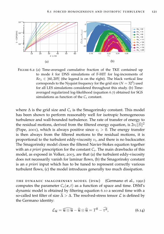
6.1 forced homogeneous and isotropic turbulence 121
(a) (b)
Figure 6.2: (a) Time-averaged cumulative fraction of the TKE contained upto mode k for DNS simulations of F-HIT for log-increments ofReλ ∈ [60, 205] (the legend is on the right). The black vertical linecorresponds to the Nyquist frequency for the grid size (N = 323) usedfor all LES simulations considered throughout this study. (b) Time-averaged regularized log-likelihood (equation 6.7) obtained for SGSsimulations as function of the Cs constant.
where ∆ is the grid size and Cs is the Smagorinsky constant. This modelhas been shown to perform reasonably well for isotropic homogeneousturbulence and wall-bounded turbulence. The rate of transfer of energy tothe residual motions, derived from the filtered energy equation, is 2νt‖S‖2
(Pope, 2001), which is always positive since νt > 0. The energy transferis then always from the filtered motions to the residual motions, it isproportional to the turbulent eddy-viscosity νt, and there is no backscatter.The Smagorinsky model closes the filtered Navier-Stokes equation togetherwith an a priori prescription for the constant Cs. The main drawbacks of thismodel, as exposed in Volker, 2003, are that (a) the turbulent eddy-viscositydoes not necessarily vanish for laminar flows, (b) the Smagorinsky constantis an a priori input which has to be tuned to represent correctly variousturbulent flows, (c) the model introduces generally too much dissipation.
the dynamic smagorinsky model (dsm) (Germano et al., 1991)computes the parameter Cs(x, t) as a function of space and time. DSM’sdynamic model is obtained by filtering equation 6.10 a second time with aso-called test filter of size ∆ > ∆. The resolved-stress tensor L is defined bythe Germano identity:
Lu = u⊗ u∧
− u⊗ u = TR − τR, (6.14)
122 turbulence modeling as multi-agent flow control
where TR = u⊗ u∧
− u⊗ u is the residual-stress tensor for the test filterwidth ∆, and τR is the test-filtered residual stress tensor for the grid size∆ (Eq. 6.11). If both residual stresses are approximated by a Smagorinskymodel, the Germano identity becomes:
Lu ≈ 2 C2s (x, t)∆2
[‖S‖S∧
− ∆2
∆2 ‖S‖S]
. (6.15)
The dynamic Smagorinsky parameter Eq. 6.15 forms an over-determinedsystem for C2
s (x, t), whose least-squares solution is (Lilly, 1992):
C2s (x, t) =
〈Lu, M〉F2∆2 ‖M‖2 , (6.16)
where M = ‖S‖S∧
− (∆/∆)2 ‖S‖S, and 〈·〉F is the Frobenius product. Be-cause the dynamic coefficient may take negative values, which representsenergy transfer from the unresolved to the resolved scales, C2
s is clipped topositive values for numerical stability.
The fraction of TKE contained in the unresolved scales increases withReλ and decreases with the grid size (figure 6.2a). For all LES simulationconsidered in this study we employ a grid of size N = 323, as compared toN = 323 for the DNS. For the higer Reλ, the SGS model accounts for up to10% of the total TKE. We employ second-order centered discretization forthe advection and the initial conditions for the velocity field are synthesizedfrom the time-averaged DNS spectrum at the same Reλ Rogallo et al., 1984.When reporting results from SSM simulation, we imply the Smagorinskyconstant Cs resulting from line-search optimization with step size 0.005 (seeFig. 6.2b). LES statistics are computed from simulations up to t = 100τI,disregarding the initial 10τI time units. For the DSM procedure we employan uniform box test-filter of width ∆ = 2∆. Finally, DSM spectra areobtained with time-stepping coefficient CFL = 0.01, while CFL = 0.1 wasused for all other LES.
6.2 multi-agent reinforcement learning for sgs modeling
RL identifies optimal strategies for agents that perform actions, contingenton their state, which affect the environment, and measure their performancevia scalar reward functions. Todate, RL has been used in fluid mechanicssolely in applications of control (Biferale et al., 2019; Gazzola et al., 2014;
6.2 multi-agent reinforcement learning for sgs modeling 123
Reddy et al., 2016; Verma et al., 2018). In these examples the control actionis defined by an embodied agent capable of spontaneous motion. By inter-acting with the flow field, agents trained through RL were able to gatherrelevant information and optimize their decision process to perform collec-tive swimming (Gazzola et al., 2014), soar (Reddy et al., 2016), minimizetheir drag (Novati et al., 2017; Verma et al., 2018), or reach a target location(Biferale et al., 2019; Novati et al., 2019b). Here we cast the TM problemas an optimization (Langford et al., 1999) and introduce RL to control anunder-resolved simulation (LES) with the objective of reproducing quanti-ties of interest computed by fully resolved DNS. The methodology by whichRL is incorporated as part of the flow solver has a considerable effect on thecomputational efficiency of the resulting algorithm. As an example, follow-ing the common practice in video games (Mnih et al., 2015), the state of theagent could be defined as the full three-dimensional flow field at a giventime-step and the action as some quantity used to compute the SGS termsfor all grid-points. However, such architecture would have the followingchallenges: it would be mesh-size dependent, it would involve a very largeunderlying NN, and the memory needed to store the experiences of theagent would be prohibitively large. We overcome these issues by deployingNagents dispersed RL agents (marked as red cubes in Fig. 6.3) with localizedactuation that use a combination of local and global information on the flowfield, encoded in the state s(x, t) ∈ RdimS (here, x is the spatial coordinateand t the time step). A policy-network with parameters w is trained byRL to select the local SGS dissipation coefficient C2
s (x, t) ∼ πw(·|s). Themulti-agent RL (MARL) advance in turns by updating C2
s (x, t) for the entireflow and integrating in time for ∆tRL to the next RL step until Tend or if anynumerical instability arises. The learning objective is to find the parametersw of the policy πw that maximize the expected sum of rewards over the LES:
J(w) = Eπw
[∑Tend
t=1 rt
].
RL requires scalar reward signals measuring the agents’ performance.Here we consider two reward functionals, described in detail in the nextsection. The first, rG, is based on the Germano identity (Germano, 1992;Germano et al., 1991) which states that the sum of resolved and modeledcontributions to the SGS stress tensor should be independent of LES res-olution. The second, rLL, penalizes discrepancies from the target energyspectra obtained by high-fidelity simulations (DNS) at a given Reλ. WhilerG is computed locally for each agent, rLL is a global relation equal for allagents which measures the distance of the RL-LES statistics from those offully resolved DNS. We remark that the target statistics involve spatial and
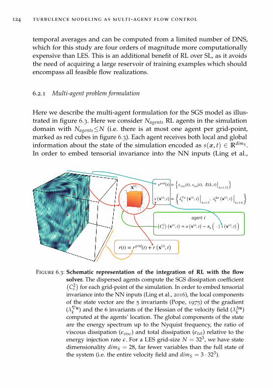
124 turbulence modeling as multi-agent flow control
temporal averages and can be computed from a limited number of DNS,which for this study are four orders of magnitude more computationallyexpensive than LES. This is an additional benefit of RL over SL, as it avoidsthe need of acquiring a large reservoir of training examples which shouldencompass all feasible flow realizations.
6.2.1 Multi-agent problem formulation
Here we describe the multi-agent formulation for the SGS model as illus-trated in figure 6.3. Here we consider Nagents RL agents in the simulationdomain with Nagents≤N (i.e. there is at most one agent per grid-point,marked as red cubes in figure 6.3). Each agent receives both local and globalinformation about the state of the simulation encoded as s(x, t) ∈ RdimS .In order to embed tensorial invariance into the NN inputs (Ling et al.,
x(i)
s (x(i), t) = λ∇uk (x(i), t)
k=1:5, λΔu
k (x(i), t)k=1:6
sgrid(t) = ϵvisc(t), ϵtot(t), E(k, t)k=1:15
(C2s ) (x(i), t) = a (x(i), t) ∼ π ( ⋅ | s (x(i), t))
agent i
r(t) = rgrid(t) + r (x(i), t)
Figure 6.3: Schematic representation of the integration of RL with the flowsolver. The dispersed agents compute the SGS dissipation coefficient(C2
s)
for each grid-point of the simulation. In order to embed tensorialinvariance into the NN inputs (Ling et al., 2016), the local componentsof the state vector are the 5 invariants (Pope, 1975) of the gradient(λ∇u
k ) and the 6 invariants of the Hessian of the velocity field (λ∆uk )
computed at the agents’ location. The global components of the stateare the energy spectrum up to the Nyquist frequency, the ratio ofviscous dissipation (εvisc) and total dissipation (εtot) relative to theenergy injection rate ε. For a LES grid-size N = 323, we have statedimensionality dimS = 28, far fewer variables than the full state ofthe system (i.e. the entire velocity field and dimS = 3 · 323).
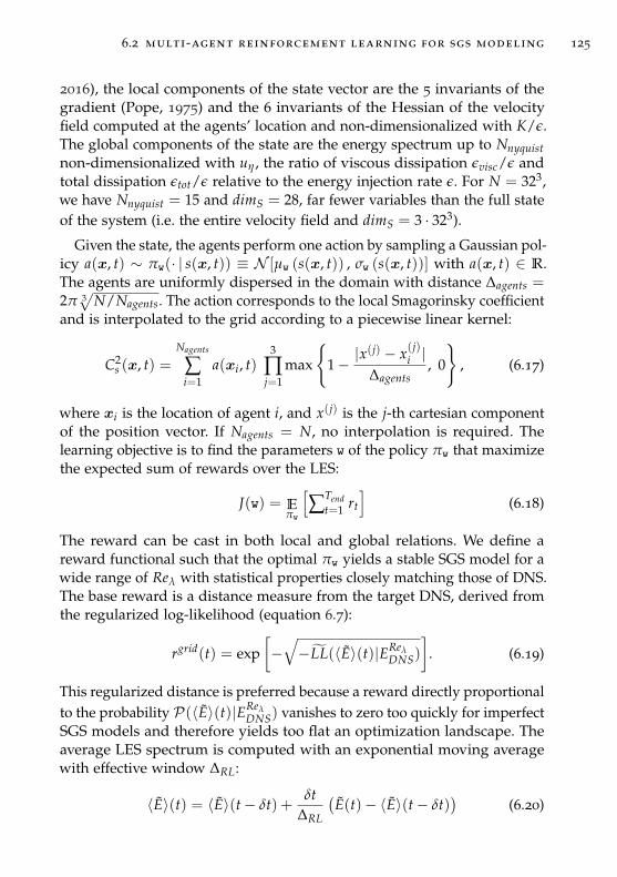
6.2 multi-agent reinforcement learning for sgs modeling 125
2016), the local components of the state vector are the 5 invariants of thegradient (Pope, 1975) and the 6 invariants of the Hessian of the velocityfield computed at the agents’ location and non-dimensionalized with K/ε.The global components of the state are the energy spectrum up to Nnyquistnon-dimensionalized with uη , the ratio of viscous dissipation εvisc/ε andtotal dissipation εtot/ε relative to the energy injection rate ε. For N = 323,we have Nnyquist = 15 and dimS = 28, far fewer variables than the full stateof the system (i.e. the entire velocity field and dimS = 3 · 323).
Given the state, the agents perform one action by sampling a Gaussian pol-icy a(x, t) ∼ πw(· | s(x, t)) ≡ N [µw (s(x, t)) , σw (s(x, t))] with a(x, t) ∈ R.The agents are uniformly dispersed in the domain with distance ∆agents =2π 3√
N/Nagents. The action corresponds to the local Smagorinsky coefficientand is interpolated to the grid according to a piecewise linear kernel:
C2s (x, t) =
Nagents
∑i=1
a(xi, t)3
∏j=1
max
1− |x
(j) − x(j)i |
∆agents, 0
, (6.17)
where xi is the location of agent i, and x(j) is the j-th cartesian componentof the position vector. If Nagents = N, no interpolation is required. Thelearning objective is to find the parameters w of the policy πw that maximizethe expected sum of rewards over the LES:
J(w) = Eπw
[∑Tend
t=1 rt
](6.18)
The reward can be cast in both local and global relations. We define areward functional such that the optimal πw yields a stable SGS model for awide range of Reλ with statistical properties closely matching those of DNS.The base reward is a distance measure from the target DNS, derived fromthe regularized log-likelihood (equation 6.7):
rgrid(t) = exp[−√−LL(〈E〉(t)|EReλ
DNS)
]. (6.19)
This regularized distance is preferred because a reward directly proportionalto the probability P(〈E〉(t)|EReλ
DNS) vanishes to zero too quickly for imperfectSGS models and therefore yields too flat an optimization landscape. Theaverage LES spectrum is computed with an exponential moving averagewith effective window ∆RL:
〈E〉(t) = 〈E〉(t− δt) +δt
∆RL
(E(t)− 〈E〉(t− δt)
)(6.20)
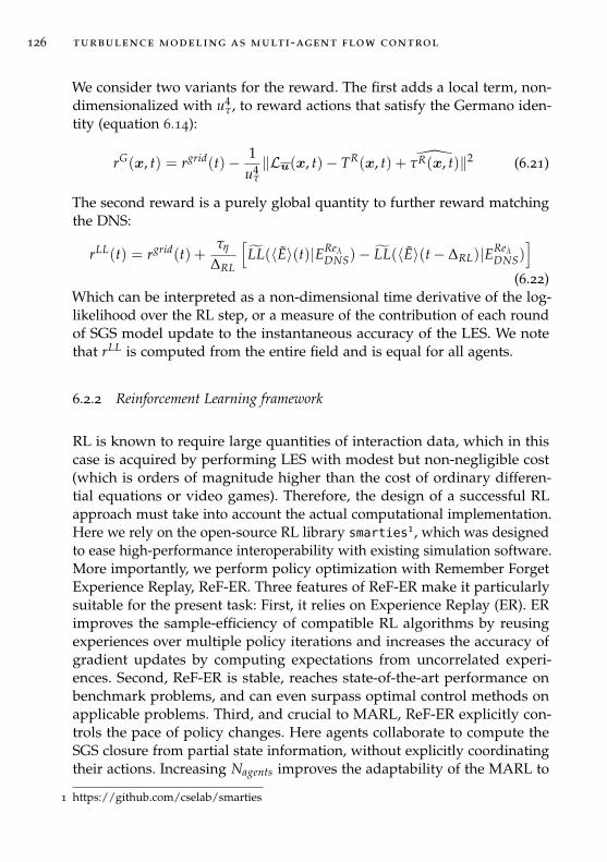
126 turbulence modeling as multi-agent flow control
We consider two variants for the reward. The first adds a local term, non-dimensionalized with u4
τ , to reward actions that satisfy the Germano iden-tity (equation 6.14):
rG(x, t) = rgrid(t)− 1u4
τ
‖Lu(x, t)− TR(x, t) + τR(x, t)‖2 (6.21)
The second reward is a purely global quantity to further reward matchingthe DNS:
rLL(t) = rgrid(t) +τη
∆RL
[LL(〈E〉(t)|EReλ
DNS)− LL(〈E〉(t− ∆RL)|EReλDNS)
](6.22)
Which can be interpreted as a non-dimensional time derivative of the log-likelihood over the RL step, or a measure of the contribution of each roundof SGS model update to the instantaneous accuracy of the LES. We notethat rLL is computed from the entire field and is equal for all agents.
6.2.2 Reinforcement Learning framework
RL is known to require large quantities of interaction data, which in thiscase is acquired by performing LES with modest but non-negligible cost(which is orders of magnitude higher than the cost of ordinary differen-tial equations or video games). Therefore, the design of a successful RLapproach must take into account the actual computational implementation.Here we rely on the open-source RL library smarties1, which was designedto ease high-performance interoperability with existing simulation software.More importantly, we perform policy optimization with Remember ForgetExperience Replay, ReF-ER. Three features of ReF-ER make it particularlysuitable for the present task: First, it relies on Experience Replay (ER). ERimproves the sample-efficiency of compatible RL algorithms by reusingexperiences over multiple policy iterations and increases the accuracy ofgradient updates by computing expectations from uncorrelated experi-ences. Second, ReF-ER is stable, reaches state-of-the-art performance onbenchmark problems, and can even surpass optimal control methods onapplicable problems. Third, and crucial to MARL, ReF-ER explicitly con-trols the pace of policy changes. Here agents collaborate to compute theSGS closure from partial state information, without explicitly coordinatingtheir actions. Increasing Nagents improves the adaptability of the MARL to
1 https://github.com/cselab/smarties
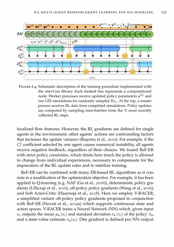
6.2 multi-agent reinforcement learning for sgs modeling 127
Figure 6.4: Schematic description of the training procedure implemented withthe smarties library. Each dashed line represents a computationalnode. Worker processes receive updated policy parameters w(k) andrun LES simulations for randomly sampled Reλ. At the top, a masterprocess receives RL data from completed simulations. Policy updatesare computed by sampling mini-batches from the N most recentlycollected RL steps.
localized flow features. However, the RL gradients are defined for singleagents in the environment; other agents’ actions are confounding factorsthat increases the update variance (Busoniu et al., 2010). For example, if theC2
s coefficient selected by one agent causes numerical instability, all agentsreceive negative feedback, regardless of their choices. We found ReF-ERwith strict policy constrains, which limits how much the policy is allowedto change from individual experiences, necessary to compensate for theimprecision of the RL update rules and to stabilize training.
ReF-ER can be combined with many ER-based RL algorithms as it con-sists in a modification of the optimization objective. For example, it has beenapplied to Q-learning (e.g. NAF (Gu et al., 2016)), deterministic policy gra-dients (Lillicrap et al., 2016), off-policy policy gradients (Wang et al., 2016),and Soft Actor-Critic (Haarnoja et al., 2018). Here we employ V-RACER,a simplified variant off-policy policy gradients proposed in conjunctionwith ReF-ER (Novati et al., 2019a) which supports continuous state andaction spaces. V-RACER trains a Neural Network (NN) which, given inputst, outputs the mean µw (st) and standard deviation σw (st) of the policy πw,and a state-value estimate vw(st). One gradient is defined per NN output.
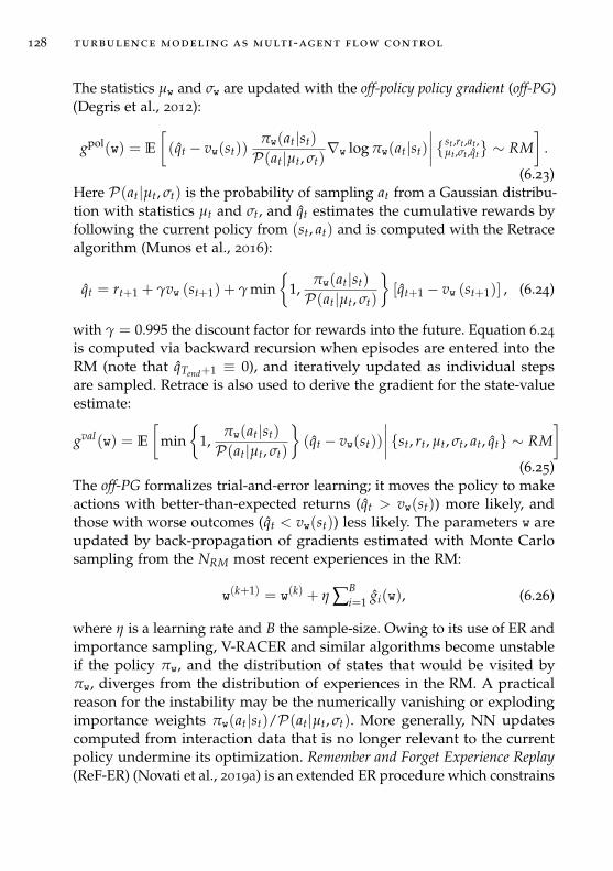
128 turbulence modeling as multi-agent flow control
The statistics µw and σw are updated with the off-policy policy gradient (off-PG)(Degris et al., 2012):
gpol(w) = E
[(qt − vw(st))
πw(at|st)
P(at|µt, σt)∇w log πw(at|st)
∣∣∣∣ st ,rt ,at ,µt ,σt ,qt
∼ RM
].
(6.23)Here P(at|µt, σt) is the probability of sampling at from a Gaussian distribu-tion with statistics µt and σt, and qt estimates the cumulative rewards byfollowing the current policy from (st, at) and is computed with the Retracealgorithm (Munos et al., 2016):
qt = rt+1 + γvw (st+1) + γ min
1,πw(at|st)
P(at|µt, σt)
[qt+1 − vw (st+1)] , (6.24)
with γ = 0.995 the discount factor for rewards into the future. Equation 6.24
is computed via backward recursion when episodes are entered into theRM (note that qTend+1 ≡ 0), and iteratively updated as individual stepsare sampled. Retrace is also used to derive the gradient for the state-valueestimate:
gval(w) = E
[min
1,
πw(at|st)
P(at|µt, σt)
(qt − vw(st))
∣∣∣∣ st, rt, µt, σt, at, qt ∼ RM]
(6.25)The off-PG formalizes trial-and-error learning; it moves the policy to makeactions with better-than-expected returns (qt > vw(st)) more likely, andthose with worse outcomes (qt < vw(st)) less likely. The parameters w areupdated by back-propagation of gradients estimated with Monte Carlosampling from the NRM most recent experiences in the RM:
w(k+1) = w(k) + η ∑Bi=1 gi(w), (6.26)
where η is a learning rate and B the sample-size. Owing to its use of ER andimportance sampling, V-RACER and similar algorithms become unstableif the policy πw, and the distribution of states that would be visited byπw, diverges from the distribution of experiences in the RM. A practicalreason for the instability may be the numerically vanishing or explodingimportance weights πw(at|st)/P(at|µt, σt). More generally, NN updatescomputed from interaction data that is no longer relevant to the currentpolicy undermine its optimization. Remember and Forget Experience Replay(ReF-ER) (Novati et al., 2019a) is an extended ER procedure which constrains
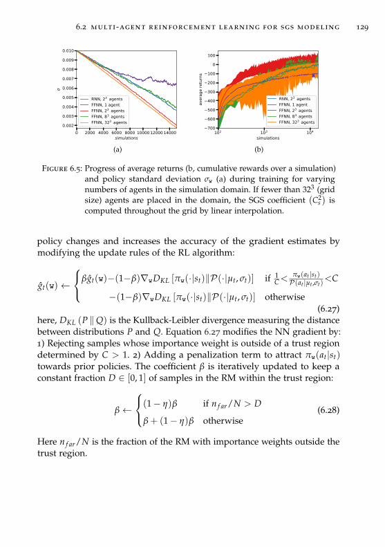
6.2 multi-agent reinforcement learning for sgs modeling 129
(a) (b)
Figure 6.5: Progress of average returns (b, cumulative rewards over a simulation)and policy standard deviation σw (a) during training for varyingnumbers of agents in the simulation domain. If fewer than 323 (gridsize) agents are placed in the domain, the SGS coefficient
(C2
s)
iscomputed throughout the grid by linear interpolation.
policy changes and increases the accuracy of the gradient estimates bymodifying the update rules of the RL algorithm:
gt(w)←
βgt(w)−(1−β)∇wDKL [πw(·|st)‖P(·|µt, σt)] if 1C<
πw(at |st)P(at |µt ,σt)
<C
−(1−β)∇wDKL [πw(·|st)‖P(·|µt, σt)] otherwise(6.27)
here, DKL (P ‖Q) is the Kullback-Leibler divergence measuring the distancebetween distributions P and Q. Equation 6.27 modifies the NN gradient by:1) Rejecting samples whose importance weight is outside of a trust regiondetermined by C > 1. 2) Adding a penalization term to attract πw(at|st)towards prior policies. The coefficient β is iteratively updated to keep aconstant fraction D ∈ [0, 1] of samples in the RM within the trust region:
β←
(1− η)β if n f ar/N > D
β + (1− η)β otherwise(6.28)
Here n f ar/N is the fraction of the RM with importance weights outside thetrust region.
130 turbulence modeling as multi-agent flow control
6.2.3 Overview of the training set-up
We summarize here the training set-up and hyper-parameters of V-RACER.Each LES is initialized for uniformly sampled Reλ ∈ 65, 76, 88, 103, 120,140, 163 and a random velocity field synthesized from the target DNSspecturum. The residual-stress tensor τR is updated with equation 6.13 andagents’ actions every ∆RL = τη/8. The LES are interrupted at Tend = 20τI(between 750, if Reλ = 65, and 1600, if Reλ = 163, actions per agent) or if‖u‖∞ > 103uη , which signals numerical instability. The policy πw is parame-terized by a NN with 2 hidden layers of 64 units each, with tanh activationsand skip connections. The NN is initialized as Glorot et al., 2010 with smallouter weights and bias shifted such that the initial policy is approximatelyπw(0)(·|s) ≈ N (0.04, 10−4) and produces Smagorinsky coefficients with
small perturbations around Ct ≈ 0.2. Updates are computed with MonteCarlo estimates of gradients with sample size B = 512 from a RM of sizeNRM = 106 and the learning rate is η = 10−5. As discussed in the maintext, because we use conventional RL update rules in a multi-agent setting,single parameter updates are imprecise. We found that ReF-ER with hyper-parameters C = 2 (Eq. 6.27) and D = 0.05 (Eq. 6.28) to stabilize training.Figure 6.5b shows the two asymptotically extreme settings Nagents = 1 (i.e.C2
s constant in space) and Nagents = 323 (i.e. C2s independently chosen by
each grid-point) to perform worse than intermediate ones. Unless otherwisestated, we set Nagents = 43 and analyze this parameter further in the nextsection. Finally, the reduced description of the system’s state mitigates thecomputational cost and simplifies πw. We considered Recurrent NN policies,which allow RL to deal with partial observability, but we find them of nouse to the present problem (see figure 6.5b).
We ran multiple training runs per reward function and whenever wevary the hyper-parameters, but we observe consistent training progressregardless of the initial random seed. Hereafter, the trained policies areevaluated by deterministically setting actions equal to the mean of theGaussian a(x, t) = µw (s(x, t)), rather than via sampling.
results
The Taylor-Reynolds number (Reλ) characterizes the breadth of the spec-trum of vortical structures present in a homogeneous isotropic turbulentflow Orszag et al., 1972; Pope, 2001; Taylor, 1935. Figure 6.6 illustrates the
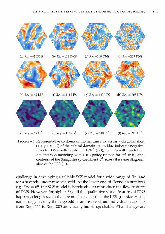
6.2 multi-agent reinforcement learning for sgs modeling 131
(a) Reλ=65 DNS (b) Reλ=111 DNS (c) Reλ=140 DNS (d) Reλ=205 DNS
(e) Reλ = 65 LES (f) Reλ = 111 LES (g) Reλ = 140 LES (h) Reλ = 205 LES
(i) Reλ = 65 Cs2 (j) Reλ = 111 Cs2 (k) Reλ = 140 Cs2 (l) Reλ = 205 Cs2
Figure 6.6: Representative contours of momentum flux across a diagonal slice(x + y + z = 0) of the cubical domain (u ·n, blue indicates negativeflux) for DNS with resolution 10243 (a-d), for LES with resolution323 and SGS modeling with a RL policy trained for rLL (e-h), andcontours of the Smagorinsky coefficient C2
s across the same diagonalslice of the LES (i-l).
challenge in developing a reliable SGS model for a wide range of Reλ andfor a severely under-resolved grid. At the lower end of Reynolds numbers,e.g. Reλ = 65, the SGS model is barely able to reproduce the flow featuresof DNS. However, for higher Reλ all the qualitative visual features of DNShappen at length-scales that are much smaller than the LES grid-size. As thename suggests, only the large eddies are resolved and individual snapshotsfrom Reλ=111 to Reλ=205 are visually indistinguishable. What changes are
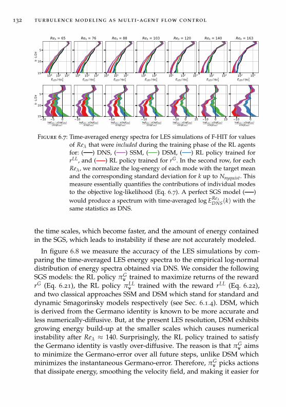
132 turbulence modeling as multi-agent flow control
Figure 6.7: Time-averaged energy spectra for LES simulations of F-HIT for valuesof Reλ that were included during the training phase of the RL agentsfor: ( ) DNS, ( ) SSM, ( ) DSM, ( ) RL policy trained forrLL, and ( ) RL policy trained for rG. In the second row, for eachReλ, we normalize the log-energy of each mode with the target meanand the corresponding standard deviation for k up to Nnyquist. Thismeasure essentially quantifies the contributions of individual modesto the objective log-likelihood (Eq. 6.7). A perfect SGS model ( )would produce a spectrum with time-averaged log EReλ
DNS(k) with thesame statistics as DNS.
the time scales, which become faster, and the amount of energy containedin the SGS, which leads to instability if these are not accurately modeled.
In figure 6.8 we measure the accuracy of the LES simulations by com-paring the time-averaged LES energy spectra to the empirical log-normaldistribution of energy spectra obtained via DNS. We consider the followingSGS models: the RL policy πG
w trained to maximize returns of the rewardrG (Eq. 6.21), the RL policy πLL
w trained with the reward rLL (Eq. 6.22),and two classical approaches SSM and DSM which stand for standard anddynamic Smagorinsky models respectively (see Sec. 6.1.4). DSM, whichis derived from the Germano identity is known to be more accurate andless numerically-diffusive. But, at the present LES resolution, DSM exhibitsgrowing energy build-up at the smaller scales which causes numericalinstability after Reλ ≈ 140. Surprisingly, the RL policy trained to satisfythe Germano identity is vastly over-diffusive. The reason is that πG
w aimsto minimize the Germano-error over all future steps, unlike DSM whichminimizes the instantaneous Germano-error. Therefore, πG
w picks actionsthat dissipate energy, smoothing the velocity field, and making it easier for
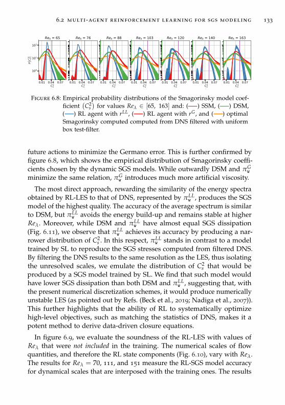
6.2 multi-agent reinforcement learning for sgs modeling 133
Figure 6.8: Empirical probability distributions of the Smagorinsky model coef-ficient
(C2
s)
for values Reλ ∈ [65, 163] and: ( ) SSM, ( ) DSM,( ) RL agent with rLL, ( ) RL agent with rG, and ( ) optimalSmagorinsky computed computed from DNS filtered with uniformbox test-filter.
future actions to minimize the Germano error. This is further confirmed byfigure 6.8, which shows the empirical distribution of Smagorinsky coeffi-cients chosen by the dynamic SGS models. While outwardly DSM and πG
w
minimize the same relation, πGw introduces much more artificial viscosity.
The most direct approach, rewarding the similarity of the energy spectraobtained by RL-LES to that of DNS, represented by πLL
w , produces the SGSmodel of the highest quality. The accuracy of the average spectrum is similarto DSM, but πLL
w avoids the energy build-up and remains stable at higherReλ. Moreover, while DSM and πLL
w have almost equal SGS dissipation(Fig. 6.11), we observe that πLL
w achieves its accuracy by producing a nar-rower distribution of C2
s . In this respect, πLLw stands in contrast to a model
trained by SL to reproduce the SGS stresses computed from filtered DNS.By filtering the DNS results to the same resolution as the LES, thus isolatingthe unresolved scales, we emulate the distribution of C2
s that would beproduced by a SGS model trained by SL. We find that such model wouldhave lower SGS dissipation than both DSM and πLL
w , suggesting that, withthe present numerical discretization schemes, it would produce numericallyunstable LES (as pointed out by Refs. (Beck et al., 2019; Nadiga et al., 2007)).This further highlights that the ability of RL to systematically optimizehigh-level objectives, such as matching the statistics of DNS, makes it apotent method to derive data-driven closure equations.
In figure 6.9, we evaluate the soundness of the RL-LES with values ofReλ that were not included in the training. The numerical scales of flowquantities, and therefore the RL state components (Fig. 6.10), vary with Reλ.The results for Reλ = 70, 111, and 151 measure the RL-SGS model accuracyfor dynamical scales that are interposed with the training ones. The results
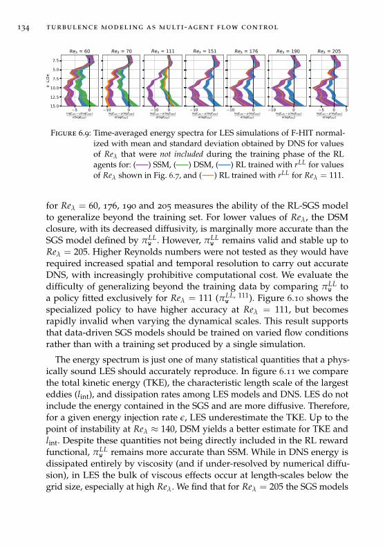
134 turbulence modeling as multi-agent flow control
Figure 6.9: Time-averaged energy spectra for LES simulations of F-HIT normal-ized with mean and standard deviation obtained by DNS for valuesof Reλ that were not included during the training phase of the RLagents for: ( ) SSM, ( ) DSM, ( ) RL trained with rLL for valuesof Reλ shown in Fig. 6.7, and ( ) RL trained with rLL for Reλ = 111.
for Reλ = 60, 176, 190 and 205 measures the ability of the RL-SGS modelto generalize beyond the training set. For lower values of Reλ, the DSMclosure, with its decreased diffusivity, is marginally more accurate than theSGS model defined by πLL
w . However, πLLw remains valid and stable up to
Reλ = 205. Higher Reynolds numbers were not tested as they would haverequired increased spatial and temporal resolution to carry out accurateDNS, with increasingly prohibitive computational cost. We evaluate thedifficulty of generalizing beyond the training data by comparing πLL
w toa policy fitted exclusively for Reλ = 111 (πLL, 111
w ). Figure 6.10 shows thespecialized policy to have higher accuracy at Reλ = 111, but becomesrapidly invalid when varying the dynamical scales. This result supportsthat data-driven SGS models should be trained on varied flow conditionsrather than with a training set produced by a single simulation.
The energy spectrum is just one of many statistical quantities that a phys-ically sound LES should accurately reproduce. In figure 6.11 we comparethe total kinetic energy (TKE), the characteristic length scale of the largesteddies (lint), and dissipation rates among LES models and DNS. LES do notinclude the energy contained in the SGS and are more diffusive. Therefore,for a given energy injection rate ε, LES underestimate the TKE. Up to thepoint of instability at Reλ ≈ 140, DSM yields a better estimate for TKE andlint. Despite these quantities not being directly included in the RL rewardfunctional, πLL
w remains more accurate than SSM. While in DNS energy isdissipated entirely by viscosity (and if under-resolved by numerical diffu-sion), in LES the bulk of viscous effects occur at length-scales below thegrid size, especially at high Reλ. We find that for Reλ = 205 the SGS models
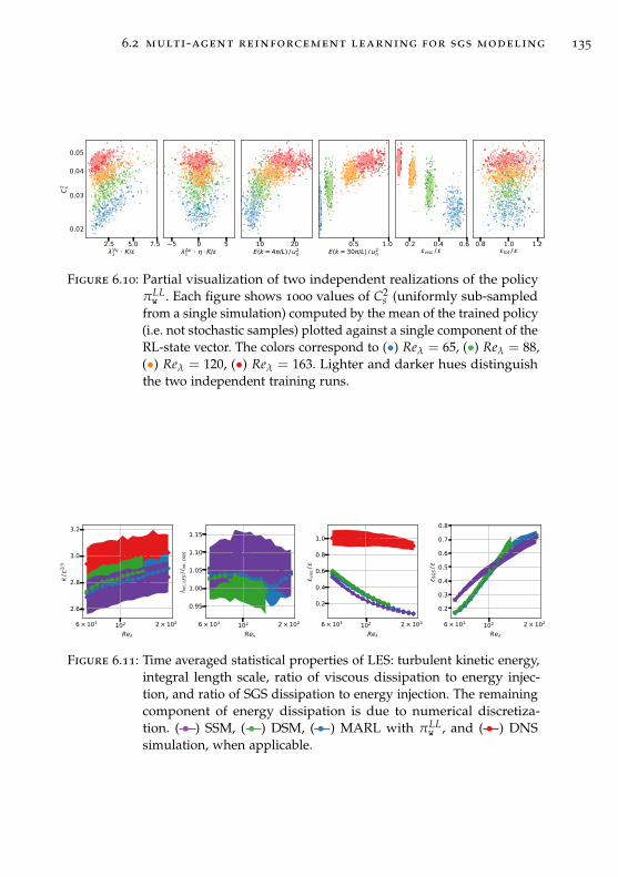
6.2 multi-agent reinforcement learning for sgs modeling 135
Figure 6.10: Partial visualization of two independent realizations of the policyπLLw . Each figure shows 1000 values of C2
s (uniformly sub-sampledfrom a single simulation) computed by the mean of the trained policy(i.e. not stochastic samples) plotted against a single component of theRL-state vector. The colors correspond to (•) Reλ = 65, (•) Reλ = 88,(•) Reλ = 120, (•) Reλ = 163. Lighter and darker hues distinguishthe two independent training runs.
Figure 6.11: Time averaged statistical properties of LES: turbulent kinetic energy,integral length scale, ratio of viscous dissipation to energy injec-tion, and ratio of SGS dissipation to energy injection. The remainingcomponent of energy dissipation is due to numerical discretiza-tion. ( • ) SSM, ( • ) DSM, ( • ) MARL with πLL
w , and ( • ) DNSsimulation, when applicable.
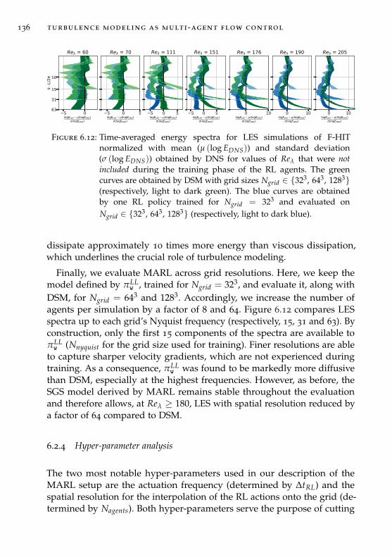
136 turbulence modeling as multi-agent flow control
Figure 6.12: Time-averaged energy spectra for LES simulations of F-HITnormalized with mean (µ (log EDNS)) and standard deviation(σ (log EDNS)) obtained by DNS for values of Reλ that were notincluded during the training phase of the RL agents. The greencurves are obtained by DSM with grid sizes Ngrid ∈ 323, 643, 1283(respectively, light to dark green). The blue curves are obtainedby one RL policy trained for Ngrid = 323 and evaluated onNgrid ∈ 323, 643, 1283 (respectively, light to dark blue).
dissipate approximately 10 times more energy than viscous dissipation,which underlines the crucial role of turbulence modeling.
Finally, we evaluate MARL across grid resolutions. Here, we keep themodel defined by πLL
w , trained for Ngrid = 323, and evaluate it, along withDSM, for Ngrid = 643 and 1283. Accordingly, we increase the number ofagents per simulation by a factor of 8 and 64. Figure 6.12 compares LESspectra up to each grid’s Nyquist frequency (respectively, 15, 31 and 63). Byconstruction, only the first 15 components of the spectra are available toπLLw (Nnyquist for the grid size used for training). Finer resolutions are able
to capture sharper velocity gradients, which are not experienced duringtraining. As a consequence, πLL
w was found to be markedly more diffusivethan DSM, especially at the highest frequencies. However, as before, theSGS model derived by MARL remains stable throughout the evaluationand therefore allows, at Reλ ≥ 180, LES with spatial resolution reduced bya factor of 64 compared to DSM.
6.2.4 Hyper-parameter analysis
The two most notable hyper-parameters used in our description of theMARL setup are the actuation frequency (determined by ∆tRL) and thespatial resolution for the interpolation of the RL actions onto the grid (de-termined by Nagents). Both hyper-parameters serve the purpose of cutting
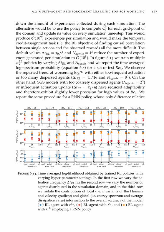
6.2 multi-agent reinforcement learning for sgs modeling 137
down the amount of experiences collected during each simulation. Thealternative would be to use the policy to compute C2
s for each grid-point ofthe domain and update its value on every simulation time-step. This wouldproduce O(109) experiences per simulation and would make the temporalcredit-assignment task (i.e. the RL objective of finding causal correlationbetween single actions and the observed reward) all the more difficult. Thedefault values ∆tRL = τη/8 and Nagents = 43 reduce the number of experi-ences generated per simulation to O(105). In figure 6.13 we train multipleπLLw policies by varying ∆tRL and Nagents and we report the time-averaged
log-spectrum probability (equation 6.8) for a set of test Reλ. We observethe repeated trend of worsening logP with either too-frequent actuationor too many dispersed agents (∆tRL = τη/16 and Nagents = 83). On theother hand, SGS models with too coarsely dispersed agents (Nagents = 23)or infrequent actuation update (∆tRL = τη/4) have reduced adaptabilityand therefore exhibit slightly lower precision for high values of Reλ. Werepeat the same procedure for a RNN-policy, whose only difference relative
Figure 6.13: Time averaged log-likelihood obtained by trained RL policies withvarying hyper-parameter settings. In the first row we vary the ac-tuation frequency ∆tRL, in the second row we vary the number ofagents distributed in the simulation domain, and in the third rowwe isolate the contribution of local (i.e. invariants of the Hessianand velocity gradient) and global (i.e. energy spectrum and averagedissipation rates) information to the overall accuracy of the model.( • ) RL agent with rLL, ( • ) RL agent with rG, and ( • ) RL agentwith rLL employing a RNN policy.
138 turbulence modeling as multi-agent flow control
to the original πLLw model is that the conventional fully-connected layers
are replaced by GRU (Chung et al., 2014). RNN are notoriously harder totrain (Sutskever, 2013) and their performance, while in general it is similarto that of πLL
w , falls off more noticeably for higher values of ∆tRL and Nagents.
discussion
This chapter introduces multi-agent RL (MARL) as a strategy to automatethe derivation of closure equations for turbulence modeling (TM). Wedemonstrate the feasibility and potential of this approach on large-eddysimulations (LES) of forced homogeneous and isotropic turbulence. RLagents are incorporated into the flow solver and observe local (e.g. invari-ants of the velocity gradient) as well as global (e.g. the energy spectrum)flow quantities. MARL develops the sub-grid scale (SGS) model as a pol-icy that relates agent observations and actions. The agents cooperate tocompute SGS residual-stresses of the flow field through the Smagorinsky(Smagorinsky, 1963) formulation in order to minimize the discrepanciesbetween the time-averaged energy spectrum of the LES and that computedfrom fully resolved simulations (DNS), which are orders of magnitudemore computationally expensive. The Remember and Forget ExperienceReplay (ReF-ER) method, combining the sample-efficiency of ER and thestability of constrained policy updates of on-policy RL (Novati et al., 2019a),is instrumental for the present results.
The results of the present study open new horizons for TM. RL maximizeshigh-level objectives computed from direct application of the learned modeland produces SGS models that are stable under perturbation and resistantto compounding errors. Moreover, MARL offers new paths to solve manyof the classic challenges of LES, such as wall-layer modeling and inflowboundary conditions, which are difficult to formulate analytically or interms of supervised learning (Zhiyin, 2015). We empirically quantifiedand explored the ability of MARL to converge to an accurate model andto generalize to unseen flow conditions. At the same time new questionsemerge from integrating RL and TM. The control policies trained by thepresent MARL method (e.g. πLL
w ) are functions with 28-dimensional inputand 6’211 parameters. Figure 6.10 provides some snapshots of the complexcorrelations between input and Smagorinsky coefficient selected by πLL
w . Weobserve that two independent training runs, over a range of Reλ, produce

6.2 multi-agent reinforcement learning for sgs modeling 139
overlapping distributions of actuation strategies, analogous to dynamicalsystems with the same attractor. While machine learning approaches canbe faulted for the lack of generality guarantees and for the difficulty ofinterpreting the trained model, we envision that sparse RL methods couldenable the analysis of causal processes in turbulent energy dissipation andthe distillation of mechanistic models.

7C O N C L U S I O N S A N D P E R S P E C T I V E S
7.1 conclusions
This thesis has been focused on the development and application of deepreinforcement learning (RL) methods to scientific flow simulations.
Remember and Forget Experience Replay
Since the work of Kakade et al., 2002, multiple approaches have beenproposed to update RL policies with some guarantees of monotonic im-provements on the returns. For example, among the most widely usedare Trust Region Policy Optimization (TRPO, Schulman et al., 2015a) andProximal Policy Optimization (PPO, Schulman et al., 2017). These worksare concerned with on-policy algorithms, where only data collected withthe current policy is used to compute the update, and they show that theupdate size should be constrained to ensure stability and accuracy. Thisintuition, of preserving the similarity between training behaviors and pol-icy, had never been extended to off-policy algorithms. Off-policy methodscompute updates by sampling a reservoir of past experiences, a featurewhich confers them much greater sample-efficiency.
At the same time, recent published works have shown that the resultsobtained by deep RL rely, in unintuitive ways, on code-level optimizations(Engstrom et al., 2019), hyper-parameter tuning (Henderson et al., 2018),and unreliable gradient estimates (Ilyas et al., 2018). Many successful ap-plications of deep RL investigate novel loss functions or architectures. Yet,these works show that more technical, and not acknowledged in the paper,implementation choices may be crucial for obtaining good performance(Andrychowicz et al., 2020a).
This context highlights the relevance of Remember and Forget Experi-ence Replay (ReF-ER). We have shown that ReF-ER can be applied to anyoff-policy RL algorithm with parameterized policies, as it consists in a mod-ification of the loss function. Instead of presenting results with one, highly
141
142 conclusions and perspectives
tuned, algorithm, we analyzed ReF-ER with Q-learning, deterministic andstochastic policy gradients and without hyper-parameter optimization. In allconsidered cases, ReF-ER leads to significantly higher performance (as highas 300% increase in returns for high-dimensional benchmark problems).Therefore ReF-ER is a modular and intuitive improvement for off-policy RL.We show that ReF-ER is robust to hyper-parameter changes, unlike manyother approaches (Henderson et al., 2018). This feature is highly beneficialwhen the RL methods are applied to expensive flow control problems oremployed by practitioners without a machine learning background.
Optimal gliding and perching maneuvers
We have applied ReF-ER to develop gliding agents that execute complexand precise control patterns using a simple model of the controlled gravity-driven descent of an elliptical object. The ODE model allowed comparisonsbetween deep RL and optimal control (OC) methods, which showed that RLagents were able to match and even surpass the performance of trajectoriesfound through OC. We examine the control strategies that emerge whenvarying the non-dimensional parameters of the ODE, and we show that thetrained policy are stable under perturbation of the system dynamics andinitial conditions. Moreover, we analyze the effect of two crucial choiceswhen designing control problems to be solved by RL: the time intervalbetween actions and the choice of state variables.
Swimmers learning to school by maximizing energy efficiency
We demonstrate that fish can reduce their energy expenditure by schooling.We answer this longstanding issue by combining state-of-the-art directnumerical simulations of the 3D Navier–Stokes equations with reinforce-ment learning, using recurrent neural networks to account for the swimmerhaving only partial information about the flow field.
These results were achieved by conducting the first viscous, two- andthree-dimensional, simulations of multiple self-propelled swimmers en-gaged in sustained schooling formation. We developed a novel scalable andflexible flow solver built upon the ‘CUBISM’ framework (Rossinelli et al.,2013) which allows solving the three-dimensional Navier-Stokes equationswith fluid-structure interaction based on the Brinkman penalization model.
7.1 conclusions 143
Therefore, the solver can simulate multiple self-propelled, deforming andarbitrarily-shaped objects in the flow. Moreover, we developed a novel time-integration schemes to perform Brinkman penalization while conservingflow momenta. We demonstrate that the proposed method produces resultsthat are almost independent of the penalization coefficient.
We demonstrate the energetic benefits of coordinated swimming througha series of simulations of swimmers in a leader-follower configuration. With-out any control strategy, the follower’s interactions with the leader’s wakecan be either energetically beneficial or detrimental, depending on the initialcondition. Furthermore, the follower tends to diverge from the leader’swake, which points to the need for active modulation of the follower’sactions to maintain a stable tandem configuration.
Automated discovery of turbulence models
Large-eddy simulations (LES) are an essential technology for the simulationof turbulent flows in applications ranging from car and aircraft aerody-namics to atmospheric flows. One of the essential elements of LES is thedynamic sub-grid scale (SGS) closure model, whose parameters can bedetermined based on the information extracted from the coarse-graineddynamics without a priori tuning. Over the last sixty years the developmentof SGS models has been founded on physical insight and engineering intu-ition. Recent efforts in developing data-driven SGS models have relied ontraining deep neural networks by supervised learning (SL). The limitationof SL is that, in order to apply modern deep learning techniques, the modelerror is required to be differentiable with respect to model parameters. Inpractice, SL-based SGS models may be trained to reproduce the stress ten-sors computed from filtered DNS, but not to reproduce high-level statisticalproperties of DNS, such as the energy spectrum. In fact, computing thederivative of the energy spectrum with respect to SGS model parameterswould require to compute a gradient of the flow solver.
We have presented the first application of RL for turbulence modeling.A key distinction between RL and SL is that RL does not require a modelof the environment, here the flow solver, or a differentiable target value.Therefore, we can directly optimize the SGS model to accurately reproducethe quantities of interest, for example the energy spectrum. Moreover, inorder to limit the computational cost and model size, we cast turbulencemodeling as multi-agent control problem. Each agent is able to perform
144 conclusions and perspectives
localized actuation and has access to both local and global flow information.While systematically analyzing the multi-agent problem we were ableto successfully train, to the best of our knowledge, the RL environmentwith the greatest number of concurrent cooperating agents: up to 32768
agents per simulation. Moreover, we show that the SGS model trained byRL generalizes to previously unseen flow conditions and resolutions. RLprovides a potent framework to solve longstanding challenges in turbulencemodeling and can have a major impact in the predictive capabilities of flowsimulations used across science and engineering.
7.2 perspectives
Inverse Reinforcement Learning
One of the principal motivations for researchers attempting to understandbiologic behaviors is to reverse engineer the solutions found by evolution.One direct approach to analyze biological functions is by optimization. Forexample, in Chapter 5 we ask "is fish schooling energetically beneficial?".The positive answer was obtained by enabling simulated swimmers toadapt their motion with a parametric control policy and the parametersoptimized to maximize energy efficiency. Because the optimal swimmingstrategy was that of schooling, assuming the flow solver to be sufficientlyaccurate, we conclude that had fish evolved to conserve energy they wouldhave done the same.
The inverse approach begins by gathering a database of observations ofbiological behaviors, in this case fish schooling. Inverse RL assumes thatinput behaviors are optimal and attempts to reconstruct which objectivefunctions these behaviors optimized. The challenges of IRL have limited itssuccessful applications. IRL is based on RL, therefore the agents performactions according to their current observed state. The database of expert be-haviors must include a description of the sensory environment of the agentcorresponding to the chosen actions. Biologic agents perceive a wide rangeof information, such as vision, hearing, olfactory and tactile information,which may be hard to reproduce in simulation. Moreover, IRL methodsare often composed of two loops: the outer loop optimizes the estimatereward function and the inner loop solves the RL problem for the estimatereward function. While this structure may be modified, IRL is expected tobe more demanding than RL, which is notorious for being computationally
7.2 perspectives 145
expensive. Finally, IRL is fundamentally under-determined, as a policymay be optimal with respect to multiple reward functions (for example, allpolicies are optimal with respect to zero rewards).
So far, much less research effort has been invested in deep IRL comparedto deep RL. As in RL, research would be propelled forward by the designof a testbed of inverse learning tasks relevant to engineering applications,in order to compare and measure the performance of already developedmethods as well as motivating algorithmic improvements. As IRL tech-niques advance, they will play an important role both in learning controlpolicies that surpass human capabilities as well as in enabling new kinds ofscientific investigations.
Data-driven closure models for scientific simulations
For centuries science has described and predicted physical phenomenawith symbolic mathematical expressions. These expressions have provendifficult to discover, but, once found, are miraculously compact, interpre-table, and often perfectly generalize to new phenomena. On the otherhand, recent continual growth of computing resources and advances inmachine learning techniques have inspired training deep neural networkson physical, biological and engineering datasets to discover data-drivenmodels of the underlying physics. Nowadays, these learned models areefficiently trainable and computable, therefore are often purported to speedup the scientific progress. However, so far they remain not compact (theyrequire over-parameterization to be trainable), not interpretable, and haveno guarantees to generalize beyond the distribution of training data.
The techniques presented in Chapter 6 for turbulence modeling belongto an intermediate paradigm where symbolic expressions (e.g. the Navier-Stokes equations) are preserved and neural networks are introduced asclosure models for the physical aspects which lack a complete theoreticalframework (e.g. sub-grid scale models). This coupling presents imple-mentation challenges, as previously discussed it may require training byreinforcement learning, but it comes with undeniable benefits. First andforemost they allow inserting all theoretical and engineering insight intothe model. For example, the SGS stress models trained in Chapter 6 byconstruction conserve momenta, have rotational and Galilean invariance,and have numerics that are consistent with time and space discretization, anecessary property to generalize to new flow condition and grid sizes. Con-
146 conclusions and perspectives
versely, fully data-driven supervised learning models (e.g. physics-informedneural networks (Raissi et al., 2019)) have to learn these property from data.Therefore, the training set needs to include all relevant conditions, they relyon the limited generalization ability of neural network, and even the mostbasic physical properties (e.g. momentum conservation) are guaranteedonly up to training error.
There are innumerable unexplored directions to apply reinforcementlearning to physics simulations. For example, in the context of turbulencemodeling, LES have prohibitive resolution requirements for the flow regionssurrounding solid boundaries, which limited their application to engineer-ing simulations. As stated in Piomelli et al., 2002, "despite the increasedattention to the problem [of wall-layer models], no universally acceptedmodel has appeared". This is a clear case where an incomplete theoreticalframework may be filled in with a data-driven model. Analogous argu-ments could be made for turbulent inflow boundary conditions (Zhiyin,2015).
Moreover, during the course of this thesis, promising preliminary resultshave been obtained in conferring local adaptivity to dissipative particledynamics (DPD) via reinforcement learning. DPD is a stochastic, particle-based model of fluid flow which can be efficiently implemented in high-performance computing architectures to perform large scale simulations.DPD particles interact via short-range pairwise-additive forces with welldefined properties (e.g. momentum conservation, Galilean invariance).These forces have functional form, guided by physical insight, and havefree parameters. While the time averaged statistics of a DPD simulationmay describe a Newtonian fluid, the local and instantaneous velocity fieldsdo not. Preliminary results indicate that local adaptation of the force param-eters by reinforcement learning allows DPD to more accurately describe aNewtonian fluid both locally and instantaneously.
B I B L I O G R A P H Y
Abas, M. B., A. Rafie, H. Yusoff, and K. Ahmad (2016). “Flapping wingmicro-aerial-vehicle: Kinematics, membranes, and flapping mechanismsof ornithopter and insect flight”. In: Chinese Journal of Aeronautics 29.5,1159.
Abrahams, M. V. and P. W. Colgan (1985). “Risk of predation, hydrodynamicefficiency and their influence on school structure”. In: Environ. Biol. Fish.13.3, 195.
Alber, M., A. B. Tepole, W. R. Cannon, S. De, S. Dura-Bernal, K. Garikipati, G.Karniadakis, W. W. Lytton, P. Perdikaris, L. Petzold, et al. (2019). “Integrat-ing machine learning and multiscale modeling—perspectives, challenges,and opportunities in the biological, biomedical, and behavioral sciences”.In: NPJ digital medicine 2.1, 1.
Aleyev, Y. G. (1977). Nekton. Springer Netherlands.Amini, A., I. Gilitschenski, J. Phillips, J. Moseyko, R. Banerjee, S. Karaman,
and D. Rus (2020). “Learning Robust Control Policies for End-to-EndAutonomous Driving From Data-Driven Simulation”. In: IEEE Roboticsand Automation Letters 5.2, 1143.
Andersen, A., U. Pesavento, and Z. Wang (2005a). “Analysis of transitionsbetween fluttering, tumbling and steady descent of falling cards”. In:Journal of Fluid Mechanics 541, 91.
– (2005b). “Unsteady aerodynamics of fluttering and tumbling plates”. In:Journal of Fluid Mechanics 541, 65.
Andrychowicz, M., F. Wolski, A. Ray, J. Schneider, R. Fong, P. Welinder,B. McGrew, J. Tobin, P. Abbeel, and W. Zaremba (2017). “Hindsightexperience replay”. In: Advances in Neural Information Processing Systems,5048.
Andrychowicz, M., A. Raichuk, P. Stanczyk, M. Orsini, S. Girgin, R. Marinier,L. Hussenot, M. Geist, O. Pietquin, M. Michalski, et al. (2020a). “WhatMatters In On-Policy Reinforcement Learning? A Large-Scale EmpiricalStudy”. In: arXiv preprint arXiv:2006.05990.
Andrychowicz, O. M., B. Baker, M. Chociej, R. Jozefowicz, B. McGrew,J. Pachocki, A. Petron, M. Plappert, G. Powell, A. Ray, et al. (2020b).“Learning dexterous in-hand manipulation”. In: The International Journalof Robotics Research 39.1, 3.
147
148 bibliography
Angot, P., C. H. Bruneau, and P. Fabrie (1999). “A penalization method totake into account obstacles in incompressible viscous flows”. In: Numer.Math. 81, 497.
Ashraf, I., H. Bradshaw, T.-T. Ha, J. Halloy, R. Godoy-Diana, and B. Thiria(2017). “Simple phalanx pattern leads to energy saving in cohesive fishschooling”. In: Proceedings of the National Academy of Sciences 114.36, 9599.
Barrett, D. S., M. S. Triantafyllou, D. K. P. Yue, M. A. Grosenbaugh, andM. J. Wolfgang (1999). “Drag reduction in fish-like locomotion”. In: J.Fluid Mech. 392, 183.
Beal, D. N., F. S. Hover, M. S. Triantafyllou, J. C. Liao, and G. V. Lauder(2006). “Passive propulsion in vortex wakes”. In: J. Fluid Mech. 549, 385.
Beck, A., D. Flad, and C.-D. Munz (2019). “Deep neural networks fordata-driven LES closure models”. In: Journal of Computational Physics 398,108910.
Becker, A. D., H. Masoud, J. W. Newbolt, M. Shelley, and L. Ristroph (2015).“Hydrodynamic schooling of flapping swimmers”. In: Nat. Commun. 6.
Bellman, R. (1952). “On the theory of dynamic programming”. In: Proceed-ings of the National Academy of Sciences 38.8, 716.
Belmonte, A., H. Eisenberg, and E. Moses (1998). “From flutter to tumble:inertial drag and Froude similarity in falling paper”. In: Physical ReviewLetters 81.2, 345.
Bergmann, M. and A. Iollo (2011). “Modeling and simulation of fish-likeswimming”. In: J. Comput. Phys. 230, 329.
Bertsekas, D. P., D. P. Bertsekas, D. P. Bertsekas, and D. P. Bertsekas (1995).Dynamic programming and optimal control. Volume 1. 2. Athena scientificBelmont, MA.
Bialek, W., A. Cavagna, I. Giardina, T. Mora, E. Silvestri, M. Viale, andA. M. Walczak (2012). “Statistical mechanics for natural flocks of birds”.In: Proc. Natl. Acad. Sci. U.S.A. 109.13, 4786.
Biferale, L., F. Bonaccorso, M. Buzzicotti, P. Clark Di Leoni, and K. Gustavs-son (2019). “Zermelo’s problem: Optimal point-to-point navigation in 2Dturbulent flows using reinforcement learning”. In: Chaos: An Interdisci-plinary Journal of Nonlinear Science 29.10, 103138.
Borazjani, I. and F. Sotiropoulos (2008). “Numerical investigation of thehydrodynamics of carangiform swimming in the transitional and inertialflow regimes”. In: J. Exp. Biol. 211, 1541.
Breder, C. M. (1965). “Vortices and fish schools”. In: Zoologica-N.Y. 50, 97.Brock, V. E. and R. H. Riffenburgh (1960). “Fish Schooling: A Possible Factor
in Reducing Predation”. In: ICES J. Mar. Sci. 25.3, 307.
bibliography 149
Brockman, G., V. Cheung, L. Pettersson, J. Schneider, J. Schulman, J. Tang,and W. Zaremba (2016). “Openai gym”. In: arXiv preprint arXiv:1606.01540.
Bruin, T. de, J. Kober, K. Tuyls, and R. Babuška (2015). “The importance ofexperience replay database composition in deep reinforcement learning”.In: Deep Reinforcement Learning Workshop, NIPS.
Brunton, S. L., B. R. Noack, and P. Koumoutsakos (2020). “Machine learningfor fluid mechanics”. In: Annual Review of Fluid Mechanics 52, 477.
Burgerhout, E., C. Tudorache, S. A. Brittijn, A. P. Palstra, R. P. Dirks, andG. E. E. J. M. van den Thillart (2013). “Schooling reduces energy con-sumption in swimming male European eels, Anguilla anguilla L.” In: J.Exp. Mar. Biol. Ecol. 448, 66.
Busoniu, L., R. Babuška, and B. De Schutter (2010). “Multi-agent reinforce-ment learning: An overview”. In: Innovations in multi-agent systems andapplications-1. Springer, 183.
Cardesa, J. I., A. Vela-Martín, and J. Jiménez (2017). “The turbulent cascadein five dimensions”. In: Science 357.6353, 782.
Carling, J., T. L. Williams, and G. Bowtell (1998). “Self-propelled anguilli-form swimming: simultaneous solution of the two-dimensional Navier-Stokes equations and Newton’s laws of motion”. In: Journal of experimentalbiology 201.23, 3143.
Cattafesta III, L. N., Q. Song, D. R. Williams, C. W. Rowley, and F. S. Alvi(2008). “Active control of flow-induced cavity oscillations”. In: Progress inAerospace Sciences 44.7-8, 479.
Chakraborty, B. and S. A. Murphy (2014). “Dynamic treatment regimes”.In: Annual review of statistics and its application 1, 447.
Chapman, J. W., R. H. G. Klaassen, V. A. Drake, S. Fossette, G. C. Hays,J. D. Metcalfe, A. M. Reynolds, D. R. Reynolds, and T. Alerstam (2011).“Animal Orientation Strategies for Movement in Flows”. In: Curr. Biol. 21,R861.
Chorin, A. J. (1968). “Numerical solution of the Navier-Stokes equations”.In: Math. Comp. 22, 745.
Chorin, A. J. (1967). “A numerical method for solving incompressibleviscous flow problems”. In: Journal of computational physics 2.1, 12.
Chung, J., C. Gulcehre, K. Cho, and Y. Bengio (2014). “Empirical evaluationof gated recurrent neural networks on sequence modeling”. In: arXivpreprint arXiv:1412.3555.
Colabrese, S., K. Gustavsson, A. Celani, and L. Biferale (2017). “Flow navi-gation by smart microswimmers via reinforcement learning”. In: PhysicalReview Letters 118.15, 158004.
150 bibliography
Cone, C. D. (1962). “Thermal soaring of birds”. In: American Scientist 50.1,180.
Constantinescu, G. and K. Squires (2004). “Numerical investigations of flowover a sphere in the subcritical and supercritical regimes”. In: Physics offluids 16.5, 1449.
Coquerelle, M. and G. H. Cottet (2008). “A vortex level set method for thetwo-way coupling of an incompressible fluid with colliding rigid bodies”.In: J. Comput. Phys. 227, 9121.
Couzin, I. D., J. Krause, et al. (2003). “Self-organization and collectivebehavior in vertebrates”. In: Advances in the Study of Behavior 32.1, 10.
Cushing, D. H. and F. R. Harden Jones (1968). “Why do Fish School?” In:Nature 218, 918.
Daghooghi, M. and I. Borazjani (2015). “The hydrodynamic advantages ofsynchronized swimming in a rectangular pattern”. In: Bioinspir. Biomim.10, 056018.
– (2016). “Self-propelled swimming simulations of bio-inspired smart struc-tures”. In: Bioinspir. Biomim. 11.5, 056001.
Degris, T., M. White, and R. S. Sutton (2012). “Off-policy actor-critic”. In:arXiv preprint arXiv:1205.4839.
Deng, Y., F. Bao, Y. Kong, Z. Ren, and Q. Dai (2016). “Deep direct reinforce-ment learning for financial signal representation and trading”. In: IEEEtransactions on neural networks and learning systems 28.3, 653.
Duan, Y., X. Chen, R. Houthooft, J. Schulman, and P. Abbeel (2016). “Bench-marking deep reinforcement learning for continuous control”. In: Interna-tional Conference on Machine Learning, 1329.
Duraisamy, K., G. Iaccarino, and H. Xiao (2019). “Turbulence modeling inthe age of data”. In: Annual Review of Fluid Mechanics 51, 357.
Durbin, P. A. (2018). “Some Recent Developments in Turbulence ClosureModeling”. In: Annual Review of Fluid Mechanics 50.1, 77.
Duriez, T., S. L. Brunton, and B. R. Noack (2017). Machine Learning Control-Taming Nonlinear Dynamics and Turbulence. Springer.
Engstrom, L., A. Ilyas, S. Santurkar, D. Tsipras, F. Janoos, L. Rudolph, andA. Madry (2019). “Implementation Matters in Deep RL: A Case Study onPPO and TRPO”. In: International Conference on Learning Representations.
Espeholt, L., H. Soyer, R. Munos, K. Simonyan, V. Mnih, T. Ward, Y. Doron, V.Firoiu, T. Harley, I. Dunning, et al. (2018). “IMPALA: Scalable DistributedDeep-RL with Importance Weighted Actor-Learner Architectures”. In:arXiv preprint arXiv:1802.01561.
bibliography 151
Fukami, K., K. Fukagata, and K. Taira (2019). “Super-resolution recon-struction of turbulent flows with machine learning”. In: Journal of FluidMechanics 870, 106.
Gamahara, M. and Y. Hattori (2017). “Searching for turbulence models byartificial neural network”. In: Physical Review Fluids 2.5, 054604.
Gazzola, M., B. Hejazialhosseini, and P. Koumoutsakos (2014). “Reinforce-ment learning and wavelet adapted vortex methods for simulations ofself-propelled swimmers”. In: SIAM Journal on Scientific Computing 36.3,B622.
Gazzola, M., A. Tchieu, D. Alexeev, A. de Brauer, and P. Koumoutsakos(2016). “Learning to school in the presence of hydrodynamic interactions”.In: Journal of Fluid Mechanics 789, 726.
Gazzola, M., P. Chatelain, W. M. van Rees, and P. Koumoutsakos (2011a).“Simulations of single and multiple swimmers with non-divergence freedeforming geometries”. In: J. Comput. Phys. 230, 7093.
Gazzola, M., W. M. van Rees, and P. Koumoutsakos (2012). “C-start: optimalstart of larval fish”. In: J. Fluid Mech. 698, 5.
Gazzola, M., O. V. Vasilyev, and P. Koumoutsakos (2011b). “Shape optimiza-tion for drag reduction in linked bodies using evolution strategies”. In:Computers & structures 89.11-12, 1224.
Geng, X., M. Zhang, J. Bruce, K. Caluwaerts, M. Vespignani, S. Sun, P.Abbeel, and S. Levine (2016). “Deep reinforcement learning for tensegrityrobot locomotion”. In: arXiv preprint arXiv:1609.09049.
Germano, M. (1992). “Turbulence: the filtering approach”. In: Journal of FluidMechanics 238, 325.
Germano, M., U. Piomelli, P. Moin, and W. H. Cabot (1991). “A dynamicsubgrid-scale eddy viscosity model”. In: Physics of Fluids A: Fluid Dynamics3.7, 1760.
Gers, F. A., J. Schmidhuber, and F. Cummins (1999). “Learning to forget:Continual prediction with LSTM”. In:
Gholami, A., J. Hill, D. Malhotra, and G. Biros (2015). “AccFFT: A libraryfor distributed-memory FFT on CPU and GPU architectures”. In: arXivpreprint arXiv:1506.07933.
Ghosal, S., T. S. Lund, P. Moin, and K. Akselvoll (1995). “A dynamic local-ization model for large-eddy simulation of turbulent flows”. In: Journal offluid mechanics 286, 229.
Gilmanov, A. and F. Sotiropoulos (2005). “A hybrid Cartesian/immersedboundary method for simulating flows with 3D, geometrically complex,moving bodies”. In: J. Comp. Phys. 207.2, 457.
152 bibliography
Glavic, M., R. Fonteneau, and D. Ernst (2017). “Reinforcement learningfor electric power system decision and control: Past considerations andperspectives”. In: IFAC-PapersOnLine 50.1, 6918.
Glorot, X. and Y. Bengio (2010). “Understanding the difficulty of train-ing deep feedforward neural networks”. In: Proceedings of the thirteenthinternational conference on artificial intelligence and statistics, 249.
Goyal, A., P. Brakel, W. Fedus, T. Lillicrap, S. Levine, H. Larochelle, andY. Bengio (2018). “Recall Traces: Backtracking Models for Efficient Rein-forcement Learning”. In: arXiv preprint arXiv:1804.00379.
Graves, A. and J. Schmidhuber (2005). “Framewise phoneme classificationwith bidirectional LSTM and other neural network architectures”. In:Neural Netw. 18, 602.
Gu, S., T. Lillicrap, I. Sutskever, and S. Levine (2016). “Continuous deepq-learning with model-based acceleration”. In: International Conference onMachine Learning, 2829.
Gu, S., T. Lillicrap, Z. Ghahramani, R. E. Turner, and S. Levine (2017).“Q-prop: Sample-efficient policy gradient with an off-policy critic”. In:International Conference on Learning Representations (ICLR).
Gurdan, D., J. Stumpf, M. Achtelik, K. Doth, G. Hirzinger, and D. Rus(2007). “Energy-efficient autonomous four-rotor flying robot controlled at1 kHz”. In: Robotics and Automation, 2007 IEEE International Conference on.IEEE, 361.
Haarnoja, T., A. Zhou, P. Abbeel, and S. Levine (2018). “Soft actor-critic: Off-policy maximum entropy deep reinforcement learning with a stochasticactor”. In: arXiv preprint arXiv:1801.01290.
Hang, K., X. Lyu, H. Song, J. A. Stork, A. M. Dollar, D. Kragic, and F. Zhang(2019). “Perching and resting—A paradigm for UAV maneuvering withmodularized landing gears”. In: Science Robotics 4.28.
Hansen, N., S. D. Müller, and P. Koumoutsakos (2003). “Reducing thetime complexity of the derandomized evolution strategy with covariancematrix adaptation (CMA-ES)”. In: Evolutionary computation 11.1, 1.
Hansen, N. and A. Ostermeier (2001). “Completely derandomized self-adaptation in evolution strategies”. In: Evolutionary computation 9.2, 159.
Hasselt, H. P. van, M. Hessel, and J. Aslanides (2019). “When to use paramet-ric models in reinforcement learning?” In: Advances in Neural InformationProcessing Systems, 14322.
Hejlesen, M. M., P. Koumoutsakos, A. Leonard, and J. H. Walther (2015). “It-erative Brinkman penalization for remeshed vortex methods”. In: Journalof Computational Physics 280, 547.
bibliography 153
Hemelrijk, C. K., D. A. P. Reid, H. Hildenbrandt, and J. T. Padding (2015).“The increased efficiency of fish swimming in a school”. In: Fish Fish. 16,511.
Henderson, P., R. Islam, P. Bachman, J. Pineau, D. Precup, and D. Meger(2018). “Deep reinforcement learning that matters”. In: Thirty-SecondAAAI Conference on Artificial Intelligence.
Herskin, J. and J. F. Steffensen (1998). “Energy savings in sea bass swimmingin a school: measurements of tail beat frequency and oxygen consumptionat different swimming speeds”. In: J. Fish Biol. 53, 366.
Hickel, S., S. Franz, N. Adams, and P. Koumoutsakos (2004). “Optimizationof an implicit subgrid-scale model for LES”. In: Proceedings of the 21stInternational Congress of Theoretical and Applied Mechanics, Warsaw, Poland.
Hochreiter, S. and J. Schmidhuber (1997). “Long Short-Term Memory”. In:Neural Comput. 9, 1735.
Hockney, R. (1970). “The potential calculation and some applications”. In:Methods Comput. Phys. 9, 136.
Hornik, K., M. Stinchcombe, H. White, et al. (1989). “Multilayer feedforwardnetworks are universal approximators.” In: Neural networks 2.5, 359.
Hunt, J. C. R., A. A. Wray, and P. Moin (1988). “Eddies, streams, andconvergence zones in turbulent flows”. In: Studying Turbulence UsingNumerical Simulation Databases, 2. Report CTR-S88, 193.
Ilyas, A., L. Engstrom, S. Santurkar, D. Tsipras, F. Janoos, L. Rudolph, andA. Madry (2018). “Are Deep Policy Gradient Algorithms Truly PolicyGradient Algorithms?” In: arXiv preprint arXiv:1811.02553.
Isele, D. and A. Cosgun (2018). “Selective Experience Replay for LifelongLearning”. In: arXiv preprint arXiv:1802.10269.
Islam, R., P. Henderson, M. Gomrokchi, and D. Precup (2017). “Reproducibil-ity of benchmarked deep reinforcement learning tasks for continuouscontrol”. In: arXiv preprint arXiv:1708.04133.
Jackson, S. (2000). “Glide angle in the genus Petaurus and a review ofgliding in mammals”. In: Mammal Review 30.1, 9.
Jaderberg, M., V. Mnih, W. M. Czarnecki, T. Schaul, J. Z. Leibo, D. Silver,and K. Kavukcuoglu (2017). “Reinforcement learning with unsupervisedauxiliary tasks”. In: International Conference on Learning Representations(ICLR).
Jie, T. and P. Abbeel (2010). “On a connection between importance samplingand the likelihood ratio policy gradient”. In: Advances in Neural InformationProcessing Systems, 1000.
154 bibliography
Johnson, T. and V. Patel (1999). “Flow past a sphere up to a Reynoldsnumber of 300”. In: Journal of Fluid Mechanics 378, 19.
Jr., F. R. P. (1973). “Reduced Metabolic Rates in Fishes as a Result of InducedSchooling”. In: T. Am. Fish. Soc. 102.1, 125.
Kaelbling, L. P., M. L. Littman, and A. W. Moore (1996). “Reinforcementlearning: A survey”. In: Journal of artificial intelligence research 4, 237.
Kakade, S. and J. Langford (2002). “Approximately optimal approximatereinforcement learning”. In: ICML. Volume 2, 267.
Katija, K. and J. O. Dabiri (2008). “In situ field measurements of aquaticanimal-fluid interactions using a Self-Contained Underwater VelocimetryApparatus (SCUVA)”. In: Limnol. Oceanogr. Methods 6.4, 162.
Kern, S. and P. Koumoutsakos (2006). “Simulations of optimized anguilli-form swimming.” In: J. Exp. Biol. 209, 4841.
Killen, S. S., S. Marras, J. F. Steffensen, and D. J. McKenzie (2012). “Aerobiccapacity influences the spatial position of individuals within fish schools”.In: Proc. Biol. Sci. 279, 357.
Kim, D. and H. Choi (2002). “Laminar flow past a sphere rotating in thestreamwise direction”. In: Journal of Fluid Mechanics 461, 365.
Kim, J. and T. R. Bewley (2007). “A linear systems approach to flow control”.In: Annu. Rev. Fluid Mech. 39, 383.
Kingma, D. P. and J. Ba (2014). “Adam: A method for stochastic optimiza-tion”. In: arXiv preprint arXiv:1412.6980 [cs.LG].
Kolmogorov, A. N. (1941). “The local structure of turbulence in incompress-ible viscous fluid for very large Reynolds numbers.” In: Dokl. Akad. NaukS.S.S.R. 30.2, 299.
Kosorok, M. R. and E. E. Moodie (2015). Adaptive treatment strategies inpractice: planning trials and analyzing data for personalized medicine. SIAM.
Koumoutsakos, P. and A. Leonard (1995). “High-resolution simulations ofthe flow around an impulsively started cylinder using vortex methods”.In: J. Fluid Mech. 296, 1.
Lamb, H. (1932). Hydrodynamics. Cambridge university press.Lang, T. G. and K. Pryor (1966). “Hydrodynamic Performance of Porpoises
(Stenella attenuata)”. In: Science 152, 531.Lange, S., T. Gabel, and M. Riedmiller (2012). “Batch reinforcement learn-
ing”. In: Reinforcement learning. Springer, 45.Langford, J. A. and R. D. Moser (1999). “Optimal LES formulations for
isotropic turbulence”. In: Journal of fluid mechanics 398, 321.
bibliography 155
Lee, C., J. Kim, D. Babcock, and R. Goodman (1997). “Application of neuralnetworks to turbulence control for drag reduction”. In: Physics of Fluids9.6, 1740.
Leonard, A. et al. (1974). “Energy cascade in large-eddy simulations ofturbulent fluid flows”. In: Adv. Geophys. A 18.A, 237.
Levine, S., C. Finn, T. Darrell, and P. Abbeel (2016). “End-to-end trainingof deep visuomotor policies”. In: The Journal of Machine Learning Research17.1, 1334.
Li, M. and P. Vitányi (1997). An Introduction to Kolmogorov Complexity and ItsApplications. Springer.
Li, Y., C. Szepesvari, and D. Schuurmans (2009). “Learning exercise policiesfor american options”. In: Artificial Intelligence and Statistics, 352.
Liao, J. C., D. N. Beal, G. V. Lauder, and M. S. Triantafyllou (2003a). “FishExploiting Vortices Decrease Muscle Activity”. In: Science 302, 1566.
– (2003b). “The Kármán gait: novel body kinematics of rainbow troutswimming in a vortex street”. In: J. Exp. Biol. 206, 1059.
Lighthill, M. (1977). “Introduction to the scaling of aerial locomotion”. In:Scale effects in animal locomotion, 365.
Lillicrap, T. P., J. J. Hunt, A. Pritzel, N. Heess, T. Erez, Y. Tassa, D. Silver,and D. Wierstra (2016). “Continuous control with deep reinforcementlearning”. In: International Conference on Learning Representations (ICLR).
Lilly, D. K. (1992). “A proposed modification of the Germano subgrid-scaleclosure method”. In: Physics of Fluids A: Fluid Dynamics 4.3, 633.
Lin, L. (1992). “Self-improving reactive agents based on reinforcementlearning, planning and teaching”. In: Machine learning 8.3/4, 69.
Ling, J., A. Kurzawski, and J. Templeton (2016). “Reynolds averaged turbu-lence modelling using deep neural networks with embedded invariance”.In: Journal of Fluid Mechanics 807, 155.
Lupashin, S., A. Schöllig, M. Sherback, and R. D’Andrea (2010). “A simplelearning strategy for high-speed quadrocopter multi-flips”. In: Roboticsand Automation (ICRA), 2010 IEEE International Conference on. IEEE, 1642.
Ma, Z., S. Ahuja, and C. Rowley (2011). “Reduced-order models for controlof fluids using the eigensystem realization algorithm”. In: Theoretical andComputational Fluid Dynamics 25.1, 233.
Maertens, A. P., A. Gao, and M. S. Triantafyllou (2017). “Optimal undula-tory swimming for a single fish-like body and for a pair of interactingswimmers”. In: J. Fluid Mech 813, 301.
Mahadevan, L., W. Ryu, and A. Samuel (1999). “Tumbling cards”. In: Physicsof Fluids 11.1, 1.
156 bibliography
Mannion, P., J. Duggan, and E. Howley (2016). “An experimental review ofreinforcement learning algorithms for adaptive traffic signal control”. In:Autonomic road transport support systems. Springer, 47.
Maulik, R. and O. San (2017). “A neural network approach for the blinddeconvolution of turbulent flows”. In: Journal of Fluid Mechanics 831, 151.
McCay, M. (2001). “Aerodynamic stability and maneuverability of the glid-ing frog Polypedates dennysi”. In: Journal of Experimental Biology 204.16,2817.
Mellinger, D., M. Shomin, N. Michael, and V. Kumar (2013). “Coopera-tive grasping and transport using multiple quadrotors”. In: Distributedautonomous robotic systems. Springer, 545.
Meuleau, N., L. Peshkin, L. P. Kaelbling, and K.-E. Kim (2000). “Off-policypolicy search”. In: MIT Articical Intelligence Laboratory.
Milano, M. and P. Koumoutsakos (2002). “Neural network modeling fornear wall turbulent flow”. In: Journal of Computational Physics 182.1, 1.
Mimeau, C., G.-H. Cottet, and I. Mortazavi (2016). “Direct numerical simula-tions of three-dimensional flows past obstacles with a vortex penalizationmethod”. In: Computers & Fluids 136, 331.
Mittal, R., V. Seshadri, and H. S. Udaykumar (2004). “Flutter, tumble andvortex induced autorotation”. In: Theoretical and Computational Fluid Dy-namics 17.3, 165.
Mnih, V., K. Kavukcuoglu, D. Silver, A. Rusu, J. Veness, M. Bellemare, A.Graves, M. Riedmiller, A. Fidjeland, G. Ostrovski, et al. (2015). “Human-level control through deep reinforcement learning”. In: Nature 518.7540,529.
Mnih, V., A. P. Badia, M. Mirza, A. Graves, T. Lillicrap, T. Harley, D. Silver,and K. Kavukcuoglu (2016). “Asynchronous methods for deep reinforce-ment learning”. In: International Conference on Machine Learning, 1928.
Moin, P. and K. Mahesh (1998). “DIRECT NUMERICAL SIMULATION: ATool in Turbulence Research”. In: Annual Review of Fluid Mechanics 30.1,539.
Montgomery, J. C., C. F. Baker, and A. G. Carton (1997). “The lateral linecan mediate rheotaxis in fish”. In: Nature 389, 960.
Mori, A. and T. Hikida (1994). “Field observations on the social behavior ofthe flying lizard, Draco volans sumatranus, in Borneo”. In: Copeia, 124.
Moser, R. D., J. Kim, and N. N. Mansour (1999). “Direct numerical simula-tion of turbulent channel flow up to Re τ= 590”. In: Physics of fluids 11.4,943.
bibliography 157
Müller, M., S. Lupashin, and R. D’Andrea (2011). “Quadrocopter ball jug-gling”. In: Intelligent Robots and Systems (IROS), 2011 IEEE/RSJ InternationalConference on. IEEE, 5113.
Munos, R., T. Stepleton, A. Harutyunyan, and M. Bellemare (2016). “Safeand efficient off-policy reinforcement learning”. In: Advances in NeuralInformation Processing Systems, 1054.
Nadiga, B. and D. Livescu (2007). “Instability of the perfect subgrid modelin implicit-filtering large eddy simulation of geostrophic turbulence”. In:Physical Review E 75.4, 046303.
Ng, A., D. Harada, and S. Russell (1999). “Policy invariance under rewardtransformations: Theory and application to reward shaping”. In: ICML.Volume 99, 278.
Novati, G., S. Verma, D. Alexeev, D. Rossinelli, W. M. van Rees, and P.Koumoutsakos (2017). “Synchronisation through learning for two self-propelled swimmers”. In: Bioinspiration & Biomimetics 12.3, 036001.
Novati, G. and P. Koumoutsakos (2019a). “Remember and Forget for Experi-ence Replay”. In: Proceedings of the 36th International Conference on MachineLearning.
Novati, G., L. Mahadevan, and P. Koumoutsakos (2019b). “Controlled glid-ing and perching through deep-reinforcement-learning”. In: PhysicalReview Fluids 4.9, 093902.
Oh, J., Y. Guo, S. Singh, and H. Lee (2018). “Self-Imitation Learning”. In:arXiv preprint arXiv:1806.05635.
OpenAI (2018). OpenAI Five. https://blog.openai.com/openai-five/.Orszag, S. A. and G. S. Patterson (1972). “Numerical Simulation of Three-
Dimensional Homogeneous Isotropic Turbulence”. In: Phys. Rev. Lett. 28
(2), 76.Oteiza, P., I. Odstrcil, G. Lauder, R. Portugues, and F. Engert (2017). “A novel
mechanism for mechanosensory-based rheotaxis in larval zebrafish”. In:Nature 547, 445.
Pan, Y., M. Zaheer, A. White, A. Patterson, and M. White (2018). “OrganizingExperience: A Deeper Look at Replay Mechanisms for Sample-based Plan-ning in Continuous State Domains”. In: arXiv preprint arXiv:1806.04624.
Paoletti, P. and L. Mahadevan (2011). “Planar controlled gliding, tumblingand descent”. In: Journal of Fluid Mechanics 689, 489.
Partridge, B. L., J. Johansson, and J. Kalish (1983). “The structure of schoolsof giant bluefin tuna in Cape Cod Bay”. In: Environ. Biol. Fish. 9.3, 253.
Partridge, B. L. and T. J. Pitcher (1979). “Evidence against a hydrodynamicfunction for fish schools”. In: Nature 279, 418.
158 bibliography
Paull, L., S. Saeedi, M. Seto, and H. Li (2014). “AUV Navigation andLocalization: A Review”. In: IEEE J. Ocean. Eng. 39.1, 131.
Pavlov, D. S. and A. O. Kasumyan (2000). “Patterns and mechanisms ofschooling behavior in fish: A review”. In: J. Ichthyol. 40, 163.
Pesavento, U. and Z. J. Wang (2004). “Falling paper: Navier-Stokes solutions,model of fluid forces, and center of mass elevation”. In: Physical reviewletters 93.14, 144501.
Petersen, K. B., M. S. Pedersen, et al. (2008). “The matrix cookbook”. In:Technical University of Denmark 7.15, 510.
Pines, D. J. and F. Bohorquez (2006). “Challenges Facing Future Micro-Air-Vehicle Development”. In: J. Aircr. 43.2, 290.
Piomelli, U. and E. Balaras (2002). “Wall-layer models for large-eddy simu-lations”. In: Annual review of fluid mechanics 34.1, 349.
Pitcher, T. J., A. E. Magurran, and I. J. Winfield (1982). “Fish in Larger ShoalsFind Food Faster”. In: Behav. Ecol. Sociobiol. 10.2, 149.
Ploumhans, P., G. Winckelmans, J. K. Salmon, A. Leonard, and M. War-ren (2002). “Vortex methods for direct numerical simulation of three-dimensional bluff body flows: application to the sphere at Re= 300, 500,and 1000”. In: Journal of Computational Physics 178.2, 427.
Pope, S. (1975). “A more general effective-viscosity hypothesis”. In: Journalof Fluid Mechanics 72.2, 331.
Pope, S. B. (2001). Turbulent flows.Portugal, S. J., T. Y. Hubel, J. Fritz, S. Heese, D. Trobe, B. Voelkl, S. Hailes,
A. M. Wilson, and J. R. Usherwood (2014). “Upwash exploitation anddownwash avoidance by flap phasing in ibis formation flight”. In: Nature505.7483, 399.
Precup, D., R. S. Sutton, and S. Dasgupta (2001). “Off-policy temporal-difference learning with function approximation”. In: ICML, 417.
Raissi, M., P. Perdikaris, and G. E. Karniadakis (2019). “Physics-informedneural networks: A deep learning framework for solving forward andinverse problems involving nonlinear partial differential equations”. In:Journal of Computational Physics 378, 686.
Rajeswaran, A., K. Lowrey, E. V. Todorov, and S. M. Kakade (2017). “To-wards generalization and simplicity in continuous control”. In: Advancesin Neural Information Processing Systems, 6553.
Rayner, J. (1977). “The intermittent flight of birds”. In: Scale effects in animallocomotion, 437.
– (1985). “Bounding and undulating flight in birds”. In: Journal of TheoreticalBiology 117.1, 47.
bibliography 159
Reddy, G., A. Celani, T. Sejnowski, and M. Vergassola (2016). “Learning tosoar in turbulent environments”. In: Proceedings of the National Academy ofSciences, 201606075.
Reddy, G., J. Wong-Ng, A. Celani, T. J. Sejnowski, and M. Vergassola(2018). “Glider soaring via reinforcement learning in the field”. In: Nature562.7726, 236.
Rees, W. M. van, M. Gazzola, and P. Koumoutsakos (2013). “Optimal shapesfor anguilliform swimmers at intermediate Reynolds numbers”. In: J.Fluid Mech. 722.
– (2015). “Optimal morphokinematics for undulatory swimmers at inter-mediate Reynolds numbers”. In: J. Fluid Mech. 775, 178.
Rees, W. M. v. (2014). “3D simulations of vortex dynamics and biolocomo-tion”. PhD thesis. ETH Zurich.
Reynolds, C. W. (1987). “Flocks, herds and schools: A distributed behavioralmodel”. In: Proceedings of the 14th annual conference on Computer graphicsand interactive techniques, 25.
Rogallo, R. S. and P. Moin (1984). “Numerical simulation of turbulent flows”.In: Annual review of fluid mechanics 16.1, 99.
Roos, F. W. and W. W. Willmarth (1971). “Some experimental results onsphere and disk drag”. In: AIAA journal 9.2, 285.
Rossinelli, D., B. Hejazialhosseini, W. M. van Rees, M. Gazzola, M. Bergdorf,and P. Koumoutsakos (2015). “MRAG-I2D: Multi-resolution adaptedgrids for remeshed vortex methods on multicore architectures”. In: J.Comput. Phys. 288, 1.
Rossinelli, D., B. Hejazialhosseini, P. Hadjidoukas, C. Bekas, A. Curioni,A. Bertsch, S. Futral, S. J. Schmidt, N. A. Adams, and P. Koumoutsakos(2013). “11 PFLOP/s simulations of cloud cavitation collapse”. In: HighPerformance Computing, Networking, Storage and Analysis (SC), 2013 Interna-tional Conference for. IEEE, 1.
Sarghini, F., G. De Felice, and S. Santini (2003). “Neural networks basedsubgrid scale modeling in large eddy simulations”. In: Computers & fluids32.1, 97.
Schaul, T., D. Horgan, K. Gregor, and D. Silver (2015a). “Universal valuefunction approximators”. In: International Conference on Machine Learning,1312.
Schaul, T., J. Quan, I. Antonoglou, and D. Silver (2015b). “Prioritized ex-perience replay”. In: International Conference on Learning Representations(ICLR).
160 bibliography
Schmidt, J. (1923). “Breeding Places and Migrations of the Eel”. In: Nature111, 51.
Schulman, J., S. Levine, P. Abbeel, M. Jordan, and P. Moritz (2015a). “Trustregion policy optimization”. In: Proceedings of the 32nd International Con-ference on Machine Learning (ICML-15), 1889.
Schulman, J., P. Moritz, S. Levine, M. Jordan, and P. Abbeel (2015b). “High-dimensional continuous control using generalized advantage estimation”.In: arXiv preprint arXiv:1506.02438.
Schulman, J., F. Wolski, P. Dhariwal, A. Radford, and O. Klimov (2017).“Proximal policy optimization algorithms”. In: arXiv preprint arXiv:1707.06347.
Shaw, E. (1978). “Schooling Fishes: The school, a truly egalitarian form oforganization in which all members of the group are alike in influence,offers substantial benefits to its participants”. In: Am. Sci. 66, 166.
Silver, D., G. Lever, N. Heess, T. Degris, D. Wierstra, and M. Riedmiller(2014). “Deterministic policy gradient algorithms”. In: ICML.
Silver, D., A. Huang, C. J. Maddison, A. Guez, L. Sifre, G. Van Den Driessche,J. Schrittwieser, I. Antonoglou, V. Panneershelvam, M. Lanctot, et al.(2016). “Mastering the game of Go with deep neural networks and treesearch”. In: nature 529.7587, 484.
Smagorinsky, J. (1963). “General circulation experiments with the primitiveequations: I. The basic experiment”. In: Monthly weather review 91.3, 99.
Socha, J. (2002). “Kinematics: Gliding flight in the paradise tree snake”. In:Nature 418.6898, 603.
Spedding, G. R., A. Hedenström, and M. Rosén (2003). “Quantitative studiesof the wakes of freely flying birds in a low-turbulence wind tunnel”. In:Exp. Fluids 34.2, 291.
Sumner, D. (2010). “Two circular cylinders in cross-flow: A review”. In: J.Fluids Struct. 26.6, 849.
Sutskever, I. (2013). Training recurrent neural networks. University of TorontoToronto, Ontario, Canada.
Sutton, R. S. and A. G. Barto (1998). Reinforcement learning: An introduction.Volume 1. 1. MIT press Cambridge.
Sutton, R., D. McAllester, S. Singh, and Y. Mansour (2000). “Policy gradientmethods for reinforcement learning with function approximation”. In:Advances in neural information processing systems, 1057.
Svendsen, J. C., J. Skov, M. Bildsoe, and J. F. Steffensen (2003). “Intra-schoolpositional preference and reduced tail beat frequency in trailing positionsin schooling roach under experimental conditions”. In: J. Fish Biol. 62.4,834.
bibliography 161
Taguchi, M. and J. C. Liao (2011). “Rainbow trout consume less oxygen inturbulence: the energetics of swimming behaviors at different speeds”.In: J. Exp. Biol. 214.9, 1428.
Taylor, G. I. (1935). “Statistical theory of turbulence: Parts I-II”. In: Pro-ceedings of the Royal Society of London. Series A-Mathematical and PhysicalSciences 151.873, 444.
Thomas, J., M. Pope, G. Loianno, E. W. Hawkes, M. A. Estrada, H. Jiang,M. Cutkosky, and V. Kumar (2016). “Aggressive flight with quadrotorsfor perching on inclined surfaces”. In: Journal of Mechanisms and Robotics8.5, 051007.
Todorov, E., T. Erez, and Y. Tassa (2012). “Mujoco: A physics engine formodel-based control”. In: Intelligent Robots and Systems (IROS), 2012IEEE/RSJ International Conference on. IEEE, 5026.
Tokic, G. and D. K. Yue (2012). “Optimal shape and motion of undulatoryswimming organisms”. In: Proceedings of the Royal Society B: BiologicalSciences 279.1740, 3065.
Tomboulides, A. G. and S. A. Orszag (2000). “Numerical investigation oftransitional and weak turbulent flow past a sphere”. In: Journal of FluidMechanics 416, 45.
Towers, J. D. (2009). “Finite difference methods for approximating Heavisidefunctions”. In: J. Comput. Phys. 228.9, 3478.
Triantafyllou, M. S., G. D. Weymouth, and J. Miao (2016). “BiomimeticSurvival Hydrodynamics and Flow Sensing”. In: Annu. Rev. Fluid Mech.48, 1.
Tsang, A. C. H. and E. Kanso (2013). “Dipole Interactions in Doubly PeriodicDomains”. In: J. Nonlinear Sci. 23.6, 971.
Tucker, G., S. Bhupatiraju, S. Gu, R. E. Turner, Z. Ghahramani, and S. Levine(2018). “The mirage of action-dependent baselines in reinforcement learn-ing”. In: arXiv preprint arXiv:1802.10031.
Tytell, E. D. and G. V. Lauder (2004). “The hydrodynamics of eel swimming”.In: J. Exp. Biol. 207, 1825.
Van der Pol, E. and F. A. Oliehoek (2016). “Coordinated deep reinforcementlearners for traffic light control”. In: Proceedings of Learning, Inference andControl of Multi-Agent Systems (at NIPS 2016).
Verma, S., G. Abbati, G. Novati, and P. Koumoutsakos (2017a). “Computingthe Force Distribution on the Surface of Complex, Deforming Geometriesusing Vortex Methods and Brinkman Penalization”. In: Int. J. Numer. Meth.Fluids 85.8, 484.
162 bibliography
Verma, S., P. Hadjidoukas, P. Wirth, and P. Koumoutsakos (2017b). “Multi-objective optimization of artificial swimmers”. In: 2017 IEEE Congress onEvolutionary Computation (CEC). IEEE.
Verma, S., G. Novati, and P. Koumoutsakos (2018). “Efficient collectiveswimming by harnessing vortices through deep reinforcement learning”.In: Proceedings of the National Academy of Sciences, 201800923.
Verma, S., C. Papadimitriou, N. Lüthen, G. Arampatzis, and P. Koumout-sakos (2020). “Optimal sensor placement for artificial swimmers”. In:Journal of Fluid Mechanics 884.
Vicsek, T., A. Czirók, E. Ben-Jacob, I. Cohen, and O. Shochet (1995). “Noveltype of phase transition in a system of self-driven particles”. In: Physicalreview letters 75.6, 1226.
Vinyals, O., I. Babuschkin, W. M. Czarnecki, M. Mathieu, A. Dudzik, J.Chung, D. H. Choi, R. Powell, T. Ewalds, P. Georgiev, et al. (2019). “Grand-master level in StarCraft II using multi-agent reinforcement learning”. In:Nature 575.7782, 350.
Volker, J. (2003). Large eddy simulation of turbulent incompressible flows: ana-lytical and numerical results for a class of LES models. Volume 34. SpringerScience & Business Media.
Vollant, A., G. Balarac, and C. Corre (2017). “Subgrid-scale scalar fluxmodelling based on optimal estimation theory and machine-learningprocedures”. In: Journal of Turbulence 18.9, 854.
Waldock, A., C. Greatwood, F. Salama, and T. Richardson (2017). “Learningto perform a perched landing on the ground using deep reinforcementlearning”. In: Journal of Intelligent & Robotic Systems, 1.
Wang, Z., V. Bapst, N. Heess, V. Mnih, R. Munos, K. Kavukcuoglu, andN. de Freitas (2016). “Sample efficient actor-critic with experience replay”.In: arXiv preprint arXiv:1611.01224.
Wang, Z., J. Birch, and M. Dickinson (2004). “Unsteady forces and flows inlow Reynolds number hovering flight: two-dimensional computations vsrobotic wing experiments”. In: Journal of Experimental Biology 207.3, 449.
Warrick, D. R., B. W. Tobalske, and D. R. Powers (2005). “Aerodynamics ofthe hovering hummingbird”. In: Nature 435, 1094.
Watkins, C. J. and P. Dayan (1992). “Q-learning”. In: Machine learning 8.3-4,279.
Weihs, D. (1973). “Hydromechanics of Fish Schooling”. In: Nature 241, 290.– (1975). “Swimming and Flying in Nature: Volume 2”. In: edited by T. Y.-T.
Wu, C. J. Brokaw, and C. Brennen. Boston, MA: Springer US. Chap-ter Some Hydrodynamical Aspects of Fish Schooling, 703.
bibliography 163
Wen, Z., D. O’Neill, and H. Maei (2015). “Optimal demand response usingdevice-based reinforcement learning”. In: IEEE Transactions on Smart Grid6.5, 2312.
Whittlesey, R. W., S. Liska, and J. O. Dabiri (2010). “Fish schooling as abasis for vertical axis wind turbine farm design”. In: Bioinspir. Biomim.5.3, 035005.
Wu, J.-L., H. Xiao, and E. Paterson (2018). “Physics-informed machinelearning approach for augmenting turbulence models: A comprehensiveframework”. In: Physical Review Fluids 3.7, 074602.
Xie, C., J. Wang, H. Li, M. Wan, and S. Chen (2019). “Artificial neuralnetwork mixed model for large eddy simulation of compressible isotropicturbulence”. In: Physics of Fluids 31.8, 085112.
Yanoviak, S. and R. Dudley (2006). “The role of visual cues in directed aerialdescent of Cephalotes atratus workers (Hymenoptera: Formicidae)”. In:Journal of Experimental Biology 209.9, 1777.
Yanoviak, S., R. Dudley, and M. Kaspari (2005). “Directed aerial descent incanopy ants”. In: Nature 433.7026, 624.
Yanoviak, S., M. Kaspari, and R. Dudley (2009). “Gliding hexapods and theorigins of insect aerial behaviour”. In: Biology letters 5.4, 510.
Yanoviak, S., Y. Munk, M. Kaspari, and R. Dudley (2010). “Aerial manoeu-vrability in wingless gliding ants (Cephalotes atratus)”. In: Proceedings ofthe Royal Society of London B: Biological Sciences, rspb20100170.
Zdravkovich, M. M. (1977). “Review of flow interference between twocircular cylinders in various arrangements”. In: ASME Trans. J. Fluids Eng.99, 618.
Zhiyin, Y. (2015). “Large-eddy simulation: Past, present and the future”. In:Chinese journal of Aeronautics 28.1, 11.

P U B L I C AT I O N S
Novati, G., S. Verma, D. Alexeev, D. Rossinelli, W. M. van Rees, and P.Koumoutsakos (2017). “Synchronisation through learning for two self-propelled swimmers”. In: Bioinspiration & Biomimetics 12.3, 036001.
Novati, G. and P. Koumoutsakos (2019a). “Remember and Forget for Experi-ence Replay”. In: Proceedings of the 36th International Conference on MachineLearning.
Novati, G., H. Lascombes de Laroussilhe, and P. Koumoutsakos (2020). “Sub–grid Scale Modeling of Turbulent Flows via Reinforcement Learning”. In:submitted to Nature Machine Intelligence, Under review.
Novati, G., L. Mahadevan, and P. Koumoutsakos (2019b). “Controlled glid-ing and perching through deep-reinforcement-learning”. In: PhysicalReview Fluids 4.9, 093902.
Rees, W. M. van, G. Novati, and P. Koumoutsakos (2015). “Self-propulsionof a counter-rotating cylinder pair in a viscous fluid”. In: Physics of Fluids27.6, 063102.
Verma, S., G. Abbati, G. Novati, and P. Koumoutsakos (2017). “Computingthe Force Distribution on the Surface of Complex, Deforming Geometriesusing Vortex Methods and Brinkman Penalization”. In: Int. J. Numer. Meth.Fluids 85.8, 484.
Verma, S., G. Novati, and P. Koumoutsakos (2018). “Efficient collectiveswimming by harnessing vortices through deep reinforcement learning”.In: Proceedings of the National Academy of Sciences, 201800923.
Weber, P., G. Arampatzis, G. Novati, S. Verma, C. Papadimitriou, and P.Koumoutsakos (2020). “Optimal Flow Sensing for Schooling Swimmers”.In: Biomimetics 5.1, 10.
165