Entropy-Based Approach for Uncertainty Propagationof Nonlinear Dynamical Systems

Kyle J. DeMars∗

U.S. Air Force Research Laboratory, Kirtland Air Force Base, New Mexico 87117

Robert H. Bishop†

Marquette University, Milwaukee, Wisconsin 53201

and

Moriba K. Jah‡

U.S. Air Force Research Laboratory, Kirtland Air Force Base, New Mexico 87117

DOI: 10.2514/1.58987

Uncertainty propagation of dynamical systems is a common need across many domains and disciplines. In

nonlinear settings, the extended Kalman filter is the de facto standard propagation tool. Recently, a new class of

propagation methods called sigma-point Kalman filters was introduced, which eliminated the need for explicit

computation of tangent linear matrices. It has been shown in numerous cases that the actual uncertainty of a

dynamical system cannot be accurately described by a Gaussian probability density function. This has motivated

work in applying the Gaussianmixture model approach to better approximate the non-Gaussian probability density

function. A limitation to existing approaches is that the number of Gaussian components of the Gaussian mixture

model is fixed throughout the propagation of uncertainty. This limitation has made previous work ill-suited for

nonstationaryprobability density functions eitherdue to inaccurate representation of the probability density function

or computational burden given a large number of Gaussian components thatmay not be needed. This work examines

an improved method implementing a Gaussian mixture model that is adapted online via splitting of the Gaussian

mixture model components triggered by an entropy-based detection of nonlinearity during the probability density

function evolution. In doing so, the Gaussian mixture model approximation adaptively includes additional

components as nonlinearity is encountered and can therefore be used tomore accurately approximate the probability

density function. This paper introduces this strategy, called adaptive entropy-based Gaussian-mixture information

synthesis. The adaptive entropy-basedGaussian-mixture information synthesismethod is demonstrated for its ability

to accurately perform inference on two cases of uncertain orbital dynamical systems. The impact of this work for

orbital dynamical systems is that the improved representation of the uncertainty of the space object can then be used

more consistently for identification and tracking.

Nomenclature

jAj = determinant of the (square) matrix Af�x�t�; t� = nonlinear dynamical system evaluated at state

x�t�H�x� = differential (Shannon) entropy of the random

variable xH�κ�R �x� = Rényi entropy of order κ of the random variable xL�·� = forward diffusion operator of the Liouville

equationL�p; q� = likelihood agreement measure between distribu-

tions p�x� and q�x�tracefAg = trace of the (square) matrix Am = mean of a Gaussian distributionP = covariance of a Gaussian distributionpg�x;m;P� = Gaussian probability density function in xvi = ith eigenvector of a matrix Ax�t� = state of the system at time tαi = weight of the ith component in a Gaussian

mixture model

γi = weight of the ith component in a Dirac mixturemodel

δ�x − μ� = Dirac delta distribution in x, centered at μλi = ith eigenvalue of a matrix Aμi = distribution center of the ith component in a

Dirac mixture model

I. Introduction

R APID advances in recursive algorithms for inference ofuncertain dynamical systems originate with Kalman’s seminal

paper on a state-space approach to stochastic estimation via what isnow known as the Kalman filter [1]. In his paper, Kalman outlinedthe general approach that influenced many of the state estimationalgorithms used from that time forward. This approach consists of atwo-step procedure, comprised of a prediction stage inwhich the stateof a dynamical system along with its uncertainty are projectedforward in time, and an update stage in which new information that ismade available via incomplete and imperfect measurements of thestate are used in such a way so as to rectify the state and reduce theuncertainty, if possible. The two-step procedure is then repeated,making use of the measurements whenever they become available.This repetition, therefore, establishes the recursive nature of theoverall algorithm.Introduction of the Kalman filter into the literature spawned

rapid advances in the applicability and implementation of recursiveestimation to dynamical systems. The first, and arguably mostinfluential, advance in applicability was the introduction of theextended Kalman filter (EKF) in the report by Smith et al. [2]. TheEKF established an approach to the estimation of nonlinear dynam-ical systems by proposing linearization of the dynamical system andobservational relationships about the current best-estimated state.

Received 18 May 2012; revision received 6 November 2012; accepted forpublication 7 November 2012; published online 13 May 2013. Copyright ©2012 by K. J. DeMars, R. H. Bishop, and M. K. Jah. Published by theAmerican Institute of Aeronautics and Astronautics, Inc., with permission.Copies of this paper may be made for personal or internal use, on conditionthat the copier pay the $10.00 per-copy fee to the Copyright Clearance Center,Inc., 222 RosewoodDrive, Danvers,MA 01923; include the code 1533-3884/13 and $10.00 in correspondence with the CCC.

*Postdoctoral Research Fellow, National Research Council; currentlyAssistant Professor, Department of Mechanical and Aerospace Engineering,Missouri University of Science and Technology. Member AIAA.

†Professor, College of Engineering. Fellow AIAA.‡Senior Research Engineer. Associate Fellow AIAA.

1047

JOURNAL OF GUIDANCE, CONTROL, AND DYNAMICS

Vol. 36, No. 4, July–August 2013

Dow

nloa

ded

by M

ISSO

UR

I S

& T

on

Apr

il 28

, 201

4 | h

ttp://

arc.

aiaa

.org

| D

OI:

10.

2514

/1.5

8987

The utilization of linearization to accomplish the recursive filteringlimits the range of applications to those in which the linearizationholds with respect to the time-scale of the observations. That is, if anonlinear dynamical system is accurately described by a first-orderlinearization approach over the time span between consecutivemeasurements, then the EKF can be used to provide accurateestimates of the system state as well its associated uncertainty. Toaddress the cases in which linearization of the nonlinear dynamicalsystem does not accurately reflect the nonlinear behavior and higher-order effects begin to play a role, the second-order EKF schemewas described by Athans et al. [3], and has been shown to yieldimprovements (especially when considering the observationalrelationships) when applied to inferring uncertain orbital dynamicalsystems [4–6]. While the second-order EKF includes the second-order terms of a Taylor series expansion in both the prediction andupdate stages of the Kalman filter structure, the governing equationsfor the second-order EKFare based on the assumption of normality ofthe state error distribution, which limits the applicability.More recently, a new class of nonlinear inference tools, called

sigma-point Kalman filters has emerged, chief among them theunscented Kalman filter (UKF) [7,8] and the central differenceKalman filter [9,10]. The UKF is based on the proposition that thedistribution of a state is easier to approximate than it is to considerarbitrarily high order terms in a Taylor series expansion of nonlinearequations [11]. In both the EKF and UKF approaches to recursiveestimation, the implicit assumption is that the uncertainty associatedto the state of the dynamical system is well represented by only thefirst two statistical moments (i.e., the mean and covariance) of thestate error distribution.An option for relaxing the necessity of assuming that the first

two statistical moments are sufficient for an accurate description ofthe uncertainty is to employ a Gaussian mixture model (GMM)approach. Sorenson and Alspach introduced a GMM approach tothe Bayesian estimation problem, which allows for the modeling ofthe distribution by a sum of Gaussian component distributions andthe application of parallel-operating filters [12]. Alspach andSorenson then used the GMM approach to describe a nonlinearrecursive estimation scheme, in which each component of the GMMdistribution is implemented via an EKF [13]. Therefore, the sameKalman filtering paradigm can be applied to a nonlinear dynamicalsystem in which the total state uncertainty description is not wellrepresented by only the first two statistical moments. Recently,Horwood et al. have applied the Gaussian mixture approach to thepropagation of uncertainty for space situational awareness [14].Additionally, the Gaussian mixture approach has been extendedby Terejanu et al. to adapt the GMM component weights duringpropagation of theGMMprobability density function (PDF) [15] andapplied to the orbit determination problem in the presence of solarradiation pressure effects [16] and drag effects [17], both of whichshow improvements in the tracking of space objects when comparedwith implementation of the UKF.This work focuses on a new approach to propagate uncertainty for

a nonlinear dynamical system, which makes use of an entropy-basedmethod for the detection of nonlinearity during the prediction of stateuncertainty and subsequently uses a splitting technique to decreasethe errors made by low-order Taylor series approximations of thenonlinear system. This new approach is shown to be able to betterapproximate the propagation of uncertainty through a nonlineardynamical system than standard approaches, which rely on first- andsecond-order approximations to predict the uncertainty along anominal path.The paper is organized as follows. In Sec. II, the statement of the

problemunder consideration ismade. Section III gives a review of therepresentation of a PDF by a GMM approximation as well asmeasures relating to information content of Gaussian PDFs, followedby a detailed development of the adaptive entropy-based Gaussian-mixture information synthesis (AEGIS) uncertainty propagationmethod in Sec. IV. The proposed method is applied to two cases ofuncertainty propagation for uncertain orbital dynamical systems inSec. V. Finally, conclusions and considerations for future work aregiven in Sec. VI.

II. Problem Statement

Many systems of interest fall under the broad classification ofnonlinear systems. An estimation algorithm that exploits at leastsome characteristics of the nonlinearities is preferable to retractingthe problem to that of a linear one. Consider the nonlinear dynamicalsystem governed by the differential equation

_x�t� � f�x�t�; t�; x�t0� � x0 (1)

where x�t� ∈ Rn is the state of the system, f�·� ∈ Rn represents thesufficiently differentiable nonlinear dynamics of the system, and x0 isthe initial condition. The initial condition is assumed to be randomwith PDF p�x0�.For the case of uncertainty prediction in nonlinear dynamical

systems, the exact evolution of the PDF is given by Liouville’sequation (also known as Kolmogorov’s forward equation or theFokker–Planck equation in the presence of no diffusion) [18]:

∂p�t; x�t�� � L�p�t; x�t���∂t (2)

where L�·� is the forward diffusion operator, given by

L�·� � −Xni�1

∂�· fi�x�t�; t��∂xi�t�

Equivalently, by expanding the terms of the partial derivative, theforward diffusion operator may be expressed as

L�p�t; x�t��� � −∂p�t; x�t��

∂x�t� f�x�t�; t�

− p�t; x�t��trace�∂f�x�t�; t�

∂x�t�

�

However, except in special cases (such as linear systems), obtainingan exact solution to Eq. (2) is not possible. Even obtainingapproximate solutions to Eq. (2) is formidable because, in the generalsetting, positivity of the PDF across the support of the PDF,normalization of the PDF (i.e., when the PDF is integrated over itsentire support, the result is unity), and dealing with no fixed domainfor the solution all present considerable issues. Approximating thePDF using a GMM that can be adapted online offers a way to imposethe aforementioned restrictions and obtain approximate solutions ofLiouville’s equation.

III. Gaussian and Gaussian MixtureModel Distributions

Given a continuous random vector x ∈ Rn, the PDF is a functionthat describes the relative likelihood of the random variable acrosspoints inRn. The PDF is a nonnegative function that, when integratedover its entire support set, is one. The most widely used PDF is theGaussian PDF. Let x be a Gaussian random variable of dimensionn, with mean and covariance denoted by m ∈ Rn and P �PT > 0 ∈ Rn×n, respectively. Then, the PDF for x is defined as

pg�x;m;P� �1

j2πPj1∕2exp

�−1

2�x −m�TP−1�x −m�

�(3)

where j · j represents thematrix determinant. As is seen in Eq. (3), thePDF is completely characterized by the mean and covariance, whichleads to the important property that the moments of a Gaussianrandom variable can be written in terms of only the mean and thecovariance.A direct extension of the Gaussian PDF is the so-called Gaussian

mixture PDF, or GMM, which is given by a sum of weightedGaussian PDFs, i.e.

p�x� �XLi�1

αipg�x;mi;Pi� (4)

1048 DEMARS, BISHOP, AND JAH

Dow

nloa

ded

by M

ISSO

UR

I S

& T

on

Apr

il 28

, 201

4 | h

ttp://

arc.

aiaa

.org

| D

OI:

10.

2514

/1.5

8987

In Eq. (4), L represents the number of components of the GMM,αi are the weights associated with each component, mi are themeans associated with each component, and Pi are the covariancesassociated with each component. To retain the properties of avalid PDF (that is, to ensure positivity across the support of thePDF and to ensure that the area under the PDF is one), the weightsmust all be nonnegative and must sum to one, which may beexpressed as

αi ≥ 0 ∀ i ∈ f1; 2; : : : ; Lg andXLi�1

αi � 1

The GMM approach to describing a PDF retains the benefits ofthe characterization and interpretation of the Gaussian PDF, whilesimultaneously extending the applicability of the Gaussian PDFbecause a large class of PDF can be approximated using theGMM approach. This was demonstrated by Sorenson and Alspach[12], where it was proven that the approximation of a PDF by aGMMPDF converges uniformly as the number of components in theGMM approximation increases without bound. This is a highlyintuitive result because each component of the GMM approaches animpulse function as the component covariance decreases to zero.Therefore, by decreasing the component covariance, increasingthe number of components, and distributing the component meansproperly, one can readily approximate the shape of a large class ofPDFs.

A. Differential Entropy of a Gaussian Distribution

Given anyPDF,p�x�, the differential entropy, is defined by [19,20]

H�x� � −ZSp�x� log p�x� dx � Ef− log p�x�g

where S is the support set of p�x�, and the expected value is takenwith respect to p�x�. The differential entropy is a measure of theaverage amount of information content associated with a randomvariable. Having the definition of the differential entropy in hand, amethod for evaluating this quantity for a Gaussian PDF is developed.By taking the negative logarithm (base e) of Eq. (3), and then takingthe expected valuewith respect top�x�, it follows that the differentialentropy for a Gaussian distribution is given in terms of the logarithmof the determinant of a scaled form of the covariance matrix, i.e.

H�x� � 1

2log j2πePj (5)

B. Rényi Entropy of a Gaussian Distribution

A generalization of the differential entropy is that of the Rényientropy, which allows for different averaging of probabilities througha control parameter κ. The Rényi entropy of order κ for a continuousrandom variable with PDF p�x� is defined by [21,22]

H�κ�R �x� �1

1 − κlog

ZSpκ�x� dx (6)

for κ > 0, κ ≠ 1, and limκ→1H�κ�R �x� � H�x�. Now, consider the

form of the Rényi entropy for the case of a Gaussian PDF. FromEq. (3), it is readily established that in the case where p�x� is aGaussian PDF with meanm and covariance P

ZSpκ�x� dx � κ−n∕2j2πPj−κ∕2j2πPj1∕2 (7)

where n is the dimension of x. Substituting Eq. (7) into Eq. (6) yields

H�κ�R �x� �1

2log j2πκ 1

κ−1Pj (8)

IV. Propagation of Uncertainty

Now, consider the time propagation of a PDF through thenonlinear dynamical system described by Eq. (1) on the time intervalt ∈ �tk−1; tk�. Let Yk−1 represent the collection of all measurementdata up to and including time tk−1, i.e., Y

k−1 � fy0; y1; : : : ; yk−1g.Therefore, it is desired to find the conditional PDF at time tk,described by p�xkjYk−1�, based on an initial condition of theconditional PDF at time tk−1, described byp�xk−1jYk−1�. Because, aspreviously discussed, a large class of PDFs can be approximatedusing the GMM approach, the propagation of uncertainty canalternatively be stated as: it is desired to approximate the conditionalPDF at time tk via

p�xkjYk−1� �XL 0l�1

α−l;kpg�xk;m−l;k;P

−l;k� (9)

based on the starting condition at time tk−1

p�xk−1jYk−1� �XLl�1

α�l;k−1pg�xk−1;m�l;k−1;P�l;k−1� (10)

The use of the superscript − indicates a value before an update, suchthat α−l;k is the component weight at time tk before incorporatingmeasurement data. Similarly, the use of the superscript� indicates avalue after an update, such that α�l;k−1 represents the componentweight at time tk−1 after measurement data at that time wereincorporated. It should be noted that the number of components inp�xkjYk−1�, given by L 0, may, in general, be different than thenumber of components in p�xk−1jYk−1�, given by L.The preceding discussion has focused on the propagation of

uncertainty for the case where the endpoints of the time interval aredefined by the acquisition of measurement data, as this is the mostcommon use of propagating uncertainty. There is, however, no needfor the endpoints of the time interval to be defined by the times atwhich measurement data are obtained.

A. Standard Approach

Recalling that the covariance matrices of the components are usedto limit the region of the state-space about which each componentis valid, the dynamical system local to each component may beapproximated via a first-order Taylor series expansion, therebyallowing the implementation of an EKF propagation scheme for eachcomponent while holding the component weights equal across thetime step. Consider the integration of

_αl�t� � 0

_ml�t� � f�ml�t�; t�_Pl�t� � F�ml�t�; t�Pl�t� � Pl�t�FT�ml�t�; t�

on the interval t ∈ �tk−1; tk�, where F�m�t�; t� represents thelinearized dynamics Jacobian, defined by

F�m�t�; t� � ∂f�x�t�; t�∂x�t�

����x�t��m�t�

and the initial conditions for the integration are given by αl�tk−1� �α�l;k−1, ml�tk−1� � m�l;k−1, and Pl�tk−1� � P�l;k−1, which are theparameters of theGMMrepresentation of the conditional PDFat timetk−1 as seen in Eq. (10). TheGMMparameters of the conditional PDFat time tk to be used in Eq. (9) are then given by the end conditions ofthe integration on t ∈ �tk−1; tk�, i.e., theweight, mean, and covariancefor each component at time tk are given by α

−l;k � αl�tk� � αl�tk−1�,

m−l;k � ml�tk�, and P−

l;k � Pl�tk�. It should be noted that theweights being constant across the time step relies on the assumptionthat the covariances describe an uncertainty region where lineariza-tion about the component means is a sufficiently valid assumption.

DEMARS, BISHOP, AND JAH 1049

Dow

nloa

ded

by M

ISSO

UR

I S

& T

on

Apr

il 28

, 201

4 | h

ttp://

arc.

aiaa

.org

| D

OI:

10.

2514

/1.5

8987

B. Adaptive Entropy-Based Gaussian-Mixture InformationSynthesis Method

The implementation of the standard Gaussian mixture approach topropagation of uncertainty through a nonlinear dynamical system(usually accomplished via the Gaussian mixture extended Kalmanfilter (GMEKF) as shown in the previous section) relies on theweights of the components of theGMMPDF to be held constant overthe propagation cycle and allows no method by which the number ofcomponents in the GMM representation of the PDF may be adaptedonline. It should be noted that when aGMMmodel of process noise isimplemented within the GMEKF approach (see [13] for details),component generation occurs due to the effects of process noise;however, when no process noise is present (as is the situationconsidered in this work), there is not a mechanism for refinement ofthe GMM components, which means that the number of componentsin a standard Gaussian mixture approach will remain constant.In contrast, the AEGIS method builds upon the standard Gaussian

mixture approach by developing a mechanism by which the numberof components in the GMM representation of the PDF may beadapted online. The AEGIS method approaches the problem ofadapting the weights of the GMM PDF by monitoring nonlinearityduring the propagation of the PDF via an entropy-based measure andthen applying a splitting step to decrease the effects of inducednonlinearity, thereby allowing for the modification of the GMMcomponents in such a way so as to avoid significant nonlineareffects on any single component of the GMM representation of theuncertainty distribution.In the following discussion, the two main mechanisms within

AEGIS, detecting nonlinearity and splitting a Gaussian distribution,are presented before describing the overall method. In describingboth the nonlinearity detection and Gaussian splitting elements ofAEGIS, the discussion is limited to a single Gaussian distribution.Because theAEGIS employs aGMMrepresentation of the PDF, eachcomponent may be considered independently for both the detectionof nonlinearity and the splitting of a Gaussian distribution, thereforerequiring only the need to deal with a single Gaussian.

1. Detecting Nonlinearity During Propagation

An integral aspect of the AEGIS method is the detection ofnonlinearity during the propagation of uncertainty. The methodemployed in theAEGIS approach is based on a property derived fromthe differential entropy (or Rényi entropy) for linearized dynamicalsystems that enables a measure of the performance of a linearizedpredictor. Recall that the differential entropy for a Gaussian randomvariable x is given by Eq. (5). From Eq. (5), it can be shown that thetemporal derivative of the differential entropy is given by

_H�x� � 1

2tracefP−1 _Pg (11)

where _P is the temporal derivative of the covariance matrix. In thecase of a linearized representation of the dynamical system in Eq. (1),the time rate of change of the covariance has the well-knowngoverning equation [23]

_P�t� � F�m�t�; t�P�t� � P�t�FT�m�t�; t� (12)

whereF�m�t�; t� is the dynamics Jacobianmatrix as a function of thecurrent distribution mean. Equation (12) can then be substituted intoEq. (11) to yield the time rate of the differential entropy for alinearized dynamical system as

_H�x� � tracefF�m�t�; t�g (13)

which is a different form of a result given by Vallée [24]. A parallelresult to that of the differential equation for differential entropy can beobtained for Rényi entropy. Employing the same process as was usedin deriving Eq. (13), it is straightforward to show that

_H�κ�R �x� � tracefF�m�t�; t�g (14)

In the remainder of the paper, the discussions will exclusively makeuse of the differential entropy with the understanding that the Rényientropy can be equivalently applied in the same manner.It is worth noting the motivation behind using the differential

entropy for performing the detection of nonlinearity. The moststraightforward approach available for detecting the effects ofnonlinearity would be to consider simultaneous implementationsof linearized and nonlinear predictors, i.e., the EKF and UKF. Theoutputs obtained from the predictors can then be compared todetermine differences between the linearized and nonlinear solu-tions; however, this requires the full solution to both the linearizedand nonlinear predictors. By working with the differential entropy,the full linearized implementation of a predictor can be replaced witha single, scalar differential equation via Eq. (13), which describesthe forward evolution of the entropy, thus enabling a measure of thelinearized performance without the need for implementing a fulllinearized predictor.Having established the general relationship for the time rate of

change of the differential entropy for a linearized dynamical systemvia Eq. (13), the utilization of entropy for detection of nonlinearity isnow discussed. The value of the entropy for a linearized system canbe determined by numerically integrating Eq. (13) for differentialentropy with an appropriate initial condition and requiring only theevaluation of the trace of the linearized dynamics Jacobian. In parallel,a nonlinear implementation of the integration of the covariance matrix(such as is done in the UKF) is considered, which allows a nonlineardetermination of the differential entropy via Eq. (5). Any deviation inthe nonlinear determination of the entropy from the linearized solutiontherefore indicates that distinguishable nonlinear effects are impactingthe GMM component in question which, if not acted upon, willbegin to cause the component to becomenon-Gaussian. This deviationcan be acted upon by specifying a threshold and monitoring thedifference between the linearized and nonlinear predictions of theentropy.When the difference between the linearized-predicted entropyand the nonlinear computation of the entropy exceeds the giventhreshold, nonlinearity has been detected in the propagation ofthe dynamical system, the propagation is halted.In the case that the governing nonlinear equation described by

Eq. (1) also has a process noise term, the preceding result establishingthe differential equation descibing the evolution of the linearizedentropy does not hold. In this case, the full linearized and nonlinearpredictors must be employed and their resultant solutions must becompared to detect the effects of nonlinearity. It is still possible toemploymeasures of entropy in this approach as described for the casewhen no process noise is present, but the entropy must be evaluatedvia Eq. (5) for both predictors to determine when the differencebetween the linearized differential entropy and nonlinear differentialentropy exceed the prescribed threshold.

2. Splitting a Gaussian Distribution

Once nonlinear effects have been detected in the previouslydiscussed manner and the propagation has been halted, a splittingalgorithm is applied to mitigate the effects of induced nonlinearity byreplacing a component of the GMM with several smaller ones.Because a GMM is being considered, the splitting algorithm onlyneeds to replace a Gaussian with several (smaller) Gaussians, and sothe developed algorithm focuses on developing splitting libraries thatenable the approximation of a multivariate Gaussian distribution by amultivariate GMM.

a. Univariate Case: As a precursor to developing a method forsplitting a multivariate Gaussian distribution, consider first thesplitting of a univariate Gaussian distribution. Without loss ofgenerality, an approximation to the standard Gaussian distributionp�x� via a GMM distribution ~p�x� is sought. That is, it is desired toapproximate

p�x� � pg�x; 0; 1� (15)

by a GMM distribution of the form

1050 DEMARS, BISHOP, AND JAH

Dow

nloa

ded

by M

ISSO

UR

I S

& T

on

Apr

il 28

, 201

4 | h

ttp://

arc.

aiaa

.org

| D

OI:

10.

2514

/1.5

8987

~p�x� �XLi�1

~αipg�x; ~mi; ~σ2� (16)

where it should be noted that the GMM has been constrained to behomoscedastic, i.e., all of the components have the same varianceparameter. To find the parameters of the GMM distribution, aminimization problem where it is desired to minimize the distancebetween p�x� and ~p�x� is posed. To develop a performance index, letthe distance be given by the beta divergence, which smoothlyconnects the Itakura–Saito distance and the L2 distance and passesthrough the Kullback–Leibler divergence [25,26]. The beta diver-gence is given by

D�β�B �pk ~p� �1

β�β − 1�

ZS�pβ�x� � �β − 1� ~pβ�x�

− βp�x� ~pβ−1�x�� dx

where S is the common support set of p�x� and ~p�x�. For the case ofβ � 2, D�β�B �pjj ~p� becomes the L2 distance (modulo scaling). It canbe shown that choosing β � 2 allows the beta divergence between aGaussian and aGMMto be found in closed form,whichmakes it wellsuited for application in optimization problems; for this reason,β � 2will be used in all following instances of the beta divergence. Inaddition to minimizing the divergence between p�x� and ~p�x�, it isdesired that the single variance parameter ~σ2 is small, such that aperformance index can be stated as

J � D�2�B �pk ~p� � λ ~σ2 subject toXLi�1

~αi � 1 (17)

where λ is a weighting term that scales the importance of minimizing~σ2 versus minimizing D�2�B �pk ~p�. Choosing λ � 0 will lead to asplitting library, in which the component covariances are dictatedsolely by the beta divergence, whereas choosing λ > 0 will lead to

splitting libraries where the size of the component covariances aresmaller than for λ � 0.With this method for splitting a standard Gaussian distribution, a

splitting library for any desired value of L can be readily determined.For brevity, the following presentation focuses only on the cases ofL � 3 and L � 5 with the understanding that other values can beconsidered. The computed values of the component weights, means,and standard deviations are given for β � 2 and λ � 0.001 forL � 3in Table 1 and for β � 2 and λ � 0.0025 for L � 5 in Table 2.Furthermore, the splitting libraries are depicted in Fig. 1, where thetarget distribution p�x�, the individual computed components of thesplit distribution, and the overall split distribution ~p�x� are shown.

b. Multivariate Case: Consider the casewhere it is desired to replace acomponent of a GMM using a splitting process. In this case, the goalis to find the N component weights, means, and covariances which,when combined in a GMM, yield the same approximate PDF as theoriginal component, that is

αpg�x;m;P� ≈XNi�1

αipg�x;mi;Pi� (18)

In Eq. (18), α,m, and P represent the weight, mean, and covariance,respectively, of the component that is to be replaced by the splittingprocess. Additionally, αi, mi, and Pi represent the individualcomponent weights, means, and covariances, respectively, that arefound through the splitting process, which replace the originalcomponent [i.e., the terms appearing on the left-hand side ofEq. (18)].To apply a univariate splitting library to the multivariate case, the

approximation must be applied in a specified direction. The best wayto think of this is to consider the principal directions of the covariancematrix (given by the eigenvectors of the covariance matrix). Then, inthe coordinate system described by the principal directions, themultivariate Gaussian distribution becomes a product of univariateGaussian distributions, which allows for the straightforwardimplementation of a univariate splitting technique to be applied toany one, several, or all of the elements in this product of univariateGaussian distributions. While thinking of the principal directionsprovides physical insight into the problem, it is not required fordescribing the general approach.To apply the univariate Gaussian splitting technique, first find a

square-root factor S such that SST � P. Then, separate the square-root factor into its columns, such that sk is the kth column ofS. Selectthe square-root factor column upon which the univariate splitting isto be performed, as well as the splitting library to be used, whichspecifies values for ~αi, ~mi, and ~σ. Then, when the splitting isperformed along the kth axis of the square-root factor, the componentweights, means, and covariances to be used in Eq. (18) are given by

αi � ~αiα mi � m� ~misk Pi � SiSTi

where Si is the square-root factor of the ith new component, which is

Si � �s1; : : : ; ~σsk; : : : ; sn�

Table 1 Three-component splitting librarywith β � 2 and λ � 0.001

i ~αi ~mi ~σ

1 0.2252246249 −1.0575154615 0.67156628872 0.5495507502 0 0.67156628873 0.2252246249 1.0575154615 0.6715662887

Table 2 Five-component splitting library withβ � 2 and λ � 0.0025

i ~αi ~mi ~σ

1 0.0763216491 −1.6899729111 0.44225553862 0.2474417860 −0.8009283834 0.44225553863 0.3524731300 0 0.44225553864 0.2474417860 0.8009283834 0.44225553865 0.0763216491 1.6899729111 0.4422555386

a) Three-Component library b) Five-Component library

Fig. 1 Components of the splitting libraries and their sum as compared with the standard Gaussian distribution for L � 3 and L � 5. The standardGaussian distribution is given by the solid black line, the individual components of the split distribution are given by the dashed gray lines, and the overallsplit distribution is given by the solid gray line.

DEMARS, BISHOP, AND JAH 1051

Dow

nloa

ded

by M

ISSO

UR

I S

& T

on

Apr

il 28

, 201

4 | h

ttp://

arc.

aiaa

.org

| D

OI:

10.

2514

/1.5

8987

By choosing the specific square-root factor to be one formed bythe eigenvalues and eigenvectors, then the physical meaning isreestablished. Therefore, consider the spectral factorization of thecovariance matrix P as

P � VΛVT

for which the square-root factor can be readily determined asS � VΛ1∕2. Because Λ is diagonal, Λ1∕2 is well defined. Using thespectral factorization, an eigenvector (along which the splitting is tobe done) is selected, and the splitting library to be used is selected.Applying the square-root factor from the spectral factorization to thegeneral case, it is seen that when the splitting is performed along thekth axis of the spectral factorization, the component weights, means,and covariances to be used in Eq. (18) become

αi � ~αiα mi � m����λp

k ~mivk Pi � VΛiVT

where vk is the kth eigenvector ofP andΛi is the set of eigenvalues ofthe ith new component, given by

Λi � diagfλ1; : : : ; ~σ2λk; : : : ; λng

Using the spectral factorization to generate the square-root factorleads to an algorithm equivalent to that of Huber et al. [27].Additionally, the distribution can be split simultaneously alongmultiple directions (multiple eigenvectors of P) by recursivelyapplying the splitting algorithm. If the splitting process is appliedalong m eigenvectors, the resultant GMM will contain Nm

components.

3. Propagation of Uncertainty

To propagate the PDF forward, the first step is to determine thesquare-root factor of the component covariance matrices at time tk−1,that is, find Sl;k−1 such that P�l;k−1 � Sl;k−1STl;k−1, which can bereadily accomplished via a Cholesky factorization. Once the square-root factor is determined, the columns of the square-root factor,given by

Sl;k−1 � �sl;1;k−1 : : : sl;n;k−1� (19)

are used to determine the set ofK � 2n sigma points, whichmake upthe symmetric sigma-point set§, such that for i ∈ f1; : : : ; ng, eachcomponent’s sigma points are given by [8]

Xl;i;k−1 � m�l;k−1 ����npsl;i;k−1 (20a)

Xl;i�n;k−1 � m�l;k−1 −���npsl;i;k−1 (20b)

Associated with each sigma point is a corresponding weight wi. Forthe symmetric sigma-point set, the weights are given by wi � 1∕2nfor all sigma points.Let the time ts denote the time at which nonlinear effects

(determined via the differential entropy condition previouslydiscussed) exceed a specified tolerance for one of the components ofthe GMM, thereby requiring a splitting step to be performed on thecomponent. Furthermore, let ts−1 denote the previous time at which asplitting step was performed; initially, no splitting step has beenperformed, so ts−1 is initialized as tk−1. Then, each sigma point isnumerically integrated through the nonlinear dynamics fort ∈ �ts−1; ts�, with an initial condition of Xl;i�ts−1� � Xl;i;s−1, i.e.

_Xl;i�t� � f�Xl;i�t�; t�; Xl;i�ts−1� � Xl;i;s−1 (21)

Additionally, to each component is the associatedweight αl, which isheld constant across each time step, or for t ∈ �ts−1; ts�

_αl�t� � 0; αl�ts−1� � αl;s−1

with a final condition of αl;s � αl�ts�. The final condition on thenumerical integration of the sigma points for t ∈ �ts−1; ts� is thengiven for each sigma point by Xl;i;s � Xl;i�ts�, which can then beused to approximate the nonlinear transformation of the componentmeans and covariances using

ml;s �XKi�1

wiXl;i;s

Pl;s �XKi�1

wi�Xl;i;s −ml;s��Xl;i;s −ml;s�T

If ts ≠ tk, then a splitting step is performed on the componentfor which nonlinearity was detected.¶ That is, if nonlinearity wasdetected in the jth component, then the jth component is replaced by

αj;spg�x;mj;s;Pj;s� ≈XGr�1

αr;spg�x;mr;s;Pr;s� (22)

where the replacement component weights, means, and covariancesare computed using the splitting algorithm that was previouslydescribed. The sigma points for the replacement components are thengenerated using Eqs. (19) and (20). After the sigma points aregenerated, return to Eq. (21) with L←L�G − 1 components, andcontinue until ts � tk is reached. Once ts � tk, the propagation stephas been completed with L 0 components having weights α−l;k, meansm−

l;k, and covariances P−l;k, which allows the propagated GMMPDF

to be evaluated via Eq. (9).

V. Results

The developed AEGIS method for uncertainty propagation isapplied to the propagation of uncertainty for two test problemscommonly found in space object tracking: an eccentric high Earthorbit under the influence of gravity only and a circular lowEarth orbitunder the influence of both gravity and atmospheric drag. Further-more, theAEGISmethod is applied to the update of uncertainty in theeccentric high-Earth-orbit test case to assess the performance gainswith respect to the UKF method. The UKF method is chosen as acomparison because it represents the current state-of-the-art inapplied space object tracking. In each test case, a set of Monte Carlosamples is drawn from the initial distribution, and each sample ispropagated through the full nonlinear dynamical system. Thesesamples serve as a set of data points representing the true distributionand enable objective comparison through utilization of the likelihoodagreement measure (LAM).

A. Likelihood Agreement Between Distributions

In cases where a sample of data points is to be compared against aGMM representation of the PDF, the LAM between two PDFs isdefined to be

L�p; q� �Zp�x�q�x� dx (23)

The likelihood measure L describes the amount of overlap betweenthe two PDFs and will therefore be larger for densities that are ingreater agreement with one another. Because the utilization of theLAM will be to determine the agreement of a GMM to a set ofsamples generated by aMonte Carlo simulation, let q�x� be given bythe Dirac mixture model (DMM):

§While the use of the symmetric sigma-point set is used here for simplicity,it should be noted that any sigma-point set for theUKF can be employed in thesamemanner. In fact, the approach is amenable to consideration of other point-based methods, such as that of Sparse Gauss-Hermite Quadrature [28].

¶Without loss of generality, nonlinearity is assumed to be detected on onlyone component. If more components detect nonlinearity, the same process isapplied to each component individually.

1052 DEMARS, BISHOP, AND JAH

Dow

nloa

ded

by M

ISSO

UR

I S

& T

on

Apr

il 28

, 201

4 | h

ttp://

arc.

aiaa

.org

| D

OI:

10.

2514

/1.5

8987

q�x� �XKi�1

γiδ�x − μi� (24)

where δ�x − μi� is a Dirac delta distribution centered at μi withweight γi � 1∕K. Furthermore, p�x� is given by a GMM of the form

p�x� �XLj�1

αjpg�x;mj;Pj� (25)

Substituting Eqs. (24) and (25) into Eq. (23) yields the LAMbetweena GMM and a DMM to be

L�p; q� �XKi�1

XLj�1

γiαjpg�μi;mj;Pj� (26)

Therefore, given a set of sample points via a DMM and a GMM towhich the samples are compared, the likelihood that the DMMrepresents the same distribution as the GMM can be computed viaEq. (26). A higher value of the LAM indicates that a given GMM ismore likely to have generated the DMM, thereby allowing multipleGMMs to be compared for accuracy to a single DMM, with the mostaccurate GMM having the highest value of the LAM.

B. High-Earth-Orbit Test Case

The governing equations of motion for the dynamical system aretaken to be

_ri � vi _vi � −μ

r3ri

where μ is the gravitational constant of the central body, r � krik, riis the inertial position of the object, andvi is the inertial velocity of theobject. Furthermore, the motion of the vehicle is confined to theequatorial plane, which allows the position to be described by twoscalar values x and y, and the velocity to be described by two scalarvalues u and v. Therefore, the state vector and equations of motionthat describe the nonlinear dynamical system are

x�t� �

2664xyuv

3775 and f�x�t�; t� �

264

uv

−μxr−3−μyr−3

375

where r �����������������x2 � y2

p. To implement the AEGIS method for

uncertainty propagation, the trace of the linearized dynamicsJacobian is also required. This value is readily obtained from thegiven nonlinear dynamical system as

tracefF�m�t�; t�g �Xi

∂fi�x�t�; t�∂xi�t�

� 0

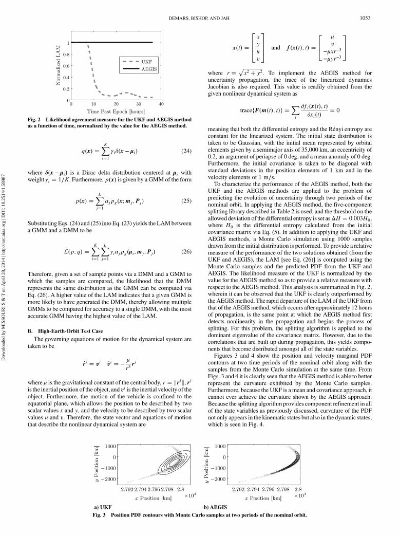
meaning that both the differential entropy and the Rényi entropy areconstant for the linearized system. The initial state distribution istaken to be Gaussian, with the initial mean represented by orbitalelements given by a semimajor axis of 35,000 km, an eccentricity of0.2, an argument of periapse of 0 deg, and a mean anomaly of 0 deg.Furthermore, the initial covariance is taken to be diagonal withstandard deviations in the position elements of 1 km and in thevelocity elements of 1 m∕s.To characterize the performance of the AEGIS method, both the

UKF and the AEGIS methods are applied to the problem ofpredicting the evolution of uncertainty through two periods of thenominal orbit. In applying the AEGIS method, the five-componentsplitting library described in Table 2 is used, and the threshold on theallowed deviation of the differential entropy is set asΔH � 0.003H0,where H0 is the differential entropy calculated from the initialcovariance matrix via Eq. (5). In addition to applying the UKF andAEGIS methods, a Monte Carlo simulation using 1000 samplesdrawn from the initial distribution is performed. To provide a relativemeasure of the performance of the two solutions obtained (from theUKF and AEGIS), the LAM [see Eq. (26)] is computed using theMonte Carlo samples and the predicted PDF from the UKF andAEGIS. The likelihood measure of the UKF is normalized by thevalue for the AEGIS method so as to provide a relative measure withrespect to the AEGIS method. This analysis is summarized in Fig. 2,wherein it can be observed that the UKF is clearly outperformed bytheAEGISmethod. The rapid departure of the LAMof theUKF fromthat of the AEGISmethod, which occurs after approximately 12 hoursof propagation, is the same point at which the AEGIS method firstdetects nonlinearity in the propagation and begins the process ofsplitting. For this problem, the splitting algorithm is applied to thedominant eigenvalue of the covariance matrix. However, due to thecorrelations that are built up during propagation, this yields compo-nents that become distributed amongst all of the state variables.Figures 3 and 4 show the position and velocity marginal PDF

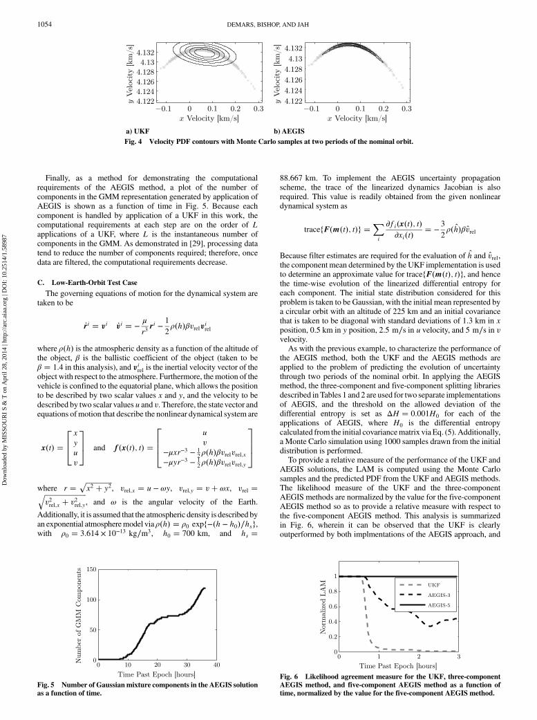
contours at two time periods of the nominal orbit along with thesamples from the Monte Carlo simulation at the same time. FromFigs. 3 and 4 it is clearly seen that the AEGISmethod is able to betterrepresent the curvature exhibited by the Monte Carlo samples.Furthermore, because the UKF is a mean and covariance approach, itcannot ever achieve the curvature shown by the AEGIS approach.Because the splitting algorithm provides component refinement in allof the state variables as previously discussed, curvature of the PDFnot only appears in the kinematic states but also in the dynamic states,which is seen in Fig. 4.

Fig. 2 Likelihood agreement measure for the UKF and AEGIS methodas a function of time, normalized by the value for the AEGIS method.

a) UKF b) AEGISFig. 3 Position PDF contours with Monte Carlo samples at two periods of the nominal orbit.

DEMARS, BISHOP, AND JAH 1053

Dow

nloa

ded

by M

ISSO

UR

I S

& T

on

Apr

il 28

, 201

4 | h

ttp://

arc.

aiaa

.org

| D

OI:

10.

2514

/1.5

8987

Finally, as a method for demonstrating the computationalrequirements of the AEGIS method, a plot of the number ofcomponents in the GMM representation generated by application ofAEGIS is shown as a function of time in Fig. 5. Because eachcomponent is handled by application of a UKF in this work, thecomputational requirements at each step are on the order of Lapplications of a UKF, where L is the instantaneous number ofcomponents in the GMM. As demonstrated in [29], processing datatend to reduce the number of components required; therefore, oncedata are filtered, the computational requirements decrease.

C. Low-Earth-Orbit Test Case

The governing equations of motion for the dynamical system aretaken to be

_ri � vi _vi � −μ

r3ri −

1

2ρ�h�βvrelvirel

where ρ�h� is the atmospheric density as a function of the altitude ofthe object, β is the ballistic coefficient of the object (taken to beβ � 1.4 in this analysis), and virel is the inertial velocity vector of theobject with respect to the atmosphere. Furthermore, themotion of thevehicle is confined to the equatorial plane, which allows the positionto be described by two scalar values x and y, and the velocity to bedescribed by two scalar values u and v. Therefore, the state vector andequations ofmotion that describe the nonlinear dynamical system are

x�t� �

264xyuv

375 and f�x�t�; t� �

2664

uv

−μxr−3 − 12ρ�h�βvrelvrel;x

−μyr−3 − 12ρ�h�βvrelvrel;y

3775

where r �����������������x2 � y2

p, vrel;x � u − ωy, vrel;y � v� ωx, vrel ��������������������������

v2rel;x � v2rel;yq

, and ω is the angular velocity of the Earth.

Additionally, it is assumed that the atmospheric density is described byan exponential atmospheremodel via ρ�h� � ρ0 expf−�h − h0�∕hsg,with ρ0 � 3.614 × 10−13 kg∕m3, h0 � 700 km, and hs �

88.667 km. To implement the AEGIS uncertainty propagationscheme, the trace of the linearized dynamics Jacobian is alsorequired. This value is readily obtained from the given nonlineardynamical system as

tracefF�m�t�; t�g �Xi

∂fi�x�t�; t�∂xi�t�

� −3

2ρ�h�βvrel

Because filter estimates are required for the evaluation of h and vrel,the component mean determined by the UKF implementation is usedto determine an approximate value for tracefF�m�t�; t�g, and hencethe time-wise evolution of the linearized differential entropy foreach component. The initial state distribution considered for thisproblem is taken to be Gaussian, with the initial mean represented bya circular orbit with an altitude of 225 km and an initial covariancethat is taken to be diagonal with standard deviations of 1.3 km in xposition, 0.5 km in y position, 2.5 m∕s in u velocity, and 5 m∕s in vvelocity.As with the previous example, to characterize the performance of

the AEGIS method, both the UKF and the AEGIS methods areapplied to the problem of predicting the evolution of uncertaintythrough two periods of the nominal orbit. In applying the AEGISmethod, the three-component and five-component splitting librariesdescribed in Tables 1 and 2 are used for two separate implementationsof AEGIS, and the threshold on the allowed deviation of thedifferential entropy is set as ΔH � 0.001H0 for each of theapplications of AEGIS, where H0 is the differential entropycalculated from the initial covariancematrix via Eq. (5). Additionally,a Monte Carlo simulation using 1000 samples drawn from the initialdistribution is performed.To provide a relative measure of the performance of the UKF and

AEGIS solutions, the LAM is computed using the Monte Carlosamples and the predicted PDF from the UKF and AEGIS methods.The likelihood measure of the UKF and the three-componentAEGIS methods are normalized by the value for the five-componentAEGIS method so as to provide a relative measure with respect tothe five-component AEGIS method. This analysis is summarizedin Fig. 6, wherein it can be observed that the UKF is clearlyoutperformed by both implmentations of the AEGIS approach, and

a) UKF b) AEGISFig. 4 Velocity PDF contours with Monte Carlo samples at two periods of the nominal orbit.

Fig. 5 Number of Gaussian mixture components in the AEGIS solutionas a function of time.

Fig. 6 Likelihood agreement measure for the UKF, three-componentAEGIS method, and five-component AEGIS method as a function oftime, normalized by the value for the five-component AEGIS method.

1054 DEMARS, BISHOP, AND JAH

Dow

nloa

ded

by M

ISSO

UR

I S

& T

on

Apr

il 28

, 201

4 | h

ttp://

arc.

aiaa

.org

| D

OI:

10.

2514

/1.5

8987

that the five-component implementation of AEGIS outperforms thethree-component implementation of AEGIS. The rapid departure ofthe LAM of the UKF from that of the AEGIS methods, which occursafter approximately 30min of propagation, is the same point at whichthe AEGIS method first detects nonlinearity in the propagationand begins the process of splitting. As with the previous example,the splitting algorithm is applied to the dominant eigenvalue of thecovariance matrix, which, through correlations, yields componentsthat become distributed amongst all of the state variables.Figures 7 and 8 show the position and velocity marginal PDF

contours at two time periods of the nominal orbit along with thesamples from the Monte Carlo simulation at the same time. FromFigs. 7 and 8 it is clearly seen that both implementations of theAEGISapproach enable a better representation the curvature exhibited bythe Monte Carlo samples. Unlike the analysis of the LAM, however,little distinction between the three-component and five-componentAEGIS solutions can be detected from the position and velocitymarginal PDF contours.Figure 9 illustrates the number of components in the GMM

representation generated by both applications of AEGIS as a functionof time. As previously discussed, because each component is handled

by application of aUKF in thiswork, the computational requirementsat each step are on the order of L applications of a UKF, where Lis the instantaneous number of components in the GMM. FromFig. 9, it can be seen that the computational requirements of thethree-component implementation of AEGIS are lower than the

a) UKF

b) Three-Component AEGIS c) Five-Component AEGIS

Fig. 7 Position PDF contours with Monte Carlo samples at two periods of the nominal orbit.

a) UKF

b) Three-component AEGIS c) Five-component AEGISFig. 8 Velocity PDF contours with Monte Carlo samples at two periods of the nominal orbit.

Fig. 9 Number of Gaussian mixture components in the three-component and five-component AEGIS solutions as a function of time.

DEMARS, BISHOP, AND JAH 1055

Dow

nloa

ded

by M

ISSO

UR

I S

& T

on

Apr

il 28

, 201

4 | h

ttp://

arc.

aiaa

.org

| D

OI:

10.

2514

/1.5

8987

requirements of the five-component implementation of AEGIS;however, because the number of components in each application aresimilar, there is no drastic increase in the computational requirementswhen applying the five-component splitting library in AEGIS.

VI. Conclusions

The proposed adaptive entropy-based Gaussian-mixtureinformation synthesis method (termed the AEGIS method) isbased on the detection of nonlinearity during the prediction of stateuncertainty via entropy measures and on the subsequent splittingof Gaussian distributions to obtain a more accurate probabilitydensity function (PDF). The detection of nonlinearity duringthe propagation of uncertainty is based on a property derivedfrom the differential entropy (or Rényi entropy) for linearizeddynamical systems that enables a measure of the performanceof a linearized predictor without directly employing a linearizedpredictor. An improved algorithm was also presented forperforming the splitting of a Gaussian distribution into multiplecomponents, using splitting libraries that enable the approxi-mation of a multivariate Gaussian distribution by a multivariateGaussian mixture model distribution as nonlinearity is detected.A more accurate approximate of the PDF is then propagatedforward in time using a symmetric sigma-point set. The proposedmethod of uncertainty propagation was applied to orbit uncer-tainty prediction for the case of a space object in an eccentrichigh Earth orbit under the influence of gravity only and for the caseof a space object in a circular low Earth orbit under the influenceof both gravity and atmospheric drag. It was demonstrated thatthe obtained PDF contours were more representative of thecurvature of the true distribution as determined by Monte Carlosimulation, and that the likelihood agreement measure exceedsthat of the unscented Kalman filter chosen as a comparison, be-cause it represents the current state-of-the-art in applied spaceobject tracking. This new approach was shown to better approxi-mate the propagation of uncertainty through a nonlinear dynamicalsystem than standard approaches, which rely on first- and second-order approximations along a nominal path.The improved forward prediction of the probability density func-

tion exhibited by theAEGISmethod provides several advantages thatare to be explored in the future. Chief among these advantages are anincreased robustness and performance in the subsequent processingof measurement data and increased likelihood of reacquiring theobject during long arcs of uncertainty prediction that are necessitatedby the sparsity of measurement data.

Appendix A: Adaptive Entropy-Based Gaussian-MixtureInformation Synthesis Algorithm

See Algorithm 1.

Acknowledgments

The work presented herein was performed with support from theU.S. Air ForceOffice of Scientific Research.Many thanks go to KentMiller, Doug Cochran, Fariba Fahroo, and Tristan Nguyen for theirsupport via various mechanisms (U.S. Air Force Office of ScientificResearch Lab Task and National Research Council ResearchAssociateship).

References

[1] Kalman, R. E., “A New Approach to Linear Filtering and PredictionProblems,” Transactions of the ASME–Journal of Basic Engineering,Vol. 82, Series D, March 1960, pp. 35–45.

[2] Smith, G. L., Schmidt, S. F., and McGee, L. A., “Application ofStatistical Filter Theory to the Optimal Estimation of Position andVelocity on Board a Circumlunar Vehicle,” NASA TR-R-135,Jan. 1962.

[3] Athans, M., Wishner, R. P., and Bertolini, A., “Suboptimal StateEstimation for Continuous-Time Nonlinear Systems from DiscreteNoisy Measurements,” IEEE Transactions on Automatic Control,Vol. 13, No. 5, Oct. 1968, pp. 504–514.doi:10.1109/TAC.1968.1098986

[4] Huxel, P. J., and Bishop, R. H., “Navigation Algorithms andObservability Analysis for Formation Flying Missions,” Journal of

Guidance, Control, and Dynamics, Vol. 32, No. 4, 2009, pp. 1218–1231.doi:10.2514/1.41288

[5] Zanetti, R., DeMars, K. J., and Bishop, R. H., “UnderweightingNonlinear Measurements,” Journal of Guidance, Control, and

Dynamics, Vol. 33, No. 5, 2010, pp. 1670–1675.doi:10.2514/1.50596

[6] Woodburn, J., and Tanygin, S., “Detection of Non-Linearity EffectsDuring Orbit Estimation,” 20th AAS/AIAA Space Flight Mechanics

Meeting, AAS Paper 10-239, Feb. 2010.[7] Julier, S. J.,Uhlmann, J.K., andDurrant–Whyte,H. F., “ANewApproach

for Filtering Nonlinear Systems,” Proceedings of the American Control

Conference, Vol. 3, June 1995, pp. 1628–1632.doi:10.1109/ACC.1995.529783

[8] Julier, S., and Uhlmann, J., “Unscented Filtering and NonlinearEstimation,” Proceedings of the IEEE, Vol. 92, No. 3, 2004, pp. 401–422.doi:10.1109/JPROC.2003.823141

[9] Ito, K., and Xiong, K., “Gaussian Filters for Nonlinear FilteringProblems,” IEEE Transactions on Automatic Control, Vol. 45, No. 5,May 2000, pp. 910–927.doi:10.1109/9.855552

[10] van der Merwe, R., Sigma-Point Kalman Filters for Probabilistic

Inference inDynamic State-SpaceModels, Ph.D. Thesis, OregonHealthand Science Univ., Portland, Oregon, 2004.

[11] Uhlmann, J. K., Simultaneous Map Building and Localization for Real

Time Applications, Ph.D. Thesis, Univ. of Oxford, Oxford, England,U.K., 1994.

[12] Sorenson, H. W., and Alspach, D. L., “Recursive Bayesian EstimationUsing Gaussian Sums,” Automatica, Vol. 7, No. 4, 1971, pp. 465–479.doi:10.1016/0005-1098(71)90097-5

[13] Alspach, D. L., and Sorenson, H. W., “Nonlinear Bayesian EstimationUsing Gaussian Sum Approximations,” IEEE Transactions in

Automatic Control, Vol. AC-17, No. 4, Aug. 1972, pp. 439–448.doi:10.1109/TAC.1972.1100034

[14] Horwood, J. T., Aragon, N. D., and Poore, A. B., “Gaussian Sum Filtersfor Space Surveillance: Theory and Simulations,” Journal of Guidance,Control, and Dynamics, Vol. 34, No. 6, 2011, pp. 1839–1851.doi:10.2514/1.53793

[15] Terejanu, G., Singla, P., Singh, T., and Scott, P., “UncertaintyPropagation for Nonlinear Dynamic Systems Using Gaussian MixtureModels,” Journal of Guidance, Control, and Dynamics, Vol. 31, No. 6,2008, pp. 1623–1633.doi:10.2514/1.36247

[16] DeMars, K. J., Jah, M. K., Giza, D. R., and Kelecy, T. M., “OrbitDetermination Performance Improvements for High Area-to-MassRatio Space Object Tracking Using an Adaptive Gaussian MixturesEstimation Algorithm,” 21st International Symposium on Space Flight

Dynamics, Toulouse, France, Sept. 2009.[17] Giza, D. R., Singla, P., and Jah, M. K., “An Approach for Nonlinear

Uncertainty Propagation: Application to Orbital Mechanics,” AIAA

Guidance, Navigation, and Control Conference, AIAA Paper 2009-6082, Aug. 2009.

Algorithm 1 AEGIS using the symmetric sigma-point set

Dynamical System Model: _x�t� � f�x�t�; t�Initialization: p�x0� �

PLl�1 αl;0pg�x0;ml;0;Pl;0�

Propagation, t ∈ �tk−1; tk�Set ts−1 � tk−1, αl;s−1 � α�l;k−1,ml;s−1 � m�l;k−1, and Pl;s−1 � P�l;k−11. Determine sigma points at ts−1Pl;s−1 � Sl;s−1STl;s−1 to find Sl;s−1Sl;s−1 � �sl;1;s−1 : : : sl;n;s−1�Xl;i;s−1 � ml;s−1 �

���npsl;i;s−1

Xl;i�n;s−1 � ml;s−1 −���npsl;i;s−1

2. Propagate sigma points through the dynamics until nonlinearity detected at

time ts on jth component_Xl;i�t� � f�Xl;i�t�; t�, Xl;i�ts−1� � Xl;i;s−1, Xl;i;s � Xl;i�ts�3. Calculate propagated mean and covariance for jth component

mj;s �P

Ki�1 wiX j;i;s

Pj;s �P

Ki�1 wi�X j;i;s −mj;s��X j;i;s −mj;s�T

4. Replace weight, mean, and covariance of jth component by splitting intoGcomponents

αj;spg�x;mj;s;Pj;s� ≈P

Gr�1 αr;spg�x;mr;s;Pr;s�

5. Return to Step 1with ts−1 � ts,αl;s−1 � αl;s,ml;s−1 � ml;s, andPl;s−1 �Pl;s and continue until ts � tk

1056 DEMARS, BISHOP, AND JAH

Dow

nloa

ded

by M

ISSO

UR

I S

& T

on

Apr

il 28

, 201

4 | h

ttp://

arc.

aiaa

.org

| D

OI:

10.

2514

/1.5

8987

[18] Jazwinski, A. H., Stochastic Processes and Filtering Theory, Dover,New York, 1998, pp. 126–139.

[19] Shannon, C. E., “AMathematical Theory of Communication,” The BellSystem Technical Journal, Vol. 27, July–Oct. 1948, pp. 379–423.

[20] Cover, T.M., andThomas, J. A.,Elements of Information Theory,Wiley,New York, 1991, pp. 224–225.

[21] Rényi, A., “On Measures of Entropy and Information,” Proceedings ofthe Fourth Berkeley Symposium on Mathematical Statistics and

Probability, edited by Neyman, J., Vol. 1 of Contributions to theTheory of Statistics, Univ. of California Press, Berkeley, CA, June–July 1961,pp. 547–561.

[22] Zografos, K., and Nadarajah, S., “Expressions for Rényi and ShannonEntropies for Multivariate Distributions,” Statistics & Probability

Letters, Vol. 71, No. 1, Jan. 2005, pp. 71–84.doi:10.1016/j.spl.2004.10.023

[23] Grewal, M. S., and Andrews, A. P., Kalman Filtering: Theory

and Practice, Prentice–Hall, Upper Saddle River, NJ, 1993, pp. 165–171.

[24] Vallée, R., “Information Entropy and State Observation of a DynamicalSystem,” Uncertainty in Knowledge-Based Systems, edited by

Bouchon, B., and Yager, R., Vol. 286 of Lecture Notes in ComputerScience, Springer–Verlag, Berlin, 1987, pp. 403–405.

[25] Basu, A., Harris, I. R., Hjort, N. L., and Jones, M. C., “Robust andEfficient Estimation by Minimising a Density Power Divergence,”Biometrika, Vol. 85, No. 3, 1998, pp. 549–559.doi:10.1093/biomet/85.3.549

[26] Cichocki, A., and Amari, S., “Families of Alpha- Beta- and Gamma-Divergences: Flexible and Robust Measures of Similarities,” Entropy,Vol. 12, No. 6, 2010, pp. 1532–1568.doi:10.3390/e12061532

[27] Huber, M. F., Bailey, T., Durrant–Whyte, H., and Hanebeck, U. D., “OnEntropy Approximation for Gaussian Mixture Random Vectors,” IEEEInternational Conference on Multisensor Fusion and Integration for

Intelligent Systems, Paper TA2-3, 2008, pp. 181–188.[28] Jia, B., Xin, M., and Cheng, Y., “Sparse Gauss-Hermite Quadrature

Filter with Application to Spacecraft Attitude Estimation,” Journal ofGuidance, Control, and Dynamics, Vol. 34, No. 2, 2011, pp. 367–379.doi:10.2514/1.52016

[29] DeMars, K. J., Nonlinear Orbit Uncertainty Prediction and

Rectification for Space Situational Awareness, Ph.D. Thesis, Univ. ofTexas at Austin, Austin, TX, 2010.

DEMARS, BISHOP, AND JAH 1057

Dow

nloa

ded

by M

ISSO

UR

I S

& T

on

Apr

il 28

, 201

4 | h

ttp://

arc.

aiaa

.org

| D

OI:

10.

2514

/1.5

8987