Efficient Design Space Exploration for ApplicationSpecific Systems-on-a-Chip

Giuseppe Asciaa, Vincenzo Cataniaa, Alessandro G. Di Nuovoa,∗,Maurizio Palesia, Davide Pattia

aDipartimento di Ingegneria Informatica e delle TelecomunicazioniUniversita di Catania, Viale A. Doria 6, 95125 Catania, Italy

Abstract

A reduction in the time-to-market has led to widespread use of pre-designedparametric ar-chitectural solutions known as system-on-a-chip (SoC) platforms. A system designer has toconfigure the platform in such a way as to optimize it for the execution of a specific appli-cation. Very frequently, however, the space of possible configurations that can be mappedonto a SoC platform is huge and the computational effort needed to evaluatea single sys-tem configuration can be very costly. In this paper we propose an approach which tacklesthe problem of design space exploration (DSE) in both of the fronts of the reduction ofthe number of system configurations to be simulated and the reduction of the time requiredto evaluate (i.e., simulate) a system configuration. More precisely, we propose the use ofMulti-objective Evolutionary Algorithms as optimization technique and Fuzzy Systems forthe estimation of the performance indexes to be optimized. The proposed approach is ap-plied on a highly parameterized SoC platform based on a parameterized VLIWprocessorand a parameterized memory hierarchy for the optimization of performance and power dis-sipation. The approach is evaluated in terms of both accuracy and efficiency and comparedwith several established DSE approaches. The results obtained for a set of multimedia ap-plications show an improvement in both accuracy and exploration time.

Key words: Design Space Exploration, Multiobjective Optimization, Embedded SystemDesign, Very Long Instruction Word Processor, Fuzzy Estimation, EvolutionaryComputation

∗ Corresponding AuthorEmail addresses:gascia@diit.unict.it (Giuseppe Ascia),

vcatania@diit.unict.it (Vincenzo Catania),adinuovo@diit.unict.it(Alessandro G. Di Nuovo),mpalesi@diit.unict.it (Maurizio Palesi),dpatti@diit.unict.it (Davide Patti).

Preprint submitted to Journal of System Architecture 21 December 2006

1 Introduction

The design flow of a SoC features the combined use of heterogeneous techniques,methodologies and tools with which an architectural template is gradually refinedstep by step on the basis of functional specifications and system requirements. Eachphase in the design flow can be considered as an optimization problem which is re-solved by defining and/or setting some of the system’s free parameters in such away as to optimize certain performance indexes. These optimization problems areusually tackled by means of processes based on successive cyclic refinements: start-ing from an initial system configuration, they introduce transformations at each it-eration in order to enhance its quality. In this paper we focus onPlatform-based de-sign. In particular we refer to a design flow based on parameterized SoC platforms.With the term “platform” we intend a coordinated family of hardware-software ar-chitectures developed to promote high levels of re-use of hardware and softwarecomponents in the rapid, low-risk design of application-oriented derivative prod-ucts. These could take the form of a SoC or more complex electronic systems, andthe platforms will be offered by a number of different vendors working in variousproduct application domains, in the form of both relativelyfixed platforms and onesincorporating reconfigurability.

The apparent rigidity of a platform, due to a fixed architecture, is made flexibleby means of a high degree of programmability and great parameterizations of themodules it contains [1]. Variations in parameters have a considerable impact onthe performance indexes being optimized (such as performance, power consump-tion, area, etc.). Defining strategies to ”tune” parametersso as to establish the opti-mal configuration for a system is a challenge known asDesign Space Exploration(DSE). Obviously, it is computationally unfeasible to use an exhaustive explorationstrategy. The size of the design space grows as the product ofthe cardinalities of thevariation sets for each parameter. In addition, evaluationof a single configurationalmost always requires the use of simulators or analytical models which are oftenhighly complex. Another problem is that the objectives being optimized are oftenconflicting. The result of the exploration will therefore not be a single solution buta set of tradeoffs which make up the Pareto set.

Any DSE technique can be schematically represented as in Figure 1. Starting with abase configuration, the exploration process is an iterativerefinement process com-prising two main stages: evaluation and tuning of the parameters of the configu-ration. The evaluation phase often boils down to a system-level simulation whichconstitutes a bottleneck in the exploration process. The tuning phase uses the re-sults of the evaluation phase to modify the system configuration parameters so asto optimize certain performance indexes. The cycle ends when a system configura-tion that meets the design constraints has been obtained, or, more frequently, whena set of Pareto-optimal configurations for the indexes to be optimized have beenaccumulated.

2

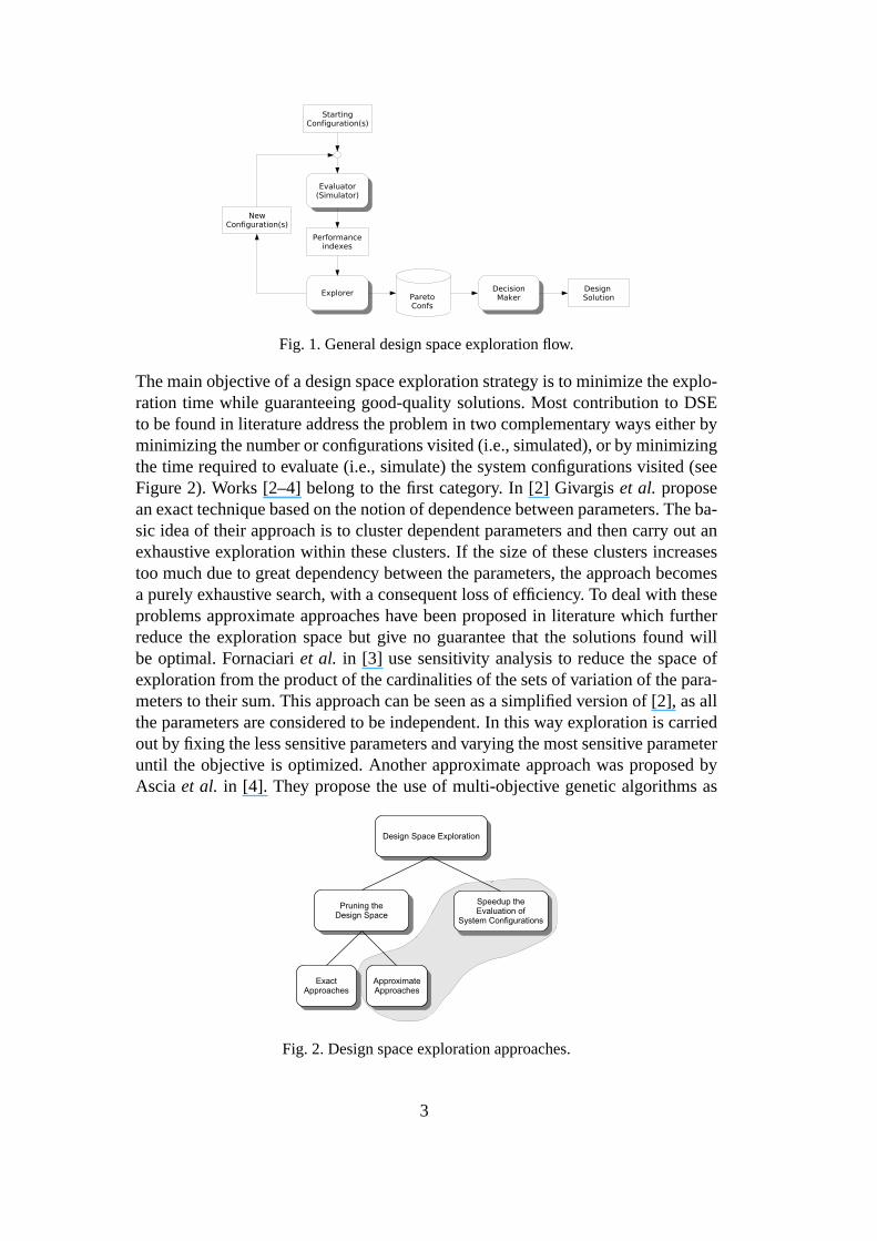
Fig. 1. General design space exploration flow.

The main objective of a design space exploration strategy isto minimize the explo-ration time while guaranteeing good-quality solutions. Most contribution to DSEto be found in literature address the problem in two complementary ways either byminimizing the number or configurations visited (i.e., simulated), or by minimizingthe time required to evaluate (i.e., simulate) the system configurations visited (seeFigure 2). Works [2–4] belong to the first category. In [2] Givargiset al. proposean exact technique based on the notion of dependence betweenparameters. The ba-sic idea of their approach is to cluster dependent parameters and then carry out anexhaustive exploration within these clusters. If the size of these clusters increasestoo much due to great dependency between the parameters, theapproach becomesa purely exhaustive search, with a consequent loss of efficiency. To deal with theseproblems approximate approaches have been proposed in literature which furtherreduce the exploration space but give no guarantee that the solutions found willbe optimal. Fornaciariet al. in [3] use sensitivity analysis to reduce the space ofexploration from the product of the cardinalities of the sets of variation of the para-meters to their sum. This approach can be seen as a simplified version of [2], as allthe parameters are considered to be independent. In this wayexploration is carriedout by fixing the less sensitive parameters and varying the most sensitive parameteruntil the objective is optimized. Another approximate approach was proposed byAscia et al. in [4]. They propose the use of multi-objective genetic algorithms as

Fig. 2. Design space exploration approaches.

3

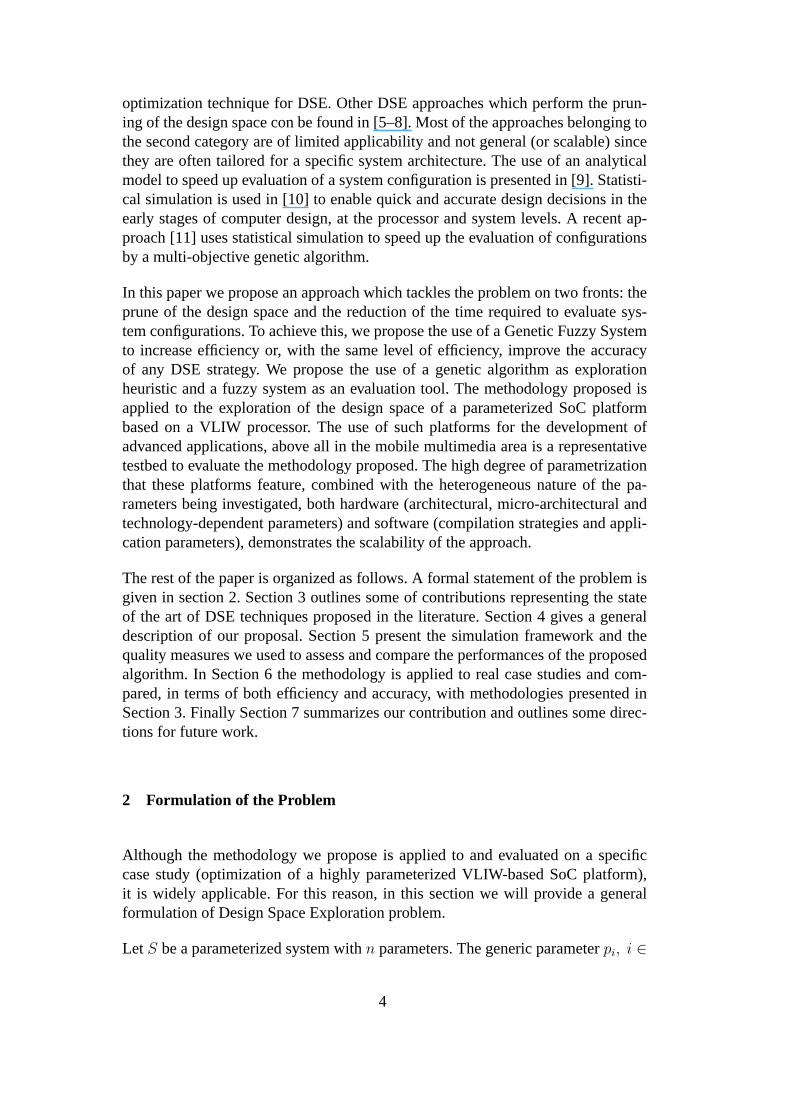
optimization technique for DSE. Other DSE approaches whichperform the prun-ing of the design space con be found in [5–8]. Most of the approaches belonging tothe second category are of limited applicability and not general (or scalable) sincethey are often tailored for a specific system architecture. The use of an analyticalmodel to speed up evaluation of a system configuration is presented in [9]. Statisti-cal simulation is used in [10] to enable quick and accurate design decisions in theearly stages of computer design, at the processor and systemlevels. A recent ap-proach [11] uses statistical simulation to speed up the evaluation of configurationsby a multi-objective genetic algorithm.

In this paper we propose an approach which tackles the problem on two fronts: theprune of the design space and the reduction of the time required to evaluate sys-tem configurations. To achieve this, we propose the use of a Genetic Fuzzy Systemto increase efficiency or, with the same level of efficiency, improve the accuracyof any DSE strategy. We propose the use of a genetic algorithmas explorationheuristic and a fuzzy system as an evaluation tool. The methodology proposed isapplied to the exploration of the design space of a parameterized SoC platformbased on a VLIW processor. The use of such platforms for the development ofadvanced applications, above all in the mobile multimedia area is a representativetestbed to evaluate the methodology proposed. The high degree of parametrizationthat these platforms feature, combined with the heterogeneous nature of the pa-rameters being investigated, both hardware (architectural, micro-architectural andtechnology-dependent parameters) and software (compilation strategies and appli-cation parameters), demonstrates the scalability of the approach.

The rest of the paper is organized as follows. A formal statement of the problem isgiven in section 2. Section 3 outlines some of contributionsrepresenting the stateof the art of DSE techniques proposed in the literature. Section 4 gives a generaldescription of our proposal. Section 5 present the simulation framework and thequality measures we used to assess and compare the performances of the proposedalgorithm. In Section 6 the methodology is applied to real case studies and com-pared, in terms of both efficiency and accuracy, with methodologies presented inSection 3. Finally Section 7 summarizes our contribution and outlines some direc-tions for future work.

2 Formulation of the Problem

Although the methodology we propose is applied to and evaluated on a specificcase study (optimization of a highly parameterized VLIW-based SoC platform),it is widely applicable. For this reason, in this section we will provide a generalformulation of Design Space Exploration problem.

Let S be a parameterized system withn parameters. The generic parameterpi, i ∈

4

{1, 2, . . . , n} can take any value in the setVi. A configurationc of the systemS is an-tuple〈v1, v2, . . . , vn〉 in whichvi ∈ Vi is the value fixed for the parameterpi. Theconfiguration space(or design space) of S [which we will indicate asC(S)] is thecomplete range of possible configurations [C(S) = V1 × V2 × . . . × Vn]. Naturallynot all the configurations ofC(S) can really be mapped onS. We will call the set ofconfigurations that can be physically mapped onS thefeasible configuration spaceof S [and indicate it asC∗(S)].

Let m be the number of objectives to be optimized (e.g. power, cost, performance,etc.). Anevaluation functionE : C∗(S) × B −→ ℜm is a function that associateseach feasible configuration ofS with an m-tuple of values corresponding to theobjectives to be optimized when any application belonging to the set of benchmarksB is executed.

Given a systemS, an applicationb ∈ B and two configurationsc′, c′′ ∈ C∗(S), c′ issaid todominate(or eclipse) c

′′, and is indicated asc′ ≻ c′′, if given o

′ = E(c′, b)ando

′′ = E(c′′, b) it results thato′ ≤ o′′ ando

′ 6= o′′. Where vector comparisons

are interpreted component-wise and are true only if all of the individual compar-isons are true (o′i ≤ o′′i ∀ i = 1, 2, . . . ,m).

ThePareto-optimal setof S for the applicationb is the set:

P(S, b) = {c ∈ C∗(S) : ∄ c′ ∈ C∗(S), c′ ≻ c}

that is, the set of configurationsc ∈ C∗(S) not dominated by any other config-uration. Pareto-optimal configurations are configurationsbelonging to the Pareto-optimal set and thePareto-optimal frontis the image of the Pareto-optimal config-urations, i.e. the set:

PF (S, b) = {o : o = E(c, b), c ∈ P(S, b)}

The aim of the paper is to define a Design Space Exploration (DSE) strategy thatwill give a good approximation of the Pareto-optimal front for a systemS and anapplicationb, simulating as few configurations as possible.

3 Design Space Exploration Approaches

In this section we will present and discuss three approachesto DSE. The first,GA,uses Genetic Algorithms as the optimization engine. A configuration is mappedonto a chromosome and a population of configurations is made to evolve until itconverges on the Pareto-optimal set. The second approach,PBSA(Pareto BasedSensitivity Analysis), uses sensitivity analysis to orderthe parameters by impor-tance. Each parameter is thus made to vary independently of the others, the imme-

5

diate consequence being the need to visit a number of configurations, which growin a linear fashion as the number of parameters increases (rather than exponen-tially as happens in an exhaustive analysis). The third,DEP (short for DEPendencyanalysis), is an exact approach. It uses parameter dependence information to dividethe configuration space up into subspaces of a size that will enable an exhaustivesearch to be made.

The following subsection will give a detailed description of these approaches, con-cluding each one with a list of their strong and weak points.

3.1 Genetic-based Approach

In general, when the configuration space is too large for exhaustive exploration,the use of evolutionary techniques represents an alternative solution. Genetic al-gorithms (GAs) have been applied in various VLSI design environments [12], forexample in layout problems such as partitioning [13], placement [14] and rout-ing [15]; in design problems such as power estimation [16], technology mapping [17]and netlist partitioning [18]; and in reliable chip testingthrough efficient test vectorgeneration [19]. All these problems are untractable in the sense that no polynomialtime algorithm can guarantee an optimal solution and they actually belong to theNP-complete and NP-hard categories.

The GA-based approach is highly suitable for a general, efficient solution to theseproblems. It is a general approach because the GA solution toa problem only re-quires the definition of a representation of the configuration, the genetic operatorsand the objective functions to be optimized. In addition, itdoes not require detailedknowledge of the system, for example the internal architecture or parameter de-pendency, if any, unlikeDEP. We applied GAs for the design space exploration ofparameterized systems based on both RISC processor [20,21] and VLIW proces-sor [4].

Strengths. The approach is a general one and its application does not require de-tailed knowledge of the system. The only thing that needs to be defined is the map-ping of a system configuration onto a chromosome. The most simple way to do thisis to use a gene for each system parameter and limit their range of variation to thatof the parameters they represent.

Weaknesses. UnlikeDEP, a GA-based approach is an approximate one. This meansthat the set of solutions found is not the Pareto-optimal setbut an approximation ofit.

6

3.2 Pareto Based Sensitivity Analysis

The Pareto-Based Sensitivity Analysis (PBSA) is a generalization of the sensitivityanalysis approach proposed by Fornaciariet al. in [3]. In its basic formulation, sen-sitivity analysis is a mono-objective approach in the sensethat it provides one andonly one solution that optimizes a certain objective function. This objective func-tion may be expressed as a combination of several objective functions (in [22,3],for example, it is expressed as the power-delay product for amemory hierarchy).

Sensitivity analysis reduces the space of possible configurations in two phases. Theaim of the first phase is to identify the parameters which mostinfluence the objec-tive function to be optimized—the sensitivity analysis phase. For a system withnparameters, determination of the degree of sensitivity of each parameter consists offixing n− 1 parameters and varying one of them, determining the maximumrangeof variation of the objective function. The set of parameters that do not reach a userdefined sensitivity threshold can be ignored at the purpose of the exploration. Thenext phase, design space exploration phase, identifies the optimal value for eachparameter, from the most to the least sensitive. The number of configurations tobe evaluated goes down from

∏ni=1 |Vi| to

∑ni=1 |Vi|. To overcome the limits of the

mono-objective approach described, in [23] we defined a new technique based onsensitivity analysis to perform multi-objective optimization based on the notion ofPareto optimum.

Strengths. As in GA, thePBSAapplication does not require detailed knowledge ofthe system. The user can also establish the accuracy/efficiency tradeoff by actingon the value of the threshold. A low threshold value means considering more para-meters. This leads to an increase in the configuration space (and therefore the timerequired to explore it) but consequently to an improvement in terms of the accuracyof the solutions found. Vice versa, using a high threshold value means that only themost sensitive parameters are considered, thus limiting the space of exploration butreducing the accuracy of the solutions.

Weaknesses. This approach is an approximate one and the quality of the solutionsfound depends on the threshold value. However, once a threshold value has beenset, the number of parameters exceeding it depends on the application involved. Athreshold value that gives excellent results in terms of accuracy and/or efficiencyfor one application may not do so for another.

3.3 Dependency Approach

The dependency approach (DEP) was proposed by Givargiset al. in [2]. The basicidea is to exploit information regarding the dependency of certain parameters of thesystem being examined in order to reduce the dimensions of the exploration space.

7

Parameter dependency is captured by an oriented graph (dependency graph), inwhich nodes represent parameters and oriented arcs represent dependency betweentwo nodes (parameters).

A path from a nodeA to a nodeB indicates that the Pareto-optimal configurationsof B only have to be calculated after the Pareto-optimal configurations of all thenodes on the path connectingA to B have been calculated. During calculation, allthe parameters that are not on the path connectingA andB can be set to an arbitraryvalue.

The exploration algorithm operates on the dependency graphin two phases. Thefirst phase is a local search for the Pareto-optimal configurations and can be furtherdivided into two sub-phases. The first clusters the parameters in relation to theirdegree of dependency, while the second performs an exhaustive exploration of thesubspace of configurations generated by each cluster to obtain the Pareto-optimalconfigurations. The second phase of the algorithm combines the clusters two bytwo and extracts their Pareto-optimal configurations. Thisis repeated until all theclusters have been combined.

Strengths. The dependency approach is an exact approach in the sense that if thedependency graph is correct it is possible to obtain all the Pareto-optimal configu-rations.

Weaknesses. Application of the method requires detailed knowledge of the sys-tem in order to plot the dependency graph. In [2] the authors suggest that when thedependency between two parameters is uncertain, the conservative choice is to con-sider them as being dependent. The problem is that by doing sothere is a possibilityof generating cluster containing such a large number of parameters that the asso-ciated configuration space is too large to be explored exhaustively. Another weakpoint is the scalability of the approach as the complexity ofthe system increases: ifthe parameters are highly interdependent the approach may become inapplicable.

4 The Genetic Fuzzy Approach for Design Space Exploration

Unfortunately, the approaches introduced in the previous section may be expensive(sometimes computationally infeasible) when a single simulation (i.e., the evalua-tion of a single system configuration) requires a long compilation and/or executiontime. For the sake of example, referring to the computer system architecture consid-ered in this paper, Table 1 reports the computation effort needed for one evaluation(i.e. simulation) of just a single system configuration for several media and digitalsignal processing application benchmarks. By a little multiplication we can noticethat a few thousands of simulations (just a drop in the immense ocean of feasibleconfigurations) could last from a day to weeks!

8

Table 1Evaluation time for a simulation (compilation + execution) for several multimedia bench-marks on a Pentium IV Xeon 2.8 GHz Linux Workstation.

Benchmark Description Input size Evaluation time

(KB) (sec)

wave Audio Wavefront computation 625 5.4

g721-enc CCITT G.711, G.721 and G.723voice compressions

8 25.9

jpeg-codec jpeg compression and decom-pression

32 33.2

mpeg2-dec MPEG-2 video decoding 400 143.7

adpcm-enc Adaptive Differential PulseCode Modulation speechencoding

295 22.6

adpcm-dec Adaptive Differential PulseCode Modulation speechdecoding

16 20.2

fir FIR filter 64 9.1

The primary goal of this work was to create a new approach which could run asfew simulations as possible without affecting the good performance of theGA ap-proach. For this reason we developed an intelligentGA approach which has theability to avoid the simulation of configurations that it foresees to be not goodenough to belong the Pareto-set and to give them fitness values according to a fastestimation of the objectives. This feature was implementedusing a Fuzzy System(FS) to approximate the unknown function from configurationspace to objectivespace. The approach could be briefly described as follows: the GA evolves nor-mally; in the meanwhile the FS learns from simulations untilit becomes expert andreliable. From this moment on the GA stops launching simulations and uses the FSto estimate the objectives. Only if the estimated objectivevalues are good enoughto enter the Pareto-set will the associated configuration besimulated.

We chose a fuzzy rule-based system as an estimator above all because it has cheapadditional computational time requirements for the learning process, which are neg-ligible as compared with simulation time. A further advantage of the system offuzzy rules is that these rules can be easily interpreted by the designer. The rulesobtained can thus be used to for detailed analysis of the dynamics of the system.

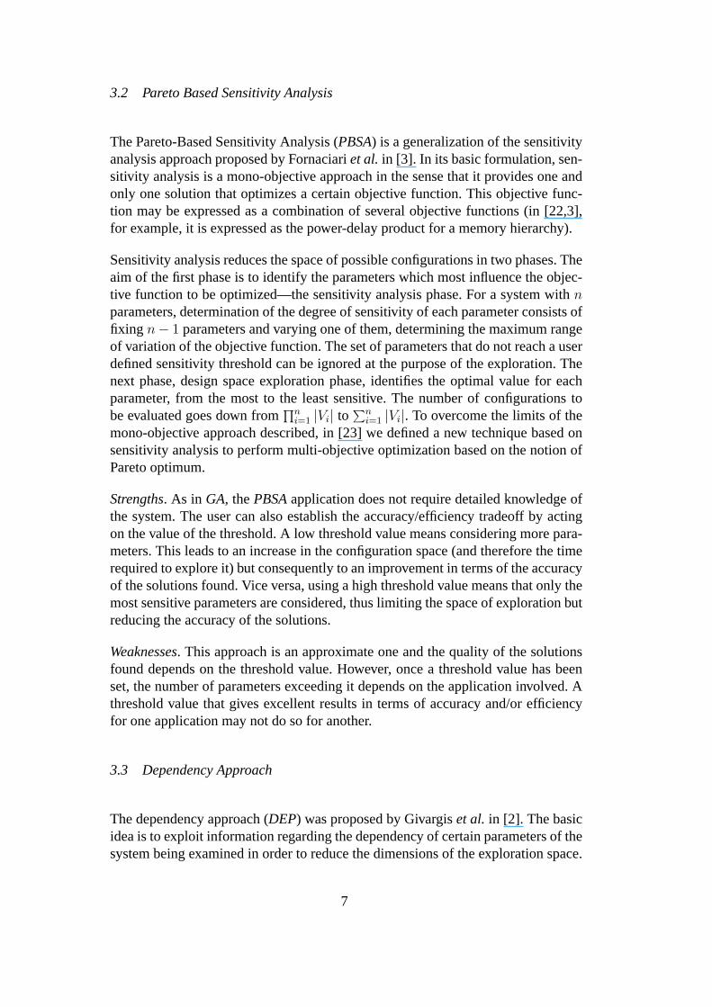
The basic idea of our methodology is depicted in Figure 3. Thequalitative graphshows the exploration time versus the number of system configurations evaluated. Ifwe consider a constant simulation time, the exploration time grows linearly with thenumber of system configurations to be visited. Our proposal is to use an estimator

9

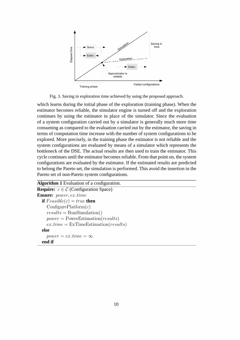
Fig. 3. Saving in exploration time achieved by using the proposed approach.

which learns during the initial phase of the exploration (training phase). When theestimator becomes reliable, the simulator engine is turnedoff and the explorationcontinues by using the estimator in place of the simulator. Since the evaluationof a system configuration carried out by a simulator is generally much more timeconsuming as compared to the evaluation carried out by the estimator, the saving interms of computation time increase with the number of systemconfigurations to beexplored. More precisely, in the training phase the estimator is not reliable and thesystem configurations are evaluated by means of a simulator which represents thebottleneck of the DSE. The actual results are then used to train the estimator. Thiscycle continues until the estimator becomes reliable. Fromthat point on, the systemconfigurations are evaluated by the estimator. If the estimated results are predictedto belong the Pareto set, the simulation is performed. This avoid the insertion in thePareto set of non-Pareto system configurations.

Algorithm 1 Evaluation of a configuration.Require: c ∈ C (Configuration Space)Ensure: power, ex time

if Feasible(c) = true thenConfigurePlatform(c)results = RunSimulation()power = PowerEstimation(results)ex time = ExTimeEstimation(results)

elsepower = ex time = ∞

end if

10

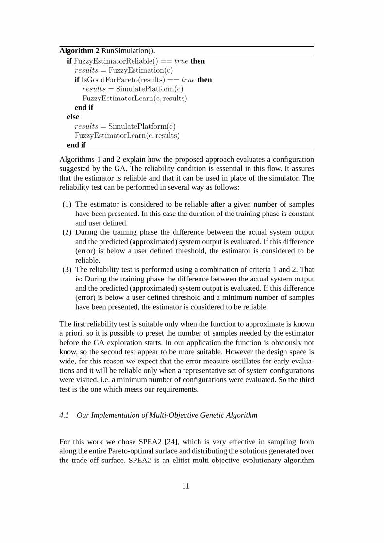
Algorithm 2 RunSimulation().if FuzzyEstimatorReliable() == true then

results = FuzzyEstimation(c)if IsGoodForPareto(results) == true then

results = SimulatePlatform(c)FuzzyEstimatorLearn(c, results)

end ifelse

results = SimulatePlatform(c)FuzzyEstimatorLearn(c, results)

end if

Algorithms 1 and 2 explain how the proposed approach evaluates a configurationsuggested by the GA. The reliability condition is essentialin this flow. It assuresthat the estimator is reliable and that it can be used in placeof the simulator. Thereliability test can be performed in several way as follows:

(1) The estimator is considered to be reliable after a given number of sampleshave been presented. In this case the duration of the training phase is constantand user defined.

(2) During the training phase the difference between the actual system outputand the predicted (approximated) system output is evaluated. If this difference(error) is below a user defined threshold, the estimator is considered to bereliable.

(3) The reliability test is performed using a combination ofcriteria 1 and 2. Thatis: During the training phase the difference between the actual system outputand the predicted (approximated) system output is evaluated. If this difference(error) is below a user defined threshold and a minimum numberof sampleshave been presented, the estimator is considered to be reliable.

The first reliability test is suitable only when the functionto approximate is knowna priori, so it is possible to preset the number of samples needed by the estimatorbefore the GA exploration starts. In our application the function is obviously notknow, so the second test appear to be more suitable. However the design space iswide, for this reason we expect that the error measure oscillates for early evalua-tions and it will be reliable only when a representative set of system configurationswere visited, i.e. a minimum number of configurations were evaluated. So the thirdtest is the one which meets our requirements.

4.1 Our Implementation of Multi-Objective Genetic Algorithm

For this work we chose SPEA2 [24], which is very effective in sampling fromalong the entire Pareto-optimal surface and distributing the solutions generated overthe trade-off surface. SPEA2 is an elitist multi-objectiveevolutionary algorithm

11

which incorporates a fine-grained fitness assignment strategy, a density estimationtechnique, and an enhanced archive truncation method.

Fig. 4. Mapping of a system configuration into a chromosome.

The representation of a system configuration is on a chromosome whose genes de-fine the parameters of the system. The chromosome of the GA will then be definedwith as many genes as there are free parameters and each gene will be coded ac-cording to the set of values it can take. For instance Figure 4shows our referenceparameterized architectures and its mapping on the chromosome. Crossover (re-combination) and mutation operators produce the offspring. In our specific case, themutation operator randomly modifies the value of a parameterchosen at random.The crossover between two configuration exchanges the valueof two parameterschosen at random. Application of these operators may generate non-valid config-urations (i.e. ones that cannot be mapped on the system). Although it is possibleto define the operators in such a way that they will always givefeasible configura-tions, or to define recovery functions, these have not been taken into considerationin the paper. Any unfeasible configurations are filtered by the feasible function. Afeasible functionfF : C −→ {true, false} assigns a generic configurationcbelonging to the configuration spaceC a value oftrue if it is feasible andfalse

if c cannot be mapped onto the parameterized system. A stop criterion based onconvergence makes it possible to stop iterations when thereis no longer any appre-ciable improvement in the Pareto sets found. The convergence criterion we proposeuses the function of coverage [25] between two sets to establish when the GA hasreached convergence.

4.2 Fuzzy Function Approximation

In our approach we used the well-known Wang and Mendel method[26], whichconsists of five steps:

• Step 1Divides the input and output space of the given numerical data into fuzzyregions.

• Step 2Generates fuzzy rules from the given data.

12

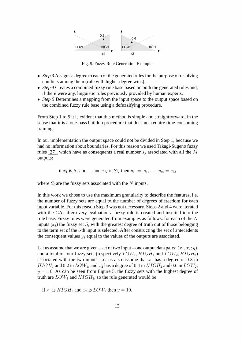
Fig. 5. Fuzzy Rule Generation Example.

• Step 3Assigns a degree to each of the generated rules for the purpose of resolvingconflicts among them (rule with higher degree wins).

• Step 4Creates a combined fuzzy rule base based on both the generatedrules and,if there were any, linguistic rules previously provided by human experts.

• Step 5Determines a mapping from the input space to the output spacebased onthe combined fuzzy rule base using a defuzzifying procedure.

From Step 1 to 5 it is evident that this method is simple and straightforward, in thesense that it is a one-pass buildup procedure that does not require time-consumingtraining.

In our implementation the output space could not be divided in Step 1, because wehad no information about boundaries. For this reason we usedTakagi-Sugeno fuzzyrules [27], which have as consequents a real numbersj associated with all theMoutputs:

if x1 is S1 and. . . andxN is SN theny1 = s1, . . . , ym = sM

whereSi are the fuzzy sets associated with theN inputs.

In this work we chose to use the maximum granularity to describe the features, i.e.the number of fuzzy sets are equal to the number of degrees of freedom for eachinput variable. For this reason Step 3 was not necessary. Steps 2 and 4 were iteratedwith the GA: after every evaluation a fuzzy rule is created and inserted into therule base. Fuzzy rules were generated from examples as follows: for each of theNinputs (xi) the fuzzy setSi with the greatest degree of truth out of those belongingto the term set of thei-th input is selected. After constructing the set of antecedentsthe consequent valuesyj equal to the values of the outputs are associated.

Let us assume that we are given a set of two input – one output data pairs:(x1, x2; y),and a total of four fuzzy sets (respectivelyLOW1, HIGH1 andLOW2, HIGH2)associated with the two inputs. Let us also assume thatx1 has a degree of0.8 inHIGH1 and0.2 in LOW1, andx2 has a degree of0.4 in HIGH2 and0.6 in LOW2,y = 10. As can be seen from Figure 5, the fuzzy sets with the highest degree oftruth areLOW1 andHIGH2, so the rule generated would be:

if x1 is HIGH1 andx2 is LOW2 theny = 10.

13

Fig. 6. Defuzzyfication example.

The rules generated in this way are “and” rules, i.e., rules in which the conditionof the IF part must be met simultaneously in order for the result of the THEN partto occur. For the problem considered in this paper, i.e., generating fuzzy rules fromnumerical data, only “and” rules are required since the antecedents are differentcomponents of a single input vector.

The defuzzifying procedure chosen for Step 5 was, as suggested in [26], the weightedsum of the values estimated by theK rules (yi) with degree of truth (mi) of the pat-tern to be estimated as weight:

y =

K∑i=1

miyi

K∑i=1

mi

(1)

For the sake of example let us consider a fuzzy estimation system composed by thefuzzy sets in Figure 5 and the following rule base:

if x1 is HIGH1 and x2 is HIGH2 then y = 5if x1 is HIGH1 and x2 is LOW2 then y = 8if x1 is LOW1 and x2 is HIGH2 then y = 4if x1 is LOW1 and x2 is LOW2 then y = 3

Using this fuzzy estimation system we can approximate the output from any coupleof inputs. For example considerx1 = 2 andx2 = 4 as input pair, as can be seengraphically in Figure 6, this pair has0.6, 0.3, 0.2 and 0.8 degree of truth withrespectivelyLOW1 , HIGH1, LOW2 andHIGH2. Applying (1) we have that theapproximated objective value (y) is:

y(x1, x2) =5 × (0.3 × 0.8) + 8 × (0.3 × 0.2) + 4 × (0.6 × 0.8) + 3 × (0.6 × 0.2)

(0.3 × 0.8) + (0.3 × 0.2) + (0.6 × 0.8) + (0.6 × 0.2)

= 4.4

In our implementation the defuzzifying procedure and the shape of the fuzzy setswere chosen a priori. This choice proved to be effective as well as a more intelli-gent implementation which could embed a selection procedure to choose the bestdefuzzifying function and shape to use online. The main advantage of our imple-mentation is a lesser complexity of the algorithm and a faster convergence withoutappreciable losses in accuracy as will be shown in the rest ofthe paper.

14

5 Simulation Framework and Quality Measures

In this section we present the simulation framework we used to evaluate the fitnessobjectives, and the quality measures we used to assess and tocompare the proposedapproach.

5.1 Parameterized System Architecture

Architectures based onVery Long Instruction Word(VLIW) processors [28] areemerging in the domain of modern, increasingly complex embedded multimediaapplications, given their capacity to exploit high levels of performance while main-taining a reasonable trade-off between hardware complexity, cost and power con-sumption. A VLIW architecture, like a superscalar architecture, allows several in-structions to be issued in a single clock cycle, with the aim of obtaining a gooddegree of Instruction Level Parallelism (ILP). But the feature which distinguishesthe VLIW approach from other multiple issue architectures is that the compileris exclusively responsible for the correct parallel scheduling of instructions. Thehardware, in fact, only carries out aplan of executionthat is statically establishedin the compilation phase. A plan of execution consist of a sequence ofvery longinstructions, where a very long instruction consists of a set of instructions that canbe issued in the same clock cycle.

The decision as to which and how many operations can be executed in parallel ob-viously depends on the availability of hardware resources.For this reason severalfeatures of the hardware, such as the number of functional units and their rela-tive latencies, have to be “architecturally visible”, in such a way that the compilercan schedule the instructions correctly. Shifting the complexity from the proces-sor control unit to the compiler considerably simplifies design of the hardware andthe scalability of the architecture. It is preferable to modify and test the code ofa compiler than to modify and simulate complex hardware control structures. Inaddition, the cost of modifying a compiler can be spread overseveral instances ofa processor, whereas the addition of new control hardware has to be replicated ineach instance.

These advantages presuppose the presence of a compiler which, on the basis of thehardware configuration, schedules instructions in such a way as to achieve optimalutilization of the functional units available.

15

5.2 Evaluation of a Configuration

To evaluate and compare the performance indexes of different architectures for aspecific application, one needs to simulate the architecture running the code of theapplication. When the architecture is based on a VLIW processor this is impossi-ble without a compiler because it has to schedule instructions. In addition, to makearchitectural exploration possible both the compiler and the simulator have to beretargetable. Trimaran [29] provides these tools and thus represents the pillar cen-tral to the EPIC-Explorer [30], which is a framework that not only allows us toevaluate any instance of a platform in terms of area, performance and power, ex-ploiting the state of the art in estimation approaches at a high level of abstraction,but also implements various techniques for exploration of the design space. TheEPIC-Explorer platform, which can be freely downloaded fromthe Internet [31],allows the designer to evaluate any application written in Cand compiled for anyinstance of the platform. For this reason it is an excellent testbed for comparisonbetween different design space exploration algorithms.

The tunable parameters of the architecture can be classifiedin three main cate-gories:

• Register files. Each register file is parameterized with respect to the number ofregisters it contains. These include a set of general purpose registers (GPR) com-prising 32-bit registers for integers with or without sign;FPR registers compris-ing 64-bit registers for floating point values (with single and double precision);Predicate registers (PR) comprising 1-bit registers used tostore the Boolean val-ues of instructions using predication; and BTR registers comprising 64-bit regis-ters containing information about possible future branches.

• The functional units. Four different types of functional units are available: inte-ger, floating point, memory and branch. Here parametrization regards the numberof instances for each unit.

• The memory sub-system. Each of the three caches, level 1 data cache, level 1instruction cache, and level 2 unified cache, is independently specified with thefollowing parameters: size, block size and associativity.

Together with the configuration of the system, the statistics produced by simulationcontain all the information needed to apply he area, performance and power con-sumption estimation models. The results obtained from these models are the inputfor the exploration strategy, the aim of which is to modify the parameters of theconfiguration so as to minimize the objectives.

16

Fig. 7. Evaluation flow.

Each of these parameters can be assigned a value from a finite set of values. Acomplete assignment of values to all the parameters is a configuration. A completecollection of all possible configurations is the configuration space, (also known asthe design space). A configuration of the system generates aninstance that is sim-ulated and evaluated for a specific application according tothe scheme in Figure 7.The application written in C is first compiled. Trimaran usesthe IMPACT com-piler system as its front-end. This front-end performs ANSIC parsing, code profil-ing, classical code optimizations and block formation. Thecode produced, togetherwith the High Level Machine Description Facility (HMDES) machine specifica-tion, represents the Elcor input. The HMDES is the machine description languageused in Trimaran. This language describes a processor architecture from the com-piler’s point of view. Elcor is Trimaran’s back-end for the HPL-PD architectureand is parameterized by the machine description facility toa large extent. It per-forms three tasks: code selection and scheduling, registerallocation, and machinedependent code optimizations. The Trimaran framework alsoconsists of a simula-tor which is used to generate various statistics such as compute cycles, total numberof operations, etc. In order to consider the impact of the memory hierarchy, a cachesimulator has been added to the platform.

Together with the configuration of the system, the statistics produced by simulationcontain all the information needed to apply the area, performance and power con-sumption estimation models. The results obtained by these models are the input forthe exploration block. This block implements an optimization algorithm, the aim ofwhich is to modify the parameters of the configuration so as tominimize the threecost functions (area, execution time and power dissipation).

The performance statistics produced by the simulator are expressed in clock cycles.To evaluate the execution time it is sufficient to multiply the number of clock cyclesby the clock period. This was set to 200MHz, which is long enough to access cachememory in one single clock cycle.

17

Fig. 8. A block scheme of the Hierarchical Fuzzy System used. SoC components (Proc,L1D$,L1I$ and L2D$) are modeled with a MIMO Fuzzy System, which is connected withothers following the SoC hierarchy.

5.3 The Fuzzy System

The estimation block of the framework consists of a hierarchical FS [32] as shownin Figure 8. We split the system into three levels: the processor level, the L1 cachememory level, and the L2 cache memory level. A FS at levell uses as inputs theoutputs of the FS at levell−1. For example, the FS used to estimate misses and hitsin the first-level instruction cache uses as inputs the number of integer operations,float operations and branch operations estimated by the processor level FS as wellas the cache configuration (size, block size, and associativity). This hierarchicaldecomposition of the system allows us to reduce drasticallythe complexity of theestimation problem with the additional effect of improvingestimation accuracy.

The knowledge base was defined on the basis of experience gained from an ex-tensive series of tests. We verified that a fuzzy system with afew thousands rulestakes milliseconds to approximate the objectives, which issome orders of magni-tude less than the time required for a simulation. We therefore chose to use themaximum granularity, equal to the number of degrees of freedom for each inputvariable. The shape chosen for the sets was Gaussian intersecting at a degree of0.5.

5.4 Assessment of Pareto set approximations

It is difficult to define appropriate quality measures for Pareto set approximations,and as a consequence graphical plots were until recently used to compare the out-comes of multi-objective algorithms. Nevertheless quality measures are necessaryin order to compare the outcomes of multi-objective optimizers in a quantitativemanner. Several quality measures have been proposed in the literature in recentyears, an analysis and review of these is to be found in [33]. In this work we follow

18

the guidelines suggested in [34], that is a recent tutorial on performance assessmentof stochastic multi-objective optimizers. The quality measures we considered mostsuitable for our context are the followings:

(1) Hypervolume, This is a widely-used index, that measures the hypervolumeofthat portion of the objective space that is weakly dominatedby the Pareto setto be evaluated. In order to measure this index the objectivespace must bebounded- if it is not, then a bounding reference point that is(at least weakly)dominated by all points should be used. In this work we define as boundingpoint the one which has coordinates in the objective space equal to the highestvalues obtained. Higher quality corresponds to smaller values.

(2) Cardinality, this is an integer and represents the configurations selected forinclusion in the Pareto set. A high cardinality indicates that the designer hasseveral solutions at his disposal, so can generally be considered to be positive.However, this index generally needs to be accompanied by others in order toprovide significant information, because quantity is not always accompaniedby quality.

(3) Pareto Dominance, the value this index takes is equal to the ratio betweenthe total number of points in Pareto setP that are also present in a referencePareto setR (i.e. it is the number of non-dominated points by the other Paretoset). In this case a higher value obviously corresponds to a better Pareto set.Using the same reference Pareto set, it is possible to compare quantitativelyresults from different algorithms.

(4) Distance, this index explains how close a Pareto set (P ) is to a reference set(R). We define the average and maximum distance index as follows:

distanceaverage=∑

∀xi∈P

min∀yj∈R

(d(xi,yj))

distancemax = maxxi∈P

( min∀yj∈R

(d(xi,yj)))

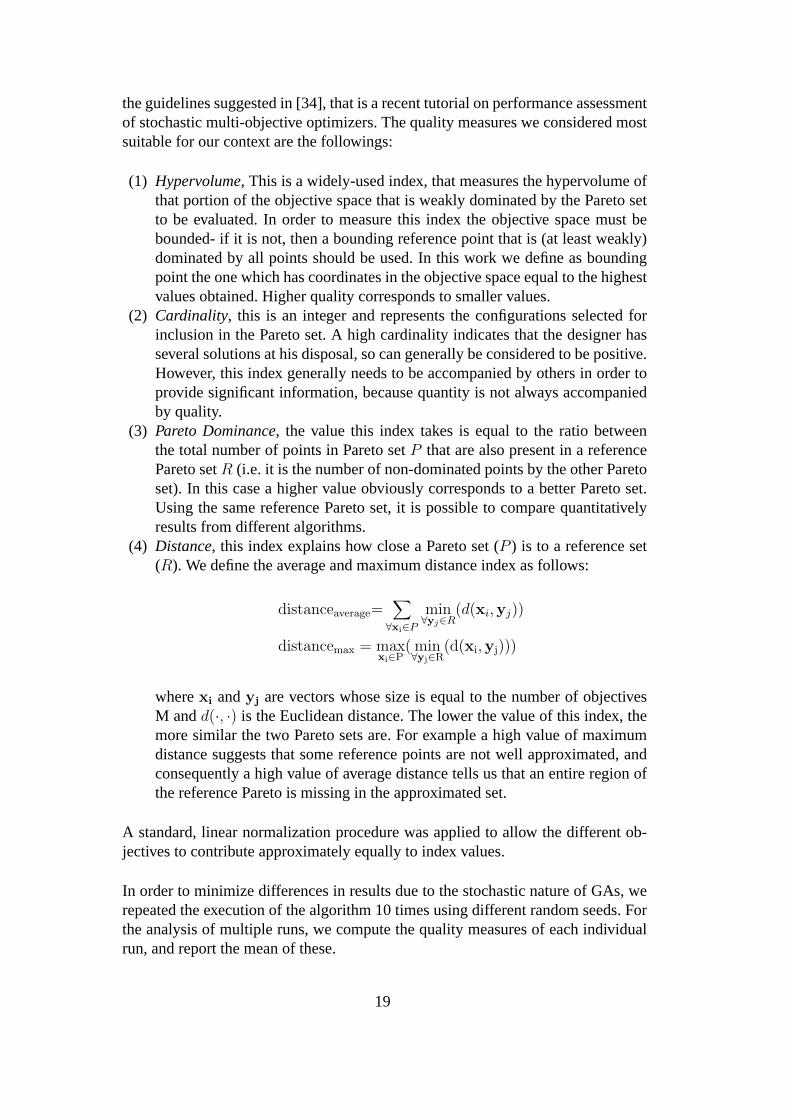
wherexi andyj are vectors whose size is equal to the number of objectivesM andd(·, ·) is the Euclidean distance. The lower the value of this index,themore similar the two Pareto sets are. For example a high valueof maximumdistance suggests that some reference points are not well approximated, andconsequently a high value of average distance tells us that an entire region ofthe reference Pareto is missing in the approximated set.

A standard, linear normalization procedure was applied to allow the different ob-jectives to contribute approximately equally to index values.

In order to minimize differences in results due to the stochastic nature of GAs, werepeated the execution of the algorithm 10 times using different random seeds. Forthe analysis of multiple runs, we compute the quality measures of each individualrun, and report the mean of these.

19

Fig. 9. Dependency graph of the parameterized VLIW-based system architecture.

6 Comparison between Methods

In this section we perform an extensive evaluation of the proposed approach by thecomparison with the DSE approaches presented in Section 3. The comparison iscarried out in terms of both accuracy and efficiency, on the parameterized systemarchitecture described in Section 5. Efficiency can be defined as the number ofsystem configurations simulated to complete the exploration, and is proportional tothe execution time of the exploration algorithm. Accuracy is an index of quality ofthe solutions obtained.

The parameters used for the GA-based approaches (GA andGA-Fuzzy) are as fol-lows: The internal and external population were set as comprising 30 individuals,using a crossover probability of0.8 and a mutation probability of0.1. These valueswere set following the indications given in [21], where the convergence times andaccuracy of the results were evaluated with various crossover and mutation proba-bilities, and it was observed that the performance of the algorithm with the variousbenchmarks was very similar. ForGA-Fuzzythe estimation error is calculated ina window of20 evaluations for the objectives, and the threshold was set to5% ofthe Euclidean distance between the real point and estimatedone in the objectivespace. The minimum number of evaluations, before which consider the error testto assess the reliability of the fuzzy estimator, was set to90. Both thresholds werechosen after extensive series of experiments with computationally inexpensive testfunctions. The dependency graph used forDEP is depicted in Figure 9. It should bepointed out, however, that the dependency graph shown in Figure 9 is a simplifiedversion of the actual dependency graph. This was due to the fact that it is unfea-sible to applyDEP using the actual dependency graph, because exploration willrun for a very long time. The logic followed was to remove somedependencies byrequiring the parameters to be explored in order of importance. For example, weintroduced an approximation whereby the parameters of the first level cache areexplored independently of those of the second level cache.

20

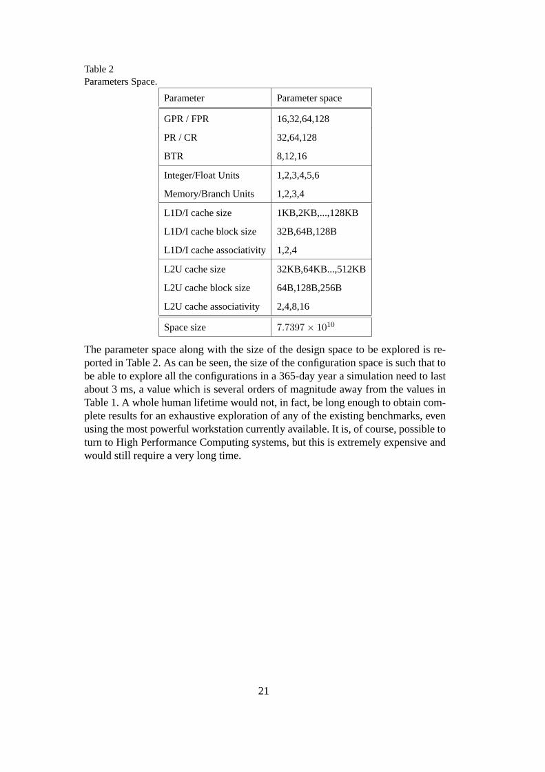
Table 2Parameters Space.

Parameter Parameter space

GPR / FPR 16,32,64,128

PR / CR 32,64,128

BTR 8,12,16

Integer/Float Units 1,2,3,4,5,6

Memory/Branch Units 1,2,3,4

L1D/I cache size 1KB,2KB,...,128KB

L1D/I cache block size 32B,64B,128B

L1D/I cache associativity 1,2,4

L2U cache size 32KB,64KB...,512KB

L2U cache block size 64B,128B,256B

L2U cache associativity 2,4,8,16

Space size 7.7397 × 1010

The parameter space along with the size of the design space tobe explored is re-ported in Table 2. As can be seen, the size of the configurationspace is such that tobe able to explore all the configurations in a 365-day year a simulation need to lastabout 3 ms, a value which is several orders of magnitude away from the values inTable 1. A whole human lifetime would not, in fact, be long enough to obtain com-plete results for an exhaustive exploration of any of the existing benchmarks, evenusing the most powerful workstation currently available. It is, of course, possible toturn to High Performance Computing systems, but this is extremely expensive andwould still require a very long time.

21

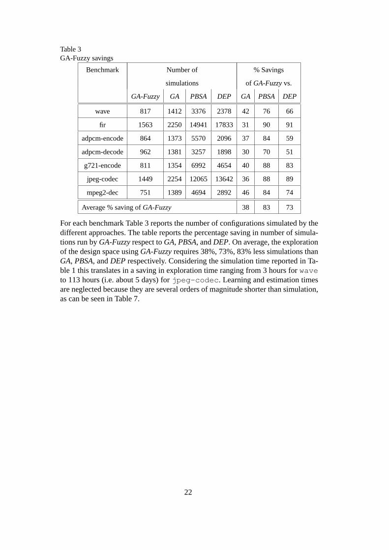
Table 3GA-Fuzzy savings

Benchmark Number of % Savings

simulations of GA-Fuzzyvs.

GA-Fuzzy GA PBSA DEP GA PBSA DEP

wave 817 1412 3376 2378 42 76 66

fir 1563 2250 14941 17833 31 90 91

adpcm-encode 864 1373 5570 2096 37 84 59

adpcm-decode 962 1381 3257 1898 30 70 51

g721-encode 811 1354 6992 4654 40 88 83

jpeg-codec 1449 2254 12065 13642 36 88 89

mpeg2-dec 751 1389 4694 2892 46 84 74

Average % saving ofGA-Fuzzy 38 83 73

For each benchmark Table 3 reports the number of configurations simulated by thedifferent approaches. The table reports the percentage saving in number of simula-tions run byGA-Fuzzyrespect toGA, PBSA, andDEP. On average, the explorationof the design space usingGA-Fuzzyrequires 38%, 73%, 83% less simulations thanGA, PBSA, andDEP respectively. Considering the simulation time reported in Ta-ble 1 this translates in a saving in exploration time rangingfrom 3 hours forwaveto 113 hours (i.e. about 5 days) forjpeg-codec. Learning and estimation timesare neglected because they are several orders of magnitude shorter than simulation,as can be seen in Table 7.

22

Table 4Quality assessment: distance from reference Pareto-optimal front.

Benchmark Distance from reference Pareto-optimal front%

Average/Max (%)

GA-Fuzzy GA PBSA DEP

wave 0.18/0.97 0.24/6.65 1.24/8.41 0.59/7.52

fir 0.05/5.61 0.07/1.19 0.14/6.15 0.02/6.15

adpcm-encode 0.16/2.03 0.27/1.69 0.10/7.26 0.09/1.28

adpcm-decode 0.18/6.46 1.09/30.48 1.01/30.38 0.03/0.95

g721-encode 0.24/6.01 0.64/17.98 0.52/16.73 0.51/25.11

jpeg 0.83/7.76 0.62/6.90 0.12/1.93 0.80/4.07

mpeg2-decode 0.91/11.45 1.22/4.84 0.92/6.66 1.09/11.22

Average 0.36/5.76 0.59/9.96 0.58/11.07 0.45/8.04

To assess the accuracy of the different approaches, we need to know the Pareto-optimal system configurations. Since the whole design spacecannot be exhaus-tively explored in order to obtain them, we used the following approach to computea reference Pareto-set. First, we merged all the Pareto-setobtained by each ap-proach, then we removed all the dominated configurations. Thus, the remainingpoints, which are not dominated by any of the approximationssets, form the ref-erence set. Table 4 reports the average and maximum distancebetween the Paretofronts obtained by the different approaches and the reference Pareto front. As canbe observed the accuracy exhibited byGA-Fuzzyis very close to that obtained byDEP. In particular for two of the benchmarks (wave andg721-encode) GA-Fuzzyoutperforms the other approaches. As expected,DEP does not dominate theother approaches. In fact, as stated before, to makeDEP computationally feasible,the dependency graph used in the experiments does not include all the parameters’dependencies.

23

Table 5Quality assessment: Hypervolume.

Benchmark Hypervolume (%)

GA-Fuzzy GA PBSA DEP

wave 25.19 25.44 28.41 26.69

fir 30.09 30.21 30.66 30.09

adpcm-encode 28.79 29.15 28.54 28.73

adpcm-decode 19.44 19.70 19.43 19.15

g721-encode 18.03 18.64 18.52 19.12

jpeg 16.31 16.61 15.90 16.33

mpeg2-decode 20.19 20.30 20.86 20.91

Average 22.58 22.86 23.18 23.00

To further confirm the accuracy ofGA-Fuzzy, Table 5 reports the hypervolume mea-sure (normalized respect to the boundaries of the objectivespace and expressed inpercentage) of the Pareto-fronts obtained by the differentapproaches. Once again,the results confirm the accuracy characteristics ofGA-Fuzzy. Actually, using thismetric, all the approaches seem perform almost the same for all benchmarks. How-ever, looking at the average results in Tables 4 and 5, it can be stated that GA-Fuzzyperforms slightly better than the other approaches.

Table 6Accuracy comparison betweenGAandGA-Fuzzyafter an equal number of simulations.

Benchmark Simulations Cardinality Pareto

Dominance (%)

GA-Fuzzy GA GA-Fuzzy GA

wave 1412 43 42 97.43 89.65

fir 2250 108 106 98.15 84.11

adpcm-encode 1373 53 48 82.55 68.22

adpcm-decode 1381 48 42 95.92 76.57

g721-encode 1354 118 118 74.81 59.85

jpeg 2254 166 127 74.95 64.87

mpeg2-dec 1389 157 152 80.22 54.72

Finally, in the last experiment, we perform the explorationof the design space byusingGAandGA-Fuzzyon an equal number of simulations. Table 6 show thatGA-Fuzzyyields a Pareto front which in many points dominates the set provided byGAthanks to its ability to evaluate much more system configurations thanGA. This is

24

numerically expressed by the higher Pareto Dominance valueand the greater num-ber of points in the Pareto set obtained by theGA-Fuzzyapproach. This means thatthe results obtained byGA-Fuzzyare both qualitatively and quantitatively betterthan that obtained byGA.

In summary, the proposed approach yields similar results tothose of the other ap-proaches, with a 40–90% saving on computation time, which translates in severalhours or days depending on the benchmark being considered. The equivalence ofPareto sets obtained is numerically justified by the short distance between the setsand the similar hypervolume values.

Table 7Efficiency and accuracy of fuzzy estimation system builded by GA-Fuzzyon a random testset of 10,000 configurations

Benchmark

fir adpcm-enc adpcm-dec mpeg2-dec jpeg g721-enc

Simulations 2250 1373 1381 1389 2254 1354

Rules 2172 1338 1342 1354 2168 1313

Avg Time (ms)

- Learn 3.44 3.36 3.39 3.81 5.37 3.09

- Estimate 6.87 6.72 6.88 7.51 10.68 6.26

Avg Estimation Error (%)

Whole Set

- Avg Power 6.76 8.12 7.13 12.12 7.08 7.41

- Exec Time 6.33 8.01 7.02 18.89 6.07 6.42

Pareto Set

- Avg Power 2.21 2.41 2.22 7.88 2.88 2.72

- Exec Time 4.21 3.45 4.99 8.21 2.49 4.04

Another interesting feature of the approach proposed is that at the end of the geneticevolution we obtain a fuzzy system that can approximate any configuration. Thedesigner can exploit this to conduct a more in-depth exploration. Table 7 gives theestimation errors for the fuzzy system obtained after 100 generations on a randomset of configurations other than those used in the learning phase. The same tablealso shows the time required to simulate a system configuration on a Pentium IV2.8GHz workstation. Despite the great number of rules this time is several orders ofmagnitude shorter as compared to the time required to perform a simulation withoutany appreciable impact on estimation accuracy.

25

1.5 1.6 1.7 1.8 1.9 2

0.09

0.095

0.1

0.105

0.11

0.115

0.12

0.125

Average Power Consumption (W)

Exec

ution

Tim

e(m

s)

PBSADEPGAGAF

Fig. 10.wave: Pareto sets and attainment surfaces obtained by DEP, PBSA, GA and GA–Fuzzy (GAF).

1.4 1.45 1.5 1.55 1.6 1.65 1.7 1.75

42

44

46

48

50

52

54

56

58

60

62

Average Power Consumption (W)

Exec

ution

Tim

e(m

s)

PBSADEPGAGAF

Fig. 11.adpcm-encoder: Pareto sets and attainment surfaces obtained by DEP, PBSA,GA and GA-Fuzzy (GAF).

7 Conclusion and Future Works

In this paper we presented a new DSE approach based on a Hierarchical FuzzySystem hybridized with a Genetic Algorithm. The approach reduces the number of

26

simulations while minimizing the time required to simulate: GA smartly exploresthe design space, in the meanwhile the FS learn from the experience accumulatedduring theGA evolution, storing knowledge in fuzzy rules. The joined rules buildthe Knowledge Base through which the integrated system quickly predict the resultsof complex simulations thus avoiding their long execution times. A comparisonbetweenGA-Fuzzyand established DSE approaches, performed on various mul-timedia benchmarks, showed that integration with the fuzzysystem saves a greatamount of time and also gives slightly more accurate results. Further developmentsmay involve the use of acquired knowledge to create a set of generic linguistic rulesto speed up the learning phase, providing an aid for designers and a basis for teach-ing. Finally, we are interested in applying the estimation technique by means of afuzzy system to the other approaches as well, with a view to speeding them up.

References

[1] F. Vahid, T. Givargis, Platform tuning for embedded systems design,IEEE Computer34 (3) (2001) 112–114.

[2] T. Givargis, F. Vahid, J. Henkel, System-level exploration for Pareto-optimalconfigurations in parameterized System-on-a-Chip, IEEE Transactions on Very LargeScale Integration Systems 10 (2) (2002) 416–422.

[3] W. Fornaciari, D. Sciuto, C. Silvano, V. Zaccaria, A sensitivity-based design spaceexploration methodology for embedded systems, Design Automation for EmbeddedSystems 7 (2002) 7–33.

[4] G. Ascia, V. Catania, M. Palesi, A multi-objective genetic approach forsystem-levelexploration in parameterized systems-on-a-chip, IEEE Transactions on Computer-Aided Design of Integrated Circuits and Systems 24 (4) (2005) 635–645.

[5] G. Hekstra, D. L. Hei, P. Bingley, F. Sijstermans, TriMedia CPU64 design spaceexploration, in: International Conference on Computer Design, Austin Texas, 1999,pp. 599–606.

[6] S. G. Abraham, B. R. Rau, R. Schreiber, Fast design space exploration through validityand quality filtering of subsystem designs, Tech. Rep. HPL-2000-98, HP LaboratoriesPalo Alto (Jul. 2000).

[7] R. Szymanek, F. Catthoor, K. Kuchcinski, Time-energy design space exploration formulti-layer memory architectures, in: Design, Automation and Test in Europe, 2004,pp. 181–190.

[8] S. Neema, J. Sztipanovits, G. Karsai, Design-space construction and explorationin platform-based design, Tech. Rep. ISIS-02-301, Institute for Software IntegratedSystems Vanderbilt University Nashville Tennessee 37235 (Jun. 2002).

[9] A. Ghosh, T. Givargis, Cache optimization for embedded processorcores: Ananalytical approach, ACM Transactions on Design Automation of ElectronicSystems,9 (4) (2004) 419–440.

27

[10] L. Eeckhout, S. Nussbaum, J. E. Smith, K. D. Bosschere, Statisticalsimulation:Adding efficiency to the computer designer’s toolbox, IEEE Micro 23 (5) (2003) 26–38.

[11] S. Eyerman, L. Eechhout, K. D. Bosschere, Efficient design space exploration of highperformance embedded out-of-order processors, in: DATE, 2006.

[12] P. Mazumder, E. M. Rudnick, Genetic Algorithms for VLSI Design, Layout & TestAutomation, Prentice Hall, Inc., 1999.

[13] C. J. Alpert, L. W. Hagen, A. B. Kahng, A hybrid multilevel/genetic approach forcircuit partitioning, in: Fifth ACM/SIGDA Physical Design Workshop, 1996, pp. 100–105.

[14] K. Shahookar, P. Mazumder, A genetic approach to standard cellplacement usingmetagenetic parameter optimization, IEEE Transactions on Computer-Aided Design9 (1990) 500–511.

[15] J. Lienig, K. Thulasiraman, A genetic algorithm for channel routing inVLSI circuits,Evolutionary Computation 1 (4) (1993) 293–311.

[16] Y.-M. Jiang, K.-T. Cheng, A. Krstic, Estimation of maximum power and instantaneouscurrent using a genetic algorithm, in: Proceedings of IEEE Custom Integrated CircuitsConference, 1997, pp. 135–138.

[17] V. Kommu, I. Pomenraz, GAFAP: Genetic algorithm for FPGA technology mapping,in: European Design Automation Conference, 1993, pp. 300–305.

[18] C. J. Alpert, A. B. Kahng, Recent developments in netlist partitioning:A survey, VLSIJournal 19 (1–2) (1995) 1–81.

[19] D. Saab, Y. Saab, J. Abraham, Automatic test vector cultivation for sequential VLSIcircuits using genetic algorithms, IEEE Transactions on Computer-Aided Design15 (10) (1996) 1278–1285.

[20] G. Ascia, V. Catania, M. Palesi, Parameterized system design basedon geneticalgorithms, in: 9th. International Symposium on Hardware/Software Co-Design,Copenhagen, Denmark, 2001, pp. 177–182.

[21] G. Ascia, V. Catania, M. Palesi, A GA based design space exploration frameworkfor parameterized system-on-a-chip platforms, IEEE Transactions on EvolutionaryComputation 8 (4) (2004) 329–346.

[22] W. Fornaciari, D. Sciuto, C. Silvano, V. Zaccaria, A design framework toefficiently explore energy-delay tradeoffs, in: 9th. International Symposium onHardware/Software Co-Design, Copenhagen, Denmark, 2001, pp. 260–265.

[23] G. Ascia, V. Catania, M. Palesi, Tuning methodologies for parameterized systemsdesign, in: K. A. Publisher (Ed.), System on Chip for Realtime Systems, 2002.

[24] E. Zitzler, M. Laumanns, L. Thiele, SPEA2: Improving the performance of thestrength pareto evolutionary algorithm, in: EUROGEN 2001. Evolutionary Methodsfor Design, Optimization and Control with Applications to Industrial Problems,Athens, Greece, 2001, pp. 95–100.

28

[25] E. Zitzler, L. Thiele, Multiobjective evolutionary algorithms: A comparative casestudy and the strength pareto approach, IEEE Transactions on EvolutionaryComputation 4 (3) (1999) 257–271.

[26] L.-X. Wang, J. M. Mendel, Generating fuzzy rules by learning from examples, IEEETransactions on System, Man and Cybernetics 22 (1992) 1414–1427.

[27] T. Takagi, M. Sugeno, Fuzzy identification of systems and its application to modelingand control, IEEE Transactions on System, Man and Cybernetics 15 (1985) 116–132.

[28] J. A. Fisher, Very long instruction word architectures and the ELI512, in: Tenth AnnualInternational Symposium on Computer Architecture, 1983, pp. 140–150.

[29] An infrastructure for research in instruction-level parallelism,http://www.trimaran.org/.

[30] G. Ascia, V. Catania, M. Palesi, D. Patti, EPIC-Explorer: A parameterized VLIW-based platform framework for design space exploration, in: First Workshop onEmbedded Systems for Real-Time Multimedia (ESTIMedia), Newport Beach,California, USA, 2003, pp. 65–72.

[31] D. Patti, M. Palesi, EPIC-Explorer,http://epic-explorer.sourceforge.net/ (Jul. 2003).

[32] X.-J. Zeng, J. A. Keane, Approximation capabilities of hierarchicalfuzzy systems,IEEE Transactions on Fuzzy Systems 13 (5) (2005) 659–672.

[33] E. Zitzler, L. Thiele, M. Laumanns, C. M. Fonseca, V. G. da Fonseca, Performanceassessment of multiobjective optimizers: An analysis and review, IEEE Transactionson Evolutionary Computation 7 (2) (2003) 117–132.

[34] J. D. Knowles, L. Thiele, E. Zitzler, A tutorial on the performance assessment ofstochastive multiobjective optimizers, Tech. Rep. TIK-Report No. 214, ComputerEngineering and Networks Laboratory, ETH Zurich, Swiss (Feb. 2006).URL http://dbk.ch.umist.ac.uk/knowles/TIK214b.pdf

29