cut-on cut-off transition in flow ducts: comparing multiple-scales and finite-element solutions
TRANSCRIPT
Cut-on cut-off transition in flow ducts: comparingmultiple-scales and finite-element solutions
Nick C. Ovenden∗University College London, WC1E 6BT, United Kingdom.
Walter Eversman†
University of Missouri-Rolla, Rolla, MO 65409-0257, USA.
Sjoerd W. Rienstra‡
Eindhoven University of Technology, 5600 MB Eindhoven, The Netherlands.
The phenomenon of cut-on cut-off transition of acoustic modes in ducts with mean flow is examined us-ing an analytical multiple-scales solution, and compared to solutions obtained from a numerical finite-elementmethod. The analytical solution, derived for an arbitrary duct with irrotational mean flow, remains valid toleading-order throughout the duct. In other words, it is a composite solution, encompassing both the innerboundary-layer solution in the neighbourhood of the transition point and the outer slowly varying modal solu-tion far upstream and downstream. Several test cases are defined and presented within a geometry representa-tive of a high-bypass turbofan engine. The cases span a wide realistic range of frequencies and circumferentialmode numbers both with and without mean flow, including one numerically-challenging investigation of cut-off cut-on transition of a mode. The agreement is in most cases remarkably good. Slight differences in positionof the pressure pattern can be observed for cases with mean flow, which seem due to the slight variations inmean flow fields obtained from both methods. When cut-on cut-off transition occurs for high Helmholtz num-ber and high radial mode number a certain amount of modal scattering is observed. An attempt is made toexplain this by incorporating the presence of neighbouring modes in the asymptotic scaling arguments for theturning point region. The composite solution should enable designers to continue to use multiple-scales theoryto examine flow pressure and noise transmission inside an engine duct, whilst now being able to include directlythe contributions of modes undergoing transition without encountering singular behaviour.
Nomenclature
Ai, Bi = Airy functionsE = mean flow Bernoulli constantF = mean flow mass fluxJm , Ym = Bessel functions of the first and second kinds of ordermm = circumferential modal wave numberM = Mach numbern = radial modal orderN = slowly varying modal amplituden1, n2 = unit outer normal vectors ofR1, R2Q = constant to fix modal amplitudeQ = related toQ, see Eq. (22)R1, R2 = inner, outer walls of duct
∗Research Fellow, Department of Mathematics, UniversityCollege London, Gower Street, London WC1E 6BT, United Kingdom. AIAAMember.
†Curators’ Professor, Department of Mechanical and Aerospace Engineering and Engineering Mechanics,University of Missouri-Rolla, 1870Miner Circle, Rolla, MO 65409-0257, USA. AIAA Member.
‡Associate Professor, Department of Mathematics and Computer Science, Eindhoven University of Technology, P.O. Box 513, 5600 MB Eind-hoven, The Netherlands. AIAA Member.
1 of 18
American Institute of Aeronautics and Astronautics
10th AIAA/CEAS Aeroacoustics Conference AIAA 2004-2945
Copyright © 2004 by N.C. Ovenden, W. Eversman and S.W. Rienstra. Published by the American Institute of Aeronautics and Astronautics, Inc., with permission.
R∞, ρ∞, c∞ = reference values,v, p, ρ, c, φ = velocity, pressure, density, sound speed, potentialv, p, ρ, c, φ = time-harmonic velocity, pressure, density, sound speed, potential perturbationsV , P, D, C = mean flow velocity, pressure, density, sound speedU0, V⊥0, P0, D0, C0 = approximate mean flow variablesx , r , θ , t = axial, radial, azimuthal angle, time coordinateex , er , eθ = unit vectors inx , r , θ -directionX = εx , slow variableXt , xt = cut-on cut-off transition point inX , x coordinate
α = (square root of) eigenvalue ofψ; in axisymmetric geometry: radial modal wave numberγ = ratio of specific heatsε = small parameter, representing typical axial duct slopeζ = 2
3|x |3/2µ = axial modal wave numberσ = reduced axial wave number, Eq. (19)ϒ = factor ofYm in annular duct eigensolutionψ = eigensolution of Laplace operator in a cross-sectional planeω = Helmholtz number (dimensionless angular frequency)
I. Introduction
SOUND transmission through a duct of slowly-varying crosssection can be modelled using the theory of multiplescales. This theory was first applied to ducts without mean flow1 and extended in later works to include cases
with mean irrotational flow2 , mean swirling flow3 and most recently non-axisymmetricducts (with mean irrotationalflow).4 The multiple scales approach provides an attractive alternative to a full numerical solution of acoustic modesin aeroengine ducts, as the calculation complexities are only marginally more than finding the eigenmodes inside astraight duct. Indeed, a recent comparison of multiple-scales solutions of sound propagation with those obtained froma numerical finite-element method shows good agreement across a range of realistic engine frequencies.5
The multiple-scales approach allows sound transmission to be represented by a summation ofslowly varyingmodes, which depend on a slow axial variable based on the the slope of the duct walls as a small parameter. Crucially,the amplitudes of these modes vary on the slow scale and are determined via a solvability condition. However, themultiple-scales approximation breaks down at positions where the amplitude of a particular mode becomes singular.These singular transition points are analogous to the turning points observed in solutions to Schrödinger’s equation,and represent the complete reflection of a cut-on propagating mode and transmission of a cut-off attenuating mode (orvice-versa).
The turning-point behaviour of such a mode can be analysed by examining the solution in a boundary-layer regionencompassing the singularity. Within this region, the original slowly-varying assumption fails to hold and a differentapproximation leads to the non-convective axial variation of the mode satisfying Airy’s equation. Such an analysiswas performed for both axisymmetric1,3,6 and non-axisymmetric ducts4 alike in cases of no mean flow, irrotationalmean flow and mean swirling flow (axisymmetric only). In all cases it was shown that the incident cut-on mode iscompletely reflected in the axial plane with a phase shift ofπ/2. In the event that an isolated acoustic mode undergoescut-on cut-off transition, no energy is propagated beyond the transition point. Similar partial reflection of modes alsoappear to occur in lined ducts (so-called near transition) where the reflection coefficient has magnitude and phasedetermined by the properties of the mean flow and liner impedance.7
An understanding of cut-on cut-off behaviour in hard-walled ducts is important for engine design applications. Theusual design of rotors and stators is such that at least for the first harmonic all interaction modes are cut-off. Cuttingoff acoustic modes by varying the duct geometry could, in principle, add to further reduction of the noise output of anengine. However, reflection of a cut-on mode may also result in the mode becoming trapped inside a section of theduct, possibly leading to acoustic resonance and instability; such a scenario has been investigated previously.8
In this paper, an explicit analytical solution for transition, either from cut-on to cut-off or vice-versa, is comparedagainst the solution obtained from a numerical finite-element method. The analytical solution9 , derived for an arbitraryduct with mean irrotational flow, remains uniformly valid to leading-order throughout the duct. In other words, it is acomposite solution, encompassing both the inner boundary-layer solution in the neighbourhood of the transition pointand the outer slowly varying modal solution far upstream and downstream. This composite solution can therefore be
2 of 18
American Institute of Aeronautics and Astronautics

applied exactly as a normal slowly-varying mode, without any need to calculate the size of the boundary layer aroundthe transition point, nor match the inner and outer solutions together at some intermediate interface. Such a solutionshould enable designers to continue touse multiple-scales theory to examine flow pressure and noise transmissioninside an engine duct, whilst now being able to include directly the contributions of modes undergoing transitionwithout encountering singular behaviour. The finite-element solution10 solves directly the potential flow equations forlinear acoustic perturbations of a compressible inviscid isentropic irrotational mean flow, which form the original basisfor the multiple scales approximation.
To test the analytical composite solution, absolute pressure plots are compared against those obtained from thefinite-element model. Following in a similar manner as a previous comparison of two of the authors5 , several casesof modes undergoing transition from cut-on to cut-off are examined within a generic engine inlet-duct geometry atrealistic engine frequencies, with and without irrotational mean flow. An additional numerically challenging case ofan attenuating mode cutting-on in the duct is also examined.
The outline of the paper is as follows. Section II details the derivation of the potential flow governing equationsand boundary conditions which are common to both models, along with a description of the duct geometry. Thesubsequent sections III and IV then describe briefly the derivation of the multiple-scales solution for simple modaltransition and the finite-element model respectively. The results and discussion of seven test cases are presented insection V followed by an discussion on the occurrence of modal scattering in section VI and conclusions in sectionVII.
II. Potential Flow Model
A. Derivation of the governing equations
Consider compressible perfect isentropic irrotational gas flow, consisting of a subsonic mean flow and small acousticdisturbances, inside a duct of slowly-varying cross section. The problem can be non-dimensionalised by scaling allspatial dimensions on a typical duct widthR∞, densityρ on some reference value for the gasρ∞, velocitiesv andsound speedc on a reference sound speed of the gasc∞, time t on R∞/c∞ and pressurep onρ∞c2∞. The perfect gascondition implies constant heat capacities and the ratio of specific heats at constant pressure and volume is taken asγ = 1.4. It is further assumed that (i) the acoustic variationsare too rapid for heat conduction (Péclet number is large)and (ii) the viscous forces are negligible (Reynolds number is large). The resulting governing equations are
∂ρ
∂ t+ ∇·(ρv) = 0, ρ
(∂ v∂ t
+ v·∇v)
+ ∇ p = 0, γ p = ργ , c2 = dp
dρ= ργ−1. (1)
The assumption that the flow is irrotational allows us to introduce a velocity potentialφ, wherev = ∇φ, and tointegrate the above momentum equation to obtain a variant of Bernoulli’s equation, where
∂φ
∂ t+ 1
2
∣∣∇φ∣∣2 + c2
γ − 1(2)
is a conserved quantity throughout the flow.Following the analysis of Rienstra2 , the flow is split into a steady irrotational mean flow, with no swirling compo-
nent, and infinitesimally small harmonic perturbations of angular frequency (Helmholtz number)ω > 0 to representthe acoustic part. Thus, [
v, ρ, p, c] = [
V , D, P,C] + Re
{[∇φ, ρ, p, c]
eiωt}. (3)
Substitution of this form into the governing equation leads to the following system
∇·(DV ) = 0,1
2
∣∣V ∣∣2 + C2
γ − 1= E, C2 = γ
P
D= Dγ−1, (4)
for the mean flow field, given some constantE . The acoustic field can be described, after eliminating pressure anddensity perturbations, as a solution to the general convected wave equation
∇·(D∇φ) − D(iω + V ·∇)[C−2(iω +V ·∇)φ]= 0. (5)
The pressure and density perturbations can subsequently be recovered fromφ by the expressions
p = −D(iω + V ·∇)φ, p = C2ρ. (6)
3 of 18
American Institute of Aeronautics and Astronautics
B. Test geometry and boundary conditions
0 0.5 1 1.5 2 −1
−0.8
−0.6
−0.4
−0.2
0
0.2
0.4
0.6
0.8
1
x
r
R1(x)
R2(x)
Figure i. Generic inlet duct of a high-bypass turbofanengine.
Both the multiple-scales solution4,9 and the finite-element model10
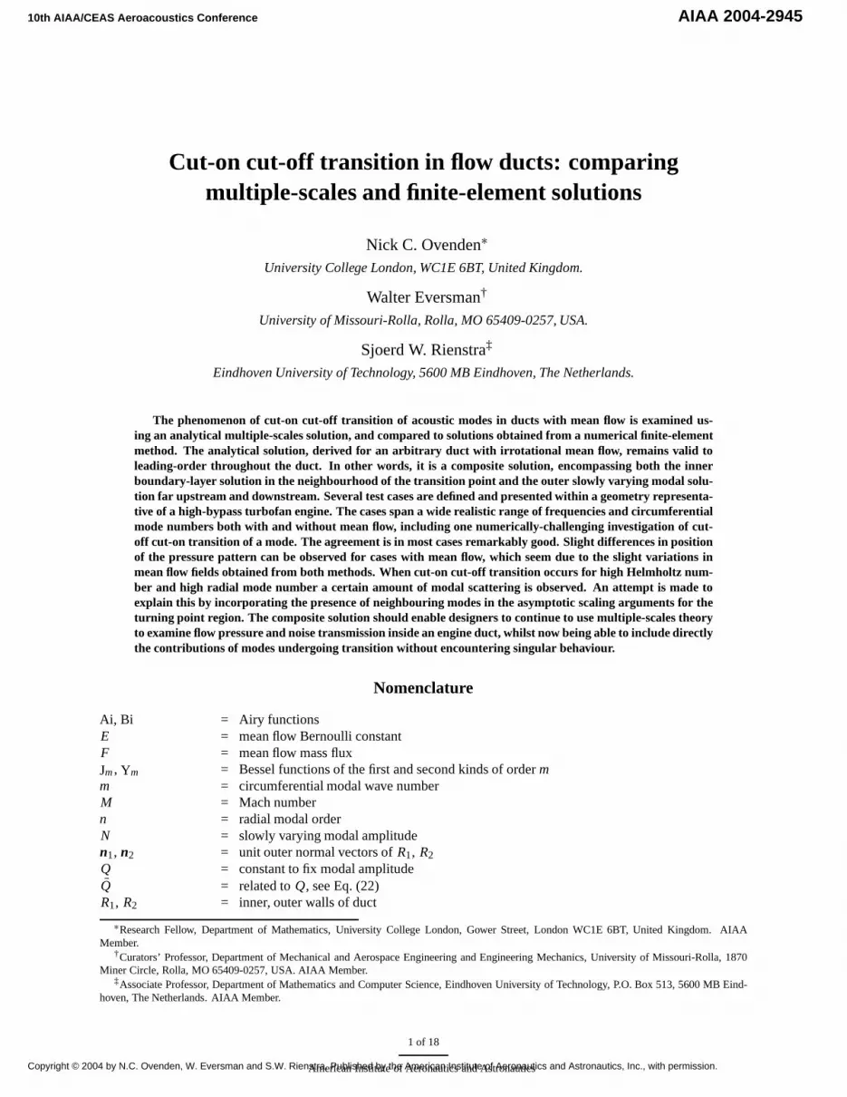
can be applied to ducts of arbitrary shape, although for this paper theinlet duct is taken to be axisymmetric. The duct geometry can bedescribed ideally in cylindrical coordinates(x, r, θ) wherex is theaxial coordinate with unit vectorex , r is the radial coordinate withunit vectorer and θ is the azimuthal coordinate with unit vectoreθ . The test geometry chosen represents a realistic generic inletduct geometry of a high-bypass turbofan engine, similar to the oneused in a previous comparison paper of two of the authors.5 Thepositions of the inner spinner and outer nacelle can thus be definedby two nondimensional radial functionsr = R1(x) andr = R2(x)respectively. A cross-sectional schematic of the inlet duct used isshown in Fig. i. The reference values for nondimensionalisation aretaken atx = 0, such thatR2(0) = 1. The outer radiusR2 and innerradiusR1 are described by the following formulas
R2(x) = 1 − 0.18453y2 + 0.10158e−11(1−y)− e−11
1 − e−11 ,
R1(x) = max[0,0.64212− (0.04777+ 0.98234y2)1/2],(7)
wherey = x/L andL = 2 (and not 1.86393 like in5) is the length of the duct.The sound is taken to be emitted from the left of the source plane atx = 0, which roughly represents the position of
the turbofan inside a real aeroengine. The incident cut-on sound waves then propagate from left-to-right in a positivesense axially. As this is an inlet duct, any mean flow is assumed to come from the opposite direction to the incidentsound, approaching the fan from the right of the picture. For both solutions, the mean flow is selected by its MachnumberM attained at the source planex = 0 with nondimensional sound speedC and densityD set equal to unitythere (soU(0) = M). These conditions fix the constantE in the mean flow governing equations, and the axial massflux F . Applying radial boundaryconditions that the normal velocity vanishes at the spinner and at the outer wallconsequently determines the mean flow field completely throughout the duct.
As we are examining the phenomenon of cut-on cut-off transition, both inner and outer walls are assumed to behard with infinite impedance. Hence for the acoustic field, the necessary boundary condition to be imposed at the wallsis that the normal velocity vanishes at both inner and outer walls. In other words,∇φ·ni = 0 atr = Ri (x), wheren1andn2 are the outer normals forR1 andR2 respectively.
III. Multiple-scales approach and composite solution
A. Slowly varying mean flow
The WKB approximation is based on the assumption that the geometry and mean flow areslowly-varying on a lengthscale much longer than a typical acoustic wave length. As we are interested in waves typically equal to or shorterthan a duct radius, geometry and mean flow should vary slowly on a lengthscale much longer than the duct radius.The approximate mean flow solution, compatible with the WKB approach, is then obtained by the method of slowvariation.11 For the analysis, a slow axial variableX = εx is defined, whereε � 1 is a small nondimensionalparameter representing the typical slope of the duct walls. The slowly varying duct walls can therefore be expressedas functions of this slow variable, so that for any arbitrarily ductr = R1(X, θ) andr = R2(X, θ) for inner and outerwalls respectively. Note that without change of notation we use in the actual calculationsand results the definitionfrom Eqs. (7) ofRi (x), i.e. depending onx , whereas in the analysis the functionsRi will be assumed to depend onX .
Assuming the mean flow is irrotational with axial variations in the slow variableX only, it follows4 that it is nearlyuniform, and we can expand the mean flow variables in terms ofε to obtain
V (X, r, θ; ε) = U0(X)ex + εV⊥0(X, r, θ)+ O(ε2), P(X, r, θ; ε) = P0(X)+ O(ε2),
D(X, r, θ; ε) = D0(X)+ O(ε2), C(X, r, θ; ε) = C0(X)+ O(ε2).(8)
Here,εV⊥0 represents a small crosswise mean flow component in theer andeθ directions; for the case of an axisym-metric duct, this is purely radial.2 The solution to the mean flow equations, Eqs. (4), in terms of the two defined
4 of 18
American Institute of Aeronautics and Astronautics

physical constantsE andF is given by
U0(X) = F
D0(X)∫ 2π
0
∫ R2R1
rdrdθ,
1
2U2
0 + Dγ−10
(γ − 1)= E, (9)
with C0 andP0 obtained from the other relations in Eqs. (4).
B. Slowly varying acoustic modes
On obtaining a mean flow consistent with the slowly-varying approximation, the method of multiple-scales (MS)enables the acoustic field in a slowly varying duct to be represented as a summation of slowly varying modes of theform4
φ(x, r, θ; ε) = N(X)ψ(r, θ; X) exp
(− i
ε
∫ X
µ(ζ ; ε)dζ). (10)
The functionψ(r, θ; X) is the solution to the following eigenvalue problem in the cross-sectional plane
−(
1
r
∂
∂r
(r∂
∂r
)+ 1
r2
∂2
∂θ2
)ψ = α2ψ, (11)
with hard-wall boundary conditions
∂ψ
∂r= 1
Ri
∂Ri
∂θ
∂ψ
∂θat r = Ri (X, r, θ), i = 1,2 (12)
and the slow axial variableX acts as a parameter. The eigenvalueα2 with eigensolutionψ satisfies the dispersionrelation
(ω − µU0)2
C20
− µ2 = α2, (13)
which, in turn, determines the axial wavenumberµ(X; ε) = µ(X) + O(ε2). It expedites the analysis4 to normalisethe eigensolution by integrating its square across the cross-sectional plane at eachX-station, ensuring∫ 2π
0
∫ R2(X,θ)
R1(X,θ)ψ2(r, θ; X) r drdθ = 1. (14)
For our test case of an axisymmetric annular duct, the eigensolution is a combination of Bessel functions of first andsecond kinds multiplied bye−imθ for circumferential wavenumberm (for a spinning modem �= 0). Explicitly then,we have9
ψ(r, θ; X) = Jm(αr)−ϒ(X)Ym(αr)√2π
(R2
2−m2/α2
[αR2 Y′m(αR2)]2 − R1
2−m2/α2
[αR1 Y′m(αR1)]2
) e−imθ for m �= 0, (15)
whereϒ(X) and the radial eigenvalueα(X) can be determined from the hard-walled boundary condition in Eq. (12)now simplified to∂ψ
∂r = 0. Thus,
J′m [α(X)R2(X)]Y′
m [α(X)R2(X)] = J′m [α(X)R1(X)]Y′
m [α(X)R1(X)] = ϒ(X). (16)
For a hollow cylindrical duct (R1 = 0) these expressions reduce toϒ(X) = 0, α(X) determined from the boundaryconditionJ′
m(αR2) = 0, and
ψ(r, θ; X) = Jm(αr)
Jm(αR2)
√2
π
(R2
2 − m2
α2
)−1/2
e−imθ for m �= 0. (17)
Lastly, the slowly varying amplitudeN(X) is determined from asolvability condition2,4,12to be
N(X) = Q
√C0(X)
ωσ(X)D0(X), (18)
5 of 18
American Institute of Aeronautics and Astronautics

for some constantQ (obtained from the sound source) and where
σ(X) =√
1 − (C20 − U2
0 )α2
ω2 , (19)
is defined as the reduced axial wavenumber.2 The reduced axial wavenumber is the axial wavenumber rescaled withoutits convected part, explicitly
µ = ωC0σ − U0
C20 − U2
0
.
The two solutions of the square root represent two counterpart modes travelling in opposite directions axially alongthe duct. For cut-on modes that propagate axially in the duct,σ is purely real, whereas for cut-off modes that areattenuated and do not propagate along the duct,σ is purely imaginary (see Fig. ii).
C. Cut-on cut-off transition
Hard-wall transition points occur in a slowly-varying duct when the reduced axial wavenumber, Eq. (19), becomeszero (see Fig. ii) making the modal amplitudeN(X) in Eq. (18) singular. Hence in the neighbourhood of such apoint Xt , with σ(Xt ) = 0, the slowly varying assumption breaks down and a new approximation to the leading-ordergoverning equations is necessary. For non-swirling mean flow, the analysis performed4,6 for an isolated propagatingcut-on mode reveals that at the singular point, the mode is completely reflected into its opposite running counterpartwith a phase shift of12π . Thus, for such an isolated mode propagating in the positiveX-direction towards the singular(transitional) point atXt we find that ahead of transition (X < Xt ),
φ = N(X)ψ(r, θ; X) exp( i
ε
∫ X
Xt
ωU0
C20 − U2
0
dX ′)[exp(− i
ε
∫ X
Xt
ωC0σ
C20 − U2
0
dX ′)+ i exp( i
ε
∫ X
Xt
ωC0σ
C20 − U2
0
dX ′)] , (20)
where the first term represents the incident mode and the second the reflected mode. Beyond the transition pointX > Xt , a cut-off attenuated mode is transmitted of the form
φ = N(X)ψ(r, θ; X) exp( i
ε
∫ X
Xt
ωU0
C20 − U2
0
dX ′)exp(−1
ε
∫ X
Xt
ωC0|σ |C2
0 − U20
dX ′), (21)
which does not propagate axially and carries no energy. It is important to remark here that the inclusion of the reflectedmode is needed to conserve acoustic energy throughout the duct.6
The expressions Eq. (20) and Eq. (21) represent the so-calledouter solution to the problem, as they are only validaway from the transition locationXt when|X − Xt | ∼ 1. In the neighbourhood|X − Xt | ∼ ε2/3 an inner solutionholds to leading order, the non-convective axially varying part of which is a solution to Airy’s equation.4,6 Whilst itis relatively straightforward tomatch the inner and outer solutions to obtain the required reflection coefficient, it isextremely difficult to use them alone to evaluate the resulting pressure and velocity perturbations inside the duct. Thisis because the inner region can take up a sizable proportional of the duct in reality and, of course, no exact axial stationX exists where the inner solution ceases to be valid and the outer solution can be substituted instead. Such a problemmay be circumvented by finding a composite solution9 which is valid to leading order throughout the duct. For thecase of an incident cut-on mode propagating in the positiveX-direction described above, a composite multiple-scalessolution for this mode can be derived to leading order of the form
φ = Q
√C0
ωD0ψ(r, θ; X)
[− 3
2ε
1
σ 3
∫ X
Xt
ωC0σ
C20 − U2
0
dX ′]1/6
Ai
(
3i
2ε
∫ X
Xt
ωC0σ
C20 − U2
0
dX ′)2/3
e
iε
∫ XXt
ωU0C2
0−U20
dX ′. (22)
Here, Ai is the Airy function of the first kind, and the eigensolutionψ(r, θ; X) and the mean flow field are exactlyas those determined for a normal slowly-varying mode in previous analyses.4,9 The constantQ is obtained from thesource of the incident sound and differs from theQ in Eq. (18) by some constants:Q = 2
√π e
iπ4 Q. As one might
expect, using the asymptotes of Ai(s) given in the appendix by Eqs. (28) it can be shown that in the limitsX � Xt
andX Xt , the composite solution, Eq. (22), tends to Eq. (20) and Eq. (21) respectively.
6 of 18
American Institute of Aeronautics and Astronautics

real axis
ima
gina
rya
xis
• •⊗⊗
⊗
⊗ ⊗
⊗����
����
������
���
σ(Xt ) = 0
1−1
cut-off left-running
cut-off right-running
cut-on right-runningcut-on left-running
σ ∈ C
Figure ii. Sketch of the location ( ) of the reduced axial wavenumber of three right-running (σ ) and their corresponding left-running(−σ ) modes (
⊗) in complex plane. The second mode is about the pass the turning point Xt , corresponding to σ = 0.
D. Cut-off cut-on transition
A more general composite solution9 derived directly from the acoustic governing equation, Eq. (5), is
φ = Q
√C0
ωD0ψ(r, θ; X)
[− 3
2ε
1
σ 3
∫ X
Xt
ωC0σ
C20 − U2
0
dX ′]1/6 {
a Ai(s)+ b Bi(s)}
eiε
∫ XXt
ωU0C2
0−U20
dX ′, (23)
for
s =( 3i
2ε
∫ X
Xt
ωC0σ
C20 − U2
0
dX ′)2/3. (24)
The arbitrary constantsa andb are set by the two counterpart modes approachingXt from either side. From sucha general solution we can derive cut-off cut-on transition, when an isolated cut-off mode propagating in the positiveX-direction becomes cut-on at the pointXt . Clearly in this case, forX > Xt and|X − Xt | ∼ 1 we must only have atransmitted cut-on propagating mode (σ real and positive) of the form
φ =N(X)ψ(r, θ; X) eiε
∫ XXt
ωU0C2
0−U20
dX ′e− iε
∫ XXt
ωC0σ
C20−U2
0dX ′
. (25)
From applying the large argument asymptotes in Eqs. (28) for both Airy functions Ai(s) and Bi(s) as s → −∞(corresponding toX > Xt andσ real and positive), the required composite solution for cut-off cut-on transitionsatisfying Eq. (25) can be found and takes the form
φ = √πQ
√C0
ωD0ψ(r, θ; X)
[− 3
2ε
1
σ 3
∫ X
Xt
ωC0σ
C20 − U2
0
dX ′]1/6 {
Bi(s)− i Ai (s)}
eiε
∫ XXt
ωU0C2
0−U20
dX ′. (26)
IV. Finite-element solution
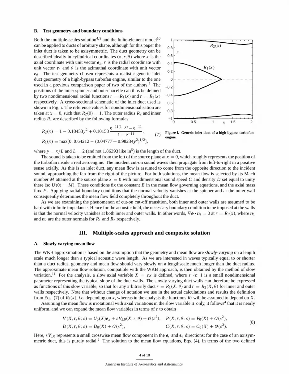
The numerical model for duct propagation is based on a finite element (FEM) discretization of the steady flowfield equations, Eqs. (4), and the acoustic field equations, Eq. (5) and Eq. (6) on the axisymmetric domain shown inFig. iii. The computational domain consists of the defined duct geometry, shown between dashed boundaries, plusextensions which are required in the mean flow model to assure locally uniform flow. The acoustic source plane is at
7 of 18
American Institute of Aeronautics and Astronautics
0 1x
spinner
duct
20
0.5
r
sour
ce p
lane
1
inle
t pla
ne
exit
plan
e
Figure iii. Calculational domain of FEM solution (including the lead-in)
the left domain boundary. The right domain boundary is extended from the nominal inlet plane, defined by the realduct geometry, to the exit plane where mean flow and acoustic boundary conditions are imposed.
A. FEM model for duct propagation
The steady compressible flow field is obtained from a Galerkin FEM formulation in terms of velocity potential of thefirst of equations Eqs. (4), the continuity equation, linearized at each step of an iterative process with density allowedto be spatially dependent. The secondand third of equations Eqs. (4), the momentum equation and state equations,are subsidiary relations used to update the density and speed of sound at each step. Mass flow rate is specified onthe source plane and the exit plane is assumed an equi-potential surface. The computational source and exit planesare generally placed a distance from the non-uniform region of the duct to assure locally uniform flow. In acousticresults presented here the source plane extension is 0.08 times the local outer duct radius, and at the termination planethe extension is 0.35 times the local duct radius. The mean flow field is described in terms of the mean flow velocitypotential which is required as input data for the acoustic FEM model. The mean flow mesh is the same as the acousticmesh to simplify data transfer.
The finite element model for acoustic propagation is also a Galerkin formulation based on the acoustic convectedwave equation in terms of acoustic potential, Eq. (5). Equations (6) are the acoustic momentum (or energy) andstate equations used to post process the acoustic potential to obtain the acoustic pressure and the acoustic density.The source is introduced at the source plane in terms of incident (right-running) acoustic potential modal amplitudes.Reflected (left-running) acoustic potential modal amplitudes are obtained as part of the solution. At the terminationplane the acoustic field is represented by transmitted (right running) acoustic potential modal amplitudes and reflected(left running) acoustic potential modal amplitudes. The termination plane is assumed to be non-reflecting, and thisis forced by requiring that reflected modal amplitudes vanish. Acoustic power is computed at the source plane andtermination plane based on acoustic potential modal amplitudes by using the definition of Morfey13 , valid in thecase of irrotational acoustic perturbations on irrotational mean flow. In addition, acoustic power is computed at anyspecified axial location using the Morfey definition, but by post-processing the acoustic potential.
FEM modelling of acoustic propagation and radiation innon-uniform mean flow is presented in detail in previ-ous works.10,14 More specific details of FEM applications to ducted flows terminated by reflection-free boundaryconditions can be found elsewhere.15,16
B. Comparison of the multiple scales (MS) and FEM formulations
There are no differences in the field equations (3-6) used in the multiple scales solution and the finite element model,including the convention for non-dimensionalisation. The MS solution proceeds on the basis of the primitive variables,whereas FEM is in terms of mean flow and acoustic potentials, with acoustic pressure recovered by post-processing.In both formulations the source is introduced by acoustic modal amplitudes.
The FEM formulation admits scattering as an integral part of the solution, manifested at the source and termina-tion planes by coupling between incident, transmitted and reflected modal amplitudes. In general there is observedreflection of the incident mode and other modes which are not incident as well as transmission of modes which are notincident. This will be clearly seen in examples which are presented. Such scattering is not such a direct feature of themultiple-scales solution.
8 of 18
American Institute of Aeronautics and Astronautics

The ability of the MS solution to capture the essential details of the FEM solution is of principal interest in thisinvestigation.
V. Results
The seven test cases considered examine a single radialacoustic mode undergoing transition from cut-on to cut-off(or vice-versa) at one axial location along the test geometry. The cases have realistic engine frequencies (Helmholtznumbers)ω lying in the range 11− 66 and realistic circumferential wavenumbers lying in the range 5− 51. Three ofthe cases are without mean flow to serve as useful benchmarks, whereas the other four have a mean flow which attainsan axial mach number of 0.5 at the source plane. To ensure the mean flow profiles are equal for both methods at thesource plane, the straight lead-in required for the FEM solution to the left of the test geometry is also included in theMS solution and its plots; see Figs. i and iii. For cases 1− 6, the mode in question undergoes cut-on cut-off transitionand the finite-element (FEM) solution is compared to the multiple-scales (MS) composite solution given by Eq. (22).Case 7, however, is of an incident attenuated mode that cuts on close to the source plane, and here the FEM solutionis compared to the appropriate composite solution given by Eq. (26).
For each test case, contour plots of absolute pressure are obtained from both FEM and MS solutions and plottedside-by-side for direct comparison. On the contour plot from the MS solution, a black dotted line is drawn at the axiallocation where transition is predicted to occur,i.e. at x = xt . From the FEM solution, a data table is also provided foreach case, containing the power and amplitudes (magnitude and phase) of all the relevant incident and reflected modesat the source plane as well as of all the transmitted modes at the termination plane. This data highlights the magnitudeand extent of any modal scattering predicted by the FEM model.
Error estimates and the brief discussion later on the occurrence of modal scattering requires some estimate of thesmall parameterε. This can be given by the typical slope of the duct geometry, which for the outer nacelle is about 0.1.Of course, the slope of the inner spinnerO(R′
1(x)) is clearly larger than this. However, the spinner’s centralness in theduct means that its slope is actually less important. This is due to the behaviour of the cross-sectional eigenfunctionψ at smallr , which goes likerm for circumferential orderm. Therefore, takingε = 0.1 can be regarded as a highlyreasonable estimate.
Case 1. No-flow with m = 21, ω = 41 and n = 4
We start with a benchmark case (Fig. 1) without mean flow, but with realisticm andω in aero-engine applications.Transition point occurs (from MS) atxt = 1.49. The agreement is evidently excellent. The WKB assumption of noexchange of energy between other radial modes than the incident and its mirror reflection is confirmed by Table 1 ofmodal powers (from FEM). Note important features such as (i) interference of incident and reflected modes createsthe bumps in absolute pressure implying a standing wave8 ; (ii) the largest pressure rise occurs just ahead of transitiondue to Airy function’s behaviour.
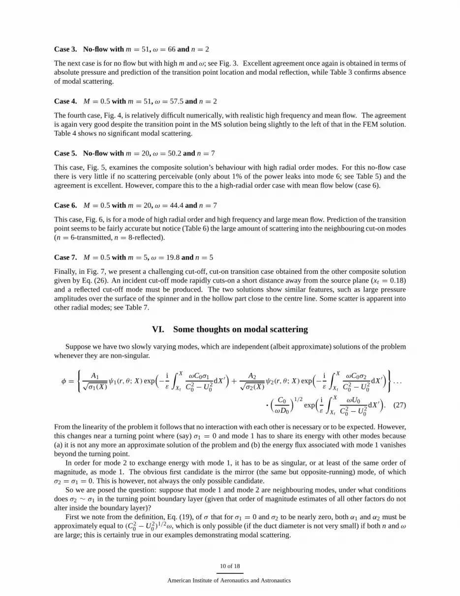
Case 2. M = 0.5 with m = 10, ω = 11 and n = 1
The second case is with low radial moden = 1, relatively lowm andω, but with strong mean flow (Fig. 2). It is basedon a case already attempted by Thiele et al.17 , which provides a further comparison. The inner solution appears tospan the majority (if not all) of the duct. From Table 2 we see that no scattering into neighbouring modes occurs. Theunadjusted MS solution (M = 0.5 andω = 11) is already very similar to the FEM solution, but is slightly receded.We speculate (given the excellent agreement of the no-flow case above and the typical error in the approximate MSmean flow ofO(ε2) which is here a few percent) that this may largelybe explained by the slight mean flow differencesbetween MS and FEM. The MS solution can be ‘tuned’ to achieve a better match, either by adjusting the frequency orthe mean flow. The position of the turning point is highly sensitive; 2− 3% mean flow and< 1% frequency alterationis required. Indeed, Thiele et al. also found for a similar configuration (ω = 11.129) the same features including ahighly sensitive position of the turning point to mean flow variations.
This is easily explained by noting that the position ofXt is determined byσ(Xt ) = 0 with Eqs. (9), (16) and (19),which may be considered as a set of algebraic equations inM, ω andX . This means that
Xt (M +�M, ω +�ω) = Xt (M, ω)+ O(�M)+ O(�ω).
If �M = O(ε2) (which may be expected), the error inXt is alsoO(ε2), and thus the error inxt is O(ε), in otherwords, in the order of 10%, which is indeed what we observe. In the same way it is clear that only a shift ofO(ε2) ineitherM orω should suffice for readjustment.
9 of 18
American Institute of Aeronautics and Astronautics
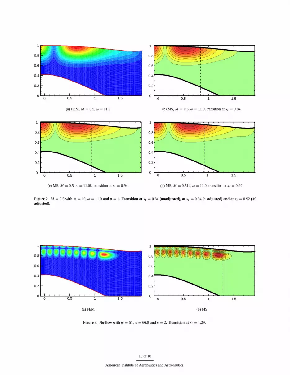
Case 3. No-flow with m = 51, ω = 66 and n = 2
The next case is for no flow but with highm andω; see Fig. 3. Excellent agreement once again is obtained in terms ofabsolute pressure and prediction of the transition point location and modal reflection, while Table 3 confirms absenceof modal scattering.
Case 4. M = 0.5 with m = 51, ω = 57.5 and n = 2
The fourth case, Fig. 4, is relatively difficult numerically, with realistic high frequency and mean flow. The agreementis again very good despite the transition point in the MS solution being slightly to the left of that in the FEM solution.Table 4 shows no significant modal scattering.
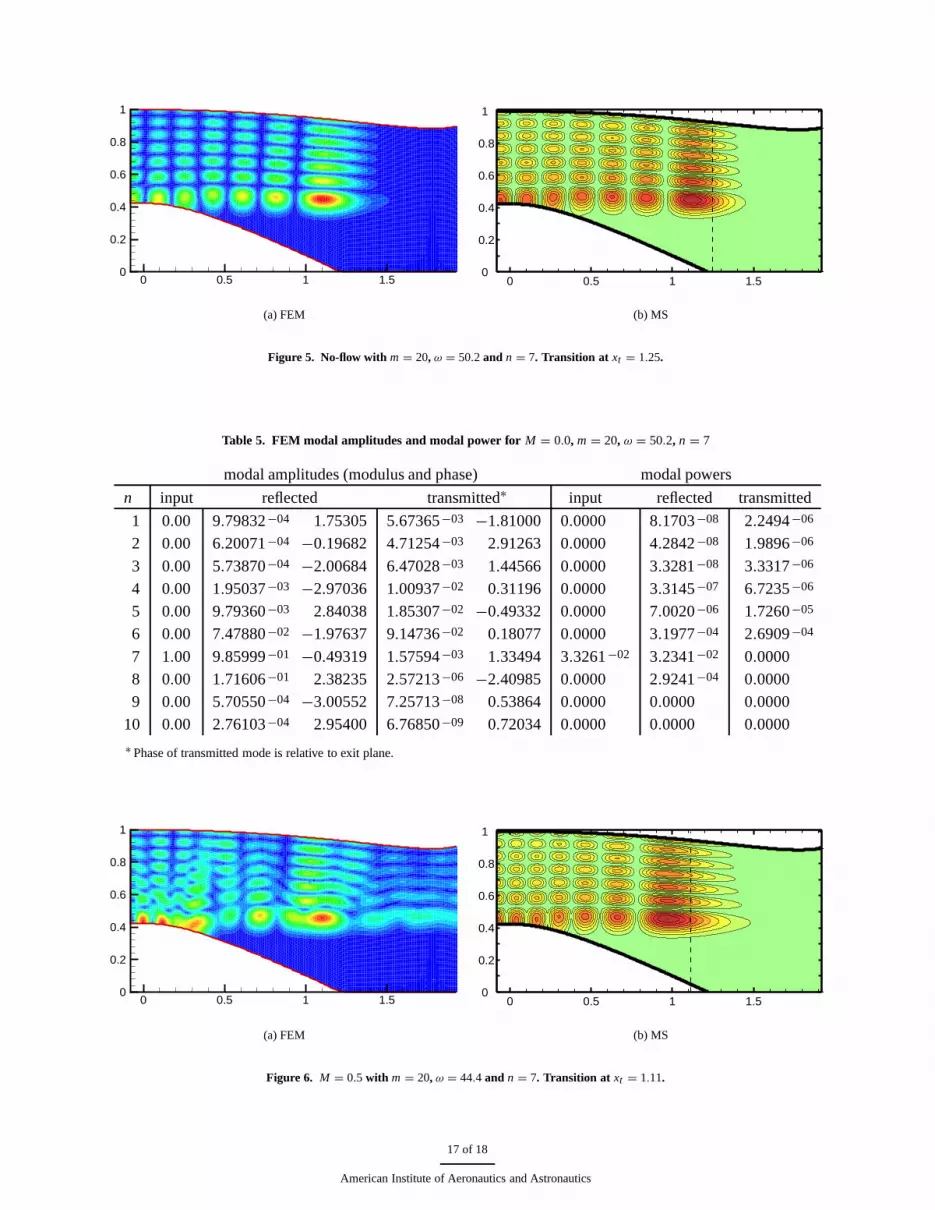
Case 5. No-flow with m = 20, ω = 50.2 and n = 7
This case, Fig. 5, examines the composite solution’s behaviour with high radial order modes. For this no-flow casethere is very little if no scattering perceivable (only about 1% of the power leaks into mode 6; see Table 5) and theagreement is excellent. However, compare this to the a high-radial order case with mean flow below (case 6).
Case 6. M = 0.5 with m = 20, ω = 44.4 and n = 7
This case, Fig. 6, is for a mode of high radial order and high frequency and large mean flow. Prediction of the transitionpoint seems to be fairly accurate but notice (Table 6) the large amount of scattering into the neighbouring cut-on modes(n = 6-transmitted,n = 8-reflected).
Case 7. M = 0.5 with m = 5, ω = 19.8 and n = 5
Finally, in Fig. 7, we present a challenging cut-off, cut-on transition case obtained from the other composite solutiongiven by Eq. (26). An incident cut-off mode rapidly cuts-on a short distance away from the source plane (xt = 0.18)and a reflected cut-off mode must be produced. The two solutions show similar features, such as large pressureamplitudes over the surface of the spinner and in the hollow part close to the centre line. Some scatter is apparent intoother radial modes; see Table 7.
VI. Some thoughts on modal scattering
Suppose we have two slowly varying modes, which are independent (albeit approximate) solutions of the problemwhenever they are non-singular.
φ ={
A1√σ1(X)
ψ1(r, θ; X) exp(− i
ε
∫ X
Xt
ωC0σ1
C20 − U2
0
dX ′)+ A2√σ2(X)
ψ2(r, θ; X) exp(− i
ε
∫ X
Xt
ωC0σ2
C20 − U2
0
dX ′)} . . .·( C0
ωD0
)1/2exp
( i
ε
∫ X
Xt
ωU0
C20 − U2
0
dX ′). (27)
From the linearity of the problem it follows that no interaction with each other is necessary or to be expected. However,this changes near a turning point where (say)σ1 = 0 and mode 1 has to share its energy with other modes because(a) it is not any more an approximate solution of the problem and (b) the energy flux associated with mode 1 vanishesbeyond the turning point.
In order for mode 2 to exchange energy with mode 1, it has to be as singular, or at least of the same order ofmagnitude, as mode 1. The obvious first candidate is the mirror (the same but opposite-running) mode, of whichσ2 = σ1 = 0. This is however, not always the only possible candidate.
So we are posed the question: suppose that mode 1 and mode 2 are neighbouring modes, under what conditionsdoesσ2 ∼ σ1 in the turning point boundary layer (given that order of magnitude estimates of all other factors do notalter inside the boundary layer)?
First we note from the definition, Eq. (19), ofσ that forσ1 = 0 andσ2 to be nearly zero, bothα1 andα2 must beapproximately equal to(C2
0 − U20 )
1/2ω, which is only possible (if the duct diameter is not very small) if bothn andωare large; this is certainly true in our examples demonstrating modal scattering.
10 of 18
American Institute of Aeronautics and Astronautics

From the previous analyses4,6,9 it follows that in the boundary layer,
X = Xt + ε2/3λ−1ξ,
we have
σ 21 (X) = σ 2
1 (Xt + ε2/3λ−1ξ) = −2ε2/3(C0t C ′
0t − U0tU ′0t
C20t − U2
0t
+ α′t
αt
)λ−1ξ + O(ε4/3ξ2),
where subscriptt indicates evaluation atX = Xt andλ is given by
λ3 = 2ω2C20t
(C20t − U2
0t )2
(C0t C ′0t − U0tU ′
0t
C20t − U2
0t
+ α′t
αt
).
In the original analysisλ = O(1) by assumption, but this is not fully satisfied here asω is large. For the question:when isσ2 ∼ σ1, we first note that
1 − σ 21
α21
= 1 − σ 22
α22
,
from which we immediately get
σ 22 = α2
1 − α22
α21
+ α22
α21
σ 21 .
For large order, the difference�α between consecutive eigenvalues tends to a constant, soσ2 is of the same order asσ1 if:
�α
α 1
2σ21 = ε2/3λ2 (C
20 − U2
0 )2
2ω2C20
ξ.
Since normally the termα′/α in λ dominates, we have
�α
α ε2/3
(α′
α
)2/3 (C20 − U2
0 )2/3
(2ω2C20)
1/3ξ.
Asω (C20 − U2
0 )1/2α, this turns into
ω ε−2 2(�α)3C20
(α′/α)2(C20 − U2
0)1/2ξ3
.
For a hollow duct we have for large order18 α = j ′mn/R(X) (n + 1
2m − 34)π/R and so�α = π/R. For an annular
duct of hub-tip ratioh we haveα nπ/(1 − h)R and so�α = π/(1 − h)R. In either case we see that forn andωhigh enough indeed modal scattering may be expected. The order of magnitudeω = O(ε−2) is indeed consistent withourε = 0.1 andω ∼ 50 of the cases in question where scattering was observed.
VII. Conclusions
A theoretical framework has been established for the modelling of the propagation of sound in a non-uniform ductwith mean subsonic compressible flow in the case when the incident mode of propagation encounters a cut-off or cut-on transition. The analysis is based on the assumption that the duct geometry and flow field are slowly varying, leadingto application of the method of multiple scales. Far away from the transition the multiple scales solution consists ofslowly varying duct modes. At the transition they becomesingular, and a local solution is necessary to connect thecut-on and the cut-off parts of the mode. This set of local solutions is impractical, but it has been shown possible toconstruct a composite solution, encompassing the boundarylayer solution in the neighbourhood of the transition pointand the outer slowly varying modal solution far from the transition into a single expression. Such a theoretical modelhas been benchmarked here by comparison with a fully numerical model based on the finite element method.
Cases used for our comparison are varied, with and without mean flow, and over a range of circumferential modes,radial modes and frequencies. Cases include those withas few as one incident propagating mode to as many as eightpropagating modes, and include a particularly interesting case with an incident non-propagating mode (cut-off at thesource) which cuts on close to the source.
11 of 18
American Institute of Aeronautics and Astronautics

Comparisons between multiple scales results and finite element results are presented in the form of contours ofequal pressure magnitude, which for most cases show the standing wave character associated with the analyticallypredicted complete reflection of the incident mode into its mirror image propagating in the opposite direction. Contourplots are supplemented with tables of incident, reflected, and transmitted modal power and reflected and transmittedmodal amplitudes generated by the finiteelement model. The finite element solution always shows some scatteringinto reflected and transmitted modes adjacent to the incidentmodes. This scattering is small in most instances, inaccordance with the assumptions of the multiple scales analysis. In these cases the agreement between FEM and themultiple scales solution is invariably good (with flow) or excellent (without flow). An explanation for this difference,which is consistent with theory, is that the accuracy of the analytical mean flow (O(ε2), typically a few percent) isseen to produce an error ofO(ε), of the order of 10 percent, in the position of the transition.
In some cases, one of which is shown here, the finite element solution shows significant scattering into adjacentmodes, which is not predicted by the multiple scales solution. In our study such an occurrence was limited to cases withmean flow and with many initially propagating modes (eight in the case shown here), with the highest order modeshaving cut-off ratios which cluster near unity. In these cases with scattering, the multiple scales solution capturesthe basic features of the acoustic field, but does not predict the scattering mechanism by which acoustic power leaksthrough the turning point.
The observation of significant scattering in certain cases has led to an extension of the multiple scales analysis byasymptotic scaling arguments in the turning point region. This has identified circumstances under which the presenceof neighbouring modes is necessary and modal interaction is likely to occur.
The challenging case of an incident mode, cut-off at the source, and cutting on close to the source, shows generallygood agreement between the multiple-scales solution and the finite-element solution, with FEM showing evidence ofscattering into adjacent modes. This, however, doesnot seem to be a particular property of this configuration.
Aside from the benchmark comparisons which were the main thrust of the current investigation, calculations ofthe standing wave field associated with cut-off phenomenon revealed high acoustic pressures in the neighbourhood ofthe turning point. This may well have implications for nacelle structural integrity and structure-borne noise.
Appendix
Related to Bessel functions of order13 are the Airy functions18 Ai and Bi, solutions ofy ′′ − xy = 0, with the
following asymptotic behaviour (introduceζ = 23|x |3/2)
Ai(x) cos(ζ − 14π)√
π |x |1/4 (x → −∞), e−ζ
2√π x1/4
(x → ∞), (28a)
Bi(x) cos(ζ + 14π)√
π |x |1/4 (x → −∞), eζ√π x1/4
(x → ∞). (28b)
Acknowledgements
N.C. Ovenden would like to thank UCL Graduate School, the Department of Mathematics at UCL and EindhovenUniversity of Technology for financial support.
S.W. Rienstra’s contribution was partly carried out in the context of the “Messiaen” project of the European Union’s6th Framework and partly under a grant of the Royal Society at the University of Cambridge. The financial support ofboth parties is greatly acknowledged.
We wish to thank Nigel Peake (University of Cambridge) for his stimulating interest and useful suggestions andremarks.
Finally, we wish to thank Frank Thiele and his group at the Technical University of Berlin for their initiating theproblem along with their enthusiasm and interest.
References1A.H. Nayfeh and D.P. Telionis, “Acoustic propagation in ducts of varying cross sections.”Journal of the Acoustical Society of America 54
(1973) 1654–1661.2S.W. Rienstra, “Sound transmission in slowly varying circular and annular lined ducts with flow.”Journal of Fluid Mechanics 380 (1999)
279–296.
12 of 18
American Institute of Aeronautics and Astronautics

3A.J. Cooper and N. Peake, “Propagation of unsteady disturbances in a slowly varying duct with mean swirling flow.”Journal of FluidMechanics 445 (2001) 207–234.
4S.W. Rienstra, “Sound propagation in slowly varying lined flow ducts of arbitrary cross section.”Journal of Fluid Mechanics 495 (2003),157–173.
5S.W. Rienstra and W. Eversman, “A numerical comparison between the multiple-scales and finite-element solution for sound propagation inlined flow ducts.”Journal of Fluid Mechanics 437 (2001) 367–384.
6S.W. Rienstra, “Cut-on cut-off transition of sound in slowly varying flow ducts.”Aerotechnica - Missili e Spazio, special issue in memory ofDavid Crighton. (edited by L. Morino and N. Peake)79, nos. 3–4, (2000) 93–97.
7N.C. Ovenden, “Near cut-on/cut-off transitions in lined ducts with flow.”Paper AIAA 2002-2445 of the 8th AIAA/CEAS Aeroacoustics Con-ference in Breckenridge, CO, 17-19 June (2002).
8A.J. Cooper and N. Peake, “Trapped acoustic modes in aeroengine intakes with swirling flow.”Journal of Fluid Mechanics 419 (2000)151–175.
9N.C. Ovenden, “A composite multiple-scales solution for cut-on cut-off transition in a hard-walled duct with flow.”submitted to Journal ofSound and Vibration (2004).
10I. Danda Roy and W. Eversman, “Improved finite element modeling of the turbofan engine inlet radiation problem.”ASME Journal ofVibration and Acoustics 117 (1995), 109–115.
11M. Van Dyke, “Slow Variations in Continuum Mechanics”, in:Advances in Applied Mechanics 25, 1–45, Academic Press, Orlando (1987)12A.H. Nayfeh,Perturbation Methods. John Wiley Sons Inc., New York (1973)13C.L. Morfey, “Acoustic energy in non-uniform flows.”Journal of Sound and Vibration 14, (1971), 159–170.14I. Danda Roy and W. Eversman, “Far field calculations for turbofan noise.”AIAA Journal 39(12), (2001), 2255–2261.15W. Eversman, “A reverse flow theorem and acoustic reciprocity in compressible potential flow in ducts.”Journal of Sound and Vibration
246(1), (2001), 71–95.16W. Eversman, “Numerical experiments on acoustic reciprocity in compressible potential flows in ducts.”Journal of Sound and Vibration
246(1), (2001), 97–113.17X.D. Li, C. Schemel, U. Michel and F. Thiele, “On theazimuthal mode propagation in axisymmetric duct flows.”Paper 2002-2521 of the
8th AIAA/CEAS Aeroacoustics Conference in Breckenridge, CO, USA, 17-19 June (2002). In revised form, entitled: “On the azimuthal sound modepropagation in axisymmetric flow ducts”, accepted for publication inAIAA-Journal (2004).
18M. Abramowitz and I.A. Stegun,Handbook of Mathematical Functions, National Bureau of Standards, Dover Publications, Inc., New York(1964)
13 of 18
American Institute of Aeronautics and Astronautics

0 0.5 1 1.50
0.2
0.4
0.6
0.8
1
(a) FEM
0 0.5 1 1.50
0.2
0.4
0.6
0.8
1
(b) MS
Figure 1. No-flow with m = 21, ω = 41.0 and n = 4. Transition at xt = 1.49.
Table 1. FEM modal amplitudes and modal power for M = 0.0, m = 21, ω = 41.0, n = 4
modal amplitudes (modulus and phase) modal powers
n input reflected transmitted∗ input reflected transmitted
1 0.00 1.28806−03 −0.16011 4.65308−03 −1.00415 0.0000 1.2609−07 1.3199−06
2 0.00 1.24518−03 −2.07156 7.59902−03 −2.41687 0.0000 1.4446−07 4.1023−06
3 0.00 1.49994−02 1.32924 1.78118−02 −2.74923 0.0000 1.7160−05 1.6330−05
4 1.00 9.98636−01 1.73083 7.33522−02 0.73351 5.2870−02 5.2734−02 9.4760−05
5 0.00 1.30240−02 −1.43072 1.96820−05 −2.72645 0.0000 2.1353−06 0.0000
6 0.00 7.97316−05 0.84398 2.66586−07 0.20589 0.0000 0.0000 0.0000
7 0.00 1.49995−05 1.13319 1.25423−08 −3.04410 0.0000 0.0000 0.0000
∗ Phase of transmitted mode is relative to exit plane.
Table 2. FEM modal amplitudes and modal power for M = 0.5, m = 10, ω = 11.0, n = 1
modal amplitudes (modulus and phase) modal powers
n input reflected transmitted∗ input reflected transmitted
1 1.00 6.83653−01 0.31240 4.95448−02 −1.34561 2.0844−02 2.0844−02 0.0000
2 0.00 8.13841−03 −0.67365 1.58488−04 −2.14545 0.0000 0.0000 0.0000
3 0.00 6.58219−04 2.66479 1.49392−05 0.74636 0.0000 0.0000 0.0000
∗ Phase of transmitted mode is relative to exit plane.
14 of 18
American Institute of Aeronautics and Astronautics
0 0.5 1 1.50
0.2
0.4
0.6
0.8
1
(a) FEM,M = 0.5,ω = 11.0
0 0.5 1 1.50
0.2
0.4
0.6
0.8
1
(b) MS, M = 0.5,ω = 11.0, transition atxt = 0.84.
0 0.5 1 1.50
0.2
0.4
0.6
0.8
1
(c) MS, M = 0.5,ω = 11.08, transition atxt = 0.94.
0 0.5 1 1.50
0.2
0.4
0.6
0.8
1
(d) MS, M = 0.514,ω = 11.0, transition atxt = 0.92.
Figure 2. M = 0.5 with m = 10, ω = 11.0 and n = 1. Transition at xt = 0.84 (unadjusted), at xt = 0.94 (ω adjusted) and at xt = 0.92 (Madjusted).
0 0.5 1 1.50
0.2
0.4
0.6
0.8
1
(a) FEM
0 0.5 1 1.50
0.2
0.4
0.6
0.8
1
(b) MS
Figure 3. No-flow with m = 51, ω = 66.0 and n = 2. Transition at xt = 1.29.
15 of 18
American Institute of Aeronautics and Astronautics

Table 3. FEM modal amplitudes and modal power for M = 0.0, m = 51, ω = 66.0, n = 2
modal amplitudes (modulus and phase) modal powers
n input reflected transmitted∗ input reflected transmitted
1 0.00 6.72025−03 2.25428 7.97928−03 0.58151 0.0000 1.4091−06 1.3114−06
2 1.00 9.99891−01 −3.03406 7.10642−05 0.79078 3.3347−02 3.3344−02 0.0000
3 0.00 9.32808−04 1.64194 6.79870−09 3.04031 0.0000 0.0000 0.0000
4 0.00 8.70045−05 −1.51414 3.34634−09 −1.99459 0.0000 0.0000 0.0000
∗ Phase of transmitted mode is relative to exit plane.
0 0.5 1 1.50
0.2
0.4
0.6
0.8
1
(a) FEM
0 0.5 1 1.50
0.2
0.4
0.6
0.8
1
(b) MS
Figure 4. M = 0.5 with m = 51, ω = 57.5 and n = 2. Transition at xt = 0.9356(unadjusted).
Table 4. FEM modal amplitudes and modal power for M = 0.5, m = 51, ω = 57.5, n = 2
modal amplitudes (modulus and phase) modal powers
n input reflected transmitted∗ input reflected transmitted
1 0.00 4.64375−03 0.25482 2.33365−02 −2.18438 0.0000 7.6128−07 4.3142−06
2 1.00 6.71150−01 1.91208 7.01745−05 −0.88275 1.3573−02 1.3525−02 0.0000
3 0.00 1.54454−01 2.41438 1.53737−06 0.93476 0.0000 4.3465−05 0.0000
4 0.00 3.86885−03 1.23189 2.86459−07 −2.59817 0.0000 0.0000 0.0000
5 0.00 2.47703−04 −1.30422 1.03903−07 −0.08191 0.0000 0.0000 0.0000
∗ Phase of transmitted mode is relative to exit plane.
16 of 18
American Institute of Aeronautics and Astronautics
0 0.5 1 1.50
0.2
0.4
0.6
0.8
1
(a) FEM
0 0.5 1 1.50
0.2
0.4
0.6
0.8
1
(b) MS
Figure 5. No-flow with m = 20, ω = 50.2 and n = 7. Transition at xt = 1.25.
Table 5. FEM modal amplitudes and modal power for M = 0.0, m = 20, ω = 50.2, n = 7
modal amplitudes (modulus and phase) modal powers
n input reflected transmitted∗ input reflected transmitted
1 0.00 9.79832−04 1.75305 5.67365−03 −1.81000 0.0000 8.1703−08 2.2494−06
2 0.00 6.20071−04 −0.19682 4.71254−03 2.91263 0.0000 4.2842−08 1.9896−06
3 0.00 5.73870−04 −2.00684 6.47028−03 1.44566 0.0000 3.3281−08 3.3317−06
4 0.00 1.95037−03 −2.97036 1.00937−02 0.31196 0.0000 3.3145−07 6.7235−06
5 0.00 9.79360−03 2.84038 1.85307−02 −0.49332 0.0000 7.0020−06 1.7260−05
6 0.00 7.47880−02 −1.97637 9.14736−02 0.18077 0.0000 3.1977−04 2.6909−04
7 1.00 9.85999−01 −0.49319 1.57594−03 1.33494 3.3261−02 3.2341−02 0.0000
8 0.00 1.71606−01 2.38235 2.57213−06 −2.40985 0.0000 2.9241−04 0.0000
9 0.00 5.70550−04 −3.00552 7.25713−08 0.53864 0.0000 0.0000 0.0000
10 0.00 2.76103−04 2.95400 6.76850−09 0.72034 0.0000 0.0000 0.0000
∗ Phase of transmitted mode is relative to exit plane.
0 0.5 1 1.50
0.2
0.4
0.6
0.8
1
(a) FEM
0 0.5 1 1.50
0.2
0.4
0.6
0.8
1
(b) MS
Figure 6. M = 0.5 with m = 20, ω = 44.4 and n = 7. Transition at xt = 1.11.
17 of 18
American Institute of Aeronautics and Astronautics
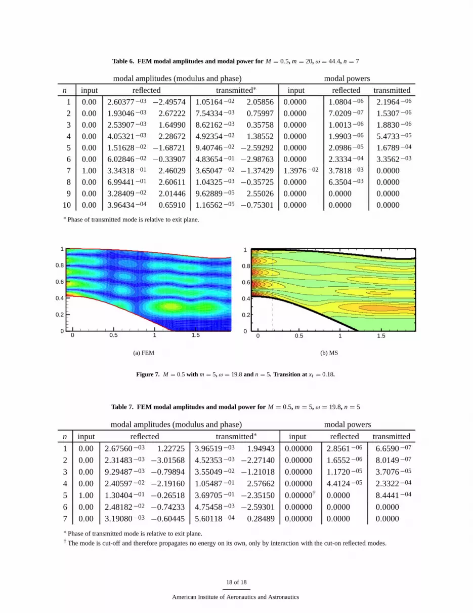
Table 6. FEM modal amplitudes and modal power for M = 0.5, m = 20, ω = 44.4, n = 7
modal amplitudes (modulus and phase) modal powers
n input reflected transmitted∗ input reflected transmitted
1 0.00 2.60377−03 −2.49574 1.05164−02 2.05856 0.0000 1.0804−06 2.1964−06
2 0.00 1.93046−03 2.67222 7.54334−03 0.75997 0.0000 7.0209−07 1.5307−06
3 0.00 2.53907−03 1.64990 8.62162−03 0.35758 0.0000 1.0013−06 1.8830−06
4 0.00 4.05321−03 2.28672 4.92354−02 1.38552 0.0000 1.9903−06 5.4733−05
5 0.00 1.51628−02 −1.68721 9.40746−02 −2.59292 0.0000 2.0986−05 1.6789−04
6 0.00 6.02846−02 −0.33907 4.83654−01 −2.98763 0.0000 2.3334−04 3.3562−03
7 1.00 3.34318−01 2.46029 3.65047−02 −1.37429 1.3976−02 3.7818−03 0.0000
8 0.00 6.99441−01 2.60611 1.04325−03 −0.35725 0.0000 6.3504−03 0.0000
9 0.00 3.28409−02 2.01446 9.62889−05 2.55026 0.0000 0.0000 0.0000
10 0.00 3.96434−04 0.65910 1.16562−05 −0.75301 0.0000 0.0000 0.0000
∗ Phase of transmitted mode is relative to exit plane.
0 0.5 1 1.50
0.2
0.4
0.6
0.8
1
(a) FEM
0 0.5 1 1.50
0.2
0.4
0.6
0.8
1
(b) MS
Figure 7. M = 0.5 with m = 5, ω = 19.8 and n = 5. Transition at xt = 0.18.
Table 7. FEM modal amplitudes and modal power for M = 0.5, m = 5, ω = 19.8, n = 5
modal amplitudes (modulus and phase) modal powers
n input reflected transmitted∗ input reflected transmitted
1 0.00 2.67560−03 1.22725 3.96519−03 1.94943 0.00000 2.8561−06 6.6590−07
2 0.00 2.31483−03 −3.01568 4.52353−03 −2.27140 0.00000 1.6552−06 8.0149−07
3 0.00 9.29487−03 −0.79894 3.55049−02 −1.21018 0.00000 1.1720−05 3.7076−05
4 0.00 2.40597−02 −2.19160 1.05487−01 2.57662 0.00000 4.4124−05 2.3322−04
5 1.00 1.30404−01 −0.26518 3.69705−01 −2.35150 0.00000† 0.0000 8.4441−04
6 0.00 2.48182−02 −0.74233 4.75458−03 −2.59301 0.00000 0.0000 0.0000
7 0.00 3.19080−03 −0.60445 5.60118−04 0.28489 0.00000 0.0000 0.0000
∗ Phase of transmitted mode is relative to exit plane.† The mode is cut-off and therefore propagates no energy onits own, only by interaction with the cut-on reflected modes.
18 of 18
American Institute of Aeronautics and Astronautics