1

INTEGRAL LENGTH SCALES AND TIME SCALES OF TURBULENCE

IN AN OPTICAL SPARK-IGNITION ENGINE

P.G. Aleiferis*

Department of Mechanical Engineering, Imperial College London, UK

M.K. Behringer1 and J.S. Malcolm

2

Department of Mechanical Engineering, University College London, UK

*Author for Correspondence:

Prof. Pavlos Aleiferis

Imperial College London

Department of Mechanical Engineering

Exhibition Road, London SW7 2AZ, UK

Tel: +44-(0)20-75947032

E-mail: p.aleiferis@imperial.ac.uk

1Currently at Micro-Epsilon, Ortenburg, Germany.

2Currently at Ford Motor Company, Dunton, UK.

Full length article accepted for publication by Flow, Turbulence and Combustion.

2

ABSTRACT

In-cylinder air flow structures are known to play a major role in mixture preparation and flame development in

spark-ignition engines. In this paper both LDV and PIV measurements were undertaken in an optical spark-ignition

at 1500 RPM, 0.5 bar inlet plenum pressure. One of the primary PIV planes was vertical, cutting through the

centrally located spark plug (tumble plane) inside the pentroof at ignition timing. The other plane was horizontal

inside the pentroof 1 mm below the spark plug. LDV was conducted 1 mm below the spark plug on a line from

inlet to exhaust but also on a lower line 14 mm below the spark plug. In-cylinder PIV data at specific crank angles

in the intake and compression strokes were also analysed on the central tumble plane and on a horizontal plane 14

mm below the spark plug. The combination of both techniques allowed high spatial and temporal resolution as the

two data sets complemented each other to provide details of mean flow and turbulence characteristics on different

levels, aiming ultimately for quantification of integral time scales and length scales. LDV cycle-resolved analysis

distinguished between the classic approach of using the time integral of the autocorrelation function to obtain the

integral time scale and a high-frequency cut-off analysis to obtain high- and low-frequency fluctuations about an

in-cycle mean.

3

INTRODUCTION

BACKGROUND

Direct Injection Spark Ignition (DISI) engine technology has become commonplace within the automotive industry

as a replacement for port fuel injection engines. This is due to benefits associated with improved efficiency from

charge cooling effects and increased flexibility in mixture formation by a variety of injection strategies. Therefore,

understanding in-cylinder air flow characteristics in DISI engines is of great importance because air flow is

inherently coupled to mixture formation via spray-flow interactions. A variety of velocimetry techniques can be

used to characterise in-cylinder flows. Laser Doppler Velocimetry (LDV) provides highly time-resolved data of the

flow field at fixed points in space, whilst Particle Image Velocimetry (PIV) returns 2D maps of the flow field.

Although early PIV studies of engine flows had highlighted the issue of bias in the statistical analysis of small

batches of engine cycles [1, 2], data storage issues and processing time have forced most researchers to use no

more than 50–200 cycles for their analysis [3–6]. More recently kHz range high-speed PIV has been utilised for

typical 2D flow mapping but also with volume-based characterisation that can be used for validation of Large Eddy

Simulation (LES) of engine flows [7–9]. High-speed PIV allows crank-angle resolved measurements to be

undertaken and has been shown to give insights into the field of cycle-to-cycle flow variability, including spray-

flow and flame-flow interactions [10–16], nevertheless at the expense of data storage requirements, especially if

large numbers of cycles are sought after for statistical analysis. Moreover, for turbulent time scale analysis at

engine speeds of 1500 RPM or higher, imaging frequencies in the tens of kHz are necessary to achieve sub-crank-

angle resolution. This poses further camera and storage challenges when one needs to maintain whole-field spatial

image resolution and over a series of many hundreds of cycles. Therefore, ‘low-speed’ high spatial resolution

cycle-resolved PIV still has its own merits as an experimental tool for in-cylinder flows because it can provide with

relative ease the number of samples needed for faithful statistical analysis of the flow at predefined crank angles of

interest, especially if information on turbulent kinetic energy (TKE) and integral length scales is also aimed for. An

integral length scale represents an average of all turbulent scales in the flow, but with the larger energy containing

eddies governing mainly its magnitude. Data on in-cylinder integral length scales carry great significance in

understanding fundamental phenomena like airflow effects on initial flame kernel wrinkling and the turbulent flame

speeds of various fuels [17, 18], as well as fuel atomisation during high-pressure in-cylinder injection processes

[19], especially under low-load engine operation.

PRESENT CONTRIBUTION

There are very few studies in the literature that have conducted direct comparisons between PIV and LDV data for

an engine at identical operating conditions. More to the point, most of these studies discussed effects on engine-

head test benches at steady-state flow conditions, e.g. see [20–23], and not inside the pentroof and cylinder of a

running optical engine with DISI configuration. Within the objectives of the current paper, cycle-resolved PIV

experiments were undertaken in a pentroof geometry DISI optical engine running at 1500 RPM, low-load

conditions of 0.5 bar inlet plenum pressure. Two planes were primarily considered inside the pentroof: one vertical

‘tumble’ plane passing through the centre of the combustion chamber and one horizontal ‘swirl’ plane 1 mm below

the spark plug’s ground electrodes close to compression Top Dead Centre (TDC), both imaged at ignition timing.

The main aim was to quantify, apart from ‘mean’ velocity and turbulence intensity, maps of integral length scales

of the flow at ignition timing that do not really exist in the literature at such engine operating conditions; most

4

earlier studies on integral length scales in 4-valve engines focused on 600–1200 RPM wide-open-throttle, without

direct pentroof access, e.g. [3, 4]. LDV measurements were also conducted at 1 mm below the spark plug electrode

along a horizontal axis from inlet to exhaust in order to provide time history data of the flow inside the pentroof

and quantify integral time scales. Filtering was also applied to LDV data in an attempt to distinguish between

ensemble-averaging effects and cycle-resolved low- and high-frequency components. Some additional LDV and

PIV measurements were analysed inside the cylinder 14 mm below the spark plug to study the time history and

flow effects on a plane associated typically with spray/flow interactions for injection strategies in the early intake

stroke.

EXPERIMENTAL ARRANGEMENT

OPTICAL ENGINE AND OPERATING PARAMETERS

The optical engine on which the present work was performed was a single-cylinder research engine designed and

built by MAHLE Powertrain Ltd., specifically for optical studies of air flows, fuel sprays and combustion. The

engine head was based on a serial production 4-cylinder 2-litre 16-valve DISI engine. The Bowditch style piston

allowed for a 45° mirror to be positioned inside the extended hollow piston core and give optical access to the

combustion chamber through a titanium piston crown equipped with a sapphire circular window. The cylinder liner

was fully optical and contoured at the top to fit the pent-roof gable ends; it was clamped in place by four hydraulic

rams. Sealing was achieved by the installation of a silicon gasket in a spark-eroded groove on the underside of the

engine head. The piston rings were made of high-temperature-grade Torlon material in order to provide good

sealing and wear resistance in a non-lubricated environment. Figure 1 shows an image of the engine with the fully

optical liner in place (viewed from the timing belt side of the engine) and an image of the combustion chamber as

seen view through the optical piston crown (timing belt side of the engine on the left of this picture, flywheel side

on the right). The intake manifold design consisted of an intake runner of similar diameter and length to that of the

commercial engine. A large volume intake plenum chamber was connected upstream the intake runner to allow

damping of the manifold impulse pressure fluctuations. The cam profiles and valve timings were of ‘standard’ type

with maximum valve overlap of 11 °CA (measured to 0.02 mm lift). The valve timings along with other basic

specifications of the engine are presented in Table 1. All timings given in °CA refer to ‘crank angle time

equivalent’ at 1500 RPM, with one 1 °CA corresponding to 0.111 ms. The load was controlled by throttling to 0.5

bar (0.01 bar) absolute pressure in the intake plenum. The spark plug was of triple ground electrode type with

asymmetric orientation inside the combustion chamber. Under gasoline operation at 1500 RPM, 0.5 bar load, the

Minimum spark advance for Best Torque (MBT) was 26 °CA, hence this timing was selected for the PIV

measurements that were conducted inside the pentroof. More details about the engine and its ancillary systems can

be found in previous publications [24–25].

Due to the need for prolonged engine running, all PIV and LDV measurements were undertaken at motoring

conditions. However, these were set to match nominally as nearly as possible those of previous work published on

this engine by the current authors on direct-injection spray formation and combustion with various fuels [24, 25].

The crank and cam shafts were equipped with shaft encoders resolving 1800 increments per revolution. An

AVL427 engine timing unit was employed for provision of synchronised triggering to Lasers and cameras.

Acquisition of pressure and temperature data was realised by a 12-bit National Instruments (NI) PCI-6023E DAQ

card capable of a sampling rate of 200 kS/s for 16 channels. Pressure sensors with respective amplifiers for in-

5

cylinder pressure, intake plenum pressure, intake runner and exhaust pressure were used, logged and referenced as

needed (Kistler 6041A, 4075A10V39, Kistler 4045A2V39, Kistler 7531, respectively). Their digitisation rate

corresponded to 0.2 °CA at 1500 RPM. Temperatures were recorded on a separate low-speed data acquisition

system which formed part of the dynamometer control system, as were all other engine running parameters.

PARTICLE IMAGE VELOCIMETRY

Test Procedure PIV

Oil droplets with a density of 920 kg/m3 were created by an atomisation seeder and introduced into the engine’s

intake flow on four evenly distributed ports around the intake runner approximately 150 mm upstream the intake

valves. The size of the seeding particles was measured in free flow at atmospheric conditions and these were found

to be about 1–2 µm in diameter. Studying particle-size histograms and considering size changes with increasing

temperatures, calculated particle response times showed that the seeding would respond well to flow frequencies of

the order 0.1–0.2 °CA. The Laser/camera arrangement was based on a Quantel Big Sky ULTRA CFR 120 Nd:YAG

Laser (120 mJ per pulse) and a TSI Powerview Plus 4 MP camera (20482048 pixels). A Nikon 60 mm f/2.8 lens

was used. Two planes were primarily studied inside the pentroof, a horizontal plane (also called ‘swirl’ plane

hereafter) located 1 mm below the spark plug’s ground electrode, or 3 mm above the engine’s fire-face (i.e. 3 mm

above the TDC location of the piston crown’s top land) and another one, vertical centrally located, cutting through

the spark-plug from inlet to exhaust side (also called ‘tumble’ plane hereafter). Following extensive analysis on the

minimum number of cycles required for representative mean and turbulent fluctuations data from PIV data [26, 27],

540 individual cycles were averaged for each experimental test point in batches of 60 cycles per run. It is

recognised though that this was still at the limit and, ideally, more than 1000 cycles should have been acquired. The

practice of batching was based on memory storage capabilities and image quality deterioration by fouling of the

optical access with increased duration of test runs. Due to the maximum imaging speed of the PIV-system, the data

acquisition was at 6.25 Hz, so that every second cycle was recorded at 1500 RPM engine speed.

For the swirl view measurements, the Laser beam was converted to a sheet of about 0.5–1 mm thickness by a

combination of spherical and cylindrical lenses, fired horizontally through the pent-roof of the engine in full optical

setup (quartz liner and sapphire piston window); the camera was positioned in front of the 45° mirror that was

situated within the Bowditch piston arrangement. The arrangement was reversed for the tumble plane

measurements with the Laser firing at the 45° mirror and the camera aligned normal to the optical liner for pent-

roof view access. The lens aperture was set to f/11. The image resolution was 18.4 µm per pixel on the tumble

plane and 34.6 µm per pixel on the swirl plane view. PIV images 10 mm below the fire-face (14 mm below the

spark plug) were also analysed during both intake and compression strokes for comparison with LDV at the same

location. These data were obtained with the same settings to those of the PIV data inside the pentroof but the lens

aperture was set to f/8 and the resolution was higher on the horizontal plane (swirl), namely 23.8 μm, due to focus

closer to the central area of the optical piston bore, and lower on the vertical plane (tumble), namely 38.3 μm, due

to visualising a large portion of the piston’s stroke. Figure 2 shows the location of the two horizontal planes.

Several aspects of the PIV technique, including practical application, precision and uncertainties were optimised

according to [28] and in consultation with seminal publications on the specifics of PIV [29–36] and previously

published PIV studies focused on internal combustion engine measurements [6–9, 37–39]. In this context, Table 2

summarises the system’s main settings and several other details of the PIV measurements presented in this paper,

6

e.g. Laser pulse time separation, interrogation area, density per interrogation window, etc. It is also noted that the

FFT processing algorithms of the PIV system have been tested in-house using the standard images created by

Okamoto et al. [36]. Issues of ‘peak locking’ were eliminated in the current set of measurements by ensuring

settings that led to seeding particles being displayed typically over 2.5–3 pixels. The velocity bias error was

calculated to be 0.06 m/s. Issues related to imaging through curved surfaces were eliminated by keeping the field of

view smaller than about 30 mm in radius around the centre of the bore/pentroof, e.g. see [4, 37]. The average

accumulated uncertainty of the PIV measurements performed was of the order 5–10 %.

Data Processing PIV

Spurious velocity vectors were typically less than 1%, and few cycles with more spurious vectors, usually due to

increased window fowling with ongoing measurement duration, had to be exempted from analysis. The ensemble-

average images for the PIV results presented later have been superimposed over a background image for positional

clarity, showing the spark plug protruding into the combustion chamber in the centre of the tumble plane images

and the outlining of the valve edges clearly visible in the swirl plane images. The ensemble-averaged velocity fields

UEA were obtained over N number of cycles as follows:

𝑈𝐸𝐴(𝜃, 𝑥, 𝑦) =1

𝑁∑ 𝑈(𝜃, 𝑥, 𝑦, 𝑖)𝑁𝑖=1 (1)

where U the instantaneous velocity, i the running cycle number and x, y the spatial co-ordinates, and θ the

measurement crank angle (fixed at 26 °CA BTDC). The required velocity fluctuation for each cycle and spatial

position u(θ,x,y,i) was calculated as the difference between the instantaneous velocity U(θ,x,y,i) and the ensemble-

averaged mean velocity UEA(θ,x,y) over all cycles. The fluctuation intensity u(θ,x,y) was obtained as the standard

deviation at each spatial co-ordinate over the number of cycles N:

𝑢(𝜃, 𝑥, 𝑦, 𝑖) = 𝑈(𝜃, 𝑥, 𝑦, 𝑖) − 𝑈𝐸𝐴(𝜃, 𝑥, 𝑦) (2)

𝑢(, 𝑥, 𝑦) = √1

𝑁−1∑ [𝑢(𝜃, 𝑥, 𝑦, 𝑖)]2𝑁𝑖=1 (3)

LDV measurements along central symmetry lines from the intake to the exhaust side indicated that the flow during

late compression was close to isotropy (i.e. approximately u=v=w), therefore, it was decided that the Turbulent

Kinetic Energy (TKE), k=0.5(u2+v

2+w

2), would be established using the measured RMS of each velocity

component at each point on that plane and estimating the 3rd

velocity component as the arithmetic average of the

other two. This was done because characterisation of k values by 3 velocity components was deemed necessary for

future comparison with 3D engine simulations that are typically based on solving various forms of transport

equations for k. Effects of this approximation are discussed further in the results section.

Cross-correlation coefficients were calculated at each point on the PIV flow fields and integral length scale maps

were produced for all velocity components, Lu, Lv, Lw. In general, the integral length scale Lu is defined as the

integral of the spatial correlation coefficient Rx of the fluctuation velocity u (instantaneous minus mean) at two

adjacent points in space, one at x0 and another one at a distance from x0 as follows (similarly for Lv and Lw):

𝐿𝑥 = ∫ 𝑅𝑥∞

0𝑑𝑥, 𝑅𝑥 =

𝑢(𝑥0,𝑡)𝑢(𝑥0+,𝑡)̅̅ ̅̅ ̅̅ ̅̅ ̅̅ ̅̅ ̅̅ ̅̅ ̅̅ ̅̅ ̅̅ ̅̅ ̅

𝑢(𝑥0,𝑡)𝑢(𝑥0+,𝑡) (4)

The numerical implementation was conducted as follows: The correlation coefficients Rcol,vel1(θ, Δcol, row) for the

horizontal velocity component (vel1) along the image columns of the 2D velocity maps were calculated at each

location, e.g. the correlation coefficient in direction x for velocity u as follows:

7

𝑅𝑥𝑢(𝜃, ∆𝑥, 𝑦) =1

𝑁−1∑ 𝑢(𝜃,𝑥,𝑦,𝑖)𝑢(𝜃,𝑥+∆𝑥,𝑦,𝑖)𝑁𝑖=1

𝑢(𝜃,𝑥,𝑦)𝑢(𝜃,𝑥+∆𝑥,𝑦) (5)

𝐿𝑥𝑢(𝜃, 𝑥, 𝑦) = ∫ 𝑅𝑥𝑢∞

0(𝜃, ∆𝑥, 𝑦)𝑑𝑥 (6)

At each cycle i the calculation was done for each image row and a 2D correlation map was obtained and converted

into the respective length scale map Lcol,vel1(θ, col, row); similarly for the horizontal velocity along rows, i.e.

Rrow,vel1(θ, col, Δrow). Accordingly, the correlation coefficients for the vertical velocity (vel2) along image columns

and rows, i.e. Rcol,vel2(θ, Δcol, row) and Rrow,vel2(θ, col, Δrow), could be obtained. However, only the correlation of

the velocity in its natural direction was considered, i.e. Rxu(θ, Δx, y), Ryv(θ, x, Δy) and Rzw(θ, y, Δz), i.e. the

longitudinal integral length scales were derived for each velocity component. For homogeneous isotropic

turbulence the transversal integral length scales for any velocity component should be half the longitudinal ones.

LASER DOPPLER VELOCIMETRY

Test Procedure LDV

The LDV measurements on air-flow were conducted using a TSI system, based on a 5 W Coherent Innova 70C-5

Series Ar+ Laser. A TSI Fiberlight Multicolor Beam Separator split the single multi-mode Laser beam into three

components with wavelengths of 514.5 nm, 488 nm and 476.5 nm, each of which was divided into two coherent

beam pairs with identical polarity. A Bragg cell shifted one beam of each pair by 40 MHz to enable the

measurement of flow reversals. The beams were coupled into a fibre-optic cable that connected the beam separator

and the transmitter probe (TM250-TLN05-250). Only the 514.5 nm and 488 beams were used though, the former

for the vertical velocity component and the latter for the horizontal velocity components, as will be explained in

more detail in the next section. The frequency shifting of the Bragg cell caused the fringes to move to create a

frequency signal at the receiver, even when seed particles were motionless. Flow in positive and negative direction

could be measured as long as the fringes moved faster than the seeding particles. The receiving probe (RV70)

collected the scattered light and fed it into the Photo Detecting Module (PDM 1000-2C). A Multi-bit Digital Burst

Correlator (FSA 4000–2P), which was synchronised and reset with engine TDC, was used to derive the signal

frequency. The velocity of a seeding particle crossing the measurement volume could thus be obtained by

multiplying the frequency signal of the scattered light with the related fringe spacing. Table 3 summarises the main

parameters of the system.

Several aspects of the technique, including practical application, precision and uncertainties were optimised

according to [40, 41] and in consultation with seminal studies on the specifics of LDV [42–45] and its application

on internal combustion engines [46–55]. The main sources of uncertainty in LDV measurements are velocity bias,

velocity broadening, and statistical uncertainty. Velocity bias can occur in heavily seeded flows due to the positive

correlation between particle arrival rate and convection velocity in the fluid where a larger number of high velocity

particles are recorded with respect to slower ones over the measured time. Several correction methods have been

proposed, e.g. [42, 43] and it has been concluded that 2% and 5% uncertainties arise in mean and RMS velocities

for turbulence levels similar to the present experiments [46]. Gate time weighting was used to account for velocity

bias in the current set of data. This was not found to have any significant effect over a range of crank angles.

Velocity broadening effects occur when the dimensions of the optical control volume are comparable to flow scales

over which changes in mean velocity arise [45]. The error is present even in stationary laminar flows and this

uncertainty increases where regions of high velocity gradients are present. Typical way to overcome this error

8

source is to reduce the effective length of the control volume by using a spatial filter slit in front of the

photomultipliers. A 150 m slit was used for the current set of experiments. In the case of unsteady flows and

ensemble averaged results, velocity broadening also occurs in the time domain and depends on the averaging time

window. For the case of engine flows the maximum uncertainty in velocity broadening can be about 3% and 10%

in mean and RMS velocities, respectively [47]. Regarding statistical analysis, following the work of [44] and

assuming a Gaussian velocity distribution, uncertainty errors based on the sample size for the LDV measurements

(typically in excess of 5000 samples per crank angle per measurement position) were less than 2% in the mean and

5% in the RMS velocities. Other factors can also influence the uncertainty of LDV measurements but are typically

negligible. These include the accuracy of the frequency counter, stability of the frequency shift and the position of

the measurement volume, with the sum of those being less than 1%.

Measurement Setup LDV

Defining the axes system inside the engine, the x-axis was selected to be the vertical axis with the origin at the

engine’s fire-face and positive in downwards direction from the fire-face towards the engine’s bottom end. The

origin of the horizontal y and z axis was located at the centre of the bore. The y-axis was defined positive in the

direction from exhaust to intake side, while the z-axis from the engine’s ‘control’ side (timing belt side) to the

flywheel side. The definition of all in-cylinder coordinates/axes is shown in Figure 2. The velocities in x, y and z

direction (u, v and w velocities, respectively) were measured at two vertical positions 10 mm below and 3 mm

above the fire-face, i.e. at x=10 mm and x=-3 mm. The x=-3 mm location corresponded to 1 mm below the spark

plug and the x=10 mm location to 14 mm below the spark plug where PIV measurements were also obtained.

Measurement locations on the x=10 mm plane along the y- and z-direction were at 0 mm, 2 mm from the centre

and further in steps of 4 mm with respect to the previous position until reaching the liner walls. Similar spacing was

selected for the measurements on the x=-3 mm plane, but measurements were only taken until 20 mm from the

centre of the cylinder due to the confined pentroof space.

The transmitter and receiver probes were mounted on two translation stages that allowed movement perpendicular

to the engine liner axis, focusing the Laser beams through the liner walls. Careful positioning calculations were

required to account for refraction effects of the Laser beams on the quartz liner walls. The difference in curvature

that the horizontal beams experience due to their distance to each other when reaching the liner wall caused

different measurement positions between horizontal and vertical beams. This meant that the positioning of the

transmitter would have to be different for horizontal and vertical velocity measurements as the respective beam

crossing points were not identical. While it would have been possible to overcome this by beam steering using

alignment prisms inside the transmitter or other methods using external optics, this would have to be done at each

measurement location that proved impractical. It was therefore chosen to measure horizontal and vertical velocities

individually at the cost of information that could be obtained from their simultaneous measurement, such as

calculation of Reynolds stresses. Effects of ray refraction on cylindrical surfaces were calculated using geometrical

optics based on Snell’s law [56–58]. The angular error of the horizontal measurements, which indicates the

deviation of the fringes to the measurement direction, was calculated to be approximately 2° for positions from the

centre between -24 mm and +24 mm. The calculated positioning results were verified and adjusted at various in-

cylinder positions using positioning markers. The relative positioning accuracy between neighbouring locations

was estimated to be better than ±0.1 mm.

9

For u and v components (x- and y-directions, respectively), the transmitter fired the Laser beams through the liner

on the side of the pentroof window. Once the correct transmitter beam crossing position was established, the

receiver position had to be adjusted. The LDV receiver was positioned for forward scattering mode on the exhaust

side of the engine in the flywheel side quadrant. Whenever possible, the transmitter-receiver angle was 30° off-axis

but geometrical constraints such as the hydraulic pillars of the liner clamping mechanism did not always allow for

this setup to be fixed so that the angle was varied between 20°–70°. The angular position was however not as

critical for LDV as it would have been for phase Doppler droplet sizing and it was therefore selected for best

optical access according to in-cylinder location of the probe volume. The measurement of w (z-direction velocity

component) on the layer 1 mm below the spark plug ground electrode required up to ∼5° vertical tilting of the

receiver and transmitter (placed on the intake and exhaust side, respectively) to fire the Laser beams at a slight

upwards angle into the pent-roof past the edge of the engine head (the tilt was then accounted for in the calculation

of w).

The Laser power was set to 1.5 W, resulting in individual beam power of ~150 mW (514.5 nm) for u and ~110 mW

(488 nm) for v and w measurements. As the velocities during intake stroke were much higher than those in the

compression stroke, a wide band-pass filter range of 2–20 MHz was used to cover the engine cycle. The down-mix

frequency was set between 30–36 MHz to ensure all velocities were within the measurement range after

compensation for the brag cell’s frequency shift. Photomultiplier tube (PMT) voltages (typically 400–500 V), burst

thresholds (typically 50–120 V) and the signal-to-noise ratio of the burst detection were adjusted depending on the

measurement location for best data rate.

Approximately 60 s of motoring were allowed for flow stabilisation prior to acquisition of measurements.

Velocities of at least 1200 cycles were obtained for each measurement location and direction. The time stamps of

the LDV signal bursts were obtained relative to a TDC marker created by the AVL427 engine timing unit. LDV

showed high sensitivity with respect to the positioning accuracy of the transmitter and receiver. Maximum LDV

sampling frequencies for ideal system setup of the Laser and data acquisition system were beyond 40 kHz

(equivalent to 0.22 CA at 1500 RPM) and were considered sufficient in comparison to particle response time for

the ensemble-average analysis and also for investigations regarding turbulent time scales. Typical data rates were

between 20–40 kHz but cycles were accepted during post processing, if the average data rate was above 9 kHz, i.e.

one measurement per crank angle.

Data Processing LDV – Ensemble Averaged Analysis

The quasi continuous velocity signal of 1200 cycles including the respective time stamp was exported and split into

individual cycles. The cyclic velocity data was then sorted into bins of 0.5 °CA and the binned data were further

processed to create ensemble-averaged velocity traces over all cycles. The averaging analysis of quasi-periodic

flows splits the value of the instantaneous velocity U at crank angle θ of cycle i, U(θ, i), into an ensemble averaged

mean value UEA(θ) and a fluctuating component u(θ). For conventional ensemble averaging, the mean velocity at θ

was derived by averaging the instantaneous velocities of all cycles (N) at that required θ (i.e. phase averaging):

𝑈𝐸𝐴() =1

𝑁∑ 𝑈(, 𝑖)𝑁𝑖=1 (7)

𝑢() = √1

𝑁−1∑ [𝑈(, 𝑖) − 𝑈𝐸𝐴()]

2𝑁𝑖=1 (8)

More elaborate cycle-resolved processing procedures will be introduced in the relevant LDV results section.

10

RESULTS AND DISCUSSION

Instantaneous Flow Field at Ignition Timing

The images in Figure 3 show raw flow field images of a single cycle at 26 °CA BTDC on the swirl and tumble

planes. The reader may refer to Figure 2 for axes definition. No distinct general flow directionality could be seen

on the swirl plane except along the main tumble plane y-axis from intake to exhaust. Vortex structures with

diameters 5–10 mm were typically present all over the swirl plane, distributed evenly throughout. The tumble plane

view however reveals a strong flow directionality from intake (left) to exhaust (right), showing velocities typically

of the order of 5–8 m/s, higher on the left of the spark plug (black shadow area in the centre). Between spark plug

ground electrode and piston top, medium scale vortex structures were visible in many images, typically of the order

3–5 mm in diameter but occasionally up to 8 mm. Some spurious velocity vectors could be seen close to the spark

plug electrode (and retained in this figure), stemming from reflections of the Laser sheet hitting metal surfaces. To

the right of the spark plug, the flow velocity was reduced and several small vortices and eddies were visible, before

the velocities increase and directionality strengthens again towards the right extremity of the image on the exhaust

side. All images showed very similar structures with natural variations in the size and position of vortices for

different cycles.

PIV Flow Field and TKE at Ignition Timing

The ensemble averaged flow and TKE fields at 26 °CA BTDC are shown in Figure 4 for the tumble and in Figure

5 for the swirl view (both based on 540 cycles). With respect to axes definition in Figure 2, the zero value on the x-

axis of the tumble view indicates the location of the engine’s fire-face with the piston top land being at

approximately x=6 mm at the time of measurement. Maximum velocity values of up to 5 m/s were present towards

the intake side (top left corner of the images in Figure 4), where the bulk tumble flow came into the image area

from the engine squish area and intake pentroof while the large-scale flow ‘propagated’ towards the exhaust side.

Successively, the flow was forced against and around the spark plug. In the wake of the spark plug the velocities

were strongly reduced to levels of 1–1.5 m/s, still predominantly in the direction of the exhaust port, with a

recirculation zone towards the top right edge of the spark plug. None of the vortex structures that could be seen in

the instantaneous images were present in the ensemble averaged field, being evidence of their ‘randomness’ and

turbulent nature of the flow. The flow field just above the piston top showed upwards directed velocities, most

probably driven directly by the motion of the piston.

The swirl view velocities are consistent with the general velocity structure on the tumble plane: high velocities on

the intake side and low velocities past the spark plug. The mean flow showed two counter rotating vortices with

their centres below the intake valves. The mean velocities along the y-axis in the centre of the bore (i.e. the axis

through which the tumble plane was measured) was the nominal engine geometrical symmetry line between the

two large scale-vortices. The w-velocity component (z-direction) was very small (close to zero) in comparison to

the dominant flow direction from intake to exhaust, i.e. in agreement with the expected behavior across a symmetry

plane.

The TKE on the tumble plane was typically between 10–16 m2/s

2. Increased levels of TKE featured in the area

below the spark plug electrode and towards the exhaust side of the combustion chamber. Similar levels of TKE

were obtained on the swirl plane, with largest values in the negative z-direction. When looking along the y-axis

where the tumble view was obtained, TKE values between 8–13 m2/s

2 were obtained. The lower values compared

11

to the tumble view are believed to be a result of the estimation of the 3rd

velocity fluctuation component which was

taken as the average between the two other velocity fluctuation. LDV showed that w was of the same order but

generally slightly lower than the average between u and v, what effectively corresponded to an overestimation of

the TKE by about 20% on the tumble plane, which also highlights the degree of isotropy. The TKE derived from

the ensemble averaged LDV measurements showed similar values of 9–16 m2/s

2, with highest TKE in the negative

y and z direction. This comparison will be discussed further later.

Ensemble Averaged LDV Flow Field at x=-3 mm

To provide a time frame to the in-cylinder flow, Figure 6 shows the ensemble average velocity components in the

vertical (x) and horizontal (y) directions, u and v, respectively, and their RMS fluctuations u and v from intake

TDC to compression TDC. These were measured at the centre of the bore 3 mm above the fire-face (1 mm below

spark plug), i.e. at position x=-3 mm, y=0 mm, z=0 mm. The w-velocity component is not shown at this stage

because measurements on the symmetry line of the engine resulted in mean w velocities close to zero. The RMS

velocity fluctuation has also been included as error bars (in red) on the mean velocity traces of u and v for even

better clarity. Despite mean w being close to zero, w was generally of the same order to u and v as will be

discussed in more detail later. Compression TDC and the timing of IVC has both been indicated in Figure 6. It is

noted here that the crank angles in this figure and subsequent graphs are all shown with respect to TDC

compression and labelled as negative °CA After TDC (ATDC) compression, being equivalent to positive °CA

Before TDC (BTDC) compression.

During the intake stroke from 360 °CA BTDC to 180 °CA BTDC (i.e. -360 °CA ATDC to -180 °CA ATDC), the

vertical velocity (u) was positive and the incoming flow followed the direction of the piston’s motion. The

measured intake peak velocity was 53 m/s at 320 °CA BTDC and was followed by a plateau at ~27 m/s around the

nominal start of injection at 300 °CA BTDC. Successively, low-frequency velocity fluctuations were seen on the

mean velocity trace that followed a shape similar to the pressure oscillations measured in the intake runner, until

the flow approached zero around intake BDC. Dynamic charging effects may therefore be considered small, as

expected at such low engine speed. After BDC, the flow direction at this central location just below the spark plug

remained mainly positive (i.e. downwards) until TDC compression (0 °CA BTDC), with low magnitudes up to 3

m/s, despite the upwards moving piston. This indicated the persistence of a clockwise tumble motion with reference

to the engine schematic with the x-y axes definition in Figure 2. By the late stage of compression in the region of

typical ignition timings (40 °CA to 20 °CA BTDC), the vertical velocity component was near zero, as can be seen

more clearly in the PIV flow field of Figure 4.

The horizontal velocity component (v) on the tumble plane featured a flow pattern predominantly directed towards

the exhaust valves during intake. This was driven by the incoming air flowing over the top of the intake valves and

will be seen more clearly in the PIV images during intake presented in the next section vertically and on the x=10

mm plane. The direction was clearly reverse only during the very early intake stroke just after valve overlap, when

the in-cylinder pressure gradually equalised between the exhaust and intake runner, causing outward flow from

exhaust to intake. Slightly positive values were also found around BDC. The RMS velocity values u and v were

7–10 m/s at the timing of injection (300 °CA BTDC) and 2–3 m/s at ignition timing (26 °CA BTDC). Approaching

12

TDC compression, the predominant flow direction was from the intake side towards the exhaust with magnitudes

of up to 5–7 m/s, as also characterized by PIV.

Velocity maps including all measurement locations on the x=-3 mm layer are presented in Figures 7–8.

Specifically, the graphs show the ensemble averaged velocities u, v and w as well as their fluctuation components

u, v and w, at positions between -16 to +16 mm from the centre of the cylinder versus °CA ATDC compression

along the y and z axes. Intake and compression TDC, BDC and IVC, as well as the intake and exhaust side, have all

been indicated on the first graph of the figure matrix for clarity. A signal interruption is visible between 320 to 200

°CA BTDC (-320 to -200 °CA ATDC on the graph axis), caused by the opening intake valves travelling through

the Laser beams at positive y directions when the transmitter was firing through the pentroof window. The signal

drop out due to inlet valve clipping affected the w component as the transmitter location for w measurements was

on the exhaust side of the engine and the receiver on the intake side. The protruding valves covered the visual

access of the measurement location from 320 to 160 °CA BTDC, with the exception of the valve gap. Another

dropout occurred for the w measurements along the y-axis towards maximum y positions at late crank angles 5 to 0

°CA BTDC (top right greyed corner in the charts), caused by the measurement arrangement as the transmitter was

firing through the narrow gap between the piston at TDC and the engine head. The u and v components were not

affected as the transmitter and receiver were located on the timing belt side and exhaust/flywheel quadrant of the

engine bore, respectively. The relevant affected sections in the graphs have been greyed out. The greyed out

regions for u and v differ due to the different path of the Laser beams.

The maximum measured velocities were present during the early and middle part of the intake stroke and of the

order of ~50 m/s in the vertical direction (x), while the horizontal components were ≤20 m/s in y and 10 m/s in z

direction. The low-frequency fluctuations seen during the intake stroke at the single measurement position of

Figure 6 were present for all measurements along the y-axis. These were also present on the x=10 mm layer and

can be seen more clearly in the line graphs of the next section. The high velocities reduced significantly to values

of 5 m/s when the piston approached intake BDC. The velocities close to TDC compression were low throughout,

even close to zero for u and w, while a v-velocity of -2 to -8 m/s was seen directed towards the exhaust valves. The

strongest fluctuations also occurred during the early intake stroke, showing maximum magnitudes of ~20 m/s for

u, v and w. The w fluctuations along the y axis were high and of the same order to u and v despite the mean w

velocities being generally very low across this axis of nominal symmetry dissecting each valve pair. The PIV data

on the same measurement plane also highlighted this. The fluctuations remained very consistent throughout the

compression stroke, being typically 3–5 m/s around the MBT ignition timing of 26 °CA BTDC. At TDC, the

fluctuations had dropped to values between 2–3 m/s.

Figure 8 shows that velocity magnitudes on the z-axis were similar to those along the y-axis. High vertical and

horizontal velocity components u and v were quantified in the gap between the two inlet valves. Measurement

positions further away from the centre lay in the valves’ shadows, resulting in low velocities. Here, re-circulations

were visible with directions opposite to the main intake air stream which was generally downwards and towards the

cylinder’s exhaust side (this can be identified more clearly in the PIV images on the x=10 mm plane shown later).

The velocity fluctuations on the z-axis were again similar to those found along the y-axis, and settled at values

between 3–5 m/s during compression, whilst intake stroke fluctuations were as high as 20 m/s.

13

Focusing solely on the flow field in late compression in Figures 9–10, the predominant flow along the y-axis was

horizontal from intake to exhaust (strong negative v-velocity component). At 26 °CA BTDC, v-velocities were -6 to

-8 m/s with lowest values towards the exhaust side. Fluctuations v were in the region of 3 m/s, larger on the

exhaust side. The w-component along the symmetry axis showed fluctuations up to 3 m/s. Vertical velocities u

were very low, between ±1.5 m/s, with fluctuations u lower than 3 m/s. TKE levels, using all u, v, w components

in k0.5(u2+v

2+w

2), were about 15 m

2/s

2, hence an equivalent mean turbulence intensity defined as [(2/3)k]

1/2 was

about 3.2 m/s. Maps of TKE and turbulence intensity along the y-axis are shown in the left graphs of Figure 11 for

the compression stroke. The intake stroke is not shown, but largest TKE values of up to 350 m2/s

2 were found

around 280 °CA BTDC, reducing successively to levels of 100–150 m2/s

2 just before BDC. Lowest TKE values

were typically in the range 8–12 m2/s

2 and found around the time of IVC. In general, the turbulence intensity did

not agree with the usual estimation of turbulence intensity being close to half the mean piston speed [59], the latter

being 4.25 m/s, but it was of similar magnitude. This ‘overestimation’ of turbulence intensity may be related to the

fact that most earlier measurements in the literature were done at higher engine load conditions than 0.5 bar

(typically wide-open-throttle, 1 bar), or it may also be associated with the inclusion of low-frequency cyclic

variability within the conventional ensemble averaging framework of analysis. As will be shown later, by using the

high-frequency fluctuations only, the turbulence intensity was below half the mean piston speed even at the low-

load conditions of the present study.

When moving along the z-axis at 26 °CA BTDC in Figure 10, it is observed that the values shown are similar to

those along the y-axis. The v-velocities were between 0–5 m/s towards the exhaust, with largest values in the region

of the cylinder’s centre and reducing further away along the z-axis. The w-component had values of ±3 m/s,

linearly increasing from the negative to the positive z direction (timing belt to flywheel side of the engine), so that

both horizontal components were evidence of the two counter rotating swirling vortices with their centre below the

intake valves (shown more distinctly earlier by PIV). Horizontal fluctuations were around 3.2 m/s for v and 3 m/s

for w. The vertical velocities u were between 0–2 m/s with fluctuations u of 2.5 m/s, so that an average TKE of

~13 m2/s

2 and turbulence intensity of ~3 m/s can be seen in the right graphs of Figure 11. The z-axis graphs show

highest TKE towards the extremities of the measurement region (at 12–16 mm), slightly higher in the negative z-

axis side of the engine. The velocity fluctuations were of the same order of magnitude for all components along

both axes, suggesting that the highly anisotropic flow during the intake stroke had developed to conditions not too

far from isotropy along the studied in-cylinder axes during compression.

Ensemble Averaged PIV and LDV Flow Field at x=10 mm

The measurement layer at x=10 mm (14 mm below the spark plug) provides further insight into the in-cylinder flow

development during the intake stroke and early compression. It is also of direct significance to the origin of the

mixture formation process because the fuel spray as a whole crosses this horizontal plane for injection strategies in

the intake stroke, i.e. typical of ‘homogeneous’ engine operation. Therefore, the incoming air-flow characteristics

in this region can be coupled directly with the spray droplet behaviour during injection on a cycle-by-cycle basis

via two-way interactions and momentum exchange. Figure 12 shows PIV data on this plane at various crank angles

during intake and compression. To assist the reader, Figure 12 also shows the central vertical plane flow behaviour

at the same crank angles. Then Figures 13–14 show maps of u, v and w (left) and their RMS fluctuations (right)

14

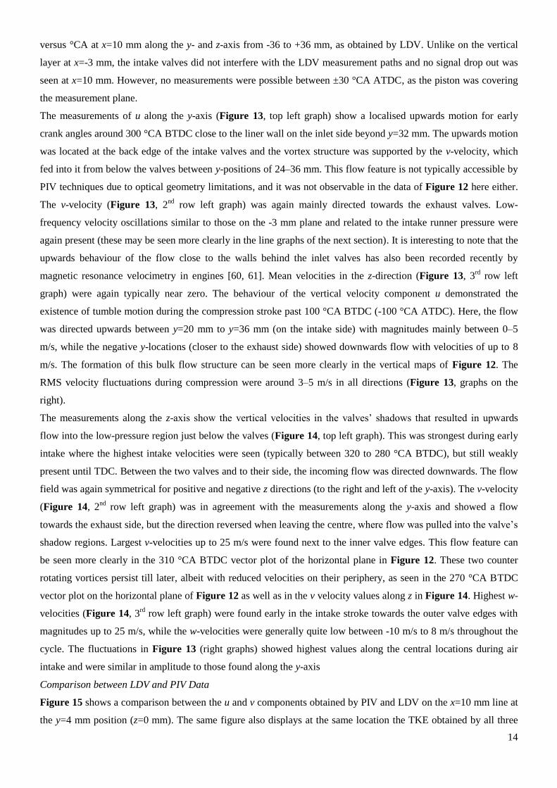
versus °CA at x=10 mm along the y- and z-axis from -36 to +36 mm, as obtained by LDV. Unlike on the vertical

layer at x=-3 mm, the intake valves did not interfere with the LDV measurement paths and no signal drop out was

seen at x=10 mm. However, no measurements were possible between ±30 °CA ATDC, as the piston was covering

the measurement plane.

The measurements of u along the y-axis (Figure 13, top left graph) show a localised upwards motion for early

crank angles around 300 °CA BTDC close to the liner wall on the inlet side beyond y=32 mm. The upwards motion

was located at the back edge of the intake valves and the vortex structure was supported by the v-velocity, which

fed into it from below the valves between y-positions of 24–36 mm. This flow feature is not typically accessible by

PIV techniques due to optical geometry limitations, and it was not observable in the data of Figure 12 here either.

The v-velocity (Figure 13, 2nd

row left graph) was again mainly directed towards the exhaust valves. Low-

frequency velocity oscillations similar to those on the -3 mm plane and related to the intake runner pressure were

again present (these may be seen more clearly in the line graphs of the next section). It is interesting to note that the

upwards behaviour of the flow close to the walls behind the inlet valves has also been recorded recently by

magnetic resonance velocimetry in engines [60, 61]. Mean velocities in the z-direction (Figure 13, 3rd

row left

graph) were again typically near zero. The behaviour of the vertical velocity component u demonstrated the

existence of tumble motion during the compression stroke past 100 °CA BTDC (-100 °CA ATDC). Here, the flow

was directed upwards between y=20 mm to y=36 mm (on the intake side) with magnitudes mainly between 0–5

m/s, while the negative y-locations (closer to the exhaust side) showed downwards flow with velocities of up to 8

m/s. The formation of this bulk flow structure can be seen more clearly in the vertical maps of Figure 12. The

RMS velocity fluctuations during compression were around 3–5 m/s in all directions (Figure 13, graphs on the

right).

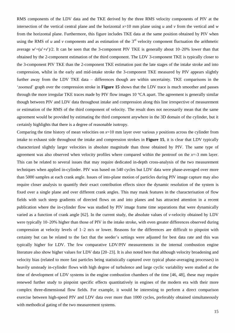
The measurements along the z-axis show the vertical velocities in the valves’ shadows that resulted in upwards

flow into the low-pressure region just below the valves (Figure 14, top left graph). This was strongest during early

intake where the highest intake velocities were seen (typically between 320 to 280 °CA BTDC), but still weakly

present until TDC. Between the two valves and to their side, the incoming flow was directed downwards. The flow

field was again symmetrical for positive and negative z directions (to the right and left of the y-axis). The v-velocity

(Figure 14, 2nd

row left graph) was in agreement with the measurements along the y-axis and showed a flow

towards the exhaust side, but the direction reversed when leaving the centre, where flow was pulled into the valve’s

shadow regions. Largest v-velocities up to 25 m/s were found next to the inner valve edges. This flow feature can

be seen more clearly in the 310 °CA BTDC vector plot of the horizontal plane in Figure 12. These two counter

rotating vortices persist till later, albeit with reduced velocities on their periphery, as seen in the 270 °CA BTDC

vector plot on the horizontal plane of Figure 12 as well as in the v velocity values along z in Figure 14. Highest w-

velocities (Figure 14, 3rd

row left graph) were found early in the intake stroke towards the outer valve edges with

magnitudes up to 25 m/s, while the w-velocities were generally quite low between -10 m/s to 8 m/s throughout the

cycle. The fluctuations in Figure 13 (right graphs) showed highest values along the central locations during air

intake and were similar in amplitude to those found along the y-axis

Comparison between LDV and PIV Data

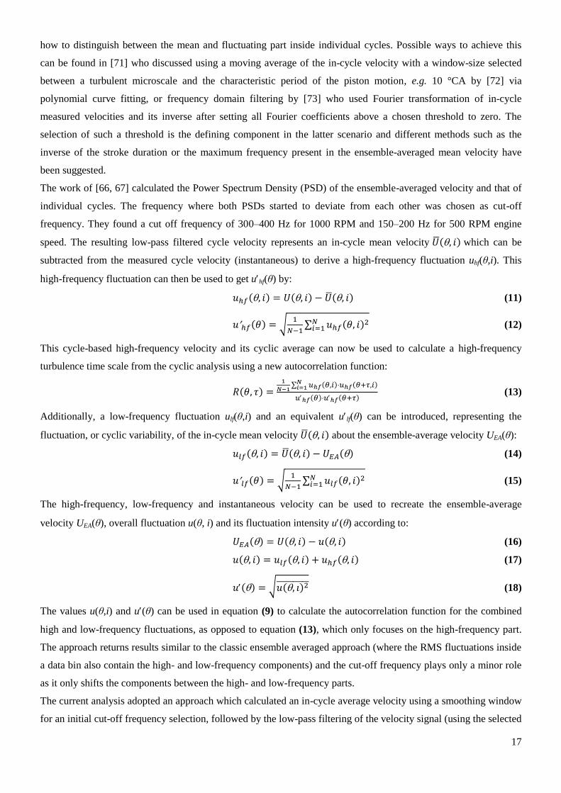
Figure 15 shows a comparison between the u and v components obtained by PIV and LDV on the x=10 mm line at

the y=4 mm position (z=0 mm). The same figure also displays at the same location the TKE obtained by all three

15

RMS components of the LDV data and the TKE derived by the three RMS velocity components of PIV at the

intersection of the vertical central plane and the horizontal x=10 mm plane using u and v from the vertical and w

from the horizontal plane. Furthermore, this figure includes TKE data at the same position obtained by PIV when

using the RMS of u and v components and as estimation of the 3rd

velocity component fluctuation the arithmetic

average w=(u+v)/2. It can be seen that the 3-component PIV TKE is generally about 10–20% lower than that

obtained by the 2-component estimation of the third component. The LDV 3-component TKE is typically closer to

the 3-component PIV TKE than the 2-component TKE estimation past the late stages of the intake stroke and into

compression, whilst in the early and mid-intake stroke the 3-component TKE measured by PIV appears slightly

further away from the LDV TKE data – differences though are within uncertainty. TKE comparisons in the

‘zoomed’ graph over the compression stroke in Figure 15 shows that the LDV trace is much smoother and passes

through the more irregular TKE traces made by PIV flow images 10 °CA apart. The agreement is generally similar

though between PIV and LDV data throughout intake and compression along this line irrespective of measurement

or estimation of the RMS of the third component of velocity. The result does not necessarily mean that the same

agreement would be provided by estimating the third component anywhere in the 3D domain of the cylinder, but it

certainly highlights that there is a degree of reasonable isotropy.

Comparing the time history of mean velocities on x=10 mm layer over various y positions across the cylinder from

intake to exhaust side throughout the intake and compression strokes in Figure 15, it is clear that LDV typically

characterized slightly larger velocities in absolute magnitude than those obtained by PIV. The same type of

agreement was also observed when velocity profiles where compared within the pentroof on the x=-3 mm layer.

This can be related to several issues that may require dedicated in-depth cross-analysis of the two measurement

techniques when applied in-cylinder. PIV was based on 540 cycles but LDV data were phase-averaged over more

than 5000 samples at each crank angle. Issues of into-plane motion of particles during PIV image capture may also

require closer analysis to quantify their exact contribution effects since the dynamic resolution of the system is

fixed over a single plane and over different crank angles. This may mask features in the characterisation of flow

fields with such steep gradients of directed flows on and into planes and has attracted attention in a recent

publication where the in-cylinder flow was studied by PIV image frame time separations that were dynamically

varied as a function of crank angle [62]. In the current study, the absolute values of v-velocity obtained by LDV

were typically 10–20% higher than those of PIV in the intake stroke, with even greater differences observed during

compression at velocity levels of 1–2 m/s or lower. Reasons for the differences are difficult to pinpoint with

certainty but can be related to the fact that the seeder’s settings were adjusted for best data rate and this was

typically higher for LDV. The few comparative LDV/PIV measurements in the internal combustion engine

literature also show higher values for LDV data [20–23]. It is also noted here that although velocity broadening and

velocity bias (related to more fast particles being statistically captured over typical phase-averaging processes) in

heavily unsteady in-cylinder flows with high degree of turbulence and large cyclic variability were studied at the

time of development of LDV systems in the engine combustion chambers of the time [46, 48], these may require

renewed further study to pinpoint specific effects quantitatively in engines of the modern era with their more

complex three-dimensional flow fields. For example, it would be interesting to perform a direct comparison

exercise between high-speed PIV and LDV data over more than 1000 cycles, preferably obtained simultaneously

with methodical gating of the two measurement systems.

16

Cycle-by-Cycle Flow Analysis

So far, only the flow field in terms of binned ensemble average velocity and RMS fluctuation components has been

established. To obtain further information about the in-cylinder turbulence, this section establishes cycle-by-cycle

turbulence characteristics such as high- and low-frequency fluctuations, as well as the integral time scale of

turbulence close to spark timing from the LDV measurements at the x=-3 mm position. The obtained integral time

scale could then be used along with the average in-cylinder velocity to obtain an estimation of the integral length

scale of turbulence. Integral length scales during intake are expected to scale with the intake valve lift (~11 mm for

the engine under study here). Close to TDC compression, integral scales are expected of the order 15–20% of the

clearance height [63–65] which was, depending on the location inside the pentroof of the current engine, about 8–

15 mm.

The time scale of turbulence in engines is generally estimated as the time integral of the autocorrelation function

(autocorrelation function) of the measured velocity signal for each crank angle and measurement location. The

calculation assumes an autocorrelation function R that is steadily reducing from a value of unity at zero time lag τ

and gradually approaching a value of zero at higher τ lags. However, the autocorrelation function can feature

significant drops below zero or oscillations around zero (with attenuating amplitudes), or the gradient can be small

and not reaching zero within the analysed time lag, etc. The former behaviour originates from low-frequency

fluctuations and the work of [66, 67] suggested three ways to treat the integral for R. The first approach was to set

the upper integral limit equal to the time when R reached 1/e. This returned the smallest values for the time scale.

About 2–3 times larger values where obtained if the integral limit was set to the initial dip point of the function

below zero, while 9–10 times larger values where derived by the third approach which used the time until R’s

whole envelope reached 1/e. Despite the time that has passed since the introduction of such techniques, the

literature still lacks consensus which approach should be adopted. Even higher uncertainty can be introduced by the

treatment of the sub-zero part of the autocorrelation function which by itself reduces or increases the time scale

depending on where the lower limit of the decay of R is considered (signed or absolute value, e.g. see [68]). The

traditional approach was introduced by [48, 69] and this was adopted for the present work to obtain the time scale

from conventional ensemble-averaging as follows:

𝑅(𝜃, 𝜏) =1

𝑁−1∑ 𝑢(𝜃,𝑖)𝑢(𝜃+𝜏,𝑖)𝑁𝑖=1

𝑢(𝜃)𝑢(𝜃+𝜏) (9)

𝐿𝑡(𝜃) = ∫ 𝑅∞

0(𝜃, 𝑡)𝑑𝑡 (10)

with u(,i) representing the velocity difference between instantaneous value and mean at crank angle , i.e.

u(,i)=U(,i)−UEA(), and u() being the standard deviation of the velocity over all cycles (=RMS fluctuation

intensity). Variations of the classical ensemble-averaging method and alternative methods based on window

averaging or frequency analysis are summarised in [59], including a suggestion of averaging over a reference

range. In any case, it should be noted that filtering techniques alone cannot ascertain the extent to which the

velocity fluctuations are random or deterministic in nature as frequencies of cycle-by-cycle variations may overlap

with the frequencies of the turbulence [70].

Filtering Approach

Newer attempts to generate more accurate time scales by calculating R on a ‘more cyclic’ basis did not use the

fluctuation about the ensemble-average mean but around an ‘in-cycle’ mean velocity. Thereof arose the issue of

17

how to distinguish between the mean and fluctuating part inside individual cycles. Possible ways to achieve this

can be found in [71] who discussed using a moving average of the in-cycle velocity with a window-size selected

between a turbulent microscale and the characteristic period of the piston motion, e.g. 10 °CA by [72] via

polynomial curve fitting, or frequency domain filtering by [73] who used Fourier transformation of in-cycle

measured velocities and its inverse after setting all Fourier coefficients above a chosen threshold to zero. The

selection of such a threshold is the defining component in the latter scenario and different methods such as the

inverse of the stroke duration or the maximum frequency present in the ensemble-averaged mean velocity have

been suggested.

The work of [66, 67] calculated the Power Spectrum Density (PSD) of the ensemble-averaged velocity and that of

individual cycles. The frequency where both PSDs started to deviate from each other was chosen as cut-off

frequency. They found a cut off frequency of 300–400 Hz for 1000 RPM and 150–200 Hz for 500 RPM engine

speed. The resulting low-pass filtered cycle velocity represents an in-cycle mean velocity �̅�(, 𝑖) which can be

subtracted from the measured cycle velocity (instantaneous) to derive a high-frequency fluctuation uhf(θ,i). This

high-frequency fluctuation can then be used to get uhf(θ) by:

𝑢ℎ𝑓(, 𝑖) = 𝑈(, 𝑖) − �̅�(, 𝑖) (11)

𝑢ℎ𝑓(𝜃) = √1

𝑁−1∑ 𝑢ℎ𝑓(𝜃, 𝑖)

2𝑁𝑖=1 (12)

This cycle-based high-frequency velocity and its cyclic average can now be used to calculate a high-frequency

turbulence time scale from the cyclic analysis using a new autocorrelation function:

𝑅(𝜃, 𝜏) =1

𝑁−1∑ 𝑢ℎ𝑓(𝜃,𝑖)𝑢ℎ𝑓(𝜃+𝜏,𝑖)𝑁𝑖=1

𝑢ℎ𝑓(𝜃)𝑢ℎ𝑓(𝜃+𝜏) (13)

Additionally, a low-frequency fluctuation ulf(θ,i) and an equivalent ulf(θ) can be introduced, representing the

fluctuation, or cyclic variability, of the in-cycle mean velocity �̅�(, 𝑖) about the ensemble-average velocity UEA(θ):

𝑢𝑙𝑓(, 𝑖) = �̅�(, 𝑖) − 𝑈𝐸𝐴() (14)

𝑢𝑙𝑓(𝜃) = √1

𝑁−1∑ 𝑢𝑙𝑓(𝜃, 𝑖)

2𝑁𝑖=1 (15)

The high-frequency, low-frequency and instantaneous velocity can be used to recreate the ensemble-average

velocity UEA(θ), overall fluctuation u(θ, i) and its fluctuation intensity u(θ) according to:

𝑈𝐸𝐴() = 𝑈(, 𝑖) − 𝑢(, 𝑖) (16)

𝑢(, 𝑖) = 𝑢𝑙𝑓(, 𝑖) + 𝑢ℎ𝑓(, 𝑖) (17)

𝑢() = √𝑢(, 𝑖)2̅̅ ̅̅ ̅̅ ̅̅ ̅̅ (18)

The values u(θ,i) and u(θ) can be used in equation (9) to calculate the autocorrelation function for the combined

high and low-frequency fluctuations, as opposed to equation (13), which only focuses on the high-frequency part.

The approach returns results similar to the classic ensemble averaged approach (where the RMS fluctuations inside

a data bin also contain the high- and low-frequency components) and the cut-off frequency plays only a minor role

as it only shifts the components between the high- and low-frequency parts.

The current analysis adopted an approach which calculated an in-cycle average velocity using a smoothing window

for an initial cut-off frequency selection, followed by the low-pass filtering of the velocity signal (using the selected

18

cut-off and other fixed cut-offs) to obtain an in-cycle mean velocity �̅�(, 𝑖) and a general in-cycle fluctuation

component uhf(θ, i) as by equation (19), which combines equations (14), (16) and (17):

𝑈(, 𝑖) = �̅�(, 𝑖) + 𝑢ℎ𝑓(, 𝑖) (19)

The turbulence fluctuation intensity uhf(θ) can then be calculated using equation (12). �̅�(, 𝑖) can be averaged over

all cycles to obtain a mean velocity which is equal to the standard ensemble-averaged velocity UEA(θ). The

autocorrelation coefficient and its integral can subsequently be calculated according to equations (13) and (10) in

order to obtain the integral time scale of turbulence. This approach avoids the low-frequency fluctuation component

for the autocorrelation, a term which is not without controversy (it is generally agreed to be a good descriptor for

cyclic variability, but if it represents any ‘real flow’ contributing actively to turbulence or if it overlaps with the

frequencies of turbulence is still a point in discussion). As mentioned earlier, the conventional ensemble averaging

technique to obtain uEA(θ) as RMS of the binned velocity over all cycles includes both the low-frequency

(representing cycle-by-cycle fluctuation) as well as the high-frequency fluctuation without differentiation, resulting

in values up to double uhf(θ). The work of [74] gave an overview over typical signal reconstruction techniques,

including re-sampling to obtain equidistant time spacing, and showed ways to obtain the autocorrelation function

and PSD from LDV data. In preparation for the used autocorrelation method, the raw measured velocity was

normally re-sampled at 18 kHz or 36 kHz using nearest neighbour point signal interpolation (sample and hold

techniques were also tried and delivered similar results) to create an equidistant time spacing necessary for FFT,

resulting in a resolution of 0.5 or 0.25 °CA. The re-sampling frequency was chosen depending on the raw signal

frequency. Before applying interpolation, cycles containing less than 1440 or 2880 samples for each 720 °CA cycle

were excluded from the analysis for the 18 and 36 kHz analysis, respectively. Typically, more than 800 of the 1200

measured cycles remained valid for the FFT analysis.

All measurements were analysed with respect to the turbulence time scale around ignition timing (26 °CA BTDC).

The following section presents the results for the independently measured velocities in x, y and z direction for all

measurement locations. The results of the cycle-to-cycle investigations will be compared at selected points for

various cut-off frequencies as well as to the conventional ensemble-average analysis to highlight the differences

and ambiguities. The processing procedure was based on the following steps:

Calculation of ensemble average velocities from all valid cycles by averaging the window-smoothed individual

cycle velocities (2–20 °CA window width for the floating average).

PSD calculation by multiplying the signal’s FFT with its complex conjugate for the individual cycles, PSD(U(θ,

i)), and the ensemble-averaged window-smoothed cycle PSD(UEA), followed by the selection of a cut-off point

at the start of divergence between both signals as suggested by [75].

In-cycle bulk velocity �̅�(, 𝑖) calculation by low-pass filtering the individual cycles with the cut-off frequency

obtained by the previous PSD analysis for fixed cut-offs of 100, 200 400 and 600 Hz. Averaging the individual

low-pass filtered cycles �̅�(, 𝑖) returned the new ensemble-average for the cycle-cycle analysis �̅�().

Calculation of the in-cycle high-frequency turbulence fluctuation uhf(θ, i) by subtracting the in-cycle mean

velocity �̅�(, 𝑖) from the instantaneous velocity U(θ, i) and calculation of ulf(θ, i) according to equation (17).

Calculation of the fluctuation intensities uhf (θ) and ulf (θ) according to equations (12) and (15).

19

Calculation of the cyclic autocorrelation function using equations (9) and (13) with a time step size τ of 0.25 or

0.5 °CA for 200 steps.

Calculation of the integral time scale of turbulence using equation (10) by evaluating the integral up to 50 °CA

until the autocorrelation function fell below zero or until a first local minimum (dip point) was reached.

Frequency Analysis

The details of the time scale analysis are explained on a single measurement location in the cylinder centre 1 mm

below the spark plug (x=-3 mm, y=0 mm, z=0 mm) for the vertical velocity component u. All other locations and

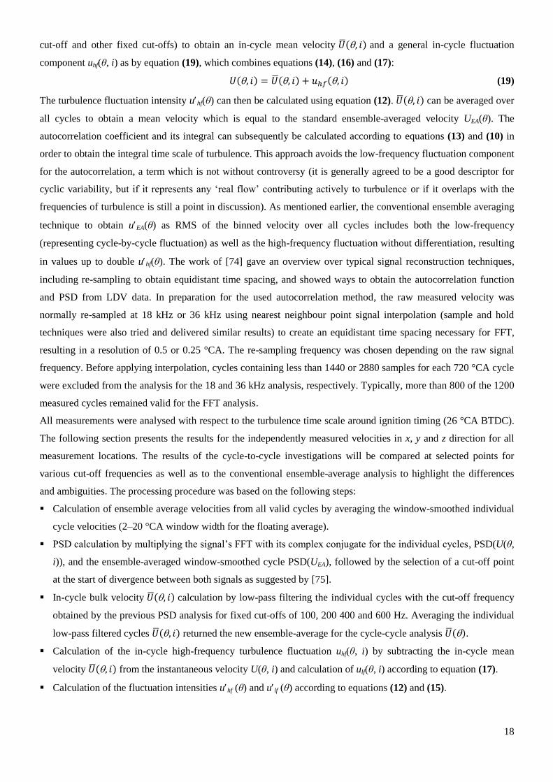
velocities were evaluated similarly. The frequency analysis to obtain the in-cycle cut-off frequency is shown in

Figure 16. The left graph shows the power spectrum of the first cycle (red dotted), the average of the FFT for all

cycles (black solid) and the theoretical -5/3 turbulence cascade (black dashed). The maximum resolvable frequency

was half the frequency of the re-sampled data of 36 kHz, i.e. 18 kHz.

A moving average filter was applied to the individual cycles with a window width of 4, 8, 12, 16 and 20 °CA. The

individual window-averaged cycles were then ensemble-averaged over all cycles to obtain the window-averaged

ensemble mean velocity. The PSDs of the various window-averaged mean velocities are shown in the graph

(various solid red). Also included in the graph is the PSD of the traditionally ensemble-averaged velocity (blue).

The location of first distinct deviation of the averaged PSD plots from the individual cycle’s PSD should be used to

select the frequency cut-off. As the individual cycle’s PSD was very noisy, it was found less ambiguous to use the

averaged PSD over all cycles (black).

Looking at the graph, the dependence of the cut-off frequency on the window width becomes obvious, as the found

point of deviation moves towards higher frequencies for smaller window sizes. The reason for this lies in the nature

of the windowing, which is in itself a filter that is mathematically described by a Dirichlet function. When applying

the formula to the current data set with a sample frequency of 36 kHz and a time interval according to the required

window sizes, the resulting -3 dB limit frequencies are given in Table 4, so that the graphically obtained limits are

a way to get the limit frequency without calculation.

An ambiguity in the selected threshold for the in-cycle mean velocity therefore still persists. However, there was a

subjective point of first strong deviation found for the 8–16 °CA windows between 300–400 Hz (greyed area in

Figure 16) and around 400 Hz for the 4 °CA window as well as the traditional ensemble average. Suggestions

based on physical relations such as the inverse of the stroke duration would return very low cut-off thresholds of 50

Hz and were discarded based on not resolving any of the fast incoming peak flow around 310 °CA BTDC. Using

the highest frequency present in the ensemble-averaged data as cut-off, as suggested by [48], was found more

useful for the current data. Two distinct peaks could be seen in the power spectrum for all ensemble-averaged

functions between 100 to 1000 Hz. The first peak started around 350 Hz while the second was at just above 600

Hz. In the right graph of Figure 16, the in-cycle mean velocity for a single cycle is shown for cut-off frequencies of

100, 200, 400 and 600 Hz, as well as for traditional ensemble averaged velocity trace. Analysis of graphs over a

range of cut-off frequencies from 600 Hz down to 100 Hz showed a distinct low-frequency fluctuation during the

intake stroke between 330 °CA and 210 °CA BTDC of about 350–450 Hz, believed to correspond to the first peak

found in the power spectrum and also to the pressure fluctuation frequency in the intake runner, so that 400 Hz was

selected as the preferred cut-off frequency for in-cycle analysis. Results for lower frequency cut-offs were also

calculated for time scale analysis.

20

Figure 17 concludes the frequency analysis for a single sample location of measurement. The zoom into the

compression stroke for the individual cycle’s velocity and the in-cycle mean velocity for various thresholds (top

left) shows how the cut-off frequencies between 200–600 Hz were within the measurement envelope, while the 100

Hz filtering did not quite fit by subjective judgement. The calculated turbulence intensity uhf over all cycles (top

right) shows that the main effect of the cut-off frequency of the filtering was during the early intake stroke in the

area of largest velocities, while the differences during the compression stroke were small throughout. Around

ignition timing (26 °CA BTDC), all high-frequency turbulence intensities were found to be between 1.8–2.5 m/s,

lowest for the highest cut-off frequency. Ensemble averages of the in-cycle mean velocities for the various cut-off

frequencies (bottom left) and the low-frequency fluctuation intensities of the in-cycle mean around the ensemble-

average are also shown (bottom right). The latter, in opposition to the high-frequency showed higher values for

higher cut-off frequencies, yet during the compression stroke the values were quite close between 1–2 m/s.

When using the 400 Hz cut-off frequency on all measurement locations at the x=-3 mm location along the y- and z-

axis, mean and fluctuation velocity maps for the compression stroke similar to those of the ensemble averaging

analysis were obtained for cyclic analysis. The graphs in Figures 18–19 show the ensemble-averaged individual

cycle low-pass mean velocities along the y- and z-axis; the left columns show the u, v and w velocity components in

the first, second and third row, respectively. The high- and low-frequency fluctuations, i.e. uhf (θ) and ulf (θ),

respectively, are given in the middle and right columns accordingly. At ignition timing, the mean u and w velocities

were close to ±1 m/s, while the v component showed values between 0 to -8 m/s, agreeing closely with the values

and structures obtained by the traditional ensemble-averaging method.

The high-frequency fluctuations around ignition timing were in the region of 1–2 m/s for all components, with vhf

and whf having slightly higher values than uhf. These values were therefore about half the fluctuation obtained by

the traditional approach, due to the exclusion of the low-frequency velocity fluctuations that can be considered to

represent cycle-to-cycle variations. Values of 1.5–3 m/s were found for the low-frequency fluctuations at ignition

timing, slightly highest for the v-component. This measure of cyclic variability was therefore of the same order of

magnitude to the mean velocities and typically higher than the high-frequency fluctuations.

When calculating TKE on the basis of the high-frequency fluctuations according to khf=0.5(u2hf+v

2hf+w

2hf) and

quantifying an equivalent average turbulence intensity as [(2/3)khf]1/2

, the graphs of Figure 20 were obtained for the

y-axis (left) and z-axis (right). The TKE values found around ignition timing were within 3–4 m2/s

2, i.e. distinctly

lower (75%) than when the low-frequency fluctuations had been included earlier in Figure 11. The TKE during

induction (especially for the highest intake charge velocities around 300–280 °CA BTDC) was not as much

affected, showing that the cyclic variability was not as dominant over the high-frequency fluctuations during the air

intake as later during the compression stroke.

Turbulence intensity close to compression TDC was now between 1.4–1.6 m/s, below the estimate of half the mean

piston speed of 4.25 m/s. The trends of TKE being slightly higher towards the negative y-axis (exhaust side) and

towards the negative z-axis as shown earlier from the typical RMS analysis are still valid, but less distinct. The

turbulence intensity and TKE during compression after IVC have their maximum values just before TDC when the

present tumble bulk motion is considered to break down into smaller scale turbulence. This flow behaviour was

also found by [76] who used cycle-resolved analysis with a 12 °CA window averaging to obtain in-cycle mean flow

21

and turbulence in a 4-valve pentroof engine of under square geometry with similar bore and compression ratio to

that of the current study, imposing various levels of swirl by valve deactivation when the engine was operated at

1500 RPM with wide-open-throttle. Furthermore, the velocities and turbulence intensities of [76] were similar to

those of the current investigation, unlike those of [66, 67] where intensities close to TDC were only of the order of

0.2–0.5 m/s for a conventional and tumble port at 500 RPM and 1000 RPM. However, the low mean piston speed

of only 1.6 m/s at 1000 RPM due to the short stroke of the over-square engine of [66, 67] could largely account for

the differences found.

Autocorrelation Function at Injection and Ignition Timings

The calculated autocorrelation functions given in Figure 21 show the results for u, v and w at the centre of the

cylinder at a vertical location of x=-3 mm at 300 °CA BTDC (left column) and at 26 °CA BTDC (right column),

representing the start of injection and ignition timing, respectively. All graphs show the results for the various cut-

off frequencies of the high-frequency cyclic analysis (coloured lines, no marker), as well as the value from the

traditional ensemble-averaging of the binned velocities of all cycles (black lines, no marker). For the latter, the

fluctuation was calculated using the RMS of the individual bins with the cyclic fluctuation component included

according to equation (13). For the data point shown, the bin size was chosen to be 0.26 °CA, to match the cyclic

data which could be re-sampled with 36 kHz due to the high raw signal frequency at the centre of the cylinder. The

combined low- and high-frequency components according to equations (17) and (18) from the frequency analysis

along with equation (13) are also included in the figure (coloured lines, circular marker). All three spatial velocity

components are shown (top row: u, middle row: v, bottom row: w). The time scales given in the graph’s legends

were calculated using the time integral of the graphs from R=1 (t=0 ms) until the time of first falling below R=0 or

reaching the minimum value within 5 ms.

Two main observations are instantly possible. Firstly, the turbulence during the high-velocity intake stroke was

unsurprisingly much higher and returned very low integral time scales of turbulence in comparison to the flow

around spark timing as shown in the figure’s annotation. Secondly, the autocorrelation functions drop much faster

for higher cut-off frequencies as larger or longer lasting flow structures are excluded. With few exceptions, the

traditional approach using the bin averaging method returned much larger time scales. This may be due to all low-

frequency fluctuations being included in this analysis as opposed to the high-frequency only cyclic analysis. Re-

combining the low- and high-frequency components obtained from the frequency analysis returned autocorrelation

function results very similar to that of traditional ensemble averaging.

At ignition timing, the traditional ensemble averaged integral time scales were 1.08 ms for u, 1.87 ms for v and

0.89 ms for the w velocity component (i.e. 8–16 °CA). The strong v component is believed to be a direct result of

the directionality of the tumble motion breaking up into smaller scale vortices. A characteristic of the

autocorrelations at ignition timing was that they did not converge to zero within the expected time lag. Only at

exhaust valve opening, 16 ms after ignition timing, an abrupt step change to zero was found. It could be that the

downwards motion of the piston and volume expansion delay turbulence dissipation, resulting in long correlations.

Autocorrelation Maps during Intake and Compression

The development of the autocorrelation for the measurement location x=-3, y=0, z=0 mm throughout the cycle can

be seen in Figure 22. Each row in the left column of graphs shows the u, v and w component, respectively, for the

traditional ensemble-averaging approach, while the right column contains the 200 Hz cut-off frequency results.

22

Increasing the cut-off frequency excluded larger scale turbulent structures, keeping only smaller eddies travelling

quicker through the measurement volume, such that the correlations for 300–400 Hz were typically shorter.

Therefore, it was decided to show the 200 Hz data here in an attempt to ensure clearer representation of the colour

maps for each velocity component when using the same scale between ensemble-averaged and filtered conditions.

According to the traditional ensemble-averaging graphs, the time scales were very low throughout the induction

stroke (<0.5 ms), but the situation changed abruptly after the piston reached BDC. From here on, no incoming flow

past the valves would have any significant fed momentum into the cylinder and high velocities were absent. The

large-scale tumble motion could now freely progress without major disturbance by external forces and vortex

structures now started to naturally dissipate due to stresses and friction. Once the piston started moving towards

TDC during compression, higher pressures and temperatures followed after IVC and the space available for the

motion of vortices reduced. It can be seen that the horizontal components returned larger values during late

compression for v, with longest correlations for w around 120 °CA BTDC (i.e. just after the IVC timing of 124 °CA

BTDC). The shortest values for v and u were returned in the region of typical advanced ignition timings (30–50

°CA BTDC), whilst w showed values reducing further towards TDC. The increasing time lag for u and v in the area

of retarded ignition timings (30–0 °CA BTDC) could be due to time lags surpassing TDC and the downwards

motion of the piston along with pressure relaxation could have an effect as mentioned earlier. However, very little

vertical movement is produced per crank angle around TDC (and BDC) and other effects such as heat transfer to

the outside and pressure loss due to leakage could also play a part. The high-frequency cut-off calculations at 200

Hz generally showed little difference in the autocorrelation lengths between intake and compression stroke. The

200 Hz cut-off should still include structures up to 5 ms equating to a piston movement interval of 45 °CA but only

time scales of up to 0.1–0.2 ms could be found. Similar autocorrelation maps for the higher cut-off frequencies

returned even shorter correlations as already indicated in Figure 21 for a single crank angle. The typical effect of

such short autocorrelations would be the estimation of smaller integral length scales than with the ensemble

approach, something that has also been seen by direct measurement of integral length scales by two-point LDV

using filtered and unfiltered velocity data in a disk-shaped combustion chamber geometry [64].

Integral Time Scales of Turbulence

Due to the ambiguity in the high-frequency approach, the large difference to the classic autocorrelation technique

and the wide spread use of the latter, the time scale analysis in the following discussion will be based on the

traditional approach only. This should maintain good comparability for other researchers. Autocorrelation functions

were calculated from 300 °CA BTDC to TDC in steps of 10 °CA for each measurement location and velocity

component. The resulting integral time scale is presented in form of surface plots for the time scale development

along the y-axis (exhaust to intake) or the z-axis (control to flywheel side) during intake and compression.

Figure 23 shows the results for the y-axis in the left column and the z-axis on the right for the x=-3 mm plane.

Velocity components u, v and w are shown in the 1st, 2

nd and 3

rd row, respectively. As already shown for the sample

autocorrelation graphs at the centre of the cylinder, all time scales during intake were very low with values

typically below 0.5 ms along the y-axis and below 1 ms along the z-axis (4.5 and 9 °CA, respectively) where the

largest values were found for regions in the inlet valve shadow. During compression, integral time scales up to 2.5

ms could be found for many measurement locations and crank angles (about 22 °CA). The time scales at the MBT

ignition timing of 26 °CA BTDC close to the spark showed values of 1.5–1.8 ms for u (about 13–16 °CA) and 1.3–

23

2.3 ms for v along the y and z axes (about 12–20 °CA). The w component was showing longer correlations along

the z-axis with time scales of 1.2–2.2 ms compared to 0.8–1.3 ms along the y-axis (11–20 °CA and 7–12 °CA,

respectively). Therefore, a developing flame kernel would experience nominally airflow timescales of the order 15

°CA and if one considers that TDC is typically associated with the timing of 5–10% , the flame would experience

about 2 integral time scales during the critical stage of early kernel development. The time scales were typically

largest between 160 °CA BTDC and 60 °CA BTDC and were increasing again close to TDC. The time scales on

the x=10 mm plane shown in Figure 24 also demonstrated very low time scales during intake with values below

0.5 ms along the y-axis for all directions, but slightly larger scales along the z-axis in the valve’s wake, with up to

1.2 ms for u and w. Largest time scales were again found between BDC and 60 °CA BTDC. It is interesting to note

here that duration of the injection in the intake stroke of this engine for stoichiometric operation at 1500 RPM with

0.5 bar inlet pressure, was about 1.3 ms and 1.8 ms for gasoline and ethanol fuelling, respectively, i.e. the spray

would experience nominally about 1–3 integral time scales of the in-coming airflow during injection..

Integral Length Scales of Turbulence

The integral length scales could not be directly obtained using the present LDV system, as a two probe setup would

be required to calculate the spatial correlation in the velocity field. Empirical equations are however often used to

estimate the length scales based on the measured time scale and velocities. As the turbulence intensity during the

compression stroke was of the same order of magnitude or even higher than the mean velocity, Taylor’s hypothesis

which uses the product of ensemble-averaged mean velocity and integral time scale 𝐿𝑥() = �̅�()𝐿𝑡() for length

scale approximation, is considered inappropriate. This is typical for engine flows close to TDC, where alternative

relations are to be used. The work of [77] suggested the use of the RMS velocities instead according to:

𝐿𝑥() = 𝐶𝑢()𝐿𝑡() (20)

with C being a constant of the order unity.

In this context, the length scales on the x=-3 mm layer in Figure 25 were calculated by using the fluctuation

velocities u, v and w of the traditional ensemble-averaging analysis, with C=1. The resulting graphs return very

small length scales during the intake stroke despite high velocity fluctuations, dominated by the very short integral

time scales. The length scales Lu and Lw between ignition timing and TDC were between 3–6 mm and slightly

larger for the v component with values up to 10 mm for Lv. Length scale maps calculated by using mean velocities

could be more suitable during the open-valve fast intake air flow motion. These showed slightly larger length scales

during the intake stroke with up to 5 mm for Lv on the x=-3 mm plane (with Lu and Lw smaller than 1 mm).

However, further down inside the cylinder at x=10 mm (Figure 26–27), Lu was largest with values up to 8 mm,

while Lv remained below 4 mm and Lw below 1 mm.

The longitudinal integral length scales obtained on the tumble and swirl plane by PIV inside the pentroof 26 °CA

BTDC are shown in Figure 28. These give clearer information than the length scales calculated by the LDV-

derived time scales and velocity fluctuations. The length scale Lu in x-direction, obtained from the tumble view on

the sides of the spark plug had values between about 3–5 mm, with largest scales towards the intake side. Smallest

Lu scales were seen below the spark plug, 1–2 mm in size, in the region where the spark plug ground electrode was

protruding into the combustion chamber and narrowing the region above the piston’s top land (y from 0 to -5 mm).

Considering an equivalent clearance height of about 15 mm (calculated by dividing the clearance volume by the

engine bore), Lu scaled to about 7–30%. Lv values along the y-axis for the swirl and tumble view measurements

24

matched reasonably well, both showing an increased length scale at y positions 0–5 mm. Lv was between 4–8 mm

along the y-axis and up to 10 mm towards the negative z-axis, i.e. about 5–12% of the bore. Lw was obtained from

the swirl view and was generally lower than Lv. Largest values for Lw can be seen towards the intake side of the

engine (7–8 mm in size), in the area of the largest w-velocities of the two counter-rotating swirl structures below

the intake valves.

Despite limitations related to equation (20), the integral length scales obtained by LDV on the basis of RMS

velocities showed generally similar range of magnitudes in all directions. Looking at each one of the scales, it is

interesting to note the following: Lu values at ignition timing (top right graph of Figure 25) show slightly larger

values in the positive y direction than those derived by PIV (intake side of engine). In further agreement, the values

at the spark plug location near (i.e. around y=0 mm) were the smallest. Even quantitatively, despite the coarse

resolution of the LDV measurement points in comparison to PIV, the values of Lu appear broadly in agreement with

PIV, being of the order 3–4 mm on the intake side and about 2 at the spark plug location. Lu plotted along the z-axis

(top left graph of Figure 25) shows larger values than those along y. The integral length scales of v showed clearly

larger values in the negative z direction in the PIV data of Figure 28 (bottom left graph); the LDV data of Figure

25 also show generally increased Lv scales in the negative z direction at the end of compression, of the order 8–10

mm (right graph, 2nd

row). However, this trend of agreement is not really holding when it comes to comparing Lv

values between PIV and LDV data along the y-axis. The left graph of the 2nd

row of Figure 25 show larger Lv

values in the negative y direction, a trend that is not really seen in the PIV data of Figure 28 (bottom left graph); if

anything, it appears to be the opposite trend despite maximum values being about 10 mm in both graphs. A match

between LDV and PIV Lv values was slightly better when mean velocities were used for LDV’s Lv estimation. This

may be due to the sufficiently large mean velocity upstream the spark plug on the intake side from the mean tumble

vortex and cannot be really associated with Taylor’s hypothesis holding better. The integral length scales of w in

the right graph of the 3rd

row of Figure 25 display increased values of the order 6–7 mm in the negative z direction,

a trend again not present in Figure 28. The larger values of Lw in the negative y direction in Figure 25 (3rd

row, left

graph) appear in some agreement with Figure 28 though. Lu and Lw scales calculated by mean velocities and

LDV’s time scales did not match PIV’s equivalent length scales, most probably because both u and w featured very

low mean values at ignition timing in comparison to v.

Analysis of the time evolution of LDV’s integral length scales showed that on the lower in-cylinder plane (Figure

27) all length scales had decreased at the latest measurement timing of 50 °CA BTDC. However, on the upper

horizontal plane inside the pentroof (Figure 25), scales showed that despite their general trend of decreasing up to

50 °CA, they increased rapidly towards TDC after that. The most drastic increase was observed for v along both y-

and z-axes and a more moderate one for u also for both axes. In contrast, the integral length scales of w showed a

continuous decrease to TDC. This indicates a redistribution of scales as the flow is squeezed inside the pentroof at

the end of compression and can be critical in how the early flame kernel grows.

Comparison of Integral Length Scales with other Engines and Conditions

The spatially averaged longitudinal integral length scales of the current study, as derived by PIV at 26 °CA BTDC,

were on the tumble plane 4.2 mm (mean of Lu and Lv) and on the swirl plane 6.1 mm (mean of Lv and Lw). At this

stage it was deemed interesting to make some quantitative comparisons with other integral length scale data found

in the engine literature. Quoting the different combustion engine geometries and operating conditions was also

25

considered necessary. Specific effort was made to quote velocity components and axes in this section with respect

to the definition adopted in the current paper in order to avoid confusion when making comparisons throughout. A

summary of these scale data is presented in Table 5. The results of the present study in this table show the length

scales derived by PIV. It is also reminded that, according to theory, a longitudinal integral length scale should be

double the size of the respective lateral one of the same velocity component according for homogeneous isotropic

turbulence. The following text elaborates further on the studies of Table 5. The exact in-cylinder locations and

measurement techniques used by the different authors have been quoted explicitly in the text in order for the

interested reader to make his own assessment and comparisons where required.

The seminal two-point LDV work of [63] in the centre of the clearance height 6 mm below the flat engine head of a

disk-shaped combustion chamber was conducted at a radial location 77% of the bore radius and showed about 3

mm lateral length scales 40 °CA BTDC, decreasing to about 2 mm at TDC. This was for radially-separated

tangential velocity measurements, equivalent to v or w of the current study since their engine combustion chamber

was a very simple cylinder with side ports (2-stroke). The length scale was found to scale 10–20% with the

clearance height. The engine was run at 600 RPM, 1 bar intake, with a compression ratio of 8 and a swirl ratio of 4.

This work was expanded in [64] where compression ratios of 5.7, 7.6 and 11.4 were employed and both raw

velocities and velocity data filtered by cut-off frequencies of 150–450 Hz were considered. Increasing the cut-off

frequency led to lateral integral length scales dropping to ~1 mm with 150 Hz, ~0.75 mm with 300 Hz and ~0.6

mm with 450 Hz. This highlighted that the large scale motions were predominantly associated with the lower

frequencies. The ensemble length scales were found to decrease to about 2–2.5 mm at TDC, with the higher

compression ratios giving the lower values in this short range; scales were about 3–6 mm at 40 °CA BTDC. This

was considered weak dependence of length scales on compression ratio. When the respective filtered data were

used in the analysis, the insensitivity to compression ratio was even stronger and a lack of clear proportionality

with the clearance height before and after TDC was obvious. The analysis was expanded to more lateral integral

length scales in [65] using axially separated tangential components, i.e. v (or w) along x, as well as radially

separated axial components, i.e. lateral integral length scales of u. The lateral tangential components did not scale

with clearance height around TDC but the lateral axial integral length scales were approximately proportional to

clearance height, with scales decreasing from about 2 mm at 40 °CA BTDC to about 1–1.5 mm at TDC for

compression ratios of 11.4 and 7.6. For a compression ratio of 5.7 this length scale remained constant at about 2.5

mm from 40 °CA BTDC to 20 °CA ATDC. The same length scale measured on the opposite hemi-circle of the

engine bore at a radial location from the centre 46% of the bore radius, showed a relatively flat value of about 2.5

mm around TDC. It was quantified that, with respect to homogeneity, length scales ~5 cm apart differed from their

respective average values by ~12–14% for all compression ratios (with 95% of the scales being within 21–29% of

their average). Similar levels of inhomogeneity were quantified for the fluctuation intensities. The axially-separated

lateral integral length scale of the tangential velocity showed similar behaviour to its radially-separated counterpart.

A recent study in a similar bore disk-shaped chamber to that of [63–65] but without swirl and a compression ratio

of 10.6 [78] measured integral length scales by PIV on a horizontal plane at 17 °CA BTDC for 1500 RPM, 1 bar

intake. These were found to be 6–8 mm for the longitudinal correlation of both u and w and about 4–5 mm for the

lateral correlation.

26

The scanning LDV study of [79] of both v and w velocity components along the z axis between intake and exhaust

valve in a disk-shaped chamber engine with a compression ratio of 9 and almost square bore-stoke geometry of 86

mm at 1200 RPM with wide-open-throttle and a swirl ratio of 3.6, showed that the longitudinal scale of w was

about 7 mm at 30 °CA BTDC and the lateral one of v about half that. These authors also commented that their

autocorrelation functions appeared to asymptote to a correlation of 0.1 rather than zero at most points, and

attributed this to cyclic variations in the bulk flow causing a velocity offset from one cycle to the next, thereby

increasing the correlation at all separations.

Measurements by [80] in an another 2-valve disk-shaped combustion chamber using a Laser homodyne technique

showed integral length scales that were fairly independent of engine speed in the range 400–1200 RPM with 1 bar

intake. The lateral scale was measured and then doubled to provide estimates of the longitudinal. The longitudinal

was found to decrease from about 4–5 mm in the early compression stroke to about 2.5 mm at TDC with

compression ratio of 8.2 and zero swirl. The initial scale past BDC was found to be about 3 mm when the

compression ratio was increased to 11.6 at 800 RPM, and it dropped monotonically to about 2 mm at TDC. With

the swirl ratio increased to 2.1, the longitudinal length scales at 800 RPM, with 8.2 compression ratio increased to

levels across the bore of about 4–6 mm at the end of compression, starting from values in the range 8–10 mm soon

after IVC.

The study of [81] in an engine with a 2-valve disk-shaped combustion chamber of 85 mm bore and a compression

ratio of 8 measured at 1000 RPM wide-open-throttle with a swirl ratio of 3.5 integral time scales of the order 0.5

ms near compression TDC for all components 6.5 mm below the engine head gasket and 16 mm from the centre of

the bore between intake and exhaust sides. Using Taylor’s hypothesis the authors derived respective longitudinal

length scales of the order 1 mm for the axial (u) and radial (w) velocity components, whilst that of the tangential

component (v velocity) was about 4 mm at TDC, having dropped rapidly from levels of about 10 mm at 90 °CA

BTDC. Decreasing the swirl ratio to 0.9 at 1000 RPM, increased significantly the axial integral time scales to about

3 ms at TDC, 4.5 mm below the engine head and 16 mm away from the centre of the bore between intake and

exhaust valve. The corresponding integral length scales were over 5 mm during the entire compression and

expansion strokes. In the vicinity of the swirl centre, higher integral time scales were registered axially after TDC

than at other measuring locations, with an order of magnitude of 0.5–1 ms. The axial integral time scales showed a

monotonic decrease when the swirl ratio was increased from 0.9 to 2.0, 2.4 and 3.5 at 1000 RPM, with levels

ranging at TDC from of 0.5 ms to 3 ms. The radial integral time scale at the lowest swirl ratio was found to scale

reciprocal with the engine speed in the range 600–1500 RPM; however, in units of °CA these scales were the same,

decreasing from about 20 °CA at 90 °CA BTDC to about 10 °CA in late compression. The corresponding radial

integral length scales were found to be unaffected by engine speed, decreasing from about 8 mm at 90 °CA BTDC

to about 5 mm at TDC.

The PIV work of [3, 4] in a pentroof engine of similar geometric characteristics to those of the current study (in

terms of bore/stroke and compression ratio) at 1200 RPM, 1 bar load, and with one of the intake ports blocked to

generate swirl, showed integral length scales in the range 6–10 mm on a horizontal plane about 12 mm below the

cylinder head gasket at 60 °CA BTDC. The smaller values applied to v and the larger to w. The longitudinal scales

were typically about 15–30% larger than the lateral. Operation at 600 RPM showed spatially averaged integral

length scales in the range 7–9 mm, generally increasing from BDC and peaking at about 90 °CA BTDC with a

27

small decrease after for the last measurement timing of 30 °CA BTDC. The differences between longitudinal and

lateral scales of w were of the order 15–20%. The lateral scale of v showed a fairly constant value of about 4–5 mm

during compression; this was about 50–60% of the longitudinal.

Spatially averaged integral length scale measurements by PIV in [82] using a 3-valve pentroof engine of 11.1

compression ratio at 60 °CA BTDC on a horizontal plane 3 mm below the engine head and on the central symmetry

vertical plane showed, for 1200 RPM, increasing values during compression from about 4 mm at BDC to about 7

mm 60 °CA BTDC for the longitudinal scales of both v and w and from about 3 mm to 6 mm for the lateral

components. Their latest measurement timing of 30 °CA BTDC showed the scales had levelled off or decreased

slightly. In contrast, the scales on the vertical symmetry plane did not show a monotonic increase during

compression. For u, an average value of the order 7 mm for the longitudinal and 5 mm for the lateral integral length

scale was quantified. For v, the mean longitudinal integral length scale on the tumble plane was in broad agreement

with the horizontal plane, increasing from about 6 mm at BDC to about 8–9 mm at 60 °CA BTDC, whilst the

lateral scale was fairly constant at about 5 mm. The longitudinal integral scales of v were larger on the intake side

of the engine and shorter under the single exhaust valve, similarly to those in the current study of the 4-valve

chamber, a characteristic most probably attributed to similarities in the tumble flow pattern in the two engines. The

longitudinal scale of w also showed similar spatial pattern to that of the current engine. However, the spatial range

of scales was typically 5–10 mm, quite narrower and with larger values than those of the current study on both

vertical and horizontal planes. This may be attributed to the later timing of 26 °CA BTDC used to derive length

scales here.

The LDV work of [66, 67] in a small over-square 4-valve pentroof engine with a bore of 56 mm and a compression

ratio of 8.5 showed relatively constant integral time scales of about 0.5 ms from mid compression to TDC at the

centre of the bore 1 mm above TDC for the v velocity component with both a conventional and a high tumble port

at 1000 RPM (mean v at mid compression was close to 5 m/s for the tumble port and close to zero for the

conventional). The time scales were about double those at 500 RPM, i.e. about the same in units of °CA

irrespective of speed. Using the suggestion of [77] for the link between length scale and time scale, i.e. equation

(20), and with a constant C=3, the respective integral length scales were quite small, typically less than 0.4 mm

with the tumble port and about half that for the conventional port. The much smaller length scales than those found

in other engines may be related to the smaller size of the engine. However, still, longitudinal v length scales lower

than ~1% of the bore, or ~2% of half the stroke, even less than ~5% of the expected clearance height at TDC, are

surprisingly small, especially when considering the C=3 value as well.

It is notable that the integral scales have shown generally similar values in different combustion chambers that span

many years of engine design. Time scales decrease with increasing engine speed but are not affected if expressed in

units of crank angle degrees. Integral length scales appear generally insensitive to engine speed. Typically the

longitudinal scales scale with the bore within 5–20%. The lateral ones are about 30–40% smaller than the

longitudinal ones, when homogeneous isotropic turbulence dictates 50% difference. This highlights the degree of

inhomogeneity and anisotropy in engines. Length scales in disk-shape chamber decrease during compression and

appear to scale with the clearance height close to TDC within 15–25%. This feature appears to be more

complicated in pentroof engines where spatially averaged length scales have shown non-monotic (but fairly

constant) values axially, and increasing values horizontally during most of compression, especially in the main

28

tumble direction from inlet to exhaust, with then a small decrease towards TDC. The current pentroof engine

showed an even more complex behaviour with decreasing scales up to 50 °CA TDC and rapid increase towards

TDC after that. The most drastic increase was for the main horizontal component of tumble from intake to exhaust

side and a moderate one for the vertical component. In contrast, the second horizontal component showed

continuous decrease to TDC. The presence of the bulk tumble vortex in pentroof engines and the altering geometric

shape of the in-cylinder volume as the flow is gradually squeezed from a broadly generic cylindrical shape into a

more irregular volume dictated by the specifics of the pentroof geometry that carries variable clearance height

across, maybe associated with such differences. However, further work is needed to understand such effects and

how the total pentroof chamber geometry (including piston top land shape) can be tailored to induce specific size of

integral scales prior to ignition in order to facilitate combustion.

CONCLUSIONS

Air flow analysis was performed using LDV and PIV in an optical engine running at 1500 RPM, 0.5 bar intake

plenum pressure. The combination of both techniques allowed high spatial and temporal resolution as the two data

sets complemented each other to provide details of mean flow and turbulence characteristics, aiming ultimately for

quantification of integral time scales and length scales. Two PIV planes were considered inside the pentroof: one

vertical ‘tumble’ plane passing through the centre of the combustion chamber and one horizontal ‘swirl’ plane 1

mm below the spark plug’s ground electrodes, both imaged at ignition timing. PIV was also conducted inside the

cylinder at different crank angles throughout the intake and compression strokes. This was done vertically but also

horizontally 10 mm below engine’s fire-face (plane that the spray crosses during injection in the intake stroke).

LDV measurements of all three components of velocity were conducted on both horizontal planes used for PIV

along two axes, in order to provide detailed time history data of the flow inside the pentroof and cylinder. Filtering

was also applied to LDV data in an attempt to distinguish between ensemble-averaging effects and high-/low-

frequency fluctuations about an in-cycle mean. The main conclusions of this study can be summarised as follows:

The predominant mean flow direction 1 mm below the spark plug at ignition timing was from intake to exhaust

side (v component), with highest velocity of 5–7 m/s on the intake side upstream the spark plug and reduced

velocities of 0–2 m/s on the exhaust side. The vertical velocity component u along the piston’s motion axis and

the horizontal component w between exhaust and inlet side of the engine were near zero at ignition timing (the

former linked to the piston’s low speed close to TDC and the latter to symmetry plane effects).

Two counter rotating swirl vortices were seen on the horizontal plane below the spark plug, with their centres

of rotation below each one of the intake valves and the y-axis as symmetry axis.

Velocity fluctuations quantified by the RMS of LDV data were typically between 2–5 m/s, strongest in y-

direction. These were generally of similar order to the mean piston speed of 4.25 m/s.

Turbulent kinetic energy during intake was up to 350 m2/s

2, reducing during compression to 8–20 m

2/s

2. Values

of 9–15 m2/s

2 were found at the time of ignition, highest towards the exhaust side of the engine.

When comparing the power spectra density of raw individual cycle data with that of windowed-averaged cycles

using windows of 8–16 °CA, a frequency cut-off between 300–400 Hz was identified as suitable to calculate an

in-cycle mean velocity by low-pass filtering. This correlated with the highest frequencies found in the FFT of

the ensemble-averaged velocity data and intake runner pressure fluctuations.

29

Decreasing the cut-off frequency gradually to 100 Hz demonstrated the degree of cyclic contribution to high-

frequency turbulent fluctuations and low-frequency cyclic ones. A low cut-off frequency returned individual

cycle mean velocities more akin to traditional ensemble-averaging. The cut-off frequency affected the intake

stroke more than the compression, as variations in the ensemble-averaged data were higher during intake.

Low-frequency fluctuations at ignition timing were of the order of 2–3 m/s (largest for v). High-frequency

fluctuations were of the order of 1–2 m/s, similar in all directions.

The cycle-resolved turbulent kinetic energy was about 3–4 m2/s

2, only 25% of that derived by typical ensemble

averaging. The resulting turbulence intensity was 1.4–1.6 m/s, lower than half the mean piston speed.

The integral time scales obtained by classic ensemble averaging were about 15 °CA, indicating that a flame

would experience about two integral timescales during the critical stage of early flame kernel development

from ignition timing to 5–10% mass fraction burned. In contrast, time scales in the early intake stroke were of

the order 5–10 °CA, indicating that, for injection durations typical of stoichiometric combustion, the spray

during injection would experience about 1–3 integral times scales depending on fuel type.

The autocorrelation function derived by the high-frequency velocity components returned very short time

scales of the order 0.5 °CA. These were not considered a proper reflection of expected integral time scales of

turbulence.

Integral length scales calculated by PIV at ignition timing inside the pentroof were for the swirl view between

4–10 mm, larger in y- than z-direction, hence they scaled to the cylinder bore by about 5–12%. Integral length

scales on the tumble view were 1–5 mm for the vertical component (lowest under the protruding spark plug),

scaling with the equivalent clearance height at ignition timing by about 7–30%. The respective horizontal

component showed integral length scales of 3–7 mm.

Integral length scales derived from LDV’s integral time scales multiplied by RMS velocities showed similar

range of values to the length scales derived by PIV. However, positions of largest scales did not always match

with PIV.

The time evolution of LDV’s integral length scales showed that on the lower in-cylinder plane all scales had

decreased at the latest measurement timing of 50 °CA BTDC. However, on the upper horizontal plane inside

the pentroof, some scales showed that despite their general trend of decreasing up to 50 °CA, they increased

rapidly towards TDC after that. The most drastic increase was for v (horizontal component of tumble) and a

moderate one for u (vertical component). In contrast, the scales of w showed continuous decrease to TDC. The

degree of this redistribution of scales at the end of compression can be quite critical for the early flame kernel

development.

At the intersection of the tumble and swirl planes, the 3-component PIV TKE was about 10–20% lower than

that obtained by the 2-component averaged estimation of the third component and generally in closer

agreement with LDV’s TKE during the cycle. LDV characterised about 10% larger velocities in absolute

magnitude than those obtained by PIV.

Parallel work focused on quantifying the integral length scales by PIV in fuelled cycles and studying their

modulation by injecting different types of hydrocarbons and alcohols and subsequent effects on the flame front

itself during the early stages of combustion [83, 84]; the interested reader is guided to these publications for further

30

analysis. Differences between PIV and LDV highlight the need for further analysis of the two techniques when

applied to in-cylinder flows with steep gradients and unsteadiness. Issues of into-plane motion of seeding particles

may require active adjustment of Laser pulse separation for better dynamic resolution. Issues of velocity bias,

related to more fast particles being statistically captured over typical LDV phase-averaging processes of many

cycles, may also require closer analysis in complex engine flows than normally considered. Future work would be

interesting in the area of comparing high-speed PIV and LDV data, preferably obtained simultaneously with

suitable gating of the two measurement systems over the same number of samples. Furthermore, simultaneous

calculation of time scales and length scales by high-speed PIV data would give unique new information on the

degree of proportionality between temporal and spatial correlations in engines and their effects on combustion.

ACKNOWLEDGMENTS

The authors would like to thank Alasdair Cairns, Dave OudeNijeweme and Paul Freeland of MAHLE Powertrain,

Ltd., UK, for financial and technical support over the duration of this study.

REFERENCES

1. Reuss, D.L., Adrian, R.J., Landreth, C.C., French, D.T. and Fansler, T.D., “Instantaneous Planar Measurements

of Velocity and Large-Scale Vorticity and Strain Rate in an Engine Using Particle-Image Velocimetry”, SAE

Paper 890616.

2. Reuss, D.L., “Cyclic Variability of Large-Scale Turbulent Structures in Directed and Undirected IC Engine

Flows”, SAE Paper 2000-01-0246, 2000.

3. Li, Y., Zhao, H., Peng, Z. and Ladommatos, N., “Particle Image Velocimetry Measurement of In-Cylinder

Flow in Internal Combustion Engines – Experiment and Flow Structure Analysis”, Proceedings of IMechE,

Part D, Journal of Automobile Engineering, Vol. 216, pp. 65–81, 2002.

4. Li, Y., Zhao, H. and Ladommatos, N., “Analysis of Large-Scale Flow Characteristics in a Four-Valve Spark

Ignition Engine”, Proceedings of IMechE, Part D, Journal of Mechanical Engineering Science, Vol. 216, pp.

923–938, 2002.

5. Burluka, A.A., El-Dein Hussin, A.M.T.A, Ling, Z.-Y. and Sheppard, C.G.W., “Effects of Large-Scale

Turbulence on Cyclic Variability in Spark Ignition Engine”, Experimental Thermal and Fluid Science, Vol. 43,

pp. 13–22, 2012.

6. Lacour, C. and Pera, C., “An Experimental Database Dedicated to the Study and Modelling of Cyclic

Variability in Spark-Ignition Engines with LES”, SAE Paper 2011-01-1282, 2011.

7. Müller, S.H.R., Böhm, B., Gleißner, M., Grzeszik, R., Arndt, S. and Dreizler, A., “Flow Field Measurements in

an Optically Accessible Direct-Injection Spray-Guided Internal Combustion Engine using High-speed PIV”,

Experiments in Fluids, Vol. 48, pp. 281–290, 2010.

8. Karhoff, D.-C., Bücker, I., Laas, M. and Schröder, W., “Time-Resolved Sterescopic PIV Measurements of

Cyclic Variations in an Internal Combustion Engine”, 10th International Symposium on Particle Image

Velocimetry – PIV13, Delft, The Netherlands, July 1–3, 2013.

9. Baum, E., Peterson, B., Böhm, B. and Dreizler, A., “On the Validation of LES Applied to Internal Combustion

Engine Flows: Part 1: Comprehensive Experimental Database”, Flow, Turbulence and Combustion, Vol. 92,

pp. 269–297, 2014.

31

10. Justham, T., Jarvis, S., Garner, C.P., Hargrave, G.K. Clarke, A. and Richardson, D., “Single Cylinder Motored

SI IC Engine Intake Runner Flow Measurement using Time Resolved Digital Particle Image Velocimetry”,

SAE Paper 2006-01-1043, 2006.

11. Jarvis, S., Justham, T., Clarke, A., Garner, C.P., Hargrave, G.K., Richardson, D., “Motored SI IC Engine In-

Cylinder Flow Field Measurement Using Time Resolved Digital PIV for Characterisation of Cyclic Variation”,

SAE Paper 2006-01-1044, 2006.

12. Rimmer, J.E.T., Long, E.J., Garner, C.P., Hargrave, G.K., Richardson, D. and Wallace, S., “The influence of

single and multiple injection strategies on in-cylinder flow and combustion within a DISI engine”, SAE paper

2009-01-0660, 2009.

13. Müller, S.H.R., Arndt, S. and Dreizler, A., “Analysis of the In-Cylinder Flow Field/Spray Injection Interaction

within a DISI IC Engine using High-Speed PIV”, SAE Paper 2011-01-1288, 2011.

14. Disch, C., Kubach, H., Spicher, U., Pfeil, J., Altenschmidt, F. and Schaupp, U., “Investigations of Spray-

Induced Vortex Structures during Multiple Injections of a DISI Engine in Stratified Operation Using High-

Speed-PIV”, SAE Paper 2013-01-0563, 2013.

15. Zeng, W., Sjöberg, M. and Reuss, D.L., “PIV Examination of Spray-Enhanced Swirl flow for Combustion

Stabilization in a Spray-Guided Stratified-Charge Direct-Injection Spark-Ignition Engine”, International

Journal of Engine Research, Vol. 16, pp. 306–322, 2014.

16. Peterson, B., Reuss, D.L. and Sick, V., “On the Ignition and Flame Development in a Spray-Guided Direct-

Injection Spark-Ignition Engine”, Combustion and Flame, Vol. 161, pp. 240–255, 2014.

17. Peters, N., “The turbulent burning velocity for large-scale and small-scale turbulence”, Journal of Fluid

Mechanics, Vol. 384, pp. 107–32, 1999.

18. Aleiferis, P.G., Serras-Pereira, J. and Richardson, D., “Characterisation of flame development with ethanol,

butanol, iso-octane, gasoline and methane in a direct-injection spark-ignition engine”, Fuel, Vol. 109, pp. 256–

278, 2013.

19. Aleiferis, P.G., van Romunde, Z.R., Larson, G., Lawes, M and Sheppard, C.G.W., “On the Effect of Ambient

Turbulence and Thermodynamic Conditions on Fuel Spray Development for Direct-Injection Spark-Ignition

Engines”, Flow, Turbulence and Combustion, Vol. 95, pp. 29–60, 2015.

20. Nomura, T., Takahashi, Y., Ishima, T., Obokata, T., “LDA and PIV Measurements and Numerical Simulation

on In-Cylinder Flow under Steady State Flow Condition”, 12th Int. Symposium on Application of Laser

Techniques to Fluid Mechanics, Lisbon, Portugal, Paper 17-4, 2004.

21. Huijen, V., Somers, L.M.T, Baert, R.S.G., de Goey, L.P.H., Olbricht, C., Sadiki, A., and Janicka, J., “Study of

Turbulent Flow Structures of a Practical Steady Engine Head Flow Using Large-Eddy Simulations”, ASME

Journal of Fluids Engineering, Vol. 128, pp. 1181–1191, 2006.

22. Ishima, T., Obokata, T., Nomura, T. and Takahashi, Y., “Analysis of In-Cylinder Flow by Means of LDA, PIV

and Numerical Simulation under Steady State Flow Condition”, SAE Paper 2008-01-1063, 2008.

23. Pitcher, G., Binjuwair, S., Picton-Turbervill, T., Wood, A., Wigley, G. and Hollis, D., “LDA and PIV Analyses

and Comparison of In-Cylinder Flow Structures under Steady State Condition”, 15th Int. Symposium on

Application of Laser Techniques to Fluid Mechanics, Lisbon, Portugal, Paper 1801, 2010.

32

24. Malcolm, J.S., Aleiferis, P.G., Todd, A.R. and Cairns, A., Hume, A., Blaxill, H., Hoffmann, H. and Rueckauf,

J., “A Study of Blended Alcohol Fuels in a New Optical Spark-Ignition Engine”, International Conference on

Internal Combustion Engines: Performance, Fuel Economy and Emissions, December 2007, IMechE, London,

UK, pp. 223-234, 2007.

25. Aleiferis, P.G., Malcolm, J.S., Todd, A.R., Cairns, A., and Hoffmann, H., “An Optical Study of Spray

Development and Combustion of Ethanol, iso-Octane and Gasoline Blends in a DISI Engine”, SAE Paper

2008-01-0073, 2008.

26. Malcolm, J. S., Behringer, M., Aleiferis, P. G., Mitcalf, J. and OudeNijeweme, D., “Characterisation of Flow

Structures in a Direct-Injection Spark-Ignition Engine using PIV, LDV and CFD”, SAE Paper 2011-01-1290,

2011.

27. Malcolm, J.S., “Alcohol Fuel Effects on Mixture Preparation and Combustion in SI Engines”, PhD Thesis,

University College London, 2015.

28. Raffel, M., Willert, C., Kompenhans, J., “Particle Image Velocimetry – A Practical Guide”, 2nd

Edition

Springer, 2007.

29. Westerweel, J., “Fundamentals of Digital Particle Image Velocimetry,” Measurement Science and Technology,

Vol. 8, 1379–1392 (1997).

30. Melling, A., “Tracer Particles and Seeding for Particle Image Velocimetry”, Measurement Science and

Technology, Vol. 8, pp. 1406–1416, 1997.

31. Adrian, R.J., “Dynamic Ranges of Velocity and Spatial Resolution of Particle Image Velocimetry”,

Measurement Science and Technology, Vol. 8, pp. 1393–1398, 1997.

32. Keane, R. and Adrian, R.J., “Optimization of particle image velocimeters. I. Double pulsed systems”,

Measurement Science and Technology, Vol. 1, 1202–1215, 1990.

33. Luff, J., Drouillard, T., Rompage, A., Linne, M. and Hertzberg, J. “Experimental uncertainties associated with

particle image velocimetry (PIV) based velocity algorithms” Experiments in Fluids 26, 36–54, 1999.

34. Megerle, M. Sick, V. and Reuss, D.L., “Measurement of digital particle image velocimetry precision using

electro-optically created particle-image displacements”, Measurement Science and Technology, Vol. 13, 997–

1005, 2002.

35. Lazar, E., DeBlauw, B. Glumac, N., Dutton, C. and Elliott, G., “A Practical Approach to PIV Uncertainty

Analysis”, AIAA Paper 2010-4355.

36. Okamoto, K., Nishio, S., Saga, T. and Kobayashi, T., “Standard images for particle-image velocimetry”,

Measurement Science and Technology, Vol. 11, pp. 685–691, 2000.

37. Reuss, D.L., Megerle, M. and Sick, V. “Particle-image velocimetry measurement errors when imaging through

a transparent engine cylinder,” Measurement Science and Technology, Vol. 13, 1029–1035, 2002.

38. Zeng, W., Sjöberg, M. and Reuss, D.L., “Using PIV Measurements to Determine the Role of the In-Cylinder

Flow Field for Stratified DISI Engine Combustion”, SAE Paper 2014-01-1237.

39. Fajardo, C. and Sick, V., “Development of a High-Speed UV Particle Image Velocimetry Technique and

Application for Measurements in Internal Combustion Engines”, Experiments in Fluids, vol. 46, pp. 43–53,

2009.

33

40. Durst F., Melling A., and Whitelaw J.H., “Principles and Practice of Laser-Doppler Anemometry”, 2nd

Ed.,

Academic Press, London, 1981.

41. Albrecht, H.-E., Damaschke, N., Borys, M. and Tropea, C., “Laser Doppler and Phase Doppler Measurement

Techniques”, Springer, 2002.

42. Dimotakis P., “Single scattering particle Laser Doppler measurements of turbulence”, Paper 10, AGARD

Conference No. 193, Applications of Non-Intrusive Instrumentation in Fluid Flow Research, 1976.

43. Durao D.F.G., Laker J. and Whitelaw J.H., “Bias effects in Laser Doppler anemometry”, Journal of Physics E,

Scientific Instruments, Vol. 13, pp. 442–445, 1980.

44. Yanta W.J. and Smith R.A., “Measurements of turbulent transport properties with a Laser Doppler

velocimeter”, AIAA 11th Aerospace Science Meeting, Washington, D.C., 1978.

45. Melling, A., “Investigation of Flow in non-circular ducts and other configurations by Laser Doppler

Anemometry”, PhD Thesis, Imperial College of Science and Technology, University of London, 1975.

46. Vafidis, C., “Aerodynamics of Reciprocating Engines”, PhD Thesis, Imperial College of Science, Technology

and Medicine, University of London, 1985.

47. Morse, A.P., “The Effect of Crank Angle Broadening on Laser-Doppler Measurements in Reciprocating

Engines”, Imperial College of Science and Technology, Mechanical Engineering Department Report FS/77/18,

1977.

48. Glover, A. R., “Towards bias-free estimates of turbulence in engines”, 3rd

Int. Symp. on Applications of Laser

Anemometry to Fluid Mechanics, Lisbon, 5.3, 1986.

49. Hall, M. J.; Bracco, E V. and Santavicca, D. A., “Cycle resolved velocity and turbulence measurements in an

IC engine with combustion”, SAE Paper 860320, 1986.

50. Liou, T.-M. and Santavicca, D. A., “Cycle resolved turbulence measurements in a ported engine with and

without swirl”, SAE Paper 830419, 1983.

51. Liou, T.-M.; Santavicca, D. A., “Cycle resolved LDV measurements in a motored IC engine”, ASME Journal

of Fluids Engineering, Vol. 107, pp. 232–240, 1985.

52. Vafidis, C., “Influence of induction swirl and piston configuration on air flow in a four-stroke model engine”,

Proc. IMechE, Part C, Journal of Mechanical Engineering Science, Vol. 198, pp. 71–79, 1984.

53. Vafidis, C., Vorropoulos, G. and Whitelaw, J. H., “Effects of intake port and combustion chamber geometry on

in-cylinder turbulence in a motored reciprocating engine”, Proceedings of Symposium on Fluid Flow and Heat

Transfer in Reciprocating Machinery, Boston/MA, ASME-FED 62, 9–15, 1987.

54. Witze, P. O.; Martin, J. K., “Cyclic-variation bias in spark ignition engine turbulence measurements. 2nd

Int.

Symp. On Applications of Laser Anemometry to Fluid Mechanics, Lisbon, 9.4, 1984.

55. Witze, P. O.; Martin, J. K.; Borgnakke, C., “Conditionally-sampled velocity and turbulence measurements in a

spark ignition engine”, Combustion Science and Technology, Vol. 36, pp. 301–317, 1986.

56. Lock, J.A. and Schock, H.J., “Incident Beam Polarization for Laser Doppler Velocimetry Employing a

Sapphire Cylindrical Window”, Applied Optics, Vol. 24, pp. 1987–1995, 1985.

57. Lowe, M.L. and Kutt, P.H., “Refraction through Cylindrical Tubes”, Experiments in Fluids, Vol. 13, pp. 315–

320, 1992.

34

58. Doukelis, A., Founti, M., Mathioudakis, K. and Papailiou, K., “Evaluation of Beam Refraction Effects in a 3D

Laser Doppler Anemometry System for Turbomachinery Applications”, Measurement Science and

Technology, Vol. 7, pp. 922–931, 1996.

59. Zhao, H. and Ladommatos, N., “Engine Combustion Instrumentation and Diagnostics”, Society of Automotive

Engineers, U.S.A., 2001.

60. Freudenhammer, D., Peterson, B., Ding, C.P., Boehm, B. and Grundman, S., “The Influence of Cylinder Head

Geometry Variations on the Volumetric Intake Flow Captured by Magnetic Resonance Velocimetry”, SAE

Paper 2015-01-1697, 2015.

61. Freudenhammer, D., Baum, E., Peterson, B., Böhm, B., Jung, B. and Grundman S., “Volumetric Intake Flow

Measurements of an IC Engine using Magnetic Resonance Velocimetry”, Experiments in Fluids, Vol. 55,

Article No. 1724, 2014.

62. Abraham, P., Reuss, D. and Sick, V., “High-Speed Particle Image Velocimetry Study of In-Cylinder Flows

with Improved Dynamic Range”, SAE Paper 2013-01-0542, 2013.

63. Fraser, R.A., Felton, P.G., Bracco, F.V. and Santavicca, D.A., “Preliminary Turbulence Length Scale

Measurements in a Motored IC Engines”, SAE Paper 860021, 1986.

64. Fraser, R.A. and Bracco, F.V., “Cycle-Resolved LDV Integral Length Scale Measurements in an IC Engine”,

SAE Paper 880381, 1988.

65. Fraser, R. and Bracco, F., “Cycle-Resolved LDV Integral Length Scale Measurements Investigating Clearance

Height Scaling, Isotropy, and Homogeneity in an I.C. Engine”, SAE Paper 890615, 1989.

66. Kang, K.Y. and Baek, Je H., “Tumble flow and turbulence characteristics in a small four-valve engine”, SAE

Paper 960265, 1996.

67. Kang, K. Y., and Baek, J. H., “Turbulence characteristics of tumble flow in a four-valve engine”, Experimental

Thermal and Fluid Science Vol. 18, pp. 231–243, 1998.

68. Liao, S. Y., Jiang, D. M., and Cheng, Q., “Turbulent time-frequency spectral structures and the extraction of the

desired turbulence component”, Proceedings of IMechE, Part D, J. Automotive Engineering, Vol. 218, pp.

1025–1033, 2004.

69. Enotiadis, A.C., Vafidis, C and Whitelaw, J.H., “Interpretation of cyclic flow variations in motored internal

combustion engines”, Experiments in Fluids, Vol. 10, pp. 77–86, 1990.

70. Fansler, T. D., and French, D., “Cycle-Resolved Laser Velocimetry Measurements in a Reentrant-Bowl-in-

Piston Engine”, SAE Paper 880377, 1988.

71. Ball, W. F., Pettifer, H. F., and Waterhouse, C.N. 1983, “Laser Doppler Velocimeter Measurements of

Turbulence in a Direct Injection Diesel Combustion Chamber”, IMechE Paper C52/83.

72. Rask, R.B., “Comparison of Windowed, Smooth-Ensemble and Cycle-by-Cycle Data Reduction techniques for

Laser Doppler Anemometer Measurements of In-Cylinder Velocity”, ASME Symposium on Fluid Mechanics

of Combustion systems, pp. 11–20, 1981.

73. Liou, T. M., and Santavicca, D. A., “Cycle Resolved LDV Measurements in a Motored IC Engine”,

Transactions of ASME, Vol. 107, pp. 232–240, 1985.

74. Benedict, L H, Nobach, H, and Tropea, C., “Estimation of turbulent velocity spectra from laser Doppler data”,

Meas. Sci. Technol. Vol. 11, pp. 1089–1104, 2000.

35

75. Catania, A.E., and Mittica, A., “Extraction Techniques and Analysis of Turbulence Quantities from In-Cylinder

Velocity Data”, ASME J. Eng. Gas Turbines Power, Vol. 111, pp. 466–478, 1989.

76. Johansson, B. and Soderberg, F., “The Effect of Valve Strategy on In-Cylinder Flow and Combustion”, SAE

Paper 960582, 1996.

77. Tabaczynski, R.J., “Turbulence measurements and modelling in reciprocating engines – An overview”, Paper

No. C51/83, IMechE, 1983.

78. Burluka, A.A., El-Dein Hussin, A.M.T.A., Ling, Z.-Y., and Sheppard, C.G.W., “Effects of large-scale

turbulence on cyclic variability in spark-ignition engine”, Experimental Thermal and Fluid Science, Vol. 43,

pp. 13–22 , 2012.

79. Glover, A.R., Hundleby, G.E. and Hdded, O, “The development of scanning LDA for the measurement of

turbulence in engines”, SAE Paper, 880378, 1988.

80. Ikegami, M., Shioji, M. and Nishimoto, K., “Turbulence intensity and spatial integral scale during compression

and expansion strokes in a four-cycle reciprocating engine”, SAE Paper 870372, 1987.

81. Dimopoulos, P. and Boulouchos, K., “Turbulent flow filed characteristics in a motored reciprocating engine”,

SAE Paper 972833, 1997.

82. Li, Y., Zhao, H., Leach, B., Ma, T. and Ladommatos, N., “Characterization of an in-cylinder flow structure in a

high-tumble spark-ignition engine”, International Journal of Engine Research, Vol. 5, pp. 375–399, 2004.

83. Aleiferis, P.G. and Behringer, M.K., “Flame Front Analysis of Ethanol, Butanol, iso-Octane and Gasoline in a

Spark-Ignition Engine Using Laser Tomography and Integral Length Scale Measurements”, Combustion and

Flame, Vol. 162, pp. 4533–4552, 2015.

84. Aleiferis, P.G, and Behringer, M.K., “Modulation of Integral Length Scales of Turbulence in an Optical SI

Engine by Direct Injection of Gasoline, iso-Octane, Ethanol and Butanol Fuels”, Fuel, in print, 2016.

36

LIST OF TABLES

Table 1. Engine Specifications.

Table 2. PIV Settings.

Table 3. LDV Settings.

Table 4. Dirichlet -3 dB limit.

Table 5. Integral Length Scales.

LIST OF FIGURES

Figure 1. View through the pentroof side of the research engine’s optical liner and through the piston crown.

Figure 2. PIV and LDV measurement positions. Two horizontal layers were measured along the y- and z-axis at a

vertical (x) level -3 mm (above the fire-face) and +10 mm (below the fire-face).

Figure 3. Top: PIV image of an individual cycle for the tumble plane motion at 26 °CA BTDC. Image width 36

mm, height 18 mm. Bottom: PIV image of an individual cycle for the swirl plane motion at 26 °CA BTDC on x=-3

mm plane. Visible diameter 56 mm.

Figure 4. Tumble mean flow field and TKE as obtained by PIV at 26 °CA BTDC.

Figure 5. Swirl mean flow field and TKE as obtained by PIV at 26 °CA BTDC on x=-3 mm plane.

Figure 6. Vertical velocity u, u and horizontal velocity v, v at the centre of the cylinder 3 mm above the fire-face

(x=-3 mm) as obtained by LDV.

Figure 7. Ensemble averaged velocities u, v and w (left) and fluctuation components u, v and w (right) vs. °CA at

3 mm above the fire-face (x=-3 mm) along the y-axis as obtained by LDV.

Figure 8. Ensemble averaged velocities u, v and w (left) and fluctuation components u, v and w (right) vs. °CA at

3 mm above the fire-face (x=-3 mm) along the z-axis as obtained by LDV.

Figure 9. Ensemble averaged velocities u, v and w (left) and fluctuation components u, v and w (right) vs. °CA at

3 mm above the fire-face (x=-3 mm) along the y-axis at the end of compression as obtained by LDV.

Figure 10. Ensemble averaged velocities u, v and w (left) and fluctuation components u, v and w (right) vs. °CA

at 3 mm above the fire-face (x=-3 mm) along the z-axis at the end of compression as obtained by LDV.

Figure 11. TKE and turbulence intensity (from ensemble averaged RMS) vs. °CA at 3 mm above fire-face (x=-3

mm) during compression along y-axis (left) and z-axis (right) as obtained by LDV.

Figure 12. Tumble and swirl mean flow fields as obtained by PIV at various crank angles on x=10 mm plane.

Figure 13. Ensemble averaged velocities u, v and w (left) and fluctuation components u, v and w (right) vs. °CA

at 10 mm below the fire-face (x=10 mm) along the y-axis as obtained by LDV.

Figure 14. Ensemble averaged velocities u, v and w (left) and fluctuation components u, v and w (right) vs. °CA

at 10 mm below the fire-face (x=10 mm) along the z-axis as obtained by LDV.

Figure 15. Ensemble averaged velocities u and v (left) and turbulent kinetic energy (right) vs. °CA at 10 mm below

the fire-face at position 4 mm as obtained by LDV and PIV. Top: 320–40 °CA BTDC, Bottom: Enlarged 180–40

°CA BTDC.

Figure 16. Frequency analysis of individual cycles and ensemble averaged cycles (left) to find the cut-off frequency

for the cycle based analysis. In-cycle mean velocities are shown for different thresholds (right).

Figure 17. Effect of the cut-off frequency on the in-cycle mean velocity (top left), the ensemble averaged mean

velocity (bottom left), the high-frequency turbulence intensity (top right) and the low-frequency turbulence

intensity (bottom right).

Figure 18. 400 Hz cut-off frequency analysis at x=-3 mm along the y-axis. Low-pass mean velocities are given in

the left column of graphs for u, v and w velocities in the first second and third row, respectively. High- and low-

frequency fluctuations are given in the middle and right columns accordingly.

37

Figure 19. 400 Hz cut-off Frequency analysis at x=-3 mm along the z-axis. Low-pass mean velocities are given in

the left column of graphs for u, v and w velocities in the first second and third row, respectively. High- and low-

frequency fluctuations are given in the middle and right columns accordingly.

Figure 20. TKE and turbulence intensity during compression stroke at x=-3 mm from 400 Hz high-frequency

fluctuation along y-axis (left) and z-axis (right).

Figure 21. Autocorrelation functions at 300 and 26 °CA BTDC. High-frequency only considerations are given in

solid coloured lines without marker and indicate very low time scales, reducing for higher cut-off frequencies. The

autocorrelation for the combined high- and low-frequency fluctuations for various cut-offs returned autocorrelation

functions (circular marker) very similar to the traditional ensemble averaging approach (black line).

Figure 22. Autocorrelation function against °CA ATDC at x=-3, y=0, z=0 mm for the traditional ensemble averaged

approach and a 200 Hz cut-off high-frequency analysis.

Figure 23. Integral time scales along y- and z-axis at x=-3 mm, LDV.

Figure 24. Integral time scales along y- and z-axis at x=10 mm, LDV.

Figure 25. Integral length scales along y- and z-axis at x=-3 mm, from integral time scale and ensemble averaged

fluctuation, LDV.

Figure 26. Integral length scales along y- and z-axis at x=10 mm, from integral time scale and ensemble averaged

mean velocity, LDV.

Figure 27. Integral length scales along y- and z-axis at x=10 mm, from integral time scale and ensemble averaged

fluctuation, LDV.

Figure 28. Integral length scale maps as obtained by PIV at 26 °CA BTDC.

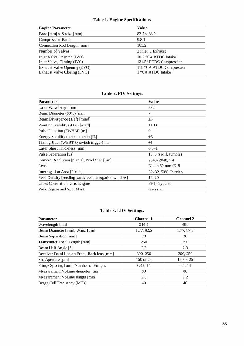
38

Table 1. Engine Specifications.

Engine Parameter Value

Bore [mm] Stroke [mm] 82.5 88.9

Compression Ratio 9.8:1

Connection Rod Length [mm] 165.2

Number of Valves 2 Inlet, 2 Exhaust

Inlet Valve Opening (IVO)

Inlet Valve, Closing (IVC)

10.5 °CA BTDC Intake

124.5° BTDC Compression

Exhaust Valve Opening (EVO)

Exhaust Valve Closing (EVC)

118 °CA ATDC Compression

1 °CA ATDC Intake

Table 2. PIV Settings.

Parameter Value

Laser Wavelength [nm] 532

Beam Diameter (90%) [mm] 7

Beam Divergence (1/e2) [mrad] 5

Pointing Stability (90%) [rad] 100

Pulse Duration (FWHM) [ns] 9

Energy Stability (peak to peak) [%] 6

Timing Jitter (WERT Q-switch trigger) [ns] 1

Laser Sheet Thickness [mm] 0.5–1

Pulse Separation [µs] 10, 5 (swirl, tumble)

Camera Resolution [pixels], Pixel Size [µm] 20482048, 7.4

Lens Nikon 60 mm f/2.8

Interrogation Area [Pixels] 3232, 50% Overlap

Seed Density [seeding particles/interrogation window] 10–20

Cross Correlation, Grid Engine FFT, Nyquist

Peak Engine and Spot Mask Gaussian

Table 3. LDV Settings.

Parameter Channel 1 Channel 2

Wavelength [nm] 514.5 488

Beam Diameter [mm], Waist [µm] 1.77, 92.5 1.77, 87.8

Beam Separation [mm] 20 20

Transmitter Focal Length [mm] 250 250

Beam Half Angle [°] 2.3 2.3

Receiver Focal Length Front, Back lens [mm] 300, 250 300, 250

Slit Aperture [µm] 150 or 25 150 or 25

Fringe Spacing [µm], Number of Fringes 6.43, 14 6.1, 14

Measurement Volume diameter [µm] 93 88

Measurement Volume length [mm] 2.3 2.2

Bragg Cell Frequency [MHz] 40 40

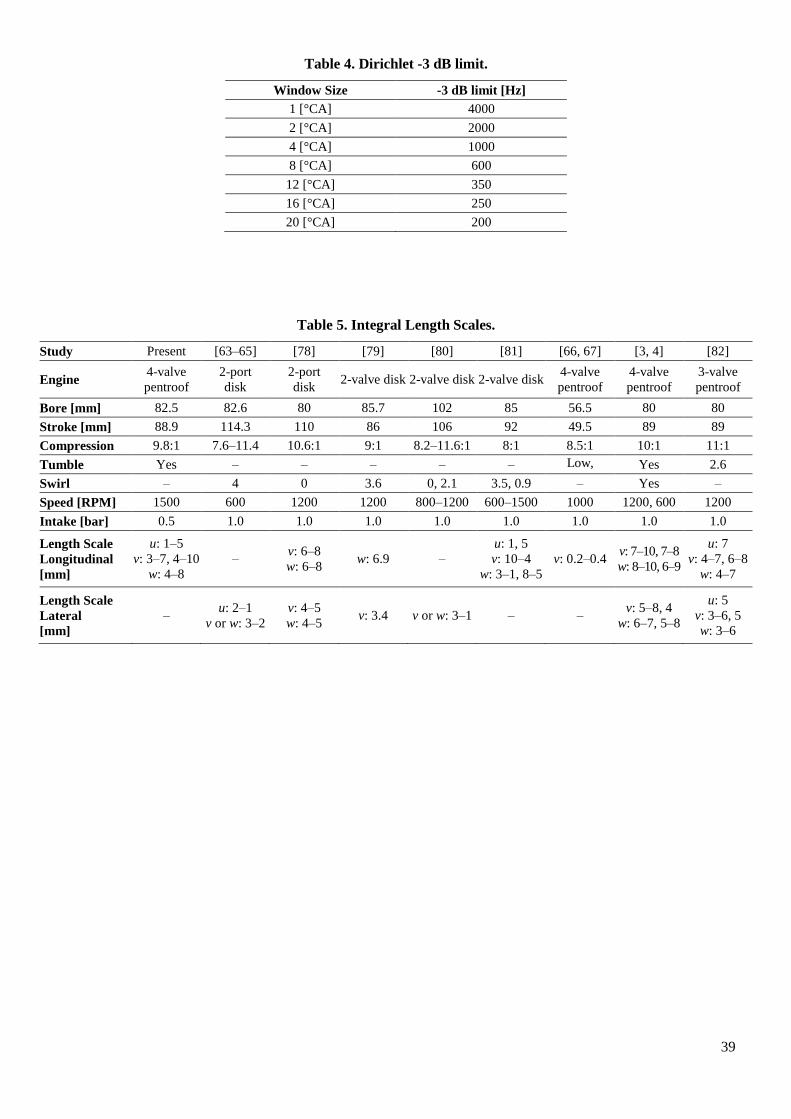
39

Table 4. Dirichlet -3 dB limit.

Window Size -3 dB limit [Hz]

1 [°CA] 4000

2 [°CA] 2000

4 [°CA] 1000

8 [°CA] 600

12 [°CA] 350

16 [°CA] 250

20 [°CA] 200

Table 5. Integral Length Scales.

Study Present [63–65] [78] [79] [80] [81] [66, 67] [3, 4] [82]

Engine 4-valve

pentroof

2-port

disk

2-port

disk 2-valve disk 2-valve disk 2-valve disk

4-valve

pentroof

4-valve

pentroof

3-valve

pentroof

Bore [mm] 82.5 82.6 80 85.7 102 85 56.5 80 80

Stroke [mm] 88.9 114.3 110 86 106 92 49.5 89 89

Compression 9.8:1 7.6–11.4 10.6:1 9:1 8.2–11.6:1 8:1 8.5:1 10:1 11:1

Tumble Yes – – – – – Low,

High Yes 2.6

Swirl – 4 0 3.6 0, 2.1 3.5, 0.9 – Yes –

Speed [RPM] 1500 600 1200 1200 800–1200 600–1500 1000 1200, 600 1200

Intake [bar] 0.5 1.0 1.0 1.0 1.0 1.0 1.0 1.0 1.0

Length Scale

Longitudinal

[mm]

u: 1–5

v: 3–7, 4–10

w: 4–8

– v: 6–8

w: 6–8 w: 6.9 –

u: 1, 5

v: 10–4

w: 3–1, 8–5

v: 0.2–0.4 v: 7–10, 7–8

w: 8–10, 6–9

u: 7

v: 4–7, 6–8

w: 4–7

Length Scale

Lateral

[mm]

– u: 2–1

v or w: 3–2

v: 4–5

w: 4–5 v: 3.4 v or w: 3–1 – –

v: 5–8, 4

w: 6–7, 5–8

u: 5

v: 3–6, 5

w: 3–6

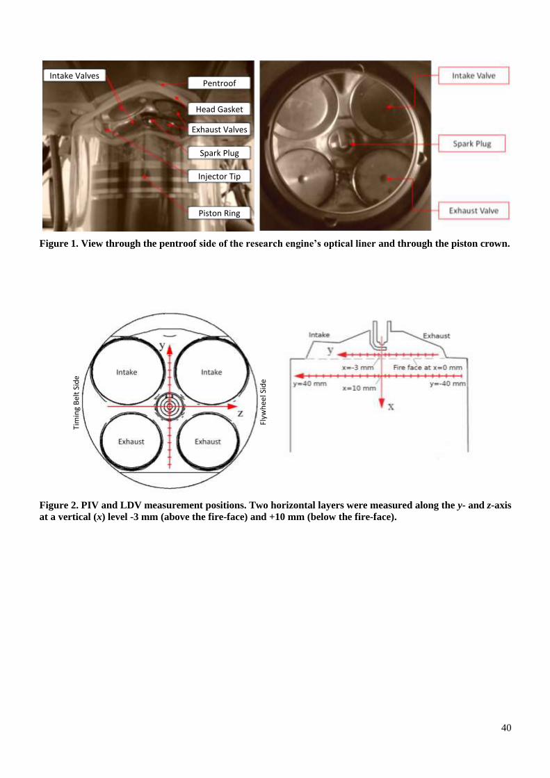
40

Figure 1. View through the pentroof side of the research engine’s optical liner and through the piston crown.

Figure 2. PIV and LDV measurement positions. Two horizontal layers were measured along the y- and z-axis

at a vertical (x) level -3 mm (above the fire-face) and +10 mm (below the fire-face).

Flyw

hee

l Sid

e

Tim

ing

Bel

t Si

de

Intake Valves

Exhaust Valves

Spark Plug

Injector Tip

Piston Ring

Head Gasket

Pentroof

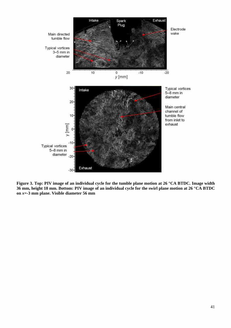
41

Figure 3. Top: PIV image of an individual cycle for the tumble plane motion at 26 °CA BTDC. Image width

36 mm, height 18 mm. Bottom: PIV image of an individual cycle for the swirl plane motion at 26 °CA BTDC

on x=-3 mm plane. Visible diameter 56 mm

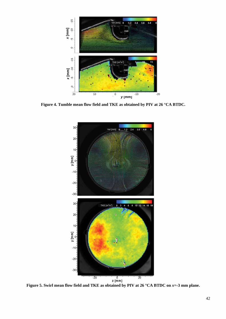
42

Figure 4. Tumble mean flow field and TKE as obtained by PIV at 26 °CA BTDC.

Figure 5. Swirl mean flow field and TKE as obtained by PIV at 26 °CA BTDC on x=-3 mm plane.

y [mm] 20 10 0 -10 -20

x [

mm

] x

[m

m]

0

-

5

-1

0

-1

5

0

-

5

-1

0

-1

5

Vel [m/s]

TKE [m2/s

2]

Vel [m/s]

TKE [m2/s

2]

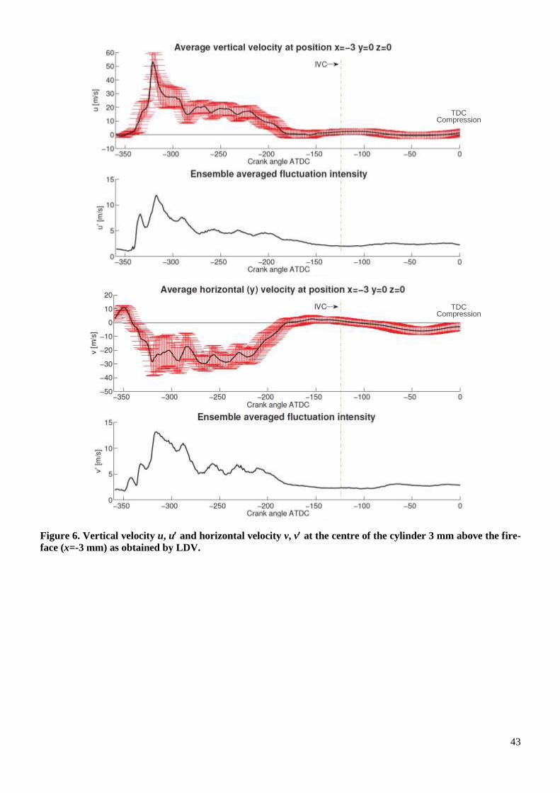
43

Figure 6. Vertical velocity u, u and horizontal velocity v, v at the centre of the cylinder 3 mm above the fire-

face (x=-3 mm) as obtained by LDV.

TDC Compression

TDC Compression

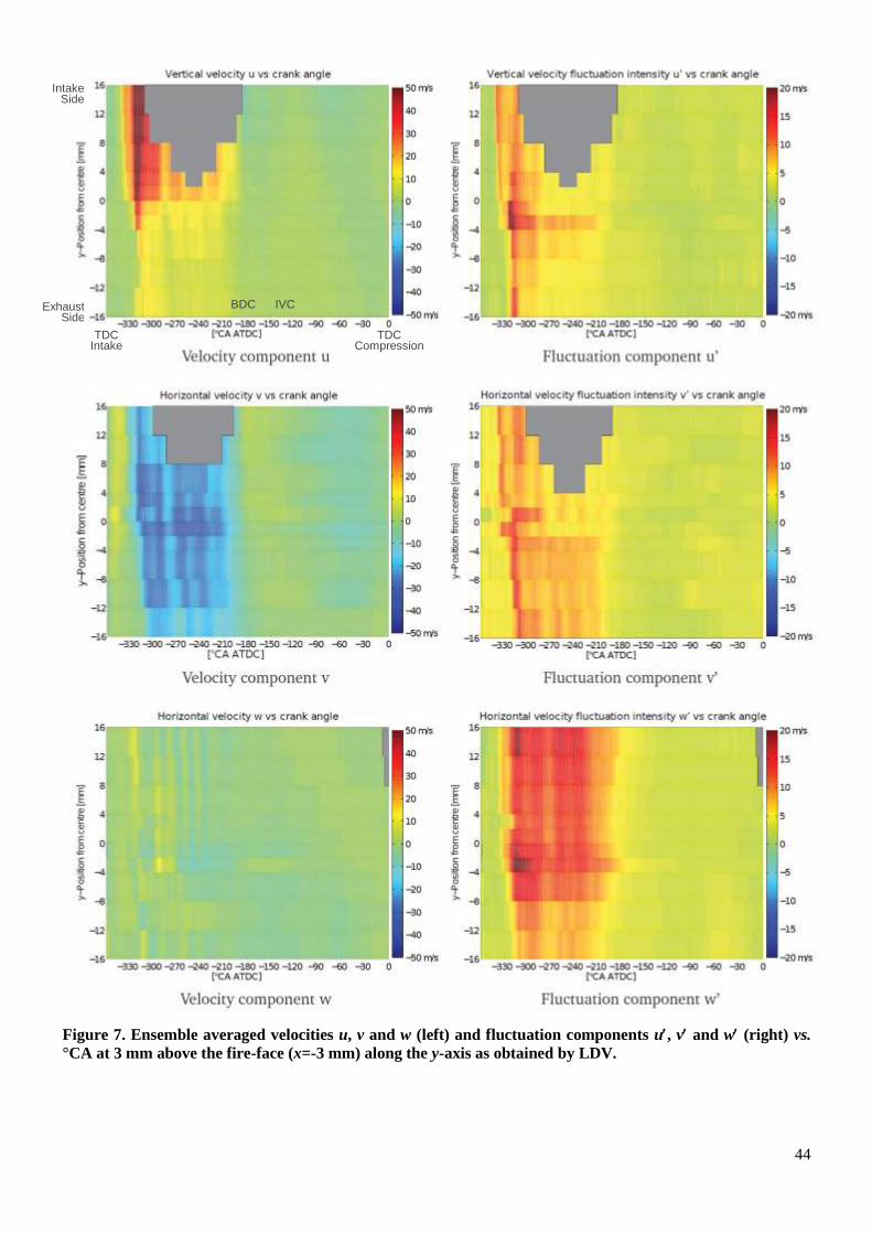
44

Figure 7. Ensemble averaged velocities u, v and w (left) and fluctuation components u, v and w (right) vs.

°CA at 3 mm above the fire-face (x=-3 mm) along the y-axis as obtained by LDV.

TDC Compression

TDC Intake

BDC IVC

Intake Side

Exhaust Side

45

Figure 8. Ensemble averaged velocities u, v and w (left) and fluctuation components u, v and w (right) vs.

°CA at 3 mm above the fire-face (x=-3 mm) along the z-axis as obtained by LDV.

46

Figure 9. Ensemble averaged velocities u, v and w (left) and fluctuation components u, v and w (right) vs.

°CA at 3 mm above the fire-face (x=-3 mm) along the y-axis at the end of compression as obtained by LDV.

47

Figure 10. Ensemble averaged velocities u, v and w (left) and fluctuation components u, v and w (right) vs.

°CA at 3 mm above the fire-face (x=-3 mm) along the z-axis at the end of compression as obtained by LDV.

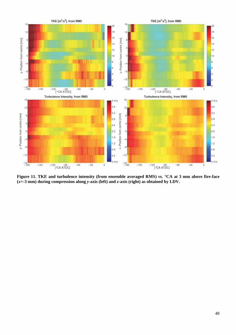
48

Figure 11. TKE and turbulence intensity (from ensemble averaged RMS) vs. °CA at 3 mm above fire-face

(x=-3 mm) during compression along y-axis (left) and z-axis (right) as obtained by LDV.

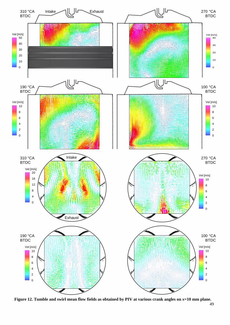
49

Vel [m/s]

10

8

6

4

2

0

Intake

Exhaust

Figure 12. Tumble and swirl mean flow fields as obtained by PIV at various crank angles on x=10 mm plane.

Vel [m/s]

20

16

12

8

4

0

Vel [m/s]

10

8

6

4

2

0

Vel [m/s]

50

40

30

20

10

0

Vel [m/s]

10

8

6

4

2

0

Vel [m/s]

10

8

6

4

2

0

Vel [m/s]

10

8

6

4

2

0

Vel [m/s]

40

30

20

10

0

310 °CA Intake Exhaust 270 °CA BTDC BTDC 190 °CA 100 °CA BTDC BTDC 310 °CA 270 °CA BTDC BTDC

190 °CA 100 °CA BTDC BTDC

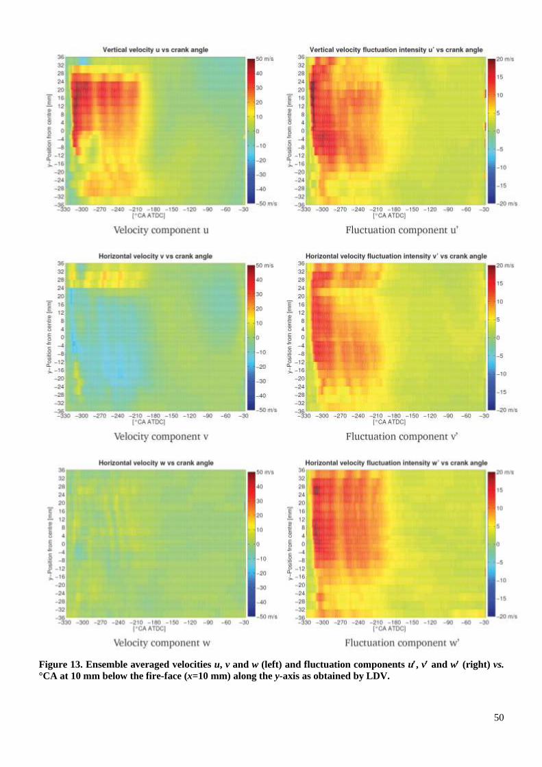
50

Figure 13. Ensemble averaged velocities u, v and w (left) and fluctuation components u, v and w (right) vs.

°CA at 10 mm below the fire-face (x=10 mm) along the y-axis as obtained by LDV.

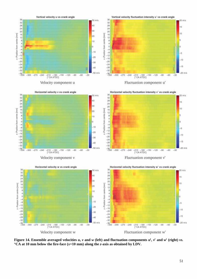
51

Figure 14. Ensemble averaged velocities u, v and w (left) and fluctuation components u, v and w (right) vs.

°CA at 10 mm below the fire-face (x=10 mm) along the z-axis as obtained by LDV.

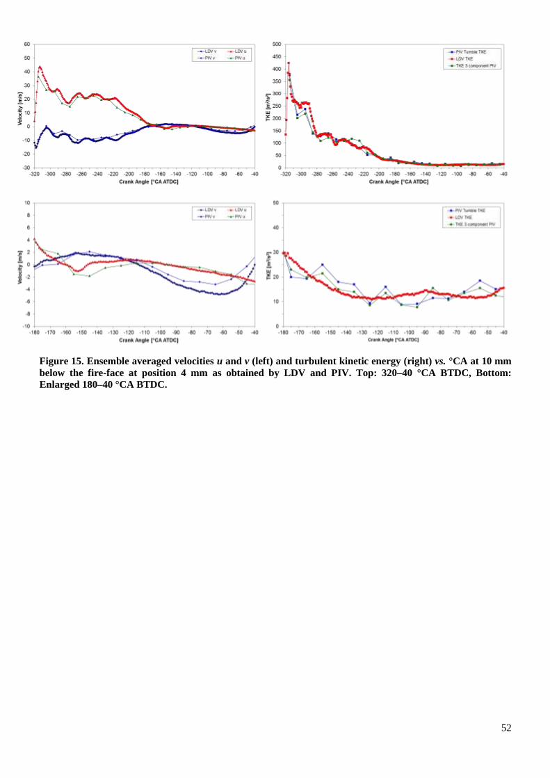
52

Figure 15. Ensemble averaged velocities u and v (left) and turbulent kinetic energy (right) vs. °CA at 10 mm

below the fire-face at position 4 mm as obtained by LDV and PIV. Top: 320–40 °CA BTDC, Bottom:

Enlarged 180–40 °CA BTDC.

53

Figure 16. Frequency analysis of individual cycles and ensemble averaged cycles (left) to find the cut-off

frequency for the cycle based analysis. In-cycle mean velocities are shown for different thresholds (right).

Figure 17. Effect of the cut-off frequency on the in-cycle mean velocity (top left), the ensemble averaged

mean velocity (bottom left), the high-frequency turbulence intensity (top right) and the low-frequency

turbulence intensity (bottom right).

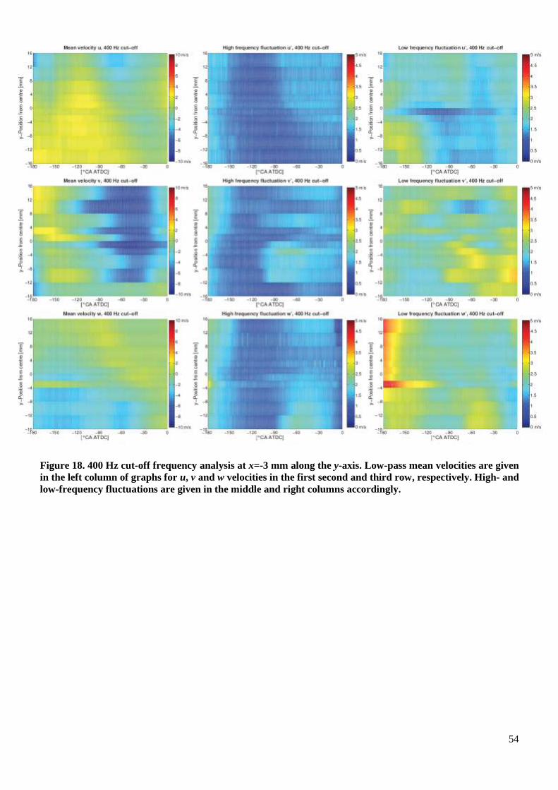
54

Figure 18. 400 Hz cut-off frequency analysis at x=-3 mm along the y-axis. Low-pass mean velocities are given

in the left column of graphs for u, v and w velocities in the first second and third row, respectively. High- and

low-frequency fluctuations are given in the middle and right columns accordingly.

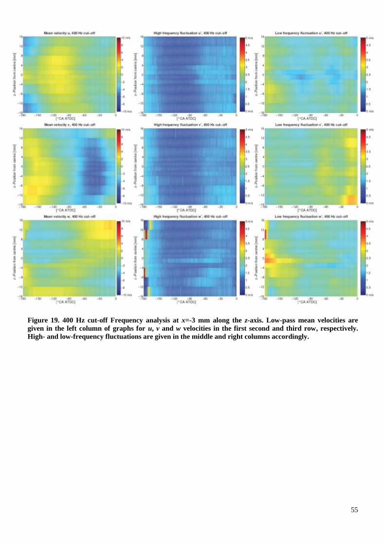
55

Figure 19. 400 Hz cut-off Frequency analysis at x=-3 mm along the z-axis. Low-pass mean velocities are

given in the left column of graphs for u, v and w velocities in the first second and third row, respectively.

High- and low-frequency fluctuations are given in the middle and right columns accordingly.

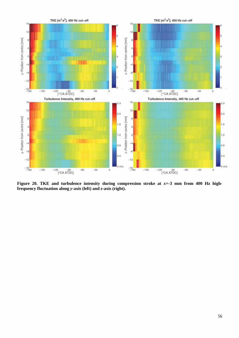
56

Figure 20. TKE and turbulence intensity during compression stroke at x=-3 mm from 400 Hz high-

frequency fluctuation along y-axis (left) and z-axis (right).

57

Figure 21. Autocorrelation functions at 300 and 26 °CA BTDC. High-frequency only considerations are

given in solid coloured lines without marker and indicate very low time scales, reducing for higher cut-off

frequencies. The autocorrelation for the combined high- and low-frequency fluctuations for various cut-offs

returned autocorrelation functions (circular marker) very similar to the traditional ensemble averaging

approach (black line).

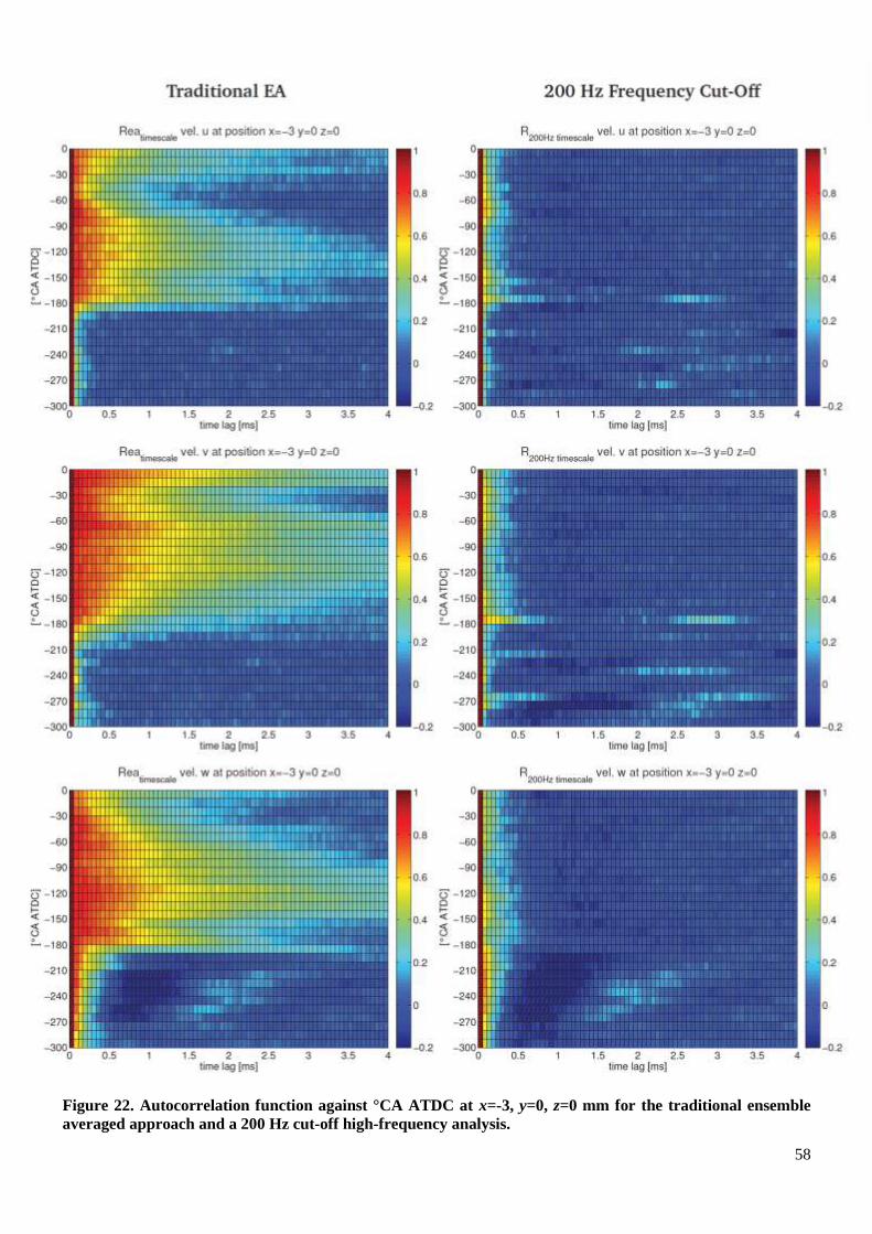
58

Figure 22. Autocorrelation function against °CA ATDC at x=-3, y=0, z=0 mm for the traditional ensemble

averaged approach and a 200 Hz cut-off high-frequency analysis.

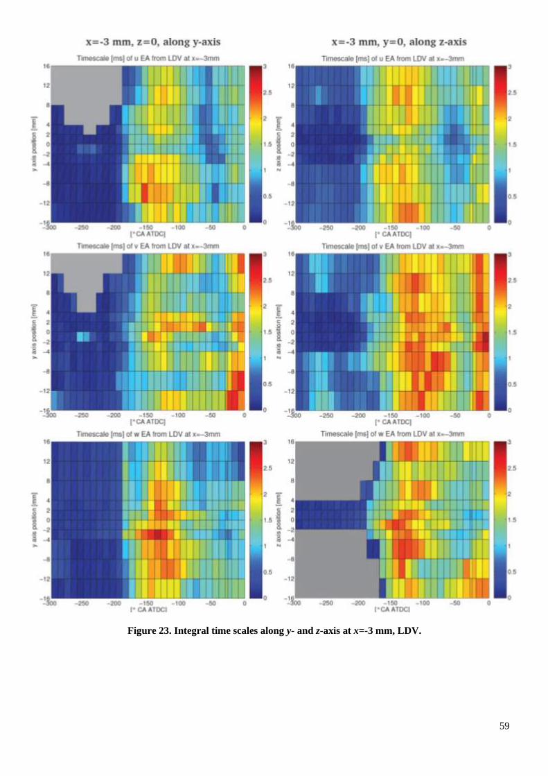
59

Figure 23. Integral time scales along y- and z-axis at x=-3 mm, LDV.

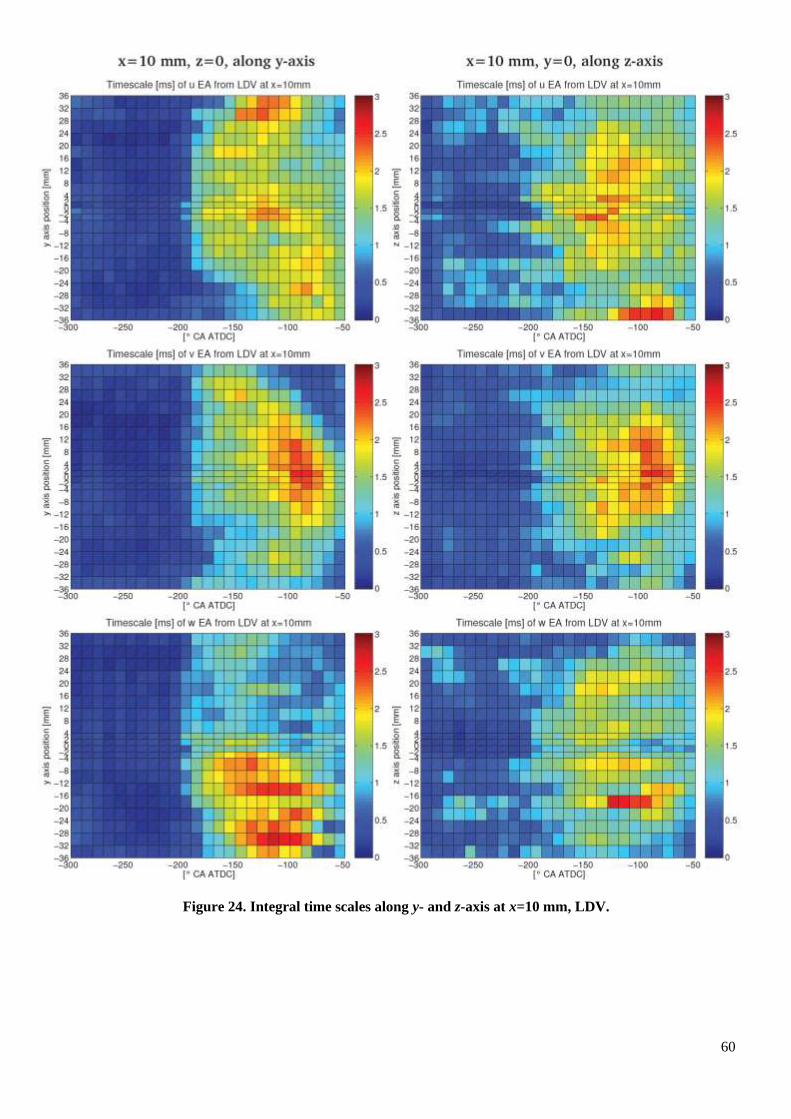
60

Figure 24. Integral time scales along y- and z-axis at x=10 mm, LDV.

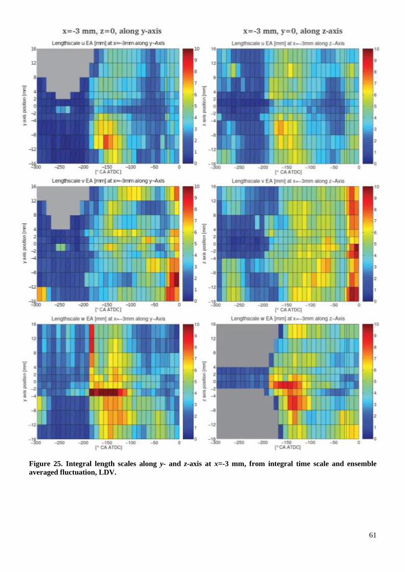
61

Figure 25. Integral length scales along y- and z-axis at x=-3 mm, from integral time scale and ensemble

averaged fluctuation, LDV.

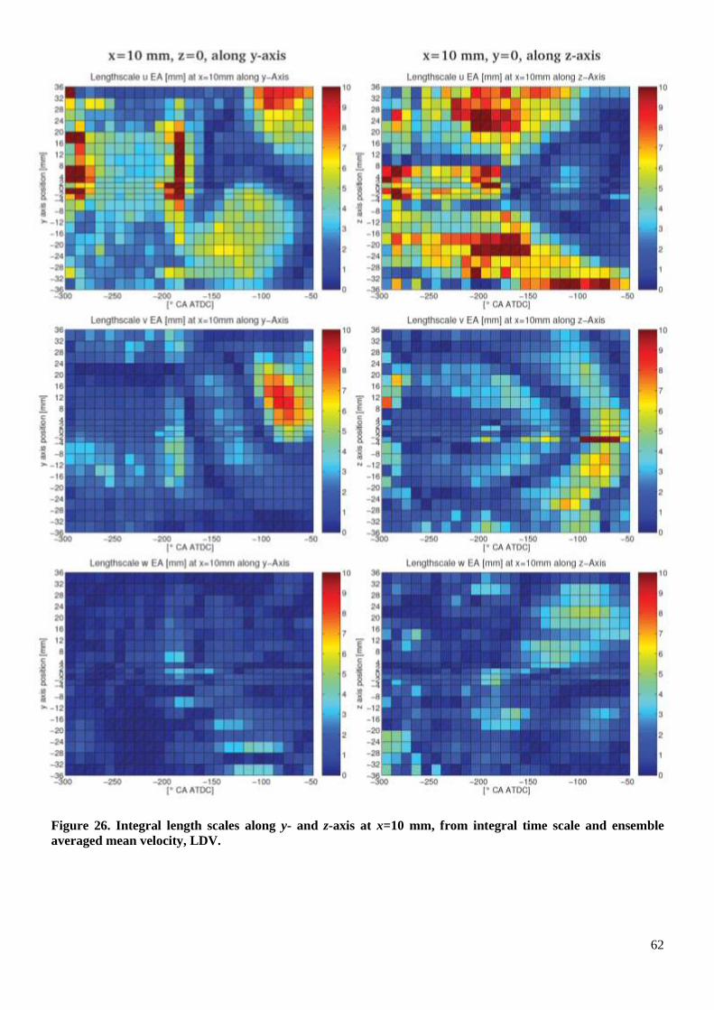
62

Figure 26. Integral length scales along y- and z-axis at x=10 mm, from integral time scale and ensemble

averaged mean velocity, LDV.

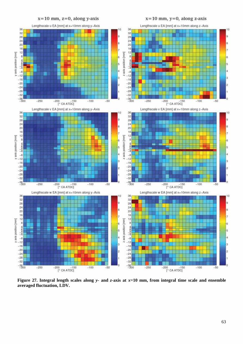
63

Figure 27. Integral length scales along y- and z-axis at x=10 mm, from integral time scale and ensemble

averaged fluctuation, LDV.

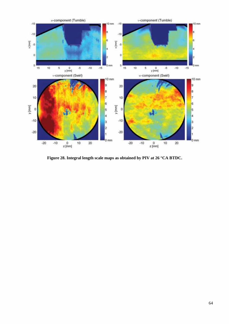
64

Figure 28. Integral length scale maps as obtained by PIV at 26 °CA BTDC.