Available online at www.sciencedirect.com

ng 28 (2010) 862–881

Magnetic Resonance Imagi

Spiral demystifiedBénédicte M.A. Delattrea,⁎, Robin M. Heidemannb, Lindsey A. Crowea,

Jean-Paul Valléea, Jean-Noël HyacintheaaRadiology Clinic, Geneva University Hospital and Faculty of Medicine, University of Geneva, 1211 Geneva 14, Switzerland

bDepartment of Neurophysics, Max Planck Institute for Human Cognitive and Brain Sciences, 04103 Leipzig, Germany

Received 2 December 2009; revised 24 February 2010; accepted 5 March 2010

Abstract

Spiral acquisition schemes offer unique advantages such as flow compensation, efficient k-space sampling and robustness against motionthat make this option a viable choice among other non-Cartesian sampling schemes. For this reason, the main applications of spiral imaginglie in dynamic magnetic resonance imaging such as cardiac imaging and functional brain imaging. However, these advantages arecounterbalanced by practical difficulties that render spiral imaging quite challenging. Firstly, the design of gradient waveforms and itshardware requires specific attention. Secondly, the reconstruction of such data is no longer straightforward because k-space samples are nolonger aligned on a Cartesian grid. Thirdly, to take advantage of parallel imaging techniques, the common generalized autocalibratingpartially parallel acquisitions (GRAPPA) or sensitivity encoding (SENSE) algorithms need to be extended. Finally, and most notably, spiralimages are prone to particular artifacts such as blurring due to gradient deviations and off-resonance effects caused by B0 inhomogeneity andconcomitant gradient fields. In this article, various difficulties that spiral imaging brings along, and the solutions, which have been developedand proposed in literature, will be reviewed in detail.© 2010 Elsevier Inc. All rights reserved.

Keywords: Spiral; Non-cartesian; Gradient; Blurring; Off-resonance; Parallel imaging

1. Introduction

In many magnetic resonance imaging (MRI) applications,it is crucial to reduce the acquisition time. One method toachieve this can be the use of non-Cartesian k-spaceacquisition schemes, such as spiral trajectories [1]. Spiralsampling, including variable density spiral, has the advan-tage of the ability to cover k-space in one single shot startingfrom the center of k-space. Moreover, spiral imaging is veryflexible. High temporal and spatial resolution, as required forspecific applications like cardiac imaging and functionalMRI, can be obtained by tuning the number of interleavesand the variable density parameter. Intrinsic properties ofthe spiral trajectory itself offer advantages that cannot befound with other types of trajectories. The major ones are an

⁎ Corresponding author. Clinic of Radiology – CIBM, GenevaUniversity Hospital, 1211 Geneva 14, Switzerland. Tel.: +41 22 37 25 212fax: +41 22 37 27 072.

E-mail addresses: benedicte.delattre@hcuge.ch, delattr1@etu.unige.ch(B.M.A. Delattre).

0730-725X/$ – see front matter © 2010 Elsevier Inc. All rights reserved.doi:10.1016/j.mri.2010.03.036

;

efficient use of the gradient performance of the system, aneffective k-space coverage since the corners are not acquired,as well as a large signal-to-noise ratio (SNR) providedby starting the acquisition at the center of k-space. In prin-ciple, spiral offers some inherent refocusing of motion andflow-induced phase error, which is not compensated byconventional sampling schemes [2]. Covering the center ofk-space in each interleave can be useful, as this informationcan be used for self-navigated sequences for example [3].Finally, very early acquisition of the k-space centre neededfor ultra-short TE sequences can be fulfilled with spiral [4].For these reasons, the main applications of spiral imaging liein dynamic MRI, such as cardiac imaging [5–7], coronaryimaging [8–11], functional MRI [12–14] and also chemicalshift imaging [15,16]. Even though a broad range of appli-cations for spiral imaging exists, this review article is focusedon examples from cardiac and head imaging to illustratespecific properties of spiral imaging. Indeed, spiral samplingallows real-time cardiac MRI with a high in-plane resolution(1.5 mm2) [6]. 3DCine images acquired with variable densityspirals show sharper images than comparable Cartesian

Fig. 1. Example of variable density spiral trajectory on a Cartesian grid.

863B.M.A. Delattre et al. / Magnetic Resonance Imaging 28 (2010) 862–881

images with the same nominal spatial and temporal resolution(1.35 mm2 and 102 ms, respectively) [8]. Moreover, its usefor 3D coronary angiography improved SNR and contrast-to-noise ratio (CNR) by a factor of 2.6 compared to currentCartesian approach [17] and reduced the acquisition time to asingle breath-hold with 1-mm isotropic spatial resolution [9].Here, image quality was improved by a fat suppressiontechnique obtained with a spectral-spatial excitation pulsethat further reduced off-resonance artifacts due to fat [18].Finally, the usefulness of variable density spiral phasecontrast was shown with its application to real-time flowmeasurement at 3T [19]. The authors showed the ability tomonitor intracardiac, carotid and proximal flow in healthyvolunteers with a typical temporal resolution of 150 ms, aspatial resolution of 1.5 mm and no need for triggering orbreath-holding. These results are very promising for cardiacpatients with dyspnea or arrhythmia. Salerno et al. [20]showed another promising example of spiral application;myocardial perfusion imaging. In conventional myocardialperfusion imaging, the so-named dark-rim artifact [21] isoften a problem. This artifact was minimized by the use ofspiral acquisition schemes.

All of these examples show the potential of spiral imagingto improve clinical diagnostic imaging by reducing theoverall acquisition time without any penalty on the spatialand the temporal resolution and by reducing the negativeeffects of flow and motion on image quality. After describingall the advantages of spiral imaging, the remaining questionis, why is the spiral sequence not used more often in clinicalroutine? A simple answer is that spiral imaging is morecomplex than Cartesian imaging. Practical difficulties makethe implementation of spiral imaging quite challenging andcounterbalance the advantages of this method. Firstly, thedesign of gradient waveforms requires specific attentionbecause hardware is most often optimized for linearwaveforms. Indeed, calculation of the trajectory requiresthe nontrivial resolution of differential equations, andspecific care must be taken to find a solution suitable onthe scanner. Secondly, the reconstruction of such images isno longer straightforward because points are not sampled ona Cartesian grid. The simple use of Fast Fourier Transform(FFT) is therefore not possible, and this also implies thatparallel imaging algorithms such as sensitivity encoding(SENSE) or generalized autocalibrating partially parallelacquisitions (GRAPPA) have to be adapted to this non-Cartesian trajectory to benefit from the acceleration they canprovide. Thirdly, and probably the most limiting factor, isthat spiral images are often prone to particular artifacts suchas distortion and blurring that have several physical origins,from gradient deviations to off-resonance effects due to B0

inhomogeneities and concomitant field, and that need to bemeasured in order to correct for them.

Due to the reasons listed above, spiral trajectories stilllack popularity and seem to be reserved for experts and a fewspecific applications. This review article aims to guide thereader through the main challenges of spiral imaging,

showing the solutions that have been proposed to addressthese problems.

2. What is spiral?

This preliminary section presents the theory necessary tounderstand the difficulties related to the spiral trajectory.Image formation is only possible by encoding the spatiallocation of the spins in the precessing frequency. This isdone by application of varying fields called gradients. Thelocation information is then contained in the phase of therotating proton spin. Neglecting the relaxation processes ofthe sample magnetization, the signal acquired, s, can beexpressed as the Fourier Transform of the proton density, ρ(for simplicity, in the following, the signal measured, s, isimplicitly considered proportional to the magnetization andthe longitudinal magnetization at equilibrium proportional tothe spin density of the sample [22]):

sðYkÞ = RqðYrÞe− i2pYk�Yr dYr ð1Þwhere k is the k-space location and is related to gradientfields:

YkðtÞ = cP

Z t

0

YGðtVÞdtV ð2Þ

where γ ̵%=γ/(2π) and γ is the gyromagnetic ratio. Theeasiest way to reconstruct the image is the use of the FFTalgorithm [23], which is computationally the most efficientalgorithm. Cartesian sampling is thus the most appropriatesampling scheme because points are placed on a Cartesiangrid. However, this trajectory has the disadvantage of beingvery slow, as the coverage of k-space must be done line byline. On this first aspect, the spiral trajectory is moreinteresting because it uses the gradient hardware veryefficiently and can also cover k-space in a single shot.Another advantage is that the sampling density can be variedin the center of k-space, which can be useful in severalapplications where more attention is given to low spatial

864 B.M.A. Delattre et al. / Magnetic Resonance Imaging 28 (2010) 862–881

frequencies. However, reconstruction of the image is thennot straightforward, as points are no longer placed onto theCartesian grid (see Fig. 1). Also, this kind of trajectory ismore sensitive to field inhomogeneities because the readout isusually longer than in Cartesian sampling. As a consequence,phase shifts from several origins can accumulate during therelatively long readout time, resulting in image degradations.

2.1. Spiral trajectory

The spiral trajectory has the advantage of the possibilityto cover k-space in a single shot. This last property can alsobe achieved with echoplanar imaging (EPI) readout, but as aCartesian trajectory, it needs a fast change of gradientintensity that produces important Eddy currents. The generalspiral trajectory can be written as:

k = ksaejxs ð3Þwhere k=k(t) is the complex location in k-space, τ=[0,1] is afunction of time t, α is the variable density parameter (α=1corresponds to uniform density), ω=2πn with n the numberof turns in the spiral and λ=N/(2*FOV) with N the matrixsize. The most common spiral scheme is Archimedeaanspiral, characterized by the fact that successive turnings of thespiral have a constant separation distance. This correspondsto the case α=1 (uniform density spiral). Fig. 2 shows anexample of this trajectory. However, interest rapidly turned tovariable density spirals (where successive turnings of thespiral are no longer equidistant, α≠1) instead of purelyArchimedean because this enhances the flexibility of thetrajectory by sampling the center of k-space differently thanthe edges resulting in a reduction of aliasing artifacts whenundersampling the trajectory [24], as well as reducing motionartifacts [2]. While k(t) defines the spiral trajectory in k-space, the exact position of sampled data points along thattrajectory is defined by the choice of the function τ(t). For thespecial case that τ(t)=t, the amount of time spent for eachwinding is constant, regardless of whether the acquiredwinding is near the center or in the outer part of the spiral. In

Fig. 2. Constant-linear-velocity (left) versus constant-angular-velocity(right) spiral trajectory: Data points acquired or interpolated onto aconstant-angular-velocity spiral trajectory (right), indicated by gray pointslie on straight lines through the origin and are collinear with the center poin(black point).

,t

other words, the readout gradients reach their maximumperformance at the end of the acquisition. This acquisitionscheme, initially proposed by Ahn et al. [1], is called theconstant-angular-velocity spiral trajectory. The constant-angular-velocity spiral trajectory can easily be transformedinto a so-called constant-linear-velocity spiral by usingτ(t)=√t, in Eq. (3). It has been shown that the constant-linear-velocity spiral offers some advantages in terms ofSNR and gradient performance as compared to theconstant-angular-velocity spiral [25]. Although constant-linear-velocity spiral trajectories are more practical, theconstant-angular-velocity spiral trajectories have someinteresting properties. In a constant-angular-velocity Archi-medean spiral, the number of sampling points per windingis constant. If this number is even, all acquired data pointsare aligned along straight lines through the origin and arecollinear with the center point, as schematically shown inFig. 2.

With the desired k-space trajectory, the gradient wave-forms G(t) and the slew-rate S(t) can be defined as:

G tð Þ =:kðtÞc

=:scdkds

=kcsðtÞaejxsðtÞ − sðt−DtÞae jxsðt−DtÞ

Dtð4Þ

S tð Þ = :G tð Þ =

:s2

cd2kds2

+̈scdkds

ð5Þ

where G(t)=Gx(t)+iGy(t) is the gradient amplitude andS(t)=Sx(t)+iSy(t) is the gradient slew-rate in both directions,Δt is the time interval of the gradient waveform. Thisformulation implies a sinusoidal waveform for Gx(t) andGy(t). The major difficulty here is to find an analyticequation for the gradient waveform G(t) by defining τ(t) inorder to enable the real-time calculation of the gradientwaveform at the magnetic resonance (MR) scanner. Eventhough sinusoidal gradient waveforms are smoother than thetrapezoidal gradients used for Cartesian sampling, imperfec-tions in the realization of the trajectory are unavoidable.Inaccurate gradient fields generate an additional phase term,which accumulates during data acquisition and result invariations of the actual trajectory from the calculated tra-jectory. This leads to image blurring, because the recon-struction is performed with improper k-space position of thedata points and thus introduces artifacts to the whole image.

2.2. Specific advantages of spiral trajectory

As mentioned in the introduction, spiral trajectory offerssome inherent advantages over other types of trajectory. Forexample, it is relatively insensitive to flow and motionartifacts. Indeed, considering the accumulated phase from anisochromat located at position r at time t placed into a staticfield B0 and a gradient field G(t), one obtains:

/ðr; tÞ = cB0ðtÞ − cZ t

0

GðtVÞrðtVÞdtV ð6Þ

865B.M.A. Delattre et al. / Magnetic Resonance Imaging 28 (2010) 862–881

The position r(t) can also be written with a Taylorseries expansion:

/ r; tð Þ=cB0 tð Þ+cZ t

0

G tVð Þ r0 +drdtV

tV+12d2rdtV2

tV2 + :::

� �dtV

ð7ÞEq. (7) can then be decomposed into the gradient moment

expansion [26]:

/ r; tð Þ= cB0 tð Þ+ cM0 tð Þr0 + cM1 tð Þ drdt

+ c12M2 tð Þ d

2rdt2

+ :::

ð8Þ

Where

M0 =Z t

0

GðtVÞdtV; 0thorder gradient moment

M1 =Z t

0

tGðtVÞdtV; 1storder gradient moment

M2 =Z t

0

t2GðtVÞdtV; 2ndorder gradient moment

ð9Þ

As a consequence, accumulated phase can be independentof position, speed and acceleration if the gradient momentsare null. In the case of spiral imaging, gradient moments areweak at the center of k-space and increase slowly with time.Moreover, due to their sinusoidal forms, gradients takeperiodically positive and negative comparable values thatcompensate phase accumulation. Those reasons lead to aweak phase accumulation and give the spiral trajectory acertain insensitivity to movement and flow artifacts.Furthermore, the symmetry of x and y gradients do notlead to a phase accumulation in a preferred direction whichwould be the case in EPI for example.

Another advantage of spiral trajectory is its robustness toaliasing artifacts due to the possibility of oversampling thecenter of k-space. Indeed, the image spectrum is sparse ink-space, with low spatial frequencies containing most ofthe image energy. Undersampling uniformly k-space willend to aliasing artifacts while sampling sufficiently thecenter of k-space by increasing the sampling density in thisregion will drastically reduce them. Tsai et al. [24]demonstrated on a short-axis cardiac image that the severealiasing artifacts produced by the chest wall with uniformdensity spiral scan were suppressed with variable densityspirals (scan parameters were: 17 interleaves, field of view(FOV)=160 mm, in-plane resolution of 0.65 mm, TE=15 ms,readout time=16 ms) [24]. Liao et al. [2] have also shownthat oversampling the center of k-space provides additionalreduction of motion artifacts. This is due to the fact thatobserved motion is a periodic phenomenon, of which thefrequency band is mainly contained in the low spatialfrequencies (scan parameters to obtain a cine with 16 frames

were TR=50 ms, FOV=300 mm, matrix size of 185×185,acquisition time=40 s).

Finally, sampling the center of k-space for each interleavegives information about the position of the object and can beused as a navigator for abdominal and cardiac applications[27]. Liu et al. [3] obtained highly improved imagereconstruction in the context of DWI by using a lowresolution image given by the first variable density interleaveof the spiral trajectory to correct the phase of the highresolution image (obtained with all the interleaves) (scanparameters were TR/TE=67/2.5 ms, FOV=220 mm, matrixsize of 256×256, 28 interleaves for one slice, acquisitiontime 8.1 min for whole brain).

2.3. Eddy currents

Time varying gradient fields induce currents in theconducting elements composing the magnet and the coils.These so-called Eddy currents create a magnetic field thatopposes the change caused by the original one (Lenz's law),deteriorating the gradient waveform. In modern scanners,Eddy currents are mainly corrected with actively shieldedgradients but residual currents can still be present. In asimple Eddy current model [26], the field generated by theEddy current Ge(t) is given by:

Ge tð Þ = −dGdt

× e tð Þ ð10Þ

where G is the applied gradient, × denotes the convolutionand e(t) is the impulse response of the system:

eðtÞ = HðtÞXn

ane− t = sn ð11Þ

where H(t) is the unit step function. Just a few terms in thissummation are necessary to characterize most of the Eddycurrent behavior. As it adds an unwanted magnetic field, theEddy current effect results in phase accumulation leading toimage distortions. It is mainly responsible for the well-known ghosting artifact in EPI, while in the case of spiraltrajectory, it causes image blurring.

2.4. Sensibility to inhomogeneities

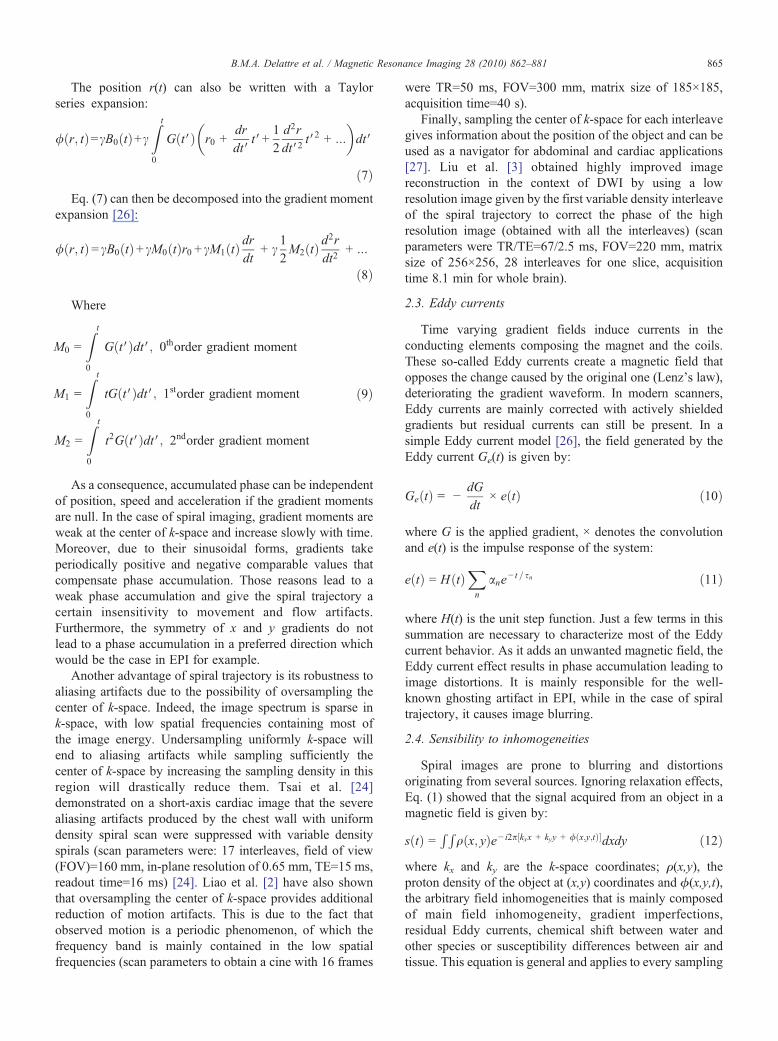
Spiral images are prone to blurring and distortionsoriginating from several sources. Ignoring relaxation effects,Eq. (1) showed that the signal acquired from an object in amagnetic field is given by:

sðtÞ = R Rqðx; yÞe− i2p½kxx + kyy + /ðx;y;tÞ�dxdy ð12Þwhere kx and ky are the k-space coordinates; ρ(x,y), theproton density of the object at (x,y) coordinates and ϕ(x,y,t),the arbitrary field inhomogeneities that is mainly composedof main field inhomogeneity, gradient imperfections,residual Eddy currents, chemical shift between water andother species or susceptibility differences between air andtissue. This equation is general and applies to every sampling

866 B.M.A. Delattre et al. / Magnetic Resonance Imaging 28 (2010) 862–881

scheme. This means that even Cartesian sampling is prone tofield inhomogeneities. However, in Cartesian sampling, onlyone gradient is varied at a time, which implies that dephasingaffects only one direction. This results in a simple shift ofthe object. It is more problematic with spiral because bothin-plane gradients are varied continuously at the same time,resulting in a shift of the object in all directions that causesimage blurring. The exact reconstruction of such a signal isgiven by:

qðx; yÞ =Z T

0sðtÞei2pðkxx + kyyÞei2p /ðx;y;tÞdt ð13Þ

This is called the conjugate phase reconstruction, becausebefore integration, the signal is multiplied by the conjugateof phase accrued due to field inhomogeneities. Theinhomogeneity term can often be written as a linear relationwith time t, ϕ(x,y,t)=tϕ(x,y) implying that it is moresignificant when t is important. There are, though, twoapproaches to eliminate this effect: the first one is to useinterleaved spirals that have a short readout time t and thenlimit phase accumulation; the second is to correct for theinhomogeneities when reconstructing the image. Distortionand blurring induced by phase accumulation due toinhomogeneities are probably the main reasons that explainthe lack of success of spiral trajectories in clinical routine;however, with the improvements of methods to measure andcorrect for these inhomogeneities, this situation should notbe definitive.

2.5. Concomitant fields

Another parameter that can alter the image quality isconcomitant gradient fields. Indeed, Maxwell's equationsimply that imaging gradients are accompanied by higherorder, spatially varying fields called concomitant fields.They can cause unwanted phase accumulation duringreadout resulting, again, in image blurring in the specialcase of spiral, but once again, even though Cartesiansampling is also affected by this additional dephasing,the effect on the image is simply less disturbing. Con-sidering identical x and y gradient coils with a relativeorientation of 90°, the lowest order concomitant field canbe expressed as [28]:

Bc=G2

z

8B0

� �x2+y2� �

+G2

x +G2y

2B0

!z2−

GxGz

2B0

� �xz−

GyGz

2B0

� �yz

ð14Þwhere x, y, z are the laboratory directions, B0 the staticfield, Gx, Gy, Gz the gradients in the laboratory system.Concomitant gradients cause phase accumulation duringthe readout gradient that is expressed by:

fcðtÞ = cP

Zt−l

Bcdt ð15Þ

The knowledge of the analytical dependence of this effectwith spatial coordinates is necessary to correct for itscontribution to image blurring.

3. Designing the trajectory

The first difficulty with spiral imaging is the design ofthe trajectory itself. Indeed, gradient solutions must befound by solving the differential Eqs. (4) and (5) that arecomputationally intensive to calculate even with the im-provement of hardware capabilities. Closed-form equationsare necessary to be easily usable on a clinical scanner. Totake maximum advantage of the gradient hardwarecapabilities, two regimes are defined. Indeed, near thecenter of k-space, the trajectory is only limited by thegradient slew-rate since gradient amplitude is low. For thisslew-rate-limited regime, S(t) is set to the maximumavailable slew-rate Sm. Then, when reaching the maximalgradient amplitude, one comes into the so called amplitude-limited regime where G(t) is equal to the maximum availablegradient amplitude Gm.

3.1. General solution

A simple analytical solution for constant density (α=1)was first given by Dyun et al. [29] for the slew-rate limitedcase only and then extended by Glover [30] for the tworegimes. It was then generalized to variable density by Kimet al. [31]. They defined the function τ(t) as follows:

s tð Þ=

ffiffiffiffiffiffiffiffiffiSmckx2

ra2+1

� �t

" #1=ða=2+1Þslew−rate−limited regime

cGm

kxa+1ð Þt

1= ða+1Þamplitude−limited regime

8>>>><>>>>:

ð16Þ

The trajectory starts in the slew-rate-limited regime andswitches to the amplitude-limited regime when t correspondsto G(t)=Gm, the maximum available gradient amplitude.This closed-form solution has the advantage of being easilyimplemented on a clinical scanner. An example of thetrajectory obtained with this formulation, as well as thegradient waveform, is illustrated in Fig. 3. However, whenthe number of interleaves is increased, this trajectory leadsto large slew-rate overflow for small k-space values (i.e.,for t→0) as illustrated in Fig. 4. Depending on the gradientperformances, this can be a real problem with most clinicalscanners because slew-rates are limited and the execution ofa trajectory with such overshoot is simply impossible. Forexample, a spiral sequence was implemented on 3T Siemensclinical scanner (Magnetom TIM Trio, Siemens Healthcare,Erlangen Germany) using a maximum slew-rate of Sm=170T/(m·s) and a maximum gradient amplitude of Gm=26 mT/mhave been used. Simulations of Figs. 3 and 4 were done

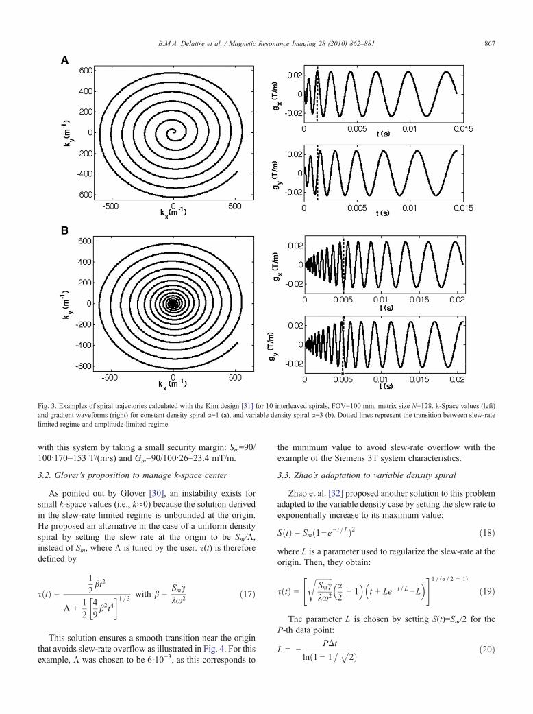
Fig. 3. Examples of spiral trajectories calculated with the Kim design [31] for 10 interleaved spirals, FOV=100 mm, matrix size N=128. k-Space values (left)and gradient waveforms (right) for constant density spiral α=1 (a), and variable density spiral α=3 (b). Dotted lines represent the transition between slew-ratelimited regime and amplitude-limited regime.

867B.M.A. Delattre et al. / Magnetic Resonance Imaging 28 (2010) 862–881

with this system by taking a small security margin: Sm=90/100·170=153 T/(m·s) and Gm=90/100·26=23.4 mT/m.

3.2. Glover's proposition to manage k-space center

As pointed out by Glover [30], an instability exists forsmall k-space values (i.e., k≈0) because the solution derivedin the slew-rate limited regime is unbounded at the origin.He proposed an alternative in the case of a uniform densityspiral by setting the slew rate at the origin to be Sm/Λ,instead of Sm, where Λ is tuned by the user. τ(t) is thereforedefined by

s tð Þ =12bt2

L +12

49b2t4

1=3 with b =Smckx2

ð17Þ

This solution ensures a smooth transition near the originthat avoids slew-rate overflow as illustrated in Fig. 4. For thisexample, Λ was chosen to be 6·10−3, as this corresponds to

the minimum value to avoid slew-rate overflow with theexample of the Siemens 3T system characteristics.

3.3. Zhao's adaptation to variable density spiral

Zhao et al. [32] proposed another solution to this problemadapted to the variable density case by setting the slew rate toexponentially increase to its maximum value:

SðtÞ = Smð1−e− t =LÞ2 ð18Þwhere L is a parameter used to regularize the slew-rate at theorigin. Then, they obtain:

s tð Þ =ffiffiffiffiffiffiffiffiffiSmckx2

ra2+ 1

� �t + Le− t =L−L� �" #1= ða =2 + 1Þ

ð19Þ

The parameter L is chosen by setting S(t)=Sm/2 for theP-th data point:

L = −PDt

lnð1 − 1 =ffiffiffiffiffi2Þp ð20Þ

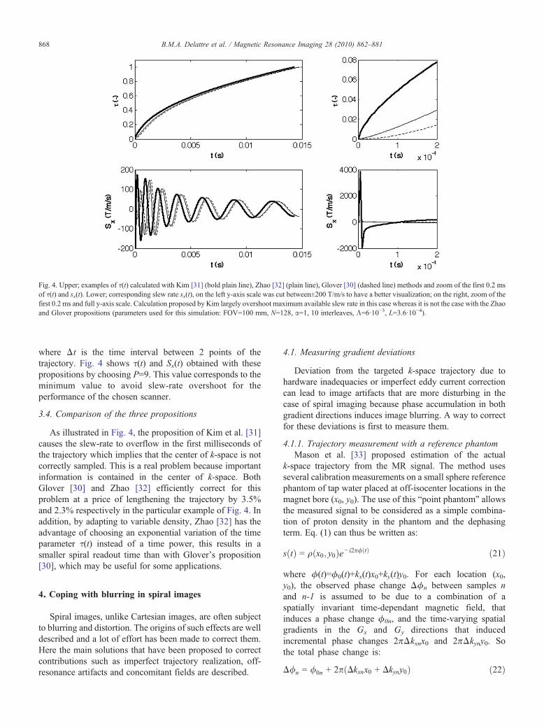
Fig. 4. Upper; examples of τ(t) calculated with Kim [31] (bold plain line), Zhao [32] (plain line), Glover [30] (dashed line) methods and zoom of the first 0.2 msof τ(t) and sx(t). Lower; corresponding slew rate sx(t), on the left y-axis scale was cut between±200 T/m/s to have a better visualization; on the right, zoom of thefirst 0.2 ms and full y-axis scale. Calculation proposed by Kim largely overshoot maximum available slew rate in this case whereas it is not the case with the Zhaoand Glover propositions (parameters used for this simulation: FOV=100 mm, N=128, α=1, 10 interleaves, Λ=6·10−3, L=3.6·10−4).

868 B.M.A. Delattre et al. / Magnetic Resonance Imaging 28 (2010) 862–881

where Δt is the time interval between 2 points of thetrajectory. Fig. 4 shows τ(t) and Sx(t) obtained with thesepropositions by choosing P=9. This value corresponds to theminimum value to avoid slew-rate overshoot for theperformance of the chosen scanner.

3.4. Comparison of the three propositions

As illustrated in Fig. 4, the proposition of Kim et al. [31]causes the slew-rate to overflow in the first milliseconds ofthe trajectory which implies that the center of k-space is notcorrectly sampled. This is a real problem because importantinformation is contained in the center of k-space. BothGlover [30] and Zhao [32] efficiently correct for thisproblem at a price of lengthening the trajectory by 3.5%and 2.3% respectively in the particular example of Fig. 4. Inaddition, by adapting to variable density, Zhao [32] has theadvantage of choosing an exponential variation of the timeparameter τ(t) instead of a time power, this results in asmaller spiral readout time than with Glover's proposition[30], which may be useful for some applications.

4. Coping with blurring in spiral images

Spiral images, unlike Cartesian images, are often subjectto blurring and distortion. The origins of such effects are welldescribed and a lot of effort has been made to correct them.Here the main solutions that have been proposed to correctcontributions such as imperfect trajectory realization, off-resonance artifacts and concomitant fields are described.

4.1. Measuring gradient deviations

Deviation from the targeted k-space trajectory due tohardware inadequacies or imperfect eddy current correctioncan lead to image artifacts that are more disturbing in thecase of spiral imaging because phase accumulation in bothgradient directions induces image blurring. A way to correctfor these deviations is first to measure them.

4.1.1. Trajectory measurement with a reference phantomMason et al. [33] proposed estimation of the actual

k-space trajectory from the MR signal. The method usesseveral calibration measurements on a small sphere referencephantom of tap water placed at off-isocenter locations in themagnet bore (x0, y0). The use of this “point phantom” allowsthe measured signal to be considered as a simple combina-tion of proton density in the phantom and the dephasingterm. Eq. (1) can thus be written as:

sðtÞ = qðx0; y0Þe− i2p/ðtÞ ð21Þ

where ϕ(t)=ϕ0(t)+kx(t)x0+ky(t)y0. For each location (x0,y0), the observed phase change Δϕn between samples nand n-1 is assumed to be due to a combination of aspatially invariant time-dependant magnetic field, thatinduces a phase change ϕ0n, and the time-varying spatialgradients in the Gx and Gy directions that inducedincremental phase changes 2πΔkxnx0 and 2πΔkyny0. Sothe total phase change is:

D/n = /0n + 2pðDkxnx0 + Dkyny0Þ ð22Þ

869B.M.A. Delattre et al. / Magnetic Resonance Imaging 28 (2010) 862–881

From the several acquisitions made at different locations(x0, y0) the data are fitted to determine the function kx(t),ky(t) and ϕ(t) by a least squares algorithm.

Some faster methods were also proposed that do notinvolve the displacement of a reference phantom but usethe signal from the studied subject. Spin location is doneby self-encoding gradients added just before readoutacquisition. Such gradients are calibrated gradientsapplied stepwise in the same direction as the fieldgradient to be measured [34]. They then combine differentacquisitions to obtain the phase change from which thek-space trajectory can be deduced the same way asMason et al. [33].

The method proposed by Alley et al. [35] uses thereadout data acquired with normal gradient waveforms andthen with reversed waveforms on a 10 cm phantom filledwith water. The signal obtained after a Fourier transform inthe phase encoding direction in one gradient direction canbe written as:

sFðx; tÞ = qðx; tÞe− i2p/Fðx;tÞ ð23Þwhere s+(t) refers to the “normal” acquisition and s-(t) to theone acquired with the reversed gradient waveform. Thephase term can be separated in odd and even terms:

/Fðx; tÞ = hðx; tÞF wðx; tÞF kðtÞx ð24ÞSubtraction of the two phases ϕ+ and ϕ− give access to

the trajectory data by a least square fit in the spatial direction.However, this method requires a high number of readoutacquisitions to characterize the whole k-space trajectory.

4.1.2. In-vivo trajectory measurementThe method proposed by Zhang et al. [36] is even faster

as it uses only two slices positioned along each gradientof interest. This method is based on the proposition ofDuyn et al. [37] and has the advantage of being used invivo, thus avoiding fastidious preliminary calibration ofthe trajectory with a phantom. The trajectory is obtaineddirectly from the phase difference between the twoacquired signals. In fact, if one assumes an infinitely thinslice, the signal for a slice normal to the x-axis located atx0 is:

sðx0; tÞ = e− i2p/ðx0;tÞR R

qðx0; y; zÞe− i2pkyðtÞydydz ð25Þwhere the phase term is:

/ðx0; tÞ = kxðtÞx0 + wðtÞ ð26Þ

Then, the trajectory is obtained by subtracting the phaseof signal from two close slices located at x1 and x2:

kx tð Þ = /ðx2; tÞ − /ðx1; tÞx2 − x1

ð27Þ

This method was compared with the small-phantommethod from Mason et al. [33], and authors have found a

very good accordance between results. This method is thusthe first that can be used directly in a human subject.However, when high resolution is needed, some significanterrors are observed for high k-space values.

A correction recently proposed by Beaumont et al. [38]greatly improves this latter technique. Indeed, from Eq.(13), they show that for a well-shimmed squared sliceprofile, the nonlinear spatial variation of B0 field canbe neglected so the term ϕ(x,y,t) becomes ϕ(t). Then, thesignal is the Fourier transform of the “effective magneti-zation density” ρ(x,y)e−i2πϕ(t). If the slice is located in thex plane at x=0 and considering an homogenous sample, theeffective magnetization density is proportional to the sliceprofile, so the signal can be written as:

s kx tð Þð Þ~ sinðp kxðtÞDsÞp kxðtÞDs ð28Þ

where Δs is the slice thickness. This function has severalzeros located at kx=nΔs−1 (n an integer N1). If kmax≥Δs−1,zero or very low signal can be encountered preventing thecalculation of the trajectory at these points. They solve thisproblem by adding another gradient that shifts k-spacepoints in order to avoid the nulling signal and allowrecovery of the high k-space values.

4.1.3. Trajectory estimation by one-time system calibrationRecently, Tan et al. [39] described an efficient method

to correct for the trajectory deviations. They described thealteration of k-space trajectory by both anisotropic gradientdelays in each physical axis as well as Eddy currents. Fortrajectories like spiral, residual Eddy currents can causesevere distortion in images. They proposed a model inwhich each contribution is separated and corrected afterapplying system calibration. The model only depends ongradient system parameters in the physical coordinates thatcan be found by measuring the real trajectory andcomparing it with the theoretical one.

Indeed, as explained by Aldefeld et al. [40], some timingdelays exist in hardware between the command and effectiveapplication of the gradient by gradient amplifiers. Thesedelays can be different in each physical axis so have to becharacterized separately. The delayed gradients in the logicalcoordinates are thus simply a rotation of those defined in thelaboratory coordinates:

GdL = RTGd = RT

"Gxðt − sxÞGyðt − syÞGzðt − szÞ

#ð29Þ

where GdL is the delayed gradient in logical coordi-nates; RT, the rotation matrix and τ, the delays in thethree directions.

Tan et al. [39] showed that Eddy currents induce ak-space trajectory which can be simply modeled as theintegration of the convolution of slew-rate of the desiredgradient waveform and the system impulse response. From

870 B.M.A. Delattre et al. / Magnetic Resonance Imaging 28 (2010) 862–881

Eq. (10), and considering the Taylor expansion of theexponential contained in Eq. (11) they obtain:

keðtÞ =Z t

0

SðtVÞ × HðtVÞdtV

cAZ t

0

GðtVÞdtV+ BZt0

GðtVÞtVdtV− BZt0

Z tV

0

ðdG = dsÞsdsdtV

ð30Þwhere A=−Σnan and B=Σn(an/bn). This last form repre-sents the scaling term for the theoretical k-space trajectoryin the first term and the two other terms are the systemresponse for gradient switching (for more details see [39]).The main advantage of this method is that the measure-ment of system parameters τx,y,z, A and B needs to bedone only once and can then be used for any sliceposition. The authors compared the improvement of imagequality with their method to the simple anisotropic gradientcompensation and noticed that eddy current model mustbe added in order to correct efficiently for the residualk-space imperfections.

4.2. Correcting off-resonance effects

Off-resonance effects refer to signal contributions withresonance frequencies different to the central water protonresonance frequency. These contributions mainly come fromthe chemical shift between water and other species, fromsusceptibility differences between different tissues orbetween air and tissue and from main field inhomogeneities.Field inhomogeneities are especially important for sequenceswhere off-center slices are difficult to shim or in areas wheresusceptibility differences and motion are important, forexample, in the thorax.

As the spiral sampling scheme usually has a longerreadout time, it is more affected by off resonance effects than

Fig. 5. Synthetic scheme of the time-segmented re

the classical Cartesian scheme. These effects accumulate allalong the readout time and result in image blurring that canbe important. One can easily see from Eq. (13) that this exactconjugate phase reconstruction needs a lot of computationtime because each pixel must be reconstructed with its ownoff resonance frequency ϕ(x,y). Fortunately, faster alter-natives to this exact reconstruction have been developed andare described below.

4.2.1. Field map estimationThe correction for these inhomogeneities first needs

knowledge of the field map to assess the term ϕ(x,y) shownin Eq. (13). A rapid method proposed by Schneider [41]consists of the acquisition of two datasets with differentecho times. The image obtained for each acquisition isgiven by:

s1ðx; yÞ = q1ðx; yÞe− i2pðTE1/ðx;yÞÞ

s2ðx; yÞ = q2ðx; yÞe− i2pðTE2/ðx;yÞÞ ð31Þ

and:

s41s2 = q1q2e− i2pð/ðx;yÞðTE2 −TE1ÞÞ ð32Þ

so the field inhomogeneity term is simply given by thephase of the two images:

/ x; yð Þ = angleðs41s2Þ2pðTE2 − TE1Þ =

angleðs41s2Þ2pDt

ð33Þ

The phase has to be unwrapped or limited by choosingΔtshort enough.

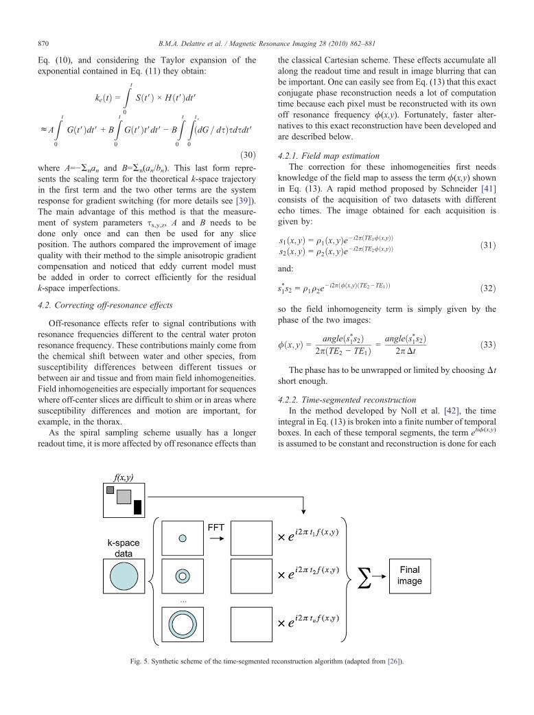
4.2.2. Time-segmented reconstructionIn the method developed by Noll et al. [42], the time

integral in Eq. (13) is broken into a finite number of temporalboxes. In each of these temporal segments, the term etiϕ(x,y)

is assumed to be constant and reconstruction is done for each

construction algorithm (adapted from [26]).

871B.M.A. Delattre et al. / Magnetic Resonance Imaging 28 (2010) 862–881

segment. The final image is obtained by adding together theintegrals over all time segments:

qðx; yÞ =XTti =0

sðtiÞei2pðkxx + kyy + ti/ðx;yÞÞ ð34Þ

As shown in Fig. 5, the computation time depends on thenumber of temporal segments used for reconstruction andcan thus be quite important.

4.2.3. Frequency-segmented reconstruction andmultifrequency interpolation

A similar method was proposed by Noll et al. [43] andconsists of segmenting the inhomogeneity term, ϕ(x,y), intomultiple constant frequencies, ϕi(x,y). For each of thesefrequencies, an image was reconstructed and the final imagewas taken as a spatial combination of these different recon-structions based on spatial varying frequency. Fig. 6 illus-trates this algorithm. A refinement to this method wasdeveloped by Man et al. [44] and consists of writing the inho-mogeneity term as a linear combination of constant frequencyterms. This is the multifrequency interpolation being:

ei2p t/ðx;yÞ =Xi

ci½f ðx; yÞ� ei2p t/iðx;yÞ ð35Þ

For each frequency ϕi(x,y), an inverse reconstruction isperformed and the image obtained is:

qiðx; yÞ =Z T

0sðtÞei2pðkxx + kyyÞei2p t/iðx;yÞdt ð36Þ

The resultant image is taken as a linear combination ofthose images.

qðx; yÞ =Xi

ci½/ðx; yÞ�qiðx; yÞ ð37Þ

The coefficients ci are typically obtained from Eq. (35)with a least square algorithm. This method is faster than the

Fig. 6. Synthetic scheme of frequency-segmented r

classical frequency segmented method because it allowsreconstruction of fewer frequencies, as unknown frequen-cies can be obtained as a linear combination of the twonearest ones.

4.2.4. Linear field map interpolationThe last two methods give good correction of field

inhomogeneities but suffer from time-consuming algorithms,as several reconstructions must be done to obtain the finalimage. One fast and efficient technique proposed byIrarrazabal et al. [45] is to consider only the first ordervariation of the inhomogeneities, so the field map is fittedwith linear terms using a least square algorithm:

/ðx; yÞ = /0 + a x + b y ð38ÞThe model of signal received then becomes:

sðtÞ = e− i2p t /0R R

qðx; yÞe− i2pððkx + a tÞx + ðky + b tÞyÞdxdy ð39ÞKnowing ϕ0, α, β from the field map fit, the

reconstruction of the data can be done by replacing thetrajectory points by the corrected ones: kx′=kx+αt, ky′=ky+βtand demodulating the signal to frequency ϕ0. Then, thesignal is reconstructed in one single operation.

4.2.5. Off-resonance correction without fieldmap acquisition

Another method proposed by Noll et al. [46] consists ofcorrecting the blurring without knowledge of a field mapto help in the conjugate phase reconstruction process. Theystart from the idea that it should be possible to minimizethe blur of an image by reconstruction at various offresonance frequencies and then choosing the least blurrypixels to form a composite image. To automate theselection process, one needs a quantification of theblurriness. For this, they propose that an image recon-structed on resonance should be real, because all excited

econstruction algorithm (adapted from [26]).

872 B.M.A. Delattre et al. / Magnetic Resonance Imaging 28 (2010) 862–881

spins are in phase. In the presence of field inhomogeneities,this assumption is no longer true and the imaginary part ofthe reconstructed image becomes important. The quantifi-cation of this imaginary part can thus be used as a criterionfor defining the extent of off-resonance:

C½x; y; fiðx; yÞ� =R R j Imfq½x; y; fiðx; yÞ�g ja dxdy ð40Þ

where α is chosen empirically between 0.5 and 1 by theuser. The minimization of this criterion reduces the blurringduring the reconstruction. This method works well whenthe range of off-resonance frequencies is small, otherwisespurious minima can appear in the objective function,increasing the risk of a wrong choice of frequency, whichcan cause artifacts in the final image.

A refinement of this method was proposed by Man et al.[47] and consists of, first, estimating a coarse field map usingrelatively few demodulating frequencies to avoid spuriousminima given by the objective function. Then the minimi-zation is repeated with a better estimation of field map (i.e.,using a higher number of frequencies) but constrained by theprevious coarse estimation.

4.2.6. Recent improvements and propositionsRecently, Chen et al. [48] proposed a semi automatic

method for off-resonance correction that represents asignificant improvement over previously described methodsand makes reconstruction more robust. They propose to firstacquire a low-resolution field map and then perform afrequency constrained off resonance reconstruction from theacquired map. The first strategy used to perform thereconstruction is to incorporate a linear off-resonancecorrection term in the image as previously done in [45]and to add a parameter used to search for non linearcomponents of the off-resonance frequency, here ϕi:

qðx; yÞ = R sðtÞe− i2pt/0e− i2pððkx + a tÞx + ðky + b tÞyÞe− i2pt/i dt

ð41ÞThis modification can significantly improve the compu-

tational efficiency of the algorithm as it searches for a rangeof non-linear terms, and not for the actual off resonancefrequency directly.

The second strategy is to take into account regions wherethe field map varies nonlinearly by interpolating the fieldmap with polynomial terms instead of only linear terms.Thus, the model becomes:

qðx; yÞ = R sðtÞe− i2ptð/i + /pðx;yÞÞe− i2pðkxx + kyyÞdt ð42Þwhere ϕp(x,y) is the polynomial fit of field map and ϕi areconstant offset frequencies. Reconstruction can then be doneby multiple frequency interpolation [44].

Also recently, Barmet et al. [49] proposed a conceptuallydifferent approach to assess field inhomogeneities. Theyproposed to simply measure the magnetic field around theinvestigated object with an array of miniature field probes

that do not interfere with the main experiment. This has themain advantage of knowing the phase accrued during thesignal acquisition, i.e., in exactly the same conditions asthe experiment, so it does not require additional scan timefor the acquisition of a field map. The efficiency of thismethod was evaluated by Lechner at al. [50] in comparisonwith the so called “Duyn calibration Technique” (DCT)which is the method of trajectory measurement proposed byDuyn et al.[37] and Zhang et al. [36] and improved byBeaumont et al. [38]. They found that both DCT andmagnetic field monitoring effectively detect k-space offsetsand trajectory error propagation, and correct for general errorsources such as timing delays. Also, artifacts such asdeformation and blurring were dramatically reduced.

4.3. Managing with concomitant fields

As seen before, off-resonance effects can be assessedby a field map acquired with the method proposed bySchneider [41]. However, concomitant gradient effectsare independent of acquisition time (i.e., echo time TE)and can therefore not be assessed this way. Knowledgeof the analytical dependence of this effect with spatialcoordinates is necessary to correct for its contribution toimage blurring.

King et al. [51] have shown that the effect of concomitantgradients can be separated into 2 parts: the through-planeeffect and the in-plane effect which can be corrected withdifferent methods. The through-plane effect can be under-stood by considering a 2D axial scan (Gz=0). From Eq. (14):

Bc =G2

0

2B0

� �z2 with G0 tð Þ =

ffiffiffiffiffiffiffiffiffiffiffiffiffiffiffiffiffiffiffiffiffiffiffiffiffiffiffiG2

xðtÞ + G2yðtÞ

qð43Þ

This means that the concomitant field is 0 at isocenter andincreases quadratically with off-center distance z. It is,however, independent of position within any given axialplane. Therefore, with some approximations, the phase shiftdue to this contribution can be seen as a time-dependantfrequency shift varying with plane position zc given by:

/c zc; tð Þ = cPz2c2B0

G20 tð Þ ð44Þ

Then the signal received becomes:

sðtÞ = ei2p/cðzc;tÞR Rqðx; yÞei2pðkxx + kyyÞdxdy ð45ÞThe correction for this effect can be done by demodulat-

ing the signal data over the time with frequency ϕc(zc,t)before the reconstruction of the image.

The in-plane effect of concomitant fields can beunderstood by considering, this time, a 2D sagittal plane(i.e. Gx=0). Again, from Eq. (14):

Bc =1

2B0

G2z x

2

4+

Gzy2

−Gyz

� �2" #

ð46Þ

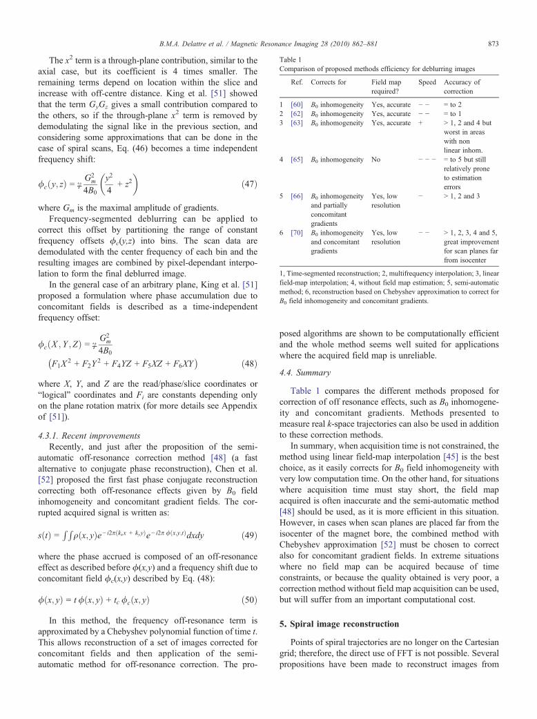
Table 1Comparison of proposed methods efficiency for deblurring images

Ref. Corrects for Field maprequired?

Speed Accuracy ofcorrection

1 [60] B0 inhomogeneity Yes, accurate − − = to 22 [62] B0 inhomogeneity Yes, accurate − − = to 13 [63] B0 inhomogeneity Yes, accurate + N 1, 2 and 4 but

worst in areaswith nonlinear inhom.

4 [65] B0 inhomogeneity No − − − = to 5 but stillrelatively proneto estimationerrors

5 [66] B0 inhomogeneityand partiallyconcomitantgradients

Yes, lowresolution

− N 1, 2 and 3

6 [70] B0 inhomogeneityand concomitantgradients

Yes, lowresolution

− − N 1, 2, 3, 4 and 5,great improvementfor scan planes farfrom isocenter

1, Time-segmented reconstruction; 2, multifrequency interpolation; 3, linearfield-map interpolation; 4, without field map estimation; 5, semi-automaticmethod; 6, reconstruction based on Chebyshev approximation to correct forB0 field inhomogeneity and concomitant gradients.

873B.M.A. Delattre et al. / Magnetic Resonance Imaging 28 (2010) 862–881

The x2 term is a through-plane contribution, similar to theaxial case, but its coefficient is 4 times smaller. Theremaining terms depend on location within the slice andincrease with off-centre distance. King et al. [51] showedthat the term GyGz gives a small contribution compared tothe others, so if the through-plane x2 term is removed bydemodulating the signal like in the previous section, andconsidering some approximations that can be done in thecase of spiral scans, Eq. (46) becomes a time independentfrequency shift:

/c y; zð Þ = cPG2

m

4B0

y2

4+ z2

� �ð47Þ

where Gm is the maximal amplitude of gradients.Frequency-segmented deblurring can be applied to

correct this offset by partitioning the range of constantfrequency offsets ϕc(y,z) into bins. The scan data aredemodulated with the center frequency of each bin and theresulting images are combined by pixel-dependant interpo-lation to form the final deblurred image.

In the general case of an arbitrary plane, King et al. [51]proposed a formulation where phase accumulation due toconcomitant fields is described as a time-independentfrequency offset:

/c X ; Y ; Zð Þ = cPG2

m

4B0

F1X2 + F2Y

2 + F4YZ + F5XZ + F6XY� � ð48Þ

where X, Y, and Z are the read/phase/slice coordinates or“logical” coordinates and Fi are constants depending onlyon the plane rotation matrix (for more details see Appendixof [51]).

4.3.1. Recent improvementsRecently, and just after the proposition of the semi-

automatic off-resonance correction method [48] (a fastalternative to conjugate phase reconstruction), Chen et al.[52] proposed the first fast phase conjugate reconstructioncorrecting both off-resonance effects given by B0 fieldinhomogeneity and concomitant gradient fields. The cor-rupted acquired signal is written as:

sðtÞ = R Rqðx; yÞe− i2pðkxx + kyyÞe− i2p /ðx;y;tÞdxdy ð49Þ

where the phase accrued is composed of an off-resonanceeffect as described before ϕ(x,y) and a frequency shift due toconcomitant field ϕc(x,y) described by Eq. (48):

/ðx; yÞ = t /ðx; yÞ + tc /cðx; yÞ ð50Þ

In this method, the frequency off-resonance term isapproximated by a Chebyshev polynomial function of time t.This allows reconstruction of a set of images corrected forconcomitant fields and then application of the semi-automatic method for off-resonance correction. The pro-

posed algorithms are shown to be computationally efficientand the whole method seems well suited for applicationswhere the acquired field map is unreliable.

4.4. Summary

Table 1 compares the different methods proposed forcorrection of off resonance effects, such as B0 inhomogene-ity and concomitant gradients. Methods presented tomeasure real k-space trajectories can also be used in additionto these correction methods.

In summary, when acquisition time is not constrained, themethod using linear field-map interpolation [45] is the bestchoice, as it easily corrects for B0 field inhomogeneity withvery low computation time. On the other hand, for situationswhere acquisition time must stay short, the field mapacquired is often inaccurate and the semi-automatic method[48] should be used, as it is more efficient in this situation.However, in cases when scan planes are placed far from theisocenter of the magnet bore, the combined method withChebyshev approximation [52] must be chosen to correctalso for concomitant gradient fields. In extreme situationswhere no field map can be acquired because of timeconstraints, or because the quality obtained is very poor, acorrection method without field map acquisition can be used,but will suffer from an important computational cost.

5. Spiral image reconstruction

Points of spiral trajectories are no longer on the Cartesiangrid; therefore, the direct use of FFT is not possible. Severalpropositions have been made to reconstruct images from

874 B.M.A. Delattre et al. / Magnetic Resonance Imaging 28 (2010) 862–881

k-space data. One idea was to use the extension of thediscrete Fourier transform, also called phase conjugatereconstruction [53], but this method is very time consuming.Other methods are based on regularized model basedreconstructions [54,55]. For now, the most commonly usedmethod is the regridding algorithm [56,57]. This basicallyconsists of interpolation of k-space points on the Cartesiangrid that then allows the application of an FFT, whichremains the most computationally efficient algorithm forreconstruction. However, interpolation in k-space leads toerrors that are spread over the whole image once recon-structed. This part must therefore be done with caution.Moreover, variable density sampling encountered in spiralmust be taken into account before interpolation onto theCartesian grid, this requires compensation for differentlysampled areas by multiplying the data by a densitycompensation function (DCF). This implies also postcom-pensation of data after the gridding step. To generate thegridded data points, the problem of data resampling canalso be solved by the BURS (block uniform resampling)algorithm [58], where a set of linear equation is given anoptimal solution using the pseudoinverse matrix computedwith singular value decomposition (SVD). Moreover, noiseand artifact reduction can be obtained by using truncatedSVD [59]. This algorithm has the advantage to avoid thepre and post compensation steps of the gridding algorithm.Other alternatives to calculation of DCF were proposedeither by iteratively reconstructing data using matricesscaled larger than target matrix [60] or by using an iterativedeconvolution-interpolation algorithm [61]. Another prop-osition is to calculate a generalized FFT (GFFT) toreconstruct data which is mathematically the same algo-rithm than regridding with a Gaussian kernel; however,GFFT was shown to be more precise in the case ofreconstruction of small matrices [62]. This review focuseson the regridding algorithm because it is still the mostwidely used and is the basis of a large number of otherreconstruction alternatives.

5.1. Density compensation function

As spiral sampling is not uniform over k-space somecompensation must be done in order to avoid an over-weighting of low spatial frequencies compared to highfrequencies, which would result in signal intensity distor-tions. This can be done in several ways. For example, if thedensity varies smoothly, Meyer et al. [63] showed goodreconstructed image quality by using the analytical formu-lation of the trajectory to compensate for the variable density.However, this method is no longer reliable when the densityvaries sharply or in the case of less ideal spiral trajectories.Hoge et al. [64] compared several analytical propositionswith their method using the determinant of the Jacobianmatrix between Cartesian coordinates and the spiralsampling parameters of time and interleave rotation angleused as a density compensation function. They could show

the reliability of their method even in the case of trapezoidalor distorted gradient waveforms.

However, when the real trajectory moves too far awayfrom the theoretical one, another approach independent ofthe sampling pattern should be used. This is based on theVoronoi diagram [65] to calculate the area around eachsampling point. This area is then used to compensate fordensity variation, the bigger the area around the sample (thesize of the Voronoi cell), the smaller the density sampling.Rasche et al. [66] have shown the power of this technique inthe case of a distorted spiral trajectory, the advantage beingthat this technique depends only on the sampling pattern andnot on the acquisition order. This technique neverthelessneeds knowledge of the real trajectory (see section“Measuring gradient deviation” in “Coping with blurringin spiral images”) and may be limited due to the highcomputational complexity of the Voronoi diagram.

5.2. Interpolation onto the Cartesian grid

Once the samples have been corrected for the non-uniformdensity, they need to be interpolated onto the Cartesiangrid in order to perform the FFT algorithm for imagereconstruction. O'Sullivan [57] showed that the best way tointerpolate samples was the use of an infinite sinc function.Samples in the Fourier domain are convolved with a sincfunction, resulting in a multiplication with the Fouriertransformation of a sinc function (a boxcar function) in theimage domain. In practice, the use of an infinite sincfunction is not possible. In regridding, this function isreplaced by compactly supported kernels. However, thecomputational simplicity of the kernel must be balancedwith the level of artifacts in the resulting image, which is notan easy tradeoff. Jackson et al. [56] investigated severalkernels and showed that the Kaiser-Bessel kernel gave thebest reconstructed image quality. In this case, however, thefinal image must be corrected by dividing by the Fouriertransform of the kernel to avoid distorted intensities due tothe fact that it is no longer a rectangular function; this is theso-called roll-off correction.

5.3. Spiral imaging and parallel imaging

As mentioned earlier, spiral acquisition schemes are stillnot commonly used in the clinic, even though spiralimaging has several advantages over standard Cartesianacquisitions. One main reason for this is that Cartesianacquisitions are routinely accelerated with parallel imaging,whereas this is not trivial for spiral acquisitions. Withoutparallel imaging, the speed advantage of spiral trajectoriesis compromised. However, recently introduced methods fornon-Cartesian parallel imaging, in conjunction with im-proved computer performance, will enable the use ofaccelerated spiral acquisition schemes for both clinicalroutine and research.

In parallel imaging, acceleration of the image acquisitionis performed by reducing the sampling density of the k-space

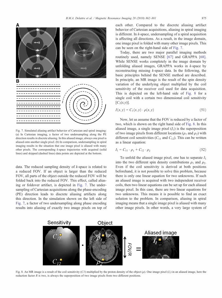
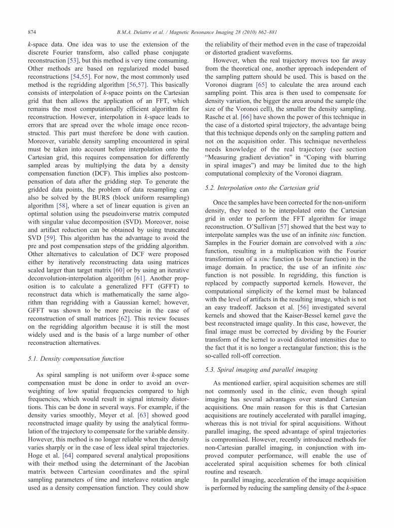
Fig. 7. Simulated aliasing artifact behavior of Cartesian and spiral imaging:(a) In Cartesian imaging, a factor of two undersampling along the PEdirection results in discrete aliasing. In this aliased image, always one pixel isaliased onto another single pixel. (b) In comparison, undersampling in spiralimaging results in the situation that one image pixel is aliased with manyother pixels. The corresponding k-space trajectories with acquired (solidlines) and skipped (dashed lines) data points are depicted at the bottom.

875B.M.A. Delattre et al. / Magnetic Resonance Imaging 28 (2010) 862–881

data. The reduced sampling density of k-space is related toa reduced FOV. If an object is larger than the reducedFOV, all parts of the object outside the reduced FOV will befolded back into the reduced FOV. This effect, called alias-ing or foldover artifact, is depicted in Fig. 7. The under-sampling of Cartesian acquisitions along the phase-encoding(PE) direction leads to discrete aliasing artifacts alongthis direction. In the simulation shown on the left side ofFig. 7, a factor of two undersampling along phase encodingresults into aliasing of exactly two image pixels on top of

Fig. 8. An MR image is a result of the coil sensitivity (C1) multiplied by the protonreduction factor R is two, is always the superposition of two image pixels from tw

each other. Compared to the discrete aliasing artifactbehavior of Cartesian acquisitions, aliasing in spiral imagingis different. In k-space, undersampling of a spiral acquisitionis affecting all directions. As a result, in the image domain,one image pixel is folded with many other image pixels. Thiscan be seen on the right-hand side of Fig. 7.

Today, there are two major parallel imaging methodsroutinely used, namely SENSE [67] and GRAPPA [68].While SENSE works completely in the image domain byunfolding aliased images, GRAPPA works in k-space byreconstructing missing k-space data. In the following, thebasic principles behind the SENSE method are described.In principle, an MR image is the result of the spin densityvariation of the underlying object multiplied by the coilsensitivity of the receiver coil used for data acquisition.This is depicted on the left-hand side of Fig. 8 for asingle coil with a certain two dimensional coil sensitivity[C1(x,y)].

Iðx; yÞ = C1ðx; yÞ � qðx; yÞ ð51Þ

Now, let us assume that the FOV is reduced by a factor oftwo, which is shown on the right hand side of Fig. 8. In thisaliased image, a single image pixel (I1) is the superpositionof two image pixels from different locations (ρ1 and ρ2) withdifferent coil sensitivities (C11 and C12). This can be writtenas a linear equation:

I1 = C11 � q1 + C12 � q2 ð52ÞTo unfold the aliased image pixel, one has to separate I1

into the two different spin density contributions ρ1 and ρ2.Even if the coil sensitivity is derived at both positionsbeforehand, it is not possible to solve this problem, becausethere is only one linear equation for two unknowns. If suchan aliased image is acquired with two independent receivercoils, then two linear equations can be set up for each aliasedimage pixel. In this case, there are two linear equations fortwo unknowns. This means it is possible to find an exactsolution to the problem. In comparison, aliasing in spiralimaging means that a single image pixel is aliased with manyother image pixels. In other words, a very large system of

density of the object (ρ). One image pixel (I1) in an aliased image, here theo different positions.

Fig. 9. Schematic depiction of the Conjugate Gradient SENSE reconstruction. Symbols are: CN* , conjugate of the sensitivity map of the Nth coil, IFFT, inverse

fast Fourier transform, GRID, gridding algorithm, DEGRID, degridding algorithm, CN, Sensitivity map of the Nth coil.

876 B.M.A. Delattre et al. / Magnetic Resonance Imaging 28 (2010) 862–881

linear equations has to be solved for each folded image pixel.Therefore, this kind of direct solution of the problem isimpractical due to computational burden. To address thisproblem, an iterative method, the Conjugate-Gradient (CG)method [69], was proposed for non-Cartesian SENSEreconstructions [70,71].

A schematic depiction of the Conjugate-GradientSENSE algorithm is shown in Fig. 9 (adapted from [71]).The iterative process starts with the undersampled,originally acquired, single-coil spiral k-space data. In afirst step, the spiral data are density corrected, gridded andFourier-transformed. Then the single coil images aremultiplied by the corresponding complex conjugate coilsensitivities and combined using a complex sum. Thisinitial image is the input for the CG algorithm as the firstguess for the actual image. The CG algorithm providesiteratively refined guesses by minimizing the residualbetween those guesses and the initial image. During eachiteration, the current guess is multiplied with the individualcoil sensitivities, which results in a separation into singlecoil images. The single coil images are Fourier-transformedand the resulting k-space data are degridded to obtain theupdated spiral k-space data. The subsequent procedure ofgridding, Fourier transform, conjugate sensitivity multipli-cation and summation is the same as for the originallyacquired data. A regularization term may be factored intothe iteration. A stopping criterion for the iteration has to bedefined, which is difficult, because stopping the process tooearly will yield aliasing artifacts, while stopping too latewill introduce noise to the reconstruction.

Even though the CG SENSE method significantlyreduces the computational burden, and allowed Weigeret al. [72] to demonstrate the benefits of accelerated spiralacquisitions, the major hindrance of this method was still

the reconstruction time. Parallel image reconstruction timesfor 2D spiral acquisitions have been reported to requireseveral hours and sometimes even days to reconstruct allimages from a typical functional MRI (fMRI) investigation[72–74]. Whereas these previous investigations haveperformed the reconstruction using coil sensitivity informa-tion from the image domain, recent approaches for parallelimaging of non-Cartesian k-space sampling by means of theGRAPPA algorithm, work completely in k-space andrepresent a promising approach to overcome computationallimits [75–77]. While Heberlein et al. [76] described adirect application of the radial GRAPPA approach to spiralimaging by Griswold et al. [75], Heidemann et al. [77]developed a more sophisticated algorithm. Both methodsenable accelerated single-shot spiral acquisitions, withoutthe need of a fully sampled spiral reference data set.However, Heidemann et al. [77] included an interpolationand reordering of the k-space data to generate radialsymmetry in the data, which simplifies the reconstructionprocess significantly.

It has been shown earlier that a constant-angular-velocity trajectory has a radial symmetry (see Fig. 2).Another important property of such a spiral is that thedistances in k-space between sampled data points alongsuch a line through the origin are constant, except forthose points directly adjacent to the central k-space point.The symmetry of the constant-angular-velocity spiral canbe used to simplify the parallel image reconstruction. For adirect spiral GRAPPA reconstruction, this symmetryenables the use of a conventional Cartesian GRAPPAreconstruction. The whole process is depicted in Fig. 10.The spiral data are acquired along a constant-angular-velocity trajectory to benefit from the advantages of thistrajectory. The data are then interpolated onto a constant-

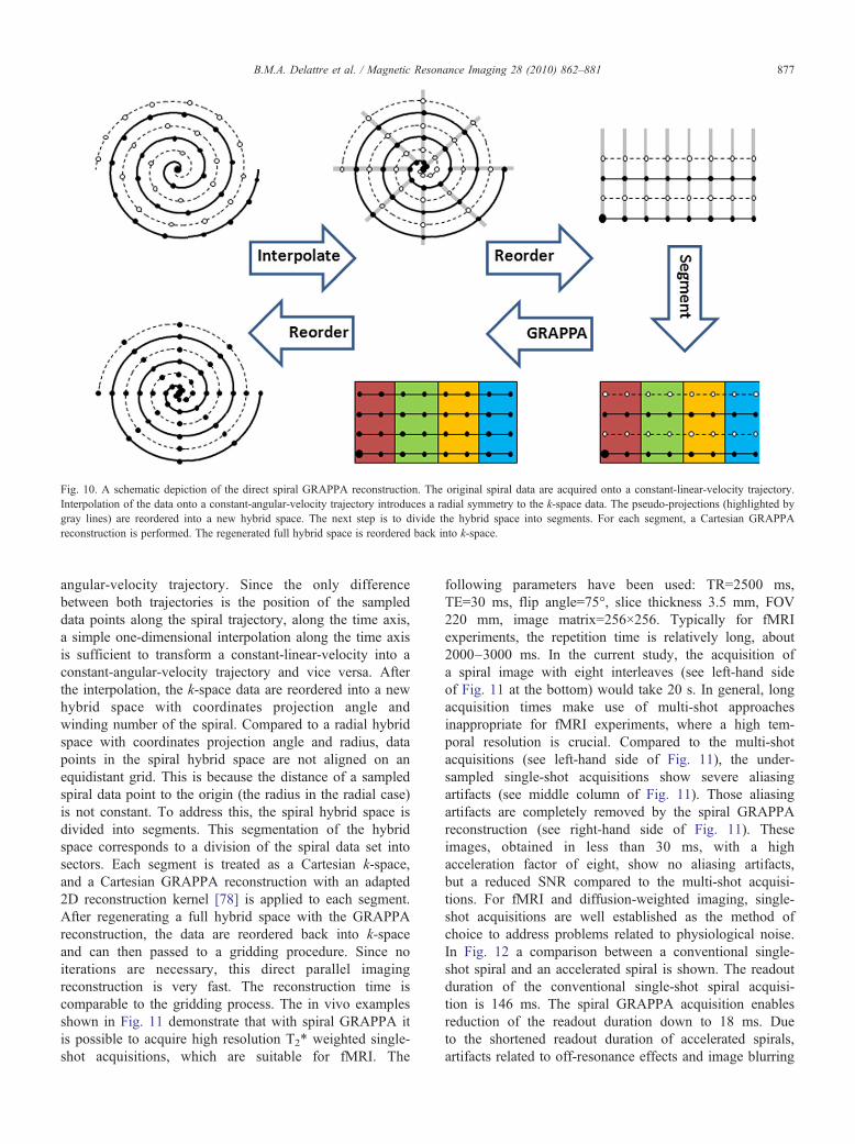
Fig. 10. A schematic depiction of the direct spiral GRAPPA reconstruction. The original spiral data are acquired onto a constant-linear-velocity trajectory.Interpolation of the data onto a constant-angular-velocity trajectory introduces a radial symmetry to the k-space data. The pseudo-projections (highlighted bygray lines) are reordered into a new hybrid space. The next step is to divide the hybrid space into segments. For each segment, a Cartesian GRAPPAreconstruction is performed. The regenerated full hybrid space is reordered back into k-space.

877B.M.A. Delattre et al. / Magnetic Resonance Imaging 28 (2010) 862–881

angular-velocity trajectory. Since the only differencebetween both trajectories is the position of the sampleddata points along the spiral trajectory, along the time axis,a simple one-dimensional interpolation along the time axisis sufficient to transform a constant-linear-velocity into aconstant-angular-velocity trajectory and vice versa. Afterthe interpolation, the k-space data are reordered into a newhybrid space with coordinates projection angle andwinding number of the spiral. Compared to a radial hybridspace with coordinates projection angle and radius, datapoints in the spiral hybrid space are not aligned on anequidistant grid. This is because the distance of a sampledspiral data point to the origin (the radius in the radial case)is not constant. To address this, the spiral hybrid space isdivided into segments. This segmentation of the hybridspace corresponds to a division of the spiral data set intosectors. Each segment is treated as a Cartesian k-space,and a Cartesian GRAPPA reconstruction with an adapted2D reconstruction kernel [78] is applied to each segment.After regenerating a full hybrid space with the GRAPPAreconstruction, the data are reordered back into k-spaceand can then passed to a gridding procedure. Since noiterations are necessary, this direct parallel imagingreconstruction is very fast. The reconstruction time iscomparable to the gridding process. The in vivo examplesshown in Fig. 11 demonstrate that with spiral GRAPPA itis possible to acquire high resolution T2* weighted single-shot acquisitions, which are suitable for fMRI. The

following parameters have been used: TR=2500 ms,TE=30 ms, flip angle=75°, slice thickness 3.5 mm, FOV220 mm, image matrix=256×256. Typically for fMRIexperiments, the repetition time is relatively long, about2000–3000 ms. In the current study, the acquisition ofa spiral image with eight interleaves (see left-hand sideof Fig. 11 at the bottom) would take 20 s. In general, longacquisition times make use of multi-shot approachesinappropriate for fMRI experiments, where a high tem-poral resolution is crucial. Compared to the multi-shotacquisitions (see left-hand side of Fig. 11), the under-sampled single-shot acquisitions show severe aliasingartifacts (see middle column of Fig. 11). Those aliasingartifacts are completely removed by the spiral GRAPPAreconstruction (see right-hand side of Fig. 11). Theseimages, obtained in less than 30 ms, with a highacceleration factor of eight, show no aliasing artifacts,but a reduced SNR compared to the multi-shot acquisi-tions. For fMRI and diffusion-weighted imaging, single-shot acquisitions are well established as the method ofchoice to address problems related to physiological noise.In Fig. 12 a comparison between a conventional single-shot spiral and an accelerated spiral is shown. The readoutduration of the conventional single-shot spiral acquisi-tion is 146 ms. The spiral GRAPPA acquisition enablesreduction of the readout duration down to 18 ms. Dueto the shortened readout duration of accelerated spirals,artifacts related to off-resonance effects and image blurring

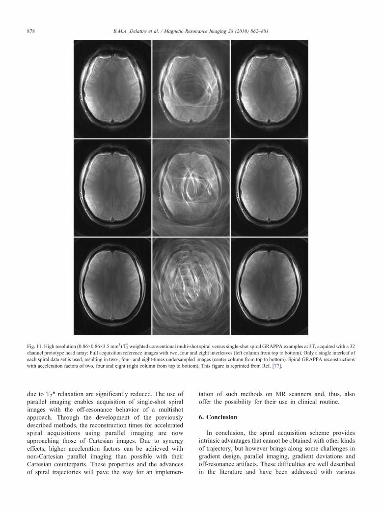
Fig. 11. High resolution (0.86×0.86×3.5 mm3) T2* weighted conventional multi-shot spiral versus single-shot spiral GRAPPA examples at 3T, acquired with a 32

channel prototype head array: Full acquisition reference images with two, four and eight interleaves (left column from top to bottom). Only a single interleaf ofeach spiral data set is used, resulting in two-, four- and eight-times undersampled images (center column from top to bottom). Spiral GRAPPA reconstructionswith acceleration factors of two, four and eight (right column from top to bottom). This figure is reprinted from Ref. [77].

878 B.M.A. Delattre et al. / Magnetic Resonance Imaging 28 (2010) 862–881

due to T2* relaxation are significantly reduced. The use ofparallel imaging enables acquisition of single-shot spiralimages with the off-resonance behavior of a multishotapproach. Through the development of the previouslydescribed methods, the reconstruction times for acceleratedspiral acquisitions using parallel imaging are nowapproaching those of Cartesian images. Due to synergyeffects, higher acceleration factors can be achieved withnon-Cartesian parallel imaging than possible with theirCartesian counterparts. These properties and the advancesof spiral trajectories will pave the way for an implemen-

tation of such methods on MR scanners and, thus, alsooffer the possibility for their use in clinical routine.

6. Conclusion

In conclusion, the spiral acquisition scheme providesintrinsic advantages that cannot be obtained with other kindsof trajectory, but however brings along some challenges ingradient design, parallel imaging, gradient deviations andoff-resonance artifacts. These difficulties are well describedin the literature and have been addressed with various

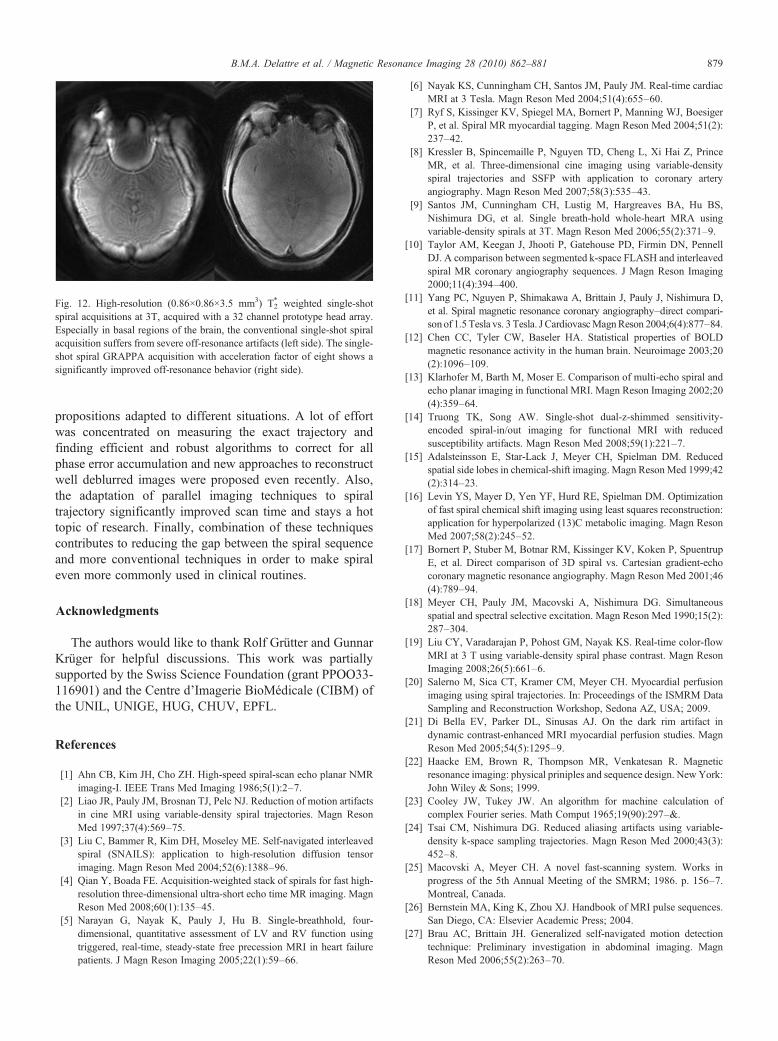
Fig. 12. High-resolution (0.86×0.86×3.5 mm3) T2* weighted single-shot

spiral acquisitions at 3T, acquired with a 32 channel prototype head array.Especially in basal regions of the brain, the conventional single-shot spiralacquisition suffers from severe off-resonance artifacts (left side). The single-shot spiral GRAPPA acquisition with acceleration factor of eight shows asignificantly improved off-resonance behavior (right side).

879B.M.A. Delattre et al. / Magnetic Resonance Imaging 28 (2010) 862–881

propositions adapted to different situations. A lot of effortwas concentrated on measuring the exact trajectory andfinding efficient and robust algorithms to correct for allphase error accumulation and new approaches to reconstructwell deblurred images were proposed even recently. Also,the adaptation of parallel imaging techniques to spiraltrajectory significantly improved scan time and stays a hottopic of research. Finally, combination of these techniquescontributes to reducing the gap between the spiral sequenceand more conventional techniques in order to make spiraleven more commonly used in clinical routines.

Acknowledgments

The authors would like to thank Rolf Grütter and GunnarKrüger for helpful discussions. This work was partiallysupported by the Swiss Science Foundation (grant PPOO33-116901) and the Centre d'Imagerie BioMédicale (CIBM) ofthe UNIL, UNIGE, HUG, CHUV, EPFL.

References

[1] Ahn CB, Kim JH, Cho ZH. High-speed spiral-scan echo planar NMRimaging-I. IEEE Trans Med Imaging 1986;5(1):2–7.

[2] Liao JR, Pauly JM, Brosnan TJ, Pelc NJ. Reduction of motion artifactsin cine MRI using variable-density spiral trajectories. Magn ResonMed 1997;37(4):569–75.

[3] Liu C, Bammer R, Kim DH, Moseley ME. Self-navigated interleavedspiral (SNAILS): application to high-resolution diffusion tensorimaging. Magn Reson Med 2004;52(6):1388–96.

[4] Qian Y, Boada FE. Acquisition-weighted stack of spirals for fast high-resolution three-dimensional ultra-short echo time MR imaging. MagnReson Med 2008;60(1):135–45.

[5] Narayan G, Nayak K, Pauly J, Hu B. Single-breathhold, four-dimensional, quantitative assessment of LV and RV function usingtriggered, real-time, steady-state free precession MRI in heart failurepatients. J Magn Reson Imaging 2005;22(1):59–66.

[6] Nayak KS, Cunningham CH, Santos JM, Pauly JM. Real-time cardiacMRI at 3 Tesla. Magn Reson Med 2004;51(4):655–60.

[7] Ryf S, Kissinger KV, Spiegel MA, Bornert P, Manning WJ, BoesigerP, et al. Spiral MR myocardial tagging. Magn Reson Med 2004;51(2):237–42.

[8] Kressler B, Spincemaille P, Nguyen TD, Cheng L, Xi Hai Z, PrinceMR, et al. Three-dimensional cine imaging using variable-densityspiral trajectories and SSFP with application to coronary arteryangiography. Magn Reson Med 2007;58(3):535–43.

[9] Santos JM, Cunningham CH, Lustig M, Hargreaves BA, Hu BS,Nishimura DG, et al. Single breath-hold whole-heart MRA usingvariable-density spirals at 3T. Magn Reson Med 2006;55(2):371–9.

[10] Taylor AM, Keegan J, Jhooti P, Gatehouse PD, Firmin DN, PennellDJ. A comparison between segmented k-space FLASH and interleavedspiral MR coronary angiography sequences. J Magn Reson Imaging2000;11(4):394–400.

[11] Yang PC, Nguyen P, Shimakawa A, Brittain J, Pauly J, Nishimura D,et al. Spiral magnetic resonance coronary angiography–direct compari-son of 1.5Tesla vs. 3 Tesla. J CardiovascMagnReson 2004;6(4):877–84.

[12] Chen CC, Tyler CW, Baseler HA. Statistical properties of BOLDmagnetic resonance activity in the human brain. Neuroimage 2003;20(2):1096–109.

[13] Klarhofer M, Barth M, Moser E. Comparison of multi-echo spiral andecho planar imaging in functional MRI. Magn Reson Imaging 2002;20(4):359–64.

[14] Truong TK, Song AW. Single-shot dual-z-shimmed sensitivity-encoded spiral-in/out imaging for functional MRI with reducedsusceptibility artifacts. Magn Reson Med 2008;59(1):221–7.

[15] Adalsteinsson E, Star-Lack J, Meyer CH, Spielman DM. Reducedspatial side lobes in chemical-shift imaging. Magn ResonMed 1999;42(2):314–23.

[16] Levin YS, Mayer D, Yen YF, Hurd RE, Spielman DM. Optimizationof fast spiral chemical shift imaging using least squares reconstruction:application for hyperpolarized (13)C metabolic imaging. Magn ResonMed 2007;58(2):245–52.

[17] Bornert P, Stuber M, Botnar RM, Kissinger KV, Koken P, SpuentrupE, et al. Direct comparison of 3D spiral vs. Cartesian gradient-echocoronary magnetic resonance angiography. Magn Reson Med 2001;46(4):789–94.

[18] Meyer CH, Pauly JM, Macovski A, Nishimura DG. Simultaneousspatial and spectral selective excitation. Magn Reson Med 1990;15(2):287–304.

[19] Liu CY, Varadarajan P, Pohost GM, Nayak KS. Real-time color-flowMRI at 3 T using variable-density spiral phase contrast. Magn ResonImaging 2008;26(5):661–6.

[20] Salerno M, Sica CT, Kramer CM, Meyer CH. Myocardial perfusionimaging using spiral trajectories. In: Proceedings of the ISMRM DataSampling and Reconstruction Workshop, Sedona AZ, USA; 2009.

[21] Di Bella EV, Parker DL, Sinusas AJ. On the dark rim artifact indynamic contrast-enhanced MRI myocardial perfusion studies. MagnReson Med 2005;54(5):1295–9.

[22] Haacke EM, Brown R, Thompson MR, Venkatesan R. Magneticresonance imaging: physical priniples and sequence design. NewYork:John Wiley & Sons; 1999.

[23] Cooley JW, Tukey JW. An algorithm for machine calculation ofcomplex Fourier series. Math Comput 1965;19(90):297–&.

[24] Tsai CM, Nishimura DG. Reduced aliasing artifacts using variable-density k-space sampling trajectories. Magn Reson Med 2000;43(3):452–8.

[25] Macovski A, Meyer CH. A novel fast-scanning system. Works inprogress of the 5th Annual Meeting of the SMRM; 1986. p. 156–7.Montreal, Canada.

[26] Bernstein MA, King K, Zhou XJ. Handbook of MRI pulse sequences.San Diego, CA: Elsevier Academic Press; 2004.

[27] Brau AC, Brittain JH. Generalized self-navigated motion detectiontechnique: Preliminary investigation in abdominal imaging. MagnReson Med 2006;55(2):263–70.

880 B.M.A. Delattre et al. / Magnetic Resonance Imaging 28 (2010) 862–881

[28] Bernstein MA, Zhou XJ, Polzin JA, King KF, Ganin A, Pelc NJ, et al.Concomitant gradient terms in phase contrast MR: analysis andcorrection. Magn Reson Med 1998;39(2):300–8.

[29] Duyn JH, Yang Y. Fast spiral magnetic resonance imaging withtrapezoidal gradients. J Magn Reson 1997;128(2):130–4.

[30] Glover GH. Simple analytic spiral k-space algorithm. Magn ResonMed 1999;42(2):412–5.

[31] Kim DH, Adalsteinsson E, Spielman DM. Simple analytic variabledensity spiral design. Magn Reson Med 2003;50(1):214–9.

[32] Zhao T, Qian Y, Hue Y-K, Ibrahim TS, Boada F. An improvedanalytical solution for variable density spiral design. Proc Int SocMagn Reson Med 2008;16:1342.

[33] Mason GF, Harshbarger T, Hetherington HP, Zhang Y, PohostGM, Twieg DB. A method to measure arbitrary k-spacetrajectories for rapid MR imaging. Magn Reson Med 1997;38(3):492–6.

[34] Onodera T, Matsui S, Sekihara K, Kohno H. A method of measuringfield-gradient modulation shapes — application to high-speed NMRspectroscopic imaging. J Phys E 1987;20(4):416–9.

[35] Alley MT, Glover GH, Pelc NJ. Gradient characterization usinga Fourier-transform technique. Magn Reson Med 1998;39(4):581–7.

[36] Zhang Y, Hetherington HP, Stokely EM, Mason GF, Twieg DB. Anovel k-space trajectory measurement technique. Magn Reson Med1998;39(6):999–1004.

[37] Duyn JH, Yang Y, Frank JA, van der Veen JW. Simple correctionmethod for k-space trajectory deviations in MRI. J Magn Reson1998;132(1):150–3.

[38] Beaumont M, Lamalle L, Segebarth C, Barbier EL. Improved k-spacetrajectory measurement with signal shifting. Magn Reson Med2007;58(1):200–5.

[39] Tan H, Meyer CH. Estimation of k-space trajectories in spiral MRI.Magn Reson Med 2009;61(6):1396–404.

[40] Aldefeld B, Bornert P. Effects of gradient anisotropy in MRI. MagnReson Med 1998;39(4):606–14.

[41] Schneider E, Glover G. Rapid in vivo proton shimming. Magn ResonMed 1991;18(2):335–47.

[42] Noll DC, Meyer CH, Pauly JM, Nishimura DG, Macovski A. Ahomogeneity correction method for magnetic resonance imagingwith time-varying gradients. IEEE Trans Med Imaging 1991;10(4):629–37.

[43] Noll DC. “Reconstruction techniques for magnetic resonance imaging”PhD. Thesis, Stanford University. 1991.

[44] Man LC, Pauly JM, Macovski A. Multifrequency interpolation for fastoff-resonance correction. Magn Reson Med 1997;37(5):785–92.

[45] Irarrazabal P, Meyer CH, Nishimura DG, Macovski A. Inhomogeneitycorrection using an estimated linear field map. Magn Reson Med1996;35(2):278–82.

[46] Noll DC, Pauly JM, Meyer CH, Nishimura DG, Macovski A.Deblurring for non-2D Fourier transform magnetic resonance imaging.Magn Reson Med 1992;25(2):319–33.

[47] Man LC, Pauly JM, Macovski A. Improved automatic off-resonancecorrection without a field map in spiral imaging. Magn Reson Med1997;37(6):906–13.

[48] Chen W, Meyer CH. Semiautomatic off-resonance correction in spiralimaging. Magn Reson Med 2008;59(5):1212–9.

[49] Barmet C, Zanche ND, Pruessmann KP. Spatiotemporal magnetic fieldmonitoring for MR. Magn Reson Med 2008;60(1):187–97.

[50] Lechner SM, Sipila PT, Wiesinger F, Kerr AB, Vogel MW. Spiralimaging artifact reduction: a comparison of two k-trajectory measure-ment methods. J Magn Reson Imaging 2009;29(6):1485–92.

[51] King KF, Ganin A, Zhou XJ, Bernstein MA. Concomitant gradientfield effects in spiral scans. Magn Reson Med 1999;41(1):103–12.

[52] Chen W, Sica CT, Meyer CH. Fast conjugate phase imagereconstruction based on a Chebyshev approximation to correct forB0 field inhomogeneity and concomitant gradients. Magn Reson Med2008;60(5):1104–11.

[53] Maeda A, Sano K, Yokoyama T. Reconstruction by weightedcorrelation for MRI with time-varying gradients. IEEE Trans MedImaging 1988;7(1):26–31.

[54] Boubertakh R, Giovannelli JF, De Cesare A, Herment A. Non-quadratic convex regularized reconstruction of MR images from spiralacquisitions. Signal Process 2006;86(9):2479–94.

[55] Delattre B, Hyacinthe JN, Vallee JP, Van de Ville D. Spline-basedvariational reconstruction of variable density spiral k-space data withautomatic parameter adjustment. Proceedings of the of the 17th AnnualMeeting of the ISMRM, Hawai'i, USA; 2009. p. 2066.

[56] Jackson JI, Meyer CH, Nishimura DG, Macovski A. Selection of aconvolution function for Fourier inversion using gridding [compu-terised tomography application]. IEEE Trans Med Imaging 1991;10(3):473–8.

[57] O'Sullivan JD. A fast sinc function gridding algorithm for Fourierinversion in computer tomography. IEEE Trans Med Imaging 1985;4(4):200–7.

[58] Rosenfeld D. An optimal and efficient new gridding algorithmusing singular value decomposition. Magn Reson Med 1998;40(1):14–23.

[59] Moriguchi H, Duerk JL. Modified block uniform resampling (BURS)algorithm using truncated singular value decomposition: fast accurategridding with noise and artifact reduction. Magn Reson Med 2001;46(6):1189–201.

[60] Moriguchi H, Duerk JL. Iterative next-neighbor regridding(INNG): improved reconstruction from nonuniformly sampled k-space data using rescaled matrices. Magn Reson Med 2004;51(2):343–52.

[61] Gabr RE, Aksit P, Bottomley PA, Youssef AB, Kadah YM.Deconvolution-interpolation gridding (DING): accurate reconstructionfor arbitrary k-space trajectories. Magn Reson Med 2006;56(6):1182–91.

[62] Sarty GE, Bennett R, Cox RW. Direct reconstruction of non-Cartesiank-space data using a nonuniform fast Fourier transform. Magn ResonMed 2001;45(5):908–15.

[63] Meyer CH, Hu BS, Nishimura DG, Macovski A. Fast spiral coronaryartery imaging. Magn Reson Med 1992;28(2):202–13.

[64] Hoge RD, Kwan RK, Pike GB. Density compensation functions forspiral MRI. Magn Reson Med 1997;38(1):117–28.

[65] Aurenhammer F. Voronoi diagrams — a survey of afundamental geometric data structure. Comput Surv 1991;23(3):345–405.

[66] Rasche V, Proksa R, Sinkus R, Bornert P, Eggers H. Resampling ofdata between arbitrary grids using convolution interpolation. IEEETrans Med Imaging 1999;18(5):385–92.

[67] Pruessmann KP, Weiger M, Scheidegger MB, Boesiger P. SENSE:sensitivity encoding for fast MRI. Magn Reson Med 1999;42(5):952–62.

[68] Griswold MA, Jakob PM, Heidemann RM, Nittka M, Jellus V, WangJ, et al. Generalized autocalibrating partially parallel acquisitions(GRAPPA). Magn Reson Med 2002;47(6):1202–10.

[69] Hestenes MR, Stiefel E. Methods of conjugate gradients for solvinglinear systems. J Res Natl Bur Stand 1952;49(6):409–36.

[70] Kannengiesser SAR, Brenner AR, Noll TG. Accelerated imagereconstruction for sensitivity encoded imaging with arbitrary k-spacetrajectories. Proceedings of the 8th Annual meeting of ISMRM,Denver, CO; 2000. p. 155.

[71] Pruessmann KP, Weiger M, Bornert P, Boesiger P. Advances insensitivity encoding with arbitrary k-space trajectories. Magn ResonMed 2001;46(4):638–51.

[72] Weiger M, Pruessmann KP, Osterbauer R, Bornert P, Boesiger P,Jezzard P. Sensitivity-encoded single-shot spiral imaging for reducedsusceptibility artifacts in BOLD fMRI. Magn Reson Med 2002;48(5):860–6.

[73] Stenger VA, Sutton BP, Boada F, Fessler JA, Noll DC. Reversed spiralSENSE for fMRI. Proceedings of the 12th Scientific Meeting ISMRM,Kyoto, Japan; 2004. p. 1024.

881B.M.A. Delattre et al. / Magnetic Resonance Imaging 28 (2010) 862–881

[74] Yeh EN, McKenzie CA, Ohliger MA, Sodickson DK. Parallelmagnetic resonance imaging with adaptive radius in k-space(PARS): constrained image reconstruction using k-space locality inradiofrequency coil encoded data. Magn Reson Med 2005;53(6):1383–92.

[75] Griswold MA, Heidemann RM, Jakob PM. Direct parallel imagingreconstruction of radially sampled data using GRAPPA with relativeshifts. Proceedings of the 11th Annual Meeting of the ISMRM,Toronto, Canada; 2003. p. 2349.

[76] Heberlein K, Hu X. Auto-calibrated parallel spiral imaging. MagnReson Med 2006;55(3):619–25.

[77] Heidemann RM, Griswold MA, Seiberlich N, Kruger G, Kannen-giesser SA, Kiefer B, et al. Direct parallel image reconstructionsfor spiral trajectories using GRAPPA. Magn Reson Med 2006;56(2):317–26.

[78] Griswold MA. Advanced k-space techniques. Proceedings of the 2ndInternational Workshop on Parallel Imaging, Zuerich, Switzerland;2004. p. 16–8.