Reflection of Higher Order Modes at the End of a Baffled

Rectangular Duct

Ralph T. Muehleisen, David C. Swanson

Graduate Program in Acoustics and Applied Research Lab

Applied Science Building, University Park, PA 16802

(October 9, 1997)

Abstract

The reflection coefficients of the plane wave and some higher order in

a baffled duct modes were computed and measured. Analytical expressions

for the modal impedances and reflection coefficients were determined. The

analytical expressions show that there is no coupling between even and odd

order modes. The resulting integrals were numerically evaluated for a number

of modes to determine low order self reflection and coupling coefficients. The

computed values show coupling coefficients a factor of 5 below that of the self

reflection coefficients. Measurements fit the computations fairly well at low

frequencies.

1

INTRODUCTION

Rectangular ducts occur in a variety of industrial HVAC systems. Often the frequencies

of the propagating acoustics waves are high enough that many modes can propagate. It is

therefore important to look at how these modes reflect, couple, and radiate at the end of

the duct. Much research has been done on the reflection and radiation characteristics of

circular ducts, but surprisingly little has been done on rectangular ducts.

Research on radiation from the ends of ducts dates back at least as far as Rayleigh

[1]. Rayleigh was able to determine analytic expressions for the end corrections for the

radiation from baffled circular ducts. He also determined empirical expressions for the

corrections for unbaffled circular ducts. Analytical expressions for the unbaffled case were

finally determined by Levine and Schwinger [2] using Wiener-Hopf techniques. This analysis

was still only for the plane wave mode. Weinstein [3] developed expressions for higher order

modes. In addition, he was able to determine reflection coefficients from the end of plane

parallel (2-D) waveguides, but not for 3-D rectangular waveguides. Doak’s excellent works

[4,5] on the propagation in rectangular ducts lacks the explicit inclusion of modal coupling.

In omitting the coupling, much of the important physics is lost.

The purpose of this paper is to develop expressions for the modal impedances and reflec-

tion coefficients of baffled rectangular ducts. The resulting expressions for the normalized

modal impedances must be numerically integrated. The reflection coefficients are found in

terms of the normalized modal impedances of the baffled end.

I. DERIVATION OF NORMALIZED MODAL IMPEDANCES

The duct is assumed to be semi-infinite with rigid walls at x = 0, y = 0, x = a and y = b

and a baffled end at z = 0. Inside the duct the pressure field can be written

p(x, y, z) =∑M

(AMe−jkMz + BMejkMz)ψM(x, y) (1)

2

where ψM (x, y) = cos(mπ xa)cos(nπ y

b) and the single capital letter M is used to denote a

modal pair (m,n).

If modal coupling is assumed to occur at the baffled end, equation 1 can be rewritten as

p(x, y, z) =∑M

AMe−jkMzψM(x, y) +∑N

∑P

RNP AP ejkNzψN (x, y) (2)

where RNP is the reflection coefficient between modes P and N , i.e. how much of mode

P goes into mode N upon reflection.

Using Euler’s equation the velocity in the duct is found to be

uz(x, y, z) =∑M

kM

kρcAMe−jkMzψM(x, y) −

∑N

∑P

RNPkN

kρcAP e−jkNzψN(x, y) (3)

where kM =√

k2 − (mπ/a)2 − (nπ/b)2.

In the half space outside the duct, given the normal velocity at the end of the duct, the

radiated pressure can be determined using the Rayleigh integral [6–8]. The expression for

the pressure is then

p(x0, y0, 0) =jkρc

4π

∫∫

S

uz(x, y, 0)g(�x| �x0)dS. (4)

where uz is the normal velocity at z = 0 and g(�x| �x0) is the half space Green’s function

g(�x| �x0) = 2ejkr

r(5)

where r =√

(x − x0)2 + (y − y0)2 .

At z = 0 the pressure and normal velocity are continuous. Equation 3 can be substituted

in equation 4 to yield the equation

∑M

AMψM(x, y) +∑N

∑P

RNP AP ψN (x, y) =j

2π

∑M

kMAM

a∫

0

b∫

0

ψM(x0, y0)e−jkr

rdx0dy0

−∑N

∑P

kNRNP AP

a∫

0

b∫

0

ψN (x0, y0)e−jkr

rdx0dy0. (6)

Multiplying equation 6 by ψR and integrating across the duct cross section will eliminate

one of the sums on the left hand side of the equation. Equation 6 then reduces to

3

AR +∑P

RRP AP =∑M

AMζRM −∑N

∑P

RNP AP ζRN (7)

where

ζRM =jkM

2πabΛR

a∫

0

b∫

0

a∫

0

b∫

0

ψR(x, y)ψM(x0, y0)e−jkr

rdx0dy0dxdy. (8)

ζRM is the normalized complex mutual modal impedance between modes M and R. The

reason for this identification will become clear later on.

Because of the symmetric nature of the inner integral some general properties of ζRM

can be discussed. First, since the Green’s function is an even function, if R and M are not

both even or both odd, the overall integral must be equal to zero. Therefore there is no

coupling between even and odd numbered modes. Also, switching the modal numbers R

and M does not change the integrand. The only difference between ζRM and ζMR are the

multiplicative factors of KM and 1/ΛR, thus only the integral for one of the two situations

must be computed to find both impedances.

By rewriting equation 7 in matrix form, it will be possible to determine an expression

for RRM in terms of ζRM . Defining the matrices

A =

⎡⎢⎢⎢⎢⎢⎢⎣

A0

A1

...

⎤⎥⎥⎥⎥⎥⎥⎦

R =

⎡⎢⎢⎢⎢⎢⎢⎣

R00 R01 · · ·

R10 R11 · · ·...

......

⎤⎥⎥⎥⎥⎥⎥⎦

ζ =

⎡⎢⎢⎢⎢⎢⎢⎣

ζ00 ζ01 · · ·

ζ10 ζ11 · · ·...

......

⎤⎥⎥⎥⎥⎥⎥⎦

(9)

equation 7 can be rewritten

ζ + Rζ = ζA − ζRA (10)

from which R is found to be

R = (ζ + I)−1(ζ − I). (11)

From equation 11 it is clear that ζ should be identified as the normalized complex radi-

ation impedance matrix and ζRM as the normalized complex coupling impedance between

modes M and R.

4

Although the matrices R and ζ in the above equations are infinite in size, the coefficients

drop off fast enough for baffled ends that the matrices can be truncated to a relatively small

size. Because there is no coupling between even and odd modes, the matrices are less likely

to be singular and inversion is relatively straight forward.

II. DIRECTIVITY AND RADIATED POWER

Once the reflection coefficients are obtained, the pressure and velocity at the end of the

duct can be determined. From the pressure and velocity the radiated pressure directivity

and radiated power can be obtained.

The radiated pressure is obtained once again by using equation 5, the Rayleigh integral.

However, this time the observation point is not on the end of the duct, but is any point in

space. Assuming only one incident mode M on the end of the duct and using equation 3 in

5 the pressure can be written as

p(x, y, z) =jkM

2πAM

a∫

0

b∫

0

ψMejkR

Rdx0dy0

− j

2πAM

∑R

kRRRM

a∫

0

b∫

0

ψR(x0, y0)ejkR

Rdx0dy0. (12)

where

R =√

(x − x0)2 + (y − y0)2 + z2. (13)

To determine the directivity pattern and radiated power, the pressure can be evaluated

in the far field. The standard far field approximation is

R ≈ r − x sin(θ) cos(φ) − y sin(θ) sin(φ) (14)

With this approximation, equation 12 can be rewritten

p(r, θ, φ) =j

2π(AMkMΨM(α, β) − AM

∑N

RNMkNΨN(α, β))ejkr

r(15)

where α = k sin(θ) cos(φ) and β = k sin(θ) sin(φ) and

5

ΨM(α, β) =

a∫

0

b∫

0

ψM(x, y)e−jαxe−jβydxdy

=

a∫

0

b∫

0

cos(mπx

a) cos(nπ

y

b)e−jαxe−jβydxdy

=−4αβa2b2e−jαa/2e−jβb/2

[(mπ)2 − (αa)2][(nπ)2 − (βb)2]

⎛⎜⎜⎝j sin(αa/2)

cos(αa/2)

⎞⎟⎟⎠

⎛⎜⎜⎝j sin(βb/2)

cos(βb/2)

⎞⎟⎟⎠ (16)

In equation 16, j sin(αa/2) is used when m is even and cos(αa/2) is used when m is odd.

Similarly, j sin(βb/2) is used when n is even and cos(βb/2) is used when n is odd.

As expected, this is nearly the same result as for a simply supported baffled plate [8–10].

The difference is that for the plate the cosine terms are used for even m and the sine terms

for odd n. So, the directivity can be obtained from the results for the simply supported

plates, exchanging even and odd modes. The books by Junger and Feit [8] and Fahy [10]

give a thorough discussion on radiation from rectangular plates.

Given the reflection coefficients, the radiated power is easy to compute directly from

the duct modal coefficients. From the incident modes and the modal reflection coefficients

the power traveling toward and away from the duct termination can be determined. Since

there are no losses in the system, the difference must be the radiated power. Defining a new

matrix

C =1√kρc

⎡⎢⎢⎢⎢⎢⎢⎢⎢⎢⎢⎣

√k0 0 0 ...

0√

k 0 ...

0 0√

k2 ...

......

......

⎤⎥⎥⎥⎥⎥⎥⎥⎥⎥⎥⎦

(17)

the total power traveling toward the duct termination is

Π+ = AHCHCA. (18)

The total power traveling away from the duct termination is

Π− = BHCHCB = (RA)HCHRA = AHRHCHCRA. (19)

6

Thus the total radiated power is

ΠRad = AH(CHC − RHCHCR)A. (20)

III. EVALUATION OF INTEGRALS

Determination of ζRM requires numerical calculation of a four-fold integral with singu-

larities (whenever x = x0 and y = y0 the integral is singular). For the work in this paper,

the calculation was accomplished by dividing the problem into a pair two dimensional in-

tegrals. The duct region was broken into into small rectangles and the inner two integrals

were evaluated at the center point of each the rectangle using standard Gaussian integration

techniques.

For evaluation of the integral over the rectangle containing the observation point, the

singularity of the Green’s function makes numerical evaluation difficult. For that region,

transformation methods were used to remove the singularity. A simple polar transformation

was first applied, but the resulting integrand, while not singular, was still difficult to inte-

grate. Instead, it was found that the transformation used in the CHIEF [11] program was

found to work much better.

Once the inner two integrals were evaluated at the center of each rectangle, the outer

integrals were obtained by evaluating the remaining function at the center of each rectangle

and summing over all the rectangles. Because the result of the inner two integrals should

be a simple function which is is relatively easy to integrate a more involved integration

technique was not required.

The initial program was written in MATLAB using the freely available NIT integration

package, but in order to speed up the calculation the program was rewritten in FORTRAN.

7

IV. RESULTS

The following results are based on a duct of dimensions a = 0.228m and b = 0.10 m.

Only the M = 0, 1, 2 and R = 0, 1, 2 modes were considered so n = 0 and s = 0 throughout

while m = 0, 1, 2 and r = 0, 1, 2. In other words, only modes across the width of the duct

were considered, modes across the height of the duct were ignored.

Figure 1 shows the self reflection coefficients R00, R11, and R22. Each of the coefficients

has a value of 1 at the cutoff frequency of the mode, meaning that at just above the cutoff

frequency all the energy in the mode is reflected from the end of the duct;none is radiated.

Figure 2 shows the mutual reflection coefficients R02, R20. R02 tells us how much of mode

2 is reflected back into mode 0. At the cutoff frequency R02 is zero because all the energy is

reflected back into the mode itself (R22 =1). R20 represents how much of mode 0 is reflected

back into mode 2. R20 is always positive because the plane wave mode always propagates

and hence can always couple into mode 2, even if mode 2 is evanescent. For the baffled

end, the amplitudes of the coupling coefficients are about a factor of 5 below those of the

self reflection coefficients. This means that coupling is not a major factor in reflection and

radiation at higher frequencies, but it is not necessarily negligible. For an unbaffled duct,

where much more diffraction takes place at the end, the values are expected to be much

higher and therefore coupling is expected to be more important.

Figure 3 shows the normalized self radiation resistance (Re{Z}) Zr00, Zr11, Zr22. As

expected Zr00 starts at zero and tends to unity as the frequency increases. Similarly Z11

and Z22 start at zero at their cutoff frequencies and tend to 1/2 as the frequency increases.

They do not tend to unity because of the ΛR term in ζ .

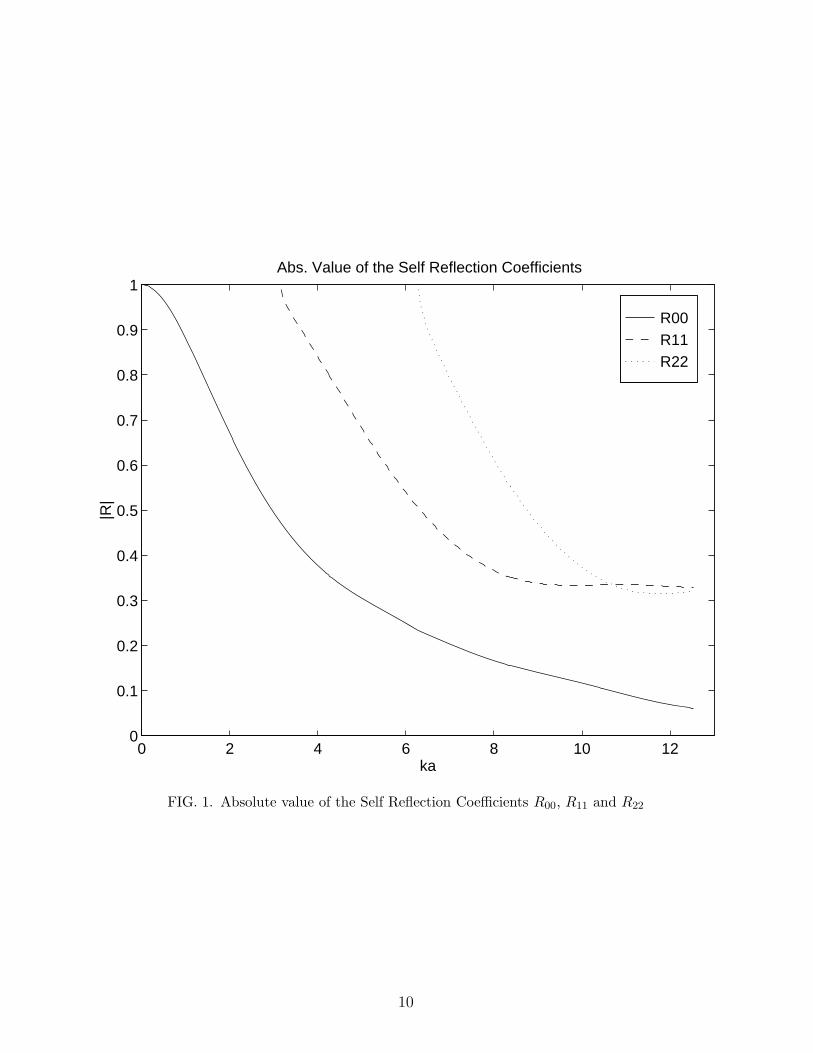
Figure 4 shows the normalized mutual radiation resistance Zr02 and Zr20. Like R20,

Zr20 > 0 even below the cutoff frequency of mode 2. It is interesting to note that Z20 has

its maximum value at the cutoff frequency of the mode. Zr02 = 0 at cutoff, and is positive

above the cutoff frequency. The peak amplitudes are a factor of 5 or 10 below those of the

self impedance.

8

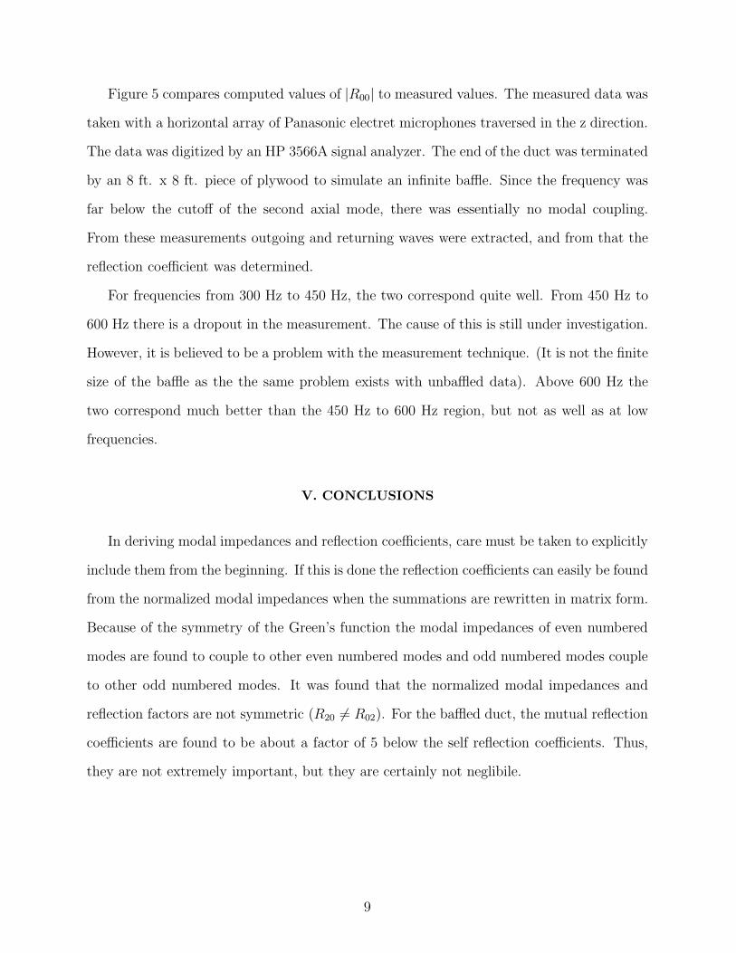
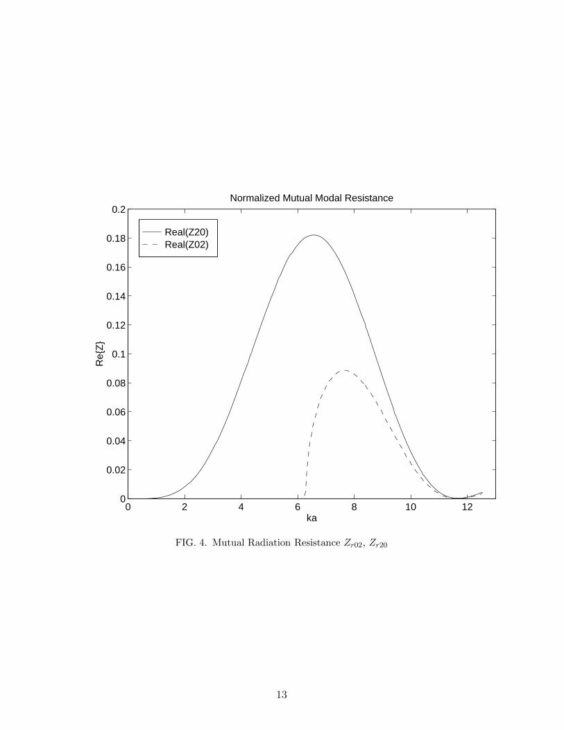
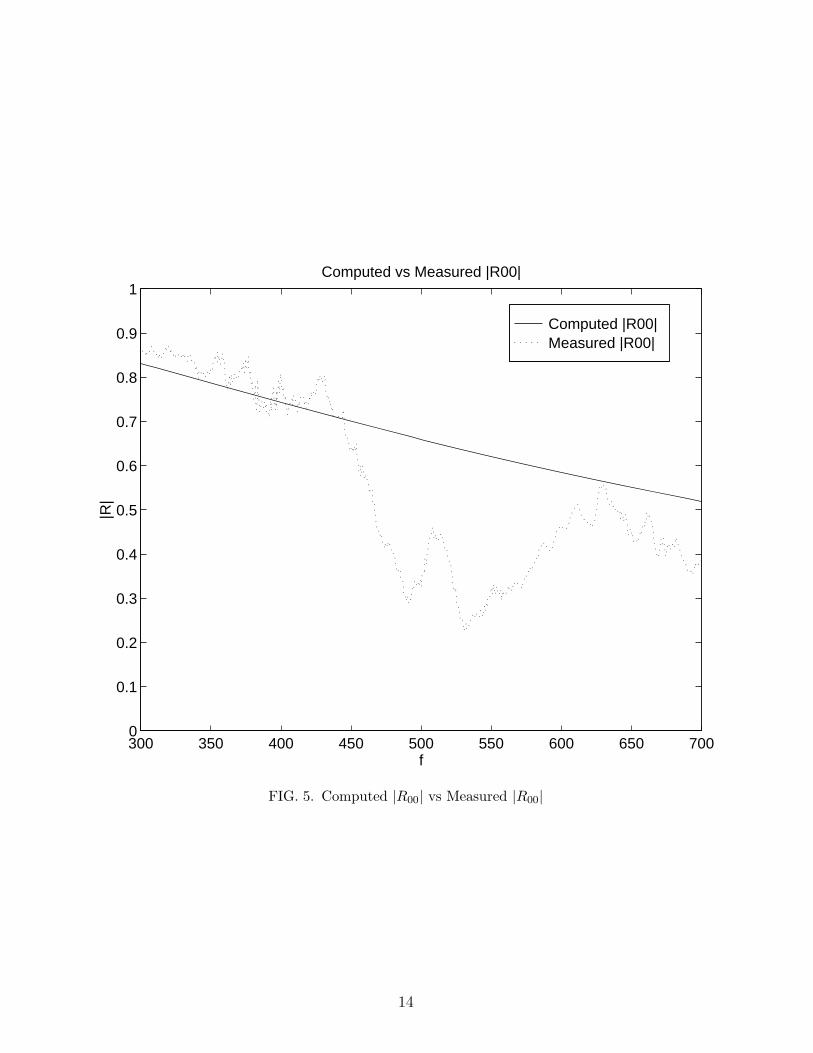
Figure 5 compares computed values of |R00| to measured values. The measured data was

taken with a horizontal array of Panasonic electret microphones traversed in the z direction.

The data was digitized by an HP 3566A signal analyzer. The end of the duct was terminated

by an 8 ft. x 8 ft. piece of plywood to simulate an infinite baffle. Since the frequency was

far below the cutoff of the second axial mode, there was essentially no modal coupling.

From these measurements outgoing and returning waves were extracted, and from that the

reflection coefficient was determined.

For frequencies from 300 Hz to 450 Hz, the two correspond quite well. From 450 Hz to

600 Hz there is a dropout in the measurement. The cause of this is still under investigation.

However, it is believed to be a problem with the measurement technique. (It is not the finite

size of the baffle as the the same problem exists with unbaffled data). Above 600 Hz the

two correspond much better than the 450 Hz to 600 Hz region, but not as well as at low

frequencies.

V. CONCLUSIONS

In deriving modal impedances and reflection coefficients, care must be taken to explicitly

include them from the beginning. If this is done the reflection coefficients can easily be found

from the normalized modal impedances when the summations are rewritten in matrix form.

Because of the symmetry of the Green’s function the modal impedances of even numbered

modes are found to couple to other even numbered modes and odd numbered modes couple

to other odd numbered modes. It was found that the normalized modal impedances and

reflection factors are not symmetric (R20 �= R02). For the baffled duct, the mutual reflection

coefficients are found to be about a factor of 5 below the self reflection coefficients. Thus,

they are not extremely important, but they are certainly not neglibile.

9

R00R11R22

0 2 4 6 8 10 120

0.1

0.2

0.3

0.4

0.5

0.6

0.7

0.8

0.9

1

ka

|R|

Abs. Value of the Self Reflection Coefficients

FIG. 1. Absolute value of the Self Reflection Coefficients R00, R11 and R22

10

R20R02

0 2 4 6 8 10 120

0.05

0.1

0.15

0.2

0.25

0.3

0.35

0.4

0.45

0.5

ka

|R|

Abs. Value of the Mutual Reflection Coefficients

FIG. 2. Absolute value of the Mutual Reflection Coefficients R02 and R20

11

Real(Z00)Real(Z11)Real(Z22)

0 2 4 6 8 10 120

0.2

0.4

0.6

0.8

1

ka

Re{

Z}

Normalized Self Modal Resistance

FIG. 3. Self Radiation Resistance Zr00, Zr11 and Zr22

12

Real(Z20)Real(Z02)

0 2 4 6 8 10 120

0.02

0.04

0.06

0.08

0.1

0.12

0.14

0.16

0.18

0.2

ka

Re{

Z}

Normalized Mutual Modal Resistance

FIG. 4. Mutual Radiation Resistance Zr02, Zr20

13

Computed |R00|Measured |R00|

300 350 400 450 500 550 600 650 7000

0.1

0.2

0.3

0.4

0.5

0.6

0.7

0.8

0.9

1

f

|R|

Computed vs Measured |R00|

FIG. 5. Computed |R00| vs Measured |R00|

14

REFERENCES

[1] J. W. S. Rayleigh, The Theory of Sound (Dover, New York, 1945), Vol. 2.

[2] H. Levine and J. Schwinger, Physical Review 73, 383 (1948).

[3] L. A. Weinstein, The Theory of Diffraction and The Factorization Method (The Golem

Press, Boulder, Colorado, 1969).

[4] P. E. Doak, Journal of Sound and Vibration 31, 1 (1973).

[5] P. E. Doak, Journal of Sound and Vibration 31, 137 (1973).

[6] P. M. Morse and K. U. Ingard, Theoretical Acoustics (Princeton Univerisity Press,

Princeton, New Jersey, 1968).

[7] A. D. Pierce, Acoustics - An Introduction into Its Physical Principles and Applications,

1989 ed. (Acoustical Society of America, Woodbury, New York, 1989).

[8] M. C. Junger and D. Feit, Sound, Structures and Their Interaction, 2nd ed. (MIT Press,

Cambridge, Massachussettes, 1986).

[9] C. E. Wallace, Journal of the Acoustical Society of America 51, 946 (1972).

[10] F. Fahy, Sound and Structural Vibration (Academic Press, London, 1993).

[11] D. G. G. Benthien, D. Barach, CHIEF Users Manual, NOSC Technical Document 970,

Naval Ocean Systems Center, 1988.

15