NOTE / NOTE

Boundary shear stress analysis in smoothrectangular channels

Galip Seckin, Neslihan Seckin, and Recep Yurtal

Abstract: This study reports on experiments concerning the boundary shear stress and boundary shear force distribu-tions in a smooth rectangular flume. Nonlinear regression-based equations are derived from experimental analysis togive the percentage of the total shear force carried by the walls and mean wall and bed shear stresses around the wet-ted perimeter as functions of the ratio of channel width to channel depth.

Key words: boundary shear, shear force, open channel flow.

Résumé : La présente étude examine les résultats expérimentaux concernant les distributions de la contrainte de cisail-lement limite et de la force de cisaillement limite dans un canal rectangulaire lisse. Les équations basées sur une ré-gression non linéaire sont dérivées d’une analyse expérimentale afin d’obtenir le pourcentage de la force totale decisaillement supportées par les murs ainsi que les contraintes de cisaillement moyennes dans le mur et le lit autour dupérimètre mouillé en tant que fonctions du rapport largeur/profondeur.

Mots clés : cisaillement limite, force de cisaillement, écoulement à surface libre.

[Traduit par la Rédaction] Seckin et al. 342

1. Introduction

The flow structure in an open channel is directly affectedby the shear stress distribution along the wetted perimeter. Itis difficult to determine boundary shear distributions in real-life applications. Laboratory flume studies have still beenserving to cope with this difficulty.

Knight et al. (1984) developed the following equations(i.e., eqs. [1]–[8]) giving the percentage of the shear force,mean wall, and bed shear stresses and the variation of themean bed shear velocity in an open channel:

[1] log(%SFw) = –1.4026 log(B/H + 3) + 2.6692

or

[2] SFw = exp(α)

in which

[3] α = –3.23 log(B/H + 3) + 6.146

where α is the coefficient used in eq. [2], %SFw is the per-centage of the shear force acting on the walls along a unitlength of the channel, B is the width of the channel, and H isthe depth of the channel;

[4]τ

ρw

fw0.01 SF

gHSBH

= ⎛⎝⎜ ⎞

⎠⎟%

2

[5]τ

ρb

fw0.01 SF

gHS= −1 %

where τw and τb are the mean wall and bed shear stresses,respectively; ρ is the density; g is gravitational acceleration;and Sf is the energy gradient;

[6]τ

ρw

fw0.01 SF

gRSBH

= +⎛⎝⎜ ⎞

⎠⎟% 1

2

[7]τ

ρb

fw0.01 SF

gRSHB

= − +⎛⎝⎜ ⎞

⎠⎟( % )1 1

2

where R is the hydraulic radius; and

[8]u* /

( / )% )b

bw0.01 SF

τ ρ= −1 1 2

where u* b is the mean bed shear velocity.Knight et al. (1984) used 43 data points for the range

0.3 < B/H < 6 and 12 data points for 6 < B/H < 15 to de-velop their empirically derived eqs. [1]–[8]. In the currentstudy, boundary shear stress distributions were measured de-

Can. J. Civ. Eng. 33: 336–342 (2006) doi:10.1139/L05-110 © 2006 NRC Canada

336

Received 13 December 2004. Revision accepted 11 November2005. Published on the NRC Research Press Web site athttp://cjce.nrc.ca on 31 March 2006.

G. Seckin,1 N. Seckin, and R. Yurtal. Department of CivilEngineering, Cukurova University, 01330 Balcali-Adana,Turkey.

Written discussion of this note is welcomed and will bereceived by the Editor until 31 July 2006.

1Corresponding author (e-mail: gseckin@cu.edu.tr).

liberately with aspect ratios between 6 and 15 to fill in andbolster the seemingly few data points in that interval in theformer study. Furthermore, an attempt was made to developnew nonlinear regression-based equations giving the per-centage of the total shear force carried by the walls and themean wall and bed shear stresses in an open channel.

2. Experimental work

The apparatus and procedure used by the writers havebeen adequately described elsewhere (Seckin 2004) and willtherefore only be outlined here.

The experiments were performed in a 22 m long non-tilting flume with a test length of 18 m, moulded into a com-pound channel at the University of Birmingham, Birming-ham, UK. The flood plains were isolated with L-shapedprofiles at the bankfull level to obtain a single rectangularcross section of the flume.

Discharges were measured by an electromagnetic flowmeter, a venturimeter, and a dall tube. For a given test dis-charge, the tailgate at the downstream end of the flume wasadjusted to produce uniform flow conditions in the 18 m testlength. Water-surface profiles were measured directly usingpoint gauges. Bed slope was fixed at 2.024 × 10–3.

The boundary shear stress was measured using a Prestontube (Preston 1954) of 4.75 mm outer diameter. Static andtotal heads were measured by connecting the tube to a sim-ple manometer. The static head was measured separately us-ing a Pitot static tube at the centreline of the measuringsection. Dynamic heads determined as the differences be-tween the total and static heads were converted to localboundary shear stress using the calibration relationships ofPatel (1965).

3. Results

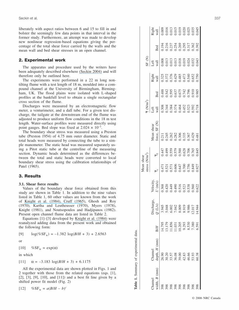
3.1. Shear force resultsValues of the boundary shear force obtained from this

study are shown in Table 1. In addition to the nine valueslisted in Table 1, 60 other values are known from the workof Knight et al. (1984), Cruff (1965), Ghosh and Roy(1970), Kartha and Leutheusser (1970), Myers (1978),Knight (1981), and Noutsopoulos and Hadjipanos (1982).Present open channel flume data are listed in Table 2.

Equations [1]–[3] developed by Knight et al. (1984) werereanalyzed adding data from the present work and obtainedthe following form:

[9] log(%SFw) = –1.382 log(B/H + 3) + 2.6563

or

[10] %SFw = exp(α)

in which

[11] α = –3.183 log(B/H + 3) + 6.1175

All the experimental data are shown plotted in Figs. 1 and2 together with those from the related equations (eqs. [1],[2], [3], [9], [10], and [11]) and a best fit line given by ashifted power fit model (Fig. 2)

[12] %SFw = a(B/H – b)c

© 2006 NRC Canada

Seckin et al. 337

Mea

nsh

ear

stre

ss(N

/m2 )

τ(N

/m2 )

SF

(N)

Cha

nnel

wid

th,

B(m

m)

Cha

nnel

dept

h,H

(mm

)B

/HD

isch

arge

,Q

(L/s

)V

eloc

ity,

U(m

/s)

τ eτ 0

Mea

nsh

ear

forc

e,S

F(N

)L

eft

wal

lB

edR

ight

wal

lL

eft

wal

lB

edR

ight

wal

l

398

26.9

014

.795

3.94

50.

368

0.47

10.

447

0.21

10.

308

0.48

80.

325

0.00

80.

194

0.00

939

830

.20

13.1

795.

048

0.42

00.

521

0.49

90.

245

0.34

40.

542

0.37

20.

013

0.21

60.

016

398

33.5

711

.856

6.00

20.

449

0.57

10.

559

0.26

20.

384

0.59

50.

376

0.01

30.

237

0.01

339

836

.08

11.0

317.

042

0.49

00.

606

0.57

90.

282

0.37

40.

637

0.42

90.

013

0.25

40.

015

398

39.0

010

.205

8.00

90.

516

0.64

70.

588

0.30

60.

464

0.67

50.

485

0.01

80.

269

0.01

939

842

.83

9.29

38.

919

0.52

30.

700

0.62

80.

335

0.45

20.

742

0.47

30.

019

0.29

50.

020

398

46.6

68.

530

9.98

60.

538

0.75

60.

706

0.36

70.

523

0.79

60.

540

0.02

40.

317

0.02

539

853

.93

7.38

012

.017

0.56

00.

849

0.76

50.

429

0.59

20.

910

0.65

20.

032

0.36

20.

035

398

60.3

86.

591

14.9

440.

622

0.92

70.

845

0.48

10.

718

0.98

50.

750

0.04

30.

392

0.04

5

Tab

le1.

Sum

mar

yof

expe

rim

enta

lda

ta.

where a = 933.57, b = –3.93, and c = –1.64 as constants.

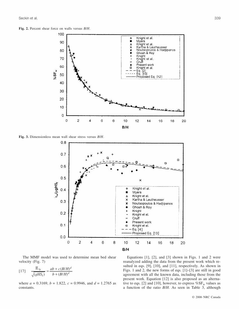
3.2. Mean wall and bed shear stresses resultsA rational function model was used to determine mean

wall shear stress (Fig. 3)

[13]τ

ρw

fgHSa b B H

c B H d B H= +

+ +( / )

( / ) ( / )1 2

where a = –0.115, b = 0.833, c = 1.004, and d = 0.021 asconstants.

The Morgan–Mercer–Flodin (MMF) model was used todetermine mean bed shear stress (Fig. 4)

[14]τ

ρb

fgHSab c B H

b B H

d

d= +

+( / )

( / )

where a = 0.0875, b = 2.9937, c = 0.9896, and d = 1.311 asconstants.

Alternatively, the mean wall and bed shear stresses can bedetermined nondimensionally dividing by the mean overallshear stress ( )= ρgRSf , as done by Knight et al. (1984). A lo-gistic model was used to determine mean wall shear stress(Fig. 5)

[15]τ

ρw

fgRSa

b c B H=

+ −1 exp[ ( / )]

where a = 0.011, b = –0.989, and c = 0.00034 as constants.A rational function model was used to determine mean

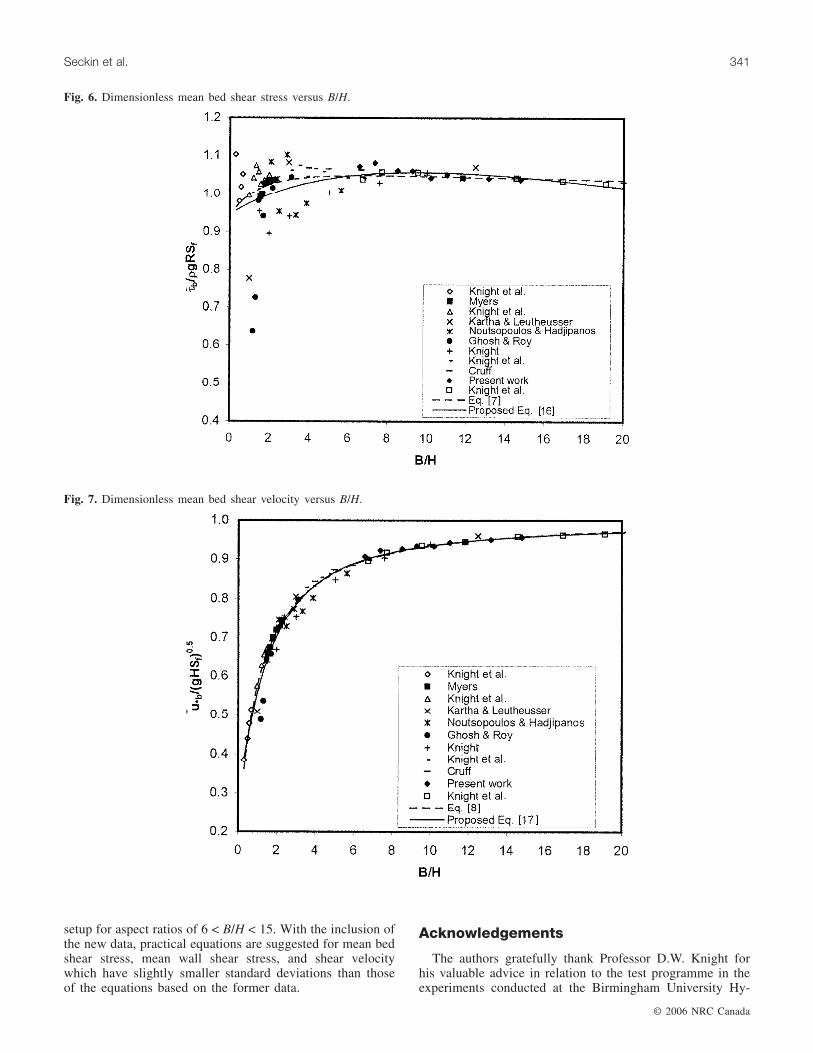
bed shear stress (Fig. 6)

[16]τ

ρb

fgRSa b B H

c B H d B H= +

+ +( / )

( / ) ( / )1 2

where a = 0.946, b = 0.117, c = 0.088, and d = 0.0011 asconstants.

© 2006 NRC Canada

338 Can. J. Civ. Eng. Vol. 33, 2006

B/H

Percent shearforce onwalls, %SFw

Mean wallshear stress,τw/ρgHSf

Mean bedshear stress,τb/ρgHSf

Mean wallshear stress,τw/ρgRSf

Mean bedshear stress,τb/ρgRSf

Mean bedshear velocity,u gHS*

//( )b f1 2

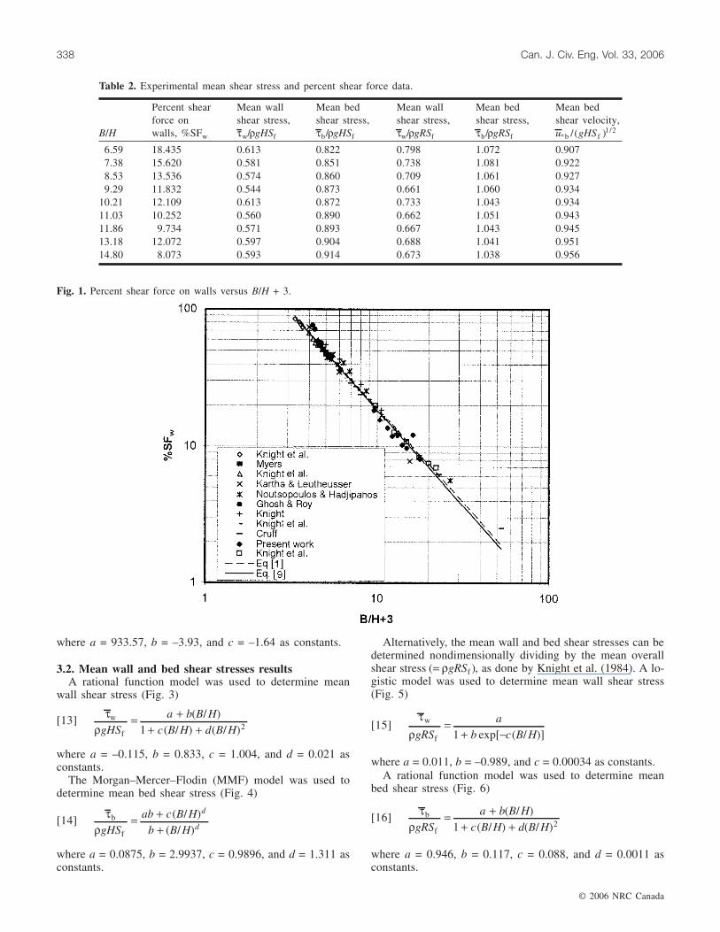
6.59 18.435 0.613 0.822 0.798 1.072 0.9077.38 15.620 0.581 0.851 0.738 1.081 0.9228.53 13.536 0.574 0.860 0.709 1.061 0.9279.29 11.832 0.544 0.873 0.661 1.060 0.934

10.21 12.109 0.613 0.872 0.733 1.043 0.93411.03 10.252 0.560 0.890 0.662 1.051 0.94311.86 9.734 0.571 0.893 0.667 1.043 0.94513.18 12.072 0.597 0.904 0.688 1.041 0.95114.80 8.073 0.593 0.914 0.673 1.038 0.956

Table 2. Experimental mean shear stress and percent shear force data.

Fig. 1. Percent shear force on walls versus B/H + 3.

The MMF model was used to determine mean bed shearvelocity (Fig. 7)

[17]u

gHS

ab c B Hb B H

d

d*

( )

( / )( / )

b

f

= ++

where a = 0.3169, b = 1.822, c = 0.9946, and d = 1.2765 asconstants.

Equations [1], [2], and [3] shown in Figs. 1 and 2 werereanalyzed adding the data from the present work which re-sulted in eqs. [9], [10], and [11], respectively. As shown inFigs. 1 and 2, the new forms of eqs. [1]–[3] are still in goodagreement with all the known data, including those from thepresent work. Equation [12] is also proposed as an alterna-tive to eqs. [2] and [10], however, to express %SFw values asa function of the ratio B/H. As seen in Table 3, although

© 2006 NRC Canada

Seckin et al. 339

Fig. 2. Percent shear force on walls versus B/H.

Fig. 3. Dimensionless mean wall shear stress versus B/H.

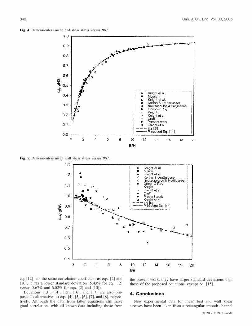
eq. [12] has the same correlation coefficient as eqs. [2] and[10], it has a lower standard deviation (5.43% for eq. [12]versus 5.67% and 6.02% for eqs. [2] and [10]).

Equations [13], [14], [15], [16], and [17] are also pro-posed as alternatives to eqs. [4], [5], [6], [7], and [8], respec-tively. Although the data from latter equations still havegood correlations with all known data including those from

the present work, they have larger standard deviations thanthose of the proposed equations, except eq. [15].

4. Conclusions

New experimental data for mean bed and wall shearstresses have been taken from a rectangular smooth channel

© 2006 NRC Canada

340 Can. J. Civ. Eng. Vol. 33, 2006

Fig. 4. Dimensionless mean bed shear stress versus B/H.

Fig. 5. Dimensionless mean wall shear stress versus B/H.

setup for aspect ratios of 6 < B/H < 15. With the inclusion ofthe new data, practical equations are suggested for mean bedshear stress, mean wall shear stress, and shear velocitywhich have slightly smaller standard deviations than thoseof the equations based on the former data.

Acknowledgements

The authors gratefully thank Professor D.W. Knight forhis valuable advice in relation to the test programme in theexperiments conducted at the Birmingham University Hy-

© 2006 NRC Canada

Seckin et al. 341

Fig. 6. Dimensionless mean bed shear stress versus B/H.

Fig. 7. Dimensionless mean bed shear velocity versus B/H.

draulic Laboratory in England. The authors are also gratefulto Professor Tefaruk Haktanir for his very helpful commentson this paper.

References

Cruff, R.W. 1965. Cross-channel transfer of linear momentum insmooth rectangular channels. US Geological Survey, Washing-ton, D.C. Geological Survey Water-Supply Paper 1592-B,pp. B1–B26.

Ghosh, S.N., and Roy, N. 1970. Boundary shear distribution inopen channel flow. ASCE Journal of the Hydraulics Division,96(4): 967–994.

Kartha, V.C., and Leutheusser, H.J. 1970. Distribution of tractiveforce in open channels. ASCE Journal of the Hydraulics Divi-sion, 96(7): 1469–1483.

Knight, D.W. 1981. Boundary shear in smooth and rough channels.ASCE Journal of the Hydraulics Division, 107(7): 839–851.

Knight, D.W., Demetriou, J.D., and Hamed, M.E. 1984. Boundaryshear in smooth rectangular channels. ASCE Journal of Hydrau-lic Engineering, 110(4): 405–422.

Myers, W.R.C. 1978. Momentum transfer in a compound channel.Journal of Hydraulic Research, 16(2): 139–150.

Noutsopoulos, G.C., and Hadjipanos, P.A. 1982. Discussion of“Boundary shear in smooth and rough channels” by D.W. Knight.ASCE Journal of Hydraulic Engineering, 108(6): 809–812.

Patel, V.C. 1965. Calibration of the preston tube and limitations onits use in pressure gradients. Journal of Fluid Mechanics, 23(1):185–208.

Preston, J.H. 1954. The determination of turbulent skin friction bymeans of pitot tube. Journal of the Royal Aeronautical Society,58(1): 109–121.

Seckin, G. 2004. A comparison of one-dimensional methods forestimating discharge capacity of straight compound channels.Canadian Journal of Civil Engineering, 31: 619–631.

List of symbols

a, b, c, d constantsB channel widthg gravitational accelerationH channel depthP wetted perimeterQ dischargeR hydraulic radiusSf energy slope

SF shear force%SF percent shear force

u*b mean bed shear velocityU section mean velocity obtained from the venturimeterα coefficient used in eq. [2]ρ densityτ local shear stressτ mean shear stress

τe mean boundary shear stress calculated by τ ρe f= gRSτ0 measured mean boundary shear stress

Subscripts

b bedw wall

© 2006 NRC Canada

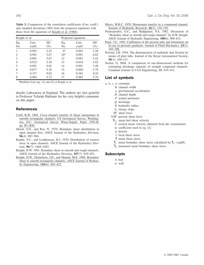
342 Can. J. Civ. Eng. Vol. 33, 2006

Knight et al. Proposed equations

Eq.No.

Corr.coeff.

SD(%)

Eq.No.

Corr.coeff.

SD(%)

1 0.993 2.25 9a 0.993 2.292 0.991 5.67 10a 0.991 6.022 0.991 5.67 12 0.991 5.434 0.933 5.39 13 0.934 4.925 0.991 9.03 14 0.991 7.496 0.877 5.38 15 0.869 5.797 0.337 9.02 16 0.383 8.248 0.964 5.72 17 0.965 5.35

aModified from eqs. [1] and [2] of Knight et al.

Table 3. Comparison of the correlation coefficients (Corr. coeff.)and standard deviations (SD) from the proposed equations withthose from the equations of Knight et al. (1984).