direct numerical simulation of turbulent flow in elliptical ducts
TRANSCRIPT
J. Fluid Mech. (2005), vol. 532, pp. 141–164. c© 2005 Cambridge University Press
doi:10.1017/S0022112005003964 Printed in the United Kingdom
141
Direct numerical simulation of turbulentflow in elliptical ducts
By NIKOLAY NIKITIN1 AND ALEXANDER YAKHOT2
1Institute of Mechanics, Moscow State University, 1 Michurinsky prospect, 119899 Moscow, Russia2The Pearlstone Centre for Aeronautical Engineering Studies, Department of Mechanical Engineering,
Ben-Gurion University of the Negev, Beersheva 84105, Israel
(Received 6 June 2004 and in revised form 28 December 2004)
Direct numerical simulation (DNS) of fully developed turbulent flow in ellipticalducts is performed. The mean cross-stream secondary flows exhibited by two counter-rotating vortices which are symmetrical about the major ellipse’s axis are examined.The mean flow characteristics and turbulence statistics are obtained. The variation ofthe statistical quantities such as the Reynolds stresses and turbulence intensities alongthe minor axis of the elliptical cross-section are found to be similar to plane channeldata. The turbulent statistics along the major axis are found to be inhibited by thesecondary flow transferring high-momentum fluid from the duct’s centre towards thewall. The instantaneous velocity fields in the near-wall region reveal structures similarto the ‘streaks’ except in the vicinity of the major axis endpoints where significantreduction of the turbulent activity due to the wall transverse curvature effect is found.
1. IntroductionDuring the last decade, direct numerical simulation (DNS) has been recognized as
a powerful and reliable tool for studying turbulent flows. Numerous studies showedthat results obtained by DNS are in excellent agreement with experimental findings,if they are reliable (see Moin & Mahesh 1998). DNS-based studies are advantageousto experimental methods in that a practically unrestrained, far more detailed studyof the flow-field structure can be achieved. Another, perhaps even more importantadvantage is that DNS allows exposure of new important physical mechanisms ofturbulence production and self-sustainability. However, one major difficulty that ariseswith a numerical investigation of turbulent flow is the presence of a vast continuousrange of excited scales of motion which must be correctly resolved by numericalsimulation. DNS of turbulent wall-bounded flows requires order Re21/8 storage andorder Re7/2 work to resolve dynamically significant velocity fluctuations at largeReynolds numbers. Even if computer power continues to increase at its present highrate, application of DNS to realistic flows of engineering importance will continue tobe restricted by relatively moderate Reynolds numbers. Another principal restrictionis that most DNS-based works have focused on simple-geometry flows. For wall-bounded turbulent flows, the majority of successful DNS-based simulations dealt withsimple geometry cases such as a plane channel, a flat-plate boundary layer, a pipe anda straight square duct (see Kim, Moin, & Moser 1987; Spalart 1988; Gavrilakis 1992;Huser & Biringen 1993; Madabhushi & Vanka 1993; Eggels et al. 1994; Nikitin 1994,1996, 1997). Discretization of Navier–Stokes equations in the vicinity of complexgeometry boundaries is the most difficult problem for numerical simulating flowproblems. The use of boundary-fitted, structured or non-structured grids solves this
142 N. Nikitin and A. Yakhot
problem, but implementing such grids leads to low-order numerical algorithms whichinvolve high-cost computer time, are memory consuming, and cannot be efficientlyused for DNS.
An alternative approach is based on the immersed-boundary (IB) method asintroduced by Peskin (1972). IB methods were originally used to reduce the simulationof complex geometry flows to that defined on simple (rectangular) domains. This canbe illustrated if we consider a flow of an incompressible fluid around an obstacle Ω
(S is its boundary) placed onto a rectangular domain Π . The flow is governed by theNavier–Stokes and incompressibility equations with the no-slip boundary conditionon S. The fundamental idea behind IB methods is to describe the flow problem,defined in Π − Ω , by solving the governing equations inside an entire rectangularΠ without an obstacle using simple rectangular (Cartesian or cylindrical) meshes,which, generally speaking, do not coincide with the boundary S. To impose the no-slip condition on an obstacle surface S (which becomes an internal surface for therectangular domain wherein the problem is formulated), a source term f (an artificialbody force) is added to the Navier–Stokes equations. The purpose of the forcingterm is to impose the no-slip boundary condition on the xS-points which define theimmersed boundary S.
IB-based approaches differ by the methods used to introduce an artificial force intothe governing equations. References of different immersed-boundary methods can befound in Balaras (2004) and Moin (2002). For example, a ‘direct forcing’ approachwas suggested by Mohd-Yusof (1997) for numerical schemes using spectral methods.Fadlun et al. (2000) and Kim, Kim & Choi (2001) developed the idea of ‘directforcing’ for implementing finite-volume methods on a staggered grid. Kim et al. (2001)contributed two basic approaches for introducing direct forcing when using immersed-boundary methods. One was a new numerically stable interpolation procedure forevaluating the forcing term, and the other approach introduced a mass source/sinkto enhance the solution’s accuracy.
The main advantages of IB methods are that they are based on relatively simplenumerical codes and highly effective algorithms, both of which result in considerablereduction of required computing resources. The main disadvantage, however, in usingsimple computational meshes is the difficulty in resolving local regions with steep(sharp, abrupt) variation of flow characteristics. These are especially pronouncedfor high-Reynolds number flows. In addition, in order to impose the boundaryconditions, numerical algorithms require that the node velocity values should beinterpolated onto the boundary points because the boundary S does not coincide withthe gridpoints of a rectangular mesh. Finally, because of the time-stepping algorithmsused in ‘direct forcing’ IB methods, the no-slip boundary condition is imposed withO(t2) accuracy. Therefore, implementation of IB methods to simulate turbulentflows requires careful monitoring to avoid possible contamination of numerical resultsarising from inaccurate boundary conditions.
Our present study is based on the direct forcing approach suggested by Kim et al.(2001). In this paper, we applied the IB method for DNS of fully developed turbulentflow in ducts with an elliptical cross-section. (The suggested numerical algorithm canbe used for simulating flows in ducts of arbitrary cross-section.) An elliptical pipe is aslight modification of a classic pipe and the simplest type of non-circular duct. To thebest of our knowledge, only Cain & Duffy (1971) have presented experimental dataon turbulent flow in elliptical duct. As in other non-circular ducts, the flow is peculiarby developing secondary mean motions in the plane perpendicular to the streamwiseflow direction known as secondary flows of the Prandtl second kind, and created
Direct numerical simulation of turbulent flow in elliptical ducts 143
by generating the mean streamwise vorticity due to the anisotropy of the Reynoldsstresses. Such motions are an intrinsic feature of turbulent flow in non-circular ductsand do not take place in a plane channel or a circular pipe. Despite the fact that thesecondary velocity in non-circular ducts is only 1–3 % of the streamwise bulk velocity,secondary motions play a significant role by cross-stream transferring momentum,heat and mass (see Demuren & Rodi 1984). The development of turbulent closuremodels that can reliably predict turbulence-driven secondary flows in non-circularducts is currently unfeasible owing to a lack of detailed experimental data. ReportedDNS-based studies only relate to turbulent flow through straight ducts of squarecross-section (see Gavrilakis 1992; Huser & Biringen 1993; Nikitin 1997). To the bestof our knowledge, ours is the first study to perform a DNS of turbulent flow inelliptical ducts and to report the results of DNS calculations.
2. Numerical method: description and validationWe consider an incompressible fluid forced by pressure difference to move through
an elliptical duct
G = (x, y, z): x2/a2 + y2/b2 < 1, 0 z Lz. (2.1)
Fully developed flow in a duct is governed by the Navier–Stokes equations
∂u∂t
= −(u∇)u + ν∇2u − ∇p + kp
ρLz
, (2.2)
subjected to the incompressibility constraint
∇ · u = 0, (2.3)
where u = (ux, uy, uz) is the velocity field, p is the kinematic pressure, ν is the kinematicviscosity, and k is the unit vector in the z-direction. We imply the no-slip boundarycondition at the wall and periodic boundary conditions in the streamwise z-direction.In (2.2), we split the pressure gradient into two terms, where, owing to the impliedperiodicity, the first (∇p) does not contribute to the overall pressure drop. In orderto maintain a constant flow rate Q0, the pressure drop is determined by the value ofp(t), which is obtained at each time instant from the constraint∫ ∫
Ω
uz(x, y, z, t) dx dy = Q0 = const. (2.4)
In (2.4), Ω denotes the duct’s cross-section, and the integral does not depend on z
owing to incompressibility.Numerical solution to the system of equations (2.2)–(2.3) was obtained by using
the IB approach suggested by Kim et al. (2001). The only difference is that instead ofusing the time-advancement scheme of Rai & Moin (1991) we employed the algorithmsuggested in Nikitin (1996). Both schemes exploit third-order accurate explicit Runge–Kutta methods for convective terms and second-order accurate implicit methods forviscous terms; thus, overall accuracy of both schemes is of second order in time.The advantage of the scheme we adapted is that it includes a built-in local accuracyestimation and time-step control algorithm. A variable time step is convenient, espe-cially for simulations of flows with varying-in-time characteristic time scale, forexample, for simulating a laminar–turbulent transition with randomly imposed initialperturbations. This process is usually accompanied by abrupt changes in the velocityfield, which requires considerable reductions in the time-step size.
144 N. Nikitin and A. Yakhot
Following the IB approach, we solve the governing equations in a three-dimensionalcomputational rectangular domain Π
Π = (x, y, z): |x| A, |y| B, 0 z Lz, A > a, B > b, (2.5)
which includes the elliptical (generally speaking, arbitrary) cross-section duct G, (2.1).We used the second-order accurate finite-difference discretization on a rectangularmesh incorporating the concept of staggered grids introduced by Harlow & Welsh(1965). Derivation of the finite-difference equations is similarly done as in Schumann(1975), but we also take into account the grid’s non-uniformity in the x- and y-directions. The Poisson equation for the pressure is solved by fast direct methodsusing the fast Fourier transform in the z-direction and the cyclic reduction methodin the (x, y)-plane (see Swarztrauber 1974).
The non-uniform grid in the cross-sectional plane was constructed using mappingof the uniform grid in computational space −1 ξ, η 1 by x = Af (ξ ), y = Bf (η).Here, the mapping function f (ζ ) = ζ [1+(1− ζ 2)(7−3ζ 2)/16] provides the gridpointsclustering near the boundaries |x| = A, |y| = B . In the axial z-direction the gridpointswere equally spaced.
The numerical procedure can be described as follows. Starting with some initialthree-dimensional velocity field, the governing equations are integrated in time untila statistically steady state is reached. Then the mean flow and turbulence statisticalquantities are obtained by further time-advancing and averaging both in time andalong the homogeneous z-direction†. A result of this averaging procedure is that themean fields depend on x and y.
In this paper, the presented results of the calculated velocities and turbulenceintensities are normalized by the bulk velocity, Ub. The ellipse’s major semi-axis, a, isthe characteristic length; lτ = ν/uτ and uτ = (τw/ρ)1/2 are the wall length and shear-velocity units, respectively‡. For the fully developed flow, the mean wall shear stress,τw , is balanced by the mean pressure drop, p, and defined from
τw = pDh
4Lz
, Dh =4Ω
Pw
, (2.6)
where Dh is the hydraulic diameter, and Ω and Pw are the duct (ellipse) cross-sectionarea and perimeter length, respectively.
2.1. Circular pipe: computational domain, spatial and temporal resolution
A cylindrical coordinate system is a natural choice for performing a simulation ofa circular pipe flow. However, the application of the cylindrical coordinates causessome difficulty in implementing the numerical scheme. Besides the singularity at thecentreline, the curvature of the cylindrical coordinates leads to small grid spacingclose to the centreline, which may result in a strong restriction on the time step.Such peculiarities that arise when employing a cylindrical coordinate system forDNS of turbulent flows have been addressed in Eggels et al. (1994), Fukagata &Kasagi (2002), Morinishi, Vasilyev & Ogi (2004) and Verzicco & Orlandi (1996).The IB method used in this study does not encounter these difficulties. To validatethe method, DNS of turbulent flow through a circular pipe was carried out. This
† In this paper, 〈〉 denotes averaging in time and over the streamwise direction. For convenience,an upper case letter Ξ is used for Ξ ≡ 〈ξ〉. A quantity ξ ′ means an instantaneous fluctuation of ξ ,i.e. ξ = 〈ξ〉 + ξ ′.
‡ For ξ+, the subscript + denotes that a quantity ξ is normalized by the wall units.
Direct numerical simulation of turbulent flow in elliptical ducts 145
Case CP1 CP2 CP3
Rem = UbD/ν 4000 4000 6000Nx × Ny × Nz 64 × 64 × 64 120 × 120 × 128 120 × 120 × 128Reτ = uτa/ν 142 141 204
Lz/a 6.0 6.0 6.0
L+z 851 846 1227
h+x,y,min 2.3 1.2 1.7
h+x,y,max 6.6 3.4 5.0
h+x 4.6 2.4 3.5
h+y 4.6 2.4 3.5
h+z 13.3 6.6 9.6
s+ 6.5 3.4 4.9
+ 6.5 3.4 4.9
d+1,min 0.0 0.0 0.0
d+1,max 2.3 1.5 2.2
d+1,mean 1.2 0.7 1.0
t+ 0.5 0.25 0.35
CFL 0.7 0.7 0.7
Tavuτ /a 570 30 40
Cf 0.0101 0.00994 0.00929
(Cf ) 1.2 % −0.03 % 3.4%
Uc/Ub 1.32 1.33 1.30
U+c 18.66 18.81 19.10
Table 1. Circular pipe runs.
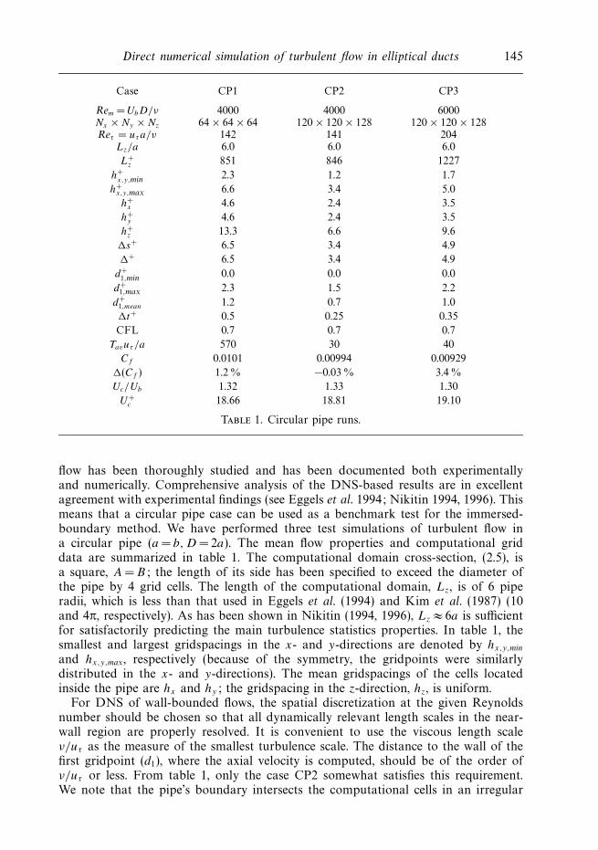
flow has been thoroughly studied and has been documented both experimentallyand numerically. Comprehensive analysis of the DNS-based results are in excellentagreement with experimental findings (see Eggels et al. 1994; Nikitin 1994, 1996). Thismeans that a circular pipe case can be used as a benchmark test for the immersed-boundary method. We have performed three test simulations of turbulent flow ina circular pipe (a = b, D =2a). The mean flow properties and computational griddata are summarized in table 1. The computational domain cross-section, (2.5), isa square, A= B; the length of its side has been specified to exceed the diameter ofthe pipe by 4 grid cells. The length of the computational domain, Lz, is of 6 piperadii, which is less than that used in Eggels et al. (1994) and Kim et al. (1987) (10and 4π, respectively). As has been shown in Nikitin (1994, 1996), Lz ≈ 6a is sufficientfor satisfactorily predicting the main turbulence statistics properties. In table 1, thesmallest and largest gridspacings in the x- and y-directions are denoted by hx,y,min
and hx,y,max, respectively (because of the symmetry, the gridpoints were similarlydistributed in the x- and y-directions). The mean gridspacings of the cells locatedinside the pipe are hx and hy; the gridspacing in the z-direction, hz, is uniform.
For DNS of wall-bounded flows, the spatial discretization at the given Reynoldsnumber should be chosen so that all dynamically relevant length scales in the near-wall region are properly resolved. It is convenient to use the viscous length scaleν/uτ as the measure of the smallest turbulence scale. The distance to the wall of thefirst gridpoint (d1), where the axial velocity is computed, should be of the order ofν/uτ or less. From table 1, only the case CP2 somewhat satisfies this requirement.We note that the pipe’s boundary intersects the computational cells in an irregular
146 N. Nikitin and A. Yakhot
manner. Moreover, most of the grid points nearest to the boundary surface, where theaxial velocity is calculated, are located at a distance less than the near-wall cell size.The spanwise (circumferential) resolution in the near-wall region can be estimated as
s ≈√
h2x + h2
y . For all cases given in table 1, the resolution was sufficient to resolve
the near-wall streaks with the mean spanwise spacing of λ+ 80–120. It is believedthat the mean grid width + = (h+
x h+y h+
z )1/3 satisfies the constraint + πη+, whereη+ is the Kolmogorov length scale (see Eggels et al. 1994). With η+ ≈ 1.6, the criterion+ 5.0 is satisfied for cases CP2 and CP3.
The time steps t in table 1 correspond to a fully developed regime. The initialvelocity field with imposed randomly chosen perturbations undergoes transition toturbulence through non-physical states. This process might be accompanied by abruptchanges of the velocity field, which requires reducing the time step. This was done usingan effective time-step control procedure developed in Nikitin (1996). As was notedin § 1 the ‘direct forcing’ IB method developed by Kim et al. (2001) and employedin this paper introduces an error of O(t2) in the no-slip boundary condition. Toestimate this error, the maximum of the velocity components at the boundary pointshave to be monitored in time. The criterion for the time step t in our circular pipetest calculations (as well as in simulations of elliptical duct flows considered below)was to maintain the maximum error in the no-slip condition at a level of 2–3×10⁻³Ub.It should be emphasized that the error L2-norm is about one order of magnitudeless than the maximum value. Besides the requirement to minimize the error in theno-slip condition, the resolution in time should be sufficiently small to resolve allscales of motion. For the so-called ‘minimal flow unit’ of Jimenez & Moin (1991) –the computational domain with minimum sizes in the streamwise and spanwisedirections to sustain channel flow turbulence – Choi & Moin (1994) demonstrated thatthe computational time step should be perceptibly less than the Kolmogorov timescale in the viscous sublayer, τ+ ≡ (u4
τ /εν)1/2 2.4, where ε is the dissipation rate.Their computations indicated that the turbulence statistics obtained with the non-dimensional time step t+ = 0.4 are sufficiently close to those predicted with t+ =0.2. DNS of turbulent flow in a full channel showed that the estimation t+ 0.2 isapparently too conservative. On the other hand, simulations with t+ ∼ 1.0 predictedvery good turbulence statistics (see Nikitin 1994, 1996, 1997). For DNS of a circularpipe flow, Eggels et al. (1994) used t+ =0.072, which is much smaller than theKolmogorov time scale. Akselvoll & Moin (1996) used a domain decompositionmethod for temporal integration of the Navier–Stokes equations written in cylindricalcoordinates. Their method yielded the maximum time step t+ = 0.18, which is afactor 2.5 higher than that employed in Eggels et al. (1994). The time steps used inthis study are presented in table 1. As is clear from table 1 (and from the simula-tions of turbulent flows in elliptical ducts discussed in the next section, table 2),the numerical scheme used in this study allows the time steps t+ = 0.16–0.5.These computational time steps correspond to reasonable CFL numbers, CFL =t maxux/hx, uy/hy, uz/hz.
2.2. Circular pipe: mean flow and turbulence statistics properties
Statistically steady-state data for DNS of turbulent flows in a pipe using a cylindricalcoordinate system are usually generated by spatial averaging over the homogenousstreamwise and circumferential directions and by averaging in time. The time-averaging interval, normally used to reach the time-independent turbulence statisticsby averaging over two homogeneous direction, is Tav = 5–10a/uτ , where a/uτ is thetime scale usually referred to as the ‘turnover time’. For the IB method, which is based
Direct numerical simulation of turbulent flow in elliptical ducts 147
0.1
0.1 0.1
0.1
0.1
0.2
0.20.2
0.2
0.2
0.3
0.3
0.3
0.3
0.3
0.4
0.4
0.4
0.4
0.4
0.5
0.5
0.5
0.5
0.5
0.6
0.6
0.6
0.6
0.6
0.7
0.7
0.7
0.7
0.70.8
0.8
0.8
0.8
0.8
0.9
0.9
0.9
0.9
0.9
11
1
1
1.1
1.1
1.1
1.1
1.2
1.2
1.2
1.3 1.3
(a)
0.02
0.02
0.02
0.02
0.02
0.02
0.04
0.04
0.04
0.04
0.04
0.04
0.06
0.06
0.06
0.0
6
0.06
0.08
0.08
0.08
0.08
0.08
0.08
0.1
0.1
0.1
0.1
0.1
0.1 0.1
0.1
2
0.12 0.12
0.1
2
0.12
0.12
0.12
0.1
4
0.14
0.14
0.14
0.14
0.14
0.14
0.14
0.16
0.16
0.16
0.1
6
0.16
0.16
0.16
0.16
0.16
0.18
0.18
0.18
0.1
8
0.18
0.1
8
0.18
0.18
0.18
0.2
0.2
0.2
0.2
0.2
0.2
0.2
0.2
0.2
0.2
(b)
0.1
0.10.1
0.1
0.1
0.2
0.2
0.2
0.2
0.2
0.2
0.3
0.3
0.3
0.3
0.3
0.4
0.4
0.4
0.4
0.4
0.5
0.5
0.5
0.5
0.5
0.6
0.6
0.6
0.6
0.6
0.6
0.7
0.7
0.7
0.7
0.7
0.8
0.8
0.8
0.8
0.8
0.9
0.9
0.9
0.9
0.9
1
1
1
1
1
1.1
1.1
1.1
1.1
1.2
1.2
1.2
1.3
1.3
(c)
0.02
0.02
0.02
0.02
0.02
0.02
0.04
0.0
4
0.04
0.04
0.04
0.04
0.06
0.06
0.06
0.0
6
0.06
0.08
0.08
0.08
0.08
0.08
0.08
0.1
0.1
0.1
0.1
0.1
0.1
0.12
0.12
0.12
0.1
2
0.12
0.12
0.12
0.14
0.1
4
0.14
0.14
0.14
0.14
0.14
0.14
0.1
4
0.14
0.16
0.1
6
0.16
0.16
0.16
0.16
0.1
6
0.16
0.16
0.16
0.1
8
0.18
0.18
0.18
0.18
0.18
0.18
0.18
0.18
0.2 0.2
0.2
0.2
0.2
0.22
0.22
0.22
0.22(d)
0.1
0.1
0.1
0.1
0.1
0.1
0.2
0.2
0.2
0.2
0.2
0.3
0.30.3
0.3
0.3
0.4
0.4
0.4
0.4
0.4
0.4
0.5
0.5
0.5
0.5
0.5
0.5
0.6
0.6
0.6
0.6
0.6
0.7
0.7
0.7
0.7
0.7
0.7
0.8
0.80.8
0.8
0.8
0.9
0.9
0.9
0.9
0.9
1
1
1
1
1
1.1 1.1
1.1
1.2
1.2
1.3
(e)
0.02
0.0
2
0.02
0.02
0.02
0.02
0.04
0.04
0.04
0.0
4
0.04
0.06
0.0
6
0.06
0.06
0.06
0.06
0.08
0.0
8
0.08
0.08
0.08
0.08
0.1
0.1
0.1
0.1
0.1
0.1
0.1
0.1
2
0.12
0.12
0.12
0.12
0.12
0.12
0.12
0.14
0.14
0.14
0.14
0.14
0.14
0.14
0.14
0.14
0.1
6
0.16 0.16
0.1
6
0.16
0.16
0.16
0.16
0.16
0.16
0.18
0.180.18
0.1
8
0.18
0.18
0.18
0.18
0.18
0.18
0.2
0.2
0.2( f )
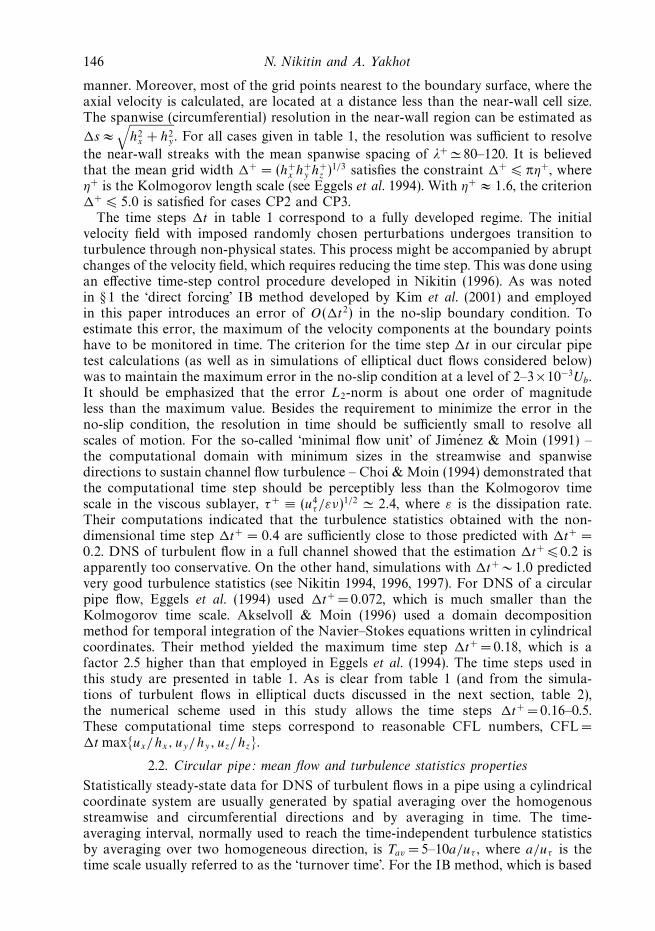
Figure 1. Contours of (a, c, e) Uz and (b, d, f ) |u′|rms; (a, b)CP1, (c, d)CP2, (e, f )CP3.
on a Cartesian coordinate system, averaging over one homogenous streamwise direc-tion is insufficient, for which Tav must be considerably increased. In figure 1, we showthe contours of the averaged streamwise velocity Uz normalized by the bulk velocity Ub
and the root-mean-square of the velocity total fluctuations |u′|rms = 〈u′x2 + u′
y2 + u′
z2〉1/2.
148 N. Nikitin and A. Yakhot
Uz+
100 101 1020
5
10
15
20(a) (b)
d+d +
urms+
0 50 100
1
2
3
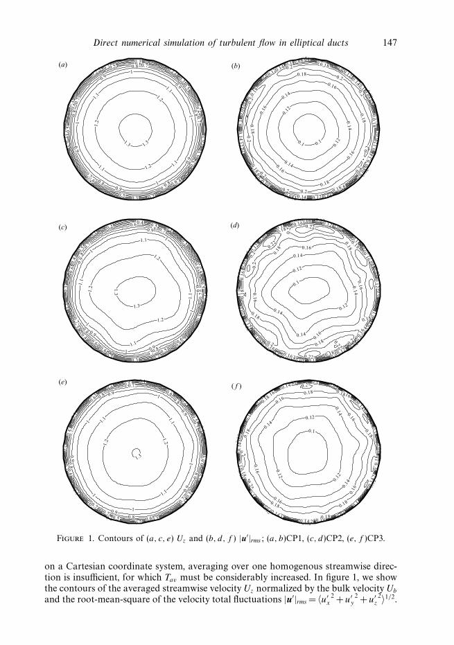
Figure 2. Radial distribution of (a) Uz and (b) |u′|rms averaged over four radii; —, θ = 0,π/2, π, 3π/2; – – –, θ = π/4, 3π/4, 5π/4, 7π/4.
For the cases CP2 and CP3, the insufficiency of the time-averaging intervals isexhibited by the azimuthal asymmetry. As seen from table 1, the time-averaginginterval Tav =570a/uτ , employed for case C1, was larger than that of case CP2 by afactor of about 20. Thus, it can be inferred that for a relatively short computationaldomain Lz/a = 6 (as used for our circular pipe simulations), the time-averaginginterval should be several hundreds of a turn-over time measured in a/uτ units.
In figure 2, the radial distributions of Uz and |u′|rms averaged over two sets of fourradii (θπ/2 = 0, π/2, π, 3π/2 and θπ/4 = π/4, 3π/4, 5π/4, 7π/4) are shown forcase CP2 which was performed with the smallest time-averaging interval. It should beespecially noted that this additional radius-averaging is effectively equivalent to theincreasing Tav by a factor of 4. The four radii of the θπ/2-set are parallel to the co-ordinate lines, while those of the θπ/4-set intersect them at angle π/4. Despite thelack of axial symmetry (figures 1c, d , CP2) and different orientation of the radii withrespect to the Cartesian coordinate lines, the data in figure 2 show no significantangular anisotropy. A similar radius-averaging procedure applied to cases CP1 andCP3 resulted in practically identical distributions along the radii θπ/4 and θπ/4.
In table 1, Cf is the friction coefficient computed from the DNS data,
Cf = 2τw/ρU 2b , (2.7)
where τw is defined in (2.6) and (Cf ) is the relative deviation of the calculated Cf
from that of the Blasius’ law, namely
Cf = 0.0791 Re−0.25m . (2.8)
The present results are in good agreement with Blasius’ law for Rem = 6000, and forRem =4000 the agreement is even better.
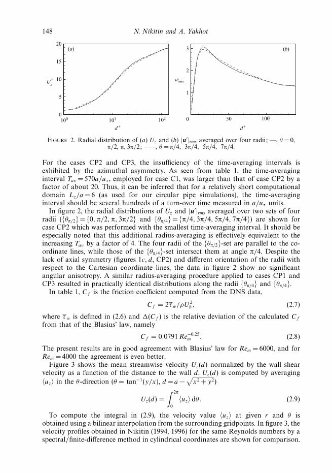
Figure 3 shows the mean streamwise velocity Uz(d) normalized by the wall shearvelocity as a function of the distance to the wall d . Uz(d) is computed by averaging
〈uz〉 in the θ-direction (θ = tan−1(y/x), d = a −√
x2 + y2)
Uz(d) =
∫ 2π
0
〈uz〉 dθ. (2.9)
To compute the integral in (2.9), the velocity value 〈uz〉 at given r and θ isobtained using a bilinear interpolation from the surrounding gridpoints. In figure 3, thevelocity profiles obtained in Nikitin (1994, 1996) for the same Reynolds numbers by aspectral/finite-difference method in cylindrical coordinates are shown for comparison.
Direct numerical simulation of turbulent flow in elliptical ducts 149
100 101 102
d+d+
U +
100 101 1020
5
10
15
20
0
5
10
15
20(a) (b)
2.5 log d+ + 5.0
2.5 log d+ + 5.0
z
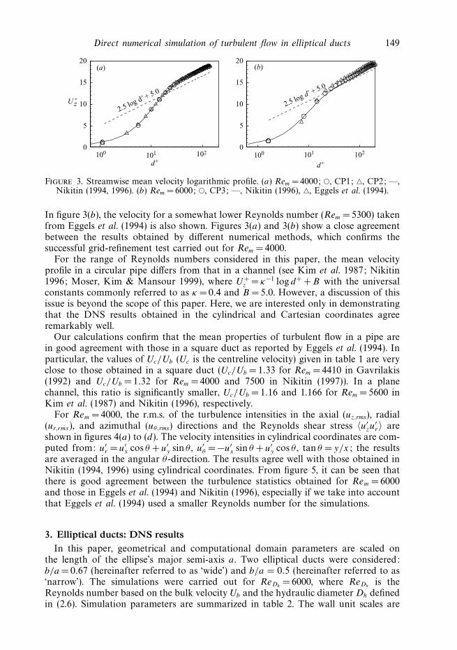
Figure 3. Streamwise mean velocity logarithmic profile. (a) Rem = 4000; , CP1; , CP2; —,Nikitin (1994, 1996). (b) Rem = 6000; , CP3; —, Nikitin (1996), , Eggels et al. (1994).
In figure 3(b), the velocity for a somewhat lower Reynolds number (Rem = 5300) takenfrom Eggels et al. (1994) is also shown. Figures 3(a) and 3(b) show a close agreementbetween the results obtained by different numerical methods, which confirms thesuccessful grid-refinement test carried out for Rem = 4000.
For the range of Reynolds numbers considered in this paper, the mean velocityprofile in a circular pipe differs from that in a channel (see Kim et al. 1987; Nikitin1996; Moser, Kim & Mansour 1999), where U+
z = κ−1 log d+ + B with the universalconstants commonly referred to as κ = 0.4 and B =5.0. However, a discussion of thisissue is beyond the scope of this paper. Here, we are interested only in demonstratingthat the DNS results obtained in the cylindrical and Cartesian coordinates agreeremarkably well.
Our calculations confirm that the mean properties of turbulent flow in a pipe arein good agreement with those in a square duct as reported by Eggels et al. (1994). Inparticular, the values of Uc/Ub (Uc is the centreline velocity) given in table 1 are veryclose to those obtained in a square duct (Uc/Ub = 1.33 for Rem = 4410 in Gavrilakis(1992) and Uc/Ub = 1.32 for Rem = 4000 and 7500 in Nikitin (1997)). In a planechannel, this ratio is significantly smaller, Uc/Ub = 1.16 and 1.166 for Rem =5600 inKim et al. (1987) and Nikitin (1996), respectively.
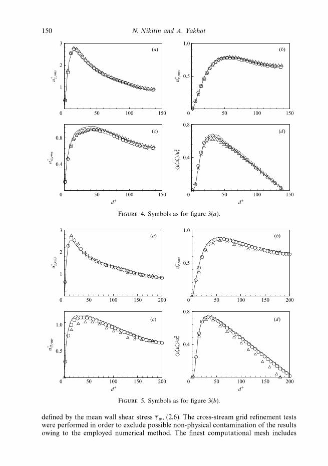
For Rem = 4000, the r.m.s. of the turbulence intensities in the axial (uz,rms), radial(ur,rms), and azimuthal (uθ,rms) directions and the Reynolds shear stress 〈u′
zu′r〉 are
shown in figures 4(a) to (d). The velocity intensities in cylindrical coordinates are com-puted from: u′
r = u′x cos θ + u′
y sin θ , u′θ = −u′
x sin θ + u′y cos θ , tan θ = y/x; the results
are averaged in the angular θ-direction. The results agree well with those obtained inNikitin (1994, 1996) using cylindrical coordinates. From figure 5, it can be seen thatthere is good agreement between the turbulence statistics obtained for Rem = 6000and those in Eggels et al. (1994) and Nikitin (1996), especially if we take into accountthat Eggels et al. (1994) used a smaller Reynolds number for the simulations.
3. Elliptical ducts: DNS resultsIn this paper, geometrical and computational domain parameters are scaled on
the length of the ellipse’s major semi-axis a. Two elliptical ducts were considered:b/a = 0.67 (hereinafter referred to as ‘wide’) and b/a = 0.5 (hereinafter referred to as‘narrow’). The simulations were carried out for ReDh
= 6000, where ReDhis the
Reynolds number based on the bulk velocity Ub and the hydraulic diameter Dh definedin (2.6). Simulation parameters are summarized in table 2. The wall unit scales are
150 N. Nikitin and A. Yakhot
u+ z,rm
s
50 100 150 50 100 1500
1
2
3(a) (b)
(c) (d)
0
0.5
1.0u+ θ
,rm
s
0.4
0.8
0.4
0.8
d+d+
u′ r
u′ z
/u2 τ
50 100 150 50 100 1500 0
u+ r,rm
s
Figure 4. Symbols as for figure 3(a).
u+ z,rm
s
50 150100 2000
1
2
3(a) (b)
(c) (d)
0
0.5
1.0
u+ θ,r
ms
0.5
1.0
0.4
0.8
d+d+
u′ r
u′ z
/u2 τ
50 150100 200
50 150100 200 50 150100 2000 0
u+ r,rm
s
Figure 5. Symbols as for figure 3(b).
defined by the mean wall shear stress τw , (2.6). The cross-stream grid refinement testswere performed in order to exclude possible non-physical contamination of the resultsowing to the employed numerical method. The finest computational mesh includes
Direct numerical simulation of turbulent flow in elliptical ducts 151
Case EP1 EP2 EP3 EP4 EP5
b/a 0.67 0.67 0.5 0.5 0.5Dh/a 1.59 1.59 1.30 1.30 1.30Re2a 7547 7547 9252 9252 9252ReDh
6000 6000 6000 6000 6000Nx × Ny 140 × 100 200 × 160 140 × 100 160 × 120 200 × 160
Nz 256 256 256 256 256a+ 258 256 314 313 312b+ 173 171 157 157 156
Lz/Dh 6.0 6.0 6.0 6.0 6.0L+
z 2472 2453 2450 2443 2431
h+x,min 1.9 1.3 2.3 2.0 1.6
h+x,max 5.4 3.7 6.5 5.7 4.5
h+y,min 1.8 1.1 1.6 1.3 1.0
h+y,max 5.1 3.1 4.6 3.8 2.8
h+z 9.7 9.6 9.6 9.5 9.5
+max 6.4 4.8 6.6 5.9 4.9
t+ 0.22 0.37 0.32 0.32 0.16
CFL 0.43 0.69 0.63 0.63 0.32
Tavuτ /a 110 60 100 50 60
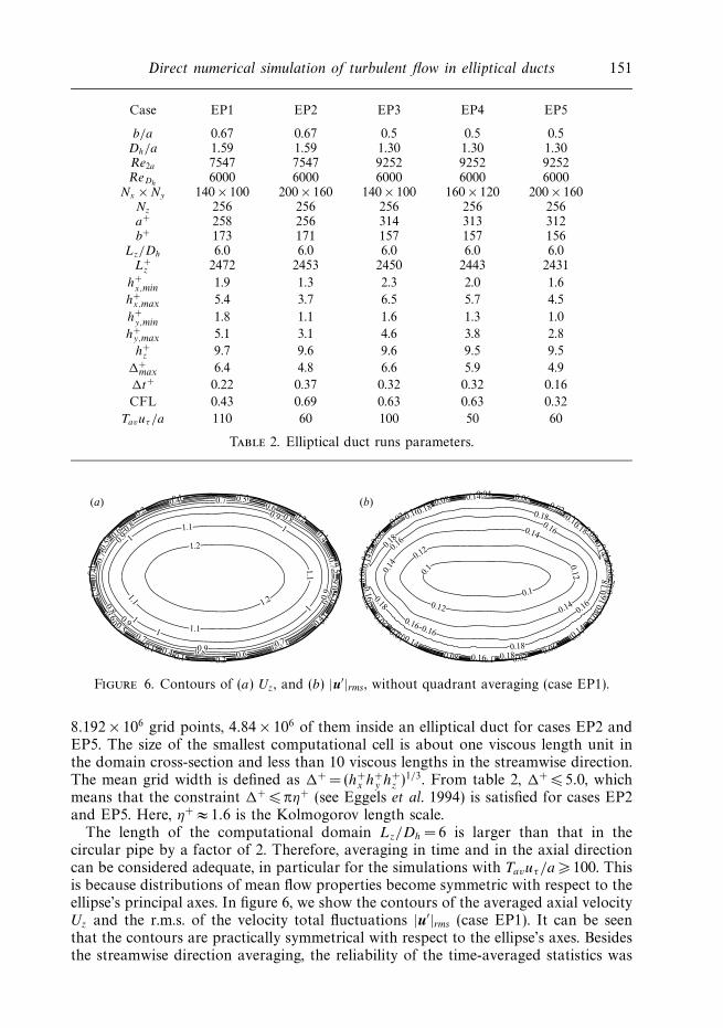
Table 2. Elliptical duct runs parameters.
0.1
0.1
0.1
0.1
0.1
0.1
0.2
0.2 0.2
0.2
0.2
0.3
0.3
0.3
0.3
0.3
0.4
0.4
0.4
0.4
0.4
0.5
0.5
0.5
0.5
0.5
0.6
0.6
0.6
0.6
0.6
0.7
0.7
0.7
0.7
0.7
0.8
0.80.8
0.8
0.8
0.9
0.9
0.9
0.9
0.9
1
11
1
1
1.1
1.1
1.1
1.1
1.2
1.2
(a)
0.02
0.020.02
0.02
0.02
0.04
0.04
0.04
0.04
0.04
0.06
0.06
0.06
0.06
0.06
0.08
0.08
0.08
0.08
0.08
0.1
0.1 0.1
0.1
0.1
0.1
0.1
0.12
0.12
0.12
0.12
0.12
0.12
0.12
0.12
0.14
0.14
0.14
0.14
0.14
0.14
0.14
0.14
0.16
0.16 0.16
0.16
0.16
0.16
0.16
0.16
0.16
0.16
0.18
0.18
0.18
0.18
0.18
0.18
0.18
0.18
(b)
Figure 6. Contours of (a) Uz, and (b) |u′|rms, without quadrant averaging (case EP1).
8.192 × 10⁶ grid points, 4.84 × 10⁶ of them inside an elliptical duct for cases EP2 andEP5. The size of the smallest computational cell is about one viscous length unit inthe domain cross-section and less than 10 viscous lengths in the streamwise direction.The mean grid width is defined as + = (h+
x h+y h+
z )1/3. From table 2, + 5.0, whichmeans that the constraint + πη+ (see Eggels et al. 1994) is satisfied for cases EP2and EP5. Here, η+ ≈ 1.6 is the Kolmogorov length scale.
The length of the computational domain Lz/Dh =6 is larger than that in thecircular pipe by a factor of 2. Therefore, averaging in time and in the axial directioncan be considered adequate, in particular for the simulations with Tavuτ/a 100. Thisis because distributions of mean flow properties become symmetric with respect to theellipse’s principal axes. In figure 6, we show the contours of the averaged axial velocityUz and the r.m.s. of the velocity total fluctuations |u′|rms (case EP1). It can be seenthat the contours are practically symmetrical with respect to the ellipse’s axes. Besidesthe streamwise direction averaging, the reliability of the time-averaged statistics was

152 N. Nikitin and A. Yakhot
Run EP1 EP2 EP3 EP4 EP5
Cf 0.00932 0.00917 0.00922 0.00917 0.00908(Cf ) 3.6 % 2.1% 2.6% 2.1% 1.0%Uc/Ub 1.29 1.29 1.27 1.27 1.28U+
c 18.84 19.00 18.72 18.82 18.96
max√
U 2x + U 2
y /Ub 0.0101 0.0104 0.0139 0.0137 0.0135
max|u′|rms/Ub 0.198 0.195 0.198 0.197 0.197
Table 3. Elliptical duct runs: global characteristics.
increased by additional quadrant averaging over four points located symmetricallyto the ellipse’s axes. In this paper, all time-averaged statistics are obtained by usingaveraging over the four quadrants.
Mean flow properties are summarized in table 3. Cf is the friction coefficientcomputed from the DNS data and (Cf ) is its relative deviation from the correlationbased on Blasius’ law when it is applied to non-circular ducts by using the hydraulicdiameter
Cf = 0.0791Re−0.25Dh
, ReDh= UmDh/ν. (3.1)
Comparison of the results shows only minor differences between the friction coeffi-cients Cf obtained for different computational meshes, which indicates that the gridrefinement test we performed was successful. In general, our computations confirmthe validity of the Blasius’ law (3.1) for low-Reynolds numbers considered in thispaper. The difference between Cf computed from (3.1) for ReDh
= 6000 and thatobtained from the Prandtl correlation
1/√λ = 2 log10(ReDh
√λ) − 0.8, Cf = λ/4, (3.2)
is only 1.2 %.To calculate the Reynolds number for non-circular ducts, Jones (1976) suggested
using a hydraulic diameter D′h, instead of that defined in (2.6), as follows
D′h = Dh
16
ReDhCflam
, (3.3)
where Cflam is the friction coefficient for a fully developed laminar flow in the ductdefined in (2.7). For a laminar flow through an elliptical pipe
uz(x, y) =p
2µLz
a2b2
a2 + b2
(1 − x2
a2− y2
b2
), (3.4)
where µ is a dynamic viscosity. Calculating the bulk velocity Ub from (3.4), forReynolds number Re ′
Dh, we have
Re ′Dh
= ReDh
8a2b2
D2h(a
2 + b2). (3.5)
In our calculations, Re ′Dh
=5844 and 5680 for b/a = 0.67 and 0.5, respectively. Using
Re ′Dh
instead of ReDhin (3.1) and (3.2) improves the agreement with the friction
coefficient obtained by DNS by 0.7 % and 1.4 % for wide and narrow elliptical pipes,respectively.
The global characteristics obtained on different meshes were found to be quitesimilar. Moreover, the cross-stream section distributions for different meshes were,
Direct numerical simulation of turbulent flow in elliptical ducts 153
0.1
0.1
0.2
0.2
0.3
0.3
0.4
0.4
0.5
0.5
0.6
0.6
0.7
0.7
0.80.9
1
11.1
1.2
1.2
0.2 0.4 0.6 0.8 1.00
0.1
0.1
0.2
0.2
0.3
0.3
0.4
0.4
0.5
0.5
0.6
0.6
0.6
0.7
0.7
0.8
0.8
0.9
0.9
1
1
1.1
1.1
1.2
0 0.2 0.4 0.6 0.8 1.0
0.2
0.4
0.6
0.2
0.4
0.6(a) (b)
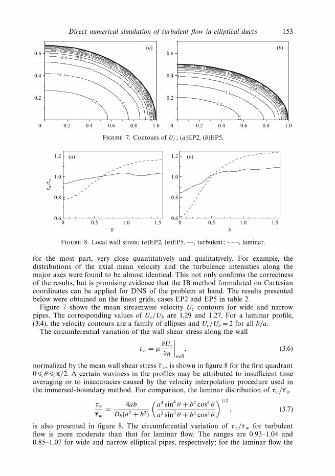
Figure 7. Contours of Uz; (a)EP2, (b)EP5.
θ θ
0 0.5 1.0 1.50.6
0.8
1.0
1.2 (a) (b)
τ w/τw
0 0.5 1.0 1.50.6
0.8
1.0
1.2
Figure 8. Local wall stress; (a)EP2, (b)EP5. —, turbulent; – – –, laminar.
for the most part, very close quantitatively and qualitatively. For example, thedistributions of the axial mean velocity and the turbulence intensities along themajor axes were found to be almost identical. This not only confirms the correctnessof the results, but is promising evidence that the IB method formulated on Cartesiancoordinates can be applied for DNS of the problem at hand. The results presentedbelow were obtained on the finest grids, cases EP2 and EP5 in table 2.
Figure 7 shows the mean streamwise velocity Uz contours for wide and narrowpipes. The corresponding values of Uc/Ub are 1.29 and 1.27. For a laminar profile,(3.4), the velocity contours are a family of ellipses and Uc/Ub = 2 for all b/a.
The circumferential variation of the wall shear stress along the wall
τw = µ∂Uz
∂n
∣∣∣∣wall
, (3.6)
normalized by the mean wall shear stress τw , is shown in figure 8 for the first quadrant0 θ π/2. A certain waviness in the profiles may be attributed to insufficient timeaveraging or to inaccuracies caused by the velocity interpolation procedure used inthe immersed-boundary method. For comparison, the laminar distribution of τw/τw
τw
τw
=4ab
Dh(a2 + b2)
(a4 sin4 θ + b4 cos4 θ
a2 sin2 θ + b2 cos2 θ
)1/2
, (3.7)
is also presented in figure 8. The circumferential variation of τw/τw for turbulentflow is more moderate than that for laminar flow. The ranges are 0.93–1.04 and0.85–1.07 for wide and narrow elliptical pipes, respectively; for the laminar flow the
154 N. Nikitin and A. Yakhot
0.2 0.4 0.6 0.8 1.000 0.2 0.4 0.6 0.8 1.0
0.2
0.4
0.6
0.2
0.4
0.6(a) (b)
Figure 9. Mean secondary flow contours; (a)EP2, (b)EP5.
0.2 0.4 0.6 0.8 1.000 0.2 0.4 0.6 0.8 1.0
0.2
0.4
0.6
0.2
0.4
0.6(a) (b)
0.002
0.0020.002
0.0020.002
0.004
0.004
0.004
0.00
4
0.004
0.00
6
0.006
0.006
0.00
6
0.008
0.008
0.0080.01
0.002
0.002
0.002 0.0020.003
0.0040.
003
0.004
0.005
0.005
0.006
00 05
0.007
0.008
0.006
0.008
0.011
0.011
Figure 10. Isovels of Uxy =√
U 2x + U 2
y ; (a)EP2, (b)EP5.
corresponding ranges are 0.78–1.16 and 0.62–1.23. Similar to laminar flows, the localwall shear stress in turbulent flows is minimal at the points far from the pipe’s centre(x = ±a, y = 0). The difference between the wall stress τw computed at the minor andmajor axes endpoints is caused by the wall curvature. For a laminar flow, from (3.7),τw(θ = 0)/τw(θ = π/2) = b/a.
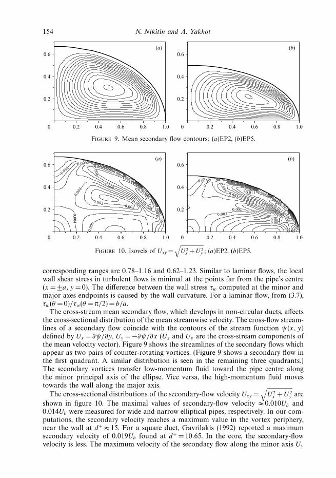
The cross-stream mean secondary flow, which develops in non-circular ducts, affectsthe cross-sectional distribution of the mean streamwise velocity. The cross-flow stream-lines of a secondary flow coincide with the contours of the stream function ψ(x, y)defined by Ux = ∂ψ/∂y, Uy = −∂ψ/∂x (Ux and Uy are the cross-stream components ofthe mean velocity vector). Figure 9 shows the streamlines of the secondary flows whichappear as two pairs of counter-rotating vortices. (Figure 9 shows a secondary flow inthe first quadrant. A similar distribution is seen in the remaining three quadrants.)The secondary vortices transfer low-momentum fluid toward the pipe centre alongthe minor principal axis of the ellipse. Vice versa, the high-momentum fluid movestowards the wall along the major axis.
The cross-sectional distributions of the secondary-flow velocity Uxy =√
U 2x + U 2
y are
shown in figure 10. The maximal values of secondary-flow velocity ≈ 0.010Ub and0.014Ub were measured for wide and narrow elliptical pipes, respectively. In our com-putations, the secondary velocity reaches a maximum value in the vortex periphery,near the wall at d+ ≈ 15. For a square duct, Gavrilakis (1992) reported a maximumsecondary velocity of 0.019Ub found at d+ = 10.65. In the core, the secondary-flowvelocity is less. The maximum velocity of the secondary flow along the minor axis Uy
Direct numerical simulation of turbulent flow in elliptical ducts 155
d+
Uz+
10 20 30 40 500
5
10
15
20
d+
10 20 30 40 500
5
10
15
20
0π/16π/8π/43π/16π/2
(a) (b)
θ0π/16π/8π/43π/8π/2
θ
Figure 11. Mean streamwise velocity distribution along the lines perpendicularto the wall; (a)EP2, (b)EP5.
d+
Un+
10 20 30 40 500
–0.05
–0.10
0.05
0.00
0.10
d+10 20 30 40 500
(a) (b)
–0.05
–0.10
0.05
0.00
0.10
0.15
Figure 12. Mean secondary flow Un-velocity distribution along the line perpendicular to thewall; (a)EP2, (b)EP5. For key see figure 11.
d+
Ut+
10 20 30 40 500
0
0.1
0.2
d+
10 20 30 40 500
(a) (b)
0
0.1
0.2
Figure 13. Mean secondary flow Ut -velocity distribution along the line perpendicular to thewall; (a)EP2, (b)EP5. For key see figure 11.
towards the centre is about 0.0045Ub for a wide pipe and 0.0035Ub for a narrow pipe.The corresponding values for the secondary flow towards the wall along the majoraxis Ux are 0.0072Ub and 0.0105Ub.
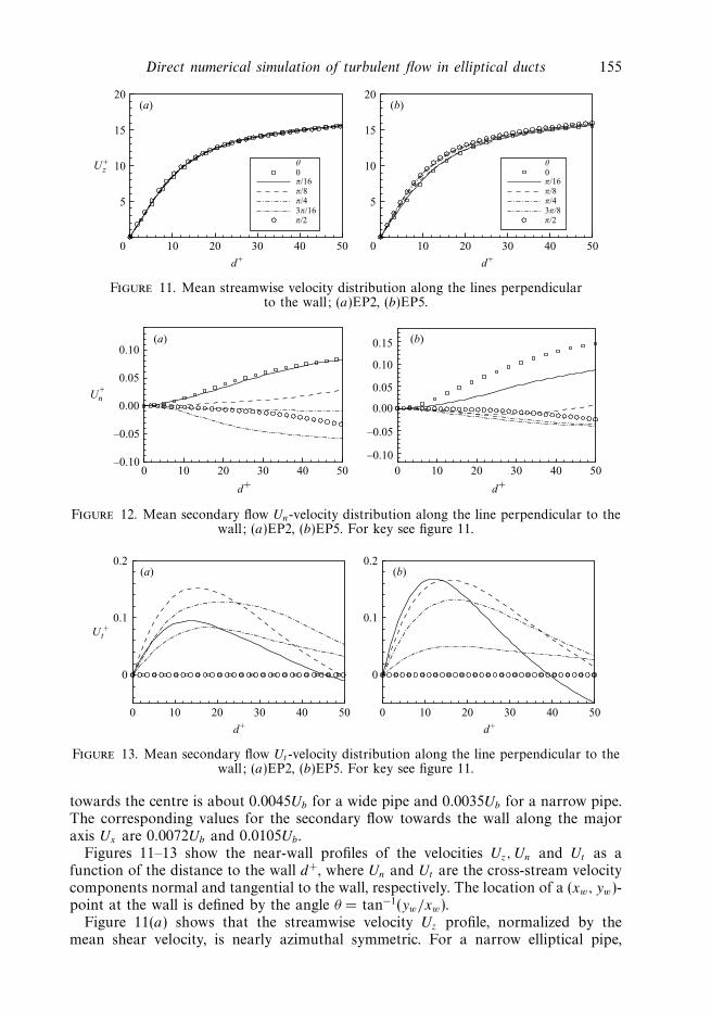
Figures 11–13 show the near-wall profiles of the velocities Uz, Un and Ut as afunction of the distance to the wall d+, where Un and Ut are the cross-stream velocitycomponents normal and tangential to the wall, respectively. The location of a (xw, yw)-point at the wall is defined by the angle θ = tan−1(yw/xw).
Figure 11(a) shows that the streamwise velocity Uz profile, normalized by themean shear velocity, is nearly azimuthal symmetric. For a narrow elliptical pipe,
156 N. Nikitin and A. Yakhot
d+
Uz+
0
5
10
15
20
d+
100 101 102 100 101 102
(a) (b)
0
5
10
15
20
2.5 log y+ + 5.0
2.5 log y+ + 5.0
Figure 14. Mean streamwise velocity logarithmic profile along the minor (open circles) andmajor (squares) axes; dashed line – scaling on the local shear velocity.
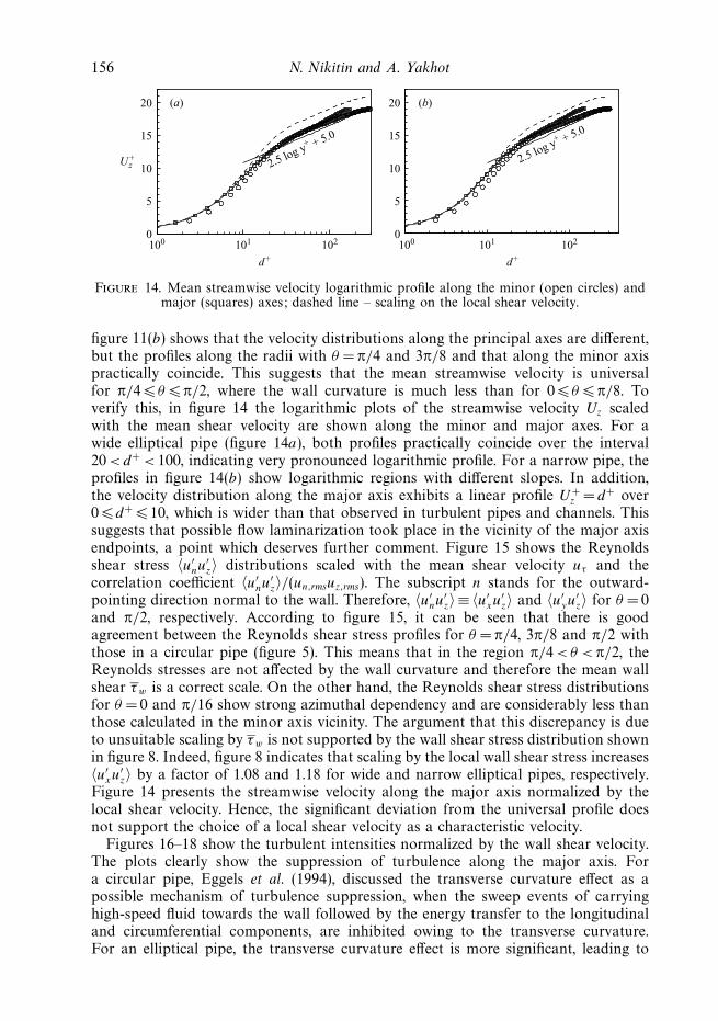
figure 11(b) shows that the velocity distributions along the principal axes are different,but the profiles along the radii with θ = π/4 and 3π/8 and that along the minor axispractically coincide. This suggests that the mean streamwise velocity is universalfor π/4 θ π/2, where the wall curvature is much less than for 0 θ π/8. Toverify this, in figure 14 the logarithmic plots of the streamwise velocity Uz scaledwith the mean shear velocity are shown along the minor and major axes. For awide elliptical pipe (figure 14a), both profiles practically coincide over the interval20 <d+ < 100, indicating very pronounced logarithmic profile. For a narrow pipe, theprofiles in figure 14(b) show logarithmic regions with different slopes. In addition,the velocity distribution along the major axis exhibits a linear profile U+
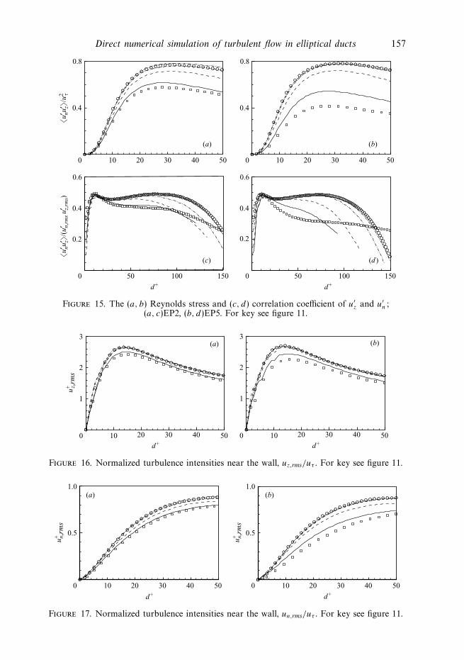
z = d+ over0 d+ 10, which is wider than that observed in turbulent pipes and channels. Thissuggests that possible flow laminarization took place in the vicinity of the major axisendpoints, a point which deserves further comment. Figure 15 shows the Reynoldsshear stress 〈u′
nu′z〉 distributions scaled with the mean shear velocity uτ and the
correlation coefficient 〈u′nu
′z〉/(un,rmsuz,rms). The subscript n stands for the outward-
pointing direction normal to the wall. Therefore, 〈u′nu
′z〉 ≡ 〈u′
xu′z〉 and 〈u′
yu′z〉 for θ = 0
and π/2, respectively. According to figure 15, it can be seen that there is goodagreement between the Reynolds shear stress profiles for θ = π/4, 3π/8 and π/2 withthose in a circular pipe (figure 5). This means that in the region π/4 <θ < π/2, theReynolds stresses are not affected by the wall curvature and therefore the mean wallshear τw is a correct scale. On the other hand, the Reynolds shear stress distributionsfor θ = 0 and π/16 show strong azimuthal dependency and are considerably less thanthose calculated in the minor axis vicinity. The argument that this discrepancy is dueto unsuitable scaling by τw is not supported by the wall shear stress distribution shownin figure 8. Indeed, figure 8 indicates that scaling by the local wall shear stress increases〈u′
xu′z〉 by a factor of 1.08 and 1.18 for wide and narrow elliptical pipes, respectively.
Figure 14 presents the streamwise velocity along the major axis normalized by thelocal shear velocity. Hence, the significant deviation from the universal profile doesnot support the choice of a local shear velocity as a characteristic velocity.
Figures 16–18 show the turbulent intensities normalized by the wall shear velocity.The plots clearly show the suppression of turbulence along the major axis. Fora circular pipe, Eggels et al. (1994), discussed the transverse curvature effect as apossible mechanism of turbulence suppression, when the sweep events of carryinghigh-speed fluid towards the wall followed by the energy transfer to the longitudinaland circumferential components, are inhibited owing to the transverse curvature.For an elliptical pipe, the transverse curvature effect is more significant, leading to
Direct numerical simulation of turbulent flow in elliptical ducts 157
u′ n
u′ z
/u2 τ
10 20 30 40 500
0.4
0.8
(a) (b)
(c) (d )
d+ d+
u′ n
u′ z
/(u′ n
,rm
s u′ z
,rm
s)
50 100 150
10 20 30 40 500
0.4
0.8
0
0.4
0.2
0.6
50 100 1500
0.4
0.2
0.6
Figure 15. The (a, b) Reynolds stress and (c, d) correlation coefficient of u′z and u′
n;(a, c)EP2, (b, d)EP5. For key see figure 11.
d+
u+ z ,rm
s
10 20 30 40 500
1
2
3(a) (b)
d+10 20 30 40 500
1
2
3
Figure 16. Normalized turbulence intensities near the wall, uz,rms/uτ . For key see figure 11.
d+
u+ n ,rm
s
10 20 30 40 500
0.5
1.0(a) (b)
d+
10 20 30 40 500
u+ n ,rm
s
0.5
1.0
Figure 17. Normalized turbulence intensities near the wall, un,rms/uτ . For key see figure 11.
158 N. Nikitin and A. Yakhot
d+
u+ t , rm
s
10 20 30 40 500
0.5
1.0(a) (b)
d+
10 20 30 40 500
0.5
1.0
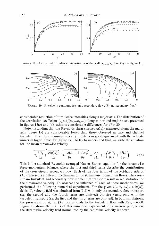
Figure 18. Normalized turbulence intensities near the wall, ut,rms/uτ . For key see figure 11.
0.2 0.4 0.6 0.8 1.00
0.2
0.4
(a) (b)
0.2 0.4 0.6 0.8 1.00
0.2
0.40.1
0.1
0.2
0.2
0.3
0.3
0.4
0.4
0.50.5
0.6
0.6
0.7
0.80.8
0.90.9
1
1
1.11.2
0.1
0.1
0.2
0.2
0.3
0.3
0.4
0.4
0.5
0.5
0.6
0.6
0.7
0.7
0.8
0.9
Figure 19. Uz-velocity contours. (a) ‘only-secondary flow’, (b) ‘no-secondary flow’.
considerable reduction of turbulence intensities along a major axis. The distribution ofthe correlation coefficient 〈u′
nu′z〉/(un,rmsuz,rms) along minor and major axes, presented
in figures 15(c) and (d), exhibits considerable differences for d+ > 20.Notwithstanding that the Reynolds shear stresses 〈u′
xu′z〉 measured along the major
axis (figure 15) are considerably lower than those observed in pipe and channelturbulent flow, the streamwise velocity profile is in good agreement with the velocityuniversal logarithmic law (figure 14). To try to understand that, we write the equationfor the mean streamwise velocity
︷ ︸︸ ︷Ux
∂Uz
∂x+
∂〈u′xu
′z〉
∂x+
︷ ︸︸ ︷Uy
∂Uz
∂y+
∂〈u′yu
′z〉
∂y=
p
ρLz
+ ν
(∂2Uz
∂x2+
∂2Uz
∂y2
). (3.8)
This is the standard Reynolds-averaged Navier–Stokes equation for the streamwiseforce–momentum balance, where the first and third terms describe the contributionof the cross-stream secondary flow. Each of the four terms of the left-hand side of(3.8) represents a different mechanism of the streamwise momentum fluxes. The cross-stream turbulent and secondary flow momentum transport result in redistribution ofthe streamwise velocity. To observe the influence of each of these mechanisms, weperformed the following numerical experiment. For the given Ux, Uy, 〈u′
xu′z〉, 〈u′
yu′z〉
fields, Uz-velocity field was obtained from (3.8) with only the secondary flow transport(i.e. the second and the fourth terms are omitted) or, vice versa, only with theturbulent transport (i.e. the first and the third terms are omitted). In both simulations,the pressure drop p in (3.8) corresponds to the turbulent flow with ReDh
= 6000.Figure 19 shows the results of this numerical experiment for a narrow pipe, wherethe streamwise velocity field normalized by the centreline velocity is shown.
Direct numerical simulation of turbulent flow in elliptical ducts 159
d+
10 20 30 40 500
0 0
0.001
0.002
0.001
0.002(a) (b)
d+
10 20 30 40 500
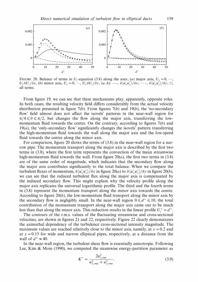
Figure 20. Balance of terms in Uz-equation (3.8) along the axes; (a) major axis, Uy = 0, —,Ux∂Uz/∂x, (b) minor axis, Ux = 0, —, Uy∂Uz/∂y; (a, b): - - -, ∂〈u′
xu′z〉/∂x; – · –, ∂〈u′
yu′z〉/∂y; ,
all terms.
From figure 19, we can see that these mechanisms play, apparently, opposite roles.In both cases, the resulting velocity field differs considerably from the actual velocitydistribution presented in figure 7(b). From figures 7(b) and 19(b), the ‘no-secondaryflow’ field almost does not affect the isovels’ patterns in the near-wall region forπ/4 θ π/2, but changes the flow along the major axis, transferring the low-momentum fluid towards the centre. On the contrary, according to figures 7(b) and19(a), the ‘only-secondary flow’ significantly changes the isovels’ pattern transferringthe high-momentum fluid towards the wall along the major axis and the low-speedfluid towards the centre along the minor axis.
For comparison, figure 20 shows the terms of (3.8) in the near-wall region for a nar-row pipe. The momentum transport along the major axis is described by the first twoterms in (3.8), where the first term represents the convection of the mean streamwisehigh-momentum fluid towards the wall. From figure 20(a), the first two terms in (3.8)are of the same order of magnitude, which indicates that the secondary flow alongthe major axis contributes significantly to the total balance. When we compare theturbulent fluxes of momentum, ∂〈u′
xu′z〉/∂x in figure 20(a) to ∂〈u′
yu′z〉/∂y in figure 20(b),
we can see that the reduced turbulent flux along the major axis is compensated bythe induced secondary flow. This might explain why the velocity profile along themajor axis replicates the universal logarithmic profile. The third and the fourth termsin (3.8) represent the momentum transport along the minor axis towards the centre.According to figure 20(b), the low-momentum fluid transport along the minor axis bythe secondary flow is negligibly small. In the near-wall region 0 d+ 10, the totalcontribution of the momentum transport along the major axis came out to be muchless than that along the minor axis. This reduction results in the linear profile U+
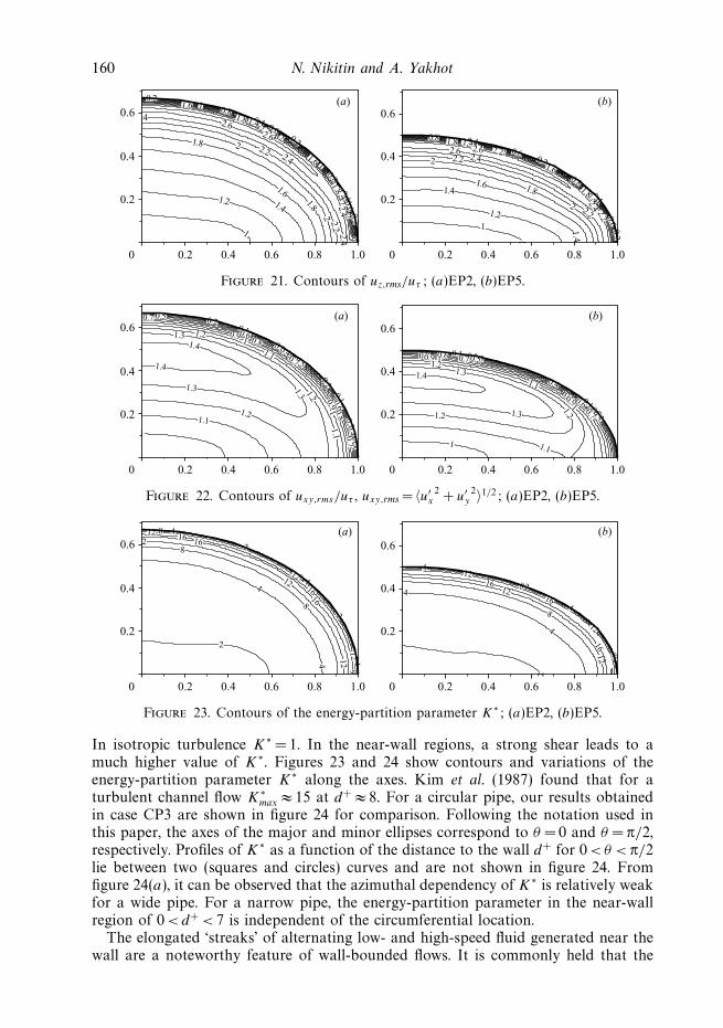
z = d+.The contours of the r.m.s. values of the fluctuating streamwise and cross-sectional
velocities, are shown in figures 21 and 22, respectively. Figure 22 clearly demonstratesthe azimuthal dependency of the turbulence cross-sectional intensity magnitude. Themaximum values are reached relatively close to the minor axis, namely, at x = 0.2 andat x = 0.15 for wide and narrow elliptical pipes, respectively, at a distance from thewall of d+ ≈ 40.
In the near-wall region, the turbulent shear flow is essentially anisotropic. FollowingLee, Kim & Moin (1990), we computed the steamwise energy-partition parameter as
K∗ =2u2
z,rms
u2x,rms + u2
y,rms
. (3.9)
160 N. Nikitin and A. Yakhot
0.2 0.4 0.6 0.8 1.00
0.2
0.4
0.6 0.6(a) (b)
0.2 0.4 0.6 0.8 1.00
0.2
0.4
0.2
0.2
0.2
0.4
0.4
0.6
0.6
0.8
0.8
1
1
1.2
1.2
1.
1.
2
1.4
1.4
1.4
1.6
1.6
.6
1.6
1.8
1.8
1.8
1.8
2
2
2
2
2.2
2.2
2.2
2.2
2.4
2.4
.4
2.4
2.4
2.62.6
0.2
0.2
0.40.4
0.6
0.6
0.8
0.8
1
1
1.21.2
1.2
1.41.4
1.4
1.4
1.6
1.6
1.8
1.81.8
2
2
2
2
2.2
2.2
2.2
2.2
2.4
2.4
2.42.6 2.6
1
Figure 21. Contours of uz,rms/uτ ; (a)EP2, (b)EP5.
0.2 0.4 0.6 0.8 1.00
0.2
0.4
0.6 0.6(a) (b)
0.2 0.4 0.6 0.8 1.00
0.2
0.4
0.1
0.1
0.2
0.2
0.3
0.3
0.4
0.4
0.5
0.50.5
0.6
0.6
0.7
0.7
0.7
0.8
0.8
0.9
0.9
1
1
1
1.1
1.1
1.1
1.2
1.21.2
1.3
1.3
1.3
1.4
1.4
0.1
0.1
0.2
0.2
0.3
0.3
0.4
0.5
0.5
0.6
0.6
0.7
0.7
0.8
0.8
0.9
0.9
1
1
1
1.1
1.1
1.2
1.21.2
1.3
1.3
1.4
Figure 22. Contours of uxy,rms/uτ , uxy,rms = 〈u′x2 + u′
y2〉1/2; (a)EP2, (b)EP5.
0.2 0.4 0.6 0.8 1.00
0.2
0.4
0.6 0.6(a) (b)
0.2 0.4 0.6 0.8 1.00
0.2
0.4
2
2
2
4
4
4
4
4
8
8
8
8
8
12
12
12
2
12
12
16
1616
16
6
2
2
2
4
4
4
4
8
8
8
12
12
12
12
16
16
16
Figure 23. Contours of the energy-partition parameter K∗; (a)EP2, (b)EP5.
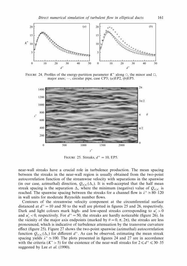
In isotropic turbulence K∗ = 1. In the near-wall regions, a strong shear leads to amuch higher value of K∗. Figures 23 and 24 show contours and variations of theenergy-partition parameter K∗ along the axes. Kim et al. (1987) found that for aturbulent channel flow K∗
max ≈ 15 at d+ ≈ 8. For a circular pipe, our results obtainedin case CP3 are shown in figure 24 for comparison. Following the notation used inthis paper, the axes of the major and minor ellipses correspond to θ =0 and θ = π/2,respectively. Profiles of K∗ as a function of the distance to the wall d+ for 0 < θ < π/2lie between two (squares and circles) curves and are not shown in figure 24. Fromfigure 24(a), it can be observed that the azimuthal dependency of K∗ is relatively weakfor a wide pipe. For a narrow pipe, the energy-partition parameter in the near-wallregion of 0 <d+ < 7 is independent of the circumferential location.
The elongated ‘streaks’ of alternating low- and high-speed fluid generated near thewall are a noteworthy feature of wall-bounded flows. It is commonly held that the
Direct numerical simulation of turbulent flow in elliptical ducts 161
d+
K*
10 20 30 40 500
5
10
15
20 (a) (b)
d+
10 20 30 40 500
5
10
15
20
Figure 24. Profiles of the energy-partition parameter K∗ along , the minor and ,major axes; —, circular pipe, case CP3; (a)EP2, (b)EP5.
z+
s+
500 1000 1500 20000
200
400
600
800
1000
1200
1400
0
2π
3π/2
π
π/2
θ
Figure 25. Streaks, d+ = 10, EP5.
near-wall streaks have a crucial role in turbulence production. The mean spacingbetween the streaks in the near-wall region is usually obtained from the two-pointautocorrelation function of the streamwise velocity with separations in the spanwise(in our case, azimuthal) direction, Qu′
zu′z(s). It is well-accepted that the half mean
streak spacing is the separation s where the minimum (negative) value of Qu′zu
′z
isreached. The spanwise spacing between the streaks for a channel flow is λ+ 80–120in wall units for moderate Reynolds number flows.
Contours of the streamwise velocity component at the circumferential surfacedistanced at d+ = 10 and 50 to the wall are plotted in figures 25 and 26, respectively.Dark and light colours mark high- and low-speed streaks corresponding to u′
z > 0and u′
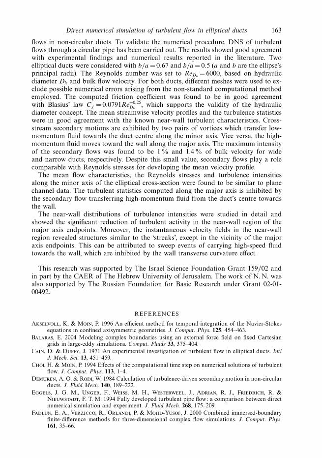
z < 0, respectively. For d+ =50, the streaks are hardly noticeable (figure 26). Inthe vicinity of the major axis endpoints (marked by θ = 0, π, 2π), the streaks are lesspronounced, which is indicative of turbulence attenuation by the transverse curvatureeffect (figure 25). Figure 27 shows the two-point spanwise (azimuthal) autocorrelationfunction Qu′
zu′z(s) for different d+. As can be observed, estimating the mean streak
spacing yields λ+ 100. The plots presented in figures 24 and 27 are in accordancewith the criteria (K∗ > 5) for the existence of the near-wall streaks for 2 d+ 30–35suggested by Lee et al. (1990).
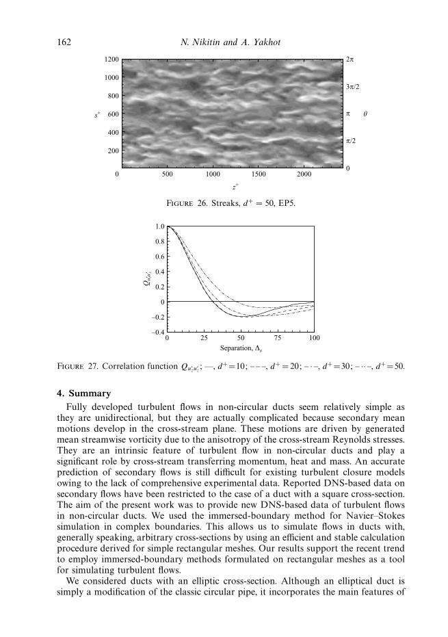
162 N. Nikitin and A. Yakhot
z+
s+
500 1000 1500 20000
200
400
600
800
1000
1200
0
2π
3π/2
π
π/2
θ
Figure 26. Streaks, d+ = 50, EP5.
Separation, ∆s
Qu′ z
u′ z
0 25 50 75 100–0.4
–0.2
0
0.2
0.4
0.6
0.8
1.0
Figure 27. Correlation function Qu′zu
′z; —, d+=10; – – –, d+ = 20; – · –, d+=30; – ·· –, d+=50.
4. SummaryFully developed turbulent flows in non-circular ducts seem relatively simple as
they are unidirectional, but they are actually complicated because secondary meanmotions develop in the cross-stream plane. These motions are driven by generatedmean streamwise vorticity due to the anisotropy of the cross-stream Reynolds stresses.They are an intrinsic feature of turbulent flow in non-circular ducts and play asignificant role by cross-stream transferring momentum, heat and mass. An accurateprediction of secondary flows is still difficult for existing turbulent closure modelsowing to the lack of comprehensive experimental data. Reported DNS-based data onsecondary flows have been restricted to the case of a duct with a square cross-section.The aim of the present work was to provide new DNS-based data of turbulent flowsin non-circular ducts. We used the immersed-boundary method for Navier–Stokessimulation in complex boundaries. This allows us to simulate flows in ducts with,generally speaking, arbitrary cross-sections by using an efficient and stable calculationprocedure derived for simple rectangular meshes. Our results support the recent trendto employ immersed-boundary methods formulated on rectangular meshes as a toolfor simulating turbulent flows.
We considered ducts with an elliptic cross-section. Although an elliptical duct issimply a modification of the classic circular pipe, it incorporates the main features of
Direct numerical simulation of turbulent flow in elliptical ducts 163
flows in non-circular ducts. To validate the numerical procedure, DNS of turbulentflows through a circular pipe has been carried out. The results showed good agreementwith experimental findings and numerical results reported in the literature. Twoelliptical ducts were considered with b/a = 0.67 and b/a =0.5 (a and b are the ellipse’sprincipal radii). The Reynolds number was set to ReDh
= 6000, based on hydraulicdiameter Dh and bulk flow velocity. For both ducts, different meshes were used to ex-clude possible numerical errors arising from the non-standard computational methodemployed. The computed friction coefficient was found to be in good agreementwith Blasius’ law Cf = 0.0791Re−0.25
Dh, which supports the validity of the hydraulic
diameter concept. The mean streamwise velocity profiles and the turbulence statisticswere in good agreement with the known near-wall turbulent characteristics. Cross-stream secondary motions are exhibited by two pairs of vortices which transfer low-momentum fluid towards the duct centre along the minor axis. Vice versa, the high-momentum fluid moves toward the wall along the major axis. The maximum intensityof the secondary flows was found to be 1 % and 1.4 % of bulk velocity for wideand narrow ducts, respectively. Despite this small value, secondary flows play a rolecomparable with Reynolds stresses for developing the mean velocity profile.
The mean flow characteristics, the Reynolds stresses and turbulence intensitiesalong the minor axis of the elliptical cross-section were found to be similar to planechannel data. The turbulent statistics computed along the major axis is inhibited bythe secondary flow transferring high-momentum fluid from the duct’s centre towardsthe wall.
The near-wall distributions of turbulence intensities were studied in detail andshowed the significant reduction of turbulent activity in the near-wall region of themajor axis endpoints. Moreover, the instantaneous velocity fields in the near-wallregion revealed structures similar to the ‘streaks’, except in the vicinity of the majoraxis endpoints. This can be attributed to sweep events of carrying high-speed fluidtowards the wall, which are inhibited by the wall transverse curvature effect.
This research was supported by The Israel Science Foundation Grant 159/02 andin part by the CAER of The Hebrew University of Jerusalem. The work of N. N. wasalso supported by The Russian Foundation for Basic Research under Grant 02-01-00492.
REFERENCES
Akselvoll, K. & Moin, P. 1996 An efficient method for temporal integration of the Navier-Stokesequations in confined axisymmetric geometries. J. Comput. Phys. 125, 454–463.
Balaras, E. 2004 Modeling complex boundaries using an external force field on fixed Cartesiangrids in large-eddy simulations. Comput. Fluids 33, 375–404.
Cain, D. & Duffy, J. 1971 An experimental investigation of turbulent flow in elliptical ducts. IntlJ. Mech. Sci. 13, 451–459.
Choi, H. & Moin, P. 1994 Effects of the computational time step on numerical solutions of turbulentflow. J. Comput. Phys. 113, 1–4.
Demuren, A. O. & Rodi, W. 1984 Calculation of turbulence-driven secondary motion in non-circularducts. J. Fluid Mech. 140, 189–222.
Eggels, J. G. M., Unger, F., Weiss, M. H., Westerweel, J., Adrian, R. J., Friedrich, R. &
Nieuwstadt, F. T. M. 1994 Fully developed turbulent pipe flow: a comparison between directnumerical simulation and experiment. J. Fluid Mech. 268, 175–209.
Fadlun, E. A., Verzicco, R., Orlandi, P. & Mohd-Yusof, J. 2000 Combined immersed-boundaryfinite-difference methods for three-dimensional complex flow simulations. J. Comput. Phys.161, 35–66.
164 N. Nikitin and A. Yakhot
Fukagata, K. & Kasagi, N. 2002 Highly energy-conservative finite difference method for thecylindrical coordinate system. J. Comput. Phys. 181, 478–498.
Gavrilakis, S. 1992 Numerical simulation of low-Reynolds-number turbulent flow through astraight square duct. J. Fluid Mech. 244, 101–129.
Harlow, F. H. & Welsh, J. E. 1965 Numerical calculation of time-dependent viscous incompressibleflow with free surface. Phys. Fluids 8, 2182–2189.
Huser, A. & Biringen, S. 1993 Direct numerical simulation of turbulent flow in a square duct.J. Fluid Mech. 257, 65–95.
Jimenez. J. & Moin. P. 1991 The minimal flow unit in near-wall turbulence. J. Fluid Mech. 225,213–240.
Jones, O. C. 1976 An improvement in the calculation of turbulent friction in rectangular ducts.J. Fluids Engng 96, 173–181.
Kim, J., Kim, D. & Choi, H. 2001 An immersed-boundary finite-volume method for simulations offlow in complex geometries. J. Comput. Phys. 171, 132–150.
Kim, J., Moin, P. & Moser, R. 1987 Turbulence statistics in fully developed channel flow at lowReynolds number. J. Fluid Mech. 177, 133–166.
Lee, M., Kim, J. & Moin, P. 1990 Structure of turbulence at high shear rate. J. Fluid Mech. 190,561–583.
Madabhushi, R. K. & Vanka, S. P. 1993 Direct numerical simulations of turbulent flow in a squareduct at low Reynolds number. In Near-Wall Turbulent Flows (ed.) R. M. C. So, C. G. Speziale& B. E. Launder, pp. 297–306. Elsevier.
Mohd-Yusof, J. 1997 Combined immersed boundaries/B-splines method for simulations of flowsin complex geometries. CTR Annu. Res. Briefs. NASA Ames/Stanford University.
Moin, P. 2002 Advances in large eddy simulation methodology for complex flows. Intl J. Heat FluidFlow 23, 710–720.
Moin, P. & Mahesh, K. 1998 Direct numerical simulation: a tool in turbulence research. Annu.Rev. Fluid Mech. 30, 539–578.
Morinishi, Y., Vasilyev, O. V. & Ogi, T. 2004 Fully conservative finite difference scheme incylindrical coordinates for incompressible flow simulations. J. Comput. Phys. 197, 686–710.
Moser, R., Kim, J. & Mansour, N. 1999 Direct numerical simulation of turbulent channel flow upto Reτ = 590. Phys. Fluids 11, 943–945.
Nikitin, N. 1994 Direct numerical modelling of three-dimensional turbulent flows in pipes ofcircular cross section. Fluid Dyn. 29, 749–757.
Nikitin, N. 1996 Statistical characteristics of wall turbulence. Fluid Dyn. 31, 361–370.
Nikitin, N. 1997 Numerical simulation of turbulent flows in a pipe of square cross section. Phys.Dokl. 42, 158–162.
Peskin, C. S. 1972 Flow patterns around heart valves: a numerical method. J. Comput. Phys. 10,252–271.
Rai, M. M. & Moin, P. 1991 Direct simulations of turbulent flow using finite-difference schemes.J. Comput. Phys. 96, 15–53.
Schumann, U. 1975 Subgrid scale model for finite difference simulations of turbulent flows in planechannels and annuli. J. Comput. Phys. 18, 376–401.
Spalart, P. R. 1988 Direct simulation of a turbulent boundary layer up to Reθ = 1410. J. FluidMech. 187, 61–98.
Swarztrauber, P. N. 1974 A direct method for the discrete solution of separable elliptic equations.SIAM J. Numer. Anal. 11, 1136–1150.
Verzicco, R. & Orlandi, P. 1996 A finite-difference scheme for three-dimensional incompressibleflows in cylindrical coordinates. J. Comput. Phys. 123, 402–414.