Scaling Effects In Elliptical Patches With Marginal Effects

Cook, F.J. 1, 2,3, Z. Paydar3,6, E. Xevi3,5, K.L. Bristow 3,7 and J.H. Knight 1, 4

1 CSIRO Land and Water, Indooroopilly, Queensland2 The University of Queensland, St Lucia, Queensland

3Cooperative Research Centre for Irrigation Futures4Griffith University, Nathan, Queensland5 CSIRO Land and Water, Griffith, NSW6CSIRO Land and Water, Canberra, ACT

7 CSIRO Land and Water, Townsville, QueenslandEmail: freeman.cook@csiro.au

Keywords: Scaling, irrigation, marginal impacts,

EXTENDED ABSTRACT

The problem of determining the benefit or cost of irrigation mosaics compared to a contiguous area of irrigation required the development of a suitable method. Here we describe a method which was developed using scaling of a property or process using power law scaling based on the area of the patch and given by:

a b

a bf C a a (1)

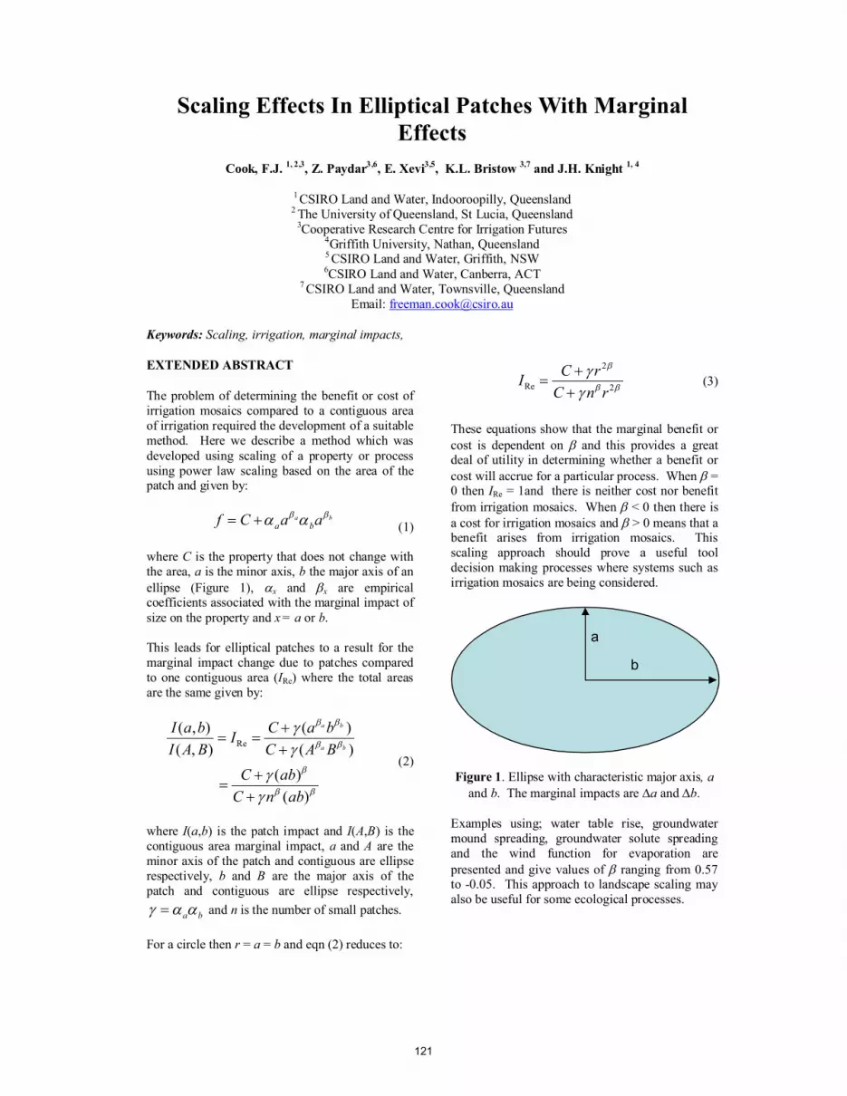
where C is the property that does not change with the area, a is the minor axis, b the major axis of an ellipse (Figure 1), x and x are empirical coefficients associated with the marginal impact of size on the property and x = a or b.

This leads for elliptical patches to a result for the marginal impact change due to patches compared to one contiguous area (IRe) where the total areas are the same given by:

Re

( , ) ( )

( , ) ( )

( )

( )

a b

a b

I a b C a bI

I A B C A B

C ab

C n ab

(2)

where I(a,b) is the patch impact and I(A,B) is the contiguous area marginal impact, a and A are the minor axis of the patch and contiguous are ellipse respectively, b and B are the major axis of the patch and contiguous are ellipse respectively,

a b and n is the number of small patches.

For a circle then r = a = b and eqn (2) reduces to:

2

Re 2

C rI

C n r

(3)

These equations show that the marginal benefit or cost is dependent on and this provides a great deal of utility in determining whether a benefit or cost will accrue for a particular process. When =0 then IRe = 1and there is neither cost nor benefit from irrigation mosaics. When < 0 then there is a cost for irrigation mosaics and > 0 means that a benefit arises from irrigation mosaics. This scaling approach should prove a useful tool decision making processes where systems such as irrigation mosaics are being considered.

Figure 1. Ellipse with characteristic major axis, aand b. The marginal impacts are a and b.

Examples using; water table rise, groundwater mound spreading, groundwater solute spreading and the wind function for evaporation are presented and give values of ranging from 0.57 to -0.05. This approach to landscape scaling may also be useful for some ecological processes.

b

a

121

1. INTRODUCTION

Natural and many other systems have features which are a function of characteristic properties of the system. These properties are often associated with the temporal or spatial processes. In ecology the size, shape and the spatial arrangement of patches have been studied by many authors and recently reviewed by Wu and Li (2006). Here we will develop some scaling which is based around the patches of an elliptical shape. This kind of scaling has similarities to that of landscape analysis (Gardner 1987, Milne 1992, Wiens et al. 1997, Nikora et al. 1999, Hoffman and Greef2004). Here though we will look at the marginal impact on bio-physical processes associated with irrigation mosaics.

Irrigation schemes where the scale of an individual irrigation area is small, but the total area irrigated may be large are term irrigation mosaics (Paydar et al. 2007a, Cook et al. 2007a). In determining whether benefits may accrue from irrigation mosaics a method is need to compare them to more traditional contiguous area of irrigation. We will use the scaling approach developed here to show how this could be used to determine benefit or dis-benefit of irrigation mosaics compared with tradition contiguous irrigation schemes.

2. THEORY

We will assume homogeneous conditions occur throughout the region and that the marginal costs or benefits are related to the size of the patch. Schematically this is presented in Figure 1, but the property and marginal value does not necessarily have to be the physical area so long as the property and marginal effects scale with area. Under these conditions we can characterise the system in terms of some length scale that allows us to examine the effects of the size of the mosaics on the hydrological or other properties. We can consider the characteristics of the spatial extent as being described approximately by an ellipse (Figure 1). The perimeter (P) and area (A) of an ellipse are given by:

2 2/2 220

2 2

4 1 sin

2 1/2

.

a bP a d

a

a b

A ab

(4)

In a mosaic we will have patches spread throughout a region and the total area will then be

the sum of each patch. If an irrigation scheme was implemented such that rather than one contiguous irrigated area, it consisted of a number of smaller patches, we consider this to be and irrigation mosaic.

We assume that some property of the system, f,scales with the area of the patch such that:

a b

a bf C a a (5)

where C is the property that does not change with the area, a is the minor axis, b the major axis of an ellipse, x and x are empirical coefficients associated with the marginal impact of size on the property and x = a or b. We define the impact of this property as:

( , ) .

.

a b

a b

a bI a b a b C a a

a b C a a

(6)

where = ab. For a system such as irrigation mosaics we wish to determine the effect of isolated distributed patches compared to one large contiguous patch. If the total area is the same for one contiguous area and n number of smaller patches of the same size then:

1

n

i ii

a b n ab AB

ABn

ab

(7)

We define the relative impact of n patches compared to one contiguous area and the result is eqn (2). Simplification of eqn (2) can be achieved by assuming that a = b and with substitution of eqn (7) results in:

Re

( )

( )

C abI

C n ab

(8)

A further simplification occurs when a = b = R and A = B = RT which means that the ellipse becomes a circle and eqn (8) becomes eqn (3) above.

The interesting thing about the solutions given by eqns (3) and (8), is that the term n is the only difference between the numerator and denominator. This means that the marginal effect of irrigation mosaics can be determined from the value of . When = 0 then IRe = 1 and the impact

122

will be the same for irrigation mosaics and one contiguous area. However, when > 0 irrigation mosaics will have a reduced impact, while for < 0 irrigation mosaics will have an enhanced impact, compared to a contiguous irrigated area. This has now provided us with a powerful tool for analysing the various impacts that maybe occur if irrigation mosaics are introduced.

Here we will examine a number of bio-physical properties where we have determined the effect of the size of the patches on this property (Cook et al. 2007a). These properties are: the maximum height of the water table under the patch at a particular time, the extent of watertable rise outside the irrigated area at a particular time, the extent of solute transport into the surrounding area and the effect on the wind function on evaporation.

3. METHOD

A study to determine the advantages and disadvantages of irrigation mosaics was undertaken (Cook et al. 2007a) and we will use the results from this study here. We will considercircular patches so that eqn (5) simplifies to:

2 2f C r (9)

The processes that will be studied are; the maximum water table rise, the extent of groundwater mound spreading, extent of solute leakage and wind function in relation to evaporation. Below we show how these processes were calculated and then in Section 4 eqn (9) is applied to these processes.

3.1. Groundwater rise and spreading

The rise of the water table caused by recharge to groundwater is discussed in detail elsewhere (Cook et al. 2007a,b). We used the solutions of Cook et al. (2007a,b) to calculate the water table rise and converted these from the non-dimensional time and space to dimensional time and space using the methods presented by Cook et al. (2007b). Radial dimensions varied from 100 m to 100 km were chosen for the calculations. The maximum water table height was calculated as the height the watertable reached at the centre of the irrigated patch. The results at a time of 100 years are presented in (Cook et al. 2007b) and used here. In the calculations we used values of saturated hydraulic conductivity (K) of 1 m day-1, recharge rate to the groundwater (I) of 1 mm day-1, specific yield () of 0.1 m3 m-3, and h0 of 10 m.

To determine the extent of groundwater mound spreading into the surrounding area we used:

( 0.001)r r H R (10)

where H = h(r) – h0, h(r) is the height of the water table at radial distance r [L] and h0 initial water table height above the impervious base [L]. The same values for the aquifer properties were used as given above.

3.2. Solute leaching

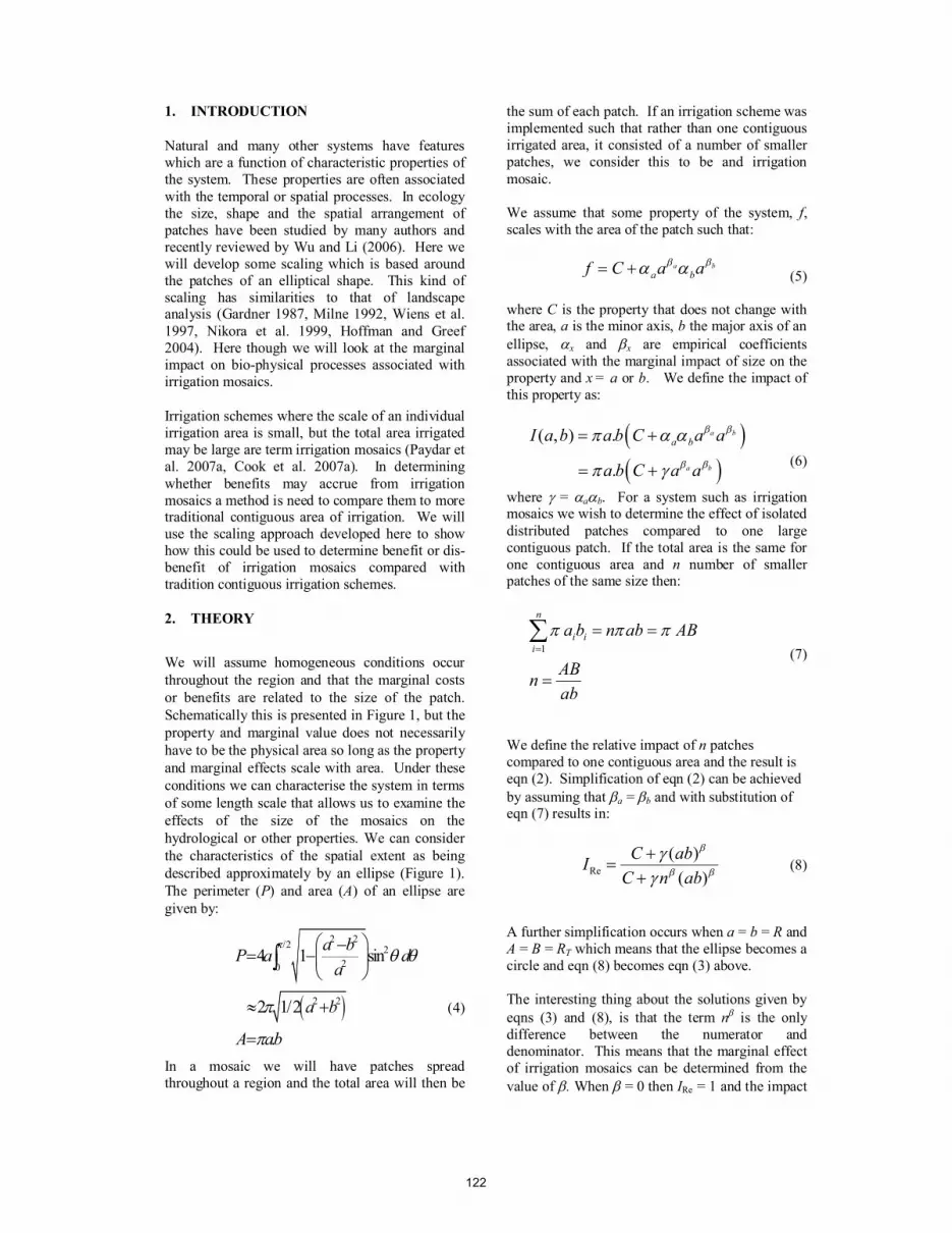
We consider the leaching of a tracer solute (chloride or tritium) to the groundwater and use two schemes to bound the radial extent of the solute spreading beyond the irrigated area (Cook et al. 2007a). These schemes consider that the solute is mixed throughout the saturated zone to the impermeable layer (Figure 2a) and the other where the solute is contain in the water table above the initial water table height (Figure 2b).

Figure 2. Diagram of the two advective solute transport shemes used to estimate the position of the solute front: a) complete displacement of old water by new water to the impermeable base and

b) the new water sits on top of the old water.

For these calculations we assume that the tracer solute reaches the water table at the same time as the water does. In reality this will not be true as the water present in the profile prior to the increase in recharge rate will be displaced ahead of the solute front. This will mean that the results overestimate the extent of solute spreading from the edge of the irrigated patch. The radial distance is calculated by matching the water volumes. The volume of water applied (Vi [L

3]) is given by:

2iV R It (11)

z

x or r

ho

h

a

bz

x or r

hoh

Solute front

123

The volume of water stored in the water table (Vs) is given by:

0( , ) ( )

r

s st

V r t h r dr (12)

where ( ) ( )

t th r h r

for the case given by

Figure 2a, th

is h [L] at time t, s is the saturated volumetric water content of the aquifer and

0( ) ( )t t

h r h r h for the case given by

Figure 2b. The radius the solute has advected to is determined by finding the value of r at which Vs =Vi. The integral in eqn (12) were solved numerically using trapezoidal integration.

3.3. Evaporation – wind factor

Enhanced evaporation of water due to advection caused by hot dry air moving over a wet patch or at the edge of irrigated areas is a well known phenomena (Priestley 1955, McNaughton 1983,Lang et al.1983, Kadar and Yaglom 1990). There is little research available on how evaporation varies with patch size but a good body of research for water bodies, which was summarised by Sweers (1976). The evaporation rate from a water body is (Sweers 1976):

( )( )s aE f u e e (13)

where es and ea are the saturated and actual vapour pressure deficit respectively and f(u) is the wind speed function. Sweers (1976) reviewed the existing literature and concluded that the wind speed function was best given by:

0.05

0.05

0.05

( )

( )

ee e e

e e e e

af u b c u S A

S

A a b c u

(14)

where ae, be and ce are empirical constants (see Sweers (1976) for values), S is the representative area of the evaporating area [L2] and u is windspeed . Assuming that the patches are

circular then 2S R and that u is the same,then the effect of R on the wind factor can be obtained from eqn (14). The comparative windspeed effect can be calculated by:

0.050.05 2

2r TS R

S R

(15)

where Sr is a the reference area and RT is the radius of the large contiguous irrigation area (reference area), assuming patches are circular.

Conway and van Bavel (1967) showed that the Dalton equation for evaporation (eqn (13)) was applicable to soils. This means that the form of eqn (14) and the scaling with the power of 0.05 should be applicable.

4. RESULTS

The results presented here are for mosaics of isolated irrigated patches where the complication of interaction between the patches is not considered. This is so that the effect of size of apatch on the processes of interest can be estimated, without having to include the effect of spacing.

4.1. Groundwater rise

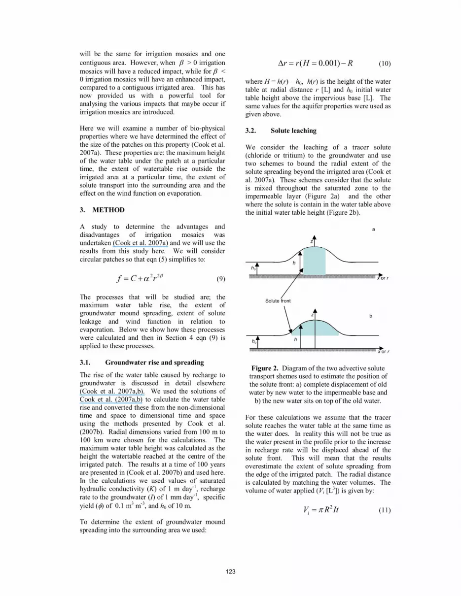
The maximum groundwater rise (hm) was calculated using the methods presented by Cook et al. (2007a,b) and a time of 100 years. The scaling model presented in eqn (9) was fitted to this data and gives = 0.35 (Figure 3). is > 0 and suggests that for patches, which are sufficiently isolated that there is no appreciable interaction of the groundwater mounds, irrigation mosaics could reduce hm.

R (m)

0 2000 4000 6000 8000 10000 12000

hm -

h0 (

m)

-50

0

50

100

150

200

250

300

Figure 3. Maximum change in water table height (hm – h0), (hm = h(r = 0)) with radius (R), with t = 100 years and recharge rate and aquifer properties given in text. The line is a regression of eqn (9) against the data, which results in a value of =

0.35, (regression coefficient of 0.999).

The extent of groundwater spreading beyond the irrigated area as a function of R was determined using different values of non-dimensional time () (Figure 4). The relationship between and dimensional time (t) is:

124

2Rt

bK

(16)

where is the specific yield [L3 L-3] and

0( ) / 2mb h h is the linearization parameter

[L]. The data are plotted as f – R as C will be equal to R for this case.

R (m)

1e+1 1e+2 1e+3 1e+4 1e+5 1e+6

f - R

(m

)

1e+2

1e+3

1e+4

1e+5

1e+6

1e+7 = 0.75Regression = 0.75 = 5Regression = 5 = 10Regression = 10

Figure 4. Relationship between f-R and R for various values of. The regression lines gave

values of of 0.58, 0.57 and 0.57 for = 0.75. 5.0 and 10.0 respectively

The value of 0.57 indicates that the area impacted by water table spread is likely to be slightly less with irrigation mosaics that with one contiguous irrigation area. This assumes that the patches in the irrigation mosaic are far enough apart for there to be not interaction. Although not shown here calculations were done to check that variation in the other parameters I, Sy, and K did not affect this result.

4.2. Solute leaching

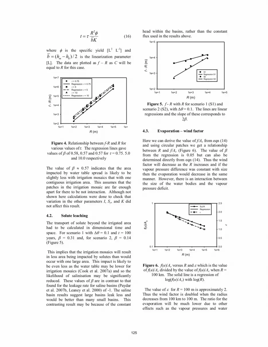
The transport of solute beyond the irrigated area had to be calculated in dimensional time and space. For scenario 1 with = 0.1 and t = 100 years, = 0.31 and, for scenario 2, = 0.14(Figure 5).

This implies that the irrigation mosaics will result in less area being impacted by solutes than would occur with one large area. This impact is likely to be even less as the water table may be lower for irrigation mosaics (Cook et al. 2007a) and so the likelihood of salinisation may be significantly reduced. These values of are in contrast to that found for the leakage rate for saline basins (Paydar et al. 2007b, Leaney et al. 2000) of -1. The saline basin results suggest large basins leak less and would be better than many small basins. This contrasting result may be because of the constant

head within the basins, rather than the constant flux used in the results above.

R (m)

1e+1 1e+2 1e+3 1e+4 1e+5

f - R

(m

)

1e+2

1e+3

1e+4

1e+5

S1Regression S1S2Regression S2

Figure 5. f - R with R for scenario 1 (S1) and scenario 2 (S2), with = 0.1. The lines are linear regressions and the slope of these corresponds to

2.

4.3. Evaporation – wind factor

Here we can derive the value of f/Ae from eqn (14)and using circular patches we get a relationship between R and f/Ae (Figure 6). The value of from the regression is 0.05 but can also be determined directly from eqn (14). Thus the wind factor will decrease as the R increases and if the vapour pressure difference was constant with size then the evaporation would decrease in the same manner. However, there is an interaction between the size of the water bodies and the vapour pressure deficit.

R (m)

1e+1 1e+2 1e+3 1e+4 1e+5 1e+6

f(u

)/A

e

0.1

1

0.0

0.5

1.0

1.5

2.0

2.5f(u)/A

Regression

Figure 6. f(u)/Ae versus R and which is the value of f(u)/Ae divided by the value of f(u)/Ae when R =

100 km. The solid line is a regression of log(f(u)/Ae) with log(R).

The value of for R = 100 m is approximately 2. Thus the wind factor is doubled when the radius decreases from 100 km to 100 m. The ratio for the evaporation will be much lower due to other effects such as the vapour pressures and water

125

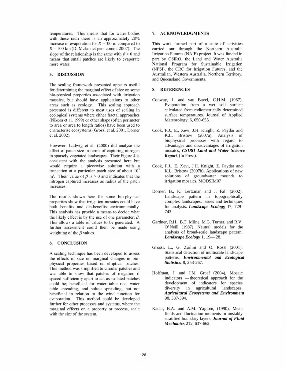
temperatures. This means that for water bodies with these radii there is an approximately 28% increase in evaporation for R =100 m compared to R = 100 km (D. McJannet pers comm. 2007). The slope of the relationship is the same with > 0 and means that small patches are likely to evaporate more water.

5. DISCUSSION

The scaling framework presented appears useful for determining the marginal effect of size on some bio-physical properties associated with irrigation mosaics, but should have applications to other areas such as ecology. This scaling approach presented is different to most uses of scaling in ecological systems where either fractal approaches (Nikora et al. 1999) or other shape (often perimeter to area or area to length ratios) have been used to characterise ecosystems (Grossi et al. 2001, Dorner et al. 2002).

However, Ludwig et al. (2000) did analyse the effect of patch size in terms of capturing nitrogen in sparsely vegetated landscapes. Their Figure 4 is consistent with the analysis presented here but would require a piecewise solution with a truncation at a particular patch size of about 103

m2. Their value of is > 0 and indicates that the nitrogen captured increases as radius of the patch increases.

The results shown here for some bio-physical properties show that irrigation mosaics could have both benefits and dis-benefits environmentally. This analysis has provide a means to decide what the likely effect is by the use of one parameter, . This allows a table of values to be generated. A further assessment could then be made using weighting of the values.

6. CONCLUSION

A scaling technique has been developed to assess the effects of size on marginal changes in bio-physical properties based on elliptical patches. This method was simplified to circular patches and was able to show that patches of irrigation if spaced sufficiently apart to act as isolated patches could be; beneficial for water table rise, water table spreading, and solute spreading; but not beneficial in relation to the wind function for evaporation. This method could be developed further for other processes and systems, where the marginal effects on a property or process, scale with the size of the system.

7. ACKNOWLEDGMENTS

This work formed part of a suite of activities carried our through the Northern Australia Irrigation Futures (NAIF) project. It was funded in part by CSIRO, the Land and Water Australia National Program for Sustainable Irrigation (NPSI), the CRC for Irrigation Futures, and the Australian, Western Australia, Northern Territory, and Queensland Governments.

8. REFERENCES

Conway, J. and van Bavel, C.H.M. (1967), Evaporation from a wet soil surface calculated from radiometrically determined surface temperatures. Journal of Applied Meteorology, 6, 650-655.

Cook, F.J., E., Xevi, J.H. Knight, Z. Paydar and K.L. Bristow (2007a), Analysis of biophysical processes with regard to advantages and disadvantages of irrigation mosaics, CSIRO Land and Water Science Report, (In Press).

Cook, F.J., E. Xevi, J.H. Knight, Z. Paydar and K.L. Bristow (2007b), Applications of new solutions of groundwater mounds to irrigation mosaics, MODSIM07

Dorner, B., K. Lertzman and J. Fall (2002),Landscape pattern in topographically complex landscapes: issues and techniques for analysis. Landscape Ecology, 17, 729-743.

Gardner, R.H., B.T. Milne, M.G. Turner, and R.V. O’Neill (1987), Neutral models for the analysis of broad-scale landscape pattern. Landscape Ecology, 1, 19— 28.

Grossi, L., G. Zurlini and O. Rossi (2001), Statistical detection of multiscale landscape patterns. Environmental and Ecological Statistics, 8, 253-267.

Hoffman, J. and J.M. Greef (2004), Mosaic indicators — theoretical approach for the development of indicators for species diversity in agricultural landscapes. Agricultural Ecosystems and Environment, 98, 387-394.

Kadar, B.A. and A.M. Yaglom, (1990), Mean fields and fluctuation moments in unstably stratified boundary layers. Journal of Fluid Mechanics, 212, 637-662.

126

Lang, A.R.G., K.G. McNaughton, C. Fazu, E.F. Bradley and E. Ohtaki (1983), An experimental appraisal of terms in heat and moisture flux equations for local advection. Boundary Layer Meteorology, 25, 89-102.

Leaney, F.W.J., E.W. Christen, I.D. Jolly, and G.R. Walker (2000), On-farm and community-scale salt disposal basins on the Riverine Plain: Guidelines summary. CSIRO Land and Water Technical Report 24/00, CRC for Catchment Hydrology Technical Report 00/15, CSIRO Land and Water, Adelaide.

Ludwig, J.A., J.A. Wiens and D.J. Tongway(2000), A scaling rule for landscape patches and how it applies to conserving soil resources in savannas, Ecosystems, 3, 84-97.

McNaughton, K.G. (1983), The direct effect of shelter on evaporation rates: Theory and an experimental test. Agricultural Meteorology, 29, 125-136.

Nikora, V.I., C.P. Pearson and U. Shankar (1999),Scaling properties in landscape patterns: New Zealand experience. Landscape Ecology, 14, 17-33.

Milne, B.T. (1992), Spatial aggregation and neutral models in fractal landscapes. American Naturalist, 139(1), 32— 57.

Paydar, Z., F.J. Cook, E. Xevi and K. L. Bristow(2007a), Review of current understanding of irrigation mosaics. CSIRO Land and Water Science Report, 40/07, 38p.

Paydar, Z., F.J. Cook, E. Xevi and K. L. Bristow (2007b), Irrigation mosaics. How are they different? MODSIM07

Priestley, C.H.B. (1955), Free and forced convection in air near the ground. Quarterly Journal of the Royal Meteorological Society, 81, 139-143.

Sweers, H.E. 1976, A nomogram to estimate the heat-exchange coefficient at the air-water interface as a function of wind speed and temperature; A critical survey of some literature. Journal of Hydrology, 30, 375-401.

Wiens, J.A., R.L. Schooley and R.D. Weeks(1997), Patchy landscapes and animal

movements: do beetles percolate? Oikos, 78, 257— 264.

Wu, J. and H. Li (2006), Concepts of scale and scaling. In J. Wu, K.B. Jones, H. Li and O.L. Loucks (eds) Scaling and uncertainty analysis in Ecology, Chapter 1, Methods and Applications, Springer, Dordrecht: pp 3 - 15.

127