flexural analysis of thin rectangular plates

i

FLEXURAL ANALYSIS OF THIN RECTANGULAR

PLATES USING GALERKIN METHOD

BY

OKOYE MMADUAKONAM OBIORA

2009226002P

DEPARTMENT OF CIVIL ENGINEERING

FACULTY OF ENGINEERING

NNAMDI AZIKIWE UNIVERSITY, AWKA.

MARCH, 2021

i

FLEXURAL ANALYSIS OF THIN RECTANGULAR

PLATES USING GALERKIN METHOD

OKOYE MMADUAKONAM OBIORA

(2009226002P)

A THESIS SUBMITTED TO THE DEPARTMENT OF CIVIL

ENGINEERING, FACULTY OF ENGINEERING, NNAMDI

AZIKIWE UNIVERSITY, AWKA IN PARTIAL FULFILLMENT

OF THE REQUIREMENTS FOR THE DEGREE OF MASTER OF

ENGINEERING (STRUCTURES).

MARCH, 2021

ii

CERTIFICATION PAGE

I, Mmaduakonam Obiora Okoye, with registration number 2009226002P hereby certify that I amresponsible for the work submitted in this Thesis and that this is an original work which has notbeen submitted to this University or any other institution for the award of a degree or a diploma.

……………………………. ……………….

Signature of Candidate Date

iii

APPROVAL PAGE

This Thesis written by Okoye Mmaduakonam Obiora has been examined and approved for the

award of master degree of Nnamdi Azikiwe University, Awka.

……………………………. ....……………

Engr. Prof. C. H., Aginam. Date

Supervisor 1

……………………………. ....……………

Engr. Dr. P. D., Onodagu. Date

Supervisor 11

………………………………… ……………….

Engr. Prof. C. A., Chidolue. Date

Head of Department

……………………………… ………………..

Engr. Prof. J. C. Ezeh Date

External Examiner

………………………………. …………………

Engr. Prof. H.C Godwin Date

Dean, Faculty of Engineering

……………………………….. ………………..

Engr. Prof. P. K Igbokwe Date

Dean, School of Post-Graduate Studies

iv

DEDICATION

This work is dedicated to the almighty God for His immeasurable grace throughout the duration

of this work and programme.

v

ACKNOWLEDGEMENTS

I gladly express my deepest gratitude and appreciation to my supervisors, Engr. Prof. C.H.

Aginam and Engr. Dr. P.D. Onodagu, whose profound grasp of plate was a beacon of light throughout the

duration of this research. Thank you, Sirs. Also, I say a very big thank you to the meticulous head of

department, Engr. Prof. C. A Chidolue, whose technical lessons to me are priceless. Thank you sir.

Again, I extend my appreciation to all the members of staff of the Civil Engineering Department,

Nnamdi Azikiwe University, Awka, for providing me with the opportunity to enrich my knowledge and

be a better engineer. Among them are: Engr. Prof. C.M.O Nwaiwu, Engr. Prof. O. E. Ekenta, Engr. Prof.

(Mrs.) N. E. Nwaiwu, Engr. Dr. B.O. Adinna, , Engr. Dr. C.A Ezeagu ,Engr. (Mrs) P.I. Nwajuaku, Engr.

Dr. V.O. Okonkwo, Engr. A.I. Nwajuaku, Engr. A.A. Ezenwamma, Engr. C. Nwakaire just to mention a

few. You have all contributed to making this work a success.

My gratitude also goes to all non-academic staff of civil engineering department and my

colleagues in the programme. You played a very significant role in my achieving this feat.

Finally, I would like to thank my family members for their selfless support. Your prayers and

encouragement to me are worth more than gold. I love you all.

vi

ABSTRACT

The flexure of thin rectangular isotropic plates subjected to uniformly distributed loads usingGalerkin variational method has been studied for five different boundary conditions namely,CCCS, SSSS, CCCC, CCSS and CSCS. The deflected surface was approximated using a gridwork of beams. The deflection functions of the deformed surfaces were derived in terms ofcharacteristic coordinate polynomials with unknown coefficients which satisfy the prescribedboundary conditions of the plate. Different approximations of the derived deflection functionscorresponding to the first, second, truncated third and third approximations were developed foreach case. These deflection functions were substituted into the fourth-order governingdifferential equation of plate and the Galerkin method reduced the solution of the differentialequations to the evaluation of definite integrals of simple functions. The unknown coefficientswere obtained by solving the resulting set of linear functions. These obtained coefficients werethen put back into the different approximations of the deflection functions to calculate thedeflections and their corresponding span moments. Results were obtained for the five differentsets of boundary conditions considered and the aspect ratio (p = b a ) was varied from 1.0 to 2.0for each approximation. The accuracy and pattern of convergence of the present formulationswere assessed by comparing them with the results of the classical solutions. The variations of thedeflections and span moments with respect to aspect ratios for the different approximations werepresented in graphical forms and discussed. For the clamped rectangular plate, it was discoveredthat the accuracy and convergence to the classical solution improved as the approximationincreased from the first through third. For instance, the average percentage difference betweenthe present study and the results in literature gave 1.98, 1.96 and 8.46 for deflection, short-spanmoment and long-span moment respectively for the clamped plate at the third approximation.This level of convergence makes the present study invaluable for the design engineer. Moreover,the present study provides computer algorithm in MATLAB (M-Files) for the differentapproximations which can be of help to the design engineer for the calculation of the mechanicalproperties of plates at arbitrary points on the plate surface. In conclusion, the accuracy andconvergence of results as the number of terms of deflection function increased were found to bedependent on the boundary condition of the plate for the present formulation.

vii

TABLE OF CONTENTS

Cover Page

Title Page

Certification page

Approval page

Dedication

Acknowledgements

Abstract

Table of Contents

List of Tables

List of Figures

Notations

Chapter One: INTRODUCTION

1.1 Background to the Study

1.2 Statement of Problem

1.3 Aim and objectives of the Study

1.4 Justification of the Study

1.5 Scope of Study

Chapter Two: LITERATURE REVIEW

2.1 Historical Development of Plate Analysis

2.2 Rectangular Plates

2.2.1 Navier’s Method

2.2.2 Levy’s Method

i

ii

iii

iv

v

vi

vii

xi

xv

xviii

1

1

4

5

5

5

7

7

7

7

9

viii

2.2.3 Classical Solution

2.2.4 Approximate Solutions

2.3 Governing Equation of Plates in Cartesian Coordinate System

2.4 Boundary Conditions

2.5 Material Property

2.6 Formulation of Plate Bending Problems

2.6.1 Numerical Methods

2.6.1.1 Finite Difference Method (FDM)

2.6.1.2 Boundary Element Method (BEM)

2.6.1.3 Finite Element Method (FEM)

2.6.1.4 Boundary Collocation Method (BEM)

2.6.2 Variational Methods

2.6.2.1 The Ritz Method

2.6.2.2 The Kantorovich Method

2.6.2.3 The Galerkin (Petrov-Galerkin) Method

2.6.2.4 The Principle of Virtual Work

2.7 Characteristic Coordinate Polynomials

2.7.1 Development of Characteristic Coordinate Polynomial Shape Function

for a Uniformly Distributed Load

2.8 Expression of Governing Differential Equation of Plate in Non-dimensional Parameters

2.9 Summary of Previous Works on Flexure of Rectangular Plates

Chapter Three: METHODOLOGY

3.1 General Introduction

3.2 Development of Shape Functions for Various Boundary Conditions

11

11

14

18

20

20

21

21

22

23

24

24

25

25

26

29

30

33

34

34

38

38

38

ix

3.2.1 Case 1 (Type CCCS)

3.2.2 Case 2 (Type SSSS)

3.2.3 Case 3 (Type CCCC)

3.2.4 Case 4 (Type CCSS)

3.2.5 Case 5 (Type CSCS)

3.3 Application of Galerkin Principle on Multi-Term Thin Rectangular Plate Problems






3.4 Multi-Term Bending Moment Expressions for Thin Rectangular Plates






3.5 Evaluation of Results






Chapter Four: RESULTS AND DISCUSSION

38

42

46

50

53

57

57

98

139

177

221

260

261

264

267

271

274

277

278

293

308

323

338

354

x

4.1 Results






4.2 Discussion






Chapter Five: CONCLUSIONS AND RECOMMENDATIONS

5.1 Conclusions

5.2 Justification/Contributions of the Study

5.3 Recommendations

References

Appendix A.1 Comparison of Edge Moment Coefficient Values

Appendix A.2 Deflection Curves at Aspect Ratio of Unity

Appendix A.3 Short Span Moment Curve at Aspect Ratio of Unity

Appendix A.4 Typical Excel Spreadsheet

Appendix A.5 M-File for CCCS

354

354

356

358

360

361

363

364

366

372

378

380

386

386

386

387

388

395

397

400

403

404

xi

LIST OF TABLES

Table 2.1: Properties of Materials.

Table 2.2: Previous works on Flexure of Rectangular Plates.

Table 3.1: Stiffness Coefficient Values for CCCS Plate at Varying Aspect Ratio.

Table 3.2: First Approximation Coefficient Values for CCCS Plate at Varying Aspect Ratio.

Table 3.3: Second Approximation Coefficient Values for CCCS Plate at Varying Aspect

Ratio.

Table 3.4: Truncated Third Approximation Coefficient Values for CCCS Plate at

Varying Aspect Ratio.

Table 3.5: Third Approximation Coefficient Values for CCCS Plate at Varying Aspect Ratio.

Table 3.6: Stiffness Coefficient Values for SSSS Plate at Varying Aspect Ratio.

Table 3.7: First Approximation Coefficient Values for SSSS Plate at Varying Aspect Ratio.

Table 3.8: Second Approximation Coefficient Values for SSSS Plate at Varying Aspect

Ratio.

Table 3.9: Truncated Third Approximation Coefficient Values for SSSS Plate at


Table 3.10: Third Approximation Coefficient Values for SSSS Plate at Varying Aspect Ratio.

Table 3.11: Stiffness Coefficient Values for CCCC Plate at Varying Aspect Ratio.

Table 3.12: First Approximation Coefficient Values for CCCC Plate at Varying Aspect Ratio.

Table 3.13: Second Approximation Coefficient Values for CCCC Plate at Varying Aspect

Ratio.

Table 3.14: Truncated Third Approximation Coefficient Values for CCCC Plate at


Table 3.15: Third Approximation Coefficient Values for CCCC Plate at Varying Aspect

20

35

280

284

285

285

285

295

299

299

300

300

310

314

314

315

xii

Ratio.

Table 3.16: Stiffness Coefficient Values for CCSS Plate at Varying Aspect Ratio.

Table 3.17: First Approximation Coefficient Values for CCSS Plate at Varying Aspect Ratio.

Table 3.18: Second Approximation Coefficient Values for CCSS Plate at Varying Aspect

Ratio.

Table 3.19: Truncated Third Approximation Coefficient Values for CCSS Plate at


Table 3.20: Third Approximation Coefficient Values for CCSS Plate at Varying Aspect Ratio.

Table 3.21: Stiffness Coefficient Values for CSCS Plate at Varying Aspect Ratio.

Table 3.22: First Approximation Coefficient Values for CSCS Plate at Varying Aspect Ratio.

Table 3.23: Second Approximation Coefficient Values for CSCS Plate at Varying Aspect

Ratio.

Table 3.24: Truncated Third Approximation Coefficient Values for CSCS Plate at


Table 3.25: Third Approximation Coefficient Values for CSCS Plate at Varying Aspect

Ratio.

Table 4.1a: Mid-span (X =0.5, Y =0.5) Deflection Coefficient Values, , for CCCS Plate

at Varying Aspect Ratio (Wmax= α qa4/D ).

Table 4.1b: Short Span Moment Coefficient Values, βx, at Mid-Span (X =0.5, Y =0.5)

for CCCS Plate at Varying Aspect Ratio ( Mx max = qa2β ).

Table 4.1c: Long Span Moment Coefficient Values, βy, at Mid-Span (X =0.5, Y =0.5)

for CCCS Plate at Varying Aspect Ratio ( My max= qa2β ).

Table 4.2a: Mid-span (X =0.5, Y =0.5) Deflection Coefficient Values, , for SSSS Plate


315

325

329

329

329

330

340

343

344

344

345

354

355

355

356

xiii


for SSSS Plate at Varying Aspect Ratio ( Mx max = qa2β ).

Table 4.2c: Long Span Moment Coefficient Values, βy, at Mid-Span (Q =0.5, R =0.5)

for SSSS Plate at Varying Aspect Ratio ( My max= qa2β ).

Table 4.3a: Mid-span (X =0.5, Y =0.5) Deflection Coefficients Values, , for CCCC

Plate at Varying Aspect Ratio (Wmax= α qa4/D).


for CCCC Plate at Varying Aspect Ratio ( Mx max = qa2β ).


for CCCC Plate at Varying Aspect Ratio ( My max= qa2β ).

Table 4.4a: Mid-span (X =0.5, Y =0.5) Deflection Coefficient Values, , for CCSS Plate



for CCSS Plate at Varying Aspect Ratio ( Mx max = qa2β ).


for CCSS Plate at Varying Aspect Ratio ( My max= qa2β ).

Table 4.5a: Mid-span (X =0.5, Y =0.5) Deflection Coefficients Values, , for CSCS

Plate at Varying Aspect Ratio (Wmax= α qa4/D ).


for CSCS Plate at Varying Aspect Ratio ( Mx max = qa2β ).

Table 4.5c: Long Span Moment Coefficient Values, βy, at Mid-Span (Q =0.5, R =0.5)

for CSCS Plate at Varying Aspect Ratio ( My max= qa2β ).

Table 4.2d: Anova: Single Factor for W1 versus W (SSSS).

Table 4.2e: Anova: Single Factor for W3 Versus W (SSSS).

Table 4.2f: Anova: Single Factor for Mx1 Versus Mx (SSSS).

356

357

358

358

359

360

360

361

361

362

363

367

368

369

xiv

Table 4.2g: Anova: Single Factor for Mx3 Versus Mx (SSSS).

Table 4.2h: Anova: Single Factor for My1 Versus My (SSSS).

Table 4.2i: Anova: Single Factor for My3 Versus My (SSSS).

Table 4.3d: Anova: Single Factor for W1 Versus W (CCCC).

Table 4.3e: Anova: Single Factor for W4 Versus W (CCCC).

Table 4.3f: Anova: Single Factor for Mx1 Versus Mx (CCCC).

Table 4.3g: Anova: Single Factor for Mx4 Versus Mx (CCCC).

Table 4.3h: Anova: Single Factor for My1 Versus My (CCCC).

Table 4.3i: Anova: Single Factor for My4 Versus My (CCCC).

Table 4.5d: Anova: Single Factor for W1 Versus W (CSCS).

Table 4.5e: Anova: Single Factor for W3 Versus W (CSCS).

Table 4.5f: Anova: Single Factor for Mx1 Versus Mx (CSCS).

Table 4.5g: Anova: Single Factor for Mx3 Versus Mx (CSCS).

Table 4.5h: Anova: Single Factor for My1 Versus My (CSCS).

Table 4.5i: Anova: Single Factor for My3 Versus My (CSCS).

370

371

371

373

373

375

375

377

377

381

381

383

383

384

385

xv

LIST OF FIGURES

Figure 1.1: Edge Numbering of Rectangular Plate.

Figure 1.2: Cross-Section of Types of Loads for a Plate.

Figure 2.1: External and Internal Forces on the Element of the Middle Surface.

Figure 2.2: Some Edge Conditions of a Plate.

Figure 2.3: Elastic Beam of Arbitrary Support Conditions Subjected to Uniformly.

Distributed Load.

Figure 3.1: Thin Rectangular Plate with Two Opposite Edges Clamped and One of the Other

Two Opposite Edges Clamped and the Other Simply Supported (CCCS).

Figure 3.2: All Edges Simply Supported Rectangular Plate (Type SSSS).

Figure 3.3: All Edges Clamped Rectangular Plate (Type CCCC).

Figure 3.4: Thin Rectangular Plate Clamped on Two Adjacent Near Edges and Simply

Supported on Two Adjacent Far Edges (CCSS).

Figure 3.5: Thin Rectangular Plate Clamped on Two Opposite Short Edges and Simply

Supported on Two Opposite Long Edges (Type CSCS).

Figure 3.6: CCCS Plate under Uniformly Distributed Load.

Figure 3.7: SSSS Plate under Uniformly Distributed Load.

Figure 3.8: CCCC Plate under Uniformly Distributed Load.

Figure 3.9: CCSS Plate under Uniformly Distributed Load.

Figure 3.10: CSCS Plate under Uniformly Distributed Load.

Figure 3.11: CCCS Plate under Uniformly Distributed Load.

Figure 3.12: SSSS Plate under Uniformly Distributed Load.

Figure 3.13: CCCC Plate under Uniformly Distributed Load.

Figure 3.14: CCSS Plate under Uniformly Distributed Load.

2

3

15

19

33

38

42

46

50

54

57

98

139

177

221

261

264

267

271

xvi

Figure 3.15: CSCS Plate under Uniformly Distributed Load.

Figure 3.16: Flowchart for Calculation of Deflection, Short and Long term Moment

Coefficient Values.

Figure 4.1a: Comparison of Deflection Coefficient Values for CCCS at Mid-Span at


Figure 4.1b: Comparison of Short Span Moment Coefficient Values for CCCS at Mid-Span

at Varying Aspect Ratio.

Figure 4.1c: Comparison of Long Span Moment Coefficient Values for CCCS at Mid-Span


Figure 4.2a: Comparison of Deflection Coefficient Values for SSSS at Mid-Span at


Figure 4.2b: Comparison of Short Span Moment Coefficient Values for SSSS at Mid-Span


Figure 4.2c: Comparison of Long Span Moment Coefficient Values for SSSS at Mid-Span


Figure 4.3a: Comparison of Deflection Coefficient Values for CCCC at Mid-Span at


Figure 4.3b: Comparison of Short Span Moment Coefficient Values for CCCC at Mid-Span


Figure 4.3c: Comparison of Long Span Moment Coefficient Values for CCCC at Mid-Span


Figure 4.4a: Comparison of Deflection Coefficient Values for CCSS at Mid-Span at


Figure 4.4b: Comparison of Short Span Moment Coefficient Values for CCSS at Mid-Span

274

353

364

365

366

366

368

370

372

374

376

378

xvii


Figure 4.4c: Comparison of Long Span Moment Coefficient Values for CCSS at Mid-Span


Figure 4.5a: Comparison of Deflection Coefficient Values for CSCS at Mid-Span at


Figure 4.5b: Comparison of Short Span Moment Coefficient Values for CSCS at Mid-Span


Figure 4.5c: Comparison of Long Span Moment Coefficient Values for CSCS at Mid-Span


379

379

380

382

384

xviii

NOTATIONS

a Primary in-plane dimension or typical dimension of a plate in a plane

aj, Ci Unknown coefficients

, Stiffness matrix

aQ Non-dimensional parameter for primary dimension

, Constants of shape functions along x and y axes respectively

b Secondary in-plane dimension

bR Non-dimensional parameter for secondary dimension

C Clamped support

D Flexural rigidity of plate

E Young’s modulus of elasticity

F Free support

f (.) Function

(.) Singular solutions of the unit normal concentrated force

(.) Singular solutions of a unit concentrated moment

h Thickness of plate

l Span length

L(.) Differential operators

m, n Positive integers (1, 2, 3,…)

M Moment

p Aspect ratio

P(.) A given load term

q Uniformly distributed load

Q Shear forces

Nodal force matrix

Ri Support reactions

S Simple support

U Strain energy

V Volume or potential of external forces

W Deflection of plate

xix

w(.), (.), WN(. ) Shape functions, trial functions, unknown functions of two variables

We, W Work of external and internal forces, respectively

Approximate particular solution

x, y, z Cartesian coordinates

, Shear strain, shear strain in X, Y plane

Displacement matrix

, Normal strains in X and Y directions, respectively

∅ Functions of y alone

ν Poisson ratio

Г Plate boundary

Π Total potential energy

ρ Density

, Normal stresses in X and Y direction, respectively

, Shear stresses

(.) Stress functions

Ω Plate domain

∇2(. ) Laplace operator

∇4(.) Biharmonic operator

2

CHAPTER ONE

INTRODUCTION

1.1 Background to the Study

Thin plates are initially flat structural members bounded by two parallel planes, called faces, and

either a plane or cylindrical surface, called an edge or boundary (Ventsel and Krauthammer, 2001).

According to Ventsel and Krauthammer (2001), the distance between the plane faces is called the

thickness (h) of the plate. It will be assumed that the plate thickness is small compared with other

characteristic dimensions of the faces (length, width, diameter, etc.). Like their counterparts, the

beams, they not only serve as structural components but can also form complete structures such as

bridge slabs, for example. Statically, plates have free, simply supported and fixed boundary

conditions, including point supports etc. The static and dynamic loads carried by plates are

predominantly perpendicular to the plate surface. These external loads are carried by internal

bending and torsional moments and by transverse shear forces.

Traditionally, the mechanical properties of plate can be divided into two groups, namely:

i. Isotropic

ii Anisotropic

The mechanical properties of a plate are said to be isotropic if they are the same in all directions

and at all points. Examples include Steel, Aluminum, etc. They are anisotropic if they are

direction-dependent. Examples include, wood, fiber-reinforced plastics, etc. If an anisotropic

material has three mutually perpendicular planes of symmetry with respect to its elastic properties,

it is called orthotropic (i.e., orthogonally anisotropic).

Conventionally, four categories of plate can be distinguished (Szilard, 2004):

i. Thin plates under small deflection

ii. Thin plates under large deflection, and

iii. Thick plates

iv. Membrane.

A plate is said to be thin when the ratio of its lateral dimensions to its thickness is within the range

of 10 to 100. A thin plate under small deflection, also known as stiff plate, is characterized by a

deflection, w, always small compared to the thickness h (w/h ≤ 0.2). The phrase thin plate under

large deflection or simply flexible plate refers to a thin plate that undergoes deflections not small

when compared to the thickness (w/h ≥ 0.3). The third category i.e. thick plate is associated with a

plate whose thickness is considerable in comparison to the lateral dimensions. The ratio of the

latter to the thickness is less than 10. However, if w/h > 5, the plate is considered a membrane as

the flexural stress can be neglected when compared with membrane stress.

2

A large number of structural components in engineering structures can be classified as plates.

Typical examples in civil engineering structures are floor and foundation slabs, lock-gates, thin

retaining walls, bridge decks etc. A plate can be of a uniform or varying thickness. A plate can also

be rectangular, circular, triangular or polygonal in shape. Rectangular plates are those plates that

have four plane surfaces (edges). They have wide applications in Civil and Mechanical engineering.

They have three dimensions a, b and h. Where b and a are respectively secondary and primary in-

plane dimensions and h is the plate thickness.

According to Timoshenko and Woinowsky-Krieger (1959), the fundamental assumptions of the

linear, elastic, small-deflection theory of bending for thin plates may be stated as follows:

1. The material of the plate is elastic, homogenous, and isotropic.

2. The plate is initially flat.

3. The deflection of the midplane is small compared with the thickness of the plate. The slope

of the deflected surface is therefore very small and the square of the slope is a negligible

quantity in comparison with unity.

4. The straight lines, initially normal to the middle plane before bending, remain straight and

normal to the middle surface during the deformation and the length of such elements is not

altered.

5. The stress normal to the middle plane is small compared with the other stress components

and may be neglected in the stress-strain relations.

6. Since the displacements of a plate are small, it is assumed that the middle surface remains

unstrained after bending.

In this study, only the small deflection theory of thin plates will be considered.

A thin rectangular isotropic plate has four edges and the numbering pattern of the edges differ

according to the choice of the analyst. For example, CSFC means edge 1 is clamped, edge 2 is

simply supported, edge 3 is free and edge 4 is clamped. In this research, plates are named

according to conditions at the edges in line with the order of their arrangement shown in figure 1.1.

0

Figure 1.1: Edge Numbering for Rectangular Plate

Edge 1

b

ax

y Edge

2 Edge4

Edge 3

3

Plates are subjected to different types of external loads depending on the type of use they are put to;

a plate that is under a hydrostatic pressure is subjected to a triangular load. Figure 1.2 shows the

cross-section of some of the different types of loads a plate could be subjected to.

1)

2)

3)

4)

*P, q, q1 and q11denote the external loads.

Figure 1.2: Cross-section of types of loads for a plate

l

q

1

1

2

l

P

11

l

Uniformly distributed load

Hydrostatic load

Point load

Patch load

4

The majority of plate structures are analyzed by applying the governing equations of the theory of

elasticity. From the theory of elasticity, the governing equations for stresses, strains, and

displacements for thin rectangular plates are represented in the differential form. From the theory

of plate bending, many solutions to plate problems have been developed; some of them are

analytical like the principle of virtual work, the Ritz method, the Galerkin method etc. while others

are numerical like the Finite Element Method, the Finite Difference Method etc. In all structural

analysis the engineer is forced, due to the complexity of any real structure, to replace the structure

by a simplified analysis model equipped only with those important parameters that mostly

influence its static or dynamic response to loads. In plate analysis such idealization concern:

1. The geometry of the plate and its supports,

2. The behaviour of the material used, and

3. The type of loads and their way of application.

This research will use the Galerkin method to analyze thin rectangular isotropic plates subjected to

uniformly distributed loads for five different boundary conditions namely: CCCS, CCCC, SSSS

CCSS and CSCS.

1.2 Statement of Problem

The exact and analytical elastic analyses of isotropic rectangular plate have been a subject of

continuous study from the conceptual time to the recent time. But with increased application of

plate in the construction and manufacturing industry, the need for better understanding of their

mechanical behaviour cannot be overemphasized. Just recently, attention is moving away from

finding the solution of plate problems through assumptions that its solutions existed in the single

displacement term domain. As it is known that engineering members are more of multi – term

systems by mere way of their continuous nature, weight and positions; researches on engineering

members are focused presently on behaviours such as this. Such solutions when derived would

give improved expressions and enhance convergence of the mechanical behaviours of plate

problems. However, not all mechanical behaviours converge when the terms of their shape

functions are increased. The understanding of these mechanical behaviours which are functions of

the assumed deformation shape functions makes for improved safety and economy as well as

opening new areas for more researches. No researcher has ever bothered to investigate, to my

knowledge, the accuracy and pattern of convergence to the exact solutions of multi-term

characteristic coordinate polynomial deflection shape functions using the Galerkin method on thin

isotropic rectangular plate problems of different edge conditions subjected to uniformly distributed

transverse load. This development is not good for our engineering industry.

5

1.3 Aim and Objectives of the Study

The aim of this study is to investigate the flexural behaviour of thin rectangular plates subjected to

uniformly distributed load using Galerkin method for CCCS, CCCC, SSSS, CCSS and CSCS plate

types. The objectives are:

1. To develop multi-term coordinate polynomial shape functions for thin rectangular isotropic

plate analysis.

2. To use the Galerkin method for the elastic analysis of isotropic rectangular plates of

different edge conditions, subjected to uniformly distributed transverse load using the

developed multi-term deflection functions.

3. To determine different deflection and moment coefficient values for each plate at varying

aspect ratio.

4. To compare the results of the study with the classical solution (Timoshenko and

Woinowsky-Krieger, 1970).

1.4 Justification of the Study

This research

1. Provides solutions to the challenges faced when approximating the deflected shape function

of plates using trigonometric series.

2. Shows how finite multi-term coordinate polynomials are used in approximating the

deflected surface of plate problems.

3. Gives greater insight into the potentials of the Galerkin method in terms of its suitability in

elastic analysis of multi-term deflection functions of isotropic rectangular plates.

4. Provides better understanding of the deflections and moments of elastic materials which

makes for safer designs for construction and manufacturing industries.

5. Provides design charts/tables that engineers and other professionals can work with.

6. Provides an easier and more straightforward approach to plate continuum analysis.

7. Provides M-Files that make light work of plate problems.

1.5 Scope of Study

This research work is limited to thin rectangular plates. Non-linear study, patch loads, point loads,

varying loads, buckling effects and damping are not accounted for in this work. The Equations

established in this study are associated with the assumptions, equations, experiments and results of

previous works done on elastic materials. This work includes:

1. Explanation of the different boundary conditions of plate problems.

2. Development of plate equation based on small deflection plate theory.

6

3. Determination/Development of multi-term coordinate polynomial shape functions for

various boundary conditions, namely: CCCS Plate, SSSS Plate, CCCC Plate, CCSS Plate

and CSCS Plate.

4. Application of determined shape functions in the analysis of deflections for plates of

various boundary conditions for different approximations each using Galerkin variational

method.

5. Application of determined shape functions in the analysis of moments of plates of various

boundary conditions for different approximations each using Galerkin variational method.

6. Comparison of the values of the deflection and moment coefficients obtained with that of

classical solution and drawing justifiable inferences.

7

CHAPTER TWO

LITERATURE REVIEW

2.1 Historical Development of Plate Analysis

Plates have occupied an important part of human development since the ancient times when

finely cut stone slabs were employed in monumental buildings and tomb-stones. Solutions to plate

problems have been handed down from generation to generation, whereas nowadays engineers

determine solutions to plate problems by applying various proven scientific methods.

From late sixteenth century till date, many scholars have made mathematical statements of

plate problems and the first analytical and experimental studies on plates were devoted almost

exclusively to free vibrations (Chladni, 1802; Euler, 1766, as cited in Ventsel & Kruathammer,

2001). Early works on plate were geared towards defining an all-inclusive equation that truly

depicts the behaviour of plates subjected to static lateral loads (Kirchhoff, 1850; Krylov, 1898 as

cited in Ventsel & Kruathammer, 2001). With the definition of the governing equation

accomplished, attention shifted to understanding the complete theory of plate bending (Henky, 1921;

Panov, 1941; Timoshenko, 1915, 1938 as cited in Szilard, 2004). Advances made in the theory of

plate bending yielded many analytical and numerical solutions that are used for different plate

problems today (Aginam, 2011; Bassah, 2007; Aseeri, 2008; Hsu, 2003; Imrak and Gerdemeli

2007a; Zhang and Qu, 2017; Musa and Al-Gahtani, 2017; Oba, Anyadiegwu, George and Nwadike,

2018; Wang and Sheik, 2005; Zenkor, 2003).

2.2 Rectangular Plates

Rectangular plates have gained special importance and notably increased applications in

recent years due to their simple geometry (Benvenuto, 1990). They have a multitude of

applications in the building, aerospace, shipbuilding and automobile industries. Consequently, the

flexural behaviour of rectangular plates has been a subject of study in solid mechanics for more

than a century. Many exact solutions for isotropic linear elastic thin plates have been developed,

most of them can be found in Timoshenko’s monographs (Timoshenko and Woinowsky-Krieger,

1959) and in Navier’s and Levy’s solutions (Szilard, 2004). Many authors have calculated

approximate flexural behaviour of rectangular plates with various boundary conditions using

different methods (Aseeri, 2008; Baraigi, 1986; Bassah, 2007; Cerdem and Ismail, 2007; Chainarin

and Pairod, 2006; Lekhnitskii, 1968; Mbakogu and Pavlovic, 2000; Mikhlin, 1964; Musa and Al-

Gahtani, 2017; Nitin, 2009; Timoshenko and Woinowsky-Krieger, 1970; Okafor and Oguaghamba,

2009; Osadebe and Aginam, 2011; Zhang and Qu, 2017;).

2.2.1 Navier’s Method

Gould (1999) noted that among his many accomplishments, Navier is credited with

developing the first satisfactory theory of plates in the form of equation. Navier’s solution is the

8

most widely used solution technique for all round, simply supported plate as noted by Timoshenko

and Woinowsky-Krieger (1959).

Gould (1999) further explained that although Navier’s solution is straight forward, the

resulting expressions often require that many terms be included in the summation to attain

acceptable precision and concluded that, Navier’s solution is well suited for the simply supported

boundary conditions only, and the desire to treat other boundary condition gave rise to Levy’s

method which involves single series.

In 1820, Navier presented a paper to the French Academy of Sciences on the solution of

bending of simply supported rectangular plates by double trigonometric series (Szilard, 2004).

Navier’s solution is sometimes called the forced solution of the differential Equations since it

“forcibly” transforms the differential equation into an algebraic equation, thus considerably

facilitating the required mathematical operations. The boundary conditions of rectangular plates,

for which the Navier’s solution is applicable, are

w x=0, x=a = 0 , M x=0,x=a = 0

w y=0, y=b = 0 , M y=0,y=b = 0

representing simply supported edge conditions at all edges.

The governing differential equation of plate is given as (Szilard, 2004):

∂4w∂x4 + 2

∂4w∂x2∂y2 +

∂4w∂y4 =

P(x, y)D (2.1)

The solution of the governing differential equation of the plate subjected to a transverse loading is

obtained by Navier’s method as follows:

1. The deflections are expressed by a double sine series, which satisfies all the above-stated boundary

conditions.

w x, y =m=1

∞

n=1

∞

Wmn sinmπx

asin

nπyb (2.2 )

Where Wmn is unknown.

2. The lateral load pz is also expanded into a double sine series:

p x, y =m=1

∞

n=1

∞

Pmn sinmπx

asin

nπyb (2.3a)

For m, n = 1,2,3, … . The coefficients Pmn of the double Fourier expansion of the load are

determined from

pmn = 4ab 0

a0b p(x, y)sin mπx

asin nπy

bdxdy∫∫ . (2.3b)

3. Substituting Equations (2.2) and (2.3a) into the governing differential equation (2.1), an algebraic

equation is obtained from which the unknown Wmn can be readily calculated,

9

hence

Wmn =Pmn

Dπ4 [m2

a2 +n2

b2 ]2(2.4)

Summing the individual terms, an analytical solution for the deflection of the plate is obtained.

Thus, we can write

w x, y =1

Dπ4m=1

∞

n=1

∞Pmn

[m2

a2 +n2

b2 ]2sin

mπxa

sinnπy

b(2.5)

Timoshenko and Woinowsky-kreiger (1959) claimed that using Navier’s method, the

infinite series solution for the deflections, w, generally converges quickly. Thus, satisfactory

accuracy can be obtained by considering only a few terms. The convergence of the series solution

is, however, slow in the vicinity of concentrated forces. Since the internal forces are obtained from

second and third derivatives of the deflections w(x, y), some loss of accuracy in this process is

inevitable. Although the convergence of the infinite series expressions of the internal forces is less

rapid, especially in the vicinity of the plate edges, the results are acceptable, since the accuracy of

the solution can be improved by considering more terms.

2.2.2 Levy’s Method

In 1899 Levy developed a method for solving rectangular plate bending problems with simply

supported two opposite edges and with arbitrary conditions of supports on the two remaining

opposite edges using single Fourier series (Ventsel and Krauthammer, 2001). Levy suggested the

governing differential equation of plate be expressed in terms of complementary, wh , and

particular, wp, parts, each of which consists of a single Fourier series where unknown functions are

determined from the prescribed boundary conditions. Thus, the solution is expressed as follows:

w = wh, + wp, (2.6)

Consider a plate with opposite edges, x = 0 and x = a, simply supported, and two remaining

opposite edges, y = 0 and y = b, which may have arbitrary supports, infinitely long. The boundary

conditions on the simply supported edges are:

w = 0|x=0,x=a and Mx =∂2w∂x2 = 0|x=0, x=a (2.7)

The complementary solution is taken to be

wh, =m=1

∞

fm y sinmπx

a , (2.8)

Where fm y is a function of y only; wh, also satisfies the simply supported boundary conditions in

Equation (2.7). Substituting Equation (2.8) into the following homogeneous differential equation

10

∇2∇2w = 0 (2.9)

gives

=1

∞mπ

a

4fm y − 2

mπa

2 d2fm ydy2 +

d4fm ydy4 sin

mπxa = 0 ,

which is satisfied when the bracketed term is equal to zero. Thus,

d4fm ydy4 − 2

mπa

2 d2fm ydy2 +

mπa

4fm y = 0 (2.10)

The solution of the homogenous Equation (2.10) can be expressed in terms of hyperbolic functions

thus,

fm y = Amcoshmπy

a + Bmmπy

a sinhmπy

a + Cmsinhmπy

a + Dmmπy

a coshmπy

a , (2.11)

Hence, the complimentary solution given by Equation (2.8) becomes

wh =m=1

∞

Amcoshmπy

a+ Bm

mπya

sinhmπy

a+ Cmsinh

mπya

+ Dmmπy

acosh

mπya

sinmπx

a

(2.12)

Where the constants Am, Bm, Cm, and Dm are obtained from the boundary conditions on the four

edges.

Since b →∞, the governing differential equation (2.1) for the particular solution is reduced to

∂4w(x)∂x4 =

P(x)D

(2.13)

Hence, wp, in Equation (2.6), can also be expressed in a single Fourier series as

wp (x) =m=1

∞

gm sinmπx

a , (2.14a)

The lateral distributed load p(x) is taken to be the following

p(x) =m=1

∞

pm sinmπx

a, (2.14b)

Where pm =2a 0

a p x sin mπxa

∫ dx (2.15)

Substituting Equations (2.14a) and (2.14b) into Equation (2.13) givesmπ

a

4gm =

pm

D(2.16)

From Equation (2.16), we can determine gm and finally find the particular solution, wp x .

Although Levy’s method, which uses a single trigonometric series, is more general than

Navier’s solution, the former does not have an entirely general character either since in its original

form it can be applied only if the two opposite edges of the plate are simply supported and the

11

shape of the loading function is the same for all sections parallel to the direction of the other two

edges (parallel to the X axis).

Vinson (1974) noted that, Levy’s single series solution is usually more rapidly converging than the

double series of Navier’s solution, even in the case of concentrated or line loads. On the other hand,

the required mathematical manipulations can be quite complex.

2.2.3 Classical Solutions

Timoshenko and Woinowsky-Krieger (1970) obtained the solution of plate problems by

first getting the solution of the problem for a simply supported rectangular plate and then

superposing on the deflection of such a plate the deflection of the plate by moments distributed

along the edges. These moments they adjusted in such a manner as to satisfy the boundary

conditions of the plate. They used an infinite series of a combination of trigonometric and

hyperbolic series. They calculated different deflections and moments for different plate problems

and aspect ratios. They compared some of their results with earlier works and got excellent results.

2.2.4 Approximate Solutions

Bassah (2007) used Rayleigh-Ritz method to obtain the solutions for thin rectangular isotropic

plates with all round simply supported edges, all round fixed edges and two edges simply

supported and fixed either edges when subjected to transverse point and uniformly distributed load.

He noted that a relatively approximately satisfactory result was obtained for all round simply

supported edges, all round fixed edges and two edges simply supported and the other two edges

fixed when subjected to uniformly distributed load using the derived energy method equation.

However, there were slight discrepancies which he attributed to the displacement function chosen

which reasonably satisfied the specified geometric boundary conditions but did not satisfy the plate

exact deflection curve.

Mahavir, Pandita and Kheer (2016) employed a known infinite trigonometric deflection

function for the simply supported plate problem. They adapted the simple support to the boundary

condition of interest and using the principle of quasi work, they calculated the deflections in

topologically similar plates with different loading and boundary conditions. Their results when

compared to the results found in literature were significantly fair.

Imrak and Gerdemeli (2007b) examined the exact solution of the governing equation for

clamped isotropic rectangular plate under uniformly distributed loads in terms of trigonometric and

hyperbolic series. The solution is such that the known solution for the simply supported plate with

uniform loading giving the deflection function for the strip case is superposed on a solution of

deflection function which shows the effects due to the edges. They found out that the method is

easier and effective. Also the result showed reasonable agreement with other available results.

12

Mbakogu and Pavlovic (2000) applied the Galerkin method to the classical bending

problem of a uniformly-loaded orthotropic rectangular plate with clamped edges. They produced

several solutions based on the different approximations of the functions they used to approximate

the assumed deformation surface, thereby extending previous works in literature. These

approximations are in form of infinite polynomial series. They used computer algebra system to

tackle the tedious computations inherent in such an approach. The accuracy of their formulations

agreed tremendously with the classical solutions except for minimal deviations.

Ajagbe, Rufai and Labiran (2014) used a twelve-term polynomial deflection function in

finite element method for the analysis of an orthotropic rectangular plate with two opposite edges

clamped and the other two free. They tried to predict the distribution of the stress resultants in a

more rational approach. They found out that the variation of stress resultants across a section of the

plate is non-uniform and causes lateral sway of the whole plate towards the clamped edges.

Aseeri (2008) used a rational mapping function with complex constants in order to study

the effect of complex constants in rectangular plates. Complex variable method was applied to

deduce exact expressions for Gaursat functions for the first and second fundamental problems of an

infinite isotropic rectangular plate weakened by a hole having arbitrary shape. The edge of the hole

was conformally mapped on the domain outside a unit circle by means of the rational mapping

function. Furthermore, the interesting cases when the hole takes different shapes were considered

besides applying computer work to determine strong and weak points of stress and strain

components.

Oba, Anyadiegwu, George and Nwadike (2018) undertook the analysis of thin rectangular

isotropic plates using one-term polynomial deflection functions in the direct variational method of

Rayleigh-Ritz. They calculated the coefficients of deflection only for the four boundary conditions

investigated. They compared their results with those found in literature and noticed some

discrepancies.

Baraigi (1986) and Lekhnitskii (1968) undertook, in their separate works, the solution of

the bending problem of rectangular isotropic and orthotropic plates through the derivation of the

deflection function corresponding to a one-term polynomial approximation. The deflection

functions were used in the Ritz method to calculate the deformation of the uniformly loaded

rectangular plates.

Chainarin and Pairod (2006) investigated the buckling behavior of rectangular and skew

thin composite plates with various boundary conditions using the Ritz method along with the

proposed out-of-plane displacement functions. The boundary conditions considered in their study

were combinations of simple support, clamped support and free edge. The out-of-plane

displacement functions in the form of trigonometric and hyperbolic functions were determined

13

from the buckling problem of an orthotropic plate solved by the Kantorovich method. For

rectangular plates with any combination of simple, clamped, and free support, the proposed

displacement function yielded very good results compared with the available solutions. However,

for skew plates, the accurate results were obtained only for plates with clamped support. The

solutions of plates with simple support or free support did not have a good convergence.

Ibearugbulem, Ettu and Ezeh (2013) used direct integration of the governing differential

equation of plates to get a one-term deflection function for the simply supported rectangular plate

under different loadings. They employed the work principle to determine the deflection and

bending moment coefficients at the center of the plate for different aspect ratios. Their results

showed some divergence with the exact solutions.

Mikhlin (1964) used the Ritz method to derive a one-term polynomial solution for a

rectangular plate and a three-term polynomial solution for a square plate but without calculating

the associated stress couples for the uniformly loaded rectangular plate.

Zhang and Qu (2017) examined the bending solutions of rectangular thick plates with all

edges clamped. Double infinite sine series were used for both the deflection function and the

rotation of the normal line due to plate bending. The basic governing equations used for analysis

are based on mindlin’s higher-order shear deformation plate theory. Using a new function, they

modified the three coupled governing equations to independent partial equations that can be solved

separately. These equations are coded in terms of deflection of the plate and the mentioned

functions. By solving these coupled equations, the analytic solutions of rectangular thick plates

with all edges clamped were derived. The solutions were for aspect ratios 3, 5 and 10. This method

somehow avoided the derivation for calculating coefficients.

Nitin (2009) studied the stresses and deflection distributions in rectangular isotropic and

orthotropic plates with central circular hole under transverse static loading using finite element

method. His aim was to analyze the effect of D/A ratio (where D is hole diameter and A is plate

width) upon stress concentration factor (SCF) and deflection in isotropic and orthotropic plates

under transverse static loading. The D/A ratio were varied from 0.01 to 0.9. The analysis was done

for plates of isotropic and two different orthotropic materials. The different ratio of D/A is

compared with deflection in transverse direction in plate without hole. The results were obtained

for three different boundary conditions. The variations of SCF and deflection with respect to D/A

ratio were presented in graphical forms.

Osadebe and Aginam (2011) presented a variational symbolic solution to the bending

analysis of isotropic rectangular plate with all edges clamped. They used a modification of Ritz

variational approach for the bending analysis of thin isotropic clamped plate. A form of

constructed polynomials was used to approximate the deflected surface of the plate for up to the

14

fourth term. The obtained deflections and moments compared favourably with the results in

literature.

Musa and Al-Gahtani (2017) applied series-based solution for analysis of simply supported

rectangular thin plate with internal rigid supports. They extended Navier’s solution for the analysis

of simply supported rectangular plates to consider rigid internal supports. Double trigonometric

series (Fourier series) was used to approximate the deflection function of the plate. To study the

series convergence, different number of terms in the series are selected in this order: 5, 15, 25, 35,

45, 55, and 65. The patched area corresponding to the internal rigid support is divided into cells

assuming that the reaction over each cell is distributed uniformly over the area of the cell and the

deflection vanishes at the center of each cell. For the deflection, 1-cell model and 4-cell models

converged at 15, 9-cell model at 35, 16-cell model at 45 and 25-cell model at 55 when compared

with literature. The deflection converged very quickly with lower number of cells per support but

converged with a slower rate when more cells are used to model the column. This is mainly due to

the fact that approximation of a patched load over a very small area using Fourier series requires a

large number of terms to get closer to the exact load function. A similar trend but with a slower

convergence rate was observed for the bending moment solution.

Okafor and Oguaghamba (2009) used Galerkin method to analyze the free vibration of

orthotropic rectangular plates. Their results with the indirect method for all round simply supported

plates using double trigonometric series gave satisfactory solutions.

This research would use the Galerkin method to investigate the accuracy and pattern of

convergence of multi-term characteristic coordinate polynomials to the exact solution for isotropic

rectangular plates of different support conditions – CCCS, SSSS, CCCC, CCSS and CSCS – with

different approximations each, subjected to a uniformly distributed load.

2.3 Governing Equation of Plates in Cartesian Coordinate System

The components of stress (and, thus, the stress resultants and stress couples) generally vary from

point to point in a loaded plate. These variations are governed by static conditions of equilibrium

(Iyengar, 1988).

Considering the equilibrium of an elemental parallelepiped dxdy of the plate subject to a

vertical distributed load of intensity p(x, y) applied to an upper surface of the plate, as shown in

Figure 2.1, it is observed that since the stress resultants and stress couples are assumed to be

applied to the middle of this element, a distributed load, P(x, y) is transferred to the middle surface

(Szilard, 2004). Again, it is observed that as the element is very small, the force and moment

components would be considered to be distributed uniformly over the middle surface of the plate

element.

15

Figure 2.1: External and internal forces on the element of the middle surface

Then, for the system of forces and moments shown in Figure 2.1, the following three independent

conditions of equilibrium may be derived.

The force summation in the z axis gives:

∂Qx

∂xdxdy +

∂Qy

∂ydydx + qdxdy = 0 (2.17)

The moment summation about the axis leads to:

∂Mxy

∂xdxdy +

∂My

∂ydydx − Qy dxdy = 0 (2.18)

The moment summation about the y axis results in:

∂Myx

∂ydydx +

∂Mx

∂xdxdy − Qxdxdy = 0 (2.19)

From Equations 2.18 and 2.19, the shear forces Qx and Qy can be expressed in terms of the

moments, as follows:

Qx =∂Mx

∂x+

∂Mxy

∂y(2.20)

+ +

+ +

+ +

Qy

Myx My

h/2

h/2

Middle surface X

+

+

Y

0

Z, w

dy dx

16

Qy =∂Mxy

∂x+

∂My

∂y(2.21)

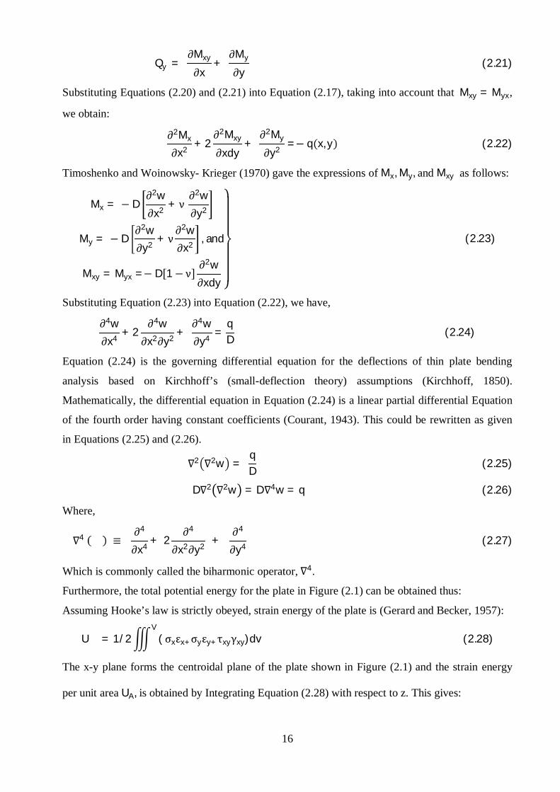
Substituting Equations (2.20) and (2.21) into Equation (2.17), taking into account that Mxy = Myx,

we obtain:

∂2Mx

∂x2 + 2∂2Mxy

∂xdy+

∂2My

∂y2 =− q x, y (2.22)

Timoshenko and Woinowsky- Krieger (1970) gave the expressions of Mx, My, and Mxy as follows:

Mx = − D∂2w∂x2 + ν

∂2w∂y2

My = − D∂2w∂y2 + ν

∂2w∂x2 , and

Mxy = Myx =− D 1− ν∂2w∂xdy

(2.23)

Substituting Equation (2.23) into Equation (2.22), we have,

∂4w∂x4 + 2

∂4w∂x2∂y2 +

∂4w∂y4 =

qD (2.24)

Equation (2.24) is the governing differential equation for the deflections of thin plate bending

analysis based on Kirchhoff’s (small-deflection theory) assumptions (Kirchhoff, 1850).

Mathematically, the differential equation in Equation (2.24) is a linear partial differential Equation

of the fourth order having constant coefficients (Courant, 1943). This could be rewritten as given

in Equations (2.25) and (2.26).

∇2 ∇2w =qD

(2.25)

D∇2 ∇2w = D∇4w = q (2.26)

Where,

∇4 aa ≡∂4

∂x4 + 2∂4

∂x2∂y2 +∂4

∂y4 (2.27)

Which is commonly called the biharmonic operator, ∇4.

Furthermore, the total potential energy for the plate in Figure (2.1) can be obtained thus:

Assuming Hooke’s law is strictly obeyed, strain energy of the plate is (Gerard and Becker, 1957):

U = 1/2V

(σxεx+σyεy+τxyγxy)dv (2.28)

The x-y plane forms the centroidal plane of the plate shown in Figure (2.1) and the strain energy

per unit area UA, is obtained by Integrating Equation (2.28) with respect to z. This gives:

17

UA =12 −h

2

+h2

( σx εx + σyεy + τxyγxy)dz (2.29)

Where σx = normal stress along the x-axis, σy = normal stress along the y-axis, τxy = shear stress

along the x-y plane. εx, εy and τxy are the respective strains on x, y, axes and x-y plane.

But σx =− EZ(1−v2)

∂2w∂x2 + ν ∂

2w∂y2 (2.30a)

σy =− EZ(1−v2)

∂2w∂y2 + ν ∂

2w∂x2 (2.30b)

τxy = −1− v Ez1− v2 .

∂2wdxdy

(2.30c)

εx =− Zd2wdx2 (2.31a)

εy =− Zd2wdy2 (2.31b)

γxy = − 2 Z∂2w∂x∂y

(2.31c)

Where E = modulus of Elasticity, ν = poisson ratio.

The strain energy U can be written in terms of curvature by substituting the respective values of

stresses and strains of Equations (2.30) (a-c) and (2.31) (a-c) into Equation (2.29) and simplifying

to obtain:

Strain EnergyArea

=12

EZ2

(1−v2)∫ dZ ∂2w

∂x2

2+ ∂2w

∂y2

2+ 2v ∂2w

∂x2 . ∂2w∂y2 + 2(1 − v) ∂2w

dxdy

2

(2.32)

Integrating the first term of Equation (2.32) over the entire thickness of the surface from - h2

to + h2

we obtain:

12 −h

2

+h2 EZ2

1−v2∫ dz

12

EZ3

3(1−v2) −h2

+h2

12

E h2

3

3(1−v2)+

E h2

3

3(1−v2)

12

2Eh3

24(1−v2)= 1

2Eh3

12(1−v2)(2.33)

18

Where D = flexural rigidity = D = Eh3

12 1−ν2

Hence,

UA =D2

∂2w∂x2

2+ ∂2w

∂y2

2+ 2v ∂2w

∂x2 . ∂2w∂y2 + 2(1 − v) ∂2w

dxdy

2(2.34)

Then Strain energy, U, shall be obtained by Integrating Equation (2.34) over the entire area of the

plate:

U = UAdxdy∬

U = D2

∂2w∂x2

2+ ∂2w

∂y2

2+ 2v ∂2w

∂x2 . ∂2w∂y2 + 2(1 − v) ∂2w

dxdy

2∬ dxdy (2.35)

If acted upon by an external transverse load, the external work gives:

we = A qw x, y + q1w x, y + q11w x, y dxdy + Pw(x, y)∬ (2.36)

If only uniformly distributed load is considered, we have:

Total potential energy, Π = U - we (2.37a)

Π =D2

∂2w∂x2

2+ ∂2w

∂y2

2+ 2v ∂2w

∂x2 . ∂2w∂y2 + 2 1 − v ∂2w

dxdy

2− qw(x, y)∬ dxdy

(2.37b)

For a system in equilibrium, Equation (2.37b) equals zero, hence

D2

∂2w∂x2

2+ ∂2w

∂y2

2+ 2v ∂2w

∂x2 . ∂2w∂y2 + 2(1 − v) ∂2w

dxdy

2∬ dxdy = qw x, y dxdy∬

(2.38)

Equation (2.38) is the total potential energy Equation for a rectangular plate subjected to a

transverse uniformly distributed load (Guarracino and Walker, 2008).

2.4 Boundary Conditions

An exact solution of the governing plate equation in Equation (2.24) must simultaneously

satisfy the differential equation and the boundary conditions of any given plate problem. Since

Equation (2.24) is a fourth-order differential equation, two boundary conditions either for the

displacements or for the internal forces, are required at each boundary. In bending theory of plates,

three internal force components are to be considered: bending moment, torsional moment and

transverse shear. Similarly, the displacement components to be used in formulating the boundary

conditions are lateral deflections and slope (Volmir, 1963).

Moreover, only rectangular plates whose edges are parallel to the axes Ox and Oy , as

shown in Figure 2.2 are considered in this study.

19

xX=xxx = a

Figure 2.2: Some Edge Conditions of a Plate

Clamped, or Built in or Fixed Edge,

At the clamped edge the deflection and slope are zero,

i.e.

(w)x = 0 ,∂w∂y x

= 0 at x = 0, a, (2.39)

and

(w)y = 0 ,∂w∂y y

= 0 at x = 0, b, (2.40)

Simply Supported Edge,

At this edge, the deflection and bending moment are both zero, i.e.;

(w)x = 0, (M)x =d2wdx2 = 0 at x = 0, a, (2.41)

and

(w)y = 0, (M)y =d2wdy2 = 0 at y = 0, b, (2.42)

(a) Fixed edge

(b) Free edge

(c) Simple support

x = a

x = a

20

Free Edge,

At an unloaded free plate edge, we can state that the edge moment and the transverse shear force

(Q) are zero, which gives

(mx)x = (Qx)x = 0 at x = 0, a

Or (2.43)

(my)y = (Qy)y = 0 at x = 0, b.

2.5 Material Property

The structural analysis of structures requires not only the strength analysis but also the stiffness

analysis. In analyzing solids and structures, Weaver, Timoshenko and Young (1990) suggested that

the physical properties of the structures needed to be known. For analytical problems, they said

that the essential material properties are modulus of elasticity, E, Poisson’s ratio, υ and mass

density ρ . They went further to present properties of some common materials as given in Table

(2.1).

Table 2.1 Properties of Materials

Materials Modulus of Elasticity GPa Poisson’s ratio,υ Mass Density, ρ Mg/m3

Aluminium 69 0.33 2.62

Brass 103 0.34 8.66

Concrete 25 0.25 2.40

Steel 207 0.30 7.85

Titanium 117 0.33 4.49

(Weaver, Timoshenko and Young, 1990)

2.6 Formulation of Plate Bending Problems.

Structural plates have a multitude of applications in extremely diverse fields of engineering.

Consequently, economical and reliable analysis of various types of plate structures is of great

importance to civil, architectural, mechanical and aeronautical engineers. Equations for the flexural

behaviour of various plate types are formulated using mathematically correct partial differential

equations (Gerard and Becker, 1957). Unfortunately, the analytical solutions of these differential

equations have been limited to homogeneous plates of relatively simple geometry and loading and

boundary conditions. Even when analytical solutions could be found, they were often too difficult

and cumbersome to use in everyday engineering practice (Szilard, 2004). Thus, general solution

techniques are required that are applicable to plates of arbitrary geometry and loadings and can

handle various boundary conditions with relative ease. Moreover, an exact solution in analytical

form of plate bending problems using classical methods, are limited to relatively simple plate

21

geometry, load configuration and boundary supports (Chapra and Canale, 2010; Hoffman, 2001). If

these conditions are more complicated, the classical analysis methods become increasingly tedious

or even impossible. In such cases, approximate methods are the only approaches that can be

employed for the solution of practically important plate bending problems (Fenner, 1986).

Nevertheless, the classical solution can be used as a basis for incisively evaluating the results of

approximate solution through quantitative comparisons. Varieties of approximate methods are

available today for engineering analysis. By convention, these approximate methods may be

divided into two groups, namely: numerical and variational methods.

2.6.1 Numerical Methods.

These methods provide suitable computational algorithms for obtaining approximate

numerical solutions to difficult problems of mathematical physics. Also they can be defined as

methods for solving problems on computers. Such well – known methods are the finite difference

method, the boundary element method, the boundary collocation method and the finite element

method.

2.6.1.1 Finite Difference Method (FDM)

This is the oldest – but still viable – numerical method and is especially suited for the solutions of

various plate problems. The essence of the FDM lies in the following:

The middle plane of the plate is covered by a rectangular, triangular or other reference networks,

depending on the geometry of the plate. The network is called a finite difference. Mesh points of

intersection of this mesh are referred to as mesh or nodal points.

The governing differential equation inside the plate domain is replaced by the corresponding finite

difference Equations at the mesh points using the special finite difference operators.

Boundary conditions are also formulated with the use of the above – mentioned finite difference

operators at mesh points located on the plate boundary. As a result of such replacement we obtain a

closed set of linear algebraic equations written for every nodal point within the plate. Solving this

system of equations obtains a numerical field of the nodal displacement (Ventsel and Krauthammer,

2001). The key point of the FDM is the finite difference approximation of derivatives. For the

approximation, the derivatives of a one-dimensional, continuous function f(x) at point xi are

defined as follows:

dfdx i

=Δ→0

lim fi+1−fi∆

ordfdx

=Δ→0

lim fi−fi−1∆

(2.44)

Where fi = f(xi), etc; ∆ is a finite increment of the variable x.

The FDM requires (to a certain extent) mathematically trained operators. It requires more work to

achieve complete automation of the procedure in program writing. The matrix of the

22

approximating system of linear algebraic equation is asymmetric, causing some difficulties in

numerical solution of this system and an application of the FDM to domains of complicated

geometry may run into serious difficulties (Ventsel and Krauthammer, 2001). More so, Al-Badri

and Ahmed (2009) used FDM for evaluation of elastic deflections and bending moments of

orthotropically reinforced concrete rectangular slabs.

2.6.1.2 Boundary Element Method (BEM)

In recent years, the boundary element method (BEM) has emerged as a powerful alternative to

the finite difference methods and the finite element method. While these and all other numerical

solution techniques require the discretization of the entire plate domain, the BEM applies

discretization only at the boundary of the continuum. Boundary element methods are usually

divided into two categories: direct and indirect BEMs.

In the indirect BEM formulation, the complementary function is represented by an integral

terms of some arbitrary functions, called source functions, over the boundary of a domain of the

plate. These source functions may be virtualized for example, as fictitious force and moment

distributions acting on the boundary of the given plate embedded in an infinite elastic plate (term

“fictitious” is used here because these loads are not resulting in transverse loads assigned for the

plate). Finding these source functions, one can determine the deflections, bending and twisting

moments anywhere within the plate or on its boundary.

In the direct formulation, the partial differential equation of the plate bending problem for the

complementary function is transformed by the use of the reciprocal work identity to an integral

equation in terms of boundary values of the deflections and stress resultants. From the indirect

method, the deflection surface of the infinite plate due to the fictitious and given loads can be

represented in the following form:

W(x,y)=wp(x, y)+ Г q x, y Gq x, y; ζ, η + Mn ζ, η Gm(x, y; ζ,η)∫ ds; (x, y)ϵΩ (2.45)

Where wp (x, y) = Ω p ξ, ζ Gq∬ (x,y; , )d dz (2.46)

is a particular solution of the governing differential equation of thin plate. Gp (x,y; , ) and

Gm (x,y; , ) denote the singular solutions of the unit normal concentrated force, and a unit

concentrated moment respectively. (x, y) is a point inside the domain whereas a point (ζ,η) is

on the boundary Г.

The direct BEM is formulated in terms of the natural variables interpretable as deflection, slope,

bending moment, and effective shear force assigned along the plate boundary Г. It states that for

any two equilibrium states, say, A and B of an elastic body, the work that would be done by forces

23

A if given the displacements B is equal to the work that would be done by the forces B if given the

displacements A. This means that the following expression can be written for any elastic plate:

Ω PAWB dΩ + Г QAW − MAφB∫ ds = Ω PB∬ WA dΩ + Г QBWA − MBφA∫∬ ds (2.47)

Where W, , M and Q are the deflection, slope, moment and shear force respectively.

BEM can be successfully applied primarily to linear problems. It begins with elementary

solutions and uses computer implementation mostly in the very last stages (Ventsel and

Krauthammer, 2001). Some scholars have used BEM for their analysis (Banerjee and Butterfield,

1981; Brebbia, Tellas and Wrobel, 1984; Hartman, 1991; Ventsel, 1997).

2.6.1.3 Finite Element Method (FEM)

The FEM applies a physical discretization in which the actual continuum is replaced by an

assembly of discrete elements (usually, triangular or rectangular in shape) referred to as finite

elements, connected together to form a two- or three- dimensional structure. Several types of FEMs

have been developed for analyzing various plate problems. The three major categories are (a) FEM

based on displacements, (b) mixed or hybrid FEM and (c) equilibrium-based FEM. Of the three

approaches, the displacement method is the most natural and therefore the most used in

engineering. As already mentioned earlier, the continuum of the plate is replaced by an assembly

of a number of individual elements connected only at a limited number of so-called node points.

The method assumes that if the load deformation characteristics of each element can be defined,

then by assembling the elements the load deflection behaviour of the plate can be approximated.

Mathematically, the FEM is based on the Ritz variational approach. In this case, however, we

apply this classical energy method piecewise over the plate.

For a rectangular plate, if Πe = Ue + Ve is the total potential energy associated with the element, we

have:

Πe = 12 δ e

T K e δ eT - δ e

T Q e (2.48a)

If we apply the principle of minimum potential energy to Equation (2.48a), thus

∂Πe

∂ δ e= 0 or ∂Πe

∂ δq= 0

We obtain

K δ = Q (2.48b)

Equation (2.48b) is the governing equation of the FEM for the entire plate

Where, Q e = element nodal force matrix.

K e = element stiffness matrix.

δ e = element displacement matrix.

24

The FEM requires the use of powerful computers of considerable speed and storage capacity. It is

difficult to ascertain the accuracy of numerical results when large structural systems are analyzed.

The method is poorly adapted to a solution of the so-called singular problems (e.g., plates and

shells with cracks, corner points, discontinuity internal actions, etc.), and of problems for

unbounded domains (Ventsel and Krauthammer, 2001). FEM has been investigated by many

authors (Alvarez, Vampa and Martin, 2009; Gallagher, 1975; Hughes, 1987; Murli and Prathap,

2003; Nguyen, 2008; Pal, Sinha and Bhattacharyya, 2001; Vanam, Rajyalakshmi and inala, 20112).

2.6.1.4 Boundary Collocation Method (BCM)

The boundary collocation method is among the simplest methods of solving partial

differential equations, both from a conceptual, as well as a Computation point of view. The

solution is expressed as sum of known solutions of the governing differential equations, and

boundary conditions are satisfied at selected points on the boundary. Thus, the obtained solution

satisfied the governing differential equation exactly and the prescribed boundary conditions only

approximately. An estimation of the error of approximation can be found by simply checking the

boundary conditions at some intermediate points located between the collocation ones. The method

is easily applied to irregular domains (simply or multiply connected) with arbitrary boundary

conditions. This method can be considered as a particular case of the more general method, the so-

called the weighted residual method, when the weighting functions are chosen in the form of the

Dirac Delta functions at discrete points of a boundary. In the BCM an unknown deflection W(x,y)

is approximated by an expression of the form:

W(x, y) = j=1N ajΦj∑ (x, y) + wp (x,y) (2.49)

Where ϕj(x,y) are some prescribed trial (or basis) functions; aj are unknown coefficients, and

wp is an approximate particular solution of the non-homogeneous governing differential Equation

for the deflection of thin plates.

However, the BCM is limited to linear problems. A complete set of solutions to the differential

equations must be known (Ventsel and Krauthammer, 2001).

2.6.2 Variational Methods

These methods use the principle of virtual work for determining numerical fields of unknown

functions (deflections, internal forces, and moments). They replace the force vectors by work and

potential energy. These energy methods are among the most powerful analytical tools of

mathematical physics for the engineer. Among the variational methods enjoying wide acceptance

are:

25

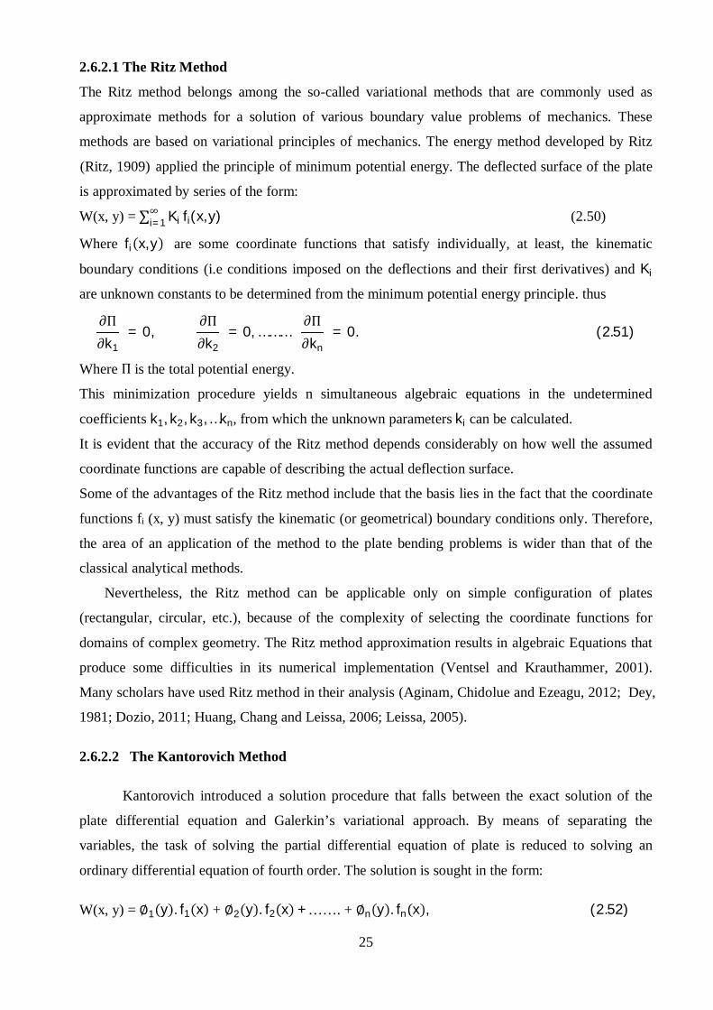
2.6.2.1 The Ritz Method

The Ritz method belongs among the so-called variational methods that are commonly used as

approximate methods for a solution of various boundary value problems of mechanics. These

methods are based on variational principles of mechanics. The energy method developed by Ritz

(Ritz, 1909) applied the principle of minimum potential energy. The deflected surface of the plate

is approximated by series of the form:

W(x, y) = i=1∞ Ki∑ fi(x, y) (2.50)

Where fi x, y are some coordinate functions that satisfy individually, at least, the kinematic

boundary conditions (i.e conditions imposed on the deflections and their first derivatives) and Ki

are unknown constants to be determined from the minimum potential energy principle. thus

∂Π∂k1

= 0,∂Π∂k2

= 0, ………∂Π∂kn

= 0. (2.51)

Where Π is the total potential energy.

This minimization procedure yields n simultaneous algebraic equations in the undetermined

coefficients k1, k2, k3, …kn, from which the unknown parameters ki can be calculated.

It is evident that the accuracy of the Ritz method depends considerably on how well the assumed

coordinate functions are capable of describing the actual deflection surface.

Some of the advantages of the Ritz method include that the basis lies in the fact that the coordinate

functions fi (x, y) must satisfy the kinematic (or geometrical) boundary conditions only. Therefore,

the area of an application of the method to the plate bending problems is wider than that of the

classical analytical methods.

Nevertheless, the Ritz method can be applicable only on simple configuration of plates

(rectangular, circular, etc.), because of the complexity of selecting the coordinate functions for

domains of complex geometry. The Ritz method approximation results in algebraic Equations that

produce some difficulties in its numerical implementation (Ventsel and Krauthammer, 2001).

Many scholars have used Ritz method in their analysis (Aginam, Chidolue and Ezeagu, 2012; Dey,

1981; Dozio, 2011; Huang, Chang and Leissa, 2006; Leissa, 2005).

2.6.2.2 The Kantorovich Method

Kantorovich introduced a solution procedure that falls between the exact solution of the

plate differential equation and Galerkin’s variational approach. By means of separating the

variables, the task of solving the partial differential equation of plate is reduced to solving an

ordinary differential equation of fourth order. The solution is sought in the form:

W(x, y) = ∅1 y . f1 x + ∅2 y . f2 x +……. + ∅n y . fn x , (2.52)

26

Where ∅1 , ∅2,….. ∅n are functions of y alone and satisfy the prescribed boundary conditions of

the plate in the Y direction.

f x = A1 cosh αx cos βx + A2 cosh αx sin βx + B1 sinh αx sin βx + B2 sinh αx cos βx +

f0 x , (2.53)

Where f0 x is the particular solution of this differential equation. The constants A1, A2, B1and B2

must be determined from the boundary conditions of the plate in X direction. The Kantorovich

method however, has the limitation that the required mathematical operations are extremely time

consuming (Szilard, 2004). Kerr (1969) had extended the Kantorovich method for the solution of

eigenvalue problem. Singh and Lal (1984) used the Kantorovich method for the solution of

magnetohydrodynamic flow problems through channels.

2.6.2.3 The Galerkin (Petrov-Galerkin) Method

The method formulated by Galerkin (1915) can be applied successfully to diverse types of

problems as small and large deflection theories, linear and nonlinear vibration and stability

problems of plates and shell, provided that differential equations of the problem under

investigation have already been determined. Although the mathematical theory behind the Galerkin

method is quite complicated, its physical interpretation is relatively simple. Mathematically, it is

given in the form:

A L WN − P∬ fi(x, y)dxdy = 0 (for 2D problems) (2.54)

v (L(∭ WN))fi x, y, z dxdydz = A P fi(x, y)dxdy∬ (for 3D problems) (2.55)

Where WN= i=1N CiWi∑ (x, y) is an unknown function of two variables and WN= i=1

N CiWi∑ (x, y, z)

is an unknown function of three variables each term satisfying all boundary conditions of the

problem but not necessarily the governing differential Equation of the plate.

fi x, y and fi x, y, z are trial functions and P is a given load term defined also in the domain. The

symbol L indicates either a linear or nonlinear differential operator.

However, we observe that in Equation (2.54), the unknown functions and the functions of the

given load term belong to the same function space i.e dxdy. But in Equation (2.55), the function

space on the right hand side differs from that of the left hand side. If the function space differs in

this manner, the Galerkin method becomes the Petrov-Galerkin method. The Petrov-Galerkin

method is a mathematical method used to obtain approximate solutions of partial differential

equations which contain terms with odd order. In these types of problems a weak formulation with

similar function space for the test function and solution function is not possible. Hence, the Petrov-

27

Galerkin method is used. Furthermore, the Petrov-Galerkin method is mainly required in the

nonsymmetric case while Galerkin handles symmetric bilinear forms.

Galerkin method is a valuable approximation tool for the solution of Partial Differential

Equations (PDE’s) when the analytical solutions are difficult or impossible to obtain due to

complicated geometry or support conditions. It is a method that uses a spatial discretization and a

weighted residual formulation to transform the governing PDE into an integral equation that upon

variational treatment yields the solution of a system of matrix equations.

An approximate solution of Equation (2.54) is sought in the following form.

WN x, y =i=1

N

CiWi x, y (2.56)

Where,

… are unknown coefficients to be determined.

.. , are the linearly independent functions (they are also called trial or displacement

Equations) that satisfy all the prescribed support conditions but not necessarily satisfy Equation

(2.54).

From Calculus, any two functions are called mutually orthogonal in the interval (a,

b) if they satisfy the condition:

= ( . )

For example, a set of functions: 1, Sin x, Cos x, Cos 2x, Sin 2x, . . . , Cos Kx, Sin Kx, . . . is

orthogonal in the interval (0, 2 ) because any two functions from the set satisfy the condition in

Equation (2.57). If one of the functions – for example, - is identically equal to zero, then the

condition in Equation (2.57) is satisfied for any function . Thus, if a function , is an

exact solution of the given boundary value problem, then, the function − will be

orthogonal to any set of functions. Since the deflection function, .. , in the form of

Equation (2.56) is an approximate solution only if Equation (2.54) − ≠ , and it is no

longer orthogonal to any set of functions. However, we can require that the magnitude of the

function − be minimum. This requirement is equivalent to the condition that the above

function should be orthogonal to some bounded set of functions; first of all, to the trial

functions , . It leads to the following Galerkin equation:

− , = ( . )

28

Substituting for from Equation (2.56) one obtains

=

, − , = ( . )

i = 1,2,3….N

Introducing a residual error function E( ) as follows:

E( ) = =∑ , − ( . )

Rewriting the above Galerkin equation in the form

, , ; , = ( . )

i, j = 1,2,3….N

Replacing the above Equation (2.61) by the sum of integrals, we obtain the following set of linear

algebraic equations:+ + ……… + =+ + ……… + =+ + ……… + =+ + ……… + =

...

+ + ……… + =

( . )

Where = ∬ . ( ) ,

= ∬ . ( ) ,

= ∬ . ( ) ,

= ∬ ,

= ∬ i = 1, 2, 3 ………N

Solving Equation (2.62), we obtain the coefficients Ci…N, which in conjunction with Equation (2.56)

gives the solution of the given plate problem.

Mathematically, the Galerkin method is looked at as an approach invoking the principle of

orthogonality of functions (Ventsel and Krauthammer, 2001). It is also considered as a weighted

residual method (Hoffman, 2001). What is irrefutable is that the Galerkin’s method is a variational

approach (Galerkin, 1933). In fact it is an algorithmic statement of the variational approach (Soedel,

2005). The Galerkin’s method has become a general algorithm for solving a variety of equations

and problems and its variational birthmark has disappeared. Numerous researchers applied the

29

Galerkin’s method to static and dynamic analysis of plates. Among them is Odman (1955) who

used a variation of the Galerkin’s method and mode shapes of the form below for vibration

analysis of thin rectangular plates.

W x, y = X x Y y (2.63)

Where xuAxuAxuAxuAxX 24231211 sinhcoshsinhcosh)(

yuByuByuByuByY 44433231 sinhcoshsinhcosh)(

u1, ….., u4 are determined by applying the Galerkin’s Formula in the differential equation of

motion. The 36 natural frequencies computed from this study are upper-bounded.

Wah (1963) applied the Galerkin’s procedure to nonlinear vibration analysis of circular plates.

Another researcher who used the Galerkin’s method for nonlinear vibration analysis of plates is

Yamaki (1961). More recently, Lei, Adhikari and Friswell (2005) applied the method to the

vibration analysis of plates and beams with non-local damping using a shape function in the form

of a trigonometric series. The results they achieved proved the method efficient for plates and

beams with simple boundary conditions. Sladek, Sladek, Zhang, Krivacek, and Wen (2006)

presented an analysis of orthotropic thick plates by meshless local Petrov-Galerkin (MLPG)

method. They used the Reissner-Mindlin theory to analyze a thick orthotropic plate resting on the

winkler elastic foundation by transforming the set of governing equations in the Reissner-mindlin

theory with a unit test function into local integral equations on local subdomains in the mean

surface of the plate. Nodal points are randomly spread on the surface of the plate and each node is

surrounded by a circular subdomain to which local integral equations are applied. Other

investigators who applied the Galerkin method to the analysis of plates include Ragesh, Mustafa

and Somasundaran (2016) who gave an integrated Kirchhoff plate element by Galerkin method for

the analysis of plates on elastic foundation. In all the studies above the shape functions adopted for

the Galerkin method were either trigonometric or polynomials functions.

Moreover, the Galerkin method is more general than some other energy methods because no

quadratic functional or virtual work principle is necessary (Ventsel and Krauthammer, 2001).

2.6.2.4 The Principle of Virtual Work

The work done by actual forces through a virtual displacement of the actual configuration is called

virtual work. It is assumed that during the virtual displacements all forces are held constant. The

virtual work is designated by δW.

The principle of virtual work is formulated as follows:

An elastic body is in equilibrium if and only if the total virtual work done by external and internal

forces is zero for any admissible virtual displacements, i.e.,

δW = δWi + δWe = 0 (2.64)

30

where δWi and δWe are the virtual works done by internal and external forces, respectively.

δWi is negative because it works against the actual displacement of the body. It can be interpreted

as follows: if a body is in equilibrium then its resultant force and resultant couple are both zero; so,

they produce no work. Ibearugbulem, Oguaghamba, Njoku and Nwaokeorie (2014) used line

continuum to explain work principle for structural continuum analysis.

Furthermore, since Galerkin is a weak function, this study will use the Galerkin method to

analyze the accuracy and pattern of convergence to the exact solution of multi-term characteristic

coordinate polynomials of thin rectangular isotropic plates with different edge conditions- CCCS,

SSSS, CCCC, CCSS and CSCS- under uniformly distributed loads for different approximations

each.

2.7 Characteristic Coordinate Polynomials

One of the most difficult tasks facing an analyst is element selection (Beslin and Nicolas, 1997).

An area for which this problem is quite pronounced is that of plate bending. The critical step,

which largely controls the accuracy of approximate solutions, is the selection of approximate shape

functions that best approximate the deflected surface of the plate. To this end, a class of

characteristic coordinate polynomials can be constructed using Gram–Schmidt process and then

these polynomials are employed as deflection functions in plate continuum analysis. The assumed

deflection shapes were normally formulated by inspection and sometimes by trial and error until

Bhat (1985) proposed a systematic method of constructing such functions in the form of

characteristic coordinate polynomials. The restrictions on the series include that they satisfy the

geometrical boundary conditions. They are complete and they do not inherently violate the natural

boundary conditions.

Different series types, namely, trigonometric, hyperbolic, polynomial, give different results

for the same number of terms in the series and the efficiency of the solution will depend to some

extent on the type of series chosen (Singhvi and Kapania, 1994).

An exact solution of the governing differential equation of Equation (2.24) in closed form is

possible only for a limited number of cases regarding a plate’s geometry and its boundary

conditions. As in the case with all approximate methods, the accuracy of the results depends

considerably on the quality of the assumed displacement functions. The choice of the functions

G(x) or H(y) may be anything like, algebraic, trigonometric, hyperbolic and so on or a combination

of these and will depend mainly on the boundary conditions of the plate.

31

For example, if the two opposite edges of the plate at x = 0 and x = a are clamped, the deflected

surface on x – z plane may be conveniently taken as a trigonometric function in the form of cosine

series as (Li, 2002):

==

∞

− = , , , … ( . )

In which, Gi-s are the coefficients (like G1, G2 . . . Gm) to be determined. It is clearly seen that

Equation (2.65) satisfies the boundary conditions namely, x = 0 and x = a. If the other two edges

namely, at y = 0 and y = b are also clamped, the function H(y) obviously can be written as:

==

∞

− = , , , … ( . )

If the boundary conditions at y = 0 and y = b are other than clamped or a combination of simply

supported, clamped, free or so on, the function H(y) should be selected accordingly to satisfy the

prescribed boundary conditions.

Thus, the displacement function for the rectangular plate is therefore assumed as a product of two

functions; one of which is a pure function of x and the other is of y so that:

, = ∙ ( . )

, ==

∞

−

∙=

∞

− ( . )

, ==

∞

=

∞

− − ( . )

Where,

= ( . )

Characteristic coordinate polynomial method for finding shape functions in rectangular plates for

quick analysis and design is simple but approximate. Thus, the popular method essentially

considers the compatibility of the deflection at any particular point of two independent plate strips

spanning along the two directions at right angles to each other through that point. The deflection

behaviour of the individual plate strip is assumed to be that of a beam with the identical boundary

conditions at the two ends as that of the plate along that corresponding direction (Onyeyili, 2012).

This method further considers that the given intensity of the loading on the plate is shared by the

beam strips as the uniform loading on them. The method is as follows:

32

Consider a rectangular plate of dimension, a, along x and b along y, then uniformly loaded. If the

deflection pattern of the plate along x is represented by a beam strip qualitatively, the beam

function along x is taken as G(x). Similarly, the corresponding beam function along y is taken as

H(y).

The solution for prismatic beam of constant EI and length spanning along x is given as:

W x = G x =m=0

∞

Xmxm (2.71)

Similarly technique in the y-direction we shall obtain:

W y = H y =n=0

∞

Ynyn (2.72)

Where,

Xm and Yn are constant parameters in x and y directions respectively

m and n are series to infinity limit.

Expressing Equations (2.71) and (2.72) in the form of non-dimensional parameters, say X and Y for

x and y directions respectively:

x = aX (2.73)

y = bY (2.74)

Then, Equations (2.71) and (2.72) become

W x = W X =m=0

∞

Xmamxm (2.75)

W y = W Y =n=0

∞

Ynbnyn (2.76)

Let:

Am = Xmam (2.77)

Bn = Ynbn (2.78)

W x = W X =m=0

∞

Amxm (2.79)

W y = W R =n=0

∞

Bnyn (2.80)

The power m and n of the shape function of Equations (2.79) and (2.80) is dependent on the type

of loading of the plate whether it is uniformly distributed, varying or point.

33

2.7.1 Development of Coordinate Polynomial Shape Function for a Uniformly Distributed

Load.

Consider a beam with an arbitrary support condition subjected to a uniformly distributed load

along an arbitrary direction as shown in Figure 2.3 Owing to the load, Reactive forces and

moments, would develop at its supports.

Figure 2.3: Elastic Beam of Arbitrary Support Conditions Subjected to Uniformly Distributed

Load.

The equation of moment of the beam at a section say x, would be given as:

Mx = R1 ∙ x −q ∙ x2

2 − M1 (2.81)

Then, employing the elastic beam equation:

Mx =− Dd2Wdx2 (2.82)

Hence, equating Equations (2.81) and (2.82):

Dd2Wdx2 =

q ∙ x2

2 + M1 −R1 ∙ x (2.83)

Obtaining the deflection function from Equation (2.83) by integrating twice with respect to the

arbitrary direction, x:

Wx = Co + C1 ∙ x + C2x2 + C3 ∙ x3 + C4 ∙ x4 (2.84)

Where, Coand C1 are constants of integration and;

C4 =q

24D ; C3 =−R6D ; C2 =

M1

2D (2.85)

Thus, the highest power of the polynomial in Equation (2.84) is 4 for a uniformly distributed load.

Hence, this suggests that if the variation of loading is uniform, a fourth order function will be

suitable.

x

q

M1

R1 R2

M2

l – x

l

34

Then, the maximum value of m and n in Equations (2.79) and (2.80) must be equal to 4 (Onyeyili,

2012) . Expanding Equations (2.79) and (2.80) to 4th series where the constants of the series along

X and Y directions are denoted by Am and Bn respectively gives:

W x = W X =m=0

4

AmXm = A0 + A1X + A2X2 + A3X3 + A4X4 (2.86)

W y = W R =n=0

∞

BnRn = B0 + B1Y + B2Y2 + B3Y3 + B4Y4 (2.87)

The coefficients Am and Bn of the series are determined from the boundary conditions at the edges

of the plate.

2.8 Expression of Governing Differential Equation of Plate in Non-dimensional Parameters

First, the governing differential equilibrium equation for pure bending of isotropic thin rectangular

plate in Equation (2.24) is given as:

∂4w∂x4 + 2

∂4w∂x2∂y2 +

∂4w∂y4 =

qD

Where q is the external load and D is the flexural rigidity.

Expressing the independent coordinates x and y in Equation (2.24) in the form of non-dimensional

coordinates, Y and X in the domain of the plate using Equations (2.77) and (2.78), we have:

∂4wa4∂X4 + 2

∂4wa2b2∂X2∂Y2 +

∂4wb4∂Y4 =

qD (2.88)

The aspect ratio p and the plate’s lateral dimensions, a and b, are related as follows:

p =ba

; b = pa (2.89)

Substituting Equation (2.89) into Equation (2.88) appropriately, we have:

∂4wa4∂X4 + 2

∂4wp2a4∂X2∂Y2 +

∂4wp4a4∂Y4 =

qD (2.90)

Rearranging Equation (2.90) through gives:

Da4

∂4W∂X4 + 2

∂4W∂X2∂Y2

1P2 +

∂4W∂Y4

1P4 = q (2.91)

Equation (2.91) is the governing differential equation of isotropic thin rectangular plates under

pure bending expressed in non – dimensional coordinates, X and Y.

2.9 Summary of Previous Works on Flexure of Rectangular Plates.

35

Table 2.2 presents the summary of some of the different works on the flexure of rectangular plates

referenced in this research in order to identify the gaps in literature that the present work seeks to

bridge.

Table 2.2 Previous Works on Flexure of Rectangular Plates.

S/No Researcher(s)

and date

Topic and Results Gap(s)

1.0 Cerdem and

Ismail (2007b)

The Problem of Isotropic

Rectangular Plate with Clamped

Edges.

They examined the solution of the

governing differential Equation of

rectangular isotropic plate. They

obtained their deflection function by

superposition of the deflection

caused by the uniform load on the

plate strip and the deflection due to

the effects of the edges. The result

for a square plate showed reasonable

agreement with the results found in

literature.

The authors did not use

polynomial functions

for the deflection

function of the plate.

They solved the

problem of the

governing Equation

directly.

The authors considered

only one boundary

condition (CCCC).

They considered only a

square plate.

2.0 Oba,

Anyadiegwu,

George and

Nwadike (2018)

Pure Bending Analysis of

Isotropic Thin Rectangular Plates

Using Third-Order Energy

Functional.

The authors used one-term

polynomial deflection functions in

Rayleigh-Ritz method to calculate

deflection coefficients only for four

boundary conditions. Beside the

exact solutions their results showed

some discrepancies.

The authors used one-

term polynomial

deflection function.

The authors used the

Rayleigh-Ritz method

of analysis.

The authors calculated

the deflection

coefficients only.

3.0 Mbakogu and

Pavlovic (2000)

Bending of Clamped Orthotropic

Rectangular Plates: A Variational

Symbolic Solution.

The authors only

solved for the

orthotropic rectangular

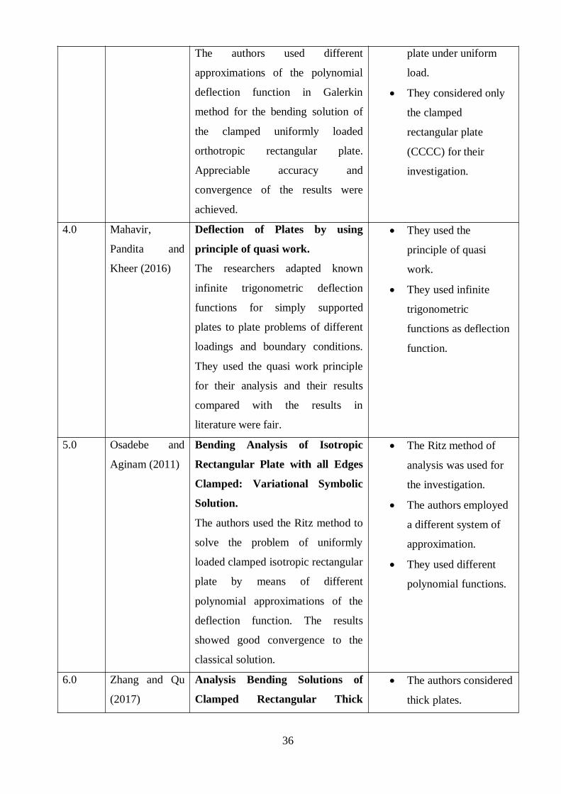
36

The authors used different

approximations of the polynomial

deflection function in Galerkin

method for the bending solution of

the clamped uniformly loaded

orthotropic rectangular plate.

Appreciable accuracy and

convergence of the results were

achieved.

plate under uniform

load.

They considered only

the clamped

rectangular plate

(CCCC) for their

investigation.

4.0 Mahavir,

Pandita and

Kheer (2016)

Deflection of Plates by using

principle of quasi work.

The researchers adapted known

infinite trigonometric deflection

functions for simply supported

plates to plate problems of different

loadings and boundary conditions.

They used the quasi work principle

for their analysis and their results

compared with the results in

literature were fair.

They used the

principle of quasi

work.

They used infinite

trigonometric

functions as deflection

function.

5.0 Osadebe and

Aginam (2011)

Bending Analysis of Isotropic

Rectangular Plate with all Edges

Clamped: Variational Symbolic

Solution.

The authors used the Ritz method to

solve the problem of uniformly

loaded clamped isotropic rectangular

plate by means of different

polynomial approximations of the

deflection function. The results

showed good convergence to the

classical solution.

The Ritz method of

analysis was used for

the investigation.

The authors employed

a different system of

approximation.

They used different

polynomial functions.

6.0 Zhang and Qu

(2017)

Analysis Bending Solutions of

Clamped Rectangular Thick

The authors considered

thick plates.

37

Plates.

The authors used double infinite sine

series for both the deflection

function and the rotation of the

normal line due to plate bending.

The solution was based on Mindlin’s

higher-order shear deformation plate

theory for aspect ratios 3, 5 and 10.

The results showed close agreement

with literature.

Infinite trigonometric

series were used to

approximate the

deflection function of

the plate.

The authors solved for

aspect ratios 3, 5 and

10 only.

7.0 Ibearugbulem,

Ettu and Ezeh

(2013)

Direct Integration and Work

Principle as New Approach in

Bending Analysis of Isotropic

Rectangular Plates.

The researchers employed one-term

polynomial deflection function for

the analysis of the deflection and

bending moment coefficient values

of the simply supported plate using

the work principle. Their results

indicated some divergence with the

classical solution.

They used one-term

polynomial deflection

function.

They used the work

principle in their

analysis.

They solved for the

simply supported plate

only.

In view of some of the gaps identified in previous works (one boundary condition,

orthotropic properties, infinite and trigonometric series, determination of deflection coefficients

only, results for few aspect ratios and using methods other than Galerkin), this research will use the

Galerkin method to investigate the accuracy and pattern of convergence of multi-term

characteristic coordinate polynomials to the classical solution for rectangular isotropic plates of

different support conditions – CCCS, SSSS, CCCC, CCSS and CSCS – with different

approximations each, subjected to a uniformly distributed load at varying aspect ratios.

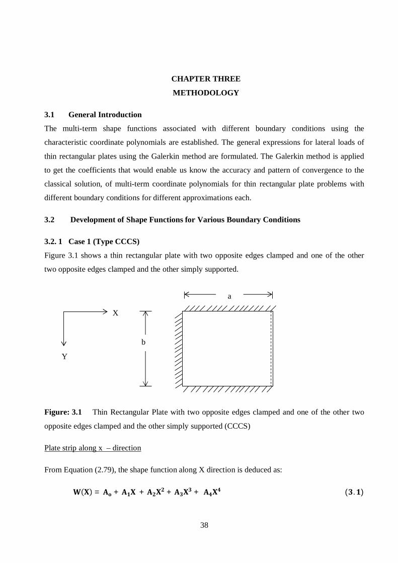
38

CHAPTER THREE

METHODOLOGY

3.1 General Introduction

The multi-term shape functions associated with different boundary conditions using the

characteristic coordinate polynomials are established. The general expressions for lateral loads of

thin rectangular plates using the Galerkin method are formulated. The Galerkin method is applied

to get the coefficients that would enable us know the accuracy and pattern of convergence to the

classical solution, of multi-term coordinate polynomials for thin rectangular plate problems with

different boundary conditions for different approximations each.

3.2 Development of Shape Functions for Various Boundary Conditions

3.2. 1 Case 1 (Type CCCS)

Figure 3.1 shows a thin rectangular plate with two opposite edges clamped and one of the other

two opposite edges clamped and the other simply supported.

Figure: 3.1 Thin Rectangular Plate with two opposite edges clamped and one of the other two

opposite edges clamped and the other simply supported (CCCS)

Plate strip along x – direction

From Equation (2.79), the shape function along X direction is deduced as:

= + + + + ( . )

a

b

Y

X

39

Boundary conditions along X – direction

a W X = 0, X = 00, andX = 1

bdWdX

X = 0 at X = 0

d2WdX2 X = 0 at X = 1

From condition a(i) and Equation (3.1):

W 0 = Ao + 0 + 0 + 0 + 0 = 0

Ao = 0dWdX

X = A1 + 2A2X + 3A3X2 + 4A4X3 (3.2)

From condition b(i) and Equation (3.2):dWdX 0 = A1 + 0 + 0 = 0

A1 = 0

From condition a(ii) and Equation (3.1):

W 1 = A2 + A3 + A4 = 0

A2 =− A3 − A4 (3.3)

d2WdX2 X = 2A2 + 6A3X + 12A4X2 (3.4)

From condition b(ii) and Equation (3.4):

d2WdX2 X = 2A2 + 6A3 + 12A4 = 0

A2 = − 3A3 − 6A4 (3.5)

Equating Equation (3.3) and Equation (3.5):

− A3 − A4 = − 3A3 − 6A4

2A3 = − 5A4

A3 =− 2.5A4 (3.6)

Substituting the value of A3 into Equation (3.6):

A2 = − − 2.5A4 − A4

A2 = 1.5A4 (3.7)

Hence, putting the obtained values of Ao, A1, A2, A3, and A4 into Equation (3.1):

W X = A4 1.5X2 − 2.5X3 + X4 (3.8)

40

Plate Strip along Y - Direction

From Equation 2.80, the shape function along Y direction is deduced as:

W Y = B0 + B1Y + B2Y2 + B3Y3 + B4Y4 (3.9)

Boundary conditions along Y – direction

a W Y = 0, andY = 00, andY = 1

bdWdY

Y = 0, andY = 00, andY = 1


W 0 = Bo + 0 + 0 + 0 + 0 = 0

Bo = 0dWdY Y = B1 + 2B2Y + 3B3Y2 + 4B4Y3 (3.10)

From condition b(i) and Equation (3.10):dWdY

0 = B1 + 0 + 0 + 0

B1 = 0


W 1 = B2 + B3 + B4 = 0

B2 =− B3 − B4 (3.11)

From condition b(ii) and Equation (3.10):dWdY

1 = 2B2 + 3B3 + 4B4 = 0

B2 = − 1.5B3 − 2B4 (3.12)

Equating Equations (3.11) and (3.12)

− B3 − B4 =− 1.5B3 − 2B4

0 =− 0.5B3 − B4

B3 =− 2B4

Substituting the value of B3 into Equation (3.11):

B2 = − − 2B4 − B4

B2 = B4 (3.13)

Hence, putting the obtained values of Bo, B1, B2, B3, and B4 into Equation (3.9):

W Y = B4 Y2 − 2Y3 + Y4 (3.14)

41

Then, according to Characteristic coordinate theory, the displacement function for the rectangular

plate is therefore assumed as a product of the two independent pure functions of X and Y as given

in Equations (3.8) and (3.14) respectively:

, = ×

W X, Y = A4 1.5X2 − 2.5X3 + X4 × B4 Y2 − 2Y3 + Y4

W X, Y = A4B4 1.5X2 − 2.5X3 + X4 Y2 − 2Y3 + Y4

Defining the product of the constants, A4and B4 as: C = A4 B4

W X, Y = C 1.5X2 − 2.5X3 + X4 Y2 − 2Y3 + Y4 (3.15)

Equation (3.15) is a single term deflection functional for two opposite edges clamped and one of

the two opposite edges clamped and the other simply supported thin rectangular plates. The second

approximation is done by multiplying Equation (3.15) with coordinates X2, and Y2 separately and

then adding the results to Equation (3.15). The truncated third approximation is obtained by

multiplying Equation (3.15) with X2Y2 and then adding it to the second approximation. The third

approximation is achieved by multiplying Equation (3.15) with coordinates X4, and Y4 separately

and then adding the results to the truncated third approximation.

The coefficient C in Equation (3.15) is set as C1. It is described as first term deflection coefficient.

That is:

First Approximation

W X, Y = C 1.5X2 − 2.5X3 + X4 Y2 − 2Y3 + Y4 (3.16)

Second Approximation

W X, Y = C1 1.5X2 − 2.5X3 + X4 Y2 − 2Y3 + Y4 + C2 1.5X2 − 2.5X3 + X4

Y2 − 2Y3 + Y4 X2 + C3 1.5X2 − 2.5X3 + X4 Y2 − 2Y3 + Y4 Y2

W X, Y = C1 1.5X2 − 2. 5X3 + X4 Y2 − 2Y3 + Y4 + C2 (1.5X4 − 2. 5X5 + X6)(Y2 − 2Y3 +Y4) + C3 1.5X2 − 2.5X3 + X4 Y4 − 2Y5 +

Y6 (3.17)

Truncated Third Approximation

W X, Y = C1 1.5X2 − 2. 5X3 + X4 Y2 − 2Y3 + Y4 + C2 1.5X4 − 2.5X5 + X6

Y2 − 2Y3 + Y4 + C3 1.5X2 − 2.5X3 + X4 Y4 − 2Y5 + Y6

+ C4 1.5X2 − 2. 5X3 + X4 Y2 − 2Y3 + Y4 X2Y2

42

W X, Y = C1 1.5X2 − 2.5X3 + X4 Y2 − 2Y3 + Y4 + C2 (1.5X4 − 2.5X5 + X6)(Y2 − 2Y3 +Y4) + C3 1.5X2 − 2.5X3 + X4 Y4 − 2Y5 + Y6 + C4 (1.5X4 − 2. 5X5 + X6)

(Y4 − 2Y5 + Y6)

Third Approximation

W X, Y = C1 1.5X2 − 2. 5X3 + X4 Y2 − 2Y3 + Y4 + C2 1.5X4 − 2.5X5 + X6

Y2 − 2Y3 + Y4 + C3 1.5X2 − 2.5X3 + X4 Y4 − 2Y5 + Y6

+ C4 1.5X4 − 2. 5X5 + X6 Y4 − 2Y5 + Y6 + C5 1.5X2 − 2. 5X3 + X4

Y2 − 2Y3 + Y4 X4 + C6 1.5X2 − 2.5X3 + X4 Y2 − 2Y3 + Y4 Y4

W X, Y = C1 1.5X2 − 2.5X3 + X4 Y2 − 2Y3 + Y4 + C2 (1.5X4 − 2.5X5 + X6)(Y2 − 2Y3 +Y4) + C3 1.5X2 − 2.5X3 + X4 Y4 − 2Y5 + Y6 + C4 (1.5X4 − 2. 5X5 + X6)

Y4 − 2Y5 + Y6 + C5 1.5X6 − 2.5X7 + X8 Y2 − 2Y3 + Y4 + C6 (1.5X2 − 2. 5X3 + X4)

(Y6 − 2Y7 + Y8) (3.18)

3.2. 2 Case 2 (Type SSSS)

Figure 3.2 shows a thin rectangular whose all edges are simply supported.

0

Figure: 3.2 All Edges Simply Supported Rectangular Plate (SSSS)

Plate strip along x - direction


= + + + + ( . )


a W X = 0, X = 00, andX = 1

a

bY

X

43

bd2WdX2 X = 0, andX = 0

0, andX = 1


W 0 = Ao + 0 + 0 + 0 + 0 = 0

Ao = 0

d2WdX2 X = 2A2 + 6A3X + 12A4X2 (3.20)

From condition b(i) and Equation (3.20):

d2WdX2 0 = 2A2 + 0 + 0 = 0

A2 = 0


W 1 = A1 + A3 + A4 = 0

A1 =− A3 − A4 (3.21)


d2WdX2 1 = 6A3 + 12A4 = 0

A3 = − 2A4 (3.22)

Then, from Equation (3.21):

A1 =− −2A4 − A4 = A4 (3.23)


W X = A4 X − 2X3 + X4 (3.24)

Plate strip along y - direction

From Equation (2.80), the shape function along Y direction is deduced as:

W Y = B0 + B1Y + B2Y2 + B3Y3 + B4Y4 (3.25)

44


a W Y = 0, andY = 00, andY = 1

bd2WdY2 Y = 0, andY = 0

0, andY = 1


W 0 = Bo + 0 + 0 + 0 + 0 = 0

Bo = 0

d2WdY2 Y = 2B2 + 6B3Y + 12B4Y2 (3.26)


d2WdY2 0 = 2B2 + 0 + 0

B2 = 0


W 1 = B1 + B3 + B4 = 0

B1 =− B3 − B4 (3.27)


d2WdY2 1 = 6B3 + 12B4 = 0

B3 = − 2B4 (3.28)


B1 =− −2B4 − B4 = B4 (3.29)


W Y = B4 Y− 2Y3 + Y4 (3.30)

45




, = ×

W X, Y = A4 X− 2X3 + X × B4 Y − 2Y3 + Y4

W X, Y = A4B4 X − 2X3 + X4 Y− 2Y3 + Y4

Defining the product of the constants, A4and B4as: C = A4 B4

W X, Y = C X − 2X3 + X4 Y − 2Y3 + Y4 (3.31)

Equation (3.31) is a single term deflection functional for all edges simply supported thin

rectangular plates. The second approximation is done by multiplying Equation (3.31) with

coordinates X2, and Y2 separately and then adding the results to Equation (3.31). The truncated

third approximation is obtained by multiplying Equation (3.31) with X2Y2 and then adding it to the

second approximation. The third approximation is achieved by multiplying Equation (3.31) with

coordinates X4, and Y4 separately and then adding the results to the truncated third approximation.


That is:

First Approximation

W X, Y = C1 X − 2X3 + X4 Y − 2Y3 + Y4 (3.32)


W X, Y = C1 X− 2X3 + X4 Y− 2Y3 + Y4 + C2 X − 2X3 + X4 Y − 2Y3 + Y4 X2 +

C3 (X − 2X3 + X4)(Y − 2Y3 + Y4)Y2

W X, Y = C1(X− 2X3 + X4 )(Y − 2Y3 + Y4) + C2 ( X3 − 2 X5 + X6)(Y− 2Y3 + Y4) +

C3 (X − 2X3 + X4 )(Y3 − 2Y5 + Y6) (3.33)



C3 X − 2X3 + X4 Y3 − 2Y5 + Y6 + C4 X − 2X3 + X4 Y − 2Y3 + Y4 X2Y2


C3 X − 2X3 + X4 Y3 − 2Y5 + Y6 + C4 X3 − 2X5 + X6 Y3 − 2Y5 + Y6 (3.34)

Third Approximation

46


C3 X − 2X3 + X4 Y3 − 2Y5 + Y6 + C4 X3 − 2X5 + X6 Y3 − 2Y5 + Y6

+ C5 X− 2X3 + X4 Y− 2Y3 + Y4 X4 + C6(X − 2X3 + X4 )(Y − 2Y3 + Y4)Y4


C3 X − 2X3 + X4 Y3 − 2Y5 + Y6 + C4 X3 − 2X5 + X6 Y3 − 2Y5 + Y6

+ C5 X5 − 2X7 + X8 Y− 2Y3 + Y4 + C6 X − 2X3 + X4

Y5 − 2Y7 + Y8 (3.34)


Figure 3.3 shows a thin rectangular plate whose all edges are clamped.

0

Figure: 3.3 All edges Clamped Rectangular Plate (CCCC)

Plate strip along x – direction


= + + + + ( . )


a W X = 0, X = 00, andX = 1

bdWdX

X = 0, andX = 00, andX = 1


W 0 = Ao + 0 + 0 + 0 + 0 = 0

Ao = 0dWdX

X = A1 + 2A2X + 3A3X2 + 4A4X3 (3.36)


a

bY

XO

47

dWdX

0 = A1 + 0 + 0 = 0

A1 = 0


W 1 = A2 + A3 + A4 = 0

A2 =− A3 − A4 (3.37)

From condition b(ii) and Equation (3.36):dWdX

1 = 2A2 + 3A3 + 4A4 = 0

A2 = − 1.5A3 − 2A4 (3.38)

Equating Equation (3.37) and Equation (3.38):

− A3 − A4 = − 1.5A3 − 2A4

0 = − 0.5A3 − A4

A3 =− 2A4

Substituting the value of A3 into Equation (3.37):

A2 = − − 2A4 − A4

A2 = A4 (3.39)


W X = A4 X2 − 2X3 + X4 (3.40)



W Y = B0 + B1Y + B2Y2 + B3Y3 + B4Y4 (3.41)


a W Y = 0, andY = 00, andY = 1

bdWdY

Y = 0, andY = 00, andY = 1


W 0 = Bo + 0 + 0 + 0 + 0 = 0

Bo = 0

48

dWdY

Y = B1 + 2B2Y + 3B3Y2 + 4B4Y3 (3.42)

From condition b(i) and Equation (3.42):dWdY

0 = B1 + 0 + 0 + 0

B1 = 0


W 1 = B2 + B3 + B4 = 0

B2 =− B3 − B4 (3.43)

From condition b(ii) and Equation (3.42):dWdY 1 = 2B2 + 3B3 + 4B4 = 0

B2 = − 1.5B3 − 2B4 (3.44)

Equating Equations (3.43) and (3.44)

− B3 − B4 =− 1.5B3 − 2B4

0 =− 0.5B3 − B4

B3 =− 2B4


B2 = − − 2B4 − B4

B2 = B4 (3.45)


W Y = B4 Y2 − 2Y3 + Y4 (3.46)




, = ×

W X, Y = A4 X2 − 2X3 + X4 × B4 Y2 − 2Y3 + Y4

W X, Y = A4B4 X2 − 2X3 + X4 Y2 − 2Y3 + Y4

Defining the product of the constants, A4and B4 as: C = A4 B4

W X, Y = C X2 − 2X3 + X4 Y2 − 2Y3 + Y4 (3.47)

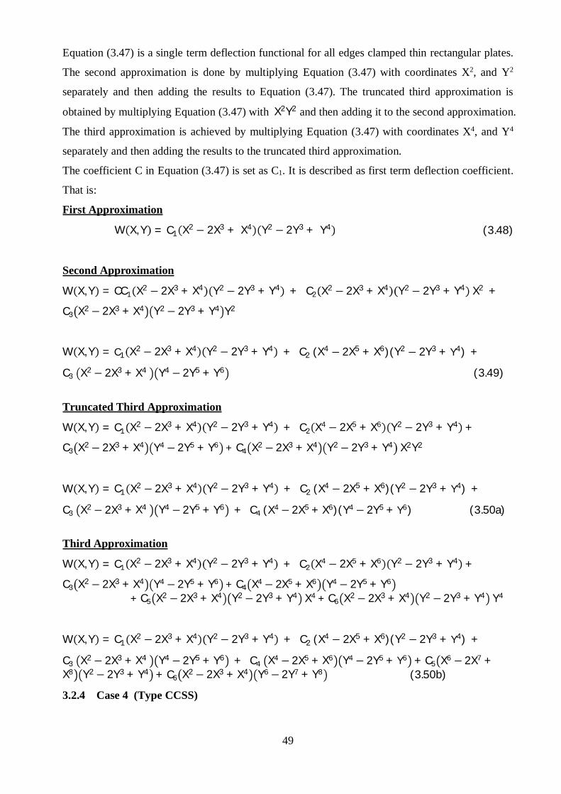
49

Equation (3.47) is a single term deflection functional for all edges clamped thin rectangular plates.

The second approximation is done by multiplying Equation (3.47) with coordinates X2, and Y2

separately and then adding the results to Equation (3.47). The truncated third approximation is

obtained by multiplying Equation (3.47) with X2Y2 and then adding it to the second approximation.

The third approximation is achieved by multiplying Equation (3.47) with coordinates X4, and Y4

separately and then adding the results to the truncated third approximation.


That is:

First Approximation

W X, Y = C1 X2 − 2X3 + X4 Y2 − 2Y3 + Y4 (3.48)


W X, Y = CC1 X2 − 2X3 + X4 Y2 − 2Y3 + Y4 + C2 X2 − 2X3 + X4 Y2 − 2Y3 + Y4 X2 +

C3 X2 − 2X3 + X4 Y2 − 2Y3 + Y4 Y2

W X, Y = C1 X2 − 2X3 + X4 Y2 − 2Y3 + Y4 + C2 (X4 − 2X5 + X6)(Y2 − 2Y3 + Y4) +

C3 X2 − 2X3 + X4 Y4 − 2Y5 + Y6 (3.49)


W X, Y = C1 X2 − 2X3 + X4 Y2 − 2Y3 + Y4 + C2 X4 − 2X5 + X6 Y2 − 2Y3 + Y4 +

C3 X2 − 2X3 + X4 Y4 − 2Y5 + Y6 + C4 X2 − 2X3 + X4 Y2 − 2Y3 + Y4 X2Y2


C3 X2 − 2X3 + X4 Y4 − 2Y5 + Y6 + C4 (X4 − 2X5 + X6)(Y4 − 2Y5 + Y6) (3.50a)

Third Approximation

W X, Y = C1 X2 − 2X3 + X4 Y2 − 2Y3 + Y4 + C2 X4 − 2X5 + X6 Y2 − 2Y3 + Y4 +

C3 X2 − 2X3 + X4 Y4 − 2Y5 + Y6 + C4 X4 − 2X5 + X6 Y4 − 2Y5 + Y6

+ C5 X2 − 2X3 + X4 Y2 − 2Y3 + Y4 X4 + C6 X2 − 2X3 + X4 Y2 − 2Y3 + Y4 Y4


C3 X2 − 2X3 + X4 Y4 − 2Y5 + Y6 + C4 X4 − 2X5 + X6 Y4 − 2Y5 + Y6 + C5 X6 − 2X7 +X8 Y2 − 2Y3 + Y4 + C6 X2 − 2X3 + X4 Y6 − 2Y7 + Y8 (3.50b)


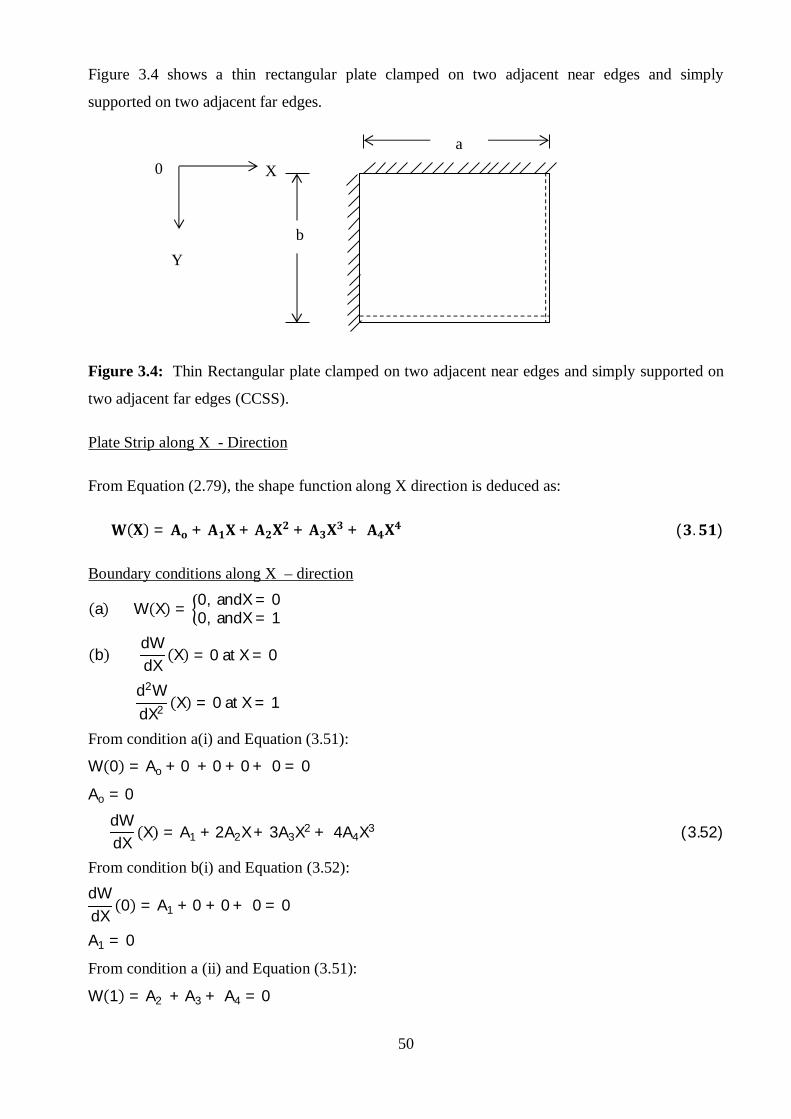
50

Figure 3.4 shows a thin rectangular plate clamped on two adjacent near edges and simply

supported on two adjacent far edges.

0

Figure 3.4: Thin Rectangular plate clamped on two adjacent near edges and simply supported on

two adjacent far edges (CCSS).

Plate Strip along X - Direction


= + + + + ( . )


a W X = 0, andX = 00, andX = 1

bdWdX

X = 0 at X = 0

d2WdX2 X = 0 at X = 1


W 0 = Ao + 0 + 0 + 0 + 0 = 0

Ao = 0dWdX

X = A1 + 2A2X + 3A3X2 + 4A4X3 (3.52)

From condition b(i) and Equation (3.52):dWdX

0 = A1 + 0 + 0 + 0 = 0

A1 = 0

From condition a (ii) and Equation (3.51):

W 1 = A2 + A3 + A4 = 0

a

bY

X

51

A2 =− A3 − A4 (3.53)

d2WdX2 X = 2A2 + 6A3X + 12A4X2 = 0 (3.54)


d2WdX2 1 = 2A2 + 6A3 + 12A4 = 0

A2 = − 3A3 − 6A4 (3.55)

Equating Equation (3.53) to Equation (3.55) gives:

− A3 − A4 = − 3A3 − 6A4

A3 =− 2.5A4 (3.56)

Substituting Equation (3.56) into Equation (3.53) gives

A2 =− ( − 2.5A4)− A4

A2 = 1.5A4 (3.57)


W X = A4 1.5X2 − 2.5X3 + X4 (3.58)



W Y = B0 + B1Y + B2Y2 + B3Y3 + B4Y4 (3.59)


a W Y = 0, andY = 00, andY = 1

bdWdY

Y = 0 at Y = 0

d2WdY2 Y = 0 at Y = 1


W 0 = Bo + 0 + 0 + 0 + 0 = 0

Bo = 0dWdY

Y = B1 + 2B2Y + 3B3Y2 + 4B4Y3 (3.60)

From condition b(i) and Equation (3.60):dWdY 0 = B1 + 0 + 0 + 0 = 0

B1 = 0


52

W 1 = B2 + B3 + B4 = 0

B2 =− B3 − B4 (3.61)

d2WdY2 Y = 2B2 + 6B3Y + 12B4Y2 = 0 (3.62)


d2WdY2 1 = 2B2 + 6B3 + 12B4 = 0

B2 = − 3B3 − 6B4 (3.63)

Equating Equation (3.61) to Equation (3.63) gives:

− B3 − B4 = − 3B3 − 6B4

B3 =− 2.5B4 (3.64)

Substituting Equation (3.64) into Equation (3.61) gives

B2 =− ( − 2.5B4) − B4

B2 = 1.5B4 (3.65)


W Y = A4 1.5Y2 − 2.5Y3 + Y4 (3.66)


plate is therefore assumed as a product of the two independent pure functions of Y and X as given


, = ×

W X, Y = A4 1.5X2 − 2.5X3 + X4 × B4 1.5Y2 − 2.5Y3 + Y4

W X, Y = A4B4 1.5X2 − 2. 5X3 + X4 1.5Y2 − 2.5Y3 + Y4

Defining the product of the constants, A4 and B4 as: C = A4 B4

W X, Y = C 1.5X2 − 2. 5X3 + X4 1.5Y2 − 2.5Y3 + Y4 (3.67)

Equation (3.67) is a single term deflection functional for two opposite edges simply supported and

the other two clamped thin rectangular plates. The second approximation is done by multiplying

Equation (3.67) with coordinates X2, and Y2 separately and then adding the results to Equation

(3.67). The truncated third approximation is obtained by multiplying Equation (3.67) with X2Y2

and then adding it to the second approximation. The third approximation is achieved by

multiplying Equation (3.67) with coordinates X4, and Y4 separately and then adding the results to

the truncated third approximation.


That is:

53

First Approximation

W X, Y = C1 1.5X2 − 2.5X3 + X4 1.5Y2 − 2.5Y3 + Y4 (3.68)


W X, Y = C1 1.5X2 − 2.5X3 + X4 1.5Y2 − 2.5Y3 + Y4 + C2 1.5X2 − 2. 5X3 + X4

1.5Y2 − 2.5Y3 + Y4 X2 + C3(1.5X2 − 2.5X3 + X4 ) 1.5Y2 − 2.5Y3 + Y4 Y2

W X, Y = C1 1.5X2 − 2.5X3 + X4 1.5Y2 − 2.5Y3 + Y4 + C2 1.5X4 − 2.5X5 + X6

1.5Y2 − 2. 5Y3 + Y4 + C3 1.5X2 − 2. 6X3 + X4 1.5Y4 − 2. 5Y5 + Y6 (3.69)


W X, Y = C1 1.5X2 − 2. 5X3 + X4 1.5Y2 − 2. 5Y3 + Y4

+ C2 1.5X4 − 2. 5X5 + X6 1.5Y2 − 2. 5Y3 + Y4 + C3(1.5X2 − 2.5X3 + X4 )

1.5Y4 − 2.5Y5 + Y6 + C4 1.5X2 − 2.5X3 + X4 1.5Y2 − 2.5Y3 + Y4 X2Y2

W X, Y = C1 1.5X2 − 2.5X3 + X4 1.5Y2 − 2.5Y3 + Y4 + C2 1.5X4 − 2.5X5 + X6

1.5Y2 − 2.5Y3 + Y4 + C3 1.5X2 − 2. 5X3 + X4 1.5Y4 − 2.5Y5 + Y6

+ C4 1.5X4 − 2.5X5 + X6 1.5Y4 − 2. 5Y5 + Y6 (3.70a)

Third Approximation

W X, Y = C1 1.5X2 − 2. 5X3 + X4 1.5Y2 − 2. 5Y3 + Y4

+ C2 1.5X4 − 2. 5X5 + X6 1.5Y2 − 2. 5Y3 + Y4 + C3(1.5X2 − 2.5X3 + X4 )

1.5Y4 − 2.5Y5 + Y6 + C4 1.5X4 − 2.5X5 + X6 1.5Y4 − 2.5Y5 + Y6 + C5 1.5X2 − 2. 5X3 +

X4 1.5Y2 − 2. 5Y3 + Y4 X4 + C6 1.5X2 − 2. 5X3 + X4 1.5Y2 − 2. 5Y3 + Y4 Y4

W X, Y = C1 1.5X2 − 2.5X3 + X4 1.5Y2 − 2.5Y3 + Y4 + C2 1.5X4 − 2.5X5 + X6

1.5Y2 − 2.5Y3 + Y4 + C3 1.5X2 − 2. 5X3 + X4 1.5Y4 − 2.5Y5 + Y6

+ C4 1.5X4 − 2.5X5 + X6 1.5Y4 − 2. 5Y5 + Y6 + C5 1.5X6 − 2.5X7 + X8

1.5Y2 − 2. 5Y3 + Y4 + C6 1.5X2 − 2.5X3 + X4 1.5Y6 − 2. 5Y7 + Y8 (3.70b)


Figure 3.5 shows a thin rectangular plate clamped on two opposite short edges and simply

supported on two opposite long edges.

a

bY

X

54

0

Figure 3.5: Thin Rectangular Plate Clamped On Two Opposite Short Edges and Simply

Supported on Two Opposite Long Edges (CSCS).

Plate Strip along X - Direction


= + + + + ( . )


a W X = 0, andX = 00, andX = 1

bd2WdY2 X = 0, andX = 0

0, andX = 1From condition a(i) and Equation (3.71):

W 0 = Ao + 0 + 0 + 0 + 0 = 0

Ao = 0

d2WdX2 X = 2A2 + 6A3X + 12A4X2 (3.72)


d2WdX2 0 = 2A2 + 0 + 0 = 0

A2 = 0


W 1 = A1 + A3 + A4 = 0

A1 =− A3 − A4 (3.73)


d2WdX2 1 = 6A3 + 12A4 = 0

A3 = − 2A4 (3.74)

55


A1 =− −2A4 − A4 = A4 (3.75)


W X = A4 Y− 2Y3 + Y4 (3.76)



W Y = B0 + B1Y + B2Y2 + B3Y3 + B4Y4 (3.77)


a W Y = 0, andY = 00, andY = 1

bdWdY Y = 0, andY = 0

0, andY = 1


W 0 = Bo + 0 + 0 + 0 + 0 = 0

Bo = 0

dWdY

Y = B1 + 2B2Y + 3B3Y2 + 4B4Y3 (3.78)

From condition b(i) and Equation (3.78):dWdY 0 = B1 + 0 + 0 + 0

B1 = 0


W 1 = B2 + B3 + B4 = 0

B2 =− B3 − B4 (3.79)

From condition b (ii) and Equation (3.78):dWdY 1 = 2B2 + 3B3 + 4B4 = 0

B2 = − 1.5B3 − 2B4 (3.80)

Equating Equations (379) and (3.80)

− B3 − B4 =− 1.5B3 − 2B4

0 =− 0.5B3 − B4

B3 =− 2B4

56


B2 = − − 2B4 − B4

B2 = B4 (3.81)


W Y = B4 Y2 − 2Y3 + Y4 (3.81)


plate is therefore assumed as a product of the two independent pure functions of Y and X as given


, = ×

W X, Y = A4 X− 2X3 + X4 × B4 Y2 − 2Y3 + Y4

W X, Y = A4B4 X − 2X3 + X4 Y2 − 2Y3 + Y4

Defining the product of the constants, A4 and B4 as: C = A4 B4

W X, Y = C X− 2X3 + X4 Y2 − 2Y3 + Y4 (3.82)

Equation (3.82) is a single term deflection functional for two opposite edges simply supported and

the other two clamped thin rectangular plates. The second approximation is done by multiplying

Equation (3.82) with coordinates X2, and Y2 separately and then adding the results to Equation

(3.82). The truncated third approximation is obtained by multiplying Equation (3.82) with X2Y2

and then adding it to the second approximation. The third approximation is achieved by

multiplying Equation (3.15) with coordinates X4, and Y4 separately and then adding the results to

the truncated third approximation.


That is:

First Approximation

W X, Y = C1 X − 2X3 + X4 Y2 − 2Y3 + Y4 (3.83)


W X, Y = C1 X − 2X3 + X4 Y2 − 2Y3 + Y4 + C2 X − 2X3 + X4 Y2 − 2Y3 + Y4 X2 +

C3(X− 2X3 + X4 ) Y2 − 2Y3 + Y4 Y2

W X, Y = C1 X − 2X3 + X4 Y2 − 2Y3 + Y4 + C2 X3 − 2X5 + X6 Y2 − 2Y3 + Y4 +

C3 X − 2X3 + X4 Y4 − 2Y5 + Y6 (3.84)



57

C3(X− 2X3 + X4 ) Y4 − 2Y5 + Y6 + C4 X − 2X3 + X4 Y2 − 2Y3 + Y4 X2Y2


C3 X − 2X3 + X4 Y4 − 2Y5 + Y6 + C4 X3 − 2X5 + X6 Y4 − 2Y5 + Y6 (3.85a)

Third Approximation


C3(X− 2X3 + X4 ) Y4 − 2Y5 + Y6 + C4 X3 − 2X5 + X6 Y4 − 2Y5 + Y6 + C5 X − 2X3 + X4 Y2 −

2Y3 + Y4 X4 + C6 X − 2X3 + X4 Y2 − 2Y3 + Y4 Y4


C3 X − 2X3 + X4 Y4 − 2Y5 + Y6 + C4 X3 − 2X5 + X6 Y4 − 2Y5 + Y6 + C5 X5 − 2X7 + X8

Y2 − 2Y3 + Y4 + C6 X − 2X3 + X4 Y6 − 2Y7 + Y8 (3.85b)

3.3 Application of Galerkin Method on Multi-term Thin Rectangular Plate Problems.


Figure 3.6 shows a thin rectangular plate subjected to uniformly distributed load. The plate is

clamped on two opposite short edges and clamped on one long edge and simply supported on the

other opposite long edge .

Figure 3.6- CCCS Plate under uniformly distributed load.

The six term deflection functional for CCCS plate is given in Equation (3.18) as:

W X, Y = C1 1.5X2 − 2.5X3 + X4 Y2 − 2Y3 + Y4 + C2 1.5X4 − 2.5X5 + X6 Y2 − 2Y3 +Y4 + C3 1.5X2 − 2.5X3 + X4 Y4 − 2Y5 + Y6 + C4 1.5X4 − 2. 5X5 + X6

Y4 − 2Y5 + Y6 + C5 1.5X6 − 2.5X7 + X8 Y2 − 2Y3 + Y4 + C6 1.5X2 − 2. 5X3 + X4

Y6 − 2Y7 + Y8

Applying Equation (2.91) in the Galerkin method given in Equation (2.62), we have:

a

b

Y

X

58

a11 =Da4

A

∂4w1

∂X4 + 2∂4w1

∂X2∂Y2

1P2 +

∂4w1

∂Y4

1P4 w1 X, Y dXdY (3.86)

Where,

w1 = 1.5X2 − 2.5X3 + X4 Y2 − 2Y3 + Y4

∂4w1

∂X4 = 24 Y2 − 2Y3 + Y4 (3.87)

∂4w1

∂Y4 = 24 1.5X2 − 2. 5X3 + X4 (3.88)

2∂4w1

∂X2∂Y2 = 2 3 − 15X + 12X2 2 − 12Y + 12Y2 ] (3.89)

∂4w1

∂X4 ∙ w1 = 24 1.5X2 − 2. 5X3 + X4 Y4 − 4Y5 + 6Y6 − 4Y7 + Y8 (3.90)

∂4w1

∂Y4 ∙ w1 = 24 2.25X4 − 7.5X5 + 9.25X6 − 5X7 + X8 Y2 − 2Y3 + Y4 (3.91)

2∂4w1

∂X2∂Y2 w1 = 2[ 4.5X2 − 30X3 + 58.5X4 − 45X5 + 12X6 2Y2 − 16Y3 + 38Y4 − 36Y5

+ 12Y6 (3.92)

Substituting Equations (3.90), (3.91), and (3.92) into Equation (3.86), we have:

a11 = Da4 0

101 24 1.5X2 − 2.5X3 + X4 Y4 − 4Y5 + 6Y6 − 4Y7 + Y8∫∫ +

2[ 4.5X2 − 30X3 + 58.5X4 − 45X5 + 12X6 2Y2 − 16Y3 + 38Y4 − 36Y5 + 12Y6 ]1

P2

+ 24 2.25X4 − 7.5X5 + 9.25X6 − 5X7 + X8 Y2 − 2Y3 + Y4 1P4 dXdY (3.93)

Integrating Equation (3.93) over the domain of the plate and simplifying the resulting integrand,

we have:

a11 =Da4 24

1.5X3

3−

2.5X4

4+

X5

5Y5

5−

4Y6

6+

6Y7

7−

4Y8

8+

Y9

9+

24.5X3

3 −30X4

4 +58.5X5

5 −45X6

6 +12X7

72Y3

3 −16Y4

4 +38Y5

5 −36Y6

6 +12Y7

71P2 +

+ 242.25X5

5 −7.5X6

6 +9.25X7

7 −5X8

8 +X9

9Y3

3 −2Y4

4 +Y5

51

P40,0

1,1

(3.94)

Substituting accordingly gives:

a11 = 2.8571 × 10−3 + 3.2653 × 10−3 1P2 + 6.0317 × 10−3 1

P4 (3.95)

For a12 we have:

59

a12 =Da4

A

∂4w1

∂X4 + 2∂4w1

∂X2∂Y2

1P2 +

∂4w1

∂Y4

1P4 w2 X, Y dXdY (3.96 )

Where,

∂4w1

∂X4 = 24 Y2 − 2Y3 + Y4 ;∂4w1

∂Y4 = 24 1.5X2 − 2. 5X3 + X4 and 2∂4w1

∂X2∂Y2

= 2 3 − 15X + 12X2 2 − 12Y + 12Y2 ] as before

∂4w1

∂X4 ∙ w2 = 24[ 1.5X4 − 2. 5X5 + X6 Y4 − 4Y5 + 6Y6 − 4Y7 + Y8 ] (3.97)

∂4w1

∂Y4 ∙ w2 = 24[ 2.25X6 − 7.5X7 + 9.25X8 − 5X9 + X10 Y2 − 2Y3 + Y4 ] (3.98)

2∂4w1

∂X2∂Y2 w2 = 2 4.5X4 − 30X5 + 58.5X6 − 45X7 + 12X8 2Y2 − 16Y3 + 38Y4 − 36Y5

+ 12Y6 (3.99)

Substituting Equations (3.97), (3.98) and (3.99) into Equation (3.96), we have:

a12 = Da4 0

101 24[ 1.5X4 − 2. 5X5 + X6 Y4 − 4Y5 + 6Y6 − 4Y7 + Y8 ]∫∫ +

2 4.5X4 − 30X5 + 58.5X6 − 45X7 + 12X8 2Y2 − 16Y3 + 38Y4 − 36Y5 + 12Y6 ]1

P2

+ 24[ 2.25X6 − 7.5X7 + 9.25X8 − 5X9 + X10 Y2 − 2Y3

+ Y4 ]1P4 dXdY (3.100)


we have:

a12 =Da4 24

1.5X5

5−

2.5X6

6+

X7

7Y5

5−

4Y6

6+

6Y7

7−

4Y8

8+

Y9

9+

24.5X5

5 −30X6

6+

58.5X7

7 −45X8

8+

12X9

92Y3

3 −16Y4

4+

38Y5

5 −36Y6

6+

12Y7

71

P2 +

242.25X7

7−

7.5X8

8+

9.25X9

9−

5X10

10+

X11

11Y3

3−

2Y4

4 +Y5

51

P40,0

1,1

(3.101)


a12 = 9.9773 × 10−4 + 1.3152 × 10−3 1P2 + 2.0924 × 10−3 1

P4 (3.102)

For a13 we have:

a13 =Da4

A

∂4w1

∂X4 + 2∂4w1

∂X2∂Y2

1P2 +

∂4w1

∂Y4

1P4 w3 X, Y dXdY (3.103)

Where,

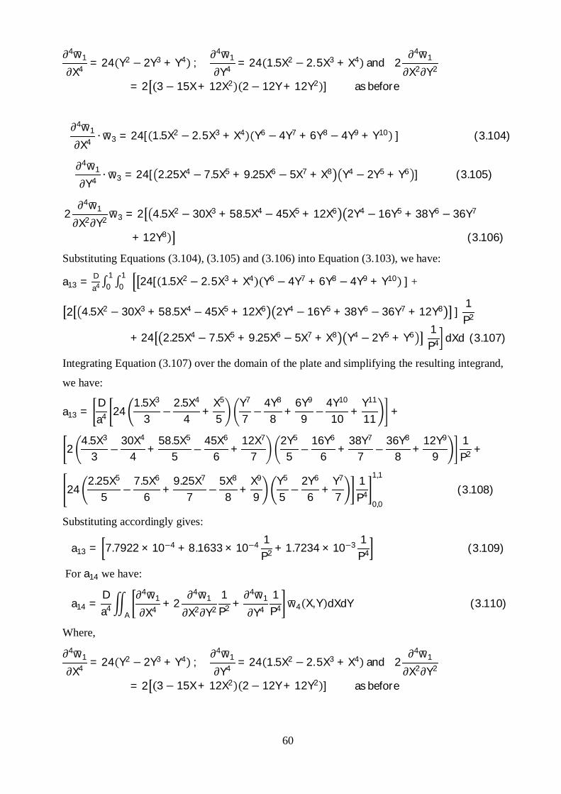
60

∂4w1

∂X4 = 24 Y2 − 2Y3 + Y4 ;∂4w1

∂Y4 = 24 1.5X2 − 2. 5X3 + X4 and 2∂4w1

∂X2∂Y2

= 2 3 − 15X + 12X2 2 − 12Y + 12Y2 ] as before

∂4w1

∂X4 ∙ w3 = 24[ 1.5X2 − 2. 5X3 + X4 Y6 − 4Y7 + 6Y8 − 4Y9 + Y10 ] (3.104)

∂4w1

∂Y4 ∙ w3 = 24[ 2.25X4 − 7.5X5 + 9.25X6 − 5X7 + X8 Y4 − 2Y5 + Y6 ] (3.105)

2∂4w1

∂X2∂Y2 w3 = 2 4.5X2 − 30X3 + 58.5X4 − 45X5 + 12X6 2Y4 − 16Y5 + 38Y6 − 36Y7

+ 12Y8 (3.106)


a13 = Da4 0

101 24[ 1.5X2 − 2. 5X3 + X4 Y6 − 4Y7 + 6Y8 − 4Y9 + Y10 ]∫∫ +

2 4.5X2 − 30X3 + 58.5X4 − 45X5 + 12X6 2Y4 − 16Y5 + 38Y6 − 36Y7 + 12Y8 ]1

P2

+ 24 2.25X4 − 7.5X5 + 9.25X6 − 5X7 + X8 Y4 − 2Y5 + Y6 1P4 dXd (3.107)


we have:

a13 =Da4 24

1.5X3

3−

2.5X4

4+

X5

5Y7

7−

4Y8

8+

6Y9

9−

4Y10

10+

Y11

11+

24.5X3

3 −30X4

4+

58.5X5

5 −45X6

6+

12X7

72Y5

5 −16Y6

6+

38Y7

7 −36Y8

8+

12Y9

91

P2 +

242.25X5

5−

7.5X6

6+

9.25X7

7−

5X8

8+

X9

9Y5

5−

2Y6

6+

Y7

71

P40,0

1,1

(3.108)


a13 = 7.7922 × 10−4 + 8.1633 × 10−4 1P2 + 1.7234 × 10−3 1

P4 (3.109)

For a14 we have:

a14 =Da4

A

∂4w1

∂X4 + 2∂4w1

∂X2∂Y2

1P2 +

∂4w1

∂Y4

1P4 w4 X, Y dXdY (3.110)

Where,

∂4w1

∂X4 = 24 Y2 − 2Y3 + Y4 ;∂4w1

∂Y4 = 24 1.5X2 − 2. 5X3 + X4 and 2∂4w1

∂X2∂Y2

= 2 3 − 15X + 12X2 2 − 12Y + 12Y2 ] as before

61

∂4w1

∂X4 ∙ w4 = 24[ 1.5X4 − 2. 5X5 + X6 Y6 − 4Y7 + 6Y8 − 4Y9 + Y10 ] (3.111)

∂4w1

∂Y4 ∙ w4 = 24[ 2.25X6 − 7.5X7 + 9.25X8 − 5X9 + X10 Y4 − 2Y5 + Y6 ] (3.112)

2∂4w1

∂X2∂Y2 w4 = 2 4.5X4 − 30X5 + 58.5X6 − 45X7 + 12X8 2Y4 − 16Y5 + 38Y6 − 36Y7

+ 12Y8 (3.113)


a14 = Da4 0

101 24[ 1.5X4 − 2. 5X5 + X6 Y6 − 4Y7 + 6Y8 − 4Y9 + Y10 ]∫∫ +

2 4.5X4 − 30X5 + 58.5X6 − 45X7 + 12X8 2Y4 − 16Y5 + 38Y6 − 36Y7 + 12Y8 ]1

P2

+ 24[ 2.25X6 − 7.5X7 + 9.25X8 − 5X9 + X10 Y4 − 2Y5

+ Y6 ]1

P4 dXdY (3.114)


we have:

a14 =Da4 24

1.5X5

5−

2.5X6

6+

X7

7Y7

7−

4Y8

8+

6Y9

9−

4Y10

10+

Y11

11+

24.5X5

5−

30X6

6+

58.5X7

7−

45X8

8+

12X9

92Y5

5−

16Y6

6+

38Y7

7−

36Y8

8+

12Y9

91

P2 +

242.25X7

7−

7.5X8

8+

9.25X9

9−

5X10

10+

X11

11Y5

5−

2Y6

6+

Y7

71

P40,0

1,1

(3.115)


a14 = 2.7211 × 10−4 + 3.2880 × 10−4 1P2 + 5.9781 × 10−4 1

P4 (3.116)

For a15 we have:

a15 =Da4

A

∂4w1

∂X4 + 2∂4w1

∂X2∂Y2

1P2 +

∂4w1

∂Y4

1P4 w5 X, Y dXdY (3.117)

Where,

∂4w1

∂X4 = 24 Y2 − 2Y3 + Y4 ;∂4w1

∂Y4 = 24 1.5X2 − 2. 5X3 + X4 and 2∂4w1

∂X2∂Y2

= 2 3 − 15X + 12X2 2 − 12Y + 12Y2 ] as before

∂4w1

∂X4 ∙ w5 = 24[ 1.5X6 − 2. 5X7 + X8 Y4 − 4Y5 + 6Y6 − 4Y7 + Y8 ] (3.118)

∂4w1

∂Y4 ∙ w5 = 24[ 2.25X8 − 7.5X9 + 9.25X10 − 5X11 + X12 Y2 − 2Y3 + Y4 ] (3.119)

62

2∂4w1

∂X2∂Y2 w2 = 2 4.5X6 − 30X7 + 58.5X8 − 45X9 + 12X10 2Y2 − 16Y3 + 38Y4 − 36Y5

+ 12Y6 (3.120)


a15 = Da4 0

101 24[ 1.5X6 − 2. 5X7 + X8 Y4 − 4Y5 + 6Y6 − 4Y7 + Y8 ]∫∫ +

2 4.5X6 − 30X7 + 58.5X8 − 45X9 + 12X10 2Y2 − 16Y3 + 38Y4 − 36Y5 + 12Y6 ]1

P2

+ 4[ 2.25X8 − 7.5X9 + 9.25X10 − 5X11 + X12 Y2 − 2Y3

+ Y4 ]1P4 dXdY (3.121)


we have:

a15 =Da4 24

1.5X7

7 −2.5X8

8 +X9

9Y5

5 −4Y6

6 +6Y7

7 −4Y8

8 +Y9

9 +

24.5X7

7−

30X8

8+

58.5X9

9−

45X10

10+

12X11

112Y3

3−

16Y4

4 +38Y5

5−

36Y6

6+

12Y7

71P2 +

242.25X9

9 −7.5X10

10 +9.25X11

11 −5X12

12 +X13

13Y3

3 −2Y4

4 +Y5

51P4

0,0

1,1

(3.122)


a15 = 4.9131 × 10−4 + 6.1843 × 10−4 1P2 + 9.3240 × 10−4 1

P4 (3.123)

For a16 we have:

a16 =Da4

A

∂4w1

∂X4 + 2∂4w1

∂X2∂Y2

1P2 +

∂4w1

∂Y4

1P4 w6 X, Y dXdY (3.124)

Where,

∂4w1

∂X4 = 24 Y2 − 2Y3 + Y4 ;∂4w1

∂Y4 = 24 1.5X2 − 2. 5X3 + X4 and 2∂4w1

∂X2∂Y2

= 2 3 − 15X + 12X2 2 − 12Y + 12Y2 ] as before

∂4w1

∂X4 ∙ w6 = 24[ 1.5X2 − 2. 5X3 + X4 Y8 − 4Y9 + 6Y10 − 4Y11 + Y12 ] (3.125)

∂4w1

∂Y4 ∙ w6 = 24[ 2.25X4 − 7.5X5 + 9.25X6 − 5X7 + X8 Y6 − 2Y7 + Y8 ] (3.126)

2∂4w1

∂X2∂Y2 w6 = 2 4.5X2 − 30X3 + 58.5X4 − 45X5 + 12X6 2Y6 − 16Y7 + 38Y8 − 36Y9

+ 12Y10 (3.127)


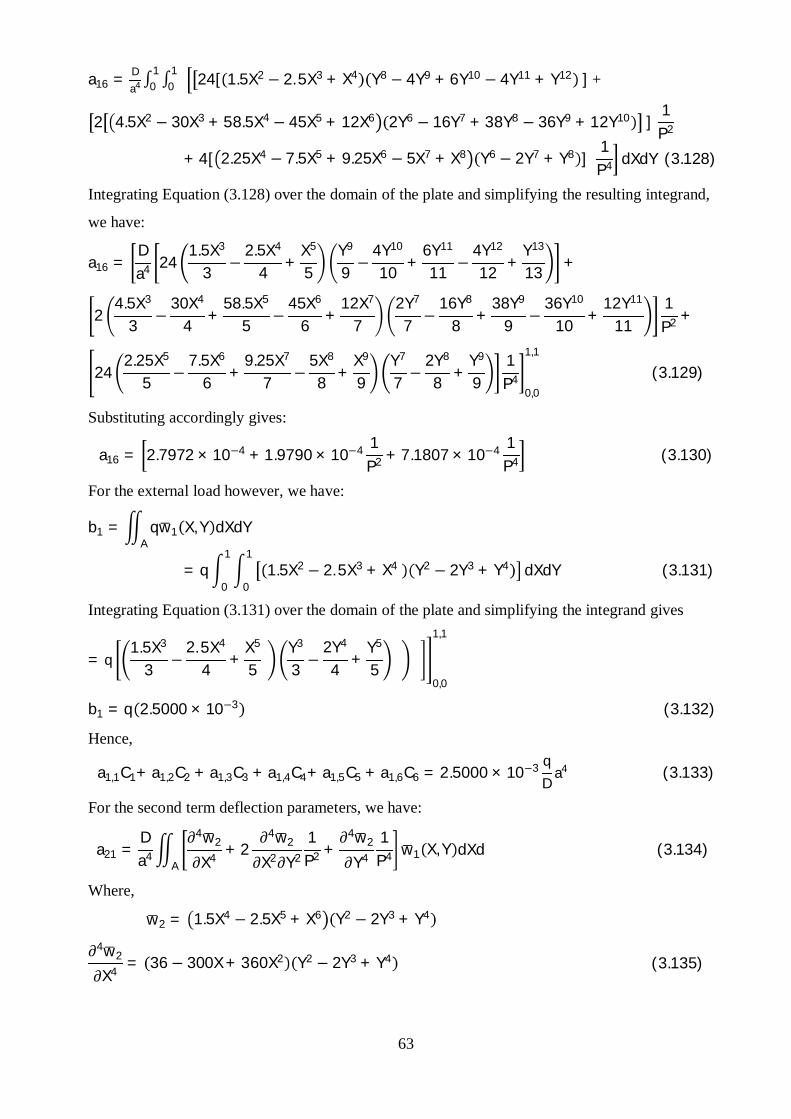
63

a16 = Da4 0

101 24[ 1.5X2 − 2. 5X3 + X4 Y8 − 4Y9 + 6Y10 − 4Y11 + Y12 ]∫∫ +

2 4.5X2 − 30X3 + 58.5X4 − 45X5 + 12X6 2Y6 − 16Y7 + 38Y8 − 36Y9 + 12Y10 ]1

P2

+ 4[ 2.25X4 − 7.5X5 + 9.25X6 − 5X7 + X8 Y6 − 2Y7 + Y8 ]1

P4 dXdY (3.128)


we have:

a16 =Da4 24

1.5X3

3 −2.5X4

4 +X5

5Y9

9 −4Y10

10 +6Y11

11 −4Y12

12 +Y13

13 +

24.5X3

3 −30X4

4 +58.5X5

5 −45X6

6 +12X7

72Y7

7 −16Y8

8 +38Y9

9 −36Y10

10 +12Y11

111P2 +

242.25X5

5 −7.5X6

6 +9.25X7

7 −5X8

8 +X9

9Y7

7 −2Y8

8 +Y9

91

P40,0

1,1

(3.129)


a16 = 2.7972 × 10−4 + 1.9790 × 10−4 1P2 + 7.1807 × 10−4 1

P4 (3.130)

For the external load however, we have:

b1 =A

qw1 X, Y dXdY

= q0

1

0

11.5X2 − 2. 5X3 + X4 Y2 − 2Y3 + Y4 dXdY (3.131)

Integrating Equation (3.131) over the domain of the plate and simplifying the integrand gives

= q1.5X3

3 −2. 5X4

4+

X5

5Y3

3 −2Y4

4+

Y5

50,0

1,1

b1 = q 2.5000 × 10−3 (3.132)

Hence,

a1,1C1+ a1,2C2 + a1,3C3 + a1,4C4+ a1,5C5 + a1,6C6 = 2.5000 × 10−3 qD

a4 (3.133)

For the second term deflection parameters, we have:

a21 =Da4

A

∂4w2

∂X4 + 2∂4w2

∂X2∂Y2

1P2 +

∂4w2

∂Y4

1P4 w1 X, Y dXd (3.134)

Where,

w2 = 1.5X4 − 2.5X5 + X6 Y2 − 2Y3 + Y4

∂4w2

∂X4 = 36 − 300X + 360X2 Y2 − 2Y3 + Y4 (3.135)

64

∂4w2

∂Y4 = 24 1.5X4 − 2. 5X5 + X6 (3.136)

2∂4w2

∂X2∂Y2 = 2 18X2 − 50X3 + 30X4 2 − 12Y + 12Y2 ] (3.137)

w1 = 1.5X2 − 2.5X3 + X4 Y2 − 2Y3 + Y4

∂4w2

∂X4 ∙ w1 = 54X2 − 540X3 + 1326X4 − 1200X5 + 360X6 Y4 − 4Y5 + 6Y6 − 4Y7

+ Y8 (3.138)

∂4w2

∂Y4 ∙ w1 = 24 2.25X6 − 7.5X7 + 9.25X8 − 5X9 + X10 Y2 − 2Y3 + Y4 (3.139)

2∂4w2

∂X2∂Y2 w1 = 2 27X4 − 120X5 + 188X6 − 125X7 + 30X8 2Y2 − 16Y3 + 38Y4 − 36Y5

+ 12Y6 (3.140)


a21 =Da4

0

1

0

154X2 − 540X3 + 1326X4 − 1200X5 + 360X6 Y4 − 4Y5 + 6Y6 − 4Y7 + Y8

+2 27X4 − 120X5 + 188X6 − 125X7 + 30X8 2Y2 − 16Y3 + 38Y4 − 36Y5 + 12Y6 1P2

+ 24 2.25X6 − 7.5X7 + 9.25X8 − 5X9 + X10 Y2 − 2Y3 + Y4 1P4 dXdY

(3.141)


we have:

a21 =Da4

54X3

3 −540X4

4 +1326X5

5 −1200X6

6 +360X7

7Y5

5 −4Y6

6 +6Y7

7 −4Y8

8 +Y9

9 +

227X5

5−

120X6

6+

188X7

7−

125X8

8+

30X9

92Y3

3−

16Y4

4+

38Y5

5−

36Y6

6+

12Y7

71

P2

+ 242.25X7

7 −7.5X8

8+

9.25X9

9 −5X10

10+

X11

11Y3

3 −2Y4

4+

Y5

51

P40,0

1,1

(3.142)


a21 = −5.8957 × 10−4 + 1.3152 × 10−3 1P2 + 2.0924 × 10−3 1

P4 (3.143)

For a22 we have:

a22 =Da4

A

∂4w2

∂X4 + 2∂4w2

∂X2∂Y2

1P2 +

∂4w2

∂Y4

1P4 w2 X, Y dYdX (3.144)

Where,

65

∂4w2

∂X4 = 36 − 300X + 360X2 Y2 − 2Y3 + Y4 ;∂4w2

∂Y4 = 24 1.5X4 − 2. 5X5 + X6 and

2∂4w2

∂X2∂Y2 = 2 18X2 − 50X3 + 30X4 2− 12Y + 12Y2 ] as before.

But w2 = 1.5X4 − 2.5X5 + X6 Y2 − 2Y3 + Y4

∂4w2

∂X4 ∙ w2 = 54X4 − 540X5 + 1326X6 − 1200X7 + 360X8 Y4 − 4Y5 + 6Y6 − 4Y7

+ Y8 (3.145)

∂4w2

∂Y4 ∙ w2 = 24 2.25X8 − 7.5X9 + 9.25X10 − 5X11 + X12 Y2 − 2Y3 + Y4 (3.146)

2∂4w2

∂X2∂Y2 w2 = 2 27X6 − 120X7 + 188X8 − 125X9 + 30X10 2Y2 − 16Y3 + 38Y4 − 36Y5

+ 12Y6 (3.147)


a22 = Da4 0

101 54X4 − 540X5 + 1326X6 − 1200X7 + 360X8 Y4 − 4Y5 + 6Y6 − 4Y7 + Y8 +∫∫

2 27X6 − 120X7 + 188X8 − 125X9 + 30X10 2Y2 − 16Y3 + 38Y4 − 36Y5 + 12Y6 ] 1P2 +

24 2.25X8 − 7.5X9 + 9.25X10 − 5X11 + X12 Y2 − 2Y3 + Y4 1P4 dXdY (3.148)


we have:

a22 =Da4

54X5

5 −540X6

6 +1326X7

7 −1200X8

8 +360X9

9Y5

5 −4Y6

6 +6Y7

7 −4Y8

8 +Y9

9 +

227X7

7 −120X8

8 +188X9

9 −125X10

10 +30X11

112Y3

3 −16Y4

4 +38Y5

5 −36Y6

6 +12Y7

71

P2

+ 242.25X9

9 −7.5X10

10 +9.25X11

11 −5X12

12 +X13

13Y3

3 −2Y4

4 +Y5

51

P40,0

1,1

(3.149)


a22 = 3.6281 × 10−4 + 1.0170 × 10−3 1P2 + 9.3240 × 10−4 1

P4 (3.150)

For a23 we have:

a23 =Da4

A

∂4w2

∂X4 + 2∂4w2

∂X2∂Y2

1P2 +

∂4w2

∂Y4

1P4 w3 X, Y dYdX (3.151)

Where,

∂4w2

∂X4 = 36 − 300X + 360X2 Y2 − 2Y3 + Y4 ;∂4w2

∂Y4 = 24 1.5X4 − 2. 5X5 + X6 and

66

2∂4w2


But w3 = 1.5X2 − 2.5X3 + X4 Y4 − 2Y5 + Y6

∂4w2

∂X4 ∙ w3 = 54X2 − 540X3 + 1326X4 − 1200X5 + 360X6 Y6 − 4Y7 + 6Y8 − 4Y9

+ Y10 (3.152)

∂4w2

∂Y4 ∙ w3 = 24 2.25X6 − 7.5X7 + 9.25X8 − 5X9 + X10 Y4 − 2Y5 + Y6 (3.153)

2∂4w2

∂X2∂Y2 w3 = 2 27X4 − 120X5 + 188X6 − 125X7 + 30X8 2Y4 − 16Y5 + 38Y6 − 36Y7

+ 12Y8 (3.154)


a23 = Da4 0

101 54X2 − 540X3 + 1326X4 − 1200X5 + 360X6 Y6 − 4Y7 + 6Y8 − 4Y9 + Y10 +∫∫

2 27X4 − 120X5 + 188X6 − 125X7 + 30X8 2Y4 − 16Y5 + 38Y6 − 36Y7 + 12Y8 1P2 +

24 2.25X6 − 7.5X7 + 9.25X8 − 5X9 + X10 Y4 − 2Y5 + Y6 1P4 dXdY (3.155)


we have:

a23 =Da4

54X3

3 −540X4

4 +1326X5

5 −1200X6

6 +360X7

7Y7

7 −4Y8

8 +6Y9

9 −4Y10

10 +Y11

11 +

227X5

5−

120X6

6+

188X7

7−

125X8

8+

30X9

92Y5

5−

16Y6

6+

38Y7

7−

36Y8

8+

12Y9

91

P2

+ 242.25X7

7−

7.5X8

8+

9.25X9

9−

5X10

10+

X11

11Y5

5−

2Y6

6+

Y7

71

P40,0

1,1

(3.156)


a23 = −1.6079E × 10−4 + 3.2880 × 10−4 1P2 + 5.9781 × 10−4 1

P4 (3.157)

For a24 we have:

a24 =Da4

A

∂4w2

∂X4 + 2∂4w2

∂X2∂Y2

1P2 +

∂4w2

∂Y4

1P4 w4 X, Y dYdX (3.158)

Where,

∂4w2

∂X4 = 36 − 300X + 360X2 Y2 − 2Y3 + Y4 ;∂4w2

∂Y4 = 24 1.5X4 − 2. 5X5 + X6 and

2∂4w2


67

But w4 = 1.5X4 − 2.5X5 + X6 Y4 − 2Y5 + Y6

∂4w2

∂X4 ∙ w4 = 54X4 − 540X5 + 1326X6 − 1200X7 + 360X8 Y6 − 4Y7 + 6Y8 − 4Y9

+ Y10 (3.159)

∂4w2

∂Y4 ∙ w4 = 24 2.25X8 − 7.5X9 + 9.25X10 − 5X11 + X12 Y4 − 2Y5Y6 (3.160)

2∂4w2

∂X2∂Y2 w2 = 2 27X6 − 120X7 + 188X8 − 125X9 + 30X10 2Y4 − 16Y5 + 38Y6 − 36Y7

+ 12Y8 (3.161)


a24 = Da4 0

101 54X4 − 540X5 + 1326X6 − 1200X7 + 360X8 Y6 − 4Y7 + 6Y8 − 4Y9 + Y10 +∫∫

2 27X6 − 120X7 + 188X8 − 125X9 + 30X10 2Y4 − 16Y5 + 38Y6 − 36Y7 + 12Y8 1P2 +

24 2.25X8 − 7.5X9 + 9.25X10 − 5X11 + X12 Y4 − 2Y5 + Y6 1P4 dXdY (3.162)


we have:

a24 =Da4

54X5

5 −540X6

6 +1326X7

7 −1200X8

8 +360X9

9Y7

7 −4Y8

8 +6Y9

9 −4Y10

10 +Y11

11 +

227X7

7 −120X8

8 +188X9

9 −125X10

10 +30X11

112Y5

5 −16Y6

6 +38Y7

7 −36Y8

8 +12Y9

91

P2

+ 242.25X9

9−

7.5X10

10+

9.25X11

11−

5X12

12+

X13

13Y5

5−

2Y6

6+

Y7

71P4

0,0

1,1

(3.163)


a24 = 9.8949 × 10−5 + 2.5424 × 10−4 1P2 + 2.6640 × 10−4 1

P4 (3.164)

For a25 we have:

a25 =Da4

A

∂4w2

∂X4 + 2∂4w2

∂X2∂Y2

1P2 +

∂4w2

∂Y4

1P4 w5 X, Y dYdX (3.165)

Where,

∂4w2

∂X4 = 36 − 300X + 360X2 Y2 − 2Y3 + Y4 ;∂4w2

∂Y4 = 24 1.5X4 − 2. 5X5 + X6 and

2∂4w2


But w5 = 1.5X6 − 2.5X7 + X8 Y2 − 2Y3 + Y4

68

∂4w2

∂X4 ∙ w5 = 54X6 − 540X7 + 1326X8 − 1200X9 + 360X10 Y4 − 4Y5 + 6Y6 − 4Y7

+ Y8 (3.166)

∂4w2

∂Y4 ∙ w5 = 24 2.25X10 − 7.5X11 + 9.25X12 − 5X13 + X14 Y2 − 2Y3 + Y4 (3.167)

2∂4w2

∂X2∂Y2 w2 = 2 27X8 − 120X9 + 188X10 − 125X11 + 30X12 2Y2 − 16Y3 + 38Y4 − 36Y5

+ 12Y6 (3.168)


a25 = Da4 0

101 54X6 − 540X7 + 1326X8 − 1200X9 + 360X10 Y4 − 4Y5 + 6Y6 − 4Y7 + Y8 +∫∫

2 27X8 − 120X9 + 188X10 − 125X11 + 30X12 2Y2 − 16Y3 + 38Y4 − 36Y5 + 12Y6 1P2 +

24 2.25X10 − 7.5X11 + 9.25X12 − 5X13 + X14 Y2 − 2Y3 + Y4 1P4 dXdY (3.169)


we have:

a25 =Da4

54X7

7 −540X8

8 +1326X9

9 −1200X10

10 +360X11

11Y5

5 −4Y6

6 +6Y7

7 −4Y8

8 +Y9

9 +

227X9

9−

120X10

10+

188X11

11−

125X12

12+

30X13

132Y3

3−

16Y4

4 +38Y5

5−

36Y6

6+

12Y7

71P2

+ 242.25X11

11−

7.5X12

12+

9.25X13

13−

5X14

14+

X15

15Y3

3−

2Y4

4+

Y5

51P4

0,0

1,1

(3.170)


a25 = 4.3634 × 10−4 + 6.8820 × 10−4 1P2 + 4.8618 × 10−4 1

P4 (3.171)

For a26 we have:

a26 =Da4

A

∂4w2

∂X4 + 2∂4w2

∂X2∂Y2

1P2 +

∂4w2

∂Y4

1P4 w6 X, Y dYdX (3.172)

Where,

∂4w2

∂X4 = 36 − 300X + 360X2 Y2 − 2Y3 + Y4 ;∂4w2

∂Y4 = 24 1.5X4 − 2. 5X5 + X6 and

2∂4w2


But w6 = 1.5X2 − 2.5X3 + X4 Y6 − 2Y7 + Y8

69

∂4w2

∂X4 ∙ w6 = 54X2 − 540X3 + 1326X4 − 1200X5 + 360X6 Y8 − 4Y9 + 6Y10 − 4Y11

+ Y12 (3.173)

∂4w2

∂Y4 ∙ w6 = 24 2.25X6 − 7.5X7 + 9.25X8 − 5X9 + X10 Y6 − 2Y7 + Y8 (3.174)

2∂4w2

∂X2∂Y2 w2 = 2 27X4 − 120X5 + 188X6 − 125X7 + 30X8 2Y6 − 16Y7 + 38Y8 − 36Y9

+ 12Y10 (3.175)


a26 = Da4 0

101 54X2 − 540X3 + 1326X4 − 1200X5 + 360X6 Y8 − 4Y9 + 6Y10 − 4Y11 +∫∫

Y12 + 2 27X4 − 120X5 + 188X6 − 125X7 + 30X8 2Y6 − 16Y7 + 38Y8 − 36Y9 +

12Y10 ] 1P2 + 24 2.25X6 − 7.5X7 + 9.25X8 − 5X9 + X10 Y6 − 2Y7 + Y8 1

P4 dXdY (3.176)


we have:

a26 =Da4

54X3

3 −540X4

4 +1326X5

5 −1200X6

6 +360X7

7Y9

9 −4Y10

10 +6Y11

11 −4Y12

12 +Y13

13 +

227X5

5−

120X6

6+

188X7

7−

125X8

8+

30X9

92Y7

7−

16Y8

8+

38Y9

9−

36Y10

10+

12Y11

111

P2

+ 242.25X7

7 −7.5X8

8+

9.25X9

9 −5X10

10+

X11

11Y7

7 −2Y8

8+

Y9

91

P40,0

1,1

(3.177)


a26 = −5.7720 × 10−5 + 7.9709 × 10−5 1P2 + 2.4909 × 10−4 1

P4 (3.178)


b2 =A

qw2 X, Y dXdY

= q0

1

0

11.5X4 − 2.5X5 + X6 Y2 − 2Y3 + Y4 dXdY (3.179)


= q1.5X5

5 −2.5X6

6 +X7

7Y3

3 −2Y4

4 +Y5

50,0

1,1

b2 = q 8.7302 × 10−4 (3.180)

Hence,

a2,1C1+a2,2C2 + a2,3C3 + a2,4C4+a2,5C5 + a2,6C6 = 8.7302 × 10−4 qD

a4 (3.181)

70

For the third term deflection parameters, we have:

a31 =Da4

A

∂4w3

∂X4 + 2∂4w3

∂X2∂Y2

1P2 +

∂4w3

∂Y4

1P4 w1 Y, X dXdY (3.182)

Where,

w3 = 1.5X2 − 2.5X3 + X4 Y4 − 2Y5 + Y6

∂4w3

∂X4 = 24 Y4 − 2Y5 + Y6 (3.183)

∂4w3

∂Y4 = 1.5X2 − 2.5X3 + X4 24− 240Y + 360Y2 (3.184)

2∂4w3

∂X2∂Y2 = 2 3 − 15X + 12X2 12Y2 − 40Y3 + 30Y4 ] (3.185)

∂4w3

∂X4 ∙ w1 = 24 1.5X2 − 2. 5X3 + X4 Y6 − 4Y7 + 6Y8 − 4Y9 + Y10 (3.186)

∂4w3

∂Y4 ∙ w1 = 24 2.25X4 − 7.5X5 + 9.25X6 − 5X7 + X8 Y2 − 12Y3 + 36Y4 − 40Y5

+ 15Y6 (3.187)

2∂4w3

∂X2∂Y2 w1 = 2 4.5X2 − 30X3 + 58.5X4 − 45X5 + 12X6 12Y4 − 64Y5 + 122Y6 − 100Y7

+ 30Y8 (3.188)


a31 =Da4

0

1

0

124 1.5X2 − 2. 5X3 + X4 Y6 − 4Y7 + 6Y8 − 4Y9 + Y10

+2 4.5X2 − 30X3 + 58.5X4 − 45X5 + 12X6 12Y4 − 64Y5 + 122Y6 − 100Y7 + 30Y8 1P2

+ 24 2.25X4 − 7.5X5 + 9.25X6 − 5X7 + X8 Y2 − 12Y3 + 36Y4 − 40Y5 +15Y6 1

P4 dXdY (3.189)


we have:

a31 =Da4 24

1.5X3

3 −2. 5X4

4 +X5

5Y7

7 −4Y8

8 +6Y9

9 −4Y10

10 +Y11

11 +

212Y5

5−

64Y6

6+

122Y7

7−

100Y8

8+

30Y9

94.5X3

3−

30X4

4 +58.5X5

5−

45X6

6+

12X7

71

P2

+ 242.25X5

5−

7.5X6

6+

9.25X7

7−

5X8

8+

X9

9Y3

3−

12Y4

4 +36Y5

5−

40Y6

6+

15Y7

71P4

0,0

1,1

(3.190)

71


a31 = 7.7922 × 10−4 + 8.1633 × 10−4 1P2 + 1.7234 × 10−3 1

P4 (3.191)

For a32 we have:

a32 =Da4

A

∂4w3

∂X4 + 2∂4w3

∂X2∂Y2

1P2 +

∂4w3

∂Y4

1P4 w2 X, Y dXdY (3.192)

Where,

∂4w3

∂X4 = 24 Y4 − 2Y5 + Y6 ;∂4w3

∂Y4 = 1.5X2 − 2.5X3 + X4 24− 240Y + 360Y2

and 2∂4w3

∂X2∂Y2 = 2 3− 15X + 12X2 12Y2 − 40Y3 + 30Y4 ] as before

But w2 = 1.5X4 − 2.5X5 + X6 Y2 − 2Y3 + Y4

∂4w3

∂X4 ∙ w2 = 24 1.5X4 − 2.5X5 + X6 Y6 − 4Y7 + 6Y8 − 4Y9 + Y10 (3.193)

∂4w3

∂Y4 ∙ w2 = 24 2.25X6 − 7.5X7 + 9.25X8 − 5X9 + X10 Y2 − 12Y3 + 36Y4 − 40Y5

+ 15Y6 (3.194)

2∂4w2

∂X2∂Y2 w2 = 2 4.5X4 − 30X5 + 58.5X6 − 45X7 + 12X8 12Y4 − 64Y5 + 122Y6 − 100Y7

+ 30Y8 (3.195)


a32 = Da4 0

101 24 1.5X4 − 2.5X5 + X6 Y6 − 4Y7 + 6Y8 − 4Y9 + Y10 +∫∫ 2 4.5X4 − 30X5 +

58.5X6 − 45X7 + 12X8 12Y4 − 64Y5 + 122Y6 − 100Y7 + 30Y8 1P2 + 24 2.25X6 − 7.5X7 +

9.25X8 − 5X9 + X10 Y2 − 12Y3 + 36Y4 − 40Y5 + 15Y6 1P4 dXdY (3.196)


we have:

a32 =Da4 24

1.5X5

5 −2. 5X6

6 +X7

7Y7

7 −4Y8

8 +6Y9

9 −4Y10

10 +Y11

11 +

24.5X5

5−

30X6

6+

58.5X7

7−

45X8

8+

12X9

912Y5

5−

64Y6

6+

122Y7

7−

100Y8

830Y9

91P2

+ 242.25X7

7−

7.5X8

8+

9.25X9

9−

5X10

10+

X11

11Y3

3−

12Y4

4 +36Y5

5−

40Y6

6

+15Y7

71P4

0,0

1,1

(3.197)


72

a32 = 2.7211 × 10−4 + 3.2880 × 10−4 1P2 + 5.9781 × 10−4 1

P4 (3.198)

For a33 we have:

a33 =Da4

A

∂4w3

∂X4 + 2∂4w3

∂X2∂Y2

1P2 +

∂4w3

∂Y4

1P4 w3 X, Y dXdY (3.199)

Where,

∂4w3

∂X4 = 24 Y4 − 2Y5 + Y6 ;∂4w3

∂Y4 = 1.5X2 − 2.5X3 + X4 24− 240Y + 360Y2

and 2∂4w3


But w3 = 1.5X2 − 2.5X3 + X4 Y4 − 2Y5 + Y6

∂4w3

∂X4 ∙ w3 = 24 1.5X2 − 2.5X3 + X4 Y8 − 4Y9 + 6Y10 − 4Y11 + Y12 (3.200)

∂4w3

∂Y4 ∙ w3 = 24 2.25X4 − 7.5X5 + 9.25X6 − 5X7 + X8 Y4 − 12Y5 + 36Y6 − 40Y7

+ 15Y8 (3.201)

2∂4w2

∂X2∂Y2 w2

= 2 4.5X2 − 30X3 + 58.5X4 − 45X5 + 12X6 12Y6 − 64Y7 + 122Y8 − 100Y9

+ 30Y10 (3.202)

Substituting Equation (3.200), (3.201) and (3.202) into Equation (3.199), we have:

a33 = Da4 0

101 24 1.5X2 − 2.5X3 + X4 Y8 − 4Y9 + 6Y10 − 4Y11 + Y12 +∫∫ 2 4.5X2 − 30X3 +

58.5X4 − 45X5 + 12X6 12Y6 − 64Y7 + 122Y8 − 100Y9 + 30Y10 1P2 + 24 2.25X4 − 7.5X5 +

9.25X6 − 5X7 + X8 Y4 − 12Y5 + 36Y6 − 40Y7 + 15Y8 1P4 dXdY (3.203)


we have:

a33 =Da4 24

1.5X3

3 −2. 5X4

4 +X5

5Y9

9 −4Y10

10 +6Y11

11 −4Y12

12 +Y13

13 +

24.5X3

3 −30X4

4 +58.5X5

5 −45X6

6 +12X7

712Y7

7 −64Y8

8 +122Y9

9 −100Y10

10 +30Y11

111

P2

+ 242.25X5

5−

7.5X6

6+

9.25X7

7−

5X8

8+

X9

9Y5

5−

12Y6

6+

36Y7

7−

40Y8

8

+15Y9

91P4

0,0

1,1

(3.204)


73

a33 = 2.7972 × 10−4 + 4.9474 × 10−4 1P2 + 1.7234 × 10−3 1

P4 (3.205)

For a34 we have:

a34 =Da4

A

∂4w3

∂X4 + 2∂4w3

∂X2∂Y2

1P2 +

∂4w3

∂Y4

1P4 w4 X, Y dXdY (3.206)

Where,

∂4w3

∂X4 = 24 Y4 − 2Y5 + Y6 ;∂4w3

∂Y4 = 1.5X2 − 2.5X3 + X4 24− 240Y + 360Y2

and 2∂4w3


But w4 = 1.5X4 − 2.5X5 + X6 Y4 − 2Y5 + Y6

∂4w3

∂X4 ∙ w4 = 24 1.5X4 − 2.5X5 + X6 Y8 − 4Y9 + 6Y10 − 4Y12 + Y13 (3.207)

∂4w3

∂Y4 ∙ w4 = 24 2.25X6 − 7.5X7 + 9.25X8 − 5X9 + X10 Y4 − 12Y5 + 36Y6 − 40Y7

+ 15Y8 (3.208)

2∂4w2

∂X2∂Y2 w4 = 2 4.5X4 − 30X5 + 58.5X6 − 45X7 + 12X8 12Y6 − 64Y7 + 122Y8 − 100Y9

+ 30Y10 (3.209)


a34 = Da4 0

101 24 1.5X4 − 2.5X5 + X6 Y8 − 4Y9 + 6Y10 − 4Y12 + Y13 +∫∫ 2 4.5X4 − 30X5 +

58.5X6 − 45X7 + 12X8 12Y6 − 64Y7 + 122Y8 − 100Y9 + 30Y10 1P2 + 24 2.25X6 −

7.5X7 + 9.25X8 − 5X9 + X10 Y4 − 12Y5 + 36Y6 − 40Y7 + 15Y8 1P4 dXdY (3.210)


we have:

a34 =Da4 24

1.5X5

5 −2. 5X6

6 +X7

7Y9

9 −4Y10

10 +6Y11

11 −4Y12

12 +Y13

13 +

24.5X5

5−

30X6

6+

58.5X7

7−

45X8

8+

12X9

912Y7

7−

64Y8

8+

122Y9

9−

100Y10

10+

30Y11

111

P2

+ 242.25X7

7 −7.5X8

8 +9.25X9

9 −5X10

10 +X11

11Y5

5 −12Y6

6 +36Y7

7 −40Y8

8

+15Y9

91P4

0,0

1,1

(3.211)


74

a34 = 9.7680 × 10−5 + 1.9927 × 10−4 1P2 + 5.9781 × 10−4 1

P4 (3.212)

For a35 we have:

a35 =Da4

A

∂4w3

∂X4 + 2∂4w3

∂X2∂Y2

1P2 +

∂4w3

∂Y4

1P4 w5 X, Y dXdY (3.213)

Where,

∂4w3

∂X4 = 24 Y4 − 2Y5 + Y6 ;∂4w3

∂Y4 = 1.5X2 − 2.5X3 + X4 24− 240Y + 360Y2

and 2∂4w3


But w5 = 1.5X6 − 2.5X7 + X8 Y2 − 2Y3 + Y4

∂4w3

∂X4 ∙ w5 = 24 1.5X6 − 2.5X7 + X8 Y6 − 4Y7 + 6Y8 − 4Y9 + Y10 (3.214)

∂4w3

∂Y4 ∙ w5 = 24 2.25X8 − 7.5X9 + 9.25X10 − 5X11 + X12 Y2 − 12Y3 + 36Y4 − 40Y5

+ 15Y6 (3.215)

2∂4w2

∂X2∂Y2 w5 = 2 4.5X6 − 30X7 + 58.5X8 − 45X9 + 12X10 12Y4 − 64Y5 + 122Y6 − 100Y7

+ 30Y8 (3.216)


a35 = Da4 0

101 24 1.5X6 − 2.5X7 + X8 Y6 − 4Y7 + 6Y8 − 4Y9 + Y10 +∫∫ 2 4.5X6 − 30X7 +

58.5X8 − 45X9 + 12X10 12Y4 − 64Y5 + 122Y6 − 100Y7 + 30Y8 1P2 + 24 2.25X8 −

7.5X9 + 9.25X10 − 5X11 + X12 Y2 − 12Y3 + 36Y4 − 40Y5 + 15Y6 1P4 dXdY (3.217)


we have:

a35 =Da4 24

1.5X7

7 −2. 5X8

8 +X9

9Y7

7 −4Y8

8 +6Y9

9 −4Y10

10 +Y11

11 +

24.5X7

7−

30X8

8+

58.5X9

9−

45X10

10+

12X11

1112Y5

5−

64Y6

6+

122Y7

7−

100Y8

8+

30Y9

91

P2

+ 242.25X9

9 −7.5X10

10 +9.25X11

11 −5X12

12 +X13

13Y3

3 −12Y4

4 +36Y5

5 −40Y6

6

+15Y7

71P4

0,0

1,1

(3.218)


75

a35 = 1.3399 × 10−4 + 1.5461 × 10−4 1P2 + 2.6640 × 10−4 1

P4 (3.219)

For a36 we have:

a36 =Da4

A

∂4w3

∂X4 + 2∂4w3

∂X2∂Y2

1P2 +

∂4w3

∂Y4

1P4 w6 X, Y dXdY (3.220)

Where,

∂4w3

∂X4 = 24 Y4 − 2Y5 + Y6 ;∂4w3

∂Y4 = 1.5X2 − 2.5X3 + X4 24− 240Y + 360Y2

and 2∂4w3


But w6 = 1.5X2 − 2.5X3 + X4 Y6 − 2Y7 + Y8

∂4w3

∂X4 ∙ w6 = 24 1.5X2 − 2.5X3 + X4 Y10 − 4Y11 + 6Y12 − 4Y13 + Y14 (3.221)

∂4w3

∂Y4 ∙ w6 = 24 2.25X4 − 7.5X5 + 9.25X6 − 5X7 + X8 Y6 − 12Y7 + 36Y8 − 40Y9

+ 15Y10 (3.222)

2∂4w2

∂X2∂Y2 w2 = 2 4.5X2 − 30X3 + 58.5X4 − 45X5 + 12X6 12Y8 − 64Y9 + 122Y10 − 100Y11

+ 30Y12 (3.223)


a36 = Da4 0

101 24 1.5X2 − 2.5X3 + X4 Y10 − 4Y11 + 6Y12 − 4Y13 + Y14 +∫∫ 2 4.5X2 − 30X3 +

58.5X4 − 45X5 + 12X6 12Y8 − 64Y9 + 122Y10 − 100Y11 + 30Y12 1P2 + 24 2.25X4 −

7.5X5 + 9.25X6 − 5X7 + X8 Y6 − 12Y7 + 36Y8 − 40Y9 +15Y10 1

P4 dXdY (3.224)


we have:

a36 =Da4 24

1.5X3

3 −2. 5X4

4 +X5

5Y11

11 −4Y12

12 +6Y13

13 −4Y14

14 +Y15

15 +

24.5X3

3 −30X4

4 +58.5X5

5 −45X6

6 +12X7

712Y9

9 −64Y10

10 +122Y11

11 −100Y12

12

+30Y13

131P2

76

+ 242.25X5

5 −7.5X6

6+

9.25X7

7 −5X8

8+

X9

9Y7

7 −12Y8

8+

36Y9

9 −40Y10

10

+15Y11

111P4

0,0

1,1

(3.225)


a36 = 1.1988 × 10−4 + 2.3976 × 10−4 1P2 + 1.1750 × 10−3 1

P4 (3.226)


b3 =A

qw3 X, Y dXdY

= q0

1

0

11.5X2 − 2. 5X3 + X4 Y4 − 2Y5 + Y6 dXdY (3.227)


= q1.5X3

3 −2. 5X4

4+

X5

5Y5

5 −2Y6

6+

Y7

70,0

1,1

b3 = q 7.1429 × 10−4 3.228

Hence,

a3,1C1+ a3,2C2 + a3,3C3 + a3,4C4+ a3,5C5 + a3,6C6 = 7.1429 × 10−4 qD

a4 (3.229)

For the fourth term deflection parameters, we have:

a41 =Da4

A

∂4w4

∂X4 + 2∂4w4

∂X2∂Y2

1P2 +

∂4w4

∂Y4

1P4 w1 Y, X dXdY (3.230)

Where,

w4 = 1.5X4 − 2. 5X5 + X6 Y4 − 2Y5 + Y6

∂4w4

∂X4 = 36 − 300X + 360X2 Y4 − 2Y5 + Y6 (3.231)

∂4w4

∂Y4 = 1.5X4 − 2. 5X5 + X6 24 − 240Y + 360Y2 (3.232)

2∂4w4

∂X2∂Y2 = 2 18X2 − 50X3 + 30X4 12Y2 − 40Y3 + 30Y4 ] (3.233)

But w1 = 1.5X2 − 2. 5X3 + X4 Y2 − 2Y3 + Y4

∂4w4

∂X4 ∙ w1 = 54X2 − 540X3 + 1326X4 − 1200X5 + 360X6 Y6 − 4Y7 + 6Y8 − 4Y9

+ Y10 (3.234)

77

∂4w4

∂Y4 ∙ w1 = 24 2.25X6 − 7.5X7 + 9.25X8 − 5X9 + X10 Y2 − 12Y3 + 36Y4 − 40Y5

+ 15Y6 (3.235)

2∂4w4

∂X2∂Y2 w1 = 2 27X4 − 120X5 + 188X6 − 125X7 + 30X8 12Y4 − 64Y5 + 122Y6 − 100Y7

+ 30Y8 (3.236)


a41 =Da4

0

1

0

154X2 − 540X3 + 1326X4 − 1200X5 + 360X6 Y6 − 4Y7 + 6Y8 − 4Y9 + Y10

+2 27X4 − 120X5 + 188X6 − 125X7 + 30X8 12Y4 − 64Y5 + 122Y6 − 100Y7 + 30Y8 1P2

+ 24 2.25X6 − 7.5X7 + 9.25X8 − 5X9 + X10 Y2 − 12Y3 + 36Y4 − 40Y5 +15Y6 1

P4 dXdY (3.237)


we have:

a41 =Da4

54X3

3 −540X4

4 +1326X5

5 −1200X6

6 +360X7

7Y7

7 −4Y8

8 +6Y9

9 −4Y10

10 +Y11

11

+ 227X5

5−

120X6

6+

188X7

7−

125X8

8+

30X9

912Y5

5−

64Y6

6+

122Y7

7−

100Y8

8

+30Y9

91P2

+ 242.25X7

7−

7.5X8

8+

9.25X9

9−

5X10

10+

X11

11Y3

3−

12Y4

4+

36Y5

5−

40Y6

6+

15Y7

71

P40,0

1,1

(3.238)


a41 = −1.6079 × 10−4 + 3.2880 × 10−4 1P2 + 5.9781 × 10−4 1

P4 (3.239)

For a42 we have:

a42 =Da4

A

∂4w4

∂X4 + 2∂4w4

∂X2∂Y2

1P2 +

∂4w4

∂Y4

1P4 w2 X, Y dXdY (3.240 )

Where,

∂4w4

∂X4 = 36 − 360X + 360X2 Y4 − 2Y5 + Y6 ;∂4w4

∂Y4 = 1.5X4 − 2.5X5 + X6

24 − 240Y + 360Y2 and

78

2∂4w4

∂X2∂Y2 = 2 18X2 − 50X3 + 30X4 12Y2 − 40Y3 + 30Y4 ] as before

But w2 = 1.5X4 − 2. 5X5 + X6 Y2 − 2Y3 + Y4

∂4w4

∂X4 ∙ w2 = 54X4 − 540X5 + 1326X6 − 1200X7 + 360X8 Y6 − 4Y7 + 6Y8 − 4Y9

+ Y10 (3.241)

∂4w4

∂Y4 ∙ w2 = 24 2.25X8 − 7.5X9 + 9.25X10 − 5X11 + X12 Y2 − 12Y3 + 36Y4 − 40Y5

+ 15Y6 (3.242)

2∂4w4

∂X2∂Y2 w2 = 2 27X6 − 120X7 + 188X8 − 125X9 + 30X10 12Y4 − 64Y5 + 122Y6 − 100Y7

+ 30Y8 (3.243)


a42 = Da4 0

101 54X4 − 540X5 + 1326X6 − 1200X7 + 360X8 Y6 − 4Y7 + 6Y8 − 4Y9 + Y10 +∫∫

2 27X6 − 120X7 + 188X8 − 125X9 + 30X10 12Y4 − 64Y5 + 122Y6 − 100Y7 + 30Y8 ] 1P2 +

24 2.25X8 − 7.5X9 + 9.25X10 − 5X11 + X12 Y2 − 12Y3 + 36Y4 − 40Y5 +15Y6 1

P4 dXdY (3.244)


we have:

a42 =Da4

54X5

5 −540X6

6 +1326X7

7 −1200X8

8 +360X9

9Y7

7 −4Y8

8 +6Y9

9 −4Y10

10 +Y11

11 +

227X7

7 −120X8

8+

188X9

9 −125X10

10+

30X11

1112Y5

5 −64Y6

6+

122Y7

7 −100Y8

8

+30Y9

91P2 +

+ 242.25X9

9−

7.5X10

10+

9.25X11

11−

5X12

12+

X13

13Y3

3−

12Y4

4 +36Y5

5−

40Y6

6

+15Y7

71P4

0,0

1,1

(3.245)


a42 = 9.8949 × 10−5 + 2.5424 × 10−4 1P2 + 2.6640 × 10−4 1

P4 (3.246)

For a43 we have:

a43 =Da4

A

∂4w4

∂X4 + 2∂4w4

∂X2∂Y2

1P2 +

∂4w4

∂Y4

1P4 w3 X, Y dXdY (3.247)

79

Where,

∂4w4

∂X4 = 36 − 360X + 360X2 Y4 − 2Y5 + Y6 ;∂4w4

∂Y4 = 1.5X4 − 2.5X5 + X6

24 − 240Y + 360Y2 and

2∂4w4


But w3 = 1.5X2 − 2. 5X3 + X4 Y4 − 2Y5 + Y6

∂4w4

∂X4 ∙ w3 = 54X2 − 540X3 + 1326X4 − 1200X5 + 360X6 Y8 − 4Y9 + 6Y10 − 4Y11

+ Y12 (3.248)

∂4w4

∂Y4 ∙ w3 = 24 2.25X6 − 7.5X7 + 9.25X8 − 5X9 + X10 Y4 − 12Y5 + 36Y6 − 40Y7

+ 15Y8 (3.249)

2∂4w4

∂X2∂Y2 w3 = 2 27X4 − 120X5 + 188X6 − 125X7 + 30X8 12Y6 − 64Y7 + 122Y8 − 100Y9

+ 30Y10 (3.250)


a43 = Da4 0

101 54X2 − 540X3 + 1326X4 − 1200X5 + 360X6 Y8 − 4Y9 + 6Y10 − 4Y11 +∫∫

Y12 + 2 27X4 − 120X5 + 188X6 − 125X7 + 30X8 12Y6 − 64Y7 + 122Y8 − 100Y9 +

30Y10 1P2 + 24 2.25X6 − 7.5X7 + 9.25X8 − 5X9 + X10 Y4 − 12Y5 + 36Y6 − 40Y7 +

15Y8 1P4 dXdY (3.251)


we have:

a43 =Da4

54X3

3 −540X4

4 +1326X5

5 −1200X6

6 +360X7

7Y9

9 −4Y10

10 +6Y11

11 −4Y12

12 +Y13

13

+ 227X5

5 −120X6

6 +188X7

7 −125X8

8 +30X9

912Y7

7 −64Y8

8 +122Y9

9 −100Y10

10

+30Y11

111P2

+ 242.25X7

7−

7.5X8

8+

9.25X9

9−

5X10

10+

X11

11Y5

5−

12Y6

6+

36Y7

7−

40Y8

8

+15Y9

91P4

0,0

1,1

(3.252)


80

a43 = −5.7720 × 10−5 + 1.9927 × 10−4 1P2 + 5.9781 × 10−4 1

P4 (3.253)

For a44 we have:

a44 =Da4

A

∂4w4

∂X4 + 2∂4w4

∂X2∂Y2

1P2 +

∂4w4

∂Y4

1P4 w4 X, Y dXdY (3.254)

Where,

∂4w4

∂X4 = 36 − 360X + 360X2 Y4 − 2Y5 + Y6 ;∂4w4

∂Y4 = 1.5X4 − 2.5X5 + X6

24 − 240Y + 360Y2 and

2∂4w4


But w4 = 1.5X4 − 2. 5X5 + X6 Y4 − 2Y5 + Y6

∂4w4

∂X4 ∙ w4 = 54X4 − 540X5 + 1326X6 − 1200X7 + 360X8 Y8 − 4Y9 + 6Y10 − 4Y11

+ Y12 (3.255)

∂4w4

∂Y4 ∙ w4 = 24 2.25X8 − 7.5X9 + 9.25X10 − 5X11 + X12 Y4 − 12Y5 + 36Y6 − 40Y7

+ 15Y8 (3.256)

2∂4w4

∂X2∂Y2 w4 = 2 27X6 − 120X7 + 188X8 − 125X9 + 30X10 12Y6 − 64Y7 + 122Y8 − 100Y9

+ 30Y10 (3.257)


a44 = Da4 0

101 54X4 − 540X5 + 1326X6 − 1200X7 + 360X8 Y8 − 4Y9 + 6Y10 − 4Y11 +∫∫

Y12 + 2 27X6 − 120X7 + 188X8 − 125X9 + 30X10 12Y6 − 64Y7 + 122Y8 − 100Y9 +

30Y10 ] 1P2 + 24 2.25X8 − 7.5X9 + 9.25X10 − 5X11 + X12 Y4 − 12Y5 + 36Y6 − 40Y7 +

15Y8 1P4 dXdY (3.258)


we have:

a44 =Da4

54X5

5 −540X6

6 +1326X7

7 −1200X8

8 +360X9

9Y9

9 −4Y10

10 +6Y11

11 −4Y12

12 +Y13

13

+ 227X7

7 −120X8

8 +188X9

9 −125X10

10 +30X11

1112Y7

7 −64Y8

8 +122Y9

9 −100Y10

10

+30Y11

111P2 +

81

+ 242.25X9

9 −7.5X10

10+

9.25X11

11 −5X12

12+

X13

13Y5

5 −12Y6

6+

36Y7

7 −40Y8

8

+15Y9

91P4

0,0

1,1

3.259


a44 = 3.5520 × 10−5 + 1.5409 × 10−4 1P2 + 2.6640 × 10−4 1

P4 (3.260)

For a45 we have:

a45 =Da4

A

∂4w4

∂X4 + 2∂4w4

∂X2∂Y2

1P2 +

∂4w4

∂Y4

1P4 w5 X, Y dXdY (3.261)

Where,

∂4w4

∂X4 = 36 − 360X + 360X2 Y4 − 2Y5 + Y6 ;∂4w4

∂Y4 = 1.5X4 − 2.5X5 + X6

24 − 240Y + 360Y2 and

2∂4w4


But w5 = 1.5X6 − 2. 5X7 + X8 Y2 − 2Y3 + Y4

∂4w4

∂X4 ∙ w5 = 54X6 − 540X7 + 1326X8 − 1200X9 + 360X10 Y6 − 4Y7 + 6Y8 − 4Y9

+ Y10 (3.262)

∂4w4

∂Y4 ∙ w5 = 24 2.25X10 − 7.5X11 + 9.25X12 − 5X13 + X14 Y2 − 12Y3 + 36Y4 − 40Y5

+ 15Y6 (3.263)

2∂4w4

∂X2∂Y2 w5 = 2 27X8 − 120X9 + 188X10 − 125X11 + 30X12 12Y4 − 64Y5 + 122Y6

− 100Y7 + 30Y8 (3.264)


a45 = Da4 0

101 54X6 − 540X7 + 1326X8 − 1200X9 + 360X10 Y6 − 4Y7 + 6Y8 − 4Y9 + Y10 +∫∫

2 27X8 − 120X9 + 188X10 − 125X11 + 30X12 12Y4 − 64Y5 + 122Y6 − 100Y7 +30Y8 ] 1

P2 + 24 2.25X10 − 7.5X11 + 9.25X12 − 5X13 + X14 Y2 − 12Y3 + 36Y4 − 40Y5 +

15Y6 1P4 dXdY (3.265)


we have:

a45 =Da4

54X7

7 −540X8

8 +1326X9

9 −1200X10

10 +360X11

11Y7

7 −4Y8

8 +6Y9

9 −4Y10

10 +Y11

11

82

+ 227X9

9 −120X10

10+

188X11

11 −125X12

12+

30X13

1312Y5

5 −64Y6

6+

122Y7

7 −100Y8

8

+30Y9

91P2 +

+ 242.25X11

11−

7.5X12

12+

9.25X13

13−

5X14

14+

X15

15Y3

3−

12Y4

4 +36Y5

5−

40Y6

6

+15Y7

71P4

0,0

1,1

(3.266)


a45 = 1.1900 × 10−4 + 1.7205 × 10−4 1P2 + 1.3891 × 10−4 1

P4 (3.267)

For a46 we have:

a46 =Da4

A

∂4w4

∂X4 + 2∂4w4

∂X2∂Y2

1P2 +

∂4w4

∂Y4

1P4 w6 X, Y dXdY (3.268)

Where,

∂4w4

∂X4 = 36 − 360X + 360X2 Y4 − 2Y5 + Y6 ;∂4w4

∂Y4 = 1.5X4 − 2.5X5 + X6

24 − 240Y + 360Y2 and

2∂4w4


But w6 = 1.5X2 − 2. 5X3 + X4 Y6 − 2Y7 + Y8

∂4w4

∂X4 ∙ w6 = 54X2 − 540X3 + 1326X4 − 1200X5 + 360X6 Y10 − 4Y11 + 6Y12 − 4Y13

+ Y14 (3.269)

∂4w4

∂Y4 ∙ w6 = 24 2.25X6 − 7.5X7 + 9.25X8 − 5X9 + X10 Y6 − 12Y7 + 36Y8 − 40Y9

+ 15Y10 (3.270)

2∂4w4

∂X2∂Y2 w6 = 2 27X4 − 120X5 + 188X6 − 125X7 + 30X8 12Y8 − 64Y9 + 122Y10 − 100Y11

+ 30Y12 (3.271)


a46 = Da4 0

101 54X2 − 540X3 + 1326X4 − 1200X5 + 360X6 Y10 − 4Y11 + 6Y12 − 4Y13 +∫∫

Y14 + 2 27X4 − 120X5 + 188X6 − 125X7 + 30X8 12Y8 − 64Y9 + 122Y10 − 100Y11 +

30Y12 ] 1P2 + 24 2.25X6 − 7.5X7 + 9.25X8 − 5X9 + X10 Y6 − 12Y7 + 36Y8 − 40Y9 +

15Y10 1P4 dXdY (3.272)

83


we have:

a46 =Da4

54X3

3 −540X4

4 +1326X5

5 −1200X6

6 +360X7

7Y11

11 −4Y12

12 +6Y13

13 −4Y14

14 +Y15

15

+ 227X5

5−

120X6

6+

188X7

7−

125X8

8+

30X9

912Y9

9−

64Y10

10+

122Y11

11−

100Y12

12

+30Y13

131P2 +

+ 242.25X7

7 −7.5X8

8 +9.25X9

9 −5X10

10 +X11

11Y7

7 −12Y8

8 +36Y9

9 −40Y10

10

+15Y11

111P4

0,0

1,1

(3.273)


a46 = −2.4737 × 10−5 + 9.6570 × 10−5 1P2 + 4.0760 × 10−4 1

P4 (3.274)


b4 =A

qw4 X, Y dXdY

= q0

1

0

11.5X4 − 2.5X5 + X6 Y4 − 2Y5 + Y6 dXdY (3.275)


= q1.5X5

5 −2.5X6

6 +X7

7Y5

5 −2Y6

6 +Y7

70,0

1,1

b4 = q 2.4943 × 10−4 (3.276)

Hence,

a4,1C1+a4,2C2 + a4,3C3 + a4,4C4+a4,5C5 + a4,6C6 = 2.4943 × 10−4 qD

a4 (3.277)

For the fifth term deflection parameters, we have:

a51 =Da4

A

∂4w5

∂X4 + 2∂4w5

∂X2∂Y2

1P2 +

∂4w5

∂Y4

1P4 w1 Y, X dXdY (3.278)

Where,

w5 = 1.5X6 − 2. 5X7 + X8 Y2 − 2Y3 + Y4

∂4w5

∂X4 = 540X2 − 2100X3 + 1680X4 Y2 − 2Y3 + Y4 (3.279)

84

∂4w5

∂Y4 = 24 1.5X6 − 2.5X7 + X8 (3.280)

2∂4w5

∂X2∂Y2 = 2 45X4 − 105X5 + 56X6 2 − 12Y + 12Y2 ] (3.281)

But w1 = 1.5X2 − 2. 5X3 + X4 Y2 − 2Y3 + Y4

∂4w5

∂X4 ∙ w1 = 810X4 − 4500X5 + 8310X6 − 6300X7 + 1680X8 Y4 − 4Y5 + 6Y6 − 4Y7

+ Y8 (3.282)

∂4w5

∂Y4 ∙ w1 = 24 2.25X8 − 7.5X9 + 9.25X10 − 5X11 + X12 Y2 − 2Y3 + Y4 (3.283)

2∂4w5

∂X2∂Y2 w1 = 2 67.56 − 270X7 + 391.5X8 − 245X9 + 56X10 2Y2 − 16Y3 + 38Y4 − 36Y5

+ 12Y6 (3.284)


a51 =Da4

0

1

0

1810X4 − 4500X5 + 8310X6 − 6300X7 + 1680X8 Y4 − 4Y5 + 6Y6 − 4Y7

+ Y8

+2 67.56 − 270X7 + 391.5X8 − 245X9 + 56X10 2Y2 − 16Y3 + 38Y4 − 36Y5 + 12Y6 1P2

+ 24 2.25X8 − 7.5X9 + 9.25X10 − 5X11 + X12 Y2 − 2Y3 + Y4 1P4 dXdY (3.285)


we have:

a51 =Da4

810X5

5 −4500X6

6+

8310X7

7 −6300X8

8+

1680X9

9Y5

5 −4Y6

6+

6Y7

7 −4Y8

8+

Y9

9+

267.5X7

7 −270X8

8+

391.5X9

9 −245X10

10+

56X11

112Y3

3 −16Y4

4+

38Y5

5 −36Y6

6

+12Y7

71P2

+ 242.25X9

9−

7.5X10

10+

9.25X11

11−

5X12

12+

X13

13Y3

3−

2Y4

4+

Y5

51

P40,0

1,1

(3.286)


a51 = −2.6833 × 10−3 + 6.1843 × 10−4 1P2 + 9.3240 × 10−4 1

P4 (3.287)

For a52 we have:

85

a52 =Da4

A

∂4w5

∂X4 + 2∂4w5

∂X2∂Y2

1P2 +

∂4w5

∂Y4

1P4 w2 X, Y dXdY (3.288)

Where,

∂4w5

∂X4 = 540X2 − 2100X3 + 1680X4 Y2 − 2Y3 + Y4 ;∂4w5

∂Y4 = 24 1.5X6 − 2.5X7 + X8

and 2∂4w5

∂X2∂Y2 = 2 45X4 − 105X5 + 56X6 2 − 12Y + 12Y2 ] as before

But w2 = 1.5X4 − 2. 5X5 + X6 Y2 − 2Y3 + Y4

∂4w5

∂X4 ∙ w2 = 810X6 − 4500X7 + 8310X8 − 6300X9 + 1680X10 Y4 − 4Y5 + 6Y6 − 4Y7

+ Y8 (3.289)

∂4w5

∂Y4 ∙ w2 = 24 2.25X10 − 7.5X11 + 9.25X12 − 5X13 + X14 Y2 − 2Y3 + Y4 (3.290)

2∂4w5

∂X2∂Y2 w2 = 2 67.5X8 − 270X9 + 391.5X10 − 245X11 + 56X12 2Y2 − 16Y3 + 38Y4 − 36Y5

+ 12Y6 (3.291)


a52 =Da4

0

1

0

1810X6 − 4500X7 + 8310X8 − 6300X9 + 1680X10 Y4 − 4Y5 + 6Y6 − 4Y7

+ Y8

+2 67.5X8 − 270X9 + 391.5X10 − 245X11 + 56X12 2Y2 − 16Y3 + 38Y4 − 36Y5 + 12Y6

1P2 + 24 2.25X10 − 7.5X11 + 9.25X12 − 5X13 + X14 Y2 − 2Y3 + Y4 1

P4 dXdY (3.292)


we have:

a52 =Da4

810X7

7 −4500X8

8 +8310X9

9 −6300X10

10 +1680X11

11Y5

5 −4Y6

6 +6Y7

7 −4Y8

8 +Y9

9+

267.5X9

9 −270X10

10+

391.5X11

11 −245X12

12+

56X13

132Y3

3 −16Y4

4+

38Y5

5 −36Y6

6

+12Y7

71

P2

+ 242.25X11

11−

7.5X12

12+

9.25X13

13−

5X14

14+

X15

15Y3

3−

2Y4

4+

Y5

51P4

0,0

1,1

(3.293)


86

a52 = −1.1510 × 10−3 + 6.8820 × 10−4 1P2 + 4.8618 × 10−4 1

P4 (3.294)

For a53 we have:

a53 =Da4

A

∂4w5

∂X4 + 2∂4w5

∂X2∂Y2

1P2 +

∂4w5

∂Y4

1P4 w3 X, Y dXdY (3.295)

Where,

∂4w5

∂X4 = 540X2 − 2100X3 + 1680X4 Y2 − 2Y3 + Y4 ;∂4w5

∂Y4 = 24 1.5X6 − 2.5X7 + X8

and 2∂4w5

∂X2∂Y2 = 2 45X4 − 105X5 + 56X6 2 − 12Y + 12Y2 ] as before

But w3 = 1.5X2 − 2. 5X3 + X4 Y4 − 2Y5 + Y6

∂4w5

∂X4 ∙ w3 = 810X4 − 4500X5 + 8310X6 − 6300X7 + 1680X8 Y6 − 4Y7 + 6Y8 − 4Y9

+ Y10 (3.296)

∂4w5

∂Y4 ∙ w3 = 24 2.25X8 − 7.5X9 + 9.25X10 − 5X11 + X12 Y4 − 2Y5 + Y6 (3.297)

2∂4w5

∂X2∂Y2 w3 = 2 67.5X6 − 270X7 + 391.5X8 − 245X9 + 56X10 2Y2 − 16Y3 + 38Y4 − 36Y5

+ 12Y6 (3.298)


a53 =Da4

0

1

0

1810X4 − 4500X5 + 8310X6 − 6300X7 + 1680X8 Y6 − 4Y7 + 6Y8 − 4Y9

+ Y10

+2 67.5X6 − 270X7 + 391.5X8 − 245X9 + 56X10 2Y2 − 16Y3 + 38Y4 − 36Y5 + 12Y6

1P2 + 24 2.25X8 − 7.5X9 + 9.25X10 − 5X11 + X12 Y4 − 2Y5 + Y6 1

P4 dXdY (3.299)


we have:

a53 =Da4

810X5

5−

4500X6

6+

8310X7

7−

6300X8

8+

1680X9

9Y7

7−

4Y8

8+

6Y9

9−

4Y10

10+

Y11

11+

267.5X7

7−

270X8

8+

391.5X9

9−

245X10

10+

56X11

112Y5

5−

16Y6

6+

38Y7

7−

36Y8

8

+12Y9

91P2

87

+ 242.25X9

9 −7.5X10

10 +9.25X11

11 −5X12

12 +X13

13Y5

5 −2Y6

6 +Y7

71P4

0,0

1,1

(3.300)


a53 = −7.3181 × 10−4 + 1.5461 × 10−4 1P2 + 2.6640 × 10−4 1

P4 (3.301)

For a54 we have:

a54 =Da4

A

∂4w5

∂X4 + 2∂4w5

∂X2∂Y2

1P2 +

∂4w5

∂Y4

1P4 w4 X, Y dXdY (3.302)

Where,

∂4w5

∂X4 = 540X2 − 2100X3 + 1680X4 Y2 − 2Y3 + Y4 ;∂4w5

∂Y4 = 24 1.5X6 − 2.5X7 + X8

and 2∂4w5

∂X2∂Y2 = 2 45X4 − 105X5 + 56X6 2 − 12Y + 12Y2 ] as befor

But w4 = 1.5X4 − 2. 5X5 + X6 Y4 − 2Y5 + Y6

∂4w5

∂X4 ∙ w4 = 810X6 − 4500X7 + 8310X8 − 6300X9 + 1680X10 Y6 − 4Y7 + 6Y8 − 4Y9

+ Y10 (3.303)

∂4w5

∂Y4 ∙ w4 = 24 2.25X10 − 7.5X11 + 9.25X12 − 5X13 + X14 Y4 − 2Y5 + Y6 (3.304)

2∂4w5

∂X2∂Y2 w4 = 2 67.5X8 − 270X9 + 391.5X10 − 245X11 + 56X12 2Y4 − 16Y5 + 38Y6 − 36Y7

+ 12Y8 (3.305)


a54 =Da4

0

1

0

1810X6 − 4500X7 + 8310X8 − 6300X9 + 1680X10 Y6 − 4Y7 + 6Y8 − 4Y9

+ Y10

+2 67.5X8 − 270X9 + 391.5X10 − 245X11 + 56X12 2Y4 − 16Y5 + 38Y6 − 36Y7 + 12Y8

1P2 + 24 2.25X10 − 7.5X11 + 9.25X12 − 5X13 + X14 Y4 − 2Y5 + Y6 1

P4 dXdY (3.306)


we have:

a54 =Da4

810X7

7−

4500X8

8+

8310X9

9−

6300X10

10+

1680X11

11Y7

7−

4Y8

7+

6Y9

9−

4Y10

10

+Y11

11 +

88

267.5X9

9 −270X10

10+

391.5X11

11 −245X12

12+

56X13

132Y5

5 −16Y6

6+

38Y7

7 −36Y8

8

+12Y9

91

P2

+ 242.25X11

11 −7.5X12

12 +9.25X13

13 −5X14

14 +X15

15Y5

5 −2Y6

6 +Y7

71P4

0,0

1,1

(3.307)


a54 = −3.1390 × 10−4 + 1.7205 × 10−4 1P2 + 1.3891 × 10−4 1

P4 (3.308)

For a55 we have:

a55 =Da4

A

∂4w5

∂X4 + 2∂4w5

∂X2∂Y2

1P2 +

∂4w5

∂Y4

1P4 w5 X, Y dXdY (3.309)

Where,

∂4w5

∂X4 = 540X2 − 2100X3 + 1680X4 Y2 − 2Y3 + Y4 ;∂4w5

∂Y4 = 24 1.5X6 − 2.5X7 + X8

and 2∂4w5

∂X2∂Y2 = 2 45X4 − 105X5 + 56X6 2− 12Y + 12Y2 ] as before

But w5 = 1.5X6 − 2. 5X7 + X8 Y2 − 2Y3 + Y4

∂4w5

∂X4 ∙ w5 = 810X8 − 4500X9 + 8310X10 − 6300X11 + 1680X12 Y4 − 4Y5 + 6Y6 − 4Y7

+ Y8 (3.310)

∂4w5

∂Y4 ∙ w5 = 24 2.25X12 − 7.5X13 + 9.25X14 − 5X15 + X16 Y2 − 2Y3 + Y4 (3.311)

2∂4w5

∂X2∂Y2 w5 = 2 67.5X10 − 270X11 + 391.5X12 − 245X13 + 56X14 2Y2 − 16Y3 + 38Y4

− 36Y5 + 12Y6 (3.312)


a55 =Da4

0

1

0

1810X8 − 4500X9 + 8310X10 − 6300X11 + 1680X12 Y4 − 4Y5 + 6Y6 − 4Y7

+ Y8 +

2 67.5X10 − 270X11 + 391.5X12 − 245X13 + 56X14 2Y2 − 16Y3 + 38Y4 − 36Y5 + 12Y6

1P2 + 24 2.25X12 − 7.5X13 + 9.25X14 − 5X15 + X16 Y2 − 2Y3 + Y4 1

P4 dXdY (3.313)


we have:

89

a55 =Da4

810X9

9 −4500X10

10+

8310X11

11 −6300X12

12+

1680X13

13Y5

5 −4Y6

6+

6Y7

7 −4Y8

8

+Y9

9 +

267.5X11

11 −270X12

12 +391.5X13

13 −245X14

14 +56X15

152Y3

3 −16Y4

4 +38Y5

5 −36Y6

6

+12Y7

71P2

+ 242.25X13

13 −7.5X14

14 +9.25X15

15 −5X16

16 +X17

17Y3

3 −2Y4

4 +Y5

51P4

0,0

1,1

(3.314)


a55 = −4.9950 × 10−4 + 5.6832 × 10−4 1P2 + 2.8227 × 10−4 1

P4 (3.315)

For a56 we have:

a56 =Da4

A

∂4w5

∂X4 + 2∂4w5

∂X2∂Y2

1P2 +

∂4w5

∂Y4

1P4 w6 X, Y dXdY (3.316 )

Where,

∂4w5

∂X4 = 540X2 − 2100X3 + 1680X4 Y2 − 2Y3 + Y4 ;∂4w5

∂Y4 = 24 1.5X6 − 2.5X7 + X8

and 2∂4w5

∂X2∂Y2 = 2 45X4 − 105X5 + 56X6 2− 12Y + 12Y2 ] as before

But w6 = 1.5X2 − 2. 5X3 + X4 Y6 − 2Y7 + Y8

∂4w5

∂X4 ∙ w6 = 810X4 − 4500X5 + 8310X6 − 6300X7 + 1680X8 Y8 − 4Y9 + 6Y10 − 4Y11

+ Y12 (3.317)

∂4w5

∂Y4 ∙ w6 = 24 2.25X8 − 7.5X9 + 9.25X10 − 5X11 + X12 Y6 − 2Y7 + Y8 (3.318)

2∂4w5

∂X2∂Y2 w6

= 2 67.5X6 − 270X7 + 391.5X8 − 245X9 + 56X10 2Y6 − 16Y7 + 38Y8 − 36Y9

+ 12Y10 (3.319)


a56 =Da4

0

1

0

1810X4 − 4500X5 + 8310X6 − 6300X7 + 1680X8 Y8 − 4Y9 + 6Y10 − 4Y11

+ Y12

90

+2 67.5X6 − 270X7 + 391.5X8 − 245X9 + 56X10 2Y6 − 16Y7 + 38Y8 − 36Y9 + 12Y10

1P2 + 24 2.25X8 − 7.5X9 + 9.25X10 − 5X11 + X12 Y6 − 2Y7 + Y8 1

P4 dXdY (3.320)


we have:

a56 =Da4

810X5

5−

4500X6

6+

8310X7

7−

6300X8

8+

1680X9

9Y9

9−

4Y10

10+

6Y11

11−

4Y12

12

+Y13

13 +

267.5X7

7−

270X8

8+

391.5X9

9−

245X10

10+

56X11

112Y7

7−

16Y8

8+

38Y9

9−

36Y10

10

+12Y11

111P2

+ 242.25X9

9 −7.5X10

10 +9.25X11

11 −5X12

12 +X13

13Y7

7 −2Y8

8 +Y9

91P4

0,0

1,1

(3.321)


a56 = −2.6270 × 10−4 + 3.7481 × 10−5 1P2 + 1.1100 × 10−4 1

P4 (3.322)


b5 =A

qw5 X, Y dXdY

= q0

1

0

11.5X6 − 2.5X7 + X8 Y2 − 2Y3 + Y4 dXdY (3.323)


= q1.5X7

7−

2. 5X8

8+

X9

9Y3

3−

2Y4

4 +Y5

50,0

1,1

b5 = q 4.2989 × 10−4 (3.324)

Hence,

a5,1C1+ a5,2C2 + a5,3C3 + a5,4C4+ a5,5C5 + a5,6C6 = 4.2989 × 10−4 qD

a4 (3.325)

For the sixth term deflection parameters, we have:

a61 =Da4

A

∂4w6

∂X4 + 2∂4w6

∂X2∂Y2

1P2 +

∂4w6

∂Y4

1P4 w1 Y, X dXdY (3.326)

Where,

w6 = 1.5X2 − 2.5X3 + X4 Y6 − 2Y7 + Y8

91

∂4w6

∂X4 = 24 Y6 − 2Y7 + Y8 (3.327)

∂4w6

∂Y4 = 24 1.5X2 − 2.5X3 + X4 15Y2 − 70Y3 + 70Y4 (3.328)

2∂4w6

∂X2∂Y2 = 2 3 − 15X + 12X2 30Y4 − 84Y5 + 56Y6 ] (3.329)

But w1 = 1.5X2 − 2. 5X3 + X4 Y2 − 2Y3 + Y4

∂4w6

∂X4 ∙ w1 = 24 1.5X2 − 2.5X3 + X4 Y8 − 4Y9 + 6Y10 − 4Y11 + Y12 (3.330)

∂4w6

∂Y4 ∙ w1 = 24 2.25X4 − 7.5X5 + 9.25X6 − 5X7 + X8 15Y4 − 100Y5 + 225Y6 − 210Y7

+ 70Y8 (3.331)

2∂4w6

∂X2∂Y2 w1 = 2 4.5X2 − 30X3 + 58.5X4 − 45X5 + 12X6 30Y6 − 144Y7 + 254Y8 − 196Y9

+ 56Y10 (3.332)


a61 =Da4

0

1

0

124 1.5X2 − 2.5X3 + X4 Y8 − 4Y9 + 6Y10 − 4Y11 + Y12 ]

+2 4.5X2 − 30X3 + 58.5X4 − 45X5 + 12X6 30Y6 − 144Y7 + 254Y8 − 196Y9 + 56Y10

1P2 + 24 2.25X4 − 7.5X5 + 9.25X6 − 5X7 + X8 15Y4 − 100Y5 + 225Y6 − 210Y7 +

70Y8 1P4 dXdY (3.333)


we have:

a61 =Da4 24

1.5X3

3 −2. 5X4

4 +X5

5Y9

9 −4Y10

10 +6Y11

11 −4Y12

12 +Y13

13 +

24.5X3

3−

30X4

4 +58.5X5

5−

45X6

6+

12X7

730Y7

7−

144Y8

8+

254Y9

9−

196Y10

10

+56Y11

111P2

+ 242.25X5

5 −7.5X6

6 +9.25X7

7 −5X8

8 +X9

915Y5

5 −100Y6

6 +225Y7

7 −210Y8

8

+70Y9

91P4

0,0

1,1

(3.334)


92

a61 = 2.7972 × 10−4 + 1.9790 × 10−4 1P2 + 7.1807 × 10−4 1

P4 (3.335)

For a62 we have:

a62 =Da4

A

∂4w6

∂X4 + 2∂4w6

∂X2∂Y2

1P2 +

∂4w6

∂Y4

1P4 w2 X, Y dXdY (3.336)

Where,

∂4w6

∂X4 = 24 Y6 − 2Y7 + Y8 ;∂4w6

∂Y4 = 24 1.5X2 − 2.5X3 + X4 15Y2 − 70Y3 + 70Y4

and 2∂4w6

∂X2∂Y2 = 2 3 − 15X + 12X2 30Y4 − 84Y5 + 56Y6 ] as before

But w2 = 1.5X4 − 2. 5X5 + X6 Y2 − 2Y3 + Y4

∂4w6

∂X4 ∙ w2 = 24 1.5X4 − 2. 5X5 + X6 Y8 − 4Y9 + 6Y10 − 4Y11 + Y12 (3.337)

∂4w6

∂Y4 ∙ w2 = 24 2.25X6 − 7.5X7 + 9.25X8 − 5X9 + X10 15Y4 − 100Y5 + 225Y6 − 210Y7

+ 70Y8 (3.338)

2∂4w6

∂X2∂Y2 w2 = 2 4.5X4 − 30X5 + 58.5X6 − 45X7 + 12X8 30Y6 − 144Y7 + 254Y8 − 196Y9

+ 56Y10 (3.339)


a62 =Da4

0

1

0

124 1.5X4 − 2. 5X5 + X6 Y8 − 4Y9 + 6Y10 − 4Y11 + Y12

+2 4.5X4 − 30X5 + 58.5X6 − 45X7 + 12X8 30Y6 − 144Y7 + 254Y8 − 196Y9 + 56Y10

1P2 + 24 2.25X6 − 7.5X7 + 9.25X8 − 5X9 + X10 15Y4 − 100Y5 + 225Y6 − 210Y7

+ 70Y8 1P4 dXdY (3.340)


we have:

a62 =Da4 24

1.5X5

5 −2. 5X6

6 +X7

7Y9

9 −4Y10

10 +6Y11

11 −4Y12

12 +Y13

13 +

24.5X5

5−

30X6

6+

58.5X7

7−

45X8

8+

12X9

930Y7

7−

144Y8

8+

254Y9

9−

196Y10

10

+56Y11

111P2

93

+ 242.25X7

7 −7.5X8

8+

9.25X9

9 −5X10

10+

X11

1115Y5

5 −100Y6

6+

225Y7

7 −210Y8

8

+70Y9

91P4

0,0

1,1

(3.341)


a62 = 9.7680 × 10−5 + 7.9709 × 10−5 1P2 + 2.4909 × 10−4 1

P4 (3.342)

For a63 we have:

a63 =Da4

A

∂4w6

∂X4 + 2∂4w6

∂X2∂Y2

1P2 +

∂4w6

∂Y4

1P4 w3 X, Y dXdY (3.343 )

Where,

∂4w6

∂X4 = 24 Y6 − 2Y7 + Y8 ;∂4w6

∂Y4 = 24 1.5X2 − 2.5X3 + X4 15Y2 − 70Y3 + 70Y4

and 2∂4w6


But w3 = 1.5X2 − 2. 5X3 + X4 Y4 − 2Y5 + Y6

∂4w6

∂X4 ∙ w3 = 24 1.5X2 − 2. 5X3 + X4 Y10 − 4Y11 + 6Y12 − 4Y13 + Y14 (3.344)

∂4w6

∂Y4 ∙ w3 = 24 2.25X4 − 7.5X5 + 9.25X6 − 5X7 + X8 15Y6 − 100Y7 + 225Y8 − 210Y9

+ 70Y10 (3.345)

2∂4w6

∂X2∂Y2 w3 = 2 4.5X2 − 30X3 + 58.5X4 − 45X5 + 12X6 30Y8 − 144Y9 + 254Y10 − 196Y11

+ 56Y12 (3.346)


a63 =Da4

0

1

0

124 1.5X2 − 2. 5X3 + X4 Y10 − 4Y11 + 6Y12 − 4Y13 + Y14

+2 4.5X2 − 30X3 + 58.5X4 − 45X5 + 12X6 30Y8 − 144Y9 + 254Y10 − 196Y11 + 56Y12

1P2 + 24 2.25X4 − 7.5X5 + 9.25X6 − 5X7 + X8 15Y6 − 100Y7 + 225Y8 − 210Y9

+ 70Y10 1P4 dXdY (3.347)


we have:

a63 =Da4 24

1.5X3

3 −2. 5X4

4 +X5

5Y11

11 −4Y12

12 +6Y13

13 −4Y14

14 +Y15

15 +

94

24.5X3

3 −30X4

4+

58.5X5

5 −45X6

6+

12X7

730Y9

9 −144Y10

10+

254Y11

11 −196Y12

12

+56Y13

131P2

+ 242.25X5

5−

7.5X6

6+

9.25X7

7−

5X8

8+

X9

915Y7

7−

100Y8

8+

225Y9

9−

210Y10

10

+70Y11

111P4

0,0

1,1

(3.348)


a63 = 1.1988 × 10−4 + 2.3976 × 10−4 1P2 + 1.1750 × 10−3 1

P4 (3.349)

For a64 we have:

a64 =Da4

A

∂4w6

∂X4 + 2∂4w6

∂X2∂Y2

1P2 +

∂4w6

∂Y4

1P4 w4 X, Y dXdY (3.350)

Where,

∂4w6

∂X4 = 24 Y6 − 2Y7 + Y8 ;∂4w6

∂Y4 = 24 1.5X2 − 2.5X3 + X4 15Y2 − 70Y3 + 70Y4

and 2∂4w6


But w4 = 1.5X4 − 2. 5X5 + X6 Y4 − 2Y5 + Y6

∂4w6

∂X4 ∙ w4 = 24 1.5X4 − 2. 5X5 + X6 Y10 − 4Y11 + 6Y12 − 4Y13 + Y14 (3.351)

∂4w6

∂Y4 ∙ w4 = 24 2.25X6 − 7.5X7 + 9.25X8 − 5X9 + X10 15Y6 − 100Y7 + 225Y8 − 210Y9

+ 70Y10 (3.352)

2∂4w6

∂X2∂Y2 w2 = 2 4.5X4 − 30X5 + 58.5X6 − 45X7 + 12X8 30Y8 − 144Y9 + 254Y10 − 196Y11

+ 56Y12 (3.353)


a64 =Da4

0

1

0

124 1.5X4 − 2. 5X5 + X6 Y10 − 4Y11 + 6Y12 − 4Y13 + Y14

+2 4.5X4 − 30X5 + 58.5X6 − 45X7 + 12X8 30Y8 − 144Y9 + 254Y10 − 196Y11 + 56Y12

1P2 + 24 2.25X6 − 7.5X7 + 9.25X8 − 5X9 + X10 15Y6 − 100Y7 + 225Y8 − 210Y9

+ 70Y10 1P4 dXdY (3.354)

95


we have:

a64 =Da4 24

1.5X5

5 −2. 5X6

6 +X7

7Y11

11 −4Y12

12 +6Y13

13 −4Y14

14 +Y15

15 +

24.5X5

5−

30X6

6+

58.5X7

7−

45X8

8+

12X9

930Y9

9−

144Y10

10+

254Y11

11−

196Y12

12

+56Y13

131P2

+ 242.25X7

7 −7.5X8

8 +9.25X9

9 −5X10

10 +X11

1115Y7

7 −100Y8

8 +225Y9

9 −210Y10

10

+70Y11

111P4

0,0

1,1

(3.355)


a64 = 4.1863 × 10−5 + 9.6570 × 10−5 1P2 + 4.0760 × 10−4 1

P4 (3.356)

For a65 we have:

a65 =Da4

A

∂4w6

∂X4 + 2∂4w6

∂X2∂Y2

1P2 +

∂4w6

∂Y4

1P4 w5 X, Y dXdY (3.357)

Where,

∂4w6

∂X4 = 24 Y6 − 2Y7 + Y8 ;∂4w6

∂Y4 = 24 1.5X2 − 2.5X3 + X4 15Y2 − 70Y3 + 70Y4

and 2∂4w6


But w5 = 1.5X6 − 2. 5X7 + X8 Y2 − 2Y3 + Y4

∂4w6

∂X4 ∙ w5 = 24 1.5X6 − 2. 5X7 + X8 Y8 − 4Y9 + 6Y10 − 4Y11 + Y12 (3.358)

∂4w6

∂Y4 ∙ w5 = 24 2.25X8 − 7.5X9 + 9.25X10 − 5X11 + X12 15Y4 − 100Y5 + 225Y6 − 210Y7

+ 70Y8 (3.359)

2∂4w6

∂X2∂Y2 w5 = 2 4.5X6 − 30X7 + 58.5X8 − 45X9 + 12X10 30Y6 − 144Y7 + 254Y8 − 196Y9

+ 56Y10 (3.360)

Substituting Equation (3.358), (3.359), and (3.360) into Equation (3.357), we have:

a65 =Da4

0

1

0

124 1.5X6 − 2. 5X7 + X8 Y8 − 4Y9 + 6Y10 − 4Y11 + Y12

96

+2 4.5X6 − 30X7 + 58.5X8 − 45X9 + 12X10 30Y6 − 144Y7 + 254Y8 − 196Y9 + 56Y10

1P2 + 24 2.25X8 − 7.5X9 + 9.25X10 − 5X11 + X12 15Y4 − 100Y5 + 225Y6 − 210Y7

+ 70Y8 1P4 dXdY (3.361)


we have:

a65 =Da4 24

1.5X7

7 −2. 5X8

8 +X9

9Y9

9 −4Y10

10 +6Y11

11 −4Y12

12 +Y13

13 +

24.5X7

7−

30X8

8+

58.5X9

9−

45X10

10+

12X11

1130Y7

7−

144Y8

8+

254Y9

9−

196Y10

10

+56Y11

111P2

+ 242.25X9

9 −7.5X10

10 +9.25X11

11 −5X12

12 +X13

1315Y5

5 −100Y6

6 +225Y7

7 −210Y8

8

+70Y9

91P4

0,0

1,1

(3.362)


a65 = 4.8100 × 10−5 + 3.7481 × 10−5 1P2 + 1.1100 × 10−4 1

P4 (3.363)

For a66 we have:

a66 =Da4

A

∂4w6

∂X4 + 2∂4w6

∂X2∂Y2

1P2 +

∂4w6

∂Y4

1P4 w6 X, Y dXdY (3.364)

Where,

∂4w6

∂X4 = 24 Y6 − 2Y7 + Y8 ;∂4w6

∂Y4 = 24 1.5X2 − 2.5X3 + X4 15Y2 − 70Y3 + 70Y4

and 2∂4w6


But w6 = 1.5X2 − 2. 5X3 + X4 Y6 − 2Y7 + Y8

∂4w6

∂X4 ∙ w6 = 24 1.5X2 − 2. 5X3 + X4 Y12 − 4Y13 + 6Y14 − 4Y15 + Y16 (3.365)

∂4w6

∂Y4 ∙ w6 = 24 2.25X4 − 7.5X5 + 9.25X6 − 5X7 + X8 15Y8 − 100Y9 + 225Y10 − 210Y11

+ 70Y12 (3.366)

97

2∂4w6

∂X2∂Y2 w6 = 2 4.5X2 − 30X3 + 58.5X4 − 45X5 + 12X6 30Y10 − 144Y11 + 254Y12

− 196Y13 + 56Y14 (3.367)


a66 =Da4

0

1

0

124 1.5X2 − 2. 5X3 + X4 Y12 − 4Y13 + 6Y14 − 4Y15 + Y16 +

2 4.5X2 − 30X3 + 58.5X4 − 45X5 + 12X6 30Y10 − 144Y11 + 254Y12 − 196Y13 + 56Y14

1P2 + 24 2.25X4 − 7.5X5 + 9.25X6 − 5X7 + X8 15Y8 − 100Y9 + 225Y10 − 210Y11

+ 70Y12 1P4 dXdY (3.368)


we have:

a66 =Da4 24

1.5X3

3 −2. 5X4

4 +X5

5Y13

13 −4Y14

14 +6Y15

15 −4Y16

16 +Y17

17 +

24.5X3

3 −30X4

4 +58.5X5

5 −45X6

6 +12X7

730Y11

11 −144Y12

12 +254Y13

13 −196Y14

14

+56Y15

151P2

+ 242.25X5

5 −7.5X6

6 +9.25X7

7 −5X8

8 +X9

915Y9

9 −100Y10

10 +225Y11

11 −210Y12

12

+70Y13

131P4

0,0

1,1

(3.369)


a66 = 5.8177 × 10−5 + 1.5984 × 10−4 1P2 + 1.0545 × 10−3 1

P4 (3.370)


b6 =A

qw6 X, Y dXdY

= q0

1

0

11.5X2 − 2. 5X3 + X4 Y6 − 2Y7 + Y8 dQdR (3.371)


= q1.5X3

3 −2. 5X4

4 +X5

5Y7

7 −2Y8

8 +Y9

90,0

1,1

b6 = q 2.9762 × 10−4 (3.372)

Hence,

98

a6,1C1+ a6,2C2 + a6,3C3 + a6,4C4+ a6,5C5 + a6,6C6 = 2.9762 × 10−4 qD

a4 (3.373)

Representing Equation 3.133, 3.181, 3.229, 3.277, 3.325 and 3.373 in matrix form, we have:

a1,1C1+ a1,2C2 + a1,3C3 + a1,4C4+ a1,5C5 + a1,6C6 = 2.5000 × 10−3 qD

a4

a2,1C1+ a2,2C2 + a2,3C3 + a2,4C4+ a2,5C5 + a2,6C6 = 8.7302 × 10−4 qD

a4

a3,1C1+ a3,2C2 + a3,3C3 + a3,4C4+ a3,5C5 + a3,6C6 = 7.1429 × 10−4 qD

a4

a4,1C1+ a4,2C2 + a4,3C3 + a4,4C4+ a4,5C5 + a4,6C6 = 2.4943 × 10−4 qD

a4

a5,1C1+ a5,2C2 + a5,3C3 + a5,4C4+ a5,5C5 + a5,6C6 = 4.2989 × 10−4 qD

a4

a6,1C1+ a6,2C2 + a6,3C3 + a6,4C4+ a6,5C5 + a6,6C6 = 2.9762 × 10−4 qD

a4 (3.374)

The Civalues are calculated as follows:

First Approximation

C1 =b1a11

qD

a4

C1 = 2.5000×10−3

a11

qD

a4 (3.375)

Second Approximationa1,1 a1,2 a1,3a2,1 a2,2 a2,3a3,1 a3,2 a3,3

C1C2C3

=b1b2b3

qa4

D

C1C2C3

=a1,1 a1,2 a1,3a2,1 a2,2 a2,3a3,1 a3,2 a3,3

−1 2.5000 × 10−3

8.7302 × 10−4

7.1429 × 10−4

qa4

D(3.376)

Truncated Third Approximationa1,1 a1,2 a1,3 a1,4a2,1 a2,2 a2,3 a2,4a3,1 a3,2 a3,3 a3,4a4,1 a4,2 a4,3 a4,4

C1C2C3C4

=

b1b2b3b4

qa4

D

C1C2C3C4

=

a1,1 a1,2 a1,3 a1,4a2,1 a2,2 a2,3 a2,4a3,1 a3,2 a3,3 a3,4a4,1 a4,2 a4,3 a4,4

−1 2.5000 × 10−3

8.7302 × 10−4

7.1429 × 10−4

2.4943 × 10−4

a4

D(3.377)

Third Approximation

99

a1,1 a1,2 a1,3 a1,4 a1,5 a1,6a2,1 a2,2 a2,3 a2,4 a2,5 a2,6a3,1 a3,2 a3,3 a3,4 a3,5 a3,6a4,1 a4,2 a4,3 a4,4 a4,5 a4,6a5,1 a5,2 a5,3 a5,4 a5,5 a5,6a6,1 a6,2 a6,3 a6,4 a6,5 a6,6

C1C2C3C4C5C6

=

b1b2b3b4b5b6

qD

a4

C1C2C3C4C5C6

=

a1,1 a1,2 a1,3 a1,4 a1,5 a1,6a2,1 a2,2 a2,3 a2,4 a2,5 a2,6a3,1 a3,2 a3,3 a3,4 a3,5 a3,6

a4,1 a4,2 a4,3 a4,4 a4,5 a4,6a5,1 a5,2 a5,3 a5,4 a5,5 a5,6a6,1 a6,2 a6,3 a6,4 a6,5 a6,6

−1 2.5000 × 10−3

8.7302 × 10−4

7.1429 × 10−4

2.4943 × 10−5

4.2989 × 10−4

2.9762 × 10−4

qD a4 (3.378)

Where,

Equations (3.375), (3.376), (3.377) and (3.378) are the Garlekin energy solutions for multi-term

CCCS thin rectangular plate problems. The matrix, ai,j is the stiffness matrix of the plate; ai,j is

obtained at specific aspect ratios of the plate.


Figure 3.7 shows a thin rectangular plate subjected to uniformly distributed load. The plate

is all edges simply supported.

0

Figure: 3.7: SSSS Plate under uniformly distributed load

The six term deflection functional for SSSS plate is given in Equation (3.34) as:

W X, Y = C1 X− 2X3 + X4 Y− 2Y3 + Y4 + C2 X3 − 2X5 + X6 Y − 2Y3 + Y4 +

C3 X − 2X3 + X4 Y3 − 2Y5 + Y6 + C4 X3 − 2X5 + X6 Y3 − 2Y5 + Y6

+ C5 X5 − 2X7 + X8 Y − 2Y3 + Y4 + C6 (X − 2X3 + X4 )(Y5 − 2Y7 + Y8)


a11 =Da4

A

∂4w1

∂X4 + 2∂4w1

∂X2∂Y2

1P2 +

∂4w1

∂Y4

1P4 w1 X, Y dXdY (3.379)

Where,

w1 = X − 2X3 + X4 Y − 2Y3 + Y4

a

bY

X

100

∂4w1

∂X4 = 24 Y− 2Y3 + Y4 (3.380)

∂4w1

∂Y4 = 24 X− 2X3 + X4 (3.381)

2∂4w1

∂X2∂Y2 = 2 −12X + 12X2 −12Y + 12Y2 ] (3.382)

∂4w1

∂X4 ∙ w1 = 24[ X− 2X3 + X4 Y2 − 4Y4 + 2Y5 + 4Y6 − 4Y7 + Y8 ] (3.383)

∂4w1

∂Y4 ∙ w1 = 24[ X2 − 4X4 + 2X5 + 4X6 − 4X7 + X8 Y− 2Y3 + Y4 ] (3.384)

2∂4w1

∂X2∂Y2 w1 = 24 − X2 + X3 + 2X4 − 3X5 + X6 − Y2 + Y3 + 2Y4 − 3Y5 + Y6 (3.385)


a11 = Da4 0

101 24 X − 2X3 + X4 Y2 − 4Y4 + 2Y5 + 4Y6 − 4Y7 + Y8 ]∫∫ +

24 − X2 + X3 + 2X4 − 3X5 + X6 − Y2 + Y3 + 2Y4 − 3Y5 + Y6 ]1

P2

+ 24 X2 − 4X4 + 2X5 + 4X6 − 4X7 + X8 Y− 2Y3 + Y4 1P4 dXdY (3.386)

Integrating Equations (3.386) over the domain of the plate and simplifying the resulting integrand,

we have:

a11 =Da4 24

X2

2−

2X4

4+

X5

5Y3

3−

4Y5

5+

2Y6

6+

4Y7

7−

4Y8

8+

Y9

9+

2 −12X3

3 +12X4

4 +24X5

5 −36X6

6 +12X7

7 −12Y3

3 +12Y4

4 +24Y5

5 −36Y6

6 +12Y7

71P2

+ 24X3

3 −4X5

5 +2X6

6 +4X7

7 −4X8

8 +X9

9Y2

2 −2Y4

4 +Y5

51

P40,0

1,1

(3.387)


a11 = 2.3619 × 10−1 + 4.7184 × 10−1 1P2 + 2.3619 × 10−1 1

P4 (3.388)

For a12 we have:

a12 =Da4

A

∂4w1

∂X4 + 2∂4w1

∂X2∂Y2

1P2 +

∂4w1

∂Y4

1P4 w2 X, Y dXdY (3.389)

Where,

101

∂4w1

∂X4 = 24 Y− 2Y3 + Y4 ;∂4w1

∂Y4 = 24 X− 2X3 + X4 and 2∂4w1

∂X2∂Y2

= 2 −12X + 12X2 −12Y + 12Y2 ] as before

∂4w1

∂X4 ∙ w2 = 24[ X3 − 2X5 + X6 Y2 − 4Y4 + 2Y5 + 4Y6 − 4Y7 + Y8 ] (3.390)

∂4w1

∂Y4 ∙ w2 = 24[ X4 − 4X6 + 2X7 + 4X8 − 4X9 + X10 Y− 2Y3 + Y4 ] (3.391)

2∂4w1

∂X2∂Y2 w2 = 24 − X4 + X5 + 2X6 − 3X7 + X8 −Y2 + Y3 + 2Y4 − 3Y5 + Y6 (3.392)


a12 = Da4 0

101 24 X3 − 2X5 + X6 Y2 − 4Y4 + 2Y5 + 4Y6 − 4Y7 + Y8 ]∫∫ +

24 − X4 + X5 + 2X6 − 3X7 + X8 −Y2 + Y3 + 2Y4 − 3Y5 + Y6 ]1

P2

+ 24 X4 − 4X6 + 2X7 + 4X8 − 4X9 + X10 Y − 2Y3 + Y4 1P4 dXdY (3.393)


we have:

a12 =Da4 24

X4

4 −2X6

6 +X7

7Y3

3 −4Y5

5 +2Y6

6 +4Y7

7 −4Y8

8 +Y9

9 +

2 −12X5

5+

12X6

6+

24X7

7−

36X8

8+

12X9

9−

12Y3

3+

12Y4

4 +24Y5

5−

36Y6

6+

12Y7

71P2 +

+ 24X5

5 −4X7

7 +2X8

8 +4X9

9 −4X10

10 +X11

11Y2

2 −2Y4

4 +Y5

51P4

0,0

1,1

(3.394)


a12 = 7.0295 × 10−2 + 1.3415 × 10−1 1P2 + 6.6840 × 10−2 1

P4 (3.395)

For a13 we have:

a13 =Da4

A

∂4w1

∂X4 + 2∂4w1

∂X2∂Y2

1P2 +

∂4w1

∂Y4

1P4 w3 X, Y dXdY (3.396)

Where,

∂4w1

∂X4 = 24 Y− 2Y3 + Y4 ;∂4w1

∂Y4 = 24 X− 2X3 + X4 and 2∂4w1

∂X2∂Y2

= 2 −12X + 12X2 −12Y + 12Y2 ] as before

∂4w1

∂X4 ∙ w3 = 24 X − 2X3 + X4 Y4 − 4Y6 + 2Y7 + 4Y8 − 4Y9 + Y10 3.397

102

∂4w1

∂Y4 ∙ w3 = 24[ X2 − 4X4 + 2X5 + 4X6 − 4X7 + X8 Y3 − 2Y5 + Y6 ] (3.398)

2∂4w1

∂X2∂Y2 w3 = 24 − X2 + X3 + 2X4 − 3X5 + X6 − Y4 + Y5 + 2Y6 − 3Y7 + Y8 (3.399)


a13 =Da4

A

∂4w1

∂X4 + 2∂4w1

∂X2∂Y2

1P2 +

∂4w1

∂Y4

1P4 w3 X, Y dXdY

a13 = Da4 0

101 24[ X − 2X3 + X4 Y4 − 4Y6 + 2Y7 + 4Y8 − 4Y9 + Y10 ]∫∫ +

24 − X2 + X3 + 2X4 − 3X5 + X6 − Y4 + Y5 + 2Y6 − 3Y7 + Y8 ]1P2

+ 24[ X2 − 4X4 + 2X5 + 4X6 − 4X7 + X8 Y3 − 2Y5 + Y6 ]1

P4 dXdY (3.400)


we have:

a13 =Da4 24

X2

2−

2X4

4+

X5

5Y5

5−

4Y7

7+

2Y8

8+

4Y9

9−

4Y10

10+

Y11

11+

2 −12X3

3+

12X4

4+

24X5

5 −36X6

6+

12X7

7 −12Y5

5+

12Y6

6+

24Y7

7 −36Y8

8+

12Y9

91P2 +

+ 24X3

3−

4X5

5+

2X6

6+

4X7

7−

4X8

8+

X9

9Y4

4−

2Y6

6+

Y7

71

P40,0

1,1

(3.401)


a13 = 6.68398 × 10−2 + 1.3415 × 10−1 1P2 + 7.02948 × 10−2 1

P4 (3.402)

For a14 we have:

a14 =Da4

A

∂4w1

∂X4 + 2∂4w1

∂X2∂Y2

1P2 +

∂4w1

∂Y4

1P4 w4 X, Y dXdY (3.403)

Where,

∂4w1

∂X4 = 24 Y− 2Y3 + Y4 ;∂4w1

∂Y4 = 24 X− 2X3 + X4 and 2∂4w1

∂X2∂Y2

= 2 −12X + 12X2 −12Y + 12Y2 ] as before

∂4w1

∂X4 ∙ w4 = 24 X3 − 2X5 + X6 Y4 − 4Y6 + 2Y7 + 4Y8 − 4Y9 + Y10 3.404

∂4w1

∂Y4 ∙ w4 = 24[ X4 − 4X6 + 2X7 + 4X8 − 4X9 + X10 Y3 − 2Y5 + Y6 ] (3.405)

2∂4w1

∂X2∂Y2 w4 = 24 − X4 + X5 + 2X6 − 3X7 + X8 − Y4 + Y5 + 2Y6 − 3Y7 + Y8 (3.406)

103


a14 = Da4 0

101 24[ X3 − 2X5 + X6 Y4 − 4Y6 + 2Y7 + 4Y8 − 4Y9 + Y10 ]∫∫ +

24 − X4 + X5 + 2X6 − 3X7 + X8 − Y4 + Y5 + 2Y6 − 3Y7 + Y8 ]1P2

+ 24[ X4 − 4X6 + 2X7 + 4X8 − 4X9 + X10 Y3 − 2Y5 + Y6 ]1P4 dXdY (3.407)


we have:

a14 =Da4 24

X4

4 −2X6

6 +X7

7Y5

5 −4Y7

7 +2Y8

8 +4Y9

9 −4Y10

10 +Y11

11 +

2 −12X5

5 +12X6

6 +24X7

7 −36X8

8 +12X9

9 −12Y5

5 +12Y6

6 +24Y7

7 −36Y8

8 +12Y9

91P2 +

+ 24X5

5 −4X7

7 +2X8

8 +4X9

9 −4X10

10 +X11

11Y4

4 −2Y6

6 +Y7

71P4

0,0

1,1

(3.408)


a14 = 1.9893 × 10−2 + 3.8141 × 10−2 1P2 + 1.9893 × 10−2 1

P4 (3.409)

For a15 we have:

a15 =Da4

A

∂4w1

∂X4 + 2∂4w1

∂X2∂Y2

1P2 +

∂4w1

∂Y4

1P4 w5 X, Y dXdY (3.410)

Where,

∂4w1

∂X4 = 24 Y− 2Y3 + Y4 ;∂4w1

∂Y4 = 24 X− 2X3 + X4 and 2∂4w1

∂X2∂Y2

= 2 −12X + 12X2 −12Y + 12Y2 ] as before

∂4w1

∂X4 ∙ w5 = 24[ X5 − 2X7 + X8 Y2 − 4Y4 + 2Y5 + 4Y6 − 4Y7 + Y8 ] (3.411)

∂4w1

∂Y4 ∙ w5 = 24[ X6 − 4X8 + 2X9 + 4X10 − 4X11 + X12 Y− 2Y3 + Y4 ] (3.412)

2∂4w1

∂X2∂Y2 w5 = 2 − 12X6 + 12X7 + 24X8 − 36X9 + 12X10 −12Y2 + 12Y3 + 24Y4 − 36Y5

+ 12Y6 (3.413)


a15 = Da4 0

101 24[ X5 − 2X7 + X8 Y2 − 4Y4 + 2Y5 + 4Y6 − 4Y7 + Y8 ]∫∫ +

104

2 − 12X6 + 12X7 + 24X8 − 36X9 + 12X10 −12Y2 + 12Y3 + 24Y4 − 36Y5 + 12Y6 ]1P2

+ 24 X6 − 4X8 + 2X9 + 4X10 − 4X11 + X12 Y − 2Y3 + Y4 1P4 dXdY (3.414)


we have:

a15 =Da4 24

X6

6 −2X8

8+

X9

9Y3

3 −4Y5

5+

2Y6

6+

4Y7

7 −4Y8

8+

Y9

9 +

2 −12X7

7 +12X8

8 +24X9

9 −36X10

10 +12X11

11 −12Y3

3 +12Y4

4 +24Y5

5 −36Y6

6 +12Y7

71P2

+ 24X7

7 −4X9

9+

2X10

10+

4X11

11 −4X12

12+

X13

13Y2

2 −2Y4

4+

Y5

51

P40,0

1,1

(3.415)


a15 = 3.2804 × 10−2 + 5.5090 × 10−2 1P2 + 2.7066 × 10−2 1

P4 (3.416)

For a16 we have:

a16 =Da4

A

∂4w1

∂X4 + 2∂4w1

∂X2∂Y2

1P2 +

∂4w1

∂Y4

1P4 w6 X, Y dXdY (3.417)

Where,

∂4w1

∂X4 = 24 Y− 2Y3 + Y4 ;∂4w1

∂Y4 = 24 X− 2X3 + X4 and 2∂4w1

∂X2∂Y2

= 2 −12X + 12X2 −12Y + 12Y2 ] as before

∂4w1

∂X4 ∙ w6 = 24[ X − 2X3 + X4 Y6 − 4Y8 + 2Y9 + 4Y10 − 4Y11 + Y12 ] (3.418)

∂4w1

∂Y4 ∙ w6 = 24[ X2 − 4X4 + 2X5 + 4X6 − 4X7 + X8 Y5 − 2Y7 + Y8 ] (3.419)

2∂4w1

∂X2∂Y2 w6 = 2 −12X2 + 12X3 + 24X4 − 36X5 + 12X6 −12Y6 + 12Y7 + 24Y8 − 36Y9

+ 12Y10 (3.420)


a16 = Da4 0

101 24[ X − 2X3 + X4 Y6 − 4Y8 + 2Y9 + 4Y10 − 4Y11 + Y12 ]∫∫ +

2 −12X2 + 12X3 + 24X4 − 36X5 + 12X6 −12Y6 + 12Y7 + 24Y8 − 36Y9 + 12Y10 ]1P2

+ 24[ X2 − 4X4 + 2X5 + 4X6 − 4X7 + X8 Y5 − 2Y7 + Y8 ]1

P4 dXdY (3.421)


we have:

105

a16 =Da4 24

X2

2 −2X4

4+

X5

5Y7

7 −4Y9

9+

2Y10

10+

4Y11

11 −4Y12

12+

Y13

13 +

2 −12X3

3 +12X4

4 +24X5

5 −36X6

6 +12X7

7 −12Y7

7 +12Y8

8 +24Y9

9 −36Y10

10 +12Y11

111P2

+ 24X3

3 −4X5

5+

2X6

6+

4X7

7 −4X8

8+

X9

9Y6

6 −2Y7

7+

Y8

81

P40,0

1,1

(3.422)


a16 = 2.7066 × 10−2 + 5.5090 × 10−2 1P2 + 7.0295 × 10−3 1

P4 (3.423)


b1

=A

qw1 X, Y dXdY (3.424)

= q0

1

0

1X − 2X3 + X4 Y− 2Y3 + Y4 dXdY (3.425)


= qX2

2 −2X4

4+

X5

5Y2

2 −2Y4

4+

Y5

50,0

1,1

b1 = q 4.00000 × 10−2 (3.426)

Hence,

a1,1C1+ a1,2C2 + a1,3C3 + a1,4C4 + a1,5C5+ a1,6C6 = 4.0000 × 10−2 (3.427)


a21 =Da4

A

∂4w2

∂X4 + 2∂4w2

∂X2∂Y2

1P2 +

∂4w2

∂Y4

1P4 w1 X, Y dXdY (3.428)

w2 = X3 − 2X5 + X6 Y− 2Y3 + Y4

Where,

w2 = X3 − 2X5 + X6 Y− 2Y3 + Y4

∂4w2

∂X4 = Y − 2Y3 + Y4 −240X + 360X2 (3.429)

∂4w2

∂Y4 = 24 X3 − 2X5 + X6 (3.430)

2∂4w2

∂X2∂Y2 = 2 6X − 40X3 + 30X4 −12Y + 12Y2 ] (3.431)

106

∂4w2

∂X4 ∙ w1 = 240 − X2 + 1.5X3 + 2X4 − 4X5 + 1.5X6 Y2 − 4Y4 + 2Y5 + 4Y6 − 4Y7

+ Y8 (3.432)

∂4w2

∂Y4 ∙ w1 = 24 Y− 2Y3 + Y4 X4 − 4X6 + 2X7 + 4X8 − 4X9 + X10 (3.433)

2∂4w2

∂X2∂Y2 w1 = 2 6X2 − 52X4 + 36X5 + 80X6 − 100X7 + 30X8 − 12Y2 + 12Y3 + 24Y4

− 36Y5 + 12Y6 (3.434)


a21 =Da4

0

1

0

1240 − X2 + 1.5X3 + 2X4 − 4X5 + 1.5X6 Y2 − 4Y4 + 2Y5 + 4Y6 − 4Y7 + Y8

+2 6X2 − 52X4 + 36X5 + 80X6 − 100X7 + 30X8 − 12Y2 + 12Y3 + 24Y4 − 36Y5 + 12Y6

1P2 + 24 Y − 2Y3 + Y4 X4 − 4X6 + 2X7 + 4X8 − 4X9 + X10 1

P4 dXdY (3.435)


we have:

a21 =Da4 240 −

X3

3+

1.5X4

4 +2X5

5−

4X6

6+

1.5X7

7Y3

3−

4Y5

5+

2Y6

6+

4Y7

7−

4Y8

8+

Y9

9+

26X3

3−

52X5

5+

36X6

6+

80X7

7−

100X8

8+

30X9

9−

12Y3

3+

12Y4

4+

24Y5

5−

36Y6

6

+12Y7

71P2 +

+ 24X5

5−

4X7

7+

2X8

8+

4X9

9−

4X10

10+

X11

11Y2

2−

2Y4

4 +Y5

51P4

0,0

1,1

(3.436)


a21 = −1.2653 × 10−1 + 1.3415 × 10−1 1P2 + 6.6840 × 10−2 1

P4 (3.437)

For a22 we have:

a22 =Da4

A

∂4w2

∂X4 + 2∂4w2

∂X2∂Y2

1P2 +

∂4w2

∂Y4

1P4 w2 X, Y dXdY (3.438)

Where,

∂4w2

∂Y4 = Y − 2Y3 + Y4 −240X + 360X2 ;∂4w2

∂Y4 = 24 X3 − 2X5 + X6 and 2∂4w2

∂X2∂Y2

= 2 6X − 40X3 + 30X4 −12Y + 12Y2 ] as before

107

∂4w2

∂X4 ∙ w2 = 240 − X4 + 1.5X5 + 2X6 − 4X7 + 1.5X8 Y2 − 4Y4 + 2Y5 + 4Y6 − 4Y7

+ Y8 3.439

∂4w2

∂Y4 ∙ w2 = 24 X6 − 4X8 + 2X9 + 4X10 − 4X11 + X12 Y − 2Y3 + Y4 3.440

2∂4w2

∂X2∂Y2 w2 = 2 6X4 − 52X6 + 36X7 + 80X8 − 100X9 + 30X10 − 12Y2 + 12Y3 + 24Y4

− 36Y5 + 12Y6 (3.441)


a22 = Da4 0

101 240 − X4 + 1.5X5 + 2X6 − 4X7 + 1.5X8 Y2 − 4Y4 + 2Y5 + 4Y6 − 4Y7 + Y8 +∫∫

2 6X4 − 52X6 + 36X7 + 80X8 − 100X9 + 30X10 − 12Y2 + 12Y3 + 24Y4 − 36Y5 +12Y6 ] 1

P2 + 24 X6 − 4X8 + 2X9 + 4X10 − 4X11 + X12 Y− 2Y3 + Y4 1P4 dXdY 3.442


we have:

a22 =Da4 240 −

X5

5+

1.5X6

6+

2X7

7−

4X8

8+

1.5X9

9Y3

3−

4Y5

5+

2Y6

6+

4Y7

7−

4Y8

8+

Y9

9+

26X5

5 −52X7

7 +36X8

8 +80X9

9 −100X10

10 +30X11

11 −12Y3

3 +12Y4

4 +24Y5

5 −36Y6

6

+12Y7

71P2

+ 24X7

7 −4X9

9+

2X10

10+

4X11

11 −4X12

12+

X13

13Y2

2 −2Y4

4+

Y5

51

P40,0

1,1

(3.443)


a22 = 2.8118 × 10−2 + 1.0920 × 10−1 1P2 + 2.7067 × 10−2 1

P4 (3.444)

For a23 we have:

a23 =Da4

A

∂4w2

∂X4 + 2∂4w2

∂X2∂Y2

1P2 +

∂4w2

∂Y4

1P4 w3 X, Y dXdY (3.445)

Where,

∂4w2

∂X4 = Y − 2Y3 + Y4 −240X + 360X2 ;∂4w2

∂Y4 = 24 X3 − 2X5 + X6 and 2∂4w2

∂X2∂Y2

= 2 6X − 40X3 + 30X4 −12Y + 12Y2 ] as before

∂4w2

∂X4 ∙ w3 = 240 − X2 + 1.5X3 + 2X4 − 4X5 + 1.5X6 Y4 − 4Y6 + 2Y7 + 4Y8 − 4Y9

+ Y10 (3.446)

108

∂4w2

∂Y4 ∙ w3 = 24[ X4 − 4X6 + 2X7 + 4X8 − 4X9 + X10 Y3 − 2Y5 + Y6 ] (3.447)

2∂4w2

∂X2∂Y2 w3 = 2 6X2 − 52X4 + 36X5 + 80X6 − 100X7 + 30X8 − 12Y4 + 12Y5 + 24Y6

− 36Y7 + 12Y8 (3.448)


a23 = Da4 0

101 240 − X2 + 1.5X3 + 2X4 − 4X5 + 1.5X6 Y4 − 4Y6 + 2Y7 + 4Y8 − 4Y9 + Y10 ]∫∫

+ 2 6X2 − 52X4 + 36X5 + 80X6 − 100X7 + 30X8 − 12Y4 + 12Y5 + 24Y6 − 36Y7 +

12Y8 ] 1P2 + 24[ X4 − 4X6 + 2X7 + 4X8 − 4X9 + X10 Y3 − 2Y5 + Y6 ] 1

P4 dXdY (3.449)


we have:

a23 =Da4 240 −

X3

3+

1.5X4

4 +2X5

5−

4X6

6+

1.5X7

7Y5

5−

4Y7

7+

2Y8

8+

4Y9

9−

4Y10

10+

Y11

11

+26X3

3 −52X5

5+

36X6

6+

80X7

7 −100X8

8+

30X9

9 −12Y5

5+

12Y6

6+

24Y7

7 −36Y8

8

+12Y9

91P2

+ 24X5

5 −4X7

7 +2X8

8 +4X9

9 −4X10

10 +X11

11Y4

4 −2Y6

6 +Y7

71P4

0,0

1,1

(3.450)


a23 = −3.5807 × 10−2 + 3.8141 × 10−2 1P2 + 1.9893 × 10−2 1

P4 (3.451)

For a24 we have:

a24 =Da4

A

∂4w2

∂X4 + 2∂4w2

∂X2∂Y2

1P2 +

∂4w2

∂Y4

1P4 w4 X, Y dXdY (3.452)

Where,

∂4w2

∂X4 = Y − 2Y3 + Y4 −240X + 360X2 ;∂4w2

∂Y4 = 24 X3 − 2X5 + X6 and 2∂4w2

∂X2∂Y2

= 2 6X − 40X3 + 30X4 −12Y + 12Y2 ] as before

∂4w2

∂X4 ∙ w4 = 240 − X4 + 1.5X5 + 2X6 − 4X7 + 1.5X8 Y4 − 4Y6 + 2Y7 + 4Y8 − 4Y9

+ Y10 (3.453)

∂4w2

∂Y4 ∙ w4 = 24[ X6 − 4X8 + 2X9 + 4X10 − 4X11 + X12 Y3 − 2Y5 + Y6 ] (3.454)

109

2∂4w2

∂X2∂Y2 w4 = 2 6X4 − 52X6 + 36X7 + 80X8 − 100X9 + 30X10 − 12Y4 + 12Y5 + 24Y6

− 36Y7 + 12Y8 (3.455)


a24 = Da4 0

101 240 − X4 + 1.5X5 + 2X6 − 4X7 + 1.5X8 Y4 − 4Y6 + 2Y7 + 4Y8 − 4Y9 + Y10 ]∫∫

+ 2 6X4 − 52X6 + 36X7 + 80X8 − 100X9 + 30X10 − 12Y4 + 12Y5 + 24Y6 − 36Y7 +

12Y8 ] 1P2 + 24[ X6 − 4X8 + 2X9 + 4X10 − 4X11 + X12 Y3 − 2Y5 + Y6 ] 1

P4 dXdY (3.456)


we have:

a24 =Da4 240 −

X5

5 +1.5X6

6 +2X7

7 −4X8

8 +1.5X9

9Y5

5 −4Y7

7 +2Y8

8 +4Y9

9 −4Y10

10 +Y11

11

+26X5

5 −52X7

7 +36X8

8 +80X9

9 −100X10

10 +30X11

11 −12Y5

5 +12Y6

6 +24Y7

7 −36Y8

8

+12Y9

91P2

+ 24X7

7−

4X9

9+

2X10

10+

4X11

11−

4X12

12+

X13

13Y4

4 −2Y6

6+

Y7

71

P40,0

1,1

(3.457)


a24 = 7.9571 × 10−3 + 3.1047 × 10−2 1P2 + 8.0554 × 10−3 1

P4 (3.458)

For a25 we have:

a25 =Da4

A

∂4w2

∂X4 + 2∂4w2

∂X2∂Y2

1P2 +

∂4w2

∂Y4

1P4 w5 X, Y dXdY (3.459)

Where,

∂4w2

∂Y4 = Y − 2Y3 + Y4 −240X + 360X2 ;∂4w2

∂Y4 = 24 X3 − 2X5 + X6 and 2∂4w2

∂X2∂Y2

= 2 6X − 40X3 + 30X4 −12Y + 12Y2 ] as before

∂4w2

∂X4 ∙ w5 = 240 − X6 + 1.5X7 + 2X8 − 4X9 + 1.5X10 Y2 − 4Y4 + 2Y5 + 4Y6 − 4Y7

+ Y8 (3.460)

∂4w2

∂Y4 ∙ w5 = 24 X8 − 4X10 + 2X11 + 4X12 − 4X13 + X14 Y− 2Y3 + Y4 (3.461)

2∂4w2

∂X2∂Y2 w5 = 2 6X6 − 52X8 + 36X9 + 80X10 − 100X11 + 30X12 − 12Y2 + 12Y3 + 24Y4

− 36Y5 + 12Y6 (3.462)

110


a25 = Da4 0

101 240 − X6 + 1.5X7 + 2X8 − 4X9 + 1.5X10 Y2 − 4Y4 + 2Y5 + 4Y6 − 4Y7 + Y8 +∫∫

2 6X6 − 52X8 + 36X9 + 80X10 − 100X11 + 30X12 − 12Y2 + 12Y3 + 24Y4 − 36Y5 +12Y6 ] 1

P2 + 24 X8 − 4X10 + 2X11 + 4X12 − 4X13 + X14 Y − 2Y3 + Y4 1P4 dXdY 3.463


we have:

a25 =Da4 240 −

X7

7 +1.5X8

8 +2X9

9 −4X10

10 +1.5X11

11Y3

3 −4Y5

5+

2Y6

6 +4Y7

7−

4Y8

8 +Y9

9 +

26X7

7 −52X9

9+

36X10

10+

80X11

11 −100X12

12+

30X13

13 −12Y3

3+

12Y4

4+

24Y5

5 −36Y6

6

+12Y7

71P2 +

+ 24X9

9 −4X11

11+

2X12

12+

4X13

13 −4X14

14+

X15

15Y2

2 −2Y4

4+

Y5

51P4

0,0

1,1

(3.464)


a25 = 3.8130 × 10−2 + 7.1447 × 10−2 1P2 + 1.3373 × 10−2 1

P4 (3.465)

For a26 we have:

a26 =Da4

A

∂4w2

∂X4 + 2∂4w2

∂X2∂Y2

1P2 +

∂4w2

∂Y4

1P4 w6 X, Y dXdY (3.466)

Where,

∂4w2

∂X4 = Y − 2Y3 + Y4 −240X + 360X2 ;∂4w2

∂Y4 = 24 X3 − 2X5 + X6 and 2∂4w2

∂X2∂Y2

= 2 6X − 40X3 + 30X4 −12Y + 12Y2 ] as before

∂4w2

∂X4 ∙ w6 = 240 − X2 + 1.5X3 + 2X4 − 4X5 + 1.5X6 Y6 − 4Y8 + 2Y9 + 4Y10 − 4Y11

+ Y12 (3.467)

∂4w2

∂Y4 ∙ w6 = 24[ X4 − 4X6 + 2X7 + 4X8 − 4X9 + X10 Y5 − 2Y7 + Y8 ] (3.468)

2∂4w2

∂X2∂Y2 w6 = 2 6X2 − 52X4 + 36X5 + 80X6 − 100X7 + 30X8 − 12Y6 + 12Y7 + 24Y8

− 36Y9 + 12Y10 (3.469)


111

a26 = Da4 0

101 240 − X2 + 1.5X3 + 2X4 − 4X5 + 1.5X6 Y6 − 4Y8 + 2Y9 + 4Y10 − 4Y11 +∫∫

Y12 ] + 2 6X2 − 52X4 + 36X5 + 80X6 − 100X7 + 30X8 − 12Y6 + 12Y7 + 24Y8 − 36Y9 +

12Y10 ] 1P2 + 24 X4 − 4X6 + 2X7 + 4X8 − 4X9 + X10 Y5 − 2Y7 + Y8 1

P4 dXdY (3.470)


we have:

a26 =Da4 240 −

X3

3+

1.5X4

4+

2X5

5−

4X6

6+

1.5X7

7Y7

7−

4Y9

9+

2Y10

10+

4Y11

11−

4Y12

12+

Y13

13

+26X3

3 −52X5

5 +36X6

6 +80X7

7 −100X8

8 +30X9

9 −12Y7

7 +12Y8

8 +24Y9

9 −36Y10

10

+12Y11

111P2

+ 24X5

5 −4X7

7 +2X8

8 +4X9

9 −4X10

10 +X11

11Y6

6 −2Y8

8 +Y9

91P4

0,0

1,1

(3.471)


a26 = −1.4500 × 10−2 + 1.5663 × 10−2 1P2 + 9.2833 × 10−3 1

P4 (3.472)


b2 =A

qw2 X, Y dXdY (3.473)

= q0

1

0

1X3 − 2X5 + X6 Y − 2Y3 + Y4 dXdY (3.474)


= qX4

4−

2X6

6+

X7

7Y2

2−

2Y4

4+

Y5

50,0

1,1

b2 = q 1.1905 × 10−2 (3.475)

Hence,

a2,1C1+a2,2C2 + a2,3C3 + a2,4C4 + a2,5C5+a2,6C6 = 1.1905 × 10−2 qD

a4 (3.476)


w3 = X − 2X3 + X4 Y3 − 2Y5 + Y6

a31 =Da4

A

∂4w3

∂X4 + 2∂4w3

∂X2∂Y2

1P2 +

∂4w3

∂Y4

1P4 w1 X, Y dXdY (3.477)

Where,

∂4w3

∂X4 = 24 Y3 − 2Y5 + Y6 (3.478)

112

∂4w3

∂Y4 = X − 2X3 + X4 −240Y + 360Y2 (3.479)

2∂4w3

∂X2∂Y2 = 2 −12X + 12X2 6Y − 40Y3 + 30Y4 ] (3.480)

∂4w3

∂X4 ∙ w1 = 24 X− 2X3 + X4 Y4 − 4Y6 + 2Y7 + 4Y8 − 4Y9 + Y10 (3.481)

∂4w3

∂Y4 ∙ w1 = 240 X2 − 4X4 + 2X5 + 4X6 − 4X7 + X8 − Y2 + 1.5Y3 + 2Y4 − 4Y5

+ 1.5Y6 (3.482)

2∂4w3

∂X2∂Y2 w1 = 2 −12X2 + 12X3 + 24X4 − 36X5 + 12X6 6Y2 − 52Y4 + 36Y5 + 80Y6

− 100Y7 + 30Y8 (3.483)


a31 =Da4

0

1

0

124 X− 2X3 + X4 Y4 − 4Y6 + 2Y7 + 4Y8 − 4Y9 + Y10

+2 −12X2 + 12X3 + 24X4 − 36X5 + 12X6 6Y2 − 52Y4 + 36Y5 + 80Y6 − 100Y7 + 30Y8

1P2 + 240 X2 − 4X4 + 2X5 + 4X6 − 4X7 + X8 − Y2 + 1.5Y3 + 2Y4 − 4Y5

+ 1.5Y6 1P4 dXdY (3.484)


we have:

a31 =Da4 24

X2

2 −2X4

4 +X5

5Y5

5 −4Y7

7 +2Y8

8 +4Y9

9 −4Y10

10 +Y11

11 +

26Y3

3−

52Y5

5+

36Y6

6+

80Y7

7−

100Y8

8+

30Y9

9−

12X3

3+

12X4

4 +24X5

5−

36X6

6

+12X7

71P2

+ 240X3

3−

4X5

5+

2X6

6+

4X7

7−

4X8

8+

X9

9−

Y3

3+

1.5Y4

4 +2Y5

5−

4Y6

6+

1.5Y7

71P4

0,0

1,1

(3.485)


a31 = 6.6840 × 10−2 + 1.3415 × 10−1 1P2 ± 1.2653 × 10−2 1

P4 (3.486)

For a32 we have:

113

a32 =Da4

A

∂4w3

∂X4 + 2∂4w3

∂X2∂Y2

1P2 +

∂4w3

∂Y4

1P4 w2 X, Y dXdY (3.487 )

Where,

∂4w3

∂X4 = 24 Y3 − 2Y5 + Y6 ;∂4w3

∂Y4 = 24 X − 2X3 + X4 −240Y + 360Y2 and

2∂4w3

∂X2∂Y2 = 2 −12X + 12X2 6Y − 40Y3 + 30Y4 ] as before

∂4w3

∂X4 ∙ w2 = 24 X3 − 2X5 + X6 Y4 − 4Y6 + 2Y7 + 4Y8 − 4Y9 + Y10 (3.488)

∂4w3

∂Y4 ∙ w2 = 240 X4 − 4X6 + 2X7 + 4X8 − 4X9 + X10 − Y2 + 1.5Y3 + 2Y4 − 4Y5

+ 1.5Y6 (3.489)

2∂4w2

∂X2∂Y2 w2 = 2 −12X4 + 12X5 + 24X6 − 36X7 + 12X8 6Y2 − 52Y4 + 36Y5 + 80Y6

− 100Y7 + 30Y8 (3.490)


a32 = Da4 0

101 24 X3 − 2X5 + X6 Y4 − 4Y6 + 2Y7 + 4Y8 − 4Y9 + Y10 +∫∫ 2 −12X4 + 12X5 +

24X6 − 36X7 + 12X8 6Y2 − 52Y4 + 36Y5 + 80Y6 − 100Y7 + 30Y8 ] 1P2 + 240 X4 − 4X6 +

2X7 + 4X8 − 4X9 + X10 − Y2 + 1.5Y3 + 2Y4 − 4Y5 +1.5Y6 1

P4 dXdY (3.491)


we have:

a32 =Da4 24

X4

4 −2X6

6 +X7

7Y5

5 −4Y7

7 +2Y8

8 +4Y9

9 −4Y10

10 +Y11

11 +

26Y3

3 −52Y5

5 +36Y6

6 +80Y7

7 −100Y8

8 +30Y9

9 −12X5

5 +12X6

6 +24X7

7 −36X8

6

+12X9

91P2 +

240X5

5−

4X7

7+

2X8

8+

4X9

9−

4X10

10+

X11

11−

Y3

3+

1.5Y4

4+

2Y5

5−

4Y6

6

+1.5Y7

71P4

0,0

1,1

(3.492)


a32 = 1.9893 × 10−2 + 4.5243 × 10−1 1P2 − 3.5807 × 10−2 1

P4 (3.493)

114

For a33 we have:

a33 =Da4

A

∂4w3

∂X4 + 2∂4w3

∂X2∂Y2

1P2 +

∂4w3

∂Y4

1P4 w3 X, Y dXdY (3.494 )

Where,

∂4w3

∂Y4 = 24 Y3 − 2Y5 + Y6 ;∂4w3

∂Y4 = 24 X − 2X3 + X4 −240Y + 360Y2 and

2∂4w3


∂4w3

∂X4 ∙ w3 = 24 X− 2X3 + X4 Y6 − 4Y8 + 2Y9 + 4Y10 − 4Y11 + Y12 (3.495)

∂4w3

∂Y4 ∙ w3 = 240 X2 − 4X4 + 2X5 + 4X6 − 4X7 + X8 − Y4 + 1.5Y5 + 2Y6 − 4Y7

+ 1.5Y8 3.496

2∂4w3

∂X2∂Y2 w3 = 2 6Y4 − 52Y6 + 36Y7 + 80Y8 − 100Y9 + 30Y10 − 12X2 + 12X3 + 24X4

− 36X5 + 12X6 (3.497)


a33 = Da4 0

101 24 X − 2X3 + X4 Y6 − 4Y8 + 2Y9 + 4Y10 − 4Y11 + Y12 ]∫∫ + 2 6Y4 − 52Y6 +

36Y7 + 80Y8 − 100Y9 + 30Y10 − 12X2 + 12X3 + 24X4 − 36X5 + 12X6 ] 1P2 + 240 X2 −

4X4 + 2X5 + 4X6 − 4X7 + X8 − Y4 + 1.5Y5 + 2Y6 − 4Y7 +1.5Y8 ] 1

P4 dXdY (3.498)


we have:

a33 =Da4 24

X2

2 −2X4

4 +X5

5Y7

7 −4Y9

9 +2Y10

10 +4Y11

11 −4Y12

12 +Y13

13

+26Y5

5−

52Y7

7+

36Y8

8+

80Y9

9−

100Y10

10+

30Y11

11−

12X3

3+

12X4

4 +24X5

5−

36X6

6

+12X7

71P2

+ 240X3

3 −4X5

5 +2X6

6 +4X7

7 −4X8

8 +X9

9 −Y5

5 +1.5Y6

6 +2Y7

7 −4Y8

8

+1.5Y9

91P4

0,0

1,1

(3.499)


115

a33 = 2.7066 × 10−2 + 1.0920 × 10−1 1P2 + 2.8118 × 10−2 1

P4 (3.500)

For a34 we have:

a34 =Da4

A

∂4w3

∂X4 + 2∂4w3

∂X2∂Y2

1P2 +

∂4w3

∂Y4

1P4 w4 X, Y dXdY (3.501 )

Where,

∂4w3

∂X4 = 24 Y3 − 2Y5 + Y6 ;∂4w3

∂Y4 = 24 X − 2X3 + X4 −240Y + 360Y2 and

2∂4w3


∂4w3

∂X4 ∙ w4 = 24 X3 − 2X5 + X6 Y6 − 4Y8 + 2Y9 + 4Y10 − 4Y11 + Y12 (3.502)

∂4w3

∂Y4 ∙ w4 = 240 X4 − 4X6 + 2X7 + 4X8 − 4X9 + X10 − Y4 + 1.5Y5 + 2Y6 − 4Y7

+ 1.5Y8 (3.503)

2∂4w3

∂X2∂Y2 w4 = 2 6Y4 − 52Y6 + 36Y7 + 80Y8 − 100Y9 + 30Y10 − 12X4 + 12X5 + 24X6

− 36X7 + 12X8 (3.504)


a34 = Da4 0

101 24 X3 − 2X5 + X6 Y6 − 4Y8 + 2Y9 + 4Y10 − 4Y11 + Y12 ]∫∫ + 2 6Y4 − 52Y6 +

36Y7 + 80Y8 − 100Y9 + 30Y10 − 12X4 + 12X5 + 24X6 − 36X7 + 12X8 ] 1P2 + 240 X4 −

4X6 + 2X7 + 4X8 − 4X9 + X10 − Y4 + 1.5Y5 + 2Y6 − 4Y7 +1.5Y8 ] 1

P4 dXdY (3.505)


we have:

a34 =Da4 24

X4

4 −2X6

6+

X7

7Y7

7−

4Y9

9+

2Y10

10+

4Y11

11−

4Y12

12+

Y13

13

+26Y5

5−

52Y7

7+

36Y8

8+

80Y9

9−

100Y10

10+

30Y11

11−

12X5

5+

12X6

6+

24X7

7−

36X8

8

+12X9

91P2

+ 240X5

5−

4X7

7+

2X8

8+

4X9

9−

4X10

10+

X11

11−

Y5

5+

1.5Y6

6+

2Y7

7−

4Y8

8

+1.5Y9

91P4

0,0

1,1

(3.506)

116


a34 = 8.0554 × 10−3 + 3.1047 × 10−2 1P2 + 7.9571 × 10−3 1

P4 (3.507)

For a35 we have:

a35 =Da4

A

∂4w3

∂X4 + 2∂4w3

∂X2∂Y2

1P2 +

∂4w3

∂Y4

1P4 w5 X, Y dXdY (3.508)

Where,

∂4w3

∂X4 = 24 Y3 − 2Y5 + Y6 ;∂4w3

∂Y4 = 24 X − 2X3 + X4 −240Y + 360Y2 and

2∂4w3


∂4w3

∂X4 ∙ w5 = 24 X5 − 2X7 + X8 Y4 − 4Y6 + 2Y7 + 4Y8 − 4Y9 + Y10 (3.509)

∂4w3

∂Y4 ∙ w5 = 240 X6 − 4X8 + 2X9 + 4X10 − 4X11 + X12 − Y2 + 1.5Y3 + 2Y4 − 4Y5

+ 1.5Y6 (3.510)

2∂4w2

∂X2∂Y2 w5 = 2 −12X6 + 12X7 + 24X8 − 36X9 + 12X10 6Y2 − 52Y4 + 36Y5 + 80Y6

− 100Y7 + 30Y8 (3.511)


a35 = Da4 0

101 24 X5 − 2X7 + X8 Y4 − 4Y6 + 2Y7 + 4Y8 − 4Y9 + Y10 +∫∫ 2 −12X6 + 12X7 +

24X8 − 36X9 + 12X10 6Y2 − 52Y4 + 36Y5 + 80Y6 − 100Y7 + 30Y8 ] 1P2 + 240 X6 − 4X8 +

2X9 + 4X10 − 4X11 + X12 − Y2 + 1.5Y3 + 2Y4 − 4Y5 +1.5Y6 1

P4 dXdY (3.512)


we have:

a35 =Da4 24

X6

6 −2X8

8 +X9

9Y5

5 −4Y7

7 +2Y8

8 +4Y9

9 −4Y10

10 +Y11

11 +

26Y3

3 −52Y5

5 +36Y6

6 +80Y7

7 −100Y8

8 +30Y9

9 −12X7

7 +12X8

8 +24X9

9 −36X10

10

+12X11

111P2 +

117

240X7

7 −4X9

9+

2X10

10+

4X11

11 −4X12

12+

X13

13 −Y3

3+

1.5Y4

4+

2Y5

5 −4Y6

6

+1.5Y7

71P4

0,0

1,1

(3.513)


a35 = 9.2833 × 10−3 + 1.5663 × 10−2 1P2 − 1.4500 × 10−2 1

P4 (3.514)

For a36 we have:

a36 =Da4

A

∂4w3

∂X4 + 2∂4w3

∂X2∂Y2

1P2 +

∂4w3

∂Y4

1P4 w6 X, Y dXdY (3.515)

Where,

∂4w3

∂Y4 = 24 Y3 − 2Y5 + Y6 ;∂4w3

∂Y4 = 24 X − 2X3 + X4 −240Y + 360Y2 and

2∂4w3


∂4w3

∂X4 ∙ w6 = 24 X − 2X3 + X4 Y8 − 4Y10 + 2Y11 + 4Y12 − 4Y13 + Y14 (3.516)

∂4w3

∂Y4 ∙ w6 = 240 X2 − 4X4 + 2X5 + 4X6 − 4X7 + X8 − Y6 + 1.5Y7 + 2Y8 − 4Y9

+ 1.5Y10 (3.517)

2∂4w3

∂X2∂Y2 w6 = 2 6Y6 − 52Y8 + 36Y9 + 80Y10 − 100Y11 + 30Y12 − 12X2 + 12X3 + 24X4

− 36X5 + 12X6 (3.518)


a36 = Da4 0

101 24 X − 2X3 + X4 Y8 − 4Y10 + 2Y11 + 4Y12 − 4Y13 + Y14 ]∫∫ + 2 6Y6 −

52Y8 + 36Y9 + 80Y10 − 100Y11 + 30Y12 − 12X2 + 12X3 + 24X4 − 36X5 + 12X6 ] 1P2 +

240 X2 − 4X4 + 2X5 + 4X6 − 4X7 + X8 − Y6 + 1.5Y7 + 2Y8 − 4Y9 +1.5Y10 ] 1

P4 dXdY (3.519)


we have:

a36 =Da4 24

X2

2 −2X4

4+

X5

5Y9

9 −4Y11

11+

2Y12

12+

4Y13

13 −4Y14

14+

Y15

15

118

+26Y7

7 −52Y9

9+

36Y10

10+

80Y11

11 −100Y12

12+

30Y13

13 −12X3

3+

12X4

4+

24X5

5 −36X6

6

+12X7

71P2

+ 240X3

3−

4X5

5+

2X6

6+

4X7

7−

4X8

8+

X9

9−

Y7

7+

1.5Y8

8+

2Y9

9−

4Y10

10

+1.5Y11

111P4

0,0

1,1

(3.520)


a36 = 1.3373 × 10−2 + 7.1447 × 10−2 1P2 + 3.8130 × 10−2 1

P4 (3.521)


b3 =A

qw3 X, Y dXdY

= q0

1

0

1X − 2X3 + X4 Y3 − 2Y5 + Y6 dXdY (3.522)


= qX2

2 −2X4

4 +X5

5Y4

4 −2Y6

6 +Y7

70,0

1,1

b3 = q 1.1905 × 10−2 (3.523)

Hence,

a3,1C1+a3,2C2 + a3,3C3 + a3,4C4+a3,5C5 + a3,6C6 = 1.1905 × 10−2 q

Da4 (3.524)


a41 =Da4

A

∂4w4

∂X4 + 2∂4w4

∂X2∂Y2

1P2 +

∂4w4

∂Y4

1P4 w1 X, Y dXdY (3.525)

Where,

w4 = X3 − 2X5 + X6 Y3 − 2Y5 + Y6

∂4w4

∂X4 = −240X + 360X2 Y3 − 2Y5 + Y6 (3.526)

∂4w4

∂Y4 = X3 − 2X5 + X6 −240Y + 360Y2 (3.527)

2∂4w4

∂X2∂Y2 = 2 6X− 40X3 + 30X4 6Y − 40Y3 + 30Y4 ] (3.528)

119

∂4w4

∂X4 ∙ w1 = 240 −X2 + 1.5X3 + 2X4 − 4X5 + 1.5X6 Y4 − 4Y6 + 2Y7 + 4Y8 − 4Y9

+ Y10 (3.529)

∂4w4

∂Y4 ∙ w1 = 240 X4 − 4X6 + 2X7 + 4X8 − 4X9 + X10 − Y2 + 1.5Y3 + 2Y4 − 4Y5

+ 1.5Y6 (3.530)

2∂4w4

∂X2∂Y2 w1 = 2 6X2 − 52X4 + 36X5 + 80X6 − 100X7 + 30X8 6Y2 − 52Y4 + 36Y5 + 80Y6

− 100Y7 + 30Y8 (3.531)


a41 =Da4

0

1

0

1240 −X2 + 1.5X3 + 2X4 − 4X5 + 1.5X6 Y4 − 4Y6 + 2Y7 + 4Y8 − 4Y9

+ Y10

+2 6X2 − 52X4 + 36X5 + 80X6 − 100X7 + 30X8 6Y2 − 52Y4 + 36Y5 + 80Y6 − 100Y7

+ 30Y8 1P2 240 X4 − 4X6 + 2X7 + 4X8 − 4X9 + X10 − Y2 + 1.5Y3 + 2Y4

− 4Y5 + 1.5Y6 1P4 dXdY (3.532)


we have:

a41 =Da4 240 −

X3

3+

1.5X4

4+

2X5

5 −4X6

6+

1.5X7

7Y5

5 −4Y7

7+

2Y8

8+

4Y9

9 −4Y10

10+

Y11

11

+ 26X3

3 −52X5

5 +36X6

6 +80X7

7 −100X8

8 +30X9

96Y3

3 −52Y5

5 +36Y6

6 +80Y7

7 −100Y8

8

+30Y9

91P2

+ 240X5

5 −4X7

7 +2X8

8 +4X9

9 −4X10

10 +X11

11 −Y3

3 +1.5Y4

4 +2Y5

5 −4Y6

6 +1.5Y7

71

P40,0

1,1

(3.533)


a41 = −3.5807 × 10−2 + 3.8141 × 10−2 1P2 +− 3.5807 × 10−2 1

P4 (3.534)

For a42 we have:

a42 =Da4

A

∂4w4

∂X4 + 2∂4w4

∂X2∂Y2

1P2 +

∂4w4

∂Y4

1P4 w2 X, Y dXdY (3.535)

Where,

120

∂4w4

∂X4 = −240X + 360X2 Y3 − 2Y5 + Y6 ;

∂4w4

∂Y4 = X3 − 2X5 + X6 −240Y + 360Y2 and

2∂4w4

∂X2∂Y2 = 2 6X − 40X3 + 30X4 6Y− 40Y3 + 30Y4 ] as before

∂4w4

∂X4 ∙ w2 = 240 − X4 + 1.5X5 + 2X6 − 4X7 + 1.5X8 Y4 − 4Y6 + 2Y7 + 4Y8 − 4Y9

+ Y10 (3.536)

∂4w4

∂Y4 ∙ w2 = 240 X6 − 4X8 + 2X9 + 4X10 − 4X11 + X12 − Y2 + 1.5Y3 + 2Y4 − 4Y5

+ 1.5Y6 (3.537)

2∂4w4

∂X2∂Y2 w2 = 2 6X4 − 52X6 + 36X7 + 80X8 − 100X9 + 30X10 6Y2 − 52Y4 + 36Y5 + 80Y6

− 100Y7 + 30Y8 (3.538)


a42 = Da4 0

101 240 − X4 + 1.5X5 + 2X6 − 4X7 + 1.5X8 Y4 − 4Y6 + 2Y7 + 4Y8 − 4Y9 + Y10 +∫∫

2 6X4 − 52X6 + 36X7 + 80X8 − 100X9 + 30X10 6Y2 − 52Y4 + 36Y5 + 80Y6 − 100Y7 +30Y8 ] 1

P2 + 240 X6 − 4X8 + 2X9 + 4X10 − 4X11 + X12 − Y2 + 1.5Y3 + 2Y4 − 4Y5 +

1.5Y6 1P4 dXdY (3.539)


we have:

a42 =Da4 240 −

X5

5 +1.5X6

6 +2X7

7 −4X8

8 +1.5X9

9Y5

5 −4Y7

7 +2Y8

8 +4Y9

9 −4Y10

10 +Y11

11 +

26Y3

3−

52Y5

5+

36Y6

6+

80Y7

7−

100Y8

8+

30Y9

96X5

5−

52X7

7+

36X8

8+

80X9

9−

100X10

10

+30X11

111P2 +

240X7

7 −4X9

9 +2X10

10 +4X11

11 −4X12

12 +X13

13 −Y3

3 +1.5Y4

4 +2Y5

5 −4Y6

6

+1.5Y7

71P4

0,0

1,1

(3.540)


a42 = 7.9571 × 10−3 + 3.1047 × 10−2 1P2 − 1.4500 × 10−2 1

P4 (3.541)

121

For a43 we have:

a43 =Da4

A

∂4w4

∂X4 + 2∂4w4

∂X2∂Y2

1P2 +

∂4w4

∂Y4

1P4 w3 X, Y dXdY (3.542)

Where,

∂4w4

∂X4 = −240X + 360X2 Y3 − 2Y5 + Y6 ;

∂4w4

∂Y4 = X3 − 2X5 + X6 −240Y + 360Y2 and

2∂4w4


∂4w4

∂X4 ∙ w3 = 240 −X2 + 1.5X3 + 2X4−4X5 + 1.5X6 Y6 − 4Y8 + 2Y9 + 4Y10 − 4Y11

+ Y12 (3.543)

∂4w4

∂Y4 ∙ w3 = 240 X4 − 4X6 + 2X7 + 4X8 − 4X9 + X10 − Y4 + 1.5Y5 + 2Y6 − 4Y7

+ 1.5Y8 (3.544)

2∂4w4

∂X2∂Y2 w3 = 2 6X2 − 52X4 + 36X5 + 80X6 − 100X7 + 30X8 6Y4 − 52Y6 + 36Y7 + 80Y8

− 100Y9 + 30Y10 (3.545)


a43 = Da4 0

101 240 −X2 + 1.5X3 + 2X4−4X5 + 1.5X6 Y6 − 4Y8 + 2Y9 + 4Y10 − 4Y11 + Y12 ]∫∫

+ 2 6X2 − 52X4 + 36X5 + 80X6 − 100X7 + 30X8 6Y4 − 52Y6 + 36Y7 + 80Y8 − 100Y9 +

30Y10 ] 1P2 + 240 X4 − 4X6 + 2X7 + 4X8 − 4X9 + X10 − Y4 + 1.5Y5 + 2Y6 − 4Y7 +

1.5Y8 ] 1P4 dXdY (3.546)


we have:

a43 =Da4 240 −

X3

3+

1.5X4

4+

2X5

5−

4X6

6+

1.5X7

7Y7

7−

4Y9

9+

2Y10

10+

4Y11

11−

4Y12

12+

Y13

13

+26X3

3 −52X5

5 +36X6

6 +80X7

7 −100X8

8 +30X9

96Y5

5 −52Y7

7 +36Y8

8 +80Y9

9 −100Y10

10

+30Y11

111P2

122

+ 240X5

5 −4X7

7+

2X8

8+

4X9

9 −4X10

10+

X11

11 −Y5

5+

1.5Y6

6+

2Y7

7 −4Y8

8

+1.5Y9

91P4

0,0

1,1

(3.547)


a43 = −1.4500 × 10−2 + 3.1047 × 10−2 1P2 + 7.9571 × 10−3 1

P4 (3.548)

For a44 we have:

a44 =Da4

A

∂4w4

∂X4 + 2∂4w4

∂X2∂Y2

1P2 +

∂4w4

∂Y4

1P4 w4 X, Y dXdY (3.549)

Where,

∂4w4

∂Y4 = −240X + 360X2 Y3 − 2Y5 + Y6 ;

∂4w4

∂Y4 = X3 − 2X5 + X6 −240Y + 360Y2 and

2∂4w4


∂4w4

∂X4 ∙ w4 = 240 −X4 + 1.5X5 + 2X6−4X7 + 1.5X8 Y6 − 4Y8 + 2Y9 + 4Y10 − 4Y11

+ Y12 (3.550)

∂4w4

∂Y4 ∙ w4 = 240 X6 − 4X8 + 2X9 + 4X10 − 4X11 + X12 − Y4 + 1.5Y5 + 2Y6 − 4Y7

+ 1.5Y8 (3.551)

2∂4w4

∂X2∂Y2 w4 = 2 6X4 − 52X6 + 36X7 + 80X8 − 100X9 + 30X10 6Y4 − 52Y6 + 36Y7 + 80Y8

− 100Y9 + 30Y10 (3.552)


a44 = Da4 0

101 240 −X4 + 1.5X5 + 2X6−4X7 + 1.5X8 Y6 − 4Y8 + 2Y9 + 4Y10 − 4Y11 +∫∫

Y12 ] + 2 6X4 − 52X6 + 36X7 + 80X8 − 100X9 + 30X10 6Y4 − 52Y6 + 36Y7 + 80Y8 −

100Y9 + 30Y10 ] 1P2 + 240 X6 − 4X8 + 2X9 + 4X10 − 4X11 + X12 − Y4 + 1.5Y5 + 2Y6 −

4Y7 + 1.5Y8 ] 1P4 dXdY (3.553)


we have:

a44 =Da4 240 −

X5

5 +1.5X6

6 +2X7

7 −4X8

8 +1.5X9

9Y7

7 −4Y9

9 +2Y10

10 +4Y11

11 −4Y12

12 +Y13

13

123

+26X5

5 −52X7

7+

36X8

8+

80X9

9 −100X10

10+

30X11

116Y5

5 −52Y7

7+

36Y8

8+

80Y9

9 −100Y10

10

+30Y11

111P2

+ 240X7

7−

4X9

9+

2X10

10+

4X11

11−

4X12

12+

X13

13−

Y5

5+

1.5Y6

6+

2Y7

7−

4Y8

8

+1.5Y9

91P4

0,0

1,1

(3.554)


a44 = 3.2222 × 10−3 + 2.5272 × 10−2 1P2 + 3.2222 × 10−3 1

P4 (3.555)

For a45 we have:

a45 =Da4

A

∂4w4

∂X4 + 2∂4w4

∂X2∂Y2

1P2 +

∂4w4

∂Y4

1P4 w5 X, Y dXdY (3.556)

Where,

∂4w4

∂X4 = −240X + 360X2 Y3 − 2Y5 + Y6 ;

∂4w4

∂Y4 = X3 − 2X5 + X6 −240Y + 360Y2 and

2∂4w4


∂4w4

∂X4 ∙ w5 = 240 −X6 + 1.5X7 + 2X8−4X9 + 1.5X10 Y4 − 4Y6 + 2Y7 + 4Y8 − 4Y9

+ Y10 (3.557)

∂4w4

∂Y4 ∙ w5 = 240 X8 − 4X10 + 2X11 + 4X12 − 4X13 + X14 − Y2 + 1.5Y3 + 2Y4 − 4Y5

+ 1.5Y6 (3.558)

2∂4w4

∂X2∂Y2 w5 = 2 6X6 − 52X8 + 36X9 + 80X10 − 100X11 + 30X12 6Y2 − 52Y4 + 36Y5

+ 80Y6 − 100Y7 + 30Y8 (3.559)


a45 = Da4 0

101 240 −X6 + 1.5X7 + 2X8−4X9 + 1.5X10 Y4 − 4Y6 + 2Y7 + 4Y8 − 4Y9 + Y10 ]∫∫ +

2 6X6 − 52X8 + 36X9 + 80X10 − 100X11 + 30X12 6Y2 − 52Y4 + 36Y5 + 80Y6 − 100Y7 +30Y8 ] 1

P2 + 240 X8 − 4X10 + 2X11 + 4X12 − 4X13 + X14 − Y2 + 1.5Y3 + 2Y4 − 4Y5 +

1.5Y6 ] 1P4 dXdY (3.560)

124


we have:

a45 =Da4 240 −

X7

7 +1.5X8

8 +2X9

9 −4X10

10 +1.5X11

11Y5

5 −4Y7

7 +2Y8

8 +4Y9

9 −4Y10

10 +Y11

11

+26X7

7−

52X9

9+

36X10

10+

80X11

11−

100X12

12+

30X13

136Y3

3−

52Y5

5+

36Y6

6+

80Y7

7−

100Y8

8

+30Y9

91P2

+ 240X9

9 −4X11

11 +2X12

12 +4X13

13 −4X14

14 +X15

15 −Y3

3 +1.5Y4

4 +2Y5

5 −4Y6

6

+1.5Y7

71P4

0,0

1,1

(3.561)


a45 = 1.0790 × 10−2 + 2.0313 × 10−2 1P2 − 7.1643 × 10−3 1

P4 (3.562)

For a46 we have:

a46 =Da4

A

∂4w4

∂X4 + 2∂4w4

∂X2∂Y2

1P2 +

∂4w4

∂Y4

1P4 w6 X, Y dXdY (3.563)

Where,

∂4w4

∂X4 = −240X + 360X2 Y3 − 2Y5 + Y6 ;

∂4w4

∂Y4 = X3 − 2X5 + X6 −240Y + 360Y2 and

2∂4w4


∂4w4

∂X4 ∙ w6 = 240 −X2 + 1.5X3 + 2X4−4X5 + 1.5X6 Y8 − 4Y10 + 2Y11 + 4Y12 − 4Y13

+ Y14 (3.564)

∂4w4

∂Y4 ∙ w6 = 240 X4 − 4X6 + 2X7 + 4X8 − 4X9 + X10 − Y6 + 1.5Y7 + 2Y8 − 4Y9

+ 1.5Y10 (3.565)

2∂4w4

∂X2∂Y2 w6 = 2 6X2 − 52X4 + 36X5 + 80X6 − 100X7 + 30X8 6Y6 − 52Y8 + 36Y9 + 80Y10

− 100Y11 + 30Y12 (3.566)


125

a46 = Da4 0

101 240 −X2 + 1.5X3 + 2X4−4X5 + 1.5X6 Y8 − 4Y10 + 2Y11 + 4Y12 − 4Y13 +∫∫

Y14 ] + 2 6X2 − 52X4 + 36X5 + 80X6 − 100X7 + 30X8 6Y6 − 52Y8 + 36Y9 + 80Y10 −

100Y11 + 30Y12 ] 1P2 + 240 X4 − 4X6 + 2X7 + 4X8 − 4X9 + X10 − Y6 + 1.5Y7 + 2Y8 −

4Y9 + 1.5Y10 ] 1P4 dXdY (3.567)


we have:

a46 =Da4 240 −

X3

3+

1.5X4

4+

2X5

5 −4X6

6+

1.5X7

7Y9

9 −4Y11

11+

2Y12

12+

4Y13

13 −4Y14

14+

Y15

15

+26X3

3 −52X5

5 +36X6

6 +80X7

7 −100X8

8 +30X9

96Y7

7 −52Y9

9 +36Y10

10 +80Y11

11 −100Y12

12

+30Y13

131P2

+ 240X5

5 −4X7

7+

2X8

8+

4X9

9 −4X10

10+

X11

11 −Y7

7+

1.5Y8

8+

2Y9

9 −4Y10

10

+1.5Y11

111P4

0,0

1,1

(3.568)


a46 = −7.1643 × 10−3 + 2.0313 × 10−2 1P2 + 1.0790 × 10−2 1

P4 (3.569)


b4 =A

qw4 X, Y dXdY

= q0

1

0

1X3 − 2X5 + X6 Y3 − 2Y5 + Y6 dXdY (3.570)


= qX4

4 −2X6

6+

X7

7Y4

4 −2Y6

6+

Y7

70,0

1,1

b4 = q 3.5431 × 10−3 (3.571)

Hence,

a4,1C1+a4,2C2 + a4,3C3 + a4,4C4 + a4,5C5 + a4,6C6 = 3.5431 × 10−3 qD

a4 (3.572)


a51 =Da4

A

∂4w5

∂X4 + 2∂4w5

∂X2∂Y2

1P2 +

∂4w5

∂Y4

1P4 w1 X, Y dXdY (3.573)

Where,

126

w5 = X5 − 2X7 + X8 Y− 2Y3 + Y4

∂4w5

∂X4 = 120 X − 14X3 + 14X4 Y− 2Y3 + Y4 (3.574)

∂4w5

∂Y4 = 24 X5 − 2X7 + X8 (3.575)

2∂4w5

∂X2∂Y2 = 2 20X3 − 84X5 + 56X6 −12Y + 12Y2 ] (3.576)

∂4w5

∂X4 ∙ w1 = 120 X2 − 16X4 + 15X5 + 28X6 − 42X7 + 14X8 Y2 − 4Y4 + 2Y5 + 4Y6 − 4Y7

+ Y8 (3.577)

∂4w5

∂Y4 ∙ w1 = 24 X6 − 4X8 + 2X9 + 4X10 − 4X11 + X12 Y − 2Y3 + Y4 (3.578)

2∂4w5

∂X2∂Y2 w1 = 2 20X4 − 124X6 + 76X7 + 168X8 − 196X9 + 56X6 −12Y2 + 12Y3 + 24Y4

− 36Y5 + 12Y6 (3.579)


a51 =Da4

0

1

0

1120 X2 − 16X4 + 15X5 + 28X6 − 42X7 + 14X8 Y2 − 4Y4 + 2Y5 + 4Y6 − 4Y7

+ Y8 + 2[ 20X4 − 124X6 + 76X7 + 168X8 − 196X9 + 56X6

−12Y2 + 12Y3 + 24Y4 − 36Y5 + 12Y6 ]1P2 + [24 X6 − 4X8 + 2X9 + 4X10 − 4X11 + X12

Y − 2Y3 + Y4 ]1P4 dXdY (3.580)


we have:

a51 =Da4 120

X3

3 −16X5

5+

15X6

6+

28X7

7 −42X8

8+

14X9

9Y3

3 −4Y5

5+

2Y6

6+

4Y7

7 −4Y8

8

+Y9

9 +

220X5

5 −124X7

7 +76X8

8 +168X9

9 −196X10

10 +56X11

11 −12Y3

3 +12Y4

4 +24Y5

5 −36Y6

6

+12Y7

71P2

+ 24X7

7 −4X9

9+

2X10

10+

4X11

11 −4X12

12+

X13

13Y2

2 −2Y4

4+

Y5

51

P40,0

1,1

(3.581)


127

a51 = −3.6085 × 10−1 + 5.5090 × 10−2 1P2 + 2.7066 × 10−2 1

P4 (3.582)

For a52 we have:

a52 =Da4

A

∂4w5

∂X4 + 2∂4w5

∂X2∂Y2

1P2 +

∂4w5

∂Y4

1P4 w2 X, Y dXdY (3.583)

Where,

∂4w5

∂X4 = 120 X − 14X3 + 14X4 Y− 2Y3 + Y4 ;∂4w5

∂Y4 = 24 X5 − 2X7 + X8

2∂4w5

∂X2∂Y2 = 2 20X3 − 84X5 + 56X6 −12Y + 12Y2 ] as before

∂4w5

∂X4 ∙ w2 = 120 X4 − 16X6 + 15X7 + 28X8 − 42X9 + 14X10 Y2 − 4Y4 + 2Y5 + 4Y6 − 4Y7

+ Y8 (3.584)

∂4w5

∂Y4 ∙ w2 = 24 X8 − 4X10 + 2X11 + 4X12 − 4X13 + X14 Y− 2Y3 + Y4 (3.585)

2∂4w5

∂X2∂Y2 w2 = 2 20X6 − 124X8 + 76X9 + 168X10 − 196X11 + 56X12 −12Y2 + 12Y3 + 24Y4

− 36Y5 + 12Y6 (3.586)


a52 = Da4 0

101 120 X4 − 16X6 + 15X7 + 28X8 − 42X9 + 14X10 Y2 − 4Y4 + 2Y5 + 4Y6 −∫∫

4Y7 + Y8 + 2 20X6 − 124X8 + 76X9 + 168X10 − 196X11 + 56X12 −12Y2 + 12Y3 + 24Y4 −

36Y5 + 12Y6 ] 1P2 + 24 X8 − 4X10 + 2X11 + 4X12 − 4X13 + X14 Y − 2Y3 +

Y4 1P4 dXdY (3.587)


we have:

a52 =Da4 120

X5

5 −16X7

7 +15X8

8 +28X9

9 −42X10

10 +14X11

11Y3

3 −4Y5

5 +2Y6

6 +4Y7

7 −4Y8

8

+Y9

9 +

220X7

7 −124X9

9+

76X10

10+

168X11

11 −196X12

12+

56X13

13 −12Y3

3+

12Y4

4+

24Y5

5 −36Y6

6

+12Y7

71P2 +

24X9

9−

4X11

11+

2X12

12+

4X13

13−

4X14

14+

X15

15Y2

2−

2Y4

4+

Y5

51

P40,0

1,1

(3.588)

128


a52 = −1.5870 × 10−1 + 7.1447 × 10−2 1P2 + 1.3373 × 10−2 1

P4 (3.589)

For a53 we have:

a53 =Da4

A

∂4w5

∂X4 + 2∂4w5

∂X2∂Y2

1P2 +

∂4w5

∂Y4

1P4 w3 X, Y dXdY (3.590 )

Where,

∂4w5

∂X4 = 120 X − 14X3 + 14X4 Y− 2Y3 + Y4 ;∂4w5

∂Y4 = 24 X5 − 2X7 + X8

2∂4w5


∂4w5

∂X4 ∙ w3 = 120 X2 − 16X4 + 15X5 + 28X6 − 42X7 + 14X8 Y4 − 4Y6 + 2Y7 + 4Y8 − 4Y9

+ Y10 (3.591)

∂4w5

∂Y4 ∙ w3 = 24 X6 − 4X8 + 2X9 + 4X10 − 4X11 + X12 Y3 − 2Y5 + Y6 (3.592)

2∂4w5

∂X2∂Y2 w3 = 2 20X4 − 124X6 + 76X7 + 168X8 − 196X9 + 56X10 −12Y4 + 12Y5 + 24Y6

− 36Y7 + 12Y8 (3.593)


a53 = Da4 0

101 120 X2 − 16X4 + 15X5 + 28X6 − 42X7 + 14X8 Y4 − 4Y6 + 2Y7 + 4Y8 − 4Y9 +∫∫

Y10 + 2 20X4 − 124X6 + 76X7 + 168X8 − 196X9 + 56X10 −12Y4 + 12Y5 + 24Y6 − 36Y7 +

12Y8 ] 1P2 + 24 X6 − 4X8 + 2X9 + 4X10 − 4X11 + X12 Y3 − 2Y5 + Y6 1

P4 dXdY

(3.594)


we have:

a53 =Da4 120

X3

3 −16X5

5 +15X6

6 +28X7

7 −42X8

8 +14X9

9Y5

5 −4Y7

7 +2Y8

8 +4Y9

9 −4Y10

10

+Y11

11 +

220X5

5−

124X7

7+

76X8

8+

168X9

9−

196X10

10+

56X11

11−

12Y5

5+

12Y6

6+

24Y7

7−

36Y8

8

+12Y9

91P2 +

129

24X7

7−

4X9

9+

2X10

10+

4X11

11−

4X12

12+

X13

13Y4

4 −2Y6

6+

Y7

71P4

0,0

1,1

(3.595)


a53 = −1.0212 × 10−1 + 1.5663 × 10−2 1P2 + 8.0554 × 10−3 1

P4 (3.596)

For a54 we have:

a54 =Da4

A

∂4w5

∂X4 + 2∂4w5

∂X2∂Y2

1P2 +

∂4w5

∂Y4

1P4 w4 X, Y dXdY (3.597 )

Where,

∂4w5

∂X4 = 120 X − 14X3 + 14X4 Y− 2Y3 + Y4 ;∂4w5

∂Y4 = 24 X5 − 2X7 + X8

2∂4w5


∂4w5

∂X4 ∙ w4 = 120 X4 − 16X6 + 15X7 + 28X8 − 42X9 + 14X10 Y4 − 4Y6 + 2Y7 + 4Y8 − 4Y9

+ Y10 (3.598)

∂4w5

∂Y4 ∙ w4 = 24 X8 − 4X10 + 2X11 + 4X12 − 4X13 + X14 Y3 − 2Y5 + Y6 (3.599)

2∂4w5

∂X2∂Y2 w4 = 2 20X6 − 124X8 + 76X9 + 168X10 − 196X11 + 56X12 −12Y6 + 12Y7 + 24Y8

− 36Y9 + 12Y10 (3.600)


a54 = Da4 0

101 120 X4 − 16X6 + 15X7 + 28X8 − 42X9 + 14X10 Y4 − 4Y6 + 2Y7 + 4Y8 −∫∫

4Y9 + Y10 + 2 20X6 − 124X8 + 76X9 + 168X10 − 196X11 + 56X12 −12Y6 + 12Y7 + 24Y8 −

36Y9 + 12Y10 ] 1P2 + 24 X8 − 4X10 + 2X11 + 4X12 − 4X13 + X14 Y3 − 2Y5 +

Y6 1P4 dXdY (3.601)


we have:

a54 =Da4 120

X5

5 −16X7

7 +15X8

8 +28X9

9 −42X10

10 +14X11

11Y5

5 −4Y7

7 +2Y8

8 +4Y9

9 −4Y10

10

+Y11

11 +

130

220X7

7 −124X9

9+

76X10

10+

168X11

11 −196X12

12+

56X13

13 −12Y5

5+

12Y6

6+

24Y7

7 −36Y8

8

+12Y9

91P2 +

24X9

9 −4X11

11 +2X12

12 +4X13

13 −4X14

14 +X15

15Y4

4 −2Y6

6 +Y7

71

P40,0

1,1

(3.602)


a54 = −4.4910 × 10−2 + 2.0313 × 10−2 1P2 + 3.9801 × 10−3 1

P4 (3.603)

For a55 we have:

a55 =Da4

A

∂4w5

∂X4 + 2∂4w5

∂X2∂Y2

1P2 +

∂4w5

∂Y4

1P4 w5 X, Y dXdY (3.604)

Where,

∂4w5

∂X4 = 120 X − 14X3 + 14X4 Y− 2Y3 + Y4 ;∂4w5

∂Y4 = 24 X5 − 2X7 + X8

2∂4w5


∂4w5

∂X4 ∙ w5 = 120 X6 − 16X8 + 15X9 + 28X10 − 42X11 + 14X12 Y2 − 4Y4 + 2Y5 + 4Y6 − 4Y7

+ Y8 (3.605)

∂4w5

∂Y4 ∙ w5 = 24 X10 − 4X12 + 2X13 + 4X14 − 4X15 + X16 Y − 2Y3 + Y4 (3.606)

2∂4w5

∂X2∂Y2 w5 = 2 20X8 − 124X10 + 76X11 + 168X12 − 196X13 + 56X14 −12Y2 + 12Y3

+ 24Y4 − 36Y5 + 12Y6 (3.607)


a55 = Da4 0

101 120 X6 − 16X8 + 15X9 + 28X10 − 42X11 + 14X12 Y2 − 4Y4 + 2Y5 + 4Y6 −∫∫

4Y7 + Y8 + 2 20X8 − 124X10 + 76X11 + 168X12 − 196X13 + 56X14 −12Y2 + 12Y3 +

24Y4 − 36Y5 + 12Y6 ] 1P2 + 24 X10 − 4X12 + 2X13 + 4X14 − 4X15 + X16 Y − 2Y3 +

Y4 1P4 dXdY (3.608)


we have:

131

a55 =Da4 120

X7

7 −16X9

9 +15X10

10 +28X11

11 −42X12

12 +14X13

13Y3

3 −4Y5

5 +2Y6

6 +4Y7

7 −4Y8

8

+Y9

9 +

220X9

9 −124X11

11 +76X12

12 +168X13

13 −196X14

14 +56X15

15 −12Y3

3 +12Y4

4 +24Y5

5 −36Y6

6

+12Y7

71P2 +

24X11

11 −4X13

13 +2X14

14 +4X15

15 −4X16

16 +X17

17Y2

2 −2Y4

4 +Y5

51P4

0,0

1,1

(3.609)


a55 = −7.4064 × 10−2 + 5.9025 × 10−2 1P2 + 7.5078 × 10−3 1

P4 (3.610)

For a56 we have:

a56 =Da4

A

∂4w5

∂X4 + 2∂4w5

∂X2∂Y2

1P2 +

∂4w5

∂Y4

1P4 w6 X, Y dXdY (3.611)

Where,

∂4w5

∂X4 = 120 X − 14X3 + 14X4 Y− 2Y3 + Y4 ;∂4w5

∂Y4 = 24 X5 − 2X7 + X8

2∂4w5


∂4w5

∂X4 ∙ w6 = 120 X2 − 16X4 + 15X5 + 28X6 − 42X7 + 14X8 Y6 − 4Y8 + 2Y9 + 4Y10 − 4Y11

+ Y12 (3.612)

∂4w5

∂Y4 ∙ w6 = 24 X6 − 4X8 + 2X9 + 4X10 − 4X11 + X12 Y5 − 2Y7 + Y8 (3.613)

2∂4w5

∂X2∂Y2 w6 = 2 20X4 − 124X6 + 76X7 + 168X8 − 196X9 + 56X10 −12Y6 + 12Y7 + 24Y8

− 36Y9 + 12Y10 (3.614)


a56 = Da4 0

101 120 X2 − 16X4 + 15X5 + 28X6 − 42X7 + 14X8 Y6 − 4Y8 + 2Y9 + 4Y10 −∫∫

4Y11 + Y12 + 2 20X4 − 124X6 + 76X7 + 168X8 − 196X9 + 56X10 −12Y6 + 12Y7 + 24Y8 −

36Y9 + 12Y10 ] 1P2 + 24 X6 − 4X8 + 2X9 + 4X10 − 4X11 + X12 Y5 − 2Y7 +

Y8 1P4 dXdY (3.615)

132


we have:

a56 =Da4 120

X3

3 −16X5

5 +15X6

6 +28X7

7 −42X8

8 +14X9

9Y7

7 −4Y9

9 +2Y10

10 +4Y11

11 −4Y12

12

+Y13

13 +

220X5

5−

124X7

7+

76X8

8+

168X9

9−

196X10

10+

56X11

11−

12Y7

7+

12Y8

8+

24Y9

9−

36Y10

10

+12Y11

111P2 +

24X7

7−

4X9

9+

2X10

10+

4X11

11−

4X12

12+

X13

13Y6

6−

2Y8

8+

Y9

91P4

0,0

1,1

(3.616)


a56 = −4.1351 × 10−2 + 6.4320 × 10−3 1P2 + 3.7592 × 10−3 1

P4 (3.617)


b5 =A

qw5 X, Y dXdY

= q0

1

0

1X5 − 2X7 + X8 Y − 2Y3 + Y4 dXdY (3.618)


= qX6

6 −2X8

8 +X9

9Y2

2 −2Y4

4 +Y5

50,0

1,1

b5 = q 5.5556 × 10−3 (3.619)

Hence,

a5,1C1+a5,2C2 + a5,3C3 + a5,4C4+a5,5C5 + a5,6C6 = 5.5556 × 10−3 q

Da4 (3.620)


w6 = X − 2X3 + X4 Y5 − 2Y7 + Y8

a61 =Da4

A

∂4w6

∂X4 + 2∂4w6

∂X2∂Y2

1P2 +

∂4w6

∂Y4

1P4 w1 X, Y dXdY (3.621)

Where,

∂4w6

∂X4 = 24 Y5 − 2Y7 + Y8 (3.622)

133

∂4w6

∂Y4 = 120 X − 2X3 + X4 Y − 14Y3 + 14Y4 (3.623)

2∂4w6

∂X2∂Y2 = 2 −12X + 12X2 20Y3 − 84Y5 + 56Y6 ] (3.624)

∂4w6

∂X4 ∙ w1 = 24 X − 2X3 + X4 Y6 − 4Y8 + 2Y9 + 4Y10 − 4Y11 + Y12 (3.625)

∂4w6

∂Y4 ∙ w1 = 120 X2 − 4X4 + 2X5 + 4X6 − 4X7 + X8 Y2 − 16Y4 + 15Y5 + 28Y6 − 42Y7

+ 14Y8 (3.626)

2∂4w6

∂X2∂Y2 w1 = 2 −12X2 + 12X3 + 24X4 − 36X5 + 12X6 20Y4 − 124Y6 + 76Y7 + 168Y8

− 196Y9 + 56Y10 (3.627)


a61 =Da4

0

1

0

124 X − 2X3 + X4 Y6 − 4Y8 + 2Y9 + 4Y10 − 4Y11 + Y12

+2 −12X2 + 12X3 + 24X4 − 36X5 + 12X6 20Y4 − 124Y6 + 76Y7 + 168Y8 − 196Y9

+ 56Y10 1P2

+ 120 X2 − 4X4 + 2X5 + 4X6 − 4X7 + X8 Y2 − 16Y4 + 15Y5 + 28Y6 − 42Y7

+ 14Y8 1P4 (3.628)


we have:

a61 =Da4 24

X2

2 −2X4

4 +X5

5Y7

7 −4Y9

9 +2Y10

10 +4Y11

11 −4Y12

12 +Y13

13 +

2 −12X3

3+

12X4

4 +24X5

5−

36X6

6+

12X7

720Y5

5−

124Y7

7+

76Y8

8+

168Y9

9−

196Y10

10

+56Y11

111P2

+ 120X3

3 −4X5

5 +2X6

6 +4X7

7 −4X8

8 +X9

9Y3

3 −16Y5

5 +15Y6

6 +28Y7

7 −42Y8

8

+14Y9

91P4

0,0

1,1

(3.629)


a61 = 2.7066 × 10−2 + 5.5090 × 10−2 1P2 − 3.6085 × 10−1 1

P4 (3.630)

For a62 we have:

134

a62 =Da4

A

∂4w6

∂X4 + 2∂4w6

∂X2∂Y2

1P2 +

∂4w6

∂Y4

1P4 w2 X, Y dXdY (3.631)

Where,

∂4w6

∂X4 = 24 Y5 − 2Y7 + Y8 ;∂4w6

∂Y4 = 120 X − 2X3 + X4 Y − 14Y3 + 14Y4

2∂4w6

∂X2∂Y2 = 2 −12X + 12X2 20Y3 − 84Y5 + 56Y6 as before

∂4w6

∂X4 ∙ w2 = 24 X3 − 2X5 + X6 Y6 − 4Y8 + 2Y9 + 4Y10 − 4Y11 + Y12 (3.632)

∂4w6

∂Y4 ∙ w2 = 120 X4 − 4X6 + 2X7 + 4X8 − 4X9 + X10 Y2 − 16Y4 + 15Y5 + 28Y6 − 42Y7

+ 14Y8 (3.633)

2∂4w6

∂X2∂Y2 w2 = 2 −12X4 + 12X5 + 24X6 − 36X7 + 12X8 20Y4 − 124Y6 + 76Y7 + 168Y8

− 196Y9 + 56Y10 (3.634)


a62 =Da4

0

1

0

124 X3 − 2X5 + X6 Y6 − 4Y8 + 2Y9 + 4Y10 − 4Y11 + Y12

+2 −12X4 + 12X5 + 24X6 − 36X7 + 12X8 20Y4 − 124Y6 + 76Y7 + 168Y8 − 196Y9

+ 56Y10 1P2 + [120( X4 − 4X6 + 2X7 + 4X8 − 4X9 + X10

Y2 − 16Y4 + 15Y5 + 28Y6 − 42Y7 + 14Y8 ]1P4 dXdY (3.635)


we have:

a62 =Da4 24

X4

4−

2X6

6+

X7

7Y7

7−

4Y9

9+

2Y10

10+

4Y11

11−

4Y12

12+

Y13

13+

2 −12X5

5 +12X6

6 +24X7

7 −36X8

8 +12X9

920Y5

5 −124Y7

7 +76Y8

8 +168Y9

9 −196Y10

10

+56Y11

111P2

+ 120X5

5−

4X7

7+

2X8

8+

4X9

9−

4X10

10+

X11

11Y3

3−

16Y5

5+

15Y6

6+

28Y7

7−

42Y8

8

+14Y9

91P4

0,0

1,1

(3.636)


135

a62 = 8.0554 × 10−3 + 1.5663 × 10−2 1P2 − 1.0212 × 10−1 1

P4 (3.637)

For a63 we have:

a63 =Da4

A

∂4w6

∂X4 + 2∂4w6

∂X2∂Y2

1P2 +

∂4w6

∂Y4

1P4 w3 X, Y dXdY (3.638)

Where,

∂4w6

∂X4 = 24 Y5 − 2Y7 + Y8 ;∂4w6

∂Y4 = 120 X − 2X3 + X4 Y − 14Y3 + 14Y4

2∂4w6


∂4w6

∂X4 ∙ w3 = 24 X− 2X3 + X4 Y8 − 4Y10 + 2Y11 + 4Y12 − 4Y13 + Y14 (3.639)

∂4w6

∂Y4 ∙ w3 = 120 X2 − 4X4 + 2X5 + 4X6 − 4X7 + X8 Y4 − 16Y6 + 15Y7 + 28Y8 − 42Y9

+ 14Y10 (3.640)

2∂4w6

∂X2∂Y2 w3 = 2 −12X2 + 12X3 + 24X4 − 36X5 + 12X6 20Y6 − 124Y8 + 76Y9 + 168Y10

− 196Y11 + 56Y12 (3.641)


a63 =Da4

0

1

0

1[ 24 X − 2X3 + X4 Y8 − 4Y10 + 2Y11 + 4Y12 − 4Y13 + Y14 ]

+2 −12X2 + 12X3 + 24X4 − 36X5 + 12X6 20Y6 − 124Y8 + 76Y9 + 168Y10 − 196Y11

+ 56Y12 1P2

+ 120 X2 − 4X4 + 2X5 + 4X6 − 4X7 + X8 Y4 − 16Y6 + 15Y7 + 28Y8 − 42Y9

+ 14Y10 1P4 (3.642)


we have:

a63 =Da4 24

X2

2 −2X4

4 +X5

5Y9

9 −4Y11

11 +2Y12

12 +4Y13

13 −4Y14

14 +Y15

15 +

2 −12X3

3 +12X4

4 +24X5

5 −36X6

6 +12X7

720Y7

7 −124Y9

9 +76Y10

10 +168Y11

11 −196Y12

12

+56Y13

131P2

136

+ 120X3

3 −4X5

5+

2X6

6+

4X7

7 −4X8

8+

X9

9Y5

5 −16Y7

7+

15Y8

8+

28Y9

9 −42Y10

10

+14Y11

111P4

0,0

1,1

(3.643)


a63 = 1.3373 × 10−2 + 7.1447 × 10−2 1P2 − 1.5870 × 10−1 1

P4 (3.644)

For a64 we have:

a64 =Da4

A

∂4w6

∂X4 + 2∂4w6

∂X2∂Y2

1P2 +

∂4w6

∂Y4

1P4 w4 X, Y dXdY (3.645)

Where,

∂4w6

∂X4 = 24 Y5 − 2Y7 + Y8 ;∂4w6

∂Y4 = 120 X − 2X3 + X4 Y − 14Y3 + 14Y4

2∂4w6


∂4w6

∂X4 ∙ w4 = 24 X3 − 2X5 + X6 Y8 − 4Y10 + 2Y11 + 4Y12 − 4Y13 + Y14 (3.646)

∂4w6

∂Y4 ∙ w4 = 120 X4 − 4X6 + 2X7 + 4X8 − 4X9 + X10 Y4 − 16Y6 + 15Y7 + 28Y8 − 42Y9

+ 14Y10 (3.647)

2∂4w6

∂X2∂Y2 w4 = 2 −12X4 + 12X5 + 24X6 − 36X7 + 12X8 20Y6 − 124Y8 + 76Y9 + 168Y10

− 196Y11 + 56Y12 (3.648)


a64 =Da4

0

1

0

1[ 24 X3 − 2X5 + X6 Y8 − 4Y10 + 2Y11 + 4Y12 − 4Y13 + Y14 ]

+2 −12X4 + 12X5 + 24X6 − 36X7 + 12X8 20Y6 − 124Y8 + 76Y9 + 168Y10 − 196Y11

+ 56Y12 1P2 + [120 X4 − 4X6 + 2X7 + 4X8 − 4X9 + X10

Y4 − 16Y6 + 15Y7 + 28Y8 − 42Y9 + 14Y10 ]1P4 dXdY (3.649)


we have:

a64 =Da4 24

X4

4 −2X6

6 +X7

7Y9

9 −4Y11

11 +2Y12

12 +4Y13

13 −4Y14

14 +Y15

15 +

137

2 −12X5

5+

12X6

6+

24X7

7 −36X8

8+

12X9

920Y7

7 −124Y9

9+

76Y10

10+

168Y11

11 −196Y12

12

+56Y13

131P2

+ 120X5

5−

4X7

7+

2X8

8+

4X9

9−

4X10

10+

X11

11Y5

5−

16Y7

7+

15Y8

8+

28Y9

9−

42Y10

10

+14Y11

111P4

0,0

1,1

(3.650)


a64 = 3.9801 × 10−3 + 2.0313 × 10−2 1P2 − 4.4910 × 10−2 1

P4 (3.651)

For a65 we have:

a65 =Da4

A

∂4w6

∂X4 + 2∂4w6

∂X2∂Y2

1P2 +

∂4w6

∂Y4

1P4 w5 X, Y dXdY (3.652 )

Where,

∂4w6

∂X4 = 24 Y5 − 2Y7 + Y8 ;∂4w6

∂Y4 = 120 X − 2X3 + X4 Y − 14Y3 + 14Y4

2∂4w6


∂4w6

∂X4 ∙ w5 = 24 X5 − 2X7 + X8 Y6 − 4Y8 + 2Y9 + 4Y10 − 4Y11 + Y12 (3.653)

∂4w6

∂Y4 ∙ w5 = 120 X6 − 4X8 + 2X9 + 4X10 − 4X11 + X12 Y2 − 16Y4 + 15Y5 + 28Y6 − 42Y7

+ 14Y8 (3.654)

2∂4w6

∂X2∂Y2 w5 = 2 −12X6 + 12X7 + 24X8 − 36X9 + 12X10 20Y4 − 124Y6 + 76Y7 + 168Y8

− 196Y9 + 56Y10 (3.655)


a65 =Da4

0

1

0

1[ 24 X5 − 2X7 + X8 Y6 − 4Y8 + 2Y9 + 4Y10 − 4Y11 + Y12 ]

+2 −12X6 + 12X7 + 24X8 − 36X9 + 12X10 20Y4 − 124Y6 + 76Y7 + 168Y8 − 196Y9

+ 56Y10 1P2 + [120 X6 − 4X8 + 2X9 + 4X10 − 4X11 + X12

Y2 − 16Y4 + 15Y5 + 28Y6 − 42Y7 + 14Y8 ]1P4 dXdY (3.656)

138


we have:

a65 =Da4 24

X6

6 −2X8

8 +X9

9Y7

7 −4Y9

9 +2Y10

10 +4Y11

11 −4Y12

12 +Y13

13 +

2 −12X7

7+

12X8

8+

24X9

9−

36X10

10+

12X11

1120Y5

5−

124Y7

7+

76Y8

8+

168Y9

9−

196Y10

10

+56Y11

111P2

+ 120X7

7 −4X9

9 +2X10

10 +4X11

11 −4X12

12 +X13

13Y3

3 −16Y5

5 +15Y6

6 +28Y7

7 −42Y8

8

+14Y9

91P4

0,0

1,1

(3.657)


a65 = 3.7592 × 10−3 + 6.4320 × 10−3 1P2 − 4.1351 × 10−2 1

P4 (3.658)

For a66 we have:

a66 =Da4

A

∂4w66

∂X4 + 2∂4w66

∂X2∂Y2

1P2 +

∂4w66

∂Y4

1P4 w6 X, Y dXdY (3.659)

Where,

∂4w6

∂X4 = 24 Y5 − 2Y7 + Y8 ;∂4w6

∂Y4 = 120 X − 2X3 + X4 Y − 14Y3 + 14Y4

2∂4w6


∂4w6

∂X4 ∙ w6 = 24 X − 2X3 + X4 Y10 − 4Y12 + 2Y13 + 4Y14 − 4Y15 + Y16 (3.660)

∂4w6

∂Y4 ∙ w6 = 120 X2 − 4X4 + 2X5 + 4X6 − 4X7 + X8 Y6 − 16Y8 + 15Y9 + 28Y10 − 42Y11

+ 14Y12 (3.661)

2∂4w6

∂X2∂Y2 w6 = 2 −12X2 + 12X3 + 24X4 − 36X5 + 12X6 20Y8 − 124Y10 + 76Y11 + 168Y12

− 196Y13 + 56Y14 (3.662)


a66 =Da4

0

1

0

1[ 24 X − 2X3 + X4 Y10 − 4Y12 + 2Y13 + 4Y14 − 4Y15 + Y16 ]

139

+2 −12X2 + 12X3 + 24X4 − 36X5 + 12X6 20Y8 − 124Y10 + 76Y11 + 168Y12 − 196Y13

+ 56Y14 1P2 + [120 X2 − 4X4 + 2X5 + 4X6 − 4X7 + X8

Y6 − 16Y8 + 15Y9 + 28Y10 − 42Y11 + 14Y12 ]1

P4 dXdY (3.663)


we have:

a66 =Da4 24

X2

2 −2X4

4 +X5

5Y11

11 −4Y13

13 +2Y14

14 +4Y15

15 −4Y16

16 +Y17

17 +

2 −12X3

3+

12X4

4+

24X5

5−

36X6

6+

12X7

720Y9

9−

124Y11

11+

76Y12

12+

168Y13

13−

196Y14

14

+56Y15

151P2

+ 120X3

3 −4X5

5 +2X6

6 +4X7

7 −4X8

8 +X9

9Y7

7 −16Y9

9 +15Y10

10 +28Y11

11 −42Y12

12

+14Y13

131

P40,0

1,1

(3.664)


66 = 7.5078 × 10−3 + 5.9025 × 10−2 12 − 7.4064 × 10−2 1

4 (3.665)


6 = 6 , d

=0

1

0

1− 2 3 + 4 5 − 2 7 + 8 (3.666)


=2

2 −2 4

4 +5

5

6

6 −2 8

8 +9

90,0

1,1

6 = 5.5556 × 10−3 (3.667)

Hence,

6,1 1+ 6,2 2 + 6,3 3 + 6,4 4+ 6,5 5 + 6,6 6 = 5.5556 × 10−3 4 (3.668)

Representing Equations (3.427), (3.476), (3.524), (3.572), (3.620) and (3.668) in matrix form, we

have:

1,1 1+ 1,2 2 + 1,3 3 + 1,4 4 + 1,5 5 + 1,6 6 = 4.0000 × 10−2 4

140

2,1 1+ 2,2 2 + 2,3 3 + 2,4 4 + 2,5 5 + 2,6 6 = 1.1905 × 10−2 4

3,1 1+ 3,2 2 + 3,3 3 + 3,4 4 + 3,5 5 + 3,6 6 = 1.1905 × 10−2 4

4,1 1+ 4,2 2 + 4,3 3 + 4,4 4 + 4,5 5 + 4,6 6 = 3.5431 × 10−3 4

5,1 1+ 5,2 2 + 5,3 3 + 5,4 4 + 5,5 5 + 5,6 6 = 5.5556 × 10−3 4

6,1 1+ 6,2 2 + 6,3 3 + 6,4 4 + 6,5 5 + 6,6 6 = 5.5556 × 10−3 4 (3.669)

The values are calculated as follows:

First Approximation

1 = 1

11

4

1 = 4.0000×10−2

11

4 (3.670)


1,1 1,2 1,32,1 2,2 2,3

3,1 3,2 3,3

1

2

3

=1

2

3

4

1

2

3

=1,1 1,2 1,32,1 2,2 2,3

3,1 3,2 3,3

−1 4.0000 × 10−2

1.1905 × 10−2

1.1905 × 10−2

4

(3.671)


1,1 1,2 1,3 1,42,1 2,2 2,3 2,4

3,1 3,2 3,3 3,44,1 4,2 4,3 4,4

1

2

3

4

=1

2

3

4

4

1

2

3

4

=

1,1 1,2 1,3 1,42,1 2,2 2,3 2,4

3,1 3,2 3,3 3,4

4,1 4,2 4,3 4,4

−1 4.0000 × 10−2

1.1905 × 10−2

1.1905 × 10−2

3.5431 × 10−3

4

(3.672)

Third Approximation

141

1,1 1,2 1,3 1,4 1,5 1,6

2,1 2,2 2,3 2,4 2,5 2,63,1 3,2 3,3 3,4 3,5 3,6

4,1 4,2 4,3 4,4 4,5 4,6

5,1 5,2 5,3 5,4 5,5 5,66,1 6,2 6,3 6,4 6,5 6,6

1

2

3

4

5

6

=

1

2

3

4

5

6

4

1

2

3

4

5

6

=

1,1 1,2 1,3 1,4 1,5 1,6

2,1 2,2 2,3 2,4 2,5 2,63,1 3,2 3,3 3,4 3,5 3,6

4,1 4,2 4,3 4,4 4,5 4,6

5,1 5,2 5,3 5,4 5,5 5,66,1 6,2 6,3 6,4 6,5 6,6

−1 4.0000 × 10−2

1.1905 × 10−2

1.1905 × 10−2

3.5431 × 10−3

5.5556 × 10−3

5.5556 × 10−3

4 (3.673)

Where, equations (3.670), (3.671), (3.672) and (3.673) are the Garlekin energy solutions for multi-

term SSSS thin rectangular plate problems. The matrix, [ ' ] is the stiffness matrix of the plate; '

is obtained at specific aspect ratios of the plate.



clamped on all the edges.

0

Figure: 3.8 CCCC Plate under uniformly distributed load

The six term deflection functional for CCCC plate is given in Equation (3.50) as:

, = 12 − 2 3 + 4 2 − 2 3 + 4 + 2

4 − 2 5 + 6 2 − 2 3 + 4 +

32 − 2 3 + 4 4 − 2 5 + 6 + 4

4 − 2 5 + 6 4 − 2 5 + 6

+ 56 − 2 7 + 8 2 − 2 3 + 4 + 6

2 − 2 3 + 4 6 − 2 7 + 8


11 = 4

41

4 + 24

12 2

12 +

41

41

4 1 , (3.674 )

Where,

1 = 2 − 2 3 + 4 2 − 2 3 + 4

a

bY

X

142

41

4 = 24 2 − 2 3 + 4 (3.675)

41

4 = 24 2 − 2 3 + 4 (3.676)

24

12 2 = 2 2 − 12 + 12 2 2 − 12 + 12 2 ] (3.677)

41

4 ∙ 1 = 24 2 − 2 3 + 4 4 − 4 5 + 6 6 − 4 7 + 8 (3.678)

41

4 ∙ 1 = 24 4 − 4 5 + 6 6 − 4 7 + 8 2 − 2 3 + 4 (3.679)

24

12 2 1 = 2[ 2 2 − 16 3 + 38 4 − 36 5 + 12 6 2 2 − 16 3 + 38 4 − 36 5

+ 12 6 (3.680)


11 = 4 01

01 24 2 − 2 3 + 4 4 − 4 5 + 6 6 − 4 7 + 8∫∫ +

2[ 2 2 − 16 3 + 38 4 − 36 5 + 12 6 2 2 − 16 3 + 38 4 − 36 5 + 12 6 ]1

2

+ 24 4 − 4 5 + 6 6 − 4 7 + 8 2 − 2 3 + 4 14 (3.681)


we have:

11 = 4 243

3 −2 4

4 +5

5

5

5 −4 6

6 +6 7

7 −4 8

8 +9

9 +

22 3

3−

16 4

4 +38 5

5−

36 6

6+

12 7

72 3

3−

16 4

4 +38 5

5−

36 6

6+

12 7

71

2 +

+ 245

5−

4 6

6+

6 7

7−

4 8

8+

9

9

3

3−

2 4

4+

5

51

40,0

1,1

(3.682)


11 = 1.2698 × 10−3 + 7.2562 × 10−4 12 + 1.2698 × 10−3 1

4 (3.683)

For 12 we have:

12 = 4

41

4 + 24

12 2

12 +

41

41

4 2 , (3.684)

Where,4

14 = 24 2 − 2 3 + 4 ;

41

4 = 24 2 − 2 3 + 4 24

12 2

= 2 2 − 12 + 12 2 2− 12 + 12 2 ]

143

41

4 ∙ 2 = 24[ 4 − 2 5 + 6 4 − 4 5 + 6 6 − 4 7 + 8 ] (3.685)

41

4 ∙ 2 = 24[ 6 − 4 7 + 6 8 − 4 9 + 10 2 − 2 3 + 4 ] (3.686)

24

12 2 2 = 2 2 4 − 16 5 + 38 6 − 36 7 + 12 8 2 2 − 16 3 + 38 4 − 36 5

+ 12 6 (3.687)


12 = 4 01

01 24[ 4 − 2 5 + 6 4 − 4 5 + 6 6 − 4 7 + 8 ]∫∫ +

2 2 4 − 16 5 + 38 6 − 36 7 + 12 8 2 2 − 16 3 + 38 4 − 36 5 + 12 6 ]1

2

+ 24[ 6 − 4 7 + 6 8 − 4 9 + 10 2 − 2 3 + 4 ]1

4 (3.688)


we have:

12 = 4 245

5 −2 6

6+

7

7

5

5 −4 6

6+

6 7

7 −4 8

8+

9

9 +

22 5

5 −16 6

6 +38 7

7 −36 8

8 +12 9

92 3

3 −16 4

4 +38 5

5 −36 6

6 +12 7

71

2 +

247

7 −4 8

8+

6 9

9 −4 10

10+

11

11

3

3 −2 4

4+

5

51

40,0

1,1

(3.689)


12 = 3.6281 × 10−4 + 1.8141 × 10−4 12 + 3.4632 × 10−4 1

4 (3.690)

For 13 we have:

13 = 4

41

4 + 24

12 2

12 +

41

41

4 3 , (3.691)

Where,4

14 = 24 2 − 2 3 + 4 ;

41

4 = 24 2 − 2 3 + 4 24

12 2

= 2 2 − 12 + 12 2 2− 12 + 12 2 ]4

14 ∙ 3 = 24[ 2 − 2 3 + 4 6 − 4 7 + 6 8 − 4 9 + 10 ] (3.692)

41

4 ∙ 3 = 24[ 4 − 4 5 + 6 6 − 4 7 + 8 4 − 2 5 + 6 ] (3.693)

24

12 2 3 = 2 2 2 − 16 3 + 38 4 − 36 5 + 12 6 2 4 − 16 5 + 38 6 − 36 7

+ 12 8 (3.694)

144


13 = 4 01

01 24[ 2 − 2 3 + 4 6 − 4 7 + 6 8 − 4 9 + 10 ]∫∫ +

2 2 2 − 16 3 + 38 4 − 36 5 + 12 6 2 4 − 16 5 + 38 6 − 36 7 + 12 8 ]1

2

+ 24[ 4 − 4 5 + 6 6 − 4 7 + 8 4 − 2 5 + 6 ]1

4 (3.695)


we have:

13 = 4 243

3 −2 4

4 +5

5

7

7 −4 8

8 +6 9

9 −4 10

10 +11

11 +

22 3

3 −16 4

4 +38 5

5 −36 6

6 +12 7

72Y5

5 −16 6

6 +38 7

7 −36 8

8 +12 9

91

2 +

245

5 −4 6

6 +6 7

7 −4 8

8 +9

9

5

5 −2 6

6 +7

71

40,0

1,1

(3.696)


13 = 3.4632 × 10−4 + 1.8141 × 10−4 12 + 3.6281 × 10−4 1

4 (3.697)

For 14 we have:

14 = 4

41

4 + 24

12 2

12 +

41

41

4 4 , (3.698 )

Where,4

14 = 24 2 − 2 3 + 4 ;

41

4 = 24 2 − 2 3 + 4 24

12 2

= 2 2 − 12 + 12 2 2− 12 + 12 2 ]4

14 ∙ 4 = 24[ 4 − 2 5 + 6 6 − 4 7 + 6 8 − 4 9 + 10 ] (3.699)

41

4 ∙ 4 = 24[ 6 − 4 7 + 6 8 − 4 9 + 10 4 − 2 5 + 6 ] (3.700)

24

12 2 4 = 2 2 2 − 16 3 + 38 4 − 36 5 + 12 6 2 4 − 16 5 + 38 6 − 36 7

+ 12 8 (3.701)


14 = 4 01

01 24[ 4 − 2 5 + 6 6 − 4 7 + 6 8 − 4 9 + 10 ]∫∫ +

2 2 4 − 16 5 + 38 6 − 36 7 + 12 8 2 4 − 16 5 + 38 6 − 36 7 + 12 8 ]1

2

+ 24[ 6 − 4 7 + 6 8 − 4 9 + 10 4 − 2 5 + 6 ]1

4 (3.702)

145


we have:

14 = 4 245

5 −2 6

6 +7

7

7

7 −4 8

8 +6 9

9 −4 10

10 +11

11 +

22 5

5−

16 6

6+

38 7

7−

36 8

8+

12 9

92 5

5−

16 6

6+

38 7

7−

36 8

8+

12 9

91

2 +

247

7 −4 8

8 +6 9

9 −4 10

10 +11

11

5

5 −2 6

6 +7

71

40,0

1,1

(3.703)


14 = 9.8949 × 10−5 + 4.5351 × 10−5 12 + 9.8949 × 10−5 1

4 (3.704)

For 15 we have:

15 = 4

41

4 + 24

12 2

12 +

41

41

4 5 , (3.705)

Where,4

14 = 24 2 − 2 3 + 4 ;

41

4 = 24 2 − 2 3 + 4 24

12 2

= 2 2 − 12 + 12 2 2− 12 + 12 2 ]4

14 ∙ 5 = 24[ 6 − 2 7 + 8 4 − 4 5 + 6 6 − 4 7 + 8 ] (3.706)

41

4 ∙ 5 = 24[ 8 − 4 9 + 6 10 − 4 11 + 12 2 − 2 3 + 4 ] (3.707)

24

12 2 5 = 2 2 6 − 16 7 + 38 8 − 36 9 + 12 10 2 2 − 16 3 + 38 4 − 36 5

+ 12 6 (3.708)


15 = 4 01

01 24[ 6 − 2 7 + 8 4 − 4 5 + 6 6 − 4 7 + 8 ]∫∫ +

2 2 6 − 16 7 + 38 8 − 36 9 + 12 10 2 2 − 16 3 + 38 4 − 36 5 + 12 6 ]1

2

+ 24[ 8 − 4 9 + 6 10 − 4 11 + 12 2 − 2 3 + 4 ]1

4 (3.709)


we have:

15 = 4 247

7 −2 8

8 +9

9

5

5 −4 6

6 +6 7

7 −4 8

8 +9

9 +

22 7

7−

16 8

8+

38 9

9−

36 10

10+

12 11

112 3

3−

16 4

4 +38 5

5−

36 6

6+

12 7

71

2 +

146

249

9 −4 10

10 +6 11

11 −4 12

12 +13

13

3

3 −2 4

4 +5

51

40,0

1,1

(3.710)


15 = 1.5117 × 10−4 + 1.4293 × 10−3 12 + 1.2432 × 10−4 1

4 (3.711)

For 16 we have:

16 = 4

41

4 + 24

12 2

12 +

41

41

4 6 , (3.712)

Where,4

14 = 24 2 − 2 3 + 4 ;

41

4 = 24 2 − 2 3 + 4 24

12 2

= 2 2 − 12 + 12 2 2− 12 + 12 2 ]4

14 ∙ 6 = 24[ 2 − 2 3 + 4 8 − 4 9 + 6 10 − 4 11 + 12 ] (3.713)

41

4 ∙ 6 = 24[ 4 − 4 5 + 6 6 − 4 7 + 8 6 − 2 7 + 8 ] (3.714)

24

12 2 6 = 2 2 2 − 16 3 + 38 4 − 36 5 + 12 6 2 6 − 16 7 + 38 8 − 36 9

+ 12 10 (3.715)


16 = 4 01

01 24[ 2 − 2 3 + 4 8 − 4 9 + 6 10 − 4 11 + 12 ]∫∫ +

2 2 2 − 16 3 + 38 4 − 36 5 + 12 6 2 6 − 16 7 + 38 8 − 36 9 + 12 10 ]1

2

+ 24[ 4 − 4 5 + 6 6 − 4 7 + 8 6 − 2 7 + 8 ]1

4 (3.716)


we have:

16 = 4 243

3 −2 4

4 +5

5

9

9 −4 10

10 +6 11

11 −4 12

12 +13

13 +

22 3

3−

16 4

4 +38 5

5−

36 6

6+

12 7

72 7

7−

16 8

8+

38 9

9−

36 10

10+

12 11

111

2 +

245

5 −4 6

6 +6 7

7 −4 8

8 +9

9

7

7 −2 8

8 +9

91

40,0

1,1

(3.717)


16 = 1.2432 × 10−4 + 4.3977 × 10−5 12 + 1.5117 × 10−4 1

4 (3.718)


147

1 = 1 ,

=0

1

0

12 − 2 3 + 4 2 − 2 3 + 4 (3.719)


=3

3−

2 4

4 +5

5

3

3−

2 4

4 +5

50,0

1,1

1 = 1.1111 × 10−3 (3.720)

Hence,

1,1 1+ 1,2 2 + 1,3 3 + 1,4 4+ 1,5 5 + 1,6 6 = 1.1111 × 10−3 4 (3.721)


21 = 4

42

4 + 24

22 2

12 +

42

41

4 1 , (3.722)

Where,

2 = 4 − 2 5 + 6 2 − 2 3 + 4

42

4 = 2 − 2 3 + 4 24 − 240 + 360 2 (3.723)

42

4 = 24 4 − 2 5 + 6 (3.724)

24

22 2 = 2 12 2 − 40 3 + 30 4 2 − 12 + 12 2 ] (3.725)

42

4 ∙ 1 = 24 2 − 12 3 + 36 4 − 40 5 + 15 6 4 − 4 5 + 6 6 − 4 7 + 8 (3.726)

42

4 ∙ 1 = 24 6 − 4 7 + 6 8 − 4 9 + 10 2 − 2 3 + 4 (3.727)

24

22 2 1 = 2 12 4 − 64 5 + 122 6 − 100 7 + 30 8 2 2 − 16 3 + 38 4 − 24 5

+ 12 6 (3.728)


21 = 40

1

0

124 2 − 12 3 + 36 4 − 40 5 + 15 6 4 − 4 5 + 6 6 − 4 7 + 8

+2 12 4 − 64 5 + 122 6 − 100 7 + 30 8 2 2 − 16 3 + 38 4 − 36 5 + 12 6 12

+ 24 6 − 4 7 + 6 8 − 4 9 + 10 2 − 2 3 + 4 14 (3.729)


we have:

148

21 = 4 243

3 −12 4

4+

36 5

5 −40 6

6+

15 7

7

5

5 −4 6

6+

6 7

7 −4 8

8+

9

9 +

212 5

5 −64 6

6 +122 7

7 −100 8

8 +30 9

92 3

3 −16 4

4 +38 5

5 −36 6

6 +12 7

71

2

+ 247

7 −4 8

8 +6 9

9 −4 10

10 +11

11

3

3 −2 4

4 +5

51

40,0

1,1

(3.730)


21 = 3.6281 × 10−4 +− 1.8866 × 10−2 12 + 3.4632 × 10−4 1

4 (3.731)

For 22 we have:

22 = 4

42

4 + 24

22 2

12 +

42

41

4 2 , (3.732)

Where,4

24 = 2 − 2 3 + 4 24 − 240 + 360 2 ;

42

4 = 24 4 − 2 5 + 6

24

22 2 = 2 12 2 − 40 3 + 30 4 2− 12 + 12 2 ]

42

4 ∙ 2 = 24 4 − 12 5 + 36 6 − 40 7 + 15 8 4 − 4 5 + 6 6 − 4 7 + 8 (3.733)

42

4 ∙ 2 = 24 8 − 4 9 + 6 10 − 4 11 + 12 2 − 2 3 + 4 (3.734)

24

22 2 2 = 2 12 6 − 64 7 + 122 8 − 100 9 + 30 10 2 2 − 52 3 + 38 4 − 36 5

+ 12 6 (3.735)


22 = 4 01

01 24 4 − 12 5 + 36 6 − 40 7 + 15 8 4 − 4 5 + 6 6 − 4 7 + 8 +∫∫

2 12 6 − 64 7 + 122 8 − 100 9 + 30 10 2 2 − 16 3 + 38 4 − 36 5 + 12 6 ] 12 +

24 8 − 4 9 + 6 10 − 4 11 + 12 2 − 2 3 + 4 14 (3.736)


we have:

22 = 4 245

5 −12 6

6 +36 7

7 −40 8

8 +15 9

95

5 −4 6

6 +6 7

7 −4 8

8 +9

9 +

212 7

7 −64 8

8 +122 9

9 −100 10

10 +30 11

112 3

3 −16 4

4 +38 5

5 −36 6

6 +12 7

71

2

149

+ 249

9 −4 10

10 +6 11

11 −4 12

12 +13

13

3

3 −2 4

4 +5

51

40,0

1,1

(3.737)


22 = 3.6281 × 10−4 + 5.2058 × 10−2 12 + 1.2432 × 10−4 1

4 (3.738)

For 23 we have:

23 = 4

42

4 + 24

22 2

12 +

42

41

4 3 , (3.739 )

Where,4

24 = 2 − 2 3 + 4 24 − 240 + 360 2 ;

42

4 = 24 4 − 2 5 + 6

24

22 2 = 2 12 2 − 40 3 + 30 4 2 − 12 + 12 2 ]

42

4 ∙ 3 = 24 2 − 12 3 + 36 4 − 40 5 + 15 6 6 − 4 7 + 6 8 − 4 9 + 10 (3.740)

42

4 ∙ 3 = 24[ 6 − 4 7 + 6 8 − 4 9 + 10 4 − 2 5 + 6 ] (3.741)

24

22 2 3 = 2 12 4 − 64 5 + 122 6 − 100 7 + 30 8 2 4 − 16 5 + 38 6 − 36 7

+ 12 8 (3.742)


23 = 4 01

01 24 2 − 12 3 + 36 4 − 40 5 + 15 6 6 − 4 7 + 6 8 − 4 9 + 10 ]∫∫ +

2 12 4 − 64 5 + 122 6 − 100 7 + 30 8 2 4 − 16 5 + 38 6 − 36 7 + 12 8 ] 12 +

[24[ 6 − 4 7 + 6 8 − 4 9 + 10 4 − 2 5 + 6 ]] 14 (3.743)


we have:

23 = 4 243

3−

12 4

4+

36 5

5−

40 6

6+

15 7

7

7

7−

4 8

8+

6 9

9−

4 10

10+

11

11

+212 5

5 −64 6

6+

122 7

7 −100 8

8+

30 9

92 5

5 −16 6

6+

38 7

7 −36 8

8+

12 9

91

2

+ 247

7−

4 8

8+

6 9

9−

4 10

10+

11

11

5

5−

2 6

6+

7

71

40,0

1,1

(3.744)


23 = 9.89487 × 10−5 + 4.53515 × 10−5 12 + 9.89487 × 10−5 1

4 (3.745)

For 24 we have:

150

24 = 4

42

4 + 24

22 2

12 +

42

41

4 4 , (3.746)

Where,4

24 = 2 − 2 3 + 4 24 − 240 + 360 2 ;

42

4 = 24 4 − 2 5 + 6

24

22 2 = 2 12 2 − 40 3 + 30 4 2 − 12 + 12 2 ]

42

4 ∙ 4 = 24 4 − 12 5 + 36 6 − 40 7 + 15 8 6 − 4 7 + 6 8 − 4 9 + 10 (3.747)

42

4 ∙ 4 = 24[ 8 − 4 9 + 6 10 − 4 11 + 12 4 − 2 5 + 6 ] (3.748)

24

22 2 4 = 2 12 6 − 64 7 + 122 8 − 100 9 + 30 10 2 4 − 16 5 + 38 6 − 36 7

+ 12 8 (3.749)


24 = 4 01

01 24 4 − 12 5 + 36 6 − 40 7 + 15 8 6 − 4 7 + 6 8 − 4 9 + 10 ]∫∫ +

2 12 6 − 64 7 + 122 8 − 100 9 + 30 10 2 4 − 16 5 + 38 6 − 36 7 + 12 8 ] 12 +

[24[ 8 − 4 9 + 6 10 − 4 11 + 12 4 − 2 5 + 6 ]] 14 (3.750)


we have:

24 = 4 245

5 −12 6

6 +36 7

7 −40 8

8 +15 9

9

7

7 −4 8

8 +6 9

9 −4 10

10 +11

11

+212 7

7−

64 8

8+

122 9

9−

100 10

10+

30 11

112 5

5−

16 6

6+

38 7

7−

36 8

8+

12 9

91

2

+ 249

9 −4 10

10 +6 11

11 −4 12

12 +13

13

5

5 −2 6

6 +7

71

40,0

1,1

(3.751)


24 = 9.89487 × 10−5 + 2.7486 × 10−5 12 + 3.5520 × 10−5 1

4 (3.752)

For 25 we have:

25 = 4

42

4 + 24

22 2

12 +

42

41

4 5 , (3.753)

Where,4

24 = 2 − 2 3 + 4 24 − 240 + 360 2 ;

42

4 = 24 4 − 2 5 + 6

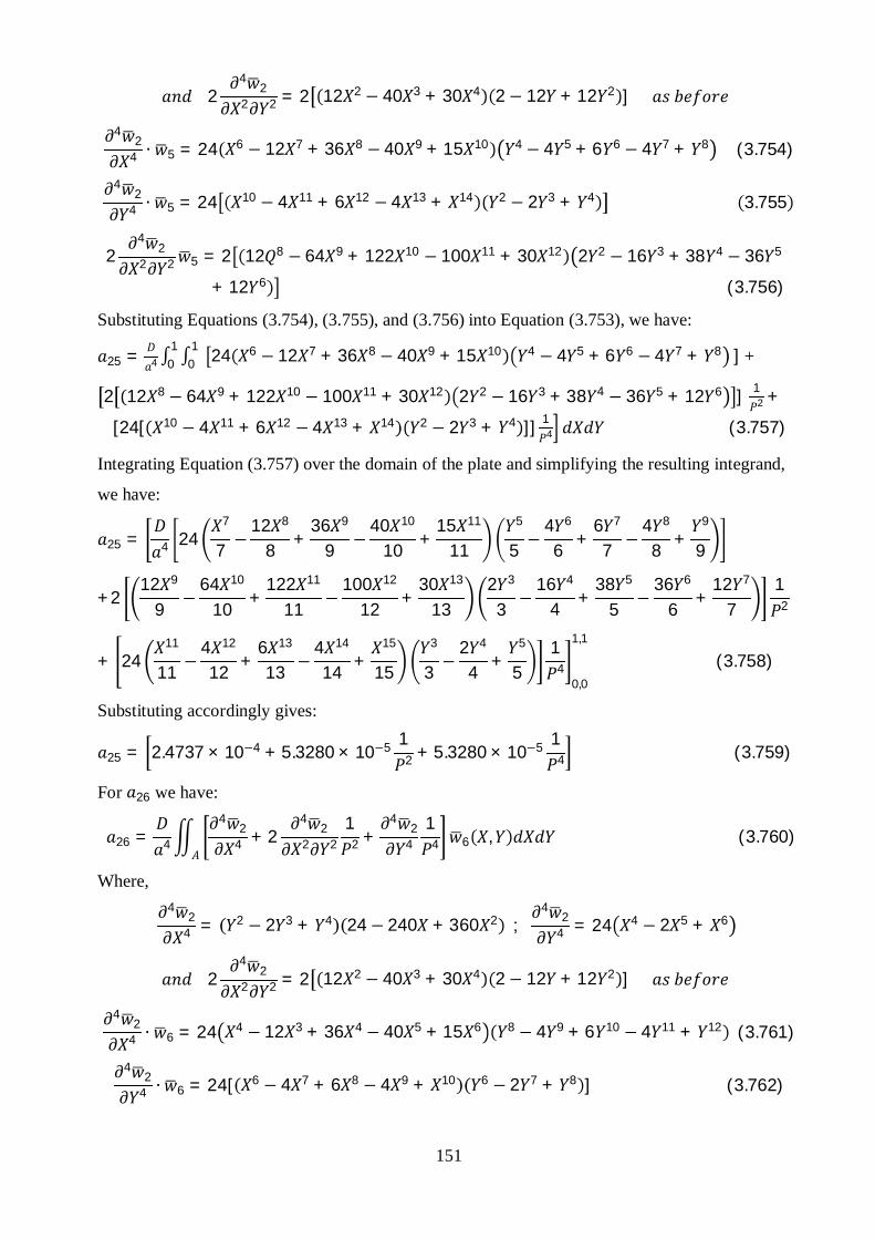
151

24

22 2 = 2 12 2 − 40 3 + 30 4 2 − 12 + 12 2 ]

42

4 ∙ 5 = 24 6 − 12 7 + 36 8 − 40 9 + 15 10 4 − 4 5 + 6 6 − 4 7 + 8 (3.754)

42

4 ∙ 5 = 24 10 − 4 11 + 6 12 − 4 13 + 14 2 − 2 3 + 4 3.755

24

22 2 5 = 2 12 8 − 64 9 + 122 10 − 100 11 + 30 12 2 2 − 16 3 + 38 4 − 36 5

+ 12 6 (3.756)


25 = 4 01

01 24 6 − 12 7 + 36 8 − 40 9 + 15 10 4 − 4 5 + 6 6 − 4 7 + 8 ]∫∫ +

2 12 8 − 64 9 + 122 10 − 100 11 + 30 12 2 2 − 16 3 + 38 4 − 36 5 + 12 6 ] 12 +

[24[ 10 − 4 11 + 6 12 − 4 13 + 14 2 − 2 3 + 4 ]] 14 (3.757)


we have:

25 = 4 247

7 −12 8

8 +36 9

9 −40 10

10 +15 11

11

5

5 −4 6

6 +6 7

7 −4 8

8 +9

9

+212 9

9−

64 10

10+

122 11

11−

100 12

12+

30 13

132 3

3−

16 4

4 +38 5

5−

36 6

6+

12 7

71

2

+ 2411

11 −4 12

12 +6 13

13 −4 14

14 +15

15

3

3 −2 4

4 +5

51

40,0

1,1

(3.758)


25 = 2.4737 × 10−4 + 5.3280 × 10−5 12 + 5.3280 × 10−5 1

4 (3.759)

For 26 we have:

26 = 4

42

4 + 24

22 2

12 +

42

41

4 6 , (3.760)

Where,4

24 = 2 − 2 3 + 4 24 − 240 + 360 2 ;

42

4 = 24 4 − 2 5 + 6

24

22 2 = 2 12 2 − 40 3 + 30 4 2 − 12 + 12 2 ]

42

4 ∙ 6 = 24 4 − 12 3 + 36 4 − 40 5 + 15 6 8 − 4 9 + 6 10 − 4 11 + 12 (3.761)

42

4 ∙ 6 = 24[ 6 − 4 7 + 6 8 − 4 9 + 10 6 − 2 7 + 8 ] (3.762)

152

24

22 2 6 = 2 12 4 − 64 5 + 122 6 − 100 7 + 30 8 2 6 − 16 7 + 38 8 − 36 9

+ 12 10 (3.763)


26 = 4 01

01 24 4 − 12 3 + 36 4 − 40 5 + 15 6 8 − 4 9 + 6 10 − 4 11 + 12 ]∫∫ +

2 12 4 − 64 5 + 122 6 − 100 7 + 30 8 2 6 − 16 7 + 38 8 − 36 9 + 12 10 ] 12 +

[24[ 6 − 4 7 + 6 8 − 4 9 + 10 6 − 2 7 + 8 ]] 14 (3.764)


we have:

26 = 4 243

3−

12 4

4 +36 5

5−

40 6

6+

15 7

7

9

9−

4 10

10+

6 11

11−

4 12

12+

13

13

+212 5

5−

64 6

6+

122 7

7−

100 8

8+

30 9

92 7

7−

16 8

8+

38 9

9−

36 10

10+

12 11

111

2

+ 247

7−

4 8

8+

6 9

9−

4 10

10+

11

11

7

7−

2 8

8+

9

91

40,0

1,1

(3.765)


26 = 3.5520 × 10−5 + 1.0994 × 10−5 12 + 4.1229 × 10−5 1

4 (3.766)


2 = 2 ,

=0

1

0

14 − 2 5 + 6 2 − 2 3 + 4 (3.767)


=5

5 −2 6

6 +7

7

3

3 −2 4

4 +5

50,0

1,1

2 = 3.1746 × 10−4 (3.768)

Hence,

2,1 1+ 2,2 2 + 2,3 3 + 2,4 4+ 2,5 5 + 2,6 6 = 3.1746 × 10−4 4 (3.769)


31 = 4

43

4 + 24

32 2

12 +

43

41

4 1 , (3.770)

Where,

3 = 2 − 2 3 + 4 4 − 2 5 + 6

153

43

4 = 24 4 − 2 5 + 6 (3.771)

43

4 = 2 − 2 3 + 4 24 − 240 + 360 2 (3.772)

24

32 2 = 2 2− 12 + 12 2 12 2 − 40 3 + 30 4 ] (3.773)

43

4 ∙ 1 = 24 2 − 2 3 + 4 6 − 4 7 + 6 8 − 4 9 + 10 (3.774)

43

4 ∙ 1 = 24 4 − 4 5 + 6 6 − 4 7 + 8 2 − 12 3 + 36 4 − 40 5 + 15 6 (3.775)

24

32 2 1 = 2 2 2 − 16 3 + 38 4 − 36 5 + 12 6 12 4 − 64 5 + 122 6 − 100 7

+ 30 8 (3.776)


31 = 40

1

0

124 2 − 2 3 + 4 6 − 4 7 + 6 8 − 4 9 + 10

+2 2 2 − 16 3 + 38 4 − 36 5 + 12 6 12 4 − 64 5 + 122 6 − 100 7 + 30 8 12

+ 24 4 − 4 5 + 6 6 − 4 7 + 8 2 − 12 3 + 36 4 − 40 5 +15 6 1

4 (3.777)


we have:

31 = 4 243

3 −2 4

4 +5

5

7

7 −4 8

8 +6 9

9 −4 10

10 +11

11 +

212 5

5−

64Y6

6+

122 7

7−

100 8

8+

30 9

92 3

3−

16 4

4 +38 5

5−

36 6

6+

12 7

71

2

+ 245

5 −4 6

6+

6 7

7 −4 8

8+

9

9

3

3 −12 4

4+

36 5

5 −40 6

6+

15 7

71

40,0

1,1

(3.778)


31 = 3.4632 × 10−4 + 1.8141 × 10−4 12 + 3.6281 × 10−4 1

4 (3.779)

For 32 we have:

32 = 4

43

4 + 24

32 2

12 +

43

41

4 2 , (3.780)

Where,4

34 = 24 4 − 2 5 + 6 ;

43

4 = 2 − 2 3 + 4 24− 240 + 360 2

154

24

32 2 = 2 2 − 12 + 12 2 12 2 − 40 3 + 30 4 ]

43

4 ∙ 2 = 24 4 − 2 5 + 6 6 − 4 7 + 6 8 − 4 9 + 10 (3.781)

43

4 ∙ 2 = 24 6 − 4 7 + 6 8 − 4 9 + 10 2 − 12 3 + 36 4 − 40 5 + 15 6 (3.782)

24

22 2 2 = 2 2 4 − 16 5 + 38 6 − 36 7 + 12 8 12 4 − 64 5 + 122 6 − 100 7

+ 30 8 (3.783)


32 = D4 0

101 24 4 − 2 5 + 6 6 − 4 7 + 6 8 − 4 9 + 10 +∫∫ 2 2 4 − 16 5 + 38 6 −

36 7 + 12 8 12 4 − 64 5 + 122 6 − 100 7 + 30 8 ] 12 + 24 6 − 4 7 + 6 8 − 4 9 +

10 2 − 12 3 + 36 4 − 40 5 + 15 6 14 (3.784)


we have:

32 = 4 245

5 −2 6

6 +7

77

7 −4 8

8 +6 9

9 −4 10

10 +11

11 +

212 5

5 −64 6

6 +122 7

7 −100 8

8 +30 9

92 5

5 −16 6

6 +38 7

7 −36 8

8 +12 9

91

2 +

247

7 −4 8

8 +6 9

9 −4 10

10 +11

11

3

3 −12 4

4 +36 5

5 −40 6

6 +15 7

71

40,0

1,1

(3.785)


32 = 9.89487 × 10−5 + 1.4331 × 10−2 12 + 9.89487 × 10−5 1

4 (3.786)

For 33 we have:

33 = 4

43

4 + 24

32 2

12 +

43

41

4 3 , (3.787 )

Where,4

34 = 24 4 − 2 5 + 6 ;

43

4 = 2 − 2 3 + 4 24− 240 + 360 2

24

32 2 = 2 2 − 12 + 12 2 12 2 − 40 3 + 30 4 ]

43

4 ∙ 3 = 24 2 − 2 3 + 4 8 − 4 9 + 6 10 − 4 11 + 12 (3.788)

43

4 ∙ 3 = 24 4 − 4 5 + 6 6 − 4 7 + 8 4 − `12 5 + 36 6 − 40 7 + 15 8 (3.789)

155

24

32 2 3 = 2 12 6 − 64 7 + 122 8 − 100 9 + 30 10 2 2 − 16 3 + 38 4 − 36 5

+ 12 6 (3.790)


33 = 4 01

01 24 2 − 2 3 + 4 8 − 4 9 + 6 10 − 4 11 + 12 ]∫∫ + 2 12 6 − 64 7 +

122 8 − 100 9 + 30 10 2 2 − 16 3 + 38 4 − 36 5 + 12 6 ] 12 + 24 4 − 4 5 +

6 6 − 4 7 + 8 4 − `12 5 + 36 6 − 40 7 + 15 8 ] 14 (3.791)


we have:

33 = 4 243

3 −2 4

4 +5

5

9

9 −4 10

10 +6 11

11 −4 12

12 +13

13

+212 7

7−

64 8

8+

122 9

9−

100 10

10+

30 11

112 3

3−

16 4

4 +38 5

5−

36X6

6+

12 7

71

2

+ 245

5 −4 6

6 +6 7

7 −4 8

8 +9

9

5

5 − `12 6

6 +36 7

7 −40 8

8 +15 9

91

40,0

1,1

(3.792)


33 = 1.2432 × 10−4 + 1.0994 × 10−4 12 + 3.6281 × 10−4 1

4 (3.793)

For 34 we have:

34 = 4

43

4 + 24

32 2

12 +

43

41

4 4 , (3.794)

Where,4

34 = 24 4 − 2 5 + 6 ;

43

4 = 2 − 2 3 + 4 24− 240 + 360 2

24

32 2 = 2 2 − 12 + 12 2 12 2 − 40 3 + 30 4 ]

43

4 ∙ 4 = 24 4 − 2 5 + 6 8 − 4 9 + 6 10 − 4 11 + 12 (3.795)

43

4 ∙ 4 = 24 6 − 4 7 + 6 8 − 4 9 + 10 4 − `12 5 + 36 6 − 40 7 + 15 8 (3.796)

24

32 2 4 = 2 12 6 − 64 7 + 122 8 − 100 9 + 30 10 2 4 − 16 5 + 38 6 − 36 7

+ 12 8 (3.797)


156

34 = 4 01

01 24 4 − 2 5 + 6 8 − 4 9 + 6 10 − 4 11 + 12 ]∫∫ + 2 12 6 − 64 7 +

122 8 − 100 9 + 30 10 2 4 − 16 5 + 38 6 − 36 7 + 12 8 ] 12 + 24 6 − 4 7 + 6 8 −

4 9 + 10 4 − `12 5 + 36 6 − 40 7 + 15 8 ] 14 (3.798)


we have:

34 = 4 245

5 −2 6

6 +7

7

9

9 −4 10

10 +6 11

11 −4 12

12 +13

13

+212 7

7−

64 8

8+

122 9

9−

100 10

10+

30 11

112 5

5−

16 6

6+

38 7

7−

36 8

8+

12 9

91

2

+ 247

7 −4 8

8 +6 9

9 −4 10

10 +11

11

5

5 − `12 6

6 +36 7

7 −40 8

8 +15 9

91

40,0

1,1

(3.799)


34 = 3.5520 × 10−5 + 2.7486 × 10−5 12 + 9.8949 × 10−5 1

4 (3.800)

For 35 we have:

35 = 4

43

4 + 24

32 2

12 +

43

41

4 5 , (3.801)

Where,4

34 = 24 4 − 2 5 + 6 ;

43

4 = 2 − 2 3 + 4 24− 240 + 360 2

24

32 2 = 2 2 − 12 + 12 2 12 2 − 40 3 + 30 4 ]

43

4 ∙ 5 = 24 6 − 2 7 + 8 6 − 4 7 + 6 8 − 4 9 + 10 ( 3.802)

43

4 ∙ 5 = 24 8 − 4 9 + 6 10 − 4 11 + 12 2 − 12 3 + 36 4 − 40 5 + 15 6 (3.803)

24

32 2 5 = 2 12 4 − 64 5 + 122 6 − 100 7 + 30 8 2 6 − 16 7 + 38 8 − 36 9

+ 12 10 (3.804)


35 = 4 01

01 24 6 − 2 7 + 8 6 − 4 7 + 6 8 − 4 9 + 10 ]∫∫ + 2 12 4 − 64 5 +

122 6 − 100 7 + 30 8 2 6 − 16 7 + 38 8 − 36 9 + 12 10 ] 12 + 24 8 − 4 9 + 6 10 −

4 11 + 12 2 − 12 3 + 36 4 − 40 5 + 15 6 ] 14 (3.805)


we have:

157

35 = 4 247

7 −2 8

8 +9

9

7

7 −4 8

8 +6 9

9 −4 10

10 +11

11 +

212 5

5 −64 6

6 +122 7

7 −100 8

8 +30 9

92 7

7 −16 8

8 +38 9

9 −36 10

10 +12 11

111

2 +

249

9 −4 10

10 +6 11

11 −4 12

12 +13

13

3

3 −12 4

4 +36 5

5 −40 6

6 +15 7

71

40,0

1,1

(3.806)


35 = 4.1229 × 10−5 + 1.0994 × 10−5 12 + 3.5520 × 10−5 1

4 (3.807)

For 36 we have:

36 = 4

43

4 + 24

32 2

12 +

43

41

4 6 , (3.808 )

Where,4

34 = 24 4 − 2 5 + 6 ;

43

4 = 2 − 2 3 + 4 24− 240 + 360 2

24

32 2 = 2 2 − 12 + 12 2 12 2 − 40 3 + 30 4 ]

43

4 ∙ 6 = 24 2 − 2 3 + 4 10 − 4 11 + 6 12 − 4 13 + 14 (3.809)

43

4 ∙ 6 = 24 4 − 4 5 + 6 6 − 4 7 + 8 6 − 12 7 + 36 8 − 40 9 + 15 10 (3.810)

24

32 2 6 = 2 12 8 − 64 9 + 122 10 − 100 11 + 30 12 2 2 − 16 3 + 38 4 − 36 5

+ 12 6 (3.811)


36 = 4 01

01 24 2 − 2 3 + 4 10 − 4 11 + 6 12 − 4 13 + 14 ]∫∫ + 2 12 8 − 64 9 +

122 10 − 100 11 + 30 12 2 2 − 16 3 + 38 4 − 36 5 + 12 6 ] 12 + 24 4 − 4 5 +

6 6 − 4 7 + 8 6 − 12 7 + 36 8 − 40 9 + 15 10 ] 14 (3.812)


we have:

36 = 4 243

3 −2 4

4 +5

5

11

11 −4 12

12 +6 13

13 −4 14

14 +15

15

+212 9

9 −64 10

10 +122 11

11 −100 12

12 +30 13

132 3

3 −16 4

4 +38 5

5 −36 6

6 +12 7

71

2

158

+ 245

5 −4 6

6 +6 7

7 −4 8

8 +9

9

7

7 −12 8

8 +36 9

9 −40 10

10 +15 11

111

40,0

1,1

(3.813)


36 = 5.3280 × 10−5 + 5.3280 × 10−5 12 + 2.4737 × 10−4 1

4 (3.814)


3 = 3 ,

=0

1

0

12 − 2 3 + 4 4 − 2 5 + 6 (3.815)


=3

3−

2 4

4+

5

5

5

5−

2 6

6+

7

70,0

1,1

3 = 3.1746 × 10−4 (3.816)

Hence,

3,1 1+ 3,2 2 + 3,3 3 + 3,4 4+ 3,5 5 + 3,6 6 = 3.1746 × 10−4 4 (3.817)


41 = 4

44

4 + 24

42 2

12 +

44

41

4 1 , (3.818)

Where,

4 = 4 − 2 5 + 6 4 − 2 5 + 6

44

4 = 24 − 240 + 360 2 4 − 2 5 + 6 (3.819)

44

4 = 4 − 2 5 + 6 24− 240 + 360 2 (3.820)

24

42 2 = 2 12 2 − 40 3 + 30 4 12 2 − 40 3 + 30 4 ] (3.821)

44

4 ∙ 1 = 24 2 − 12 3 + 36 4 − 40 5 + 15 6 6 − 4 7 + 6 8 − 4 9 + 10 (3.822)

44

4 ∙ 1 = 24 6 − 4 7 + 6 8 − 4 9 + 10 2 − 12 3 + 36 4 − 40 5 + 15 6 (3.823)

24

42 2 1 = 2 12 4 − 64 5 + 122 6 − 100 7 + 30 8 12 4 − 64 5 + 122 6 − 100 7

+ 30 8 (3.824)


159

41 = 40

1

0

124 2 − 12 3 + 36 4 − 40 5 + 15 6 6 − 4 7 + 6 8 − 4 9 + 10

+2 12 4 − 64 5 + 122 6 − 100 7 + 30 8 12 4 − 64 5 + 122 6 − 100 7 + 30 8 12 +

24 6 − 4 7 + 6 8 − 4 9 + 10 2 − 12 3 + 36 4 − 40 5 + 15 6 14 (3.825)


we have:

41 = 4 243

3 −12 4

4 +36 5

5 −40 6

6 +15 7

7

7

7 −4 8

8 +6 9

9 −4 10

10 +11

11 +

212 5

5 −64 6

6 +122 7

7 −100 8

8 +30 9

912 5

5 −64 6

6 +122 7

7 −100 8

8 +30 9

91

2

+ 247

7−

4 8

8+

6 9

9−

4 10

10+

11

11

3

3−

12 4

4 +36 5

5−

40 6

6+

15 7

71

40,0

1,1

(3.826)


41 = 9.8949 × 10−5 + 4.5351 × 10−5 12 + 9.8949 × 10−5 1

4 (3.827)

For 42 we have:

42 = 4

44

4 + 24

42 2

12 +

44

41

4 2 , (3.828 )

Where,4

44 = 24 − 240 + 360 2 4 − 2 5 + 6 ;

44

4 = 24− 240 + 360 2 4 − 2 5 + 6

24

42 2 = 2 12 2 − 40 3 + 30 4 12 2 − 40 3 + 30 4 ]

44

4 ∙ 2 = 24 4 − 12 5 + 36 6 − 40 7 + 15 8 6 − 4 7 + 6 8 − 4 9 + 10 (3.829)

44

4 ∙ 2 = 24 8 − 4 9 + 6 10 − 4 11 + 12 2 − 12 3 + 36 4 − 40 5 + 15 6 3.830

24

42 2 2 = 2 12 6 − 64 7 + 122 8 − 100 9 + 30 10 12 4 − 64 5 + 122 6 − 100 7

+ 30 8 (3.831)


42 = 4 01

01 24 4 − 12 5 + 36 6 − 40 7 + 15 8 6 − 4 7 + 6 8 − 4 9 + 10 +∫∫

2 12 6 − 64 7 + 122 8 − 100 9 + 30 10 12 4 − 64 5 + 122 6 − 100 7 +

160

30 8 ] 12 + 24 8 − 4 9 + 6 10 − 4 11 + 12 2 − 12 3 + 36 4 − 40 5 +

15 6 14 (3.832)


we have:

42 = 4 245

5 −12 6

6 +36 7

7 −40 8

8 +15 9

97

7 −4 8

8 +6 9

9 −4 10

10 +11

11 +

212 5

5 −64 6

6 +122 7

7 −100 8

8 +30 9

912 7

7 −64 8

8 +122 9

9 −100 10

10

+30 11

111

2 +

249

9 −4 10

10 +6 11

11 −4 12

12 +13

13

3

3 −12 4

4 +36 5

5 −40 6

6 +15 7

71

40,0

1,1

(3.833)


42 = 9.8949 × 10−5 + 2.7486 × 10−5 12 + 3.5520 × 10−5 1

4 (3.834)

For 43 we have:

43 = 4

44

4 + 24

42 2

12 +

44

41

4 3 , (3.835 )

Where,4

44 = 24 − 240 + 360 2 4 − 2 5 + 6 ;

44

4 = 24− 240 + 360 2 4 − 2 5 + 6

24

42 2 = 2 12 2 − 40 3 + 30 4 12 2 − 40 3 + 30 4 ]

44

4 ∙ 3 = 24 2 − 12 3 + 36 4 − 40 5 + 15 6 8 − 4 9 + 6 10 − 4 11 + 12 (3.836)

44

4 ∙ 3 = 24 6 − 4 7 + 6 8 − 4 9 + 10 4 − 12 5 + 36 6 − 40 7 + 15 8 (3.837)

24

42 2 3 = 2 12 6 − 64 7 + 122 8 − 100 9 + 30 10 12 4 − 64 5 + 122 6 − 100 7

+ 30 8 (3.838)


43 = 4 01

01 24 2 − 12 3 + 36 4 − 40 5 + 15 6 8 − 4 9 + 6 10 − 4 11 + 12 ]∫∫ +

2 12 6 − 64 7 + 122 8 − 100 9 + 30 10 12 4 − 64 5 + 122 6 − 100 7 + 30 8 ] 12 +

24 6 − 4 7 + 6 8 − 4 9 + 10

161

4 − 12 5 + 36 6 − 40 7 + 15 8 ]1

4 (3.839)


we have:

43 = 4 243

3 −12 4

4 +36 5

5 −40 6

6 +15 7

7

9

9 −4 10

10 +6 11

11 −4 12

12 +13

13

+ 212 7

7−

64 8

8+

122 9

9−

100 10

10+

30 11

1112 5

5−

64 6

6+

122 7

7

−100 8

8 +30 9

91

2

+ 247

7 −4 8

8 +6 9

9 −4 10

10 +11

11

5

5 −12 6

6 +36 7

7 −40 8

8 +15 9

91

40,0

1,1

(3.840)


43 = 3.5520 × 10−5 + 2.7486 × 10−5 12 + 9.8949 × 10−5 1

4 (3.841)

For 44 we have:

44 = 4

44

4 + 24

42 2

12 +

44

41

4 4 , (3.842)

Where,4

44 = 24 − 240 + 360 2 4 − 2 5 + 6 ;

44

4 = 24− 240 + 360 2 4 − 2 5 + 6

24

42 2 = 2 12 2 − 40 3 + 30 4 12 2 − 40 3 + 30 4 ]

44

4 ∙ 4 = 24 4 − 12 5 + 36 6 − 40 7 + 15 8 8 − 4 9 + 6 10 − 4 11 + 12 (3.843)

44

4 ∙ 4 = 24 8 − 4 9 + 6 10 − 4 11 + 12 4 − 12 5 + 36 6 − 40 7 + 15 8 (3.844)

24

42 2 4 = 2 12 6 − 64 7 + 122 8 − 100 9 + 30 10 12 6 − 64 7 + 122 8 − 100 9

+ 30 10 (3.845)


44 = 4 01

01 24 4 − 12 5 + 36 6 − 40 7 + 15 8 8 − 4 9 + 6 10 − 4 11 + 12 ]∫∫ +

2 12 6 − 64 7 + 122 8 − 100 9 + 30 10 12 6 − 64 7 + 122 8 − 100 9 +30 10 ] 1

2 + 24 8 − 4 9 + 6 10 − 4 11 + 12 4 − 12 5 + 36 6 − 40 7 +

15 8 ] 14 (3.846)

162


we have:

44 = 4 245

5 −12 6

6 +36 7

7 −40 8

8 +15 9

9

9

9 −4 10

10 +6 11

11 −4 12

12 +13

13

+212 7

7−

64 8

8+

122 9

9−

100 10

10+

30 11

1112 7

7−

64 8

8+

122 9

9−

100 10

10

+30 11

111

2 +

249

9 −4 10

10+

6 11

11 −4 12

12+

13

13

5

5 −12 6

6+

36 7

7 −40 8

8+

15 9

91

40,0

1,1

(3.847)


44 = 3.5520 × 10−5 + 1.6658 × 10−5 12 + 3.5520 × 10−5 1

4 (3.848)

For 45 we have:

45 = 4

44

4 + 24

42 2

12 +

44

41

4 5 , (3.849 )

Where,4

44 = 24 − 240 + 360 2 4 − 2 5 + 6 ;

44

4 = 24− 240 + 360 2 4 − 2 5 + 6

24

42 2 = 2 12 2 − 40 3 + 30 4 12 2 − 40 3 + 30 4 ]

44

4 ∙ 5 = 24 6 − 12 7 + 36 8 − 40 9 + 15 10 6 − 4 7 + 6 8 − 4 9 + 10 (3.850)

44

4 ∙ 5 = 24 10 − 4 11 + 6 12 − 4 13 + 14 2 − 12 3 + 36 4 − 40 5

+ 15 6 (3.851)

24

42 2 5 = 2 12 8 − 64 9 + 122 10 − 100 11 + 30 12 12 4 − 64 5 + 122 6

− 100 7 + 30 8 (3.852)


45 = 4 01

01 24 6 − 12 7 + 36 8 − 40 9 + 15 10 6 − 4 7 + 6 8 − 4 9 + 10 ]∫∫ +

2 12 8 − 64 9 + 122 10 − 100 11 + 30 12 12 4 − 64 5 + 122 6 − 100 7 +30 8 ] 1

2 + 24 10 − 4 11 + 6 12 − 4 13 + 14 2 − 12 3 + 36 4 − 40 5 +

15 6 ] 14 (3.853)

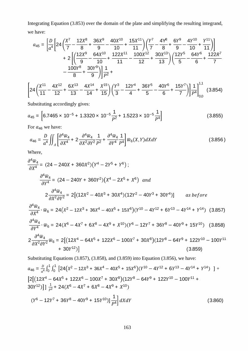
163


we have:

45 = 4 247

7 −12 8

8 +36 9

9 −40 10

10 +15 11

11

7

7 −4Y8

8 +6 9

9 −4 10

10 +11

11

+ 212 9

9−

64 10

10+

122 11

11−

100 12

12+

30 13

1312 5

5−

64 6

6+

122 7

7

−100 8

8 +30 9

91

2 +

2411

11 −4 12

12 +6 13

13 −4 14

14 +15

15

3

3 −12 4

4 +36 5

5 −40 6

6 +15 7

71

40,0

1,1

(3.854)


45 = 6.7465 × 10−5 + 1.3320 × 10−5 12 + 1.5223 × 10−5 1

4 (3.855)

For 46 we have:

46 = 4

44

4 + 24

42 2

12 +

44

41

4 6 , (3.856 )

Where,4

44 = 24 − 240 + 360 2 4 − 2 5 + 6 ;

44

4 = 24− 240 + 360 2 4 − 2 5 + 6

24

42 2 = 2 12 2 − 40 3 + 30 4 12 2 − 40 3 + 30 4 ]

44

4 ∙ 6 = 24 2 − 12 3 + 36 4 − 40 5 + 15 6 10 − 4 12 + 6 13 − 4 14 + 14 (3.857)

44

4 ∙ 6 = 24 6 − 4 7 + 6 8 − 4 9 + 10 6 − 12 7 + 36 8 − 40 9 + 15 10 (3.858)

24

42 2 6 = 2 12 4 − 64 5 + 122 6 − 100 7 + 30 8 12 8 − 64 9 + 122 10 − 100 11

+ 30 12 (3.859)


46 = 4 01

01 24 2 − 12 3 + 36 4 − 40 5 + 15 6 10 − 4 12 + 6 13 − 4 14 + 14 ]∫∫ +

2 12 4 − 64 5 + 122 6 − 100 7 + 30 8 12 8 − 64 9 + 122 10 − 100 11 +30 12 ] 1

2 + 24 6 − 4 7 + 6 8 − 4 9 + 10

6 − 12 7 + 36 8 − 40 9 + 15 10 ]1

4 (3.860)

164


we have:

46 = 4 243

3 −12 4

4 +36 5

5 −40 6

6 +15 7

7

11

11 −4 12

12 +6 13

13 −4 14

14 +15

151

2

+212 5

5−

64 6

6+

122 7

7−

100 8

8+

30 9

912 9

9−

64 10

10+

122 11

11−

100 12

12+

30 13

13+

247

7 −4 8

8+

6 9

9 −4 10

10+

11

11

7

7 −12 8

8+

36 9

9 −40 10

10+

15 11

111

40,0

1,1

(3.861)


46 = 1.5223 × 10−5 + 1.3320 × 10−5 12 + 6.7465 × 10−5 1

4 (3.862)


4 = 4 ,

=0

1

0

14 − 2 5 + 6 4 − 2 5 + 6 (3.863)


=5

5 −2 6

6 +7

7

5

5 −2 6

6 +7

70,0

1,1

4 = 9.07029 × 10−5 (3.864)

Hence,

4,1 1+ 4,2 2 + 4,3 3 + 4,4 4+ 4,5 5 + 4,6 6 = 9.07029 × 10−5 4 (3.865)


51 = 4

45

4 + 24

52 2

12 +

45

41

4 1 , (3.866)

Where,

5 = 6 − 2 7 + 8 2 − 2 3 + 4

45

4 = 120 3 2 − 14 3 + 14 4 2 − 2 3 + 4 (3.867)

45

4 = 24 6 − 2 7 + 8 (3.868)

24

52 2 = 2 30 4 − 84 5 + 56 6 2 − 12 + 12 2 ] (3.869)

165

45

4 ∙ 1 = 120 3 4 − 20 5 + 45 6 − 42 7 + 14 8 4 − 4 5 + 6 6 − 4 7 + 8 3.870

45

4 ∙ 1 = 24 8 − 4 9 + 6 10 − 4 11 + 12 2 − 2 3 + 4 (3.871)

24

52 2 1 = 2 30 6 − 144 7 + 254 8 − 196 9 + 56 10 2 2 − 16 3 + 38 4 − 36 5

+ 12 6 (3.872)


51 = 40

1

0

1120 3 4 − 20 5 + 45 6 − 42 7 + 14 8 4 − 4 5 + 6 6 − 4 7 + 8

+2 30 6 − 144 7 + 254 8 − 196 9 + 56 10 2 2 − 16 3 + 38 4 − 36 5 + 12 6

12 + 24 8 − 4 9 + 6 10 − 4 11 + 12 2 − 2 3 + 4 1

4 (3.873)


we have:

51 = 4 1203 5

5 −20 6

6 +45 7

7 −42 8

8 +14 9

9

5

5 −4 6

6 +6 7

7 −4 8

8 +9

9 +

230 7

7−

144 8

8+

254 9

9−

196 10

10+

56 11

112 3

3−

16 4

4 +38 5

5−

36 6

6+

12 7

71

2

+ 249

9−

4 10

10+

6 11

11−

4 12

12+

13

13

3

3−

2 4

4 +5

51

40,0

1,1

(3.874)


51 = 1.5117 × 10−4 + 4.3977 × 10−5 12 + 1.2432 × 10−4 1

4 (3.875)

For 52 we have:

52 = 4

45

4 + 24

52 2

12 +

45

41

4 2 , (3.876 )

Where,4

54 = 120 3 2 − 14 3 + 14 4 2 − 2 3 + 4 ;

45

4 = 24 6 − 2 7 + 8

24

52 2 = 2 30 4 − 84 5 + 56 6 2 − 12 + 12 2 ]

45

4 ∙ 2 = 120 3 6 − 20 7 + 45 8 − 42 9 + 14 10 4 − 4 5 + 6 6 − 4 7 + 8 (3.877)

45

4 ∙ 2 = 24 10 − 4 11 + 6 12 − 4 13 + 14 2 − 2 3 + 4 (3.878)

166

24

52 2 2 = 2 30 8 − 144 9 + 254 10 − 196 11 + 56 12 2 2 − 16 3 + 38 4 − 36 5

+ 12 6 (3.879)


52 = 40

1

0

1120 3 6 − 20 7 + 45 8 − 42 9 + 14 10 4 − 4 5 + 6 6 − 4 7 + 8

+2 30 8 − 144 9 + 254 10 − 196 11 + 56 12 2 2 − 16 3 + 38 4 − 36 5 + 12 6 12

+ 24 10 − 4 11 + 6 12 − 4 13 + 14 2 − 2 3 + 4 14 (3.880)


we have:

52 = 4 1203 7

7 −20 8

8+

45 9

9 −42 10

10+

14 11

11

5

5 −4 6

6+

6 7

7 −4 8

8+

9

9 +

230 9

9 −144 10

10 +254 11

11 −196 12

12 +56 13

132 3

3 −16 4

4 +38 5

5 −36 6

6 +12 7

71

2

+

2411

11 −4 12

12 +6 13

13 −4 14

14 +15

15

3

3 −2 4

4 +5

51

40,0

1,1

(3.881)


52 = 2.4737 × 10−4 + 5.3280 × 10−5 12 + 5.3280 × 10−5 1

4 (3.882)

For 53 we have:

53 = 4

45

4 + 24

52 2

12 +

45

∂ 4

14 3 , (3.883)

Where,4

54 = 120 3 2 − 14 3 + 14 4 2 − 2 3 + 4 ;

45

4 = 24 6 − 2 7 + 8

24

52 2 = 2 30 4 − 84 5 + 56 6 2 − 12 + 12 2 ]

45

4 ∙ 3 = 120 3 4 − 20 5 + 45 6 − 42 7 + 14 8 6 − 4 7 + 6 8 − 4 9 + 10 (3.884)

45

4 ∙ 3 = 24 8 − 4 9 + 6 10 − 4 11 + 12 4 − 2 5 + 6 (3.885)

24

52 2 3 = 2 30 6 − 144 7 + 254 8 − 196 9 + 56 10 2 4 − 16 5 + 38 6 − 36 7

+ 12 8 (3.886)


167

53 = 40

1

0

1120 3 4 − 20 5 + 45 6 − 42 7 + 14 8 6 − 4 7 + 6 8 − 4 9 + 10

+2 30 6 − 144 7 + 254 8 − 196 9 + 56 10 2 4 − 16 5 + 38 6 − 36 7 + 12 8

12 + 24 8 − 4 9 + 6 10 − 4 11 + 12 4 − 2 5 + 6 1

4 (3.887)


we have:

53 = 4 1203 5

5 −20 6

6+

45 7

7 −42 8

8+

14 9

9

7

7 −4 8

8+

6 9

9 −4 10

10+

11

11 +

230 7

7 −144 8

8 +254 9

9 −196 10

10 +56 11

112 5

5 −16 6

6 +38 7

7 −36 8

8 +12 9

91

2

+ 249

9 −4 10

10 +6 11

11 −4 12

12 +13

13

5

5 −2 6

6 +7

71

40,0

1,1

(3.888)


53 = 4.1229 × 10−5 + 1.0994 × 10−5 12 + 3.5520 × 10−5 1

4 (3.889)

For 54 we have:

54 = 4

45

4 + 24

52 2

12 +

45

41

4 4 , (3.890)

Where,4

54 = 120 3 2 − 14 3 + 14 4 2 − 2 3 + 4 ;

45

4 = 24 6 − 2 7 + 8

24

52 2 = 2 30 4 − 84 5 + 56 6 2 − 12 + 12 2 ]

45

4 ∙ 4 = 120 3 6 − 20 7 + 45 8 − 42 9 + 14 10 6 − 4 7 + 6 8 − 4 9 + 10 (3.891)

45

4 ∙ 4 = 24 10 − 4 11 + 6 12 − 4 13 + 14 4 − 2 5 + 6 (3.892)

24

52 2 4 = 2 30 8 − 144 9 + 254 10 − 196 11 + 56 12 2 4 − 16 5 + 38 6 − 36 7

+ 12 8 (3.893)


54 = 40

1

0

1120 3 6 − 20 7 + 45 8 − 42 9 + 14 10 6 − 4 7 + 6 8 − 4 9 + 10

+ 2 30 8 − 144 9 + 254 10 − 196 11 + 56 12 2 4 − 16 5 + 38 6 − 36 7

+ 12 8 12 + [24 10 − 4 11 + 6 12 − 4 13 + 14 4 − 2 5 + 6 ]

14

dXdY (3.894)

168


we have:

54 = 4 1203 7

7 −20 8

8 +45 9

9 −42 10

10 +14 11

11

7

7 −4 8

8 +6 9

9 −4 10

10 +11

11 +

230 9

9−

144 10

10+

254 11

11−

196 12

12+

56 13

132 5

5−

16 6

6+

38 7

7−

36 8

8+

12 9

91

2

+ 2411

11 −4 12

12+

6 13

13 −4 14

14+

15

15

5

5 −2 6

6+

7

71

40,0

1,1

(3.895)


54 = 6.7465 × 10−5 + 1.3320 × 10−5 12 + 1.5223 × 10−5 1

4 (3.896)

For 55 we have:

55 = 4∂4

54 + 2

45

2 21

2 +4

54

14 5 , (3.897)

Where,4

54 = 120 3 2 − 14 3 + 14 4 2 − 2 3 + 4 ;

45

4 = 24 6 − 2 7 + 8

24

52 2 = 2 30 4 − 84 5 + 56 6 2− 12 + 12 2 ]

45

4 ∙ 5 = 120 3 8 − 20 9 + 45 10 − 42 11 + 14 12 4 − 4 5 + 6 6 − 4 7 + 8 (3.898)

45

4 ∙ 5 = 24 12 − 4 13 + 6 14 − 4 15 + 16 2 − 2 3 + 4 (3.899)

24

52 2 5 = 2 30 10 − 144 11 + 254 12 − 196 13 + 56 14 2 2 − 16 3 + 38 4 − 36 5

+ 12 6 (3.900)


55 = 40

1

0

1120 3 8 − 20 9 + 45 10 − 42 11 + 14 12 4 − 4 5 + 6 6 − 4 7 + 8

+ 2[ 30 10 − 144 11 + 254 12 − 196 13 + 56 14

2 2 2 − 16 3 + 38 4 − 36 5 + 12 6 12 + [24 12 − 4 13 + 6 14 − 4 15 + 16

2 − 2 3 + 4 14 (3.901)


we have:

169

55 = 4 1203 9

9 −20 10

10+

45 11

11 −42 12

12+

14 13

13

5

5 −4 6

6+

6 7

7 −4 8

8+

9

9 +

230 11

11 −144 12

12 +254 13

13 −196 14

14 +56 15

152 3

3 −16 4

4 +38 5

5 −36 6

6

+12 7

71

2

+ 2413

13 −4 14

14 +6 15

15 −4 16

16 +17

17

3

3 −2 4

4 +5

51

40,0

1,1

(3.902)


55 = 2.2200 × 10−4 + 3.5520 × 10−5 12 + 2.5856 × 10−5 1

4 (3.903)

For 56 we have:

56 =a4

45

4 + 24

52 2

12 +

45

41

4 6 , (3.904)

Where,4

54 = 120 3 2 − 14 3 + 14 4 2 − 2 3 + 4 ;

45

4 = 24 6 − 2 7 + 8

24

52 2 = 2 30 4 − 84 5 + 56 6 2 − 12 + 12 2 ]

45

4 ∙ 6 = 120 3 4 − 20 5 + 45 6 − 42 7 + 14 8 8 − 4 9 + 6 10 − 4 11 + 12 (3.905)

45

4 ∙ 6 = 24 8 − 4 9 + 6 10 − 4 11 + 12 6 − 2 7 + 8 (3.906)

24

52 2 6 = 2 30 6 − 144 7 + 254 8 − 196 9 + 56 10 2 6 − 16 7 + 38 8 − 36 9

+ 12 10 (3.907)


56 = 40

1

0

1120 3 4 − 20 5 + 45 6 − 42 7 + 14 8 8 − 4 9 + 6 10 − 4 11 + 12

+ 2[ 30 6 − 144 7 + 254 8 − 196 9 + 56 10

2 6 − 16 7 + 38 8 − 36 9 + 12 10 12 + [24 8 − 4 9 + 6 10 − 4 11 + 12

6 − 2 7 + 8 14 (3.908)


we have:

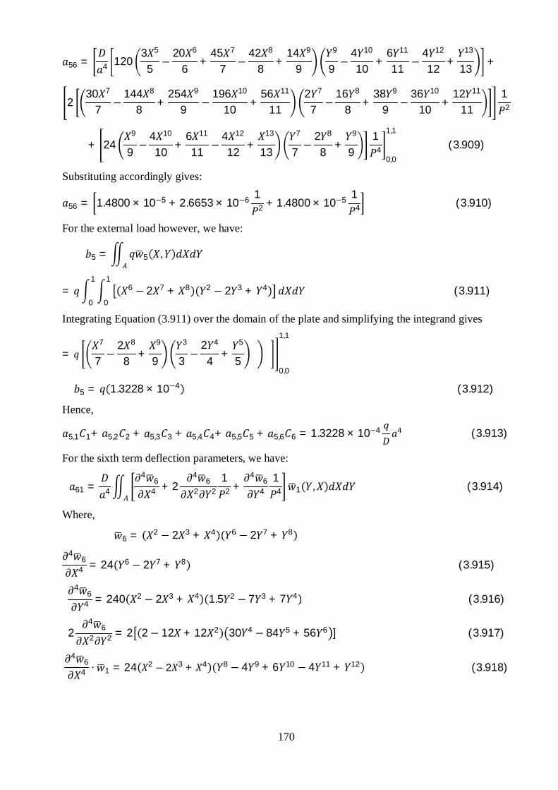
170

56 = 4 1203 5

5 −20 6

6+

45 7

7 −42 8

8+

14 9

9

9

9 −4 10

10+

6 11

11 −4 12

12+

13

13 +

230 7

7 −144 8

8 +254 9

9 −196 10

10 +56 11

112 7

7 −16 8

8 +38 9

9 −36 10

10 +12 11

111

2

+ 249

9−

4 10

10+

6 11

11−

4 12

12+

13

13

7

7−

2 8

8+

9

91

40,0

1,1

(3.909)


56 = 1.4800 × 10−5 + 2.6653 × 10−6 12 + 1.4800 × 10−5 1

4 (3.910)


5 = 5 ,

=0

1

0

16 − 2 7 + 8 2 − 2 3 + 4 (3.911)


=7

7 −2 8

8+

9

9

3

3 −2 4

4+

5

50,0

1,1

5 = 1.3228 × 10−4 (3.912)

Hence,

5,1 1+ 5,2 2 + 5,3 3 + 5,4 4+ 5,5 5 + 5,6 6 = 1.3228 × 10−4 4 (3.913)


61 = 4

46

4 + 24

62 2

12 +

46

41

4 1 , (3.914)

Where,

6 = 2 − 2 3 + 4 6 − 2 7 + 8

46

4 = 24 6 − 2 7 + 8 (3.915)

46

4 = 240 2 − 2 3 + 4 1.5 2 − 7 3 + 7 4 (3.916)

24

62 2 = 2 2 − 12 + 12 2 30 4 − 84 5 + 56 6 ] (3.917)

46

4 ∙ 1 = 24 2 − 2 3 + 4 8 − 4 9 + 6 10 − 4 11 + 12 (3.918)

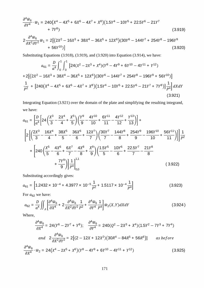
171

46

4 ∙ 1 = 240 4 − 4 5 + 6 6 − 4 7 + 8 1.5 4 − 10 5 + 22.5 6 − 21 7

+ 7 8 (3.919)

24

62 2 1 = 2 2 2 − 16 3 + 38 4 − 36 5 + 12 6 30 6 − 144 7 + 254 8 − 196 9

+ 56 10 (3.920)


61 = 40

1

0

124 2 − 2 3 + 4 8 − 4 9 + 6 10 − 4 11 + 12

+2 2 2 − 16 3 + 38 4 − 36 5 + 12 6 30 6 − 144 7 + 254 8 − 196 9 + 56 10

12 + 240 4 − 4 5 + 6 6 − 4 7 + 8 1.5 4 − 10 5 + 22.5 6 − 21 7 + 7 8 1

4

(3.921)


we have:

61 = 4 243

3 −2 4

4 +5

5

9

9 −4 10

10 +6 11

11 −4 12

12 +13

13 +

22 3

3 −16 4

4 +38 5

5 −36 6

6 +12 7

730 7

7 −144 8

8 +254 9

9 −196 10

10 +56 11

111

2

+ 2405

5 −4 6

6 +6 7

7 −4 8

8 +9

91.5 5

5 −10 6

6 +22.5 7

7 −21 8

8

+7 9

91

40,0

1,1

( 3.922)


61 = 1.2432 × 10−4 + 4.3977 × 10−5 12 + 1.5117 × 10−4 1

4 (3.923)

For 62 we have:

62 = 4

46

4 + 24

62 2

12 +

46

41

4 2 , (3.924 )

Where,4

64 = 24 6 − 2 7 + 8 ;

46

4 = 240 2 − 2 3 + 4 1.5 2 − 7 3 + 7 4

24

62 2 = 2 2 − 12 + 12 2 30 4 − 84 5 + 56 6 ]

46

4 ∙ 2 = 24 4 − 2 5 + 6 8 − 4 9 + 6 10 − 4 11 + 12 (3.925)

172

46

4 ∙ 2 = 240 6 − 4 7 + 6 8 − 4 9 + 10 1.5 4 − 10 5 + 22.5 6 − 21 7

+ 7 8 3.926

24

62 2 2 = 2 2 4 − 16 5 + 38 6 − 36 7 + 12 8 30 6 − 144 7 + 254 8 − 196 9

+ 56 10 (3.927)


62 = 40

1

0

124 4 − 2 5 + 6 8 − 4 9 + 6 10 − 4 11 + 12

+2 2 4 − 16 5 + 38 6 − 36 7 + 12 8 30 6 − 144 7 + 254 8 − 196 9 + 56 10

12 + 240 6 − 4 7 + 6 8 − 4 9 + 10 1.5 4 − 10 5 + 22.5 6 − 21 7

+ 7 8 14 (3.928)


we have:

62 = 4 245

5 −2 6

6 +7

7

9

9 −4 10

10 +6 11

11 −4 12

12 +13

13 +

22 5

5−

16 6

6+

38 7

7−

36 8

8+

12 9

930 7

7−

144 8

8+

254 9

9−

196 10

10+

56 11

111

2

+ 2407

7 −4 8

8+

6 9

9 −4 10

10+

11

111.5 5

5 −10 6

6+

22.5 7

7 −21 8

8+

7 9

91

40,0

1,1

(3.929)


62 = 3.5520 × 10−5 + 1.0994 × 10−5 12 + 4.1229 × 10−5 1

4 (3.930)

For 63 we have:

63 = 4

46

4 + 24

62 2

12 +

46

41

4 3 , (3.931)

Where,4

64 = 24 6 − 2 7 + 8 ;

46

4 = 240 2 − 2 3 + 4 1.5 2 − 7 3 + 7 4

24

62 2 = 2 2 − 12 + 12 2 30 4 − 84 5 + 56 6 ]

46

4 ∙ 3 = 24 2 − 2 3 + 4 10 − 4 11 + 6 12 − 4 13 + 14 (3.932)

173

46

4 ∙ 3 = 240 4 − 4 5 + 6 6 − 4 7 + 8 1.5 6 − 10 7 + 22.5 8 − 21 9

+ 7 10 3.933

24

62 2 3 = 2 2 2 − 16 3 + 38 4 − 36 5 + 12 6 30 8 − 144 9 + 254 10 − 196 11

+ 56 12 (3.934)


63 = 40

1

0

124 2 − 2 3 + 4 10 − 4 11 + 6 12 − 4 13 + 14

+2 2 2 − 16 3 + 38 4 − 36 5 + 12 6 30 8 − 144 9 + 254 10 − 196 11 + 56 12

12 + 240 4 − 4 5 + 6 6 − 4 7 + 8 1.5 6 − 10 7 + 22.5 8 − 21 9

+ 7 10 14 (3.935)


we have:

63 = 4 243

3 −2 4

4 +5

5

11

11 −4 12

12 +6 13

13 −4 14

14 +15

15 +

22 3

3−

16 4

4+

38 5

5−

36 6

6+

12 7

730 9

9−

144 10

10+

254 11

11−

196 12

12+

56 13

131

2

+ 2405

5 −4 6

6+

6 7

7 −4 8

8+

9

91.5 7

7 −10 8

8+

22.5 9

9 −21 10

10+

7 11

111

40,0

1,1

(3.936)


63 = 5.3280 × 10−5 + 5.3280 × 10−5 12 + 2.4737 × 10−4 1

4 (3.937)

For 64 we have:

64 = 4

46

4 + 24

62 2

12 +

46

41

4 4 , (3.938 )

Where,4

64 = 24 6 − 2 7 + 8 ;

46

4 = 240 2 − 2 3 + 4 1.5 2 − 7 3 + 7 4

24

62 2 = 2 2 − 12 + 12 2 30 4 − 84 5 + 56 6 ]

46

4 ∙ 4 = 24 4 − 2 5 + 6 10 − 4 11 + 6 12 − 4 13 + 14 (3.939)

174

46

4 ∙ 4 = 240 6 − 4 7 + 6 8 − 4 9 + 10 1.5 6 − 10 7 + 22.5 8 − 21 9

+ 7 10 (3.940)

24

62 2 4 = 2 2 4 − 16 5 + 38 6 − 36 7 + 12 8 30 8 − 144 9 + 254 10 − 196 11

+ 56 12 (3.941)


64 = 40

1

0

124 4 − 2 5 + 6 10 − 4 11 + 6 12 − 4 13 + 14

+2 2 4 − 16 5 + 38 6 − 36 7 + 12 8 30 8 − 144 9 + 254 10 − 196 11 + 56 12

12 + 240 6 − 4 7 + 6 8 − 4 9 + 10 1.5 6 − 10 7 + 22.5 8 − 21 9

+ 7 10 14 (3.942)


we have:

64 = 4 245

5 −2 6

6+

7

7

11

11 −4 12

12+

6 13

13 −4 14

14+

15

15 +

22 5

5 −16 6

6 +38 7

7 −36 8

8 +12 9

930 9

9 −144 10

10 +254 11

11 −196 12

12 +56 13

131

2

+ 2407

7−

4 8

8+

6 9

9−

4 10

10+

11

111.5 7

7−

10 8

8+

22.5 9

9−

21 10

10+

7 11

111

40,0

1,1

(3.943)


64 = 1.5223 × 10−5 + 1.3320 × 10−5 12 + 6.7465 × 10−5 1

4 (3.944)

For 65 we have:

65 = 4

46

4 + 24

62 2

12 +

46

41

4 5 , (3.945)

Where,4

64 = 24 6 − 2 7 + 8 ;

46

4 = 240 2 − 2 3 + 4 1.5 2 − 7 3 + 7 4

24

62 2 = 2 2 − 12 + 12 2 30 4 − 84 5 + 56 6 ]

46

4 ∙ 5 = 24 6 − 2 7 + 8 8 − 4 9 + 6 10 − 4 11 + 12 (3.946)

175

46

4 ∙ 5 = 240 8 − 4 9 + 6 10 − 4 11 + 12 1.5 4 − 10 5 + 22.5 6 − 21 7

+ 7 8 (3.947)

24

62 2 5 = 2 2 6 − 16 7 + 38 8 − 36 9 + 12 10 30 6 − 144 8 + 254 9 − 196 10

+ 56 11 (3.948)


65 = 40

1

0

124 6 − 2 7 + 8 8 − 4 9 + 6 10 − 4 11 + 12

+2 2 6 − 16 7 + 38 8 − 36 9 + 12 10 30 6 − 144 8 + 254 9 − 196 10 + 56 11

12 + 240 8 − 4 9 + 6 10 − 4 11 + 12 1.5 4 − 10 5 + 22.5 6 − 21 7

+ 7 8 14 (3.949)


we have:

65 = 4 247

7 −2 8

8 +9

9

9

9 −4 10

10 +6 11

11 −4 12

12 +13

13 +

22 7

7 −16 8

8 +38 9

9 −36 10

10 +12 11

1130 7

7 −144 8

8 +254 9

9 −196 10

10 +56 11

111

2

+ 2409

9−

4 10

10+

6 11

11−

4 12

12+

13

131.5 5

5−

10 6

6+

22.5 7

7−

21 8

8+

7 9

91

40,0

1,1

(3.950)


65 = 1.4800 × 10−5 + 2.6653 × 10−6 12 + 1.4800 × 10−5 1

4 (3.951)

For 66 we have:

66 = 4

46

4 + 24

62 2

12 +

46

41

4 6 , (3.952)

Where,4

64 = 24 6 − 2 7 + 8 ;

46

4 = 240 2 − 2 3 + 4 1.5 2 − 7 3 + 7 4

24

62 2 = 2 2 − 12 + 12 2 30 4 − 84 5 + 56 6 ]

46

4 ∙ 6 = 24 2 − 2 3 + 4 12 − 4 13 + 6 14 − 4 15 + 16 (3.953)

176

46

4 ∙ 6 = 240 4 − 4 5 + 6 6 − 4 7 + 8 1.5 8 − 10 9 + 22.5 10 − 21 11

+ 7 12 (3.954)

24

62 2 6 = 2 2 2 − 16 3 + 38 4 − 36 5 + 12 6 30 10 − 144 11 + 254 12 − 196 13

+ 56 14 (3.955)


66 = 40

1

0

124 2 − 2 3 + 4 12 − 4 13 + 6 14 − 4 15 + 16

+2 2 2 − 16 3 + 38 4 − 36 5 + 12 6 30 10 − 144 11 + 254 12 − 196 13 + 56 14

12 + 240 4 − 4 5 + 6 6 − 4 7 + 8 1.5 8 − 10 9 + 22.5 10 − 21 11

+ 7 12 14 (3.956)


we have:

66 = 4 243

3 −2 4

4+

5

5

13

13 −4 14

14+

6 15

15 −4 16

16+

17

17 +

22 3

3 −16 4

4 +38 5

5 −36 6

6 +12 7

730 11

11 −144 12

12 +254 13

13 −196 14

14

+56 15

151

2

+ 2405

5 −4 6

6 +6 7

7 −4 8

8 +9

91.5 9

9 −10 10

10 +22.5 11

11 −21 12

12 +7 13

131

40,0

1,1

(3.957)


66 = 2.5856 × 10−5 + 3.5520 × 10−5 12 + 2.2200 × 10−4 1

4 (3.958)


6 = 6 ,

=0

1

0

12 − 2 3 + 4 6 − 2 7 + 8 (3.959)


=3

3 −2 4

4 +5

5

7

7 −2 8

8 +9

90,0

1,1

177

6 = 1.3228 × 10−4 (3.960)

Hence,

6,1 1+ 6,2 2 + 6,3 3 + 6,4 4+ 6,5 5 + 6,6 6 = 1.3228 × 10−4 4 (3.961)

Representing Equations (3.721), (3.769), (3.817), (3.865), (3.913) and (3.961) in matrix form, we

have:

1,1 1+ 1,2 2 + 1,3 3 + 1,4 4+ 1,5 5 + 1,6 6 = 1.1111 × 10−3 4

2,1 1+ 2,2 2 + 2,3 3 + 2,4 4+ 2,5 5 + 2,6 6 = 3.1746 × 10−4 4

3,1 1+ 3,2 2 + 3,3 3 + 3,4 4+ 3,5 5 + 3,6 6 = 3.1746 × 10−4 4

4,1 1+ 4,2 2 + 4,3 3 + 4,4 4+ 4,5 5 + 4,6 6 = 9.0702 × 10−5 4

5,1 1+ 5,2 2 + 5,3 3 + 5,4 4+ 5,5 5 + 5,6 6 = 1.3228 × 10−4 4

6,1 1+ 6,2 2 + 6,3 3 + 6,4 4+ 6,5 5 + 6,6 6 = 1.3228 × 10−4 4 (3.962)


First Approximation

1 = 1

11

4

1 = 1.1111×10−2

11

4 (3.963)


1,1 1,2 1,32,1 2,2 2,3

3,1 3,2 3,3

1

2

3

=1

2

3

4

1

2

3

=1,1 1,2 1,32,1 2,2 2,3

3,1 3,2 3,3

−1 1.1111 × 10−3

3.1746 × 10−4

3.1746 × 10−4

4

(3.964)


1,1 1,2 1,3 1,42,1 2,2 2,3 2,4

3,1 3,2 3,3 3,44,1 4,2 4,3 4,4

1

2

3

4

=1

2

3

4

4

1

2

3

4

=

1,1 1,2 1,3 1,42,1 2,2 2,3 2,4

3,1 3,2 3,3 3,44,1 4,2 4,3 4,4

−1 1.1111 × 10−3

3.1746 × 10−4

3.1746 × 10−4

9.0702 × 10−5

4

(3.965)

Third Approximation

178

1,1 1,2 1,3 1,4 1,5 1,6

2,1 2,2 2,3 2,4 2,5 2,63,1 3,2 3,3 3,4 3,5 3,6

4,1 4,2 4,3 4,4 4,5 4,6

5,1 5,2 5,3 5,4 5,5 5,66,1 6,2 6,3 6,4 6,5 6,6

1

2

3

4

5

6

=

1

2

3

4

5

6

4

1

2

3

4

5

6

=

1,1 1,2 1,3 1,4 1,5 1,6

2,1 2,2 2,3 2,4 2,5 2,63,1 3,2 3,3 3,4 3,5 3,6

4,1 4,2 4,3 4,4 4,5 4,6

5,1 5,2 5,3 5,4 5,5 5,66,1 6,2 6,3 6,4 6,5 6,6

−1 1.1111 × 10−3

3.1746 × 10−4

3.1746 × 10−4

9.07029 × 10−5

1.3228 × 10−4

1.3228 × 10−4

4 (3.966)

Where,

Equations (3.963), (3.964), (3.965) and (3.966) are the Garlekin energy solutions for multi-term

CCCC thin rectangular isotropic plate problems. The matrix, , is the stiffness matrix of the

plate; , is obtained at specific aspect ratios of the plate.



clamped on two adjacent near edges and simply supported on the other two adjacent far edges.

0

Figure 3.9: CCSS Plate under uniformly distributed load.

The six term deflection functional for CCSS plate is given in Equation (3.70) as:

, = 1 1.5 2 − 2.5 3 + 4 1.5 2 − 2.5 3 + 4 + 2 1.5 4 − 2.5 5 + 6 1.5 2 −2.5 3 + 4 + 3 1.5 2 − 2.5 3 + 4 1.5 4 − 2.5 5 + 6 + 4 1.5 4 − 2. 5 5 +

6 1.5 4 − 2.5 5 + 6 + 5 1.5 6 − 2.5 7 + 8 1.5 2 − 2.5 3 + 4

+ 6 1.5 2 − 2. 5 3 + 4 1.5 6 − 2.5 7 + 8


11 = 4

41

4 + 24

12 2

12 +

41

41

4 1 , (3.967)

Where,

a

bY

X

179

1 = 1.5 2 − 2.5 3 + 4 1.5 2 − 2.5 3 + 4

41

4 = 24 1.5 2 − 2.5 3 + 4 (3.968)

41

4 = 24 1.5 2 − 2. 5 3 + 4 (3.969)

24

12 2 = 2 3 − 15 + 12 2 3 − 15 + 12 2 ] (3.970)

41

4 ∙ 1 = 24 1.5 2 − 2. 5 3 + 4 2.25 4 − 7.5 5 + 9.25 6 − 5 7 + 8 (3.971)

41

4 ∙ 1 = 24 2.25 4 − 7.5 5 + 9.25 6 − 5 7 + 8 1.5 2 − 2.5 3 + 4 (3.972)

24

12 2 1 = 2[ 4.5 2 − 30 3 + 58.5 4 − 45 5 + 12 6 4.5 2 − 30 3 + 58.5 4 − 45 5

+ 12 6 (3.973)


11 = 4 01

01 24 1.5 2 − 2. 5 3 + 4 2.25 4 − 7.5 5 + 9.25 6 − 5 7 + 8∫∫ +

2 4.5 2 − 30 3 + 58.5 4 − 45 5 + 12 6 4.5 2 − 30 3 + 58.5 4 − 45 5 + 12 6 12

+ 24 2.25 4 − 7.5 5 + 9.25 6 − 5 7 + 8 1.5 2 − 2.5 3

+ 4 14 (3.974)


we have:

11 = 4 241.5 3

3 −2.5 4

4+

5

52.25 5

5 −7.5 6

6+

9.25 7

7 −5 8

8+

9

9 +

24.5 3

3 −30 4

4 +58.5 5

5 −45 6

6 +12 7

74.5 3

3 −30 4

4 +58.5 5

5 −45 6

6 +12 7

71

2

+ 242.25 5

5 −7.5 6

6 +9.25 7

7 −5 8

8 +9

91.5 3

3 −2.5 4

4 +5

51

40,0

1,1

(3.975)


11 = 1.3571 × 10−2 + 1.4694 × 10−2 12 + 1.3571 × 10−2 1

4 (3.976)

For 12 we have:

12 = 4

41

4 + 24

12 2

12 +

41

41

4 2 , (3.977)

Where,

180

41

4 = 24 1.5 2 − 2.5 3 + 4 ;4

14 = 24 1.5 2 − 2. 5 3 + 4 2

41

2 2

= 2 3 − 15 + 12 2 2− 15 + 12 2 ]4

14 ∙ 2 = 24[ 1.5 4 − 2. 5 5 + 6 2.25 4 − 7.5 5 + 9.25 6 − 5 7 + 8 ] (3.978)

41

4 ∙ 2 = 24[ 2.25 6 − 7.5 7 + 9.25 8 − 5 9 + 10 1.5 2 − 2.5 3 + 4 ] (3.979)

24

12 2 2 = 2 4.5 4 − 30 5 + 58.5 6 − 45 7 + 12 8 4.5 2 − 30 3 + 58.8 4 − 45 5

+ 12 6 (3.980)


12 = 4 01

01 24 1.5 4 − 2. 5 5 + 6 2.25 4 − 7.5 5 + 9.25 6 − 5 7 + 8 ]∫∫ +

2 4.5 4 − 30 5 + 58.5 6 − 45 7 + 12 8 4.5 2 − 30 3 + 58.8 4 − 45 5 + 12 6 12

+ 24[ 2.25 6 − 7.5 7 + 9.25 8 − 5 9 + 10 1.5 2 − 2.5 3

+ 4 ]1

4 (3.981)


we have:

12 = 4 241.5 5

5 −2.5 6

6 +7

72.25 5

5 −7.5 6

6 +9.25 7

7 −5 8

8 +9

9 +

24.5 5

5 −30 6

6 +58.5 7

7 −45 8

8 +12 9

94.5 3

3 −30 4

4 +58.5 5

5 −45 6

6 +12 7

71

2

+ 242.25 7

7 −7.5 8

8 +9.25 9

9 −5 10

10 +11

111.5 3

3 −2.5 4

4 +5

51

40,0

1,1

(3.982)


12 = 4.7392 × 10−3 + 5.9184 × 10−3 12 + 4.7078 × 10−3 1

4 (3.983)

For 13 we have:

13 = 4

41

4 + 24

12 2

12 +

41

41

4 3 , (3.984)

Where,4

14 = 24 1.5 2 − 2.5 3 + 4 ;

41

4 = 24 1.5 2 − 2. 5 3 + 4 24

12 2

= 2 3 − 15 + 12 2 2− 15 + 12 2 ]4

14 ∙ 3 = 24[ 1.5 2 − 2. 5 3 + 4 2.25 6 − 7.5 7 + 9.25 8 − 5 9 + 10 ] (3.985)

181

41

4 ∙ 3 = 24[ 2.25 4 − 7.5 5 + 9.25 6 − 5 7 + 8 1.5 4 − 2.5 5 + 6 ] (3.986)

24

12 2 3 = 2 4.5 2 − 30 3 + 58.5 4 − 45 5 + 12 6 4.5 4 − 30 5 + 58.5 6 − 45 7

+ 12 8 (3.987)


13 = 4 01

01 24[ 1.5 2 − 2. 5 3 + 4 2.25 6 − 7.5 7 + 9.25 8 − 5 9 + 10 ] ]∫∫ +

2 4.5 2 − 30 3 + 58.5 4 − 45 5 + 12 6 4.5 4 − 30 5 + 58.5 6 − 45 7 + 12 8 ]1

2

+ 24[ 2.25 4 − 7.5 5 + 9.25 6 − 5 7 + 8 1.5 4 − 2.5 5

+ 6 ]1

4 (3.988)


we have:

13 = 4 241.5 3

3 −2.5 4

4 +5

52.25 7

7 −7.5 8

8 +9.25 9

9 −5 10

10 +11

11 +

24.5 3

3−

30 4

4 +58.5 5

5−

45 6

6+

12 7

74.5 5

5−

30 6

6+

58.5 7

7−

45 8

8+

12 9

91

2

+ 242.25 5

5 −7.5 6

6 +9.25 7

7 −5 8

8 +9

91.5 5

5 −2.5 6

6 +7

71

40,0

1,1

(3.989)


13 = 4.7078 × 10−3 + 5.9184 × 10−3 12 + 4.7392 × 10−3 1

4 (3.990)

For 14 we have:

14 = 4

41

4 + 24

12 2

12 +

41

41

4 4 , (3.991)

Where,4

14 = 24 1.5 2 − 2.5 3 + 4 ;

41

4 = 24 1.5 2 − 2. 5 3 + 4 24

12 2

= 2 3 − 15 + 12 2 2− 15 + 12 2 ]4

14 ∙ 4 = 24[ 1.5 4 − 2. 5 5 + 6 2.25 6 − 7.5 7 + 9.25 8 − 5 9 + 10 ] (3.992)

41

4 ∙ 4 = 24[ 2.25 6 − 7.5 7 + 9.25 8 − 5 9 + 10 1.5 4 − 2.5 5 + 6 ] (3.993)

24

12 2 4 = 2 4.5 4 − 30 5 + 58.5 6 − 45 7 + 12 8 4.5 4 − 30 5 + 58.5 6 − 45 7

+ 12 8 (3.994)


182

14 = 4 01

01 24[ 1.5 4 − 2. 5 5 + 6 2.25 6 − 7.5 7 + 9.25 8 − 5 9 + 10 ]∫∫ +

2 4.5 4 − 30 5 + 58.5 6 − 45 7 + 12 8 4.5 4 − 30 5 + 58.5 6 − 45 7 + 12 8 ]1

2

+ 24[ 2.25 6 − 7.5 7 + 9.25 8 − 5 9 + 10 1.5 4 − 2.5 5

+ 6 ]1

4 (3.995)


we have:

14 = 4 241.5 5

5−

2.5 6

6+

7

72.25 7

7−

7.5 8

8+

9.25 9

9−

5 10

10+

11

11+

24.5 5

5 −30 6

6+

58.5 7

7 −45 8

8+

12 9

94.5 5

5 −30 6

6+

58.5 7

7 −45 8

8+

12 9

91

2

+ 242.25 7

7−

7.5 8

8+

9.25 9

9−

5 10

10+

11

111.5 5

5−

2.5 6

6+

7

71

40,0

1,1

(3.996)


14 = 1.6440 × 10−3 + 2.3838 × 10−3 12 + 1.6440 × 10−3 1

4 (3.997)

For 15 we have:

15 = 4

41

4 + 24

12 2

12 +

41

41

4 5 , (3.998 )

Where,4

14 = 24 1.5 2 − 2.5 3 + 4 ;

41

4 = 24 1.5 2 − 2. 5 3 + 4 24

12 2

= 2 3 − 15 + 12 2 2− 15 + 12 2 ]4

14 ∙ 5 = 24[ 1.5 6 − 2. 5 7 + 8 2.25 4 − 7.5 5 + 9.25 6 − 5 7 + 8 ] (3.999)

41

4 ∙ 5 = 24[ 2.25 8 − 7.5 9 + 9.25 10 − 5 11 + 12 1.5 2 − 2.5 3 + 4 ] (3.1000)

24

12 2 5 = 2 4.5 6 − 30 7 + 58.5 8 − 45 9 + 12 10 4.5 2 − 30 3 + 58.5 4 − 45 5

+ 12 6 (3.1001)


15 = 4 01

01 24 1.5 6 − 2. 5 7 + 8 2.25 4 − 7.5 5 + 9.25 6 − 5 7 + 8 ]∫∫ +

2 4.5 6 − 30 7 + 58.5 8 − 45 9 + 12 10 4.5 2 − 30 3 + 58.5 4 − 45 5 + 12 6 ]1

2

+ 24 2.25 8 − 7.5 9 + 9.25 10 − 5 11 + 12 1.5 2 − 2.5 3

+ 4 14 (3.1002)

183


we have:

15 = 4 241.5 7

7 −2.5 8

8 +9

92.25 5

5 −7.5 6

6 +9.25 7

7 −5 8

8 +9

9 +

24.5 7

7−

30 8

8+

58.5 9

9−

45 10

10+

12 11

114.5 3

3−

30 4

4 +58.5 5

5−

45 6

6+

12 7

71

2

+ 242.25 9

9 −7.5 10

10 +9.25 11

11 −5 12

12 +13

131.5 3

3 −2.5 4

4 +5

51

40,0

1,1

(3.1003)


15 = 2.3337 × 10−3 + 2.7829 × 10−3 12 + 2.0979 × 10−3 1

4 (3.1004)

For 16 we have:

16 = 4

41

4 + 24

12 2

12 +

41

41

4 6 , (3.1005 )

Where,4

14 = 24 1.5 2 − 2.5 3 + 4 ;

41

4 = 24 1.5 2 − 2. 5 3 + 4 24

12 2

= 2 3 − 15 + 12 2 2− 15 + 12 2 ]4

14 ∙ 6 = 24[ 1.5 2 − 2. 5 3 + 4 2.25 8 − 7.5 9 + 9.25 10 − 5 11 + 12 ] (3.1006)

41

4 ∙ 6 = 24[ 2.25 4 − 7.5 5 + 9.25 6 − 5 7 + 8 1.5 6 − 2.5 7 + 8 ] (3.1007)

24

12 2 6 = 2 4.5 2 − 30 3 + 58.5 4 − 45 5 + 12 6 4.5 6 − 30 7 + 58.5 8 − 45 9

+ 12 10 (3.1008)


16 = 4 01

01 24 1.5 2 − 2. 5 3 + 4 2.25 8 − 7.5 9 + 9.25 10 − 5 11 + 12 ]∫∫ +

2 4.5 2 − 30 3 + 58.5 4 − 45 5 + 12 6 4.5 6 − 30 7 + 58.5 8 − 45 9 + 12 10 ]1

2

+ 24[ 2.25 4 − 7.5 5 + 9.25 6 − 5 7 + 8 1.5 6 − 2.5 7

+ 8 ]1

4 (3.1009)


we have:

16 = 4 241.5 3

3 −2.5 4

4 +5

52.25 9

9 −7.5 10

10 +9.25 11

11 −5 12

12 +13

13 +

184

24.5 3

3 −30 4

4+

58.5 5

5 −45 6

6+

12 7

74.5 7

7 −30 8

8+

58.5 9

9 −45 10

10+

12 11

111

2

+ 242.25 5

5−

7.5 6

6+

9.25 7

7−

5 8

8+

9

91.5 7

7−

2.5 8

8+

9

91

40,0

1,1

(3.1011)


16 = 2.0979 × 10−3 + 2.7829 × 10−3 12 + 2.3337 × 10−3 1

4 (3.1012)


1 = 1 ,

=0

1

0

11.5 2 − 2. 5 3 + 4 1.5 2 − 2.5 3 + 4 (3.1013)


=1.5 3

3 −2. 5 4

4 +5

51.5 3

3 −2.5 4

4 +5

50,0

1,1

1 = 5.6250 × 10−3 (3.1014)

Hence,

1,1 1+ 1,2 2 + 1,3 3 + 1,4 4+ 1,5 5 + 1,6 6 = 5.6250 × 10−3 4 (3.1015)


21 = 4

42

4 + 24

22 2

12 +

42

41

4 1 , (3.1016)

Where,

2 = 1.5 4 − 2.5 5 + 6 1.5 2 − 2.5 3 + 4

42

4 = 36 − 300 + 360 2 1.5 2 − 2.5 3 + 4 (3.1017)

42

4 = 24 1.5 4 − 2. 5 5 + 6 (3.1018)

24

22 2 = 2 18 2 − 50 3 + 30 4 3 − 15 + 12 2 ] (3.1019)

1 = 1.5 2 − 2.5 3 + 4 1.5 2 − 2.5 3 + 4

42

4 ∙ 1 = 54 2 − 540 3 + 1326 4 − 1200 5 + 360 6 2.25 4 − 7.5 5 + 9.25 6 − 5 7

+ 8 (3.1020)4

24 ∙ 1 = 24 2.25 6 − 7.5 7 + 9.25 8 − 5 9 + 10 1.5 2 − 2.5 3 + 4 (3.1021)

185

24

22 2 1 = 2 27 4 − 120 5 + 188 6 − 125 7 + 30 8 4.5 2 − 30 3 + 58.5 4 − 45 5

+ 12 6 (3.1022)


21 = 40

1

0

1[ 54 2 − 540 3 + 1326 4 − 1200 5 + 360 6 2.25 4 − 7.5 5 + 9.25 6

− 5 7 + 8 ] + 2[ 27 4 − 120 5 + 188 6 − 125 7 + 30 8

4.5 2 − 30 3 + 58.5 4 − 45 5 + 12 6 ]1

2

+ 24 2.25 6 − 7.5 7 + 9.25 8 − 5 9 + 10 1.5 2 − 2.5 3 + 4 14 (3.1023)


we have:

21 = 454 3

3 −540 4

4 +1326 5

5 −1200 6

6 +360 7

72.25 5

5 −7.5 6

6 +9.25 7

7 −5 8

8

+9

9+

227 5

5−

120 6

6+

188 7

7−

125 8

8+

30 9

94.5 3

3−

30 4

4 +58.5 5

5−

45 6

6+

12 7

71

2

+ 242.25 7

7−

7.5 8

8+

9.25 9

9−

5 10

10+

11

111.5 3

3−

2.5 4

4+

5

51

40,0

1,1

(3.1024)


21 = −2.8005 × 10−3 + 5.9184 × 10−3 12 + 4.7078 × 10−3 1

4 (3.1025)

For 22 we have:

22 = 4

42

4 + 24

22 2

12 +

42

41

4 2 , (3.1026)

Where,4

24 = 36− 300 + 360 2 1.5 2 − 2.5 3 + 4 ;

42

4 = 24 1.5 4 − 2. 5 5 + 6

24

22 2 = 2 18 2 − 50 3 + 30 4 3 − 15 + 12 2 ] .

But 2 = 1.5 4 − 2.5 5 + 6 1.5 2 − 2.5 3 + 4

42

4 ∙ 2 = 54 4 − 540 5 + 1326 6 − 1200 7 + 360 8 2.25 4 − 7.5 5 + 9.25 6 − 5 7

+ 8 (3.1027)

186

42

4 ∙ 2 = 24 2.25 8 − 7.5 9 + 9.25 10 − 5 11 + 12 1.5 2 − 2.5 3 + 4 (3.1028)

24

22 2 2 = 2 27 6 − 120 7 + 188 8 − 125 9 + 30 10 4.5 2 − 30 3 + 58.5 4 − 45 5

+ 12 6 (3.1029)


22 =a4 0

101 54 4 − 540 5 + 1326 6 − 1200 7 + 360 8 2.25 4 − 7.5 5 + 9.25 6 −∫∫

5 7 + 8 + 2 27 6 − 120 7 + 188 8 − 125 9 + 30 10 4.5 2 − 30 3 + 58.5 4 − 45 5 +

12 6 12 + 24 2.25 8 − 7.5 9 + 9.25 10 − 5 11 + 12 1.5 2 − 2.5 3 +

4 14 (3.1030)


we have:

22 = 454 5

5 −540 6

6 +1326 7

7 −1200 8

8 +360 9

92.25 5

5 −7.5 6

6 +9.25 7

7 −5 8

8

+9

9 +

227 7

7 −120 8

8 +188 9

9 −125 10

10 +30 11

114.5 3

3 −30 4

4 +58.5 5

5 −45 6

6

+12 7

71

2

+ 242.25 9

9 −7.5 10

10 +9.25 11

11 −5 12

12 +13

131.5 3

3 −2.5 4

4 +5

51

40,0

1,1

(3.1031)


22 = 1.7234 × 10−3 + 4.5764 × 10−3 12 + 2.0979 × 10−3 1

4 (3.1032)

For 23 we have:

23 = 4

42

4 + 24

22 2

12 +

42

41

4 3 , (3.1033)

Where,4

24 = 36− 300 + 360 2 1.5 2 − 2.5 3 + 4 ;

42

4 = 24 1.5 4 − 2. 5 5 + 6

24

22 2 = 2 18 2 − 50 3 + 30 4 3 − 15 + 12 2 ] .

But 3 = 1.5 2 − 2.5 3 + 4 1.5 4 − 2.5 5 + 6

187

42

4 ∙ 3 = 54 2 − 540 3 + 1326 4 − 1200 5 + 360 6 2.25 6 − 7.5 7 + 9.25 8 − 5 9

+ 10 (3.1034)4

24 ∙ 3 = 24 2.25 6 − 7.5 7 + 9.25 8 − 5 9 + 10 1.5 4 − 2.5 5 + 6 (3.1035)

24

22 2 3 = 2 27 4 − 120 5 + 188 6 − 125 7 + 30 8 4.5 4 − 30 5 + 58.5 6 − 45 7

+ 12 8 (3.1036)


23 = 4 01

01 54 2 − 540 3 + 1326 4 − 1200 5 + 360 6 2.25 6 − 7.5 7 + 9.25 8 −∫∫

5 9 + 10 + 2 27 4 − 120 5 + 188 6 − 125 7 + 30 8 4.5 4 − 30 5 + 58.5 6 − 45 7 +

12 8 12 + 24 2.25 6 − 7.5 7 + 9.25 8 − 5 9 + 10 1.5 4 − 2.5 5 +

6 14 (3.1037)


we have:

23 = 454 3

3 −540 4

4 +1326 5

5 −1200 6

6 +360 7

72.25 7

7 −7.5 8

8 +9.25 9

9 −5 10

10

+11

11 +

227 5

5 −120 6

6+

188 7

7 −125 8

8+

30 9

94.5 5

5 −30 6

6+

58.5 7

7 −45 8

8+

12 9

91

2

+ 242.25 7

7 −7.5 8

8 +9.25 9

9 −5 10

10 +11

111.5 5

5 −2.5 6

6 +7

71

40,0

1,1

(3.1038)


23 = −9.7145 × 10−4 + 2.3838 × 10−3 12 + 1.6440 × 10−3 1

4 (3.1039)

For 24 we have:

24 = 4

42

4 + 24

22 2

12 +

42

41

4 4 , (3.1040)

Where,4

2

X4 = 36− 300 + 360 2 1.5 2 − 2.5 3 + 4 ;4

24 = 24 1.5 4 − 2. 5 5 + 6

24

22 2 = 2 18 2 − 50 3 + 30 4 3 − 15 + 12 2 ] .

But 4 = 1.5 4 − 2.5 5 + 6 1.5 4 − 2.5 5 + 6

188

42

4 ∙ 4 = 54 4 − 540 5 + 1326 6 − 1200 7 + 360 8 2.25 6 − 7.5 7 + 9.25 8 − 5 9

+ 10 (3.1041)4

24 ∙ 4 = 24 2.25 8 − 7.5 9 + 9.25 10 − 5 11 + 12 1.5 4 − 2.5 5 + 6 (3.1042)

24

22 2 2 = 2 27 6 − 120 7 + 188 8 − 125 9 + 30 10 4.5 4 − 30 5 + 58.5 6 − 45 7

+ 12 8 (3.1043)


24 = 4 01

01 54 4 − 540 5 + 1326 6 − 1200 7 + 360 8 2.25 6 − 7.5 7 + 9.25 8 −∫∫

5 9 + 10 + 2 27 6 − 120 7 + 188 8 − 125 9 + 30 10 4.5 4 − 30 5 + 58.5 6 −

45 7 + 12 8 12 + 24 2.25 8 − 7.5 9 + 9.25 10 − 5 11 + 12 1.5 4 − 2.5 5 +

6 14 (3.1044)


we have:

24 = 454 5

5 −540 6

6 +1326 7

7 −1200 8

8 +360 9

92.25 7

7 −7.5 8

8 +9.25 9

9 −5 10

10

+11

11 +

227 7

7 −120 8

8+

188 9

9 −125 10

10+

30 11

114.5 5

5 −30 6

6+

58.5 7

7 −45 8

8

+12 9

91

2

+ 242.25 9

9 −7.5 10

10+

9.25 11

11 −5 12

12+

13

131.5 5

5 −2.5 6

6+

7

71

40,0

1,1

(3.1045)


24 = 5.9781 × 10−4 + 1.8433 × 10−3 12 + 7.3260 × 10−4 1

4 (3.1046)

For 25 we have:

25 = 4

42

4 + 24

22 2

12 +

42

41

4 5 , (3.1047)

Where,4

24 = 36− 300 + 360 2 1.5 2 − 2.5 3 + 4 ;

42

4 = 24 1.5 4 − 2. 5 5 + 6

24

22 2 = 2 18 2 − 50 3 + 30 4 3 − 15 + 12 2 ] .

189

But 5 = 1.5 6 − 2.5 7 + 8 1.5 2 − 2.5 3 + 4

42

4 ∙ 5 = 54 6 − 540 7 + 1326 8 − 1200 9 + 360 10 2.25 4 − 7.5 5 + 9.25 6 − 5 7

+ 8 (3.1048)4

24 ∙ 5 = 24 2.25 10 − 7.5 11 + 9.25 12 − 5 13 + 14 1.5 2 − 2.5 3 + 4 (3.1049)

24

22 2 2 = 2 27 8 − 120 9 + 188 10 − 125 11 + 30 12 4.5 2 − 30 3 + 58.5 4

− 45 5 + 12 6 (3.1050)


25 = 4 01

01 54 6 − 540 7 + 1326 8 − 1200 9 + 360 10 2.25 4 − 7.5 5 + 9.25 6 −∫∫

5 7 + 8 + 2 27 8 − 120 9 + 188 10 − 125 11 + 30 12 4.5 2 − 30 3 + 58.5 4 −

45 5 + 12 6 12 + 24 2.25 10 − 7.5 11 + 9.25 12 − 5 13 + 14 1.5 2 − 2.5 3 +

4 14 (3.1051)


we have:

25 = 454 7

7 −540 8

8 +1326 9

9 −1200 10

10 +360 11

112.25 5

5 −7.5 6

6 +9.25 7

7 −5 8

8

+9

9 +

227 9

9 −120 10

10+

188 11

11 −125 12

12+

30 13

134.5 3

3 −30 4

4+

58.5 5

5 −45 6

6

+12 7

71

2 +

242.25 11

11 −7.5 12

12+

9.25 13

13 −5 14

14+

15

151.5 3

3 −2.5 4

4+

5

51

40,0

1,1

(3.1052)


25 = 2.0726 × 10−3 + 3.0969 × 10−3 12 + 1.0939 × 10−3 1

4 (3.1053)

For 26 we have:

26 = 4

42

4 + 24

22 2

12 +

42

41

4 6 , (3.1054)

Where,4

24 = 36− 300 + 360 2 1.5 2 − 2.5 3 + 4 ;

42

4 = 24 1.5 4 − 2. 5 5 + 6

190

24

22 2 = 2 18 2 − 50 3 + 30 4 3 − 15 + 12 2 ] .

But 6 = 1.5 2 − 2.5 3 + 4 1.5 6 − 2.5 7 + 8

42

4 ∙ 6 = 54 2 − 540 3 + 1326 4 − 1200 5 + 360 6 2.25 8 − 7.5 9 + 9.25 10 − 5 11

+ 12 (3.1055)4

24 ∙ 6 = 24 2.25 6 − 7.5 7 + 9.25 8 − 5 9 + 10 1.5 6 − 2.5 7 + 8 (3.1056)

24

22 2 2 = 2 27 4 − 120 5 + 188 6 − 125 7 + 30 8 4.5 6 − 30 7 + 58.5 8 − 45 9

+ 12 10 (3.1057)


26 = 4 01

01 54 2 − 540 3 + 1326 4 − 1200 5 + 360 6 2.25 8 − 7.5 9 + 9.25 10 −∫∫

5 11 + 12 + 2 27 4 − 120 5 + 188 6 − 125 7 + 30 8 4.5 6 − 30 7 + 58.5 8 −

45 9 + 12 10 12 + 24 2.25 6 − 7.5 7 + 9.25 8 − 5 9 + 10 1.5 6 − 2.5 7 +

8 14 (3.1058)


we have:

26 = 454 3

3 −540 4

4 +1326 5

5 −1200 6

6 +360 7

72.25 9

9 −7.5 10

10 +9.25 11

11 −5 12

12

+13

13

227 5

5 −120 6

6 +188 7

7 −125 8

8 +30 9

94.5 7

7 −30 8

8 +58.5 9

9 −45 10

10

+12 11

111

2

+ 242.25 7

7 −7.5 8

8 +9.25 9

9 −5 10

10 +11

111.5 7

7 −2.5 8

8 +9

91

40,0

1,1

(3.1059)


26 = −4.3290 × 10−4 + 1.1209 × 10−3 12 + 8.0954 × 10−4 1

4 (3.1060)


2 = 2 ,

=0

1

0

11.5 4 − 2.5 5 + 6 1.5 2 − 2.5 3 + 4 (3.1061)

191


=1.5 5

5−

2.5 6

6+

7

71.5 3

3−

2.5 4

4 +5

50,0

1,1

2 = 1.9643 × 10−3 (3.1062)

Hence,

2,1 1+ 2,2 2 + 2,3 3 + 2,4 4+ 2,5 5 + 2,6 6 = 1.9643 × 10−3 4 (3.1063)


31 = 4

43

4 + 24

32 2

12 +

43

41

4 1 , (3.1064)

Where,

3 = 1.5 2 − 2.5 3 + 4 1.5 4 − 2.5 5 + 6

43

4 = 24 1.5 4 − 2.5 5 + 6 (3.1065)

43

4 = 1.5 2 − 2.5 3 + 4 36 − 300 + 360 2 (3.1066)

24

32 2 = 2 3 − 15 + 12 2 18 2 − 50 3 + 30 4 ] (3.1067)

43

4 ∙ 1 = 24 1.5 2 − 2. 5 3 + 4 2.25 6 − 7.5 7 + 9.25 8 − 5 9 + 10 (3.1068)

43

4 ∙ 1 = 2.25 4 − 7.5 5 + 9.25 6 − 5 7 + 8 54 2 − 540 3 + 1326 4 − 1200 5

+ 360 6 (3.1069)

24

32 2 1 = 2 4.5 2 − 30 3 + 58.5 4 − 45 5 + 12 6 27Y4 − 120 5 + 188 6 − 125 7

+ 30 8 (3.1070)


31 = 40

1

0

124 1.5 2 − 2. 5 3 + 4 2.25 6 − 7.5 7 + 9.25 8 − 5 9 + 10 ]

+2 4.5 2 − 30 3 + 58.5 4 − 45 5 + 12 6 27 4 − 120 5 + 188 6 − 125 7 + 30 8

12 + 2.25 4 − 7.5 5 + 9.25 6 − 5 7 + 8 54 2 − 540 3 + 1326 4 − 1200 5 +

360 6 14 (3.1071)


we have:

31 = 4 241.5 3

3 −2. 5 4

4 +5

52.25 7

7 −7.5 8

8 +9.25 9

9 −5 10

10 +11

11 +

192

24.5 3

3 −30 4

4+

58.5 5

5 −45 6

6+

12 7

727 5

5 −120 6

6+

188 7

7 −125 8

8+

30 9

91

2

+2.25 5

5−

7.5 6

6+

9.25 7

7−

5 8

8+

9

954 3

3−

540 4

4+

1326 5

5−

1200 6

6

+360 7

71

40,0

1,1

(3.1072)


31 = 4.7078 × 10−3 + 5.9184 × 10−3 12 − 2.8005 × 10−3 1

4 (3.1073)

For 32 we have:

32 = 4

43

4 + 24

32 2

12 +

43

41

4 2 , (3.1074)

Where,4

34 = 24 1.5 4 − 2.5 5 + 6 ;

43

4 = 1.5 2 − 2.5 3 + 4 36 − 300 + 360 2

24

32 2 = 2 3 − 15 + 12 2 18 2 − 50 3 + 30 4 ]

But 2 = 1.5 4 − 2.5 5 + 6 1.5 2 − 2.5 3 + 4

43

4 ∙ 2 = 24 1.5 4 − 2.5 5 + 6 2.25 6 − 7.5 7 + 9.25 8 − 5 9 + 10 (3.1075)

43

4 ∙ 2 = 2.25 6 − 7.5 7 + 9.25 8 − 5 9 + 10 37.5 2 − 540 3 + 1326 4 − 1200 5

+ 360 6 (3.1076)

24

22 2 2 = 2 4.5 4 − 30 5 + 58.5 6 − 45 7 + 12 8 27 4 − 120 5 + 188 6 − 125 7

+ 30 8 (3.1077)


32 = 4 01

01 24 1.5 4 − 2.5 5 + 6 2.25 6 − 7.5 7 + 9.25 8 − 5 9 + 10 +∫∫ 2 4.5 4 −

30 5 + 58.5 6 − 45 7 + 12 8 27 4 − 120 5 + 188 6 − 125 7 + 30 8 12 + 2.25 6 −

7.5 7 + 9.25 8 − 5 9 + 10 37.5 2 − 540 3 + 1326 4 − 1200 5 +360 6 1

4 (3.1078)


we have:

32 = 4 241.5 5

5 −2. 5 6

6 +7

72.25 7

7 −7.5 8

8 +9.25 9

9 −5 10

10 +11

11 +

193

24.5 5

5 −30 6

6+

58.5 7

7 −45 8

8+

12 9

927 5

5 −120 6

6+

188 7

7 −125 8

8+

30 9

91

2

+2.25 7

7−

7.5 8

8+

9.25 9

9−

5 10

10+

11

1137.5 3

3−

540 4

4+

1326 5

5−

1200 6

6

+360 7

71

40,0

1,1

(3.1079)


32 = 1.6440 × 10−3 + 2.3838 × 10−3 12 − 1.5356 × 10−2 1

4 (3.1080)

For 33 we have:

33 = 4

43

4 + 24

32 2

12 +

43

41

4 3 , (3.1081 )

Where,4

34 = 24 1.5 4 − 2.5 5 + 6 ;

43

4 = 1.5 2 − 2.5 3 + 4 36 − 300 + 360 2

24

32 2 = 2 3 − 15 + 12 2 18 2 − 50 3 + 30 4 ]

But 3 = 1.5 2 − 2.5 3 + 4 1.5 4 − 2.5 5 + 6

43

4 ∙ 3 = 24 1.5 2 − 2.5 3 + 4 2.25 8 − 7.5 9 + 9.25 10 − 5 11

+ 12 (3.1082)4

34 ∙ 3 = 2.25 4 − 7.5 5 + 9.25 6 − 5 7 + 8 54 4 − 540 5 + 1326 6 − 1200 7

+ 360 8 (3.1083)

24

22 2 2 = 2 4.5 2 − 30 3 + 58.5 4 − 45 5 + 12 6 27 6 − 120 7 + 188 8 − 125 9

+ 30 10 (3.1084)


33 = 4 01

01 24 1.5 2 − 2.5 3 + 4 2.25 8 − 7.5 9 + 9.25 10 − 5 11 + 12 +∫∫

2 4.5 2 − 30 3 + 58.5 4 − 45 5 + 12 6 27 6 − 120 7 + 188 8 − 125 9 +30 10 1

2 + 2.25 4 − 7.5 5 + 9.25 6 − 5 7 + 8 54 4 − 540 5 + 1326 6 − 1200 7 +

360 8 14 (3.1085)


we have:

33 = 4 241.5 3

3 −2. 5 4

4 +5

52.25 9

9 −7.5 10

10 +9.25 11

11 −5 12

12 +13

13 +

194

24.5 3

3 −30 4

4+

58.5 5

5 −45 6

6+

12 7

727 7

7 −120 8

8+

188 9

9 −125 10

10

+30 11

111

2

+2.25 5

5−

7.5 6

6+

9.25 7

7−

5 8

8+

9

954 5

5−

540 6

6+

1326 7

7−

1200 8

8

+360 9

91

40,0

1,1

(3.1086)


33 = 2.0979 × 10−3 + 4.5764 × 10−3 12 + 1.7234 × 10−3 1

4 (3.1087)

For 34 we have:

34 = 4

43

4 + 24

32 2

12 +

43

41

4 4 , (3.1088)

Where,4

34 = 24 1.5 4 − 2.5 5 + 6 ;

43

4 = 1.5 2 − 2.5 3 + 4 36 − 300 + 360 2

24

32 2 = 2 3 − 15 + 12 2 18 2 − 50 3 + 30 4 ]

But 4 = 1.5 4 − 2.5 5 + 6 1.5 4 − 2. 5 5 + 6

43

4 ∙ 4 = 24 1.5 4 − 2.5 5 + 6 2.25 8 − 7.5 9 + 9.25 10 − 5 11

+ 12 (3.1089)4

34 ∙ 4 = 2.25 6 − 7.5 7 + 9.25 8 − 5 9 + 10 54 4 − 540 5 + 1326 6 − 1200 7

+ 360 8 (3.1090)

24

22 2 4 = 2 4.5 4 − 30 5 + 58.5 6 − 45 7 + 12 8 27 6 − 120 7 + 188 8 − 125 9

+ 30 10 (3.1091)


34 = 4 01

01 24 1.5 4 − 2.5 5 + 6 2.25 8 − 7.5 9 + 9.25 10 − 5 11 + 12 ] +∫∫

2 4.5 4 − 30 5 + 58.5 6 − 45 7 + 12 8 27 6 − 120 7 + 188 8 − 125 9 +30 10 1

2 + 2.25 6 − 7.5 7 + 9.25 8 − 5 9 + 10 54 4 − 540 5 + 1326 6 −

1200 7 + 360 8 14 (3.1092)


we have:

195

34 = 4 241.5 5

5 −2. 5 6

6 +7

72.25 9

9 −7.5 10

10 +9.25 11

11 −5 12

12 +13

13 +

24.5 5

5 −30 6

6 +58.5 7

7 −45 8

8 +12 9

927 7

7 −120 8

8 +188 9

9 −125 10

10

+30 11

111

2

+2.25 7

7 −7.5 8

8+

9.25 9

9 −5 10

10+

11

1154 5

5 −540 6

6+

1326 7

7 −1200 8

8

+360 9

91

40,0

1,1

(3.1093)


34 = 7.3260 × 10−4 + 1.8433 × 10−3 12 + 5.9781 × 10−4 1

4 (3.1094)

For 35 we have:

35 = 4

43

4 + 24

32 2

12 +

43

41

4 5 , (3.1095)

Where,4

34 = 24 1.5 4 − 2.5 5 + 6 ;

43

4 = 1.5 2 − 2.5 3 + 4 36 − 300 + 360 2

24

32 2 = 2 3 − 15 + 12 2 18 2 − 50 3 + 30 4 ]

But 5 = 1.5 6 − 2.5 7 + 8 1.5 2 − 2.5 3 + 4

43

4 ∙ 5 = 24 1.5 6 − 2.5 7 + 8 2.25 6 − 7.5 7 + 9.25 8 − 5 9 + 10 (3.1096)

43

4 ∙ 5 = 2.25 8 − 7.5 9 + 9.25 10 − 5 11 + 12 54 2 − 540 3 + 1326 4 − 1200 5

+ 360 6 (3.1097)

24

22 2 5 = 2 4.5 6 − 30 7 + 58.5 8 − 45 9 + 12 10 27 4 − 120 5 + 1 6 − 125 7

+ 30 8 (3.1098)


35 = 4 01

01 24 1.5 6 − 2.5 7 + 8 2.25 6 − 7.5 7 + 9.25 8 − 5 9 + 10 +∫∫ 2 4.5 6 −

30 7 + 58.5 8 − 45 9 + 12 10 27 4 − 120 5 + 1 6 − 125 7 + 30 8 12 + 2.25 8 −

7.5 9 + 9.25 10 − 5 11 + 12 54 2 − 540 3 + 1326 4 − 1200 5 +360 6 1

4 (3.1099)

196


we have:

35 = 4 241.5 7

7 −2. 5 8

8 +9

92.25 7

7 −7.5 8

8 +9.25 9

9 −5 10

10 +11

11 +

24.5 7

7 −30 8

8+

58.5 9

9 −45 10

10+

12 11

1127 5

5 −120 6

6+

188 7

7 −125 8

8

+30 9

91

2

+2.25 9

9 −7.5 10

10 +9.25 11

11 −5 12

12 +13

1354 3

3 −540 4

4 +1326 5

5 −1200 6

6

+360 7

71

40,0

1,1

(3.1101)


35 = 8.0954 × 10−4 + 1.1209 × 10−3 12 − 4.3290 × 10−4 1

4 (3.1102)

For 36 we have:

36 = 4

43

4 + 24

32 2

12 +

43

41

4 6 , (3.1103 )

Where,4

34 = 24 1.5 4 − 2.5 5 + 6 ;

43

4 = 1.5 2 − 2.5 3 + 4 36 − 300 + 360 2

24

32 2 = 2 3 − 15 + 12 2 18 2 − 50 3 + 30 4 ]

But 6 = 1.5 2 − 2.5 3 + 4 1.5 6 − 2.5 7 + 8

43

4 ∙ 6 = 24 1.5 2 − 2.5 3 + 4 2.25 10 − 7.5 11 + 9.25 12 − 5 13 + 14 (3.1104)

43

4 ∙ 6 = 2.25 4 − 7.5 5 + 9.25 6 − 5 7 + 8 54 6 − 540 7 + 1326 8 − 1200 9

+ 360 10 (3.1105)

24

22 2 2 = 2 4.5 2 − 30 3 + 58.5 4 − 45 5 + 12 6 27 8 − 120 9 + 188 10

− 125 11 + 30 12 (3.1106)


36 = 4 01

01 24 1.5 2 − 2.5 3 + 4 2.25 10 − 7.5 11 + 9.25 12 − 5 13 + 14 ] +∫∫

2 4.5 2 − 30 3 + 58.5 4 − 45 5 + 12 6 27 8 − 120 9 + 188 10 − 125 11 +

197

30 12 12 + 2.25 4 − 7.5 5 + 9.25 6 − 5 7 + 8 54 6 − 540 7 + 1326 8 − 1200 9 +

360 10 14 (3.1107)


we have:

36 = 4 241.5 3

3 −2. 5 4

4 +5

52.25 11

11 −7.5 12

12 +9.25 13

13 −5 14

14 +15

15 +

24.5 3

3 −30 4

4 +58.5 5

5 −45 6

6 +12 7

727 9

9 −120 10

10 +188 11

11 −125 12

12

+30 13

131

2

+2.25 5

5 −7.5 6

6+

9.25 7

7 −5 8

8+

9

954 7

7 −540 8

8+

1326 9

9 −1200 10

10

+360 11

111

40,0

1,1

(3.1108)


36 = 1.0939 × 10−3 + 3.0969 × 10−3 12 + 2.0726 × 10−3 1

4 (3.1109)


3 = 3 ,

=0

1

0

11.5 2 − 2. 5 3 + 4 1.5 4 − 2.5Y5 + 6 (3.1110)


=1.5 3

3 −2. 5 4

4+

5

51.5 5

5 −2.5 6

6+

7

70,0

1,1

3 = 1.9643 × 10−3 (3.1111)

Hence,

3,1 1+ 3,2 2 + 3,3 3 + 3,4 4+ 3,5 5 + 3,6 6 = 1.9643 × 10−3 4 (3.1112)


41 = 4

44

4 + 24

42 2

12 +

44

41

4 1 , (3.1113)

Where,

4 = 1.5 4 − 2. 5 5 + 6 1.5 4 − 2.5 5 + 6

198

44

4 = 36 − 300 + 360 2 1.5 4 − 2.5 5 + 6 (3.1114)

44

4 = 1.5 4 − 2. 5 5 + 6 36− 300 + 360 2 (3.1115)

24

42 2 = 2 18 2 − 50 3 + 30 4 18 2 − 50 3 + 30 4 ] (3.1116)

But 1 = 1.5 2 − 2. 5 3 + 4 1.5 2 − 2.5 3 + 4

44

4 ∙ 1 = 54 2 − 540 3 + 1326 4 − 1200 5 + 360 6 2.25 6 − 7.5 7 + 9.25 8 − 5 9

+ 10 (3.1117)4

44 ∙ 1 = 2.25 6 − 7.5 7 + 9.25 8 − 5 9 + 10 54 2 − 540 3 + 1326 4 − 1200 5

+ 360 6 (3.1118)

24

42 2 1 = 2 27 4 − 120 5 + 188 6 − 125 7 + 30 8 27 4 − 120 5 + 188 6

− 125 7 + 30 8 (3.1119)


41 = 40

1

0

1[ 54 2 − 540 3 + 1326 4 − 1200 5 + 360 6 2.25 6 − 7.5 7 + 9.25 8 − 5 9

+ 10 ]

+2 27 4 − 120 5 + 188 6 − 125 7 + 30 8 27 4 − 120 5 + 188 6 − 125 7

+ 30 8 12

+ 2.25 6 − 7.5 7 + 9.25 8 − 5 9 + 10 54 2 − 540 3 + 1326 4 − 1200 5 +360 6 1

4 (3.1120)


we have:

41 = 454 3

3−

540 4

4 +1326 5

5−

1200 6

6+

360 7

72.25 7

7−

7.5 8

8+

9.25 9

9−

5 10

10

+11

11

+ 227 5

5 −120 6

6+

188 7

7 −125 8

8+

30 9

927 5

5 −120 6

6+

188 7

7 −125 8

8

+30 9

91

2

199

+2.25 7

7 −7.5 8

8+

9.25 9

9 −5 10

10+

11

1154 3

3 −540 4

4+

1326 5

5 −1200 6

6

+360 7

71

40,0

1,1

(3.1121)


41 = −9.7145 × 10−4 + 2.3838 × 10−3 12 − 9.7145 × 10−4 1

4 (3.1122)

For 42 we have:

42 = 4

44

4 + 24

42 2

12 +

44

41

4 2 , (3.1123)

Where,4

44 = 36 − 360 + 360 2 1.5 4 − 2.5 5 + 6 ;

44

4 = 1.5 4 − 2.5 5 + 6 36− 300 + 360 2

24

42 2 = 2 18 2 − 50 3 + 30 4 18 2 − 50 3 + 30 4 ]

But 2 = 1.5 4 − 2. 5 5 + 6 1.5 2 − 2.5 3 + 4

44

4 ∙ 2 = 54 4 − 540 5 + 1326 6 − 1200 7 + 360 8 2.25 6 − 7.5 7 + 9.25 8 − 5 9

+ 10 (3.1124)4

44 ∙ 2 = 2.25 8 − 7.5 9 + 9.25 10 − 5 11 + 12 54 2 − 540 3 + 1326 4 − 1200 5

+ 360 6 (3.1125)

24

42 2 2 = 2 27 6 − 120 7 + 188 8 − 125 9 + 30 10 27 4 − 120 5 + 188 6

− 125 7 + 30 8 (3.1126)


42 = 4 01

01 54 4 − 540 5 + 1326 6 − 1200 7 + 360 8 2.25 6 − 7.5 7 + 9.25 8 −∫∫

5 9 + 10 + 2 27 6 − 120 7 + 188 8 − 125 9 + 30 10 27 4 − 120 5 + 188 6 −

125 7 + 30 8 12 + 2.25 8 − 7.5 9 + 9.25 10 − 5 11 + 12 54 2 − 540 3 + 1326 4 −

1200 5 + 360 6 14 (3.1127)


we have:

200

42 = 454 5

5 −540 6

6 +1326 7

7 −1200 8

8 +360 9

92.25 7

7 −7.5 8

8 +9.25 9

9 −5 10

10

+11

11 +

227 7

7 −120 8

8 +188 9

9 −125 10

10 +30 11

1127 5

5 −120 6

6 +188 7

7 −125 8

8

+30 9

91

2 +

+2.25 9

9 −7.5 10

10+

9.25 11

11 −5 12

12+

13

1354 3

3 −540 4

4+

1326 5

5 −1200 6

6

+360 7

71

40,0

1,1

(3.1128)


42 = 5.9781 × 10−4 + 1.8433 × 10−3 12 − 4.3290 × 10−4 1

4 (3.1129)

For 43 we have:

43 = 4

44

4 + 24

42 2

12 +

44

41

4 3 , (3.1130)

Where,4

44 = 36 − 360 + 360 2 1.5 4 − 2.5 5 + 6 ;

44

4 = 1.5 4 − 2.5 5 + 6 36− 300 + 360 2

24

42 2 = 2 18 2 − 50 3 + 30 4 18 2 − 50 3 + 30 4 ]

But 3 = 1.5 2 − 2. 5 3 + 4 1.5 4 − 2.5 5 + 6

44

4 ∙ 3 = 54 2 − 540 3 + 1326 4 − 1200 5 + 360 6 2.25 8 − 7.5 9 + 9.25 10 − 5 11

+ 12 (3.1131)4

44 ∙ 3 = 2.25 6 − 7.5 7 + 9.25 8 − 5 9 + 10 54 4 − 540 5 + 1326 6 − 1200 7

+ 360 8 (3.1132)

24

42 2 3 = 2 27 4 − 120 5 + 188 6 − 125 7 + 30 8 27 6 − 120 7 + 188 8

− 125 9 + 30 10 (3.1133)


201

43 = 4 01

01 54 2 − 540 3 + 1326 4 − 1200 5 + 360 6 2.25 8 − 7.5 9 + 9.25 10 −∫∫

5 11 + 12 + 2 27 4 − 120 5 + 188 6 − 125 7 + 30 8 27 6 − 120 7 + 188 8 −

125 9 + 30 10 12 + 2.25 6 − 7.5 7 + 9.25 8 − 5 9 + 10 54 4 − 540 5 + 1326 6 −

1200 7 + 360 8 14 (3.1134)


we have:

43 = 454 3

3 −540 4

4 +1326 5

5 −1200 6

6 +360 7

72.25 9

9 −7.5 10

10 +9.25 11

11 −5 12

12

+13

13

+ 227 5

5−

120 6

6+

188 7

7−

125 8

8+

30 9

927 7

7−

120 8

8+

188 9

9−

125 10

10

+30 11

111

2

+2.25 7

7 −7.5 8

8 +9.25 9

9 −5 10

10 +11

1154 5

5 −540 6

6 +1326 7

7 −1200 8

8

+360 9

91

40,0

1,1

(3.1135)


43 = −4.3290 × 10−4 + 1.8433 × 10−3 12 + 5.9781 × 10−4 1

4 (3.1136)

For 44 we have:

44 = 4

44

4 + 24

42 2

12 +

44

41

4 4 , (3.1137 )

Where,4

44 = 36 − 360 + 360 2 1.5 4 − 2.5 5 + 6 ;

44

4 = 1.5 4 − 2.5 5 + 6 36− 300 + 360 2

24

42 2 = 2 18 2 − 50 3 + 30 4 18 2 − 50 3 + 30 4 ]

But 4 = 1.5 4 − 2. 5 5 + 6 1.5 4 − 2.5 5 + 6

44

4 ∙ 4 = 54 4 − 540 5 + 1326 6 − 1200 7 + 360 8 2.25 8 − 7.5 9 + 9.25 10 − 5 11

+ 12 (3.1138)

202

44

4 ∙ 4 = 2.25 8 − 7.5 9 + 9.25 10 − 5 11 + 12 54 4 − 540 5 + 1326 6 − 1200 7

+ 360 8 (3.1139)

24

42 2 4 = 2 27 6 − 120 7 + 188 8 − 125 9 + 30 10 27 6 − 120 7 + 188 8

− 125 9 + 30 10 (3.1140)


44 = 4 01

01 54 4 − 540 5 + 1326 6 − 1200 7 + 360 8 2.25 8 − 7.5 9 + 9.25 10 −∫∫

5 11 + 12 + [2 27 6 − 120 7 + 188 8 − 125 9 + 30 10 27 6 − 120 7 + 188 8 −

125 9 + 30 10 ] 12 + 2.25 8 − 7.5 9 + 9.25 10 − 5 11 + 12 54 4 − 540 5 +

1326 6 − 1200 7 + 360 8 14 (3.1141)


we have:

44 = 454 5

5 −540 6

6 +1326 7

7 −1200 8

8 +360 9

92.25 9

9 −7.5 10

10 +9.25 11

11 −5 12

12

+13

13

+ 227 7

7 −120 8

8+

188 9

9 −125 10

10+

30 11

1127 7

7 −120 8

8+

188 9

9 −125 10

10

+30 11

111

2 +

+2.25 9

9−

7.5 10

10+

9.25 11

11−

5 12

12+

13

1354 5

5−

540 6

6+

1326 7

7−

1200 8

8

+360 9

91

40,0

1,1

(3.1142)


44 = 2.6640 × 10−4 + 1.4253 × 10−3 12 + 2.6640 × 10−4 1

4 (3.1143)

For 45 we have:

45 = 4

44

4 + 24

42 2

12 +

44

41

4 5 , (3.1144)

Where,4

44 = 36 − 360 + 360 2 1.5 4 − 2.5 5 + 6 ;

44

4 = 1.5 4 − 2.5 5 + 6 36− 300 + 360 2

203

24

42 2 = 2 18 2 − 50 3 + 30 4 18 2 − 50 3 + 30 4 ]

But 5 = 1.5 6 − 2. 5 7 + 8 1.5 2 − 2.5 3 + 4

44

4 ∙ 5 = 54 6 − 540 7 + 1326 8 − 1200 9 + 360 10 2.25 6 − 7.5 7 + 9.25 8 − 5 9

+ 10 (3.1145)4

44 ∙ 5

= 2.25 10 − 7.5 11 + 9.25 12 − 5 13 + 14 54 2 − 540 3 + 1326 4 − 1200 5

+ 360 6 (3.1146)

24

42 2 5 = 2 27 8 − 120 9 + 188 10 − 125 11 + 30 12 27 4 − 120 5 + 188 6

− 125 7 + 30 8 (3.1147)


45 = 4 01

01 54 6 − 540 7 + 1326 8 − 1200 9 + 360 10 2.25 6 − 7.5 7 + 9.25 8 −∫∫

5 9 + 10 + [2 27 8 − 120 9 + 188 10 − 125 11 + 30 12 27 4 − 120 5 + 188 6 −

125 7 + 30 8 ] 12 + 2.25 10 − 7.5 11 + 9.25 12 − 5 13 + 14 54 2 − 540 3 +

1326 4 − 1200 5 + 360 6 14 (3.1148)


we have:

45 = 454 7

7 −540 8

8 +1326 9

9 −1200 10

10 +360 11

112.25 7

7 −7.5 8

8 +9.25 9

9 −5 10

10

+11

11

+ 227 9

9 −120 10

10+

188 11

11 −125 12

12+

30 13

1327 5

5 −120 6

6+

188 7

7 −125 8

8

+30 9

91

2 +

+ 42.25 11

11−

7.5 12

12+

9.25 13

13−

5 14

14+

15

1554 3

3−

540 4

4 +1326 5

5−

1200 6

6

+360 7

71

40,0

1,1

(3.1149)


45 = 7.1896 × 10−4 + 1.2474 × 10−3 12 − 2.2573 × 10−4 1

4 (3.1150)

For 46 we have:

204

46 = 4

44

4 + 24

42 2

12 +

44

41

4 6 , (3.1151)

Where,4

44 = 36 − 360 + 360 2 1.5 4 − 2.5 5 + 6 ;

44

4 = 1.5 4 − 2.5 5 + 6 36− 300 + 360 2

24

42 2 = 2 18 2 − 50 3 + 30 4 18 2 − 50 3 + 30 4 ]

But 6 = 1.5 2 − 2. 5 3 + 4 1.5 6 − 2. 5 7 + 8

44

4 ∙ 6 = 54 2 − 540 3 + 1326 4 − 1200 5 + 360 6 2.25 10 − 7.5 11 + 9.25 12

− 5 13 + 14 (3.1152)4

44 ∙ 6 = 2.25 6 − 7.5 7 + 9.25 8 − 5 9 + 10 54 6 − 540 7 + 1326 8 − 1200 9

+ 360 10 (3.1153)

24

42 2 6 = 2 27 4 − 120 5 + 188 6 − 125 7 + 30 8 27 8 − 120 9 + 188 10

− 125 11 + 30 12 (3.1154)


46 = 4 01

01 54 2 − 540 3 + 1326 4 − 1200 5 + 360 6 2.25 10 − 7.5 11 + 9.25 12 −∫∫

5 13 + 14 + [2 27 4 − 120 5 + 188 6 − 125 7 + 30 8 27 8 − 120 9 + 188 10 −

125 11 + 30 12 ] 12 + 2.25 6 − 7.5 7 + 9.25 8 − 5 9 + 10 54 6 − 540 7 +

1326 8 − 1200 9 + 360 10 14 (3.1155)


we have:

46 = 454 3

3 −540 4

4 +1326 5

5 −1200 6

6 +360 7

72.25 11

11 −7.5 12

12 +9.25 13

13 −5 14

14

+15

15

+ 227 5

5 −120 6

6+

188 7

7 −125 8

8+

30 9

927 9

9 −120 10

10+

188 11

11 −125 12

12

+30 13

131

2 +

205

+2.25 7

7 −7.5 8

8+

9.25 9

9 −5 10

10+

11

1154 7

7 −540 8

8+

1326 9

9 −1200 10

10

+360 11

111

40,0

1,1

(3.1156)


46 = −2.2573 × 10−4 + 1.2474 × 10−3 12 + 7.1896 × 10−4 1

4 (3.1157)


4 = 4 ,

=0

1

0

11.5 4 − 2.5 5 + 6 1.5 4 − 2.5 5 + 6 (3.1158)


=1.5 5

5 −2.5 6

6+

7

71.5 5

5 −2.5 6

6+

7

70,0

1,1

4 = 6.8594 × 10−4 (3.1159)

Hence,

4,1 1+ 4,2 2 + 4,3 3 + 4,4 4+ 4,5 5 + 4,6 6 = 6.8594 × 10−4 4 (3.1160)


51 = 4

45

4 + 24

52 2

12 +

45

41

4 1 , (3.1161)

Where,

5 = 1.5 6 − 2. 5 7 + 8 1.5 2 − 2. 5 3 + 4

45

4 = 540 2 − 2100 3 + 1680 4 1.5 2 − 2. 5 3 + 4 (3.1162)

45

4 = 24 1.5 6 − 2.5 7 + 8 (3.1163)

24

52 2 = 2 45 4 − 105 5 + 56 6 3 − 15 + 12 2 ] (3.1164)

But 1 = 1.5 2 − 2. 5 3 + 4 1.5 2 − 2.5 3 + 4

45

4 ∙ 1 = 810 4 − 4500 5 + 8310 6 − 6300 7 + 1680 8 2.25 4 − 7.5 5 + 9.25 6 − 5 7

+ 8 (3.1165)4

54 ∙ 1 = 24 2.25 8 − 7.5 9 + 9.25 10 − 5 11 + 12 1.5 2 − 2.5 3 + 4 (3.1166)

206

24

52 2 1 = 2 67.56 − 270 7 + 391.5 8 − 245 9 + 56 10 4.5 2 − 30 3 + 58.5 4

− 45 5 + 12 6 3.1167


51 = 40

1

0

1810 4 − 4500 5 + 8310 6 − 6300 7 + 1680 8 2.25 4 − 7.5 5 + 9.25 6

− 5 7 + 8 + 2[ 67.56 − 270 7 + 391.5 8 − 245 9 + 56 10

4.5 2 − 30 3 + 58.5 4 − 45 5 + 12 6 ] 12 +[24 2.25 8 − 7.5 9 + 9.25 10 − 5 11 + 12

1.5 2 − 2.5 3 + 4 ] 14 (3.1168)


we have:

51 = 4810 5

5 −4500 6

6 +8310 7

7 −6300 8

8 +1680 9

92.25 5

5 −7.5 6

6 +9.25 7

7

−5 8

8+

9

9+

267.5 7

7 −270 8

8 +391.5 9

9 −245 10

10 +56 11

114.5 3

3 −30 4

4 +58.5 5

5 −45 6

6

+12 7

71

2

+ 242.25 9

9 −7.5 10

10 +9.25 11

11 −5 12

12 +13

131.5 3

3 −2.5 4

4 +5

51

40,0

1,1

(3.1169)


51 = −1.2746 × 10−2 + 2.7829 × 10−3 12 + 2.0979 × 10−3 1

4 (3.1170)

For 52 we have:

52 = 4

45

4 + 24

52 2

12 +

45

41

4 2 , (3.1171)

Where,4

54 = 540 2 − 2100 3 + 1680 4 1.5 2 − 2.5 3 + 4 ;

45

4 = 24 1.5 6 − 2.5 7 + 8

24

52 2 = 2 45 4 − 105 5 + 56 6 3 − 15 + 12 2 ]

But 2 = 1.5 4 − 2. 5 5 + 6 1.5 2 − 2.5 3 + 4

207

45

4 ∙ 2 = 810 6 − 4500 7 + 8310 8 − 6300 9 + 1680 10 2.25 4 − 7.5 5 + 9.25 6 − 5 7

+ 8 (3.1172)4

54 ∙ 2 = 24 2.25 10 − 7.5 11 + 9.25 12 − 5 13 + 14 1.5 2 − 2.5 3 + 4 (3.1173)

24

52 2 2 = 2 67.5 8 − 270 9 + 391.5 10 − 245 11 + 56 12 4.5 2 − 30 3 + 58.5 4

− 45 5 + 12 6 (3.1174)


52 = 40

1

0

1810 6 − 4500 7 + 8310 8 − 6300 9 + 1680 10 2.25 4 − 7.5 5 + 9.25 6

− 5 7 + 8 + 2[(67.5 8 − 270 9 + 391.5 10 − 245 11

+ 56 12) 4.5 2 − 30 3 + 58.5 4 − 45 5 + 12 6 ]1

2

+ 24 2.25 10 − 7.5 11 + 9.25 12 − 5 13 + 14 1.5 2 − 2.5 3 + 4 14 (3.1175)


we have:

52 = 4810 7

7−

4500 8

8+

8310 9

9−

6300 10

10+

1680 11

112.25 5

5−

7.5 6

6+

9.25 7

7

−5 8

8+

9

9 +

267.5 9

9−

270 10

10+

391.5 11

11−

245 12

12+

56 13

134.5 3

3−

30 4

4+

58.5 5

5−

45 6

6

+12 7

71

2

+ 242.25 11

11−

7.5 12

12+

9.25 13

13−

5 14

14+

15

151.5 3

3−

2.5 4

4 +5

51

40,0

1,1

(3.1176)


52 = −5.4671 × 10−3 + 3.0969 × 10−3 12 + 1.0939 × 10−3 1

4 (3.1177)

For 53 we have:

53 = 4

45

4 + 24

52 2

12 +

45

41

4 3 , (3.1178 )

Where,4

54 = 540 2 − 2100 3 + 1680 4 1.5 2 − 2.5 3 + 4 ;

208

45

4 = 24 1.5 6 − 2.5 7 + 8

24

52 2 = 2 45 4 − 105 5 + 56 6 3 − 15 + 12 2 ]

But 3 = 1.5 2 − 2. 5 3 + 4 1.5 4 − 2.5 5 + 6

45

4 ∙ 3 = 810 4 − 4500 5 + 8310 6 − 6300 7 + 1680 8 2.25 6 − 7.5 7 + 9.25 8 − 5 9

+ 10 (3.1179)4

54 ∙ 3 = 24 2.25 8 − 7.5 9 + 9.25 10 − 5 11 + 12 1.5 4 − 2.5 5 + 6 (3.1180)

24

52 2 3 = 2 67.5 6 − 270 7 + 391.5 8 − 245 9 + 56 10 4.5 2 − 30 3 + 58.5 4

− 45 5 + 12 6 (3.1181)


53 = 40

1

0

1810 4 − 4500 5 + 8310 6 − 6300 7 + 1680 8 2.25 6 − 7.5 7 + 9.25 8

− 5 9 + 10 + 2[ 67.5 6 − 270 7 + 391.5 8 − 245 9 + 56 10

4.5 2 − 30 3 + 58.5 4 − 45 5 + 12 6 12 +

24 2.25 8 − 7.5 9 + 9.25 10 − 5 11 + 12 1.5 4 − 2.5 5 + 6 14 (3.1182)


we have:

53 = 4810 5

5−

4500 6

6+

8310 7

7−

6300 8

8+

1680 9

92.25 7

7−

7.5 8

8+

9.25 9

9

−5 10

10+

11

11 +

267.5 7

7 −270 8

8+

391.5 9

9 −245 10

10+

56 11

114.5 5

5 −30 6

6+

58.5 7

7 −45 8

8

+12 9

91

2

+ 242.25 9

9 −7.5 10

10+

9.25 11

11 −5 12

12+

13

131.5 5

5 −2.5 6

6+

7

71

40,0

1,1

(3.1183)


53 = −4.4213 × 10−3 + 1.1209 × 10−3 12 + 2.3310 × 10−3 1

4 (3.1184)

For 54 we have:

209

54 = 4

45

4 + 24

52 2

12 +

45

41

4 4 , (3.1185)

Where,4

54 = 540 2 − 2100 3 + 1680 4 1.5 2 − 2.5 3 + 4 ;

45

4 = 24 1.5 6 − 2.5 7 + 8

24

52 2 = 2 45 4 − 105 5 + 56 6 3 − 15 + 12 2 ]

But 4 = 1.5 4 − 2. 5 5 + 6 1.5 4 − 2.5 5 + 6

45

4 ∙ 4 = 810 6 − 4500 7 + 8310 8 − 6300 9 + 1680 10 2.25 6 − 7.5 7 + 9.25 8 − 5 9

+ 10 (3.1186)4

54 ∙ 4 = 24 2.25 10 − 7.5 11 + 9.25 12 − 5 13 + 14 1.5 4 − 2. 5 5 + 6 (3.1187)

24

52 2 4 = 2 67.5 8 − 270 9 + 391.5 10 − 245 11 + 56 12 4.5 4 − 30 5 + 58.5 6

− 45 7 + 12 8 (3.1188)


54 = 40

1

0

1810 6 − 4500 7 + 8310 8 − 6300 9 + 1680 10 2.25 6 − 7.5 7 + 9.25 8

− 5 9 + 10 + 2[ 67.5 8 − 270 9 + 391.5 10 − 245 11 + 56 12

4.5 4 − 30 5 + 58.5 6 − 45 7 + 12 8 12 +

24 2.25 10 − 7.5 11 + 9.25 12 − 5 13 + 14 1.5 4 − 2. 5 5 + 6 14 (3.1189)


we have:

54 = 4810 7

7−

4500 8

8+

8310 9

9−

6300 10

10+

1680 11

112.25 7

7−

7.5 8

8+

9.25 9

9

−5 10

10+

11

11+

267.5 9

9−

270 10

10+

391.5 11

11−

245 12

12+

56 13

134.5 5

5−

30 6

6+

58.5 7

7−

45 8

8

+12 9

91

2

210

+ 242.25 11

11 −7.5 12

12 +9.25 13

13 −5 14

14 +15

151.5 5

5 −2.5 6

6 +7

71

40,0

1,1

3.1190


54 = −1.8965 × 10−3 + 1.2474 × 10−3 12 + 3.8200 × 10−4 1

4 (3.1191)

For 55 we have:

55 = 4

45

4 + 24

52 2

12 +

45

41

4 5 , (3.1192)

Where,4

54 = 540 2 − 2100 3 + 1680 4 1.5 2 − 2.5 3 + 4 ;

45

4 = 24 1.5 6 − 2.5 7 + 8

24

52 2 = 2 45 4 − 105 5 + 56 6 3− 15 + 12Y2 ]

But 5 = 1.5 6 − 2. 5 7 + 8 1.5 2 − 2. 5 3 + 4

45

4 ∙ 5 = 810 8 − 4500 9 + 8310 10 − 6300 11 + 1680 12 2.25 4 − 7.5 5 + 9.25 6

− 5 7 + 8 (3.1193)4

54 ∙ 5 = 24 2.25 12 − 7.5 13 + 9.25 14 − 5 15 + 16 1.5 2 − 2.5 3 + 4 (3.1194)

24

52 2 5 = 2 67.5 10 − 270 11 + 391.5 12 − 245 13 + 56 14 4.5 2 − 30 3 + 58.5 4

− 45 5 + 12 6 (3.1195)


55 = 40

1

0

1810 8 − 4500 9 + 8310 10 − 6300 11 + 1680 12 2.25 4 − 7.5 5 + 9.25 6

− 5 7 + 8 + 2[ 67.5 10 − 270 11 + 391.5 12 − 245 13 + 56 14

4.5 2 − 30 3 + 58.5 4 − 45 5 + 12 6 ] 12 + 24 2.25 12 − 7.5 13 + 9.25 14 − 5 15 +

16 1.5 2 − 2.5 3 + 4 14 (3.1196)


we have:

55 = 4810 9

9 −4500 10

10 +8310 11

11 −6300 12

12 +1680 13

132.25 5

5 −7.5 6

6 +9.25 7

7

−5 8

8 +9

9 +

211

267.5 11

11 −270 12

12+

391.5 13

13 −245 14

14+

56 15

154.5 3

3 −30 4

4+

58.5 5

5 −45 6

6

+12 7

71

2

+ 242.25 13

13 −7.5 14

14+

9.25 15

15 −5 16

16+

17

171.5 3

3 −2.5 4

4+

5

51

40,0

1,1

(3.1197)


55 = −2.3726 × 10−3 + 2.5574 × 10−3 12 + 6.3510 × 10−4 1

4 (3.1198)

For 56 we have:

56 = 4

45

4 + 24

52 2

12 +

45

41

4 6 , (3.1199)

Where,4

54 = 540 2 − 2100 3 + 1680 4 1.5 2 − 2.5 3 + 4 ;

45

4 = 24 1.5 6 − 2.5 7 + 8

24

52 2 = 2 45 4 − 105 5 + 56 6 3 − 15 + 12 2 ]

But 6 = 1.5 2 − 2. 5 3 + 4 1.5 6 − 2.5 7 + 8

45

4 ∙ 6 = 810 4 − 4500 5 + 8310 6 − 6300 7 + 1680 8 2.25 8 − 7.5 9 + 9.25 10

− 5 11 + 12 (3.1200)4

54 ∙ 6 = 24 2.25 8 − 7.5 9 + 9.25 10 − 5 11 + 12 1.5 6 − 2.5 7 + 8 (3.1201)

24

52 2 6 = 2 67.5 6 − 270X7 + 391.5 8 − 245 9 + 56 10 4.5 6 − 30 7 + 58.5 8

− 45 9 + 12 10 (3.1202)

Substituting Equations (3.1200), (3.1201), and (3.1202) into Equation (3.1199) we have:

56 = 40

1

0

1810 4 − 4500 5 + 8310 6 − 6300 7 + 1680 8 2.25 8 − 7.5 9 + 9.25 10

− 5 11 + 12 + 2[ 67.5 6 − 270 7 + 391.5 8 − 245 9 + 56 10

4.5 6 − 30 7 + 58.5 8 − 45 9 + 12 10 ]1

2 +

24 2.25 8 − 7.5 9 + 9.25 10 − 5 11 + 12 1.5 6 − 2.5 7 + 8 14 (3.1203)


we have:

212

56 = 4810 5

5 −4500 6

6+

8310 7

7 −6300 8

8+

1680 9

92.25 9

9 −7.5 10

10+

9.25 11

11

−5 12

12 +13

13 +

267.5 7

7 −270 8

8 +391.5 9

9 −245 10

10 +56 11

114.5 7

7 −30 8

8 +58.5 9

9 −45 10

10

+12 11

111

2

+ 242.25 9

9 −7.5 10

10 +9.25 11

11 −5 12

12 +13

131.5 7

7 −2.5 8

8 +9

91

40,0

1,1

(3.1204)


56 = −1.9703 × 10−3 + 5.2707 × 10−4 12 + 3.6075 × 10−4 1

4 (3.1205)


5 = 5 ,

=0

1

0

11.5 6 − 2.5 7 + 8 1.5 2 − 2.5 3 + 4 (3.1206)


=1.5 7

7−

2. 5 8

8+

9

91.5 3

3−

2.5 4

4 +5

50,0

1,1

5 = 9.6726 × 10−4 (3.1207)

Hence,

5,1 1+ 5,2 2 + 5,3 3 + 5,4 4+ 5,5 5 + 5,6 6 = 9.6726 × 10−4 4 (3.1208)


61 = 4

46

4 + 24

62 2

12 +

46

41

4 1 , (3.1209)

Where,

6 = 1.5 2 − 2.5 3 + 4 1.5 6 − 2.5 7 + 8

46

4 = 24 1.5 6 − 2.5 7 + 8 (3.1210)

46

4 = 24 1.5 2 − 2.5 3 + 4 540 2 − 2100 3 + 1680 4 (3.1211)

24

62 2 = 2 3 − 15 + 12 2 45 4 − 105 5 + 56 6 ] (3.1212)

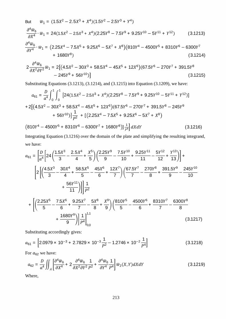
213

But 1 = 1.5 2 − 2. 5 3 + 4 1.5 2 − 2.5 3 + 4

46

4 ∙ 1 = 24 1.5 2 − 2.5 3 + 4 2.25 8 − 7.5 9 + 9.25 10 − 5 11 + 12 (3.1213)

46

4 ∙ 1 = 2.25 4 − 7.5 5 + 9.25 6 − 5 7 + 8 810 4 − 4500 5 + 8310 6 − 6300 7

+ 1680 8 (3.1214)

24

62 2 1 = 2 4.5 2 − 30 3 + 58.5 4 − 45 5 + 12 6 67.5 6 − 270 7 + 391.5 8

− 245 9 + 56 10 (3.1215)


61 = 40

1

0

124 1.5 2 − 2.5 3 + 4 2.25 8 − 7.5 9 + 9.25 10 − 5 11 + 12 ]

+2 4.5 2 − 30 3 + 58.5 4 − 45 5 + 12 6 67.5 6 − 270 7 + 391.5 8 − 245 9

+ 56 10 12 + [ 2.25 4 − 7.5 5 + 9.25 6 − 5 7 + 8

810 4 − 4500 5 + 8310 6 − 6300 7 + 1680 8 ] 14 (3.1216)


we have:

61 = 4 241.5 3

3 −2. 5 4

4 +5

52.25 9

9 −7.5 10

10 +9.25 11

11 −5 12

12 +13

13 +

24.5 3

3 −30 4

4 +58.5 5

5 −45 6

6 +12 7

767.5 7

7 −270 8

8 +391.5 9

9 −245 10

10

+56 11

111

2

+2.25 5

5 −7.5 6

6+

9.25 7

7 −5 8

8+

9

9810 5

5 −4500 6

6+

8310 7

7 −6300 8

8

+1680 9

91

40,0

1,1

(3.1217)


61 = 2.0979 × 10−3 + 2.7829 × 10−3 12 − 1.2746 × 10−2 1

4 (3.1218)

For 62 we have:

62 = 4

46

4 + 24

62 2

12 +

46

41

4 2 , (3.1219)

Where,

214

46

4 = 24 1.5 6 − 2.5 7 + 8 ;

46

4 = 1.5 2 − 2.5 3 + 4 540 2 − 2100 3 + 1680 4

24

62 2 = 2 3 − 15 + 12 2 45 4 − 105 5 + 56 6 ]

But 2 = 1.5 4 − 2. 5 5 + 6 1.5 2 − 2.5 3 + 4

46

4 ∙ 2 = 24 1.5 4 − 2. 5 5 + 6 2.25 8 − 7.5 9 + 9.25 10 − 5 11 + 12 (3.1220)

46

4 ∙ 2 = 2.25 6 − 7.5 7 + 9.25 8 − 5 9 + 10 810 4 − 4500 5 + 8310 6 − 6300 7

+ 16800 8 (3.1221)

24

62 2 2 = 2 4.5 4 − 30 5 + 58.5 6 − 45 7 + 12 8 67.5 6 − 270 7 + 391.5 8

− 245 9 + 56 10 (3.1222)


62 = 40

1

0

124 1.5 4 − 2. 5 5 + 6 2.25 8 − 7.5 9 + 9.25 10 − 5 11 + 12 ]

+2 4.5 4 − 30 5 + 58.5 6 − 45 7 + 12 8 67.5 6 − 270 7 + 391.5 8 − 245 9

+ 56 10 12 + 2.25 6 − 7.5 7 + 9.25 8 − 5 9 + 10

810 4 − 4500 5 + 8310 6 − 6300 7 + 16800 8 14 (3.1223)


we have:

62 = 4 241.5 5

5−

2. 5 6

6+

7

72.25 9

9−

7.5 10

10+

9.25 11

11−

5 12

12+

13

13+

24.5 5

5 −30 6

6 +58.5 7

7 −45 8

8 +12 9

967.5 7

7 −270 8

8 +391.5 9

9 −245 10

10

+56 11

111

2

+2.25 7

7−

7.5 8

8+

9.25 9

9−

5 10

10+

11

11810 5

5−

4500 6

6+

8310 7

7−

63000 8

8

+1680 9

91

40,0

1,1

(3.1224)


215

62 = 7.3260 × 10−4 + 1.1209 × 10−3 12 − 4.4213 × 10−3 1

4 (3.1225)

For 63 we have:

63 = 4

46

4 + 24

62 2

12 +

46

41

4 3 , (3.1226 )

Where,4

64 = 24 1.5 6 − 2.5 7 + 8 ;

46

4 = 1.5 2 − 2.5 3 + 4 540 2 − 2100 3 + 1680 4

24

62 2 = 2 3 − 15 + 12 2 45 4 − 105 5 + 56 6 ]

But 3 = 1.5 2 − 2. 5 3 + 4 1.5 4 − 2.5 5 + 6

46

4 ∙ 3 = 24 1.5 2 − 2. 5 3 + 4 2.25 10 − 7.5 11 + 9.25 12 − 5 13 + 14 (3.1227)

46

4 ∙ 3 = 2.25 4 − 7.5 5 + 9.25 6 − 5 7 + 8 810 6 − 4500 7 + 8310 8 − 6300 9

+ 1680 10 (3.1228)

24

62 2 3 = 2 4.5 2 − 30 3 + 58.5 4 − 45 5 + 12 6 67.5 8 − 270 + 391.5 10

− 245 11 + 56 12 (3.1229)


63 = 40

1

0

124 1.5 2 − 2. 5 3 + 4 2.25 10 − 7.5 11 + 9.25 12 − 5 13 + 14

+[2 4.5 2 − 30 3 + 58.5 4 − 45 5 + 12 6 67.5 8 − 270 + 391.5 10 − 245 11

+ 56 12 12 + [ 2.25 4 − 7.5 5 + 9.25 6 − 5 7 + 8

810 6 − 4500 7 + 8310 8 − 6300 9 + 1680 10 ]1

4 (3.1230)


we have:

63 = 4 241.5 3

3 −2. 5 4

4 +5

52.25 11

11 −7.5 12

12 +9.25 13

13 −5 14

14 +15

15 +

24.5 3

3−

30 4

4 +58.5 5

5−

45 6

6+

12 7

767.5 9

9−

270 10

10+

391.5 11

11−

245 12

12

+56 13

131

2

216

+2.25 5

5 −7.5 6

6+

9.25 7

7 −5 8

8+

9

9810 7

7 −4500 8

8+

8310 9

9 −6300 10

10

+1680 11

111

40,0

1,1

(3.1231)


63 = 1.0939 × 10−3 + 3.0969 × 10−3 12 − 5.4671 × 10−3 1

4 (3.1232)

For 64 we have:

64 = 4

46

4 + 24

62 2

12 +

46

41

4 4 , (3.1233 )

Where,4

64 = 24 1.5 6 − 2.5 7 + 8 ;

46

4 = 1.5 2 − 2.5 3 + 4 540 2 − 2100 3 + 1680 4

24

62 2 = 2 3− 15 + 12 2 45 4 − 105 5 + 56 6 ]

But 4 = 1.5 4 − 2. 5 5 + 6 1.5 4 − 2. 5 5 + 6

46

4 ∙ 4 = 24 1.5 4 − 2. 5 5 + 6 2.25 10 − 7.5 11 + 9.25 12 − 5 13 + 14 (3.1234)

46

4 ∙ 4 = 2.25 6 − 7.5 7 + 9.25 8 − 5 9 + 10 810 6 − 4500 7 + 8310 8 − 6310 9

+ 1680 10 (3.1235)

24

62 2 2 = 2 4.5 4 − 30 5 + 58.5 6 − 45 7 + 12 8 67.5 8 − 270 9 + 391.5 10

− 245 11 + 56 12 (3.1236)


64 = 40

1

0

124 1.5 4 − 2. 5 5 + 6 2.25 10 − 7.5 11 + 9.25 12 − 5 13 + 14

+2 4.5 4 − 30 5 + 58.5 6 − 45 7 + 12 8 67.5 8 − 270 9 + 391.5 10 − 245 11

+ 56 12 12 + [ 2.25 6 − 7.5 7 + 9.25 8 − 5 9 + 10

810 6 − 4500 7 + 8310 8 − 6310 9 + 1680 10 ]1

4 (3.1237)


we have:

64 = 4 241.5 5

5 −2. 5 6

6 +7

72.25 11

11 −7.5 12

12 +9.25 13

13 −5 14

14 +15

15 +

217

24.5 5

5 −30 6

6+

58.5 7

7 −45 8

8+

12 9

967.5 9

9 −270 10

10+

391.5 11

11 −245 12

12

+56 13

131

2

+2.25 7

7−

7.5 8

8+

9.25 9

9−

5 10

10+

11

11810 7

7−

4500 8

8+

8310 9

9−

6310 10

10

+1680 11

111

40,0

1,1

(3.1238)


64 = 3.8200 × 10−4 + 1.2474 × 10−3 12 − 4.5119 × 10−3 1

4 (3.1239)

For 65 we have:

65 = 4

46

4 + 24

62 2

12 +

46

∂ 4

14 5 , (3.1240 )

Where,4

64 = 24 1.5 6 − 2.5 7 + 8 ;

46

4 = 1.5 2 − 2.5 3 + 4 540 2 − 2100 3 + 1680 4

24

62 2 = 2 3 − 15 + 12 2 45 4 − 105 5 + 56 6 ]

But 5 = 1.5 6 − 2. 5 7 + 8 1.5 2 − 2. 5 3 + 4

46

4 ∙ 5 = 24 1.5 6 − 2. 5 7 + 8 2.25 8 − 7.5 9 + 9.25 10 − 5 11 + 12 (3.1241)

46

4 ∙ 5 = 2.25 8 − 7.5 9 + 9.25 10 − 5 11 + 12 810 4 − 4500 5 + 8310 6 − 6300 7

+ 1680 8 (3.1242)

24

62 2 5 = 2 4.5 6 − 30 7 + 58.5 8 − 45 9 + 12 10 67.5 6 − 270 7 + 391.5 8

− 245 9 + 56 10 (3.1243)


65 = 40

1

0

124 1.5 6 − 2. 5 7 + 8 2.25 8 − 7.5 9 + 9.25 10 − 5 11 + 12

+2 4.5 6 − 30 7 + 58.5 8 − 45 9 + 12 10 67.5 6 − 270 7 + 391.5 8 − 245 9

+ 56 10 12 + [ 2.25 8 − 7.5 9 + 9.25 10 − 5 11 + 12

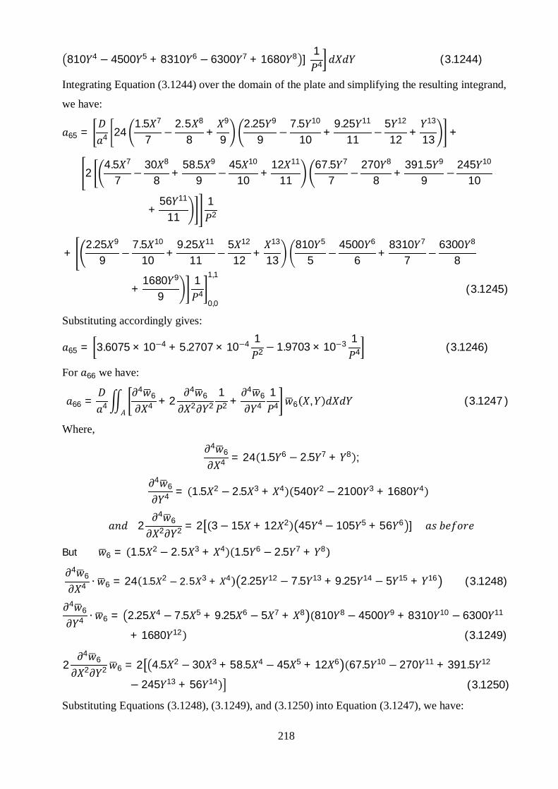
218

810 4 − 4500 5 + 8310 6 − 6300 7 + 1680 8 ]1

4 (3.1244)


we have:

65 = 4 241.5 7

7−

2. 5 8

8+

9

92.25 9

9−

7.5 10

10+

9.25 11

11−

5 12

12+

13

13+

24.5 7

7−

30 8

8+

58.5 9

9−

45 10

10+

12 11

1167.5 7

7−

270 8

8+

391.5 9

9−

245 10

10

+56 11

111

2

+2.25 9

9 −7.5 10

10 +9.25 11

11 −5 12

12 +13

13810 5

5 −4500 6

6 +8310 7

7 −6300 8

8

+1680 9

91

40,0

1,1

(3.1245)


65 = 3.6075 × 10−4 + 5.2707 × 10−4 12 − 1.9703 × 10−3 1

4 (3.1246)

For 66 we have:

66 = 4

46

4 + 24

62 2

12 +

46

41

4 6 , (3.1247 )

Where,4

64 = 24 1.5 6 − 2.5 7 + 8 ;

46

4 = 1.5 2 − 2.5 3 + 4 540 2 − 2100 3 + 1680 4

24

62 2 = 2 3 − 15 + 12 2 45 4 − 105 5 + 56 6 ]

But 6 = 1.5 2 − 2. 5 3 + 4 1.5 6 − 2.5 7 + 8

46

4 ∙ 6 = 24 1.5 2 − 2. 5 3 + 4 2.25 12 − 7.5 13 + 9.25 14 − 5 15 + 16 (3.1248)

46

4 ∙ 6 = 2.25 4 − 7.5 5 + 9.25 6 − 5 7 + 8 810 8 − 4500 9 + 8310 10 − 6300 11

+ 1680 12 (3.1249)

24

62 2 6 = 2 4.5 2 − 30 3 + 58.5 4 − 45 5 + 12 6 67.5 10 − 270 11 + 391.5 12

− 245 13 + 56 14 (3.1250)


219

66 = 40

1

0

124 1.5 2 − 2. 5 3 + 4 2.25 12 − 7.5 13 + 9.25 14 − 5 15 + 16 +

2 4.5 2 − 30 3 + 58.5 4 − 45 5 + 12 6 67.5 10 − 270 11 + 391.5 12 − 245 13

+ 56 14 12 + [ 2.25 4 − 7.5 5 + 9.25 6 − 5 7 + 8

810 8 − 4500 9 + 8310 10 − 6300 11 + 1680 12 ] +1

4 (3.1251)


we have:

66 = 4 241.5 3

3−

2. 5 4

4+

5

52.25 13

13−

7.5 14

14+

9.25 15

15−

5 16

16+

17

17+

24.5 3

3 −30 4

4 +58.5 5

5 −45 6

6 +12 7

767.5 11

11 −270 12

12 +391.5 13

13 −245 14

14

+56 15

151

2

+2.25 5

5−

7.5 6

6+

9.25 7

7−

5 8

8+

9

9810 9

9−

4500 10

10+

8310 11

11−

6300 12

12

+1680 13

131

40,0

1,1

(3.1252)


66 = 6.3510 × 10−4 + 2.5574 × 10−3 12 − 2.3726 × 10−3 1

4 (3.1253)


6 = 6 ,

=0

1

0

11.5 2 − 2. 5 3 + 4 1.5 6 − 2.5 7 + 8 (3.1254)


=1.5 3

3 −2. 5 4

4+

5

51.5 7

7 −2.5 8

8+

9

90,0

1,1

6 = 9.6726 × 10−4 (3.1255)

Hence,

6,1 1+ 6,2 2 + 6,3 3 + 6,4 4+ 6,5 5 + 6,6 6 = 9.6726 × 10−4 4 (3.1256)

Representing Equations (3.1015), (3.1063), (3.1112), (3.1160), (3.1208) and (3.1256) in matrix

form, we have:

220

1,1 1+ 1,2 2 + 1,3 3 + 1,4 4+ 1,5 5 + 1,6 6 = 5.36250 × 10−3 4

2,1 1+ 2,2 2 + 2,3 3 + 2,4 4+ 2,5 5 + 2,6 6 = 1.9643 × 10−3 4

3,1 1+ 3,2 2 + 3,3 3 + 3,4 4+ 3,5 5 + 3,6 6 = 1.9643 × 10−3 4

4,1 1+ 4,2 2 + 4,3 3 + 4,4 4+ 4,5 5 + 4,6 6 = 6.8594 × 10−4 4

5,1 1+ 5,2 2 + 5,3 3 + 5,4 4+ 5,5 5 + 5,6 6 = 9.6726 × 10−4 4

6,1 1+ 6,2 2 + 6,3 3 + 6,4 4+ 6,5 5 + 6,6 6 = 9.6726 × 10−4 4 (3.1257)


First Approximation

1 = 1

11

4

1 = 5.36250×10−3

11

4 (3.1258)


1,1 1,2 1,32,1 2,2 2,3

3,1 3,2 3,3

1

2

3

=1

2

3

4

1

2

3

=1,1 1,2 1,32,1 2,2 2,3

3,1 3,2 3,3

−1 5.36250 × 10−3

1.9643 × 10−3

1.9643 × 10−3

4

(3.1259)


1,1 1,2 1,3 1,42,1 2,2 2,3 2,4

3,1 3,2 3,3 3,44,1 4,2 4,3 4,4

1

2

3

4

=1

2

3

4

4

1

2

3

4

=

1,1 1,2 1,3 1,42,1 2,2 2,3 2,4

3,1 3,2 3,3 3,44,1 4,2 4,3 4,4

−1 5.36250 × 10−3

1.9643 × 10−3

1.9643 × 10−3

6.8594 × 10−4

4

(3.1260)

Third Approximation

1,1 1,2 1,3 1,4 1,5 1,62,1 2,2 2,3 2,4 2,5 2,6

3,1 3,2 3,3 3,4 3,5 3,6

4,1 4,2 4,3 4,4 4,5 4,65,1 5,2 5,3 5,4 5,5 5,6

6,1 6,2 6,3 6,4 6,5 6,6

1

2

3

4

5

6

=

1

2

3

4

5

6

4

221

1

2

3

4

5

6

=

1,1 1,2 1,3 1,4 1,5 1,6

2,1 2,2 2,3 2,4 2,5 2,63,1 3,2 3,3 3,4 3,5 3,6

4,1 4,2 4,3 4,4 4,5 4,6

5,1 5,2 5,3 5,4 5,5 5,66,1 6,2 6,3 6,4 6,5 6,6

−1 5.36250 × 10−3

1.9643 × 10−3

1.9643 × 10−3

6.8594 × 10−4

9.6726 × 10−4

9.6726 × 10−4

4 (3.1261)

Where,

Equations (3.1258), (3.1259), (3.1260) and (3.1261) are the Garlekin energy solutions for multi-

term CCSS thin rectangular isotropic plate problems. The matrix, , is the stiffness matrix of the

plate; , is obtained at specific aspect ratios of the plate.



clamped on two opposite edges and simply supported on the other two opposite edges.

0

Figure 3.10: CSCS Plate under uniformly distributed load.

The six term deflection functional for CSCS plate is given in Equation (3.85) as:

, = 1 − 2 3 + 4 2 − 2 3 + 4 + 23 − 2 5 + 6 2 − 2 3 + 4 +

3 − 2 3 + 4 4 − 2 5 + 6 + 43 − 2 5 + 6 4 − 2 5 + 6 +

55 − 2 7 + 8 2 − 2 3 + 4 + 6 − 2 3 + 4 6 − 2 7 + 8


11 = 4

41

4 + 24

12 2

12 +

41

41

4 1 , (3.1262)

Where,

1 = − 2 3 + 4 2 − 2 3 + 4

41

4 = 24 2 − 2 3 + 4 (3.1263)

a

bY

X

222

41

4 = 24 − 2 3 + 4 (3.1264)

24

12 2 = 2 −12 + 12 2 2 − 12 + 12 2 ] (3.1265)

41

4 ∙ 1 = 24 − 2 3 + 4 4 − 4 5 + 6 6 − 4 7 + 8 (3.1266)

41

4 ∙ 1 = 24 2 − 4 4 + 2 5 + 4 6 − 4 7 + 8 2 − 2 3 + 4 (3.1267)

24

12 2 1 = 2[ −12 2 + 12 3 + 24 4 − 36 5 + 12 6 2 2 − 16 3 + 38 4 − 36 5

+ 12 6 (3.1268)


11 = 4 01

01 24 − 2 3 + 4 4 − 4 5 + 6 6 − 4 7 + 8∫∫ +

2[ −12 2 + 12 3 + 24 4 − 36 5 + 12 6 2 2 − 16 3 + 38 4 − 36 5 + 12 6 ]1

2

+ 24 2 − 4 4 + 2 5 + 4 6 − 4 7 + 8 2 − 2 3 + 4 14 (3.1269)


we have:

11 = 4 242

2 −2 4

4 +5

5

5

5 −4 6

6 +6 7

7 −4 8

8 +9

9 +

2 −12 3

3+

12 4

4+

24 5

5−

36 6

6+

12 7

72 3

3−

16 4

4+

38 5

5−

36 6

6+

12 7

71

2 +

243

3 −4 5

5+

2 6

6+

4 7

7 −4 8

8+

9

9

3

3 −2 4

4+

5

51

40,0

1,1

(3.1270)


11 = 7.6190 × 10−3 + 1.8503 × 10−2 12 + 3.9365 × 10−2 1

4 (3.1271)

For 12 we have:

12 = 4

41

4 + 24

12 2

12 +

41

41

4 2 , ( 3.1272)

Where,4

14 = 24 2 − 2 3 + 4 ;

41

4 = 24 − 2 3 + 4 24

12 2

= 2 −12 + 12 2 2 − 12 + 12 2 ]

223

41

4 ∙ 2 = 24 3 − 2 5 + 6 4 − 4 5 + 6 6 − 4 7 + 8 (3.1273)

41

4 ∙ 2 = 24 4 − 4 6 + 2 7 + 4 8 − 4 9 + 10 2 − 2 3 + Y (3.1274)

24

12 2 2 = 2 −12 4 + 12 5 + 24 6 − 36 7 + 12 8 2 2 − 16 3 + 38 4 − 36 5

+ 12 6 (3.1275)


12 = 4 01

01 24 3 − 2 5 + X 4 − 4 5 + 6 6 − 4 7 + 8 ]∫∫ +

2 −12 4 + 12 5 + 24 6 − 36 7 + 12 8 2 2 − 16 3 + 38 4 − 36 5 + 12 6 ]1

2

+ 24 4 − 4 6 + 2 7 + 4 8 − 4 9 + 10 2 − 2 3 + 4 14 (3.1276)


we have:

12 = 4 244

4 −2 6

6+

7

7

5

5−

4 6

6+

6 7

7−

4 8

8+

9

9+

2 −12 5

5+

12 6

6+

24 7

7 −36 8

8+

12 9

92 3

3 −16 4

4+

38 5

5 −36 6

6+

12 7

71

2 +

245

5−

4 7

7+

2 8

8+

4 9

9−

4 10

10+

11

11

3

3−

2 4

4 +5

51

40,0

1,1

(3.1277)


12 = 2.2676 × 10−3 + 5.2608 × 10−3 12 + 1.1140 × 10−2 1

4 (3.1278)

For 13 we have:

13 = 4

41

4 + 24

12 2

12 +

41

41

4 3 , (3.1279)

Where,4

14 = 24 2 − 2 3 + 4 ;

41

4 = 24 − 2 3 + 4 24

12 2

= 2 −12 + 12 2 2 − 12 + 12 2 ]4

14 ∙ 3 = 24 − 2 3 + 4 6 − 4 7 + 6 8 − 4 9 + 10 (3.1280)

41

4 ∙ 3 = 24 2 − 4 4 + 2 5 + 4 6 − 4 7 + 8 4 − 2 5 + 6 (3.1281)

24

12 2 3 = 2 −12 2 + 12 3 + 24 4 − 36 5 + 12 6 2 4 − 16 5 + 38 6 − 36 7

+ 12 8 (3.1282)

224


13 = 4 01

01 24 − 2 3 + 4 6 − 4 7 + 6 8 − 4 9 + 10 ]∫∫ +

2 −12 2 + 12 3 + 24 4 − 36 5 + 12 6 2 4 − 16 5 + 38 6 − 36 7 + 12 8 ]1

2

+24 2 − 4 4 + 2 5 + 4 6 − 4 7 + 8 4 − 2 5 + 6 14 (3.1283)


we have:

13 = 4 242

2 −2 4

4+

5

5

7

7 −4 8

8+

6 9

9 −4 10

10+

11

11 +

2 −12 3

3 +12 4

4 +24 5

5 −36 6

6 +12 7

72 5

5 −16 6

6 +38 7

7 −36 8

8 +12 9

91

2 +

243

3 −4 5

5+

2 6

6+

4 7

7 −4 8

8+

9

9

5

5 −2 6

6+

7

71

40,0

1,1

(3.1284)


13 = 2.0779 × 10−3 + 4.6259 × 10−3 12 + 1.1247 × 10−2 1

4 (3.1285)

For 14 we have:

14 = 4

41

4 + 24

12 2

12 +

41

41

4 4 , (3.1286)

Where,4

14 = 24 2 − 2 3 + 4 ;

41

4 = 24 − 2 3 + 4 24

12 2

= 2 −12 + 12 2 2 − 12 + 12 2 ]4

14 ∙ 4 = 24 3 − 2 5 + 6 6 − 4 7 + 6 8 − 4 9 + 10 (3.1287)

41

4 ∙ 4 = 24[ 4 − 4 6 + 2 7 + 4 8 − 4 9 + 10 4 − 2 5 + 6 ] (3.1288)

24

12 2 4 = 2 −12 4 + 12 5 + 24 6 − 36 7 + 12 8 2 4 − 16 5 + 38 6 − 36 7

+ 12 8 (3.1289)


14 = 4 01

01 24 3 − 2 5 + 6 6 − 4 7 + 6 8 − 4 9 + 10 ]∫∫ +

2 −12 4 + 12 5 + 24 6 − 36 7 + 12 8 2 4 − 16 5 + 38 6 − 36 7 + 12 8 ]1

2

+24 4 − 4 6 + 2 7 + 4 8 − 4 9 + 10 4 − 2 5 + 6 14 (3.1290)

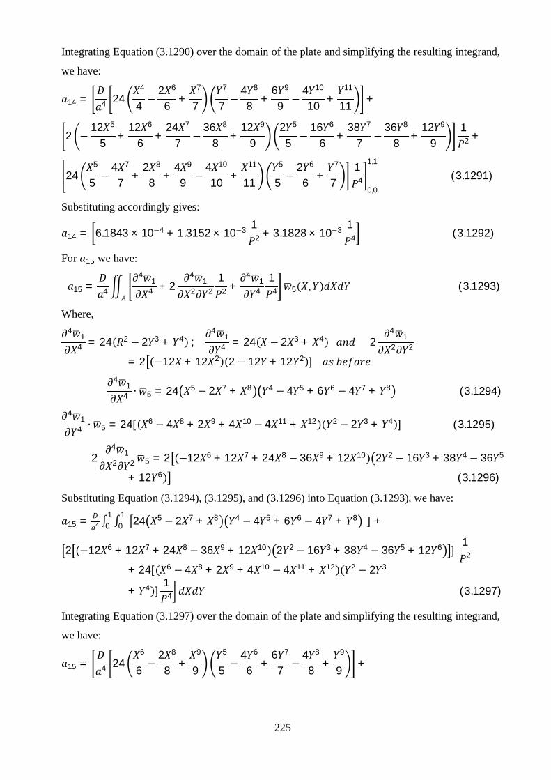
225


we have:

14 = 4 244

4 −2 6

6 +7

7

7

7 −4 8

8 +6 9

9 −4 10

10 +11

11 +

2 −12 5

5+

12 6

6+

24 7

7−

36 8

8+

12 9

92 5

5−

16 6

6+

38 7

7−

36 8

8+

12 9

91

2 +

245

5 −4 7

7 +2 8

8 +4 9

9 −4 10

10 +11

11

5

5 −2 6

6 +7

71

40,0

1,1

(3.1291)


14 = 6.1843 × 10−4 + 1.3152 × 10−3 12 + 3.1828 × 10−3 1

4 (3.1292)

For 15 we have:

15 = 4

41

4 + 24

12 2

12 +

41

41

4 5 , (3.1293)

Where,4

14 = 24 2 − 2 3 + 4 ;

41

4 = 24 − 2 3 + 4 24

12 2

= 2 −12 + 12 2 2 − 12 + 12 2 ]4

14 ∙ 5 = 24 5 − 2 7 + 8 4 − 4 5 + 6 6 − 4 7 + 8 (3.1294)

41

4 ∙ 5 = 24[ 6 − 4 8 + 2 9 + 4 10 − 4 11 + 12 2 − 2 3 + 4 ] (3.1295)

24

12 2 5 = 2 −12 6 + 12 7 + 24 8 − 36 9 + 12 10 2 2 − 16 3 + 38 4 − 36 5

+ 12 6 (3.1296)


15 = 4 01

01 24 5 − 2 7 + 8 4 − 4 5 + 6 6 − 4 7 + 8 ]∫∫ +

2 −12 6 + 12 7 + 24 8 − 36 9 + 12 10 2 2 − 16 3 + 38 4 − 36 5 + 12 6 ]1

2

+ 24[ 6 − 4 8 + 2 9 + 4 10 − 4 11 + 12 2 − 2 3

+ 4 ]1

4 (3.1297)


we have:

15 = 4 246

6 −2 8

8 +9

9

5

5 −4 6

6 +6 7

7 −4 8

8 +9

9 +

226

2 −12 7

7+

12 8

8+

24 9

9 −36 10

10+

12 11

112 3

3 −16 4

4+

38 5

5 −36 6

6+

12 7

71

2 +

247

7−

4 9

9+

2 10

10+

4 11

11−

4 12

12+

13

13

3

3−

2 4

4+

5

51

40,0

1,1

(3.1298)


15 = 1.0582 × 10−3 + 2.1604 × 10−3 12 + 4.5110 × 10−3 1

4 ( 3.1299)

For 16 we have:

16 = 4

41

4 + 24

12 2

12 +

41

41

4 6 , (3.1300 )

Where,4

14 = 24 2 − 2 3 + 4 ;

41

4 = 24 − 2 3 + 4 24

12 2

= 2 −12 + 12 2 2 − 12 + 12 2 ]4

14 ∙ 5 = 24 − 2 3 + 4 8 − 4 9 + 6 10 − 4 11 + 12 (3.1301)

41

4 ∙ 5 = 24[ 2 − 4 4 + 2 5 + 4 6 − 4 7 + 8 6 − 2 7 + 8 ] (3.1302)

24

12 2 5 = 2 −12 2 + 12 3 + 24 4 − 36 5 + 12 6 2 6 − 16 7 + 38 8 − 36 9

+ 12 10 (3.1303)


16 = 4 01

01 24 − 2 3 + 4 8 − 4 9 + 6 10 − 4 11 + 12 ]∫∫ +

2 −12 2 + 12 3 + 24 4 − 36 5 + 12 6 2 6 − 16 7 + 38 8 − 36 9 + 12 10 ]1

2

+24 2 − 4 4 + 2 5 + 4 6 − 4 7 + 8 6 − 2 7 + 8 14 (3.1304)


we have:

16 = 4 242

2 −2 4

4 +5

5

9

9 −4 10

10 +6 11

11 −4 12

12 +13

13 +

2 −12 3

3+

12 4

4 +24 5

5−

36 6

6+

12 7

72 7

7−

16 8

8+

38 9

9−

36 10

10+

12 11

111

2 +

243

3 −4 5

5 +2 6

6 +4 7

7 −4 8

8 +9

9

7

7 −2 8

8 +9

91

40,0

1,1

(3.1305)


227

16 = 7.4592 × 10−4 + 1.1214 × 10−3 12 + 4.6863 × 10−3 1

4 (3.1306)


1 = 1 ,

=0

1

0

1− 2 3 + 4 2 − 2 3 + 4 (3.1307)


=2

2 −2 4

4 +5

5

3

3 −2 4

4 +5

50,0

1,1

1 = 6.6667 × 10−3 (3.1308)

Hence,

1,1 1+ 1,2 2 + 1,3 3 + 1,4 4+ 1,5 5 + 1,6 6 = 6.6667 × 10−3 4 (3.1309)


21 = 4

42

4 + 24

22 2

12 +

42

41

4 1 , (3.1310)

Where,

2 = 3 − 2 5 + 6 2 − 2 3 + 4

42

4 = 2 − 2 3 + 4 −240 + 360 2 (3.1311)

42

4 = 24 3 − 2 5 + 6 (3.1312)

24

22 2 = 2 6 − 40 3 + 30X4 2− 12 + 12 2 ] (3.1313)

42

4 ∙ 1 = 240 − 2 + 1.5 3 + 2 4 − 4 5 + 1.5 6 4 − 4 5 + 6 6 − 4 7

+ 8 (3.1314)4

24 ∙ 1 = 24 4 − 4 6 + 2 7 + 4 8 − 4 9 + 10 2 − 2 3 + 4 (3.1315)

24

22 2 1 = 2 6 2 − 52 4 + 36 5+80 6 − 100 7 + 30 8 2 2 − 16 3 + 38 4 − 24 5

+ 12 6 (3.1316)


21 = 40

1

0

1240 − 2 + 1.5 3 + 2 4 − 4 5 + 1.5 6 4 − 4 5 + 6 6 − 4 7 + 8

+2 6 2 − 52 4 + 36 5+80 6 − 100 7 + 30 8 2 2 − 16 3 + 38 4 − 24 5 + 12 6 12

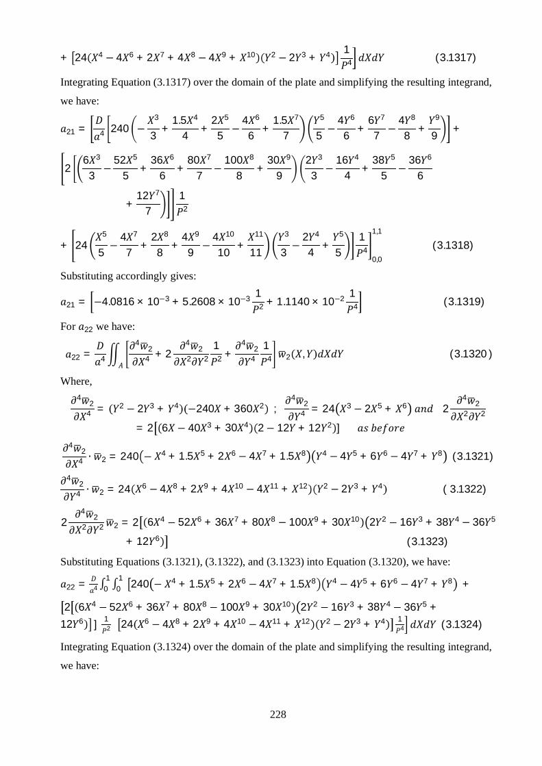
228

+ 24 4 − 4 6 + 2 7 + 4 8 − 4 9 + 10 2 − 2 3 + 4 14 (3.1317)


we have:

21 = 4 240 −3

3 +1.5 4

4 +2 5

5 −4 6

6 +1.5 7

7

5

5 −4 6

6 +6 7

7 −4 8

8 +9

9 +

26 3

3−

52 5

5+

36 6

6+

80 7

7−

100 8

8+

30 9

92 3

3−

16 4

4 +38 5

5−

36 6

6

+12 7

71

2

+ 245

5−

4 7

7+

2 8

8+

4 9

9−

4 10

10+

11

11

3

3−

2 4

4 +5

51

40,0

1,1

(3.1318)


21 = −4.0816 × 10−3 + 5.2608 × 10−3 12 + 1.1140 × 10−2 1

4 (3.1319)

For 22 we have:

22 = 4

42

4 + 24

22 2

12 +

42

41

4 2 , (3.1320 )

Where,4

24 = 2 − 2 3 + 4 −240 + 360 2 ;

42

4 = 24 3 − 2 5 + 6 24

22 2

= 2 6 − 40 3 + 30 4 2 − 12 + 12 2 ]4

24 ∙ 2 = 240 − 4 + 1.5 5 + 2 6 − 4 7 + 1.5 8 4 − 4 5 + 6 6 − 4 7 + 8 (3.1321)

42

4 ∙ 2 = 24 6 − 4 8 + 2 9 + 4 10 − 4 11 + 12 2 − 2 3 + 4 ( 3.1322)

24

22 2 2 = 2 6 4 − 52 6 + 36 7 + 80 8 − 100 9 + 30 10 2 2 − 16 3 + 38 4 − 36 5

+ 12 6 (3.1323)


22 = 4 01

01 240 − 4 + 1.5 5 + 2 6 − 4 7 + 1.5 8 4 − 4 5 + 6 6 − 4 7 + 8 +∫∫

2 6 4 − 52 6 + 36 7 + 80 8 − 100 9 + 30 10 2 2 − 16 3 + 38 4 − 36 5 +12 6 ] 1

2 24 6 − 4 8 + 2 9 + 4 10 − 4 11 + 12 2 − 2 3 + 4 14 (3.1324)


we have:

229

22 = 4 240 −5

5 +1.5 6

6 +2 7

7 −4 8

8 +1.5 9

95

5 −4 6

6 +6 7

7 −4 8

8 +9

9 +

26 5

5 −52 7

7 +36 8

8 +80 9

9 −100 10

10 +30 11

112 3

3 −16 4

4 +38 5

5 −36 6

6

+12 7

71

2 +

247

7 −4 9

9 +2 10

10 +4 11

11 −4 12

12 +13

13

3

3 −2 4

4 +5

51

40,0

1,1

(3.1325)


22 = 9.0703 × 10−4 + 4.2823 × 10−3 12 + 4.5110 × 10−3 1

4 (3.1326)

For 23 we have:

23 = 4

42

4 + 24

22 2

12 +

42

41

4 3 , (3.1327)

Where,4

24 = 2 − 2 3 + 4 −240 + 360 2 ;

42

4 = 24 3 − 2 5 + 6 24

22 2

= 2 6 − 40 3 + 30 4 2 − 12 + 12 2 ]4

24 ∙ 3 = 240 − 2 + 1.5 3 + 2 4 − 4 5 + 1.5 6 6 − 4 7 + 6 8 − 4 9 + 10 (3.1328)

42

4 ∙ 3 = 24 4 − 4 6 + 2 7 + 4 8 − 4 9 + 10 4 − 2 5 + 6 (3.1329)

24

22 2 3 = 2 6 2 − 52 4 + 36 5 + 80 6 − 100 7 + 30 8 2 4 − 16 5 + 38 6 − 36 7

+ 12 8 (3.1330)


23 = 4 01

01 240 − 2 + 1.5X3 + 2 4 − 4 5 + 1.5 6 6 − 4 7 + 6 8 − 4 9 + 10 ]∫∫ +

2 6 2 − 52 4 + 36 5 + 80 6 − 100 7 + 30 8 2 4 − 16 5 + 38 6 − 36 7 +12 8 ] 1

2 + 24 4 − 4 6 + 2 7 + 4 8 − 4 9 + 10 4 − 2 5 + 6 14 (3.1331)


we have:

23 = 4 240 −3

3 +1.5 4

4 +2 5

5 −4 6

6 +1.5 7

7

7

7 −4 8

8 +6 9

9 −4 10

10 +11

11

230

+26 3

3 −52 5

5+

36 6

6+

80 7

7 −100 8

8+

30 9

92 5

5 −16 6

6+

38 7

7 −36 8

8

+12 9

91

2

+ 245

5 −4 7

7 +2 8

8 +4 9

9 −4 10

10 +11

11

5

5 −2 6

6 +7

71

40,0

1,1

(3.1332)


23 = −1.1132 × 10−3 + 1.3152 × 10−3 12 + 3.1828 × 10−3 1

4 (3.1333)

For 24 we have:

24 = 4

42

4 + 24

22 2

12 +

42

41

4 4 , (3.1334)

Where,4

24 = 2 − 2 3 + 4 −240 + 360 2 ;

42

4 = 24 3 − 2 5 + 6 24

22 2

= 2 6 − 40 3 + 30 4 2 − 12 + 12 2 ]4

24 ∙ 4 = 240 − 4 + 1.5 5 + 2 6 − 4 7 + 1.5 8 6 − 4 7 + 6 8 − 4 9

+ 10 (3.1335)4

24 ∙ 4 = 24 6 − 4 8 + 2 9 + 4 10 − 4 11 + 12 4 − 2 5 + 6 (3.1336)

24

22 2 4 = 2 6 4 − 52 6 + 36 7 + 80 8 − 100 9 + 30 10 2 4 − 16 5 + 38 6 − 36 7

+ 12 8 (3.1337)


24 = 4 01

01 240 − 4 + 1.5 5 + 2 6 − 4 7 + 1.5 8 6 − 4 7 + 6 8 − 4 9 + 10 ]∫∫ +

2 6 4 − 52 6 + 36 7 + 80 8 − 100 9 + 30 10 2 4 − 16 5 + 38 6 − 36 7 +12 8 ] 1

2 + [24 6 − 4 8 + 2 9 + 4 10 − 4 11 + 12 4 − 2 5 + 6 ] 14 (3.1338)


we have:

24 = 4 240 −5

5+

1.5 6

6+

2 7

7 −4 8

8+

1.5 9

9

7

7 −4 8

8+

6 9

9 −4 10

10+

11

11

+26 5

5 −52 7

7 +36 8

8 +80 9

9 −100 10

10 +30 11

112 5

5 −16 6

6 +38 7

7 −36 8

8

+12 9

91

2

231

+ 247

7 −4 9

9 +2 10

10 +4 11

11 −4 12

12 +13

13

5

5 −2 6

6 +7

71

40,0

1,1

(3.1339)


24 = 2.4737 × 10−4 + 1.0706 × 10−3 12 + 1.2889 × 10−3 1

4 (3.1340)

For 25 we have:

25 = 4

42

4 + 24

22 2

12 +

42

41

4 5 , (3.1341)

Where,4

24 = 2 − 2 3 + 4 −240 + 360 2 ;

42

4 = 24 3 − 2 5 + 6 24

22 2

= 2 6 − 40 3 + 30 4 2 − 12 + 12 2 ]4

24 ∙ 5 = 240 − 6 + 1.5 7 + 2 8 − 4 9 + 1.5 10 4 − 4 5 + 6 6 − 4 7

+ 8 (3.1342)4

24 ∙ 5 = 24 8 − 4 10 + 2 11 + 4 12 − 4 13 + 14 2 − 2 3 + 4 (3.1343)

24

22 2 5 = 2 6 6 − 52 8 + 36 9 + 80 10 − 100 11 + 30 12 2 2 − 16 3 + 38 4

− 36 5 + 12 6 (3.1344)


25 = 4 01

01 240 − 6 + 1.5 7 + 2 8 − 4 9 + 1.5 10 4 − 4 5 + 6 6 − 4 7 + 8 ]∫∫ +

2 6 6 − 52 8 + 36 9 + 80 10 − 100 11 + 30 12 2 2 − 16 3 + 38 4 − 36 5 +12 6 ] 1

2 + [24 8 − 4 10 + 2 11 + 4 12 − 4 13 + 14 2 − 2 3 + 4 ] 14

(3.1345)


we have:

25 = 4 240 −7

7+

1.5 8

8+

2 9

9−

4 10

10+

1.5 11

11

5

5−

4 6

6+

6 7

7−

4 8

8+

9

9

+26 7

7 −52 9

9+

36 10

10+

80 11

11 −100 12

12+

30 13

132 3

3 −16 4

4+

38 5

5 −36 6

6

+12 7

71

2

+ 249

9 −4 11

11+

2 12

12+

4 13

13 −4 14

14+

15

15

3

3 −2 4

4+

5

51

40,0

1,1

(3.1346)


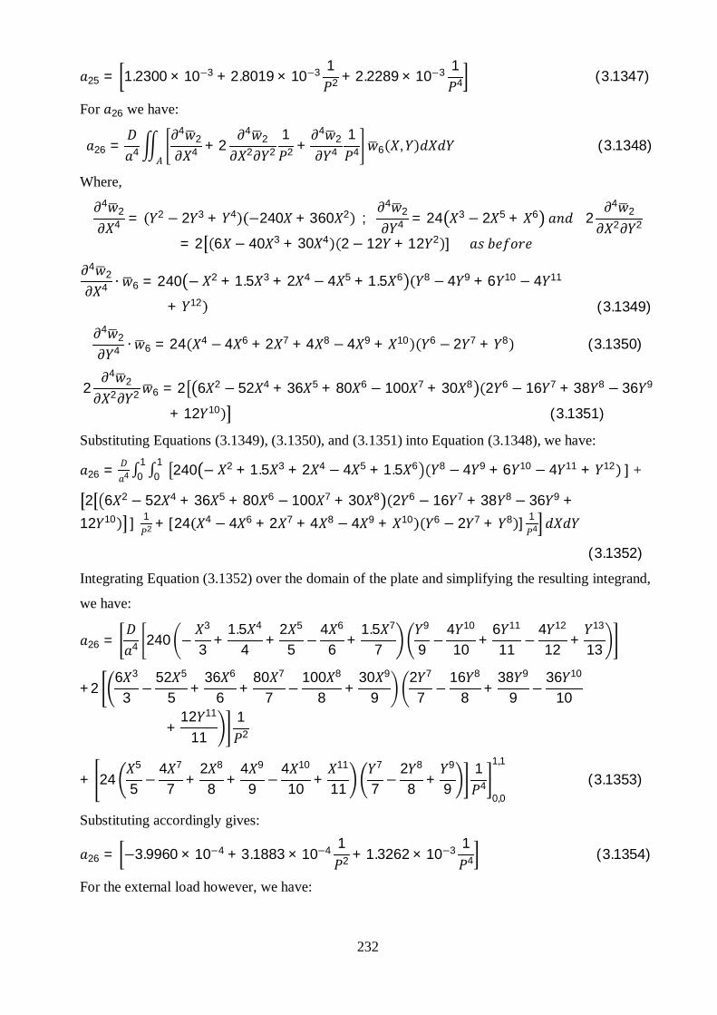
232

25 = 1.2300 × 10−3 + 2.8019 × 10−3 12 + 2.2289 × 10−3 1

4 (3.1347)

For 26 we have:

26 = 4

42

4 + 24

22 2

12 +

42

41

4 6 , (3.1348)

Where,4

24 = 2 − 2 3 + 4 −240 + 360 2 ;

42

4 = 24 3 − 2 5 + 6 24

22 2

= 2 6 − 40 3 + 30 4 2 − 12 + 12 2 ]4

24 ∙ 6 = 240 − 2 + 1.5 3 + 2 4 − 4 5 + 1.5 6 8 − 4 9 + 6 10 − 4 11

+ 12 (3.1349)4

24 ∙ 6 = 24 4 − 4 6 + 2 7 + 4 8 − 4 9 + 10 6 − 2 7 + 8 (3.1350)

24

22 2 6 = 2 6 2 − 52 4 + 36 5 + 80 6 − 100 7 + 30 8 2 6 − 16 7 + 38 8 − 36 9

+ 12 10 (3.1351)


26 = 4 01

01 240 − 2 + 1.5 3 + 2 4 − 4 5 + 1.5 6 8 − 4 9 + 6 10 − 4 11 + 12 ]∫∫ +

2 6 2 − 52 4 + 36 5 + 80 6 − 100 7 + 30 8 2 6 − 16 7 + 38 8 − 36 9 +12 10 ] 1

2 + [24 4 − 4 6 + 2 7 + 4 8 − 4 9 + 10 6 − 2 7 + 8 ] 14

(3.1352)


we have:

26 = 4 240 −3

3+

1.5 4

4+

2 5

5 −4 6

6+

1.5 7

7

9

9 −4 10

10+

6 11

11 −4 12

12+

13

13

+26 3

3 −52 5

5 +36 6

6 +80 7

7 −100 8

8 +30 9

92 7

7 −16 8

8 +38 9

9 −36 10

10

+12 11

111

2

+ 245

5 −4 7

7 +2 8

8 +4 9

9 −4 10

10 +11

11

7

7 −2 8

8 +9

91

40,0

1,1

(3.1353)


26 = −3.9960 × 10−4 + 3.1883 × 10−4 12 + 1.3262 × 10−3 1

4 (3.1354)


233

2 = 2 ,

=0

1

0

13 − 2 5 + 6 2 − 2 3 + 4 (3.1355)


=4

4 −2 6

6 +7

7

3

3 −2 4

4 +5

50,0

1,1

2 = 1.9841 × 10−3 (3.1356)

Hence,

2,1 1+ 2,2 2 + 2,3 3 + a2,4 4+ 2,5 5 + 2,6 6 = 1.9841 × 10−3 4 (3.1357)


31 = 4

43

4 + 24

32 2

12 +

43

41

4 1 , (3.1358)

Where,

3 = − 2 3 + 4 4 − 2 5 + 6

43

4 = 24 4 − 2 5 + 6 (3.1359)

43

4 = − 2 3 + 4 24− 240 + 360 2 (3.1360)

24

32 2 = 2 −12 + 12 2 12 2 − 40 3 + 30 4 ] (3.1361)

43

4 ∙ 1 = 24 − 2 3 + 4 6 − 4 7 + 6 8 − 4 9 + 10 (3.1362)

43

4 ∙ w1 = 24 2 − 4 4 + 2 5 + 4 6 − 4 7 + 8 2 − 12 3 + 36 4 − 40 5

+ 15 6 (3.1363)

24

32 2 1 = 2 −12 2 + 12 3 + 24 4 − 36 5 + 12 6 12 4 − 64 5 + 122 6 − 100 7

+ 30 8 (3.1364)


31 = 40

1

0

124 − 2 3 + 4 6 − 4 7 + 6 8 − 4 9 + 10

+2 −12 2 + 12 3 + 24 4 − 36 5 + 12 6 12 4 − 64 5 + 122 6 − 100 7 + 30 8 12

+ 24 2 − 4 4 + 2 5 + 4 6 − 4 7 + 8 2 − 12 3 + 36 4 − 40 5 + 15 6 14

(3.1365)

234


we have:

31 = 4 242

2 −2 4

4 +5

5

7

7 −4 8

8 +6 9

9 −4 10

10 +11

11 +

212 5

5−

64 6

6+

122 7

7−

100 8

8+

30 9

9−

12 3

3+

12 4

4 +24 5

5−

36 6

6+

12 7

71

2

+ 243

3−

4 5

5+

2 6

6+

4 7

7−

4 8

8+

9

9

3

3−

12 4

4+

36 5

5−

40 6

6+

15 7

71

40,0

1,1

(3.1366)


31 = 2.0779 × 10−3 + 4.6259 × 10−3 12 + 1.1247 × 10−2 1

4 (3.1367)

For 32 we have:

32 = 4

43

4 + 24

32 2

12 +

43

41

4 2 , (3.1368)

Where,4

34 = 24 4 − 2 5 + 6 ;

43

4 = − 2 3 + 4 24 − 240 + 360 2

24

32 2 = 2 −12 + 12 2 12 2 − 40 3 + 30 4 ]

43

4 ∙ 2 = 24 3 − 2 5 + 6 6 − 4 7 + 6 8 − 4 9 + 10 (3.1369)

43

4 ∙ 2 = 24 4 − 4 6 + 2 7 + 4 8 − 4 9 + 10 2 − 12 3 + 36 4 − 40 5

+ 15 6 (3.1370)

24

22 2 2 = 2 −12 4 + 12 5 + 24 6 − 36 7 + 12 8 12 4 − 64 5 + 122 6 − 100 7

+ 30 8 (3.1371)


32 = 4 01

01 24 3 − 2 5 + 6 6 − 4 7 + 6 8 − 4 9 + 10 +∫∫ [2 −12 4 + 12 5 +

24 6 − 36 7 + 12 8 12 4 − 64 5 + 122 6 − 100 7 + 30 8 ] 12 + 24 4 − 4 6 +

2 7 + 4 8 − 4 9 + 10 2 − 12 3 + 36 4 − 40 5 + 15 6 14 (3.1372)


we have:

32 = 4 244

4 −2 6

6 +7

77

7 −4 8

8 +6 9

9 −4 10

10 +11

11 +

235

212 5

5 −64 6

6+

122 7

7 −100 8

8+

30 9

9 −12 5

5+

12 6

6+

24 7

7 −36 8

8+

12 9

91

2

+ 245

5−

4 7

7+

2 8

8+

4 9

9−

4 10

10+

11

11

3

3−

12 4

4+

36 5

5−

40 6

6

+15 7

71

40,0

1,1

(3.1373)


32 = 6.1843 × 10−4 + 1.3152 × 10−3 12 + 3.1828 × 10−3 1

4 (3.1374)

For 33 we have:

33 = 4

43

4 + 24

32 2

12 +

∂43

41

4 3 , (3.1375)

Where,4

34 = 24 4 − 2 5 + 6 ;

43

4 = − 2 3 + 4 24 − 240 + 360 2

24

32 2 = 2 −12 + 12 2 12 2 − 40 3 + 30 4 ]

43

4 ∙ 3 = 24 − 2 3 + 4 8 − 4 9 + 6 10 − 4 11 + 12 (3.1376)

43

4 ∙ 3 = 24 2 − 4 4 + 2 5 + 4 6 − 4 7 + 8 4 − 12 5 + 36 6 − 40 7

+ 15 8 (3.1377)

24

32 2 3 = 2 12 6 − 64 7 + 122 8 − 100 9 + 30 10 −12 2 + 12 3 + 24 4 − 36 5

+ 12 6 (3.1378)


33 = 4 01

01 24 − 2 3 + 4 8 − 4 9 + 6 10 − 4 11 + ]∫∫ + 2 12 6 − 64 7 +

122 8 − 100 9 + 30 10 −12 2 + 12 3 + 24 4 − 36 5 + 12 6 ] 12 + 24 2 − 4 4 +

2 5 + 4 6 − 4 7 + 8 4 − 12 5 + 36 6 − 40 7 + 15 8 (3.1379)


we have:

33 = 4 242

2 −2 4

4+

5

5

9

9 −4 10

10+

6 11

11 −4 12

12+

13

13

236

+212 7

7 −64 8

8+

122 9

9 −100 10

10+

30 11

11 −12 3

3+

12 4

4+

24 5

5 −36 6

6

+12 7

71

2

+ 243

3−

4 5

5+

2 6

6+

4 7

7−

4 8

8+

9

9

5

5−

12 6

6+

36 7

7−

40 8

8

+15 9

91

40,0

1,1

(3.1380)


33 = 7.4592 × 10−4 + 2.8035 × 10−3 12 + 1.1247 × 10−2 1

4 (3.1381)

For 34 we have:

34 = 4

43

4 + 24

32 2

12 +

43

41

4 4 , (3.1382 )

Where,4

34 = 24 4 − 2 5 + 6 ;

43

4 = − 2 3 + 4 24 − 240 + 360 2

24

32 2 = 2 −12 + 12 2 12 2 − 40 3 + 30 4 ]

43

4 ∙ 4 = 24 3 − 2 5 + 6 8 − 4 9 + 6 10 − 4 11 + 12 (3.1383)

43

4 ∙ 4 = 24 4 − 4 6 + 2 7 + 4 8 − 4 9 + 10 4 − 12 5 + 36 6 − 40 7

+ 15 8 (3.1384)

24

32 2 4 = 2 12 6 − 64 7 + 122 8 − 100 9 + 30 10 −12 4 + 12 5 + 24 6 − 36 7

+ 12 8 (3.1385)


34 = 4 01

01 24 3 − 2 5 + 6 8 − 4 9 + 6 10 − 4 11 + 12 ]∫∫ + 2 12 6 − 64 7 +

122 8 − 100 9 + 30 10 −12 4 + 12 5 + 24 6 − 36 7 + 12 8 ] 12 + 24 4 − 4 6 +

2 7 + 4 8 − 4 9 + 10 4 − 12 5 + 36 6 − 40 7 + 15 8 (3.1386)


we have:

34 = 4 244

4 −2 6

6+

7

7

9

9−

4 10

10+

6 11

11−

4 12

12+

13

13

237

+212 7

7 −64 8

8+

122 9

9 −100 10

10+

30 11

11 −12 5

5+

12 6

6+

24 7

7 −36 8

8

+12 9

91

2

+ 245

5−

4 7

7+

2 8

8+

4 9

9−

4 10

10+

11

11

5

5−

12 6

6+

36 7

7−

40 8

8

+15 9

91

40,0

1,1

(3.1387)


34 = 2.2200 × 10−4 + 7.9709 × 10−4 12 + 3.1828 × 10−3 1

4 (3.1388)

For 35 we have:

35 = 4

43

4 + 24

32 2

12 +

43

41

4 5 , (3.1389 )

Where,4

34 = 24 4 − 2 5 + 6 ;

43

4 = − 2 3 + 4 24 − 240 + 360 2

24

32 2 = 2 −12 + 12 2 12 2 − 40 3 + 30 4 ]

43

4 ∙ 5 = 24 5 − 2 7 + 8 6 − 4 7 + 6 8 − 4 9 + 10 (3.1390)

43

4 ∙ 5 = 24 6 − 4 8 + 2 9 + 4 10 − 4 11 + 12 2 − 12 3 + 36 4 − 40 5

+ 15 6 (3.1391)

24

32 2 5 = 2 −12 6 + 12 7 + 24 8 − 36 9 + 12 10 12 4 − 64 5 + 122 6 − 100 7

+ 30 8 (3.1392)


35 = 4 01

01 24 5 − 2 7 + 8 6 − 4 7 + 6 8 − 4 9 + 10 ]∫∫ + 2 −12 6 + 12 7 +

24 8 − 36 9 + 12 10 12 4 − 64 5 + 122 6 − 100 7 + 30 8 ] 12 + [24 6 − 4 8 + 2 9 +

4 10 − 4 11 + 12 2 − 12 3 + 36 4 − 40 5 + 15 6 ] 14 (3.1393)


we have:

35 = 4 246

6−

2 8

8+

9

9

7

7−

4 8

8+

6 9

9−

4 10

10+

11

11

238

+2 −12 7

7+

12 8

8+

24 9

9 −36 10

10+

12 11

1112 5

5 −64 6

6+

122 7

7 −100 8

8

+30 9

91

2

+ 247

7−

4 9

9+

2 10

10+

4 11

11−

4 12

12+

13

13

3

3−

12 4

4+

36 5

5−

40 6

6

+15 7

71

40,0

1,1

(3.1394)


35 = 2.8860 × 10−4 + 5.4009 × 10−4 12 + 1.2889 × 10−3 1

4 (3.1395)

For 36 we have:

36 = 4

43

4 + 24

32 2

12 +

43

41

4 6 , (3.1396)

Where,4

34 = 24 4 − 2 5 + 6 ;

43

4 = − 2 3 + 4 24 − 240 + 360 2

24

32 2 = 2 −12 + 12 2 12 2 − 40 3 + 30 4 ]

43

4 ∙ 6 = 24 − 2 3 + 4 10 − 4 11 + 6 12 − 4 13 + 14 (3.1397)

43

4 ∙ 6 = 24 2 − 4 4 + 2 5 + 4 6 − 4 7 + 8 6 − 12 7 + 36 8 − 40 9

+ 15 10 (3.1398)

24

32 2 6 = 2 −12 2 + 12 3 + 24 4 − 36 5 + 12 6 12 8 − 64 9 + 122 10 − 100 11

+ 30 12 (3.1399)


36 = 4 01

01 24 − 2 3 + 4 10 − 4 11 + 6 12 − 4 13 + 14 ]∫∫ + 2 −12 2 + 12 3 +

24 4 − 36 5 + 12 6 12 8 − 64 9 + 122 10 − 100 11 + 30 12 ] 12 + 24 2 − 4 4 +

2 5 + 4 6 − 4 7 + 8 6 − 12 7 + 36 8 − 40 9 + 15 10 14 (3.1400)


we have:

36 = 4 242

2 −2 4

4 +5

5

11

11 −4 12

12 +6 13

13 −4 14

14 +15

15

239

+2 −12 3

3+

12 4

4+

24 5

5 −36 6

6+

12 7

712 9

9 −64 10

10+

122 11

11 −100 12

12

+30 13

131

2

+ 243

3−

4 5

5+

2 6

6+

4 7

7−

4 8

8+

9

9

7

7−

12 8

8+

36 9

9−

40 10

10

+15 11

111

40,0

1,1

(3.1401)


36 = 3.1968 × 10−4 + 1.3586 × 10−3 12 + 7.6685 × 10−3 1

4 (3.1402)


3 = 3 ,

=0

1

0

1− 2 3 + 4 4 − 2 5 + 6 (3.1403)


=2

2−

2 4

4 +5

5

5

5−

2 6

6+

7

70,0

1,1

3 = 1.9048 × 10−3 (3.1404)

Hence,

3,1 1+ 3,2 2 + 3,3 3 + 3,4 4+ 3,5 5 + 3,6 6 = 1.9048 × 10−3 4 (3.1405)


41 = 4

44

4 + 24

42 2

12 +

44

41

4 1 , (3.1406)

Where,

4 = 3 − 2 5 + 6 4 − 2 5 + 6

44

4 = −240 + 360 2 4 − 2 5 + 6 (3.1407)

44

4 = 3 − 2 5 + 6 24 − 240 + 360 2 (3.1408)

24

42 2 = 2 6 − 40 3 + 30 4 12 2 − 40 3 + 30 4 ] (3.1409)

44

4 ∙ 1 = 240 − 2 + 1.5 3 + 2 4 − 4 5 + 1.5 6 6 − 4 7 + 6 8 − 4 9

+ 10 (3.1410)

240

44

4 ∙ 1 = 24 4 − 4 6 + 2 7 + 4 8 − 4 9 + 10 2 − 12 3 + 36 4 − 40 5

+ 15 6 (3.1411)

24

42 2 1 = 2 6 2 − 52 4 + 36 5 + 80 6 − 100 7 + 30 8 12 4 − 64 5 + 122 6

− 100 7 + 30 8 (3.1412)


41 = 4 01

01 240 − 2 + 1.5 3 + 2 4 − 4 5 + 1.5 6 6 − 4 7 + 6 8 − 4Y + 10 +∫∫

2 6 2 − 52 4 + 36 5 + 80 6 − 100 7 + 30 8 12 4 − 64 5 + 122 6 − 100 7 + 30 8 12

+[24 4 − 4 6 + 2 7 + 4 8 − 4 9 + 10 2 − 12 3 + 36 4 − 40 5 +

15 6 14 (3.1413)


we have:

41 = 4 240 −3

3 +1.5 4

4 +2 5

5 −4 6

6 +1.5 7

7

7

7 −4 8

8 +6 9

9 −4 10

10 +11

11 +

212 5

5−

64 6

6+

122 7

7−

100 8

8+

30 9

96 3

3−

52 5

5+

36 6

6+

80 7

7−

100 8

8

+30 9

91

2

+ 245

5−

4 7

7+

2 8

8+

4 9

9−

4 10

10+

11

11

3

3−

12 4

4+

36 5

5−

40 6

6+

15 7

71

40,0

1,1

(3.1414)


41 = −1.1132 × 10−3 + 1.3152 × 10−3 12 + 3.1828 × 10−3 1

4 (3.1415)

For 42 we have:

42 = 4

44

4 + 24

42 2

12 +

44

41

4 2 , (3.1416)

Where,4

44 = −240 + 360 2 4 − 2 5 + 6 ;

44

4 = 3 − 2 5 + 6 24− 240 + 360 2

24

42 2 = 2 6 − 40 3 + 30 4 12 2 − 40 3 + 30 4 ]

241

44

4 ∙ 2 = 240 − 4 + 1.5 5 + 2 6−4 7 + 1.5 8 6 − 4 7 + 6 8 − 4 9

+ 10 (3.1417)4

44 ∙ 2 = 24 6 − 4 8 + 2 9 + 4 10 − 4 11 + 12 2 − 12 3 + 36 4 − 40 5

+ 15 6 (3.1418)

24

42 2 2 = 2 6 4 − 52 6 + 36 7 + 80 8 − 100 9 + 30 10 12 4 − 64 5 + 122 6

− 100 7 + 30 8 (3.1419)


42 = 4 01

01 240 − 4 + 1.5 5 + 2 6−4 7 + 1.5 8 6 − 4 7 + 6 8 − 4 9 + 10 +∫∫

[2 6 4 − 52 6 + 36 7 + 80 8 − 100 9 + 30 10 12 4 − 64 5 + 122 6 − 100 7 +30 8 ] 1

2 + 24 6 − 4 8 + 2 9 + 4 10 − 4 11 + 12 2 − 12 3 + 36 4 − 40 5 +

15 6 14 (3.1420)


we have:

42 = 4 240 −5

5 +1.5 6

6 +2 7

7 −4 8

8 +1.5 9

97

7 −4 8

8 +6 9

9 −4 10

10 +11

11 +

212 5

5−

64 6

6+

122 7

7−

100 8

8+

30 9

96 5

5−

52 7

7+

36 8

8+

80 9

9−

100 10

10

+30 11

111

2

+ 247

7 −4 9

9 +2 10

10 +4 11

11 −4 12

12 +13

13

3

3 −12 4

4 +36 5

5 −40 6

6

+15 7

71

40,0

1,1

(3.1421)


42 = 2.4737 × 10−4 + 1.0706 × 10−3 12 + 1.2889 × 10−3 1

4 (3.1422)

For 43 we have:

43 = 4

44

4 + 24

42 2

12 +

44

41

4 3 , (3.1423)

Where,4

44 = −240 + 360 2 4 − 2 5 + 6

242

44

4 = 3 − 2 5 + 6 24− 240 + 360 2

24

42 2 = 2 6 − 40 3 + 30 4 12 2 − 40 3 + 30 4 ]

44

4 ∙ 3 = 240 − 2 + 1.5 3 + 2 4 − 4 5 + 1.5 6 8 − 4 9 + 6 10 − 4 11

+ 12 (3.1424)4

44 ∙ 3 = 24 4 − 4 6 + 2 7 + 4 8 − 4 9 + 10 4 − 12 5 + 36 6 − 40 7

+ 15 8 (3.1425)

24

42 2 3 = 2 12 6 − 64 7 + 122 8 − 100 9 + 30 10 6 2 − 52 4 + 36 5 + 80 6

− 100 7 + 30 8 (3.1426)


43 = 4 01

01 240 − 2 + 1.5 3 + 2 4 − 4 5 + 1.5 6 8 − 4 9 + 6 10 − 4 11 + 12 ]∫∫ +

2 12 6 − 64 7 + 122 8 − 100 9 + 30 10 6 2 − 52 4 + 36 5 + 80 6 − 100 7 +30 8 ] 1

2 + 24 4 − 4 6 + 2 7 + 4 8 − 4 9 + 10 4 − 12 5 + 36 6 − 40 7 +15 8 (3.1427)


we have:

43 = 4 240 −3

3 +1.5 4

4 +2 5

5 −4 6

6 +1.5 7

7

9

9 −4 10

10 +6 11

11 −4 12

12 +13

13

+212 7

7 −64 8

8 +122R9

9 −100 10

10 +30 11

116 3

3 −52 5

5 +36 6

6 +80 7

7 −100 8

8

+30 9

91

2

+ 245

5 −4 7

7 +2 8

8 +4 9

9 −4 10

10 +11

11

5

5 −12 6

6 +36 7

7 −40 8

8

+15 9

91

40,0

1,1

(3.1428)


43 = −3.9960 × 10−4 + 7.9709 × 10−4 12 + 3.1828 × 10−3 1

4 (3.1429)

For 44 we have:

44 = 4

44

4 + 24

62 2

12 +

46

41

4 4 , (3.1430)

Where,

243

44

4 = −240 + 360 2 4 − 2 5 + 6

44

4 = 3 − 2 5 + 6 24− 240 + 360 2

24

42 2 = 2 6 − 40 3 + 30 4 12 2 − 40 3 + 30 4 ]

44

4 ∙ 4 = 240 − 4 + 1.5 5 + 2 6−4 7 + 1.5 8 8 − 4 9 + 6 10 − 4 11

+ 12 (3.1431)4

44 ∙ 4 = 24 6 − 4 8 + 2 9 + 4 10 − 4 11 + 12 4 − 12 5 + 36 6 − 40 7

+ 15 8 (3.1432)

24

42 2 4 = 2 12 6 − 64 7 + 122 8 − 100 9 + 30 10 6 4 − 52 6 + 36 7 + 80 8

− 100 9 + 30 10 (3.1433)


44 = 4 01

01 240 − 4 + 1.5 5 + 2 6−4 7 + 1.5 8 8 − 4 9 + 6 10 − 4 11 + 12 ]∫∫ +

2 12 6 − 64 7 + 122 8 − 100 9 + 30 10 6 4 − 52 6 + 36 7 + 80 8 − 100 9 +30 10 ] 1

2 + 24 6 − 4 8 + 2 9 + 4 10 − 4 11 + 12 4 − 12 5 + 36 6 − 40 7 +15 8 (3.1434)


we have:

44 = 4 240 −5

5+

1.5 6

6+

2 7

7 −4 8

8+

1.5 9

9

9

9 −4 10

10+

6 11

11 −4 12

12+

13

13

+212 7

7 −64 8

8 +122 9

9 −100 10

10 +30 11

116 5

5 −52 7

7 +36 8

8 +80 9

9 −100 10

10

+30 11

111

2

+ 247

7 −4 9

9+

2 10

10+

4 11

11 −4 12

12+

13

13

5

5 −12 6

6+

36 7

7 −40 8

8

+15 9

91

40,0

1,1

(3.1435)


44 = 8.8800 × 10−5 + 6.4883 × 10−4 12 + 1.2889 × 10−3 1

4 (3.1436)

For 45 we have:

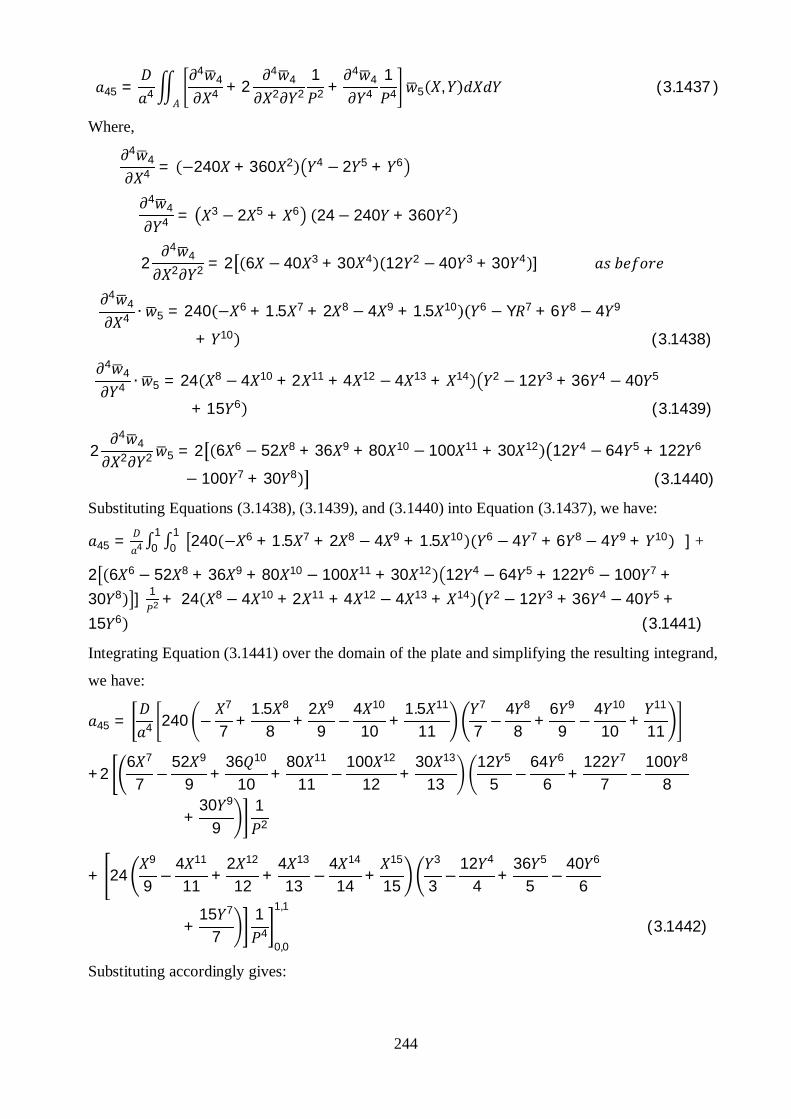
244

45 = 4

44

4 + 24

42 2

12 +

44

41

4 5 , (3.1437 )

Where,4

44 = −240 + 360 2 4 − 2 5 + 6

44

4 = 3 − 2 5 + 6 24− 240 + 360 2

24

42 2 = 2 6 − 40 3 + 30 4 12 2 − 40 3 + 30 4 ]

44

4 ∙ 5 = 240 − 6 + 1.5 7 + 2 8 − 4 9 + 1.5 10 6 − Y 7 + 6 8 − 4 9

+ 10 (3.1438)4

44 ∙ 5 = 24 8 − 4 10 + 2 11 + 4 12 − 4 13 + 14 2 − 12 3 + 36 4 − 40 5

+ 15 6 (3.1439)

24

42 2 5 = 2 6 6 − 52 8 + 36 9 + 80 10 − 100 11 + 30 12 12 4 − 64 5 + 122 6

− 100 7 + 30 8 (3.1440)


45 = 4 01

01 240 − 6 + 1.5 7 + 2 8 − 4 9 + 1.5 10 6 − 4 7 + 6 8 − 4 9 + 10 ]∫∫ +

2 6 6 − 52 8 + 36 9 + 80 10 − 100 11 + 30 12 12 4 − 64 5 + 122 6 − 100 7 +30 8 ] 1

2 + 24 8 − 4 10 + 2 11 + 4 12 − 4 13 + 14 2 − 12 3 + 36 4 − 40 5 +15 6 (3.1441)


we have:

45 = 4 240 −7

7+

1.5 8

8+

2 9

9 −4 10

10+

1.5 11

11

7

7 −4 8

8+

6 9

9 −4 10

10+

11

11

+26 7

7 −52 9

9 +36 10

10 +80 11

11 −100 12

12 +30 13

1312 5

5 −64 6

6 +122 7

7 −100 8

8

+30 9

91

2

+ 249

9 −4 11

11+

2 12

12+

4 13

13 −4 14

14+

15

15

3

3 −12 4

4+

36 5

5 −40 6

6

+15 7

71

40,0

1,1

(3.1442)


245

45 = 3.3545 × 10−4 + 7.0046 × 10−4 12 + 6.3682 × 10−4 1

4 (3.1443)

For 46 we have:

46 = 4

44

4 + 24

42 2

12 +

44

41

4 6 , (3.1444)

Where,4

44 = −240 + 360 2 4 − 2 5 + 6

44

4 = 3 − 2 5 + 6 24− 240 + 360 2

24

42 2 = 2 6 − 40 3 + 30 4 12 2 − 40 3 + 30 4 ]

44

4 ∙ 6 = 240 − 2 + 1.5 3 + 2 4 − 4 5 + 1.5X6 10 − 4 11 + 6 12 − 4 13

+ 14 (3.1445)4

44 ∙ 6 = 24 4 − 4 6 + 2 7 + 4 8 − 4 9 + 10 6 − 12 7 + 36 8 − 40 9

+ 15 10 (3.1446)

24

42 2 6 = 2 6 2 − 52 4 + 36 5 + 80 6 − 100 7 + 30 8 12 8 − 64 9 + 122 10

− 100 11 + 30 12 (3.1447)


46 = 4 01

01 240 − 2 + 1.5 3 + 2 4 − 4 5 + 1.5 6 10 − 4 11 + 6 12 − 4 13 + 14 ]∫∫ +

2 6 2 − 52 4 + 36 5 + 80 6 − 100 7 + 30 8 12 8 − 64 9 + 122 10 − 100 11 +30 12 ] 1

2 + 24 4 − 4 6 + 2 7 + 4 8 − 4 9 + 10 6 − 12 7 + 36 8 − 40 9 +15 10 (3.1448)


we have:

46 = 4 240 −3

3 +1.5 4

4 +2 5

5 −4 6

6 +1.5 7

7

11

11 −4 12

12 +6 13

13 −4 14

14 +15

15

+26 3

3−

52 5

5+

36 6

6+

80 7

7−

100 8

8+

30 9

912 9

9−

64 10

10+

122 11

11−

100 12

12

+30 13

131

2

246

+ 245

5 −4 7

7+

2 8

8+

4 9

9 −4 10

10+

11

11

7

7 −12 8

8+

36 9

9 −40 10

10

+15 11

111

40,0

1,1

(3.1449)


46 = −1.7126 × 10−4 + 3.8628 × 10−4 12 + 2.1701 × 10−3 1

4 (3.1450)


4 = 4 ,

=0

1

0

13 − 2 5 + 6 4 − 2 5 + 6 (3.1451)


=4

4 −2 6

6+

7

7

5

5 −2 6

6+

7

70,0

1,1

4 = 5.6689 × 10−4 (3.1452)

Hence,

4,1C1+ 4,2 2 + 4,3 3 + 4,4 4+ 4,5 5 + 4,6 6 = 5.6689 × 10−4 4 (3.1453)


51 = 4

45

4 + 24

52 2

12 +

45

41

4 1 , (3.1454)

Where,

5 = 5 − 2 7 + 8 2 − 2 3 + 4

45

4 = 120 − 14 3 + 14 4 2 − 2 3 + 4 (3.1455)

45

4 = 24 5 − 2 7 + 8 (3.1456)

24

52 2 = 2 20 3 − 84 5 + 56 6 2 − 12 + 12 2 ] (3.1457)

45

4 ∙ 1 = 120 2 − 16 4 + 15 5 + 28 6 − 42 7 + 14 8 4 − 4 5 + 6 6 − 4 7

+ 8 (3.1458)4

54 ∙ 1 = 24 6 − 4 8 + 2 9 + 4 10 − 4 11 + 12 2 − 2 3 + 4 (3.1459)

247

24

52 2 1 = 2 20 4 − 144 6 + 76 7 + 168 8 − 196 9 + 56 10 2 2 − 16 3 + 38 4

− 36 5 + 12 6 (3.1460)


51 = 4 01

01 120 2 − 16 4 + 15 5 + 28 6 − 42 7 + 14 8 4 − 4 5 + 6 6 − 4 7 + 8∫∫

+2 20 4 − 144 6 + 76 7 + 168 8 − 196 9 + 56 10 2 2 − 16 3 + 38 4 − 36 5 +

12 6 12 + 24 6 − 4 8 + 2 9 + 4 10 − 4 11 + 12 2 − 2 3 + 4 1

4 (3.1461)


we have:

51 = 4 1203

3−

16 5

5+

15 6

6+

28 7

7−

42 8

8+

14 9

9

5

5−

4 6

6+

6 7

7−

4 8

8+

9

9

+ 220 5

5 −124 7

7+

76 8

8+

168 9

9 −196 10

10+

56 11

112 3

3 −16 4

4+

38 5

5 −36 6

6

+12 7

71

2

+ 247

7−

4 9

9+

2 10

10+

4 11

11−

4 12

12+

13

13

3

3−

2 4

4+

5

51

40,0

1,1

(3.1462)


51 = −1.1640 × 10−2 + 2.1604 × 10−3 12 + 4.5110 × 10−3 1

4 (3.1463)

For 52 we have:

52 = 4

45

4 + 24

52 2

12 +

45

41

4 2 , (3.1464 )

Where,4

54 = 120 − 14 3 + 14 4 2 − 2 3 + 4 ;

45

4 = 24 5 − 2 7 + 8

24

52 2 = 2 20 3 − 84 5 + 56 6 2 − 12 + 12 2 ]

45

4 ∙ 2 = 120 4 − 16 6 + 15 7 + 28 8 − 42 9 + 14 10 4 − 4 5 + 6 6 − 4 7

+ 8 (3.1465)4

54 ∙ 2 = 24 8 − 4 10 + 2 11 + 4 12 − 4 13 + 14 2 − 2 3 + 4 (3.1466)

24

52 2 2 = 2 20 6 − 124 8 + 76 9 + 168 10 − 196 11 + 56 12 2 2 − 16 3 + 38 4

− 36 5 + 12 6 (3.1467)


248

52 = 4 01

01 120 4 − 16 6 + 15 7 + 28 8 − 42 9 + 14 10 4 − 4 5 + 6 6 − 4 7 +∫∫

8 +2 20 6 − 124 8 + 76 9 + 168 10 − 196 11 + 56 12 2 2 − 16 3 + 38 4 − 36 5 +

12 6 12 + 24 8 − 4 10 + 2 11 + 4 12 − 4 13 + 14 2 − 2 3 + 4 1

4 (3.1468)


we have:

52 = 4 1205

5−

16 7

7+

15 8

8+

28 9

9−

42 10

10+

14 11

11

5

5−

4 6

6+

6 7

7−

4 8

8+

9

9+

220 7

7−

124 9

9+

76 10

10+

168 11

11−

196 12

12+

56 13

132 3

3−

16 4

4 +38 5

5−

36 6

6

+12 7

71

2

+ 249

9−

4 11

11+

2 12

12+

4 13

13−

4 14

14+

15

15

3

3−

2 4

4 +5

51

40,0

1,1

(3.1469)


52 = −5.1192 × 10−3 + 2.8019 × 10−3 12 + 2.2289 × 10−3 1

4 (3.1470)

For 53 we have:

53 = 4

45

4 + 24

52 2

12 +

45

41

4 3 , (3.1471)

Where,4w5

4 = 120 − 14 3 + 14 4 2 − 2 3 + 4 ;4

54 = 24 5 − 2 7 + 8

24

52 2 = 2 20 3 − 84 5 + 56 6 2 − 12 + 12 2 ]

45

4 ∙ 3 = 120 2 − 16 4 + 15 5 + 28 6 − 42 7 + 14 8 6 − 4 7 + 6 8 − 4 9

+ 10 (3.1472)4

54 ∙ 3 = 24 6 − 4 8 + 2 9 + 4 10 − 4 11 + 12 4 − 2 5 + 6 (3.1473)

24

52 2 3 = 2 20 4 − 124 6 + 76 7 + 168 8 − 196 9 + 56 10 2 4 − 16 5 + 38 6

− 36 7 + 12 8 (3.1474)


249

53 = 4 01

01 120 2 − 16 4 + 15 5 + 28 6 − 42 7 + 14 8 6 − 4 7 + 6 8 − 4 9 +∫∫

10 +2 20 4 − 124 6 + 76 7 + 168 8 − 196 9 + 56 10 2 4 − 16 5 + 38 6 − 36 7 +

12 8 12 + 24 6 − 4 8 + 2 9 + 4 10 − 4 11 + 12 4 − 2 5 + 6 1

4 (3.1475)


we have:

53 = 4 1203

3−

16 5

5+

15 6

6+

28 7

7−

42 8

8+

14 9

9

7

7−

4 8

8+

6 9

9−

4 10

10+

11

11+

220 5

5−

124 7

7+

76 8

8+

168 9

9−

196 10

10+

56 11

112 5

5−

16 6

6+

38 7

7−

36 8

8

+12 9

91

2

+ 247

7−

4 9

9+

2 10

10+

4 11

11−

4 12

12+

13

13

5

5−

2 6

6+

7

71

40,0

1,1

(3.1476)


53 = −3.1746 × 10−3 + 5.4009 × 10−4 12 + 1.2889 × 10−3 1

4 (3.1477)

For 54 we have:

54 = 4

45

4 + 24

52 2

12 +

45

41

4 4 , (3.1478)

Where,4

54 = 120 − 14 3 + 14 4 2 − 2 3 + 4 ;

45

4 = 24 5 − 2 7 + 8

24

52 2 = 2 20 3 − 84 5 + 56 6 2− 12 + 12 2 ]

45

4 ∙ 4 = 120 4 − 16 6 + 15 7 + 28 8 − 42 9 + 14 10 6 − 4 7 + 6 8 − 4 9

+ 10 (3.1479)4

54 ∙ 4 = 24 8 − 4 10 + 2 11 + 4 12 − 4 13 + 14 4 − 2 5 + 6 (3.1480)

24

52 2 4 = 2 20 6 − 124 8 + 76 9 + 168 10 − 196 11 + 56 12 2 4 − 16 5 + 38 6

− 36 7 + 12 8 (3.1481)


250

54 = 4 01

01 120 4 − 16 6 + 15 7 + 28 8 − 42 9 + 14 10 6 − 4 7 + 6 8 − 4 9 +∫∫

10 +2 20 6 − 124 8 + 76 9 + 168 10 − 196 11 + 56 12 2 4 − 16 5 + 38 6 − 36 7 +

12 8 12 + 24 8 − 4 10 + 2 11 + 4 12 − 4 13 + 14 4 − 2 5 + 6 1

4 (3.1482


we have:

54 = 4 1205

5−

16 7

7+

15 8

8+

28 9

9−

42 10

10+

14 11

11

7

7−

4 8

8+

6 9

9−

4 10

10

+11

11 +

220 7

7 −124 9

9+

76 10

10+

168 11

11 −196 12

12+

56 13

132 5

5 −16 6

6+

38 7

7 −36 8

8

+12 9

91

2

+ 249

9 −4 11

11 +2 12

12 +4 13

13 −4 14

14 +15

15

5

5 −2 6

6 +7

71

40,0

1,1

(3.1483)


54 = −1.3962 × 10−3 + 7.0046 × 10−4 12 + 6.3682 × 10−4 1

4 (3.1484)

For 55 we have:

55 = 4

45

4 + 24

52 2

12 +

45

41

4 5 , (3.1485)

Where,4

54 = 120 − 14 3 + 14 4 2 − 2 3 + 4 ;

45

4 = 24 5 − 2 7 + 8

24

52 2 = 2 20 3 − 84 5 + 56 6 2 − 12 + 12 2 ]

45

4 ∙ 5 = 120 6 − 16 8 + 15 9 + 28 10 − 42 11 + 14 12 4 − 4 5 + 6 6 − 4 7

+ 8 (3.1486)4

54 ∙ 5 = 24 10 − 4 12 + 2 13 + 4 14 − 4 15 + 16 2 − 2 3 + 4 (3.1487)

24

52 2 5 = 2 20 8 − 124 10 + 76 11 + 168 12 − 196 13 + 56 14 2 2 − 16 3 + 38 4

− 36 5 + 12 6 (3.1488)


251

55 = 4 01

01 1120 6 − 16 8 + 15 9 + 28 10 − 42 11 + 14 12 4 − 4 5 + 6 6 − 4 7 +∫∫

8 +2 20 8 − 124 10 + 76 11 + 168 12 − 196 13 + 56 14 2 2 − 16 3 + 38 4 − 36 5 +

12 6 12 + 24 10 − 4 12 + 2 13 + 4 14 − 4 15 + 16 2 − 2 3 +

4 14 (3.1489)


we have:

55 = 4 1207

7 −16 9

9+

15 10

10+

28 11

11 −42 12

12+

14 13

13

5

5 −4 6

6+

6 7

7 −4 8

8

+9

9 +

220 9

9 −124 11

11 +76 12

12 +168 13

13 −196 14

14 +56 15

152 3

3 −16 4

4 +38 5

5 −36 6

6

+12 7

71

2

+ 2411

11 −4 13

13 +2 14

14 +4 15

15 −4 16

16 +17

17

3

3 −2 4

4 +5

51

40,0

1,1

(3.1490)


55 = −2.3891 × 10−3 + 2.3147 × 10−3 12 + 1.2513 × 10−3 1

4 (3.1491)

For 56 we have:

56 = 4

45

4 + 24

52 2

12 +

45

41

4 6 , (3.1492)

Where,4

54 = 120 − 14 3 + 14 4 2 − 2 3 + 4 ;

45

4 = 24 5 − 2 7 + 8

24

52 2 = 2 20 3 − 84 5 + 56 6 2− 12 + 12 2 ]

45

4 ∙ 6 = 120 2 − 16 4 + 15 5 + X − 42 7 + 14 8 8 − 4 9 + 6 10 − 4 11

+ 12 (3.1493)4

54 ∙ 6 = 24 6 − 4 8 + 2 9 + 4 10 − 4 11 + 12 6 − 2 7 + 8 (3.1494)

24

52 2 6 = 2 20 4 − 124 6 + 76 7 + 168 8 − 196 9 + 56 10 2 6 − 16 7 + 38 8

− 36 9 + 12 10 (3.1495)


252

56 = 4 01

01 120 2 − 16 4 + 15 5 + X − 42 7 + 14 8 8 − 4 9 + 6 10 − 4 11 + 12∫∫ +

2 20 4 − 124 6 + 76 7 + 168 8 − 196 9 + 56 10 2 6 − 16 7 + 38 8 − 36 9 +12 10 1

2 ++ 24 6 − 4 8 + 2 9 + 4 10 − 4 11 + 12 6 − 2 7 + 8 14 (3.1496)


we have:

56 = 4 1203

3−

16 5

5+

15 6

6+

28 7

7−

42 8

8+

14 9

9

9

9−

4 10

10+

6 11

11−

4 12

12

+13

13 +

220 5

5 −124 7

7+

76 8

8+

168 9

9 −196 10

10+

56 11

112 7

7 −16 8

8+

38 9

9 −36 10

10

+12 11

111

2

+ 247

7 −4 9

9 +2 10

10 +4 11

11 −4 12

12 +13

13

7

7 −2 8

8 +9

91

40,0

1,1

(3.1497)


56 = −1.1396 × 10−3 + 1.3093 × 10−4 12 + 5.3703 × 10−4 1

4 (3.1498)


5 = 5 ,

=0

1

0

15 − 2 7 + 8 2 − 2 3 + 4 (3.1499)


=6

6−

2 8

8+

9

9

3

3−

2 4

4+

5

50,0

1,1

5 = 9.2593 × 10−4 (3.1500)

Hence,

5,1 1+ 5,2 2 + 5,3 3 + 5,4 4+ 5,5 5 + 5,6 6 = 9.2593 × 10−4 4 (3.1501)


61 = 4

46

4 + 24

62 2

12 +

46

41

4 1 , (3.1502)

253

Where,

6 = − 2 3 + 4 6 − 2 7 + 8

46

4 = 24 6 − 2 7 + 8 (3.1503)

46

4 = 240 − 2 3 + 4 1.5 2 − 7 3 + 7 4 (3.1504)

24

62 2 = 2 −12 + 12 2 30 4 − 84 5 + 56 6 ] (3.1505)

46

4 ∙ 1 = 24 − 2 3 + 4 8 − 4 9 + 6 10 − 4 11 + 12 (3.1506)

46

4 ∙ 1 = 240 2 − 4 4 + 2 5 + 4 6 − 4 7 + 8 1.5 4 − 10 5 + 22.5 6 − 21 7

+ 7 8 (3.1507)

24

62 2 1 = 2 −12 2 + 12 3 + 24 4 − 36 5 + 12 6 30 6 − 144 7 + 254 8 − 196 6

+ 56 10 (3.1508)


61 = 4 01

01 24 − 2 3 + 4 8 − 4 9 + 6 10 − 4 11 + 12∫∫ +2 −12 2 + 12 3 +

24 4 − 36 5 + 12 6 30 6 − 144 7 + 254 8 − 196 6 + 56 10 12 + 240 2 − 4 4 +

2 5 + 4 6 − 4 7 + 8 1.5 4 − 10 5 + 22.5 6 − 21 7 + 7 8 14 (3.1509)


we have:

61 = 4 242

2−

2 4

4 +5

5Y9−

4 10

10+

6 11

11−

4 12

12+

13

13+

2 −12 3

3+

12 4

4+

24 5

5−

36 6

6+

12 7

730 7

7−

144 8

8+

254 9

9−

196 10

10

+56 11

111

2

+ 2403

3 −4 5

5 +2 6

6 +4 7

7 −4 8

8 +9

91.5 5

5 −10 6

6 +22.5 7

7 −21 8

8

+7 9

91

40,0

1,1

(3.1510)


61 = 7.4592 × 10−4 + 1.1214 × 10−3 12 + 4.6863 × 10−3 1

4 (3.1511)

For 62 we have:

254

62 = 4

46

4 + 24

62 2

12 +

46

41

4 2 , (3.1512)

Where,4

64 = 24 6 − 2 7 + 8 ;

46

4 = 240 − 2 3 + 4 1.5 2 − 7 3 + 7 4

24

62 2 = 2 −12 + 12 2 30 4 − 84 5 + 56 6 ]

46

4 ∙ 2 = 24 3 − 2 5 + 6 8 − 4 9 + 6 10 − 4 11 + 12 (3.1513)

46

4 ∙ 2 = 240 4 − 4 6 + 2 7 + 4 8 − 4 9 + 10 1.5 4 − 10 5 + 22.5 6 − 21 7

+ 7 8 (3.1514)

24

62 2 2 = 2 −12 4 + 12 5 + 24 6 − 36 7 + 12 8 30 6 − 144 7 + 254 8 − 196 6

+ 56 10 (3.1515)


62 = 4 01

01 24 3 − 2 5 + 6 8 − 4 9 + 6 10 − 4 11 + 12∫∫ +2 −12 4 + 12 5 +

24 6 − 36 7 + 12 8 30 6 − 144 7 + 254 8 − 196 6 + 56 10 12 + 240 4 − 4 6 +

2 7 + 4 8 − 4 9 + 10 1.5 4 − 10 5 + 22.5 6 − 21 7 + 7 8 14 (3.1516)


we have:

62 = 4 244

4 −2 6

6 +7

7

9

9 −4 10

10 +6 11

11 −4 12

12 +13

13 +

2 −12 5

5+

12 6

6+

24 7

7−

36 8

8+

12 9

930 7

7−

144 8

8+

254 9

9−

196 10

10

+56 11

111

2

+ 2405

5 −4 7

7 +2 8

8 +4 9

9 −4 10

10 +11

111.5 5

5 −10 6

6 +22.5 7

7 −21 8

8

+7 9

91

40,0

1,1

(3.1517)


62 = 2.2200 × 10−4 + 3.1883 × 10−4 12 + 1.3262 × 10−3 1

4 (3.1518)

For 63 we have:

255

63 = 4

46

4 + 24

62 2

12 +

46

41

4 3 , (3.1519)

Where,4

64 = 24 6 − 2 7 + 8 ;

46

4 = 240 − 2 3 + 4 1.5 2 − 7 3 + 7 4

24

62 2 = 2 −12 + 12 2 30 4 − 84 5 + 56 6 ]

46

4 ∙ 3 = 24 − 2 3 + 4 10 − 4 11 + 6 12 − 4 13 + 14 (3.1520)

46

4 ∙ 3 = 240 2 − 4 4 + 2 5 + 4 6 − 4 7 + 8 1.5 6 − 10 7 + 22.5 8 − 21 9

+ 7 10 (3.1521)

24

62 2 3 = 2 −12 2 + 12 3 + 24 4 − 36 5 + 12 6 30 8 − 144 9 + 254 10 − 196 11

+ 56 12 (3.1522)


63 = 4 01

01 24 − 2 3 + 4 10 − 4 11 + 6 12 − 4 13 + 14∫∫ +2 −12 2 + 12 3 +

24 4 − 36 5 + 12 6 30 8 − 144 9 + 254 10 − 196 11 + 56 12 12 + 240 2 − 4 4 +

2 5 + 4 6 − 4 7 + 8 1.5 6 − 10 7 + 22.5 8 − 21 9 + 7 10 14 (3.1523)


we have:

63 = 4 242

2−

2 4

4 +5

5

11

11−

4 12

12+

6 13

13−

4 14

14+

15

15+

2 −12 3

3+

12 4

4+

24 5

5 −36 6

6+

12 7

730 9

9 −144 10

10+

254 11

11 −196 12

12

+56 13

131

2

+ 2403

3 −4 5

5 +2 6

6 +4 7

7 −4 8

8 +9

91.5 7

7 −10 8

8 +22.5 9

9 −21 10

10

+7 11

111

40,0

1,1

(3.1524)


63 = 3.1968 × 10−4 + 1.3586 × 10−3 12 + 7.6685 × 10−3 1

4 (3.1525)

For 64 we have:

256

64 = 4

46

4 + 24

62 2

12 +

46

41

4 4 , (3.1526)

Where,4

64 = 24 6 − 2 7 + 8 ;

46

4 = 240 − 2 3 + 4 1.5 2 − 7 3 + 7 4

24

62 2 = 2 −12 + 12 2 30 4 − 84 5 + 56 6 ]

46

4 ∙ 4 = 24 3 − 2 5 + 6 10 − 4 11 + 6 12 − 4 13 + 14 (3.1527)

46

4 ∙ 4 = 240 4 − 4 6 + 2 7 + 4 8 − 4 9 + 10 1.5 6 − 10 7 + 22.5 8 − 21 9

+ 7 10 (3.1528)

24

62 2 4 = 2 −12 4 + 12 5 + 24 6 − 36 7 + 12 8 30 8 − 144 9 + 254 10 − 196 11

+ 56 12 (3.1529)


64 = 4 01

01 24 3 − 2 5 + 6 10 − 4 11 + 6 12 − 4 13 + 14∫∫ +2 −12 4 + 12 5 +

24 6 − 36 7 + 12 8 30 8 − 144 9 + 254 10 − 196 11 + 56 12 12 + 240 4 − 4 6 +

2 7 + 4 8 − 4 9 + 10 1.5 6 − 10 7 + 22.5 8 − 21 9 + 7 10 14 (3.1530)


we have:

64 = 4 244

4 −2 6

6+

7

7

11

11−

4 12

12+

6 13

13−

4 14

14+

15

15+

2 −12 5

5+

12 6

6+

24 7

7 −36 8

8+

12 9

930 9

9 −144 10

10+

254 11

11 −196 12

12

+56 13

131

2

+ 2405

5 −4 7

7 +2 8

8 +4 9

9 −4 10

10 +11

111.5 7

7 −10 8

8 +22.5 9

9 −21 10

10

+7 11

111

40,0

1,1

(3.1531)


64 = 9.5143 × 10−5 + 3.8628 × 10−4 12 + 2.1701 × 10−3 1

4 (3.1532)

For 65 we have:

257

65 = 4

46

4 + 24

62 2

12 +

46

41

4 5 , (3.1533)

Where,4

64 = 24 6 − 2 7 + 8 ;

46

4 = 240 − 2 3 + 4 1.5 2 − 7 3 + 7 4

24

62 2 = 2 −12 + 12 2 30 4 − 84 5 + 56 6 ]

46

4 ∙ 5 = 24 5 − 2 7 + 8 8 − 4 9 + 6 10 − 4 11 + 12 (3.1534)

46

4 ∙ 5 = 240 6 − 4 8 + 2 9 + 4 10 − 4 11 + 12 1.5 4 − 10 5 + 22.5 6 − 21 7

+ 7 8 (3.1535)

24

62 2 5 = 2 −12 6 + 12 7 + 24 8 − 36 9 + 12 10 30 6 − 144 7 + 254 8 − 196 9

+ 56 10 (3.1536)


65 = 4 01

01 [ 24 5 − 2 7 + 8 8 − 4 9 + 6 10 − 4 11 + 12∫∫ +2 −12 6 + 12 7 +

24 8 − 36 9 + 12 10 30 6 − 144 7 + 254 8 − 196 9 + 56 10 12 + 240 6 − 4 8 +

2 9 + 4 10 − 4 11 + 12 1.5 4 − 10 5 + 22.5 6 − 21 7 + 7 8 14 (3.1537)


we have:

65 = 4 246

6−

2 8

8+

9

9

9

9−

4 10

10+

6 11

11−

4 12

12+

13

13+

2 −12 7

7+

12 8

8+

24 9

9 −36 10

10+

12 11

1130 7

7 −144 8

8+

254 9

9 −196 10

10

+56 11

111

2

+ 2407

7−

4 9

9+

2 10

10+

4 11

11−

4 12

12+

13

131.5 5

5−

10 6

6+

22.5 7

7−

21 8

8

+7 9

91

40,0

1,1

(3.1538)


65 = 1.0360 × 10−4 + 1.3093 × 10−4 12 + 5.3703 × 10−4 1

4 (3.1539)

For 66 we have:

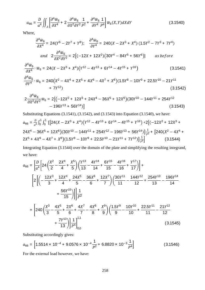
258

66 = 4

46

4 + 24

62 2

12 +

46

41

4 6 , (3.1540)

Where,4

64 = 24 6 − 2 7 + 8 ;

46

4 = 240 − 2 3 + 4 1.5 2 − 7 3 + 7 4

24

62 2 = 2 −12 + 12 2 30 4 − 84 5 + 56 6 ]

46

4 ∙ 6 = 24 − 2 3 + 4 12 − 4 13 + 6 14 − 4 15 + 16 (3.1541)

46

4 ∙ 6 = 240 2 − 4 4 + 2 5 + 4 6 − 4 7 + 8 1.5 8 − 10 9 + 22.5 10 − 21 11

+ 7 12 (3.1542)

24

62 2 6 = 2 −12 2 + 12 3 + 24 4 − 36 5 + 12 6 30 10 − 144 11 + 254 12

− 196 13 + 56 14 (3.1543)


66 = 4 01

01 [ 24 − 2 3 + 4 12 − 4 13 + 6 14 − 4 15 + 16∫∫ +2 −12 2 + 12 3 +

24 4 − 36 5 + 12 6 30 10 − 144 11 + 254 12 − 196 13 + 56 14 12 + 240 2 − 4 4 +

2 5 + 4 6 − 4 7 + 8 1.5 8 − 10 9 + 22.5 10 − 21 11 + 7 12 14 (3.1544)


we have:

66 = 4 242

2−

2 4

4 +5

5

13

13−

4 14

14+

6 15

15−

4 16

16+

17

17+

2 −12 3

3+

12 4

4+

24 5

5 −36 6

6+

12 7

730 11

11 −144 12

12+

254 13

13 −196 14

14

+56 15

151

2

+ 2403

3−

4 5

5+

2 6

6+

4 7

7−

4 8

8+

9

91.5 9

9−

10 10

10+

22.5 11

11−

21 12

12

+7 13

131

40,0

1,1

(3.1545)


66 = 1.5514 × 10−4 + 9.0576 × 10−4 12 + 6.8820 × 10−3 1

4 (3.1546)


259

6 = 6 ,

=0

1

0

1− 2 3 + 4 6 − 2 7 + 8 (3.1547)


=2

2 −2 4

4 +5

5

7

7 −2 8

8 +9

90,0

1,1

6 = 7.9365 × 10−4 (3.1548)

Hence,

6,1 1+ 6,2 2 + 6,3 3 + 6,4 4+ 6,5 5 + 6,6 6 = 7.9365 × 10−4 4 (3.1549)

Representing Equations (3.1309), (3.1370), (3.1405), (3.1453), (3.1501) and (3.1549) in matrix

form, we have:

1,1 1+ 1,2 2 + 1,3 3 + 1,4 4+ 1,5 5 + 1,6 6 = 6.6667 × 10−3 4

2,1 1+ 2,2 2 + 2,3 3 + 2,4 4+ 2,5 5 + 2,6 6 = 1.9841 × 10−3 4

3,1 1+ 3,2 2 + 3,3 3 + 3,4 4+ 3,5 5 + 3,6 6 = 1.9048 × 10−3 4

4,1 1+ 4,2 2 + 4,3 3 + 4,4 4+ 4,5 5 + 4,6 6 = 5.6689 × 10−4 4

5,1 1+ 5,2 2 + 5,3 3 + 5,4 4+ 5,5 5 + 5,6 6 = 9.2593 × 10−4 4

6,1 1+ 6,2 2 + 6,3 3 + 6,4 4+ 6,5 5 + 6,6 6 = 7.9365 × 10−4 4 (3.1550)


First Approximation

1 = 1

11

4

1 = 6.6667×10−3

11

4 (3.1551)


1,1 1,2 1,3

2,1 2,2 2,33,1 3,2 3,3

1

2

3

=1

2

3

4

1

2

3

=1,1 1,2 1,3

2,1 2,2 2,33,1 3,2 3,3

−1 6.6667 × 10−3

1.9841 × 10−3

1.9048 × 10−3

4

(3.1552)

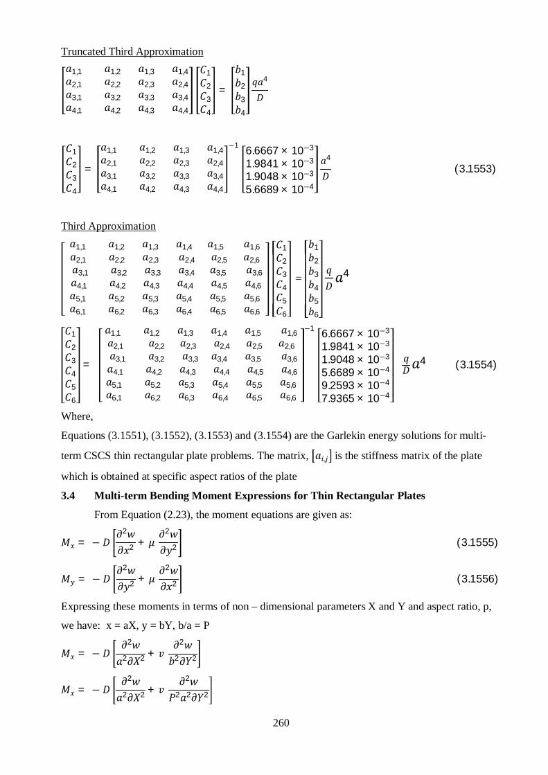
260


1,1 1,2 1,3 1,42,1 2,2 2,3 2,4

3,1 3,2 3,3 3,4

4,1 4,2 4,3 4,4

1

2

3

4

=1

2

3

4

4

1

2

3

4

=

1,1 1,2 1,3 1,42,1 2,2 2,3 2,4

3,1 3,2 3,3 3,4

4,1 4,2 4,3 4,4

−1 6.6667 × 10−3

1.9841 × 10−3

1.9048 × 10−3

5.6689 × 10−4

4

(3.1553)

Third Approximation

1,1 1,2 1,3 1,4 1,5 1,6

2,1 2,2 2,3 2,4 2,5 2,63,1 3,2 3,3 3,4 3,5 3,6

4,1 4,2 4,3 4,4 4,5 4,6

5,1 5,2 5,3 5,4 5,5 5,66,1 6,2 6,3 6,4 6,5 6,6

1

2

3

4

5

6

=

1

2

3

4

5

6

4

1

2

3

4

5

6

=

1,1 1,2 1,3 1,4 1,5 1,6

2,1 2,2 2,3 2,4 2,5 2,63,1 3,2 3,3 3,4 3,5 3,6

4,1 4,2 4,3 4,4 4,5 4,6

5,1 5,2 5,3 5,4 5,5 5,66,1 6,2 6,3 6,4 6,5 6,6

−1 6.6667 × 10−3

1.9841 × 10−3

1.9048 × 10−3

5.6689 × 10−4

9.2593 × 10−4

7.9365 × 10−4

4 (3.1554)

Where,

Equations (3.1551), (3.1552), (3.1553) and (3.1554) are the Garlekin energy solutions for multi-

term CSCS thin rectangular plate problems. The matrix, , is the stiffness matrix of the plate

which is obtained at specific aspect ratios of the plate

3.4 Multi-term Bending Moment Expressions for Thin Rectangular Plates

From Equation (2.23), the moment equations are given as:

= −2

2 +2

2 (3.1555)

= −2

2 +2

2 (3.1556)

Expressing these moments in terms of non – dimensional parameters X and Y and aspect ratio, p,

we have: x = aX, y = bY, b/a = P

= −2

2 2 +2

2 2

= −2

2 2 +2

2 2 2

261

=− 2

2

2 +2

2 2 (3.1557)

Similarly,

= − 2

2

2 +2

2 2 (3.1558)

The shape functions obtained in Equations (3.18), (3.34), (3.50), (3.70) and (3.85) for different

plate support conditions are substituted into the non – dimensional moment Equation (3.1557) and

(3.1558) as follows:


Figure 3.11 shows a thin rectangular plate with two opposite edges clamped and one of the other

two opposite edges clamped and the other simply supported.

Figure: 3.11: CCCS Plate under uniformly distributed load

The six term deflection functional is obtained in Equation (3.18) as:

, = 1 1.5 2 − 2. 5 3 + 4 2 − 2 3 + 4 + 2 (1.5 4 − 2. 5 5 + 6)( 2 − 2 3 +4) + 3 1.5 2 − 2.5 3 + 4 4 − 2 5 + 6 + 4 1.5 4 − 2.5 5 + 6 4 − 2 5 + 6 +

5 (1.5 6 − 2.5 7 + 8)( 2 − 2 3 + 4) + 6 1.5 2 − 2. 5 3 + 4 6 − 2 7 + 8

Where,2

2 = 1 3 − 15 + 12 2 ( 2 − 2 3 + 4) + 2 18 2 − 50 3 + 30 4 ( 2 − 2 3 + 4) +

3 3 − 15 + 12 2 4 − 2 5 + 6 + 4 18 2 − 50 3 + 30 4 4 − 2 5 + 6

+ 5 45 4 − 105 5 + 56 6 2 − 2 3 + 4 + 6 3 − 15 + 12 2

6 − 2 7 + 8 (3.1559)2

2 = 1 1.5 2 − 2.5 3 + 4 2 − 12 + 12 2 + 2(1.5 4 − 2.5 5 + 6) 2 − 12 + 12 2

+ 3 1.5 2 − 2.5 3 + 4 12 2 − 40 3 + 30 4

+ 4 1.5 4 − 2.5 5 + 6 12 2 − 40 3 + 30 4 + 5 1.5 6 − 2.5 7 + 8

2 − 12 + 12 2 + 6 1.5 2 − 2.5 3 + 4 30 4 − 84 5 + 56 6 (3.1560)

a

b

Y

X

262

=− 2

2

2 +2

2 2

=− 2 [ 1 3− 15 + 12 2 ( 2 − 2 3 + 4) + 2 18 2 − 50 3 + 30 4 ( 2 − 2 3 + 4

+ 3 3− 15 + 12 2 4 − 2 5 + 6 + 4 18 2 − 50 3 + 30 4

4 − 2 5 + 6 + 5 45 4 − 105 5 + 56 6 2 − 2 3 + 4 + 6 3− 15 + 12 2

6 − 2 7 + 8 ] + 2 1 1.5 2 − 2.5 3 + 4 2− 12 + 12 2 + 2 1.5 4 − 2.5 5 + 6

2− 12 + 12 2 ++ 3 1.5 2 − 2.5 3 + 4 12 2 − 40 3 + 30 4

+ 4 1.5 4 − 2.5 5 + 6 12 2 − 40 3 + 30 4 + 5 1.5 6 − 2.5 7 + 8

2 − 12 + 12 2 + 6 1.5 2 − 2.5 3 + 4 30 4 − 84 5 + 56 6 ]] (3.1561a)

In compact form, introducing the constant coefficient of the deflection coefficient, into Equation

(3.1561a), gives:

=− 2 [ 1 3− 15 + 12 2 ( 2 − 2 3 + 4) + 2 18 2 − 50 3 + 30 4 ( 2 − 2 3 + 4

+ 3 3− 15 + 12 2 4 − 2 5 + 6 + 4 18 2 − 50 3 + 30 4

4 − 2 5 + 6 + 5 45 4 − 105 5 + 56 6 2 − 2 3 + 4 + 6 3− 15 + 12 2

6 − 2 7 + 8 ] + 2 1 1.5 2 − 2.5 3 + 4 2− 12 + 12 2 + 2 1.5 4 − 2.5 5 + 6

2− 12 + 12 2 ++ 3 1.5 2 − 2.5 3 + 4 12 2 − 40 3 + 30 4

+ 4 1.5 4 − 2.5 5 + 6 12 2 − 40 3 + 30 4 + 5 1.5 6 − 2.5 7 + 8

2 − 12 + 12 2 + 6 1.5 2 − 2.5 3 + 4 30 4 − 84 5 + 56 6 ]] × 4

=− 1 3− 15 + 12 2 ( 2 − 2 3 + 4) + 2 18 2 − 50 3 + 30 4 ( 2 − 2 3 + 4)+ 3 3− 15 + 12 2 4 − 2 5 + 6 + 4 18 2 − 50 3 + 30 4

4 − 2 5 + 6 + 5 45 4 − 105 5 + 56 6 2 − 2 3 + 4 + 6 3− 15 + 12 2

6 − 2 7 + 8 ] + 2 1 1.5 2 − 2.5 3 + 4 2− 12 + 12 2 + 2 1.5 4 − 2.5 5 + 6

2− 12 + 12 2 + 3 1.5 2 − 2.5 3 + 4 12 2 − 40 3 + 30 4 + 4 1.5 4 − 2.5 5 + 6

12 2 − 40 3 + 30 4 + 5 1.5 6 − 2.5 7 + 8 2− 12 + 12 2

+ 6 1.5 2 − 2.5 3 + 4 30 4 − 84 5 + 56 6 ]] 2 (3.1561b)

= 2

=1

6

, , (3.1561c)

=− 1 3 − 15 + 12 2 ( 2 − 2 3 + 4) + 2 18 2 − 50 3 + 30 4 ( 2 − 2 3 + 4)+ 3 3 − 15 + 12 2 4 − 2 5 + 6 + 4 18 2 − 50 3 + 30 4

4 − 2 5 + 6 + 5 45 4 − 105 5 + 56 6 2 − 2 3 + 4 + 6 3− 15 + 12 2

6 − 2 7 + 8 ] + 2 1 1.5 2 − 2.5 3 + 4 2− 12 + 12 2 + 2 1.5 4 − 2.5 5 + 6

263

2− 12 + 12 2 + 3 1.5 2 − 2.5 3 + 4 12 2 − 40 3 + 30 4

+ 4 1.5 4 − 2.5 5 + 6 12 2 − 40 3 + 30 4 + 5 1.5 6 − 2.5 7 + 8

2 − 12 + 12 2 + 6 1.5 2 − 2.5 3 + 4 30 4 − 84 5 + 56 6 ]] ( 3.1561d)

Similarly,

= − 2

2

2 +2

2 2

=− 2 1 3− 15 + 12 2 ( 2 − 2 3 + 4) + 2 18 2 − 50 3 + 30 4 ( 2 − 2 3 + 4

+ 3 3− 15 + 12 2 4 − 2 5 + 6 + 4 18 2 − 50 3 + 30 4

4 − 2 5 + 6 + 5 45 4 − 105 5 + 56 6 2 − 2 3 + 4 + 6 3− 15 + 12 2

6 − 2 7 + 8 ] +1

2 1 1.5 2 − 2.5 3 + 4 2− 12 + 12 2 + 2 1.5 4 − 2.5 5 + 6

2− 12 + 12 2 ++ 3 1.5 2 − 2.5 3 + 4 12 2 − 40 3 + 30 4

+ 4 1.5 4 − 2.5 5 + 6 12 2 − 40 3 + 30 4 + 5 1.5 6 − 2.5 7 + 8

2 − 12 + 12 2

+ 6 1.5 2 − 2.5 3 + 4 30 4 − 84 5 + 56 6 ]] (3.1562a)


(3.1562a), gives:

=− 2 1 3− 15 + 12 2 ( 2 − 2 3 + 4) + 2 18 2 − 50 3 + 30 4 ( 2 − 2 3 + 4

+ 3 3− 15 + 12 2 4 − 2 5 + 6 + 4 18 2 − 50 3 + 30 4

4 − 2 5 + 6 + 5 45 4 − 105 5 + 56 6 2 − 2 3 + 4 + 6 3− 15 + 12 2

6 − 2 7 + 8 ] +1

2 1 1.5 2 − 2.5 3 + 4 2− 12 + 12 2 + 2 1.5 4 − 2.5 5 + 6

2− 12 + 12 2 ++ 3 1.5 2 − 2.5 3 + 4 12 2 − 40 3 + 30 4

+ 4 1.5 4 − 2.5 5 + 6 12 2 − 40 3 + 30 4 + 5 1.5 6 − 2.5 7 + 8

2 − 12 + 12 2 + 6 1.5 2 − 2.5 3 + 4 30 4 − 84 5 + 56 6 ]] × 4

=− 1 3− 15 + 12 2 ( 2 − 2 3 + 4) + 2 18 2 − 50 3 + 30 4 ( 2 − 2 3 + 4)+ 3 3− 15 + 12 2 4 − 2 5 + 6 + 4 18 2 − 50 3 + 30 4

4 − 2 5 + 6 + 5 45 4 − 105 5 + 56 6 2 − 2 3 + 4 + 6 3− 15 + 12 2

6 − 2 7 + 8 ] +1

2 1 1.5 2 − 2.5 3 + 4 2− 12 + 12 2 + 2 1.5 4 − 2.5 5 + 6

2− 12 + 12 2 ++ 3 1.5 2 − 2.5 3 + 4 12 2 − 40 3 + 30 4

+ 4 1.5 4 − 2.5 5 + 6 12 2 − 40 3 + 30 4 + 5 1.5 6 − 2.5 7 + 8

2 − 12 + 12 2 + 6 1.5 2 − 2.5 3 + 4 30 4 − 84 5 + 56 6 ]] 2 (3.1562b)

= 2

=1

6

, , (3.1562c)

264

=− 1 3 − 15 + 12 2 ( 2 − 2 3 + 4) + 2 18 2 − 50 3 + 30 4 ( 2 − 2 3 + 4

+ 3 3 − 15 + 12 2 4 − 2 5 + 6 + 4 18 2 − 50 3 + 30 4

4 − 2 5 + 6 + 5 45 4 − 105 5 + 56 6 2 − 2 3 + 4 + 6 3− 15 + 12 2

6 − 2 7 + 8 ] +1

2 1 1.5 2 − 2.5 3 + 4 2− 12 + 12 2 + 2 1.5 4 − 2.5 5 + 6

2− 12 + 12 2 ++ 3 1.5 2 − 2.5 3 + 4 12 2 − 40 3 + 30 4

+ 4 1.5 4 − 2.5 5 + 6 12 2 − 40 3 + 30 4 + 5 1.5 6 − 2.5 7 + 8

2 − 12 + 12 2 + 6 1.5 2 − 2.5 3 + 4 30 4 − 84 5 + 56 6 ]] (3.1562d)

Where, and are the bending moment coefficients along x and y directions respectively for

the six term deflection functional for the CCCS plate.

3.4. 2 Case 2 (Type SSSS)

Figure 3.12 shows a thin rectangular whose all edges are simply supported.

0

Figure: 3.12: SSSS Plate under uniformly distributed load


, = 1( − 2 3 + 4 )( − 2 3 + 4) + 2( 3 − 2 5 + 6)( − 2 3 + 4) +

3 − 2 3 + 4 3 − 2 5 + 6 + 4( 3 − 2 5 + 6) 3 − 2 5 + 6 +

5( 5 − 2 7 + 8)( − 2 3 + 4) + 6 − 2 3 + 4 5 − 2 7 + 8

Where,2

2 = 12 1 − + 2 ( − 2 3 + 4) + 4 2 1.5 − 10 3 + 7.5 4 ( − 2 3 + 4) +

12 3 − + 2 3 − 2 5 + 6 + 4 4 1.5 − 10 3 + 7.5 4 3 − 2 5 + 6

+ 5 20 3 − 84 5 + 56 6 − 2 3 + 4

+ 12 6 − + 2 5 − 2 7 + 8 (3.1563)2

2 = 12 1( − 2 3 + 4 ) − + 2 + 12 2( 3 − 2 5 + 6) − + 2 +

4 3 − 2 3 + 4 1.5 − 10 3 + 7.5 4 + 4 4( 3 − 2 5 + 6 ) 1.5 − 10 3 + 7.5 4 +12 5( 5 − 2 7 + 8) − + 2 + 6 − 2 3 + 4 20 3 − 84 5 + 56 6 (3.1564)

a

bY

X

265

=− 2

2

2 +2

2 2

=− 2 [12 1 − + 2 ( − 2 3 + 4) + 4 2 1.5 − 10 3 + 7.5 4 ( − 2 3 + 4) +

12 3 − + 2 3 − 2 5 + 6 + 4 4 1.5 − 10 3 + 7.5 4 3 − 2 5 + 6

+ 5 20 3 − 84 5 + 56 6 − 2 3 + 4

+ 12 6 − + 2 5 − 2 7 + 8 ] + 2 [12 1( − 2 3 + 4 ) − + 2

+12 2( 3 − 2 5 + 6) − + 2 + 4 3 − 2 3 + 4 1.5 − 10 3 + 7.5 4 + 4 4( 3

− 2 5 + 6 ) 1.5 − 10 3 + 7.5 4 + 12 5( 5 − 2 7 + 8) − + 2

+ 6 − 2 3 + 4 20 3 − 84 5 + 56 6 ]] (3.1565a)


(3.1565a), gives:

=− 2 12 1 − + 2 ( − 2 3 + 4) + 4 2 1.5 − 10 3 + 7.5 4 ( − 2 3 + 4) +

12 3 − + 2 3 − 2 5 + 6 + 4 4 1.5 − 10 3 + 7.5 4 3 − 2 5 + 6

+ 5 20 3 − 84 5 + 56 6 − 2 3 + 4

+ 12 6 − + 2 5 − 2 7 + 8 ] ] +

+ 2 [12 1( − 2 3 + 4 ) − + 2 + 12 2( 3 − 2 5 + 6) − + 2 +

4 3 − 2 3 + 4 1.5 − 10 3 + 7.5 4 + 4 4( 3 − 2 5 + 6 ) 1.5 − 10 3 + 7.5 4 +12 5( 5 − 2 7 + 8) − + 2 + 6 − 2 3 + 4 20 3 − 84 5 + 56 6 ]] × 4

=− 12 1 − + 2 ( − 2 3 + 4) + 4 2 1.5 − 10 3 + 7.5 4 ( − 2 3 + 4) +

12 3 − + 2 3 − 2 5 + 6 + 4 4 1.5 − 10 3 + 7.5 4 3 − 2 5 + 6 + 5 20 3 −84 5 + 56 6 − 2 3 + 4 +12 6 − + 2 5 − 2 7 + 8 ]] +

2 [12 1( − 2 3 + 4 ) − + 2 + 12 2( 3 − 2 5 + 6) − + 2 +

4 3 − 2 3 + 4 1.5 − 10 3 + 7.5 4 + 4 4( 3 − 2 5 + 6 ) 1.5 − 10 3 + 7.5 4 +12 5( 5 − 2 7 + 8) − + 2 + 6 − 2 3 + 4 20 3 − 84 5 + 56 6 ]] (3.1565b)

= 2

=1

6

, , = 2 , , (3.1565c)

=− 12 1 − + 2 ( − 2 3 + 4) + 4 2 1.5 − 10 3 + 7.5 4 ( − 2 3 + 4)

2 3 − + 2 3 − 2 5 + 6 + 4 4 1.5 − 10 3 + 7.5 4 3 − 2 5 + 6 + 5 20 3 −84 5 + 56 6 − 2 3 + 4 + 12 6 − + 2 5 − 2 7 + 8 ]

+ 2 12 1( − 2 3 + 4 ) − + 2 + 12 2( 3 − 2 5 + 6) − + 2 +

266

4 3 − 2 3 + 4 1.5 − 10 3 + 7.5 4 + 4 43 − 2 5 + 6 1.5 − 10 3 + 7.5 4 +

12 55 − 2 7 + 8 − + 2 + 6 − 2 3 + 4 20 3 − 84 5 + 56 6 (3.1565d)

Similarly,

= − 2

2

2 +2

2 2

=− 2 [12 1 − + 2 ( − 2 3 + 4) + 4 2 1.5 − 10 3 + 7.5 4 ( − 2 3 + 4)

2 3 − + 2 3 − 2 5 + 6 + 4 4 1.5 − 10 3 + 7.5 4 3 − 2 5 + 6 + 5 20 3 −84 5 + 56 6 − 2 3 + 4 + 12 6 − + 2 5 − 2 7 + 8 ] +

12 12 1( − 2 3 + 4 ) − + 2 + 12 2( 3 − 2 5 + 6) − + 2 +

4 3 − 2 3 + 4 1.5 − 10 3 + 7.5 4 + 4 43 − 2 5 + 6 1.5 − 10 3 + 7.5 4

+ 12 55 − 2 7 + 8 − + 2

6 − 2 3 + 4 20 3 − 84 5

+ 56 6 (3.1566a)


(3.1566a), gave:

=− 2 [12 1 − + 2 ( − 2 3 + 4) + 4 2 1.5 − 10 3 + 7.5 4 ( − 2 3 + 4)

2 3 − + 2 3 − 2 5 + 6 + 4 4 1.5 − 10 3 + 7.5 4 3 − 2 5 + 6 + 5 20 3 −84 5 + 56 6 − 2 3 + 4 + 12 6 − + 2 5 − 2 7 + 8 ] +

12 12 1( − 2 3 + 4 ) − + 2 + 12 2( 3 − 2 5 + 6) − + 2 +4 3 − 2 3 + 4

1.5 − 10 3 + 7.5 4 + 4 43 − 2 5 + 6 1.5 − 10 3 + 7.5 4

+12 55 − 2 7 + 8 − + 2

6 − 2 3 + 4 20 3 − 84 5 + 56 6 × 4

=− [12 1 − + 2 ( − 2 3 + 4) + 4 2 1.5 − 10 3 + 7.5 4 ( − 2 3 + 4)

2 3 − + 2 3 − 2 5 + 6 + 4 4 1.5 − 10 3 + 7.5 4 3 − 2 5 + 6 + 5 20 3 −84 5 + 56 6 − 2 3 + 4 + 12 6 − + 2 5 − 2 7 + 8 ] +

12 12 1( − 2 3 + 4 ) − + 2 + 12 2( 3 − 2 5 + 6) − + 2 +4 3 − 2 3 + 4

1.5 − 10 3 + 7.5 4 + 4 43 − 2 5 + 6 1.5 − 10 3 + 7.5 4

+ 12 55 − 2 7 + 8 − + 2 + 6 − 2 3 + 4

20 3 − 84 5 + 56 6 2 (3.1566b)

= 2

=1

6

, , = 2 , , (3.1566c)

267

=− [12 1 − + 2 ( − 2 3 + 4) + 4 2 1.5 − 10 3 + 7.5 4 ( − 2 3 + 4)

2 3 − + 2 3 − 2 5 + 6 + 4 4 1.5 − 10 3 + 7.5 4 3 − 2 5 + 6 + 5 20 3 −84 5 + 56 6 − 2 3 + 4 + 12 6 − + 2 5 − 2 7 + 8 ] +

12 12 1( − 2 3 + 4 ) − + 2 + 12 2( 3 − 2 5 + 6) − + 2 +4 3 − 2 3 + 4

1.5 − 10 3 + 7.5 4 + 4 43 − 2 5 + 6 1.5 − 10 3 + 7.5 4

+ 12 55 − 2 7 + 8 − + 2

+ 6 − 2 3 + 4 20 3 − 84 5 + 56 6 (3.1566d)


the six term deflection functional for the SSSS plate.


Figure 3.13 shows a thin rectangular whose all edges are clamped.

0

Figure: 3.13: CCCC Plate under uniformly distributed load


, = 12 − 2 3 + 4 2 − 2 3 + 4 + 2 ( 4 − 2 5 + 6)( 2 − 2 3 + 4) +

32 − 2 3 + 4 4 − 2 5 + 6 + 4

4 − 2 5 + 6 4 − 2 5 + 6 + 5 ( 6 − 2 7

+ 8)( 2 − 2 3 + 4) + 62 − 2 3 + 4 6 − 2 7 + 8

Where,2

2 = 2 1 1− 6 + 6 2 ( 2 − 2 3 + 4) + 4 2 3 2 − 10 3 + 7.5 4 ( 2 − 2 3 + 4) +

2 3 1 − 6 + 6 2 4 − 2 5 + 6 + 4 4 3 2 − 10 3 + 7.5 4 4 − 2 5 + 6 + 5 (30 4

− 84 5 + 56 6)( 2 − 2 3 + 4)+ 2 6 1 − 12 + 12 2 6 − 2 7 + 8 (3.1567)

2

2 = 2 12 − 2 3 + 4 1 − 6 + 6 2 + 2 2( 4 − 2 5 + 6) 1 − 6 + 6 2 +

4 32 − 2 3 + 4 3 2 − 10 3 + 7.5 4 + 4 4

4 − 2 5 + 6 3 2 − 10 3 + 30 4

+ 2 56 − 2 7 + 8 1 − 6 + 6 2 + 6

2 − 2 3 + 4

a

bY

X

268

30 4 − 84 5 + 56 6 (3.1568)

=− 2

2

2 +2

2 2

=− 2 2 1 1− 6 + 6 2 ( 2 − 2 3 + 4) + 4 2 3 2 − 10 3 + 7.5 4 ( 2 − 2 3 + 4) +

2 3 1 − 6 + 6 2 4 − 2 5 + 6 + 4 4 3 2 − 10 3 + 7.5 4 4 − 2 5 + 6 + 5 (30 4

− 84 5 + 56 6)( 2 − 2 3 + 4) + 2 6 1 − 6 + 6 2 6 − 2 7 + 8 +

2 2 12 − 2 3 + 4 1 − 6 + 6 2 + 2 2( 4 − 2 5 + 6) 1− 6 + 6 2 +

4 32 − 2 3 + 4 3 2 − 10 3 + 7.5 4 + 4 4

4 − 2 5 + 6 3 2 − 10 3 + 7.5 4

+ 2 5 ( 6 − 2 7 + 8)(1 − 6 + 6 2)+ 6

2 − 2 3 + 4 30 4 − 84 5 + 56 6 (3.1569a)


(3.1569a), gave:

=− 2 2 1 1− 6 + 6 2 ( 2 − 2 3 + 4) + 4 2 3 2 − 10 3 + 7.5 4 ( 2 − 2 3 + 4) +

2 3 1 − 6 + 6 2 4 − 2 5 + 6 + 4 4 3 2 − 10 3 + 7.5 4 4 − 2 5 + 6 + 5 (30 4

− 84 5 + 56 6)( 2 − 2 3 + 4) + 2 6 1 − 6 + 6 2 6 − 2 7 + 8 +

2 2 12 − 2 3 + 4 1 − 6 + 6 2 + 2 2( 4 − 2 5 + 6) 1− 6 + 6 2 +

4 32 − 2 3 + 4 3 2 − 10 3 + 7.5 4 + 4 4

4 − 2 5 + 6 3 2 − 10 3 + 7.5 4

+ 2 5 ( 6 − 2 7 + 8)(1 − 6 + 6 2)+ 6

2 − 2 3 + 4 30 4 − 84 5 + 56 6 × 4

=− 2 1 1− 6 + 6 2 ( 2 − 2 3 + 4) + 4 2 3 2 − 10 3 + 7.5 4 ( 2 − 2 3 + 4) +

2 3 1 − 6 + 6 2 4 − 2 5 + 6 + 4 4 3 2 − 10 3 + 7.5 4 4 − 2 5 + 6 + 5 (30 4

− 84 5 + 56 6)( 2 − 2 3 + 4) + 2 6 1 − 6 + 6 2 6 − 2 7 + 8 +

2 2 12 − 2 3 + 4 1 − 6 + 6 2 + 2 2( 4 − 2 5 + 6) 1− 6 + 6 2 +

4 32 − 2 3 + 4 3 2 − 10 3 + 7.5 4 + 4 4

4 − 2 5 + 6 3 2 − 10 3 + 7.5 4

+ 2 5 ( 6 − 2 7 + 8)(1 − 6 + 6 2)+ 6

2 − 2 3 + 4 30 4 − 84 5 + 56 6 2 (3.1569b)

= 2

=1

6

, , = 2 , , (3.1569c)

=− 2 1 1 − 6 + 6 2 ( 2 − 2 3 + 4) + 4 2 3 2 − 10 3 + 7.5 4 ( 2 − 2 3 + 4) +

2 3 1 − 6 + 6 2 4 − 2 5 + 6 + 4 4 3 2 − 10 3 + 7.5 4 4 − 2 5 + 6 + 5 (30 4

− 84 5 + 56 6)( 2 − 2 3 + 4) + 2 6 1 − 6 + 6 2 6 − 2 7 + 8 +

269

2 2 12 − 2 3 + 4 1 − 6 + 6 2 + 2 2( 4 − 2 5 + 6) 1− 6 + 6 2 +

4 32 − 2 3 + 4 3 2 − 10 3 + 7.5 4 + 4 4

4 − 2 5 + 6 3 2 − 10 3 + 7.5 4

+ 2 5 ( 6 − 2 7 + 8)(1 − 6 + 6 2)+ 6

2 − 2 3 + 4 30 4 − 84 5 + 56 6 (3.1569d)

Similarly,

= − 2

2

2 +2

2 2

=− 2 2 1 1 − 6 + 6 2 ( 2 − 2 3 + 4) + 4 2 3 2 − 10 3 + 7.5 4 ( 2 − 2 3 + 4) +

2 3 1 − 6 + 6 2 4 − 2 5 + 6 + 4 4 3 2 − 10 3 + 7.5 4 4 − 2 5 + 6 + 5 (30 4

− 84 5 + 56 6)( 2 − 2 3 + 4) + 2 6 1 − 6 + 6 2 6 − 2 7 + 8 +

12 2 1

2 − 2 3 + 4 1 − 6 + 6 2 + 2 2( 4 − 2 5 + 6) 1− 6 + 6 2 +

4 32 − 2 3 + 4 3 2 − 10 3 + 7.5 4 + 4 4

4 − 2 5 + 6 3 2 − 10 3 + 7.5 4

+ 2 5 ( 6 − 2 7 + 8)(1 − 6 + 6 2)+ 6

2 − 2 3 + 4 30 4 − 84 5 + 56 6 (3.1570a)


(3.1570a), gives:

=− 2 2 1 1 − 6 + 6 2 ( 2 − 2 3 + 4) + 4 2 3 2 − 10 3 + 7.5 4 ( 2 − 2 3 + 4) +

2 3 1 − 6 + 6 2 4 − 2 5 + 6 + 4 4 3 2 − 10 3 + 7.5 4 4 − 2 5 + 6 + 5 (30 4

− 84 5 + 56 6)( 2 − 2 3 + 4) + 2 6 1 − 6 + 6 2 6 − 2 7 + 8 +

12 2 1

2 − 2 3 + 4 1 − 6 + 6 2 + 2 2( 4 − 2 5 + 6) 1− 6 + 6 2 +

4 32 − 2 3 + 4 3 2 − 10 3 + 7.5 4 + 4 4

4 − 2 5 + 6 3 2 − 10 3 + 7.5 4

+ 2 5 ( 6 − 2 7 + 8)(1 − 6 + 6 2)+ 6

2 − 2 3 + 4 30 4 − 84 5 + 56 6 × 4

=− 2 1 1 − 6 + 6 2 ( 2 − 2 3 + 4) + 4 2 3 2 − 10 3 + 7.5 4 ( 2 − 2 3 + 4) +

2 3 1 − 6 + 6 2 4 − 2 5 + 6 + 4 4 3 2 − 10 3 + 7.5 4 4 − 2 5 + 6 + 5 (30 4

− 84 5 + 56 6)( 2 − 2 3 + 4) + 2 6 1 − 6 + 6 2 6 − 2 7 + 8 +

12 2 1

2 − 2 3 + 4 1 − 6 + 6 2 + 2 2( 4 − 2 5 + 6) 1− 6 + 6 2 +

4 32 − 2 3 + 4 3 2 − 10 3 + 7.5 4 + 4 4

4 − 2 5 + 6 3 2 − 10 3 + 7.5 4

+ 2 5 ( 6 − 2 7 + 8)(1 − 6 + 6 2)+ 6

2 − 2 3 + 4 30 4 − 84 5 + 56 6 2 (3.1570b)

270

= 2

=1

6

, , = 2 , , (3.1570c)

=− 2 1 1 − 6 + 6 2 ( 2 − 2 3 + 4) + 4 2 3 2 − 10 3 + 7.5 4 ( 2 − 2 3 + 4) +

2 3 1 − 6 + 6 2 4 − 2 5 + 6 + 4 4 3 2 − 10 3 + 7.5 4 4 − 2 5 + 6 + 5 (30 4

− 84 5 + 56 6)( 2 − 2 3 + 4) + 2 6 1 − 6 + 6 2 6 − 2 7 + 8 +

12 2 1

2 − 2 3 + 4 1 − 6 + 6 2 + 2 2( 4 − 2 5 + 6) 1− 6 + 6 2 +

4 32 − 2 3 + 4 3 2 − 10 3 + 7.5 4 + 4 4

4 − 2 5 + 6 3 2 − 10 3 + 7.5 4

+ 2 5 ( 6 − 2 7 + 8)(1 − 6 + 6 2)+ 6

2 − 2 3 + 4 30 4 − 84 5 + 56 6 (3.1570d)


the six term deflection functional for the CCCC plate.


Figure 3.14 shows a thin rectangular plate clamped on two adjacent near edges and simply

supported on two adjacent far edges.

0

Figure 3.14: CCSS Plate under uniformly distributed load.


, = 1 1.5 2 − 2.5 3 + 4 1.5 2 − 2.5 3 + 4 + 2 (1.5 4 − 2. 5 5 + 6)(1.5 2 −2.5 3 + 4) + 3 1.5 2 − 2. 5 3 + 4 1.5 4 − 2.5 5 + 6 + 4 1.5 4 − 2.5 5 +

6 1.5 4 − 2. 5 5 + 6 + 5 (1.5 6 − 2.5 7 + 8)(1.5 2 − 2.5 3 + 4) + 6 1.5 2 −2.5 3 + 4 1.5 6 − 2.5 7 + 8

Where,2

2 = 1 3 − 15 + 12 2 (1.5 2 − 2.5 3 + 4) + 2 18 2 − 50 3 + 30 4 (1.5 2 − 2.5 3

+ 4) + 3 3 − 15 + 12 2 1.5 4 − 2. 5 5 + 6

+ 4 18 2 − 50 3 + 30 4 1.5 4 − 2.5 5 + 6

a

bY

X

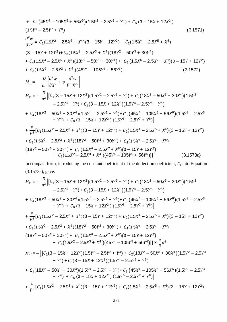
271

+ 5 45 4 − 105 5 + 56 6 1.5 2 − 2.5 3 + 4 + 6 3 − 15 + 12 2

1.5 6 − 2.5 7 + 8 (3.1571)2

2 = 1 1.5 2 − 2.5 3 + 4 3 − 15 + 12 2 + 2(1.5 4 − 2.5 5 + 6)

3− 15 + 12 2 + 3 1.5 2 − 2.5 3 + 4 18 2 − 50 3 + 30 4

+ 4 1.5 4 − 2.5 5 + 6 18 2 − 50 3 + 30 4 + 5 1.5 6 − 2. 5 7 + 8 3 − 15 + 12 2

+ 6 1.5 2 − 2.5 3 + 4 45 4 − 105 5 + 56 6 (3.1572)

=− 2

2

2 +2

2 2

=− 2 1 3− 15 + 12 2 (1.5 2 − 2.5 3 + 4) + 2 18 2 − 50 3 + 30 4 (1.5 2

− 2.5 3 + 4) + 3 3− 15 + 12 2 1.5 4 − 2. 5 5 + 6

+ 4 18 2 − 50 3 + 30 4 1.5 4 − 2.5 5 + 6 + 5 45 4 − 105 5 + 56 6 1.5 2 − 2.5 3

+ 4 + 6 3 − 15 + 12 2 1.5 6 − 2.5 7 + 8

+ 2 [ 1 1.5 2 − 2.5 3 + 4 3 − 15 + 12 2 + 2(1.5 4 − 2.5 5 + 6) 3− 15 + 12 2

+ 3 1.5 2 − 2.5 3 + 4 18 2 − 50 3 + 30 4 + 4 1.5 4 − 2.5 5 + 6

18 2 − 50 3 + 30 4 + 5 1.5 6 − 2. 5 7 + 8 3− 15 + 12 2

+ 6 1.5 2 − 2.5 3 + 4 45 4 − 105 5 + 56 6 ]] (3.1573a)


(3.1573a), gave:

=− 2 1 3− 15 + 12 2 (1.5 2 − 2.5 3 + 4) + 2 18 2 − 50 3 + 30 4 (1.5 2

− 2.5 3 + 4) + 3 3− 15 + 12 2 1.5 4 − 2. 5 5 + 6

+ 4 18 2 − 50 3 + 30 4 1.5 4 − 2.5 5 + 6 + 5 45 4 − 105 5 + 56 6 1.5 2 − 2.5 3

+ 4 + 6 3 − 15 + 12 2 1.5 6 − 2.5 7 + 8

+ 2 [ 1 1.5 2 − 2.5 3 + 4 3 − 15 + 12 2 + 2(1.5 4 − 2.5 5 + 6) 3− 15 + 12 2

+ 3 1.5 2 − 2.5 3 + 4 18 2 − 50 3 + 30 4 + 4 1.5 4 − 2.5 5 + 6

18 2 − 50 3 + 30 4 + 5 1.5 6 − 2. 5 7 + 8 3− 15 + 12 2

+ 6 1.5 2 − 2.5 3 + 4 45 4 − 105 5 + 56 6 ]] × 4

=− 1 3− 15 + 12 2 (1.5 2 − 2.5 3 + 4) + 2 18 2 − 50 3 + 30 4 (1.5 2 − 2.5 3

+ 4) + 3 3− 15 + 12 2 1.5 4 − 2. 5 5 + 6

+ 4 18 2 − 50 3 + 30 4 1.5 4 − 2.5 5 + 6 + 5 45 4 − 105 5 + 56 6 1.5 2 − 2.5 3

+ 4 + 6 3 − 15 + 12 2 1.5 6 − 2.5 7 + 8

+ 2 [ 1 1.5 2 − 2.5 3 + 4 3 − 15 + 12 2 + 2(1.5 4 − 2.5 5 + 6) 3− 15 + 12 2

272

+ 3 1.5 2 − 2.5 3 + 4 18 2 − 50 3 + 30 4 + 4 1.5 4 − 2.5 5 + 6

18 2 − 50 3 + 30 4 + 5 1.5 6 − 2. 5 7 + 8 3− 15 + 12 2

+ 6 1.5 2 − 2.5 3 + 4 45 4 − 105 5 + 56 6 ] 2 (3.1573b)

= 2

=1

6

, , = 2 , , (3.1573c)

=− 1 3 − 15 + 12 2 (1.5 2 − 2.5 3 + 4) + 2 18 2 − 50 3 + 30 4 (1.5 2 − 2.5 3

+ 4) + 3 3 − 15 + 12 2 1.5 4 − 2. 5 5 + 6

+ 4 18 2 − 50 3 + 30 4 1.5 4 − 2.5 5 + 6 + 5 45 4 − 105 5 + 56 6 1.5 2 − 2.5 3

+ 4 + 6 3 − 15 + 12 2 1.5 6 − 2.5 7 + 8

+ 2 [ 1 1.5 2 − 2.5 3 + 4 3 − 15 + 12 2 + 2(1.5 4 − 2.5 5 + 6) 3− 15 + 12 2

+ 3 1.5 2 − 2.5 3 + 4 18 2 − 50 3 + 30 4 + 4 1.5 4 − 2.5 5 + 6

18 2 − 50 3 + 30 4 + 5 1.5 6 − 2. 5 7 + 8 3− 15 + 12 2

+ 6 1.5 2 − 2.5 3 + 4 45 4 − 105 5 + 56 6 ]] (3.1573d)

Similarly,

= − 2

2

2 +2

2 2

=− 2 1 3− 15 + 12 2 (1.5 2 − 2.5 3 + 4) + 2 18 2 − 50 3 + 30 4 (1.5 2

− 2.5 3 + 4) + 3 3− 15 + 12 2 1.5 4 − 2. 5 5 + 6

+ 4 18 2 − 50 3 + 30 4 1.5 4 − 2.5 5 + 6 + 5 45 4 − 105 5 + 56 6 1.5 2 − 2.5 3

+ 4 + 6 3 − 15 + 12 2 1.5 6 − 2.5 7 + 8 +

12 [ 1 1.5 2 − 2.5 3 + 4 3 − 15 + 12 2 + 2(1.5 4 − 2.5 5 + 6) 3 − 15 + 12 2

+ 3 1.5 2 − 2.5 3 + 4 18 2 − 50 3 + 30 4 + 4 1.5 4 − 2.5 5 + 6

18 2 − 50 3 + 30 4 + 5 1.5 6 − 2. 5 7 + 8 3− 15 + 12 2

+ 6 1.5 2 − 2.5 3 + 4 45 4 − 105 5 + 56 6 ]] (3.1574a)


(3.1574a), gives:

=− 2 1 3− 15 + 12 2 (1.5 2 − 2.5 3 + 4) + 2 18 2 − 50 3 + 30 4 (1.5 2

− 2.5 3 + 4) + 3 3− 15 + 12 2 1.5 4 − 2. 5 5 + 6

+ 4 18 2 − 50 3 + 30 4 1.5 4 − 2.5 5 + 6 + 5 45 4 − 105 5 + 56 6 1.5 2 − 2.5 3

+ 4 + 6 3 − 15 + 12 2 1.5 6 − 2.5 7 + 8 +

12 [ 1 1.5 2 − 2.5 3 + 4 3 − 15 + 12 2 + 2(1.5 4 − 2.5 5 + 6) 3 − 15 + 12 2

+ 3 1.5 2 − 2.5 3 + 4 18 2 − 50 3 + 30 4 + 4 1.5 4 − 2.5 5 + 6

273

18 2 − 50 3 + 30 4 + 5 1.5 6 − 2. 5 7 + 8 3− 15 + 12 2

+ 6 1.5 2 − 2.5 3 + 4 45 4 − 105 5 + 56 6 ]] × 4

=− 1 3− 15 + 12 2 (1.5 2 − 2.5 3 + 4) + 2 18 2 − 50 3 + 30 4 (1.5 2

− 2.5 3 + 4) + 3 3− 15 + 12 2 1.5 4 − 2. 5 5 + 6

+ 4 18 2 − 50 3 + 30 4 1.5 4 − 2.5 5 + 6 + 5 45 4 − 105 5 + 56 6 1.5 2 − 2.5 3

+ 4 + 6 3 − 15 + 12 2 1.5 6 − 2.5 7 + 8 +

12 [ 1 1.5 2 − 2.5 3 + 4 3 − 15 + 12 2 + 2(1.5 4 − 2.5 5 + 6) 3 − 15 + 12 2

+ 3 1.5 2 − 2.5 3 + 4 18 2 − 50 3 + 30 4 + 4 1.5 4 − 2.5 5 + 6

18 2 − 50 3 + 30 4 + 5 1.5 6 − 2. 5 7 + 8 3− 15 + 12 2

+ 6 1.5 2 − 2.5 3 + 4 45 4 − 105 5 + 56 6 ]] 2 (3.1574b)

= 2

=1

6

, , = 2 , , (3.1574c)

=− 1 3 − 15 + 12 2 (1.5 2 − 2.5 3 + 4) + 2 18 2 − 50 3 + 30 4 (1.5 2

− 2.5 3 + 4) + 3 3 − 15 + 12 2 1.5 4 − 2. 5 5 + 6

+ 4 18 2 − 50 3 + 30 4 1.5 4 − 2.5 5 + 6 + 5 45 4 − 105 5 + 56 6 1.5 2 − 2.5 3

+ 4 + 6 3 − 15 + 12 2 1.5 6 − 2.5 7 + 8 +

12 [ 1 1.5 2 − 2.5 3 + 4 3 − 15 + 12 2 + 2(1.5 4 − 2.5 5 + 6) 3 − 15 + 12 2

+ 3 1.5 2 − 2.5 3 + 4 18 2 − 50 3 + 30 4 + 4 1.5 4 − 2.5 5 + 6

18 2 − 50 3 + 30 4 + 5 1.5 6 − 2. 5 7 + 8 3− 15 + 12 2

+ 6 1.5 2 − 2.5 3 + 4 45 4 − 105 5 + 56 6 ]] (3.1574d)


the six term deflection functional for the CCSS plate.


Figure 3.15 shows a thin rectangular plate clamped on two opposite short edges and simply

supported on two opposite long edges.

0

a

bY

X

274

Figure 3.15: CSCS Plate under uniformly distributed load.


, = 1 − 2 3 + 4 2 − 2 3 + 4 + 23 − 2 5 + 6 2 − 2 3 + 4 +

3 − 2 3 + 4 4 − 2 5 + 6 + 43 − 2 5 + 6 4 − 2 5 + 6

+ 55 − 2 7 + 8 2 − 2 3 + 4 + 6 − 2 3 + 4 6 − 2 7 + 8 (3.1575)

Where,2

2 = 12 1 − + 2 ( 2 − 2 3 + 4) + 4 2 1.5 − 10 3 + 7.5 4 ( 2 − 2 3 + 4) +

12 3 − + 2 4 − 2 5 + 6 + 4 4 1.5 − 10 3 + 7.5 4 4 − 2 5 + 6

+ 5 20 3 − 84 5 + 56 6 2 − 2 3 + 4 + 12 6 −12 + 12 2 6 − 2 7 + 8 (3.1576)2

2 = 2 1 − 2 3 + 4 1− 6 + 6 2 + 2 2( 3 − 2 5 + 6) 1 − 6 + 6 2 +

4 3 − 2 3 + 4 3 2 − 10 3 + 7.5 4 + 4 43 − 2 5 + 6 3 2 − 10 3 + 7.5 4

+ 2 55 − 2 7 + 8 1− 6 + 6 2 + 6 − 2 3 + 4 30 4 − 84 5 + 56 6 (3.1577)

=− 2

2

2 +2

2 2

=− 2 12 1 − + 2 ( 2 − 2 3 + 4) + 4 2 1.5 − 10 3 + 7.5 4 ( 2 − 2 3 + 4) +

12 3 − + 2 4 − 2 5 + 6 + 4 4 1.5 − 10 3 + 7.5 4 4 − 2 5 + 6

+ 5 20 3 − 84 5 + 56 6 2 − 2 3 + 4 + 12 6 −12 + 12 2 6 − 2 7 + 8

+ 2 2 1 − 2 3 + 4 1 − 6 + 6 2 + 2 2( 3 − 2 5 + 6) 1− 6 + 6 2 +

4 3 − 2 3 + 4 3 2 − 10 3 + 7.5 4 + 4 43 − 2 5 + 6 3 2 − 10 3 + 7.5 4 +

2 55 − 2 7 + 8 1 − 6 + 6 2 + 6 − 2 3 + 4 30 4 − 84 5 + 56 6 (3.1578a)


(3.1578a), gives:

=− 2 12 1 − + 2 ( 2 − 2 3 + 4) + 4 2 1.5 − 10 3 + 7.5 4 ( 2 − 2 3 + 4) +

12 3 − + 2 4 − 2 5 + 6 + 4 4 1.5 − 10 3 + 7.5 4 4 − 2 5 + 6

+ 5 20 3 − 84 5 + 56 6 2 − 2 3 + 4

+ 12 6 −12 + 12 2 6 − 2 7 + 8 +

2 2 1 − 2 3 + 4 1− 6 + 6 2 + 2 2( 3 − 2 5 + 6) 1 − 6 + 6 2 +

4 3 − 2 3 + 4 3 2 − 10 3 + 7.5 4 + 4 4( 3 − 2 5 + 6) 3 2 − 10 3 + 7.5 4

+ 2 55 − 2 7 + 8 1 − 6 + 6 2

+ 6 − 2 3 + 4 30 4 − 84 5 + 56 6 × 4

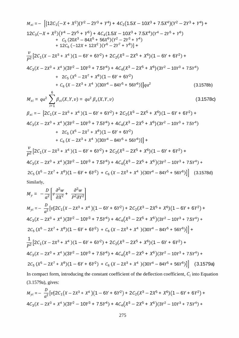
275

=− 12 1 − + 2 ( 2 − 2 3 + 4) + 4 2 1.5 − 10 3 + 7.5 4 ( 2 − 2 3 + 4) +

12 3 − + 2 4 − 2 5 + 6 + 4 4 1.5 − 10 3 + 7.5 4 4 − 2 5 + 6

+ 5 20 3 − 84 5 + 56 6 2 − 2 3 + 4

+ 12 6 −12 + 12 2 6 − 2 7 + 8 +

2 2 1 − 2 3 + 4 1− 6 + 6 2 + 2 2( 3 − 2 5 + 6) 1 − 6 + 6 2 +

4 3 − 2 3 + 4 3 2 − 10 3 + 7.5 4 + 4 4( 3 − 2 5 + 6) 3 2 − 10 3 + 7.5 4

+ 2 55 − 2 7 + 8 1 − 6 + 6 2

+ 6 − 2 3 + 4 30 4 − 84 5 + 56 6 2 (3.1578b)

= 2

=1

6

, , = 2 , , (3.1578c)

=− 2 1 − 2 3 + 4 1 − 6 + 6 2 + 2 2( 3 − 2 5 + 6) 1 − 6 + 6 2 +

4 3 − 2 3 + 4 3 2 − 10 3 + 7.5 4 + 4 4( 3 − 2 5 + 6) 3 2 − 10 3 + 7.5 4

+ 2 55 − 2 7 + 8 1 − 6 + 6 2

+ 6 − 2 3 + 4 30 4 − 84 5 + 56 6 +

2 2 1 − 2 3 + 4 1− 6 + 6 2 + 2 2( 3 − 2 5 + 6) 1 − 6 + 6 2 +

4 3 − 2 3 + 4 3 2 − 10 3 + 7.5 4 + 4 43 − 2 5 + 6 3 2 − 10 3 + 7.5 4 +

2 55 − 2 7 + 8 1 − 6 + 6 2 + 6 − 2 3 + 4 30 4 − 84 5 + 56 6 (3.1578d)

Similarly,

= − 2

2

2 +2

2 2

=− 2 [2 1 − 2 3 + 4 1− 6 + 6 2 + 2 2( 3 − 2 5 + 6) 1− 6 + 6 2 +

4 3 − 2 3 + 4 3 2 − 10 3 + 7.5 4 + 4 43 − 2 5 + 6 3 2 − 10 3 + 7.5 4 +

2 55 − 2 7 + 8 1 − 6 + 6 2 + 6 − 2 3 + 4 30 4 − 84 5 + 56 6 +

12 2 1 − 2 3 + 4 1− 6 + 6 2 + 2 2( 3 − 2 5 + 6) 1 − 6 + 6 2 +

4 3 − 2 3 + 4 3 2 − 10 3 + 7.5 4 + 4 43 − 2 5 + 6 3 2 − 10 3 + 7.5 4 +

2 55 − 2 7 + 8 1 − 6 + 6 2 + 6 − 2 3 + 4 30 4 − 84 5 + 56 6 (3.1579a)


(3.1579a), gives:

=− 2 [2 1 − 2 3 + 4 1− 6 + 6 2 + 2 2( 3 − 2 5 + 6) 1− 6 + 6 2 +

4 3 − 2 3 + 4 3 2 − 10 3 + 7.5 4 + 4 43 − 2 5 + 6 3 2 − 10 3 + 7.5 4 +

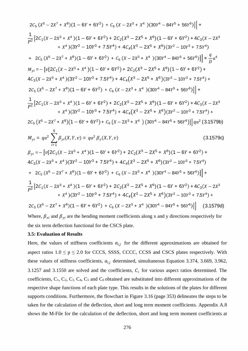
276

2 55 − 2 7 + 8 1 − 6 + 6 2 + 6 − 2 3 + 4 30 4 − 84 5 + 56 6 +

12 2 1 − 2 3 + 4 1− 6 + 6 2 + 2 2( 3 − 2 5 + 6) 1 − 6 + 6 2 +4 3 − 2 3

+ 4 3 2 − 10 3 + 7.5 4 + 4 4( 3 − 2 5 + 6) 3 2 − 10 3 + 7.5 4

+ 2 55 − 2 7 + 8 1 − 6 + 6 2 + 6 − 2 3 + 4 30 4 − 84 5 + 56 6 × 4

=− [2 1 − 2 3 + 4 1− 6 + 6 2 + 2 2( 3 − 2 5 + 6) 1− 6 + 6 2 +

4 3 − 2 3 + 4 3 2 − 10 3 + 7.5 4 + 4 43 − 2 5 + 6 3 2 − 10 3 + 7.5 4 +

2 55 − 2 7 + 8 1 − 6 + 6 2 + 6 − 2 3 + 4 30 4 − 84 5 + 56 6 +

12 2 1 − 2 3 + 4 1− 6 + 6 2 + 2 2( 3 − 2 5 + 6) 1 − 6 + 6 2 +4 3 − 2 3

+ 4 3 2 − 10 3 + 7.5 4 + 4 43 − 2 5 + 6 3 2 − 10 3 + 7.5 4 +

2 55 − 2 7 + 8 1− 6 + 6 2 + 6 − 2 3 + 4 30 4 − 84 5 + 56 6 2 (3.1579b)

= 2

=1

6

, , = 2 , , (3.1579c)

=− [2 1 − 2 3 + 4 1 − 6 + 6 2 + 2 2( 3 − 2 5 + 6) 1 − 6 + 6 2 +

4 3 − 2 3 + 4 3 2 − 10 3 + 7.5 4 + 4 4( 3 − 2 5 + 6) 3 2 − 10 3 + 7.5 4

+ 2 55 − 2 7 + 8 1 − 6 + 6 2 + 6 − 2 3 + 4 30 4 − 84 5 + 56 6 +

12 2 1 − 2 3 + 4 1− 6 + 6 2 + 2 2( 3 − 2 5 + 6) 1 − 6 + 6 2 +4 3 − 2 3

+ 4 3 2 − 10 3 + 7.5 4 + 4 43 − 2 5 + 6 3 2 − 10 3 + 7.5 4 +

2 55 − 2 7 + 8 1 − 6 + 6 2 + 6 − 2 3 + 4 30 4 − 84 5 + 56 6 (3.1579d)


the six term deflection functional for the CSCS plate.

3.5: Evaluation of Results

Here, the values of stiffness coefficients , for the different approximations are obtained for

aspect ratios 1.0 ≤ p ≤ 2.0 for CCCS, SSSS, CCCC, CCSS and CSCS plates respectively. With

these values of stiffness coefficients, , determined, simultaneous Equation 3.374, 3.669, 3.962,

3.1257 and 3.1550 are solved and the coefficients, for various aspect ratios determined. The

coefficients, C1, C2, C3, C4, C5 and C6 obtained are substituted into different approximations of the

respective shape functions of each plate type. This results in the solutions of the plates for different

supports conditions. Furthermore, the flowchart in Figure 3.16 (page 353) delineates the steps to be

taken for the calculation of the deflection, short and long term moment coefficients. Appendix A.8

shows the M-File for the calculation of the deflection, short and long term moment coefficients at

277

any arbitrary point on the plate surface. Input of the corresponding stiffness coefficients into the

M-File gives the deflection, short and long term moment coefficient for the boundary condition of

interest.


The stiffness coefficients are given in Equations 3.95 to 3.370as:

11 = 2.8571 × 10−3 + 3.2653 × 10−3 12 + 6.0317 × 10−3 1

4

12 = 9.9773 × 10−4 + 1.3152 × 10−3 12 + 2.0924 × 10−3 1

4

13 = 7.7922 × 10−4 + 8.1633 × 10−4 12 + 1.7234 × 10−3 1

4

14 = 2.7211 × 10−4 + 3.2880 × 10−4 12 + 5.9781 × 10−4 1

4

15 = 4.9131 × 10−4 + 6.1843 × 10−4 12 + 9.3240 × 10−4 1

4

16 = 2.7972 × 10−4 + 1.9790 × 10−4 12 + 7.1807 × 10−4 1

4

21 = −5.8957 × 10−4 + 1.3152 × 10−3 12 + 2.0924 × 10−3 1

4

22 = 3.6281 × 10−4 + 1.0170 × 10−3 12 + 9.3240 × 10−4 1

4

23 = −1.6079 × 10−4 + 3.2880 × 10−4 12 + 5.9781 × 10−4 1

4

24 = 9.8949 × 10−5 + 2.5424 × 10−4 12 + 2.6640 × 10−4 1

4

25 = 4.3634 × 10−4 + 6.8820 × 10−4 12 + 4.8618 × 10−4 1

4

26 = −5.7720 × 10−5 + 7.9709 × 10−5 12 + 2.4909 × 10−4 1

4

31 = 7.7922 × 10−4 + 8.1633 × 10−4 12 + 1.7234 × 10−3 1

4

32 = 2.7211 × 10−4 + 3.2880 × 10−4 12 + 5.9781 × 10−4 1

4

33 = 2.7972 × 10−4 + 4.9474 × 10−4 12 + 1.7234 × 10−3 1

4

34 = 9.7680 × 10−5 + 1.9927 × 10−4 12 + 5.9781 × 10−4 1

4

35 = 1.3399 × 10−4 + 1.5461 × 10−4 12 + 2.6640 × 10−4 1

4

278

36 = 1.1988 × 10−4 + 2.3976 × 10−4 12 + 1.1750 × 10−3 1

4

41 = −1.6079 × 10−4 + 3.2880 × 10−4 12 + 5.9781 × 10−4 1

4

42 = 9.8949 × 10−5 + 2.5424 × 10−4 12 + 2.6640 × 10−4 1

4

43 = −5.7720 × 10−5 + 1.9927 × 10−4 12 + 5.9781 × 10−4 1

4

44 = 3.5520 × 10−5 + 1.5409 × 10−4 12 + 2.6640 × 10−4 1

4

45 = 1.1900 × 10−4 + 1.7205 × 10−4 12 + 1.3891 × 10−4 1

4

46 = −2.4737 × 10−5 + 9.6570 × 10−5 12 + 4.0760 × 10−4 1

4

51 = −2.6833 × 10−3 + 6.1843 × 10−4 12 + 9.3240 × 10−4 1

4

52 = −1.1510 × 10−3 + 6.8820 × 10−4 12 + 4.8618 × 10−4 1

4

53 = −7.3181 × 10−4 + 1.5461 × 10−4 12 + 2.6640 × 10−4 1

4

54 = −3.1390 × 10−4 + 1.7205 × 10−4 12 + 1.3891 × 10−4 1

4

55 = −4.9950 × 10−4 + 5.6832 × 10−4 12 + 2.8227 × 10−4 1

4

56 = −2.6270 × 10−4 + 3.7481 × 10−5 12 + 1.1100 × 10−4 1

4

61 = 2.7972 × 10−4 + 1.9790 × 10−4 12 + 7.1807 × 10−4 1

4

62 = 9.7680 × 10−5 + 7.9709 × 10−5 12 + 2.4909 × 10−4 1

4

63 = 1.1988 × 10−4 + 2.3976 × 10−4 12 + 1.1750 × 10−3 1

4

64 = 4.1863 × 10−5 + 9.6570 × 10−5 12 + 4.0760 × 10−4 1

4

65 = 4.8100 × 10−5 + 3.7481 × 10−5 12 + 1.1100 × 10−4 1

4

66 = 5.8177 × 10−5 + 1.5984 × 10−4 12 + 1.0545 × 10−3 1

4

The stiffness coefficients, , obtained for aspect ratios, 1.0 ≤ P ≤ 2.0 using the above Equations

are shown in Table 3.1.

279

Table 3.1: Stiffness Coefficient Values for CCCS Plate at Varying Aspect Ratio

Aspectratio, P

, 1 2 3 4 5 6

1

1 0.01215 0.00441 0.00332 0.00120 0.00204 0.00120

2 0.00282 0.00231 0.00077 0.00062 0.00161 0.00027

3 0.00332 0.00120 0.00250 0.00089 0.00056 0.00153

4 0.00077 0.00062 0.00074 0.00046 0.00043 0.00048

5 -0.00113 0.00002 -0.00031 0.00000 0.00035 -0.00011

6 0.00120 0.00043 0.00153 0.00055 0.00020 0.00127

1.1

1 0.00968 0.00351 0.00263 0.00095 0.00164 0.00093

2 0.00193 0.00184 0.00052 0.00049 0.00134 0.00018

3 0.00263 0.00095 0.00187 0.00067 0.00044 0.00112

4 0.00052 0.00049 0.00052 0.00034 0.00036 0.00033

5 -0.00154 -0.00025 -0.00042 -0.00008 0.00016 -0.00016

6 0.00093 0.00033 0.00112 0.00040 0.00015 0.00091

1.2

1 0.00803 0.00292 0.00218 0.00079 0.00137 0.00076

2 0.00133 0.00152 0.00036 0.00040 0.00115 0.00012

3 0.00218 0.00079 0.00145 0.00052 0.00037 0.00085

4 0.00036 0.00040 0.00037 0.00027 0.00031 0.00024

5 -0.00180 -0.00044 -0.00050 -0.00013 0.00003 -0.00018

6 0.00076 0.00027 0.00085 0.00031 0.00013 0.00068

1.3

1 0.00690 0.00251 0.00187 0.00068 0.00118 0.00065

2 0.00092 0.00129 0.00024 0.00034 0.00101 0.00008

3 0.00187 0.00068 0.00118 0.00042 0.00032 0.00067

4 0.00024 0.00034 0.00027 0.00022 0.00027 0.00018

5 -0.00199 -0.00057 -0.00055 -0.00016 -0.00006 -0.00020

280

6 0.00065 0.00023 0.00067 0.00024 0.00011 0.00052

1.4

1 0.00609 0.00221 0.00164 0.00060 0.00105 0.00057

2 0.00063 0.00112 0.00016 0.00030 0.00091 0.00005

3 0.00164 0.00060 0.00098 0.00035 0.00028 0.00055

4 0.00016 0.00030 0.00020 0.00018 0.00024 0.00013

5 -0.00213 -0.00067 -0.00058 -0.00019 -0.00014 -0.00021

6 0.00057 0.00020 0.00055 0.00020 0.00010 0.00041

1.5

1 0.00550 0.00200 0.00148 0.00054 0.00095 0.00051

2 0.00041 0.00100 0.00010 0.00026 0.00084 0.00003

3 0.00148 0.00054 0.00084 0.00030 0.00026 0.00046

4 0.00010 0.00026 0.00015 0.00016 0.00022 0.00010

5 -0.00222 -0.00075 -0.00061 -0.00021 -0.00019 -0.00022

6 0.00051 0.00018 0.00046 0.00017 0.00009 0.00034

1.6

1 0.00505 0.00183 0.00136 0.00049 0.00088 0.00047

2 0.00024 0.00090 0.00006 0.00024 0.00078 0.00001

3 0.00136 0.00049 0.00074 0.00027 0.00024 0.00039

4 0.00006 0.00024 0.00011 0.00014 0.00021 0.00008

5 -0.00230 -0.00081 -0.00063 -0.00023 -0.00023 -0.00023

6 0.00047 0.00017 0.00039 0.00014 0.00008 0.00028

1.7

1 0.00471 0.00170 0.00127 0.00046 0.00082 0.00043

2 0.00012 0.00083 0.00002 0.00022 0.00073 0.00000

3 0.00127 0.00046 0.00066 0.00024 0.00022 0.00034

4 0.00002 0.00022 0.00008 0.00012 0.00020 0.00006

5 -0.00236 -0.00085 -0.00065 -0.00024 -0.00027 -0.00024

6 0.00043 0.00016 0.00034 0.00012 0.00007 0.00024

281

1.8

1 0.00444 0.00160 0.00120 0.00043 0.00077 0.00041

2 0.00002 0.00077 0.00000 0.00020 0.00070 -0.00001

3 0.00120 0.00043 0.00060 0.00022 0.00021 0.00031

4 0.00000 0.00020 0.00006 0.00011 0.00019 0.00004

5 -0.00240 -0.00089 -0.00066 -0.00025 -0.00030 -0.00024

6 0.00041 0.00015 0.00031 0.00011 0.00007 0.00021

1.9

1 0.00422 0.00152 0.00114 0.00041 0.00073 0.00039

2 -0.00006 0.00072 -0.00002 0.00019 0.00066 -0.00002

3 0.00114 0.00041 0.00055 0.00020 0.00020 0.00028

4 -0.00002 0.00019 0.00004 0.00010 0.00018 0.00003

5 -0.00244 -0.00092 -0.00067 -0.00026 -0.00032 -0.00024

6 0.00039 0.00014 0.00028 0.00010 0.00007 0.00018

2.0

1 0.00405 0.00146 0.00109 0.00039 0.00070 0.00037

2 -0.00013 0.00068 -0.00004 0.00018 0.00064 -0.00002

3 0.00109 0.00039 0.00051 0.00018 0.00019 0.00025

4 -0.00004 0.00018 0.00003 0.00009 0.00017 0.00002

5 -0.00247 -0.00095 -0.00068 -0.00026 -0.00034 -0.00025

6 0.00037 0.00013 0.00025 0.00009 0.00006 0.00016

Calculation of C-values

The coefficients, Ci (C1, C2, C3, C4, C5 and C6) for any aspect ratio of the CCCS plate are then

obtained by substituting the stiffness coefficients, , for that aspect ratio into Equations 3.375,

3.376, 3.377 and 3.378 and solving accordingly. For example, at aspect ratio, P = 1.0; the stiffness

coefficients , are given as (see Table 3.1):

1,1 = 0.01215, 1,2 = 0.00441, 1,3 = 0.00332, 1,4 = 0.00120, 1,5 = 0.00204, 1,6 = 0.00120

2,1 = 0.00282, 2,2 = 0.00231, 2,3 = 0.00077, 2,4 = 0.00062, 2,5 = 0.00161, 2,6 = 0.00027

3,1 = 0.00332, 3,2 = 0.00120, 3,3 = 0.00250, 3,4 = 0.00089, 3,5 = 0.00056, 3,6 = 0.00153

282

4,1 =0.00077, 4,2 = 0.00062, 4,3 = 0.00074, 4,4 = 0.00046, 4,5 = 0.00043, 4,6 = 0.00048

5,1 =-0.00113, 5,2 =0.00002, 5,3 =-0.00031, 5,4 =0.00000, 5,5 =0.00035, 5,6 =-0.00011

6,1 =0.00120, 6,2 =0.00043, 6,3 =0.00153, 6,4 =0.00055, 6,5 =0.00020, 6,6 =0.00127

The values of the coefficient functions of the external load are as follows:

1 = 0.00250; 2 = 0.00087; 3 = 0.00071; 4 = 0.00025; 5 = 0.00043; 6 = 0.00030

Substituting these stiffness coefficients into Equations 3.375, 3.376, 3.377 and 3.378 and

subsequently solving the resulting canonical equation gives:

For the first approximation,

1 = 111

= 0.002500.01215

= 0.20569.

The coefficients, C1 for other aspect ratios of the CCCS plate for the first approximation are

obtained by similar approach and their results are shown in Table 3.2.

For the second approximation,

1,1 1,2 1,3

2,1 2,2 2,33,1 3,2 3,3

1

2

3

=1

2

3

4

1

2

3

=0.01215 0.00441 0.003320.00282 0.00231 0.000770.00332 0.00120 0.00250

−1 2.50000 × 10−3

8.70000 × 10−4

7.10000 × 10−4

4 =0.117700.227350.02047

4

The coefficients, Ci (C1, C2 and C3) for other aspect ratios of the CCCS plate for the second

approximation are obtained by similar approach and their results are shown in Table 3.3.

For the truncated third approximation,

1

2

3

4

=

1,1 1,2 1,3 1,4

2,1 2,2 2,3 2,43,1 3,2 3,3 3,4

4,1 4,2 4,3 4,4

−11

2

3

4

4

1

2

3

4

=

0.01215 0.00441 0.00332 0.001200.00282 0.00231 0.00077 0.000620.00332 0.00120 0.00250 0.000890.00077 0.00062 0.00074 0.00046

−1 2.50000 × 10−3

8.70000 × 10−4

7.10000 × 10−4

2.50000 × 10−4

4

=0.120840.218590.008700.03295

4

The coefficients, Ci (C1, C2, C3 and C4) for other aspect ratios of the CCCS plate for the truncated

third approximation are obtained by similar approach and their results are shown in Table 3.4.

For the third approximation,

283

1,1 1,2 1,3 1,4 1,5 1,6

2,1 2,2 2,3 2,4 2,5 2,63,1 3,2 3,3 3,4 3,5 3,6

4,1 4,2 4,3 4,4 4,5 4,6

5,1 5,2 5,3 5,4 5,5 5,66,1 6,2 6,3 6,4 6,5 6,6

1

2

3

4

5

6

=

1

2

3

4

5

6

4

1

2

3

4

5

6

=

0.01215 0.00441 0.00332 0.00120 0.00204 0.001200.00282 0.00231 0.00077 0.00062 0.00161 0.000270.00332 0.00120 0.00250 0.00089 0.00056 0.001530.00077 0.00062 0.00074 0.00046 0.00043 0.00048

− 0.00113 0.00002 − 0.00031 0.00000 0.00035 − 0.000110.00120 0.00043 0.00153 0.00055 0.00020 0.00127

−1

2.50000 × 10−3

8.70000 × 10−4

7.10000 × 10−4

2.50000 × 10−4

4.30000 × 10−4

3.00000 × 10−4

4 =

0.67094−2.91032−0.078410.044533.548240.10615

4

The coefficients, Ci (C1, C2, C3, C4, C5 and C6) for other aspect ratios of the CCCS plate for the


Table 3.2: First Approximation Coefficient Values for CCCS Plate at Varying Aspect Ratio

Aspect ratio, P C1

1.0 0.20569

1.1 0.25838

1.2 0.31120

1.3 0.36226

1.4 0.41029

1.5 0.45456

1.6 0.49475

1.7 0.53088

1.8 0.56312

1.9 0.59179

2.0 0.61721

Table 3.3: Second Approximation Coefficient Values for CCCS Plate at Varying Aspect

Ratio

Aspect ratio, P C1 C2 C3

284

1.0 0.117700 0.227346 0.020469

1.1 0.130443 0.329141 0.030929

1.2 0.138165 0.443312 0.043878

1.3 0.141137 0.564383 0.059076

1.4 0.140017 0.687459 0.076152

1.5 0.135620 0.808683 0.094659

1.6 0.128762 0.925318 0.114131

1.7 0.120174 1.035622 0.134120

1.8 0.110468 1.138648 0.154225

1.9 0.100132 1.234023 0.174105

2.0 0.089540 1.321773 0.193488

Table 3.4: Truncated Third Approximation Coefficient Values for CCCS Plate at Varying

Aspect Ratio

Aspect ratio, P C1 C2 C3 C4

1 0.12084 0.21859 0.00870 0.03295

1.1 0.13545 0.31522 0.01213 0.05240

1.2 0.14556 0.42285 0.01616 0.07694

1.3 0.15138 0.53613 0.02072 0.10610

1.4 0.15352 0.65034 0.02566 0.13922

1.5 0.15272 0.76180 0.03080 0.17560

1.6 0.14973 0.86796 0.03592 0.21453

1.7 0.14521 0.96726 0.04085 0.25537

1.8 0.13971 1.05891 0.04541 0.29748

1.9 0.13365 1.14270 0.04950 0.34030

2 0.12735 1.21879 0.05305 0.38331

Table 3.5: Third Approximation Coefficient Values for CCCS Plate at Varying Aspect Ratio

Aspect ratio, P C1 C2 C3 C4 C5 C6

1 0.67094 -2.91032 -0.07841 0.04453 3.54824 0.10615

1.1 0.89014 -3.96084 -0.11906 0.06202 4.82264 0.16450

1.2 1.11725 -5.06744 -0.17046 0.08069 6.16307 0.24033

1.3 1.34088 -6.16981 -0.23283 0.09966 7.49664 0.33454

285

1.4 1.55298 -7.22292 -0.30625 0.11842 8.76917 0.44752

1.5 1.74895 -8.19897 -0.39072 0.13686 9.94727 0.57930

1.6 1.92694 -9.08474 -0.48617 0.15510 11.01515 0.72963

1.7 2.08702 -9.87739 -0.59246 0.17345 11.96955 0.89797

1.8 2.23034 -10.58055 -0.70929 0.19222 12.81495 1.08359

1.9 2.35856 -11.20129 -0.83625 0.21170 13.55998 1.28549

2 2.47351 -11.74812 -0.97273 0.23211 14.21497 1.50246

Deflections

The six term deflection function of CCCS plate obtained in Equation 3.18 is given as:

, = 1(1.5 2 − 2.5 3 + 4 )( 2 − 2 3 + 4) + 2(1.5 4 − 2.5 5 + 6)( 2 − 2 3

+ 4) + 3 1.5 2 − 2.5 3 + 4 4 − 2 5 + 6 + 4 1.5 4 − 2.5 5 + 6

4 − 2 5 + 6 + 5(1.5 6 − 2.5 7 + 8)( 2 − 2 3 + 4) + 6 1.5 2 − 2. 5 3 + 4

6 − 2 7 + 8

For the first approximation deflection coefficient at mid-span, we have: aspect ratio p = 1,

= = 12

. From Table 3.2, we have the C value as 1 = 0.20569;

= 1 1 = 1 1.5 2 − 2.5 3 + 4 2 − 2 3 + 4

= 1 1 = 0.20569 1.512

2

− 2.512

3

+12

4 12

2

− 212

3

+12

4

= 0.00161

Following the same procedure, the coefficients, α, at aspect ratios 1.1 ≤ ≤ 2.0 for the first

approximation were calculated and tabulated in Table 4.1a of chapter four.

For the second approximation deflection coefficient at mid-span, we have: aspect ratio p = 1,

Y = X = 12

. From Table 3.3, we have the C values as 1 = 0.117700; 2 = 0.227346; 3 =

0.020469;

= 1 1 + 2 2 + 3 3 = 1 1.5 2 − 2.5 3 + 4 2 − 2 3 + 4 +

2 1.5 4 − 2.5 5 + 6 2 − 2 3 + 4 + 3 1.5 2 − 2. 5 3 + 4 4 − 2 5 + 6

= 2 = 0.117700 1.512

2

− 2.512

3

+12

4 12

2

− 212

3

+12

4

+

0.227346 1.512

4

− 2.512

5

+12

6 12

2

− 212

3

+12

4

+0.020469 1.512

2

− 2.512

3

+12

4 12

4

− 212

5

+12

6

= 0.00140

286

Following the same procedure, the coefficients, α, at aspect ratios 1.1 ≤ ≤ 2.0 for the second


For the truncated third term deflection coefficient at mid-span, we have: aspect ratio p = 1,

= = 12

. From Table 3.4, we have the C values as: 1 = 0.12084; 2 = 0.21859; 3 =

0.00870; 4 = 0.03295;

= 1 1 + 2 2 + 3 3 + 4 4

= 1 1.5 2 − 2.5 3 + 4 2 − 2 3 + 4 + 2 1.5 4 − 2. 5 5 + 6

2 − 2 3 + 4 + 3 1.5 2 − 2. 5 3 + 4 4 − 2 5 + 6 + 4 1.5 4 − 2.5 5 + 6

4 − 2 5 + 6

= 0.12084 1.512

2

− 2.512

3

+12

4 12

2

− 212

3

+12

4

+

0.21859 1.512

4

− 2.512

5

+12

6 12

2

− 212

3

+12

4

+

0.00870 1.512

2

− 2.512

3

+12

4 12

4

− 212

5

+12

6

+

0.03295 1.512

4

− 2.512

5

+12

6 12

4

− 212

5

+12

6

= 0.00140

Following the same procedure, the coefficients, α, at aspect ratios 1.1 ≤ ≤ 2.0 for the truncated third


For the third term deflection coefficient at mid-span, we have: aspect ratio p = 1,

Y = X = 12

. From Table 3.5, we have the C values as: 1 = 0.67094; 2 =− 2.91032; 3 =−

0.07841; = 4 = 0.04453; 5 = 3.54824; 6 = 0.10615;= 1 1 + 2 2 + 3 3 + 4 4 + 5 5 + 6 6

= 1 1.5 2 − 2.5 3 + 4 2 − 2 3 + 4 + 2 1.5 4 − 2. 5 5 + 6

2 − 2 3 + 4 + 3 1.5 2 − 2.5 3 + 4 4 − 2 5 + 6 + 4 1.5 4 − 2.5 5 + 6

4 − 2 5 + 6 + 5 1.5 6 − 2.5 7 + 8 2 − 2 3 + 4 + 6 1.5 2 − 2.5 3 + 4

6 − 2 7 + 8

= 0.67094 1.512

2

− 2.512

3

+12

4 12

2

− 212

3

+12

4

+

−2.91032 1.512

4

− 2.512

5

+12

6 12

2

− 212

3

+12

4

+

287

−0.07841 1.512

2

− 2.512

3

+12

4 12

4

− 212

5

+12

6

+0.04453 1.512

4

− 2.512

5

+12

6 12

4

− 212

5

+12

6

+3.54824 1.512

6

− 2.512

7

+12

8 12

2

− 212

3

+12

4

+0.10615 1.512

2

− 2.512

3

+12

4 12

6

− 212

7

+12

8

= 0.00121

Following the same procedure, the coefficients, α, at aspect ratios 1.1 ≤ ≤ 2.0 for the third


Moments in x and y directions

The six term bending moment functions of the plate obtained in Equations 3.1561d and 3.1562d in

x and y directions respectively are given as:

=− 1 3 − 15 + 12 2 ( 2 − 2 3 + 4) + 2 18 2 − 50 3 + 30 4 ( 2 − 2 3 + 4)+ 3 3 − 15 + 12 2 4 − 2 5 + 6 + 4 18 2 − 50 3 + 30 4

4 − 2 5 + 6 + 5 45 4 − 105 5 + 56 6 2 − 2 3 + 4 + 6 3− 15 + 12 2

6 − 2 7 + 8 ] + 2 1 1.5 2 − 2.5 3 + 4 2− 12 + 12 2 + 2 1.5 4 − 2.5 5 + 6

2− 12 + 12 2 + 3 1.5 2 − 2.5 3 + 4 12 2 − 40 3 + 30 4 + 4 1.5 4 − 2.5 5 + 6

12 2 − 40 3 + 30 4 + 5 1.5 6 − 2.5 7 + 8 2− 12 + 12 2 + 6 1.5 2 − 2.5 3 +4 30 4 − 84 5 + 56 6 ]]

=− 1 3 − 15 + 12 2 ( 2 − 2 3 + 4) + 2 18 2 − 50 3 + 30 4 ( 2 − 2 3 + 4

+ 3 3 − 15 + 12 2 4 − 2 5 + 6 + 4 18 2 − 50 3 + 30 4

4 − 2 5 + 6 + 5 45 4 − 105 5 + 56 6 2 − 2 3 + 4 + 6 3− 15 + 12 2

6 − 2 7 + 8 ] +1

2 1 1.5 2 − 2.5 3 + 4 2− 12 + 12 2 + 2 1.5 4 − 2.5 5 + 6

2− 12 + 12 2 ++ 3 1.5 2 − 2.5 3 + 4 12 2 − 40 3 + 30 4

+ 4 1.5 4 − 2.5 5 + 6 12 2 − 40 3 + 30 4 + 5 1.5 6 − 2.5 7 + 8

2 − 12 + 12 2 + 6 1.5 2 − 2.5 3 + 4 30 4 − 84 5 + 56 6 ]]

288

For the first approximation bending moment coefficients 1 1, at mid-span of plate along x

– direction, we have: aspect ratio p = 1, X = Y = 12

, ν = 0.3. From Table 3.2, the C value is given

as: 1 = 0.20569;

1 = 1 =− 0.20569 3 − 1512

+ 1212

2 12

2

− 212

3

+12

4

+

0.312 0.20569 1.5

12

2

− 2.512

3

+12

4

2 − 1212 + 12

12

2

= 0.02700

Similarly,

1 = 1 =− 0.20569(0.3) 3 − 1512 + 12

12

2 12

2

− 212

3

+12

4

+

112 0.20569 1.5

12

2

− 2.512

3

+12

4

2 − 1212 + 12

12

2

= 0.03150

Following the same procedure, the coefficients, 1 1, at aspect ratios 1.1 ≤ ≤ 2.0 for the first

approximation were calculated and tabulated in Tables 4.1b and 4.1c of chapter four respectively. For the

second approximation bending moment coefficients, 1 1, at mid-span, we have aspect ratio

p = 1, X = Y = 12

, ν = 0.3. From Table 3.3, we have the C values as: C1 = 0.11770; C2 =

0.22735; C3 = 0.02047.

2 =− 0.11770 3 − 1512 + 12

12

2 12

2

− 212

3

+12

4

+

+0.22735 1812

2

− 5012

3

+ 3012

4 12

2

− 212

3

+12

4

+ 0.02047 3− 1512

+ 1212

2 12

4

− 212

5

+12

6

+

0.312 0.11770 1.5

12

2

− 2.512

3

+12

4

2− 1212 + 12

12

2

+

0.22735 1.512

4

− 2.512

5

+12

6

2− 1212

+ 1212

2

+ 0.02047 1.512

2

− 2.512

3

+12

4

1212

2

− 4012

3

+ 3012

4

= 0.0164

Similarly,

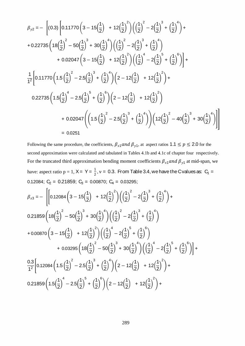
289

2 =− (0.3) 0.11770 3− 1512 + 12

12

2 12

2

− 212

3

+12

4

+

+0.22735 1812

2

− 5012

3

+ 3012

4 12

2

− 212

3

+12

4

+ 0.02047 3− 1512 + 12

12

2 12

4

− 212

5

+12

6

+

112 0.11770 1.5

12

2

− 2.512

3

+12

4

2 − 1212

+ 1212

2

+

0.22735 1.512

4

− 2.512

5

+12

6

2 − 1212 + 12

12

2

+ 0.02047 1.512

2

− 2.512

3

+12

4

1212

2

− 4012

3

+ 3012

4

= 0.0251

Following the same procedure, the coefficients, 1 1, at aspect ratios 1.1 ≤ ≤ 2.0 for the

second approximation were calculated and tabulated in Tables 4.1b and 4.1c of chapter four respectively.

For the truncated third approximation bending moment coefficients 1 1 at mid-span, we

have: aspect ratio p = 1, X = Y = 12

, ν = 0.3. From Table 3.4, we have the C values as: C1 =

0.12084; C2 = 0.21859; C3 = 0.00870; C4 = 0.03295;

3 =− 0.12084 3 − 1512

+ 1212

2 12

2

− 212

3

+12

4

+

0.21859 1812

2

− 5012

3

+ 3012

4 12

2

− 212

3

+12

4

+0.00870 3 − 1512 + 12

12

2 12

4

− 212

5

+12

6

+ 0.03295 1812

2

− 5012

3

+ 3012

4 12

4

− 212

5

+12

6

+

0.312 0.12084 1.5

12

2

− 2.512

3

+12

4

2 − 1212 + 12

12

2

+

0.21859 1.512

4

− 2.512

5

+12

6

2− 1212 + 12

12

2

+

290

+0.00870 1.512

2

− 2.512

3

+12

4

1212

2

− 4012

3

+ 3012

4

+ 0.03295 1.512

4

− 2.512

5

+12

6

1212

2

− 4012

3

+ 3012

4

= 0.01642

Similarly,

3 =− (0.3) 0.12084 3 − 1512 + 12

12

2 12

2

− 212

3

+12

4

+

0.21859 1812

2

− 5012

3

+ 3012

4 12

2

− 212

3

+12

4

+0.00870 3 − 1512

+ 1212

2 12

4

− 212

5

+12

6

+ 0.03295 1812

2

− 5012

3

+ 3012

4 12

4

− 212

5

+12

6

+

112 0.12084 1.5

12

2

− 2.512

3

+12

4

2 − 1212

+ 1212

2

+

0.21859 1.512

4

− 2.512

5

+12

6

2− 1212

+ 1212

2

+

+0.00870 1.512

2

− 2.512

3

+12

4

1212

2

− 4012

3

+ 3012

4

+ 0.03295 1.512

4

− 2.512

5

+12

6

1212

2

− 4012

3

+ 3012

4

= 0.02512

Following the same procedure, the coefficients, 1 1 , at aspect ratios 1.1 ≤ ≤ 2.0 for the

truncated third approximation were calculated and tabulated in Tables 4.1b and 4.1c of chapter four

respectively. For the third approximation bending moment coefficients at mid-span, we have: aspect

ratio p = 1; X = Y = 12


− 2.91032; C3 =− 0.07841; C4 = 0.04453; C5 = 3.54824; C6 = 0.10615

4 =− 0.67094 3 − 1512

+ 1212

2 12

2

− 212

3

+12

4

291

−2.91032 1812

2

− 5012

3

+ 3012

4 12

2

− 212

3

+12

4

−0.07841 3− 1512 + 12

12

2 12

4

− 212

5

+12

6

+ 0.04453 1812

2

− 5012

3

+ 3012

4 12

4

− 212

5

+12

6

+ 3.54824 4512

4

− 10512

5

+ 5612

6 12

2

− 212

3

+12

4

+0.10615 3− 1512

+ 1212

2 12

6

− 212

7

+12

8

+

0.312 0.67094 1.5

12

2

− 2.512

3

+12

4

2 − 1212 + 12

12

2

−2.91032 1.512

4

− 2.512

5

+12

6

2 − 1212 + 12

12

2

+

−0.07841 1.512

2

− 2.512

3

+12

4

1212

2

− 4012

3

+ 3012

4

+ 0.04453 1.512

4

− 2.512

5

+12

6

1212

2

− 4012

3

+ 3012

4

+3.54824 1.512

6

− 2.512

7

+12

8

2− 1212

+ 1212

2

+ 0.10615 1.512

2

− 2.512

3

+12

4

3012

4

− 8412

5

+ 5612

6

=− 0.00038

Similarly,

4 =− (0.3) 0.67094 3 − 1512 + 12

12

2 12

2

− 212

3

+12

4

−2.91032 1812

2

− 5012

3

+ 3012

4 12

2

− 212

3

+12

4

292

−0.07841 3− 1512 + 12

12

2 12

4

− 212

5

+12

6

+ 0.04453 1812

2

− 5012

3

+ 3012

4 12

4

− 212

5

+12

6

+ 3.54824 4512

4

− 10512

5

+ 5612

6 12

2

− 212

3

+12

4

+ 0.10615 3 − 1512

+ 1212

2 12

6

− 212

7

+12

8

+

112 0.67094 1.5

12

2

− 2.512

3

+12

4

2 − 1212

+ 1212

2

−2.91032 1.512

4

− 2.512

5

+12

6

2 − 1212

+ 1212

2

+

−0.07841 1.512

2

− 2.512

3

+12

4

1212

2

− 4012

3

+ 3012

4

+ 0.04453 1.512

4

− 2.512

5

+12

6

1212

2

− 4012

3

+ 3012

4

+3.54824 1.512

6

− 2.512

7

+12

8

2 − 1212

+ 1212

2

+ 0.10615 1.512

2

− 2.512

3

+12

4

3012

4

− 8412

5

+ 5612

6

= 0.01620

Following the same procedure, the coefficients, 1 1 , at aspect ratios 1.1 ≤ ≤ 2.0 for the third

approximation were calculated and tabulated in Tables 4.1b and 4.1c of chapter four respectively.


The stiffness coefficients are given in Equations 3.388 to 3.665 as:

11 = 2.3619 × 10−1 + 4.7184 × 10−1 12 + 2.3619 × 10−1 1

4

12 = 7.0295 × 10−2 + 1.3415 × 10−1 12 + 6.6840 × 10−2 1

4

13 = 6.68398 × 10−2 + 1.3415 × 10−1 12 + 7.02948 × 10−2 1

4

14 = 1.9893 × 10−2 + 3.8141 × 10−2 12 + 1.9893 × 10−2 1

4

293

15 = 3.2804 × 10−2 + 5.5090 × 10−2 12 + 2.7066 × 10−2 1

4

16 = 2.7066 × 10−2 + 5.5090 × 10−2 12 + 7.0295 × 10−3 1

4

21 = −1.2653 × 10−1 + 1.3415 × 10−1 12 + 6.6840 × 10−2 1

4

22 = 2.8118 × 10−2 + 1.0920 × 10−1 12 + 2.7067 × 10−2 1

P4

23 = −3.5807 × 10−2 + 3.8141 × 10−2 12 + 1.9893 × 10−2 1

4

24 = 7.9571 × 10−3 + 3.1047 × 10−2 12 + 8.0554 × 10−3 1

4

25 = 3.8130 × 10−2 + 7.1447 × 10−2 12 + 1.3373 × 10−2 1

4

26 = −1.4500 × 10−2 + 1.5663 × 10−2 12 + 9.2833 × 10−3 1

4

31 = 6.6840 × 10−2 + 1.3415 × 10−1 12 ± 1.2653 × 10−2 1

4

32 = 1.9893 × 10−2 + 4.5243 × 10−1 12 − 3.5807 × 10−2 1

4

33 = 2.7066 × 10−2 + 1.0920 × 10−1 12 + 2.8118 × 10−2 1

4

34 = 8.0554 × 10−3 + 3.1047 × 10−2 12 + 7.9571 × 10−3 1

4

35 = 9.2833 × 10−3 + 1.5663 × 10−2 12 − 1.4500 × 10−2 1

4

36 = 1.3373 × 10−2 + 7.1447 × 10−2 12 + 3.8130 × 10−2 1

4

41 = −3.5807 × 10−2 + 3.8141 × 10−2 12 +− 3.5807 × 10−2 1

4

42 = 7.9571 × 10−3 + 3.1047 × 10−2 12 − 1.4500 × 10−2 1

4

43 = −1.4500 × 10−2 + 3.1047 × 10−2 12 + 7.9571 × 10−3 1

4

44 = 3.2222 × 10−3 + 2.5272 × 10−2 12 + 3.2222 × 10−3 1

4

294

45 = 1.0790 × 10−2 + 2.0313 × 10−2 12 − 7.1643 × 10−3 1

P4

46 = −7.1643 × 10−3 + 2.0313 × 10−2 12 + 1.0790 × 10−2 1

4

51 = −3.6085 × 10−1 + 5.5090 × 10−2 12 + 2.7066 × 10−2 1

4

52 = −1.5870 × 10−1 + 7.1447 × 10−2 12 + 1.3373 × 10−2 1

4

53 = −1.0212 × 10−1 + 1.5663 × 10−2 12 + 8.0554 × 10−3 1

4

54 = −4.4910 × 10−2 + 2.0313 × 10−2 12 + 3.9801 × 10−3 1

4

55 = −7.4064 × 10−2 + 5.9025 × 10−2 12 + 7.5078 × 10−3 1

4

56 = −4.1351 × 10−2 + 6.4320 × 10−3 12 + 3.7592 × 10−3 1

4

61 = 2.7066 × 10−2 + 5.5090 × 10−2 12 − 3.6085 × 10−1 1

4

62 = 8.0554 × 10−3 + 1.5663 × 10−2 12 − 1.0212 × 10−1 1

4

63 = 1.3373 × 10−2 + 7.1447 × 10−2 12 − 1.5870 × 10−1 1

4

64 = 3.9801 × 10−3 + 2.0313 × 10−2 12 − 4.4910 × 10−2 1

4

65 = 3.7592 × 10−3 + 6.4320 × 10−3 12 − 4.1351 × 10−2 1

4

66 = 7.5078 × 10−3 + 5.9025 × 10−2 12 − 7.4064 × 10−2 1

4

The stiffness coefficients, , obtained for aspect ratios, 1.0 ≤ P ≤ 2.0 using the above Equations


Table 3.6: Stiffness Coefficient Values for SSSS Plate at Varying Aspect Ratio

Aspectratio, P

, 1 2 3 4 5 6

1

1 0.94422 0.27128 0.27128 0.07793 0.11496 0.089192 0.07446 0.16438 0.02223 0.04706 0.12295 0.010453 0.07446 0.43651 0.16438 0.04706 0.01045 0.122954 -0.03347 0.02450 0.02450 0.03172 0.02394 0.023945 -0.27869 -0.07388 -0.07840 -0.02062 -0.00753 -0.031166 -0.27869 -0.07840 -0.07388 -0.02062 -0.03116 -0.00753

295

1.1

1 0.78746 0.22681 0.22572 0.06500 0.09682 0.077402 0.02999 0.13685 0.00930 0.03912 0.10631 0.004793 0.09129 0.36934 0.13652 0.03915 0.01232 0.098464 -0.02874 0.02371 0.01659 0.02631 0.02269 0.016995 -0.29683 -0.09051 -0.08367 -0.02540 -0.02015 -0.033476 -0.17387 -0.04875 -0.03597 -0.00991 -0.01917 0.00570

1.2

1 0.67776 0.19569 0.19390 0.05597 0.08411 0.068712 -0.00114 0.11700 0.00027 0.03340 0.09420 0.000853 0.09898 0.31681 0.11646 0.03345 0.01317 0.081384 -0.02659 0.02252 0.01090 0.02233 0.02144 0.012155 -0.30954 -0.10263 -0.08735 -0.02888 -0.02945 -0.035076 -0.10870 -0.03031 -0.01354 -0.00357 -0.01172 0.01278

1.3

1 0.59808 0.17308 0.17083 0.04943 0.07488 0.062122 -0.02375 0.10221 -0.00627 0.02915 0.08509 -0.001983 0.10192 0.27506 0.10153 0.02921 0.01347 0.069004 -0.02578 0.02125 0.00666 0.01930 0.02030 0.008635 -0.31877 -0.11174 -0.09003 -0.03150 -0.03651 -0.036236 -0.06668 -0.01843 0.00009 0.00028 -0.00691 0.01650

1.4

1 0.53841 0.15614 0.15358 0.04453 0.06796 0.057002 -0.04069 0.09088 -0.01117 0.02589 0.07806 -0.004093 0.10235 0.24140 0.09010 0.02597 0.01350 0.059754 -0.02567 0.02002 0.00341 0.01695 0.01929 0.006015 -0.32569 -0.11876 -0.09203 -0.03351 -0.04199 -0.037096 -0.03876 -0.01054 0.00852 0.00265 -0.00372 0.01834

1.5

1 0.49255 0.14312 0.14035 0.04077 0.06263 0.052942 -0.05371 0.08200 -0.01493 0.02335 0.07253 -0.005703 0.10147 0.21390 0.08115 0.02343 0.01338 0.052664 -0.02593 0.01889 0.00087 0.01509 0.01840 0.004005 -0.33102 -0.12430 -0.09356 -0.03510 -0.04635 -0.037756 -0.01973 -0.00515 0.01378 0.00414 -0.00155 0.01911

1.6

1 0.45654 0.13290 0.12997 0.03783 0.05845 0.049662 -0.06393 0.07490 -0.01787 0.02131 0.06808 -0.006973 0.09993 0.19116 0.07401 0.02140 0.01319 0.047104 -0.02637 0.01787 -0.00116 0.01359 0.01763 0.00242

296

5 -0.33520 -0.12875 -0.09477 -0.03637 -0.04986 -0.038276 -0.00648 -0.00141 0.01707 0.00506 -0.00004 0.01926

1.7

1 0.42773 0.12472 0.12167 0.03547 0.05511 0.046972 -0.07211 0.06914 -0.02023 0.01966 0.06445 -0.007973 0.09811 0.17215 0.06822 0.01975 0.01297 0.042664 -0.02690 0.01696 -0.00280 0.01235 0.01696 0.001165 -0.33854 -0.13237 -0.09573 -0.03740 -0.05274 -0.038686 0.00292 0.00125 0.01909 0.00563 0.00103 0.01906

1.8

1 0.40432 0.11807 0.11494 0.03356 0.05239 0.044742 -0.07876 0.06440 -0.02214 0.01831 0.06146 -0.008783 0.09619 0.15612 0.06345 0.01840 0.01274 0.039064 -0.02745 0.01616 -0.00416 0.01133 0.01638 0.000135 -0.34127 -0.13537 -0.09651 -0.03826 -0.05513 -0.039016 0.00970 0.00316 0.02031 0.00597 0.00181 0.01867

1.9

1 0.38502 0.11258 0.10939 0.03198 0.05014 0.042872 -0.08424 0.06044 -0.02372 0.01718 0.05895 -0.009453 0.09429 0.14247 0.05947 0.01727 0.01251 0.036094 -0.02799 0.01544 -0.00529 0.01047 0.01587 -0.000715 -0.34351 -0.13788 -0.09716 -0.03898 -0.05714 -0.039286 0.01464 0.00456 0.02099 0.00616 0.00237 0.01818

2.0

1 0.36891 0.10801 0.10477 0.03067 0.04827 0.041282 -0.08882 0.05711 -0.02503 0.01622 0.05683 -0.010003 0.09247 0.13076 0.05612 0.01631 0.01229 0.033624 -0.02851 0.01481 -0.00624 0.00974 0.01542 -0.001415 -0.34538 -0.14000 -0.09770 -0.03958 -0.05884 -0.039516 0.01829 0.00559 0.02132 0.00625 0.00278 0.01764


The coefficients, Ci (C1, C2, C3, C4 , C5 and C6) for any aspect ratio of the SSSS plate are then


3.671, 3.672 and 3.673 and solving accordingly. For example, at aspect ratio, P = 1.0; the stiffness


1,1 =0.94422, 1,2 =0.27128, 1,3 =0.27128, 1,4 =0.07793, 1,5 =0.1149, 1,6 =0.08919

2,1 =0.07446, 2,2 =0.16438, 2,3 =0.02223, 2,4 =0.04706, 2,5 =0.12295, 2,6 =0.01045

297

3,1 =0.07446, 3,2 =0.43651, 3,3 =0.16438, 3,4 =0.04706, 3,5 =0.01045, 3,6 =0.12295

4,1 =-0.03347, 4,2 =0.02450, 4,3 =0.02450, 4,4 =0.03172, 4,5 =0.02394, 4,6 =0.02394

5,1 =-0.27869, 5,2 =-0.07840, 5,3 =-0.07388, 5,4 =-0.02062, 5,5 =-0.03116, 5,6 =-0.00753

6,1 =-0.27869, 6,2 =-0.07388, 6,3 =-0.07840, 6,4 =-0.02062, 6,5 =-0.00753, 6,6 =-0.03116


1 = 0.04000; 2 = 0.01190; 3 = 0.01190; 4 = 0.00354; 5 =0.00556; 6 =0.00556

Substituting these stiffness coefficients into Equation 3.670, 3.671, 3.672 and 3.673 and

subsequently solving the resulting canonical equation, gives:


1 = 111

= 0.040000.94422

= 0.04236.

The coefficients, C1 for other aspect ratios of the SSSS plate for the first approximation are



1,1 1,2 1,3

2,1 2,2 2,33,1 3,2 3,3

1

2

3

=1

2

3

4

1

2

3

=0.94422 0.27128 0.271280.07446 0.16438 0.022230.07446 0.43651 0.16438

−1 4.0000 × 10−2

1.1905 × 10−2

1.1905 × 10−2

4 =0.0586200.061887−0.11847

4

The coefficients, Ci (C1, C2 and C3) for other aspect ratios of the SSSS plate for the second



1

2

3

4

=

1,1 1,2 1,3 1,4

2,1 2,2 2,3 2,43,1 3,2 3,3 3,4

4,1 4,2 4,3 4,4

−11

2

3

4

4

1

2

3

4

=

0.94422 0.27128 0.27128 0.077930.07446 0.16438 0.02223 0.047060.07446 0.43651 0.16438 0.04706− 0.03347 0.02450 0.02450 0.03172

−1 4.0000 × 10−2

1.1905 × 10−2

1.1905 × 10−2

3.5431 × 10−3

4

=0.03351

0.016057−0.030720.15841

4

The coefficients, Ci (C1, C2, C3 and C4) for other aspect ratios of the SSSS plate for the truncated



298

1,1 1,2 1,3 1,4 1,5 1,6

2,1 2,2 2,3 2,4 2,5 2,63,1 3,2 3,3 3,4 3,5 3,6

4,1 4,2 4,3 4,4 4,5 4,6

5,1 5,2 5,3 5,4 5,5 5,66,1 6,2 6,3 6,4 6,5 6,6

1

2

3

4

5

6

=

1

2

3

4

5

6

4

1

2

3

4

5

6

=

0.94422 0.27128 0.27128 0.0779 0.1149 0.089190.07446 0.16438 0.02223 0.04706 0.12295 0.010450.07446 0.43651 0.16438 0.04706 0.01045 0.12295

− 0.03347 0.02450 0.02450 0.03172 0.02394 0.02394−0.27869 − 0.07840 − 0.07388 − 0.02062 − 0.03116 − 0.00753−0.27869 − 0.07388 − 0.07840 − 0.02062 − 0.00753 − 0.03116

−1

4.0000 × 10−2

1.1905 × 10−2

1.1905 × 10−2

3.5431 × 10−3

5.5556 × 10−3

5.5556 × 10−3

4 =

−0.12470−0.264980.64511−1.654000.975020.80082

4

The coefficients, Ci (C1, C2, C3, C4, C5 and C6) for other aspect ratios of the SSSS plate for the third


Table 3.7: First Approximation Coefficient Values for SSSS Plate at Varying Aspect Ratio

Aspect ratio, P C1

1.0 0.042361.1 0.050801.2 0.059021.3 0.066881.4 0.074291.5 0.081211.6 0.087621.7 0.093521.8 0.098931.9 0.103892.0 0.10843

Table 3.8: Second Approximation Coefficient Values for SSSS Plate at Varying Aspect Ratio


1.0 0.058620 0.061887 -0.11847

1.1 0.081374 0.08.2010 -0.18908

1.2 0.10622 0.10341 -0.26937

1.3 0.13196 0.12536 -0.35484

299

1.4 0.15747 0.14726 -0.44131

1.5 0.18188 0.16869 -0.52533

1.6 0.20453 0.18931 -0.60428

1.7 0.22500 0.20895 -0.67638

1.8 0.24303 0.22748 -0.74056

1.9 0.25855 0.24486 -0.79633

2.0 0.27158 0.26108 -0.84364

Table 3.9: Truncated Third Approximation Coefficient Values for SSSS Plate at Varying

Aspect Ratio


1.0 0.03351 0.01605 -0.03072 0.15841

1.1 0.04567 0.02295 -0.06400 0.20425

1.2 0.05951 0.03139 -0.10538 0.24933

1.3 0.07480 0.04148 -0.15387 0.29081

1.4 0.09132 0.05332 -0.20846 0.32620

1.5 0.10890 0.06706 -0.26822 0.35342

1.6 0.12739 0.08286 -0.33236 0.37075

1.7 0.14669 0.10092 -0.40022 0.37679

1.8 0.16670 0.12142 -0.47126 0.37040

1.9 0.18734 0.14459 -0.54500 0.35061

2.0 0.20851 0.17062 -0.62100 0.31666

Table 3.10: Third Approximation Coefficient Values for SSSS Plate at Varying Aspect Ratio


1.0 -0.12470 -0.26498 0.64511 -1.65400 0.97502 0.80082

1.1 -0.23856 -0.26846 1.28552 -1.61151 1.00165 0.08210

1.2 -0.36932 -0.29210 2.05071 -1.62040 1.05983 -0.70745

1.3 -0.52482 -0.32935 2.98785 -1.62399 1.12681 -1.66813

1.4 -0.71133 -0.37920 4.13745 -1.59600 1.19437 -2.86544

1.5 -0.93536 -0.44270 5.54324 -1.51841 1.25867 -4.36036

1.6 -1.20433 -0.52203 7.25607 -1.37501 1.31743 -6.21949

1.7 -1.52713 -0.62031 9.33716 -1.14873 1.36899 -8.52078

1.8 -1.91451 -0.74165 11.86150 -0.82015 1.41191 -11.35861

300

1.9 -2.37974 -0.89134 14.92205 -0.36612 1.44485 -14.84938

2.0 -2.93938 -1.07618 18.63510 0.24158 1.46645 -19.13844

Deflections

The six term deflection function of the plate obtained in Equation 3.39 is given as:

, = 1( − 2 3 + 4 )( − 2 3 + 4) + 2( 3 − 2 5 + 6)( − 2 3 + 4) +

3 − 2 3 + 4 3 − 2 5 + 6 + 43 − 2 5 + 6 3 − 2 5 + 6 +

5( 5 − 2 7 + 8)( − 2 3 + 4) + 6 − 2 3 + 4 5 − 2 7 + 8


Y = X = 12


α = C1w1 = C1 X− 2X3 + X4 Y− 2Y3 + Y4

= 1 1 = 0.0423612− 2

12

3

+12

4 12− 2

12

3

+12

4

= 0.00414



For the second approximation deflection coefficient at mid-span, we have: aspect ratio, P = 1,

Y = X = 12

. From Table 3.8, we have the C values as 1 = 0.058620; 2 = 0.061887; 3 =−

0.11847.

α = C1w1 + C2w2 + C3w3 = C1 X− 2X3 + X4 Y− 2Y3 + Y4 +

C2 X3 − 2X5 + X6 Y − 2Y3 + Y4 + C3 X − 2X3 + X4 Y3 − 2Y5 + Y6

α = W2 = 0.05862012− 2

12

3

+12

4 12− 2

12

3

+12

4

+

0.06188712

3

− 212

5

+12

6 12− 2

12

3

+12

4

− 0.1184712− 2

12

3

+12

4 12

3

− 212

5

+12

6

= 0.00434




Y = X = 12

. From Table 3.9, we have the C values as: 1 = 0.03351; 2 = 0.01605; 3 =−

0.03072; = 4 = 0.15841.

= 1 1 + 2 2 + 3 3 + 4 4

= 1 − 2 3 + 4 − 2 3 + 4 + 23 − 2 5 + 6 − 2 3 + 4 +

301

3 − 2 3 + 4 3 − 2 5 + 6 + 43 − 2 5 + 6 3 − 2 5 + 6

= 0.0335112− 2

12

3

+12

4 12− 2

12

3

+12

4

+

0.0160512

3

− 212

5

+12

6 12− 2

12

3

+12

4

+

−0.0307212− 2

12

3

+12

4 12

3

− 212

5

+12

6

+0.1584112

3

− 212

5

+12

6 12

3

− 212

5

+12

6

= 0.00388




Y = X = 12

. From Table 3.10, we have the C values as: 1 =− 0.12470; 2 =− 0.26498; 3 =

0.64511; 4 =− 1.65400; 5 = 0.97502; 6 = 0.80082.

= 1 1 + 2 2 + 3 3 + 4 4 + 5 5 + 6 6

= 1 − 2 3 + 4 − 2 3 + 4 + 23 − 2 5 + 6 − 2 3 + 4 +

3 − 2 3 + 4 3 − 2 5 + 6 + 43 − 2 5 + 6 3 − 2 5 + 6 +

55 − 2 7 + 8 − 2 3 + 4 + 6 − 2 3 + 4 5 − 2 7 + 8

=− 0.1247012− 2

12

3

+12

4 12− 2

12

3

+12

4

+

−0.2649812

3

− 212

5

+12

6 12 − 2

12

3

+12

4

+

0.6451112− 2

12

3

+12

4 12

3

− 212

5

+12

6

+

1.6540012

3

− 212

5

+12

6 12

3

− 212

5

+12

6

−0.9750212

5

− 212

7

+12

8 12− 2

12

3

+12

4

+

0.8008212 − 2

12

3

+12

4 12

5

− 212

7

+12

8

=− 0.00215

302




The six term bending moment functions of the plate obtained in Equation 3.1565d and 3.1566d in x

and y directions respectively are given as:

=− 12 1 − + 2 − 2 3 + 4 + 4 2 1.5 − 10 3 + 7.5 4 − 2 3 + 4 +

12 3 − + 2 3 − 2 5 + 6 + 4 4 1.5 − 10 3 + 7.5 4 3 − 2 5 + 6

+ 5 20 3 − 84 5 + 56 6 − 2 3 + 4 + 12 6 − + 2 5 − 2 7 + 8

+ 2 12 1 − 2 3 + 4 − + 2 + 12 23 − 2 5 + 6 − + 2 +

4 3 − 2 3 + 4 1.5 − 10 3 + 7.5 4 + 4 43 − 2 5 + 6 1.5 − 10 3 + 7.5 4

+12 55 − 2 7 + 8 − + 2 + 6 − 2 3 + 4 20 3 − 84 5 + 56 6

=− 12 1 − + 2 − 2 3 + 4 + 4 2 1.5 − 10 3 + 7.5 4 − 2 3 + 4 +

12 3 − + 2 3 − 2 5 + 6 + 4 4 1.5 − 10 3 + 7.5 4 3 − 2 5 + 6

+ 5 20 3 − 84 5 + 56 6 − 2 3 + 4 + 12 6 − + 2 5 − 2 7 + 8

+1

2 12 1 − 2 3 + 4 − + 2 + 12 23 − 2 5 + 6 − + 2 +

4 3 − 2 3 + 4 1.5 − 10 3 + 7.5 4 + 4 43 − 2 5 + 6 1.5 − 10 3 + 7.5 4

+12 55 − 2 7 + 8 − + 2 + 6 − 2 3 + 4 20 3 − 84 5 + 56 6

For the first approximation bending moment coefficient at mid-span along x – direction, we have:

aspect ratio p = 1, X = Y = 12

, v = 0.3. From Table 3.7, the C value is given as: 1 = 0.04236;

1 = 1 =− 12 0.04236 −12 +

12

2 12 − 2

12

3

+12

4

+

0.312 12 0.04236

12− 2

12

3

+12

4

−12

+12

2

= 0.05163

Similarly,

1 = 1 =− 12 0.04236 (0.3)12 − 2

12

3

+12

4

−12 +

12

2

+

112 12 0.04236

12− 2

12

3

+12

4

−12

+12

2

= 0.05163



second approximation bending moment coefficients, 1 1, at mid-span, we have: aspect

303

ratio p = 1, X = Y = 12

, v = 0.3. From Table 3.8, we have the C values as: C1 = 0.058620; C2 =

0.061887; C3 =− 0.118471.

2 =− 12 0.058620 −12

+12

2 12− 2

12

3

+12

4

+

+4 0.061887 1.512 − 10

12

3

+ 7.512

4 12 − 2

12

3

+12

4

+ 12 −0.11847 −12

+12

2 12

3

− 212

5

+12

6

+

0.312 12 0.058620

12− 2

12

3

+12

4

−12

+12

2

+

12 0.06188712

3

− 212

5

+12

6

−12 +

12

2

+ 4 −0.1184712

− 212

3

+12

4

1.512

− 1012

3

+ 7.512

4

= 0.0491

Similarly,

2 =− (0.3) 12 0.058620 −12

+12

2 12− 2

12

3

+12

4

+

+4 0.061887 1.512 − 10

12

3

+ 7.512

4 12 − 2

12

3

+12

4

+ 12 −0.11847 −12 +

12

2 12

3

− 212

5

+12

6

+

112 12 0.058620

12 − 2

12

3

+12

4

−12 +

12

2

+

12 0.06188712

3

− 212

5

+12

6

−12

+12

2

+ 4 −0.1184712 − 2

12

3

+12

4

1.512 − 10

12

3

+ 7.512

4

= 0.0737

304


second approximation are calculated and tabulated in Tables 4.2b and 4.2c of chapter four respectively. For

the truncated third approximation bending moment coefficient at mid-span, we have: aspect ratio,

P = 1, X = Y = 12


0.01605; C3 =− 0.03072; C4 = 0.15841;

3 =− 12 0.03351 −12

+12

2 12− 2

12

3

+12

4

+

4 0.01605 1.512 − 10

12

3

+ 7.512

4 12 − 2

12

3

+12

4

+

12 −0.03072 −12 +

12

2 12

3

− 212

5

+12

6

+ −0.03072 612 − 40

12

3

+ 3012

4 12

3

− 212

5

+12

6

+

0.312 12 0.03351

12− 2

12

3

+12

4

−12

+12

2

+

12 0.0160512

3

− 212

5

+12

6

−12 +

12

2

+

4 −0.0307212

− 212

3

+12

4

1.512

− 1012

3

+ 7.512

4

+ 4 0.1584112

3

− 212

5

+12

6

1.512 − 10

12

3

+ 7.512

4

= 0.03704

Similarly,

3 =− (0.3) 12 0.03351 −12 +

12

2 12 − 2

12

3

+12

4

+

4 0.01605 1.512

− 1012

3

+ 7.512

4 12

− 212

3

+12

4

+

305

12 −0.03072 −12 +

12

2 12

3

− 212

5

+12

6

+ −0.03072 612 − 40

12

3

+ 3012

4 12

3

− 212

5

+12

6

+

112 12 0.03351

12− 2

12

3

+12

4

−12 +

12

2

+

12 0.0160512

3

− 212

5

+12

6

−12

+12

2

+

4 −0.0307212

− 212

3

+12

4

1.512 − 10

12

3

+ 7.512

4

+ 4 0.1584112

3

− 212

5

+12

6

1.512

− 1012

3

+ 7.512

4

= 0.04343



respectively. For the third approximation bending moment coefficient at mid-span, we have: aspect

ratio P =1

, X = Y = 12

, ν = 0.3. From Table 3.10, we have the C values as: C1 =− 0.12470; C2 =−

0.26498; C3 = 0.64511; C4 =− 1.65400; C5 = 0.97502; C6 = 0.80082

4 =− 12 −0.12470 −12

+12

2 12− 2

12

3

+12

4

+

4 −0.26498 1.512 − 10

12

3

+ 7.512

4 12

− 212

3

+12

4

+

12 0.64511 −12

+12

2 12

3

− 212

5

+12

6

+ −1.65400 612

− 4012

3

+ 3012

4 12

3

− 212

5

+12

6

306

+ 0.97502 2012

3

− 8412

3

+ 5612

4 12 − 2

12

3

+12

4

+ 12 0.80082 −12 +

12

2 12

5

− 212

7

+12

8

+

0.312 12 −0.12470

12 − 2

12

3

+12

4

−12 +

12

2

+

12 −0.2649812

3

− 212

5

+12

6

−12

+12

2

+

4 0.6451112

− 212

3

+12

4

1.512 − 10

12

3

+ 7.512

4

+ 4 −1.6540012

3

− 212

5

+12

6

1.512

− 1012

3

+ 7.512

4

+ 12 0.97502 −12

+12

2 12

5

− 212

7

+12

8

+ 0.80082 2012

3

− 8412

5

+ 5612

6 12

− 212

3

+12

4

=− 0.26400

Similarly,

4 =− (0.3) 12 −0.12470 −12

+12

2 12− 2

12

3

+12

4

+

4 −0.26498 1.512 − 10

12

3

+ 7.512

4 12 − 2

12

3

+12

4

+

12 0.64511 −12

+12

2 12

3

− 212

5

+12

6

+ −1.65400 612 − 40

12

3

+ 3012

4 12

3

− 212

5

+12

6

+ 0.97502 2012

3

− 8412

3

+ 5612

4 12

− 212

3

+12

4

307

+12 0.80082 −12 +

12

2 12

5

− 212

7

+12

8

+

112 12 −0.12470

12 − 2

12

3

+12

4

−12 +

12

2

+

12 −0.2649812

3

− 212

5

+12

6

−12

+12

2

+

4 0.6451112

− 212

3

+12

4

1.512 − 10

12

3

+ 7.512

4

+ 4 −1.6540012

3

− 212

5

+12

6

1.512

− 1012

3

+ 7.512

4

+ 12 0.97502 −12

+12

2 12

5

− 212

7

+12

8

+ 0.80082 2012

3

− 8412

5

+ 5612

6 12 − 2

12

3

+12

4

=− 0.35267





11 = 1.2698 × 10−3 + 7.2562 × 10−4 12 + 1.2698 × 10−3 1

4

12 = 3.6281 × 10−4 + 1.8141 × 10−4 12 + 3.4632 × 10−4 1

4

13 = 3.4632 × 10−4 + 1.8141 × 10−4 12 + 3.6281 × 10−4 1

4

14 = 9.8949 × 10−5 + 4.5351 × 10−5 12 + 9.8949 × 10−5 1

4

15 = 1.5117 × 10−4 + 1.4293 × 10−3 12 + 1.2432 × 10−4 1

4

16 = 1.2432 × 10−4 + 4.3977 × 10−5 12 + 1.5117 × 10−4 1

4

21 = 3.6281 × 10−4 +− 1.8866 × 10−2 12 + 3.4632 × 10−4 1

4

308

22 = 3.6281 × 10−4 + 5.2058 × 10−2 12 + 1.2432 × 10−4 1

4

23 = 9.89487 × 10−5 + 4.53515 × 10−5 12 + 9.89487 × 10−5 1

4

24 = 9.89487 × 10−5 + 2.7486 × 10−5 12 + 3.5520 × 10−5 1

4

25 = 2.4737 × 10−4 + 5.3280 × 10−5 12 + 5.3280 × 10−5 1

4

26 = 3.5520 × 10−5 + 1.0994 × 10−5 12 + 4.1229 × 10−5 1

4

31 = 3.4632 × 10−4 + 1.8141 × 10−4 12 + 3.6281 × 10−4 1

4

32 = 9.89487 × 10−5 + 1.4331 × 10−2 12 + 9.89487 × 10−5 1

4

33 = 1.2432 × 10−4 + 1.0994 × 10−4 12 + 3.6281 × 10−4 1

4

34 = 3.5520 × 10−5 + 2.7486 × 10−5 12 + 9.8949 × 10−5 1

4

35 = 4.1229 × 10−5 + 1.0994 × 10−5 12 + 3.5520 × 10−5 1

4

36 = 5.3280 × 10−5 + 5.3280 × 10−5 12 + 2.4737 × 10−4 1

4

41 = 9.8949 × 10−5 + 4.5351 × 10−5 12 + 9.8949 × 10−5 1

4

42 = 9.8949 × 10−5 + 2.7486 × 10−5 12 + 3.5520 × 10−5 1

4

43 = 3.5520 × 10−5 + 2.7486 × 10−5 12 + 9.8949 × 10−5 1

4

44 = 3.5520 × 10−5 + 1.6658 × 10−5 12 + 3.5520 × 10−5 1

4

45 = 6.7465 × 10−5 + 1.3320 × 10−5 12 + 1.5223 × 10−5 1

4

46 = 1.5223 × 10−5 + 1.3320 × 10−5 12 + 6.7465 × 10−5 1

4

51 = 1.5117 × 10−4 + 4.3977 × 10−5 12 + 1.2432 × 10−4 1

4

52 = 2.4737 × 10−4 + 5.3280 × 10−5 12 + 5.3280 × 10−5 1

4

53 = 4.1229 × 10−5 + 1.0994 × 10−5 12 + 3.5520 × 10−5 1

4

309

54 = 6.7465 × 10−5 + 1.3320 × 10−5 12 + 1.5223 × 10−5 1

4

55 = 2.2200 × 10−4 + 3.5520 × 10−5 12 + 2.5856 × 10−5 1

4

56 = 1.4800 × 10−5 + 2.6653 × 10−6 12 + 1.4800 × 10−5 1

4

61 = 1.2432 × 10−4 + 4.3977 × 10−5 12 + 1.5117 × 10−4 1

4

62 = 3.5520 × 10−5 + 1.0994 × 10−5 12 + 4.1229 × 10−5 1

4

63 = 5.3280 × 10−5 + 5.3280 × 10−5 12 + 2.4737 × 10−4 1

4

64 = 1.5223 × 10−5 + 1.3320 × 10−5 12 + 6.7465 × 10−5 1

4

65 = 1.4800 × 10−5 + 2.6653 × 10−6 12 + 1.4800 × 10−5 1

4

66 = 2.5856 × 10−5 + 3.5520 × 10−5 12 + 2.2200 × 10−4 1

4

The stiffness coefficients, , obtained for aspect ratios, 1.0 ≤ P ≤ 2.0 using the above equations are

shown in Table 3.11.

Table 3.11: Stiffness Coefficient Values for CCCC Plate at Varying Aspect Ratio

Aspect ratio,P

, 1 2 3 4 5 6

1

1 0.00327 0.00089 0.00089 0.00024 0.00170 0.000322 0.00089 0.00060 0.00024 0.00016 0.00035 0.000093 0.00089 0.00024 0.00060 0.00016 0.00009 0.000354 0.00024 0.00016 0.00016 0.00009 0.00010 0.000105 0.00032 0.00035 0.00009 0.00010 0.00028 0.000036 0.00032 0.00009 0.00035 0.00010 0.00003 0.00028

1.1

1 0.00274 0.00075 0.00074 0.00020 0.00142 0.000262 0.00075 0.00054 0.00020 0.00015 0.00033 0.000073 0.00074 0.00020 0.00046 0.00013 0.00007 0.000274 0.00020 0.00015 0.00013 0.00007 0.00009 0.000075 0.00027 0.00033 0.00007 0.00009 0.00027 0.000036 0.00026 0.00007 0.00027 0.00007 0.00003 0.00021

1.2 1 0.00239 0.00066 0.00065 0.00018 0.00120 0.00023

310

2 0.00066 0.00050 0.00018 0.00014 0.00031 0.000063 0.00065 0.00018 0.00038 0.00010 0.00007 0.000214 0.00018 0.00014 0.00010 0.00006 0.00008 0.000065 0.00024 0.00031 0.00007 0.00008 0.00026 0.000026 0.00023 0.00006 0.00021 0.00006 0.00002 0.00016

1.3

1 0.00214 0.00059 0.00058 0.00016 0.00104 0.000202 0.00059 0.00047 0.00016 0.00013 0.00030 0.000063 0.00058 0.00016 0.00032 0.00009 0.00006 0.000174 0.00016 0.00013 0.00009 0.00006 0.00008 0.000055 0.00022 0.00030 0.00006 0.00008 0.00025 0.000026 0.00020 0.00006 0.00017 0.00005 0.00002 0.00012

1.4

1 0.00197 0.00055 0.00053 0.00015 0.00091 0.000192 0.00055 0.00045 0.00015 0.00012 0.00029 0.000053 0.00053 0.00015 0.00027 0.00008 0.00006 0.000144 0.00015 0.00012 0.00008 0.00005 0.00008 0.000045 0.00021 0.00029 0.00006 0.00008 0.00025 0.000026 0.00019 0.00005 0.00014 0.00004 0.00002 0.00010

1.5

1 0.00184 0.00051 0.00050 0.00014 0.00081 0.000172 0.00051 0.00044 0.00014 0.00012 0.00028 0.000053 0.00050 0.00014 0.00024 0.00007 0.00005 0.000134 0.00014 0.00012 0.00007 0.00005 0.00008 0.000035 0.00020 0.00028 0.00005 0.00008 0.00024 0.000026 0.00017 0.00005 0.00013 0.00003 0.00002 0.00009

1.6

1 0.00175 0.00049 0.00047 0.00013 0.00073 0.000162 0.00049 0.00042 0.00013 0.00012 0.00028 0.000053 0.00047 0.00013 0.00022 0.00006 0.00005 0.000114 0.00013 0.00012 0.00006 0.00005 0.00007 0.000035 0.00019 0.00028 0.00005 0.00007 0.00024 0.000026 0.00016 0.00005 0.00011 0.00003 0.00002 0.00007

1.7

1 0.00167 0.00047 0.00045 0.00013 0.00066 0.000162 0.00047 0.00042 0.00013 0.00011 0.00027 0.000043 0.00045 0.00013 0.00021 0.00006 0.00005 0.000104 0.00013 0.00011 0.00006 0.00005 0.00007 0.000035 0.00018 0.00027 0.00005 0.00007 0.00024 0.00002

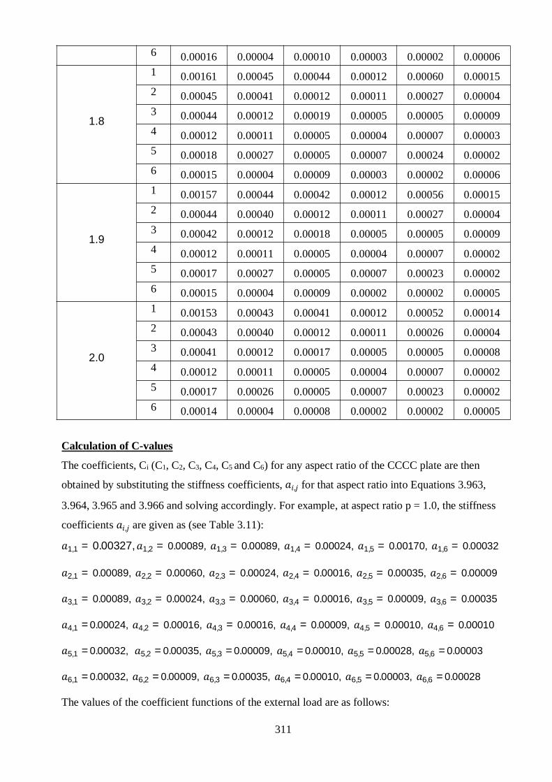
311

6 0.00016 0.00004 0.00010 0.00003 0.00002 0.00006

1.8

1 0.00161 0.00045 0.00044 0.00012 0.00060 0.000152 0.00045 0.00041 0.00012 0.00011 0.00027 0.000043 0.00044 0.00012 0.00019 0.00005 0.00005 0.000094 0.00012 0.00011 0.00005 0.00004 0.00007 0.000035 0.00018 0.00027 0.00005 0.00007 0.00024 0.000026 0.00015 0.00004 0.00009 0.00003 0.00002 0.00006

1.9

1 0.00157 0.00044 0.00042 0.00012 0.00056 0.000152 0.00044 0.00040 0.00012 0.00011 0.00027 0.000043 0.00042 0.00012 0.00018 0.00005 0.00005 0.000094 0.00012 0.00011 0.00005 0.00004 0.00007 0.000025 0.00017 0.00027 0.00005 0.00007 0.00023 0.000026 0.00015 0.00004 0.00009 0.00002 0.00002 0.00005

2.0

1 0.00153 0.00043 0.00041 0.00012 0.00052 0.000142 0.00043 0.00040 0.00012 0.00011 0.00026 0.000043 0.00041 0.00012 0.00017 0.00005 0.00005 0.000084 0.00012 0.00011 0.00005 0.00004 0.00007 0.000025 0.00017 0.00026 0.00005 0.00007 0.00023 0.000026 0.00014 0.00004 0.00008 0.00002 0.00002 0.00005


The coefficients, Ci (C1, C2, C3, C4, C5 and C6) for any aspect ratio of the CCCC plate are then


3.964, 3.965 and 3.966 and solving accordingly. For example, at aspect ratio p = 1.0, the stiffness


1,1 = 0.00327, 1,2 = 0.00089, 1,3 = 0.00089, 1,4 = 0.00024, 1,5 = 0.00170, 1,6 = 0.00032

2,1 = 0.00089, 2,2 = 0.00060, 2,3 = 0.00024, 2,4 = 0.00016, 2,5 = 0.00035, 2,6 = 0.00009

3,1 = 0.00089, 3,2 = 0.00024, 3,3 = 0.00060, 3,4 = 0.00016, 3,5 = 0.00009, 3,6 = 0.00035

4,1 =0.00024, 4,2 = 0.00016, 4,3 = 0.00016, 4,4 = 0.00009, 4,5 = 0.00010, 4,6 = 0.00010

5,1 =0.00032, 5,2 =0.00035, 5,3 =0.00009, 5,4 =0.00010, 5,5 =0.00028, 5,6 =0.00003

6,1 =0.00032, 6,2 =0.00009, 6,3 =0.00035, 6,4 =0.00010, 6,5 =0.00003, 6,6 =0.00028


312

1 = 0.00111; 2 = 0.00032; 3 = 0.00032; 4 = 0.00009; 5 = 0.00013; 6 = 0.00013




1 = 111

= 0.001110.00327

= 0.34028.

The coefficients, Ci for other aspect ratios of the CCCC plate for the first approximation are



1,1 1,2 1,3

2,1 2,2 2,33,1 3,2 3,3

1

2

3

=1

2

3

4

1

2

3

=0.00327 0.00089 0.000890.00089 0.00060 0.000240.00089 0.00024 0.00060

−1 1.1111 × 10−3

3.1746 × 10−4

3.1746 × 10−4

4 =0.3180800.0406970.040697

4

The coefficients, Ci (C1, C2 and C3) for other aspect ratios of the CCCC plate for the second



1

2

3

4

=

1,1 1,2 1,3 1,4

2,1 2,2 2,3 2,43,1 3,2 3,3 3,4

4,1 4,2 4,3 4,4

−11

2

3

4

4

1

2

3

4

=

0.00327 0.00089 0.00089 0.000240.00089 0.00060 0.00024 0.000160.00089 0.00024 0.00060 0.000160.00024 0.00016 0.00016 0.00009

−1 1.1111 × 10−3

3.1746 × 10−4

3.1746 × 10−4

9.7030 × 10−5

4

=0.318680.038470.038470.00824

4

The coefficients, Ci (C1, C2, C3 and C4) for other aspect ratios of the CCCC plate for the truncated



1,1 1,2 1,3 1,4 1,5 1,6

2,1 2,2 2,3 2,4 2,5 2,6

3,1 3,2 3,3 3,4 3,5 3,64,1 4,2 4,3 4,4 4,5 4,6

5,1 5,2 5,3 5,4 5,5 5,66,1 6,2 6,3 6,4 6,5 6,6

1

2

3

4

5

6

=

1

2

3

4

5

6

4

313

1

2

3

4

5

6

=

0.00327 0.00089 0.00089 0.00024 0.00170 0.000320.00089 0.00060 0.00024 0.00016 0.00035 0.000090.00089 0.00024 0.00060 0.00016 0.00009 0.000350.00024 0.00016 0.00016 0.00009 0.00010 0.00010

0.00032 0.00035 0.00009 0.00010 0.00028 0.000030.00032 0.00009 0.00035 0.00010 0.00003 0.00028

−1

1.1111 × 10−3

3.1746 × 10−4

3.1746 × 10−4

9.7030 × 10−5

1.3228 × 10−4

1.3228 × 10−4

4 =

0.242960.153700.15370−0.345960.063320.06332

4

The coefficients, Ci (C1, C2, C3, C4, C5 and C6) for other aspect ratios of the CCCC plate for the


Table 3.12: First Approximation Coefficient Values for CCCC Plate at Varying Aspect Ratio

Aspect ratio, P C1

1.0 0.340281.1 0.405981.2 0.465651.3 0.518291.4 0.563841.5 0.602831.6 0.635991.7 0.664161.8 0.688101.9 0.708492.0 0.72593

Table 3.13: Second Approximation Coefficient Values for CCCC Plate at Varying Aspect

Ratio


1.0 0.31808 0.04070 0.040701.1 0.37907 0.03973 0.058991.2 0.43350 0.03783 0.080221.3 0.48045 0.03541 0.103621.4 0.52004 0.03280 0.128311.5 0.55292 0.03019 0.153491.6 0.58001 0.02769 0.178481.7 0.60225 0.02536 0.20271

314

1.8 0.62051 0.02322 0.225791.9 0.63556 0.02129 0.247452.0 0.64801 0.01954 0.26755

Table 3.14: Truncated Third Approximation Coefficient Values for CCCC Plate at Varying

Aspect Ratio


1.0 0.31868 0.03847 0.03847 0.008241.1 0.37978 0.03707 0.05633 0.009871.2 0.43432 0.03475 0.07715 0.011401.3 0.48138 0.03197 0.10018 0.012751.4 0.52105 0.02905 0.12456 0.013881.5 0.55400 0.02620 0.14951 0.014731.6 0.58113 0.02354 0.17433 0.015301.7 0.60339 0.02113 0.19848 0.015601.8 0.62167 0.01897 0.22153 0.015671.9 0.63670 0.01707 0.24322 0.015542.0 0.64914 0.01540 0.26339 0.01525

Table 3.15: Third Approximation Coefficients Values for CCCC Plate at Varying Aspect

Ratio


1.0 0.24296 0.15370 0.15370 -0.34596 0.06332 0.063321.1 0.30999 0.14825 0.12128 -0.35834 0.06654 0.152231.2 0.37738 0.13779 0.05833 -0.35473 0.06821 0.279291.3 0.44350 0.12438 -0.03600 -0.33916 0.06854 0.446561.4 0.50750 0.10969 -0.16078 -0.31584 0.06781 0.654151.5 0.56901 0.09495 -0.31384 -0.28832 0.06628 0.900491.6 0.62798 0.08094 -0.49223 -0.25930 0.06418 1.182691.7 0.68450 0.06809 -0.69251 -0.23061 0.06169 1.496911.8 0.73868 0.05661 -0.91103 -0.20338 0.05896 1.838581.9 0.79065 0.04654 -1.14405 -0.17825 0.05612 2.202712.0 0.84050 0.03782 -1.38790 -0.15550 0.05323 2.58413

Deflections


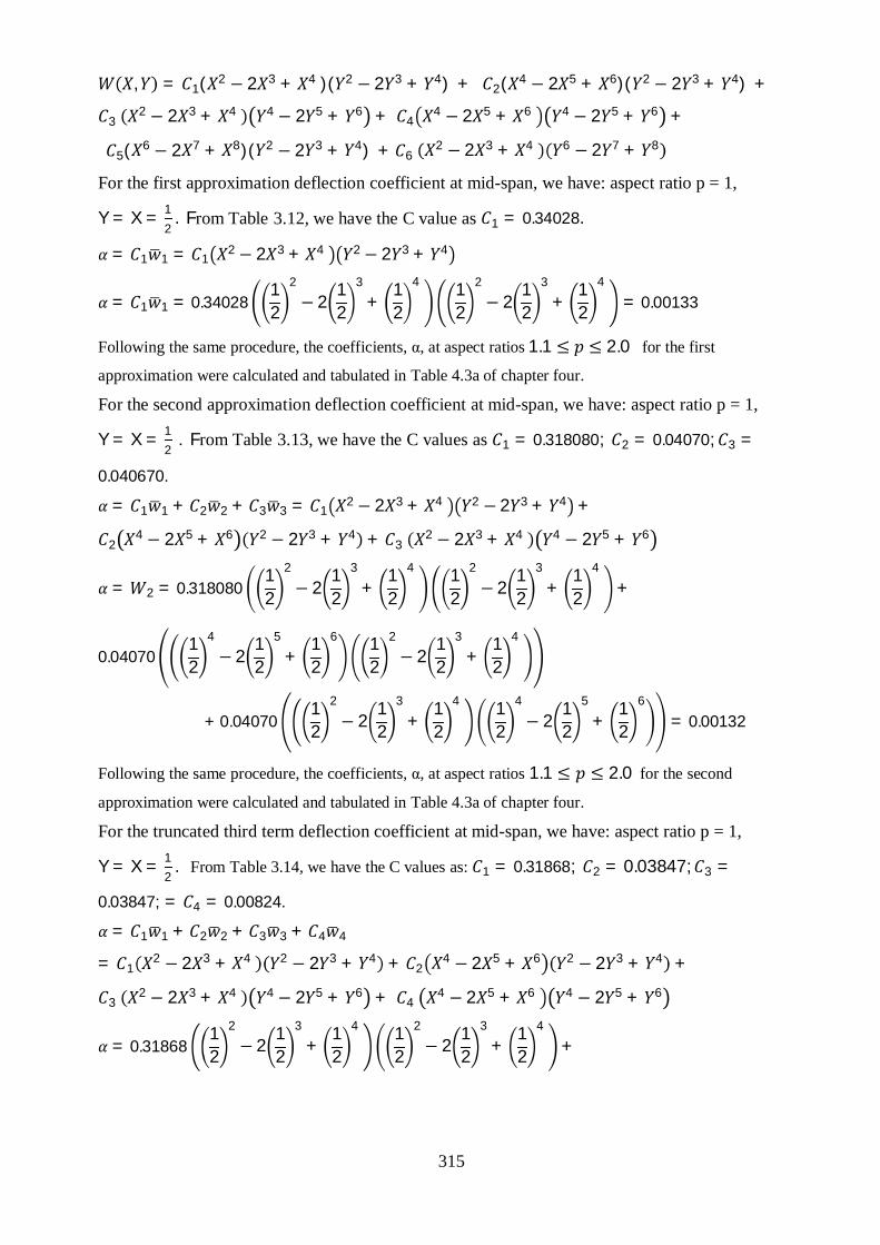
315

, = 1( 2 − 2 3 + 4 )( 2 − 2 3 + 4) + 2( 4 − 2 5 + 6)( 2 − 2 3 + 4) +

32 − 2 3 + 4 4 − 2 5 + 6 + 4

4 − 2 5 + 6 4 − 2 5 + 6 +

5( 6 − 2 7 + 8)( 2 − 2 3 + 4) + 62 − 2 3 + 4 6 − 2 7 + 8


Y = X = 12

. From Table 3.12, we have the C value as 1 = 0.34028.

= 1 1 = 12 − 2 3 + 4 2 − 2 3 + 4

= 1 1 = 0.3402812

2

− 212

3

+12

4 12

2

− 212

3

+12

4

= 0.00133




Y = X = 12

. From Table 3.13, we have the C values as 1 = 0.318080; 2 = 0.04070; 3 =

0.040670.

= 1 1 + 2 2 + 3 3 = 12 − 2 3 + 4 2 − 2 3 + 4 +

24 − 2 5 + 6 2 − 2 3 + 4 + 3

2 − 2 3 + 4 4 − 2 5 + 6

= 2 = 0.31808012

2

− 212

3

+12

4 12

2

− 212

3

+12

4

+

0.0407012

4

− 212

5

+12

6 12

2

− 212

3

+12

4

+ 0.0407012

2

− 212

3

+12

4 12

4

− 212

5

+12

6

= 0.00132




Y = X = 12


0.03847; = 4 = 0.00824.

= 1 1 + 2 2 + 3 3 + 4 4

= 12 − 2 3 + 4 2 − 2 3 + 4 + 2

4 − 2 5 + 6 2 − 2 3 + 4 +

32 − 2 3 + 4 4 − 2 5 + 6 + 4

4 − 2 5 + 6 4 − 2 5 + 6

= 0.3186812

2

− 212

3

+12

4 12

2

− 212

3

+12

4

+

316

0.0384712

4

− 212

5

+12

6 12

2

− 212

3

+12

4

+

0.0384712

2

− 212

3

+12

4 12

4

− 212

5

+12

6

+0.0082412

4

− 212

5

+12

6 12

4

− 212

5

+12

6

= 0.00132




Y = X = 12


0.15370; = 4 =− 0.34596; 5 = 0.06332; 6 = 0.06332;= 1 1 + 2 2 + 3 3 + 4 4 + 5 5 + 6 6

= 12 − 2 3 + 4 2 − 2 3 + 4 + 2

4 − 2 5 + 6 2 − 2 3 + 4 +

32 − 2 3 + 4 4 − 2 5 + 6 + 4

4 − 2 5 + 6 4 − 2 5 + 6 +

56 − 2 7 + 8 2 − 2 3 + 4 + 6

2 − 2 3 + 4 6 − 2 7 + 8

= 0.2429612

2

− 212

3

+12

4 12

2

− 212

3

+12

4

+

0.1537012

4

− 212

5

+12

6 12

2

− 212

3

+12

4

+

0.1537012

2

− 212

3

+12

4 12

4

− 212

5

+12

6

−0.3459612

4

− 212

5

+12

6 12

4

− 212

5

+12

6

+

0.0633212

6

− 212

7

+12

8 12

2

− 212

3

+12

4

+

0.0633212

2

− 212

3

+12

4 12

6

− 212

7

+12

8

= 0.00120



317


The six-term bending moment function of the plate obtained in Equations 3.1569d and 3.1570d in


=− 2 1 1 − 6 + 6 2 ( 2 − 2 3 + 4) + 4 2 3 2 − 10 3 + 7.5 4 ( 2 − 2 3 + 4) +

2 3 1 − 6 + 6 2 4 − 2 5 + 6 + 4 4 3 2 − 10 3 + 7.5 4 4 − 2 5 + 6 + 5 (30 4

− 84 5 + 56 6)( 2 − 2 3 + 4) + 2 6 1 − 6 + 6 2 6 − 2 7 + 8 +

2 2 12 − 2 3 + 4 1 − 6 + 6 2 + 2 2( 4 − 2 5 + 6) 1− 6 + 6 2 +

4 32 − 2 3 + 4 3 2 − 10 3 + 7.5 4 + 4 4

4 − 2 5 + 6 3 2 − 10 3 + 30 4

+ 2 5 ( 6 − 2 7 + 8)(1 − 6 + 6 2)+ 6

2 − 2 3 + 4 30 4 − 84 5 + 56 8

=− 2 1 1 − 6 + 6 2 ( 2 − 2 3 + 4) + 4 2 3 2 − 10 3 + 7.5 4 ( 2 − 2 3 + 4) +

2 3 1 − 6 + 6 2 4 − 2 5 + 6 + 4 4 3 2 − 10 3 + 7.5 4 4 − 2 5 + 6 + 5 (30 4

− 84 5 + 56 6)( 2 − 2 3 + 4) + 2 6 1 − 6 + 6 2 6 − 2 7 + 8 +

12 2 1

2 − 2 3 + 4 1 − 6 + 6 2 + 2 2( 4 − 2 5 + 6) 1− 6 + 6 2 +

4 32 − 2 3 + 4 3 2 − 10 3 + 7.5 4 + 4 4

4 − 2 5 + 6 3 2 − 10 3 + 7.5 4

+ 2 5 ( 6 − 2 7 + 8)(1 − 6 + 6 2)+ 6

2 − 2 3 + 4 30 4 − 84 5 + 56 8

For the first approximation bending moment coefficient at mid-span of plate along x – direction we


, ν = 0.3. From Table 3.12, the C value is given as: 1 =

0.34028.

1 = 1 =− 2 0.34028 1 − 612

+ 612

2 12

2

− 212

3

+12

4

+

0.312 2 0.34028

12

2

− 212

3

+12

4

1 − 612

+ 612

2

= 0.02765

Similarly,

1 = 1 =− 2 0.34028 (0.3) 1 − 612

+ 612

2 12

2

− 212

3

+12

4

+

112 2 0.34028

12

2

− 212

3

+12

4

1 − 612 + 6

12

2

= 0.02765

318




ratio p = 1, X = Y = 12


0.04070; C3 = 0.04070.

2 =− 2 0.31808 1 − 612 + 6

12

2 12

2

− 212

3

+12

4

+

+4 0.04070 312

2

− 1012

3

+ 7.512

4 12

2

− 212

3

+12

4

+ 2 0.04070 1 − 612

+ 612

2 12

4

− 212

5

+12

6

+

0.312 2 0.31808

12

2

− 212

3

+12

4

1− 612 + 6

12

2

+

2 0.0407012

4

− 212

5

+12

6

1 − 612

+ 612

2

+ 4 0.0407012

2

− 212

3

+12

4

312

2

− 1012

3

+ 7.512

4

= 0.0271

Similarly,

2 =− (0.3) 2 0.31808 1− 612

+ 612

2 12

2

− 212

3

+12

4

+

+4 0.04070 312

2

− 1012

3

+ 7.512

4 12

2

− 212

3

+12

4

+ 2 0.04070 1 − 612

+ 612

2 12

4

− 212

5

+12

6

+

112 2 0.31808

12

2

− 212

3

+12

4

1 − 612 + 6

12

2

+

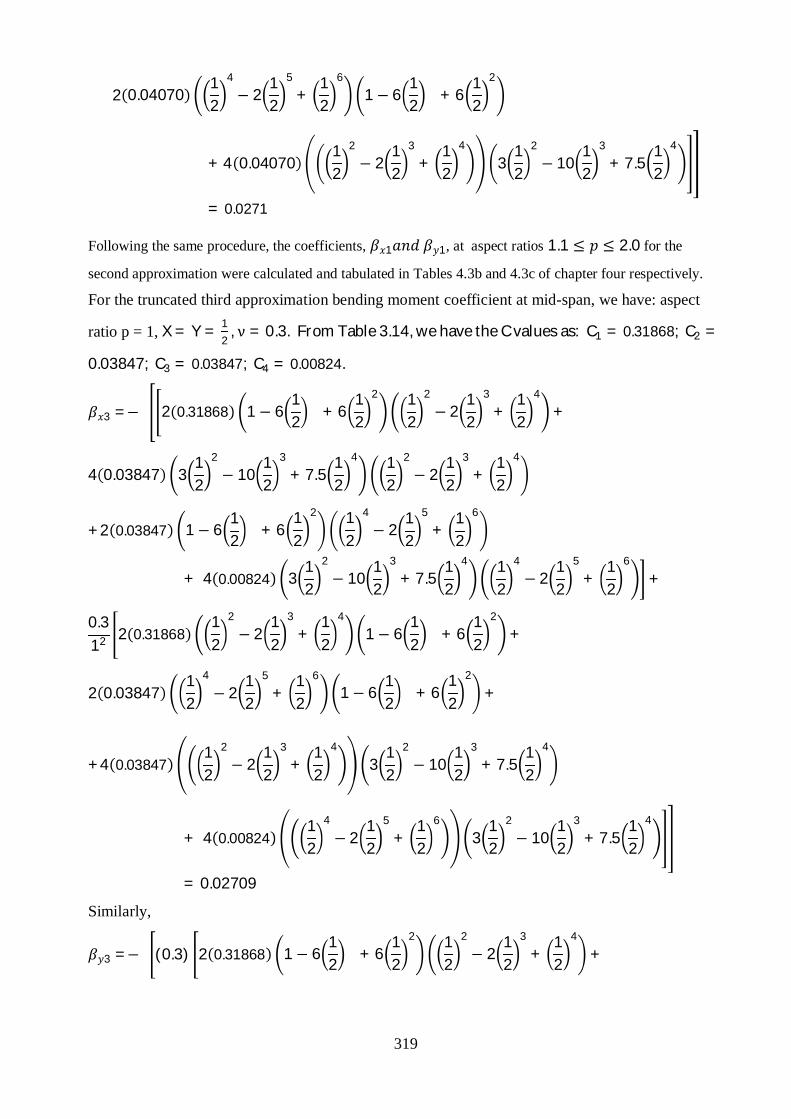
319

2 0.0407012

4

− 212

5

+12

6

1 − 612

+ 612

2

+ 4 0.0407012

2

− 212

3

+12

4

312

2

− 1012

3

+ 7.512

4

= 0.0271



For the truncated third approximation bending moment coefficient at mid-span, we have: aspect

ratio p = 1, X = Y = 12


0.03847; C3 = 0.03847; C4 = 0.00824.

3 =− 2 0.31868 1 − 612 + 6

12

2 12

2

− 212

3

+12

4

+

4 0.03847 312

2

− 1012

3

+ 7.512

4 12

2

− 212

3

+12

4

+2 0.03847 1 − 612

+ 612

2 12

4

− 212

5

+12

6

+ 4 0.00824 312

2

− 1012

3

+ 7.512

4 12

4

− 212

5

+12

6

+

0.312 2 0.31868

12

2

− 212

3

+12

4

1 − 612

+ 612

2

+

2 0.0384712

4

− 212

5

+12

6

1 − 612

+ 612

2

+

+4 0.0384712

2

− 212

3

+12

4

312

2

− 1012

3

+ 7.512

4

+ 4 0.0082412

4

− 212

5

+12

6

312

2

− 1012

3

+ 7.512

4

= 0.02709

Similarly,

3 =− (0.3) 2 0.31868 1 − 612

+ 612

2 12

2

− 212

3

+12

4

+

320

4 0.03847 312

2

− 1012

3

+ 7.512

4 12

2

− 212

3

+12

4

+2 0.03847 1 − 612 + 6

12

2 12

4

− 212

5

+12

6

+ 4 0.00824 312

2

− 1012

3

+ 7.512

4 12

4

− 212

5

+12

6

+

112 2 0.31868

12

2

− 212

3

+12

4

1 − 612

+ 612

2

+

2 0.0384712

4

− 212

5

+12

6

1 − 612 + 6

12

2

+

+4 0.0384712

2

− 212

3

+12

4

312

2

− 1012

3

+ 7.512

4

+ 4 0.0082412

4

− 212

5

+12

6

312

2

− 1012

3

+ 7.512

4

= 0.02709




ratio p = 1, X = Y = 12


0.15370; C3 = 0.15370; C4 =− 0.34596; C5 = 0.06332; C6 = 0.06332.

4 =− 2 0.24296 1 − 612

+ 612

2 12

2

− 212

3

+12

4

+

4 0.15370 312

2

− 1012

3

+ 7.512

4 12

2

− 212

3

+12

4

+ 2 0.15370 1 − 612 + 6

12

2 12

4

− 212

5

+12

6

+ 4 −0.3459612

4

− 212

5

+12

6

312

2

− 1012

3

+ 7.512

4

+ 0.06332 3012

4

− 8412

5

+ 5612

6 12

2

− 212

3

+12

4

321

+2 0.06332 1 − 612 + 6

12

2 12

6

− 212

7

+12

8

+

0.312 2 0.24296

12

2

− 212

3

+12

4

1 − 612 + 6

12

2

+

2 0.1537012

4

− 212

5

+12

6

1 − 612

+ 612

2

+

+4 0.1537012

2

− 212

3

+12

4

312

2

− 1012

3

+ 7.512

4

+ 4 −0.3459612

4

− 212

5

+12

6

312

2

− 1012

3

+ 7.512

4

+2 0.0633212

6

− 212

7

+12

8

1 − 612 + 6

12

2

+ 0.0633212

2

− 212

3

+12

4

3012

4

− 8412

5

+ 5612

6

= 0.02322

Similarly,

4 =− (0.3) 2 0.24296 1 − 612

+ 612

2 12

2

− 212

3

+12

4

+

4 0.15370 312

2

− 1012

3

+ 7.512

4 12

2

− 212

3

+12

4

+ 2 0.15370 1 − 612 + 6

12

2 12

4

− 212

5

+12

6

+ 4 −0.3459612

4

− 212

5

+12

6

312

2

− 1012

3

+ 7.512

4

+ 0.06332 3012

4

− 8412

5

+ 5612

6 12

2

− 212

3

+12

4

+ 2 0.06332 1 − 612

+ 612

2 12

6

− 212

7

+12

8

+

112 2 0.24296

12

2

− 212

3

+12

4

1 − 612

+ 612

2

+

2 0.1537012

4

− 212

5

+12

6

1 − 612

+ 612

2

+

322

+4 0.1537012

2

− 212

3

+12

4

312

2

− 1012

3

+ 7.512

4

+ 4 −0.3459612

4

− 212

5

+12

6

312

2

− 1012

3

+ 7.512

4

+2 0.0633212

6

− 212

7

+12

8

1 − 612 + 6

12

2

+ 0.0633212

2

− 212

3

+12

4

3012

4

− 8412

5

+ 5612

6

= 0.02322





11 = 1.3571 × 10−2 + 1.4694 × 10−2 12 + 1.3571 × 10−2 1

4

12 = 4.7392 × 10−3 + 5.9184 × 10−3 12 + 4.7078 × 10−3 1

4

13 = 4.7078 × 10−3 + 5.9184 × 10−3 12 + 4.7392 × 10−3 1

4

14 = 1.6440 × 10−3 + 2.3838 × 10−3 12 + 1.6440 × 10−3 1

4

15 = 2.3337 × 10−3 + 2.7829 × 10−3 12 + 2.0979 × 10−3 1

4

16 = 2.0979 × 10−3 + 2.7829 × 10−3 12 + 2.3337 × 10−3 1

4

21 = −2.8005 × 10−3 + 5.9184 × 10−3 12 + 4.7078 × 10−3 1

4

22 = 1.7234 × 10−3 + 4.5764 × 10−3 12 + 2.0979 × 10−3 1

4

23 = −9.7145 × 10−4 + 2.3838 × 10−3 12 + 1.6440 × 10−3 1

4

24 = 5.9781 × 10−4 + 1.8433 × 10−3 12 + 7.3260 × 10−4 1

4

25 = 2.0726 × 10−3 + 3.0969 × 10−3 12 + 1.0939 × 10−3 1

4

26 = −4.3290 × 10−4 + 1.1209 × 10−3 12 + 8.0954 × 10−4 1

4

323

31 = 4.7078 × 10−3 + 5.9184 × 10−3 12 − 2.8005 × 10−3 1

4

32 = 1.6440 × 10−3 + 2.3838 × 10−3 12 − 1.5356 × 10−2 1

4

33 = 2.0979 × 10−3 + 4.5764 × 10−3 12 + 1.7234 × 10−3 1

4

34 = 7.3260 × 10−4 + 1.8433 × 10−3 12 + 5.9781 × 10−4 1

4

35 = 8.0954 × 10−4 + 1.1209 × 10−3 12 − 4.3290 × 10−4 1

4

36 = 1.0939 × 10−3 + 3.0969 × 10−3 12 + 2.0726 × 10−3 1

4

41 = −9.7145 × 10−4 + 2.3838 × 10−3 12 − 9.7145 × 10−4 1

4

42 = 5.9781 × 10−4 + 1.8433 × 10−3 12 − 4.3290 × 10−4 1

4

43 = −4.3290 × 10−4 + 1.8433 × 10−3 12 + 5.9781 × 10−4 1

4

44 = 2.6640 × 10−4 + 1.4253 × 10−3 12 + 2.6640 × 10−4 1

4

45 = 7.1896 × 10−4 + 1.2474 × 10−3 12 − 2.2573 × 10−4 1

4

46 = −2.2573 × 10−4 + 1.2474 × 10−3 12 + 7.1896 × 10−4 1

4

51 = −1.2746 × 10−2 + 2.7829 × 10−3 12 + 2.0979 × 10−3 1

4

52 = −5.4671 × 10−3 + 3.0969 × 10−3 12 + 1.0939 × 10−3 1

4

53 = −4.4213 × 10−3 + 1.1209 × 10−3 12 + 2.3310 × 10−3 1

4

54 = −1.8965 × 10−3 + 1.2474 × 10−3 12 + 3.8200 × 10−4 1

4

55 = −2.3726 × 10−3 + 2.5574 × 10−3 12 + 6.3510 × 10−4 1

4

56 = −1.9703 × 10−3 + 5.2707 × 10−4 12 + 3.6075 × 10−4 1

4

61 = 2.0979 × 10−3 + 2.7829 × 10−3 12 − 1.2746 × 10−2 1

4

62 = 7.3260 × 10−4 + 1.1209 × 10−3 12 − 4.4213 × 10−3 1

4

324

63 = 1.0939 × 10−3 + 3.0969 × 10−3 12 − 5.4671 × 10−3 1

4

64 = 3.8200 × 10−4 + 1.2474 × 10−3 12 − 4.5119 × 10−3 1

4

65 = 3.6075 × 10−4 + 5.2707 × 10−4 12 − 1.9703 × 10−3 1

4

66 = 6.3510 × 10−4 + 2.5574 × 10−3 12 − 2.3726 × 10−3 1

4

The stiffness coefficients, , obtained for aspect ratios, 1.0 ≤ P ≤ 2.0 using the above equations are

shown in Table 3.16.

Table 3.16: Stiffness Coefficient Values for CCSS Plate at varying Aspect Ratio

Aspectratio, P

, 1 2 3 4 5 6

1

1 0.04184 0.01537 0.01537 0.00567 0.00721 0.007212 0.00783 0.00840 0.00306 0.00317 0.00626 0.001503 0.00783 -0.01133 0.00840 0.00317 0.00150 0.006264 0.00044 0.00201 0.00201 0.00196 0.00174 0.001745 -0.00786 -0.00128 -0.00097 -0.00027 0.00082 -0.001086 -0.00786 -0.00257 -0.00128 -0.00288 -0.00108 0.00082

1.1

1 0.03498 0.01285 0.01284 0.00474 0.00607 0.005992 0.00531 0.00694 0.00212 0.00262 0.00538 0.001053 0.00769 -0.00687 0.00706 0.00266 0.00144 0.005074 0.00034 0.00183 0.00150 0.00163 0.00160 0.001305 -0.00901 -0.00216 -0.00190 -0.00060 0.00017 -0.001296 -0.00431 -0.00136 -0.00008 -0.00167 -0.00055 0.00113

1.2

1 0.03032 0.01112 0.01110 0.00409 0.00528 0.005162 0.00358 0.00591 0.00148 0.00223 0.00475 0.000743 0.00747 -0.00411 0.00611 0.00230 0.00138 0.004244 0.00022 0.00167 0.00114 0.00138 0.00148 0.000995 -0.00980 -0.00279 -0.00252 -0.00085 -0.00029 -0.001436 -0.00212 -0.00062 0.00061 -0.00093 -0.00022 0.00127

1.3

1 0.02702 0.00989 0.00987 0.00363 0.00471 0.004562 0.00235 0.00517 0.00101 0.00195 0.00429 0.000513 0.00723 -0.00232 0.00541 0.00203 0.00132 0.003654 0.00010 0.00154 0.00087 0.00120 0.00138 0.00076

325

5 -0.01036 -0.00325 -0.00294 -0.00102 -0.00064 -0.001536 -0.00072 -0.00015 0.00101 -0.00046 -0.00002 0.00132

1.4

1 0.02460 0.00898 0.00896 0.00329 0.00430 0.004132 0.00144 0.00460 0.00067 0.00173 0.00394 0.000353 0.00700 -0.00114 0.00488 0.00183 0.00127 0.003214 -0.00001 0.00143 0.00066 0.00106 0.00130 0.000605 -0.01078 -0.00360 -0.00324 -0.00116 -0.00090 -0.001616 0.00020 0.00015 0.00125 -0.00016 0.00012 0.00132

1.5

1 0.02278 0.00830 0.00827 0.00303 0.00398 0.003802 0.00076 0.00417 0.00041 0.00156 0.00367 0.000233 0.00679 -0.00033 0.00447 0.00167 0.00122 0.002884 -0.00010 0.00133 0.00050 0.00095 0.00123 0.000475 -0.01109 -0.00387 -0.00346 -0.00127 -0.00111 -0.001666 0.00082 0.00036 0.00139 0.00005 0.00021 0.00130

1.6

1 0.02138 0.00777 0.00774 0.00283 0.00374 0.003542 0.00023 0.00383 0.00021 0.00143 0.00345 0.000133 0.00659 0.00023 0.00415 0.00154 0.00118 0.002624 -0.00019 0.00125 0.00038 0.00086 0.00117 0.000375 -0.01134 -0.00409 -0.00363 -0.00135 -0.00128 -0.001716 0.00124 0.00050 0.00147 0.00018 0.00027 0.00127

1.7

1 0.02028 0.00735 0.00732 0.00267 0.00355 0.003342 -0.00019 0.00356 0.00005 0.00132 0.00328 0.000053 0.00642 0.00063 0.00389 0.00144 0.00115 0.002414 -0.00026 0.00118 0.00028 0.00079 0.00112 0.000295 -0.01153 -0.00426 -0.00375 -0.00142 -0.00141 -0.001746 0.00153 0.00059 0.00151 0.00027 0.00031 0.00124

1.8

1 0.01940 0.00701 0.00699 0.00254 0.00339 0.003182 -0.00053 0.00334 -0.00008 0.00124 0.00313 -0.000013 0.00627 0.00092 0.00367 0.00136 0.00111 0.002254 -0.00033 0.00113 0.00019 0.00073 0.00108 0.000235 -0.01169 -0.00441 -0.00385 -0.00148 -0.00152 -0.001776 0.00174 0.00066 0.00153 0.00034 0.00034 0.00120

1.91 0.01868 0.00674 0.00671 0.00243 0.00327 0.003052 -0.00080 0.00315 -0.00018 0.00116 0.00301 -0.00006

326

3 0.00613 0.00113 0.00350 0.00129 0.00109 0.002114 -0.00039 0.00108 0.00012 0.00068 0.00105 0.000175 -0.01181 -0.00453 -0.00393 -0.00152 -0.00162 -0.001806 0.00189 0.00070 0.00153 0.00038 0.00036 0.00116

2.0

1 0.01809 0.00651 0.00648 0.00234 0.00316 0.002942 -0.00103 0.00300 -0.00027 0.00110 0.00292 -0.000103 0.00601 0.00128 0.00335 0.00123 0.00106 0.002004 -0.00044 0.00103 0.00007 0.00064 0.00102 0.000135 -0.01192 -0.00462 -0.00400 -0.00156 -0.00169 -0.001826 0.00200 0.00074 0.00153 0.00041 0.00037 0.00113


The coefficients, Ci (C1, C2, C3, C4, C5 and C6) for any aspect ratio of the CCSS plate are then


3.1259, 3.1260 and 3.1261 and solving accordingly. For example, at aspect ratio p = 1.0, the

stiffness coefficients , are given as (see Table 3.16):

1,1 =0.04184, 1,2 =0.01537, 1,3 =0.01537, 1,4 =0.00567, 1,5 =0.00721, 1,6 =0.00721

2,1 =0.00783, 2,2 =0.00840, 2,3 =0.00306, 2,4 =0.00317, 2,5 =0.00626, 2,6 =0.00150

3,1 =0.00783, 3,2 =-0.01133, 3,3 =0.00840, 3,4 =0.00317, 3,5 =0.00150, 3,6 =0.00626

4,1 =0.00044 4,2 =0.00201, 4,3 =0.00201, 4,4 =0.00196, 4,5 =0.00174, 4,6 =0.00174

5,1 =-0.00786, 5,2 =-0.00128, 5,3 =-0.00097, 5,4 =-0.00027, 5,5 =0.00082, 5,6 =-0.00108

6,1 =-0.00786, 6,2 =-0.00257, 6,3 =-0.00128, 6,4 =-0.00288, 6,5 =-0.00108, 6,6 =0.00082


1 = 0.00563; 2 = 0.00196; 3 = 0.00196; 4 = 0.00069; 5 =0.00097; 6 =0.00097


subsequently solving the resulting canonical equations gives:


1 = 111

= 0.005630.04184

= 0.13445.

The coefficients, C1 for other aspect ratios of the CCSS plate for the first approximation are



327

1,1 1,2 1,32,1 2,2 2,3

3,1 3,2 3,3

1

2

3

=1

2

3

4

1

2

3

=0.04184 0.01537 0.015370.00783 0.00840 0.003060.00783 −0.01133 0.00840

−1 5.63000 × 10−3

1.96000 × 10−3

1.96000 × 10−3

4 =−0.119270.147200.54364

4

The coefficients, Ci (C1, C2 and C3) for other aspect ratios of the CCSS plate for the second



1

2

3

4

=

1,1 1,2 1,3 1,4

2,1 2,2 2,3 2,43,1 3,2 3,3 3,4

4,1 4,2 4,3 4,4

−11

2

3

4

4

1

2

3

4

=

0.04184 0.01537 0.01537 0.005670.00783 0.00840 0.00306 0.003170.00783 − 0.01133 0.00840 0.003170.00044 0.00201 0.00201 0.00196

−1 5.63000 × 10−3

1.96000 × 10−3

1.96000 × 10−3

6.90000 × 10−4

4

=0.15850−0.06227−0.229980.61435

4

The coefficients, Ci (C1, C2, C3 and C4) for other aspect ratios of the CCSS plate for the truncated



1,1 1,2 1,3 1,4 1,5 1,6

2,1 2,2 2,3 2,4 2,5 2,6

3,1 3,2 3,3 3,4 3,5 3,64,1 4,2 4,3 4,4 4,5 4,6

5,1 5,2 5,3 5,4 5,5 5,66,1 6,2 6,3 6,4 6,5 6,6

1

2

3

4

5

6

=

1

2

3

4

5

6

4

1

2

3

4

5

6

=

0.04184 0.01537 0.01537 0.00567 0.00721 0.007210.00783 0.00840 0.00306 0.00317 0.00626 0.00150

0.00783 − 0.01133 0.00840 0.00317 0.00150 0.006260.00044 0.00201 0.00201 0.00196 0.00174 0.00174

− 0.00786 − 0.00128 − 0.00097 − 0.00027 0.00082 − 0.00108− 0.00786 − 0.00257 − 0.00128 − 0.00288 − 0.00108 0.00082

−1

5.63000 × 10−3

1.96000 × 10−3

1.96000 × 10−3

6.90000 × 10−4

9.70000 × 10−4

9.70000 × 10−4

4 =

−0.143960.081120.90862−0.643130.34737−0.33521

4

The coefficients, Ci (C1, C2, C3, C4, C5 and C6) for other aspect ratios of the CCSS plate for the


328

Table 3.17: First Approximation Coefficient Values for CCSS Plate at Varying Aspect Ratio

Aspect ratio, P C1

1.0 0.13445

1.1 0.16079

1.2 0.18552

1.3 0.20820

1.4 0.22865

1.5 0.24690

1.6 0.26307

1.7 0.27736

1.8 0.28996

1.9 0.30107

2.0 0.31089

Table 3.18: Second Approximation Coefficient Values for CCSS Plate at Varying Aspect

Ratio


1.0 -0.11927 0.14720 0.54364

1.1 -0.14438 0.20059 0.63100

1.2 -0.16326 0.25759 0.69447

1.3 -0.17518 0.31598 0.73291

1.4 -0.18044 0.37391 0.74821

1.5 -0.17994 0.43003 0.74393

1.6 -0.17488 0.48339 0.72436

1.7 -0.16647 0.53344 0.69369

1.8 -0.15583 0.57988 0.65567

1.9 -0.14387 0.62267 0.61336

2.0 -0.13133 0.66188 0.56918

Table 3.19: Truncated Third Approximation Coefficient Values for CCSS Plate at Varying

Aspect Ratio


1.0 0.15850 -0.06227 -0.22998 0.61435

1.1 0.25708 -0.12791 -0.49028 0.96422

329

1.2 0.42705 -0.26670 -0.95881 1.53665

1.3 0.79753 -0.62100 -1.99826 2.73817

1.4 2.40378 -2.32070 -6.52382 7.84620

1.5 -3.46814 4.13128 10.01469 -10.73692

1.6 -1.07669 1.57544 3.27108 -3.15664

1.7 -0.64497 1.15437 2.04686 -1.78916

1.8 -0.45756 0.99770 1.50996 -1.20066

1.9 -0.34975 0.92556 1.19687 -0.86847

2.0 -0.27829 0.89058 0.98607 -0.65459

Table 3.20: Third Approximation Coefficient Values for CCSS Plate at Varying Aspect Ratio


1.0 -0.14396 0.08112 0.90862 -0.64313 0.34737 -0.33521

1.1 -0.28480 0.13541 1.63294 -0.81716 0.41202 -0.95797

1.2 -0.50425 0.22490 2.72622 -1.02232 0.44771 -1.94652

1.3 -0.82836 0.37131 4.30170 -1.25736 0.42595 -3.41202

1.4 -1.29414 0.60863 6.52130 -1.51629 0.30372 -5.51810

1.5 -1.96264 0.99288 9.65568 -1.79188 0.01373 -8.54214

1.6 -2.94855 1.62548 14.21812 -2.08135 -0.56029 -13.00963

1.7 -4.49759 2.71704 21.31211 -2.39573 -1.65271 -20.04444

1.8 -7.24042 4.79912 33.77183 -2.78343 -3.84784 -32.52185

1.9 -13.40074 9.73424 61.58991 -3.43654 -9.18656 -60.56225

2.0 -40.23357 31.95089 182.29756 -5.87129 -33.47495 -182.65403

Deflections


, = 1(1.5 2 − 2.5 3 + 4 )(1.5 2 − 2.5 3 + 4) + 2(1.5 4 − 2.5 5 + 6)(1.5 2

−2. 5 3 + 4) + 3 1.5 2 − 2.5 3 + 4 1.5 4 − 2.5 5 + 6

+ 4 1.5 4 − 2.5 5 + 6 1.5 4 − 2.5 5 + 6 + 5(1.5 6 − 2.5 7 + 8)

(1.5 2 − 2.5 3 + 4) + 6 1.5 2 − 2. 5 3 + 4 1.5 6 − 2.5 7 + 8


Y = X = 12

. From Table 3.17, we have the C value as C1 = 0.13445.

= 1 1 = 1 1.5 2 − 2.5 3 + 4 1.5 2 − 2.5 3 + 4

330

= 1 1 = 0.20569 1.512

2

− 2.512

3

+12

4

1.512

2

− 2.512

3

+12

4

= 0.00210




Y = X = 12

. From Table 3.18, we have the C values as 1 =− 0.11927; 2 = 0.14720; 3 =

0.54364.

= 1 1 + 2 2 + 3 3 = 1 1.5 2 − 2.5 3 + 4 1.5 2 − 2. 5 3 + 4 +

2 1.5 4 − 2.5 5 + 6 1.5 2 − 2.5 3 + 4 + 3 1.5 2 − 2. 5 3 + 4

1.5 4 − 2.5 5 + 6

=− 0.11927 1.512

2

− 2.512

3

+12

4

1.512

2

− 2.512

3

+12

4

+

0.14720 1.512

4

− 2.512

5

+12

6

1.512

2

− 2.512

3

+12

4

+0.54364 1.512

2

− 2.512

3

+12

4

1.512

4

− 2.512

5

+12

6

= 0.00083



For the truncated third term deflection coefficient at mid-span, we have: aspect ratio p = 1, Y =

X = 12

. From Table 3.19, we have the C values as: 1 = 0.15850; 2 =− 0.06227; 3 =−

0.22998; 4 = 0.61435.

= 1 1 + 2 2 + 3 3 + 4 4= 1 1.5 2 − 2.5 3 + 4 1.5 2 − 2.5 3 + 4 + 2 1.5 4 − 2. 5 5 + 6

1.5 2 − 2.5 3 + 4 + 3 1.5 2 − 2. 5 3 + 4 1.5 4 − 2. 5 5 + 6

+ 4 1.5 4 − 2.5 5 + 6 1.5 4 − 2. 5 5 + 6

= 0.15850 1.512

2

− 2.512

3

+12

4

1.512

2

− 2.512

3

+12

4

+

−0.06227 1.512

4

− 2.512

5

+12

6

1.512

2

− 2.512

3

+12

4

+

331

−0.22998 1.512

2

− 2.512

3

+12

4

1.512

4

− 2.512

5

+12

6

+ 0.61435 1.512

4

− 2.512

5

+12

6

1.512

4

− 2.512

5

+12

6

= 0.00193




Y = X = 12

. From Table 3.20, we have the C values as: 1 =− 0.14396; 2 = 0.08112; 3 =

0.90862; = 4 =− 0.64313; 5 = 0.34737; 6 =− 0.33521.

= 1 1 + 2 2 + 3 3 + 4 4 + 5 5 + 6 6

= 1 1.5 2 − 2.5 3 + 4 1.5 2 − 2.5 3 + 4 + 2 1.5 4 − 2. 5 5 + 6

1.5 2 − 2.5 3 + 4 + 3 1.5 2 − 2.5 3 + 4 1.5 4 − 2.5 5 + 6

+ 4 1.5 4 − 2.5 5 + 6 1.5 4 − 2. 5 5 + 6 + 5 1.5 6 − 2.5 7 + 8

1.5 2 − 2. 5 3 + 4 + 6 1.5 2 − 2.5 3 + 4 1.5 6 − 2.5 7 + 8

=− 0.14396 1.512

2

− 2.512

3

+12

4

1.512

2

− 2. 512

3

+12

4

+

0.08112 1.512

4

− 2.512

5

+12

6

1.512

2

− 2.512

3

+12

4

+

0.90862 1.512

2

− 2.512

3

+12

4

1.512

4

− 2.512

5

+12

6

−0.64313 1.512

4

− 2.512

5

+12

6

1.512

4

− 2.512

5

+12

6

+

0.34737 1.512

6

− 2.512

7

+12

8

1.512

2

− 2.512

3

+12

4

+

−0.33521 1.512

2

− 2.512

3

+12

4

1.512

6

− 2.512

7

+12

8

= 0.00100



.Moments in x and y directions

The six-term bending moment functions of the plate obtained in Equation 3.1573d and 3.1574d in

x and y directions are given as:

332

=− 1 3 − 15 + 12 2 (1.5 2 − 2.5 3 + 4) + 2 18 2 − 50 3 + 30 4 (1.5 2

−2. 5 3 + 4) + 3 3 − 15 + 12 2 1.5 4 − 2. 5 5 + 6

+ 4 18 2 − 50 3 + 30 4 1.5 4 − 2.5 5 + 6 + 5 45 4 − 105 5 + 56 6

1.5 2 − 2. 5 3 + 4 + 6 3 − 15 + 12 2 1.5 6 − 2. 5 7 + 8 ]

+ 2 1 1.5 2 − 2.5 3 + 4 3 − 15 + 12 2 + 2 1.5 4 − 2.5 5 + 6

3− 15 + 12 2 + 3 1.5 2 − 2.5 3 + 4 18 2 − 50 3 + 30 4

+ 4 1.5 4 − 2.5 5 + 6 18 2 − 50 3 + 30 4 + 5 1.5 6 − 2.5 7 + 8 3− 15 + 12 2

+ 6 1.5 2 − 2.5 3 + 4 45 4 − 105 5 + 56 6 ]]

=− 1 3 − 15 + 12 2 (1.5 2 − 2.5 3 + 4) + 2 18 2 − 50 3 + 30 4 (1.5 2

−2.5 3 + 4 + 3 3 − 15 + 12 2 1.5 4 − 2.5 5 + 6

+ 4 18 2 − 50 3 + 30 4 1.5 4 − 2.5 5 + 6 + 5 45 4 − 105 5 + 56 6

1.5 2 − 2.5 3 + 4 + 6 3 − 15 + 12 2 1.5 6 − 2.5 7 + 8 ]

+1

2 1 1.5 2 − 2.5 3 + 4 3 − 15 + 12 2 + 2 1.5 4 − 2.5 5 + 6

3− 15 + 12 2 + 3 1.5 2 − 2.5 3 + 4 18 2 − 50 3 + 30 4

+ 4 1.5 4 − 2.5 5 + 6 18 2 − 50 3 + 30 4 + 5 1.5 6 − 2.5 7 + 8

3 − 15 + 12 2 + 6 1.5 2 − 2.5 3 + 4 45 4 − 105 5 + 56 6 ]]

For the first approximation bending moment coefficient at mid-span of plate along x – direction we



0.13445;

1 = 1 =− 0.13445 3 − 1512 + 12

12

2

1.512

2

− 2.512

3

+12

4

+

0.312 0.13445 1.5

12

2

− 2.512

3

+12

4

3 − 1512 + 12

12

2

= 0.03277

Similarly,

1 = 1 =− 0.13445(0.3) 3 − 1512 + 12

12

2

1.512

2

− 2.512

3

+12

4

+

112 0.13445 1.5

12

2

− 2.512

3

+12

4

3 − 1512 + 12

12

2

= 0.03277



333

second approximation bending moment coefficients at mid-span, we have: aspect ratio p = 1, X =

Y = 12

, ν = 0.3. From Table 3.18, we have the C values as: C1 =− 0.11927; C2 =0.14720; C3 = 0.54364.

2 =− −0.11927 3 − 1512 + 12

12

2

1.512

2

− 2.512

3

+12

4

+

+0.14720 1812

2

− 5012

3

+ 3012

4

1.512

2

− 2.512

3

+12

4

+ 0.54364 3− 1512

+ 1212

2

1.512

4

− 2.512

5

+12

6

+

0.312 −0.11927 1.5

12

2

− 2.512

3

+12

4

3 − 1512 + 12

12

2

+

0.14720 1.512

4

− 2.512

5

+12

6

3− 1512

+ 1212

2

+ 0.54364 1.512

2

− 2.512

3

+12

4

1812

2

− 5012

3

+ 3012

4

=− 0.0064

Similarly,

2 =− (0.3) −0.11927 3 − 1512

+ 1212

2

1.512

2

− 2. 512

3

+12

4

+

+0.14720 1812

2

− 5012

3

+ 3012

4

1.512

2

− 2. 512

3

+12

4

+ 0.54364 3− 1512

+ 1212

2

1.512

4

− 2.512

5

+12

6

+

112 −0.11927 1.5

12

2

− 2.512

3

+12

4

3 − 1512

+ 1212

2

+

0.14720 1.512

4

− 2.512

5

+12

6

3 − 1512

+ 1212

2

+ 0.54364 1.512

2

− 2.512

3

+12

4

1812

2

− 5012

3

+ 3012

4

=− 0.0237



334


ratio p = 1, X = Y = 12


− 0.06227; C3 =− 0.22998; C4 = 0.61435.

3 =− 0.15850 3 − 1512

+ 1212

2

1.512

2

− 2.512

3

+12

4

−0.06227 1812

2

− 5012

3

+ 3012

4

1.512

2

− 2.512

3

+12

4

−0.22998 3 − 1512 + 12

12

2

1.512

4

− 2.512

5

+12

6

+ 0.61435 1812

2

− 5012

3

+ 3012

4

1.512

4

− 2.512

5

+12

6

+

0.312 0.15850 1.5

12

2

− 2.512

3

+12

4

3 − 1512

+ 1212

2

−0.06227 1.512

4

− 2.512

5

+12

6

3 − 1512 + 12

12

2

+

−0.22998 1.512

2

− 2.512

3

+12

4

1812

2

− 5012

3

+ 3012

4

+ 0.61435 1.512

4

− 2.512

5

+12

6

1812

2

− 5012

3

+ 3012

4

= 0.02591

Similarly,

3 =− (0.3) 0.15850 3 − 1512 + 12

12

2

1.512

2

− 2.512

3

+12

4

−0.06227 1812

2

− 5012

3

+ 3012

4

1.512

2

− 2.512

3

+12

4

−0.22998 3 − 1512

+ 1212

2

1.512

4

− 2.512

5

+12

6

+ 0.61435 1812

2

− 5012

3

+ 3012

4

1.512

4

− 2.512

5

+12

6

+

112 0.15850 1.5

12

2

− 2.512

3

+12

4

3 − 1512

+ 1212

2

335

−0.06227 1.512

4

− 2.512

5

+12

6

3 − 1512 + 12

12

2

+

−0.22998 1.512

2

− 2.512

3

+12

4

1812

2

− 5012

3

+ 3012

4

+ 0.61435 1.512

4

− 2.512

5

+12

6

1812

2

− 5012

3

+ 3012

4

= 0.03325




ratio p = 1,

X = Y =12

, ν = 0.3. From Table 3.20, we have the C values as: C1 =− 0.14396; C2

= 0.08112; C3 = 0.90862; C4 =− 0.64313; C5 = 0.34737; C6 =− 0.33521.

4 =− −0.14396 3 − 1512

+ 1212

2

1.512

2

− 2.512

3

+12

4

0.08112 1812

2

− 5012

3

+ 3012

4

1.512

2

− 2.512

3

+12

4

+

0.90862 3− 1512 + 12

12

2

1.512

4

− 2.512

5

+12

6

− 0.64313 1812

2

− 5012

3

+ 3012

4

1.512

4

− 2.512

5

+12

6

+ 0.34737 4512

4

− 10512

5

+ 5612

6

1.512

2

− 2.512

3

+12

4

−0.33521 3 − 1512

+ 1212

2

1.512

6

− 2.712

7

+12

8

+

0.312 −0.14396 1.5

12

2

− 2.512

3

+12

4

3 − 1512 + 12

12

2

0.08112 1.512

4

− 2.512

5

+12

6

3− 1512 + 12

12

2

+

336

0.90862 1.512

2

− 2.512

3

+12

4

1812

2

− 5012

3

+ 3012

4

− 0.64313 1.512

4

− 2.512

5

+12

6

1812

2

− 5012

3

+ 3012

4

+0.34737 1.512

6

− 2.512

7

+12

8

3− 1512

+ 1212

2

−0.33521 1.512

2

− 2.512

3

+12

4

4512

4

− 10512

5

+ 5612

6

=− 0.00886

Similarly,

4 =− (0.3) −0.14396 3 − 1512 + 12

12

2

1.512

2

− 2.512

3

+12

4

0.08112 1812

2

− 5012

3

+ 3012

4

1.512

2

− 2.512

3

+12

4

0.90862 3 − 1512

+ 1212

2

1.512

4

− 2.512

5

+12

6

− 0.64313 1812

2

− 5012

3

+ 3012

4

1.512

4

− 2.512

5

+12

6

+ 0.34737 4512

4

− 10512

5

+ 5612

6

1.512

2

− 2.512

3

+12

4

− 0.33521 3− 1512 + 12

12

2

1.512

6

− 2.512

7

+12

8

+

112 −0.14396 1.5

12

2

− 2.512

3

+12

4

3− 1512 + 12

12

2

0.08112 1.512

4

− 2.512

5

+12

6

3 − 1512 + 12

12

2

+

0.90862 1.512

2

− 2.512

3

+12

4

1812

2

− 5012

3

+ 3012

4

− 0.64313 1.512

4

− 2.512

5

+12

6

1812

2

− 5012

3

+ 3012

4

+0.34737 1.512

6

− 2.512

7

+12

8

3 − 1512

+ 1212

2

337

−0.33521 1.512

2

− 2.512

3

+12

4

4512

4

− 10512

5

+ 5612

6

=− 0.01520





11 = 7.6190 × 10−3 + 1.8503 × 10−2 12 + 3.9365 × 10−2 1

4

12 = 2.2676 × 10−3 + 5.2608 × 10−3 12 + 1.1140 × 10−2 1

4

13 = 2.0779 × 10−3 + 4.6259 × 10−3 12 + 1.1247 × 10−2 1

4

14 = 6.1843 × 10−4 + 1.3152 × 10−3 12 + 3.1828 × 10−3 1

4

15 = 1.0582 × 10−3 + 2.1604 × 10−3 12 + 4.5110 × 10−3 1

4

16 = 7.4592 × 10−4 + 1.1214 × 10−3 12 + 4.6863 × 10−3 1

4

21 = −4.0816 × 10−3 + 5.2608 × 10−3 12 + 1.1140 × 10−2 1

4

22 = 9.0703 × 10−4 + 4.2823 × 10−3 12 + 4.5110 × 10−3 1

4

23 = −1.1132 × 10−3 + 1.3152 × 10−3 12 + 3.1828 × 10−3 1

4

24 = 2.4737 × 10−4 + 1.0706 × 10−3 12 + 1.2889 × 10−3 1

4

25 = 1.2300 × 10−3 + 2.8019 × 10−3 12 + 2.2289 × 10−3 1

4

26 = −3.9960 × 10−4 + 3.1883 × 10−4 12 + 1.3262 × 10−3 1

4

31 = 2.0779 × 10−3 + 4.6259 × 10−3 12 + 1.1247 × 10−2 1

4

32 = 6.1843 × 10−4 + 1.3152 × 10−3 12 + 3.1828 × 10−3 1

4

33 = 7.4592 × 10−4 + 2.8035 × 10−3 12 + 1.1247 × 10−2 1

4

34 = 2.2200 × 10−4 + 7.9709 × 10−4 12 + 3.1828 × 10−3 1

4

338

35 = 2.8860 × 10−4 + 5.4009 × 10−4 12 + 1.2889 × 10−3 1

4

36 = 3.1968 × 10−4 + 1.3586 × 10−3 12 + 7.6685 × 10−3 1

4

41 = −1.1132 × 10−3 + 1.3152 × 10−3 12 + 3.1828 × 10−3 1

4

42 = 2.4737 × 10−4 + 1.0706 × 10−3 12 + 1.2889 × 10−3 1

4

43 = −3.9960 × 10−4 + 7.9709 × 10−4 12 + 3.1828 × 10−3 1

4

44 = 8.8800 × 10−5 + 6.4883 × 10−4 12 + 1.2889 × 10−3 1

4

45 = 3.3545 × 10−4 + 7.0046 × 10−4 12 + 6.3682 × 10−4 1

4

51 = −1.1640 × 10−2 + 2.1604 × 10−3 12 + 4.5110 × 10−3 1

4

52 = −5.1192 × 10−3 + 2.8019 × 10−3 12 + 2.2289 × 10−3 1

4

53 = −3.1746 × 10−3 + 5.4009 × 10−4 12 + 1.2889 × 10−3 1

4

54 = −1.3962 × 10−3 + 7.0046 × 10−4 12 + 6.3682 × 10−4 1

4

55 = −2.3891 × 10−3 + 2.3147 × 10−3 12 + 1.2513 × 10−3 1

4

61 = 7.4592 × 10−4 + 1.1214 × 10−3 12 + 4.6863 × 10−3 1

4

62 = 2.2200 × 10−4 + 3.1883 × 10−4 12 + 1.3262 × 10−3 1

4

63 = 3.1968 × 10−4 + 1.3586 × 10−3 12 + 7.6685 × 10−3 1

4

64 = 9.5143 × 10−5 + 3.8628 × 10−4 12 + 2.1701 × 10−3 1

4

65 = 1.0360 × 10−4 + 1.3093 × 10−4 12 + 5.3703 × 10−4 1

4

66 = 1.5514 × 10−4 + 9.0576 × 10−4 12 + 6.8820 × 10−3 1

4

The stiffness coefficients, , obtained for aspect ratios, 1.0 ≤ p ≤ 2.0 using the above Equations


Table 3.21: Stiffness Coefficient Values for CSCS Plate at Varying Aspect Ratio

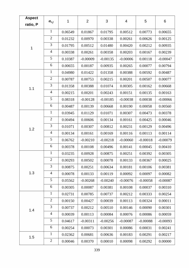
339

Aspectratio, P

, 1 2 3 4 5 6

1

1 0.06549 0.01867 0.01795 0.00512 0.00773 0.006552 0.01232 0.00970 0.00338 0.00261 0.00626 0.001253 0.01795 0.00512 0.01480 0.00420 0.00212 0.009354 0.00338 0.00261 0.00358 0.00203 0.00167 0.002395 0.10387 -0.00009 -0.00135 -0.00006 0.00118 -0.000476 0.00655 0.00187 0.00935 0.00265 0.00077 0.00794

1.1

1 0.04980 0.01422 0.01358 0.00388 0.00592 0.004872 0.00787 0.00753 0.00215 0.00201 0.00507 0.000773 0.01358 0.00388 0.01074 0.00305 0.00162 0.006684 0.00215 0.00201 0.00243 0.00151 0.00135 0.001635 0.08318 -0.00128 -0.00185 -0.00038 0.00038 -0.000666 0.00487 0.00139 0.00668 0.00190 0.00058 0.00560

1.2

1 0.03945 0.01129 0.01071 0.00307 0.00473 0.003782 0.00494 0.00606 0.00134 0.00161 0.00425 0.000463 0.01071 0.00307 0.00812 0.00231 0.00129 0.004964 0.00134 0.00161 0.00169 0.00116 0.00113 0.001145 0.06762 -0.00210 -0.00218 -0.00060 -0.00018 -0.000796 0.00378 0.00108 0.00496 0.00141 0.00045 0.00410

1.3

1 0.03235 0.00928 0.00875 0.00251 0.00392 0.003052 0.00293 0.00502 0.00078 0.00133 0.00367 0.000253 0.00875 0.00251 0.00634 0.00181 0.00106 0.003814 0.00078 0.00133 0.00119 0.00092 0.00097 0.000825 0.05562 -0.00268 -0.00240 -0.00076 -0.00058 -0.000876 0.00305 0.00087 0.00381 0.00108 0.00037 0.00310

1.4

1 0.02731 0.00785 0.00737 0.00212 0.00333 0.002542 0.00150 0.00427 0.00039 0.00113 0.00324 0.000113 0.00737 0.00212 0.00510 0.00146 0.00090 0.003014 0.00039 0.00113 0.00084 0.00076 0.00086 0.000595 0.04617 -0.00311 -0.00256 -0.00087 -0.00088 -0.000936 0.00254 0.00073 0.00301 0.00086 0.00031 0.00241

1.51 0.02362 0.00681 0.00636 0.00183 0.00291 0.002172 0.00046 0.00370 0.00010 0.00098 0.00292 0.00000

340

3 0.00636 0.00183 0.00421 0.00120 0.00078 0.002444 0.00010 0.00098 0.00058 0.00063 0.00077 0.000435 0.03859 -0.00343 -0.00268 -0.00096 -0.00111 -0.000986 0.00217 0.00063 0.00244 0.00070 0.00027 0.00192

1.6

1 0.02085 0.00602 0.00560 0.00162 0.00259 0.001902 -0.00033 0.00327 -0.00011 0.00086 0.00266 -0.000073 0.00560 0.00162 0.00356 0.00102 0.00070 0.002024 -0.00011 0.00086 0.00040 0.00054 0.00071 0.000315 0.03241 -0.00368 -0.00277 -0.00103 -0.00129 -0.001016 0.00190 0.00055 0.00202 0.00058 0.00024 0.00156

1.7

1 0.01873 0.00542 0.00503 0.00145 0.00235 0.001702 -0.00093 0.00293 -0.00028 0.00077 0.00247 -0.000133 0.00503 0.00145 0.00306 0.00088 0.00063 0.001714 -0.00028 0.00077 0.00026 0.00047 0.00065 0.000225 0.02731 -0.00388 -0.00283 -0.00108 -0.00144 -0.001036 0.00170 0.00049 0.00171 0.00049 0.00021 0.00129

1.8

1 0.01708 0.00495 0.00458 0.00133 0.00215 0.001542 -0.00140 0.00266 -0.00040 0.00070 0.00231 -0.000173 0.00458 0.00133 0.00268 0.00077 0.00058 0.001474 -0.00040 0.00070 0.00015 0.00041 0.00061 0.000155 0.02305 -0.00404 -0.00289 -0.00112 -0.00156 -0.001056 0.00154 0.00045 0.00147 0.00042 0.00020 0.00109

1.9

1 0.01577 0.00458 0.00422 0.00123 0.00200 0.001422 -0.00177 0.00244 -0.00050 0.00064 0.00218 -0.000213 0.00422 0.00123 0.00239 0.00069 0.00054 0.001284 -0.00050 0.00064 0.00007 0.00037 0.00058 0.000105 0.01945 -0.00417 -0.00293 -0.00115 -0.00165 -0.001066 0.00142 0.00041 0.00128 0.00037 0.00018 0.00093

2.0

1 0.01471 0.00428 0.00394 0.00115 0.00188 0.001322 -0.00207 0.00226 -0.00059 0.00060 0.00207 -0.000243 0.00394 0.00115 0.00215 0.00062 0.00050 0.001144 -0.00059 0.00060 0.00000 0.00033 0.00055 0.000065 0.01639 -0.00428 -0.00296 -0.00118 -0.00173 -0.001076 0.00132 0.00038 0.00114 0.00033 0.00017 0.00081

341


The coefficients, Ci (C1, C2, C3, C4, C5 and C6) for any aspect ratio of the CSCS plate are then


3.1552, 3.1553 and 3.1554 and solving accordingly. For example, at aspect ratio p = 1.0, the

stiffness coefficients , are given as (see Table 3.21):

1,1 = 0.06549, 1,2 = 0.01867, 1,3 = 0.01795, 1,4 = 0.00512, 1,5 = 0.00773, 1,6 = 0.00655

2,1 = 0.01232, 2,2 = 0.00970, 2,3 = 0.00338, 2,4 = 0.00261, 2,5 = 0.00626, 2,6 = 0.00125

3,1 = 0.01795, 3,2 = 0.00512, 3,3 = 0.01480, 3,4 = 0.00420, 3,5 = 0.00212, 3,6 = 0.00935

4,1 = 0.00338, 4,2 = 0.00261, 4,3 = 0.00358, 4,4 = 0.00203, 4,5 = 0.00167, 4,6 = 0.00239

5,1 = 0.10387, 5,2 = -0.00009, 5,3 = -0.00135, 5,4 = -0.00006, 5,5 = 0.00118, 5,6 = -0.00047

6,1 = 0.00655, 6,2 = 0.00187, 6,3 = 0.00935, 6,4 = 0.00265, 6,5 = 0.00077, 6,6 = 0.00794


1 = 0.00667; 2 = 0.00198; 3 = 0.00190; 4 = 0.00057; 5 = 0.00093; 6 = 0.00079

Substituting these stiffness coefficients into Equation 3.1551, 3.1552, 3.1553 and 3.1554 and



1 = 111

= 0.0066670.06549

= 0.10180.

The coefficients, C1 for other aspect ratios of the CSCS plate for the first approximation are



1,1 1,2 1,3

2,1 2,2 2,33,1 3,2 3,3

1

2

3

=1

2

3

4

1

2

3

=0.06549 0.01867 0.017950.01232 0.00970 0.003380.01795 0.00512 0.01480

−1 6.6667 × 10−3

1.9841 × 10−3

1.9048 × 10−3

4 =0.066030.117950.00784

4

The coefficients, Ci (C1, C2 and C3) for other aspect ratios of the CSCS plate for the second



1

2

3

4

=

1,1 1,2 1,3 1,42,1 2,2 2,3 2,4

3,1 3,2 3,3 3,44,1 4,2 4,3 4,4

−11

2

3

4

4

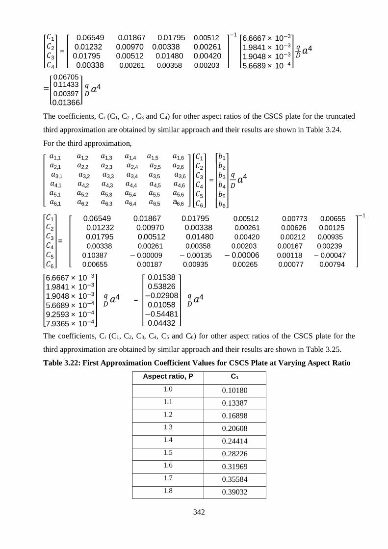
342

1

2

3

4

=

0.06549 0.01867 0.01795 0.005120.01232 0.00970 0.00338 0.002610.01795 0.00512 0.01480 0.004200.00338 0.00261 0.00358 0.00203

−1 6.6667 × 10−3

1.9841 × 10−3

1.9048 × 10−3

5.6689 × 10−4

4

=0.067050.114330.003970.01366

4

The coefficients, Ci (C1, C2 , C3 and C4) for other aspect ratios of the CSCS plate for the truncated



1,1 1,2 1,3 1,4 1,5 1,6

2,1 2,2 2,3 2,4 2,5 2,6

3,1 3,2 3,3 3,4 3,5 3,64,1 4,2 4,3 4,4 4,5 4,6

5,1 5,2 5,3 5,4 5,5 5,66,1 6,2 6,3 6,4 6,5 a6,6

1

2

3

4

5

6

=

1

2

3

4

5

6

4

1

2

3

4

5

6

=

0.06549 0.01867 0.01795 0.00512 0.00773 0.006550.01232 0.00970 0.00338 0.00261 0.00626 0.001250.01795 0.00512 0.01480 0.00420 0.00212 0.009350.00338 0.00261 0.00358 0.00203 0.00167 0.00239

0.10387 − 0.00009 − 0.00135 − 0.00006 0.00118 − 0.000470.00655 0.00187 0.00935 0.00265 0.00077 0.00794

−1

6.6667 × 10−3

1.9841 × 10−3

1.9048 × 10−3

5.6689 × 10−4

9.2593 × 10−4

7.9365 × 10−4

4 =

0.015380.53826−0.029080.01058−0.544810.04432

4

The coefficients, Ci (C1, C2, C3, C4, C5 and C6) for other aspect ratios of the CSCS plate for the


Table 3.22: First Approximation Coefficient Values for CSCS Plate at Varying Aspect Ratio

Aspect ratio, P C1

1.0 0.101801.1 0.133871.2 0.168981.3 0.206081.4 0.244141.5 0.282261.6 0.319691.7 0.355841.8 0.39032

343

1.9 0.422872.0 0.45335

Table 3.23: Second Approximation Coefficient Values for CSCS Plate at Varying Aspect

Ratio


1.0 0.06603 0.11795 0.007841.1 0.08020 0.17619 0.012281.2 0.09320 0.24754 0.018111.3 0.10445 0.33028 0.025411.4 0.11359 0.42200 0.034151.5 0.12052 0.51998 0.044231.6 0.12527 0.62157 0.055521.7 0.12802 0.72439 0.067841.8 0.12899 0.82643 0.080981.9 0.12846 0.92615 0.094732.0 0.12669 1.02240 0.10890

Table 3.24: Truncated Third Approximation Coefficient Values for CSCS Plate at Varying

Aspect Ratio


1.0 0.06705 0.11433 0.00397 0.013661.1 0.08193 0.17008 0.00575 0.023021.2 0.09591 0.23801 0.00792 0.035931.3 0.10841 0.31634 0.01049 0.052541.4 0.11909 0.40266 0.01345 0.072821.5 0.12781 0.49433 0.01678 0.096521.6 0.13461 0.58876 0.02042 0.123301.7 0.13961 0.68368 0.02431 0.152741.8 0.14303 0.77721 0.02837 0.184411.9 0.14508 0.86792 0.03251 0.217882.0 0.14602 0.95477 0.03664 0.25274

Table 3.25: Third Approximation Coefficient Values for CSCS Plate at Varying Aspect Ratio


1.0 0.01538 0.53826 -0.02908 0.01058 -0.54481 0.04432

344

1.1 0.02379 0.66224 -0.04719 0.01885 -0.62736 0.071161.2 0.03522 0.77696 -0.07189 0.03004 -0.68172 0.107821.3 0.05003 0.87444 -0.10389 0.04403 -0.70051 0.155591.4 0.06846 0.94828 -0.14366 0.06047 -0.67917 0.215411.5 0.09063 0.99399 -0.19141 0.07892 -0.61586 0.287871.6 0.11650 1.00900 -0.24716 0.09891 -0.51101 0.373181.7 0.14596 0.99243 -0.31078 0.12003 -0.36673 0.471311.8 0.17881 0.94472 -0.38202 0.14196 -0.18624 0.581941.9 0.21480 0.86733 -0.46056 0.16444 0.02662 0.704592.0 0.25364 0.76233 -0.54600 0.18734 0.26778 0.83864

Deflections

The six-term deflection function of the plate obtained in Equation 3.85 is given as:

, = 1( − 2 3 + 4 )( 2 − 2 3 + 4) + 2( 3 − 2 5 + 6)( 2 − 2 3 + 4) +

3 − 2 3 + 4 4 − 2 5 + 6 + 43 − 2 5 + 6 4 − 2 5 + 6 +

5( 5 − 2 7 + 8)( 2 − 2 3 + 4) + 6 − 2 3 + 4 6 − 2 7 + 8


Y = X = 12


= 1 1 = 1 − 2 3 + 4 2 − 2 3 + 4

= 1 1 = 0.1018012 − 2

12

3

+12

4 12

2

− 212

3

+12

4

= 0.00199




Y = X = 12

. From Table 3.23, we have the C values as 1 = 0.06603; 2 = 0.11795; 3 = 0.00784.

= 1 1 + 2 2 + 3 3 = 1 − 2 3 + 4 2 − 2 3 + 4 +

23 − 2 5 + 6 2 − 2 3 + 4 + 3 − 2 3 + 4 4 − 2 5 + 6

= 0.0660312 − 2

12

3

+12

4 12

2

− 212

3

+12

4

+

0.1179512

3

− 212

5

+12

6 12

2

− 212

3

+12

4

+ 0.0078412 − 2

12

3

+12

4 12

4

− 212

5

+12

6

= 0.00190

345




Y = X = 12

; From Table 4.24, we have the C values as: 1 = 0.06705; 2 = 0.11433; 3 =

0.00397; = 4 = 0.01366;

= 1 1 + 2 2 + 3 3 + 4 4

= 1 − 2 3 + 4 2 − 2 3 + 4 + 23 − 2 5 + 6 2 − 2 3 + 4 +

3 − 2 3 + 4 4 − 2 5 + 6 + 43 − 2 5 + 6 4 − 2 5 + 6

= 0.0670512 − 2

12

3

+12

4 12

2

− 212

3

+12

4

+

0.1143312

3

− 212

5

+12

6 12

2

− 212

3

+12

4

+

0.0039712 − 2

12

3

+12

4 12

4

− 212

5

+12

6

+0.0136612

3

− 212

5

+12

6 12

4

− 212

5

+12

6

= 0.00190




Y = X = 12

. From Table 3.25, we have the C values as: 1 = 0.01538; 2 = 0.53826; 3 =−

0.02908; = 4 = 0.01058; 5 =− 0.54481; 6 = 0.04432.= 1 1 + 2 2 + 3 3 + 4 4 + 5 5 + 6 6

= 1 − 2 3 + 4 2 − 2 3 + 4 + 23 − 2 5 + 6 2 − 2 3 + 4 +

3 − 2 3 + 4 4 − 2 5 + 6 + 43 − 2 5 + 6 4 − 2 5 + 6 +

55 − 2 7 + 8 2 − 2 3 + 4 + 6 − 2 3 + 4 6 − 2 7 + 8

= 0.0153812 − 2

12

3

+12

4 12

2

− 212

3

+12

4

+

0.5382612

3

− 212

5

+12

6 12

2

− 212

3

+12

4

+

−0.0290812 − 2

12

3

+12

4 12

4

− 212

5

+12

6

346

+0.0105812

3

− 212

5

+12

6 12

4

− 212

5

+12

6

+

−0.5448112

5

− 212

7

+12

8 12

2

− 212

3

+12

4

+

0.0443212

− 212

3

+12

4 12

6

− 212

7

+12

8

= 0.00219



.Moments in x and y directions

The six-term bending moment functions of the plate obtained in Equations 3.1578d and 3.1579d in


=− 12 1 − + 2 ( 2 − 2 3 + 4) + 4 2 1.5 − 10 3 + 7.5 4 ( 2 − 2 3 + 4) +

12 3 − + 2 4 − 2 5 + 6 + 4 4 1.5 − 10 3 + 7.5 4 4 − 2 5 + 6

+ 5 20 3 − 84 5 + 56 6 2 − 2 3 + 4

+ 12 6 −12 + 12 2 6 − 2 7 + 8 +

2 2 1 − 2 3 + 4 1− 6 + 6 2 + 2 2( 3 − 2 5 + 6) 1 − 6 + 6 2 +

4 3 − 2 3 + 4 3 2 − 10 3 + 7.5 4 + 4 4( 3 − 2 5 + 6) 3 2 − 10 3 + 7.5 4

+ 2 55 − 2 7 + 8 1 − 6 + 6 2

+ 6 − 2 3 + 4 30 4 − 84 5 + 56 6

=− 12 1 − + 2 ( 2 − 2 3 + 4) + 4 2 1.5 − 10 3 + 7.5 4 ( 2 − 2 3 + 4) +

12 3 − + 2 4 − 2 5 + 6 + 4 4 1.5 − 10 3 + 7.5 4 4 − 2 5 + 6

+ 5 20 3 − 84 5 + 56 6 2 − 2 3 + 4

+ 12 6 −12 + 12 2 6 − 2 7 + 8 +1

2 2 1 − 2 3 + 4 1− 6 + 6 2 + 2 2( 3 − 2 5 + 6) 1 − 6 + 6 2 +

4 3 − 2 3 + 4 3 2 − 10 3 + 7.5 4 + 4 4( 3 − 2 5 + 6) 3 2 − 10 3 + 7.5 4

+ 2 55 − 2 7 + 8 1 − 6 + 6 2

+ 6 − 2 3 + 4 30 4 − 84 5 + 56 6

For the first approximation bending moment coefficient at mid-span of plate along x – direction,

we have: aspect ratio p = 1, X = Y = 12


0.10180.

347

1 =− 12 0.10180 −12

+12

2 12

2

− 212

3

+12

4

+

0.312 2 0.10180

12

− 212

3

+12

4

1 − 612

+ 612

2

= 0.02863

Similarly,

1 =− 12 0.10180 (0.3) −12

+12

2 12

2

− 212

3

+12

4

+

112 2 0.10180

12 − 2

12

3

+12

4

1 − 612 + 6

12

2

= 0.03754




ratio p = 1, X = Y = 12


0.11795; C3 = 0.00784.

2 =− 12 0.06603 −12

+12

2 12

2

− 212

3

+12

4

+

4 0.11795 1.512

− 1012

3

+ 7.512

4 12

2

− 212

3

+12

4

+ 12 0.00784 −12

+12

2 12

4

− 212

5

+12

6

+

0.312 2 0.06603

12 − 2

12

3

+12

4

1 − 612 + 6

12

2

+

2 0.1179512

2

− 212

5

+12

6

1 − 612

+ 612

2

+ 4 0.0078412 − 2

12

3

+12

4

312

2

− 1012

3

+ 7.512

4

= 0.0227

Similarly,

2 =− (0.3) 2 0.06603 −12 +

12

2 12

2

− 212

3

+12

4

+

348

+4 0.11795 1.512 − 10

12

3

+ 7.512

4 12

2

− 212

3

+12

4

+ 12 0.00784 −12

+12

2 12

4

− 212

5

+12

6

+

112 2 0.06603

12 − 2

12

3

+12

4

1− 612 + 6

12

2

+

2 0.1179512

2

− 212

5

+12

6

1− 612

+ 612

2

+ 4 0.0078412 − 2

12

3

+12

4

312

2

− 1012

3

+ 7.512

4

= 0.0343




ratio p = 1, X = Y = 12


0.11433; C3 = 0.00397; C4 = 0.01366.

3 =− 12 0.06705 −12

+12

2 12

2

− 212

3

+12

4

+

4 0.11433 1.512

− 1012

3

+ 7.512

4 12

2

− 212

3

+12

4

+12 0.00397 −12

+12

2 12

4

− 212

5

+12

6

+

4 0.01366 1.512

− 1012

3

+ 7.512

4 12

4

− 212

5

+12

6

+

0.312 2 0.06705

12 − 2

12

3

+12

4

1 − 612 + 6

12

2

+

2 0.1143312

3

− 212

5

+12

6

1 − 612 + 6

12

2

+

349

+4 0.0039712 − 2

12

3

+12

4

312

2

− 1012

3

+ 7.512

4

+ 4 0.0136612

3

− 212

5

+12

6

312

2

− 1012

3

+ 7.512

4

= 0.02273

Similarly,

3 =− (0.3) 12 0.06705 −12 +

12

2 12

2

− 212

3

+12

4

+

4 0.11433 1.512 − 10

12

3

+ 7.512

4 12

2

− 212

3

+12

4

+12 0.00397 −12

+12

2 12

4

− 212

5

+12

6

+ 4 0.01366 1.512 − 10

12

3

+ 7.512

4 12

4

− 212

5

+12

6

+

112 2 0.06705

12

− 212

3

+12

4

1 − 612

+ 612

2

+

2 0.1143312

3

− 212

5

+12

6

1 − 612

+ 612

2

+

+4 0.0039712

− 212

3

+12

4

312

2

− 1012

3

+ 7.512

4

+ 4 0.0136612

3

− 212

5

+12

6

312

2

− 1012

3

+ 7.512

4

= 0.03427




ratio p = 1, X = Y = 12


0.53826; C3 =− 0.02908; C4 = 0.01058; C5 =− 0.54481; C6 = 0.04432.

4 =− 12 0.01538 −12

+12

2 12

2

− 212

3

+12

4

+

350

4 0.53826 1.512 − 10

12

3

+ 7.512

4 12

2

− 212

3

+12

4

+12 −0.02908 −12

+12

2 12

4

− 212

5

+12

6

+ 4 0.01058 1.512 − 10

12

3

+ 7.512

4 12

4

− 212

5

+12

6

+ −0.54481 2012

3

− 8412

5

+ 5612

6 12

2

− 212

3

+12

4

+ 12 0.04432 −12

+12

2 12

6

− 212

7

+12

8

+

0.312 2 0.01538

12 − 2

12

3

+12

4

1 − 612 + 6

12

2

+

2 0.5382612

3

− 212

5

+12

6

1 − 612 + 6

12

2

+

+4 −0.0290812 − 2

12

3

+12

4

312

2

− 1012

3

+ 7.512

4

+ 4 0.0105812

3

− 212

5

+12

6

312

2

− 1012

3

+ 7.512

4

+2 −0.5448112

5

− 212

7

+12

8

1 − 612 + 6

12

2

+ 0.0443212

− 212

3

+12

4

3012

4

− 8412

5

+ 5612

6

= 0.04184

Similarly,

4 =− (0.3) 12 0.01538 −12

+12

2 12

2

− 212

3

+12

4

+

351

4 0.53826 1.512 − 10

12

3

+ 7.512

4 12

2

− 212

3

+12

4

+12 −0.02908 −12

+12

2 12

4

− 212

5

+12

6

+ 4 0.01058 1.512 − 10

12

3

+ 7.512

4 12

4

− 212

5

+12

6

+ −0.54481 2012

3

− 8412

5

+ 5612

6 12

2

− 212

3

+12

4

+ 12 0.04432 −12

+12

2 12

6

− 212

7

+12

8

+

112 2 0.01538

12 − 2

12

3

+12

4

1 − 612 + 6

12

2

+

2 0.5382612

3

− 212

5

+12

6

1 − 612 + 6

12

2

+

+4 −0.0290812 − 2

12

3

+12

4

312

2

− 1012

3

+ 7.512

4

+ 4 0.0105812

3

− 212

5

+12

6

312

2

− 1012

3

+ 7.512

4

+2 −0.5448112

5

− 212

7

+12

8

1 − 612 + 6

12

2

+ 0.0443212

− 212

3

+12

4

3012

4

− 8412

5

+ 5612

6

= 0.04299

Following the same procedure, the coefficients, βx1and βy1, at aspect ratios 1.1 ≤ p ≤ 2.0 for the third


start

Boundary type

352

NB: B1 = CCCS, B2 = SSSS, B3 = CCCC, B4 = CCSS, B5 = CSCS.

Figure 3.16: Flow chart for calculation of deflection, short and long term moment coefficient

values.

CHAPTER FOUR

RESULTS AND DISCUSSIONS

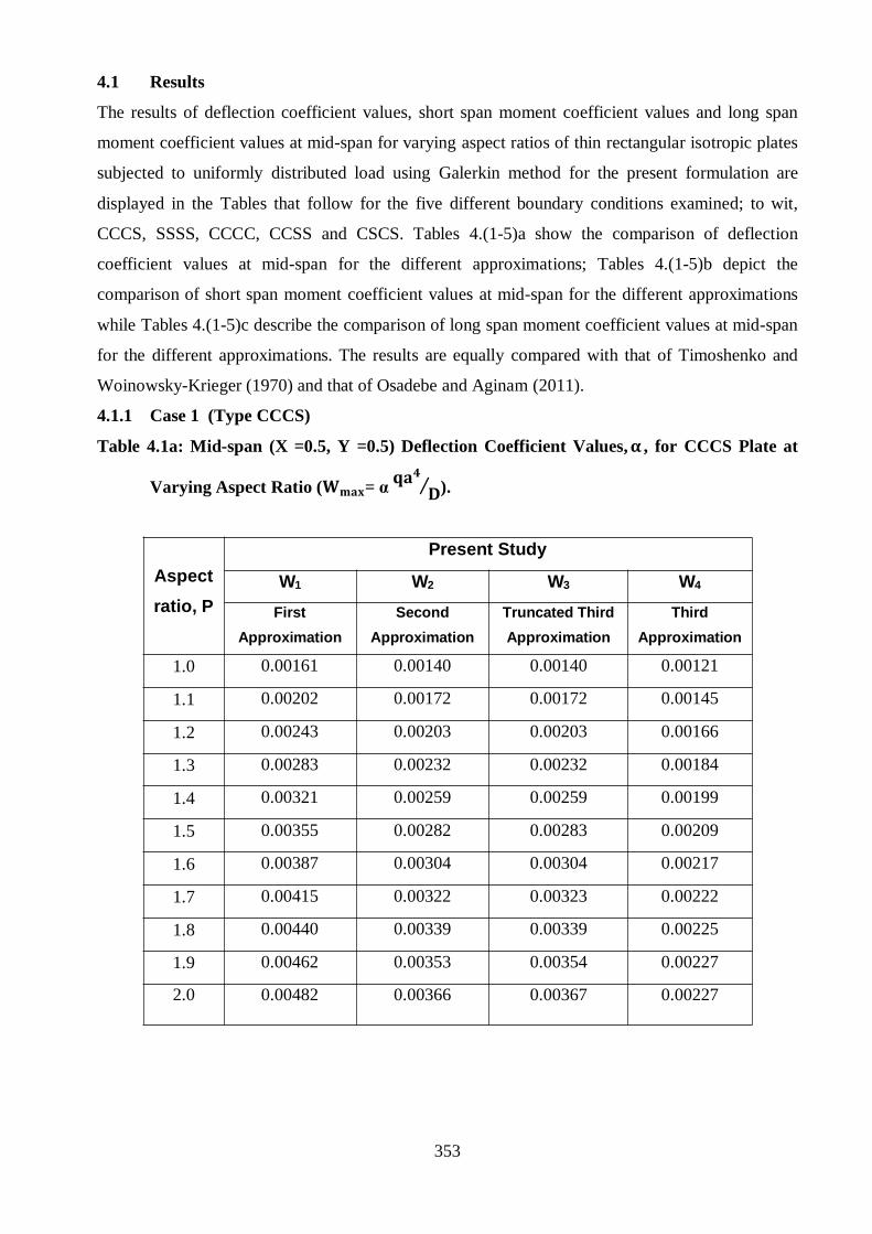
353

4.1 Results

The results of deflection coefficient values, short span moment coefficient values and long span

moment coefficient values at mid-span for varying aspect ratios of thin rectangular isotropic plates

subjected to uniformly distributed load using Galerkin method for the present formulation are

displayed in the Tables that follow for the five different boundary conditions examined; to wit,

CCCS, SSSS, CCCC, CCSS and CSCS. Tables 4.(1-5)a show the comparison of deflection

coefficient values at mid-span for the different approximations; Tables 4.(1-5)b depict the

comparison of short span moment coefficient values at mid-span for the different approximations

while Tables 4.(1-5)c describe the comparison of long span moment coefficient values at mid-span

for the different approximations. The results are equally compared with that of Timoshenko and

Woinowsky-Krieger (1970) and that of Osadebe and Aginam (2011).


Table 4.1a: Mid-span (X =0.5, Y =0.5) Deflection Coefficient Values, , for CCCS Plate at

Varying Aspect Ratio ( = α ).

Aspectratio, P

Present Study

W1 W2 W3 W4

FirstApproximation

SecondApproximation

Truncated ThirdApproximation

ThirdApproximation

1.0 0.00161 0.00140 0.00140 0.00121

1.1 0.00202 0.00172 0.00172 0.00145

1.2 0.00243 0.00203 0.00203 0.00166

1.3 0.00283 0.00232 0.00232 0.00184

1.4 0.00321 0.00259 0.00259 0.00199

1.5 0.00355 0.00282 0.00283 0.00209

1.6 0.00387 0.00304 0.00304 0.00217

1.7 0.00415 0.00322 0.00323 0.00222

1.8 0.00440 0.00339 0.00339 0.00225

1.9 0.00462 0.00353 0.00354 0.00227

2.0 0.00482 0.00366 0.00367 0.00227

354

Table 4.1b: Short Span Moment Coefficient Values, , at Mid-Span (X =0.5, Y =0.5) for

CCCS Plate at Varying Aspect Ratio ( ) = ).

Aspectratio, P

Present Study

Mx1 Mx2 Mx3 Mx4

FirstApproximation

SecondApproximation

Third TruncatedApproximation

ThirdApproximation

1 0.02700 0.01638 0.01642 -0.00038

1.1 0.03223 0.01710 0.01716 -0.00480

1.2 0.03728 0.01714 0.01723 -0.01003

1.3 0.04200 0.01663 0.01675 -0.01571

1.4 0.04631 0.01569 0.01583 -0.02150

1.5 0.05019 0.01444 0.01462 -0.02718

1.6 0.05363 0.01300 0.01322 -0.03259

1.7 0.05666 0.01146 0.01171 -0.03765

1.8 0.05931 0.00987 0.01016 -0.04233

1.9 0.06163 0.00830 0.00863 -0.04662

2 0.06365 0.00677 0.00714 -0.05055

Table 4.1c: Long Span Moment Coefficient Values, , at Mid-Span (X =0.5, Y =0.5) for

CCCS Plate at Varying Aspect Ratio ( = ).

Aspectratio, P

Present Study

My1 My2 My3 My4

FirstApproximation

SecondApproximation


ThirdApproximation

1 0.03150 0.02506 0.02513 0.01620

1.1 0.03396 0.02549 0.02559 0.01434

1.2 0.03577 0.02525 0.02537 0.01174

1.3 0.03698 0.02448 0.02463 0.00869

1.4 0.03771 0.02336 0.02353 0.00544

1.5 0.03804 0.02201 0.02221 0.00216

1.6 0.03807 0.02053 0.02076 -0.00102

1.7 0.03789 0.01902 0.01926 -0.00402

355

1.8 0.03756 0.01751 0.01777 -0.00680

1.9 0.03714 0.01605 0.01633 -0.00935

2 0.03665 0.01466 0.01496 -0.01167


Table 4.2a: Mid-span (X =0.5, Y =0.5) Deflection Coefficient Values, , for SSSS Plate at

Varying Aspect Ratio ( = α q / ).

*Values in bracket are the percentage difference between the present study and the classical


SSSS Plate at Varying Aspect Ratio ( = ).

Aspectratio, P

Present StudyClassicalSolution

Aspectratio, P


W1 W2 W3 W4 W

FirstApproximation

SecondApproximation


Third Approximation

Timoshenkoand

Woinowsky-Krieger(1970)

1.0 0.00414(1.97%) 0.00434(6.98%) 0.00388(-4.42%) -0.00215(-153.04%) 0.00406

1.1 0.00496(2.27%) 0.00533(9.95%) 0.00470(-3.00%) -0.00169(-134.80%) 0.00485

1.2 0.00576(2.13%) 0.00632(12.09%) 0.00553(-2.00%) -0.00087(-115.44%) 0.00564

1.3 0.00653(2.35%) 0.00728(14.17%) 0.00634(-0.70%) 0.00044(-93.16%) 0.00638

1.4 0.00726(2.98%) 0.00820(16.30%) 0.00712(1.01%) 0.00235(-66.70%) 0.00705

1.5 0.00793(2.72%) 0.00905(17.29%) 0.00788(2.08%) 0.00498(-35.46%) 0.00772

1.6 0.00856(3.13%) 0.00984(18.59%) 0.00861(3.76%) 0.00848(2.19%) 0.00830

1.7 0.00913(3.40%) 0.01056(19.60%) 0.00932(5.53%) 0.01302(47.43%) 0.00883

1.8 0.00966(3.76%) 0.01121(20.38%) 0.01000(7.40%) 0.01880(101.95%) 0.00931

1.9 0.01015(4.21%) 0.01179(21.00%) 0.01066(9.43%) 0.02610(167.97%) 0.00974

2.0 0.01059(4.54%) 0.01230(21.41%) 0.01130(11.54%) 0.03525(247.97%) 0.01013

356

Mx1 Mx2 Mx3 Mx4 Mx

FirstApproximation

SecondApproximation


Third Approximation

Timoshenkoand

Woinowsky-Krieger (1970)

1 0.05163(7.79%) 0.04906(2.42%) 0.03704(-22.67%) -0.26397(-651.08%) 0.04790

1.1 0.05943(7.27%) 0.05702(2.93%) 0.04253(-23.23%) -0.23126(-517.44%) 0.05540

1.2 0.06686(6.63%) 0.06410(2.23%) 0.04756(-24.15%) -0.20821(-432.07%) 0.06270

1.3 0.07383(6.38%) 0.07016(1.09%) 0.05213(-24.89%) -0.18432(-365.60%) 0.06940

1.4 0.08031(6.37%) 0.07519(-0.41%) 0.05628(-25.46%) -0.15520(-305.57%) 0.07550

1.5 0.08629(6.27%) 0.07925(-2.40%) 0.06007(-26.03%) -0.11808(-245.42%) 0.08120

1.6 0.09177(6.46%) 0.08242(-4.38%) 0.06357(-26.26%) -0.07058(-181.88%) 0.08620

1.7 0.09677(6.57%) 0.08481(-6.60%) 0.06683(-26.39%) -0.01023(-111.27%) 0.09080

1.8 0.10134(6.90%) 0.08651(-8.74%) 0.06993(-26.24%) 0.06578(-30.61%) 0.09480

1.9 0.10549(7.10%) 0.08764(-11.02%) 0.07289(-26.00%) 0.16087(63.32%) 0.08850

2 0.10927(7.44%) 0.08829(-13.19%) 0.07576(-25.51%) 0.27921(174.54%) 0.10170



SSSS Plate at Varying Aspect Ratio ( = ).

Aspectratio, P


My1 My2 My3 My4 My

FirstApproximation

SecondApproximation


Third Approximation

Timoshenkoand


1 0.05163(7.79%) 0.07372(53.89%) 0.04344(-9.32%) -0.35267(-836.26%) 0.04790

1.1 0.05364(8.80%) 0.08338(69.13%) 0.04863(-1.37%) -0.22930(-565.12%) 0.04930

1.2 0.05502(9.82%) 0.09083(81.29%) 0.05311(6.01%) -0.13988(-379.20%) 0.05010

357

1.3 0.05591(11.15%) 0.09602(90.89%) 0.05692(13.17%) -0.06142(-222.10%) 0.05030

1.4 0.05643(12.41%) 0.09912(97.45%) 0.06013(19.78%) 0.01466(-70.80%) 0.05020

1.5 0.05668(13.82%) 0.10043(101.67%) 0.06282(26.15%) 0.09269(86.12%) 0.04980

1.6 0.05673(15.30%) 0.10027(103.80%) 0.06510(32.31%) 0.17557(256.85%) 0.04920

1.7 0.05664(16.54%) 0.09896(103.63%) 0.06704(37.94%) 0.26575(446.81%) 0.04860

1.8 0.05645(17.85%) 0.09680(102.08%) 0.06871(43.45%) 0.36564(663.33%) 0.04790

1.9 0.05620(19.32%) 0.09402(99.62%) 0.07018(49.00%) 0.47790(914.65%) 0.04710

2 0.05591(20.50%) 0.09083(95.76%) 0.07148(54.06%) 0.60562(1205.22%) 0.04640


solution.


Table 4.3a: Mid-span (X =0.5, Y =0.5) Deflection Coefficients Values, , for CCCC Plate at


Aspectratio, P

Present StudyApproximate

SolutionClassicalSolution

W1 W W3 W4 W W

First

Approximation

Timoshenkoand

Woinowsky-

Krieger (1970)

TruncatedThird

Approximation

Third

Approximation

Osadebe

and Aginam(2011)

Timoshenko

andWoinowsky-

Krieger

(1970)

1.0 0.00133(5.56%) 0.00132(4.92%) 0.00132(4.92%) 0.00120(-5.10%) 0.00126(Nil) 0.00126

1.1 0.00159(6.00%) 0.00158(5.14%) 0.00163(9.00%) 0.00144(-4.00%) 0.00150(Nil) 0.00150

1.2 0.00182(5.81%) 0.00181(5.15%) 0.00188(9.04%) 0.00166(-3.26%) 0.00172(Nil) 0.00172

1.3 0.00202(5.76%) 0.00201(5.37%) 0.00209(9.28%) 0.00186(-2.53%) 0.00190(Nil) 0.00191

1.4 0.00220(6.28%) 0.00219(5.74%) 0.00227(9.66%) 0.00203(-1.85%) 0.00205(-0.97%) 0.00207

1.5 0.00235(6.82%) 0.00234(6.33%) 0.00243(10.25%) 0.00217(-1.16%) 0.00218(-0.91%) 0.00220

1.6 0.00248(7.83%) 0.00247(7.26%) 0.00256(11.16%) 0.00229(-0.33%) - 0.00230

1.7 0.00259(8.82%) 0.00258(8.20%) 0.00267(12.05%) 0.00239(-0.35%) 0.00237(-0.42%) 0.00238

1.8 0.00269(9.80%) 0.00267(8.86%) 0.00276(12.61%) 0.00246(0.60%) 0.00240(2.04%) 0.00245

1.9 0.00277(11.24%) 0.00275(10.24%) 0.00284(13.90%) 0.00252(1.39%) 0.00247(-0.8%) 0.00249

358


solution.


CCCC Plate at Varying Aspect Ratio ( ) = ).


solution.


CCCC Plate at Varying Aspect Ratio ( = ).

2.0 0.00284(11.81%) 0.00281(10.70%) 0.00290(14.22%) 0.00257(1.21%) 0.00250(1.57%) 0.00254

Aspectratio, P



W1 W W3 W4 W W

FirstApproximation

Timoshenko

andWoinowsky-

Krieger (1970)

Truncated

ThirdApproximation

Third

Approximation

Osadebe

and Aginam(2011)

Timoshenko

andWoinowsky-

Krieger (1970)

1 0.02765(19.70%) 0.02708(17.25%) 0.02709(17.25%) 0.02322(0.54%) 0.0225(-2.6%) 0.02310

1.1 0.03167(19.96%) 0.03107(17.67%) 0.03107(17.68%) 0.02701(2.32%) 0.0255(-0.76%) 0.02640

1.2 0.03517(17.63%) 0.03454(15.52%) 0.03454(15.53%) 0.03035(1.52%) 0.0298(-0.33%) 0.02990

1.3 0.03814(16.64%) 0.03750(14.67%) 0.03750(14.68%) 0.03320(1.53%) 0.0315(-3.67%) 0.03270

1.4 0.04064(16.45%) 0.03997(14.53%) 0.03997(14.54%) 0.03556(1.89%) 0.0333(-4.58%) 0.03490

1.5 0.04270(16.03%) 0.04202(14.19%) 0.04203(14.20%) 0.03747(1.83%) 0.0353(-4.08%) 0.03680

1.6 0.04441(16.56%) 0.04372(14.74%) 0.04372(14.75%) 0.03899(2.33%) - 0.03810

1.7 0.04582(16.89%) 0.04512(15.10%) 0.04512(15.11%) 0.04016(2.45%) 0.0387(-1.28%) 0.03920

1.8 0.04699(17.18%) 0.04628(15.41%) 0.04628(15.42%) 0.04105(2.37%) 0.0355(-11.7%) 0.04010

1.9 0.04796(17.84%) 0.04724(16.08%) 0.04725(16.09%) 0.04170(2.47%) 0.0358(-12.04%) 0.04070

2 0.04877(18.37%) 0.04805(16.63%) 0.04805(16.64%) 0.04216(2.34%) 0.0395(-4.13%) 0.04120

Aspectratio, P



W1 W W3 W4 W W

First

Approximation

Timoshenkoand


TruncatedThird

Approximation

Third

Approximation

Osadebe

and Aginam(2011)

Timoshenko

andWoinowsky-

Krieger

(1970)

359


solution.


Table 4.4a: Mid-span (X =0.5, Y =0.5) Deflection Coefficients Values, , for CCSS Plate at


1 0.02765(19.70%) 0.02708(17.25%) 0.02709(17.25%) 0.02322(0.54%) 0.0225(-2.6%) 0.02310

1.1 0.02858(23.72%) 0.02795(21.00%) 0.02795(21.01%) 0.02390(3.48%) 0.0220(-4.76%) 0.02310

1.2 0.02894(26.93%) 0.02825(23.92%) 0.02826(23.93%) 0.02401(5.31%) 0.0226(-0.88%) 0.02280

1.3 0.02889(30.14%) 0.02815(26.81%) 0.02815(26.82%) 0.02369(6.71%) 0.0211(-4.95%) 0.02220

1.4 0.02855(34.67%) 0.02778(31.06%) 0.02779(31.07%) 0.02307(8.83%) 0.0198(-6.6%) 0.02120

1.5 0.02805(38.18%) 0.02726(34.28%) 0.02726(34.29%) 0.02226(9.68%) 0.0189(-6.9%) 0.02030

1.6 0.02745(42.23%) 0.02665(38.09%) 0.02665(38.10%) 0.02135(10.65%) - 0.01930

1.7 0.02682(47.36%) 0.02601(42.92%) 0.02601(42.93%) 0.02040(12.10%) 0.0173(-4.94%) 0.01820

1.8 0.02618(50.46%) 0.02537(45.83%) 0.02538(45.84%) 0.01945(11.78%) 0.0141(-18.96%) 0.01740

1.9 0.02555(54.85%) 0.02476(50.05%) 0.02476(50.06%) 0.01853(12.29%) 0.0130(-21.21%) 0.01650

2 0.02495(57.91%) 0.02417(53.00%) 0.02418(53.01%) 0.01765(11.73%) 0.0139(-12.03%) 0.01580

Aspectratio, P

Present Study

W1 W2 W3 W4

FirstApproximation

SecondApproximation


ThirdApproximation

1.0 0.00210 0.00083 0.00193 0.00100

1.1 0.00251 0.00099 0.00254 0.00113

1.2 0.00290 0.00117 0.00339 0.00119

1.3 0.00325 0.00136 0.00490 0.00117

1.4 0.00357 0.00156 0.01067 0.00106

1.5 0.00386 0.00177 -0.00942 0.00085

1.6 0.00411 0.00199 -0.00097 0.00053

1.7 0.00433 0.00219 0.00068 0.00006

1.8 0.00453 0.00239 0.00147 -0.00070

1.9 0.00470 0.00258 0.00198 -0.00225

360


CCSS Plate at Varying Aspect Ratio ( ) = ).

Aspectratio, P

Present Study

Mx1 Mx2 Mx3 Mx4

FirstApproximation

SecondApproximation


ThirdApproximation

1 0.03277 -0.00637 0.02591 -0.00886

1.1 0.03762 -0.00745 0.03488 -0.01187

1.2 0.04203 -0.00821 0.04924 -0.01568

1.3 0.04597 -0.00866 0.07990 -0.02008

1.4 0.04943 -0.00889 0.21376 -0.02467

1.5 0.05247 -0.00895 -0.27960 -0.02888

1.6 0.05511 -0.00890 -0.08038 -0.03194

1.7 0.05740 -0.00880 -0.04557 -0.03262

1.8 0.05940 -0.00868 -0.03128 -0.02834

1.9 0.06114 -0.00857 -0.02366 -0.01061

2 0.06266 -0.00847 -0.01906 0.08539


CCSS Plate at Varying Aspect Ratio ( = ).

Aspectratio, P

Present Study

My1 My2 My3 My4

FirstApproximation

SecondApproximation


ThirdApproximation

1 0.03277 -0.02371 0.03325 -0.01520

1.1 0.03396 -0.02294 0.04514 -0.01552

2.0 0.00486 0.00276 0.00234 -0.00854

361

1.2 0.03459 -0.02103 0.06315 -0.01640

1.3 0.03481 -0.01848 0.09987 -0.01785

1.4 0.03473 -0.01566 0.25598 -0.01962

1.5 0.03446 -0.01288 -0.31488 -0.02136

1.6 0.03407 -0.01030 -0.08341 -0.02260

1.7 0.03360 -0.00801 -0.04258 -0.02272

1.8 0.03309 -0.00605 -0.02565 -0.02058

1.9 0.03257 -0.00443 -0.01655 -0.01263

2 0.03206 -0.00311 -0.01102 0.02825


Table 4.5a: Mid-span (X =0.5, Y =0.5) Deflection Coefficients Values, , for CSCS Plate at


Aspectratio, P


W1 W2 W3 W4 W

FirstApproximation

SecondApproximation


ThirdApproximation

Timoshenkoand


1.0 0.00199(3.65%) 0.00190(-0.84%) 0.00190(-0.84%) 0.00219(13.98%) 0.00192

1.1 0.00261(3.98%) 0.00249(-0.93%) 0.00249(-0.92%) 0.00281(12.03%) 0.00251

1.2 0.00330(3.45%) 0.00312(-2.27%) 0.00312(-2.26%) 0.00347(8.68%) 0.00319

1.3 0.00402(3.61%) 0.00378(-2.66%) 0.00378(-2.65%) 0.00413(6.40%) 0.00388

1.4 0.00477(3.70%) 0.00445(-3.35%) 0.00445(-3.33%) 0.00477(3.78%) 0.00460

1.5 0.00551(3.77%) 0.00511(-3.79%) 0.00511(-3.77%) 0.00538(1.41%) 0.00531

1.6 0.00624(3.48%) 0.00575(-4.60%) 0.00575(-4.58%) 0.00595(-1.36%) 0.00603

1.7 0.00695(4.04%) 0.00637(-4.66%) 0.00637(-4.64%) 0.00645(-3.39%) 0.00668

1.8 0.00762(4.10%) 0.00695(-5.05%) 0.00695(-5.03%) 0.00690(-5.79%) 0.00732

1.9 0.00826(4.56%) 0.00749(-5.14%) 0.00750(-5.11%) 0.00727(-7.91%) 0.00790

362


solution.


CSCS Plate at Varying Aspect Ratio ( ) = ).

Aspectratio, P


Mx1 Mx2 Mx3 Mx4 Mx

FirstApproximation

SecondApproximation


ThirdApproximation

Timoshenkoand


1 0.02863(17.34%) 0.02272(-6.90%) 0.02273(-6.84%) 0.04184(71.47%) 0.02440

1.1 0.03547(15.54%) 0.02673(-12.92%) 0.02676(-12.84%) 0.04823(57.11%) 0.03070

1.2 0.04269(13.54%) 0.03050(-18.88%) 0.03054(-18.78%) 0.05335(41.88%) 0.03760

1.3 0.05007(12.26%) 0.033919(-23.86%) 0.03396(-23.86%) 0.05684(27.44%) 0.04460

1.4 0.05745(11.77%) 0.0368(-28.25%) 0.03695(-28.12%) 0.05852(13.85%) 0.05140

1.5 0.06469(10.58%) 0.03940(-32.65%) 0.03949(-32.50%) 0.05831(-0.32%) 0.05850

1.6 0.07165(10.23%) 0.04148(-36.19%) 0.04159(-36.01%) 0.05627(-13.43%) 0.06500

1.7 0.07826(9.92%) 0.04314(-39.40%) 0.04328(-39.21%) 0.05249(-26.28%) 0.07120

1.8 0.08448(10.00%) 0.04444(-42.13%) 0.04461(-41.91%) 0.04714(-38.62%) 0.07680

1.9 0.09027(9.95%) 0.04542(-44.68%) 0.04562(-44.44%) 0.04040(-50.80%) 0.08210

2 0.09563(10.05%) 0.04613(-46.92%) 0.04636(-46.65%) 0.03245(-62.66%) 0.08690


solution.


CSCS Plate at Varying Aspect Ratio ( ) = ).

Aspectratio, P


My1 My2 My3 My4 My

2.0 0.00885(4.86%) 0.00800(-5.23%) 0.00800(-5.20%) 0.00759(-10.08%) 0.00844

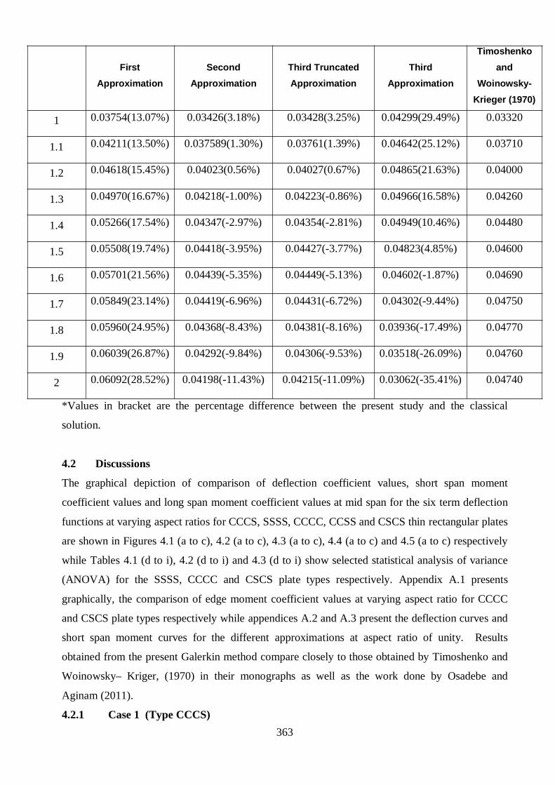
363

FirstApproximation

SecondApproximation


ThirdApproximation

Timoshenkoand


1 0.03754(13.07%) 0.03426(3.18%) 0.03428(3.25%) 0.04299(29.49%) 0.03320

1.1 0.04211(13.50%) 0.037589(1.30%) 0.03761(1.39%) 0.04642(25.12%) 0.03710

1.2 0.04618(15.45%) 0.04023(0.56%) 0.04027(0.67%) 0.04865(21.63%) 0.04000

1.3 0.04970(16.67%) 0.04218(-1.00%) 0.04223(-0.86%) 0.04966(16.58%) 0.04260

1.4 0.05266(17.54%) 0.04347(-2.97%) 0.04354(-2.81%) 0.04949(10.46%) 0.04480

1.5 0.05508(19.74%) 0.04418(-3.95%) 0.04427(-3.77%) 0.04823(4.85%) 0.04600

1.6 0.05701(21.56%) 0.04439(-5.35%) 0.04449(-5.13%) 0.04602(-1.87%) 0.04690

1.7 0.05849(23.14%) 0.04419(-6.96%) 0.04431(-6.72%) 0.04302(-9.44%) 0.04750

1.8 0.05960(24.95%) 0.04368(-8.43%) 0.04381(-8.16%) 0.03936(-17.49%) 0.04770

1.9 0.06039(26.87%) 0.04292(-9.84%) 0.04306(-9.53%) 0.03518(-26.09%) 0.04760

2 0.06092(28.52%) 0.04198(-11.43%) 0.04215(-11.09%) 0.03062(-35.41%) 0.04740


solution.

4.2 Discussions

The graphical depiction of comparison of deflection coefficient values, short span moment

coefficient values and long span moment coefficient values at mid span for the six term deflection

functions at varying aspect ratios for CCCS, SSSS, CCCC, CCSS and CSCS thin rectangular plates

are shown in Figures 4.1 (a to c), 4.2 (a to c), 4.3 (a to c), 4.4 (a to c) and 4.5 (a to c) respectively

while Tables 4.1 (d to i), 4.2 (d to i) and 4.3 (d to i) show selected statistical analysis of variance

(ANOVA) for the SSSS, CCCC and CSCS plate types respectively. Appendix A.1 presents

graphically, the comparison of edge moment coefficient values at varying aspect ratio for CCCC

and CSCS plate types respectively while appendices A.2 and A.3 present the deflection curves and

short span moment curves for the different approximations at aspect ratio of unity. Results

obtained from the present Galerkin method compare closely to those obtained by Timoshenko and

Woinowsky– Kriger, (1970) in their monographs as well as the work done by Osadebe and

Aginam (2011).


364

The graphical depiction of coefficients of deflection, short span moment and long span moment

obtained from Galerkin method at mid-span in the case of a rectangular plate whose two opposite

edges are clamped and one of the other two opposite edges clamped and the other simply supported

are shown in Figures 4.1a, 4.1b and 4.1c.

Figure 4.1a: Comparison of Deflection Coefficient Values for CCCS at Mid-Span at Varying

Aspect Ratios

From Figure 4.1a, it is shown that the first approximation gave the highest coefficient values at mid

span followed almost jointly by the second and truncated third approximations and then the third

approximation. The fourth term of the truncated third approximation did not have any significant

effect on the truncated third approximation. The approximations converged closest at aspect ratio

1.0 and diverged as the aspect ratio rose to 2.0. The slopes of the approximations are in descending

order from first through second to third approximation. Out of the four approximations, the first

approximation showed excellent compliance with the boundary conditions of the plate followed by

the second and truncated third approximation and finally the third approximation (Figure A.2.1 of

appendix A.2). Furthermore, the first approximation can be used in confidence to approximate the

deflected middle surface of the plate in engineering applications. The graph of the short span

moment coefficient values in Figure 4.1b show the same pattern of convergence as the deflection

coefficient values by giving closest convergence at aspect ratio 1.0 and greatest divergence at

aspect ratio 2.0. The coefficient values of the first approximation rose from aspect ratio 1.0 to 2.0

while that of the second approximation, truncated third approximation and third approximation

decreased as the aspect ratio increases from 1.0 to 2.0. Just as was with the deflection, the second

and truncated third approximations gave almost the same coefficient values.

365

Figure 4.1b: Comparison of Short Span Moment Coefficient Values for CCCS at Mid-Span

at Varying Aspect Ratios

The coefficient values of the first, second and truncated third approximations are all positive while

that of the third approximation are all negative. The short span moment curve showed that the first

approximation obeyed the prescribed boundary conditions while the rest violated them (Figure

A.3.1 of appendix A.3). This shows that only the first approximation is suitable for approximating

the short span moment of the plate. Figure 4.1c depicts the graph of the results of the four different

approximations undertaken in this study for the long span. The pattern of convergence is similar to

that of the short span moment. The first approximation coefficient values rose from aspect ratio 1.0

reaching their peak at aspect ratio 1.6 and then decreased from aspect ratio 1.7 to 2.0. The second

and third approximations rose from aspect ratio 1.0 to 1.1 and then decreased from aspect ratio1.2

to 2.0. The third approximation decreased from aspect ratio 1.0 to 2.0 with coefficient values

between 1.0 and 1.5 being positive while those between 1.6 and 2.0 are negative. The slope of the

first approximation coefficient values coupled with the behaviour of its deflection and short span

moment curves show that it is suitable for approximating the deflection functions and their

response parameters for the CCCS plate on the one hand, as well as showing that increasing the

number of terms for the present formulation does not improve accuracy/precision on the other hand.

366

Figure 4.1c: Comparison of Long Span Moment Coefficient Values for CCCS at Mid-Span at

Varying Aspect Ratios


The graphical description of coefficients of deflection, short span moment and long span moment

obtained from Galerkin method at mid-span in the case of a rectangular plate whose edges are all

simply supported are shown in shown in Figures 4.2a, 4.2b and 4.2c respectively. Their statistical

analysis of variance are shown in Tables 4.2d and 4.2e, 4.2f and 4.2g and 4.2h and 4.2i

respectively. At aspect ratio of unity, the deflection coefficient values from Galerkin method give a

percentage difference of 1.97, 6.98, -4.42 and -153.04 for the first, second, truncated third and third

approximations respectively when compared with the exact result from Timoshenko and

Woinowsky – Krieger (1970).

Figure 4.2a: Comparison of Deflection Coefficient Values for SSSS at Mid-Span at Varying

Aspect Ratios

367

The first, second and truncated third approximation coefficient values rise linearly from aspect

ratio 1.0 to 2.0, giving percentage difference of 4.54, 21.41 and 11.54 respectively at aspect ratio

2.0, while the third approximation rises parabolically giving a percentage difference of 247.97 at

aspect ratio 2.0. This shows that the first, second and truncated third approximation deflection

coefficient values diverge as they rise from aspect ratio 1.0 to aspect ratio 2.0. They all have their

peak values at aspect ratio 2.0. The third approximation however, shows a wide percentage

difference when compared with the classical solution. This suggests that the deflection function

might have reached its maximum approximation at the truncated third approximation when the

approximation is used in the Galerkin method. The closest that the first, second and truncated third

approximations come to results in literature is at aspect ratio 1.0 while that of the third

approximation is at aspect ratio 1.6. The first three approximations are mainly upper bounded when

compared to the classical solution. Figure A.2.2 of appendix A.2 shows the graphical depiction of

the deflection curves for SSSS plate at aspect ratio of unity. It is observed that all the

approximations satisfied the prescribed boundary condition of the plate but only the first

approximation shows a deflection curve of best fit. Table 4.2d shows the results of statistical

analysis of variance between the first approximation and the classical solution while Table 4.2e

shows that of truncated third approximation and the classical solution.

SUMMARYGroups Count Sum Average Variance

Column 1 11 0.08467 0.00769727 4.6541E-06Column 2 11 0.08201 0.00745545 4.1419E-06

ANOVASource of Variation SS df MS F P-value F critBetween Groups 3.21618E-07 1 3.2162E-07 0.0731287 0.78960566 4.3512435Within Groups 8.79595E-05 20 4.398E-06

Total 8.82811E-05 21

Table 4.2d: Anova: Single Factor for W1 versus W (SSSS).

They show the sum, average and variance between the four sets of values. The p-values of 0.79 and

0.76 for the first and truncated third approximations respectively are greater than 0.05 (P > 0.05)

which shows that there is no significant difference between both approximations and the classical

solution.

368


Column 1 11 0.085336152 0.00775783 6.0922E-06Column 2 11 0.08201 0.00745545 4.1419E-06

ANOVASource of Variation SS df MS F P-value F critBetween Groups 5.02877E-07 1 5.0288E-07 0.09827462 0.75715605 4.3512435Within Groups 0.000102341 20 5.1171E-06

Total 0.000102844 21

Table 4.2e: Anova: Single Factor for W3 versus W (SSSS)

Therefore the first, second and truncated third approximation deflection coefficients are reliable for

absolute two dimensional plate systems at mid-span. Hence, the shape function obtained for the

SSSS – plate type is satisfactory.

From Table 4.2b and Figure 4.2b, the difference in results between the present study and that of

Timoshenko and Woinowsky – Krieger (1970) for moment coefficients results about x–direction

varied with that of y–direction for aspect ratios other than 1.0. This situation is observed for both

the first approximation and the classical solution.

Figure 4.2b: Comparison of Short Span Moment Coefficient Values for SSSS at Mid-Span at


369

For the moment coefficients in the x-direction, at aspect ratio of unity, the moment coefficient

values for the first, second and truncated third approximations give 7.79, 2.42 and -22.67

percentage differences respectively. Difference in coefficient values of moment about x – direction

for present study and the literature results ranges from 7.79% (1.0 aspect ratio) to 7.44% (2.0

aspect ratio), 2.42% (1.0 aspect ratio) to -13.19% (2.0 aspect ratio) and -22.67% (1.0 aspect ratio)

to -25.51% (2.0 aspect ratio) for the first, second and truncated third approximation coefficient

values respectively. Between aspect ratios 1 and 2.0, the first, second and truncated third

approximation coefficient values give somewhat linear graphs. The coefficient values for the first

approximation converge as they rise from aspect ratio 1.0 to 1.5 and then diverge. The second

approximation coefficient values converge from aspect ratio 1.1 to 1.3 and then diverge to aspect

ratio 2.0. The truncated third approximation coefficient values diverge from aspect ratio 1.0 to 1.9

and then converge a bit. The third approximation shows a wide difference from literature for aspect

ratios 1.0 to 2.0 as is observed in the deflection coefficients. The graph rises parabolically from

negative coefficient values to positive. This shows that using the present formulation, the SSSS

plate seems to reach its maximum approximation at the truncated third approximation. Figure

A.2.2 of appendix A.2 shows the short span moment curve at aspect ratio of unity. It is observed

that only the first approximation satisfies the prescribed boundary conditions of the plate. However,

Table 4.2f shows the results of statistical analysis of variance between the first approximation and

the classical solution while Table 4.2g shows that of truncated third approximation and the

classical solution.


Column 1 11 0.92299 0.08390818 0.0003692Column 2 11 0.8641 0.07855455 0.00032332

ANOVASource of Variation SS df MS F P-value F critBetween Groups 0.000157638 1 0.00015764 0.45525989 0.50757315 4.3512435Within Groups 0.006925179 20 0.00034626

Total 0.007082817 21

Table 4.2f: Anova: Single Factor for Mx1 versus Mx (SSSS).

370


Column 1 11 0.644583146 0.05859847 0.00016138Column 2 11 0.8541 0.07764545 0.00029252

ANOVASource of Variation SS df MS F P-value F critBetween Groups 0.001995332 1 0.00199533 8.79188523 0.00765316 4.3512435Within Groups 0.004539032 20 0.00022695

Total 0.006534364 21

Table 4.2g: Anova: Single Factor for Mx3 versus Mx (SSSS)

They show the sum, average and variance between the four sets of values. The p-values of 0.51

and 0.008 for the first and truncated third approximations which are greater than 0.05 (P > 0.05)

and less than 0.05 (P < 0.05) respectively show that there is no significant difference between the

first approximation and the classical solution while there is a little significant difference between

the truncated third approximation and the classical solution

From Table 4.2c and Figure 4.2c, it is observed that at aspect ratio of unity, the moment coefficient

values for the first, second and truncated third approximations give 7.79, 53.89 and -9.32

percentage differences respectively.

Figure 4.2c: Comparison of Long Span Moment Coefficient Values for SSSS at Mid-Span at


Difference in coefficient values of moment about y – direction for present study and the classical

solution ranges from 7.79% (1.0 aspect ratio) to 20.50% (2.0 aspect ratio), 53.89% (1.0 aspect ratio)

371

to 95.76% (2.0 aspect ratio) and -9.32% (1.0 aspect ratio) to 54.06% (2.0 aspect ratio) for the first,

second and truncated third approximation coefficient values respectively. Between aspect ratios 1.0

and 2.0, the first, second and truncated third approximation coefficient values give somewhat linear

graphs. The coefficient values for the first approximation converge as they rise from aspect ratio

1.0 to 2.0. The second approximation coefficient values diverge from aspect ratio 1.0 to 1.8 and

then converge to aspect ratio 2.0. The truncated third approximation coefficient values converge

from aspect ratio 1.0 to 1.1 and then diverge to aspect ratio 2.0. The third approximation shows a

wide difference from results in literature for aspect ratios 1.0 to 2.0 as is observed in the deflection

coefficients. However, Table 4.2h shows the results of the statistical analysis of variance between

the first approximation and the classical solution while Table 4.2i shows that of truncated third

approximation and the classical solution.


Column 1 11 0.61124 0.055567 2.54156E-06Column 2 11 0.5368 0.0488 0.000001762

ANOVASource of Variation SS df MS F P-value F critBetween Groups 0.000251878 1 0.000252 117.0555468 8.28E-10 4.351244Within Groups 4.30356E-05 20 2.15E-06

Total 0.000294914 21

Table 4.2h: Anova: Single Factor for My1 versus My (SSSS).


Column 1 11 0.667556599 0.06068696 8.5034E-05Column 2 11 0.5368 0.0488 1.762E-06

ANOVA

Source of Variation SS df MS F P-value F critBetween Groups 0.000777149 1 0.00077715 17.9074617 0.00040922 4.3512435Within Groups 0.000867962 20 4.3398E-05

Table 4.2i: Anova: Single Factor for My3 versus My (SSSS)

They show the sum, average and variance between the four sets of values. The p-values of

0.000000000828 and 0.000409 which are both less than 0.05 (P < 0.05) shows there is a significant

372

difference between the four sets of results. Furthermore, this loss of accuracy is understood as the

moment coefficients are directly proportional the second derivatives of the deflection function. The

first and third approximation coefficient values are mainly upper bounded and close when

compared to the classical solution. These are satisfactory for practical purposes. By extension, this

shows that the shape functions derived by applying the characteristic coordinate polynomial

principle which were ploughed into the Galerkin method in this study are convenient and

satisfactory for two dimensional plate systems, and can be applied to grid structures.


The coefficients of deflection, short span moment and long span moment obtained from Galerkin

method at mid-span in the case of a rectangular plate whose edges are clamped are shown in

Tables 4.3a, 4.3b and 4.3c respectively. Their selected statistical analysis of variance -Anova- are

shown in Tables 4.3d and 4.3e, 4.3f and 4.3g and 4.3h and 4.3i respectively while their graphs are

shown in Figures 4.3a, 4.3b and 4.3c respectively.

Figure 4.3a: Comparison of Deflection Coefficient Values for CCCC at Mid-Span at Varying

Aspect Ratios

From Figure 4.3a and Table A.1.3 of appendix A.1, it is noted that at aspect ratio of unity, the

deflection coefficient values from Galerkin method give a percentage difference of 5.56, 4.92, 4.92

and -5.10 for the first, second, truncated third and third approximations respectively when

compared with the exact result from Timoshenko and Woinowsky – Krieger (1970). The first,

second, truncated third and third approximation coefficient values rise mostly linearly from aspect

ratio 1.0 to 2.0, giving percentage difference of 11.81, 10.70, 14.22 and 1.21 respectively at aspect

ratio 2.0. This shows that the first, second and truncated third approximation deflection coefficient

values diverge as they rise from aspect ratio 1.0 to aspect ratio 2.0 while the third approximation

converges as it rises to aspect ratio 2.0. They all have their peak values at aspect ratio 2.0. The

373

third approximation however, shows the smallest percentage difference when compared with the

classical solution. This shows that the deflection function coefficient values converge as the

number of terms of the deflection function is increased from the first approximation to the third

approximation. The closest that the first, second and truncated third approximations come to

literature is at aspect ratio 1.0 while that of the third approximation is at aspect ratio 2.0. When the

results of the present study are compared with that from Osadebe and Aginam (2011), they are

almost coincident. The first three approximations are mainly upper-bounded when compared to the

classical solution. Figure A.2.3 of appendix A.2 shows that all the approximations have a

deflection curve of good fit and satisfy the prescribed boundary conditions of the plate. Table 4.3d

shows the results of the statistical analysis of variance between the first approximation and the

classical solution while Table 4.3e shows that of the third approximation and the classical solution.

They show the sum, average and variance between the four sets of values.


Column 1 11 0.02468 0.002243636 2.51245E-07Column 2 11 0.02282 0.002074545 1.83647E-07

ANOVASource of Variation SS df MS F P-value F critBetween Groups 1.57255E-07 1 1.57255E-07 0.723187745 0.405166515 4.351243503Within Groups 4.34893E-06 20 2.17446E-07

Total 4.50618E-06 21

Table 4.3d: Anova: Single Factor for W1 versus W (CCCC).


Column 1 11 0.022608 0.00205531 2.1435E-07Column 2 11 0.02282 0.00207455 1.8365E-07

ANOVASource of Variation SS df MS F P-value F crit

Between Groups 2.03544E-09 1 2.0354E-09 0.01022844 0.92044975 4.3512435Within Groups 3.97997E-06 20 1.99E-07

Total 3.982E-06 21

Table 4.3e: Anova: Single Factor for W4 versus W (CCCC).

374

The p-values of 0.41 and 0.92 for the first and third approximations respectively are greater than

0.05 (P > 0.05) which shows that there is no significant difference between both approximations

and the classical solution. Therefore the first, second, truncated third and third approximation

deflection coefficients are reliable for absolute two dimensional plates systems. Hence, the shape

function obtained for the CCCC – plate type is satisfactory.

Figure 4.3b: Comparison of Short Span Moment Coefficient Values for CCCC at Mid-Span


Table A.2.3 of appendix A.2 shows the difference in results between the present study and that of

Timoshenko and Woinowsky – Krieger (1970) for short span moment coefficients. Moment

coefficient results about x–direction varied with that of y–direction for aspect ratios other than 1.0.

This situation is observed for the first, second, truncated third, third approximations and the

classical solution. For the moment coefficients in the x-direction, at aspect ratio of unity, the

moment coefficient values for the first, second, truncated third and third approximations give 19.70,

17.25, 17.25 and 0.54 percentage differences respectively. Difference in coefficient values of

moment about x – direction for present study and the classical solution ranges from 19.70% (1.0

aspect ratio) to 18.37% (2.0 aspect ratio), 17.25% (1.0 aspect ratio) to 16.63% (2.0 aspect ratio),

17.25% (1.0 aspect ratio) to 16.64% (2.0 aspect ratio) and 0.54% (1.0 aspect ratio) to 3.24% (2.0

aspect ratio) for the first, second, truncated third and third approximation coefficient values

respectively. From Figure 4.3b, between aspect ratios 1.0 and 2.0, the first, second, truncated third

and third approximation coefficient values give parabolic graphs. The coefficient values for the

first approximation converge as they rise from aspect ratio 1.1 to 1.7 and then diverge. The second

approximation coefficient values converge from aspect ratio 1.1 to 1.5 and then diverge to aspect

ratio 2.0. The truncated third approximation coefficient values converge from aspect ratio 1.1 to

1.5 and then diverge to aspect ratio 2.0. The third approximation converges from aspect ratio 1.1 to

375

1.5 and then diverges to 2.0. The third approximation gives the most convergent values while the

first approximation gives the most divergent values. In comparison with the results obtained by

Osadebe and Aginam (2011), there is no significant difference. Figures A.1.1 and A.1.2 of

appendix A.1 show graphical depiction of the comparison of the edge moments with that of the

classical solution. Figures A.2.3 of appendix A.2 and A.3.3 of appendix A.3 show the comparison

of the deflection curves and the short span moment curves respectively for the different

approximations at aspect ratio of unity. They all have a good fit and satisfy the prescribed

boundary conditions. However, Table 4.3f shows the results of statistical analysis of variance

between the first approximation and the classical solution while Table 4.3g shows that between the

third approximation and the classical solution.


Column 1 11 0.44992 0.040901818 4.89909E-05Column 2 11 0.3831 0.034827273 3.73982E-05

ANOVASource of Variation SS df MS F P-value F critBetween Groups 0.000202951 1 0.000202951 4.698525829 0.042431167 4.351243503Within Groups 0.00086389 20 4.31945E-05

Total 0.001066841 21

Table 4.3f: Anova: Single Factor for Mx1 versus Mx (CCCC).


Column 1 11 0.390891 0.03553554 4.0603E-05Column 2 11 0.3831 0.03482727 3.7398E-05


Between Groups 2.75907E-06 1 2.7591E-06 0.07074392 0.79297932 4.3512435Within Groups 0.000780015 20 3.9001E-05

Total 0.000782774 21

Table 4.3g: Anova: Single Factor for Mx4 versus Mx (CCCC).

They show the sum, average and variance between the four sets of values. The p-values of 0.042

and 0.79 for the first and third approximations, which are less than 0.05 (P < 0.05) and greater than

376

0.05 (P > 0.05) respectively show that there is a little significant difference between first

approximation and the classical solution on the one hand and no significant difference between the

third approximation and the classical solution on the other hand. All the approximations give

moment coefficients that are upper- bounded; therefore they are good for practical purposes.

Table 4.3c indicates that at aspect ratio of unity, the moment coefficient values for the first, second,

truncated third and third approximations give 19.70, 17.25, 17.25 and 0.54 percentage differences

respectively. Difference in coefficient values of moment about y – direction for present study and

the classical solution ranges from 19.70% (1.0 aspect ratio) to 57.91% (2.0 aspect ratio), 17.25%

(1.0 aspect ratio) to 53.00% (2.0 aspect ratio), 17.25% (1.0 aspect ratio) to 53.01% (2.0 aspect ratio)

and 0.54% (1.0 aspect ratio) to 11.73% (2.0 aspect ratio) for the first, second, truncated third and

third approximation coefficient values respectively.

Figure 4.3c: Comparison of Long Span Moment Coefficient Values for CCCC at Mid-Span


Figure 4.3c shows that between aspect ratios 1.0 and 2.0, the first, second and truncated third

approximation coefficient values give almost decreasing graphs. The coefficient values for the first,

second, truncated third and third approximations diverge as they move from aspect ratio 1.0 to 2.0.

All the present approximations and the classical solution have their maximum values at aspect ratio

1.2. The third approximation gives the most convergent values while the first approximation gives

the most divergent values. In addition, the results from the present approximation in relation to the

results obtained by Osadebe and Aginam (2011) show almost complete convergence. However,

Table 4.3h shows the results of statistical analysis of variance between the first approximation and

the classical solution while Table 4.3i shows that between the third approximation and the classical

solution.

377


Column 1 11 0.30161 0.027419091 1.90399E-06Column 2 11 0.2199 0.019990909 7.38091E-06

ANOVASource of Variation SS df MS F P-value F critBetween Groups 0.000303478 1 0.000303478 65.37031688 9.89309E-08 4.351243503Within Groups 9.2849E-05 20 4.64245E-06

Total 0.000396327 21

Table 4.3h: Anova: Single Factor for My1 versus My (CCCC).


Column 1 11 0.237554 0.02159579 5.1862E-06Column 2 11 0.2199 0.01999091 7.3809E-06



Total 0.000139837 21

Table 4.3i: Anova: Single Factor for My4 versus My (CCCC).

They show the sum, average and variance between the four sets of values. The p-value of the first

approximation gives 0.000000099 while that of the third approximation gives 0.149. This shows

that there is a significant difference between the first approximation and the classical solution. But

for the third approximation, there is no significant difference. Therefore, of all the approximations,

the third approximation is the closest to the classical solution. Hence, the mechanical properties of

the CCCC- plate improved with the expanded approximation.

In addition, the six-term shape function obtained for the CCCC- plate type is satisfactory for all

plate analysis. The preceding approximations can be used for preliminary studies since they are all

in upper bound.


378

The plot of coefficients of deflection, short span moment and long span moment obtained from

Galerkin method at mid-span in the case of a rectangular plate clamped on two adjacent near edges

and simply supported on two adjacent far edges are shown Figures 4.4a, 4.4b and 4.4c respectively.

Figure 4.4a: Comparison of Deflection Coefficient Values for CCSS at Mid-Span at Varying

Aspect Ratios

Table 4.4a and Figure 4.4a indicate that the coefficient values for the first and second

approximations increased from aspect ratio 1.0 to 2.0. The coefficient values for the truncated third

approximation increased gradually from aspect ratio 1.0 to 1.3, then sharply to 1.4 before dipping

to a negative coefficient value at aspect ratio of 1.5. From aspect ratio 1.6, it rises as it reaches

aspect ratio 2.0. The third approximation rises from aspect ratio 1.0 to 1.3 and then descends to a

negative value from aspect ratio1.8 to 2.0. The slopes of the first and second approximations are

smooth while that of the truncated third and third are not. All the approximations obeyed the

prescribed boundary conditions of the plate but the best fit came from the first approximation

(Figure A.2.4 of appendix A.2). This shows that beyond the first approximation, this

approximation may not be viable for approximating the deflected middle surface of the plate.

The short term moment coefficient values in Table 4.4b and their graphs in Figure 4.4b show

a slight deviation from the deflection coefficient values. All the results of the first approximation

are positive. All of the results of the second and third approximations are negative except at aspect

ratio 2.0 for the later while the results of the truncated third approximation are positive between

aspect ratios 1.0 to 1.4 and the remaining are negative.

379

Figure 4.4b: Comparison of Short Span Moment Coefficient Values for CCSS at Mid-Span at


The prescribed boundary conditions are only obeyed by the first approximation (Figure A.3.4 of

appendix A.3). This is indicative that only the first approximation can predict accurately, the short

span response parameters of the plate.

From Figure 4.4c, it is observed that the long span moment coefficient values showed similar

pattern with the short span coefficient values.

Figure 4.4c: Comparison of Long Span Moment Coefficient Values for CCSS at Mid-Span at


Therefore it would be similarly concluded that only the first approximation offers suitable solution

for engineering applications.

380


The coefficients of deflection, short span moment and long span moment obtained from Galerkin

method at mid-span in the case of a rectangular plate clamped on two opposite short edges and

simply supported on two opposite long edges are shown in Tables 4.5a, 4.5b and 4.5c respectively.

Their statistical analysis of variance -Anova- are shown in Tables 4.5d and 4.5e, 4.5f and 4.5g and

4.5h and 4.5i respectively while their graphs are shown in Figures 4.5a, 4.5b and 4.5c respectively.

Figure 4.5a: Comparison of Deflection Coefficient Values for CSCS at Mid-Span at Varying

Aspect Ratios

At aspect ratio of unity, Table 4.5a and Figure 4.5a indicate that the deflection coefficient

values from Galerkin method give a percentage difference of 3.65, -0.84, -0.84 and 13.98 for the

first, second, truncated third and third approximations respectively when compared with the exact

result from Timoshenko and Woinowsky – Krieger (1970). The first, second, truncated third and

third approximation coefficient values rise linearly from aspect ratio 1.0 to 2.0, giving percentage

difference of 4.86, -5.23, -5.20 and -10.08 respectively at aspect ratio 2.0. This shows that the first,

second and truncated third approximation deflection coefficient values diverge as they rise from

aspect ratio 1.0 to aspect ratio 2.0. They all have their peak values at aspect ratio 2.0. The third

approximation however, converges from aspect ratio 1.0 to 1.5 and then diverges to aspect ratio 2.0

when compared with the classical solution. The closest that the first, second and truncated third

approximations come to the results in literature is at aspect ratio 1.0 while that of the third

approximation is at aspect ratio 1.6. The first three approximations are mainly close to the classical

solution. Figure A.2.5 of appendix A.2 shows that all the approximations satisfy the boundary

conditions with respect to deflection; but best deflection curve goes to the first approximation.

Table 4.5d shows the results of statistical analysis of variance between the first approximation and

the classical solution while Table 4.5e shows that of truncated third approximation and the

classical solution.

381


Column 1 11 0.06012 0.005465455 5.42071E-06Column 2 11 0.05778 0.005252727 4.92798E-06



Total 0.000103736 21

Table 4.5d: Anova: Single Factor for W1 versus W (CSCS)


Column 1 11 0.055416445 0.005037859 4.27377E-06Column 2 11 0.05778 0.005252727 4.92798E-06


Between Groups 2.53927E-07 1 2.53927E-07 0.055191008 0.816653425 4.3512435Within Groups 9.20175E-05 20 4.60088E-06

Total 9.22715E-05 21

Table 4.5e: Anova: Single Factor for W3 versus W (CSCS).

They show the sum, average and variance between the four sets of values. The p-values of 0.83 and

0.816 for the first and truncated third approximations respectively are greater than 0.05 (P > 0.05)

which shows that there is no significant difference between both approximations and the classical

solution. Therefore the first, second and truncated third approximation deflection coefficients are

reliable for absolute two dimensional plates systems at mid-span.

From Table 4.5b and Figure 4.5b, it is observed that at aspect ratio of unity, the moment

coefficient values for the first, second, truncated third and third approximations give 17.34, -6.90, -

6.84 and 71.47 percentage differences respectively. Difference in coefficient values of moment

about x – direction for present study and the results in literature ranges from 17.34% (1.0 aspect

ratio) to 10.05% (2.0 aspect ratio), -6.90% (1.0 aspect ratio) to -46.92% (2.0 aspect ratio), -6.84%

(1.0 aspect ratio) to -46.65% (2.0 aspect ratio) and 71.47% (1.0 aspect ratio) to -62.66% (2.0 aspect

ratio) for the first, second, truncated third and third approximation respectively.

382

Figure 4.5b: Comparison of Short Span Moment Coefficient Values for CSCS at Mid-Span at


Between aspect ratios 1 and 2.0, the first, second and truncated third approximation coefficient

values give somewhat linear graphs. The coefficient values for the first approximation converge as

they rise from aspect ratio 1.0 to 1.7 and then diverge. The second approximation coefficient

values diverge from aspect ratio 1.0 to 2.0. The truncated third approximation coefficient values

diverge from aspect ratio 1.0 to 2.0. The third approximation shows convergence from aspect ratio

1.0 to 1.5 and then a divergence to aspect ratio 2.0. The values rise parabolically reaching their

maximum coefficient value at aspect ratio 1.5 and then fall to aspect ratio 2.0. Figure A.3.5 of

appendix A.3 shows that only the first approximation satisfied the boundary conditions of the plate.

However, Table 4.5f shows results of the statistical analysis of variance between the first

approximation and the classical solution while Table 4.5g shows that of truncated third

approximation and the classical solution. They show the sum, average and variance between the

four sets of values. The p-values give 0.50 for the first approximation and 0.0091 for the truncated

third approximation. This shows that there is no significant difference between the first

approximations and the classical solution (P > 0.05) while there is a significant difference between

the truncated third approximation and the classical solution (P <0.05). Therefore the expanded

shape does not give a better result for moment in x-direction. This might be due to the contribution

of the simple support to the boundary condition.

383


Column 1 11 0.69929 0.063571818 0.000512639Column 2 11 0.6292 0.0572 0.000449944


Between Groups 0.0002233 1 0.0002233 0.46396071 0.503589806 4.3512435Within Groups 0.009625831 20 0.000481292

Total 0.009849131 21

Table 4.5f: Anova: Single Factor for Mx1 versus Mx (CSCS)


Column 1 11 0.411883326 0.037443939 6.4385E-05Column 2 11 0.6292 0.0572 0.000449944


Between Groups 0.002146661 1 0.002146661 8.347423281 0.009070152 4.3512435Within Groups 0.00514329 20 0.000257164

Total 0.00728995 21

Table 4.5g: Anova: Single Factor for Mx3 versus Mx (CSCS).

Table 4.5c and Figure 4.5c show the results of the present study for moment coefficients in

the long span and their graphs respectively. At aspect ratio of unity, the moment coefficient values

for the first, second, truncated third and third approximations give 13.07, 3.18, 3.25 and 29.49

percentage differences respectively. Difference in coefficient values of moment about y – direction

for present study and the literature results ranges from 13.07% (1.0 aspect ratio) to 28.52% (2.0

aspect ratio), 3.18% (1.0 aspect ratio) to -11.43% (2.0 aspect ratio), 3.25% (1.0 aspect ratio) to -

11.09% (2.0 aspect ratio) and 29.49% (1.0 aspect ratio) to -35.41% (2.0 aspect ratio) for the first,

second, truncated third and third approximation coefficient values respectively. Between aspect

ratios 1.0 and 2.0, the first, second, truncated third and third approximation coefficient values give

parabolic graphs. The coefficient values for the first approximation diverge as they rise from aspect

ratio 1.0 to 2.0. The second and truncated third approximation coefficient values converge from

aspect ratio 1.0 to 1.2 and then diverge to aspect ratio 2.0. The third approximation shows

convergence from aspect ratio 1.0 to 1.5 and then a divergence to aspect ratio 2.0.

384

Figure 4.5c: Comparison of Long Span Moment Coefficient Values for CSCS at Mid-Span at


The graph rises parabolically reaching its maximum coefficient value at aspect ratio 1.3 and then

falls to aspect ratio 2.0. However, Table 4.5h shows the results of statistical analysis of variance

between the first approximation and the classical solution while Table 4.5i shows that between the

truncated third approximation and the classical solution. They show the sum, average and variance

between the four sets of values. The p-values are 0.0045 and 0.302 for the first and truncated third

approximations respectively. From this we observe that there is a significant difference between

the first approximation and the classical solution (P < 0.05) while there is no significant difference

between the truncated third approximation and the classical solution (P > 0.05). Hence, the

expanded shape function improved the mechanical properties of the CSCS – plate type for the

moment in y-direction.


Column 1 11 0.57968 0.052698182 6.25565E-05Column 2 11 0.4808 0.043709091 2.44789E-05


Between Groups 0.000444421 1 0.000444421 10.21241308 0.004540691 4.3512435Within Groups 0.000870354 20 4.35177E-05

Total 0.001314775 21

Table 4.5h: Anova: Single Factor for My1 versus My (CSCS)

385


Column 1 11 0.460021877 0.041820171 1.05034E-05

Column 2 11 0.4808 0.043709091 2.44789E-05



Total 0.000369447 21

Table 4.5i: Anova: Single Factor for My3 versus My (CSCS).

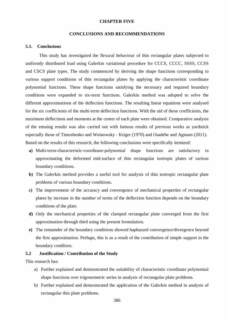
386

CHAPTER FIVE

CONCLUSIONS AND RECOMMENDATIONS

5.1. Conclusions

This study has investigated the flexural behaviour of thin rectangular plates subjected to

uniformly distributed load using Galerkin variational procedure for CCCS, CCCC, SSSS, CCSS

and CSCS plate types. The study commenced by deriving the shape functions corresponding to

various support conditions of thin rectangular plates by applying the characteristic coordinate

polynomial functions. These shape functions satisfying the necessary and required boundary

conditions were expanded to six-term functions. Galerkin method was adopted to solve the

different approximations of the deflection functions. The resulting linear equations were analysed

for the six coefficients of the multi-term deflection functions. With the aid of these coefficients, the

maximum deflections and moments at the center of each plate were obtained. Comparative analysis

of the ensuing results was also carried out with famous results of previous works as yardstick

especially those of Timoshenko and Woinowsky - Kriger (1970) and Osadebe and Aginam (2011).

Based on the results of this research, the following conclusions were specifically itemized:

a) Multi-term-characteristic-coordinate-polynomial shape functions are satisfactory in

approximating the deformed mid-surface of thin rectangular isotropic plates of various

boundary conditions.

b) The Galerkin method provides a useful tool for analysis of thin isotropic rectangular plate

problems of various boundary conditions.

c) The improvement of the accuracy and convergence of mechanical properties of rectangular

plates by increase in the number of terms of the deflection function depends on the boundary

conditions of the plate.

d) Only the mechanical properties of the clamped rectangular plate converged from the first

approximation through third using the present formulation.

e) The remainder of the boundary conditions showed haphazard convergence/divergence beyond

the first approximation. Perhaps, this is as a result of the contribution of simple support in the

boundary condition.

5.2 Justification / Contribution of the Study

This research has:

a) Further explained and demonstrated the suitability of characteristic coordinate polynomial

shape functions over trigonometric series in analysis of rectangular plate problems.

b) Further explained and demonstrated the application of the Galerkin method in analysis of

rectangular thin plate problems.

387

c) Shed more light on the mechanical behaviour of thin rectangular isotropic plates.

d) Demonstrated that increase in number of terms of the deflection function does not always

yield improved accuracy and convergence of solutions.

e) Formulated new design charts that will make for safer structures of plate in engineering.

f) Provided M-Files that would make for easier and accurate results of rectangular plate

problems.

5.3 Recommendations

The following recommendations are made:

a) Future research work should extend the application of multi term characteristic coordinate

polynomials principles and Galerkin method to rectangular orthotropic plates, circular plates

and plates on elastic foundations.

b) Future studies should use the multi term characteristic coordinate polynomial theorem used

herein and Galerkin method to analyse plates of different support conditions under forced

vibration regime.

c) Future studies should use the multi term characteristic coordinate polynomial theorem used

herein and Galerkin method to analyse rectangular plates with different types of loading like

point loads, patched loads, triangular loads etc.

d) More research should go into increasing the terms of the characteristic coordinate polynomial

shape function used herein to solve further plate problems.

e) Future studies should use odd approximations of characteristic coordinate polynomial

theorem used herein to solve rectangular plate problems.

388

ReferencesAginam, C. H. (2011). Application of direct variational methods in the analysis of thin rectangular

plates. (Doctoral dissertation). University of Nigeria, Nsukka, Nigeria.

Aginam, C. H., Chidolue, C. A., and Ezeagu, C. A. (2012). Application of direct variationalmethod in the analysis of isotropic thin rectangular plates. ARPN Journal of Engineeringand Applied Sciences, 7(9), 1128-1138.

Ajagbe, W. O., Rufai, O. A., and Labiran, J. O. (2014). Finite element analysis of a free-standingstaircase. Nigerian Journal of Technology (NIJOTECH), 33(4), 610-617.

Al-Badri, S. A., and Ahmad, A. A. (2009). Evaluation of elastic deflections and bending momentsfor orthotropically reinforced concrete rectangular slabs supported on three edges only andsubjected to triangular load. Diyala Journal of Engineering Sciences, 2(2), 15-29.

Alvarez, L. D., Vampa, V., and Martin, M. T. (2009). The construction of plate finite elementsusing wavelet basis functions. Revista Investigation Operational, 30(3), 193-204.

Aseeri, S. A. (2008). Goursat functions for a problem of an isotropic plate with a curvilinearhole. Int. J. Open Problems Compt. Math., 1(3).

Banerjee, P. K., and Butterfield, Y. (1981). Boundary Element Methods in Engineering Science.New York, NY: Mc-GrawHill.

Baraigi, N. K. (1986). A text book of plate analysis. Delhi, India: Khanna Publishers.

Bassah, E. J. (2007). Analysis of thin rectangular isotropic plates by polynomial functions

using energy method. (Master’s thesis). University of Nigeria, Nsukka, Nigeria.

Benvenuto, E. (1990). An introduction to the history of structural mechanics. Berlin, BL:Springer-verlag.

Beslin, O., and Nicolas J. A (1997). Hierarchical functions set for predicting very high order platebending modes with any boundary conditions. Journal of Sound and Vibration, 202(5),633-655.

Bhat, R. B. (1985). Natural frequencies of rectangular plates using characteristic othogonalpolynomials in Rayleigh - Ritz method. Journal of Sound and Vibration, 102 (4), 493 - 499.

Birman, V. (2011). Plate structures. New York, NY: Springer Science.

Brebbia, C. A., Telles, J. C., and Wrobel, L. C. (1984). Theory and application in engineering:boundary element techniques. Berlin, BL: Springer - Verlag.

Bryan, G. N. (1981). On the stability of a plane plate under thrusts in its own plane. Proc LondonMath Soc, 22, 54-67.

Chainarin, P. and Pairod S. (2006). Buckling analysis of composite laminate rectangular and

skew plates with various edge support conditions. Paper presented at the 20th Conference

389

of Mechanical Engineering Network of Thailand, pp.18-20.

Chapra, S. C., and Canale, Y. P. (2010). Numerical methods for engineers (6th ed.). New York,NY: McGraw-Hill Companies, Inc.

Cheung, Y. K. (1976). Finite strip method in structural analysis. Oxford, United Kingdom:Pergamon press.

Civalek, O. And Okyay, K. (2007). Discrete singular convolution for free vibration analysis ofanisotropic rectangular plates. Mathematical and Computational Applications, 12(3), 151-160.

Courant, Y.(1943). Variational methods for the solution of problems of equilibrium and vibration.Bulletin of the American Mathematical Society, 49, 1-23.

Cox, H.I.(1963). The buckling of plates and shells. New York, NY: Macmillan.

Dal, H., and Morgul O. (2011). Vibration of elastically restrained rectangular plates. ScientificResearch and Essays, 6(34), 6911-6816.

Dalaei, M., and Kerr, A.D. (1996). Natural vibration analysis of clamped rectangular orthotropicplates. Journal of Sound and Vibrations, 189(3), 399-406.

Den Hartog, J.P.(1958). Mechanical vibrations. New York, NY: McGraw-Hill.

Deobald, L. R., and Gibson, R. F. (1988). Determination of elastic constants of orthotropic platesby a modal analysis/rayleigh-ritz technique. Journal of Sound and Vibration, 124(2), 269-283.

Dey, S.S. (1981). Semi-numerical analysis of rectangular plates in bending. Computers andStructures, 14(56), 568-376.

Dozio, L. (2011). On the use of trigonometric Ritz method for general vibration analysis ofrectangular Kirchhoff plates. Thin-Walled Structures, 49, 129-144.

Fenner, Y. T. (1986). Engineering Elasticity: An application of numerical and analytical techniques.Chichester, Sussex: Ellis Horwood.

Galerkin, B.G. (1933). Thin elastic plates. Leningrad, NG: Scientific and Technical Publishinghouse.

Gallagher, Y. H. (1975). Finite Element Analysis. New Jersey, NJ: Prentice-Hall Englewood Cliffs.

Gerard, G., and Becker, H. (1957). Handbook of structural stability, Part1 – Buckling of flatplates. New York, NY: NACA TN 3781.

Gould, P.L. (1999). Analysis of shells and plates. New Jersey, NJ: Prentice-Hall Englewood Cliffs.

Guarracino F., and Walker A. (2008). Some comments on the numerical analysis of plates andthin-walled structures. Thin-Walled Struct., 46, 975-980.

Hartman, F. (1991). Static analysis of plates: Boundary element analysis of plates and shells.Berlin, BL: Springer - Verlay.

390

Hoffman, J. D. (2001). Numerical methods for engineers and scientists. New York, NY: MarcelDekker, Inc.

Hrennikoff, A. (1941). Solutions of problems of elasticity by framework method. J. Appl. Mech., 8,A169 - A175.

Hsu, M. (2003). Vibration analysis of isotropic and orthotropic plates with mixed boundaryconditions. Tamkang Journal of Science and Engineering , 6 (4), 217 – 226.

Huang, C. S., Chang, M.J. and Leissa, A.W. (2006). Vibrations of mindlin sectoriel plates usingthe Ritz method considering stress singularities. Journal of Vibration and Control, 12(6),635-65.

Hughes, T. J. Y. (1987). The Finite Element Method. New Jersey, NJ: Prentice-Hill EnglewoodCliffs.

Hutchinson, J. Y., (1992). On the bending of rectangular plates with two opposite edges simplysupported. Journal of Applied Mechanics, 59, 679-681.

Ibearugbulem, O. M., Ettu, L. O., and Ezeh, J. C. (2013). Direct integration and work principle asnew approach in bending analysis of isotropic rectangular plates. International Journal ofEngineering and Science (IJES), 2(3), 28-36.

Ibearugbulem, O. M., Oguaghamba, O. A., Njoku, K. O., and Nwaokorie, M. (2014). Using linecontinuum to explain work principle method for structural continuum analysis.International Journal of Innovative Research and Development, 3(9), 365 - 370.

İmrak, C. E., and Gerdemeli, I. (2007a). A Numerical method for clamped thin rectangular platescarrying a uniformly distributed load. Int. J. Appl. Mech., 3.

Imrak, C. E., & Gerdemeli, I. ((2007b). The problem of isotropic rectangular plate with fourclamped edges. Indian Academy of Sciences SADHANA, 32(3), 181-186.

Iyengar, N. G. (1988). Structural stability of columns and plates. New York, NY: Ellis HorwoodLimited.

Kaneda, K., Takamine, T., Chinen, Y., and Iraha, S. (2004): An analytical study and applicationof earth pressures loaded rectangular plates in the condition of two adjacent sides fixed andthe other sides free. Journal of Structural Engineering, 50A, 1025-1034.

Karman, T., Sechler, E.E., and Donnel, L.H. (1952). The strength of thin plates in compression.Trans ASME, 54, 53-57.

Kerr, A.D. (1969). An extended kantorovich method for the solution of eigenvalue problem.International Journal of Solids and Structures, 15, 559-572.

Krishnan, P. A., and Rajitha, T. P. (2009). Static and dynamic analysis of rectangular plates withlinearly varying thickness. IE (I) Journal-CV, 89, 34-38.

Lei, Y., Friswell, M. I., and Adhikari. S. (2006). A Galerkin method for distributed systems with

391

non-local damping. International Journal of Solids and Structures, 45(11), 58-65.

Leissa, A. W. (1969). Vibration of plates. NASA, Washington D.C.,

Leissa A. W. (2005). The historical bases of the rayleigh and ritz methods. Journal and Soundand Vibration, 287, 961-978.

Leknitskii, S.G. (1968). Anisotropic plates (English translation of the original Russian work).New York, NY: Gordon and Breach.

Levy, S. (1942). Bending of rectangular plates with large deflections. NACA, Rep. No.737.

Li, W. L. (2002). Comparison of Fourier sine and cosine series expressions for beams witharbitrary boundary conditions. Journal of Sound and Vibration, 265(1), 185-194.

Li, W. L. (2004). Vibration analysis of rectangular plates with general elastic boundarysupports. Journal of Sound and Vibration, 273, 619-635.

Mahavir, S., Pandita, I. K., and Kheer, S. K. (2016). Deflection of plates by using principle ofquasi work. Journal of Applied Engineering Sciences, 6(2), 21-24.

Mbakogu, F.C., and Pavlovic, M, N. (2000). Bending of clamped orthotropic rectangular plates: avariational symbolic solution. Computers and Structures,77, 117-128.

Mikhlin, S. G. (1964). Variational methods in mathematical physics. Oxford, United Kingdom:Pergamon Press.

Murli, K. R., and Prathap, G. (2003). Studies on variational correctness of finite elementelastodynamics of some plate elements. Research Report CM 0306, CSIY Centre forMathematical Modeling and Computer Simulation, Bangalore, India.

Musa, A. E. S., and Al-Gahtani, H. J. (2017). Series-based solution for analysis of simplysupported rectangular thin plate with internal rigid supports. Advances in CivilEngineering, 2017(2017). http://doi.org/10.1155/2017/6516471.

Nguyen, H. X. (2008). A strain smoothing method in finite elements for structural analysis.(Master’s thesis) University of Liege, France.

Nitin, K. J. (2009). Analysis of stress concentration and deflection in isotropic and

orthotropic rectangular plates with central circular hole under transverse static loading.

World Academy of Science, Engineering and Technology 60.

Oba, E. C., Anyadiegwu, P. C., George, A. G. T., and Nwadike, E. C. (2018). Pure bending

analysis of isotropic thin rectangular plates using third-order energy functional.

International Journal of Scientific and Research Publications, 8(3), 254-262.

392

Odman, S. T. A. (1955). Studies of boundary value problems. Swedish Cement and Concrete

Research Institute, Royal Institute of Technology, Stockholm, 2, 7-62.

Okafor, F. O., and Oguaghamba, O. (2009). Effects of flexural rigidity of reinforcement bars on thefundamental natural frequency of reinforced concrete slabs. Nigerian Journal ofTechnology , 28 (2), 48 - 57.

Onyeyili, I. O. (2012). Advanced Theory of Plates and Shells [Lecture notes]. SPGS, FederalUniversity of Technology, Owerri, Nigeria.

Osadebe, N. N., and Aginam, C. H. (2011). Bending analysis of isotropic rectangular plate withall edges clamped: Variational symbolic solution. Journal of Emerging in Engineeringand Applied Sciences (JETEAS), 2(5), 846 - 852.

Pal, N. C., Sinha, P. K., and Bhattacharyya, S. K. (2001). Finite element dynamic analysis ofsubmerged laminated composite plates. Journal of Reinforced Plastics and Composites,20 (07), 547-563.

Panov, D.Yu. (1941). On large deflections of circular plates. Prikl Matem Mech, 5(2), 45-56.

Ragesh, P. P., Mustafa, V., and Somasundaran, T. P (2016). An integrated kirchhoff element bygalerkin method for free vibration analysis of plates on elastic foundation. ProcediaTechnology, 24, 148-154.

Reissner, E. (1954). The effect of transverse shear deformation on the bending of elastic plates. JAppl Mech Trans ASME. 12, A69-A77.

Shufrin, I., Rabinovitch, O., and Eisenberger, M. (2009). Elastic non linear stability analysis of thinrectangular plates through a semi-analytical approach. International Journal of Solids andStructures, 46, 2075-2092.

Singh, B., and Lal, J. (1984). Kantorovich method in magnetohydrodynamic flow problemsthrough channels. Indian J. Pure Appl. Math., 15(9), 1048-1063.

Singhvi S., and Kapania, Y. K. (1994). Comparison of simple and chebychev polynomials inrayleigh-ritz analysis. J. Eng. Mech., 120, 2126-2135.

Sladek, J., Sladek, V., Zhang, Ch., Krivacek, J., and Wen, P.H. (2006). Analysis of orthotropicthick plates by meshless local Petro-Galerkin (MLPG) method. International Journal forNumerical Methods in Engineering, 67(13), 1830-1850.

Soedel, W. (2005). Vibrations of Shells and Plates (3rd ed.). New York, NY: Marcel Dekker, Inc.

Southwell, Y.V., and Scan, S. (1924). On the stability under shearing forces of a flat elastic strip.Proe Yoy Soc, A105, 582.

Stroud, K. A. (1996). Further engineering mathematics (3rd ed.). New York, NY: PALGYAVE.

393

Szilard, R. (2004). Theories and applications of plate analysis: Classical, numerical andengineering methods. Hoboken, New Jersy: John Wiley and Sons, Inc.

Thompson, W.T. (1973). Theory of vibrations and applications. New Jersey, NJ: Prentice-Hill,Englewood Cliffs.

Timoshenko, S.P. (1938). Bending of rectangular plates with clamped edges. Proceedings of 5thInternational Applied Mechanics, MIT-USA, (pp. 40-43).

Timoshenko, S.P., and Woinowsky-Krieger, S. (1959). Theory of plates and shells (2nd ed.). NewYork, NY: McGraw-Hill.

Timoshenko, S.P., and Gere, J.M. (1961). Theory of elastic stability (2nd ed.). New York, NY:McGraw-Hill Inc.

Timoshenko, S.P., and Young, D.H. (1963). Vibration problems in engineering. New York, NY:John Wiley and Sons.

Timoshenko, S. P., and Woinowsky - Krieger, S. (1970). Theory of plates and shells. Auckland,NewZealand: McGraw-Hill Inc.

Tottenham, H. (1979). The boundary element method for plates and shells: Developments inboundary element method - 1. London, England: Applied Science Publishers.

Turner, M. J., Martin, H.C., and Topp, L. J. (1956). Stiffness and deflection analysis of complexstructures. Aeronaut. Sci., 28(9), 805-823.

Ugural, A. C. (1999). Stresses in plates and shells (2nd ed.). Singapore, SP: McGraw- hill.

Vanam, B. C. L., Rajyalakshmi, M., and Inala, R. (2012). Static analysis of an isotropic rectangularplate using finite element analysis (FEA). Journal of Mechanical Engineering Research,4(4), 148-162.

Ventsel, E., and Krauthammer, T. (2001). Thin Plates and Shells: Theory, analysis, andapplications. New York, NY: Marcel Dekker, Inc.

Ventsel, E. S. (1997). An indirect boundary element method for plate bending analysis. Int. J.Numer. Math. Eng., 9, 1597-1611.

Vinson, J. R. (1974). Structural mechanics: The behavior of plates and shells. New York, NY:

John Wiley & Sons Inc.

Wang, D., and Sheik, A. (2005). Large deflections, moments and shears for uniformly loadedrectangular plate with camped edge. J. Applied Mechanics Trans. ASME. 4, A173-A176.

Wang, C, M., Wang, Y. C., and Yeddy, J. N. (2002). Problems and remedy for the ritz method indetermining stress resultant of corner supported rectangular plates. Computers &Structures, 80,145-154.

394

Weaver, W., Young, D. H., and Timoshenko, S. (1990). Vibration problems in engineering(5th ed.). New York, NY: John Wiley and Sons Inc.

Wojtaszak, I. A. (1937). The calculation of maximum deflection, moments and shear for uniformlyloaded rectangular plate with clamped edge. J. Appl. Mechanics, Trans. ASME. 4, A173-A176.

Yamaki, N. (1961). Influence of Large Amplitudes on Flexural Vibrations of Elastic Plates.Journal of Applied Mathematics and Mechanics, 41(12), 501-510.

Zenkour, A. M. (2003). Exact mixed-classical solutions for the bending analysis of shear

deformable rectangular plates. Applied Mathematical Modelling, 27(7), 515-534.

Zhong, Y., and Xu, X. (2017). Analysis bending solutions of clamped rectangular thick plates.

Mathematical Problems in Engineering, 2017(2017). http://doi.org/10.1155/2017/7539276.

.

395

Appendix A.1

Comparison of Edge Moment Coefficient Values

Figure A.1.1: CCCC vs Classical Solution at Varying Aspect Ratio

Figure A.1.2: CCCC vs Classical Solution at Varying Aspect Ratio

396

Figure A.1.3: CSCS vs Classical Solution at Varying Aspect Ratio

397

Appendix A.2

Deflection Curves at Aspect Ratio of Unity

Figure A.2.1: CCCS at Varying Non-dimensional Span, X

Figure A.2.2: SSSS at Varying Non-dimensional Span, X

398

Figure A.2.3: CCCC at Varying Non-dimensional Span, X

Figure A.2.4: CCSS at Varying Non-dimensional Span, X

399

Figure A.2.5: CSCS at Varying Non-dimensional Span, X

400

Appendix A.3

Short Span Moment Curve at Aspect Ratio of Unity

Figure A.3.1: CCCS at Varying Non-dimensional Span, X

Figure A.3.2: SSSS at Varying Non-dimensional Span, X

401

Figure A.3.3: CCCC at Varying Non-dimensional Span, X

Figure A.3.4: CCSS at Varying Non-dimensional Span, X

402

Figure A.3.5: CSCS at Varying Non-dimensional Span, X

403

Appendix A.4

Typical Excel Spread Sheet

404

Appendix A.5M-File for CCCS

%Program for computation of the deflection and moment of thin plates%Boundary types B1 = CCCS,B2 = SSSS, B3 = CCCC, B4= CCSS, B5 = CSCS

%Approximation F1=First approximation, F2= Second approximation F3=%truncated third approximation, F4= third approximation%Aspect ratio=p

Boundary type='B1';Approximation=input('approximation (F):');p=input ('aspect ratio (p):');X=input ('short span (x):');Y=input ('long span (y):');

v=0.3;

switch Boundarytypecase 'B1'

f1=(1.5*X.^2 - 2.5*X.^3 + X.^4).*(Y.^2 - 2*Y.^3 + Y.^4);f2=(1.5*X.^4 - 2.5*X.^5 + X.^6).*(Y.^2 - 2*Y.^3 + Y.^4);f3=(1.5*X.^2 - 2.5*X.^3 + X.^4).*(Y.^4 - 2*Y.^5 + Y.^6);f4=(1.5*X.^4 - 2.5*X.^5 + X.^6).*(Y.^4 - 2*Y.^5 + Y.^6);f5=(1.5*X.^6 - 2.5*X.^7 + X.^8).*(Y.^2 - 2*Y.^3 + Y.^4);f6=(1.5*X.^2 - 2.5*X.^3 + X.^4).*(Y.^6 - 2*Y.^7 + Y.^8);switch Approximation

case 'F1'a11= 2.8571*10^-3+3.2653*10^-3*1/(p*p)+6.0317*10^-3/(p*p*p*p);

b1=2.5*10^-3;C1=b1/a11;disp('The deflection coefficent is')defcoeff = C1*f1Bxi = -(C1*(3-15*X+12*X.^2)*(Y^2-2*Y.^3+Y.^4) +...

v/(p*p)*(C1*(1.5*X.^2-2.5*X.^3+X.^4)*(2-12*Y+12*Y.^2)));Byi = -(v*C1*(3-15*X+12*X.^2)*(Y^2-2*Y.^3+Y.^4) +...

1/(p*p)*(C1*(1.5*X.^2-2.5*X.^3+X.^4)*(2-12*Y+12*Y.^2)));disp('The short span moment coefficent is')Bxidisp('The long span moment coefficent is')Byi

case 'F2'a11= 2.8571*10^-3+3.2653*10^-3*1/(p*p)+6.0317*10^-3/(p*p*p*p);

a12= 9.9773*10^-4+1.3152*10^-3*1/(p*p)+2.0924*10^-3/(p*p*p*p);a13= 7.7922*10^-4+8.1633*10^-4*1/(p*p)+1.7234*10^-3/(p*p*p*p);a21= -5.8957*10^-4+1.3152*10^-3*1/(p*p)+2.0924*10^-3/(p*p*p*p);a22= 3.6281*10^-4+1.0170*10^-3*1/(p*p)+9.3240*10^-4/(p*p*p*p);a23= -1.6079*10^-4+3.2880*10^-4*1/(p*p)+5.9781*10^-4/(p*p*p*p);a31= 7.7922*10^-4+8.1633*10^-4*1/(p*p)+1.7234*10^-3/(p*p*p*p);a32= 2.7211*10^-4+3.2880*10^-4*1/(p*p)+5.9781*10^-4/(p*p*p*p);a33= 2.7972*10^-4+4.9474*10^-4*1/(p*p)+1.7234*10^-3/(p*p*p*p);

b1=2.5*10^-3;b2= 8.7302*10^-4;b3= 7.1429*10^-4;a=[a11 a12 a13;a21 a22 a23;a31 a32 a33];b=[b1;b2;b3];C=a\b;defcoeff=C(1,1)*f1+C(2,1)*f2+C(3,1)*f3;disp('The deflection coefficent is')defcoeffBxi = -((C(1,1)*(3-15*X+12*X.^2)*(Y^2-2*Y.^3+Y.^4) + ...

C(2,1)*(18*X^2-50*X^3+30*X^4)*(Y^2-2*Y^3+Y^4)+...C(3,1)*(3-15*X+12*X^2)*(Y^4-2*Y^5+Y^6))+ ...

405

v/(p*p)*(C(1,1)*(1.5*X.^2-2.5*X.^3+X.^4)*(2-12*Y+12*Y.^2)+...C(2,1)*(1.5*X^4-2.5*X^5+X^6)*(2-12*Y+12*Y^2)+...C(3,1)*(1.5*X^2-2.5*X^3+X^4)*(12*Y^2-40*Y^3+30*Y^4)));

Byi = -(v*(C(1,1)*(3-15*X+12*X.^2)*(Y^2-2*Y.^3+Y.^4) + ...C(2,1)*(18*X^2-50*X^3+30*X^4)*(Y^2-2*Y^3+Y^4)+...C(3,1)*(3-15*X+12*X^2)*(Y^4-2*Y^5+Y^6))+ ...

1/(p*p)*(C(1,1)*(1.5*X.^2-2.5*X.^3+X.^4)*(2-12*Y+12*Y.^2)+...C(2,1)*(1.5*X^4-2.5*X^5+X^6)*(2-12*Y+12*Y^2)+...C(3,1)*(1.5*X^2-2.5*X^3+X^4)*(12*Y^2-40*Y^3+30*Y^4)));

disp('The short span moment coefficent is')Bxidisp('The long span moment coefficent is')Byi

case 'F3'a11= 2.8571*10^-3+3.2653*10^-3*1/(p*p)+6.0317*10^-3/(p*p*p*p);a12= 9.9773*10^-4+1.3152*10^-3*1/(p*p)+2.0924*10^-3/(p*p*p*p);a13= 7.7922*10^-4+8.1633*10^-4*1/(p*p)+1.7234*10^-3/(p*p*p*p);a14= 2.7211*10^-4+3.2880*10^-4*1/(p*p)+5.9781*10^-4/(p*p*p*p);a21= -5.8957*10^-4+1.3152*10^-3*1/(p*p)+2.0924*10^-3/(p*p*p*p);a22= 3.6281*10^-4+1.0170*10^-3*1/(p*p)+9.3240*10^-4/(p*p*p*p);a23= -1.6079*10^-4+3.2880*10^-4*1/(p*p)+5.9781*10^-4/(p*p*p*p);a24= 9.8949*10^-5+2.5424*10^-4*1/(p*p)+2.6640*10^-4/(p*p*p*p);a31= 7.7922*10^-4+8.1633*10^-4*1/(p*p)+1.7234*10^-3/(p*p*p*p);a32= 2.7211*10^-4+3.2880*10^-4*1/(p*p)+5.9781*10^-4/(p*p*p*p);a33= 2.7972*10^-4+4.9474*10^-4*1/(p*p)+1.7234*10^-3/(p*p*p*p);a34= 9.7680*10^-5+1.9927*10^-4*1/(p*p)+5.9781*10^-4/(p*p*p*p);a41= -1.6079*10^-4+3.2880*10^-4*1/(p*p)+5.9781*10^-4/(p*p*p*p);a42= 9.8949*10^-5+2.5424*10^-4*1/(p*p)+2.6640*10^-4/(p*p*p*p);a43= -5.7720*10^-5+1.9927*10^-4*1/(p*p)+5.9781*10^-4/(p*p*p*p);a44= 3.5520*10^-5+1.5409*10^-4*1/(p*p)+2.6640*10^-4/(p*p*p*p);

b1=2.5*10^-3;b2= 8.7302*10^-4;b3= 7.1429*10^-4;b4= 2.4943*10^-4;

a=[a11 a12 a13 a14;a21 a22 a23 a24;a31 a32 a33 a34; a41 a42 a43 a44];b=[b1;b2;b3;b4];C=a\b;defcoeff=C(1,1)*f1+C(2,1)*f2+C(3,1)*f3+ C(4,1)*f4;disp('The deflection coefficent is')defcoeffBxi = -((C(1,1)*(3-15*X+12*X.^2)*(Y^2-2*Y.^3+Y.^4) + ...

C(2,1)*(18*X^2-50*X^3+30*X^4)*(Y^2-2*Y^3+Y^4)+...C(3,1)*(3-15*X+12*X^2)*(Y^4-2*Y^5+Y^6)+ ...C(4,1)*(18*X^2-50*X^3+30*X^4)*(Y^4-2*Y^5+Y^6))+...

v/(p*p)*(C(1,1)*(1.5*X.^2-2.5*X.^3+X.^4)*(2-12*Y+12*Y.^2)+...C(2,1)*(1.5*X^4-2.5*X^5+X^6)*(2-12*Y+12*Y^2)+...C(3,1)*(1.5*X^2-2.5*X^3+X^4)*(12*Y^2-40*Y^3+30*Y^4)+...C(4,1)*(1.5*X^4-2.5*X^5+X^6)*(12*Y^2-40*Y^3+30*Y^4)));

Byi = -(v*(C(1,1)*(3-15*X+12*X.^2)*(Y^2-2*Y.^3+Y.^4) + ...C(2,1)*(18*X^2-50*X^3+30*X^4)*(Y^2-2*Y^3+Y^4)+...C(3,1)*(3-15*X+12*X^2)*(Y^4-2*Y^5+Y^6)+ ...C(4,1)*(18*X^2-50*X^3+30*X^4)*(Y^4-2*Y^5+Y^6))+...

1/(p*p)*(C(1,1)*(1.5*X.^2-2.5*X.^3+X.^4)*(2-12*Y+12*Y.^2)+...C(2,1)*(1.5*X^4-2.5*X^5+X^6)*(2-12*Y+12*Y^2)+...C(3,1)*(1.5*X^2-2.5*X^3+X^4)*(12*Y^2-40*Y^3+30*Y^4)+...C(4,1)*(1.5*X^4-2.5*X^5+X^6)*(12*Y^2-40*Y^3+30*Y^4)));


case 'F4'a11= 2.8571*10^-3+3.2653*10^-3*1/(p*p)+6.0317*10^-3/(p*p*p*p);a12= 9.9773*10^-4+1.3152*10^-3*1/(p*p)+2.0924*10^-3/(p*p*p*p);a13= 7.7922*10^-4+8.1633*10^-4*1/(p*p)+1.7234*10^-3/(p*p*p*p);

406

a14= 2.7211*10^-4+3.2880*10^-4*1/(p*p)+5.9781*10^-4/(p*p*p*p);a15= 4.9131*10^-4+6.1843*10^-4*1/(p*p)+9.3240*10^-4/(p*p*p*p);a16= 2.7972*10^-4+1.9790*10^-4*1/(p*p)+7.1807*10^-4/(p*p*p*p);a21= -5.8957*10^-4+1.3152*10^-3*1/(p*p)+2.0924*10^-3/(p*p*p*p);a22= 3.6281*10^-4+1.0170*10^-3*1/(p*p)+9.3240*10^-4/(p*p*p*p);a23= -1.6079*10^-4+3.2880*10^-4*1/(p*p)+5.9781*10^-4/(p*p*p*p);a24= 9.8949*10^-5+2.5424*10^-4*1/(p*p)+2.6640*10^-4/(p*p*p*p);a25= 4.3634*10^-4+6.8820*10^-4*1/(p*p)+4.8618*10^-4/(p*p*p*p);a26= -5.7720*10^-5+7.9709*10^-5*1/(p*p)+2.4909*10^-4/(p*p*p*p);a31= 7.7922*10^-4+8.1633*10^-4*1/(p*p)+1.7234*10^-3/(p*p*p*p);a32= 2.7211*10^-4+3.2880*10^-4*1/(p*p)+5.9781*10^-4/(p*p*p*p);a33= 2.7972*10^-4+4.9474*10^-4*1/(p*p)+1.7234*10^-3/(p*p*p*p);a34= 9.7680*10^-5+1.9927*10^-4*1/(p*p)+5.9781*10^-4/(p*p*p*p);a35= 1.3399*10^-4+1.5461*10^-4*1/(p*p)+2.6640*10^-4/(p*p*p*p);a36= 1.1988*10^-4+2.3976+10^-4*1/(p*p)+1.1750*10^-3/(p*p*p*p);a41= -1.6079*10^-4+3.2880*10^-4*1/(p*p)+5.9781*10^-4/(p*p*p*p);a42= 9.8949*10^-5+2.5424*10^-4*1/(p*p)+2.6640*10^-4/(p*p*p*p);a43= -5.7720*10^-5+1.9927*10^-4*1/(p*p)+5.9781*10^-4/(p*p*p*p);a44= 3.5520*10^-5+1.5409*10^-4*1/(p*p)+2.6640*10^-4/(p*p*p*p);a45= 1.1900*10^-4+1.7205*10^-4*1/(p*p)+1.3891*10^-4/(p*p*p*p);a46= -2.4737*10^-5+9.6570*10^-5*1/(p*p)+4.0760*10^-4/(p*p*p*p);a51= -2.6833*10^-3+6.1843*10^-4*1/(p*p)+9.3240*10^-4/(p*p*p*p);a52= -1.1510*10^-3+6.8820*10^-4*1/(p*p)+4.8618*10^-4/(p*p*p*p);a53= -7.3181*10^-4+1.5461*10^-4*1/(p*p)+2.6640*10^-4/(p*p*p*p);a54= -3.1390*10^-4+1.7205*10^-4*1/(p*p)+1.3891*10^-4/(p*p*p*p);a55= -4.9950*10^-4+5.6832*10^-4*1/(p*p)+2.8227*10^-4/(p*p*p*p);a56= -2.6270*10^-4+3.7481*10^-5*1/(p*p)+1.1100*10^-4/(p*p*p*p);a61= 2.7972*10^-4+1.9790*10^-4*1/(p*p)+7.1807*10^-4/(p*p*p*p);a62= 9.7680*10^-5+7.9709*10^-5*1/(p*p)+2.4909*10^-4/(p*p*p*p);a63= 1.1988*10^-4+2.3976*10^-4*1/(p*p)+1.1750*10^-3/(p*p*p*p);a64= 4.1863*10^-5+9.6570*10^-5*1/(p*p)+4.0760*10^-4/(p*p*p*p);a65= 4.8100*10^-5+3.7481*10^-5*1/(p*p)+1.1100*10^-4/(p*p*p*p);a66= 5.8177*10^-5+1.5984*10^-4*1/(p*p)+1.0545*10^-3/(p*p*p*p);

b1=2.5*10^-3;b2= 8.7302*10^-4;b3= 7.1429*10^-4;b4= 2.4943*10^-4;b5= 4.2989*10^-4;b6= 2.9762*10^-4;a=[a11 a12 a13 a14 a15 a16;a21 a22 a23 a24 a25 a26;...

a31 a32 a33 a34 a35 a36; a41 a42 a43 a44 a45 a46;...a51 a52 a53 a54 a55 a56; a61 a62 a63 a64 a65 a66];

b=[b1;b2;b3;b4;b5;b6];C=a\b;defcoeff=C(1,1)*f1+C(2,1)*f2+C(3,1)*f3+C(4,1)*f4+C(5,1)*f5+...

C(6,1)*f6;disp('The deflection coefficent is')defcoeffBxi = -((C(1,1)*(3-15*X+12*X.^2)*(Y^2-2*Y.^3+Y.^4) + ...

C(2,1)*(18*X^2-50*X^3+30*X^4)*(Y^2-2*Y^3+Y^4)+...C(3,1)*(3-15*X+12*X^2)*(Y^4-2*Y^5+Y^6)+ ...C(4,1)*(18*X^2-50*X^3+30*X^4)*(Y^4-2*Y^5+Y^6)+...C(5,1)*(45*X^4-105*X^5+56*X^6)*(Y^2-2*Y^3+Y^4)+...C(6,1)*(3-15*X+12*X^2)*(Y^6-2*Y^7+Y^8))+...

v/(p*p)*(C(1,1)*(1.5*X.^2-2.5*X.^3+X.^4)*(2-12*Y+12*Y.^2)+...C(2,1)*(1.5*X^4-2.5*X^5+X^6)*(2-12*Y+12*Y^2)+...C(3,1)*(1.5*X^2-2.5*X^3+X^4)*(12*Y^2-40*Y^3+30*Y^4)+...C(4,1)*(1.5*X^4-2.5*X^5+X^6)*(12*Y^2-40*Y^3+30*Y^4)+ ...C(5,1)*(1.5*X^6-2.5*X^7+X^8)*(2-12*Y+12*Y^2)+...C(6,1)*(1.5*X^2-2.5*X^3+X^4)*(30*Y^4-84*Y^5+56*Y^6)));

Byi = -(v*(C(1,1)*(3-15*X+12*X.^2)*(Y^2-2*Y.^3+Y.^4) + ...C(2,1)*(18*X^2-50*X^3+30*X^4)*(Y^2-2*Y^3+Y^4)+...C(3,1)*(3-15*X+12*X^2)*(Y^4-2*Y^5+Y^6)+ ...C(4,1)*(18*X^2-50*X^3+30*X^4)*(Y^4-2*Y^5+Y^6)+...

407

C(5,1)*(45*X^4-105*X^5+56*X^6)*(Y^2-2*Y^3+Y^4)+...C(6,1)*(3-15*X+12*X^2)*(Y^6-2*Y^7+Y^8))+...

1/(p*p)*(C(1,1)*(1.5*X.^2-2.5*X.^3+X.^4)*(2-12*Y+12*Y.^2)+...C(2,1)*(1.5*X^4-2.5*X^5+X^6)*(2-12*Y+12*Y^2)+...C(3,1)*(1.5*X^2-2.5*X^3+X^4)*(12*Y^2-40*Y^3+30*Y^4)+...C(4,1)*(1.5*X^4-2.5*X^5+X^6)*(12*Y^2-40*Y^3+30*Y^4)+ ...C(5,1)*(1.5*X^6-2.5*X^7+X^8)*(2-12*Y+12*Y^2)+...C(6,1)*(1.5*X^2-2.5*X^3+X^4)*(30*Y^4-84*Y^5+56*Y^6)));


endend

flexural analysis of thin rectangular plates

Documents