algorithm optimization in molecular dynamics simulation

This article was published in an Elsevier journal. The attached copyis furnished to the author for non-commercial research and

education use, including for instruction at the author’s institution,sharing with colleagues and providing to institution administration.

Other uses, including reproduction and distribution, or selling orlicensing copies, or posting to personal, institutional or third party

websites are prohibited.

In most cases authors are permitted to post their version of thearticle (e.g. in Word or Tex form) to their personal website orinstitutional repository. Authors requiring further information

regarding Elsevier’s archiving and manuscript policies areencouraged to visit:

http://www.elsevier.com/copyright

http://www.elsevier.com/copyright

Author's personal copy

Computer Physics Communications 177 (2007) 551–559

www.elsevier.com/locate/cpc

Algorithm optimization in molecular dynamics simulation

Di-Bao Wang a,∗, Fei-Bin Hsiao a, Cheng-Hsin Chuang b, Yung-Chun Lee c

a Institute of Aeronautics and Astronautics, National Cheng Kung University, 70101 Tainan, Taiwanb Department of Mechanical Engineering, Southern Taiwan University of Technology, 71005 Tainan, Taiwan

c Department of Mechanical Engineering, National Cheng Kung University, 70101 Tainan, Taiwan

Received 12 February 2007; received in revised form 16 May 2007; accepted 21 May 2007

Available online 5 June 2007

Abstract

Establishing the neighbor list to efficiently calculate the inter-atomic forces consumes the majority of computation time in molecular dynam-ics (MD) simulation. Several algorithms have been proposed to improve the computation efficiency for short-range interaction in recent years,although an optimized numerical algorithm has not been provided. Based on a rigorous definition of Verlet radius with respect to temperatureand list-updating interval in MD simulation, this paper has successfully developed an estimation formula of the computation time for each MDalgorithm calculation so as to find an optimized performance for each algorithm. With the formula proposed here, the best algorithm can be chosenbased on different total number of atoms, system average density and system average temperature for the MD simulation. It has been shown thatthe Verlet Cell-linked List (VCL) algorithm is better than other algorithms for a system with a large number of atoms. Furthermore, a generalizedVCL algorithm optimized with a list-updating interval and cell-dividing number is analyzed and has been verified to reduce the computation timeby 30 ∼ 60% in a MD simulation for a two-dimensional lattice system. Due to similarity, the analysis in this study can be extended to othermany-particle systems.© 2007 Elsevier B.V. All rights reserved.

Keywords: Molecular dynamics; Neighbor list; Algorithm; Optimization

1. Introduction

Molecular dynamics (MD) simulation has been developedfor more than half a century. MD is a very useful tool in study-ing the momentum exchange and energy transfer in submicronscales or even in atomic levels. Specifically, MD is usuallyused to investigate the thermodynamics during an equilibriumprocess, to estimate the transport coefficients during a non-equilibrium process and even to provide information on atomicscales in a multi-scale simulation. MD simulation thus plays animportant role in nano science and nano technology.

No matter what algorithm is utilized or what physical quan-tity is going to be derived, the typical flow chart of a MD

* Corresponding author at: Institute of Aeronautics and Astronautics, Na-tional Cheng Kung University, No. 1, Dasyue Rd., Tainan 70101, Taiwan. Tel.:+886 6 2757575 63642; fax: +886 6 2088214.

E-mail addresses: [email protected] (D.-B. Wang),[email protected] (F.-B. Hsiao), [email protected](C.-H. Chuang), [email protected] (Y.-C. Lee).

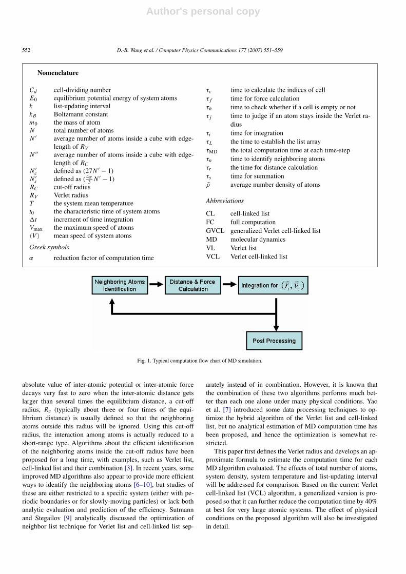
simulation can be illustrated in Fig. 1. The post processing heremeans the calculation of system energy (potential and kineticenergy) and transport coefficients through displacement and ve-locity. With regard to the computational cost at each time-step,the identification of neighboring atoms and the calculation ofinter-atomic distance/force require the majority of CPU time.Usually there are two ways to accelerate the computation ofMD. One is to use and optimize parallel computation [1,2] andthe other is to improve the MD algorithm implemented on asingle machine [4–10], and it is the latter method that this studywill concentrate on.

MD computation acceleration can be achieved either throughchoosing the most suitable algorithm or optimizing the numer-ical parameters for each algorithm. Frenkel [3] provided someempirical criteria for choosing a certain kind of algorithm for acertain class of MD problems. However, they are only qualita-tive instead of quantitative and thus hard to implement in realMD simulations.

With considering the long-range forces, some early effortwas made to obtain a computational cost of O(N) [4]. Since the

0010-4655/$ – see front matter © 2007 Elsevier B.V. All rights reserved.doi:10.1016/j.cpc.2007.05.009


552 D.-B. Wang et al. / Computer Physics Communications 177 (2007) 551–559

Nomenclature

Cd cell-dividing numberE0 equilibrium potential energy of system atomsk list-updating intervalkB Boltzmann constantm0 the mass of atomN total number of atomsN ′ average number of atoms inside a cube with edge-

length of RV

N ′′ average number of atoms inside a cube with edge-length of RC

N ′c defined as (27N ′ − 1)

N ′s defined as ( 4π

3 N ′ − 1)

RC cut-off radiusRV Verlet radiusT the system mean temperaturet0 the characteristic time of system atoms�t increment of time integrationVmax the maximum speed of atoms〈V 〉 mean speed of system atoms

Greek symbols

α reduction factor of computation time

τc time to calculate the indices of cellτf time for force calculationτh time to check whether if a cell is empty or notτj time to judge if an atom stays inside the Verlet ra-

diusτi time for integrationτL the time to establish the list arrayτMD the total computation time at each time-stepτn time to identify neighboring atomsτr the time for distance calculationτs time for summationρ̄ average number density of atoms

Abbreviations

CL cell-linked listFC full computationGVCL generalized Verlet cell-linked listMD molecular dynamicsVL Verlet listVCL Verlet cell-linked list

Fig. 1. Typical computation flow chart of MD simulation.

absolute value of inter-atomic potential or inter-atomic forcedecays very fast to zero when the inter-atomic distance getslarger than several times the equilibrium distance, a cut-offradius, Rc (typically about three or four times of the equi-librium distance) is usually defined so that the neighboringatoms outside this radius will be ignored. Using this cut-offradius, the interaction among atoms is actually reduced to ashort-range type. Algorithms about the efficient identificationof the neighboring atoms inside the cut-off radius have beenproposed for a long time, with examples, such as Verlet list,cell-linked list and their combination [3]. In recent years, someimproved MD algorithms also appear to provide more efficientways to identify the neighboring atoms [6–10], but studies ofthese are either restricted to a specific system (either with pe-riodic boundaries or for slowly-moving particles) or lack bothanalytic evaluation and prediction of the efficiency. Sutmannand Stegailov [9] analytically discussed the optimization ofneighbor list technique for Verlet list and cell-linked list sep-

arately instead of in combination. However, it is known thatthe combination of these two algorithms performs much bet-ter than each one alone under many physical conditions. Yaoet al. [7] introduced some data processing techniques to op-timize the hybrid algorithm of the Verlet list and cell-linkedlist, but no analytical estimation of MD computation time hasbeen proposed, and hence the optimization is somewhat re-stricted.

This paper first defines the Verlet radius and develops an ap-proximate formula to estimate the computation time for eachMD algorithm evaluated. The effects of total number of atoms,system density, system temperature and list-updating intervalwill be addressed for comparison. Based on the current Verletcell-linked list (VCL) algorithm, a generalized version is pro-posed so that it can further reduce the computation time by 40%at best for very large atomic systems. The effect of physicalconditions on the proposed algorithm will also be investigatedin detail.


D.-B. Wang et al. / Computer Physics Communications 177 (2007) 551–559 553

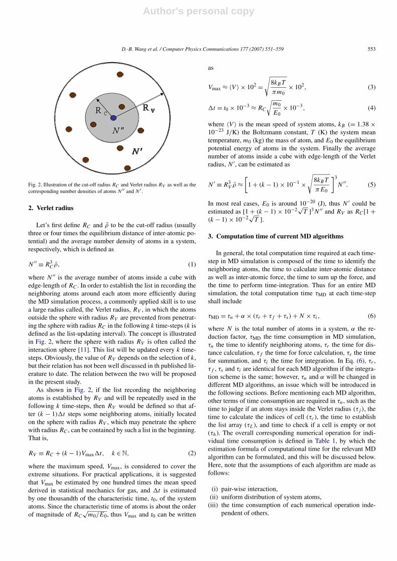
Fig. 2. Illustration of the cut-off radius RC and Verlet radius RV as well as thecorresponding number densities of atoms N ′′ and N ′ .

2. Verlet radius

Let’s first define RC and ρ̄ to be the cut-off radius (usuallythree or four times the equilibrium distance of inter-atomic po-tential) and the average number density of atoms in a system,respectively, which is defined as

(1)N ′′ ≡ R3Cρ̄,

where N ′′ is the average number of atoms inside a cube withedge-length of RC . In order to establish the list in recording theneighboring atoms around each atom more efficiently duringthe MD simulation process, a commonly applied skill is to usea large radius called, the Verlet radius, RV , in which the atomsoutside the sphere with radius RV are prevented from penetrat-ing the sphere with radius RC in the following k time-steps (k isdefined as the list-updating interval). The concept is illustratedin Fig. 2, where the sphere with radius RV is often called theinteraction sphere [11]. This list will be updated every k time-steps. Obviously, the value of RV depends on the selection of k,but their relation has not been well discussed in th published lit-erature to date. The relation between the two will be proposedin the present study.

As shown in Fig. 2, if the list recording the neighboringatoms is established by RV and will be repeatedly used in thefollowing k time-steps, then RV would be defined so that af-ter (k − 1)�t steps some neighboring atoms, initially locatedon the sphere with radius RV , which may penetrate the spherewith radius RC , can be contained by such a list in the beginning.That is,

(2)RV ≡ RC + (k − 1)Vmax�t, k ∈ N,

where the maximum speed, Vmax, is considered to cover theextreme situations. For practical applications, it is suggestedthat Vmax be estimated by one hundred times the mean speedderived in statistical mechanics for gas, and �t is estimatedby one thousandth of the characteristic time, t0, of the systematoms. Since the characteristic time of atoms is about the orderof magnitude of RC

√m0/E0, thus Vmax and t0 can be written

as

(3)Vmax ≈ 〈V 〉 × 102 =√

8kBT

πm0× 102,

(4)�t = t0 × 10−3 ≈ RC

√m0

E0× 10−3,

where 〈V 〉 is the mean speed of system atoms, kB (= 1.38 ×10−23 J/K) the Boltzmann constant, T (K) the system meantemperature, m0 (kg) the mass of atom, and E0 the equilibriumpotential energy of atoms in the system. Finally the averagenumber of atoms inside a cube with edge-length of the Verletradius, N ′, can be estimated as

(5)N ′ ≡ R3V ρ̄ ≈

[1 + (k − 1) × 10−1 ×

√8kBT

πE0

]3

N ′′.

In most real cases, E0 is around 10−20 (J), thus N ′ could beestimated as [1 + (k − 1) × 10−2

√T ]3N ′′ and RV as RC[1 +

(k − 1) × 10−2√

T ].

3. Computation time of current MD algorithms

In general, the total computation time required at each time-step in MD simulation is composed of the time to identify theneighboring atoms, the time to calculate inter-atomic distanceas well as inter-atomic force, the time to sum up the force, andthe time to perform time-integration. Thus for an entire MDsimulation, the total computation time τMD at each time-stepshall include

(6)τMD = τn + α × (τr + τf + τs) + N × τi,

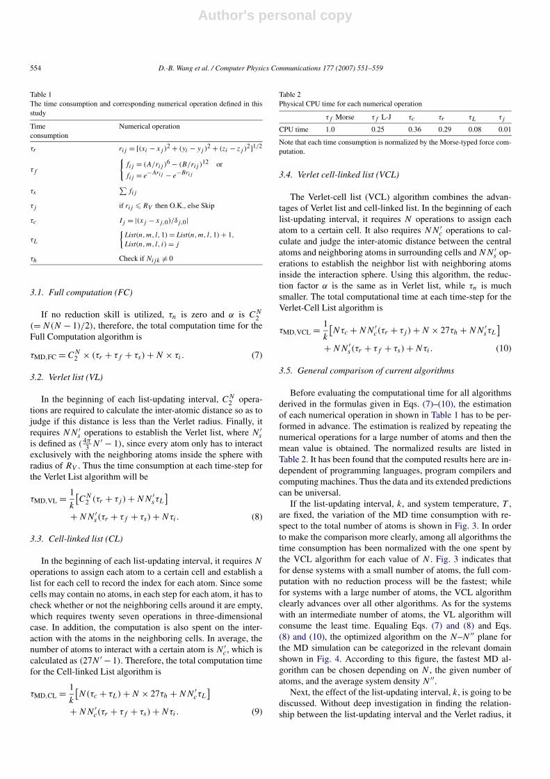
where N is the total number of atoms in a system, α the re-duction factor, τMD the time consumption in MD simulation,τn the time to identify neighboring atoms, τr the time for dis-tance calculation, τf the time for force calculation, τs the timefor summation, and τi the time for integration. In Eq. (6), τr ,τf , τs and τi are identical for each MD algorithm if the integra-tion scheme is the same; however, τn and α will be changed indifferent MD algorithms, an issue which will be introduced inthe following sections. Before mentioning each MD algorithm,other terms of time consumption are required in τn, such as thetime to judge if an atom stays inside the Verlet radius (τj ), thetime to calculate the indices of cell (τc), the time to establishthe list array (τL), and time to check if a cell is empty or not(τh). The overall corresponding numerical operation for indi-vidual time consumption is defined in Table 1, by which theestimation formula of computational time for the relevant MDalgorithm can be formulated, and this will be discussed below.Here, note that the assumptions of each algorithm are made asfollows:

(i) pair-wise interaction,(ii) uniform distribution of system atoms,

(iii) the time consumption of each numerical operation inde-pendent of others.



Table 1The time consumption and corresponding numerical operation defined in thisstudy

Timeconsumption

Numerical operation

τr rij = [(xi − xj )2 + (yi − yj )2 + (zi − zj )2]1/2

τf

{fij = (A/rij )6 − (B/rij )12 or

fij = e−Arij − e

−Brij

τs∑

fij

τj if rij � RV then O.K., else Skip

τc Ij = |(xj − xj,0)/δj,0|

τL

{List(n,m, l,1) = List(n,m, l,1) + 1,

List(n,m, l, i) = j

τh Check if Nijk �= 0

3.1. Full computation (FC)

If no reduction skill is utilized, τn is zero and α is CN2

(= N(N − 1)/2), therefore, the total computation time for theFull Computation algorithm is

(7)τMD,FC = CN2 × (τr + τf + τs) + N × τi .

3.2. Verlet list (VL)

In the beginning of each list-updating interval, CN2 opera-

tions are required to calculate the inter-atomic distance so as tojudge if this distance is less than the Verlet radius. Finally, itrequires NN ′

s operations to establish the Verlet list, where N ′s

is defined as ( 4π3 N ′ − 1), since every atom only has to interact

exclusively with the neighboring atoms inside the sphere withradius of RV . Thus the time consumption at each time-step forthe Verlet List algorithm will be

τMD,VL = 1

k

[CN

2 (τr + τj ) + NN ′sτL

](8)+ NN ′

s(τr + τf + τs) + Nτi.

3.3. Cell-linked list (CL)

In the beginning of each list-updating interval, it requires N

operations to assign each atom to a certain cell and establish alist for each cell to record the index for each atom. Since somecells may contain no atoms, in each step for each atom, it has tocheck whether or not the neighboring cells around it are empty,which requires twenty seven operations in three-dimensionalcase. In addition, the computation is also spent on the inter-action with the atoms in the neighboring cells. In average, thenumber of atoms to interact with a certain atom is N ′

c, which iscalculated as (27N ′ − 1). Therefore, the total computation timefor the Cell-linked List algorithm is

τMD,CL = 1

k

[N(τc + τL) + N × 27τh + NN ′

cτL

](9)+ NN ′

c(τr + τf + τs) + Nτi.

Table 2Physical CPU time for each numerical operation

τf Morse τf L-J τc τr τL τj

CPU time 1.0 0.25 0.36 0.29 0.08 0.01

Note that each time consumption is normalized by the Morse-typed force com-putation.

3.4. Verlet cell-linked list (VCL)

The Verlet-cell list (VCL) algorithm combines the advan-tages of Verlet list and cell-linked list. In the beginning of eachlist-updating interval, it requires N operations to assign eachatom to a certain cell. It also requires NN ′

c operations to cal-culate and judge the inter-atomic distance between the centralatoms and neighboring atoms in surrounding cells and NN ′

s op-erations to establish the neighbor list with neighboring atomsinside the interaction sphere. Using this algorithm, the reduc-tion factor α is the same as in Verlet list, while τn is muchsmaller. The total computational time at each time-step for theVerlet-Cell List algorithm is

τMD,VCL = 1

k

[Nτc + NN ′

c(τr + τj ) + N × 27τh + NN ′sτL

](10)+ NN ′

s(τr + τf + τs) + Nτi.

3.5. General comparison of current algorithms

Before evaluating the computational time for all algorithmsderived in the formulas given in Eqs. (7)–(10), the estimationof each numerical operation in shown in Table 1 has to be per-formed in advance. The estimation is realized by repeating thenumerical operations for a large number of atoms and then themean value is obtained. The normalized results are listed inTable 2. It has been found that the computed results here are in-dependent of programming languages, program compilers andcomputing machines. Thus the data and its extended predictionscan be universal.

If the list-updating interval, k, and system temperature, T ,are fixed, the variation of the MD time consumption with re-spect to the total number of atoms is shown in Fig. 3. In orderto make the comparison more clearly, among all algorithms thetime consumption has been normalized with the one spent bythe VCL algorithm for each value of N . Fig. 3 indicates thatfor dense systems with a small number of atoms, the full com-putation with no reduction process will be the fastest; whilefor systems with a large number of atoms, the VCL algorithmclearly advances over all other algorithms. As for the systemswith an intermediate number of atoms, the VL algorithm willconsume the least time. Equaling Eqs. (7) and (8) and Eqs.(8) and (10), the optimized algorithm on the N–N ′′ plane forthe MD simulation can be categorized in the relevant domainshown in Fig. 4. According to this figure, the fastest MD al-gorithm can be chosen depending on N , the given number ofatoms, and the average system density N ′′.

Next, the effect of the list-updating interval, k, is going to bediscussed. Without deep investigation in finding the relation-ship between the list-updating interval and the Verlet radius, it



(a)

(b)

(c)

Fig. 3. Variation of MD time consumption with respect to total number of atomsfor each algorithm. (a) N ′′ = 20, (b) N ′′ = 2.0, (c) N ′′ = 0.2. The time con-sumption for each algorithm is normalized by that of VCL at each value of N .

Fig. 4. Optimization territory for each current MD reduction algorithm inN–N ′′ plane (k = 1, T = 300 K).

Fig. 5. Variation of MD time consumption with respect to list-updating intervalfor each algorithm. Here N ′′ = 2.0.

is often misunderstood that a large value of k always resultsin a less computation time to identify the neighboring atomsfor each atom. Such a misunderstanding is mainly due to theimpression of a fixed value of the Verlet radius. However, ifEq. (5) and Eqs. (8)–(10) are observed in detail, it will be foundthat the fact is not that simple and intuitive. Although the fac-tor of 1/k in Eqs. (8)–(10) represents the decreasing effect forthe time consumption in MD computation, the terms such asN ′

c and N ′s , represent the increasing effect. Therefore, it is not

clear whether the increase of k will reduce τMD until the vari-ation of τMD is examined. Since an analytical solution of k ofequation ∂τMD/∂k = 0 does not exit, it can only be examinedin a graphic manner.

Fig. 5 illustrates the typical variation of MD computationtime with respect to the list-updating interval for algorithmsVL, CL and VCL. For the first glance at this figure, only the



VL algorithm has an optimized choice of k, where the time con-sumption reaches a minimum; whereas an increase in k causes amonotonic increase for both CL and VCL algorithms. Note thatthe variation of τMD or the existence of the minimum of τMD isinfluenced by the system average temperature and average den-sity, and thus the effects of T and N ′′ should be investigatedmore carefully.

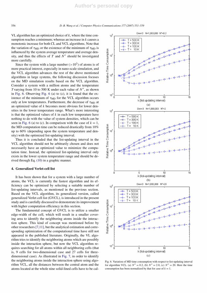
Since the system with a large number (>103) of atoms is ofmore practical interest, especially in nano-scale simulation, andthe VCL algorithm advances the rest of the above mentionedalgorithms in large systems, the following discussion focuseson the MD simulation results based on the VCL algorithm.Consider a system with a million atoms and the temperatureT varying from 10 to 500 K under each value of N ′′, as shownin Fig. 6. Observing Fig. 6 (a) to (c), it is found that the ex-istence of the minimum of τMD for the VCL algorithm occursonly at low temperatures. Furthermore, the decrease of τMD atan optimized value of k becomes more obvious for lower den-sities in the lower temperature range. What’s more interestingis that the optimized values of k in each low temperature havenothing to do with the value of system densities, which can beseen in Fig. 6 (a) to (c). In comparison with the case of k = 1,the MD computation time can be reduced drastically from 10%up to 60% (depending upon the system temperature and den-sity) with the optimized list-updating interval.

Thus it is concluded that the list-updating interval in theVCL algorithm should not be arbitrarily chosen and does notnecessarily have an optimized value to minimize the compu-tation time. Instead, the optimized list-updating interval onlyexists in the lower system temperature range and should be de-rived through Eq. (10) in a graphic manner.

4. Generalized Verlet-cell list

It has been shown that for a system with a large number ofatoms, the VCL is currently the fastest algorithm and its ef-ficiency can be optimized by selecting a suitable number oflist-updating intervals, as mentioned in the previous section.Based on the VCL algorithm, its generalized version, calledgeneralized Verlet cell list (GVCL), is introduced in the presentstudy and is carefully discussed to demonstrate its improvementwith higher computation efficiency in this section.

The fundamental concept of GVCL is to utilize a smalleredge-width of the cell, which will result in a smaller cover-ing area to identify the neighboring atoms inside the interac-tion sphere. This kind of concept was mentioned before byother researchers [7,11], but the analytical estimation and corre-sponding optimization of the computational time have still notappeared in the published literature. Originally, the VL algo-rithm tries to identify the neighboring atoms which are possiblyinside the interaction sphere, but now the VCL algorithm re-quires searching for all atoms within all neighboring cells (thatis, 9 cells for two-dimensional case and 27 cells for three-dimensional case). As illustrated in Fig. 7, in order to identifythe neighboring atoms inside the interaction sphere using algo-rithm VCL, all the distances between the central atom and theatoms located at the whole nine solid-lined cells have to be cal-

(a)

(b)

(c)

Fig. 6. Variation of MD time consumption with respect to list-updating intervalfor algorithm VCL. (a) N ′′ = 0.2, (b) N ′′ = 2.0, (c) N ′′ = 20. Here the timeconsumption has been normalized by that for case of k = 1.



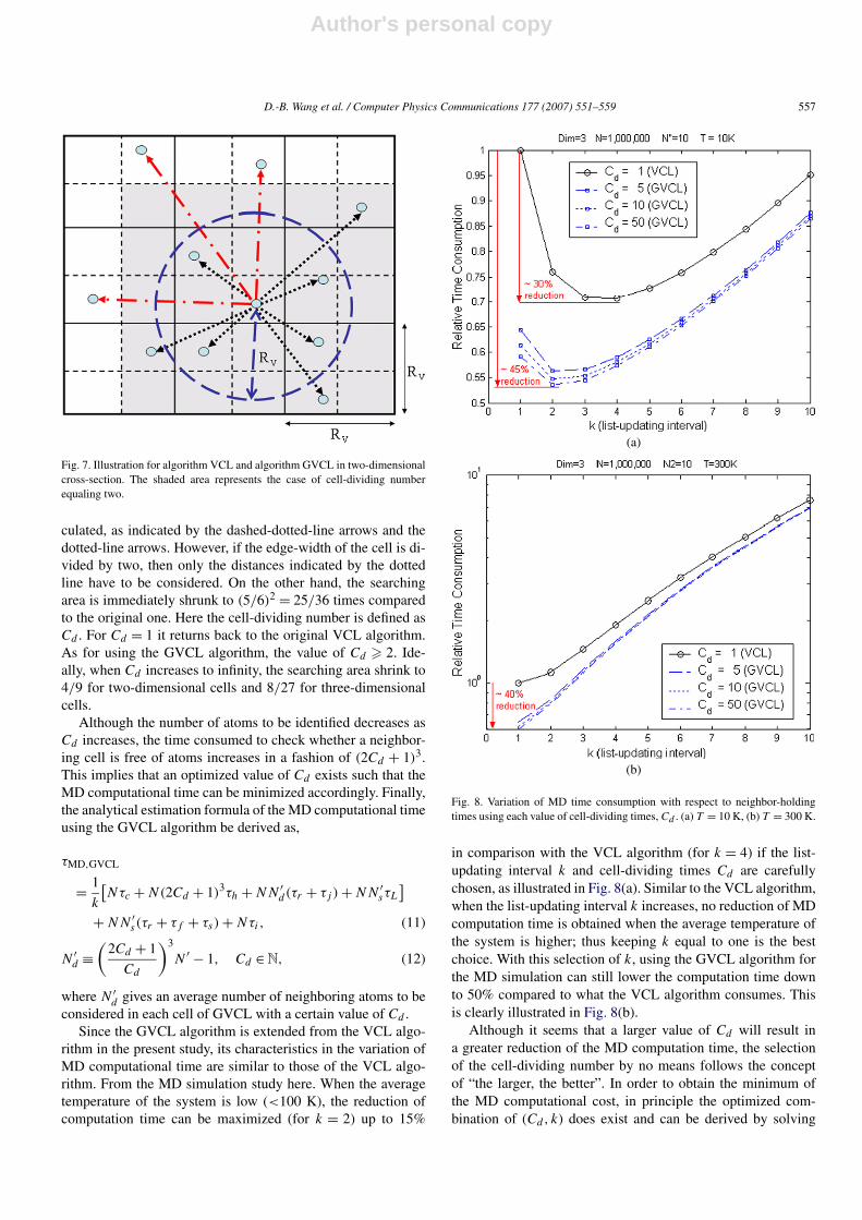
Fig. 7. Illustration for algorithm VCL and algorithm GVCL in two-dimensionalcross-section. The shaded area represents the case of cell-dividing numberequaling two.

culated, as indicated by the dashed-dotted-line arrows and thedotted-line arrows. However, if the edge-width of the cell is di-vided by two, then only the distances indicated by the dottedline have to be considered. On the other hand, the searchingarea is immediately shrunk to (5/6)2 = 25/36 times comparedto the original one. Here the cell-dividing number is defined asCd . For Cd = 1 it returns back to the original VCL algorithm.As for using the GVCL algorithm, the value of Cd � 2. Ide-ally, when Cd increases to infinity, the searching area shrink to4/9 for two-dimensional cells and 8/27 for three-dimensionalcells.

Although the number of atoms to be identified decreases asCd increases, the time consumed to check whether a neighbor-ing cell is free of atoms increases in a fashion of (2Cd + 1)3.This implies that an optimized value of Cd exists such that theMD computational time can be minimized accordingly. Finally,the analytical estimation formula of the MD computational timeusing the GVCL algorithm be derived as,

τMD,GVCL

= 1

k

[Nτc + N(2Cd + 1)3τh + NN ′

d(τr + τj ) + NN ′sτL

](11)+ NN ′

s(τr + τf + τs) + Nτi,

(12)N ′d ≡

(2Cd + 1

Cd

)3

N ′ − 1, Cd ∈ N,

where N ′d gives an average number of neighboring atoms to be

considered in each cell of GVCL with a certain value of Cd .Since the GVCL algorithm is extended from the VCL algo-

rithm in the present study, its characteristics in the variation ofMD computational time are similar to those of the VCL algo-rithm. From the MD simulation study here. When the averagetemperature of the system is low (<100 K), the reduction ofcomputation time can be maximized (for k = 2) up to 15%

(a)

(b)

Fig. 8. Variation of MD time consumption with respect to neighbor-holdingtimes using each value of cell-dividing times, Cd . (a) T = 10 K, (b) T = 300 K.

in comparison with the VCL algorithm (for k = 4) if the list-updating interval k and cell-dividing times Cd are carefullychosen, as illustrated in Fig. 8(a). Similar to the VCL algorithm,when the list-updating interval k increases, no reduction of MDcomputation time is obtained when the average temperature ofthe system is higher; thus keeping k equal to one is the bestchoice. With this selection of k, using the GVCL algorithm forthe MD simulation can still lower the computation time downto 50% compared to what the VCL algorithm consumes. Thisis clearly illustrated in Fig. 8(b).

Although it seems that a larger value of Cd will result ina greater reduction of the MD computation time, the selectionof the cell-dividing number by no means follows the conceptof “the larger, the better”. In order to obtain the minimum ofthe MD computational cost, in principle the optimized com-bination of (Cd, k) does exist and can be derived by solving



∂τMD,GVCL/∂k = 0 and ∂τMD,GVCL/∂Cd = 0 simultaneouslythrough Eq. (11), but the optimized values of (Cd, k) are usuallysolved by numerical schemes, such as the Newton–Raphsonmethod, and may not be convenient to apply. Therefore, thepractical way to determine the optimized (Cd, k) is carried outby conducting several combinations of testing through real MDsimulation in a systematic manner. Fortunately, according to thetesting experiences in the present study, the optimized (Cd, k)usually ranges from (1,1) to (5,5) in most cases tested withdifferent temperatures and densities. Hence, before running fora large number of time-steps, a suggested procedure would beto run the real MD simulation for decades or thousands of time-steps with these twenty five combinations of (Cd, k) to find outthe most favorable numerical parameters.

5. Numerical validation of GVCL algorithm

Before an algorithm comes to realization, its accuracy andefficiency first have to be verified. Since the number of neigh-boring atoms to interact with for the GVCL algorithm is thesame as that for the VCL algorithm, the accuracy of MD sim-ulation results such as displacement and velocity are identicaland thus do not need to be inspected. However, only the theoret-ical prediction for the efficiency optimization has been providedso far, and the numerical validation through a real case is stillrequired.

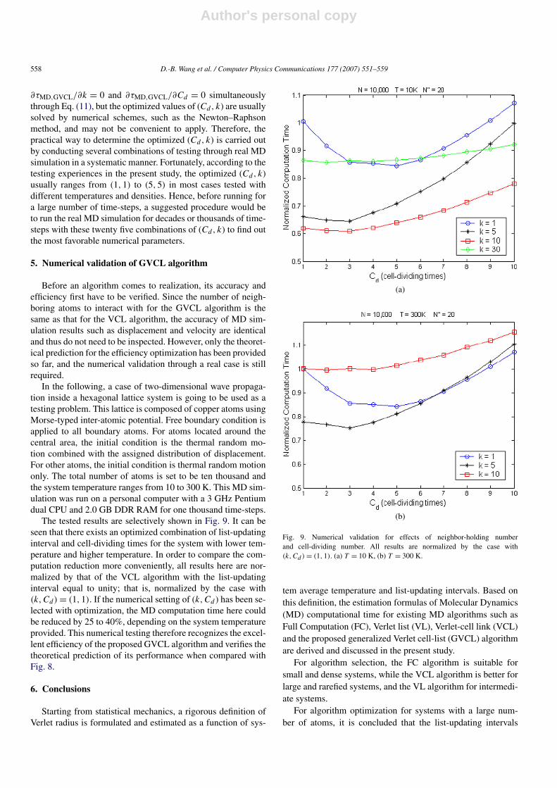
In the following, a case of two-dimensional wave propaga-tion inside a hexagonal lattice system is going to be used as atesting problem. This lattice is composed of copper atoms usingMorse-typed inter-atomic potential. Free boundary condition isapplied to all boundary atoms. For atoms located around thecentral area, the initial condition is the thermal random mo-tion combined with the assigned distribution of displacement.For other atoms, the initial condition is thermal random motiononly. The total number of atoms is set to be ten thousand andthe system temperature ranges from 10 to 300 K. This MD sim-ulation was run on a personal computer with a 3 GHz Pentiumdual CPU and 2.0 GB DDR RAM for one thousand time-steps.

The tested results are selectively shown in Fig. 9. It can beseen that there exists an optimized combination of list-updatinginterval and cell-dividing times for the system with lower tem-perature and higher temperature. In order to compare the com-putation reduction more conveniently, all results here are nor-malized by that of the VCL algorithm with the list-updatinginterval equal to unity; that is, normalized by the case with(k,Cd) = (1,1). If the numerical setting of (k,Cd ) has been se-lected with optimization, the MD computation time here couldbe reduced by 25 to 40%, depending on the system temperatureprovided. This numerical testing therefore recognizes the excel-lent efficiency of the proposed GVCL algorithm and verifies thetheoretical prediction of its performance when compared withFig. 8.

6. Conclusions

Starting from statistical mechanics, a rigorous definition ofVerlet radius is formulated and estimated as a function of sys-

(a)

(b)

Fig. 9. Numerical validation for effects of neighbor-holding numberand cell-dividing number. All results are normalized by the case with(k,Cd) = (1,1). (a) T = 10 K, (b) T = 300 K.

tem average temperature and list-updating intervals. Based onthis definition, the estimation formulas of Molecular Dynamics(MD) computational time for existing MD algorithms such asFull Computation (FC), Verlet list (VL), Verlet-cell link (VCL)and the proposed generalized Verlet cell-list (GVCL) algorithmare derived and discussed in the present study.

For algorithm selection, the FC algorithm is suitable forsmall and dense systems, while the VCL algorithm is better forlarge and rarefied systems, and the VL algorithm for intermedi-ate systems.

For algorithm optimization for systems with a large num-ber of atoms, it is concluded that the list-updating intervals



of VCL and GVCL algorithms should not be arbitrarily cho-sen and not necessarily have an optimized value to minimizethe computation time. The optimized list-updating interval onlyexits in the lower temperature system and should be derivedfrom Eqs. (10)–(11) in a graphic manner. Therefore, for sys-tems around or above room temperature, establishing the list ateach time-step would be the best choice.

As for the GVCL algorithm herein proposed, it is foundthat with the cell-dividing times optimized the MD computa-tion cost could be further reduced by 15% in low-temperaturesystems and reduced by 30 ∼ 60% in high-temperature sys-tems, compared with the VCL algorithm. With the success-ful verification by the real MD simulation, the value of theGVCL algorithm discussed in this study has been demon-strated.

Due to the similarities in computational procedures, theanalysis in this study can be extended to other many-particlesystems such as point-vortex method in computational fluiddynamics and celestial dynamics in astronomy to identify theneighboring particles or objects in a more efficient way.

Acknowledgements

This research was partially supported by the National Sci-ence Council of Taiwan through Grant NSC 95-2120-M-006-002.

References

[1] M. Mu, J. Comput. Phys. 179 (2002) 539.[2] R. Murty, D. Okunbor, Parallel Comput. 25 (1999) 217.[3] D. Frenkel, B. Smit, Understanding Molecular Simulation: From Algo-

rithms to Applications, second ed., Academic Press, San Diego, 2002.[4] R.W. Hockney, S.P. Goel, J.W. Eastwood, Chem. Phys. Lett. 21 (1973)

589.[5] B. Quentrec, C. Brot, J. Comput. Phys. 13 (1973) 430.[6] D.R. Mason, Comput. Phys. Comm. 170 (2005) 31.[7] Z. Yao, J.-S. Wang, G.-R. Liu, M. Cheng, Comput. Phys. Comm. 161

(2004) 27.[8] T.N. Heinz, P.H. Hunenberger, J. Comput. Chem. 25 (2004) 1474.[9] G. Sutmann, V. Stegailov, J. Mol. Liq. 125 (2006) 197.

[10] T. Maximova, C. Keasar, J. Comput. Biol. 13 (2006) 1041.[11] M.P. Allen, D.J. Tildesley, Computer Simulation of Liquids, Oxford Univ.

Press, New York, 1990.

algorithm optimization in molecular dynamics simulation

Documents