artificial bee colony (abc) optimization algorithm for solving

Artificial Bee Colony (ABC) OptimizationAlgorithm for Solving Constrained Optimization

Problems

Dervis Karaboga and Bahriye Basturk

Erciyes University, Engineering Faculty, The Department of Computer [email protected], [email protected]

Abstract. This paper presents the comparison results on the perfor-mance of the Artificial Bee Colony (ABC) algorithm for constrained op-timization problems. The ABC algorithm has been firstly proposed forunconstrained optimization problems and showed that it has superiorperformance on these kind of problems. In this paper, the ABC algo-rithm has been extended for solving constrained optimization problemsand applied to a set of constrained problems .

1 Introduction

Constrained Optimization problems are encountered in numerous applications.Structural optimization, engineering design, VLSI design, economics, allocationand location problems are just a few of the scientific fields in which CO problemsare frequently met [1]. The considered problem is reformulated so as to take theform of optimizing two functions, the objective function and the constraint vio-lation function [2]. General constrained optimization problem is to find x so as to

minimize f(x), x = (x1, . . . , xn) ∈ Rn

where x ∈ F ∈ S. The objective function f is defined on the search space S ⊆ Rn

and the set F ⊆ S defines the feasible region. Usually, the search space S is de-fined as a n-dimensional rectangle in �n (domains of variables defined by theirlower and upper bounds):

l(i) ≤ x(i) ≤ u(i), 1 ≤ i ≤ n

whereas the feasible region F ⊆ S is defined by a set of m additional constraints(m ≥ 0):

gj(x) ≤ 0, for j = 1, . . . , q

hj(x) = 0, for j = q + 1, . . . , m.

P. Melin et al. (Eds.): IFSA 2007, LNAI 4529, pp. 789–798, 2007.c© Springer-Verlag Berlin Heidelberg 2007

790 D. Karaboga and B. Basturk

At any point x ∈ F, the constraints gk that satisfy gk(x) = 0 are calledthe active constraints at x. By extension, equality constraints hj are also calledactive at all points of S [3].

Different deterministic as well as stochastic algorithms have been developedfor tackling constrained optimization problems. Deterministic approaches such asFeasible Direction and Generalized Gradient Descent make strong assumptionson the continuity and differentiability of the objective function [4,5]. Thereforetheir applicability is limited since these characteristics are rarely met in prob-lems that arise in real life applications. On the other hand, stochastic optimiza-tion algorithms such as Genetic Algorithms, Evolution Strategies, Evolution-ary Programming and Particle Swarm Optimization (PSO) do not make suchassumptions and they have been successfully applied for tackling constrainedoptimization problems during the past few years [6,7,8,9,16].

Karaboga has described an Artificial Bee Colony (ABC) algorithm based onthe foraging behaviour of honey bees for numerical optimization problems [11].Karaboga and Basturk have compared the performance of the ABC algorithmwith those of other well-known modern heuristic algorithms such as Genetic Al-gorithm (GA), Differential Evolution (DE), Particle Swarm Optimization (PSO)on unconstrained problems [12]. In this work, ABC algorithm is extended forsolving constrained optimization (CO) problems. Extension of the algorithm de-pends on replacing the selection mechanism of the simple ABC algorithm withDeb’s [13] selection mechanism in order to cope with the constraints. The per-formance of the algorithm has been tested on 13 well-known constrained opti-mization problems taken from the literature and compared with Particle SwarmOptimization (PSO) and Differential Evolution (DE) [14]. The Particle SwarmOptimization (PSO) algorithm was introduced by Eberhart and Kennedy in1995 [15]. PSO is a population based stochastic optimization technique and welladapted to the optimization of nonlinear functions in multidimensional space. Itmodels the social behaviour of bird flocking or fish schooling. The DE algorithmis also a population based algorithm using crossover, mutation and selectionoperators. Although DE uses crossover and mutation operators as in GA, themain operation is based on the differences of randomly sampled pairs of solu-tions in the population. Paper is organized as follows. In Section II, the ABCalgorithm and the ABC algorithm adapted for solving constrained optimizationproblems are introduced. In Section III, a benchmark of 13 constrained func-tions are tested. Results of the comparison with the PSO and DE algorithms arepresented and discussed. Finally, a conclusion is provided.

2 Artificial Bee Colony Algorithm

2.1 The ABC Algorithm Used for Unconstrained OptimizationProblems

In ABC algorithm [11,12], the colony of artificial bees consists of three groupsof bees: employed bees, onlookers and scouts. First half of the colony consistsof the employed artificial bees and the second half includes the onlookers. For

Artificial Bee Colony (ABC) Optimization Algorithm 791

every food source, there is only one employed bee. In other words, the numberof employed bees is equal to the number of food sources around the hive. Theemployed bee whose the food source has been abandoned by the bees becomesa scout.

In ABC algorithm, the position of a food source represents a possible solutionto the optimization problem and the nectar amount of a food source correspondsto the quality (fitness) of the associated solution. The number of the employedbees or the onlooker bees is equal to the number of solutions in the population.At the first step, the ABC generates a randomly distributed initial populationP (G = 0) of SN solutions (food source positions), where SN denotes the size ofpopulation. Each solution xi (i = 1, 2, ..., SN) is a D-dimensional vector. Here,D is the number of optimization parameters. After initialization, the populationof the positions (solutions) is subjected to repeated cycles, C = 1, 2, ..., MCN , ofthe search processes of the employed bees, the onlooker bees and scout bees. Anemployed bee produces a modification on the position (solution) in her memorydepending on the local information (visual information) and tests the nectaramount (fitness value) of the new source (new solution). Provided that the nectaramount of the new one is higher than that of the previous one, the bee memorizesthe new position and forgets the old one. Otherwise she keeps the position ofthe previous one in her memory. After all employed bees complete the searchprocess, they share the nectar information of the food sources and their positioninformation with the onlooker bees on the dance area. An onlooker bee evaluatesthe nectar information taken from all employed bees and chooses a food sourcewith a probability related to its nectar amount. As in the case of the employedbee, she produces a modification on the position in her memory and checks thenectar amount of the candidate source. Providing that its nectar is higher thanthat of the previous one, the bee memorizes the new position and forgets the oldone.

An artificial onlooker bee chooses a food source depending on the probabilityvalue associated with that food source, pi , calculated by the following expression(1):

pi =fiti

SN∑

n=1fitn

(1)

where fiti is the fitness value of the solution i which is proportional to the nec-tar amount of the food source in the position i and SN is the number of foodsources which is equal to the number of employed bees (BN).

In order to produce a candidate food position from the old one in memory,the ABC uses the following expression (2):

vij = xij + φij(xij − xkj) (2)


where k ∈ {1, 2,..., SN} and j ∈ {1, 2,..., D} are randomly chosen indexes. Al-though k is determined randomly, it has to be different from i. φi,j is a randomnumber between [-1, 1]. It controls the production of neighbour food sourcesaround xi,j and represents the comparison of two food positions visually by abee. As can be seen from (2), as the difference between the parameters of thexi,j and xk,j decreases, the perturbation on the position xi,j gets decrease, too.Thus, as the search approaches to the optimum solution in the search space, thestep length is adaptively reduced.

If a parameter value produced by this operation exceeds its predeterminedlimit, the parameter can be set to an acceptable value. In this work, the valueof the parameter exceeding its limit is set to its limit value.

The food source of which the nectar is abandoned by the bees is replacedwith a new food source by the scouts. In ABC, this is simulated by producinga position randomly and replacing it with the abandoned one. In ABC, pro-viding that a position can not be improved further through a predeterminednumber of cycles, then that food source is assumed to be abandoned. The valueof predetermined number of cycles is an important control parameter of the ABCalgorithm, which is called “limit” for abandonment. Assume that the abandonedsource is xi and j ∈ {1, 2,..., D} , then the scout discovers a new food source tobe replaced with xi. This operation can be defined as in (3)

xji = xj

min + rand(0, 1)(xjmax − xj

min) (3)

After each candidate source position vi,j is produced and then evaluated bythe artificial bee, its performance is compared with that of its old one. If thenew food has an equal or better nectar than the old source, it is replaced withthe old one in the memory. Otherwise, the old one is retained in the memory. Inother words, a greedy selection mechanism is employed as the selection operationbetween the old and the candidate one.

It is clear from the above explanation that there are four control parametersused in the ABC: The number of food sources which is equal to the number ofemployed or onlooker bees (SN), the value of limit, the maximum cycle number(MCN).

Detailed pseudo-code of the ABC algorithm is given below:1: Initialize the population of solutions xi,j , i = 1 . . . SN, j = 1 . . .D2: Evaluate the population3: cycle=14: repeat5: Produce new solutions υi,j for the employed bees by using (2) and evaluate

them6: Apply the greedy selection process7: Calculate the probability values Pi,j for the solutions xi,j by (1)8: Produce the new solutions υi,j for the onlookers from the solutions xi,j

selected depending on Pi,j and evaluate them9: Apply the greedy selection process


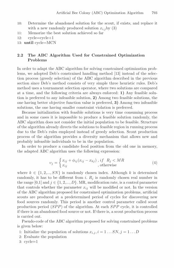
10: Determine the abandoned solution for the scout, if exists, and replace itwith a new randomly produced solution xi,jby (3)

11: Memorize the best solution achieved so far12: cycle=cycle+113: until cycle=MCN

2.2 The ABC Algorithm Used for Constrained OptimizationProblems

In order to adapt the ABC algorithm for solving constrained optimization prob-lems, we adopted Deb’s constrained handling method [13] instead of the selec-tion process (greedy selection) of the ABC algorithm described in the previoussection since Deb’s method consists of very simple three heuristic rules. Deb’smethod uses a tournament selection operator, where two solutions are comparedat a time, and the following criteria are always enforced: 1) Any feasible solu-tion is preferred to any infeasible solution, 2) Among two feasible solutions, theone having better objective function value is preferred, 3) Among two infeasiblesolutions, the one having smaller constraint violation is preferred.

Because initialization with feasible solutions is very time consuming processand in some cases it is impossible to produce a feasible solution randomly, theABC algorithm does not consider the initial population to be feasible. Structureof the algorithm already directs the solutions to feasible region in running processdue to the Deb’s rules employed instead of greedy selection. Scout productionprocess of the algorithm provides a diversity mechanism that allows new andprobably infeasible individuals to be in the population.

In order to produce a candidate food position from the old one in memory,the adapted ABC algorithm uses the following expression:

υj ={

xij + φij(xij − xkj) , if Rj < MRxij , otherwise (4)

where k ∈ {1, 2,..., SN} is randomly chosen index. Although k is determinedrandomly, it has to be different from i. Rj is randomly chosen real number inthe range [0,1] and j ∈ {1, 2,..., D}. MR, modification rate, is a control parameterthat controls whether the parameter xij will be modified or not. In the versionof the ABC algorithm proposed for constrained optimization problems, artificialscouts are produced at a predetermined period of cycles for discovering newfood sources randomly. This period is another control parameter called scoutproduction period (SPP ) of the algorithm. At each SPP cycle, it is controlledif there is an abandoned food source or not. If there is, a scout production processis carried out.

Pseudo-code of the ABC algorithm proposed for solving constrained problemsis given below:1: Initialize the population of solutions xi,j , i = 1 . . . SN, j = 1 . . .D2: Evaluate the population3: cycle=1


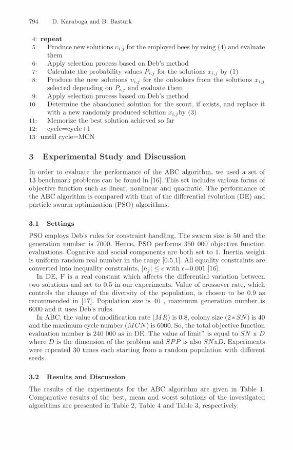
4: repeat5: Produce new solutions υi,j for the employed bees by using (4) and evaluate

them6: Apply selection process based on Deb’s method7: Calculate the probability values Pi,j for the solutions xi,j by (1)8: Produce the new solutions υi,j for the onlookers from the solutions xi,j

selected depending on Pi,j and evaluate them9: Apply selection process based on Deb’s method

10: Determine the abandoned solution for the scout, if exists, and replace itwith a new randomly produced solution xi,jby (3)

11: Memorize the best solution achieved so far12: cycle=cycle+113: until cycle=MCN

3 Experimental Study and Discussion

In order to evaluate the performance of the ABC algorithm, we used a set of13 benchmark problems can be found in [16]. This set includes various forms ofobjective function such as linear, nonlinear and quadratic. The performance ofthe ABC algorithm is compared with that of the differential evolution (DE) andparticle swarm optimization (PSO) algorithms.

3.1 Settings

PSO employs Deb’s rules for constraint handling. The swarm size is 50 and thegeneration number is 7000. Hence, PSO performs 350 000 objective functionevaluations. Cognitive and social components are both set to 1. Inertia weightis uniform random real number in the range [0.5,1]. All equality constraints areconverted into inequality constraints, |hj | ≤ ε with ε=0.001 [16].

In DE, F is a real constant which affects the differential variation betweentwo solutions and set to 0.5 in our experiments. Value of crossover rate, whichcontrols the change of the diversity of the population, is chosen to be 0.9 asrecommended in [17]. Population size is 40 , maximum generation number is6000 and it uses Deb’s rules.

In ABC, the value of modification rate (MR) is 0.8, colony size (2 ∗SN) is 40and the maximum cycle number (MCN) is 6000. So, the total objective functionevaluation number is 240 000 as in DE. The value of limit” is equal to SN x Dwhere D is the dimension of the problem and SPP is also SNxD. Experimentswere repeated 30 times each starting from a random population with differentseeds.

3.2 Results and Discussion

The results of the experiments for the ABC algorithm are given in Table 1.Comparative results of the best, mean and worst solutions of the investigatedalgorithms are presented in Table 2, Table 4 and Table 3, respectively.


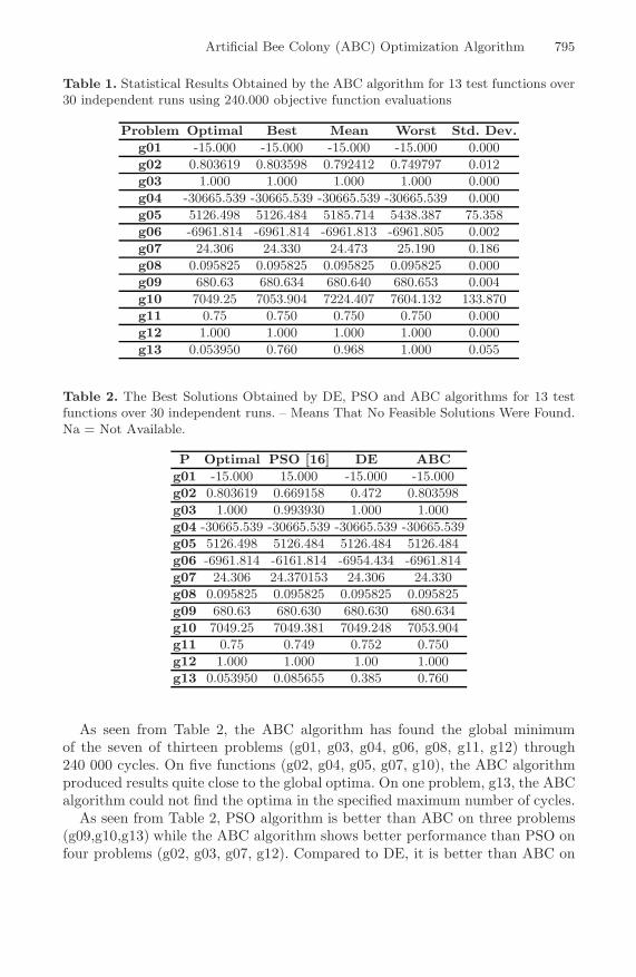
Table 1. Statistical Results Obtained by the ABC algorithm for 13 test functions over30 independent runs using 240.000 objective function evaluations

Problem Optimal Best Mean Worst Std. Dev.g01 -15.000 -15.000 -15.000 -15.000 0.000g02 0.803619 0.803598 0.792412 0.749797 0.012g03 1.000 1.000 1.000 1.000 0.000g04 -30665.539 -30665.539 -30665.539 -30665.539 0.000g05 5126.498 5126.484 5185.714 5438.387 75.358g06 -6961.814 -6961.814 -6961.813 -6961.805 0.002g07 24.306 24.330 24.473 25.190 0.186g08 0.095825 0.095825 0.095825 0.095825 0.000g09 680.63 680.634 680.640 680.653 0.004g10 7049.25 7053.904 7224.407 7604.132 133.870g11 0.75 0.750 0.750 0.750 0.000g12 1.000 1.000 1.000 1.000 0.000g13 0.053950 0.760 0.968 1.000 0.055

Table 2. The Best Solutions Obtained by DE, PSO and ABC algorithms for 13 testfunctions over 30 independent runs. – Means That No Feasible Solutions Were Found.Na = Not Available.

P Optimal PSO [16] DE ABCg01 -15.000 15.000 -15.000 -15.000g02 0.803619 0.669158 0.472 0.803598g03 1.000 0.993930 1.000 1.000g04 -30665.539 -30665.539 -30665.539 -30665.539g05 5126.498 5126.484 5126.484 5126.484g06 -6961.814 -6161.814 -6954.434 -6961.814g07 24.306 24.370153 24.306 24.330g08 0.095825 0.095825 0.095825 0.095825g09 680.63 680.630 680.630 680.634g10 7049.25 7049.381 7049.248 7053.904g11 0.75 0.749 0.752 0.750g12 1.000 1.000 1.00 1.000g13 0.053950 0.085655 0.385 0.760

As seen from Table 2, the ABC algorithm has found the global minimumof the seven of thirteen problems (g01, g03, g04, g06, g08, g11, g12) through240 000 cycles. On five functions (g02, g04, g05, g07, g10), the ABC algorithmproduced results quite close to the global optima. On one problem, g13, the ABCalgorithm could not find the optima in the specified maximum number of cycles.

As seen from Table 2, PSO algorithm is better than ABC on three problems(g09,g10,g13) while the ABC algorithm shows better performance than PSO onfour problems (g02, g03, g07, g12). Compared to DE, it is better than ABC on


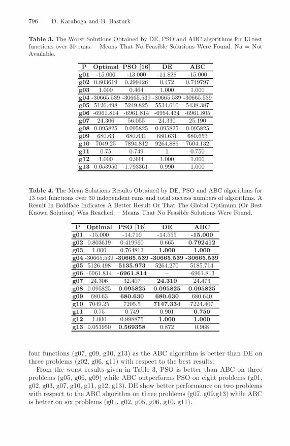
Table 3. The Worst Solutions Obtained by DE, PSO and ABC algorithms for 13 testfunctions over 30 runs. – Means That No Feasible Solutions Were Found. Na = NotAvailable.

P Optimal PSO [16] DE ABCg01 -15.000 -13.000 -11.828 -15.000g02 0.803619 0.299426 0.472 0.749797g03 1.000 0.464 1.000 1.000g04 -30665.539 -30665.539 -30665.539 -30665.539g05 5126.498 5249.825 5534.610 5438.387g06 -6961.814 -6961.814 -6954.434 -6961.805g07 24.306 56.055 24.330 25.190g08 0.095825 0.095825 0.095825 0.095825g09 680.63 680.631 680.631 680.653g10 7049.25 7894.812 9264.886 7604.132g11 0.75 0.749 1 0.750g12 1.000 0.994 1.000 1.000g13 0.053950 1.793361 0.990 1.000

Table 4. The Mean Solutions Results Obtained by DE, PSO and ABC algorithms for13 test functions over 30 independent runs and total success numbers of algorithms. AResult In Boldface Indicates A Better Result Or That The Global Optimum (Or BestKnown Solution) Was Reached. – Means That No Feasible Solutions Were Found.

P Optimal PSO [16] DE ABCg01 -15.000 -14.710 -14.555 -15.000g02 0.803619 0.419960 0.665 0.792412g03 1.000 0.764813 1.000 1.000g04 -30665.539 -30665.539 -30665.539 -30665.539g05 5126.498 5135.973 5264.270 5185.714g06 -6961.814 -6961.814 − -6961.813g07 24.306 32.407 24.310 24.473g08 0.095825 0.095825 0.095825 0.095825g09 680.63 680.630 680.630 680.640g10 7049.25 7205.5 7147.334 7224.407g11 0.75 0.749 0.901 0.750g12 1.000 0.998875 1.000 1.000g13 0.053950 0.569358 0.872 0.968

four functions (g07, g09, g10, g13) as the ABC algorithm is better than DE onthree problems (g02, g06, g11) with respect to the best results.

From the worst results given in Table 3, PSO is better than ABC on threeproblems (g05, g06, g09) while ABC outperforms PSO on eight problems (g01,g02, g03, g07, g10, g11, g12, g13). DE show better performance on two problemswith respect to the ABC algorithm on three problems (g07, g09,g13) while ABCis better on six problems (g01, g02, g05, g06, g10, g11).


Similarly, with respect to the mean solutions in Table 4, PSO shows betterperformance with respect to the ABC algorithm on five problems (g05, g06, g09,g10, g13) and ABC algorithm is better than PSO on six problems (g01, g02, g03,g07, g11, g12). DE has better performance than ABC on four problems (g07,g09, g10, g13) while ABC is better than DE on five problems (g01, g02, g05,g06, g11).

From the mean results presented in Table 4, it can be concluded that theABC algorithm performs better than DE and PSO.

Consequently, the ABC algorithm using Deb’s rules can not find the optimumsolution for g05, g10 and g13 for each run. g05 and g13 are nonlinear problemsand the value of ρ (ρ = |F| / |S|, F:Feasible Space, S:Search Space) for g05 andg13 is %0.000. Also, these problems have nonlinear equality constraints. g10 islinear and the value of ρ is %0.0020 for this problem. However, g10 has no linearequality and nonlinear equality constraints. Therefore, it is not possible to makeany generalization for the ABC algorithm such that it is better or not for aspecific set of problems. In other words, it is not clear what characteristics ofthe test problems make it difficult for ABC.

4 Conclusion

A modified version of the ABC algorithm for constrained optimization problemshas been introduced and its performance has been compared with that of thestate-of-art algorithms. It has been concluded that the ABC algorithm can beefficiently used for solving constrained optimization problems. The performanceof the ABC algorithm can be also tested for real engineering problems existingin the literature and compared with that of other algorithms. Also, the effect ofconstraint handling methods on the performance of the ABC algorithm can beinvestigated in future works.

References

1. K. E. Parsopoulos, M. N. Vrahatis, Particle Swarm Optimization Method forConstrained Optimization Problems, Intelligent Technologies - Theory and Appli-cations: New Trends in Intelligent Technologies,pp. 214–220. IOS Press, 2002.

2. A. R. Hedar, M. Fukushima, Derivative-Free Filter Simulated Annealing Methodfor Constrained Continuous Global Optimization

3. Z. Michalewicz, M. Schoenauer, Evolutionary Algorithms for Constrained Pa-rameter Optimization Problems, Evolutionary Computation, 4:1 (1995), pp. 1–32.

4. C. A. Floudas, P. M. Pardalos, A collection of test problems for constrainedglobal optimization algorithms, In: LNCS. Vol. 455. Springer-Verlag (1987).

5. D. M. Himmelblau, Applied Nonlinear Programming, McGrawHill (1972).6. J. A. Joines, C. R. Houck, On the use of nonstationary penalty functions to

solve nonlinear constrained optimization problems with gas, In: Proc. IEEE Int.Conf. Evol. Comp. (1994) 579-585.

7. X. Hu and R. C. Eberhart,Solving constrained nonlinear optimization problemswith particle swarm optimization. In Proceedings of the Sixth World Multiconfer-ence on Systemics, Cybernetics and Informatics 2002.


8. X. Hu, R. C. Eberhart, Y. H. Shi, Engineering optimization with particle swarm,IEEE Swarm Intelligence Symposium, 2003: 53-57.

9. K. E. Parsopoulos, , M. N. Vrahatis,A Unified Particle Swarm Optimiza-

tion for solving constrained engineering optimization problems, dvancesin Natural Computation, Pt. 3 , pages 582-591, 2005. Lecture Notes in ComputerScience Vol. 3612.

10. A. E. M. Zavala, A. H. Aguirre, E. R. V. Diharce, Constrained optimizationvia particle evolutionary swarm optimization algorithm (PESO) , In Proceedingsof the 2005 conference on Genetic and evolutionary computation (GECCO’05), pp.209–216.

11. D. Karaboga, An Idea Based On Honey Bee Swarm For Numerical Optimiza-tion, Technical Report-TR06, Erciyes University, Engineering Faculty, ComputerEngineering Department, 2005.

12. B. Basturk, D.Karaboga, An Artificial Bee Colony (ABC) Algorithm for Nu-meric function Optimization, IEEE Swarm Intelligence Symposium 2006, May 12-14, 2006, Indianapolis, Indiana, USA.

13. D.E. Goldberg, K. Deb, A comparison of selection schemes used in ge-

netic algorithms Foundations of Genetic Algorithms, edited by G. J. E. Rawlins,pp. 69-93,1991.

14. R. Storn, K. Price, , Differential evolution – a simple and efficient heuristicfor global optimization over continuous spaces., Journal of Global Optimization,11(1997), pp. 341–359.

15. J. Kennedy, R. C. Eberhart,Particle swarm optimization,1995 IEEE Interna-tional Conference on Neural Networks, 4 (1995), 1942–1948.

16. A. E. M. Zavala, A. H. Aguirre, E. R. V. Diharce, Constrained optimizationvia particle evolutionary swarm optimization algorithm (PESO) , In Proceedingsof the 2005 conference on Genetic and evolutionary computation (GECCO’05), pp.209–216.

17. D. Corne, M. Dorigo, F. Glover.,(Editors), New Ideas in Optimization,McGraw-Hill, 1999.

artificial bee colony (abc) optimization algorithm for solving

Documents