multi-objective optimization based reverse strategy with differential evolution algorithm for...
TRANSCRIPT
Expert Systems with Applications xxx (2015) xxx–xxx
Contents lists available at ScienceDirect
Expert Systems with Applications
journal homepage: www.elsevier .com/locate /eswa
Multi-objective optimization based reverse strategy with differentialevolution algorithm for constrained optimization problems
http://dx.doi.org/10.1016/j.eswa.2015.03.0160957-4174/� 2015 Elsevier Ltd. All rights reserved.
⇑ Corresponding author. Tel.: +86 27 87557742; fax: +86 27 87543074.E-mail addresses: [email protected] (L. Gao), [email protected]
(Y. Zhou), [email protected] (X. Li), [email protected] (Q. Pan),[email protected] (W. Yi).
Please cite this article in press as: Gao, L., et al. Multi-objective optimization based reverse strategy with differential evolution algorithm for consoptimization problems. Expert Systems with Applications (2015), http://dx.doi.org/10.1016/j.eswa.2015.03.016
Liang Gao, Yinzhi Zhou, Xinyu Li ⇑, Quanke Pan, Wenchao YiState Key Laboratory of Digital Manufacturing Equipment & Technology, Huazhong University of Science and Technology, Wuhan 430074, PR China
a r t i c l e i n f o a b s t r a c t
Article history:Available online xxxx
Keywords:Constrained optimization problemsReverse modelMulti-objective optimization techniquesDifferential evolution
Solving constrained optimization problems (COPs) has been gathering attention from many researchers.In this paper, we defined the best fitness value among feasible solutions in current population as gbest.Then, we converted the original COPs to multi-objective optimization problems (MOPs) with one con-straint. The constraint set the function value f(x) should be less than or equal to gbest; the objectivesare the constraints in COPs. A reverse comparison strategy based on multi-objective dominance conceptis proposed. Compared with usual strategies, the innovation strategy cuts off the worse solutions withsmaller fitness value regardless of its constraints violation. Differential evolution (DE) algorithm is usedas a solver to search for the global optimum. The method is called multi-objective optimization basedreverse strategy with differential evolution algorithm (MRS-DE). The experimental results demonstratethat MRS-DE can achieve better performance on 22 classical benchmark functions compared with severalstate-of-the-art algorithms.
� 2015 Elsevier Ltd. All rights reserved.
1. Introduction
In real world applications, many optimization problems, such aspressure vessel design problem (Hedar & Fukushima, 2006),welded beam design problem (Deb, 2000), can be formulated asconstrained optimization problems (COPs). Without loss ofgenerality, the general COPs can be modeled as follows (namedas P):
min f ðxÞðPÞ s:t: gjðxÞ 6 0; j ¼ 1; . . . ; q
hjðxÞ ¼ 0; j ¼ qþ 1; . . . ;m
ð1Þ
where x 2 Rn, with the parametric constraints: L 6 x 6 U. L and Uare lower and upper bound of variable x. The feasible region Xcan be defined as:
X¼ xjx2Rn;gjðxÞ60; j¼1; . . . ;q; hjðxÞ¼0; j¼ qþ1; . . . ;m� �
ð2Þ
For unconstrained optimization problems, meta-heuristic algo-rithms have proven its advantage over exact algorithms and havebecome mostly common used methods recently. However, almostall these meta-heuristic algorithms are designed for the
unconstrained optimization problems. Therefore, the constraint-handling techniques have become the important supplements forthe theory of meta-heuristic algorithms.
In the early years, the most common constraint-handlingmethod is the penalty function method (Coello Coello, 2000;Smith & Coit, 1997). Its basic idea is to punish the infeasible solu-tion by adding weighted penalty terms in objective function, socompared with feasible solution, the infeasible solution can barelysurvive into next iteration. The general penalty function formula isas the following:
/ðxÞ ¼ f ðxÞ þXq
i¼1
ri �max ð0; giðxÞÞ2 þ
Xm
j¼qþ1
cjjhjðxÞj ð3Þ
where ri and cj are the positive constants called penalty factors. Thisapproach converts the constraint problem to unconstraint problem.However, although different setting strategies have been proposed,how to determine the penalty factors reasonably is remained to be achallenge, which limits its application.
Unlike combining objective function and constraints into anunconstraint function, the idea of separating objective functionand constraints has attracted many attentions and has made greatimpact on this area recently. In constrained optimization, thedifficulty lays on how to evaluate the influence of constraint onfunction value. The idea of separating objective function and con-straints provides a simple and efficient solution. There are severaltechniques that can be included into this filed, such as feasibility
trained
2 L. Gao et al. / Expert Systems with Applications xxx (2015) xxx–xxx
rules, stochastic ranking, e-constrained method, multi-objectiveconcepts etc.
Feasibility rule proposed by Deb (2000) is a simple constraint-handling scheme for comparing two solutions. It includes threefeasibility criteria:
(1) If one solution is feasible and another one is infeasible, thefeasible solution is preferred to the infeasible solution;
(2) If two solutions are both feasible solutions, the one with bet-ter objective function will triumph;
(3) If two solutions are both infeasible solutions, the one withsmaller degree of constraints violation will outperform theother one.
Stochastic ranking was proposed by Runarsson and Yao (2000). Itprovides a solution to the challenge of how to choose the properpenalty factors. It uses a self-defined probability parameter calledPf to control which criterion is used for comparison: based on theirsum of constraint violation or based only on objective functionvalue. Some future development can be seen in Zhang, Geng, Luo,Huang, and Wang (2006) and Mallipeddi, Suganthan, and Qu (2009).
Takahama and Sakai (2004) proposed an approach called thea–constrained method and improved the method to e-constrainedmethod (Takahama, Sakai & Iwane, 2005). It presents e-level com-parisons under the flame of feasibility rules. It modifies the secondcriteria listed above by relaxing the concept of feasible solution withe value (not 0 in feasibility rules). Several variants of this methodhave been proposed by Takahama and Sakai (2006, 2008, 2013).
Multi-objective optimization techniques (MOTs) are relativelypopular in recent literature (Mezura-Montes & Coello Coello,2008). Its main idea is to convert the COPs into the unconstraintmulti-objective optimization problems. Multi-objective concepts,including Pareto dominance (Coello Coello & Mezura-Montes,2002; Liu, Zhong, & Hao, 2007), Pareto ranking (Reynoso-Meza,Blasco, Sanchis, & Martínez, 2010; Venter & Haftka, 2010) andnon-dominated sorting (Ray, Singh, Isaacs & Smith, 2009), are uti-lized to tackle these multi-objective optimization problems.According to the number of objectives, these problems can bedivided into bi-objective problems or many-objective problems.
In this paper, we propose a novel constraint-handling approachcalled multi-objective based reverse strategy (MRS). It converts theoriginal constraints in (P) to the objectives, then sets the best fea-sible function value found at Gth generation as gbest, and addsf ðxÞ 6 gbest as the constraint to the new model. The new modelcan be regarded as a multi-objective problem with one constraint.The comparison criteria of solutions have been given in this article.Differential evolution (DE) algorithm is used to solve the COPs asoptimizer. The details of the proposed approach will be providedin the following sections. Four experiments are conducted toevaluate the efficiency of the methods. The results show that themethod has achieved significant improvement.
The rest of the paper is organized as follows: Section 2 describesthe proposed MRS in detail; Section 3 introduces the classical DEalgorithm after reviewing some modified DE algorithm for COPs,and then gives the working step of MRS-DE; In Section 4, theexperimental results and the comparisons based on 22 benchmarkproblems are presented; Finally Section 5 concludes the paper withremarks.
2. Multi-objective Optimization based Reverse Strategy forConstraints Handling
In this section, a new constrained optimization method calledmulti-objective optimization based reverse strategy (MRS) isproposed.
Please cite this article in press as: Gao, L., et al. Multi-objective optimization boptimization problems. Expert Systems with Applications (2015), http://dx.doi.o
2.1. Converted model
We change the objective function and constraints in (P) intoconstraints and objective function respectively (named as R).
min f ðxÞ ¼ fuðgiðxÞ;0Þ;uðjhjðxÞj; dÞ; i ¼ 1; . . . ; q; j ¼ qþ 1; . . . ;mgðRÞs:t: f ðxÞ 6 gbestG
ð4Þ
The explanation of this model is listed as follows: in eachgeneration G, the best feasible function value is denoted asgbestG. Set the objective function in next generation (G + 1) betterthan gbestG, i.e. f ðxÞ 6 gbestG. f ðxÞ is the objective function valueof (P) (in Section 1). We use this in equation as constraint. Onepoint should be noted here is that gbestG is updated in eachgeneration.
The constraints in (P) are converted to the objective functions,which can be expressed as:
f ðxÞ ¼ fuðgiðxÞ;0Þ;uðjhjðxÞj; dÞ; i ¼ 1; . . . ; q; j ¼ qþ 1; . . . ;mg ð5Þ
where uða;bÞ ¼ 0; if a 6 ba; else
�is an indicator function. d is the tol-
erance allowed for equality constraints. The minimum of f ðxÞ is all
the elements f iðxÞði ¼ 1; . . . ;mÞ equal to 0, which means this solu-tion satisfies all constraints in model (P).
We should mention that the initial solutions in evolutionarycomputation are randomly generated, which may be all infeasible.In this situation, gbest is defined as the smallest fitness value in thepopulation. Once a feasible solution is found, gbest should bereplaced by the fitness value of the feasible solution.
2.2. Comparison of two solutions in proposal strategy
In this part, we introduce the selection strategy to determinesituations that offspring can replace parent. It can be summarizedas follows. The fitness value and constraints represent the conceptsin model (P).
(1) If parent and offspring are both feasible, and offspring hasbetter fitness value, then offspring is better than parent.
(2) If parent is not feasible, and has smaller fitness value thangbest, then if offspring has smaller fitness value than gbest,choose the solution with smaller constraints violation; if off-spring has better fitness value than gbest, then parent is bet-ter than offspring.
(3) If parent is not feasible, and has bigger fitness value thangbest, then if offspring has bigger fitness value than gbest,choose the solution with smaller constraints violation; if off-spring has smaller fitness value than gbest, than offspring isbetter than parent.
So, the first rule in comparison strategy can assure that feasiblesolution will not be replaced by infeasible solution. The second andthird rules choose better solution using model (R). If parent isinfeasible, we first consider their fitness value. If one solution hassmaller fitness value than gbest, and another one has not, thenthe former one is better solution. If both solutions are smaller orbigger than gbest, choose the dominating solution as the bettersolution.
The comparison strategy using the concepts of dominance canbe summarized as follows:
(1) If f iðaÞ 6 f iðbÞ for all i ¼ 1; . . . ;m, solution a has smallerobjective function value.
ased reverse strategy with differential evolution algorithm for constrainedrg/10.1016/j.eswa.2015.03.016
L. Gao et al. / Expert Systems with Applications xxx (2015) xxx–xxx 3
(2) If f iðaÞP f iðbÞ for all i ¼ 1; . . . ;m, solution b has smallerobjective function value.
(3) If solutions a and b do not satisfy above two situations, nei-ther a nor b can dominance each other. The one with moreconstraints that equals to 0 is better.
2.3. Comparisons and discussions of MRS and MOTs
In this part, we will briefly discuss the comparison strategy ofMRS and MOTs for COPs. It is obviously MRS and MOTs use thesame mechanism when both solutions are feasible for constraintsin model (P).
The differences are mainly on the selection rule when parent isinfeasible. In usual method, offspring with better constraints viola-tion is better. Then, the population can be updated directing to fea-sible region. However, in the proposed method, fitness value is amore important criteria than constraint violation. The reason canbe explained as follows.
Usually, the feasible region is a continuous area surrounded byinfeasible solutions and the optimum is located in the boundary,which means at least one constraint is active, or closed to theboundary. Using traditional comparison strategy, the infeasibleregion are dispersed around the boundary. But in the proposedmethod, the population are gathering around the optimum region.It has more possibility to generate better offspring around the opti-mum, so the method will improve the convergence speed.
3. Proposed MRS-DE algorithm
In Section 2, we introduced the MRS approach and gave theguidelines for comparison of two solutions. In this part, we willcombine the DE algorithm as an optimizer with MRS to solve theCOPs.
3.1. Review of DE algorithm used for constrained optimizationproblems
In this section, we briefly review several DE algorithm variantsproposed for constrained optimization problems in recent years.
DE is firstly proposed by Storn and Price (1997). It is a powerfuland efficient algorithm for global optimization. DE has been com-bined with different constraint-handling techniques for COPs inmany studies.
Storn (1999) applied the technique of constraint adaptation toDE for COPs, called CADE. CADE relaxes all constraints so that allindividuals are feasible at first, and then fortifies the constraintsduring the iteration. Zou, Liu, Gao, and Li (2011) proposed a modi-fied differential evolution algorithm, which can be abbreviated asNMDE. The NMDE algorithm adapts scale factor and crossover rate.Combined with penalty function method, the algorithm turns outto be an efficient solver for COPs. Zhang, Luo, and Wang (2008)combined dynamic stochastic selection (DSS) with the frameworkof multimember differential evolution and proposed a simple ver-sion called DSS-MDE, where the comparison probability decreaseslinearly.
Mezura-Montes, Miranda-Varela, and Gomez-Ramon (2010)designed three experiments to study the behavior of different DEvariants with a list of suggestions from the obtained results.Huang, Qin, and Suganthan (2006) combined modified DE algorithmcalled SaDE with feasibility rules for COPs. During some iterations,sequential quadratic programming is applied to a subset of pop-ulations. Takahama and Sakai (2006) proposed an improved e con-straint differential evolution algorithm called e DE by usingdynamic control of allowable violation to solve problems withequality constraints. The authors also proposed an improved version
Please cite this article in press as: Gao, L., et al. Multi-objective optimization boptimization problems. Expert Systems with Applications (2015), http://dx.doi.o
(Takahama & Sakai, 2010). Brest (2009) propose a self-adaptiveparameter setting of DE using stochastic values with e constrainedmethod was adopted as a constraint-handling technique.
There are many highly competitive constraint-handling tech-niques based on multi-objective concepts. Gong and Cai (2008)employed an archive to store the non-dominate solutions basedon a relaxed form of Pareto dominance. A hybrid selection mecha-nism is proposed to guide the search process with the knowledgeof the archive solutions. Reynoso-Meza, Blasco, Sanchis, andMartínez (2010) used multi-objective differential evolution algo-rithm with spherical pruning to solve real-parameter optimization.A spherical pruning in the objective space is used to reduce thecardinality of best discrete approximation of Pareto set and main-tain diversity of solutions. Wang and Cai presented a list of impres-sive work in this area in recent years. Wang and Cai (2011)designed a constraint-handling mechanism for three main situa-tions in an improved trade-off model: the infeasible situation,the semi-feasible situation, and the infeasible situation. Animproved differential evolution algorithm adopted three mutationstrategies is used. Furthermore, Jia, Wang, Cai, and Jin (2013) pro-posed an improved version to overcome the tolerance setting forequality constraint used in Wand and Cai (2011). They improvedthe handling mechanism for each situation and proposed a novelarchiving-based adaptive tradeoff model. In another work, Wangand Cai (2012) converted the constrained optimization probleminto an unconstraint one by applying the level comparison. Thelevel increases monotonously to stress the feasibility gradually.DE with random mutation factor is used for global optimization.It is an improved version of the CW method (Cai & Wang, 2006),which is a constrained optimization evolutionary algorithm.
For more related articles and detail discussion, readers can referto the survey (Huang et al. 2006; Mezura-Monetes et al. 2010). Fromthe literature review, we can see that DE algorithm is an efficientalgorithm for COPs. So DE algorithm is chosen as solver in this paper.
Most literatures try to develop better algorithm in three ways:more efficient meta-heuristic algorithm and more efficient con-straint handling technique, or combing two methods. The trendis reflected in recent literatures. For the part of proposing bettermeta-heuristic algorithm, Elsayed, Saker, and Essam (2014)pro-posed a self adaptive differential evolution algorithm with e con-straint method; Niu, Wang, and Wang (2015) used modifiedversion of recently reported bacterial foraging optimization (BFO;Passino, 2002) algorithm for solving constrained optimizationproblems. For the part of proposing better constraint handlingtechnique, Long, Liang, Huang, and Chen (2013) proposed an aug-mented lagrangian method with classical DE algorithm;Asafuddoula, Bay, and Sarker (2015) proposed an improved self-adaptive constraint sequencing approach with DE algorithm.Gong, Cai, and Liang (2014) combined an improved mutationoperator and diversity maintain diversity for engineeringoptimization. In this paper, we focus on a new constraint handlingtechnique and use classical DE algorithm.
3.2. Classical DE algorithm
DE contains three operations: mutation, crossover and selec-tion. The population consists of NP individuals xi;G; i ¼ 1; . . . ;NP, Gdenotes the number of generation. Each individual xi;G consists ofD variables that are constrained to the search range½xminj; xmaxj�; j ¼ 1; . . . ;D. The initial individuals are randomlygenerated.
3.2.1. Mutation operationDE/rand/1/bin is one of the most commonly used strategies
among several strategies proposed in the literature. The mutation
ased reverse strategy with differential evolution algorithm for constrainedrg/10.1016/j.eswa.2015.03.016
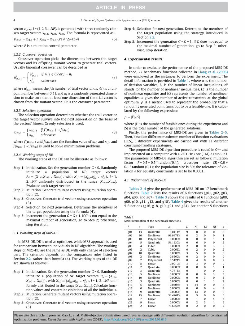
Table 1Main information of the benchmark functions.
f n Type q LI NI LE NE a
g01 13 Quadratic 0.0111% 9 0 0 0 6g02 20 Nonlinear 99.9971% 0 2 0 0 1g03 10 Polynomial 0.0000% 0 0 0 1 1g04 5 Quadratic 51.1230% 0 6 0 0 2g05 4 Cubic 0.0000% 2 0 0 3 3g06 2 Cubic 0.0066% 0 2 0 0 2g07 10 Quadratic 0.0003% 3 5 0 0 6g08 2 Nonlinear 0.8560% 0 2 0 0 0g09 7 Polynomial 0.5121% 0 4 0 0 2g10 8 Linear 0.0010% 3 3 0 0 0g11 2 Quadratic 0.0000% 0 0 0 1 1g12 3 Quadratic 4.7713% 0 1 0 0 0g13 5 Nonlinear 0.0000% 0 0 0 3 3g14 10 Nonlinear 0.0000% 0 0 3 0 3g15 3 Quadratic 0.0000% 0 0 1 1 2g16 5 Nonlinear 0.0204% 4 34 0 0 4g17 6 Nonlinear 0.0000% 0 0 0 4 4g18 9 Quadratic 0.0000% 0 13 0 0 0g19 15 Nonlinear 33.4761% 0 5 0 0 0g21 7 Linear 0.0000% 0 1 0 5 6g23 9 Linear 0.0000% 0 2 3 1 6g24 2 Linear 79.6556% 0 2 0 0 2
4 L. Gao et al. / Expert Systems with Applications xxx (2015) xxx–xxx
vector vi,G+1, i = (1,2,3. . .NP), is generated with three randomly cho-sen target vectors xr1,G, xr2,G, xr3,G. The formula is represented as:
v i;Gþ1 ¼ xr1;G þ Fðxr2;G � xr3;GÞ; r1–r2–r3–i ð6Þ
where F is a mutation control parameter.
3.2.2. Crossover operationCrossover operation picks the dimensions between the target
vectors and its offspring mutant vector to generate trial vectors.Usually binomial crossover can be described as:
u ji;Gþ1 ¼
v ji;Gþ1 if rðjÞ 6 CR or j ¼ nj
x ji;G otherwise
(ð7Þ
where uji;Gþ1 means the jth number of trial vector ui,G+1, r(j) is a ran-
dom number between [0,1], and nj is a randomly generated dimen-sion to make sure that at least one dimension of the trial vector ischosen from the mutant vector. CR is the crossover parameter.
3.2.3. Selection operationThe selection operation determines whether the trail vector or
the target vector survive into the next generation on the basis ofthe vectors’ fitness. Greedy selection is used:
xi;Gþ1 ¼ui;Gþ1 if f ðui;Gþ1Þ � f ðxi;GÞxi;G otherwise
�ð8Þ
where f ðui;Gþ1Þ and f ðxi;GÞ are the function value of ui,G and xi,G, andf ðui;Gþ1Þ � f ðxi;GÞ is used to solve minimization problems.
3.2.4. Working steps of DEThe working steps of the DE can be illustrate as follows:
Step 1: Initialization. Set the generation number G = 0. Randomlyinitialize a population of NP target vectorsPG ¼ fX1;G;X2;G . . . XNP;Gg, with Xi;G ¼ fx1
i;G; x2i;G . . . xn
i;Gg, i = 1,2. . .NP uniformly distributed in the range ½Xmin;Xmax�.Evaluate each target vectors.
Step 2: Mutation. Generate mutant vectors using mutation opera-tion (2).
Step 3: Crossover. Generate trial vectors using crossover operation(3).
Step 4: Selection for next generation. Determine the members ofthe target population using the formula (4).
Step 5: Increment the generation G = G + 1. If G is not equal to themaximal number of generation, go to Step 2; otherwise,stop iteration.
3.3. Working steps of MRS-DE
In MRS-DE, DE is used as optimizer, while MRS approach is usedfor comparison between individuals in DE algorithm. The workingsteps of MRS-DE are the same as DE with only change of selectionpart. The criterion depends on the comparison rules listed inSection 2.2, rather than formula (4). The working steps of the DEare shown as follows:
Step 1: Initialization. Set the generation number G = 0. Randomlyinitialize a population of NP target vectors PG ¼ fX1;G;
X2;G . . . XNP;Gg, with Xi;G ¼ fx1i;G; x
2i;G . . . xn
i;Gg, i = 1, 2. . .NP uni-formly distributed in the range ½Xmin;Xmax�. Calculate func-tion values and constraint violations of all the individuals.
Step 2: Mutation. Generate mutant vectors using mutation opera-tion (2).
Step 3: Crossover. Generate trial vectors using crossover operation(3).
Please cite this article in press as: Gao, L., et al. Multi-objective optimization boptimization problems. Expert Systems with Applications (2015), http://dx.doi.o
Step 4: Selection for next generation. Determine the members ofthe target population using the strategy introduced inSection 2.2.
Step 5: Increment the generation G = G + 1. If G does not equal tothe maximal number of generation, go to Step 2; other-wise, stop iteration.
4. Experimental results
In order to evaluate the performance of the proposed MRS-DEmethod, 22 benchmark functions collected in Liang et al. (2006)were employed as the instances to perform the experiment. Thedetail information is provided in Table 1, where n is the numberof decision variables, LI is the number of linear inequalities, NIstands for the number of nonlinear inequalities, LE is the numberof nonlinear equalities and NE represents the number of nonlinearequalities. a gives the number of active constraints at the globaloptimum. q is a metric used to represent the probability that arandomly generated point turns out to be a feasible one. It is calcu-lated by the following expression:
q ¼ jFj=jSj
where jFj is the number of feasible ones during the experiment andjSj is the total number of the generated solutions.
Firstly, the performance of MRS-DE are given in Tables 2–5.Then, based on different maximum number of function evaluations(FES), 3 different experiments are carried out with 11 differentconstraint-handling strategies.
The proposed MRS-DE algorithm procedure is coded in C++ andimplemented on a computer with a 2.0 GHz Core (TM) 2 Duo CPU.The parameters of MRS-DE algorithm are set as follows: mutationfactor F = 0.5 + 0.5 ⁄ random(0,1); crossover rate CR = 0.9 +0.1 ⁄ random (0,1); the population size is 30; the tolerance of vio-lation d for equality constraints is set to be 0.0001.
4.1. Performance of MRS-DE
Tables 2–4 give the performance of MRS-DE on 17 benchmarkfunctions. Table 2 lists the results of 6 functions (g01, g02, g03,g04, g06, and g07). Table 3 shows the results of 6 functions (g08,g09, g10, g11, g12, and g15). Table 4 gives the results of another5 functions (g16, g18, g19, g21 and g24). For another 5 functions
ased reverse strategy with differential evolution algorithm for constrainedrg/10.1016/j.eswa.2015.03.016
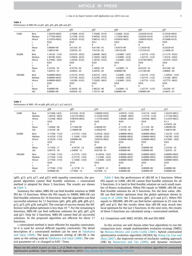
Table 2Performance of MRS-DE on g01, g02, g03, g04, g06 and g07.
g01 g02 g03 g04 g06 g07
5,000 Best 1.9247E+00(0) 2.7580E�01(0) 7.7940E�01(0) 1.2446E�01(0) 2.0343E+01(0) 9.3763E+00(0)Median 2.7776E+00(0) 3.5150E�01(0) 9.9992E�01(0) 1.1765E+00(0) 9.8265E+01(0) 3.3287E+01(0)Worst 5.2107E+00(0) 4.3932E�01(0) 9.9851E�01(1) 6.9583E+00(0) 3.0083E+02(0) 9.5260E+01(0)c 0,0,0 0,0,0 0,0,1 0,0,0 0,0,0 0,0,0v 0 0 0 0 0 0Mean 3.0609E+00 3.6132E�01 9.4110E�01 1.6597E+00 1.1263E+02 4.2423E+01Std 1.0401E+00 3.9455E�01 7.0152E�02 1.4915E+00 7.5725E+01 2.3360E+01
50,000 Best 1.3413E�11(0) 9.9327E�05(0) 2.6660E�06(0) �3.6380E�12(0) �1.6371E�11(0) 2.1117E�05(0)Median 1.9678E-10(0) 2.5992E�02(0) 5.1865E�04(0) �3.6380E�12(0) �1.6371E�11(0) 1.7621E�04(0)Worst 6.2784E�10(0) 1.4243E�01(0) 1.3073E�01(0) �3.6380E�12(0) 9.3579E+00(0) 1.8197E�03(0)c 0,0,0 0,0,0 0,0,0 0,0,0 0,0,0 0,0,0v 0 0 0 0 0 0Mean 2.2353E�10 4.3275E�02 1.3492E�03 �3.6380E�12 8.6523E�01 4.6154E�04Std 1.8291E�10 4.0465E�02 3.2055E�02 0.0000E+00 2.3110E+00 5.0880E�04
500,000 Best 0.0000E+00(0) 2.3571E�07(0) 6.4531E�12(0) �3.6380E�12(0) �1.6371E�11(0) �2.3093E�13(0)Median 0.0000E+00(0) 2.5776E�02(0) 4.3339E�07(0) �3.6380E�12(0) �1.6371E�11(0) 1.3156E�08(0)Worst 0.0000E+00(0) 1.4238E�01(0) 7.3502E�06(0) �3.6380E�12(0) �1.6371E�11(0) 1.0777E�06(0)c 0,0,0 0,0,0 0,0,0 0,0,0 0,0,0 0,0,0v 0 0 0 0 0 0Mean 0.0000E+00 4.3026E�02 1.0822E�06 �3.6380E�12 �1.6371E�11(0) 1.0526E�07Std 0.0000E+00 4.0583E�02 1.7011E�06 0.0000E+00 0.0000E+00 2.4441E�07
Table 3Performance of MRS�DE on g08, g09, g10, g11, g12 and g15.
g08 g09 g10 g11 g12 g15
5,000 Best 6.5184E-14(0) 8.5163E�01(0) 2.9660E+03(0) 3.0391E�12(0) 5.5511E�16(0) 1.9247E+00(2)Median 1.4655E�09(0) 2.2217E+00(0) 5.7236E+03(0) 1.4588E�08(0) 1.7377E�11(0) 2.7776E+00(2)Worst 7.2164E�08(0) 9.9835E+00(0) 1.1575E+04(0) 5.0020E�02(0) 3.0556E�08(0) 5.2107E+00(2)c 0,0,0 0,0,0 0,0,0 0,0,0 0,0,0 0,1,1v 0 0 0 0 0 4.3587E�02Mean 1.2604E�08 2.7144E+00 6.4826E+03 2.7135E�03 2.1123E�09 3.0609E+00Std 2.1014E�08 2.1080E+00 2.2962E+03 1.0333E�02 6.2984E�09 1.0401E+00
50,000 Best 2.7756E�17(0) �2.2737E�13(0) 5.2933E�03(0) 0.0000E+00(0) 0.0000E+00(0) 1.3413E�11(0)Median 4.1633E�17(0) �1.1369E�13(0) 1.8628E�02(0) 0.0000E+00(0) 0.0000E+00(0) 1.9678E�10(0)Worst 4.1633E�17(0) 0.0000E+00 3.8591E+00(0) 0.0000E+00(0) 0.0000E+00(0) 6.2784E�10(0)c 0,0,0 0,0,0 0,0,0 0,0,0 0,0,0 0,0,0v 0 0 0 0 0 0Mean 3.7192E�17 �4.5475E�14 2.8980E�01 0.0000E+00 0.0000E+00 2.2353E�10Std 6.6071E�18 1.6409E�13 8.0276E�01 0.0000E+00 0.0000E+00 1.8291E�10
500,000 Best 2.7756E�17(0) �2.2737E�13(0) �8.1855E�12(0) 0.0000E+00(0) 0.0000E+00(0) 0.0000E+00(0)Median 2.7756E�17(0) �2.2737E�13(0) �7.2760E�12(0) 0.0000E+00(0) 0.0000E+00(0) 0.0000E+00(0)Worst 2.7756E�17(0) �1.1368E�13(0) �3.6380E�12(0) 0.0000E+00(0) 0.0000E+00(0) 0.0000E+00(0)c 0,0,0 0,0,0 0,0,0 0,0,0 0,0,0 0,0,0v 0 0 0 0 0 0Mean 2.7756E�17(0) �2.1373E�13 �7.3487E�12 0.0000E+00 0.0000E+00 0.0000E+00Std 0.0000E+00 3.7706E�14 8.6760E�13 0.0000E+00 0.0000E+00 0.0000E+00
L. Gao et al. / Expert Systems with Applications xxx (2015) xxx–xxx 5
(g05, g13, g14, g17, and g23) with equality constraints, the pro-posed algorithm cannot find feasible solutions. e constrainedmethod is adopted for these 5 functions. The results are shownin Table 5.
Summary the tables, MRS-DE can find feasible solution in 5000FES for 13 functions. When the FES equals to 50000, MRS-DE canfind feasible solutions for 16 functions. And the algorithm can findsuccessful solutions for 11 functions (g01, g04, g06, g08, g09, g11,g12, g15, g16, g18, and g24). The concept of success means the dif-ference with global optimum is less than 10�4. For the remaining 6functions, MRS-DE can find sufficient solutions for g03, g07, g10and g21. Only for 2 functions, MRS-DE cannot find all successfulsolutions. So the proposed algorithm are efficient for these 17functions.
e constrained method is more efficient for equality constraints.So it is used for several difficult equality constraints. The detaildescription of e constrained method can be seen in Takahamaand Sakai (2006). The basic parameter setting of eRS-DE is thesame as the setting used in Takahama and Sakai (2006). The con-trol parameter of e is changed to 0.05 ⁄ Tmax.
Please cite this article in press as: Gao, L., et al. Multi-objective optimization boptimization problems. Expert Systems with Applications (2015), http://dx.doi.o
Table 5 lists the performance of eRS-DE in 5 functions. WhenFES equals to 5,000, eRS-DE cannot find feasible solutions for all5 functions. It is hard to find feasible solution on such small num-ber of fitness evaluations. When FES equals to 50000, eRS-DE canfind feasible solution for all 5 functions. For the best value, eRS-DE can find better optimum than the global optimum shown inLiang et al. (2006) for 3 functions (g05, g13 and g17). When FESequals to 500,000, eRS-DE can find better optimum in 25 runs forg05 and g13. But the results show that eRS-DE may struck intolocal optimum for the last 3 functions. In the next tests, the resultsof these 5 functions are calculated using e constrained method.
4.2. Comparison with SMES, HCOEA, ISR and DSS-MDE
In this section, we will choose other four algorithms to run thecomparison tests: simple multimember evolution strategy (SMES)by Mezura-Montes and Coello Coello (2005), hybrid constrainedoptimization evolution algorithm (HCOEA) by Wang Cai, Guo andZhou (2007), the improved version of stochastic ranking approach(ISR) by Runarsson and Yao (2000), and dynamic stochastic
ased reverse strategy with differential evolution algorithm for constrainedrg/10.1016/j.eswa.2015.03.016
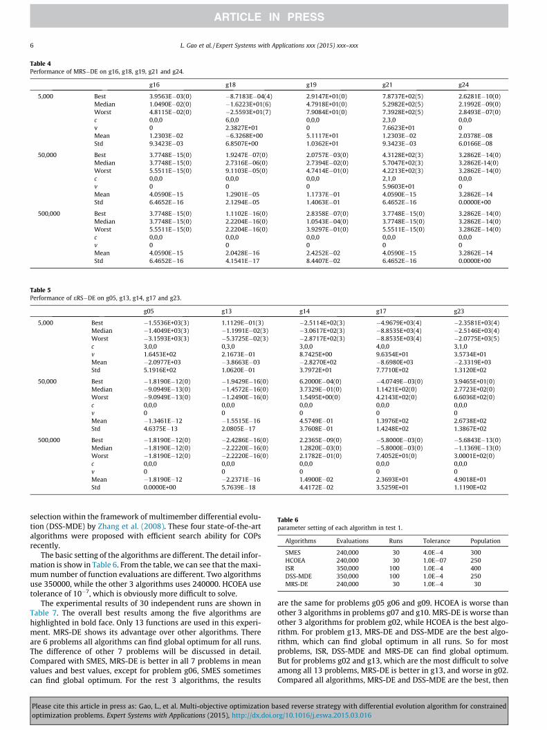
Table 4Performance of MRS�DE on g16, g18, g19, g21 and g24.
g16 g18 g19 g21 g24
5,000 Best 3.9563E�03(0) �8.7183E�04(4) 2.9147E+01(0) 7.8737E+02(5) 2.6281E�10(0)Median 1.0490E�02(0) �1.6223E+01(6) 4.7918E+01(0) 5.2982E+02(5) 2.1992E�09(0)Worst 4.8115E�02(0) �2.5593E+01(7) 7.9084E+01(0) 7.3928E+02(5) 2.8493E�07(0)c 0,0,0 6,0,0 0,0,0 2,3,0 0,0,0v 0 2.3827E+01 0 7.6623E+01 0Mean 1.2303E�02 �6.3268E+00 5.1117E+01 1.2303E�02 2.0378E�08Std 9.3423E�03 6.8507E+00 1.0362E+01 9.3423E�03 6.0166E�08
50,000 Best 3.7748E�15(0) 1.9247E�07(0) 2.0757E�03(0) 4.3128E+02(3) 3.2862E�14(0)Median 3.7748E�15(0) 2.7316E�06(0) 2.7394E�02(0) 5.7047E+02(3) 3.2862E-14(0)Worst 5.5511E�15(0) 9.1103E�05(0) 4.7414E�01(0) 4.2213E+02(3) 3.2862E�14(0)c 0,0,0 0,0,0 0,0,0 2,1,0 0,0,0v 0 0 0 5.9603E+01 0Mean 4.0590E�15 1.2901E�05 1.1737E�01 4.0590E�15 3.2862E�14Std 6.4652E�16 2.1294E�05 1.4063E�01 6.4652E�16 0.0000E+00
500,000 Best 3.7748E�15(0) 1.1102E�16(0) 2.8358E�07(0) 3.7748E�15(0) 3.2862E�14(0)Median 3.7748E�15(0) 2.2204E�16(0) 1.0543E�04(0) 3.7748E�15(0) 3.2862E�14(0)Worst 5.5511E�15(0) 2.2204E�16(0) 3.9297E�01(0) 5.5511E�15(0) 3.2862E�14(0)c 0,0,0 0,0,0 0,0,0 0,0,0 0,0,0v 0 0 0 0 0Mean 4.0590E�15 2.0428E�16 2.4252E�02 4.0590E�15 3.2862E�14Std 6.4652E�16 4.1541E�17 8.4407E�02 6.4652E�16 0.0000E+00
Table 5Performance of eRS�DE on g05, g13, g14, g17 and g23.
g05 g13 g14 g17 g23
5,000 Best �1.5536E+03(3) 1.1129E�01(3) �2.5114E+02(3) �4.9679E+03(4) �2.3581E+03(4)Median �1.4049E+03(3) �1.1991E�02(3) �3.0617E+02(3) �8.8535E+03(4) �2.5146E+03(4)Worst �3.1593E+03(3) �5.3725E�02(3) �2.8717E+02(3) �8.8535E+03(4) �2.0775E+03(5)c 3,0,0 0,3,0 3,0,0 4,0,0 3,1,0v 1.6453E+02 2.1673E�01 8.7425E+00 9.6354E+01 3.5734E+01Mean �2.0977E+03 �3.8663E�03 �2.8270E+02 �8.6980E+03 �2.3319E+03Std 5.1916E+02 1.0620E�01 3.7972E+01 7.7710E+02 1.3120E+02
50,000 Best �1.8190E�12(0) �1.9429E�16(0) 6.2000E�04(0) �4.0749E�03(0) 3.9465E+01(0)Median �9.0949E�13(0) �1.4572E�16(0) 3.7329E�01(0) 1.1421E+02(0) 2.7723E+02(0)Worst �9.0949E�13(0) �1.2490E�16(0) 1.5495E+00(0) 4.2143E+02(0) 6.6036E+02(0)c 0,0,0 0,0,0 0,0,0 0,0,0 0,0,0v 0 0 0 0 0Mean �1.3461E�12 �1.5515E�16 4.5749E�01 1.3976E+02 2.6738E+02Std 4.6375E�13 2.0805E�17 3.7608E�01 1.4248E+02 1.3867E+02
500,000 Best �1.8190E�12(0) �2.4286E�16(0) 2.2365E�09(0) �5.8000E�03(0) �5.6843E�13(0)Median �1.8190E�12(0) �2.2220E�16(0) 1.2820E�03(0) �5.8000E�03(0) �1.1369E�13(0)Worst �1.8190E�12(0) �2.2220E�16(0) 2.1782E�01(0) 7.4052E+01(0) 3.0001E+02(0)c 0,0,0 0,0,0 0,0,0 0,0,0 0,0,0v 0 0 0 0 0Mean �1.8190E�12 �2.2371E�16 1.4900E�02 2.3693E+01 4.9018E+01Std 0.0000E+00 5.7639E�18 4.4172E�02 3.5259E+01 1.1190E+02
Table 6parameter setting of each algorithm in test 1.
Algorithms Evaluations Runs Tolerance Population
SMES 240,000 30 4.0E�4 300HCOEA 240,000 30 1.0E�07 250ISR 350,000 100 1.0E�4 400DSS-MDE 350,000 100 1.0E�4 250MRS-DE 240,000 30 1.0E�4 30
6 L. Gao et al. / Expert Systems with Applications xxx (2015) xxx–xxx
selection within the framework of multimember differential evolu-tion (DSS-MDE) by Zhang et al. (2008). These four state-of-the-artalgorithms were proposed with efficient search ability for COPsrecently.
The basic setting of the algorithms are different. The detail infor-mation is show in Table 6. From the table, we can see that the maxi-mum number of function evaluations are different. Two algorithmsuse 350000, while the other 3 algorithms uses 240000. HCOEA usetolerance of 10�7, which is obviously more difficult to solve.
The experimental results of 30 independent runs are shown inTable 7. The overall best results among the five algorithms arehighlighted in bold face. Only 13 functions are used in this experi-ment. MRS-DE shows its advantage over other algorithms. Thereare 6 problems all algorithms can find global optimum for all runs.The difference of other 7 problems will be discussed in detail.Compared with SMES, MRS-DE is better in all 7 problems in meanvalues and best values, except for problem g06, SMES sometimescan find global optimum. For the rest 3 algorithms, the results
Please cite this article in press as: Gao, L., et al. Multi-objective optimization boptimization problems. Expert Systems with Applications (2015), http://dx.doi.o
are the same for problems g05 g06 and g09. HCOEA is worse thanother 3 algorithms in problems g07 and g10. MRS-DE is worse thanother 3 algorithms for problem g02, while HCOEA is the best algo-rithm. For problem g13, MRS-DE and DSS-MDE are the best algo-rithm, which can find global optimum in all runs. So for mostproblems, ISR, DSS-MDE and MRS-DE can find global optimum.But for problems g02 and g13, which are the most difficult to solveamong all 13 problems, MRS-DE is better in g13, and worse in g02.Compared all algorithms, MRS-DE and DSS-MDE are the best, then
ased reverse strategy with differential evolution algorithm for constrainedrg/10.1016/j.eswa.2015.03.016
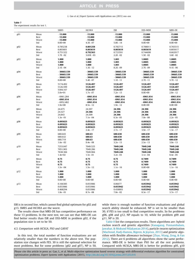
Table 7The experiment results for test 1.
SMES HCOEA ISR DSS-MDE MRS-DE
g01 Mean �15.000 �15.000 �15.000 �15.000 �15.000Best �15.000 �15.000 �15.000 �15.000 �15.000Worst �15.000 �15.000 �15.000 �15.000 �15.000Std 0.0E+00 4.3E�07 5.8E�14 0.0E+00 0.0E+00
g02 Mean 0.785238 0.801258 0.782715 0.788011 0.765515Best 0.803601 0.803619 0.803619 0.803619 0.803617Worst 0.751322 0.792363 0.723591 0.744690 0.662017Std 1.7E�02 3.83E�03 2.2E�02 1.5E�02 3.6E�02
g03 Mean 1.000 1.000 1.001 1.0005 1.0005Best 1.000 1.000 1.001 1.0005 1.0005Worst 1.000 1.000 1.001 1.0005 1.0005Std 2.1E�04 1.3E�12 8.2E�09 2.7E�09 9.1E�06
g04 Mean �30665.539 �30665.539 �30665.539 �30665.539 �30665.539Best �30665.539 �30665.539 �30665.539 �30665.539 �30665.539Worst �30665.539 �30665.539 �30665.539 �30665.539 �30665.539Std 0.0E+00 5.4E�07 1.1E�11 2.7E�11 3.7E�12
g05 Mean 5174.492 5126.497 5126.497 5126.497 5126.497Best 5126.599 5126.497 5126.497 5126.497 5126.497Worst 5304.167 5126.497 5126.497 5126.497 5126.497Std 5.0e+01 1.7e�07 7.2e�13 0.0E+00 2.8e�12
g06 Mean �6961.284 �6961.814 �6961.814 �6961.814 �6961.814Best �6961.814 �6961.814 �6961.814 �6961.814 �6961.814Worst �6952.482 �6961.814 �6961.814 �6961.814 �6961.814Std 1.9e+00 8.5e�12 1.9e�12 0.0E+00 0.0E+00
g07 Mean 24.475 24.307 24.306 24.306 24.306Best 24.327 24.306 24.306 24.306 24.306Worst 24.843 24.309 24.306 24.306 24.306Std 1.3e�01 7.1e�04 6.3e�05 7.0e�08 2.2e�05
g08 Mean 0.095825 0.095825 0.095825 0.095825 0.095825Best 0.095825 0.095825 0.095825 0.095825 0.095825Worst 0.095825 0.095825 0.095825 0.095825 0.095825Std 0.0E+00 2.4e�17 2.7e�17 3.9e�17 1.3e�17
g09 Mean 680.643 680.63 680.630 680.630 680.630Best 680.632 680.63 680.630 680.630 680.630Worst 680.719 680.63 680.630 680.630 680.630Std 1.6e�02 9.4e�08 3.2e�13 2.5e�13 3.0e�13
g10 Mean 7253.047 7049.525 7049.248 7049.248 7049.248Best 7051.903 7049.286 7049.248 7049.248 7049.248Worst 7638.366 7049.984 7049.248 7049.248 7049.248Std 1.4e+02 1.5e�01 3.2e�03 3.1e�04 8.4e�05
g11 Mean 0.75 0.75 0.75 0.7499 0.7499Best 0.75 0.75 0.75 0.7499 0.7499Worst 0.75 0.75 0.75 0.7499 0.7499Std 1.5e�04 1.5e�12 1.1e�16 0.0E+00 1.1e�16
g12 Mean 1.000 1.000 1.000 1.000 1.000Best 1.000 1.000 1.000 1.000 1.000Worst 1.000 1.000 1.000 1.000 1.000Std 0.0E+00 0.0E+00 0.0E+00 0.0E+00 0.0E+00
g13 Mean 0.166385 0.053986 0.06677 0.053942 0.053942Best 0.053986 0.053986 0.053942 0.053942 0.053942Worst 0.468294 0.053986 0.438803 0.053942 0.053942Std 1.8e�01 8.7e�08 7.0e�02 8.3e�17 3.7e�17
L. Gao et al. / Expert Systems with Applications xxx (2015) xxx–xxx 7
ISR is in second line, which cannot find global optimum for g02 andg13. SMES and HCOEA are the worst.
The results show that MRS-DE has competitive performance onthese 13 problems. In the next test, we can see that MRS-DE canfind better results than ISR and DSS-MDE in problem g02, if thepopulation size is set to be 50.
4.3. Comparison with HCSGA, PSO and GAFAT
In this test, the total number of function evaluations are setrelatively smaller than the numbers in the above test. The pop-ulation size changes with FES. 30 is still the optional selection formost problems. But for some problems (g02 and g07), NP is 50,
Please cite this article in press as: Gao, L., et al. Multi-objective optimization boptimization problems. Expert Systems with Applications (2015), http://dx.doi.o
while there is enough number of function evaluations and globalsearch ability should be enhanced. NP is set to be smaller than30, if FES is too small to find competitive results. So for problemsg06, g08 and g12, NP equals to 10, while for problem g09 andg11, NP is 20.
Table 8 list the comparison results. Three algorithms are: hybridcuckoo search and genetic algorithm (Kanagaraj, Ponnambalam,Jawahar, & Mukund Nilakantan 2014), particle swarm optimization(Mazhoud, Hadj-Hamou, Bigeon, & Joyeux, 2013) and genetic algo-rithm with flexible allowance technique (Zhao, Wang, Zeng, & Fan2012). There are 6 problems all algorithms show the same perfor-mance. MRS-DE is better than PSO for all the rest problems.Compared with HCSGA, MRS-DE is better for problems g05, g10
ased reverse strategy with differential evolution algorithm for constrainedrg/10.1016/j.eswa.2015.03.016
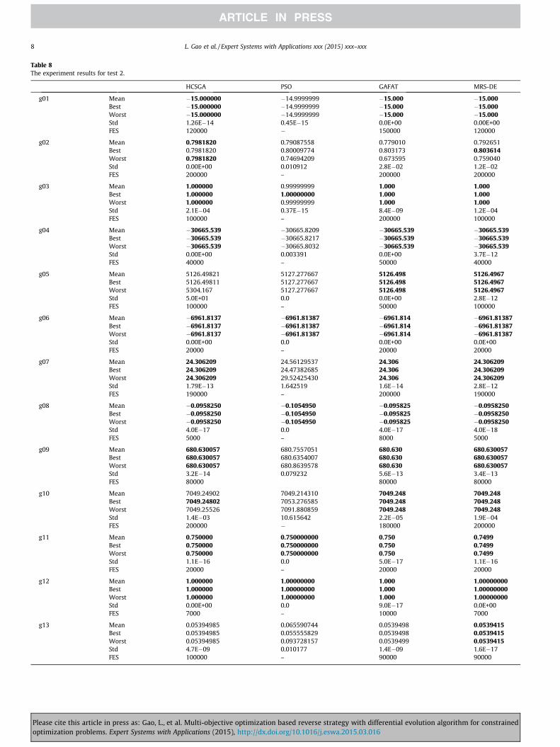
Table 8The experiment results for test 2.
HCSGA PSO GAFAT MRS-DE
g01 Mean �15.000000 �14.9999999 �15.000 �15.000Best �15.000000 �14.9999999 �15.000 �15.000Worst �15.000000 �14.9999999 �15.000 �15.000Std 1.26E�14 0.45E�15 0.0E+00 0.00E+00FES 120000 � 150000 120000
g02 Mean 0.7981820 0.79087558 0.779010 0.792651Best 0.7981820 0.80009774 0.803173 0.803614Worst 0.7981820 0.74694209 0.673595 0.759040Std 0.00E+00 0.010912 2.8E�02 1.2E�02FES 200000 – 200000 200000
g03 Mean 1.000000 0.99999999 1.000 1.000Best 1.000000 1.00000000 1.000 1.000Worst 1.000000 0.99999999 1.000 1.000Std 2.1E�04 0.37E�15 8.4E�09 1.2E�04FES 100000 – 200000 100000
g04 Mean �30665.539 �30665.8209 �30665.539 �30665.539Best �30665.539 �30665.8217 �30665.539 �30665.539Worst �30665.539 �30665.8032 �30665.539 �30665.539Std 0.00E+00 0.003391 0.0E+00 3.7E�12FES 40000 – 50000 40000
g05 Mean 5126.49821 5127.277667 5126.498 5126.4967Best 5126.49811 5127.277667 5126.498 5126.4967Worst 5304.167 5127.277667 5126.498 5126.4967Std 5.0E+01 0.0 0.0E+00 2.8E�12FES 100000 – 50000 100000
g06 Mean �6961.8137 �6961.81387 �6961.814 �6961.81387Best �6961.8137 �6961.81387 �6961.814 �6961.81387Worst �6961.8137 �6961.81387 �6961.814 �6961.81387Std 0.00E+00 0.0 0.0E+00 0.0E+00FES 20000 – 20000 20000
g07 Mean 24.306209 24.56129537 24.306 24.306209Best 24.306209 24.47382685 24.306 24.306209Worst 24.306209 29.52425430 24.306 24.306209Std 1.79E�13 1.642519 1.6E�14 2.8E�12FES 190000 – 200000 190000
g08 Mean �0.0958250 �0.1054950 �0.095825 �0.0958250Best �0.0958250 �0.1054950 �0.095825 �0.0958250Worst �0.0958250 �0.1054950 �0.095825 �0.0958250Std 4.0E�17 0.0 4.0E�17 4.0E�18FES 5000 – 8000 5000
g09 Mean 680.630057 680.7557051 680.630 680.630057Best 680.630057 680.6354007 680.630 680.630057Worst 680.630057 680.8639578 680.630 680.630057Std 3.2E�14 0.079232 5.6E�13 3.4E�13FES 80000 80000 80000
g10 Mean 7049.24902 7049.214310 7049.248 7049.248Best 7049.24802 7053.276585 7049.248 7049.248Worst 7049.25526 7091.880859 7049.248 7049.248Std 1.4E�03 10.615642 2.2E�05 1.9E�04FES 200000 � 180000 200000
g11 Mean 0.750000 0.750000000 0.750 0.7499Best 0.750000 0.750000000 0.750 0.7499Worst 0.750000 0.750000000 0.750 0.7499Std 1.1E�16 0.0 5.0E�17 1.1E�16FES 20000 – 20000 20000
g12 Mean 1.000000 1.00000000 1.000 1.00000000Best 1.000000 1.00000000 1.000 1.00000000Worst 1.000000 1.00000000 1.000 1.00000000Std 0.00E+00 0.0 9.0E�17 0.0E+00FES 7000 – 10000 7000
g13 Mean 0.05394985 0.065590744 0.0539498 0.0539415Best 0.05394985 0.055555829 0.0539498 0.0539415Worst 0.05394985 0.093728157 0.0539499 0.0539415Std 4.7E�09 0.010177 1.4E�09 1.6E�17FES 100000 – 90000 90000
8 L. Gao et al. / Expert Systems with Applications xxx (2015) xxx–xxx
Please cite this article in press as: Gao, L., et al. Multi-objective optimization based reverse strategy with differential evolution algorithm for constrainedoptimization problems. Expert Systems with Applications (2015), http://dx.doi.org/10.1016/j.eswa.2015.03.016

Table 9Comparison results of g01, g02, g03, g04, g05 and g06 in test 3.
Best Median Worst Mean SD
g01 eDE 0.0000E+00 0.0000E+00 0.0000E+00 0.0000E+00 0.0000E+00CMODE 0.0000E+00 0.0000E+00 0.0000E+00 0.0000E+00 0.0000E+00ICDE 0.00E+00 0.00E+00 0.00E+00 0.00E+00 0.00E+00ICEM 0.0000E+00 0.0000E+00 0.0000E+00 0.0000E+00 0.0000E+00eDE-PM 0.0000E+00 0.0000E+00 0.0000E+00 0.0000E+00 0.0000E+00
g02 eDE 4.0394E�09 3.0933E�08 7.3163E�08 3.0333E�08 1.7523E�08CMODE 4.1726E�09 1.1372E�08 1.1836E�07 2.0387E�08 2.4195E�08ICDE 1.28E�08 1.39E�07 7.43E�07 2.28E�07 2.06E�07ICEM 2.2823E�06 5.4463E�06 1.1014E�02 1.3617E�03 2.6951E�03eDE-PM 2.3571E�07 2.5776E�02 1.4238E�01 4.3026E�02 4.0583E�02
g03 eDE �4.4409E�16 �4.4409E�16 �4.4409E�16 �4.4409E�16 2.9682E�31CMODE 2.3964E�10 1.1073E�09 2.5794E�09 1.1665E�09 5.2903E�10ICDE �1.00E�11 �1.00E�11 �1.00E�11 �1.00E�11 1.63E�16ICEM 3.2984E�11 3.3199E�08 1.3832E�06 1.3609E�07 2.7619E�07eDE-PM 6.4531E�12 4.3339E�07 7.3502E�06 1.0822E�06 1.7011E�06
g04 eDE 0.0000E+00 0.0000E+00 0.0000E+00 0.0000E+00 0.0000E+00CMODE 7.6398E�11 7.6398E�11 7.6398E�11 7.6398E�11 2.6382E�26ICDE 7.64E�11 7.64E�11 7.64E�11 7.64E�11 2.64E�26ICEM 7.2760E�11 7.2760E�11 7.6398E�11 7.2905E�11 7.1290E�13eDE-PM �3.6390E�12 �3.6390E�12 �3.6390E�12 �3.6390E�12 0.0000E+00
g05 eDE 0.0000E+00 0.0000E+00 0.0000E+00 0.0000E+00 0.0000E+00CMODE �1.8190E�12 �1.8190E�12 �1.8190E�12 �1.8190E�12 1.2366E�27ICDE �1.82E�12 �1.82E�12 �1.82E�12 �1.82E�12 1.24E�27ICEM �1.8190E�12 �1.8190E�12 �9.0950e�013 �1.7462E�12 2.4674E�13eDE-PM �1.8190E�12 �1.8190E�12 �1.8190E�12 �1.8190E�12 0.0000E+00
g06 eDE 1.1823E�11 1.1823E�11 1.1823E�11 1.1823E�11 0.0000E+00CMODE 3.3651E�11 3.3651E�11 3.3651E�11 3.3651E�11 1.3191E�26ICDE 3.37E�11 3.37E�11 3.37E�11 3.37E�11 3.37E�11ICEM 3.3651E�11 3.3651E�11 3.3651E�11 3.3651E�11 0.0000E+00eDE-PM �1.6371E�11 �1.6371E�11 �1.6371E�11 �1.6371E�11 0.0000E+00
Table 10Comparison results of g07, g08, g09, g10, g11 and g12 in test 3.
Best Median Worst Mean SD
g07 eDE �1.8474E�13 �1.8474E�13 �1.7764E�13 �1.8360E�13 2.1831E�15CMODE 7.9783E�11 7.9783E�11 7.9783E�11 7.9783E�11 7.6527E�15ICDE 7.98E�11 7.98E�11 7.98E�11 7.98E�11 5.26E�15ICEM 7.9762E�11 7.9769E�11 7.9787E�11 7.9770E�11 6.0526E�15eDE-PM �2.3093E�13 1.3156E�08 1.0777E�06 1.0526E�07 2.4441E�07
g08 eDE 4.1633E�17 4.1633E�17 4.1633E�17 4.1633E�17 1.2326E�32CMODE 8.1964E�11 8.1964E�11 8.1964E�11 8.1964E�11 6.3596E�18ICDE 8.20E�11 8.20E�11 8.20E�11 8.20E�11 2.78E�18ICEM 8.1964E�11 8.1964E�11 8.1964E�11 8.1964E�11 3.8774E�26eDE-PM 2.7756E�17 2.7756E�17 2.7756E�17 2.7756E�17 0.0000E+00
g09 eDE 0.0000E+00 0.0000E+00 0.0000E+00 0.0000E+00 0.0000E+00CMODE �9.8225E�11 �9.8225E�11 �9.8225E�11 �9.8225E�11 4.9554E�14ICDE �9.82E�11 �9.81E�11 �9.81E�11 �9.82E�11 5.76E�14ICEM �9.8225E�11 �9.8225E�11 �9.8225E�11 �9.8225E�11 4.4556E�13eDE-PM �2.2737E�013 �2.2737E�013 �1.1369E�013 �2.1373E�13 3.7706E�14
g10 eDE �1.8190E�12 �9.0949E�13 �9.0949E�13 �1.2005E�12 4.2426E�13CMODE 6.2755E�11 6.2755E�11 6.3664E�11 6.2827E�11 2.5183E�13ICDE 6.18E�11 6.28E�11 6.28E�11 6.27E�11 2.64E�26ICEM 6.1846E�11 6.2755E�11 6.2755E�11 6.2391E�11 7.1290E�13eDE-PM �8.1854E�12 �7.2760E�12 �3.6380E�12 �7.3487E�12 8.6760E�13
g11 eDE 0.0000E+00 0.0000E+00 0.0000E+00 0.0000E+00 0.0000E+00CMODE 0.0000E+00 0.0000E+00 0.0000E+00 0.0000E+00 0.0000E+00ICDE 0.00E+00 0.00E+00 0.00E+00 0.00E+00 0.00E+00ICEM 0.0000E+00 0.0000E+00 0.0000E+00 0.0000E+00 0.0000E+00eDE-PM 0.0000E+00 0.0000E+00 0.0000E+00 0.0000E+00 0.0000E+00
g12 eDE 0.0000E+00 0.0000E+00 0.0000E+00 0.0000E+00 0.0000E+00CMODE 0.0000E+00 0.0000E+00 0.0000E+00 0.0000E+00 0.0000E+00ICDE 0.00E+00 0.00E+00 0.00E+00 0.00E+00 0.00E+00ICEM 0.0000E+00 0.0000E+00 0.0000E+00 0.0000E+00 0.0000E+00eDE-PM 0.0000E+00 0.0000E+00 0.0000E+00 0.0000E+00 0.0000E+00
L. Gao et al. / Expert Systems with Applications xxx (2015) xxx–xxx 9
Please cite this article in press as: Gao, L., et al. Multi-objective optimization based reverse strategy with differential evolution algorithm for constrainedoptimization problems. Expert Systems with Applications (2015), http://dx.doi.org/10.1016/j.eswa.2015.03.016
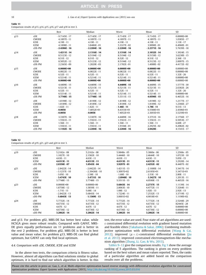
Table 11Comparison results of g13, g14, g15, g16, g17 and g18 in test 3.
Best Median Worst Mean SD
g13 eDE �9.7145E�17 �9.7145E�17 �9.7145E�17 �9.7145E�17 0.0000E+00CMODE 4.1897E�11 4.1897E�11 4.1897E�11 4.1897E�11 1.0385E�17ICDE 4.19E�11 4.19E�11 4.19E�11 4.19E�11 1.13E�17ICEM 4.1898E�11 3.8486E�01 5.3327E�02 3.9090E�01 6.4960E�01eDE-PM �2.4286E�16 �2.2204E�16 �2.2204E�16 �2.2371E�16 5.7639E�18
g14 eDE 1.4211E�14 2.1316E�14 2.1316E�14 2.1032E�14 1.3924E�15CMODE 8.5123E�12 8.5194E�12 8.5194E�12 8.5159E�12 3.6230E�15ICDE 8.51E�12 8.51E�12 8.52E�12 8.51E�12 2.36E�15ICEM 8.5052E�12 8.5123E�12 8.5194E�12 8.5123E�12 2.0097E�15eDE-PM 2.2365E�09 1.2820E�03 2.1782E�01 1.4900E�02 4.4172E�02
g15 eDE 0.0000E+00 0.0000E+00 0.0000E+00 0.0000E+00 0.0000E+00CMODE 6.0822E�11 6.0822E�11 6.0822E�11 6.0822E�11 0.0000E+00ICDE 6.52E�11 6.52E�11 6.52E�11 6.52E�11 1.32E�26ICEM 6.5214E�11 6.5214E�11 6.5214E�11 6.5214E�11 0.0000E+00eDE-PM 0.0000E+00 0.0000E+00 0.0000E+00 0.0000E+00 0.0000E+00
g16 eDE 4.4409E�15 4.4409E�15 4.4409E�15 4.4409E�15 1.5777E�30CMODE 6.5213E�11 6.5213E�11 6.5213E�11 6.5213E�11 2.6382E�26ICDE 6.52E�11 6.52E�11 6.52E�11 6.52E�11 1.32E�26ICEM 6.5214E�11 6.5214E�11 6.5214E�11 6.5214E�11 0.0000E+00eDE-PM 3.7748E�15 3.7748E�15 5.5511E�15 4.0590E�15 6.4652E�16
g17 eDE 1.8190E�12 1.8190E�12 1.8190E�12 1.8190E�12 1.2177E�17CMODE 1.8189E�12 1.8189E�12 1.8189E�12 1.8189E�12 1.2366E�27ICDE �1.82E�11 �1.82E�11 �1.46E�11 �1.78E�11 9.51E�13ICEM �0.0058 7.4052E+01 8.4353E+01 6.5588E+01 2.4306E+01eDE-PM �0.0058 �0.0058 7.4052E+01 2.3693E+01 3.5259E+01
g18 eDE 3.3307E�16 3.3307E�16 4.4409E�16 3.3751E�16 2.1756E�17CMODE 1.5561E�11 1.5561E�11 1.5561E�11 1.5561E�11 6.5053E�17ICDE 1.56E�11 1.56E�11 1.56E�11 1.56E�11 6.60E�27ICEM 1.5561E�11 1.5561E�11 1.9104E�01 2.2925E�02 6.2082E�02eDE-PM 1.1102E�16 2.2204E�16 2.2204E�16 2.0428E� 4.1541E�17
Table 12Comparison results of g19, g21, g23 and g24 in test 3.
Best Median Worst Mean SD
g19 eDE 5.2162e�08 5.2162e�08 5.9840e�05 5.3860e�06 1.2568e�05CMODE 1.1027E�10 2.1582E�10 5.4446E�10 2.4644E�10 1.0723E�10ICDE 4.63E�11 4.63E�11 4.63E�11 4.63E�11 5.05E�15ICEM 4.6313E�11 4.6313E�11 4.6313E�11 4.6313E�11 3.2920E�14eDE-PM 2.8358E�07 1.0543E�04 3.9297E�01 2.4252E�02 8.4407E�02
g21 eDE �2.8422E�14 �2.8422E�14 1.4211E�13 �2.1600E�14 3.3417E�14CMODE �3.1237E�10 �2.39436E�10 1.3097E+02 2.6195E+01 5.3471E+01ICDE �3.05E�10 �2.58E�10 �1.68E�10 �2.53E�10 2.80E�11ICEM �3.4743E�10 �3.4731E�10 �2.8948E�10 �3.3427E�10 1.2013E�11eDE-PM 3.7748E�15 3.7748E�15 5.5511E�15 4.0590E�15 6.4652E�16
g23 eDE 0.0000E+00 0.0000E+00 5.6843E�14 2.2737E�15 1.1139E�14CMODE 1.8758E�12 1.5859E�11 2.8063E�10 4.4772E�11 7.3264E�11ICDE �1.71E�13 5.68E�14 1.08E�12 1.02E�13 2.92E�13ICEM �2.8422E�13 5.6843E�14 1.7224E�11 7.2532E�13 3.3719E�12eDE-PM �5.6843E�13 �1.1369E�13 3.0001E+02 4.9018E+01 1.1190E+02
g24 eDE 5.7732E�14 5.7732E�14 5.7732E�14 5.7732E�14 2.5244E�29CMODE 4.6735E�12 4.6735E�12 4.6735E�12 4.6735E�12 82445E�28ICDE 4.67E�12 4.67E�12 4.67E�12 4.67E�12 0.0000E+00ICEM 4.6736E�12 4.6736E�12 4.6736E�12 4.6736E�12 0.0000E+00eDE-PM 3.2862E�14 3.2862E�14 3.2862E�14 3.2862E�14 0.0000E+00
10 L. Gao et al. / Expert Systems with Applications xxx (2015) xxx–xxx
and g13. For problem g02, MRS-DE has better best value, whileHCSGA gives more robust results. Compared with GAFAT, MRS-DE gives equally performance on 11 problems and is better inthe rest 2 problems. For problem g02, MRS-DE is better in bestvalue and mean value; for problem g13, MRS-DE can find globaloptimum, but GAFAT can only find local optimum.
4.4. Comparison with eDE, CMODE, ICDE and ICEM
In the above two tests, the comparison criteria is fitness value.However, almost all algorithms can find solutions similar to globaloptimum, it is hard to find out which algorithm is better. In this
Please cite this article in press as: Gao, L., et al. Multi-objective optimization boptimization problems. Expert Systems with Applications (2015), http://dx.doi.o
test, the error value are used. Four state-of-art algorithms are used:e constrained differential evolution with gradient based mutationand feasible elites (Takahama & Sakai, 2006); Combining multiob-jective optimization with differential evolution (Wang & Cai,2012); improved ðlþ kÞ-constrained differential evolution (Jiaet al. 2013); improved constrained electromagnetism-like mecha-nism algorithm (Zhang, Li, Gao, & Wu, 2013).
Tables 9–12 give the comparison results. Fig 1 show the averageranking of 5 algorithms. The ranking is given on every problembased on the best values and mean values reported. Then, the ranksof a particular algorithm are added based on the comparisonresults over all the problems.
ased reverse strategy with differential evolution algorithm for constrainedrg/10.1016/j.eswa.2015.03.016
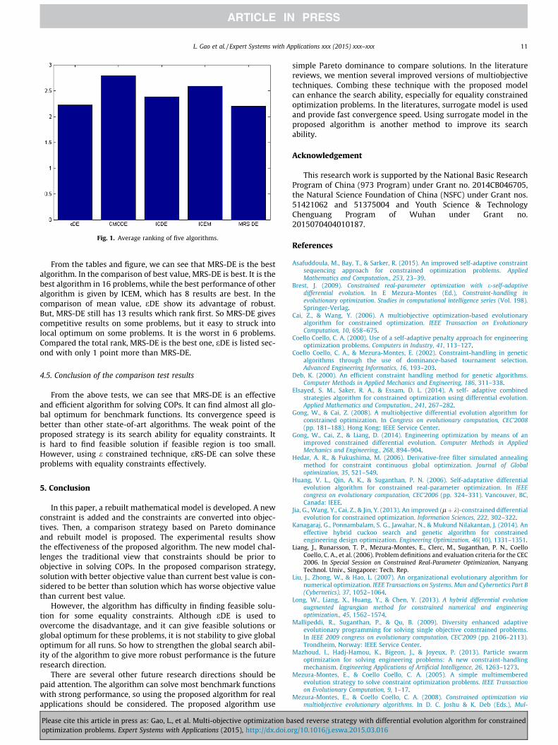
Fig. 1. Average ranking of five algorithms.
L. Gao et al. / Expert Systems with Applications xxx (2015) xxx–xxx 11
From the tables and figure, we can see that MRS-DE is the bestalgorithm. In the comparison of best value, MRS-DE is best. It is thebest algorithm in 16 problems, while the best performance of otheralgorithm is given by ICEM, which has 8 results are best. In thecomparison of mean value, eDE show its advantage of robust.But, MRS-DE still has 13 results which rank first. So MRS-DE givescompetitive results on some problems, but it easy to struck intolocal optimum on some problems. It is the worst in 6 problems.Compared the total rank, MRS-DE is the best one, eDE is listed sec-ond with only 1 point more than MRS-DE.
4.5. Conclusion of the comparison test results
From the above tests, we can see that MRS-DE is an effectiveand efficient algorithm for solving COPs. It can find almost all glo-bal optimum for benchmark functions. Its convergence speed isbetter than other state-of-art algorithms. The weak point of theproposed strategy is its search ability for equality constraints. Itis hard to find feasible solution if feasible region is too small.However, using e constrained technique, eRS-DE can solve theseproblems with equality constraints effectively.
5. Conclusion
In this paper, a rebuilt mathematical model is developed. A newconstraint is added and the constraints are converted into objec-tives. Then, a comparison strategy based on Pareto dominanceand rebuilt model is proposed. The experimental results showthe effectiveness of the proposed algorithm. The new model chal-lenges the traditional view that constraints should be prior toobjective in solving COPs. In the proposed comparison strategy,solution with better objective value than current best value is con-sidered to be better than solution which has worse objective valuethan current best value.
However, the algorithm has difficulty in finding feasible solu-tion for some equality constraints. Although eDE is used toovercome the disadvantage, and it can give feasible solutions orglobal optimum for these problems, it is not stability to give globaloptimum for all runs. So how to strengthen the global search abil-ity of the algorithm to give more robust performance is the futureresearch direction.
There are several other future research directions should bepaid attention. The algorithm can solve most benchmark functionswith strong performance, so using the proposed algorithm for realapplications should be considered. The proposed algorithm use
Please cite this article in press as: Gao, L., et al. Multi-objective optimization boptimization problems. Expert Systems with Applications (2015), http://dx.doi.o
simple Pareto dominance to compare solutions. In the literaturereviews, we mention several improved versions of multiobjectivetechniques. Combing these technique with the proposed modelcan enhance the search ability, especially for equality constrainedoptimization problems. In the literatures, surrogate model is usedand provide fast convergence speed. Using surrogate model in theproposed algorithm is another method to improve its searchability.
Acknowledgement
This research work is supported by the National Basic ResearchProgram of China (973 Program) under Grant no. 2014CB046705,the Natural Science Foundation of China (NSFC) under Grant nos.51421062 and 51375004 and Youth Science & TechnologyChenguang Program of Wuhan under Grant no.2015070404010187.
References
Asafuddoula, M., Bay, T., & Sarker, R. (2015). An improved self-adaptive constraintsequencing approach for constrained optimization problems. AppliedMathematics and Computation., 253, 23–39.
Brest, J. (2009). Constrained real-parameter optimization with e-self-adaptivedifferential evolution. In E Mezura-Montes (Ed.), Constraint-handling inevolutionary optimization. Studies in computational intelligence series (Vol. 198).Springer-Verlag.
Cai, Z., & Wang, Y. (2006). A multiobjective optimization-based evolutionaryalgorithm for constrained optimization. IEEE Transaction on EvolutionaryComputation, 10, 658–675.
Coello Coello, C. A. (2000). Use of a self-adaptive penalty approach for engineeringoptimization problems. Computers in Industry, 41, 113–127.
Coello Coello, C. A., & Mezura-Montes, E. (2002). Constraint-handling in geneticalgorithms through the use of dominance-based tournament selection.Advanced Engineering Informatics, 16, 193–203.
Deb, K. (2000). An efficient constraint handling method for genetic algorithms.Computer Methods in Applied Mechanics and Engineering, 186, 311–338.
Elsayed, S. M., Saker, R. A., & Essam, D. L. (2014). A self- adaptive combinedstrategies algorithm for constrained optimization using differential evolution.Applied Mathematics and Computation., 241, 267–282.
Gong, W., & Cai, Z. (2008). A multiobjective differential evolution algorithm forconstrained optimization. In Congress on evolutionary computation, CEC’2008(pp. 181–188). Hong Kong: IEEE Service Center.
Gong, W., Cai, Z., & Liang, D. (2014). Engineering optimization by means of animproved constrained differential evolution. Computer Methods in AppliedMechanics and Engineering., 268, 894–904.
Hedar, A. R., & Fukushima, M. (2006). Derivative-free filter simulated annealingmethod for constraint continuous global optimization. Journal of Globaloptimization, 35, 521–549.
Huang, V. L., Qin, A. K., & Suganthan, P. N. (2006). Self-adaptative differentialevolution algorithm for constrained real-parameter optimization. In IEEEcongress on evolutionary computation, CEC’2006 (pp. 324–331). Vancouver, BC,Canada: IEEE.
Jia, G., Wang, Y., Cai, Z., & Jin, Y. (2013). An improved ðlþ kÞ-constrained differentialevolution for constrained optimization. Information Sciences, 222, 302–322.
Kanagaraj, G., Ponnambalam, S. G., Jawahar, N., & Mukund Nilakantan, J. (2014). Aneffective hybrid cuckoo search and genetic algorithm for constrainedengineering design optimization. Engineering Optimization, 46(10), 1331–1351.
Liang, J., Runarsson, T. P., Mezura-Montes, E., Clerc, M., Suganthan, P. N., CoelloCoello, C. A., et al. (2006). Problem definitions and evaluation criteria for the CEC2006. In Special Session on Constrained Real-Parameter Optimization, NanyangTechnol. Univ., Singapore: Tech. Rep.
Liu, J., Zhong, W., & Hao, L. (2007). An organizational evolutionary algorithm fornumerical optimization. IEEE Transactions on Systems. Man and Cybernetics Part B(Cybernetics), 37, 1052–1064.
Long, W., Liang, X., Huang, Y., & Chen, Y. (2013). A hybrid differential evolutionaugmented lagrangian method for constrained numerical and engineeringoptimization., 45, 1562–1574.
Mallipeddi, R., Suganthan, P., & Qu, B. (2009). Diversity enhanced adaptiveevolutionary programming for solving single objective constrained problems.In IEEE 2009 congress on evolutionary computation, CEC’2009 (pp. 2106–2113).Trondheim, Norway: IEEE Service Center.
Mazhoud, I., Hadj-Hamou, K., Bigeon, J., & Joyeux, P. (2013). Particle swarmoptimization for solving engineering problems: A new constraint-handlingmechanism. Engineering Applications of Artificial Intelligence, 26, 1263–1273.
Mezura-Montes, E., & Coello Coello, C. A. (2005). A simple multimemberedevolution strategy to solve constraint optimization problems. IEEE Transactionon Evolutionary Computation, 9, 1–17.
Mezura-Montes, E., & Coello Coello, C. A. (2008). Constrained optimization viamultiobjective evolutionary algorithms. In D. C. Joshu & K. Deb (Eds.), Mul-
ased reverse strategy with differential evolution algorithm for constrainedrg/10.1016/j.eswa.2015.03.016
12 L. Gao et al. / Expert Systems with Applications xxx (2015) xxx–xxx
tiobjective problems solving from nature: from concepts to applications. Naturalcomputing series (Vol. 2008). Springer-Verlag.
Mezura-Montes, E., Miranda-Varela, M. E., & Gomez-Ramon, R. G. (2010).Differential evolution in constraint numerical optimization: An empiricalstudy. Information Sciences, 180, 4223–4262.
Niu, B., Wang, J., & Wang, H. (2015). Bacterial-inspired algorithms for solvingconstrained optimization problems. Neurocomputing, 148, 54–62.
Passino, K. M. (2002). Biomimicry of bacterial foraging for distributed optimizationand control. IEEE Control Systems Magazine, 22(3), 52–67.
Ray, T., Singh, H. K., Isaacs, A., & Smith, W. (2009). Infeasibility driven evolutionaryalgorithm for constrained optimization. In E. Mezura-Montes (Ed.), Constraint-handling in evolutionary optimization. Studies in computational intelligence series(Vol. 198, pp. 145–165). Springer-Verlag.
Reynoso-Meza, G., Blasco, X., Sanchis, J., & Martínez, M. (2010). Multiobjectiveoptimization algorithm for solving constrained single objective problems. InCongress on evolutionary computation, CEC’2010 (pp. 3418–3424). Barcelona,Spain: IEEE Service Center.
Runarsson, T. P., & Yao, X. (2000). Stochastic ranking for constraint evolutionaryoptimization. IEEE Transaction on Evolutionary Computation, 4, 284–294.
Smith, A. E., & Coit, DW. (1997). Constraint handling techniques—penalty functions.In T. Bäck, D. B. Fogel, & Z. Michalewicz (Eds.), Handbook of evolutionarycomputation. Oxford University Press and Institute of Physics Publishing.
Storn, R., & Price, K. (1997). Differential evolution—A simple and efficient heuristicfor global optimization over continuous spaces. Journal of Global optimization,11, 341–359.
Storn, R. (1999). System design by constraint adaptation and differential evolution.IEEE Transaction on Evolutionary Computation, 3, 22–34.
Takahama, T., & Sakai, S. (2004). Constrained optimization by a constrained geneticalgorithm (aGA). Systems and Computers in Japan, 35, 11–22.
Takahama, T., & Sakai, S. (2006). Constrained optimization by the e constraineddifferential evolution with gradient-based mutation and feasible elites. In IEEEcongress on evolutionary computation, CEC’2006 (pp. 308–315). Vancouver, BC,Canada: IEEE.
Takahama, T., & Sakai, S. (2008). Constrained optimization by e constraineddifferential evolution with dynamic e-level control. In U. K. Chakraborty (Ed.),Advances in differential evolution (pp. 139–154). Berlin: Springer.
Takahama, T., & Sakai, S. (2010). Constrained optimization by the e-constraineddifferential evolution with an archive and gradient-based mutation. In Congress
Please cite this article in press as: Gao, L., et al. Multi-objective optimization boptimization problems. Expert Systems with Applications (2015), http://dx.doi.o
on evolutionary computation, CEC’2010 (pp. 1680–1688). Barcelona, Spain: IEEEService Center.
Takahama, T. & Sakai, S. (2013). Efficient constrained optimization by the econstrained differential evolution with rough approximation using kernelregression. In 2013 IEEE Congress on Evolutionary Computation (pp: 1334-1341).Cancun, Mexico.
Takahama, T., Sakai, S., & Iwane, N. (2005). Constrained optimization by the epsilonconstrained hybrid algorithm of particle swarm optimization and genetic algorithm.In AI2005: Advances in artificial intelligence. Lecture notes in artificial intelligence(Vol. 3809, pp. 389–400). Springer-Verlag.
Venter, G., & Haftka, R. T. (2010). Constrained particle searm optimization using abi-objective formulation. Structural and Multidisciplinary Optimization, 40,65–76.
Wang, Y., & Cai, Z. (2011). Constrained evolutionary optimization by means ofðlþ kÞ-differential evolution and improved adaptive trade-off model.Evolutionary Computation, 19, 249–285.
Wang, Y., & Cai, Z. (2012). Combining multiobjective optimization with differentialevolution to solve constrained optimization problems. IEEE Transaction onEvolutionary Computation, 16, 117–134.
Wang, Y., Cai, Z., Guo, G., & Zhou, Y. (2007). Multiobjective optimization and hybridevolutionary algorithm to solve constrained optimization problems. IEEETransactions on Systems, Men, and Cybernetics, Part B, Cybernetics, 37, 560–575.
Zhang, M., Geng, H., Luo, W., Huang, L., & Wang, X. (2006). A novel search biasesselection strategy for constrained evolutionary optimization. In IEEE Congress onEvolutionary Computation, CEC’ 2006 (pp. 6736–6741). Vancouver, BC, Canada:IEEE.
Zhang, C., Li, X., Gao, L., & Wu, Q. (2013). An improved electromagnetism-likemechanism algorithm for constrained optimization. Expert Systems withApplications, 40, 5621–5634.
Zhang, M., Luo, W., & Wang, X. (2008). Differential evolution with dynamicstochastic selection for constrained optimization. Information Sciences, 178,3043–3074.
Zhao, J. Q., Wang, L., Zeng, P., & Fan, W. H. (2012). An effective hybrid geneticalgorithm with flexible allowance technique for constrained engineering designoptimization. Expert Systems with Applications, 39(5), 6041–6051.
Zou, D., Liu, H., Gao, L., & Li, S. (2011). A novel modified differential evolutionalgorithm for constraint optimization problems. Computers and Mathematicswith Applications, 61, 1608–1623.
ased reverse strategy with differential evolution algorithm for constrainedrg/10.1016/j.eswa.2015.03.016