chance-constrained quasi-convex optimization with

Proceedings of Machine Learning Research vol 144:1–13, 2021

Chance-constrained quasi-convex optimization with application todata-driven switched systems control

Guillaume O. Berger [email protected]

Raphael M. Jungers [email protected]

Zheming Wang [email protected]

Institute of Information and Communication Technologies, Electronics and Applied Mathematics, Depart-ment of Mathematical Engineering (ICTEAM/INMA) at UCLouvain, 1348 Louvain-la-Neuve, Belgium

AbstractWe study quasi-convex optimization problems, where only a subset of the constraints can be sam-pled, and yet one would like a probabilistic guarantee on the obtained solution with respect to theinitial (unknown) optimization problem. Even though our results are partly applicable to generalquasi-convex problems, in this work we introduce and study a particular subclass, which we call“quasi-linear problems”. We provide optimality conditions for these problems. Thriving on this, weextend the approach of chance-constrained convex optimization to quasi-linear optimization prob-lems. Finally, we show that this approach is useful for the stability analysis of black-box switchedlinear systems, from a finite set of sampled trajectories. It allows us to compute probabilistic upperbounds on the JSR of a large class of switched linear systems.Keywords: Data-driven control, chance-constrained optimization, quasi-convex programming,switched systems.

1. Introduction

Data-driven control has gained a lot of interest from the control community in recent years; see,e.g., Duggirala et al. (2013); Huang and Mitra (2014); Blanchini et al. (2016); Kozarev et al. (2016);Balkan et al. (2017); Boczar et al. (2018). In many modern applications of control systems, one can-not rely on having a model of the system, but rather has to design a controller in a blackbox, data-driven fashion. This is the case for instance for proprietary systems; more usually, this happensbecause the system is too complex to be modeled, or because the obtained model is too complicatedto be analyzed with classical control techniques. In these situations, the control engineer can onlyrely on data — which sometimes come in huge amounts —, but make the problem of very differ-ent nature than the classical, model-based control problems. Examples of such situations includeself-driving cars, where the input to the controller is made of huge heterogeneous data (harvestedfrom cameras, lidars, etc.); or smart grid applications, where the heterogeneous parts of the system(prosumers, smart buildings, etc.) are best described with data harvested from observing these partsthan with a rigid, closed-form model (Aswani et al., 2012; Zhou et al., 2017).

Data collected from a control system can be seen as samples extracted from a large set of pos-sible behaviors. Controller design can then be approached by synthesizing controllers based onthe sampled set of behaviors; the challenge is then to provide guarantees on the correctness of thecontroller for the whole behavior of the system. In optimization, this approach is known as chance-constrained optimization, which consists in sampling a subset of the constraints of an optimization

© 2021 G.O. Berger, R.M. Jungers & Z. Wang.

CHANCE-CONSTRAINED QUASI-CONVEX OPTIMIZATION

problem and solving the problem with these constraints only. The solution obtained in this way willin general not satisfy all of the constraints of the problem; however, probabilistic guarantees can beobtained on the measure of the set of constraints that are compatible with this solution (Calafiore,2010; Margellos et al., 2014; Campi et al., 2018).

The approach of chance-constrained optimization has already proved useful in several areas ofcontrol, like robust control design (Calafiore and Campi, 2006) or quantized control (Campi et al.,2018). Recently, it has been successfully applied to data-driven control problems, as a techniqueto bridge the gap between data and model-based control; see, e.g., applications in data-enabledpredictive control (Van Parys et al., 2015; Coulson et al., 2020) and stability analysis of black-boxdynamical systems (Kenanian et al., 2019; Wang and Jungers, 2020).

A large class of control problems can be formulated as Linear Matrix Inequalities or BilinearMatrix Inequalities (VanAntwerp and Braatz, 2000; Safonov et al., 1994). For some of these prob-lems, replacing the matrix inequalities with their sampled counter-part leads to Linear Programs orQuadratic Programs. The approach of chance-constrained optimization then allows to bridge thegap between the original and the sampled formulations. To enable the systematic analysis of suchproblems in a data-driven fashion, we introduce the class of quasi-linear optimization problems,as a subclass of quasi-convex optimization problems (see, e.g., Eppstein, 2005), and we study it inthe context of chance-constrained optimization. As we will see, this special class of optimizationproblems arises for instance from data-driven stability analysis of some hybrid systems.

In particular, we extend the results from Calafiore (2010) for chance-constrained optimizationof convex problems to quasi-linear optimization problems. This is achieved by showing that forany such optimization problem there is a subset of constraints, called an essential set, with boundedcardinality, which provides the same optimal solution as the original problem. This result draws onan akin result for quasi-convex problems in Eppstein (2005), and improves it in two ways: we geta better upper bound on the cardinality of essential sets, while removing the assumption that theconstraints are “continuously shrinking” (Eppstein, 2005).

As a proof of concept, we apply the setting of chance-constrained quasi-linear optimization forthe stability analysis of black-box switched linear systems. Switched Linear Systems are systemsdescribed by a finite set of linear modes among which the system can switch over time. They con-stitute a paradigmatic class of hybrid and cyber-physical systems, and appear naturally in manyengineering applications, or as abstractions of more complicated systems (Alur et al., 2009; Jad-babaie et al., 2003). These systems turn out to be extremely challenging in terms of control andanalysis, even for basic questions like stability or stabilizability. In particular, the computation ofthe Joint Spectral Radius (JSR), a measure of stability of switched linear systems, has been used asa benchmark for testing new approaches in complex systems (Blondel and Nesterov, 2005; Parriloand Jadbabaie, 2008; Jungers et al., 2017).

Recently, the problem of JSR approximation was introduced for black-box switched linear sys-tems. It is well known that bounds on the JSR of switched linear systems can be obtained from theresolution of adequate quasi-convex optimization problems built from the system (Jungers et al.,2017). In Kenanian et al. (2019), the authors extend this approach when the system is not knownbut only a few trajectories are observed, and apply chance-constrained optimization techniques toobtain probabilistic upper bounds and lower bounds on the JSR of the system. In this work, weshow that this approach fits in fact into the framework of chance-constrained quasi-linear optimiza-tion. From this, probabilistic upper and lower bounds on the JSR of the system can be obtained

2


straightforwardly, by applying the results introduced in this paper; the bounds obtained in that wayare also better than the ones proposed in Kenanian et al. (2019).

The paper is organized as follows. In Section 2, we introduce the class of quasi-linear optimiza-tion problems and discuss their properties. In Section 3, we state and prove the main theorem ofthis paper, which extends the results of chance-constrained convex optimization to quasi-linear opti-mization problems. Then, in Section 4, we apply the framework of chance-constrained quasi-linearoptimization to the problem of stability analysis of black-box switched linear systems, and we showhow this framework can be used to obtain probabilistic bounds on the JSR of the system. Finally, inSection 5, we demonstrate the applicability of our results with several numerical examples.

Notation. N denotes the set of nonnegative integers, and N∗ the set of positive integers. For aset of vectors V ⊆ Rd, conv(U) denotes the convex hull of U , and cone(U) its conic hull. For aconvex function f : Rd → R and x ∈ Rd, we let Subx(f) be the subdifferential of f at x, i.e., theset of vectors g ∈ Rd such that f(y)− f(x) ≥ g>(y − x) for all y ∈ Rd; for a convex set C ⊆ Rd,we let Norx(C) be the normal cone of C at x, i.e., the set of vectors g ∈ Rd such that g>(y−x) ≤ 0for all y ∈ C. If ∆ is a set, ω := (δ1, . . . , δN ) ∈ ∆N and δN+1 ∈ ∆, we use ω‖δN+1 to denote theirconcatenation: ω‖δN+1 := (δ1, . . . , δN+1); in Section 3, for the sake of simplicity, we will slightlyabuse the notation and write ω to denote the set obtained from the elements of ω := (δ1, . . . , δN ),i.e., ω = δ1, . . . , δN.

2. Quasi-linear optimization problems

In this section, we introduce a novel class of optimization problems, which are a particular caseof quasi-convex problems. We particularize and improve some classical results of quasi-convexprogramming to this class.

Let X be a compact convex subset of Rd, with nonempty interior and with 0 /∈ X . Let ∆ bea set, and aδδ∈∆ and bδδ∈∆ be two collections — indexed by δ ∈ ∆ — of vectors in Rd andsuch that b>δ x > 0 for all x ∈ X and δ ∈ ∆. Consider the following optimization problem:

minx∈Rd, λ≥0

(λ, c(x)) s.t. x ∈ X , and a>δ x ≤ λb>δ x, ∀ δ ∈ ∆, (1)

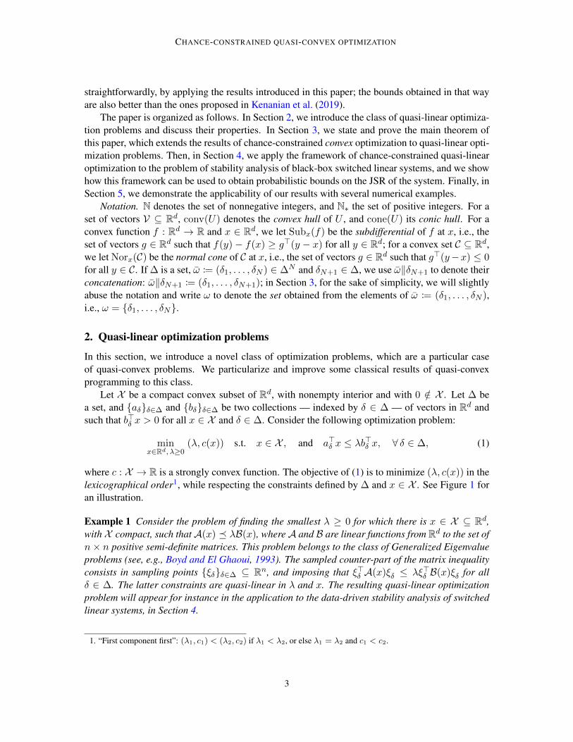
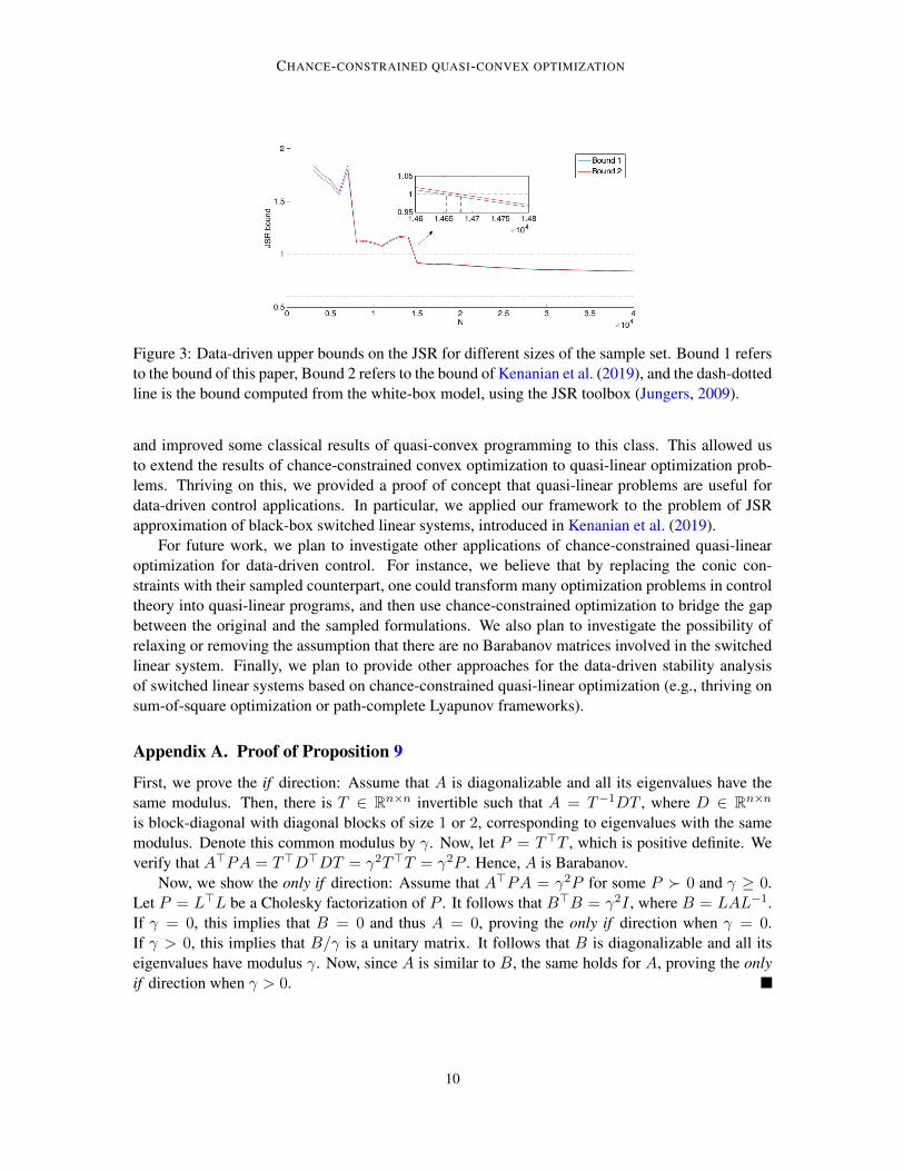
where c : X → R is a strongly convex function. The objective of (1) is to minimize (λ, c(x)) in thelexicographical order1, while respecting the constraints defined by ∆ and x ∈ X . See Figure 1 foran illustration.

Example 1 Consider the problem of finding the smallest λ ≥ 0 for which there is x ∈ X ⊆ Rd,with X compact, such thatA(x) λB(x), whereA and B are linear functions from Rd to the set ofn× n positive semi-definite matrices. This problem belongs to the class of Generalized Eigenvalueproblems (see, e.g., Boyd and El Ghaoui, 1993). The sampled counter-part of the matrix inequalityconsists in sampling points ξδδ∈∆ ⊆ Rn, and imposing that ξ>δ A(x)ξδ ≤ λξ>δ B(x)ξδ for allδ ∈ ∆. The latter constraints are quasi-linear in λ and x. The resulting quasi-linear optimizationproblem will appear for instance in the application to the data-driven stability analysis of switchedlinear systems, in Section 4.

1. “First component first”: (λ1, c1) < (λ2, c2) if λ1 < λ2, or else λ1 = λ2 and c1 < c2.

3


𝒳𝑎(2)⊤ 𝑥 ≤ 𝜆 1 𝑏(2)

⊤ 𝑥

𝑥1

𝑥2

𝑎 1⊤ 𝑥 ≤ 𝜆(1)𝑏 1

⊤ 𝑥𝒳

𝑥1

𝑥2

𝒳

𝑥1

𝑥2

𝑥∗

𝑐 𝑥 = 𝑐𝑡𝑒

𝑎 1⊤ 𝑥 ≤ 𝜆(2)𝑏 1

⊤ 𝑥 𝑎(2)⊤ 𝑥 ≤ 𝜆 2 𝑏(2)

⊤ 𝑥 𝑎 1⊤ 𝑥 ≤ 𝜆∗𝑏 1

⊤ 𝑥 𝑎(2)⊤ 𝑥 ≤ 𝜆∗𝑏(2)

⊤ 𝑥

𝜆(1) > 𝜆 2 > 𝜆∗

𝑐 𝑥 = 𝑐𝑡𝑒 𝑐 𝑥 = 𝑐𝑡𝑒

Figure 1: Set of feasible points x ∈ Rd of a quasi-linear optimization problem (1), for three differentvalues of λ. The blue set X represents the fixed constraints, while the two quasi-linear constraintsare represented in black. The dotted curves are level-curves of the secondary cost function c(x).The smallest λ for which there is a feasible point x is the optimal λ, denoted λ∗. For this value ofλ, the feasible point x that minimizes c is the optimal point x, denoted x∗.

Sometimes, it is not possible to solve (1) with all the constraints defined by ∆, either becauseonly a subset of these constraints are known (as it is the case for instance in data-driven controlproblems), or because the set ∆ is so large (or even infinite) that it is algorithmically impracticableto enforce all of these constraints. In these cases, for a finite set ω ⊆ ∆, we consider the followingsampled optimization problem:

P(ω) : minx∈Rd, λ≥0

(λ, c(x)) s.t. x ∈ X , and a>δ x ≤ λb>δ x, ∀ δ ∈ ω. (2)

We let Opt(ω) be the optimal solution2 of P(ω) and we let Cost(ω) be its optimal cost. Theconstraints of P(ω) defined by ω will be called the sampled constraints, while the constraint x ∈ Xis the common constraint.

For a fixed value of λ, the sampled constraints of P(ω) are linear in x. Therefore, we will saythat P(ω) is a quasi-linear optimization problem. Note that P(ω) is a particular instance of quasi-convex optimization problems, as defined in Eppstein (2005). It is shown there that, under sometechnical assumption on the continuity of the constraints, the cardinality of any essential set (seeDefinition 1 below) of a quasi-convex problem is upper bounded by d+1, where d is the dimensionof x. In this paper, we provide for quasi-linear problems a better upper bound on the cardinality oftheir essential sets, and without the technical assumption of “continuously shrinking” constraints,present in Eppstein (2005).

Definition 1 (Calafiore, 2010, Definition 2.9) An essential set for P(ω) is a set β ⊆ ω, with mini-mal cardinality, satisfying Cost(β) = Cost(ω).

Theorem 2 Let P(ω) be as in (2). The cardinality of any essential set β of P(ω) satisfies |β| ≤ d.

To prove this theorem, we will need the following lemma.

2. By the strong convexity of c, Opt(ω) is unique.

4


Lemma 3 (Rockafellar, 1970, Theorem 27.4) Let f : Rd → R be a convex function and C ⊆ Rd anonempty convex set. Then, x ∈ C is a mininizer3 of f over C if and only if 0 ∈ Subx(f)+Norx(C).

Proof of Theorem 2 Let β be an essential set for P(ω) and let (λ∗, x∗) = Opt(ω). For each δ ∈ ω,let hδ = aδ − λ∗bδ. Let γ ⊆ ω be the set of all δ ∈ ω such that h>δ x

∗ = 0. We divide the proof intwo cases.

Case 1: First, we consider the case when λ∗ = 0. Assume that x ∈ X is a support constraint,meaning that the optimal cost of P(ω) without this constraint is strictly smaller than Cost(ω).Then, by the classical argument4, there is a set of at most d constraints among those of P(ω) (i.e.,among the constraints defined by ω, and the constraint x ∈ X ) such that the optimal solution of theproblem with these constraints only is equal to Cost(ω). Because x ∈ X is a support constraint, itmust belong to this set of constraints. Hence, there is a set β′ ⊆ ω, with |β′| ≤ d − 1, such thatCost(β′) = Cost(ω). This shows that |β| ≤ d− 1 when x ∈ X is a support constraint.

Now, assume that x ∈ X is not a support constraint, i.e., the optimal cost of P(ω) without thisconstraint is the same as Cost(ω). By Lemma 3, it holds that 0 ∈ Subx∗(c) + cone(hδδ∈γ). Notethat, by definition of γ, the vectors hδδ∈γ are all orthogonal to x∗, so that they belong to a (d−1)-dimensional subspace. Hence, by Caratheodory theorem5, there is a set γ′ ⊆ γ, with |γ′| ≤ d − 1,such that 0 ∈ Subx∗(c) + cone(hδδ∈γ′). By Lemma 3, it thus follows that Cost(γ′) = Cost(ω).This shows that |β| ≤ d − 1 when x ∈ X is not a support constraint; concluding the proof for thefirst case.

Case 2: Now, we consider the case when λ∗ > 0. By Lemma 3 applied on f(x) = supδ∈γ h>δ x

and C = X , it follows that 0 ∈ conv(hδδ∈γ) + Norx∗(X ). Let γ′ ⊆ γ be a nonempty subset withminimal cardinality such that 0 ∈ conv(hδδ∈γ′) + Norx∗(X ). By Caratheodory theorem, it holdsthat |γ′| ≤ d − f + 1 where f is the dimension of the linear subspace orthogonal to hδδ∈γ′ . Weconclude the proof by using the same argument as in case 1: since the problem is now restricted toan f -dimensional problem (because x is in the subspace orthogonal to hδδ∈γ′), we may find a setβ′ ⊆ ω, with |β′| ≤ f−1, such that Opt(γ′∪β′) = (λ∗, x∗). This shows that |β| ≤ |γ′|+ |β′| ≤ d;concluding the proof for the second case.

3. Chance-constrained quasi-linear optimization

Let P be a probability measure on ∆. Suppose that the constraints δ1, . . . , δN are sampled from∆ according to P, and that we solve the problem P(ωN ) where ωN = δ1, . . . , δN. This ap-proach of solving the optimization problem for a few randomly sampled constraints is called chance-constrained optimization. Under certain assumptions, probabilistic guarantees can be obtained onthe measure of the set of constraints δ ∈ ∆ that are compatible with the optimal solution of P(ωN ).This is the case, for instance, for a large class of convex optimization problems (see, e.g., Calafiore,2010) and non-convex optimization problems (though with weaker probabilistic guarantees; see,e.g., Campi et al., 2018). In this section, we extend the results from chance-constrained convexoptimization (Calafiore, 2010) to chance-constrained quasi-linear problems.

3. I.e., f(x∗) = infx∈C f(x).4. Indeed, P(ω) with λ fixed to zero is a convex optimization problem, and the cardinality of essential sets of feasible

convex optimization problems is bounded by d (see, e.g., Calafiore and Campi, 2006, Theorem 3).5. See, e.g., Rockafellar (1970, Corollary 17.1.2).

5


Therefore, we make the following standing assumption (Assumption 5) on the set ∆ and on itsprobability measure P. First, let us introduce the notion of non-degenerate vector of constraints.

Definition 4 (Calafiore, 2010, Definition 2.11) Consider Problem (1). Let N ∈ N∗. We say thatωN := (δ1, . . . , δN ) ∈ ∆N is non-degenerate if there is a unique set I ⊆ 1, . . . , N such thatδii∈I is an essential set for P(ωN ).

Assumption 5 (Calafiore, 2010, Assumption 2) For every N ∈ N∗, the vector ωN ∈ ∆N is non-degenerate with probability one.

For any vector of constraints ωN ∈ ∆N , we define the violating probability associated to ωN :

V (ωN ) = P(δ ∈ ∆ : Cost(ωN ∪ δ) > Cost(ωN )).

We are now able to present the extension of Calafiore (2010, Theorem 3.3) to chance-constrainedquasi-linear programs. Therefore, let ζ ∈ N∗ be an upper bound on the cardinality of any essentialset of P(ω), with finite ω ⊆ ∆. From Theorem 2, it holds that ζ ≤ d.

Theorem 6 Consider the sampled quasi-linear optimization problem (2), and let V (ωN ) and ζ beas above. Let Assumption 5 hold. Let N ∈ N, N ≥ ζ, and let ε ∈ (0, 1). Then,

PN (ωN ∈ ∆N : V (ωN ) > ε) ≤ Φ(ε, ζ − 1, N),

where Φ(·, ζ − 1, N) is the regularized incomplete beta function6.

Using Theorem 2, different proofs can be used to get the above result; see, e.g., Campi andGaratti (2018, Theorem 3). Here, we present a proof based on Calafiore (2010, Theorem 3.3).

Proof (Adapted from Calafiore, 2010) Fix N ∈ N, N ≥ ζ. By Assumption 5, we may assumewithout loss of generality that ωN is non-degenerate for all ωN ∈ ∆N . Hence, for each ωN :=(δ1, . . . , δN ) ∈ ∆N , we let J(ωN ) be the unique set I ⊆ 1, . . . , N such that δii∈I is anessential set for P(ωN ). Label the elements of ∆ with labels belonging to a totally order set.7 LetJ∗(ωN ) be a completion of J(ωN ) with the ζ − |J(ωN )| elements of 1, . . . , N \ J(ωN ) suchthat δii∈J∗(ωN )\J(ωN ) have the largest labels among the elements of ωN . From Assumption 5, itfollows that J∗(ωN ) is well defined with probability one; hence, in the following, we will assumewithout loss of generality that J∗(ωN ) is well defined for all ωN ∈ ∆N .

Let I1, . . . , IM be the set of all subsets of 1, . . . , N with ζ elements; in particular, M =N !/(ζ!(N − ζ)!) , C(N, ζ). For each i = 1, . . . ,M , let Si = ωN ∈ ∆N : J∗(ωN ) = Ii. Thesets Si1≤i≤M are disjoint and their union is equal to ∆N . Moreover, by the symmetry of theirdefinition, they have the same probability; hence P(Si) = 1/C(N, ζ).

Now, for each ωζ ∈ ∆ζ , we let V ∗(ωζ) be the violating probability of ωζ with respect to (2) andthe labelling of the constraints: that is, V ∗(ωζ) = P(δ ∈ ∆ : J∗(ωζ‖δ) 6= 1, . . . , ζ). From theuniqueness of the optimal solution of the problems P(ω), ω ⊆ ∆, it follows that for every L ∈ N∗,

6. See, e.g., Kenanian et al. (2019, Definition 2).7. This approach, from Calafiore (2010), requires the axiom of choice when ∆ is a general set. However, it is not needed

for instance if ∆ ⊆ Rn, as it is the case in our application (see Section 4).

6


ωL ∈ ∆L and δ, η ∈ ∆, if J∗(ωL‖δ) = J∗(ωL‖η) = J∗(ωL), then J∗((ωL‖δ)‖η) = J∗(ωL).8 Itfollows that, for any v ∈ [0, 1],

P[Si | V ∗(ωN,i) = v] = (1− v)N−ζ , ∀N ≥ ζ, i = 1, . . . , C(N, ζ),

where ωN,i is the restriction of ωN to the indices in Ii: ωN,i = (δi)i∈Ii . Hence, we get that

P(Si) =w 1

0(1− v)N−ζ dFi(v) = 1/C(N, ζ), ∀N ≥ ζ, i = 1, . . . , C(N, ζ), (3)

where Fi(v) = PN (ωN ∈ ∆N : V ∗(ωN,i) ≤ v). Equation (3) describes a Hausdorff momentproblem; it is shown in Calafiore (2010, p. 3436) that (3) implies that Fi(v) = vζ .

Finally, for each i = 1, . . . , C(N, ζ), we let Bi = ωN ∈ ∆N : V ∗(ωN,i) > ε. Using theexpression of Fi, it can be shown9 that PN (Bi) = Φ(ε, ζ − 1, N)/C(N, ζ). By symmetry, we getthat PN (

⋃1≤i≤M Bi) = Φ(ε, ζ − 1, N). Since ωN ∈ ∆N : V (ωN ) > ε ⊆

⋃1≤i≤M Bi, we

obtain the desired result.

4. Application to data-driven stability analysis of switched linear systems

Let A = A1, . . . , Am be a fixed set of matrices in Rn×n, and let S be the unit sphere (boundaryof the unit Euclidean ball) in Rn. Let ∆ = A× S, and let P be the uniform distribution on ∆.10 Fora finite set ω ⊆ ∆, we consider the following sampled quasi-linear optimization problem:

Pjsr(ω) : minP=P>∈Rn×n,

γ≥0

(γ, ‖P‖2F ) s.t. P ∈ X := P : P I ∧ ‖P‖F ≤ C,

(Ax)>P (Ax) ≤ γ2x>Px, ∀ (A, x) ∈ ω,(4)

for some fixed parameter C ≥ n. Note that Pjsr(ω) is a sampled, data-driven version of the clas-sical quadratic Lyapunov framework for the approximation of the Joint Spectral Radius (JSR) ofthe switched linear system defined by A; see, e.g., Jungers (2009, Theorem 2.11). The JSR is aubiquituous measure of stability of switched linear systems (Blondel and Nesterov, 2005; Parriloand Jadbabaie, 2008; Jungers et al., 2017); it also appears in other areas of hybrid system control,like wireless networked control (Berger and Jungers, 2020).

In order to apply the results from Section 3 on Pjsr(ω), we make the following assumption onthe matrices in A. First, let us introduce the notion of Barabanov matrix (referring to the fact thatthese matrices admit a quadratic Barabanov norm; see Jungers, 2009, Definition 2.3).

Definition 7 A matrix A ∈ Rn×n is said to be Barabanov if there exists a symmetric matrix P 0and γ ≥ 0 such that A>PA = γ2P .

Assumption 8 There is no Barabanov matrix in A.

We claim that Assumption 8 is not restrictive in most of the practical situations. To motivate thisclaim, we provide an equivalent characterization of Barabanov matrices in the proposition below,whose proof can be found in Appendix A. For further work, we plan to investigate the possibility torelax or remove this technical assumption.

8. See, e.g., Calafiore (2010, §2.1) for details.9. See, e.g., Calafiore (2010, Theorem 3.3).

10. I.e., P = P1 ⊗ P2 where P1 and P2 are the uniform distributions on A and S respectively.

7


Proposition 9 A matrix A ∈ Rn×n is Barabanov if and only if it is diagonalizable and all itseigenvalues have the same modulus.

We now show that Assumption 8 ensures that Assumption 5 holds for (4).

Proposition 10 Consider the sampled problem (4). Let Assumption 8 hold. Then, for every N ∈N∗, the vector ωN ∈ ∆N is non-degenerate with probability one.

We will need the following lemma.

Lemma 11 Let P (x1, . . . , xn) be a nonzero polynomial on Rn. The zero set of P , i.e., the set ofpoints x ∈ Rn such that P (x) = 0, has zero Lebesgue measure.

We skip the proof of this well-known fact (see, e.g., Teschl, Problem 2.15).

Proof of Proposition 10 Let ωN = δ1, . . . , δN. Let 1 ≤ i ≤ N−1. Let us look at the probabilitythat β := δ1, . . . , δi is an essential set for Pjsr(ω) and that δN is in another essential set. Thisprobability is smaller than or equal to the probability that β is an essential set for Pjsr(ω) and that(Ax)>P (Ax) = γ2x>Px, where (γ, P ) = Optjsr(β) and δN = (A, x).

Assume that the above probability is nonzero. Then, since A is finite, that there is A ∈ A suchthat (Ax)>P (Ax) = γ2x>Px for all x in a set S ⊆ S with nonzero measure. Thus, by Lemma 11,it holds that (Ax)>P (Ax) = γ2x>Px for all x ∈ S. This contradicts the assumption that thereis no Barabanov matrix in A. Hence, the probability that β is a basis for Pjsr(ω) and that δN is inanother basis is zero. Since β and δN were arbitrary, this concludes the proof.

Theorem 6 can thus be applied to Pjsr(ω).

Corollary 12 Consider the sampled problem (4). Let Assumption 8 hold. Let N ∈ N, N ≥ d :=n(n+1)

2 , and let ε ∈ (0, 1). Then,

PN (ωN ∈ ∆N : Vjsr(ωN ) > ε) ≤ Φ(ε, d− 1, N), (5)

where Vjsr(ωN ) = P(δ ∈ ∆ : Costjsr(ωN ∪ δ) > Costjsr(ωN )).

Remark 13 We note the improvement of the right-hand side term of (5), compared to Kenanianet al. (2019, Theorem 10); this term becomes Φ(ε, d − 1, N) instead of Φ(ε, d,N) in Kenanianet al. (2019). This is due to the improvement of the bound on the cardinality of essential sets ofquasi-linear problems; see Theorem 2.

From Corollary 12, we deduce the following probabilistic guarantee on the upper bound on theJSR of the switched linear system given by A, that we can get from the solution of the sampledproblem Pjsr(ω). The derivation of this result follows the same lines as in Kenanian et al. (2019,Theorems 14 and 15), so that the details are omitted here.

Corollary 14 Consider the sampled problem (4). Let Assumption 8 hold. Let N ∈ N, N ≥ d :=n(n+1)

2 , and let ε ∈ (0, 1). Then, for all ωN ∈ ∆N , except possibly those ωN in a subset Ω ⊆ ∆N

with measure PN (Ω) ≤ Φ(ε, d− 1, N), it holds that

ρ(A) ≤ γ∗/√

1− I−1(εκ(P ∗)

m;d− 1

2;1

2

),

8


where (γ∗, P ∗) = Optjsr(ωN ), κ(P ) =√

det(P )λmin(P )n , I−1 is the inversed regularized incomplete

beta function11 and ρ(A) is the JSR of the switched linear system defined by A.

5. Numerical experiments: consensus of hidden network

We consider the problem of consensus in a switching and hidden network. The interaction betweenthe nodes in the network over time can be modeled as a switched linear dynamical system:

x(t+ 1) = Aσ(t)x(t), x(t) ∈ Rn, Aσ(t) ∈ A := A1, . . . , Am ⊆ Rn×n,

where x(t) is the state vector (n is the number of nodes) at time t and Aσ(t) is the interactionmatrix at time t, with Ai being unknown row-stochastic matrices, i.e., Ai1 = 1, i = 1, . . . ,m,where 1 is the all-one vector in Rn. The goal is to verify that x(t) = Aσ(t−1) · · ·Aσ(1)Aσ(0)x(0)converges to c1 for some c as t → ∞. As shown by Jadbabaie et al. (2003), this question boilsdown to the computation of the JSR of A′ := A′1, . . . , A′m ⊆ Rn−1×n−1 where A′i = BAiB

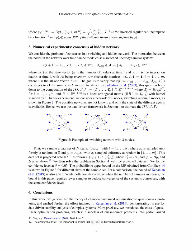
>,for i = 1, . . . ,m, and B ∈ Rn−1×n is a fixed orthogonal matrix (BB> = In−1) with kernelspanned by 1. In our experiment, we consider a network of 8 nodes, switching among 3 modes, asshown in Figure 2. The possible networks are not known, and only the state of the different agentsis available. Hence, we use the data-driven framework in Section 4 to estimate the JSR of A′.

Figure 2: Example of switching network with 3 modes.

First, we sample a data set of N pairs: (xi, yi), with i = 1, . . . , N , where xi is sampled uni-formly at random on S and yi = Aσixi, with σi sampled uniformly at random in 1, . . . ,m. Thisdata set is projected onto Rn−1 as follows: (xi, yi) 7→ (x′i, y

′i) where x′i = Bxi and y′i = Byi and

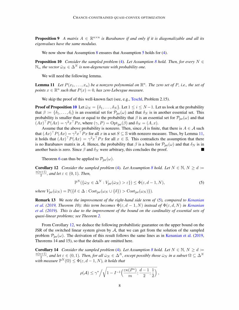
B is as above.12 We then solve the problem in Section 4 with the projected data set. We fix theconfidence level at β = 0.05. The probabilistic upper bound on the JSR obtained from Corollary 14is shown in Figure 3 for different sizes of the sample set. For a comparison, the bound of Kenanianet al. (2019) is also given. While both bounds converge when the number of samples increases, thebound in this paper requires fewer samples to deduce convergence of the system to consensus, withthe same confidence level.

6. Conclusions

In this work, we generalized the theory of chance-constrained optimization to quasi-convex prob-lems, and pushed further the effort initiated in Kenanian et al. (2019), demonstrating its use fordata-driven stability analysis of complex systems. More precisely, we introduced the class of quasi-linear optimization problems, which is a subclass of quasi-convex problems. We particularized

11. See, e.g., Kenanian et al. (2019, Definition 2).12. The orthogonality of B is important to ensure that x′i/‖x′i‖ is distributed uniformly on S.

9


Figure 3: Data-driven upper bounds on the JSR for different sizes of the sample set. Bound 1 refersto the bound of this paper, Bound 2 refers to the bound of Kenanian et al. (2019), and the dash-dottedline is the bound computed from the white-box model, using the JSR toolbox (Jungers, 2009).

and improved some classical results of quasi-convex programming to this class. This allowed usto extend the results of chance-constrained convex optimization to quasi-linear optimization prob-lems. Thriving on this, we provided a proof of concept that quasi-linear problems are useful fordata-driven control applications. In particular, we applied our framework to the problem of JSRapproximation of black-box switched linear systems, introduced in Kenanian et al. (2019).

For future work, we plan to investigate other applications of chance-constrained quasi-linearoptimization for data-driven control. For instance, we believe that by replacing the conic con-straints with their sampled counterpart, one could transform many optimization problems in controltheory into quasi-linear programs, and then use chance-constrained optimization to bridge the gapbetween the original and the sampled formulations. We also plan to investigate the possibility ofrelaxing or removing the assumption that there are no Barabanov matrices involved in the switchedlinear system. Finally, we plan to provide other approaches for the data-driven stability analysisof switched linear systems based on chance-constrained quasi-linear optimization (e.g., thriving onsum-of-square optimization or path-complete Lyapunov frameworks).

Appendix A. Proof of Proposition 9

First, we prove the if direction: Assume that A is diagonalizable and all its eigenvalues have thesame modulus. Then, there is T ∈ Rn×n invertible such that A = T−1DT , where D ∈ Rn×nis block-diagonal with diagonal blocks of size 1 or 2, corresponding to eigenvalues with the samemodulus. Denote this common modulus by γ. Now, let P = T>T , which is positive definite. Weverify that A>PA = T>D>DT = γ2T>T = γ2P . Hence, A is Barabanov.

Now, we show the only if direction: Assume that A>PA = γ2P for some P 0 and γ ≥ 0.Let P = L>L be a Cholesky factorization of P . It follows that B>B = γ2I , where B = LAL−1.If γ = 0, this implies that B = 0 and thus A = 0, proving the only if direction when γ = 0.If γ > 0, this implies that B/γ is a unitary matrix. It follows that B is diagonalizable and all itseigenvalues have modulus γ. Now, since A is similar to B, the same holds for A, proving the onlyif direction when γ > 0.

10


References

Rajeev Alur, Alessandro D’Innocenzo, Karl H Johansson, George J Pappas, and Gera Weiss. Mod-eling and analysis of multi-hop control networks. In 2009 15th IEEE Real-Time and EmbeddedTechnology and Applications Symposium, pages 223–232. IEEE, 2009. doi: 10.1109/RTAS.2009.40.

Anil Aswani, Neal Master, Jay Taneja, Virginia Smith, Andrew Krioukov, David Culler, andClaire J Tomlin. Identifying models of HVAC systems using semiparametric regression. In2012 American Control Conference (ACC), pages 3675–3680. IEEE, 2012. doi: 10.1109/ACC.2012.6315566.

Ayca Balkan, Paulo Tabuada, Jyotirmoy V Deshmukh, Xiaoqing Jin, and James Kapinski. Under-miner: a framework for automatically identifying nonconverging behaviors in black-box systemmodels. ACM Transactions on Embedded Computing Systems (TECS), 17(1):1–28, 2017. doi:10.1145/3122787.

Guillaume O Berger and Raphael M Jungers. Worst-case topological entropy and minimal datarate for state observation of switched linear systems. In Proceedings of the 23rd InternationalConference on Hybrid Systems: Computation and Control, pages 1–11. ACM, 2020. doi: 10.1145/3365365.3382195.

Franco Blanchini, Gianfranco Fenu, Giulia Giordano, and Felice Andrea Pellegrino. Model-freeplant tuning. IEEE Transactions on Automatic Control, 6(62):2623–2634, 2016. doi: 10.1109/TAC.2016.2616025.

Vincent D Blondel and Yurii Nesterov. Computationally efficient approximations of the joint spec-tral radius. SIAM Journal on Matrix Analysis and Applications, 27(1):256–272, 2005. doi:10.1137/040607009.

Ross Boczar, Nikolai Matni, and Benjamin Recht. Finite-data performance guarantees for theoutput-feedback control of an unknown system. In 2018 IEEE Conference on Decision andControl (CDC), pages 2994–2999. IEEE, 2018. doi: 10.1109/CDC.2018.8618658.

Stephen Boyd and Laurent El Ghaoui. Method of centers for minimizing generalized eigenvalues.Linear algebra and its applications, 188:63–111, 1993. doi: 10.1016/0024-3795(93)90465-Z.

Giuseppe C Calafiore. Random convex programs. SIAM Journal on Optimization, 20(6):3427–3464, 2010. doi: 10.1137/090773490.

Giuseppe C Calafiore and Marco C Campi. The scenario approach to robust control design. IEEETransactions on Automatic Control, 51(5):742–753, 2006. doi: 10.1109/TAC.2006.875041.

Marco C Campi and Simone Garatti. Wait-and-judge scenario optimization. Mathematical Pro-gramming, 167(1):155–189, 2018. doi: 10.1007/s10107-016-1056-9.

Marco C Campi, Simone Garatti, and Federico A Ramponi. A general scenario theory for non-convex optimization and decision making. IEEE Transactions on Automatic Control, 63(12):4067–4078, 2018. doi: 10.1109/TAC.2018.2808446.

11


Jeremy Coulson, John Lygeros, and Florian Dorfler. Distributionally robust chance constraineddata-enabled predictive control. arXiv:2006.01702, 2020.

Parasara Sridhar Duggirala, Sayan Mitra, and Mahesh Viswanathan. Verification of annotated mod-els from executions. In 2013 Proceedings of the International Conference on Embedded Software(EMSOFT), pages 1–10. IEEE, 2013. doi: 10.1109/EMSOFT.2013.6658604.

David Eppstein. Quasiconvex programming. Combinatorial and Computational Geometry, 52:287–331, 2005.

Zhenqi Huang and Sayan Mitra. Proofs from simulations and modular annotations. In Proceedingsof the 17th International Conference on Hybrid Systems: Computation and Control, pages 183–192. ACM, 2014. doi: 10.1145/2562059.2562126.

Ali Jadbabaie, Jie Lin, and A Stephen Morse. Coordination of groups of mobile autonomous agentsusing nearest neighbor rules. IEEE Transactions on Automatic Control, 48(6):988–1001, 2003.doi: 10.1109/TAC.2003.812781.

Raphael M Jungers. The joint spectral radius: theory and applications, volume 385 of LectureNotes in Control and Information Sciences. Springer-Verlag Berlin Heidelberg, 2009. doi: 10.1007/978-3-540-95980-9.

Raphael M Jungers, Amir Ali Ahmadi, Pablo A Parrilo, and Mardavij Roozbehani. A characteriza-tion of Lyapunov inequalities for stability of switched systems. IEEE Transactions on AutomaticControl, 62(6):3062–3067, 2017. doi: 10.1109/TAC.2017.2671345.

Joris Kenanian, Ayca Balkan, Raphael M Jungers, and Paulo Tabuada. Data driven stability analysisof black-box switched linear systems. Automatica, 109:108533, 2019. doi: 10.1016/j.automatica.2019.108533.

Alexandar Kozarev, John Quindlen, Jonathan How, and Ufuk Topcu. Case studies in data-drivenverification of dynamical systems. In Proceedings of the 19th International Conference on HybridSystems: Computation and Control, pages 81–86. ACM, 2016. doi: 10.1145/2883817.2883846.

Kostas Margellos, Paul J Goulart, and John Lygeros. On the road between robust optimizationand the scenario approach for chance constrained optimization problems. IEEE Transactions onAutomatic Control, 59(8):2258–2263, 2014. doi: 10.1109/TAC.2014.2303232.

Pablo A Parrilo and Ali Jadbabaie. Approximation of the joint spectral radius using sum of squares.Linear Algebra and Its Applications, 428(10):2385–2402, 2008. doi: 10.1016/j.laa.2007.12.027.

R Tyrrell Rockafellar. Convex analysis. Princeton University Press, 1970.

Michael G Safonov, Keat-Choon Goh, and JH Ly. Control system synthesis via bilinear matrixinequalities. In Proceedings of 1994 American Control Conference – ACC ’94, pages 45–49.IEEE, 1994. doi: 10.1109/ACC.1994.751690.

Gerald Teschl. Topics in real analysis. Graduate studies in mathematics. American MathematicalSociety. https://www.mat.univie.ac.at/˜gerald/ftp/book-ra/ra.pdf.

12

https://www.mat.univie.ac.at/~gerald/ftp/book-ra/ra.pdf


Bart PG Van Parys, Daniel Kuhn, Paul J Goulart, and Manfred Morari. Distributionally robustcontrol of constrained stochastic systems. IEEE Transactions on Automatic Control, 61(2):430–442, 2015. doi: 10.1109/TAC.2015.2444134.

Jeremy G VanAntwerp and Richard D Braatz. A tutorial on linear and bilinear matrix inequalities.Journal of process control, 10(4):363–385, 2000. doi: 10.1016/S0959-1524(99)00056-6.

Zheming Wang and Raphael M Jungers. A data-driven method for computing polyhedral invariantsets of black-box switched linear systems. arXiv:2009.10984, 2020.

Datong P Zhou, Qie Hu, and Claire J Tomlin. Quantitative comparison of data-driven and physics-based models for commercial building HVAC systems. In 2017 American Control Conference(ACC), pages 2900–2906. IEEE, 2017. doi: 10.23919/ACC.2017.7963391.

13

chance-constrained quasi-convex optimization with

Documents