Linear Algebra and its Applications 437 (2012) 1264–1284

Contents lists available at SciVerse ScienceDirect

Linear Algebra and its Applications

journal homepage: www.elsevier .com/locate/ laa

SOC-monotone and SOC-convex functions vs.

matrix-monotone and matrix-convex functions<

Shaohua Pana, Yungyen Chiangb, Jein-Shan Chenc,∗,1,2aDepartment of Mathematics, South China University of Technology, Wushan Road 381, Tianhe District, Guangzhou 510641, China

bDepartment of Applied Mathematics, National Sun Yat-sen University, Kaohsiung 80424, Taiwan

cDepartment of Mathematics, National Taiwan Normal University, Taipei 11677, Taiwan

A R T I C L E I N F O A B S T R A C T

Article history:

Received 30 September 2010

Accepted 9 April 2012

Available online 12 May 2012

Submitted by R.A. Brualdi

AMS classification:

26B05

26B35

90C33

65K05

Keywords:

Hilbert space

Second-order cone

SOC-monotonicity

SOC-convexity

The SOC-monotone function (respectively, SOC-convex function) is a

scalar valued function that induces amap to preserve themonotone

order (respectively, the convex order),when imposedon the spectral

factorization of vectors associated with second-order cones (SOCs)

in general Hilbert spaces. In this paper, we provide the sufficient

and necessary characterizations for the two classes of functions, and

particularly establish that the set of continuous SOC-monotone (re-

spectively, SOC-convex) functions coincides with that of continuous

matrix monotone (respectively, matrix convex) functions of order 2.

© 2012 Elsevier Inc. All rights reserved.

1. Introduction

Let H be a real Hilbert space of dimension dim(H) ≥ 3 endowed with an inner product 〈·, ·〉and its induced norm ‖ · ‖. Fix a unit vector e ∈ H and denote by 〈e〉⊥ the orthogonal complementary

< This work was supported by National Young Natural Science Foundation (No. 10901058) and the Fundamental Research Funds

for the Central Universities.∗ Corresponding author.

E-mail addresses: shhpan@scut.edu.cn (S. Pan), chiangyy@math.nsysu.edu.tw (Y. Chiang), jschen@math.ntnu.edu.tw (J.-S. Chen).1 The author’s work is supported by National Science Council of Taiwan, Department of Mathematics, National Taiwan Normal

University, Taipei 11677, Taiwan.2 Also a Member of Mathematics Division, National Center for Theoretical Sciences, Taipei Office.

0024-3795/$ - see front matter © 2012 Elsevier Inc. All rights reserved.

http://dx.doi.org/10.1016/j.laa.2012.04.030

S. Pan et al. / Linear Algebra and its Applications 437 (2012) 1264–1284 1265

space of e, i.e., 〈e〉⊥ = {x ∈ H | 〈x, e〉 = 0} . Then each x can be written as

x = xe + x0e for some xe ∈ 〈e〉⊥ and x0 ∈ R.

The second-order cone (SOC) in H, also called the Lorentz cone, is a set defined by

K :={x ∈ H | 〈x, e〉 ≥ 1√

2‖x‖

}={xe + x0e ∈ H | x0 ≥ ‖xe‖

}.

From [7, Section 2], we know that K is a pointed closed convex self-dual cone. Hence, H becomes a

partially ordered space via the relation K . In the sequel, for any x, y ∈ H, we always write x K y

(respectively, x K y) when x − y ∈ K (respectively, x − y ∈ intK); and denote xe by the vectorxe‖xe‖

if xe �= 0, and otherwise by any unit vector from 〈e〉⊥.

Associated with the second-order cone K , each x = xe + x0e ∈H can be decomposed as

x = λ1(x)u1(x) + λ2(x)u2(x), (1)

where λi(x) ∈ R and ui(x) ∈ H for i = 1, 2 are the spectral values and the associated spectral vectors

of x, defined by

λi(x) = x0 + (−1)i‖xe‖, ui(x) = 1

2

(e + (−1)ixe

). (2)

Clearly, when xe �= 0, the spectral factorization of x is unique by definition.

Let f : J ⊆ R → R be a scalar valued function, where J is an interval (finite or infinite, closed or

open) in R. Let S be the set of all x ∈ H whose spectral values λ1(x) and λ2(x) belong to J. Unless

otherwise stated, in this paper S is always taken in this way. By the spectral factorization of x in (1)

and (2), it is natural to define f soc : S ⊆ H → H by

f soc(x) := f (λ1(x))u1(x) + f (λ2(x))u2(x), ∀x ∈ S. (3)

It is easy to see that the function f soc is well defined whether xe = 0 or not. For example, by taking

f (t) = t2, we have that f soc(x) = x2 = x ◦ x, where “◦” means the Jordan product and the detailed

definition is see in the next section. Note that

(λ1(x) − λ1(y))2 + (λ2(x) − λ2(y))

2 = 2(‖x‖2 + ‖y‖2 − 2x0y0 − 2‖xe‖‖ye‖)≤ 2

(‖x‖2 + ‖y‖2 − 2〈x, y〉

)= 2‖x − y‖2.

We may verify that the domain S of f soc is open in H if and only if J is open in R. Also, S is always

convex since, for any x = xe + x0e, y = ye + y0e ∈ S and β ∈ [0, 1],λ1 [βx + (1 − β)y] = (

βx0 + (1 − β)y0)− ‖βxe + (1 − β)ye‖ ≥ min{λ1(x), λ1(y)},

λ2 [βx + (1 − β)y] = (βx0 + (1 − β)y0

)+ ‖βxe + (1 − β)ye‖ ≤ max{λ2(x), λ2(y)},which implies that βx + (1 − β)y ∈ S. Thus, f soc (βx + (1 − β)y) is well defined.

In this paper we are interested in two classes of special scalar valued functions that induce the

maps via (3) to preserve the monotone order and the convex order, respectively.

Definition 1.1. A function f : J → R is said to be SOC-monotone if for any x, y ∈ S,

x K y �⇒ f soc(x) K f soc(y); (4)

and f is said to be SOC-convex if, for any x, y ∈ S and any β ∈ [0, 1],f soc (βx + (1 − β)y) �K βf soc(x) + (1 − β)f soc(y). (5)

FromDefinition 1.1 and Eq. (3), it is easy to see that the set of SOC-monotone and SOC-convex functions

are closed under positive linear combinations and pointwise limits.

1266 S. Pan et al. / Linear Algebra and its Applications 437 (2012) 1264–1284

The concept of SOC-monotone (respectively, SOC-convex) functions above is a direct extension of

those given by [5,6] to general Hilbert spaces, and is analogous to that of matrix monotone (respec-

tively, matrix convex) functions and more general operator monotone (respectively, operator convex)

functions; see, e.g., [17,15,14,2,11,23]. Just as the importance ofmatrixmonotone (respectively,matrix

convex) functions to the solution of convex semidefinite programming [19,4], SOC-monotone (respec-

tively, SOC-convex) functions also play a crucial role in the design and analysis of algorithms for convex

second-order cone programming [3,22]. For matrix monotone and matrix convex functions, after the

seminal work of Löwner [17] and Kraus [15], there have been systematic studies and perfect char-

acterizations for them; see [8,16,4,13,12,21,20] and the references therein. However, the study on

SOC-monotone and SOC-convex functions just begins with [5], and the characterizations for them are

still imperfect. Particularly, it is not clearwhat is the relation between the SOC-monotone (respectively,

SOC-convex) functions and the matrix monotone (respectively, matrix convex) functions.

In thiswork,we provide the sufficient and necessary characterizations for SOC-monotone and SOC-

convex functions in the setting of Hilbert spaces, and show that the set of continuous SOC-monotone

(SOC-convex) functions coincideswith that of continuousmatrixmonotone (matrix convex) functions

of order 2. Some of these results generalize those of [5,6] (see Propositions 3.2 and 4.2), and some are

new, which are difficult to achieve by using the techniques of [5,6] (see, for example, Proposition

4.4). In addition, we also discuss the relations between SOC-monotone functions and SOC-convex

functions, verify Conjecture4.2 in [5] under a little stronger condition (seeProposition6.2), andpresent

a counterexample to show that Conjecture 4.1 in [5] generally does not hold. It is worthwhile to point

out that the analysis in this paper depends only on the inner product of Hilbert spaces, whereas most

of the results in [5,6] are obtained with the help of matrix operations.

Throughout this paper, all differentiability means Fréchet differentiability. If F : H → H is (twice)

differentiable at x ∈ H, we denote by F ′(x) (F ′′(x)) the first-order F-derivative (the second-order

F-derivative) of F at x. In addition, we use Cn(J) and C∞(J) to denote the set of n times and infinite

times continuously differentiable real functions on J, respectively. When f ∈ C1(J), we denote by f [1]the function on J × J defined by

f [1](λ, μ) :=⎧⎨⎩

f (λ)−f (μ)λ−μ

if λ �= μ,

f ′(λ) if λ = μ;

and when f ∈ C2(J), denote by f [2] the function on J × J × J defined by

f [2](τ1, τ2, τ3) := f [1](τ1, τ2) − f [1](τ1, τ3)τ2 − τ3

if τ1, τ2, τ3 are distinct, and for other values of τ1, τ2, τ3, f[2] is defined by continuity; e.g.,

f [2](τ1, τ1, τ3) = f (τ3) − f (τ1) − f ′(τ1)(τ3 − τ1)

(τ3 − τ1)2, f [2](τ1, τ1, τ1) = 1

2f ′′(τ1).

For a linear operator L from H into H, we write L ≥ 0 (respectively, L > 0) to mean that L is positive

semidefinite (respectively, positive definite), i.e., 〈h,Lh〉 ≥ 0 for any h ∈ H (respectively, 〈h,Lh〉 > 0

for any 0 �= h ∈ H).

2. Preliminaries

This section recalls some background material and gives several lemmas that will be used in the

subsequent sections. We start with the definition of Jordan product [9]. For any x = xe + x0e, y =ye + y0e ∈ H, the Jordan product of x and y is defined as

x ◦ y := (x0ye + y0xe) + 〈x, y〉e.

S. Pan et al. / Linear Algebra and its Applications 437 (2012) 1264–1284 1267

A simple computation can verify that for any x, y, z ∈ H and the unit vector e, (i) e◦e = e and e◦x = x;

(ii) x ◦ y = y ◦ x; (iii) x ◦ (x2 ◦ y) = x2 ◦ (x ◦ y), where x2 = x ◦ x; (iv) (x + y) ◦ z = x ◦ z + y ◦ z. For

any x ∈ H, define its determinant by

det(x) := λ1(x)λ2(x) = x20 − ‖xe‖2.

Then each x = xe + x0e with det(x) �= 0 is invertible with respect to the Jordan product, i.e., there is

a unique x−1 = (−xe + x0e)/det(x) such that x ◦ x−1 = e.

We next give several lemmas where Lemma 2.1 is used in Section 3 to characterize SOC-

monotonicity, and Lemmas 2.2 and 2.3 are used in Section 4 to characterize SOC-convexity.

Lemma 2.1. Let B := {z ∈ 〈e〉⊥ | ‖z‖ ≤ 1}. Then, for any given u ∈ 〈e〉⊥ with ‖u‖ = 1 and θ, λ ∈ R,

the following results hold.

(a) θ + λ〈u, z〉 ≥ 0 for any z ∈ B if and only if θ ≥ |λ|.(b) θ − ‖λz‖2 ≥ (θ − λ2)〈u, z〉2 for any z ∈ B if and only if θ − λ2 ≥ 0.

Proof. (a) Suppose that θ + λ〈u, z〉 ≥ 0 for any z ∈ B. If λ = 0, then θ ≥ |λ| clearly holds. If λ �= 0,

take z = −sign(λ)u. Since ‖u‖ = 1, we have z ∈ B, and consequently, θ + λ〈u, z〉 ≥ 0 reduces to

θ −|λ| ≥ 0. Conversely, if θ ≥ |λ|, then using the Cauchy–Schwartz inequality yields θ +λ〈u, z〉 ≥ 0

for any z ∈ B.

(b) Suppose that θ − ‖λz‖2 ≥ (θ − λ2)〈u, z〉2 for any z ∈ B. Then we must have θ − λ2 ≥ 0. If not,

for those z ∈ B with ‖z‖ = 1 but 〈u, z〉 �= ‖u‖‖z‖, it holds that(θ − λ2)〈u, z〉2 > (θ − λ2)‖u‖2‖z‖2 = θ − ‖λz‖2,

which contradicts the given assumption. Conversely, if θ − λ2 ≥ 0, the Cauchy–Schwartz inequality

implies that (θ − λ2)〈u, z〉2 ≤ θ − ‖λz‖2 for any z ∈ B. �

Lemma 2.2. For any given a, b, c ∈ R and x = xe + x0e with xe �= 0, the inequality

a[‖he‖2 − 〈he, xe〉2

]+ b

[h0 + 〈xe, he〉]2 + c

[h0 − 〈xe, he〉]2 ≥ 0 (6)

holds for all h = he + h0e ∈ H if and only if a ≥ 0, b ≥ 0 and c ≥ 0.

Proof. Suppose that (6) holds for all h = he + h0e ∈ H. By letting he = xe, h0 = 1 and he =−xe, h0 = 1, respectively, we get b ≥ 0 and c ≥ 0 from (6). If a ≥ 0 does not hold, then by taking

he =√

b+c+1|a|

ze‖ze‖ with 〈ze, xe〉 = 0 and h0 = 1, (6) gives a contradiction −1 ≥ 0. Conversely, if

a ≥ 0, b ≥ 0 and c ≥ 0, then (6) clearly holds for all h ∈ H. �

Lemma 2.3. Let f ∈C2(J) and ue ∈〈e〉⊥ with ‖ue‖= 1. For any h = he + h0e ∈ H, define

μ1(h) := h0 − 〈ue, he〉√2

, μ2(h) := h0 + 〈ue, he〉√2

, μ(h) :=√

‖he‖2 − 〈ue, he〉2.

Then, for any given a, d ∈ R and λ1, λ2 ∈ J, the following inequality

4f ′′(λ1)f′′(λ2)μ1(h)

2μ2(h)2 + 2(a − d)f ′′(λ2)μ2(h)

2μ(h)2

+2 (a + d) f ′′(λ1)μ1(h)2μ(h)2 +

(a2 − d2

)μ(h)4

−2 [(a − d) μ1(h) + (a + d) μ2(h)]2 μ(h)2 ≥ 0 (7)

holds for all h = he + h0e ∈ H if and only if

a2 − d2 ≥ 0, f ′′(λ2)(a − d) ≥ (a + d)2 and f ′′(λ1)(a + d) ≥ (a − d)2. (8)

1268 S. Pan et al. / Linear Algebra and its Applications 437 (2012) 1264–1284

Proof. Suppose that (7) holds for all h = he + h0e ∈ H. Taking h0 = 0 and he �= 0 with 〈he, ue〉 = 0,

we have μ1(h) = 0, μ2(h) = 0 and μ(h) = ‖he‖ > 0, and then (7) gives a2 − d2 ≥ 0. Taking

he �= 0 such that |〈ue, he〉| < ‖he‖ and h0 = 〈ue, he〉 �= 0, we have μ1(h) = 0, μ2(h) = √2h0 and

μ(h) > 0, and then (7) reduces to the following inequality

4[(a − d)f ′′(λ2) − (a + d)2

]h20 + (a2 − d2)(‖he‖2 − h20) ≥ 0.

This implies that (a − d)f ′′(λ2) − (a + d)2 ≥ 0. If not, by letting h0 be sufficiently close to ‖he‖, thelast inequality yields a contradiction. Similarly, taking h with he �= 0 satisfying |〈ue, he〉| < ‖he‖ and

h0 = −〈ue, he〉, we get f ′′(λ1)(a + d) ≥ (a − d)2 from (7).

Next, suppose that (8) holds. Then, the inequalities f ′′(λ2)(a− d) ≥ (a+ d)2 and f ′′(λ1)(a+ d) ≥(a − d)2 imply that the left-hand side of (7) is greater than

4f ′′(λ1)f′′(λ2)μ1(h)

2μ2(h)2 − 4(a2 − d2)μ1(h)μ2(h)μ(h)2 +

(a2 − d2

)μ(h)4,

which is obviously nonnegative ifμ1(h)μ2(h) ≤ 0. Now assume thatμ1(h)μ2(h) > 0. If a2−d2 = 0,

then the last expression is clearly nonnegative, and if a2 − d2 > 0, then the last two inequalities in

(8) imply that f ′′(λ1)f′′(λ2) ≥ (a2 − d2) > 0, and therefore,

4f ′′(λ1)f′′(λ2)μ1(h)

2μ2(h)2 − 4(a2 − d2)μ1(h)μ2(h)μ(h)2 +

(a2 − d2

)μ(h)4

≥ 4(a2 − d2)μ1(h)2μ2(h)

2 − 4(a2 − d2)μ1(h)μ2(h)μ(h)2 +(a2 − d2

)μ(h)4

= (a2 − d2)[2μ1(h)μ2(h) − μ(h)2

]2 ≥ 0.

Thus, we prove that inequality (7) holds. The proof is complete. �

To close this section, we introduce the regularization of a locally integrable real function. Let ϕ be a

real functionof classC∞ with the followingproperties:ϕ ≥ 0,ϕ is even, the support suppϕ = [−1, 1],and

∫R ϕ = 1. Foreachε > 0, letϕε(t) = 1

εϕ( t

ε). Thensuppϕε = [−ε, ε]andϕε hasall theproperties

of ϕ listed above. If f is a locally integrable real function, we define its regularization of order ε as the

function

fε(s) :=∫

f (s − t)ϕε(t)dt =∫

f (s − εt)ϕ(t)dt. (9)

Note that fε is a C∞ function for each ε > 0, and limε→0 fε(x) = f (x) if f is continuous.

3. Characterizations of SOC-monotone functions

In this section we present some characterizations for SOC-monotone functions, by which the set of

continuous SOC-monotone functions is shown to coincide with that of continuous matrix monotone

functions of order 2. To this end, we need the following technical lemma.

Lemma 3.1. For any given f : J → R with J open, let f soc : S → H be defined by (3).

(a) f soc is continuous on S if and only if f is continuous on J.

(b) f soc is (continuously) differentiable on S iff f is (continuously) differentiable on J. Also, when f is

differentiable on J, for any x = xe + x0e ∈ S and v = ve + v0e ∈ H,

(f soc)′(x)v =

⎧⎪⎪⎪⎨⎪⎪⎪⎩

f ′(x0)v if xe = 0;(b1(x) − a0(x))〈xe, ve〉xe + c1(x)v0xe

+a0(x)ve + b1(x)v0e + c1(x)〈xe, ve〉e if xe �= 0,

(10)

where a0(x) = f (λ2(x))−f (λ1(x))λ2(x)−λ1(x)

, b1(x) = f ′(λ2(x))+f ′(λ1(x))2

, c1(x) = f ′(λ2(x))−f ′(λ1(x))2

.

S. Pan et al. / Linear Algebra and its Applications 437 (2012) 1264–1284 1269

(c) If f is differentiable on J, then for any given x ∈ S and all v ∈ H,

(f soc)′(x)e = (f ′)soc(x) and 〈e, (f soc)′(x)v〉 =⟨v, (f ′)soc(x)

⟩.

(d) If f ′ is nonnegative (respectively, positive) on J, then for each x ∈ S,

(f soc)′(x) ≥ 0 (respectively, (f soc)′(x) > 0).

Proof. (a) Suppose that f soc is continuous. Let � be the set composed of those x = te with t ∈ J.

Clearly, � ⊆ S, and f soc is continuous on �. Noting that f soc(x) = f (t)e for any x ∈ �, it follows that

f is continuous on J. Conversely, if f is continuous on J, then f soc is continuous at any x = xe + x0e ∈ S

with xe �= 0 since λi(x) and ui(x) for i = 1, 2 are continuous at such points. Next, let x = xe + x0e

be an arbitrary element from S with xe = 0, and we prove that f soc is continuous at x. Indeed, for any

z = ze + z0e ∈ S sufficiently close to x, it is not hard to verify that

‖f soc(z) − f soc(x)‖ ≤ |f (λ2(z)) − f (x0)|2

+ |f (λ1(z)) − f (x0)|2

+ |f (λ2(z)) − f (λ1(z))|2

.

Since f is continuous on J, and λ1(z), λ2(z) → x0 as z → x, it follows that

f (λ1(z)) → f (x0) and f (λ2(z)) → f (x0) as z → x.

The last two equations imply that f soc is continuous at x.

(b)When f soc is (continuously) differentiable, using the similar arguments as in part (a) can show that

f is (continuously) differentiable. Next assume that f is differentiable. Fix any x = xe+x0e ∈ S.Wefirst

consider the casewhere xe �= 0. Sinceλi(x) for i = 1, 2and xe‖xe‖ are continuously differentiable at such

x, it follows that f (λi(x)) and ui(x) are differentiable and continuously differentiable, respectively, at

x. Then f soc is differentiable at such x by the definition of f soc. Also, an elementary computation shows

that

[λi(x)]′v = 〈v, e〉 + (−1)i〈xe, v − 〈v, e〉e〉

‖xe‖ = v0 + (−1)i〈xe, ve〉‖xe‖ , (11)

(xe

‖xe‖)′

v = v − 〈v, e〉e‖xe‖ − 〈xe, v − 〈v, e〉e〉xe

‖xe‖3= ve

‖xe‖ − 〈xe, ve〉xe‖xe‖3

(12)

for any v = ve + v0e ∈ H, and consequently,

[f (λi(x))]′ v = f ′(λi(x))

[v0 + (−1)i

〈xe, ve〉‖xe‖

],

[ui(x)]′ v = 1

2(−1)i

[ve

‖xe‖ − 〈xe, ve〉xe‖xe‖3

].

Together with the definition of f soc, we calculate that (f soc)′(x)v is equal to

f ′(λ1(x))

2

[v0 − 〈xe, ve〉

‖xe‖] (

e − xe

‖xe‖)

− f (λ1(x))

2

[ve

‖xe‖ − 〈xe, ve〉xe‖xe‖3

]

+ f ′(λ2(x))

2

[v0 + 〈xe, ve〉

‖xe‖] (

e + xe

‖xe‖)

+ f (λ2(x))

2

[ve

‖xe‖ − 〈xe, ve〉xe‖xe‖3

]

= b1(x)v0e + c1(x) 〈xe, ve〉 e + c1(x)v0xe + b1(x)〈xe, ve〉xe+a0(x)ve − a0(x)〈xe, ve〉xe,

where λ2(x) − λ1(x) = 2‖xe‖ is used for the last equality. Thus, we get (10) for xe �= 0. We next

consider the case where xe = 0. Under this case, for any v = ve + v0e ∈ H,

1270 S. Pan et al. / Linear Algebra and its Applications 437 (2012) 1264–1284

f soc(x + v) − f soc(x) = f (x0 + v0 − ‖ve‖)2

(e − ve) + f (x0 + v0 + ‖ve‖)2

(e + ve) − f (x0)e

= f ′(x0)(v0 − ‖ve‖)2

e + f ′(x0)(v0 + ‖ve‖)2

e

+ f ′(x0)(v0 + ‖ve‖)2

ve − f ′(x0)(v0 − ‖ve‖)2

ve + o(‖v‖)= f ′(x0)(v0e + ‖ve‖ve) + o(‖v‖),

where ve = ve‖ve‖ if ve �= 0, and otherwise ve is an arbitrary unit vector from 〈e〉⊥. Hence,

‖f soc(x + v) − f soc(x) − f ′(x0)v‖ = o(‖v‖).This shows that f soc is differentiable at such x with (f soc)′(x)v = f ′(x0)v.

Assume that f is continuously differentiable. From (10), it is easy to see that (f soc)′(x) is continuousat every x with xe �= 0. We next argue that (f soc)′(x) is continuous at every x with xe = 0. Fix any

x = x0e with x0 ∈ J. For any z = ze + z0e with ze �= 0, we have

‖(f soc)′(z)v − (f soc)′(x)v‖ ≤ |b1(z) − a0(z)|‖ve‖ + |b1(z) − f ′(x0)||v0|+|a0(z) − f ′(x0)|‖ve‖ + |c1(z)|(|v0| + ‖ve‖). (13)

Since f is continuously differentiable on J and λ2(z) → x0, λ1(z) → x0 as z → x, we have

a0(z) → f ′(x0), b1(z) → f ′(x0) and c1(z) → 0.

Together with Eq. (13), we obtain that (f soc)′(z) → (f soc)′(x) as z → x.

(c) The result is direct by the definition of (f ′)soc and a simple computation from (10).

(d) Suppose that f ′(t) ≥ 0 for all t ∈ J. Fix any x = xe + x0e ∈ S. If xe = 0, the result is direct. It

remains to consider the case xe �= 0. Since f ′(t) ≥ 0 for all t ∈ J, we have b1(x) ≥ 0, b1(x) − c1(x) =f ′(λ1(x)) ≥ 0, b1(x) + c1(x) = f ′(λ2(x)) ≥ 0 and a0(x) ≥ 0. From part (b) and the definitions of

b1(x) and c1(x), it follows that for any h = he + h0e ∈ H,

〈h, (f soc)′(x)h〉 = (b1(x) − a0(x))〈xe, he〉2 + 2c1(x)h0〈xe, he〉 + b1(x)h20 + a0(x)‖he‖2

= a0(x)[‖he‖2 − 〈xe, he〉2

]+ 1

2(b1(x) − c1(x)) [h0 − 〈xe, he〉]2

+1

2(b1(x) + c1(x)) [h0 + 〈xe, he〉]2 ≥ 0.

This implies that the operator (f soc)′(x) is positive semidefinite. Particularly, if f ′(t) > 0 for all t ∈ J,

we have that 〈h, (f soc)′(x)h〉 > 0 for all h �= 0. The proof is complete. �

Lemma 3.1(d) shows that the differential operator (f soc)′(x) corresponding to a differentiable non-

decreasing f is positive semidefinite. So, the differential operator (f soc)′(x) associated with a differen-

tiable SOC-monotone function is also positive semidefinite.

Proposition 3.1. Assume that f ∈ C1(J)with J open. Then f is SOC-monotone if and only if (f soc)′(x)h ∈ K

for any x ∈ S and h ∈ K.

Proof. If f is SOC-monotone, then for any x ∈ S, h ∈ K and t > 0, we have

f soc(x + th) − f soc(x) K 0,

which, by the continuous differentiability of f soc and the closedness of K , implies that

(f soc)′(x)h K 0.

S. Pan et al. / Linear Algebra and its Applications 437 (2012) 1264–1284 1271

Conversely, for any x, y ∈ S with x K y, from the given assumption we have that

f soc(x) − f soc(y) =∫ 1

0(f soc)′(x + t(x − y))(x − y)dt ∈ K.

This shows that f soc(x) K f soc(y), i.e., f is SOC-monotone. The proof is complete. �

Proposition 3.1 shows that the differential operator (f soc)′(x) associated with a differentiable SOC-

monotone function f leaves K invariant. If, in addition, the linear operator (f soc)′(x) is bijective, then(f soc)′(x) belongs to the automorphism group of K . Such linear operators are important to study the

structure of the cone K (see [9]).

Corollary 3.1. Assume that f ∈ C1(J) with J open. If f is SOC-monotone, then

(a) (f ′)soc(x) ∈ K for any x ∈ S;

(b) f soc is a monotone function, i.e., 〈f soc(x) − f soc(y), x − y〉 ≥ 0 for any x, y ∈ S.

Proof. Part (a) is direct by using Proposition 3.1with h = e and Lemma3.1(c). By part (a), f ′(τ ) ≥ 0 for

all τ ∈ J. Together with Lemma 3.1(d), (f soc)′(x) ≥ 0 for any x ∈ S. Applying the integral mean-value

theorem, it then follows that

〈f soc(x) − f soc(y), x − y〉 =∫ 1

0〈x − y, (f soc)′(y + t(x − y))(x − y)〉dt ≥ 0.

This proves the desired result of part (b). The proof is complete. �

Note that the converse of Corollary 3.1(a) is not correct. For example, for the function f (t) =−t−2 (t > 0), it is clear that (f ′)soc(x) ∈ K for any x ∈ intK , but it is not SOC-monotone by Exam-

ple 5.1(ii). The following proposition provides another sufficient and necessary characterization for

differentiable SOC-monotone functions.

Proposition 3.2. Let f ∈ C1(J) with J open. Then f is SOC-monotone if and only if

⎡⎣ f [1](τ1, τ1) f [1](τ1, τ2)f [1](τ2, τ1) f [1](τ2, τ2)

⎤⎦=

⎡⎢⎢⎢⎣

f ′(τ1)f (τ2) − f (τ1)

τ2 − τ1f (τ1) − f (τ2)

τ1 − τ2f ′(τ2)

⎤⎥⎥⎥⎦ ≥ 0, ∀τ1, τ2 ∈ J. (14)

Proof. The equality is direct by the definition of f [1]. It suffices to prove that f is SOC-monotone if and

only if the inequality in (14) holds for any τ1, τ2 ∈ J. Assume that f is SOC-monotone. By Proposition

3.1, (f soc)′(x)h ∈ K for any x ∈ S and h ∈ K . Fix any x = xe + x0e ∈ S. It suffices to consider the case

where xe �= 0. Since (f soc)′(x)h ∈ K for any h ∈ K , we particularly have (f soc)′(x)(z + e) ∈ K for any

z ∈ B, where B is the set defined in Lemma 2.1. From Lemma 3.1(b), it follows that

(f soc)′(x)(z + e) = [(b1(x) − a0(x)) 〈xe, z〉 + c1(x)] xe + a0(x)z + [b1(x) + c1(x)〈xe, z〉] e.This means that (f soc)′(x)(z + e) ∈ K for any z ∈ B if and only if

b1(x) + c1(x)〈xe, z〉 ≥ 0, (15)

[b1(x) + c1(x)〈xe, z〉]2 ≥ ∥∥[ (b1(x) − a0(x)) 〈xe, z〉 + c1(x)]xe + a0(x)z

∥∥2 . (16)

By Lemma 2.1(a), we know that (15) holds for any z ∈ B if and only if b1(x) ≥ |c1(x)|. Since by a

simple computation the inequality in (16) can be simplified as

b1(x)2 − c1(x)

2 − a0(x)2 ‖z‖2 ≥

[b1(x)

2 − c1(x)2 − a0(x)

2]〈z, xe〉2 ,

1272 S. Pan et al. / Linear Algebra and its Applications 437 (2012) 1264–1284

applying Lemma 2.1(b) yields that (16) holds for any z ∈ B if and only if

b1(x)2 − c1(x)

2 − a0(x)2 ≥ 0.

This shows that (f soc)′(x)(z + e) ∈ K for any z ∈ B if and only if

b1(x) ≥ |c1(x)| and b1(x)2 − c1(x)

2 − a0(x)2 ≥ 0. (17)

The first condition in (17) is equivalent to b1(x) ≥ 0, b1(x)− c1(x) ≥ 0 and b1(x)+ c1(x) ≥ 0, which,

by the expressions of b1(x) and c1(x) and the arbitrariness of x, is equivalent to f ′(τ ) ≥ 0 for all τ ∈ J;

whereas the second condition in (17) is equivalent to

f ′(τ1)f ′(τ2) −[f (τ2) − f (τ1)

τ2 − τ1

]2≥ 0, ∀τ1, τ2 ∈ J.

The two sides show that the inequality in (14) holds for all τ1, τ2 ∈ J.

Conversely, if the inequality in (14) holds for all τ1, τ2 ∈ J, then from the arguments above we have

(f soc)′(x)(z + e) ∈ K for any x = xe + x0e ∈ S and z ∈ B. This implies that (f soc)′(x)h ∈ K for any

x ∈ S and h ∈ K . By Proposition 3.1, f is SOC-monotone. �

Propositions 3.1 and 3.2 provide the characterizations for continuously differentiable SOC-

monotone functions. When f does not belong to C1(J), one may check the SOC-monotonicity of f

by combining the following proposition with Propositions 3.1 and 3.2.

Proposition 3.3. Let f : J → R be a continuous function on the open interval J, and fε be its regularization

defined by (9). Then, f is SOC-monotone if and only if fε is SOC-monotone on Jε for every sufficiently small

ε > 0, where Jε := (a + ε, b − ε) for J = (a, b).

Proof. Throughout the proof, for every sufficiently small ε > 0, we let Sε be the set of all x ∈ Hwhose

spectral values λ1(x), λ2(x) belong to Jε . Assume that fε is SOC-monotone on Jε for every sufficiently

small ε > 0. Let x, y be arbitrary vectors from S with x K y. Then, for any sufficiently small ε > 0,

we have x+ εe, y+ εe ∈ Sε and x+ εe K y+ εe. Using the SOC-monotonicity of fε on Jε yields that

f socε (x + εe) K f socε (y+ εe). Taking the limit ε → 0 and using the convergence of f socε (x) → f soc(x)and the continuity of f soc on S implied by Lemma 3.1(a), we readily obtain that f soc(x) K f soc(y). Thisshows that f is SOC-monotone.

Now assume that f is SOC-monotone. Let ε > 0 be an arbitrary sufficiently small real number. Fix

any x, y ∈ Sε with x K y. Then, for all t ∈ [−1, 1], wehave x−tεe, y−tεe ∈ S and x−tεe K y−tεe.Therefore, f soc(x − tεe) K f soc(y − tεe), which is equivalent to

f (λ1 − tε) + f (λ2 − tε)

2− f (μ1 − tε) + f (μ2 − tε)

2

≥∥∥∥∥∥ f (λ1 − tε) − f (λ2 − tε)

2xe − f (μ1 − tε) − f (μ2 − tε)

2ye

∥∥∥∥∥ .

Together with the definition of fε , it then follows that

fε(λ1) + fε(λ2)

2− fε(μ1) + fε(μ2)

2

=∫ [

f (λ1 − tε) + f (λ2 − tε)

2− f (μ1 − tε) + f (μ2 − tε)

2

]ϕ(t)dt

≥∫ ∥∥∥∥∥ f (λ1 − ε) − f (λ2 − ε)

2xe − f (μ1 − ε) − f (μ2 − ε)

2ye

∥∥∥∥∥ϕ(t)dt

S. Pan et al. / Linear Algebra and its Applications 437 (2012) 1264–1284 1273

≥∥∥∥∥∥∫ [

f (λ1 − ε) − f (λ2 − ε)

2xe − f (μ1 − ε) − f (μ2 − ε)

2ye

]ϕ(t)dt

∥∥∥∥∥=∥∥∥∥∥ fε(λ1) − fε(λ2)

2xe − fε(μ1) − fε(μ2)

2ye

∥∥∥∥∥ .

By the definition of f socε , this shows that f socε (x) K f socε (y), i.e., fε is SOC-monotone. �

From Proposition 3.2 and [2, Theorem V. 3.4], f ∈ C1(J) is SOC-monotone if and only if it is matrix

monotone of order 2. When the continuous f is not in the class C1(J), the result also holds due to

Proposition 3.3 and the fact that f is matrix monotone of order n if and only if fε is matrix monotone

of order n. Thus, we have the following main result.

Theorem 3.1. The set of continuous SOC-monotone functions on the open interval J coincides with that of

continuous matrix monotone functions of order 2 on J.

Remark 3.1. Combining Theorem 3.1 with Löwner’s theorem [17] shows that if f : J → R is a

continuous SOC-monotone function on the open interval J, then f ∈ C1(J).

4. Characterizations of SOC-convex functions

This section is devoted itself to the characterizations of SOC-convex functions, and shows that

the continuous f is SOC-convex if and only if it is matrix convex of order 2. First, for the first-order

differentiable SOC-convex functions, we have the following characterizations.

Proposition 4.1. Assume that f ∈ C1(J) with J open. Then, the following results hold.

(a) f is SOC-convex if and only if for any x, y ∈ S,

f soc(y) − f soc(x) − (f soc)′(x)(y − x) K 0. (18)

(b) If f is SOC-convex, then (f ′)soc is a monotone function on S.

Proof. By following the arguments as in [1, Proposition B.3(a)], the proof of part (a) can be done easily,

and we omit the details. From part (a), it follows that for any x, y ∈ S,

f soc(x) − f soc(y) − (f soc)′(y)(x − y) K 0,

f soc(y) − f soc(x) − (f soc)′(x)(y − x) K 0.

Adding the last two inequalities, we immediately obtain that

[(f soc)′(y) − (f soc)′(x)

](y − x) K 0.

Using the self-duality of K and Lemma 3.1(c) then yields

0 ≤⟨e,[(f soc)′(y) − (f soc)′(x)

](y − x)

⟩=⟨y − x, (f ′)soc(y) − (f ′)soc(x)

⟩.

This shows that (f ′)soc is monotone. The proof is complete. �

Toprovide sufficient andnecessary characterizations for twicedifferentiable SOC-convex functions,

we need the following lemma that offers the second-order differential of f soc.

1274 S. Pan et al. / Linear Algebra and its Applications 437 (2012) 1264–1284

Lemma 4.1. For any given f : J → R with J open, let f soc : S → H be defined by (3).

(a) f soc is twice (continuously) differentiable on S if and only if f is twice (continuously) differentiable

on J. Furthermore, when f is twice differentiable on J, for any given x = xe + x0e ∈ S and u =ue + u0e, v = ve + v0e ∈ H, we have that

(f soc)′′(x)(u, v) = f ′′(x0)u0v0e + f ′′(x0)(u0ve + v0ue) + f ′′(x0)〈ue, ve〉eif xe = 0; and otherwise

(f soc)′′(x)(u, v) = (b2(x) − a1(x))u0〈xe, ve〉xe + (c2(x) − 3d(x))〈xe, ue〉〈xe, ve〉xe+d(x)

[〈ue, ve〉xe + 〈xe, ve〉ue + 〈xe, ue〉ve]+ c2(x)u0v0xe

+(b2(x) − a1(x))〈xe, ue〉v0xe + a1(x)

(v0ue + u0ve

)+b2(x)u0v0e + c2(x)

[v0〈xe, ue〉 + u0〈xe, ve〉]e

+a1(x)〈ue, ve〉e + (b2(x) − a1(x))〈xe, ue〉〈xe, ve〉e, (19)

where

c2(x) = f ′′(λ2(x)) − f ′′(λ1(x))

2, b2(x) = f ′′(λ2(x)) + f ′′(λ1(x))

2,

a1(x) = f ′(λ2(x)) − f ′(λ1(x))

λ2(x) − λ1(x), d(x) = b1(x) − a0(x)

‖xe‖ .

(b) If f is twice differentiable on J, then for any given x ∈ S and u, v ∈ H,

(f soc)′′(x)(u, v) = (f soc)′′(x)(v, u),

〈u, (f soc)′′(x)(u, v)〉 = 〈v, (f soc)′′(x)(u, u)〉.Proof. (a) The first part is direct by the given conditions and Lemma 3.1(b), andwe only need to derive

the differential formula. Fix any u = ue + u0e, v = ve + v0e ∈ H. We first consider the case where

xe = 0. Without loss of generality, assume that ue �= 0. For any sufficiently small t > 0, using Lemma

3.1(b) and x + tu = (x0 + tu0) + tue, we have that

(f soc)′(x + tu)v = [b1(x + tu) − a0(x + tu)] 〈ue, ve〉ue + c1(x + tu)v0ue

+a0(x + tu)ve + b1(x + tu)v0e + c1(x + tu)〈ue, ve〉e.In addition, from Lemma 3.1(b), we also have that (f soc)′(x)v = f ′(x0)v0e + f ′(x0)ve. Using the

definition of b1(x) and a0(x), and the differentiability of f ′ on J, it follows that

limt→0

b1(x + tu)v0e − f ′(x0)v0et

= f ′′(x0)u0v0e,

limt→0

a0(x + tu)ve − f ′(x0)vet

= f ′′(x0)u0ve,

limt→0

b1(x + tu) − a0(x + tu)

t= 0,

limt→0

c1(x + tu)

t= f ′′(x0)‖ue‖.

S. Pan et al. / Linear Algebra and its Applications 437 (2012) 1264–1284 1275

Using the above four limits, it is not hard to obtain that

(f soc)′′(x)(u, v) = limt→0

(f soc)′(x + tu)v − (f soc)′(x)vt

= f ′′(x0)u0v0e + f ′′(x0)(u0ve + v0ue) + f ′′(x0)〈ue, ve〉e.We next consider the case where xe �= 0. From Lemma 3.1(b), it follows that

(f soc)′(x)v = (b1(x) − a0(x)) 〈xe, ve〉 xe + c1(x)v0xe

+a0(x)ve + b1(x)v0e + c1(x) 〈xe, ve〉 e,which in turn implies that

(f soc)′′(x)(u, v) = [(b1(x) − a0(x)) 〈xe, ve〉 xe]′ u + [c1(x)v0xe]′ u

+ [a0(x)ve + b1(x)v0e]′ u + [c1(x) 〈xe, ve〉 e]′ u. (20)

By the expressions of a0(x), b1(x) and c1(x) and equations (11) and (12), we calculate that

(b1(x))′u = f ′′(λ2(x)) [u0 + 〈xe, ue〉]

2+ f ′′(λ1(x)) [u0 − 〈xe, ue〉]

2

= b2(x)u0 + c2(x)〈xe, ue〉,(c1(x))

′u = c2(x)u0 + b2(x)〈xe, ue〉,

(a0(x))′u = f ′(λ2(x)) − f ′(λ1(x))

λ2(x) − λ1(x)u0 + b1(x) − a0(x)

‖xe‖ 〈xe, ue〉

= a1(x)u0 + d(x)〈xe, ue〉,

(〈xe, ve〉)′u =⟨

1

‖xe‖ue − 〈xe, ue〉‖xe‖ xe, ve

⟩.

Using these equalities and noting that a1(x) = c1(x)/‖xe‖, we obtain that[(b1(x) − a0(x)

)〈xe, ve〉xe]′u =[(b2(x) − a1(x)

)u0 + (c2(x) − d(x))〈xe, ue〉

]〈xe, ve〉xe

+(b1(x) − a0(x))

⟨1

‖xe‖ue − 〈xe, ue〉‖xe‖ xe, ve

⟩xe

+ (b1(x) − a0(x)) 〈xe, ve〉[

1

‖xe‖ue − 〈xe, ue〉‖xe‖ xe

]

=[(b2(x) − a1(x))u0 + (c2(x) − d(x))〈xe, ue〉

]〈xe, ve〉xe

+d(x)〈ue, ve〉xe − 2d(x)〈xe, ve〉〈xe, ue〉xe + d(x)〈xe, ve〉ue;[a0(x)ve + b1(x)v0e

]′u =

[a1(x)u0 + d(x)〈xe, ue〉

]ve +

[b2(x)u0 + c2(x)〈xe, ue〉

]v0e;

[c1(x)v0xe

]′u =

[c2(x)u0 + b2(x)〈xe, ue〉

]v0xe + c1(x)v0

ue − 〈xe, ue〉xe‖xe‖

=[c2(x)u0 + b2(x)〈xe, ue〉

]v0xe + a1(x)v0

[ue − 〈xe, ue〉xe

];

1276 S. Pan et al. / Linear Algebra and its Applications 437 (2012) 1264–1284

and

[c1(x)〈xe, ve〉e

]′u =

[c2(x)u0 + b2(x)〈xe, ue〉

]〈xe, ve〉e + c1(x)

⟨ue − 〈xe, ue〉xe

‖xe‖ , ve

⟩e

= c2(x)u0〈xe, ve〉e + (b2(x) − a1(x)

)〈xe, ue〉 〈xe, ve〉 e + a1(x)〈ue, ve〉e.Adding the equalities above and using Eq. (20) yields the formula in (19).

(b) By the formula in part (a), a simple computation yields the desired result. �

Proposition 4.2. Assume that f ∈ C2(J) with J open. Then, the following results hold.

(a) f is SOC-convex if and only if for any x ∈ S and h ∈ H, (f soc)′′(x)(h, h) ∈ K.(b) f is SOC-convex if and only if f is convex and for any τ1, τ2 ∈ J,

f ′′(τ2)2

f (τ2) − f (τ1) − f ′(τ1)(τ2 − τ1)

(τ2 − τ1)2≥[f (τ1) − f (τ2) − f ′(τ2)(τ1 − τ2)

(τ2 − τ1)2

]2. (21)

(c) f is SOC-convex if and only if f is convex and for any τ1, τ2 ∈ J,

1

4f ′′(τ1)f ′′(τ2)≥ f (τ2)−f (τ1)−f ′(τ1)(τ2 − τ1)

(τ2−τ1)2· f (τ1) − f (τ2) − f ′(τ2)(τ1 − τ2)

(τ2 − τ1)2. (22)

(d) f is SOC-convex if and only if for any τ1, τ2 ∈ J and s = τ1, τ2,⎡⎣ f [2](τ2, s, τ2) f [2](τ2, s, τ1)f [2](τ1, s, τ2) f [2](τ1, s, τ1)

⎤⎦ 0.

Proof. (a) Suppose that f is SOC-convex. Since f soc is twice continuously differentiable by Lemma

4.1(a), we have for any given x ∈ S, h ∈ H and sufficiently small t > 0,

f soc(x + th) = f soc(x) + t(f soc)′(x)h + 1

2t2(f soc)′′(x)(h, h) + o(t2).

Applying Proposition 4.1(a) yields that 12(f soc)′′(x)(h, h) + o(t2)/t2 K 0. Taking the limit t ↓ 0, we

obtain (f soc)′′(x)(h, h) ∈ K . Conversely, fix any z ∈ K and x, y ∈ S. Applying the mean-value theorem

for the twice continuously differentiable 〈f soc(·), z〉 at x, we have

〈f soc(y), z〉 = 〈f soc(x), z〉 + 〈(f soc)′(x)(y − x), z〉+1

2〈(f soc)′′(x + t1(y − x))(y − x, y − x), z〉

for some t1 ∈ (0, 1). Since x + t1(y − x) ∈ S, the given assumption implies that

〈f soc(y) − f soc(x) − (f soc)′(x)(y − x), z〉 ≥ 0.

This, by the arbitrariness of z in K , implies that f soc(y) − f soc(x) − (f soc)′(x)(y − x) K 0. From

Proposition 4.1(a), it then follows that f is SOC-convex.

(b) By part (a), it suffices to prove that (f soc)′′(x)(h, h) ∈ K for any x ∈ S and h ∈ H if and only if f is

convex and (21) holds. Fix any x = xe + x0e ∈ S. By the continuity of (f soc)′′(x), we may assume that

xe �= 0. From Lemma 4.1(a), for any h = he + h0e ∈ H,

(f soc)′′(x)(h, h) =[(c2(x) − 3d(x)

)〈xe, he〉2 + 2(b2(x) − a1(x)

)h0〈xe, he〉

]xe

+[c2(x)h

20 + d(x)‖he‖2

]xe +

[2a1(x)h0 + 2d(x)〈xe, he〉

]he

S. Pan et al. / Linear Algebra and its Applications 437 (2012) 1264–1284 1277

+[2c2(x)h0 〈xe, he〉 + b2(x)h

20 + a1(x)‖he‖2

]e

+(b2(x) − a1(x))〈xe, he〉2e.Therefore, (f soc)′′(x)(h, h) ∈ K if and only if the following two inequalities hold:

b2(x)(h20 + 〈xe, he〉2

)+ 2c2(x)h0〈xe, he〉 + a1(x)

(‖he‖2 − 〈xe, he〉2

)≥ 0 (23)

and [b2(x)

(h20 + 〈xe, he〉2

)+ 2c2(x)h0〈xe, he〉 + a1(x)

(‖he‖2 − 〈xe, he〉2

) ]2

≥∥∥∥(c2(x)h20 + d(x)‖he‖2

)xe + 2 (b2(x) − a1(x)) h0〈xe, he〉xe

+ (c2(x) − 3d(x)) 〈xe, he〉2xe + 2 (a1(x)h0 + d(x)〈xe, he〉) he∥∥∥2 . (24)

Observe that the left-hand side of (23) can be rewritten as

f ′′(λ2(x))(h0 + 〈xe, he〉)22

+ f ′′(λ1(x))(h0 − 〈xe, he〉)22

+ a1(x)(‖he‖2 − 〈xe, he〉2).From Lemma 2.2, it then follows that (23) holds for all h = he + h0e ∈ H if and only if

f ′′(λ1(x)) ≥ 0, f ′′(λ2(x)) ≥ 0 and a1(x) ≥ 0. (25)

In addition, by the definition of b2(x), c2(x) and a1(x), the left-hand side of (24) equals[f ′′(λ2(x))μ2(h)

2 + f ′′(λ1(x))μ1(h)2 + a1(x)μ(h)2

]2, (26)

where μ1(h), μ2(h) and μ(h) are defined as in Lemma 2.3 with ue replaced by xe. In the following,

we use μ1, μ2 and μ to represent μ1(h), μ2(h) and μ(h) respectively. Note that the sum of the first

three terms in ‖ · ‖2 on the right-hand side of (24) equals

1

2(c2(x) + b2(x) − a1(x)) (h0 + 〈xe, he〉)2 xe

+1

2(c2(x) − b2(x) + a1(x)) (h0 − 〈xe, he〉)2 xe

+d(x)(‖he‖2 − 〈xe, he〉2

)xe − 2d(x)〈xe, he〉2xe

= f ′′(λ2(x))μ22xe − f ′′(λ1(x))μ

21xe − (

a1(x) + d(x))μ2

2xe

+(a1(x) − d(x))μ2

1xe + 2d(x)μ2μ1xe + d(x)μ2xe

=: E(x, h)xe,where (μ2 − μ1)

2 = 2〈xe, he〉2 is used for the equality, while the last term is

(a1(x) − d(x)) (h0 − 〈xe, he〉) he + (a1(x) + d(x)) (h0 + 〈xe, he〉) he= √

2 (a1(x) − d(x)) μ1he + √2 (a1(x) + d(x)) μ2he.

Thus, we calculate that the right-hand side of (24) equals

E(x, h)2 + 2[(a1(x) − d(x)

)μ1 + (

a1(x) + d(x))μ2

]2‖he‖2

+2√

2E(x, h)[a1(x) − d(x)

]μ1〈xe, he〉 + 2

√2E(x, h)

[a1(x) + d(x)

]μ2〈xe, he〉

1278 S. Pan et al. / Linear Algebra and its Applications 437 (2012) 1264–1284

= E(x, h)2 + 2[(a1(x) − d(x)

)μ1 + (

a1(x) + d(x))μ2

]2 [μ2 + (μ2 − μ1)

2

2

]

+2E(x, h)(μ2 − μ1)[(a1(x) − d(x))μ1 + (a1(x) + d(x))μ2

]=[E(x, h) + (μ2 − μ1) [(a1(x) − d(x))μ1 + (a1(x) + d(x))μ2]

]2+2

[(a1(x) − d(x)) μ1 + (a1(x) + d(x)) μ2

]2μ2, (27)

where the expressions ofμ1, μ2 andμ are used for the first equality. Now substituting the expression

of E(x, h) into (27) yields that the right-hand side of (27) equals[f ′′(λ2(x))μ

22 − f ′′(λ1(x))μ

21 + d(x)μ2

]2 + 2[(a1(x) − d(x)) μ1 + (a1(x) + d(x)) μ2

]2μ2.

Together with Eq. (26), it follows that (24) is equivalent to

4f ′′(λ1(x))f′′(λ2(x))μ

21μ

22 + 2 (a1(x) − d(x)) f ′′(λ2(x))μ

22μ

2

+2 (a1(x) + d(x)) f ′′(λ1(x))μ21μ

2 +(a1(x)

2 − d(x)2)μ4

−2 [(a1(x) − d(x)) μ1 + (a1(x) + d(x)) μ2]2 μ2 ≥ 0.

By Lemma 2.3, this inequality holds for any h = he + h0e ∈ H if and only if

a1(x)2 − d(x)2 ≥ 0, f ′′(λ2(x))

(a1(x) − d(x)

) ≥ (a1(x) + d(x)

)2,

f ′′(λ1(x))(a1(x) + d(x)

) ≥ (a1(x) − d(x)

)2,

which, by the expression of a1(x) and d(x), are respectively equivalent to

f (λ2) − f (λ1) − f ′(λ1)(λ2 − λ1)

(λ2 − λ1)2· f (λ1) − f (λ2) − f ′(λ2)(λ1 − λ2)

(λ2 − λ1)2≥ 0,

f ′′(λ2)

2

f (λ2) − f (λ1) − f ′(λ1)(λ2 − λ1)

(λ2 − λ1)2≥[f (λ1) − f (λ2) − f ′(λ2)(λ1 − λ2)

(λ2 − λ1)2

]2, (28)

f ′′(λ1)

2

f (λ1) − f (λ2) − f ′(λ2)(λ1 − λ2)

(λ2 − λ1)2≥[f (λ2) − f (λ1) − f ′(λ1)(λ2 − λ1)

(λ2 − λ1)2

]2,

where λ1 = λ1(x) and λ2 = λ2(x). Summing up the discussions above, f is SOC-convex if and only

if (25) and (28) hold. In view of the arbitrariness of x, we have that f is SOC-convex if and only if f is

convex and (21) holds.

(c) It suffices to prove that (21) is equivalent to (22). Clearly, (21) implies (22). We next prove that (22)

implies (21). Fixing any τ2 ∈ J, we consider g(t) : J → R defined by

g(t) = f ′′(τ2)2

[f (τ2) − f (t) − f ′(t)(τ2 − t)

]− [f (t) − f (τ2) − f ′(τ2)(t − τ2)]2

(t − τ2)2

if t �= τ2, and otherwise g(τ2) = 0. From the proof of [12, Theorem 2.3], we know that (21) implies

that g(t) attains its global minimum at t = τ2. Consequently, (21) follows.

(d) The result is immediate by part (b) and the definition of f [2] given in Section 2. �

By Proposition 4.2(b) and (c), using the same arguments as in [12] gives the following result.

Corollary 4.1. Let f ∈ C4(J) with J open. Then, the following results hold.

S. Pan et al. / Linear Algebra and its Applications 437 (2012) 1264–1284 1279

(a) f is SOC-convex if and only if for any t ∈ J,⎡⎢⎢⎢⎣

f ′′(t)2

f (3)(t)

6f (3)(t)

6

f (4)(t)

24

⎤⎥⎥⎥⎦ 0

where f (3) and f (4) denote the third and the fourth derivatives of f , respectively.

(b) If f ′′(t) > 0 for every t ∈ J, then f is SOC-convex if and only if there exists a positive concave function

c(t) on J such that f ′′(t) = c(t)−3 for every t ∈ J.

Propositions 4.1 and 4.2 and Corollary 4.1 provide the characterizations for continuously differen-

tiable SOC-convex functions, which extend the corresponding results of [6, Section 4]. When f is not

continuously differentiable, the following proposition shows that one may check the SOC-convexity

of f by checking that of its regularization fε . Since the proof can be done easily by following that of

Proposition 3.3, we omit the details.

Proposition 4.3. Let f : J → R be a continuous function on the open interval J, and fε be its regularization

defined by (9). Then, f is SOC-convex if and only if fε is SOC-convex on Jε for every sufficiently small ε > 0,

where Jε := (a + ε, b − ε) for J = (a, b).

By Corollary 4.1, [12, Theorem 2.3] and Proposition 4.3, we have the following result.

Theorem 4.1. The set of continuous SOC-convex functions on the open interval J coincides with that of

continuous matrix convex functions of order 2 on J.

Remark 4.1. Combining Theorem4.1with Kraus’ theorem [15] shows that if f : J → R is a continuous

SOC-convex function, then f ∈ C2(J).

To close this section, we establish another sufficient and necessary characterization for twice con-

tinuously differentiable SOC-convex functions f by the differential operator (f soc)′.

Proposition 4.4. Let f ∈C2(J) with J open. Then f is SOC-convex if and only if

x K y �⇒ (f soc)′(x) − (f soc)′(y) ≥ 0, ∀x, y ∈ S. (29)

Proof. Suppose that f is SOC-convex. Fix any x, y ∈ S with x K y, and h ∈ H. Since f soc is twice con-

tinuously differentiable by Lemma4.1(a), applying themean-value theorem for the twice continuously

differentiable 〈h, (f soc)′(·)h〉 at y, we have⟨h,[(f soc)′(x) − (f soc)′(y)

]h⟩=⟨h, (f soc)′′(y + t1(x − y))(x − y, h)

⟩=⟨x − y, (f soc)′′(y + t1(x − y))(h, h)

⟩(30)

for some t1 ∈ (0, 1), where Lemma 4.1(b) is used for the second equality. Noting that y+ t1(x−y) ∈ S

and f is SOC-convex, from Proposition 4.2(a) we have

(f soc)′′(y + t1(x − y))(h, h) ∈ K.

This, together with x − y ∈ K , yields that⟨x − y, (f soc)′′(x + t1(x − y))(h, h)

⟩ ≥ 0. Then, from (30)

and the arbitrariness of h, we have (f soc)′(x) − (f soc)′(y) ≥ 0.

Conversely, assume that the implication in (29) holds for any x, y ∈ S. For any fixed u ∈ K , clearly,

x + tu K x for all t > 0. Consequently, for any h ∈ H, we have⟨h,[(f soc)′(x + tu) − (f soc)′(x)

]h⟩≥ 0.

1280 S. Pan et al. / Linear Algebra and its Applications 437 (2012) 1264–1284

Note that (f soc)′(x) is continuously differentiable. The last inequality implies that

0 ≤⟨h, (f soc)′′(x)(u, h)

⟩= 〈u, (f soc)′′(x)(h, h)〉.

By the self-duality of K and the arbitrariness of u in K , this means that (f soc)′′(x)(h, h) ∈ K . Together

with Proposition 4.2(a), it follows that f is SOC-convex. �

5. Examples and applications

This section gives some examples of SOC-monotone functions and SOC-convex functions, and then

discusses their applications in establishing certain important inequalities. First, by Proposition 3.2, one

may easily verify that the following functions are SOC-monotone.

Example 5.1. (i) f (t) = tr on [0, +∞) is SOC-monotone if and only if 0 ≤ r ≤ 1.

(ii) f (t) = −t−r on (0, +∞) is SOC-monotone if and only if 0 ≤ r ≤ 1.

(iii) f (t) = ln(t) on (0, +∞) is SOC-monotone.

(iv) f (t) = − cot(t) on (0, π) is SOC-monotone.

(v) f (t) = tc+t

on (−∞, c) and (c, +∞) are SOC-monotone, where c ≥ 0 is a constant.

(vi) f (t) = tc−t

on (−∞, c) and (c, +∞) are SOC-monotone, where c ≥ 0 is a constant.

By Corollary 4.1, it is easy to verify that the following functions are SOC-convex.

Example 5.2. (i) The function f (t) = tr with r ≥ 0 is SOC-convex on [0, +∞) if and only if

r ∈ [1, 2]; and the function f (t) = t−r with r > 0 is SOC-convex on (0, +∞) if and only if

r ∈ [0, 1]. Particularly, f (t) = t2 is SOC-convex on R.

(ii) The function f (t) = tr with r ≥ 0 is SOC-concave if and only if r ∈ [0, 1].(iii) The entropy function f (t) = t ln t (t ≥ 0) is SOC-convex.(iv) The logarithmic function f (t) = − ln t (t > 0) is SOC-convex.(v) f (t) = t/(t − σ) with σ ≥ 0 on (σ, +∞) is SOC-convex.(vi) f (t) = −t/(t + σ) with σ ≥ 0 on (−σ, +∞) is SOC-convex.(vii) f (t) = t2/(1 − t) on (−1, 1) is SOC-convex.

Nextwe illustrate the applications of the SOC-monotonicity and SOC-convexity of certain functions

in establishing some important inequalities. For example, by the SOC-monotonicity of−t−r and tr with

r ∈ [0, 1], one can get the order-reversing inequality and the Löwner–Heinz inequality, and by the

SOC-monotonicity and SOC-concavity of−t−1, onemay obtain the general harmonic-arithmeticmean

inequality.

Proposition 5.1. For any x, y ∈ H and 0 ≤ r ≤ 1, the following inequalities hold:

(a) y−r K x−r if x K y K 0;

(b) xr K yr if x K y K 0;

(c)[βx−1 + (1 − β)y−1

]−1 �K βx + (1 − β)y for any x, y K 0 and β ∈ (0, 1).

From the second inequality of Proposition 5.1, we particularly have the following result which

generalizes [10, Eq. (3.9)], and is often used when analyzing the properties of the generalized FB SOC

complementarity function φp(x, y) := (|x|p + |y|p)1/p − (x + y).

Corollary 5.1. For any x, y ∈ H, let z(x, y) := (|x|p + |y|p)1/p for any p > 1. Then,

z(x, y) K |x| K x and z(x, y) K |y| K y.

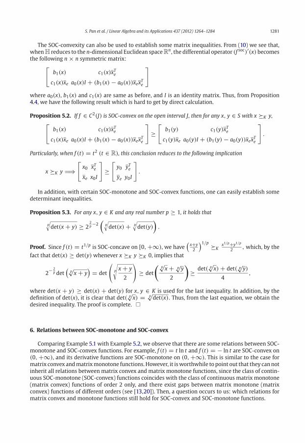
S. Pan et al. / Linear Algebra and its Applications 437 (2012) 1264–1284 1281

The SOC-convexity can also be used to establish some matrix inequalities. From (10) we see that,

whenH reduces to the n-dimensional Euclidean spaceRn, the differential operator (f soc)′(x) becomes

the following n × n symmetric matrix:⎡⎣ b1(x) c1(x)x

Te

c1(x)xe a0(x)I + (b1(x) − a0(x))xexTe

⎤⎦

where a0(x), b1(x) and c1(x) are same as before, and I is an identity matrix. Thus, from Proposition

4.4, we have the following result which is hard to get by direct calculation.

Proposition 5.2. If f ∈ C2(J) is SOC-convex on the open interval J, then for any x, y ∈ S with x K y,⎡⎣ b1(x) c1(x)x

Te

c1(x)xe a0(x)I + (b1(x) − a0(x))xexTe

⎤⎦ ≥

⎡⎣ b1(y) c1(y)x

Te

c1(y)xe a0(y)I + (b1(y) − a0(y))xexTe

⎤⎦ .

Particularly, when f (t) = t2 (t ∈ R), this conclusion reduces to the following implication

x K y �⇒⎡⎣ x0 xTe

xe x0I

⎤⎦ ≥

⎡⎣ y0 yTe

ye y0I

⎤⎦ .

In addition, with certain SOC-monotone and SOC-convex functions, one can easily establish some

determinant inequalities.

Proposition 5.3. For any x, y ∈ K and any real number p ≥ 1, it holds that

p√det(x + y) ≥ 2

2p−2(

p√det(x) + p

√det(y)

).

Proof. Since f (t) = t1/p is SOC-concave on [0, +∞), we have(x+y

2

)1/p Kx1/p+y1/p

2, which, by the

fact that det(x) ≥ det(y) whenever x K y K 0, implies that

2− 2

p det(

p√

x + y)

= det

⎛⎝ p

√x + y

2

⎞⎠ ≥ det

(p√

x + p√

y

2

)≥ det( p

√x) + det( p

√y)

4,

where det(x + y) ≥ det(x) + det(y) for x, y ∈ K is used for the last inequality. In addition, by the

definition of det(x), it is clear that det( p√

x) = p√

det(x). Thus, from the last equation, we obtain the

desired inequality. The proof is complete. �

6. Relations between SOC-monotone and SOC-convex

Comparing Example 5.1 with Example 5.2, we observe that there are some relations between SOC-

monotone and SOC-convex functions. For example, f (t) = t ln t and f (t) = − ln t are SOC-convex on

(0, +∞), and its derivative functions are SOC-monotone on (0, +∞). This is similar to the case for

matrix convex andmatrixmonotone functions. However, it isworthwhile to point out that they cannot

inherit all relations between matrix convex and matrix monotone functions, since the class of contin-

uous SOC-monotone (SOC-convex) functions coincides with the class of continuous matrix monotone

(matrix convex) functions of order 2 only, and there exist gaps between matrix monotone (matrix

convex) functions of different orders (see [13,20]). Then, a question occurs to us: which relations for

matrix convex and monotone functions still hold for SOC-convex and SOC-monotone functions.

1282 S. Pan et al. / Linear Algebra and its Applications 437 (2012) 1264–1284

Lemma 6.1. Assume that f : J → R is three times differentiable on the open interval J. Then, f is a

non-constant SOC-monotone function if and only if f ′ is strictly positive and (f ′)−1/2 is concave.

Proof. “⇐”. Clearly, f is a non-constant function. Also, by [12, Proposition 2.2], we have

f (t2) − f (t1)

t2 − t1≤√f ′(t2)f ′(t1), ∀t2, t1 ∈ J. (31)

This, by the strict positivity of f ′ and Proposition 3.2, shows that f is SOC-monotone.

“⇒”. The result is direct by [8, Theorem III] and Theorem 3.1. �

UsingLemma6.1,wemayverify thatSOC-monotoneandSOC-convex functions inherit the following

relation of matrix monotone and matrix convex functions.

Proposition 6.1. If f : J → R is a continuous SOC-monotone function, then the function g(t) = ∫ ta f (s)ds

with some a ∈ J is SOC-convex.

Proof. It suffices to consider the case where f is a non-constant SOC-monotone function. Due to

Proposition 3.3, we may assume f ∈ C3(J). By Lemma 6.1, f ′(t) > 0 for all t ∈ J and (f ′)−1/2 is

concave. Since g ∈ C4(J) and g′′(t) = f ′(t) > 0 for all t ∈ J, by Corollary 4.1 in order to prove that g

is SOC-convex, we only need to argue

g′′(t)g(4)(t)

48≥[g(3)(t)

]236

⇐⇒ f ′(t)f (3)(t)48

≥[f ′′(t)

]236

, ∀t ∈ J. (32)

Since (f ′)−1/2 is concave, its second-order derivative is nonpositive. From this, we have

1

32

(f ′′(t)

)2 ≤ 1

48f ′(t)f (3)(t) ∀t ∈ J,

which implies the inequality (32). The proof is complete. �

Similar to matrix monotone and matrix convex functions, the converse of Proposition 6.1 does not

hold. For example, f (t) = t2/(1 − t) on (−1, 1) is SOC-convex by Example 5.2(vii), but its derivative

g′(t) = 1

(1−t)2− 1 is not SOC-monotone by Proposition 3.2. As a consequence of Proposition 6.1 and

Proposition 4.4, we have the following corollary.

Corollary 6.1. Let f ∈ C2(J). If f ′ is SOC-monotone, then f is SOC-convex. This is equivalent to saying that

for any x, y ∈ S with x K y,

(f ′)soc(x) K (f ′)soc(y) �⇒ (f soc)′(x) − (f soc)′(y) 0.

From [2, Theorem V. 2.5], we know that a continuous function f mapping [0, +∞) into itself is

matrix monotone if and only if it is matrix concave. However, for such f we can not prove that f is

SOC-concave when it is SOC-monotone, but f is SOC-concave under a little stronger condition than

SOC-monotonicity, i.e., the matrix monotonicity of order 4.

Proposition 6.2. Let f be a continuous function mapping [0, +∞) into itself. Then,

(a) f is SOC-monotone whenever f is SOC-concave;

(b) f is SOC-concave whenever f is matrix monotone of order 4.

Proof. Using the same arguments as [5, Proposition 4.1], we can prove part (a). By [18, Theorem 2.1],

if f is continuous and matrix monotone of order 2n, then f is matrix concave of order n. This, together

with Theorem 4.1, implies part (b). �

S. Pan et al. / Linear Algebra and its Applications 437 (2012) 1264–1284 1283

Note that Proposition6.2 verifiesConjecture4.2of [5] partially. From[2],weknowthat the functions

in Example 5.1(i)–(iii) are all matrix monotone, and so they are SOC-concave by Proposition 6.2(b). In

addition, using Proposition 6.2(b) and noting that −t−1 (t > 0) is SOC-monotone and SOC-concave

on (0, +∞), we readily have the following corollary.

Corollary 6.2. Let f be a continuous function from (0, +∞) into itself. If f is matrix monotone of order 4,

then the function g(t) = 1f (t)

is SOC-convex.

Proposition 6.3. Let f be a continuous real function on the interval [0, α). If f is SOC-convex, then the

indefinite integral off (t)t

is also SOC-convex.

Proof. The result follows directly by [21, Proposition 2.7] and Theorem 4.1. �

For a continuous real function f on the interval [0, α), TheoremV. 2.9 of [2] states that the following

two conditions are equivalent:

(i) f is matrix convex and f (0) ≤ 0;

(ii) The function g(t) = f (t)/t is matrix monotone on (0, α).

Nowwe cannot establish the equivalence between the two conditions for the SOC-monotone and SOC-

convex functions though the given examples in Examples 5.1 and 5.2 imply that this seems to hold,

and we will leave it as a future topic.

At the end of this section, let us take a look at Example 5.1(i)–(iii) and (v)–(vi). We find that these

functions are continuous, nondecreasing and concave. Then, one naturally askwhether such functions

are SOC-monotone or not. This is exactly Conjecture 4.1(a) of [5]. The following counterexample shows

that Conjecture 4.1(a) of [5] does not hold generally.

Example 6.1. Consider f (t) =⎧⎨⎩−t ln t + t t ∈ (0, 1),

1 t ∈ [1, +∞).This function is continuously differen-

tiable, nondecreasing and concave on (0, +∞). However, letting t1 = 0.1 and t2 = 3,

f ′(t1)f ′(t2) −(f (t1) − f (t2)

t1 − t2

)2

= −(−t1 ln t1 + t1 − 1

t1 − t2

)2

= −0.0533.

By Proposition 3.2, we know that the function f is not SOC-monotone.

7. Conclusions

We provided the necessary and sufficient characterizations for SOC-monotone and SOC-convex

functions in the setting of a general Hilbert space, by which the set of continuous SOC-monotone

(respectively, SOC-convex) functions is shown to coincide with that of continuous matrix monotone

(respectively, matrix convex) functions of order 2. These results will be helpful to characterize the SC-

monotone (i.e., symmetric conemonotone) and SC-convex functions,which are scalar valued functions

that induce Löwner operators in Euclidean Jordan algebra to preserve themonotone order and convex

order, respectively.

Acknowledgements

The authors would like to thank an anonymous referee for helpful and detailed suggestions on

the revision of this paper. The first author would like to thank Department of Applied Mathematics,

National Sun Yat-sen University for supporting her to visit there in July, 2009.

1284 S. Pan et al. / Linear Algebra and its Applications 437 (2012) 1264–1284

References

[1] D.P. Bertsekas, Nonlinear Programming, second ed., Athena Scientific, Massachusetts, 1999.

[2] R. Bhatia, Matrix Analysis, Springer-Verlag, New York, 1997.[3] J.-F. Bonnans, H.C. Ramírez, Perturbation analysis of second-order cone programming problems, Math. Program. 104 (2005)

205–227.[4] J. Brinkhuis, Z.-Q. Luo, S. Zhang, Matrix convex functions with applications to weighted centers for semi-definite programming,

Technical report, SEEM, The Chinese University of Hong Kong, 2005.[5] J.-S. Chen, The convex and monotone functions associated with second-order cone, Optimization 55 (2006) 363–385.

[6] J.-S. Chen, X. Chen, S.-H. Pan, J.-W. Zhang, Some characterizations of SOC-monotone and SOC-convex functions, J. Global Optim.

45 (2009) 259–279.[7] Y.-Y. Chiang, S.-H. Pan, J.-S. Pan, A merit function method for infinite-dimensional SOCCPs, J. Math. Anal. Appl. 383 (2011)

159–178.[8] W. Donoghue, Monotone Matrix Functions and Analytic Continuation, Springer, Berlin, Heidelberg, New York, 1974.

[9] J. Faraut, A. Korányi, Analysis on Symmetric Cones, OxfordMathematical Monographs, Oxford University Press, New York, 1994.[10] M. Fukushima, Z.-Q. Luo, P. Tseng, Smoothing functions for second-order cone complementarity problems, SIAM J. Optim. 12

(2002) 436–460.

[11] F. Hansen, G.K. Pedersen, Jensens inequality for operators and Löwners theorem, Math. Ann. 258 (1982) 229–241.[12] F. Hansen, J. Tomiyama, Differential analysis of matrix convex functions, Linear Algebra Appl. 420 (2007) 102–116.

[13] F. Hansen, G.-X. Ji, J. Tomiyama, Gaps between classes of matrix monotone functions, Bull. London Math. Soc. 36 (2004) 53–58.[14] R.A. Horn, C.R. Johnson, Topics in Matrix Analysis, Cambridge University Press, Cambridge, 1991.

[15] F. Kraus, Über konvekse Matrixfunktionen, Math. Z. 41 (1936) 18–42.[16] M.K. Kwong, Some results on matrix monotone functions, Linear Algebra Appl. 118 (1989) 129–153.

[17] K. Löwner, Über monotone matrixfunktionen, Math. Z. 38 (1934) 177–216.[18] R. Mathias, Concavity of monotone matrix functions of finite orders, Linear and Multilinear Algebra 27 (1990) 129–138.

[19] M. Kovara, M. Stingl, On the solution of large-scale SDP problems by the modified barrier method using iterative solvers, Math.

Program. Ser. B 109 (2007) 413–444.[20] H. Osaka, S. Silvestrov, J. Tomiyama, Monotone operator functions, gaps and power moment problem, Math. Scand. 100 (2007)

161–183.[21] H. Osaka, J. Tomiyama, Double piling structure of matrix monotone functions and of matrix convex functions, Linear Algebra

Appl. 431 (2009) 1825–1832.[22] S.-H. Pan, J.-S. Chen, A class of interior proximal-like algorithms for convex second-order cone programming, SIAM J. Optim. 19

(2008) 883–910.

[23] M. Uchiyama, M. Hasumi, On some operator monotone functions, Integral Equations Operator Theory 42 (2011) 243–251.