Comput. Methods Appl. Mech. Engrg. 194 (2005) 3496–3515

www.elsevier.com/locate/cma

Multi-objective design optimization using cascadeevolutionary computations

Nikos D. Lagaros, Vagelis Plevris, Manolis Papadrakakis *

Institute of Structural Analysis and Seismic Research, National Technical University of Athens, 9, Iroon Polytechniou Str.,

Zografou Campus, GR-15780 Athens, Greece

Received 20 June 2004; received in revised form 10 November 2004; accepted 29 December 2004

Abstract

The consideration of uncertainties in conjunction with the probability of violation of the constraints imposed by the

design codes is examined in the framework of structural optimization. The optimum design achieved based on a deter-

ministic formulation is compared, in terms of the optimum weight, the probability of violation of the constraints and

the probability of failure, with the optimum designs achieved through a robust design formulation where the variance of

the response is considered as an additional criterion. The stochastic finite element problem is solved using the Monte

Carlo Simulation method, combined with the Latin Hypercube Sampling technique for improving its computational

efficiency. A non-dominant cascade evolutionary algorithm-based methodology is adopted for the solution of the

multi-objective optimization problem encountered, in order to obtain the global Pareto front curve.

� 2005 Elsevier B.V. All rights reserved.

Keywords: Multi-objective optimization; Latin hypercube; Robust design optimization; Cascade evolutionary algorithms

1. Introduction

In deterministic-based structural sizing optimization problems the aim is to minimize the weight or the

cost of the structure taking into account certain behavioral constraints, mainly on stresses and displace-

ments, as imposed by the design codes. On the other hand, stochastic performance measures are increas-

ingly being taken into consideration in many contemporary engineering applications that involve various

reliability requirements. Reliability is defined as the probability that a system will meet the design demands

0045-7825/$ - see front matter � 2005 Elsevier B.V. All rights reserved.

doi:10.1016/j.cma.2004.12.029

* Corresponding author. Tel.: +30 210 7721694; fax: +30 210 7721693.

E-mail addresses: nlagaros@central.ntua.gr (N.D. Lagaros), vplevris@central.ntua.gr (V. Plevris), mpapadra@central.ntua.gr (M.

Papadrakakis).

N.D. Lagaros et al. / Comput. Methods Appl. Mech. Engrg. 194 (2005) 3496–3515 3497

during its life time. In structural optimization, stochastic performance measures can be taken into account

using two distinct formulations, Robust Design Optimization (RDO) and Reliability-Based Design Opti-

mization (RBDO) [9]. According to the RDO formulation the objective is to minimize the influence of

the stochastic variation of some structural parameters on the design, while the main goal in the RBDO for-

mulation is to achieve optimum design with respect to extreme uncertain events.Although a great deal of studies has been proposed during the last three decades for structural optimi-

zation, those devoted to RDO are rather limited. Chen and Lewis [2] presented some preliminary results of

robust design for multi-disciplinary optimization applying efficient methods for the uncertainty analysis.

Lee and Park [12] solved a RDO problem where the multi-objective problem considered had two criteria

to be minimized, the mean value and the standard deviation of the structural weight. The multi-objective

problem was solved using the weighting sum method in the context of a mathematical programming algo-

rithm. Sandgren and Cameron [21] proposed a hybrid genetic/non-linear programming algorithm for the

solution of the multi-objective problem in the framework of RDO. Messac and Ismail-Yahaya [16] devel-oped the flexible physical programming-based RDO methodology that formulates the RDO problem in

terms of physically meaningful design performance degradation levels. Jung and Lee [11] incorporated

the probability of feasibility into the RDO problem, where each probability constraint was transformed

into a sub-optimization problem by the advanced first-order second moment method. Doltsinis and Kang

[5] dealt with the RDO problem considering the minimization of the mean value and the standard deviation

of a nodal displacement and treating the structural weight as a constraint function. Papadrakakis et al. [19]

studied a RDO problem where both the weight of the structure and the variance of the structural response

were minimized, while the Linear Weighting Sum (LWS) method was used for the solution of the multi-objective optimization problem.

In the present work, the non-dominant Cascade Evolutionary Algorithm (CEA)-based multi-objec-

tive optimization scheme is proposed for the solution of structural RDO problems, together with an

improved handling of the multi-objective optimization problem, and is compared to the LWS method.

The stochastic finite element problem is solved using the Monte Carlo simulation method combined

with the Latin Hypercube Sampling (LHS) technique in order to reduce the number of simulations

needed for the calculation of the required statistical quantities. Up to a hundred LHS simulations

proved to be sufficient, for the test cases considered for calculating the statistical quantities. Further-more, the advantages of the proposed cascade multi-objective optimization methodology over the clas-

sical LWS method and the importance of considering the variance of the structural response as a

criterion are demonstrated. Two real-scale truss structures have been examined subject to constraints

imposed by the Eurocode 3 [8].

The paper is organized as follows: in Section 2, the formulation and solution of the stochastic finite ele-

ment problem is described. The next section presents the multi-objective optimization problem and the

description of the methodology adopted which encompasses non-dominant search, cascade evolutionary

computations and the Tchebycheff metric. Subsequently, in Section 4 the definition of a RDO problemis given. The numerical tests, that demonstrate the potential of the proposed multi-objective optimization

scheme in solving realistic problems compared to the LWS method, are presented in Section 5 together with

a verification of the efficiency of LHS. A comparative study between DBO and RDO optimum solutions is

also given in Section 5, followed by the concluding remarks in Section 6.

2. Stochastic finite element analysis

During the last two decades much progress has been achieved on stochastic finite element methods

[20,22]. However, comparatively few studies have been performed in structural optimization taking into

account uncertain parameters.

3498 N.D. Lagaros et al. / Comput. Methods Appl. Mech. Engrg. 194 (2005) 3496–3515

2.1. Stochastic response basics

In this work several parameters that affect the structural performance, such as the modulus of elasticity,

yield stress and applied loading have been considered as uncertain variables. Let nr be the total number of

the uncertain variables considered and r is the corresponding vector. The stochastic finite element equationthat has to be solved can be stated as follows

KðrÞuðrÞ ¼ pðrÞ; ð1Þ

where K(r) is the global uncertain stiffness matrix, u(r) is the vector of nodal displacements and p(r) is the

loading vector. The statistical quantities that are usually required in the framework of a RDO problem are

the mean value and/or the variance of the objective function, such as the weight, or the structural response.

If the uncertain variables r are not correlated with each other, as it is assumed in this work, the mean value�ui and the variance r2ui of the displacement of the ith degree of freedom can be calculated as follows

�ui ¼Z Z

� � �Z

uiðrÞpdf1ðr1Þ � � � pdfnrðrnrÞdr; ð2aÞ

r2ui ¼Z Z

� � �Z

½uiðrÞ � �ui�2pdf1ðr1Þ � � � pdfnrðrnrÞdr; ð2bÞ

where pdfj, j = 1, . . ., nr, is the probability density function of the j-th uncertain variable. For the solution ofthe problem of Eq. (1) which results in the calculation of the statistical quantities of Eqs. (2a) and (2b), anumber of methods have been proposed that can be classified into statistical and non-statistical ones. In this

work, a statistical method and in particular Monte Carlo Simulation combined with the Latin Hypercube

Sampling is employed.

2.2. Monte Carlo Simulation (MCS) method

The MCS method is particularly applicable for the stochastic analysis of structures when an analytical

solution is not attainable. This is mainly the case in problems of complex nature with a large number ofuncertain variables, where all other stochastic analysis methods are inapplicable. Despite the fact that the

mathematical formulation of the MCS is simple, the method has the capability of handling practically every

possible case regardless of its complexity and the variation of the uncertain variables. The MCS method has

proven to be efficient [18] for the calculation of the statistical quantities in the framework of a RBDO

problem.

For the structural stochastic analysis problems examined in this study, the probability of violation of the

behavioral constraints and the probability of failure are calculated along with the mean value and the var-

iance of a characteristic nodal displacement that represents the response of the structure. Expressing thelimit state function as G(r) < 0, the probability of violation of the behavioral constraints can be written as

pviol ¼ZGðrÞP0

frðrÞdr; ð3Þ

where fr(r) denotes the joint probability of violation. A similar expression is used for the probability of

failure.

Since MCS is based on the theory of large numbers (N1), an unbiased estimator of the probability of

violation, the mean value and the variance of the nodal displacement in question is given by

pviol ¼1

N1

XN1

j¼1IðrjÞ; ð4aÞ

N.D. Lagaros et al. / Comput. Methods Appl. Mech. Engrg. 194 (2005) 3496–3515 3499

�ui ¼1

N1

XN1

j¼1uiðrjÞ; ð4bÞ

r2ui ¼1

N1

XN1

j¼1½uiðrjÞ � �ui�2; ð4cÞ

where rj is the jth vector of the random structural parameters, and I(rj) is an indicator for successful and

unsuccessful simulations defined as

IðrjÞ ¼1 if GðrjÞ P 0;

0 if GðrjÞ < 0:

�ð5Þ

In order to estimate �ui and r2ui from Eqs. (4b) and (4c) an adequate number of N independent random

samples is produced, while pviol is given in terms of sample mean by

pviol ffiNH

N; ð6Þ

where NH is the number of successful simulations and N is the total number of simulations. The probability

of failure is calculated using a similar estimator of Eqs. (4a) and (6).

2.3. Latin Hypercube Sampling

The Latin Hypercube Sampling (LHS) method was introduced by MacKay et al. [15] in an effort to

reduce the required computational cost of purely random sampling methodologies. Latin hypercube

sampling is a strategy for generating random sample points ensuring that all portions of the random

space in question are properly represented. LHS is generally recognized as one of the most efficient size

reduction techniques. The basis of LHS is a full stratification of the sampled distribution with a random

selection inside each stratum. In consequence, sample values are randomly shuffled among different vari-

ables. A Latin hypercube sample is constructed by dividing the range of each of the nr uncertain vari-

ables into N non-overlapping segments of equal marginal probability. Thus, the whole parameter space,consisting of N parameters, is partitioned into Nnr cells. A single value is selected randomly from each

interval, producing N sample values for each input variable. The values are randomly matched to create

N sets from the Nnr space with respect to the density of each interval for the N simulation runs. The

advantage of the LHS approach is that the random samples are generated from all the ranges of possible

values.

3. Multi-objective optimization

In many practical applications a single criterion rarely gives a representative measure of the actual struc-

tural performance, as several conflicting and usually incommensurable criteria have to be taken into ac-

count simultaneously. The optimization problem with more than one objective is called as multi-criteria,

multi-objective or vector optimization problem [4].

3.1. Conflict and criteria

The engineer looking for the optimum design of a structure is faced with the question of selecting the

most suitable criteria for measuring the economy, strength, serviceability or any other factor that affects

3500 N.D. Lagaros et al. / Comput. Methods Appl. Mech. Engrg. 194 (2005) 3496–3515

the performance of the structure. Any quantity that has an influence on the structural performance can be

considered as a criterion. One important basic property in the multi-criterion formulation is the conflict

that should exist among the various criteria. Only those quantities that are conflicting with each other

should be treated as independent criteria whereas the others can be combined into a single criterion repre-

senting the whole group.Two functions fi and fj are called locally collinear with no conflict at point s if there is c > 0 such that

$fi(s) = c$fj(s). Otherwise, the functions are called locally conflicting at point s. According to this definition

any two criteria are locally conflicting at a point of the design space if their maximum improvement is

achieved in different directions. On the other hand, the two functions fi and fj are called globally conflicting

in the feasible region F of the design space if the two optimization problems minffiðsÞ : s 2 Fg andminffjðsÞ : s 2 Fg have different optimal solutions.

3.2. Formulation of the multi-objective optimization problem

In general, the mathematical formulation of a multi-objective problem that includes a set of n design

variables, a set of m objective functions and a set of k constraint functions can be defined as follows

mins2F

½f1ðsÞ; f2ðsÞ; . . . ; fmðsÞ�T

subject to gjðsÞ 6 0 j ¼ 1; . . . ; k;si 2 Rd ; i ¼ 1; . . . ; n;

ð7Þ

where the vector s = [s1 s2 � � � sn]T represents a design variable vector and F is the feasible region, a sub-

space of the design space Rn for which the constraint functions g(s) are satisfied

F ¼ fs 2 RnjgjðsÞ 6 0 j ¼ 1; . . . ; kg ð8Þ

If the m objective functions are globally conflicting, there is no unique point that would represent the

optimum for all m objectives. Thus, the common optimality condition used in single-objective optimization

must be replaced by a new concept, the so called Pareto optimum: a design vector s� 2 F is a Pareto opti-

mum for the problem of Eq. (7) if and only if there is no other design vector s 2 F such that

fiðsÞ 6 fiðs�Þ for i ¼ 1; . . . ;m;with f jðsÞ < fjðs�Þ for at least one objective j:

ð9Þ

The geometric locus of the Pareto optimum solutions is called Pareto front curve and represents the solu-

tion of the optimization problem with multiple objectives. In practical applications however, the designer

seeks for a unique final solution to be implemented in practice, thus a compromise should be made among

the available Pareto optimal solutions.

3.3. Domination and non-domination

In single objective optimization problems the feasible set F can be ordered univocally according to the

value of the objective function. For example, in the case of the minimization problem of f (s), two solutions

sa and sb 2 F can be classified using the condition f(sa) < f(sb). In a multi-objective optimization problem

two solutions sa and sb 2 F cannot be classified in a univocal manner. The concept of the Pareto domi-

nance is used for assessing the two solutions, which for a minimization problem can be defined as follows

sa dominates sb if f iðsaÞ < fiðsbÞ 8i ¼ 1; . . . ;m;sa weakly dominates sb if f iðsaÞ 6 fiðsbÞ 8i ¼ 1; . . . ;m;sa is indifferent to sb otherwise:

ð10Þ

N.D. Lagaros et al. / Comput. Methods Appl. Mech. Engrg. 194 (2005) 3496–3515 3501

Using the definition of Eq. (10), the Pareto optimality can be stated as follows: A solution s� 2 F is Pareto

optimal if it is not dominated by any other feasible design.

3.4. Solving the multi-objective optimization problem

Several methods have been proposed for treating structural multi-objective optimization problems

[3,10,13]. According to Marler and Arora [14] these methods can be divided into: (i) methods with a priori

articulation of preferences, (ii) methods with a posteriori articulation of preferences and (iii) methods with

no articulation of preferences. The proposed Cascade Evolutionary Algorithm-based (CEA) multi-objec-

tive optimization scheme belongs to the first category. This algorithm is compared to the Linear Weighting

Sum method (LWS), also belonging to the a priori articulation of preferences. The LWS method, due to its

simplicity, is the most widely implemented method for solving such problems. In both methods employed,

the problem in finding the Pareto front curve is reduced into a sequence of parameterized single-objectiveoptimization subproblems, using scalarizing functions.

In general, when using scalarizing functions, locally Pareto optimal solutions are obtained. Global Pareto

optimality can be guaranteed only when the objective functions and the feasible region are both convex or

quasi-convex and convex, respectively. For non-convex cases, such as the majority of structural multi-objec-

tive optimization problems, a global single objective optimizer must be implemented. Evolutionary Algo-

rithms (EA) are considered as global optimizers since they are not prone to being trapped in local optima

and therefore can be considered as the most reliable methods in approaching the global optimum for

non-convex constrained optimization problems. For this reason an evolutionary algorithm has been consi-dered in this study for the solution of the sequence of the parameterized single objective optimization

problems.

The quality of the Pareto front curve obtained can be assessed according to the following rules:

• Distance from the exact Global Pareto front curve.

• Number of Pareto optimum solutions.

• Distribution of the Pareto optimum solutions along the front curve.

3.4.1. Linear Weighting Sum method

In the LWS method all the objectives are combined into a scalar parameterized function by using weight-

ing coefficients. If wi, i = 1,2, . . ., m are the weighting coefficients, the problem of Eq. (7) can be written asfollows:

mins2F

Xmi¼1

wijfiðsÞ � z�i j

fiðsÞ; ð11Þ

where z�i is the utopian objective function value. With no loss of generality the following normalization ofthe weighting coefficients is employed:

Xmi¼1

wi ¼ 1: ð12Þ

The values of the weighting coefficients can be adjusted according to the importance of each criterion.

Every combination of the weighting coefficients correspond to a single Pareto optimal solution, thus by per-forming a sequence of optimization runs using different weighting coefficients a set of Pareto optimal solu-

tions is obtained.

3502 N.D. Lagaros et al. / Comput. Methods Appl. Mech. Engrg. 194 (2005) 3496–3515

3.4.2. Non-dominant multi-objective search using the Tchebycheff metric

The proposed Cascade Evolutionary Algorithm (CEA)-based optimization scheme combines the CEA

methodology with a non-dominance search and the Tchebycheff metric.

3.4.2.1. Augmented weighted Tchebycheff problem. The augmented weighted Tchebycheff method belongs tothe methods with a priori articulation of the preferences for treating the multi-objective optimization prob-

lem and, unlike the linear weighting sum method, can be applied effectively to convex as well as to non-

convex problems [17]. The weighted Tchebycheff metric can generate any optimal solution, to any type

of optimization problem [23]. In order to overcome weakly Pareto optimal solutions, the Tchebycheff

method formulates the distance minimization problem as a weighted Tchebycheff problem

mins2F

maxi¼1;...;m

wijfiðsÞ � z�i j

fiðsÞþ q

Xmi¼1

jfiðsÞ � z�i jfiðsÞ

" #; ð13Þ

where q is a sufficiently small positive scalar (in this work q = 0.1). The weight parameters wi are random

numbers, uniformly distributed between 0 and 1. These weight parameters have to fulfil the requirement of

Eq. (12), if not, they are updated according to the following expression:

wi ¼wi þ

1�Pm

i wiPmi wi

wi; ifPm

i wi 6¼ 1;

wi; ifPm

i wi ¼ 1:

8<: ð14Þ

3.4.2.2. CEA-based multi-objective optimization scheme. It is generally accepted that there is still no uniqueoptimization algorithm capable of handling with equal efficiency all existing optimization problems. Cas-

cade optimization attempts to alleviate this deficiency by applying a multi-stage procedure in which various

optimizers are implemented successively. In the present work the idea of cascading is implemented in the

EA-context (CEA) for solving multi-objective structural optimization problems. In particular, the CEA

method is employed for the solution of the sequence of parameterized single objective optimization prob-

lems. The resulting cascade evolutionary procedure consists of a number of optimization stages (csteps),

each of which employs the same EA optimizer. In order to differentiate the search paths followed by the

same optimization algorithm during the cascade stages, the initial conditions of the individual optimizationruns are suitably controlled by using at each stage a different initial design (each stage initiates from

the solution of the previous stage) and a different seed for the random number generator of the EA proce-

dure [1].

A non-dominant search is performed in the context of the CEA and the Tchebycheff metric in the sense

that all non-dominated solutions attained so far are kept in a set called temporary Pareto set. It was men-

tioned before that the multi-objective optimization problems are decomposed into subproblems which are

solved with independent runs (nruns in total) of the CEA methodology. Each subproblem is independent

from the other and therefore all subproblems can be dealt with simultaneously. Furthermore, in every glo-bal generation a non-dominant search is applied for updating the temporary Pareto set. The global gener-

ation is achieved when all local generations of the independent CEA runs are completed. According to this

procedure in every global generation a local Pareto front is produced which approaches the global one.

The optimization algorithm proposed in this study is denoted as: non-dominant CEATm(l + k)nruns,cstepswhere l, k are the number of the parent and offspring vectors used in the ES optimization strategy, nruns isthe number of independent CEA runs and csteps is the number of cascade stages employed. The proposed

optimization scheme can easily be applied in two parallel computing levels, an external and an internal

one. As it was mentioned earlier the multi-objective optimization problem is converted into a series ofsingle objective optimization problems. The solution of each subproblems can be performed concurrently

N.D. Lagaros et al. / Comput. Methods Appl. Mech. Engrg. 194 (2005) 3496–3515 3503

constituting the external parallel computing level. On the other hand, the utilization of the natural paral-

lelization capabilities of the CEA methodology within each independent run defines the internal parallel

computing level. The basic steps inside an independent run of the multi-objective algorithm, as adopted

in this study, are the following:

Independent run i, i = 1, . . . ,nrunGenerate the weight coefficients wi,j, j = 1, . . ., m of the Tchebycheff metric. Check if the requirement ofEq. (12) is fulfilled, if not change the weight parameters using Eq. (14).

CEATm loop

1. Initial generation:

1a. Generate sk (k = 1, . . . ,l) vectors1b. Structural analysis step

1c. Evaluation of the Tchebycheff metric, Eq. (13)1d. Constraint check: if satisfied k = k + 1 else k = k. Go to step 1a

2. Global non-dominant search: Check if global generation is accomplished. If yes, then non-dominant

search is performed according to Eq. (10), else wait until global generation is accomplished

3. New generation:

3a. Generate s‘ (‘ = 1, . . . ,k) vectors3b. Structural analysis step

3c. Evaluation of the Tchebycheff metric, Eq. (13)

3d. Constraint check: if satisfied ‘ = ‘ + 1 else ‘ = ‘. Go to step 3a4. Selection step: selection of the next generation parents according to (l + k) or (l,k) scheme5. Global non-dominant search: Chech If global generation is accomplished. If yes, then non-dominant

search is performed according to Eq. (10), else wait until global generation is accomplished

6. Convergence check: If satisfied stop, else go to step 5

End of CEATm loop

End of Independent run i

4. Robust design optimization

In the present study the robust design versus the deterministic-based design optimization of large-scale

3D truss structures is investigated. The random variables chosen are the cross-sectional dimensions of struc-

tural members, the material properties of modulus of elasticity E, the yield stress ry as well as the appliedloading.

4.1. Deterministic-based optimization

In a Deterministic-Based Optimization (DBO) problem the aim is to optimize the performance of the

structural system which usually tends to be the minimization of the weight under certain deterministic

behavioral constraints. A discrete DBO problem can be formulated in the following form:

min f ðsÞsubject to gjðsÞ 6 0 j ¼ 1; . . . ; k;

si 2 Rd ; i ¼ 1; . . . ; n;ð15Þ

where f(s) is the objective function and gj(s) are the deterministic constraints. Most frequently these con-

straints refer to member stresses and nodal displacements or inter-storey drifts for building structures.

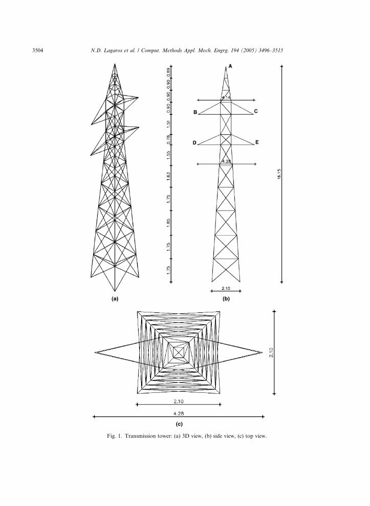
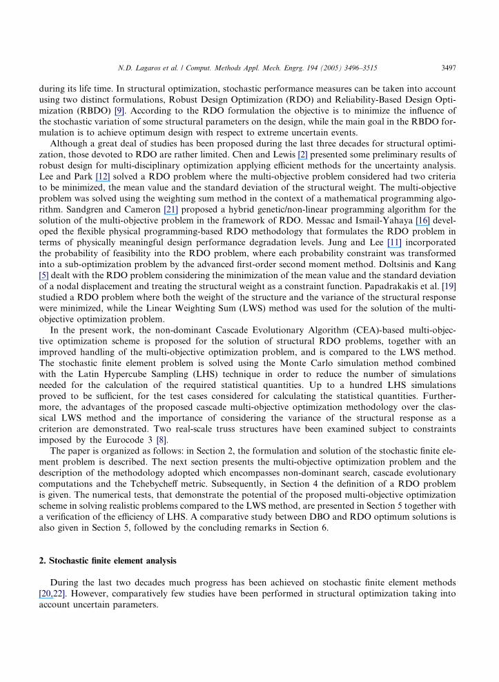
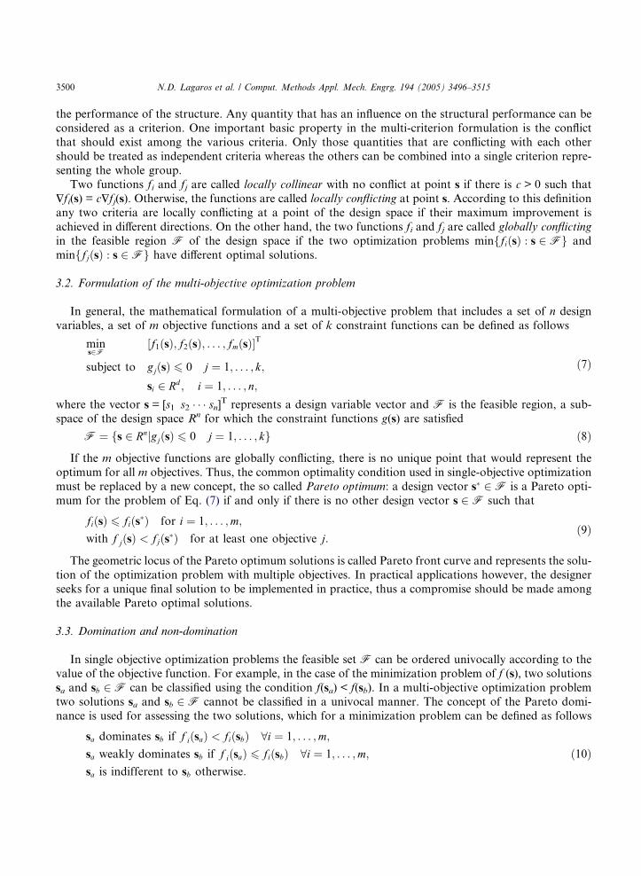
Fig. 1. Transmission tower: (a) 3D view, (b) side view, (c) top view.

3504 N.D. Lagaros et al. / Comput. Methods Appl. Mech. Engrg. 194 (2005) 3496–3515

N.D. Lagaros et al. / Comput. Methods Appl. Mech. Engrg. 194 (2005) 3496–3515 3505

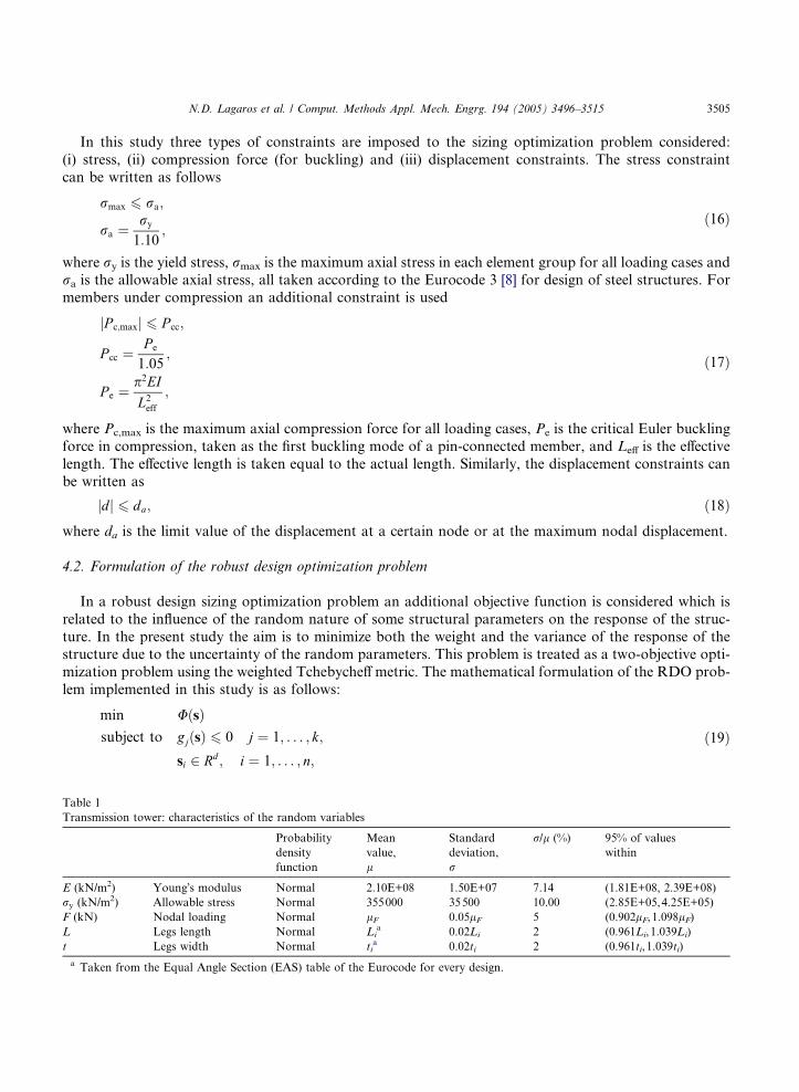
In this study three types of constraints are imposed to the sizing optimization problem considered:

(i) stress, (ii) compression force (for buckling) and (iii) displacement constraints. The stress constraint

can be written as follows

Table

Transm

E (kN

ry (kNF (kN)

L

t

a Tak

rmax 6 ra;

ra ¼ry1:10

;ð16Þ

where ry is the yield stress, rmax is the maximum axial stress in each element group for all loading cases andra is the allowable axial stress, all taken according to the Eurocode 3 [8] for design of steel structures. Formembers under compression an additional constraint is used

jP c;maxj 6 P cc;

P cc ¼P e1:05

;

P e ¼p2EI

L2eff;

ð17Þ

where Pc,max is the maximum axial compression force for all loading cases, Pe is the critical Euler buckling

force in compression, taken as the first buckling mode of a pin-connected member, and Leff is the effective

length. The effective length is taken equal to the actual length. Similarly, the displacement constraints can

be written as

jdj 6 da; ð18Þ

where da is the limit value of the displacement at a certain node or at the maximum nodal displacement.

4.2. Formulation of the robust design optimization problem

In a robust design sizing optimization problem an additional objective function is considered which is

related to the influence of the random nature of some structural parameters on the response of the struc-

ture. In the present study the aim is to minimize both the weight and the variance of the response of thestructure due to the uncertainty of the random parameters. This problem is treated as a two-objective opti-

mization problem using the weighted Tchebycheff metric. The mathematical formulation of the RDO prob-

lem implemented in this study is as follows:

min UðsÞsubject to gjðsÞ 6 0 j ¼ 1; . . . ; k;

si 2 Rd ; i ¼ 1; . . . ; n;ð19Þ

1

ission tower: characteristics of the random variables

Probability

density

function

Mean

value,

l

Standard

deviation,

r

r/l (%) 95% of values

within

/m2) Young�s modulus Normal 2.10E+08 1.50E+07 7.14 (1.81E+08, 2.39E+08)

/m2) Allowable stress Normal 355000 35500 10.00 (2.85E+05,4.25E+05)

Nodal loading Normal lF 0.05lF 5 (0.902lF, 1.098lF)

Legs length Normal Lia 0.02Li 2 (0.961Li, 1.039Li)

Legs width Normal tia 0.02ti 2 (0.961ti,1.039ti)

en from the Equal Angle Section (EAS) table of the Eurocode for every design.

3506 N.D. Lagaros et al. / Comput. Methods Appl. Mech. Engrg. 194 (2005) 3496–3515

where U(s) is the multi-objective function, which is expressed as

UðsÞ ¼ max w1jf ðsÞ � z�1j

f ðsÞ þ qXmi¼1

jf ðsÞ � z�1jf ðsÞ ; w2

jruiðsÞ � z�2jruiðsÞ

þ qXmi¼1

jruiðsÞ � z�2jruiðsÞ

" #; ð20Þ

where f(s) is the weight of the structure and ruiðsÞ is the standard deviation of the response of the structure.

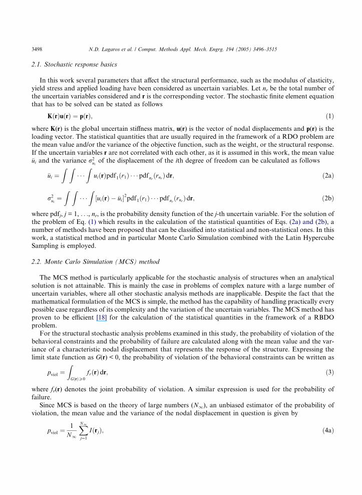
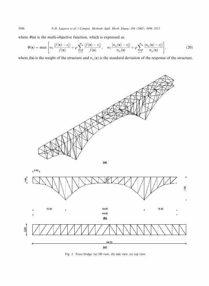
Fig. 2. Truss bridge: (a) 3D view, (b) side view, (c) top view.

N.D. Lagaros et al. / Comput. Methods Appl. Mech. Engrg. 194 (2005) 3496–3515 3507

5. Numerical tests

The numerical tests examined are performed in three stages. In the first stage the statistical methods used

for the stochastic analysis are verified. The number of LHS simulations required for the calculation of the

mean value and the standard deviation of the characteristic displacement representing the structural re-sponse is compared with the corresponding number required by the basic MCS. In the second stage the

advantages of the proposed non-dominant CEATm method over the LWS method are demonstrated

through the comparison of the Pareto front curves obtained. While in the third stage, the differences be-

tween DBO and RDO optimum designs, in terms of the final structural weight, the variance of response,

the probability of violation of the constraints and the probability of failure, are illustrated in two 3D truss

structures.

The first test example is the transmission tower, depicted in Fig. 1, together with its geometric charac-

teristics. The design variables considered are the dimensions of the structural members, divided into sevengroups, taken from the Equal Angle Section (EAS) table of the Eurocode. For each design variable, two

stochastic variables are assigned: The length L and the width t of the legs of the section. The following load-

ing vectors [Fx,Fy,Fz] in kN are applied to the structure: node A [�8.51,0.00,�4.82], node B [�9.77,0.00,�5.36], node C [�9.77,0.00,�5.36], node D [�10.70,0.00,�5.36] and node E [�10.70,0.00,�5.36], whilethe type of probability density function, the mean value, and the variance of the random parameters are

given in Table 1. A constraint maximum deflection of 200 mm is imposed.

The second test example is the pedestrian truss bridge shown in Fig. 2. The design variables considered

are the dimensions of the structural members divided into 12 groups, taken from the double Equal AngleSection (double EAS) table of the Eurocode. For each design variable, three stochastic variables are as-

signed: the length L, the width t of the legs and the distance d between the two identical equal angle sec-

tions. The applied loading consists of: (i) distributed load equal to 5 kN/m2 (dead load), (ii) live loads

(visiting vehicle) and (iii) wind actions according to Eurocode [6,7]. The type of probability density func-

tion, the mean value, and the variance of the random parameters are given in Table 2, while a maximum

deflection constraint of 200 mm is imposed on the nodes of the structure.

5.1. Efficiency of the stochastic analysis method

In the first stage of the numerical study, the performance of the LHS procedure in calculating the stat-

istical parameters required during the RDO procedure compared to the basic MCS is examined. For both

test examples it is examined the influence of the number of simulations on the computed value of the

Table 2

Truss bridge: characteristics of the random variables

Probability

density

function

Mean

value,

l

Standard

deviation,

r

r/l (%) 95% of values

within

E (kN/m2) Young�s modulus Normal 2.10E+08 1.50E+07 7.14 (1.81E+08,2.39E+08)

ry (kN/m2) Allowable stress Normal 355000 35500 10.00 (2.85E+05,4.25E+05)

FP (kN) Permanent loading Normal lF P 0:05lF P 5 ð0:902lF P ; 1:098lF P ÞFL (kN) Live loading Normal lF L 0:05lF L 5 ð0:902lF L , 1:098lF L ÞFW (kN) Wind loading Normal lFW 0:10lFW 10 ð0:804lFW ; 1:196lFW ÞL Legs length Normal Li

a 0.02Li 2 (0.961Li, 1.039Li)

t Legs width Normal tia 0.02ti 2 (0.961ti,1.039ti)

d EAS section distance Normal dia 0.02di 2 (0.961di, 1.039di)

a Taken from the double Equal Angle Section (double EAS) table of the Eurocode for every design.

3508 N.D. Lagaros et al. / Comput. Methods Appl. Mech. Engrg. 194 (2005) 3496–3515

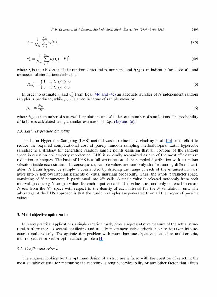
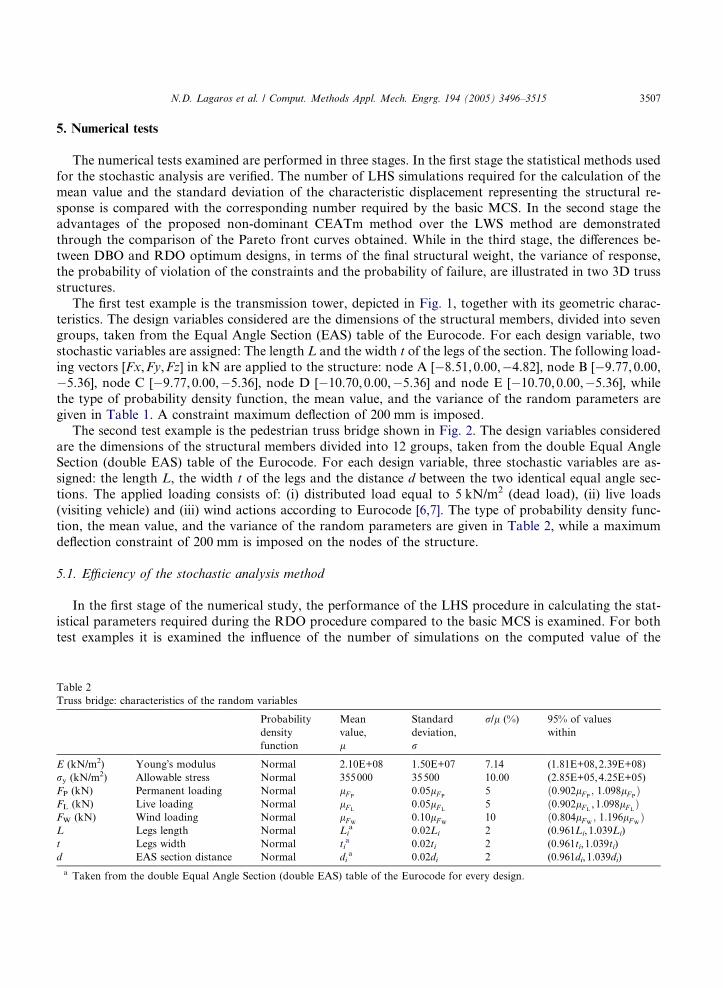
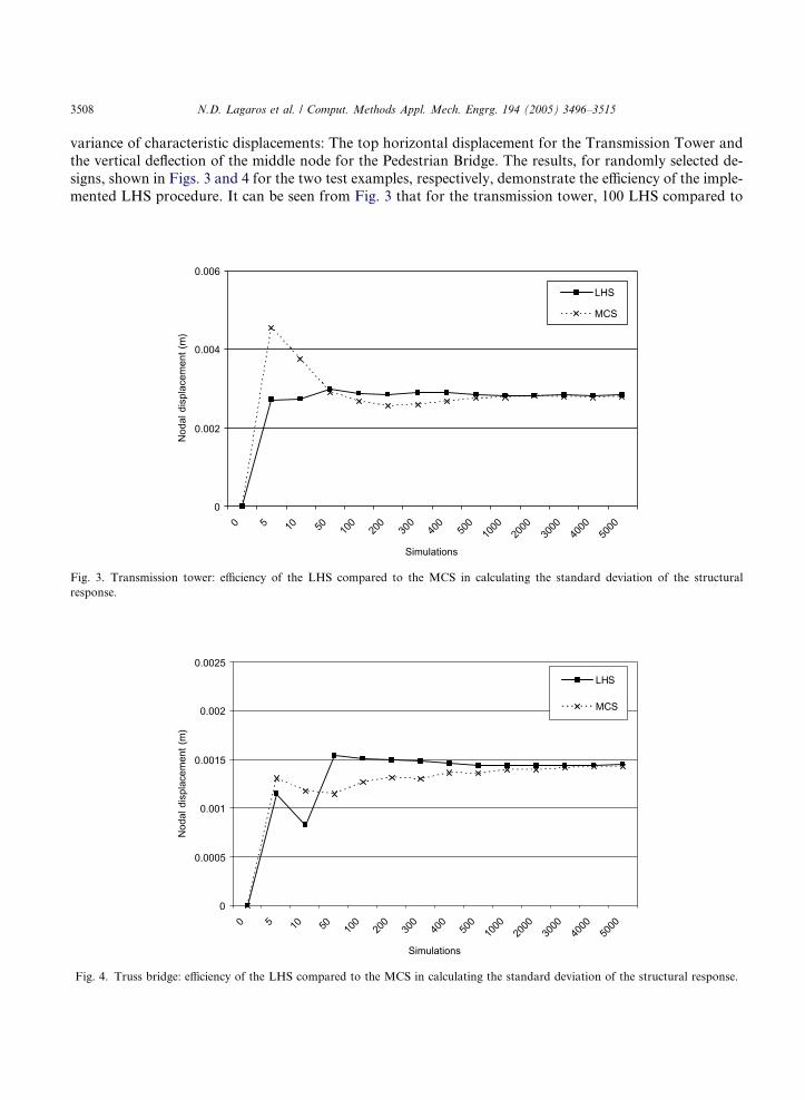
variance of characteristic displacements: The top horizontal displacement for the Transmission Tower and

the vertical deflection of the middle node for the Pedestrian Bridge. The results, for randomly selected de-

signs, shown in Figs. 3 and 4 for the two test examples, respectively, demonstrate the efficiency of the imple-

mented LHS procedure. It can be seen from Fig. 3 that for the transmission tower, 100 LHS compared to

0

0.002

0.004

0.006

0 5 10 50 100

200

300

400

500

1000

2000

3000

4000

5000

Simulations

Nod

al d

ispl

acem

ent (

m)

LHS

MCS

Fig. 3. Transmission tower: efficiency of the LHS compared to the MCS in calculating the standard deviation of the structural

response.

0

0.0005

0.001

0.0015

0.002

0.0025

0 5 10 50 100

200

300

400

500

1000

2000

3000

4000

5000

Simulations

Nod

al d

ispl

acem

ent (

m)

LHS

MCS

Fig. 4. Truss bridge: efficiency of the LHS compared to the MCS in calculating the standard deviation of the structural response.

N.D. Lagaros et al. / Comput. Methods Appl. Mech. Engrg. 194 (2005) 3496–3515 3509

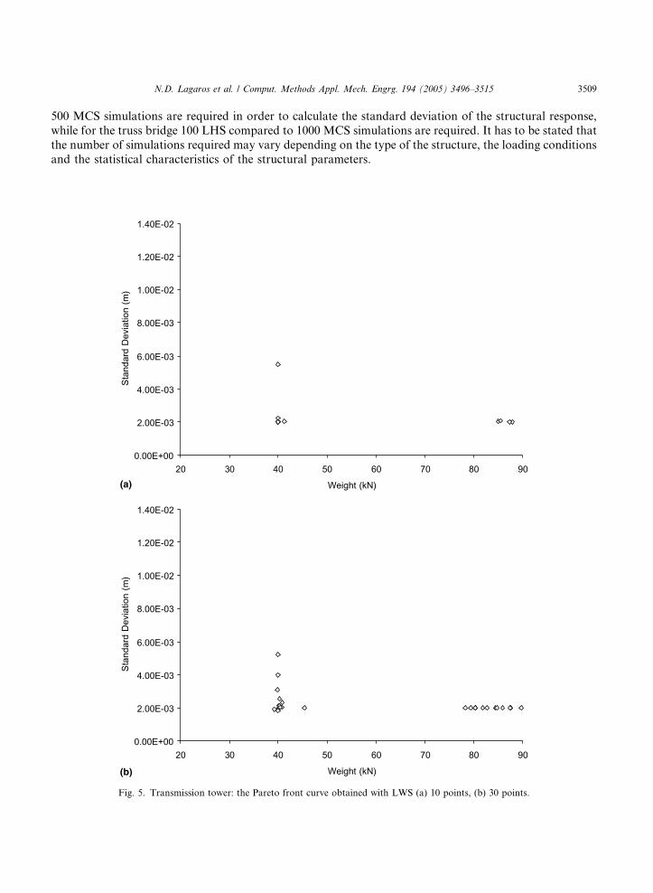
500 MCS simulations are required in order to calculate the standard deviation of the structural response,

while for the truss bridge 100 LHS compared to 1000 MCS simulations are required. It has to be stated that

the number of simulations required may vary depending on the type of the structure, the loading conditions

and the statistical characteristics of the structural parameters.

0.00E+00

2.00E-03

4.00E-03

6.00E-03

8.00E-03

1.00E-02

1.20E-02

1.40E-02

20 30 40 50 60 70 80 90

Weight (kN)

Stan

dard

Dev

iatio

n (m

)

0.00E+00

2.00E-03

4.00E-03

6.00E-03

8.00E-03

1.00E-02

1.20E-02

1.40E-02

20 30 40 50 60 70 80 90

Weight (kN)

Stan

dard

Dev

iatio

n (m

)

(a)

(b)

Fig. 5. Transmission tower: the Pareto front curve obtained with LWS (a) 10 points, (b) 30 points.

3510 N.D. Lagaros et al. / Comput. Methods Appl. Mech. Engrg. 194 (2005) 3496–3515

5.2. Comparison between LWS and CEATm

In the second stage of this study the advantages of the cascade evolutionary multi-objective optimization

scheme using the Tchebycheff metric are demonstrated over the linear weighing sum method. As it was

mentioned in Section 3.4 the quality of the Pareto front curve can be assessed by the number of Pareto opti-mum solutions obtained and their distribution along the front curve. Well distributed solutions along the

curve is an indication of the efficiency of the multi-objective optimization method employed. The main

drawback of the multi-objective optimization methods using scalarizing functions, such as the LWS, is that

it is difficult to fulfil these two requirements.

For the comparative study performed in this study the robust design optimization problem considered

has been solved with the LWS method and the proposed non-dominant CEATm multi-objective optimiza-

tion scheme. For both test examples the LWS method has been implemented through two different runs

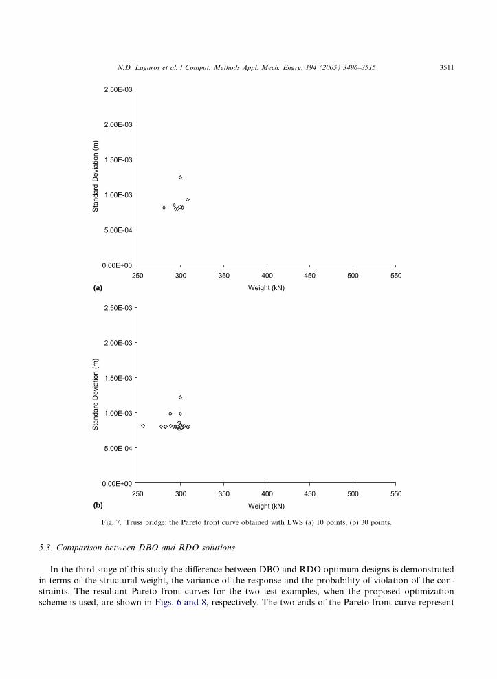
with 10 and 30 points using the ES(l + k) optimization algorithm where l = k = 5 are the number of par-ents and offsprings, respectively. For the non-dominant CEATm(l + k)nrun,csteps optimization scheme thecorresponding parameters are l = k = 5, nrun = 10 and csteps = 3. The resultant Pareto front curves, forthe first test example, are depicted in Figs. 5 and 6 for the LWS and the CEATm, respectively. The hori-

zontal axis corresponds to the structural weight and the vertical axis to the standard deviation of the char-

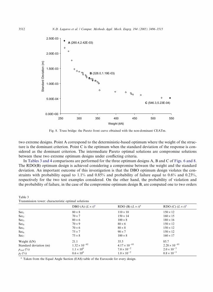
acteristic node displacement. For the second test example the corresponding front curves are depicted in

Figs. 7 and 8.

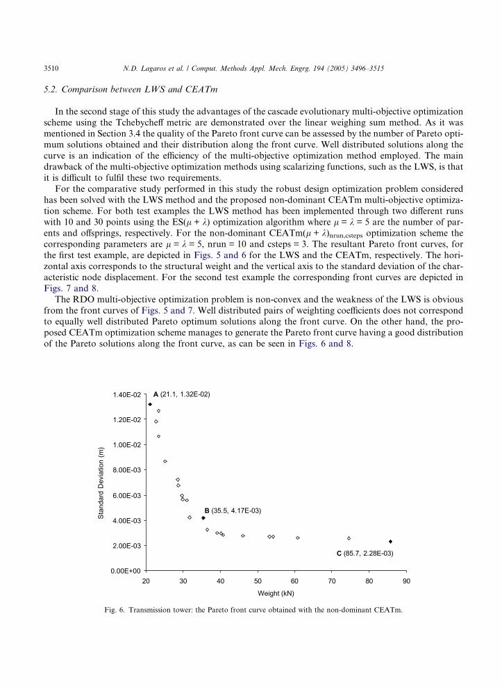
The RDO multi-objective optimization problem is non-convex and the weakness of the LWS is obvious

from the front curves of Figs. 5 and 7. Well distributed pairs of weighting coefficients does not correspondto equally well distributed Pareto optimum solutions along the front curve. On the other hand, the pro-

posed CEATm optimization scheme manages to generate the Pareto front curve having a good distribution

of the Pareto solutions along the front curve, as can be seen in Figs. 6 and 8.

0.00E+00

2.00E-03

4.00E-03

6.00E-03

8.00E-03

1.00E-02

1.20E-02

1.40E-02

20 30 40 50 60 70 80 90

Weight (kN)

Stan

dard

Dev

iatio

n (m

)

A (21.1, 1.32E-02)

B (35.5, 4.17E-03)

C (85.7, 2.28E-03)

Fig. 6. Transmission tower: the Pareto front curve obtained with the non-dominant CEATm.

0.00E+00

5.00E-04

1.00E-03

1.50E-03

2.00E-03

2.50E-03

250 300 350 400 450 500 550

Weight (kN)

Stan

dard

Dev

iatio

n (m

)

0.00E+00

5.00E-04

1.00E-03

1.50E-03

2.00E-03

2.50E-03

250 300 350 400 450 500 550

Weight (kN)

Stan

dard

Dev

iatio

n (m

)

(a)

(b)

Fig. 7. Truss bridge: the Pareto front curve obtained with LWS (a) 10 points, (b) 30 points.

N.D. Lagaros et al. / Comput. Methods Appl. Mech. Engrg. 194 (2005) 3496–3515 3511

5.3. Comparison between DBO and RDO solutions

In the third stage of this study the difference between DBO and RDO optimum designs is demonstrated

in terms of the structural weight, the variance of the response and the probability of violation of the con-

straints. The resultant Pareto front curves for the two test examples, when the proposed optimization

scheme is used, are shown in Figs. 6 and 8, respectively. The two ends of the Pareto front curve represent

0.00E+00

5.00E-04

1.00E-03

1.50E-03

2.00E-03

2.50E-03

250 300 350 400 450 500 550

Weight (kN)

Stan

dard

Dev

iatio

n (m

)A (260.4,2.42E-03)

B (328.0,1.19E-03)

C (546.3,5.23E-04)

Fig. 8. Truss bridge: the Pareto front curve obtained with the non-dominant CEATm.

3512 N.D. Lagaros et al. / Comput. Methods Appl. Mech. Engrg. 194 (2005) 3496–3515

two extreme designs. Point A correspond to the deterministic-based optimum where the weight of the struc-

ture is the dominant criterion. Point C is the optimum when the standard deviation of the response is con-sidered as the dominant criterion. The intermediate Pareto optimal solutions are compromise solutions

between these two extreme optimum designs under conflicting criteria.

In Tables 3 and 4 comparisons are performed for the three optimum designs A, B and C of Figs. 6 and 8.

The RDO(B) optimum design is achieved considering a compromise between the weight and the standard

deviation. An important outcome of this investigation is that the DBO optimum design violates the con-

straints with probability equal to 1.1% and 0.85% and probability of failure equal to 0.6% and 0.23%,

respectively for the two test examples considered. On the other hand, the probability of violation and

the probability of failure, in the case of the compromise optimum design B, are computed one to two orders

Table 3

Transmission tower: characteristic optimal solutions

DBO (A) (L · t)a RDO (B) (L · t)a RDO (C) (L · t)a

Sec1 80 · 8 110 · 10 150 · 12Sec2 70 · 7 150 · 14 160 · 15Sec3 80 · 6 100 · 8 180 · 16Sec4 70 · 9 80 · 6 150 · 12Sec5 70 · 6 80 · 8 150 · 12Sec6 75 · 7 90 · 7 150 · 12Sec7 75 · 8 100 · 8 160 · 17

Weight (kN) 21.1 35.5 85.7

Standard deviation (m) 1.32 · 10�02 4.17 · 10�03 2.28 · 10�03

pviol (%) 1.1 · 100 7.0 · 10�2 2.0 · 10�3

pf (%) 0.6 · 100 1.0 · 10�2 0.8 · 10�3

a Taken from the Equal Angle Section (EAS) table of the Eurocode for every design.

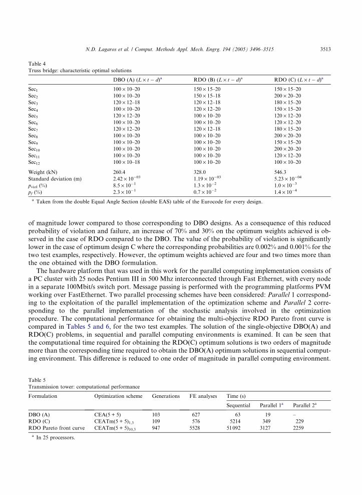
Table 4

Truss bridge: characteristic optimal solutions

DBO (A) (L · t � d)a RDO (B) (L · t � d)a RDO (C) (L · t � d)a

Sec1 100 · 10–20 150 · 15–20 150 · 15–20Sec2 100 · 10–20 150 · 15–18 200 · 20–20Sec3 120 · 12–18 120 · 12–18 180 · 15–20Sec4 100 · 10–20 120 · 12–20 150 · 15–20Sec5 120 · 12–20 100 · 10–20 120 · 12–20Sec6 100 · 10–20 100 · 10–20 120 · 12–20Sec7 120 · 12–20 120 · 12–18 180 · 15–20Sec8 100 · 10–20 100 · 10–20 200 · 20–20Sec9 100 · 10–20 100 · 10–20 150 · 15–20Sec10 100 · 10–20 100 · 10–20 200 · 20–20Sec11 100 · 10–20 100 · 10–20 120 · 12–20Sec12 100 · 10–18 100 · 10–20 100 · 10–20

Weight (kN) 260.4 328.0 546.3

Standard deviation (m) 2.42 · 10�03 1.19 · 10�03 5.23 · 10�04

pviol (%) 8.5 · 10�1 1.3 · 10�2 1.0 · 10�3

pf (%) 2.3 · 10�1 0.7 · 10�2 1.4 · 10�4

a Taken from the double Equal Angle Section (double EAS) table of the Eurocode for every design.

N.D. Lagaros et al. / Comput. Methods Appl. Mech. Engrg. 194 (2005) 3496–3515 3513

of magnitude lower compared to those corresponding to DBO designs. As a consequence of this reduced

probability of violation and failure, an increase of 70% and 30% on the optimum weights achieved is ob-

served in the case of RDO compared to the DBO. The value of the probability of violation is significantly

lower in the case of optimum design C where the corresponding probabilities are 0.002% and 0.001% for the

two test examples, respectively. However, the optimum weights achieved are four and two times more thanthe one obtained with the DBO formulation.

The hardware platform that was used in this work for the parallel computing implementation consists of

a PC cluster with 25 nodes Pentium III in 500 Mhz interconnected through Fast Ethernet, with every node

in a separate 100Mbit/s switch port. Message passing is performed with the programming platforms PVM

working over FastEthernet. Two parallel processing schemes have been considered: Parallel 1 correspond-

ing to the exploitation of the parallel implementation of the optimization scheme and Parallel 2 corre-

sponding to the parallel implementation of the stochastic analysis involved in the optimization

procedure. The computational performance for obtaining the multi-objective RDO Pareto front curve iscompared in Tables 5 and 6, for the two test examples. The solution of the single-objective DBO(A) and

RDO(C) problems, in sequential and parallel computing environments is examined. It can be seen that

the computational time required for obtaining the RDO(C) optimum solutions is two orders of magnitude

more than the corresponding time required to obtain the DBO(A) optimum solutions in sequential comput-

ing environment. This difference is reduced to one order of magnitude in parallel computing environment.

Table 5

Transmission tower: computational performance

Formulation Optimization scheme Generations FE analyses Time (s)

Sequential Parallel 1a Parallel 2a

DBO (A) CEA(5 + 5) 103 627 63 19 –

RDO (C) CEATm(5 + 5)1,3 109 576 5214 349 229

RDO Pareto front curve CEATm(5 + 5)10,3 947 5528 51092 3127 2259

a In 25 processors.

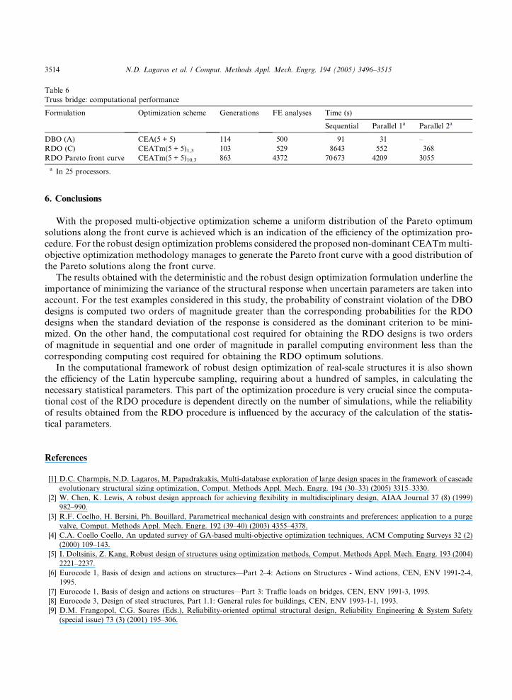
Table 6

Truss bridge: computational performance

Formulation Optimization scheme Generations FE analyses Time (s)

Sequential Parallel 1a Parallel 2a

DBO (A) CEA(5 + 5) 114 500 91 31 –

RDO (C) CEATm(5 + 5)1,3 103 529 8643 552 368

RDO Pareto front curve CEATm(5 + 5)10,3 863 4372 70673 4209 3055

a In 25 processors.

3514 N.D. Lagaros et al. / Comput. Methods Appl. Mech. Engrg. 194 (2005) 3496–3515

6. Conclusions

With the proposed multi-objective optimization scheme a uniform distribution of the Pareto optimum

solutions along the front curve is achieved which is an indication of the efficiency of the optimization pro-

cedure. For the robust design optimization problems considered the proposed non-dominant CEATmmulti-

objective optimization methodology manages to generate the Pareto front curve with a good distribution of

the Pareto solutions along the front curve.

The results obtained with the deterministic and the robust design optimization formulation underline theimportance of minimizing the variance of the structural response when uncertain parameters are taken into

account. For the test examples considered in this study, the probability of constraint violation of the DBO

designs is computed two orders of magnitude greater than the corresponding probabilities for the RDO

designs when the standard deviation of the response is considered as the dominant criterion to be mini-

mized. On the other hand, the computational cost required for obtaining the RDO designs is two orders

of magnitude in sequential and one order of magnitude in parallel computing environment less than the

corresponding computing cost required for obtaining the RDO optimum solutions.

In the computational framework of robust design optimization of real-scale structures it is also shownthe efficiency of the Latin hypercube sampling, requiring about a hundred of samples, in calculating the

necessary statistical parameters. This part of the optimization procedure is very crucial since the computa-

tional cost of the RDO procedure is dependent directly on the number of simulations, while the reliability

of results obtained from the RDO procedure is influenced by the accuracy of the calculation of the statis-

tical parameters.

References

[1] D.C. Charmpis, N.D. Lagaros, M. Papadrakakis, Multi-database exploration of large design spaces in the framework of cascade

evolutionary structural sizing optimization, Comput. Methods Appl. Mech. Engrg. 194 (30–33) (2005) 3315–3330.

[2] W. Chen, K. Lewis, A robust design approach for achieving flexibility in multidisciplinary design, AIAA Journal 37 (8) (1999)

982–990.

[3] R.F. Coelho, H. Bersini, Ph. Bouillard, Parametrical mechanical design with constraints and preferences: application to a purge

valve, Comput. Methods Appl. Mech. Engrg. 192 (39–40) (2003) 4355–4378.

[4] C.A. Coello Coello, An updated survey of GA-based multi-objective optimization techniques, ACM Computing Surveys 32 (2)

(2000) 109–143.

[5] I. Doltsinis, Z. Kang, Robust design of structures using optimization methods, Comput. Methods Appl. Mech. Engrg. 193 (2004)

2221–2237.

[6] Eurocode 1, Basis of design and actions on structures—Part 2–4: Actions on Structures - Wind actions, CEN, ENV 1991-2-4,

1995.

[7] Eurocode 1, Basis of design and actions on structures—Part 3: Traffic loads on bridges, CEN, ENV 1991-3, 1995.

[8] Eurocode 3, Design of steel structures, Part 1.1: General rules for buildings, CEN, ENV 1993-1-1, 1993.

[9] D.M. Frangopol, C.G. Soares (Eds.), Reliability-oriented optimal structural design, Reliability Engineering & System Safety

(special issue) 73 (3) (2001) 195–306.

N.D. Lagaros et al. / Comput. Methods Appl. Mech. Engrg. 194 (2005) 3496–3515 3515

[10] D. Greiner, J.M. Emperador, G. Winter, Single and multiobjective frame optimization by evolutionary algorithms and the auto-

adaptive rebirth operator, Comput. Methods Appl. Mech. Engrg. 193 (33–35) (2004) 3711–3743.

[11] D.-H. Jung, B.-C. Lee, Development of a simple and efficient method for robust optimization, Int. J. Numer. Meth. Engrg. 53

(2002) 2201–2215.

[12] K.-H. Lee, G.-J. Park, Robust optimization considering tolerances of design variables, Comput. Struct. 79 (2001) 77–86.

[13] G.-C. Luh, C.-H. Chueh, Multi-modal topological optimization of structure using immune algorithm, Comput. Methods Appl.

Mech. Engrg. 193 (36–38) (2004) 4035–4055.

[14] R.T. Marler, J.S. Arora, Survey of multi-objective optimization methods for engineering, Struct. Multidisc. Optim. 26 (6) (2004)

369–395.

[15] M.D. McKay, R.J. Beckman, W.J. Conover, A comparison of three methods for selecting values of input variables in the analysis

of output from a computer code, Technometrics 21 (2) (1979) 239–245.

[16] A. Messac, A. Ismail-Yahaya, Multi-objective robust design using physical programming, Struct. Multidisc. Optim. 23 (2002)

357–371.

[17] K. Miettinen, Non Linear Multi-objective Optimization, Kluwer Academic Publishers, 2002.

[18] M. Papadrakakis, N.D. Lagaros, Reliability-based structural optimization using neural networks and Monte Carlo simulation,

Comput. Methods Appl. Mech. Engrg. 191 (32) (2002) 3491–3507.

[19] M. Papadrakakis, V. Plevris, N.D. Lagaros, V. Papadopoulos, Robust design optimization of 3D truss structures using

evolutionary computation, 6th WCCM in Conjunction with APCOM�04, Beijing, China, September, 5–10, 2004.[20] H.J. Pradlwarter, G.I. Schueller, C.A. Schenk, A computational procedure to estimate the stochastic dynamic response of large

non-linear FE-models, Comput. Methods Appl. Mech. Engrg. 192 (7–8) (2003) 777–801.

[21] E. Sandgren, T.M. Cameron, Robust design optimization of structures through consideration of variation, Comput. Struct. 80

(2002) 1605–1613.

[22] G.I. Schueller (Ed.), Computational stochastic structural mechanics and analysis as well as structural reliability, Comput.

Methods Appl. Mech. Engrg. (2005) (special issue).

[23] R.E. Steuer, Multiple Criteria Optimization: Theory Computation and Applications, John Wiley & Sons, 1986.