large scale computations in air pollution modelling
TRANSCRIPT

Computational andNumerical Challengesin Environmental Modelling
Z. Zlatev and I. Dimov
ElsevierAmsterdamThe Netherlands
Elsevier


Preface
The protection of our environment is one of the most important problems facingmodern society. The importance of this problem has been steadily increasing dur-ing the last three to four decades, and protecting the environment is becoming evenmore important now, in the 21st century. Reliable and robust control strategies forkeeping the pollution caused by harmful chemical compounds below certain safelevels have to be developed and used in a routine way. Large mathematical mod-els, in which all of the important physical and chemical processes are adequatelydescribed, can successfully be used to support this task. However, the use of large-scale mathematical models in which all of the important physical and chemicalprocesses are adequately described leads, after the application of appropriate dis-cretization and splitting procedures, to the treatment of huge computational tasks.In a typical simulation one has to perform several hundred runs. In each of theseruns one has to carry out several thousand time-steps and at each time-step onehas to solve numerically systems of coupled ordinary differential equations contain-ing up to several million equations. Therefore, it is difficult to treat such largemathematical models numerically even when fast modern computers are available.Combined research by specialists from the fields of
• environmental and ecological modelling,
• numerical analysis, and
• scientific computing
must be carried out in an attempt to resolve successfully the challenging computa-tional problems that appear when comprehensive environmental studies are to becarried out.
In some areas of Europe, as well as in some other parts of the world, the pol-lution levels are so high that preventive actions are urgently needed. Therefore,robust and reliable control strategies must be developed in order to find out whereand by how much the emissions of harmful pollutants should be reduced. The solu-tions found must be optimal (or, at least, close to optimal), because the reductionof the emissions is as a rule an expensive process. This means that great eco-nomical problems may appear when the task of optimal reduction of the emissions
v

vi Preface
is not correctly solved. Optimal (or nearly optimal) solutions can successfully befound only by performing long series of simulation experiments consisting of manyhundreds of runs of several comprehensive mathematical models. Then the resultsobtained by different models must be carefully compared in order to answer thefollowing questions:
• are there any discrepancies, and
• what are the reasons for discrepancies?
In the cases where the answer to the first question is positive, the needed correctionsof some of the models have to be made and the simulation experiments must berepeated for the corrected models. This shows that the process of finding an optimalsolution will in general be very long and, thus, efficiency of the codes is highlydesirable. Achieving efficiency of the codes by selecting faster (but still sufficientlyaccurate) numerical algorithms and by improving the performance on different highspeed computers will be the major topics of this book.
Running mathematical models in real time can be of essential and even lifesaving importance in the case of accidental, hazardous releases (as, for example,the accident at Chernobyl in 1986). Real time calculations are also needed inconnection with short periods (episodes) with very high pollution levels, whichmight have damaging effects on human health. A special abatement strategy insuch periods can be based on temporal reductions of emissions from specific sources;e.g. traffic regulations, the energy sector, large industries (such as petrochemicalplants). Reliable mathematical models coupled with weather forecasting modelsare run operationally in order
• to predict the appearance of harmful pollution levels, and
• to make the right decision in such situations.
Running comprehensive mathematical models (in which all of the importantphysical and chemical processes are adequately described) in real time is anothervery difficult and very challenging problem that must urgently be solved.
Computer architectures are becoming faster and faster. Supercomputers thathave top performance of several Tflops will become easily available in the nearfuture. New and efficient numerical methods, by which the great potential powerof the parallel computers can be better exploited, are also gradually becomingavailable. However, many unresolved problems are still remaining. One of themost important problems is the great gap between the top performance of amodern supercomputer and the speeds actually achieved when large applicationcodes are run. The task of achieving high computational speeds close to the topperformance of the computers available, is very difficult and, at the same time, verychallenging for the comprehensive mathematical models (not only for the large-scaleenvironmental models). This is also true for the heterogeneous computations, where

Preface vii
it is possible to achieve very high computational speed when the computationalprocess is properly organized.
Some non-realistic simplifying assumptions are always made, in all of the ex-isting large-scale ecological and environmental models, in order to be able to treatthem numerically on the computers that are available. Many such assumptionsare no longer absolutely necessary, because both the computers and the numericalalgorithms are much faster than before, and will become even faster in the nearfuture. Therefore, it becomes more and more essential to describe all of the impor-tant physical and chemical processes in an adequate way (according to the presentknowledge) and to try to solve the problems by exploiting extensively the moderncomputational and numerical tools.
This short analysis of the major tasks, which must be solved in the field ofenvironmental and ecological modelling, shows clearly that there are great compu-tational and numerical challenges in the attempts to resolve efficiently these tasks.The computational and numerical challenges related to the treatment of large-scaleair pollution models will be the main topic of this book. However, the mathe-matical problems that have to be handled in the treatment of the large-scale airpollution models are rather general (systems of partial differential equations, sys-tems of ordinary differential equations, systems of linear algebraic equations, etc.).Such mathematical problems appear also during the treatment of models arising inother fields in science and engineering. Therefore, the approaches discussed in thisbook might also be useful when different large-scale scientific models are treatedon computers.
This book is divided into eleven chapters. The contents of the different chapterscan shortly be described as follows.
• A general discussion of the systems of partial differential equations (PDEs),which arise in air pollution modelling and in several other fields of scienceand engineering, is presented in the first chapter.
• It is very difficult to handle directly the systems of PDEs, by which large-scale environmental and ecological models are described. Therefore, differentsplitting techniques are commonly used in the computer treatment of suchmodels. The use of splitting techniques is discussed in the second chapter.
• One of the most important, and also one of the most difficult, processes in-volved in an air pollution model is the horizontal transport. The descriptionof the horizontal transport by mathematical terms and some numerical algo-rithms that are used to treat these terms are discussed in the third chapter.
• General ideas about the treatment of the chemical part of an air pollutionmodel are presented in the fourth chapter. The major numerical methods,which are used (can be used) in this part of the models, are also discussed inthe fourth chapter. It is explained that the same technique can be used inconnection with many other large-scale models.

viii Preface
• The systems of ordinary differential equations (ODEs), which arise duringthe treatment the chemical part of the air pollution models, can efficiently behandled by using partitioning procedures. The use of partitioning procedures(and mainly the theoretical justification of using partitioning procedures dur-ing the treatment of large-scale applications, which are not necessarily airpollution models) is described in detail in the fifth chapter.
• The application of numerical methods in the treatment of comprehensive airpollution models on computers leads to different kinds of matrix computa-tions. It is very important to carry out all these computations in an efficientway. The efficient performance of the matrix computations during the treat-ment of the air pollution models is described in the sixth chapter. Efficienttreatment of very large sparse matrices (in this book ”very large” means thatthe matrices are of order N > 106) is a great computational challenge. Theefficient treatment of very large sparse matrices is also discussed in the sixthchapter.
• While it is clear that the use of parallel computers can improve significantlythe performance of the code, it is well known that the efficient use of a par-allel computer is not an easy task when large-scale applications are to be runin parallel. Again, this statement holds not only for large-scale air pollu-tion models, but also for large-scale models arising in other fields of scienceand engineering. The use of standard tools for achieving both efficiency andportability when large-scale air pollution models are run on parallel comput-ers is discussed in the seventh chapter. The ideas are fairly general and,therefore, can also be applied when large-scale models arising in some otherareas are to be treated on parallel computers.
• Some typical applications related to different environmental studies (includinghere the important study of the influence of the biogenic emissions on the highozone levels that can cause damages on plants, animals and/or human health)are shortly described in the eighth chapter.
• The future climate changes due to the green house effect have been the majortopic of many studies in the last two-three decades. In the ninth chapterwe study the impact of future climate changes on pollution levels.
• Data assimilation is becoming more and more popular when large-scale math-ematical models arising in different fields of science and engineering are han-dled. Different problems related to the implementation of data assimilationalgorithms are discussed in the tenth chapter.
• There are still many open problems related to environmental and ecologi-cal modelling. Some of these open problems are discussed in the eleventhchapter of the book.

Preface ix
Difficult computational problems, which arise when large-scale scientific andengineering models have to be efficiently treated on computers, are discussed inthis book. Efficiency is essential, because the computational tasks are normallyhuge. We are mainly discussing the basic ideas, which can be applied in the effortsto deal with the challenges when large-scale models are to be treated on moderncomputers, without going into details that are related to the numerical methodsused. Including many details will make the book unnecessarily long and, what iseven more important, the main topic will be diffused in long explanations. How-ever, adequate references to all appropriate numerical methods are given and/orcommented in the book. Moreover, some new methods, which have not yet beentreated in detail elsewhere, are fully described. This is done, for example, when
• the stability control of the solution of the semi-discretized transport equations,
• the analysis of the error of the partitioned systems of ordinary differentialequations arising from the chemical schemes used in air pollution models,
• some problems related to very large sparse matrices, and
• the problems arising in the implementation of data assimilation algorithms inlarge-scale mathematical problems
are studied. We are sure that the approach, which was sketched in this paragraphand which was used systematically in the preparation of all eleven chapters, willmake our book easily understandable for specialists working in the following fourfields:
• environmental modelling,
• scientific computing,
• applied mathematics, and
• numerical analysis.
It is important to illustrate the fact that the ideas described in the book cansuccessfully be applied to develop different air pollution models which can be usedin the solution of a large class of important applications, such as studying effects ofclimate changes on pollution levels in Europe, investigating the influence of naturalemissions on high ozone levels, etc. The success of the chosen algorithms anddevices in treating efficiently such applications is demonstrated in Chapter 8 andChapter 9 of the book.
Finally, it should be emphasized, once again, that many of the particular al-gorithms and devices that are discussed in this book are applicable not only tolarge-scale air pollution models, but also for large scale problems arising in otherfields of science and engineering.


Acknowledgements
Most of the numerical methods and results discussed in this book have been imple-mented after many discussions with specialists from
• the National Environmental Research Institute (Ruwim Bertkowicz, JesperChristensen, Jørgen Brandt, Lise Frohn and Carsten Ambelas Skjøth),
• the Bulgarian Academy of Sciences (Krassimir Georgiev and Tzvetan Ostrom-sky),
• the Department of Applied Analysis of the University of Budapest (IstvanFarago and Agnes Havasi),
• the Institute of Informatics and Mathematical Modelling at the Technical Uni-versity of Denmark (Per Grove Thomsen, Per Christian Hansen and VincentAlan Barker),
• the Computer Science Department of the University of Copenhagen (StigSkelboe),
• the Computer Science Department of the Purdue University, Indiana, USA(Ahmed Sameh).
The authors should like to thank very much all of them.All parallel methods were implemented at the computers of UNI-C (the Danish
Center for Research and Education) and DCSC (the Danish Center for ScientificComputing). The specialists from these two institutions helped us to run the modelsor some modules of the models on different vector and parallel architectures. Weshould like to thank very much all of these specialists for their great help in differentruns of the models on high performance computers; especially Bjarne S. Andersen,Jørgen Moth, Carl Niels Hansen, Bernd Dammann, Wojciech Owczarz and JerzyWasniewski.
The different mechanisms implemented in the physical and chemical parts of themodel where developed in cooperation with many scientists from different Europeancountries (the cooperation being documented in many scientific publications):
• Lars P. Prahm (director of the Danish Meteorological Institute),
xi

xii Acknowledgements
• Dimiter Syrakov (from the Bulgarian Academy of Sciences),
• Adolf Ebel and his co-workers (from the University of Cologne, Germany),
• Heinz Hass and his co-workers (from the Ford Research Centre in Aachen,Germany),
• Anton Eliassen and Øystein Hov (from the Norwegian Meteorological Insti-tute).
The authors should like to thank very much all of these scientists for the help-ful discussions related to different issues from the field of large-scale air pollutionmodelling.
We are also very much obligated to Simon Branford from the University ofReading, UK, who read the manuscript and made a number of suggestions thatimproved the manuscript.
The research on many of the topics discussed in this book was a part of manydifferent projects funded by
• the European Union (EU),
• the North Atlantic Treaty Organization (NATO),
• the Nordic Council of Ministers (NMR),
• the Danish Research Council,
• the National Science Foundation of Bulgaria,
• the Bulgarian Academy of Sciences,
• the Danish Centre for Scientific Computing (DCSC),
• the Danish Environmental Protection Agency.
The authors should like to thank very much all of these institutions for thefinancial support of our research.
Zahari Zlatev was invited to give a course on ”Numerical and ComputationalChallenges in Environmental Modelling” at the Fields Institute for Research inMathematical Sciences (University of Toronto, Canada) in 2002. Zahari Zlatev hadmany useful discussions there with Kenneth R. Jackson, Wayne Enright and otherparticipants in the course. This book is based on the lectures given in Toronto.

Contents
Preface v
Acknowledgements xi
Contents xiii
1 PDE systems arising in air pollution modelling and justificationof the need for high speed computers 11.1 Need for large-scale air pollution modelling . . . . . . . . . . . . . . 21.2 The Danish Eulerian Model (DEM) . . . . . . . . . . . . . . . . . . 51.3 Input data . . . . . . . . . . . . . . . . . . . . . . . . . . . . . . . . . 131.4 Output data . . . . . . . . . . . . . . . . . . . . . . . . . . . . . . . . 181.5 Measurement data . . . . . . . . . . . . . . . . . . . . . . . . . . . . 211.6 Some results obtained by DEM . . . . . . . . . . . . . . . . . . . . . 241.7 Applicability to PDEs arising in other areas . . . . . . . . . . . . . . 351.8 Concluding remarks . . . . . . . . . . . . . . . . . . . . . . . . . . . 39
2 Using splitting techniques in the treatment of air pollution models 432.1 Four types of splitting procedures . . . . . . . . . . . . . . . . . . . . 442.2 Sequential splitting procedures . . . . . . . . . . . . . . . . . . . . . 452.3 Symmetric splitting procedures . . . . . . . . . . . . . . . . . . . . . 512.4 Weighted sequential splitting procedures . . . . . . . . . . . . . . . . 522.5 Weighted symmetric splitting procedures . . . . . . . . . . . . . . . . 532.6 Advantages and disadvantages
of the splitting procedures . . . . . . . . . . . . . . . . . . . . . . . . 532.7 Comparison of different splitting procedures . . . . . . . . . . . . . . 542.8 Numerical experiments . . . . . . . . . . . . . . . . . . . . . . . . . . 582.9 Using splitting procedures in connection
with other applications . . . . . . . . . . . . . . . . . . . . . . . . . . 862.10 Conclusions and plans for future research . . . . . . . . . . . . . . . 86
xiii

xiv Contents
3 Treatment of the advection-diffusion phenomena 893.1 Treatment of the horizontal advection . . . . . . . . . . . . . . . . . 903.2 Semi-discretization of the advection equation . . . . . . . . . . . . . 923.3 Time integration of the semi-discretized
advection equation . . . . . . . . . . . . . . . . . . . . . . . . . . . . 953.4 Numerical treatment
of the horizontal diffusion . . . . . . . . . . . . . . . . . . . . . . . . 1053.5 Numerical treatment of the vertical exchange . . . . . . . . . . . . . 1053.6 Applicability to other large-scale models . . . . . . . . . . . . . . . . 1063.7 Concluding remarks and
plans for future research . . . . . . . . . . . . . . . . . . . . . . . . . 106
4 Treatment of the chemical part: general ideas and major numer-ical methods 1094.1 The chemical sub-model . . . . . . . . . . . . . . . . . . . . . . . . . 1104.2 Why is it difficult to handle
the chemical sub-model? . . . . . . . . . . . . . . . . . . . . . . . . . 1114.3 Algorithms for the numerical integration
of the chemical ODE systems . . . . . . . . . . . . . . . . . . . . . . 1144.4 Numerical results . . . . . . . . . . . . . . . . . . . . . . . . . . . . . 1274.5 Treatment of the deposition . . . . . . . . . . . . . . . . . . . . . . . 1344.6 Applicability to other large-scale models . . . . . . . . . . . . . . . . 1344.7 Plans for future work . . . . . . . . . . . . . . . . . . . . . . . . . . . 135
5 Error analysis of the partitioning procedures 1375.1 Statement of the problem . . . . . . . . . . . . . . . . . . . . . . . . 1375.2 When is ‖y[µ]
n+1 − z[ν]n+1‖ small? . . . . . . . . . . . . . . . . . . . . . 139
5.3 An application to air pollution problems . . . . . . . . . . . . . . . . 1505.4 Applicability to other models . . . . . . . . . . . . . . . . . . . . . . 1535.5 Concluding remarks and plans for future work . . . . . . . . . . . . . 154
6 Efficient organization of the matrix computations 1576.1 The horizontal advection-diffusion sub-model . . . . . . . . . . . . . 1586.2 Matrices in the vertical exchange sub-model . . . . . . . . . . . . . . 1616.3 Matrices arising in the chemical sub-model . . . . . . . . . . . . . . 1626.4 Treatment of the model without splitting . . . . . . . . . . . . . . . 1646.5 Use of sparse matrix techniques . . . . . . . . . . . . . . . . . . . . . 1656.6 Utilizing the cache memory
for large sparse matrices . . . . . . . . . . . . . . . . . . . . . . . . . 1876.7 Comparisons with another sparse code . . . . . . . . . . . . . . . . . 1976.8 Applicability to other models . . . . . . . . . . . . . . . . . . . . . . 1996.9 Concluding remarks . . . . . . . . . . . . . . . . . . . . . . . . . . . 199

Contents xv
7 Parallel computations 2017.1 The IBM SMP architecture . . . . . . . . . . . . . . . . . . . . . . . 2037.2 Running the codecode on one processor . . . . . . . . . . . . . . . . 2047.3 Parallel runs on one node of the IBM SMP computer . . . . . . . . . 2127.4 Parallel runs of the code across the nodes . . . . . . . . . . . . . . . 2157.5 Scalability of the code . . . . . . . . . . . . . . . . . . . . . . . . . . 2167.6 When is it most desirable
to improve the performance? . . . . . . . . . . . . . . . . . . . . . . 2177.7 Unification of the different versions of the model . . . . . . . . . . . 2197.8 OpenMP implementation versus
MPI implementation . . . . . . . . . . . . . . . . . . . . . . . . . . . 2227.9 Parallel computations for general
sparse matrices . . . . . . . . . . . . . . . . . . . . . . . . . . . . . . 2237.10 Applicability to other large-scale models . . . . . . . . . . . . . . . . 2277.11 Concluding remarks and plans for future work . . . . . . . . . . . . . 228
8 Studying high pollution levels 2338.1 Exceedance of some critical levels for ozone . . . . . . . . . . . . . . 2348.2 How to reduce the number of ”bad” days? . . . . . . . . . . . . . . . 2358.3 Influence of the biogenic V OC emissions on the ozone pollution levels2378.4 Studying the transport of pollutants
to a given country . . . . . . . . . . . . . . . . . . . . . . . . . . . . 2378.5 Prediction of the pollution levels for 2010 . . . . . . . . . . . . . . . 2408.6 Some conclusions . . . . . . . . . . . . . . . . . . . . . . . . . . . . . 243
9 Impact of future climate changes on high pollution levels 2459.1 Climate changes and air pollution levels . . . . . . . . . . . . . . . . 2469.2 Definition of six scenarios . . . . . . . . . . . . . . . . . . . . . . . . 2479.3 Validation of the results . . . . . . . . . . . . . . . . . . . . . . . . . 2529.4 Variations of emissions and of meteorological parameters . . . . . . . 2599.5 Results from the climatic scenarios . . . . . . . . . . . . . . . . . . . 2669.6 Conclusions and plans for future work . . . . . . . . . . . . . . . . . 276
10 Implementation of variational data assimilation 27710.1 Basic ideas . . . . . . . . . . . . . . . . . . . . . . . . . . . . . . . . 27810.2 Calculating the gradient of the functional . . . . . . . . . . . . . . . 27910.3 Forming the adjoint equations . . . . . . . . . . . . . . . . . . . . . . 28010.4 Algorithmic representation of
a data assimilation algorithm . . . . . . . . . . . . . . . . . . . . . . 28210.5 Variational data assimilation
for some one-dimensional examples . . . . . . . . . . . . . . . . . . . 28710.6 Numerical results for the one-dimensional
transport equation . . . . . . . . . . . . . . . . . . . . . . . . . . . . 29010.7 Treatment of some simple non-linear tests-problems . . . . . . . . . 299

xvi Contents
10.8 Concluding remarks . . . . . . . . . . . . . . . . . . . . . . . . . . . 315
11 Discussion of some open questions 31711.1 Avoiding the use of splitting procedures . . . . . . . . . . . . . . . . 31711.2 Need for reliable error control . . . . . . . . . . . . . . . . . . . . . . 31911.3 Running of air pollution models on fine grids . . . . . . . . . . . . . 31911.4 Transition from regional to urban scale . . . . . . . . . . . . . . . . . 32011.5 Static and dynamic local refinement . . . . . . . . . . . . . . . . . . 32111.6 Need for advanced optimization techniques . . . . . . . . . . . . . . 32211.7 Use of data assimilation techniques . . . . . . . . . . . . . . . . . . . 32211.8 Special modules for treatment of particles . . . . . . . . . . . . . . . 32411.9 Use of computational grids . . . . . . . . . . . . . . . . . . . . . . . 32411.10Applicability of the methods
to other large mathematical models . . . . . . . . . . . . . . . . . . . 326
Appendix A: Colour plots 327
Bibliography 333
Symbol Table 357
Author Index 359
Subject Index 367

Chapter 1
PDE systems arising in airpollution modelling andjustification of the need for highspeed computers
It is well-known that mathematics bridges gaps in culture, science and technology.This statement will be illustrated in this book
• by studying a large class of mathematical models arising in the area of airpollution modelling (as well as in mathematical models that arise in manyother areas of science and engineering), and
• by discussing how long sequences of challenging problems from different sci-entific and engineering areas can be resolved by using powerful tools fromthe numerical mathematics and scientific computing during the treatment ofadvanced models in which all underlying physical and chemical processes areadequately described.
Air pollution, especially the reduction of the air pollution to some acceptablelevels, is a highly relevant environmental problem, which is becoming more and moreimportant. This problem can successfully be studied only when high-resolutioncomprehensive mathematical models, described by systems of partial differentialequations (PDEs), are developed and used on a routine basis. However, such modelsare very time-consuming, even when modern high-speed computers are available.Indeed, if an air pollution model is to be applied on a large space domain by usingfine grids, then its discretization will always lead to huge computational problems,even in the case when two-dimensional versions of the models are used. Assume,for example, that the two-dimensional space domain on which the model underconsideration is defined is discretized by using a (480 × 480) grid and that the
1

2 Chapter 1
number of chemical species studied by the model is 35. Then several systemsof ordinary differential equations (ODEs) containing 8064000 equations have to betreated at every time-step (the number of time-steps typically being several hundredthousand). If a three-dimensional version of the air pollution model is to be used,then the above quantity must be multiplied by the number of layers. Moreover,hundreds and even thousands of simulation runs have to be carried out in most ofthe studies related to policy making. Therefore, it is extremely difficult to treatsuch large computational problems. This is true even when the fastest computersthat are available at present are used.
The computational time needed to run such a model causes, of course, themajor difficulty. However, there is another difficulty which is at least as importantas the problem with the computational time. The models need a great amount ofinput data (meteorological, chemical and emission data). Furthermore, the modelproduces huge files of output data, which have to be stored for future uses (forvisualization and animation of the results). Finally, huge sets of measurement data(normally taken at many stations located in different countries) have to be used inthe efforts to validate the model results.
The short discussion of the difficulties, which arise when large-scale mathemat-ical models are treated on high-speed computers, shows clearly that both
• the computational time requirements, and
• the storage requirements
impose many challenging problems when large-scale air pollution models (or otherlarge-scale models) are to be developed and used in different studies. A generaldiscussion of the major numerical and computational challenges in air pollutionmodelling will be presented in this chapter.
After that, specific numerical and computational challenges will be studied indetail in the following chapters.
It must be emphasized here that many results from this book, results that arerelated to the numerical solution of systems of PDEs and/or ODEs, might be usedin some other fields of science and engineering (several examples arising in otherareas of environmental modelling are given in Section 7 of this chapter).
1.1 Need for large-scale air pollution modelling
The control of the pollution levels in different highly developed regions of Europeand North America (and also in other highly industrialized regions of the world)is an important task for modern society. Its relevance has been steadily increasingduring the last two to three decades. The need to establish reliable control strate-gies for the air pollution levels will become even more important in the future.Large-scale air pollution models can successfully be used to design reliable controlstrategies. Many different tasks must be solved before starting to run operationallyan air pollution model. The following tasks are most important:

PDE systems arising in air pollution models 3
1. Describe in an adequate way all important physical and chemical processes.
2. Apply fast and sufficiently accurate numerical methods in the different partsof the model.
3. Ensure that the model runs efficiently on modern high-speed computers (and,first and foremost, on different types of parallel computers).
4. Use high quality input data (both meteorological data and emission data) inthe runs.
5. Verify the model results by comparing them with reliable measurements takenin different parts of the space domain of the model.
6. Carry out some sensitivity experiments to check the response of the model tochanges of different key parameters.
7. Visualize and animate the output results to make them easily understandableeven to non-specialists.
It is absolutely necessary to solve efficiently all these tasks. However, the treat-ment of such large-scale air pollution models, in which all relevant physical andchemical processes are adequately described, leads to great computational difficul-ties related both to the CPU time needed to run the models and to the input andoutput data used during the runs and saved for future applications. Therefore, itis necessary to give an answer to the question:
Why are large-scale comprehensive mathematical modelsneeded (and also used) in many environmental studies?
A short, but also adequate, answer to this question can be given in the followingway. It is well-known, by the broad public in Europe, North America and all otherparts of the world, that the air pollution levels in a given region depend not onlyon the emission sources located in it, but also on emission sources located outsidethe region under consideration, and even on sources that are far away from thestudied region. This is due to the transboundary transport of air pollutants. Theatmosphere is the major medium where pollutants can quickly be transported overlong distances. Harmful effects on plants, animals and humans can also occur inareas which are far away from big emission sources. Chemical reactions take placeduring the transport. This leads to the creation of secondary pollutants, which canalso be harmful. The air pollution levels in densely populated and highly developedregions of the world, such as Europe and North America (but this will soon becometrue also for many other regions), must be studied carefully to find out how the airpollution can be reduced to safe levels and, moreover, to develop reliable controlstrategies by which air pollution can be kept under certain prescribed critical levels.The reduction of the air pollution is an expensive process. This is why one musttry to optimize this process by solving two important tasks:

4 Chapter 1
• the air pollution levels must be reduced to reliably determined critical levels(but no more if costs are high), and
• since the air pollution levels in different parts of a big region (as, for example,Europe or North America) are varying in a quite wide range, the optimalsolution (a solution which is as cheap as possible) will require reducing theemissions by different amounts in different parts of a big region.
Reliable mathematical models, in which all relevant physical and chemical proces-ses are adequately described (according to the available at present knowledge aboutthese processes) are needed in the efforts to solve successfully these two tasks. Largecomprehensive models for studying air pollution phenomena were first developedin North America: see, for example, Binkowski and Shankar [21], Carmichael andPeters [38], Carmichael et al. [39], [40], [41], Chang et al. [42], Dabdub and Seinfeld[51], Peters et. al. [194], Stockwell et al. [234] and Venkatram et al. [257]. Thereare several such large models in Europe: see Ackermann et al. [2], Aloyan [7],Builtjes [34], [35], D’Ambra et al. [57], Elbern et al. [91], Hongisto, [138], Hongistoet al. [139], Langner et al. [156], Jonson et al. [149], San Jose et al. [214], Simpson[222], [223], Tomlin et al. [250] and Zlatev [282].
The recent development of many of the existing large-scale air pollution mod-els is described in several papers from the proceedings of two NATO AdvancedResearch Workshops:
• ”Large Scale Computations in Air Pollution Modelling”, see Zlatev et al.[291], and
• ”Advances in Air Pollution Modelling for Environmental Security”, see Faragoet al. [99].
A comprehensive review of latest results achieved in the efforts to improve theperformance of the large-scale environmental models is given in a very well-writtenpaper of Ebel, see [84].
The use of the Danish Eulerian Model (DEM), which is fully described in Zlatev[282] (see also the web-site of the model [284]), for the solution of the tasks listedabove will be discussed in this book. However, the particular choice of thismodel is made only in order to facilitate the understanding of the state-ments. The ideas used in the development of all comprehensive mathematicalmodels for studying air pollution phenomena are rather similar. Therefore, theconsideration of any other large-scale air pollution model will in general lead tosimilar results and conclusions. It should be emphasized, once again, that someother applications from different fields of science and engineering are describedmathematically by similar systems of PDEs and, thus, the methods and techniquesused in the following chapters in relation to DEM can also be applied to such appli-cations (this is demonstrated by discussing several examples, which are taken fromother areas of environmental modelling, in Section 7 of this chapter).

PDE systems arising in air pollution models 5
1.2 The Danish Eulerian Model (DEM)
Some information about the last versions of the Danish Eulerian Model (DEM),which was developed at the National Environmental Research Institute (Roskilde,Denmark) and used in many environmental studies, will be presented in this andthe following sections.
1.2.1 Some historical information
The work on the development of DEM has been initiated in the beginning of 80’s.Only two species, sulphur dioxide and sulphate, were studied in the first versionof the model. The space domain was rather large (the whole of Europe), butthe discretization was very crude; the space domain was discretized by using of a(32×32) grid, which means, roughly speaking, that (150 km×150 km) grid-squareswere used. Both a two-dimensional version and a three-dimensional version of thismodel were developed. In both versions the chemical scheme was very simple.There was only one, linear, chemical reaction: it was assumed that a fixed part ofthe sulphur dioxide concentration is transformed, at each time step, into sulphateconcentration. The two-dimensional version of this model is fully described inZlatev [277], while the three-dimensional version was discussed in Zlatev et al.[288].
This first version was gradually upgraded to much more advanced versions bycarrying out successively the following actions:
1. Introducing physical mechanisms in a more adequate way.
2. Increasing the number of chemical compounds which can be studied by themodel (chemical schemes with 35, 56 and 168 compounds were implemented).
3. Improving the spatial resolution of the model by transition from the original(32 × 32) grid to a (96 × 96) grid, a (288 × 288) grid and a (480 × 480) grid,i.e. by reducing the (150 km × 150 km) grid-squares used in the originalversions to (50 km× 50 km), (16.667 km× 16.667 km) and (10 km× 10 km)grid-squares.
4. Developing more advanced three-dimensional versions of the model with tenvertical layers.
5. Attaching new and faster numerical algorithms to the different parts of themodel.
6. Preparing the model for efficient runs on different high-speed computers (bothvector processors and parallel computer architectures).
DEM is well-structured and the above changes have been made by replacing onlyone module at a time. In this way the response of the model to different changes

6 Chapter 1
was also studied. Different versions of the model obtained during the upgradingprocedure were described and discussed in many publications; see, for example,Zlatev [282], Zlatev et al. [294] and [295].
Results, obtained in comparisons of the concentrations and depositions calcu-lated by different versions of the model with measurements taken at stations lo-cated in different European countries, were presented in Zlatev [282] and Zlatev etal. [292], [293]. Some comparisons of model results with measurements taken oversea were also carried out; see Harrison et al. [128].
Different versions of the model were also used in long simulations connectedwith studies of the relationships between high ozone concentrations in Europe andrelated emissions (NOx emissions and V OC emissions). Many results, which wereobtained in these simulations, were discussed in Ambelas Skjøth et al. [9], Bastrup-Birk et al. [18] and Zlatev et al. [297].
The improvement of the physical and chemical mechanisms used in the modeldemanded an improvement also of the numerical algorithms used in the computertreatment of the model. Furthermore, high-speed computers became necessary.It is normally very difficult to achieve a good performance on the new moderncomputer architectures. A long and careful work, which is still carried out, isnecessary in order to achieve a high computational speed when the model is runon such architectures. On the other hand, it will be impossible to carry out severalhundreds (and in many cases even several thousands) of runs with DEM in the longsimulation process when its code does not run very efficiently on the computersavailable. Different procedures used in the attempts to achieve high computationalspeeds on different computers are presented in Brown et al. [32], Georgiev andZlatev [116], [117], Owczarz and Zlatev [188], [189], [190] and Zlatev [278], [280],[282].
Some more details about the last versions of DEM will be given in the followingsub-sections. Recently, the different versions of DEM were united in a flexible andpowerful model, the Unified Danish Eulerian Model (UNI-DEM). UNI-DEM willbe discussed in Chapter 7.
1.2.2 Chemical species treated in the model
The European pollution levels of all important chemical pollutants can be studiedby using DEM. The chemical species involved in the model are:
• sulphur pollutants,
• nitrogen pollutants,
• ozone,
• ammonia-ammonium,
• several radicals, and
• a large number of relevant hydrocarbons.

PDE systems arising in air pollution models 7
1.2.3 Mathematical formulation of the model
DEM, as many other large-scale air pollution models, is described mathematicallyby a system of partial differential equations (PDEs):
∂cs
∂t= −∂(ucs)
∂x− ∂(vcs)
∂y− ∂(wcs)
∂z(1.1)
+∂
∂x
(Kx
∂cs
∂x
)+
∂
∂y
(Ky
∂cs
∂y
)+
∂
∂z
(Kz
∂cs
∂z
)
+Es + Qs(c1, c2, . . . , cNs)
−(κ1s + κ2s)cs,
s = 1, 2, . . . , Ns.
The different quantities that are involved in the mathematical model have thefollowing meaning:
• the concentrations are denoted by cs,
• u, v and w are wind velocities,
• Kx, Ky and Kz are diffusion coefficients,
• the emission sources in the space domain are described by the functions Es,
• κ1s and κ2s are deposition coefficients,
• the chemical reactions used in the model are described by the non-linearfunctions Qs(c1, c2, . . . , cNs).
The number of equations Ns is equal to the number of chemical species thatare involved in the model and varies in different studies. Until now, the model hasmainly been used with a chemical scheme containing 35 species (it may be necessaryto involve more species in the future; experiments with chemical schemes containing56 and 168 species have recently been carried out). The chemical scheme with 35species is the well-known CBM IV scheme (described in Gery et al. [118]) with afew enhancements which have been introduced in order to make it possible to usethe model in studies concerning the distribution of ammonia-ammonium concen-trations in Europe as well as the transport of ammonia-ammonium concentrationsfrom Central and Western Europe to Denmark. Recently, some other chemicalschemes were developed and successfully tested in different models; see, for ex-ample, Stockwell et al. [233]. There are plans to implement some of these newchemical mechanisms in DEM in the near future.

8 Chapter 1
The number of chemical species used in different large air pollution models variesfrom 20 to about 200 (see, for example, Borrell et al. [22], Carmichael and Peters[38], Carmichael et al. [39], Chang et al. [42], Ebel et al. [85], Hass et al. [129], [130],Peters et. al. [194], Stockwell et al. [234] and Venkatram et al. [257]). The use ofless than 20 chemical species will require crude parameterization of some chemicalprocesses and, thus, the use of such chemical schemes is in general not advisable,when the accuracy requirements that are to be satisfied are not very crude. Onthe other hand, the use of more than 200 chemical species is connected with hugecomputational tasks that cannot be handled, at least when long-term simulationsare to be carried out, on the computers available at present without imposing asequence of simplifying assumptions, which will lead to a crude parameterizationof the other physical processes involved in the air pollution models (advection,diffusion, deposition and emission) and/or to discretizations of the models on coarsegrids. Thus, the chemical scheme containing 35 species seems to be a good choice.Nevertheless, as mentioned above, experiments with two other chemical schemes,containing 56 and 168 chemical species, are at present carried out.
It should be pointed out that although the use of more than 100 chemical speciesin the chemical scheme (but less than 200) leads at present, as mentioned above,to the necessity both
• to apply certain simplifying assumptions in the description of the physicaland chemical mechanisms, and/or
• to apply coarse grids in the dsicretization of the space domain of the modelunder consideration,
the computers are becoming faster and faster and, therefore, such actions will prob-ably not be necessary in the near future.
The non-linear functions Qs from (1.1) can as a rule be rewritten in the followingform:
Qs(c1, c2, . . . , cNs) = −Ns∑i=1
αsici +Ns∑i=1
Ns∑j=1
βsijcicj , (1.2)
where s = 1, 2, ..., Ns.This is a special kind of non-linearity, but it is not obvious how to exploit this
fact during the numerical treatment of the model.It follows from the above description of the quantities involved in the mathemati-
cal model that all five physical processes (advection, diffusion, emission, depositionand chemical reactions) can be studied by using the system of PDEs describedby (1.1). The most important processes, when the computations are considered,are the horizontal advection (the horizontal transport) and the chemical reactions.Kernels for these two parts of the model must be treated numerically by using bothfast and sufficiently accurate algorithms.

PDE systems arising in air pollution models 9
1.2.4 Space domain
The space domain of the model (it contains the whole of Europe together with partsof Asia, Africa and the Atlantic Ocean) is discretized by using a (96 × 96) grid inthe version of DEM which is operationally used at present. This means that
• Europe is divided into 9216 grid-squares, and
• the grid resolution is approximately (50 km × 50 km).
It has been mentioned above that some work is carried out at present to runDEM by using much higher resolution applying either a (288 × 288) grid or a(480 × 480) grid. If these two grids are used, then
• Europe is divided into 82944 grid-squares for the (288×288) grid and 230400grid-squares for the (480 × 480) grid, and
• the grid resolution is approximately (16.67 km×16.67 km) for the (288×288)grid and (10 km × 10 km) for the (480 × 480) grid.
It will be shown in the next sections that the high resolution versions of DEMimpose severe storage requirements; both the input files and the output files that areneeded in the runs become much larger than those used in the operational version.Also, of course, the computational time needed to run this version is increasedvery considerably. Nevertheless, some rather comprehensive studies were recentlyperformed by using fine resolution options of DEM (see Zlatev and Syrakov [299],[300]).
1.2.5 Initial and boundary conditions
Appropriate initial and boundary conditions are needed. If initial conditions areavailable (for example from a previous run of DEM and/or another model), thenthese are read from the files where they are stored. If initial conditions are notavailable, then a five day start-up period is used to obtain initial conditions (i.e.the computations are started five days before the desired starting date with somebackground concentrations and the concentrations found at the end of the fifth dayare actually used as starting concentrations).
The choice of lateral boundary conditions is in general very important. Thisissue has been discussed in Brost [31]. However, if the space domain is very large,then the choice of lateral boundary conditions becomes less important; which isstated on p. 2386 in Brost [31]: ”For large domains the importance of the bound-ary conditions may decline”. The lateral boundary conditions are represented inDEM with typical background concentrations which are varied, both seasonally anddiurnally. The use of background concentrations is justified by the facts that:
• the space domain is very large (approximately 4800 km × 4800 km), and

10 Chapter 1
• the boundaries are located far away from the highly polluted regions (in theAtlantic Ocean, North Africa, Asia and the Arctic areas).
Nevertheless, it would perhaps be better to use values of the concentrations atthe lateral boundaries that are calculated by a hemispheric or global model.
For some chemical species, as for example ozone, it is necessary to introducesome exchange with the free troposphere. Three such rules have been tested inZlatev et al. [292]. The third rule described in Zlatev et al. [292] is at present usedin DEM, because the experiments, which were carried out there, indicated that thisrule performs in general better than the other two rules.
1.2.6 Need for splitting procedures
It is difficult to treat the system of PDEs (1.1) directly. This is the reason forusing different kinds of splitting.
The mathematical model is divided into several simpler sub-models whena splitting procedure is applied. Consider any of these sub-models. Assume thatthe space domain is a parallelepiped which is discretized by using a grid withNx×Ny ×Nz grid-points, where Nx, Ny and Nz are the numbers of the grid-pointsalong the grid-lines parallel to the Ox, Oy and Oz axes. Assume further that thenumber of chemical species involved in the model is Ns. Finally, assume that thespatial derivatives in (1.1) are discretized by some numerical algorithm. Then thesystem of PDEs, by which the sub-model under consideration is represented, willbe transformed into a system of ODEs (ordinary differential equations)
dg
dt= f(t, g), (1.3)
where g(t) is a vector-function with Nx × Ny × Nz × Ns components. Moreover,the components of function g(t) are the concentrations (at time t) at all grid-pointsand for all species. The right-hand side f(t, g) of (1.3) is also a vector function withNx×Ny×Nz×Ns components which depends both on the particular discretizationmethod used and on the concentrations of the different chemical species at the grid-points. If the space discretization method is fixed and if the concentrations arecalculated (at all grid-points and for all species), then the right-hand side vector in(1.3) can also be calculated.
The number of systems of ODEs of type (1.3) is equal to the number of sub-models obtained when the selected splitting procedure is applied. If no splitting isused and the spatial derivatives in (1.1) are discretized, then only one system oftype (1.3) will appear. The latter system and the systems of type (1.3) obtainedby applying some splitting procedure are of the same order. Therefore, the firstimpression is that the computational work will be increased when splitting is used,because one has to handle several systems of ODEs instead of only one for thecase where (1.1) is treated without splitting. However, this is in general not true,because the systems (1.3) induced by the selected splitting procedure are much

PDE systems arising in air pollution models 11
simpler. In fact, these systems are normally formed of many independent relativelysmall sub-systems (see also Chapter 7). The advantage of solving several simplerand relatively small systems of type (1.3) when splitting is used has much greatereffect on the efficiency of the solution process than the disadvantage that severalsuch systems are to be handled instead of only one system in the case where (1.1) issolved without splitting. This is why splitting is used in all operational large-scaleair pollution models.
Splitting procedures will be studied in the next chapter. The space discretiza-tion of the spatial derivatives in the different sub-models, which are obtained byusing the selected splitting procedure, will be studied in detail in Chapter 3. Thetime discretization of the systems of ODEs which arise in the different sub-modelswill be studied in Chapter 3 to Chapter 6. The exploitation of the properties of dif-ferent splitting procedures in the efforts to obtain efficient performance on parallelcomputers will be discussed in Chapter 7.
1.2.7 Need for high speed computers
The size of the systems, which arise after the space discretization and the splittingprocedures used to treat (1.1) numerically, is enormous. Consider the case wherethe model is two-dimensional. Let us assume that
• the model is discretized on a (96 × 96) grid (such a grid has been used inDEM after 1993), and
• Ns = 35.
As mentioned in Sub-section 1.2.6, the model is split to several sub-modelsby the selected splitting procedure. After the application of a semi-discretization,each sub-model is reduced to a system of ODEs. The number of equations ineach of these systems of ODEs is 96 × 96 × 35 = 322560. The time-step size usedin the advection step is 15 min The chemical sub-model cannot be treated withsuch a large time-step size (because it is very stiff; especially when photochemicalreactions are involved). Therefore six small chemical time-steps are carried out foreach advection time-step (this means that the chemical time-step size is 2.5 min).
Assume, furthermore, that a one-year run (and, more precisely, 365 days + 5days to start-up the computations) is to be carried out. This will result in 35 520advection time-steps and in 213 120 chemical time-steps.
Consider now the case where the model is three-dimensional. Assume that tenlayers are used in the vertical direction. Then the number of equations in everysystem of ODEs is 3 225 600 (i.e. ten times greater than in the previous case). Thenumbers of advection and chemical time-steps remain the same, 35 520 and 213120 respectively.
More general, the number of equations in each ODE system is equal to the prod-uct of the number of the grid-points and the number of chemical species. Therefore,

12 Chapter 1
Table 1.1: The numbers of equations per system of ODEs that are to betreated at every time-step when different discretizations and different chemicalschemes (number of species) are used.
Number of (32 × 32 × 10) (96 × 96 × 10) (288 × 288 × 10) (480 × 480 × 10)species
1 10240 92160 829440 23040002 20480 184320 1658880 4608000
10 102400 921600 8294400 2304000035 358400 3225600 29030400 8064000056 573440 5160960 46448640 129024000
168 1720320 15482880 139345920 387072000
this number grows very quickly when the number of grid-points and/or the num-ber of chemical species is increased. The numbers of equations treated at everytime-step, which are obtained for different numbers of grid-points and for differentnumbers of chemical species, are given in Table 1.1. It should be mentioned thatthe coarsest grid, i.e. the 32 × 32 × 10 grid is no longer used.
It is clear (and this has already been mentioned) that such large problems canbe solved only if new and modern high speed computers are used. Moreover, itis necessary to select the right numerical algorithms (which are most suitable forthe high speed computers available) and to perform the programming work verycarefully in order to exploit fully the great potential power of the vector and/orparallel computers. Different versions of DEM have already been successfully runon several high-speed computers (see Brown et al. [32], Georgiev and Zlatev [116],[117], Owczarz and Zlatev [188], [189], [190], Zlatev [278], [280], [282] and Zlatev etal. [294]).
Standard tools for achieving parallelism, such as
• OpenMP ([265]),
• the Parallel Virtual Machine (PVM, Geist et al. [114]) and
• the Message Passing Interface (MPI, Gropp et al. [124]),
have been used to facilitate the transition of the code from one high-speed computerto another and, hopefully, to facilitate the implementation of the code on computerarchitectures which will appear in the near future.
However, we are still not able to solve all the problems listed in Table 1.1. Someof the problems are only treated as two-dimensional models. This means that it isstill necessary to improve the performance of the different algorithms on differenthigh speed computers. Therefore, many more experiments are needed (and will becarried out in the future). High-quality algorithms and software for solving some

PDE systems arising in air pollution models 13
standard mathematical problems are now available (see, for example, Anderson etal. [11], Barrett et al. [15], Demmel [60], Dongarra et al. [80] and Trefethen andBau III [252]) and one should try to use them extensively in the attempts to achievehigh efficiency when large air pollution models are to be treated numerically on highperformance computers.
Finally, it should be emphasized here that there are many other activities in theefforts to utilize in a better way the great potential power of the modern high-speedcomputers; see, for example, Bruegge et al. [33], D’Ambra et al. [57], Dabdub andMahonar [50], Dabdub and Seinfeld [52], Elbern [87], Elbern et al. [91], Jacobsenand Turco [143].
1.3 Input data
It is necessary to prepare large files of input data which are to be used when an airpollution model is run on the available computers. Of course, this is also true whenlarge-scale models arising in other fields are to be handled. Some of the problemsconnected with the necessity to handle huge input data sets will be discussed inthis section.
1.3.1 General information about the input data
Two types of input data are needed when a large-scale air pollution model is to behandled numerically on a computer:
• meteorological data, and
• emission data.
The input data needed in DEM (both the meteorological data and the emissiondata) have been prepared within EMEP (the European Monitoring and EvaluationProgramme). EMEP is a common European project in which nearly all Europeancountries participate. The project was initiated in the 70s and is supported finan-cially by the United Nations Economic Commission for Europe, UN-ECE. In thepast we used the data prepared by DNMI (the Norwegian Meteorological Institute).Now a lot of data can be obtained from specialized Internet sites; see, for example,EMEP Home Page [94].
Input data, which have been received from other sources, have occasionally beenused.
Measurement data are also to be used for different purposes (as, for example,in the validation of the reliability of the model results). Measurement data fromthe network of the EMEP measurement stations are also available on the Internet(see again EMEP Home Page [94]), and have been regularly used in
• order to verify the model results, and

14 Chapter 1
Table 1.2: Meteorological fields used at present in the two-dimensional ver-sions of DEM
Meteorological input data LevelHorizontal wind velocities σ = 0.925, z = 750m
Vertical wind velocities σ = 0.850, z = 1500mMixing height Above ground
Average precipitation GroundCloud covers Free troposphere
Temperature in the mixing layer σ = 0.925Surface temperature z = 2m
Relative humidity σ = 0.925
• an attempt to improve the quality of some fields used in the model (initialconcentrations, emissions, etc.) by applying different data assimilation pro-cedures.
1.3.2 Meteorological data
The meteorological data for the two-dimensional versions of DEM contain hori-zontal wind velocity fields, vertical wind velocity fields (at the top of the boundarylayer), temperatures (both surface temperatures and temperatures of the bound-ary layer), precipitation fields, mixing heights, cloud covers and pressures. Theresolution of the meteorological fields is normally coarser than the resolution usedin the model: the time resolution for all fields except the mixing heights fields isat present six hours (the resolution for the mixing heights fields is 12 hours), thespatial resolution of the available now data is 150 km × 150 km. Simple linearinterpolation rules are used both
• in time (because the time-steps used are 15 min for the 50 km × 50 km gridand 2.5 min for 10 km × 10 km grid), and
• in space (because we are not running the model with a grid resolution 150 km×150 km anymore).
The main meteorological fields which are used at present in the two-dimensionalversions of DEM are given in Table 1.2. For the three-dimensional versions mostof these data are given in several vertical layers, which as a rule do not correspondto the vertical layers that are actually used in DEM (i.e. interpolation is neededwhen this is the case).
PDE systems arising in air pollution models 15
The total amount of data stored in the meteorological fields, which are neededto run the model over a time period of one month, is about 8 MBytes. It is clearthat this figure is increased by a factor of 12 if a one-year run is to be carried out(which is the operational mode when the code is run on the 50 km × 50 km grid)and by a factor of 120 when the code is run over a time period of ten years. Suchruns were carried out in the study described in Zlatev et al. [296]. Some resultswill be presented in Chapter 9.
In the near future it is expected that the resolution of the meteorological datawill be improved (in both space and time). This process has already been started.The meteorological data used by us after 1999 is prepared on a 50 km × 50 kmgrid and the time resolution is one hour (instead of six hours). If all the data areprepared in this way, then the amount of meteorological data needed for a ten yearrun will be about 432 MBytes.
Let us consider the three-dimensional case now. The meteorological centerswhich prepare the data are normally calculating the data on layers which are notquite compatible with the layers used in the air pollution model. Therefore, everytime new data are received one should either adapt the model to the data usedor interpolate the data (adapt the data to the model). Anyway, normally theamount of data is proportional to the number of layers. This means that thethree-dimensional runs have severe storage requirements. The problems are tackledeither by using some kind of secondary storage or by preparing a long series of runs(instead of running one job over a very long time-interval).
1.3.3 Emission data
Five fields containing human-made (anthropogenic) emissions are currently used inDEM:
• sulphur dioxide, SO2, emissions,
• nitrogen oxides, NOx, emissions,
• volatile organic compounds, V OC, emissions,
• carbon monoxide, CO, emissions, and
• ammonia-ammonium, NH3 + NH4, emissions.
The emission data in all of these five fields are available on a 50 km × 50 kmgrid. However, only the annual means of the human-made emissions are given(i.e. only one number per grid-square per year). Simple rules must be used toget seasonal variations for the SO2 and the ammonia-ammonium emissions. Bothseasonal variations and diurnal variations are simulated for the NOx emissions, forthe human-made V OC emissions and for the CO emissions. Some more detailsabout the mechanisms used to obtain an appropriate temporal resolution can befound in Havasi and Zlatev [131].

16 Chapter 1
While interpolation in time is needed when the air pollution model is discretizedon a 50 km× 50 km grid, interpolation in both space and time is needed when thefine resolution version, discretized on a 10 km × 10 km grid, is run.
The natural (biogenic) emissions should also be taken into account. Only naturalV OC emissions are at present used in DEM. These emissions are calculated on anhourly basis by using a mechanism based on ideas proposed by Lubkert and Schopp[169] and Simpson et al. [225]. Information about the forest distribution in Europeand about the surface temperatures is needed in this algorithm.
The amount of emission data is much lower than the amount of meteorologicaldata, because the emissions are at present given on annual basis. The total amountof data needed to run the two-dimensional version of the model on a time-periodof ten years (1989-1998) is more than 4 MBytes. However, improvement of thetemporal resolution of the emissions is highly desirable. If the emission inventoriesare prepared on a monthly basis (it should be noted that even this is a rather crudeapproximation), then the amount of the emission data will be increased by a factorof twelve. If the emission inventories are prepared on a 10 km × 10 km grid, thenthe amount of the emission data will be further increased by a factor of 25.
The amount of emission data does not grow too much in the transition fromtwo-dimensional computations to three-dimensional computations, because most ofthe emission sources are located on the surface. However, it may be necessary todistinguish between low sources and higher sources. The latter sources must be putin higher layers (in most of the cases, in the second layer).
Emissions from the aircraft traffic are normally not used in the large-scale airpollution models, in spite of the fact that such emissions have been the central topicin several studies. It should be emphasized here that the emissions from the aircrafttraffic have been steadily growing during the last decade (and they will continueto grow in the near future). Therefore, the modellers must start to include suchemissions in their models. Of course, it is necessary, first and foremost, to preparehigh-quality emission inventories for the emissions from the aircraft traffic and tomake them easily available for the modellers. Some more details on this issue canbe found in Forster et al. [109].
Emission inventories on a (16.667 km× 16.667 km) grid were recently preparedat NERI (the National Environmental Research Institute), see Hertel et el. [133].Again, only annual values of the emissions are available in these inventories.
It should be mentioned that some emission fields with very high resolution(both a very high time resolution and a very high spatial resolution) are availablefor rather short time periods (from several days to several weeks); see, for example,Friedrich [108]. These fields are mainly used to study episodes (short periods withvery high concentrations of certain pollutants).
1.3.4 Input data for air pollution forecasts
The prediction of high air pollution levels (which may be harmful for plants, animalsand humans) is becoming more and more important. In some extreme cases, when

PDE systems arising in air pollution models 17
certain pollution levels are likely to become too high in the next two-three days,the population must be warned (see, for example, EU Ozone Directive [96] andthe Ozone Position Paper [95]). This can be done if air pollution forecasts for thenext two-three days become available on a routinely basis. If such an air pollutionforecast is to be prepared one needs the following data:
• data from some weather forecast for the same period (the period for whichan air pollution prediction is required),
• an initial field of the concentrations for the starting point of the air pollutionforecast, and
• reliable emissions for the period for which air pollution prediction is required.
Some meteorological input data are to be received in the first stage. Such dataare normally calculated at meteorological offices and have to be received by usingsome fast and reliable tools (such as ftp, Internet protocols or others). Some limitedarea model (LAM) for weather forecasts might be selected and used in parallel withthe model for preparing the air pollution forecast. The major advantage of such anapproach is the possibility to prepare the needed meteorological data on preciselythe same grid as that used in the air pollution model. It should be emphasized here,however, that the necessity of receiving data is not completely avoided when somelimited area model for weather forecasts is run in parallel with the air pollutionmodel. The problem is that one still needs reliable starting meteorological datawhich can only be prepared at a meteorological office where one has access to manymeteorological measurements (which are necessary for obtaining, by using dataassimilation procedures, reliable initial fields for the meteorological input data).Furthermore, some meteorological data are needed at the boundaries of the spacedomain used in the limited area weather forecast models. These data have alsoto be transmitted from some meteorological office. The amount of meteorologicaldata which has to be received is reduced considerably when some limited area modelfor weather forecasts is run in parallel with the air pollution model. Interpolationrules have to be applied in order to attach the received data to the limited areamodel for weather forecasts. It is important to reiterate here that the limitedarea meteorological weather forecast model and the air pollution prediction modelmust be run on the same grid; if this is not done, then some interpolation of themeteorological data is necessary (at every time step) and this may seriously affectthe air pollution forecast. The best solution is to totally merge the two models(i.e. at every time step to prepare first the meteorological data and then the airpollution forecast).
Some measurements in the beginning phase of the computations, if such mea-surements are available, and data assimilation techniques (similar to the data as-similation technique used for the chemical scheme in air pollution models by Daescuand Carmichael [53], Daescu and Navon [54], Daescu et al. [55], Elbern and Schmidt[88] [89] and Elbern et al. [90], [91], [92]) can in principle be applied to prepare the

18 Chapter 1
initial concentration fields for the air pollution forecast model. It is very difficultto provide the measurement data needed in the beginning of the computations.However, the situation is gradually improved. Some measurement data are alreadyavailable on the Internet. The use of data assimilation techniques in this field isstill quite new, but some progress has been made during the last decade; see againDaescu and Carmichael [53], Daescu and Navon [54], Daescu et al. [55], Elbern andSchmidt [88] [89] and Elbern et al. [90], [91], [92].
The third task (i.e. the task of obtaining reliable emissions) is still not suffi-ciently well resolved. More efforts are needed here to prepare reliable and robustalgorithms by which the needed emissions can be prepared by using some given(and not very accurate) emission inventories. The major problem here is that thetime resolution of the existing emission inventories is very poor. Therefore, theattempt to improve the available emission inventories by using appropriate dataassimilation techniques is crucial when air pollution forecasts are to be prepared.Some progress in this direction was recently reported in Elbern et al. [90], [91],[92].
Some work related to the implementation of variational data assimilation proce-dures in air pollution models is carried out at present at the National EnvironmentalResearch Institute, Roskilde, Denmark. When such procedures are prepared, theywill be attached to the existing software for air pollution forecasts (this software isdescribed, for example, in Brandt et al. [27]). The models for air pollution forecastscan also be modified for usage in case of nuclear accidents, see Brandt et al. [28].Data assimilation procedures will be very useful also when nuclear accidents arestudied (assuming that the needed measurement data are available).
1.4 Output data
When a run with the model is completed, several very big output data files con-taining digital information are prepared and moved from the high speed computersat the Danish Centre for Scientific Computing (DCSC) to several powerful work-stations at the National Environmental Research Institute (NERI). Thus, the out-put data at present are processed using these work-stations. The main principlesthat are applied in the treatment of the output data will be discussed in this section.
1.4.1 Visualization of the output data
The digital data cannot directly be used in the efforts to understand better therelationships between different quantities. These data must be visualized by usingpowerful graphic tools. Four types of visualizations are currently used (accordingto the processes that are studied and to the requirements for presentation of therelationships of interest):

PDE systems arising in air pollution models 19
1. scatter plots where the mean values of the calculated concentrations and depo-sitions are compared with corresponding measurements (mainly on monthly,seasonal and yearly basis),
2. time-series plots where temporal variations of the calculated concentrationsand depositions at a given measurement station are compared with the cor-responding observations,
3. colour plots presenting concentration and deposition levels of the calculatedquantities in a given area (the whole of Europe or a prescribed part of Europe),
4. animations of the concentration and deposition levels in Europe or in a partof Europe in a given period of time (say, the ozone concentration levels duringan episode with high ozone concentrations).
Several examples, which illustrate the application of different visualization toolsin several air pollution studies, will be presented in this chapter, in Chapter 8 andin Chapter 9.
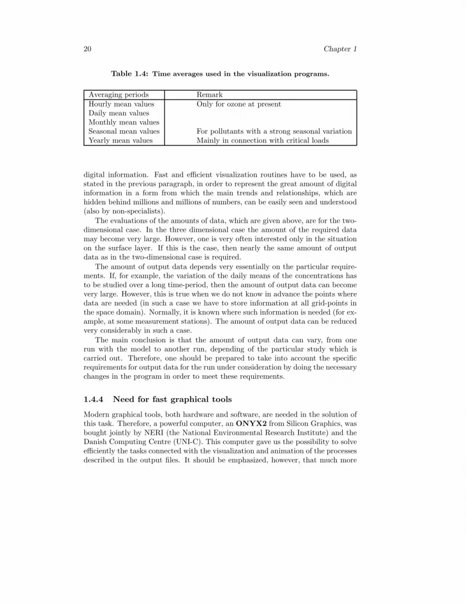
1.4.2 Types of output data
The output quantities, which are used in the visualization procedures, are given inTable 1.3. Average values of the concentrations and depositions are normally usedduring the visualization procedures. The different averaging lengths are given inTable 1.4.
Table 1.3: Output quantities used in the visualization programs.
Output quantitiesAir concentrationsConcentrations in precipitationWet depositionsDry depositionsTotal depositions
1.4.3 Amount of the output data
The information given above shows clearly that the visualization of the resultsobtained by a large-scale air pollution model is by no means an easy task. A largeenvironmental model, in which all physical and chemical processes are adequatelydescribed, produces huge output files. The output data produced after a longsimulation (as the simulations carried out in Bastrup-Birk et al., [18] and Zlatevet al., [297]) contain normally several hundred MBytes, or even several GBytes, of
20 Chapter 1
Table 1.4: Time averages used in the visualization programs.
Averaging periods RemarkHourly mean values Only for ozone at presentDaily mean valuesMonthly mean valuesSeasonal mean values For pollutants with a strong seasonal variationYearly mean values Mainly in connection with critical loads
digital information. Fast and efficient visualization routines have to be used, asstated in the previous paragraph, in order to represent the great amount of digitalinformation in a form from which the main trends and relationships, which arehidden behind millions and millions of numbers, can be easily seen and understood(also by non-specialists).
The evaluations of the amounts of data, which are given above, are for the two-dimensional case. In the three dimensional case the amount of the required datamay become very large. However, one is very often interested only in the situationon the surface layer. If this is the case, then nearly the same amount of outputdata as in the two-dimensional case is required.
The amount of output data depends very essentially on the particular require-ments. If, for example, the variation of the daily means of the concentrations hasto be studied over a long time-period, then the amount of output data can becomevery large. However, this is true when we do not know in advance the points wheredata are needed (in such a case we have to store information at all grid-points inthe space domain). Normally, it is known where such information is needed (for ex-ample, at some measurement stations). The amount of output data can be reducedvery considerably in such a case.
The main conclusion is that the amount of output data can vary, from onerun with the model to another run, depending of the particular study which iscarried out. Therefore, one should be prepared to take into account the specificrequirements for output data for the run under consideration by doing the necessarychanges in the program in order to meet these requirements.
1.4.4 Need for fast graphical tools
Modern graphical tools, both hardware and software, are needed in the solution ofthis task. Therefore, a powerful computer, an ONYX2 from Silicon Graphics, wasbought jointly by NERI (the National Environmental Research Institute) and theDanish Computing Centre (UNI-C). This computer gave us the possibility to solveefficiently the tasks connected with the visualization and animation of the processesdescribed in the output files. It should be emphasized, however, that much more

PDE systems arising in air pollution models 21
powerful graphical tools are necessary for the new more advanced versions of DEM(these new versions are united in a new model, UNI-DEM, see Chapter 7).
It is not sufficient to have a fast and big computer in order to visualize andanimate the output information. It is also necessary to use efficient software. Apowerful program has been developed. This program is based on new and modernideas used at present in the visualization techniques. Some more efforts are neededto make this program both faster and more user friendly.
1.4.5 Requirement for flexible visualization programs
Sometimes it is required to investigate the variation of the pollution levels in thewhole space domain (in the whole of Europe). In other cases one needs moredetailed information for a part of the space domain (for example, in a part con-taining Denmark and some surroundings of Denmark). Therefore, the visualizationprogram must allow the user to get such more detailed information when this isrequired by applying the following devices:
• using different zooming procedures,
• representing the grid-lines on the plots,
• giving the numerical values of the changes in each grid-square,
• plotting the wind fields or the temperatures when the changes of the pollutionlevels are animated.
The visualization program developed at the National Environmental ResearchInstitute can be used to get more detailed and more representative informationabout the studied processes by applying the above devices.
1.5 Measurement data
The reliability of the measurement data is an important issue. This is true bothin the case where the measurement data are used to verify the reliability of themodel results (see the results presented in Chapter 9) and in the case where themeasurement data are applied in data assimilation algorithms (such algorithms arediscussed in Daescu and Carmichael [53], Daescu and Navon [54], Daescu et al.[55], Elbern and Schmidt [88] [89] and Elbern et al. [90], [91], [92]). The incor-poration of measurements in large-scale air pollution models by using variationaldata assimilation techniques will be discussed in Chapter 10.
1.5.1 Measurements used in the verification procedures
Mainly measurements collected at the EMEP network of measurement stations havebeen used to verify the reliability of the model output results. There are more than

22 Chapter 1
200 such stations located in different European countries. The measurement datathat are taken at the EMEP network of stations are collected at the Norwegian AirResearch Institute (NILU, Oslo, Norway), where these are analyzed and then manymodellers in Europe can obtain these data and use them in their studies. There aremany NILU publications about the measurements collected there; see, for example,Hjellbrekke [136].
Many chemical species are measured at the stations of the EMEP network ofmeasurement stations. The measurements, which are relevant for the validation ofthe results from DEM, can be divided into two groups:
• measurements of concentrations in air, and
• measurements of concentrations in precipitation.
The measurements from the first group, which have mainly been used untilnow in comparisons with results obtained by using DEM, are:
• nitrogen dioxide,
• nitrate,
• sulphur dioxide,
• sulphate,
• ozone, and
• ammonia + ammonium.
The measurements of the second group, which have mainly been used untilnow in comparisons with results obtained by using DEM, are:
• nitrate,
• sulphate, and
• ammonium.
It should be mentioned here that not all measurement stations measure all of theconcentrations listed above. Moreover, there are periods (some days, some monthsand even some years) in which some measurements at some stations are missing.
Recently, concentrations of several hydrocarbons have been measured at someof the measurement stations in the EMEP network. A few comparisons of modelresults with the corresponding measurements of hydrocarbons have been carriedout. This activity is still in a very preliminary stage.
Finally, it should be mentioned that not only measurements from the EMEPnetwork have been used in the efforts to verify the reliability of the results obtainedby DEM. Occasionally, measurements from some other sources have also been usedin some studies.

PDE systems arising in air pollution models 23
1.5.2 Time and space resolution of the measurement data
Most of the measurement data are available as daily mean values of the concentra-tions over a long time-period (the measurement data used in DEM are from theperiod 1989-2003).
The ozone concentrations can also be obtained as hourly mean values (the ozoneconcentrations vary on a diurnal basis; the availability of hourly mean values of theozone concentrations allows the modellers to study the diurnal variations of theozone concentrations in different places in Europe in different seasons).
The space distribution of the available measurements depends very much on themeasured compound and on the year of consideration. For some compounds (as,for example ozone and sulphate) the number of stations that measure regularly (atleast 15 measurements per every month of the year under consideration) is about 60.For the remaining compounds the number of measurement stations is considerablysmaller. The number of stations which measure regularly (at least 5 measurementsper every month of the year under consideration) concentrations in precipitation isalso rather small.
In the ten-year period, from 1989 to 1998, which has been used in the studyrelated to the impact of climate changes on the pollution levels in Europe (someof the results, which were obtained in this study will be presented and discussedin detail in Chapter 9), it has been discovered that the number of measurementstations in the EMEP network tends to grow during the latter years. However,most of the measurement stations are still mainly located in the countries of WesternEurope and Scandinavia.
1.5.3 Amount of the measurement data
The files containing measurement data are, at present, smaller than the files contain-ing input data and output data. Anyway, if the model results are to be comparedwith measurements over a long time-period, then the files of the measurement dataneeded are quite large; several hundreds of MBytes. The amount of these datatends to grow, because more and more stations have been opened during the lastyears and more and more of the existing stations are starting to measure morecompounds.
It should be mentioned here that the EMEP measurement data are available onthe Internet. Therefore, one can download the needed data for the particular studyunder consideration and delete the downloaded files when the study is completed.Moreover, if the study is very large (over a time period of many years), then itcan be performed in parts (say, studies over one year at a time). If the work isorganized in such a way, then one can
• download only the data that are needed in the current part of the study,
• delete the downloaded files after completing the current part of the study,and

24 Chapter 1
• down-load data for the next part of the study and carry out the same proce-dure until all parts of the study are finished.
The storage requirements can be reduced considerably when this approach isused.
1.5.4 Measurement data for real time computations
It has already been stated that measurement data are needed for preparation ofhigh-quality initial fields of concentrations (by using data assimilation techniques)when air pollution forecasts are to be prepared. It is important to have these data asquickly as possible (say, one or two hours after performing the measurements). Thiswas, of course, a very big problem only two to three years ago. Now the situationis rapidly changing due to the possibilities to use the Internet and to carry out fasttransition of large amounts of data. The needed data can be taken from many siteswhere such data are available. It should be mentioned here that also the NationalEnvironmental Research Institute is regularly exposing measurement data on theInternet.
1.6 Some results obtained by DEM
DEM, together with the graphical tools associated by this model, can be consideredas a powerful tool for
• treating very large sets of input data,
• preparing very large sets of output data,
• verifying the sets of output data by using very large sets of measurement data,and
• applying the verified sets of output data in different studies by also addingresults from long sequences of scenarios performed by the model.
A few results will be presented in this section as well as in Chapter 8 andChapter 9. Many more results obtained by this model have been described anddiscussed in Ambelas Skjøth et al. [9], Bastrup-Birk et al. [18], [19] Harrison et al.[128], Zlatev [282], Zlatev and Ambelas Skjøth [284] and Zlatev et al. [292], [293],[294], [295], [297].
Only three features of DEM, but these are very important issues, will be dis-cussed here and/or illustrated by some results, which will be presented in the nextsubsections:
• the ability of the model to calculate output results by using very high resolu-tion and to zoom at sub-domains that are of particular interest,

PDE systems arising in air pollution models 25
• the ability of the model to produce reliable results, and
• the use of the model with different scenarios.
1.6.1 Results obtained with the high resolution version
In the two-dimensional high-resolution version of DEM the space domain (contain-ing the whole of Europe together with parts of Asia, Africa and the Atlantic Ocean)is discretized by using a (480×480) grid of (10 km×10 km ) grid-squares. It is stillnot possible, as mentioned in Section 1.2, to run operationally this version of themodel on long time-intervals (up to ten years). Therefore, only some interestingsituations, which occur on shorter time-intervals (the typical length of such a time-interval being a month or a year), were studied by this version until now. Someresults obtained when the model was run with meteorological data for 1997 areshown in Fig. 1.1 and Fig. 1.2. More results can be found in Zlatev and Syrakov[299], [300].
The distribution of the nitrogen dioxide pollution in Europe is shown in Fig.1.1. It is seen that the most polluted areas in Europe are
• parts of United Kingdom,
• the Netherlands,
• Belgium,
• Germany
• and parts of France,
• the Check Republic, and
• Poland
as well as
• the Northern part of Italy.
Moreover, in the parts of Europe which are not very polluted one can locatelarge cities, such as Madrid, Rome, Oslo, Stockholm, Helsinki, St. Petersburgand Moscow, which are large sources of nitrogen pollution (the most importantreason being that pollution from the traffic is one of the major sources for nitrogenemissions).

26 Chapter 1
Figure 1.1: The distribution of the nitrogen dioxide concentrations in differ-
ent parts of Europe and its surroundings.

PDE systems arising in air pollution models 27
185 186 187 188 189 190 191 192 193 194 195 196
281
282
283
284
285
286
287
288
289
290
291
292
Figure 1.2: The nitrogen dioxide concentrations in area around the Danish
capital Copenhagen and the Swedish city Malmo (the Øresund region).
28 Chapter 1
The same output data as used to draw Fig. 1.1, are also used to draw Fig. 1.2.Indeed, Fig. 1.2 could be viewed as a result from zooming in Fig. 1.1 onto the areaaround Copenhagen, the capital of Denmark, and the Swedish city of Malmo.
The grid-lines are drawn in Fig. 1.2. This is impossible when the whole spacedomain is used. Indeed, Fig. 1.1 will become completely black if the option fordrawing the grid-lines is switched on when results on the whole space domain,containing 230 400 grid-squares, are plotted.
The number of grid-squares used in Fig. 1.2 is 144, obtained by using only atiny part, a (12×12) sub-grid, of the whole (480×480) grid. At the same time, thisarea is nearly twice smaller than one grid-square of the (32 × 32) grids which werecommonly used only a few years ago, and are still used in some models (see, forexample, Amann et al. [8] and the EMEP Report 1/98 [93]). While the size of onegrid-square is 22500 km2 when a (32× 32) grid is applied, the size of the combinedarea of all 144 grid-squares used in Fig.1.2 is 14400 km2. This means that, while itwill not be possible to see any difference in the area shown in Fig. 1.2 when a coarse(32 × 32) grid is used, the results from the high resolution model presented in Fig.1.2 show clearly that there are several different levels of the nitrogen pollution inthis area. This illustrates the great potential power of the high resolution models.However, there is a price that is to be paid: very large sets of digital data are tobe handled when such models are run.
It is also necessary to emphasize here that Fig. 1.2 is only one example forzooming. Zooming could also be done for any other sub-domain of the space domainof DEM.
1.6.2 Checking the reliability of the model results
The validation of the results calculated by a model is an important task. Manyquestions related to the validation procedures used are still open. Some resultsobtained in the validation of the results calculated by DEM will be discussed inthis sub-section.
(A) Correctness of the numerical results.
The first question which is to be answered during the validation process is connectedto the reliability of the numerical algorithms used in the model. There are differenttests which can be used to test the accuracy of the numerical algorithms. For theadvection part, the so-called rotation test is well known. It has been introducedsimultaneously by Crowley [48] and Molenkampf [183] in 1968. Both the classicalrotation test and many modifications of this test have been used in several hundredpublications in the field of air pollution modelling; see, for example, Chock [43],[44], Chock and Dunker [45], Fornberg [103] and [104], Pepper and Baker [192] andPepper et al. [193].
A set of tests concerning both the advection and the diffusion part is discussedin Zlatev [282] and Zlatev et al. [287].

PDE systems arising in air pollution models 29
An extension of the rotation test for the combined advection-chemistry moduleof an air pollution model has been proposed and tested in Hov et al. [141]; see alsoZlatev [282].
It should be emphasized that successful tests of the performance of the numericalmethod do not ensure the reliability of the results when the full model is run. Thesuccess of the numerical tests is only indicating that if there are errors, then theseerrors are not caused by the numerical methods and, thus, the source for the errorsshould be searched in other places (as, for example, uncertainties in the emissioninventories, uncertainties in the meteorological data, uncertainties in parametersused in the description of some physical and/or chemical mechanisms, etc.). Theconclusion is that one should not overestimate the importance of the numericaltests. On the other hand, one should not underestimate the importance of thenumerical tests either. Successful numerical tests indicate that
• one of the major sources for errors in the model results has been removed(it should be mentioned here that this is crucial when Eulerian models areused in different environmental studies),
and, more importantly,
• there will be no interference of numerical errors with other errors when thesensitivity of the model results to variation of some key parameters (as, forexample, emissions and meteorological conditions) is studied.
(B) Qualitative validation.
Comparison of the distribution of the concentrations in the different parts of thespace domain with the distribution of related emissions can give us some qualitativeestimation of the reliability of the results. Comparing the results in Fig. 1.1 withthe distribution of the NOx emissions in Europe (the distribution of the NOx
emissions in Europe can be seen in upper right-hand-side plot in Fig. 8.2; see alsoBastrup-Birk et al. [18], [19]) we can conclude that
• DEM is producing highest levels of the nitrogen dioxide pollution precisely inthe parts of the space domain where the NOx emissions are highest, and
• in the large European cities (which are in general also big sources of NOx
emissions), the levels of the nitrogen dioxide pollution is also high.
The qualitative correctness of the model results allows us to draw two conclu-sions. The first conclusion is that there are no crude errors in the description ofthe physical and chemical mechanisms. The second conclusion is that there are nottoo big uncertainties in the meteorological data used in the model. It should benoted here that both conclusions are drawn under an assumption that the numer-ical methods work sufficiently well (which emphasizes once again the importance

30 Chapter 1
of checking the accuracy of the numerical algorithms that are implemented in themodel).
(C) Quantitative validation.
Of course, quantitative correctness of the model results is the most desirable prop-erty of an air pollution model. Most of the unresolved problems become immedi-ately visible when one attempts to validate quantitatively the model results. Thebest that we can do at present (in the attempts to validate quantitatively the modelresults) is to compare model results with measurements taken at representativemeasurement stations located in different parts of the space domain.
There are two major ways to present the results which are obtained when calcu-lated by the model concentrations are compared with corresponding measurements.The results from such comparisons can be represented:
• by scatter plots where the mean values of the calculated concentrations anddepositions are compared with corresponding measurements (mainly on month-ly, seasonal and yearly basis), and
• by time-series plots where temporal variations of the calculated concentra-tions and depositions at a given measurement station are compared with thecorresponding observations.
Both approaches have extensively been used when different versions of DEMhave been developed. Results from validation procedures applied to different ver-sions of DEM can be found in many publications; see, for example, Ambelas Skjøthet al. [9], Bastrup-Birk et al. [18], [19], Harrison et al. [128], Zlatev [277] [282],Zlatev and Berkowicz [286], Zlatev and Ambelas Skjøth [284] and Zlatev et al.[292], [293], [294], [295], [297]. Some results are also presented and discussed inChapter 9. Nevertheless, many more comparisons are necessary.
1.6.3 Running the model with different scenarios
Results calculated by using comprehensive mathematical models can successfullybe used in different studies (assuming here that some validation process based oncomparison of model results and measurements has successfully been completed).An example for such a study will be given here as an illustration. Other examplescan be found in Ambelas Skjøth et al. [9], Bastrup-Birk et al. [18], [19], Zlatev[282], Zlatev and Ambelas Skjøth [284] and Zlatev et al. [297] as well as in Chapter8 and Chapter 9.
Different critical levels of the concentrations of certain pollutants have beendefined and used in many countries; especially in the European Union (EU), see,for example, Amann et al. [8]. Concerning ozone, one of the critical levels, whichis under discussion now in the European Union, is the number of days in which theozone concentrations were higher than 120 ppb for at least one hour (this critical

PDE systems arising in air pollution models 31
level is introduced in the EU directive for ozone and the ”Ozone Position Paper”of the Commission of EU, [96], [95]). According to the EU directive for ozone andthe ”Ozone Position Paper” of the Commission of EU ([96], [95]), the populationmust be warned if this is likely to happen in the next two-three days (this is one ofthe reasons for calculating air pollution forecasts - see also Section 1.4).
There exist some predictions concerning the anthropogenic (human-made) emis-sions in Europe for year 2010. These emission inventories have been prepared bya large group of European specialists in this field. It is agreed that the Europeancountries will work for achieving the predicted emission levels by the year 2010.These emission levels are well-known (in Europe, at least) as Scenario 2010.
In connection with this critical level (number of days in which the ozone concen-trations were higher than 120 ppb for at least one hour) and with the emissions fromScenario 2010, it is important to have the answers to the following two importantquestions:
• How frequently is the ozone level of 120 ppb exceeded?
• What will be the effect of using the emissions from Scenario 2010 on thenumber of days in which the ozone level of 120 ppb is exceeded?
DEM, and more precisely the version of this model which is discretized by using(50 km × 50 km) grid-squares, have been run twice over a time-interval of tenyears (from 1989 to 1998). For each year N , where N = 1989, 1990, . . . , 1998, theexisting emission inventories for year N were used in the first run. The predictedemissions in Scenario 2010 were used for all of the ten years in the second run.The meteorological data used in both runs were the same; for each year N , whereN = 1989, 1990, . . . , 1998, the meteorological data for year N were used. The firstrun will be called Basic Scenario, while the name Scenario 2010 will be used forthe second run.
Results concerning Denmark and the region surrounding Denmark are given inFig. 1.3 (the Basic Scenario) and in Fig. 1.4 (Scenario 2010). The total numbersof days (for the whole period of ten years) in which the ozone level of 120 ppb hasbeen exceeded for at least one hour are given in these two figures.
The results given in Fig. 1.3 show that the total numbers of days (for the all tenyears) in which the ozone level of 120 ppb has been exceeded in at least one hourvary between 3 and 14 in the different parts of Denmark when the Basic scenariois used. This means that the answer to the first question for the different parts ofDenmark is the following:
• the exceedance of this critical level does not occur very often in Denmark, butmay take place sometimes.
The results given in Fig. 1.4 are the same as those in Fig. 1.3 (numbers ofdays in which the critical level of 120 ppb is exceeded), but here the emissions fromScenario 2010 are used. The results indicate that practically

32 Chapter 1
• no exceedance of the critical level for ozone of 120 ppb takes place in Den-mark when the emissions from Scenario 2010 are used (excluding the islandof Bornholm).
Thus, the reduction of the emissions to the levels prescribed in Scenario 2010will be very beneficial for Denmark in connection with the critical level of 120 ppb.Let us emphasize here that it is assumed in Scenario 2010 that the emissions in allEuropean countries will be reduced.
Only results related to Denmark were presented here. However, the huge outputdata sets can be used to zoom at any other sub-domain of the space domain of DEM.It should be mentioned here that the results indicate that, while it is true that thenumber of occurrences of days in which the critical level of 120 ppb is reducedconsiderably in the countries in Central and Western Europe when Scenario 2010is used, it is also true that the reduction of the European emissions as plannedin Scenario 2010 will not totally remove the exceedances of this critical level forozone in these countries. This is why some scenarios for additional reductions ofthe anthropogenic emissions in the 15 EU countries are currently being discussed(see, for example, Amann et al. [8]).
Most of the experiments are at present carried out by varying in a suitable waythe anthropogenic emissions. However, it is also necessary to study the sensitivity ofthe concentrations and depositions to changes of the biogenic (natural) emissions.This issue is becoming more and more important, because recent investigationsindicate that the biogenic emissions are strongly underestimated (by up to tentimes: see, for example, Bouchet et al., [25], [26]). Moreover, the relative part ofthe biogenic emissions in Europe has clearly been increased during the last twodecades, because the anthropogenic emissions were considerably decreased (thereduction of the anthropogenic emissions in Europe is documented in the annualreports of EMEP; see, for example, Vestreng and Støren [261]). Some preliminaryresults about the sensitivity of the ozone concentrations to variations of biogenicemissions are presented in Geernaert and Zlatev [112], [113]. This study is veryimportant and, therefore, it will be further discussed in Chapter 8.
1.6.4 Sensitivity tests
Systematic sensitivity tests of the variations of the model results caused by thevariations of certain physical parameters can give very useful results. If the resultsare very sensitive to the variations of the selected parameter, then this is an in-dication that it is necessary to use a very accurate value of the parameter underconsideration. If we are not able to provide a sufficiently accurate value of the criti-cal parameter, then it may be more profitable to replace the physical mechanism inwhich the critical parameter occurs with another mechanism which is perhaps notso accurate, but more robust (in the sense that the results are not very sensitive tothe variation of the physical parameters involved in the new mechanism).

PDE systems arising in air pollution models 33
19 20 22 22 14 13 12 16 20 25 27 31 30
16 14 11 10 10 10 11 12 15 17 16 22 23
12 12 6 4 5 6 8 9 8 12 12 20 20
8 6 5 4 6 6 6 6 7 10 11 14 17
6 6 5 4 6 6 6 6 7 9 9 13 14
4 3 4 4 4 4 3 2 4 6 10 12 9
2 3 3 3 4 4 2 2 4 6 8 9 8
1 3 2 2 4 4 2 2 2 5 8 8 7
1 1 1 1 1 1 1 0 1 5 7 7 7
1 1 1 1 1 0 0 0 1 3 5 5 4
2 1 1 0 0 0 0 0 0 1 3 2 3
1 1 0 0 0 0 0 0 0 0 2 2 2
1 1 0 0 0 0 0 0 0 0 2 2 2
Figure 1.3: The total numbers of days in the period 1989-1998 in which the
ozone concentrations in Denmark exceeded the critical level of 120 ppb - Basic
Scenario.

34 Chapter 1
1 1 0 0 0 0 0 0 1 1 3 4 4
0 0 0 0 0 0 0 0 1 1 2 3 4
0 0 0 0 0 0 0 0 0 0 0 0 1
0 0 0 0 0 0 0 0 0 0 0 0 1
0 0 0 0 0 0 0 0 0 0 0 0 0
0 0 0 0 0 0 0 0 0 1 1 0 0
0 0 0 0 0 0 0 0 0 1 1 0 0
0 0 0 0 0 0 0 0 1 2 0 0 0
0 0 0 0 0 0 0 0 1 2 1 0 0
0 0 0 0 0 0 0 0 1 1 0 0 0
0 0 0 0 0 0 0 0 0 0 0 0 0
0 0 0 0 0 0 0 0 0 0 0 0 0
0 0 0 0 0 0 0 0 0 0 0 0 0
Figure 1.4: The total numbers of days in the period 1989-1998 in which the
ozone concentrations in Denmark exceeded the critical level of 120 ppb - Sce-
nario 2010.

PDE systems arising in air pollution models 35
Some carefully chosen tests, appropriate to study the sensitivity of the modelresults to variations of the rate coefficients of some of the chemical reactions, werecarried out in Dimov and Zlatev [74]. Monte Carlo techniques were used in Dimovand Zlatev [74] in order
• to find the rate coefficients to the variation of which the model results aremost sensitive, and
• to study in a more systematic way the variation of the model results causedby random variations in a prescribed range of the selected rate coefficients.
A simple box-model (one grid-point only and no other processes except thechemical reactions) is quite sufficient in the first part. The second part is muchmore complicated, because it requires a large number of runs of the whole airpollution model. It has been established in this study that the magnitude of thechanges in the different parts of Europe was not the same. More details and otherconclusions can be found in Dimov and Zlatev [74].
1.7 Applicability to PDEs arising in other areas
Air pollution models were discussed in the previous sections of this chapter. Asmentioned several times in the previous sections of this chapter, this has beendone only in order to facilitate the presentation of the results. All (or, at least,nearly all) methods and devices, which were discussed in the previous sectionsand will be discussed in the remaining part of the book, are also applicable whensystems of PDEs arising in some other fields of science and engineering are to behandled on computers. Several examples will be given in this section to illustratethe correctness of this statement.
It should be mentioned here that the physical and chemical processes in theexamples given in this section are slower than the corresponding processes takingplace in the atmosphere. This means that the requirements that must be satisfiedby the numerical methods used in the treatment of air pollution models are nor-mally stronger than the requirements that are to be satisfied when similar systemsof ODEs arising from other fields of science and engineering are handled. Twoconclusions can be drawn by using this fact:
• The numerical methods used in an air pollution model can be applied in thetreatment of models arising in many other areas (however, the opposite is notnecessarily true), and
• it might be more efficient to select some simpler numerical methods when thephysical and chemical processes studied by the model under consideration arenot so fast as the corresponding processes in the atmosphere.

36 Chapter 1
1.7.1 Models used to study multicomponent transport inground-water
Ground-water resources are becoming more and more threatened by
• contaminants containing industrial and household waste,
• infiltration of pesticides and fertilizers from agricultural areas, and
• leakage of organic pollutants from petrol stations, refineries and pipelines.
Mathematical models of the following type can be used in ground-water studies(see Prommer et al. [197] and Mao et al. [171]):
∂cs
∂t= −∂(ucs)
∂x− ∂(vcs)
∂y− ∂(wcs)
∂z(1.4)
+∂
∂x
(Kx
∂cs
∂x
)+
∂
∂y
(Ky
∂cs
∂y
)+
∂
∂z
(Kz
∂cs
∂z
)
+Qs(c1, c2, . . . , cNs)
−qk
θcks,
s = 1, 2, . . . , Ns.
The different quantities that are involved in the mathematical model have thefollowing meaning:
• the concentrations are denoted by cs,
• u, v and w are fluid velocities,
• Kx, Ky and Kz are hydrodynamic dispersion coefficients,
• cks are the total aqueous concentrations in the water coming from sinks andsources,
• qk is the volumetric flow rate per unit volume of the aquifer representingsources and sinks,
• θ is the volumetric porosity,
• the chemical reactions used in the model are described by the non-linearfunctions Qs(c1, c2, . . . , cNs).

PDE systems arising in air pollution models 37
It is seen that (1.4) is nearly the same as (1.1). Of course, the physical inter-pretation of the involved quantities is different. However, since the mathematicaldescription is quite similar, the same methods and devices, which are used in treat-ment of the PDE system (1.1), can also be applied in the treatment of (1.4).
More details about mathematical models used in ground-water studies can befound, for example, in Prommer et al. [197] and Mao et al. [171].
1.7.2 PDEs arising in oil spill studies
Oil spill spreading and drifting can cause serious environmental problems. Math-ematical models, which are developed to study these problems, lead to systems ofPDEs similar to (1.1). An example, which is taken from Tkalich [249], is given inthis subsection to illustrate the similarity. The model consists of two parts. Thefirst part is describing the thickness of the oil slick
∂h
∂t= −∂(uhh)
∂x− ∂(vhh)
∂y(1.5)
+∂
∂x
(Dx
∂h
∂x
)+
∂
∂y
(Dy
∂h
∂y
)
+Qh(h)
while the second one is describing the processes in the water column:
∂cs
∂t= −∂(ucs)
∂x− ∂(vcs)
∂y− ∂(wcs)
∂z(1.6)
+∂
∂x
(Kx
∂cs
∂x
)+
∂
∂y
(Ky
∂cs
∂y
)+
∂
∂z
(Kz
∂cs
∂z
)
+Qs(c1, c2, c3)
s = 1, 2, 3.
The different quantities that are involved in the mathematical model describedby (1.5) and (1.6) have the following meaning:
• h is the oil slick thickness, while the oil concentrations in droplet, dissolvedand particulate phases in the water column are denoted by cs,
• uh and vh are representing the slick drifting velocities, while u, v and w arerepresenting the fluid velocity,

38 Chapter 1
• Dx and Dy are diffusion coefficient in the oil slick,s
• Kx, Ky and Kz are diffusion coefficients in the water column,
• the chemical kinetic terms used in the model are described by the non-linearfunctions Qh(h) and Qs(c1, c2, c3).
It is again seen that the system of PDEs defined by (1.5) and (1.6) is very similarto (1.1), which indicates that the numerical algorithms and the computationaldevices discussed in the remaining part of this book can successfully be used in thecomputer treatment of problems connected to oil spill.
More details about this class of environmental problems can be found in Fingas[101], Reed et al. [200], Spaulding [231] and Tkalich [249].
1.7.3 Contaminated disposal facilities
It is important to study the environmental significance of contaminated losses fromin-lake disposal facilities. The mathematical modelling of this process leads (underan assumption for incompressible flow and homogeneous medium) to two equations:a flow equation
S∂h
∂t=
∂
∂x
(Kx
∂h
∂x
)+
∂
∂y
(Ky
∂h
∂y
)(1.7)
and an equation describing the contaminant transport
S0∂c
∂t= −∂(uc)
∂x− ∂(vc)
∂y(1.8)
+∂
∂x
[Dxx
∂c
∂x+ Dxy
∂c
∂y
]+
∂
∂z
[Dyx
∂c
∂x+ Dyy
∂c
∂y.
]
The different quantities that are involved in the mathematical model describedby (1.7) and (1.8) have the following meaning:
• h is representing the potential function of the flows,
• c is the contaminant concentration,
• S is representing the specific storage coefficient,
• S0 is representing the porosity of the aquifer,
• u and v are representing the fluid velocities,
• Kx and Ky are hydraulic conductivity components,
• Dxx, Dxy, Dyx and Dyy are diffusion coefficients.

PDE systems arising in air pollution models 39
This example is taken from Priklonsky et al. [196]. Some other examples canbe found in Su [238], Su et al. [239].
Note that there are no chemical reactions in this example. However, the methodsused in the advection-diffusion part of (1.1) can also be used in the computertreatment of (1.7) and (1.8).
1.7.4 Other applications
It is difficult to prepare a full list of applications which lead to systems of PDEsthat are similar to (1.1), because such a list will be very long. While it is truethat it is not necessary to present in this book such a long list, we do believe thatsome readers might be interested in recent references where models which lead tosystems of PDEs similar to (1.1) are discussed. Different such applications can befound in Jennings, [147], Gupta et al., [125], Umgiesser et al., [253], Cichota et al.,[47] and Lee et al., [161].
1.8 Concluding remarks
Remark 1.1. Different problems connected with the needs of using large data setsin air pollution modelling have been discussed by using a particular model, DEM.It has already been emphasized that this approach has been chosen only in orderto simplify the exposition of the results. The same conclusions could also be drawnif any other large-scale air pollution model is used. Moreover, similar problemsalso occur when models arising in other fields of science and engineering are to behandled (several examples were given in the previous section).
The development of DEM is similar to the development of many other models.The development of a more advanced air pollution model is normally carried outin two stages:
• starting with models defined on coarse grids with a few chemical compounds,and
• arriving gradually to very advanced mathematical models utilizing fine gridsand involving many more chemical compounds.
Similar stages are also used in the development of advanced mathematical mod-els in other areas of science and engineering.
Remark 1.2. The question:
Are the mathematical models used at present sufficient forstudying the most important environmental problems?
is relevant. The answer is, of course, no. While many problems can successfully bestudied and are successfully studied by the models that are available at present,

40 Chapter 1
it is also true that many other problems cannot be handled with the models whichexist at present. The question of having models discretized on finer grids (say,by using 2 km × 2 km grid-squares) is already a topic of discussion. Also thehigh-resolution three-dimensional models are still not tractable even on the largestcomputers existing at present (at least in the case where calculations over a longtime-interval with many scenarios are required). This indicates clearly that
• there is a lot of work to be done in this field, and
• the need of developing good tools for handling efficiently very large data sets(input data sets, output data sets and data sets containing measurements) issteadily increasing in the environmental studies which are carried out by usinglarge-scale mathematical models.
Remark 1.3. The performance of the computers that are available at presentis a central problem in the field of the large-scale environmental modelling (as wellas in many other fields of science and engineering where large-scale mathematicalmodels are to be treated on computers). We are going to handle larger and largerenvironmental models on computers (as well as larger and larger models that appearin other fields of science and engineering). Therefore, the following two questions,which arise in connection with this development, should be adequately answered:
• Are the computers that are available at present sufficiently fast and is itpossible to resolve by using them all the comprehensive scientific problemsthat are to be treated now?
• Do we need bigger and faster computers for the treatment of the environmen-tal problems that have to be resolved in the near future?
These two questions can best be answered by using a quotation taken from apaper ”Ordering the universe: The role of mathematics” written by Arthur Jaffe([144]):
”Although the fastest computers can execute millions of op-erations in one second they are always too slow. This mayseem a paradox, but the heart of the matter is: the biggerand better computers become, the larger are the problemsscientists and engineers want to solve.”
This paper of Jaffe was published in 1984. At that time it was difficult tohandle the version of DEM containing, after the discretization, 2048 equations.One of the biggest problems solved, which can be treated successfully at present byDEM, contains, again after the discretization, more than 8000000 equations. Oneof the major reasons for being able to handle such huge problems, about 4000 times

PDE systems arising in air pollution models 41
larger than the problems that were solved in 1984, is the availability of much biggerand much faster computers. There is no reason to assume that the developmentof bigger and faster computers will not continue. Therefore, the scientists couldcontinue to plan the formulation and the treatment of bigger and bigger tasks thatimpose strong requirements for handling larger and larger data sets, because thesolutions obtained in this way
• will be closer to the reality,
• will contain more details and more useful details, and
• will give reliable answers to questions which are at present open.
Remark 1.4. The conclusions that were made in the previous three remarksillustrate clearly the fact that the introduction of new and more advanced modulesfor the mathematical description of the physical and chemical processes that areinvolved in the large-scale models leads necessarily to bigger computational tasks.In other words, both
• the computational time, and
• the storage requirements
are normally increased very considerably when more advanced physical and chem-ical modules are developed and implemented in a large air pollution model. Theefficient treatment of the more difficult tasks that appear when more adequate mod-ules are incorporated in the models will be the main topic in most of the chaptersin the remaining part of this book (and, more precisely, the discussion in Chapter2 to Chapter 7 and Chapter 10 is completely related to the computational issues).However, we shall also illustrate the usefulness of the efficient treatment of thecomputational tasks by showing some results from comprehensive environmentalstudies in Chapter 8 and Chapter 9. It was possible to complete successfully thesestudies only because the computational tasks are efficiently carried out. Only a fewexamples for comprehensive studies, which were performed by the our air pollutionmodel, are discussed in Chapter 8 and Chapter 9. It should be mentioned here thatmany other comprehensive studies were also successfully completed. However, itshould also be mentioned that further improvements of the numerical methods andthe computational devices is necessary, because there are still problems, which can-not be solved at present. Several examples for such difficult and/or open problemswill be given in Chapter 11.


Chapter 2
Using splitting techniques in thetreatment of air pollution models
The application of splitting procedures in the treatment of large scientific andengineering problems is an excellent tool (and, very often, the only tool) by whichhuge computational tasks can be made tractable on the available computers bydividing them to a sequence of smaller and simpler tasks.
A simple splitting procedure for partial differential equations was proposed, asan example, in 1957 by Bagrinovskii and Godunov in [14]. This was probably thefirst attempt to apply a splitting procedure in the numerical solution of partialdifferential equations. Different splitting procedures have been developed and/orstudied in many scientific papers; see, for example, Csomos et al. [49], Dyakonov,[83], Lanser and Verwer, [157], Marchuk, [172], [173], [175], [177], Penenko andObraztsov, [191], Strang, [235], Tikhonov and Samarski, [248], Yanenko, [269].
A detailed theoretical study and analysis of some splitting procedures can befound in Marchuk, [173], [176], Farago and Havasi, [97] and Farago et al., [100].Some convergence properties of splitting procedures were recently discussed inFarago and Havasi [98].
Results that are directly related to the use of splitting procedures in the fieldof air pollution modelling can be found in Bartholy et al. [16], Marchuk [174] andMcRae et al. [181]. Splitting procedures for air pollution models are also discussedin detail in Hundsdorfer and Verwer [142].
Splitting techniques are, to our knowledge, used in all large-scale air pollutionmodels, which are
• discretized using fine resolution grids,
• run over long time-intervals (time-intervals of ten or more years),
and/or
• run operationally with many scenarios (emission scenarios, meteorologicalscenarios, climatic scenarios, etc.).
43

44 Chapter 2
Several different ways of implementing splitting procedures in large-scale models(not necessarily large-scale air pollution models) as well as the advantages anddisadvantages of using splitting procedures in such models will be discussed in thischapter.
The discussion in this chapter is fairly general and, therefore, the basic ideasused in the different splitting techniques that are discussed in this chapter areapplicable to many large-scale mathematical models arising in different fields ofscience and engineering.
2.1 Four types of splitting procedures
Let us reiterate here that splitting techniques are used not only in problems arisingin air pollution modelling, but also in many other scientific and engineering prob-lems. This is why it is worthwhile to give a general presentation of some of thebasic ideas used when splitting techniques are to be designed.
We shall assume here that the following rather general mathematical problemis to be solved:
∂c(x, t)∂t
= A(c(x, t)), (2.1)
where
• t ∈ [0, T ],
• x ∈ D (D being some space domain), and
• A(c(x, t)) is a differential operator.
The abbreviation A will be used instead of A(c(x, t)) when there is no dangerfor misunderstanding.
We shall assume that operator A from (2.1) can be represented as a sum of moperators, which are in some sense simpler than the original operator A:
A =m∑
i=1
A[i]. (2.2)
It should be noted here that the division of the operator A from (2.1) to a sumof simpler operators is in general not unique (this will be illustrated by severalexamples in the next sections of this chapter).
It is as a rule worthwhile to replace the numerical treatment of the originalproblem (2.1) with a numerical treatment of a sequence of smaller problems. Eachof the smaller problems can formally be obtained from the original problem (2.1)by exchanging A with A[i]. This means that the original problem (2.1) can be split

Using splitting techniques 45
into the following m sub-problems by replacing successively A with the simpleroperators A[i] from (2.2):
∂c[i](x, t)∂t
= A[i](c[i](x, t)), i = 1, 2, . . . , m. (2.3)
Moreover, the time-interval [0, T ] is divided to N = T/τ small sub-intervals,where τ is called the splitting time-step size (it is assumed here that the splittingtime-step size is constant, equal to τ , but this is done only in order to facilitate theexplanation of the results; such an assumption is in fact not needed). The smallerproblems from (2.3) are treated (in some chosen by the user ordering) at everysplitting time-step (i.e., for n = 1, 2, ..., N).
It is said that a splitting procedure is used when an approximation of thesolution of (2.1) is obtained by treating (in the manner sketched above) a sequenceof smaller problems (2.3) involving the simpler operators A[i] from (2.2). Theparticular splitting procedure depends on
• the way in which the operator A from (2.1) is represented as a sum of simpleroperators A[i], and
• the order in which the smaller and simpler problems that were defined by(2.3) are treated.
Assume that the representation (2.2) of the original operator A as a sum ofsimpler operators A[i] is fixed. Then four types of splitting procedures can beconstructed by ordering the simpler operators from (2.2) in different ways:
• sequential splitting procedures,
• symmetric splitting procedures,
• weighted sequential splitting procedures,
• weighted symmetric splitting procedures.
The main ideas, on which these four types of splitting procedures are based, willbe discussed in the following four sections. Some particular examples of splittingprocedures used in large-scale air pollution models will also be presented in thenext four sections.
2.2 Sequential splitting procedures
If the sub-problems from (2.3) are treated one after the other, then the resultingalgorithm is called a sequential splitting procedure. Different sequential splittingprocedures can be obtained if the ordering, in which the simpler problems (2.3) aretreated, is varied. There are two requirements:

46 Chapter 2
• each of the simpler problems must be treated only once per a splitting step,and
• each of the simpler problems must be treated with the same splitting time-stepsize τ .
Three examples for sequential splitting procedures used in air pollution modelsare given below. The description of the first example is given with some moredetails in the next sub-section (it is also explained there how the simpler modelsthat are used in the splitting procedures are coupled).
It should be mentioned here that similar examples can be constructed in relationwith many environmental models (as those described in Section 7 of Chapter 1) aswell as in connection with many large-scale mathematical models arising in otherfields of science and engineering.
2.2.1 The old splitting procedure used in DEM
It is sometimes more convenient to rewrite in a vector form the system of partialdifferential equations (PDEs), which is given in Chapter 1 and by which DEM isdescribed mathematically:
∂c(x, t)∂t
= −∂(uc)∂x
− ∂(vc)∂y
− ∂(wc)∂z
(2.4)
+∂
∂x
(Kx
∂c∂x
)+
∂
∂y
(Ky
∂c∂y
)+
∂
∂z
(Kz
∂c∂z
)
+E + Q(c)
−κ c,
where Ns is the number of chemical species and
• x = (x, y, z),
• c = (c1, c2, . . . , cNs)T ,
• E = (E1, E2, . . . , ENs)T ,
• Q = (Q1, Q2, . . . , QNs)T , and
• κ is a diagonal matrix, the diagonal elements of which are κ11 + κ21, κ12 +κ22, . . . , κ1Ns + κ2Ns .

Using splitting techniques 47
By using this notation, the sequential splitting, which has been used in DEMuntil about two years ago, can be defined by the following five simpler sub-models:
∂c[1](x, t)∂t
= −∂(uc[1])∂x
− ∂(vc[1])∂y
(2.5)
∂c[2](x, t)∂t
=∂
∂x
(Kx
∂c[2]
∂x
)+
∂
∂y
(Ky
∂c[2]
∂y
)(2.6)
∂c[3](x, t)∂t
= E + Q(c[3]) (2.7)
∂c[4](x, t)∂t
= −κ c[4] (2.8)
∂c[5](x, t)∂t
= −∂(wc[5])∂z
+∂
∂z
(Kz
∂c[5]
∂z
). (2.9)
Five physical and chemical processes:
• the horizontal advection,
• the horizontal diffusion,
• the chemistry,
• the deposition, and
• the vertical exchange
are described mathematically with the terms in the right-hand-side of the systems(2.5)-(2.9).
These five systems are solved successively at every time-step (i.e., for t =t1, t2, . . . , tN with t0 = 0 and tn − tn−1 = τ , where n = 1, 2, . . . , N). The order ofcomputations at time-step n+1 can be explained in the following way. Assume thatthe first n splitting steps are successfully completed. In other words, assume thatsome approximations of the values of the concentrations c are known for t = tn,where n ∈ 0, 1, . . . , N − 1. Then these approximations are used as initial valueswhen solving system (2.5) at time-step n + 1 (i.e., when an approximation to c[1]
is computed at t = tn+1). After that the following steps are carried out:
• the solution c[1] at t = tn+1 is used as an initial value when (2.6) is solvedat time-step n + 1 (i.e., when an approximation to c[2] is computed at timet = tn+1),

48 Chapter 2
• the solution c[2] at t = tn+1 is used as an initial value when (2.7) is solvedat time-step n + 1 (i.e., when an approximation to c[3] is computed at timet = tn+1),
• the solution c[3] at t = tn+1 is used as an initial value when (2.8) is solvedat time-step n + 1 (i.e., when an approximation to c[4] is computed at timet = tn+1),
• the solution c[4] at t = tn+1 is used as an initial value when (2.9) is solvedat time-step n + 1 (i.e., when an approximation to c[5] is computed at timet = tn+1).
The solution of the last sub-model, i.e., the approximation to c[5] calculated attime t = tn+1 = tn + τ , is accepted as an approximation of the solution c of theoriginal system (2.4) at splitting time-step n + 1. This means that the splittingtime-step n + 1 is completed and everything is ready to carry out the same kind ofcomputations at splitting time-step n + 2.
The only question that remains to be answered is how to start the computationsat the first splitting time-step (i.e., n = 1). This is not a problem, because the initialconditions can be used at the first splitting time-step.
It should be mentioned here that the same (or, at least, a very similar) prin-ciple can be used to couple the smaller problems in all other splitting procedures.Therefore, this issue will not be discussed in the description of the other splittingprocedures in the following part of this chapter.
The relationship between the particular splitting procedure used in this sub-section and splitting procedures for the more general problem discussed in theprevious section can be explained as follows. It is clear that if we denote the right-hand-side of (2.4) with A, then (2.1) will be obtained. In the same way, if we replacethe right-hand-sides of (2.5) - (2.9) with A[1], A[2], A[3], A[4] and A[5] respectively,then simpler sub-models of type (2.3) will be obtained. Thus, (2.4) and (2.5) - (2.9)are the result of using the notation in the previous section for the particular caseof problems arising in air pollution modelling with m = 5.
It is very often worthwhile to describe how the different splitting procedures areto be applied in practice by
• giving the order in which the the simple operators A[i], where i = 1, 2, . . . , m,are applied, and
• indicating the splitting time-step size τ , which is actually used.
For the particular case discussed in this sub-section (i.e., for the sequentialsplitting procedure with m = 5 that is related to DEM), such a description is givenby the following sequence:
(A[1])τ , (A[2])τ , (A[3])τ , (A[4])τ , (A[5])τ . (2.10)

Using splitting techniques 49
2.2.2 The new splitting procedure used in DEM
There were good reasons for using the splitting procedure described in the previoussub-section when the pseudo-spectral method was applied in the numerical treat-ment of the horizontal transport (advection) and the horizontal diffusion. Trun-cated series of trigonometric functions are used in the pseudo-spectral method.Both sines and cosines are involved in the trigonometric series that are used in thediscretization of the horizontal advection. It is more efficient to apply trigonomet-ric series containing only cosines when the horizontal diffusion is treated. Thus,it is better to split the horizontal advection and the horizontal diffusion when thepseudo-spectral method is implemented in an air pollution model (see more detailsin Zlatev [276], [282]).
Finite elements are now used in the discretization of the horizontal transportand the horizontal diffusion. Therefore, there is no need to split these two processesand they are combined in the new splitting procedure used in DEM. Furthermore,the deposition process is added to the chemical part. In this way, the number of thesub-models, obtained when the new splitting procedure is implemented, is reducedfrom five to three.
The three sub-models that are obtained by applying the new DEM splittingprocedure are given below:
∂c[1](x, t)∂t
= −∂(wc[1])∂z
+∂
∂z
(Kz
∂c[1]
∂z
)(2.11)
∂c[2](x, t)∂t
= −∂(uc[2])∂x
− ∂(vc[2])∂y
(2.12)
+∂
∂x
(Kx
∂c[2]
∂x
)+
∂
∂y
(Ky
∂c[2]
∂y
)
∂c[3](x, t)∂t
= E + Q(c[3]) − κ c[3]. (2.13)
The first of these sub-models, (2.11), describes the vertical exchange. The sec-ond sub-model, (2.12), describes the combined horizontal transport (the advection)and the horizontal diffusion. The last sub-model, (2.13), describes the chemicalreactions together with emission sources and deposition terms.
Let us denote the operators in the right-hand-sides of (2.11), (2.12) and (2.13)by A[1], A[2] and A[3] respectively. Then the computations are to be carried outusing the operators in the following order when the new splitting procedure is usedwith some splitting time-step size τ :
(A[1])τ , (A[2])τ , (A[3])τ , (2.14)

50 Chapter 2
The correspondence between the operators used in the new splitting procedureand the operators used in the old one (see the previous sub-section) can be expressedby the following relationships:
• The operator A[1] in the new splitting procedure is equal to the operator A[5]
in the old one.
• The operator A[2] in the new splitting procedure is equal to the sum of theoperators A[1] + A[2] in the old one.
• The operator A[3] in the new splitting procedure is equal to the sum of theoperators A[3] + A[4] in the old one.
The boundary conditions can be treated in a natural way when the splittingprocedure described by (2.11) - (2.13) is used. The implementation of the boundaryconditions is performed as follows:
• The boundary conditions on the top and the bottom of the space domain aretreated in (2.11), where the computations are carried out along the verticalgrid-lines.
• The lateral boundary conditions are handled in (2.12), where the computa-tions are carried out in each of the horizontal grid-planes.
• The computations related to (2.13) are carried out by performing the chemicalreactions at each grid-point. It is clear that the computations at any of thegrid-points do not depend on the computations at the remaining grid-points.Therefore, no boundary conditions are needed when (2.13) is handled.
The fact that the boundary conditions can be introduced in a natural way whenthe splitting based on (2.11) - (2.13) is selected is a great advantage of this splittingprocedure, because the boundary conditions are normally causing problems whensplitting techniques are used.
2.2.3 A third sequential splitting procedure
The new DEM splitting procedure was obtained from the old one by reducing thenumber of operators (combining together some of them; see the previous section)as well as by changing the order of the computations. A new splitting procedurecan also be obtained by keeping the number of simpler operators the same as inthe old DEM splitting procedures (i.e., by keeping m = 5), but by taking anothercombination of the terms from the right-hand-side of (2.4) in the formation of thesimpler operators. An example will be given in this sub-section as an illustrationof this possibility.
Consider again (2.4). The operator in the right-hand-side can be represented asa sum of five simpler operators not only as shown in (2.5) - (2.9), but also in thefollowing way:

Using splitting techniques 51
∂c[1](x, t)∂t
= −∂(uc[1])∂x
− ∂(vc[1])∂y
− ∂(wc[1])∂z
(2.15)
∂c[2](x, t)∂t
=∂
∂x
(Kx
∂c[2]
∂x
)+
∂
∂y
(Ky
∂c[2]
∂y
)+
∂
∂z
(Kz
∂c[2]
∂z
)(2.16)
∂c[3](x, t)∂t
= −κ c[3] (2.17)
∂c[4](x, t)∂t
= E (2.18)
∂c[5](x, t)∂t
= Q(c[5]) (2.19)
It is clear that if the operators in the right-hand-sides of (2.15) - (2.19) aredenoted by A[i], i = 1, 2, 3, 4, 5, then the order in which the computations are carriedout when this sequential splitting procedure is used is the same as in (2.10), i.e., asin the case where the old DEM sequential splitting procedure is used. However, notethat the simpler operators used in splitting procedure described in this sub-sectionand in the old DEM splitting procedure are different; compare the right-hand-sidesof (2.5) - (2.9) with the right-hand-sides of (2.15) - (2.19).
The sequential splitting procedure based on the formulae (2.15) - (2.19) has beenused by Dimov et al. ([68], [69]) in the derivation of some important theoreticaland practical results for splitting procedures that are applicable in air pollutionmodelling.
2.3 Symmetric splitting procedures
Consider (2.2) and (2.3). Assume that the first m − 1 simpler sub-problems in(2.3) are solved using a splitting time-step size τ/2. Assume that the last of thesimpler sub-problems, the mth sub-problem, is after that treated using a splittingtime-step size τ . Finally, assume that the computations at the splitting time-stepunder consideration are completed by performing (again, but in reverse order) thecomputations with the first m − 1 simpler problems by using a splitting time-stepsize τ/2. It is easy to express the computations using same representation as in(2.10) and (2.14). For the general case of m simpler operators, this can be done asfollows:
(A[1])τ/2, (A[2])τ/2, . . . , (A[m−1])τ/2, (A[m])τ , (A[m−1])τ/2, . . . , (2.20)
. . . , (A[2])τ/2, (A[1])τ/2.

52 Chapter 2
The splitting procedure is called symmetric when it is defined by the equal-ity (2.20). Different properties of symmetric splitting procedures are discussed inMcRae et al. [181], Hundsdorfer and Verwer [142], Marchuk, [172], [173], [175],[177] and Strang, [235]. Splitting procedures of this type are rather popular in airpollution modelling.
2.4 Weighted sequential splitting procedures
Consider again (2.2) and (2.3). Assume that the computations at the splitting time-step under consideration are carried out by applying successively the sub-problemsas shown by the following two sequences of operators:
(A[1])τ , (A[2])τ , . . . , (A[m−1])τ , (A[m])τ (2.21)
and
(A[m])τ , (A[m−1])τ , . . . , (A[2])τ , (A[1])τ . (2.22)
It is seen from (2.21) and (2.22) that only the order in which the simpler sub-problems are treated is different. In the first of these two formulae the computationsare performed by taking sequentially the operators (the index numbers of the op-erators being increasing). The splitting procedure in the second formula (2.22) isalso sequential, but now the index numbers of the operators are decreasing.
Denote by cforward and cbackward the results obtained when (2.21) and (2.22)are applied at a given splitting time-step. Then an approximation:
c = θ cforward + (1 − θ) cbackward (2.23)
of the solution of the original problem (2.1) at the splitting time-step under consid-eration is calculated using some weighting parameter θ and one can proceed withthe calculations for the next splitting time-step.
The splitting procedures based on the performance of the calculations at eachsplitting time-step using the formulae (2.21), (2.22) and (2.23) are called weightedsequential splitting procedures.
The definition of weighted sequential splitting procedures given in this sub-section can be slightly generalized. In (2.22) one can apply ordering with up-per indices r1, r2, . . . , rm−1, rm instead of ordering with upper indices m, m −1, . . . , 2, 1, where r1, r2, . . . , rm−1, rm is any permutation of 1, 2, . . . , m−1, m.Then the procedure defined by (2.21) and (2.22) is a special case of the generalizedweighted splitting procedures. Probably, it is most natural to use the weightedsplitting procedure defined by (2.21) and (2.22).

Using splitting techniques 53
2.5 Weighted symmetric splitting procedures
Assume that the calculations at each splitting time-step are carried out in the ordersthat are shown in the two sequences given below; see (2.24) and (2.25):
(A[1])τ/2, (A[2])τ/2, . . . , (A[m−1])τ/2, (A[m])τ , (A[m−1])τ/2, . . . , (2.24)
. . . , (A[2])τ/2, (A[1])τ/2
and
(A[m])τ/2, (A[m−1])τ/2, . . . , (A[2])τ/2, (A[1])τ , (A[2])τ/2, . . . , (2.25)
. . . , (A[m−1])τ/2, (A[m])τ/2.
It is seen that the same principles as in the previous section are used. How-ever, symmetric splitting procedures are used both in the forward mode and in thebackward mode; in fact, formula (2.24) is precisely the same as (2.20).
Denote again (as in the previous section) by cforward and cbackward the resultsobtained when (2.24) and (2.25) are applied at a given splitting time-step. Then,as in the previous section, the approximation:
c = θ cforward + (1 − θ) cbackward (2.26)
of the solution of the original problem (2.1) at the splitting time-step under con-sideration is calculated using some weighting parameter θ and one can proceed bythe calculations for the next splitting time-step.
Some results showing that weighted splitting procedures have some advantageswith regard to accuracy when compared with other splitting procedures can befound in Botchev et al. [23].
The splitting procedures based on the performance of the calculations at eachsplitting time-step using the formulae (2.24), (2.25) and (2.26) are called weightedsymmetric splitting procedures.
It should be mentioned here that the definition of weighted symmetric splittingprocedures can be generalized in a similar way as the generalization of the weightedsequential procedures, which was described at the end of the previous sub-section.
2.6 Advantages and disadvantagesof the splitting procedures
The replacement of the original problem (2.1) by a series of simpler problems con-taining the operators given in (2.2) has several advantages:
• It is in general much easier to find optimal (or, at least, good) numericalmethods for the simpler systems that are generated by the operators in (2.2)than for the big system arising after the direct discretization of operator A inthe right-hand-side of (2.1).

54 Chapter 2
• It is easy to change numerical algorithms and physical mechanisms used inthe different sub-problems arising as a results of the implementation of thesplitting procedure chosen. Thus, improvements of the code can easily beachieved.
• The application of splitting procedure facilitates the preparation of efficientcodes for different parallel computers. In many cases, the splitting procedureis leading directly to parallel tasks. Consider, for example, the second ofthe sub-models defined by (2.12) in the new DEM splitting procedure. It isimmediately seen that this sub-model consists of Ns parallel tasks (where Ns
is the number of chemical species studied by the model under consideration).The ability of the splitting procedures to create directly parallel tasks will bestudied in detail in Chapter 7.
It must be emphasized here that, while the use of splitting procedures facili-tates the treatment of large-scale air pollution models (as well as the treatment ofmany large-scale models arising in different fields of science and engineering), thesplitting procedures introduce splitting errors. It is difficult to control these errors.Therefore, it is desirable to avoid the use of splitting procedures when large-scalemathematical models are treated numerically on computers. Unfortunately, it ishard to see how this can be done at present. This is why, as mentioned in the begin-ning of this chapter, splitting procedures are still used in all operational large-scaleair pollution models (and also in many other large-scale models).
More research results related to the splitting procedures are needed. It is espe-cially important to develop reliable and robust tools for the automatically evaluatingthe error caused by the use of splitting procedures when these are applied in largescientific and engineering problems.
2.7 Comparison of different splitting procedures
It is desirable to define some clear rules for choosing the best possible splittingprocedure. However, this is not an easy task (and, in fact, the solution of this taskis a great challenge). The choice depends essentially on the following factors:
• on the particular application (i.e., on the particular model that is to be han-dled),
• on the numerical methods selected for the different sub-problems,
• on the grid resolution that is used in the numerical treatment of the model,and
• on several other issues.
An attempt to give some recommendations about the choice of a suitable split-ting procedure according to two important criteria:

Using splitting techniques 55
• the computational cost, and
• the accuracy of the results
will be made in this section. We shall also try, in the next section, to justify theconclusions by performing some numerical experiments. However, it is importantto emphasize, as at the end of the previous section, that much more research effortis still needed in this area.
2.7.1 Comparing the computational cost
Assume that the number of simpler operators m used in (2.2) is fixed. Assume alsothat the same numerical methods are used in the treatment of the sub-problemscontaining the simpler operators A[i], i = 1, 2, . . . , m, when different types of split-ting procedures are used (more precisely, the numerical methods may be differentfor two operators A[i] and A[j], but the same numerical method for treatment of A[i]
is to be used for the different types of splitting procedures). Some recommendationsrelated to the choice of a splitting procedure can be given when such assumptionsare made.
• The sequential splitting procedures have the cheapest computational cost(among the four types of splitting procedures) when the number of simpleoperators m is fixed.
• If a symmetric splitting procedure is to be selected, then it is best (in theefforts to reduce the computational work as much as possible) to put themost expensive operator at the end of (2.2) or, in other words, in the middleof (2.20). In this way the total computational cost of the symmetric splittingprocedure is reduced, but this cost will always be higher than the cost of thecorresponding sequential procedure.
• The computational cost of a weighted sequential splitting procedure is higher,by a factor approximately equal to two, than that of the corresponding sequen-tial procedure. If two processors are available when the weighted sequentialprocedure is used and only one processor is applied with the sequential split-ting procedure, then the computer time needed will be nearly the same forthe two splitting procedures. This is due to the fact that
(a) the two tasks (2.21) and (2.22) can be carried out in parallel, and
(b) the parallelization will be efficient, because the computational cost of(2.21) and (2.22) is much greater than the computational cost of (2.23).
However, it must also be emphasized here that if the code based on the use of asequential splitting procedure is parallelized and if the fact that two processorsare available is utilized also when the sequential splitting procedure is run,

56 Chapter 2
then this is no more true (it will be shown in Section 7 that it is possible todevelop efficient parallel codes in the case when sequential splitting proceduresare used). Of course, a similar conclusion can be drawn if 2p processorsare available when the weighted sequential splitting procedure is used, whilethe number of processors available when the sequential splitting procedureis used is only p: if the parallel codes for the two splitting procedures arescalable (see Chapter 7), then approximately the same computational timewill be used for the two splitting procedures. However, if 2p processors arealso available when the sequential splitting procedure is used, then the aboveconclusion is in general no longer true (assuming again that the sequentialsplitting procedure is efficiently parallelized and that the parallel algorithmis scalable; see Chapter 7).
• Similar conclusions (as those for the relationship between weighted sequen-tial splitting procedures and sequential splitting procedures) are valid for therelationship between weighted symmetric splitting procedures and symmetricsplitting procedures.
It follows from the above discussion that the choice of a sequential splittingprocedure is more preferable than the choice of a splitting procedure from theother three cases in the following two situations:
• when the accuracy requirements are relatively low
and/or
• when the computational time is the most important issue.
2.7.2 Comparing the accuracy properties
The accuracy of computations is another very important requirement. The accuracyof the different types of splitting procedures will be discussed in this subsection.
• All sequential splitting procedures are of first order, i.e., of order O(τ). Thismeans that the errors due to these splitting procedures are proportional tothe splitting time-step size τ . Thus, if the time-step size τ is sufficiently smalland if the error due to the use of the splitting procedure chosen is dominant,then one should expect the errors caused by the splitting procedure to bereduced by a factor of two when the splitting time-step size is reduced fromτ to τ/2.
• Symmetric splitting procedures of second order, of order O(τ2), can be con-structed. This means that if the splitting time-step size τ is sufficiently smalland if the error due to the use of the splitting procedure chosen is dominant,then one should expect the errors caused by the splitting procedure to bereduced by a factor of four when the splitting time-step size is reduced fromτ to τ/2.

Using splitting techniques 57
• Weighted sequential and symmetric splitting procedure of order higher thantwo can be constructed.
The discussion in this subsection shows that if the accuracy is the most impor-tant issue, then symmetric splitting procedures and even weighted (either sequentialor symmetric) splitting procedures are to be selected.
Combining the conclusions in this subsection with those in the previous subsec-tion makes it clear that the selection of a splitting procedure is a trade off betweentwo requirements (the requirement for reducing the computational time and therequirement for achieving sufficiently accurate results). Unfortunately, these tworequirements are working in opposite directions. This is why in the general case itis very difficult to find a choice that satisfies sufficiently well both requirements.
Normally, the results related to the order of the local error are derived by in-vestigating only the magnitude of the first non-vanishing term in the differencebetween the expansion of the unknown function in Taylor series and the splittingprocedure. Some stronger results related to the convergence of the splitting proce-dures are even more desirable. Such results were recently reported by Farago andHavasi [98].
If some assumptions are satisfied, then the errors due to the splitting procedurescan vanish. Such results were proved by Lanser and Verwer ([157]) using the conceptof ”L-commutativity of two operators”. It is not necessary to define formally theconcept of ”L-commutativity of two operators” in this book. It is sufficient to pointout that
• if the operators are linear, then L-commutativity reduces to ordinary com-mutativity,
• if the representation from (2.2) contains only two operators (i.e., if m = 2) andif these operators L-commute then the errors due to the splitting proceduredisappear, and
• if more than two operators are involved in the splitting procedure under con-sideration, then in the general case the errors due to splitting will vanish onlyif all pairs of operators L-commute.
Some of the results proved by Lanser and Verwer ([157]) were slightly improvedby Dimov et al. ([68]). The results proved in Dimov et al. [68] are related to thethird sequential splitting procedure defined by (2.15) - (2.19). The main result canbe formulated by the following theorem.
Theorem 2.1. Consider the splitting defined by (2.15 - 2.19). The followingstatements are proved in Dimov et al. ([68]).
(A) If
∂u
∂x+
∂v
∂y+
∂w
∂z= 0, (2.27)

58 Chapter 2
∂κs
∂x+
∂κs
∂y+
∂κs
∂z= 0, s = 1, 2, . . . , Ns (2.28)
∂Es
∂x+
∂Es
∂y+
∂Es
∂z= 0, s = 1, 2, . . . , Ns, (2.29)
then the pairs (A[1], A[3]), (A[1], A[4]), (A[1], A[5]), (A[2], A[3]) and (A[1], A[5]) L-commute.
(B) If furthermore
Kx, Ky, Kz and κ are constants, (2.30)
while u, v, w, Q and c are linear functions, then the pairs (A[1], A[2]), (A[2], A[5])and (A[3], A[5]) L-commute.
(C) Finally, if also E lies in the null space of the Jacobian of Q (i.e., if E ∈ker(∂Q/∂c)), then the pair (A[4], A[5]) L-commutes.
The conditions of Theorem 2.1 are too restrictive and one should not expectthese conditions to be satisfied in realistic cases related to large-scale air pollutionmodels. However, similar results for splitting procedures applied to models arisingin some other fields of science and engineering might be very useful.
2.8 Numerical experiments
Many numerical experiments were carried out in the efforts to justify the reliabilityof the splitting procedure in the solution of some classes of large-scale problems.The selected tests are rather artificial, but they allow us to study different propertiesof the splitting procedures and to draw some valuable conclusions.
Some of the numerical experiments will be presented in this section. Four im-portant cases were studied by these experiments:
• The behaviour of the results in the case where only splitting errors appear inthe computations.
• The behaviour of the results in the case where the splitting errors are appear-ing together with errors due to the spatial discretization and the errors dueto the time integration.
• The behaviour of the results in the case where there are no splitting errors(i.e., all pairs of the involved operators L-commute).
• The behaviour of the results in the case where different splitting proceduresand different numerical methods are used.
Some information about the way in which the numerical results will be presentedwill be given in the next subsection.

Using splitting techniques 59
2.8.1 Information about the presentation of the results
The analytical solution of all examples presented in the following subsections isknown and this fact is exploited to calculate an estimation of the numerical errorsmade in the computer treatment of these examples.
The magnitude of the errors is measured by the parameter ERRMAX , whichis calculated in the following way. Assume that Nx and Ny are the numbers of grid-points in the Ox and Oy axes, respectively. At every time-step n, n ∈ 1, 2, . . . , N,approximations of the solution at the Nx ×Ny grid-points are to be calculated. Weshall denote these approximations by
ci,j,n ≈ c(xi, yj , tn) (2.31)
with
i ∈ 1, 2, . . . , Nx, j ∈ 1, 2, . . . , Ny, n ∈ 1, 2, . . . , N. (2.32)
Then the error ERRn at time-step n is evaluated by
ERRn =DIFFERENCEn
MAXV ALUEn, (2.33)
where
DIFFERENCEn = maxi=1,2,...,Nx, j=1,2,...,Ny
(| ci,j,n − c(xi, yj , tn) |) (2.34)
MAXV ALUEn = maxi=1,2,...,Nx, j=1,2,...,Ny
(| c(xi, yj , tn) |). (2.35)
The global error ERRMAX (which is the maximal error over the whole time-integration interval) is evaluated by
ERRMAX = maxn=1,2,...,N
(ERRn). (2.36)
The values of ERRMAX , rounded to the third significant digit, will be consid-ered in the tables.
The two-dimensional case is discussed in this section. Three-dimensional ex-amples will also be used in this chapter. It is clear that values of ERRMAX forthree-dimensional problems can be calculated in a similar manner.
It is necessary here to discuss shortly the choice of boundary conditions. Bound-ary conditions are, of course, very important. This is a problem, which is, in general,not fully resolved yet. The boundary conditions normally cause great difficulties inthe large-scale models, even when no splitting is applied and sometimes even whenperfect numerical methods are used. Therefore, the boundary condition should becarefully chosen. In all examples used in this chapter we applied exact Dirichletboundary conditions for all modules (i.e., for all sub-models obtained when the

60 Chapter 2
selected splitting procedure was applied). This was possible, because we know theexact solutions of all these sub-models. Such an approach is fully justified, becausewe are only interested in the investigation of the relationship between splitting er-rors and errors caused by the numerical methods (and, therefore, we do not wantthe errors caused by the boundary conditions to interfere with the other errors).
The purpose with the numerical examples, which are given in this chapter, isnot to test the performance of different splitting procedures. The main purpose isto show that the errors caused by any splitting procedure are only a part of thetotal error. Therefore, it is essential to know both when these errors become im-portant and why they are becoming important. To answer these questions, we havedesigned examples that allow us to quantify the significance of the splitting errorsin four carefully chosen and very important situations that were formulated in thebeginning of this section. If we treat these examples with different splitting proce-dures, then we shall obtain results that are qualitatively the same. This is why theuse of only one splitting procedure is quite sufficient when the relationship betweensplitting errors and other errors is studied. We have shown, among other things,that the behaviour of the total error reflects the order of the splitting procedure
only when the splitting errors aredominat over the other errors.
This explains the importance of our analysis ”accuracy versus computationalcost” in a previous section of this chapter: there is no use to select a more accuratebut also a more computationally expensive splitting procedure when we are not surethat the splitting errors are dominant over the errors caused by other sources. Inother words, the choice of a more accurate splitting procedure should normally beconnected with a choice of more accurate numerical methods if the numerical andthe splitting errors are the only errors that appear in the computational process.
2.8.2 Only splitting errors appear in the computations
The splitting errors are normally not the only errors that appear during the com-putations. Other important sources of errors are the errors caused by the spatialdiscretization of the problem as well as the errors caused by the time discretization.Of course, there are many other sources for errors (errors due to uncertainties inthe input data, errors due to uncertainties in the mechanisms by which the physi-cal and chemical processes are described mathematically in the model, etc.). It isdifficult to study the errors due to the splitting procedure when these are mixedwith errors from other sources. Therefore, it is important to construct examplesin which all other errors are equal to zero. The extra benefit of experiments withsuch examples is that one can study whether the behaviour of the errors when thesplitting time-step size is reduced is the same as the behaviour that is expected.For example, if
• the splitting procedure is of order one, and

Using splitting techniques 61
• the splitting stepsize is sufficiently small
then one should expect the error to be reduced by a factor approximately equalto two when the splitting time-step size is reduced by a factor of two. It shouldbe stressed here that the same effect can be observed when other errors do appearduring the computations, but the splitting errors are much larger than the othererrors. However, in practice it is very difficult to establish that for the particularproblem under consideration the splitting errors are much larger than the othererrors. This is why a test, in which all errors excepting the splitting errors arevanishing, is very useful in the efforts to check the correctness of the implementationof the particular splitting procedure used in the model.
Consider the following problem:
∂c
∂t= y
∂c
∂x− x
∂c
∂y+ 1 + x − y, t ∈ (0, 1], c(x, y, 0) = x + y (2.37)
with exact solution
c(x, y, t) = x + y + t. (2.38)
Assume that a sequential splitting procedure is applied in the solution of (2.37)by using the following two simpler operators:
∂c[1]
∂t= y
∂c[1]
∂x− x
∂c[1]
∂y, (2.39)
∂c[2]
∂t= 1 + x − y. (2.40)
Linear finite elements are used in the semi-discretization of the first sub-problem(2.39). The resulting system of ODEs is treated by third-order predictor-correctormethod. The second sub-problem (2.40) is solved exactly. Since the exact solution(2.38) of (2.37) is a linear function in x, y and t, this means that the numericalmethods are not causing errors. Thus, the only error is caused by the splittingprocedure.
Some results obtained by using different spatial discretizations and differenttime-step sizes (the time-step size t used in the time-integration method and thesplitting time-step size τ are the same in this experiment) are given in Table 2.1and Table 2.2. For this simple problem the results obtained without splitting werealso calculated and presented in the tables.
Two important conclusions can be drawn using the results given in Table 2.1and Table 2.2:

62 Chapter 2
Table 2.1: The values of ERRMAX obtained when (2.37) is solved withoutsplitting and with splitting (the number of time-steps is 1500 for all grids, butthe values of ERRMAX are rather insensitive to variations of the number ofthe time-steps when no splitting is used). The values of ERRMAX are close tothe machine precision when no splitting is used. The values of ERRMAX areof order O(10−4) for all grids when the splitting time-step size is kept constantfor all spatial grids.
Grid Without splitting With splitting8 × 8 3.34E-14 1.70E-4
16 × 16 3.79E-14 1.80E-432 × 32 3.99E-14 1.80E-496 × 96 7.21E-14 1.97E-4
288 × 288 4.57E-14 1.99E-4480 × 480 4.28E-14 1.99E-4
Table 2.2: The values of ERRMAX obtained when (2.37) is solved usingdifferent numbers of time-steps without splitting and with splitting. The 16×16grid is used in the discretization of the spatial derivatives. The experimentshows that the values of ERRMAX does not depend on the number of time-steps when no splitting is used, while in the case where splitting is applied,the values of ERRMAX are reduced when the number of steps is increased,because as stated in the text t = τ .
Steps Stepsize Without splitting With splitting10 0.1 4.35E-14 2.42E-2
100 0.01 4.36E-15 2.39E-31000 0.001 5.76E-14 2.39E-4
10000 0.0001 7.24E-13 2.39E-5
• As mentioned above, there are no errors caused by the numerical algorithms.Therefore, all errors (excepting the rounding errors, which are negligible, be-cause the computations were carried out in double precision) are caused bythe use of the splitting procedure. This implies that refining the grids shouldhave no effect on the accuracy of the approximate solution. This statementis fully confirmed by the results shown in Table 2.1.
• Since the sequential splitting procedure used is of first order, one shouldexpect the errors to depend linearly on the splitting time-step size. Theresults shown in Table 2.2 indicate that this is true (reducing the splitting

Using splitting techniques 63
time-step size by a factor of ten is leading to a reduction of the errors of thenumerical solution by a factor approximately equal to ten).
2.8.3 Splitting errors versus other numerical errors
The combined effect of splitting errors and errors caused
• by the numerical algorithms applied in the discretization of the spatial deriva-tives, and
• by the numerical methods applied in the treatment of the systems of ODEsarising after the semi-discretization
will be illustrated in this subsection.Consider the following three-dimensional problem:
∂c
∂t= y
∂c
∂x− x
∂c
∂y+
∂c
∂z+ y(cos z − sin z) + x(sin z + cos z), t ∈ [0, 1], (2.41)
with an initial condition
c(x, y, z, 0) = ez(x2 + y2). (2.42)
The analytical solution of this problem is
c(x, y, z, t) = ez+t(x2 + y2) + t[y(cos z − sin z) + x(sin z + cos z)]. (2.43)
A sequential splitting procedure is used in the solution of this problem. Thisprocedure is based on the sequential treatment of the following sub-problems:
∂c[1]
∂t= y
∂c[1]
∂x− x
∂c[1]
∂y, (2.44)
∂c[2]
∂t= y(cos z − sin z) + x(sin z + cos z) (2.45)
∂c[3]
∂t=
∂c[3]
∂z(2.46)
Results obtained with this splitting procedure for τ = t are given in Table 2.3for different grid sizes and different values of t.
The results in Table 2.3 indicate that the error due to the spatial discretization isvery quickly becoming dominant (excepting the results for the finest grid). Furtherreductions of the t do not lead to a reduction of the total error when the errorscaused by the spatial discretization become dominant.
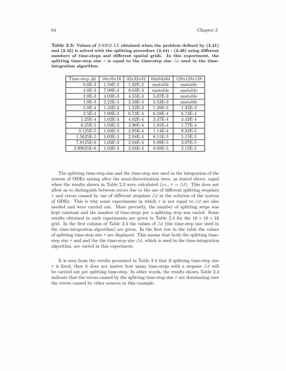
64 Chapter 2
Table 2.3: Values of ERRMAX obtained when the problem defined by (2.41)and (2.42) is solved with the splitting procedure (2.44) - (2.46) using differentnumbers of time-steps and different spatial grids. In this experiment, thesplitting time-step size τ is equal to the time-step size t used in the time-integration algorithm.
Time-step ∆t 16x16x16 32x32x32 64x64x64 128x128x1288.0E-3 1.58E-2 1.92E-2 unstable unstable4.0E-3 7.99E-3 9.03E-3 unstable unstable2.0E-3 4.03E-3 4.55E-3 5.07E-3 unstable1.0E-3 2.22E-3 2.33E-3 2.53E-3 unstable5.0E-4 1.32E-3 1.22E-3 1.28E-3 1.35E-32.5E-4 1.00E-3 6.73E-4 6.58E-4 6.74E-4
1.25E-4 1.02E-3 4.02E-4 3.47E-4 3.43E-46.25E-5 1.03E-3 2.96E-4 1.91E-4 1.77E-4
3.125E-5 1.03E-3 2.95E-4 1.14E-4 9.32E-51.5625E-5 1.03E-3 2.94E-4 8.11E-5 5.15E-57.8125E-6 1.03E-3 2.94E-4 8.09E-5 3.07E-5
3.90625E-6 1.03E-3 2.94E-4 8.08E-5 2.15E-5
The splitting time-step size and the time-step size used in the integration of thesystem of ODEs arising after the semi-discretization were, as stated above, equalwhen the results shown in Table 2.3 were calculated (i.e., τ = t). This does notallow us to distinguish between errors due to the use of different splitting stepsizesτ and errors caused by use of different stepsizes t in the solution of the systemof ODEs. This is why some experiments in which τ is not equal to t are alsoneeded and were carried out. More precisely, the number of splitting steps waskept constant and the number of time-steps per a splitting step was varied. Someresults obtained in such experiments are given in Table 2.4 for the 16 × 16 × 16grid. In the first column of Table 2.4 the values of t (the time-step size used inthe time-integration algorithm) are given. In the first row in the table the valuesof splitting time-step size τ are displayed. This means that both the splitting time-step size τ and and the the time-step size t, which is used in the time-integrationalgorithm, are varied in this experiment.
It is seen from the results presented in Table 2.4 that if splitting time-step sizeτ is fixed, then it does not matter how many time-steps with a stepsize t willbe carried out per splitting time-step. In other words, the results shown Table 2.4indicate that the errors caused by the splitting time-step size τ are dominating overthe errors caused by other sources in this example.

Using splitting techniques 65
Table 2.4: Values of ERRMAX obtained when the problem defined by (2.41)and (2.42) is solved using with different numbers of time-steps t per splittingtime-step τ (the values of τ are given in the first row of the table).
∆t 8.0E − 3 4.0E − 3 2.0E − 3 1.0E − 3 5.0E − 4 2.5E − 48.0E-3 1.59E-2 - - - - -4.0E-3 1.59E-2 7.99E-3 - - - -2.0E-3 1.59E-2 7.99E-3 4.03E-3 - - -1.0E-3 1.59E-2 7.99E-3 4.03E-3 2.22E-3 - -5.0E-4 1.59E-2 7.99E-3 4.03E-3 2.22E-3 1.32E-3 -2.5E-4 1.59E-2 7.99E-3 4.03E-3 2.22E-3 1.33E-3 1.00E-3
1.25E-4 1.59E-2 7.99E-3 4.03E-3 2.22E-3 1.33E-3 1.01E-36.25E-5 1.59E-2 7.99E-3 4.03E-3 2.22E-3 1.32E-3 1.01E-3
3.125E-5 1.59E-2 7.99E-3 4.03E-3 2.22E-3 1.32E-3 1.00E-31.5625E-5 1.59E-2 7.99E-3 4.03E-3 2.22E-3 1.32E-3 1.01E-37.8125E-6 1.59E-2 7.99E-3 4.03E-3 2.22E-3 1.32E-3 1.01E-3
3.90625E-6 1.59E-2 7.99E-3 4.03E-3 2.22E-3 1.32E-3 1.01E-3
2.8.4 Vanishing splitting errors
There are no errors caused by the splitting procedure when all pairs of simpleroperators in (2.2) are L-commuting (it should be reiterated here that if both op-erators in a given pair are linear, then L-commutativity is reduced to ordinarycommutativity of the involved operators).
In the following example the two operators involved commute and, thereforethere is no error caused by the splitting procedure:
∂c
∂t= y
∂c
∂x− x
∂c
∂y+ 1, t ∈ (0, 1], c(x, y, 0) = x2 + y2. (2.47)
The exact solution of (2.47) is given by
c(x, y, t) = x2 + y2 + t. (2.48)
Sequential splitting procedure based on the following two operators is used:
∂c[1]
∂t= y
∂c[1]
∂x− x
∂c[1]
∂y, (2.49)
∂c[2]
∂t= 1. (2.50)

66 Chapter 2
Table 2.5: The values of ERRMAX obtained when the problem defined by(2.47) is solved without splitting and with splitting (the values for the samegrid are equal when rounded to three significant digits). The same time-stepsize t = τ = 1.5625 × 10⁻⁵ has been used in the runs on different grids.
Grid Without splitting With splitting16 × 16 1.47E-3 1.47E-332 × 32 3.97E-4 3.97E-496 × 96 4.67E-5 4.67E-5
288 × 288 5.35E-6 5.35E-6480 × 480 1.94E-6 1.94E-6
Since these operators are linear and commutative, there are no errors due tothe splitting procedure. Thus, the results obtained by using the splitting procedureshould be the same as those obtained without using any splitting (of course, this isstrictly speaking only true if there are no rounding errors, but the rounding errorsare in this case negligible, because double precision is used in the computations).The results shown in Table 2.5 and in Table 2.6 show that the results are practicallythe same when no splitting is used and when splitting is used. This is true bothwhen different spatial grids are applied (see Table 2.5) and when the time-step sizeused in the solution of the semi-discretized problem is varied (see Table 2.6). Sincethe exact solution of this problem is linear in the time variable t, the numericalmethods used in the time-integration part are not causing errors. This means thatthe errors shown in Table 2.5 and Table 2.6 are caused only by the particular finitediscretization used to discretize the spatial derivatives in the right-hand-side of(2.49).
Table 2.6: The values of ERRMAX obtained when the problem defined by(2.47) is solved using different time-steps ∆t without splitting and with split-ting. The 16 × 16 grid is used in the discretization of the spatial derivatives.The experiment shows that the values of ERRMAX does not depend on thelength of time-steps. As in the previous table, these values remain the sameboth when no splitting is used and when splitting is applied.
∆t = τ Without splitting With splitting3.33E − 3 1.47E-3 1.47E-36.67E − 3 1.47E-3 1.47E-36.67E − 4 1.47E-3 1.47E-3

Using splitting techniques 67
2.8.5 Splitting procedures versus numerical methods
In this subsection we shall show that there is an interaction between the numericalmethods and the splitting results. This means that
• if the splitting procedure has been chosen, then some rules have to be appliedwhen the numerical method is to be selected, and
• if the numerical method has been chosen, then, again, some rules have to beapplied when the splitting procedure is to be selected.
A simple example will be used (only in order to facilitate the understanding ofthe main ideas). Consider the system of ordinary differential equation:
dc1
dt= c2,
dc2
dt=
c2(c2 − 1)c1
, (2.51)
where t ∈ [0, 10] and the initial values are given by
c1(0) = 0.5, c2(0) = 0.5. (2.52)
The problem defined by (2.51) and (2.52) is very simple. Nevertheless, it hasseveral properties that are typical for the problems arising in the chemical part ofair pollution models:
• the problem is non-linear,
• the mass preservation law holds, and
• the components of the solution vector are non-negative on the whole time-integration interval.
Moreover, there is at least one clear advantage when this problems is used: theexact solution of this problem is known. The components of the exact solution ofthe initial value problems defined by (2.51) and (2.52) are given by
c1(t) = 1.0 − 0.5 exp(−t), c2(t) = 0.5 exp(−t). (2.53)
Rewrite (2.51) as
dc1
dt= f1(c1, c2),
dc2
dt= f2(c1, c2). (2.54)
The right-hand-side vector in (2.54) can be represented as a sum of two simpleroperators defined by
f[1]1 = 0.0, f
[1]2 = −c2
c1(2.55)

68 Chapter 2
and
f[2]1 = c2, f
[2]2 =
(c2)2
c1. (2.56)
It is clear that (a) f[1]1 + f
[2]1 = f1, while f
[1]2 + f
[2]2 = f2 and (b) the four types
of splitting procedures, which were discussed in the beginning of this chapter canbe constructed for the particular problem (2.51) using the simpler operators (2.55)and (2.56). We shall solve (2.51) both without splitting and with the four splittingprocedures:
• sequential splitting,
• symmetric splitting,
• weighted sequential splitting (with θ = 0.5), and
• weighted symmetric splitting (with θ = 0.5).
Three numerical methods will be used in the solution (both in the case whereno splitting is used and in the case where the four splitting procedures are applied).If the problem (2.51) is rewritten in vector form as
dc
dt= f(c), (2.57)
where c is a vector with components c1 and c2, then the numerical methods, whichwill be used in this subsection, can be represented by the following formulae:
(A) Backward Euler Method.
This is an implicit first-order numerical method for the solution of ordinarydifferential equations (see, for example, Butcher [37], Hairer and Wanner [127],Hundsdorfer and Verwer [142], Lambert [155]). The calculations are carried outstep by step using the formula:
cn+1 = cn + tf(cn+1). (2.58)
where c is the vector containing the two components of the particular problem(2.51) and the sub-scripts denote the number of the time-step (which means thathaving an approximation cn of the solution at t = tn it is possible to calculate thenext approximation cn+1 at the next mesh-point tn+1 = tn + t using the aboveformula).

Using splitting techniques 69
(B) Implicit Mid-point Rule.
This is an implicit second-order numerical method for the solution of ordinarydifferential equations (see, again, Butcher [37], Hairer and Wanner [127], Hunds-dorfer and Verwer [142], Lambert [155]). The calculations are carried out step bystep using the formula:
cn+1 = cn + tf(0.5(cn + cn+1)). (2.59)
where cn+1 and cn are defined in the same way as the corresponding quantities aredefined for the Backward Euler Method (see the previous paragraph).
(C) Fully Implicit Three-stage Runge-Kutta Method.
This is an implicit sixth-order numerical method for the solution of ordinarydifferential equations (more details can be found Butcher [37], Hairer and Wanner[127], Hundsdorfer and Verwer [142], Lambert [155]). The calculations are carriedout step by step using the following formula:
cn+1 = cn + t[α1f(Y1) + α2f(Y2) + α3f(Y3)], (2.60)
the quantities Y1, Y2 and Y3 being calculated by
Y1 = cn + t[γ11f(Y1) + γ12f(Y2) + γ13f(Y3)], (2.61)
Y2 = cn + t[γ21f(Y1) + γ22f(Y2) + γ23f(Y3)], (2.62)
Y3 = cn + t[γ31f(Y1) + γ32f(Y2) + γ33f(Y3)]. (2.63)
The coefficients in formulae (2.60) - (2.63 (i.e., the coefficients αi and γij , wherei = 1, 2, 3 and j = 1, 2, 3) are given below:
α1 =518
, α2 =818
, α3 =518
, (2.64)
γ11 =536
, γ12 =10 − 3
√15
45, γ13 =
25 − 6√
15180
, (2.65)
γ21 =10 + 3
√15
72, γ22 =
29, γ23 =
10 − 3√
1572
, (2.66)
γ31 =25 + 6
√15
180, γ32 =
10 + 3√
1545
, γ33 =536
. (2.67)
The particular problem (2.51), which is considered in this subsection is an au-tonomous system of ordinary differential equations (i.e., the independent variable

70 Chapter 2
t does not participate explicitly in the right-hand-side of the system). If the non-autonomous problem dc/dt = f(t, c) is solved, then three additional coefficients areneeded:
β1 =5 −√
1510
, β2 =12, β3 =
5 +√
1536
. (2.68)
In this case, i.e., when the system of ordinary differential equations is non-autonomous, it is necessary to calculate values of the right-hand-side function fat times tn + βit, where i = 1, 2, 3 (much more details about the application ofRunge-Kutta type of methods for non-autonomous systems can be found in Butcher[37], Hairer and Wanner [127], Hundsdorfer and Verwer [142], Lambert [155]).
The transformation defined by
z1 = Y1 − yn, z2 = Y2 − yn, z3 = Y3 − yn (2.69)
is sometimes advocated (see, for example, Hairer and Wanner [127]). Our exper-iments indicate that this transformation is very useful when chemical schemes forlarge-scale air pollution models are treated by the Fully Implicit Three-stage Runge-Kutta Method. The transformation (2.69) has been used in the implementation ofthe Fully Implicit Three-stage Runge-Kutta Method for our tests.
(D) The notation used in the tables presented in this subsection.
Numerical results are calculated in the following way. For each numericalmethod and for each splitting procedure (considering here ”no splitting” as a specialcase of splitting), we start with t = 0.25. In this case the numerical integrationis completed in 40 time-steps. Then we are successively increasing the number oftime-steps by a factor of two (increasing the number of time-steps by a factor oftwo implies a decrease of the time-step size t by a factor of two).
The notation used in connection with the tables given in this subsection can beexplained as follows:
• ”Steps” refers to the number of time-steps used in the run under considera-tion,
• ”Splitting 0” refers to the case where no splitting is used,
• ”Splitting 1” refers to the case where sequential splitting is used,
• ”Splitting 2” refers to the case where symmetric splitting is used,
• ”Splitting 3” refers to the case where weighted sequential splitting is used,
• ”Splitting 4” refers to the case where weighted symmetric splitting is used,
• the global errors found during the whole integration process will simply becalled errors

Using splitting techniques 71
• the ratios between the errors obtained in two successive runs will simply becalled ratios.
(E) What should be expected when the numerical methods arecombined with different splitting procedures?
If no splitting is used, then the results should reflect the order of the numericalmethod used to solve the system of differential equations. In our study this meansthat the order of accuracy is
• one for the Backward Euler Method,
• two for the Implicit Mid-point Rule, and
• six for the Fully Implicit Three-stage Runge-Kutta Method,
when no splitting procedure is used.Assume now that some splitting procedure has been applied. Assume also that
the order of accuracy of the splitting procedure selected is q (q is equal to one forthe sequential splitting, while q is equal to two for the remaining three splittingprocedures). It is clear that, if the order of the numerical method used is p, then oneshould expect the order r of the combined method (i.e., the method obtained whenthe splitting procedure chosen is applied together with some numerical method) tosatisfy the relationship
r = min(q, p). (2.70)
Numerical experiments indicate that the relationship (2.70) will normally hold,but some artificial examples where this relationship is not satisfied can be con-structed. For example, one can construct particular problems for which
r > min(q, p). (2.71)
It is not very clear how this fact can be exploited in practice. If a particularproblem has to be solved again and again, one can try to design, for this particularproblem, a splitting procedure and a numerical method such that for the combinedmethod the relationship r > min(q, p) holds for the particular numerical methodsselected and for the particular splitting procedure applied. There is no guaranteethat such an attempt will be successful, but if the attempt is successful then theremaining runs (which are presumably many) can be run in a more efficient manner.At the end of this section it will be demonstrated that for some particular problemsthe relationship r > min(q, p) is satisfied.
It will be assumed in this subsection that the relationship r = min(q, p) holdsand it will be investigated what are the consequences of this fact for the resultsobtained with different splittings and the numerical methods described above. As-sume that the time-stepsize t is succesively decreased by a factor of two in several

72 Chapter 2
runs. Then there are three possibilities for the ratios of the errors obtained in twosuccessive runs:
• If the combined method (formed by the splitting procedure used and by thenumerical method applied) is of order one, then one should expect the ratiosto be approximately equal to two.
• If the combined method (formed by the splitting procedure used and by thenumerical method applied) is of order two, then one should expect the ratiosto be approximately equal to four.
• If the combined method is of order six (this happens only for the Fully ImplicitThree-stage Runge-Kutta Method when no splitting is used), then one shouldexpect the ratios to be approximately equal to 64 (excepting the case wherethe error becomes very small and, therefore, the accuracy is limited not by thecombined numerical method, but by other factors as, for example, roundingerrors, tolerances used to stop iterations, etc.).
The numerical results indicate that the behaviour of the error obtained duringthe computations is in fact determined by the rules formulated above.
(F) Behaviour of the errors obtained when numerical methodsare combined with different splitting procedures.
(F1) Backward Euler Method
It is appropriate to start the discussion of the results obtained by differentnumerical methods with the case where the simple Backward Euler Method isused with different splitting procedures (including here the case where no splittingprocedure is applied).
Results from 15 runs (beginning with a run where 40 time-steps are performed,increasing the number of time-steps by a factor of two after each run and finishingwith a run where 327 680 rime-steps were performed) are given
• in Table 2.7, showing the accuracy achieved for different time-step sizes, and
• in Table 2.8, showing the ratios of the errors between successive runs.
It is seen that the reduction of the stepsize by a factor of two is always resultingin a reduction of the error by a factor of two. In other words, the combined methodbehaves in this situation as a method of order one for all kinds of splitting. Theconclusion is that in general the use of splitting procedures of order higherthan one is not advisable when the numerical method used is of orderone.
If the process of doubling the number of time-steps, and consequently reducingthe time-step size by a factor of two, is continued (actually the time-steps were

Using splitting techniques 73
Table 2.7: Accuracy results achieved when the Backward Euler Method isused with five splitting procedures and when problem (2.51) is solved. Theabbreviations Steps, ”Splitting 0”, ”Splitting 1”, ”Splitting 2”, ”Splitting 3”and ”Splitting 4” are used for (i) the number of time-steps and (ii) the caseswhere no splitting, sequential splitting, symmetric splitting, weighted sequen-tial splitting and weighted symmetric splitting are used in the computations.
Steps Splitting 0 Splitting 1 Splitting 2 Splitting 3 Splitting 440 2.08E-2 2.08E-2 1.40E-1 2.60E-1 1.81E-180 1.09E-2 1.09E-2 7.40E-2 1.26E-2 9.22E-2
160 5.60E-3 5.60E-3 3.80E-2 6.26E-2 4.64E-2320 2.84E-3 2.84E-3 1.93E-2 3.12E-2 2.33E-2640 1.43E-3 1.48E-3 9.70E-3 1.56E-2 1.17E-2
1280 7.16E-4 7.16E-4 4.86E-3 7.81E-3 5.85E-32560 3.59E-4 3.59E-4 2.44E-3 3.91E-3 2.93E-35120 1.79E-4 1.79E-4 1.22E-3 1.95E-3 1.46E-3
10240 8.98E-5 8.98E-5 6.10E-4 9.76E-4 7.31E-420480 4.49E-5 4.49E-5 3.05E-4 4.88E-4 3.66E-440960 2.24E-5 2.24E-5 1.52E-4 2.44E-4 1.83E-481920 1.12E-5 1.12E-5 7.63E-5 1.22E-4 9.15E-5
163840 5.61E-6 5.61E-6 3.81E-5 6.10E-5 4.58E-5327680 2.81E-6 2.81E-6 1.91E-5 3.05E-5 2.28E-5
increased in this way to 20 971 520 in the experiments), then the same trend canbe observed (i.e. the accuracy is improved twice every time when the number oftime-steps is doubled). Accuracy of order O(10−8) has been achieved in the lastrun; the run with 20 971 520 time-steps.
It should be mentioned that the accuracy achieved when no splitting is used isprecisely the same as the accuracy achieved when a sequential splitting procedureis used. This is a surprising result. Istvan Farago from the University of Budapestinvestigated the situation closely. He proved that for the particular problem (2.51)the sequential splitting procedure performed using first the operator from (2.55)and then the operator from (2.56) does not cause additional errors (in comparisonwith the case where no splitting is used). However, this result is no longer true ifthe order of the operators in the sequential splitting procedure is reversed. Thisexample illustrates the fact that the order in which the simpler operators are

74 Chapter 2
Table 2.8: The ratios of the errors between successive runs that are obtainedwhen the Backward Euler Method is used with five splitting procedures andwhen problem (2.51) is solved. The abbreviations Steps, ”Splitting 0”, ”Split-ting 1”, ”Splitting 2”, ”Splitting 3” and ”Splitting 4” are used for (i) the num-ber of time-steps and (ii) the cases where no splitting, sequential splitting,symmetric splitting, weighted sequential splitting and weighted symmetricsplitting are used in the computations.
Steps Splitting 0 Splitting 1 Splitting 2 Splitting 3 Splitting 440 - - - - -80 1.908 1.908 1.894 2.061 1.966
160 1.951 1.951 1.947 2.015 1.983320 1.975 1.975 1.974 2.004 1.992640 1.987 1.987 1.987 2.001 1.996
1280 1.994 1.994 1.993 2.000 1.9982560 1.997 1.997 1.997 2.000 1.9995120 1.999 1.999 1.998 2.000 2.000
10240 1.999 1.999 1.999 2.000 2.00020480 2.000 2.000 2.000 2.000 2.00040960 2.000 2.000 2.000 2.000 2.00081920 2.000 2.000 2.000 2.000 2.000
163840 2.000 2.000 2.000 2.000 2.000327680 2.000 2.000 2.000 2.000 2.000
applied in the splitting procedure might be important in some situations.
(F2) Implicit Mid-point Rule
Let us consider now the application of the Implicit Mid-point Rule with differentsplitting procedures (including also here the case where no splitting procedure isapplied).
Results from 15 runs (beginning again with a run where 40 time-steps are per-formed, increasing the number of time-steps by a factor of two after each run andfinishing with a run where 327 680 rime-steps were performed) are given
• in Table 2.9, showing the accuracy achieved for different time-step sizes, and
• in Table 2.10, showing the ratios of the errors between successive runs.
It is seen that the reduction of the stepsize by a factor of two is resulting ina reduction of the error by a factor of four in all cases excepting the case wherethe sequential splitting procedure is used. In the latter case the reduction of the

Using splitting techniques 75
stepsize by a factor of two is resulting in a reduction of the error by a factor of two.In other words, the combined method behaves in this situation as a method of ordertwo for all splitting procedures excepting the sequential splitting procedure. For thesequential splitting procedure the combined method is of order one. The conclusionis that the use of splitting procedures of order one is not advisable whenthe numerical method used is of order two.
It should be noted that, if the weighted sequential splitting procedure is usedtogether with the Implicit Mid-point Rule, then the combined method is performingas a method of order approximately equal to three for large time-step sizes. How-ever, the combined method behaves as a method of order two when the time-stepsize is sufficiently small. It is not very clear what is the reason for this behaviour ofthe combined method. Some cancellation of errors is probably taking place whenthis particular test problem is run.
Table 2.9: Accuracy results achieved when the Implicit Mid-point Rule isused with five splitting procedures and when problem (2.51) is solved. Theabbreviations Steps, ”Splitting 0”, ”Splitting 1”, ”Splitting 2”, ”Splitting 3”and ”Splitting 4” are used for (i) the number of time-steps and (ii) the caseswhere no splitting, sequential splitting, symmetric splitting, weighted sequen-tial splitting and weighted symmetric splitting are used in the computations.
Steps Splitting 0 Splitting 1 Splitting 2 Splitting 3 Splitting 440 9.65E-04 2.00E-01 2.12E-02 6.67E-03 3.70E-0380 2.40E-04 1.11E-01 5.47E-03 8.16E-04 9.64E-04
160 5.99E-05 5.88E-02 1.38E-03 1.17E-04 2.43E-04320 1.50E-05 3.03E-02 3.45E-04 2.13E-05 6.10E-05640 3.74E-06 1.54E-02 8.64E-05 4.49E-06 1.53E-05
1280 9.36E-07 7.75E-03 2.16E-05 1.03E-06 3.81E-062560 2.34E-07 3.89E-03 5.40E-06 2.45E-07 9.52E-075120 5.85E-08 1.95E-03 1.35E-06 5.99E-08 2.38E-07
10240 1.46E-08 9.75E-04 3.38E-07 1.48E-08 5.96E-0820480 3.65E-09 4.88E-04 8.44E-08 3.68E-09 1.49E-0840960 9.14E-10 2.44E-04 2.11E-08 9.16E-10 3.72E-0981920 2.28E-10 1.22E-04 5.27E-09 2.29E-10 9.30E-10
163840 5.11E-11 6.10E-05 1.32E-09 5.72E-11 2.33E-10327680 1.43E-11 3.05E-05 3.30E-10 1.43E-11 5.83E-11
(F3) Fully Implicit Three-stage Runge-Kutta Method
Finally, we shall consider the application of the Fully Implicit Three-stageRunge-Kutta Method when this method is used with different splitting procedures

76 Chapter 2
Table 2.10: The ratios of the errors between successive runs that are obtainedwhen the Implicit Mid-point Rule is used with five splitting procedures whenwhen problem (2.51) is solved. The abbreviations Steps, ”Splitting 0”, ”Split-ting 1”, ”Splitting 2”, ”Splitting 3” and ”Splitting 4” are used for (i) the num-ber of time-steps and (ii) the cases where no splitting, sequential splitting,symmetric splitting, weighted sequential splitting and weighted symmetricsplitting are used in the computations.
Steps Splitting 0 Splitting 1 Splitting 2 Splitting 3 Splitting 440 - - - - -80 4.021 1.800 3.879 8.181 3.835
160 4.005 1.889 3.968 6.944 3.962320 4.001 1.941 3.992 5.502 3.991640 4.000 1.970 3.998 4.751 3.998
1280 4.000 1.985 3.999 4.377 3.9992560 4.000 1.992 4.000 4.189 4.0095120 4.000 1.996 4.000 4.094 4.000
10240 4.000 1.998 4.000 4.047 4.00020480 4.000 1.999 4.000 4.024 4.00040960 4.000 2.000 4.000 2.012 4.00081920 4.000 2.000 4.000 4.006 4.000
163840 4.000 2.000 4.000 4.003 3.999327680 4.000 2.000 4.000 4.003 3.996
(including also here the case where no splitting procedure is applied).As for the previous two numerical methods (the Backward Euler Method and
the Implicit Mid-point Rule), results from 15 runs (beginning with a run where 40time-steps are performed, increasing the number of time-steps by a factor of twoafter each run and finishing with a run where 327 680 rime-steps were performed)are given
• in Table 2.11, showing the accuracy achieved for different time-step sizes, and
• in Table 2.12, showing the ratios of the errors between successive runs.
Consider first the case where no splitting is used. It is seen from Table 2.12 thatthe reduction of the stepsize by a factor of two is resulting, when no other factorsare limiting the accuracy of the results, in a reduction of the error by a factor of64 when no splitting is used (which should be expected, because the Fully ImplicitThree-stage Runge-Kutta Method is of order six). The results, which are presentedin Table 2.11, show that in this case the accuracy is very quickly approaching themachine precision, and the results cannot be further improved when this happens.

Using splitting techniques 77
Table 2.11: Accuracy results achieved when the Fully Implicit Three-stageRunge Kutta Method is used with five splitting procedures and when problem(2.51) is solved. The abbreviations Steps, ”Splitting 0”, ”Splitting 1”, ”Splitting2”, ”Splitting 3” and ”Splitting 4” are used for (i) the number of time-stepsand (ii) the cases where no splitting, sequential splitting, symmetric splitting,weighted sequential splitting and weighted symmetric splitting are used in thecomputations.
Steps Splitting 0 Splitting 1 Splitting 2 Splitting 3 Splitting 440 4.47E-10 1.90E-01 1.95E-02 1.66E-02 2.62E-0380 6.96E-12 1.08E-01 5.12E-03 3.39E-03 6.49E-04
160 1.09E-13 5.82E-02 1.30E-03 7.49E-04 1.62E-04320 1.99E-15 3.01E-02 3.25E-04 1.75E-04 4.07E-05640 6.66E-16 1.53E-02 8.13E-05 4.22E-05 1.02E-05
1280 2.78E-15 7.74E-03 2.03E-05 1.03E-05 2.54E-062560 1.78E-15 3.89E-03 5.08E-06 5.08E-06 6.36E-075120 4.77E-15 1.95E-03 1.27E-06 6.39E-07 1.59E-07
10240 3.22E-15 9.75E-04 3.17E-07 1.59E-07 3.97E-0820480 6.88E-15 4.88E-04 7.94E-08 3.98E-08 9.93E-0940960 8.54E-15 2.44E-04 1.99E-08 9.94E-09 2.48E-0981920 2.08E-14 1.22E-04 4.97E-09 2.48E-09 6.21E-10
163840 9.77E-15 6.10E-05 1.24E-09 6.21E-10 1.55E-10327680 1.23E-14 3.05E-05 3.10E-10 1.55E-10 3.86E-11
The reduction of the stepsize by a factor of two is resulting in a reduction of theerror by a factor of two when the sequential splitting is used. This should also beexpected because the sequential splitting procedure is of order one, see also (2.70).
The reduction of the stepsize by a factor of two is resulting in a reductionof the error by a factor greater than four in the beginning when the weightedsequential splitting is used, however the reduction is by a factor of four when thestepsize become small. Similar results, even more pronounced, were, as mentionedabove, observed when the Implicit Mid-point Rule is used. It is not very clearwhy the reduction of the error is by a factor greater than four when the time-stepsize is larger than four when the time-stepssizes are large (probably some kind ofcancelation of errors caused by the numerical method and errors caused by thesplitting procedure takes place for this particular problem when the time-step sizeis large).
The reduction of the stepsize by a factor of two is resulting in a reduction of theerror by a factor of four when the symmetric and the weighted symmetric splittingprocedures are used.

78 Chapter 2
Table 2.12: The ratios of the errors between successive runs that are obtainedwhen the Fully Implicit Three-stage Runge Kutta Method is used with fivesplitting procedures and when problem (2.51) is solved. The abbreviationsSteps, ”Splitting 0”, ”Splitting 1”, ”Splitting 2”, ”Splitting 3” ”Splitting 4”,Error and Ratio are used for (i) the number of time-steps, (ii) the cases nosplitting, sequential splitting, symmetric splitting, weighted sequential split-ting and symmetric splitting, (iii) the global error found during the integrationand (iv) the ratio between two successive errors.
Steps Splitting 0 Splitting 1 Splitting 2 Splitting 3 Splitting 440 - - - - -80 64.116 1.753 3.815 4.892 4.037
160 64.002 1.866 3.950 4.531 3.995320 54.458 1.930 3.987 4.283 3.997640 3.000 1.964 3.997 4.145 3.999
1280 0.240 1.982 3.999 4.074 4.0002560 1.562 1.991 4.000 4.037 4.0005120 0.372 1.995 4.000 4.019 4.000
10240 1.483 1.998 4.000 4.009 4.00020480 0.468 1.999 4.000 4.005 4.00040960 0.805 1.999 4.000 2.002 4.00081920 0.412 2.000 4.000 4.001 4.000
163840 2.125 2.000 4.000 4.001 3.999327680 0.793 2.000 4.000 4.000 3.996
Two important conclusions can be drawn using the numerical results presentedin Table 2.11 and in Table 2.12.
• The example, which is treated in this subsection indicates that the use of anumerical method of very high order is justified only if no splittingis used.
• It might be worthwhile, in some situations at least, to try to avoid the use ofsplitting procedures by applying numerical methods of high order.The computational work per time-step will be increased if such an action istaken. This increase will be very substantial for large-scale problems. Onthe other side, however, the number of time-steps can sometimes be reduceddramatically (as the results in Table 2.11 indicate). Indeed, better accuracy(than the accuracy achieved by the other two numerical methods) is achievedwhen only 320 time-steps are performed. Let us reiterate here that performing20 971 520 time-steps with the Backward Euler Method results in numericalerrors of order O(10−8). It is also worthwhile to mention the computational

Using splitting techniques 79
times: 0.18 seconds for 320 time-steps with the Fully Implicit Three-stageRunge-Kutta Method and 31 745 seconds for 20 971 520 time-steps with theBackward Euler Method.
(G) Summarizing the results related to the order of the combinedmethod
The interaction between the numerical methods and the splitting proceduresis illustrated in Table 2.13. It should be stressed here that the results given inTable 2.13 are strictly speaking valid only for the particular problem (2.51). Oneshould expect that these results are also valid for other problems. However, moreexperiments are necessary in order to verify such a conjecture.
Table 2.13: The order of combined method (splitting procedure and numer-ical method) observed when the problem (2.51) is solved with five splittingprocedure (considering here the runs without splitting as a special case ofsplitting) and three numerical methods. The figure ”2+” for the weightedsequential splitting procedure applied with the implicit mid-point rule reflectsthe fact that the combined method seems to be of order higher than twofor large time-steps (see Table 2.9). The order of the combined method (thesequential splitting procedure + the fully implicit three-stage Runge-Kuttamethod) seems also to be slightly higher than two (see Table 2.12).
Type of splitting Backward Euler Mid-point Three-stage Runge-KuttaNo splitting 1 2 6Sequential 1 1 1Symmetric 1 2 2
Weighted sequential 1 2+ 2Weighted symmetric 1 2 2
The results in Table 2.13 reflect the general case where the order of the combinedmethod r satisfies the relationship (2.70), i.e., r is equal to the minimum of theorder p of the numerical method and the order q of the splitting procedure. It wasmentioned in the beginning of this section that for some particular problems therelationship r > min(q, p) can be observed. This statement will now be illustratedby a simple numerical example. Consider the problem:
dc1
dt= c2,
dc2
dt= −c1, (2.72)
where t ∈ [0, 10] and the initial values are given by
c1(0) = 0, c2(0) = 0. (2.73)

80 Chapter 2
The exact solution of the problem defined by (2.72)-(2.73) is given by
c1(t) = sin(t), c2(t) = cos(t). (2.74)
The problem (2.72)-(2.73) was run in the same manner as the previous problem,i.e., in the same manner as the problem defined by (2.53)-(2.54) was run. Resultsobtained with the Backward Euler Method (of order p = 1) combined with differentsplitting procedures will be studied. The accuracy of the obtained solution (withdifferent time-step sizes and different splittings is shown in Table 2.14, while theratios are displayed in Table 2.15.
It is clearly seen that for the case where no splitting is used and for the sequentialsplitting the order of the combined method is one (which should be expected becausep = q = 1). However, for the remaining three cases (i.e., for the symmetric splitting,the weighted sequential splitting and the weighted symmetric splitting) the order ofthe combined method is not one (which should be expected and which was observedin Table 2.7 and Table 2.8), but two. This means that the relationship r > min(q, p)holds for this particular problem when the three splitting procedures of order q = 2are used.
Table 2.14: Accuracy results achieved when the Backward Euler Method isused with five splitting procedures and when problem (2.72) is solved. Theabbreviations Steps, ”Splitting 0”, ”Splitting 1”, ”Splitting 2”, ”Splitting 3”and ”Splitting 4” are used for (i) the number of time-steps and (ii) the caseswhere no splitting, sequential splitting, symmetric splitting, weighted sequen-tial splitting and weighted symmetric splitting are used in the computations.
Steps Splitting 0 Splitting 1 Splitting 2 Splitting 3 Splitting 440 6.83E-01 1.46E-01 2.51E-02 1.01E-01 2.51E-0280 4.42E-01 6.77E-02 6.27E-03 2.49E-02 6.20E-03
160 2.55E-01 3.25E-02 1.57E-03 6.20E-03 1.54E-03320 1.37E-01 1.60E-02 3.92E-04 1.55E-03 3.86E-04640 7.13E-02 7.90E-03 9.80E-05 3.86E-04 9.64E-05
1280 3.62E-02 3.93E-03 2.45E-05 9.65E-05 2.41E-052560 1.83E-02 1.96E-03 6.13E-06 2.41E-05 6.03E-065120 9.21E-03 9.78E-04 1.53E-06 6.03E-06 1.51E-06
10240 4.62E-03 4.89E-04 3.83E-07 1.50E-06 3.77E-0720480 2.31E-03 2.44E-04 9.57E-08 3.77E-07 9.42E-0840960 1.16E-03 1.22E-04 2.39E-08 9.42E-08 2.35E-0881920 5.78E-04 6.10E-05 5.98E-09 2.35E-08 5.88E-09
163840 2.89E-04 3.05E-05 1.50E-09 5.88E-09 1.47E-09327680 1.45E-04 1.53E-05 3.74E-10 1.47E-09 3.68E-10

Using splitting techniques 81
Table 2.15: The ratios of the errors between successive runs that are ob-tained when the Backward Euler Method is used with five splitting proce-dures and when problem (2.51) is solved. The abbreviations Steps, ”Splitting0”, ”Splitting 1”, ”Splitting 2”, ”Splitting 3” and ”Splitting 4” are used for(i) the number of time-steps and (ii) the cases where no splitting, sequen-tial splitting, symmetric splitting, weighted sequential splitting and weightedsymmetric splitting are used in the computations.
Steps Splitting 0 Splitting 1 Splitting 2 Splitting 3 Splitting 440 - - - - -80 1.544 2.215 4.004 4.038 4.053
160 1.735 2.082 3.999 4.019 4.013320 1.858 2.041 4.000 4.009 4.002640 1.926 2.020 4.000 4.005 4.001
1280 1.962 2.005 4.000 4.002 4.0002560 1.981 2.003 4.000 4.001 4.0005120 1.990 2.001 4.000 4.001 4.000
10240 1.995 2.001 4.000 4.000 4.00020480 1.998 2.000 4.000 4.000 4.00040960 1.999 2.000 4.000 4.000 4.00081920 1.999 2.000 4.000 4.000 4.000
163840 2.000 2.000 4.000 4.000 4.000327680 2.000 2.000 4.000 4.000 4.000
(H) Need for more experiments
The results given in Table 2.7 to Table 2.13 allowed us to draw some use-ful conclusions about the combined methods (splitting procedures with numericalmethods). However, as mentioned above, these results are in fact valid only for theproblem tested, the problem (2.51). It is expected that these conclusions are rathergeneral and, therefore, hold also for many other problems. Nevertheless, much moreexperiments are needed. It is necessary to develop a powerful program which willfacilitate the efforts related with performing in a systematical way many tests withdifferent problems. Such program, EXAMINATOR, is in process of development.The basic principles used in the development of this program are sketched below.
• The same splitting procedures, as those discussed in this section, can bespecified by setting an appropriate value to a special parameter ISPLIT .The following values of ISPLIT are allowed at present:
– ISPLIT = 0 if no splitting is to be used,
– ISPLIT = 1 if a sequential splitting is to be used,

82 Chapter 2
– ISPLIT = 2 if a symmetric splitting is to be used,
– ISPLIT = 3 if a weighted sequential splitting is to be used, and
– ISPLIT = 4 if a weighted symmetric splitting is to be used.
• The numerical methods used in this subsection can be specified. However,three additional methods can also be used. The desired numerical methodcan be selected by choosing an appropriate value of parameter METHOD.The following six values of parameter METHOD can be used at present:
– METHOD = 1 for the Backward Euler Method (see Butcher [37],Hairer and Wanner [127], Hundsdorfer and Verwer [142], Lambert [155]),
– METHOD = 2 for the Implicit Mid-point Rule (see Butcher [37], Hairerand Wanner [127], Hundsdorfer and Verwer [142], Lambert [155]),
– METHOD = 3 for the Modified Diagonally Implicit Runge-Kutta Method(see Zlatev [273]),
– METHOD = 4 for the Fully Implicit Three-stage Runge-Kutta Method(see Butcher [37], Hairer and Wanner [127], Hundsdorfer and Verwer[142], Lambert [155]),
– METHOD = 5 for the Two-stage Rosenbrock Method (see Rosenbrock[206], Hundsdorfer and Verwer [142], Lambert [155]), and
– METHOD = 6 for the Trapezoidal Rule (see Hairer and Wanner [127]or Lambert [155]).
All possible combinations of the five splitting procedures and the six numericalmethods can be used. Thus, it is possible to carry out many different experimentswhen this program is used. In Chapter 10, it will be demonstrated that the pro-gram EXAMINATOR can be used to examine the performance of different splittingprocedures and numerical methods not only when the problems are solved directly,but also when some variational data assimilation technique is used.
The input data which have to be provided can be described as follows (it isclear that the parameters ISPLIT and METHOD, which were described above,are also input parameters):
• The integration interval [a, b] should be defined.
• Subroutines, which calculate the functions f from (2.54), f [1] from (2.55) andf [2] from (2.56), should be prepared.
• Subroutines, which calculate the Jacobian matrices of the functions f from(2.54), f [1] from (2.55), and f [2] from (2.56), should be prepared.
• A subroutine, which calculates the exact solution of the problem dc/dt =f(t, c) has to be prepared.

Using splitting techniques 83
It is easy to define the integration interval. Two parameters, TSTART andTEND, are be given in order to show where the computations are to be startedand where the computational process will be finished.
The subroutines for the calculation of f , f [1] and f [2] are normally very simpleand there will normally be no problems in the preparation of these subroutines.
In the present version of the program EXAMINATOR the exact Jacobian ma-trices are required. Differences might be used to prepare approximate Jacobianmatrices. Approximate Jacobian matrices might cause difficulties in some situa-tions.
If the exact solution of the problem studied, dc/dt = f(t, c), is not known, then areference solution (see, for example, Alexandrov et al. [6]) can be calculated, savedin a file and used to evaluate the behaviour of the errors obtained when differentcombinations of splitting procedures and numerical methods are tested.
The present version of the program EXAMINATOR is dealing with problems ofthe type dc/dt = f(t, c). There are plans to extend the class of the problems whichcan be handled by this program by adding options for the treatment of some otheroperators which are participating in advanced air pollution models. The problemis that if this is done, then it becomes difficult to check the behaviour of the errorsin the same manner as the procedure used in the preparation of the results shownin Table 2.7 to Table 2.13.
At the end of this section some numerical results will be presented (see Table2.16, Table 2.17, and Table 2.18) in order to demonstrate the efficiency of theprogram EXAMINATOR described above in the efforts
• to explain the results obtained by different splitting procedures and differentnumerical methods
as well as
• to facilitate the selection of the most suitable combination of a splitting pro-cedure and a numerical method.
The problem defined by (2.51) and ((2.52) is again considered. Sixteen runswere performed for each splitting procedure and for each numerical method andthe results are summarized into the three tables given below (i.e., the total numberof runs was 480, but it should be emphasized here that the conclusions were drawnusing much more experiments). For each combination of a numerical method and asplitting procedure, the first run is performed with a time-step size t = 0.25. Afterthat the stepsize is successively reduced (15 times) by a factor of two. Reducing thetime-step size by a factor of two leads to an increase of the number of time-stepsby a factor of two (the number of time steps for the first run is 40, while it becomes5242880 for the last run).
The smallest and the largest errors obtained in the runs with 16 different time-step sizes (or, in other words, the left-hand-end-points and the right-hand-end-points of the intervals in which the errors vary) are given, for each combination

84 Chapter 2
of a splitting procedure and a numerical method, in Table 2.17 and Table 2.16respectively. Taking the corresponding figures in these two table, one can obtainthe interval in which the errors are varied for a given combination of a numericalmethod and a splitting procedure.
Table 2.16: The largest errors obtained in the runs with 16 different time-stepsizes (i.e., the right-hand-end-points of the intervals in which the errors vary)are given in this table for different splittings and different numerical methods.The abbreviations ”Splitting 0”, ”Splitting 1”, ”Splitting 2”, ”Splitting 3” and”Splitting 4” are used for the different splitting, while the abbreviations ”BE”,”IMR”, ”RK2”, ”RK6”, ”ROS2” and ”TR” are denoting the Backward EulerMethod, the second-order RK method, the six-order RK method, the second-order Rosenbrock method and the Trapezoidal Rule, respectively.
Method Splitting 0 Splitting 1 Splitting 2 Splitting 3 Splitting 4BE 2.1E-02 2.1E-02 1.4E-01 2.6E-1 1.8E-01
IMR 9.6E-04 2.0E-01 2.1E-02 6.7E-3 3.7E-03RK2 8.7E-04 1.4E-01 3.7E-02 2.1E-2 2.7E-02RK6 4.5E-10 1.9E-01 2.0E-02 1.7E-2 2.6E-02
ROS2 8.6E-03 1.4E-01 3.7E-02 2.1E-2 2.7E-02TR 9.6E-04 2.0E-01 2.1E-02 6.7E-3 3.7E-03
The largest errors (i.e., the right-hand-end-points of the intervals in which theerrors vary) are normally obtained when the largest time-step size, t = 0.25, isused. It was expected that the smallest errors will be obtained when the smalleststepsizes are used. However, this is not always true for the smallest errors (i.e., theleft-hand-end-points of the intervals in which the errors vary), because if the errorsbecome less than O(10−11) and millions of time-steps are to be carried out, then therounding error start to interfere with the other errors. Accuracy of order O(10−11)is achieved very quickly, when the RK6 method is used without splitting).
The rates of decreasing the errors when the time-step sizes are decreased aregiven in Table 2.18. These values are approximate values. For some combinations”numerical method with splitting procedure”, the rates are lower in the beginning.If the errors become very small, then rates start to oscillate around 1. However,the figures in Table 2.18 give quite adequate information about the rates whichcan be achieved by different combinations of a numerical method and a splittingprocedure.
Several conclusions can be drawn using the results from the 480 runs (as wellas results from some other runs, including here runs performed by other test-problems):
• If the sequential splitting is used, then the errors caused by this splitting(which is of order one) are dominating. Therefore, in this case it does not

Using splitting techniques 85
Table 2.17: The smallest errors obtained in the runs with 16 different time-step sizes (i.e., the left-hand-end-points of the intervals in which the errorsvary) are given in this table for different splittings and different numericalmethods. The abbreviations ”Splitting 0”, ”Splitting 1”, ”Splitting 2”, ”Split-ting 3” and ”Splitting 4” are used for the different splitting, while the ab-breviations ”BE”, ”IMR”, ”RK2”, ”RK6”, ”ROS2” and ”TR” are denotingthe Backward Euler Method, the second-order RK method, the six-order RKmethod, the second-order Rosenbrock method and the Trapezoidal Rule, re-spectively.
Method Splitting 0 Splitting 1 Splitting 2 Splitting 3 Splitting 4BE 1.8E-07 1.8E-07 1.2E-06 1.9E-06 1.4E-06
IMR 8.7E-14 1.9E-06 1.2E-12 2.2E-12 1.7E-12RK2 9.2E-13 1.9E-06 6.2E-13 1.3E-13 5.9E-12RK6 6.7E-16 1.9E-06 1.1E-12 2.8E-12 1.3E-12
ROS2 9.5E-13 1.9E-06 6.6E-13 1.2E-11 7.4E-12TR 8.7E-14 1.9E-06 1.2E-12 2.2E-13 1.7E-13
Table 2.18: The approximate rates of convergence (measured by the ratio ofthe error found at run i and the error found at run i− 1, where i = 2, 3, . . . , 16).The abbreviations ”Splitting 0”, ”Splitting 1”, ”Splitting 2”, ”Splitting 3” and”Splitting 4” are used for the different splitting, while the abbreviations ”BE”,”IMR”, ”RK2”, ”RK6”, ”ROS2” and ”TR” are denoting the Backward EulerMethod, the second-order RK method, the six-order RK method, the second-order Rosenbrock method and the Trapezoidal Rule, respectively.
Method Splitting 0 Splitting 1 Splitting 2 Splitting 3 Splitting 4BE 2 2 2 2 2
IMR 4 2 4 4 4RK2 4 2 4 4 4RK6 64 2 4 4 4
ROS2 4 2 4 4 4TR 4 2 4 4 4
matter too much what numerical method is selected. In fact, practically thenumerical method does not have any influence on the results (excluding herethe Backward Euler Method, which has, as mentioned before, some specialproperties for this particular test-problem)
• As mentioned before, the combination of a second-order numerical method
86 Chapter 2
and a second-order splitting procedure results in a second-order of the com-bined method. However, one should be careful when the second-order Rosen-brock methods is used for non-autonomous problems. In this case one shouldfirst transform the problem, by adding an extra equation, to an autonomousproblem. This transformation was not needed here, because the problem(2.51) is autonomous.
• There is, in general, no sense to use a combination of a high-order split-ting procedure with a low-order numerical method and vice-versa. This isprescribed by the relationship (2.70), but it is immediately seen that the nu-merical results are in a very good agreement with this relationship. However,let us re-iterate that for a particular problem one can also design combina-tions in which the relationship (2.71) holds instead of (2.70). An example,where this happens, was given in Table 2.14 and Table 2.15.
2.9 Using splitting procedures in connectionwith other applications
The presentation of the splitting procedures made in this chapter is very general.Therefore, it is quite clear that all splitting procedures that were discussed in theprevious sections of this chapter can be applied with some obvious modificationswhen the applications discussed in Section 7 of Chapter 1 or other large-scale ap-plications are to be treated on high-speed computers.
2.10 Conclusions and plans for future research
The examples given in Section 8 of this chapter show that even in very simplecases the splitting procedure will in general cause splitting errors. Therefore, itis worthwhile to carry out work on the solution of the following four importantproblems:
• to attempt to avoid the use of splitting procedures when this is possible (itshould be emphasized, however, that at present this is not always possible),
• to construct splitting procedures of order higher than two,
• to search for optimal combinations of splitting procedures and numericalmethods such that the order of the combined methods is as higher as possible,and
• to find reliable and robust methods for evaluating the splitting errors.
These four problems are still open (or, at least, not satisfactorily well resolved)both when general large-scale air pollution models are treated and when otherlarge-scale mathematical problems are to be handled. Success in the solution of

Using splitting techniques 87
any of these four problems is a very desirable, but also a very challenging task.It should be noted that even a partial solution of any of these four problems willlead to a very considerable progress in the numerical treatment of large-scale airpollution models, as well as in the numerical treatment of many other large-scalecomputational problems arising in science and engineering.
Better understanding of the interferences of errors due to the splitting proce-dures and errors that are caused by other reasons (numerical methods, uncertaintiesof the input data, etc.) is highly desirable. Research efforts in this directions areneeded.


Chapter 3
Treatment of theadvection-diffusion phenomena
The advection-diffusion phenomena in a large-scale air pollution model can be di-vided (for example, by using an appropriate splitting procedure; see the previouschapter) in three parts
• the mathematical terms describing the horizontal advection,
• the mathematical terms describing the horizontal diffusion, and
• the mathematical terms describing the vertical exchange (the vertical ex-change is a combination of vertical advection and vertical diffusion).
Several numerical methods, which can be applied to treat the advection-diffusionphenomena, will be discussed in this chapter. It should be emphasized here that weare mainly interested in the computational aspect of the treated problems. There-fore, we shall try to emphasize the fact that the application of different numericalmethods leads to the same type of computational problems and the resulting com-putational problems will be the main topic of the discussions in this chapter. Moredetails about
• the choice of particular numerical methods, and
• the properties of different classes of numerical methods
can be found, for example, in the monograph ”Numerical Solution of Time-DependentAdvection-Diffusion-Reaction Equations” written by Hundsdorfer and Verwer [142].
It should also be emphasized, before the beginning of the discussion of differentcomputational problems, that the use of some splitting procedure is assumed in thischapter. This is a natural assumption, because all operationally used large-scale airpollution models are treated, as mentioned in the previous chapters, by applyingsome splitting procedure. Some of the computational problems, which arise whenno splitting procedure is used, will be shortly described in Chapter 6.
89

90 Chapter 3
3.1 Treatment of the horizontal advection
We shall start by assuming that the splitting procedure described by (2.5) - (2.9)is used. The horizontal advection, which is described by the system of PDEs (2.5),is separated from the other physical processes when this assumption is made. Itis immediately seen that the system of PDEs (2.5) consists of independent par-tial differential equations (one equation per each chemical compound when a two-dimensional version of the model is studied, while the number of equations is equalto the product of the number of chemical compounds and the number of layerswhen the horizontal transport in a three-dimensional version of the model is tobe handled). This means that in many cases (as, for example, the important casewhere a fast and reliable numerical method is to be found) it is quite sufficient toconsider only one of these equations. Under this assumption, the horizontal trans-port of any pollutant in the atmosphere can be described mathematically by thefollowing first-order partial differential equation:
∂c
∂t= −∂(uc)
∂x− ∂(vc)
∂y. (3.1)
Let us introduce the parameter zk (where k = 1 in the two dimensional case,while k ∈ 1, 2, . . . , 10 when a three-dimensional version of the particular modeldiscussed in the Chapter 1, DEM, is used). Assume that the value of k is fixed.Then the notation used in (3.1) can (as in the previous chapters) be explained asfollows:
• the unknown function c = c(x, y, zk, t) is the concentration of some pollutantin the kth layer of the model, and
• the known functions u = u(x, y, zk, t) and v = v(x, y, zk, t) are wind velocities(again in the kth layer of the model) along the Ox and Oy axes respectively.
This means that the quantity c in (3.1) is representing the concentration of any ofthe chemical species both in the two-dimensional case and in the three-dimensionalcase. It is clear that in the two-dimensional case there are q = Ns (q being thenumber of the chemical species studied by the model) independent equations of type(3.1). In the three-dimensional case, the number of independent equations of type(3.1) is equal to the product of the number of chemical species q and the number oflayers k. As mentioned above, it is sufficient to consider only one equation of type(3.1) when a good numerical method for the treatment of the advection sub-modelis to be found. However, sometimes it is better to combine several equations and toconsider the enlarged problem obtained by the combination chosen (for example,when parallel computers are used this is done in order to obtain bigger paralleltasks; see Chapter 7).

Treatment of the advection-diffusion phenomena 91
The numerical solution of (3.1) causes some great difficulties in the case whenthis equation is a part of a large-scale air pollution model, because the computa-tional tasks can become very large. This can be explained by the following exam-ple (see also Chapter 1). Assume that a three-dimensional air pollution model is tobe handled and that the number of pollutants is Ns. Assume also that the modelis discretized on a (Nx × Ny × Nz) grid, where Nx, Ny and Nz are the numbersof grid-points along the coordinate axes. Then the application of some splittingprocedure followed by some kind of discretization of the spatial derivatives leads tothe treatment of Ns ×Nz systems of ordinary differential equations (ODEs) duringmany (typically several hundred thousand) time-steps. Each of these ODE systemscontains Nx × Ny equations. If Nx = 480, Ny = 480, Nz = 10, Ns = 35, then 350ODE systems each of them containing 230400 equations have to be treated at everytime-step. It is difficult to treat such a model on the available supercomputers whenthe time interval is long (say, several years) or when many different scenarios haveto be run. This is why the two-dimensional version of DEM is often used in thiscase (i.e. Nz = 1 is chosen). The number of ODE systems that are to be handled atevery time-step is reduced considerably, from 350 to 35, when the two-dimensionalversion is used. However, even under this assumption it is not possible to handle
• long-term runs (by using meteorological data for many, at present up to ten,years), or
• simulations consisting of many (several hundred or even several thousand)scenarios.
Coarser grids have to be used in these two cases (Nx = Ny = 96). Of course, thisis a compromise. It is much more desirable to use finer grids (avoiding in this waythe use of non-physical simplifications; i.e. avoiding introducing such simplificationsonly in order to be able to treat large-scale air pollution models on the computersthat are available at present).
The actual situation is in fact more complex, when (3.1) is arising from air pollu-tion models, because similar systems of ODEs have also to be treated in connectionwith the other physical processes (chemistry, diffusion, deposition and vertical ex-change). The five major physical and chemical processes are treated successivelyat every time-step in the older version of DEM; see (2.5)-(2.9) in Chapter 2. Inthe latest version of DEM the horizontal advection is combined with the horizontaldiffusion as described in (2.12); the remaining processes are treated by (2.11) and(2.13).
The short description of the computational difficulties, which has been sketchedabove, explains clearly that (a) the treatment of the horizontal advection is a verychallenging problem and (b) it is very important to handle efficiently PDEs of type(3.1). Three major tasks have to be resolved in the efforts to make the treatmentof (3.1) more efficient:

92 Chapter 3
• Fast, but sufficiently accurate, numerical methods have to be selected andcarefully implemented. The use of the scalar equation (3.1) in the solution ofthis task is quite sufficient.
• The selected numerical methods have to be adjusted for efficient runs on dif-ferent high-speed computers. The organization of the computations is veryimportant when this task is handled. It is normally necessary to treat simul-taneously several equations (3.1) in order to efficiently resolve this task.
• Finally, if (3.1) is a part of an large-scale air pollution model, then the factthat (3.1) is, as mentioned above, a system of PDEs that has to be treatedtogether with several other PDE systems (arising from the other physical andchemical processes) must be taken into account. The solution of this task willbe discussed in Chapter 7.
The solution of these three tasks is important. The main part of this chapteris devoted to the choice of efficient numerical algorithms. However, the require-ments implied from the other two tasks will also be taken into account in orderto synchronize the efficient solution of the first task with the requirement for effi-cient treatment of the whole air pollution model of which (3.1) is an essential part.Therefore, we shall assume that either a single equation (3.1) is considered or thatseveral equations (3.1) are combined and treated simultaneously in an attempt toorganize better the computational process. It will either be stated directly whichof these two cases is discussed or it will be clear from the context whether (3.1) isconsidered as a single equation or several equations (3.1) are combined.
As in many other places in this book, it should be emphasized that the problemdescribed by (3.1) is rather general. Therefore many of the results presented in thischapter are also valid if (3.1) arises from some other fields of science or engineering.
3.2 Semi-discretization of the advection equation
The choice of numerical methods for the solution of (3.1) has been discussed inmany publications (many references on this topic can be found in Zlatev [282]).The following numerical methods are often used in the treatment of the horizontaladvection in large-scale air pollution models:
(a) Numerical methods, which are based on the direct use of finite differences(many details about the use of finite differences in the solution of differentscientific problems can be found in Chock [43], [44], Chock and Dunker [45],Pepper and Baker [192], Pepper et al. [193], Kreiss [152], Richtmyer andMorton [201]). Some kind of smoothing is often used when there are sharpgradients. More details about the use of finite differences in the numericalsolution of partial differential equations can also be found in the recentlypublished, by Strikwerda, text-book on this subject; see [237].

Treatment of the advection-diffusion phenomena 93
(b) Numerical methods, which are based on the direct use of finite elements (manydetails about the use of finite elements in the solution of different scientificproblems can be found in Axelsson and Barker, [13], Chock [43], [44], Chockand Dunker [45], Pepper and Baker [192], Pepper et al. [193] Segerlind [216],Strang and Fix [236], Zienkiewicz [271]). Also in this case, smoothing pro-
cedures are often used. More details about the use of finite elements in thenumerical solution of partial differential equations can also be found in therecently published, by Solin, text-book on this subject; see [229].
(c) Numerical methods, which are based on the use of either finite elements orfinite differences combined with some kind of limiting (see Hundsdorfer andVerwer [142], LeVeque, [162], [163]). Limiting can be viewed as a specialsmoothing procedure.
(d) Semi-Lagrangian methods (see Loon [167]), Rancic [198], Rancic and William-son [199], Robert et al. [204]). Some kind of interpolation must be usedtogether with the semi-Lagrangian methods. Finding a good interpolationscheme, which can efficiently be used together with the implemented semi-Lagrangian method, can be difficult.
(e) The method proposed by A. Bott is very popular in the field of large-scale airpollution modelling (see Bott [24]). In this method, an attempt is made toavoid negative concentrations (this is why the method is sometimes calledpositive definite). There have been made several attempts to improve thismethod; see, for example, Holm and Erbes [137], Syrakov [242], Syrakov andGalperin [243], [244]).
(f) Pseudo-spectral methods (different applications of this numerical technique canbe found in Fornberg [103], [104], Kreiss and Oliger [153], Lee [160], Merilees[182], Roache [202], Zlatev [276], [282]). The pseudo-spectral methods arebased on an expansion of the unknown function in Fourier series and truncat-ing this series after some number of terms. This means that sines and cosinesare used instead of the polynomials used when some of the previous meth-ods is selected. The methods requires periodic boundary conditions. If thisrequirement is satisfied, then the results are as a rule very good (see againthe above references). If the requirement for periodic boundary conditionsis satisfied, then some special procedures can be applied in order to achieveperiodicity on the boundaries of the space domain. Such special proceduresfor achieving periodicity can be based on ideas that are discussed in Lyness[170] and Roache [202], [203].
Comparisons of different numerical methods, which are used in the case where(3.1) arises from some air pollution models, are given, for example, in Chock, [43],[44] and Chock and Dunker [45].
As mentioned in the previous section, it is quite sufficient to consider a singleequation (3.1) when a numerical algorithm is to be chosen, but in many practical
94 Chapter 3
cases it is useful to combine several independent equations in order to organizebetter the computational process. To be specific, we shall assume here that thechemical compound is fixed, and the equations (3.1) are combined (in the three-dimensional case) along the layers (of course, other combinations can also be con-sidered).
It will also be assumed that finite elements are used in the discretization of thespatial derivatives in (3.1), but all results are also valid, with some small modifica-tions, when finite differences are used instead of finite elements. Assume that thethree-dimensional version of the model is handled by using ten layers in the verticaldirection. Then ten independent equations of the type (3.1) have to be consideredinstead of the single equation (3.1). Thus, the single equation (3.1) is consideredwith the two-dimensional version of the model, while ten independent equations oftype (3.1) are considered when the three-dimensional version of the model is used.Under these assumptions, the application of any finite element method leads (bothfor the two-dimensional version and for the three-dimensional version of the model)to a system of ODEs of the following type:
Pdg
dt= Hg, g ∈ RNxyz , P ∈ RNxyz×Nxyz , H ∈ RNxyz×Nxyz , (3.2)
where Nxyz = Nx ×Ny ×Nz is the total number of grid-points in the space domain(with Nz = 1 in the two-dimensional version of the model). The components of thefunction g are some approximations to the concentrations at the grid-points of thespace domain.
Matrix P is a block-diagonal matrix in which each block corresponds to one layerin the three-dimensional model. If the two-dimensional model is used, then thereis only one block. Each block is in general a banded matrix. If finite differences areused, then matrix P is the identity matrix (i.e. P = I). The elements of matrix Pare constants.
Matrix H is also a block-diagonal matrix in which each block corresponds toone layer in the three-dimensional model. If the two-dimensional model is used,then again there is only one block. Each block is a banded matrix. The elementsof matrix H depend on the wind velocity vectors (consisting of values of u and v atthe grid-points). This means that in general matrix H depends both on the spatialvariables and on the time variable.
Both the structure of matrices P and H and their non-zero elements dependon the particular finite element method or finite difference method that has beenselected.
If splitting to one-dimensional sub-models is used (see, for example, McRae et al.[181]), then both P and H are tri-diagonal matrices. In our case, one dimensionalsub-models appear after the discretization of the vertical exchange module (2.11),see Section 5 of this chapter.
Thus, the application of any finite element method or finite difference methodin the discretization of the spatial derivatives in the right-hand-side of (3.1) leads

Treatment of the advection-diffusion phenomena 95
to replacing the PDE (3.1) with a system of ODEs of type (3.2). In fact, theapplication of some other numerical methods (as, for example, the pseudo-spectralmethod; see, for example, Zlatev [282] or Zlatev et al. [289]) will also result in asystem of type (3.2).
The next problem is to decide how to handle numerically the ODE system whichis represented by (3.2).
3.3 Time integration of the semi-discretizedadvection equation
Assume that matrix P from the equation (3.2) is a non-singular matrix anddenote f(t, g) = P−1Hg. Then (3.2) can be re-written as
dg
dt= f(t, g), g ∈ RNxyz , f ∈ RNxyz . (3.3)
The following two questions are important and the answers to these questionswill be discussed in this section.
• How to select efficient methods for the solution of (3.3)?
• How to implement them taking into account the fact that (3.3) is a part of abigger computational process?
Very often simple numerical methods for solving systems of ODEs are used inthe treatment of (3.3). Moreover, these methods are as a rule explicit. Someexamples for such numerical methods that can be used in connection with thesolution of (3.3) are
• the leap-frog method (which is well-known, especially in the theory for thenumerical solution of systems of ODEs as the explicit mid-point rule; see, forexample, Lambert [155]), and
• the forward Euler method (this method is studied in nearly all text books fornumerical methods for ordinary differential equation; see, for example, theclassical book written by Henrici [132]).
The computational requirements are low when simple explicit numerical meth-ods are used. However, the use of such methods is also connected with somerestrictions on the time-step size, which have to be imposed in order preserve thestability of the computations. Normally, the simple explicit methods are used withsome sufficiently small time-step size, which is experimentally found and for whichthe computations stay stable for the particular problem under consideration. It isintuitively clear that it is much better to incorporate some rules for controllingautomatically the stability of the computational process. Methods, forwhich such rules can be used, will be discussed in this section.

96 Chapter 3
3.3.1 Predictor-corrector schemes with several correctors
Predictor-corrector schemes with several different correctors can be used in thesolution of equation (3.3). This can be done in the following way. Consider a setof predictor-corrector schemes
F = F1, F2, . . . , Fm. (3.4)
Assume that m ≥ 1 and Fj , (j ∈ M , M = 1, 2, . . . , m) is a predictor-corrector(PC) scheme PEC1EC2 . . . Cqj E in which
• P is some predictor formula,
• E denotes an evaluation of the right-hand-side of (3.3), and
• Cr, r = 1, 2, . . . , qj , are correctors, which can be different.
Assume also that
• the time-step size t is a positive constant,
• approximations gk of the exact solution g(tk) of (3.3) are to be found at thepoints tk (which satisfy tk − tk−1 = t for k = 1, 2, . . . , K) starting with agiven initial approximation g0 = g(t0), and
• fk = f(tk, gk).
Then the predictor P and the qj correctors Cr, which are involved in thepredictor-corrector scheme Fj , can be defined by the two formulae (3.5) and (3.6),which are given below (see also Zlatev [279]). More precisely, the predictor is definedbelow by (3.5), while the correctors are defined by (3.6):
g[0]k =
µ[0]j∑
i=1
α[0]ji gk−i + t
ν[0]j∑
i=1
β[0]ji fk−i, (3.5)
g[r]k =
µ[r]j∑
i=1
α[r]ji gk−i + tβ
[r]j0 f
[r−1]k + t
ν[r]j∑
i=1
β[r]ji fk−i. (3.6)
where r = 1, 2, . . . , qj, f[0]k = f(tk, g
[0]k ) and f
[r]k = f(tk, g
[r]k ).
If qj = 0, then only the predictor formula (3.5) is used in the computations.The usually used schemes with one predictor and one corrector can be obtained forqj = 1. This means that in fact
• single integration formulae,
Treatment of the advection-diffusion phenomena 97
• the usual predictor-corrector scheme with one predictor and one corrector,and
• more advanced predictor-corrector schemes containing several, not necessarilythe same) correctors
can be considered when the above formulae, (3.5) and (3.6), are used.Index j is used in the above two formulae only to show that (3.5) and (3.6)
represent element Fj from set F, which is defined by (3.4). Assume that Fj is usedat every time-step when (3.3) is solved. Let
sj = max(µ[0]j , ν
[0]j , µ
[1]j , ν
[1]j , . . . , µ
[qj ]j , ν
[qj ]j ). (3.7)
Assume furthermore that g1, g2, . . . , gsj−1 have already been obtained in someway. Then the calculations can successively be carried out for k = sj, sj+1, . . . , Kby using (3.5) and (3.6) for r = 1, 2, . . . , qj . At the end of step k it is necessary toset gk = g
[qj ]k and fk = f
[qj ]k .
This is the classical way of solving numerically (3.3): the computational processis carried out by using at every time-step the same PC scheme Fj and the sametime-step size t. If the computations are very time-consuming, then it is desirableto generalize the classical approach by allowing variations of both the PC schemesand the time-step size. This leads to variable stepsize variable formula methods(VSVFMs) based on PC schemes. Such methods can formally be defined in thefollowing way (see more details in Zlatev [275] and [279]). Introduce the non-equidistant grid G∗
K and the vector t∗kj by the two formulae that are given below:
G∗K = tk|t0 = a, tk = tk−1 + tk,tk > 0, k = 1(1)K, tK = b, (3.8)
t∗kj =tk−1
tk,tk−2
tk, . . . ,
tk−sj+1
tk
. (3.9)
The following PC scheme can be obtained by using the introduced above quan-tities G∗
K and t∗kj :
g[0]k =
µ[0]j∑
i=1
α[0]ji (t∗kj)gk−i +
ν[0]j∑
i=1
tk−iβ[0]ji (t∗kj)fk−i, (3.10)
g[r]k =
µ[r]j∑
i=1
α[r]ji (t∗kj)gk−i + tkβ
[r]j0 (t∗kj)f
[r−1]k (3.11)
+ν[r]j∑
i=1
tk−iβ[r]ji (t∗kj)fk−i.

98 Chapter 3
A VSVFM for calculating approximations to the solution of (3.3) at the pointsof G∗
K can be based on PC schemes defined by (3.10)-(3.11), the coefficients ofwhich depend on vector t∗kj (see Zlatev [275], [276], [279]). It is said, Zlatev [279],that the PC scheme (3.10)-(3.11) is corresponding to Fj with regard to t∗kj . Themost important features of such a scheme are:
• its coefficients are determined so that (3.10) and (3.11) have the same orderas the corresponding formulae (3.5) and (3.6) of the PC scheme Fj , and
• if all components of t∗kj are equal to 1 (i.e. if the same time-step size hasbeen used during the last sj − 1 steps), then the PC scheme (3.10) - (3.11)reduces to the PC scheme (3.5) - (3.6).
The elements of set F, defined by (3.4), are called basic PC schemes for theVSVFM (Zlatev [279]).
It is desirable to find a sub-class of the class defined by (3.5) - (3.6) such thatall VSVFMs based on PC schemes (3.10) - (3.11)
• are consistent, zero-stable and convergent (the properties consistency, zero-stability and convergence of predictor-corrector schemes used as constantstepsize constant formula methods are studied, for example, in Henrici [132]and Lambert [155]), and
• have good absolute stability properties on the imaginary axis (absolute sta-bility properties have been first studied by Dahlquist [56] in connection withthe test-equation y′ = −λy, where λ is a positive constant; see also Hairer etal. [126], Hairer and Wanner [127], Lambert [155] or Shampine and Gordon[218]).
It can be proved that the well-known and commonly used VSVFMs that arebased on Adams PC schemes (see Shampine [217]) satisfy the first of these tworequirements but not the second one. If the following conditions are imposed onthe coefficients of formulae (3.10)-(3.11), then both requirements can be satisfiedfor the resulting PC schemes:
t = max1≤k≤K
(tk) and tK ≤ c < ∞ for ∀K (3.12)
(i.e. K → ∞ implies ∀tk → 0);
0 < α ≤ tktk−1
≤ β < ∞ for ∀k ∈ 1, 2, . . . , K def= K∗; (3.13)
α[r]j1 (∗
kj) = α[r]j1 = α
[r]j , α
[r]j2 (∗
kj) = α[r]j2 = 1 − α
[r]j ; (3.14)
α[r]js (∗
kj) = α[r]js = 0 (s = 3(1)µj, r = 0(1)qj, j ∈ M, k ∈ K∗); (3.15)

Treatment of the advection-diffusion phenomena 99
the PC scheme used at step k ∈ K∗ is such that sj ≤ k. (3.16)
The time-step size selection strategy is said to be stable when (3.12) and (3.13)are satisfied. If (3.14) and (3.15) hold and if the order of the predictor is ν
[0]j while
the order of the rth corrector is ν[r]j + 1, r = 1, 2, . . . , qj , then it is said that Fj
is two-ordinate. The order requirements lead to the solution of qj + 1 systems ofalgebraic equations the unknowns of which are the coefficients β
[r]ji (t∗kj). It can
be proved that each of these systems has a unique solution. The VSVFM is self-starting if (3.16) is satisfied. The desired properties of the VSVFM (consistency,zero-stability and convergence) follow from the following theorem (this theorem hasbeen proved in Zlatev [276]).
Theorem 3.1 If a self-starting VSVFM, which is based on two-ordinate PCschemes corresponding to two-ordinate basic PC schemes of some set F defined asin (3.4), is applied on a grid G∗
K which determines a stable time-step size selectionstrategy, then the VSVFM is consistent, zero-stable and convergent when 0 ≤ α
[qj ]j <
2 for ∀j ∈ M .
3.3.2 Absolute stability properties
While the requirement for constructing numerical schemes which are consistent,zero-stable and convergent is absolutely necessary, it is not sufficient in the effortsto ensure an efficient computational process. It is also necessary to select methodswith good absolute stability properties along the imaginary axis (Zlatev [276]). IfPC schemes are to be used, then there are some barriers of the length himag of theabsolute stability interval on the positive part of the imaginary axis that can beachieved. More precisely, the following theorem holds (see Jeltsch and Nevanlinna[146] or Zlatev [276]).
Theorem 3.2 The length himag of the absolute stability interval on the positivepart of the imaginary axis cannot exceed qj+1 when a PC scheme of type (3.5)-(3.6)with qj correctors is used.
Theorem 3.2 indicates that the absolute stability properties along the imagi-nary axis can be improved by selecting PC schemes that contain more correctors.However, increasing the number of correctors does not automatically lead to a PCscheme with better absolute stability properties. This is why the two-ordinate PCschemes were introduced. This class of PC schemes ensures the important proper-ties consistency, zero-stability and convergence. Moreover, there are free parameters(α[r]
j , r = 0, 1, . . . , qj , j ∈ M) that can be used to search for particular PC schemeswith good absolute stability properties. The PC schemes listed in Table 3.1 havebeen obtained (see Zlatev [276]) by organizing an optimization process based onthe use of subroutines from Fletcher [102].

100 Chapter 3
Table 3.1: Absolute stability intervals on the imaginary axis of three PCschemes which are actually used in DEM. The figures in the brackets areshowing how close (in percent) the absolute stability intervals are to the bar-riers from Theorem 3.2.
PC scheme Values of the parameters (α[r]j ) himag
F1 = PEC1EC2E2EC3E -0.3412, 0.3705, 0.5766, 0.4584 3.26 (81.5%)F2 = PEC1EC2E -0.65, 1.5, 1.0 2.51 (83.7%)F3 = PEC1E -0.90, 1.6 1.62 (81.0%)
3.3.3 Restrictions on the time-step size
Several additional assumptions are needed in the efforts to apply the absolute stabil-ity intervals derived in the previous section in the solution of our problems, becausethese intervals are valid when matrix P−1H is a constant matrix with distinct eigen-values, which are purely imaginary numbers. If matrix P−1H is a constant matrixwith distinct eigenvalues, then there exists a decomposition P−1H = QΛQT , whereΛ is a diagonal matrix the diagonal elements of which are the eigenvalues of P−1H ,while Q is an orthogonal matrix. This means that (3.2) can be transformed into
dh
dt= Λh (3.17)
by applying the substitution QT g = h. It is clear that (3.17) consists of independentequations. Assume that
• all eigenvalues of P−1H (or, in other words, all diagonal elements of Λ) lie onthe imaginary axis, and
• the largest in absolute value eigenvalue of P−1H is λ.
It should be noted that the second of these two requirements implies that λsatisfies the following inequality
λ = max1≤i≤Nxyz
| λi | (3.18)
The following conclusion can be drawn when these two requirements are satis-fied. If a numerical method with an absolute stability interval on the imaginaryaxis himag is applied in the solution of (3.17), then the computations will be stablewhen the condition
λt ≤ himag (3.19)

Treatment of the advection-diffusion phenomena 101
is satisfied. Some further assumptions are needed in order to demonstrate the role ofparameter λ from (3.18) in the efforts to preserve the stability of the computationalprocess. Consider the one-dimensional equation
∂c
∂t= −u
∂c
∂x(3.20)
where u is a positive constant. Assume that the finite element discretization isperformed on an equidistant spatial grid with an increment x. The result is asystem of type (3.2) with Nxyz = Nx.
The first assumption for matrix P−1H that was made after formula (3.17) (i.e.the assumption that all eigenvalues of P−1H lie on the imaginary axis) is in generalnot satisfied when different finite element or finite difference algorithms are used. Itwill be assumed here that the finite element method from Pepper and Baker [192]and Pepper et al. [193] is applied. This method is currently used in DEM (seeZlatev [282], Georgiev and Zlatev [117]). Both P and H are tri-diagonal matriceswhen finite element methods are used to disscretize (3.20). The particular finiteelement method proposed by Pepper and Baker [192] and Pepper et al. [193] leadsto a matrix P that has elements 2/3 on the main diagonal and 1/6 on the twoadjacent diagonals for all rows excepting the first and the last rows. The first rowof P has elements p1,1 = 1/3 and p1,2 = 1/6. The last row of P has elementspNx,Nx = 1/3 and pNx−1,Nx = 1/6. Matrix H has elements 0 on the main diagonal,u/(2x) on the diagonal over the main diagonal and −u/(2x) on the diagonalunder the main diagonal for all rows excepting the first and the last rows. The firstrow of H has elements h1,1 = u/(2x) and h1,2 = −u/(2x). The last row of Hhas elements hNx,Nx = −u/(2x) and hNx−1,Nx = u/(2x).
It is relatively easy to compute the eigenvalues for the particular matrix P−1Hwhen P and H are defined as above, because the size of matrix P−1H is not verylarge when the selected numerical method is applied to discretize the right-hand-side of (3.20). This has actually been done by using standard eigenvalue subroutinesfrom LAPACK (see Anderson et al. [11]). All eigenvalues were purely imaginarynumbers in this particular case. It is not clear if this will be true for all finiteelements methods. However, if the discretization of (3.20) is based on the use offinite differences, then the eigenvalues will be purely imaginary numbers (becausein the latter case P = I and, thus, P−1H = H , where H is as above, an anti-symmetric matrix).
Having the eigenvalues of matrix P−1H , one can proceed by calculating λ; see(3.18). The experiments show that, for the particular matrix P−1H arising in ourcase, the value of λ can be expressed by the following formula:
λ ≈ 1.73u
x. (3.21)

102 Chapter 3
The substitution of λ from (3.21) in (3.19) leads to the following relationship:
λ∗ut
x< himag, λ∗ ≈ 1.73. (3.22)
Formula (3.22) depends on three parameters: x, u and himag. Assume thatonly one of these three quantities (i.e. either only x or only u or only himag)is varied (while the remaining two quantities are kept fixed). The impact of thesevariations on the time-step size t can be summarized in the following three con-clusions:
• If the spatial resolution is improved (i.e. if x is reduced), then t has alsoto be reduced in order to preserve stability of the computations.
• If the wind velocity u is increased, then t has to be reduced in order to keepthe computations stable.
• If a numerical method with better stability properties (i.e. with a largerhimag) is selected, then the time-step size t can be increased if the accuracyrequirements are not stringent.
The factor λ∗ depends on the numerical method used in the discretization ofthe spatial derivatives. For the particular method used in DEM (based on the finiteelements from Pepper and Baker [192] and Pepper et al. [193]) this factor is, asseen in (3.22), approximately equal to 1.73. If a pseudo-spectral method is usedin the discretization of ∂c/∂x from (3.20), see Zlatev [276], [282] and [289], thenλ∗ = π(Nx − 1)/Nx, which is about 1.8 times larger when Nx is sufficiently large.
If the numerical method is fixed and the number of grid-points Nx is varied underthe condition that x is kept unchanged (by decreasing or increasing the spatialinterval), then the computations show that λ∗ from (3.22) remains practically thesame; some results are given in Table 3.2. This factor can probably be determinedanalytically for the particular finite element discretization applied in DEM (notethat the numbers in Table 3.2 are very good approximations of
√3). However, this
is not very important, because the results are obtained under an assumption thatthe wind velocity u is a positive constant. It is much more important to emphasizethe fact that experiments indicate that the stability of the computations seems to bepreserved very well when the requirement for a constant wind velocity u is removedprovided that some norm U of the wind velocity vector (formed by the values of thewind velocity at all grid-points and at the time-point under consideration) is usedin the determination of the time-step size t instead of the constant wind velocityu. More precisely, the experiments indicate that the inequality
t < αhimag
λ∗Ux (3.23)

Treatment of the advection-diffusion phenomena 103
Table 3.2: Values of the factor λ∗ when the number Nx of grid-points is varied(the variation of Nx implies variations of the size of matrix P−1H).
Number of grid-points Size of matrix P−1H λ∗
96 (96x96) 1.73078850874288 (288x288) 1.73191245476480 (480x480) 1.73200113778
1024 (1024x1024) 1.732039917852048 (2048x2048) 1.732048087793072 (3072x3072) 1.732049599174096 (4096x4096) 1.73205012795
can successfully be used to decide whether the computations should be expectedto be stable or not (0 < α < 1 being used, as in many ODE codes, to increase thereliability of the experimentally derived criterion).
Consider again the two-dimensional case described by (3.1). Assume that Uand V are some norms of the wind velocity vectors (formed by the values of thewind velocities at the grid-points). Then the inequality
t < αhimag
λ∗(U + V )x (3.24)
can be used, instead of (3.23), to decide whether the computations that are carriedout with a time-step size t will be stable or not. It is necessary to mention herethat, although it is not possible to justify rigorously the above criterion, it is basedon some plausible assumptions and it works very well in practice.
3.3.4 Implementation of the PC schemesin the advection module of DEM
As mentioned in the previous subsection, experiments indicate that (3.24) is arather efficient tool in the efforts to check in a reliable way whether the stability ofthe computations is preserved or not. This formula can be used in two ways:
1. to build a fully VSVFM code in which both the time-step size and the formulacan be varied in an attempt to optimize the computational process (as thosediscussed in Zlatev [276], [277]),
2. to try to choose a more stable formula when the test (3.24) indicates thatthe stability requirements will be violated if the formula currently used is not

104 Chapter 3
replaced with a more stable formula (or, in other words, we try to preventreductions of the time-step size by selecting a more stable formula).
If only the advection problem (3.1) is to be solved, then it will be relativelyeasy to solve the first task. The same is true in the case where only a few simplelinear chemical reactions are used in a two-dimensional model. In this case, thetime-step size, which is used in the advection part, can also be applied in the otherparts of the model (diffusion, deposition and chemistry). Thus, the determinationof a time-step size and a PC scheme for the advection part by using (3.24) will notaffect the efficiency of the computations in the other parts of the model. The useof VSVFMs for such simple air pollution models is discussed in Zlatev [277], [278]and [290] (it should also been mentioned that a pseudo-spectral method is used inthe advection part of the codes described in Zlatev [277], [278] and [290]).
The solution of the first task becomes rather difficult when (3.1) is a part ofmuch more complicated air pollution models, in which a large number of non-linearchemical reactions are involved. In this case it is not clear anymore whether thechanges of the time-step size in the advection module will cause problems in theother parts of the model (the critical part being the stiff chemical module). On theother hand, the problem of keeping the time-step size unchanged (the second task)is very important for the successful computer treatment of such models. It turnsout that this second task can efficiently be handled by using the powerful stabilitycriterion (3.24). There arise two major cases in the efforts to keep the time-stepsize unchanged.
1. Need for a more stable formula. Assume that the stability condition(3.24) is not satisfied at some time-step and that the PC scheme used is F3
from Table 3.1. Then PC scheme with a longer stability interval on the imag-inary axis (either F2 or F1: if both F2 and F1 satisfy the stability condition,then F2 should be chosen) has to be selected. If the same situation occursbut the PC scheme currently used is F2, then F1 has to be selected. Thesituation will be critical if F1 is used and if the test (3.24) fails. However, thiscould occur only if the wind velocity is extremely high, and in practice thisnever happens (in order to achieve this, ∆tk must be kept smaller than ∆tmax
which is such that the PC-scheme F1 is stable also when the wind velocitiesare very high).
2. Using more economical formulae. If a PC scheme has better stabilityproperties, then it is also more expensive (because more formulae have to beused in such a scheme, see Table 3.1). Therefore, every time when it becomespossible to change to a more economical PC scheme (a PC schemes usingsmaller number of formulae), such a change is performed. One should takecare to perform the change safely, with regard to the stability control, i.e.requiring (3.24) to be satisfied for the PC scheme which is to be chosen.
The major part of the additional computational work that has to be carried outin order to use the algorithm, which was sketched above, is the calculation of the

Treatment of the advection-diffusion phenomena 105
norms of the two wind velocity vectors U and V . This additional work is normallyfully compensated because
• the computational process is much safer with a stability control, and
• reductions of the time-step size, caused by the fact that the stability condition(3.24) is not satisfied, are fully avoided.
The stability check sketched above is currently used to keep the time-step sizeunchanged in the operational versions of DEM. This increased considerably theefficiency of the computations and, thus, it was possible to run the model
• over very long-time periods (until now up to 10 years), and
• with many scenarios (up to several hundred scenarios in some of the compre-hensive studies that were performed with DEM).
The ability of DEM to solve such big computational tasks is demonstrated in thepapers where the comprehensive studies performed until now are described Zlatevet al. [296], [298]. The studies discussed in Chapter 8 and Chapter 9 are anotherillustration of the ability of DEM to resolve very challenging computational tasks.
3.4 Numerical treatmentof the horizontal diffusion
As mentioned in Subsection 2.2.2, the horizontal advection sub-model and the hor-izontal diffusion sub-model are united in the current splitting (2.11) - (2.13) used inDEM. It is easy to add horizontal diffusion in the finite element discretization (seeGeorgiev and Zlatev [117]). When the spatial derivatives in the united horizontaladvection-diffusion part are discretized, the same time-integration methods as thetime-integration methods discussed in the previous sections of this chapter can beapplied. Moreover, the addition of the horizontal diffusion part is not affectingthe stability of the time-integration scheme, because the horizontal advection pro-cess is dominating (this fact is exploited by some modellers to neglect totally thehorizontal diffusion when they build up their large-scale air pollution models).
3.5 Numerical treatment of the vertical exchange
The vertical exchange sub-model is given by the system of PDEs (2.11). Theequations in this system are independent. Exploiting this fact, it is sufficient toconsider in this section the following scalar equation (where also the indices inducedby the splitting procedure are omitted) instead of (2.11):
∂c
∂t= −∂(wc)
∂z+
∂
∂z
(Kz
∂c
∂z
)(3.25)

106 Chapter 3
The semi-discretization of the spatial derivatives leads to a system of ODEswhich is of the same type as (3.2). However, there is a substantial difference. Thesystem of ODEs (3.2), which appear in the horizontal transport sub-model, is non-stiff. Therefore, it was possible to use explicit methods for numerical integrationin the numerical solution of this system of ODEs (see the methods discussed inthe previous sections of this chapter). The system of ODEs which appear whenthe spatial derivatives in (3.25) are discretized is stiff. The stiffness is caused bythe vertical diffusion term (in this case the vertical diffusion is dominating over thevertical advection). This implies the use of implicit methods in the solution of thesystem of ODEs arising after the discretization of the spatial derivatives in (3.25).
The same finite element discretization as that used in the previous sections isused to discretize the spatial derivatives in (3.25). After that the θ−method (seeLambert [155]) is used in the treatment of the resulting system of ODEs. Theimplementation of these methods is straight-forward.
3.6 Applicability to other large-scale models
It was established in Section 7 of Chapter 1 that many other large scale models canbe described with a system of PDEs that is similar to the system of PDEs (1.1),which has been obtained, in Chapter 1, for the particular air pollution model,DEM, which is discussed in this book. This means that the methods discussed inthis chapter will be applicable also to the systems of PDEs that were discussed inSection 7 of Chapter 1 (assuming that some splitting procedure has been applied toseparate the transport processes from the other physical and chemical processes).
It is necessary to point out that it might be worthwhile to take into accountsome specific properties of the particular model under consideration in order toimprove the efficiency. This is especially true when the model under considerationleads to very big computational tasks.
Furthermore, one should be careful when combined advection-diffusion sub-models are treated. The approach sketched in Section 3 of this chapter is onlyapplicable if the advection process is dominating over the diffusion process. If thisis not the case, then one might consider a splitting procedure in which the advectionand the diffusion are treated as separate sub-models.
3.7 Concluding remarks andplans for future research
The implementation of a truly VSVFM in the advection part is a challenging taskwhen large-scale air pollution models with advanced chemical schemes are to betreated. Such an implementation requires a closer investigation of the impact of atime-step size changes in the horizontal advection module on the computations inthe other parts of the air pollution model.

Treatment of the advection-diffusion phenomena 107
Finding formulae with better stability properties, for example formulae of Runge-Kutta type (different properties of Runge-Kutta methods are fully described inButcher [37], Hairer et al. [126], Hairer and Wanner [127] and Lambert [155]), maylead to improvements of the performance of the horizontal advection part. How-ever, note that the computational work per time-step for these formulae is muchmore expensive than computational work per time-step for the formulae proposedin this chapter. Therefore, improvements will be achieved only if it becomes pos-sible to run the horizontal advection sub-model with a sufficiently large stepsizewhen Runge-Kutta formulae are used.
It should be mentioned here that if the requirement for a constant wind velocityis imposed (as in Subsection 3.3.3) and if P = I, then all the eigenvalues of matrixP−1H = H lie on the imaginary axis. If these requirements are removed, then thereis no guaranty that this will still be the case. Therefore, the numerical methodsshould have good stability properties not only on the imaginary axis, but also in asufficiently large stability region in the part of the complex plane to the left of theimaginary axis. It should be mentioned here that many Runge-Kutta methods havegood stability properties in this part of the complex plane. Thus, this is anotherreason to try to apply Runge-Kutta formulae (as, for example, some of the Runge-Kutta methods studied in Butcher [37] Hairer et al. [126], Hairer and Wanner [127]and Lambert [155]) in the horizontal advection part.
Only some basic ideas, which are related to the particular finite elements thatare used in the discretization of the spatial derivatives in the horizontal transportsub-model, have been sketched in this chapter. These methods are rather simple.More details about the implementation of such methods in large-scale air pollutionmodels can be found in Georgiev and Zlatev [117]i; see also Pepper and Baker[192], Pepper et al. [193]. However, it should be emphasized here that several othermethods have also been tested and used in the runs with DEM. The use of thepseudo-spectral method is discussed in detail in Zlatev [282] and in Zlatev et al.[289], [290].
It is very important (in our opinion) to explain the principle that can be appliedin order to carry out in an reliable way the computations without changing the time-step size when explicit time-integration algorithms are selected for the horizontaladvection sub-model. The algorithms that are used in the efforts to avoid changingthe time-step size have been fully described in Section 3.3.
Note that the algorithms from Section 3.3 do not depend very much on theparticular numerical methods that are used for discretization of the spatial deriva-tives. The algorithms from Section 3.3 were successfully tested in connections withseveral traditionally used methods for discretization of the spatial derivatives (bothmethods based on the use of finite differences and the pseudo-spectral method).
Furthermore, the algorithms presented in Section 3.3 were used with successin a previous version of our air pollution model, DEM, in which a pseudo-spectraldiscretization of the spatial derivatives in the advection sub-model was applied. Thepseudo-spectral discretization is based on an expansion of the unknown function ina Fourier series.

108 Chapter 3
The possibility of using the algorithm from Section 3.3 in connection with dif-ferent algorithms for the discretization of the spatial derivatives in the horizontaladvection sub-model shows that this algorithm can be viewed as a template bywhich an attempt to avoid changing the time-step size during the run is made.
Other numerical methods can also be applied in the vertical exchange sub-model.However, this is not urgently needed, because this part of the computations is muchcheaper than the horizontal advection-diffusion part, which will be demonstratedin Chapter 7.

Chapter 4
Treatment of the chemical part:general ideas and major numericalmethods
The numerical treatment of the chemical part of a large-scale air pollution model isvery often the most time consuming part of the computational work. Therefore,it is important to select fast and sufficiently accurate numerical methods for thetreatment of the chemical part of a large-scale air pollution model.
The application of appropriate discretization and splitting procedures, as thosedescribed in Chapter 2, reduces the chemical sub-model to a large number of in-dependent and relatively small systems of ODEs (ordinary differential equations).One system of ODEs per each grid-point is to be handled at each time-step. There-fore, in the process of searching for efficient numerical algorithms for the chemicalsub-models one can carry out experiments by using only one such ODE system inorder to facilitate the work.
The above approach has been used in connection with a particular chemicalscheme, the condensed CBM IV scheme developed by Gery et al. [118]. CBMstands for carbon-bond-mechanism. All reactions of the version of this chemicalscheme, which is currently used in model discussed in this book, DEM, are listedin Zlatev [282]. The CBM IV chemical scheme is used in several other large-scaleair pollution models. The same approach (i.e. the use of only one system of ODEs,corresponding to an arbitrary grid-point, in order to facilitate the search for goodnumerical methods) can also be used when any other chemical scheme is usedinstead of the CBM IV scheme.
Six algorithms for solving systems of ODEs have been tested on a set of typicalscenarios (consisting of different starting concentrations and/or of different values ofthe emissions). The advantages and the disadvantages of the numerical algorithms,which are tested in this chapter, are also discussed.
The use of a small system of ODEs, which represent the chemical reactions
109

110 Chapter 4
at a given grid-point (sometimes considering additionally several typical situationsat the grid-point chosen by applying several scenarios) is only possible when anappropriate splitting procedure is properly implemented in the air pollution modelunder consideration. Therefore, it should again be mentioned that in this chapterit will always be assumed (as in the previous chapter) that some splitting procedurehas been applied. Let us also reiterate here that some details about the case whereno splitting procedure is used will be discussed in Chapter 6 (this has also beenmentioned in the beginning of Chapter 3).
4.1 The chemical sub-model
The chemical sub-model can formally be obtained from (2.7). Note that the chem-ical reactions are considered together with the emissions in (2.7). This means thatthe treatment of the chemical sub-model leads, as the treatment of the other foursub-models in Subsection 2.1 in Chapter 2, to the solution of a very large systemof Nx ×Ny ×Nz ×Ns ODEs. However, it can easily be established that the chemi-cal sub-model consists (after the implementation of appropriate discretization andsplitting procedures) of Nx ×Ny ×Nz independent ODE systems. Each of thesesystems will be called a chemical ODE system. The size of each chemical ODE sys-tem is equal to the number Ns of the chemical species studied by the model. Thephysical interpretation of the fact that the chemical ODE systems are independentis the following: the chemical species at each grid-point react with each other, butnot with chemical species from other grid-points.
The above observation can be exploited in different ways. For example, thetreatment of a chemical ODE system at each grid-point can be considered as aparallel task. Thus, the total number of parallel tasks in the treatment of thechemical sub-model at a given time-step is equal to the number of grid-points.Parallel computations will be discussed in detail in Chapter 7.
The treatment of the chemical sub-model is often, as mentioned above, themost time consuming part of the computational work. Therefore, it is crucial toapply efficient numerical methods when the chemical part is handled. The factthat the chemical ODE systems at every grid-point are independent can easily beexploited when the efficiency of different numerical methods is tested, i.e. one cantest different numerical methods by using a small system of ODEs representing thechemical reactions at an arbitrary grid-point. This approach will consistently beused in this chapter. This means that we shall select the chemical ODE systemarising at an arbitrary grid-point and use this system in the experiments (the termbox model is commonly used when a chemical ODE system is considered at anarbitrary grid-point). Sometimes several scenarios will be used in order to carryout the experiments in different typical situations that occur often in practice whenlarge-scale air pollution models are used in different studies.
The system of ODEs at any point of the grid can be written in the form tradi-

Treatment of the chemical part 111
tionally used when ODE systems are treated numerically:
y′ = f(t, y), y ∈ RNs , f ∈ RNs , (4.1)
where
• the components of vector y from (4.1) are the concentrations of the chemicalspecies at the grid-point under consideration, and
• the components of vector f in the right-hand-side of (4.1) are formed by thechemical reactions in which the corresponding components of y are involvedand by appropriate emission terms.
A remark about the dependence of function f(t, y) on the independent variable(the time variable) t is needed here. This function can, also in the general case, beeasily rewritten in an autonomous form, i.e. the system of ODEs can be representedin the form
y′ = f(y). (4.2)
This can be done by increasing the number of equations by one (adding the equa-tion t′ = 1). However, the function f(t, y) from (4.1) depends indirectly on thetime variable t. The term indirectly can be explained as follows. The chemical ratecoefficients depend on several parameters (such as temperature, pressure, humidity,etc.). These parameters vary in time, but it is not possible to express this depen-dence by analytical terms; all these parameters are read from huge input files (theinput data files needed when large-scale air pollution models are to be run werediscussed in Chapter 1). Therefore, one must be careful when numerical methods,which require ∂f/∂t, are used in the chemical part of the model, because it isnot very easy to evaluate this quantity. The class of the Rosenbrock methods (seeRosenbrock [206], Hundsdorfer and Verwer [142], Lambert [155]) can be given asan example where the partial derivative ∂f/∂t is needed.
4.2 Why is it difficult to handlethe chemical sub-model?
Several difficulties occur when the chemical sub-model of a large air pollution modelis to be treated numerically. The main difficulties are discussed below.
4.2.1 The number of relatively small ODE systemsthat are to be solved is very large
For example, if the space domain of the air pollution model is discretized by usinga (96 × 96 × 10) grid and if the number of chemical species involved in the modelis 35, then 92160 ODE systems, each of them containing 35 equations, are to be

112 Chapter 4
treated during many time-steps (in conjunction with the other physical processes).If (480×480×10) grid is used, then the size of the ODE systems remains the same(35 equations), but the number of the ODE systems that have to be treated atevery time-step is increased from 92160 to 2304000.
4.2.2 The chemical ODE systems are normally very stiff
Some of the chemical reactions are very fast, others are rather slow. As a rule, thisfact implies stiffness.
There are periods (sun-rises and sun-sets) when certain chemical processes (theso-called photochemical reactions) are activated or deactivated. This also causesquick changes of some of the chemical species and, thus, introduces extra difficulties.Therefore, one should be very careful in the selection of numerical methods for thechemical sub-models.
4.2.3 The chemical ODE systems are very badly scaled
The concentrations of the chemical species involved in an air pollution model, whichare often measured in molecules/cm3, vary in different ranges. An example, whichdemonstrates this fact, is given in Table 4.1. It is seen that
• the unknown quantities (i.e. the concentrations of the different chemicalspecies) have different magnitudes, and
• some chemical species vary very slowly (as CO), while other chemical speciesvary in very large intervals (which is easily seen by comparing the minimalconcentrations with the maximal concentrations for NO and O(1)D in Table4.1).
Table 4.1: Variations of some chemical species in the case where Scenario 2(see Subsection 4.4.2) is used.
Species Starting concentration Min. concentration Max. concentrationNO 10+10 3.6 ∗ 10+03 1.8 ∗ 10+10
NO2 10+11 8.8 ∗ 10+08 10+11
CO 3.8 ∗ 10+14 3.7 ∗ 10+14 3.8 ∗ 10+14
O(1)D 10+03 2.1 ∗ 10−43 1.3 ∗ 10+03

Treatment of the chemical part 113
4.2.4 Coupling with the other atmospheric processes
The use of a splitting procedure allows us to treat the chemical sub-model withnumerical methods that are specially designed for this sub-model. However, thechemical sub-model has to be coupled with the other physical processes:
• horizontal transport (advection),
• horizontal diffusion,
• deposition, and
• vertical exchange between the different layers.
This implies that the chemical ODE systems should be integrated over a seriesof very short time-intervals (see also Chapter 2 where the coupling of the sub-models, which are obtained after the implementation of an appropriate splittingprocedure, is discussed). After the integration of the chemical ODE system overa short time-interval (consisting of one or several chemical time-steps), the otherphysical processes are handled (which may lead to considerable changes of theconcentrations) and the modified concentrations are used as starting values in thechemical sub-model for the next short time-interval. This means that the difficultproblem of starting the integration process with the selected numerical methodoccurs very often during the treatment of the chemical part of a large air pollutionmodel (in most of the cases, this happens at every time-step). Moreover, thismeans that some difficulties may arise when linear multistep methods are applied(different linear multistep methods are discussed in Hairer et al. [126], Hairer andWanner [127], Lambert [155] and Shampine and Gordon [218]). The well-known andcommonly used (when stiff systems of ODEs are solved) backward differentiationformulae form a sub-class of the class of linear multistep methods.
4.2.5 The use of efficient integration techniques is crucial
The difficulties discussed above show that the choice of numerical methods for thesolution of the ODE systems in the chemical sub-model is very important. Inmany atmospheric models, the treatment of the chemical sub-models is the mosttime consuming part. The problem of finding the optimal numerical method thetreatment of the chemical ODEs, with regard to both
• the requirement to reduce the computational time as much as possible, and
• the requirement to achieve the required accuracy
is still open.Several algorithms that can be applied in the treatment of the chemical sub-
model of a large-scale air pollution model will be discussed in the following sectionsof this chapter.

114 Chapter 4
4.3 Algorithms for the numerical integrationof the chemical ODE systems
Consider the chemical system (4.1). Numerical experiments with several algorithmshave been carried out. A short description of these algorithms for the treatment of(4.1) is given in this section. Some of these algorithms together with some otheralgorithms have been studied in Brandt et al. [29], Chock et al. [46], Hertel et al.[134], Jay et al. [145], Odman et al. [187], Sandu et al. [211], [213], [212], Shiehet al. [221], Verwer and van Loon [259], Verwer and Simpson [260], Verwer et al.[258].
The case where the chemical part is combined with the vertical exchange istreated together with appropriate splitting procedures and with applications onparallel computers in Botchev et al. [23].
The interest in developing efficient numerical algorithms for ODE systems aris-ing in atmospheric chemistry seems to be increasing during the last decade.
4.3.1 The original QSSA algorithm
QSSA stands for quasi-steady-state-approximation. Methods of this type have beenused (and are still used) in many areas of science and engineering. This algorithmhas originally been suggested for usage in the area of air pollution modelling in Hes-stvedt et al. [135]. The QSSA algorithm, which has been introduced in Hesstvedtet al. [135], can be described as follows. Let us rewrite (4.1) in the following form:
dys
dt= Ps(t, y1, y2, ..., yq) − Ls(t, y1, y2, ..., yq)ys, s = 1, 2, ..., q, q = Ns, (4.3)
where
Ps = Ps(t, y1, y2, ..., yq) and Ls = Ls(t, y1, y2, ..., yq) (4.4)
are non-negative functions which are called production terms and loss terms re-spectively.
Assume that some approximations yns to the solutions ys(tn) of (4.3) at t = tn
have been found for all values of s, where s = 1, 2, . . . , q. Let t be a givenincrement such that tn+1 = tn + t. Then the QSSA algorithm can be applied tocalculate approximations yn+1
s to the solutions ys(tn+1) of (4.3) at t = tn+1. InHesstvedt et al. [135] the QSSA is defined by using (for s = 1, 2, ..., q ) the followingthree formulae:
yn+1s =
Ps
Lsfor tLs > 10, (4.5)
yn+1s =
Ps
Ls+ (yn
s − Ps
Ls)e−tLs for 0.01 < tLs ≤ 10, (4.6)
yn+1s = yn
s + t(Ps − Lsyns ) for tLs ≤ 0.01, (4.7)

Treatment of the chemical part 115
where it is assumed that the functions Ps and Ls are calculated for t = tn. Weshall refer to the version of the algorithm which is defined by the formulae (4.5) -(4.7) as the original QSSA algorithm.
It is seen that any of the three formulae (4.5) - (4.7) is, in fact, an explicitformula. However, the original QSSA algorithm is normally combined with someiterative process. The following actions are to be carried out at each iteration (untilcertain stopping criteria are satisfied) when an iterative procedure is used:
• Step 1. Calculate approximations yn+1s for s = 1, 2, ..., q (q = Ns).
• Step 2. Update the values of Ps and Ls for s = 1, 2, ..., q (q = Ns) by usingthe approximation found in the previous step.
• Step 3. Check the selected stopping criteria (if these are satisfied, then stop,else go to Step 1).
Such an iterative process is often used in practice (it is called either the func-tional iteration or the simple iteration), but there is no guarantee that it will con-verge. Moreover, very often no stopping criteria are specified (i.e. the third step inthe algorithm given above is simply omitted, and the iteration is stopped after someprescribed number of iterations; five iterations are often used). The original QSSAalgorithm is in fact an explicit algorithm when it is applied with a fixed number ofiterations. The chemical species are often divided into two groups: slowly varyingspecies and quickly varying species. Iterations are carried out only for the quicklyvarying species. Finally, the lumped mass principle is often used in an attempt toimprove the accuracy (much more details about the practical implementation ofthe original QSSA algorithm, which is defined by the three formulae (4.5) - (4.7),can be found in Hesstvedt et al. [135]).
Many experiments, which were carried in Hesstvedt et al. [135], indicated thatthe original QSSA algorithm (implemented as sketched above) will often give goodresults when the time-steps are small (t ≤ 30 seconds is recommended in Hes-stvedt et al. [135]).
The original QSSA algorithm has at least two important advantages:
• the formulae used in this algorithm are very simple, and
• the algorithm can very efficiently be implemented in the treatment of large-scale air pollution models on high-speed computers which will be demon-strated in Chapter 7 (see also Alexandrov et al. [5], Dimov et al. [70], [71],Georgiev and Zlatev [116], [117] and Owczarz and Zlatev [188], [189], [190]).
The original QSSA algorithm has also some drawbacks. It is desirable to increasefurther the speed of computations (although the algorithm as mentioned aboveis faster than most of the other algorithms). Moreover, the algorithm producesinaccurate results in cases where the concentrations are both high and rapidlyvarying (see Table 4.6 and Table 4.7).

116 Chapter 4
Because of the use of equation (4.5), the original QSSA method can be viewedas an attempt to transform dynamically, during the process of integration, thesystem of ordinary differential equation (4.3) into two systems: a system of ordinarydifferential equations and a system of non-linear algebraic equations. The approachused in the original QSSA method is rather crude. There are more advanced and,therefore, more accurate methods. The main idea can be sketched as follows. Thetwo systems, the system of ordinary differential equations and the system of non-linear algebraic equations, are written in the following generic form:
dg1
dt= f1(t, g1, g2), (4.8)
0 = f2(t, g1, g2), (4.9)
and these two systems have to be treated simultaneously at every time-step.In this way we arrive at a system of differential-algebraic equations (DAEs).
There are special methods for treating such systems as, for example, the codeDASSL (see Brenan et al. [30]). Problem-solving environments (such as MATLABor Simulink) can be used in the preparation stage (where a small chemical systemsat one grid-point only is used in the tests). More details about the use of suchproblem solving environments can be found in Shampine et al. [220].
Solvers for systems of DAEs are not very popular in the area of the air pollutionmodels. However, some results in this direction were recently reported in Djouadand Sportisse [76].
4.3.2 An improved QSSA algorithm
Several attempts to improve the original QSSA algorithm has been carried out (see,for example, Jay et al. [145], Verwer and van Loon [259], Verwer and Simpson [260]).An improvement based on ideas proposed in [259] and [260]) will be discussed inthis subsection.
It is not possible to achieve a very high performance on some computers byusing the original QSSA algorithm because:
1. Three questions, are to be asked at every grid-point and for every species.These questions are expressed by logical operations (normally by IF constructswhen the code is written in FORTRAN) and used in very long loops. Thismeans that the questions are to be asked up to 106 times at each time-stepwhen the chemical part of a large air pollution model is handled (it should bementioned here that several hundred thousand time-steps are often neededwhen large-scale air pollution models are run).
2. The calculation of the exponential function which appears in (4.6) is expensiveon some computers.
Therefore, it is worthwhile to try to improve the performance of the originalversion of QSSA algorithm by performing the following two actions:

Treatment of the chemical part 117
• using only one formula, formula (4.6), in the numerical integration of thesystem of ODEs defined by (4.1), and
• replacing the exponential function in formula (4.6) with the following approx-imation:
e−tLs ≈ 11 + tLs + 0.5(tLs)2
. (4.10)
If the approximation given by (4.10) is used, then it can easily be proved thatthe following formula can be obtained from formula (4.6) and this single formula canbe used to calculate approximations to yn+1
s , where s = 1, 2, ..., q and n = 1, 2, ...(assuming here that some starting approximations y0
s for s = 1, 2, ..., q are given):
yn+1s =
yns + [1 + 0.5tLs]tPs
1 + tLs + 0.5(tLs)2. (4.11)
The use of the last formula leads to a new QSSA algorithm, which will becalled the improved QSSA algorithm. The improved QSSA algorithm can becombined with all devices that are usually used together with the original QSSAalgorithm. For example, the lumped mass principle can be applied and/or the chem-ical species can be separated into two groups (slowly varying species and quicklyvarying species). Furthermore, this formula can be applied both as
• an explicit formula (inserting in Ps and Ls the values of the concentrationswhich are obtained at time-step n)
or as
• an implicit formula (inserting in Ps and Ls the values of the concentrationswhich are obtained at time-step n + 1).
An iterative method must be used in the latter case. One can use again thefunctional iteration, but a more advanced iterative method (some modification ofthe classical Newton method, methods based on the use of a Krylov subspace orthe Gauss-Seidel iteration) can also be applied.
The improved QSSA algorithm based on (4.11) is implemented and used in thesame way as the original QSSA algorithm proposed in Hesstvedt et al. [135]. Thiswill allow us to see directly the effects of using
• only one formula, (4.11), in the improved QSSA algorithm instead of the threeformulae (4.5) - (4.7), which are used in the original QSSA algorithm, and
• the rational approximation of the exponential function, which is defined byformula (4.10).

118 Chapter 4
4.3.3 Using the Backward Euler Method
Consider again the ODE system defined by (4.1). It is worthwhile to change thenotation when any of the classical numerical methods for solving systems of ODEsis to be used. In this and in the following sections the lower indices will showthe number of the time-step under consideration, while the upper indices in squarebrackets (when used) will show the number of the current iteration. Let us alsointroduce the following abbreviations under the assumption that yn is an approx-imation to the exact solution y(tn) of the system of ODEs under consideration att = tn:
f = f(t, y) and fn = f(tn, yn) for n = 0, 1, 2, . . . . (4.12)
Then the Backward Euler Method (see, for example, Hairer and Wanner [127]or Lambert [155]) can be defined as follows:
yn+1 = yn + tfn+1, for n = 0, 1, 2, . . . , with y0 given. (4.13)
The last equation is in general non-linear in yn+1, because fn+1 = f(tn+1, yn+1)depends also on yn+1. Therefore, some iterative method must be applied when theBackward Euler Method is used (the case where f is a linear, in y, function beingan exception). The classical Newton method is often used. This method can beintroduced as follows. Consider the quantities:
F (yn+1) = yn+1 − yn −tfn+1 (4.14)
and
Jn+1 =∂f(t, y)
∂y
∣∣∣∣t=tn+1,y=yn+1
. (4.15)
The relationship (I being the identity matrix):
∂F (yn+1)∂yn+1
= I −tJn+1 (4.16)
follows from (4.14) and (4.15).Assume that the classical Newton method is used to solve (approximately, ac-
cording to some prescribed accuracy) the system:
F (yn+1) = 0, (4.17)
which is in fact the same as (4.13).The major formulae that are needed in the classical Newton method can be
written in the following form (assuming that the iteration numbers are given assuperscripts in square brackets):
(I −tJ[i−1]n+1 )y
[i]n+1 = −y
[i−1]n+1 + yn + tf(tn+1, y
[i−1]n+1 ) (4.18)

Treatment of the chemical part 119
and
y[i]n+1 = y
[i−1]n+1 + y
[i]n+1. (4.19)
Some initial approximation y[0]n+1 is needed to start the iterative process defined
by (4.18)-(4.19). The following two choices are often used in practice:
y[0]n+1 = yn, (4.20)
y[0]n+1 = yn +
tn+1
tn(yn − yn−1), (4.21)
where tn+1 and tn are the last two time-step sizes applied in the integrationprocess. The second choice is always used in the experiments described in Section4.4.
Consider an arbitrary iteration step i (where i = 1, 2, . . . , µ, where µ is thelast iteration step, i.e. the iteration step at which the iterative process will bestopped) of the classical Newton method used to calculate an approximation yn+1
to the exact solution y(tn+1) of the problem defined by (4.1). Such an iterationstep consists of six major parts:
1. Part 1 - Function evaluation. Calculate the components of the right-handside vector f(tn+1, y
[i−1]n+1 ).
2. Part 2 - Jacobian evaluation. Compute the elements of the Jacobianmatrix J
[i−1]n+1 .
3. Part 3 - Form a system of linear algebraic equations. Calculate theelements of the shifted Jacobian matrix I −tJ
[i−1]n+1 and the components of
vector −y[i−1]n+1 + yn + tf(tn+1, y
[i−1]n+1 ).
4. Part 4 - Solve the system of linear algebraic equations formed inthe previous part. Use the well-known Gaussian elimination method tosolve the system of linear algebraic equations defined by (4.18).
5. Part 5 - Update the solution. Use formula (4.19) to calculate the com-ponents of vector y
[i]n+1.
6. Part 6 - Stopping checks. Apply some set of stopping criteria and
• If all stopping criteria are satisfied, then set yn+1 equal to y[i]n+1 and stop
the iteration.
• If there are stopping criteria that are not satisfied and the iterativeprocess is converging sufficiently fast, then set i := i+1 and go to Part1 to start the next Newton iteration.

120 Chapter 4
• If there are stopping criteria that are not satisfied and the iterativeprocess is either divergent or the convergence rate is very slow, then seti := 0, reduce t and restart the Newton iteration.
Some modifications of the classical Newton iteration are often used in practice.One of the following two procedures, which are described in Remark 4.1 and Remark4.2, can be applied in the efforts to reduce the amount of computational work.
Remark 4.1. The iterative algorithm described above can be carried out underthe assumption that the calculations needed in Part 2 are only performed duringthe first Newton iteration at time step n + 1. If the algorithm is implemented inthis way, then the elements of the coefficient matrix are also calculated only duringthe first Newton iteration at time step n + 1. Finally, an LU decomposition ofI −tJ
[0]n is calculated only during the first iteration and used in all consecutive
iterations at time step n + 1.Remark 4.2. One can try to apply a Jacobian matrix calculated in a previous
integration step (say, step m with m ≤ n). It is not necessary to calculate theJacobian matrix at the first Newton iteration of step m; we shall assume that theJacobian matrix has been calculated at some iteration j, where j ≥ 0. If this isdone, then the elements of the coefficient matrix are also calculated only at iterationj of step m. Finally, an LU decomposition of I − tJ
[j]m is calculated, kept and
used at all iterations from iteration j of step m to the current iteration of step n.The use of any of the modified Newton procedures sketched above may lead
to some considerable reduction in the computational work per iteration (Part 2is not carried out at many iterations and the computations at Part 3 and Part 4are considerably reduced). The reduction tends to be greater when the problemis larger. On the other hand, while the convergence rate of the classical Newtonmethod is of order two, the convergence rate of the modified versions is linear (see,for example, Zlatev [273]). Thus, the number of iterations may be increased whenthe latter versions are used.
If any of the modified Newton procedures is applied, then some rules, by whicha decision whether a new Jacobian matrix should be calculated or not, are to begiven. The simplest way to do this is to insert an additional condition in Part 6:
If the convergence rate is judged (by the code) to be slow,then recalculate the Jacobian matrix.
It should be noted here that a reduction of the step-size t should be carried outonly if the recalculation of the Jacobian matrix (performed when the condition inthe additional rule introduced above is satisfied) does not accelerate the convergencerate.
4.3.4 Using the Trapezoidal Rule
Assume that y0 is given. Then the well-known and commonly used TrapezoidalRule (see again Hairer and Wanner [127] or Lambert [155]) can be defined in the

Treatment of the chemical part 121
following way:
yn+1 = yn + 0.5t(fn + fn+1), for n = 0, 1, 2, . . . . (4.22)
The non-linear system that has to be solved when the Trapezoidal Rule is usedand its Jacobian matrix are given by the following formulae (which are rather similarto the corresponding formulae which were used with the Backward Euler Methodin the previous subsection):
F (yn+1) = yn+1 − yn − 0.5t(fn + fn+1) (4.23)
and
∂F (yn+1)∂yn+1
= I − 0.5tJn+1. (4.24)
The major formulae that are needed in the classical Newton method appliedfor the Trapezoidal Rule can now be written in the following form (assuming againthat the iteration numbers are given as superscripts in square brackets):
A[i−1]n+1 y
[i]n+1 = −y
[i−1]n+1 + yn + 0.5t
[f(tn, yn) + f(tn+1, y
[i−1]n+1 )
](4.25)
where A[i−1]n+1 = I − 0.5tJ
[i−1]n+1 and
y[i]n+1 = y
[i−1]n+1 + y
[i]n+1. (4.26)
The rules for stopping the iterative process in the classical Newton method canbe defined as in the previous subsection, but these rules are now related to theabove four formulae, (4.23)-(4.26). Moreover, modifications of the classical Newtonmethod that are similar to those discussed in the previous subsection (based onRemark 4.1 and Remark 4.2) can also be introduced for the Trapezoidal Rule, inan attempt to reduce the computational work.
4.3.5 Partitioning the chemical ODE system:using a dense matrix technique
As mentioned before, some of the chemical reactions are very fast, while otherchemical reactions are relatively slow. The fast reactions introduce stiffness to thesystem (4.1). Therefore, it is worthwhile to try to separate these reactions, andto treat the equations in which they appear independently. This can be done bypartitioning both the vector yn+1 and the matrix I −tJn+1 (n = 1, 2, . . . , N −1).
Let us assume that the components of vector yn have been partitioned in someway into NBLOCKS blocks, where NBLOCKS ≤ q = Ns. The partitioning ofvector yn+1 implies a unique partitioning of matrix I −tJn+1 into two groups ofblocks. Consider one of the blocks of vector yn+1; say the block that contains the

122 Chapter 4
components r1, r2, . . . , rp, p ≤ q. Consider the sub-matrix of I − tJn+1 formedby the rows r1, r2, . . . , rp. This sub-matrix consists of two blocks. The first one isformed by the columns r1, r2, . . . , rp, while the second block contains the remainingcolumns. The first block will be called a strong block, while the name weak blockwill be used for the second one. It is clear that each block of vector yn+1 inducesa pair of blocks (one strong and the other weak) in an appropriate sub-matrix ofmatrix I−tJn+1. We shall assume here that r1, r2, . . . , rp are consecutive integers(i.e. r2 = r1 + 1, r3 = r2 + 1, . . . , rp = rp−1 + 1). It is clear that this is not arestriction, because it can be achieved by permuting the components of vector yn+1.It should be mentioned here that the permutation of the components of vector yn+1
induces row and column permutations in matrix I −tJn+1.Denote
An+1 = I −tJn+1. (4.27)
Matrix An+1 can be represented as
An+1 = Sn+1 + Wn+1, (4.28)
where matrix Sn+1 contains only elements of the strong blocks, while Wn+1 containsonly elements of the weak blocks. It can easily be verified that matrix Sn+1 isa block-diagonal matrix under the assumption that the permutations mentionedabove have been performed.
Assume again that the classical Newton method is used. By using superscriptsand (4.27), we can rewrite (4.18) as follows:
A[i−1]n+1 y
[i]n+1 = −y
[i−1]n+1 + yn + tf(tn+1, y
[i−1]n+1 ) (4.29)
By applying (4.28), the last equation can be expressed by the strong and theweak blocks of matrix A
[i−1]n+1 :
S[i−1]n+1 y
[i]n+1 = −y
[i−1]n+1 + yn + tf(tn+1, y
[i−1]n+1 ) − W
[i−1]n+1 y
[i]n+1. (4.30)
The expression on the left-hand-side of (4.30) is very nice; it is a block-diagonalmatrix (or, at least, can be permuted to a block-diagonal matrix under the assump-tion made above). The trouble is that the unknown vector y
[i]n+1 appears also on
the right-hand-side. This problem can be solved by using an inner iteration loopin order to obtain an approximate solution of (4.30). This means that we have tocarry out successively the following computations (the second superscript in thesquare brackets denotes the iteration number in the inner iteration loop):
S[i−1]n+1 y
[i,k]n+1 = −y
[i−1]n+1 + yn + tf(tn+1, y
[i−1]n+1 ) − W
[i−1]n+1 y
[i,k−1]n+1 . (4.31)
Consider again the ith iteration of the classical Newton method. By using thesplitting of the matrix to strong and weak blocks and an inner iteration, we canrewrite the algorithm for performing the ith iteration, which has be presented inSubsection 4.3.3, as follows:

Treatment of the chemical part 123
1. Part 1 - Function evaluation. Calculate the components of the right-handside vector f(tn+1, y
[i−1]n+1 ).
2. Part 2 - Jacobian evaluation. Compute the elements of the Jacobianmatrix J
[i−1]n+1 .
3. Part 3 - Form a set of systems of linear algebraic equations. Calculatethe elements of matrix S
[i−1]n+1 and the components of vector −y
[i−1]n+1 + yn +
tf(tn+1, y[i−1]n+1 ) − W
[i−1]n+1 y
[i,0]n+1.
4. Part 4 - Solve the systems of linear algebraic equations formedin previous part. Gaussian elimination is used to factorize every block ofmatrix S
[i−1]n+1 . Then an inner iteration loop is used in order to get a sufficiently
accurate approximation to vector y[i]n+1 (for k + 1, 2, . . . , K). If the inner
iteration loop converges in K iterations, then vector y[i]n+1 is set equal to
y[i,K]n+1 . If the inner iteration loop is not convergent, then reduce the stepsize
and restart the Newton iteration process.
5. Part 5 - Update the solution. Use formula (4.19) to calculate the com-ponents of vector y
[i]n+1.
6. Part 6 - Stopping checks. Apply some set of stopping criteria and
• If all stopping criteria are satisfied, then set yn+1 equal to y[i]n+1 and stop
the iteration.
• If there are stopping criteria that are not satisfied and the iterativeprocess is converging sufficiently fast, then set i := i+1 and go to Part1 to start the next Newton iteration.
• If there are stopping criteria that are not satisfied and the iterativeprocess is either divergent or the convergence rate is very slow, then seti := 0, reduce t and restart the Newton iteration.
Comparing the algorithm given above with the algorithm in the previous section,it is seen that changes only appear in Part 3 and in Part 4.
The computational process can be further simplified by removing W[i−1]n+1 y
[i,k−1]n+1
from the right-hand side of (4.31). This is equivalent to decoupling the ODE sys-tem (4.1) into sub-systems (the number of equations in any of these sub systemsis equal to the order of the corresponding diagonal block of S
[i−1]n+1 ). It is clear
that such decoupling of the ODE system can only be carried out if the problemstudied has some appropriate physical properties. In the next chapter it will bejustified that the term W
[i−1]n+1 y
[i,k−1]n+1 can be omitted for ODE systems arising in
the chemical part of air pollution models. Therefore, in the numerical examples,which will be given in the second part of this chapter, the term W
[i−1]n+1 y
[i,k−1]n+1

124 Chapter 4
will be removed. This leads to the solution of systems of the following type (thesub-index r, r = 1, 2, . . . , NBLOCKS, shows the number of the block):
S[i−1]n+1,ry
[i]n+1,r = −y
[i−1]n+1,r + yn,r + t g (4.32)
with
g = f(tn+1, y∗n+1,1, y
∗n+1,2, . . . , y
∗n+1,r−1, y
[i−1]n+1,r, (4.33)
y∗n+1,r+1, . . . , y
∗n+1,NBLOCKS),
where S[i−1]n+1,r is the r’th diagonal block of matrix S
[i−1]n+1 evaluated at iteration i
and the quantities y∗n+1,1, y
∗n+1,2, . . . , y
∗n+1,r−1, y
∗n+1,r+1, . . . , y
∗n+1,NBLOCKS are as-
sumed to be known. The following two choices are often used for these quantities:
y∗n+1,r = yn,r, r = 1, 2, . . . , NBLOCKS, (4.34)
or
y∗n+1,r = yn,r +
tn+1
tn(yn,r − yn−1,r), r = 1, 2, . . . , NBLOCKS. (4.35)
where tn+1 and tn are the last two time-step sizes used in the integrationprocess. The second choice will always be used in the experiments.
It is clear that (4.32)-(4.33) can be handled by the Newton iterative procedurewas used used to handle (4.18) in Subsection 4.3.3.
The algorithm sketched above, and based on the use of (4.32)-(4.33), is veryconvenient for computations on parallel computers, because the computations foreach r, r = 1, 2, . . . , NBLOCKS, can be carried out concurrently. However, in ourcase this is not needed, because we have much more and much larger parallel tasks.The number of parallel tasks in an air pollution model is equal to the number ofgrid-points (see Subsection 4.1) and a parallel task contains all NBLOCKS systems(4.32)-(4.33). Therefore, it is natural to use in the right hand side of (4.33) theapproximations already calculated. Let us denote the calculated approximationsby yn+1,k, k = 1, 2, . . . , r − 1. By inserting these values in (4.33), the followingformulae can be obtained:
S[i−1]n+1,ry
[i]n+1,r = −y
[i−1]n+1,r + yn,r + tg (4.36)
with
g = f(tn+1, yn+1,1, yn+1,2, . . . , yn+1,r−1, y[i−1]n+1,r, (4.37)
y∗n+1,r+1, . . . , y
∗n+1,NBLOCKS),

Treatment of the chemical part 125
The last two formulae will be used in the experiments described in Section 4.4.Normally, it will be necessary to introduce an outer ”Gauss-Seidel-type” iterationby using the following two formulae (where m is the iteration index for the outeriteration loop):
y[m]n+1,r = yn,r + tg (4.38)
with
g = f(tn+1, y[m]n+1,1, y
[m]n+1,2, . . . , y
[m]n+1,r−1, y
[m]n+1,r, (4.39)
y[m−1]n+1,r+1, . . . , y
[m−1]n+1,NBLOCKS),
where y[m]n+1,1, y
[m]n+1,2, . . . , y
[m]n+1,r−1 have already been calculated at the current outer
iteration m, while y[m−1]n+1,r+1, . . . , y
[m−1]n+1,NBLOCKS are known from the previous outer
iteration m − 1. Thus, one has to calculate, in an inner iteration loop, y[m]n+1,r.
When this is done, one proceeds with the calculation of y[m]n+1,r+1. The m’th outer
iteration is finished when y[m]n+1,NBLOCKS is calculated. After that outer iteration
m + 1 is to be started if the accuracy required is not achieved.If the iteration process (4.38)-(4.39) converges for all r, then the final approxi-
mation yn+1 is formed (as a combination of the sub-vectors yn+1,r) and one proceedswith the next step; step n+2. If the process does not converge or converges slowly,then the stepsize t is reduced and the iteration is restarted with the reducedstepsize.
The algorithm described in this section is based on ideas discussed in Skelboeand Zlatev [227].
The Backward Euler Method has been applied in this section. However, othernumerical methods can also be selected and used.
More details about partitioning and splitting of systems of ODEs can be found inthe monograph of Burrage, see [36]. It is shown in [36] that partitioning is a rathergeneral procedure, which can be applied in many fields of science and engineering.
Some theoretical aspects of the partitioning procedures will be studied in detailin the next chapter. We shall proceed now with a sparse matrix implementation ofthe partitioning procedure and with numerical examples.
4.3.6 Partitioning the chemical ODE system:using a sparse matrix technique
The partitioning techniques applied in Subsection 4.3.5 leads to the solutionof several systems of linear algebraic equations during the Newton iteration (orthe modified Newton iteration). Moreover, it has been assumed that some dense
126 Chapter 4
matrix technique is to be used in Subsection 4.3.5. The diagonal blocks of matrixS are sparse matrices. However, these matrices are normally rather small when airpollution models are to be handled. This is why the straight forward applicationof a general sparse matrix code (as, for example, the codes discussed in Duff et al.[81] or Zlatev [281]) will be inefficient. Therefore, a special sparse matrix techniquehas been developed. This technique is based on the following steps:
1. A preliminary reordering procedure based on the application of a Markowitzpivotal strategy (see Zlatev [281]) is performed.
2. The positions, in which new non-zero elements will be created, are determinedand locations for these elements are reserved in the arrays where the LUfactorization of the diagonal block under consideration is stored.
3. A loop-free code for the numerical calculation of the LU factorization of thediagonal block under consideration is used.
4. A loop-free code for the back-substitution with the LU factorization computedin the previous step is used.
Moreover, it must be emphasized that no implicit addressing is used during thecalculations.
The advantage of this approach is that the use of sparse matrix techniquesbecomes more efficient than the use of dense matrix techniques. On vector machinesone can achieve high speed computations by vectorizing across the grid-points (seeZlatev [282], [278]).
The special sparse matrix technique based on the ideas sketched above hasseveral disadvantages (compared with the general sparse matrix codes studied inDuff et al. [81] or Zlatev [281]; it should be mentioned here that some algorithmsfor treating general sparse matrices will be discussed in Section 6):
• There is no pivoting for numerical stability and this may sometimes causeproblems. However, the problems will normally be detected (because theNewton iterative procedure will not converge). The code will then automati-cally reduce the stepsize, which will lead to an improvement of the numericalstability of the computations during the LU factorization.
• Loop-free codes have been developed in the 60’s (see Willoughby [268]). Itbecame very quickly clear that if the matrix is very large, then these codesbecome too long and the compilers cannot deal with them. However, thenumber of chemical species that are to be handled in a single grid-pointremains reasonably small when large air pollution models are handled. Thismeans that the sparse matrices involved are also reasonably small and, thus,the use of a loop-free code in the sparse subroutines does not cause problemsin this particular situation.

Treatment of the chemical part 127
It should be mentioned here that an approach based on the application of similarideas has been used in Sandu et al. [213] and Swart and Bloom [240]; see also someof the references in these papers.
Sometimes the use of general-purpose methods for solving linear algebraic equa-tions with large and sparse coefficient matrices is nevertheless more profitable. Thisis especially true when no splitting procedure is used in the discretization of thelarge-scale air pollution model under consideration. As mentioned above, somemethods for the treatment of large and very large general sparse matrices will beintroduced and discussed in Chapter 6.
4.4 Numerical results
The condensed CBM IV scheme has been used in the experiments, results of whichwill be presented in this section. The scheme has been run over a time periodof 42 hours (starting at 6 o’clock in the morning and finishing at 24 o’clock thenext day). This period contains several changes from day to night or from night today. It is important to include such changes because the photochemical reactionscause quick changes of some concentrations in these periods (around sunrises andsunsets). Therefore, it is absolutely necessary to check the performance of thenumerical algorithms used in the treatment of the chemical part of a large-scale airpollution model when changes
• from day-time to nigh-time, and
• from night-time to day-time
take place during the computations.The rate coefficients of most of the chemical reactions depend on the tempera-
ture. Therefore, it is necessary to introduce some temperature variation during theexperiments. A diurnal variation of the temperature has been simulated by usinga simple cosine function.
4.4.1 Implementation of the different algorithms
The implementation of the QSSA algorithms is quite straight-forward. For theoriginal QSSA, we just followed the recommendation in Hesstvedt et al. [135]. Thespecies have been divided into two groups (slowly varying and quickly varying).An iterative process with a fixed number of iterations (five) has been carried outfor the quickly varying species; this means that the method is in fact explicit. Thesame division and the same type of iteration has been applied with the improvedQSSA. This is done in order to be able to compare directly the effect of using(4.10) and (4.11) instead of (4.5) - (4.7). It should be emphasized here that theimplementation of the improved QSSA based on (4.10)-(4.11) could be made in amore efficient way (which will lead to the achievement of more accurate results;while it is not very clear whether one can also achieve better computational times).

128 Chapter 4
The two classical numerical ODE methods, the Backward Euler Method andthe Trapezoidal Rule, are implemented in a rather traditional way. The basic ideais to reduce the number of evaluations of the Jacobian matrix and the number offactorizations of the shifted Jacobian matrix I − tJ . This is done by using theideas sketched in Remark 4.2 in Subsection 4.3.3.
The partitioning algorithms, which were introduced and discussed in the previ-ous sections of this chapter, have been used with
• one big block containing 13 species, and
• 22 small blocks, each of them containing only one species.
The treatment of the small blocks is carried out by the Newton method appliedfor a scalar equation. The Jacobian matrix of the large block is treated as theJacobian matrix in the Backward Euler Method and the Trapezoidal Rule. Theideas discussed in Subsection 4.3.6 are used in the sparse matrix version of thepartitioned algorithm.
Two starting time-step sizes, a large one (t = 30 sec.) and a small one t = 1sec., have been used.
The rules, which are used in order to determine the time-step size at a giventime-step n can be described as follows:
• The time-step size is kept fixed (equal to the starting time-step size) whenthe two QSSA algorithms are used.
• The time-step size is varied in the Backward Euler Method, the TrapezoidalRule and the two partitioning algorithms. If the iterative method is slowlyconvergent or diverges, then first the Jacobian matrix is re-evaluated (whena Jacobian matrix calculated at a previous step or at a previous iterationis used; see Remark 4.2 in Subsection 4.3.3) and a new LU-factorization iscalculated. If the iterative process is still slowly convergent or divergent, thenthe time-step size is reduced (and again a new Jacobian matrix as well asa new LU-factorization is calculated). This process can be repeated severaltimes (until sufficiently fast convergence is achieved). The time-step size canalso be increased when the convergence is fast (but the chemical time-step sizecannot become larger than the stepsize which is used in the other sub-modelsobtained when an appropriate splitting procedure, see Chapter 2, has beenapplied).
4.4.2 The scenarios used in the experiments
Six scenarios, which are related to the starting concentrations and/or to the emis-sions, have been used in the runs. In the first three scenarios there are no emissions.Emissions are used in the last three scenarios. A qualitative characterization of thesix scenarios, which have been selected by us, is given in Table 4.2.

Treatment of the chemical part 129
Table 4.2: Qualitative descriptions of the six scenarios used in the experi-ments.
Scenario Short description1 Small starting concentrations (remote rural areas)2 Medium starting concentrations (areas close to big cities)3 Large starting concentrations (big cities)4 As Scenario 1 but also emissions are added5 As Scenario 2 but also emissions are added6 As Scenario 3 but also emissions are added
Table 4.3: The nitrogen oxide starting concentrations and the NOx emissionsfor the six scenarios used in the experiments. The concentrations are measuredin molecules/cm3, while molecules/(cm2s) are used for the emissions.
Scenario Nitrogen oxide NOx emissions1 1.0E+08 0.02 1.0E+10 0.03 2.6E+12 0.04 1.0E+08 3.3E+065 1.0E+10 3.3E+066 2.6E+12 3.3E+06
An example is given in Table 4.3 to illustrate how different some of the startingconcentrations are and how big some of the emissions used are in the differentscenarios. Concentrations of nitrogen oxide (NO) and emissions of nitrogen oxides(NOx) are used in Table 4.3 to show the differences in the six scenarios.
4.4.3 Computational times for the different algorithms
The computational times (measured in seconds), which were obtained for the sixscenarios by the different algorithms that are used in this study, are given
• in Table 4.4 (with a starting time-step size t = 30 sec.), and
• in Table 4.5 (with a starting time-step size t = 1 sec.).
All experiments have been run on a SUN workstation with a 170 MHz pro-cessor. All subroutines have been compiled by using option ”-fast” of the SUNFORTRAN 77 compiler. No other jobs have been run on the workstation duringthe experiments.
130 Chapter 4
4.4.4 Accuracy of the results obtained by the six algorithms
Three chemical species have been chosen when the accuracy of the six numericalalgorithms was tested:
• nitrogen dioxide (NO2),
• ozone (O3), and
• sulphur dioxide (SO2).
The first two species participate in many chemical reactions and vary in largeintervals (for Scenario 3, NO2 varies in the interval from 4.463E+09 to 1.665E+12,while O3 varies in the interval from 4.443E+10 to 2.972E+12). The third speciesis participating only in two reactions and varies in a small interval (in the intervalfrom 1.796E+11 to 2.647E+11 for Scenario 3).
The accuracy achieved by the different algorithms for these species is shown in
• Table 4.6 for nitrogen dioxide,
• Table 4.7 for ozone, and
• Table 4.8 for sulphur dioxide.
The accuracy of the concentration of the ith species at a given time tN (wheret0 = 21600, tN = t0 + 900 ∗ N, N = 1, 2, . . . , 168) is measured by the quantity:
εi,N =| ycalc
i,N − yrefi,N |
max(yrefi,N , 10−6ybackground
i )(4.40)
where
• ycalci,N is the value calculated by the numerical method under consideration,
• yrefi,N is the corresponding value of the reference solution, and
• ybackgroundi is some small background concentration of the ith species.
The factor ybackgroundi is only used to prevent division by zero when the con-
centrations become very small and could be set by the computer to zero whenunderflows take place (the results given in Table 4.1 indicate that this is a real dan-ger for some species on some computers). The reference solution, yref
i,N , has beenobtained by running the Backward Euler Method with a very small time-step size(t = 0.001). The maximal values (taken over the whole time-integration intervalof 42 hours) of the relative errors εi,N for the three selected species are given inTable 4.6 to Table 4.9.

Treatment of the chemical part 131
Table 4.4: Computational times obtained by running six numerical algorithmswith t = 30 sec. on a SUN workstation. ”QSSA1” is the original QSSA,”QSSA2” is the improved version of QSSA, ”Euler” is the Backward EulerMethod, ”Trapez” is the Trapezoidal Rule, ”Dense” and ”Sparse” refer to thedense and sparse versions of the partitioned algorithm.
Scenario QSSA1 QSSA2 Euler Trapez Dense Sparse1 0.42 0.38 0.52 0.58 0.39 0.322 0.43 0.38 0.53 1.03 0.39 0.323 0.45 0.39 0.55 0.69 0.37 0.314 0.45 0.38 0.61 0.68 0.39 0.325 0.45 0.39 0.62 0.85 0.41 0.336 0.45 0.39 0.55 0.73 0.37 0.32
Table 4.5: Computational times obtained by running six numerical algorithmswith t = 1 sec. on a SUN workstation. ”QSSA1” is the original QSSA,”QSSA2” is the improved version of QSSA, ”Euler” is the Backward EulerMethod, ”Trapez” is the Trapezoidal Rule, ”Dense” and ”Sparse” refer to thedense and sparse versions of the partitioned algorithm.
Scenario QSSA1 QSSA2 Euler Trapez Dense Sparse1 12.85 11.72 15.11 15.94 10.09 9.212 12.38 11.72 15.10 16.69 10.08 9.223 12.78 11.78 15.27 16.10 10.28 9.344 12.59 11.79 15.67 16.90 10.29 9.335 12.64 11.77 15.12 15.98 10.08 9.226 12.86 11.79 15.28 16.12 10.40 9.41
4.4.5 Conclusions from the experiments
Six scenarios have been used in the experiments. These scenarios are typical ex-amples for situations that arise when large air pollution models are to be treatedover a large space domain and a long time-interval. Several main conclusions canbe drawn from these experiments:
• The QSSA algorithms (both the original and the improved) are faster than theclassical ODE algorithms (the Backward Euler Method and the TrapezoidalRule) when these are implemented in the traditional manner. However, notethat the difference is not very large and if an attempt to exploit the sparsityof the Jacobian matrix is made, then these methods may become competitive

132 Chapter 4
Table 4.6: Accuracy of the nitrogen dioxide concentrations obtained by run-ning six numerical algorithms with t = 30 sec. on a SUN workstation.”QSSA1” is the original QSSA, ”QSSA2” is the improved version of QSSA,”Euler” is the Backward Euler Method, ”Trapez” is the Trapezoidal Rule,”Dense” and ”Sparse” refer to the dense and sparse versions of the parti-tioned algorithm.
Scenario QSSA1 QSSA2 Euler Trapez Dense Sparse1 3.08E-03 1.16E-03 1.78E-03 5.17E-04 1.69E-3 1.69E-32 2.01E-02 5.33E-02 1.08E-02 2.91E-03 9.76E-3 9.79E-33 4.05E-00 1.18E-00 1.03E-02 2.78E-02 1.03E-2 1.09E-24 1.87E-02 2.11E-02 6.01E-03 6.01E-03 6.03E-3 6.02E-35 1.38E-02 4.97E-02 1.85E-03 1.36E-03 2.03E-3 2.01E-36 2.86E-00 8.38E-01 7.50E-03 2.97E-03 8.03E-3 7.96E-3
with the QSSA algorithms.
• The use of partitioning in conjunction with the Backward Euler Method leadsto an improvement of the performance. The two partitioned versions of theBackward Euler Method (the dense version and the sparse version) are atleast competitive with the QSSA algorithms with regard to the computationaltime (see the results given in Table 4.4 and Table 4.5). However, this is truewhen a sequential computer is used. It is not clear at present whether thesetwo versions of the partitioned algorithm will be as efficient as the QSSAalgorithms on modern high-speed computers. In this chapter we have shownthat the partitioned algorithms are good candidates for methods that couldbe applied instead of the QSSA algorithms. Such a replacement seems tobe necessary, because in some situations the QSSA algorithms are ratherinaccurate (see Table 4.6 and Table 4.7).
• The accuracy is an important issue. While a low accuracy is normally quitesufficient when large air pollution models are treated numerically, it is alsoimportant to achieve the required accuracy. The experiments indicate thatthe QSSA algorithms may have severe accuracy problems for the chemicallyactive species in the important case, from a practical point of view, wherethe concentrations are very high. As a matter of fact, the QSSA algorithmsmay produce completely wrong results in this situation (see the results forScenario 3 in Table 4.6 and Table 4.7).
• It is desirable to be able to improve the accuracy by reducing the time-stepsize. The reduction of the time-step size from 30 seconds to 1 second resulted

Treatment of the chemical part 133
Table 4.7: Accuracy of the ozone concentrations obtained by running sixnumerical algorithms with t = 30 sec. on a SUN workstation. ”QSSA1”is the original QSSA, ”QSSA2” is the improved version of QSSA, ”Euler” isthe Backward Euler Method, ”Trapez” is the Trapezoidal Rule, ”Dense” and”Sparse” refer to the dense and sparse versions of the partitioned algorithm.
Scenario QSSA1 QSSA2 Euler Trapez Dense Sparse1 9.73E-05 1.44E-04 3.58E-05 3.43E-05 3.59E-5 3.59E-52 3.20E-03 3.39E-03 5.78E-04 5.78E-04 5.72E-4 5.73E-43 4.01E-01 3.88E-01 3.56E-03 3.56E-03 3.25E-3 3.25E-34 9.22E-03 1.22E-02 7.47E-04 7.13E-04 7.89E-4 67.89-45 5.55E-03 5.79E-03 7.82E-04 7.82E-04 7.53E-4 7.53E-46 4.39E-01 3.86E-01 3.57E-03 3.57E-03 3.26E-3 3.26E-3
Table 4.8: Accuracy of the sulphur dioxide concentrations obtained by run-ning six numerical algorithms with t = 30 sec. on a SUN workstation.”QSSA1” is the original QSSA, ”QSSA2” is the improved version of QSSA,”Euler” is the Backward Euler Method, ”Trapez” is the Trapezoidal Rule,”Dense” and ”Sparse” refer to the dense and sparse versions of the parti-tioned algorithm.
Scenario QSSA1 QSSA2 Euler Trapez Dense Sparse1 3.09E-05 3.48E-05 2.99E-05 3.49E-05 2.30E-3 2.30E-32 5.35E-05 6.59E-05 1.76E-05 1.76E-05 1.04E-5 1.04E-53 1.96E-02 1.49E-02 2.58E-04 1.18E-04 2.98E-4 2.98E-44 8.41E-04 3.81E-04 5.70E-03 5.70E-03 2.30E-4 2.30E-45 9.17E-05 9.13E-05 2.28E-04 2.28E-04 3.41E-5 3.41E-56 1.32E-02 1.11E-02 2.24E-04 8.32E-05 2.84E-4 2.83E-4
in a considerable improvement of the accuracy of all classical numerical meth-ods. For the QSSA algorithms this is not true. Some results, which illustratethe above statements are given in Table 4.9 (the results in Table 4.9 shouldbe compared with the results in Table 4.6). It should be noted here thatwe measure the accuracy by the largest error found during the integration.Therefore the fact that the largest errors obtained when the QSSA algorithmsare run with t = 30 sec. and t = 1 sec. are nearly the same does notmean that the accuracy achieved is nearly the same in all sub-intervals of theperiod of 42 hours. This means only that there are some critical sub-intervals(where the concentrations change very quickly) for which the reduction of the

134 Chapter 4
Table 4.9: Accuracy of the nitrogen dioxide concentrations obtained by run-ning six numerical algorithms with t = 1 sec. on a SUN workstation.”QSSA1” is the original QSSA, ”QSSA2” is the improved version of QSSA,”Euler” is the Backward Euler Method, ”Trapez” is the Trapezoidal Rule,”Dense” and ”Sparse” refer to the dense and sparse versions of the parti-tioned algorithm.
Scenario QSSA1 QSSA2 Euler Trapez Dense Sparse1 2.49E-03 7.65E-04 3.30E-05 1.09E-05 3.28E-5 3.28E-52 2.23E-02 2.89E-02 2.88E-04 2.90E-05 2.88E-4 2.88E-33 3.90E-00 3.74E-00 2.56E-04 8.50E-05 5.49E-4 5.49E-44 2.02E-02 8.94E-03 6.02E-05 3.35E-05 3.70E-5 3.70E-55 1.47E-02 3.45E-03 6.22E-05 3.77E-05 6.25E-5 6.25E-36 2.75E-00 2.66E-00 1.63E-04 6.61E-05 5.00E-4 5.00E-4
stepsize does not lead to an improvement of the accuracy.
4.5 Treatment of the deposition
The deposition process can be treated as an independent sub-model, see (2.8) inChapter 2. In this case the deposition process is described mathematically bya linear system of ODEs. Moreover, each equation of this system of ODEs isindependent. This means that the system of ODEs is split to Nx × Ny × Nz × Ns
independent equations each of which is linear. These equations can be solved exactlyby using the analytical formula for the solution of scalar linear ODEs.
In the last version of DEM, the deposition process is treated, as mention inSubsection 2.2.2, together with the chemical problems. This means that somelinear terms are added to the non-linear terms by which the chemical reactions aredescribed. It is obvious that the same methods, as the methods discussed in theprevious sections of this chapter, can be used for the combined chemistry-depositionsub-model.
The short description of the treatment of the deposition process shows thatthere are no numerical difficulties related to this process. This is true both in thecase where the deposition is considered as a separate sub-model and in the casewhere the deposition terms are added to the chemical sub-model.
4.6 Applicability to other large-scale models
Other models (and, first and foremost, models for studying other large-scale envi-ronmental and ecological problems; see Section 7 of Chapter 1) lead, after applying

Treatment of the chemical part 135
both splitting and discretization, to similar mathematical tasks. Therefore, the nu-merical methods, which were discussed in the previous sections of this chapter, cansuccessfully be applied also when other large-scale models are treated numericallyon high-speed computers. It is necessary to point out, as in the previous chapter,that it might be worthwhile to take into account some specific properties of the par-ticular model under consideration in order to improve the overall efficiency. This isespecially true when the model under consideration leads to very big computationaltasks.
4.7 Plans for future work
The work on improving the performance of the algorithms used in the chem-ical schemes must be continued. Faster, but also sufficiently accurate numericalprocedures are still needed. Methods of Runge-Kutta type (Butcher [37], Haireret al. [126], Hairer and Wanner [127]) as well as methods of Rosenbrock type(Rosenbrock [206], Hundsdorfer and Verwer [142], Lambert [155]) must be system-atically investigated. These methods are more expensive (require more arithmeticoperations per time-step), but they are more accurate. If the later property cansuccessfully be applied in order to carry out the computations with large stepsizes,then the number of time-steps will be reduced. This will, of course, lead to a re-duction of the computational time, which might make these methods competitive(in terms of computational time) with the numerical methods that were discussedin this chapter.
It should be mentioned here that the program discussed in Section 2.8 of Chapter2 can be used in the experiments. Solvers based both on Runge-Kutta methods(including the Fully Implicit Three-stage Runge-Kutta Method of order six) andon Rosenbrock methods are already included into this program. Some results werepresented in Chapter 2, but more experiments and some systematical investigationsusing this program might give useful information about the ability of the differentmethods to run efficiently when these are included into large-scale mathematicalmodels.
Moreover, it is necessary to investigate the performance of the algorithms whenthese are combined with the horizontal transport sub-model. In the latter case, itis again necessary both
• to achieve a good accuracy, and
• a fast computational speed.
Some results, which were obtained when the whole model is treated on high-speed computers will be presented in Chapter 7.


Chapter 5
Error analysis of the partitioningprocedures
Numerical results, which are obtained when partitioning procedures are applied totreat the particular ODE systems arising in air pollution modelling, were discussedin the previous chapter. It will be shown in this chapter that the partitioningprocedures are rather general tools which are applicable for a much broader class ofproblems. Some algebraic conditions, under which such procedures can successfullybe applied, will be derived. Then it will be shown that these conditions are satisfiedwhen the system of ODEs is arising after the discretization of an air pollution model.
All ideas discussed in the first part of this chapter are applicable, under anassumption that certain requirements (stated in the theorems that are proven inthis chapter) are satisfied, for many mathematical models, arising in different fieldsof science and engineering.
In the second part of this chapter, it will be shown that the requirements for asuccessful application of some partitioning procedures are satisfied for the chemicalsub-model of a large-scale air pollution model.
It is assumed in the second part of this chapter (as in the previous two chapters)that some splitting procedure has been applied. Under this assumption, a chemicalsystem of ODEs arising at an arbitrary grid-point (a box model) will be treatedusing the same partitioning procedure as that considered in the previous chapter.Moreover, the same scenarios (as those used in the previous chapter) will be appliedin the experiments.
5.1 Statement of the problem
Systems of ordinary differential equations (ODEs) appear often in practical com-putations. In fact, the discretization of the spatial derivatives in systems of partialdifferential equations (PDEs) leads to the solution of ODE systems. Many mod-els arising in science and engineering are described mathematically by systems of
137

138 Chapter 5
PDEs; see, for example, Burrage [36] or Zlatev [282]). Partitioning can sometimessuccessfully be used in the numerical treatment of these ODE systems. The majorprinciples used in the implementation of partitioning procedures were discussed inthe previous chapter.
Some theoretical properties, which are related to the partitioning procedures,will be studied in this chapter. Only one numerical method, the Backward EulerMethod, which was described in Subsection 4.3.5, will be used in this chapter (butthis is not a restriction: the same ideas can also be applied when other numericalmethods are used). We shall assume that the modified Newton iterative method(see Remark 4.1 in the previous chapter), which is defined by
(I −tJ[0]n+1)y
[i]n+1 = −y
[i−1]n+1 + yn + tf(tn+1, y
[i−1]n+1 ), (5.1)
is used. Let us denote
A[0]n+1 = I −tJ
[0]n+1. (5.2)
Matrix A[0]n+1 can be represented as
A[0]n+1 = S
[0]n+1 + W
[0]n+1, where S
[0]n+1 = I −tS
[0]n+1. (5.3)
Matrix S[0]n+1 can, as in the previous chapter, be reordered to a block-diagonal
matrix by using appropriate permutations to a block-diagonal matrix. It will alwaysbe assumed in this chapter that the permutations, by which matrix S
[0]n+1 is
transformed into a block-diagonal matrix, are performed. Thus, matrix S[0]n+1 has
non-zero elements only in its diagonal blocks; these blocks were called strong blocksin Chapter 4.
Assume that the modified version (5.1) of the Newton method produces, in µ
iterations, some acceptable approximation y[µ]n+1 when the classical Backward Euler
Method (i.e. when the Backward Euler Method is applied without partitioning)is used. By this assumption and by applying (5.3), vector yµ
n+1 is obtained bysolving the following system of linear algebraic equations in the last iteration in themodified Newton process (5.1):
A[0]n+1y
[µ]n+1 = −y
[µ−1]n+1 + yn + tf(tn+1, y
[µ−1]n+1 ). (5.4)
We should like to use matrix S[0]n+1 instead of A
[0]n+1 in an attempt to save some
computations. When this replacement is done, we have to apply
S[0]n+1z
[i]n+1 = −z
[i−1]n+1 + zn + tf(tn+1, z
[i−1]n+1 ) (5.5)
instead of (5.1) or (5.4). Note that (5.5) consists of several independent ODEsystems. The number of these systems is equal to the number of blocks into whichvector y, in (4.1), is partitioned. Note too that the weak blocks, which are contained

Error analysis of the partitioning procedure 139
in matrix W[0]n+1, are not used when (5.5) is used instead of (5.1); the weak blocks
were also discussed in the previous chapter. In other words, the matrix W[0]n+1,
which contains the weak blocks, is neglected when (5.5) is used instead of (5.4). Theconditions under which (5.5) can successfully be used in the treatment of systemsof ODEs (not necessarily systems of ODEs arising from the chemical sub-model ofa large-scale air pollution model) will be studied in this chapter.
The use of a partitioned version (5.5) of the Backward Euler Method has severaladvantages:
• it is not necessary to calculate the non-zero elements of the weak blocks,
• several small matrices are to be factorized when (5.5) is used instead of thefactorization of only one big matrix in (5.1), because matrix S
[0]n+1 is block-
diagonal, and
• several small systems of linear algebraic equations are to be solved at eachNewton iteration (instead of the solution of only one large system of linearalgebraic equations).
Assume that (5.5) produces in ν iterations some approximation z[ν]n+1 and that
‖z[ν]n+1‖ is sufficiently small. It is clear that vector z
[ν]n+1 may differ very much
from y[µ]n+1 even when ‖z
[ν]n+1‖ is very small. Therefore, not only should ‖z
[ν]n+1‖
be sufficiently small, but one must also require that some norm of the differencey[µ]n+1−z
[ν]n+1 is sufficiently small. The conditions under which the latter requirement
is satisfied will be studied in the next section.
5.2 When is ‖y[µ]n+1 − z
[ν]n+1‖ small?
Assume again that the modified version (5.1) of the Newton method producesin µ iterations some acceptable approximation y
[µ]n+1 when the classical Backward
Euler Method is used. In this section we shall first derive two expressions for thedifference y
[µ]n+1 − z
[i]n+1 , where z
[i]n+1 is obtained from (5.5) after performing i
iterations, i ∈ 1, 2, . . . , ν, with the modified Newton iterative method. After thatwe shall study ‖y[µ]
n+1 − z[i]n+1‖ under different assumptions.
5.2.1 Derivation of two expressions for y[µ]n+1 − z
[i]n+1
Theorem 5.1. Assume that (S[0]n+1)
−1 exists. Then the difference y[µ]n+1 − z
[i]n+1
can be expressed in the following form:
y[µ]n+1 − z
[i]n+1 = B
[i−1]n+1 (y[µ]
n+1 − z[i−1]n+1 ) + Cn+1(yn − zn) − Dn+1y
[µ]n+1, (5.6)

140 Chapter 5
where
Cn+1 = (S[0]n+1)
−1, (5.7)
B[i−1]n+1 = t(S[0]
n+1)−1 (T [i−1]
n+1 − S[0]n+1), (5.8)
D[i−1]n+1 = (S[0]
n+1)−1 W
[0]n+1 + B
[i−1]n+1 , (5.9)
with
T[i−1]n+1 =
∫ 1
0
∂f(tn+1, λy[µ−1]n+1 + (1 − λ)z[i−1]
n+1 )∂y
dλ. (5.10)
Proof. Subtract (5.5) from (5.4). Apply (5.3). Move the term containing W[0]n+1 to
the right-hand-side. The result is:
S[0]n+1(y
[µ]n+1 −z
[i]n+1) = − (y[µ−1]
n+1 − z[i−1]n+1 ) + (yn − zn) (5.11)
+ t[f(tn+1, y
[µ−1]n+1 ) − f(tn+1, z
[i−1]n+1
]
− W[0]n+1 y
[µ]n+1.
Apply (4.19) to eliminate y[µ]n+1 and z
[i]n+1 from the left-hand-side of
(5.11). Move the terms calculated at iterations µ − 1 and i − 1 to the right-hand-side. Use the integral mean theorem (this theorem has been used in connection witherror estimations of the numerical solutions of ODE systems in Losinskii [168], seeLemma 3 on pp. 65-66 in [168]; it should also be noted here that this theorem iscalled ”Lagrange theorem for vector functions” in [168]) to eliminate the differencef(tn+1, y
[µ−1]n+1 ) − f(tn+1, z
[i−1]n+1 ) from the right-hand-side of (5.11). The following
formula will be obtained when all these modifications are done:
S[0]n+1(y
[µ]n+1 − z
[i]n+1) = (S[0]
n+1 − I) (y[µ−1]n+1 − z
[i−1]n+1 ) + (yn − zn) (5.12)
+ t
[∫ 1
0
g(λ)dλ
](y[µ−1]
n+1 − z[i−1]n+1 )
− W[0]n+1 y
[µ]n+1
with
g(λ) =∂f(tn+1, λy
[µ−1]n+1 + (1 − λ)z[i−1]
n+1 )∂y
. (5.13)

Error analysis of the partitioning procedure 141
Multiply from the left with (S[0]n+1)
−1 . Group the first and the third termsin the right hand side. Use, in the term so obtained, (5.3) and (5.10). Thesetransformations lead to
y[µ]n+1 − z
[i]n+1 = t(S[0]
n+1)−1 (T [i−1]
n+1 − S[0]n+1) (y[µ−1]
n+1 − z[i−1]n+1 ) (5.14)
+ (S[0]n+1)
−1 (yn − zn)
− (S[0]n+1)
−1 W[0]n+1 y
[µ]n+1.
It is clear now that (5.6) can be obtained by substituting (5.7)-(5.9) in (5.14)and by adding and subtracting B
[i−1]n+1 y
[µ]n+1. This proves the theorem.
Remark 5.1. The equality (5.6) tells us that the ”local” error due to theapplication of S
[0]n+1 instead of A
[0]n+1 contains three terms. The first of them
depends on the error in the previous iteration. The second term depends on theerror in the previous time-step. The third term depends on difference of the lasttwo iterates, y
[µ]n+1, in the Newton iterative method carried out with the classical
Backward Euler Method. Assume that
• there is no error from the previous time-step (i.e. yn − zn = 0 ), and
• there is no error made in the solution of (4.13) when the classical BackwardEuler Method is used (i.e. y
[µ]n+1 = 0 ).
If these two requirements are satisfied, then the iterative process (5.5) will convergeand, moreover, z
[i]n+1 → y
[µ]n+1 as i → ∞ when ‖B[i]
n+1‖ < 1 for all values ofi . Of course, these two requirements are not realistic assumptions. Nevertheless,we shall show that the condition imposed on matrix B
[i]n+1 ensures convergence
also under some much weaker assumptions. Further transformations are needed toconfirm this statement.
Theorem 5.2. Use the notation introduced in Theorem 5.1 and assume that (S[0]n+1)
−1
exists. Then (5.6) can be rewritten as follows:
y[µ]n+1 − z
[i]n+1 =
⎛⎝ i∏
j=1
B[i−j]n+1
⎞⎠ (y[µ]
n+1 − z[0]n+1) (5.15)
+
⎡⎣i−1∑
k=0
⎛⎝ k∏
j=1
B[i−j]n+1
⎞⎠⎤⎦Cn+1(yn − zn)

142 Chapter 5
−⎡⎣i−1∑
k=0
⎛⎝ k∏
j=1
B[i−j]n+1
⎞⎠D
[i−1−k]n+1
⎤⎦y
[µ]n+1,
where it is assumed that a product is equal to the identity matrix if the lower indexis greater than the upper one.
Proof. Write (5.6) for j = i, i − 1, i− 2, . . . , 1. Multiply the first of these equalitieswith I, the second with B
[i−1]n+1 , the third with B
[i−1]n+1 B
[i−2]n+1 , ... , the last one with∏i−1
j=1 B[i−j]n+1 . Sum all the equalities so found. The result is (5.15), which proves the
theorem.
Remark 5.2. The second and the third terms in the right-hand-side of (5.15)depend on the same quantities as the second and the third terms in right-hand-side of (5.6): the error at the previous time-step and the difference of the last twoiterates in the Newton procedure (5.1) carried out with the classical Backward EulerMethod. The first term in the right-hand-side of (5.15) depends on the startingapproximation used at time-step n+1 in the partitioned method. If ‖B[i]
n+1‖ < 1for all indices i, then this term can be made arbitrarily small if sufficiently manyiterations have been carried out. This fact will be exploited in some of the nexttheorems.
5.2.2 Evaluation of the ”local” error due to the use of S[0]n+1
Assume that the errors made in the previous time-steps (k = 1, 2, . . . , n) are suf-ficiently small. Assume also that the Newton iterative method converges for theclassical (non-partitioned) Backward Euler Method. Then it could be shown thatthe error made at time-step n + 1 is also small if the number of iterations i carriedout by (5.5) is sufficiently large and if
Bn+1 < 1, (5.16)
where
Bn+1 ≥ max0<j<i−1
(‖B[j]
n+1‖)
for all values of i. (5.17)
Some bounds of the errors caused by the use of the iterative process defined by(5.5), instead of that defined by (5.1), will be derived in this and in the followingsubsections. Two cases will be considered:
• Idealized case. The exact solution yn+1 of (4.13) is used with the classical(non-partitioned) Backward Euler Method.

Error analysis of the partitioning procedure 143
• More realistic situation. The Newton iterative method (5.1), whichis used in the treatment of the classical (non-partitioned) Backward EulerMethod, converges. Moreover, the calculations with (5.1) are carried outuntil certain accuracy stopping criteria are satisfied.
Both cases are important. Theorems based on the assumption made in the ide-alized case are telling us that under certain conditions the Newton iterative methodused in the partitioned algorithm converges to the exact solution of (4.13) (althoughwe are normally not able to find this solution in practice). Theorems based on thesecond case are telling us that under certain conditions the Newton iterative methodused in the partitioned algorithm will produce as accurate results as those obtainedwhen the calculations in the Newton iterative method (5.1) applied in the classical(non-partitioned) Backward Euler Method are carried out until certain stoppingcriteria are satisfied.
Theorem 5.3. Assume that the exact solution yn+1 of (4.13) is used in the com-putations with the classical (non-partitioned) Backward Euler Method. Assume alsothat Bn+1 from (5.17) satisfies (5.16). Then for any choice of a real number ε > 0the inequality
‖yn+1 − z[i]n+1‖ < ε (5.18)
will be satisfied if
• the number of iterations that are carried out in (5.5) is sufficiently large, and
• the error from the previous time-step, ‖yn − zn‖, is sufficiently small.
Proof. It is clear that if yn+1 is the exact solution of (4.13), then (5.4) is satisfiedwith y
[µ]n+1 = y
[µ−1]n+1 = yn+1 and y
[µ]n+1 = 0. This means that all transformations
carried out to obtain (5.15) can also be carried out when yn+1 is used insteadof y
[µ]n+1. Moreover, the last term of (5.15) vanishes when yn+1 is used (because
y[µ]n+1 = 0). Thus, (5.15) can be replaced by
yn+1 − z[i]n+1 =
⎛⎝ i∏
j=1
B[i−j]n+1
⎞⎠ (yn+1 − z
[0]n+1) (5.19)
+
⎡⎣i−1∑
k=0
⎛⎝ k∏
j=1
B[i−j]n+1
⎞⎠⎤⎦Cn+1(yn − zn).
The following bound can be obtained from the last equality by using (a) in-equality (5.16) and (b) some basic properties of the norms:
‖yn+1 − z[i]n+1‖ < (Bn+1)
i ‖yn+1 − z[0]n+1‖ +
‖Cn+1‖1 − Bn+1
‖yn − zn‖. (5.20)

144 Chapter 5
Consider the first term in the right-hand-side of (5.20). Since ‖yn+1 − z[0]n+1‖ is
a constant and Bn+1 < 1 , it is clear that there exists an integer i0 such that forall i ≥ i0 we have:
(Bn+1)i ‖yn+1 − z
[0]n+1‖ <
ε
2. (5.21)
Consider now the second term in the right-hand-side of (5.20). Assume that theerror from the previous time-step satisfies the following inequality:
‖yn − zn‖ <1 − Bn+1
‖Cn+1‖ε
2. (5.22)
Use the last two inequalities, (5.21) and (5.22), in (5.20). The result is inequality(5.18), which proves Theorem 5.3
Remark 5.3. The requirement for finding the exact solution of (4.13) can bereplaced with a requirement that (4.13) is solved in a sufficiently accurate way byusing the modified Newton iterative method (5.1). More precisely, the followingtheorem can be proved.
Theorem 5.4. Assume that the Newton iterative method (5.1) converges and leti be the iteration number. Assume also that Bn+1 from (5.17) satisfies (5.16).Finally, assume that
Dn+1 > max0<j<i−1
(‖D[j]
n+1‖)
for all values of i. (5.23)
Then for any choice of ε > 0 the inequality (5.18) with yn+1 replaced withy[µ]n+1 will be satisfied if
• the number of iterations carried out in (5.5) is sufficiently large,
• the error from the previous time-step, ‖yn − zn‖ , is sufficiently small, and
• the modified Newton iterative method (5.1) is stopped when ‖y[µ]n+1‖ becomes
sufficiently small.
Proof. Consider (5.15). Apply
• inequality (5.16),
• some basic properties of the norms, and
• ones again inequality (5.16)

Error analysis of the partitioning procedure 145
to obtain the following bound:
‖y[µ]n+1 − z
[i]n+1‖ < (Bn+1)
i ‖y[µ]n+1 − z
[0]n+1‖ (5.24)
+‖Cn+1‖
1 − Bn+1(‖yn − zn‖)
+Dn+1
1 − Bn+1(‖y
[µ]n+1‖).
The first and the second term in the right-hand-side of (5.24) can be boundedin a similar way as in the proof of Theorem 5.3. More precisely, the following twobounds can be written:
(Bn+1)i ‖y[µ]
n+1 − z[0]n+1‖ <
ε
3(5.25)
and
‖yn − zn‖ <1 − Bn+1
‖Cn+1‖ε
3. (5.26)
Consider now the third term in (5.24). Since the Newton iterative method (5.1)is assumed to be convergent, this term can be bounded (when sufficiently manyiterations have been performed) as follows:
‖y[µ]n+1‖ <
1 − Bn+1
Dn+1
ε
3. (5.27)
If the last three inequalities, (5.25), (5.26) and (5.27), are applied in (5.24), then(5.18) can be obtained. This proves Theorem 5.4.
Remark 5.4. The assumption that ‖y[µ]n+1‖ can be made sufficiently small,
see (5.27), is realistic. If the Newton process (5.1) is convergent, then this require-ment can be satisfied when the number of iterations, µ, is sufficiently large. If (5.16)is satisfied and if the number of iterations i, carried out in (5.5), is sufficiently large,then (5.25) will also hold. On the other hand, the assumption, imposed in (5.26),that the norm of the error from the previous time-step can be made arbitrarilysmall is not realistic. Therefore, it is worthwhile to relax this requirement.
146 Chapter 5
5.2.3 Evaluation of the ”global” error due to the use of S[0]n+1
The bounds found in the previous subsection are based on an assumption that theerrors made at the previous time-step can be made arbitrarily small; see (5.22) and(5.26). It is desirable to remove this requirement. This can be done in the followingway.
It is useful to introduce, for k = 1, 2, . . . , n + 1, the following notation in thissubsection:
B[νk]k = max
0≤i≤νk
(‖B[i]k ‖), (5.28)
Ek =‖Ck‖
1 − B[νk]k
, (5.29)
Gk =Dk
1 − B[νk]k
, (5.30)
and
E = max1≤k≤n+1
(Ek), (5.31)
where νk (k = 1, 2, . . . , n + 1) is the number of iterations needed to achieve therequired accuracy when the iterative process defined by (5.5) is used.
It is again convenient to consider the two cases, the idealized case and the morerealistic case, from Subsection 5.2.2. The following theorem holds for the idealizedcase.
Theorem 5.5. Assume that the exact solutions y1, y2, . . . , yn+1 of (4.13) fork = 1, 2, . . . , n + 1 have been used in the computations. Assume also that thefollowing conditions are satisfied (for k = 1, 2, . . . , n + 1 ):
(S
[0]k
)−1
exists, (5.32)
B[νk]k < 1, (5.33)
E < 1. (5.34)
Then for any choice of an ε > 0 the inequality
‖yn+1 − z[νn+1]n+1 ‖ < ε (5.35)
will be satisfied if the numbers of iterations νk with k = 1, 2, . . . , n + 1 aresufficiently large.

Error analysis of the partitioning procedure 147
Proof. Consider (5.24). Replace y[µ]n+1 and y
[µ]n+1 with yn+1 and 0 respectively.
Replace z[i]n+1 and zn with z
[νn+1]n+1 and z
[νn]n . Use (5.28) and (5.29). The result
is
‖yn+1 − z[νn+1]n+1 ‖ <
(B
[νn+1]n+1
)νn+1 ‖yn+1 − z[0]n+1‖ (5.36)
+ En+1(‖yn − z[νn]n ‖).
Consider the first term in the right-hand-side in (5.36). Since (5.33) holds, it isclear that this term can be made smaller than any δ > 0 if νn+1 is sufficientlylarge. This means that the following inequality can be obtained from (5.36).
‖yn+1 − z[νn+1]n+1 ‖ < En+1(‖yn − z[νn]
n ‖) + δ. (5.37)
Write (5.37) for k = n + 1, n, n− 1, . . . , 2, 1. Multiply the first of these inequal-ities with I, the second with En+1, the third with En+1En, . . . and the last onewith
∏nk=0 En+1−k. Sum all these inequalities. These transformations lead to
‖yn+1 − z[νn+1]n+1 ‖ <
(n+1∏k=1
Ek
)(‖y0 − z0‖) (5.38)
+
⎡⎣n+1∑
j=0
⎛⎝ n+1∏
k=n+1−j
Ek
⎞⎠⎤⎦ δ.
The last inequality, inequality (5.38), can be rewritten in a simpler form byusing (5.31) and ((5.34):
‖yn+1 − z[νn+1]n+1 ‖ < En+1 (‖y0 − z0‖) +
11 − E
δ. (5.39)
Assume now that
• the difference between the two starting approximations is sufficiently small,and
• δ is sufficiently small.
The first of these two requirements is natural; one often starts with y0 = z0 .The second requirement will be satisfied when the number of iterations at each time-step is sufficiently large (which is assumed in the theorem). If both requirementsare satisfied, then the following two relationships can be obtained:
‖y0 − z0‖ <ε
2, (5.40)

148 Chapter 5
δ < (1 − E)ε
2, (5.41)
The assertion of the theorem, the inequality (5.35), can be obtained from (5.39)by using (5.40) and (5.41).
Remark 5.5. The requirement for using the exact solutions y1, y2, . . . , yn+1
of (4.13), which is imposed in Theorem 5.5, can be replaced by a requirement forconvergence of the Newton iteration process defined by (5.1) at every time-step.
Theorem 5.6. Assume that the Newton iteration process defined by (5.1) is con-vergent at every iteration step k with k = 1, 2, . . . , n + 1. Assume that in-equalities (5.32) - (5.34) are satisfied for all appropriate values of k; i.e. fork = 1, 2, . . . , n + 1. Then for any choice of an ε > 0 the inequality
‖y[µn+1]n+1 − z
[νn+1]n+1 ‖ < ε (5.42)
will be satisfied if the numbers of iterations µk and νk with k = 1, 2, . . . , n + 1are sufficiently large.
Proof. Consider (5.36). The exact solutions yk must now be replaced by ap-proximations y
[µk]k , for k = n, n + 1. An extra term must be added now to the
right-hand-side of (5.36); to take into account that (4.13) is not solved exactly (asassumed in Theorem 5.5) and some errors are present when the iterative process(5.1) is used. These changes lead to the following relationship:
‖y[µn+1]n+1 − z
[νn+1]n+1 ‖ <
(B
[νn+1]n+1
)νn+1 ‖y[µn+1]n+1 − z
[0]n+1‖ (5.43)
+ En+1(‖y[µn]n − z[νn]
n ‖)
+ Gn+1(‖y[µn+1]n+1 ‖).
The first term in the right-hand-side in (5.43) can be made smaller than anyδ/2 > 0 if νn+1 is sufficiently large, because (5.33) holds. The third term inthe right-hand-side in (5.43) can be made smaller than any δ/2 > 0 if µn+1
is sufficiently large, because ‖y[µn+1]n+1 ‖ can be made arbitrarily small when the
iterative process (5.1) is convergent. This means that (5.43) can be simplified asfollows:
‖y[µn+1]n+1 − z
[νn+1]n+1 ‖ < En+1(‖y[µn]
n − z[νn]n ‖) + δ. (5.44)
The inequality (5.44) can be treated in the same way as the inequality (5.37),because these two inequalities are of the same form. This means that the followingtwo inequalities can be obtained in precisely the same way as the correspondinginequalities (5.38) and (5.39) were obtained in the proof of Theorem 5.5:

Error analysis of the partitioning procedure 149
‖y[µn+1]n+1 − z
[νn+1]n+1 ‖ <
(n+1∏k=1
Ek
)(‖y0 − z0‖) (5.45)
+
⎡⎣n+1∑
j=0
⎛⎝ n+1∏
k=n+1−j
Ek
⎞⎠⎤⎦ δ
and
‖y[µn+1]n+1 − z
[νn+1]n+1 ‖ < En+1 (‖y0 − z0‖) +
11 − E
δ. (5.46)
It is clear that one can assume that (5.40) and (5.41) are satisfied (using thesame arguments as in the proof of Theorem 5.5). The assertion of Theorem 5.6, theinequality (5.42), can then be obtained from (5.46) by using (5.40) and (5.41).
The requirement E < 1 is essential in the proofs of both Theorem 5.5 andTheorem 5.6. This requirement can be slightly relaxed (by allowing E to becomeequal to one or even greater than one (but if the latter case takes place, then Emust stay very close to one; more precisely it is required that E is of the form 1+ εwith ε << 1). If this condition is satisfied, then the following two theorems hold.
Theorem 5.7. Let all assumptions made in Theorem 5.5 and Theorem 5.6, ex-cepting (5.34), be satisfied. Then the following two inequalities hold for E = 1and for any δ > 0:
‖yn+1 − z[νn+1]n+1 ‖ < En+1 (‖y0 − z0‖) +
1 − En+1
1 − Eδ (5.47)
and
‖y[µn+1]n+1 − z
[νn+1]n+1 ‖ < En+1 (‖y0 − z0‖) +
1 − En+1
1 − Eδ. (5.48)
Proof. The first assertion of Theorem 5.7 can be obtained from (5.38), while (5.45)must be used to obtain the second assertion.
Theorem 5.8. Let all assumptions made in Theorem 5.5 and Theorem 5.6, ex-cepting (5.34), be satisfied. Then the following two inequalities hold for E = 1and for any δ > 0:
‖yn+1 − z[νn+1]n+1 ‖ < ‖y0 − z0‖ + n δ (5.49)
and
‖y[µn+1]n+1 − z
[νn+1]n+1 ‖ < ‖y0 − z0‖ + n δ. (5.50)

150 Chapter 5
Proof. As in the proof of Theorem 5.7, the first assertion of Theorem 5.8 can beobtained from (5.38), while (5.45) must be used to obtain the second assertion.
Remark 5.6. The inequalities from the assertions of Theorem 5.7 and Theorem5.8 are telling us that if
• E is equal to one or greater than one but very close to one,
• the quantities ‖y0 − z0‖ and δ are sufficiently small, and
• n is not very large,
then one should expect to get good results by using the partitioning algorithm.An example (an ODE system arising in the chemical part of a large-scale air
pollution model), where E is greater than one but very close to one, will be givenin the next section.
5.3 An application to air pollution problems
In this section it will be shown that the conditions, under which the theorems in theprevious sections hold, are satisfied when ODE systems arising in the chemical partsof some large air pollution models are to be treated numerically; as, for example,the large-scale model discussed in Zlatev [282] and used in Ambelas Skjøth et al.[9], Bastrup-Birk et al. [18], Harrison et al. [128], Zlatev et al. [292], [293], [294],[295], [297]. It was mentioned in the previous chapters that one of the chemicalschemes used in this model is the CBM IV scheme (described in Gery et al. [118]).There exist several versions of this chemical scheme. The CBM IV chemical schemeimplemented in the model from Zlatev [282] contains 35 chemical species. Thepartitioning algorithm used has been obtained by applying the ideas discussed inHertel et al. [134], the same partitioning has also been used in Alexandrov et al.[6], Skelboe and Zlatev [227] and Zlatev [283] (see also the previous chapter). Itcontains one large (13×13) block. The following species are gathered in this block:NO, NO2, O3, O(1)D, OH , HO2, NO3, N2O5, HNO2, PAN , C2O3, PHEN andPHO. All other species are forming small (1 × 1) blocks.
It is clear that the theorems in Section 5.2 will be satisfied for any partitioningwhen the time-step size chosen, t, is sufficiently small. However, it is important,from a practical point of view, to be able to find a partitioning that gives goodresults also when large time-step sizes are used. It has experimentally been shown inAlexandrov et al. [6] and Skelboe and Zlatev [227] (some results are also given in theprevious chepter) that the partitioning algorithm described above can successfullybe used in the numerical treatment of ODE systems arising in the chemical parts ofsome large air pollution models even when the time-step size is rather large. Now,having the results from this chapter, we are able to explain why this is the case.
The same six scenarios as those used in the previous chapter will also be con-sidered here. A qualitative characterization of these scenarios is given in Table 4.2.
Error analysis of the partitioning procedure 151
It should be emphasized again that the six scenarios cover some typical situationsthat occur often in the numerical treatment of many of the situations studied byair pollution models.
System (4.1) has again, as in the previous chapter, been solved, for any of the sixscenarios, over a time interval of 42 hours (starting at six o’clock in the morning andcontinuing the time-integration until 24 o’clock in the next day). The computationshave been carried out with a time-step size t = 30 seconds in Table 5.1 - Table5.3 and with different values of the time-step size t in Table 5.4. In the beginningof the time-integration process and at the end of every period of 900 seconds, thematrices AN , SN , WN and B
[0]N have been calculated for N = 0, 1, . . . , 168.
While the calculation of the first three matrices is straight-forward, a numericaltime-integration subroutine has been used to compute the matrix T
[0]N which is
needed in the calculation of B[0]N . After that the eigenvalues of these four matrices
have been calculated for each N , N = 0, 1, . . . , 168 and the spectral radii of allmatrices have been found. The LAPACK subroutine DGEEV, see Anderson et al.[11], has been used to calculate the eigenvalues of the four matrices.
The intervals, in which the spectral radii of the relevant matrices vary (forN = 1, 2, . . . , 168) are given
• in Table 5.1 (for the matrices AN and SN ), and
• in Table 5.2 (for the matrices WN and BN ).
The values of E for the different scenarios that were used in the previouschapter (see Table 4.2) are shown in Table 5.3.
Finally the values of the quantities B , ρ(CN ) , where N = 0, 1, . . . , 168 , andE , obtained when different time-step sizes are used, can be seen in Table 5.4.
The results shown in Table 5.1 to Table 5.4 indicate that the following conclu-sions can be drawn for the systems of ODEs arising in the chemical parts of someair pollution models (as, for example, in the models studied in Zlatev [282]):
1. The spectral radii of the first two matrices, AN and SN , are practically thesame; see Table 5.1. In fact, there is no difference when the results are roundedto the second significant digit; see Table 5.1.
2. The spectral radii of WN = AN −SN are much smaller than those of AN andSN ; compare the results shown in Table 5.2 with those in Table 5.1.
3. The spectral radii of B[0]N , which are given in the last column in Table 5.2,
are considerably less than one (which indicates that convergence will also takeplace if the time-step size is larger than the time-step size used in this chapter(i.e. if t > 30 seconds). Strictly speaking, it is necessary to calculate B
[i]N
and T[i]N at every iteration i, but it has been verified experimentally that these
quantities do not vary too much from one iteration to another.
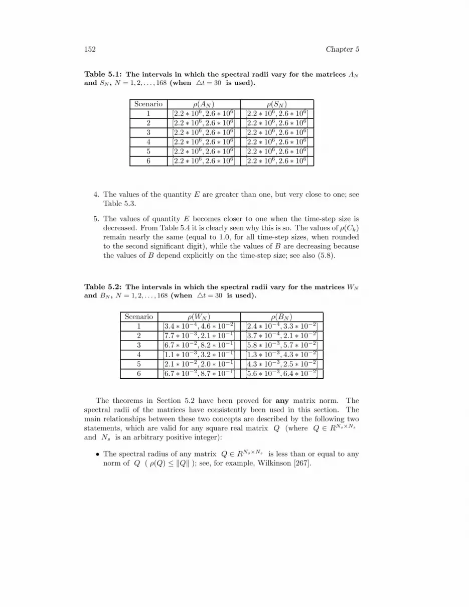
152 Chapter 5
Table 5.1: The intervals in which the spectral radii vary for the matrices AN
and SN , N = 1, 2, . . . , 168 (when t = 30 is used).
Scenario ρ(AN ) ρ(SN )1 [2.2 ∗ 106, 2.6 ∗ 106] [2.2 ∗ 106, 2.6 ∗ 106]2 [2.2 ∗ 106, 2.6 ∗ 106] [2.2 ∗ 106, 2.6 ∗ 106]3 [2.2 ∗ 106, 2.6 ∗ 106] [2.2 ∗ 106, 2.6 ∗ 106]4 [2.2 ∗ 106, 2.6 ∗ 106] [2.2 ∗ 106, 2.6 ∗ 106]5 [2.2 ∗ 106, 2.6 ∗ 106] [2.2 ∗ 106, 2.6 ∗ 106]6 [2.2 ∗ 106, 2.6 ∗ 106] [2.2 ∗ 106, 2.6 ∗ 106]
4. The values of the quantity E are greater than one, but very close to one; seeTable 5.3.
5. The values of quantity E becomes closer to one when the time-step size isdecreased. From Table 5.4 it is clearly seen why this is so. The values of ρ(Ck)remain nearly the same (equal to 1.0, for all time-step sizes, when roundedto the second significant digit), while the values of B are decreasing becausethe values of B depend explicitly on the time-step size; see also (5.8).
Table 5.2: The intervals in which the spectral radii vary for the matrices WN
and BN , N = 1, 2, . . . , 168 (when t = 30 is used).
Scenario ρ(WN ) ρ(BN )1 [3.4 ∗ 10−4, 4.6 ∗ 10−2] [2.4 ∗ 10−4, 3.3 ∗ 10−2]2 [7.7 ∗ 10−3, 2.1 ∗ 10−1] [3.7 ∗ 10−4, 2.1 ∗ 10−2]3 [6.7 ∗ 10−2, 8.2 ∗ 10−1] [5.8 ∗ 10−3, 5.7 ∗ 10−2]4 [1.1 ∗ 10−3, 3.2 ∗ 10−1] [1.3 ∗ 10−3, 4.3 ∗ 10−2]5 [2.1 ∗ 10−2, 2.0 ∗ 10−1] [4.3 ∗ 10−3, 2.5 ∗ 10−2]6 [6.7 ∗ 10−2, 8.7 ∗ 10−1] [5.6 ∗ 10−3, 6.4 ∗ 10−2]
The theorems in Section 5.2 have been proved for any matrix norm. Thespectral radii of the matrices have consistently been used in this section. Themain relationships between these two concepts are described by the following twostatements, which are valid for any square real matrix Q (where Q ∈ RNs×Ns
and Ns is an arbitrary positive integer):
• The spectral radius of any matrix Q ∈ RNs×Ns is less than or equal to anynorm of Q ( ρ(Q) ≤ ‖Q‖ ); see, for example, Wilkinson [267].

Error analysis of the partitioning procedure 153
Table 5.3: The values of the quantity E for the different scenarios (whent = 30 is used).
Scenario E1 1.0342496512 1.0217919173 1.0604020034 1.0460554315 1.0252204546 1.068816212
Table 5.4: Values of the quantities B, max(ρ(CN)) (where N = 0, 1, . . . , 168) andE for different time-step sizes and for Scenario 5.
Stepsize B max(ρ(CN )) E30.00 2.5 ∗ 10−2 1.0 1.02510.00 1.4 ∗ 10−2 1.0 1.0141.00 2.6 ∗ 10−3 1.0 1.00260.10 3.6 ∗ 10−4 1.0 1.000360.01 5.3 ∗ 10−5 1.0 1.000053
• The spectral radius of any matrix Q ∈ RNs×Ns is equal to the infinum takenover all norms of Q in RNs×Ns ( ρ(Q) = inf(‖Q‖) ); see, for example,Belitzkii and Ljubich [20]. In other words, for any ε > 0 there exists a normof matrix Q ∈ RNs×Ns such that ‖Q‖ = ρ(Q) + ε .
5.4 Applicability to other models
Partitioning is a rather general procedure, which is very successful when certainconditions (discussed in the previous sections of this chapter) are satisfied. There-fore, it is worthwhile to check whether these conditions are satisfied or not whenthe chemical part of the model under consideration is to be treated numerically. Ifthe conditions are satisfied, then it may be worthwhile to apply the method of par-titioning, which has been discussed in this chapter and in Chapter 4. One shouldexpect the conditions studied in this chapter to be satisfied for many of the modelsdiscussed in Section 7 of Chapter 1.
154 Chapter 5
5.5 Concluding remarks and plans for future work
Several concluding remarks concerning the results obtained in this chapter andsome plans for future research in this direction are needed.
Remark 5.7. It has been assumed in the end of Section 5.1 (and this as-sumption has been used in Section 5.2) that a sufficiently accurate approximationz[ν]n+1 can be obtained in ν iterations from (5.5). In fact, (5.5) consists of sev-
eral independent sub-systems. The iterative process in each of these sub-systemswill in practice be carried out until the norm of the error of the current iteratebecomes less than some prescribed tolerance. This shows clearly that the numbersof iterations needed to achieve the accuracy required will in general be different forthe different sub-systems. Therefore, in the practical computations, ν should beviewed as the largest number of iterations needed in the iterative solution of thedifferent sub-systems in (5.5).
Remark 5.8. All results have been proved under the assumption that themodified version of the Newton iterative method defined by (5.1) is used. It can,however, be easily verified that all results hold also in the case where the classicalNewton iterative method (4.18) is used and in the case where the other modifiedversion of the Newton iterative method is chosen (i.e. the modified version describedin Remark 4.2).
Remark 5.9. Theorem 5.1 to Theorem 5.8 have been proved under the usualassumption, not explicitly stated, that all computations can be carried out in exactarithmetic. If a computer is used, then rounding errors (due to operations withnumbers with a finite number of digits) are practically unavoidable. The resultswill hold if the influence of the rounding errors is sufficiently small. In manypractical problems the accuracy requirements are low and the above requirementwill be satisfied. Nevertheless, an extension of the results presented in this chapter,in which some rounding error analysis is included, is desirable.
Remark 5.10. It is worthwhile to extend the results, which were proved inSection 5.2 for the Backward Euler Method to other time-integration methods (as,for example, for some Backward Differentiation Formulae of order higher than oneand/or for some methods of Runge-Kutta type).
Remark 5.11. The results obtained in Section 5.4 have been used in Section5.5 to explain why the partitioning used in Alexandrov et al. [6] and Skelboe andZlatev [227] gives good results. One can use the results from Section 5.4 in anattempt to find automatically a good partitioning. This will be a topic for futureresearch.
Remark 5.12. It is also necessary to compare the partitioning algorithmswith other algorithms that are popular and efficient when ODE systems arising inair pollution models are to be treated numerically; see, for example, Chock et al.[46], Jay et al. [145], Odman et al. [187], Sandu et al. [211], [213], [212], Shiehet al. [221], Verwer and van Loon [259], Verwer and Simpson [260], Verwer et al.[258]. The extrapolation time-integration methods used by Deuflhard and his co-workers ([63], [64], [65], [66], [67]) or methods of Runge-Kutta type as those studied

Error analysis of the partitioning procedure 155
in Butcher [37] are promising candidates when large air pollution models are to beused and, thus, comparisons with these methods are also needed.
Remark 5.13. It may be worthwhile to apply some sparse matrix techniquein the treatment of (4.1). This topic was discussed in Subsection 4.3.6 for thepartitioning procedure applied to the system of ODEs arising from the chemicalpart of DEM. The same technique is also applicable in the case where partitioningprocedures are applied to other scientific and engineering problems.
Remark 5.14. In the application of the partitioning procedure to the airpollution model, which was made in this chapter (and also in Chapter 4), it hasbeen assumed that some splitting procedure has been applied and, after that, thepartitioning procedure has been applied only to the chemical sub-model. It isinteresting to investigate the possibility of using some partitioning procedures alsoin the case where no splitting procedure is applied in the treatment of large-scalemodels on computers. The application of partitioning procedures in the case whereno splitting is used might lead to more efficient computational process, which ishighly desirable.


Chapter 6
Efficient organization of the matrixcomputations
After the discretization of the spatial and/or the temporal derivatives one mustnormally perform some matrix computations during the treatment of the selectednumerical algorithms. Typical examples for matrix computations, which often haveto be carried out when large-scale models are treated on computers, are:
• matrix-vector multiplications,
• inner products, and
• solving systems of linear algebraic equations (including here the importantcase where the coefficient matrix of the system is large and sparse).
The treatment of these matrix computations is often very time consuming. Thisis especially true when systems of linear algebraic equations are to be solved. Thisis why it is important to select fast methods for performing matrix computations.Several such methods will be discussed in this chapter.
In the beginning of this chapter (the first three sections) it is assumed thatsome of the splitting procedures that were discussed in Chapter 2 have been ap-plied. The application of an appropriate splitting procedure leads to computationaltasks involving structured matrices (banded matrices and in some cases tri-diagonalmatrices). Efficient numerical methods for the treatment of such matrices are welldescribed in the literature. Moreover, very efficient standard packages, which caneasily be applied when large scale models are handled, exist and can in many casesbe downloaded from the Internet. Two well-known examples are
• the package LAPACK (see Anderson et al. [11]), and
• the package ITPACK (see Kincaid et al. [150], [151]).
157

158 Chapter 6
In four sections of this chapter (from Section 4 to Section 7), we discuss someproblems which arise when no splitting technique is used. The direct discretizationof the system of PDEs (1.1), i.e. the discretization of the system of PDEs withoutusing splitting procedures, results in large non-linear systems of algebraic equations,which have to be treated at every time-step. The application of the Newton iterativeprocedure leads to the solution of many systems of linear algebraic equations. Thecoefficient matrices of these systems are general sparse matrices. It is important tofind fast methods for the solution of the systems of linear algebraic equations, i.e.methods that exploit efficiently the sparsity of the coefficient matrices. The mainprinciples on which such methods should be based are described in Section 5 toSection 7. Numerical examples are given there in order to illustrate the efficiencyof the proposed algorithms.
The fact that the algorithms proposed and discussed in the first seven sectionsof this chapter are applicable not only when large-scale air pollution models aretreated, but also when many other large-scale mathematical problems are to behandled is discussed in Section 8.
Some general conclusions about the algorithms described in this chapter aregiven in the last section, Section 9.
6.1 The horizontal advection-diffusion sub-model
If finite differences are chosen in the discretization of the spatial derivatives, thenthe matrices arising when the horizontal advection-diffusion phenomena are handledare banded matrices (see also Chapter 4). Banded matrices also arise when finiteelements are selected instead of finite differences. Matrices that can efficientlybe treated by applying Fast Fourier Transforms (FFTs) arise in the case wherepseudo-spectral methods are used (see Zlatev [282] or Zlatev et al. [289]). Thematrix computations arising in these three cases will be discussed in this section.
6.1.1 Matrix computations when finite differences are used
As stated above, the matrices arising when finite differences are used to discretizethe spatial derivatives are banded matrices. It is necessary to distinguish betweenthe case where the time-integration methods used is explicit and the case wherethe time-integration method is implicit.
• Application of explicit time-integration methods. If the finite dif-ference discretization of the spatial derivatives in the horizontal advection-diffusion sub-model is followed by some explicit time-integration method, thenthe system of PDEs is transformed to a system of ODEs dg/dt = Hg, whereas stated above H is a banded matrix. Only matrix-vector multiplicationsinvolving banded matrices are to be carried out in this case. These opera-tions can be performed in a very straight-forward way. One can also apply

Efficient organization of matrix computations 159
standard subroutines from BLAS (Basic Linear Algebra Subprograms); see,for example, Dongarra et al. [78], [79].
• Application of implicit time-integration methods with a direct solverfor the resulting systems of linear algebraic equations. If the finitedifference discretization of the spatial derivatives is followed by some implicittime integration method, then systems of linear algebraic equations, whosecoefficient matrices I − γtH are banded, are to be handled at every time-step. The coefficient matrices depend on values of the wind velocities at thegrid-points and, thus, these vary both in space and time. One can applydirect methods for the solution of linear systems of algebraic equations withbanded matrices. Subroutines from LAPACK (see Anderson et al. [11]) orLINPACK (see Dongarra et al. [77]) can efficiently be used when this choiceis made.
• Application of implicit time-integration methods with an iterativesolver for the resulting systems of linear algebraic equations. Thealternative choice is the use of iterative methods. Subroutines from packageITPACK might be used when the second choice is made (see Kincaid et al.[150], [151]). It should be noted here that some kind of preconditioning mightbe necessary when iterative methods are selected. It is not always very easy tofind a good preconditioner (thus, several trials with different preconditionersmight be needed). Many of the iterative methods used in ITPACK can beused together with different preconditioners. Efficient methods for large linearsystems are discussed in details in the recently published book of H. A. vander Vorst (see [256]). The advantage of the use of iterative methods is thatmatrices with wide bandwidths may be efficiently treated when the rate ofconvergence is fast. However, the rate of convergence for some matrices mightalso be very slow when good preconditioners are used. This may happen,because the matrices are in general non-symmetric. If the latter case occurs,then it might be more profitable to go back to the direct methods (i.e., if theconvergence rate of the iterative process is very slow, then it might be moreprofitable to switch to direct methods).
6.1.2 Matrix computations when finite elements are used
In this case it is also necessary to distinguish between the two major groups ofnumerical methods (explicit methods and implicit methods) which might be appliedin the time-integration part.
• Application of explicit time-integration methods. If the finite elementdiscretization of the spatial derivatives in the horizontal advection-diffusionsub-model is followed by some explicit time-integration method, then one hasin general to treat problems, see (3.2), of the type: Pdg/dt = Hg, where Pis a constant matrix depending of the particular finite element discretization
160 Chapter 6
used, while H is depending of the wind velocities and, therefore is varyingin both time and space. Both matrices, P and H , are banded matrices.Both direct methods and iterative methods can be applied in the solution ofPdg/dt = Hg.
(a) Direct methods. Let us start with the direct methods. The fact that Pis normally constant can be exploited (matrix P can be factorized in thevery beginning of the computational process and, after that, the factorscan be used during the whole computational process).
(b) Iterative methods. It should be noted that P is a symmetric andpositive definite matrix. Therefore, many iterative methods will be con-vergent. Moreover, experimental results show that the convergence rateis fast when P arises from air pollution models. This means that iterativemethods can successfully be used in many cases.
The choice of the methods depends on the splitting procedure used and onthe grid. Refined grids will often lead to matrices with a large bandwidth.Therefore, the iterative methods might be more profitable than the directmethods in this case. Iterative methods might also be more profitable whensome vector computers are used (because these vectorize very well, while thevectorization of the direct methods for banded matrices is normally ratherpoor).
• Application of implicit time-integration methods. If the finite elementdiscretization of the spatial derivatives in the horizontal advection-diffusionsub-model is followed by some implicit time-integration method, then again,as in the previous case, one has in general to solve systems of linear algebraicequations arising after the discretiziion of systems of ODEs of type (3.2),i.e. systems of the type: Pdg/dt = Hg, which are discretized this time byapplying some implicit method for solving systems of ODEs. The applicationof an implicit time-integration algorithm leads to the solution, at every time-step, of systems of linear algebraic equations whose coefficient matrices areof the type P − γtH , where γ depends on the particular time-integrationalgorithm chosen while t is the time-step size. This case is very similar tothe case where the finite differences of the spatial derivatives is followed byimplicit time-integration methods. Indeed, matrices I −γtH are to be used(instead of P − γtH) when finite differences are applied instead of finiteelements. This means that in principle the same methods for solving systemsof linear algebraic equations as those discussed in the previous subsection canbe applied when implicit time-integration algorithms are selected after thespatial discretization carried out by either finite differences or finite elements.

Efficient organization of matrix computations 161
6.1.3 Matrix computations for the pseudo-spectral method
As mentioned in Chapter 3, one can also use a pseudo-spectral discretization dur-ing the treatment of the advection-diffusion sub-model. The application of suchmethods is discussed in detail in Zlatev [277], [278], [282] as well as in Zlatev etal. [289]. The pseudo-spectral method is based on the use of truncated Fourierseries. Therefore, it is important in this case to apply some efficient fast Fouriertransforms (FFTs). FFTs proposed by Swarztrauber [241] and Temperton [246](a very good implementation of the Temperton’s FFTs can be found in the NAGLibrary [185]) have been used in a previous version of DEM (see again Zlatev [277],[278],[282] and Zlatev et al. [289]).
The pseudo-spectral discretization was implemented in DEM (by applying ex-plicit time-integration algorithms when the semi-discretized system is treated). Itis not very clear whether an efficient implementation can be achieved when implicittime-integration methods are used. The implementation of the pseudo-spectraldiscretization in DEM (where, let us reiterate, it was followed by applying ex-plicit time-integration algorithms in the discretization of the advection-diffusionsub-model) is very efficient on vector processors like CRAY. It is also very accu-rate.
Periodic boundary conditions are required (see also Chapter 3) when this algo-rithm is used, which is a serious drawback, because it is not very easy to satisfythis requirement (however, it should be mentioned here that there exist algorithms,which can be used to handle the problems arising by the requirement for periodicityon the boundaries; see, for example, Lyness [170] and Roache [202], [203]).
The pseudo-spectral method is not used in the newest versions of DEM (theseversions are united in a common model, UNI-DEM, which will be discussed in thenext chapter).
6.2 Matrices in the vertical exchange sub-model
The numerical treatment of this sub-model was discussed in Chapter 3. Finiteelements are used in the discretization of the spatial derivatives. The θ-method isused after that in the time-integration part. This means that we have finite elementsfollowed by an implicit time-integration algorithm, which leads to the solution ofsystems Pdg/dt = Hg. The solution of systems of ODEs of this type was discussedin the previous section.
However, the situation that occurs in the vertical exchange sub-model is muchsimpler, from computational point of view, than the situation discussed in theprevious section when the complexity of the computational process is taken intoaccount, because the application of some splitting procedure leads to many inde-pendent problems (one for each vertical grid-line; i.e. 8 064 000 problems are to betreated at every time-step when the model with 35 chemical species is discretizedon 480 × 480 × 10 grid). This is why the matrices which arise and have to betreated in this part are tri-diagonal. The treatment of systems with tri-diagonal

162 Chapter 6
matrices is very cheap; the computational cost being O(3Nz). This simplifies theimplementation of the algorithms. Therefore, the vertical exchange sub-model doesnot cause great computational difficulties when the vertical exchange is separatedfrom the other physical and chemical processes by using some splitting procedure.
Standard subroutines for tri-diagonal matrices are easily available. Such sub-routines can, for example, be found in package LAPACK (see Anderson et al. [11])or in the older package LINPACK (see Dongarra et al. [77].
6.3 Matrices arising in the chemical sub-model
It has been mentioned several times in the previous chapters that the chemical partof the model is normally the most time consuming module. The computationalwork in this part of the model consists of the solution of a very large numberof stiff ODE systems (one such system per grid-point), which can be treated asparallel tasks. One can use the following three methods (see also Chapter 4) in thesolution of each of the small ODE systems.
• QSSA algorithms (either the original QSSA algorithm or the improved QSSAalgorithm).
• Classical integration methods for solving stiff systems of ODEs (such methodsare normally implicit and, therefore, lead to the solution of systems of non-linear algebraic systems). The use of two simple methods (the BackwardEuler Method and the Trapezoidal Rule) was discussed in Chapter 4. Fourother methods for solving systems of ODEs (the Implicit Mid-point Rule, aDiagonally Implicit Runge-Kutta method of order 2, a Fully Implicit Three-stage Runge-Kutta Method of order six and a Rosenbrock method of order2) were also used; see Chapter 2.
• Methods based on applying partitioning (the fact that some of the chemicalreactions are fast while others are slow is exploited in the construction ofpartitioned methods). Partitioning procedure as well as some properties ofthese procedures were discussed both in Chapter 4 and in Chapter 5.
The numerical treatment of the chemical part of a large-scale air pollution mod-els by using the three types of methods listed above was discussed in Chapter 4.Before starting the discussion in this section it is important to emphasize the factthat
• the QSSA algorithms can normally be implemented by using only simplematrix-vector operations, while
• systems of linear algebraic equations are to be solved both when the classicalintegration methods for solving stiff systems of ODEs are applied and whenmethods based on applying partitioning are developed and used.

Efficient organization of matrix computations 163
6.3.1 Implementation of the QSSA algorithms
As mentioned above, the QSSA algorithms, both the original QSSA algorithm andthe improved QSSA algorithm, can normally be implemented by using matrix-vector products. The matrix is a general sparse matrix and it might be worthwhileto exploit the sparsity during the implementation. It is clear that the number ofsimple arithmetic operations needed in the treatment of the chemical reactions ateach grid point is constant when the QSSA algorithm discussed in Chapter 4 isused. This means that the parallel tasks are perfectly balanced.
The main conclusion is that if only the computational issues are taken intoaccount, the QSSA algorithms are very efficient. Unfortunately, there may ariseproblems with the accuracy when some concentrations vary very quickly (this hasbeen demonstrated by using some simple examples in Chapter 4).
6.3.2 Implementation of classical time-integration algorithms
If classical time-integration algorithms as well as algorithms based on partitioningare applied, then non-linear systems are to be treated. This means that iterativemethods are to be used and, therefore, systems of linear algebraic equations are tobe solved at each iteration. There are many systems of linear algebraic equations,but each of these systems is small. The number of equations in each of thesesystems is equal to the number of chemical species involved in the model. If themodel with only 35 chemical species is discretized on a 480 × 480 × 10 grid, then2 304 000 systems, each of them containing 35 equations, have to be treated atevery time-step. This is why it is possible to neglect the fact that the Jacobian issparse and to use dense matrix technique in the treatment of the matrix operations(for the methods based on partitioning this was illustrated in Subsection 4.3.5,but precisely the same ideas can be used also when any classical time-integrationmethod is applied without partitioning).
The use of sparse matrix technique in this particular case (where the matricestreated are small) can be efficient only if the special rules discussed in Subsection4.3.6 are used (in fact these rules are used only for the algorithm based on parti-tioning in Subsection 4.3.6, but they can also be applied in connection with anyclassical time-integration method).
The use of the classical time-integration algorithms and/or algorithms based onpartitioning leads to more accurate computations (see again Chapter 4). However,these methods are normally more expensive (especially when the classical time-integration methods are directly, i.e. without using some partitioning procedure,implemented in the subroutines for the solution of the chemical ODE systems) and,therefore, the efficiency depends strongly on the ability of the method to producesufficiently accurate results when a large time-step size is used.
The use of the classical time-integration algorithms and/or algorithms basedon partitioning may give some problems with load balancing of the parallel tasks.The reason for this is the fact that some iterative method has to be applied in the

164 Chapter 6
solution of the non-linear systems arising after the space and time discretization.While the number of simple arithmetic operations per a system of linear algebraicequations, i.e. per one iteration in the solution of (4.18), is remaining the sameduring the whole computational process, the number of iterations per a non-linearsystem of type (4.17) is varying from one grid-point to another. This problem willfurther be discussed in the next chapter.
6.3.3 The QSSA algorithms versus the other algorithms
The discussion in the previous subsection indicates clearly that it is difficult toanswer the question:
Is it better to use the QSSA algorithms or should one pre-fer the other algorithms (the classical time-integration al-gorithms and/or algorithms based on partitioning)?
The essential issue is to find out whether the QSSA algorithms applied with asmall time-step size are still better than the other algorithms in spite of the factthat the other algorithms are used with a larger time-step size. At present we haveno definite answer to the above question. Much more experiments with differentnumerical algorithms in different situations are needed in order to obtain a reliableanswer. We are continuing the experiments with different numerical methods.
6.4 Treatment of the model without splitting
In the previous sections of this chapter it was assumed that some splitting procedureis used. This simplifies, very considerably, the computations. This is why splittingprocedures are, as mentioned in the previous chapters, used in all large-scale airpollution models that are operationally run in different comprehensive studies asthose, which will be discussed in Chapter 8 and Chapter 9.
The price which has to be paid is the fact that splitting will normally causeerrors and, moreover, it is difficult to control these errors (see also Chapter 2).Therefore, as mentioned several times in the previous chapters, it is important toavoid splitting when this is possible. The size of the computational tasks when nosplitting is used will be discussed in this section.
If no splitting is used, then the discretization of the spatial derivatives in (1.1)with either finite differences or finite elements leads to a large stiff system of ODEs(the stiffness being introduced mainly by the presence of the chemical terms, butthe vertical exchange also introduces stiffness). The number of equations in theresulting system, obtained when splitting is not used, is equal to the product ofgrid-points and chemical species. The time-integration must be carried out byimplicit time-integration algorithms for stiff systems of ODEs, because stiffness isintroduced by some of the physical and chemical processes (as mentioned above the

Efficient organization of matrix computations 165
terms containing chemical reactions are the major reason for the stiffness of theresulting system of ODEs, but the terms describing the vertical transport are alsointroducing stiffness in the semi-discretized model when no splitting procedure isused). This means that non-linear systems of algebraic equations are to be handledat every time-step when no splitting procedure is applied in the discretization of(1.1). The application of the Newton iterative method (or some of its modifications,see Remark 4.1 and Remark 4.2 in Chapter 4) leads to the solution of several largeand sparse systems of linear algebraic equations at every time-step. Some attemptsto handle these systems with general methods for sparse matrices from Zlatev [281]were not very successful (however, we are still working on the improvement ofthe implementation of sparse matrix codes: some results that are related to theperformance of sparse matrix codes will be given in the following sections).
The results in this direction, which have been obtained by us until now, canbe summarized as follows. On the available computers (some SUN computers atthe Danish Centre for Scientific Computing), we were able to run problems of thesame size as the model with 35 chemical species discretized on (96× 96× 10) grid.However, the computational times were very large. We were not able to run themodel for period longer than a couple of months. The version, in which no splittingprocedure is applied, may be (and is) applicable in some studies related to shortperiods with high pollution levels. However, this version of the model cannot yet beused in comprehensive studies over long time-periods and/or with many differentscenarios.
It is not clear, at present, whether it is possible to design some special sparsematrix technique which will reduce substantially the computational time. On theother side, it is worthwhile to continue the efforts to avoid the use of splittingprocedures. The computers are becoming faster and faster, which means that oneshould expect that the treatment of large-scale air pollution models without usingsplitting will become possible in the near future and the modellers have to be wellprepared for this, which means that some efficient codes for handling general sparsematrices have to be developed and attached as soon as possible to the existing large-scale air pollution models. This is also valid for other large-scale mathematicalmodels used in other fields of science and engineering.
As mentioned above, some current results, obtained with codes for general sparsematrices, in which an attempt to exploit the properties of the modern computerarchitectures is made, will be presented in the next three sections.
6.5 Use of sparse matrix techniques
The matrices, which appear after the discretization of large-scale mathematicalmodels (not necessarily air pollution models) by using either finite differences orfinite elements are banded matrices. There are well-described and easily availabletools for treating such matrices; such as BLAS (Basic Linear Algebra Subprograms)described in Dongarra et al. [78], [79], LAPACK documented in Anderson et al.

166 Chapter 6
[11] and LINPACK presented in Dongarra et al. [77]. These tools are commonlyused and very often lead to very efficient solution of the systems of linear algebraicequations, which are to be treated during many time-steps. However, the use ofthese tools is less efficient when the problems are very large, because the bandwidthof the matrices also becomes large in such a case. The problems are caused by
• the necessity to store all matrix elements that are within the band, and
• the necessity to carry out computations with all matrix elements within theband.
Most of these elements are originally zero elements, but nearly all of the zeroelements within the band of the matrix will gradually become non-zero elementsduring the computations.
The use of sparse matrix techniques, where one stores only the non-zero elementsand works with only non-zero elements, might be a good alternative approach forvery large problems. It has been mentioned at the end of the previous sectionthat even the use of sparse matrix techniques does not solve all the problems.Nevertheless, the exploitation of the sparsity normally leads to some significantsavings in comparison with the other methods when the problems is very large.
The possibility of implementing fast and reliable methods for general sparsematrices will be discussed in this section and in the following two sections. It mustbe emphasized, however, that the methods for general sparse matrices which willbe described in the remaining part of this chapter are applicable only in the casewhere no splitting procedure is used (or, at least, if the splitting procedure appliedleads to the treatment of large general sparse matrices). Special sparse matrixtechniques that are efficient in the case where the splitting procedure chosen leadsto the treatment to many but small sparse matrices (each of them of order 35) werediscussed in the end of Chapter 4. It should be further emphasized that the sparsematrices that are to be treated when no splitting procedure is used are normallyvery large (of order greater than 106).
We shall start with the description of two storage schemes for sparse matricesand, after that, we shall continue with discussion of
• some techniques for preserving the sparsity,
• the use of preconditioners
and, which is perhaps most important when the matrices are very large,
• the exploitation of the cache memory.
The efficiency of the proposed algorithms will be demonstrated by perform-ing some comparisons with a well-known code for the solutions of linear algebraicequations the coefficient matrices of which are general sparse matrices (the code

Efficient organization of matrix computations 167
SuperLU, which is documented in Demmel et al. [61], [62] and Li and Demmel[165]).
Parallel codes for general sparse matrices must also be constructed and used.Implementation of parallel methods for general sparse matrices will be discussedin Chapter 7. Some results from runs performed on several parallel computers willalso be given there.
6.5.1 Storage schemes for sparse matrices
The simplest storage scheme for general sparse matrices can be described in thefollowing way. Assume that matrix A is of order N and has NZ non-zero elements(where NZ is much smaller than N2). Assume also that three arrays of lengthgreater than or equal to NZ, a real array AORIG as well as two integer arraysRNORIG and CNORIG, are available. The elements of matrix A are stored inthe first NZ locations of array AORIG. The order in which the non-zero elementsare stored in array AORIG is arbitrary. However, if a non-zero element aij ofmatrix A is stored in position K ( 1 ≤ K ≤ NZ) in array AORIG (or, in otherwords, if AORIG(K) = aij), then RNORIG(K) = i and CNORIG(K) = j mustalso be assigned. This storage scheme is called static.
Some matrix operations can easily be performed by using the static storagescheme. This can, for example, be done when the residual vector, defined by
r = b − Axn, (6.1)
where xn is an approximation of the solution x of the system of linear algebraicequations Ax = b, is to be calculated. Assume, as above, that the order of matrixA is N and that vectors r, b and xn are stored in three real arrays R, B and X oflength N . Then the residual vector r can be calculated by using the simple codethat is given in Fig. 6.1.
CDO I=1,N
R(I) = B(I)END DO
CDO I =1,NZ
R(RNORIG(I)) = R(RNORIG(I) - AORIG(I) * X(CNORIG(I))END DO
C
Figure 6.1: Calculating the residual vector by using the static storage scheme.
Other examples of matrix operations, which can easily be performed when thestatic storage scheme is used, can be found in Zlatev [281]. Unfortunately, the

168 Chapter 6
static storage scheme cannot be used when the structure of the non-zero elementsin matrix A is dynamically changing during the computational process. As a typicalexample consider the major formula
a(s+1)i,j = a
(s)i,j − a
(s)i,s a
(s)s,j
a(s)s,s
, s = 1, 2, . . . , n − 1, i, j = s + 1, s + 2, . . . , n, (6.2)
with
a(s)s,s = 0, a
(1)i,j = ai,j ∈ A, (6.3)
which is used when a system Ax + b of linear algebraic equations is solved by thewell-known Gaussian elimination (the application of the Gaussian elimination leadsto the calculation of two triangular matrices, a lower triangular matrix L and anupper triangular matrix U , such that LU = A + E, where E is a result of therounding errors which are practically unavoidable in calculations on computers; seeZlatev [281]). It is clear that if a
(s)i,j is equal to zero but both a
(s)i,s and a
(s)s,j are
non-zeros, then a new non-zero element, a(s+1)i,j , will be produced in a position,
(i, j), where a zero element was located before the performance of the arithmeticoperations in (6.2). Such a new non-zero element is called fill-in. The appearance offill-ins and the need to store both the fill-ins and some information about the fill-ins(row numbers, column numbers, etc.) dynamically in the appropriate arrays showwhy the static storage scheme for sparse matrices cannot be used in the solution oflinear algebraic equations by Gaussian elimination. Much more complicated storageschemes, called dynamic storage schemes for general sparse matrices, have to beused in this case.
Different dynamic storage schemes for sparse matrices can be designed (seeChapter 2 in Zlatev [281]). Schemes based on row ordered lists are popular. Thenon-zero elements are ordered by rows in a one-dimensional real array, say arrayALU . If a non-zero element is located in position K of array ALU , then its columnnumber must be stored in position K of a one-dimensional integer array CNLU .The length of these two arrays is NN ≥ 2 ∗ NZ. The integer NN must be largeenough in order to ensure place, ”elbow room”, for fill-ins, which in general willbe produced during the computations and which have dynamically to be insertedin the storage scheme. If row I (1 ≤ I ≤ N) of matrix A starts in position K1(1 ≤ K1 ≤ NN) and ends in position K2 (1 ≤ K1 < K2 ≤ NN), then we musthave ROWSTART (I) = K1 and ROWEND(I) = K2, where ROWSTART andROWEND are two integer arrays of length N .
The row ordered list provides full information about the locations of the non-zero elements of matrix A. It is efficient to use this list when the elements of thematrix are scanned by rows. It is desirable, however, to be able to scan the non-zero elements also by columns in order to make the computational process moreefficient. This is done by using a similar structure, a column ordered list. Thisstructure contains three integer arrays, RNLU of length NN1 with NN1 ≥ NZ

Efficient organization of matrix computations 169
as well as COLSTART and COLEND (both of length N). The row numbers ofthe ordered by columns non-zero elements are stored in array RNLU . The rownumbers of column J (1 ≤ J ≤ N) are stored from position COLSTART (J) toposition COLEND(J) in array RNLU . Note that the non-zero elements of matrixA are not needed in the column ordered list.
Assume that a new non-zero element, fill-in, is created in position (i, j) of matrixA. Then the following actions are carried out in the row ordered list:
• the non-zero elements of row i and their column numbers are copied to theend of arrays ALU and CNLU ,
• the positions where the non-zero elements of row i were located before makingthe copy to the end of the row ordered list are declared as free positions (bysetting zeros in the all locations between ROWSTART (i) and ROWEND(i)in array CNLU),
• the new non-zero element and its column number are stored after the lastoccupied position in ALU and CNLU (this position is saved because it willbe needed when the next fill-in is to be inserted in the row ordered list), and
• the contents of ROWSTART (i) and ROWEND(i) are updated.
Similar transformations are to be carried out in the column ordered list in order toinsert the row number i of the fill-in created in position (i, j):
• the row numbers of the non-zero elements of column j copied to the end ofarrays RNLU ,
• the positions where row numbers of the non-zero elements of column j werelocated before coping them to the end are declared as free positions (by settingzeros in all locations between COLSTART (j) and COLEND(j) in arrayRNLU),
• the row number of the new non-zero element is stored after the last occupiedposition in RNLU (this position is saved because it will be needed when therow number of the next fill-in is to be inserted in the column ordered list),and
• the contents of COLSTART (j) and COLEND(j) are updated.
It is clear that in general the length of the arrays ALU , RNLU and CNLU willnot allow us to make too many copies. Therefore, the structure of the lists (the rowordered list and the column ordered list) should from time to time be compressed(utilizing here the fact that, when rows and columns are moved to the end of theappropriate arrays, some free locations are, as explained above, created in the lists).This action is called ”garbage collection”.
170 Chapter 6
Garbage collections are expensive. The number of garbage collections can bereduced in the following way (exploiting here the fact that some free locations arecreated between two rows and/or two columns every time when a copy of a row ora column is made in the end of the appropriate ordered list). If a fill-in is produced,then a copy of its row(column) should be made only if there are no free positions atthe beginning or at the end of the row(column). If there are free positions then thefill-in and its column number (the row number of the fill-in) should be put there,updating appropriately the information about row start or row end (column startor column end).
Another way to reduce the number of garbage collections is by using pivotingfor preservation of the sparsity of the original matrix. Pivoting for general sparsematrices will be discussed in the next subsection.
Finally, the number of the garbage collections can be reduced if some smallelements are dropped (in fact, replaced by zeros). Assume that the updated by(6.2) element a
(s+1)i,j satisfies the following inequality:
| as+1i,j |≤ RELTOL max
s≤j≤N| a
(s)i,j | . (6.4)
where 0 ≤ RELTOL < 1 is a user-selected parameter, called the relative drop-tolerance. Then a
(s+1)i,j is dropped. In fact, it is removed from the lists by making
some simple modifications. Assume that a(s+1)i,j is stored in position K of array
ALU . Then one must set
• ALU(K) = ALU(ROWEND(i)),
• CNLU(K) = CNLU(ROWEND(i)),
• CNLU(ROWEND(i)) = 0, and
• ROWEND(i) = ROWEND(i) − 1.
Assume that the row number of a(s+1)i,j is stored in position K1 of array RNLU .
Then one must set
• RNLU(K1) = RNLU(COLEND(j)),
• RNLU(COLEND(j) = 0, and
• COLEND(j) = COLEND(j) − 1.
It is seen that by dropping the element a(s+1)i,j not only might a new copy of a row
(column) be avoided, but also a free location where fill-ins can be stored mightbe created. Thus, dropping small elements makes the computational process moreefficient, but this process also introduces errors in the triangular factors L and U .Therefore, these factors cannot be used directly to calculate the solution of Ax = bwhen positive values of the relative drop-tolerance are used. However, they could beused as a preconditioner in an iterative process for solving Ax = b. Preconditioningwill be discussed in one of the following subsections.
Efficient organization of matrix computations 171
6.5.2 Pivoting for sparse matrices
If dense matrices are to be handled in connection with solving systems of linearalgebraic equations by Gaussian elimination, then pivoting (either partial pivotingor complete pivoting) is used in an attempt to preserve the numerical stability of thecomputational process (see Golub and Van Loan, [122], Stewart [232], Wilkinson[266], [267]). Pivoting, for the preservation of the numerical stability, has to also beused when general sparse matrices are treated. However, the situation here is morecomplicated because pivoting has also to be used in an attempt to preserve (asmuch as possible) the sparsity of the original matrix. These two requirements (thepreservation of the numerical stability and the preservation of the sparsity) workin opposite directions. Therefore a compromise is needed. Both the experimentalresults and some theoretical results indicate that the pivotal strategy proposed inZlatev [272] is a good compromise. This pivoting strategy will be outlined in thissubsection (more results about different pivotal strategies for sparse matrices canbe found in Duff et al. [81], and Zlatev [281]).
Denote by As the sub-matrix that has to be updated by using (6.2). Let a(s)i,j = 0
be an element in As. Assume that r(i, s) is the number of non-zero elements of rowi which are in As, and that c(j, s) is the number of non-zero elements of column j
which are in As. The Markowitz cost of element a(s)i,j is defined by
Mijs = [r(i, s) − 1] [c(j, s) − 1]. (6.5)
It is worthwhile to select as a pivotal element the element a(s)i,j with a minimal
Markowitz cost when only the preservation of the sparsity is taken into account. Ifthe element with a minimal Markowitz cost is found, then it must be moved (byrow and column interchanges) to position (s, s). When this is done, the calculationswith formula (6.2) are to be performed.
There are two major difficulties related to the strategy which has been sketchedabove:
• the search for the non-zero element with a minimal Markowitz cost can bevery expensive when the matrix is large, and
• no attempt to preserve the numerical stability of the computations is carriedout when pivots are chosen by using only the minimal Markowitz cost.
It was observed in Zlatev [272] that the search for the element with the minimalMarkowitz cost could successfully be replaced by a search for an element with thebest Markowitz cost in a few ”best” rows only (rows with minimal numbers of non-zero elements are called ”best” rows here). Experiments in Zlatev [272] indicatedthat the search in three ”best” rows only is normally giving very good results. Inan attempt to preserve also the numerical stability an additional constraint is tobe imposed: the pivotal element must satisfy the following inequality:
| a(s)i,j |≥ u max
s≤k≤N| a
(s)i,j |, (6.6)

172 Chapter 6
with some parameter u which satisfies 0 < u ≤ 1. Parameter u is called the stabilityfactor in Zlatev [272] and [281].
It should be mentioned here that the rows must be ordered so that if i < kthe number of non-zero elements in row i is less than or equal to the number ofnon-zero elements in row k and, moreover this order must be kept during the wholefactorization process (this ordering is fully explained in Zlatev [281]).
The idea of using (6.5) in the choice of a good pivot was first suggested inMarkowitz [180]. Other implementations of this idea and/or other pivoting strate-gies for general sparse matrices can be found in Davis and Davidson [58], Davisand Yew [59], Duff et al. [81], George and Ng [115], Gilbert and Peierls [119],Pissanetzki [195], Sherman [219], Tewarson [247], Zlatev [281].
6.5.3 Using preconditioning
As mentioned in the previous subsection, dropping small non-zero elements canbe useful in the attempts to preserve better the sparsity of the original matrixand, thus, to improve the performance of the selected sparse algorithm. While theperformance is often improved when dropping of small non-zero elements is appliedduring the Gaussian elimination, the accuracy of the calculated triangular matricesL and U will often become very poor. This is why a preconditioning is necessarywhen this approach is used.
Ten preconditioned methods
Ten well-known numerical methods for solving systems of linear algebraic equationsby using a direct method based on the Gaussian elimination and preconditionedmethods for sparse matrices are discussed below. The methods are listed in Table6.1. Some information about the abbreviations, as well as references, where moredetails about the ten methods can be found, are given in Table 6.1.
The method for calculating directly the solution (DIR) is based on the use ofa sparse matrix technique for calculation of an LU factorization of the coefficientmatrix of the system of linear algebraic equations without dropping small non-zeroelements, as in (Zlatev [281]).
The same method is also used to calculate approximate LU factorizations, whichare used as preconditioners in the iterative methods. Let us reiterate here that aspecial parameter RELTOL (relative drop-tolerance), 0 ≤ RELTOL < 1, is usedto calculate an approximate LU factorization. The use of this parameter to dropsmall non-zero elements during the Gaussian elimination was described in one ofthe previous subsections.
It should be added here that the relative drop-tolerance can also be used todrop all small non-zero elements in the original matrix before the beginning of theGaussian elimination. The situation is very similar to that described in the previoussubsection. If the absolute value of an element aij of the original coefficient matrixis smaller than the product of RELTOL and the largest in absolute value in row

Efficient organization of matrix computations 173
i, then aij is dropped (replaced by zero). This means that aij is dropped when thefollowing inequality
| ai,j |≤ RELTOL max1≤j≤N
| ai,j | (6.7)
is satisfied. Note that (6.7) is very similar to (6.4), but while (6.7) is applied to theelements of the original matrix, (6.4) is applied to the elements calculated at somestage s + 1 of the Gaussian elimination.
If RELTOL is set equal to zero, then the direct solution can be calculated (seealso the previous paragraph). However, if 0 < RELTOL < 1 then the LU factor-ization obtained by using the selected positive value of the relative drop-toleranceRELTOL must be used as a preconditioner in one of the iterative methods.
If RELTOL becomes larger, then in general the obtained LU factorization isbecoming less accurate, but more sparse. This means that the number of iterationsneeded to obtain the required accuracy of the solution of the system of linearalgebraic equations will tend to become greater for larger values of RELTOL, butthe computational work per iteration will, in general, become smaller. If RELTOLis very large, then the rate of convergence can be very slow or the preconditionediterative method may even not converge (the calculations must be repeated byusing a smaller value of the relative drop-tolerance RELTOL when this happens;it might be necessary sometimes to reduce the value of RELTOL several times).This shows that it is very important to select robust and reliable stopping criteriawhen preconditioned iterative methods are used. The proper implementation ofsuch stopping criteria will allow us to decide
• whether the required accuracy is achieved or not (and to stop the iterativeprocess when the required accuracy is achieved), and
• whether the iterative process is slowly convergent or does not convergent atall and,
– to reduce the relative drop-tolerance, and
– to recalculate the LU factorization with the reduced drop-tolerance
when there are problems with the convergence.
It should be emphasized here that robust and reliable stopping criteria are alsoneeded when pure iterative methods are applied.
Preconditioning is always used when the system of linear algebraic equations issolved by the last seven methods in Table 6.1. The Modified Orthomin Method(Zlatev [281]) is used both as a pure iterative method (PURE) and as a precondi-tioned iterative method (ORTH). If an approximate LU factorization is used in IR,then this method can be considered as a preconditioned iterative method.

174 Chapter 6
Table 6.1: Solvers for systems of linear algebraic equations with general sparsecoefficient matrices, which are used in this section.
No. Method Abbreviation Reference1 Direct solution DIR [272], [281]2 Iterative Refinement IR [274], [281]3 Pure Modified Orthomin PURE [262], [281]4 Preconditioned Modified Orthomin ORTH [262], [281]5 Conjugate Gradients Squared CGS [230]6 Bi-Conjugate Gradients STAB BiCGSTAB [255]7 Transpose-Free Quasi Min. Residual TFQMR [107]8 Generalized Minimum Residual GMRES [207]9 Eirola-Nevanlinna Method EN [86], [263]10 Block Eirola-Nevanlinna Method BEN [270]
It must be emphasized here that if the preconditioned iterative method usedeither is not convergent or the convergence is not sufficiently fast, then the pre-conditioner can automatically be improved, as described above, by reducing therelative drop-tolerance RELTOL (see more details in Zlatev [281]).
6.5.4 Description of the stopping criteria
Let xn be the approximation of the exact solution x of the system of linear algebraicequations Ax = b obtained after n iterations of the chosen iterative method. Letrn = b − Axn be the corresponding residual vector. We shall assume that allcomponents of x are of the same order of magnitude and use vector norms in thestopping criteria. The desired accuracy of the approximate solution will be definedby a parameter ACCUR.
(A) Traditionally used stopping criteria
One of the following stopping criteria is as a rule selected when an iterative methodis used (see, for example, Freund [107], Saad and Schultz [207], Vorst [255]): stopthe iterative process if
‖xn − xn−1‖ ≤ ACCUR, (6.8)
‖rn‖ ≤ ACCUR, (6.9)
‖xn − xn−1‖‖xn‖ ≤ ACCUR, (6.10)

Efficient organization of matrix computations 175
‖rn‖‖r0‖ ≤ ACCUR. (6.11)
(B) Difficulties related to the traditional stopping criteria
Difficulties which may arise when (6.8) is used. It is intuitively clear thatif the iterative process is slowly convergent, then (6.8) can be satisfied even if theexact error ‖xn − x‖ is much larger than ACCUR.
Difficulties that may arise when (6.9) is used. Assume that xn = x+εn, whereεn is the exact error after n iterations. Then rn = b−Axn = b−A(x+ εn) = −Aεn.From this relationship we can conclude that the fact that (6.9) is satisfied doesnot always mean that the required accuracy is achieved and the fact that (6.9)is not satisfied does not necessarily mean that ‖xn − x‖ > ACCUR. Indeed,consider the scalar case (the number of equations is equal to one) and assumethat ACCUR = 10−4, εn = 10−4 and A = 1. Then (6.9) is telling us that therequired accuracy has been achieved and this is true. Replace A = 1 with A = 100.Now (6.9) is telling us that the required accuracy has not been achieved, whilethe opposite is true. Finally, replace εn = 10−4 with εn = 10−2 and A = 1 withA = 10−2. In this case (6.9) is telling us that the required accuracy has beenachieved, which is certainly not true. This scalar example shows that check (6.9)will give good results in the scaler case only when the problem is scaled so thatA = 1.
It is clear that similar problems (as the problems discussed above for the scalercase) are also unavoidable in the multi-dimensional case. However, the difficultiesare much greater in this case, because it is not immediately clear what kind ofscaling should be used in order to get a reliable estimate by using (6.9). It caneasily be shown that (6.9) will give good results if a very good preconditioner Chas been selected and the preconditioned system CAx = Cb is solved instead ofAx = b. To show that this is true, assume that the preconditioner C is equal to A−1.Let ACCUR = 10−4 and ‖εn‖ = 10−4. Denote by r∗n the residual vector Cb−CAxn
of the preconditioned system. Then ‖r∗n‖ = ‖CAεn‖ = ‖εn‖ ≤ ACCUR. Thus,very good preconditioning makes (6.9) reliable. It is very often recommended touse in the stopping criterion the residual vector of the original system also whenpreconditioning is used. The above analysis indicates that if the preconditioner isvery good, then the use of the residual vector of the preconditioned system shouldbe preferred. If the preconditioner is not very accurate, then the situation is notclear. The extension of the analysis of the scalar case to the multi-dimensionalcase indicates that both the residual vector of the original system and the residualvector of the preconditioned system may cause difficulties in the latter case.
Difficulties which may arise when (6.10) is used. It is clear that if the firstapproximation x0 is very bad and if the rate of convergence is very slow, then (6.10)

176 Chapter 6
will probably give very bad results.
Difficulties which may arise when (6.11) is used. In some evolutionary prob-lems, where many time steps are used, one normally takes as a first approximationx0 the accepted solution at the previous time-step. If the process approaches thesteady state case, then x0 chosen in this way can be very accurate. If this hap-pens, then ‖r0‖ will become very small and, thus, the check (6.11) can cause severeproblems.
General conclusion about the use of the traditional stopping criteria.The above analysis shows that the simple stopping criteria (6.8) - (6.11) may causedifficulties in some situations. We shall illustrate by numerical examples that thisactually happens when the problem is difficult for the iterative methods.
(C) Derivation of more reliable stopping criteria
Checking the behaviour of the iteration parameters. More reliable stoppingcriteria can be derived as follows. In many iterative methods the key operation isthe calculation of a new approximation xn+1 = xn +αnpn. If the process convergesthen we have that xn → x as i → ∞ which implies x = x0 +
∑∞i=0 αnpn, where pn
is some vector calculated during iteration n. The convergence of the infinite sumimplies that αnpn → 0 as n → ∞. The reverse relations do not hold, but it isnevertheless reasonable to expect that if the following two conditions are satisfied:
• αnpn → 0 as i → ∞and
• αn does not vary too much and αn is of order O(1),
then xn → x as i → ∞.The requirement related to αn indicates that it is reasonable to require that thefollowing conditions are satisfied:
(A1) αn does not decrease too quickly,
(A2) αn does not increase too quickly, and
(A3) αn does not oscillate too much.
If any of the requirements (A1) - (A3) is not satisfied, then the stopping criteriashould be made more stringent (which essentially leads to reducing the value ofACCUR).
Checking the behaviour of convergence rate. Assume again that the iterativeprocess is convergent. Then the following inequality holds:
‖x − xn‖ ≤ |αn| ‖pn‖⎛⎝1 +
∞∑j=n+1
|αj | ‖pj‖|αn| ‖pn‖
⎞⎠ (6.12)

Efficient organization of matrix computations 177
Assume that
|αj | ‖pj‖|αn| ‖pn‖ = (RATE)j−i < 1 for ∀ j > i. (6.13)
Then (6.12) reduces to
‖x − xn‖ ≤ |αn| ‖pn‖⎛⎝ ∞∑
j=0
(RATE)j
⎞⎠ =
|αn| ‖pn‖1 − RATE
. (6.14)
In general, RATE varies from one iteration to another. Denote by RATEn
the value of RATE at iteration n. If RATEn does not vary too much during sev-eral iterations and if all three conditions (A1) to (A3) are satisfied, then the lastterm in (6.14) can be used in the stopping criteria with the following modifica-tion: RATE should be replaced by some appropriate parameter as, for example,0.25(RATEn−3 + RATEn−2 + RATEn−1 + RATEn); see Gallivan et al. [111] andZlatev [281]. If the requirement that RATEn does not vary too much is not satis-fied, then some extra requirements (leading again to the use of a reduced value ofACCUR) are to be imposed.
If we replace x with xn−1 in (6.14), then the stopping criterion can be derivedby imposing the requirement that the important quantity |αn| ‖pn‖ satisfies:
|αn| ‖pn‖ ≤ (1 − RATE)ACCUR (6.15)
It is quite clear that this criterion can be considered as an improved versionof the stopping criterion defined by (6.8). This criterion is only used when thecondition RATE < 1 is satisfied. If this condition is not satisfied and n < n0
(n0 = 7 is used in our experiments), then the iterative process is continued. Thismeans that if the behaviour of the iterative process in the beginning is not stable, weallow some extra iterations (hopping that the process will gradually be stabilized).If RATE ≥ 1 and n ≥ n0 then the iterative process is declared as divergent andstopped.
The stopping criterion defined by (6.15) is used in most of the experiments thatwill be discussed in the following part of this chapter.
(D) Discussion of the rules and some extensions
The particular rules (based on the above principles) for the Modified OrthominMethod are described in Gallivan et al. [111] and Zlatev [281]. Similar rules weredeveloped for each of the other iterative methods in Table 6.1. In some of theiterative methods updating is made not by the formula xn+1 = xn + αn pn, but bya formula which contains some linear combination of vectors instead of the termαn pn. However, the rules sketched above can easily be extended to cover thesecases too.

178 Chapter 6
It should be mentioned that relative stopping criteria are used in the experimentspresented in this chapter. These criteria are obtained by performing in (6.14) thereplacements described above and by dividing both sides of of the obtained in thisway equality with ‖xn‖. We shall use criteria based on norms of the involvedvectors.
One of the additional benefits of using stopping criteria based on (6.15) isthe fact that these can easily be modified for component-wise checks. A relativecomponent-wise criterion derived from (6.15) for the component k of the error canbe written in the following way:
|xk − xkn||xkn| ≤ |αn| |pkn|
(1 − RATE) |xkn| ≤ ACCUR. (6.16)
Component-wise stopping criteria are useful in the cases where the componentsof the solution vector are varying in a wide range (this is the case for some problemsarising in atmospheric chemistry, see Chapter 4 and Zlatev [282]). These criteriarequire some more careful work in the cases where (A1) - (A3) are not satisfiedand/or when the values of RATEn vary considerably from one iteration to another.This is why only relative stopping criteria based on (6.15) will be used in theremaining part of this chapter.
6.5.5 Generating test matrices accordingto different requirements
In order to ensure systematic investigation of the abilities of the discussed in theprevious section stopping criteria to produce reliable results, we need test-matricesthat have the following properties:
• matrices of different orders can be created,
• the pattern of the non-zero elements can be varied, and
• the condition number of the matrices can be varied.
A matrix generator which creates matrices that satisfy these three conditionshas been developed. The matrices that are created by using this matrix generatordepend on four parameters:
• the order N of the matrix,
• a parameter C by which the location of some of the non-zero elements can bevaried, and
• parameters δ and γ by which the size of certain elements can be varied.

Efficient organization of matrix computations 179
The first two parameters, N and C, are integers, while δ and γ are reals. Allfour parameters can be freely varied.
The non-zero elements of a matrix created by this matrix generator are obtainedby using the following rules:
• all elements on the main diagonal are equal to 4,
• the elements on the diagonal with first positions (1,2) and (1,C+1) are equalto −1 + δ,
• the elements on the diagonals with first position (2,1) and (C+1,1) are equalto −1 − δ, and
• the elements on the diagonal with first position (1,C+2) are equal to γ.
The matrix created with N = 16, C = 4, δ = 3 and γ = 5 is given in Fig. 6.2in order to show how the above rules are used.
4 2 0 0 2 5 0 0 0 0 0 0 0 0 0 0-4 4 2 0 0 2 5 0 0 0 0 0 0 0 0 00 -4 4 2 0 0 2 5 0 0 0 0 0 0 0 00 0 -4 4 2 0 0 2 5 0 0 0 0 0 0 0
-4 0 0 -4 4 2 0 0 2 5 0 0 0 0 0 00 -4 0 0 -4 4 2 0 0 2 5 0 0 0 0 00 0 -4 0 0 -4 4 2 0 0 2 5 0 0 0 00 0 0 -4 0 0 -4 4 2 0 0 2 5 0 0 00 0 0 0 -4 0 0 -4 4 2 0 0 2 5 0 00 0 0 0 0 -4 0 0 -4 4 2 0 0 2 5 00 0 0 0 0 0 -4 0 0 -4 4 2 0 0 2 50 0 0 0 0 0 0 -4 0 0 -4 4 2 0 0 20 0 0 0 0 0 0 0 -4 0 0 -4 4 2 0 00 0 0 0 0 0 0 0 0 -4 0 0 -4 4 2 00 0 0 0 0 0 0 0 0 0 -4 0 0 -4 4 20 0 0 0 0 0 0 0 0 0 0 -4 0 0 -4 4
Figure 6.2: A matrix created with N = 16, C = 4, δ = 3 and γ = 5.
When the non-zero elements of the matrix are created by using the above fourrules, the type of the matrix depends on the choice of parameters δ and γ in thefollowing way:
• symmetric and positive definite matrices (similar to the matrices obtained bythe discretization of the Laplacian operator by the 5-point rule) are createdwhen δ = γ = 0,
• the matrices are symmetric in structure when δ = 0 and γ = 0 (i.e. aij = 0implies aji = 0 for ∀i, j, where i, j = 1, 2, . . . , N),

180 Chapter 6
• general matrices are produced when γ = 0.
The condition numbers of the created matrices are normally increased whenthe order is increased and/or the values of the parameters δ and γ are increased.Some condition numbers are given in Table 6.2. It is seen that the conditionnumbers of the matrices created by the pair δ = 0, γ = 0 are greater than thecondition numbers created by the two other pairs. It will be shown in the nextsection, however, that the iterative methods perform normally better in the solutionof the systems created with the pair δ = 0, γ = 0. This is, of course, not asurprise, because symmetric and positive definite matrices are generated when thepair δ = 0, γ = 0 is used.
Table 6.2: Condition numbers of matrices that are generated by differentvalues of parameters N , C, δ and γ.
N C δ = 0, γ = 0 δ = 4, γ = 0 δ = 4, γ = 4100 10 9.3E+1 1.5E+1 3.3E+1400 20 3.5E+2 2.8E+1 6.3E+1900 30 7.7E+2 4.2E+1 9.1E+1
1600 40 1.4E+3 5.5E+1 1.2E+22500 50 2.1E+3 6.8E+1 1.5E+23600 60 3.0E+3 8.1E+1 1.8E+24900 70 4.1E+3 9.4E+1 2.0E+26400 80 5.3E+3 1.1E+2 2.3E+28100 90 6.7E+3 1.2E+2 2.6E+2
10000 100 8.3E+3 1.3E+2 2.9E+2
It is easy to verify the fact that the requirements that were stated in the be-ginning of this section are satisfied when parameters N , C, δ and γ are used togenerate test-matrices.
6.5.6 Testing the reliability of the stopping criteria
Matrices have been created by selecting five values of δ (δ = 0, 2, 4, 8, 16). Foreach value of δ, six values of γ were chosen with γ = 0(1)5. This means that 30 pairs(δ, γ) were used in the experiments. For every pair (δ, γ), 20 matrices were createdwith C = 10(10)200 and N = C2. Every matrix was factorized by using 10 valuesof the relative drop-tolerance RELTOL, RELTOL = 0 and RELTOL = 2−k
where k = 9(−1)1. The LU factorizations calculated by the sparse code whichwas sketched in the previous sections (much more details can be found in Zlatev[281]) were used as preconditioners of the iterative methods. An experiment with
Efficient organization of matrix computations 181
matrices produced by a fixed pair (δ, γ) leads to the solution of 1840 systems oflinear algebraic equations (200 per each preconditioned iterative method and 20both for DIR and PURE) in the range from N = 100 to N = 40000. The right-hand-side b for each system of linear algebraic equations is created with a solutionx all components of which are equal to 1.
The conclusions, which will be made in this section and in the following sec-tion, are based on results obtained in all runs discussed above (i.e. not only on theresults presented in the Table 6.3 - Table 6.6). The ability of the stopping criteriato successfully terminate the iterative process is mainly discussed, but some com-putational times are also given (see Table 6.6). The computational times becomeeven more important when the matrices are large (i.e. of order greater than 106).Large sparse matrices will be handled in the next section.
Accuracy requirements
It is worthwhile to test the stopping criteria both in the case where the accuracyrequirement is stringent and when a low accuracy is required. A stringent accuracyrequirement is defined by setting ACCUR = 10−10, i.e. it is desirable to obtain anapproximate solution, the relative error of which satisfies ‖x − xn‖/‖x‖ ≤ 10−10,when iterative methods are used. In a similar way, ACCUR = 10−4 is used in theexperiments, when a low accuracy is required.
The code tries to evaluate the relative error and to stop the calculations whenthe evaluated relative error becomes less than ACCUR. The run is counted assuccessful every time when this happens. The maximal number of successful runsfor a given pair (δ, γ) is 200 for every preconditioned iterative method (20 matrices,each of them being factorized by using 10 values of RELTOL) and 20 for DIR andPURE.
The error evaluated by the code can be less than ACCUR, while for the exacterror this relation is not satisfied. If this happens, then the code is ”lying”. It isalso necessary to count how many times the code is ”lying”. The run is acceptedas successful when the exact error of the solution obtained by the code is less than10 ∗ACCUR, which means that the accuracy requirement is slightly relaxed whenthe number of accepted runs is counted. Thus, it is declared that the code is ”lying”when it is telling us that the accuracy requirement is satisfied, but the exact erroris greater than 10 ∗ ACCUR.
During the iterative process, the requirements for stopping the iterations areincreased when certain conditions are not satisfied (when some appropriate param-eters of the method, RATE, α and others, are varying too much). Because ofthese increased requirements, which are necessary in the efforts to make the stop-ping criteria more reliable and more robust, there is a danger that the code willtell us that the computed solution is not sufficiently accurate (the evaluated erroris greater than ACCUR), while the exact error satisfies the relaxed requirement‖x− xn‖/‖x‖ ≤ 10 ∗ACCUR. Therefore, it is also necessary to count the cases inwhich the code cannot find out that the accuracy requirement has been satisfied.

182 Chapter 6
Results obtained by using the stringent accuracy test
Some results, which are obtained with the stringent accuracy test ACCUR = 10−10,are given in Table 6.3.
One should expect that the iterative methods will perform best when the pair(δ = 0, γ = 0) is selected, because in this case the matrices are symmetric andpositive definite. It is seen from Table 6.3 that this is so.
It was also expected that the results obtained by using the second pair (δ =4, γ = 0) will be better than the results obtained by using the third pair, (δ =4, γ = 4), because in the former case the matrices are symmetric in structure andthe number of non-zero elements is smaller. However, the results for the third pairare often better.
The number of cases where the code is telling us that the accuracy required isachieved, while the exact error is greater than 10 ∗ ACCUR is not very high (seethe results in the columns under ”WR” in Table 6.3). Also the cases where the factthat the accuracy required has been achieved remains undetected are low (see theresults in the columns under ”UN” in Table 6.3). Nevertheless, the results indicatethat some more work on the stopping criteria is desirable.
Table 6.3: Numerical results for matrices generated with three pairs (δ, γ)are solved by ACCUR = 10−10. ”SU” refers to the number of successful runs.”WR” refers to number of cases where the code is reporting successful runs,but the exact error does not satisfy the relaxed accuracy requirement. ”UN”refers to number of cases in which the code is not able to detect the fact thatthe accuracy requirement is satisfied. If DIR is used, then the run is successfulonly when RELTOL = 0. If PURE is used, then the solution does not dependon the value of RELTOL (RELTOL is only used to calculate a preconditioner).
δ = 0, γ = 0 δ = 4, γ = 0 δ = 4, γ = 4Method SU WR UN SU WR UN SU WR UN
DIR 20 0 0 20 0 0 20 0 0IR 173 0 1 154 0 2 159 0 0
PURE 16 0 0 19 0 1 17 0 1ORTH 194 0 0 170 0 0 177 0 0
CGS 174 0 0 163 1 0 144 0 0BiCGSTAB 200 1 0 177 2 0 176 0 0
TFQMR 175 3 5 167 5 3 177 2 3GMRES 194 0 2 173 0 8 181 0 0
EN 174 0 6 158 0 0 152 0 1BEN 188 0 6 159 0 0 182 0 2

Efficient organization of matrix computations 183
Results obtained when the accuracy requirement is low
The same matrices have also been tested with an accuracy requirement ACCUR =10−4. The results are given in Table 6.4.
Comparing the results in Table 6.4 with those in Table 6.3, it is seen that thenumber of successful runs is increased when the value of ACCUR is decreased.For some methods and for some pairs (δ, γ) the difference is rather considerable.Compare, for example, the results for CGS in Table 6.4 when the pair (δ = 4, γ = 4)is used with the corresponding results in Table 6.3.
Results obtained by using the traditional stopping criteria
It is also necessary to test the performance of the traditionally used stopping crite-ria, i.e. the stopping criteria that are based on one of the following four tests (with-out any attempt to evaluate the convergence rate and/or the reliability of any of theimportant iteration parameters): (i) ‖rn‖ < ACCUR, (ii) ‖rn‖/‖r0‖ < ACCUR,(iii) ‖xn−xn−1‖ < ACCUR and (iv) ‖xn−xn−1‖/‖xn‖ < ACCUR. Some results,obtained when ACCUR = 10−10 are given in Table 6.5. It should immediately bementioned, that it was extremely difficult to run the experiment when the second ofthese criteria is used. This was especially true when the preconditioner was a verygood approximation of A−1, which is, for example, true when the preconditioner isobtained by using RELTOL = 0). Therefore, we replaced this criterion with (ii.a)‖rn‖/ max(‖r0‖, 1.0) < ACCUR. This means that a pure residual test is carriedout when ‖r0‖ ≤ 1.0, while a relative residual test is used in the stopping criteriawhen ‖r0‖ > 1.0. The results in Table 6.5 were obtained by using the mixed crite-rion (ii.a). Moreover, only the results obtained by using stopping criteria based on(i), (ii.a) and (iii) are given in Table 6.5. The results obtained by using a stoppingcriterion based on (iv) are very similar to those obtained by using (iii), because allcomponents of the solution vectors are equal to one in the experiments.
The comparison of the results given in Table 6.5 with the corresponding resultsin Table 6.3 (the results in columns 2 to 4) shows that
• the numbers of ”successful runs” (i.e. the cases where the code tells us thatthe problem is successfully solved) is increased when the traditionally usedstopping criteria is used,
however, it is unfortunately also true that
• the comparison of the calculated by the code error with the exact one revealsthe fact that very often the problem has not been successfully solved.
On the other hand, there are only a few cases where the code cannot detect thatthe desired accuracy is achieved.
The comparison of the results in columns 2 to 4 in Table 6.3 with the results inTable 6.5 indicates that one must be careful when the stopping criteria are selected

184 Chapter 6
Table 6.4: Numerical results for matrices obtained when three pairs (δ, γ) aresolved with ACCUR = 10−4. ”SU” refers to the number of successful runs.”WR” refers to number of cases where the code is reporting successful runs,but the exact error does not satisfy the relaxed accuracy requirement. ”UN”refers to number of cases in which the code is not able to detect the fact thatthe accuracy requirement is satisfied. If DIR is used, then the run is successfulonly when RELTOL = 0. If PURE is used, then the solution does not dependon the value of RELTOL (RELTOL is only used to calculate a preconditioner).
δ = 0, γ = 0 δ = 4, γ = 0 δ = 4, γ = 4Method SU WR UN SU WR UN SU WR UN
DIR 20 0 0 20 0 0 20 0 0IR 182 0 4 157 0 0 159 0 0
PURE 17 0 1 20 0 0 18 0 2ORTH 194 0 2 170 0 0 177 0 0
CGS 200 3 0 174 0 0 189 1 0BiCGSTAB 200 3 0 177 0 2 175 1 1
TFQMR 188 7 0 171 1 0 180 9 2GMRES 200 0 0 181 0 0 181 0 0
EN 178 0 22 176 14 0 194 27 0BEN 192 0 8 160 0 0 182 0 1
for the iterative methods that are to be used in the treatment of large scientific andengineering problems. In order to achieve better reliability and robustness of theiterative methods, it is desirable to apply more advanced stopping criteria in whichattempts are made
• to evaluate the convergence rate, and
• to prevent stopping the iterative process when some iteration parameters varyin a wide range.
Stopping criteria based on these principles have been applied in an attempt toimprove the performance of the fourth traditionally used stopping criterion (thatbased on checking ‖xn − xn−1‖/‖xn‖). It is clear that similar principles mightbe applied in the efforts to improve the performance of the other three stoppingcriteria.
Comparison of computational times
The results in Table 6.3 indicate that both DIR and PURE seem often to workrather well (when the accuracy is taken into account). It is also important tocompare the computational times (especially in the important case where the matrix

Efficient organization of matrix computations 185
Table 6.5: Numerical results obtained when three traditionally used stoppingcriteria with ACCUR = 10−10 are applied in the solution of 20 problems withmatrices obtained with the parameters δ = 0 and γ = 0 and with 10 valuesof the relative drop tolerance for each matrix. The quantities used in thestopping criteria are given in the first row of the table. ”SU” refers to thenumber of successful runs. ”WR” refers to number of cases where the codeis reporting successful runs, but the exact error does not satisfy the relaxedaccuracy requirement. ”UN” refers to number of cases in which the code isnot able to detect the fact that the accuracy requirement is satisfied. If DIRis used, then the run is successful only when RELTOL = 0. If PURE is usedthe solution does not depend on the value of RELTOL (RELTOL is only usedto calculate a preconditioner).
‖rn‖ ‖rn‖/max(‖r0‖, 1.0) ‖xn − xn−1‖Method SU WR UN SU WR UN SU WR UN
DIR 20 0 0 20 0 0 20 0 0IR 180 150 0 176 138 0 180 144 0
PURE 17 15 0 16 4 1 16 7 1ORTH 194 97 0 194 13 2 194 21 0
CGS 178 37 0 178 22 0 178 0 0BiCGSTAB 200 100 0 200 18 0 200 41 0
TFQMR 192 78 0 191 32 1 200 36 0GMRES 200 116 0 200 34 0 200 116 0
EN 184 141 0 180 9 0 184 14 0BEN 198 160 0 194 24 0 196 30 0
is large). The results in Table 6.6 show that great savings in computational timecan be achieved when the preconditioned methods are used with a well-chosendrop-tolerance. The computational times are reduced in some cases by a factormore than 100 when preconditioned methods are used instead of the pure iterativemethod. Sometimes the preconditioned iterative methods converge and give goodresults while the pure iterative method is not convergent. There are also someproblems. If only one system is to be solved, then it is difficult to find the bestvalue of RELTOL. However, in practice one has normally to solve a long sequenceof problems with similar matrices. In such a case, it will be profitable to spendsome extra time in the beginning of the process in order to find a good value ofRELTOL. After that one should expect to solve the remaining systems efficientlyby using the obtained value of the drop-tolerance.
Some observations from the numerical experiments
The results presented above show that the preconditioned methods can be a very

186 Chapter 6
useful tool when large scale problems have to be handled (see the results in Table 6.3to Table 6.6). However, several requirements have to be satisfied in order to achievereasonable efficiency. First, one should be able to improve the preconditioner whenthe iterative process is slowly convergent or even not converging. In our case thiscan be achieved by reducing the value of the relative drop-tolerance RELTOL.
It is also highly desirable to achieve the required accuracy. More advancedstopping criteria were developed and used for this purpose. The results indicatethat the solution process becomes more reliable when these stopping criteria areproperly implemented in the codes.
Table 6.6: Best computational times for N = 40000 together with the value ofthe RELTOL for which they were obtained. ”N.C” refers to the case wherethe method does not converge. The runs have been carried out on a SUNworkstation.
δ = 0, γ = 0 δ = 4, γ = 0 δ = 4, γ = 4Method Time RELTOL Time RELTOL Time RELTOL
DIR 45.3 0 46.9 0 409.9 0IR 45.4 0 2.9 2−5 39.6 2−8
PURE 222.7 - 301.5 - N. C. -ORTH 19.6 2−9 2.9 2−5 36.8 2−7
CGS 12.3 2−9 2.7 2−5 38.0 2−8
BiCGSTAB 11.2 2−8 2.7 2−5 37.5 2−8
TFQMR 13.7 2−8 3.0 2−5 37.5 2−8
GMRES 15.0 2−8 3.0 2−6 37.7 2−8
EN 13.3 2−8 3.1 2−5 37.5 2−8
BEN 13.6 2−8 2.8 2−5 37.2 2−8
Many hundreds of runs have been used in the experiments (some of the resultsobtained in these experiments are shown in Table 6.3 to Table 6.6). Nevertheless,more experiments might give additional useful information, which can be used tofurther improve the efficiency. The development of a benchmark of matrices, wherematrices of different orders, with different structure and with different propertiescan be easily generated and used to check systematically the efficiency of the nu-merical algorithms for solving systems of linear algebraic equations, is a challengingtask. Such a benchmark will be very useful both for developers of new algorithmsand for users in their search for an appropriate algorithm. It should be mentionedhere that other generators for sparse matrices are described in detail in Zlatev [281];some of them will be used in the next section.
The efficiency of the results obtained by the different algorithms is normally de-pendent on the particular matrices involved in the problems that are to be treated.The efficiency does not automatically mean a requirement to reduce the CPU time

Efficient organization of matrix computations 187
as much as possible. Other parameters may also be important for a particular user.For example, some users might be interested in reduction of the storage require-ments. It should be noted here that the use of a large RELTOL will often result ina reduction of the storage needed but the CPU time can be increased considerablybecause the process becomes slowly convergent and many iterations are needed toachieve the required accuracy.
The above conclusions show clearly that several different algorithms must beincluded in a good package for solving systems of linear algebraic equations.
6.6 Utilizing the cache memoryfor large sparse matrices
The problems solved in the previous section were very useful for checking the relia-bility of the stopping criteria, but all these problems were not really large (indeed,these problems are very small according to the modern standards). In this sectionwe shall discuss the solution of very large problems (the sizes of these problemsbeing comparable with the sizes of real-life problems appearing in air pollutionmodelling and in some other areas of science and engineering). The main purposein the remaining part of this chapter will be to demonstrate the fact that it is nec-essary to exploit efficiently the cache memories of the high-speed computers whensuch problems are treated. Moreover, we shall show that some very large matricescan be handled on the existing computers only when the cache memory is properlyutilized.
6.6.1 Major assumptions related to the matrices
We shall again assume that systems of N linear algebraic equations written in thefollowing form:
Ax = b, A ∈ RN×N , b ∈ RN , x ∈ RN , (6.17)
are to be solved. Matrix A is assumed to be
• very large,
• non-symmetric (i.e. ai,j is in general not equal to aj,i), and
• very badly scaled.
All three assumptions are important when problems arising in air pollutionmodelling are to be handled. It has been seen in the previous chapters of this bookthat the discretized models contain millions of equations. Therefore, in this partof Chapter 6, ”very large” means that N > 106. Both the advection part andthe chemical part of an air pollution models are leading after the discretization tonon-symmetric matrices. This is why the second assumption is imposed. The last
188 Chapter 6
assumption is made in order to meet the requirements appearing in the chemicalpart of large-scale air pollution models, where matrix A will depend on the concen-trations of the chemical species, which vary in the range from O(10−3) to O(1013)because these quantities are measured by using the number of molecules in cubiccentimeter (see Chapter 4).
It should be emphasized here that the direct use of pure iterative methods isnot advisable when the second and the third assumptions are satisfied.
In many large practical problems, matrix A is banded. However, if A is verylarge, then the bandwidth is also large and the use of direct methods for bandedmatrices might become, as mentioned in the previous sections of this chapter, pro-hibitive (in spite of the fact that very efficient software for banded matrices isavailable; see Anderson et al. [11]).
Matrix A is sparse. However, it is also very difficult to exploit the sparsitydirectly when matrix A is very large. The major reason for this is the fact that severecache problems arise, because the structure of the sparse matrices is irregular and itis very difficult to utilize properly the different caches of the computer available. Ofcourse, there are many other difficulties (and these were discussed in the previoussections of this chapter). The appearance of many of fill-ins during the factorizationis another major difficulty in the solution of very large systems of linear algebraicequations. Many fill-ins do appear when the matrices are very large even if a goodpivoting strategy (as, for example, some of the pivoting strategies introduced inZlatev [272] and [281]; these strategies are briefly described in one of the previoussubsections) is used in the efforts to preserve better the original sparsity pattern ofmatrix A.
It is well-known that general sparse matrices cannot directly be treated in anefficient way. It is necessary to reorder the non-zero elements of the matrix. Anattempt
• to reorder the data (consisting of the non-zero elements of the matrix) intoblocks, and then
• to carry out the computations by executing successively the blocks (so thatonly the non-zero elements of the block under consideration participate in thecomputational process when the block is executed).
will be discussed here. The major advantage of such an approach is the possibilityto obtain better utilization of the cache memories. However, the algorithm can alsosuccessfully be used on parallel computers. This property of the algorithm will bedemonstrated in the next chapter.
6.6.2 Description of the algorithm
The algorithm used to obtain an approximate LU -factorization of matrix A (thatcan be used as a preconditioner in the solution of the system of linear algebraicequations by some iterative method), consists of the following five steps.

Efficient organization of matrix computations 189
Step 1 - Obtaining an upper block-triangular matrix
A simple reordering is performed in an attempt to push the non-zeros in the lowertriangular part of matrix A as close to the main diagonal as possible. First thecolumns of A are ordered. Let cj be the number of non-zeros in column j. Columninterchanges are applied to obtain a permutation of A such that
j < k ⇒ cj ≤ ck. (6.18)
After that the rows are ordered in a similar way. Assume that ri is the numberof non-zeros in row i. Row interchanges are applied to obtain a permutation (ofthe matrix obtained after the column interchanges) such that
i < m ⇒ ri ≤ rm. (6.19)
The result of the column and row interchanges performed as described aboveis a matrix in which the non-zero elements under the main diagonal are located asclose as possible to the main diagonals. This fact allows us to represent easily thematrix obtained after these interchanges as an upper block-triangular matrix withrectangular diagonal blocks.
Some other reordering algorithms can also be used. For example, the algorithmLORA from Gallivan et al.[110] can be applied. The advantage of the algorithmsketched above is that it is very cheap; its computational cost is O(NZ), where NZis the number of non-zeros in A. The computational cost of LORA is O(NZ log N)which is a considerable increase when N is very large. On the other hand, a moreexpensive computationally, but also more advanced, algorithms (such as LORA)may lead to a better reordering of the matrix and, thus, to a better performancein the remaining steps of the algorithm.
Step 2 - Dividing the reordered matrix into block-rows
The reordered, as described in the previous subsection, matrix can be divided intoseveral block-rows, the diagonal blocks of which are rectangular matrices. Denotethe reordered matrix by B (i.e. B = PAQ, where P and Q the permutationmatrices that are induced by the row and column interchanges). It is desirable todivide matrix B into q block-rows which can be processed either sequentially or inparallel. A simple example for such a division with q = 4 is given in Fig. 6.3.
While the special case q = 4 is used both in Fig. 6.3 and in the other figures(in order to facilitate the understanding of the ideas), all remarks given below arefor the general case (i.e. for an arbitrary q).
Note that all the blocks located under the diagonal blocks Bii, where i =1, 2, . . . , q − 1 contain only zero elements. This is essential in the attempts toachieve parallel computations when the different block-rows are processed.
It should also be noted that the diagonal blocks are rectangular. The number ofrows is greater than or equal to the number of columns for the first q − 1 diagonal

190 Chapter 6
blocks. The situation is changed for the last diagonal block Bqq , i.e. the number ofcolumns is greater than or equal to the number of rows.
B11 B12 B13 B14
0 B22 B23 B24
0 0 B33 B34
0 0 0 B44
Figure 6.3: Division of matrix B into rectangular blocks when q = 4 .
Step 3 - Factorizing the block-rows
Gaussian transformations are carried out in order to produce zero elements underthe main diagonal of each diagonal block Bii, i = 1, 2, . . . , q. These calculationscan be performed in parallel. The result of performing Gaussian transformationsfor the matrix given in Fig. 6.3. is shown in Fig. 6.4.
While the special case q = 4 is used in Fig. 6.4 in order to facilitate theunderstanding of the ideas, the remarks given below are again for the general case(i.e. for an arbitrary q).
It is seen (compare Fig. 6.4 with Fig. 6.3) that each of the first q−1 block-rowsof matrix B is divided into two block-rows. Consider the diagonal block-row Bii,i = 1, 2, . . . , q−1. Assume that this diagonal block contains mi rows and ni columnswith mi ≥ ni. Then, as a results of the Gaussian transformations in block-rows i,the diagonal block Bii is split to an upper triangular matrix Cii ∈ Rni×ni and azero matrix of order (mi − ni) × ni.
Consider block Bqq and assume that it contains mq rows and nq columns withmq ≤ nq. The results of performing Gaussian transformation in block-row Bqq willlead to an upper triangular matrix Cqq ∈ Rnq×nq and a matrix Eqq ∈ Rmq×(nq−mq).
The dimensions of the remaining blocks in Fig. 6.4 are listed below:
• Cij ∈ Rni×nj with i = 1, 2, . . . , q − 1, j = 2, 3, . . . q − 1, and i < j;
• Dij ∈ R(mi−ni)×nj with i = 1, 2, . . . , q − 1, j = 2, 3, . . . q and i < j;
• Eiq ∈ Rni×(nq−mq) with i = 1, 2, . . . , q − 1;
• Fiq ∈ R(mi−ni)×(nq−mq) with i = 1, 2, . . . , q − 1.
The computations related to the blocks Cij (i, j = 1, 2, . . . , q and i ≤ j) as wellas the computations related to the blocks Eiq (i = 1, 2, . . . , q−1) are finished at theend of Step 3. The further computations are carried out in the remaining blocks.Therefore, it is desirable that these blocks are small (the reordering procedure fromStep 1 is performed in attempt to reduce as much as possible the size of theseblocks).

Efficient organization of matrix computations 191
C11 C12 C13 C14 E14
0 D12 D13 D14 F14
0 C22 C23 C24 E24
0 0 D23 D24 F24
0 0 C33 C34 E34
0 0 0 D34 F34
0 0 0 C44 E44
Figure 6.4: The result of the factorization of the block-rows of the matrix
given in Fig. 6.3.
Step 4 - Producing zeros in blocks Dij
The computations should be continued by producing zeros in the blocks Dij withi = 1, 2, . . . , q − 1, j = 2, 3, . . . q and i < j. It is appropriate to carry out thecalculations by ”diagonals”.
During the calculations along the ”first diagonal”, the pivotal elements of blockC22 are used to produce non-zeros in D12, the pivotal elements of C33 are usedto produce non-zeros in D23, and so on. The number of of blocks Di,i+1, i =1, 2, . . . , q − 1, which are to be treated, is q − 1 and the computations needed toproduce zero elements in any of these blocks is independent of the computationsin the other blocks. Thus, the computations can be carried out in parallel and thenumber of parallel tasks is q − 1..
When the calculations along the ”first diagonal” are finished, the calculationsalong the ”second diagonal” can be started. The pivotal elements of block C33 areused to produce non-zeros in D13, the pivotal elements of C44 are used to producenon-zeros in D24, and so on. The number of blocks, which are to be handled, isnow q − 2, which means that the number of parallel tasks is also q − 2.
The calculations are carried out in a similar manner along the ”remaining diag-onals”. It is important to emphasize that the number of blocks in which zeros areto be produced is reduced by one when the calculations along the next diagonal areto be carried out. This means that the number of parallel tasks is also reduced byone in the transition from diagonal i to the diagonal i+1. This is not a big problemwhen the blocks Dij are small. In order to improve the performance it is worth-while to choose the number of block-rows q considerably larger than the number ofprocessors p that will be used. We shall consider parallel computations in the nextchapter. However, it is important to emphasize the fact that the choice of largenumber of blocks q is also good in the efforts to utilize better the cache memory ofthe available computer. This will be illustrate by many numerical examples.
When the calculations in Step 4 are completed, the matrix shown in Fig. 6.4will be transformed so that the structure given in Fig. 6.5 will be obtained.

192 Chapter 6
C11 C12 C13 C14 E14
0 0 0 0 F14
0 C22 C23 C24 E24
0 0 0 0 F24
0 0 C33 C34 E34
0 0 0 0 F34
0 0 0 C44 E44
Figure 6.5: The result of producing zeros in the blocks Dij of the matrix given
in Fig. 6.4.
Step 5 - Reordering and finishing the computations
The matrix, which structure is shown in Fig. 6.5, can be reordered (by row permu-tations) to the form given in Fig. 6.6. It should be emphasized here that it is notnecessary to perform the actual row interchanges, it is sufficient to renumber therows.
C11 C12 C13 C14 E14
0 C22 C23 C24 E24
0 0 C33 C34 E34
0 0 0 C44 E44
0 0 0 0 F14
0 0 0 0 F24
0 0 0 0 F34
Figure 6.6: The result of reordering the blocks in the matrix given in Fig.
6.5.
The large block consisting of the blocks Cij and the appropriate zero blocks isforming a square upper triangular matrix. The order of this matrix is
q−1∑i=1
ni + mq (6.20)
The block-column formed by the blocks Eiq is a rectangular matrix. It is clearthat the first dimension of this block is the same as that of the square matrix formedby the blocks Cij , which is given in (6.20). The second dimension of this matrix isnq − mq.
Simple calculations show that the matrix formed by the blocks Fiq is square. Itsorder is nq −mq. This matrix is normally not very large. Furthermore, it should be

Efficient organization of matrix computations 193
expected that this matrix is relatively dense, because a lot of computations involvingthe blocks Fiq have already been carried out in the previous steps. Therefore, it isworthwhile to switch to dense matrix technique in Step 5 and to apply subroutinesfor treatment of dense matrices from, for example, Anderson et al. [11].
6.6.3 Numerical results
The numerical algorithm discussed in this section has been tested by using differentmatrices produced by the matrix generators described in Zlatev [281]. There areseveral advantages when such generators are used:
• one can produce arbitrarily many matrices (while the number of test matricesin the available databases of general sparse matrices is limited),
• one can vary the size of the matrices,
• one can vary the sparsity pattern,
• one can vary the number of non-zero elements, and
• one can vary the condition number of the matrices tested.
Note that the matrices used in the previous section were suitable for testingthe preconditioned methods and the stopping criteria used in connection with pre-conditioned methods, because it was possible to generate three types of matrices(symmetric matrices, matrices that are symmetric in structure and non-symmetricmatrices). It was important to test the stopping criteria in these situations. How-ever, the number of non-zero elements per row was fixed (and very small) for thesparse matrices used in the previous section. Now, when we should like to testthe ability of the proposed algorithm to exploit efficiently the cache memory ofthe available computers, it is important to be able to vary the average number ofnon-zero elements per row. This is why the matrix-generator, the major propertiesof which were outlined above, has been chosen. It is difficult to represent a matrixfrom this new class with a figure similar to Fig. 6.1, because the smallest matrixis of order 22 and it is necessary to use even larger matrices in order to give anadequate information about the structure of the matrices of this type. However,adequate information about these matrices, together with the algorithm used togenerate them, can be found in Zlatev [281].
Results from several experiments will be given in this section to demonstrate theperformance of the algorithm. It will be shown that the behaviour of the numericalalgorithm when the number q of block-rows is varied for very large matrices isdifferent from the corresponding behaviour for small matrices. It should be notedthat matrices of order O(105) are called here small. Such matrices are consideredas large (and even as very large) in many papers on the solution of sparse systemsof linear algebraic equations.

194 Chapter 6
The conclusions drawn in this section and in the next one are based on resultsobtained in much more experiments, than those used in the preparation of Table6.7 - Table 6.9.
Some attempts to generate matrices which are to some degree similar to thosethat arise after the discretization of air pollution models were made by applyingthe following rules:
• the average number of non-zero elements per row was no less than 10,
• the non-zero elements were widely spread, and
• the matrices chosen for the experiments were badly scaled.
All experiments, which are reported here were carried out on SUN computersat DCSC (the Danish Center for Scientific Computing). Some experiments on IBMcomputers at the University of Aarhus gave quite similar results.
(A) Varying the number of block-rows for small matrices
Systems containing 512 000 linear algebraic equations are used in this subsection.The number of the non-zero elements is 5 120 110 (i.e. the average number of non-zero elements per row is about 10). The number q, of block-rows, is varied in therange from 4 to 512. The results are shown in Table 6.7 (the computational timesare given in seconds). Computational times measured in seconds are also used inthe remaining tables (Table 6.8 and Table 6.9). If the dropping parameter is used,then it is always set equal to 0.1 (i.e. small non-zero elements are dropped by using(6.4) with RELTOL = 0.1). The notation that is applied in all the tables can beexplained as follows:
• ORD time is the sum of the time needed for the reordering of the matrix(described in Step 1) and the time needed to divide the matrix into block-rows(Step 2).
• FACT time is the time need to obtain the approximate LU -factorization,which is used as a preconditioner in the solution part (the preconditioner iscalculated in Step 3 to Step 5).
• SOLV time is the time needed to obtain a starting approximation for theiterative procedure (the back substitution step) and, after that, to carry outiterations until a prescribed accuracy (an accuracy requirement of 10−7 wasactually used in all experiments) is achieved by the preconditioned iterativemethod chosen (the Modified Orthomin Method from Zlatev [281] was actu-ally used in all runs).
• TOTAL time is the total computational time spent in the run.

Efficient organization of matrix computations 195
Several conclusions can be drawn by studying the results in Table 6.7 (similarconclusions can be drawn by using the results of many other runs which wereperformed).
1. The ORD times and the SOLV times do not depend too much on the param-eter q (on the number of block-rows).
2. The FACT times (and, therefore, also the TOTAL times) depend on the choiceof q. For this matrix, the best result is obtained with the choice q = 128.Using a small number of blocks (see the results in Table 6.7 for q = 4) is veryexpensive. It should be mentioned here that the use of a very large numberq of blocks is also inefficient.
3. When the FACT time is the best one (i.e. when q = 128), the sum of theORD time and the SOLV time is comparable with the FACT time.
Table 6.7: Computational times (measured in seconds) obtained in the so-lution of a system of 512000 linear algebraic equations with different valuesof parameter q (different numbers of block-rows). The number of non-zeroelements in the coefficient matrix is 5120110. RELTOL = 0.1 is used.
Block-rows ORD time FACT time SOLV time TOTAL time4 7.34 647.52 4.68 659.54
32 7.79 73.16 4.72 85.65128 7.87 17.58 4.85 30.30512 7.80 53.70 5.63 67.03
(B) Varying the number of block-rows for large matrices
The number of equations in the system of linear algebraic equations is increased32 times, i.e. from 512000 to 16384000. The number of non-zero elements in thematrix is increased from 5120110 to 163840110, i.e. the average number of non-zeroelements per row is again about 10. This very large system was also solved by usingdifferent values of q. Results are shown in Table 6.8.
Similar conclusions, as those drawn in the previous subsection, can be drawnby studying the results in Table 6.8.
1. It is clearly seen that both the ORD times and the SOLV times practicallydo not depend on the parameter q (on the number of block-rows).
2. The FACT times (and, therefore, also the TOTAL times) depend on the choiceof q. For this matrix, the best result is obtained with the choice q = 1024.Using a small number of blocks is very expensive.

196 Chapter 6
Table 6.8: Computational times (measured in seconds) obtained in the so-lution of a system of 16384000 linear algebraic equations with different valuesof parameter q (different numbers of block-rows). The number of non-zeroelements in the coefficient matrix is 163840110. RELTOL = 0.1 is used.
Block-rows ORD time FACT time SOLV time TOTAL time4 259 679563 176 679999
32 270 86244 178 86691256 256 10845 183 11301512 268 5390 179 5837
1024 275 2887 185 3348
3. The FACT time is the largest part of the TOTAL time also with the bestchoice of q (i.e. when q = 1024).
It should again be emphasized that the results obtained in many other runsshow the same trends. We shall give an example with even bigger matrix in order toillustrate this statement. The number of equations in the system of linear algebraicequations is increased 4 times, i.e. from 16384000 to 65536000. The number ofnon-zero elements in the matrix is increased from 163840110 to 655360110, i.e. theaverage number of non-zero elements per row is again about 10. Results are shownin Table 6.9. It is a computational disaster to run this matrix with q = 4. Eventhe run with 32 block-rows is very difficult when the matrix is so large.
Table 6.9: Computational times (measured in seconds) obtained in the so-lution of a system of 65536000 linear algebraic equations with different valuesof parameter q (different numbers of block-rows). The number of non-zeroelements in the coefficient matrix is 655360110. RELTOL = 0.1 is used.
Block-rows ORD time FACT time SOLV time TOTAL time32 1497 1401211 936 1403646
512 1491 87338 891 897211024 1550 44664 1002 47216
(C) Some conclusions from the runs
If the matrices become very large, then it might become practically impossible tohandle them without using some special devices for utilizing efficiently the cachememory of the available computer. On the other hand, the use of the algorithmproposed here may lead to dramatical decrease of the computational time.

Efficient organization of matrix computations 197
An extra benefit of the proposed algorithm is that it might be applied (nearlydirectly, by adding appropriate OpenMP directives in a few places in the code)on parallel machines. The performance of the algorithm in the solution of verylarge systems of linear algebraic equations on parallel machines will be discussed inChapter 7.
6.7 Comparisons with another sparse code
The numerical results obtained with the sparse code (in which an attempt to utilizebetter the cache memory is made) indicate that very considerable reductions of thecomputational time can be achieved the following two conditions are satisfied:
• when the matrices are very large, and
• when the number of block-rows is carefully chosen.
The natural question, which has to be answered, is:
could we conclude (by using the numerical results presentedin the previous section) that algorithms based on usingblock-rows is efficient?
The answer is that the results that were presented in the previous section donot allow us to draw such a conclusion, because the algorithm studied by us mightbe slower (even when used with the best division of the matrix into block-rows)than other codes for sparse matrices. Therefore, it is necessary to compare theperformance of our algorithm with the performance of a good code for generalsparse matrices.
We have selected the code SuperLU. This code is well-known, has been usedby many scientists and can be down-loaded from the Internet (this can be done bysearching for ”SuperLU” using the search-machine Google). Documentation of thecode is also available on the Internet, but basic ideas applied in the developmentof the code are furthermore well-described in several papers:
• The version of the SuperLU, which is best designed for sequential computers,is described in Demmel et al. [61].
• The version of SuperLU, which is best designed for shared memory comput-ers, is described in Demmel et al. [62].
• The version of SuperLU which is best designed for distributed memory com-puters, is described in Li and Demmel [165].

198 Chapter 6
The sequential version of SuperLU is used in this section (the shared memoryversion of SuperLU will be used in Chapter 7).
Dropping of small non-zero elements is not used in SuperLU. Therefore, wehad to use smaller matrices in this section (in comparison with the matrices whichwere used in the previous section).
Some results are presented in Table 6.10. It is clear that the following conclu-sions can be drawn:
• If the code described in the two previous sections is run without dropping,then it is at least comparable with the performance of SuperLU.
• The code described in the previous two sections is performing much betterwhen it is used with the option for dropping small non-zero elements (droppingis carried out by using RELTIOL = 0.1 in Table 6.10).
It should be mentioned here that the utilization of the cache memory will requiresome search for the number of blocks that gives best results. However, it hasbeen shown in the previous section that this option is performing best when thematrices treated are very large. If this is the case, then one has, as a rule, to runmany different scenarios. Therefore, it is worthwhile to try (at the beginning of thecomputations) to find a good value of the number of blocks and then to carry outthe whole computational process (i.e. to handle all scenarios) by using this numberof blocks.
The choice of a good value of the drop-tolerance RELTOL may also requiresome search at the beginning of the computations. The results in the previoussection and in this section show clearly that a good value of RELTOL can givegreat savings in both computational time and storage. In fact, some of the problemssolved in the previous section can be treated successfully only by using a properpositive value of RELTOL.
Table 6.10: Comparison of computational times obtained by SuperLU withresults obtained by the code in which the cache memory is exploited by usingblock-rows. The latter code was run both with dropping and without droppingof small non-zero elements. RELTOL = 0.1 is used to drop small elements.Dropping is switched off with RELTOL = 0. The numbers of blocks used inour sparse matrix code are given in brackets.
Order SuperLU Without dropping With dropping128000 33 21 (16) 8 ( 32)256000 67 45 (32) 14 ( 64)512000 139 112 (32) 30 (128)
1024000 277 237 (64) 68 (256)2048000 560 551 (96) 179 (512)

Efficient organization of matrix computations 199
6.8 Applicability to other models
The proper organization of the matrix computations is becoming more and moreimportant when high-speed computers with hierarchical memory (based on severallevels of caches) are used in the treatment of large computational tasks. Matrixcomputations are used in the treatment of nearly all large-scale models. Moreover,as emphasized in the previous sections of this chapter, standard methods for efficientperformance of different matrix computations are available and can be used in theefforts to handle efficiently different computational tasks arising when the modelsfrom Section 7 in Chapter 1 are to be treated on modern high-speed computers.
It should be emphasized that the methods for handling sparse matrices by anattempt to exploit efficiently the cache memory of the available computer, whichwere discussed in the previous three sections, are very general. Indeed, no specialproperty of the matrices arising in air pollution modelling is exploited during theconstruction of these methods. Therefore these methods are applicable when manylarge-scale mathematical models are treated.
6.9 Concluding remarks
Mainly two types of matrices arise when large-scale air pollution models (or largemathematical models from other fields of science and engineering) are to be handledon computers: banded matrices and general sparse matrices. The organizationof the computations, in which such matrices are involved, was discussed in thischapter. The main conclusions can be summarized as follows.
• Treatment of banded matrices. Everything seems to be quite straight-forward when the problems are reduced to tasks involving matrix computa-tions if these matrices are banded, because standard subroutines for handlingsuch operations are available in many commercial packages as well as packageswhich are public domains. Moreover, it is normally very easy to implementsuch subroutines in air pollution codes. However, one should be careful. Ifthe discretization has not been carefully done, then the tasks involving matrixcomputations may be rather inefficient. This will happen if data participatingin the computations is stored in very large arrays which will lead to manycache misses and, thus, to deterioration of the performance. The problemof efficient exploitation of the cache memory is a serious one in spite of thefact that the main principle is very simple: one should work withsmall amounts of data (stored in short arrays) for as long as pos-sible. However, it is very difficult to achieve this in practical computationswhen the models are very big. It is much easier to deal with this problemwhen some splitting procedure is used. This is especially true for the chemical

200 Chapter 6
sub-model, which is very often the most time consuming part of the compu-tational process. The efficient exploitation of the cache memories during thecomputations in the chemical sub-model will be discussed in the next chapter.
• Treatment of general sparse matrices. The treatment of general sparsematrices is causing many more difficulties. An algorithm that allows us totreat efficiently very large matrices has been described in this chapter. Thisalgorithm can very easily be applied on parallel machines (this will be dis-cussed in Chapter 7). It must be noted here that it is necessary to improvefurther the sparse algorithms for very large matrices. ”Very large” meanshere that the matrices that are to be handled are of order greater than onemillion (and very often even much greater than one million).
A lot of linear algebra operations have to be carried out after the discretizationof any large-scale mathematical model. These operations are normally very time-consuming. Therefore, it is important to perform them in an efficient way. Thefact that the order in which the computations are carried out is essential for linearalgebra operations was recognized many years ago. A special package for linearalgebra equations, BLAS (Basic Linear Algebra Subprograms) has been developedand is commonly used in the treatment of many large-scale mathematical models.The first version of package BLAS was created in 1979 by Lawson, Hanson, Kincaidand Krogh [158]. This version was used in LINPACK (package for solving systemsof linear algebraic equations, see Dongarra et al. [77]. The main tool used in thisfirst version in the efforts to improve the efficiency of the computational process wasthe organization of the double loops. Several more advanced versions of BLAS weredeveloped (see Dongarra et al. [78], [79]) and used in Anderson et al. [11], Barretet al. [15], Demmel [60], Dongarra et al. [80]. Basic Linear Algebra Subprogramsfor sparse matrices were also developed; see Duff et al. [82]. We have shown inthis chapter that the organization of the computations is becoming much moreimportant when the matrices are really very large and that special techniquesmust be used for very large sparse matrices. Many of the matrices discussed in thischapter can be treated on hte available computers only when the computations areproperly organized.

Chapter 7
Parallel computations
The application of suitable numerical methods to the different parts of an air pol-lution model has been discussed in the previous chapters. The fact that splittingprocedures are applied is essential and has been exploited in Chapter 3 to Chapter6. The application of any splitting procedure leads to several sub-models. Eachof these sub-models consists of many (sometimes up to many millions) indepen-dent small tasks. In the chemical part, for example, the chemical reactions at agiven grid-point can be treated independently from the treatment of the chemicalreactions of all the other grid-points. Thus, it was possible to consider relativelysmall computational tasks when different numerical methods were discussed and/ortested. In this chapter we shall describe how all the small tasks can be efficientlyhandled when the whole air pollution model is to be treated.
Assume that the whole model (or, in other words, the system of PDEs by whichthe model is described mathematically) has to be treated on a given computer. Thediscretization of the system of PDEs (1.1) results as a rule in very time consumingcomputational tasks. It is very difficult to handle these tasks, even when modernhigh-speed computers are available. Indeed, if an air pollution model is to beapplied on a large space domain by using fine grids, then its discretization willalways lead to huge computational problems (see Subsection 1.2.7).
There is an additional great difficulty, which is very often underestimated (oreven neglected) when large application packages are moved from sequential com-puters to modern parallel machines. The high-speed computers normally have avery complicated architecture and, therefore, the task of producing an efficient codefor the particular high-speed computer that is available is both extremely hard andvery laborious.
In this chapter we shall consider the solution of the following computationaltasks, which arise when large-scale air pollution models are handled on modernhigh-speed computers (it should also be emphasized here that most of the resultsand conclusions remain true also when large-scale mathematical models arising inother fields of science and engineering are to be treated on parallel computers):
201

202 Chapter 7
1. The need to optimize the computations when only one processor is used.
2. The need to implement standard tools for parallelization.
Both tasks are important. If the code is giving good speed-ups, but the perfor-mance on one processor is bad, then it is not necessarily true that one has achievedgood results. If the code is tuned too much to the computer used, then it might bevery difficult to switch to another computer when this becomes necessary.
OpenMP ([265]) and MPI (Gropp et al. [124]), are becoming more and morestandard. Both OpenMP and MPI tools were used in the efforts to facilitate thetransportability of the code from one computer to another.
We shall start by considering the implementation of DEM on a particular com-puter, an IBM SMP computer, which is done only in order to make the understand-ing of the main ideas easier. We shall also demonstrate that the code is portableby showing results obtained when it was run on several other computers.
The IBM SMP computer is a relatively advanced parallel computer architecturewhich allows the user to achieve parallelism on two levels. The architecture of theIBM SMP computer will be discussed in the next section. It should be mentionedhere that the OpenMP mode can be applied within the processors of each node ofthe IBM SMP computer, while the MPI mode should be used across the nodes. Itis nearly clear that one can easily switch to the use of only one of these two modes,i.e., one can apply either only the OpenMP mode (but the OpenMP mode can onlybe used when a shared memory computer is available or within a given node ofthe IBM SMP computer) or only the MPI mode (MPI was originally designed fordistributed memory computers, but it was after that discovered that this tool cansuccessfully be used also when shared memory computers are available).
After the description of the main principles used during the parallelization of thecode on the IBM SMP computer, we shall introduce a unified version of DEM andshall illustrate that this new and more advanced code is also portable by runningit on several computers.
Scalability of a parallel code is an important property. We shall demonstrateby several examples that our parallel code is scalable.
Parallel codes for sparse matrices might be very important in the effort to avoidthe use of splitting procedure. In Section 7.9 it will be shown that the sparsealgorithms discussed in Chapter 6 can be run in parallel.
The applicability of the algorithms used in this chapter for the treatment oflarge-scale mathematical models arising in several other fields of science and engi-neering on parallel computers will be discussed in Section 7.10.
Finally, some conclusions and remarks will be given in the last section of thischapter, Section 7.11.
In all sections before Section 7.9, (the performance of the air pollution code onparallel computers is discussed in these sections), it is assumed, as in the previouschapters, that some of the splitting procedures presented in Chapter 2 is used (andthe discussion is carried out for the different sub-models obtained when the selectedsplitting procedure is implemented in the code).

Parallel computations 203
The results in Section 7.9 are very general. It is not assumed that any splittingprocedure is used in this section. These results are not directly related to thetreatment of air pollution codes, but they can easily be applied in any air pollutioncode (and also in models arising in some other areas).
7.1 The IBM SMP architecture
It is very difficult to achieve high performance on a traditional, either shared mem-ory or distributed memory, parallel architecture when a large application code isrun. The code should be adjusted to the properties of the particular parallel ma-chine that is available. Some parallelization tools can be used in the attempts tofacilitate this task. Examples for such tools are the Message Passing Interface (MPI,Gropp et al. [124]), OpenMP ([265]) and the Parallel Virtual Machine (PVM, Geistet al. [114]). All these standard tools for parallelization are very efficient when alarge application code, which works efficiently on a given parallel computer, is tobe ported to another parallel computer. However, the preparation of the first par-allel version of a large application code is normally a very difficult job. During thepreparation of such a version, one should carry out a lot of work in order to identifythe parallel tasks and to reorganize some of the computations (in order to separatethe parallel tasks, to achieve a better loading balance, to utilize better the cachememory, etc.).
On the IBM SMP computer (which has a more complicated structure that allowsus to achieve two levels of parallelization) the task of improving the performanceof a large application code becomes even more difficult. A short description of thearchitecture of the IBM SMP computer is given below in order to explain why thetask of achieving a high computational speed (when large applications are to berun on this computer) is more difficult compared with the case where the computeris either only a shared memory computer or only a distributed memory computer.
The IBM SMP architecture is very similar to the architecture of the CEDARcomputer, which has been developed at the Center for Supercomputing Researchand Development (CSRD) at the University of Illinois at Urbana-Champaign in the80ies; see, for example, Kuck et al. [154].
The IBM SMP computer consists of several nodes (the particular computer usedin our experiments has only two nodes, but this still allows us to perform manymeaningful tests). Each node contains eight processors, which share memory. Thismeans that each node works in a shared memory mode. Each processor of theCEDAR computer also had a vectorization capabilities, which is not the case forthe processors of the IBM SMP computer (however, each processor of the IBM SMPcomputer is much more powerful than the processors of the CEDAR computer).
Each node has its own memory. This means that several nodes work togetherin a distributed memory mode and, thus, message passing is needed in the commu-nications between the nodes.
204 Chapter 7
It is clear from this short description of the major features of the IBM SMPcomputer that efforts on two levels are needed in order to obtain an efficient parallelcode:
• application of parallelization rules within each node, by which the sharedmemory mode has to be utilized, and
• application of parallelization rules across the nodes, by which the features ofmessage passing machines have to be exploited.
This information about the IBM SMP computer, which is by no means complete(much more details can be found in the SMP/E Internet Library [228]), is quitesufficient to explain why the task of achieving high performance becomes moredifficult. There are at least two reasons for this:
• one should exploit the features of both the shared memory machines and thedistributed memory machines, and
• one should be very careful in the efforts to avoid conflicts between the devicesused in the shared memory code and the devices used in the distributedmemory code.
While the task of achieving high performance becomes more difficult when sucha complicated architecture as the IBM SMP computer is used, it is also true thatif the work is carefully done, then very good results can be achieved. This will bedemonstrated in the next sections.
7.2 Running the code on one processor
It is intuitively clear that the first task, which has to be solved, is to optimize thecode when it is run on one processor only (i.e., when it is run in a sequential mode).This is why we first tried to increase the performance of the code when it is run onone processor.
The most important task, which has to be solved when a big application code isto be run on one processor, is to exploit better the cache memory of the processorused. The efforts in this direction and the results obtained when different testswere carried out, will be discussed in this section.
It should be mentioned here that the results derived in this section are validnot only for the IBM SMP computer, but also for any computer on which cachememory is available.
7.2.1 Main modules of the two-dimensional code
The code for the two-dimensional version of the Danish Eulerian Model (DEM),the version with 35 chemical species discretized on a 96 × 96 grid, is used in most

Parallel computations 205
of the experiments, which will be discussed in this section. This code is based onthe splitting procedure given in Subsection 2.2.2 applied for the two-dimensionalcase with the addition of pieces of codes for performing input operations, outputoperations and some initializations. This choice is made only in order to facilitatethe exposition of the results. All statements made in this and in the followingsections could easily be extended for the other versions of DEM and also for alloptions of UNI-DEM (the latter model will be discussed in Section 7.7).
The code representing the two-dimensional version of DEM consists of the fol-lowing modules:
• Advection module. This module treats the horizontal transport. Thediffusion subroutines have been added to this module. This means that theadvection module is the code that treats the sub-model (2.12) from Chapter2.
• Chemical module. This module handles the chemical reactions involved inthe model. The deposition subroutines have been added to this module. Thismeans that the chemical module is the code that treats the sub-model (2.13)from Chapter 2.
• Initialization module. All operations needed to initialize arrays and toperform the first readings of input data are united in this module.
• Input operations module. Input data are read in this module when suchdata are available at the time step under consideration. If no input data areavailable at the time step under consideration, then simple interpolation rulesare used, both in space and in time, to produce the needed data. Some moredetails about the input data which is needed in air pollution models are givenin Chapter 1.
• Output operations module. This module prepares output data. The totalnumber of output files prepared in this version of the model is eight. Thetotal amount of the output data is about 75 MBytes when the model is runover a time period of one month. For some of the concentrations (ozone andnitrogen dioxide) hourly mean values are calculated. For other concentrationsand some depositions, daily mean values are prepared. For all concentrationsand depositions studied by the model, monthly mean values are calculated inone of the files. Some additional information about the output data preparedwhen large-scale air pollution models are run in different scientific studies canbe found in Chapter 1.
The initialization module is called only once (in the beginning of the computa-tions), while all other modules are called at every time-step.
If a three-dimensional version is to be applied instead of the two-dimensionalversion discussed above, then only one extra module for treating the vertical trans-port is to be added. The same rules as the rules discussed in this section are to beused in the preparation of this extra module.

206 Chapter 7
7.2.2 Running the code without special preparations
The results, which were obtained by the code without any attempt to optimize itfor runs on the IBM SMP computer, are given in Table 7.1. The subroutines of thecode were compiled by using the following options of the IBM SMP FORTRANcompiler:
xlf r -O4 -qextchk -qhot -qipa -qstrict -qarch=auto
Thus, although we did not tried to optimize the code for runs on the IBM SMPcomputer, we compiled it with a very high level of optimization.
Table 7.1: Computational times (measured in seconds) obtained when thefirst version of the code was run on one processor of the IBM SMP computer.The parts of the computational time spent in the modules (compared with thetotal time for the run) are given in percent in the last column of this table.
Module Comp. time PercentChemistry 16147 83.09Advection 3013 15.51Initialization 2 0.00Input operations 50 0.26Output operations 220 1.13Total time 19432 100.00
7.2.3 Structuring the code for the chemical part
The results presented in Table 7.1 show clearly that the chemistry module is themost time-consuming part of the code. Therefore, a lot of efforts were spent in theattempts to improve the performance of this part of the code.
We started with some traditionally used actions (such as unrolling loops, revers-ing the order of performance the inner and the outer loops in double loops, etc.).The improvements due to these actions were minimal, because many of the moderncompilers automatically do such optimizations.
The main improvement was achieved by introducing some blocking when thechemical reactions are performed. This has been achieved by dividing the data intoseveral chunks and performing the computations in the chunks sequentially.
It should be mentioned here that the use of chunks is in some sense similar tothe use of blocks in the algorithm for solving very large systems of linear algebraicequations with sparse coefficient matrices (this algorithm has been introduced inChapter 6; the parallel properties of this algorithm will be described in Section 7.9).The algorithm based on using chunks in the chemical sub-model can be described

Parallel computations 207
in the following way. Assume that a module that performs the chemical reactionsat a given grid-point (such a module is normally called a box model) has beendeveloped. Assume also that the number of grid-points is M . Then the chemicalpart of the code can be performed by using the code shown in Fig. 7.1.
CDO I=1,M
Call the box modelEND DO
C
Figure 7.1: Pseudo-Fortran code for executing the chemical part under the
assumption that a box-subroutine is used. M is the number of the grid-points
used in the discretization of the space domain of the air pollution model used.
The important issue is that the body of this loop (”Call the box model”) is infact an inner loop in the above piece of code, because when we execute the code”Call the box model” at step I of the loop, we have to perform successively thechemical reactions for all involved compounds: 1, 2, . . . , NSPECIES. This meansthat the code, which is given in Fig. 7.1, can, in principle at least, be equivalentlyrewritten as shown in Fig. 7.2.
CDO I=1,M
DO J=1,NSPECIESPerform all chemical reactionsthat involve the chemical species J
END DOEND DO
C
Figure 7.2: Rewriting the code given in Fig. 7.1 as a double loop. M is again
the number of the grid-points used in the discretization of the space domain
of the air pollution model used, while NSPECIES is the number of chemical
species that are studied by the model.
It should be emphasized here that the inner loop normally consists of a verycomplicated code, where several subroutines are to be called. In fact, in most ofthe codes describing atmospheric chemical schemes a lot of work has to be donein order to obtain the simple structure of the chemical module given above. Theother important fact is that the two codes given in Fig. 7.1 and Fig. 7.2 areextremely inefficient on vector machines. Therefore this code should be replaced by

208 Chapter 7
a vectorized version which can be obtained by reversing the order of the loops (thisis easy when the double loop is already written in the above form; the difficult taskis, let us reiterate this, to rewrite the chemical module as shown above). Reversingthe order of the inner and the outer loops in the code given in Fig. 7.2 leads to thecode given in Fig. 7.3.
It should be noted that the third code performs well not only on vector machinesbut also on many other computers (because the stride in the inner loop of theinvolved arrays is one). However, this code cannot efficiently exploit the cachememory of the computer used. The reason for this is that there are several bigtwo-dimensional arrays which are referenced by rows in the inner loop. Consider,for example, the most important array, the array containing the concentrations ofthe chemical species. This array is denoted by C(M, NSPECIES) in the code. Instep I, I = 1, 2, . . .M , of the inner loop C(I, J) is updated, but the new value of thechemical species J depends on some of the other species K, K = 1, 2, . . . , J −1, J +1, . . . , NSPECIES. Thus, when we are performing the I’th step of the secondcode, we have to refer to some addresses in row I of array C(M, NSPECIES).There are eight such arrays. It is intuitively clear that it is worthwhile to dividethese arrays into chunks and to carry out the computations by chunks.
CDO J=1,NSPECIES
DO I=1,MPerform all chemical reactionsthat involve the chemical species J
END DOEND DO
C
Figure 7.3: Reversing the order in which the two loops in the code given in
Fig. 7.2 are executed. M and NSPECIES are as in Fig. 7.2.
Assume that we want to use NCHUNKS chunks. If M is a multiple ofNCHUNKS, then the size of every chunks is NSIZE = M/NCHUNKS, andthe third code given above, i.e., the code given in Fig. 7.3, can be modified asshown in Fig. 7.4.
The computational work, which is carried out in the first three codes (i.e., thecodes that are shown in Fig. 7.1 to Fig. 7.3), is the same (only the order in whichthe operations are performed is different). Both the operations that are performedin the beginning and in the end of the first loop in the fourth code, the code shownin Fig. 7.4, are extra. A straight-forward procedure will be to copy the currentchunks of all eight arrays in the corresponding small arrays. However, this is notnecessary, because some of the arrays are only used as helping arrays in the chemicalmodule. In fact, copies from five arrays are needed in the beginning of the first

Parallel computations 209
loop. The remaining three arrays can be defined locally, as small arrays of length(NSIZE, NSPECIES), in the subroutine that performs the body of the inner doubleloop of fourth code. This leads to a reduction of the storage used, because threelarge working arrays of length (M, NSPECIES) are replaced by small arrays oflength (NSIZE, NSPECIES). The reduction is very considerable, because NSIZE isnormally much smaller than M. Let us illustrate this statement by one example. Ifthe three-dimensional version of the model is discretized on a 480 × 480 × 10grid, then M is equal to 2304000, while NSIZE = 48 can successfully be used asin the examples presented in this chapter.
The situation at the end of the first loop is similar; it is necessary to copy back tothe appropriate sections of the large arrays only the contents of three small arrays.The number of copies made at the end of the first loop has been reduced from fiveto three because some information (as, for example, the emissions) is needed in thechemical module (and has to be copied from the large arrays to the small ones),but it is not modified in the chemical module (and, thus, there is no need to copyit back to the large arrays in the end of the first loop).
CDO ICHUNK=1,NCHUNKS
Copy chunk ICHUNK from some of the eightlarge arrays into small two-dimensionalarrays with leading dimension NSIZEand second dimension NSPECIES
CDO J=1,NSPECIES
DO I=1,NSIZEPerform all chemical reactionsthat involve the chemical species J
END DOEND DO
CCopy some of the small two-dimensionalarrays with leading dimension NSIZEinto chunk ICHUNK of the correspondinglarge arrays
END DOC
Figure 7.4: Introducing chunks in the code shown in Fig. 7.3. M and
NSPECIES are as in Fig. 7.2. NCHUNKS is the selected number of chunks,
while NSIZE is the leading dimension of the small arrays in which data is
copied. It is required that the condition NCHUNKS ∗NSIZE = M is satisfied.

210 Chapter 7
One can ask the question:
”Is the improvement obtained by using the piece of code thatis shown in Fig. 7.4 optimal?”
The answer is probably not. However, it will be shown in the next subsectionthat very good results can be achieved by using this device. Note too that thecode given, which is given in Fig. 7.4, can be viewed as a template by the useof which an efficient exploitation of the caches of the available computer can beachieved when different numerical methods are used. Indeed, different numericalmethods can be used in the body of the double loop in the middle of the code thatis presented in Fig. 7.4.
The only task, which remains to be solved, is to find an optimal (or, at least, agood) value of parameter NSIZE for the available computer. However, it should berelatively easy to find a good value by performing several experiments. The choiceof NSIZE will be further commented on in the next section.
7.2.4 Illustration of the effect of using chunks
The straightforward use of a box model in the first piece of code (the code given inFig. 7.1) from the previous subsection (and running it over all grid-points) or theslight improvement given by the second piece of code (i.e., the piece of code shownon Fig. 7.2) corresponds to the use of chunks of minimal size (the size of each chunkbeing 1). However, the use of this version on a vector processor is, as mentionedabove, a disaster. On the other hand, the vectorized version, represented above bythe third piece of code (shown in Fig. 7.3), corresponds to the use of chunks witha maximal size (in fact, only one chunk, in our particular case of size 9216, beingused). It is very easy to implement the former device (the codes shown on Fig. 7.1and Fig. 7.2). The latter device (the device illustrated on Fig. 7.3) is very efficienton vector processors. However, on parallel machines with complicated architectures(which impose in a much stronger way the requirement of utilizing caches on severallevels) it is best to use chunks with medium sizes (i.e., with NSIZE in the rangefrom 16 to about 100 in Table 7.4), while the vectorized version performs very poorin this case.
Some results, which demonstrate the performance of the code when chunks ofdifferent sizes are used, are given in Table 7.2. These runs have been performed onthree typical computers:
• a vector processor (Fujitsu),
• a parallel computer with shared memory (SGI ORIGIN 2000), and
• a parallel computer, which can be used in both shared memory mode anddistributed memory mode (the IBM SMP computer).

Parallel computations 211
All runs, the results of which are given in Table 7.2, were carried out by usingone processor only. It is seen that
• the particular computer that is available has to be taken into account whenthe size of chunks is to be selected, and
• the proper selection of the size of the chunks will normally lead to considerablesavings in computer time and storage (the reduction of storage was explainedin the previous section).
As expected, the maximal chunks are the best choice when the vector processor,Fujitsu, is used, while the minimal chunks should not be selected for this computer.
The maximal chunks should not be chosen when the SGI ORIGIN 2000 com-puter is to be used, while the difference between minimal chunks (chunks of size 1)and medium chunks (chunks of size 48) is not very large (the selection of chunks ofmedium size being, nevertheless, preferable).
The maximal chunks should not be chosen when the IBM SMP computer isavailable. The use of minimal chunks is also a bad choice in this case. It is best toselect chunks with a medium size.
The numerical results that are given in Table 7.2 illustrate, once again, animportant fact:
• the choice of an efficient numerical algorithm might not be sufficient in theefforts to achieve an efficient computational process when modern computersare used.
It is sometimes even more important to order the computations properly.Moreover, it is seen from Table 7.2 that this action (achieving a proper order of thecomputational operations) is computer dependent.
Table 7.2: Computational times (measured in seconds) obtained with differ-ent chunks on three computers (using one processor only).
Size of the chunks Fujitsu SGI ORIGIN 2000 IBM SMP1 76964 14847 10313
48 2611 12114 52259216 494 18549 19432
We shall proceed in the following way. In the next two sections of this chapterit will be shown:

212 Chapter 7
• how the selection of chunks influence the parallel runs on the eight processorswithin a given node of the IBM SMP computer, and
• how to solve the task of achieving efficient parallel runs across the nodes ofthis computer.
7.3 Parallel runs on one node of the IBM SMP computer
As mentioned above, each node of the available IBM SMP computer contains eightprocessors with shared memory. The results given in Table 7.1 indicate that itis quite sufficient to achieve efficient parallel computations only in the advectionmodule and in the chemistry module in order to improve the performance of the airpollution model when several processors on one node are to be used, because about98% of the total computational work is spent in these two modules. This meansthat one has, first and foremost, to identify parallel tasks in the advection andchemistry modules. Moreover, it is desirable for the parallel tasks to be both largeand of equal size. There is no problem to find such parallel tasks in the advectionmodule, because each chemical species can be treated separately. Thus, the numberof parallel tasks in the advection module is equal to the number of chemical species,and the code used is of the following type:
CDO J=1,NSPECIES
Perform the advection-diffusion operationsfor the J’th chemical species
END DOC
Figure 7.5: The main loop in the advection module. NSPECIES is the num-
ber of species involved in the model. This loop can be parallelized in OpenMP
environment by using the directive ”parallel do” in the beginning of the loop.
The OpenMP directive ”parallel do” should be inserted in the beginning of thiscode. If this directive is used, then the loop in the piece of code that is given abovewill be run in parallel on any shared memory computer when OpenMP optionsof the compiler are specified. Furthermore, the parallel tasks in the body of theloop in the above piece of code are of equal size. Therefore, there will be a perfectloading balance when the number of chemical species is a multiple of the numberof processors. However, this is not the case for our air pollution model; the numberof chemical species is 35. Nevertheless, very good speed-ups can be achieved in theadvection module; see the computational times and the speed-ups for 2, 4 and 8processors under the column ”Advection” in Table 7.3 and Table 7.4 respectively.

Parallel computations 213
Table 7.3: Computational times (measured in seconds) obtained by using 1,2, 4 and 8 processors in one node as well as by using all 16 processors in twonodes of the IBM SMP computer.
Processors Advection Chemistry Total1 933 4185 52252 478 1878 24274 244 1099 14058 144 521 79916 62 272 424
Table 7.4: Speed ups obtained by using 2, 4 and 8 processors in one node aswell as by using all 16 processors in two nodes of the IBM SMP computer.
Processors Advection Chemistry Total2 1.95 (98%) 2.23 (112%) 2.15 (108%)4 3.82 (96%) 3.81 ( 95%) 3.72 ( 93%)8 6.48 (81%) 8.01 (100%) 6.54 ( 82%)16 15.01 (94%) 15.39 ( 96%) 12.32 ( 72%)
There is no problem to achieve efficient parallel computations in the chemistrymodule. The performance of the chemical reactions at a given grid-point is a paralleltask. Thus, the number of parallel tasks is equal to the number of grid-points, andconcurrent computations are achieved by inserting a directive ”parallel do” beforethe loop in which the chemical reactions are performed. This is the straightforwardway of exploiting the parallelism. In the previous section it was shown that chunkscan successfully be used in an attempt to better exploit the cache memory. Theparallel code shown in Fig. 7.6 can be used when the number of processors is eight(assuming here that the number of chunks is a multiple of eight).
The term ”chemical module”, which is used in Fig. 7.6, refers to some subroutinewhich contains the body of the outer loop in the fourth code given in the previoussection. The fourth code from the previous section, the code given in Fig. 7.4, canalso be called directly (with a ”parallel do” directive before the first loop). Theexperiments show that the code with parallel sections, which is given Fig. 7.6,performs slightly better.
It is necessary to point out that the parallelization of the advection module doesnot depend on the numerical method used. The loops in Fig. 7.5 will be parallelizedwhen any numerical method is selected. This means that the code shown in thisfigure can be considered as template, which can be used in connection of any

214 Chapter 7
numerical method for designing a parallel code for the advection module. Thisillustrates once again why the use of splitting techniques is very efficient whenlarge-scale mathematical models are to be handled on modern computers.
CC$OMP parallel sections
DO ICHUNK=1,NCHUNKS/8Call the chemical module for chunk ICHUNK
END DOC$OMP section
DO ICHUNK=NCHUNKS/8+1,2*NCHUNKS/8Call the chemical module for chunk ICHUNK
END DOC$OMP section
DO ICHUNK=2*NCHUNKS/8+1,3*NCHUNKS/8Call the chemical module for chunk ICHUNK
END DOC$OMP section
DO ICHUNK=3*NCHUNKS/8+1,4*NCHUNKS/8Call the chemical module for chunk ICHUNK
END DOC$OMP section
DO ICHUNK=4*NCHUNKS/8+1,5*NCHUNKS/8Call the chemical module for chunk ICHUNK
END DOC$OMP section
DO ICHUNK=5*NCHUNKS/8+1,6*NCHUNKS/8Call the chemical module for chunk ICHUNK
END DOC$OMP section
DO ICHUNK=6*NCHUNKS/8+1,7*NCHUNKS/8Call the chemical module for chunk ICHUNK
END DOC$OMP section
DO ICHUNK=7*NCHUNKS/8+1,8*NCHUNKS/8Call the chemical module for chunk ICHUNK
END DOC$OMP end parallel sectionsC
Figure 7.6: Using parallel sections in the chemical module. NCHUNKS is the
number of chunks. ”Chemical module” refers to the body of the outer loop
in Fig. 7.4.

Parallel computations 215
Also the code for performing the chemical sub-model parallel computations,which is shown in Fig. 7.6, can be considered as a template for parallel compu-tations. Parallel computations will be achieved for any numerical method appliedin the chemistry module. However, in this case the loading balance depends on theselected numerical algorithm (this was not the case for the code for the advectionmodule which is shown in Fig. 7.5). If the improved QSSA algorithm as applied inSubsection 4.3.2 is used, then the loading balance is perfect (because the numberof arithmetic operations per processor is the same). The situation changes whenthe classical time integration methods (Subsection 4.3.3 and Subsection 4.3.4) ormethods based on partitioning (Subsection 4.3.5 and Subsection 4.3.6) are used.In these two cases non-linear systems are to be solved by some modified Newtoniterative procedure (see Remark 4.1 and Remark 4.2). The number of iterationsneeded to obtain the required accuracy may change from one grid-point to another.This explains why the loading balance is not perfect when these methods are used.The improved QSSA algorithm is used in this chapter.
Some results can be seen under the column ”Chemistry” in Table 7.3 and Table7.4. The speed-ups for the chemical module are usually better than those achievedin the advection module.
Of course, we are mainly interested in the results for the whole air pollutionmodel. These results can be seen under the column ”Total” in Table 7.3 and Table7.4.
7.4 Parallel runs of the code across the nodes
A version of the parallel code for the IBM SP2 computer (IBM SP2 is a distributedmemory parallel computer), which is described in Georgiev and Zlatev [117], hasbeen modified for the runs on two IBM SMP nodes. MPI (Gropp et al. [124]), isused in this code.
The main ideas on which the particular version used in this chapter is basedcan been sketched as follows. Assume that the concentrations are stored in arrayC(96, 96, 35) and that two nodes are to be used. Array C is divided into two sub-arrays C1(1 : 49, 96, 35), and C2(48 : 96, 96, 35). For every chemical compound s,s = 1, 2, . . . , 35, the sub-arrays C1 and C2 contain 49 rows. The advection process(united as in the previous sections with the diffusion process) can be carried outconcurrently for each sub-array (assuming here that the wind velocities and thearrays containing the matrices induced by the application of the finite elementsare appropriately divided into sub-arrays). It is necessary to update (both in theadvection part and in the chemical part) the concentrations of rows 1-48 for C1 androws 49-96 of C2. The concentrations of row 49 are only used as an inner boundarycondition in the calculations involving C1, while the concentrations of row 48 areonly used as inner boundary conditions during the calculations involving C2. Sinceexplicit integration methods, described in Zlatev [276] and [282] (see also Chapter3 and Chapter 6), are used to treat the systems of ODEs arising after the finite

216 Chapter 7
element discretization, the values of the concentrations obtained during the last ap-plication of the chemical procedure can be used in the inner boundary conditions.Both the advection part and the chemical part can be treated concurrently for everysub-domain (defined by the two sub-arrays) as in the sequential case provided thatthe inner boundaries are treated by taking the last updates of the concentrationsin the chemical procedure. This means that the following communications mustbe done at each time-step after the chemical part: the contents of row 48 must becommunicated from the first node to the second one, while the contents of row 49must be communicated from the second node to the first one. Thus, communica-tions take place only once per time step and, moreover, only one row per chemicalspecies is to be communicated by each node. The same procedure, as that describedin the previous section, is used within each node. It is assumed here that
• a preprocessor module is used to distribute the data to scratch files in thelocal memories of the two nodes in the very beginning of the computationalprocess, and
• a post-processor module is used to collect the output data from the scratchfiles of the two nodes to the output files needed.
More details about the preprocessor and the post-processor can be found inAlexandrov et al. [5], Dimov et al. [70], [71], Georgiev and Zlatev [116], [117] andOwczarz and Zlatev [188], [189], [190].
The situation is very similar if more nodes are used; the main difference be-ing that for the inner sub-domains it is necessary to communicate to neighboringprocessors two rows per chemical species (again this has to be done only once pertime-step).
Results obtained by using the parallel algorithm sketched above are given in thelast lines of of the IBM SMP computerTable 7.3 and Table 7.4.
7.5 Scalability of the code
It is important to preserve the efficiency of the code when the size of some of theinvolved arrays is increased (for example, as a result of refining the grid, increas-ing of the number of chemical compounds, the transition from the two-dimensionalversion to a three-dimensional version, etc.). This property is often referred to asa scalability of the code. While such a property is highly desirable (the require-ments to the air pollution codes are permanently increasing and, therefore, refiningthe grids is becoming more and more desirable), it is by no means clear in ad-vance whether the code has such a property or not when the modern complicatedcomputer architectures are in use.
Some experiments were performed in an attempt to check the scalability of theparallel devices discussed in the previous sections of this chapter. A (288 × 288)grid was used in the experiments together with the (96 × 96) grid considered in

Parallel computations 217
Table 7.5: Computational times obtained by using a refined (288 × 288) gridand a coarse (96 × 96) grid. The ratios of the times for the refined and coarsegrids are given in the last column. The two codes were run on 16 processorsof the IBM SMP computer, the size of the chunks was 48.
Process (288 × 288) (96 × 96) RatioAdvection 1523 63 24.6Chemistry 2883 288 10.0
Total 6209 424 14.6
the previous sections. This corresponds to a transition from cells of size (50 km ×50 km) to cells of size (16.67 km × 16.67 km). The number of chemical specieswas kept 35. This means that in this version of the code the number of grid-pointswas increased by a factor of 9.
In the advection part, we had also to decrease the time stepsize by a factorof 3 in order to preserve the stability of the computations. Thus, the number ofarithmetic operations (or, in other words, the amount of computational work) isroughly speaking increased by a factor of 27 in the advection part.
There was no need to decrease the time stepsize in the chemical part. Thismeans that the number of arithmetic operations (or, in other words, the amount ofcomputational work) is increased, roughly speaking, by a factor of 9 in the chemicalpart.
This short analysis indicates that if the code is scalable, then the computa-tional times should be increased by factors approximately equal to 27 and 9 inthe advection part and the chemical part respectively. The results given in Table7.5 show clearly that this is precisely what happens (see the ratios between thecomputational times for the refined grid and the coarse grid in Table 7.5). Theconclusion from this experiment is that the code is scalable. This conclusion wasfurther supported
• by some runs with the more precise version obtained by using a (480 × 480)grid, and
• by performing some runs with the three-dimensional version obtained by usinga (96 × 96 × 10) grid.
7.6 When is it most desirableto improve the performance?
The computers are becoming faster and faster and their memory discs are becomingbigger and bigger. Many of the problems which only several years ago had to be

218 Chapter 7
solved on big supercomputers can now be treated on workstations or even on bigPCs. Therefore it is reasonable to ask the question:
”Why and when is it necessary to improve theperformance?”
This question is further justified by the fact that the new supercomputer archi-tectures are becoming more and more complicated and, thus, it is more and moredifficult to achieve efficiency when big application codes are run on the new andmodern supercomputers. It is true, however, that if the work is properly done, thenthe code is becoming very efficient.
Let us reiterate here that the results from the first run of the code on the IBMSMP computer were very poor (see Table 7.1). The total computational time forthis non-optimized code was 19432 seconds. We should like to compare this timewith the best computational times obtained on the IBM SMP computer when thetwo versions of the code (defined on a coarse and refined grids respectively) are run.The results, computational times and ratios of improvements when compared withthe non-optimized version, are given in Table 7.6.
Table 7.6: The best results obtained by using a refined (288 × 288) gridand a coarse (96× 96) grid on 16 processors with chunks of size 48. Theratios of the total time (19432) given in Table 7.1 and the times in thesecond column of the present table are given in the third column.
Process Comp. time Ratio(96 × 96) 424 45.8
(288 × 288) 6209 3.1
Most of the runs, results from which were presented until now in this chapter,were performed by using meteorological data covering a period of one month (July1994). However, the model is run on much longer time periods when comprehensivestudies are to be carried out. Runs with meteorological data covering a time periodof ten years (1989-1998) have been carried out with the Danish Eulerian Model (seeZlatev et al. [296], [298] and Chapter 9 of this book). Recently, 24 scenarios withthese data have been completed to study the influence of the biogenic emissionson the formation of ozone in different part of Europe (see Geernaert and Zlatev[112], [113] and Chapter 8). This is a very comprehensive task; 2880 times biggerthan the simple experimental task used in the previous sections. More than twoyears CPU time will be necessary to run the 24 scenarios with meteorological datacovering a timer-period of ten years when the non-optimized version of the code isused. While it is perhaps theoretically possible to do this, it is obvious that it isquite impossible to complete such a comprehensive task in practice. At the same

Parallel computations 219
time, this task was resolved, very successfully, with the optimized version in severalweeks. Some results about the influence of the biogenic emissions on the high ozonelevels in Europe were reported at one of the GLOREAM annual workshops, whichwas held in September 2000 in Cottbus, Germany; as mentioned above more detailsfor this comprehensive study can be found in Geernaert and Zlatev [112] and [113]and Chapter 8.
The results in Table 7.5 and Table 7.6 show that even the refined, on a (288×288)grid, version can be used in the solution of some realistic tasks (but not yet in thesolution of the task to run 24 scenarios over a period of ten years).
Finally, even finer resolution is sometimes desirable. Some runs have recentlybeen performed by using a version of the code discretized on a (480 × 480) grid.Here, also highly optimized versions of large-scale air pollution models are required.
The main conclusion from the discussion given in this section is that, althoughthere are more and more problems which can successfully be handled (without anyattempt to optimize the computational process) on workstations and PCs, it isstill necessary, when the problems are very large, to run highly optimized codeson big modern supercomputers. The set of problems, which could be treatedon workstations and PCs will become bigger and bigger in the future, because thecomputer power of the workstations and PCs will continue to increase. However, therequirements for greater accuracy (i.e., the need to calculate more accurate and,thus, more reliable results) and for obtaining more detailed information are alsosteadily increasing. This means that the models are becoming bigger and bigger.Of course, this is a well-known fact to the specialists. As an illustration of this factsee again the quotation from the paper of Jaffe [144] in Remark 1.3 in the end ofChapter 1. In this paper Jaffe stated (about 20 years ago) that the computers willalways be too slow for the scientists who are dealing with very large applications.He was right, is still right and will certainly continue to be right in the future: therewill always exist very advanced and very important, to modern society, scientificproblems which cannot be solved even if the fastest available computers are used.
7.7 Unification of the different versions of the model
Recently the Danish Eulerian Model, DEM, was upgraded in a new more powerfulmodel, the Unified Danish Eulerian Model (UNI-DEM). All existing versions ofDEM as well as several new versions were united in this new model and all theseversions could now be specified as options in the new model UNI-DEM. The mostimportant features of UNI-DEM are listed below.
• The new model can be used both as a two-dimensional model and as a three-dimensional model. Ten layers are used in present in the three-dimensionaloption.
• Different resolutions in the horizontal planes can be specified. Three horizon-tal grids can be chosen at present: 96×96, 288×288 and 480×480. This leads

220 Chapter 7
to the use of 50 km × 50 km, 16.67 km × 16.67 km and 10 km × 10 kmcells respectively.
• Different chemical schemes can be selected (chemical schemes containing 35,56 and 168 chemical compounds are available at present).
• Dividing into chunks can automatically be applied in an attempt to exploitbetter the cache memory. The user can specify the number of chunks that areto be applied in the job. The use of small chunks is also resulting in reductionof the storage requirements.
• Parallelization based on the use of MPI is available. The OpenMP versionsare not yet included in UNI-DEM.
It is important to emphasize here that the different options can be specified byselecting proper values of a few parameters in a very short input file containing nomore than ten records. For each parameter used in UNI-DEM (which has to beinitialized in the input file) a list of the valid values are given. For example, it is atpresent allowed to use values 96, 288 and 480 for parameter Nx. It is stated thatonly square grids are allowed (i.e., Ny must be set equal to Nx). Similar instructionsare given for the other key parameters. Thus, it is not necessary either
• to recompile the code, or
• to use another code
if the options are to be changed. The whole work can be done by resetting thevalues of a few parameters in the input file. Great flexibility is achieved in this waywhen the code is to be used for different purposes in different comprehensive airpollution studies.
UNI-DEM was run on several SUN computers at the Danish Centre for ScientificComputing (DCSC) as well as on the IBM computer at the University of Arhus.The chemical scheme with 35 chemical species was used in all runs, the resultsof which will be presented in the remaining part of this chapter. The size of thecomputational tasks for the different options which were used in the runs are givenin Table 7.7. The number of time-steps that are needed to complete a job coveringmeteorological data for one year (the actual year being 1997 and the model was infact run on time interval of 370 days, because 5 days are needed to start-up themodel) are given in Table 7.8. All runs were performed by using 8 processors. Thecomputational times, measured in CPU hours, are given in Table 7.9.
The runs performed on the DCSC’s SUN computers, the results of which havebeen shown in Table 7.7 to Table 7.9, indicate that the following conclusions canbe drawn.
• It is possible to use different options of UNI-DEM on the SUN computers.However, more powerful processors and more processors will be needed if

Parallel computations 221
Table 7.7: Numbers of equations when six options of UNI-DEM are usedwith 35 chemical compounds.
Horizontal spatial resolution 2-D version 3-D version(96 × 96) 322 560 3 225 600
(288 × 288) 2 903 040 29 030 400(480 × 480) 8 064 000 80 640 000
Table 7.8: Numbers of time-steps when six options of UNI-DEM are usedwith 35 chemical compounds.
Horizontal spatial resolution 2-D version 3-D version(96 × 96) 35 520 35 520
(288 × 288) 106 560 106 560(480 × 480) 313 120 313 120
Table 7.9: Computational times in CPU hours when six options of UNI-DEMare run on eight SUN processors.
Horizontal space resolution 2-D version 3-D version(96 × 96) 1.41 12.39
(288 × 288) 19.56 152.72(480 × 480) 98.72 856.75
the three-dimensional options with fine horizontal resolution are to be usedin comprehensive air pollution studies that require runs with many differentscenarios.
• The use of more processors is highly desirable (especially for the expensive,with regard to computational time, jobs). The use of 32 processors (insteadof eight processors) for the most expensive job (the three-dimensional optionof UNI-DEM discretized on a 480 × 480 grid in the horizontal planes) leadsto a reduction of the computational time from 856.75 CPU hours (see Table7.9) to 192.02 CPU hours (i.e., the speed-up is super-linear, 4.46).
• It is practically impossible to run the most time consuming jobs on one pro-cessor. Indeed, it will be necessary to use about 286 days in order to completethe most time expensive run (the three-dimensional option of UNI-DEM dis-

222 Chapter 7
cretized on a 480×480 grid). It is clear that such a job will never be completedin practice, because the computer cannot run continuously for 286 days (with-out re-booting, with no upgrading, with no crashes, etc.).
• The results shown in Table 7.9 can be considered as another illustration ofthe scalability of the code.
7.8 OpenMP implementation versusMPI implementation
The SUN computers used to calculate the results in previous section, are sharedmemory machines. Therefore, it is natural to expect that the OpenMP versions ofthe code will be more efficient than the MPI versions. However, the MPI versionsare in fact more efficient. This can be explained as follows. It is important toemphasize here that the introduction of p sub-domains (p being the number ofprocessors which are to be used in the job) leads to a reduction of the main arraysby a factor of p. Consider as an illustration the major arrays used in the chemicalsub-model when a two-dimensional option of UNI-DEM is run. The dimensions ofthese arrays are reduced from (Nx×Ny, Ns) to (Nx×Ny/p, Ns). It is clear that thisis equivalent to the use of p chunks; see Section 7.2. Chunks of length Nx × Ny/pare still very large. Therefore, the division into chunks described in Section 7.2 hasalso to be used (in each sub-domain related to the chemical sub-model) when theMPI versions are used. However, the reduction of the arrays leads to reductions ofthe copies that are to be made in the beginning and in the end of the algorithmbased on chunks from Section 7.2 (see Fig. 7.4). Thus, the reduction of the arraysleads to a better utilization of cache memory.
The automatic reduction in the sizes of the involved arrays and the resultingbetter utilization of the cache memory, make the MPI versions attractive, evenwhen shared memory machines are available. The MPI versions of UNI-DEM areoften performing better than the corresponding OpenMP versions, when the SUNcomputers at DCSC (Danish Centre for Scientific Computing) are used.
Some results are given in Table 7.10 in order to illustrate the fact that the reduc-tion of the leading dimension of arrays when the MPI versions are used results notonly in a considerable reduction of the storage requirements, but also in reductionof the computational times when very large problems are to be handled (the useof refined grid requires the use of a smaller time stepsize in the advection module,while the time stepsize needed in the chemical module remains the same as thatused when the coarse grids are used).
It should be noted that for these runs the advection-diffusion part is becomingmore expensive than the chemical part.

Parallel computations 223
Table 7.10: Running DEM discretized on a 480 × 480 × 1 grid on 8 processorsby using the MPI version and the OpenMP version. The computational timesare given in seconds. The time period for these two runs was one year.
Process MPI version OpenMP versionADV 822291 1663812CHEM 393158 596920COMM 255785 -TOTAL 1782752 2614983
7.9 Parallel computations for generalsparse matrices
The algorithm for treating general sparse matrices on modern computers with multi-hierarchical memories, which was described in Chapter 6, is very useful in theattempts to exploit more efficiently the cache memory of the computer available.However, it is much more important that this algorithm can very easily be used forparallel computations in the OpenMP mode. This is achieved by a simple insertionof ”parallel do” directives in several places of the code.
First and foremost, the most time consuming operations related to the factor-ization of the matrix (these operations are carried out in Step 3 and Step 4 of thealgorithm described in Chapter 6) have to be parallelized by using the directiveparallel do”. The use of this directive in the parallelization of the computations inStep3 and Step 4 is very successful; some results are presented in Table 7.11 andTable 7.12.
OpenMP directives were used in several other places of the code, but without agreat success (see the speed-ups obtained in the ordering and iterative parts of thecode, which are shown in Table 7.11 and in Table 7.12).
Finally, the code was compiled by selecting high optimization options (whichmeans that the compiler tries to automatically parallelize some loops), but this wasnot very successful either; see again the numerical results, which are presented inTable 7.11 and Table 7.12.
The statements made above indicate that one should not rely on automaticparallelization and/or on the use of simple OpenMP directives when general sparsematrices are to be handled. The development of special algorithms,
• which are designed for parallel computations, and
• by which an efficient exploitation of the cache memory is achieved,
is much more important in this case.

224 Chapter 7
7.9.1 Some numerical examples
A very large systems produced by the matrix generator used in the previous chapter,a system with 32768000 equations and with 327680110 non-zero elements in itscoefficient matrix, was run on up to eight processors. Results are shown in Table7.11 and in Table 7.12. The same notation as that applied in the tables presentedin Section 6.6 is used in the tables given in this section (i.e. ORD time, FACTtime, SOLV time and TOTAL time refer to the reordering time, the factorizationtime, the solution time and the total time, respectively).
The speed-ups have also been calculated by taking the ratios of the computa-tional times obtained in the runs on one processor and the computational timesobtained on p processors, p = 2, 4, 8. The speed-ups are shown in Table 7.12.
It is seen, from the results shown in Table 7.12, that good speed-ups are achievedin the factorization part. The speed-ups for the total times are also good (becausethe factorization times are much larger that the times spent for the remaining partsof the computational work).
The speed-ups for the ORD times and the SOLV times are rather poor. We havenot developed special techniques for the parallelization of these two parts (exceptingthe fact that some directives were inserted before several loops in these parts;however, the effect of this attempt to obtain parallelization is, as mentioned above,minimal). It is not very clear at present how to improve the parallel performancein these two parts. Fortunately, the computational time spent in these two parts ismuch smaller than the computational time spent in the factorization part when thematrices treated are very large. Nevertheless, some efforts have to be carried outin order to improve the parallelization in the ordering part and in the solution partwhen large systems of linear algebraic equations the coefficient matrices of whichare general sparse matrices.
It is interesting to investigate whether the performance will become poorer ornot when the order of the matrices becomes larger. An experiment with a ma-trix of order 65536000 and with 655360110 non-zero elements have been run inorder to answer this question. The results from these runs are given in Table 7.13(computational times) and in Table 7.14 (speed-ups).
The following conclusions can be drawn by using the results shown in the Table7.13 and Table 7.14:
• the behaviour of the ordering part and the solution part of the code remainsthe same as for the smaller matrix of order 32768000 (i.e., the computationaltimes are slightly decreasing when more processors are used, while the speed-up remains slightly greater than one), and
• the computational time for the factorization part and the total computationaltime are reduced by factor approximately equal to two when twice more pro-cessors are used (which is a very desirable property of the code).

Parallel computations 225
Table 7.11: Computational times (measured in seconds) obtained in the solu-tion of a system of 32768000 linear algebraic equations when different numbersof processors are used. The number of non-zero elements in the coefficientmatrix is 327680110. These runs were performed by using RELTOL = 0.1. Thenumber of blocks used in these runs is q = 512.
Processors ORD time FACT time SOLV time TOTAL time1 584 17710 353 186472 541 8911 273 97254 558 4521 247 53278 513 2346 223 3083
Table 7.12: Speed-ups obtained in the solution of a system of 32768000 lin-ear algebraic equations when different numbers of processors are used (theefficiency achieved is given in brackets). The number of non-zero elementsin the coefficient matrix is 327680110. These runs were performed by usingRELTOL = 0.1 The number of blocks used in these runs is q = 512. Thecomputational times for the same runs are given in Table 7.11.
Processors ORD time FACT time SOLV time TOTAL time2 1.08 (54%) 1.99 (99%) 1.29 (64%) 1.92 (96%)4 1.05 (26%) 3.92 (98%) 1.43 (36%) 3.50 (87%)8 1.14 (14%) 7.55 (94%) 1.58 (20%) 6.05 (76%)
The main conclusion is that the code is producing very good speed-ups whenvery large matrices are run on the SUN computers of the Danish Centre for ScientificComputing (DCSC).
7.9.2 Comparisons with another codefor sparse matrix computations
As in Chapter 6, we shall compare the results obtained by our algorithm withresults obtained by SuperLU (see Demmel et al. [61], [62] and Li and Demmel[165].
As stated in Chapter 6, dropping of small non-zero elements is not used inSuperLU. Therefore, we had to use small matrices in this section (as in the com-parisons performed in Chapter 6). In fact, the largest matrix which could be runby SuperLU when eight processors are used is of order 1024000. It should bementioned here that the Fortran interface in the SuperLU package has been usedin all runs, results of which are given in Chapter 6 and in this chapter. It shouldalso be mentioned that larger matrices (of order up to 4096000) can be handled byusing our code without dropping small non-zero elements. The ability of the code

226 Chapter 7
Table 7.13: Computational times (measured in seconds) obtained in the solu-tion of a system of 65536000 linear algebraic equations when different numbersof processors are used. The number of non-zero elements in the coefficientmatrix is 655360110. These runs were performed by using RELTOL = 0.1. Thenumber of blocks used in these runs is q = 512.
Processors ORD time FACT time SOLV time TOTAL time1 1085 70964 676 727242 1008 35532 540 370814 979 17871 473 193238 959 9050 441 10452
Table 7.14: Speed-ups obtained in the solution of a system of 65536000 lin-ear algebraic equations when different numbers of processors are used (theefficiency achieved is given in brackets). The number of non-zero elementsin the coefficient matrix is 655360110. These runs were performed by usingRELTOL = 0.1 The number of blocks used in these runs is q = 512. Thecomputational times for the same runs are given in Table 7.13.
Processors ORD time FACT time SOLV time TOTAL time2 1.08 (54%) 1.99 (99%) 1.25 (63%) 1.96 (98%)4 1.11 (28%) 3.97 (99%) 1.43 (36%) 3.76 (94%)8 1.13 (14%) 7.84 (98%) 1.53 (19%) 6.96 (87%)
to solve much larger systems might be increased very considerably when small non-zero elements are dropped during the computations. This has been demonstratedin Chapter 6 and also in the previous section of this chapter.
Results obtained when a system of 1024000 linear algebraic equations is solvedare given in Table 7.15 and Table 7.16. The number of non-zero elements is10240110; i.e., again the average number of non-zero elements per row is 10.
Computational times obtained in the parallel runs are given in Table 7.15.Speed-ups are given in Table 7.16.
It is seen (see the second column in Table 7.16) that the direct solution versionof our code is not performing well when the matrices are not very large. The reasonfor this is that perhaps the large blocks are not very well balanced in this case. Thesituation becomes slightly better when the preconditioned version is used (see thethird column of Table 7.16). However, the speed-ups obtained by SuperLU arealso in this case better (see the first column of Table 7.16).
On the other hand, the computational times for the direct version of our code

Parallel computations 227
Table 7.15: Comparison of computational times obtained by SuperLU withresults obtained by the code in which the cache memory is exploited by usingblock-rows. The latter code was run both with dropping and without droppingof small non-zero elements. RELTOL = 0.1 is used to drop small elements (thenumber of blocks is q = 512 in this case). Dropping is switched off by settingRELTOL = 0 (the number of blocks is q = 80 in this case; this choice is probablynot optimal).
Processors SuperLU Without dropping With dropping1 277 217 922 162 158 624 115 143 458 101 140 41
Table 7.16: Speed-ups obtained by SuperLU with results obtained by the codein which the cache memory is exploited by using block-rows. The latter codewas run both with dropping and without dropping of small non-zero elements.RELTOL = 0.1 is used to drop small elements (the number of blocks is q =512 in this case). Dropping is switched off with RELTOL = 0 (the number ofblocks is q = 80 in this case; this choice is probably not optimal) The efficiencyachieved in the parallel runs is shown in brackets.
Processors SuperLU Without dropping With dropping2 1.71 (86%) 1.37 (69%) 1.48 (74%)4 2.41 (60%) 1.52 (38%) 2.04 (51%)8 2.74 (34%) 1.55 (19%) 2.24 (28%)
are comparable with the computational times for SuperLU (compare the resultsgiven in the second and the first columns in Table 7.15), while the preconditionedversion is performing clearly better for this matrix (compare the results given inthe third and the first columns in Table 7.15).
7.10 Applicability to other large-scale models
Some very large models can be treated only when parallel computations are effi-ciently implemented. On the other hand, the parallelization of a large model is stillnot an easy task. Therefore, one should try
• to use only standard parallelization tools (this will allow the user to move, ina relatively easy way, the code from one computer to another), and

228 Chapter 7
• to prepare some templates for parallel computations, which can be used whendifferent numerical methods are applied in the discretization of the modelunder consideration.
Only standard tools for parallelization (such as OpenMP and MPI) are used inthe code. It is also worthwhile to reiterate here that the templates, which werepresented in this chapter are quite general and standard devices.
This short discussions shows clearly that the parallel devices studied in thischapter can successfully be used in the parallelization of other models (and, firstand foremost, the models discussed in Section 7 of Chapter 1 not only because thesemodels lead to systems of PDEs that are similar to (1.1), but also because onlystandard tools and devices were discussed in the previous sections of this chapter.
7.11 Concluding remarks and plans for future work
The optimization of a large air pollution code for runs on several parallel computershave been described in the previous sections of this chapter. The results illustratethe well-known fact that the computations should be carefully organized in orderto better exploit the great potential power of the modern high-speed computers(compare the results in Table 7.1 with the results in the other tables). If this isnot done then the results can be very bad (see again the results obtained withoutusing chunks on one processor in Table 7.1). On the other hand, a successfulreorganization of the computations can improve the performance considerably inmost of the cases.
The speed-ups, which were obtained when large sparse matrices are run onseveral parallel computers, are quite satisfactory for all runs. In fact, they are inthe most of the cases close to linear. In some cases the speed-ups are even super-linear. However, the optimal for the available computers speed of computations isstill not sufficient to treat the large air pollution models when
• the grid is refined,
• three-dimensional versions of the models are to be used, and
• long simulation processes containing many hundreds of scenarios are to beperformed.
Much faster computers (perhaps IBM SMP computers with many more nodes orSUN computers with more processors and more powerful processors) are needed inthe situations listed above.
The choice of numerical methods is not very important for achieving efficientparallel computations; see Section 7.2 to Section 7.5. From the contents of these foursections it is clear that all devices used in this chapter can also be applied when anyof the numerical methods discussed in Chapter 3 to Chapter 6 is used. The structureof the parallel sections will remain the same when other numerical methods are used.

Parallel computations 229
This is why nearly optimal speed-ups will be achieved for many other numericalalgorithms. The size of chunks for which best results can be achieved will in generaldepend both on the methods selected and on the particular computer used. It iseasy to find the best size by performing several experiments where the size of thechunks is varied (similar to experiments carried out in Section 7.2 to Section 7.5).
The ideas used in this chapter are pretty general and could also be efficient onother computers too. Thus, it will be rather easy to port this code to other parallelcomputers on which MPI and OpenMP are available. PVM tools, see Geist et al.[114], can also be used on message passing computers. In our experiments the MPIversions of the code performed better than the PVM versions.
Three major tasks have to be solved in the attempts to run efficiently a largeapplication code (not necessarily an air pollution code):
• one has to run the code on a fast computer,
• one has to select fast numerical methods, and
• one has to organize very carefully the computational process.
The last of these three tasks is very often underestimated. In this chapterwe have shown (by fixing both the computer used and the numerical methodsselected) that a success in the efforts to solve the third task in a more efficientmanner leads to big savings in computational time. Indeed, the total time for thesolution of the problem without any optimization was 19432 seconds (see Table 7.1),while the best achievements (obtained without changing the computer, the compileroptions or the numerical methods) was 5225 seconds on one processor (see Table7.2) and 424 seconds on 16 processors (see Table 7.3). Thus, only by improvingthe solution of the third task, i.e., by reorganizing the computations, is it possibleto achieve results which can be achieved by the non-optimized code only if manymore processors are available; the number of processors should (roughly speaking)be greater by more than a factor of two or even three if we want to obtain the samecomputational times as when the optimized version is run. The crucial role of theproper organization of the computations in the efforts to improve the performanceof a big application code on parallel architectures is the most important conclusionfrom the results presented in Section 7.3 to Section 7.6.
The construction and the implementation of codes for the treatment of verylarge general sparse matrices, which is mainly relevant when one attempts to avoidthe application of splitting procedures, is a very difficult problem. One algorithm,by which an attempt
• to exploit efficiently the cache memory, and
• to parallelize the computations has been described in Chapter 6.
Some results from runs on parallel computers were given in this chapter. Theresults indicate that in spite of the good speed-ups achieved it is necessary to
230 Chapter 7
improve further the algorithm (or to design other algorithms) in order to be able torun successfully large-scale air pollution models (or models arising in other fields ofscience and engineering) on parallel computers. Furthermore, the codes for sparsematrices that are described in this book are based on the use of OpenMP tools. Ithas been shown in this chapter (see Section 8) that in some cases MPI tools aremore efficient than OpenMP tools. Therefore, the development of a code for generalsparse matrices that is based on MPI tools is desirable. For the code described inSection 6, this task (the development of a code based MPI technology) should not bevery difficult, because the data is already divided into sub-domains in the attemptto better exploit the cache memory.
One of the great challenges in the near future will be the utilization of computergrids in the treatment of very large applications. It was pointed out, in severalplaces in this book, that there are many problems which we want to solved, evenproblems that must be solved, but it is impossible to handle these problems onthe presently available computers. Such problems must probably be handled oncomputer grids. Computer grids open the way to resolving a series of challengingtasks. As an example let us mention the task of running several loosely connectedlarge-scale models in order to treat a set of complex problems involving
• weather forecasts on different regional scales (starting with results obtainedon a global scale),
• weather forecasts on an urban scale (perhaps in parallel for several urbanareas),
• air pollution forecasts on different regional scales,
• air pollution forecasts on an urban scale (perhaps in parallel for several urbanareas),
• treatment of the output results in order to prepare them for the people whowill use them (utilizing data mining algorithms and high-speed visualizationtools),
• sending the relevant data to appropriate media (TV stations, radio stations,Internet sites, GMSs, etc.).
It is clear that computer grids will be very powerful tools in the solution ofthe very challenging task related to the possibility to treat efficiently the set ofproblems described above. Such sets of problems are at present solved only byimposing many simplifying (and very often not physical) assumptions. At the sametime, it is also clear that a lot of difficulties must be overcomed in the efforts torun such complex tasks efficiently on a computer grid. The greatest difficulties arethe tasks of
• achieving reliable and robust transition from one scale to another,

Parallel computations 231
• communicating relevant data from one part of the computational grid to an-other, and
• preparing the final results, which should be easily understandable by therecipients.
Several additional comments related to computater grids and to the utilizationof such grids in very large application problems related to air pollution modellingwill be given in Chapter 11.


Chapter 8
Studying high pollution levels
Many questions must be answered when the damaging effects caused by high pol-lution levels are studied. The following three questions are very important andreliable answers to these questions are highly desirable.
• Are the present pollution levels under the prescribed critical levels? Criticallevels are such pollution levels which should not be exceed (because the ex-ceedance of these levels will cause damages on plants, animals, eco-systemsand/or human health). The critical levels are established on the basis of thepresent knowledge. Many critical levels are introduced in the European Union(EU); see, for example, the EU Ozone Directive, [96].
• What is the trend of the development of the pollution levels in different partsof the world?
• If some pollution levels are over the critical levels (or if the trends indicatethat they will be over the critical levels in the near future), then what are themost appropriate measures that can (must) be taken in the efforts to keepour environment safe?
The Unified Danish Eulerian Model, UNI-DEM, has been used in many com-prehensive studies related to air pollution levels in Europe as well as in severalEuropean countries (for example, Denmark, Hungary and Bulgaria) in an attemptto get some answers to the three questions stated above. The most important ofthese studies are listed below.
• Studying the impact of future climate changes on the pollution levels in Den-mark and in Europe (see Dimov et al. [72]).
• Studying the influence of the biogenic (natural) emissions on high ozone levelsin Europe (see Geernaert and Zlatev [112], [113]).
233

234 Chapter 8
• Economical estimates of losses of crops in Denmark and in Bulgaria that arecaused by high ozone levels (see Dimov et al. [73] and Zlatev et al. [296]).
• Long-term variations of the pollution levels in Denmark, Hungary, Bulgariaand Europe (see Ambelas Skjøth et al. [9], Bastrup-Birk et al. [18] Dimov etal. [73], Havasi and Zlatev [131] and Zlatev et al. [296]).
• Studying the relationship between the human-made emissions and the pollu-tion levels in Denmark, Hungary, Bulgaria and Europe (see again AmbelasSkjøth et al. [9], Bastrup-Birk et al. [18] Dimov et al. [73], Havasi and Zlatev[131] and Zlatev et al. [296]).
• Studying the frequency of appearance of pollution levels that exceed the es-tablished by EU critical levels and, thus, might lead to damages on plants,animals and human health (see Geernaert and Zlatev [112], [113] and Havasiand Zlatev [131]).
• Studying the contribution of emission sources from a given area in Europeto another area (for example, studying the contribution from the Europeanemission sources outside a given country to the pollution levels in this country)(see Ambelas Skjøth et al. [9], Bastrup-Birk et al. [18], Dimov et al. [73],Havasi and Zlatev [131], Zlatev et al. [296], Zlatev and Syrakov, [299], [300]).
It is impossible to give full descriptions of all these studies here. However, someselected results will be presented in this chapter. Then the important topic of theimpact of future climate changes on the air pollution levels in Denmark and Europewill be discussed in some more detail in the next chapter.
8.1 Exceedance of some critical levels for ozone
High ozone concentrations can cause damage to human health. Therefore somecritical levels for ozone have been established in the European Union ([96]). Some ofthese critical levels are legislated in the EU Ozone Directive (see again [96]). Assumethat cmax is the maximum of the 8-hour averages of the ozone concentrations ina given day at a given site. If cmax > 60 ppb, then the day under considerationis declared as a ”bad” day for the site under consideration. ”Bad” days havedamaging effects on some groups of human beings (for example people who sufferfrom asthmatic diseases). Therefore, the number of such days should be reducedas much as possible. Two aims are stated in the EU Ozone Directive:
• Target aim. The number of ”bad” days in the European Union should notexceed 25 after year 2010.
• Long-term aim. No ”bad” day should occur in the European Union (theyear after which the long-term aim has to be satisfied is not specified in theEU Ozone Directive).
Studying high pollution levels 235
Results showing the distribution of the numbers of ”bad” days in Europe havebeen obtained using UNI-DEM for different years see Zlatev et al. [298]). Thesituation in 1995 is shown on the upper left-hand-side plot in Fig. 8.1. It is mucheasier to see different details within the area under considereation if colour plotsare used instead of plots in black-white. A colour version of Fig 8.1 is given inAppendix A (see Fig. 8.1.col there and note that colour versions of the other twofigures in this chapter are also given in Appendix A). The comments given belowrefer mainly to the colour version, Fig. 8.1.col, of Fig. 8.1. The use of differentcolours in Fig. 8.1.col can be explained as follows:
• The areas in Europe where the long-term aim of the EU Ozone Directive issatisfied are given in light green.
• The regions, where the target aim is satisfied are colored in dark green.
• In the areas colored in yellow the critical level (the target aim) is exceeded,but by no more than 50%.
• The exceedances of the target aim of the critical level are between 50% and100% in the areas colored orange.
• Finally, areas in which the critical level (the target aim) is exceed by greaterthan 200% are given in red.
8.2 How to reduce the number of ”bad” days?
It is clear (see again the upper left-hand-side plot in Fig. 8.1 or the correspondingplot in Fig. 8.1.col) that the target aim for 2010 is not satisfied in some parts ofEurope. Therefore, some measures are to be taken in an attempt to satisfy thetarget aim in all countries of the European Union. Plans to reduce the human-made emissions are one of the means which can be used in the efforts to reduce toacceptable levels the pollution levels. These reductions, the so-called Scenario 2010(Amann et al. [8]), have been applied in a second run of UNI-DEM. The results areshown in the upper right-hand-side plot of Fig. 8.1 (and in the correspondng plotin Fig.8.1.col). It is seen that the reduced human-made emissions, Scenario 2010,do lead to considerable reductions of the ozone levels. However, it is also seen thatthe major aim, to reduce the number of ”bad” days to less than 25 in the whole ofEurope, is still not achieved.

236 Chapter 8
Figure 8.1: Distribution of ”bad” days in Europe: (a) results for 1995 human-
made emissions with normal biogenic emissions are given on the upper left-
hand-side plot, (b) results for the 2010 human-made emissions with normal
biogenic emissions are given on the upper right-hand-side plot, (c) results for
1995 human-made emissions with high biogenic emissions are given on the
lower left-hand side plot and (d) results for 2010 human-made emissions with
high biogenic emissions are given on the lower right-hand side plot. The areas
in black are representing the water areas in the model domain (i.e. the black
colour is not refering to ”days with more than 60 ppb”). A colour version of
this figure is given in Appendix A (see Fig. 8.1.col there).

Studying high pollution levels 237
8.3 Influence of the biogenic V OC emissions on the ozonepollution levels
The results shown in the two upper plots of Fig. 8.1 (and in the correspondngplots in Fig.8.1.col) are obtained by biogenic emission inventories calculated byan algorithm based on some ideas from Lubkert and Schopp [169] and Simpsonet al. [225]. The biogenic emissions calculated by this algorithm (they are called”Normal Biogenic Emissions” in Fig. 8.1 and in Fig. 8.1.col) are much smallerthan the human-made emissions and, thus, have not a great influence on the ozonepollution levels. However, the uncertainties are very big (see Section 4 in Simpsonet al. [225]).
It is worthwhile to test the influence of the biogenic emissions on the ozone levels.To do this we used some suggestions made in Anastasi et al. [10] in order to produceanother scenario for the biogenic emissions. According to this scenario, the biogenicemissions from forest trees are roughly speaking increased by a factor of five, whilethe biogenic emissions from crops were increased by a factor of approximately 20.The scenario for biogenic emissions obtained in this way is called ”High BiogenicEmissions” in the two lower plots of Fig. 8.1 (and in the corresponding plots inFig. 8.1.col).
The two scenarios for human-made emissions (the emissions for 1995 and theexpected emissions for 2010) were run with the scenario ”High Biogenic Emissions”.The results are shown in the two lower plots in Fig. 8.1 (and in the correspondingplots in Fig. 8.1.col).
The results shown on the lower two plots indicate clearly that the influence ofthe biogenic V OC emissions is considerable and, thus, should not be neglected.
It should be emphasized here that the results presented in this section are only asmall part of the results which were obtained by running the 24 scenarios mentionedabove. More results from this comprehensive study of the influence of the natural(biogenic) emissions on the high ozone levels in Europe can be found in Geernaertand Zlatev [112], [113].
More and more scientists (see, for example, Bouchet et al., [25], [26]) claim thatthe biogenic emissions used at present are greatly underestimated. This fact andthe results presented in Fig. 8.1 (and in Fig. 8.1.col) indicate that the efforts tocontrol the ozone levels by reduction of the human-made emissions as in Scenario2010 may not be sufficient to achieve the target aim in the EU Ozone Directive.
The main conclusion is that much more research is needed in this area in theefforts to obtain more reliable and more robust results.
8.4 Studying the transport of pollutantsto a given country
It is important to know how big a portion of the pollution in a given country iscaused by emission sources that are located outside the country. Several studies

238 Chapter 8
related to this topic were carried out. Results related to the contribution of theEuropean sources, which are outside Hungary, to pollution levels in Hungary werepresented in Havasi and Zlatev [131].
Some results showing the contribution of the European sources, which are out-side Bulgaria, to pollution levels in Bulgaria are given in Fig. 8.2 and, in colour,in Fig. 8.2.col in Appendix A. More details about the influence of the Europeanemission sources on the pollution levels in Bulgaria can be found in Zlatev andSyrakov, [299], [300]).
The SO2 and NOx emissions in Europe for 1997 are given in the upper twoplots of Fig. 8.2 (and in the corresponding plots in Fig. 8.2.col). It is seen that theSO2 emissions in Bulgaria are rather high (comparable with the highest emissionsin Europe). It is also seen that the largest value of the SO2 emissions in Europeis rather high (1555 Ktonnes). It should be mentioned here, however, that thishappens only in one grid-cell in Sicily where the volcano Etna is located. The SO2
emissions in the all other grid-cells are at least one order of magnitude smaller.The NOx emissions in Bulgaria are considerably smaller than the highest NOx
emissions in Europe.The contribution of the European sources on the Bulgarian area is shown in the
lower two plots in Fig. 8.2 (and in the corresponding plots in Fig. 8.2.col). Theresults are obtained by running UNI-DEM twice:
• the first time with all European emissions (including the Bulgarian emissions),and
• the second time with all European emissions excluding the Bulgarian emis-sions.
Consider now a given grid-cell and assume that the result from the first runfor the considered chemical species is B, while the corresponding result from thesecond run is A. The ratios A/B multiplied by 100 are given in the lower twoplots of Fig. 8.2 (and in the corresponding plots in Fig. 8.2.col). This means thatthe contribution of the European sources outside Bulgaria in the Bulgarian area iscalculated in percent and presented in the lower two plots of Fig. 8.2 (and in thecorresponding plots in Fig. 8.2.col).
It is seen (compare the lower two plots in Fig. 8.2 (or the corresponding plotsin Fig. 8.2.col)) that the influence of the European sources on the sulphur dioxidelevels in Bulgaria is less than the influence of the European sources on the nitrogendioxide levels. This should be expected, because, as mentioned above, the SO2
emissions in Bulgaria are rather high, while the NOx emissions in Bulgaria areconsiderably smaller. Thus, the influence of the local SO2 emissions on the sulphurdioxide levels in Bulgaria should be greater than the influence of the local NOx
emissions on the nitrogen dioxide. This can also be considered as an indicationthat the model is producing qualitatively correct results (the topic of the qualita-tive validation of the results, which are calculated by the model, was discussed inChapter 1).

Studying high pollution levels 239
Figure 8.2: Influence of European emission sources to pollution levels in
Bulgaria: (a) European SO2 emission sources, (b) European NOx emission
sources, (c) contribution of the European SO2 emission sources to the SO2
concentrations in Bulgaria (in percent), (d) contribution of the European NOx
emission sources to the NO2 concentrations in Bulgaria (in percent). A colour
version of this figure is given in Appendix A (see Fig. 8.2.col there).

240 Chapter 8
Such a study can also be carried out for any other country in Europe. Moreover,one can consider a part of a given country (which is relevant for large Europeancountries (as, for example, Russia, Germany and France). Finally, one can alsoconsider effects involving a group of countries (as, for example, Scandinavia, theBalkan countries, etc.). Some results about the effects of European countries onthe high ozone levels in the Balkan countries will be presented in the next section.
8.5 Prediction of the pollution levels for 2010
Expected inventories of the European emissions for 2010 were prepared as a resultof a combined work of many European specialists in this fields; among others spe-cialists from IIASA (Laxenburg, Austria) and EMEP (European Monitoring andEvaluation Programme). The obtained emission inventories are often called Sce-nario 2010 (see also Section 8.2). Some realistic requirements for reductions of theEuropean human-made emissions (compared to the level for 1990) were used in thepreparation of Scenario 2010.
The major purpose in the efforts related to the development of Scenario 2010is to reduce the pollution levels in Europe and (as a consequence of this reduction)to avoid, if possible, the exceeding of some critical levels, which may have differentdamaging effects.
UNI-DEM was used in different studies related to the expected pollution levelsin 2010. Results related to the numbers of ”bad” days in Europe were given in Fig.8.1 (and in the corresponding plots in Fig. 8.1.col) and discussed in Section 8.2.Some results, which show the differences in the development in the different partsof Europe with some more details about the Balkan countries, will be presented inthis section.
High ozone levels might have damaging effects (including damaging effects onhuman health). Therefore one is interested in keeping the ozone daily maxima ata low level.
In the lower two plots of Fig. 8.3 (and in the corresponding plots of Fig. 8.3.colin Appendix A) the effects from using Scenario 2010 are shown. Two runs wereperformed by using UNI-DEM; one by using the emission inventories for 2010 andanother by using the emission inventories for 1997. Then for each grid-cell theratios of the two runs were calculated and multiplied by hundred (in order to getthe changes in percent). Results for the whole of Europe are shown in the left-hand-side lower plot of Fig. 8.3 (and in the corresponding plot in Fig. 8.3.col).Results for the Balkan countries are given in the right-hand-side lower plot of Fig.8.3 (and in the corresponding plot in Fig. 8.3.col).

Studying high pollution levels 241
Figure 8.3: Changes of 1997 levels of the emissions and ozone concentrations
according to Scenario 2010: (a) changes of the European NOx emissions, (b)
changes of the European V OC emissions, (c) changes of the ozone concentra-
tions in different parts of Europe, (d) changes of the ozone concentrations in
the Balkan countries. The areas: in black are representing the water areas in
the model domain (i.e. the black colour is not refering to ”emissions” or to
”daily ozone maxima”). A colour version of this figure is given in Appendix
A (see Fig. 8.3.col there).

242 Chapter 8
Table 8.1: The annual emissions in Germany (1000 tonnes per year as SO2,NO2, V OC and NH3 for 1990, 1997 and 2010). The changes, in percent, ofthe annual German emissions in the transition from 1997 to 2010 are given inbrackets.
Pollutant 1990 1997 2010SO2 6165 1359 678 (50%)NOx 2709 1846 1192 (65%)V OC 3225 1780 1161 (65%)NH3 765 634 573 (90%)
Table 8.2: The annual emissions in Bulgaria (1000 tonnes per year as SO2,NO2, V OC and NH3 for 1990, 1997 and 2010). The changes, in percent, of theannual Bulgarian emissions in the transition from 1997 to 2010 are given inbrackets.
Pollutant 1990 1997 2010SO2 2008 1365 884 ( 65%)NOx 361 225 303 (135%)V OC 217 120 210 (175%)NH3 144 77 128 (166%)
Consider first the results presented in the left-hand-side lower plot of Fig. 8.3(and in the corresponding plot in Fig. 8.3.col). It is immediately seen that whilethe ozone concentrations in Western Europe are reduced, the ozone concentrationsin Eastern Europe are increased. This fact seems to be strange, because the mainobjective which one wants to achieve with Scenario 2010 is to reduce the pollutionlevels (by reduction of the appropriate emissions). However, the reductions of theemissions in Scenario 2010 are related to the emission levels in 1990. Due to theeconomical crisis in Eastern Europe the emission levels in the middle of the 1990swere reduced more than the prediction for 2010 levels. For the emissions related toproduction of ozone, i.e. the NOx and the V OC emissions, this is illustrated in thetwo upper plots of Fig. 8.3 (and in the corresponding plots in Fig. 8.3.col). Thiseffect is further demonstrated, this time quantitatively, in Table 8.1 and in Table8.2. Two typical countries were selected:
• Germany as a representative country in West Europe, and
• Bulgaria as a representative country in Eastern Europe.

Studying high pollution levels 243
The annual emissions for these countries are given in Table 8.1 and Table 8.2 foryears 1990, 1997 and 2010.
In these two tables, the emissions for 1990 and 1997 are again taken from theEMEP report written by Vestreng and Støren [261]. The predictions for 2010 areobtained by using the factors given in Amann et al. [8].
The results given in Table 8.1 and Table 8.2 show clearly that in Germany thepredicted emissions for 2010 are smaller than the corresponding emissions for forboth 1990 and 1997. In Bulgaria, the situation is not the same. The predictedemissions for 2010 are still smaller than the corresponding emissions in 1990, butthey are in general greater than the corresponding emissions for 1997. The samerelationship between the predicted emissions for 2010 and the actual emissions in theperiod 1990 to 1999 as that for Germany takes place for most of the other Westerncountries, while for most of the countries in Eastern Europe the correspondingrelationship is similar to that shown in Table 8.2 for Bulgaria.
Let us return now to the expected ozone levels in the countries in the Balkanpeninsula. These levels are shown on the right-hand-side lower plot in Fig. 8.3(and in the corresponding plot in Fig. 8.3.col). It is seen that in general the ozonelevels in the Balkan peninsula are expected to become increase by 2010 (comparedwith 1997).
In some of the countries in the Western part of the Balkan peninsula, however,one should expect some reductions (in spite of the fact that not all countries therewill reduce the appropriate emissions). The reductions are due to the reducedamount of ozone transported from Western Europe (where the reductions of theNOx and the V OC emissions are considerable).
8.6 Some conclusions
It has been shown in this chapter (by using a few examples) that the applicationof advanced mathematical models in comprehensive environmental studies is veryhelpful in the efforts to understand better the relationships between high pollutionlevels (which might cause different damages) and some important parameters thatare involved in the models (as, for example, emissions). Furthermore, the results ofthe application of advanced mathematical models can be used to find out whetherthe critical levels of harmful pollutants will still be exceeded or not when certainmeasures (as, for example, emission reductions) will be taken in an attempt to avoiddamaging effects from high pollution levels.
Note that most of the comprehensive environmental studies similar to thosediscussed in this chapter are still carried out with the coarse resolution options(50 km × 50 km cells in the horizontal planes) and with the simplest chemicalscheme (which involves 35 chemical species). It is highly desirable to carry out,in the future, similar studies using fine resolution options and chemical schemesinvolving more chemical species. Moreover, it is also desirable to run UNI-DEM on
244 Chapter 8
longer time-intervals with more emissions and/or meteorological scenarios. Theseobjectives can be achieved only when
• the numerical methods are considerably improved,
• the speed of the parallel codes is increased, and
• more powerful computers become available.
Hopefully, it will be possible in the near future to resolve successfully all theseproblems and, thus, to increase the class of comprehensive environmental studiesthat can be handled by UNI-DEM.
It should also be mentioned that the successful solution of the three problemsabove will allow the scientists to apply more advanced mechanisms in the descrip-tion of the physical and chemical processes involved in the model (some advancedmechanisms are not used at present only because it is not possible to treat themodels on the existing now computers when these mechanisms are implemented).
The definitions of some physical and chemical mechanisms should be made morerobust for computational studies. This is especially true for the AOT40 values.Some results obtained in this direction were recently published; see, for example,Simpson et al. [226] and Tuovinen [251].

Chapter 9
Impact of future climate changeson high pollution levels
Changes in climate variability as well as changes in extreme weather and climateevents in the 20th century, especially those which took place during the last twoto three decades of the 20th century, have been discussed in many recent scientificpublications. Attempts to project the results of such studies in the future havebeen made under different assumptions. In this chapter, we have chosen one ofthe well known scenarios predicting changes of the climate in world during the last30 years of the 21st century. This scenario is used, together with several generalpredictions related to the future climate, to produce three climatic scenarios. Thederived climatic scenarios are used to calculate predictions for future pollutionlevels in Denmark and in Europe by applying the Unified Danish Eulerian Model(UNI-DEM), on a space domain containing the whole of Europe.
It is first shown that UNI-DEM is able to produce reliable results. After thatthe results that are obtained by the climatic scenarios are compared with resultsobtained by using some more traditional scenarios in an attempt to evaluate thesize of the changes in the pollution levels that are due to warming processes in thefuture climate.
It is explained why calculations over a long time period are essential for sucha study. A time-period of ten years was actually used. The results indicate that,although the annual means of the concentrations of many pollutants are ratherinsensitive to the predicted climate changes, some quantities, which are related tohigh ozone levels, are increased rather considerably. This is an important fact,because, these quantities, when they exceed certain critical levels (different prob-lems related to exceeded critical levels were discussed in the previous chapter), cancause damaging effects on humans, animals and plants (some of problems relatedto damaging effects were also discussed in the previous chapter).
245

246 Chapter 9
9.1 Climate changes and air pollution levels
There have been many programs designed to predict the future state of the world’sclimate, and to explore the effects of such changes on a variety of policy sectors,e.g., food, water, energy, socioeconomic development, and regional security (see,e.g., Houghton et al. [140]). Environmental degradation is also of concern in fu-ture climate scenarios, and much effort has been dedicated to understand changingpressures on an already stressed system. We focus our attention in this chapter onair pollution in the future climate.
Within many regions on planet earth air pollution policy has been regionalizedin order to achieve two major aims:
• to control and reduce transboundary pollution, and
• to meet policy objectives to limit air pollution impacts on human health andsensitive ecosystems.
The effort to achieve these two aims has been a daunting task. Within Europe,the Convention on Long Range Transport of Air Pollution (CLRTAP), see [254],has been dedicated to establishing a legal framework for reducing air pollutionand assuring the safety of humans and ecosystems within prescribed limits. Limitvalues for a variety of pollutants have been established, where a finite number ofexceedance days per year are allowable. However, in reaching compliance to theair quality directives, very few studies have considered the possibility that climatechange may induce a controlling factor in the rate of reaching compliance. In thischapter, we will attempt to answer the question:
Will climate change add to the rate of reaching complianceto Europe’s air quality policy objectives, or will it make theprocess of reaching compliance more difficult?
Without the possibility of accessing future data, we will attempt to answer thisquestion by carrying out a modelling study, based on scenarios of future climatestates that are published in the IPCC (Intergovernmental Panel on Climate Change)report prepared by Houghton et al. [140].
We shall introduce three scenarios for climatic changes and shall study theimpact of the predicted climatic changes on different pollution levels in Europe byusing the results obtained by these scenarios as input data in UNI-DEM. Differentoptions of UNI-DEM are, as stated in the previous chapters, described in detailin Zlatev [282]. Several studies related to exceeded critical levels have alreadybeen carried out by using this model; see, for example, Zlatev et al. [296] and thereferences given there. As mentioned in the previous chapter, the model results havesystematically been compared with measurements taken both over land (AmbelasSkjøth et al. [9], Bastrup-Birk et al. [18] and Zlatev et al. [292], [293], [297])

Impact of climate changes on high pollution levels 247
and over sea (Harrison et al. [128]). It is nevertheless necessary to answer twoimportant questions:
• Is the air pollution model chosen, UNI-DEM, producing reliable results?
and
• What is the relationship between changes of pollution levels that are causedby variations of emissions and changes of pollution levels that are caused byvariations of meteorological parameters?
In order to answer the first question, we shall compare the results obtained byusing UNI-DEM over a time-period of ten years, from 1989 until 1998, with thecorresponding measurements. It should be mentioned here that the input data, boththe meteorological data and the emission data, that are used in these runs of UNI-DEM are obtained from EMEP (European Monitoring and Evaluation Programme);see Sandnes Lenschow and Tsyro [208] and Vestreng and Støren [261].
In order to answer the second question, we have run UNI-DEM by using twotraditional scenarios. In the first of them, we kept the emissions during the wholeperiod, 1989 to 1998, the same as those in 1989; while the same meteorology (themeteorology for 1989) was used in the second traditional scenario for every year.
Not only are the results showing that the pollution levels depend essentiallyon the variations of both the emissions and the meteorological parameters, but itbecomes clear that a long time period should be used in the study of the impactof climatic changes on the pollution levels. This is why we are consistently using atime period of ten years in the whole chapter, i.e. also when the influence of theclimatic changes on the concentrations of different air pollutants is studied.
9.2 Definition of six scenarios
Six scenarios, which will be used in the following sections of this chapter, are de-scribed are described in this section:
• The first scenario is the basic one (it will be used both in the validation testsand in comparisons with results obtained by the other five scenarios).
• The next two scenarios (or, at least, scenarios that are similar to the nexttwo scenarios) are traditionally used in air pollution studies.
• The last three scenarios are based on some expectations for climatic changesin the last thirty years of the 21st century that are discussed in Houghton etal. [140]. These three scenarios will be called climatic scenarios.

248 Chapter 9
9.2.1 Scenario 1 - Basic Scenario
The Basic Scenario is run for the time period 1989 to 1998. The EMEP emissioninventories, Vestreng and Støren [261], for these ten years are used together with me-teorological data, Sandnes Lenschow and Tsyro [208], which are also supplied fromEMEP. If the model is run for a given year, year NY EAR, NY EAR ∈ [1989, 1998],then both the emission inventories for year NY EAR and the meteorological data foryear NY EAR are used in the run.
The period 1989 to 1998 is an important period when air pollution levels inEurope are studied, because the European emissions were, in general, reduced dur-ing this period. For some countries the reductions are rather considerable. This iswhy long-term calculations for this period are very valuable. The results from suchcomputations can be used in the solution of two major tasks:
• to study the impact of the emission reductions to the pollution levels in someparts of Europe, and
• to validate the model results by comparing them with measurements takenat representative stations in the EMEP network.
The second task is very important. If the model results reflect correctly theemission reductions during the period 1989 to 1998 (by showing reductions of thepollution levels, which do agree with measurements) then the application of themodel in runs with other scenarios becomes more reliable. Some results obtainedin the treatment of the second task will be presented in Section 9.3.
9.2.2 Scenario 2 - keeping the emissions unchanged
The same period of ten years is used in the second scenario. The meteorologicaldata for year NY EAR are used when the model is run for year NY EAR, NY EAR ∈[1989, 1998]. The same emission inventories, those for year 1989, are used for allyears in the interval [1989, 1998]. Thus, the changes in the pollution levels are onlycaused by the variation in the meteorological parameters when this scenario is run(because only the meteorological data are varied). This explains the major purposewith the second scenario:
we should like to see to what extent the meteorological datainfluence the pollution levels.
The comparison of the results obtained when this scenario is run with the re-sults from the Basic Scenario, i.e. Scenario 1, will reveal the relationship betweenmeteorological data and pollution levels.
9.2.3 Scenario 3 - keeping the meteorology unchanged
In the third scenario the emissions are varied from one year to another as in Scenario1, while the same meteorological data (the meteorological data for year 1989) are

Impact of climate changes on high pollution levels 249
used for all years in the interval [1989, 1998]. The changes in the pollution levelsare now caused only by the changes in the emissions (because only the emissioninventories are varied in the runs). Scenarios where only the emissions are varied arecommonly used in different comprehensive environmental studies; see, for example,Amann et al. [8].
9.2.4 Scenario Climate 1
Several climatic scenarios, called SRES (Special Report on Emissions Scenarios),are discussed in detail in Houghton et al. [140]. We chose to follow the predictedclimatic changes in the SRES A2 scenario. In fact the SRES A2 is presented inHoughton et al. [140] on p. 532 as a storyline and scenario family which describea very heterogeneous world. We digitalized the information related to the annualtemperature changes in Europe for the period 2071-2100. The predicted, for thisperiod, changes of the temperature in the different parts of Europe and its sur-roundings are shown in Fig. 9.1.
In Scenario Climate 1, we used the temperature data for 1989 to 1998 to simulatechanges in a ten hypothetical years according to the prescribed in the SRES A2Scenario increases of the temperatures. This means that for the given hypotheticalyear, corresponding to year NY EAR, we add some amount α to the temperature ateach grid-square of the space domain and at every time step. Consider any grid-square and assume that this grid-square is located in a region in Fig. 9.1 where theprescribed by the SRES A2 scenario annual change is in the interval [β, γ]. Thetemperature at the grid-square under consideration at a time-step n, n = 1, 2, . . ., isincreased by an amount τn where τn is a randomly generated numbers in the interval[0, γ−β] (which means that the amount α for the increase of the temperature in theconsidered grid-square at time-step n is equal to τn). The mathematical expectationof the annual mean of the increase of the temperature at each grid-square is givenby the quantity (γ − β)/2. It should be mentioned that only the temperaturesare varied in this scenario. Scenario Climate 1 was run for ten hypothetical years,corresponding to the ten years that are used in the Basic Scenario.
9.2.5 Scenario Climate 2
It is emphasized many times in the comprehensive report written by Houghton etal. [140] that the extreme cases will become even stronger in the future climate. Inthe second climate scenario an attempt to take into account this expectation hasbeen carried out. More precisely, the following recommendations made in Table9.6 on p. 575 in Houghton et al. [140] were taken into account when the ScenarioClimate 2 was developed:

250 Chapter 9
Figure 9.1: Predicted (by Scenario SRES A2, from Houghton et al. [140])
changes of the temperatures in different parts of Europe.

Impact of climate changes on high pollution levels 251
• There will be higher maximum temperatures and more hot days in the landareas.
• There will be higher minimum temperatures, fewer cold days and fewer frostdays in nearly all land areas.
• The diurnal temperature range will be reduced over land areas.
It is not very easy to satisfy simultaneously all these three conditions. In thisscenario we increased the temperatures during the night with a factor larger thanthe factor by which the daytime temperatures were increased. In this way, thesecond and the third requirements are satisfied. The first requirement is satisfiedin the following way. During the summer periods the daytime temperatures areincreased by a larger amount in hot days. It should be pointed out here that allthese changes are carried out only over land. Furthermore, all changes describedabove are interposed over the changes made in the first climatic scenario. Thismeans that, while the changes of the temperature are more or less smooth in thefirst climatic scenario, now some additional changes are imposed in order to meetthe above three requirements.
In this scenario we also varied the data about cloud cover during the summerperiods of the ten hypothetical years. Since there will be more hot days, it is naturalto reduce the clouds cover during these periods. A factor of two has been used inthe reduction of the cloud cover during the summer periods.
9.2.6 Scenario Climate 3
Two important recommendations are made in Table 9.6 on p. 575 in Houghtonet al. [140] in connection with the amount of precipitation events in the futureclimate:
• There will be more intense precipitation events.
• There will be increased summer drying and associated risk of drought.
In order to satisfy these recommendations we increased the precipitation eventsduring winter (both over land and over water). During summer, the precipitationevents in the continental parts of Europe were reduced.
Similar changes in the humidity data were made. The humidity was increasedduring winter (both over land and over water). The humidity in the continentalparts of Europe during summer was reduced.
The changes in precipitation events and humidity imply some changes of cloudcover. The cloud cover during winter was increased, while the same cloud coveras those used in the second climatic scenario were applied in the third climaticscenario.
All these changer were superimposed over the changes made in the second cli-matic scenario (Scenario Climate 2). The climatic scenario obtained in this waywill be referred to as Scenario Climate 3.

252 Chapter 9
9.2.7 Running the six scenarios
Each of the six scenarios was run on several powerful supercomputers by using the(96x96x10) option of UNI-DEM over a time-period of ten years. This is a hugecomputational task that was handled by using an efficient parallel code, which wasdiscussed in detail in Chapter 7 (some more details can be found in Brown et al.[32], Georgiev and Zlatev [116], [117], Owczarz and Zlatev [188], [189], [190] andZlatev [278], [280], [282]). The computers, which were actually used, were SUNcomputers at the Danish Centre for Scientific Computing. Up to 32 processorswere applied in these runs. The calculated data were transmitted to workstationsat the National Environmental Research Institute, where different graphical tools(see the discussion in Chapter 1) were used to visualize the digital information.
It must be emphasized here that it was possible to accomplish successfully thiscomprehensive study only because (i) powerful suppercomputer were available and(ii) an efficient powerful code was developed.
9.3 Validation of the results
The first scenario, the Basic Scenario, is used in this section to validate the results,which are calculated by UNI-DEM, by comparing them with measurements takenat Danish sites. The sites are Tange, Keldsnor and Anholt for all measured speciesexcepting ozone. Ozone concentrations are measured on hourly basis in Ulfborgand Frederiksborg. It should be mentioned here that all these stations belong to tothe EMEP network of measurement stations. The locations of these five sites areshown in Fig. 9.2.
The curves representing the temporal variations of the annual means of the con-centrations (measured and calculated by the model) for the major species (SO2,SO=
4 , NO2, HNO3 + NO−3 , NH3 + NH+
4 and O3) as well as for four quantitiesrelated to high ozone concentrations (AOT40 values for crops and forest trees, num-bers of days in which the averaged 8-hour ozone concentrations exceed at least oncethe limit of 60 ppb and averaged daily ozone maxima, see European Commission,[96], [95] or Zlatev et al. [296]), are given in Fig. 9.3. Curves representing the tem-poral variation of the averaged concentrations (over the 38 Danish 50 km × 50 kmgrid-squares) are also given in the plots of Fig. 9.3.
The comparison is not very easy. The stations do not measure regularly. Some-times, measurements for many years are missing (see the upper plot in Fig. 9.3.c).Even if the station measures for all years (from 1989 until 1998) measurements formany days are sometimes missing. This causes great problems when AOT40 valuescalculated by the model have to be compared with the corresponding quantitiesobtained by using measurements. The AOT40 values are normally calculated byusing the formula
AOT40 =Nhours∑
i=1
max(ci − 40, 0), (9.1)

Impact of climate changes on high pollution levels 253
o Tange
o Keldsnor
G E R M A N Y
o Anholt
S W E D E N
o Ulfborg
o Frederiksborg
Figure 9.2: Locations of the Danish measurement stations which are included
in the EMEP network.

254 Chapter 9
COMPARING MODEL RESULTS WITH MEASUREMENTS
SULPHUR DIOXIDE CONCENTRATIONS
THE UNITS ARE PPB
ANHOLT: CALCULATED OBSERVEDTANGE: CALCULATED OBSERVEDKELDSNOR: CALCULATED OBSERVEDWHOLE DENMARK: CALCULATED
YEAR
CO
NC
EN
TR
AT
ION
S IN
AIR
0
1
2
3
4
1989 1990 1991 1992 1993 1994 1995 1996 1997 1998
Figure 9.3.a: Comparison of annual means of SO2 concentrations.
COMPARING MODEL RESULTS WITH MEASUREMENTS
SULPHATE CONCENTRATIONS
THE UNITS ARE PPB
ANHOLT: CALCULATED OBSERVEDTANGE: CALCULATED OBSERVEDKELDSNOR: CALCULATED OBSERVEDWHOLE DENMARK: CALCULATED
YEAR
CO
NC
EN
TR
AT
ION
S IN
AIR
0
1
2
3
1989 1990 1991 1992 1993 1994 1995 1996 1997 1998
Figure 9.3.b: Comparison of annual means of SO=4 concentrations.

Impact of climate changes on high pollution levels 255
COMPARING MODEL RESULTS WITH MEASUREMENTS
NITROGEN DIOXIDE CONCENTRATIONS
THE UNITS ARE PPB
ANHOLT: CALCULATED OBSERVEDTANGE: CALCULATED OBSERVEDKELDSNOR: CALCULATED OBSERVEDWHOLE DENMARK: CALCULATED
YEAR
CO
NC
EN
TR
AT
ION
S IN
AIR
0.0
2.5
5.0
7.5
1989 1990 1991 1992 1993 1994 1995 1996 1997 1998
Figure 9.3.c: Comparison of annual means of NO2 concentrations.
COMPARING MODEL RESULTS WITH MEASUREMENTS
NITRATE CONCENTRATIONS
THE UNITS ARE PPB
ANHOLT: CALCULATED OBSERVEDTANGE: CALCULATED OBSERVEDKELDSNOR: CALCULATED OBSERVEDWHOLE DENMARK: CALCULATED
YEAR
CO
NC
EN
TR
AT
ION
S IN
AIR
0
1
2
3
4
5
1989 1990 1991 1992 1993 1994 1995 1996 1997 1998
Figure 9.3.d: Comparison of annual means of HNO3 + NO−3 concentrations.

256 Chapter 9
COMPARING MODEL RESULTS WITH MEASUREMENTS
AMMONIA + AMMONIUM CONCENTRATIONS
THE UNITS ARE PPB
ANHOLT: CALCULATED OBSERVEDTANGE: CALCULATED OBSERVEDKELDSNOR: CALCULATED OBSERVEDWHOLE DENMARK: CALCULATED
YEAR
CO
NC
EN
TR
AT
ION
S IN
AIR
0.0
2.5
5.0
7.5
1989 1990 1991 1992 1993 1994 1995 1996 1997 1998
Figure 9.3.e: Comparison of annual means of NH3 + NH+4 concentrations.
COMPARING MODEL RESULTS WITH MEASUREMENTS
ANNUAL MEANS OF OZONE CONCENTRATIONS
THE UNITS ARE PPB
ULFBORG: CALCULATED OBSERVEDFREDERIKSBORG: CALCULATED OBSERVEDWHOLE OF DENMARK:CALCULATED
YEAR
CO
NC
EN
TR
AT
ION
S IN
AIR
0
10
20
30
40
1989 1990 1991 1992 1993 1994 1995 1996 1997 1998
Figure 9.3.f: Comparison of annual means of O3 concentrations.

Impact of climate changes on high pollution levels 257
COMPARING MODEL RESULTS WITH MEASUREMENTS
SCALED AOT40C VALUES ARE COMPARED
UNITS: PERCENT, 100.0 (AOT40C / 3000.0)
THE THICK STRAIGHT LINE SHOWS THE EU LIMIT
ULFBORG: CALCULATED OBSERVEDFREDERIKSBORG: CALCULATED OBSERVEDWHOLE OF DENMARK:CALCULATED
YEAR
Scal
ed A
OT
40C
val
ues
0
250
500
750
1000
1989 1990 1991 1992 1993 1994 1995 1996 1997 1998
Figure 9.3.g: Comparison of AOT40C (AOT40 for crops) values. The units
are ppb.hours.
COMPARING MODEL RESULTS WITH MEASUREMENTS
SCALED AOT40F VALUES ARE COMPARED
UNITS: PERCENT, 100.0 (AOT40F / 10000.0)
THE THICK STRAIGHT LINE SHOWS THE EU LIMIT
ULFBORG: CALCULATED OBSERVEDFREDERIKSBORG: CALCULATED OBSERVEDWHOLE OF DENMARK:CALCULATED
YEAR
Scal
ed A
OT
40F
val
ues
0
100
200
300
400
500
1989 1990 1991 1992 1993 1994 1995 1996 1997 1998
Figure 9.3.h: Comparison of AOT40F (AOT40 for forest trees) values. The
units are ppb.hours.

258 Chapter 9
COMPARING MODEL RESULTS WITH MEASUREMENTS
BAD DAYS IN WHICH 8-HOURS AVERAGES EXCEED 60 PPB
UNITS: NUMBER OF BAD DAYS
THE THICK LINE SHOWS THE EU LIMIT OF 25 DAYS
ULFBORG: CALCULATED OBSERVEDFREDERIKSBORG: CALCULATED OBSERVEDWHOLE OF DENMARK:CALCULATED
YEAR
Num
ber
of b
ad d
ays
0
25
50
1989 1990 1991 1992 1993 1994 1995 1996 1997 1998
Figure 9.3.i: Comparison of numbers of days in which the 8-hour averaged
ozone concentrations exceed at least once the limit of 60 ppb. The units are
days.
COMPARING MODEL RESULTS WITH MEASUREMENTS
AVERAGED DAILY MAXIMA 0F THE OZONE CONCENTRATIONS
UNITS: PPB, PERIOD: April - September
THE THICK STRAIGHT LINE SHOWS THE 50 PPB LEVEL
ULFBORG: CALCULATED OBSERVEDFREDERIKSBORG: CALCULATED OBSERVEDWHOLE OF DENMARK:CALCULATED
YEAR
Ave
rage
d da
ily o
zone
max
ima
0
25
50
1989 1990 1991 1992 1993 1994 1995 1996 1997 1998
Figure 9.3.j: Comparison of average daily maxima of ozone concentrations.
The units are ppb.

Impact of climate changes on high pollution levels 259
where Nhours is the number of day-time hours in the period under consideration(for crops this period contains the months May, June and July, while the periodfrom April to September is used for forest trees), ci is the calculated by some modelor measured at some station ozone concentration.
With a model we can calculate ci for all i, i = 1, 2, . . . , Nhours. However,when many measurements at the stations under consideration are missing, thenone should expect the AOT40 values that are measured at the EMEP stations tobe considerably less than the calculated by the model AOT40 values. From Fig.9.3.g and Fig. 9.3.h it is seen that precisely this happens in our comparisons,because many measurements are missing (see also Table 1 in Zlatev et al. [296]).
Missing measurements cause similar problems also when numbers of days inwhich the 8-hour averaged ozone exceed at least once the limit of 60 ppb.
It should also be emphasized that some of the quantities that are related tohigh ozone concentrations (AOT40 values for crops and forest trees and numbersof days in which the averaged 8-hour ozone concentrations exceed at least once thelimit of 60 ppb) are very sensitive to small errors (see again Zlatev et al. [296]).
The missing measurements do not cause great problems when the averaged dailyozone maxima are compared. In this case we can use the number of measurementsat a given station in order to obtain the averaged value at the measurement stationat consideration. This is why the results of the comparison of calculated by themodel and measured averaged daily ozone maxima gives much better results thanthe results of the corresponding comparisons for AOT40 values and for averaged8-hour ozone concentrations that exceed at least once the limit of 60 ppb (compareFig. 9.3.j with Fig. 9.3.h - Fig. 9.3.i).
It is clearly seen (Fig. 9.3) that the reductions in the European emissions in theperiod 1989 to 1998 do result in some reductions of the concentrations (both themeasured and the calculated concentrations) of most of the pollutants in Denmark.An exception is the variation of the ozone concentrations. While the calculated re-sults show a slight trend of reduction, the measurements at the two Danish stationsshow a slight trend of increasing. Note, however, that the model results are closerto the measurements at the end of the period.
9.4 Variations of emissions and of meteorologicalparameters
Comparing the results obtained with the second and the third scenarios with theresults obtained with the Basic scenario (the first scenario) will allow us to evaluate
• the sensitivity of the concentrations to the variations of the meteorologicalparameters, and
• the sensitivity of the concentrations to the variations of the emissions.

260 Chapter 9
AVERAGED RESULTS FOR THE WHOLE OF DENMARK
THE CHEMICAL COMPOUND IS SULPHUR DIOXIDE
THE UNITS ARE PPB
BASIC SCENARIO:SCENARIO WITH METEOROLOGY FOR 1989:SCENARIO WITH EMISSIONS FOR 1989:
YEAR
Ann
ual m
eans
of
the
conc
entr
atio
ns
1.0
1.5
2.0
1989 1990 1991 1992 1993 1994 1995 1996 1997 1998
Figure 9.4.a: Averaged (over the Danish cells) annual means of SO2 concen-
trations obtained by three scenarios.
AVERAGED RESULTS FOR THE WHOLE OF DENMARK
THE CHEMICAL COMPOUND IS SULPHATE
THE UNITS ARE PPB
BASIC SCENARIO:SCENARIO WITH METEOROLOGY FOR 1989:SCENARIO WITH EMISSIONS FOR 1989:
YEAR
Ann
ual m
eans
of
the
conc
entr
atio
ns
0.5
0.75
1.0
1989 1990 1991 1992 1993 1994 1995 1996 1997 1998
Figure 9.4.b: Averaged (over the Danish cells) annual means of SO=4 concen-
trations obtained by three scenarios.

Impact of climate changes on high pollution levels 261
AVERAGED RESULTS FOR THE WHOLE OF DENMARK
THE CHEMICAL COMPOUND IS NITROGEN DIOXIDE
THE UNITS ARE PPB
BASIC SCENARIO:SCENARIO WITH METEOROLOGY FOR 1989:SCENARIO WITH EMISSIONS FOR 1989:
YEAR
Ann
ual m
eans
of
the
conc
entr
atio
ns
4.0
4.5
5.0
5.5
1989 1990 1991 1992 1993 1994 1995 1996 1997 1998
Figure 9.4.c: Averaged (over the Danish cells) annual means of NO2 concen-
trations obtained by three scenarios.
AVERAGED RESULTS FOR THE WHOLE OF DENMARK
THE CHEMICAL COMPOUND IS NITRATE
THE UNITS ARE PPB
BASIC SCENARIO:SCENARIO WITH METEOROLOGY FOR 1989:SCENARIO WITH EMISSIONS FOR 1989:
YEAR
Ann
ual m
eans
of
the
conc
entr
atio
ns
2.0
2.5
3.0
3.5
1989 1990 1991 1992 1993 1994 1995 1996 1997 1998
Figure 9.4.d: Averaged (over the Danish cells) annual means of HNO3 +NO−3
concentrations obtained by three scenarios.

262 Chapter 9
AVERAGED RESULTS FOR THE WHOLE OF DENMARK
AMMONIA + AMMONIUM CONCENTRATIONS
THE UNITS ARE PPB
BASIC SCENARIO:SCENARIO WITH METEOROLOGY FOR 1989:SCENARIO WITH EMISSIONS FOR 1989:
YEAR
Ann
ual m
eans
of
the
conc
entr
atio
ns
4
5
6
1989 1990 1991 1992 1993 1994 1995 1996 1997 1998
Figure 9.4.e: Averaged (over the Danish cells) annual means of NH3 + NH+4
concentrations obtained by three scenarios.
AVERAGED RESULTS FOR THE WHOLE OF DENMARK
THE CHEMICAL COMPOUND IS OZONE
THE UNITS ARE PPB
BASIC SCENARIO:SCENARIO WITH METEOROLOGY FOR 1989:SCENARIO WITH EMISSIONS FOR 1989:
YEAR
Ann
ual m
eans
of
the
conc
entr
atio
ns
35
40
45
1989 1990 1991 1992 1993 1994 1995 1996 1997 1998
Figure 9.4.f: Averaged (over the Danish cells) annual means of O3 concentra-
tions obtained by three scenarios.

Impact of climate changes on high pollution levels 263
AVERAGED RESULTS FOR THE WHOLE OF DENMARK
SCALED AOT40C VALUES ARE COMPARED
UNITS: PERCENT, 100.0 (AOT40C / 3000.0)
THE THICK STRAIGHT LINE SHOWS THE EU LIMIT
BASIC SCENARIO:SCENARIO WITH METEOROLOGY FOR 1989:SCENARIO WITH EMISSIONS FOR 1989:
YEAR
Scal
ed A
OT
40C
val
ues
0
500
1000
1989 1990 1991 1992 1993 1994 1995 1996 1997 1998
Figure 9.4.g: AOT40C (AOT40 for crops) values obtained by three scenarios.
AVERAGED RESULTS FOR THE WHOLE OF DENMARK
SCALED AOT40F VALUES ARE COMPARED
UNITS: PERCENT, 100.0 (AOT40F / 10000.0)
THE THICK STRAIGHT LINE SHOWS THE EU LIMIT
BASIC SCENARIO:SCENARIO WITH METEOROLOGY FOR 1989:SCENARIO WITH EMISSIONS FOR 1989:
YEAR
Scal
ed A
OT
40F
val
ues
0
250
500
1989 1990 1991 1992 1993 1994 1995 1996 1997 1998
Figure 9.4.h: AOT40F (AOT40 for forest trees) values obtained by three
scenarios.

264 Chapter 9
AVERAGED RESULTS FOR THE WHOLE OF DENMARK
BAD DAYS IN WHICH 8-HOURS AVERAGES EXCEED 60 PPB
UNITS: NUMBER OF BAD DAYS
THE THICK LINE SHOWS THE EU LIMIT OF 25 DAYS
BASIC SCENARIO:SCENARIO WITH METEOROLOGY FOR 1989:SCENARIO WITH EMISSIONS FOR 1989:
YEAR
Num
ber
of b
ad d
ays
0
25
50
1989 1990 1991 1992 1993 1994 1995 1996 1997 1998
Figure 9.4.i: Comparison of numbers of days in which the 8-hour averaged
ozone concentrations exceed at least once the limit of 60 ppb obtained by
three scenarios. The units are days.
AVERAGED RESULTS FOR THE WHOLE OF DENMARK
AVERAGED DAILY MAXIMA 0F THE OZONE CONCENTRATIONS
UNITS: PPB, PERIOD: April - September
THE THICK STRAIGHT LINE SHOWS THE 50 PPB LEVEL
BASIC SCENARIO:SCENARIO WITH METEOROLOGY FOR 1989:SCENARIO WITH EMISSIONS FOR 1989:
YEAR
Ave
rage
d da
ily o
zone
max
ima
0
25
50
75
1989 1990 1991 1992 1993 1994 1995 1996 1997 1998
Figure 9.4.j: Averaged daily maxima of ozone concentrations obtained by
three scenarios. The units are ppb.

Impact of climate changes on high pollution levels 265
Some results are given in Fig. 9.4 for the same compounds as those used inthe previous section an in Fig. 9.3. Three major conclusions can be derived bystudying these plots:
• The comparison of the results obtained by the Basic Scenario with the re-sults obtained by using the second scenario (in which the emissions are keptconstant) shows that
(a) the variations of the concentrations (from one year to another) are similar(in the sense that when the concentrations from one year to the nextyear are increasing for the Basic Scenario they are also increasing for thesecond scenario, while when they are decreasing for the Basic Scenario,they are also decreasing for the second scenario), and
(b) while a trend of decreasing can be seen for the Basic Scenario, no trendcan be seen for the second scenario.
Of course, this should be expected when the emissions are not varied and thefact that the model is giving results which are in agreement with the expectedresults indicates that the model produces qualitatively correct results.
• The comparison of the results obtained by the Basic Scenario with the re-sults obtained by using the third scenario (in which the meteorology is keptconstant) shows that
(a) there is a clear trend of reductions of the concentrations for both scenar-ios, and
(b) the results obtained by using the Basic Scenario show a clear variabilityfrom one year to another, while the curves representing the variationsobtained by the third scenario are very smooth.
Again, this should be expected and the fact that the results are as they shouldbe expected to be indicates that the model is able to compute qualitativelycorrect results.
• The immediate consequence from the previous two conclusionsis that using meteorology from one year only is not sufficient forreliable conclusions. It is absolutely necessary to run the model over a longperiod of time in order to investigate the model response to the variability ofthe meteorology. This is why a time period of ten years is simulated in thethree climatic scenarios. It is perhaps more appropriate to use even a longerperiod of time (say, 25 to 30 years).

266 Chapter 9
9.5 Results from the climatic scenarios
The results obtained by using the particular tool chosen by us, the Unified DanishEulerian Model, were validated (by using measurement data) in Section 9.3. It wasshown, by using a scenario with constant emissions and a scenario with constantmeteorology, that it is necessary to run the model on a long time-interval. In thisway, the necessary preliminary work is completed and we are ready to start theinvestigation of the influence of the climate changes on pollution levels. The threeclimatic scenarios from Section 9.2 are used in this part of the climatic study.
We shall first compare the temporal variations of the mean Danish concentra-tions of the major pollutants (averaged over the Danish cells of the grid) for thethree climatic scenarios with the variation obtained when the Basic Scenario isused. After that we shall consider the changes of some quantities related to ozonelevels for the whole of Europe. In the first case we shall consider the period of tenyears, as in the previous sections, while results for a representative year (year 1997)will be used in the comparisons related to the second case.
9.5.1 Temporal variations of the concentrations
The results obtained when the three climatic scenarios were run for ten hypotheticalyears, each of them corresponding to one year in the period 1989 to 1998 (seeSection 9.2), are compared with the corresponding results obtained by using theBasic Scenario in Fig. 9.5 for the same compounds as those used in the previoustwo sections. The following major conclusions can be drawn from this comparison.
• The results obtained by the three climatic scenarios are very similar to theseobtained by the Basic Scenario. For some pollutants, as for example SO2
it is very difficult to distinguish the different curves. The differences areslightly more considerable for ozone, but here the changes are also within afew percent.
• The annual Danish ozone concentrations are reduced when the three climaticscenarios are used (see Fig. 9.5.f). The reductions, are rather small.
• The quantities related to high ozone concentrations are slightly increasedwhen the climatic scenarios are used (see Fig. 9.5.g to Fig. 9.5.j). In thenext subsection we shall show that the increase of these quantities when theclimatic scenarios are used is rather considerable in some parts of Europe.
9.5.2 Changes in other parts of Europe
Changes in Denmark were studied until now. It is also interesting to investigate thechanges in other parts of Europe. High ozone levels can cause damages to plants,animals and human health when these exceed certain critical levels. Therefore, weshall concentrate our attention to the quantities related to high ozone levels. Wechoose again the quantities studied in the previous sections:

Impact of climate changes on high pollution levels 267
AVERAGED RESULTS FOR THE WHOLE OF DENMARK
THE CHEMICAL COMPOUND IS SULPHUR DIOXIDE
THE UNITS ARE PPB
BASIC SCENARIO:CLIMATIC SCENARIO 1:CLIMATIC SCENARIO 2:
CLIMATIC SCENARIO 3:YEAR
Ann
ual m
eans
of
the
conc
entr
atio
ns
0.8
1.0
1.2
1.4
1.6
1.8
1989 1990 1991 1992 1993 1994 1995 1996 1997 1998
Figure 9.5.a: Comparison of SO2 concentrations (climatic scenarios vs the
Basic Scenario).
AVERAGED RESULTS FOR THE WHOLE OF DENMARK
THE CHEMICAL COMPOUND IS SULPHATE
THE UNITS ARE PPB
BASIC SCENARIO:CLIMATIC SCENARIO 1:CLIMATIC SCENARIO 2:
CLIMATIC SCENARIO 3:YEAR
Ann
ual m
eans
of
the
conc
entr
atio
ns
0.25
0.5
0.75
1.0
1989 1990 1991 1992 1993 1994 1995 1996 1997 1998
Figure 9.5.b: Comparison of SO=4 concentrations (climatic scenarios vs the
Basic Scenario).

268 Chapter 9
AVERAGED RESULTS FOR THE WHOLE OF DENMARK
THE CHEMICAL COMPOUND IS NITROGEN DIOXIDE
THE UNITS ARE PPB
BASIC SCENARIO:CLIMATIC SCENARIO 1:CLIMATIC SCENARIO 2:
CLIMATIC SCENARIO 3:YEAR
Ann
ual m
eans
of
the
conc
entr
atio
ns
4.0
4.5
5.0
1989 1990 1991 1992 1993 1994 1995 1996 1997 1998
Figure 9.5.c: Comparison of NO2 concentrations (climatic scenarios vs the
Basic Scenario).
AVERAGED RESULTS FOR THE WHOLE OF DENMARK
THE CHEMICAL COMPOUND IS NITRATE
THE UNITS ARE PPB
BASIC SCENARIO:CLIMATIC SCENARIO 1:CLIMATIC SCENARIO 2:
CLIMATIC SCENARIO 3:YEAR
Ann
ual m
eans
of
the
conc
entr
atio
ns
1.5
2.0
2.5
3.0
1989 1990 1991 1992 1993 1994 1995 1996 1997 1998
Figure 9.5.d: Comparison of HNO3 + NO−3 concentrations (climatic scenarios
vs the Basic Scenario).
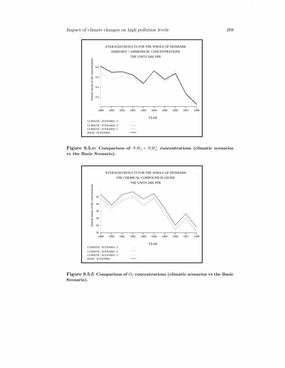
Impact of climate changes on high pollution levels 269
AVERAGED RESULTS FOR THE WHOLE OF DENMARK
AMMONIA + AMMONIUM CONCENTRATIONS
THE UNITS ARE PPB
BASIC SCENARIO:CLIMATIC SCENARIO 1:CLIMATIC SCENARIO 2:
CLIMATIC SCENARIO 3:YEAR
Ann
ual m
eans
of
the
conc
entr
atio
ns
4.0
4.5
5.0
5.5
1989 1990 1991 1992 1993 1994 1995 1996 1997 1998
Figure 9.5.e: Comparison of NH3 + NH+4 concentrations (climatic scenarios
vs the Basic Scenario).
AVERAGED RESULTS FOR THE WHOLE OF DENMARK
THE CHEMICAL COMPOUND IS OZONE
THE UNITS ARE PPB
BASIC SCENARIO:CLIMATIC SCENARIO 1:CLIMATIC SCENARIO 2:
CLIMATIC SCENARIO 3:YEAR
Ann
ual m
eans
of
the
conc
entr
atio
ns
32
34
36
38
40
42
1989 1990 1991 1992 1993 1994 1995 1996 1997 1998
Figure 9.5.f: Comparison of O3 concentrations (climatic scenarios vs the Basic
Scenario).

270 Chapter 9
AVERAGED RESULTS FOR THE WHOLE OF DENMARK
SCALED AOT40C VALUES ARE COMPARED
UNITS: PERCENT, 100.0 (AOT40C / 3000.0)
BASIC SCENARIO:CLIMATIC SCENARIO 1:CLIMATIC SCENARIO 2:
CLIMATIC SCENARIO 3:YEAR
Scal
ed A
OT
40C
val
ues
400
500
600
700
800
1989 1990 1991 1992 1993 1994 1995 1996 1997 1998
Figure 9.5.g: AOT40C (AOT40 for crops) values (climatic scenarios vs the
Basic Scenario). The units are ppb.hours.
AVERAGED RESULTS FOR THE WHOLE OF DENMARK
SCALED AOT40F VALUES ARE COMPARED
UNITS: PERCENT, 100.0 (AOT40F / 10000.0)
BASIC SCENARIO:CLIMATIC SCENARIO 1:CLIMATIC SCENARIO 2:
CLIMATIC SCENARIO 3:YEAR
Scal
ed A
OT
40F
val
ues
200
250
300
350
1989 1990 1991 1992 1993 1994 1995 1996 1997 1998
Figure 9.5.h: AOT40F (AOT40 for forest trees) values (climatic scenarios vs
the Basic Scenario). The units are ppb.hours.

Impact of climate changes on high pollution levels 271
AVERAGED RESULTS FOR THE WHOLE OF DENMARK
BAD DAYS IN WHICH THE 8-HOUR AVERAGES EXCEED 60 PPB
UNITS: NUMBER OF BAD DAYS
BASIC SCENARIO:CLIMATIC SCENARIO 1:CLIMATIC SCENARIO 2:
CLIMATIC SCENARIO 3:YEAR
Num
ber
of b
ad d
ays
30
35
40
45
1989 1990 1991 1992 1993 1994 1995 1996 1997 1998
Figure 9.5.i: Comparison of numbers of days in which the 8-hour averaged
ozone concentrations exceed at least once the limit of 60 ppb (climatic scenar-
ios vs the Basic Scenario) The units are days.
AVERAGED RESULTS FOR THE WHOLE OF DENMARK
AVERAGED DAYLY MAXIMA OF OZONE CONCENTRATIONS
UNITS: NUMBER OF BAD DAYS
BASIC SCENARIO:CLIMATIC SCENARIO 1:CLIMATIC SCENARIO 2:
CLIMATIC SCENARIO 3:YEAR
Num
ber
of b
ad d
ays
45
50
55
60
1989 1990 1991 1992 1993 1994 1995 1996 1997 1998
Figure 9.5.j: Averaged daily maxima of ozone concentrations (climatic sce-
narios vs the Basic Scenario). The units are ppb.

272 Chapter 9
• AOT40C values (causing damages to crops when the critical level of 3000ppb.hours is exceeded),
• AOT60F values (causing damages to forest trees when the critical level of10000 ppb.hours is exceeded),
• numbers of ”bad” days in which the 8-hour average of the ozone concentra-tions exceeds at least once the critical value of 60 ppb (causing health damagesfor certain groups of humans; the number of ”bad” days should not exceed25 after year of 2010, the long-term aim is to reduce this number to zero inthe European Union [96]), and
• averaged daily maxima of ozone concentrations.
Some results for 1997, obtained when the Basic Scenario and Climatic Scenario3 are used, are compared in Fig. 9.6. (a colour version of this figure is given inAppendix A (see Fig. 9.6.col there). In all plots of this figure the relative changes,in percent, of the considered ozone levels are presented (i.e. at each cell of the gridthe result obtained by using Climatic Scenario 3 is divided by the results obtainedby the Basic Scenario and the obtained ratio is multiplied by 100).
It is seen from Fig. 9.6, and from its colour verision 9.6.col in Appendix A, thatthe quantities related to high ozone concentrations are in general increased whenClimatic Scenario 3 is used. For some parts of Europe the increases are ratherconsiderable.
9.5.3 Why are the high ozone levels increased?
It has already been mentioned, in Subsection 9.5.1, that while the annual meansof the ozone concentrations in Denmark are reduced when the climatic scenariosare used, the quantities related to high ozone concentrations tend to be increased(compare the results given in Fig. 9.5.f with the corresponding results in Fig.9.5.g to Fig. 9.5.j). For 1997, the increases of the quantities related to high ozoneconcentrations are rather considerable in some parts of Europe (see Fig. 9.6 andFig. 9.6.col). This particular behaviour of quantities related to ozone deserves someadditional explanation. It is useful to consider two typical situations: the diurnalvariation of the ozone concentrations in summer time and in winter time.
(A) Diurnal ozone variation in summer time.
In a typical day during summer, the ozone concentration have a maximum duringthe afternoon and a minimum during the night. The photochemical reactions playan essential role in the production of ozone, while the destruction of ozone is thedominating process when these reactions are deactivated (which happens during thenight). If the temperature is higher and the cloud cover is lower, then one shouldexpect more ozone to be produced. The climate scenarios (and especially Climate

Impact of climate changes on high pollution levels 273
Scenario 3) simulate meteorological conditions in summer days, according to thepredictions for climate changes, with both higher temperatures and lower cloudcover in comparison with these quantities for the Basic Scenario. Therefore, theconclusion is that we should expect the climatic scenarios to produce more ozoneduring daytime in summer, because the photochemical reactions are producingozone in a higher rate. Some experiments were carried out in order to confirmthis conclusion. In Fig. 9.7.a, we show the averaged diurnal variation of the ozoneconcentrations at the Danish site Frederiksborg for July 1997. It is seen that duringthe day Climatic Scenario 3 produces more ozone than the Basic Scenario. It isalso seen that the patterns of the diurnal variation for the two scenarios are verysimilar to the pattern of the diurnal variations of the measured concentrations.
(B) Diurnal ozone variation in winter time.
The ozone concentrations in summer are higher than the ozone concentrations inwinter. This means that the photochemical reactions (which cause production ofozone) are more active in clear summer days, while they do not play an essential rolein cloudy winter days. In some cloudy winter days the photochemical reactions canbe fully deactivated. When this happens one cannot anymore observe considerableincrease of the ozone concentrations during the day. This is illustrated in Fig. 9.7.b,where the averaged diurnal variation of the ozone concentrations at the Danish siteFrederiksborg for July 1997 is given for the Basic Scenario, Climatic Scenario 3and the observations. It is again seen that the patterns of the diurnal variation forthe two scenarios are very similar to the pattern of the diurnal variations of themeasured concentrations. In this case it is even more important that the ozoneconcentrations produced by the Basic Scenario are higher than those produced byClimatic Scenario 3.
It is important to emphasize here that the relevant period for obtaining thequantities shown in Fig. 9.6 and Fig. 9.6.col is an extended summer period (eitherthe period from April to September or the period from May to July). Moreover, allquantities shown in Fig. 9.6 and in Fig. 9.6.col are related to high ozone concentra-tions (occurring mainly during the afternoon). Therefore, all these quantities arevery sensitive to small variations of the high ozone concentrations. For example, anincrease of the high ozone concentrations with 1-2 ppb might lead to an exceedanceof the 8-hour limit of 60 ppb (which will cause a switch from a ”good” day to a”bad” one).
The results shown in Fig. 9.7.a to Fig. 9.7.b together with the analysis pre-sented above explain the difference in the behaviour of the annual means of theozone concentrations and in the behaviour of the quantities related to high ozoneconcentrations. It should be mentioned here that some more details about thesephenomena can be found in Havasi and Zlatev [131].

274 Chapter 9
Figure 9.6: Relative changes (in percent) of quantities related to high ozone
levels when Climatic Scenario 3 is used instead of the Basic Scenario. The
areas in black are representing the water areas in the model domain (i.e.
the black colour is not refering to ”changes of AOT40C levels”, ”changes of
AOT40F levels”, ”days with more than 60 ppb” or ”changes of daily ozone
maxima”). A colour version of this figure is given in Appendix A (see Fig.
9.6.col there).

Impact of climate changes on high pollution levels 275
OZONE CONCENTRATIONS AT FREDERIKSBORG
AVERAGED DIURNAL VARIATION FOR JULY 1998
UNITS: PPB
BASIC SCENARIO:CLIMATIC SCENARIO 3:OBSERVATIONS:
HOUR
Ave
rage
d co
ncen
trat
ions
0
10
20
30
40
1 2 3 4 5 6 7 8 9 10 11 12 13 14 15 16 17 18 19 20 21 22 23 24
Figure 9.7.a: Averaged diurnal patterns of the ozone concentrations at the
Danish measurement station Frederiksborg for July 1998.
OZONE CONCENTRATIONS AT FREDERIKSBORG
AVERAGED DIURNAL VARIATION FOR JANUARY 1998
UNITS: PPB
BASIC SCENARIO:CLIMATIC SCENARIO 3:OBSERVATIONS:
HOUR
Ave
rage
d co
ncen
trat
ions
0
10
20
30
40
1 2 3 4 5 6 7 8 9 10 11 12 13 14 15 16 17 18 19 20 21 22 23 24
Figure 9.7.b: Averaged diurnal patterns of the ozone concentrations at the
Danish measurement station Frederiksborg for February 1998.

276 Chapter 9
9.6 Conclusions and plans for future work
The results presented in this chapter indicate that the annual values of the concen-trations of the pollutants will not be influenced strongly by the climate changes.However, the influence of the climate changes on some quantities (such as AOT40C,AOT40F, days in which the rolling 8-hour averages of the ozone concentrationsexceed at least once the critical limit of 60 ppb and daily maxima of the ozoneconcentrations) related to high ozone levels) is rather considerable. This is impor-tant, because recent investigations show that these quantities have damaging effectswhen certain critical levels are exceeded, see European Commission ([96], [95]) orZlatev et al. [296].
Studying effects of climatic changes on air pollution levels is connected with agreat number of uncertainties. While it is clear that it is not possible to eliminateall uncertainties, it is highly desirable to reduce some of them. One can reduce theuncertainties caused by numerical errors (which arise when a coarse grid is used)by refining the grid. This implies that runs by using the high resolution optionsof UNI-DEM are desirable. Also the time interval of ten years (which was used inthis study) is, as already mentioned, not sufficiently long, i.e. run on time-intervalsof 20 to 30 years are more desirable. Finally, the use of more scenarios can revealmore details about the studied relationships. The application of
• fine resolution options of UNI-DEM,
• longer time-intervals, and
• more scenarios,
leads to huge computational tasks. This shows that great computational chal-lenges are also present when the effect of future climatic changes on highpollution levels are to be studied in more details.
It should be mentioned here that studying the future pollution levels is a hottopic and many results related to future pollution levels have been published in thelast decade; see, for example, Jonson et al. [148].

Chapter 10
Implementation of variational dataassimilation
The variational data assimilation approach could be viewed as an attempt to adjustglobally the results obtained by a given model to a set of available observations.This approach has the theoretical advantage of providing consistency between thedynamics of the model and the final results of the assimilation. The idea wasprobably applied for the first time (within the field of atmospheric sciences) in1971 in a paper written by Morel et al. [184]. They defined and implemented aprocedure in which the assimilating model is repeatedly integrated forward andbackward in time, the observations being constantly introduced in the model. Theheuristic idea behind that procedure, supported by a number of numerical results,was that repeated calculations and corrections of model results would converge toa solution which would be compatible, at least to a certain degree of accuracy, withthe observations.
Results from some preliminary investigations (based mainly on running simpletests) will be presented in this chapter. Several conclusions will be drawn. Dataassimilation techniques will normally lead to huge computational tasks, which im-plies that one should try to find out, a priori, whether it us profitable or not toapply variational data assimilation in a particular study. The important problemof formulating a set of conditions under which the data assimilation approach willprobably not give good results (these conditions have to be checked carefully beforeapplying the data assimilation procedure in a comprehensive study similar to thestudies, which were presented in Chapter 8 and Chapter 9), will be discussed inSection 6 and Section 7.
Some results, which were obtained by using an atmospheric chemical schemecontaining 56 chemical compounds, will be presented in the end of Section 7.
A general discussion of the possibilities of improving the models by using dataassimilation techniques as well as some plans for future work will be outlined in theend of the chapter.
277

278 Chapter 10
10.1 Basic ideas
Assume that observations are available at time-points tp , where p ∈ 0, 1, 2, . . . , P.These observations can be taken into account in an attempt to improve the resultsobtained by a given model. This can be done by minimizing the value of thefollowing functional (see, for example, Lewis and Derber [164]):
Jc0 =12
P∑p=0
< W (tp) (cp − cobsp ) , cp − cobs
p >, (10.1)
where
• the functional Jc0 is depending on the initial value c0 of the vector of theconcentrations at time t0 (because the model results cp depend on c0),
• W (tp) is a matrix containing some weights, and
• <, > is an inner product in an appropriately defined Hilbert space (it will beassumed in this chapter that the usual vector space is used, i.e. it is assumedthat c ∈ Rs where s is the number of chemical species which are involved inthe model).
It is seen that the functional Jc0 depends on both the weights and the dif-ferences between calculated by the model concentrations cp and observations cobs
p
at the time-levels tp at which observations are available. W (tp) will be assumed tobe the identity matrix I in this study, but in general weights are to be defined insome way and used in the computations.
The task is to find an improved initial field c0 , which minimizes the functionalJc0 . This can be achieved by using some optimization algorithm. Most of theoptimization algorithms are based on the application of the gradient of Jc0 . Theadjoint equation has to be defined and used in the calculation of the gradient ofthe functional Jc0.
It should be stressed that other formulations of the functional Jc0 can alsobe used (see, for example, Daescu and Navon [54], Daescu et al. [55], Le Dimet etal. [159], Elbern and Schmidt, [88], [89], Elbern et al., [90], [91], [92], Talagrandand Courtier, [245]).
It is assumed here that data assimilation techniques are applied to improvean initial field of concentrations, but data assimilation can be applied for otherpurposes too. Other applications are
• improving emission fields,
• checking boundary conditions
and, in a more general context,

Variational data assimilation 279
• checking the sensitivity of the concentrations to variation of different parame-ters (the major purpose being the improvement of some chemical and physicalmechanisms used in the description of the model under consideration).
More details about data assimilation techniques and their implementation indifferent models can be found in Akella and Navon [3], Alekseev and Navon [4],Daescu et al. [55], Elbern et al., [92], Sandu et al., [209], [210], Wang et al., [264].The relationship between the use of data assimilation and the use of a Kalman filteris studied in Li and Navon, [166].
10.2 Calculating the gradient of the functional
It is convenient to explain the basic ideas that are used when the gradient of thefunctional Jc0 is calculated by the following very simple example. Assume thatobservations are available only at five time-points: t0, t1, t2, t3 and t4. The gradientof the functional can be calculated by using the scheme which is shown in Fig. 10.1(a colour version of Fig. 10.1, Fig. 10.1.col, is given in Appendix A). Assume thatsome tool, model, by which the values of the unknown vectors c(t0), c(t1), c(t2),c(t3) and c(t4) can be calculated, is available. The tool model can, for example, besome air pollution model, but in some simpler cases model can be some ordinarysolver for systems of PDEs or ODEs. Under this assumption, the calculations haveto be performed, for this particular example with P = 4, in five steps.
• Step 1. Use the model to calculate c1 (performing integration, in a forwardmode, from time-point t0 to time-point t1). Calculate the adjoint variableq1 = c1 − cobs
1 . Form the adjoint equation (corresponding to the model usedin the forward mode; adjoint equations will be discussed in the next section).Perform backward integration (by applying the adjoint equation) from time-point t1 to time-point t0 to calculate the vector q1
0 , where the lower indexshows that q1
0 is calculated at time-point t0 , while the upper index showsthat q1
0 is obtained by using q1 = c1− cobs1 as an initial vector in the backward
integration.
• Step 2 to Step 4. Perform the same type of calculations, as those in Step1 to obtain q2
0 , q30 and q4
0 . More precisely, the following operations are to becarried out for p = 2, 3, 4:
(a) use the forward mode to proceed from time-point tp−1 to time-point tp,(b) form the adjoint variable qp = cp − cobs
p ,(c) use the adjoint equation in a backward mode from time-point tp to time-
point t0 to calculate cp0.
• Step 5. The sum of the vectors q10 , q2
0 , q30 , q4
0 obtained in Step 1 to Step 4 andvector q0
0 = q0 = c0 − cobs0 gives an approximation to the required gradient of
the functional Jc0.

280 Chapter 10
Figure 10.1: Computing the gradient of Jc0 when observations in five time-
points are available. A Colour version of this figure is given in Appendix A
(see Fig. 10.1.col there).
It is clear that the above procedure can easily be extended for any number Pof time-points at which observations are available.
It is seen from the scheme shown in Fig. 10.1 and Fig. 10.1.col that thegradient of the functional Jc0 can be calculated by performing one forward stepfrom time-point t0 to time-point tP and P backward steps from time-points tp,p = 1, 2, . . . , P , to time-point t0. This explains the main idea, on which the dataassimilation algorithms are based, in a very clear way, but it is expensive when Pis large. In fact, the computational work can be reduced, performing only oncethe backward calculations. This possibility will be discussed in one of the followingsections. It should be mentioned here that the reduction of the computational workby performing only once the backward calculations is leading to an increase of thestorage requirements when non-linear problems are to be handled. Also this issuewill be further discussed in the following sections.
10.3 Forming the adjoint equations
The adjoint equation has to be formed and used during the backward mode (see Fig.10.1 and Fig. 10.1.col). The formation of the adjoint equation in two important

Variational data assimilation 281
cases, the case where the operator is linear and the case where the operator isnon-linear will be discussed in this section.
Assume that the model is linear and, furthermore, that the model is written inthe following general form:
∂c
∂t= Ac. (10.2)
Let q = c − cobs be the adjoint variable (it is assumed here that some interpo-lation rules are used in order to get the continuous variable cobs from the availablediscrete values of the observations). Then the adjoint equation, to equation (10.2)is defined by
∂q
∂t= −AT q. (10.3)
where the superscript T means that if we form the matrix by which the adjointoperator is represented after some kind of discretization, then this matrix is trans-posed to the matrix that represents operator A when the continuous equation (10.2)is discretized by applying some numerical algorithm.
It must be noted here that the notation A∗ is normally used instead of AT . Theoperator A∗ is the conjugate operator of operator A. The reasons for using thenotation AT can be explain as follows:
• we should like to use the same notation both for the operator and for the ma-trix induced by some kind of discretization of the right-hand-side of equation(10.2), and
• if we agree to use the same notation for the operator A and for the matrixinduced when when the right-hand-side of (10.2) is discretized, then it isnatural to apply the notation for the transposed matrix, which is normallyused in the numerical linear algebra studies.
Let us consider now the non-linear case. If the model under consideration isnon-linear, then it is first necessary to produce a linearized version of the model.In other words, the non-linear model
∂c
∂t= B(c). (10.4)
is rewritten as
∂(δc)∂t
= B′(c) δc. (10.5)
where δc is some small variation of c and B′ is a linear operator obtained bydifferentiation of B. The adjoint equation of the linear model (10.5) can be formedin the following way:
∂q
∂t= − [B′(c)]T q. (10.6)
282 Chapter 10
Note that the adjoint equation is linear both in the linear case and in thenon-linear case, see (10.3) and (10.6). Much more important is the fact that inthe non-linear case the adjoint operator depends on the values of c. This causesdifficulties (all values of c calculated during the forward mode, see Fig. 10.1 andFig. 10.1.col, have to be saved because they are needed in the backward mode).The linear case, (10.2)-(10.3) is not causing difficulties related to the storage whichhas to be used with data assimilation procedures.
More details about adjoint equations can be found in Marchuk [178], Marchuket al., [179], Wang et al., [264].
We shall finish this section with two remarks.
Remark 10.1. Adjoint equations of the continuous models have been discussedabove. Sometimes it is more appropriate to form the adjoint equations of thediscretised model (see, for example, Lewis and Derber [164]). Such formulationswill be given in one of the next sections.
Remark 10.2. Very often splitting techniques are used in connection withlarge-scale models (Hundsdorfer and Verwer [142] and Zlatev [276], [282]; see alsoChapter 2). If splitting is used, then one normally forms the adjoint equationscorresponding to the obtained (by the splitting procedure chosen) sub-models; see,for example, Elbern and Schmidt, [88] or Sandu et al., [209] .
10.4 Algorithmic representation ofa data assimilation algorithm
A data assimilation algorithm can be represented by applying the procedure de-scribed in Fig. 10.2. An optimization procedure is needed for the calculations thatare to be carried out in the loop ”DO ITERATIONS”. In many optimization sub-routines, the direction of the steepest descent is to be found and then the value ofparameter ρ that gives the largest decrease in the direction found is to be used toimprove the current solution. In practice, however, it is only necessary here to finda good standard minimization subroutine. In our experiments we used the sub-routine E04DGF from the NAG Numerical Library [186]. This subroutine uses apreconditioned conjugate gradient methods and is based on the algorithm PLMA,described by Gill and Murray [120] and in Section 4.8.3 of Gill et al. [121]. Itshould be relatively easy to call another appropriate subroutine.

Variational data assimilation 283
CInitialize scalar variables, vectors and arrays; set gradient to zero
CDO ITERATIONS = 1, MAX ITERATIONS
CDO LARGE STEPS = 1, P STEP
CF START=(LARGE STEPS-1)∗P LENGTH+1F END=LARGE STEPS∗P LENGTHDO FORWARD STEPS = F START,F END
Perform forward steps by using the modelEND DO FORWARD STEPS
CForm the adjoint equation and update the value of the functionalDO BACKWARD STEPS = F END,1,-1
Perform backward steps by using the adjoint equationEND DO BACKWARD STEPSUpdate the value of the gradient of the functional
CEND DO LARGE STEPS
CCompute an approximation of the optimization parameter ρUpdate the initial values field:NEW FIELD=OLD FIELD + ρ∗GRADIENTCheck the stopping criteriaExit from loop DO ITERATIONSwhen the stopping criteria are satisfied
CEND DO ITERATIONS
CPerform output operations and stop the computations
C
Figure 10.2: An algorithm for performing variational data assimilation by per-
forming multiple backward calculations. P STEP is equal to P . P LENGTH
is equal to the number of time-steps that are to be carried out between two
time-points tp and tp+1 at which observations are available.

284 Chapter 10
CInitialize scalar variables, vectors and arrays; set gradient to zero
CDO ITERATIONS = 1, MAX ITERATIONS
CDO FORWARD STEPS = 1, P STEP∗P LENGTH
Perform forward steps by using the modelEND DO FORWARD STEPS
CDO BACKWARD STEPS = P STEP∗P LENGTH, 1, -1
Perform backward steps by using the adjoint equationEND DO BACKWARD STEPS
CCompute an approximation of the optimization parameter ρUpdate the initial values field:NEW FIELD=OLD FIELD + ρ∗GRADIENTCheck the stopping criteriaExit from loop DO ITERATIONSwhen the stopping criteria are satisfied
CEND DO ITERATIONS
CPerform output operations and stop the computations
C
Figure 10.3: An algorithm for performing variational data assimilation by
performing the backward mode only once. P STEP is equal to P . P LENGTH
is equal to the number of time-steps that are to be carried out between two
time-points tp and tp+1 at which observations are available.
Nearly all optimization subroutines (as mentioned in the previous sections of thischapter) need the value of the functional Jc0 and its gradient. The calculationof these values is performed in the loop ”DO LARGE STEPS” in Fig. 10.2. Thisis a major part of the computational work and is based on scheme described in Fig.10.1 and in Fig. 10.1.col. Let us reiterate here that the repeated backward stepscan be avoided. An algorithm, in which only one backward step is carried out isgiven in Fig. 10.3. It is seen from Fig. 10.3 that one can perform the forward modeon the whole time-interval and then carry out the backward mode from the end ofthe interval to the starting point. The theory on which this algorithm is based isdiscussed in the remaining part of this section.
We shall show now that a single backward mode, from the end-point to the start-point of the integration interval, can be carried out instead of multiple backward

Variational data assimilation 285
modes that are used in the algorithm shown in Fig. 10.2. Let W (tp), p = 0, 1, . . . , P ,be the identity matrix. Assume that the ordinary inner product is used. Then (10.1)can be rewritten as
Jc0 =12
P∑p=0
(cp − cobs
p
)2. (10.7)
It is also possible to consider Jc0 as a function of the concentrations cp,p = 0, 1, . . . , P , i.e.
Jc0 = Jc0, c1, . . . , cP . (10.8)
It is clear that Jc0, c1, . . . , cP : Rs(P+1) → R. Denote by Mp :Rs → Rs the operator which is used at the pth step of the forward mode;i.e. cp = Mp cp−1. The following relationship is obtained by using this definitionof operator Mp in (10.8) and, furthermore, assuming that there exists an operatorM0, which satisfies the equality M0 c0 = c0:
Jc0, c1, . . . , cP = Jc0,M1 c0,M2 M1 c0, . . . ,MP . . . , M2 M1 c0 (10.9)
Let M : c0 → (c0, c1, . . . , cP )T . It is obvious that (i) Ms : R → Rs(P+1)
and (ii) the following relationship holds
M = (M0, M1M0, M2M1M0 . . . , MP · · ·M2M1M0). (10.10)
The minimization of J requires the evaluation of the gradient of the compositionJ M, because
GradJ(c0) = (J M)′ (c0). (10.11)
By using the chain rule in the differentiation of the right-hand-side, one canobtain:
GradJ(c0) = (M′)T (c0) (J′(M (c0))). (10.12)
Here M′ (c0) stands for the derivative of M and the superscript T refers to theadjoint operator (i.e. to the transpose of the corresponding matrix). This mean(M′ (c0))T should be applied to the vector
J′(M (c0)) = J′(c0, c1, . . . , cP) ∈ Rs(P+1) (10.13)
in order to compute the gradient in the left-hand-side of equality (10.12).As stated above, M′ (c0) : R → Rs(P+1). Therefore, (M′ (c0))T : Rs(P+1) →
R. Consider q = (q0, q1, . . . , qP), where qp = cp − cobsp , p = 1, 2, . . . , P. It is
readily seen that q ∈ Rs(P+1) and that the following equality holds:
(M′)T (q0) = (q0, MT1 (q1), MT
1 MT2 (q2), . . ., MT
1 MT2 · · ·MT
P(qP )) (10.14)

286 Chapter 10
with MTp , p = 1, 2, . . . , P. The rule for forming the transposed matrix of a
product of matrices is used in (10.14).It follows from (10.7) and (10.8) that
J′ (c0, c1, . . . , cP) = (q0, q1, . . . , qP) (10.15)
= (c0 − cobs0 , c1 − cobs
1 , . . . cP − cobsP )
∈ Rs(P+1).
Now the desired gradient of the functional Jc0 can be obtained by using(10.12), (10.14) and (10.15):
GradJ(c0) = M′ (c0)T (J′ (c0)) (10.16)
= (c0 − cobs0 )
+ MT1 (c1 − cobs
1 )
+ MT1 MT
2 (c2 − cobs2 )
+ . . .
+ MT1 MT
2 · · ·MTP(cP − cobs
P ).
The right-hand-side of (10.16) can be rewritten as
(c0 − cobs0 ) + MT
1 (c1 − cobs1 (10.17)
+ MT2 (c2 − cobs
2
+ MT3 (c3 − cobs
3 + . . .)) · · ·),which allows us to reduce considerably the computational work. It is necessary,according to (10.17) to use the algorithm shown in Table 10.1 instead of computingone by one the term in the right-hand-side of (10.16).
The algorithm shown in Table 10.1 has to be implemented when the secondloop in Fig. 10.3 is to be executed. In this way, the number of backward loops is

Variational data assimilation 287
Table 10.1: Algorithm for calculating the backward mode only once.
Step Action1 Set i = P and GRAD = 02 Evaluate the difference ci − cobs
i and add it to GRAD3 Apply MT
i to the updated GRAD4 Decrease the value of i by one5 If i ≥ 0 go to Step 26 The needed gradient GRAD is calculated; exit
reduced from P (see Fig. 10.2) to only one. For large values of P this will resultin a substantial reduction of the computational time. It is necessary to save allvalues cp, p = 1, 2, . . . , P , which are calculated during the forward mode when thealgorithm from Fig. 10.3 is used. If the problem solved is non-linear, then thishas to be done anyway. For linear problems, however, this is not needed when thealgorithm in Fig. 10.2 is used. This means that for linear problems there aretwo alternatives:
• the algorithm from Fig. 10. 2 is more profitable when the reduction of thestorage used is more important than the reduction of the computational time,and
• the algorithm from Fig. 10.3, which is based on the algorithm shown in Table10.1 is more profitable when the reduction of the computational time is moreimportant than the reduction of the storage needed.
10.5 Variational data assimilationfor some one-dimensional examples
It is relatively easy to understand the main ideas on which the variational dataassimilation is based by studying the process for simple one-dimensional transportequations. Assume that the unknown variable c ∈ R is the concentration of a givenchemical compound and V is some given function (”wind velocity field”), whichmay depend on t, x and c . Numerical experiments with
• V is a constant,
• V depending on t and/or x, and
• V = c
have been carried out. In all three cases the analytic solution was known, whichallowed us to check easily the correctness of both the calculated results and the

288 Chapter 10
implementation of the algorithms. Only results obtained by using V depending onx (i.e. only results obtained in the solution of one-dimensional transport equations)will be presented in this section.
Any of the three cases can be described mathematically by the following partialdifferential equation (PDE):
∂c
∂t= −V
∂c
∂x, x ∈ [a, b], t ∈ [0, T ], c(x, 0) = f(x). (10.18)
If the spatial interval, the initial value conditions and function V are chosen tobe
[a, b] = [0.2π], f(x) = sin(x), V (x) =6x(2π − x)
(2π)2, (10.19)
then (10.18) becomes identical to one of the examples, which are studied in Lewisand Derber [164]. Its analytical solution is given by
c(x, t) = sin(
2πx
x + (2π − x) exp (3tπ )
). (10.20)
Assume that
xi − xi−1 = x for i = 1, 2, . . . , Nx (10.21)
and
tn − tn−1 = t for n = 1, 2, . . . , Nt (10.22)
Consider the grids:
Gx = xi|i = 0, 1, . . . , Nx, x0 = 0, xNx = 2π (10.23)
and
Gt = tn|n = 0, 1, . . . , Nt, t0 = 0, tNt = 2π (10.24)
Let xi ∈ Gx and tn ∈ Gt . Different numerical methods can be used to calculateapproximations
ci,n ≈ c(xi, tn) (10.25)
of the exact solution at point (xi, tn).The formula (10.26), which is given below, can be obtained by using the notation
wi = (V xit)/4x) and simple finite differences:
−wici−1,n+1 + ci,n+1 + wici+1,n+1 = wici−1,n + ci,n − wici+1,n. (10.26)

Variational data assimilation 289
Dirichlet boundary conditions can be introduced by the following formulae (notethat these boundary conditions are the values of the analytical solution in the end-points of the x-interval):
c0,n = 0, cNx,n = 0, n = 0, 1, . . . , Nt. (10.27)
By applying (10.27), formula (10.26) can be rewritten for i = 1 as
c1,n+1 + w1c2,n+1 = c1,n − w1c2,n (10.28)
and for i = Nx − 1 as
−wNx−1cNx−2,n+1 + cNx−1,n+1 = wNx−1cNx−2,n + cNx−1,n. (10.29)
Denote
cn = (c1,n, c2,n, . . . , cNx−1,n)T . (10.30)
By using the notation introduced by (10.30), it is possible to rewrite (10.26),(10.28) and (10.29) in a matrix form:
(I − A)cn+1 = (I + A)cn ⇒ cn+1 = Dcn, (10.31)
Ddef= (I − A)−1(I + A), (10.32)
where I is the identity matrix and A is a matrix which has non-zero elements onlyon the two diagonals that are adjacent to the main diagonal (and, more precisely,−wi on the diagonal below the main diagonal and wi on the diagonal above themain diagonal).
If cn has already been calculated, then (5.12) can be used to proceed with thecalculation of cn+1 . Thus, if an initial field, c0, is given, then (10.31) can be usedto calculate successively, step-by-step, approximations of the exact solution.
As mentioned above, it is necessary to calculate the gradient GradJ of thefunctional Jc0 from (10.1) in order to find an improved initial field c0. Assume asin the first section of this chapter that observations are available at times tp | p =0, 1, . . . , P. Assume also that the calculations by formula (10.31) for some n+1 = phave been completed. It is then necessary to form the adjoint variable
qp = Wp (cp − cobsp ) (10.33)
and to use it as a starting value in the integration of the adjoint equation backwardfrom t = tp to t = t0 (let us reiterate that we have assumed that Wp = I for allvalues of p). The backward calculations can be carried out by using the followingformula, which is the discrete adjoint equation corresponding to (10.31):
qn = −DT qn+1, (10.34)
where D is defined in (10.32).
290 Chapter 10
10.6 Numerical results for the one-dimensionaltransport equation
Several numerical experiments were designed in the efforts to check the correctnessof the implementation of the variational data assimilation modules. The followingissues were tested during these experiments:
• the correct implementation of the forward module,
• the effects of using different grids,
• the application of unbiased perturbations of the initial values,
• the insertion of biased perturbations in the initial values,
• the effects of reducing the number of observations, and
• the effects of varying the number P (or, in other words, the effects of thevariation of the number of time-points at which observations are available).
10.6.1 Checking the module for forward integration
One of the major requirements (at least for the special case treated here) is that themodule for performing forward integration should be able to improve the accuracyof the results when the discretization is refined (i.e. when the grid-points in spaceand time are increased). Results obtained in an experiment where the values ofthe parameters and are successively increased (both by a factor of ten) are givenin Table 10.2. It is seen that the module is performing as it should. The globalerror decreases by a factor of approximately 100 (or, in other words, the accuracyis increased by a factor approximately equal to 100). Of course, one has to paysomething for the increased accuracy; the figures in the last column show that thecomputational time is increased by a factor approximately equal to 100 when thegrids are refined.
10.6.2 Applying the same perturbation parameteron different grids
The next important issue is to check the potential ability of the variational dataassimilation algorithm to improve the initial values of the concentrations whensufficiently many accurate observations are available. This can be done in thefollowing way. Assume that the initial values of the exact solution c(x, 0) = sin(x)on the selected grid are perturbed by using the formula:
ci,0 = 1 − [0.5 − DRAND(0)]α sin(xi) (10.35)
where DRAND is a double precision UNIX generator of random numbers in theinterval [0, 1] and α is a parameter which can freely be chosen in the interval [0, 1]. It is easily seen that

Variational data assimilation 291
Table 10.2: Results obtained when the module for forward integration ischecked. Nx and Nt are the number of grid-points the spatial and time axes.ERROR is the largest in absolute value error found during the calculations.RATE 1 is the rate of improving the error in the transition from run i to runi+1. RATE 2 is the rate of increasing the computational time in the transitionfrom run i to run i + 1.
Nx Nt ERROR RATE 1 Time RATE 211 100 3.01 ∗ 10−0 - 0.00124 -
101 1000 4.29 ∗ 10−3 701.63 0.0127 102.421001 10000 4.33 ∗ 10−5 99.08 1.44 113.39
10001 100000 4.34 ∗ 10−7 99.77 179.89 124.23100001 1000000 4.28 ∗ 10−9 101.40 18855.19 105.40
1000000 10000000 2.04 ∗ 10−9 2.10 562389.65 298.27
• if α = 0 , then the initial values of the exact solution are not perturbed, and
• if α = 0.1 (as in Table 10.3, below), then the perturbations of the initialvalues are in the interval [−5%, 5%] without any bias.
In the forward mode the calculations are carried out by using the perturbedwith (10.35) and with α = 0.1 initial values. The values of the adjoint variableused in the backward mode are obtained as the differences between the calculatedwith the perturbed initial condition values and the exact values at the grid-points,i.e. the exact values play the role of the observations in (10.33). The results thatare shown in Table 10.3 allow us to draw the following conclusions:
• the global error, ERRglobal, in the forward solution obtained with perturbedinitial values is large and cannot be improved by refining the grids,
• the error ERRimpr0 in the initial solution can be improved significantly by the
data assimilation algorithm when the resolution is sufficiently good (comparethe corresponding values of ERR0 and ERRimpr
0 ), and
• The error ERRimprglobal obtained when the forward mode is carried out with
the improved (by the data assimilation algorithm) initial values is clearlybecoming smaller when the grid is refined. Moreover, the errors are of thesame order of magnitude as those obtained when exact initial values are used(Table 10.2). This means that we are getting an optimal result, which cannotbe further improved when the numerical method and the grid are alreadychosen.

292 Chapter 10
Table 10.3: Results obtained in the checks of the performance of the vari-ational data assimilation algorithm when the initial values are perturbed byrandom errors generated by using α = 0.1. ERR0 is the error induced by therandom perturbations, ERRglobal is the global error when the forward inte-gration is performed with the perturbed initial field, ERRimpr
0 is the errorin the improved by the variational data assimilation algorithm initial field,ERRimpr
global is the global error when the forward integration is performed withthe improved by the variational data assimilation algorithm initial field.
Nx Nt ERR0 ERRglobal ERRimpr0 ERRimpr
global
11 100 4.55 ∗ 10−2 2.93 ∗ 10−1 1.94 ∗ 10−1 1.94 ∗ 10−1
101 1000 4.47 ∗ 10−2 7.53 ∗ 10−2 2.62 ∗ 10−3 2.62 ∗ 10−3
1001 10000 4.99 ∗ 10−2 1.10 ∗ 10−1 2.64 ∗ 10−5 2.64 ∗ 10−5
10001 100000 4.99 ∗ 10−2 1.44 ∗ 10−1 2.93 ∗ 10−7 2.93 ∗ 10−7
10.6.3 Results obtained with different valuesof parameter α
The results given in Table 10.3 are obtained, as stated in the previous subsection,by using α = 0.1, which means that small errors, of about 5%, are introduced inthe initial solution. Therefore, it is necessary to investigate the case where theperturbations are larger. Larger perturbations can be created by increasing thevalue of α . Results that are obtained with Nx = 1001, Nt = 10001 and differentvalues of parameter α are given in Table 10.4. It is clearly seen that the magnitudeof the errors in the forward mode obtained with the improved initial values arepractically not depending on the size of parameter α .
10.6.4 Results obtained when the perturbationscreate some bias
The perturbations used in previous three subsections are not creating any bias.Bias could be simulated by using the following formulae:
ci,0 = 1 + DRAND(0) α sin(xi), (10.36)
ci,0 = 1 − DRAND(0) α sin(xi), (10.37)
The first formula, (10.36), is producing over-estimated values of the initial so-lution. The second formula, (10.37), is giving under-estimated values of the initialsolution.

Variational data assimilation 293
Table 10.4: Results obtained in the checks of the performance of the varia-tional data assimilation algorithm with Nx = 1001, Nt = 10001 and α varyingfrom 0.1 to 1.0. ERR0, ERRglobal, ERRimpr
0 and ERRimprglobal are defined in Table
10.3.
α ERR0 ERRglobal ERRimpr0 ERRimpr
global
0.1 4.99 ∗ 10−2 1.10 ∗ 10−1 2.64 ∗ 10−5 2.64 ∗ 10−5
0.2 9.94 ∗ 10−2 2.31 ∗ 10−1 2.64 ∗ 10−5 2.64 ∗ 10−5
0.3 1.47 ∗ 10−1 3.28 ∗ 10−1 2.64 ∗ 10−5 2.64 ∗ 10−5
0.4 2.00 ∗ 10−1 4.14 ∗ 10−1 2.64 ∗ 10−5 2.64 ∗ 10−5
0.5 2.46 ∗ 10−1 5.83 ∗ 10−1 2.64 ∗ 10−5 2.64 ∗ 10−5
0.6 2.99 ∗ 10−1 6.79 ∗ 10−1 2.64 ∗ 10−5 2.64 ∗ 10−5
0.7 3.43 ∗ 10−1 9.47 ∗ 10−1 2.64 ∗ 10−5 2.64 ∗ 10−5
0.8 3.96 ∗ 10−1 8.55 ∗ 10−1 2.64 ∗ 10−5 2.64 ∗ 10−5
0.9 4.49 ∗ 10−1 1.07 ∗ 100 2.64 ∗ 10−5 2.64 ∗ 10−5
1.0 4.90 ∗ 10−1 1.02 ∗ 100 2.64 ∗ 10−5 2.64 ∗ 10−5
Table 10.5: Results obtained in the checks of the performance of the varia-tional data assimilation algorithm with Nx = 1001, Nt = 10001 and α varyingfrom 0.1 to 1.0. Bias is produced by using formula (10.36). ERR0, ERRglobal,ERRimpr
0 and ERRimprglobal are defined in Table 10.3.
α ERR0 ERRglobal ERRimpr0 ERRimpr
global
0.1 1.00 ∗ 10−1 1.77 ∗ 10−1 2.64 ∗ 10−5 2.64 ∗ 10−5
0.2 1.99 ∗ 10−1 3.63 ∗ 10−1 2.64 ∗ 10−5 2.64 ∗ 10−5
0.3 2.96 ∗ 10−1 5.37 ∗ 10−1 2.64 ∗ 10−5 2.64 ∗ 10−5
0.4 4.00 ∗ 10−1 7.08 ∗ 10−1 2.64 ∗ 10−5 2.64 ∗ 10−5
0.5 4.96 ∗ 10−1 8.97 ∗ 10−1 2.64 ∗ 10−5 2.64 ∗ 10−5
0.6 5.98 ∗ 10−1 1.00 ∗ 100 2.64 ∗ 10−5 2.64 ∗ 10−5
0.7 6.98 ∗ 10−1 1.33 ∗ 100 2.64 ∗ 10−5 2.64 ∗ 10−5
0.8 7.89 ∗ 10−1 1.40 ∗ 100 2.64 ∗ 10−5 2.64 ∗ 10−5
0.9 8.95 ∗ 10−1 1.65 ∗ 100 2.64 ∗ 10−5 2.64 ∗ 10−5
1.0 9.87 ∗ 10−1 1.88 ∗ 100 2.64 ∗ 10−5 2.64 ∗ 10−5
Results obtained by producing perturbations in the initial value by using (10.36)are given in Table 10.5. The error in the improved initial field as well as the globalerror in the forward mode do not depend on the value of α (and, as a matter of fact,the rounded to the third significant decimal numbers are the same for all values of

294 Chapter 10
α). Results obtained by using (10.37) instead of (10.36) are quite similar to theresults shown in Table 10.5.
10.6.5 Results obtained by usingreduced number of observations
The results given in the previous sections were obtained by using ”observations”(exact values of the solution) at all spatial grid-points xi, i = 0, 1, . . . , Nx, at thetime-points p = 1, 2, . . . , P (i.e. at every point where backward calculations areinitiated). In the practical situations the number of observations will be limited.Therefore, it is necessary to investigate the accuracy of the results when the numberof observations is reduced. Two different cases should be investigated:
• the adjoint variable is set to zero if there is no observation at spatial grid-points under consideration, and
• an attempt to get observations at all spatial grid-points (by interpolation) ismade.
Case A - The adjoint variable is set to zerowhen no observation is available
It is easy to apply this possibility. Some results are given in Table 10.6. It isassumed that observations are available at every second spatial grid-point. Thisis a very restrictive assumption when refined grids are used. Nevertheless, it isseen that the results are much less accurate than those presented in Table 10.3(where observations in all grid-points were used in the calculations). The resultsindicate that if the spatial grid is fine (100 or more grid-points), then the resultscan be improved by using data assimilation by a factor approximately equal to2. The results shown in Table 10.7 indicate that this statement seems to be truealso when the magnitude of the perturbations is increased by varying parameter α.Comparing the results in Table 10.7 with the corresponding results in Table 10.4,it is seen that
• the results in the third and the fourth columns are identical in the two tables,and
• while the errors given in the fifth and the sixth columns in Table 10.4 do notdepend on parameter α, the corresponding errors in Table 10.7 grow whenthe value of α is increased.

Variational data assimilation 295
Table 10.6: Results obtained in the checks of the performance of the varia-tional data assimilation algorithm when the initial values are perturbed byrandom errors produced by using α = 0.1. Observations are available inevery second spatial grid-point. The adjoint variable is set to zero at thepoints where observations are not available. ERR0, ERRglobal, ERRimpr
0 andERRimpr
global are defined in Table 10.3.
Nx Nx ERR0 ERRglobal ERRimpr0 ERRimpr
global
11 100 4.55 ∗ 10−2 2.93 ∗ 10−1 1.01 ∗ 10−1 2.28 ∗ 10−1
101 1000 4.47 ∗ 10−2 7.53 ∗ 10−2 2.47 ∗ 10−2 3.97 ∗ 10−2
1001 10000 4.99 ∗ 10−2 1.10 ∗ 10−1 2.54 ∗ 10−2 5.56 ∗ 10−2
Table 10.7: Results obtained in the checks of the performance of the varia-tional data assimilation algorithm with Nx = 1001, Nt = 10001 and α varyingfrom 0.1 to 1.0. Observations are available in every second spatial grid-point.The adjoint variable is set to zero at the points where observations are notavailable. ERR0, ERRglobal, ERRimpr
0 and ERRimprglobal are defined in Table 10.3.
α ERR0 ERRglobal ERRimpr0 ERRimpr
global
0.1 4.99 ∗ 10−2 1.10 ∗ 10−1 2.54 ∗ 10−2 5.56 ∗ 10−2
0.2 9.94 ∗ 10−2 2.31 ∗ 10−1 5.00 ∗ 10−2 1.16 ∗ 10−1
0.3 1.47 ∗ 10−1 3.28 ∗ 10−1 7.38 ∗ 10−1 1.62 ∗ 10−1
0.4 2.00 ∗ 10−1 4.14 ∗ 10−1 1.00 ∗ 10−1 2.07 ∗ 10−1
0.5 2.46 ∗ 10−1 5.83 ∗ 10−1 1.28 ∗ 10−1 2.94 ∗ 10−1
0.6 2.99 ∗ 10−1 6.79 ∗ 10−1 1.52 ∗ 10−1 3.43 ∗ 10−1
0.7 3.43 ∗ 10−1 9.47 ∗ 10−1 1, 72 ∗ 10−1 4.72 ∗ 10−1
0.8 3.96 ∗ 10−1 8.55 ∗ 10−1 2.00 ∗ 10−1 4.26 ∗ 10−1
0.9 4.49 ∗ 10−1 1.07 ∗ 100 2.31 ∗ 10−1 5.37 ∗ 10−1
1.0 4.90 ∗ 10−1 1.02 ∗ 100 2.46 ∗ 10−1 5.15 ∗ 10−1
Case B - Using interpolation to obtain observationsat all spatial points
The results in given in the previous paragraph show that it is not advisable to setthe adjoint variable to zero when no observation is available at the spatial grid-pointunder consideration. It will be shown now that it might be more profitable, in somesituations at least, to try to calculate approximations to the missing observations

296 Chapter 10
by using some interpolation rules. For our purposes, the application of simple rulesfor linear interpolation is quite sufficient and such rules will be used in this section.However, some more advanced interpolation rules (as, for example, cubic splines)may be more successful in some other situations.
The results in Table 10.8 are obtained using the same parameters as thoseused to calculate the results in Table 10.6 with the only exception that linearinterpolation is used to obtain approximations of the observations in the spatialgrid-points at which ”observations” are not available.
Some results for ERRimprglobal obtained when both the number of ”available ob-
servations” and parameter α are varied are given in Table 10.9. It is seen that theresults become poorer when the number of observations is decreased. However, theaccuracy of the results is very insensitive to variations of α (i.e. the variations ofthe magnitude of the perturbations inserted in the initial values).
Table 10.8: Results obtained in the checks of the performance of the vari-ational data assimilation algorithm when the initial values are perturbed byrandom errors produced by using α = 0.1. Observations are available in everysecond spatial grid-point. Interpolation is used at the points where observa-tions are not available. ERR0, ERRglobal, ERRimpr
0 and ERRimprglobal are defined
in Table 10.3.
Nx Nx ERR0 ERRglobal ERRimpr0 ERRimpr
global
11 100 4.55 ∗ 10−2 2.93 ∗ 10−1 1.01 ∗ 10−1 2.28 ∗ 10−1
101 1000 4.47 ∗ 10−2 7.53 ∗ 10−2 2.61 ∗ 10−3 3.17 ∗ 10−3
1001 10000 4.99 ∗ 10−2 1.10 ∗ 10−1 2.64 ∗ 10−5 3.21 ∗ 10−5
10001 100000 4.99 ∗ 10−2 1.44 ∗ 10−1 2.64 ∗ 10−7 2.64 ∗ 10−7
10.6.6 Varying the number of time-pointsat which observations are available)
In all experiments in the previous subsections the number of time-steps per a back-ward step was fixed (i.e. after performing 10 time-steps the adjoint variable wasformed and a new backward step was calculated by performing backward inte-gration to the initial time-point t0). This might be very expensive (in terms ofcomputational time). On the other hand (and this may be much more importantin practice), observations are often available at a few time-points. Therefore, it isworthwhile to investigate the behaviour of the variational data assimilation whenthe number of backward steps is varied. It is desirable to be able to use as manyas possible time-steps per backward step (or, in other words, to reduce the numberof backward steps as much as possible). Some results, which are obtained by using
• Nx = 1001,

Variational data assimilation 297
Table 10.9: Values of ERRimprglobal (see the caption in Table 10.3) obtained by
using the variational data assimilation algorithm with Nx = 1001, Nt = 10001and α varying from 0.1 to 1.0. The number of observations N OBS is variedin this experiment.
Number of observations N OBSα 1000 500 125 20 50.1 2.64 ∗ 10−5 3.21 ∗ 10−5 3.39 ∗ 10−4 1.34 ∗ 10−2 2.05 ∗ 10−1
0.2 2.64 ∗ 10−5 3.21 ∗ 10−5 3.39 ∗ 10−4 1.34 ∗ 10−2 2.05 ∗ 10−1
0.3 2.64 ∗ 10−5 3.21 ∗ 10−5 3.39 ∗ 10−4 1.34 ∗ 10−2 2.05 ∗ 10−1
0.4 2.64 ∗ 10−5 3.21 ∗ 10−5 3.39 ∗ 10−4 1.34 ∗ 10−2 2.05 ∗ 10−1
0.5 2.64 ∗ 10−5 3.21 ∗ 10−5 3.39 ∗ 10−4 1.34 ∗ 10−2 2.05 ∗ 10−1
0.6 2.64 ∗ 10−5 3.21 ∗ 10−5 3.39 ∗ 10−4 1.34 ∗ 10−2 2.05 ∗ 10−1
0.7 2.64 ∗ 10−5 3.21 ∗ 10−5 3.39 ∗ 10−4 1.34 ∗ 10−2 2.05 ∗ 10−1
0.8 2.64 ∗ 10−5 3.21 ∗ 10−5 3.39 ∗ 10−4 1.34 ∗ 10−2 2.05 ∗ 10−1
0.9 2.64 ∗ 10−5 3.21 ∗ 10−5 3.39 ∗ 10−4 1.34 ∗ 10−2 2.05 ∗ 10−1
1.0 2.64 ∗ 10−5 3.21 ∗ 10−5 3.39 ∗ 10−4 1.34 ∗ 10−2 2.05 ∗ 10−1
• Nt = 10001,
• α = 0.1 ,
• five different values of N OBS, and
• different numbers of backward steps (P STEP),
are given in Table 10.10.
10.6.7 Conclusions from the experimentswith one-dimensional problems
The test-example defined by (10.18)-(10.20) is very simple. Therefore, it is onlypossible to make conclusions about the cases in which
• it is quite certain that the data assimilation algorithm is not performing well(it is quite clear that if the algorithm does not work for such a simple example,then it will not work when more complicated situations are to be handled),and
• there is some hope that the data assimilation algorithm will perform well (butit should be emphasized that more experiments with test examples that arecloser to real cases are necessary in order to confirm such expectations).
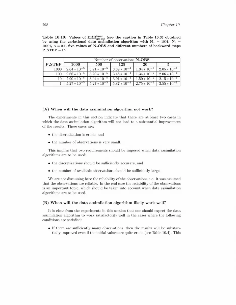
298 Chapter 10
Table 10.10: Values of ERRimprglobal (see the caption in Table 10.3) obtained
by using the variational data assimilation algorithm with Nx = 1001, Nt =10001, α = 0.1, five values of N OBS and different numbers of backward stepsP STEP = P.
Number of observations N OBSP STEP 1000 500 125 20 5
1000 2.64 ∗ 10−5 3.21 ∗ 10−5 3.39 ∗ 10−4 1.34 ∗ 10−2 2.05 ∗ 10−1
100 2.66 ∗ 10−5 3.20 ∗ 10−5 3.48 ∗ 10−4 1.34 ∗ 10−2 2.06 ∗ 10−1
10 2.90 ∗ 10−5 3.04 ∗ 10−5 3.91 ∗ 10−4 1.50 ∗ 10−2 2.15 ∗ 10−1
1 5.27 ∗ 10−5 5.27 ∗ 10−5 5.87 ∗ 10−4 2.75 ∗ 10−2 3.55 ∗ 10−1
(A) When will the data assimilation algorithm not work?
The experiments in this section indicate that there are at least two cases inwhich the data assimilation algorithm will not lead to a substantial improvementof the results. These cases are:
• the discretization is crude, and
• the number of observations is very small.
This implies that two requirements should be imposed when data assimilationalgorithms are to be used:
• the discretizations should be sufficiently accurate, and
• the number of available observations should be sufficiently large.
We are not discussing here the reliability of the observations, i.e. it was assumedthat the observations are reliable. In the real case the reliability of the observationsis an important topic, which should be taken into account when data assimilationalgorithms are to be used.
(B) When will the data assimilation algorithm likely work well?
It is clear from the experiments in this section that one should expect the dataassimilation algorithm to work satisfactorily well in the cases where the followingconditions are satisfied:
• If there are sufficiently many observations, then the results will be substan-tially improved even if the initial values are quite crude (see Table 10.4). This

Variational data assimilation 299
is also true when there is some bias of the errors in the initial values (see Table10.5).
• Assume that the number of observations is less than the number of spatialgrid-points (which will be always the case in real situations). In this case,it might be useful to calculate (by applying some interpolation rules) ap-proximate observations in the grid-points where there are not observations(compare the results in Table 10.6 and Table 10.7 with the results in Table10.8 and Table 10.9).
• The results seem to be rather insensitive to the number of backward stepsthat are actually used (see Table 10.10). It is important to check furtherwhether this nice property holds in more complicated cases, because the dataassimilation procedure will become extremely expensive if many backwardsteps are needed.
• It is important to improve the performance of the data assimilation algorithmwith regard to computational time (it is seen that there are problems withthe computational time even for the simple one-dimensional example treatedin this paper). Parallel algorithms, similar to those used in Alexandrov etal. [5] and Dimov et al. [71] (see also Chapter 7) might lead to a considerableimprovement of the performance.
(C) How to continue the verification of the algorithmfor transport equations?
It is clear that, before applying data assimilation algorithms in particular studiesinvolving large-scale air pollution models, it is necessary to eliminate the cases inwhich these algorithms will not work well. In this section it was shown, by using asimple example, that there are at least two such cases.
The problem defined by (10.18)-(10.20) is a simple one-dimensional transportequation. In the further investigations two and three-dimensional test-examplesshould also be studied.
Some numerical examples, which are similar in some sense to the chemical re-action schemes that are used in large-scale air pollution models (as well as in somelarge-scale models that appear in other fields of science and engineering) will betreated in the next section of this chapter. We shall conclude the chapter by study-ing the impact of operational splitting, which is practically unavoidable in realapplications (see Chapter 2), on the data assimilation algorithms.
10.7 Treatment of some simple non-linear tests-problems
The program EXAMINATOR, which has been discussed and tested in Chapter 2to examine the performance of different numerical methods combined with different

300 Chapter 10
splitting procedures in the case when the problems are solved without using dataassimilation techniques, will be applied in this section to study the performanceof the same 30 combinations of numerical methods and splitting procedures in thecase where some data assimilation technique is applied.
The test-example studied at the end of Chapter 2, will also be used in thischapter. In Chapter 2 the interaction of the splitting procedures and the numericalmethods was studied. Now the performance of the data assimilation modules forfor non-linear problems will be investigated by using this test-example.
The test-example is defined by (2.51) and (2.52). Let us reiterate here that thistest-example is non-linear, the mass conservation law holds and the components ofthe solution are non-negative. This means that the problem formulated by (2.51)and (2.52) has the same properties as the chemical schemes. Moreover, the exactsolution is known, given by (2.53), and, therefore, it is possible to use the sametechniques as in the previous sections of this chapter, i.e. to perturb the initialvalues and to study the ability of the data assimilation modules to calculate a goodapproximation of the initial values.
The same numerical methods, as those used in Chapter 2, will be used in thesolution of the problem (2.51) and (2.52). In other words, the numerical methods,which are used to produce the results given in the tables presented in the remainingpart of this chapter, are:
• the Backward Euler Method defined by (10.38),
• the Implicit Mid-point Rule defined by (2.59) , and
• the Fully Implicit Three-stage Runge-Kutta Method defined (2.60) - (2.67).
Three other well-known numerical methods for integration of systems of ordi-nary differential equations
• the Modified Diagonally Implicit Runge Kutta Method (Zlatev [273]),
• the Two-stage Rosenbrock Method (Hundsdorfer and Verwer [142]), and
• the Trapezoidal Rule (Hairer and Wanner [127])
were also used in the experiments.Most of the results presented in the remaining part of this chapter were obtained
by using the first three numerical methods. However, a few results obtained whenall these six numerical methods were used will also be shown and discussed.
The same splitting procedures, as those used in Chapter 2, will be used inthis chapter, i.e. the sequential splitting, the symmetric splitting, the weightedsequential splitting and the weighted symmetric splitting. Tests where no splittingprocedure is applied will also be carried out. The simple operators defined by (2.55)and (2.56) are used in all splitting procedures.
Two major issues will be discussed in this section: (i) the ability of the dataassimilation modules to improve the accuracy of the solution and (ii) the interactionbetween numerical methods and splitting procedures.

Variational data assimilation 301
10.7.1 Application of the Backward Euler Method
The forward mode of the data assimilation procedure is carried out by using (2.58)from Chapter 2. For convenience this formula is given below:
cn+1 = cn + tf(cn+1). (10.38)
The fact that the test-example (2.51) is an autonomous system of ODEs isexploited in (10.38). If the problem is non-autonomous, then f(tn+1, cn+1) shouldbe used in (10.38) instead of f(cn+1) (the alternative is to transform the non-autonomous system of ODEs to an autonomous one by adding the equation t′ = 1).
The adjoint equation, which has to be used in the backward mode, is defined asfollows:
qn = qn+1 −t
[−∂f(cn)
∂c
]T
qn. (10.39)
Also the adjoint equation (10.39) is written for autonomous systems of ODEs.As above, f(cn) should be replaced by f(tn, cn) when the system of ODEs is non-autonomous (the alternative is to transform, as above, the non-autonomous systemof ODEs to an autonomous one).
The accuracy of the results obtained when the data assimilation modules areused with different splitting procedures is shown in Table 10.11. In fact, the greatesterrors obtained with the improved solution are given in Table 10.11. This meansthat the following actions are performed:
• the initial solution is perturbed by using α = 1.0 in (10.35), which means thatthe size of perturbations being about 50% of the values of the initial solution,
• the accuracy of the initial solution is recovered by the data assimilation mod-ules, and, finally,
• a forward run is performed with the improved initial solution.
The greatest errors obtained during this final run are given Table 10.11.Increasing the number of time-steps by a factor of two leads, as in Chapter 2, to
a reduction of the time-step size by a factor of two. Therefore, one should expectthat the accuracy will be improved when the number of time-steps is increased.The results in Table 10.11 shows that the accuracy is indeed improved when moretime-steps are used.
It is also important to investigate the rate of the improvement of the accuracy.The rates of improvement (i.e. the ratios between the greatest errors found intwo successive runs) are given in Table 10.12. The Backward Euler Method is afirst-order numerical method. Therefore, we should expect, see also (2.70), thatthe combined method (the Backward Euler Method with the selected splitting pro-cedure) will always perform as a first-order method. It is seen from Table 10.12

302 Chapter 10
Table 10.11: Performance of the data assimilation modules for non-linearproblems. Accuracy results achieved when the Backward Euler Method isused with five splitting procedures. The abbreviations Steps, ”Splitting 0”,”Splitting 1”, ”Splitting 2”, ”Splitting 3” and ”Splitting 4” are used for (i) thenumber of time-steps and (ii) the cases where no splitting, sequential splitting,symmetric splitting, weighted sequential splitting and weighted symmetricsplitting are used in the computations.
Steps Splitting 0 Splitting 1 Splitting 2 Splitting 3 Splitting 440 2.09E-2 2.08E-2 1.40E-1 2.60E-1 1.81E-180 1.09E-2 1.09E-2 7.40E-2 1.26E-2 9.22E-2
160 5.60E-3 5.60E-3 3.80E-2 6.26E-2 4.64E-2320 2.84E-3 2.84E-3 1.93E-2 3.12E-2 2.33E-2640 1.43E-3 1.48E-3 9.70E-3 1.56E-2 1.17E-2
1280 7.16E-4 7.16E-4 4.86E-3 7.81E-3 5.85E-32560 3.59E-4 3.59E-4 2.44E-3 3.91E-3 2.93E-35120 1.79E-4 1.79E-4 1.22E-3 1.95E-3 1.46E-3
10240 8.98E-5 8.98E-5 6.10E-4 9.76E-4 7.31E-420480 4.49E-5 4.49E-5 3.05E-4 4.88E-4 3.66E-440960 2.24E-5 2.24E-5 1.52E-4 2.44E-4 1.83E-481920 1.12E-5 1.12E-5 7.63E-5 1.22E-4 9.15E-5
163840 5.61E-6 5.61E-6 3.81E-5 6.10E-5 4.58E-5327680 2.81E-6 2.81E-6 1.91E-5 3.05E-5 2.28E-5
that the combined method behaves as a first-order numerical method for all fivesplitting procedures (including here the case when no splitting is used).
The results given in Table 10.11 and Table 10.12 are nearly identical to theresults obtained when the data assimilation modules are not used (i.e. when theexact values of the initial solution are used and only the forward mode is carriedout); compare the results in Table 10.11 and Table 10.12 with the correspondingresults in Table 2.7 and Table 2.8. This means that when the perturbed valuesof the initial solution are improved, the errors of made by the Backward EulerMethod and the selected splitting procedure are becoming the majors sources forerrors during the forward mode with the improved solution.
10.7.2 Application of the Implicit Mid-point Rule
The forward mode of the data assimilation procedure is carried out by using (2.59)from Chapter 2. For convenience this formula, representing the Implicit Mid-pointRule, is given below:
cn+1 = cn + tf(0.5(cn + cn+1)). (10.40)

Variational data assimilation 303
Table 10.12: Performance of the data assimilation modules for non-linearproblems. The ratios of the errors between successive runs that are obtainedwhen the Backward Euler Method is used with five splitting procedures. Theabbreviations Steps, ”Splitting 0”, ”Splitting 1”, ”Splitting 2”, ”Splitting 3”and ”Splitting 4” are used for (i) the number of time-steps and (ii) the caseswhere no splitting, sequential splitting, symmetric splitting, weighted sequen-tial splitting and weighted symmetric splitting are used in the computations.
Steps Splitting 0 Splitting 1 Splitting 2 Splitting 3 Splitting 440 - - - - -80 1.908 1.908 1.894 2.061 1.966
160 1.951 1.951 1.947 2.015 1.983320 1.975 1.975 1.974 2.004 1.992640 1.987 1.987 1.987 2.001 1.996
1280 1.994 1.994 1.993 2.000 1.9982560 1.997 1.997 1.997 2.000 1.9995120 1.999 1.999 1.998 2.000 2.000
10240 1.999 1.999 1.999 2.000 2.00020480 2.000 2.000 2.000 2.000 2.00040960 2.000 2.000 2.000 2.000 2.00081920 2.000 2.000 2.000 2.000 2.000
163840 2.000 2.000 2.000 2.000 2.000327680 2.000 2.000 2.000 2.000 2.000
The fact that the test-example (2.51) is an autonomous system of ODEs isexploited in (10.40). If the system of ODEs is non-autonomous, then f(tn +0.5t, 0.5(cn + cn+1)) should be used in (10.40) instead of f(0.5(cn + cn+1)) (thetransformation of the non-autonomous system of ODEs to an autonomous one canbe used).
The adjoint equation, which has to be used in the backward mode, is defined asfollows:
qn = qn+1 −t
[−∂f(0.5(cn + cn+1))
∂c
]T
qn. (10.41)
Also the adjoint equation (10.41) is written for autonomous systems of ODEs.As above, f(0.5(cn + cn+1)) should be replaced by f(tn + 0.5t, 0.5(cn + cn+1))when the system of ODEs is non-autonomous (again the non-autonomous systemof ODEs can alternatively be transformed to an autonomous one).
The experiments were carried out as in the case where the Backward EulerMethod is used. Accuracy results are given in Table 10.13. Ratios of errors obtainedin successive runs (indicating the rate of convergence) are given in Table 10.14.

304 Chapter 10
Table 10.13: Performance of the data assimilation modules for non-linearproblems. Accuracy results achieved when the Implicit Mid-point Rule isused with five splitting procedures. The abbreviations Steps, ”Splitting 0”,”Splitting 1”, ”Splitting 2”, ”Splitting 3” and ”Splitting 4” are used for (i) thenumber of time-steps and (ii) the cases where no splitting, sequential splitting,symmetric splitting, weighted sequential splitting and weighted symmetricsplitting are used in the computations.
Steps Splitting 0 Splitting 1 Splitting 2 Splitting 3 Splitting 440 9.65E-04 2.00E-01 2.12E-02 6.67E-03 3.70E-0380 2.40E-04 1.11E-01 5.47E-03 8.16E-04 9.64E-04
160 5.99E-05 5.88E-02 1.38E-03 1.17E-04 2.43E-04320 1.50E-05 3.03E-02 3.45E-04 2.13E-05 6.10E-05640 3.74E-06 1.54E-02 8.64E-05 4.49E-06 1.53E-05
1280 9.36E-07 7.75E-03 2.16E-05 1.03E-06 3.81E-062560 2.34E-07 3.89E-03 5.40E-06 2.45E-07 9.52E-075120 5.85E-08 1.95E-03 2.90E-06 3.33E-07 2.38E-07
10240 1.46E-08 9.75E-04 3.38E-07 2.15E-07 5.96E-0820480 1.47E-07 4.88E-04 6.95E-07 3.29E-07 6.93E-0740960 1.49E-06 2.44E-04 3.07E-08 8.85E-07 1.51E-0881920 4.25E-08 1.22E-04 4.42E-07 4.48E-08 4.36E-08
163840 1.27E-08 6.10E-05 1.25E-08 1.29E-08 1.27E-08327680 5.47E-07 3.05E-05 5.48E-07 5.23E-07 5.51E-08
It is seen that the combined method behaves as a second order method forall splitting procedures (including the case where no splitting procedure is used)excepting the sequential splitting procedure. The combined method formed by theImplicit Mid-point Rule + the sequential splitting procedure behaves as a first-ordermethod (which, of course, should be expected).
The following conclusions can be drawn by comparing the results in Table 10.13and Table 10.14 with the corresponding results obtained in Chapter 2 (the resultsgiven in Table 2.9 and Table 2.9):
• the results for the sequential splitting are the same (when rounded to foursignificant digits), and
• the results for the other splitting procedures (including the case where nosplitting procedure is applied) are the same for large time-step sizes, but theaccuracy is not improved furthermore when the time-step size becomes verysmall.
It is not very clear why the accuracy cannot be further improved when theaccuracy achieved become O(10−7). Perhaps the optimization subroutine is limiting

Variational data assimilation 305
the accuracy that can be achieved when the data assimilation algorithm is used.
Table 10.14: Performance of the data assimilation modules for non-linearproblems. The ratios of the errors between successive runs that are obtainedwhen the Implicit Mid-point Rule is used with five splitting procedures. Theabbreviations Steps, ”Splitting 0”, ”Splitting 1”, ”Splitting 2”, ”Splitting 3”and ”Splitting 4” are used for (i) the number of time-steps and (ii) the caseswhere no splitting, sequential splitting, symmetric splitting, weighted sequen-tial splitting and weighted symmetric splitting are used in the computations.
Steps Splitting 0 Splitting 1 Splitting 2 Splitting 3 Splitting 440 - - - - -80 4.021 1.800 3.879 8.179 3.835
160 4.005 1.889 3.968 6.944 3.962320 4.001 1.941 3.992 5.502 3.991640 4.000 1.970 3.998 4.752 3.998
1280 4.000 1.985 3.999 4.377 3.9992560 4.000 1.992 4.000 4.189 4.0005120 4.000 1.996 1.863 0.735 3.997
10240 4.000 1.998 8.587 1.548 4.00320480 0.099 1.999 0.485 0.654 0.08640960 0.099 2.000 22.646 0.372 45.84081920 34.934 2.000 0.694 19.744 0.347
163840 3.346 2.000 3.527 3.478 3.433327680 0.023 2.000 0.023 0.053 0.023
10.7.3 Application of the Fully Implicit Three-stageRunge-Kutta Method
The forward mode of the variational data assimilation procedure is carried out byusing (2.60) - (2.63). For convenience these formulae are given below ( without thevalues of the coefficients used in the formulae; these are listed in Chapter 2):
cn+1 = cn + t[α1f(Y1) + α2f(Y2) + α3f(Y3)], (10.42)
the quantities Y1, Y2 and Y3 being calculated by
Y1 = cn + t[γ11f(Y1) + γ12f(Y2) + γ13f(Y3)], (10.43)
Y2 = cn + t[γ21f(Y1) + γ22f(Y2) + γ23f(Y3)], (10.44)
Y3 = cn + t[γ31f(Y1) + γ32f(Y2) + γ33f(Y3)]. (10.45)

306 Chapter 10
The fact that the test-example (2.51) is an autonomous system of ODEs isexploited in (2.60) - (2.63). If the system of ODEs is non-autonomous, then f(tn +βit, Yi) should be used in (2.60) - (2.63) instead of f(Yi), where i = 1, 2, 3 andthe coefficients βi are defined in Chapter 2: see (2.68). As in the previous two cases(the application of the Backward Euler Method or the Implicit Mid-point Rule),the non-autonomous system of ODEs can be transformed to an autonomous one.
The adjoint equation, which has to be used in the backward mode, is defined asfollows:
qn = qn+1 − α1 t
[−∂f(Y1)
∂Y1
]T
Q1 (10.46)
− α2 t
[−∂f(Y2)
∂Y2
]T
Q2
− α3 t
[−∂f(Y3)
∂Y3
]T
Q3,
where
Q1 = qn+1 − γ11 t
[−∂f(Y1)
∂Y1
]T
Q1 (10.47)
− γ12 t
[−∂f(Y2)
∂Y2
]T
Q2
− γ13 t
[−∂f(Y3)
∂Y3
]T
Q3,
Q2 = qn+1 − γ21 t
[−∂f(Y1)
∂Y1
]T
Q1 (10.48)
− γ22 t
[−∂f(Y2)
∂Y2
]T
Q2
− γ23 t
[−∂f(Y3)
∂Y3
]T
Q3,
Q3 = qn+1 − γ31 t
[−∂f(Y1)
∂Y1
]T
Q1 (10.49)

Variational data assimilation 307
− γ32 t
[−∂f(Y2)
∂Y2
]T
Q2
− γ33 t
[−∂f(Y3)
∂Y3
]T
Q3,
Also in this case, the adjoint equations (10.46) - (10.49) are written for au-tonomous systems of ODEs. As above, f(Yi) should be replaced by f(tn−βit, Yi)for i = 1, 2, 3 when the system of ODEs is non-autonomous. The non-autonomoussystem of ODEs can alternatively be transformed to an autonomous one.
The experiments were carried out as the corresponding experiments performedby using the Backward Euler Method and the Implicit Mod-point Rule. Accu-racy results are given in Table 10.15. Ratios of errors obtained in successive runs(indicating the rate of convergence) are given in Table 10.16.
Table 10.15: Performance of the data assimilation modules for non-linearproblems. Accuracy results achieved when the Fully Implicit Three-stageRunge Kutta Method is used with five splitting procedures. The abbreviationsSteps, ”Splitting 0”, ”Splitting 1”, ”Splitting 2”, ”Splitting 3” and ”Splitting 4”are used for (i) the number of time-steps and (ii) the cases where no split-ting, sequential splitting, symmetric splitting, weighted sequential splittingand weighted symmetric splitting are used in the computations.
Steps Splitting 0 Splitting 1 Splitting 2 Splitting 3 Splitting 440 2.60E-07 7.01E-01 1.95E-02 1.66E-02 2.62E-0380 2.13E-06 1.08E-01 5.12E-03 3.39E-03 6.49E-04
160 4.27E-08 5.82E-02 1.30E-03 7.49E-04 1.62E-04320 1.25E-06 3.01E-02 3.25E-04 1.75E-04 4.07E-05640 1.89E-06 1.53E-02 8.13E-05 4.22E-05 1.02E-05
1280 4.54E-07 7.74E-03 2.03E-05 1.03E-05 2.54E-062560 8.81E-07 3.89E-03 5.08E-06 2.56E-06 6.36E-075120 7.74E-07 1.95E-03 1.27E-06 6.39E-07 1.69E-07
10240 1.29E-06 9.75E-04 7.27E-07 1.59E-07 4.80E-0620480 1.28E-07 4.88E-04 1.88E-07 2.79E-07 1.48E-0740960 1.02E-07 2.44E-04 1.60E-06 1.12E-06 5.43E-0881920 8.52E-07 1.22E-04 1.61E-07 2.48E-09 1.18E-06
163840 1.08E-10 6.10E-05 1.62E-07 3.39E-07 3.64E-06327680 1.73E-09 3.05E-05 3.10E-10 1.10E-06 2.18E-06
The results for the Fully Implicit Three-stage Runge-Kutta Method are in gen-eral similar to the results obtained with the Implicit Mid-point Rule. The combinedmethod behaves again as a second order method for all splitting procedures (except-

308 Chapter 10
Table 10.16: Performance of the data assimilation modules for non-linearproblems. The ratios of the errors between successive runs that are obtainedwhen the Fully Implicit Three-stage Runge Kutta Method is used with fivesplitting procedures. The abbreviations Steps, ”Splitting 0”, ”Splitting 1”,”Splitting 2”, ”Splitting 3” and ”Splitting 4” are used for (i) the number oftime-steps, (ii) the cases no splitting, sequential splitting, symmetric split-ting, weighted sequential splitting and symmetric splitting are used in thecomputations.
Steps Splitting 0 Splitting 1 Splitting 2 Splitting 3 Splitting 440 - - - - -80 0.122 6.417 3.815 4.892 4.037
160 49.892 1.866 3.950 4.531 3.995320 0.034 1.930 3.987 4.283 3.997640 6.604 1.964 3.997 4.145 3.999
1280 0.416 1.982 3.999 4.074 4.0002560 0.515 1.991 4.000 4.037 4.0005120 1.138 1.995 4.000 4.019 0.376
10240 0.602 1.998 1.762 4.009 0.35220480 10.027 1.999 3.840 0.570 32.51540960 1.259 1.999 0.118 452.413 2.71481920 0.120 2.000 1.000 0.007 0.046
163840 7867.257 2.000 9.951 0.308 0.325327680 0.063 2.000 522.113 0.249 1.666
ing the cases where no splitting procedure is used and where the sequential split-ting procedure is applied). The combined method consisting of the Fully ImplicitThree-stage Runge-Kutta Method and the sequential splitting procedure behaves asa first-order method. There is an exception: if no splitting procedure is applied,then the method should behave as a six-order method. It is, however, difficult tosee such a behaviour when this particular example is treated, because accuracy oforder O(10−6) (which is, as mentioned above, the accuracy of the reference solu-tion and, thus, the best accuracy that can be obtained) is achieved with the largeststepsize and, therefore, the rate of improving the accuracy oscillates around one.
10.7.4 Conclusions from the experimentswith simple non-linear problems
The use of the data assimilation modules in the solution of non-linear problems canbe combined
• with different numerical methods for integration of systems of ODEs, and

Variational data assimilation 309
• with different splitting procedures (including here the case where no splittingprocedure is used).
Results obtained by using three numerical methods and five splitting procedureswere shown in Table 10.11 to Table 10.16. The results shown in these tables as wellas the results of many other runs indicate that the following conclusion can bedrawn:
• the use of a high-order numerical method (as the sixth order Fully ImplicitThree-stage Runge-Kutta Method) is only justified when no splitting is used(if some splitting procedure is used, then the order of the combined methodwill in general be lower than the order of the numerical method),
• if the order of the splitting procedure is only one (this is the case for thesequential splitting procedure), then the use of the simple Backward EulerMethod is probably the best choice, and
• if the splitting procedure is of order two, then it is probably best to use asecond-order numerical method (as, for example the Implicit Mid-point Ruleor the Trapezoidal Rule).
Note that these conclusions are similar to the conclusion which were made inChapter 2. These conclusions can also be derived by using the relationship given in(2.70) or by applying the results presented in Table 2.13. In fact, the results givenin Table 10.11 to Table 10.16 can be viewed as an experimental confirmation of theof the relationship (2.70) and of the results in Table 2.13.
Only the relationship between numerical methods and splitting procedures isstudied here. Such a study was quite sufficient in Chapter 2. In the case where dataassimilation modules are studied, there is another important factor, which shouldbe taken into account: the performance of the optimization subroutine. Only oneoptimization subroutine is currently used in the data assimilation modules, thesubroutine E04DGF from the NAG Numerical Library [186], which is based onthe algorithm PLMA, described by Gill and Murray [120], as well as in Section4.8.3 of Gill et al. [121]. It is also necessary to carry out experiments with otheroptimization subroutines.
10.7.5 Checking all combinations of splitting procedures andnumerical methods.
More complete tests were performed by using the program EXAMINATOR. All30 combinations of splitting procedures and numerical methods which were run inChapter 2 without applying data assimilation algorithms (see the results given inTable 2.16, Table 2.17, and Table 2.18), were also run by using the data assimilationalgorithm discussed in this chapter.
The experiments can shortly be described as follows. As in Chapter 2 and in theprevious part of this section, the problem defined by (2.51) and (2.52) is considered.
310 Chapter 10
Sixteen runs were performed for each splitting procedure and for each numericalmethod and the results are summarized in the three tables given below (i.e. thetotal number of runs was 480, but it should be emphasized here that the conclusionswere drawn by using much more experiments). For each combination of a numericalmethod and a splitting procedure, the first run is performed with a time-step sizet = 0.25. After that the stepsize is successively reduced (15 times) by a factorof two. Reducing the time-step size by a factor of two leads to an increase of thenumber of time-steps by a factor of two (the number of time steps for the first runis 40, while it becomes 5242880 for the last run). The initial values of the solutionare perturbed by using α = 0.2 in all runs. The initial solution is first improved andthen the problems is solved with the improved initial solution. The results given inthe three tables below (Table 10.17, Table 10.18 and Table 10.19) are related to theaccuracy obtained by using the improved with the data assimilation solution initialvalues. In this way, it is possible to compare directly the results obtained withoutusing data assimilation with the results obtained by using the data assimilationprocedure.
The smallest and the largest errors obtained in the runs with 16 different time-step sizes (or, in other words, the left-hand-end-points and the right-hand-end-points of the intervals in which the errors vary) are given, for each combinationof a splitting procedure and a numerical method, in Table 10.18 and Table 10.17respectively. Let uis emphasize the fact that one can obtain the intervals in whichthe errors are varied for a given combination of a numerical method and a splittingprocedure by taking the corresponding figures in these two tables.
The largest errors (i.e. the right-hand-end-points of the intervals in which theerrors vary) are normally obtained when the largest time-step size, t = 0.25, isused. It was expected that the smallest errors will be obtained when the smalleststepsizes are used. However, this is not always true for the smallest errors (i.e.the left-hand-end-points of the intervals in which the errors vary), because if theerrors become less than O(10−8) (note that this limit is considerably lower than thecorresponding limit in Chapter 2) and millions of time-steps are to be carried out,then the rounding error start to interfere with the other errors. Accuracy of orderO(10−8) is achieved very quickly, when the RK6 method is used without splitting).
The rates of decreasing the errors when the time-step sizes decrease are givenin Table 10.19. These values are approximate values. For some combinations”numerical method with splitting procedure”, the rates are lower in the beginning.If the errors become very small, then rates start to oscillate around 1. However,the figures in Table 10.19 give quite adequate information about the rates whichcan be achieved by different combinations of a numerical method and a splittingprocedure.
Similar conclusions, as those made in Chapter 2 after Table 2.18 can be drawnby using the results given in Table 10.17 to Table 10.19. Instead of repeatingthese conclusions, we shall concentrate our attention on some similarities and somedifferences between runs carried out without using the data assimilation procedureand runs carried out with the data assimilation procedure.

Variational data assimilation 311
Table 10.17: The largest errors obtained in the runs with 16 different time-step sizes (i.e. the right-hand-end-points of the intervals in which the errorsvary) are given in this table for different splittings and different numericalmethods. The initial solution is perturbed by using α = 0.2 and the perturbedsolution is improved by applying data assimilation. Results obtained by run-ning the problem with the improved initial solution are given in this table.The abbreviations ”Splitting 0”, ”Splitting 1”, ”Splitting 2”, ”Splitting 3” and”Splitting 4” are used for the different splitting, while the abbreviations ”BE”,”IMR”, ”RK2”, ”RK6”, ”ROS2” and ”TR” are denoting the Backward EulerMethod, the second-order RK method, the six-order RK method, the second-order Rosenbrock method and the Trapezoidal Rule, respectively.
Method Splitting 0 Splitting 1 Splitting 2 Splitting 3 Splitting 4BE 2.1E-02 2.1E-02 1.4E-01 2.6E-1 1.8E-01
IMR 9.6E-04 2.0E-01 2.1E-02 6.7E-3 3.7E-03RK2 8.6E-04 1.4E-01 3.7E-02 1.2E-1 2.7E-02RK6 2.6E-07 7.1E-01 2.0E-02 1.7E-2 2.6E-02
ROS2 8.6E-03 1.4E-01 3.7E-02 4.9E-2 3.9E-02TR 9.6E-04 4.6E-01 2.1E-02 6.7E-3 3.7E-03
• The largest errors (i.e. the right-hand-end-points of the intervals in whichthe error vary), which are given in Table 10.17, are very similar to thosegiven in Table 2.16 (in fact, many of the results becomes equal when theseare rounded to the second significant digit). However, the accuracy obtainedwhen the time-step size becomes very small is much better when the exactinitial solution is used (i.e. when no data assimilation is applied); comparethe results in Table 2.17 with those in Table 10.18. It is not very clear whatis the reason for this behaviour. This is probably, as mentioned above, dueto the fact that the optimization subroutine used with the data assimilationprocedure has difficulties to find a very accurate optimal solution when therequired accuracy is very high.
• The rates of convergence of the combined methods (splitting procedure withnumerical method) are also very similar in the two cases (runs without apply-ing data assimilation and run with applying data assimilation). This is clearlyseen by comparing the results in Table 2.18 with the results in Table 10.19.The only difference is the case where the RK6 method is run without usingsplitting. If the data assimilation algorithm is used, then the highest accuracywhich can be achieved is around O(10−9), see Table 10.18. Accuracy that isclose to this limit is achieved in the very beginning of the runs, when thelargest value of the time-stepsize t is used. Therefore, the accuracy cannotbe further improved too much. In fact, it is improved by a factor of 48 after

312 Chapter 10
Table 10.18: The smallest errors obtained in the runs with 16 different time-step sizes (i.e. the left-hand-end-points of the intervals in which the errorsvary) are given in this table for different splittings and different numericalmethods. The initial solution is perturbed by using α = 0.2 and the perturbedsolution is improved by applying data assimilation. Results obtained by run-ning the problem with the improved initial solution are given in this table.The abbreviations ”Splitting 0”, ”Splitting 1”, ”Splitting 2”, ”Splitting 3” and”Splitting 4” are used for the different splitting, while the abbreviations ”BE”,”IMR”, ”RK2”, ”RK6”, ”ROS2” and ”TR” are denoting the Backward EulerMethod, the second-order RK method, the six-order RK method, the second-order Rosenbrock method and the Trapezoidal Rule, respectively.
Method Splitting 0 Splitting 1 Splitting 2 Splitting 3 Splitting 4BE 3.5E-07 1.8E-07 1.2E-06 1.9E-06 1.4E-06
IMR 8.0E-09 1.9E-06 5.9E-09 3.7E-09 2.5E-08RK2 1.6E-08 1.9E-06 5.3E-08 1.1E-08 1.2E-08RK6 1.1E-10 1.9E-06 3.1E-10 2.5E-09 5.2E-10
ROS2 6.5E-08 1.9E-06 4.9E-10 9.9E-09 4.5E-08TR 1.2E-08 2.8E-06 2.0E-08 6.3E-09 2.2E-08
the second run. After that the error starts to oscillate (but there is a trendof improving slowly the accuracy). If no data assimilation is used, then it isimproved by a factor of about 64 three times and only after that the errorstarts to oscillate (again there is a trend of improving slowly the accuracy).
10.7.6 Experiments with an atmospheric chemistry scheme
A series of experiments with an atmospheric chemical scheme containing 56 chem-ical compounds have been carried out in order to check the ability of the dataassimilation algorithm discussed in the previous sub-sections of this chapter to im-prove a perturbed initial solution. Some results from these experiments will bepresented here. The program EXAMINATOR is used in these experiments. Theresults obtained by using the Backward Euler Method without splitting will beshown.
The atmospheric chemical scheme, which is used in this subsection, is simi-lar to the chemical scheme used in the EMEP models (see Andersson-Skold andSimpson, [12], Bartnicki et al. [17] and Simpson et al. [224]) and in the Swedishmodel MATCH (see Robertson [205] and Zlatev et al. [285]). Some experiments inwhich this scheme was used in UNI-DEM have been carried out (see Chapter 1 andChapter 7). Now the scheme will be used in some runs with the data assimilationalgorithm.

Variational data assimilation 313
Table 10.19: The approximate rates of convergence (measured by the ratio ofthe error found at run i and the error found at run i− 1, where i = 2, 3, . . . , 16).The initial solution is perturbed by using α = 0.2 and the perturbed solutionis improved by applying data assimilation. Results obtained by running theproblem with the improved initial solution are given in this table. The abbre-viations ”Splitting 0”, ”Splitting 1”, ”Splitting 2”, ”Splitting 3” and ”Splitting4” are used for the different splitting, while the abbreviations ”BE”, ”IMR”,”RK2”, ”RK6”, ”ROS2” and ”TR” are denoting the Backward Euler Method,the second-order RK method, the six-order RK method, the second-orderRosenbrock method and the Trapezoidal Rule, respectively.
Method Splitting 0 Splitting 1 Splitting 2 Splitting 3 Splitting 4BE 2 2 2 2 2
IMR 4 2 4 4 4RK2 4 2 4 4 4RK6 48 2 4 4 4
ROS2 4 2 4 4 4TR 4 2 4 4 4
The atmospheric chemistry scheme was used as a box model as in Chapter 4and Chapter 5. However, a scheme with only 35 compounds was used in Chapter4 and Chapter 5, while a more advanced chemical scheme with 56 compounds isused in this chapter.
The runs were organized as in Section 4.4. The most important issues relatedto the runs can be summarized as follows:
• The time-interval was sufficiently large, containing changes from day-time tonigh-time and from night-time to day-time.
• Diurnal variations of the temperature were simulated using a cosine function.
• A reference solution was calculated by applying a time-step size t = 10−5
and used in the attempts to evaluate the results.
• Formula (4.40) was used in a similar way as in Section 4.4 to control theaccuracy achieved during the computations.
• The first run is performed with a time-step size t = 150 seconds. After thatnine additional runs are performed by using smaller time-step sizes (reducingsuccessively the time-step size by a factor of two).
• Only the Backward Euler Method without any splitting was used in experi-ments until now.

314 Chapter 10
This information about the runs is sufficient for the purposes in this chapter(more details can be found in Section 4.4).
Some results for the accuracy of the ozone concentrations obtained both whenno data assimilation is used and when the data assimilation algorithm is applied aregiven in Table 10.20. When the data assimilation algorithm is used, the initial valueof the ozone concentration is perturbed by using α = 0.2 (the initial values of theother concentrations were not perturbed). The data assimilation algorithm is thenused to calculate an improved value of the initial value of the ozone concentration.
Table 10.20: Numerical results obtained when the chemical schemes with 56compounds is run both without data assimilation and with the data assimila-tion algorithm. The Backward Euler Method is used without splitting. Theinitial value of the ozone concentration is perturbed by a factor α = 0.2 whendata assimilation is used and the results obtained with the improved initialvalue are presented in this table.
Without assimilation With assimilationSteps Error Ratio Error Ratio1008 3.2E-01 - 3.2E-01 -2016 1.5E-01 2.108 1.5E-01 2.1034032 7.4E-02 2.054 7.4E-02 2.0598064 3.6E-02 2.027 3.6E-02 2.026
16128 1.8E-02 2.014 1.8E-02 2.01132256 9.0E-03 2.007 9.0E-03 2.00864512 4.5E-03 2.004 4.5E-03 2.005
129024 2.2E-03 2.003 2.2E-03 2.002258048 1.1E-03 2.004 1.1E-03 2.003512096 5.6E-04 2.007 5.6E-04 2.006
The results shown in Table 10.20 indicate that the data assimilation algorithmallows us to produce results of the same accuracy as the accuracy obtained withthe non-perturbed initial value of the ozone concentration (indeed, the errors arethe same when these are rounded to the second significant digit). This is a verygood result. However, there are still a lot of not resolved problems. We are listingbelow some of these problems:
• The computational times are increased enormously (in comparison with thecase where no data assimilation is used).
• The storage requirements are becoming very high when the data assimilationalgorithm is used.
• While for ozone and for some of the other basic compounds the data assimi-lation algorithm produces good accuracy results, it fails for some radicals.

Variational data assimilation 315
The problems listed above show that a lot of work still has to be done in theefforts to obtain a data assimilation algorithm, which is sufficiently fast, does notrequire a lot of additional storage and, what is perhaps most important, is bothrobust and reliable. It should be mentioned here that some improvements of theprogram EXAMINATOR are needed in the efforts to ensure more efficient searchfor better data assimilation algorithms. It is, for example, absolutely necessary toinclude several optimization algorithms in EXAMINATOR. This will allow us toexamine the performance of the data assimilation procedure not only for differentcombinations of numerical methods and splitting procedures, but also when theoptimization algorithms used are varied.
10.8 Concluding remarks
Data assimilation techniques were used in this chapter to illustrate their usefulnessin the efforts to improve the initial values of the concentrations. This is importantin the case where air pollution forecasts are to be prepared. However, as mentionedbefore, data assimilation technique can be used for many other purposes.
It was shown in this chapter that it is in principle possible to build up dataassimilation modules that can be applied in large-scale applications (not necessar-ily in large-scale air pollution modules). However, the experiments indicate veryclearly, that a proper implementation of data assimilation modules in a large-scalemodel will necessarily lead to a great increase of both
• the computational time, and
• the storage needed.
This leads, of cause to great difficulties because these two factors (computa-tional time and storage requirements) are causing great problems also when nodata assimilation is to be used. It should be mentioned that the computationaltime might be increase by a factor of 100 or more (which is illustrated in some ofthe tables presented in this chapter). Therefore, the proper implementation and theapplication on a routinely basis of efficient variational data assimilation routines isa great challenge.
The computational aspects of the implementation of reliable and robust vari-ational data modules were discussed in this chapter. There are also a lot of openproblems related
• to the availability of sufficiently many representative and reliable measure-ments which are to be used in the variational data assimilation routines,
• to the availability of sufficiently many representative and reliable measure-ments for the validation of the model results (the set of these measurementsshould not be used in the variational data assimilation routines), and

316 Chapter 10
• as well as to the determination of the reliable weights in formula (10.1).
This means that two independent sets of representative and reliable measure-ments (or, more preferably, two independent sets of measurements stations) areneeded. The requirement for representative and reliable measurements does notrefer only to the accuracy of the measurements (in spite of the fact that inaccuratemeasurements can cause great problems). There might be also problems with theunfortunate locations of the measurement stations (strong emission sources closeto the station, some problems with the terrain around the station, etc.).
It should also be noted that the variational data assimilation technique is notan universal tool that can be used in all situations. If different scenarios are usedto study the response of the model to the variation of different parameter (emis-sions, meteorological conditions, climatic changes, etc), then no measurements areavailable. This means that we have to rely on the model in such studies. This factindicates that it is absolutely necessary to use data assimilation techniques not onlyto improve directly the model results by incorporating measurements, but also inorder to improve some of the physical and chemical mechanisms implemented inthe model. The hope is that the improved in this way model will give more reliableresults also in situations where no measurements are available.
The general conclusion is that there are a lot of unresolved problems connectedwith the practical implementation of variational data assimilation modules. This iswhy, variational data assimilation issues will also be discussed in the next chaptertogether with other open problems.

Chapter 11
Discussion of some open questions
Many challenging numerical and computational problems, which appear when com-prehensive air pollution studies are to be carried out, were studied in the previouschapters. It was also emphasized in all chapters of this book (excepting Chapter8 and Chapter 9) that the ideas are applicable not only in connection with dif-ferent air pollution models, but also when many mathematical models arising inother fields of science and engineering are to be handled on high-speed moderncomputers. It is relevant now to ask the question:
Are the mathematical models used at present suffi-cient for studying the most important problems, thesolution of which is highly desirable by the modernsociety?
The general answer to this question is, of course, no. While many problemscan successfully be studied and are successfully studied by the models that areavailable at present, it is also true that many other problems cannot be handled(or, at least, it is very difficult to treat them on the available at present computerarchitectures) with the models which are existing at present.
Several open problems will be discussed in this chapter. The successful solutionof each of these problems will increase the ability of the scientists and engineers tohandle situations which cannot be handled by the existing at present models.
11.1 Avoiding the use of splitting procedures
The use of splitting procedures was discussed in Chapter 2. It has been pointed outthere that the use of any splitting procedure will in general lead to splitting errors.It is difficult to keep these errors into control. Therefore one must try to avoidsplitting errors if this is possible. Avoiding the use of splitting procedures is oneof the greatest computational challenges in the treatment of very large airpollution models. This is also true for many environmental and ecological modelsas well as for many models arising in other fields of science and engineering.
317

318 Chapter 11
The discretization of an air pollution models (or, in other words, of the sys-tem of partial differential equations by which the large-scale air pollution modelis described mathematically) will lead to the solution of a very large system ofnon-linear algebraic equations when no splitting is used. This system can containmany millions of equations. The largest systems solved by us contained about 387million equations. Such big systems arise in the case where the considered three-dimensional space domain is discretized by using a (480 × 480 × 10) grid and thenumber of chemical species is 168; see Table 1.1. It is true that the Jacobian ma-trix of the non-linear system of algebraic equations is a banded matrix. This meansthat the application of the version of the Newton iterative method, which has beenselected, will lead to the solution of several systems of linear algebraic equations pertime-step, whose coefficient matrices are banded. The treatment of these systems,however, will cause difficulties. The use of direct methods can be very inefficient(especially if three-dimensional models are used), because the bandwidth is verylarge. Iterative methods can be applied, but there is a danger (because of thestiffness) that they will converge only when the time-step size is very small whichincreases the computational work. Preconditioning can be applied in an attemptto keep the time-step size large, but most of the preconditioned iterative methodscannot be easily parallelized. Some of the methods described in the books of Don-garra et al. [80] and van der Vorst [256] might be very useful in the efforts to resolvethe difficult computational problems.
Some methods for general sparse matrices, which exploit the cache memories ofthe existing now computers, were described in Chapter 6. Some examples, whichdemonstrate the efficiency of these algorithms in the attempt to exploit the cachememories of some SUN computers, were also presented in Chapter 6. These meth-ods can in an obvious way be designed for parallel computations. This was illus-trated in Chapter 7. However, much more efforts are needed in the attempts toimplement efficiently the methods for handling general sparse matrices in the casewhere comprehensive air pollution studies involving
• the use of fine grid,
• the integration of the model over long time-intervals
and
• runs of many scenarios
are to be performed.This short analysis indicates that it is probably worthwhile to try to exploit
some special properties of the matrices that arise after the discretization of large airpollution models in the efforts to treat efficiently such models without using splittingprocedures. The use of some kind of partitioning of the chemical species (like theprocedure discussed in Chapter 4 and Chapter 5) followed by some reordering of thearising matrices may give substantial improvements. However, it is not clear how

Discussion of some open questions 319
to extend the partitioning procedures, which were applied in connection only withthe chemical schemes, for the case where the other physical and chemical processesare not separated, by the splitting procedure chosen, from the chemical scheme.
11.2 Need for reliable error control
It is worthwhile to control the size of the errors caused by the numerical algorithmsand/or by the splitting procedure used. This is a very challenging and still an openproblem.
In nearly all existing large-scale air pollution models, which are run opera-tionally, the error control is indirect. This means that the errors from the appliedin the model numerical methods have been checked by running some appropriatenumerical tests. The well-known Crowley-Molenkampf test, which is also calledthe rotation test (see [48] and [183]), is normally used to check the reliability ofthe numerical methods used in the horizontal advection (Zlatev [282]). In Hov etal., [141], the Crowley-Molenkampf test was extended to cover additionally termsdescribing horizontal diffusion and chemistry.
The reliability of the splitting procedures has been tested by performing runswith different time-steps and comparing the results (this approach has been dis-cussed in Chapter 1 and after that applied in Chapter 2 and Chapter 10).
It is clear that it is much more desirable to insert a device for performing errorcontrol directly in the code. In this way, the error test will be carried out atthe end of every time-step in order to decide whether the results are acceptableor not and furthermore to decide what has to be done if they are not. This is avery difficult task, especially when splitting procedures are used. It is not clear atpresent how to solve this task. At the same time, it is also clear that one shouldcontinue to work on the solution of the problem with the automatic error controlin large scale air pollution models.
The problem of finding ways to control automatically the errors caused by thenumerical methods is relevant not only for large scale air pollution models, but alsofor many other large-scale applications which arise in different fields of science andengineering. Therefore, it is important to study carefully the results obtained inother fields that are related to the attempts to resolve this problem and to applysome of these results in the solution of problems arising in air pollution modelling.
11.3 Running of air pollution models on fine grids
Two of the greatest challenges in the 21st centuries, which are related to the re-quirement to keep our environment sufficiently clean, can be formulated (see alsoChapter 1) in the following way:
• Requirement for more detailed information about the pollution levels and thepossible damaging effects.
320 Chapter 11
• Requirement for more reliable information (especially for the worst cases).
More advanced mechanisms are to be used in description of the physical andchemical processes. Moreover, the models are to be discretized on fine grids inorder to satisfy these two requirements. The application of these two actions leadsto very large computational problems the treatment of which is very difficult, alsowhen modern high-speed computers are used.
11.4 Transition from regional to urban scale
It is sometimes necessary to study the air pollution in urban area. The grid-cellsrelevant for urban areas are normally 2 km× 2 km or 1 km× 1 km. The procedureused at present is often called ”nesting”. One first calculates results by using acoarse grid. Then the model is run on a smaller sub-domain by using a finer grid.On the boundaries of the smaller domain the concentrations obtained in the runon the large domain are applied (by using interpolation for the intermediate grid-points). This procedure can be repeated several times (i.e. multiple nesting can beapplied). It is intuitively clear that the information passed from the coarser gridto the finer grid (or from the coarser grids to the finer grids when multiple nestingis used) is not sufficient. Moreover, there is no feed-back from the finer grid to thecoarser grid (or from the finer grids to the coarser grids when multiple nesting isused) when the nesting procedure is implemented in the simple manner sketchedabove (which is often called ”one-way nesting”).
One can apply ”two-way nesting” in order to resolve the problem with feed-back. After each time-step on the coarser grid the model is also run on the finergrid. Also here multiple nesting can be used (in this case, at each time-step runs onall grids are carried out). Appropriate results from the coarser grid (coarser gridswhen multiple nesting is applied) are again used as boundary conditions on thefiner grid (finer grids when multiple nesting is applied). However, one additionalaction is carried out: the information obtained on the finer grid (finer grids) isprojected back to the coarser grid (coarser grids) at each time-step. It is clearthat the results obtained by using two-way nesting (two-way multiple nesting) aremore reliable than the results obtained by using a corresponding one-way nestingprocedure. The two-way nesting can be viewed as an attempt to achieve feed-backfrom the fine grid (finer grids) to the coarse grid (coarser grids). However, theproblems related to the fact that the information passed from the coarser grid tothe finer grid (finer grids) is not sufficient remains also when two-way nesting isused.
The correct way to perform the transition from a regional scale to an urbanscale is the use of local refinement of the grid. If this is done, then the transitionfrom the coarse grid to the fine grid can be carried out by reducing gradually thesize of the grid-cells. This means that the main problem of the nesting procedure(insufficient information in the transition from coarser grids to fine grids) will be

Discussion of some open questions 321
treated in a more reliable way. Moreover, the use of local refinement ensures feed-back from the urban area to the remaining parts of the space domain. Anotheradvantage of the local refinement of the grid is the fact that local refinement canbe specified simultaneously around several urban areas. There are some difficulties.It will, for instance, be not very easy to get the needed input data for the area oftransition from the coarse grid to the fine grid (to the finer grids).
11.5 Static and dynamic local refinement
In the examples given in the previous section the refinement of the grid dependson the sub-domain which is of interest and, therefore, can be made in advance, i.e.before the actual computations. This means that the refinement is fixed and notchanged during the run. Such refinements of the grid are called static.
Sometimes it is desirable to refine dynamically, when this is judged by the codeto be necessary, the grid in some sub-domains (not a priori defined) during therun. In other words, dynamic refinement of the grid might in some situations benecessary. The application of dynamic refinement of the grid is an useful approachin the cases where some sharp gradients of some concentrations appear during thecomputations. Tools for performing dynamic refinement of the grid are available(first and foremost, advanced packages based on the use of finite elements in thediscretization of the space derivatives). However, two major problems arise in theattempts to implement such tools in large-scale air pollution models (and also inlarge-scale mathematical models arising in other areas of science and engineering):
• the codes become very time-consuming (even when modern high speed com-puters are used)
and
• it is not very easy to adjust the input data for the refined grid when the gridis refined dynamically in sub-domains which are not defined in advance beforethe run.
The second difficulty is very serious and causes difficult problems in the practicalimplementation of the dynamic refinement procedures in large air pollution codes.This is the reason for not using dynamic refinement in the existing operational large-scale air pollution model (however, there are some exceptions, see, for example,Tomlin et al. [250]). On the other hand, the idea of using dynamic refinement isvery attractive and, therefore, it is highly desirable to resolve the very challengingtask of implementing and using on a routine basis efficient tools for performingautomatically dynamic refinement of the grid. This is especially true for the casewhen large-scale air pollution models are to be run over long time-intervals.

322 Chapter 11
11.6 Need for advanced optimization techniques
Reductions of human-made (anthropogenic) emissions are needed in the attemptsto reduce the high pollution levels to some prescribed acceptable levels or to keepthem under the prescribed acceptable levels. However, reductions of human-made(anthropogenic) emissions are normally very expensive. Therefore, it is necessaryto try to find out
• where to reduce the emissions, and
• by how much to reduce them.
Normally, one tries to find answers to these questions by running different emis-sion scenarios and analyzing the results obtained in the selected scenarios. It isclear that the answers found in this way may not be optimal. Therefore, it may bemore worthwhile to try to formulate an optimization problem and to get optimalanswers by solving this problem. However, the optimization problems related tofinding optimal reductions of emissions in a large area (space domain covering thewhole of Europe) will lead to very large computational tasks. It will probably notbe possible to handle such optimization problems on the existing at present com-puters. However, the computers are becoming faster and faster. This is why oneshould expect that such problems will become tractable in the near future. It isnecessary to resolve this problem, because one of the big advantages of air pollutionmodelling is to support decision-makers in finding where and by how much toreduce the emissions in order to reach the requirements for achieving acceptablepollution levels.
The application of different variational data assimilation techniques in large-scale mathematical models (not necessarily large-scale air pollution models) is alsoleading to the solution of optimization problems (see the discussion in the begin-ning of Chapter 10). It should again be stressed here that the use of variationaldata assimilation techniques is becoming more and more popular in the area ofair pollution modelling. The computational challenges, which arise when differentvariational data assimilation procedures are to be used, are discussed in some moredetail in the next section.
Optimization techniques can be used to resolve many other problems relatedto environmental issues. Some topics in this context are discussed in Dimov andZlatev, [75]).
11.7 Use of data assimilation techniques
Several ideas related to the application of variational data assimilation techniquesin large-scale air pollution models were discussed in the previous chapter. Manytest-results were also presented in Chapter 10. The major problems arising whendata assimilation techniques are used will be summarized in this section.

Discussion of some open questions 323
Initial concentration fields are needed when air pollution models are to betreated numerically. The problem of finding good initial concentration fields isvery difficult. Normally, one starts with some background concentrations and runsthe model over a certain sufficiently large period (say, five days) to generate initialconcentration fields. It is expected that the initial fields so found are good, butthere is no guarantee that this is so. Moreover, this is an unnatural solution in thecase where an air pollution forecast for the next two-three days is to be produced(because the time to start-up the model, five days, is much larger than the periodof two-three days that is needed for the forecast).
An alternative approach is based on the use of time series of measurementsto analyze the initial data that is to be used in the air pollution model underconsideration. The experiments indicate the remarkable fact that time series of onlya few key chemical species are sufficient to produce initial fields (also for speciesthat are not measured; by exploiting their coupling with the measured species).
There are several different ways of implementing the data assimilation approach.Since the mid-eighties the approach based on the principle of optimal control the-ory is becoming more and more popular. In this approach the initial values areviewed as control parameters. Then a distance function is defined. This functionprovides weighted and accumulated distances between the available measurementsand the values of the corresponding state variables calculated by the model duringa predefined assimilation window. A minimization procedure is applied to mini-mize the distance function (i.e. optimization methods, see the previous section, arealso needed here). This requires some knowledge of local gradients with respect tothe initial state. To obtain these gradients one has to use adjoint equations. Theprocedure is normally called a four-dimensional variational data assimilation.
It must be emphasized here that data assimilation is a very powerful approach.Not only can it be used to analyze the initial data (as sketched above), but also toobtain optimal estimations of
• emission fields,
• deposition rates, and
• other model parameters.
However, one must also be careful. The measurement data which are used mustbe reliable. Even when the reliability of the measurements is validated, one shouldcheck carefully whether the measurement data are representative or not. An un-fortunate location of a measurement station very close to a very strong emissionsource will make the results not representable for usage in a large-scale air pollu-tion model, although the results might be very suitable for other purposes (as, forexample, in the case where the exposure of the population around the source tohigh pollution levels is to be monitored).
More details about different implementations of data assimilation techniques inair pollution models can be found in Chapter 10 as well as in the works of D. N.

324 Chapter 11
Daescu and his co-workers (see [53], [54], [55] and [209]) as well as in the works ofH. Elbern and his co-workers (see Elbern and Schmidt [88] [89] and Elbern et al.[90], [91], [92]).
It is necessary to emphasize here the fact that also the introduction of a dataassimilation module in an air pollution model leads to a very considerable increaseof the computational work and, thus, is a great computational challenge.
11.8 Special modules for treatment of particles
It is highly desirable to incorporate special modules for treatment of particles instate-of-the-art air pollution models. If this is properly done, then the air pollu-tion model will be able to provide sufficient information about both the chemicalcomposition and the size distribution of the particles.
The Modal Aerosol Dynamics Model for Europe (MADE) is such an advancedmodule for the treatment of particles (see, for example, Ackermann et al., [1], [2]).It is based on the Regional Particulate Model (RPM) developed by Binkowski andShankar, [21]. MADE was incorporated in the EURAD models system and used insimulations of tropospheric aerosols over Europe (see Ackermann et al. [1]). Thisfirst version was limited to sub-micron particles consisting of inorganic mattersand water. The MADE module was after that further extended to include coarseparticle size range and a more complete fine particle chemistry (see, for example,Ackermann et al., [2]). Finally, an extension for organic particles was developedand tested in Schell et al. [215].
Also the incorporation of an advanced module for treatment of particles is in-creasing the computational work very considerably and, again, this is another greatcomputational challenge.
11.9 Use of computational grids
Grid computing (or the use of computational grids) is based on applying the re-sources of many computers in a network to a single task at the same time - usuallyto a scientific or technical problem that requires a great number of computer pro-cessing cycles or access to large amounts of data. ”A computational grid is a hard-ware and software infrastructure that provides dependable, consistent, pervasive andinexpensive access to high-end computational capabilities” (see, Foster and Kessel-man, [105]). Grid computing can be thought of as a powerful tool for performingcomprehensive computations on a distributed and large-scale computer cluster. Itrequires the use of software that can divide and farm out pieces of a program to asmany as several thousand computers.
Grid computing appears to be a very promising tool both for improving theperformance of the existing large-scale air pollution models and for the developmentand successful treatment of sets of many models, which are different but haveto be coupled in order to study some important interrelations between different

Discussion of some open questions 325
processes. The sets of models can, for example, consist of economical models,models controlling the energy development in a given region of the world, modelscontrolling the sustainability of the industrial and agricultural development, modelscontrolling the air pollution levels, etc. It is quite clear that
• the air pollution models are only a part of such big sets of mathematicalmodels (and not necessarily the most time-consuming part), and
• the computational tasks that are to be resolved, when such big sets of modelsare to be used (perhaps by running hundreds of carefully chosen scenarios),are enormous.
The great potential power of the computational grids can make it possible toresolve the enormous tasks related to the treatment of big sets of coupled modelswhen this power is efficiently exploited. Several reasons for this expectation arelisted below.
• Grid computing is a way to handle tasks that cannot be approached withoutan enormous amount of computing power.
• Grid computing suggests that the resources of many computers can be co-operatively and perhaps synergistically managed as a collaboration toward acommon objective.
• Grid computing allows the users to apply in a more efficient way the dis-tributed storage of the data, which are needed as input data in big applica-tions (in the case of large-scale air pollution models the most relevant inputdata are the sets of meteorological data and emission data) when these dataare produced and kept in different sites (which is practically always the case).
• A computational grid is potentially able to make more cost-effective use of agiven amount of computer resources.
More information about the grid computing could be found in the papers ofFoster and Kesselman [105] and Foster et al. [106]. Information about computa-tional grids can also be found in the Internet; see, for example, Grid ComputingInfo Centre, [123]. In this website, one can find a definition of a computational grid(which differ from the definition of Foster and Kesselman given above) and someinformation about international activities related to computational grids (includingconferences, projects, applications, grid portals, grid programming environments,etc.).
An example for a possible need of a computational grids in connection witha comprehensive set of air pollution tasks (including the use of advanced weatherforecast models, which have to be run together, at every time-step and on the samespatial grid, with the air pollution models) was defined and shortly discussed in theend of Chapter 7. Such tasks cannot be treated at present without imposing somecrude and as a rule non-physical simplifications.

326 Chapter 11
11.10 Applicability of the methodsto other large mathematical models
It should be emphasized, also in this chapter, that the application of splittingtechniques and discretization methods in the computer treatment of large-scalemodels arising in different fields of science and engineering leads in a natural wayto the numerical solution of systems of PDEs which are very similar to the systemsof PDEs (1.1) arising in air pollution modelling. For several environmental modelsthis was demonstrated in Section 7 of Chapter 1. We concentrated our attentionin the discussion of a particular air pollution model, the Unified Danish EulerianModel (UNI-DEM) with regard to the following important issues:
• the choice of numerical methods (different numerical methods were discussedin Chapter 2 to Chapter 5),
• efficient ways of performing matrix computations (this important issue wasmainly discussed in Section 6),
• the development of standard parallelization devices (the parallelization tech-niques were discussed in detail in Chapter 7)
• the application of a variational data assimilation algorithm (implantationproblems and test-results related to data assimilation were presented in Chap-ter 10), and
• the discussion of selected application studies for air pollution problems (com-prehensive air pollution studies were discussed in Section 1, Section 8 andSection 9).
This has been done only in order to facilitate the presentation of the results(without presenting long discussions about the treatment of different special cases).However, the problems solved by using UNI-DEM are, in fact, large systems ofpartial differential equations that appear in many other fields of science and engi-neering. Therefore, the methods and the devices used when UNI-DEM is handledon modern computers can also be used in connection with many other large-scalemodels. There are short sections in this book, which provide explanations aboutthe applicability of the numerical methods and the parallelization devices used inthe computer treatment of UNI-DEM to other models (and, first and foremost, toenvironmental models). Such sections have been added in the end of the relevantchapters (Chapter 1 to Chapter 7).

Appendix A
Colour plots
Colour plots give usually better possibilities to see different details in the figures.In this appendix several colour plots are given in order to facilitate the understand-ing of the information which was presented in some of the plots in Chapter 8,Chapter 9 and Chapter 10.
It must be emphasize here that the following notation is used in the numberingof the figures in this appendix as well as in references in the previous chaptes tofigures from this appendix.
• The figures in this appendix have the same numbers as the correspondingfigures in the previous chapters + an ending ”col”. For example, Figure8.1.col is a colour version of Figure 8.1 in Chapter 8.
• When we refer (in the previous chapters) to a figure that has also a colourversion, we give a clear message that the colour version exists and can be seenin Appendix A.
327

328 Appendix A
Figure 8.1.col: Distribution of ”bad” days in Europe: (a) results for 1995
human-made emissions with normal biogenic emissions are given on the upper
left-hand-side plot, (b) results for the 2010 human-made emissions with normal
biogenic emissions are given on the upper right-hand-side plot, (c) results for
1995 human-made emissions with high biogenic emissions are given on the
lower left-hand side plot and (d) results for 2010 human-made emissions with
high biogenic emissions are given on the lower right-hand side plot.

Colour plots 329
Figure 8.2.col: Influence of European emission sources to pollution levels in
Bulgaria: (a) European SO2 emission sources, (b) European NOx emission
sources, (c) contribution of the European SO2 emission sources to the SO2
concentrations in Bulgaria (in percent), (d) contribution of the European NOx
emission sources to the NO2 concentrations in Bulgaria (in percent).

330 Appendix A
Figure 8.3.col: Changes of 1997 levels of the emissions and ozone concentra-
tions according to Scenario 2010: (a) changes of the European NOx emissions,
(b) changes of the European V OC emissions, (c) changes of the ozone concen-
trations in different parts of Europe, (d) changes of the ozone concentrations
in the Balkan countries.
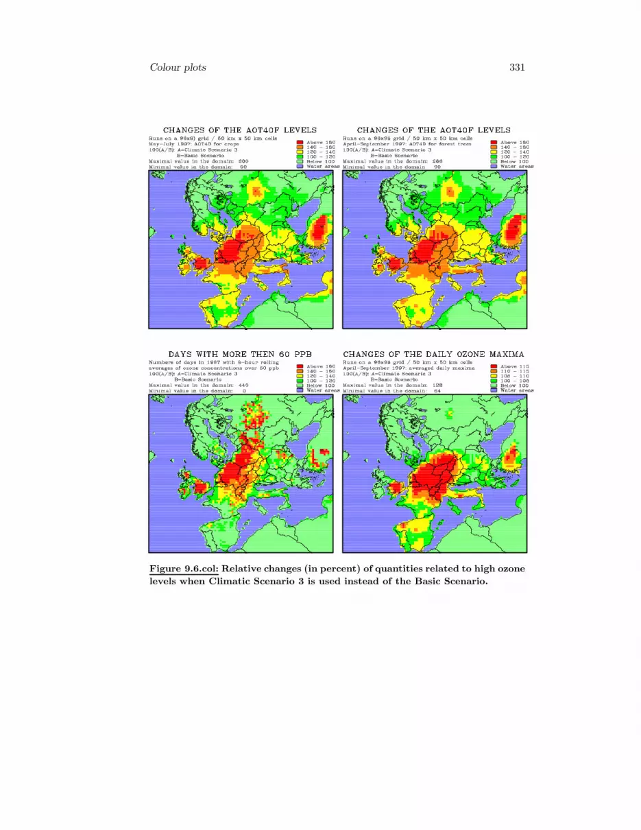
Colour plots 331
Figure 9.6.col: Relative changes (in percent) of quantities related to high ozone
levels when Climatic Scenario 3 is used instead of the Basic Scenario.

332 Appendix A
Figure 10.1.col: Computing the gradient of Jc0 when observations infive time-points are available.

Bibliography
[1] Ackermann, I., Hass, H., Memmesheimer, M., Ebel, A., Binkowski, F. S. andShankar, U. (1998). Modal aerosol dynamics model for Europe: developmentand first applications. Atmospheric Environment, 32: 2981-2999.
[2] Ackermann, I., Hass, H., Schell, B. and Binkowski, F. S. (1999). Regionalmodelling of particulate matter with MADE. Environmental Managementand Health, 10: 201-208.
[3] Akella, S. and Navon, I. M. (2004). Documentation of the TLM and ad-joint models of the Lin-Rood spherical shallow water finite volume model.Report. CSIT and Department of Mathematics, Florida State University,Tallahassee, Florida, USA.
[4] Alekseev, A. K. and Navon I. M. (2005). A posteori pointwise error esti-mation for compressible fluid flows using adjoint parameters and Lagrangeremainder. International Journal for Numerical Methods in Fluids, 47: 45-74.
[5] Alexandrov, V., Owczarz, W., Thomsen, P. G. and Zlatev, Z. (2004). Paral-lel runs of a large air pollution models on a grid of SUN computers. Math-ematics and Computers in Simulations, 65: 557-577.
[6] Alexandrov, V., Sameh, A., Siddique, Y. and Zlatev, Z. (1997). Numeri-cal integration of chemical ODE problems arising in air pollution models.Environmental Modelling and Assessment, 2: 365-377.
[7] Aloyan, A. E. (1999). Modelling of global and regional transport and trans-formation of air pollutants. In: Large Scale Computations in Air PollutionModelling (Zlatev, Z. Brandt, J. Builtjes, P. J. H., Carmichael, G., Dimov,I. Dongarra, J., van Dop, H., Georgiev, K. Hass, H. and San Jose, R.,eds.), pp. 15-24. NATO Science Series, 2. Environmental Security - Vol. 57.Kluwer Academic Publishers, Dordrecht-Boston-London.
[8] Amann, M., Bertok, I., Cofala, J., Gyarfas, F., Heyes, C., Klimont, Z.,Makowski, M., Schopp, W. and Syri, S. (1999). Cost-effective control of
333

334 Bibliography
acidification and ground-level ozone. Seventh Interim Report, IIASA (In-ternational Institute for Applied System Analysis), Laxenburg, Austria.
[9] Ambelas Skjøth, C., Bastrup-Birk, A., Brandt, J. and Zlatev, Z. (2000).Studying variations of pollution levels in a given region of Europe during along time-period. Systems Analysis Modelling Simulation, 37: 297-311.
[10] Anastasi, C., Hopkinson, L. and Simpson, V. J. (1991). Natural hydrocarbonemissions in the United Kingdom. Atmospheric Environment, 25A: 1403-1408.
[11] Anderson, E., Bai, Z, Bischof, C, Demmel, J, Dongarra, J., Du Croz,J., Greenbaum, A., Hammarling, S., McKenney, A., Ostrouchov, S. andSorensen, D. (1992). LAPACK: Users’ Guide. SIAM, Philadelphia.
[12] Andersson-Skold, Y. and Simpson, D. (1999). Comparison of the chemicalschemes of the EMEP MSC-W and IVL photochemical trajectory models.Atmospheric Environment, 33: 1111-1129.
[13] Axelsson, O. and Barker, V. A. (1984). Finite element solution of boundaryvalue problems. Academic Press, Orlando, Florida, USA.
[14] Bagrinovskii, K. A. and Godunov, S. K. (1957). Difference schemes formultidimensional problems. Dokl. Akad. Nauk USSR, 115: 431-433.
[15] Barrett, R., Berry, M., Chan, T. F., Demmel, J., Donato, J., Dongarra, J.,Eijkhout, V., Pozo, R., Romine, C. and van der Vorst, H. (1994). Templatesfor the Solution of Linear Systems: Building Blocks for Iterative Methods.SIAM, Philadelphia.
[16] Bartholy, J., Farago, I. and Havasi, A. (2001). Splitting method and itsapplication in air pollution modelling. IDOJARAS, 105: 39-58.
[17] Bartnicki, J., Olendrzynski, K., Jonson, J. E. and Unger, S. (1998) Descrip-tion of the Eulerian Acid Deposition Model. In: EMEP/MSC-W Report1/98, Appendix A2. Meteorological Synthesizing Centre-West, NorwegianMeteorological Institute, P. O. Box 43-Blindern, N0313 Oslo 3, Norway.
[18] Bastrup-Birk, A., Brandt, J., Uria, I. and Zlatev, Z. (1997). Studying cu-mulative ozone exposures in Europe during a seven-year period. Journal ofGeophysical Research, 102: 23917-23935.
[19] Bastrup-Birk, A., Brandt, J. and Zlatev, Z. (1998). Using partitioned ODEsolvers in large air pollution models. Systems Analysis Modelling Simula-tion, 32: 3-17.
[20] Belitzkii, G. R. and Ljubich, Ju. I. (1984). Matrix norms and their applica-tions. Naukova Dumka, Kiev (in Russian).
Bibliography 335
[21] Binkowski, F. and Shankar, U. (1995). The regional particulate model 1:Model description and preliminary results. Journal of Geophysical Research,100: 26191-26209.
[22] Borrell, P, Borrell, P. M. and Seiler, W. (1990). Transport and Transfor-mation of Pollutants in the Troposphere. SPB Academic Publishing, TheHague.
[23] Botchev, M., Farago, I. and Havasi, A. (2004). Testing weighted splittingschemes on a one-column transport-chemistry model. International Journalof Environmental Pollution, 22 (No. 1-2): 3-16.
[24] Bott, A. (1989) A positive definite advection scheme obtained by nonlinearrenormalization of the advective fluxes. Monthly Weather Review, 117:1006-1015.
[25] Bouchet, V. S., Laprise, R., Torlaschi, E. and McConnel, J. C. (1999).Studying ozone climatology with a regional climate model 1. Model descrip-tion and evaluation. Journal of Geophysical Research, 104: 30351-30371.
[26] Bouchet, V. S., Laprise, R., Torlaschi, E., McConnel, J. C. and Plummer,D. A. (1999). Studying ozone climatology with a regional climate model 2.Climatology. Journal of Geophysical Research, 104: 30373-30385.
[27] Brandt, J., Christensen, J., Frohn L. M., Berkowicz, R. and Zlatev, Z.(2000). Optimization of operational air pollution forecast modelling fromEuropean to local scale. In: Global and Regional Atmospheric Modelling(Barone, G., Builtjes, P. J. H. Giunta, G., eds.), pp. 269-279. Annalli, Fa-colta di Scienze Nautiche, Instituto Universario Navale, Napoli, Italy.
[28] Brandt, J., Christensen, J. and Zlatev, Z. (1999). Real time predictions oftransport, dispersion and deposition from nuclear accidents. EnvironmentalManagement and Health, 10: 216-223.
[29] Brandt, J., Wasniewski, J. and Zlatev, Z. (1996). Handling the chemicalpart in large air pollution models. Appl. Math. and Comp. Sci., 6: 101-121.
[30] Brenan, K., Campbell, S. and Petzold, L. (1996). Numerical solution of ini-tial value problems in differential-algebraic equations. SIAM, Philadelphia.
[31] Brost, R. A. (1988) The sensitivity to input parameters of atmospheric con-centrations simulated by a regional chemical model. Journal of GeophysicalResearch, 93: 2371-2387.
[32] Brown, J., Wasniewski J. and Zlatev, Z. (1995). Running air pollution mod-els on massively parallel machines. Parallel Computing, 21: 971-991.

336 Bibliography
[33] Bruegge, B., Riedel, E. Russell, A., Segall, E. and Steenkiste, P. (1995).Heterogeneous distributed environmental modelling. SIAM News, No. 28.
[34] Builtjes, P. J. H. (1992). The LOTOS - LOng Term Ozone Simulationproject. TNO Report No. R92/240. TNO (Institute of Environmental Sci-ences, Energy Research and Process Information), P. O. Box 342, 7300 AHApeldoorn, The Netherlands.
[35] Builtjes, P. J. H. (1999). The EUROTRAC contribution to the develop-ment of tools for the study of environmentally relevant trace constituents.In: Photo-oxidants, Acidification and Tools: Policy Applications of EURO-TRAC Results (Borrell, P., Builtjes, P., Grennfelt, P. and Hov, Ø., eds.),pp. 143-194. Springer, Berlin.
[36] Burrage, K. (1995). Parallel and sequential methods for ordinary differentialequations. Oxford University Press, Oxford-New York.
[37] Butcher, J. C. (1987). The numerical analysis of ordinary differential equa-tions. Runge-Kutta methods and general linear methods. Wiley, New York.
[38] Carmichael, G. R. and Peters, L. P. (1984). An Eulerian transport-transformation-removal model for SO2 and sulphate: I. Model development.Atmospheric Environment, 18: 937-952.
[39] Carmichael, G. R., Peters, L. P. and Kitada, T. (1986). A second gener-ation model for regional-scale transport-chemistry-deposition. AtmosphericEnvironment, 20: 173-188.
[40] Carmichael, G. R., Sandu, A., Potra, F. A., Damian, V. and Damian, M.(1996). The current state and the future directions in air quality modeling.Systems Analysis Modelling Simulation, 25: 75-105.
[41] Carmichael, G. R., Sandu, A., Song, C. H., He, S. Phandis, M. J., Daescu,D., Damian-Iordache, V. and Potra, F. A. (1999). Computational challengesof modelling interactions between aerosol and gas phase processes in large-scale air pollution models. In: Large Scale Computations in Air PollutionModelling (Zlatev, Z. Brandt, J. Builtjes, P. J. H., Carmichael, G., Dimov,I. Dongarra, J., van Dop, H., Georgiev, K. Hass, H. and San Jose, R.,eds.), pp. 99-136. NATO Science Series, 2. Environmental Security - Vol.57. Kluwer Academic Publishers, Dordrecht-Boston-London.
[42] Chang, J. S., Brost, R. A., Isaksen, I. S. A., Madronich, S., Middleton,P., Stockwell, W. R. and Walcek, C. J. (1987). A three dimensional Eule-rian acid deposition model: Physical concepts and formulation. Journal ofGeophysical Research, 92: 14691-14700.
[43] Chock, D. P. (1985). A comparison of numerical methods for solving advec-tion equations - II. Atmospheric Environment, 19: 571-586.

Bibliography 337
[44] Chock, D. P. (1991). A comparison of numerical methods for solving advec-tion equations - III. Atmospheric Environment, 25A: 853-871.
[45] Chock, D. P. and Dunker, A. M. (1983). A comparison of numerical methodsfor solving advection equations - I. J. Comp. Phys., 19: 571-586.
[46] Chock, D. P., Winkler, S. L. and Sun, P. (1994). Comparison of stiff chem-istry solvers for air quality models. Environ. Sci. Technol., 28: 1882-1892.
[47] Cichota, R., Elias, E. A. and Lier, Q. J. van. (2004). Testing a finite-difference model for soil hear transfer by comparing numerical and analyticalsolutions. Environmental Modelling & Sortware, 19: 495-506.
[48] Crowley, W. P. (1968). Numerical advection experiments. Monthly WeatherReview, 96: 1-11.
[49] Csomos, P., Farago, I. and Havasi, A. (2005). Weighted sequential splittingsand their analysis. Comput. Math. Appl. (to appear).
[50] Dabdub, D. and Manohar, R. (1997). Performance and portability of an airpollution model. Parallel Computing, 23: 2187-2200.
[51] Dabdub, D. and Seinfeld, J. H. (1994). Numerical advective schemes usedin air quality models - sequential and parallel implementation. AtmosphericEnvironment, 29: 403-410.
[52] Dabdub, D. and Seinfeld, J. H. (1996). Parallel computation in atmosphericchemical modelling. Parallel Computing, 22: 111-130.
[53] Daescu, D. N. and Carmichael, G. R. (2003). An adjoint sensitivity methodfor the adaptive location of the observations in air quality modeling. Journalof the Atmospheric Sciences, 60: 434-450.
[54] Daescu, D. N. and Navon, I. M. (2003). An analysis of a hybrid optimizationmethod for variational data assimilation. International Journal of Compu-tational Fluid Dynamics, 17: 299-306.
[55] Daescu, D. N., Sandu, A. and Carmichael, G. R. (2003). Direct and adjointsensitivity analysis of chemical kinetic systems with KKP: II. Numerical;validation and applications. Atmospheric Environment, 37: 5097-5114.
[56] Dahlquist, G. (1963). A special stability problem for linear multistep meth-ods. BIT, 3: 27-43.
[57] D’Ambra, P., Barone, G., di Serafino, D., Giunta, G., Murli, A. and Riccio,A. (1999). PNAM: parallel software for air quality simulations in the Naplesarea. Environmental Management and Health, 10: 209-215.

338 Bibliography
[58] Davis, T. A. and Davidson, E. S. (1988). Pairwise reduction for the directparallel solution of sparse unsymmetric sets of linear equations. IEEE Trans.Comput., 37: 1648-1654.
[59] Davis, T. A. and Yew, P.-C. (1990). A nondeterministic parallel algorithmfor general unsymmetric sparse LU factorization. SIAM J. Matrix Anal.Appl., 3: 383-402.
[60] Demmel, J. W. (1997). Applied Numerical Linear Algebra. SIAM, Philadel-phia.
[61] Demmel, J. W., Eisenstat, S. C., Gilbert, J. R., Li, X. S. and Liu, J. W. H.(1999). A supernodal approach to sparse partial pivoting. SIAM Journal ofMatrix Analysis and Applications, 20: 720-755.
[62] Demmel, J. W., Gilbert, J. R. and Li, X. S. (1999). An asynchronous par-allel supernodal algorithm for sparse Gaussian elimination. SIAM Journalof Matrix Analysis and Applications, 20: 915-952.
[63] Deuflhard, P. (1983). Order and stepsize control in extrapolation methods.Numerische Mathematik, 41: 399-422.
[64] Deuflhard, P. (1985). Recent progress in extrapolation methods for ordinarydifferential equations. SIAM Review, 27: 505-535.
[65] Deuflhard, P., Hairer, E. and Zugch, M. (1987). One step and extrapolationmethods for differential-algebraic equations. Numerische Mathematik, 51:501-516.
[66] Deuflhard, P. and Nowak, U. (1986). Efficient numerical simulation andidentification of large reaction systems. Ber. Bensendes Phys. Chem., 90:940-946.
[67] Deuflhard, P., Nowak, U. and Wulkow, M. (1990). Recent development inchemical computing. Computers Chem. Engng., 14: 1249-1258.
[68] Dimov, I., Farago, I., Havasi, A. and Zlatev, Z. (2001). Commutativity ofthe operators in splitting methods for air pollution models. Annalles Univ.Sci. Budapest., 44: 129-150.
[69] Dimov, I., Farago, I., Havasi, A. and Zlatev, Z. (2004). Operator splittingand commutativity analysis in the Danish Eulerian Model. Mathematics andComputers in Simulation, 67: 217-233.
[70] Dimov, I., Farago, I. and Zlatev, Z. (2003). Parallel computations with large-scale air pollution models. Problems in Programming, 5(3): 44-52.

Bibliography 339
[71] Dimov, I., Georgiev, K., Ostromsky, Tz. and Zlatev, Z. (2004). Computa-tional challenges in the numerical treatment of large air pollution models.Ecological modelling, 179: 187-203.
[72] Dimov, I., Geernaert, G. and Zlatev, Z. (2003). Influence of fu-ture climate changes in Europe on ozone critical levels. In: Proceed-ings of Nordic Meteorological Meeting 23 (Joergensen, H. E., ed.).http://www.dams.dk/nmm2002/proceedings.htm
[73] Dimov, I., Ostromsky, Tz., Tzvetanov, I. and Zlatev, Z. (1999). Economicalestimations of the losses of crops due to high ozone levels. AgriculturalEconomics and Management, 5: 48-52.
[74] Dimov, I. and Zlatev, Z. (1999). Testing the sensitivity of air pollutionlevels to variations of some chemical rate constants. In: Large-Scale Scien-tific Computations and Environmental Problems (Griebel, M., Iliev, O. P.,Margenov, S. D. and Vassilevski, P. S., eds.), pp. 167-175. Vieweg, Braun-schweig/Wiesbaden.
[75] Dimov, I. and Zlatev, Z. (2002). Optimization problems in air pollutionmodelling. In: Handbook on Applied Optimization (Pardalos, P. M. andResende, M. G. C., eds.), pp. 943-956. Oxford University Press, Oxford-New York.
[76] Djouad, R. and Sportisse, B. (2003). Solving reduced chemical models in airpollution modelling. Applied Numerical Mathematics, 44: 49-61.
[77] Dongarra, J. J., Moler, C. B., Bunch, J. R. and Stewart, G. W. (1979).LINPACK Users’ Guide. SIAM, Philadelphia, 1979.
[78] Dongarra, J. J., Du Croz, J. Duff, I. S. and Hammarling, S. (1988). Anextended set of FORTRAN Basic Linear Algebra Subprograms. ACM Trans-action on Mathematical Software, 14: 1-17.
[79] Dongarra, J. J., Du Croz, J. Duff, I. S. and Hammarling, S. (1990). Anextended set of FORTRAN Basic Linear Algebra Subprograms. ACM Trans-action on Mathematical Software, 16: 18-28.
[80] Dongarra, J. J., Duff, I. S., Sorensen, D. C. and van der Vorst, H. A.(1998). Numerical Linear Algebra for High-Performance Computers. SIAM,Philadelphia.
[81] Duff, I. S., Erisman, A. M. and Reid, J. K. (1986). Direct methods for sparsematrices. Oxford University Press, Oxford-London.
[82] Duff, I. S., Marone, M., Radicati, G. and Vittoli, C. (1997). Level 3 Ba-sic Linear Algebra Subprograms for sparse matrices: a user level interface.ACM Transaction on Mathematical Software, 23: 379-401.

340 Bibliography
[83] Dyakonov, E. G. (1962). Difference schemes with splitting operators for mul-tidimensional stationary problems. Journal of Computational Mathematicsand Mathematical Physics, 2(4): 57-79 (in Russian).
[84] Ebel, A. (2000). Chemical Transfer and Transport Modelling. In: Transportand Chemical Transformation of Pollutants in the Troposphere (Borrell, P.and Borrell, P. M., eds.), pp. 85-128. Springer, Berlin.
[85] Ebel, A., Memmesheimer, M. and Jacobs, H. (1997). Regional modellingof tropospheric ozone distributions and budgets. In: Atmospheric OzoneDynamics: I. Global Environmental Change, (Varotsos, C., ed.), pp. 37-57.NATO ASI Series, Vol. 53. Springer, Berlin.
[86] Eirola, T. and Nevanlinna, O. (1989). Accelerating with rank-one updates.Lin. Alg. Appl., 121: 511-520.
[87] Elbern, H. (1997). Parallelization and load balancing of a comprehensiveatmospheric chemistry model. Atmospheric Environment, 31: 3561-3574.
[88] Elbern, H. and Schmidt, H. (1999). A four-dimensional variational chem-istry data assimilation scheme for Eulerian chemistry transport modelling.Journal of Geophysical Research, 104: 18583-18598.
[89] Elbern, H. and Schmidt, H. (2002). 4D-var data assimilation and its nu-merical implications for case study analyses. In: Atmospheric Modeling,(Chock, D. P. and Carmichael, G. R., eds.), pp. 165-183. Springer, NewYork.
[90] Elbern, H., Schmidt, H. and Ebel, A. (1997). Variational data assimilationfor tropospheric chemistry modelling. Journal of Geophysical Research, 102:15967-15985.
[91] Elbern, H., Schmidt, H. and Ebel, A. (1999). Implementation of a paral-lel 4D-variational chemistry data-assimilation scheme. Environmental Man-agement and Health, 10: 236-244.
[92] Elbern, H., Schmidt, H., Talagrand, O. and Ebel, A. (2000). 4D-variationaldata assimilation with an adjoint air quality model for emission analysis.Environmental Modelling & Software, 15: 539-548.
[93] EMEP (1998). Transboundary acidifying air pollution in Europe: Part 1,Estimated dispersion of acidifying and eutrofying compounds and compari-son with observations. Status Report 1/98. EMEP MSC-W (MeteorlogicalSynthesizing Centre - West), Norwegian Meteorological Institute, P. O. Box43 - Blindern, N-0313 Oslo, Norway.
[94] EMEP Home Page. (2005). http//www.emep.int.

Bibliography 341
[95] European Commission (1999). Ozone position paper. European Commis-sion, Directorate XI: ”Environment, Nuclear Safety and Civil Protection”,Brussels.
[96] European Parliament (2002). Directive 2002/3/EC of the European Parlia-nent and the Council of 12 February 2002 relating to ozone in ambient air.Official Journal of the European Communities, L67, 9.3.2002, pp. 14-30.
[97] Farago, I. and Havasi, A. (2002). The mathematical background of opera-tor splitting and the effect of non-commutativity. In: Large Scale ScientificComputations III (Margenov, S., Yalamov P. and Wasniewski, J. eds.), pp.264-271. Springer, Berlin.
[98] Farago, I. and Havasi, A. (2005) On the convergence and local splitting errorof different splitting schemes. Progress in Computational Fluid Dynamics,to appear.
[99] Farago, I., Havasi, A. and Georgiev, K. (2005) Advances in Air PollutionModelling for Environmental Security. Springer, Berlin.
[100] Farago, I., Havasi A. and Korotov, S. (2002) Mathematical analysis of theweighted splitting. Technical Report, University of Jyvaskyla.
[101] Fingas, M. F. (1995). A literature review of the physics and predictive mod-elling of oil spill evaporation. Journal of Hazardous Materials, 42: 157-175.
[102] Fletcher, R. (1972) FORTRAN subroutines for minimization by quasi-Newton methods. Report No. R7125, A.E.R.E, Harwell, England.
[103] Fornberg, B. (1975). On a Fourier method for the integration of hyperbolicequations. SIAM J. Numer. Anal., 12: 509-528.
[104] Fornberg, B. (1996). A practical guide to pseudospectral methods. CambridgeMonographs on Applied and Computational Mathematics. Cambridge Uni-versity Press, Cambridge.
[105] Foster, I. and Kesselman, C. (1998). Computational Grids. In: The Grid:Blueprint for a New Computing Infrastructure (Foster, I. and Kesselman,C., eds.), pp. 15-52. Morgan Kaufmann Publishers, San Francisco, Califor-nia.
[106] Foster, I., Kesselman, C. and Tuecke, S. (2001). The Anatomy of the Grid:Enabling Scalable Virtual Organizations. Intl. J. Supercomputer Applica-tions, 15(3): 1-25.
[107] Freund, R. W. (1993). A transpose-free quasi-minimal residual algorithm fornon-Hermitian linear systems. SIAM J. Sci. Statist. Comput., 14: 470-482.
342 Bibliography
[108] Friedrich, R. (1997). Tropospheric modelling and emission estimation.Springer-Verlag, Berlin, pp. 179-357.
[109] Forster, C., Stohl, A., James, P. and Thouret, V. (2003) The residence timesfor aircraft emissions in the stratosphere and emissions along actual flighttracks. Journal of Geophysical Research, 108, No. D12, 8524.
[110] Gallivan, K., Hansen, P. C., Ostromsky, Tz. and Zlatev, Z. (1995). A locallyoptimized reordering algorithm and its application to a parallel sparse linearsystem solver. Computing, 54: 39-67.
[111] Gallivan, K. A., Sameh, A. H. and Zlatev, Z. (1990). A parallel hybrid sparselinear system solver, Computing Systems in Engineering, 1: 183-195.
[112] Geernaert, G. and Zlatev, Z. (2002). Testing the influence of the biogenicemissions on high ozone levels in Denmark and in Europe. In: Proceedingsfrom the EUROTRAC-2 Symposium 2002 (Midgley, P. M. and Reuther,M., eds.). Margraf Verlag, Weikersheim.
[113] Geernaert, G. and Zlatev, Z. (2004). Studying the influence of biogenic emis-sions on AOT40 values in Europe. International Journal of Environmentand Pollution, 22 (No. 1-2): 29-42.
[114] Geist, A., Beguelin, A. Dongarra, J., Jiang, W., Manchek, R. and Sun-deram, V. (1994). PVM: Parallel Virtual Machine, A User’s Guide andTutorial for Networking Parallel Computing. MIT Press, Cambridge, Mas-sachusetts.
[115] George, J. A. and Ng, E. (1985). An implementation of Gaussian elimina-tion with partial pivoting for sparse systems. SIAM J. Sci. Statist. Comput.,6: 390-405.
[116] Georgiev, K. and Zlatev, Z. (1998). Running an advection-chemistry codeon message passing computers. In: Recent Advances in Parallel VirtualMachine and Message Passing Interface (Alexandrov, V. and Dongarra, J.,eds.), pp. 354-363. Springer, Berlin.
[117] Georgiev, K. and Zlatev, Z. (2000). Parallel Sparse Matrix Algorithms forAir Pollution Models. Parallel and Distributed Computing Practices, 2: 429-442.
[118] Gery, M. W., Whitten, G. Z., Killus, J. P. and Dodge, M. C. (1989). Aphotochemical kinetics mechanism for urban and regional modeling. Journalof Geophysical Research, 94: 12925-12956.
[119] Gilbert, J. R. and Peierls, T. (1988). Sparse partial pivoting in time propor-tional to arithmetic operations. SIAM J. Sci. Statist. Comput., 9, 862-874.

Bibliography 343
[120] Gill, P. E. and Murray. W. (1979). Conjugate-gradient methods for large-scale nonlinear optimization. Technical Report SOL 79-15. Department ofOperations Research, Stanford University, Stanford, California, USA.
[121] Gill, P. E., Murray. W. and Wright, M. H. (1981). Practical Optimization.Academic Press, New York.
[122] Golub, G. H. and Van Loan, C. F. (1983). Matrix computations JohnsHopkins University Press, Baltimore, Maryland.
[123] Grid Computing Info Centre: GRID Infoware. (2005) Grid Computing InfoCentre Newsletter. http://www.gridcomputing.com/.
[124] Gropp, W., Lusk, E. and Skjellum, A. (1994). Using MPI: Portable pro-gramming with the message passing interface. MIT Press, Cambridge, Mas-sachusetts.
[125] Gupta, I., Dhage, S., Chandorkar, A. A. and Srivastav, A. (2004). Numericalmodeling for Thane creek. Environmental Modelling & Software 19: 571-579.
[126] Hairer, E., Nørsett, S. P. and Wanner, G. (1987). Solving Ordinary Dif-ferential Equations, I: Nonstiff Problems. Springer, Berlin-Heidelberg-NewYork-London.
[127] Hairer, E. and Wanner, G. (1991). Solving Ordinary Differential Equations,II: Stiff and Differential-algebraic Problems. Springer, Berlin-Heidelberg-New York-London.
[128] Harrison, R. M., Zlatev, Z. and Ottley, C. J. (1994). A comparison of thepredictions of an Eulerian atmospheric transport chemistry model with mea-surements over the North Sea. Atmospheric Environment, 28: 497-516.
[129] Hass, H., Ebel, A., Feldmann, H., Jacobs, H. J. and Memmesheimer, M.(1993). Evaluation studies with a regional chemical transport model (EU-RAD) using air quality data from the EMEP monitoring network. Atmo-spheric Environment, 27A: 867-887.
[130] Hass, H., Jacobs, H. J. and Memmesheimer, M. (1995). Analysis of a re-gional model (EURAD) near surface gas concentration predictions usingobservations from networks. Atmos. Phys., 57: 173-200.
[131] Havasi, A. and Zlatev, Z. (2002). Trends of Hungarian air pollution levelson a long time-scale. Atmospheric Environment, 36: 4145-4156.
[132] Henrici, P. (1962). Discrete variable methods in ordinary differential equa-tions. Wiley, New York.

344 Bibliography
[133] Hertel, O. Ambelas Skøth, C., Frohn, L. M., Vignati, E., Frydendall, J., deLeeuw, G., Schwarz, U. and Reis, S. (2002). Assessment of the atmosphericnitrogen and sulphur inputs into the North Sea using a Lagrangian model.Physics and Chemistry of the Earth, 27: 1507-1515.
[134] Hertel, O., Berkowicz, R., Christensen, J. and Hov Ø. (1993). Test of twonumerical schemes for use in atmospheric transport-chemistry models. At-mospheric Environment, 27A: 2591-2611.
[135] Hesstvedt, E., Hov, Ø. and Isaksen, I. A. (1978). Quasi-steady-state approx-imations in air pollution modelling: Comparison of two numerical schemesfor oxidant prediction. International Journal of Chemical Kinetics, 10: 971-994.
[136] Hjellbrekke, A. G. (1995). Ozone measurements 1990-1992. EMEP/CCCReport 4/95, Norwegian Institute for Air Research (NILU), POSTBOKS64, N-2001 Lillestøm, Norway.
[137] Holm, E. and Erbes, G. (1991). Solving the advection equation in flows withsharp gradients using Bott’s flux scheme. Report No. DM-59. Departmentof Meteorology, Stockholm University, Stockholm.
[138] Hongisto, M. (2003). HILATAR, a limited area simulation model for acidcontaminants. Part I. Model description and verification. Atmospheric En-vironment, 37: 1535-1447.
[139] Hongisto, M., Sofiev, M. and Joffre, S. (2003). HILATAR, a limited areasimulation model for acid contaminants. Part II. Long-term simulation re-sults. Atmospheric Environment, 37: 1549-1560.
[140] Houghton, J. T., Ding, Y., Griggs, D. J., Noguer, M., van der Linden, P.J., Dai, X., Maskell, K. and Johnson, C. A., eds. (2001). Climate Change2001: The Scientific Basis. Cambridge University Press, Cambridge-NewYork-Melbourne-Madrid-Cape Town.
[141] Hov, Ø., Zlatev, Z., Berkowicz, R., Eliassen, A. and Prahm, L. P. (1988).Comparison of numerical techniques for use in air pollution models withnon-linear chemical reaction. Atmospheric Environment, 23: 967-983.
[142] Hundsdorfer, W. and Verwer, J. G. (2003) Numerical solution of time-dependent advection-diffusion-reaction equations. Springer, Berlin.
[143] Jacobson, M. Z. and Turco, R. P. (1994). SMVGEAR: a sparse-matrix,vectorized Gear code for atmospheric models. Atmospheric Environment,28: 273-284.
[144] Jaffe, A. (1984). Ordering the universe: The role of mathematics. SIAMRev., 26: 475-488.

Bibliography 345
[145] Jay, L. O., Sandu, A., Potra, F. A. and Carmichael, G. R. (1997). Im-proved QSSA methods for atmospheric chemistry integration. SIAM J. Sci.Comput., 18: 182-202.
[146] Jeltsch, R. and Nevanlinna, O. (1981). Stability of explicit time discretiza-tions for solving initial value problems. Numerische Mathematik, 37: 61-91.
[147] Jennings, A. A. (2003). Modelling sedimentation and scour in small urbanlakes. Environmental Modelling & Software 18: 281,291.
[148] Jonson, J. E., Sundet, J. and Tarrason, L. (2001). Model calculations ofpresent and future levels of ozone and ozone precursors with a global and aregional model. Atmospheric Environment, 35: 525-537.
[149] Jonson, J. E., Tarrason, L. and Sundet, J. (1999). Calculation of ozoneand other pollution for the summer, 1996. Environmental Management andHealth, 10: 245-257.
[150] Kincaid, D., Oppe, T., Respess, J. and Young, D. (1984). ITPACKV 2C:User’s giude. Report No. CNA-191. Center for Numerical Analysis, Univer-sity of Texas at Austin, Austin, Texas.
[151] Kincaid, D., Respess, J., Young, D. and Grimes, R. (1982). Algorithm 586,ITPACKV 2C: A FORTRAN package for solving large sparse systems byadaptive accelerated iterative methods. ACM Trans. Math. Softeware, 8:302-322.
[152] Kreiss, H. O. (1978). Difference methods for stiff ordinary differential equa-tions. SIAM Journal on Numerical Analysis, 15: 21-58.
[153] Kreiss, H. O. and Oliger J. (1972). Comparison of accurate methods for theintegration of hyperbolic equations. Tellus, 24: 199-215.
[154] Kuck, D. J., Davidson, E. S., Lawrie D. and Sameh, A., H. (1986). Parallelsupercomputing today and the CEDAR approach. Science, 231: 967-974.
[155] Lambert, J. D. (1991). Numerical Methods for Ordinary Differential Equa-tions. Wiley, Chichester-New York-Brisbane-Toronto-Singapore.
[156] Langner, J., Robertson, L., Persson, C. and Ullerstig, A. (1998). Validationof the operational emergency response model at the Swedish Meteorologicaland Hydrological Institute using data from ETEX and the Chernobyl acci-dent. Atmospheric Environment, 32: 4325-4333.
[157] Lanser, D. and Verwer, J. G. (1999). Analysis of operators splitting inadvection-diffusion-reaction problems in air pollution modelling. Journal ofComputational and Applied Mathematics, 111: 201-216.

346 Bibliography
[158] Lawson, C., Hanson, R., Kincaid, D. and Krogh, F. (1979). Basic Linear Al-gebra Subprograms for Fortran usage. ACM Transactions on MathematicalSoftware, 5: 308-323.
[159] Le Dimet, F.-X., Navon, I. M. and Daescu, D. N. (2002). Second orderinformation in data assimilation. Monthly Weather Review, 130: 629-648.
[160] Lee H, N. (1981). An alternative pseudospectral model for pollutant trans-port, diffusion and deposition in the atmosphere. Atmospheric Environment,15: 1017-1024.
[161] Lee, H. S., Matthews, C. J., Braddock, R. D., Sander, G. C. and Gandola,F. (2004) A MATLAB method of lines template for transport equations.Environmental Modelling & Software, 19: 603-614.
[162] LeVeque, R. J. (1992). Numerical methods for conservation laws. LectureNotes in Mathematics, ETH Zurich, Birkhauser Verlag, Basel.
[163] LeVeque, R. J. (1992). Finite volume methods for hyperbolic problems. Cam-bridge Texts in Applied Mathematics, Cambridge University Press, Cam-bridge.
[164] Lewis, J. M. and Derber, J. C. (1985). The use of adjoint equations to solvea variational adjustment problem with advective constraints. Tellus, 37A:309-322.
[165] Li, X. S. and Demmel, J. W. (1999). Super LU DIST: A scalable distributed-memory sparse direct solver for unsymmetric linear system. ACM Transac-tions on Mathematical Software, 29: 110-140.
[166] Li, Z. and Navon, I. M. (2001). Optimality of 4D-Var and its relationshipwith the Kalman filter and the Kalman smoother. Quarterly Journal of theRoyal Meteorological Society, 127B: 661-684.
[167] Loon, M. van, (1993). Testing interpolation and filtering techniques in con-nection with a semi-Lagrangian method. Atmospheric Environment, 27A:2351-2364.
[168] Losinskii, S. M. (1958). Error estimates in the numerical integration of or-dinary differential equations. Communications of the High Schools - Math-ematics, 5(6): 52-90 (in Russian)
[169] Lubkert, B. and Schopp, W. (1989). A model to calculate natural V OCemissions from forests in Europe. Report WP-89-082, International Insti-tute for Applied System Analysis (IIASA), Laxenburg, Austria.
[170] Lyness, J. N. (1974). Computational techniques based on the Lanczos trans-formation. Mathematics of Computation, 28: 81-123.
Bibliography 347
[171] Mao, X., Prommer, H., Barry, D. A., Langevin, C. D., Panteleit, B. and Li,L. (2005). Three-dimensional model for multi-component reactive transportwith variable density groundwater flow. Environment Modelling & Software,to appear (available on line at www.sciencedirect.com).
[172] Marchuk, G. I. (1968). Some application of splitting-up methods to the so-lution of mathematical physics problems. Applik. Mat., 13(2).
[173] Marchuk, G. I. (1980). Methods of computational mathematics. Nauka,Moscow, 1980.
[174] Marchuk, G. I. (1982). Mathematical Modeling for the Problem of the En-vironment. Nauka, Moscow (in Russian).
[175] Marchuk, G. I. (1986). Mathematical modelling for the problem of the envi-ronment. Studies in Mathematics and Applications, No. 16, North-Holland,Amsterdam.
[176] Marchuk, G. I. (1988). Methods of Splitting. Nauka, Moscow, (in Russian).
[177] Marchuk, G. I. (1994). Applications of Adjoint Equations to Problems ofGlobal Change and Environmental Protection. In: Proceedings of HER-MIS’94, Vol. 1, (E.A. Lipitakis, ed.), pp. 1-20. Hellenic Mathematical Soci-ety, Athens.
[178] Marchuk, G. I. (1995): Adjoint equations and analysis of complex systems.Kluwer Academic Publishers, Dordrecht.
[179] Marchuk, G. I., Agoshkov, P. V. and Shutyaev, I. V. (1996). Adjoint equa-tions and perturbation algorithms in nonlinear problems. CRC Press, NewYork.
[180] Markowitz, H. M. (1957). The elimination form of the inverse and its ap-plications to linear programming. Management Science, 3: 255-267.
[181] McRae, G. J., Goodin, W. R. and Seinfeld, J. H. (1982). Numerical solutionof the atmospheric diffusion equations for chemically reacting flows. Journalof Computational Physics, 45: 1-42.
[182] Merilees, P. E. (1974). Numerical experiments with the pseudospectralmethod in spherical coordinates. Atmosphere, 12:77-96.
[183] Molenkampf, C. R. (1968). Accuracy of finite-difference methods applied tothe advection equation. Journal of Applied Meteorology, 7: 160–167.
[184] Morel, P., Lefevre, G. and Rabreau, G. (1971). On initialization and non-synoptic data assimilation. Tellus, 23: 197-206.

348 Bibliography
[185] NAG Library Fortran Manual (1979). Mark 7, Vol. 3-4. Numerical Algo-rithms Group (NAG), Banbury Road 7, Oxford, England.
[186] NAG Library Fortran Manual (2004). E04 - minimizing and maximizinga function. http://www.nag.co.uk. Numerical Algorithms Group (NAG),Banbury Road 7, Oxford, England.
[187] Odman, M. T., Kumar, N. and Russell, A. G. (1992). A comparison of fastchemical kinetic solvers for air quality modeling. Atmospheric Environment,26A: 1783-1789.
[188] Owczarz, W. and Zlatev, Z. (2000). Running a large-scale air pollutionmodel on fast super computer. In: Atmospheric Modeling (Chock, D. P.and Carmichael, G. R., eds.), pp. 185-204. Spinger, Berlin.
[189] Owczarz, W. and Zlatev, Z. (2001). Running a large air pollution model onan IBM SMP computer. International Journal of Computer Research, 10:485-500.
[190] Owczarz, W. and Zlatev, Z. (2002). Parallel matrix computations in airpollution modelling. Parallel Computing, 28: 355-368.
[191] Penenko V. V. and Obraztsov, N. N. (1976). A variational initializationmodel for the fields of meteorological elements. Soviet Meteorol. Hydrol.,11: 1-11.
[192] Pepper, D. W. and Baker, A. J. (1979). A simple one-dimensional finite ele-ment algorithm with multidimensional capabilities. Numerical Heath Trans-fer, 3: 81-95.
[193] Pepper, D. W., Kern, C. D. and Long, Jr., P. E. (1979). Modelling the dis-persion of atmospheric pollution using cubic splines and chapeau functions.Atmospheric Environment, 13: 223-237.
[194] Peters, L. K., Berkowitz, C. M., Carmichael, G. R., Easter, R. C., Fair-weather, G., Ghan, S. J., Hales, J. M., Leung, L. R., Pennell, W. R., Potra,F. A., Saylor, R. D. and Tsang, T. T. (1995). The current state and fu-ture direction of Eulerian models in simulating tropospheric chemistry andtransport of trace species: A review. Atmospheric Environment, 29: 189-222.
[195] Pissanetzki, S. (1984). Sparse matrix technology. Academic Press, New York.
[196] Priklonsky, V. I. Reible, D. D. and Tyler, J. M. (2005). Consistent uncon-fined contaminated disposal facilities dike tidal flow and transport model.Environmental Modelling and Software, to appear, (available online onwww.sciencedirect.com).

Bibliography 349
[197] Prommer, H., Barry, D. A. and Zheng, C. (2003). MPDFLOW/MT3DMS-based reactive multicomponent transport modelling. Ground Water, 41: 247-257.
[198] Rancic, M. (1992). Semi-Lagrangian piecewise by parabolic scheme for twodimensional horizontal advection of a passive scalar. Monthly Weather Re-view, 120: 1394-1406.
[199] Rancic, M. and Williamson, D. L. (1991). On shape preserving interpolationand semi-Lagrangian transport. SIAM Journal of Scientific and StatisticalComputing, 4: 656-687.
[200] Reed, M., Johansen, Ø, Brandvik, P. J., Dailing, P., Lewis, A., Fiocco, R.,Mackay, D. and Prentki, R. (1999) Oil spill modelling toward the close of the20th century: overview of the state of the art. Spill Science and TechnologyBulletin, 5: 3-16.
[201] Richtmyer, R. D. and Morton, K. W. (1967). Difference methods for initialvalue problems. Interscience Publishers, New York, 1967.
[202] Roache, P. J. (1971). Computational fluid dynamics. Hermosa, Albu-querque, New Mexico, USA.
[203] Roache, P. J. (1978). A pseudo-spectral FFT technique for non-linear prob-lems. Journal of Computational Physics, 27: 204-220.
[204] Robert, A. J., Yee, T. L. and Ritchie, H. (1985). A semi-Lagrangian andsemi-implicit numerical integration scheme for multi-level atmospheric mod-els. Monthly Weather Review, 113: 388-394.
[205] Robertson, L., Langner, J. and Engardt, M. (1999). An Eulerian limited-area atmospheric transport model. Journal of Applied Meteorology, 38: 190-210.
[206] Rosenbrock, H. H. (1963). Some implicit processes for the numerical solutionof ordinary differential equations. Computer Journal, 5: 329-330.
[207] Saad, Y. and Schultz, M. H. (1986). GMRES: a generalized minimal residualalgorithm for solving nonsymmetric linear systems. SIAM J. Sci. Statist.Comput., 7: 856-869.
[208] Sandnes Lenschow, H. and Tsyro, S. (2000). Meteorological input data forEMEP/MSC-W air pollution models. EMEP Note 2/00. MeteorologicalSynthesizing Centre - West, Norwegian Meteorological Institute, P. O. Box43 - Blindern, N-0313 Oslo 3, Norway.
[209] Sandu, A., Daescu, D. N. and Carmichael, G. R. (2003). Direct and adjointsensitivity analysis of chemical kinetic systems with KKP: I. Theory andsoftware tools. Atmospheric Environment, 37: 5083-5096.

350 Bibliography
[210] Sandu, A., Daescu, D. N., Carmichael, G. R. and Chai, T. (2005). Adjointsensitivity analysis of regional air quality models. Journal of ComputationalPhysics, 2005; to appear.
[211] Sandu, A., Potra, F. A., Carmichael, G. R. and Damian, V. (1996). Efficientimplementation of fully implicit methods for atmospheric chemical kinetics.J. Comp. Phys., 129: 101-110.
[212] Sandu, A., Verwer, J. G., van Loon, M., Carmichael, G. R., Potra, F. A.,Dabdub, D. and Seinfeld, J. H. (1997). Benchmarking stiff ODE systems foratmospheric chemistry problems: I. Implicit versus Explicit. AtmosphericEnvironment, 31: 3151-3166.
[213] Sandu, A., Verwer, J. G., Bloom, J. G., Spee, E. J. and Carmichael, G. R.(1997). Benchmarking stiff ODE systems for atmospheric chemistry prob-lems: II. Rosenbrock solvers. Atmospheric Environment, 31: 3459-3472.
[214] San Jose, R. Rodriguez, M. A., Cortes, E. and Gonzalez, R. M. (1999).EMMA model: an advanced operational mesoscale air quality model forurban and regional environments. Environmental Management and Health,10: 258-266.
[215] Schell, B., Ackermann, I. J., Hass, H., Binkowski, F. S. and Ebel, A. (2001).Modelling the formation of secondary organic aerosol within a comprehen-sive air quality model system. Journal of Geophysical Research, 106: 28275-28293.
[216] Segerlind, L. J. (1976). Applied Finite Element Analysis. Wiley, New York.
[217] Shampine, L. F. (1994). Numerical solution of ordinary differential equa-tions. Chapman and Hall, New York.
[218] Shampine, L. F. and Gordon, M. K. (1975). Computer solution of ordinarydifferential equations: The initial value problem. Freeman, San Francisco.
[219] Sherman, A. H. (1978). Algorithms for sparse Gaussian elimination withpartial pivoting. ACM Trans. Math. Software, 4: 330-338.
[220] Shampine, L. F., Reichelt, M. W. and Kierzenka, J. A. (1999). SolvingIndex-1 DAEs in MATLAB and Simulink. SIAM Rev., 41: 538-552.
[221] Shieh, D. S., Chang, Y. and Carmichael, G. R. (1988). The evaluationof numerical techniques for solution of stiff ordinary differential equationsarising from chemical kinetic problems. Environ. Software, 3: 28-38.
[222] Simpson, D. (1992). Long-period modelling of photochemical oxidants inEurope. Model calculations for July 1985. Atmospheric Environment, 26A:1609-1634.

Bibliography 351
[223] Simpson, D. (1993). Photochemical model calculations over Europe for twoextended summer periods: 1985 and 1989. Model results and comparisonswith observations. Atmospheric Environment, 27A: 921-943.
[224] Simpson, D., Andersson-Skold, Y. and Jenkin, M. E. (1993). Updating thechemical scheme for the EMEP MCD-W oxidant model: current status.EMEP/MSC-W Report 2/93. Meteorological Synthesizing Centre-West,Norwegian Meteorological Institute, P. O. Box 43-Blindern, N0313 Oslo3, Norway.
[225] Simpson, D., Guenther, A., Hewitt, C. N. and Steinbrecher, R. (1995).Biogenic emissions in Europe: I. Estimates and uncertainties. Journal ofGeophysical Research, 100: 22875-22890.
[226] Simpson, D., Tuovinen, J.-P., Emberson, L. D. and Ashmore, M. R. (2003).Characteristics of an ozone deposition module II. densitivity analysis. Wa-ter, Air and Soil Pollution, 143: 123-137.
[227] Skelboe, S. and Zlatev, Z. (1997). Exploiting the natural partitioning in thenumerical solution of ODE systems arising in atmospheric chemistry. In:Numerical Analysis and Its Applications (Vulkov, L., Wasniewski, J. andYalamov, P., eds.), pp. 458-465. Springer, Berlin.
[228] SMP/E Internet Library (2005). http://www-03.ibm.com/servers/eserver/zseries/zos/smpe/smpepubs.html.
[229] Solin, P. Partial differential equations and the finite element method. Wiley,New York, 2005.
[230] Sonneveld, P. (1989). CGS, a fast Lanczos-type solver for nonsymmetriclinear systems. SIAM J. Sci. Statist. Comput., 10: 36-52.
[231] Spaulding, M. L. (1988). A state-of-the-art review of oil spill trajectory andfate modelling. Oil and Chemical Pollution, 4: 39-55.
[232] Stewart, G. W. (1973). Introduction to matrix computations. AcademicPress, New York.
[233] Stockwell, W. R., Kirchner, F. and Kuhn, M. (1997). A new mechanism forregional atmospheric chemistry modelling. Journal of Geophysical Research,102: 25847-25879.
[234] Stockwell, W. R., Middleton, P., Chang, J. S. and Tang, X. (1990). A secondgeneration regional acid deposition model chemical mechanism for regionalair quality modeling. Journal of Geophysical Research, 95: 16343-16367.
[235] Strang, G. (1968). On the construction and comparison of differenceschemes. SIAM J. Numer. Anal., 5: 505-517.

352 Bibliography
[236] Strang, G. and Fix, G. J. (1973). An analysis of the finite element method.Prentice-Hall, Englewood Cliffs, New Jersey.
[237] Strikwerda, J. C. Finite difference schemes and partial differential equa-tions. Second Edition, SIAM, Philadelphia, 2004.
[238] Su, N. (2004). Generalization of various hydrological and environmentaltransport models using the Fokker-Planck equation. Environmental Mod-elling and Software, 19: 345-356.
[239] Su, N., Liu, F. and Anh, V. (2003). Tides as phase-modulated waves in-ducing periodic groundwater flow in coastal aquifers overlaying a slopingimpervious base. Environmental Modelling and Software, 18: 937-942.
[240] Swart, J. and Blom, J. (1996). Experience with sparse matrix solvers inparallel ODE software. Comp. Math. Appl., 31: 43-55.
[241] Swarztrauber, P. N. (1982). Vectorizing FFT’s. In: Parallel Computations(Rodrigue, G., ed.). Academic Press, London - New York.
[242] Syrakov, D. (1997). On the TRAP advection scheme - descriptions, testsand applications. In: Regional modelling of Air Pollution in Europe (Geer-naert, G, Walløe Hansen, A. and Zlatev, Z., eds.), pp. 141-152. Proceedingsof the First REMAPE Workshop, Copenhagen September 1996, NationalEnvironmental Research Institute, Roskilde, Denmark.
[243] Syrakov, D. and Galperin, M. (1999). On some flux-type advection schemesfor dispersion modelling application. In: Large-Scale Computations in AirPollution Modelling (Zlatev, Z. Brandt, J. Builtjes, P. J. H., Carmichael, G.,Dimov, I. Dongarra, J., van Dop, H., Georgiev, K. Hass, H., and San Jose,R., eds.), pp. 303-312. NATO Science Series, 2. Environmental Security -Vol. 57. Kluwer Academic Publishers, Dordrecht-Boston-London.
[244] Syrakov, D. and Galperin, M. (2000) On some explicit advection schemesfor dispersion modelling applications. International Journal of Environmentand Pollution, 14: 267-277.
[245] Talagrand, O. and Courtier, Ph. (1987). Variational assimilation of meteo-rological observations with the adjoint vorticity equation. I: Theory. Quar-terly Journal of the Royal Meteorological Society, 113: 1311-1328.
[246] Temperton, C. (1979). Fast Fourier transforms on Cray-1. Report No. 21.European Centre for Medium Range Weather Forecasts, Reading, England.
[247] Tewarson, R. P. (1973). Sparse matrices. Academic Press, New York.
[248] Tikhonov, A. N. and Samarski, A. A. (1977). Equations of the MathematicalPhysics. Nauka, Moscow.
Bibliography 353
[249] Tkalich, P. (2005). A CFD solution of oil spil problems. EnvironmentalModelling & Software, to appear (available at www.sciencedirect.com).
[250] Tomlin, A. S., Ghorai, S., Hart, G. and Berzins, M. (1999). 3D adaptive un-structured meshes for air pollution modelling. Environmental Managementand Health, 10: 267-274.
[251] Tuovinen, J.-P. (2000). Assessing vegetation exposure to ozone: properties ofthe AOT40 index and modifications by deposition modelling. EnvironmentalPollutiont, 109: 361-372.
[252] Trefethen, L. N. and Bau III, D. (1997). Numerical Linear Algebra. SIAM,Philadelphia.
[253] Umgiesser, G., Canu, D. M., Solidoro, C. and Ambrose, R. (2003). A finiteelement ecological model: a first application to the Venice Lagoon. Environ-mental Modelling & Software, 18: 131-145.
[254] UNECE (1999). Protocol to the 1979 Convention on Long-Range AirPollution to abate acidification, eutrophication and ground level ozone.EB.AIR/1999/1, Gothenburg, Sweden, 15. October 1999.
[255] van der Vorst, H. A. (1992). BI-CGSTAB: A fast and smoothly convergingvariant of BI-CG for the solution of nonsymmetric linear systems, SIAM J.Sci. Statist. Comput., 13: 631-644.
[256] van der Vorst, H. A. (2003). Iterative Krylov Methods for Large LinearSystems. Cambridge University Press, Cambridge.
[257] Venkatram, A., Karamchandani, P. K. and Misra, P. K. (1988). Testing acomprehensive acid deposition model. Atmospheric Environment, 22: 737-747.
[258] Verwer, J. G., Blom, J. G, van Loon, M. and Spee, E. J. (1996). A compar-ison of stiff ODE solvers for atmospheric chemistry problems. AtmosphericEnvironment, 30: 49-58.
[259] Verwer, J. G. and van Loon, M. (1994). An evaluation of explicit pseudo-steady state approximation for stiff ODE systems from chemical kinetics. J.Comput. Phys., 113: 347-352.
[260] Verwer, J. G. and Simpson, D. (1995). Explicit methods for stiff ODE’s fromatmospheric chemistry. Appl. Numer. Math., 18: 413-430.
[261] Vestreng, V. and Støren, E. (2000). Analysis of UNECE/EMEP emissiondata. EMEP MSC-W Note 1/00. Meteorological Synthesizing Centre - West,Norwegian Meteorological Institute, P. O. Box 43 - Blindern, N-0313 Oslo3, Norway.

354 Bibliography
[262] Vinsome, P. (1976). ORTHOMIN, an iterative method for solving sparsesets of simultaneous linear equations. Proc. Fourth Sympos. on ReservoirSimulation, Society of Petr. Eng. of AIME.
[263] Vuik, C. and van der Vorst, H. A. (1992). A comparison of some GMRES-like methods. Lin. Alg. Appl., 160: 131-160.
[264] Wang, K. Y., Lary, D. J., Shallcross, D. E., Hall, S. M. and Pyle, J. A.(2001). A review on the use of the adjoint method in four-dimensionalatmospheric-chemistry data assimilation. Quarterly Journal of the RoyalMeteorological Society, 127B: 2181-2204.
[265] WEB-site for OPEN MP tools, (1999). http://www.openmp.org
[266] Wilkinson, J. H. (1963). Rounding errors in algebraic processes. Notes inApplied Sciences, No. 32, HMSO, London.
[267] Wilkinson, J. H. (1965). The algebraic eigenvalue problem. Oxford Univer-sity Press, Oxford-London.
[268] Willoughby, R. A. (1970). Sparse matrix algorithms and their relation toproblem classes and computer architecture. In: Large Sparse Sets of LinearEquations (Reid, J. K., ed.), pp. 255-277, Academic Press, London-NewYork.
[269] Yanenko, N. N. (1962). On convergence of the splitting method for heatequation with variable coefficients. Journal of Computational Mathematicsand Mathematical Physics, 2(5): 933-937 (in Russian).
[270] Yang, U. M. and K. Gallivan, K. (1999). A family of preconditioned iterativesolvers for sparse linear systems. Applied Numerical Mathematics, 30: 155-173.
[271] Zienkiewicz, O. C. (1971). The finite element method in engineering science.McGraw-Hill, London.
[272] Zlatev, Z. (1980). On some pivotal strategies in Gaussian elimination bysparse technique. SIAM Journal on Numerical Analysis, 17: 18-30.
[273] Zlatev, Z. (1981). Modified diagonally implicit Runge-Kutta methods. SIAMJournal on Scientific and Statistical Computing, 2: 321-334.
[274] Zlatev, Z. (1982). Use of iterative refinement in the solution of sparse linearsystems. SIAM Journal on Numerical Analysis, 19: 381-399.
[275] Zlatev, Z. (1983). Consistency and convergence of general multistep variablestepsize variable formula methods. Computing, 31: 47-67.

Bibliography 355
[276] Zlatev, Z. (1984). Application of predictor-corrector schemes with severalcorrectors in solving air pollution problems. BIT, 24: 700-715.
[277] Zlatev, Z. (1985). Mathematical model for studying the sulphur pollution inEurope. Journal of Computational and Applied Mathematics, 12: 651-666.
[278] Zlatev, Z. (1989). Treatment of some mathematical models describing long-range transport of air pollutants on vector processors. Parallel Computing,6: 87-98.
[279] Zlatev, Z. (1989). Advances in the theory of variable stepsize variable for-mula methods for ordinary differential equations. Applied Mathematics andComputation, 31: 209-249.
[280] Zlatev, Z. (1990) Running large air pollution models on high speed comput-ers. Math. Comput. Modelling, 14: 737-740.
[281] Zlatev, Z. (1991). Computational methods for general sparse matrices.Kluwer Academic Publishers, Dordrecht-Boston-London.
[282] Zlatev, Z. (1995). Computer treatment of large air pollution models. KluwerAcademic Publishers, Dordrecht-Boston-London.
[283] Zlatev, Z. (2001). Partitioning ODE systems with an application to air pol-lution models. Computers and Mathematics with Applications, 42: 817-832.
[284] Zlatev, Z. and Ambelas Skjøth, C. (1999) The WEB-site of the DanishEulerian Model developed at the National Environmental Research Institute(NERI). http://www.dmu.dk/AtmosphericEnvironment/DEM.
[285] Zlatev, Z., Bergstrom, R., Brandt, J., Hongisto, M., Jonson, J. E. Langner,J. and Sofiev, M. (2001). Studying sensitivity of air pollution levels caused byvariations of different key parameters. TemaNord 2001:569. Nordic Councilof Ministers, Copenhagen.
[286] Zlatev, Z. and Berkowicz, R. (1988). Numerical treatment of large-scale airpollution models. Computers and Mathematics with Applications, 15: 93-109.
[287] Zlatev, Z., Berkowicz, R. and Prahm, L. P. (1983). Testing subroutinessolving advection-diffusion equations in atmospheric environments. Com-put. Fluids, 11: 12-38.
[288] Zlatev, Z., Berkowicz, R. and Prahm, L. P. (1983). Three dimensionaladvection-diffusion modelling for regional scale. Atmospheric Environment,17: 491-499.

356 Bibliography
[289] Zlatev, Z., Berkowicz, R. and Prahm, L. P. (1983). Stability restrictionson time stepsize for numerical integration of first-order partial differentialequations. Journal of Computational Physics, 51: 1-27.
[290] Zlatev, Z., Berkowicz, R. and Prahm, L. P. (1984). Implementation of avariable stepsize variable formula method in the time-integration part of acode for long-range transport of air pollutants. Journal of ComputationalPhysics, 55: 279-301.
[291] Zlatev, Z. Brandt, J. Builtjes, P. J. H., Carmichael, G., Dimov, I. Don-garra, J., van Dop, H., Georgiev, K. Hass, H. and San Jose, R. (1999).Large Scale Computations in Air Pollution Modelling. Kluwer AcademicPublishers, Dordrecht-Boston-London.
[292] Zlatev, Z., Christensen, J. and Eliassen, A. (1993). Studying high ozone con-centrations by using the Danish Eulerian Model. Atmospheric Environment,27A: 845-865.
[293] Zlatev, Z., Christensen, J. and Hov, Ø. (1992). An Eulerian air pollutionmodel for Europe with nonlinear chemistry. Journal of Atmospheric Chem-istry, 15: 1-37.
[294] Zlatev, Z., Dimov, I. and Georgiev, K. (1994). Studying long-range transportof air pollutants. Computational Science and Engineering, 1(3): 45-52.
[295] Zlatev, Z., Dimov, I. and Georgiev, K. (1996). Three-dimensional versionof the Danish Eulerian Model. Zeitschrift fur Angewandte Mathematik undMechanik, 76(S4): 473-476.
[296] Zlatev, Z., Dimov, I., Ostromsky, Tz., Geernaert, G., Tzvetanov, I. andBastrup-Birk, A. (2001). Calculating losses of crops in Denmark caused byhigh ozone levels. Environmental Modeling and Assessment, 6: 35-55.
[297] Zlatev, Z., Fenger, J. and Mortensen, L. (1996). Relationships between emis-sion sources and excess ozone concentrations. Computers and Mathematicswith Applications, 32(11): 101-123.
[298] Zlatev, Z., Geernaert, G. and Skov, H. (1999). A study of ozone criticallevels in Denmark. EUROSAP Newsletter 36: 1-9.
[299] Zlatev, Z. and Syrakov, D. (2004). A fine resolution modelling study ofpollution levels in Bulgaria. Part 1: SOx and NOx pollution. InternationalJournal of Environment and Pollution, 22 (No. 1-2): 186-202.
[300] Zlatev, Z. and Syrakov, D. (2004). A fine resolution modelling study ofpollution levels in Bulgaria. Part 2: High ozone levels. International Journalof Environment and Pollution, 22 (No. 1-2): 203-222.

Symbol Table
• (x, y, z) ∈ Ω ⊂ R3 - point in R3
• R3 - 3-dimensional Euclidean space
• Ω - domains in the Euclidean space
• t ∈ [0, T ] - time
• ∆t or τ - time-stepsize
• Nx, Ny, Nz - numbers of grid-points along the coordinate axes in the spacedomain
• ‖ f ‖ - norm of f
• A ∈ Rm×n - m × n matrix
• aij - element in the ith row and jth column of the matrix A
• xT - transposed vector
• AT - transposed matrix
• Λ - diagonal matrix containing the eigenvalues of P−1H
• g[i]n - approximation to the vector g at time-step n and at iteration i
• J[0]k - Jacobian matrix of function f calculated at the Newton iterative pro-
cedure at time step k
• F = F1, F2, . . . , Fm - predictor-corrector (PC) method (set of predictor-corrector schemes Fj)
• Fj , (where j ∈ M , M = 1, 2, . . . , m) - predictor-corrector (PC) schemePEC1EC2 . . . Cqj E in which P is some predictor formula, E denotes an eval-uation of the right-hand-side of the equation and Cr, r = 1, 2, . . . , qj , arecorrectors
357

358 Symbol Table
• G∗K = tk|t0 = a, tk = tk−1 + tk,tk > 0, k = 1(1)K, tK = b - non-
equidistant grid
• ci, i = 1, . . . , q - concentration of ith pollutant
• Ns = q - number of pollutants
• u, v, w - wind velocities (projections of the wind field on axes x, y and z,correspondingly)
• Kx, Ky, Kz - diffusion coefficients (projections of the diffusion field on axesx, y and z, correspondingly)
• Es - function describing the emission sources in the space domain
• κ1s, κ2s - deposition coefficients
• Qs(c1, c2, . . . , cq) - non-linear functions describing the chemical reactions usedin the model
• AOTc =∑N
i=1 max(ci − c) - Accumulated exposition Over threshold of cppb × hours

Author Index
AAckermann, I. J. . . . . . . . . . . . . . . 4, 324Agoshkov, P. V. . . . . . . . . . . . . . . . . . 282Akella, S. . . . . . . . . . . . . . . . . . . . . . . . 279Alekseev, A. K. . . . . . . . . . . . . . . . . . 279Alexandrov, V. N. . 83, 115, 150, 154,
216, 299Aloyan, A. E. . . . . . . . . . . . . . . . . . . . . . . 4Amann, M. . 28, 30, 32, 235, 243, 249Ambelas Skjøth, C. . . 4, 6, 16, 24, 30,
150, 234, 246Ambrose, R. . . . . . . . . . . . . . . . . . . . . . . 39Anastasi, C. . . . . . . . . . . . . . . . . . . . . . 237Anderson, E. . 13, 101, 151, 157, 159,
162, 165, 188, 193, 200Andersson-Skold, Y. . . . . . . . . . . . . . 312Anh, V. . . . . . . . . . . . . . . . . . . . . . . . . . . 39Ashmore, M. R.1 . . . . . . . . . . . . . . . . 244Axelsson, O. . . . . . . . . . . . . . . . . . . . . . .93
BBagrinovskii, K. A. . . . . . . . . . . . . . . . 43Bai, Z. . . . 13, 101, 151, 157, 159, 162,
165, 188, 193, 200Baker, A. J. 28, 92, 93, 101, 102, 107Barker, V. A. . . . . . . . . . . . . . . . . . . . . . 93Barone, G. . . . . . . . . . . . . . . . . . . . . . 4, 13Barrett, R. . . . . . . . . . . . . . . . . . . 13, 200Barry, D. A. . . . . . . . . . . . . . . . . . . 36, 37Bartholy, J. . . . . . . . . . . . . . . . . . . . . . . 43Bartnicki, J. . . . . . . . . . . . . . . . . . . . . .312Bastrup-Birk, A.6, 15, 19, 24, 29, 30,
105, 150, 218, 234, 246, 252,259, 276
Bau III, D. . . . . . . . . . . . . . . . . . . . . . . . 13Beguelin, A. . . . . . . . . . . . . 12, 203, 229Belitzkii, G. R. . . . . . . . . . . . . . . . . . . 153Bergstrom, R. . . . . . . . . . . . . . . . . . . . 312Berkowicz, R. . . 5, 18, 28–30, 95, 102,
107, 114, 150, 158, 161, 319Berkowitz, C. . . . . . . . . . . . . . . . . . . . 4, 8
Berry, M. . . . . . . . . . . . . . . . . . . . . 13, 200Bertok, I. . . . 28, 30, 32, 235, 243, 249Berzins, M. . . . . . . . . . . . . . . . . . . . 4, 321Binkowski, F. S. . . . . . . . . . . . . . . 4, 324Bischof, C. . . . 13, 101, 151, 157, 159,
162, 165, 188, 193, 200Bloom, J. G. . . . . . . . . . . .114, 127, 154Borrell, P. . . . . . . . . . . . . . . . . . . . . . . . . . 8Borrell, P. M. . . . . . . . . . . . . . . . . . . . . . .8Botchev, M. . . . . . . . . . . . . . . . . . 53, 114Bott, A. . . . . . . . . . . . . . . . . . . . . . . . . . .93Bouchet, V. S. . . . . . . . . . . . . . . . 32, 237Braddock, R. D. . . . . . . . . . . . . . . . . . . 39Brandt, J. . . . .4, 6, 18, 19, 24, 29, 30,
114, 150, 234, 246Brandvik, P. J. . . . . . . . . . . . . . . . . . . . 38Brenan, K. . . . . . . . . . . . . . . . . . . . . . . 116Brost, R. A. . . . . . . . . . . . . . . . . . . 4, 8, 9Brown, J. . . . . . . . . . . . . . . . . . 6, 12, 252Bruegge, B. . . . . . . . . . . . . . . . . . . . . . . 13Builtjes, P. J. H. . . . . . . . . . . . . . . . . . . .4Bunch, J. R. . . . . . . 159, 162, 166, 200Burrage, K.. . . . . . . . . . . . . . . . .125, 138Butcher, J. C. . . . 68–70, 82, 107, 135,
155
CCampbell, S. . . . . . . . . . . . . . . . . . . . . 116Canu, D. M. . . . . . . . . . . . . . . . . . . . . . . 39Carmichael, G. R. . . . 4, 8, 17, 18, 21,
114, 116, 127, 154, 278, 279,282, 324
Chai, T. . . . . . . . . . . . . . . . . . . . . 279, 282Chan, T. F.. . . . . . . . . . . . . . . . . .13, 200Chandorkar, A. A. . . . . . . . . . . . . . . . .39Chang, J. S. . . . . . . . . . . . . . . . . . . . . 4, 8Chang, Y. . . . . . . . . . . . . . . . . . . 114, 154Chock, D. P. . . . . 28, 92, 93, 114, 154Christensen, J. 6, 10, 18, 24, 30, 114,
150, 246Cichota, R. . . . . . . . . . . . . . . . . . . . . . . . 39
359

360 Author Index
Cofala, J. . . . 28, 30, 32, 235, 243, 249Cortes, E. . . . . . . . . . . . . . . . . . . . . . . . . . 4Courtier, Ph. . . . . . . . . . . . . . . . . . . . . 278Crowley, W. P. . . . . . . . . . . . . . . 28, 319Csomos, J. . . . . . . . . . . . . . . . . . . . . . . . 43
DD’Ambra, P. . . . . . . . . . . . . . . . . . . . 4, 13Dabdub, D. . . . . . . . . . . 4, 13, 114, 154Daescu, D. N. 4, 17, 18, 21, 278, 279,
282, 324Dahlquist. . . . . . . . . . . . . . . . . . . . . . . . .98Dai, X. . . . . . . . . . . . .246, 247, 249–251Dailing, P. . . . . . . . . . . . . . . . . . . . . . . . .38Damian, M. . . . . . . . . . . . . . . . . . . . . . . . 4Damian, V. . . . . . . . . . . . . . . 4, 114, 154Damian-Iordache, V.. . . . . . . . . . . . . . .4Davidson, E. S. . . . . . . . . . . . . . 172, 203Davis, T. A. . . . . . . . . . . . . . . . . . . . . . 172Demmel, J. W. . . . . 13, 101, 151, 157,
159, 162, 165, 167, 188, 193,197, 200, 225
Derber, J. C. . . . . . . . . . . 278, 282, 288Deuflhard, P. . . . . . . . . . . . . . . . . . . . . 154Dhage, S. . . . . . . . . . . . . . . . . . . . . . . . . .39di Serafino, D. . . . . . . . . . . . . . . . . . 4, 13Dimov, I. . . . . . . . . . . . . . . . 4, 6, 12, 15,
24, 30, 35, 51, 57, 105, 115,150, 216, 218, 233, 234, 246,252, 259, 276, 299, 322
Ding, Y. . . . . . . . . . . 246, 247, 249–251Djouad, R. . . . . . . . . . . . . . . . . . . . . . . 116Dodge, M. C. . . . . . . . . . . . . 7, 109, 150Donato, J. . . . . . . . . . . . . . . . . . . . 13, 200Dongarra, J. J. . . . 4, 12, 13, 101, 151,
157, 159, 162, 165, 166, 188,193, 200, 203, 229, 318
Dop, H. van . . . . . . . . . . . . . . . . . . . . . . . 4Du Croz, J. . . . 13, 101, 151, 157, 159,
162, 165, 188, 193, 200Duff, I. S.13, 126, 159, 165, 171, 172,
200, 318Dunker, A. M. . . . . . . . . . . . . 28, 92, 93Dyakonov, E. G. . . . . . . . . . . . . . . . . . .43
EEaster, R. C. . . . . . . . . . . . . . . . . . . . . 4, 8Ebel, A.4, 8, 13, 17, 18, 21, 278, 279,
324Eijkhout, V. . . . . . . . . . . . . . . . . . 13, 200Eirola, T. . . . . . . . . . . . . . . . . . . . . . . . 173Eisenstat, S. C. . . . . . . . . 167, 197, 225Elbern, H. 4, 13, 17, 18, 21, 278, 279,
282, 324Elias, E. A. . . . . . . . . . . . . . . . . . . . . . . .39Eliassen, A. . . . 6, 10, 24, 29, 30, 150,
246, 319Emberson, L. D.. . . . . . . . . . . . . . . . .244Engardt, M. . . . . . . . . . . . . . . . . . . . . . 312Erbes, G. . . . . . . . . . . . . . . . . . . . . . . . . . 93Erisman, A. M. . . . . . . . . 126, 171, 172
FFairweather, G. . . . . . . . . . . . . . . . . . 4, 8Farago, I. . . 4, 43, 51, 53, 57, 73, 114,
115, 216Feldmann, H. . . . . . . . . . . . . . . . . . . . . . . 8Fenger, J. . . . . . 6, 19, 24, 30, 150, 246Fingas, M. F. . . . . . . . . . . . . . . . . . . . . .38Fiocco, R. . . . . . . . . . . . . . . . . . . . . . . . . 38Fix . . . . . . . . . . . . . . . . . . . . . . . . . . . . . . . 93Fletcher, R. . . . . . . . . . . . . . . . . . . . . . . 99Fornberg, B. . . . . . . . . . . . . . . . . . . 28, 93Forster, C. . . . . . . . . . . . . . . . . . . . . . . . 16Foster, I. . . . . . . . . . . . . . . . . . . . 324, 325Freund, R. W. . . . . . . . . . . . . . . 173, 174Friedrich, R. . . . . . . . . . . . . . . . . . . . . . .16Frohn, L. M. . . . . . . . . . . . . . . . . . . 16, 18Frydental, J. . . . . . . . . . . . . . . . . . . . . . 16
GGallivan, K. A. . . . . . . . . 173, 177, 189Galperin, M. . . . . . . . . . . . . . . . . . . . . . 93Gandola, F. . . . . . . . . . . . . . . . . . . . . . . 39Geernaert, G. . . 15, 32, 105, 218, 219,
233–235, 237, 246, 252, 259,276
Geist, A. . . . . . . . . . . . . . . . .12, 203, 229George, J. A. . . . . . . . . . . . . . . . . . . . . 172

Author Index 361
Georgiev, K. . . . . 4, 6, 12, 24, 30, 101,105, 107, 115, 150, 215, 216,252, 299
Gery, M. W. . . . . . . . . . . . . . 7, 109, 150Ghan, S. J. . . . . . . . . . . . . . . . . . . . . . 4, 8Ghorai, S. . . . . . . . . . . . . . . . . . . . . 4, 321Giarfas, F. . . 28, 30, 32, 235, 243, 249Gilbert, J. R. . . . . . 167, 172, 197, 225Gill, P. E. . . . . . . . . . . . . . . . . . . 282, 309Giunta, G. . . . . . . . . . . . . . . . . . . . . . 4, 13Godunov, S. K. . . . . . . . . . . . . . . . . . . . 43Golub, G. H. . . . . . . . . . . . . . . . . . . . . 171Gonzalez, R. M. . . . . . . . . . . . . . . . . . . . 4Goodin, W. R. . . . . . . . . . . . . 43, 52, 94Gordon, M. K.. . . . . . . . . . . . . . .98, 113Greenbaum, A. . . . . 13, 101, 151, 157,
159, 162, 165, 188, 193, 200Griggs, D. J. . . . . . . 246, 247, 249–251Grimes, R. . . . . . . . . . . . . . . . . . 157, 159Gropp, W. . . . . . . . . . 12, 202, 203, 215Guenter, A. . . . . . . . . . . . . . . . . . .16, 237Gupta, I . . . . . . . . . . . . . . . . . . . . . . . . . .39
HHairer, E. . . . 68–70, 82, 98, 107, 113,
118, 120, 135, 154, 300Hales, J. M. . . . . . . . . . . . . . . . . . . . . . 4, 8Hall, S. M. . . . . . . . . . . . . . . . . . 279, 282Hammarling, S.. . . .13, 101, 151, 157,
159, 162, 165, 188, 193, 200Hansen, P. C. . . . . . . . . . . . . . . . . . . . 189Hanson, R. . . . . . . . . . . . . . . . . . . . . . . 200Harrison, R. M. . . .6, 24, 30, 150, 247Hart, G. . . . . . . . . . . . . . . . . . . . . . . 4, 321Hass, H. . . . . . . . . . . . . . . . . . . . .4, 8, 324Havasi, A. . 4, 15, 43, 51, 53, 57, 114,
234, 238, 273He, S. . . . . . . . . . . . . . . . . . . . . . . . . . . . . . 4Henrici, P. . . . . . . . . . . . . . . . . . . . . 95, 98Hertel, O. . . . . . . . . . . . . . . .16, 114, 150Hesstvedt, E. . . . . . 114, 115, 117, 127Hewitt, C. N. . . . . . . . . . . . . . . . . 16, 237Heyes, C. . . . 28, 30, 32, 235, 243, 249Hjellbrekke, A. G. . . . . . . . . . . . . . . . . 22
Holm, E. . . . . . . . . . . . . . . . . . . . . . . . . . 93Hongisto, M.. . . . . . . . . . . . . . . . . .4, 312Hopkinson, L. . . . . . . . . . . . . . . . . . . . 237Houghton, J. T. . . . 246, 247, 249–251Hov, Ø.. .6, 24, 29, 30, 114, 115, 117,
127, 150, 246, 319Hundsdorfer, W.. . .43, 52, 68–70, 82,
89, 93, 111, 135, 282, 300
IIsaksen, I. S. A. . . 4, 8, 114, 115, 117,
127
JJacobs, H. J. . . . . . . . . . . . . . . . . . . . . . . 8Jacobson, M. Z. . . . . . . . . . . . . . . . . . . 13Jaffe, A. . . . . . . . . . . . . . . . . . . . . . 40, 219James, P. . . . . . . . . . . . . . . . . . . . . . . . . . 16Jay, L. O.. . . . . . . . . . . . . .114, 116, 154Jeltsch, R. . . . . . . . . . . . . . . . . . . . . . . . .99Jenkin, M. E. . . . . . . . . . . . . . . . . . . . 312Jennings, A. A . . . . . . . . . . . . . . . . . . . 39Jiang, W. . . . . . . . . . . . . . . .12, 203, 229Joffre, S. . . . . . . . . . . . . . . . . . . . . . . . . . . 4Johansen Ø. . . . . . . . . . . . . . . . . . . . . . . 38Johnson, C. A. . . . . 246, 247, 249–251Jonson, J. E. . . . . . . . . . . . . . 4, 276, 312
KKaramchandani, P. K.. . . . . . . . . . .4, 8Kern, C. D. . . . . . . . . . . . . . 28, 101, 102Kesselman, C. . . . . . . . . . . . . . . 324, 325Kierzenka, J. A. . . . . . . . . . . . . . . . . . 116Killus, J. P. . . . . . . . . . . . . . . 7, 109, 150Kincaid, D. . . . . . . . . . . . . 157, 159, 200Kirchner, F. . . . . . . . . . . . . . . . . . . . . . . . 7Kitada, T. . . . . . . . . . . . . . . . . . . . . . . 4, 8Klimont, Z. . 28, 30, 32, 235, 243, 249Korotov, S. . . . . . . . . . . . . . . . . . . . . . . . 43Kreiss, H. O.. . . . . . . . . . . . . . . . . .92, 93Krogh, F. . . . . . . . . . . . . . . . . . . . . . . . 200Kuck, D. J.. . . . . . . . . . . . . . . . . . . . . .203Kuhn, M.. . . . . . . . . . . . . . . . . . . . . . . . . .7Kumar, N.. . . . . . . . . . . . . . . . . .114, 154
362 Author Index
LLubkert, B. . . . . . . . . . . . . . . . . . . 16, 237Lambert, J. D.68–70, 82, 95, 98, 106,
107, 111, 113, 118, 120, 135Langevin, C. D. . . . . . . . . . . . . . . .36, 37Langner, J. . . . . . . . . . . . . . . . . . . . 4, 312Lanser, D. . . . . . . . . . . . . . . . . . . . . 43, 57Laprise, R. . . . . . . . . . . . . . . . . . . 32, 237Lary, D. J. . . . . . . . . . . . . . . . . . 279, 282Lawrie, D. . . . . . . . . . . . . . . . . . . . . . . .203Lawson, C. . . . . . . . . . . . . . . . . . . . . . . 200Le Dimet . . . . . . . . . . . . . . . . . . . . . . . . 278Lee, H. N. . . . . . . . . . . . . . . . . . . . . . . . . 93Lee, H. S. . . . . . . . . . . . . . . . . . . . . . . . . 39Leeuw, J. de . . . . . . . . . . . . . . . . . . . . . . 16Lefebre, G. . . . . . . . . . . . . . . . . . . . . . . 277Leung, L. R. . . . . . . . . . . . . . . . . . . . . 4, 8LeVeque, R. J. . . . . . . . . . . . . . . . . . . . 93Lewis, A. . . . . . . . . . . . . . . . . . . . . . . . . . 38Lewis, J. M. . . . . . . . . . . . 278, 282, 288Li, L. . . . . . . . . . . . . . . . . . . . . . . . . . 36, 37Li, X. S. . . . . . . . . . . . . . . . 167, 197, 225Li, Z.. . . . . . . . . . . . . . . . . . . . . . . . . . . .279Lier, Q. J. van. . . . . . . . . . . . . . . . . . . .39Liu, F. . . . . . . . . . . . . . . . . . . . . . . . . . . . 39Liu, J. W. H. . . . . . . . . . . 167, 197, 225Ljubich, Ju. I. . . . . . . . . . . . . . . . . . . .153Long, Jr., P. E. . 28, 92, 93, 101, 102,
107Loon, M. van . . . . . . . . . . . . . . . . . . . . . 93Losinskii, S. M.. . . . . . . . . . . . . . . . . .140Lusk, E. . . . . . . . . . . . 12, 202, 203, 215Lyness, J. N. . . . . . . . . . . . . . . . . 93, 161
MMackay, D. . . . . . . . . . . . . . . . . . . . . . . . 38Madronich, S. . . . . . . . . . . . . . . . . . . . 4, 8Makowski, M. . . .28, 30, 32, 235, 243,
249Manchek, R. . . . . . . . . . . . . 12, 203, 229Manohar, R.. . . . . . . . . . . . . . . . . . . . . .13Mao, X. . . . . . . . . . . . . . . . . . . . . . . 36, 37Marchuk, G. I. . . . . . . . . . . . 43, 52, 282Markowitz, H. M. . . . . . . . . . . . . . . . 172
Marone, M. . . . . . . . . . . . . . . . . . . . . . 200Maskell, K.. . . . . . . .246, 247, 249–251Matthews, C. J. . . . . . . . . . . . . . . . . . . 39McConnel, J. C. . . . . . . . . . . . . . 32, 237McKenney, A. 13, 101, 151, 157, 159,
162, 165, 188, 193, 200McRae, G. J.. . . . . . . . . . . . . .43, 52, 94Memmesheimer, M. . . . . . . . . . . . 8, 324Merilees, P. E. . . . . . . . . . . . . . . . . . . . . 93Middleton, P. . . . . . . . . . . . . . . . . . . . 4, 8Misra, P. K. . . . . . . . . . . . . . . . . . . . . .4, 8Molenkampf, C. R. . . . . . . . . . . 28, 319Moler, C. B. . . . . . . 159, 162, 166, 200Morel, P. . . . . . . . . . . . . . . . . . . . . . . . . 277Mortensen, L. . 6, 19, 24, 30, 150, 246Morton, K. W. . . . . . . . . . . . . . . . . . . . 92Murli, A. . . . . . . . . . . . . . . . . . . . . . . 4, 13Murray. W. . . . . . . . . . . . . . . . . 282, 309
NNørsett, S. P. . . . . . . 98, 107, 113, 135Navon, I. M. 17, 18, 21, 278, 279, 324Nevanlinna, O. . . . . . . . . . . . . . . 99, 173Ng, E. . . . . . . . . . . . . . . . . . . . . . . . . . . .172Noguer, M. . . . . . . . .246, 247, 249–251Nowak, U. . . . . . . . . . . . . . . . . . . . . . . .154
OObraztsov, N. N. . . . . . . . . . . . . . . . . . 43Odman, M. T. . . . . . . . . . . . . . . 114, 154Olendrzynski, K. . . . . . . . . . . . . . . . . 312Oliger J.. . . . . . . . . . . . . . . . . . . . . . . . . .93Oppe, T. . . . . . . . . . . . . . . . . . . . 157, 159Ostromsky, Tz. . . . . 15, 105, 115, 189,
216, 218, 234, 246, 252, 259,276, 299
Ostrouchov, S.13, 101, 151, 157, 159,162, 165, 188, 193, 200
Ottley, C. J. . . . . . . 6, 24, 30, 150, 247Owczarz, W.6, 12, 115, 216, 252, 299
PPanteleit, B. . . . . . . . . . . . . . . . . . . 36, 37Peierls, T. . . . . . . . . . . . . . . . . . . . . . . . 172

Author Index 363
Penenko V. V. . . . . . . . . . . . . . . . . . . . . 43Pennel, W. R. . . . . . . . . . . . . . . . . . . . 4, 8Pepper, D. W. . . 28, 92, 93, 101, 102,
107Persson, C. . . . . . . . . . . . . . . . . . . . . . . . . 4Peters, L. P. . . . . . . . . . . . . . . . . . . . . 4, 8Petzold, L. . . . . . . . . . . . . . . . . . . . . . . 116Phandis, M. J. . . . . . . . . . . . . . . . . . . . . .4Pissanetzki, S. . . . . . . . . . . . . . . . . . . .172Plummer, D. A. . . . . . . . . . . . . . 32, 237Potra, F. A. . . . . . . 4, 8, 114, 116, 154Pozo, R. . . . . . . . . . . . . . . . . . . . . . 13, 200Prahm, L. P. . 5, 28, 29, 95, 102, 107,
158, 161, 319Prentki, R. . . . . . . . . . . . . . . . . . . . . . . . 38Priklonsky, V. I. . . . . . . . . . . . . . . . . . . 39Prommer, H.. . . . . . . . . . . . . . . . . .36, 37Pyle, J. A.. . . . . . . . . . . . . . . . . .279, 282
RRabreau, G . . . . . . . . . . . . . . . . . . . . . 277Radicati, G. . . . . . . . . . . . . . . . . . . . . . 200Rancic, M. . . . . . . . . . . . . . . . . . . . . . . . 93Reed, M. . . . . . . . . . . . . . . . . . . . . . . . . . 38Reible, D. D. . . . . . . . . . . . . . . . . . . . . . 39Reichelt, M. W. . . . . . . . . . . . . . . . . . 116Reid, J. K.. . . . . . . . . . . . .126, 171, 172Reis, S. . . . . . . . . . . . . . . . . . . . . . . . . . . . 16Respess, J . . . . . . . . . . . . . . . . . . 157, 159Riccio, A. . . . . . . . . . . . . . . . . . . . . . . 4, 13Richtmyer, R. D. . . . . . . . . . . . . . . . . . 92Riedel, E. . . . . . . . . . . . . . . . . . . . . . . . . 13Ritchie, H. . . . . . . . . . . . . . . . . . . . . . . . 93Roache, P. J. . . . . . . . . . . . . . . . . 93, 161Robert, A. J. . . . . . . . . . . . . . . . . . . . . . 93Robertson, L. . . . . . . . . . . . . . . . . . 4, 312Rodriguez, M. A. . . . . . . . . . . . . . . . . . . 4Romine, C. . . . . . . . . . . . . . . . . . . 13, 200Rosenbrock, H. H. . . . . . . 82, 111, 135Russell, A. G. . . . . . . . . . . . 13, 114, 154
SSaad, Y. . . . . . . . . . . . . . . . . . . . . 173, 174Samarski, A. A. . . . . . . . . . . . . . . . . . . 43
Sameh, A. H. . .83, 150, 154, 177, 203San Jose, R. . . . . . . . . . . . . . . . . . . . . . . . 4Sander, G. C.. . . . . . . . . . . . . . . . . . . . .39Sandnes Lenschow, H. . . . . . . 247, 248Sandu, A.4, 17, 18, 21, 114, 116, 127,
154, 278, 279, 282, 324Saylor, R. D. . . . . . . . . . . . . . . . . . . . . 4, 8Schopp, W. . 16, 28, 30, 32, 235, 237,
243, 249Schell, B. . . . . . . . . . . . . . . . . . . . . . 4, 324Schmidt, H. . . . 4, 13, 17, 18, 21, 278,
279, 282, 324Schultz, M. H. . . . . . . . . . . . . . . 173, 174Schwarz, U. . . . . . . . . . . . . . . . . . . . . . . 16Segall, E. . . . . . . . . . . . . . . . . . . . . . . . . . 13Segerlind, L. J. . . . . . . . . . . . . . . . . . . . 93Seiler, W.. . . . . . . . . . . . . . . . . . . . . . . . . .8Seinfeld, J. H. . 4, 13, 43, 52, 94, 114,
154Shallcross, D. E. . . . . . . . . . . . . 279, 282Shampine, L. F.. . . . . . . . .98, 113, 116Shankar, U. . . . . . . . . . . . . . . . . . . . 4, 324Sherman, A. H. . . . . . . . . . . . . . . . . . 172Shieh, D. S. . . . . . . . . . . . . . . . . 114, 154Shutyaev. I. V. . . . . . . . . . . . . . . . . . . 282Siddique, Y. . . . . . . . . . . . . 83, 150, 154Simpson, D.4, 16, 114, 116, 154, 237,
244, 312Simpson, V. J. . . . . . . . . . . . . . . . . . . 237Skelboe, S.. . . . . . . . . . . . .125, 150, 154Skjellum, A. . . . . . . . 12, 202, 203, 215Skov, H. . . . . . . . . . . . . . . . 105, 218, 235Sofiev, M.. . . . . . . . . . . . . . . . . . . . .4, 312Solidoro, C. . . . . . . . . . . . . . . . . . . . . . . 39Solin, P. . . . . . . . . . . . . . . . . . . . . . . . . . . 93Song, C. H. . . . . . . . . . . . . . . . . . . . . . . . . 4Sonneveld, P. . . . . . . . . . . . . . . . . . . . . 173Sorensen, D. C. . . . .13, 101, 151, 157,
159, 162, 165, 188, 193, 200,318
Spaulding, M. L. . . . . . . . . . . . . . . . . . 38Spee, E. J. . . . . . . . . . . . . . 114, 127, 154Sportisse, B. . . . . . . . . . . . . . . . . . . . . 116Srivastav, A. . . . . . . . . . . . . . . . . . . . . . 39

364 Author Index
Støren, E. . . . . . . . . . . 32, 243, 247, 248Steenkiste, P. . . . . . . . . . . . . . . . . . . . . . 13Steinbrecher, R. . . . . . . . . . . . . . 16, 237Stewart, G. W. . . . 159, 162, 166, 171,
200Stockwell, W. R. . . . . . . . . . . . . . 4, 7, 8Stohl, A. . . . . . . . . . . . . . . . . . . . . . . . . . 16Strang, G. . . . . . . . . . . . . . . . . 43, 52, 93Strikwerda, J. C. . . . . . . . . . . . . . . . . . 92Su, N. . . . . . . . . . . . . . . . . . . . . . . . . . . . . 39Sun, P. . . . . . . . . . . . . . . . . . . . . . 114, 154Sunderam, V. . . . . . . . . . . . 12, 203, 229Sundet, J. . . . . . . . . . . . . . . . . . . . . 4, 276Swart, J. . . . . . . . . . . . . . . . . . . . . . . . . 127Swarztrauber, P. N. . . . . . . . . . . . . . 161Syrakov, D. . . . . . . . 9, 25, 93, 234, 238Syri, S. . . . . . 28, 30, 32, 235, 243, 249
TTalagrand, O. . . . 17, 18, 21, 278, 279,
324Tang, X. . . . . . . . . . . . . . . . . . . . . . . . . 4, 8Tarrason, L. . . . . . . . . . . . . . . . . . . 4, 276Temperton, C. . . . . . . . . . . . . . . . . . . 161Tewarson, R. P. . . . . . . . . . . . . . . . . . 172Thomsen, P. G. . . . . . . . . 115, 216, 299Thourer, V. . . . . . . . . . . . . . . . . . . . . . . 16Tikhonov, A. N. . . . . . . . . . . . . . . . . . . 43Tkalich, P. . . . . . . . . . . . . . . . . . . . . 37, 38Tomlin, A. S. . . . . . . . . . . . . . . . . . 4, 321Torlaschi, E. . . . . . . . . . . . . . . . . . 32, 237Trefethen, L. N. . . . . . . . . . . . . . . . . . . 13Tsang, T. T. . . . . . . . . . . . . . . . . . . . . 4, 8Tsyro, S. . . . . . . . . . . . . . . . . . . . 247, 248Tuecke, S. . . . . . . . . . . . . . . . . . . . . . . . 325Tuovinen, J.-P. . . . . . . . . . . . . . . . . . . 244Turco, R. P. . . . . . . . . . . . . . . . . . . . . . . 13Tyler, J. M . . . . . . . . . . . . . . . . . . . . . . . 39Tzvetanov, I. . 15, 105, 218, 234, 246,
252, 259, 276
UUllerstig, A. . . . . . . . . . . . . . . . . . . . . . . . 4Umgiesser, G. . . . . . . . . . . . . . . . . . . . . 39
Unger, S. . . . . . . . . . . . . . . . . . . . . . . . . 312Uria, I.6, 19, 24, 29, 30, 150, 234, 246
Vvan der Linden, P. J. . . . . . . .246, 247,
249–251van der Vorst, H. A. . . . .13, 159, 173,
174, 200, 318Van Loan, C. F. . . . . . . . . . . . . . . . . . 171van Loon, M. . . . . . . . . . . 114, 116, 154Venkatram, A. . . . . . . . . . . . . . . . . . . 4, 8Verwer, J. G. . . . . . . . . . . . . . 43, 52, 57,
68–70, 82, 89, 93, 111, 114,116, 127, 135, 154, 282, 300
Vestreng, V. . . . . . . . 32, 243, 247, 248Vignati, E. . . . . . . . . . . . . . . . . . . . . . . . 16Vinsome,.P. . . . . . . . . . . . . . . . . . . . . . 173Vittoli, C. . . . . . . . . . . . . . . . . . . . . . . . 200Vuik, C. . . . . . . . . . . . . . . . . . . . . . . . . . 173
WWalchek, C. J. . . . . . . . . . . . . . . . . . . 4, 8Wang, K. Y. . . . . . . . . . . . . . . . .279, 282Wanner, G. . .68–70, 82, 98, 107, 113,
118, 120, 135, 300Wasniewski, J. . . . . . . . 6, 12, 114, 252Whitten, G. Z. . . . . . . . . . . . 7, 109, 150Wilkinson, J. H. . . . . . . . . . . . . 152, 171Williamson, D. L. . . . . . . . . . . . . . . . . 93Willoughby, R. A. . . . . . . . . . . . . . . . 126Winkler, S. L. . . . . . . . . . . . . . . 114, 154Wright, M. H. . . . . . . . . . . . . . . 282, 309Wulkow, M. . . . . . . . . . . . . . . . . . . . . . 154
YYanenko, N. N. . . . . . . . . . . . . . . . . . . . 43Yang, U. M. . . . . . . . . . . . . . . . . . . . . . 173Yee, T. L. . . . . . . . . . . . . . . . . . . . . . . . . 93Yew, P.-C. . . . . . . . . . . . . . . . . . . . . . . 172Young, D. . . . . . . . . . . . . . . . . . . 157, 159
ZZheng, C . . . . . . . . . . . . . . . . . . . . . 36, 37Zienkiewicz, O. C. . . . . . . . . . . . . . . . . 93

Author Index 365
Zlatev, Z.. . . . . .4–6, 9, 10, 12, 15, 18,19, 24, 25, 28–30, 32, 35, 49,51, 57, 82, 83, 92, 93, 95–99,101–105, 107, 109, 114, 115,120, 125, 126, 138, 150, 151,154, 158, 161, 165, 167, 168,171–174, 177, 178, 180, 186,188, 189, 193, 194, 215, 216,218, 219, 233–235, 237, 238,246, 247, 252, 259, 273, 276,282, 299, 300, 312, 319, 322
Zugch, M. . . . . . . . . . . . . . . . . . . . . . . . 154


Subject Index
Aacceptable levels . . . . . . . . . 1, 235, 322accuracy 115, 118, 125, 130, 132–135,
215, 219adjoint equation . . . . . . . . . . . . 279, 280adjoint variable. . . . . . . . . . . . . . . . . .279advection8, 11, 28, 29, 104, 106, 212,
215–217, 319horizontal . . . . . . . . 47, 49, 89–91,
105–107, 113vertical . . . . . . . . . . . . . . . . . 89, 106
advection module . . . . . . 205, 212, 215advection-diffusion phenomena . . . 89,
158, 161, 222air pollution forecast 17, 24, 230, 323air pollution levels . 2–4, 16, 233, 234,
238, 240, 242air pollution modelling . . 1, 2, 39, 43,
51, 219, 231animation . . . . . . . . . . . . . . . . . . 2, 19, 20AOT40 . . . . . . . . . . . . . . . . . . . . . . . . . . 272AOT40 values . . . . . . . . . 244, 252, 259
Bbackward differentiation formulae113,
154Backward Euler Method . . 68, 71, 82,
84, 117, 118, 121, 125, 128,130–134, 138, 139, 141–143,154, 162, 300, 302, 309, 310,312
bad days . . . . . . . . . . 234, 235, 240, 272Basic Linear Algebra Subprograms159,
165, 200BLAS . . . . . . . . . . . . . . . . . 159, 165, 200Bott’s scheme . . . . . . . . . . . . . . . . . . . . 93boundary conditions . 9, 50, 278, 288,
320inner . . . . . . . . . . . . . . . . . . . . . . . 215periodic . . . . . . . . . . . . . . . . . 93, 161related to splitting . . . . . . . . . . . 50
box model . . . . . . . . 110, 137, 207, 313
Ccache memory . . . . 196, 203, 204, 208,
213, 220, 222utilization of . . . . . . . . . . . . . . . . 187
CBM IV scheme. . . . .7, 109, 127, 150CEDAR computer . . . . . . . . . . . . . . . 203chemical compound90, 150, 155, 161,
163–165, 318, 323, 324chemical kinetic terms . . . . . . . . . . . . 38chemical module . . . . . . . . . . . . . . . . 205chemical reaction . 3, 7, 8, 35, 36, 49,
92, 104, 320chemical scheme. . .5, 7, 12, 109, 150,
219, 220, 243, 277, 312with 168 compounds5, 7, 12, 219with 35 compounds5, 7, 12, 219,
220, 243with 56 compounds5, 7, 12, 219,
277, 312chemical species . . . . . . . . . . . . . . . . . 110chemical sub-model150, 162–164, 199chemistry module . . . . . . . . . . .212, 213climate change . . . 233, 234, 245, 246,
266, 276code201–210, 212, 213, 215–220, 222,
228, 229computational grid . . . . 231, 324, 325computational time . . . 206, 212, 217,
218, 220–223, 229computer architecture . . . . . . . . . . 5, 12computer grid . . . . . . . . . . . . . . 230, 231consistency . . . . . . . . . . . . . . . . . . . 98, 99contaminant transport . . . . . . . . . . . . 38control of the pollution levels . . . . . . 2control strategies . . . . . . . . . . . . . . . . . . 2convergence . . . . 98, 99, 141, 148, 151convergence rate . . . . . . . . . . . . 120, 123critical levels . . . . . . 233–235, 240, 243
367

368 Subject Index
DDAEs . . . . . . . . . . . . . . . . . . . . . . . . . . . 116daily ozone maxima . . . . . . . . . . . . . 252Danish Centre for Scientific Comput-
ing . . . . . . . . . . . . . . . . . . . . 225,252
Danish Eulerian Model 4, 5, 204, 219Unified . . . . 6, 219, 233, 245, 246,
265, 326DASSL . . . . . . . . . . . . . . . . . . . . . . . . . . 116data
chemical . . . . . . . . . . . . . . . . . . . . . . 2emission2, 3, 13, 15, 16, 247, 325initial . . . . . . . . . . . . . . . . . . . . . . . 323input2, 3, 13, 17, 23, 24, 40, 205measurement . . .2, 13, 18, 21–24,
323meteorological . . .2, 3, 13–17, 25,
29, 31, 91output . . . 2, 3, 18–20, 24, 28, 32,
40, 205, 216data assimilation . . 14, 17, 18, 21, 24,
279, 323algorithmic representation . . 282applications . . . . . . . . . . . . . . . . .278backward mode . . . . . . . . . . . . . 279boundary conditions . . . . . . . . 278emission fields . . . . . . . . . . . . . . 278forward mode . . . . . . . . . . . . . . . 279four dimensional variational .323functional. . . . . . . . . . . . . . . . . . .278gradient of the functional . . . 279optimization algorithms 278, 315sensitivity . . . . . . . . . . . . . . . . . . 278variational . . . . . . . . . 82, 277, 278weights . . . . . . . . . . . . . . . . . . . . . 278
DCSC. . . . . . . . .18, 194, 220, 222, 225DEM . . . . . . . 4–7, 9–16, 21–25, 28–32,
39, 40, 49, 91, 100–102, 105,107, 155, 202, 204, 205, 219
dense matrix technique 125, 126, 163deposition 6–8, 19, 30, 32, 47, 49, 91,
104, 113, 134, 205, 323DGEEV. . . . . . . . . . . . . . . . . . . . . . . . . 151
differential equationsordinary. . . . . . . . . . . . . . . . . .2, 137partial . . . . . . . . . . . . . . . . . 1, 7, 137
differential-algebraic equations . . .116diffusion . . 7, 8, 28, 91, 104, 205, 215,
319horizontal . . . 47, 49, 89, 91, 105,
113vertical . . . . . . . . . . . . . . . . . 89, 106
DRAND. . . . . . . . . . . . . . . . . . . .290, 292
EE04DGF . . . . . . . . . . . . . . . . . . . 282, 309effects . . . . . . . . . . . . . . . 3, 233, 240, 319EMEP . . . 13, 21–23, 28, 32, 240, 247,
248, 252, 259, 312measurement stations . . . . . . . . 13
EMEP Home Page . . . . . . . . . . . . . . . 13emission fields . . . . . . . . . . . . . . . . . . . 278emission inventories . . . 16, 18, 29, 31,
248, 249emission sources . . . . . . . . . . . . . 3, 7, 49emissions . 6, 8, 17, 18, 209, 237, 247,
259, 265, 322, 323ammonia-ammonium. . . . . . . . .15anthropogenic . . . 15, 31, 32, 322biogenic . . . 16, 32, 218, 219, 233,
236, 237carbon monoxide. . . . . . . . . . . . .15from aircraft traffic . . . . . . . . . . 16human-made . . . 15, 31, 235–237,
240, 322natural . . . . . . . . . . . . . . 16, 32, 237nitrogen oxides. . . . . . . . . . . . . . .15reduction of . . . . . . . . . . . . . . . 4, 32Scenario 2010 . . . . . . . . . . . . . . . . 31sulphur dioxide . . . . . . . . . . . . . . 15volatile organic compounds. . .15
error control. . . . . . . . . . . . . . . . . . . . .319automatic. . . . . . . . . . . . . . . . . . .319
EU Ozone Directive . . . . . . . . . . . . . 234long-term aim. . . . . . . . . .234, 235target aim . . . . . . . . . . . . . 234, 235
EURAD. . . . . . . . . . . . . . . . . . . . . . . . . 324

Subject Index 369
EXAMINATOR81–83, 299, 309, 312,315
Ffast Fourier transforms . . . . . 158, 161FFTs . . . . . . . . . . . . . . . . . . . . . . . 158, 161finite differences92, 94, 101, 158–160,
164finite elements . . . . . . 93, 94, 101, 102,
105–107, 158–161, 164fluid velocity . . . . . . . . . . . . . . . . . . 36–38Fourier series . . . . . . . . . . . . . . . . . . . . 161Fujitsu computer . . . . . . . . . . . 210, 211Fully Implicit Three-stage Runge-Kutta
Method . 69, 71, 82, 84, 162,300, 305, 310
GGauss-Seidel iteration . . . . . . . . . . . 117Gaussian elimination . . . . . . . . . . . . 168
DIR . . . . . . . . . . . . . . . . . . . . . . . . 173Google . . . . . . . . . . . . . . . . . . . . . . . . . . 197grid.1, 5, 8–12, 14–17, 21, 25, 28, 39,
40, 91, 97, 99, 101, 160, 161,163, 165, 216–219, 221–223,228, 318, 320
coarse . . . . . . . . . . . . . . . . . . . . . . 320fine . . . . . . . . . . . . . . . . . . . . . . . . . 320local refinement of . . . . . . . . . . 320
Grid Computing Info Centre. . . . .325grid-line . . . . . . . . . . . . . . . . . . . . . . 10, 28grid-point . 10–12, 20, 35, 91, 94, 102,
103, 159, 162–164, 201, 207,210, 213, 215, 217, 320
grid-square . . . 5, 9, 15, 21, 25, 28, 31,40, 320
Hhigh-speed computer1, 3, 5, 6, 12, 13,
92, 201, 228, 320, 322, 324horizontal advection . . . . . . . . . . . . . . . 8hydraulic conductivity . . . . . . . . . . . . 38hydrodynamic dispersion . . . . . . . . . 36
IIBM SMP computer . . . 202–204, 206,
210–212, 215, 218, 228IBM SP2 computer . . . . . . . . . . . . . . 215IIASA. . . . . . . . . . . . . . . . . . . . . . . . . . .240Implicit Mid-point Rule . . 69, 71, 82,
84, 162, 300, 302, 310initial approximation . . . . . . . . . . . . . 96initial conditions . 9, 48, 63, 290–292,
299, 312biased perturbations in . . . . . 292perturbed . . . . 290, 291, 299, 312start-up period . . . . . . . . . . . . . . . . 9
initial value 47, 48, 290–292, 299, 312biased perturbations in . . . . . 292perturbed . . . . 290, 291, 299, 312
initialization module. . . . . . . . . . . . .205input data
emissions . . . . 6, 15, 16, 109, 128,233, 237, 247, 248, 259, 321
measurement. . . . . . . . . . . . . . . . .13meteorological . . . . . . . . . . . . . . . 15
input operations module . . . . . . . . .205Intergovernmental Panel
on Climate Change . . . . . . . . . 246Internet . . . . . . . . . . . . . . . . . . . . . 13, 197interpolation . . . . . . . . . 14, 16, 17, 320IPCC . . . . . . . . . . . . . . . . . . . . . . . . . . . 246iterative methods .159, 160, 163, 174,
176, 181BEN. . . . . . . . . . . . . . . . . . . . . . . .173BiCGSTAB. . . . . . . . . . . . . . . . . 173CGS . . . . . . . . . . . . . . . . . . . . . . . . 173convergence rate . . . . . . . . . . . . 159convergent rate . . . . . . . . . . . . . 176EN . . . . . . . . . . . . . . . . . . . . . . . . . 173GMRES . . . . . . . . . . . . . . . . . . . . 173Orthomin . . . . . . . . . . . . . . . . . . . 173preconditioned . . . . 159, 172–174,
176, 180pure . . . . . . . . . . . . . . . . . . . . . . . . 173rate of convergence . . . . . . . . . 173stopping criteria . . 173, 174, 176,
184

370 Subject Index
iterative process . . 115, 119, 120, 123,128, 318
preconditioned . . . . . . . . . . . . . . 318Iterative Refinement . . . . . . . . . . . . .173ITPACK . . . . . . . . . . . . . . . . . . . 157, 159
JJacobian matrix . . 119, 120, 123, 128,
131, 163, 318
KKalman filter . . . . . . . . . . . . . . . . . . . . 279Krylov subspace . . . . . . . . . . . . . . . . . 117
LLAM . . . . . . . . . . . . . . . . . . . . . . . . . . . . . 17LAPACK . . . . 151, 157, 159, 162, 165limiting . . . . . . . . . . . . . . . . . . . . . . . . . . 93linear multistep methods . . . . . . . . 113LINPACK . . . . . . . . . . . . . 159, 162, 166loading balance . . . . . . . . . . . . . 212, 215local refinement . . . . . . . . . . . . 320, 321
dynamic . . . . . . . . . . . . . . . . . . . . 321static . . . . . . . . . . . . . . . . . . . . . . . 321
LORA . . . . . . . . . . . . . . . . . . . . . . . . . . 189LU factorization . . . . . . . . . . . . . . . . . 120
MMADE . . . . . . . . . . . . . . . . . . . . . . . . . . 324MATCH . . . . . . . . . . . . . . . . . . . . . . . . 312MATLAB . . . . . . . . . . . . . . . . . . . . . . . 116matrices . 138, 139, 141, 142, 151–153
banded . . . . . . . . . . . . . . . . 158, 318block-diagonal. . . . .122, 138, 139general . . . . . . . . . . . . . . . . . . . . . 318sparse. . .125, 155, 157, 162, 163,
165, 167, 172, 178, 181, 187,188, 194, 197, 202, 222, 223,225, 318
matrix computations . . . . . . . . . . . . 157inner products . . . . . . . . . . . . . . 157linear algebraic equations . . . 157matrix-vector multiplications157
measurement data . . . . . . . . . . . . . . . . 13
measurements 6, 17, 21, 23, 246–248,252, 259, 315, 323
Message Passing Interface . . . . . . . . 12meteorological data
cloud covers. . . . . . . . . . . . . . . . . .14mixing height . . . . . . . . . . . . . . . . 14precipitation . . . . . . . . . . . . . . . . . 14pressure . . . . . . . . . . . . . . . . . . . . . 14temperature . . . . . . . . . . . . . . . . . 14wind velocity . . . . . . . . . . . . . . . . 14
Modal Aerosol Dynamics Model forEurope . . . . . . . . . . . . . . . . . 324
model . . . . . . . . . . . . . . . . . . 9, 43, 54, 87air pollution . . 16, 17, 89, 91–93,
104, 106, 137, 150, 151, 154,201, 212, 215, 228, 317–319,323, 324
limited area . . . . . . . . . . . . . . . . . . 17mathematical . 1, 3, 4, 10–16, 30,
39, 40, 317Modified Diagonally Implicit Runge-
Kutta Method. .82, 84, 162,300, 310
Monte Carlo Method . . . . . . . . . . . . . 35MPI 12, 202, 203, 215, 220, 222, 229,
230
NNAG LIBRARY FORTRAN MANUAL
282, 309NERI . . . . . . . . . . . . . . . . . . . . . . . . . 18, 20nesting . . . . . . . . . . . . . . . . . . . . . . . . . . 320
one-way . . . . . . . . . . . . . . . . . . . . 320two-way . . . . . . . . . . . . . . . . . . . . 320
Newton iteration . . . . . . . 120, 123–126Newton iterative procedure . 158, 165Newton method. . . . . . . .145, 148, 318
classical . . . . . . . . . . . 117–122, 154modified 120, 125, 138, 139, 144,
154, 215NILU. . . . . . . . . . . . . . . . . . . . . . . . . . . . .22

Subject Index 371
OODE system.137, 138, 140, 150, 154,
162, 164badly scaled . . . . . . . . . . . . . . . . 112chemical . . . . . . . . . . 110, 112, 113linear . . . . . . . . . . . . . . . . . . . . . . . 134small . . . . . . . . . . . . . . . . . . . . . . . 111stiff . . . . . . . . . . 112, 113, 162, 164
ODEs . 2, 10–12, 91, 94, 95, 103, 106,109, 110
oil concentrations . . . . . . . . . . . . . . . . . 37oil slick . . . . . . . . . . . . . . . . . . . . . . . . . . . 37oil slick thickness . . . . . . . . . . . . . . . . . 37oil spill . . . . . . . . . . . . . . . . . . . . . . . . . . . 37
drifting . . . . . . . . . . . . . . . . . . . . . . 37spreading . . . . . . . . . . . . . . . . . . . . 37
OpenMP.12, 197, 202, 203, 220, 222,223, 229, 230
directives . . . . . . . . . . . . . . . . . . . 212parallel do . . . . . . . . . . . . . . . . . . 212parallel sections . . . . . . . . . . . . .213
optimization techniques . . . . . . . . . 321ordinary differential equations10, 109
Backward Euler Method . 68, 71,82, 84, 117, 138, 300, 302,309, 310, 312
Fully Implicit Three-stage Runge-Kutta Method . . . 69, 71, 82,84, 162, 300, 305, 310
Implicit Mid-point Rule. .69, 71,82, 84, 162, 300, 302, 310
MDIRKM. . . . . . . . . . . . . . .82, 162Modified Diagonally Implicit Runge-
Kutta Method . . . . . 84, 300,310
Rosenbrock Method.82, 84, 111,135, 300, 310
Rosenbrock method . . . . . . . . . 162Trapezoidal Rule. . . .82, 84, 120,
300, 310Two-stage Rosenbrock Method300
output operations module . . 205, 216ozone daily maxima . . . . . . . . . . . . . 240Ozone Directive . . . . . . . . . . . . . . . . . 233
ozone levels . . 233–235, 237, 240, 243
Pparallel algorithm . . . . . . . . . . . . . . . 216parallel architecture . . . . . . . . . . . . . 203parallel computations . 213, 215, 227,
228parallel computer . . . . 3, 12, 203, 210,
228, 229distributed memory . . . . . . . . . 215shared memory . . . . . . . . 210, 212
parallel runs . . . . . . . . . . . . . . . . . . . . .212parallel tasks . . . . . . . . . . 203, 212, 213Parallel Virtual Machine. . . . . . . . . .12partial differential equations . . . . . . 43particles
organic . . . . . . . . . . . . . . . . . . . . . 324size distribution of . . . . . . . . . . 324treatment of . . . . . . . . . . . . . . . . 324
partitioning . 121, 125, 128, 132, 155,162, 318
dense . . . . . . . . . . . . . . 121, 131–134sparse . . . . . . . . . . . . . 125, 131–134strong blocks . . . . . . . . . . . . . . . 122weak blocks . . . . . . . . . . . . 122, 138
partitioning procedure . . . . . . . . . . . 138PC scheme . . . . . . . . . . . . . . . 97–99, 104PDE . 1, 2, 4, 7, 8, 10, 46, 91, 92, 95,
105, 137, 201photochemical reactions . . . . 112, 127PLMA . . . . . . . . . . . . . . . . . . . . . 282, 309plots
colour. . . . . . . . . . . . . . . . . . . . . . . .19scatter . . . . . . . . . . . . . . . . . . . 18, 30time-series . . . . . . . . . . . . . . . 19, 30
porosity of the aquifer . . . . . . . . . . . . 38potential function of the flow . . . . . 38preconditioning . . . . . . . . . . . . . 159, 318predictor-corrector. . . . . . . . . . . . . . . .96problem-solving environment . . . . 116processor202–204, 212, 213, 215, 216,
218, 220–222, 228, 229pseudo-spectral method. . .49, 93, 95,
102, 104, 107, 161

372 Subject Index
periodic boundary conditions 93,161
PVM . . . . . . . . . . . . . . . . . . . 12, 203, 229
QQSSA algorithm. . .114, 127, 131–133
improved116, 117, 131–134, 162,163, 215
original . .114–117, 131–134, 162,163
Rrandom numbers . . . . . . . . . . . 249, 290
generator of . . . . . . . . . . . . 290, 292reference solution . . . . . . . 83, 130, 313Regional Particulate Model . . . . . . 324resolution. . . . . . . . . . . . . . . . . . . . . . . . . .9
coarse. . . . . . . . . . . . . . . . . . . . . . . .14fine . . . . . . . . . . . . . . . . . . . . . . . . . . . 9grid . . . . . . . . . . . . . . . . . . . . . . . 9, 14high. . . . . . . . . . . . . . . . .1, 9, 25, 28spatial. . . . . . . . . . . . . . . . . . . . .5, 14temporal . . . . . . . . . . . . . . . . . . . . . 16time . . . . . . . . . . . . . . . . . . . . . . . . . 14
Rosenbrock Method 82, 84, 111, 135,162, 300, 310
rotation test . . . . . . . . . . . . . 28, 29, 319extended. . . . . . . . . . . . . . . . . . . .319
RPM. . . . . . . . . . . . . . . . . . . . . . . . . . . . 324Runge-Kutta methods . 107, 135, 154
Sscenario . . . . . . . 24, 25, 31–33, 43, 91,
105, 109, 128, 129, 131, 218,219, 221, 228, 245–249, 252,259–261, 265, 266, 272, 273
climatic . . . . . . . 43, 245, 249, 251emission . . . . . . . . . . . . . . . . 43, 322meteorological . . . . . . . . . . . . . . . 43SRES A2 . . . . . . . . . . . . . . . . . . . 249
Scenario 2010 . . . . . . . . 31, 32, 34, 235semi-Lagrangian methods . . . . . . . . . 93
interpolation . . . . . . . . . . . . . . . . . 93sensitivity tests . . . . . . . . . . . . . . . . . . . 32
SGI ORIGIN 2000 computer210, 211Simulink . . . . . . . . . . . . . . . . . . . . . . . . 116SMP/E Internet Library. . . . . . . . .204space domain 1, 3, 5, 7, 9, 10, 20, 21,
25, 28–30, 32, 94, 201, 318sparse matrices . . . 125, 126, 165, 172
back substitution for . . . . . . . . 126column ordered list . . . . 168, 169dropping. . . . . . . . . . . . . . . . . . . .172dropping small elements . . . . 170dynamic storage scheme for . 168elbow room . . . . . . . . . . . . . . . . . 168exploitation of the cache memory
for . . . . . . . . . . . . . . . . . . . . . 166fill-in . . . . . . . . . . . . . . 168–170, 188garbage collection . . . . . . . . . . . 169Gaussian elimination. . . . . . . .172general. .126, 127, 158, 163, 166,
171, 223, 229loop-free code . . . . . . . . . . . . . . .126LU factorization of. . . . . . . . . .126Markowitz cost . . . . . . . . . . . . . 171Markowitz pivotal strategy for126pivoting . . . . . . . . . . . . . . . .170, 171preconditioners for . . . . . . . . . . 166preconditioning . . . . . . . . 170, 172preservation of the sparsity .170,
171preservation of the stability . 171relative drop-tolerance . 170, 172reordering procedure for . . . . 126row ordered list . . . . . . . . 168, 169stability factor . . . . . . . . . . . . . . 172static storage scheme . . . . . . . 167stopping criteria . . . . . . . . . . . . 174storage schemes for . . . . . . . . . 166SuperLU . . . . . . . . . . 167, 197, 225
sparse matrix technique125, 126, 155general . . . . . . . . . . . . . . . . . . . . . 126pivoting for . . . . . . . . . . . . . . . . . 126special . . . . . . . . . . . . . . . . . 126, 165
sparsitypreservation of . . . . . . . . . . . . . . 166
specific storage coefficient. . . . . . . . .38

Subject Index 373
splitting 43, 45, 57, 66, 157, 158, 160,161, 282, 299, 318
accuracy . . . . . . . . . . . . . . 53, 55–57computational cost . . . . . . . . . . . 55convergence of. . . . . . . . . . . .43, 57errors . . . . . . . . . . . . . . . . . . . 86, 317order of . . . . . . . . . . . 56, 57, 60, 62procedure 43–45, 48, 54, 86, 201,
205, 282, 299, 317–319sequential . 44–48, 51, 55, 56, 70,
301, 303, 307, 310stepsize . . . . . . . . . . . . . . . . . . . . . . 61symmetric . 44, 45, 51–53, 55–57,
70, 301, 303, 307, 310time-step . . . . . . . . . . . . . . . . . . . . 48time-step size . . . . . . . . . . . . . . . . 48weighted . . . . . . . . . . . . . . . . . . . . . 53weighted sequential . . . . . . . . . .44,
45, 52, 55, 57, 70, 301, 303,307, 310
weighted symmetric . . 44, 45, 52,53, 55–57, 70, 301, 303, 307,310
splitting procedure . . . . . . . . . 165, 300splitting time-step . . . . . . . . . . . . . . . . 48stability . . . . . . . . . . . . . . . . . . . . 102, 103
absolute . . . . . . . . . . . . . . . . . . 98, 99check . . . . . . . . . . . . . . . . . . . . . . . 105condition . . . . . . . . . . . . . . 104, 105control . . . . . . . . . . . . . . . . . . . . . .105zero . . . . . . . . . . . . . . . . . . . . . . 98, 99
stiffness . 106, 112, 121, 164, 165, 318sub-model . . . . . . . . . . . . . . 49, 161, 162SUN computers . . . . . . . . . . . . . . . . . 220SuperLU . . . . . 167, 197, 198, 225–227
Ttemplate . . . . . 108, 210, 213, 215, 228time-step . . . . 2, 11, 12, 14, 47, 48, 66
advection . . . . . . . . . . . . . . . . . . . . 11chemical . . . . . . . . . . . . . . . . . . . . . 11splitting . . . . . . . . . . . . . . . . . . 45, 46
time-step size . . . . . . . . 96–99, 102–106transboundary transport . . . . . . 3, 246
transport equation . . . . . . . . . .288, 299Trapezoidal Rule . . . 82, 84, 120, 121,
128, 131–134, 162, 300, 310Two-stage Rosenbrock Method . . 300
UUNI-C. . . . . . . . . . . . . . . . . . . . . . . . . . . .20UNI-DEM. .6, 21, 161, 205, 219–222,
233, 235, 238, 240, 245–247,252, 276, 326
Unified Danish Eulerian Model. .219,233, 245, 246, 265, 266, 326
Vvalidation of model results . . . . . . . . 2,
13, 22, 28–30, 247, 248, 252,265, 315, 323
qualitative . . . . . . . . . . . . . . . . . . . 29quantitative . . . . . . . . . . . . . . . . . .30
variable formula . . . . . . . . . . . . . . . . . . 97variable stepsize . . . . . . . . . . . . . . . . . . 97vertical exchange .47, 49, 89, 91, 105,
108, 113visualization . . . . . . . . . . . . . . . . 2, 18–21VOC emissions 16, 237, 241–243, 330Volatile Organic Compounds . . . . . 16volumetric flow rate . . . . . . . . . . . . . . 36volumetric porosity . . . . . . . . . . . . . . . 36VSVFM. . . . . . . . . . . . . . . . . . 97–99, 106
consistency of . . . . . . . . . . . . . . . . 99convergence of . . . . . . . . . . . . . . . 99self-starting . . . . . . . . . . . . . . . . . . 99zero-stability of . . . . . . . . . . . . . . 99
Wweather forecast . . . . . . . . . . . . . . . . . . 17wind velocity 7, 90, 94, 102–105, 107,
159, 160, 215, 287horizontal . . . . . . . . . . . . . . . . . . . . 14vertical . . . . . . . . . . . . . . . . . . . . . . 14
Zzero-stability . . . . . . . . . . . . . . . . . . . . . 99zooming procedures . . . . . . . . . . . . . . 21
