performance evaluation of air pollution models
TRANSCRIPT
PERFORMANCE EVALUATION OF AIR POLLUTION MODELS
A DISSERTATION Submitted in partial fulfilment of the
requirements for the award of the degree of
MASTER OF TECHNOLOGY in
CIVIL ENGINEERING (With Specialization in Transportation Engineering
with Diversification to Traffic En eenng
1 4G
By //
ASIHJ UII'®~IHf
, ~ ov tes,10
Xv ~X
DEPARTMENT OF CIVIL ENGINEERING INDIAN INSTITUTE OF TECHNOLOGY ROORKEE
ROORKEE-247 667 (INDIA)
JULY, 2003
CANDIDATE DECLARATION
I hereby declare that the work being presented in the dissertation titled "Performance
Evaluation of Air Pollution Models" in partial fulfillment of the requirements for the award of
the degree of Master of Technology in Civil Engineering with specialization in Transportation
Engineering with diversification in Traffic Engineering, submitted in the Department of Civil
Engineering, Indian Institute of Technology, Roorkee, Roorkee, is an authentic record of my own
work carried out for a period of seven months from September 2002 to November 2002 and from
March 2003 to July 2003 under the supervision of Prof.(Dr.) S.S.Jain, Professor and
co-ordinator, Centre of Transportation Engineering, Department of Civil Engineering, Indian
Institute of Technology, Roorkee, Roorkee, Dr. M.Parida Assistant Professor, Transportation
Engineering Section, Department of Civil Engineering, Indian Institute of Technology Roorkee,
Roorkee.
The matter embodied in this dissertation has not been submitted by me for the award of
any other degree or diploma.
r Roorkee
Dated:2A July, 2003
ASHUTOSH RASTOGI
This is to certify that the above statement made by the candidate is correct to the best of
our knowledge
Dr. M.Parida Assistant Professor Transportation Engineering Section Department of Civil Engineering Indian Institute of Technology, Roorkee, Roorkee-247667 (U.A.) India
Prof.(Dr.) S.S.Jain, Professor and Co-ordinator, Centre of Transportation Engineering(COTE), Department of Civil Engineering, Indian Institute of Technology, Roorkee, Roorkee-247667 (U.A.) India
ACKNOWLEDGEMENTS
I wish to express my most sincere appreciation and deep sense of gratitude to
Prof. S.S.Jain, Professor and Co-ordinator, Centre of Transportation Engineering (COTE),
Department of Civil Engineering, Indian Institute of Technology Roorkee, Roorkee and
Dr. M. Panda, Assistant Professor, Transportation Engineering Section, Department of Civil
Engineering, Indian Institute of Technology Roorkee, Roorkee for their kind help, constant
encouragement and invaluable guidance throughout the course of this thesis work. I also wish to
express my sincere thanks to the entire faculty of Transportation Engineering section, Department
of Civil Engineering for their constant encouragement.
Thanks are also due to Ms. Namita Mittal, Junior Research Fellow, AICTE NCP Project;
Dr.M.P.S.Chauhan, Fellow-C; Mr. Ram Kumar, Project Technician and Mr. B.S.Karki Mobile
Lab Van Operator of the Centre of Transportation Engineering for the assistance and co-
operation extended by them during various stages of field studies and data collection.
Thanks are due to my friends especially Mr. Ritesh Kumar and Mr. Jitendra Kumar Yadav
and all my other batch mates for providing constant encouragement and unforgettable assistance
during various phases of my work.
It's my privilege to express my fathomless gratitude to my parents, elder brother and sister
and brother-in-law for their constant support and encouragement; without their blessing, this
thesis would not have reached to its present form. And always the Almighty GOD.
)-9, July2003
(Ashutosh Rastogi)
it
ABSTRACT
In a rapidly developing country like India, the transport sector is growing rapidly and
number of vehicles on Indian roads has increased from 0.3 million in 1951 to 37.2 million in
1997 i.e. a increase of almost 124 times. This has lead to overcrowded roads and a polluted
environment. These alarming increases in the pollution in our metropolitan cities cause various
health hazards.
To predict the vehicular pollutants various models have been developed abroad and the
most popular among them are the CALINE models and the Finite Line Source Models. However,
the suitability of these models for Indian conditions must be thoroughly investigated before they
are applied for prediction of pollutants concentration in India.
In this dissertation, an effort has been made to study the various air quality models and to
evaluate the performance of CALINE-4 and General Finite Line Source Model for eight locations
in Delhi in terms of carbon monoxide concentration.
The General Finite Line Source Model was developed for Indian conditions and CALINE-4
was developed for American conditions. Prediction of carbon monoxide concentration has been
done for all the eight selected locations of Delhi. The Comparison between model predicted
concentration and observed concentration was performed using statistical methods, like regression
analysis, significance test and Index of agreement, to evaluate model performance.
After doing statistical analysis both models gives satisfactory results. The t-test shows that
tcaicu lated value is always less than t,ab„iates value for degree of freedom 15 and level of significance
0.05 for all the eight locations for both models which imply that difference between observed and
predicted value is insignificant. Regression analysis shows good correlation between observed and
predicted values by both models with r2 value ranged from 0.575 to 0.9398 for CALINE-4 and
0.7006 to 0.8751 for GFLSM. The minimum value of Index of agreement for CALINE-4 is 0.51
and 0.61 for GFLSM, which implies that GFLSM predictions are more error free than CALINE-4
predictions. Hence evaluation of the performance of both models has been satisfactory in terms of
statistical analysis.
The application of CAL[NE-4 and GFLSM for prediction of CO concentrations shows that
both models generally under predicts in most cases. This means the predicted values will generally
be less than the observed values and therefore the modeled values can be safely adopted for
decision-making purpose.
iv
LIST OF TABLES
Serial Title Page
No.
1.1 Sources of Pollution 2
1.2 Tonnes of Emission per Day in Metropolitan Cities in India 3
1.3 Emission Characteristics of Different Vehicles in grams 3
per liter of Fuel Consumed
1.4 Summaries of the Results of Various Studies Conducted 4
in Delhi in 2000
1.5 Indian and Euro Norms for Petrol Driven Cars 5
1.6 Indian and EURO Norms for Diesel Light Duty Vehicles (3.5 Tonnes) 6
1.7 Major Vehicle-Emitted Pollutants and Their Adverse Effects 7
1.8 Distribution of the Population of Delhi vs the Distribution of NDMC 8
Deaths Among the Three Areas of Delhi by Place of Residence
2.1 Validation of CALINE-4 23
2.2 Quantitative Evaluation of GFLSM for CO 24
2.3 Model Evaluation: Statistical Analysis Parameters for CO 24
3.1 Location Chosen for Field Studies 27
3.2 Details of Locations Chosen for Field Studies 27
3.3 Summary of Traffic Volume for all the selected locations. 41
V
3.4 Observed Concentration of CO(pg/m3) 45
4.1 Parameters Used 61
5.1 Sample Calculation, Index of Agreement, LI (Safardarjung)
63
5.2 Sample Calculation oft —test: Location L1(Safdarjung) Using GFLSM 65
5.3 t-test for Location LI (CALINE-4) 67
5.4 t-test for Location L2 (CALINE-4) 69
5.5 t-test for Location L3 (CALINE-4) 71
5.6 t-test for Location L4 (CALINE-4) 73
5.7 t-test for Location L5 (CALINE-4) 75
5.8 t-test for Location L6 (CALINE-4) 77
5.9 t-test for Location L7 (CALINE-4) 79
5.10 t-test for Location L8 (CALINE-4) 81
5.11 Observed and Predicted Concentrations of Carbon Monoxide 82
in gg/m3 for eight different identified locations using CALINE-4
5.12 Index of Agreement d, for all Locations (CALINE-4) 84
5.13 t-test for Location L1(GFLSM) 87
5.14 t-test for Location L2(GFLSM) 89
5.15 t-test for Location L3(GFLSM) 91
5,16 t-test for Location L4(GFLSM) 93
v1
5.17 t-test for Location L5(GFLSM) 95
5.18 t-test for Location L6(GFLSM) 97
5.19 t-test for Location L7(GFLSM) gg
5.20 t-test for Location L8(GFLSM) 101
5.21 Observed and Predicted Concentrations of Carbon Monoxide 102
in µg/m3 for eight different identified locations using GFLSM
5.22 Index of Agreement d, for all Locations (GFLSM) 104
vii
LIST OF FIGURES
Serial Title Page
No. No.
2.1 Axis System of the Gaussian Plume Model 11
2.2 Parameters of BOX Model 13
2.3 Finite Line Source Axis System 16
2.4 Line Source and Receptor Relationship 18
3.1 Map of Delhi Showing Identified Locations of Field Studies 30
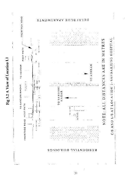
3.2 A View of Location L1 31
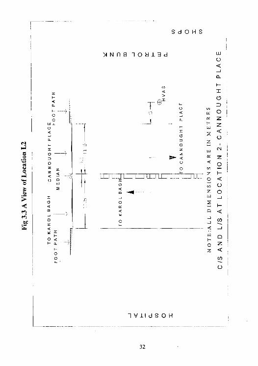
3.3 A View of Location L2 32
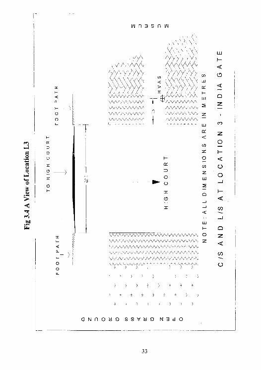
3.4 A View of Location L3 33
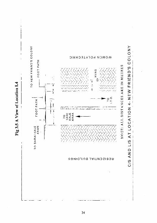
3.5 A View of Location L4 34
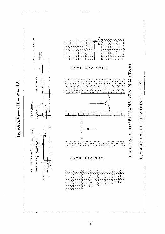
3.6 A View of Location L5 35
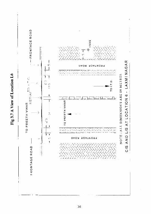
3.7 A View of Location L6 36
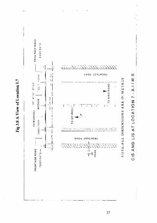
3.8 A View of Location L7 37
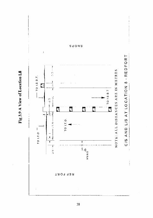
3.9 A View of Location L8 38
3.10 a Hourly observed concentration of CO at Safdarjung 48
3.10 b Hourly observed concentration of CO at Karol Bagh 48
3.10 c Hourly observed concentration of CO at India Gate 48
3.10 d Hourly observed concentration of CO at New Friends Colony 48
3.10 e Hourly observed concentration of CO at ITO 49
3.10 f Hourly observed concentration of CO at Laxmi Nagar 49
viii
3.10 g Hourly observed concentration of CO at AIIMS
49
3.10 h Hourly observed concentration of CO at Red Fort
49
4.1 Relationship between wind co-ordinate system 57
and line source co-ordinate system.
5.1 Location L1: Observed Vs Predicted concentration of CO in Using CALINE-4
66
5.2 Location L1: observed Vs Predicted (CO-Standard case)
67
5.3 Location L2: Observed Vs Predicted concentration of CO in Using CALINE-4
68
5.4 Location L2: observed Vs Predicted (CO-Standard case)
69
5.5 Location L3: Observed Vs Predicted concentration of CO in Using CALINE-4
70
5.6 Location [3: observed Vs Predicted (CO-Standard case)
71
5.7 Location L4: Observed Vs Predicted concentration of CO in Using CALINE-4
72
5.8 Location L4: observed Vs Predicted (CO-Standard case)
73
5.9 Location L5: Observed Vs Predicted concentration of CO in Using CALINE-4
74
5.10 Location L5: observed Vs Predicted (CO-Standard case)
75
5.11 Location L6: Observed Vs Predicted concentration of CO in Using CALINE-4
76
5.12 Location L6: observed Vs Predicted (CO-Standard case)
77
5.13 Location L7: Observed Vs Predicted concentration of CO in Using CALINE-4
78
5.14 Location L7: observed Vs Predicted (CO-Standard case)
79
5.15 Location L8: Observed Vs Predicted concentration of CO in Using CALINE-4
80
5.16 Location L8: observed Vs Predicted (CO-Standard case)
81
5.17 Observed Vs Predicted concentration of CO (CALINE-4)
83
5.18 Location L1: Observed Vs Predicted concentration of CO in Using GFLSM
86
ix
5 1 Location L1: observed Vs Predicted (CO-Standard case)
87
5.20 Location L2: Observed Vs Predicted concentration of CO in Using GFLSM
88
5.21 Location L2: observed Vs Predicted (CO-Standard case)
89
5.22 Location L3: Observed Vs Predicted concentration of CO in Using GFLSM
90
5.23 Location L3: observed Vs Predicted (CO-Standard case)
91
5.24 Location L4: Observed Vs Predicted concentration of CO in Using GFLSM
92
5.25 Location L4: observed Vs Predicted (CO-Standard case)
93
5.26 Location L5: Observed Vs Predicted concentration of CO in Using GFLSM
94
5.27 Location L5: observed Vs Predicted (CO-Standard case)
95
5.28 Location L6: Observed Vs Predicted concentration of CO in Using GFLSM
96
5.29 Location L6: observed Vs Predicted (CO-Standard case)
97
5.30 Location L7: Observed Vs Predicted concentration of CO in Using GFLSM
98
5.31 Location L7: observed Vs Predicted (CO-Standard case)
99
5.32 Location L8: Observed Vs Predicted concentration of CO in Using GFLSM
100
5.33 Location L8: observed Vs Predicted (CO-Standard case)
101
5.34 Observed Vs Predicted concentration of CO (GFLSM)
103
x
LIST OF PHOTOGRAPHS
Serial Title o No. No.
3.1 A View of Location 1 (Safadarjung Hospital) 28
3.2 A View of Location 4 (New Friends Colony) 28
3.3 A View of Location 5 (I.T.O.) 28
3.4 A View of Location 6 ( Laxmi Nagar) 29
3.5 A View of Location 7 (AIIMS)
29
xi
CONTENTS Page No.
CANDIDATE'S DECLARATION i
ACKNOWLEDGEMENT ii
ABSTRACT iii
LIST OF TABLES iv
LIST OF FIGURES viii
LIST OF PHOTOGRAPHS xi
CHAPTER 1: INTRODUCTION
1.1 General
1.2 Air Pollution Scenario in India 2
1.3 Air Pollution Standards in India 4
1.4 Health Hazards Due to Vehicular Pollution 6
1.5 Study of Delhi 7
1.6 Objective and Scope of the Study 8
1.7 Composition of Dissertation 9
CHAPTER 2: REVIEW OF MODELS FOR AIR POLLUTION
2.1 General 10
2.2 Gaussian Plume Model 10
2.3 The BOX Model 12
2.4 Finite Line Source Models 14
2.4.1 Finite line source model 14
2.4.2 General finite line source model 17
2.4.3 EPA Hiway model 17
2.5 Infinite Line Source Models 19
2.5.1 California line source model 19
2.5.2 General Motors (GM) model 20
2.6 Softwares Available for Air Pollution Modeling 20
2.6.1 CALINE-4
20
2.6.2 HIWAY-2
21
2.7 Case Studies 21
2.7.1 Case study of Delhi
21
2.7.2 Case study of Madras 23
2.8 Selection of Models 25
CHAPTER 3: FIELD SURVEY, DATA COLLECTION AND LABORATORY
STUDIES
3.1 General
26
3.2 Selection of Sites 26
3.3 Equipments Used in Data Collection 39
3.4 Field Study and Data Collection Procedure 39
3.4.1 Traffic volume studies 39
3.4.2 Air pollution monitoring 40
3.5 Laboratory Studies 46
3.5.1 Monitoring of carbon monoxide 46
CHAPTER 4: MODELING OF AIR POLLUTANT CONCENTRATION
4.1 General 50
4.2 Modeling of Air Pollutant Concentration Using CALINE-4 50
4.2.1 Working with CALINE-4 model 50
4.2.2 Prediction of carbon monoxide Using CALINE-4 55
4.3 Modeling of Air Pollutant Concentration Using GFLSM 56
4.3.1 Working with GFLSM 56
4.3.2 Determination of input parameters to the model 58
CHAPTER 5: PERFORMANCE EVALUATION OF AIR POLLUTION MODELS
5.1 Overview 62
5.2 Site Wise Performance Evaluation 62
5.2.1 Index of agreement 63
5.2.2 Significance test 64
5.3 Performance of CALINE-4 65
5.3.1 CALINE-4 performance for L 1
66
5.3.2 CALINE-4 performance for L2
68
5.3.3 CALINE-4 performance for L3 70
5.3.4 CALINE-4 performance for L4
72
5.3.5 CALINE-4 performance for L5 74
5.3.6 CALINE-4 performance for L6
76
5.3.7 CALINE-4 performance for L7
78
5.3.8 CALINE-4 performance for L8
80
5.3.9 Validation of CALINE-4
84
5.4 Performance of General Finite Line Source Model (GFLSM)
85
5.4.1 GFLSM performance for L1
86
5.4.2 GFLSM performance for L2
88
5.4.3 GFLSM performance for L3
90
5.4.4 GFLSM performance for L4
92
5.4.5 GFLSM performance for L5
94
5.4.6 GFLSM performance for L6
96
5.4.7 GFLSM performance for L7
98
5,4.8 GFLSM performance for L8
100
5.4.9 Validation of GFLSM
104
CHAPTER 6: CONCLUSION AND RECOMMENDATIONS
6.1 Conclusions 105
6.2 Recommendations 106
REFERENCES
APPENDICES
CHAPTER 1
INTRODUCTION
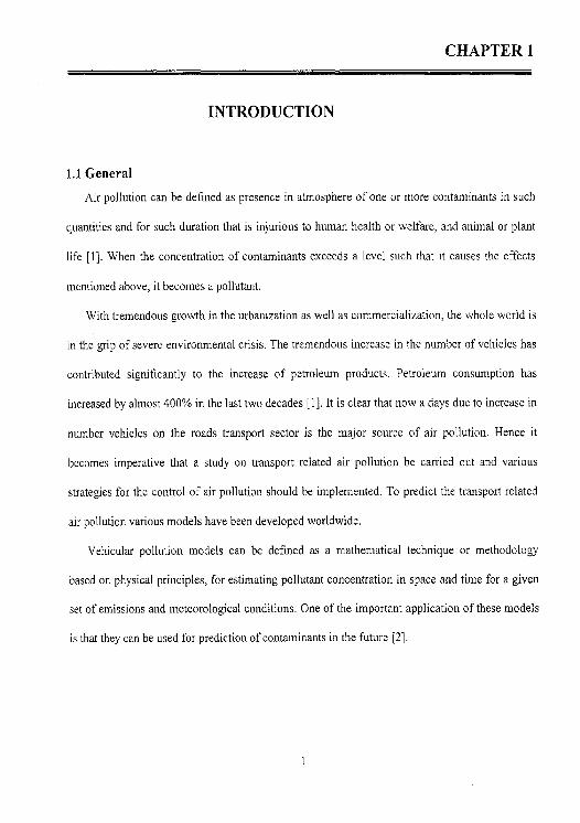
1.1 General Air pollution can be defined as presence in atmosphere of one or more contaminants in such
quantities and for such duration that is injurious to human health or welfare, and animal or plant
life [1]. When the concentration of contaminants exceeds a level such that it causes the effects
mentioned above, it becomes a pollutant.
With tremendous growth in the urbanization as well as commercialization, the whole world is
in the grip of severe environmental crisis. The tremendous increase in the number of vehicles has
contributed significantly to the increase of petroleum products. Petroleum consumption has
increased by almost 400% in the last two decades [1]. It is clear that now a days due to increase in
number vehicles on the roads transport sector is the major source of air pollution. Hence it
becomes imperative that a study on transport related air pollution be carried out and various
strategies for the control of air pollution should be implemented. To predict the transport related
air pollution various models have been developed worldwide.
Vehicular pollution models can be defined as a mathematical technique or methodology
based on physical principles, for estimating pollutant concentration in space and time for a given
set of emissions and meteorological conditions. One of the important application of these models
is that they can be used for prediction of contaminants in the future [2].
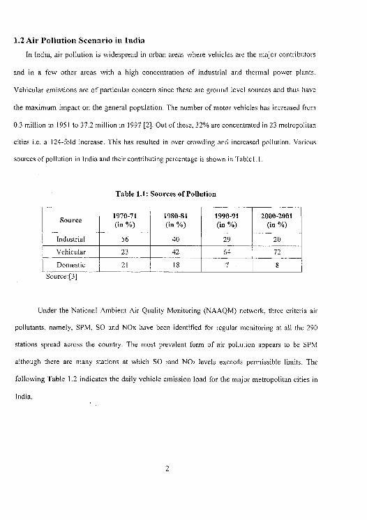
1.2 Air Pollution Scenario in India
In India, air pollution is widespread in urban areas where vehicles are the major contributors
and in a few other areas with a high concentration of industrial and thermal power plants.
Vehicular emissions are of particular concern since these are ground level sources and thus have
the maximum impact on the general population. The number of motor vehicles has increased from
0.3 million in 1951 to 37.2 million in 1997 [2]. Out of these, 32% are concentrated in 23 metropolitan
cities i.e. a 124-fold increase. This has resulted in over crowding and increased pollution. Various
sources of pollution in India and their contributing percentage is shown in Tablel.l.
Table 1.1: Sources of Pollution
Source 1970-71 (in %)
1980-81 (in %)
1990-91 (in %)
2000-2001 (in %)
Industrial 56 40 29 20
Vehicular 23 42 64 72
Domestic 21 18 7 8 Source:[31
Under the National Ambient Air Quality Monitoring (NAAQM) network, three criteria air
pollutants, namely, SPM, SO and NOx have been identified for regular monitoring at all the 290
stations spread across the country. The most prevalent form of air pollution appears to be SPM
although there are many stations at which SO land NO2 levels exceeds permissible limits. The
following Table 1.2 indicates the daily vehicle emission load for the major metropolitan cities in
India.
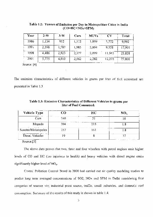
Table 1.2: Tonnes of Emission per Day in Metropolitan Cities in India (CO+HC+NOx+SPM)
Year 2-W 3-W Cars MUVs CV Total
1986 1,134 912 1,112 1,059 5,772 9,992
1991 2,598 1,787 1,985 2,004 9,528 17,901
1998 4,486 2,923 2,377 2,099 11,943 23,828
2001 5,775 4,910 2,562 2,282 12,272 27,800
source: 141
The emission characteristics of different vehicles in grams per liter of fuel consumed are
presented in Table 1.3.
Table 1.3: Emission Characteristics of Different Vehicles in grams per liter of Fuel Consumed.
Vehicle Type CO HC NO.
Cars 240 31 16
Mopeds 304 215 1.8
Scooter/Motorcycles 257 161 1.8
Diesel Vehicles 19 8 37
Source:pl
The above data proves that two, three and four wheelers with petrol engines emit higher
levels of CO and HC (too injurious to health) and heavy vehicles with diesel engine emits
significantly higher level of NOR .
Central Pollution Control Board in 2000 had carried out air quality modeling studies to
predict long term averaged concentrations of S02, NOx and SPM in Delhi considering four
categories of sources viz; industrial point source, traffic, small industries, and domestic coal
consumption. Summary of the results of this study is shown in table 1.4.
3
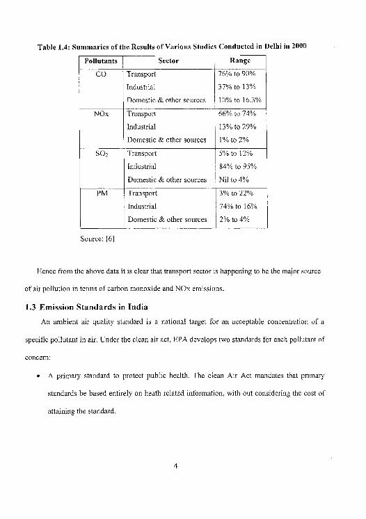
Table 1.4: Summaries of the Results of Various Studies Conducted in Delhi in 2000
Pollutants Sector Range
CO Transport 76% to 90%
Industrial 37% to 13%
Domestic & other sources 10% to 16.3%
NOx Transport 66% to 74%
Industrial 13% to 29%
Domestic & other sources 1% to 2%
SO2 Transport 5% to 12%
Industrial 84% to 95%
Domestic & other sources Nil to 4%
PM Transport 3% to 22%
Industrial 74% to 16%
Domestic & other sources 2% to 4%
Source: [6l
Hence from the above data it is clear that transport sector is happening to be the major source
of air pollution in terms of carbon monoxide and NOx emissions.
1.3 Emission Standards in India
An ambient air quality standard is a national target for an acceptable concentration of a
specific pollutant in air. Under the clean air act, EPA develops two standards for each pollutant of
concern:
• A primary standard to protect public health. The clean Air Act mandates that primary
standards be based entirely on heath related information, with out considering the cost of
attaining the standard.
• A secondary standard to protect public welfare. Public welfare effects on soils, water,
crops, vegetation, buildings, property, animals, wild life, weather, visibility, transportation
and other economic values, as well as personal comfort and well-being.
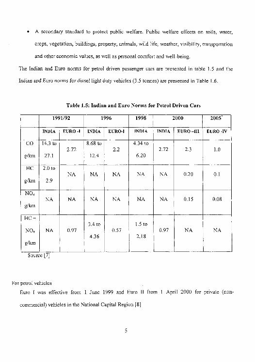
The Indian and Euro norms for petrol driven passenger cars are presented in table 1.5 and the
Indian and Euro norms for diesel light duty vehicles (3.5 tonnes) are presented in Table 1.6.
Table 1.5: Indian and Euro Norms for Petrol Driven Cars
1991/92 1996 1998 2000 2005
INDIA EURO -I INDIA EURO-I INDIA INDIA EURO -III EURO -IV
CO 14.3 to 8.68 to 4.34 to 2.72 2.2 2.72 2.3 1.0
g/km 27.1 12.4 6.20
HC 2.0 to NA NA NA NA NA 0.20 0.1
g/km 2.9
NO NA NA NA NA NA NA 0.15 0.08
g/km
HC + 3.4 to 1.5 to
NO, NA 0.97 0.57 0.97 NA NA 4.36 2.18
g/km
Source [7]
For petrol vehicles
Euro I was effective from 1 June 1999 and Euro II from 1 April 2000 for private (non-
commercial) vehicles in the National Capital Region [8]
5
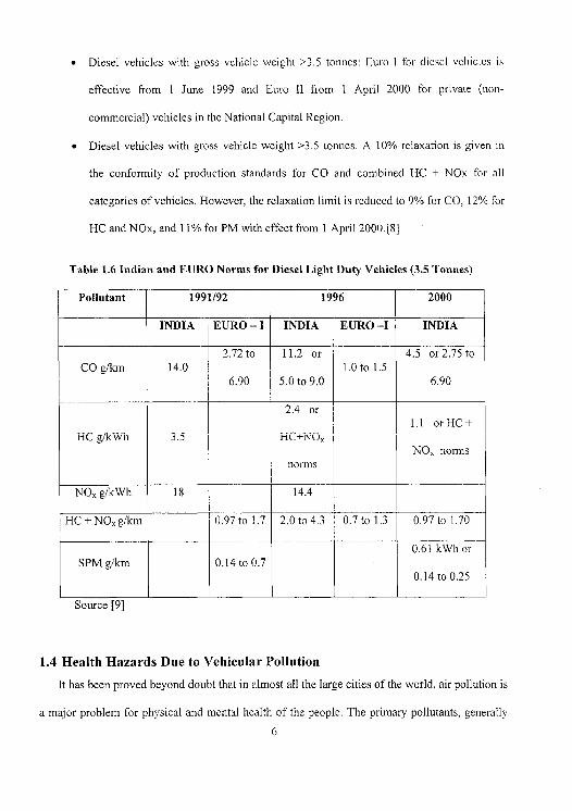
• Diesel vehicles with gross vehicle weight >3.5 tonnes: Euro I for diesel vehicles is
effective from 1 June 1999 and Euro 11 from 1 April 2000 for private (non-
commercial) vehicles in the National Capital Region.
• Diesel vehicles with gross vehicle weight >3.5 tonnes: A 10% relaxation is given in
the conformity of production standards for CO and combined HC + NOx for all
categories of vehicles. However, the relaxation limit is reduced to 9% for CO, 12% for
HC and NOx, and 11% for PM with effect from 1 April 2000.[8]
Table 1.6 Indian and EURO Norms for Diesel Light Duty Vehicles (3.5 Tonnes)
Pollutant 1991/92 1996 2000
INDIA EURO —I INDIA EURO —I INDIA
2.72 to 11.2 or 4.5 or 2.75 to CO g/l m 14.0 1.0 to l.5
6.90 5.0 to 9.0 6.90
2.4 or 1.1 or HC +
iiC g/xwh 3.5 HC+1NO NO norms
norms
NO, g/kWh 18 14.4
HC + NOx g/km 0.97 to 1.7 2,0 to 4.3 0.7 to 1.3 0.97 to 1.70
0.61 kWh or SPMg/km 0.14to0.7
0.14 to 0.25
Source [9j
1.4 Health Hazards Due to Vehicular Pollution
It has been proved beyond doubt that in almost all the large cities of the world, air pollution is
a major problem for physical and mental health of the people. The primary pollutants, generally
6
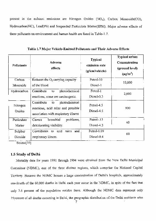
present in the exhaust emissions are Nitrogen Oxides (NO), Carbon Monoxide(CO),
Hydrocarbon(HC), Lead(Pb) and Suspended Particulate Matter(SPM). Major adverse effects of
these pollutants on environment and human health are listed in Table-1.7.
Table 1.7 Major Vehicle-Emitted Pollutants and Their Adverse Effects
Typical urban Typical
Adverse Concentration Pollutants emission rate
effects (ground level) (g/km/vehicle)
(µg/m3)
Carbon Reduces the 02 carrying capacity Petrol- 10 10,000
Monoxide of the blood Diesel-1
Hydrocarbon Contribute to photochemical Petrol-1 2,000
reactions, some are carcinogenic. Diesel-0.3
Contribute to photochemical Nitrogen Petrol-4.5
reactions, acid rains and possible 900 Oxides Diesel-4.5
association with respiratory illness
Particulate Causes bronchial problems, Petrol-. 13 40
Matter deteriorating visibility. Diesel-4.3
Sulphur Contributes to acid rains and Petrol-0.09 60
Dioxide respiratory illness. Diesel-0.4
Source[10j
1.5 Study of Delhi Mortality data for years 1991 through 1994 were obtained from the New Delhi Municipal
Committee (NDMC), one of the three distinct regions, which comprise the National Capital
Territory. Because the NDMC houses a large concentration of Delhi's hospitals, approximately
one-fourth of the 60,000 deaths in Delhi each year occur in the NDMC, in spite of the fact that
only 3.6 percent of the population resides there. Although the NDMC data represent only
25percent of all deaths occurring in Delhi, the geographic distribution of the Delhi residents who 7
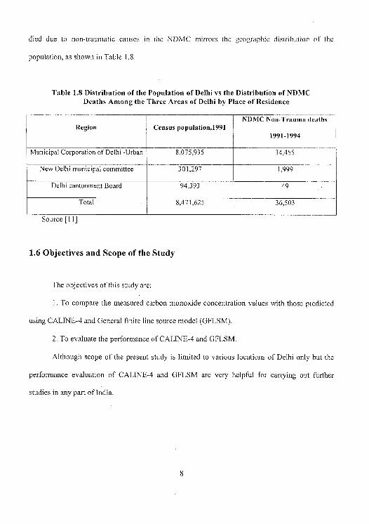
died due to non-traumatic causes in the NDMC mirrors the geographic distribution of the
population, as shown in Table 1.8.
Table 1.8 Distribution of the Population of Delhi vs the Distribution of NDMC Deaths Among the Three Areas of Delhi by Place of Residence
Region Census population,1991 NDMC NmrTrauma deaths
1991-1994
Municipal Corporation of Delhi -Urban 8,075,935 34,455
New Delhi municipal committee 301,297 1,999
Delhi cantonment Board 94,393 49
Total 8,471,625 36,503
Source [ I 1 ]
1.6 Objectives and Scope of the Study
The objectives of this study are:
1. To compare the measured carbon monoxide concentration values with those predicted
using CALINE-4 and General finite line source model (GFLSM).
2. To evaluate the performance of CALINE-4 and GFLSM.
Although scope of the present study is limited to various locations of Delhi only but the
performance evaluation of CALINE-4 and GFLSM are very helpful for carrying out further
studies in any part of India.
1.7 Composition of Thesis This thesis report has been divided in to seven chapters. The First Chapter introduces the
topic. An overview of some of the models, prediction software and selection of models for the
present study are presented in Chapter Two. Chapter Three deals with the procedures of data
collection, field studies and laboratory experimentation for determination of pollutant
concentrations. Chapter Four deals with modelling of air pollutant concentration using
CALINE-4 and GFLSM.. Fifth chapter deals with Performance Evaluation, of selected Air
Pollution prediction models, through statistical analysis. For this, CALINE-4 and General Finite
Line Source Model (GFLSM) have been used. Sixth Chapter lists the conclusions and
recommendations for further study.
9
CHAPTER 2
REVIEW OF MODELS FOR AIR POLLUTION
2.1 General
Environment planning for any urban area can be achieved by means of theoretical
mathematical models, which requires the knowledge of emission inventory and meteorology.
Rapid progress has been made in studies on mathematical models of urban air pollution during
past 10 years [12]. The models have become more accurate and complex in parallel with
computer software development. Numerous air pollution prediction models have been developed
which are for finite line source as well as for infinite line source. Line source models are used to
simulate dispersion from roadways where vehicles are continually emitting pollutants. These
models are based on Gaussian dispersion phenomenon. Line source models can be for finite
length or for infinite length of roadway. Some of the most popular air quality prediction models
are discussed in the following sections.
2.2 Gaussian Plume Model This is a generic mathematical model developed and widely used to describe the
dispersion phenomenon. This distribution of material with in the plum of pollutants is assumed to
be Gaussian in both the vertical and horizontal direction [13].
The axis system shown in Figure 21 is utilized and the following assumptions are
made [14].
i). The plume has a Gaussian distribution in both horizontal and vertical planes with ay , az as the
standard deviation across horizontal and vertical dimension of plume at downwind direction.
10
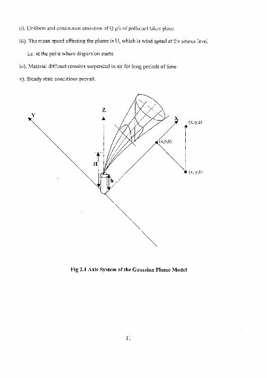
ii). Uniform and continuous emission of Q g/s of pollutant takes place.
iii). The mean speed affecting the plume is U, which is wind speed at the source level
i.e. at the point where dispersion starts.
iv). Material diffused remains suspended in air for long periods of time.
v). Steady state conditions prevail.
(x,-Y,z)
(x,-Y,0)
Fig 2.1 Axis System of the Gaussian Plume Model
Gaussian model equation is given by zz
X(x,y,z) = 1 exp(- y ~_) [exp(- (Z — H)2 ) +
exp(- (z +
2iru o- o- , lay 2Q_ 26__ Y
..........(2.1)
Where,
X(x,y,z) = Concentration of pollutants at the point (x,y,z) in
space (g/m3).
Q = Emission rate (g/m2/s)
u = Horizontal wind speed at the source level (m/s).ss
H = Height of emission (m).
ay , 6z =Standard deviation across horizontal and vertical dimension of plume at down
wind direction.
The disadvantage of using Gaussian plume models in field lies in specifying the n's
and the mean wind direction over an extended period of time, which makes it impractical.
Gaussian plume model works best for averaging times between 10 minutes and a few hours[ l31.
2.3 The BOX Model This is the simplest form of a dispersion model, which is often used to estimate air
pollution due to area sources [14]. This model may be considered as derived from the idea of the
continuity of mass of a volume element.
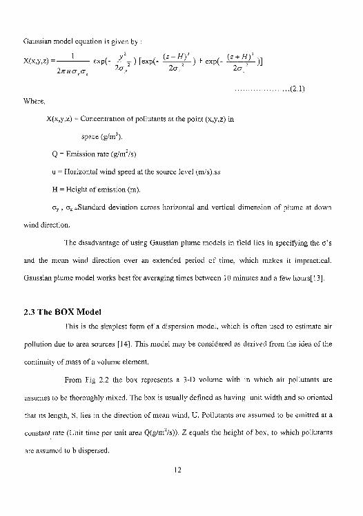
From Fig 2.2 the box represents a 3-D volume with in which air pollutants are
assumes to be thoroughly mixed. The box is usually defined as having unit width and so oriented
that its length, S, lies in the direction of mean wind, U. Pollutants are assumed to be emitted at a
constant rate (Unit time per unit area Q(g/m2/s)). Z equals the height of box, to which pollutants
are assumed to h dispersed.
12
Top of Mixing Layer Z
ind !locity, U
E uilibrium Concentration, Ce
/A\ GROUND Fig 2.2 Parameters of BOX Model
QS is equal to total emission rate per unit width when divided by ventilation rate, UZ, gives
the upwind edge of the area source.
Area source strength, Q = Mass * Area (2.2)
Time
Equilibrium Concentration, Cr =2 ............... (2.3) UZ
Box models can be used to obtain order of magnitude estimates of ambient pollution level.
However, the simplifying assumption of the model (uniform mixing to a constant level, Z) lead to
results that do not simulate true atmosphere conditions accurately. Special application of the box
model is an elevated inversion above a point source in valley.
Then,
Q .................(2.4) C= HWC
Q: Area source strength (g/m2/s)
W: Width of the valley (m)
H: Mixing height (m)
U: Mean wind speed (m/s)
N V
13
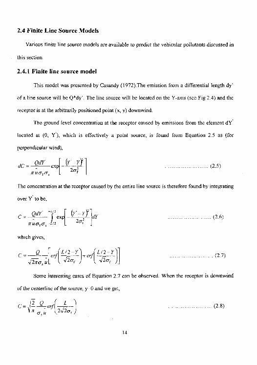
2.4 Finite Line Source Models
Various finite line source models are available to predict the vehicular pollutants discussed in
this section.
2.4.1 Finite line source model
This model was presented by Casandy (1972).The emission from a differential length dy'
of a line source will be Q*dy'. The line source will be located on the Y-axis (see Fig 2.4) and the
receptor is at the arbitrarily positioned point (x, y) downwind.
The ground level concentration at the receptor caused by emissions from the element dY
located at (0, Y'), which is effectively a point source, is found from Equation 2.5 as (for
perpendicular wind),
dC = QdY
ex — ''11 J (2.5) L rruQY6. 20
The concentration at the receptor caused by the entire line source is therefore found by integrating
over Y to be,
C= QdY f lex Y —Y Y
r u o v_ -L12 p 2cr; (2.6)
which gives,
C'— Q [er~LQ Y)+er rL/2+Y
IJ
Some interesting cases of Equation 2.7 can be observed. When the receptor is downwind
of the centerline of the source, y0 and we get,
'~2 Q r~ L ........................ (2.8) C Y n u e 2 F2
14
For large values of L - Equation 2.5 reduces to (since crf(mo) I from the property of error 2J2c,
function),
c=fcL Q u . (2.9)
This is the expression for the concentration downwind of an infinite line source normal to the
mean wind vector.
From the tables of the error function we find erf(t) = 0.95 when t = 1.38, and therefore, a
line source can be approximated as an infinite line source to an accuracy of 5% or better if
L >1.38 or L > 3.90 c, where receptor is at the plume centerline. The concentration at this 2', 2o.
receptor is only 5% less than the concentration that would be produced by an infinite line source
of equal strength.
15
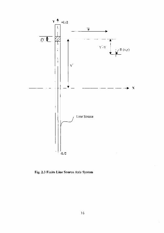
anrr
Fig. 2.3 Finite Line Source Axis System
L
2.4.2 General finite line source model
Most of the models available for prediction of transportation related air pollutant works
on the principle of Gaussian plume theory and most of these models have been developed for the
conditions prevailing in America. To overcome this problem Luhar and Patil [2] developed
General Finite Line Source Model in 1986. This model also works on the methodology of
Gaussian Plume theory. This model also overcomes the infinite line source constraints. A lot of
work for prediction of air pollutant concentrations using this model had already been done
in India as well as abroad. This model gives quiet satisfactory results.
2.4.3 EPA HIWAY model
This is a short term (one hour) line source dispersion model. It was developed by Zimmerman and
Thompson in Feb.1975. This model simulates a highway with a finite number of point sources
and the total contribution of all points is calculates by numerical integration of the Gaussian point
source equation over a finite length. The co-ordinates (m.) of the end points of a line source of
length L (m), representing a single lane extending from point A to point B as shown in Fig2.4.[2]
Because of the physical significance of mechanical mixing above the roadway, some
initial values of the vertical and horizontal dispersion parameters are assumed. To accomplish
this, the point source is displaced by a virtual distance upwind such that cr, and a. have initial
values at roadside [15].
17
B (RR,S°)
Line source
Source
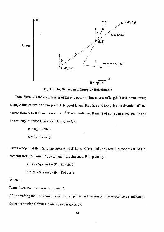
Fig 2.4 Line Source and Receptor Relationship
From figure 2.3 the co-ordinates of the end points of line source of length D (m), representing
a single line extending from point A to point B are ERA, SA) and (RB , SB).the direction of line
source from A to B from the north is 13°.The co-ordinates R and S of any point along the line at
an arbitrary distance L (m) from A is given by:
R=RA+L sin (3
S=SA +L cos 13
Given receptor at (Rk, SL) , the down wind distance X (m) and cross wind distance Y (m) of the
receptor from the point (R , S) for any wind direction 9° is given by
X = (S - SK) cosO + (R — RK) sin 0
Y= (S - SK) sin A - (R — RK) cos o
Where,
Rand S are the function of L , X and Y.
After breaking the line source in number of points and finding out the respective co-ordinates
the concentration C from the line source is given by:
1R
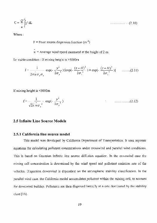
C=OffdL .(2.10) ua
Where
F = Point source dispersion function (m'2)
u = Average wind speed measured at the height of 2 m.
for stable condition : If mixing height is >5000m
z z z f =
c 2Q exp(-
rz) [exp(- ( 2~ ) ) + exp( (~2Q ) )~ (2.11)
2~c u
If mixing height is <5000m
yz
f = 1
exp(- ) ..............(2.12) z 2~uor 2 2o-r
2.5 Infinite Line Source Models
2.5.1 California line source model This model was developed by California Department of Transportation. It uses separate
equations for calculating pollutant concentrations under crosswind and parallel wind conditions.
This is based on Gaussian Infinite line source diffusion equation. In the crosswind case the
mixing cell concentration is determined by the wind speed and pollutant emission rate of the
vehicles. Dispersion downwind is dependant on the atmospheric stability classification. In the
parallel wind case, the California model accumulates pollutant within the mixing cell, to account
for downwind buildup. Pollutants are then dispersed laterally at a rate dominated by the stability
class [161
CALINE-4 is the latest version in a series of line source air quality model developed by
California Department of Transportation in contrast to CALINE-3 which is used for CO only,
CALINE-4 is used to predict concentrations of Nitrogen Oxide (NOx) and suspended particulate
concentration along with CO.
2.5.2 General Motors (GM) model
This model describes the downwind dispersion of pollutants near the roadway. This model
was developed by Chock (1978), on the basis of experimental data obtained in the General
Motors dispersing study on a test track. This experiment and experiment reported by Dabberdt
(1976) showed the mechanical mixing plays an important role in dispersing pollutants near
roadways while plume rise due to heated exhaust couldn't be ignored at low crosswinds. The
model avoids the cumbersome integration necessary for conventional Gaussian models, based on
infinite line source approach, the model specifies the dispersion parameters as a function of wind
road orientation angle and distance from the source to the receptor and includes plume rise over
the highway under very stable and light wind condition [ 17].
2.6 Softwares Available For Air Pollution Modeling
2.6.1 CALINE-4
The California Department of Transportation (CALTRANS) has been the leader in the
development of dispersion models for highways. The first line source model, CALINE was
published in 1972, for predicting CO concentrations.
In 1975, a revised version of original model, CALINE-2 was developed. This model could
compute concentration for depressed sections and for wind parallel to the road ways. Subsequent
20
studies indicated that CALINE-2 seriously over-predicted the concentration for stable, parallel
wind conditions.
In 1979, a third version, CALINE-3 was developed. CALINE-3 retained the basic
Gaussian dispersion methodology but used new horizontal and vertical dispersion curves
modified for the effects of surface roughness, averaging time and vehicle induced turbulence.
CALINE-4 is the latest version and the concentration of CO, NO2 and aerosols can be
predicted using this model. Software for this model is freely available and it is very helpful as it
saves time as respect to hand-calculations. [ 18]
2.6.2 HIWAY models
HIWAY is a short term (I hour) line source dispersion model. It was developed in
February, 1975 by EPA. The model is written in FORTRAN. HIWAY-2 is the upgraded version
of the model and was released by the EPA in 1980, and gives more realistic concentration
estimates due to an upgrade dispersion algorithm. The main disadvantage of the model is that it
still does not acknowledge the existence of 3-lane and 5-lane highways [19].
2.7 Case Studies
2.7.1 Case study of Delhi
Vivian Robert [20] conducted a study at Delhi in 2001 to predict the vehicular pollution in
eight selected location in Delhi in terms of the concentrations of CO with the help of CALINE-4
model.
The carbon monoxide concentrations for the selected location in the city have been
predicted using CALINE-4 software for two different conditions: Standard and Worst Case Wind
Angle
21
Using the inputs, hourly predictions of carbon monoxide have been done of all the unit oil
for both the run conditions using CALINE-4. The following regression analysis results between
predicted CALINE-4 outputs and observed concentration are derived for both these cases and t-
test is applied to check the reliability of inter-relationship between predicted and observed values
Case 1- Standard case:
Y = 0.6858 X + 1682.9 ....................(2.13)
R2 = 0.66
Case-2 Worst case wind angle
Y = 0.5849X + 1881.3 ....................(2.14)
R2 = 0.62
Where,
Y = Measured concentration
X = Predicted concentration
Using the above regression equations, the validation of predicted concentration of carbon
monoxide has been carried out for observed concentration at km. 174.0 on NH-58.The predicted
values are corrected by applying the calibration equation i.e.
Y = 0.6858 X+ 1682.9
Where,
Y = Corrected value of CO concentration.
X = Predicted value of CO concentration.
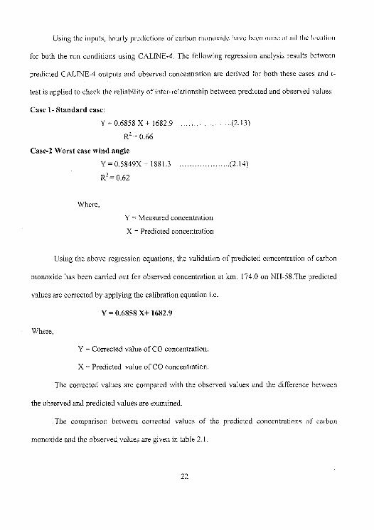
The corrected values are compared with the observed values and the difference between
the observed and predicted values are examined.
The comparison between corrected values of the predicted concentrations of carbon
monoxide and the observed values are given in table 2.1.
22
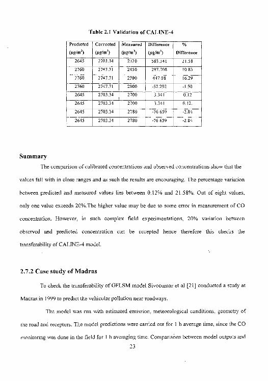
Table 2.1 Validation of CALINE-4
Predicted
(µg/m')
Corrected (µg/m')
Measured
(µg/m') Difference
(ttg/m') %
Difference
2645 2703.34 2120 583.341 21.58
2760 2747.71 2450 297.708 10.83
2760 2747.71 2300 447,08 16.29
2760 2747.71 2800 -52.292 -1.90
2645 2703.34 2700 3.341 0.12
2645 2703.34 2700 3.341 0.12.
2645 2703.34 2780 -76.659 -2.84
2645 2703.34 2780 -76.659 -2.84
Summary
The comparison of calibrated concentrations and observed concentrations show that the
values fall with in close ranges and as such the results are encouraging. The percentage variation
between predicted and measured values lies between 0.12% and 21.58%. Out of eight values,
only one value exceeds 20%.The higher value may be due to some error in measurement of CO
concentration. However, in such complex field experimentations, 20% variation between
observed and predicted concentration can be accepted hence therefore this checks the
transferability of CALINE-4 model.
2.7.2 Case study of Madras
To check the transferability of GFLSM model Sivocumar et al [21] conducted a study at
Madras in 1999 to predict the vehicular pollution near roadways.
The model was run with estimated emission, meteorological conditions, geometry of
the road and receptors. The model predictions were carried out for 1 h average time, since the CO
monitoring was done in the field for 1 h averaging time. Comparisons between model outputs and
23
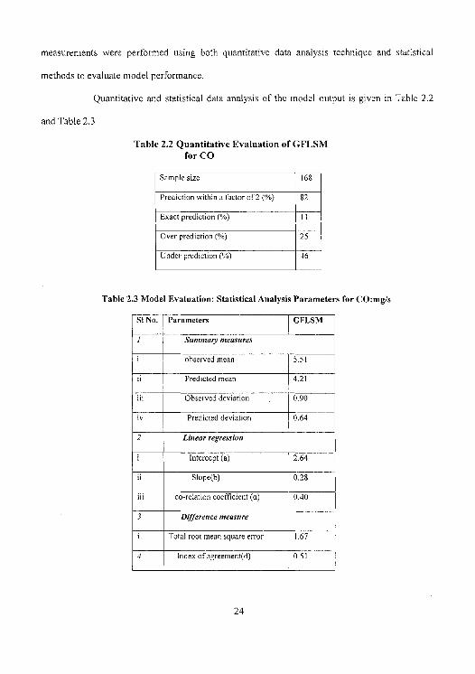
measurements were performed using both quantitative data analysis technique and statistical
methods to evaluate model performance.
Quantitative and statistical data analysis of the model output is given in Table 2.2
and Table 2.3.
Table 2.2 Quantitative Evaluation of GFLSM for CO
Sample size 168
Prediction within a factor of 2 (%) 82
Exact prediction (%) 1
Over prediction (%) 25
Under prediction (%) 46
Table 2.3 Model Evaluation: Statistical Analysis Parameters for CO:mg/s
SI No. Parameters GFLSM
Summary measures
observed mean 5.51
ii Predicted mean 4.21
iii Observed deviation 0.90
iv Predicted deviation 0.64
2 Linear regression
i Intercept (a) 2.64
ii Slope(b) 0.28
iii co-relation coefficient (a) 0.40
3 Difference measure
i Total root mean square error 1.67
4 Index of agreement(d) 0.51
24
From the Table 2.3 it is seen that GFLSM is able to describe the observed variability
closely. The measures which are next important are the regression coefficients a and b. The value
of b is nearer to 1 and also the value of a is close to zero, indicating better prediction.
The relatively comprehensive difference measure of the degree to which the observed
variate is accurately estimated by the simulated variate, the index agreement (d), gives the degree
to which model prediction are error free. In other words, it suggests that the model has explained
the percentage of the potential for error. Thus, 51 % of the potential for error has been explained
by the model, which implies that there is a lower error in GFLSM results.
It can be observed from the analysis presented that GFLSM which is derived for the
Bombay conditions perform well for Madras also. Hence, it is transferable to other locations also.
However, there is slight over prediction when the wind direction is parallel to the roadway.
2.8 Selection of Models
In this study to evaluate the performance of air pollution models, two models have been
selected and these are CALINE-4 and General Finite Line Source Model (GFLSM).
CALINE-4 is the model developed by California transportation Department
(CALTRANS) and this is the most popular model, which has been used worldwide. CALINE-4 is
the latest model available at present. Also software of CALINE-4 is also available which is user
friendly and saves the time from very lengthy hand calculations.
General Finite Line Source Model (GFLSM) is the model developed by Luhar et al in
1986 for Indian conditions, which is based on Gaussian plume model. A lot of work for
prediction of air pollutant concentrations using this model had already been done.
25
CHAPTER 3
FIELD SURVEY, DATA COLLECTION
AND LABORATORY STUDIES
3.1 General To evaluate the performance of the selected models the following database has been
collected at Delhi during the period of November 2002 and March 2003.
(i) Classified traffic volume.
(ii) Air samples of CO
(iii) Meteorological parameters like wind speed, wind direction, Temperature, Mixing height
and Stability class.
(iv) Geometric parameters like road width, number of lanes, lane width, shoulder width,
presence of medians and its width.
(v) Longitudinal section parameters like the distance of receptor point from the intersection.
Except the data given in (iii) all other data has been collected from the field.
3.2 Selection of Sites
Keeping in view the objective of the study, the sites were so selected as to represent the
whole urban area in different land use zones like, Residential area, Commercial Zone, Silence
Zone and Heavy Traffic zone. Total eight locations have been selected and categorized in
different zones as indicated in table 3.1.The locations are shown in photo 3.1 to 3.5 and the map
of Delhi showing the sites selected for field studies is shown in fig.3.1 and the site diagrams of all
locations are shown in fig 3.2 to 3.9.
26
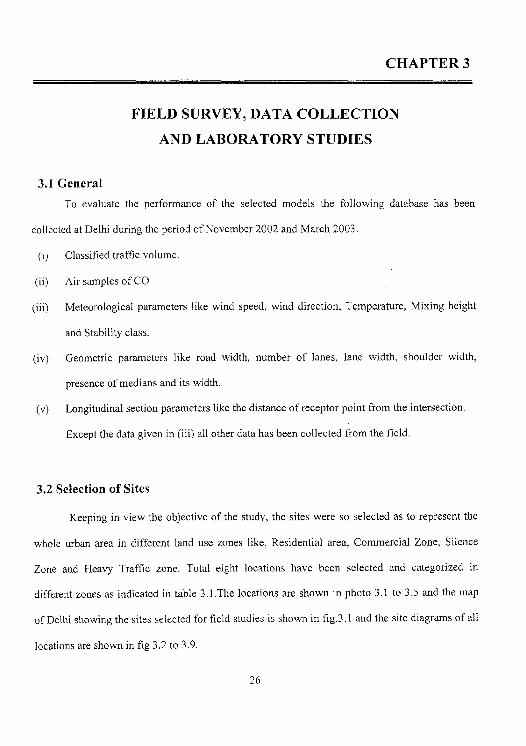
Table 3.1 Location Chosen for Field Studies
Type of Zone Location
Residential Zone • New Friends colony • Laxmi Nagar
Commercial • Karol Bagh Zone • Redfort
Silence Zone • Safdarjung Hospital • AIIMS Hospital
Heavy Traffic • India Gate Zone • ITO
Table3.2 Details of Locations Chosen for Field Studies
Location Data Name of the No of Details of Type of Type of
Code and Duration place Lanes median Land use Road
Number (day/night)
Safadarjung LI 6 Present Silence Bituminous 8/8Hours
Hospital
Karol L2 I 6 Present Commercial Bituminous 8/81-tours
Bagh
U India
6 Present Heavy
Bituminous 8I8Hours Gate Traffic
New friends I, L4 4 Present Residential Bituminous 8/8Hours
Colony
Heavy L5 I.T.O. 7 Present Bituminous 8/8Hours
Traffic
Laxmi L6 7 Present Residential Bituminous 8/8Hours
Nagar
AIIMS L7 6 Present Silence Bituminous 8/8Hours
Hospital
Red L8 7 Present Commercial Bituminous 8/8Hours
fort
27
Photo 3.1 A View of Location 1(Safdarjung Hospital)
Photo 3.2 A View of Location 4(New Friends Colony)
Photo 3.3 A View of Location 5 (I.T.0)
i
28
z
SDt'IIQ'Ilflfl '1VIIP' UIS I 1
0 SjlKA- FLL2IVdd 31ITh IH'I3Q w
H z 0 Of LL
— r I i III 1
C' I O ~ i
O x cn
1~
O
a
Z u'
N
Q
H ~ a I- o LL[T_1
W 0 Q z
LL
1
.4-
eq
SdOHS
>lNfl9 1OLLd W 0 1
0 I—,
I F- ml 0
LU
LLj
a. Z z
0 F-- = LU
0 r
F- Ifl 0 z - I z a z < Z o 0 2 2 0
--•IiJI1 ULLJLIL1JJLLLJLD w
m Z Ot II) o 0
ccl S < 0< 1
-- - I-
0< \S H
z< i 0
0
1VIIdSOH
32
M
C U
C3 =
w =
O
x F
F- O p LL
w n A s n w
)\t\ U)
\\ Q v\/\ ' v w
C Vv'~"v Vv\M U w M~\Mn. W,. .wv,,NAA/Vvv~ nwwv
z ✓ A' \ VY IVVVIlA -
T w
z
H 0
z o w
2 ~
J
= J
w
V\%V`.N\vvVV ✓V i IV✓vW"VWV,. 0 V /'/ w' ,✓vvvwvvv A(v AzA Z vvv,V'AA'V '\t, nnn ✓ ,Jvvv,'V'V
V/ ✓ /A ,t'/ 1/`.nnAnn.
/ i j
w I-
0
Q I
❑ z
M
z 0
I-
C-) 0 J
I-
J
z
0)
U
0 N n O 2~ J S S V 2i J N 3 d O
33
-
z z 0
0 OINH031A1Od N3WOM - U) = 0 a U z a a
o v \y >z> _
- ~ > A\~~< z - wv~N n N v -tip LL I .M_,v
' /\,' \7~~. ,0~___ tiptC [ Q >I
S ► o°. Lx- C)
1- rl Fir F-~-r1LZl_GC' '.- FBI
`f, z
O I- oE W Q
~
Q
Y y - Q
~- w 2
YY Z Y >'/\V/\\/ fy N
c O J F- Q
Z
SDNlciiin8 lVl1N301S321
U
34
-
1 12-1 ~LIL
CIO
OYO DV1NOd
H
I- /N"V/
0 -
if I- -
C -
0 j_LlJ__[JJ1____FE] Hi L t1 )
LJ
al
(11 0 z
L GVOU 3 OVINOI < LI) z
0
LO
h
z 0 I-
C-) 0 -J H
C/) -J
z
C!)
0
35
N
44
0
W Q)
o
K( /KKKY/\, J
OVOJ OViNOH
-
0 0
CD
LJ
H—
H
---0
c/DO z-
> [I)
0
w 0
H raAz/~jia xAjx 'cx ~r~_'\t.
I' o aVOH V1N0Hd H
w 0
H z 0
U-
36
44
0
O H
U O a
I- 0 z 0 O LL
LSLL 1
0YOa 30ViNOaj Cl)
1 7VT"TXTC', - 'G~4` J` ✓C ~^T- "]C v°; -„" TIGr W
u o
Z N c - z
u a Ii W Z
o ~ ~ 0 Z o U
o Q z H a W
AVON 30ViNO213 J J
u7 (O - F- Q Q
Q Q r= z cn U
o z o ~ LL
LL
37
SdOHS
w I
m
0
C
ou w s
0
0 T I-
0
0 H
en
0 I-
F-
0 U-0 w
00
z 0 I- 4: U 0 J I- 4:
J 0 Z Q
7
38
3.3 Equipments Used In Data Collection
In addition to manual data recording of classified traffic volume count, a number of field
instrument with all the accessories are required for this job. Following are the instruments used in
air pollution monitoring.
• Air sample collection tubes: In these tubes air samples of Carbon monoxide and
hydrocarbon were collected using water replacement method.
• Other instruments: Measuring wheel and measuring tape were used to measure the
geometric parameters of locations. Generator was also engaged in field for permanent
power supply to run high volume sampler.
3.4 Field Study and Data Collection Procedure
Delhi is one of the major metropolitan cities of India where transportation facilities are
improving every year to meet increase demand due to excessive population growth. Following are
the studies conducted for data collection.
3.4.1 Traffic volume studies
At all the selected locations, Traffic volume studies were conducted continuously for a
period of 8 hours day and night. Directional classified traffic volume data were manually
recorded Proforma shown in AppendixAl.This Performa covers the all categories of vehicles.
The summarized traffic volume is given in table3.3.
39
3.4.2 Air pollution monitoring
The air pollution parameter carbon Monoxide was monitored at the selected locations
shown in table4.1. The major vehicular pollutant considered in this study is Carbon monoxide
(CO). The Proforma used is shown in Appendix A2. The observed concentration of Carbon
monoxide is given in table 3.4.
40
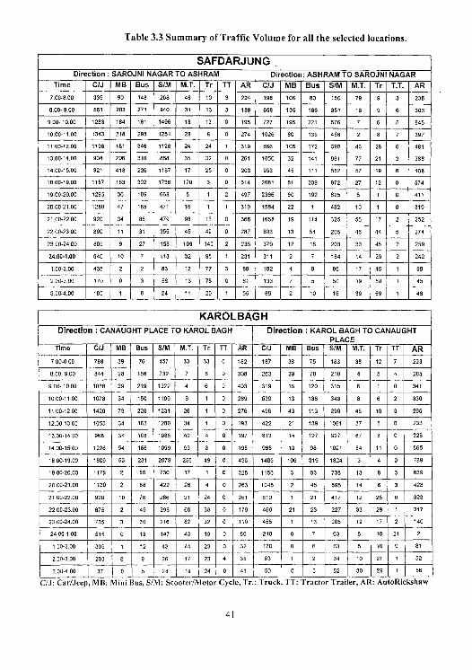
Table 3.3 Summary of Traffic Volume for all the selected locations.
~~mm~mmo~~om~mm~ ® ©m~mm~~om~mm ®om~mmom~oomME ®ommmmom~MEEMIN ' m
C/J: Car/Jeep, MR: Mini Bus, S/M: Scooter/Motor Cycle, Tr.: Truck, TT: Tractor Trailer, AR: AutoRickshaw
!II
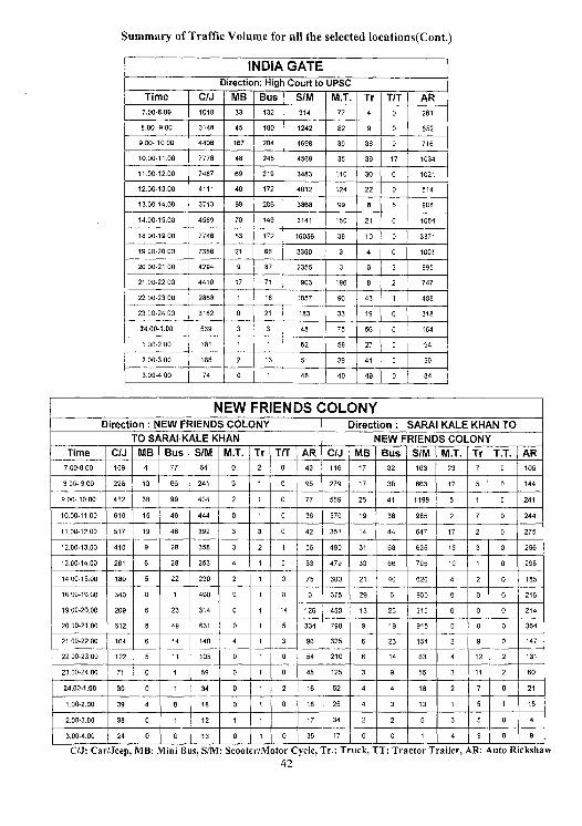
Summary of Traffic Volume for all the selected locations(Cont.)
•
i • •
~0~000m~ommom ©® ; IMME Nom® ©om©m©m
, moom000mm © ©v ©boo m~ao~■oomm0000 vv C/J: Car/Jeep, MB: Mini Bus, S/M: Scooter/Motor Cycle, Tr.: Truck, TT: Tractor Trailer, AR: Auto Rickshaw
42
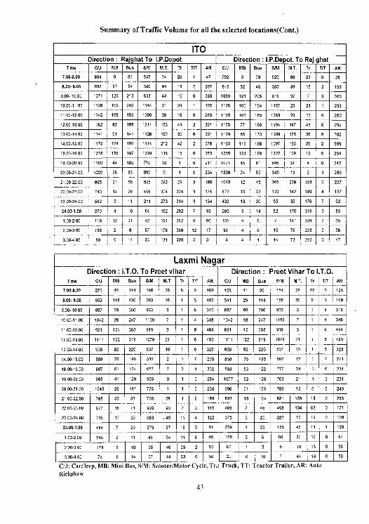
Summary of Traffic Volume for all the selected locations(Cont.)
ku
~~ ©om~~mmmoomm~om momm ®~ © ®moom ®mom
mmm ®mom ® ®mm
a m~mmom~o~m ®~mo~ ■~ammm o mmmam ©I ©mmo°© ©mmom mom ®~m~om~omamman C/J: Car/Jeep, M6: Mini Bus, S/M: Scooter/Motor Cycle, Tr.: 't ruck, TT: Tractor'[ railer, AK: Auto Rickshaw
43
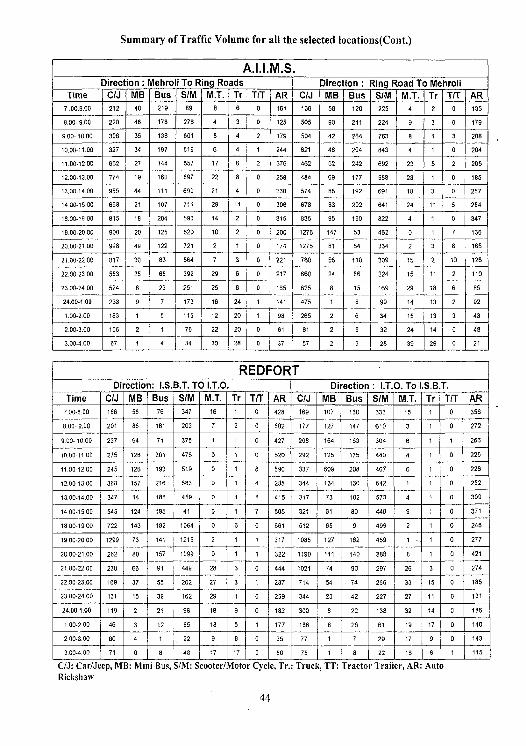
Summary of Traffic Volume for all the selected locations(Cont.)
m mm ®mom ® ®mmm
C/J: Car/Jeep, MB: Mini Bus, S/M: Scooter/Motor Cycle, Tr.: Truck, TT: Tractor Trailer, AR: Auto Rickshaw
44
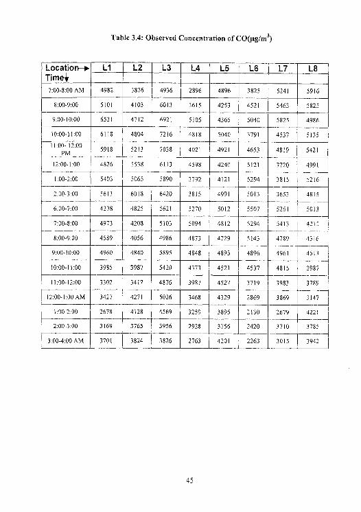
Table 3.4: Observed Concentration of CO(µg/m3)
Location—► L1 L2 L3 L4 L5 L6 L7 L8 Timed _ 7:00-8:00 AM 4982 3876 4936 2896 4896 3825 5241 5916
8:00-9:00 5101 4103 6013 3615 4253 4521 5463 5825
9:00-10:00 6531 4712 6921 5105 4365 5040 5825 4986
10:00-11:00 6118 4804 7216 4818 5040 3791 4537 5135
11:00-1200 PM
5918 5213 7038 4021 4921 4653 4819 5421
12:00-1:00 4826 5538 6113 4598 4240 5121 3720 4991
1:00-2:00 5403 5065 5890 3792 4121 5294 3815 5216
2:00-3:00 5613 6018 6420 3815 4991 5013 3653 4815
48255621 6:00-7:00
7:00-8:00
4298
4973 4208 5103
5270
5094
5012
4812
5507
5294
5261
5413
5013
a21`
8:00-9:00 4589 4056 4986 4873 4729 5143 4789 4316
9:00-10:00 4960 4840 5895 4848 4893 4896 4961 4513
10:00-11:00 3985 3987 5420 4373 ' 4521 4537 4815 3987
11:00 -12:00 3302 3417 4876 3789 3987 4527 3719 3983
12_00-1:00 AM
1:00-2:00
2:00-3:00
3427
2678
3169
4271
4128
3765
5026
4569
3956
3468
3259
2928
4329
3895
3756
2869
2130
2420
3869
2679
3710
3147
4221
3785
3:00-4:OO AM 3701 3824 3826 2763 4201 2263 3015 3942
45
3.5 Laboratory Studies
3.5.1 Monitoring of carbon monoxide
Indian standard code IS: 5152(Part X)-1976[22(i)] has suggested the following methods
for monitoring the ambient carbon monoxide concentration.
1. Iodine Peroxide Method
2. Indicator Tube Method
3. Non-Dispersive Infrared Absorption Method
4. Gas Chromatography Method
The ambient air samples at all the identified locations were collected using the glass air sample
collection tubes by water replacement method.
The gas chromatograph (AIMIt, NUCON, Series 5700) was used for the analysis of the
air samples. A sample of the air containing carbon monoxide is injected in to the gas
chromatograph where it is carried from one end of the column to other. During its movement, the
constituents of the sample undergo distribution at different rates and ultimately get separated from
another. The separated constituents emerge from the end of the column one after the other and are
detected by suitable means whose response is related to the amount of a specific component
leaving the column. The concentration of the different constituents is plotted in the form of
inverted "V" shape curve(s) one after the other by the recorder. The peaks of the curves depend
upon the concentration of the different gases detected by the instrument. Concentrations of the
constitutes is calculated on the basis of the peak areas on the chromatograph obtained known
amount of constituent, namely, carbon monoxide, hydrocarbon etc. using the same apparatus
under identical conditions.
The samples were tested under the following testing conditions as suggested by Indian
standard IS: 5182(Part X)-1976
• Temperature - 50°C
46
• Carrier Gas - Hydrogen
• Carrier Gas Flow — 5 liters/hour
• Sample loop — .10 ml
• Bridge Current — 350 mA
• Chart Speed — 30 cm/Hour
Results:
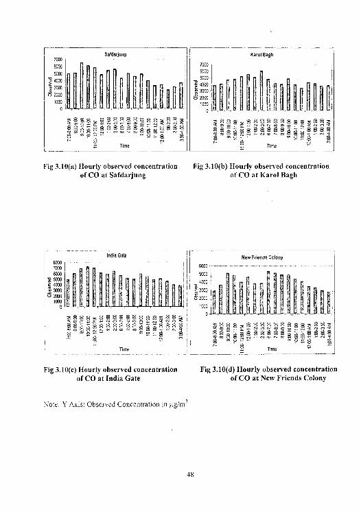
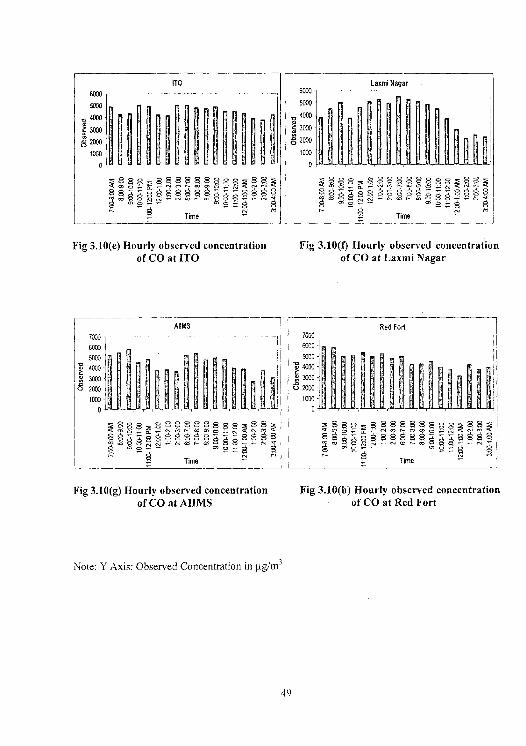
The hourly average concentrations of carbon monoxide were determined using the
procedure explained above and the results for all the locations are presented in the form of bar
charts in fig 3.10(a) to 3.10(h).The Carbon Monoxide Concentrations exceed the safe limit of
4000 pg/m3[23] prescribed for Indian conditions in most cases.
47
III Karol Bagh
r0i II,
ri
Q S o 8 o S o S 8 0 °0 8 8 S 53 sa
g o d o o 0 o do o d d o o g g roo~~, .n r o
Time
~8o8n g_so88aSS. 8,~8.85a
o $ f Time
Fig 3.10(a) Hourly observed concentration Fig 3.10(b) Hourly observed concentration of CO at Safdarjung of CO at Karol Bagh
India Gate 6000 .. _._ .. ._.. _.
7000
6000 5000
4000 3000
0 2000 1000
~so~ a gssaa gseq
Time
Fig 3.10(c) Hourly observed concentration of CO at India Gate
Note: Y Axis: Observed Concentration in µg/m3
New Friends Colony 6000........ _..... ._._. .._.
5000
4000 j z 3000
1000 iiHiUiILUiiiii 0
Time
Fig 3.10(d) Hourly observed concentration of CO at New Friends Colony
48
ITO
Time
Fig 310(e) Hourly observed concentration of CO at ITO
Laxmi Nagar 6000
5000
4000
0 2000 1 000 ilfiftilhilfi iftikui
Time
Fig 3.10(f) Hourly observed concentration of CO at Laxmi Nagar
AIIMS
7000i 6000
5000
40
O IILUi1~~l J rUulililE 2000
1000 oil
Time
Fig 3.10(g) Hourly observed concentration of CO at AIIMS
Time
Fig 3.10(h) Hourly observed concentration of CO at Red Fort
Note: Y Axis: Observed Concentration in jig/rn3
49
CHAPTER 4
Modeling of Air Pollutant Concentration
4.1 General In the present study, total eight sites have been selected as given in table 4.1 In this total
eight hours day and eight hours night data had been collected for all the eight locations selected.
4.2 Modeling of Air Pollutant Concentration Using CALINE-4
4.2.1 CALINE 4 model
The various input parameters in the five different input screens of CALINE-4 are briefly
described in the following sections [24]:
Job Parameters
The Job Parameters Screen contains general information that identifies the job, defines
general modelling parameters, and sets the units (feet or meters) that will be used to input data on
the Link Geometry and Receptor Positions Screens.
File Name: Display only, not editable. Displays the name of the file where the current job is
stored.
Job Title: Optional, Provides a space for the user to enter a brief job description, up to 40
characters in length.
Run Type: Different choices determine averaging times (for CO concentrations) and how the
hourly average wind angle(s) will be determined. (Wind angle is the angle between the roadway
link and the wind direction. CALINE-4 calculates the angles based on data in the Link Geometry
and Run Conditio Sc Most users should invoke the "worst-case wind angle" run type
and apply a persistence factor of 0.6 to 0.7 in order to estimate an 8-hour average CO
concentration.
• Standard - Calculates 1-hour average CO concentrations at the receptors.
• Multi-Run - Calculates 8-hour average CO concentrations at the receptors.
• Worst-case wind angle - Calculates 1-hour average CO concentrations at the receptors. The
model selects the wind angles that produce the highest CO concentrations at each of the
receptors.
• Multi-Run/Worst-Case hybrid - Calculates 8-hour average CO concentrations at the
receptors. The model selects the wind angles that produce the highest CO concentrations at
each of the receptors.
Aerodynamic Roughness Coefficient: Also known as the Davenport-Wieringa roughness-
length. These choices determine the amount of local air turbulence that affects plume spreading.
CL4 offers the following 4 choices for aerodynamic roughness coefficient:
• Rural: Roughness Coefficient = 10 cm
• Suburban: Roughness Coefficient = 100 cm
• Central Business District: Roughness Coefficient = 400 cm
• Other: Appropriate values as specified by CALINE-4.
Model Information: Provides summary information for convenience and quality assurance.
• Link/Receptor Geometry Units: Select whether meters or feet will be used to define the
geometry of the roadway links and receptor positions.
• Altitude above Sea Level: Define the altitude above mean sea level. This input is used to
determine the rate of plume spreading
• Number of Links: The sum total number of links that the user has defined on the Link
Geometry Page.
51
• Number of Receptors: The sum total number of receptors that the user has defined on the
Receptor Positions page.
• Averaging Interval: Indicates whether the user has opted to calculate 1-hour or 8-hour
average CO concentrations at the receptors.
"Run" - Clickthis button to run the job as specified. First, be sure that the information on all
five pages of CL4 is complete: Job Parameters, Link Geometry, Link Activity, Run Conditions,
and Receptor Conditions.
"Exit" - Click this button to exit the CL4 program. CL4 issues a warning if changes or new user
inputs might be lost.
Link Geometry
Fill in the matrix to define the roadway network to be modelled. Each row in the matrix
defines a single link. Up to 20 links may be entered. Links are defined as straight-line segments.
Link Name: Optional. The user may define a 12-character description for the link.
Link Type: The user must select one of the following 5 choices to define the type of roadway
that each link represents.
• At-Grade - For at-grade sections, CALINE does not permit the plume to mix below ground
level, which is assumed to be at a height of zero. The height of the link above the ground is
defined in the Link Height cell.
• Fill - For fill sections, CALINE-4 automatically resets the link height to zero, and assumes
that air flow follows the surface terrain, undisturbed
52
• Depressed - For depressed sections, CALINL-4 increases the residence time of an air parcel
in the mixing zone. The residence time increases in relation to the depth of the roadway
depression.
• Bridge - For bridge sections, CALINE-4 allows air to flow above and below the link. The
plume is permitted to mix downward from the link, until it reaches the distance defined in the
Link Height cell.
• Parking Lot - Parking lot links should be defined to be coincident with the parking lot access
ways.
Endpoint Coordinates: Links are defined as straight-line segments. The entire length of each
link should deviate no further than 3 meters from the centreline of the actual roadway. The
endpoint coordinates, (xl, yl) and (x2, y2), defines the positions of link endpoints. A map of the
link geometry is shown on the Receptor Positions Page.
Link Height: For all link types except bridges, Link Height represents the height of the link
above the surrounding terrain. Ground level is defined at 0 meters or feet (z=0).
Mixing Zone Width: Mixing zone is defined as the width of the roadway, plus 3 meters on
either side. The minimum allowable value is 10 meters, or 32.81 feet.
Canyon/Bluff Mix: The Canyon/Bluff Mix feature has not been validated with field
measurements. Only very rare circumstances warrant its use. This feature must be used with
extreme caution.
Link Activity
The Link Activity screen defines the level of traffic and auto emission rate observed at
each link.
53
Traffic Volume: The hourly traffic volume anticipated to travel on each link, in units of vehicles
per hour. If a multi-run scenario is selected, traffic volume must be defined for 8 hours.
Emission Factor: The weighted average emission rate of the local vehicle fleet, expressed in
terms of grams per mile per vehicle. Emission rates vary by time of day. Therefore, if a multi-run
scenario is selected, emission factors must be defined for 8 hours.
Run Conditions
The Run Conditions screen contains the meteorological parameters needed to run
CALINE-4. The worst-case meteorological conditions that can be anticipated at the project
location must be employed.
Wind Speed - Expressed in meters per second. The minimum choice available for CALINE-4 is
0.5 m/s. Alternatively, EPA recommends a value of 1 m/s as the worst-case wind speed.
Wind Direction - The direction the wind is blowing from, measured clockwise in degrees from
the north (0 = north, 90 = east, 180 = south, 270 = west). Most users should opt for the "Worst-
Case Wind Angle" choice on the Job Parameters screen. If "Worst-Case" is selected, CALINE-4
does not use this input.
Wind Direction Standard Deviation - The statistical standard deviation of the Wind Direction,
sometimes termed "sigma theta".
Atmospheric Stability Class - A measure of the turbulence of the atmosphere. Values 1 through
7 correspond to the standard definitions for stability class A through E. Stability class E (or 7)
represents the most stable conditions.
Mixing Height - The altitude to which thermal turbulence occurs due to solar heating of the
ground. Reasonable values for the worst-case mixing height rarely have a significant impact on
CALINE-4 model results.
54
Ambient Pollutant Concentration - This measure reflects the pre-existing background level of
carbon monoxide, expressed in parts per million. CALINE-4 adds the pre-existing and modelled
CO concentrations together to determine the total impact at each receptor.
Ambient Temperature - The ambient air temperature significantly affects vehicle CO emissions.
A temperature that reflects wintertime conditions should be selected, expressed in degrees Celsius
Receptor Position
The Receptor Positions Screen contains the data inputs for all receptor positions, and also
displays a diagram of the link geometry and receptor positions. Receptors should be defined with
the same Cartesian coordinate system and units of measure as the link geometry. For each
receptor (maximum no. of receptors = 20), space is provided for an 8-character description, the
X-coordinate, the Y-coordinate, and the height (Z).
4.2.2 Prediction of carbon monoxide using CALINE-4
The sample weighted emission factors and meteorological data used for the prediction
have been given in APPENDIX B and APPENDIX C respectively. The total traffic volume for
both directions has been used for prediction and has been presented in Table 3.3
Using the inputs mentioned above, hourly predictions of Carbon monoxide have been
done at all the locations for standard wind run condition. Sample run screens and output have
been shown in APPENDIX D1 and APPENDIX D2.
55
4.3 Modeling of Air Pollutant Concentration Using GFLSM
4.3.1 Working with GFLSM
A simple general finite line source model was developed be Luhar and Patil [2] in 1986,
which overcomes the infinite line source constraints. The basic methodology used in the
developing this model includes co-ordinate transformation between the wind co-ordinate system
(x i ,y i ,z i ) and the line source coordinate system (x,y,z).The middle point of the line source can be
assumed as the origin for both coordinate systems, which also have the same z-axis. The position
of the receptor R in the line source coordinate system is (x,y,z) and that in wind co-ordinate
system is(xj,yi,zi)as shown in fig4.l.In the line source co-ordination system all the parameters
viz. x ,y ,z can be evaluated from road receptor geometry. This model specifies the dispersion
parameter as a function of wind-road orientation angle and distance from the source.
56
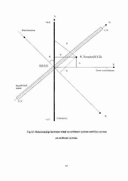
Fig 4.1 Relationship between wind co-ordinate system and line source
co-ordinate system.
57
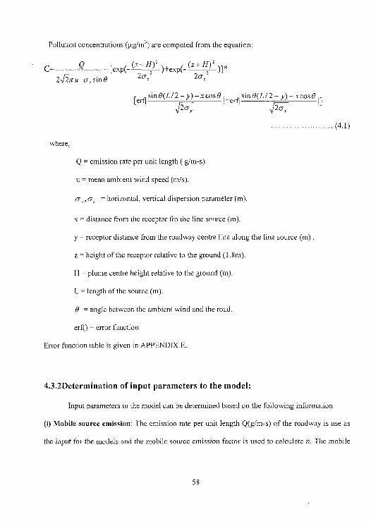
Pollutant concentrations (jig/m}) are computed from the equation:
z—H z z C= Q [exp( ( 2~ z) )texp(-(~2a
H) )]* 257ru v_ sing
lerfl sin O(L l 2 — y) — x cos 9 +er fl sin O(L / 2 + y) + x cos 9 I]
20 y. 2-y
(4.1)
where,
Q = emission rate per unit length ( g/m-s).
u = mean ambient wind speed (m/s).
= horizontal, vertical dispersion parameter (m).
x = distance from the receptor fro the line source (m).
y = receptor distance from the roadway centre line along the line source (m)..
z = height of the receptor relative to the ground (1,8m).
H = plume centre height relative to the ground (m).
L = length of the source (m).
B = angle between the ambient wind and the road.
erfO = error function
Error function table is given in APPENDIX E.
4.3.2Determination of input parameters to the model:
Input parameters to the model can be determined based on the following information
(i) Mobile source emission: The emission rate per unit length Q(g/m-s) of the roadway is use as
the input for the models and the mobile source emission factor is used to calculate it. The mobile
58
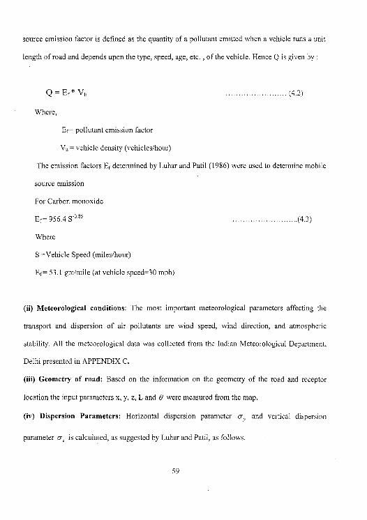
source emission factor is defined as the quantity of a pollutant emitted when a vehicle runs a unit
length of road and depends upon the type, speed, age, etc. , of the vehicle. Hence Q is given by :
Q = Ef* Vh ..... (4.2) ................... Where,
Ef= pollutant emission factor
= vehicle density (vehicles/hour)
The emission factors Ef determined by Luhar and Patil (1986) were used to determine mobile
source emission.
For Carbon monoxide
Ef= 956.4 S-o.ss ..........................(4.3)
Where
S =Vehicle Speed (miles/hour)
Ef= 53.1 gm/mile (at vehicle speed=30 mph)
(ii) Meteorological conditions: The most important meteorological parameters affecting the
transport and dispersion of air pollutants are wind speed, wind direction, and atmospheric
stability. All the meteorological data was collected from the Indian Meteorological Department,
Delhi presented in APPENDIX C.
(iii) Geometry of road: Based on the information on the geometry of the road and receptor
location the input parameters x, y, z, L and B were measured from the map.
(iv) Dispersion Parameters: Horizontal dispersion parameter o and vertical dispersion
parameter o. is calculated, as suggested by Luhar and Patil, as follows.
59
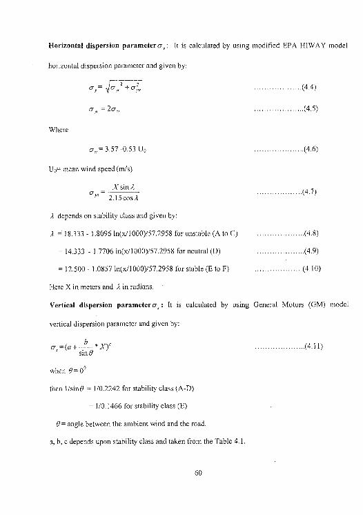
Horizontal dispersion parameter a,: It is calculated by using modified EPA HI WAY model
horizontal dispersion parameter and given by:
z z
= 2Q., ....................(4.5)
Where
o-,,= 3.57 -0.53 Uo ....................(4.6)
U0= mean wind speed (m(s)
sinA I o .... (4.7) —-- ...................
2.15cosA
1. depends on stability class and given by
A. = 18.333 - 1.8096 ln(x/l 000)/57.2958 for unstable (A to C) ....................(4.8)
= 14.333 - 1.7706 in(x/1000)/57.2958 for neutral (D) ....................(4.9)
= 12.500 - 1.0857 ln(x/1000)/57.2958 for stable (E to F) ...................(4.10)
Here X in meters and /, in radians.
Vertical dispersion parameters, : It is calculated by using General Motors (GM) model
vertical dispersion parameter and given by:
6~=(a+ sin B
when B= 0°
then I/sing = 1/0.2242 for stability class (A-D)
= 1/0.1466 for stability class (E)
B = angle between the ambient wind and the road.
a, b, c depends upon stability class and taken from the Table 4.1.
...................(4.11)
60
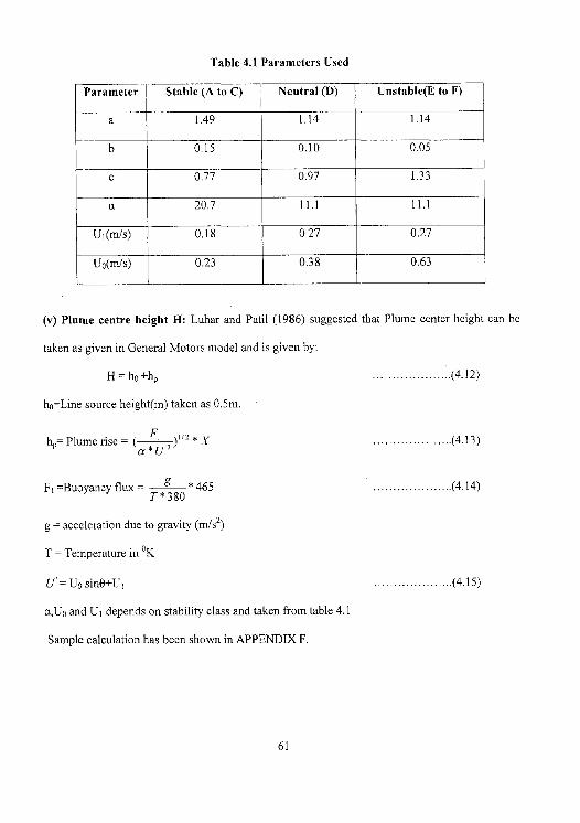
Table 4.1 Parameters Used
Parameter Stable (A to C) Neutral (D) Unstable(E to F)
a 1.49 1.14 1.14
b 0.15 0.10 0.05
c 0.77 0.97 1.33
a 20.7 11.1 11.1
Ui(m/s) 0.18 0.27 0.27
U°(m/s) 0.23 0.38 0.63
(v) Plume centre height H: Luhar and Patil (1986) suggested that Plume center height can be
taken as given in General Motors model and is given by:
H = h°+hp ....................(4.12)
h°=Line source height(m) taken as 0.5m.
hp=Plume rise= (4.13)
( a*U .3 11/2 *,x ....................
F, =Buoyancy flux = g * 465 ....................(4.14) T*380
g = acceleration due to gravity (m/s2)
T = Temperature in °K
U' = U° sin0+UI ....................(4.15)
a,U° and U1 depends on stability class and taken from table 4.1
Sample calculation has been shown in APPENDIX F.
61
CHAPTER 5
PERFORMANCE EVALUATION OF AIR POLLUTION MODELS
5.1 Overview
The evaluation of model performance is a matter of great interest and it becomes
particularly important in all those fields in which modeling is used as a decision making tool.
Evaluation of the performance of an air-quality model generally focuses on assessing the
accuracy of the model prediction relative to observed concentrations [25]. In this study model
evaluation is carried out by comparing the observed data from the field with predicted data. A
significance test is also applied to check the consistency of the observed data with the predicted
data to have confidence in prediction exercise.
5.2 Site-wise Performance Evaluation
Performance evaluation of both models has been done for all locations. The concentration
of Carbon Monoxide, which was monitored in the field, compared with predicted concentration
using CALINE-4 and GFLSM. The index agreement (d) for each location is also calculated which
is explained in section 5.2.1.
Statistical test to determine the reliability of inter-relationship between predicted and
observed values like t-test has also been performed and found to give acceptable results at a 95%
confidence level. A line of regression between the predicted and the observed values has also
been developed and a good co-relation has been obtained for CALINE-4 as well as GFLSM.
62
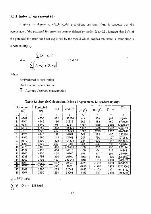
5.2.1 Index of agreement (d)
It gives the degree to which model predictions are error free. It suggests that the
percentage of the potential for error has been explained by model. If d=0.51 it means that 51% of
the potential for error has been explained by the model which implies that there is lower error in
model result[16].
Y ( P —Or )2
d=1— "-' 0<_d_<l
—°+° —°U 2 Where,
Pr Predicted concentration
0, Observed concentration
O = Average observed concentration
Table 5.1 Sample Calculation, Index of Agreement, L1 (Safardarjung)
Observed (0)
Predicted (P) P-O
2
(P-O) -
(P-O) -
(O-O) I 5H61 (7)2
si 1 2 3 4 5 6 7 8 1. 4982 4600 -382 145924 -43 339 382 145924 2. 5101 4945 -156 24336 302 458 760 577600 3. 6531 6440 -91 8281 1797 1888 3685 13579225 4. 6118 5750 -368 135424 1107 1475 2582 6666724 5. 5918 6325 407 165649 1682 1275 2957 8743849 6. 4826 4945 119 14161 302 183 485 235225 7. 5403 5290 -113 12769 647 760 1407 1979649 8. 5613 5290 -323 104329 647 970 1617 2614689 9. 4298 4600 302 91204 -43 -345 388 150544 10, 4973 4485 -488 238144 -158 330 488 238144 11. 4589 4485 -104 10816 -158 -54 212 44944 12. 4960 4830 -130 16900 187 317 504 254016 13. 3985 3795 -190 36100 -848 -658 1506 2268036 14. 3302 3795 493 243049 -848 -1341 2189 4791721 15 3427 3220 -207 42849 -1423 -1216 2639 6964321 16 2678 2645 -33 1089 -1998 -1965 3963 15705369 17 3169 2990 -179 32041 -1653 -1474 3127 9778129 18 3701 3450 -251 63001 1193 942 2135 4558225
0=4643 µg/m3 IB
1_O)2 = 1386066
63
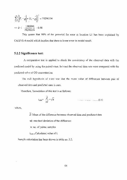
O+O,—O ~)' =79296334
_> d=1— 1386066 = 0.98 79296334
This means that 98% of the potential for error at location L1 has been explained by
CALINE-4 model which implies that there is lower error in model result.
5.2.2 Significance test:
A comparative test is applied to check the consistency of the observed data with the
predicted model by using the paired t-test. In t-test the observed data sets were compared with the
predicted value of CO concentration.
The null hypothesis of t-test was that the mean value of difference between pair of
observed data and predicted ones is zero.
Therefore, formulation of this test is as follows:
d ~ halt —
d * V n ............................(5.1)
s
where,
d :Mean of the difference between observed data and predicted data
sd: standard deviation of the difference.
n: no. of paired samples
tcaic =Calculated value oft.
Sample calculation has been shown in table no. 5.2.
64
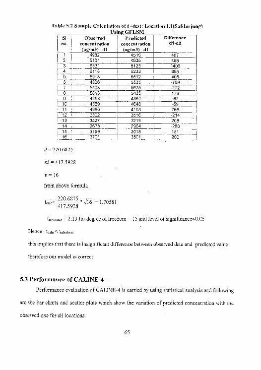
Table 5.2 Sample Calculation oft —test: Location I,1(Sa Ida r,jung) Using GFLSM
SI no.
Observed concentration
_gittL.tiL_1
Predicted concentration (}Lt;/m3) dl
Difference dl d2
1 4982 4515 467 2 5101 4635 466 3 6531 5125 1406 4 6118 5233 885 5 5918 5512 406 6 4826 5535 -709 7 5403 5675 -272 8 5613 5435 178 9 4298 4360 -62
10 4589 4648 -59 11 4960 4194 766 12 3302 3516 -214 13 3427 3219 208 14 2678 2964 -286 15 3169 3018 151 16 3701 3501 200
d= 220.6875
sd=417.5928
n=16
from above formula
220.6875 tcalc=
* 16 =1.70581 417.5928
ttabulated = 2.13 for degree of freedom = 15 and level of significance=0.05
Hence tcalc < ttabulated
this implies that there is insignificant difference between observed data and predicted value
therefore our model is correct
5.3 Performance of CALINE-4 Performance evaluation of CALINE-4 is carried by using statistical analysis and following
are the bar charts and scatter plots which show the variation of predicted concentration with the
observed one for all locations.
65
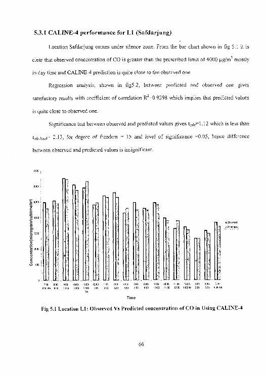
5.3.1 CALINE-4 performance for LI (Safdarjung)
Location Safdarjung comes under silence zone. From the bar chart shown in fig 5.1 it is
clear that observed concentration of CO is greater than the prescribed limit of 4000 µg/m3 mostly
in day time and CALINE-4 prediction is quite close to the observed one.
Regression analysis, shown in fig5.2, between predicted and observed one gives
satisfactory results with coefficient of correlation R2=0.9398 which implies that predicted values
is quite close to observed one.
Significance test between observed and predicted values gives t,,,,=1.12 which is less than
t,at ui„< ;= 2.13, for degree of freedom = 15 and level of significance =0.05, hence difference
between observed and predicted values is insignificant.
M
G000.
soonl
v ~
L0014000
E
rn ~
° ]000
2000
U 1000 ,
709-. 900 now 9:00
Time
Fig 5.1 Location L1: Observed Vs Predicted concentration of CO in Using CALINE-4
66
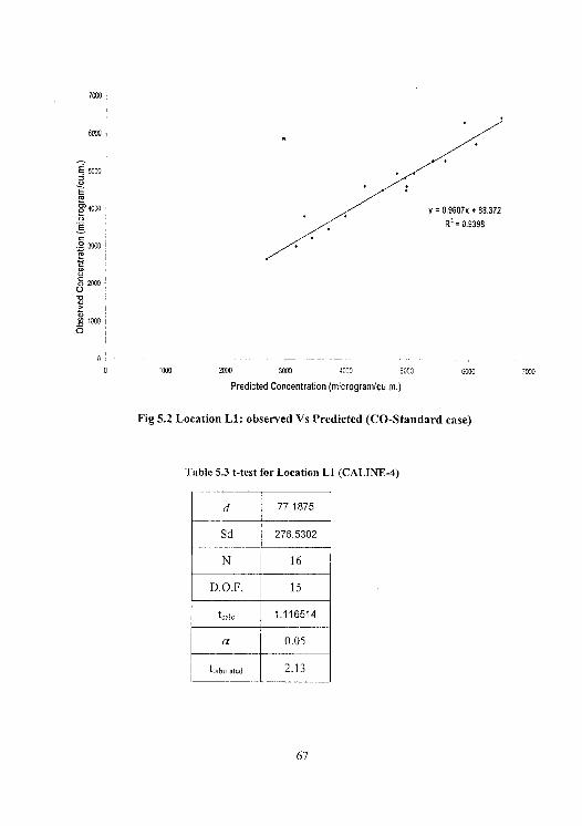
1000 2000 3000 4000 5000 6000
Predicted Concentration (microgram/cu.m.)
Fig 5.2 Location LI: observed Vs Predicted (CO-Standard case)
Table 5.3 t-test for Location Li (CALINE-4)
77.1875
Sd 2765302
N 16
D.O.F. 15
tcaic 1.116514
a 0.05
tniaird 2.13
7000
6000 ,
E 5000
E m
0 4000
° 3000 R i C
2000: U
7000 I O
0.,
0 WA
67
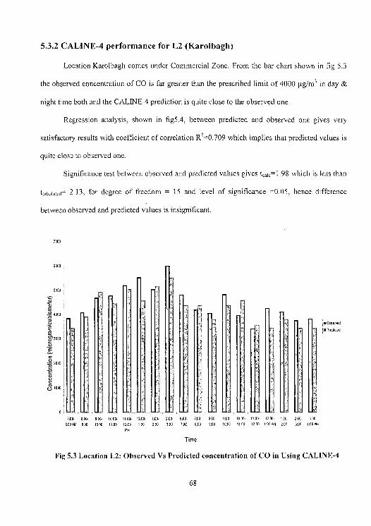
5.3.2 CALINE-4 performance for i,2 (Karolbagh)
Location Karolbagh comes under Commercial Zone. From the bar chart shown in fig 5.3
the observed concentration of CO is far greater than the prescribed limit of 4000 µg/m3 in day &
night time both and the CALINE-4 prediction is quite close to the observed one.
Regression analysis, shown in fig5.4, between predicted and observed one gives very
satisfactory results with coefficient of correlation R2"0.709 which implies that predicted values is
quite close to observed one.
Significance test between observed and predicted values gives t,aIc= l .98 which is less than
[tabulated — 2.13, for degree of freedom = 15 and level of significance =0.05, hence difference
between observed and predicted values is insignificant.
7000
6000
5000
E 4000
o 0000 }
2000 t
c ~
V 1000
700 8:00. 9.00. 1000- 1100- 1200- I:00-
80055 9D0 1000 11 00 1200 100 2:00
PM
Time
Fig 5.3 Location L2: Observed Vs Predicted concentration of CO in Using CALINE-4
68
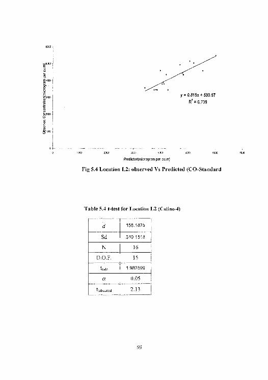
6000
._5000 E
%4000
0
EE'S000
92000 U
oi-a
y=0.815x+590.57
R'=0.709
1000 2000 3000 6000 5000 6000
Predicted(microgram per cu,mj
Fig 5.4 Location L2: observed Vs Predicted (CO-Standard
Table 5.4 t-test for Location L2 (Caline-4)
158.1875
Sd 319.1518
N 16
D.O.F. 15
tcaic 1.982599
a 0.05
toabulated 2.13
tE
69
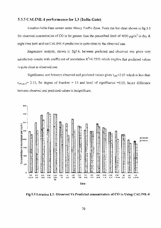
between observed and predicted values is insignificant.
7000
6500
E
fl }
i
900- 1005- 1100- 1260- 100 200- 000-
1000 1107 1200 1:00!4.1 7:00 000 50004 1:00- 200- 600- 760- 020-
0:00 3:00 0:00 8:00 9:00
5000
E
of 4000 o
E ]000
0 04
2000
C ~ 0
V 1000
100- 800- 900. 0000M 900 1000
5.3.3 CALINE-4 performance for L3 (India Gate)
Location India Gate comes under Heavy Traffic Zone. From the bar chart shown in fig 5.5
the observed concentration of CO is far greater than the prescribed limit of 4000 1g/m3 in day &
night time both and the CALINE-4 prediction is quite close to the observed one.
Regression analysis, shown in fig5.6, between predicted and observed one gives very
satisfactory results with coefficient of correlation R2 0.7533 which implies that predicted values
is quite close to observed one.
Significance test between observed and predicted values gives t4.4.1 4.=2.05 which is less than
t,,,h„i„oDci= 2.13, for degree of freedom = 15 and level of significance =0.05, hence difference
Time
Fig 5.5 Location L3: Observed Vs Predicted concentration of CO in Using CALINE-4
70
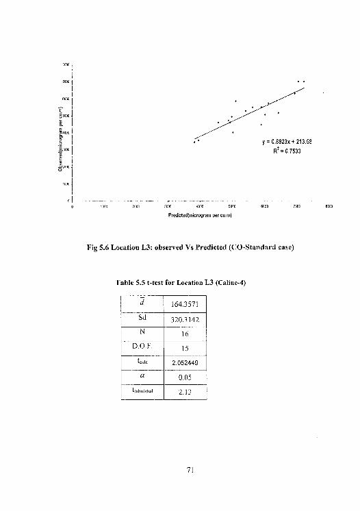
7000 1
epos i .
E ~
~saao i • • •
.4000
j y = 0.8923x + 213.58
aoo { R2 = 0.7533
ozwo~
1000
0 1000 2000 3000 4000 5000 6090 7000 9000
Predicted(microgram per cu.m)
Fig 5.6 Location L3: observed Vs Predicted (CO-Standard case)
Table 5.5 t-test for Location L3 (Caline-4)
164.3571
Sd 320.3142
N 16
D.O.F. 15
tcalc 2.052449
a 0.05
tmbwued 2.13
71
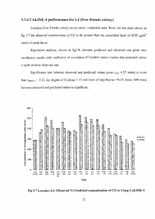
5.3.4 CALINE-4 performance for L4 (New friends colony)
Location New friends colony comes under residential area. From the bar chart shown in
fig 5.7 the observed concentration of CO is far greater than the prescribed limit of 4000 .sg/m3
mostly in peak hours.
Regression analysis, shown in fig5.8, between predicted and observed one gives very
satisfactory results with coefficient of correlation R2=0.8441 which implies that predicted values
is quite close to observed one.
Significance test between observed and predicted values gives tcuu~ 4.57 which is more
than ttabu ated= 2.13, for degree of freedom = 15 and level of significance =0.05, hence difference
between observed and predicted values is significant.
.11
5000
E
i" IIITllhII IlIIIl E
m 3000
0
E 2000
10001. .
i ■ oe~:~ei im aree~nedl
00. 900- t000- ttno 1200 f9a 2:00- 200-
00 1100 1100 1200 1:00 M1 200 ] oa 4.00 AM
Time
Fig 5.7 Location L4: Observed Vs Predicted concentration of CO in Using CALINE-4
72
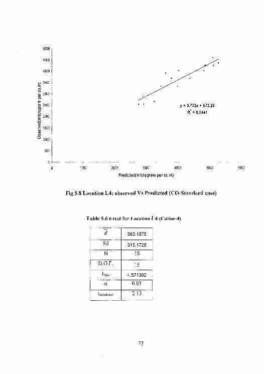
5000
4500
' y = 0.733x + 673.26 RZ = 0.8441
1000 2000 3000 4000 5000 6000
Predicted(microgram per cum)
Fig 5.8 Location L4: observed Vs Predicted (CO-Standard case)
Table 5.6 t-test for Location L4 (Catine-4)
d 360.1875
Sd 315.1728
N 16
D.O.F. 15
tc41c 4.571302
a 0.05
ttabulatcd 2.13
4000 j
3500
3 ~ 3000 1
2 2500
E 2000
1500
a ~
0 1000
500
0?-
0
73
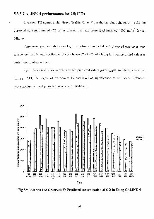
between observed and predicted values is insignificant.
6000
5000 m d E
:0 4000
0 n E 122 3000
0 L0
E
S 2000
0 a)
~aoo
700- 8:00- 800)0 9:00
290- 8100 700- 0:00 700 8 00
5.3.5 CALINE-4 performance for L5(ITO)
Location ITO comes under Heavy Traffic Zone. From the bar chart shown in fig 5.9 the
observed concentration of CO is far greater than the prescribed limit of 4000 µg/m3 for all
24hours.
Regression analysis, shown in fig5.10, between predicted and observed one gives very
satisfactory results with coefficient of correlation R2=0.575 which implies that predicted values is
quite close to observed one.
Significance test between observed and predicted values gives tcai,=1.84 which is less than
tz ~ ul ztcd= 2.13, for degree of freedom = 15 and level of significance =0.05, hence difference
i oo~o~e. n wea~mea ~,
809- 900 10.00 11.00 1200- 100- 200- 000- 900 1000 1100 1200 1 DOOM 200 300 480001
Time
Fig 5.9 Location L5: Observed Vs Predicted concentration of CO in Using CALINE-4
74
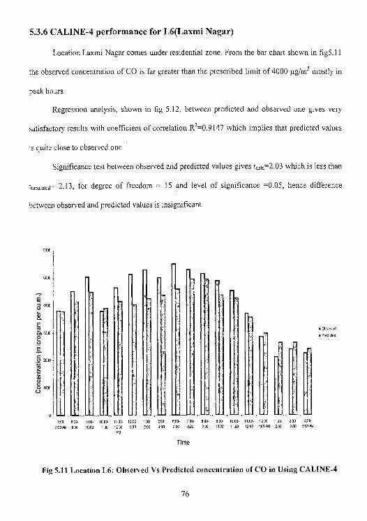
5000
0000
a° E
~ 3000 -I
O 1
E c I 0 2000
CM
a
M Observed
5.3.6 CALINE-4 performance for L6(Laxmi Nagar)
Location Laxmi Nagar comes under residential zone. From the bar chart shown in fig5.l 1
the observed concentration of CO is far greater than the prescribed limit of 4000 µg/m3 mostly in
peak hours.
Regression analysis, shown in fig 5.12, between predicted and observed one gives very
satisfactory results with coefficient of correlation R2=0.9147 which implies that predicted values
is quite close to observed one.
Significance test between observed and predicted values gives t391 3= 2.03 which is less than
ttahu jalcd= 2.13, for degree of freedom = 15 and level of significance =0.05, hence difference
between observed and predicted values is insignificant.
RM
700 0:0 9.00- 10:00. 1100- 1200- 1:00- 200- 600- 7:00- 500- 900- 1000- 11.00- 1200- I: 00- 2:00- 300.
890 644 900 10:00 11:00 1200 1:00 200 300 790 8.00 0:00 1000 1190 1200 100 AM 200 300 4:00964
PM
Time
Fig 5.11 Location L6: Observed Vs Predicted concentration of CO in Using CALINE-4
76
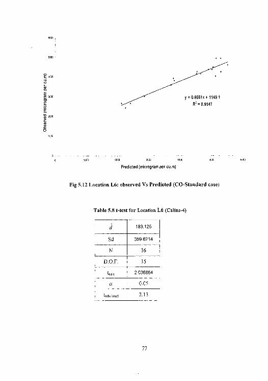
6000
00°°
E dc°o
O. I' E m 3000 l rn y = 0.6551 x + 1149.1
2000
2
a 0
1200
0 1000 2000 7000 1000 5000 5000
Predicted (microgram per cu.m)
Fig 5.12 Location L6: observed Vs Predicted (CO-Standard case)
Table 5.8 t-test for Location L6 (Caline-4)
d 183.125
Sd 359.6214
N 16
D.O.F. 15
tca c 2.036864
a 0.05
ttabulated 2.13
77
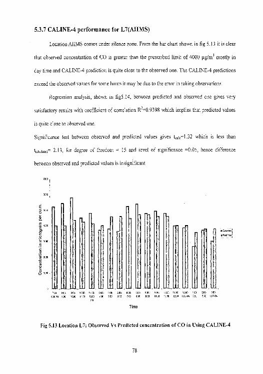
5.3.7 CALINE-4 performance for L7(AIIMS)
Location AIIMS comes under silence zone. From the bar chart shown in fig 5.13 it is clear
that observed concentration of CO is greater than the prescribed limit of 4000 4g/m3 mostly in
day time and CALINE-4 prediction is quite close to the observed one. The CALINE-4 predictions
exceed the observed values for some hours it may be due to the error in taking observations.
Regression analysis, shown in fig5.14, between predicted and observed one gives very
satisfactory results with coefficient of correlation R2=0.9398 which implies that predicted values
is quite close to observed one.
Significance test between observed and predicted values gives talc 1.32 which is less than
ttab,hL,d= 2.13, for degree of freedom = 15 and level of significance =0.05, hence difference
between observed and predicted values is insignificant
1000
6000
E j 0007
a E 4000
T 0
V_ E 0006
C
2 2000
C
CO
L) 1000
:
100- 600- 900. 1000- 1100- 1200- 100- 200.
B 00 M1 900 1090 1120 12:00 100 200 000
PM
900- 100- 900- 900. 1000- 11.00 rzao- Ias 700 800 900 1000 1100 1200 102P 100
106286
1
000-
4 -0 2 206
Time
Fig 5.13 Location L7: Observed Vs Predicted concentration of CO in Using CALINE-4
78
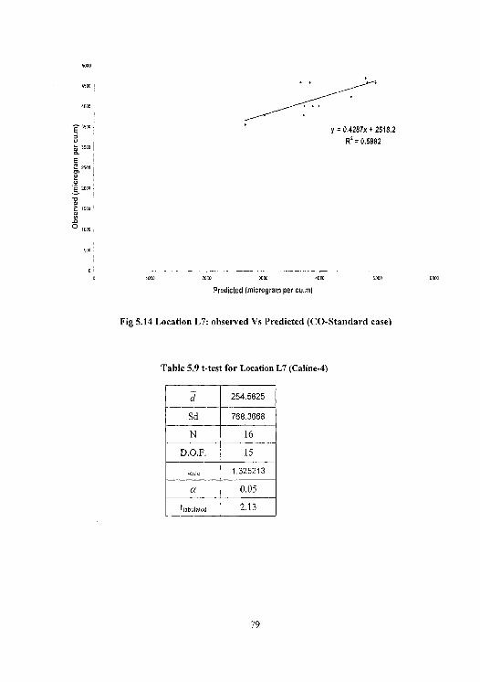
MI
4100 1
4000 1
4500
y = 0.4287x + 2518.2
R0 = 0.5882 3000
E 2500
Z000
Z 1500
0 1020
in
-------
0 1000 2000 3000 4000 5000 5000
Predicted (microgram per cu.m)
Fig 5.14 Location L7: observed Vs Predicted (CO-Standard case)
Table 5.9 t-test for Location L7 (Caline-4)
254.5625
Sd 768.3668
N 16
D.O.F. 15
tc0~0 1.325213
a 0.05
ttabulated 2.13
79
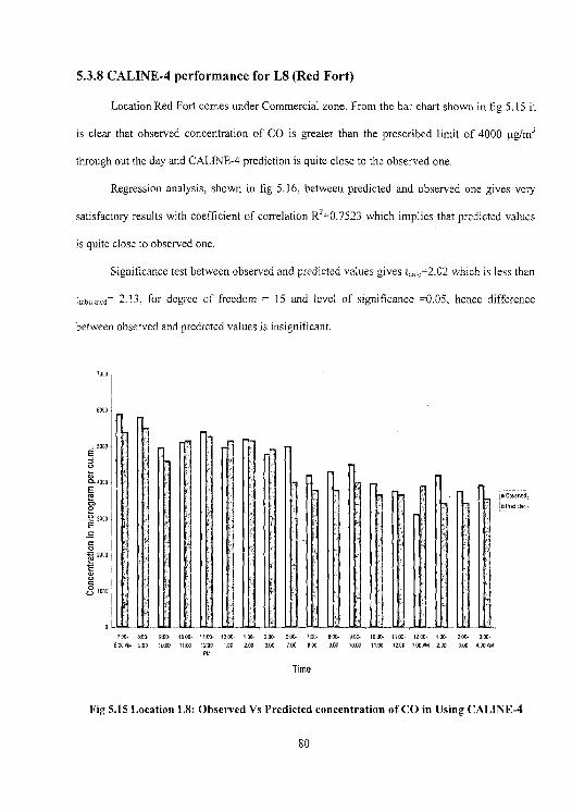
5.3.8 CALINE-4 performance for L8 (Red Fort)
Location Red Fort comes under Commercial zone. From the bar chart shown in fig 5.15 it
is clear that observed concentration of CO is greater than the prescribed limit of 4000 jig/m3
through out the day and CALINE-4 prediction is quite close to the observed one.
Regression analysis, shown in fig 5.16, between predicted and observed one gives very
satisfactory results with coefficient of correlation R2=0.7523 which implies that predicted values
is quite close to observed one.
Significance test between observed and predicted values gives t,=2.02 which is less than
t b„iaicd= 2.13, for degree of freedom = 15 and level of significance =0.05, hence difference
between observed and predicted values is insignificant.
ass
5000 E V
N o_ 4000
CM E rn 0
3000 a C 0
2000
C C
7000
0
j I obtuse: ® PreeAted
700- 890 900- 1000. 1100- 1200- 1:00- 2:00- 600- 700- 600. 900- 10.00- 1190- 12:00- 1:00- 200. 0:00- 8;00964 8:00 10.00 1100 1200 100 2.00 5:00 0.00 0:00 900 1000 11.00 1200 150969 2:00 3:00 40005
PM
Time
Fig 5.15 Location L8: Observed Vs Predicted concentration of CO in Using CALINE-4
80
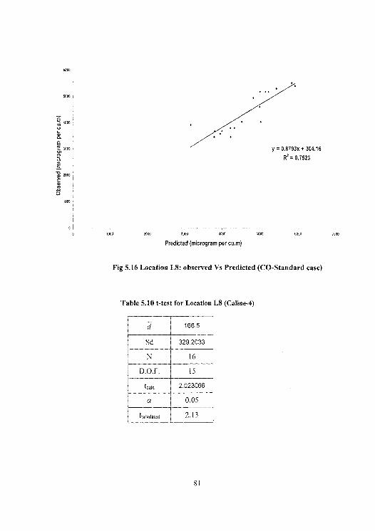
6000
5000
j 4000
a 3000
E d 2000 Z N 0
1000
y = 0.8793x + 304.16
R2 = 0.7523
1000 2000 3000 4000 5000 6000 7000
Predicted (microgram per cu.m)
Fig 5.16 Location L8: observed Vs Predicted (CO-Standard case)
Table 5.10 t-test for Location L8 (Caline-4)
166.5
Sd 329.2033
N 16
D.O.F. 15
tea l0 2.023066
a 0.05
ttabulatcd j
2.13
81
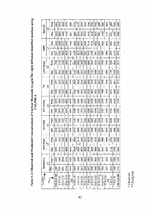
o O O N O O N r Ul
0O N
0O r
45 to Y') N
to 01 N 01
~O N
O ~
O O to
O tO N t0
LL W J
O
tO to O to 0 tO O 0 N N
to O to N U) i0 O O M a a to d O d t0 Q to
V V M d Q Q to to to V N M
Q c0 N M N ~O t0 W fD r
O
to O N O O N N t0 0 O 4'l O to to m
to to N
O N d d
O h M
d to
W Q Q
N M
V Q
N O O
N to
d W Q
O (D Q
d O1 to
V O) to M
V N to
(D N N N
N N N N
Z
N ~O O M C M r a M W r QI M O O M
O [0 — O O tO N O O W
O W N to to O
O uo F- J
to M O O N N O) O
O) N N
.- W M O O7 N
A O Io W W N W N O V N
O N V Q C< N O V V' to d M N M to Q Q
to O N N N tO O O O O N to O N to to O O G ZS W N
CC N
N O N
O O W N
W (O M
N O ID N
N N f0
M M
M M d
N M N ~O
O d ON Q to V O M M to Q V V M M M N N
U J
LL y to N N W W N N O Q M W M r W to W M Z to '- 0 O> O) N to N Q r W to i[] N to
O N W8 d d M M ~O N O O V M M N N
M O V N O7 N r O fD N K
00 tO J
C a t0 M.
M ~-- N
W N
M r 0 to O N N
M O
to to N m O
O W r
to N to
tD ~O
to N
O Q O c0 to N
r O r <D ~O
y t0
to O u1
Oo Q
W ~O N
W Q
O u~
to N M
N M
-p O ~O O O ~1 O A O O L N •- Q W 0 O r N r M 0) r r O fp iD l0 i0 Q n ~fl Q d
Q M? d M M M M M IL N O J
• t0 N M O F to O M to M
to t0 W to
N to O to
to O Q to r N
W N
N tO to N
O
O U) O N N to 0 0 0 to to O 0) U) O V
O O C ~1 l0 W r M O) N N (D d V W r N t0 OI Q
(t) d• W O
~ O~ N
` Q O Q O O 00 O 00
O O I N c']
..
OlA W { N M
pF p o o a It! 0 00
00
o
!iI O
0
I
° a 00 o ~ O ~- cV 10 f` O ~ ~- N
n
82
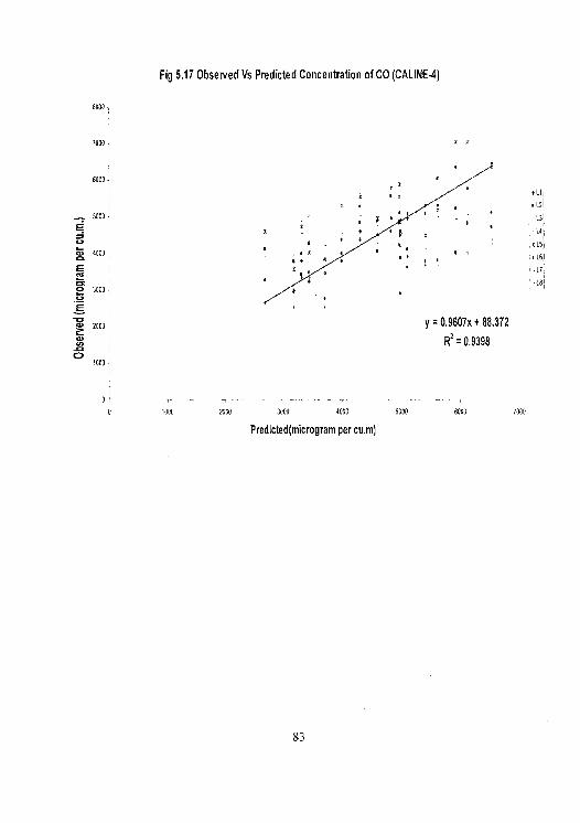
Fig 5.17 Observed Vs Predicted Concentration of CO (CALINE-4)
7000
6000 1
j x
S • X X ~ ,
~.~ 560 i • ~ '
d aaao ~ x
o aaoo -I
1 1
2000 y = 0.9607x + 88.372
R2 =09398 0
1000
0 1000 2007 3000 4000 5000 6000
Predicted(microgram per cu.m)
83
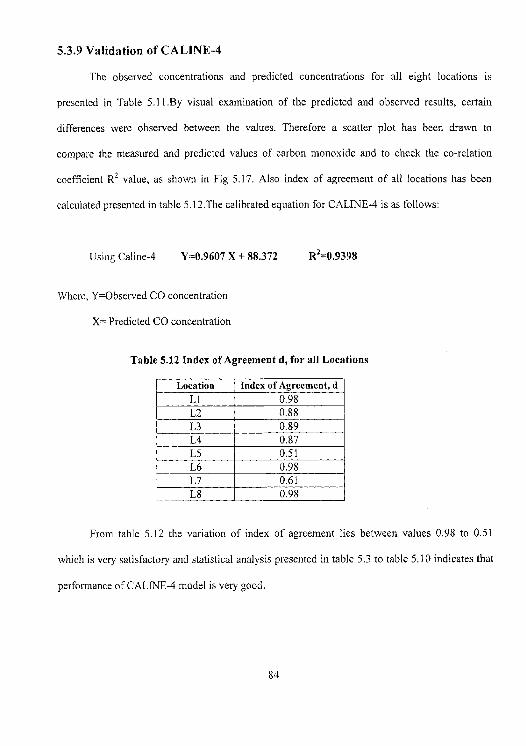
5.3.9 Validation of CALINE-4
The observed concentrations and predicted concentrations for all eight locations is
presented in Table 5.11 By visual examination of the predicted and observed results, certain
differences were observed between the values. Therefore a scatter plot has been drawn to
compare the measured and predicted values of carbon monoxide and to check the co-relation
coefficient R2 value, as shown in Fig 5.17. Also index of agreement of all locations has been
calculated presented in table 5.12.The calibrated equation for CALINE-4 is as follows:
Using Caline-4 Y=0.9607 X + 88.372 R2 0.9398
Where, Where, Y=Observed CO concentration
X= Predicted CO concentration
Table 5.12 Index of Agreement d, for all Locations
Location Index of Agreement, d L 1 0.98 L2 0.88 L3 0.89 L4 0.87 L5 J 0.51 L6 0.98 L7 0.61 L8 0.98
From table 5.12 the variation of index of agreement lies between values 0.98 to 0.51
which is very satisfactory and statistical analysis presented in table 5.3 to table 5.10 indicates that
performance of CALINE-4 model is very good.
84
5.4 Performance of General Finite Line Source Model (GFLSM) Performance evaluation of GFLSM is carried out in the same manner as completed for
CALINE-4. Following are the bar charts and scatter plots, which show the variation of predicted
concentration with the observed one.
85
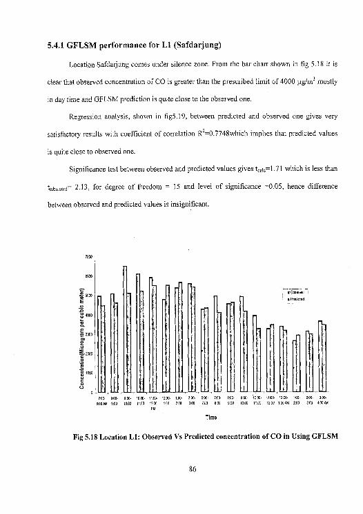
5.4.1 GFLSM performance for Li (Safdarjung)
Location Safdarjung comes under silence zone. From the bar chart shown in fig 5.18 it is
clear that observed concentration of CO is greater than the prescribed limit of 4000 µg/m3 mostly
in day time and GFLSM prediction is quite close to the observed one.
Regression analysis, shown in fig5.19, between predicted and observed one gives very
satisfactory results with coefficient of correlation R2=0.7748which implies that predicted values
is quite close to observed one.
Significance test between observed and predicted values gives t,at~ 1.71 which is less than
ttabMtatud° 2.13, for degree of freedom = 15 and level of significance =0.05, hence difference
between observed and predicted values is insignificant.
7000
6000
5000
E
4000
E n ~a 3000 rn 0
-2000
E N
1000
0 U
700. 000. 900- 1000. 11'00- 1200- 1:00. 200. 6:00- 700- 8.00 900- 10:00- 1100- 12:00- 100, 200- 0:00-
800494 500 1600 1120 1200 1:00 2:00 300 700 000 900 10'.00 11:00 1200 1:00 AM 200 390 400 AM PM
Time
Fig 5.18 Location Li: Observed Vs Predicted concentration of CO in Using GFLSM
86
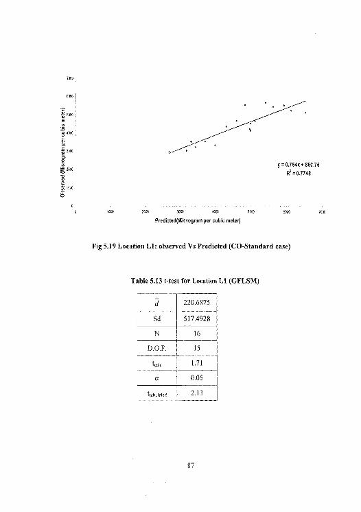
7000
4000 I
5200 ' E
4000
2000
rn 0
2000
1000
0
i . y = 0.754x + 860.75
R2 = 0.7748
1000 2000 3000 4000 5000 6000
7000
Predicted(Microgram per cubic meter)
Fig 5.19 Location LI: observed Vs Predicted (CO-Standard case)
Table 5.13 t-test for Location LI (GFLSM)
220.6875
Sd 517.4928
N 16
D.O.F. 15
teals 1.71
a 0.05
ttabulatcd 2.13
87
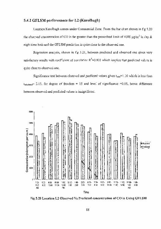
u06served LPredialedJ
6:00- 9:00- 10D0. 11:00- 1200- 1:00- 900 1000 1100 12:00 1:00 200
AM
5.4.2 GFLSM performance for L2 (Karolbagh)
Location Karolbagh comes under Commercial Zone. From the bar chart shown in fig 5.20
the observed concentration of CO is far greater than the prescribed limit of 4000 µg/m3 in day &
night time both and the GFLSM prediction is quite close to the observed one.
Regression analysis, shown in fig 5.21, between predicted and observed one gives very
satisfactory results with coefficient of correlation R2=0.801 which implies that predicted values is
quite close to observed one.
Significance test between observed and predicted values gives tca,c 1.16 which is less than
t,abuiaLed= 2.13, for degree of freedom = 15 and level of significance =0.05, hence difference
between observed and predicted values is insignificant.
Time
Fig 5.20 Location L2 Observed Vs Predicted concentration of CO in Using GFLSM
88
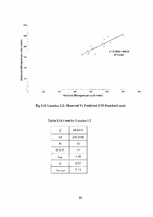
6000 i
5000
yI • •
E 4000 u a
y=0.7562x+645.24
E~ a R'=0.801
0 o u g_ 2000 J 00 d
N
0 1000
0 1000 2000 ]000 4000 5000 6000
Predicted (Microgram per cubic meter)
Fig 5.21 Location L2: Observed Vs Predicted (CO-Standard case)
Table 5.14 t-test for Location L2
d 68.6875
Sd 235.3728
N 16
D.O.F. 15
talc 1.16
a 0.05
ttahulalal 2.13
7000
89
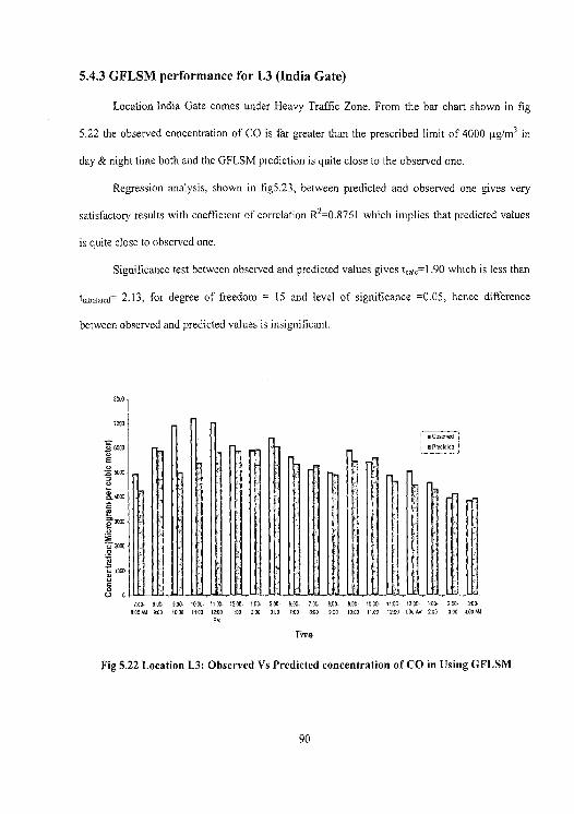
loss
S 6002
a a 5000
.4002
5.4.3 GFLSM performance for L3 (India Gate)
Location India Gate comes under Heavy Traffic Zone. From the bar chart shown in fig
5.22 the observed concentration of CO is far greater than the prescribed limit of 4000 µg/m3 in
day & night time both and the GFLSM prediction is quite close to the observed one.
Regression analysis, shown in fig5.23, between predicted and observed one gives very
satisfactory results with coefficient of correlation R2=0.8761 which implies that predicted values
is quite close to observed one.
Significance test between observed and predicted values gives t,ai~ 1.90 which is less than
t(abojated= 2.13, for degree of freedom = 15 and level of significance =0.05, hence difference
between observed and predicted values is insignificant.
700. 800 8.00- 1000- 1100- +zoo- too- zoo- 8:00- 700 9:00- BAO. M00- 11 DO- 1200- 100. 2:00- 200- 8.00 Rd 800 1000 1100 1200 too 2:00 0,00 Loo 800 800 1090 1100 12:00 .001614 200 000 4:00444
PM
Time
Fig 5.22 Location L3: Observed Vs Predicted concentration of CO in Using GFLSM
90
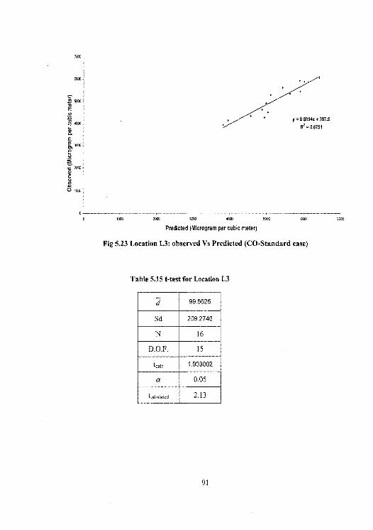
7000
d 5000 E E
4000
a E @ 3WO
D
y = 0.8B94x + 97.5 R' = 0.8751
2000
100D 2000 3000 400 5000 6000 7O
Predicted (Microgram per cubic meter)
Fig 5.23 Location L3: observed Vs Predicted (CO-Standard case)
Table 5.15 t-test for Location L3
99.5625
Sd 209.2746
N 16
D.O.F. 15
tcalc 1.903002
a 0.05
ttabulated 2.13
91
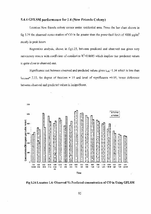
5.4.4 GFLSM performance for L4 (New Friends Colony)
Location New friends colony comes under residential area. From the bar chart shown in
fig 5.24 the observed concentration of CO is far greater than the prescribed limit of 4000 pg/m3
mostly in peak hours.
Regression analysis, shown in fig5.25, between predicted and observed one gives very
satisfactory results with coefficient of correlation R2 0.8685 which implies that predicted values
is quite close to observed one.
Significance test between observed and predicted values gives team1.34 which is less than
ttabulated° 2.13, for degree of freedom = 15 and level of significance =0.05, hence difference
between observed and predicted values is insignificant.
6000
5000
4000
3000
E
Z3 2000
0
1000
U
700- 000- 900- 10:00- 1100- 1200- 100- 200- 6:00- 790. 0:02- 900- 1000- 11:00- 1200- 100- 200- 3:00- 900004 900 1000 1100 1200 100 2:00 300 700 0:00 900 1000 1100 1200 100041 2:00 300 410016
PM
Time
Fig 5.24 Location L4: Observed Vs Predicted concentration of CO in Using GFLSM
92
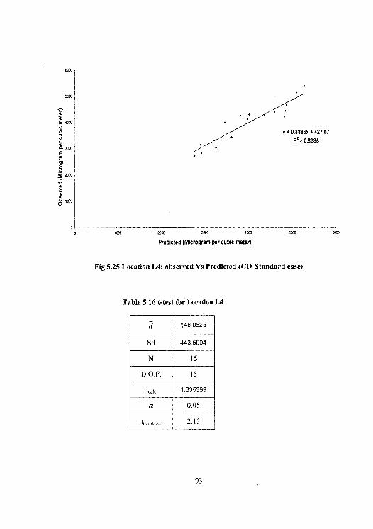
M
a
E40 j
0000
E ~ I 0 `u
iaoo
0
y = 0.8886x + 427.07 R2 0.8685
1000 2000 0000 4000 5000 6000
Predicted (Microgram per cubic meter)
Fig 5.25 Location L4: observed Vs Predicted (CO-Standard case)
Table 5.16 t-test for Location L4
d 148.0625
Sd 443.5004
N 16
D.O.F. 15
teak 1.335399
a 0.05
ttabulatcd 2.13
93
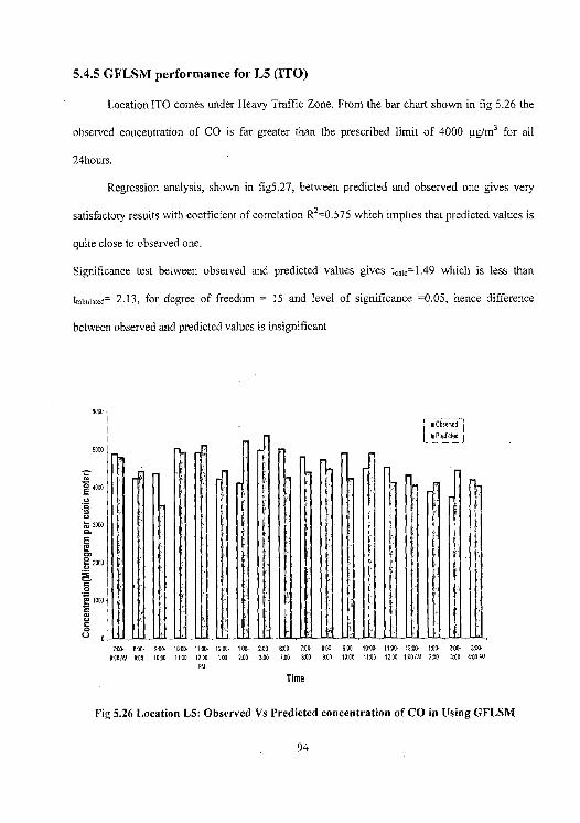
5.4.5 GFLSM performance for L5 (ITO)
Location ITO comes under Heavy Traffic Zone. From the bar chart shown in fig 5.26 the
observed concentration of CO is far greater than the prescribed limit of 4000 µg/m3 for all
24hours.
Regression analysis, shown in fig5.27, between predicted and observed one gives very
satisfactory results with coefficient of correlation R2=0.575 which implies that predicted values is
quite close to observed one.
Significance test between observed and predicted values gives t,1 =1 .49 which is less than
tcanuiaeed= 2.13, for degree of freedom = 15 and level of significance =0.05, hence difference
between observed and predicted values is insignificant
6000
M3
4000
a ci v
3000 C-
2 rn
2000
C 0
1000 c c 0 U
7.00- 890- 000- 1000- 11:00- 1200- 1D0- 2:00- 600- 700- 8:00- 9:00- 1000- 1100. 1200- 100- 200- 200-
800AM 9:00 1000 1100 1200 100 2:00 100 7:00 8.00 900 10:00 1100 1200 1:00AM 2:00 300 490 AM
PM
Time
Fig 5.26 Location L5: Observed Vs Predicted concentration of CO in Using GFLSM
94
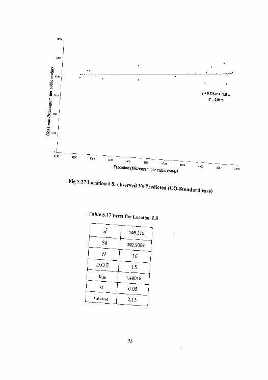
LM
U I
U
°' I Y' 8.7361x. 1126.5 a a0001
00 0 0
2000
a
4130 4200 1700 4400 4500 4600 ~----~-~-- ~_ ...o 4600 --
Predicted (Microgram per cubic meter) shoo 00
Fig 5.27 Location L5; observed Vs Predicted (CO- Standard case)
Table 5.17 t-test for Location L5
d 146.375
Sd 392.9056
N 16
D.O.F. 15
tcaic 1.49018
a 0.05
ttabulared 2.13
95
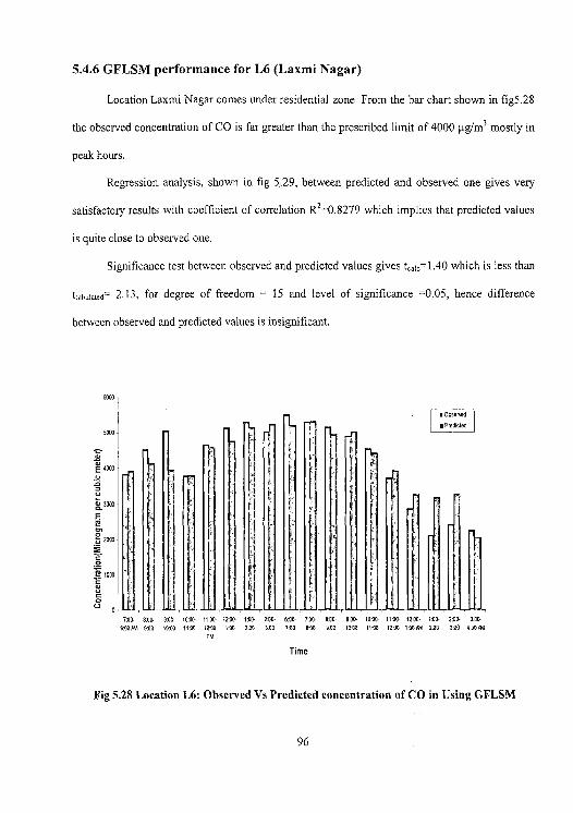
5.4.6 GFLSM performance for L6 (Laxmi Nagar)
Location Laxmi Nagar comes under residential zone. From the bar chart shown in fig5.28
the observed concentration of CO is far greater than the prescribed limit of 4000 µg/m3 mostly in
peak hours.
Regression analysis, shown in fig 5.29, between predicted and observed one gives very
satisfactory results with coefficient of correlation R2=0.8279 which implies that predicted values
is quite close to observed one.
Significance test between observed and predicted values gives t,,i~ 1.40 which is less than
tn,b„iated= 2.13, for degree of freedom = 15 and level of significance =0.05, hence difference
between observed and predicted values is insignificant.
6000
5000
4000
i,
47000
E
0
E 2000
0 0
loco
a. U
700- 800. 900- 1000- 11:00- 1200- 1:00- 2:00- 0:00- 7:00- 800- 9:00. 7020- 1100- 1200. 7:00- 200- 2.00- 920PM 900 10.00 1100 1200 100 2:00 020 700 0:00 990 10:00 11:00 12.00 120712 200 390 400701
PM
Time
Fig 5.28 Location L6: Observed Vs Predicted concentration of CO in Using GFLSM
96
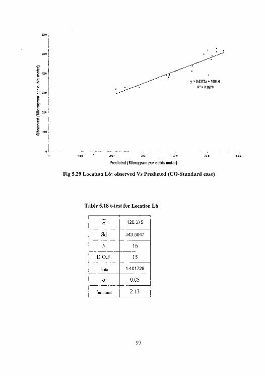
6000
5000
4000
a
p 3000
C
0
3~ 2000 1
v m
y = 0.6372x + 1584.6 R'=0.8279
0 1000 2000 3000
00 40
5000 6000
Predicted (Microgram per cubic meter)
Fig 5.29 Location L6: observed Vs Predicted (CO-Standard case)
Table 5.18 t-test for Location L6
120.375
Sd 343.5047
N 16
D.O.F. 15
tcalc 1.401728
a 0.05
ttabulated 2.13
97
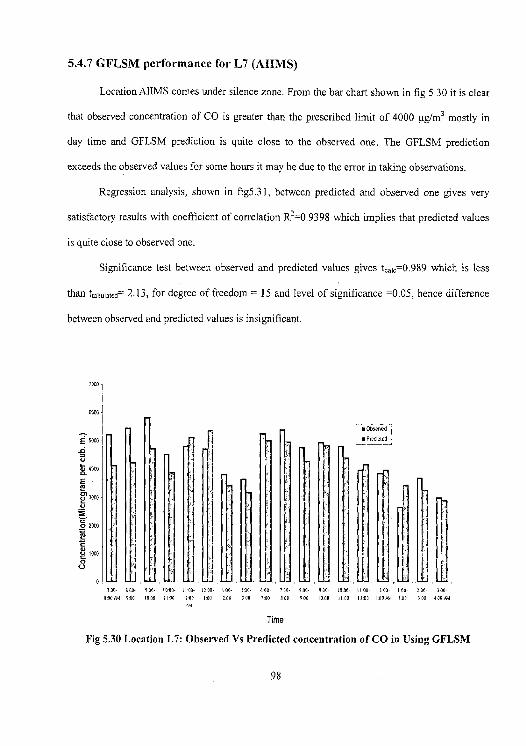
5.4.7 GFLSM performance for L7 (AIIMS)
Location AIIMS comes under silence zone. From the bar chart shown in fig 5.30 it is clear
that observed concentration of CO is greater than the prescribed limit of 4000 sg/m3 mostly in
day time and GFLSM prediction is quite close to the observed one. The GFLSM prediction
exceeds the observed values for some hours it may be due to the error in taking observations.
Regression analysis, shown in fig5.31, between predicted and observed one gives very
satisfactory results with coefficient of correlation R2=0.9398 which implies that predicted values
is quite close to observed one.
Significance test between observed and predicted values gives t0010 0.989 which is less
than tabulated= 2.13, for degree of freedom = 15 and level of significance =0.05, hence difference
between observed and predicted values is insignificant.
M
6000
E 5000
.n V
4000 Oa
3000
O 2000
moo 0 U
100- 820- 9Q3. 1000. 1100- 1153- 135- 200- 0:00- 700- 802- 900- 1000. 1100- 1200. 100- 200- 000- 00/01 900 1500 1190 200 1:cc 200 300 700 300 9.00 10.00 1150 1200 00/014 200 ).50 400 AM
PM
Time
Fig 5.30 Location L7: Observed Vs Predicted concentration of CO in Using GFLSM
98
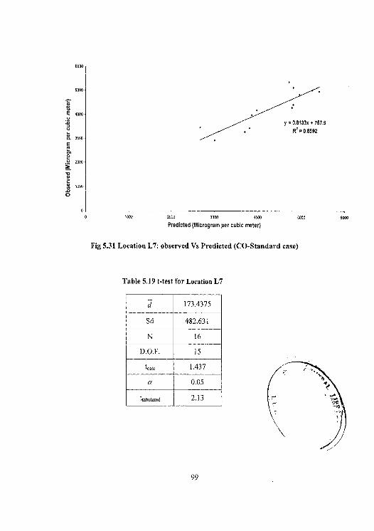
M
5000
£ 4000
y= 0.8133x+757.9
W 0.8592 a 3000
E
0 2000
V
1000
O
0 4 -• _
0 1000 2000 3000 4000 5000
Predicted (Microgram per cubic meter)
Fig 5.31 Location L7: observed Vs Predicted (CO-Standard case)
Table 5.19 t-test for Location L7
M
173.4375
Sd 482.631
N 16
D.O.F. 15
tease 1.437
a 0.05
ttabulated 2.13
99
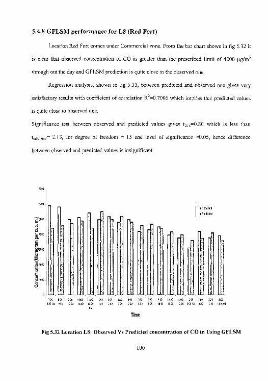
5.4.8 GFLSM performance for L8 (Red Fort)
Location Red Fort comes under Commercial zone. From the bar chart shown in fig 5.32 it
is clear that observed concentration of CO is greater than the prescribed limit of 4000 pg/m3
through out the day and GFLSM prediction is quite close to the observed one.
Regression analysis, shown in fig 5.33, between predicted and observed one gives very
satisfactory results with coefficient of correlation R2=0.7006 which implies that predicted values
is quite close to observed one.
Significance test between observed and predicted values gives tcaiG 0.80 which is less than
ttabu laled= 2.13, for degree of freedom = 15 and level of significance =0.05, hence difference
between observed and predicted values is insignificant
7000
6000
E aoo a
4000 n E
o coo
020,
Toro 0 U
700. eoo. 904. 1090. Iloo. 1100. loo. 233. 600. loo- Boo- 900. 7000- 1100. 1000- loo. dmo- 300. 803 761 900 1000 1100 1200 100 200 100 700 ego 900 1000 1100 1000 100761 too 000 400761
PM
Time
Fig 5.32 Location L8: Observed Vs Predicted concentration of CO in Using GFLSM
100
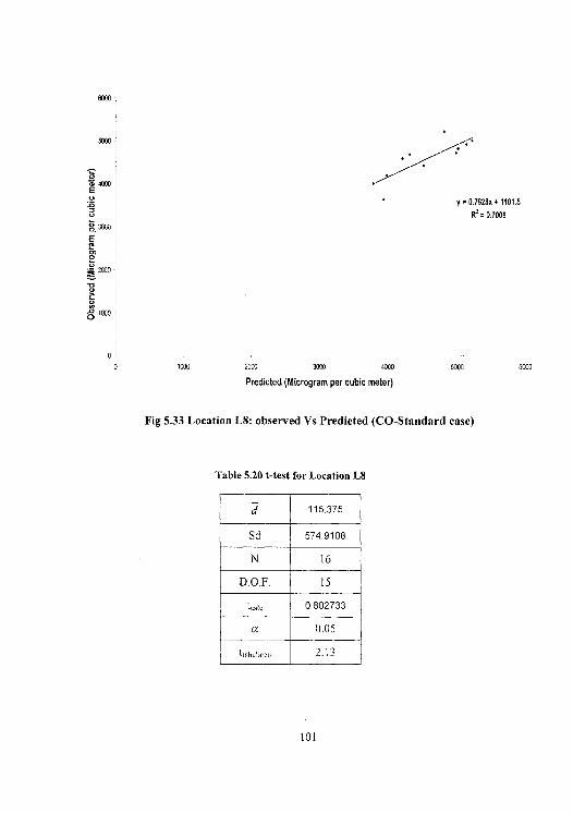
6000
5000
v Z 4000 E a
0.3000
rn O
2000
Z 01000{
0 1000
y = 0.7628x t 1101.5
R' = 0.7006
2000 3000 4000 5000 6000
Predicted (Microgram per cubic meter)
Fig 5.33 Location L8: observed Vs Predicted (CO-Standard case)
Table 5.20 t-test for Location L8
d 115.375
Sd 574.9108
N 16
D.O.F. 15
tcatc 0.802733
a 0.05
ttabutated 2.13
101
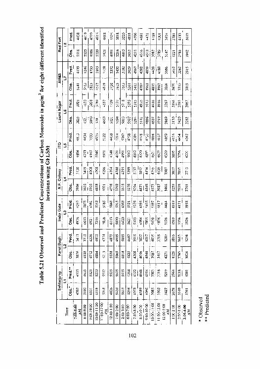
(I)
00
0
N N NN NN NNNNN
0 - o NNNNOONN N
c N
LD N N N N
NNOONNNOOr
NNNNNN
-N 00 00
N
0
N
'0 N
N
N
N 00
N Q\ Q\ 0 N
o N N N N NNNNNN N 41 11
2 S
5 S
5 S
S - -
5252 - - -
52222525; - - -
S 5555
N
o S NNNNNNNNN N
-
N N N N S N N 255
N
fl o 0
LD N
00
N 5555 00 0
N N N N
NN0CN0\NNNNNNNNfl
NNNNNNNNNNNN 5 2
U Z
NNN '0-N S
ONNO NN0000 NN NON
N
0
- 5 Q.NNNNNNN'0NNNNN 50N5N0NONN555'0N5_ NNNNONNNNNNNNN_0
-- N N N N N
0 '0N -'00N0O-N0N 0 '0 '0 00
- '0 '0
o N '0'ONN'0N N NNNOONNN
'ONNNNNNN•tN N ON N
N
V .0 5 Ø rU N
N N QNNNNN0 NNNNNNNNNNN -
'ONNNNNNNNNN
N NN0 '0 00 '0 N N N
CL N N 2 N N NNNNNNN 25
00 5250 '0 o
00 -N --NOON\ONNN NN'0'0NNNNNNNNNNNNNN N N N N '0 N
5gO.o5g5
881
5555o555<
102
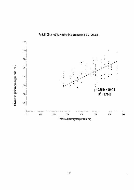
Fig 5.34 Observed Vs Predicted Concentration of CO (GFLSM)
8000
70001
6000
E 5000
U 4000
Q ~
E To
C7 30001 o
E 20001
c ,000 0
x c ,
r • ,
i t ,
y = 0.754x + 860.75
R2 = 0.7748
I
0 1000 2000 3000 4000 3000 6000 7000
Predicted(microgram per cub. m.)
103
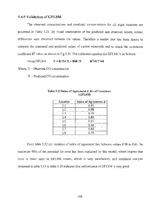
5.4.9 Validation of GFLSM
The observed concentrations and predicted concentrations for all eight locations are
presented in Table 5.21. By visual examination of the predicted and observed results, certain
differences were observed between the values. Therefore a scatter plot has been drawn to
compare the measured and predicted values of carbon monoxide and to check the co-relation
coefficient R2 value, as shown in Fig 5,34. The calibrated equation for GFLSM is as follows:
Using GFLSM Y = 0.754 X + 860.75 R2=0.7748
Where, Y = Observed CO concentration
X = Predicted CO concentration
Table 5.22 Index of Agreement d, for all Locations (GFLSM)
Location Index of Agreement, d L l 0.91 L2 0.98 L3 0.79 L4 0.89 L5 0.61 L6 0.94 L7 0.84 L8 0.74
From table 5.22 the variation of index of agreement lies between values 0.98 to 0.61. So
maximum 98% of the potential for error has been explained by this model, which implies that
there is lower error in GFLSM results, which is very satisfactory, and statistical analysis
presented in table 5.13 to table 5.20 indicates that performance of GFLSM is very good.
104
CHAPTER 6
CONCLUSIONS AND RECOMMENDATIONS
6.1 CONCLUSIONS
Based on the results of field, laboratories studies and statistical analysis results
following conclusions have been drawn:
1. The observed CO concentrations exceed the safe permissible one hour concentration of
4000µg/m3 at all the locations during day and night times both. The observed CO
Concentration was maximum of 7216pg/m3 in morning peak at India Gate and minimum
of 2896µg/m3 at New Friends Colony at night.
2. Location wise statistical analysis on the results of CALINE-4 indicating a very good
correlation with observed values with r2 values ranged from 0.9398 to 0.575.
3. Location wise statistical analysis on the results of GFLSM prediction indicates a very
good correlation with observed values with r2 values ranged from 0.8751 to 0.7006.
4. Significance test (t-test) done on the results of CALINE-4 gives satisfactory results and
shows tcaiculaled value less than ttahulated for degree of freedom 15 and level of significance
0.05 for seven out of eight locations. Hence performance of CALINE-4 is satisfactory.
5. Significance test (t-test) done on the results of GFLSM gives very satisfactory results and
shows tc;,ic„i;,«d value less than ttah„i,«d for degree of freedom 15 and level of significance
0.05 for all the eight locations. Hence performance of GFLSM is very satisfactory.
105
6. Index of agreement (d) value for CALINE-4 varies from 0.51 to 0.98, which implies that
minimum 51% of the potential for error has been explained by the model. Hence there is
lower error in CALINE-4 results.
7. Index of agreement (d) value for GFLSM varies from 0.61 to 0.98.Hence, which implies
that minimum 51% of the potential for error has been explained by the model. Hence most
of GFLSM predictions are error free.
8. On the basis of statistical analysis GFLSM performance is better than CALINE-4 because
minimum value of r2 for GFLSM and CALINE-4 are 0.7006 and 0.575 respectively,
Minimum values of Index of agreement for GFLSM and CALINE-4 are 0.61 and 0.51
respectively and t-test shows that there is insignificant difference between observed and
predicted values of GFLSM for all the eight locations while for CALINE-4 there are
seven, out of eight, locations where insignificant difference between observed and
predicted values is obtained. This may be due to that CALINE-4 predictions may not be
suitable for Indian conditions.
6.2 RECOMMENDATIONS
The recommendations for further work in this topic may be as follows:
1. Since GFLSM was developed for Indian conditions only hence there is a need to carry out
geographical transferability of this model.
2. GFLSM predictions involve a very lengthy hand calculation and are very time taking
hence there is a need for user-friendly software for this model like CALINE-4.
106
REFERENCES
1. htty:llwww.teriin.org
2. Luhar, A. K. (1985), "Vehicular pollution modeling" M.Tech Thesis, IIT-Bombay.
3. "White paper on Delhi with an action Plan", (2001) Govt. of India, Ministry of Environment
and Forests, New Delhi
4. SIAM(2001) ," I and M for in use vehicle in India",GITE Regional Workshop on I and M
Maintenance Policy in Asia, Bangkok.
5. Vinod Sibal and Yash Sachdeva (2001)," Urban transport scenario in India and its linkages
with energy and environment." Urban Transport Journal, pp 34-55.
6. http:l\www.petrolium.nic.in
7. Chitra Rajgopal, Kapoor, J.C. (2001), "Environment pollution from mobile sources- An
important consideration for long-term transport policy." Proc., Seminar of Indian National
Academy of Engineering, Hyderabad, pp234-264.
8. http://www.teriin.org/urban/fuelfm.htm
9. Renu Jain (2001)," Dispersion modeling of gaseous pollutants in Jaipur city and assessment
of their health effects on residents" Ph.D Thesis, University of Rajasthan.
10. http://www.worldbank.ori(nipr/work paper/ 1860/delhipap.pdf.
11. http:// www. defra.gov.uk
12. Pickett, E. E.(1986), "Atmosphere pollution" Second Edition, Published by John Wiley and
Sons, New York
13. Benarie, M.M.(1980), "Urban air pollution modeling" Published by The M.I.T. Press,
London.
14. Yeh, J.T. (1977), "Modelling atmospheric dispersion of pollutants." Air Pollution Control
and Design Handbook, Part 1, Published by: Marcel Dekker, pp-167-178.
15. M. L. Terry and N. E. Kennith (1976), "Measured vs predicted air quality near highways",
Journal of the Environmental Engineering Division, Vol. 102, Nos. EE 1-6.
16. Benson, P. E. (1988), "Development and verification of California line source model",
Transport Research Record No. 1176, pp. 69-76.
17. Chock D.P. (1977a)" General motors sulfate dispersion experiment: An overview of the
wind, temperature and concentration fields" Atmospheric Environment, (11) pp553-559.
18. Benson, P.E., Nokes, W.A. and Cramer R.L. (1986), "Evaluation of the CALINE-4 line
source dispersion model for complex terrains" Transport Research Record No. 1058,pp 7-13.
19. Cohn, L. F. and Mevoy, G.R. (1982), "Environmental analysis of transportation systems."
Published by John Wiley and Sons, New York.
20. Robert,V.(2001), "A Study on transport related pollution" M.Tech Thesis, Department of
Civil Engineering,IIT-Roorkee,Roorkee.
21. Sivacoumar, R. and Thansekaran, K.(1999), "Line source model for vehicular pollution
prediction near roadways and model evaluation through statistical analysis" Journal of
Environment Pollution, Vol. 104,pp 389-395.
22. Indian Standard Code Related to Air Pollution Measurement:
i). IS:5182(PartX)-1976, "Indian standard method for measurement of air pollution,
carbon monoxide"
23. "Air quality status and trends in India" National Ambient Air Quality Monitoring
Series" CPCB, Ministry of environment and Forests, NAAQMS/14/1999-2000.
24. Nirjar R.S., Jain S.S., Parida M., Sharma N., Robert V., Mittal N. (Sept. 2002).
"Development of transport related air pollutants modeling for an urban area" Journal of IRC
(Discussion Paper No.487), Vol. 63-2, Sept. 2002, pp 289-324.
25. Jain S.S., Parida M., Mittal N.(2003),"A Modelling framework for transport related air
pollution prediction for urban areas" Journal of Institute of Urban Transport (India),Special
Issue, Vol.4, No.1, March(2003).
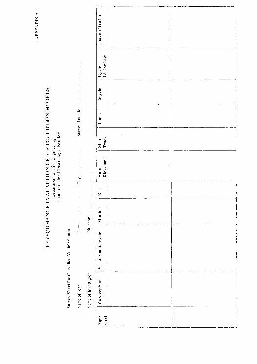
0
vi z z
u
F
i
° ~
az
I
F
o
ti
IU
F -.
O
0
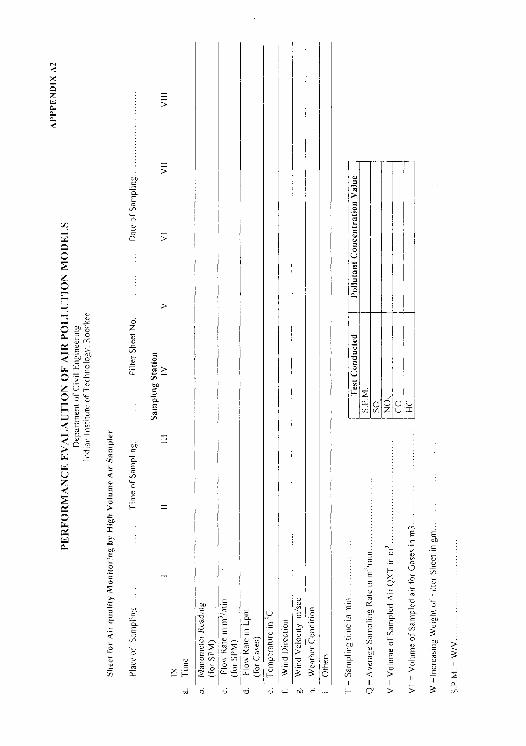
z_ 1 1
on
0
on - ~u •-
C) 0 c ~~n ~ v fl -a a - v
2 -
3 3 3 0 .-
E on
F _ v c ~ V
an Q R pl,
E - n
E • - ° ti E
C II i a > > 3
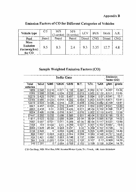
Appendix B
Emission Factors of CO for Different Categories of Vehicles
Vehicle type C/J (2-stroke) MIS
(4 -stroke) LCV BUS Truck A.R.
Fuel Petrol Petrol Petrol Diesel CNG Diesel CNG Mass
Emission 9.5 8.3 2.4 9.3 5.35 12.7 4.8 Factors(g/km) for CO
Sample Weighted Emission Factors (CO)
India Gate Emission factor (CO)
Total vehicles
%CIJ %MB %BUS %S/M M.T. %Tr. %AR glkm g/mile
1859 0.548 0.018 0.071 0.169 0.041 0.002 0.151 8.287 13.29 5358 0.588 0.008 0.034 0.232 0.015 0.002 0.122 8.511 13.65
10279 0.429 0.016 0.02 0.457 0.004 0.004 0.07 8.541 13.7 13765 0.565 0.003 0.018 0.332 0.003 0.003 0.075 8.671 13.91 12419 0.603 0.006 0.018 0.28 0.009 0.002 0.082 8.709 13.97 9001 0.457 0.005 0.019 0.446 0.014 0.002 0.057 8.621 13.83 8893 0.418 0.01 0.023 0.435 0.011 9E-04 0.102 8.396 13.47 9204 0.499 0.008 0.016 0.341 0.016 0.002 0.118 8.472 13.59
27447 0.282 0.002 0.006 0.585 0.001 4E-04 0.123 8.195 13.15 11811 0.623 0.002 0.006 0.284 3E-04 3E-04 0.085 8.738 14.02 7652 0.561 0.001 0.011 0.308 4E-04 8E-04 0.117 8.532 13.69 7354 0.6 0.002 0.01 0.259 0.027 0.001 0.102 8.667 13.9 4566 0.628 2E-04 0.004 0.231 0.02 0.009 0.107 8.728 14 3736 0.846 0 0.006 0.049 0.009 0.005 0.085 9.032 14.49
888 0.607 0.003 0.003 0.054 0.084 0.063 0.185 8.737 14.01 424 0.427 0.002 0.002 0.146 0.137 0.064 0.222 8A449 13.55 384 0.49 0.005 0.034 0.133 0.102 0.107 0.13 8.908 14.29 246 0.301 0 0.004 0.195 0.163 0.199 0.138 9.204 14.76
C/J: Car/Jccp, MR: Mini Bus, S/M: Scooter/Motor Cycle,'Fr.: Truck, AR: Auto Rickshaw
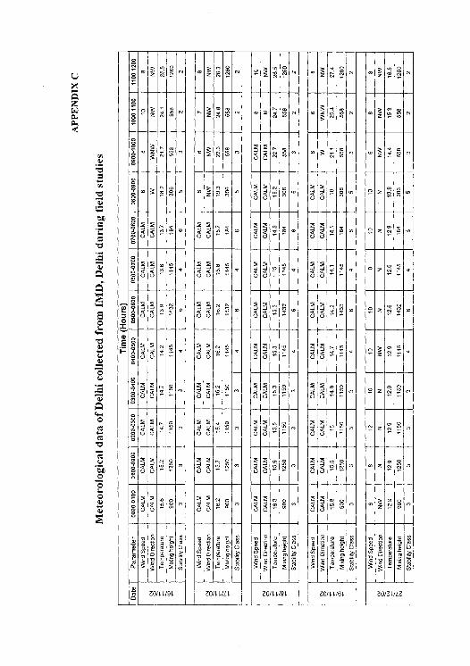
3 z ~ 3 3 z z z 3 z
0 3 d n Z z d 0 2 v m
OZ8O 0o 8 0 3 3
3
3 3 z V U
z
° Z 0 200 00 00- 00
o m U U` U` U U`
z N
0 0 00
e
2 00 00
o Z 00
U U U U~ U U` • U U
00 n 0O 0 00 4
o V U U U U U U U
a s
o o a a U U m
00 00 <<08 0 a¢
00
jc c C
8c0 E- D c 9 E 9 9 %= a a E c
Of/9L ZO/lt /Ll ZO/LL /9L ZO /L Ll6L ZO//L?
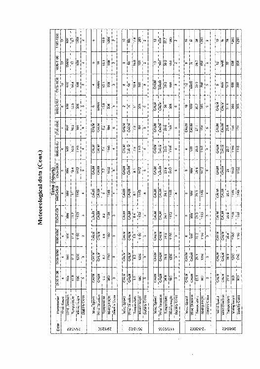
z w z z z z
3 3 m m Z f Z m z N z
y z Z w z a¢ U U
3 z Z 3 z
m y 4 a a Q a s U U 00 00 00 0U
<<,, Q Q m Q¢ 00 00 U U 00
o =
00 00 00 00
3 No 00 U U m 00
m 3 00
Z U U U U m U U y U U
y U U U U U U U U U
m U
N °1 N
j d C d
j P
c}~
dJ N 'o v v
~
N ~ ~' m~ N O ~' m V
N O ' N O ~' m _~ N iIII t:Jt!
v
D ° ~ x ~m ~O ° ~ x ° ° !Jfl a ° E ~~ a n
m/u /9Z ZOlZLl6Z ZO /ZNO£ £OOZ1EilI £OOZf£2L
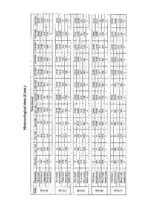
o U U U U
!:
:z N ~ ~ U
:::'
°o U
V V U U
goo U m 00 ` 00 00
0O U U U U m U V 00
Q ¢ 00
¢ ¢ 00
¢ ¢ 00
Q ¢ 00
z
~ o U U U U U U U U Z
1O z NO • 2 n Z U U Z
Z 2 z Z ! !! z z z z z
3 3 z 3 z n Z z z z
v a a ro n a H yam h y „ N
m m Z011 l/9l Z07/L l ZOIL/ Z011 l/6l ZO/ZI/LZ 0
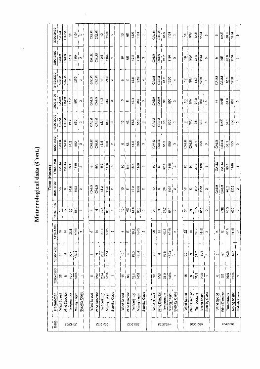
G ►_j
- o¢ Q
2 a¢
T - z ¢ a m z m z o
Z~ U< N M S W A S
6 m W V U! U U
o
00
NO 5200
00
5 5 0. 0 2500
W
22 = Z
o a a 00 ¢ a 00 = Z m
00 z '° z
Z c'
5 2 n j O o w m 0 < a<< ¢ Q z ¢ a Q¢ 00 00 00 00 00
m o 2 2 a a
N 0
© z 0
= z 0
° Z N O 0
Z N 0 N O 5 5 a s
,_ 00 00
D 2
00 Z W Z 2 ¢ a
00
d o
f
z z Z z z m z
z o = =Z0= z0o z m w
:::: z ::: z Z z
~
iII i 2, n
v~ 'o
!!I!L: `
v~ 3
ZO /ZL/6Z ZO/ZL /6Z ZO/ZL10E COO/€/LL COO//L E01£0/9Z m
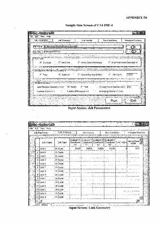
APPENDIX D1
Sample Run Screen of CALINE-4
Input Screen: Job Parameters
Input Screen: Link Geometry
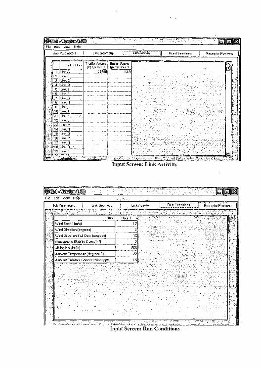
Input Screen: Link Activilty
11I File Edit View Help -
[ Job Parameters I Link Geometry Link Activity 11 Rum Conditions Receptor Positions
hun hours
Wind Speed (m/s) 1 7
Wind Direction (degrees) - Wind Direction Std. Den (degrees) 1St
Atmospheric Stability Class (1 -7) 2 - Mixing Height (m) SEE
Ambient Temperature (degrees C) 22
Ambient Pollutant Concentration (ppm) 1
Input Screen: Run Conditions
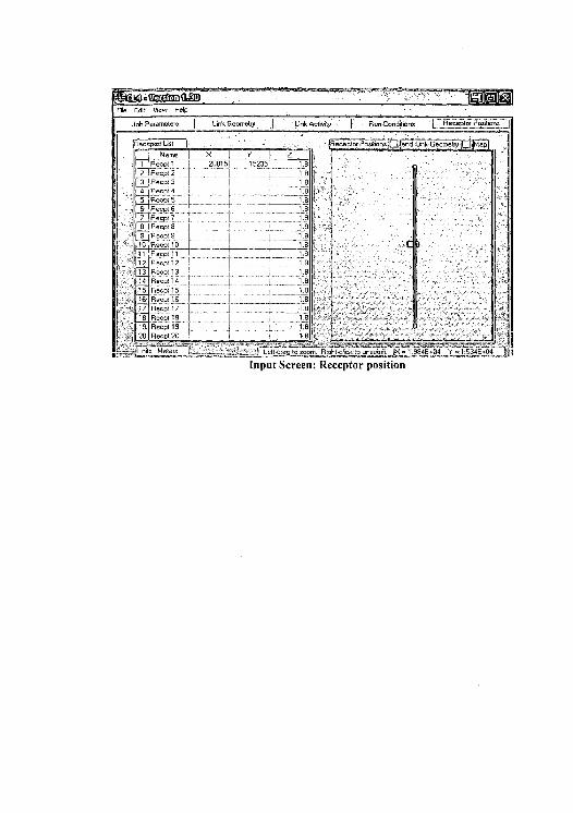
Input Screen: Receptor position
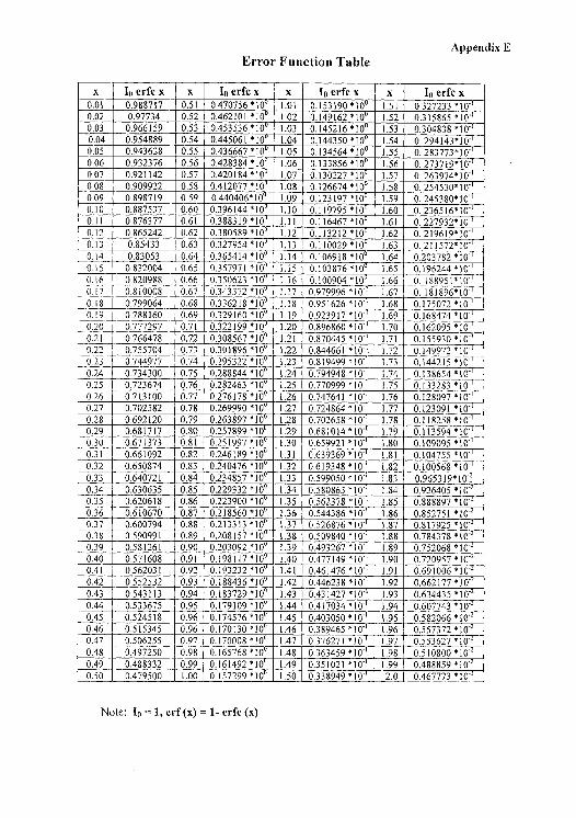
Appendix E Error Function Table
x 1e erfe x x 1p erfe x x to erfe x x Io erfc x 0.01 0.988717 0.51 0.470756 * 10 1.01 0153,90*100 1.51 0.327233 * 0" 0.02 0.97734 1022 0.462!01 *10 1.02 0.149162*l0 1.52 0.3 15865 *l0' 0.03 0.966159 0.53 0.453536 *10 1.03 0.145216 *10 1.53 0.304838 *10" 0.04 0.954889 0.54 0.445061 *100 1.04 0.144350 *10 1.54 0.294143*10' 0.05 0.943628 0.55 0.436667 * 10 1.05 0134564*100 1.55 _ 0.283773 * 10" 0.06 0.932376 0.56 0.428384 *10 1.66 0.133856 *10 1.56 0.273719*10 0.07 0.921142 0.57 0.420184 *10 1.07 0.130227 *10 1.57 0.263974*10" 0.08 0.909922 0.58 0.412077 * 10 1.08 0.126674 * 10 1.58 0.254530* 10" 0.09 0.898719 0.59 0.440406* 10 1.09 0,123197*100 1.59 0. 245380* 10" 0.10 0.887537 0.60 0.396144 * 10 1.10 0.119795 *100 1.60 0.236516* 10 0.11 0.876377 0.61 0.388319 * 10 III _V.1164 77 * 10 1.61 0. 227932* 10" 0.12 0,865242 0.62 0.380589 * 10 1.12 - 0.113212 I0 1.62 0. 'i'61'10' 0.13 0.85433 0.63 0.327954 * 10 1.13 0.110029 * 10 1.63 0. 211572* 10" 0.14 0.83053 0.64 0.365414 *10 1.14 0.106918 *10 1.64 0.203782 *10" 0.15 0.832004 0.65 0.357971 *10 1.15 0.103876 *10 1.65 0.196244 *i0" 0.16 0.820988 0.66 0.350623 *100 1.16 0.100904 * 10 1.66 0. 198951 * 10" 0.17 0.810008 0.67 0.343372 * I0 1.17 0.979996 * 10" 1.67 0. 181896* l0" 0.18 0.799064 0.68 0.336218 *10 1.18 0.951626 *10' 1.68 0.175072 *10" 0.19 0.788 (60 0.69 0.329160 * I0 1.19 0.923917 * 10" 1.69 0.168474 * l0" 0.20 0.777297 031 0.322199 * 10 1.20 0.896860 * 10" 1.70 0.162095 * 10 0.21 0.766478 0.72 0.308567 *100 1.21 0.870445 * 10' 1.71 0.155930 * 10 022 0.755704 0.73 0.301896 * 10 1.22 0.844661 *10" 1.72 0.149972 *10" 0.23 0.744977 0.74 0295322* 0.295322*100 1.23 6.81949-9* 10- 1.73 0.144215 * 10" 0.24 0.734300 0.75 0.288844 *100 1.24 0.794948 *10' 1.74 0.138654 *10- 0.25 0.723674 0.76 0.282463 * 10 1.25 0.770999 * 10" 1.75 0.133283 * 1 T 0.26 0.713100 0.77 0.276178 *100 1.26 0.747641 *0" 1.76 0.128097 * 10" 0.27 0.702582 0.88 0,269990*100 1.27 0.724864 * 10- 1.77 0.123091 *10" 0.28 0.692120 0.79 0.2638'"'i' 1.28 0.702658 *10' 1.78 0.118258 *10- 0.29 0.681717 0.80 0.257899 *10 1.29 0.681014 *10' 1.79 0.113594 *10" 0.30 0.671373 0.81 0.251997 *l0 1.30 0.659921 * 10.1 1.80 'i1091"101'" 0.31 0.661092 0.82 0.246 0246189*100 1.31 0.639369 * 10- 1.81 0.104755 * t 0" 0.32 0.650874 0.83 0.240476 *100 1.32 0.619348 * 10- 1.82 0.100568 * 0.33 0.640721 0.84 0.234857 0,00 1.33 0.599050*10" 1.83 0.965319*101 0.34 0.630635 0.85 0.229332 *10 1.34 0.580863 *10' 1.84 0.926405 *10 0.35 0.620618 0.86 111"l0 1.35 0.562378 *10" 1.85 0.888897 *10 0.36 0.610670 0.87 0.218560*100 1.36 0.544386 *10 1.86 0.852751 *10 0.37 0.600794 0.88 0.213313 * 10 1.37 0.526876 * 10' 1.87 0.817925 * l0' 0.38 0.590991 0.89 0.208157 *10 138 0.509840 * 10" 1.88 0.784378 * 10 0.39 0.581261 0.90 0.203092 *100 .39 0.493267 *10" 1.89 0.752068 * l0' 0.40 0.571608 0.91 0.1981 17 * 10 1.40 0.477149 * 10" 1.90 "111951''l0' ~I 0.4] 0.562031 0.92 0.193232 * 10 1.41 0.461476 * 10' 1.91 0.691006 * 10" 0.42 0.552532 0.93 0.188436 *10 1.42 0.446238 *l0" 1.92 0.662177 *10' 0.43 0.543113 0.94 0.183729 *10 1.43 0.431427 *l0" 1.93 0.634435 *10 0.44 0.533675 0.95 0,1791090100 1.44 0.417034 * 10- 1.94 0.607743 * 10'2 0.45 0.524518 0.96 0.174576 * 10 1.45 0.403050 * 10- 1.95 0.582066 *10.2 0.46 0.515345 0.96 -6.170130 * 10 1.46 0.389465 * 10- 1.96 0,557372*10.2 0.47 0.506255 0.97 0.170008 0,00 1.47 0.376271 *lo" 1.97 0,553627 *10 2 0.48 0.497250 0.98 0.165768 *10 1.48 0.363459 *10 1.98 0.510800 *10" 0.49 0.488332 0.99 0.161492 *100 1-49 0.351021 * 10" 1.99 0.488859 * 10 0.50 0.479500 1.00 0.157299 *10 (.50 0.338949 * 10" 2.0 0.467773 * l0"
Note: Io = 1, erf (x) = 1- erfe (x)
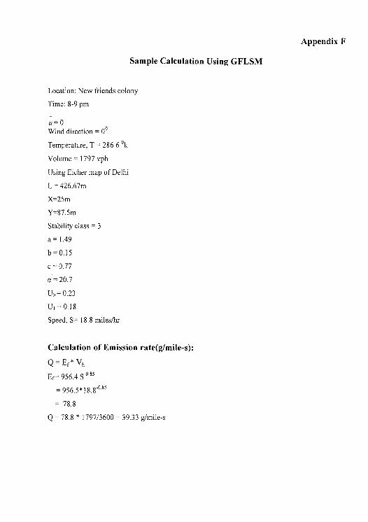
Appendix F
Sample Calculation Using GFLSM
Location: New friends colony
Time: 8-9 pm
u=0 Wind direction = 00
Temperature, T = 286.6 °k
Volume = 1797 vph
Using Eicher map of Delhi
L = 426.67m
X=25m
Y=87.5m
Stability class = 3
a= 1.49
b=0.15
c = 0.77
a=20.7
U0= 0.23
U1 = 0.18
Speed, S= 18.8 miles/hr
Calculation of Emission rate(g/mile-s):
Q=Ef * un Ef= 956.4 S"o.ss
= 956.5 * 18.8-0.85
= 78.8
Q = 78.8 * 1797/3600 = 39.33 g/mile-s
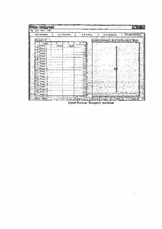
Input Screen: Receptor position
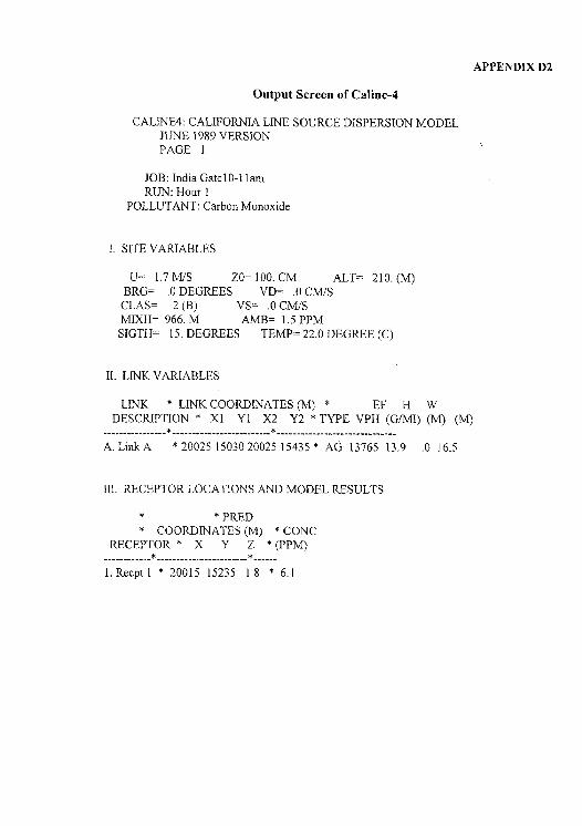
APPENDIX D2
Output Screen of Caline-4
CALINE4: CALIFORNIA LINE SOURCE DISPERSION MODEL JUNE 1989 VERSION PAGE I
JOB: India Gate 10-I l am RUN: Hour I
POLLUTANT: Carbon Monoxide
I. SITE VARIABLES
U= 1.7 MIS Z0= 100. CM ALT= 210. (M) BRG= .0 DEGREES VD= .0 CM/S CLAS= 2 (B) VS= .0 CM/S MIXH= 966. M AMB= 1.5 PPM
SIGTH= 15. DEGREES TEMP= 22.0 DEGREE (C)
II. LINK VARIABLES
LINK * LINK COORDINATES (M) * EF H W DESCRIPTION * X1 Yl X2 Y2 * TYPE VPH (G/MI) (M) (M)
A. Link A * 20025 15030 20025 15435 * AG 13765 13.9 .0 16.5
III. RECEPTOR LOCATIONS AND MODEL RESULTS
* * PRED COORDINATES (M) * CONC
RECEPTOR * X Y Z * (PPM) * * ------------ ---------------------- ------
1. Recpt 1 * 20015 15235 1.8 * 6.1
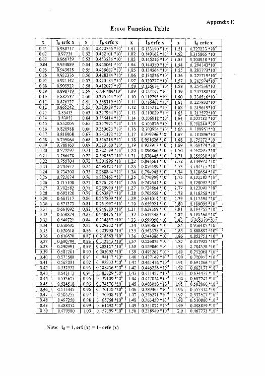
Appendix E Error Function Table
x 10 erfc x x Io erfe x x IQ erfc x x Io erfc x 1101 0.988717 0.51 0.470756 * 10 1.01 0.153190*100 1.51 0.327233 10" 0.02 0.97734 0.52 6.462101 * 10 1.02 0.149162 * 10 1.52 0315865 * 10 0.03 0.966159 0.53 0.453536 *10 1.03 0.1452 66 *10 1.53 0.304838 *10 0.04 0.954889 0.54 0.445061 *10 1.04 0.144350*10 1.54 0.294143*10 0.05 0.943628 0.55 0.436667 *10 1.05 0.134564 *10 1.55 0.283773*10' 0.06 0.932376 0.56 0.428384*10 1.06 0.133856*10 .56 0.273719*10 0.07 0.921142 0.57 0.420184*100 1.07 0.130227 *10 1.57 0. 263974*10- 0.08 0.909922 0.58 0.412077 * 10 1.08 0.126674 * 10 1.58 0. 254530* 10 0.09 0.898719 0.59 0.440406* 10 1.09 0.123197 * 10 1.59 0. 245380* 10 0.10 0.887537 0.60 0.396144 *10 1.10 0.119795 *I0 1.60 0.236516*10 0. l I 0.876377 0.61 0.3883 19 * 10 1.11 1 16467 * 10 1.61 0. 227932* 10- 0. 12 0.865242 0.62 0.380589 * 10 1.12 0.113212 * 10 1.62 9619* 10 0.13 0.85433 0.63 0.327954 * 10 1.13 0. 0.1l0029*100 1.63 0.211572* 10 0.14 0.83053 0.64 0.365414 *10 1.14 0.106918 *10 1.64 *10' 0203782 0.15 0.832004 0.65 0357971 *100 1.15 0.103876 *10 1.65 0.196244 *10" 0.16 0.820988 0.66 0.350623 * 10 1.16 0. 0.100904*100 1.66 0. 183951 * I0 0.17 0.810008 0.67 0.343372 * 10 1_ 17 0.979996 *10'T 1.67 0. 181896* 10" 0.18 0.799064 0.68 0.336218 *10 1.18 0.951626 *10- 1.68 0.175072 *10 0.19 0.788160 0.69 0.329160*100 1.19 0.923917 *10" 1.69 1 88474 *10 0.20 0.777297 0.71 0.322199 * 10 1.20 0.896860 * 10- 1.70 0.162095 * I0' 0.21 0.766478 0.72 0.308567 *100 1.21 0.870445 *10" 1.71 0.155930 * 10 0.22 0.755704 0.73 0.301896 *10 1.22 0.844661 *10- 1.72 0.149972 *10- 0.23 0.744977 0.74 0.295322 *100 1.23 0.819499 * 10- 1.73 0.144215 * 10 0.24 0.734300 0.75 0.288844 * 10 1.24 0.794948 *10" 1.74 0.138654 *101 0.25 0.723674 0.76 0.282463 *100 1.25 0.770999 31 1.75 0.133283 * 1" 0.26 0.713100 0.77 0.276178 *100 1.26 0.747641 * 10- 1.76 0.128097 0.27 0.702582 0.78 0.269990 * 10 1.27 0.724864 * 10 1.77 0.123091 *I0'1
0.28 0.692120 0.79 0.263897 *10 1.28 0.702658 *10" 1.78 0.1 18258 *10- 0.29 0.681717 0.80 0.257899 *10 1.29 0.681014 *10" 1.79 0.113594 *10 0.30 0.671373 0.81 0.251997 * 10 1.30 0.659921 *10" 1.80 0.109095 * l0 0.31 0.661092 0.82 0.246189 *100 1.31 0.639369 * 10 1.81 0.104755 * 10 0.32 0.650874 0.83 0.240476 * 10 1.32 0.619348 *10" 1.82 0.100568 1 0.33 0.640721 0.84 0.234857 *100 1.33 0,599050 * l 1.83 0.965 1913 0.34 0.630635 0.85 0.229332 *10 1.34 0.580863 *10" 1.84 0.926405 *10 0.35 0.620618 0.86 0.223900 *00 1.35 0.562378 *10- 1.85 0.888897 *10 0.36 0.610670 0.87 0.218560 *10 1.36 0.544386 *10" 1.86 0.852751 *10- 0.37 0.600794 0.88 0.213313 *100 1.37 0.526876 *10" 1.87 0.817925 * 10 0.38 0.590991 0.89 0.2081 S7 10 1.38 0.509840 * 10 1.88 0.784378 * 10 2 0839 0.581261 0.90 0.203092 *10 L39 0.493267 *l0" 1.89 0.752068 *10 0.40 0.571608 0.91 0. 0.198117*100 1.40 0.477149 * 10- 1.90 0.720957 * l0 0.41 0.562031 0.92 0. 0,193232*100 1.41 0,461476'108' 1.91 0.691006 * 10" 0.42 0.552532 0.93 0.188436 * 10 1.42 0.446238 * 10" 1.92 0.662177 * 10" 0.43 0.543113 0.94 0.183729 * l0 1.43 0.431427 *10' 1.93 0.634435 *10.2 0.44 0.533675 0.95 0.179109*10 1.44 0,417034 '10" 1,94 0.607743 *102 0.45 0.524518 0.96 0.174576*100 1.45 0.403050 * 10 1.95 --6.582066 * 10 0.46 0.515345 0.96 0.170130 *10 1.46 0.389465 *10- 1.96 0.557372 *10- 0.47 0.506255 0.97 0.170008 * 10 1.47 0.376271 * 10- 1.97 0.553627 * 10 0.48 0.497250 0.98 0.165768 *100 1.48 0.363459 * 10- .98 0.510800 ,101r" 0.49 0.488332 0.99 0.161492 *10 1.49 0.351021 *10- 1.99 0.488859 *10 0.50 0.479500 1.00 0.157299 * 10 1.50 0.338949 * 10" 2.0 0.467773 * 10"
Note: 1p = 1, erf (x) = 1- erfc (x)
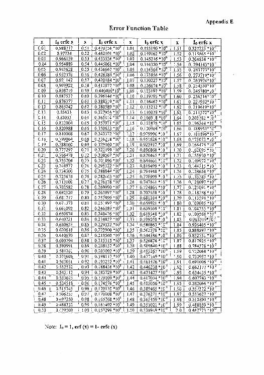
Appendix E Error Function Table
x to erfc x x to erfc x x Io erfc x x L0 erfc x 0.01 0.988717 0.51 0.470756 *I0 1.01 0.153190 * 10 1.51 0.327233 * 10 0.02 0.97734 0.52 0.462101 * 10 1.02 0.149162 * 10 1.52 0.315865 *10" 0.03 0.966159 0.53 0,453536*10 1.03 0. 0.l45216*100 1.53 0.304838 * 10 0.04 0.954889 0.54 0.445061 * 10 1.04 0.144350 * 10 1.54 0.294143* 10 0.05 0.943628 0.55 0.436667 *10 1.05 0.134564 *10 1.55 0.283773*10 0.06 0.932376 0.56 0.428384*100 1.06 0.133856 *10 1,56 0.273719*10 0.07 0.921142 0.57 0.420184 *10 1.07 0.130227 *10 1,57 0.263974*10' 0.08 0.909922 0.58 0.412077 *10 1.08 0.126674 *10 1.58 0.254530*10 0.09 0.898719 0.59 0.440406*10 1.09 -0.123197 *10 1.59 0.245380*10 0.10 0.887537 0.60 0.396144*10 1.10 0.119795*10 1.60 0.236516*10" 0.11 0.876377 0.61 0.388319 * 10 1.1] 0.116467 * 10 1.61 0. 227932* 10- 0.12 0.865242 0.62 0.380589 *10 1.12 0.113212 *10 1.62 0. 219619*10 0.13 0.85433 0.63 0.327954*10 1.13 0.110029*l0 1.63 0.211572*10 0.14 0.83053 0.64 0.365414 *10 1,14 0.106918 *10 1.64 0.203782 *l0 0.15 0.832004 0.65 0.357971 *10 1.15 0.103876 *10 1.65 0.196244 *10 0.16 0.820988 0.66 0.350623 *10° 1.16 0.100904 * 1 O 1.66 0. 188951 * 10" 0.17 0.810008 0.67 0.343372 *10 1.17 0.979996 *10 1.67 0.181896*10 0.18 0.799064 0.68 0.336218 * 10 1.18 .951626 * 10 1.68 0.175072 * 10 0.19 0.788160 0.69 0.329160 * l0 1.19 -C9-2-3917 * 10 1.69 0.168474 * 10 0.20 0.777297 0.71 0.322199 * 10 1.20 0.896860 *10" 1.70 0.162095 * I o' 0.21 0.766478 0.72 0.308567 * 10 1.21 0.870445 10' 1.71 0.155930 *10" 0.22 0.755704 0.73 0.301896 * 10 1.22 0.844661 * 10" 1.72 0.149972 * 10 0.23 0.744977 0.74 0.295322 * 10 1.23 0.819499'10" 1.73 0.144215 *10" 0.24 0.734300 0.75 0.288844 *10 1.24 0.794948 *10 1.74 0.138654 *10 0.25 0,723674 0.76 0.282463 *10 1.25 0,770999 *10 1.75 0.133283 10 0.26 0.713100 0.77 0.276178 *10 1.26 0.747641 *10 .76 .1280 77 *10' 0.27 0.702582 0.78 0.269990 * 10 1.27 0.724864 * 10 1.77 0.123091 *10" 0.28 0.692120 0.79 0.263897 *10 1.28 0.702658 *10 1.78 0.118258 *10 0.29 0.681717 0.80 0.257899 *10 1.29. 0.681014 *10 1.79 0.113594 *t0 0.30 0.671373 0.81 0.251997 *10 1.30 0.659921 *10 1.80 0.109095 *10" 0.31 0.661092 0.82 0.246189 *10 1.31 0,639369 *10 1.81 0.104755 *10 0.32 0.650874 0.83 0.240476 * 10 1.32 0.619348 * 10 1.82 0.100568 * l0 0.33 0.640721 0.84 0.234857 *10 1.33 0.599050 *10 1.83 0.965319*10-. 0.34 0.630635 0.85 0229332 *10 1.34 0.580863 *10 1.84 0.926405 *10" 0.35 0.620618 0.86 0.223900 *10 1.35 0.562378*l'ö21' 1.85 0.888897 *10 0.36 0.610670 0.87 0.218560 *10 1.36 0.544386 *10" 1.86 0.852751 *10 0.37 0.600794 0.88 0.213313 * 10 1.37 0.526876 * 10 1.87 0.817925 * 10' 0.38 0.590991 0.89 0.208157 * 10 1.38 0.509840 *10" 1.88 0.784378 * l0 0.39 0.581261 0.90 0.203092 *10 1.39 0.493267 *10' 1.89 0.752068* 10. 0.40 0.571608 0.91 0.1981 17 * 10 1.40 0.477149°10" 1.90 0.720957 * 10 0.41 0.562031 0.92 0.193232 * 10 1.41 0.461476 * 10 1.91 0.691006 * 10 0.42 0.552532 0.93 0.188436 * 10 1.42 0.446238 * 10 1.92 0.662177 * 10 0.43 0.543113 0.94 0.183729*100 1.43 0.431427 * 10 1.93 0.634435 * 10 0.44 0.533675 0.95 0.179109 *10 1.44 0.417034 *10 1.94 0.607743 *10' 0.45 0.524518 0.96 0.174576 * 10 1.45 0.403050 * 10' 1.95 0.5820 6 0.46 0.515345 0.96 0.170130 *10 1.46 0.389465 *10 1.96 0.557372 *10' 0.47 0.506255 0.97 0.170008 *100 1.47 0.376271 * 10 1.97 0.553627 * 10 0.48 0.497250 0.98 0.165768 *100 1.48 0.363459 * 10 1.98 0.510800 *10.2 0.49 0.488332 0.99 0.161492 *10 1.49 0.351021 *10" 1.99 0.488859 *10 0.50 0.479500 1.00 0,157299 *10 1.50 0.338949 *10 2.0 0.467773 *10
Note: I9 = 1, erf (x) = 1- erfc (x)
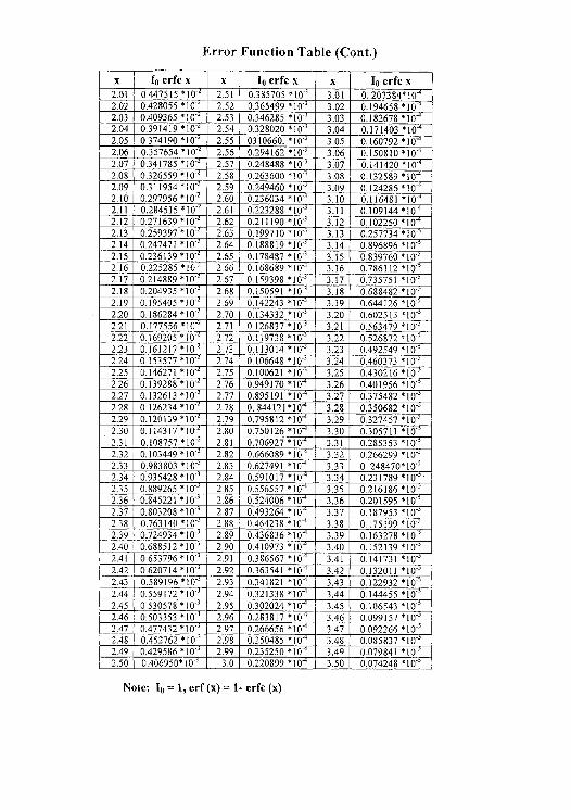
Error Function Table (Cont.)
x to erfc x x Io erfc x x Io erfc x 2.01 0.447515 *10 2.51 0.385705 *l0-' 3.01 0.207384 2O2t 0.428055 *10.2 2.52 0.365499 * 10' 3.02 0.194658 * iö' 03t 0.409365 * 10 2.53 0.346285 *I' 3.03 0.182678 * i 0"
2.041 0.391419*102 2.54 0.328020 * 10- 3.04 0.171403 * 10 205t 0.374190 *10" 2.55 0310660.*10 3.05 0.160792 *10 2.06 0.357654 *I0' 2.56 0.294162 *10' 3.06 0.150810 *10' 2.07 0.341785 *10.2 2.57 0.248488 *10-3 3.07 0.141420 * 10 2.08 0.326559 * 10 2.58 0.263600 *T 3.08 0.132589 * 10" 2.09 0.311954 * 10 2.59 0.249460 *RyS 3.09 0.124286 *l 2.10 0.297956 * 10 2.60 0.236034 * 10 3.10 0.116481 *10-4 2.11 0.284515 *j'2 0.223288 *10 3 3.11 0.109144 *10 2.12 0.271639 * 10- 2.62 0.211 190 *13 5 3.12 0.102250 * 10" 2.13 0.259397 *102 2.63 0.199710 * 10- 3.13 0257734 *10-5 2.14 0.247471 *10.2 2.64 0.188819 *10.5 3.14 0.896896 *10-5 2.15 0.236139 * l0 2.65 0.178487 * 10" 3.15 0.839760 * 10" 2.16 0.225285 *102 2.66 0.168689 * 10' 3.16 0.7861 12 * 10 2.17 0.214889 *l0 2.67 0.159398 *10-3 3.17 0.735751 *10'* 2.18 0.204935*10.2 2.68 0.150591 *10' 3.18 0.688482 *10' 2.19 0.195405 *104 2.69 0.142243 * 10- 3.19 0.644126 * 10 2.20 0.186284 * 10 2.70 0.134332 * 10" 3.20 0.602513 * 10 2.21 0.177556 * 10- 2.71 0.126837 * 10 3.21 0.563479*10-5 2.22 0.169205 * 10 2.72 0.119738 * 10' 3.22 0.526872 * I0' 2.23 0. U.161217*102 2.73 0.113014 * 10 3.23 0.492549 * 10-' 2.24 0.153577 * 10- 2.74 0.106648 * 10' 3.24 0.460373 *j0" 2.25 0.146271 *10.2 2.75 0.100621 *10.3 3.25 0.430216 * 10 2.26 0,139288*10.2 2.76 0.949170 *10 3.26 0.401956 *10" 2.27 0.132613 *'2 2.77 0.895191 * 10' 3.27 0.375482 *10.5 2.28 0. 0,126234*10.2 2.78 0. 844121 *10 3.28 0.350682 *10' 2.29 0.120139 *103 2.79 0.795812 *10 3.29 0.327457 *10 5 2.30 0.114317*10.2 2.80 0.750126 *10" 3.30 0.305711 *10" 2,31 0.108757 * 10.2 2.81 0.706927 *10 3.31 0.285353 *10' 2.32 0.103449 *102 2.82 0.666089 * 10 3.32 0.266299 *10.5 2.33 0.983803 * 10" 2.83 0.627491 * 10- 3.33 0. 248470* 10' 2.34 0,935428*10.3 2.84 0.591017 * 10- 3.34 0.231789 * 10' 2.35 0.889265 *10.3 2.85 0.556557 * 10" 3.35 0.216186 *10-5 2.36 0.845221 *10-3 2.86 0.524006 * 10 3.36 0.201595 *10 5 2.37 0,803208 *10.3 2.87 0.493264 * 10" 3.37 0.187953 *10-5 2.38 0.763140 * 10- 188 0.464238 * l0 3.38 0.175199 * l0 2.39 0.724934 *10' 2.89 0.436836 *10 3.39 0.163278 *10 2.40 0.688512 *10-3 2.90 0.410973 *10.4 3.40 0.152139 *10 2.41 0.653796 *103 2.91 0.386567 *10 4 3.41 0.141731 *10-5 142 0.620714 * 10 2.92 0.363541 * 10 3.42 0.132011 *10 5 2.43 0.589196 * 10; 2.93 0.341821 * 10' 3.43 0.122932 * 10 2.44 0.559172 *10' 2.94 0.321338 *-4 3.44 0.144455 *10' 2.45 0.530578 *103 2.95 0.302024 *10" 3.45 0.106543 *10 5 2.46 0.503353 * 10 2.96 0.283817 *10 4 3.46 0.099157 * 00" 2.47 0.477432 *103 2.97 0.266656 * 10' 3.47 0.092266 *10.5 2.48 0.452762 *10" 2.98 0.250485 *10-4 3.48 0.085837 *10 5 2.49 0.429586 *10.3 2.99 0.235250 *10" 3.49 0.079841 *10' 2.50 0.406950*10- 3.0 0.220899 *10 3.50 0.074248 *10-
Note: Io =1, erf (x) = 1- erfc (x)
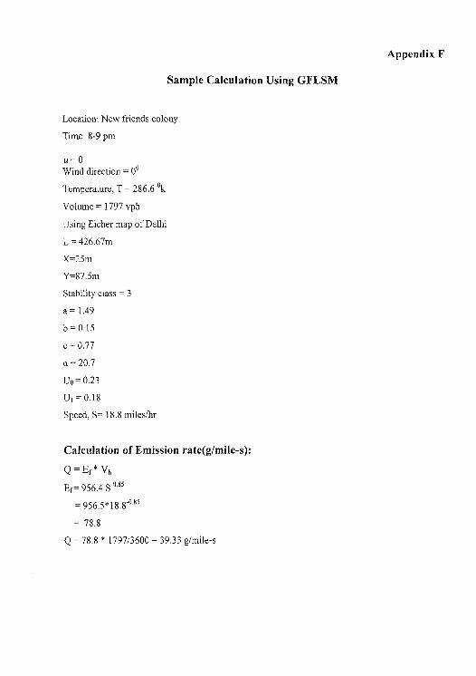
Appendix F
Sample Calculation Using GFLSM
Location: New friends colony
Time: 8-9 pm
u=0 Wind direction = 00
Temperature, T = 286.6 °k
Volume = 1797 vph
Using Eicher map of Delhi
L = 426.67m
X=25m
Y=87.5m
Stability class = 3
a= 1.49
b=0.15
c = 0.77
a=20.7
U° = 0.23
U, =0.18
Speed, S= 18.8 miles/hr
Calculation of Emission rate(g/mile-s):
Q=Ef * Vh
E f = 956.4 S °85
=956.5*18.8-085
= 78.8
Q = 78.8 * 1797/3600 = 39.33 g/mile-s
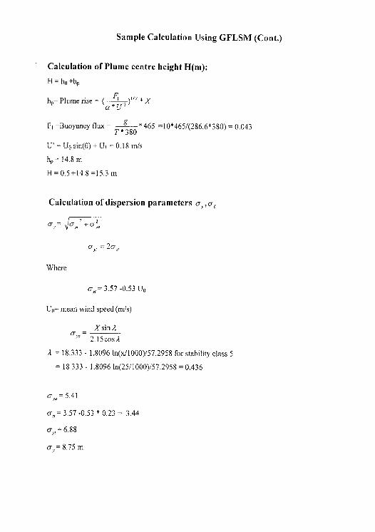
Sample Calculation Using GFLSM (Cont.)
Calculation of Plume centre height H(m):
H = h0 +h
hP Plume rise = ( a FU3 )112 * X
Fi =Buoyancy flux = T*380 * 465 =10*465/(286.6*380) = 0.043
U'=Uosin(0)+UI=0.18m/s
ht,= 14.8 m
H=0.5+14.8=15.3m
Calculation of dispersion parameters a v ,o Z
2 z o.„_
cr =2o- ,
Where
o- ,= 3.57 -0.53 Uo
Uo= mean wind speed (m/s)
X sin 2 via = 2.15cosA
d = 18,333 - 1.8096 ln(x/1000)/57.2958 for stability class 5
= 18.333 - 1.8096 ln(25/1000)/57.2958 = 0.436
cr = 5.41
6., = 3.57 -0.53 * 0.23 = 3.44
ay, = 6.88
Q~,= 8.75 m
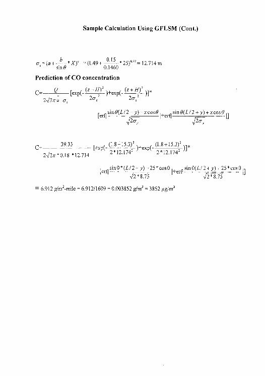
Sample Calculation Using GFLSM (Cont.)
o-' —(a+ 12.714 m sing
*X)` =(1.49+0.1460*
25)°"=
Prediction of CO concentration z z
C=-- Q Lexp( (Z2, ) )+exp( (Z2a ) )]* 2\/ru 6_
[erfl sin9(L/2—y)—xcos0
I+erfl sin9(L/2+y)+xcos0 I ~ 2Q,, 2a y
C= 39.33
2 J r*0.18 *12.714
ex (1.8 15.3)z
)+exp(- (1.8+15.3)2
p(~ 2 * 12.1742) p( 2 * 12.174 2 )~
[ergsin0*(L/2—y)-25* cos 0 I+erfl sin 0(L/2+y)+25* cos 0,) ~2*8.75 2*8.75
= 6.912 g/mz-mile = 6.912/1609 = 0.003852 g/m3 = 3852 µg/m3
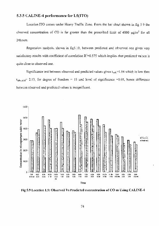
5000 d E U -0 4000
0
3000 01 0
E 2000
0 C
1000
U
5.3.5 CALINE-4 performance for L5(TI'O)
Location ITO comes under Heavy Traffic Zone. From the bar chart shown in fig 5.9 the
observed concentration of CO is far greater than the prescribed limit of 4000 .tg/m3 for all
24hours.
Regression analysis, shown in fig5.10, between predicted and observed one gives very
satisfactory results with coefficient of correlation R2=0.575 which implies that predicted values is
quite close to observed one.
Significance test between observed and predicted values gives tc,ic=1.84 which is less than
t,abulated= 2.13, for degree of freedom = 15 and level of significance =0.05, hence difference
between observed and predicted values is insignificant.
6000
700. 800. 90U f 000. 1100. 1200. 1:00. 200. 600. 7:00- 800- 800A41 900 1000 11.00 1200 100 200 700 7:00 800 960
Time
900. 1000. 1100- 1200. 100- 200.
UflH 300.
1000 100 1200 10001 200 300 400PM
n Pr¢d61,d I
Fig 5.9 Location L5: Observed Vs Predicted concentration of CO in Using CALINE-4
74
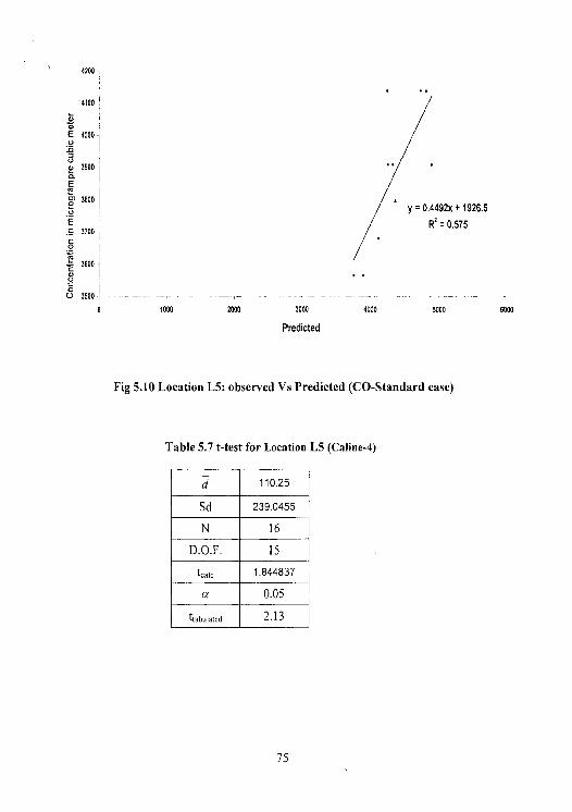
E 4000
el U
3900
E
0 3800
3700 C
o
3600
O U 3500
~ ii'
y = 0.4492x + 1926.5
Rt = 0.575
2000 3000 4000 5000 6000
Predicted
Fig 5.10 Location L5observed Vs Predicted (CO-Standard case)
Table 5.7 t-test for Location L5 (Caline-4)
d 110.25
Sd 239.0455
N 16
D.O.F. 15
tcalc 1.844837
a 0.05
tabulated 2.13
75
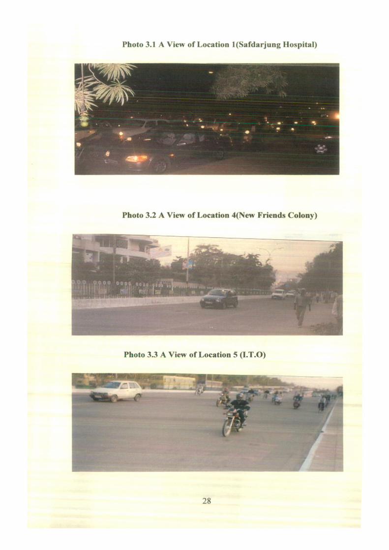
Photo 3.1 A Vie" of Location 1(Safdarjung Hospital)
Photo 3.2 A View of Location 4(New Friends Colony)
Photo 3.3 A View of Location 5 (I.T.0)
~s 0
28
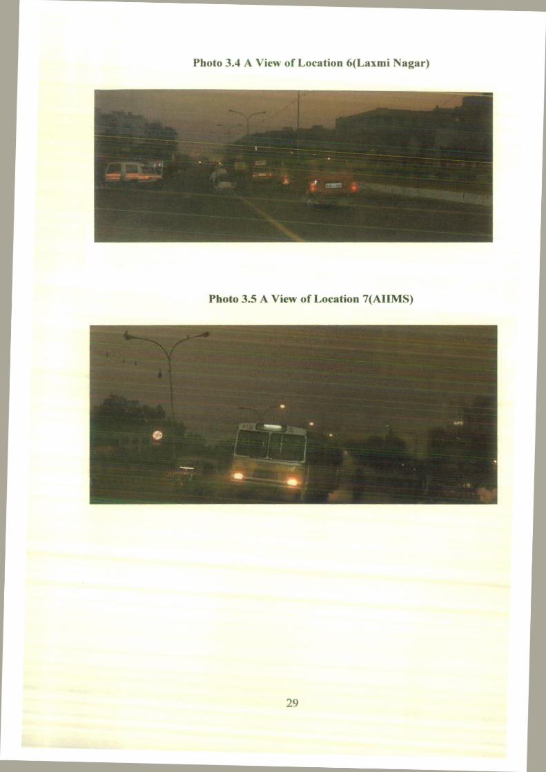
Photo 3.4 A View of Location 6(Laxmi Nagar)
Photo 3.5 A View of Location 7(AIIMS)
29
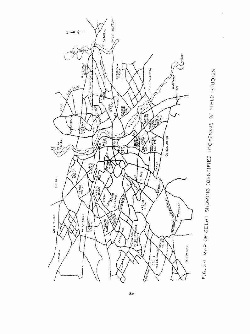
u, w 0
Cr)
Lu L- Lu 0
U) z O
a u Cr
30