Air Pollution Studies No. 18

Part B: Mercury

Hemispheric Transportof Air Pollution

2010

Hem

ispheric Transport of Air Pollution 2010 - A

ir Pollution Studies No. 18

Printed at United Nations, GenevaGE.11-22145–June 2011–2,130

ECE/EB.AIR/101

United Nations publicationSales No. E.11.II.E.8ISSN 1014-4625

USD 38ISBN 978-92-1-117044-3

ECONOMIC COMMISSION FOR EUROPE

Geneva

HEMISPHERIC TRANSPORT OF AIR POLLUTION

2010

PART B: MERCURY

AIR POLLUTION STUDIES No. 18

Edited by Nicola Pirrone and Terry Keating

Prepared by the Task Force on Hemispheric Transport of Air Pollution acting within the framework of the

Convention on Long-range Transboundary Air Pollution

UNITED NATIONS

New York and Geneva, 2010

NOTE

Symbols of United Nations documents are composed of capital letters combined with figures. Mention of such symbols indicates a reference to a United Nations document. The designations employed and the presentation of the material in this publication do not imply the expression of any opinion whatsoever on the part of the Secretariat of the United Nations concerning the legal status of any country, territory, city or area, or of its authorities, or concerning the delimitation of its frontiers or boundaries. In United Nations texts, the term “ton” refers to metric tons (1,000 kg or 2,204.6 lbs).

Acknowledgements The task force co-chairs and the secretariat would like to acknowledge the assistance of EC/R, Inc., in preparing this publication. We would also like to acknowledge the invaluable contribution of the individual experts and the Convention’s Programme Centres and Task Forces.

ECE/EB.AIR/101

UNITED NATIONS PUBLICATION Sales No. E.11.II.E.8

ISSN 1014-4625 ISBN 978-92-1-117044-3

Copyright ® United Nations, 2010 All rights reserved

UNECE Information Service Phone: +41 (0) 22 917 44 44 Palais des Nations Fax: +41 (0) 22 917 05 05 CH-1211 Geneva 10 E-mail: info.ece@unece.org Switzerland Website: http://www.unece.org

iii

Contents

Tables .................................................................................................................................................... vii Figures .................................................................................................................................................. ixChemical Symbols, Acronyms and Abbreviations ................................................................................ xi Preface ............................................................................................................................................... xvii

Chapter 1 Conceptual Overview ............................................................................................ 1 1.1. Introduction and Background .................................................................................................... 1 1.2. Concepts Related to Sources and Inter-Continental Cycling of Mercury .................................. 5 1.3. Overview of Atmospheric Mercury Dynamics .......................................................................... 7 1.4. Spatial and Temporal Variability in Inter-Continental Transport .............................................. 9 1.5. Assessing Global Natural and Anthropogenic Sources and Deposition .................................. 11 1.6 Data and Knowledge Gaps in Atmospheric Chemistry, Transport and Fate ........................... 14

1.6.1. Understanding and Modelling Atmospheric Mercury Chemistry ........................... 15 1.7. The Impact of Climate Change on the Long Range Transport of Mercury ............................. 17 References ............................................................................................................................................. 19

Chapter 2 Observations ......................................................................................................... 27 2.1. Spatial coverage and temporal trends of land-based atmospheric mercury measurements in the northern and southern hemispheres............................................................................... 27

2.1.1. Observations of air concentrations at single locations in the Northern Hemisphere .............................................................................................................. 28

2.1.2. Trends of air concentrations at single locations in the Northern Hemisphere ....... 32 2.1.3. Monitoring Networks and trends in the Northern Hemisphere ............................... 32 2.1.4. Observations of air concentrations at single locations in the Southern

Hemisphere .............................................................................................................. 34 2.1.5. Trends of air concentrations at single locations in the Southern Hemisphere ........ 35 2.1.6. Monitoring Networks and trends in the Southern Hemisphere ............................... 35 2.1.7. Mercury speciation in ambient air .......................................................................... 36 2.1.8. Measurements related to source attribution and intercontinental transport........... 39 2.1.9. Summary and conclusion for observations in the temperate Northern and

Southern Hemispheres ............................................................................................. 41 2.2. Spatial coverage & temporal trends of atmospheric mercury measurements in Polar Regions ........................................................................................................................... 43

2.2.1. Atmospheric mercury in the Arctic .......................................................................... 44 2.2.2. Atmospheric Mercury in the Antarctic .................................................................... 48 2.2.3. The role of snow surfaces on atmospheric Hg trends .............................................. 50 2.2.4. Summary and Conclusion for Observations in the Arctic and Antarctic regions ... 51

2.3. Spatial coverage and temporal trends of over-water, air-surface exchange, surface and deep sea water mercury measurements ............................................................................. 51

2.3.1. Atlantic Ocean ......................................................................................................... 52 2.3.2. Pacific Ocean .......................................................................................................... 53 2.3.3. Mediterranean Sea .................................................................................................. 55 2.3.4. Air-Water Mercury Exchange ................................................................................. 58

iv

2.4. The need for a coordinated global mercury monitoring network for global and regional models validations ................................................................................................................... 60 2.4.1. Existing Global Monitoring Programs .................................................................... 61 2.4.2. Ambient measurements ............................................................................................ 61 2.4.3. Mercury measurements at altitude .......................................................................... 62 2.4.4. Meteorological measurements ................................................................................. 62 2.4.5. Atmospheric deposition ........................................................................................... 62 2.4.6. Proposed Measurements to enhance model development ....................................... 63

2.4.7. Establishment of the Coordinated Global Mercury Observation System ................ 63 References ............................................................................................................................................. 64

Chapter 3 Emissions ........................................................................................................................... 75 3.1 Introduction .............................................................................................................................. 75 3.2 Emissions ................................................................................................................................. 76 3.3 Uncertainty of assessments ...................................................................................................... 82 3.4 Future emission scenarios ........................................................................................................ 84 3.5 Policy implications................................................................................................................... 89 3.6 Findings, gaps and recommendations ...................................................................................... 90

3.6.1. Findings ................................................................................................................... 903.6.2. Gaps......................................................................................................................... 91 3.6.3 Recommendations .................................................................................................... 92

References ............................................................................................................................................. 93

Chapter 4 Global and Regional Modelling ....................................................................................... 97 4.1. Introduction .............................................................................................................................. 97 4.2. Model methods for quantifying mercury dispersion and fate in the environment ................... 97

4.2.1. Overview of model approaches ............................................................................... 97 4.2.2. Goals and conditions of HTAP multi-model experiment for mercury ................... 100

4.3. Global concentration and deposition levels ........................................................................... 102 4.3.1. Review of previous mercury modelling studies ..................................................... 102 4.3.2. Findings of HTAP experiment (SR1) ..................................................................... 105

4.4. Intercontinental transport of mercury .................................................................................... 113 4.4.1. Characteristics of mercury intercontinental transport .......................................... 113 4.4.2. Current knowledge from previous modelling assessments .................................... 114 4.4.3. Source-receptor relationships from HTAP experiment (SR7) ............................... 116

4.5. Future trends of mercury pollution: HTAP experiment results (FE1, FE7) .......................... 123 4.6. Modelling uncertainty ............................................................................................................ 128

4.6.1. Sources of modelling uncertainty .......................................................................... 128 4.6.2. Variability of model results based on HTAP experiment ...................................... 134

4.7. Key findings and recommendations ....................................................................................... 136 References ........................................................................................................................................... 138

Chapter 5 Impacts of Intercontinental Mercury Transport on Human & Ecological Health ... 145 5.1. Introduction ............................................................................................................................ 145

5.1.1. Effects of methylmercury on childhood neurodevelopmental outcomes ................ 146 5.1.2. Effects of methylmercury on cardiovascular outcomes in adults .......................... 146 5.1.3. Safety reference doses ........................................................................................... 147

5.2. Human and ecological mercury exposures attributable to intercontinental sources .............. 148 5.2.1. Human exposure and safety standards .................................................................. 148 5.2.2. Fish consumption patterns and human exposures ................................................. 148

5.3. Contribution of intercontinental transport to atmospheric mercury deposition ..................... 150 5.4. Impacts on terrestrial and freshwater ecosystems .................................................................. 152

5.4.1. Freshwater and terrestrial ecosystems .................................................................. 152 5.4.2. Impacts on ecosystem health based on fish and wildlife exposure ........................ 154

v

5.5. Impacts on marine ecosystems ............................................................................................... 156 5.5.1. Source attribution of depostion to major ocean regions.......................................156 5.5.2. Intercontinental transport from major hydrographic circulation patterns

in the oceans ......................................................................................................... 157 5.5.3. Enrichment of oceans from anthropogenic mercury inputs .................................. 158 5.5.4. Impacts on marine fish mercury levels and trends ................................................ 159

5.6. Impacts on polar ecosystems ................................................................................................. 159 5.7. Implications for policy ........................................................................................................... 161

5.7.1. Projected changes in mercury deposition and exposure between 2020-2050 ....... 161 5.7.2. Potential impacts of climate change on mercury deposition and exposures ......... 163 5.7.3. Biomass burning as a present and future emission source.................................... 164 5.7.4. Future effectiveness of local and regional source emissions control .................... 166

References ........................................................................................................................................... 167

Chapter 6 Summary ............................................................................................................ 179 6.1 A Global Mercury Observation System ................................................................................. 180

6.1.1 Emissions ............................................................................................................... 180 6.1.2 Modelling ............................................................................................................... 180 6.1.3 Exchange fluxes at environmental interfaces ........................................................ 181

6.2 Atmospheric chemistry studies .............................................................................................. 182 6.3 Field measurements to determine mercury exchange fluxes at interfaces ............................. 183

6.3.1 Emissions ............................................................................................................... 183 6.3.2 Modelling ............................................................................................................... 183 6.3.3 Ecosystem Impacts................................................................................................. 184

6.4 Improved measurement techniques ........................................................................................ 184 6.4.1 Atmospheric Mercury and Mercury Compounds .................................................. 184 6.4.2 Emission speciation ............................................................................................... 184 6.4.3 Mercury Species Flux Measurements .................................................................... 185

6.5 The Link Among Air, Water and Biota Concentrations of Mercury ..................................... 186 6.6 Conclusions ............................................................................................................................ 186 References ........................................................................................................................................... 187

Appendix

Appendix A Editors, Authors, & Reviewers ..................................................................... 189

vii

Tables Chapter 1 Conceptual Overview Table 1.1. Classification of emissions of mercury to the atmosphere ........................................... 6

Chapter 2 Observations Table 2.1. Summary of Hg0, RGM and Hg(p) measurements made at remote, rural and

urban locations in the United States. NR means “not reported”. ................................ 30 Table 2.2. TGM, RGM and TPM average values observed at the five sites in the

Mediterranean during the 4 sampling campaigns of the MAMCS project. ................ 38 Table 2.3. Average TGM, RGM and TPM values from coastal stations during four seasons ..... 39 Table 2.4. Atmospheric mercury measurements conducted in arctic and sub-arctic sites ........... 45 Table 2.5. Summary of atmospheric mercury measurements performed at different

Antarctic locations from 1985 to 2005 ....................................................................... 49 Table 2.6. Summary of measurements of Total Gaseous Mercury over the Atlantic Ocean ....... 54 Table 2.7. Mercury measurements programme carried out during the cruises over the

Mediterranean Sea from 2000 to 2007 ........................................................................ 56 Table 2.8. Main Statistical Parameters for atmospheric Hg species concentrations observed

over the Mediterranean Sea Basin during the MED-OCEANOR campaigns from 2000 to 2007 ............................................................................................................... 56

Table 2.9. Main Statistical Parameters for atmospheric Hg species concentrations observed over the East sector of the Mediterranean Sea Basin during the MED-OCEANOR campaigns from 2000 to 2006..................................................................................... 57

Table 2.10. Main Statistical Parameters for atmospheric Hg species concentrations observed over the West sector of the Mediterranean Sea Basin during the MED-OCEANOR campaigns from 2000 to 2007..................................................................................... 57

Table 2.11. Main Statistical Parameters for atmospheric Hg species concentrations observed over the Adriatic Sea during the MED-OCEANOR campaigns from 2004 to 2005 .. 57

Table 2.12. Mercury evasion from some aquatic environments reported in the literature including this study ..................................................................................................... 59

Chapter 3 Emissions Table 3.1. Comparison of global mercury emission from anthropogenic sources ....................... 77Table 3.2. Comparison of global mercury emission from natural sources .................................. 79 Table 3.3. Comparison of mercury emission from anthropogenic sources as reported in

literature and National Pollution Inventories (NPIs) .................................................. 82 Table 3.4. Uncertainty of Hg emission estimates by source category. ........................................ 83 Table 3.5. Uncertainty of Hg emission estimates by continent.................................................... 83 Table 3.6. DROPS scenario assumptions .................................................................................... 87 Table 3.7. Degree of FGD penetration in coal-fired power plants in 2050 by scenario .............. 87 Table 3.8. Mercury Emissions in 2020 and 2050 by Scenario and World ................................... 87

Chapter 4 Global and Regional Modelling Table 4.1. Characteristics of chemical transport models participated in the comparison .......... 101 Table 4.2. Global estimates of mercury emissions utilized by the models. ............................... 101 Table 4.3. Statistical parameters of the model-to-observation comparison ............................... 112 Table 4.4. Mercury global emission scenarios for 2020 considered in the analysis .................. 123

Chapter 5 Impacts of Intercontinental Mercury Transport on Human & Ecological Health Table 5.1. Sources of U.S. population-wide mercury exposure. ................................................ 149 Table 5.2. Modelled percentage of total deposition, by emission source, for different ocean

basins. ....................................................................................................................... 156

ix

Figures Chapter 1 Conceptual Overview Figure 1.1. A conceptual diagram illustrating the major pathways between atmospheric

deposition of inorganic mercury (Hg(II)) and the accumulation of methylmercury (CH3Hg(II)) in fish. ...................................................................................................... 3

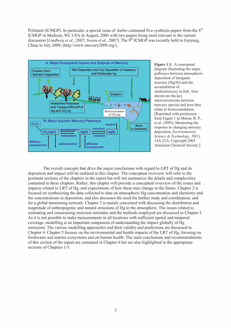
Figure 1.2. A representation of the global cycling of mercury showing the major sources and sinks at the Earth’s surface ........................................................................................... 4

Figure 1.3. Diagram showing major forms of mercury in the atmosphere: elemental mercury, ionic gaseous mercury, and mercury attached to or within aerosols ............................. 5

Chapter 2 Observations Figure 2.1. Total mercury concentration from the Mercury Deposition Network in 2006. .......... 33 Figure 2.2. Average TGM, values obtained at campaign MOE 1-5 and MAMCS 1-4. ................ 37 Figure 2.3. Average TPM, values obtained at campaign MOE 1-5 and MAMCS 1-4. ................ 37 Figure 2.4. Average RGM, values obtained at campaign MOE 1-5 and MAMCS 1-4. ............... 37 Figure 2.5. Scatter plot of total airborne mercury vs. CO measured during 22 pollution

events at Mt. Bachelor Observatory, Oregon during 2004-2005 ................................ 40 Figure 2.6. Measurement site for atmospheric mercury in the Arctic. .......................................... 44 Figure 2.7. Temporal trends of Hg0 measurements conducted in the Arctic in 2002.................... 47 Figure 2.8. The cruise track for the 2002 North Pacific cruise from Japan to Hawaii. ................. 55

Chapter 3 Emissions Figure 3.1. Spatial distribution of anthropogenic mercury emissions in 2000. ............................. 80 Figure 3.2. Average monthly mercury emissions for the period 1997-2006 ................................. 80 Figure 3.3. Mercury emissions from biomass burning in Equatorial Asia, boreal Asia,

southern hemisphere South America, northern hemisphere Africa, southern hemisphere Africa, southeast Asia , central America, Australia, temperate North America, boreal North America, central Asia, northern hemisphere South America, Europe, Middle East .................................................................................... 81

Figure 3.4. Uncertainty (%) in mercury emission estimates by sector in China ........................... 83 Figure 3.5. Future global mercury emissions in 2006 and forecast for 2050 A1B scenario ......... 88

Chapter 4 Global and Regional Modelling Figure 4.1. Global distribution of ensemble mean annual Hg0 concentration in ambient air

and standard deviation of the simulation results among the models ......................... 106Figure 4.2. South-to-north cross-sections of simulated annual mean Hg0 concentration

in the ambient air corresponding to fixed geographical longitudes .......................... 107 Figure 4.3. Global distribution of ensemble mean annual Hg total deposition and standard

deviation of the simulation results among the models .............................................. 108 Figure 4.4. South-to-north cross-sections of simulated annual Hg deposition corresponding

to fixed geographical longitudes ............................................................................... 108 Figure 4.5. Average concentration of gaseous elemental mercury, total deposition, wet

deposition, and dry deposition in different regions of the globe in 2001 as well as location of receptor regions .................................................................................. 110

Figure 4.6. Seasonal variation of total Hg deposition to five selected receptor regions ............. 111 Figure 4.7. Comparison of simulated gaseous elemental mercury concentration in ambient

air and wet deposition flux against long-term measurements ................................... 112 Figure 4.8. Response of Hg deposition in different regions of the globe to emission

reduction in East Asia simulated by GLEMOS ........................................................ 114 Figure 4.9. Global distribution of anthropogenic mercury emissions in 2000 and the relative

contribution of four source regions to the global mercury emission ........................ 117 Figure 4.10. Relative decrease in mercury deposition due to a 20% emission reduction

in the four source regions .......................................................................................... 118

x

Figure 4.11. Ensemble mean spatial distribution of Hg deposition decrease in the receptor regions due to a 20% emission reduction in the four source regions ........................ 119

Figure 4.12. Seasonal variation of Hg deposition decrease in the receptor regions due to a 20% emission reduction in the four source regions. .............................................. 121

Figure 4.13. Relative Hg deposition response in Europe, North America, East Asia, South Asia and the Arctic to emission reduction in four HTAP source regions ................. 122

Figure 4.14. Ensemble mean monthly relative import response of Hg deposition in four major receptor regions .............................................................................................. 122

Figure 4.15. Global distribution of anthropogenic Hg emissions in 2005 and change of total Hg emission in four major source regions according to three emission scenarios ... 124

Figure 4.16. Simulated average Hg deposition fluxes and contribution major source regions to Hg deposition in Europe, North America, East Asia, South Asia, and Arctic in 2005 ...................................................................................................................... 125

Figure 4.17. Contribution of foreign anthropogenic sources to Hg deposition in different receptor regions in 2005 ........................................................................................... 125

Figure 4.18. Relative change of Hg deposition between 2005 and 2020 in Europe, North America, East Asia, South Asia and Arctic according to three emission scenarios (SQ, EXEC, MFTR).................................................................................. 126

Figure 4.19. Ensemble average relative contribution of major source regions to Hg deposition in the reference year 2005 and according to the three emission scenarios for 2020 (SQ, EXEC, MFTR). .................................................................. 127

Figure 4.20. Impact of mercury chemistry uncertainty on the simulated monthly mercury wet deposition in a summer month ........................................................................... 131

Figure 4.21. The 2001 wet deposition as simulated by the CMAQ, REMSAD, and TEAM regional models using lateral boundary concentrations from the CTM-Hg, GEOS-Chem, and GRAHM global models .............................................................. 133

Figure 4.22. Fractional bias between simulated and observed Hg0 surface concentration and Hg wet deposition flux ....................................................................................... 134

Figure 4.23. Inter-model relative deviation of simulated Hg0 surface air concentration and total deposition flux in different receptor regions. .................................................... 135

Figure 4.24. Inter-model relative deviation of absolute and relative contributions of major source regions to Hg deposition in various receptor regions .................................... 135

Chapter 5 Impacts of Intercontinental Mercury Transport on Human & Ecological Health Figure 5.1. Reported mercury concentrations in fish sold in the U.S. commercial market. ........ 149 Figure 5.2. Seafood consumption and total mercury intake from estuarine and marine

fish and shellfish in the U.S. commercial market ..................................................... 150 Figure 5.3. Relative change in water, sediment, and fish mercury concentrations ..................... 153 Figure 5.4. Soil storage and emissions of mercury in soils simulated by the model for pre-

industrial and present-day conditions ....................................................................... 154 Figure 5.5. Atmospheric HgII deposition from Asian sources over the North Pacific Ocean.

Source ....................................................................................................................... 157 Figure 5.6. Surface water total mercury concentrations in the North Pacific Ocean. ................. 157 Figure 5.7. Enrichment of total mercury concentrations in intermediate waters of the North

Pacific Ocean ............................................................................................................ 158 Figure 5.8. Decreasing total mercury concentrations in intermediate waters of the Algerian

sub-basin between 1990 and 2004. ........................................................................... 158 Figure 5.9. Modelled future mercury deposition scenarios for Asia ........................................... 162 Figure 5.10. Modelled U.S. mercury deposition rates ................................................................... 162 Figure 5.11. Temporal evolution of fish MeHg source attributions for various model lake

ecosystems to deposition scenarios for the northeast and southeast United States. .. 163 Figure 5.12. Seasonal contribution of biomass burning CO to total CO as derived from

MOZART4 tagged CO simulations. ......................................................................... 166

xi

Chemical Symbols, Acronyms and Abbreviations

Chemical Abbreviations

Br – bromine atom Br2 – bromine molecule BrO – bromine monoxide radical C – carbon 13C – carbon-13 isotope 14C – carbon-14 isotope Cd – cadmium CH4 – methane Cl – chlorine Cl2 – molecular chlorine ClO – chlorine monoxide CO – carbon monoxide CO2 – carbon dioxide Cu – copper Fe – iron Hg – mercury Hg(I) – inorganic mercurous ion Hg(II) – inorganic mercuric ion HgII – divalent mercury Hg0 – elemental mercury HgBr2 – mercuric bromide or mercury (II) bromide HgCl2 – mercuric chloride or mercury (II) chloride HgClBr – mercuric chlorobromide Hg-P – particulate mercury HgO – mercuric oxide HgOH – mercurous hydroxide Hg(OH)2 – mercuric hydroxide HgX2 (g) – ionic gaseous mercury (II) Hg-SO3 – mercuric sulphite HO2 – hydroperoxyl radical H2O2 – hydrogen peroxide HOCl – hypochlorous acid I – iodine IO – iodine oxide radical KCl – potassium chloride CH3Hg – methyl mercury MeHg – methyl mercury Mn – manganese 15N – nitrogen-15 isotope N – nitrogen NaCl – sodium chloride NO2 – nitrogen dioxide NOx – nitrogen oxides (NO and NO2) NOy – total reactive nitrogen oxide compounds O3 – ozone O2 – oxygen OCl– – hypoclorite ion OH – hydroxyl radical Pb – lead

xii

Rn – radon S – sulphur SO2 – sulphur dioxide SOx – anthropogenic sulphur oxides (combination of SO2 and SO4)

Acronyms and Abbreviations

ABC – Atmospheric Brown Clouds AC&C – Atmospheric Chemistry and Climate ACE-Asia – Asian Pacific Regional Aerosol Characterization Experiment ACI – Activated Carbon Injection AER – Atmospheric and Environmental Research, Inc. AEROCE – Atmosphere/Ocean Chemistry Experiment ACS – American Chemical Society ALRT – Asian Long-range Transport AMAP – Arctic Monitoring and Assessment Programme AMCOTS – Atmospheric Mercury Chemistry over the Sea AMDEs – Atmospheric Mercury Depletion Events AMIBS – Arsenic Mercury Intake Biometric Study AMNET – Atmospheric Mercury Network AMMA – African Monsoon Multidisciplinary Analysis ART – Agroscope Reckenholz-Tänikon ATSDR – Agency for Toxic Substances and Disease Registry AUST – Australia BACTs – Best Achievable Control Technologies BAU+C – Business as Usual, with a Component Related to Actions to Address Climate

Change BB Alaska – Biomass Burning from Alaska BB PNW – Biomass Burning from the Pacific Northwest BCs – Boundary Conditions BCAA – Antarctic Environmental Specimen Bank (Banca Campioni Ambientali Antartici) BDL – Below Detection Limit BEIS3 – Biogenic Emissions Inventory System 3 BL – Below Limit BMB – Biomass Burning BOAS – Boreal Asia BONA – Boreal North America CARIBIC – Civil Aircraft for Regular Investigation of the Atmosphere Based on an

Instrumented Container CAMNet – Canadian Atmospheric Mercury Network CC – Climate Change CEAM – Central America CEAS – Central Asia CEREA – Centre d’Enseignement et de Recherche en Environment Atmoshperique CHAAMS – Cape Hedo Atmosphere and Aerosol Monitoring Station CI – Confidence Interval CIRES – Cooperative Institute for Research in Environmental Science CLRTAP – Convention on Long Range Transboundary Air Pollution cm3 – cubic centimetre CMAQ – Community Multiscale Air Quality Model CMAQ-Hg – CMAQ for mercury CNR – National Research Council CNRS – Centre National de la Recherché Scientifique CRC – Chemical Rubber Company

xiii

CSFII – Continuing Study of Food Intake by Individuals CTM – Chemical Transport Model CTM-Hg – Chemical Transport Model for Mercury CUNY – The City University of New York DEHM – Danish Eulerian Hemispheric Model DGM (DGHg) – Dissolved Gaseous Hg concentration DOC – Dissolved Organic Carbon DROPS – Development of macro and sectoral economic models to evaluate the role of public

health externalities on society DSS – Decision Support Systems E – East EC – Elemental Carbon ECHMERIT – coupled mercury chemistry and global transport model EF – Emission Factors E-MCM –Everglades Mercury Cycling Model EMEP – Cooperative Programme for Monitoring and Evaluation of the Long-range

Transmission of Air Pollutants in Europe EPRI – Electric Power Research Institute EQAS – Equatorial Asia ESPs – Electrostatic Precipitators ESPREME – Integrated Assessment of Heavy Metal Releases in Europe EU – European Union EU-15 – European Union thru the 1995 Enlargement - Belgium, France, West Germany,

Italy, Luxembourg, Netherlands, Denmark, Ireland, United Kingdom, Greece, Portugal, Spain, Austria, Finland, and Sweden

EXEC – Extended Emissions Control FC – Flux Chamber FE – Future Emissions FFs – Fabric Filters FGC – Flue-Gas Conditioning Systems FGD – Flue-Gas Desulfurization FSANZ – Food Standards Australia New Zealand fw – Fresh Weight Fx – Deviation Factor X GAW – Global Atmospheric Watch Programme (within WMO) GEM – Gaseous Elemental Mercury GEOS-CHEM – A global 3-D atmospheric composition model driven by data from the

Goddard Earth Observing System GFEDv2 – Global Fire Emissions Database version 2 g/km2/y – grams per square kilometre year GLEMOS – Global EMEP Multi-media Modelling System GMA – Global Mercury Assessment Report GMOS – Global Mercury Observation System GPCP – Global Precipitation Climatology Project GRAHM – Global/Regional Atmospheric Heavy Metals Model hPa – hectopascal HTAP – Hemispheric Transport of Air Pollution hν – light energy HYSPLIT – Hybrid Single Particle Lagrangian Integrated Trajectory Model ICES – International Council for the Exploration of the Sea ICMGP – International Conferences on Mercury as a Global Pollutant ICP-MS – Inductively Coupled Plasma Mass Spectrograph IGCC – Integrated Gasification Combined Cycle IQ - Intelligence Quotient IPCC – Intergovernmental Panel on Climate Change

xiv

IPPC – Integrated Pollution Prevention and Control ITCZ – Intertropical Convergence Zone JGSEE – The Joint Graduate School of Energy and Environment JRC – Joint Research Centre km – kilometre km2 – square kilometre LATMOS-IPSL – Laboratoire Atmospheres, Milieux et Observations Spatiales-Pierre

Simon Laplace Institute LIDAR – Light Detection and Ranging LOAEL – Lowest Observed Adverse Effect Level LRT – Long-range Transport LRTAP – Long-range Transboundary Air Pollution m – metre m asl – Meters Above Sea Level MAMCS – Mediterranean Atmospheric Mercury Cycle System MARM – Ministry of the Environment, Rural and Marine Media of Spain Max. – Maximum MBL – Marine Boundary Layer MDN – Mercury Deposition Network MFTR – Maximum Feasible Technological Reduction mg/kg – milligram per kilogram mg kg-1 body weight d-1 – milligram per kilogram body weight per day mg MeHg kg-1 ww – milligram methyl mercury per kilogram wet weight mg kg-1 ww – milligram per kilogram wet weight mg kg-1 dry weight – milligram per kilogram dry weight Mg yr-1 – megagram per year Mg/y – megagram per year MIDE – Middle East MIF – Mass Independent Fractionation Min. – Minimum MOE – Mercury Species Over Europe MOZART4 – Model of Ozone and Related Tracers, version 4 MSC-E – Meteorological Synthesizing Centre-East MSCE-HM – EMEP Hemispheric Mercury Transport Model mth – Month N – North NA – Data not available NADP – National Atmospheric Deposition Program NADP-MDN – National Atmospheric Deposition Program - Mercury Deposition Network NAMMIS – North American Mercury Model Intercomparison Study NAS – National Academy of Sciences NASA – National Aeronautics and Space Administration ng m-3 – nanograms per cubic meter ng Hg/g – nanograms mercury per gram ng Hg m-3 yr-1 – nanograms mercury per cubic meter per year ng m-2 hr-1 – nanograms mercury per square meter per hour ng L-1 – nanograms per litre NHAF – Northern Hemisphere Africa NHANES – National Health and Nutrition Examination Survey NHSA – Northern Hemisphere South America NILU – Norwegian Institute for Air Research NMFS – National Marine Fisheries Service (part of NOAA) NOAA GFDL – National Oceanic and Atmospheric Administration Geophysical Fluid

Dynamics Laboratory NOAEL – No Observed Adverse Effect Levels

xv

NPIs – National Pollution Inventories NPIW – North Pacific Intermediate Water Mass NR – Not reported NRC – National Research Council OECD – Organisation for Economic Co-operation and Development OSPAR – Convention for the Protection of the Marine Environment of the North-East

Atlantic PBL – Planetary Boundary Layer pg/L – picograms per litre pg m-3 – picograms per cubic meter PM – particulate matter PM2.5 – particulate matter with an aerodynamic diameter of 2.5 micrometers or less PM10 – particulate matter with an aerodynamic diameter of 10 micrometers or less POPs – Persistent Organic Pollutants ppbv – parts per billion by volume ppm – parts per million PWM – Porewater Mercury RAIR – Relative Annual Intercontinental Response RAMS – Regional Atmospheric Modelling System RDR – Relative Deposition Response RELMAP – Regional Lagrangian Model of Air Pollution REMSAD – Regional Modelling System for Aerosols and Deposition REMSAD-Hg – Regional Modelling System for Aerosols and Deposition, mercury version RfD – Reference Dose RGM (RGHg) – Reactive Gaseous Mercury RMSE – Root Mean Square Error ROR – Relative Intercontinental Response R/V – Research Vessel S – South SD – Standard Deviation SEAS – Southeast Asia SHAF – Southern Hemisphere Africa SHSA – Southern Hemisphere South America SQ – Status Quo S/R – Source-receptor SR1 – reference simulation for 2001 under the Hemispheric Transport of Air Pollution

(HTAP) program SR7 – perturbation simulations under HTAP that reduce anthropogenic emissions by 20% in

Europe, North America, East Asia, and South Asia SRES – Special Report on Emissions Scenarios STEM-Hg – Sulphur Transport Eulerian Model, including mercury TAM – Total Airborne Mercury TCM – Tropospheric Chemistry Module TEAM – Trace Element Analysis Model TENA – Temperate North America TF HTAP – Task Force on Hemispheric Transport of Air Pollutants TGM – Total Gaseous Mercury TMDL – Total Maximum Daily Load UCAR – University Corporation for Atmospheric Research UJF – Universite Joseph Fourier USA – United States of America USDA ARS – U.S. Department of Agriculture Agricultural Research Service U.S. EPA – United States Environmental Protection Agency U.S. FDA – United States Food and Drug Administration USGS – United States Geological Survey

xvi

USSR – Union of Soviet Socialist Republics UTLS – Upper Troposphere-Lower Stratosphere UNECE – United Nations Economic Commission for Europe UNEP – United Nations Environmental Programme UNEP-GC – Governing Council of the United Nations Environmental Programme UNEP-MFTP – UNEP Global Partnership for Mercury Air Transport and Fate Research UNFCCC – United Nations Framework Convention on Climate Change UPMC – University of Pierre et Marie Curie UV – Ultraviolet light UV-B – Medium wave ultraviolet light, from 315 to 280 nanometers wavelength UV A+B – Long and medium wave ultraviolet light, from 400 to 280 nanometers wavelength UVSQ – University of Versailles Saint Quentin VK – Variation Coefficient WHO – World Health Organization ww – Wet weight W m-2 – Watts per square meter μm – micrometer μg m-2 – micrograms per square meter μg/L – micrograms per litre μg g-1 – micrograms per gram μg m-2 yr-1 – micrograms per square meter per year μg/kg/day – micrograms per kilogram per day

xvii

PrefaceIn December 2004, in recognition of an increasing body of scientific evidence suggesting

the potential importance of intercontinental flows of air pollutants, the Convention on Long-range Transboundary Air Pollution (LRTAP Convention) created the Task Force on Hemispheric Transport of Air Pollution (TF HTAP). Under the leadership of the European Union and the United States, the TF HTAP was charged with improving the understanding of the intercontinental transport of air pollutants across the Northern Hemisphere for consideration by the Convention. Parties to the Convention were encouraged to designate experts to participate, and the task force chairs were encouraged to invite relevant experts to participate from countries outside the Convention.

Since its first meeting in June 2005, the TF HTAP has organized a series of projects and collaborative experiments designed to advance the state-of-science related to the intercontinental transport of ozone (O3), particulate matter (PM), mercury (Hg), and persistent organic pollutants (POPs). It has also held a series of 15 meetings or workshops convened in a variety of locations in North America, Europe, and Asia, which have been attended by more than 700 individual experts from more than 38 countries. The TF HTAP leveraged its resources by coordinating its meetings with those of other task forces and centres under the convention as well as international organisations and initiatives such as the World Meteorological Organization, the United Nations Environment Programme’s Chemicals Programme and Regional Centres, the International Geosphere-Biosphere Program-World Climate Research Program’s Atmospheric Chemistry and Climate (AC&C) Initiative, and the Global Atmospheric Pollution Forum.

In 2007, drawing upon some of the preliminary results of the work program, the TF HTAP developed a first assessment of the intercontinental transport of ozone and particulate matter to inform the LRTAP Convention’s review of the 1999 Gothenburg Protocol (UNECE Air Pollution Series No. 16).

The current 2010 assessment consists of 5 volumes. The first three volumes are technical assessments of the state-of-science with respect to intercontinental transport of ozone and particulate matter (Part A), mercury (Part B, this volume), and persistent organic pollutants (Part C). The fourth volume (Part D) is a synthesis of the main findings and recommendations of Parts A, B, and C organized around a series of policy-relevant questions that were identified at the TF HTAP’s first meeting and, with some minor revision along the way, have guided the TF HTAP’s work. The fifth volume of the assessment is the TF HTAP Chairs’ report to the LRTAP Convention, which serves as an Executive Summary.

The objective of HTAP 2010 is not limited to informing the LRTAP Convention but, in a wider context, to provide data and information to national governments and international organizations on issues of long-range and intercontinental transport of air pollution and to serve as a basis for future cooperative research and policy action.

HTAP 2010 was made possible by the commitment and voluntary contributions of a large network of experts in academia, government agencies and international organizations. We would like to express our most sincere gratitude to all the contributing experts and in particular to the Editors and Chapter Lead Authors of the assessment, who undertook a coordinating role and guided the assessment to its finalisation.

We would also like to thank the other task forces and centres under the LRTAP Convention as well as the staff of the Convention secretariat and EC/R Inc., who supported our work and the production of the report.

André Zuber and Terry Keating Co-chairs of the Task Force on Hemispheric Transport of Air Pollution

Chapter 1 Conceptual Overview

Lead Author: Robert Mason

Contributing Authors: Nicola Pirrone, Ian Hedgecock, Noriyuki Suzuki, Leonard Levin

1.1. Introduction and Background While mercury (Hg) is globally distributed mainly through the atmosphere, it differs from other

major atmospheric pollutants (e.g. ozone, particulates) in that its environmental impact is not directly related to the atmospheric burden. While the major redistribution of Hg is via the atmosphere, its primary environmental and health impact is in aquatic systems, and for aquatic organisms and their consumers, as this is the location where the inorganic Hg deposited directly or indirectly from the atmosphere is converted into the highly toxic and bioaccumulative methylmercury (MeHg) (Figure 1.1). Consumption of aquatic organisms with elevated MeHg concentrations is the primary route of exposure for humans [Mahaffey et al., 2004; Sunderland, 2007] and for freshwater and marine fish-eating wildlife [Braune et al., 2006; García-Hernández et al., 2007; Kemper et al., 1994; Landers et al., 2008] (Chapter 5). In terms of relative toxicity, MeHg is orders of magnitude more toxic than the inorganic forms (ionic Hg (HgII) and elemental Hg (Hg0)) [Clarkson and Magos, 2006]. Because Hg is globally distributed, due to its relatively long residence time in the atmosphere, fish in remote regions may be impacted by regional and global sources. For example, in the United States, 48 states have Hg consumption advisories, [U.S. EPA, 2006] and many are associated with water bodies located in areas with no apparent land-based Hg contamination or local anthropogenic Hg source. However, while long range transport (LRT) is important, there are locations where Hg0 is efficiently oxidized and deposited, and for these regions, regional inputs are more important and local hotspots of Hg accumulation can be found. Since MeHg is bioconcentrated in organisms and biomagnified in aquatic food webs, large fish and those with high trophic stature tend to have higher concentrations. Thus, marine and freshwater advisories often target specific fish species and are size based [Burger and Gochfeld, 2004; Chen et al., 2008]. Since the developing human nervous system is sensitive to MeHg, young children and children of women who consume fish during pregnancy are potentially at risk [Clarkson et al., 2003; NRC, 2000; WHO, 1990], and are therefore the target of most advisories.

Local and global sources have a different ecosystem impact, due mainly to the residence time of different Hg forms. Besides Hg0, which constitutes >95% of the total atmospheric Hg, and has the longest residence time, the other major forms of Hg are HgII, which can exist in both the gaseous state (so-called reactive gaseous mercury (RGHg or RGM)) and attached to or incorporated into aerosols (so-called particulate Hg; Hg-P) [Landis et al., 2002; Mason, 2005], both of which are readily deposited. For example, using the GEOS-Chem model, Selin et al. [2010] modelled the contribution of outside emissions sources to MeHg accumulating in two freshwater ecosystems, one in the Northeast and one in the Southeast USA. For the Northeast USA, the model attributed 9% of deposition to non-USA anthropogenic sources compared to 23% for the Southeast location, likely partially reflecting increased contributions to deposition in this regions from oxidation in the upper troposphere and deep convection [Selin and Jacob, 2008].

However, many additional factors can affect the net MeHg production and accumulation within a particular ecosystem (Figure 1.1)[Mason et al., 2005]. Two adjoining water bodies receiving the same atmospheric deposition can therefore have significantly different fish MeHg concentrations [Driscoll et al., 2007]. Ecosystem-specific factors that affect both the bioavailability of inorganic Hg to methylating microbes (e.g., sulphide, dissolved organic carbon) and the activity of the microbes themselves (e.g., temperature, organic carbon, redox status) determine the rate of MeHg production and subsequent accumulation in fish [Benoit et al., 2003]. Knightes et al. [2009] illustrated this potential variability in ecosystem responses by modelling the changes in fish MeHg in several

1

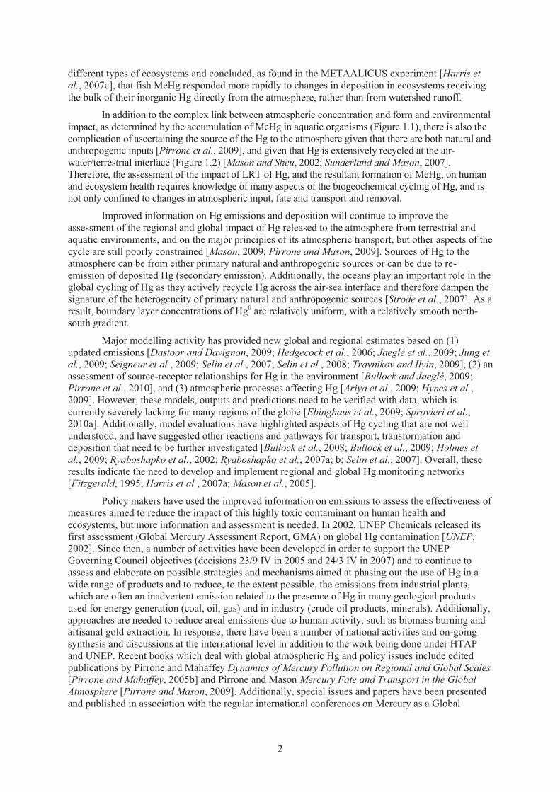
different types of ecosystems and concluded, as found in the METAALICUS experiment [Harris et al., 2007c], that fish MeHg responded more rapidly to changes in deposition in ecosystems receiving the bulk of their inorganic Hg directly from the atmosphere, rather than from watershed runoff.

In addition to the complex link between atmospheric concentration and form and environmental impact, as determined by the accumulation of MeHg in aquatic organisms (Figure 1.1), there is also the complication of ascertaining the source of the Hg to the atmosphere given that there are both natural and anthropogenic inputs [Pirrone et al., 2009], and given that Hg is extensively recycled at the air-water/terrestrial interface (Figure 1.2) [Mason and Sheu, 2002; Sunderland and Mason, 2007]. Therefore, the assessment of the impact of LRT of Hg, and the resultant formation of MeHg, on human and ecosystem health requires knowledge of many aspects of the biogeochemical cycling of Hg, and is not only confined to changes in atmospheric input, fate and transport and removal.

Improved information on Hg emissions and deposition will continue to improve the assessment of the regional and global impact of Hg released to the atmosphere from terrestrial and aquatic environments, and on the major principles of its atmospheric transport, but other aspects of the cycle are still poorly constrained [Mason, 2009; Pirrone and Mason, 2009]. Sources of Hg to the atmosphere can be from either primary natural and anthropogenic sources or can be due to re-emission of deposited Hg (secondary emission). Additionally, the oceans play an important role in the global cycling of Hg as they actively recycle Hg across the air-sea interface and therefore dampen the signature of the heterogeneity of primary natural and anthropogenic sources [Strode et al., 2007]. As a result, boundary layer concentrations of Hg0 are relatively uniform, with a relatively smooth north-south gradient.

Major modelling activity has provided new global and regional estimates based on (1) updated emissions [Dastoor and Davignon, 2009; Hedgecock et al., 2006; Jaeglé et al., 2009; Jung et al., 2009; Seigneur et al., 2009; Selin et al., 2007; Selin et al., 2008; Travnikov and Ilyin, 2009], (2) an assessment of source-receptor relationships for Hg in the environment [Bullock and Jaeglé, 2009; Pirrone et al., 2010], and (3) atmospheric processes affecting Hg [Ariya et al., 2009; Hynes et al., 2009]. However, these models, outputs and predictions need to be verified with data, which is currently severely lacking for many regions of the globe [Ebinghaus et al., 2009; Sprovieri et al., 2010a]. Additionally, model evaluations have highlighted aspects of Hg cycling that are not well understood, and have suggested other reactions and pathways for transport, transformation and deposition that need to be further investigated [Bullock et al., 2008; Bullock et al., 2009; Holmes et al., 2009; Ryaboshapko et al., 2002; Ryaboshapko et al., 2007a; b; Selin et al., 2007]. Overall, these results indicate the need to develop and implement regional and global Hg monitoring networks [Fitzgerald, 1995; Harris et al., 2007a; Mason et al., 2005].

Policy makers have used the improved information on emissions to assess the effectiveness of measures aimed to reduce the impact of this highly toxic contaminant on human health and ecosystems, but more information and assessment is needed. In 2002, UNEP Chemicals released its first assessment (Global Mercury Assessment Report, GMA) on global Hg contamination [UNEP, 2002]. Since then, a number of activities have been developed in order to support the UNEP Governing Council objectives (decisions 23/9 IV in 2005 and 24/3 IV in 2007) and to continue to assess and elaborate on possible strategies and mechanisms aimed at phasing out the use of Hg in a wide range of products and to reduce, to the extent possible, the emissions from industrial plants, which are often an inadvertent emission related to the presence of Hg in many geological products used for energy generation (coal, oil, gas) and in industry (crude oil products, minerals). Additionally, approaches are needed to reduce areal emissions due to human activity, such as biomass burning and artisanal gold extraction. In response, there have been a number of national activities and on-going synthesis and discussions at the international level in addition to the work being done under HTAP and UNEP. Recent books which deal with global atmospheric Hg and policy issues include edited publications by Pirrone and Mahaffey Dynamics of Mercury Pollution on Regional and Global Scales [Pirrone and Mahaffey, 2005b] and Pirrone and Mason Mercury Fate and Transport in the Global Atmosphere [Pirrone and Mason, 2009]. Additionally, special issues and papers have been presented and published in association with the regular international conferences on Mercury as a Global

2

Pollutant (ICMGP). In particular, a special issue of Ambio contained five synthesis papers from the 8th ICMGP in Madison, WI, USA in August, 2006 with two papers being most relevant to the current discussion [Lindberg et al., 2007; Swain et al., 2007]. The 9th ICMGP was recently held in Guiyang, China in July 2009; (http://www.mercury2009.org/).

Figure 1.1. A conceptual diagram illustrating the major pathways between atmospheric deposition of inorganic mercury (Hg(II)) and the accumulation of methylmercury in fish. Also shown are the key interconversions between mercury species and how they relate to bioaccumulation. [Reprinted with permission from Figure 1 in Mason, R. P., et al. (2005), Monitoring the response to changing mercury deposition, Environmental Science & Technology, 39(1), 14A-22A. Copyright 2005 American Chemical Society.]

The overall concepts that drive the major conclusions with regard to LRT of Hg and its deposition and impact will be outlined in this chapter. The conceptual overview will refer to the pertinent sections of the chapters in the report but will not summarize the details and complexities contained in these chapters. Rather, this chapter will provide a conceptual overview of the issues and impacts related to LRT of Hg, and expectations of how these may change in the future. Chapter 2 is focused on synthesizing the data collected to date on atmospheric Hg concentration and chemistry and the concentrations in deposition, and also discusses the need for further study and coordination, and for a global monitoring network. Chapter 3 is mainly concerned with discussing the distribution and magnitude of anthropogenic and natural emissions of Hg to the atmosphere. The issues related to estimating and constraining emission estimates and the methods employed are discussed in Chapter 3. As it is not possible to make measurements in all locations with sufficient spatial and temporal coverage, modelling is an important component of understanding the impact globally of Hg emissions. The various modelling approaches and their validity and predictions are discussed in Chapter 4. Chapter 5 focuses on the environmental and health impacts of the LRT of Hg, focusing on freshwater and marine ecosystems and on human health. The main conclusions and recommendations of this section of the report are contained in Chapter 6 but are also highlighted in the appropriate sections of Chapters 1-5.

Wet Deposition and Dry Deposition of Gaseous and Particulate Hg

Bioaccumulationof CH3Hg

Watershed Retention and Transport/Runoff ofHg and CH3Hg

Evasion fromSoil and Vegetation

Evasion

A: Major Ecosystem Inputs and Outputs of Mercury

B: Major Aquatic Mercury Pathways

Hg(II) methylation

demethylationCH3Hg(II)

oxidation

evasion

Hg(0)

sedimentation

reduction

diffusionresuspension

diffusionresuspension

Burialin Sediments

Wet Deposition and Dry Deposition of Gaseous and Particulate Hg

Bioaccumulationof CH3Hg

Watershed Retention and Transport/Runoff ofHg and CH3Hg

Evasion fromSoil and Vegetation

Evasion

A: Major Ecosystem Inputs and Outputs of Mercury

B: Major Aquatic Mercury Pathways

Hg(II) methylation

demethylationCH3Hg(II)

oxidation

evasion

Hg(0)

sedimentation

reduction

diffusionresuspension

diffusionresuspension

Hg(II) methylation

demethylationCH3Hg(II)

oxidation

evasion

Hg(0)

sedimentation

reduction

diffusionresuspension

diffusionresuspension

Burialin Sediments

Biota

3

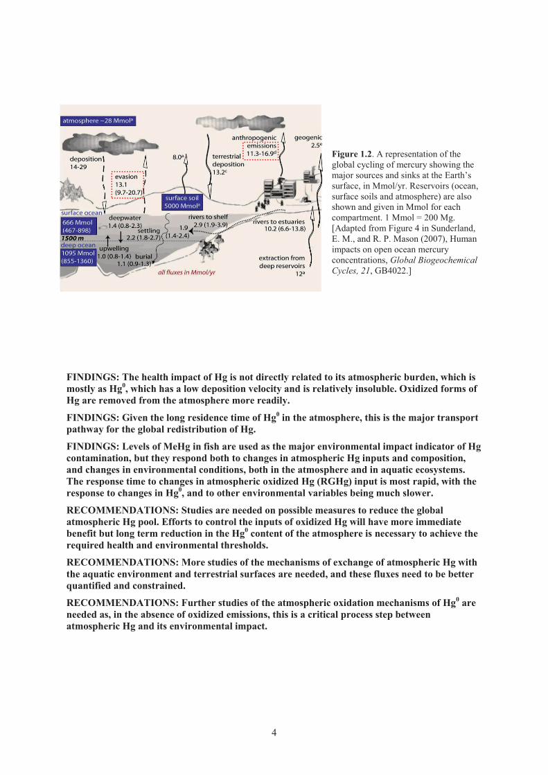
Figure 1.2. A representation of the global cycling of mercury showing the major sources and sinks at the Earth’s surface, in Mmol/yr. Reservoirs (ocean, surface soils and atmosphere) are also shown and given in Mmol for each compartment. 1 Mmol = 200 Mg. [Adapted from Figure 4 in Sunderland, E. M., and R. P. Mason (2007), Human impacts on open ocean mercury concentrations, Global Biogeochemical Cycles, 21, GB4022.]

FINDINGS: The health impact of Hg is not directly related to its atmospheric burden, which is mostly as Hg0, which has a low deposition velocity and is relatively insoluble. Oxidized forms of Hg are removed from the atmosphere more readily.

FINDINGS: Given the long residence time of Hg0 in the atmosphere, this is the major transport pathway for the global redistribution of Hg.

FINDINGS: Levels of MeHg in fish are used as the major environmental impact indicator of Hg contamination, but they respond both to changes in atmospheric Hg inputs and composition, and changes in environmental conditions, both in the atmosphere and in aquatic ecosystems. The response time to changes in atmospheric oxidized Hg (RGHg) input is most rapid, with the response to changes in Hg0, and to other environmental variables being much slower.

RECOMMENDATIONS: Studies are needed on possible measures to reduce the global atmospheric Hg pool. Efforts to control the inputs of oxidized Hg will have more immediate benefit but long term reduction in the Hg0 content of the atmosphere is necessary to achieve the required health and environmental thresholds.

RECOMMENDATIONS: More studies of the mechanisms of exchange of atmospheric Hg with the aquatic environment and terrestrial surfaces are needed, and these fluxes need to be better quantified and constrained.

RECOMMENDATIONS: Further studies of the atmospheric oxidation mechanisms of Hg0 are needed as, in the absence of oxidized emissions, this is a critical process step between atmospheric Hg and its environmental impact.

4

1.2. Concepts Related to Sources and Inter-Continental Cycling of Mercury Mercury exists in the atmosphere at trace concentrations, being around 1 ng m-3 for the remote

South Hemispheric surface air, and higher in the Northern Hemisphere. Mercury is added to the atmosphere by a number of sources and is ultimately removed primarily due to the deposition and removal of ionic Hg species. The average residence time of Hg in the atmosphere is 6 months to a year, and this estimate is based on the overall cycling of the major atmospheric form of Hg, which is elemental mercury (Hg0), found mostly in the gas phase (also referred to as gaseous elemental Hg or GEM). In this report, residence time is estimated from comparison of the rate of addition of Hg from all sources to a reservoir relative to the amount of Hg in that reservoir, and gives an estimate of the overall average total time an atom of Hg spends in the reservoir before being finally sequestered or removed. The residence time in the atmosphere is very short (6 months to a year) compared to that in the surface ocean (top 1000 m; 5 years to several decades) and the terrestrial surface (years to decades, depending on the form of deposition) [Mason and Sheu, 2002; Sunderland and Mason, 2007]. For the atmosphere, recent evidence suggests that this average value for Hg0 can vary widely spatially as oxidation in the atmospheric boundary layer is a spatially heterogeneous process, and because of the relatively rapid deposition of oxidized Hg, especially in the gas phase [Hedgecock and Pirrone, 2004; Hedgecock et al., 2006; Hirdman et al., 2009; Holmes et al., 2009; Laurier and Mason, 2007; Schroeder et al., 1998; Sillman et al., 2007; Sprovieri et al., 2010b]. Current models do not account for this heterogeneity, and use a first order constant or constant fraction to account for the rapid recycling of Hg at surfaces. The removal mechanisms and the transport processes are distinctly different for the different forms of Hg (Figure 1.3). Elemental Hg is relatively insoluble in water and has a substantial vapour pressure so the dissolved Hg0 concentration in equilibrium with average atmospheric concentrations (~1.5 ng m-3) is around 5 pg/L. Many surface waters are saturated relative to the atmosphere, resulting in gas evasion (emission) being an important process in global Hg cycling. Given the low equilibrium concentration of Hg0, most of the removal of Hg from the atmosphere via wet deposition is through the scavenging of RGHg, which is substantially more soluble. Some forms of oxidized Hg (e.g. HgCl2; HgBr2) have a measurable vapour pressure; thus, oxidized Hg can be found in the gaseous phase in the atmosphere, and typically exists at low pg m-3 concentrations (i.e. a few percent of the total atmospheric Hg burden) [Mason, 2005; Schroeder and Munthe, 1998]. Such compounds are efficiently and rapidly dry deposited. Additionally, most of the Hg in atmospheric aerosols is as HgII and the Hg-P fraction typically has a residence time similar to that of aerosols. Finally, however, it has recently been demonstrated that Hg0 can be taken up by vegetation and this provides an important deposition (removal) mechanism, especially in temperate environments.

Figure 1.3. Diagram showing the major forms of mercury in the atmosphere: elemental mercury (Hg0), ionic gaseous mercury (HgX2 (g)), which refers to the sum of all gaseous complexes, and mercury attached to or within aerosols. The removal mechanisms and potential sources of each species are also indicated.

Mercury emissions (Figure 1.2), as detailed in Chapter 3, can be from natural and anthropogenic sources (Table 1.1). In discussing Hg emissions, attempts have been made to further categorize sources. Primary natural sources are those pertaining to Hg release from volcanoes, geothermal sources, and areas enriched in Hg (in the mineral soil), and also Hg release as a result of weathering. Primary anthropogenic emissions relate to the release of Hg from activities such as the burning of coal and other fossil fuels for energy, the extraction and processing of minerals, and the release of Hg during gold extraction using Hg amalgamation approaches (both artisanal and commercial use). These activities mostly represent the

Hg0(g)

Hg0(aq)

HgX2hv

OxidantsHgX2 (g)

HgX2 (g)

Hg

WET & DRYDEPOSITION

DropletAerosol

Hg0(g)

5

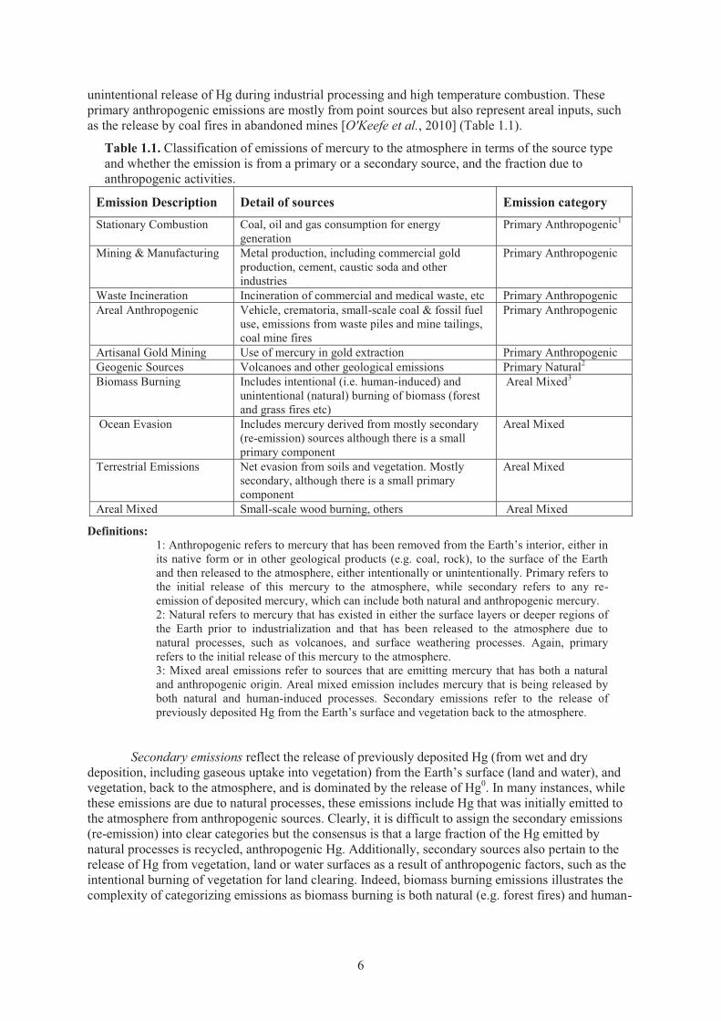
unintentional release of Hg during industrial processing and high temperature combustion. These primary anthropogenic emissions are mostly from point sources but also represent areal inputs, such as the release by coal fires in abandoned mines [O'Keefe et al., 2010] (Table 1.1).

Table 1.1. Classification of emissions of mercury to the atmosphere in terms of the source type and whether the emission is from a primary or a secondary source, and the fraction due to anthropogenic activities.

Emission Description Detail of sources Emission category Stationary Combustion Coal, oil and gas consumption for energy

generation Primary Anthropogenic1

Mining & Manufacturing Metal production, including commercial gold production, cement, caustic soda and other industries

Primary Anthropogenic

Waste Incineration Incineration of commercial and medical waste, etc Primary Anthropogenic Areal Anthropogenic Vehicle, crematoria, small-scale coal & fossil fuel

use, emissions from waste piles and mine tailings, coal mine fires

Primary Anthropogenic

Artisanal Gold Mining Use of mercury in gold extraction Primary Anthropogenic Geogenic Sources Volcanoes and other geological emissions Primary Natural2

Biomass Burning Includes intentional (i.e. human-induced) and unintentional (natural) burning of biomass (forest and grass fires etc)

Areal Mixed3

Ocean Evasion Includes mercury derived from mostly secondary (re-emission) sources although there is a small primary component

Areal Mixed

Terrestrial Emissions Net evasion from soils and vegetation. Mostly secondary, although there is a small primary component

Areal Mixed

Areal Mixed Small-scale wood burning, others Areal Mixed

Definitions: 1: Anthropogenic refers to mercury that has been removed from the Earth’s interior, either in its native form or in other geological products (e.g. coal, rock), to the surface of the Earth and then released to the atmosphere, either intentionally or unintentionally. Primary refers to the initial release of this mercury to the atmosphere, while secondary refers to any re-emission of deposited mercury, which can include both natural and anthropogenic mercury. 2: Natural refers to mercury that has existed in either the surface layers or deeper regions of the Earth prior to industrialization and that has been released to the atmosphere due to natural processes, such as volcanoes, and surface weathering processes. Again, primary refers to the initial release of this mercury to the atmosphere. 3: Mixed areal emissions refer to sources that are emitting mercury that has both a natural and anthropogenic origin. Areal mixed emission includes mercury that is being released by both natural and human-induced processes. Secondary emissions refer to the release of previously deposited Hg from the Earth’s surface and vegetation back to the atmosphere.

Secondary emissions reflect the release of previously deposited Hg (from wet and dry deposition, including gaseous uptake into vegetation) from the Earth’s surface (land and water), and vegetation, back to the atmosphere, and is dominated by the release of Hg0. In many instances, while these emissions are due to natural processes, these emissions include Hg that was initially emitted to the atmosphere from anthropogenic sources. Clearly, it is difficult to assign the secondary emissions (re-emission) into clear categories but the consensus is that a large fraction of the Hg emitted by natural processes is recycled, anthropogenic Hg. Additionally, secondary sources also pertain to the release of Hg from vegetation, land or water surfaces as a result of anthropogenic factors, such as the intentional burning of vegetation for land clearing. Indeed, biomass burning emissions illustrates the complexity of categorizing emissions as biomass burning is both natural (e.g. forest fires) and human-

6

related (forest clearing and burning; seasonal burning of savannah; and wood burning for heat and energy), and the Hg in biomass has both an anthropogenic and a natural source.

Contributions of various natural emission sources vary in time and space depending on a number of factors including the activity of volcanic belts or geothermal activities. Exchange processes between surface water and atmosphere, re-emission of previously deposited Hg from top soils and plants, and biomass burning all have a spatial and temporal component [Mason, 2009; Pirrone et al., 2009; Shetty et al., 2008]. Most models do not adequately account for such variability. Additionally, as all forms of Hg are released from point and areal anthropogenic sources mostly, and Hg0 and Hg-P are released via natural processes, the relative global distribution of these sources has an important impact on the extent of Hg fate and transport. Overall, at any given location, there is both local and regional input of all forms of Hg in addition to Hg that resides in the “global pool” derived from LRT and from re-emission of deposited Hg.

Overall, the problem of changing atmospheric Hg0 concentrations is similar to that of ozone, while the impact and concerns for Hg-P are similar to those of particulate matter, which is more a regional than a global concern. Over time, the changes in emissions have had a relatively small impact on the global atmospheric reservoir as the direct anthropogenic inputs are relatively small compared to the atmospheric reservoir, and globally distributed. Essentially, given such a scenario, global regulation and cooperation in reducing anthropogenic Hg emissions is needed as the impact of changes in one continent will be muted by any changes in inputs in other regions of the globe, and, as noted above, the exchange with the ocean dampens the rate of change over time. Additionally, however, there is the potential for the transport of Hg globally through international trade [Maxson, 2005]. Therefore, the overall strategy for mitigating atmospheric Hg concentrations in the future needs to be global and to be built on a strong knowledge base on the fate, transport and reactivity of Hg in the atmosphere, and of the relative importance of primary versus secondary inputs to the atmosphere, which reflect the legacy of past emissions of Hg.

FINDINGS: Although direct emissions are temporally and spatially very heterogeneous, both the lifetime of Hg0 and the significant re-emission of previously deposited Hg that occurs, serve to reduce this heterogeneity and result in the relatively uniform distribution of Hg0 globally and particularly hemispherically, except in the close proximity to major sources.

FINDINGS: The importance of the ocean in the recycling is acknowledged but the level of understanding of the primary controlling factors involved in this process are not well understood. Similarly, there is little detailed knowledge of the recycling of Hg deposited to the terrestrial environment.

RECOMMENDATION: Given the substantial recycling that occurs, any action to reduce Hg impact on the environment would need to be made on a global basis in order to reduce the global atmospheric Hg pool. Unilateral initiatives would have relatively little regional impact except in the immediate vicinity of major sources.

1.3. Overview of Atmospheric Mercury Dynamics Similar to other atmospheric contaminants that have a strong anthropogenic signal, Hg

emissions and deposition are currently elevated in Asia and its vicinity (the coastal North Pacific), especially in rapidly developing countries [e.g. Pirrone et al., 2010; Quan et al., 2008; Streets et al., 2009; Wan et al., 2009]. While elevated, Hg emissions and deposition are declining in North America and Europe as a result of legislation and mitigation [Pacyna et al., 2003; Pirrone et al., 2010; Selin et al., 2008]. Emissions over the world are therefore heterogeneous and dependent on energy consumption and sources, industrial activity, the use of emission control technology, and the extent of inputs from natural sources. Essentially all emission is into the planetary boundary layer (PBL; bottom 1-2 km of the troposphere), while most of the transport is in the upper troposphere [NRC, 2010]. Therefore, the mechanisms related to transfer between these layers are important for the overall distribution of Hg on a global scale.

7

Although most pollutants are released into the PBL, their horizontal transport usually is quite slow in this layer due to relatively weak winds near the Earth’s surface. For Hg, RGHg is rapidly deposited and removed from the PBL (lifetime hours to days) and therefore is not transported globally [e.g. Jaffe et al., 2005; Jaffe and Strode, 2008]. However, there is the potential for its formation in the PBL and/or the upper atmosphere via photochemical processes [Fain et al., 2009; Holmes et al., 2006; Radke et al., 2007] and therefore HgII (as both RGHg and Hg-P) is found in the atmosphere in remote regions due to its in situ production. Additionally, it is also suggested, although there is little supportive information, that oxidation of Hg0 can be enhanced in the upper troposphere. The importance of this process depends on the mechanisms for transport of Hg from the upper atmosphere to the terrestrial and water surface. Also, the impact of stratospheric-tropospheric mixing [Cooper et al., 2005; Meloen et al., 2003; Stohl et al., 2003] on Hg speciation and concentration needs further investigation. Models suggest that sinking of upper air masses can transport substantial HgII formed in the upper atmosphere to the Earth’s surface under specific meteorological conditions [e.g. Selin et al., 2008].

Conversely, Hg0 can be transported from the PBL into the free troposphere and can often travel great distances because of the stronger winds aloft, including the jet streams, which are the strongest upper atmospheric flows that encircle the Earth [NRC, 2010]. The mechanisms producing upward transport into the free atmosphere (e.g., thunderstorms and mid-latitude low-pressure systems) play important roles in determining the extent of long-range pollutant transport. These weather phenomena range in size from small, short-lived turbulent eddies to large, long-lived systems that span continents and can last weeks or months [NRC, 2010]. Thunderstorms, sea breezes, and high and low-pressure systems all play a role in transporting pollutants both horizontally and vertically.

Therefore, overall, the major processes (meteorological, chemical, physical) that control the large-scale atmospheric transport of Hg0 are similar to those for other relatively long-lived atmospheric species and Hg0 trends parallel the distribution of ozone. Additionally, as is the case for ozone, LRT and import of Hg from outside a continental domain is not trivial and needs to be considered in policy and impact assessment. As noted, sources are heterogeneously distributed and the locations of major sources are in regions where large scale air transport pathways occur, with the result that Hg0 can be rapidly transported over large distances. For example, episodic events of elevated air Hg0 concentrations have been recorded at the Mt. Bachelor Observatory in central Oregon [Jaffe et al., 2005; Weiss-Penzias et al., 2007] and during aircraft measurement campaigns [Friedli et al., 2004; Radke et al., 2007; Swartzendruber et al., 2008]. These have been linked, based on correlation with other atmospheric pollutant concentrations, such as CO, to air masses originating from Asia. Similar results have been measured off the Asian continent [Jaffe et al., 2005]. However, elevated RGHg did not occur in air masses with elevated Hg0 and CO, suggesting local formation rather than LRT.

The main impacts of global atmospheric circulation are dictated to a large extent by the winds, which in the middle-latitude troposphere are mostly from the west (zonal flow) in the Northern Hemisphere, causing most intercontinental transport to be from west to east, and are much stronger than the north-south (meridional) component of the wind in the middle and upper troposphere. Near the surface, in the PBL, winds are more similar for both components. Wind speeds generally are stronger during winter than summer, generally increase with altitude, and the jet streams in the upper troposphere are regions of the strongest winds. The resultant vertical motion experienced by air parcels due to these factors is vitally important since Hg and other pollutants transported from the surface to higher altitudes will be horizontally transported most rapidly and farther than Hg residing in the PBL. It should be noted, however, that meteorological conditions cause both the rising and sinking of air masses. Generally, areas of rising air tend to be smaller and shorter lived than areas of subsidence, which generally cover larger areas and persist for longer periods [NRC, 2010].

Synoptic circulation events (cyclones) are important Hg transport events [NRC, 2010]. For example, low-pressure areas are important regions of strong horizontal and vertical pollution transport, and mostly result in west-east gradients in deposition. For example, given the air transport patterns, and the distribution of anthropogenic sources in the USA, deposition of Hg is higher in the

8

eastern USA compared to the west, as manifest in data from the Mercury Deposition Network (MDN)which is part of the US National Atmospheric Deposition Program (NADP) [MDN, 2009]. Important formation areas for cyclones are over eastern Asia and the western Pacific Ocean, as well as the east coast of North America, and these events are important mechanisms for transporting Hg and other pollutants from the east coasts of both Asia and North America to the associated oceans, and globally [Hains et al., 2008; Owen et al., 2006; Prados et al., 1999; Stohl et al., 2002]. Another preferred formation region is downwind of major mountain ranges such as the Rocky Mountains or the Alps. It is noteworthy that Europe and western Asia are not major regions of cyclone formation or transit.

Additionally, smaller and less persistent mesoscale weather systems [NRC, 2010] can also be important vectors for Hg. Important examples associated with pollutant transport are thunderstorms, land and sea circulations, and mountain and valley breezes. Thunderstorms could rapidly move Hg into the upper troposphere where it can be transported great distances by the stronger horizontal winds aloft. Conversely, the downdrafts that occur during the mature and dissipating stages of a thunderstorm transport upper tropospheric air to the surface. Modelling suggests that such phenomena are important in Hg transport from altitude to the surface in the southeastern USA and to the Gulf of Mexico [Selin and Jacob, 2008]. Additionally, strong updrafts, such as those associated with intense biomass burning, can transport boundary layer air to the upper troposphere or lower stratosphere on the order of minutes, compared with hours or days for synoptic systems. This is an important consideration for short-lived or rapidly deposited chemical species, such as HgII. Overall, many meteorological systems can move long distances during their lifetimes and produce strong vertical transport over a large area for an extended time.

FINDINGS: The transport of Hg above the boundary layer in the free troposphere is fundamental to its rapid global redistribution, although the details of this transport are not well studied.

FINDINGS: Major convective events are important in the deposition of Hg from the middle and upper troposphere, where substantial oxidation is thought to occur. However, almost nothing is known about the speciation and reaction chemistry of Hg, particularly the oxidation of Hg0, above the boundary layer.

RECOMMENDATION: Measurements of Hg concentration and speciation in the free troposphere are crucial to better understanding of global Hg cycling. Airborne measurement campaigns must be a major priority and focus of future field campaigns, and more long-term measurement sites with speciated Hg are needed in the free troposphere (e.g. on mountains or making use of commercial aircraft).

1.4. Spatial and Temporal Variability in Inter-Continental Transport Given the above discussion, and knowledge of the main air mass transport pathways, it is

clear that there is a high potential for emissions in Asia, North America and Europe, especially of Hg0, to be transported globally, and similar conclusions are likely for the Southern Hemisphere although there is little data available to confirm this. As Hg0 is not an inert atmospheric species and can be oxidized by homogeneous and heterogeneous processes, the presence of other pollutants or reactive species in the atmosphere can have important impacts on its transport and deposition.

Transport from Asia appears to be important on the global scale given the large inputs of Hg species to the atmosphere from both anthropogenic and natural sources [Quan et al., 2008; Streets et al., 2009; Wan et al., 2009]. Emissions and export are dependent on season, given the propensity for storms and dust transport in winter/early spring, and seasonal differences in coal use. Estimates suggest that much of the Hg released as RGHg from coal combustion and other emissions contributes to elevated local deposition while the Hg0 released is mostly mixed into the global pool. Because significant amounts of coal are burned in homes and small industrial facilities in developing countries, without any kind of emission control, emissions of HgII are higher in developing countries than in the developed World.

9

Numerous studies have examined the transport of pollutants from North America to the North Atlantic and have evaluated the role of high pressure systems over the Atlantic (Bermuda high) in controlling this transport [Doddridge et al., 1994; Hains et al., 2008; Owen et al., 2006; Wu and Boyle, 1997]. Alternatively, the same meteorology is responsible for the transport of air masses from Africa to the southeastern USA at certain times of the year. While regional models for Hg have documented similar effects, there is little observational evidence to support their conclusions [Lamborg et al., 1998; Laurier and Mason, 2007; Mason and Fitzgerald, 1996; Slemr et al., 1981]. Similarly, transport of contaminants from Europe and North America to the Arctic is again a well-known and documented phenomenon [Burkow and Kallenborn, 2000; Garbarino et al., 2002; Macdonald, 2005] but the conclusive evidence demonstrating the impact of anthropogenic Hg is sparse, besides the demonstration that Arctic wildlife have elevated Hg levels in their tissues [Campbell et al., 2005; Macdonald et al., 2008].

The direct source-receptor relationship and the impact of changes in atmospheric anthropogenic inputs on the ocean and other regions are hard to demonstrate. For example, the sources of HgII to the Arctic (and Antarctic) include both transport from lower latitudes as well as halogen-mediated Hg0 oxidation, in concert with ozone depletion, and its efficient removal [Ebinghaus et al., 2002; Poissant et al., 2008; Steffen et al., 2008]. Demonstration of these oxidation processes is now well-documented and have built on the pioneering research of Schroeder and colleagues [Barrie et al., 2001; Steffen et al., 2002; Steffen et al., 2005]. The role of halogen chemistry has been more clearly delineated [Seigneur and Lohman, 2008; Xie et al., 2008] and the processes controlling such events better constrained and understood. Recently, Hirdman et al. [2009] combined measurements of Hg0 at the Arctic site with the output of the Lagrangian particle dispersion model FLEXPART, for a statistical analysis of Hg0 source and sink regions. They found that the Arctic is a strong net sink region for Hg0 in April/May, indicating Hg accumulation in the Arctic snow pack. In summer, however, the Arctic is a net Hg0 source, indicating the importance of re-emission of previously deposited Hg when the snow and/or ice melts, and evasion of Hg0 from the ocean through sea ice leads and polynyas. Others have reached similar conclusions [Ariya et al., 2004]. Net inputs of Hg to the Arctic terrestrial ecosystem are reflected by measurements of higher concentrations in coastal regions compared to more terrestrial locations [Douglas and Sturm, 2004; Garbarino et al., 2002].

The role of hurricanes/cyclones in the Atlantic and in the Pacific, and other extreme events, on the LRT of Hg has not been investigated in any specific study. However, in addition to the heightened vertical mixing that would occur and the potential for rapid LRT via the contained weather system, there is also the potential for these events to result in enhanced evasion of Hg0 from the ocean, as found for CO2 [Bates et al., 1998; Koch et al., 2009] and for enhanced deposition associated with the elevated rainfall of tropical systems. Such large weather systems are clearly important but have been little studied.

Overall, there are large scale regional and latitudinal differences in the extent of LRT but this has not been evaluated for many regions and for many different scenarios, especially in the Southern Hemisphere. In the Northern Hemisphere, the potential for LRT transport from Asia to North America has received the most attention primarily as a result of the importance globally of emissions in Asia, and of the potential for these to impact North America. Clearly, however, there is the potential for emissions in North America to impact the North Atlantic and continents to the east, although, given the emissions in Europe, this may be difficult to clearly demonstrate.

Much of the current longer-term and synthesized observations of Hg concentration, on which the above discussion is based and on which the models rely for validation, and the long-term trends are contained in Chapter 2, which summarizes and collates the current available information. Recent analytical advances have substantially improved the quantity and quality of the data, and have resulted in an increasing number of long-term observations that has allowed for a better understanding of both long-term trends and short-term dynamics, such as diurnal cycles in Hg species, and the importance of atmospheric chemistry in Hg fate and transport.

10

While there have been major advances and improvements in data quality, there is more that needs to be done, especially in locations besides North America and Europe. There are efforts to increase and improve monitoring in Asia and other locations with heightened point source emissions, but there is a clear need for coordination and global cooperation in monitoring, data sharing and in model development [Bullock and Jaeglé, 2009; Fitzgerald, 1995; Harris et al., 2007b; Keeler et al., 2009; Mason et al., 2005; Pirrone and Mahaffey, 2005a; Pirrone et al., 2009]. A network of monitoring stations would provide a coordinated approach to consolidate current and future global efforts and would allow further harmonization of collection and analytical methods, and foster and provide a platform for international intercomparisons, definitions of proper quality control procedures, and validation of results. Such a network could also provide a central database for collation of results and information that would be an important resource for managers, modelers and other scientists. Finally, a coordinated sampling network would provide information that is needed to confirm and update the models and their predictions. It is therefore evident that there is an urgent need to gather sufficient information to demonstrate the importance of LRT. The collection of additional data will allow an assessment of both the local/regional and the global impact of emissions from various source regions. Finally, studies should focus both on point source contributions and large-scale areal emissions, such as the net emission of Hg0 from the surface ocean, and from the terrestrial landscape, as the factors controlling these emissions are poorly understood.

FINDING: The fluctuations in the scale and extent of inter-continental transport are almost impossible to identify because of the scarcity of measurement data in appropriate locations (i.e. the free troposphere) and the near absence of long-term monitoring data in such locations.

RECOMMENDATION: A world wide monitoring network with measurement sites in strategic positions, especially in the free troposphere, to detect continental outflow is essential to evaluate trends in hemispherical Hg transport. Such a network should have sites throughout both hemispheres.

1.5. Assessing Global Natural and Anthropogenic Sources and Deposition Estimates of emissions of Hg to the atmosphere from both natural processes and

anthropogenic sources are detailed in Chapter 3 of this report. The discussion below summarizes the most important concepts and approaches that are used to obtain such estimates, and presents the relevant related information. It is important to present and consider the uncertainties and methodologies used to make Hg emission estimates. For anthropogenic point sources, measurements of the concentration and speciation of Hg in stack gases can be used to provide a constraint on the fraction of Hg in the source material that is released to the atmosphere. Such estimates of emission factors have been done for different sources but the amount of information, especially in terms of speciation is limited in number, and also has been completed mostly in North America and Europe [Feng et al., 2009; Pacyna et al., 2001; Pirrone et al., 1996; Pirrone et al., 2001]. For many countries, no measurements exist and therefore emission estimates use extrapolation of the existing information in making global point source emission estimates [Feng et al., 2009; Leaner et al., 2009]. Additionally, most estimates assume a constant emission factor over time although it is relatively clear that emissions from sources related to energy production would vary seasonally and sources related to local economic activity may vary on a weekly basis. For natural sources, light intensity and temperature appear to be important, and result in diurnal variations in emissions.

Emissions related to coal burning have been the most studied, while emission factors from the various industrial processes are not well constrained [Pirrone et al., 2009]. Emissions from incineration of municipal and medical waste incinerators have been examined in very few studies. Emissions from anthropogenic sources (Chapter 3) are currently dominated by emissions related to coal and oil consumption (~35% of the total anthropogenic inputs) for electricity generation. It is expected that coal will continue to be an important and growing source of energy for much of the world, especially in developing countries, in the future. While crude oil is a widely used energy source, its Hg content is relatively low and therefore Hg released from the refined products is typically a small component of the overall anthropogenic flux globally. Similarly, Hg levels in natural gas are generally low as Hg is often removed during the recovery of the natural gas. The long-term

11

implications for Hg emission and deposition from energy-related coal and fossil fuel consumption will depend upon the rate of world economic growth, the specific type of fuel used, and the pollution control technologies employed as the speciation of the emissions is directly related to the type of control technologies used. The Hg emissions from non-energy sectors, such as mining, refining and industrial operations and waste incineration (~20% of the global total) may also increase, as economic growth leads to greater extraction and processing of natural resources. Pollution control technologies that remove HgII or Hg-P have a regional benefit. However, in terms of LRT and deposition, there will be little impact without control of Hg0 emissions from such sources. Thus, the prediction is that the global atmospheric Hg pool will continue to increase.

Generally, emissions from coal burning appear to be predominantly as Hg0 while emissions from incineration are mostly as HgII, but there is wide variability in speciation estimates [Pirrone et al., 2009]. Overall, the speciation of Hg in emissions is not well characterized. Therefore, while it is acknowledged that the speciation is vitally important in estimating the regional versus LRT of Hg, in discussing emissions in this report no specific information for individual sources is presented in Chapter 3, reflecting the lack of knowledge in this regard. Clearly, more information is needed on the speciation of Hg in point source emissions and how the speciation may change with different control technologies. This is crucial for future predictions on the impact of changing emissions and control technologies on Hg fate, transport and bioaccumulation.

In terms of areal terrestrial emissions and deposition, such as the uptake and emission from vegetation and from soils, estimates mostly assume that emissions are as Hg0 [Gustin and Lindberg, 2005; Mason, 2005; 2009]. For deposition, estimates are based on a variety of measurement techniques: either the direct measurement of deposition or estimation based on an indirect method. For direct methods, fluxes are measured directly using the collection of the material (gas or particles) on a surface – a so-called surrogate surface that mimics the actual surface – or by measurement of the flux in the air close to the surface. Typical surrogate surfaces include a recirculating water container of known surface area (to mimic the water surface) and, for particles, aerodynamic surfaces that are coated to capture particles effectively. These have been used for particle collection and for dry deposition estimates of both RGHg and Hg-P [Caldwell et al., 2006; Malcolm et al., 2003; Marsik et al., 2007], although such approaches need further validation. Micrometeorological approaches, which measure the flux directly, have been used in a limited way to date but are likely to become more widely used in the future [Bash et al., 2007; Lyman et al., 2007; Skov et al., 2006]. These approaches can estimate both deposition and emission (evasion) depending on the net flux direction and this is an advantage as other methods must estimate both deposition and emission separately and then determine the overall flux by difference, with likely higher error. All approaches appear to provide a reasonable estimate of dry deposition when compared with the alternative approach of measuring atmospheric concentrations and estimating fluxes based on an estimation of the deposition velocity.

Additionally, to estimate dry deposition of Hg, many investigators have compared the concentration in wet deposition collected in an open area to that of precipitation collected beneath the forest canopy (called throughfall deposition) and have inferred dry deposition as the difference between these two values [Guentzel et al., 1998; Lawson and Mason, 2001; Rea et al., 1996]. Finally, as one of the main processes of dry deposition of Hg0 is uptake into vegetation, this has been estimated using the concentration of Hg in litterfall (the loss of leaves from trees) in temperate environments [Rea et al., 1996; Sheehan et al., 2006]. To assess deposition to the canopy, leaf washing and analysis can also be used to determine the change in concentration over time, and with the surface area known, such techniques can be used to estimate deposition [Rea et al., 2001].

For areal emissions, a variety of measurements and approaches are used. Biomass burning estimates are based on measurements in controlled laboratory environments and also on measurements during burning events, and extrapolation globally is based on the relationship between Hg/CO developed from these limited studies [Ebinghaus et al., 2007; Friedli et al., 2003; Friedli et al., 2009a; Weiss-Penzias et al., 2007]. Emissions from water surfaces are normally determined by measurement of the dissolved gaseous Hg concentration (DGHg, which is essentially Hg0 for most waters) and calculation of the evasion flux based on gas exchange models; and the surface film model

12

approach is most widely used [Gårdfeldt et al., 2003; Lindberg and Zhang, 2000; Loux, 2000]. The exchange velocity, sometimes referred to as the piston velocity, is related to the wind speed and temperature and a number of formulations exist in the literature. Overall, most Hg studies have taken models for other gases, such as CO2, and converted them to Hg0 based on the relative values of the diffusion coefficient or the Schmidt number [Andersson et al., 2008c; Fitzgerald and Rolfhus, 2001; Lamborg et al., 1999]. Continuous systems for measurement of surface water Hg0 have been developed and a recent innovation has been the use of an air equilibrator followed by the measurement of the equilibrium concentration in the air, and calculation of the water Hg0 concentration based on Henry’s Law [Andersson et al., 2007; Andersson et al., 2008a; Andersson et al., 2008b; Sprovieri et al., 2010b].

Clearly, the estimation of dry deposition is the more difficult task. There are gaseous and particulate HgII species in the atmosphere, as well as Hg0, all of which can be deposited to the terrestrial and water surface. Additionally, Hg0 can be emitted to the atmosphere from both terrestrial and aquatic systems after reduction. There is no evidence to suggest that RGHg is emitted to the atmosphere from terrestrial surfaces. A small emission of Hg-P associated with dust and particle resuspension also occurs. Wet deposition estimates are mostly made by the collection of event or weekly precipitation samples with the concordant recording of rainfall depth. This allows the flux to be estimated directly. As noted, the errors involved in the estimation of deposition or evasion depend on the approach used, the frequency of sampling and the errors associated with the measurements. It is difficult in most instances to properly constrain the errors associated with the estimation of dry deposition, but it likely is greater than 30% in most cases.

Overall, recent global emission assessments have focused not only on stationary anthropogenic emissions, such as coal, oil and wood combustion, solid waste incineration and pyro-metallurgical processes [Nriagu and Pacyna, 1988; Pacyna et al., 2006; Pacyna et al., 2003; Pirrone et al., 1996; Pirrone et al., 2009] but studies have also addressed emissions from volcanoes [Ferrara et al., 2000; Nriagu and Becker, 2003; Pyle and Mather, 2003], gold mining [Lacerda, 1995; Veiga et al., 2006], water surfaces [Mason and Sheu, 2002], soils and vegetation [Gustin et al., 2000] and biomass burning [Cinnirella and Pirrone, 2006; Ebinghaus et al., 2007; Friedli et al., 2003; Wiedinmyer and Friedli, 2007]. Global assessments have compiled estimates for both anthropogenic and natural sources [AMAP/UNEP, 2008; Pirrone et al., 2009] and have considered the emissions in categorical subdivisions, such as primary and secondary anthropogenic and natural sources, as defined earlier in the chapter. A recent assessment, completed under the UNEP framework, integrated these assessments of anthropogenic and natural sources, and also included assessments of sources that have not been included in previous global estimates (e.g. coal-bed fires, biomass burning) [Friedli et al., 2009a; Mason, 2009; Pirrone et al., 2009]. Overall, direct anthropogenic emissions are about 30% of the total Hg input to the atmosphere. Artisanal gold mining is the most important anthropogenic areal source (4% of the total). Total primary anthropogenic emissions account for 30-35% of the emissions.

Emissions from natural processes that are wholly or partially impacted by human activity include release due to biomass burning, and landscape change (logging, clearing and construction) [Cinnirella and Pirrone, 2006; Cinnirella et al., 2008; Ebinghaus et al., 2007; Friedli et al., 2003; Friedli et al., 2009a; Friedli et al., 2009b; Wiedinmyer and Friedli, 2007]. The evasion of Hg0 from surface waters is primarily driven by the concentration gradient of Hg0 between the surface water and air above, and the turbulence of the system, which is mainly a function of wind speed. In conjunction, solar irradiation, which alters the net photo-reduction of HgII in surface waters (both photochemical oxidation and reduction reactions occur), alters the rate of production of Hg0. Temperature influences the reaction kinetics, the rate of diffusion in both the water and air [Pirrone and Hedgecock, 2005], and the solubility of Hg0. While most ocean waters are saturated with Hg0 relative to the atmosphere, regions of low net reduction and high wind speed can become undersaturated and uptake of Hg0 from the atmosphere is possible [e.g. Strode et al., 2007]. The evasion of Hg from lake surfaces on an areal basis is generally higher than that observed over the sea, but given the large surface area of the ocean, global ocean emissions are a major flux in the global Hg cycle (~34% of global emissions) [Mason, 2009].

13

In summary, Hg deposition to the Earth’s surface has increased markedly since the beginning of the industrial revolution, as anthropogenic releases have increased. There is a continual need to improve emission inventories for natural and anthropogenic sources to refine these estimates. The initiation of further research and measurement campaigns, including studies aimed at assessing the magnitude and speciation of emissions in sectors where there is significant uncertainty, should be an important priority. Such studies will also be useful for improving and verifying model results. Model sensitivity analyses would be useful for further defining research needs and to support management actions.

As noted above, methods of measurement of emissions, deposition and fluxes are disparate and need better coordination and inter-comparison. There is a further need to develop methods that allow for the measurement of concentrations and deposition of Hg that are easy to apply and do not require elaborate field stations. In addition to the development of a global atmospheric Hg monitoring network, there is clearly also an advantage in developing a coordinated effort to estimate the emissions from terrestrial areal sources and to develop a better understanding of the extent of emission from the ocean and the controlling factors. Some of these methods and approaches require substantial expertise. Further development of measurements tools will help advance knowledge.

FINDINGS: In terms of anthropogenic emissions, the largest source is coal burning, while the largest uncertainty is human-related emissions from waste incineration, artisanal mining, and biomass burning. Incineration is potentially a serious local problem because of the high concentration of oxidized Hg in these emissions.

FINDINGS: Data on the speciation of emissions is very sparse and more studies need to be done outside of developed countries and in the Southern Hemisphere. A fundamental understanding of the factors controlling these areal emissions is lacking. The magnitude of the net flux of Hg from terrestrial (barren or vegetative) and water surfaces is not well understood or constrained.

RECOMMENDATIONS: In terms of estimating deposition, it is the dry deposition flux of gaseous oxidized Hg that is mostly poorly constrained. Methods and measurements are needed to advance understanding and improve estimation. However, as wet deposition measurements are regionally focused in the developed world, more measurement and better estimation of deposition fluxes are needed globally.

RECOMMENDATIONS: Well designed experiments and carefully controlled and performed field campaigns must be undertaken to provide understanding that will allow fluxes to be estimated with far greater certainty than they are at present.

RECOMMENDATIONS: Campaigns evaluating deposition should also include emission measurements to allow for an estimation of the magnitude and direction of the net flux.

1.6. Data and Knowledge Gaps in Atmospheric Chemistry, Transport and Fate It is difficult to distinguish the source of Hg once it is mixed into the atmosphere; therefore,

there are significant challenges in deriving source attribution scenarios for Hg. Furthermore, as Hg is emitted in various forms and additionally transformed between oxidation states in the atmosphere (Figure 1.3), deposited and re-emitted to the atmosphere, its tracking can only be done currently using model evaluations. For many locations globally, inputs from LRT are substantial and it is possible to constrain the sources and perform source attribution estimations to understand the differences between regional and LRT. In a sense, Hg is similar to ozone with respect to LRT as the atmospheric reservoir is relatively large compared to the inputs.

A number of approaches can and have been used to examine Hg transport and the impact of the source profile on its deposition. Correlation of Hg concentrations and changes over time with that of other pollutants, which have a known source profile and atmospheric residence time and chemistry, can allow for an examination of the relative sources at a particular location. Such an analysis was done by Jaffe et al. [2005] where a correlation between CO and Hg0 was used to examine the export of anthropogenically-derived Hg0 from Asia. In contrast, Laurier et al. [2003] concluded that the RGHg measured in the North Pacific Ocean marine boundary layer (MBL) was due to in situ

14

production as the low CO present was indicative of unpolluted air, and the low ozone indicative of active halogen chemistry. Correlations were found between RGHg diurnal formation, ozone decrease and UV intensity, suggesting in situ production [Laurier et al., 2003]. Other studies have found similar results [Hedgecock and Pirrone, 2001; Laurier and Mason, 2007; Sprovieri et al., 2010a].

The potential of using differences in the relative ratio of the 7 Hg isotopes to track sources and transport is driving active research, but the differences are small and therefore sophisticated equipment (a multicollector ICP-MS) and extreme care is needed to make the measurements. Sample size is also a constraint. However, recent advances in analytical instrumentation now allow for the determination of the stable isotope fractions in a sample with high precision. Two types of fractionation have been identified with mass independent fractionation (MIF) appearing to occur through photochemical reduction/decomposition reactions, and potentially other processes, and being largest for the odd isotopes of Hg [Bergquist and Blum, 2007; 2008; Carignan et al., 2009; Jackson et al., 2008]. These analyses have a number of applications, but one potential use would be in source identification of atmospheric Hg. Biswas et al. [2008] analyzed coal deposits and found a range of both mass dependent fractionation (MDF, reported as the change in isotope Hg-202) and mass independent fractionation, reported as the change in isotope Hg-201. Given the observed variability, it was suggested that by combining these two Hg isotope signals results, there may be a unique isotopic "fingerprint" for many coal deposits. However, whether these data could be used in atmospheric Hg “tracking” is still doubtful given that many other Hg-containing minerals also have their own signatures, and surface soils appear to carry the isotopic signal of the deposited Hg [Biswas et al., 2008], making it difficult to distinguish between primary and secondary sources of Hg.

In addition to using measurements for source apportionment, computer models can be run in a manner that allows for “tagging” (tracking) of a particular source or source category and this can allow an assessment, for example, of the relative sources of Hg deposition in a specific region. Such analyses have been done for the USA [Bullock et al., 2008; Bullock et al., 2009; Jaffe and Strode, 2008; Selin and Jacob, 2008], Europe, and globally for ocean emissions and emissions from Asia [Dastoor and Davignon, 2009; Jaeglé et al., 2009; Jung et al., 2009; Seigneur et al., 2009; Strode et al., 2008; Travnikov and Ilyin, 2009]. Therefore, models have the ability to distinguish between sources and flows of Hg in the environment, and can ascertain the relative importance of natural sources versus historic or current anthropogenic emissions, and can assist in the assessment of the importance of re-emission. However, most models to date have a very simplified approach to quantifying and estimating the re-emission component and this is one major area of needed future research. One approach [Smith-Downey et al., 2010] that is being currently studied is tying the recycling of Hg at the terrestrial-air interface to that of carbon, as there are relatively sophisticated carbon cycling models. For the ocean, the modelling framework of Strode et al. [2007] for air-sea exchange is being updated with the results of Holmes et al. [2009], and is incorporating more complex ocean Hg chemistry [Soerensen et al., 2010]. This approach is yielding results that are more comparable with measurements of surface ocean Hg0 [Mason, 2009]. Continued model development will rely and require more comprehensive data and development needs to work concurrently to help identify data gaps and to improve the model formulations and parameterizations.

In summary, the measurements and model results suggest that, once emitted from any source, Hg has the potential to be transformed to different chemical forms, transported through the atmosphere, and deposited long distances from the point of origin. Hence, LRT is an important process that clearly affects global exposures. Continued emissions will increase the amount of Hg in the global pool available for LRT and recycling between reservoirs.

1.6.1. Understanding and Modelling Atmospheric Mercury Chemistry The various global Hg models currently used in evaluations of the global Hg cycle have been

discussed in the sections above, in detail in Chapter 4, and in recent publications, such as Pirrone and Mason [2009]. The major differences in the models are the formulations of atmospheric chemistry and the major reactions occurring. Many models, until recently, did not include oxidation of Hg0 by reactive halogen species, and only included reactions with ozone and the hydroxyl radical. Including these reactions is a necessary and important modification, as there is growing evidence that the

15

reactions with bromine atoms (Br) may be the controlling reaction in the atmosphere [Holmes et al., 2006; Holmes et al., 2009; Seigneur and Lohman, 2008]. Hynes et al. [2009] reviewed the current state of knowledge of the chemical processes that transform atmospheric Hg species via gas and aqueous phase reactions and the physical processes of deposition and concluded that the understanding of the basic chemistry that controls Hg is incomplete and the experimental data either limited or nonexistent. Recent experimental and theoretical studies of Hg reaction kinetics are however clarifying some issues, and more study is recommended to extend and expand these initial studies.

In addition to understanding the gas phase chemistry it is imperative to understand the fundamentals of the kinetics and thermodynamics of the elementary and complex reactions of Hg0 and oxidized Hg in the aqueous and heterogeneous phases at atmospheric interfaces such as aerosols, fogs, clouds, and snow-water-air interfaces. A recent review by Ariya et al [2009] compiled the recent theoretical, laboratory and field observations involving both homogeneous and heterogeneous reactions, described the current lack of knowledge of Hg chemical, physical and biological interactions at environmental surfaces, and discussed the impact of the type of surface, and the environmental conditions on the transformation rate of Hg in the gas phase or aqueous phase. The challenges to understanding the surface chemistry of Hg include the need for theoretical calculations, particularly for large molecules and clusters, and condensed phase systems. Limited studies on the kinetics of gas-phase Hg0 oxidation on surfaces have been done [e.g., Flora et al., 1998; Lee et al., 2004; Vidic et al., 1998] and further experimental studies on uptake or kinetics of heterogeneous reactions of Hg on various environmentally relevant surfaces (ice, snow, and aerosols and biomaterials) are needed.

Overall, the lack of knowledge of detailed Hg chemical speciation in field studies is due to the limitations of existing analytical and collection techniques, operational definitions of fractions, and the detailed chemical structure of gas phase HgII compounds. The fractions are, however, not based on fundamental understanding of physical and chemical structures of molecules, but on the separation techniques of the typical collection devices (i.e. use of denuders to collect the total RGHg fraction). Further development of targeted techniques for detailed quantification of gas phase ionic Hg speciation is therefore essential.

Understanding of atmospheric chemistry can be tested through the use of models. The predictions of atmospheric chemical models are limited by the accuracy of our understanding of the basic physical and chemical processes that underlie the models. One way to evaluate the models is through model intercomparison and there have been a number of efforts in this regard [Bullock et al., 2008; Ryaboshapko et al., 2002; Ryaboshapko et al., 2007a; b]. The details of the models and their comparison are contained in these papers. In performing a model intercomparison it is of great importance to know exactly how each section of each model compares. The more complex the models, the more difficult it becomes to ascertain what drives differences in model output. Therefore, when examining the potential reactions described in individual studies of reactions kinetics in the laboratory, and examining their potential impact in the environment, modelers often make use of detailed box model studies as these box models can incorporate detail and fine scale processes that cannot be incorporated into global fate and transport models. In order to isolate and examine the atmospheric Hg chemistry (i.e. remove the influence of transport, precipitation, emission and deposition), box models run under a given set of initial conditions can examine and integrate the chemical mechanisms for a set period of time. The more complex mechanisms used in box models serve, via sensitivity analyses, to identify the most important reactions and the related uncertainty that should be parameterized and included in global models, thus preserving the most important reactions and compounds in the large scale modelling. As box models largely ignore transport, they are really only suitable for modelling situations of high atmospheric stability, such as the anticyclonic conditions that persist for days, or when a very stable inversion layer forms in the Arctic, for example.

In addition to the global models, many countries and regions are also developing regional atmospheric Hg models. Such models focus on a limited portion of the global biosphere and therefore require definition of meteorological and chemical conditions at the boundaries of the model domain,

16

especially for Hg0 which is relatively long-lived [Bullock and Jaeglé, 2009]. Regional models have been used to estimate source attribution for observed Hg deposition to the United States and to various nations in Europe. When compared, these models differed in their conclusions. For example, three regional models (the Community Multiscale Air Quality (CMAQ) model, the Regional Modelling System for Aerosols and Deposition (REMSAD), and the Trace Element Analysis Model (TEAM)) were tested under conditions in which the domain, boundary conditions and inputs were more constrained but still showed the importance of: 1) the boundary values for Hg and their definition; 2) intercontinental transport of Hg; and 3) reaction chemistry of Hg [Bullock et al., 2008]. They explained 50-70% of the site-to-site variance in annual Hg wet deposition (compared to MDN data). Generally, all of the models tended to simulate more wet Hg deposition than was observed. An analysis of model accuracy at each observation site showed no obvious geographic patterns for correlation, bias, or error. Adjusting simulated Hg deposition on the basis of the difference between observed and simulated precipitation data improved the correlation and error scores for all of the models.

In summary, therefore, the key limitations for understanding long-range Hg transport and its exchange among different reservoirs are due to the lack of knowledge of atmospheric chemical reaction pathways and the oxidation-reduction mechanisms, the mechanisms of dry deposition, and the potential for Hg deposited by wet and dry processes to be emitted back to the atmosphere on a timescale of months to years. Evaluation of model results is limited by the availability of key observational data, especially for the exchanges at the air-sea interface and between the vegetated terrestrial locations and the atmosphere. Further research focused on understanding Hg atmospheric chemistry and the detailed reaction kinetics is required, and the mechanisms of dry deposition of Hg species and methods for their quantification in the environment need to be better understood. It is imperative that more measurements are made, and the initiation of a coordinated global Hg network would facilitate this process. However, more data are required to allow for an accurate estimate of the global spatial (horizontal and vertical) and temporal variability in air concentrations and deposition, and potential for recycling of current and legacy Hg back to the atmosphere.

FINDINGS: The magnitude of yearly primary Hg emissions are relatively small compared to the inventory already in the atmosphere. The extent of re-emission after deposition makes it difficult to (1) track the movement of Hg through the atmosphere with any certainty and (2) allow the development of source – receptor relationships with sufficient confidence.

FINDINGS: There is uncertainty, to a greater or lesser extent, in many aspects of Hg cycling, Hg0 oxidation mechanisms, atmospheric Hg speciation, the magnitude of deposition versus emission from different surfaces, and the factors (e.g. surface wetness, sunlight, temperature) which influence the net flux.

FINDINGS: Models at both the regional and global scale have been developed. In order for them to provide validated predictions, which could help elucidate source-receptor relationships, there is a need for more detailed knowledge, and also a need for detailed long-term monitoring data, including ancillary data (e.g. co-emitted atmospheric constituents and their reaction products) for validation. As noted above, long-term monitoring data are sparse.

RECOMMENDATIONS: Major investment in process studies, and in the development of new techniques which are capable of identifying the compounds which make up gaseous oxidized Hg (RGHg), is required.

RECOMMENDATIONS: In addition, the establishment of a coordinated global Hg monitoring network is needed to provide data for model validations.

1.7. The Impact of Climate Change on the Long Range Transport of Mercury There is a large uncertainty in how the natural and recycled emissions of Hg, and the

atmospheric chemistry and transport processes, will change in the future in response to climate change (CC). It is apparent that meteorological changes due to CC will affect the major transport pathways, while changes in ozone, aerosols, or other pollutants will alter the reactivity and fate of Hg. It is not clear, however, what the potential effects will be due to changes in land use, vegetation, or in

17

ecosystems, in conjunction with the impact of these changes on inputs, atmospheric Hg cycling and deposition. The impacts of CC and changes in anthropogenic activity can be broken down into those that impact emissions; those that impact deposition; and those that impact atmospheric Hg chemistry. Changes due to changes in anthropogenic emissions, especially those related to point sources, are not included in this discussion.

It has been predicted that CC will result in warmer temperatures, an increase in the frequency of forest fires, enhanced plant growth and more rapid decomposition of plant material on the terrestrial surface [NRC, 2008]. These changes will impact the Hg cycle though changes in terrestrial-atmospheric exchange. Warming temperatures could increase the release of Hg0 to the air from soils and oceans, through the enhancement of the rate of photochemical reduction and biological reduction of HgII. In contrast, enhanced plant growth (resulting from elevated atmospheric CO2 levels and increased temperatures) could increase Hg0 uptake from the air into vegetation while more rapid plant decomposition may result in release of the Hg stored in leaf litter. Increased emissions of Hg0 from the warming of soils in the polar regions will also be enhanced by the potential release of Hg0 from defrosting permafrost. Studies in the Arctic have shown that there is substantial Hg0 release to the atmosphere each polar spring as the snow melts and similar releases from permafrost are likely. Ongoing and projected increases in boreal wildfire activity due to CC will also increase atmospheric Hg emissions [Kelly et al., 2006; Turetsky et al., 2006], contributing to the anthropogenic alteration of the global Hg cycle and exacerbating Hg accumulation in polar food chains [Kelly et al., 2006]. There will also be increased release of Hg from forest fires in temperate and tropical regions. Indirect effects of fires in watersheds on aquatic system dynamics are also possible. One study showed higher levels of Hg in fish when the trees in the watershed were burnt [Kelly et al., 2006]. An increased frequency of forest fires would increase the emissions of deposited (secondary or legacy) Hg from the soils and vegetation to the atmosphere.

While increased temperature may increase evasion rates, it is not clear that the overall effect will increase net HgII reduction in ocean surface waters. Both oxidation of Hg0 and reduction of HgII in surface waters are predominantly photochemically driven and therefore the net effect may be small. If so, this could effectively mitigate the potential increase in evasion. Since the evasion rate is currently the rate limiting step, it may be that photochemical processes become limiting in the future. Increased evasion of Hg0 from the ocean may also be mitigated by a concomitant increase in atmospheric oxidation of Hg0 in the MBL, and its resultant deposition. It has been suggested that the atmosphere is becoming more oxidizing over time and this will increase given predicted climate trends, resulting in more oxidation of Hg0 in MBL and in Polar Regions and higher deposition to the ocean surface. If there is also an increase in the aerosol concentrations, as has been suggested, this would likely result in more Hg deposition. One aspect of ocean Hg0 evasion is the potential importance of extreme events. While there is little data, it has been suggested that this will result in increased evasion from the ocean due to higher winds and more hurricanes/ocean storms [Gualdi et al., 2008]. Increased emission of CO2 during hurricanes has been demonstrated [Bates et al., 1998].

Overall changes in atmospheric circulation patterns with CC will affect the dynamics of Hg transport and deposition, but there is little information or model output to suggest what the net impact will be. Given the atmospheric chemistry of Hg, any changes in atmospheric oxidant concentrations (related to CC or other causes) could affect the patterns of Hg deposition. Air quality is strongly dependent on weather and is therefore sensitive to CC [Jacob and Winner, 2009]. The future climate is expected to be more stagnant, due to a weaker global circulation and a decreasing frequency of mid-latitude cyclones. Model outputs suggest that CC will increase summertime surface ozone in polluted regions, with the largest effects in urban areas. Higher water vapour in the future climate is expected to decrease the ozone background. Thus, the ozone in polluted regions and background locations will change differently through time. Overall, any impacts of CC on atmospheric Hg load will be transferred to impacts within aquatic systems and increased exposure and human health concerns, especially in the polar regions [Booth and Zeller, 2005; Ferguson, 2008; Macdonald, 2005].

FINDINGS: The current lack of understanding of a number of important processes in the environmental cycling of Hg between the earth's surface and the atmosphere, and the

18

transformations which take place in the atmosphere, make it almost impossible to predict the changes that might occur due to climate change.

FINDINGS: Without detailed information from a monitoring network, it will be very difficult to estimate the changes that may occur and to make accurate predictions of future trends.

RECOMMENDATION: The recommendations made in the sections above are pertinent and relevant to the topic of predicting the impact of climate change

References AMAP/UNEP (2008), Technical background report to the global atmospheric mercury assessment, 159 pp,

Arctic Monitoring and Assessment Programme/UNEP Chemicals Branch. Andersson, M. E., et al. (2007), Seasonal and daily variation of mercury evasion at coastal and off shore sites

from the Mediterranean Sea, Marine Chemistry, 104: 214-226. Andersson, M. E., et al. (2008a), A description of an automatic continuous equilibrium system for the

measurement of dissolved gaseous mercury, Analytical and Bioanalytical Chemistry, 391(6): 2277-2282.

Andersson, M. E., et al. (2008b), Determination of Henry's law constant for elemental mercury, Chemosphere, 73(4): 587-592.

Andersson, M. E., et al. (2008c), Enhanced concentrations of dissolved gaseous mercury in the surface waters of the Arctic Ocean, Marine Chemistry, 110(3-4): 190-194.

Ariya, P., et al. (2009), Mercury chemical transformation in the gas, aqueous, and heterogenous phases: State-of-the-art science and uncertainties in Mercury Fate and Transport in the Global Atmosphere: Emissions, Measurements, and Models, edited by N. Pirrone and R. Mason, 459-502 pp., Springer, New York.

Ariya, P. A., et al. (2004), The Arctic: a sink for mercury, Tellus Series B - Chemical and Physical Meteorology, 56: 397-403.

Barrie, L. A., et al. (2001), Magnification of atmospheric mercury deposition to polar regions in springtime: the link to tropospheric ozone depletion chemistry, Geophysical Research Letters, 28: 3219-3222.

Bash, J. O., et al. (2007), Dynamic surface interface exchanges of mercury: A review and compartmentalized modeling framework, Journal of Applied Meteorology and Climatology, 46(10): 1606-1618.

Bates, N. R., et al. (1998), Contribution of hurricanes to local and global estimates of air-sea exchange of CO2, Nature, 395(6697): 58-61.

Benoit, J. M., et al. (2003), Geochemical and biological controls over methylmercury production and degradation in aquatic systems, ACS Symposium Series, 835: 262-297.

Bergquist, B. A., and J. D. Blum (2007), Mass-dependent and -independent fractionation of Hg isotopes by photoreduction in aquatic systems, Science, 318(5849): 417-420.

Bergquist, B. A., and J. D. Blum (2008), Mass dependent and mass independent fractionation of Mercury isotopes, Geochimica et Cosmochimica Acta, 72(12): A76-A76.

Biswas, A., et al. (2008), Natural Mercury Isotope Variation in Coal Deposits and Organic Soils, Environmental Science & Technology, 42(22): 8303-8309.

Booth, S., and D. Zeller (2005), Mercury, food webs, and marine mammals: Implications of diet and climate change for human health, Environmental Health Perspectives, 113(5): 521-526.

Braune, B. M., et al. (2006), Elevated mercury levels in a declining population of ivory gulls in the Canadian Arctic, Marine Pollution Bulletin, 52(8): 5978-5982.

Bullock, O. R., and L. Jaeglé (2009), Importance of a global scale approach to using regional models in the assessment of source-receptor relationships for mercury, in Mercury Fate and Transport in the Global Atmosphere: Emissions, Measurements, and Models, edited by N. Pirrone and R. P. Mason, 503-517 pp., Springer, New York.

Bullock, O. R., Jr., et al. (2008), The North American Mercury Model Intercomparison Study (NAMMIS): Study description and model-to-model comparisons, Journal of Geophysical Research, 113(D17310).

Bullock, O. R., Jr., et al. (2009), An analysis of simulated wet deposition of mercury from the North American Mercury Model Intercomparison Study, Journal of Geophysical Research, 114(D08301).

19

Burger, J., and M. Gochfeld (2004), Mercury in canned tuna: White versus light and temporal variation, Environmental Research, 96(3): 239-249.

Burkow, I. C., and R. Kallenborn (2000), Sources and transport of persistent pollutants to the Arctic, Toxicology Letters, 112-113: 87-92.

Caldwell, C. A., et al. (2006), Concentration and dry deposition of mercury species in arid south central New Mexico (2001-2002), Environmental Science & Technology, 40(24): 7535-7540.

Campbell, L. M., et al. (2005), Mercury and other trace elements in a pelagic Arctic marine food web (Northwater Polynya, Baffin Bay), Science of the Total Environment, 351: 247-263.

Carignan, J., et al. (2009), Odd isotope deficits in atmospheric Hg measured in Lichens, Environmental Science & Technology, 43(15): 5660-5664.

Chen, C. Y., et al. (2008), Meeting report: Methylmercury in marine ecosystems - from sources to seafood consumers, Environmental Health Perspectives, 116(12): 1706-1712.

Cinnirella, S., and N. Pirrone (2006), Spatial and temporal distribution of mercury emission from forest fires in Mediterraniean region and Russian federation, Atmospheric Environment, 40(38): 7346-7361.

Cinnirella, S., et al. (2008), Modeling mercury emissions from forest fires in the Mediterranean region, Environmental Fluid Mechanics, 8(2): 129-145.

Clarkson, T. W., et al. (2003), The toxicology of mercury - current exposures and clinical manifestations, New England Journal of Medicine, 349(18): 1731-1737.

Clarkson, T. W., and L. Magos (2006), The toxicology of mercury and its chemical compounds, Critical Reviews in Toxicology, 36(8): 609-662.

Cooper, O. R., et al. (2005), Direct transport of midlatitude stratospheric ozone into the lower troposphere and marine boundary layer of the tropical Pacific Ocean, Journal of Geophysical Research, 110: D23310.

Dastoor, A. P., and D. Davignon (2009), Global mercury modeling at Environment Canada, in Mercury Fate and Transport in the Global Atmosphere: Emissions, Measurements, and Models, edited by N. Pirrone and R. P. Mason, 519-531 pp., Springer, New York.

Doddridge, B. G., et al. (1994), Interannual variability over the eastern North-Atlantic ocean - chemical and meteorological evidence for tropical influence on regional-scale transport in the extratropics, Journal of Geophysical Research - Atmospheres, 99(D11): 22923-22935.

Douglas, T. A., and M. Sturm (2004), Arctic haze, mercury and the chemical composition of snow scross northwestern Alaska, Atmospheric Environment, 38(6): 805-820.

Driscoll, C. T., et al. (2007), Mercury contamination in forest and freshwater ecosystems in the Northeastern United States, BioScience, 57: 17-28.

Ebinghaus, R., et al. (2002), Antarctic Springtime Depletion of Atmospheric Mercury, Environmental Science & Technology, 36(6): 1238–1244.

Ebinghaus, R., et al. (2007), Emissions of gaseous mercury from biomass burning in South America in 2005 observed during CARIBIC flights, Geophysical Research Letters, 34: L08813.

Ebinghaus, R., et al. (2009), Spatial coverage and temporal trends of land-based atmospheric mercury measurements in the Northern and Southern Hemispheres, in Mercury Fate and Transport in the Global Atmosphere: Emissions, Measurements, and Models, edited by N. Pirrone and R. P. Mason, 223-291 pp., Springer, New York.

Fain, X., et al. (2009), High levels of reactive gaseous mercury observed at a high elevation research laboratory in the Rocky Mountains, Atmospheric Chemistry and Physics, 9(20): 8049-8060.

Feng, X., et al. (2009), Mercury emissions from industrial sources in China, in Mercury Fate and Transport in the Global Atmosphere: Emissions, Measurements, and Models, edited by N. Pirrone and R. P. Mason, 67-79 pp., Springer, New York.

Ferguson, R. (2008), Mercury, Climate, and the Food Web, Disaster Advances, 1(1): 47-58. Ferrara, R., et al. (2000), Volcanoes as Emission Sources of Atmospheric Mercury in the Mediterranean basin,

Water, Air, and Soil Pollution, 259(1-3): 115-121. Fitzgerald, W. F. (1995), Is mercury increasing in the atmosphere? The need for an atmospheric mercury

network (AMNET), Water, Air, and Soil Pollution, 80: 245-254. Fitzgerald, W. F., and K. R. Rolfhus (2001), The evasion and spatial/temporal distribution of mercury species in

Long Island Sound, CT-NY, Geochimica et Cosmochimica Acta, 65: 407-418.

20

Flora, J. R. V., et al. (1998), Modeling powdered activated carbon injection for the uptake of elemental mercury vapors, Journal of Air & Waste Management Association, 48(11): 1051-1059.

Friedli, H. R., et al. (2003), Mercury emissions from burning of biomass from temperate North American forests: laboratory and airborne measurements, Atmospheric Environment, 37(2): 253-267.

Friedli, H. R., et al. (2004), Mercury in the atmosphere around Japan, Korea, and China as observed during the 2001 ACE-Asia field campaign: Measurements, distributions, sources, and implications, Journal of Geophysical Research, 109: D19S25.

Friedli, H. R., et al. (2009a), Mercury emissions from global biomass burning: spatial and temporal distribution, in Mercury Fate and Transport in the Global Atmosphere: Emissions, Measurements, and Models, edited by N. Pirrone and R. P. Mason, 193-221 pp., Springer, New York.

Friedli, H. R., et al. (2009b), Initial estimates for mercury emissions to the atmosphere from global biomass burning, Environmental Science & Technology, 43(10): 3507-3513.

Garbarino, J. R., et al. (2002), Contaminants in arctic snow collected over northwest Alaskan sea ice, Water, Air, and Soil Pollution, 139(1-4): 183-214.

García-Hernández, J., et al. (2007), Total mercury content found in edible tissues of top predator fish from the Gulf of California, Mexico, Toxicological and Environmental Chemistry, 89(3): 507-522.

Gårdfeldt, K., et al. (2003), Evasion of mercury from coastal and open waters of the Atlantic Ocean and the Mediterranean Sea, Atmospheric Environment, 37(S1): 73-84.

Gualdi, S., et al. (2008), Changes in tropical cyclone activity due to global warming: Results from a high-resolution coupled general circulation model, Journal of Climate, 21(20): 5204-5228.

Guentzel, J. L., et al. (1998), Mercury and major ions in rainfall, throughfall, and foliage from the Florida Everglades, Science of the Total Environment, 213(1-3): 43-51.

Gustin, M., and S. Lindberg (2005), Terrestrial mercury fluxes: Is the net exchange up, down or neither?, in Dynamics of mercury pollution on regional and global scales: Atmospheric processes, human exposure around the world, edited by N. Pironne and K. Mahaffey, Springer Publisher, Nowell, MA.

Gustin, M. S., et al. (2000), Assessing the contribution of natural sources to regional atmospheric mercury budgets, Science of the Total Environment, 259(1-3): 61-71.

Hains, J. C., et al. (2008), Origins of chemical pollution derived from Mid-Atlantic aircraft profiles using a clustering technique, Atmospheric Environment, 42(8): 1727-1741.

Harris, R., et al. (2007a), Introduction, in Ecosystem Responses to Mercury Contamination: Indicators of Change, edited by R. Harris, et al., 1-11 pp., CRC Press, Boca Raton.

Harris, R., et al. (Eds.) (2007b), Ecosystem Responses to Mercury Contamination: Indicators of Change, 240 pp., CRC Press, Boca Raton

Harris, R. C., et al. (2007c), Whole-ecosystem study shows rapid fish-mercury response to changes in mercury deposition, Proceedings of the National Academy of Sciences of the U.S.A., 104(42): 16586-16591.

Hedgecock, I. M., and N. Pirrone (2001), Mercury and photochemistry in the marine boundary layer- modelling studies suggest the in situ production of reactive gas phase mercury, Atmospheric Environment, 35(17): 3055-3062.

Hedgecock, I. M., and N. Pirrone (2004), Chasing quicksilver: modeling the atmospheric lifetime of Hg0 (g) in the marine boundary layer at various latitudes, Environmental Science & Technology, 38(1): 69-76.

Hedgecock, I. M., et al. (2006), Integrated mercury cycling, transport and air-water exchange (MECAWEx) model, Journal of Geophysical Research 111: D20302.

Hirdman, D., et al. (2009), Transport of mercury in the Arctic atmosphere: Evidence for a springtime net sink and summer-time source, Geophysical Research Letters, 36(L12814).

Holmes, C. D., et al. (2006), Global lifetime of elemental mercury against oxidation by atomic bromine in the free troposphere, Geophysical Research Letters, 33(L20808).

Holmes, C. D., et al. (2009), Sources of deposition of reactive gaseous mercury in the marine atmosphere, Atmospheric Environment, 43(14): 2278-2285.

Hynes, A. J., et al. (2009), Our current understanding of the major chemical and physical processes affecting mercury dynamics in the atmosphere and at the air-water/terrestrial interfaces, in Mercury Fate and Transport in the Global Atmosphere: Emissions, Measurements, and Models, edited by N. Pirrone and R. P. Mason, 427-458 pp., Springer, New York.

Jackson, T. A., et al. (2008), Evidence for mass-independent and mass-dependent fractionation of the stable isotopes of mercury by natural processes in aquatic ecosystems, Applied Geochemistry, 23(3): 547-571.

21

Jacob, D. J., and D. A. Winner (2009), Effect of climate change on air quality, Atmospheric Environment, 43(1): 51-63.

Jaeglé, L., et al. (2009), The Geos-Chem Model, in Mercury Fate and Transport in the Global Atmosphere: Emissions, Measurements, and Models, edited by N. Pirrone and R. P. Mason, 533-545 pp., Springer, Dordrecht.

Jaffe, D. A., et al. (2005), Export of atmospheric mercury from Asia, Atmospheric Environment, 39(17): 3029-3038.

Jaffe, D. A., and S. Strode (2008), Sources, fate and transport of atmospheric mercury from Asia, Environmental Chemistry, 5(2): 121-126.

Jung, G., et al. (2009), The ECHMERIT model, in Mercury Fate and Transport in the Global Atmosphere: Emissions, Measurements, and Models, edited by N. Pirrone and R. P. Mason, 547-569 pp., Springer, New York.

Keeler, G. J., et al. (2009), The need for a coordinated global mercury monitoring network for global and regional models validations, in Mercury Fate and Transport in the Global Atmosphere: Emissions, Measurements, and Models, edited by N. Pirrone and R. Mason, 391-426 pp., Springer, New York.

Kelly, E. N., et al. (2006), Forest fire increases mercury accumulation by fishes via food web restructuring and increased mercury inputs, Proceedings of the National Academy of Sciences, 103(51): 19380-19385.

Kemper, C., et al. (1994), A review of heavy metal and organochlorine levels in marine mammals in Australia, Science of the Total Environment, 154(2-3): 129-139.

Knightes, C. D., et al. (2009), Application of ecosystem scale fate and bioaccumulation models to predict fish mercury response times to changes in atmospheric deposition, Environmental Toxicology and Chemistry, 28(4): 881-893.

Koch, J., et al. (2009), Do hurricanes cause significant interannual variability in the air-sea CO2 flux of the subtropical North Atlantic?, Geophysical Research Letters, 36(L07606).

Lacerda, L. D. (1995), Amazon mercury emissions, Nature, 374: 20-21. Lamborg, C. H., et al. (1998), The atmospheric cycling and air-sea exchange of mercury species in the south and

equatorial Atlantic Ocean, in Ocean Sciences Meeting, edited, San Diego. Lamborg, C. H., et al. (1999), The atmospheric cycling and air-sea exchange of mercury species in the south and

equatorial Atlantic Ocean, Deep Sea Research, Part II: Topical Studies in Oceanography, 46(5): 957-977.

Landers, D. H., et al. (2008), The fate, transport, and ecological impacts of airborne contaminants in western national parks (USA), U.S. Environmental Protection Agency, Office of Research and Development, NHEERL, Corvallis, Oregon. EPA/600/R-07/138

Landis, M. S., et al. (2002), Development and characterization of an annular denuder methodology for the measurement of divalent inorganic reactive gaseous mercury in ambient air, Environmental Science & Technology, 36(13): 3000-3009.

Laurier, F., and R. P. Mason (2007), Mercury concentration and speciation in the coastal and open ocean boundary layer, Journal of Geophysical Research, 112(D06302).

Laurier, F. J. G., et al. (2003), Reactive gaseous mercury formation in the North Pacific Ocean’s marine boundary layer: A potential role of halogen chemistry, Journal of Geophysical Research, 108(D17): 4529-4540.

Lawson, N. M., and R. P. Mason (2001), Concentration of mercury, methylmercury, cadmium, lead, arsenic, and selenium in the rain and stream water of two contrasting watersheds in Western Maryland, Water Research, 35(17): 4039-4052.

Leaner, J. J., et al. (2009), Mercury emissions from point sources in South Africa, in Mercury Fate and Transport in the Global Atmosphere: Emissions, Measurements, and Models, edited by N. Pirrone and R. P. Mason, 113-129 pp., Springer, New York.

Lee, R. G. M., et al. (2004), PBDEs in the atmosphere of three locations in Western Europe, Environmental Science & Technology, 38(3): 699-706.

Lindberg, S. E., and H. Zhang (2000), Air/water exchange of mercury in the Everglades II: measuring and modeling evasion of mercury from surface waters in the Everglades Nutrient Removal Project, Science of the Total Environment, 259(1-3): 135-143.

Lindberg, S. E., et al. (2007), A synthesis of progress and uncertainties in attributing the sources of mercury in deposition, AMBIO: A Journal of the Human Environment, 36(1): 19-32.

22

Loux, N. T. (2000), Diel temperature effects on the exchange of elemental mercury between the atmosphere and underlying waters, Environmental Toxicology and Chemistry, 19(4): 1191-1198.

Lyman, S. N., et al. (2007), Estimation of dry deposition of atmospheric mercury in Nevada by direct and indirect methods, Environmental Science & Technology, 41(6): 1970-1976.

Macdonald, R. W. (2005), Climate change, risks and contaminants: A perspective from studying the arctic, Human and Ecological Risk Assessment, 11(6): 1099-1104.

Macdonald, R. W., et al. (2008), The overlooked role of the ocean in mercury cycling in the Arctic, Marine Pollution Bulletin, 56(12): 1963-1965.

Mahaffey, K. R., et al. (2004), Blood organic mercury and dietary mercury intake: National Health and Nutrition Examination Survey, 1999 and 2000, Environmental Health Perspectives, 112(5): 562-670.

Malcolm, E. G., et al. (2003), The effects of the coastal environment on the atmospheric mercury cycle, Journal of Geophysical Research, 108(D12): 4357-4366.

Marsik, F. J., et al. (2007), The dry-deposition of speciated mercury to the Florida Everglades: Measurements and modeling, Atmospheric Environment, 41: 136-149.

Mason, R. P., and W. F. Fitzgerald (1996), Sources, sinks, and biogeochemical cycling of mercury in the ocean, in Global and Regional Mercury Cycles: Sources, Fluxes, and Mass Balances, edited by W. B. e. al., 249-272 pp., Kluwer Academic, Netherlands.

Mason, R. P., and G.-R. Sheu (2002), Role of the ocean in the global mercury cycle, Global Biogeochemical Cycles, 16(4): 1093-1107.

Mason, R. P. (2005), Air-sea exchange and marine boundary layer atmospheric transformations of mercury and their importance in the global mercury cycle, in Dynamics of Mercury Pollution on Regional and Global Scales, edited by N. Pirrone and R. P. Mason, 213-239 pp., Springer, New York.

Mason, R. P., et al. (2005), Monitoring the response to changing mercury deposition, Environmental Science & Technology, 39(1): 14A-22A.

Mason, R. P. (2009), Mercury emissions from natural processes and their importance in the global mercury cycle, in Mercury Fate and Transport in the Global Atmosphere: Emissions, Measurements, and Models, edited by N. Pirrone and R. P. Mason, 173-191 pp., Springer, Dordrecht.

Maxson, P. (2005), Global mercury production, use and trade, in Dynamics of Mercury Pollution on Regional and Global Scales, edited by N. Pirrone and K. Mahaffey, 25-50 pp., Springer, New York.

MDN (2009), Mercury Deposition Network, The National Atmospheric Deposition Program (NADP), http://nadp.sws.uiuc.edu/MDN/contacts.aspx

Meloen, J., et al. (2003), Stratosphere-troposphere exchange: A model and method intercomparison, Journal of Geophysical Research, 108(D12): 8526-8542.

NRC (2000), Toxicological Effects of Methylmercury, 368 pp, National Research Council, The National Academies, Washington, DC. http://books.nap.edu/catalog.php?record_id=9899#orgs

NRC (2008), Ecological impacts of climate change, 58 pp, National Research Council, The National Academies, Washington, DC. http://dels.nas.edu/dels/rpt_briefs/ecological_impacts.pdf

NRC (2010), Global sources of local pollution: an Assessment of long-range transport of key air pollutants to and from the United States, 234 pp, National Research Council, The National Academies, Washington, DC.

Nriagu, J., and C. Becker (2003), Volcanic emissions of mercury to the atmosphere: Global and regional inventories, Science of the Total Environment, 304(1-3): 3-12.

Nriagu, J. O., and J. M. Pacyna (1988), Quantitative assessment of worldwide contamination of air, water and soils by trace metals, Nature, 333(12): 134-139.

O'Keefe, J. M., et al. (2010), OC2, CO and Hg emissions from the Truman Shepard and Ruth Mullins coal fires, eastern Kentucky, USA, Science of the Total Environment, 408: 1628-1633.

Owen, R. C., et al. (2006), An analysis of the mechanisms of North American pollutant transport to the Central North Atlantic lower free troposphere, Journal of Geophysical Research, 111: D23S58.

Pacyna, E. G., et al. (2006), Global anthropogenic mercury emission inventory for 2000, Atmospheric Environment, 40(22): 4048-4063.

Pacyna, J. M., et al. (2001), European emissions of atmospheric mercury from anthropogenic sources in 1995, Atmospheric Environment, 35(17): 2987-2996.

23

Pacyna, J. M., et al. (2003), Mapping 1995 global anthropogenic emissions of mercury, Atmospheric Environment, 37(S1): 109-117.

Pirrone, N., et al. (1996), Regional differences in worldwide emissions of mercury to the atmosphere, Atmospheric Environment, 30(17): 2981-2987.

Pirrone, N., et al. (2001), Mercury emissions to the atmosphere from natural and anthropogenic sources in the Mediterranean region, Atmospheric Environment, 35(17): 2997-3006.

Pirrone, N., and I. M. Hedgecock (2005), Climate Change and the Mercury Biogeochemical Cycle, in Climate Change and the European Water Dimension: A Report to the European Water Directors 2005, edited by S. J. Eisenreich, et. al., 7 pp., European Commission - Joint Research Centre, Ispra, Italy.

Pirrone, N., and K. Mahaffey (2005a), Where we Stand on Mercury Pollution and its Health Effects on Regional and Global Scales, in Dynamics of Mercury Pollution on Regional and Global Scales, edited by N. Pirrone and K. Mahaffey, 21 pp., Springer Verlag Publishers, Norwell, MA, U.S.A.

Pirrone, N., and K. R. Mahaffey (2005b), Dyanamics of mercury pollution in regional and global scale: Atmospheric process and Human Exposures around the World, 748 pp, Springer-Verlag, New York.

Pirrone, N., et al. (2009), Global mercury emissions to the atmosphere from natural and anthropogenic sources, in Mercury Fate and Transport in the Global Atmosphere: Emissions, Measurements, and Models, edited by N. Pirrone and R. P. Mason, 3-49 pp., Springer, Dordecht.

Pirrone, N., and R. P. Mason (Eds.) (2009), Mercury Fate and Transport in the Global Atmosphere: Emissions, Measurements, and Models, 637 pp., Springer, New York

Pirrone, N., et al. (2010), Global mercury emissions to the atmosphere from anthropogenic and natural sources, Atmospheric Chemistry and Physics, 10(13): 5951-5964.

Poissant, L., et al. (2008), Critical review of mercury fates and contamination in the arctic tundra ecosystem, Science of the Total Environment, 400(1-3): 173-211.

Prados, A. I., et al. (1999), Transport of ozone and pollutants from North America to the North Atlantic Ocean during the 1996 Atmosphere/Ocean Chemistry Experiment (AEROCE) intensive, Geophysical Research Letters, 104(D21): 26219-26233.

Pyle, D. M., and T. A. Mather (2003), The importance of volcanic emissions for the global atmospheric mercury cycle, Atmospheric Environment, 37(36): 5115-5124.

Quan, J. N., et al. (2008), Estimation of vegetative mercury emissions in China, Journal of Environmental Sciences - China, 20(9): 1070-1074.

Radke, L. F., et al. (2007), Atmospheric mercury over the NE Pacific during spring 2002: Gradients, residence time, upper troposphere lower stratosphere loss, and long-range transport, Journal of Geophysical Research, 112(D19305).

Rea, A. W., et al. (1996), The deposition of mercury in throughfall and litterfall in the Lake Champlain watershed: A short-term study, Atmospheric Environment, 30(19): 3257-3263.

Rea, A. W., et al. (2001), Dry deposition and foliar leaching of mercury and selected trace elements in deciduous forest throughfall, Atmospheric Environment, 35(20): 3453-3462.

Ryaboshapko, A., et al. (2002), Comparison of mercury chemistry models, Atmospheric Environment, 36(24): 3881-3898.

Ryaboshapko, A., et al. (2007a), Intercomparison study of atmospheric mercury models: 1. Comparison of models with short-term measurements, Science of the Total Environment, 376(1-3): 228-240.

Ryaboshapko, A., et al. (2007b), Intercomparison study of atmospheric mercury models: 2. Modelling results vs. long-term observations and comparison of country deposition budgets, Science of the Total Environment, 376(2-3): 319-333.

Schroeder, W. H., et al. (1998), Arctic springtime depletion of mercury, Nature, 394: 331-332. Schroeder, W. H., and J. Munthe (1998), Atmospheric mercury--an overview, Atmospheric Environment, 32:

809-822. Seigneur, C., and K. Lohman (2008), Effect of bromine chemistry on the atmospheric mercury cycle, Journal of

Geophysical Research, 113: D23309. Seigneur, C., et al. (2009), The AER/EPRI global chemical transport model for mercury (CTM-HG), in Mercury

Fate and Transport in the Global Atmosphere: Emissions, Measurements, and Models, edited by N. Pirrone and R. P. Mason, 589-601 pp., Springer, New York.

Selin, N. E., et al. (2007), Chemical cycling and deposition of atmospheric mercury: Global constraints from observations, Journal of Geophysical Research, 112: D02308.

24

Selin, N. E., et al. (2008), Global 3-D land-ocean-atmosphere model for mercury: Present-day versus preindustrial cycles and anthropogenic enrichment factors for deposition, Global Biogeochemical Cycles, 22: GB3099.

Selin, N. E., and D. J. Jacob (2008), Seasonal and spatial patterns of mercury wet deposition in the United States: Constraints on the contribution from North American anthropogenic sources, Atmospheric Environment, 42(21): 5193-5204.

Selin, N. E., et al. (2010), Sources of mercury exposure for US seafood consumers: Implications for policy, Environmental Health Perspectives, 118(1): 137-143.

Sheehan, K. D., et al. (2006), Litterfall mercury in two forested watersheds at Acadia National Park, Maine, USA, Water, Air, and Soil Pollution, 170(1-4): 249-265.

Shetty, S. K., et al. (2008), Model estimate of mercury emission from natural sources in East Asia, Atmospheric Environment, 42(37): 8674-8685.

Sillman, S., et al. (2007), Reactive mercury in the troposphere: Model formation and results for Florida, the northeastern United States, and the Atlantic Ocean, Journal of Geophysical Research, 112: D23305.

Skov, H., et al. (2006), Fluxes of reactive gaseous mercury measured with a newly developed method using relaxed eddy accumulation, Atmospheric Environment, 40(28): 5452-5463.

Slemr, F., et al. (1981), Latitudinal distribution of mercury over the Atlantic Ocean, Journal of Geophysical Research, 86: 1159-1166.

Smith-Downey, N. V., et al. (2010), Anthropogenic impacts on global storage and emissions of mercury from terrestrial soils: Insights from a new global model Journal of Geophysical Research, 115: G03008.

Soerensen, A. L., et al. (2010), An Improved Global Model for Air-Sea Exchange of Mercury: High Concentrations over the North Atlantic, Environmental Science & Technology, 44(22): 8574-8580.

Sprovieri, F., et al. (2010a), A review of worldwide atmospheric mercury measurements, Atmospheric Chemistry and Physics, 10(17): 8245-8265.

Sprovieri, F., et al. (2010b), An investigation of the origins of reactive gaseous mercury in the Mediterranean marine boundary layer, Atmospheric Chemistry and Physics, 10(8): 3985-3997.

Steffen, A., et al. (2002), Atmospheric mercury concentrations: Measurements and profiles near snow and ice surfaces in the Canadian Arctic during Alert 2000, Atmospheric Environment, 36(15-16): 2653-2661.

Steffen, A., et al. (2005), Mercury in the Arctic atmosphere: An analysis of eight years of measurements of GEM at Alert (Canada) and a comparison with observations at Amderma (Russia) and Kuujjuarapik (Canada), Science of The Total Environment, 342(1-3): 185-198.

Steffen, A., et al. (2008), A synthesis of atmospheric mercury depletion event chemistry in the atmosphere and snow, Atmospheric Chemistry and Physics, 8(6): 1445-1482.

Stohl, A., et al. (2002), On the pathways and timescales of intercontinental air pollution transport, Journal of Geophysical Research, 107(D23): 4684-4700.

Stohl, A., et al. (2003), A new perspective of stratosphere-troposphere exchange, Bulletin of the American Meteorological Society, 84(11): 1565-1573.

Streets, D. G., et al. (2009), Mercury emissions from coal combustion in China, in Mercury Fate and Transport in the Global Atmosphere: Emissions, Measurements, and Models, edited by N. Pirrone and R. P. Mason, 51-65 pp., Springer, New York.

Strode, S. A., et al. (2007), Air-sea exchange in the global mercury cycle, Global Biogeochemical Cycles, 21: GB1017.

Strode, S. A., et al. (2008), Trans-Pacific transport of mercury, Journal of Geophysical Research, 113: D15305. Sunderland, E. M. (2007), Mercury exposure from domestic and imported estuarine and marine fish in the US

seafood market, Environmental Health Perspectives, 115(2): 235-242. Sunderland, E. M., and R. P. Mason (2007), Human impacts on open ocean mercury concentrations, Global

Biogeochemical Cycles, 21: GB4022. Swain, E. B., et al. (2007), Socioeconomic consequences of mercury use and pollution, Ambio A Journal for the

Human Environment, 36(1): 45-61. Swartzendruber, P. C., et al. (2008), Vertical distribution of mercury, CO, ozone, and aerosol scattering

coefficient in the Pacific Northwest during the spring 2006 INTEX-b campaign, Journal of Geophysical Research, 113: D10305.

25

Travnikov, O., and I. Ilyin (2009), The EMEP/MSC-E mercury modeling system, in Mercury Fate and Transport in the Global Atmosphere: Emissions, Measurements, and Models, edited by N. Pirrone and R. P. Mason, 571-587 pp., Springer, New York.

Turetsky, M., et al. (2006), Wildfires threaten mercury stocks in northern soils, Geophysical Research Letters, 33: L16403.

U.S. EPA (2006), EPA's Roadmap for Mercury, 79 pp, U.S. Environmental Protection Agency, Washington, DC. EPA-HQ-OPPT-2005-0013. http://www.epa.gov/mercury

UNEP (2002), Global mercury assessment, 270 pp, United Nations Environmental Programme (UNEP), Geneva, Switzerland.

Veiga, M. M., et al. (2006), Origin and consumption of mercury in small-scale gold mining, Journal of Cleaner Production, 14: 436-447.

Vidic, R. D., et al. (1998), Kinetics of vapor-phase mercury uptake by virgin and sulfur impregnated activated carbons, Journal of Air & Waste Management Association, 48(3): 247-255.

Wan, Q., et al. (2009), Atmospheric mercury in Changbai Mountain area, northeastern China I. The seasonal distribution pattern of total gaseous mercury and its potential sources, Environmental Research, 109(3): 201-206.

Weiss-Penzias, P., et al. (2007), Quantifying Asian and biomass burning sources of mercury using the Hg/CO ratio in pollution plumes observed at the Mount Bachelor observatory, Atmospheric Environment, 41(21): 4366-4379.

WHO (1990), Methylmercury, World Health Organization, Geneva. Environmental health criteria 101. http://www.inchem.org/documents/ehc/ehc/ehc101.htm

Wiedinmyer, C., and H. Friedli (2007), Mercury emission estimates from fires: An initial inventory for the United States, Environmental Science & Technology, 41(23): 8092-8098.

Wu, J. F., and E. A. Boyle (1997), Lead in the western North Atlantic Ocean: Completed response to leaded gasoline phaseout, Geochimica et Cosmochimica Acta, 61(15): 3279-3283.

Xie, Z. Q., et al. (2008), Simulation of Atmospheric Mercury Depletion Events (AMDEs) during polar springtime using the MECCA box model, Atmospheric Chemistry and Physics, 8(23): 7165-7180.

26

Chapter 2 Observations

Lead Author: Ralf Ebinghaus

Contributing Authors: Aurélien Dommergue, Dan Jaffe, Gerald J. Keeler, Hans Herbert Kock, Nicola Pirrone, David Schmeltz, Francesca Sprovieri

2.1. Spatial coverage and temporal trends of land-based atmospheric mercury measurements in the northern and southern hemispheres

A large number of activities have been carried out in different regions of the world aiming to assess the level of mercury (Hg) in ambient air and precipitation, its variation over time, and how it varies with changing meteorological conditions. Recent studies have highlighted that in fast developing countries (i.e., China, India), Hg emissions are increasing in a dramatic fashion due primarily to a sharp increase in energy production from the combustion of coal [Mukherjee et al., 2009; Pacyna et al., 2010; Pan et al., 2007; Streets et al., 2005; Streets et al., 2009; Wu et al., 2006].

As elemental Hg is a semi-volatile contaminant, it continuously cycles between the atmosphere, ocean and soil. Mercury is emitted into the atmosphere from a variety of anthropogenic (e.g. power generation facilities, smelters, cement production, waste incineration and many others) [Pirrone et al., 1996; Pirrone et al., 1998; Pirrone et al., 2001a] and natural sources (e.g., volcanoes, crustal degassing, oceans) in different chemical and physical forms [Carpi, 1997 ; Pacyna et al., 2001]. Its cycling among different environmental compartments depends on the rate of different chemical and physical mechanisms (i.e., dry deposition, wet scavenging) and meteorological conditions, which affect its fate in the global environment. Both source categories, i.e., anthropogenic and natural, contribute to the global atmospheric pool. It has been suggested that, due to intensified anthropogenic release of Hg into the atmosphere since the beginning of industrialization, this global pool has increased in the past 150 years. Evidence of long-term changes in the atmospheric Hg burden can be derived from chemical analysis of lake sediments, ice cores and peat deposits [Biester et al., 2002. ; Bindler et al., 2001; Engstrom and Swain, 1997; Lamborg et al., 2002] or can also be extracted directly from firn air records [Faïn et al., 2009], that shows a peak of atmospheric gaseous elemental mercury (GEM) in the 1970s in the Northern Hemisphere. A growing number of these records from both hemispheres demonstrate about a threefold increase of Hg deposition since pre-industrial times [Lindberg et al., 2007, and references therein].

In principle, an increase in the global atmospheric pool should also be reflected in the background concentration. Since first reliable measurement data were published about 3 decades ago, it is extremely difficult to derive a multi-decadal global trend estimate based on these spatially and temporally inchoate air concentration data sets. For example, Asian Hg emissions are suggested to be rapidly increasing, at least in the past decade, however, this is neither reflected in the long-term measurement of Total Gaseous Mercury (TGM) at Mace Head, Ireland covering the period between 1996 to 2006 [Ebinghaus et al., 2002a; Slemr et al., 2006], nor in the precipitation data of the North American Mercury Deposition Network (MDN).

In 1995, Fitzgerald [1995] argued for and defined the basic requirements of an Atmospheric Mercury Network (AMNET). This has partly been accomplished on a regional scale within the Canadian Atmospheric Mercury Network (CAMNet) that may be considered as seminal in this respect. Nevertheless, although atmospheric Hg monitoring stations have increased [Kim et al., 2005], the database is sparse, especially in remote locations. Fully aware of these constraints, Slemr et al. [2003] attempted to reconstruct the worldwide trend of atmospheric Hg (TGM) concentrations from long-term measurements of known, documented quality at 6 sites in the Northern Hemisphere, 2 sites in the Southern Hemisphere, and multiple ship cruises over the Atlantic Ocean made since 1977. The authors interpreted this information to suggest that the TGM concentrations in the global atmosphere had been increasing since the first measurements in 1977 to a maximum in the late 1980s, after which Hg concentrations decreased to a minimum in 1996 and then remained constant at a level of about 1.7 ng m-3 in the Northern Hemisphere. It was also hypothesized that the observed temporal profile was primarily the result of the trends in global Hg use, supply, and emissions.

27

In contrast, Lindberg et al. [2007] have pointed out a number of reasons to support the null hypothesis (i.e., there has been little change in TGM since 1977). Additional support for the null hypothesis is provided by TGM measurements for the Southern Hemisphere. TGM results for the Southern Hemisphere do not suggest that there has been much change in TGM levels in the global remote atmosphere over the past 25–30 years [Sprovieri and Pirrone, 2000; Sprovieri et al., 2002]. Although it may appear that these competing hypotheses on atmospheric TGM levels in recent times would be disconcerting, this situation is not unusual and often aids the development of research strategies. For example, the value of long-term atmospheric Hg monitoring stations and the need for additional sites is obvious, especially in the remote Southern Hemisphere.

General scientific consensus exists about the current global background concentration that refers to the average sea-level atmospheric elemental Hg (Hg0) at remote sites. The background concentration is currently taken as ca. 1.5 to 1.7 ng m-3 in the Northern Hemisphere and ca. 1.1 to 1.3 ng m-3 in the Southern Hemisphere.

2.1.1. Observations of air concentrations at single locations in the Northern Hemisphere The dominance of the main anthropogenic European Hg source categories varies country-by-

country. However, it appears that the contribution of combustion sources in general is about one third, while industrial emissions make the maximum contribution. Atmospheric Hg levels around the world's largest mining and refining complex (Almaden, Spain) were determined during two field campaigns (September 1993 and February 1994) using both point monitors and LIDAR techniques [Ferrara et al., 1998]. High Hg concentrations (0.1-5 μg m-3) were measured over the village of Almaden in the prevailing wind direction. At the second largest Hg mine in Idrija, Slovenia five centuries of mining have influenced atmospheric Hg concentrations. Kotnik et al. [Kotnik et al., 2005] have reported that TGM concentrations have decreased significantly in the last decade, from more than 20,000 ng m-3 in the early 1970s to values below 100 ng m-3

in the 1980s, and finally reached a level of 10 ng m-3 or even lower at the summer of the year 2004.

De la Rosa et al. [2004] sampled at four sites in Mexico for a few days at each site. High values and high variability were found at the Mexico City and Zacatecas sites, suggesting strong nearby sources. Mean Hg values at Zacatecas were very high at 71.7 ng m-3, whereas the Mexico City site was not as elevated (9.8 ng m-3). At two rural sites, mean TGM values were near accepted global background concentrations (1.46 and 1.32 ng m-3). Brick manufacturing, using mining waste, and mining tailings were attributed by the authors as the most likely source of high Hg at the Zacatecas site.

Kim et al. [1996] have reported TGM concentrations from 13 remote mountainous sampling stations in Korea, for the time period October 1987 through February 1993. The TGM concentrations determined during these field campaigns were found to be in the range of 1.48 to 8.00 ng m-3, 75% of them spanning between 2 to 5 ng m-3. Kim et al. [1996] concluded that the observed Hg levels and the wide spread of the observed data suggests that Hg pollution in the Korean atmosphere may result in generally enhanced levels compared to other Northern hemispheric regions. This finding is supported by Sohn et al. [1993] who reported rural concentrations in Korea to be between 1.0 to 7.0 ng m-3 (mean 3.8 ng m-3) for the years 1988 – 1989.

TGM monitoring data for the Korean Global Atmospheric Watch (GAW) station (An-Myun Island) have been published by Nguyen et al. [2007]. Measurements were routinely recorded on An-Myun Island off the coast of Korea between December 2004 and April 2006. The mean TGM concentration for the measurement period was 4.61 ± 2.21 ng m-3 with a range of 0.10-25.4 ng m-3. Analysis of the seasonal patterns indicated TGM concentration levels generally peaked in spring, while reaching a minimum in summer. Nguyen et al. [2007] concluded that Hg concentration levels at An-Myun Island can be affected intensively by trans-boundary input processes over certain periods of time, and that its springtime dominance suggests combined effects of various local source processes and the meteorological conditions favourable for the massive air mass transport phenomenon (such as Asian Dust storms).

Urban data for Beijing, China, show a similar distribution between summer and winter. Liu et al. [2002] and Wang et al. [2007] give winter concentration ranges between 8 and 25 ng m-3, lower summer values between 5 and 13 ng m-3, and autumn and spring concentrations in between. Feng et al. [2004] have reported TGM concentration data for Guiyang city, in 2001. The mean TGM concentration at this site is 8.40 ng m-3 on the basis of one year observation. Feng et al. [2004] concluded that TGM concentrations in Guiyang are significantly elevated compared to the continental global background values and that coal

28

combustion from both industrial and domestic uses is probably the primary atmospheric source. Similar data were obtained earlier [Feng et al., 2003] during 4 measurement campaigns in 2000 and 2001 in Guiyang. The seasonal geometric mean of TGM in Guiyang was 7.45 ng m-3 for winter, 8.56 ng m-3 for spring, 5.20 ng m-3 for summer and 8.33 ng m-3 for autumn. The overall average TGM covering the sampling periods was 7.39 ng m-3. Data for Guangzhou were reported to be 13.5 ±7.1 ng m-3 [Wang et al., 2007].

The Japanese Ministry of the Environment started a pilot project at remote background area in Okinawa in 2007 [Sheu et al., 2010]. The objectives of the pilot project are to:

• Monitor current levels of Hg and other heavy metals in air, airborne particles, and precipitation and obtain information to assess the long-range transportation of hazardous trace elements in the Asia-Pacific region;

• Develop monitoring methodologies and contribute to the international efforts in ambient atmospheric monitoring.

Pilot monitoring is conducted at “Cape Hedo Atmosphere and Aerosol Monitoring Station (CHAAMS)” operated by the National Institute for Environment Studies, in Okinawa. Cape Hedo is located on the north end of the island of Okinawa [Chand et al., 2008; Jaffe et al., 2005a]. Cape Hedo Station has been used for many years to study the outflow of pollution from East Asia and the Asian continent and was assigned as one of the major sites in Japan for the UNEP/ABC (Atmospheric Brown Clouds) project.

Therefore, the data for the assessment of background levels of toxic trace elements across Japan, including the contribution from the Asian continent and other sources, are most likely to be obtained. Measurements of Hg species and other heavy metals started in February 2007. Monthly mean concentrations of Hg0 from October 2007 to January 2008 were approximately 1.3 to 1.7 ng m-3, which were slightly lower than the spring observation in 2004.

Table 2.1 presents an overview of the measurement efforts that have occurred in the contiguous United States since high-precision measurements have been made (since early 1990s). Generally, a mean and standard deviation is presented, or a range of means from different subsets of the data.

29

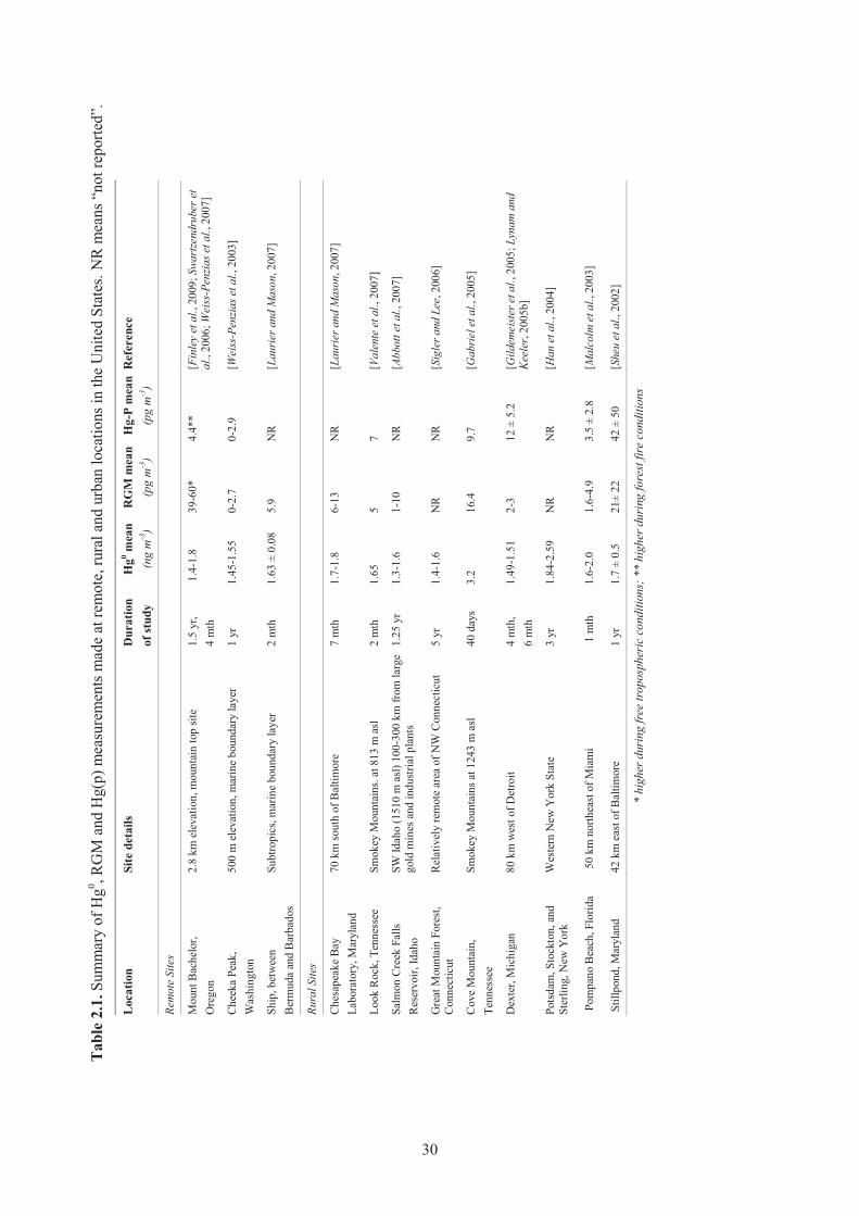
Tab

le 2

.1. S

umm

ary

of H

g0 , RG

M a

nd H

g(p)

mea

sure

men

ts m

ade

at re

mot

e, ru

ral a

nd u

rban

loca

tions

in th

e U

nite

d St

ates

. NR

mea

ns “

not r

epor

ted”

.

Loca

tion

Site

det

ails

D

urat

ion

of

stud

y H

g0 mea

n (n

g m

-3)

RG

M m

ean

(pg

m-3

) H

g-P

mea

n (p

g m

-3)

Ref

eren

ce

Rem

ote

Site

s

Mou

nt B

ache

lor,

O

rego

n 2.

8 km

ele

vatio

n, m

ount

ain

top

site

1.5

yr,

4 m

th

1.4

-1.8

39

-60*

4.

4**

[Fin

ley

et a

l., 2

009;

Swa

rtze

ndru

ber e

t al

. , 20

06; W

eiss

-Pen

zias e

t al.,

200

7]

Che

eka

Peak

, W

ashi

ngto

n 50

0 m

ele

vatio

n, m

arin

e bo

unda

ry la

yer

1 yr

1.

45-1

.55

0-2.

7 0-

2.9

[Wei

ss-P

enzia

s et a

l., 2

003]

Ship

, bet

wee

n

Ber

mud

a an

d B

arba

dos

Subt

ropi

cs, m

arin

e bo

unda

ry la

yer

2 m

th

1.63

± 0

.08

5.9

NR

[L

aurie

r and

Mas

on, 2

007]

Rura

l Site

s

Che

sape

ake

Bay

La

bora

tory

, Mar

ylan

d 70

km

sout

h of

Bal

timor

e 7

mth

1.

7-1.

8 6-

13

NR

[L

aurie

r and

Mas

on, 2

007]

Look

Roc

k, T

enne

ssee

Sm

okey

Mou

ntai

ns. a

t 813

m a

sl

2 m

th

1.65

5

7 [V

alen

te e

t al.,

200

7]

Salm

on C

reek

Fal

ls

Res

ervo

ir, Id

aho

SW Id

aho

(151

0 m

asl

) 100

-300

km

from

larg

e go

ld m

ines

and

indu

stria

l pla

nts

1.25

yr

1.3-

1.6

1-10

N

R

[Abb

ott e

t al.,

200

7]

Gre

at M

ount

ain

Fore

st,

Con

nect

icut

R

elat

ivel

y re

mot

e ar

ea o

f NW

Con

nect

icut

5

yr

1.4-

1.6

NR

N

R

[Sig

ler a

nd L

ee, 2

006]

Cov

e M

ount

ain,

Te

nnes

see

Smok

ey M

ount

ains

at 1

243

m a

sl

40 d

ays

3.2

16.4

9.

7 [G

abrie

l et a

l., 2

005]

Dex

ter,

Mic

higa

n 80

km

wes

t of D

etro

it 4

mth

, 6

mth

1.

49-1

.51

2-3

12 ±

5.2

[G

ildem

eiste

r et a

l., 2

005;

Lyn

am a

nd

Kee

ler ,

2005

b]

Pots

dam

, Sto

ckto

n, a

nd

Ster

ling,

New

Yor

k W

este

rn N

ew Y

ork

Stat

e 3

yr

1.84

-2.5

9 N

R

NR

[H

an e

t al.,

200

4]

Pom

pano

Bea

ch, F

lorid

a 50

km

nor

thea

st o

f Mia

mi

1 m

th

1.6-

2.0

1.6-

4.9

3.5

± 2.

8 [M

alco

lm e

t al.,

200

3]

Stil

lpon

d, M

aryl

and

42 k

m e

ast o

f Bal

timor

e 1

yr

1.7

± 0.

5 21

± 22

42

± 5

0 [S

heu

et a

l., 2

002]

* hi

gher

dur

ing

free

tropo

sphe

ric

cond

ition

s; *

* hi

gher

dur

ing

fore

st fir

e co

nditi

ons

30

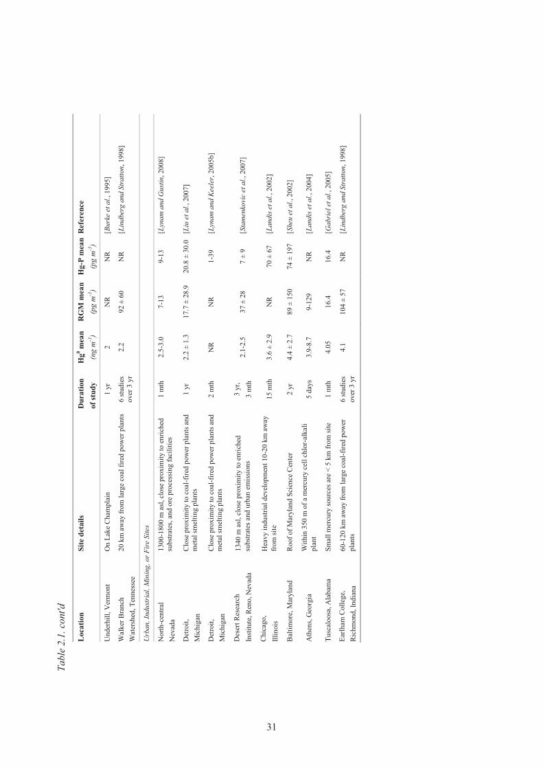
Tabl

e 2.

1. c

ont'd

Loca

tion

Site

det

ails

D

urat

ion

of

stud

y H

g0 mea

n (n

g m

-3)

RG

M m

ean

(pg

m-3

) H

g-P

mea

n (p

g m

-3)

Ref

eren

ce

Und

erhi

ll, V

erm

ont

On

Lake

Cha

mpl

ain

1 yr

2

NR

N

R

[Bur

ke e

t al.,

199

5]

Wal

ker B

ranc

h

Wat

ersh

ed, T

enne

ssee

20

km

aw

ay fr

om la

rge

coal

fire

d po

wer

pla

nts

6 stu

dies

ov

er 3

yr

2.2

92 ±

60

NR

[L

indb

erg

and

Stra

tton,

199

8]

Urb

an, I

ndus

tria

l, M

inin

g, o

r Fire

Site

s

Nor

th-c

entra

l N

evad

a 13

00-1

800

m a

sl, c

lose

pro

xim

ity to

enr

iche

d su

bstra

tes,

and

ore

proc

essi

ng fa

cilit

ies

1 m

th

2.5-

3.0

7-13

9-

13

[Lyn

am a

nd G

ustin

, 200

8]

Det

roit,

M

ichi

gan

Clo

se p

roxi

mity

to c

oal-f

ired

pow

er p

lant

s and

m

etal

smel

ting

plan

ts

1 yr

2.

2 ±

1.3

17.7

± 2

8.9

20.8

± 3

0.0

[Liu

et a

l., 2

007]

Det

roit,

M

ichi

gan

Clo

se p

roxi

mity

to c

oal-f

ired

pow

er p

lant

s and

m

etal

smel

ting

plan

ts

2 m

th

NR

N

R

1-39

[L

ynam

and

Kee

ler,

2005

b]

Des

ert R

esea

rch

In

stitu

te, R

eno,

Nev

ada

1340

m a

sl, c

lose

pro

xim

ity to

enr

iche

d su

bstra

tes a

nd u

rban

em

issio

ns

3 yr

, 3

mth

2.

1-2.

5 37

± 2

8 7

± 9

[Sta

men

kovi

c et

al.,

200

7]

Chi

cago

, Ill

inoi

s H

eavy

indu

stria

l dev

elop

men

t 10-

20 k

m a

way

fr

om si

te

15 m

th

3.6

± 2.

9 N

R

70 ±

67

[Lan

dis e

t al.,

200

2]

Bal

timor

e, M

aryl

and

Roo

f of M

aryl

and

Scie

nce

Cen

ter

2 yr

4.

4 ±

2.7

89 ±

150

74

± 1

97

[She

u et

al.,

200

2]

Ath

ens,

Geo

rgia

W

ithin

350

m o

f a m

ercu

ry c

ell c

hlor

-alk

ali

plan

t 5

days

3.

9-8.

7 9-

129

NR

[L

andi

s et a

l., 2

004]

Tusc

aloo

sa, A

laba

ma

Smal

l mer

cury

sour

ces a

re <

5 k

m fr

om si

te

1 m

th

4.05

16

.4

16.4

[G

abrie

l et a

l., 2

005]

Earlh

am C

olle

ge,

Ric

hmon

d, In

dian

a 60

-120

km

aw

ay fr

om la

rge

coal

-fire

d po

wer

pl

ants

6

studi

es

over

3 y

r 4.

1 10

4 ±

57

NR

[L

indb

erg

and

Stra

tton,

199

8]

31

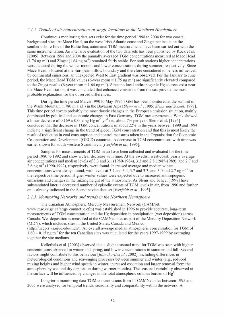
2.1.2. Trends of air concentrations at single locations in the Northern Hemisphere Continuous monitoring data sets exist for the time period 1998 to 2004 for two coastal

background sites. At Mace Head, on the west-Irish Atlantic coast and Zingst peninsula on the southern shore-line of the Baltic Sea, automated TGM measurements have been carried out with the same instrumentation. An intensive evaluation of the two data sets has been published by Kock et al. [2005]. Between 1998 and 2004 the annually averaged TGM concentrations measured at Mace Head (1.74 ng m-3) and Zingst (1.64 ng m-3) remained fairly stable. For both stations higher concentrations were detected during the winter months and lower concentrations during summer, respectively. Since Mace Head is located at the European inflow boundary and therefore considered to be less influenced by continental emissions, an unexpected West to East gradient was observed. For the January to June period, the Mace Head TGM values (6-year mean = 1.75 ng m-3) are significantly elevated compared to the Zingst results (6-year mean = 1.64 ng m-3). Since no local anthropogenic Hg sources exist near the Mace Head station, it was concluded that enhanced emissions from the sea provide the most probable explanation for the observed differences.

During the time period March 1990 to May 1996 TGM has been monitored at the summit of the Wank Mountain (1780 m a.s.l.) in the Bavarian Alps [Slemr et al., 1995; Slemr and Scheel, 1998]. This time period covers probably the most drastic changes in the European emission situation, mainly dominated by political and economic changes in East Germany. TGM measurements at Wank showed a linear decrease of 0.169 ± 0.009 ng Hg m-3 yr-1 i.e., about 7% per year. Slemr et al. [1995] concluded that the decrease in TGM concentrations of about 22% in the years between 1990 and 1994 indicate a significant change in the trend of global TGM concentration and that this is most likely the result of reduction in coal consumption and control measures taken in the Organisation for Economic Co-operation and Development (OECD) countries. A decrease in TGM concentrations with time was earlier shown for south-western Scandinavia [Iverfeldt et al., 1995].

Samples for measurements of TGM in air have been collected and evaluated for the time period 1980 to 1992 and show a clear decrease with time. At the Swedish west-coast, yearly average air concentrations and median levels of 3.3 and 3.1 (1980-1984), 3.2 and 2.8 (1985-1989), and 2.7 and 2.6 ng m-3 (1990-1992), respectively, were found. Increased average and median winter concentrations were always found, with levels at 3.7 and 3.4, 3.7 and 3.3, and 3.0 and 2.7 ng m-3 for the respective time period. Higher winter values were expected due to increased anthropogenic emissions and changes in the mixing height of the atmosphere. As Slemr and Scheel [1998] have substantiated later, a decreased number of episodic events of TGM levels in air, from 1990 and further on is already indicated in the Scandinavian data set [Iverfeldt et al., 1995].

2.1.3. Monitoring Networks and trends in the Northern Hemisphere The Canadian Atmospheric Mercury Measurement Network (CAMNet,

www.msc.ec.gc.ca/arqp/ camnet_e.cfm) was established in 1996 to provide accurate, long-term measurements of TGM concentration and the Hg deposition in precipitation (wet deposition) across Canada. Wet deposition is measured at the CAMNet sites as part of the Mercury Deposition Network (MDN), which includes sites in the United States, Canada and Mexico (http://nadp.sws.uiuc.edu/mdn/). An overall average median atmospheric concentration for TGM of 1.60 ± 0.15 ng m-3 for the ten Canadian sites was calculated for the years 1997-1999 by averaging together the site medians.

Kellerhals et al. [2003] observed that a slight seasonal trend for TGM was seen with higher concentrations observed in winter and spring, and lower concentrations in summer and fall. Several factors might contribute to this behaviour [Blanchard et al., 2002], including differences in meteorological conditions and scavenging processes between summer and winter (e.g., reduced mixing heights and higher wind speeds in winter, increased oxidation and larger removal from the atmosphere by wet and dry deposition during warmer months). The seasonal variability observed at the surface will be influenced by changes in the total atmospheric column burden of Hg0.

Long-term monitoring data TGM concentrations from 11 CAMNet sites between 1995 and 2005 were analysed for temporal trends, seasonality and comparability within the network. A

32

statistically significant decreasing trend for TGM concentrations at several rural CAMNet sites was seen for the time period 1995 to 2005. TGM concentrations at all the CAMNet sites (mean = 1.58 ng m-3) were similar to or slightly lower than those observed at European background sites within a comparable time frame. Seasonal variations of TGM concentrations are observed for all sites. Most sites show higher concentrations in winter and spring, and lower concentrations in summer and fall.

Since Canadian measurements began in 1995, Hg levels in the air have shown only a slight decline throughout most of Canada. The greatest decline of airborne Hg in Canada occurred close to the major urban areas of Toronto and Montreal, where levels fell by about 10% between 1996 and 2005. The largest decreases in TGM were seen at Point Petre, on the north shore of Lake Ontario, near Toronto, where levels declined by 17% and at St. Anicet, near Montréal, where levels fell by 13%. This is in good agreement with the overall trend in total Hg concentrations in precipitation observed within the comparable NADP-MDN sites, indicating that these changes are most likely driven by local or regional changes in Hg emissions.

Recognizing that TGM and Hg in wet deposition are spatially heterogeneous, several studies have aimed to set up monitoring networks in order to compare trends among sites in the same region, among regions, and to determine the influence of local and regional emissions sources. There is also interest in understanding the processes that contribute to Hg variability on a diurnal, weekly, seasonal, and annual basis. The largest, most ambitious network of sites is the MDN, which has sites across the United States that collect weekly precipitation samples and measure dissolved Hg (Figure 2.1).

Figure 2.1. Total mercury concentration from the Mercury Deposition Network in 2006. [Data provided by National Atmospheric Deposition Program, NADP Program Office, Illinois State Water Survey, Champaign, Illinois, http://nadp.sws.uiuc.edu]

The spatial pattern of Hg concentrations in wet deposition has some aspects that have been difficult to reconcile based on known sources and removal processes. For example, there are high Hg concentrations in Florida, where there are few Hg sources, and there are relatively low concentrations in Pennsylvania and Ohio, where there are many coal-fired power plants.

In summary, it seems that not enough attention has been focused on monitoring networks in the United States due to the difficulty and cost in carrying out sensitive measurements at many sites simultaneously. The MDN is essential for understanding the spatial and temporal patterns of Hg in wet deposition, but without at least TGM measurements (and speciated Hg measurements would be the best) in conjunction with precipitation measurements, little can be inferred about the processes responsible for controlling Hg deposition. It is not well understood, for example, which sites would respond most quickly to emissions reduction in various industrial sectors (e.g. coal-fired power plants, incineration, mining, manufacturing, etc.), or if enhanced deposition events are independent of local or regional sources and supplied predominantly by the global Hg pool being caused by natural variations in photochemistry and meteorology. The few studies that have both speciated Hg measurements as well as Hg in wet deposition suggest that Hg in deposition can vary by 2-fold

33

between an urban and a rural site, TGM might vary by 50-75%, and total particulate mercury (TPM or Hg-P) may vary 5-10 fold between sites.

Butler et al. [2007] showed declines in Hg precipitation concentrations from 1998 to 2005 for both the northeast and midwest regions of the United States, corresponding to declines of Hg emissions in the United States between the 1990s and the beginning of this decade, largely due to the closure of municipal and medical waste incinerators. In contrast, the southeast United States does not show any significant trend in wet deposition of Hg during this period.

During this time, global emissions of Hg declined in Europe, increased in Asia and Africa, and remained roughly constant globally [Pacyna et al., 2006]. Using the GEOS-Chem Hg model, Selin and Jacob [2008] showed that high wet deposition over the southeast United States during the summer months is due to scavenging of upper altitude HgII by deep convection. They also found that scavenging of HgII from above the boundary layer accounts for over half of the modelled wet deposition across the United States and that most of the boundary layer HgII originates from oxidation in the upper troposphere. Thus, the lack of declines in wet deposition of Hg in the southeast United States may be due to the influence of global sources in this region deposited due to convective scavenging.

An extensive evaluation of Hg measurements in air and precipitation at EMEP or OSPAR stations respectively has been carried out by Wangberg et al. [2007]. These data were obtained at coastal sites around the North Sea and originate from Ireland, Netherlands, Germany, Norway and Sweden. The observation period is 1995 to 2002 and the two periods 1995 to 1998 and 1999 to 2002 were compared. The reduction in deposition is 10 – 30% when comparing the two periods and the authors relate the decrease to emission controls in Europe. In contrast, no decreasing trend in TGM data could be observed during the same time periods. The authors suggest a plausible explanation is that TGM concentrations measured in the OSPAR area are to a larger extent dominated by the hemispherical background than before, i.e., European emission reductions may be over-compensated by increasing emissions in other Northern hemispheric regions.

This conclusion is supported by Berg et al. [2006 ] who found that current Hg levels in surface sediments, surface soils and mosses at background in Norway are substantially affected by long-range atmospheric transport. The project “Mercury species over Europe” (MOE) was aimed at identifying sources, occurrence and atmospheric behaviour of atmospheric Hg species [Munthe et al., 2003 ; Pirrone et al., 2001a]. Within MOE, simultaneous measurements were carried out on a regional scale. Wangberg et al. [2001] compared the MOE data with results of a similar project focusing on southern European sites around the Mediterranean Sea (EU funded project MAMCS) and reported that observed concentrations of TGM (and other species such as TPM and RGM as well) were generally slightly higher in the Mediterranean region compared with northwest Europe.

2.1.4. Observations of air concentrations at single locations in the Southern Hemisphere Relatively few observations of atmospheric Hg have been carried out in the Southern

Hemisphere. The few observations to date have mostly been carried out near to, or downwind of, major sources. This includes mining, industrial facilities and biomass fires. For nearly all South American observations, measured Hg0 concentrations were substantially greater than the accepted global background level. Relatively few publications have converted the observed air concentrations into an emission flux. One emission inventory for Hg emissions associated with gold mining has been conducted using estimated gold production and an Hg emission factor. This inventory suggests that gold mining is the largest source of TGM to the atmosphere in South America.

Wide scale mining has occurred in the Amazon Basin since at least the 18th century [e.g. Hachiya et al., 1998; Higueras et al., 2005, and references therein]. Associated with current and past operations, a number of researchers have examined the TGM air concentrations in mining regions. Hachiya et al. [1998] sampled in urban and rural areas of Brazil near several tributaries of the Amazon river. Urban areas sampled included Rio de Janeiro, Manaus and Brasilia, where concentrations up to 10 ng m-3 were found. Adjacent to mining areas, concentrations up to 16 ng m-3 were found. In some gold workshops, very high levels of TGM were found (maximum of 3.7 ng m-3).

34

Higueras et al. [2005] sampled along roads in the Coquimbo region of Northern Chile. Their sampling took them past several major ore mining and processing operations for gold and other metals (e.g. Hg, Cu and Mn). Very high concentrations of TGM were found in these current and historical mining regions (some mining back to 16th century). Extreme TGM concentrations, up to nearly 100 μg m-3 were observed at some gold recovery operations (milling and amalgamation).

Fostier and Michelazzo [2006] sampled at two sites in Sao Paulo state, Brazil, near the Paulínia industrial area. The two sites had an overall mean TGM concentration of 7.0 ng m-3, with no significant difference between the two sites. The enhancement in TGM, compared to the global background, was attributed to the wide array of industrial sources in the area. Concentrations of TPM were high, 400 pg m-3.

From the above data, it is clear that past and current gold mining represents a large source of Hg to the atmosphere. Lacerda [1997] estimated global Hg emissions to the environment from gold mining. By this estimate 460 Mg yr-1 are released to the environment globally, 300 Mg or 65%, of this is released to the atmosphere. Of this total, nearly 60% is released in South America. The atmospheric emissions of Hg in South America by gold mining (179 Mg yr-1) calculated by Lacerda [1997] are nearly twice the total Hg emissions from all sources in South America estimated by Pacyna et al. [2006]. This estimate was updated by Lacerda [2003] to 107-228 Mg yr-1. However, it should be noted that the Pacyna et al. [2006] inventory does not quantify Hg emissions from South American gold mining nor does it attempt to quantify Hg emissions from illegal gold mining activities. In addition, the Pacyna study used a Hg emission factor of 0.5 gram Hg emitted/gram gold mined, whereas Lacerda uses a factor of 1.5. Thus, while emissions of Hg from gold mining in South America are clearly a substantial source to the global atmosphere, there is significant uncertainty in the actual emissions. Future work on Hg emissions in South America should focus on reducing the large uncertainty in the emissions, with emphasis on artisanal gold mining activities in the Latin Americas.

2.1.5. Trends of air concentrations at single locations in the Southern Hemisphere At present, there is no information in South America that can be used to establish long-term

trends.

To the best of our knowledge, the Cape Point observations constitute the only long term data set of atmospheric TGM in the Southern Hemisphere. The monitoring of TGM was established at the Cape Point GAW)station in September 1995. Baker et al. [2002] presented the data obtained until June 1999. Atmospheric Hg concentrations were found to be fairly homogeneous fluctuating between 1.2-1.4 ng m-3. Whilst no significant diurnal variation is detectable, a slight seasonal variation with a TGM minimum in March-May and maximum in June-August was observed. A minimum annual TGM concentration was detected in 1997. The existing Cape Point TGM data base comprises both manual measurements with low temporal resolution as well as automated measurements with a resolution of 15 min. Good agreement exists between the manual analysis method and the automated measurements [Ebinghaus et al., 1999]. The most prominent feature of the highly resolved TGM data is the frequent occurrence of events with almost complete Hg depletion which have so far not been observed at any other non-polar stations [Brunke et al., 2010]. The Cape Point GAW station was found to constitute a suitable site for monitoring TGM concentrations in the Southern Hemisphere.

During mid-January 2000 the plume from a fire, which destroyed 9000 ha of mixed vegetation in the southern part of the Cape Peninsula, passed over the Cape Point GAW station (34°S, 18°E). Measurements of TGM made during this episode provided Hg/CO and Hg/CO2 emission ratios of (2.10 ± 0.21) * 10-7 and (1.19 ± 0.30) * 10-8 mol/mol, respectively [Brunke et al., 2001].

2.1.6. Monitoring Networks and trends in the Southern Hemisphere Information on monitoring networks in the Southern Hemisphere is not available in the peer-

reviewed literature.

35

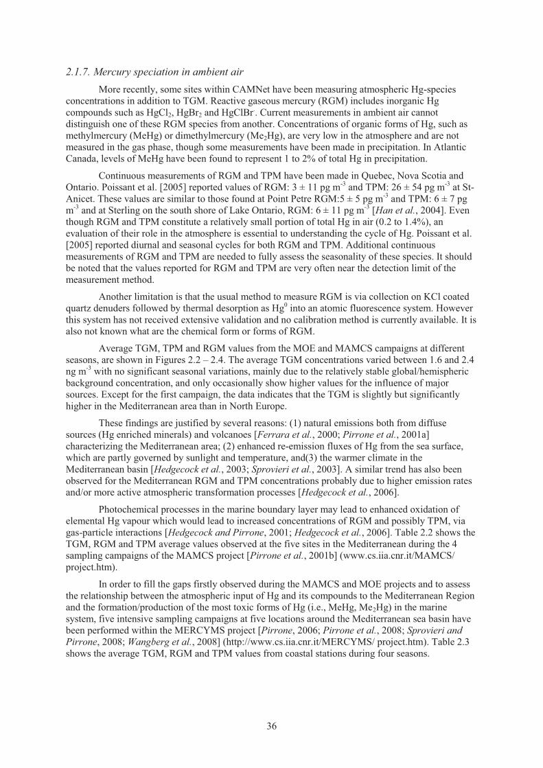
2.1.7. Mercury speciation in ambient air More recently, some sites within CAMNet have been measuring atmospheric Hg-species

concentrations in addition to TGM. Reactive gaseous mercury (RGM) includes inorganic Hg compounds such as HgCl2, HgBr2 and HgClBr.. Current measurements in ambient air cannot distinguish one of these RGM species from another. Concentrations of organic forms of Hg, such as methylmercury (MeHg) or dimethylmercury (Me2Hg), are very low in the atmosphere and are not measured in the gas phase, though some measurements have been made in precipitation. In Atlantic Canada, levels of MeHg have been found to represent 1 to 2% of total Hg in precipitation.

Continuous measurements of RGM and TPM have been made in Quebec, Nova Scotia and Ontario. Poissant et al. [2005] reported values of RGM: 3 ± 11 pg m-3 and TPM: 26 ± 54 pg m-3 at St-Anicet. These values are similar to those found at Point Petre RGM:5 ± 5 pg m-3 and TPM: 6 ± 7 pg m-3 and at Sterling on the south shore of Lake Ontario, RGM: 6 ± 11 pg m-3 [Han et al., 2004]. Even though RGM and TPM constitute a relatively small portion of total Hg in air (0.2 to 1.4%), an evaluation of their role in the atmosphere is essential to understanding the cycle of Hg. Poissant et al. [2005] reported diurnal and seasonal cycles for both RGM and TPM. Additional continuous measurements of RGM and TPM are needed to fully assess the seasonality of these species. It should be noted that the values reported for RGM and TPM are very often near the detection limit of the measurement method.

Another limitation is that the usual method to measure RGM is via collection on KCl coated quartz denuders followed by thermal desorption as Hg0 into an atomic fluorescence system. However this system has not received extensive validation and no calibration method is currently available. It is also not known what are the chemical form or forms of RGM.

Average TGM, TPM and RGM values from the MOE and MAMCS campaigns at different seasons, are shown in Figures 2.2 – 2.4. The average TGM concentrations varied between 1.6 and 2.4 ng m-3 with no significant seasonal variations, mainly due to the relatively stable global/hemispheric background concentration, and only occasionally show higher values for the influence of major sources. Except for the first campaign, the data indicates that the TGM is slightly but significantly higher in the Mediterranean area than in North Europe.

These findings are justified by several reasons: (1) natural emissions both from diffuse sources (Hg enriched minerals) and volcanoes [Ferrara et al., 2000; Pirrone et al., 2001a] characterizing the Mediterranean area; (2) enhanced re-emission fluxes of Hg from the sea surface, which are partly governed by sunlight and temperature, and(3) the warmer climate in the Mediterranean basin [Hedgecock et al., 2003; Sprovieri et al., 2003]. A similar trend has also been observed for the Mediterranean RGM and TPM concentrations probably due to higher emission rates and/or more active atmospheric transformation processes [Hedgecock et al., 2006].

Photochemical processes in the marine boundary layer may lead to enhanced oxidation of elemental Hg vapour which would lead to increased concentrations of RGM and possibly TPM, via gas-particle interactions [Hedgecock and Pirrone, 2001; Hedgecock et al., 2006]. Table 2.2 shows the TGM, RGM and TPM average values observed at the five sites in the Mediterranean during the 4 sampling campaigns of the MAMCS project [Pirrone et al., 2001b] (www.cs.iia.cnr.it/MAMCS/ project.htm).

In order to fill the gaps firstly observed during the MAMCS and MOE projects and to assess the relationship between the atmospheric input of Hg and its compounds to the Mediterranean Region and the formation/production of the most toxic forms of Hg (i.e., MeHg, Me2Hg) in the marine system, five intensive sampling campaigns at five locations around the Mediterranean sea basin have been performed within the MERCYMS project [Pirrone, 2006; Pirrone et al., 2008; Sprovieri and Pirrone, 2008; Wangberg et al., 2008] (http://www.cs.iia.cnr.it/MERCYMS/ project.htm). Table 2.3 shows the average TGM, RGM and TPM values from coastal stations during four seasons.

36

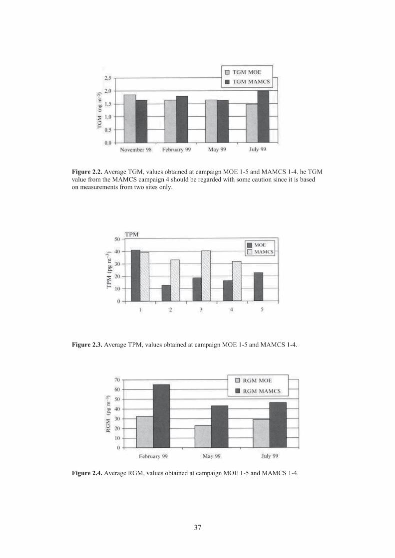
Figure 2.2. Average TGM, values obtained at campaign MOE 1-5 and MAMCS 1-4. he TGM value from the MAMCS campaign 4 should be regarded with some caution since it is based on measurements from two sites only.

Figure 2.3. Average TPM, values obtained at campaign MOE 1-5 and MAMCS 1-4.

Figure 2.4. Average RGM, values obtained at campaign MOE 1-5 and MAMCS 1-4.

37

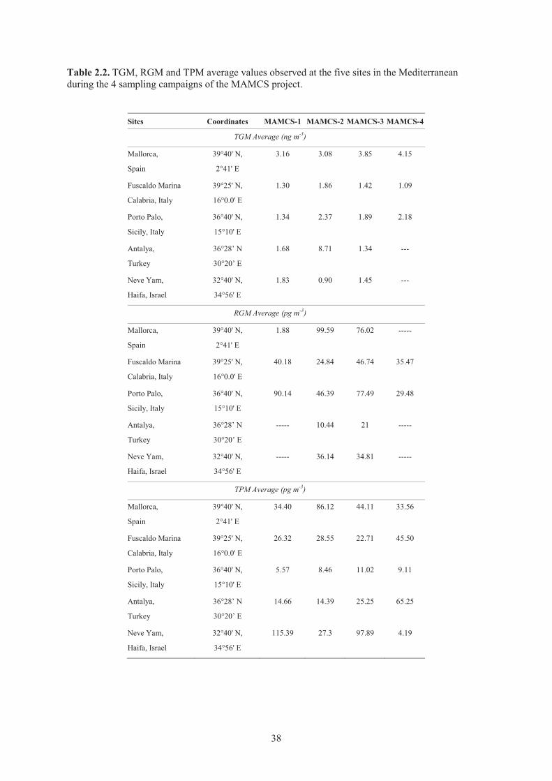
Table 2.2. TGM, RGM and TPM average values observed at the five sites in the Mediterranean during the 4 sampling campaigns of the MAMCS project.

Sites Coordinates MAMCS-1 MAMCS-2 MAMCS-3 MAMCS-4

TGM Average (ng m-3)

Mallorca,

Spain

39°40' N,

2°41' E

3.16 3.08 3.85 4.15

Fuscaldo Marina

Calabria, Italy

39°25' N,

16°0.0' E

1.30 1.86 1.42 1.09

Porto Palo,

Sicily, Italy

36°40' N,

15°10' E

1.34 2.37 1.89 2.18

Antalya,

Turkey

36°28’ N

30°20’ E

1.68 8.71 1.34 ---

Neve Yam,

Haifa, Israel

32°40' N,

34°56' E

1.83 0.90 1.45 ---

RGM Average (pg m-3)

Mallorca,

Spain

39°40' N,

2°41' E

1.88 99.59 76.02 -----

Fuscaldo Marina

Calabria, Italy

39°25' N,

16°0.0' E

40.18 24.84 46.74 35.47

Porto Palo,

Sicily, Italy

36°40' N,

15°10' E

90.14 46.39 77.49 29.48

Antalya,

Turkey

36°28’ N

30°20’ E

----- 10.44 21 -----

Neve Yam,

Haifa, Israel

32°40' N,

34°56' E

----- 36.14 34.81 -----

TPM Average (pg m-3)

Mallorca,

Spain

39°40' N,

2°41' E

34.40 86.12 44.11 33.56

Fuscaldo Marina

Calabria, Italy

39°25' N,

16°0.0' E

26.32 28.55 22.71 45.50

Porto Palo,

Sicily, Italy

36°40' N,

15°10' E

5.57 8.46 11.02 9.11

Antalya,

Turkey

36°28’ N

30°20’ E

14.66 14.39 25.25 65.25

Neve Yam,

Haifa, Israel

32°40' N,

34°56' E

115.39 27.3 97.89 4.19

38

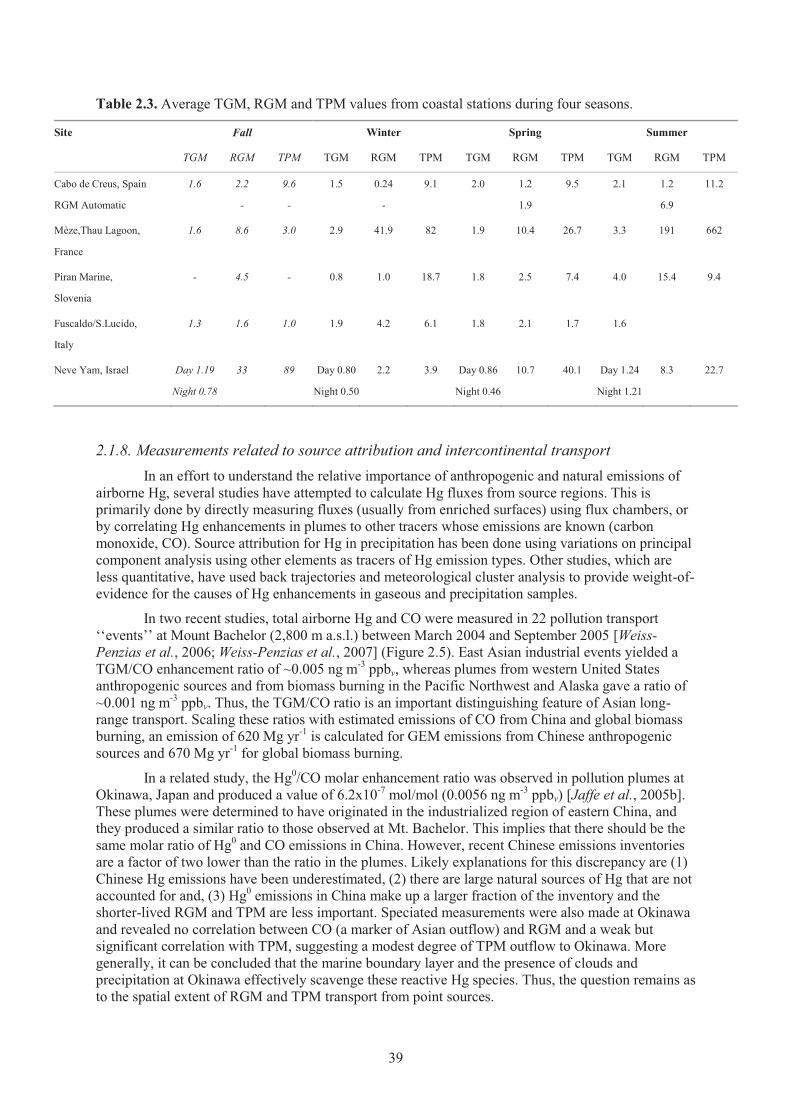
Table 2.3. Average TGM, RGM and TPM values from coastal stations during four seasons.

Site Fall Winter Spring Summer

TGM RGM TPM TGM RGM TPM TGM RGM TPM TGM RGM TPM

Cabo de Creus, Spain

RGM Automatic

1.6 2.2

-

9.6

-

1.5 0.24

-

9.1 2.0 1.2

1.9

9.5 2.1 1.2

6.9

11.2

Mèze,Thau Lagoon,

France

1.6 8.6 3.0 2.9 41.9 82 1.9 10.4 26.7 3.3 191 662

Piran Marine,

Slovenia

- 4.5 - 0.8 1.0 18.7 1.8 2.5 7.4 4.0 15.4 9.4

Fuscaldo/S.Lucido,

Italy

1.3 1.6 1.0 1.9 4.2 6.1 1.8 2.1 1.7 1.6

Neve Yam, Israel Day 1.19

Night 0.78

33 89 Day 0.80

Night 0.50

2.2 3.9 Day 0.86

Night 0.46

10.7 40.1 Day 1.24

Night 1.21

8.3 22.7

2.1.8. Measurements related to source attribution and intercontinental transport

In an effort to understand the relative importance of anthropogenic and natural emissions of airborne Hg, several studies have attempted to calculate Hg fluxes from source regions. This is primarily done by directly measuring fluxes (usually from enriched surfaces) using flux chambers, or by correlating Hg enhancements in plumes to other tracers whose emissions are known (carbon monoxide, CO). Source attribution for Hg in precipitation has been done using variations on principal component analysis using other elements as tracers of Hg emission types. Other studies, which are less quantitative, have used back trajectories and meteorological cluster analysis to provide weight-of-evidence for the causes of Hg enhancements in gaseous and precipitation samples.

In two recent studies, total airborne Hg and CO were measured in 22 pollution transport ‘‘events’’ at Mount Bachelor (2,800 m a.s.l.) between March 2004 and September 2005 [Weiss-Penzias et al., 2006; Weiss-Penzias et al., 2007] (Figure 2.5). East Asian industrial events yielded a TGM/CO enhancement ratio of ~0.005 ng m-3 ppbv, whereas plumes from western United States anthropogenic sources and from biomass burning in the Pacific Northwest and Alaska gave a ratio of ~0.001 ng m-3 ppbv. Thus, the TGM/CO ratio is an important distinguishing feature of Asian long-range transport. Scaling these ratios with estimated emissions of CO from China and global biomass burning, an emission of 620 Mg yr-1 is calculated for GEM emissions from Chinese anthropogenic sources and 670 Mg yr-1 for global biomass burning.

In a related study, the Hg0/CO molar enhancement ratio was observed in pollution plumes at Okinawa, Japan and produced a value of 6.2x10-7 mol/mol (0.0056 ng m-3 ppbv) [Jaffe et al., 2005b]. These plumes were determined to have originated in the industrialized region of eastern China, and they produced a similar ratio to those observed at Mt. Bachelor. This implies that there should be the same molar ratio of Hg0 and CO emissions in China. However, recent Chinese emissions inventories are a factor of two lower than the ratio in the plumes. Likely explanations for this discrepancy are (1) Chinese Hg emissions have been underestimated, (2) there are large natural sources of Hg that are not accounted for and, (3) Hg0 emissions in China make up a larger fraction of the inventory and the shorter-lived RGM and TPM are less important. Speciated measurements were also made at Okinawa and revealed no correlation between CO (a marker of Asian outflow) and RGM and a weak but significant correlation with TPM, suggesting a modest degree of TPM outflow to Okinawa. More generally, it can be concluded that the marine boundary layer and the presence of clouds and precipitation at Okinawa effectively scavenge these reactive Hg species. Thus, the question remains as to the spatial extent of RGM and TPM transport from point sources.

39

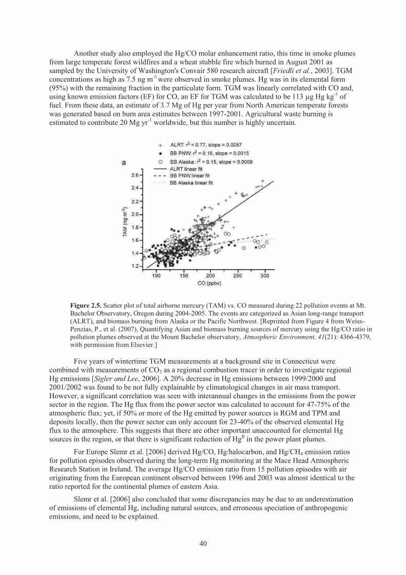
Another study also employed the Hg/CO molar enhancement ratio, this time in smoke plumes from large temperate forest wildfires and a wheat stubble fire which burned in August 2001 as sampled by the University of Washington's Convair 580 research aircraft [Friedli et al., 2003]. TGM concentrations as high as 7.5 ng m-3 were observed in smoke plumes. Hg was in its elemental form (95%) with the remaining fraction in the particulate form. TGM was linearly correlated with CO and, using known emission factors (EF) for CO, an EF for TGM was calculated to be 113 μg Hg kg-1 of fuel. From these data, an estimate of 3.7 Mg of Hg per year from North American temperate forests was generated based on burn area estimates between 1997-2001. Agricultural waste burning is estimated to contribute 20 Mg yr-1 worldwide, but this number is highly uncertain.

Figure 2.5. Scatter plot of total airborne mercury (TAM) vs. CO measured during 22 pollution events at Mt. Bachelor Observatory, Oregon during 2004-2005. The events are categorized as Asian long-range transport (ALRT), and biomass burning from Alaska or the Pacific Northwest. [Reprinted from Figure 4 from Weiss-Penzias, P., et al. (2007), Quantifying Asian and biomass burning sources of mercury using the Hg/CO ratio in pollution plumes observed at the Mount Bachelor observatory, Atmospheric Environment, 41(21): 4366-4379, with permission from Elsevier.]

Five years of wintertime TGM measurements at a background site in Connecticut were combined with measurements of CO2 as a regional combustion tracer in order to investigate regional Hg emissions [Sigler and Lee, 2006]. A 20% decrease in Hg emissions between 1999/2000 and 2001/2002 was found to be not fully explainable by climatological changes in air mass transport. However, a significant correlation was seen with interannual changes in the emissions from the power sector in the region. The Hg flux from the power sector was calculated to account for 47-75% of the atmospheric flux; yet, if 50% or more of the Hg emitted by power sources is RGM and TPM and deposits locally, then the power sector can only account for 23-40% of the observed elemental Hg flux to the atmosphere. This suggests that there are other important unaccounted for elemental Hg sources in the region, or that there is significant reduction of HgII in the power plant plumes.

For Europe Slemr et al. [2006] derived Hg/CO, Hg/halocarbon, and Hg/CH4 emission ratios for pollution episodes observed during the long-term Hg monitoring at the Mace Head Atmospheric Research Station in Ireland. The average Hg/CO emission ratio from 15 pollution episodes with air originating from the European continent observed between 1996 and 2003 was almost identical to the ratio reported for the continental plumes of eastern Asia.

Slemr et al. [2006] also concluded that some discrepancies may be due to an underestimation of emissions of elemental Hg, including natural sources, and erroneous speciation of anthropogenic emissions, and need to be explained.

40

Ebinghaus et al. [2007] observed enhanced CO and TGM on two CARIBIC (Civil Aircraft for Regular Investigation of the Atmosphere Based on an Instrumented Container) flights between São Paolo and Santiago de Chile in 2005. The CARIBIC container is operated monthly onboard a Lufthansa Airbus 340-600 during regular passenger flights. The measured TGM/CO ratio on these two flights, 1.2 10-7 and 2.4 x 10-7 mole/mole, respectively, were similar to previous reports of biomass burning plumes, despite significant differences in geographic regions. From these ratios the authors estimate global emissions of TGM from biomass burning in the range of 210-750 Mg yr-1.

Japan has started a monitoring program that will provide background air monitoring data of Hg and other trace elements to contribute to the understanding of their atmospheric long-range transport [Suzuki et al., 2009]. For this purpose, Japan started a pilot project in 2007 to monitor levels of Hg, obtain information on the long range transport of Hg and other heavy metals in the Asia-Pacific region, develop monitoring methodologies, and contribute to international efforts in ambient atmospheric monitoring. The project will also develop fate modelling methodology to help explain the global cycling of Hg in the atmosphere and environment by expanding the information from the monitoring outputs. Pilot monitoring is conducted at the “Cape Hedo Atmosphere and Aerosol Monitoring Station” operated by the National Institute for Environment Studies, in Okinawa. Mercury speciation such as gaseous elemental mercury (Hg0), divalent RGM, and TPM are continuously measured with a Tekran Hg speciation system. Hazardous heavy metals in particles and in precipitation are also measured. Japan will continue the monitoring at Cape Hedo station to understand the background levels of Hg and other toxic substances and contribute to the better understanding of the current status of Hg in the environment by joining in the international efforts in ambient atmospheric monitoring. In addition to the monitoring program, fate analysis using modelling methodology is also studied in the project framework.

2.1.9. Summary and Conclusion for Observations in the temperate Northern and Southern Hemispheres

Mercury concentration measurements in ambient air of documented and accepted quality have been available since the mid-1970s; the concentration data are available for both hemispheres. Long-term monitoring of atmospheric Hg with high time resolution has been started at Alert, Canada (January 1995) and Mace Head, Ireland (September 1995), followed by numerous other sites since then. General scientific consensus exists about the current global background concentration of airborne Hg which is taken as ca. 1.5 to 1.7 ng m-3 in the Northern Hemisphere and ca. 1.1 to 1.3 ng m-3 in the Southern Hemisphere. Seasonal variations of TGM concentrations are observed at almost all sites with sufficient data coverage. Most sites show higher concentrations in winter and spring, and lower in summer and fall. It is suggested that the meteorological seasonal variability is the most important factor in the establishment of the observed seasonal cycles of the TGM concentrations. Temporal dynamics of TGM and also Hg in wet deposition are complex, with the magnitude of diurnal and seasonal changes often being larger than annual changes.

Canadian data show that the seasonality of Hg concentration in precipitation exhibits an opposite pattern to TGM air concentrations, with higher concentrations during the summer months. Two possible factors have been suggested for this seasonal behaviour: increased particle scavenging capacity of rain relative to snow and/or increase in the oxidation of Hg, either in cloud or in the gas phase, during summer. However, sites with the highest observed concentrations do not necessarily have the highest Hg deposition per unit and surface area, since the deposition is also dependent on the precipitation amount. Regional differences, temporal trends and potential sources and source regions can be identified by monitoring, especially when carried out in networks. In principal, an increase of the global atmospheric pool should also be reflected in the background concentration of Hg in ambient air. Fitzgerald’s initiative for the installation of a global AMNET has partly been accomplished on a regional scale within the CAMNet that may be considered as seminal in this respect. CAMNet has revealed a decreasing trend for TGM at a number of rural sites for the time period 1995 to 2005. The largest declines were observed close to urban areas of Toronto and Montreal. This is supported by data from United States giving evidence that TGM concentrations at rural locations on the eastern United States seaboard, downwind of major urban and industrial centres, are decreasing.

41

The changes are mostly driven by local or regional changes, such as cutbacks in emissions. Many of the TGM changes are comparable with the overall trends of total Hg concentrations in precipitation, again reflecting local or regional emission reductions in decreasing concentration levels. For remote sites in Europe and North America, it could be shown that only slight decreases or no statistically significant trend in the TGM concentration exist over the same time period. This is in contrast with emission estimates especially for Europe, where drastic reductions have taken place over the past 10 to 20 years. It has been suggested that TGM concentration in the north-western European atmosphere are to a larger extent dominated by hemispherical background than before; i.e., European emission reductions may be over-compensated by increasing emissions in other northern hemispheric regions. It should be noted that, for the same time period and same set of stations (1995 to 1998 vs. 1999 to 2002), a reduction in deposition of 10 to 30% was found which can possibly be related to emissions controls in Europe.

Deposition networks on a regional scale are essential for understanding the spatial and temporal patterns of Hg in wet deposition. However without at least TGM measurement and additional speciated Hg measurements wherever possible in conjunction with precipitation measurements, little can be inferred about the processes responsible for controlling Hg deposition. It is still not well understood which sites would respond most quickly to emission reductions in certain industrial sectors, or if enhanced deposition events are independent of local or regional sources and supplied predominantly by the global pool being caused by natural variations in photochemistry and meteorology. United States studies show that, between an urban and a rural site, Hg deposition can vary by 2-fold, TGM might vary by 50-75%, and TPM may vary 5 – 10 fold. Regional differences of individual speciation have also been reported for Europe. Observed concentrations of TGM, TPM and RGM are generally slightly higher in the Mediterranean region than in northwest Europe.

In general, it may be concluded that RGM in situ formation is very important in both the marine boundary layer under cloud-free conditions and in the free troposphere, where concentrations reach those of the most polluted urban atmosphere. Additionally, because of the diurnal nature of photochemistry and boundary layer/free tropospheric exchange, RGM, and to a lesser extent Hg0, and TPM generally have prominent diel cycles. Superimposed on the natural variability is the episodic nature of advection of more or less polluted air masses to a sampling site from urban/industrial/mining sources. With regard to long-term changes in RGM or TPM concentrations, the data do not go back far enough or have sufficient spatial coverage to appropriately address this question.

Asian emissions are considered to be of global importance and are suggested to be rapidly increasing in the past decade. The importance of Asian emissions is obvious from recent emission estimates. Furthermore, experimental data are showing long-range transport across the Pacific and suggest a significant underestimate of Asian Hg emissions. However, potentially increased Asian emissions are neither reflected in the long-term measurement of TGM at Mace Head (1995 – 2007) nor in the precipitation data of the North American MDN. The reason for this is not yet clear, however, it was hypothesized that atmospheric Hg cycling is possibly going on at a faster rate than previously thought.

In general, it can be concluded that monitoring at single locations or in networks is a very useful scientific tool in order to identify regional differences, temporal trends and for source attribution. Monitoring is necessary to evaluate the effectiveness of control measures, as demonstrated on regional scales. In connection with air quality data, Hg monitoring can be used to verify and/or improve emission estimates. Monitoring data can give new insights in the Hg cycling on different temporal and spatial scales, due to “unexpected findings”, such as Atmospheric Mercury Depletion Events (AMDEs) as a prominent example. They help us to improve our understanding of the global Hg cycle in order to evolve purposeful regulations on an international scale. The value of long-term atmospheric Hg monitoring and the need for additional sites is obvious, especially in the remote Southern Hemisphere.

42

2.2. Spatial coverage and temporal trends of atmospheric mercury measurements in Polar Regions

Polar Regions used to be considered pristine environments. Indeed, the Arctic is relatively far from industrial centres, which are located at mid-latitude in the Northern Hemisphere, and is less populated than other parts of the world. Indigenous peoples of the Arctic are estimated to comprise nearly 650 000 individuals, most of whom live in northern Russia [AMAP, 2003]. In the Southern Hemisphere, Antarctica is even less populated and impacted by anthropogenic activities, except on a local scale by a few scientific stations. However, due to a combination of long-range transport and a specific climatology, the Arctic and, to a lesser extent the Antarctic, are affected on a large scale by pollutants originating from the mid-latitudes of the Northern Hemisphere. It is now established that several pollutants including Persistent Organic Pollutants (POPs) and heavy metals are present in several compartments of the polar ecosystems [AMAP, 2003]. For example, certain Arctic species, particularly those at the upper end of the marine food chain as well as sea birds, carry high levels of PCBs and organo-chlorine pesticides [Braune et al., 2005]. POPs are transported to the Arctic by regional and global physical processes and are then subjected to biological mechanisms that lead to the high levels found in certain species.

In addition to organic compounds, heavy metals such as (Hg can be dispersed and contaminate Polar Regions. Mercury is transported far from its emission sources, mainly fossil fuel combustion, industry and mining, to Polar Regions. A recent review paper [Steffen et al., 2008]; provides a comprehensive assessment of the state of the Hg science in the context of AMDEs in Polar Regions since 1995. The substantial different geographical distribution of landmasses around both poles influences the Hg0 annual mean concentration observed in the Arctic (~ 1.6 ng m-3) and Antarctica (~1.0 ng m-3). While the Antarctic region is remote from human activities and far from landmasses,, the Arctic region, in contrast, is surrounded by northern North America, northern Europe and northern Asia; therefore, anthropogenic influences are stronger in the Arctic. Atmospheric Hg concentrations, however, are several times lower than Hg levels measured at mid-latitude sites. After its oxidation to divalent species (HgII), which are more water soluble and reactive than the elemental form, Hg is deposited and has the potential to be converted into organo-metallic forms such as (MeHg), although currently there are no measurements to confirm this link.

MeHg bioaccumulates and biomagnifies in the polar ecosystem and can be found at high and increasing levels in marine species. In some mammals, the level of Hg increases with their age; for example, high concentrations of more than 10 ppm (by weight) have been found in ringed seals from the Canadian Arctic [Braune et al., 2005]. In the Antarctic, Hg levels are much lower in the food chain; however, data are limited. Still, increasing trends of Hg in the marine (coastal) food web can be observed [Riva et al., 2004]. Of concern is the fact that people in Greenland or in Canada, who have a traditional marine diet (fish, seabird, seals and whales), exhibit high blood concentration of Hg. At times, the intake of Hg exceeds the acceptable daily intake level [Johansen et al., 2007]. In Canada, Hg levels from Inuit are higher in both maternal and cord blood than in the rest of other ethnic groups, indicating that the consumption of marine species is potentially a source of Hg. Despite a global decrease in Hg emissions since the 1970s, pressure is still exerted on Arctic ecosystems and native populations are more exposed to Hg contamination than populations outside Arctic regions [AMAP, 2005].

Polar Regions, like other regions of the planet, are impacted by anthropogenic emissions of Hg. Therefore, studying the cycling of Hg in Polar Regions is necessary to understand and follow the extent of the contamination within these ecosystems. Additionally, the ice and snow cover play an important role in the reactivity of the overlying atmosphere. The rapid changes observed in Polar Regions (temperature, sea-ice extent, and precipitation) during the last years may complicate our understanding of how Hg cycles within these regions.

Pollutants such as Hg in the Arctic result from an accumulation due to a combination of robust stratification, resulting from strong surface temperature inversions inhibiting turbulent transport, and the atmospheric transport of pollutants from mid-latitudes. This poleward transport of pollutants is due to the geographic position of a meteorological phenomenon known as blocking

43

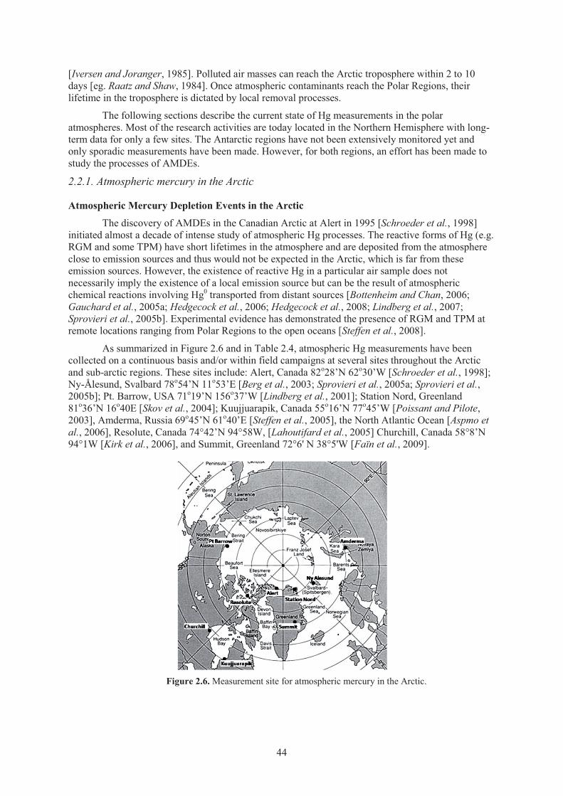
[Iversen and Joranger, 1985]. Polluted air masses can reach the Arctic troposphere within 2 to 10 days [eg. Raatz and Shaw, 1984]. Once atmospheric contaminants reach the Polar Regions, their lifetime in the troposphere is dictated by local removal processes.

The following sections describe the current state of Hg measurements in the polar atmospheres. Most of the research activities are today located in the Northern Hemisphere with long-term data for only a few sites. The Antarctic regions have not been extensively monitored yet and only sporadic measurements have been made. However, for both regions, an effort has been made to study the processes of AMDEs.

2.2.1. Atmospheric mercury in the Arctic

Atmospheric Mercury Depletion Events in the Arctic

The discovery of AMDEs in the Canadian Arctic at Alert in 1995 [Schroeder et al., 1998] initiated almost a decade of intense study of atmospheric Hg processes. The reactive forms of Hg (e.g. RGM and some TPM) have short lifetimes in the atmosphere and are deposited from the atmosphere close to emission sources and thus would not be expected in the Arctic, which is far from these emission sources. However, the existence of reactive Hg in a particular air sample does not necessarily imply the existence of a local emission source but can be the result of atmospheric chemical reactions involving Hg0 transported from distant sources [Bottenheim and Chan, 2006; Gauchard et al., 2005a; Hedgecock et al., 2006; Hedgecock et al., 2008; Lindberg et al., 2007; Sprovieri et al., 2005b]. Experimental evidence has demonstrated the presence of RGM and TPM at remote locations ranging from Polar Regions to the open oceans [Steffen et al., 2008].

As summarized in Figure 2.6 and in Table 2.4, atmospheric Hg measurements have been collected on a continuous basis and/or within field campaigns at several sites throughout the Arctic and sub-arctic regions. These sites include: Alert, Canada 82o28’N 62o30’W [Schroeder et al., 1998]; Ny-Ålesund, Svalbard 78o54’N 11o53’E [Berg et al., 2003; Sprovieri et al., 2005a; Sprovieri et al., 2005b]; Pt. Barrow, USA 71o19’N 156o37’W [Lindberg et al., 2001]; Station Nord, Greenland 81o36’N 16o40E [Skov et al., 2004]; Kuujjuarapik, Canada 55o16’N 77o45’W [Poissant and Pilote, 2003], Amderma, Russia 69o45’N 61o40’E [Steffen et al., 2005], the North Atlantic Ocean [Aspmo et al., 2006], Resolute, Canada 74°42’N 94°58W, [Lahoutifard et al., 2005] Churchill, Canada 58°8’N 94°1W [Kirk et al., 2006], and Summit, Greenland 72°6' N 38°5'W [Faïn et al., 2009].

Figure 2.6. Measurement site for atmospheric mercury in the Arctic.

44

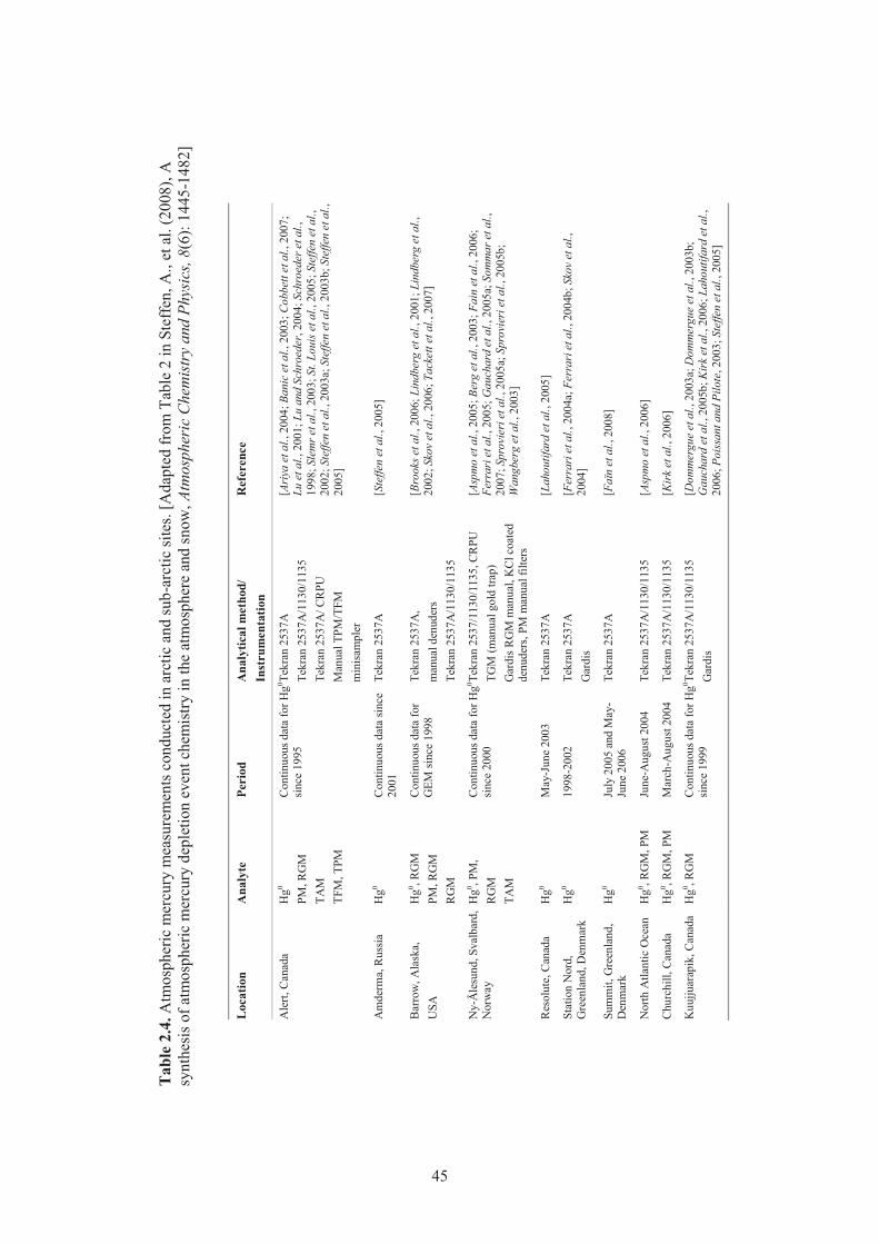
Tab

le 2

.4. A

tmos

pher

ic m

ercu

ry m

easu

rem

ents

con

duct

ed in

arc

tic a

nd su

b-ar

ctic

site

s. [A

dapt

ed fr

om T

able

2 in

Ste

ffen

, A.,

et a

l. (2

008)

, A

synt

hesi

s of a

tmos

pher

ic m

ercu

ry d

eple

tion

even

t che

mis

try in

the

atm

osph

ere

and

snow

, Atm

osph

eric

Che

mis

try

and

Phys

ics,

8(6)

: 144

5-14

82]

Loca

tion

Ana

lyte

Pe

riod

A

naly

tical

met

hod/

In

stru

men

tatio

n R

efer

ence

Ale

rt, C

anad

a H

g0

PM, R

GM

TA

M

TFM

, TPM

Con

tinuo

us d

ata

for H

g0 si

nce

1995

Te

kran

253

7A

Tekr

an 2

537A

/113

0/11

35

Tekr

an 2

537A

/ CR

PU

Man

ual T

PM/T

FM

min

isam

pler

[Ariy

a et

al.,

200

4; B

anic

et a

l., 2

003;

Cob

bett

et a

l., 2

007;

Lu

et a

l., 2

001;

Lu

and

Schr

oede

r, 20

04; S

chro

eder

et a

l.,

1998

; Sle

mr e

t al.,

200

3; S

t. Lo

uis e

t al.,

200

5; S

teffe

n et

al.,

20

02; S

teffe

n et

al.,

200

3a; S

teffe

n et

al.,

200

3b; S

teffe

n et

al.,

20

05]

Am

derm

a, R

ussia

H

g0 C

ontin

uous

dat

a sin

ce

2001

Te

kran

253

7A

[Ste

ffen

et a

l., 2

005]

Bar

row

, Ala

ska,

U

SA

Hg0 , R

GM

PM

, RG

M

RG

M

Con

tinuo

us d

ata

for

GEM

sinc

e 19

98

Tekr

an 2

537A

, m

anua

l den

uder

s Te

kran

253

7A/1

130/

1135

[Bro

oks e

t al.,

200

6; L

indb

erg

et a

l., 2

001;

Lin

dber

g et

al.,

20

02; S

kov

et a

l., 2

006;

Tac

kett

et a

l., 2

007]

Ny-

Åle

sund

, Sva

lbar

d,

Nor

way

H

g0 , PM

, R

GM

TA

M

Con

tinuo

us d

ata

for H

g0 si

nce

2000

Tekr

an 2

537/

1130

/113

5, C

RPU

TG

M (m

anua

l gol

d tra

p)

Gar

dis R

GM

man

ual,

KC

l coa

ted

denu

ders

, PM

man

ual f

ilter

s

[Asp

mo

et a

l., 2

005;

Ber

g et

al.,

200

3; F

ain

et a

l., 2

006;

Fe

rrar

i et a

l., 2

005;

Gau

char

d et

al.,

200

5a; S

omm

ar e

t al.,

20

07; S

prov

ieri

et a

l., 2

005a

; Spr

ovie

ri e

t al.,

200

5b;

Wan

gber

g et

al.,

200

3]

Res

olut

e, C

anad

a H

g0 M

ay-J

une

2003

Te

kran

253

7A

[Lah

outif

ard

et a

l., 2

005]

Stat

ion

Nor

d,

Gre

enla

nd, D

enm

ark

Hg0

1998

-200

2 Te

kran

253

7A

Gar

dis

[Fer

rari

et a

l., 2

004a

; Fer

rari

et a

l., 2

004b

; Sko

v et

al.,

20

04]

Sum

mit,

Gre

enla

nd,

Den

mar

k H

g0 Ju

ly 2

005

and

May

-Ju

ne 2

006

Tekr

an 2

537A

[F

aïn

et a

l., 2

008]

Nor

th A

tlant

ic O

cean

H

g0 , RG

M, P

M

June

-Aug

ust 2

004

Tekr

an 2

537A

/113

0/11

35

[Asp

mo

et a

l., 2

006]

Chu

rchi

ll, C

anad

a H

g0 , RG

M, P

M

Mar

ch-A

ugus

t 200

4 Te

kran

253

7A/1

130/

1135

[K

irk

et a

l., 2

006]

Kuu

jjuar

apik

, Can

ada

H

g0 , RG

M

Con

tinuo

us d

ata

for H

g0 si

nce

1999

Te

kran

253

7A/1

130/

1135

G

ardi

s [D

omm

ergu

e et

al.,

200

3a; D

omm

ergu

e et

al.,

200

3b;

Gau

char

d et

al.,

200

5b; K

irk e

t al.,

200

6; L

ahou

tifar

d et

al.,

20

06; P

oiss

ant a

nd P

ilote

, 200

3; S

teffe

n et

al.,

200

5]

45

The first Arctic annual time series of high-resolution atmospheric Hg vapour data was collected at Alert in 1995 [Schroeder et al., 1998]. It was found that after sunrise the Hg0 concentrations underwent extraordinary fluctuations, decreasing at times from values approximately 1.7 ng m-3 to less than 0.1 ng m-3 within periods of 24 hours. This behaviour runs counter to what is expected for an air pollutant characterized by a long atmospheric residence time [Schroeder and Munthe, 1995]. This depletion of Hg0 from the Arctic atmosphere was confirmed at several locations throughout the Arctic [Steffen et al., 2008]. In 1998, Lu et al. [2001] and Lu and Schroeder [2004] reported high levels of TPM during AMDEs that anti-correlated with measured gas phase Hg. They suggested that Hg0 was being converted to TPM and RGM when AMDEs occurred. This hypothesis that RGM is produced during AMDEs was confirmed in 2000 through direct measurements by Lindberg et al. [2001] at Barrow, Alaska, USA. Steffen et al. [2002] measured total atmospheric Hg at Alert in 2000 and showed that, during depletion events, other forms of Hg species exist in the air besides Hg0. This study also demonstrated that, during depletion events, not all of the converted Hg0 remains in the air; it was proposed that the remainder of the converted Hg is deposited onto the nearby snow and ice surfaces. It is now thought that the chemistry that causes the well known ozone depletion events [Barrie et al., 1988; Bottenheim et al., 1986; Simpson et al., 2007] is similar to what drives AMDEs [Ariya et al., 2002; Lindberg et al., 2001; Lindberg et al., 2002] in that Hg0 is oxidized by reactive halogens, namely Br atoms or BrO radicals [Ariya et al., 2004; Goodsite et al., 2004; Hedgecock et al., 2008; Skov et al., 2004].The oxidation of Hg0 with these reactive halogens yields inorganic RGM. While there are mechanisms and theoretical calculations that suggest that RGM is predominantly a bromide compound [Calvert and Lindberg, 2004], its identity has not been directly elucidated and thus RGM is operationally defined. The reactive halogen species oxidizing Hg0 are assumed to be generated from open water regions, such as leads or polynyas from refreezing sea ice (nilas) forming on open waters, and UV radiation. Measurements have shown that AMDEs occur right at the snow surface [Berg et al., 2003; Sommar et al., 2007; Sprovieri et al., 2005b; Steffen et al., 2002] and are limited to the surface up to a maximum of 1 km [Banic et al., 2003; Tackett et al., 2007]. Lindberg et al. [2001; 2002] reported the first and highest measured concentration levels of RGM (up to 900 pg/m3) during AMDEs at Barrow and showed a strong correlation between RGM production and UV-B irradiation and with an increase in surface snow Hg concentrations.

The discovery of AMDEs has revolutionized our understanding of the cycling of Hg in Polar Regions while stimulating a significant amount of research to understand its impact to this fragile ecosystem.

Temporal trends of atmospheric mercury and comparisons among sites

Continuous long-term TGM measurements in the Arctic using highly time-resolved automatic monitors have been carried out at several observatory sites within the Northern Hemisphere. Hg0 measurements have been collected at Ny-Ålesund, Norway (1994-2000 [manual samples]; 2000-present [automated samples]) and Alert, Canada (1995-present). Other long-term measurements of Hg0 in the Arctic include Amderma Russia (2001-present) and Kuujjuarapik Canada (1999-present). Trend analysis was conducted on these measurements and has showed some temporal and spatial trends. An illustration of some of these measurements is provided on Figure 2.7.

The data sets that have been collected for more than 5 years were subjected to robust statistical trend analysis [Temme et al., 2007] and both of these time series showed no evidence of annual long-term trends during each respective monitoring period. In the springtime, highly variable Hg0 concentrations, as well as the lowest median concentrations of all the seasons, were found and are a result of AMDEs that are known to occur in these regions. While the low springtime median concentrations at Alert revealed no significant trend (95% CI) from 1995 to 2002, the summer Hg0 concentrations indicated a statistically significant (95% CI) decrease from 1995 to 2002. Mercury concentrations measured in the summer were higher than the springtime at Alert, perhaps due to the emission of Hg from tundra and snow surfaces [Steffen et al., 2005].

46

Figure 2.7. Temporal trends of Hg0 measurements conducted in the Arctic in 2002.

This decreasing summer trend in Hg0 concentration is in contrast to a more recent report of a trend at Alert, between 1995 and 2005, where it is shown that no statistically significant trend for each season was found [Temme et al., 2007]. The authors hypothesize that this change in trends may be due to higher re-emission from the oceans coupled with effects from rising air temperatures during Arctic summer and effects from decreasing European emission rates during that time period. Analysis of the measurements from Ny-Ålesund reveals statistically significant decreases in the fall and winter months between 2000 and 2005. It is speculated that this decrease is a reflection of the decrease in European emissions reported during that time period [Pacyna et al., 2006; Steffen, 2007]. Some analysis was made of the measurements from Alert, Amderma and Kuujjuarapik [Steffen et al., 2005] which showed distinct repeating seasonal patterns for all sites, yet the sites at higher latitude showed higher seasonal amplitude. Longer time series of measurements are not available; however, firn air records in Greenland allow for a reconstruction of the past Hg0 signal in the Arctic atmosphere [Faïn et al., 2009]. These data suggest that Hg0 levels were the highest during the 1970s and decreased since then. Such a trend is similar to the worldwide Hg production.

To the best of the authors’ knowledge, only Alert, Canada has long term measurements of RGM and TPM in the Arctic. However, several field campaigns have measured these species during AMDEs [see Steffen et al., 2008]. RGM can exist in the gas phase but will be readily sorbed onto aerosols present in the air because of its hygroscopic properties [Ariya et al., 2004]. At Alert, the overall predominant species in spring is TPM but a clear shift from the predominance of TPM to RGM is observed during the spring [Cobbett et al., 2007; Kirk et al., 2006; Steffen et al., 2008]. At Barrow, RGM is the predominant species observed [Lindberg et al., 2002]. Several studies at Ny-Ålesund have shown that, in general, there is no predominance of either RGM or TPM [Gauchard et al., 2005a; Sprovieri et al., 2005a; Sprovieri et al., 2005b]. Some researchers have suggested that the distribution of the RGM and TPM is an indication of the age of an air mass [Hedgecock et al., 2008; Lindberg et al., 2002; Sprovieri et al., 2005a] while others suggest that the distribution is an indication of local versus transported events (to the measurement site) [Gauchard et al., 2005a; Wangberg et al., 2003].

The presence of UV radiation is also thought to contribute to the distribution of RGM and TPM as suggested by Lindberg et al. [2002]. While considerable work has been done to study Hg in the Arctic, research continues to fully understand the behaviour of Hg over time and the transport of Hg to this area. The processes involved in its conversion between differing media and the impact that this contaminant has on this

47

vulnerable region need more study. It is important to understand how all of these issues may be affected by a changing climate, which is occurring at such a rapid pace in the Arctic region.

2.2.2. Atmospheric Mercury in the Antarctic Antarctica and the Southern Ocean are located in a remote region, with no indigenous human

population and no industrial activity. Human activity is minimal and localized. Human presence in the region largely consists of scientific investigations and logistical operations in support of these investigations. The greatest human impact can be expected where research is carried out at long-term stations; yet these typically have populations of fewer than 100 people. The overwhelming majority of anthropogenic Hg loading to the environment and biota derives from global rather than local input. Antarctica is characterized by a vast, cold, dry, high-altitude polar plateau and a coastal region where the seasonal freezing and melting of sea ice surrounding the continent is the Earth’s largest seasonal energy exchange event. This vast freezing of sea ice liberates sea salt bromine. Far from anthropogenic emissions, and isolated by the circumpolar vortex, only the longest-lived of the global atmospheric contaminants, such as GEM, make their way to the Antarctica polar plateau.

Similar to the Arctic (see section above), atmospheric Hg and ozone depletion events are most noticeable along Antarctic coastlines where polynyas and coastal, or flaw, leads provide frequently freezing sea ice surfaces as a source of atmospheric bromine. Far from the coasts, the main source of bromine is photochemical recycling between the cold surface snow pack and the atmosphere [Piot and von Glasow, 2008]. Evidence of Br emissions from snow surfaces was first reported by Foster et al. [2001] and enhancements of BrO above the snow pack were reported by Avallone et al. [2003]. Recent chemical modelling studies, including Saiz-Lopez et al. [2008] and Piot and von Glasow [2008], show that bromine recycling in the surface snow is required to match air column chemical observations.

Atmospheric measurements on the Antarctic Region

Few field Hg experiments have been performed in Antarctica, compared to those carried out in the Arctic. Mercury measurements performed at different locations of the Antarctic region are reported in Table 2.5. The Hg0 levels are far below the concentrations observed in the Arctic due to the remoteness from anthropogenic sources.

The first baseline data for the concentration and speciation of atmospheric Hg in Antarctica were reported by De Mora et al. [1993]. Mercury measurements were carried out at three sampling locations throughout 1985 and 1988. In particular, a preliminary study was carried out on the frozen surface of Lake Vanda (77°33’S, 161°37’E) in the Wright Valley during December 1985. While obviously limited, the data were interesting and suggested that TGM concentrations in Antarctica were substantially lower than those observed elsewhere (0.23 ng m-3). Therefore, further studies were conducted throughout 1987 and 1988 at Scott Base (77°51’S 166°46’E) and during 1989 at Arrival Heights (77°11’S, 166°40’E) on Ross Island. The mean TGM for 1987 was 0.52 ± 0.14 ng m-3 whereas the corresponding 1988 value was 0.60 ± 0.40 ng m-3. At the third site, mean TGM value was 0.52 ± 0.16 ng m-3. The first data reporting and referring to AMDEs were obtained at Neumayer (70°39’S, 8°15’W), a coastal location in Antarctica [Ebinghaus et al., 2002b].

Simultaneous Hg0, RGM and ozone ambient concentrations have been also performed during Antarctic summer 2000 [Sprovieri et al., 2002] at the Terra Nova Bay (74°41’S, 164°70’E) coastal site on the Ross sea. The high RGM levels observed in the absence of simultaneous ozone and Hg depletion events were comparable to those reported by Temme et al. [2003a]. The very high RGM concentrations at both Antarctic coastal sites could be influenced by the local production of oxidized gaseous Hg species over the Antarctic continent or by shelf ice during polar summer.

48

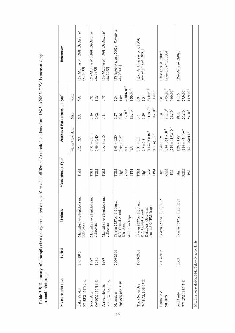
Tab

le 2

.5. S

umm

ary

of a

tmos

pher

ic m

ercu

ry m

easu

rem

ents

per

form

ed a

t diff

eren

t Ant

arct

ic lo

catio

ns fr

om 1

985

to 2

005.

TPM

is m

easu

red

by

man

ual m

ini-t

raps

.

Mea

sure

men

t site

s Pe

riod

M

etho

ds

Mea

sure

men

t Typ

e St

atis

tical

Par

amet

ers i

n ng

/m3

Ref

eren

ces

Mea

n ±

Std

dev.

M

in.

Max

.

Lake

Van

da

77°3

3’S

161°

37’E

D

ec 1

985

Man

ual-s

ilver

ed/g

ilded

sand

co

llect

ors

TGM

0.

23 ±

NA

N

A

NA

[D

e M

ora

et a

l., 1

991;

De

Mor

a et

al

., 19

93]

Scot

t Bas

e 90

°00’

S 13

9°16

’E

1987

19

88

Man

ual-s

ilver

ed/g

ilded

sand

co

llect

ors

TGM

TG

M

0.52

± 0

.14

0.60

± 0

.40

0.16

0.

02

0.83

1.

85

[De

Mor

a et

al.,

199

1; D

e M

ora

et

al.,

1993

]

Arr

ival

Hei

ghts

77

°11’

S 16

6°40

’E

1989

M

anua

l-silv

ered

/gild

ed sa

nd

colle

ctor

s TG

M

0.52

± 0

.16

0.11

0.

78

[De

Mor

a et

al.,

199

1; D

e M

ora

et

al.,

1993

]

Neu

may

er

70°3

9’S

08°1

5’W

20

00-2

001

Tekr

an 2

537A

; 113

0 an

d K

Cl-C

oate

d A

nnul

ar

Den

uder

s;

AES

min

i-Tra

ps

TGM

H

g°

RG

M

TPM

1.08

± 0

.29

0.99

± 0

.27

NA

N

A

0.27

0.

16

5x10

-3

15x1

0-3

2.34

1.

89

~ 30

0x10

-3

120x

10-3

[Ebi

ngha

us e

t al.,

200

2b; T

emm

e et

al

., 20

03a]

Terr

a N

ova

Bay

74

°41’

S, 1

64°0

7’E

1999

-200

1 Te

kran

253

7A; 1

130

and

KC

l-Coa

ted

Ann

ular

D

enud

ers;

Gol

d-m

ini

Trap

s;A

E-TP

M T

raps

TGM

H

g°

RG

M

TPM

0.81

± 0

.1

0.9

± 0.

3 (1

16±7

8)x1

0-3

(12±

6)x

10-3

0.5

0.29

~1

1x10

-3

~4x1

0-3

0.9

2.3

334x

10-3

20

x10-3

[Spr

ovie

ri a

nd P

irro

ne, 2

000;

Sp

rovi

eri e

t al.,

200

2]

Sout

h Po

le

90°0

0’S

2003

-200

5 Te

kran

253

7A; 1

130,

113

5

Hg°

R

GM

PM

0.54

± 0.

19

(344

±151

)x10

-3

(224

± 1

19)x

10-3

0.24

95

x10-3

71

x10-3

0.82

70

5x10

-3

660x

10-3

[Bro

oks e

t al.,

200

8a]

[Ari

mot

o et

al.,

200

4]

McM

urdo

77

°13’

S 16

6°45

’E

2003

Te

kran

253

7A; 1

130,

113

5 H

g°

RG

M

PM

1.20

± 1

.08

(116

± 4

5)x1

0-3

(49

±36)

x10-3

BD

L 29

x10-3

5x

10-3

11.1

6 27

5x10

-3

182x

10-3

[Bro

oks e

t al.,

200

8b]

NA

: dat

a no

t ava

ilabl

e; B

DL:

Bel

ow d

etec

tion

limit

49

Antarctica versus Arctic

A comparison between the two Polar Regions is problematic because both spatial and temporal coverage of Hg measurements are limited. The behaviour of Hg species may be associated with a number of reactive chemicals and reactions that take place in the atmosphere after polar sunrise. The tropospheric chemistry of the polar areas is distinctly different than in the other parts of the Earth due to natural differences of meteorological and solar radiation conditions. During the winter months, in total lack of solar radiation, temperature and humidity conditions are very low, so the vertical mixing of the lower stratified Antarctic troposphere is hindered. The direct consequence is that the abundance of photochemically labile compounds will rise, while the level of photochemical products will be low. During spring and summer, solar radiation is present 24 hours a day and, under sunlight conditions, the elevated concentrations of reactants present in the Antarctic atmosphere can initiate a sequence of atmospheric chemical transformations often different than other latitudes.

It can be anticipated that in the polar troposphere, free radical precursors that build up in the darkness of the polar winter begin to photo-dissociate and the resulting gas-phase radicals may play a fundamental role in the elemental gas phase Hg decrease seen in Antarctica and in Arctic. Although in the Arctic the highest RGM concentrations were found during AMDEs, elevated concentrations were found at Barrow during snowmelt. Snowmelt is more limited in the Antarctic, even at coastal sites, than it is in the Arctic at sites such as Barrow, which suggests that the snowpack is directly involved in maintaining high RGM concentrations. The higher Hg0 concentrations observed in the Arctic, when compared to the Antarctica, clearly indicate the different chemical composition of the troposphere as a result of the location of the measurements areas. In fact, the Arctic is surrounded by populated continents from which pollution is released and transported to the north. In contrast, the Antarctic is entirely surrounded by the Pacific Ocean and is far from any anthropogenic emissions. In particular, fluxes of Hg to the atmosphere, mainly from anthropogenic and continental sources in the Northern Hemisphere (particularly from Eurasia and North America in late winter and spring), are greater than those in the Southern Hemisphere and higher atmospheric concentrations are found in the North than the South.

The dynamic transformations of atmospheric Hg species during the polar spring illustrate the complexity of photochemical reactions in Polar Regions and have revealed the limitations in our understanding of the chemical cycling of Hg and other atmospheric constituents/contaminants in remote regions with seasonally variable sea-ice coverage. More research and investigation on possible reaction mechanisms and chemical kinetics of these phenomena are required to successfully improve our understanding of chemical-physical processes involved in the Hg cycle in order to assess the resulting net input into the polar biosphere.

2.2.3. The role of snow surfaces on atmospheric Hg trends Snow surfaces are well recognized as important sites of chemical transformations in Polar

Regions for many organic compounds. It has recently been established that Hg can also undergo oxidation-reduction transformation at the snow/air interface [for a review, see Steffen et al., 2008]. Since the reduced form of Hg, Hg0, is volatile, these interfacial transformations may lead to changes in the evasion and deposition of Hg in cold regions. However, there have been debates on the importance of these snow processes on atmospheric Hg trends.

Snowpacks can alter atmospheric Hg concentrations by two types of processes. On one hand, they can promote the deposition of Hg0 by, for instance, favouring its conversion into oxidized species through heterogeneous processes. On the other hand, newly deposited HgII can be transformed within the snowpack into Hg0, leading to snow-to-air transfer of Hg. In the latter case, oxidative processes within the snowpack may hinder this transfer. The balance between these evasional and depositional processes will change temporally (on seasonal and daily scales) and spatially (e.g. coastal vs. inland snowpacks).

Snow can influence Hg deposition through physical and/or chemical processes. First, snow packs can act as a source of halogens to the lower troposphere, thereby contributing to the halogen-

50

assisted atmospheric oxidation of Hg0 into RGM in Polar Regions. This phenomenon is particularly likely to occur in snow over sea ice and in coastal snow packs, where halogen levels in snow are high [Brooks et al., 2006; Lindberg et al., 2002; Simpson et al., 2007]. This impact of snow on atmospheric processes is partly supported by data showing that RGM formation is occurring mostly at the snow/air interface [Steffen et al., 2002].

Once RGM is formed in the atmosphere, snow can act as an efficient surface for the sorption of newly formed RGM. Douglas et al. [2005] hypothesized that active growth of snow and ice crystals from the vapour phase near leads readily scavenged available RGM, leading to the highest Hg levels ever reported in snow and ice. However, the sorptive properties of snow towards Hg species are still very poorly documented and represent a fruitful field of future research.

Oxidation-reduction reactions within the snowpack may also lead to the formation of Hg0, and its release to the atmosphere. This reduction of Hg can either be driven by photochemical or biological processes, although the latter have received less attention until recently.

Overall, coastal and sea ice snowpacks can be considered as important sites promoting the deposition and retention of HgII on the ground, leading to higher risk of contamination for neighbouring ecosystems, when compared to inland snowpacks.

2.2.4. Summary and Conclusion for Observations in the Arctic and Antarctic regions The Arctic is currently undergoing rapid and remarkable changes, including warming which

is changing the timing and extent of sea ice [Serreze et al., 2003; Stroeve et al., 2005] and is affecting the seasons, with winter coming later and spring melt coming earlier. As well, coal and fossil fuel combustion in Asia, a major global source of Hg, are expected to increase up to 350% between 1990 levels and 2020 [van Aardenne et al., 1999]. The effects of these increasing emissions on AMDEs processes and the long term deposition of Hg to the Polar Regions will only be discernible if long term measurements are collected at numerous locations. In Antarctica, gross Hg input is controlled by the South Hemisphere emissions. While Northern Hemisphere Hg emissions have been decreasing over the last couple decades, Southern Hemisphere Hg emissions increased from 1990 to 1995 and have stayed roughly constant since 1995. From 1990 to 1995 African emissions increased from 200 to 400 Mg yr-1, Australian from 50 to 100 Mg yr-1, and South American from 55 to 80 Mg yr-1 [Lindberg et al., 2007; Pacyna et al., 2006]. A warmer and wetter environment will have positive and negative effects. On the plateau, the formation of HgII will decrease with the enhanced thermal decomposition of the intermediate HgI radical, HgBr. However, a wetter environment will increase snowfall rates and bury (sequester) a greater proportion of the deposited HgII.

Long term measurements of Hg0 and other atmospheric Hg species in the Polar Regions are very limited and need to be increased. These types of measurements can yield critical information to better understand the processes involved in the cycling of Hg in the polar atmosphere and thus the deposition of this pollutant to this fragile environment. Long-term measurements of Hg in the polar atmosphere must be put into place so that the effects of these changes to Hg distribution in this environment can be monitored and scrutinized.

2.3. Spatial coverage and temporal trends of over-water, air-surface exchange, surface and deep sea water mercury measurements

The world's oceans and seas are both sources and sinks of Hg. Although it appears that the atmosphere is the major transport/distribution medium for Hg because most Hg emissions are to the atmosphere, oceans and seas also play an important role. The transformations of Hg and its compounds, which take place in marine water are of crucial importance to the understanding of the way in which Hg released to the atmosphere is eventually incorporated into biota, thereby becoming a risk to human and ecosystem well being. This section provides an overview of where and when measurements of atmospheric and aquatic concentrations of Hg and its compounds have been made in the marine environment. These measurements cover – in part obviously – the Pacific and Atlantic oceans and the North, Baltic, and Mediterranean seas. There are relatively few direct measurements of the air-sea exchange of Hg, however simultaneous measurements of Dissolved Gaseous Hg (DGM)

51

and Hg in air, when combined with measurements of the sea and air temperature and wind speed, can be used to estimate the evasion and deposition fluxes. The magnitude of these fluxes is one of the indispensable parameters in compartmental and atmospheric Hg models. There remains some uncertainty as a result of the, so far, limited spatial and temporal coverage of the measurements.

The major environmental and health problems associated with Hg pollution result from high concentrations of MeHg in fish. In most systems, the primary cause of high fish MeHg concentrations is thought to be elevated atmospheric inputs of Hg to the water bodies and their watersheds [Andersson et al., 2007; Fitzgerald et al., 1998; Horvat et al., 2003; Kotnik et al., 2007; Lindberg et al., 2007], mostly by wet deposition. Over 60% of the Hg input is from direct deposition [Mierle, 1990], although in some cases, geologic sources of Hg may also be important [Cossa et al., 1997; Rasmussen, 1994]. The Hg inventories in the atmosphere and surface seawater are tightly coupled by an effective precipitation/volatilisation cycle driven by oxidation-reduction reactions [Hedgecock and Pirrone, 2004; Hedgecock et al., 2006; Sprovieri et al., 2003]. In this context, factors that influence the reduction and oxidation of Hg represent a knowledge gap that must be addressed. At present, it is thought that Hg reduction proceeds mostly via photochemical processes [Amyot et al., 1997], although in some systems, biologically-mediated reduction may be significant [Mason et al., 1995a].

The biogeochemical cycle of Hg involves the transfer of quantities of this metal among atmospheric, aquatic and biological reservoirs. This transfer is facilitated by the mobility of Hg, in part due to its volatility and long atmospheric lifetime. Global scale models predict that atmospheric transport and deposition are the principal pathways for Hg to the surface open ocean. Further, these models indicate the important role which oceanic processes, especially air-sea exchange, play in distributing Hg across the Earth’s surface [Mason et al., 1994]. The evasion of Hg from the surface ocean recycles both natural and anthropogenic contributions to deposition back to the atmosphere. Atmospheric deposition to surface waters supplies Hg for important reactions such as reduction to Hg0, methylation and particulate scavenging. Biotic/abiotic production of Hg0 in surface waters results in supersaturation and thereby a wind-induced efflux of Hg0 from the surface mixed layer. This evasion process recycles Hg from the ocean surface waters into the marine atmosphere and is the major biogeochemical remobilization of Hg from aquatic systems [Mason et al., 1994]. Aspects of the atmospheric Hg cycle in open-ocean environments have been investigated with a focus principally on determining concentrations of species and their variations with latitude and atmospheric transport [Mason and Fitzgerald, 1991], as well as atmospheric Hg chemistry and the biogeochemical controls on Hg reduction and evasion [Laurier et al., 2004].

TGM measurements onboard ships proved to provide valuable complementary information to measurements from the ground-based monitoring network. This information consists of a snapshot of large-scale geographical distribution. With proper quality control to ensure comparability and a relatively low measurement uncertainty, the combination of intermittent shipboard and long-term ground measurements can provide information about the worldwide distribution and trend of atmospheric Hg. Occasional shipboard measurements should thus be a part of the global monitoring network for atmospheric Hg.

2.3.1. Atlantic Ocean The first measurements made onboard ships during north–south traverses of the Atlantic

Ocean were made between 1977–1980 [Slemr et al., 1981; Slemr et al., 1985] and the cruises were repeated in 1990 [Slemr and Langer, 1992] and 1994 [Slemr et al., 1995].

In 1996, Lamborg et al. [1999] performed Hg measurements in the south and equatorial Atlantic Ocean during a cruise from Montevideo, Uruguay to Barbados (Figure 11.1) on the research vessel R/V Knorr. TGM ranged between 1.17 and 1.99 ng m-3 with a weighted mean of 1.61±0.09 ng m-3.

From 1996 to 2001 atmospheric Hg measurements were carried out on board the RV Polarstern during three cruises [Temme et al., 2003b].

52

The results of all cruises made over the Atlantic Ocean by these investigators are summarised in Table 2.6 in statistical terms. In the Northern Hemisphere the medians are almost always smaller than averages pointing to an asymmetric distribution with a few higher TGM concentrations in the vicinity of Hg sources. In the Southern Hemisphere, the medians and the averages are mostly equal. A rather homogeneous distribution of TGM in the Southern Hemisphere was observed during the previous cruises [Slemr et al., 1981; Slemr et al., 1985; Slemr and Langer, 1992; Slemr et al., 1995]; higher median TGM concentrations in both hemispheres were observed in 1990. The median TGM concentrations in each hemisphere in 1977–1980 are comparable with those observed in 1994–2000. Temme et al. [2003b] data for 1977–1980 in both hemispheres are comparable to the respective TGM measurements reported by Fitzgerald [1995] for the Pacific Ocean in 1980–1983. When latitude is taken into account, the TGM concentrations measured onboard a ship are also comparable to measurements at remote coastal sites such as Mace Head (Ireland), Cape Point (South Africa), and Lista (Norway). The agreement shows that combination of long-term measurements at several sites with snapshots of latitudinal distribution obtained by ship measurements is feasible and may provide information about the worldwide trends of atmospheric Hg. All cruises show a pronounced concentration gradient between the hemispheres. The average Northern/Southern ratio of TGM hemispheric medians of all Polarstern cruises is 1.49 ± 0.12 (n = 8). This ratio is almost the same as 1.45 used by Slemr et al. [1985] to estimate the atmospheric residence time of Hg, approximately 1 year. This atmospheric residence time is also consistent with the variability of the TGM concentrations of about 21% in the Northern and about 8% in the Southern Hemispheres.

The gradient and the higher variability in the Northern Hemisphere suggest that the majority of emissions and re-emissions are located in the Northern Hemisphere. The TGM concentrations observed over the Atlantic Ocean in 1996 and 1999–2001 were comparable with those measured in 1977–1980, but they were lower than those measured in 1990. Similar concentrations have been found in other studies [Fitzgerald, 1995; Lamborg et al., 1998; Lamborg et al., 2002; Laurier and Mason, 2007; Mason et al., 2001]. There have been suggestions of a possible global decrease of TGM concentrations between 1990 and 1996 [Slemr et al., 2003], which could be linked with changes and/or a decrease of anthropogenic emissions, although there is no consensus within the scientific community of the degree to which remote ocean BL concentrations have changed over time. Several processes might have contributed to this reduction; such as a reduction of emissions from waste incineration, and closure of large emitters and introduction of desulphurisation in the power plants in the countries of the former Eastern Block [Slemr and Scheel, 1998]. The inter-hemispherical gradient with higher TGM concentrations in the Northern Hemisphere remained nearly constant over the years. The former estimate of the TGM atmospheric residence time [Slemr et al., 1985], based on the inter-hemispherical TGM concentration difference, thus, does not need any revision; although there is evidence, and atmospheric models predict, that the residence time may be lower and a value between 0.5-1 year appears more reasonable.

2.3.2. Pacific Ocean Measurements made over the Pacific Ocean in the early 1980s have been summarized in a

number of publications and will be briefly reviewed here [Fitzgerald, 1995; Lamborg et al., 2002; Laurier and Mason, 2007]. There is insufficient data from the recent measurements, given their relative wide distribution latitudinally and the differences in the seasons of sampling, to conclude that the apparent recent increase in concentrations in the North Pacific boundary layer atmosphere are statistically significant.

More recent studies have included speciation measurements, particularly during a cruise between Japan and Hawaii in May/June 2002 that sampled both the surface waters and the atmosphere. The atmospheric results are shown in Figure 2.8 [Laurier et al., 2003].

53

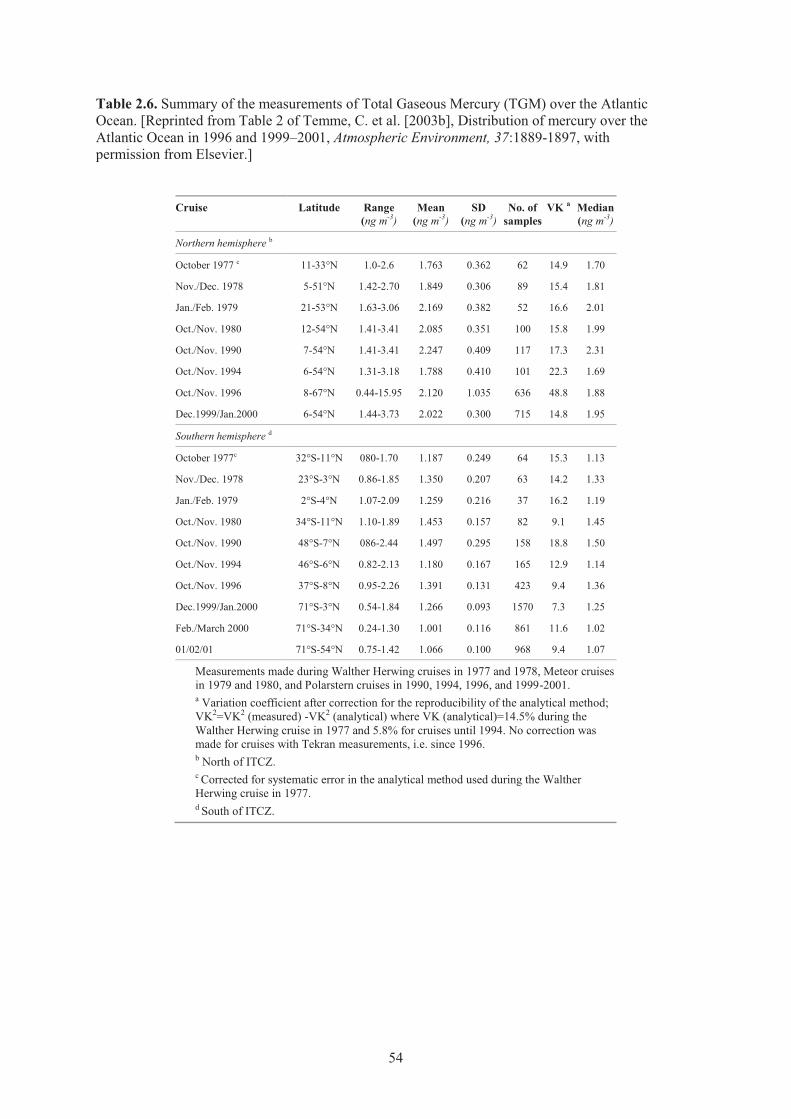
Table 2.6. Summary of the measurements of Total Gaseous Mercury (TGM) over the Atlantic Ocean. [Reprinted from Table 2 of Temme, C. et al. [2003b], Distribution of mercury over the Atlantic Ocean in 1996 and 1999–2001, Atmospheric Environment, 37:1889-1897, with permission from Elsevier.]

Cruise Latitude Range (ng m-3)

Mean (ng m-3)

SD (ng m-3)

No. of samples

VK a Median (ng m-3)

Northern hemisphere b

October 1977 c 11-33°N 1.0-2.6 1.763 0.362 62 14.9 1.70

Nov./Dec. 1978 5-51°N 1.42-2.70 1.849 0.306 89 15.4 1.81

Jan./Feb. 1979 21-53°N 1.63-3.06 2.169 0.382 52 16.6 2.01

Oct./Nov. 1980 12-54°N 1.41-3.41 2.085 0.351 100 15.8 1.99

Oct./Nov. 1990 7-54°N 1.41-3.41 2.247 0.409 117 17.3 2.31

Oct./Nov. 1994 6-54°N 1.31-3.18 1.788 0.410 101 22.3 1.69

Oct./Nov. 1996 8-67°N 0.44-15.95 2.120 1.035 636 48.8 1.88

Dec.1999/Jan.2000 6-54°N 1.44-3.73 2.022 0.300 715 14.8 1.95

Southern hemisphere d

October 1977c 32°S-11°N 080-1.70 1.187 0.249 64 15.3 1.13

Nov./Dec. 1978 23°S-3°N 0.86-1.85 1.350 0.207 63 14.2 1.33

Jan./Feb. 1979 2°S-4°N 1.07-2.09 1.259 0.216 37 16.2 1.19

Oct./Nov. 1980 34°S-11°N 1.10-1.89 1.453 0.157 82 9.1 1.45

Oct./Nov. 1990 48°S-7°N 086-2.44 1.497 0.295 158 18.8 1.50

Oct./Nov. 1994 46°S-6°N 0.82-2.13 1.180 0.167 165 12.9 1.14

Oct./Nov. 1996 37°S-8°N 0.95-2.26 1.391 0.131 423 9.4 1.36

Dec.1999/Jan.2000 71°S-3°N 0.54-1.84 1.266 0.093 1570 7.3 1.25

Feb./March 2000 71°S-34°N 0.24-1.30 1.001 0.116 861 11.6 1.02

01/02/01 71°S-54°N 0.75-1.42 1.066 0.100 968 9.4 1.07

Measurements made during Walther Herwing cruises in 1977 and 1978, Meteor cruises in 1979 and 1980, and Polarstern cruises in 1990, 1994, 1996, and 1999-2001. a Variation coefficient after correction for the reproducibility of the analytical method; VK2=VK2 (measured) -VK2 (analytical) where VK (analytical)=14.5% during the Walther Herwing cruise in 1977 and 5.8% for cruises until 1994. No correction was made for cruises with Tekran measurements, i.e. since 1996. b North of ITCZ. c Corrected for systematic error in the analytical method used during the Walther Herwing cruise in 1977. d South of ITCZ.

54

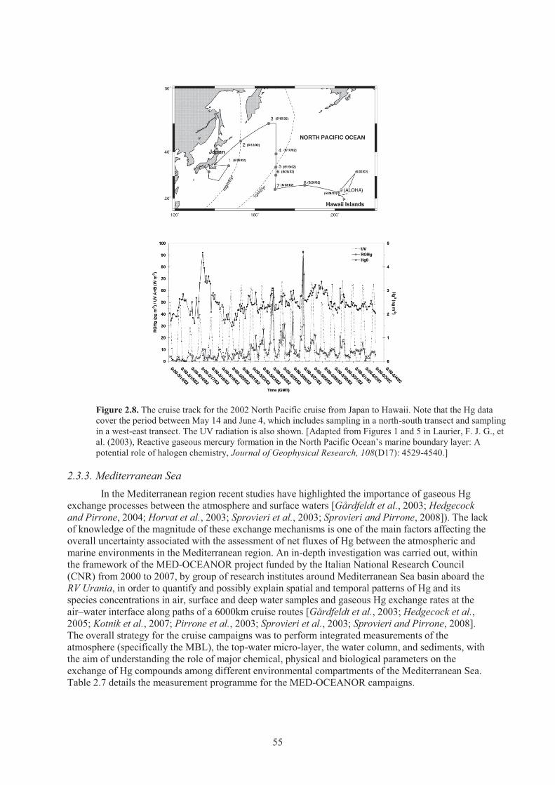
Figure 2.8. The cruise track for the 2002 North Pacific cruise from Japan to Hawaii. Note that the Hg data cover the period between May 14 and June 4, which includes sampling in a north-south transect and sampling in a west-east transect. The UV radiation is also shown. [Adapted from Figures 1 and 5 in Laurier, F. J. G., et al. (2003), Reactive gaseous mercury formation in the North Pacific Ocean’s marine boundary layer: A potential role of halogen chemistry, Journal of Geophysical Research, 108(D17): 4529-4540.]

2.3.3. Mediterranean Sea In the Mediterranean region recent studies have highlighted the importance of gaseous Hg

exchange processes between the atmosphere and surface waters [Gårdfeldt et al., 2003; Hedgecock and Pirrone, 2004; Horvat et al., 2003; Sprovieri et al., 2003; Sprovieri and Pirrone, 2008]). The lack of knowledge of the magnitude of these exchange mechanisms is one of the main factors affecting the overall uncertainty associated with the assessment of net fluxes of Hg between the atmospheric and marine environments in the Mediterranean region. An in-depth investigation was carried out, within the framework of the MED-OCEANOR project funded by the Italian National Research Council (CNR) from 2000 to 2007, by group of research institutes around Mediterranean Sea basin aboard the RV Urania, in order to quantify and possibly explain spatial and temporal patterns of Hg and its species concentrations in air, surface and deep water samples and gaseous Hg exchange rates at the air–water interface along paths of a 6000km cruise routes [Gårdfeldt et al., 2003; Hedgecock et al., 2005; Kotnik et al., 2007; Pirrone et al., 2003; Sprovieri et al., 2003; Sprovieri and Pirrone, 2008]. The overall strategy for the cruise campaigns was to perform integrated measurements of the atmosphere (specifically the MBL), the top-water micro-layer, the water column, and sediments, with the aim of understanding the role of major chemical, physical and biological parameters on the exchange of Hg compounds among different environmental compartments of the Mediterranean Sea. Table 2.7 details the measurement programme for the MED-OCEANOR campaigns.

55

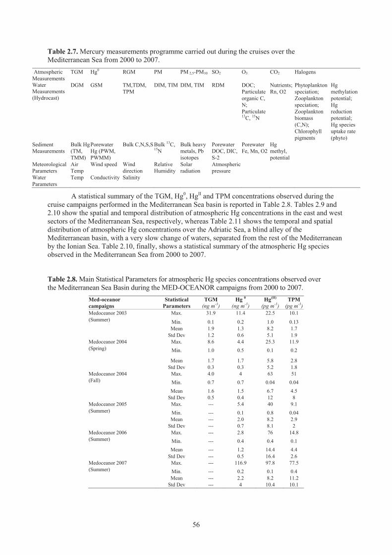
Table 2.7. Mercury measurements programme carried out during the cruises over the Mediterranean Sea from 2000 to 2007.

Atmospheric Measurements

TGM Hg0 RGM PM PM 2,5-PM10 SO2 O3 CO2 Halogens

Water Measurements (Hydrocast)

DGM GSM TM,TDM, TPM

DIM, TIM DIM, TIM RDM DOC; Particulate organic C, N; Particulate 13C, 15N

Nutrients; Rn, O2

Phytoplankton speciation; Zooplankton speciation; Zooplankton biomass (C,N); Chlorophyll pigments

Hg methylation potential; Hg reduction potential; Hg species uptake rate (phyto)

Sediment Measurements

Bulk Hg (TM, TMM)

Porewater Hg (PWM, PWMM)

Bulk C,N,S,S Bulk 13C, 15N

Bulk heavy metals, Pb isotopes

Porewater DOC, DIC, S-2

Porewater Fe, Mn, O2

Hg methyl, potential

Meteorological Parameters

Air Temp

Wind speed Wind direction

Relative Humidity

Solar radiation

Atmospheric pressure

Water Parameters

Temp Conductivity Salinity

A statistical summary of the TGM, Hg0, HgII and TPM concentrations observed during the cruise campaigns performed in the Mediterranean Sea basin is reported in Table 2.8. Tables 2.9 and 2.10 show the spatial and temporal distribution of atmospheric Hg concentrations in the east and west sectors of the Mediterranean Sea, respectively, whereas Table 2.11 shows the temporal and spatial distribution of atmospheric Hg concentrations over the Adriatic Sea, a blind alley of the Mediterranean basin, with a very slow change of waters, separated from the rest of the Mediterranean by the Ionian Sea. Table 2.10, finally, shows a statistical summary of the atmospheric Hg species observed in the Mediterranean Sea from 2000 to 2007.

Table 2.8. Main Statistical Parameters for atmospheric Hg species concentrations observed over the Mediterranean Sea Basin during the MED-OCEANOR campaigns from 2000 to 2007.

Med-oceanor campaigns

Statistical Parameters

TGM (ng m-3)

Hg 0

(ng m-3) Hg(II)

(pg m-3) TPM

(pg m-3) Medoceanor 2003 (Summer)

Max. 31.9 11.4 22.5 10.1

Min. 0.1 0.2 1.0 0.13 Mean 1.9 1.3 8.2 1.7 Std Dev 1.2 0.6 5.1 1.9 Medoceanor 2004 (Spring)

Max. 8.6 4.4 25.3 11.9 Min. 1.0 0.5 0.1 0.2

Mean 1.7 1.7 5.8 2.8 Std Dev 0.3 0.3 5.2 1.8 Medoceanor 2004 (Fall)

Max. 4.0 4 63 51 Min. 0.7 0.7 0.04 0.04 Mean 1.6 1.5 6.7 4.5

Std Dev 0.5 0.4 12 8 Medoceanor 2005 (Summer)

Max. --- 5.4 40 9.1 Min. --- 0.1 0.8 0.04

Mean --- 2.0 8.2 2.9 Std Dev --- 0.7 8.1 2 Medoceanor 2006 (Summer)

Max. --- 2.8 76 14.8 Min. --- 0.4 0.4 0.1 Mean --- 1.2 14.4 4.4

Std Dev --- 0.5 16.4 2.6 Medoceanor 2007 (Summer)

Max. --- 116.9 97.8 77.5 Min. --- 0.2 0.1 0.4

Mean --- 2.2 8.2 11.2 Std Dev --- 4 10.4 10.1

56

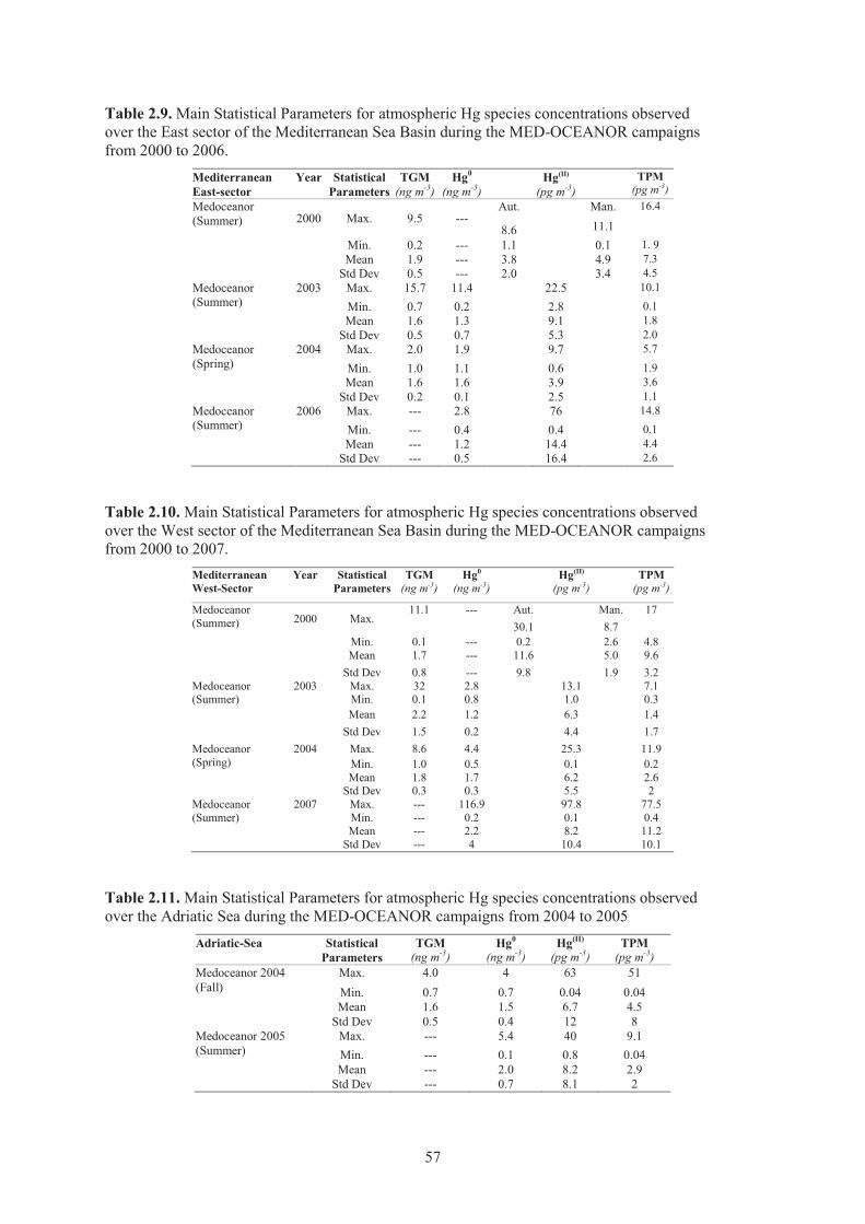
Table 2.9. Main Statistical Parameters for atmospheric Hg species concentrations observed over the East sector of the Mediterranean Sea Basin during the MED-OCEANOR campaigns from 2000 to 2006.

Mediterranean East-sector

Year Statistical Parameters

TGM (ng m-3)

Hg0

(ng m-3) Hg(II)

(pg m-3) TPM

(pg m-3) Medoceanor (Summer) 2000 Max. 9.5 ---

Aut. Man. 16.4

8.6 11.1 Min. 0.2 --- 1.1 0.1 1. 9

Mean 1.9 --- 3.8 4.9 7.3 Std Dev 0.5 --- 2.0 3.4 4.5 Medoceanor (Summer)

2003 Max. 15.7 11.4 22.5 10.1

Min. 0.7 0.2 2.8 0.1 Mean 1.6 1.3 9.1 1.8 Std Dev 0.5 0.7 5.3 2.0 Medoceanor (Spring)

2004 Max. 2.0 1.9 9.7 5.7

Min. 1.0 1.1 0.6 1.9 Mean 1.6 1.6 3.9 3.6 Std Dev 0.2 0.1 2.5 1.1 Medoceanor (Summer)

2006 Max. --- 2.8 76 14.8

Min. --- 0.4 0.4 0.1 Mean --- 1.2 14.4 4.4 Std Dev --- 0.5 16.4 2.6

Table 2.10. Main Statistical Parameters for atmospheric Hg species concentrations observed over the West sector of the Mediterranean Sea Basin during the MED-OCEANOR campaigns from 2000 to 2007.

Mediterranean West-Sector

Year Statistical Parameters

TGM (ng m-3)

Hg0

(ng m-3) Hg(II)

(pg m-3) TPM

(pg m-3)

Medoceanor (Summer) 2000 Max.

11.1 --- Aut. Man. 17 30.1 8.7

Min. 0.1 --- 0.2 2.6 4.8 Mean 1.7 --- 11.6 5.0 9.6 Std Dev 0.8 --- 9.8 1.9 3.2 Medoceanor (Summer)

2003 Max. 32 2.8 13.1 7.1 Min. 0.1 0.8 1.0 0.3

Mean 2.2 1.2 6.3 1.4 Std Dev 1.5 0.2 4.4 1.7 Medoceanor (Spring)

2004 Max. 8.6 4.4 25.3 11.9 Min. 1.0 0.5 0.1 0.2

Mean 1.8 1.7 6.2 2.6 Std Dev 0.3 0.3 5.5 2 Medoceanor (Summer)

2007 Max. --- 116.9 97.8 77.5 Min. --- 0.2 0.1 0.4

Mean --- 2.2 8.2 11.2 Std Dev --- 4 10.4 10.1

Table 2.11. Main Statistical Parameters for atmospheric Hg species concentrations observed over the Adriatic Sea during the MED-OCEANOR campaigns from 2004 to 2005

Adriatic-Sea Statistical Parameters

TGM (ng m-3)

Hg0

(ng m-3) Hg(II)

(pg m-3) TPM

(pg m-3) Medoceanor 2004 (Fall)

Max. 4.0 4 63 51 Min. 0.7 0.7 0.04 0.04

Mean 1.6 1.5 6.7 4.5 Std Dev 0.5 0.4 12 8 Medoceanor 2005 (Summer)

Max. --- 5.4 40 9.1 Min. --- 0.1 0.8 0.04

Mean --- 2.0 8.2 2.9 Std Dev --- 0.7 8.1 2

57

2.3.4. Air-Water Mercury Exchange Open-ocean investigations have demonstrated the importance of air–sea exchange in

controlling the Hg concentration in the atmosphere, and ultimately, in determining the long-term fate of Hg released to the atmosphere from both natural and anthropogenic sources. Hg exists as a dissolved gas in ocean waters, both as Hg0 and as Me2Hg. However, in the upper ocean, Hg0 appears to be the dominant form of the DGM fraction. In most studies, Hg0 concentrations in surface waters have been found to be saturated relative to the atmosphere, and thus the resultant flux of Hg0 is from the ocean to the atmosphere. Flux estimates have been made on cruises in both the Atlantic [Cossa et al., 1997; Lamborg et al., 1998; Mason et al., 1998; Mason and Sullivan, 1999] and Pacific Oceans [Kim and Fitzgerald, 1988; Mason and Fitzgerald, 1993] as well as in the Mediterranean Sea basin [Andersson et al., 2007; Gårdfeldt et al., 2001; Gårdfeldt et al., 2003; Kotnik et al., 2007]. The results of the more recent studies suggest that the evasional flux, as estimated based on DGM concentrations in the surface waters, is greater than the estimated inputs from both atmospheric and riverine inputs.

The ocean receives 90% of its Hg through wet and dry deposition, and a significant fraction of the Hg is in the oxidised form [Mason et al., 1994]. Oxidised Hg may be transformed by several processes in the aqueous phase and reemitted to the atmosphere. Gas exchange of Hg between the surface water and the atmosphere is considered the major mechanism driving Hg from the seawater to the atmosphere [e.g., Hedgecock et al., 2003; Mason et al., 1994; Sprovieri et al., 2003; Sprovieri and Pirrone, 2008]. The major components of total mercury in seawater are mercuric chloride complexes, mercuric ions associated with dissolved organic carbon (DOC) [Munthe et al., 1991] and suspended particles. Some of these Hg forms can be reduced to Hg0 both through biotic (that is enzymatically catalysed by microorganisms) [Mason et al., 1995a] and abiotic processes [Allard and Arsenie, 1991; Costa and Liss, 1999; Xiao et al., 1994; Xiao et al., 1995]. In fact, these processes may significantly contribute to the supersaturation of DGM found in many natural waters and thus to the evasion of Hg to the atmosphere. It has been found that a majority of aquatic environments are supersaturated with respect to dissolved DGM [Schroeder and Munthe, 1998]. Part of this Hg0 may be emitted to the atmosphere. Mason et al. [1994] estimated the emission (mostly Hg0) from the water surfaces to account for 30% (2000 tons per year) of the total emission of Hg to the atmosphere. The total global emission from the sea surface has been re-evaluated [Mason and Sheu, 2002] to 2600 tons per year, however the error in this estimation could, according to the authors, be as high as a factor of 5.

Evasion occurs at the air-water interface. The top water micro-layer probably plays an important role in this process, although it is difficult to sample this layer. The efficiency of these processes depends upon the intensity of the solar radiation, the ambient temperature of the air parcel above the seawater, and the water temperature. It could be assumed that the temperature of the micro-layer is influenced by solar radiation in the same way as that of the air, and this could explain the correlation observed between the temporal trend of Hg0 evasion and air temperature. Ferrara et al. [2003] report Hg depth profile measurements in the Mediterranean Sea showing that DGM losses may also be a result of oxidation in the upper thermocline. The influence of sunlight on both the reduction of mercuric complexes and the oxidation of DGM in the aqueous phase has been observed by many scientists and was investigated during an Atlantic Ocean cruise as reported by Mason et al. [2001] and others [Whalin et al., 2007; Whalin and Mason, 2006]. Additionally, the major DGM species Hg0 can be formed from microbial degradation of methylmercury [Cossa et al., 2009; Mason et al., 1995b]. It has been shown that the photo-induced processes in open-ocean surface waters could result in either a net oxidation or net reduction of Hg species.

The Mediterranean Sea is a source of atmospheric Hg0 that can influence the European domain [Andersson et al., 2007; Hedgecock et al., 2005; Pirrone et al., 1996; Pirrone, 2006; Pirrone et al., 2008; Sprovieri et al., 2003]. Table 2.7 shows the observations from the Mediterranean Sea which have been sorted into four regional categories: Western, Tyrrhenian, Strait of Sicily and Eastern Mediterranean Sector. The average evasion from the western Mediterranean Sea was lower than the eastern sector. As shown in Table 2.7, the mean wind speed was nearly the same at the eastern and western Mediterranean sites. Therefore, the higher Hg0 evasion from the eastern region is explained by the higher mean degree of Hg0 saturation in the east compared to the west. The average

58

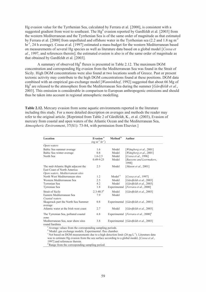
Hg evasion value for the Tyrrhenian Sea, calculated by Ferrara et al. [2000], is consistent with a suggested gradient from west to southeast. The Hg0 evasion reported by Gardfeldt et al. [2003] from the western Mediterranean and the Tyrrhenian Sea is of the same order of magnitude as that estimated by Ferrara et al. [2000] from unpolluted and offshore water in the Tyrrhenian sea (2.2 and 1.8 ng m-2 hr-1, 24 h average). Cossa et al. [1997] estimated a mass-budget for the western Mediterranean based on measurements of several Hg species as well as literature data based on a global model [Cossa et al., 1997, and references therein]; the estimated evasion is also is of the same order of magnitude as that obtained by Gardfeldt et al. [2003].

A summary of observed Hg0 fluxes is presented in Table 2.12. The maximum DGM concentration and corresponding Hg evasion from the Mediterranean Sea was found in the Strait of Sicily. High DGM concentrations were also found at two locations south of Greece. Past or present tectonic activity may contribute to the high DGM concentrations found at these positions. DGM data combined with an empirical gas-exchange model [Wanninkhof, 1992] suggested that about 66 Mg of Hg0 are released to the atmosphere from the Mediterranean Sea during the summer [Gårdfeldt et al., 2003]. This emission is considerable in comparison to European anthropogenic emissions and should thus be taken into account in regional atmospheric modelling.

Table 2.12. Mercury evasion from some aquatic environments reported in the literature including this study. For a more detailed description on averages and methods the reader may refer to the original article. [Reprinted from Table 2 of Gårdfeldt, K., et al. (2003), Evasion of mercury from coastal and open waters of the Atlantic Ocean and the Mediterranean Sea, Atmospheric Environment, 37(S1): 73-84, with permission from Elsevier.]

Location Evasion a

(ng m-2 hr-1) Method b Author

Open waters Baltic Sea summer average 1.6 Model [Wängberg et al., 2001] Baltic Sea winter average 0.8 Model [Wängberg et al., 2001] North Sea 1.6-2.5 Model [Cossa et al., 1996] 0.49-9.25 Model [Baeyens and Leermakers,

1998] The mid-Atlantic Bight adjacent the East Coast of North America

2.5 Model [Mason et al., 2001]

Open waters, Mediterranean sites North West Mediterranean sites 1.2 Model c [Cossa et al., 1997] Western Mediterranean Sea 2.5 Model [Gårdfeldt et al., 2003] Tyrrenian Sea 4.2 Model [Gårdfeldt et al., 2003] Tyrrenian Sea 1.8 Experimental [Ferrara et al., 2000] Strait of Sicily 2.3-40.5d Model [Gårdfeldt et al., 2003] Eastern Mediterranean Sea 7.9 Model Coastal waters Skagerack part the North Sea Summer average

0.8 Experimental [Gårdfeldt et al., 2001]

Atlantic water at the Irish west coast 2.7 Model [Gårdfeldt et al., 2003]

The Tyrrenian Sea, polluted coastal zone

6.8 Experimental [Ferrara et al., 2000]a

Mediterranean Sea, near shore sites round Sardinia

3.8 Experimental [Gårdfeldt et al., 2003]

a Average values from the corresponding sampling periods. b Model: gas exchange models. Experimental: flux chamber. c Not based on DGM measurements due to a high detection limit (26 pg L-1). Literature data was to estimate Hg evasion from the sea surface according to a global model, [Cossa et al., 1997] and references therein. d Range from the corresponding sampling period.

59

2.4. The need for a coordinated global mercury monitoring network for global and regional models validations

Currently, there is not a coordinated observational network for Hg that could be used by the modelling community or for establishing recommendations for protecting human and environmental health on a global scale. Current national networks are inadequate as they lack (1) observations of all forms of Hg in the ambient air and in both wet and dry deposition; (2) long-term measurements of Hg and other air pollutants; (3) comprehensive monitoring sites in the free-troposphere; and (4) measurement sites that permit a careful investigation of inter-hemispheric transport and trends in background concentrations. Programs such as the World Meteorological Organization's GAW have made substantial efforts to establish data centres and quality control programs to enhance integration of air quality measurements from different national and regional networks and to establish observational sites in under-sampled, remote regions around the world. Similarly, the International Global Atmospheric Chemistry project (of the International Geosphere-Biosphere Programme) has strongly endorsed the need for international exchange of calibration standards and has helped coordinate multinational field campaigns to address a variety of important issues related to global air quality. Following the lead of these programs, incorporation of a well-defined Hg monitoring component into the existing network sites would be the most expeditious and efficient approach. Close coordination of the global modelling community with the global measurement community would lead to major advances in the global models and advance our understanding of the Hg science while decreasing the uncertainties in global assessments for Hg.

It has become clear that there is a need for a global Hg monitoring network incorporating existing long-term atmospheric Hg monitoring stations, but with the incorporation of a number of additional sites to obtain a globally representative picture of atmospheric Hg in the troposphere. While atmospheric Hg models have had some success in predicting the levels and trends in ambient Hg levels, the scarcity of global measurement data available for the comparisons make the exercise and results less significant. Efforts to improve our understanding of atmospheric Hg chemistry and inter-hemispheric transport will require a comprehensive research framework that integrates observations covering a wide range of temporal and spatial scales with modelling and process studies. Hence, there is a critical need for a coordinated global Hg monitoring network designed to support the development of global and regional scale Hg models relied upon in the policy making process. A well-planned international network is required to provide a consistent, standardized set of long-term data on the concentrations and deposition of atmospheric Hg in its various forms, together with trace gases, particles, and physical parameters at strategic sites that are globally distributed.

Such a global Hg network should leverage its efforts by collocating with other existing monitoring programs such as the World Meteorological Organization’s GAW sites, United States and Canadian Monitoring sites, and UN-ECE's European Monitoring and Evaluation Programme (EMEP) sites. In addition, as noted in Section 2.1, there are already aspects of such a monitoring program in Europe, Canada and the United States. In the United States, there has been a recent concerted effort to develop and design a monitoring network that would be able to evaluate the ecosystem response to changing concentrations of Hg in the atmosphere and in deposition, and to examine how this impacts levels of MeHg in fish [Mason and Gill, 2005]. While this program focuses on all aspects of Hg biogeochemical cycling, the conclusions of Driscoll [2007] have relevance to the approach to designing a global Hg monitoring network. These authors suggest that a successful network would consist of a relatively small number of “intensive” sites, where the full range of measurements are made (e.g. atmospheric Hg speciation and dry deposition estimation, event-based wet deposition and flux, and the measurement of required ancillary parameters and detailed meteorology), and a larger number of “cluster” sites, where only weekly wet deposition is collected. The cluster sites would allow for integration among the intensive sites, and examine the effects of local and regional conditions, while the intensive sites would provide the detailed information needed to calibrate and test global and regional Hg models [Driscoll et al., 2007; Saltman et al., 2007]. This approach is one model of how such a network would be constructed.

60

Clearly, the over-arching benefit of a coordinated global Hg monitoring network would be the universal availability of high-quality measurement data that are desperately needed to develop, refine, and validate models on different spatial and temporal scales. The data from the set of coordinated monitoring sites would support the evaluation and ground-truthing of models as research and management tools to evaluate our understanding of the global cycling of Hg and deposition to sensitive ecosystems. This section will specifically highlight the need for a global Hg monitoring network designed to support the development of global and regional scale Hg models that should be considered as the scientific basis of the policy making process.

- To reiterate, the principal goals of a global Hg monitoring network are:

- To study the temporal and spatial variability of atmospheric Hg and atmospheric composition;

- To provide long-term monitoring of changes in the physical and chemical state of Hg in the lower atmosphere; in particular to provide the means to discern and understand the causes of such changes;

- To establish the links among changes in atmospheric Hg, tropospheric chemistry and climate;

- To support intensive field campaigns focusing on specific Hg processes occurring at various latitudes and seasons and in highly sensitive ecosystems;

- To produce verified data sets for testing and improving global and regional models for atmospheric Hg and those coupled to aquatic and terrestrial ecosystem models.

2.4.1. Existing Global Monitoring Programs Currently, a global monitoring network for Hg does not exist. There are a number of state and

national programs that are collecting atmospheric Hg data but the parameters monitored, the locations of the monitoring sites, and the methods employed may prohibit their utility in assessing global trends and changes. It is important to stress that the measurement of Hg by itself is not sufficient for us to improve our understanding of Hg sources and impacts. Measurements of other key atmospheric constituents at the global monitoring sites are necessary for us to develop a better understanding of the global redistribution of Hg and to further refine our model parameterizations of the key processes. The co-location of Hg measurements with ongoing global programs is the most efficient approach to initiating this coordinated monitoring network.

2.4.2. Ambient measurements Current air monitoring programs for air pollutants, such as ozone, sulphur dioxide, and

nitrogen compounds, include (1) regulatory monitoring networks that report daily air quality changes at sites located primarily in urban or populated areas; (2) global and regional networks designed to measure background atmospheric composition at selected remote sites or at regionally representative sites; (3) remote-sensing (satellite) instruments that provide global-scale observations of selected atmospheric species; and (4) a variety of radiosonde and aircraft based instrument programs focused on specialized measurement campaigns. These different observational approaches vary widely in their scope and degree of analytical quality. Initial efforts are underway to develop such monitoring capabilities for Hg in the Northern Hemisphere, as detailed in earlier sections. In the United States, there is currently an effort underway to expand the MDN network to include measurements of Hg speciation in air and for estimating dry deposition (http://nadp.sws.uiuc.edu/mdn/). Coordination of such efforts globally will help advance the development of a global network.

Programs such as the World Meteorological Organization's GAW have established data centres and quality control programs to push for the integration of air quality measurements from different national and regional networks, and to establish observational sites in data spare and remote regions of the globe. The International Global Atmospheric Chemistry project (of the International Geosphere-Biosphere Programme) has strongly endorsed the need for international exchange of

61

calibration standards and has helped coordinate multinational field campaigns to address a variety of important issues related to global air quality.

2.4.3. Mercury measurements at altitude Most air quality monitoring networks rely entirely upon ground-based sites that sample within

the boundary layer (the lowest portion of atmosphere in contact with the surface). Addressing global air quality problems such as Hg contamination, however, will require observations that are made at higher altitudes, above the boundary layer. Studies have shown that transport of pollution including Hg between Asia and the United States occurs primarily through the middle and upper troposphere. Because of the highly episodic nature of this transport, there can be significant inhomogeneity in the air masses reaching the continental United States. Thus, networks that only sample air masses within the boundary layer would not allow a quantitative determination of long-range pollutant fluxes. While sampling with aircraft can provide detailed information about Hg in the upper atmosphere [Banic et al., 2003; Ebinghaus and Slemr, 2000; Friedli et al., 2004; Swartzendruber et al., 2008; Talbot et al., 2007], in terms of long-term monitoring, the use of aircraft has obvious limitations. The preferred approach it to use mountain-top monitoring sites that are frequently in the free-troposphere and are located around the globe; these are essential to understanding the global transport of Hg and other pollutants [Jaffe et al., 2005b]. Currently, there are a number of such sites in existence, including Mt. Batchelor in the western United States [Jaffe et al., 2005b] Mona Loa in Hawaii [Landis et al., 2005], Wank Mt. in Germany [Slemr et al., 2003], and the Lulin station in Taiwan [Sheu et al., 2007].

2.4.4. Meteorological measurements Meteorological processes operating over a wide range of spatial scales play a central role in

the air quality and deposition of all atmospheric pollutants including Hg. The emissions, chemical transformations, deposition, and re-emission of Hg are strongly affected by meteorological parameters such as temperature, cloud cover, humidity, mixing height, and wind speed and direction. In addition, dynamic forces, related to vertical temperature profiles, control the dispersion of pollution within the urban/local boundary layer and the release of pollutants from the boundary layer into the free troposphere. Finally, the long-range transport of pollutants is influenced by atmospheric high- and low-pressure systems occurring on synoptic scales (100s to 1000s km). Thus, the meteorological context of atmospheric chemical measurements must be established in order to accurately assess impacts of Hg loadings and to develop the models used for studying long-range Hg transport and climate-Hg interactions.

2.4.5. Atmospheric deposition The atmosphere provides the main environmental pathway for redistribution of Hg around the

globe, and therefore, quantifying the transfer of Hg from the air to the earth’s surface via wet and dry deposition is critically important. Like ambient Hg, there is currently not a globally coordinated network of atmospheric Hg deposition sites. However, there are currently a few coordinated networks in certain regions of the world including: North American Mercury Deposition Network (MDN) that was initiated in the early 1990s as part of the National Atmospheric Deposition Program (NADP); EMEP in Europe; and networks in Japan as well as other parts of Asia. Coordination of the national networks in the various regions and formation of a standard set of measurement objectives and techniques will be important at the onset of the project. While wet deposition networks are currently in-place for Hg, the measurements challenges involved in quantifying Hg dry deposition have thus far prevented these measurements from becoming routine. Dry deposition measurement techniques have been developed using both surrogate surface approaches [Keeler and Dvonch, 2005], and using inferential techniques that measure the various forms of Hg in the atmosphere as well as meteorological parameters to model the dry deposition flux at the measurement site [as discussed in Driscoll et al., 2007]. Inferential methods have been used in both United States Environmental Protection Agency and Environment Canada Networks for acid rain species and may hold the most promise for the global network as well. The key to estimating the dry deposition flux will be the accurate measurement of atmospheric Hg in the gaseous forms and on size-fractionated particulate

62

matter. There is evidence that particulate Hg is bimodal in the atmosphere and undergoes reversible gas-particle partitioning during transport from source to receptor.

2.4.6. Proposed Measurements to enhance model development A consistent set of measurements made on a global scale would dramatically improve our

ability to test and validate global and regional scale atmospheric Hg models. The models would benefit from measurements at surface-based sites performed as part of the coordinated network, but would also benefit from closely linked intensive aircraft studies. Below is a brief list of some of the most critical measurement needs for model development.

1. A network for monitoring Hg wet deposition at global background sites far from anthropogenic sources, as well as sites strategically located in/downwind of various source areas.

2. Surface sites for continuous monitoring of Hg0, RGM and TPM, along with fundamental gas-phase species: CO, O3, particulate and possibly reactive nitrogen and sulphate. Sites should include the following:

a) Remote locations for tropospheric background condition (i.e. sites at elevated altitudes);

b) Locations suitable for measuring continental outflow and intercontinental transport;

c) Locations subject to influence from local sources reflecting short term responses; and

d) Locations that can examine the reactions in the MBL and the reactions occurring in polar regions, where oxidation of Hg0 is enhanced.

3. Aircraft-based studies to identify the vertical distribution of Hg and correlations between Hg and other atmospheric species (CO, O3, aerosols).

4. Aircraft-based studies to evaluate the evolution of Hg0, RGM and Hg-P (or TPM) in plumes downwind of major emission sources, in combination with measurements of gas-phase species (O3, CO, NOx, SOx). Such measurements can be used to resolve the rate of oxidation of Hg0 through reaction with O3 and OH, and evidence for reduction of RGM through reaction with CO or photolysis.

5. Aircraft-based studies to evaluate the effect of cloud processing on ambient Hg, as a basis for assessing the possible reduction of RGM through aqueous reactions.

2.4.7. Establishment of the Coordinated Global Mercury Observation System (GMOS)

Key components of a coordinated long-term network

All global networks must document quality and consistency of routine operations and data treatment through development of protocols for primary and auxiliary measurements, data processing, instrument comparisons, analysis, and data validation. Establishment of a coordinated global Hg monitoring network would benefit greatly from the experience and lessons learned from other global measurement networks, and from the on-going design of regional and national Hg networks. Additionally, climate change research and studies of atmospheric CO2 and carbon cycling have taught us valuable lessons about what is needed to initiate and maintain effective, reliable networks for observing the chemical state of the atmosphere. As suggested by Driscoll et al. [Driscoll et al., 2007] and by Nriagu [1999], some of the keys in establishing a successful global network include:

� Commitment to long-term Hg data collection. Maintaining high-quality, long-term measurement programs for atmospheric Hg requires vision, governmental and international support. There is a need to ensure that the support for observations is adequate to prevent breaks in the data record. Similarly, mechanisms are needed to provide support for development and validation of new instrumentation and its deployment in the field, which can often take many years.

63

� Calibration. Inadequate calibration of instruments in a measurement program limits the value of observations for understanding global atmospheric changes. Absolute calibration is critical for calculating the budgets and lifetimes of different chemical species. Relative calibration is essential in applications that require the use of observations from multiple measurement stations or networks. The goal should be to calibrate each species with an absolute accuracy approaching the analytical precision of the measurement technique.

� Measurement/Analytical Quality Control/Quality Assurance. If a quality assurance/quality control structure has not been established or is inadequately funded for a particular measurement program, then the uncertainties associated with the measurements may render them unusable for trend analysis and model evaluation, and thus the collection efforts are wasted. Standardized quality assurance criteria are especially important in efforts to integrate data from multiple observational programs.

� Collaboration among researchers with different missions but similar data needs. Each type of measurement has limitations and is most useful when it can be meaningfully combined with other types of data. Effective coordination among programs with related observational needs can avoid redundant data collection efforts or data gaps that occur when individual programs lack the resources to adequately support continued observational efforts. For example, coordination of ambient Hg measurements with plant uptake or terrestrial cycling can aid both the air quality and biological cycling research communities.

� Institutional and Personnel Requirements. Experience has shown that maintaining and advancing long-term observational science in atmospheric chemistry depends primarily on highly qualified and dedicated individuals. Attracting such individuals requires strong educational programs and promising career opportunities. Having more than one laboratory striving for the same goal is all the most effective way to assure that the highest quality observations will be made (i.e., all key species should be measured by more than one research group). The complexity in making speciated Hg measurements mandates that well-trained operators be identified for this task.

References Abbott, M., et al. (2007), Atmospheric Mercury Near Salmon Falls Creek Reservoir in Southern Idaho, Idaho

Department of Environmental Quality. http://www.osti.gov/bridge/product.biblio.jsp?osti_id=923511 Allard, B., and I. Arsenie (1991), Abiotic reduction of mercury by humic substances in aquatic system — an

important process for the mercury cycle, Water, Air, & Soil Pollution, 56(1): 457-464. AMAP (2003), AMAP Assessment 2002: Human Health in the Arctic, 137 pp, Arctic Monitoring and

Assessment Programme, Oslo, Norway. AMAP (2005), Fact Sheet: Mercury--a priority pollutant, 4 pp, Arctic Monitoring and Assessment Programme

(AMAP) and Arctic Council Action Plan to Eliminate Pollution of the Arctic, Oslo, Norway. Amyot, M., et al. (1997), Production and Loss of Dissolved Gaseous Mercury in Coastal Seawater,

Environmental Science & Technology, 31(12): 3606-3611. Andersson, M. E., et al. (2007), Seasonal and daily variation of mercury evasion at coastal and off shore sites

from the Mediterranean Sea, Marine Chemistry, 104: 214-226. Arimoto, R., et al. (2004), Lead and mercury in aerosol particles collected over the South Pole during ISCAT-

2000, Atmospheric Environment, 38(32): 5485-5491. Ariya, P. A., et al. (2002), Reactions of gaseous mercury with atomic and molecular halogens: kinetics, product

studies, and atmospheric implications, Journal of Physical Chemistry A, 106: 7310-7320. Ariya, P. A., et al. (2004), The Arctic: a sink for mercury, Tellus Series B - Chemical and Physical Meteorology,

56: 397-403.

64

Aspmo, K., et al. (2005), Measurements of atmospheric mercury species during an international study of mercury depletion events at Ny-Alesund, Svalbard, spring 2003. How reproducible are our present methods?, paper presented at Atmospheric Environment, 7th International Conference on Mercury as a Global Pollutant, 2005/12.

Aspmo, K., et al. (2006), Mercury in the atmosphere, snow and melt water ponds in the North Atlantic Ocean during Arctic summer, Environmental Science & Technology 40: 4083-4089.

Avallone, L. M., et al. (2003), In situ measurements of bromine oxide at two high-latitude boundary layer sites: Implications of variability, Journal of Geophysical Research, 108(D3): 4089-4095.

Baeyens, W., and M. Leermakers (1998), Elemental mercury concentrations and formation rates in the Scheldt estuary and the North Sea, Marine Chemistry, 60(3-4): 257-266.

Baker, P. G. L., et al. (2002), Atmospheric mercury measurements at Cape Point, South Africa, Atmospheric Environment 36(14): 2459-2465.

Banic, C. M., et al. (2003), Vertical distribution of gaseous elemental mercury in Canada, Journal of Geophysical Research 108(D9): 4264-4277.

Barrie, L. A., et al. (1988), Ozone destruction and photochemical reactions at polar in the lower Arctic atmosphere, Nature, 334: 138-141.

Berg, T., et al. (2003), Springtime depletion of mercury in the European Arctic as observed at Svalbard Science of the Total Environment, 304: 43-52.

Berg, T., et al. (2006 ), Atmospheric mercury in Norway: Contributions from different sources, Science of the Total Environment, 368(1): 3-9.

Biester, H., et al. (2002. ), Elevated mercury accumulation in a peat bog of the Magellanic Moorlands, Chile (538S)-An anthropogenic signal from the Southern Hemisphere, Earth and Planetary Science Letters, 201: 609-620.

Bindler, R., et al. (2001), Mercury accumulation rates and spatial patterns in lake sediments from West Greenland: A coast to ice margin transect, Environmental Science & Technology, 35(9): 1736-1741.

Blanchard, P., et al. (2002), Four years of continuous total gaseous mercury (TGM) measurements at sites in Ontario, Canada, Atmospheric Environment, 36(23): 3735-3743.

Bottenheim, J., and H. M. Chan (2006), A trajectory study into the origin of spring time Arctic boundary layer ozone depletion, Journal of Geophysical Research, 111(D19301).

Bottenheim, J. W., et al. (1986), Measurements of NOy species and O3 at 82oN latitude, Geophysical Research Letters 22: 599-602.

Braune, B. M., et al. (2005), Persistent organic pollutants and mercury in marine biota of the Canadian Arctic: An overview of spatial and temporal trends, Science of The Total Environment, 351-352: 4-56.

Brooks, S., et al. (2008a), Antarctic polar plateau snow surface conversion of deposited oxidized mercury to gaseous elemental mercury with fractional long-term burial, Atmospheric Environment, 42(12): 2877-2884.

Brooks, S., et al. (2008b), Springtime atmospheric mercury speciation in the McMurdo, Antarctica coastal region, Atmospheric Environment, 42(12): 2885-2893.

Brooks, S. B., et al. (2006), The mass balance of mercury in the springtime arctic environment, Geophysical Research Letters, 33( L13812).

Brunke, E.-G., et al. (2010), Total gaseous mercury depletion events observed at Cape Point during 2007-2008, Atmospheric Chemistry and Physics Discussions, 10: 1121-1131.

Brunke, E. G., et al. (2001), Gaseous Hg emissions from a fire in the Cape Peninsula, South Africa, during January 2000, Geophysical Research Letters, 28(8): 1483-1486.

Burke, J., et al. (1995), Wet deposition of mercury and ambient mercury concentrations at a site in the Lake Champlain basin, Water, Air, and Soil Pollution 80: 353-361.

Butler, T., et al. (2007), Regional precipitation mercury trends in the eastern USA 1998-2005, Atmospheric Environment, 42: 1582-1592.

Calvert, J. G., and S. E. Lindberg (2004), The potential influences of iodine containing compounds on the chemistry of the troposphere in the polar spring II. , Atmospheric Environment 38: 5105-5116.

65

Carpi, A. (1997 ), Mercury from combustion sources: a review of the chemical species emitted and their transport in the atmosphere, Water, Air, and Soil Pollution 98: 241-254.

Chand, D., et al. (2008), Reactive and particulate mercury in the Asian marine boundary layer, Atmospheric Environment, 42(34): 7988-7996.

Cobbett, F. D., et al. (2007), GEM fluxes and atmospheric mercury concentrations (GEM, RGM and HgP) in the Canadian Arctic at Alert, Nunavut, Canada (February-June 2005), Atmospheric Environment, 41: 6527-6543.

Cossa, D., et al. (1996), Mercury fluxes at the ocean margins, in Global and regional mercury cycles: sources, fluxes and mass balances, edited by W. Baeyens, 229-247 pp., Kluwer Academic Publishers, Dordrecht.

Cossa, D., et al. (1997), The distribution and cycling of mercury species in the western Mediterranean, Deep Sea Research, Part II: Topical Studies in Oceanography, 44: 721-740.

Cossa, D., et al. (2009), The origin of methylmercury in open Mediterranean waters, Limnology and Oceanography, 54: 837-844.

Costa, M., and P. S. Liss (1999), Photoreduction of mercury in sea water and its possible implications for Hg0 air-sea fluxes, Marine Chemistry, 68(1-2): 87-95.

De La Rosa, D. A., et al. (2004), Survey of atmospheric total gaseous mercury in Mexico, Atmospheric Environment 38(29): 4893-4900.

De Mora, S. J., et al. (1991), Baseline concentration and speciation of atmospheric mercury at Baring Head (41"S), New Zealand, Environmental Technology 12: 943-946.

De Mora, S. J., et al. (1993), Baseline atmospheric mercury studies at Ross Island, Antarctica, Antarctic Science 5: 323-326.

Dommergue, A., et al. (2003a), The fate of mercury species in a sub-arctic snow-pack during snowmelt, Geophysical Research Letters 30(12): 1621-1623.

Dommergue, A., et al. (2003b), Chemical and photochemical processes at the origin of the diurnal cycle of gaseous mercury within the snow-pack at Kuujjuarapik, Québec, Environmental Science & Technology 37(15): 3289–3297.

Douglas, T. A., et al. (2005), Elevated mercury measured in snow and frost flowers near Arctic sea ice leads, Geophysical Research Letters, 32(4): L04502.

Driscoll, C. T., et al. (2007), Mercury contamination in forest and freshwater ecosystems in the Northeastern United States, BioScience, 57: 17-28.

Ebinghaus, R., et al. (1999), International field intercomparison measurements of atmospheric mercury species at Mace Head, Ireland, Atmospheric Environment, 33(18): 3063-3073.

Ebinghaus, R., and F. Slemr (2000), Aircraft measurements of atmospheric mercury over southern and eastern Germany, Atmospheric Environment, 34(6): 895-903.

Ebinghaus, R., et al. (2002a), Long-term measurements of atmospheric mercury at Mace Head, Irish west coast, between 1995 and 2001, Atmospheric Environment, 36(34): 5267-5276.

Ebinghaus, R., et al. (2002b), Antarctic Springtime Depletion of Atmospheric Mercury, Environmental Science & Technology, 36(6): 1238–1244.

Ebinghaus, R., et al. (2007), Emissions of gaseous mercury from biomass burning in South America in 2005 observed during CARIBIC flights, Geophysical Research Letters, 34: L08813.

Engstrom, D. R., and E. B. Swain (1997), Recent declines in atmospheric mercury deposition in the upper midwest, Environmental Science & Technology, 31(4): 960–967.

Fain, X., et al. (2006), Fast depletion of elemental gaseous mercury in Skongsvegen Glacier snowpack in Svalbard, Geophysical Research Letters, 33(L06826).

Faïn, X., et al. (2008), Mercury in the snow and firn at Summit Station, Central Greenland, and implications for the study of past atmospheric mercury levels, Atmos, Atmospheric Chemistry and Physics, 8: 3441-3457.

Faïn, X., et al. (2009), Polar firn air reveals large-scale impact of anthropogenic mercury emissions during the 1970s, Proceedings of the National Academy of Sciences of the U.S.A., 106(38): 16114-16119.

66

Feng, X., et al. (2003), Total gaseous mercury in the atmosphere of Guiyang, PR China, Science of the Total Environment, 304(1-3): 61-72.

Feng, X., et al. (2004), Temporal variation of total gaseous mercury in the air of Guiyang, China, Journal of Geophysical Research 109(D03303).

Ferrara, R., et al. (1998), Atmospheric mercury sources in the Ms. Amiata area, Italy, Science of the Total Environment, 213(1-3): 13-23.

Ferrara, R., et al. (2000), Temporal trends in gaseous mercury evasion from the Mediterranean seawaters, Science of the Total Environment, 259(1-3): 183-190.

Ferrara, R., et al. (2003), Profiles of dissolved gaseous mercury concentration in the Mediterranean seawater, Atmospheric Environment, 37(Supplement 1): 85-92.

Ferrari, C. P., et al. (2004a), Profiles of mercury in the snow pack at Station Nord, Greenland shortly after polar sunrise, Geophysical Research Letters 31(L03401).

Ferrari, C. P., et al. (2004b), Nighttime production of elemental gaseous mercury in interstitial air of snow at Station Nord, Greenland, Atmospheric Environment 38(17): 2727-2735.

Ferrari, C. P., et al. (2005), Snow-to-air exchanges of mercury in an Arctic seasonal snow pack in Ny-Alesund, Svalbard, paper presented at Atmospheric Environment, 7th International Conference on Mercury as a Global Pollutant, 2005/12.

Finley, B., et al. (2009), Particulate mercury emissions in regional wildfire plumes observed at the Mount Bachelor Observatory Atmospheric Environment, 43(38): 6074-6083.

Fitzgerald, W. F. (1995), Is mercury increasing in the atmosphere? The need for an atmospheric mercury network (AMNET), Water, Air, and Soil Pollution, 80: 245-254.

Fitzgerald, W. F., et al. (1998), The case for atmospheric mercury contamination in remote areas, Environmental Science & Technology, 32(1): 1-7.

Foster, K. L., et al. (2001), The role of Br2 and BrCl in surface ozone destruction at polar sunrise, Science 291: 471-474.

Fostier, A. H., and P. A. M. Michelazzo (2006), Gaseous and particulate atmospheric mercury concentrations in the Campinas Metropolitan Region (São Paulo State, Brazil), Journal of the Brazilian Chemical Society 17 (5): 886-894.

Friedli, H. R., et al. (2003), Mercury emissions from the August 2001 wildfires in Washington State and an agricultural waste fire in Oregon and atmospheric mercury budget estimates Global Biogeochemical Cycles, 17(2): 1039-1046.

Friedli, H. R., et al. (2004), Mercury in the atmosphere around Japan, Korea, and China as observed during the 2001 ACE-Asia field campaign: Measurements, distributions, sources, and implications, Journal of Geophysical Research, 109: D19S25.

Gabriel, M. C., et al. (2005), Atmospheric speciation of mercury in two contrasting Southeastern US airsheds, Atmospheric Environment, 39(27): 4947-4958.

Gårdfeldt, K., et al. (2001), Oxidation of atomic mercury by hydroxyl radicals and photoinduced decomposition of methylmercury in the aqueous phase, Atmospheric Environment, 35(17): 3039-3047.

Gårdfeldt, K., et al. (2003), Evasion of mercury from coastal and open waters of the Atlantic Ocean and the Mediterranean Sea, Atmospheric Environment, 37(S1): 73-84.

Gauchard, P.-A., et al. (2005a), Study of the origin of atmospheric mercury depletion events recorded in Ny-Alesund, Svalbard, spring 2003, paper presented at Atmospheric Environment, 7th International Conference on Mercury as a Global Pollutant, 2005/12.

Gauchard, P. A., et al. (2005b), Atmospheric particle evolution during a nighttime atmospheric mercury depletion event in sub-Arctic at Kuujjuarapik/Whapmagoostui, Quebec, Canada, Science of the Total Environment 336(1-3): 215-224.

Gildemeister, A. E., et al. (2005), Source proximity reflected in spatial and temporal variability in particle and vapor phase Hg concentrations in Detroit, MI, Atmospheric Environment 39(2): 353-358.

Goodsite, M. E., et al. (2004), A theoretical study of the oxidation of Hg-0 to HgBr2 in the troposphere, Environmental Science & Technology, 38: 1772-1776.

67

Hachiya, N., et al. (1998), Atmospheric mercury concentrations in the basin of the Amazon, Brazil, Environmental Health and Preventive Medicine 2(4): 183–187.

Han, Y.-J., et al. (2004), Atmospheric gaseous mercury concentrations in New York State: Relationships with meteorological data and other pollutants, Atmospheric Environment, 38 (37): 6431-6446.

Hedgecock, I., et al. (2003), Reactive gaseous mercury in the marine boundary layer: modeling and experimental evidence of its formation in the Mediterranean, Atmospheric Environment, 37(S1): 41-49.

Hedgecock, I. M., and N. Pirrone (2001), Mercury and photochemistry in the marine boundary layer- modelling studies suggest the in situ production of reactive gas phase mercury, Atmospheric Environment, 35(17): 3055-3062.

Hedgecock, I. M., and N. Pirrone (2004), Chasing quicksilver: modeling the atmospheric lifetime of Hg0 (g) in the marine boundary layer at various latitudes, Environmental Science & Technology, 38(1): 69-76.

Hedgecock, I. M., et al. (2005), Mercury chemistry in the MBL: Mediterranean case and sensitivity studies using the AMCOTS (Atmospheric Mercury Chemistry over the Sea) model, Atmospheric Environment, 39(38): 7217-7230.

Hedgecock, I. M., et al. (2006), Integrated mercury cycling, transport and air-water exchange (MECAWEx) model, Journal of Geophysical Research 111: D20302.

Hedgecock, I. M., et al. (2008), Chasing quicksilver northward: mercury chemistry in the Arctic troposphere, Environmental Chemistry, 5(2): 131-134.

Higueras, P., et al. (2005), Atmospheric mercury data for the Coquimbo region, Chile: Influence of mineral deposits and metal recovery practices, paper presented at Atmospheric Environment, 7th International Conference on Mercury as a Global Pollutant, 2005/12.

Horvat, M., et al. (2003), Speciation of mercury in surface and deep-sea waters in the Mediterranean Sea, Atmospheric Environment, 37(Supplement 1): 93-108.

Iverfeldt, A., et al. (1995), Long-term changes in concentration and deposition of atmospheric mercury over Scandinavia, Water, Air, and Soil Pollution 80(1-4): 227-233.

Iversen, T., and E. Joranger (1985), Arctic air pollution and large scale atmospheric flows, Atmospheric Environment, 19(12): 2099-2108

Jaffe, D., et al. (2005a), Seasonal cycle and composition of background fine particles along the west coast of the US Atmospheric Environment, 39(2): 297-306.

Jaffe, D. A., et al. (2005b), Export of atmospheric mercury from Asia, Atmospheric Environment, 39(17): 3029-3038.

Johansen, P., et al. (2007), Human accumulation of mercury in Greenland, Science of the Total Environment, 377: 173-178.

Keeler, G. J., and J. T. Dvonch (2005), Atmospheric Mercury: A Decade of Observations in the Great Lakes, in Dynamics of Mercury Pollution on Regional and Global Scales: Atmospheric Processes and Human Exposures Around the World, edited by N. Pirrone and K. Mahaffey, 611-636 pp., Springer, New York.

Kellerhals, M., et al. (2003), Temporal and spatial variability of total gaseous mercury in Canada: results from the Canadian Atmospheric Mercury Measurement Network (CAMNet), Atmospheric Environment, 37(7): 1003-1011.

Kim, J., and W. Fitzgerald (1988), Gaseous mercury profiles in the tropical Pacific Ocean, Geophysical Research Letters, 15(1): 40-43.

Kim, K.-H., and M. Y. Kim (1996), Preliminary measurements of atmospheric mercury in mountainous regions of Korea, Journal of Environmental Science and Health - Part A Toxic/Hazardous Substances and Environmental Engineering 31(8): 2023-2032.

Kim, K.-H., et al. (2005), Atmospheric mercury concentrations from several observatory sites in the Northern Hemisphere, Journal of Atmospheric Chemistry, 50(1): 1-24.

Kirk, J. L., et al. (2006), Rapid reduction and reemission of mercury deposited into snowpacks during atmospheric mercury depletion events at Churchill, Manitoba, Canada, Environmental Science & Technology, 40(24): 7590–7596.

68

Kock, H. H., et al. (2005), Comparison of long-term trends and seasonal variations of atmospheric mercury concentrations at the two European coastal monitoring stations Mace Head, Ireland, and Zingst, Germany, paper presented at Atmospheric Environment, 7th International Conference on Mercury as a Global Pollutant, 2005/12.

Kotnik, J., et al. (2005), Current and past mercury distribution in air over the Idrija Hg mine region, Slovenia, Atmospheric Environment, 39 (39 SPEC. ISS.): 7570-7579.

Kotnik, J., et al. (2007), Mercury speciation in surface and deep waters of the Mediterranean Sea, Marine Chemistry, 107(1): 13-30.

Lacerda, L. D. (1997), Global mercury emissions from gold and silver mining, Water, Air, and Soil Pollution,97(3-4): 209-221.

Lacerda, L. D. (2003), Updating global Hg emissions from small-scale gold mining and assessing its environmental impacts, Environmental Geology, 43: 308-314.

Lahoutifard, N., et al. (2005), Total and methyl mercury patterns in Arctic snow during springtime at Resolute, Nunavut, Canada, paper presented at Atmospheric Environment, 7th International Conference on Mercury as a Global Pollutant, 2005/12.

Lahoutifard, N., et al. (2006), Scavenging of gaseous mercury by acidic snow at Kuujjuarapik, Northern Quebec, Science of the Total Environment 355(1-3): 118-126.

Lamborg, C. H., et al. (1998), The atmospheric cycling and air-sea exchange of mercury species in the south and equatorial Atlantic Ocean, in Ocean Sciences Meeting, San Diego, February 1998.

Lamborg, C. H., et al. (1999), The atmospheric cycling and air-sea exchange of mercury species in the south and equatorial Atlantic Ocean, Deep Sea Research, Part II: Topical Studies in Oceanography, 46(5): 957-977.

Lamborg, C. H., et al. (2002), Modern and historic atmospheric mercury fluxes in both hemispheres: Global and regional mercury cycling implications, Global Biogeochemical Cycles, 16(4): 1104-1114.

Landis, M., et al. (2005), The Monitoring and Modelling of Hg Species in Support of Local, Regional and Global Modelling, in Dynamics of Mercury Pollution on Regional and Global Scales: Atmospheric Processes and Human Exposures Around the World, edited by N. Pirrone and K. R. Mahaffey, 123-151 pp., Springer US, New York.

Landis, M. S., et al. (2002), Atmospheric mercury in the Lake Michigan basin: Influence of the Chicago/Gary urban area, Environmental Science & Technology 36 (21): 4508–4517.

Landis, M. S., et al. (2004), Divalent inorganic reactive gaseous mercury emissions from a mercury cell chlor-alkali plant and its impact on near-field atmospheric dry deposition, Atmospheric Environment, 38(4): 613-622.

Laurier, F., et al. (2004), Mercury distributions in the North Pacific Ocean - 20 years of observations, Marine Chemistry, 90(1-4): 3-19.

Laurier, F., and R. P. Mason (2007), Mercury concentration and speciation in the coastal and open ocean boundary layer, Journal of Geophysical Research, 112(D06302).

Laurier, F. J. G., et al. (2003), Reactive gaseous mercury formation in the North Pacific Ocean’s marine boundary layer: A potential role of halogen chemistry, Journal of Geophysical Research, 108(D17): 4529-4540.

Lindberg, S., et al. (2001), Formation of reactive gaseous mercury in the Arctic: evidence of oxidation of Hg(0) to gas-phase Hg(II) compounds after arctic sunrise, Water, Air, and Soil Pollution, 1: 295-302.

Lindberg, S. E., and W. J. Stratton (1998), Atmospheric mercury speciation: concentrations and behaviour of reactive gaseous mercury in ambient air, Environmental Science & Technology, 32(1): 49–57.

Lindberg, S. E., et al. (2002), Dynamic oxidation of gaseous mercury in the arctic troposphere at polar sunrise, Environmental Science & Technology, 36(6): 1245-1256.

Lindberg, S. E., et al. (2007), A synthesis of progress and uncertainties in attributing the sources of mercury in deposition, AMBIO: A Journal of the Human Environment, 36(1): 19-32.

Liu, B., et al. (2007), Temporal variability of mercury speciation in urban air, Atmospheric Environment, 41(9): 1911-1923.

Liu, S., et al. (2002), Atmospheric mercury monitoring survey in Beijing, China, Chemosphere, 48(1): 97-107.

69

Lu, J. Y., et al. (2001), Magnification of atmospheric mercury deposition to polar regions in springtime: The link to tropospheric ozone depletion chemistry, Geophysical Research Letters 28(17): 3219-3222.

Lu, J. Y., and W. H. Schroeder (2004), Annual time-series of total filterable atmospheric mercury concentrations in the Arctic, Tellus 56B(3): 213 - 222.

Lynam, M., and G. J. Keeler (2005b), Artifacts associated with the measurement of particulate mercury in an urban environment: The influence of elevated ozone concentrations, Atmospheric Environment, 39(17): 3081-3088.

Lynam, S. N., and M. S. Gustin (2008), Speciation of atmospheric mercury at two sites in northern Nevada, USA, Atmospheric Environment, 42: 927-939.

Malcolm, E. G., et al. (2003), The effects of the coastal environment on the atmospheric mercury cycle, Journal of Geophysical Research, 108(D12): 4357-4366.

Mason, R. P., and W. Fitzgerald (1991), Mercury speciation in open ocean waters, Water, Air, & Soil Pollution, 56(1): 779-789.

Mason, R. P., and W. F. Fitzgerald (1993), The distribution and biogeochemical cycling of mercury in the equatorial Pacific Ocean, Deep Sea Research, Part II: Topical Studies in Oceanography, 40(9): 1897-1924.

Mason, R. P., et al. (1994), The biogeochemical cycling of elemental mercury: Anthropogenic influences, Geochimica et Cosmochimica Acta, 38(15): 3191-3198.

Mason, R. P., et al. (1995a), The role of microorganisms in elemental mercury formation in natural waters, Water, Air, & Soil Pollution, 80(1): 775-787.

Mason, R. P., et al. (1995b), Bioaccumulation of mercury and methylmercury, Water, Air, & Soil Pollution, 80(1): 915-921.

Mason, R. P., et al. (1998), Mercury in the North Atlantic, Marine Chemistry, 61(1-2): 37-53. Mason, R. P., and K. A. Sullivan (1999), The distribution and speciation of mercury in the South and equatorial

Atlantic, Deep-Sea Research II, 46: 937-956. Mason, R. P., et al. (2001), Mercury in the Atlantic Ocean: Factors controlling air-sea exchange of mercury and

its distribution in the upper waters, Deep Sea Research, Part II: Topical Studies in Oceanography, 48(13): 2829-2853.

Mason, R. P., and G.-R. Sheu (2002), Role of the ocean in the global mercury cycle, Global Biogeochemical Cycles, 16(4): 1093-1107.

Mason, R. P., and G. A. Gill (2005), Mercury in the marine environment, in Mercury: Sources, Measurements, Cycles, and Effects, edited by M. B. Parsons and J. B. Percival, 179-216 pp., Mineralogical Association of Canada Short Course 34, Halifax, Nova Scotia.

Mierle, G. (1990), Aqueous inputs of mercury to precambrian shield lakes in Ontario, Environmental Toxicology and Chemistry, 9(7): 843-851.

Mukherjee, A. B., et al. (2009), Mercury emissions from industrial sources in India and its effects in the environment, in Mercury Fate and Transport in the Global Atmosphere: Emissions, Measurements, and Models, edited by N. Pirrone and R. Mason, 81-112 pp., Springer, New York.

Munthe, J., et al. (1991), The aqueous reduction of divalent mercury by sulfite, Water, Air, and Soil Pollution, 56: 621-630.

Munthe, J., et al. (2003 ), Distribution of atmospheric mercury species in Northern Europe: Final results from the MOE project, Atmospheric Environment 37 (S1): 9-20.

Nguyen, H. T., et al. (2007), Monitoring of atmospheric mercury at a Global Atmospheric Watch (GAW) site on An-Myun Island, Korea, Water, Air, and Soil Pollution, 185: 149-164.

Nriagu, J. O. (1999), paper presented at Mercury as a Global Pollutant – The Fifth International Conference, Rio de Janeiro, Brazil.

Pacyna, E. G., et al. (2006), Global anthropogenic mercury emission inventory for 2000, Atmospheric Environment, 40(22): 4048-4063.

Pacyna, E. G., et al. (2010), Global emission of mercury to the atmosphere from anthropogenic sources in 2005 and projections to 2020, Atmospheric Environment, 40(20): 2487-2499.

70

Pacyna, J. M., et al. (2001), European emissions of atmospheric mercury from anthropogenic sources in 1995, Atmospheric Environment, 35(17): 2987-2996.

Pan, L., et al. (2007), Top-down estimate of mercury emissions in China using four-dimensional variational data assimilation, Atmospheric Environment, 41(13): 2804-2819.

Piot, M., and R. von Glasow (2008), The potential importance of frost flowers, recycling on snow, and open leads for ozone depletion events, Atmospheric Chemistry and Physics 8: 2437-2467.

Pirrone, N., et al. (1996), Regional differences in worldwide emissions of mercury to the atmosphere, Atmospheric Environment, 30(17): 2981-2987.

Pirrone, N., et al. (1998), Historical atmospheric mercury emissions and depositions in North America compared to mercury accumulations in sedimentary records, Atmospheric Environment, 32(5): 929-940.

Pirrone, N., et al. (2001a), Mercury emissions to the atmosphere from natural and anthropogenic sources in the Mediterranean region, Atmospheric Environment, 35(17): 2997-3006.

Pirrone, N., et al. (2001b), Mediterranean Atmospheric Mercury Cycle System (MAMCS) Project Final Report, 253 pp, CNR Institute for Atmospheric Pollution Research (CNR-IIA), Rende, Italy. CNR/IIA/2001/08

Pirrone, N., et al. (2003), Dynamic Processes of Mercury Over the Mediterranean Region: results from the Mediterranean Atmospheric Mercury Cycle System (MAMCS) project, Atmospheric Environment, 37(S1): 21-39.

Pirrone, N. (2006), An integrated approach to assess the mercury cycling in the Mediterranean basin (MERCYMS), 377 pp, Rende, Italy. Technical report CNR/IIA/2006/08

Pirrone, N., et al. (2008), New Directions: Atmospheric mercury, easy to spot and hard to pin down: Impasse?, Atmospheric Environment, 42: 8549-8551.

Poissant, L., and M. Pilote (2003), Time series analysis of atmospheric mercury in Kuujjuarapik/Whapmagoostui (Quebec), Journal de Physique IV, 107: 1079-1082.

Poissant, L., et al. (2005), A year of continuous measurements of three atmospheric mercury species (Hg0, RGM and Hgp) in southern Québec, Canada, Atmospheric Environment, 39(7): 1275-1287.

Raatz, W. E., and G. E. Shaw (1984), Long-range tropospheric transport of pollution aerosols into the Alaskan Arctic, Journal of Climatology and Applied Meteorology 7: 1052-1064.

Rasmussen, P. E. (1994), Current Methods of Estimating Atmospheric Mercury Fluxes in Remote Areas, Environmental Science & Technology, 28(13): 2233-2241.

Riva, S. D., et al. (2004), The utilization of the Antarctic environmental specimen bank (BCAA) in monitoring Cd and Hg in an Antarctic coastal area in Terra Nova Bay (Ross Sea-Northern Victoria Land), Chemosphere, 56: 59-69.

Saiz-Lopez, A., et al. (2008), On the vertical distribution of boundary layer halogens over coastal Antarctica: Implications for O3, HOx, NOx and the Hg lifetime, Atmospheric Chemistry and Physics, 8(4): 887-900.

Saltman, T., et al. (2007), An Integrated Framework for Ecological Mercury Assessments, in Ecosystem Responses to Mercury Contamination: Indicators of Change, edited by R. Harris, et al., 191-206 pp., CRC Press, New York.

Schroeder, W. H., and J. Munthe (1995), Atmospheric mercury: An overview, Atmospheric Environment, 32(5): 809-822.

Schroeder, W. H., et al. (1998), Arctic springtime depletion of mercury, Nature, 394: 331-332. Schroeder, W. H., and J. Munthe (1998), Atmospheric mercury--an overview, Atmospheric Environment, 32:

809-822. Selin, N. E., and D. J. Jacob (2008), Seasonal and spatial patterns of mercury wet deposition in the United

States: Constraints on the contribution from North American anthropogenic sources, Atmospheric Environment, 42(21): 5193-5204.

Serreze, M. C., et al. (2003), A record minimum arctic sea ice extent and area in 2002, Geophysical Research Letters, 30(3): 1110-1114.

Sheu, G.-R., et al. (2002), Speciation and distribution of atmospheric mercury over the northern Chesapeake Bay, ACS Symposium Series 806: 223-242.

71

Sheu, G.-R., et al. (2010), Temporal distribution and potential sources of atmospheric mercury measured at a high-elevation background station in Taiwan, Atmospheric Environment, 44(20): 2393-2400.

Sheu, G., et al. (2007), Measurements of Atmospheric Mercury at a High Elevation Site (Lulin Atmospheric Background Station, LABS) in Taiwan, in American Geophysical Union Fall Meeting, San Francisco, 12/2007.

Sigler, J. M., and X. Lee (2006), Recent trends in anthropogenic mercury emission in the northeast United States, Journal of Geophysical Research, 111(D14316).

Simpson, W., et al. (2007), Halogens and their role in polar boundary-layer ozone depletion, Atmospheric Chemistry and Physics 7: 4375-4418.

Skov, H., et al. (2004), Fate of elemental mercury in the Arctic during atmospheric depletion episodes and the load of atmospheric mercury to the Arctic, Environmental Science & Technology 38(8): 2373-2382.

Skov, H., et al. (2006), Fluxes of reactive gaseous mercury measured with a newly developed method using relaxed eddy accumulation, Atmospheric Environment, 40(28): 5452-5463.

Slemr, F., et al. (1981), Latitudinal distribution of mercury over the Atlantic Ocean, Journal of Geophysical Research, 86: 1159-1166.

Slemr, F., et al. (1985), Distribution, speciation, and budget of atmospheric mercury, Journal of Atmospheric Chemistry, 3(4): 407-434.

Slemr, F., and E. Langer (1992), Increase in global atmospheric concentrations of mercury inferred from measurements over the Atlantic Ocean, Nature, 355(6359): 434-437.

Slemr, F., et al. (1995), Indication of change in global and regional trends of atmospheric mercury concentrations, Geophysical Research Letters, 22(16): 2143-2146.

Slemr, F., and H. E. Scheel (1998), Trends in atmospheric mercury concentrations at the summit of the Wank Mountain, Southern Germany, Atmospheric Environment, 32: 845-853.

Slemr, F., et al. (2003), Worldwide trend of atmospheric mercury since 1977, Geophysical Research Letters,30(10).

Slemr, F., et al. (2006), European emissions of mercury derived from long-term observations at Mace Head, on the western Irish coast, Atmospheric Environment 40(36): 6966-6974.

Sohn, D. H., et al. (1993), Distribution of total mercury in the ambient atmosphere of Seoul and its diurnal, monthly and altitudinal variations, Japanese Journal of Toxicology and Environmental Health, 39(6): 582-588.

Sommar, J., et al. (2007), Circumpolar transport and air-surface exchange of atmospheric mercury at Ny-A°lesund (79° N), Svalbard, spring 2002, Atmospheric Chemistry and Physics, 7(1): 151-166.

Sprovieri, F., and N. Pirrone (2000), A preliminary assessment of mercury levels in the Antarctic and Arctic troposphere, Journal of Aerosol Science, 31: 757-758.

Sprovieri, F., et al. (2002), Intensive atmospheric mercury measurements at Terra Nova Bay in Antarctica during November and December 2000, Journal of Geophysical Research, 107(D23): 4722-4729.

Sprovieri, F., et al. (2003), Mercury speciation in the marine boundary layer along a 6000 km cruise path around the Mediterranean Sea, Atmospheric Environment, 37(S1): 63-71.

Sprovieri, F., et al. (2005a), Oxidation of gaseous elemental mercury to gaseous divalent mercury during 2003 polar sunrise at Ny-Alesund, Environmental Science & Technology, 39(23): 9156-9165.

Sprovieri, F., et al. (2005b), Atmospheric mercury behavior at different altitudes at Ny Alesund during Spring 2003, paper presented at Atmospheric Environment 7th International Conference on Mercury as a Global Pollutant, 2005/12.

Sprovieri, F., and N. Pirrone (2008), Spatial and temporal distribution of atmospheric mercury species over the Adriatic Sea, Environmental Fluid Mechanics, 8(2): 117-128.

St. Louis, V. L., et al. (2005), Some sources and sinks of monomethyl and inorganic mercury on Ellesmere Island in the Canadian High Arctic, Environmental Science & Technology, 39: 2686-2701.

Stamenkovic, J., et al. (2007), Seasonal and diel variation of atmospheric mercury concentrations in the Reno (Nevada, USA) airshed, Atmospheric Environment 41(31): 6662-6672.

72

Steffen, A., et al. (2002), Atmospheric mercury concentrations: Measurements and profiles near snow and ice surfaces in the Canadian Arctic during Alert 2000, Atmospheric Environment, 36(15-16): 2653-2661.

Steffen, A., et al. (2003a), Mercury throughout polar sunrise 2002, Journal de Physique IV 107: 1267-1270. Steffen, A., et al. (2003b), Mercury in the Arctic Atmosphere in the Canadian Arctic Contaminants Assessment

Report II, Indian and Northern Affairs Canada, Ottawa. Steffen, A., et al. (2005), Mercury in the Arctic atmosphere: An analysis of eight years of measurements of

GEM at Alert (Canada) and a comparison with observations at Amderma (Russia) and Kuujjuarapik (Canada), Science of The Total Environment, 342(1-3): 185-198.

Steffen, A. (2007), Mercury Measurements at Alert, Ministry of Indian Affairs and Northern Development, Ottawa.

Steffen, A., et al. (2008), A synthesis of atmospheric mercury depletion event chemistry in the atmosphere and snow, Atmospheric Chemistry and Physics, 8(6): 1445-1482.

Streets, D. G., et al. (2005), Anthropogenic mercury emissions in China, Atmospheric Environment, 39(40): 7789-7806.

Streets, D. G., et al. (2009), Projections of global mercury emissions in 2050, Environmental Science & Technology, 43(8): 2983-2988.

Stroeve, J. C., et al. (2005), Tracking the Arctic's shrinking ice cover: Another extreme September minimum in 2004, Geophysical Research Letters, 32(L04501).

Suzuki, N., et al. (2009), Monitoring and modeling the fate of Mercury species in Japan, in Mercury Fate and Transport in the Global Atmosphere: Emissions, Measurements, and Models, edited by R. Mason and N. Pirrone, 381-390 pp., Springer, New York.

Swartzendruber, P. C., et al. (2006), Observations of reactive gaseous mercury in the free troposphere at the Mount Bachelor observatory, Journal of Geophysical Research, 111(D24301).

Swartzendruber, P. C., et al. (2008), Vertical distribution of mercury, CO, ozone, and aerosol scattering coefficient in the Pacific Northwest during the spring 2006 INTEX-b campaign, Journal of Geophysical Research, 113: D10305.

Tackett, P. J., et al. (2007), A Study of the vertical scale of halogen chemistry in the Arctic troposphere during polar sunrise at Barrow, AK, Journal of Geophysical Research 112(D07306).

Talbot, R., et al. (2007), Total depletion of Hg° in the upper troposphere-lower stratosphere, Geophysical Research Letters, 34(L23804).

Temme, C., et al. (2003a), Measurements of atmospheric mercury species at a coastal site in the Antarctic and over the South Atlantic Ocean during polar summer, Environmental Science & Technology 37(1): 22-31.

Temme, C., et al. (2003b), Distribution of mercury over the Atlantic Ocean in 1996 and 1999-2001, Atmospheric Environment, 37: 1889-1897.

Temme, C., et al. (2007), Trend, seasonal and multivariate analysis study of total gaseous mercury data from the Canadian Atmospheric Mercury Measurement Network (CAMNet), Atmospheric Environment 41: 5423-5441.

Valente, R. J., et al. (2007), Atmospheric mercury in the Great Smoky Mountains compared to regional and global levels, Atmospheric Environment, 41(9): 1861-1873.

van Aardenne, J. A., et al. (1999), Anthropogenic NOx emissions in Asia in the period 1990-2020, Atmospheric Environment, 33: 633-646.

Wang, Z., et al. (2007), Gaseous elemental mercury concentration in atmosphere at urban and remote sites in China, Journal of Environmental Sciences 19 (2): 176-180.

Wangberg, I., et al. (2001), Atmospheric mercury distribution in Northern Europe and in the Mediterranean region, Atmospheric Environment 35(17): 3019-3025.

Wangberg, I., et al. (2003), Interpretation of mercury depletion events observed at Ny-Alesund, Svalbard during spring 2002, Journal de Physique IV 107(1): 1353-1356.

Wangberg, I., et al. (2008), Atmospheric mercury at Mediterranean coastal stations, Environmental Fluid Mechanics, 8(2): 101-116.

73

Wängberg, I., et al. (2001), Estimates of air-sea exchange of mercury in the Baltic Sea, Atmospheric Environment, 35(32): 5477-5484.

Wängberg, I., et al. (2007), Trends in air concentration and deposition of mercury in the coastal environment of the North Sea area, Atmospheric Environment, 41(12): 2612-2619.

Wanninkhof, R. (1992), Relationship Between Wind Speed and Gas Exchange Over the Ocean, Journal of Geophysical Research, 97(C5): 7373-7382.

Weiss-Penzias, P., et al. (2003), Gaseous elemental mercury in marine boundary layer: Evidence for rapid removal in anthropogenic pollution, Environmental Science & Technology, 37(17): 3755-3763.

Weiss-Penzias, P., et al. (2006), Observations of Asian air pollution in the free troposphere at Mount Bachelor observatory during the spring of 2004, Journal of Geophysical Research, 111(D10304).

Weiss-Penzias, P., et al. (2007), Quantifying Asian and biomass burning sources of mercury using the Hg/CO ratio in pollution plumes observed at the Mount Bachelor observatory, Atmospheric Environment, 41(21): 4366-4379.

Whalin, L., et al. (2007), Factors influencing the oxidation, reduction, methylation and demethylation of mercury species in coastal waters, Marine Chemistry, 107(3): 278-294.

Whalin, L. M., and R. P. Mason (2006), A new method for the investigation of mercury redox chemistry in natural waters utilizing deflatable Teflon® bags and additions of isotopically labeled mercury, Analytica Chimica Acta, 558(1-2): 211-221.

Wu, Y., et al. (2006), Trends in anthropogenic mercury emissions in China from 1995 to 2003, Environmental Science & Technology, 40(17): 5312-5318.

Xiao, Z. F., et al. (1994), Photochemical Behavior of Inorganic Mercury Compounds in Aqueous Solution, in Mercury pollution: integration and synthesis, edited by C. J. Watras and J. W. Huckabee, 581-591 pp., Lewis, Boca Raton.

Xiao, Z. F., et al. (1995), Influence of humic substances on photolysis of divalent mercury in aqueous solution, Water, Air, & Soil Pollution, 80(1): 789-798.

74

Chapter 3 Emissions

Lead Author: Nicola Pirrone

Contributing Authors: Sergio Cinnirella, Xinbin Feng, Hans Friedli, Leonard Levin, Jozef Pacyna, Elisabeth G. Pacyna, David Streets, Kyrre Sundseth

This chapter reviews global mercury emission estimates published in recent years, and describes relative contributions from major anthropogenic and natural sources as well as from natural ecosystem-driven processes (re-emissions/recycling). The assessment of historical and current emissions for both anthropogenic and natural source categories is supplemented by scenario evaluations for the target years of 2025 and 2050.

3.1 Introduction Questions/topics:

� Focus on the major consequences of emissions from long range transport � How emissions are estimated

Environmental issues related to mercury releases to the atmosphere by anthropogenic sources have gained growing attention for their effects on human health and ecosystems [Lindberg et al.,2007]. In the last two decades a substantial body of peer-reviewed literature has focused on assessing the potential for impact on human health and ecosystem viability of mercury emissions from point and area sources transported by major long-range atmospheric circulation patterns [e.g., AMAP/UNEP,2008; Lindberg et al., 2007; Pacyna et al., 2010; Pirrone and Mason, 2009; Swain et al., 2007].

Once released to the atmosphere, mercury and its compounds can be transported over long distances before being removed by particle and gas-phase dry deposition (including both settling and gas-phase down-gradient transfer) and wet scavenging by precipitation [e.g., Bullock and Jaeglé,2009; Hedgecock and Pirrone, 2001; Hedgecock et al., 2005; Pirrone et al., 2003; Pirrone and Wichmann-Fiebig, 2003; Travnikov and Ilyin, 2009]. The temporal and spatial scales of mercury transport in the atmosphere and its transfer to aquatic and terrestrial receptors depend primarily on the chemical and physical forms of mercury; those forms determine the interactions of mercury with other atmospheric constituents, as well as with surface terrestrial and marine waters. Studies carried out in the last decade have shown that mercury is transported and deposited to very remote locations such as the Arctic and the Antarctic [e.g., Ebinghaus et al., 2002; Lindberg et al., 2002; Schroeder and Munthe, 1998; Sprovieri et al., 2002].

The most important consequence of atmospheric deposition to marine waters is the number of chemical and physical transformations [e.g., Mason et al., 2001] to which mercury is subject. Mercury is found in the mixed layer and in deeper waters of the ocean in its oxidised form (HgII) and in the most toxic organic forms. The occurrence of these two primary forms, monomethylmercury (CH3Hg) and dimethylmercury [(CH3)2Hg)] [Pirrone and Mahaffey, 2005], can pose a neurotoxic and developmental threat to both aquatic and terrestrial wildlife and, ultimately, to human consumers of fish.

A number of concerted initiatives have been undertaken at a global scale to assess the current state of our knowledge on atmospheric mercury emissions, transport and deposition to and evasion from terrestrial and aquatic ecosystems. An important component of these initiatives has been the effort to identify and quantify the relative contributions of natural and anthropogenic mercury sources to the global atmospheric mercury budget. At the beginning of 2005, the Governing Council of the United Nations Environment Programme (UNEP-GC), via Decision 23/9 IV, urged governments, inter-governmental and non-governmental organizations, and the private sector to develop and implement partnerships as one approach to reducing the risk to human health and the environment from the release of mercury and its compounds. An additional goal of this decision was improving the

75

global understanding of international mercury emission sources, fate and transport. Under this framework, the UNEP Global Partnership for Mercury Air Transport and Fate Research (UNEP-MFTP) was initiated in 2005 to encourage collaborative research activities on different aspects of atmospheric mercury cycling at local to hemispheric and global scales. Under the UNEP-MFTP umbrella, major issues related to the interactions of mercury with terrestrial and aquatic ecosystems and the relative contribution of anthropogenic and natural sources to the global atmospheric mercury budget have been analysed [Pirrone and Mason, 2009]. Over 70 world-recognized scientists contributed to an updated assessment of mercury fate and transport in the global atmosphere. Their research review and re-evaluation encompassed new findings on emissions, monitoring requirements, modelling approaches, and other aspects of mercury atmospheric cycling and transport.

As part of the UNEP effort to reply to the request of the GC decision, in 2007, UNEP and the Arctic Monitoring and Assessment Program agreed to prepare a report focused on mercury atmospheric emissions and trends. The joint report included an assessment of factors driving such trends, as well as applicable regulatory mechanisms, and provided information on source-receptor relationships and atmospheric deposition patterns [AMAP/UNEP, 2008].

During the last year, newly published papers have provided revised global assessments of mercury emissions from both anthropogenic and natural sources [e.g., Friedli et al., 2009a; Friedli et al., 2009b; Pacyna et al., 2010; Streets et al., 2009a].

These global assessments have improved information on mercury emissions from both anthropogenic sources and natural sources [AMAP/UNEP, 2008; Pirrone et al., 2009; Pirrone et al.,2010], provided new global and regional assessments of atmospheric mercury transport and deposition patterns [Dastoor and Davignon, 2009; Hedgecock et al., 2008; Jaeglé et al., 2009; Jung et al., 2009; Seigneur et al., 2009; Travnikov and Ilyin, 2009], highlighted major issues related to the definition of source-receptor relationships [Bullock and Jaeglé, 2009], and provided new scenarios of projected future mercury emissions [AMAP/UNEP, 2008; Pacyna et al., 2010; Streets et al., 2009b].

This chapter analyses and compares the most recent assessments of global mercury emissions currently available in the literature, highlights gaps and discusses future work that is needed in order to reduce the uncertainty associated to emission inventories currently used for global and regional atmospheric mercury models applications.

3.2 EmissionsQuestions/topics:

� Historical assessments (temporal trends)� Survey on emissions from anthropogenic sources and natural sources derived from recent

assessments (spatial distribution)� Survey on emissions derived from National pollution inventories (spatial distribution)

Current global emission inventories show differences with respect to regional boundaries, the source categories and their spatial and temporal resolution. The very first estimates were based on macro-regions (e.g. North America, Europe, and Africa) and on annual time-steps. Some new estimates consider a more detailed division in emission categories and a monthly temporal resolution. Additional information can be retrieved from National pollution inventories (NPIs), which are often based on measurements but are limited to anthropogenic sources. Estimates of anthropogenic mercury emissions on a global scale were carried out by Nriagu and Pacyna[1988], which was the first published emission inventory for major trace metals. The first detailed overview of mercury emissions trends for each world region for the years 1983-1992 was published by Pirrone et al. [1996], which was followed by the publication by Pirrone et al. [1998] of mercury emissions and atmospheric deposition trends in North America for the period of 1850 to 1992. Estimates were discretized by considering world regions and major source categories. This study was followed by Pacyna et al.[2003] that, for a 1990 datum, employed a similar source category subdivision. Later Pacyna and co-workers published an update for the year 2000 [Pacyna et al., 2006], along with an integration of emission source categories. Recently, a comprehensive overview of global emissions by source

76

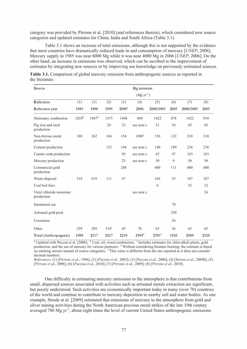
category was provided by Pirrone et al. [2010] (and references therein), which considered new source categories and updated estimates for China, India and South Africa (Table 3.1).

Table 3.1 shows an increase of total emissions, although this is not supported by the evidence that most countries have dramatically reduced trade in and consumption of mercury [UNEP, 2006].Mercury supply in 1985 was near 6000 Mg while it was near 4000 Mg in 2006 [UNEP, 2006]. On the other hand, an increase in emissions was observed, which can be ascribed to the improvement of estimates by integrating new sources or by improving our knowledge on previously estimated sources.

Table 3.1. Comparison of global mercury emission from anthropogenic sources as reported in the literature.

SSource HHg emission

(Mg yr-1)

RReference (1) (1) (2) (3) (4) (5) (6) (7) (8)

RReference year 11985 11990 11995 22000a 22006 22000/2005 22005 22000/2005 22005

Stationary combustion 1024b 1047b 1475 1448 809 1422 878 1422 810

Pig iron and steel production

29 33 see note c 31 54 43 43

Non-ferrous metal production

188 262 166 154 1008c 156 132 310 310

Cement production 132 144 see note c 140 189 236 236

Caustic soda production 93 see note c 65 47 163 163

Mercury production 23 see note c 50 9 50 50

Commercial gold production

248 400 111 400 400

Waste disposal 518 619 111 67 166 35 187 187

Coal bed fires 6 32 32

Vinyl chloride monomerproduction

see note c 24

Intentional use 70

Artisanal gold prod. 350

Cremation 26

Other 259 289 514c 45 76 65 26 65 65

TTotal (Anthropogenic) 11989 22217 22427 22254 11894d 22501e 11926 22909 22320a Updated with Pacyna et al. [2006]; b Coal, oil, wood combustion; c Includes estimates for chlor-alkali plants, gold production, and the use of mercury for various purposes; d Without considering biomass burning; the estimate is based on emitting sectors instead of source categories; e This value is different from the one reported as it does not consider decimal numbers.References: (1) [Pirrone et al., 1996]; (2) [Pacyna et al., 2003]; (3) [Pacyna et al., 2006]; (4) [Streets et al., 2009b]; (5)[Pirrone et al., 2008]; (6) [Pacyna et al., 2010]; (7) [Pirrone et al., 2009]; (8) [Pirrone et al., 2010].

One difficulty in estimating mercury emissions to the atmosphere is that contributions from small, dispersed sources associated with activities such as artisanal metals extraction are significant,but poorly understood. Such activities are economically important today in many (over 70) countries of the world and continue to contribute to mercury deposition to nearby soil and water bodies. As one example, Strode at al. [2009] estimated that emissions of mercury to the atmosphere from gold and silver mining activities during the North American precious metal strikes of the late 19th century averaged 780 Mg yr-1, about eight times the level of current United States anthropogenic emissions.

77

Long term atmospheric mercury measurements at Alert in Canada [Steffen, 2007], at Mace Head in Ireland and at Zingst in Germany [Kock et al., 2005]have demonstrated that natural emissions (including re-emissions) are more significant than believed earlier. Atmospheric gaseous elemental mercury concentrations at these sites were relatively steady from 1995 to 2004, while anthropogenic mercury emissions in Asia (making up more than half of the total anthropogenic mercury emissions) increased at 5 to 7 percent per year [Streets et al., 2005]. Meanwhile, anthropogenic mercuryemissions from North America and Europe stayed constant or deceased slightly during 2000-2004. If direct anthropogenic emissions are most important, this upward trend in mercury emissions from Asia should have been observed to some extent at these global background sites.

In the context of understanding long-range transport of atmospheric mercury, it is important to consider the contribution of the re-emission of previously deposited mercury to net continental fluxes. Typically, re-emission is thought to be about as large as direct anthropogenic inputs, but there is not a great deal of evidence to support this assertion. In regions where historical inputs of mercury to the atmosphere have been large, the re-emission term should be a significant contributor. For example, when Jaffe et al.[2005]inferred the flux of elemental mercury leaving the Asian continent from measurements at Okinawa and the Mt. Bachelor Observatory in Oregon, U.S.A., the value they obtained (1460 Mg yr-1) was about twice as much as the estimated direct mercury emissions from East Asia. Subsequently, while investigating this discrepancy, Shettyetal [2008] estimated that the natural emissions from vegetation, soil, and water surfaces in East Asia could be as high as 834 Mg yr-1,comparable with the direct emissions. More work is needed to reconcile direct anthropogenic mercury emissions, natural or re-emitted mercury, and measured fluxes around the world.

“Native” mercury is emitted naturally from volcanoes and hydrothermal vents. Fluxes from these sources depend on how active each individual source is, and, in the case of volcanoes, whether it is a shield or cinder cone form. Other sources usually considered as “natural”, rather than anthropogenic sources, include area sources such as mercury-rich soils and the ocean surface. In such cases, there may well be a significant contribution from re-emission of previously deposited mercury (a legacy of past emissions and deposition), although this is very difficult to quantify. The contributions from these sources depend greatly on solar irradiation, meteorological conditions and, in the case of top soils, onthe soil humidity. To avoid confusion, the contribution related to the re-emission of historically deposited mercury will be labelled as “mercury re-emission from natural sources”.

Estimates of mercury emissions from natural sources have been based on indirect measurements by advanced techniques (e.g. LIDAR) in naturally enriched soil areas [Ferrara et al.,1992] or by direct measurements of gaseous mercury fluxes [Gustin et al., 1999]. Global and regional assessments have been done by scaling-up field measurements with Global Information System tools and considering external variables controlling fluxes such as temperature, light and precipitation.

Global natural source emissions range from 800 to 5200 Mg yr-1[Gustin et al., 2008; Lindqvist et al., 1991; Mason and Sheu, 2002; Nriagu, 1989; Pirrone et al., 2009; Pirrone et al., 2010; Seigneur et al., 2004] (Table 3.2).

In this case, differences among estimates are primarily due to a progressive inclusion of new sources, better source term estimates following improved information, or a combination of both factors.

Since modelling activities play a key role in efforts to understand the long-range atmospheric transport and fate of mercury, the availability of better information concerning the spatial distribution of emissions can have a powerful influence on models’ outcomes.

78

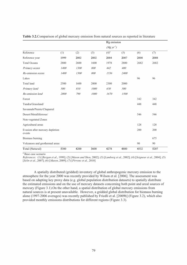
Table 3.2.Comparison of global mercury emission from natural sources as reported in literatureHHg emission

(Mg yr-1)

Reference (1) (2) (3) (4)a (5) (6) (7)

Reference year 11999 22002 22002 22004 22007 22008 22008

Total Oceans 2800 2600 1600 1978 2800 2682 2682

Primary ocean 1400 1300 800 442 400

Re-emission ocean 1400 1300 800 1536 2400

Lakes 96 96

Total land 2500 1600 2000 2300 2000

Primary land 500 810 1000 630 500

Re-emission land 2000 790 1000 1670 1500

Forest 342 342

Tundra/Grassland/

Savannah/Prairie/Chaparral

448 448

Desert/Metalliferrous/

Non-vegetated Zones

546 546

Agricultural areas 128 128

Evasion after mercury depletion events

200 200

Biomass burning 675

Volcanoes and geothermal areas 90 90

TTotal (Natural) 55300 44200 33600 44278 44800 44532 55207a Base case scenarioReferences: (1) [Bergan et al., 1999]; (2) [Mason and Sheu, 2002]; (3) [Lamborg et al., 2002]; (4) [Seigneur et al., 2004]; (5) [Selin et al., 2007]; (6) [Mason, 2009]; (7) [Pirrone et al., 2010]

A spatially distributed (gridded) inventory of global anthropogenic mercury emission to the atmosphere for the year 2000 was recently provided by Wilson et al. [2006]. The assessment was based on adapting key proxy data (e.g. global population distribution datasets) to spatially distribute the estimated emissions and on the use of mercury datasets concerning both point and areal sources of mercury (Figure 3.1).On the other hand, a spatial distribution of global mercury emissions from natural sources is at present unavailable. However, a gridded global distribution for biomass burning alone (1997-2006 averages) was recently published by Friedli et al. [2009b] (Figure 3.2), which also provided monthly emissions distributions for different regions (Figure 3.3).

79

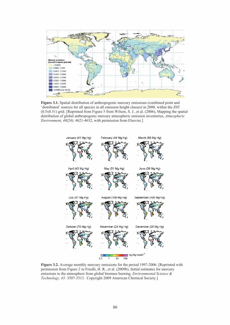
Figure 3.1. Spatial distribution of anthropogenic mercury emissions (combined point and ‘distributed’ sources for all species in all emission height classes) in 2000, within the Z05 (0.5x0.51) grid. [Reprinted from Figure 5 from Wilson, S. J., et al. (2006), Mapping the spatial distribution of global anthropogenic mercury atmospheric emission inventories, AtmosphericEnvironment, 40(24): 4621-4632, with permission from Elsevier.]

Figure 3.2. Average monthly mercury emissions for the period 1997-2006. [Reprinted with permission from Figure 2 in Friedli, H. R., et al. (2009b), Initial estimates for mercury emissions to the atmosphere from global biomass burning, Environmental Science & Technology, 43: 3507-3513. Copyright 2009 American Chemical Society.]

80

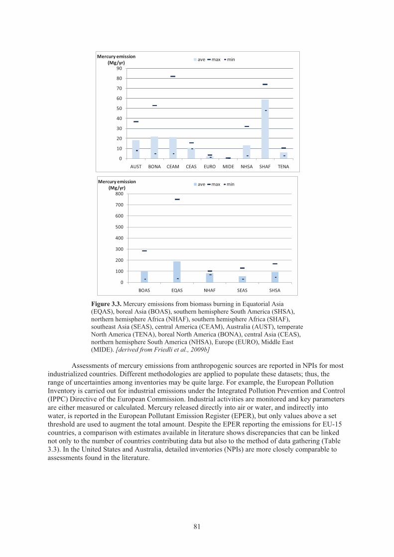
Figure 3.3. Mercury emissions from biomass burning in Equatorial Asia (EQAS), boreal Asia (BOAS), southern hemisphere South America (SHSA), northern hemisphere Africa (NHAF), southern hemisphere Africa (SHAF), southeast Asia (SEAS), central America (CEAM), Australia (AUST), temperate North America (TENA), boreal North America (BONA), central Asia (CEAS), northern hemisphere South America (NHSA), Europe (EURO), Middle East (MIDE). [derived from Friedli et al., 2009b]

Assessments of mercury emissions from anthropogenic sources are reported in NPIs for most industrialized countries. Different methodologies are applied to populate these datasets; thus, the range of uncertainties among inventories may be quite large. For example, the European Pollution Inventory is carried out for industrial emissions under the Integrated Pollution Prevention and Control (IPPC) Directive of the European Commission. Industrial activities are monitored and key parameters are either measured or calculated. Mercury released directly into air or water, and indirectly into water, is reported in the European Pollutant Emission Register (EPER), but only values above a set threshold are used to augment the total amount. Despite the EPER reporting the emissions for EU-15countries, a comparison with estimates available in literature shows discrepancies that can be linked not only to the number of countries contributing data but also to the method of data gathering (Table 3.3). In the United States and Australia, detailed inventories (NPIs) are more closely comparable to assessments found in the literature.

0

10

20

30

40

50

60

70

80

90

AUST BONA CEAM CEAS EURO MIDE NHSA SHAF TENA

Mercury emission (Mg/yr)

ave max min

0

100

200

300

400

500

600

700

800

BOAS EQAS NHAF SEAS SHSA

Mercury emission (Mg/yr)

ave max min

81

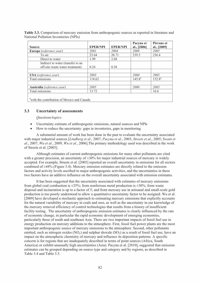
Table 3.3. Comparison of mercury emission from anthropogenic sources as reported in literature and National Pollution Inventories (NPIs)

Source EPER/NPI EPER/NPIPacyna et al., [2006]

Pirrone et al., [2009]

Europe (reference year) 2001 2004 2000 2005To air 23.64 26.71 239.3 236.4Direct to water 1.99 2.68Indirect to water (transfer to an off-site waste water treatment) 0.24 0.38

USA (reference year) 2003 2000 2005Total emissions 118.62 145.8a 152.8a

Australia (reference year) 2005 2000 2005Total emissions 13.72 16.6

awith the contribution of Mexico and Canada

3.3 Uncertainty of assessmentsQuestions/topics:

� Uncertainty estimate of anthropogenic emissions, natural sources and NPIs� How to reduce the uncertainty: gaps in inventories, gaps in monitoring

A substantial amount of work has been done in the past to evaluate the uncertainty associated with major industrial sources [Lindberg et al., 2007; Pacyna et al., 2003; Streets et al., 2005; Swain et al., 2007; Wu et al., 2009; Wu et al., 2006].The primary methodology used was described in the work of Streets et al. [2003].

Although estimates of current anthropogenic emissions for many other pollutants are cited with a greater precision, an uncertainty of ±30% for major industrial sources of mercury is widely accepted. For example, Streets et al. [2005] reported an overall uncertainty in emissions for all sectors combined of ±44% (Figure 3.4). Mercury emission estimates are directly related to the emission factors and activity levels ascribed to major anthropogenic activities, and the uncertainties in these two factors have an additive influence on the overall uncertainty associated with emission estimates.

It has been suggested that the uncertainty associated with estimates of mercury emissions from global coal combustion is ±25%; from nonferrous metal production is ±30%; from waste disposal and incineration is up to a factor of 5; and from mercury use in artisanal and small-scale gold production is too poorly understood to allow a quantitative uncertainty factor to be assigned. Wu et al. [2009] have developed a stochastic approach to estimating mercury emissions that explicitly accounts for the natural variability of mercury in coals and ores, as well as the uncertainty in our knowledge of the mercury removal efficiency of control technologies that results from a history of insufficient facility testing. The uncertainty of anthropogenic emission estimates is clearly influenced by the rate of economic change, in particular the rapid economic development of emerging economies, particularly those of south and southeast Asia. There are two important impacts of fossil fuel use in energy production on mercury additions to the atmosphere. First, fossil fuel power plants are the most important anthropogenic source of mercury emissions to the atmosphere. Second, other pollutants emitted, such as nitrogen oxides (NOx) and sulphur dioxide (SO2) as a result of fossil fuel use, have an impact on the atmospheric chemistry of mercury and influence its deposition patterns. A specific concern is for regions that are inadequately described in terms of point sources (Africa, South America) or exhibit unusually high uncertainties (Asia). Pacyna et al. [2010], suggested that emission estimates can be grouped depending on source type and category and by regions, as described in Table 3.4 and Table 3.5.

82

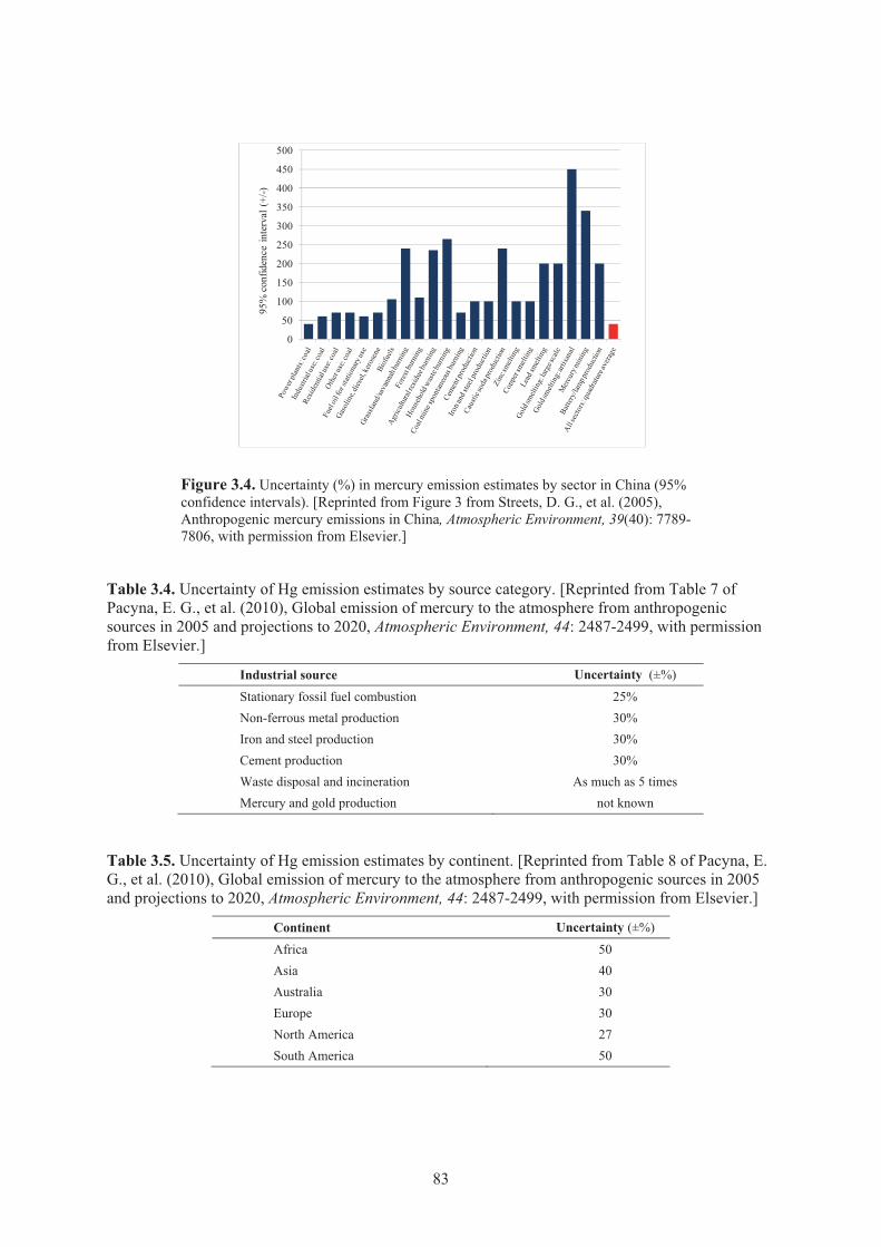
Figure 3.4. Uncertainty (%) in mercury emission estimates by sector in China (95% confidence intervals). [Reprinted from Figure 3 from Streets, D. G., et al. (2005), Anthropogenic mercury emissions in China, Atmospheric Environment, 39(40): 7789-7806, with permission from Elsevier.]

Table 3.4. Uncertainty of Hg emission estimates by source category. [Reprinted from Table 7 of Pacyna, E. G., et al. (2010), Global emission of mercury to the atmosphere from anthropogenic sources in 2005 and projections to 2020, Atmospheric Environment, 44: 2487-2499, with permission from Elsevier.]

Industrial source Uncertainty (±%)

Stationary fossil fuel combustion 25%Non-ferrous metal production 30%Iron and steel production 30%Cement production 30%Waste disposal and incineration As much as 5 times Mercury and gold production not known

Table 3.5. Uncertainty of Hg emission estimates by continent. [Reprinted from Table 8 of Pacyna, E. G., et al. (2010), Global emission of mercury to the atmosphere from anthropogenic sources in 2005 and projections to 2020, Atmospheric Environment, 44: 2487-2499, with permission from Elsevier.]

Continent Uncertainty (±%)

Africa 50 Asia 40 Australia 30 Europe 30 North America 27 South America 50

0

50

100

150

200

250

300

350

400

450

500

95%

conf

iden

ce in

terv

al (

+/-)

83

The uncertainty associated with estimates of mercury emissions from natural sources has not yet been evaluated since global estimates have only recently been done (see above paragraph). Top-down and bottom-up methodologies involve different uncertainties since different factors accumulate to contribute to the final assessment. In the case of biomass burning, some of the inventories are based on scaling from estimates of carbon emissions, which are estimated from ground-based, airborne or remote sensing measurements, providing constraints for CO sources (top-down approach). These assessments are constrained and updated by other independent datasets to better match atmospheric CO concentrations. Even so, these inventories have associated uncertainties, such as representation of CO transport in global chemical transport models, which need to be accounted for. Other inventories are based on carbon emission models and observed site specific emission factors (bottom-upapproach). In this case, the uncertainties in the estimate result from many contributions, including the influence of burn severity, inclusion of measurements of all mercury species, paucity of measurement for all fuel types (especially for grasses, shrubs and agricultural waste products) and uncertainties in the emission factor estimation technique.

The precision and accuracy of estimates of mercury emissions as reported in NPIs is strongly country-dependent and only useful in some cases for global assessments. Few countries give information detailed enough to qualify as expert assessments. Most national inventories provide mercury emission values that are quite different from emissions calculated from emission factors and statistical data on national productivity levels.

3.4 Future emission scenariosQuestions/topics:

� Adopted technologies and best available technologies� Ongoing policies (panels, conventions, regulations, legislations)� Scenarios and uncertainty

The major categories of abatement technologies available to reduce mercury emissions are primarily related to industrial processes, such as power generation.

In the case of coal combustion for power generation, emission control devices are: fabric filters (FFs), electrostatic precipitators (ESPs) and flue-gas conditioning systems (FGCs or scrubbers) [Dabrowski et al., 2008]. Due to the general dominance of gas-phase mercury in flue gases and the very low concentrations of particle-bound mercury, ESPs are relatively ineffective in removing total mercury [U.S. EPA, 1997]. A recent study [U.S. EPA, 2002] shows average mercury reductions of 36% via the use of ESPs. Overall, the use of a default mercury reduction factor of 10% has been recommended for mercury inventory studies [UNEP, 2005]. Fabric filters are more effective in trapping fine particles and appear to be more effective in reducing gaseous mercury emissions. Measured mercury reductions range from 8 to 90% [Meij, 1991; Pavlish et al., 2003; U.S. EPA, 1997;2002]. A default mercury reduction factor of 50% for fabric filters has been recommended for inventory calculations [UNEP, 2005]. Flue-gas conditioning systems that remove gaseous acidic SO2and NOx gases can also be very beneficial in reducing mercury emissions, at least those of divalent mercury. Wet flue-gas desulfurization (FGD) systems remove SO2 from flue-gas by oxidising it when an aqueous solution of slaked lime or limestone is introduced into the stack. In addition, the relatively low temperatures in wet FGDs results in condensation of gaseous mercury, removing it from the flue gas [Pacyna et al., 2006]. Wet FGDs, in combination with particulate matter control devices, have reduced atmospheric mercury emissions by between 22.6 and 95% [Pavlish et al., 2003; U.S. EPA,1997; 2002]. A default reduction factor of 50% has been recommended for use in inventory calculations [UNEP, 2005].

The main technologies applied for chlor-alkali production are mercury, diaphragm, andmembrane cell electrolysis. These mainly use sodium chloride (NaCl) as feed or, to a lesser extent, potassium chloride (KCl) for the production of potassium hydroxide. Switching from mercury cells to diaphragm and membrane cells is considered the best available control technology [IPPC, 2001].

84

Dusts from the production of cement contain trace amounts of metals such as arsenic, cadmium and mercury. As a consequence, abatement strategies for metals from those sources are accommodated by particulate removal measures. One way to minimise mercury emissions is to lower the exhaust temperature. Non-volatile elements remain within the process and exit the kiln as part of the cement clinker composition. When high concentrations of volatile metals (especially mercury) occur, adsorption on activated carbon is an option [IPPC, 2007].

Sedimentation – or clarification – of suspended particles and floating material by gravitational settling from municipal waste removes sludge. When the particles cannot be separated by simple gravitational means (e.g., they are too small, their density is too close to that of water, or they form colloids), special chemicals are added to cause the solids to settle. These chemicals cause the destabilisation of colloidal and small suspended particles (e.g., clay, silica, iron, heavy metals, dyes, organic solids, and oil in waste water), emulsions entrapping solids (coagulation), and/or the agglomeration of these particles to flocs large enough to settle (flocculation). Coagulation can remove 70% of inorganic mercury. [IPPC, 2003]

Mercury enters the gas phase directly during the sintering process in iron and steel plants. Emission levels depend on the mercury content of the sinter feed, but are normally very low. In the case of iron ore, the relevant amounts of mercury emissions are considerable. Well-designed and carefully operated ESPs, plus fine wet scrubbing systems are applied as abatement techniques [IPPC,2008].

Stack emissions of mercury from non-ferrous metal smelters are largely related to dust loading. The minimisation of dust emissions will therefore also minimise possible mercury emissions. This holds true for this source sector for all metals of concern. Uniquely among metals, the high vapour pressure of elemental mercury may cause gaseous emissions which are not correlated with dust loading. In view of the implementation of a European policy on mercury emissions, there is a need for research on the emissions of mercury from smelting processes in general and, more specifically, from (non-ferrous) foundries [IPPC, 2005]. Metal smelters (for zinc, lead, etc.) have been shown to be large emitters of ore-associated mercury in developing countries. Small, older installations may have no effective mercury control technology at all. Larger, more modern facilities may have acid plants to remove excess sulphur, so that these plants can also reduce mercury emissions to the atmosphere. Recently, advanced direct leaching processes, such as the Finnish Outotec process [Haakana et al., 2008], have shown great potential for efficient mercury capture during smelting.

Mercury is an important heavy metal associated with crude oil deposits and is emitted to some extent with both extraction and refining processes. A portion of the mercury may react with equipment surfaces or deposit on catalysts in the reactors of refining or processing plants. Mercury, if present in the feedstock of the refinery, will concentrate in elevated sections of such facilities, particularly coolers, due to its relatively high vapour pressure. Liquefied petroleum gas, tops and naphtha coolers are most likely involved. ESP or fabric filters are the most common BACTs to reduce mercury release to the environment [IPPC, 2003].

For municipal waste collection, processing, and incineration facilities, mercury can partition to different waste streams. The waste collection and pre-treatment systems utilised can have a great impact on the type and nature of waste that will finally be received at the incinerator (e.g., mixed municipal waste or refuse-derived fuel) and, hence, on the type of incinerator that is best suited to the waste. Provision for the separate collection of various fractions of household waste can have a large influence on the average composition of the waste received at the municipal solid waste incinerator.For example, the separate collection of some batteries and dental amalgam can significantly reduce mercury inputs to the incineration plant [IPPC, 2006].

When pre-treatment systems are unavailable, special treatment (neutralisation, precipitation of heavy metals) is used to remove volatile mercury compounds, such as HgCl2, by condensation when the flue gas is cooled, and dissolved in the scrubber effluent.

85

Mercury abatement technologies for other sources that emit mercury to the atmosphere are not available either technologically or economically. This includes emissions from small coal combustion systems, including residential coal combustion, small brick kilns, etc., especially in developing countries. Also, because forest fires and other vegetation burning are now known to be large contributors to atmospheric mercury production, it is worth considering forest and agricultural management strategies for mercury abatement.

Only two studies thus far have attempted to forecast future global emissions of mercury to the atmosphere, namely, estimates for 2020 under three emission scenarios [AMAP/UNEP, 2008; Pacyna et al., 2010] and estimates for 2050 under four IPCC SRES scenarios [Streets et al., 2009b]. More such work needs to be done to refine our understanding of the likely pathways of future mercury emissions.

In the first of these studies, emission scenarios were developed on the basis of information on emission factors elaborated within the EU projects ESPREME (http://espreme.ier.uni-stuttgart.de) and DROPS (http://drops.nilu.no) and statistical data on the production of industrial goods, consumption of raw materials, and incineration of wastes [AMAP/UNEP, 2008].

For the target year of 2020, three emissions scenarios were considered:

� The “Status Quo” (SQ) scenario assumes that current patterns, practices and uses that result in mercury emissions to air will continue. Economic activity is assumed to increase, including in those sectors that produce mercury emissions, but emission control practices remain unchanged.

� The “Extended Emissions Control” (EXEC) scenario assumes economic progress at a rate dependent on the future development of industrial technologies and emissions control technologies; that is, mercury-reducing technology currently generally employed throughout Europe and North America would be implemented elsewhere. It further assumes that emissions control measures currently implemented or committed to in Europe to reduce mercury emissions to air or water would be implemented around the world. These include certain measures adopted under the LRTAP Convention, EU Directives, and also agreements to meet IPCC Kyoto targets on reduction of greenhouse gases causing climate change (which will cause reductions in mercury emissions).

� The “Maximum Feasible Technological Reduction” (MFTR) scenario assumes implementation of all available solutions/measures, leading to the maximum degree of reduction of mercury emissions and its discharges to any environment; cost is taken into account but only as a secondary consideration.

Assumptions for mercury emission control scenarios are reported in Table 3.6 for large combustion plants, iron and steel production, cement production and the chlor-alkali industry. Four scenarios are described: "BAU+C 2010” (Business as Usual, with a component related to actions to address climate change), “BAU+C 2020” and MFTR scenarios for 2010 and 2020. As described in AMAP/UNEP (2008), the “BAU+C” scenario is the same as the “EXEC” scenario.

In the second of these forecasting studies [Streets et al., 2009b], the IPCC SRES was used to define future pathways of energy and economic development around the world and to assess mercury emissions in 2050. The authors developed estimates of combustion-related energy and fuel use, disaggregated among many different sector/fuel/technology options for 17 world regions. Parameterization of the model consisted of the mercury content of fuels and the efficiency of mercury removal by FGD. Initial release rate, ash retention efficiency, capture efficiency, etc., were considered in the development of the 2050 emissions under A1B, A2, B1, and B2 IPCC scenarios. Data on the expected application of FGD to coal-fired power plants around the world was parameterized on the basis of SO2 emission forecasts. The assumptions are listed by world region in Table 3.7. Mercury emissions forecasts for these two studies in 2020 and 2050 are reported in Table 3.8.

86

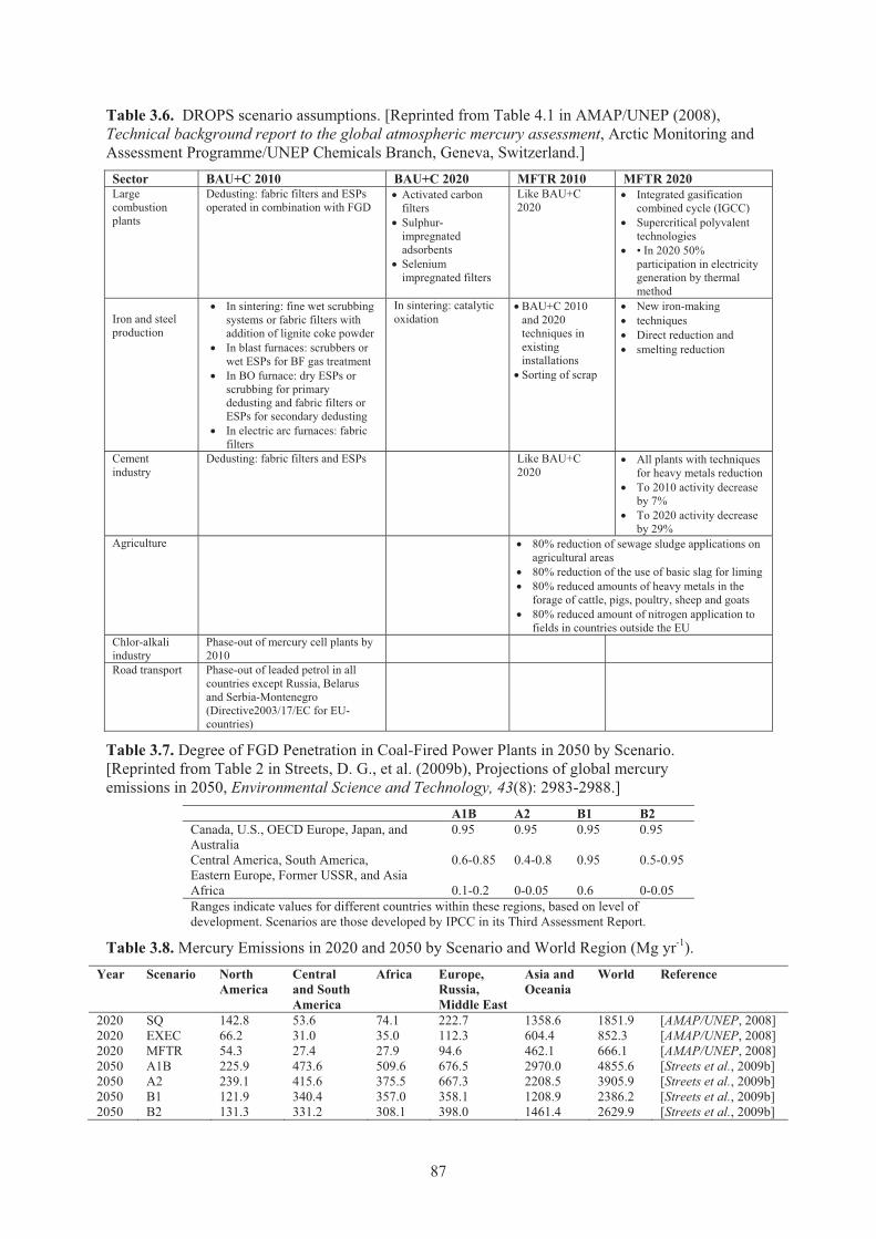
Table 3.6. DROPS scenario assumptions. [Reprinted from Table 4.1 in AMAP/UNEP (2008), Technical background report to the global atmospheric mercury assessment, Arctic Monitoring and Assessment Programme/UNEP Chemicals Branch, Geneva, Switzerland.]Sector BAU+C 2010 BAU+C 2020 MFTR 2010 MFTR 2020Large combustion plants

Dedusting: fabric filters and ESPs operated in combination with FGD

� Activated carbon filters

� Sulphur-impregnated adsorbents

� Selenium impregnated filters

Like BAU+C 2020

� Integrated gasification combined cycle (IGCC)

� Supercritical polyvalent technologies

� • In 2020 50% participation in electricity generation by thermal method

Iron and steel production

� In sintering: fine wet scrubbing systems or fabric filters with addition of lignite coke powder

� In blast furnaces: scrubbers or wet ESPs for BF gas treatment

� In BO furnace: dry ESPs or scrubbing for primary dedusting and fabric filters or ESPs for secondary dedusting

� In electric arc furnaces: fabric filters

In sintering: catalytic oxidation

� BAU+C 2010 and 2020 techniques in existing installations

� Sorting of scrap

� New iron-making� techniques� Direct reduction and� smelting reduction

Cement industry

Dedusting: fabric filters and ESPs Like BAU+C 2020

� All plants with techniques for heavy metals reduction

� To 2010 activity decrease by 7%

� To 2020 activity decrease by 29%

Agriculture � 80% reduction of sewage sludge applications on agricultural areas

� 80% reduction of the use of basic slag for liming� 80% reduced amounts of heavy metals in the

forage of cattle, pigs, poultry, sheep and goats� 80% reduced amount of nitrogen application to

fields in countries outside the EUChlor-alkali industry

Phase-out of mercury cell plants by 2010

Road transport Phase-out of leaded petrol in all countries except Russia, Belarus and Serbia-Montenegro (Directive2003/17/EC for EU-countries)

Table 3.7. Degree of FGD Penetration in Coal-Fired Power Plants in 2050 by Scenario. [Reprinted from Table 2 in Streets, D. G., et al. (2009b), Projections of global mercury emissions in 2050, Environmental Science and Technology, 43(8): 2983-2988.]

A1B A2 B1 B2Canada, U.S., OECD Europe, Japan, andAustralia

0.95 0.95 0.95 0.95

Central America, South America,Eastern Europe, Former USSR, and Asia

0.6-0.85 0.4-0.8 0.95 0.5-0.95

Africa 0.1-0.2 0-0.05 0.6 0-0.05Ranges indicate values for different countries within these regions, based on level of development. Scenarios are those developed by IPCC in its Third Assessment Report.

Table 3.8. Mercury Emissions in 2020 and 2050 by Scenario and World Region (Mg yr-1).Year Scenario North

AmericaCentral and South America

Africa Europe, Russia, Middle East

Asia and Oceania

World Reference

2020 SQ 142.8 53.6 74.1 222.7 1358.6 1851.9 [AMAP/UNEP, 2008]2020 EXEC 66.2 31.0 35.0 112.3 604.4 852.3 [AMAP/UNEP, 2008]2020 MFTR 54.3 27.4 27.9 94.6 462.1 666.1 [AMAP/UNEP, 2008]2050 A1B 225.9 473.6 509.6 676.5 2970.0 4855.6 [Streets et al., 2009b]2050 A2 239.1 415.6 375.5 667.3 2208.5 3905.9 [Streets et al., 2009b]2050 B1 121.9 340.4 357.0 358.1 1208.9 2386.2 [Streets et al., 2009b]2050 B2 131.3 331.2 308.1 398.0 1461.4 2629.9 [Streets et al., 2009b]

87

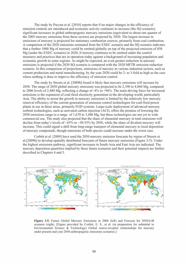
The study by Pacyna et al. [2010] reports that if no major changes in the efficiency of emission controls are introduced and economic activity continues to increase (the SQ scenario), significant increases in global anthropogenic mercury emissions (equivalent to about one quarter of the 2005 mercury emissions from these sectors) are projected by 2020. The largest increase in emissions of mercury is projected for stationary combustion sources, primarily from coal combustion. A comparison of the 2020 emissions estimated from the EXEC scenario and the SQ scenario indicates that a further 1000 Mg of mercury could be emitted globally on top of the projected emission of 850 Mg (under the EXEC scenario) in 2020, if mercury continues to be emitted under the control measures and practices that are in operation today against a background of increasing population and economic growth in some regions. As might be expected, an even greater reduction in mercury emissions is projected if the 2020 SQ scenario is compared with the 2020 MFTR emission reduction scenario. In this comparison of projections, emissions of mercury in various industrial sectors, such as cement production and metal manufacturing, by the year 2020 could be 2- to 3-fold as high as the case where nothing is done to improve the efficiency of emission control.

The study by Streets et al. [2009b] found it likely that mercury emissions will increase by 2050. The range of 2050 global mercury emissions was projected to be 2,390 to 4,860 Mg, compared to 2006 levels of 2,480 Mg, reflecting a change of -4% to +96%. The main driving force for increased emissions is the expansion of coal-fired electricity generation in the developing world, particularly Asia. The ability to arrest the growth in mercury emissions is limited by the relatively low mercury removal efficiency of the current generation of emission control technologies for coal-fired power plants in use in those areas, primarily FGD systems. Large-scale deployment of advanced mercury sorbent technologies, such as activated carbon injection (ACI), offers the promise of lowering the 2050 emissions range to a range of 1,670 to 3,480 Mg, but these technologies are not yet in wide commercial use. The study also projected that the share of elemental mercury in total emissions will decline from today’s levels of ~65% to ~50-55% by 2050, while the share of divalent mercury will increase. This could signal a shift from long-range transport of elemental mercury to local deposition of mercury compounds, though emissions of both species could increase under the worst case.

Corbitt et al. [2009] have used the 2050 mercury emission forecasts by region of Streets et al.[2009b] to develop spatially distributed forecasts of future mercury emissions (Figure 3-5). Under the highest emissions pathway, significant increases in South Asia and East Asia are indicated. The mercury deposition quantities implied by these future scenarios and their potential impacts are further described in Chapters 4 and 5.

Figure 3.5. Future Global Mercury Emissions in 2006 (left) and Forecast for 2050A1B scenario (right). [Figure provided by Corbitt, E. S., et al. (in preparation for submittal to Environmental Science & Technology) Global source-receptor relationships for mercury under present and year 2050 anthropogenic emissions scenarios.]

88

3.5 Policy implicationsQuestions/topics:

� Forcing emission reduction� Supporting abatement policies� Improving abatement technologies

Policies to eliminate mercury uses, reduce the export and trade of mercury, and significantly reduce mercury exposures at the local, national, and international levels have been adopted by several countries. Strategies have been developed from global to local levels.

For example, the World Health Organization issued a policy paper in 2005 calling for short, medium and long-term measures to substitute safer alternatives for mercury-based medical devices. In early 2008 the Medical Academic and Scientific Community Organization, a non-profit organization providing technical and community support to Harvard Medical Institutions in Boston, issued a detailed analysis of substitution technologies for medical devices employing mercury. Similarly, the World Medical Association passed a resolution in 2008 calling for the substitution of safer alternatives for mercury-based medical devices.

At a regional level, the European Commission proposed to ban mercury in measuring devices as part of a wider mercury strategy tabled in January 2005. Recently, European Union (EU) ministers supported a proposal to ban all exports of mercury by 2011. The Commission followed up with a proposal for a regulation in that vein.

At the national level, the Philippines issued an Administrative Order in 2008 calling for the phase-out of mercury-based medical devices across the country by 2010; Taiwan has banned mercury thermometers; the United States health care sector has virtually phased out mercury-based medical devices, making it nearly impossible to purchase a mercury thermometer in the United States today; Sweden, the Netherlands and Denmark have successfully phased out all mercury-based medical devices, including sphygmomanometers; and since the 1980s, Cuba has implemented a national policy of replacing its mercury sphygmomanometers with aneroid devices purchased from China.

State and provincial governments have also initiated mercury phase-out policies. The Province of Kwa Zulu Natal, South Africa has issued and is implementing directives banning the purchase of mercury thermometers and sphygmomanometers. In the United States, 30 states have banned mercury thermometers and more than one-third of the United States population is covered by state laws restricting or banning mercury blood pressure devices. In August 2007, the Provincial Government of Chaco, in northern Argentina, committed to making all of the 8 hospitals and 296 clinics and health centres under its jurisdiction mercury-free.

In addition, a number of electronics companies have taken steps to reduce or eliminate the use of mercury as a primary or secondary component in manufacturing or products. For example, by autumn 2009, Apple Inc. had removed mercury from the production line for its flat-screen monitors, some of its portable computers, and its personal electronics lines. This continued into the introduction of new products in April 2010.

There are both well-established and emerging technologies for removing mercury from combustion streams emitting to the atmosphere, the primary starting point for long-range transport. Which technologies are most effective depend on a number of factors, including stack or exhaust temperature, co-pollutants involved, speciation of mercury, mercury concentrations in the exhaust gases, water vapour content, etc. Generally, divalent mercury as well as particulate-bound forms are captured in large part by “scrubbers” or flue gas desulfurization equipment, and in part by particulate capture equipment, especially baghouses or electrostatic filters. Elemental mercury is much more difficult to capture, although recent tests and deployments of activated carbon injection installations (with and without added halogens, primarily bromine) have shown very high effectiveness, often exceeding ninety percent capture rates. To date, these maximum capture rates are highly variable among power plant combustion configurations, coal quality, and relative amount of sorbent injected into the flue gas stream. Generally, for a given sorbent rate, capture is much more efficient for

89

bituminous than for subbituminous or lignite coals; similarly, brominated carbon injection is, overall, more capture-efficient than non-brominated injection [Srivastava et al., 2006]. Since long-rangeatmospheric transport is the primary concern in uncontrolled mercury exchange among nations, the control of the less easily removed elemental form is a key element of abatement policies being considered.

Is dilution the solution to pollution, in the case of mercury? In other words, is it feasible and advisable for nations to minimize cross-boundary contributions by placing contributing sources in the “upwind” region of their jurisdictions (with respect to prevailing large-scale wind patterns)? Generally, the benefits of such constraints are limited by the fraction of global anthropogenic emissions represented by the sources in question: no steps short of mercury emissions reduction or controls will reduce contributions to deposition below the fractional contribution to global emissions. Additionally, movement along the axis of the dominant wind direction will not lessen contributions that are advected in secondary directions initially but eventually captured by large-scale centres of action. Furthermore, frequent source-region episodes of highly stable boundary layer conditions will allow movement of mercury emissions into geostrophic wind patterns uninterrupted by the additional distance upwind from eventual receptor regions.

3.6 Findings, gaps and recommendations3.6.1. Findings

The following findings rise up in the assessment of mercury emissions from both anthropogenic and natural sources.

1. Introduction

In the last years a number of concerted initiatives have been undertaken at a global scale to assess the current state of our knowledge on atmospheric mercury emissions, transport and deposition to and evasion from terrestrial and aquatic ecosystems. These global assessments have improved our information on mercury emissions from both anthropogenic sources and natural sources, provided new global and regional assessments of atmospheric mercury transport and deposition patterns, highlighted major issues related to the definition of source-receptor relationships and given new scenarios of projected future mercury emissions.

2. Emissions

Major emission sources encompass both anthropogenic and natural sources. The origin of mercury emissions from anthropogenic sources can be referred to as the intentional use of mercury or a by-product of processes. Mercury released from natural sources or reservoirs involves both releases of native mercury and the re-emission of mercury due to previous deposition processes. Anthropogenic emissions are believed to be in the range of 1900 to 2900 Mg yr-1 while natural source emission estimates range from 4600 to 5300 Mg yr-1.

3. Uncertainty of assessments

Mercury emission estimates are closely related to derived emission factors and estimated activity levels of major human activities; these have great influences on the uncertainty associated with emission estimates.

4. Future emission scenarios

Only two studies have attempted to forecast future global emissions of mercury to the atmosphere, namely, estimates for 2020 under three emission scenarios and estimates for 2050 under four IPCC SRES scenarios. The study by Pacyna et al. [2010] reports that if no major changes in the efficiency of emission controls are introduced and economic activity continues to increase (the SQ scenario), significant increases in global anthropogenic mercury emissions (equivalent to about one quarter of the 2005 mercury emissions from these sectors) are projected by 2020. The largest increase

90

in emissions of mercury is projected for stationary combustion sources, primarily from coal combustion. As might be expected, an even greater reduction in mercury emissions is projected if the 2020 SQ scenario is compared with the 2020 MFTR emission reduction scenario. In this comparison of projections, emissions of mercury in various industrial sectors, such as cement production and metal manufacturing by the year 2020 could be 2- to 3-fold as high as the case where nothing is done to improve the efficiency of emission control. The study by Streets et al. [2009b]found it likely that mercury emissions will increase by 2050. The range of 2050 global mercury emissions was projected to be 2,390-4,860 Mg, compared to 2006 levels of 2,480 Mg, reflecting a change of -4% to +96%. The main driving force for increased emissions is the expansion of coal-fired electricity generation in the developing world, particularly Asia. The ability to arrest the growth in mercury emissions is limited by the relatively low mercury removal efficiency of the current generation of emission control technologies for coal-fired power plants (FGD).

5. Policy implications

Policies to eliminate mercury uses, reduce the export and trade of mercury, and significantly reduce potential mercury exposures at the local, national, and international levels have been adopted by several countries. Strategies have been developed from global to local levels.

3.6.2. GapsAlthough the mercury emission data presented above are the best data currently available,

improvements can be made in their accuracy and completeness through the following efforts:

At the country level

1. Measurement programs can be organized to improve the quality of emission factors for major source categories, particularly for fossil fuel combustion in large combustion plants (over 350 Megawatts), waste incinerators, non-ferrous metal smelters, cement kilns and iron and steel foundries. These measurements may include:- Mercury concentrations in flue gases before and after application of emission control

equipment; and- Mercury content in raw materials, such as coal, oil, natural gas, ores, limestone, etc. and

various wastes, including hazardous, hospital, industrial and municipal wastes.

2. Collection of information and reporting to UNEP should be more complete. The UNEP Toolkit should be employed and more accurate data and information should be provided concerning:- industrial technologies for production of energy and industrial goods, such as chlor-alkali,

ferrous and non-ferrous metals, and cement;- type and efficiency of mercury emission control measures;- changes in industrial technologies and emission control measures over time; and - changes in various uses of mercury, particularly in chlor alkali plants, vinyl chloride

monomer, etc.

3. Collection and reporting of information needed for spatial distribution of mercury emissions with a focus on:- geographical location of major point sources, emission quantities, geometric height of the

source, temperature of the flue gases; and- chemical and physical speciation of emitted mercury.

At the international level

4. Improvement in the accuracy and completeness of emission factor data available in emission factor guidebooks, through inclusion of information from individual countries.

5. Improvement of information on statistical data for the consumption of raw materials and production of industrial goods along major fuel types and industrial technologies.

91

6. Improvement of existing toolkits through collection of information available from various Decision Support Systems (DSS), e.g., the DSS developed within various EU projects to support implementation of the EU legislation.

3.6.3 Recommendations

1. Introduction

Use the appropriate language to describe mercury emissions as defined in the terminology and glossary Annexes. Establish a common framework of emission categories to enhance inter-comparison among different assessments.

2. Emissions

The most important recommendations are to consider (1) natural sources as larger and uncontrollable contributors to mercury emission to the atmosphere and (2) the large uncertainty of anthropogenic emission estimates, as several undiscovered new emission sources have never been considered.

3. Uncertainty of assessments

For sectors emitting mercury due to intentional use, information on the mercury life cycle should be added to the emission estimates based on mercury consumption. There is a need to take into account that parts of the consumed mercury are exported to other regions. Dynamic material flow modelling is needed to account for accumulations in products, production systems and waste streams. Thus, more research is needed on emissions from product use and disposal. In addition, estimates of source-category mercury emissions should always be stated as a central, or best, estimate accompanied by relative (percent) or absolute uncertainty range. It should be understood, unless stated otherwise, that these uncertainty estimates are usually based on expert judgment rather than a formal uncertainty analysis.

4. Future emission scenarios

More work needs to be done to refine our understanding of the likely pathways of future mercury emissions. A major development in information is necessary for predicting mercuryemissions in the future. Information presented in this report should be regarded as a first step towards achieving mercury emission scenarios. The improvement in developing scenarios for future emissions of mercury can be made through the following efforts:

At the country level

1. Information should be improved on economic indices describing future development of economies in individual countries, such as indices of the industrial production growth, use of fuels for electricity and heat production, etc.

2. Information can be improved and made available on national plans for:- use of mercury in various industrial and commercial sectors;- change of fuel types and amounts to meet future energy plans in individual countries;- change of industrial technologies to meet future energy and industrial good demands in

individual countries; and - change of emission control technology types and mercury control efficiencies in

individual countries.

At the international level

3. Information on targets of emission reductions within various international conventions, emission reduction agreements and protocols can be improved and employed to develop emission scenarios for various regions and the whole globe.

92

4. Information on emission scenarios for other pollutants relevant for the development of mercury emission scenarios should be collected, e.g. for greenhouse gases and acid rain generation agents. This information should be analyzed with the purpose of using it in development of mercury emission scenarios.

Improvement of historical trends of mercury emissions in various geographical regions should be made in order to assess indicators for the development of emission scenarios, particularly for sources, such as artisanal gold production and other uses of mercury in commerce.

5. Policy implications

There is a need for information in order to refine and revise technical specifications of emitting sectors either as country or region averages or on an individual plant basis. Improved information is also needed on current and planned implementation of control measures for air pollutants, as well as information on restructuring and modernization of the sectors. Although there have been significant national and local governmental efforts to cease the use of mercury in commercial and medical products and processes, little work has been undertaken to evaluate human exposure to these sources of mercury, nor to the waste disposal chain-of-custody of discarded mercury-laden material. The outright ban on mercury in products follows a “precautionary principle” and is thus a conservative approach to management of mercury in commerce.

References AMAP/UNEP (2008), Technical background report to the global atmospheric mercury assessment, 159 pp,

Arctic Monitoring and Assessment Programme/UNEP Chemicals Branch, Geneva, Switzerland.Bergan, T., et al. (1999), Mercury in the global troposphere: a three-dimensional model study, Atmospheric

Environment, 33(10): 1575-1585. Bullock, O. R., and L. Jaeglé (2009), Importance of a global scale approach to using regional models in the

assessment of source-receptor relationships for mercury, in Mercury Fate and Transport in the Global Atmosphere: Emissions, Measurements, and Models, edited by N. Pirrone and R. P. Mason, 503-517 pp., Springer, New York.

Corbitt, E. S., et al. (2009), Global source-receptor relationships for mercury under present and year 2050 anthropogenic emissions scenarios, American Geophysical Union, Fall Meeting 2009, 90(52).

Dabrowski, J. M., et al. (2008), Anthropogenic mercury emissions in South Africa: Coal combustion in power plants, Atmospheric Environment, 42: 6620-6626.

Dastoor, A. P., and D. Davignon (2009), Global mercury modeling at Environment Canada, in Mercury Fate and Transport in the Global Atmosphere: Emissions, Measurements, and Models, edited by N. Pirrone and R. P. Mason, 519-531 pp., Springer, New York.

Ebinghaus, R., et al. (2002), Long-term measurements of atmospheric mercury at Mace Head, Irish west coast, between 1995 and 2001, Atmospheric Environment, 36(34): 5267-5276.

Ferrara, R., et al. (1992), Mercury emissions into the atmosphere from a chlor-alkali complex measured with the lidar technique, Atmospheric Environment, 26(7): 1253-1258.

Friedli, H. R., et al. (2009a), Mercury emissions from global biomass burning: spatial and temporal distribution, in Mercury Fate and Transport in the Global Atmosphere: Emissions, Measurements, and Models,edited by N. Pirrone and R. P. Mason, 193-221 pp., Springer, New York.

Friedli, H. R., et al. (2009b), Initial estimates for mercury emissions to the atmosphere from global biomass burning, Environmental Science & Technology, 43(10): 3507-3513.

Gustin, M. S., et al. (1999), Nevada storms project: Measurement of mercury emissions from naturally enriched surfaces, Journal of Geophysical Research, 104(D17): 21831-21844.

Gustin, M. S., et al. (2008), An update on the natural sources and sinks of atmospheric mercury, Applied Geochemistry, 23(3): 482-493.

Haakana, T., et al. (2008), Outotec direct leaching application in China, Journal of Southern African Institute of Mining and Metallurgy, 108: 245-251.

93

Hedgecock, I. M., and N. Pirrone (2001), Mercury and photochemistry in the marine boundary layer- modelling studies suggest the in situ production of reactive gas phase mercury, Atmospheric Environment, 35(17): 3055-3062.

Hedgecock, I. M., et al. (2005), Mercury chemistry in the MBL: Mediterranean case and sensitivity studies using the AMCOTS (Atmospheric Mercury Chemistry over the Sea) model, Atmospheric Environment,39(38): 7217-7230.

Hedgecock, I. M., et al. (2008), Chasing quicksilver northward: mercury chemistry in the Arctic troposphere, Environmental Chemistry, 5(2): 131-134.

IPPC (2001), Reference Document on Best Available Techniques in the Chlor-Alkali Manufacturing Industry, 178 pp, Integrated Pollution Prevention and Control (IPPC), European Commission, Seville, Spain. ftp://ftp.jrc.es/pub/eippcb/doc/cak_bref_1201.pdf

IPPC (2003), Reference Document on Best Available Techniques for Mineral Oil and Gas Refineries, 624 pp, Integrated Pollution Prevention and Control (IPPC), European Commission, Seville, Spain. http://eippcb.jrc.es/reference/ref.html

IPPC (2005), Reference Document on Best Available Techniques in the Smitheries and Foundries Industry, 397 pp, Integrated Pollution Prevention and Control (IPPC), European Commission, Seville, Spain. ftp://ftp.jrc.es/pub/eippcb/doc/sf_bref_0505.pdf

IPPC (2006), Reference Document on the Best Available Techniques for Waste Incineration, 638 pp, Integrated Pollution Prevention and Control (IPPC), European Commission, Seville, Spain. ftp://ftp.jrc.es/pub/eippcb/doc/wi_bref_0806.pdf

IPPC (2007), Reference Document on Best Available Techniques in the Cement and Lime Manufacturing Industries, Integrated Pollution Prevention and Control (IPPC), European Commission, Seville, Spain. http://eippcb.jrc.es/reference/ref.html

IPPC (2008), Best Available Techniques Reference Document on the Production of Iron and Steel, 594 pp, Integrated Pollution Prevention and Control (IPPC), European Commission, Seville, Spain. ftp://ftp.jrc.es/pub/eippcb/doc/isp_d2_0709.pdf

Jaeglé, L., et al. (2009), The Geos-Chem Model, in Mercury Fate and Transport in the Global Atmosphere: Emissions, Measurements, and Models, edited by N. Pirrone and R. P. Mason, 533-545 pp., Springer, Dordrecht.

Jaffe, D. A., et al. (2005), Export of atmospheric mercury from Asia, Atmospheric Environment, 39(17): 3029-3038.

Jung, G., et al. (2009), The ECHMERIT model, in Mercury Fate and Transport in the Global Atmosphere: Emissions, Measurements, and Models, edited by N. Pirrone and R. P. Mason, 547-569 pp., Springer, New York.

Kock, H. H., et al. (2005), Comparison of long-term trends and seasonal variations of atmospheric mercury concentrations at the two European coastal monitoring stations Mace Head, Ireland, and Zingst, Germany, paper presented at Atmospheric Environment, 7th International Conference on Mercury as a Global Pollutant, 2005/12.

Lamborg, C. H., et al. (2002), A non-steady-state compartmental model of global-scale mercury biogeochemistry with interhemispheric atmospheric gradients, Geochimica et Cosmochimica Acta,66(7): 1105-1118.

Lindberg, S. E., et al. (2002), Dynamic flux chamber measurement of gaseous mercury emission fluxes over soils: Part 2 - effect of flushing flow rate and verification of a two-resistance exchange interface simulation model, Atmospheric Environment, 36(5): 847-859.

Lindberg, S. E., et al. (2007), A synthesis of progress and uncertainties in attributing the sources of mercury in deposition, AMBIO: A Journal of the Human Environment, 36(1): 19-32.

Lindqvist, O., et al. (1991), Mercury in the Swedish environment: Recent research on causes, consequences and corrective methods, Water, Air, and Soil Pollution, 55(1-2): xi-261.

Mason, R. P., et al. (2001), Mercury in the Atlantic Ocean: Factors controlling air-sea exchange of mercury and its distribution in the upper waters, Deep Sea Research, Part II: Topical Studies in Oceanography,48(13): 2829-2853.

94

Mason, R. P., and G.-R. Sheu (2002), Role of the ocean in the global mercury cycle, Global Biogeochemical Cycles, 16(4): 1093-1107.

Mason, R. P. (2009), Mercury emissions from natural processes and their importance in the global mercury cycle, in Mercury Fate and Transport in the Global Atmosphere: Emissions, Measurements, and Models, edited by N. Pirrone and R. P. Mason, 173-191 pp., Springer, Dordrecht.

Meij, R. (1991), The fate of mercury in coal-fired power plants and the influence of wet flue-gas desulphurisation, Water, Air, and Soil Pollution, 56: 21-33.

Nriagu, J. O., and J. M. Pacyna (1988), Quantitative assessment of worldwide contamination of air, water and soils by trace metals, Nature, 333(12): 134-139.

Nriagu, J. O. (1989), A global assessment of natural sources of atmospheric trace metals, Nature, 338: 47-49. Pacyna, E. G., et al. (2006), Global anthropogenic mercury emission inventory for 2000, Atmospheric

Environment, 40(22): 4048-4063. Pacyna, E. G., et al. (2010), Global emission of mercury to the atmosphere from anthropogenic sources in 2005

and projections to 2020, Atmospheric Environment, 40(20): 2487-2499. Pacyna, J. M., et al. (2003), Mapping 1995 global anthropogenic emissions of mercury, Atmospheric

Environment, 37(S1): 109-117. Pavlish, J. H., et al. (2003), Status review of mercury control options for coal-fired power plants, Fuel

Processing Technology, 82(2-3): 89-165. Pirrone, N., et al. (1996), Regional differences in worldwide emissions of mercury to the atmosphere,

Atmospheric Environment, 30(17): 2981-2987. Pirrone, N., et al. (1998), Historical atmospheric mercury emissions and depositions in North America compared

to mercury accumulations in sedimentary records, Atmospheric Environment, 32(5): 929-940. Pirrone, N., et al. (2003), Dynamic Processes of Mercury Over the Mediterranean Region: results from the

Mediterranean Atmospheric Mercury Cycle System (MAMCS) project, Atmospheric Environment,37(S1): 21-39.

Pirrone, N., and M. Wichmann-Fiebig (2003), Some recommendations on mercury measurements and research activities in the European Union, Atmospheric Environment, 37(S1): 3-8.

Pirrone, N., and K. Mahaffey (2005), Where we Stand on Mercury Pollution and its Health Effects on Regional and Global Scales, in Dynamics of Mercury Pollution on Regional and Global Scales, edited by N. Pirrone and K. Mahaffey, 21 pp., Springer Verlag Publishers, Norwell, MA, U.S.A.

Pirrone, N., et al. (2008), Global mercury emissions to the atmosphere from natural and anthropogenic sources, in Mercury Fate and Transport in the Global Atmosphere: Measurements, models and policy implications, edited by N. Pirrone and R. P. Mason, 1-36 pp., United Nations Environmental Programme.

Pirrone, N., et al. (2009), Global mercury emissions to the atmosphere from natural and anthropogenic sources, in Mercury Fate and Transport in the Global Atmosphere: Emissions, Measurements, and Models,edited by N. Pirrone and R. P. Mason, 3-49 pp., Springer, Dordecht.

Pirrone, N., and R. P. Mason (Eds.) (2009), Mercury Fate and Transport in the Global Atmosphere: Emissions, Measurements, and Models, 637 pp., Springer, New York

Pirrone, N., et al. (2010), Global mercury emissions to the atmosphere from anthropogenic and natural sources, Atmospheric Chemistry and Physics, 10(13): 5951-5964.

Schroeder, W. H., and J. Munthe (1998), Atmospheric mercury--an overview, Atmospheric Environment, 32:809-822.

Seigneur, C., et al. (2004), Global source attribution for mercury deposition in the United States, Environmental Science & Technology, 38(2): 555-569.

Seigneur, C., et al. (2009), The AER/EPRI global chemical transport model for mercury (CTM-HG), in Mercury Fate and Transport in the Global Atmosphere: Emissions, Measurements, and Models, edited by N. Pirrone and R. P. Mason, 589-601 pp., Springer, New York.

Selin, N. E., et al. (2007), Chemical cycling and deposition of atmospheric mercury: Global constraints from observations, Journal of Geophysical Research, 112: D02308.

95

Shetty, S. K., et al. (2008), Model estimate of mercury emission from natural sources in East Asia, AtmosphericEnvironment, 42(37): 8674-8685.

Sprovieri, F., et al. (2002), Intensive atmospheric mercury measurements at Terra Nova Bay in Antarctica during November and December 2000, Journal of Geophysical Research, 107(D23): 4722-4729.

Srivastava, R. K., et al. (2006), Control of mercury emissions from coal-fired electric utility boilers, Environmental Science & Technology, 40(5): 1385-1393.

Steffen, A. (2007), Mercury Measurements at Alert, Ministry of Indian Affairs and Northern Development, Ottawa.

Streets, D. G., et al. (2003), An inventory of gaseous and primary aerosol emissions in Asia in the year 2000, Journal of Geophysical Research, 108(D21): 8809-8831.

Streets, D. G., et al. (2005), Anthropogenic mercury emissions in China, Atmospheric Environment, 39(40): 7789-7806.

Streets, D. G., et al. (2009a), Mercury emissions from coal combustion in China, in Mercury Fate and Transport in the Global Atmosphere: Emissions, Measurements, and Models, edited by N. Pirrone and R. P. Mason, 51-65 pp., Springer, New York.

Streets, D. G., et al. (2009b), Projections of global mercury emissions in 2050, Environmental Science & Technology, 43(8): 2983-2988.

Strode, S., et al. (2009), Impact of mercury emissions from historic gold and silver mining: Global modeling, Atmospheric Environment, 43(12): 2012-2017.

Swain, E. B., et al. (2007), Socioeconomic consequences of mercury use and pollution, Ambio A Journal for the Human Environment, 36(1): 45-61.

Travnikov, O., and I. Ilyin (2009), The EMEP/MSC-E mercury modeling system, in Mercury Fate and Transport in the Global Atmosphere: Emissions, Measurements, and Models, edited by N. Pirrone and R. P. Mason, 571-587 pp., Springer, New York.

U.S. EPA (1997), Mercury study report to congress, U.S. Environmental Protection Agency, Washington, D.C.EPA-452/R-97-007. http://www.epa.gov/mercury/report.htm

U.S. EPA (2002), Control of mercury emissions from coal-fired electric utility boilers, Interim Report including errata dated 3-21-02, 485 pp, National Risk Management Research Laboratory, U.S. Environmental Protection Agency, Research Triangle Park, NC. EPA-600/R-01-109.http://www.epa.gov/nrmrl/pubs/600r01109/600R01109.pdf

UNEP (2005), Toolkit for Identification and Quantification of Mercury Releases, United Nations Environment Programme.

UNEP (2006), Summary of supply, trade and demand information on mercury, Technical Report, Geneva, Switzerland.

Wilson, S. J., et al. (2006), Mapping the spatial distribution of global anthropogenic mercury atmospheric emission inventories, Atmospheric Environment, 40(24): 4621-4632.

Wu, R., et al. (2009), Findings from quality assurance activities in the Integrated Atmospheric Deposition Network, Journal of Environmental Monitoring, 11: 277-296.

Wu, Y., et al. (2006), Mercury emissions from China: Current status and future trend, paper presented at Proceedings of the 2006 Air & Waste Management Association 99th Annual Conference, New Orleans, LA.

96

Chapter 4Global and Regional Modelling

Lead Authors: Oleg Travnikov, Che-Jen Lin, Ashu Dastoor

Contributing Authors: O. Russell Bullock, Ian M. Hedgecock, Christopher Holmes, Ilia Ilyin, Lyatt Jaeglé, Gerlinde Jung, Li Pan, Pruek Pongprueksa, Andrew Ryzhkov, Christian Seigneur, Henrik Skov

4.1. IntroductionChemical transport modelling is a universal tool of mercury pollution assessment. Its role is

particularly important for the evaluation of atmospheric mercury dispersion over long distances, taking into account the limited coverage of existing monitoring networks (see Chapter B2). In particular, model simulations provide estimates of mercury ambient concentration and deposition on global and regional scales, evaluation of intercontinental transport and forecasts of future pollution changes. Thus, application of chemical transport models can supplement direct measurements, giving more comprehensive and detailed information on mercury pollution.

In spite of the considerable progress in analytical chemistry of atmospheric mercury and the development of contemporary modelling approaches during the last decade, current knowledge on mercury behaviour in the atmosphere and its potential to cycle among different environmental media is still incomplete. There are significant gaps in our understanding of chemical processes affecting mercury atmospheric transport and deposition, the characteristics of air-surface exchange and the processes responsible for re-emission of mercury to the atmosphere. Therefore, application of self-consistent global scale mercury models, in combination with extensive monitoring data, could facilitate further understanding of the principle mechanisms governing mercury dispersion and cycling in the environment as well as improving model parameterizations.

Another supplementary use of atmospheric modelling is the evaluation of global emission inventories. Mercury is released into the atmosphere through primary anthropogenic emissions that are directly derived from human activities, primary natural emissions that are from volcanoes and geological sources and secondary emissions (or areal mixed emissions) that are a result ofenvironmental cycling of mercury from both anthropogenic and natural sources. Existing global mercury emissions data contain significant uncertainties, particularly as they relate to estimates of natural emissions from terrestrial and oceanic sources. Application of global atmospheric models, utilizing different emission estimates and subsequent comparison of the modelling results with measurements, can provide an additional evaluation of the emission inventories. In this aspect, development of the integrated approach, including combined consideration of emissions inventories, monitoring data and modelling results, could significantly improve the assessment process. A key element of such an integrated approach is the availability of feedbacks between the assessment elements (emissions, monitoring, and modelling).

This chapter contains an overview of contemporary modelling approaches applied in mercury pollution assessment, as well as discussion of the state-of-the-art model estimates of mercury dispersion on a global scale and of intercontinental transport. The assessment results are based both on literature review of previous modelling studies and on the new findings of the HTAP multi-model experiment for mercury.

4.2. Model methods for quantifying mercury dispersion and fate in the environment4.2.1. Overview of model approaches

A number of mathematical models have been developed to simulate the emission, dispersion, transport and deposition of mercury in the atmosphere (please refer to Section 4.3.1 for details and references). These models vary widely in their scope, formulation and spatial scales depending on the

97

scientific and policy questions concerned. The simulation of atmospheric mercury is a challenging task, because it requires extensive treatment of multiple species (e.g., elemental mercury (Hg0), reactive gaseous mercury (RGHg), and particulate mercury (Hg-P)) that exhibit distinct physical and chemical properties and exist in multiple phases in the atmosphere. The diverse interactions between various mercury species and the atmospheric environment are complex and require careful consideration of the science processes in atmospheric mercury models. Contemporary modellingapproaches that have been applied in the assessment of atmospheric mercury dispersion are summarized below.

Local-scale models can be applied for the evaluation of concentration and deposition in the immediate vicinity of large emission sources or in the urban environment. These models are typically Gaussian type, or plume models, that account for advection and diffusion with simplified assumptions in one or more source emissions, model coordinates, and atmospheric processes including chemistry and deposition. Application of these models is restricted to short distances from emission sources where the influence of the global mercury background is relatively insignificant.

Regional or continent-scale models address atmospheric dispersion and trans-boundary transport within a continent or particular region. These models are usually applied for the simulations of mercury dispersion over large continents containing numerous emission sources (e.g., Europe, North America, and East Asia). The primary strengths of these models are the detailed treatment of planetary boundary layer processes and relatively high spatial resolutions. Mercury deposition is mostly determined by regional emissions of short-lived mercury forms (e.g., RGHg and Hg-P) and by in-situ oxidation of Hg0 transported regionally and globally. Because the inflow of various mercury species from the domain boundaries can significantly influence the simulation results of regional models, they rely on appropriate boundary concentration fields for simulations, typically by assuming background mercury concentrations at domain boundaries or interpolated from global model results.

To avoid the restrictions of boundary conditions, as well as to generate estimates of global mercury dispersion and intercontinental transport, global transport models are applied. Hemispheric models are an intermediate case between regional and global models because they cover mercury dispersion over one of the hemispheres but still have a lateral boundary along the equator. Global and hemispheric models are commonly applied for long-term simulations (one to several years including the model spin-up). In addition to the detailed treatment of gaseous chemistry and upper air circulations, one important benefit of global models over regional models is that they are capable of creating global concentration fields constrained to available field measurements. However, they commonly have lower spatial resolution compared to regional models.

Multi-media box models represent a special case of mercury environmental modelling. These models describe the cycling and exchange of mercury masses between different environmental reservoirs (e.g., atmosphere, ocean, soil, vegetation) using a mass balance technique based on prescribed exchange rates among media or measurement data. The exchange rates are estimated from limited field observations. Typically, the atmospheric and other environmental processes are greatly simplified in multi-media box models. However, this simple approach allows the integration and simulation of the mercury cycle in the environment over very long periods (hundreds of years) and an evaluation of global mercury fluxes among media.

Most regional and global models consider the full chain of mercury processes in the atmosphere, including emissions from anthropogenic and natural sources, atmospheric dispersion and transport, chemical transformations, and deposition to terrestrial or oceanic surfaces. Some models also include secondary emissions of previously deposited mercury back to the atmosphere, as part of an inter-media exchange coupled to mercury emission input or in the form of parameterized indirect sources. Except mass-balance box models, all models employ extensive mechanisms describing chemical transformations of mercury species in the atmosphere. To date, most modelling assessments of atmospheric mercury have been performed in an off-line fashion (i.e., no coupling of atmospheric mercury processes with model meteorology, photochemistry and/or real-time emissions). Future model studies may gradually incorporate on-line simulations.

98

The chemical transformations of mercury in the atmosphere occur in both gaseous and aqueous phases. In the gaseous phase, oxidation reactions are the predominant pathways, although there is also limited evidence indicating RGHg reduction in plumes. The primary gaseous oxidants of Hg0 considered in models include ozone (O3), hydroxyl radical (OH), hydrogen peroxide (H2O2) and reactive halogen species (Br, Cl, I, Br2, Cl2, BrO, ClO, IO, etc.). In the aqueous phase (e.g., cloud, fog and rain), both oxidation and reduction pathways are considered in models. The oxidants include O3,OH and HOCl/OCl-; while the reductants include dissolved SO2 (through the reduction of Hg-SO3complexes), HO2 and photo-reduction dissolved ionic mercury Hg(II). Since the aqueous reduction reaction is species specific, most models also consider the aqueous speciation equilibria that calculate the species distribution of dissolved Hg(II). Few models include explicit treatment of chemical transformations and air-surface exchange during Arctic Mercury Depletion Events (AMDEs, [Schroeder et al., 1998]) and halogen chemistry in the marine boundary layer. In the former case, rapid oxidation of Hg0 under certain conditions leads to considerable increase in mercury deposition in the Polar Regions. In the latter case, fast reactions of mercury oxidation by halogen radicals result in significant enhancement of mercury exchange between the atmosphere and seawater.

One of the biggest challenges in modelling the transport and deposition of atmospheric mercury is that the chemistry of mercury in the atmosphere is insufficiently understood. This lack of knowledge presents one of the largest uncertainties in atmospheric models (more detailed discussion in Section 4.6.1). The uncertainties mainly arise from both the wide range of measured and theoreticalreaction rate kinetics for the same reactions and a lack of product identification from those chemical reactions. There is ongoing scientific debate regarding the principal reactions that may be responsible for removing Hg0 from the atmosphere and large efforts have been devoted to the study of the chemical removal of Hg0. Because the atmospheric reactions of mercury are critical to determining how mercury is transported in the atmosphere and where it is deposited, there is a critical need to further advance our understanding of mercury oxidation-reduction (redox) chemistry.

Processes responsible for removing mercury from the atmosphere include scavenging of gaseous and particulate mercury species into atmospheric droplets followed by precipitation (wet deposition), and direct deposition to the earth's surface (dry deposition). All dispersion mercury models consider both processes. Wet deposition is commonly distinguished between in-cloud andbelow-cloud washout and is presented in the models using simplified scavenging coefficients or more complicated cloud microphysics techniques. Mercury species undergoing wet deposition include RGHg, Hg-P and Hg(II) species dissolved in cloud water. Gaseous Hg0 does not undergo significant scavenging and precipitation removal because of its low solubility. However, it can be washed out indirectly through oxidation followed by dissolution in the aqueous phase.

Dry deposition in contemporary mercury models is estimated as the product of dry deposition velocity and the air concentration of the mercury species of interest. The dry deposition velocity is typically calculated using the resistance analogy method or prescribed as a fixed value for Hg0 and RGHg; while the dry deposition velocity of Hg-P is treated as fine particulate matter. In the former case, dry deposition velocity is defined as the inverse sum of successive resistances (aerodynamic resistance, quasi-laminar sub-layer resistance, and surface resistance) and describes the deposition process more accurately under different atmospheric stability conditions. All mercury models consider dry deposition of two short-lived mercury species – RGHg and Hg-P. For Hg0, some models explicitly simulate dry deposition of Hg0 to water surfaces, soils and vegetations; while others (mainly regional models) assume its deposition is balanced by the secondary emissions of Hg0.

The secondary emissions of Hg0 caused by historical mercury deposition and accumulation require further quantification for models to better determine the source-receptor relationship of mercury chemical transport in the atmosphere. As a part of the air-surface exchange process, the secondary emissions can be from either anthropogenic sources or natural sources of mercury emission that deposited previously. However, it is currently unclear how rapidly and what fraction of the deposited mercury can be recycled back to the atmosphere. According to available estimates, from 5% to 60% of mercury deposited to terrestrial surfaces is promptly recycled to the atmosphere and the remainder is incorporated into a long-lived soil pool [Selin, 2009]. To improve model

99

parameterizations of secondary emission processes and model validation, more measurements in the environmental compartments other than the atmosphere are needed.

4.2.2. Goals and conditions of HTAP multi-model experiment for mercuryGoals of the mercury portion of the HTAP modelling study include evaluation of the global

atmospheric dispersion, current levels of mercury concentration and deposition in different regions, and the role of the intercontinental transport in mercury contamination. The mercury multi-model experiment was conducted in two phases. Because of the considerable duration of the experiment, conditions and participants of the two phases were somewhat different. The first phase included a reference simulation for 2001 (SR1) and emission perturbation simulations that reduce anthropogenic emissions by 20% in Europe, North America, East Asia, and South Asia (SR7). The second phase included a number of future emissions reduction scenarios (FE). At the time of the initiation of the second phase, a new, improved global mercury emissions inventory had been elaborated for 2005 along with emission scenarios for 2020 [AMAP/UNEP, 2008]. In order to have consistency between the reference case and the cases with different emission scenarios, the reference year was changed to 2005 for the second phase of the experiment. In addition, the number of source regions was increased to include Central Asia, Africa, South America and Australia with Oceania.

Participants in the multi-model experiment also partly changed and some models took part with different versions. A description of the models participating in both stages is given in Table 4.1. Five global models (CTM-Hg, ECHMERIT, GEOS-Chem, GLEMOS, GRAHM) and one regional/hemispheric model (CMAQ-Hg) participated in the study. The latter was presented in two versions, covering the trans-Pacific region (East Asia, Northern Pacific, and North America) in the first phase, and the Northern Hemisphere in the second phase. GEOS-Chem was also presented in two versions with different atmospheric chemistry. ECHMERIT participated in the study with preliminary results produced by an experimental version of the model; therefore, its results are presented in the analysis but are not included in the statistics.

The models significantly differ in their formulation (see Table 4.1). In particular, their spatial resolution ranges from 8 × 10° for CTM-Hg to 1° × 1° for GRAHM. On the other hand, of the four models CTM-Hg includes the most complicated chemical scheme. Some models contain the chemical mechanism for mercury oxidation by reactive halogens, which is particularly important for the marine boundary layer. Furthermore, GRAHM, GLEMOS, and the recent version of GEOS-Chem include explicit treatment of the AMDE phenomenon in the Polar Regions. Only one of the four models (GEOS-Chem) explicitly considered dynamic cycling of mercury between the atmosphere and the ocean using a coupled mixed-layer slab ocean model. Thus, comparison of the modelling results obtained with these models enables estimates of the uncertainty level of current state-of-the-art mercury modelling.

Along with the model parameterization, each model used its own estimates of anthropogenic, natural and secondary emissions, particularly in relation to the latter, which commonly includes mercury emissions from purely natural sources (volcanoes, evasion from mercury enriched soils) and re-emission of previously deposited mercury. Table 4.2 presents global emission estimates used by the models in this study. For the first phase, all the models used anthropogenic emissions data based on the global emissions inventory for 2000 [Pacyna et al., 2006]. However, the original data were modified for GEOS-Chem increasing emissions by 50% in Asia and by 30% in other parts of the globe and including additional sources (artisanal mining). Therefore, anthropogenic emissions used by GEOS-Chem were about 55% higher in total than those used by other models. For the second phase, all the models utilized the updated global inventory for 2005 and three future emission scenarios for 2020 – SQ, EXEC, MFTR [AMAP/UNEP, 2008]

The difference in natural emission and secondary emission estimates among the models is much larger (see Table 4.2). The highest natural emission values were estimated by GEOS-Chem (5830 Mg/yr and 6235-6770 Mg/yr for the first and second stages, respectively). As previously mentioned, this model includes the explicit treatment of mercury cycling between different media and predicts secondary emission processes dynamically, whereas other models use prescribed fluxes of

100

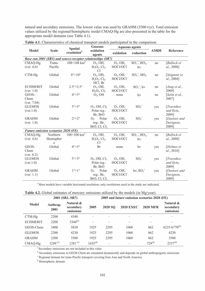
natural and secondary emissions. The lowest value was used by GRAHM (3500 t/yr). Total emission values utilized by the regional/hemispheric model CMAQ-Hg are also presented in the table for the appropriate model domains (see Table 4.1).

Table 4.1. Characteristics of chemical transport models participated in the comparison

Model Scale Spatialresolutiona

Gaseous oxidation

agents

Aqueous agentsAMDE Reference

oxidation reductionBase run 2001 (SR1) and source-receptor relationships (SR7)CMAQ-Hg (ver. 4.6)

Trans-Pacific

108×108 km2 O3, OH, H2O2, Cl2,

Cl

O3, OH, HOCl/OCl-

SO3=, HO2, h�

no [Bullock et al., 2008]

CTM-Hg Global 8°×10° O3, OH, H2O2, Cl2, HCl, Br

O3, OH, HOCl/OCl-

SO3=, HO2 no [Seigneur et

al., 2004]

ECHMERIT (ver. 1.0)

Global 2.5°×2.5° O3, OH, H2O2, Cl2

O3, OH, HOCl/OCl-

SO3=, h� no [Jung et al.,

2009]GEOS-Chem(ver. 7.04)

Global 4°×5° O3, OH none h� no [Selin et al., 2007]

GLEMOS(ver.1.0)

Global 5°×5° O3, OH, Cl2Polar reg.: Br, BrO

O3, OH, HOCl/OCl-

SO3= yes [Travnikov

and Ilyin, 2009]

GRAHM(ver. 1.0)

Global 2°×2° O3 Polar reg.: Br,

BrO, Cl, Cl2

O3, OH, HOCl/OCl-

SO3= yes [Dastoor and

Davignon, 2009]

Future emission scenarios 2020 (FE)CMAQ-Hg(ver. 4.6)

Northern Hemispher

e

108×108 km2 O3, OH, H2O2, Cl2,

Cl

O3, OH, HOCl/OCl-

SO3=, HO2, h�

no [Bullock et al., 2008]

GEOS-Chem(ver. 8.2)

Global 4°×5° Br none �� yes [Holmes et al., 2010]

GLEMOS (ver.1.0)

Global 5°×5° O3, OH, Cl2Polar reg.: Br, BrO

O3, OH, HOCl/OCl-

SO3= yes [Travnikov

and Ilyin, 2009]

GRAHM(ver. 1.1)

Global 1°×1° O3 Polar reg.: Br,

BrO, Cl, Cl2

O3, OH, HOCl/OCl-

��, SO3= yes [Dastoor and

Davignon, 2009]

a Most models have variable horizontal resolution; only resolutions used in the study are indicated.

Table 4.2. Global estimates of mercury emissions utilized by the models (in Mg/year).

Model

2001 (SR1, SR7) 2005 and future emission scenarios 2020 (FE)

Anthrop.2001

Natural &secondary emissions

2005 2020 SQ 2020 EXEC 2020 MFRNatural &secondary emissions

CTM-Hg 2200 4340 – – – – –ECHMERIT 2200 5344(a) – – – – –GEOS-Chem 3400 5830 1925 2295 1060 862 6235-6770(b)

GLEMOS 2200 4230 1925 2295 1060 862 4230GRAHM 2200 3500 1925 2295 1060 862 3500CMAQ-Hg 1249 (c) 1281 (c) 1635(d) – – 729(d) 2537(d)

a Secondary emissions are not included in this valueb Secondary emissions in GEOS-Chem are simulated dynamically and depends on global anthropogenic emissionsc Regional domain for trans-Pacific transport covering East Asia and North Americad Hemispheric domain

101

4.3. Global concentration and deposition levels 4.3.1. Review of previous mercury modelling studies Global scale modelling

Currently available global and hemispheric mercury models include the Chemical Transport Model for Mercury (CTM-Hg; [Seigneur et al., 2001; Seigneur et al., 2004]), the Danish Eulerian Hemispheric Model (DEHM; [Christensen et al., 2004]) , the Canadian Global/Regional Atmospheric Heavy Metals Model (GRAHM; [Ariya et al., 2004; Dastoor and Larocque, 2004; Dastoor and Davignon, 2009; Durnford et al., 2010], the EMEP Hemispheric Mercury Transport Model (MSCE-HM; [Travnikov, 2005]), the global atmosphere-ocean coupled mercury dispersion model (GEOS-Chem; [Selin and Jacob, 2008]), the Global EMEP Multi-media Modeling System (GLEMOS;[Travnikov and Ilyin, 2009]) and the recently developed global model ECHMERIT [Jung et al.,2009]. The global mercury models are self-consistent, closed-boundary models that are driven by global mercury emissions and constrained by measurements. Global atmospheric mercury models have been extensively applied to simulate mercury air concentrations and deposition fluxes to land and oceans, and have been used to investigate the consistency of mercury chemical mechanisms suggested in the literature by reproducing observed mercury concentrations and deposition. Other applications of global models have included characterization of intercontinental transport of mercury, source attribution of mercury, impacts of changing emissions on mercury budgets, and interpretation of observed mercury levels in the environment and biogeochemical mercury budgets and their relative changes from pre-industrial to present day environment. The studies related to intercontinental transport and source attribution are discussed in section B4.4.2.

Seigneur [2001] developed a global mercury model by including gas-phase oxidation of Hg0

by O3, OH, and Cl2, as well as aqueous redox chemistry and simulated annual average total gaseous mercury (TGM) concentrations consistent with observations and an atmospheric lifetime for TGM of 1.2 years. They reproduced background concentrations of mercury species on a global scale, inter-hemispheric gradients, and vertical gradients consistent with available measurements. Dastoor and Larocque [2004] developed an integrated high resolution meteorology and mercury atmospheric chemistry model. They examined the seasonal variations in atmospheric mercury circulation and concluded that the meteorological seasonal variability is responsible for the seasonal variability in TGM concentrations at mid-latitudes. Travnikov [2005] developed an operational mercury model to estimate pollution levels in the northern hemisphere and in Europe. He evaluated the model against global mercury concentrations, including seasonal variation, and examined intercontinental transport.GEOS-Chem was applied to interpret worldwide observations of TGM and RGHg in a study by Selin [2007]. They found that a global mercury source of 7000 t yr-1 and a TGM lifetime of 0.8 years reproduce the magnitude and large-scale variability of TGM observations at land sites. However, the model could not capture observations of high TGM from ship cruises, implying a problem either in the measurements or in our fundamental understanding of mercury sources. Using GEOS-Chem, Selin and Jacob [2008] also examined the seasonal variation and spatial pattern of wet deposition in the United States. They simulated maximum deposition in summer and minimum deposition in winter with increasing amplitude from north to south in accordance with observations. They attributed the high wet deposition over the southeast in summer to scavenging of upper-altitude Hg(II) by deep convection; and seasonal variation at mid-latitudes to a combination of enhanced summertime oxidation of Hg0 and inefficient scavenging of Hg(II) by snow. They showed that wet deposition accounts for 30% of total mercury deposition in the United States, the remainder coming from dry deposition. Durnford et al. [2010] conducted an extensive evaluation of GRAHM at 11 Canadian (8 mid-latitude and 3 sub-Arctic) and 6 Arctic ambient mercury measurement sites. They show a slight north to south gradient in Hg0 ambient concentrations over Canada with mean model Hg0

concentrations at the Arctic stations of 1.5 ng m-3, subarctic stations of 1.67 ng m-3 and mid-latitude stations of 1.68 ng m-3 in agreement with observations.

At polar sunrise, AMDEs caused by fast gas phase Hg-halogen oxidation reactions are observed. AMDEs are associated with enhanced deposition of mercury to snow that can be rapidly reduced and re-emitted to the atmosphere in the presence of sunlight [Kirk et al., 2006; Lindberg et

102

al., 2002; Poulain et al., 2007]. Their impact on Arctic mercury deposition was simulated by several models [Ariya et al., 2004; Christensen et al., 2004; Dastoor and Davignon, 2009; Travnikov, 2005].Christensen [2004] simulated AMDEs and estimated total deposition of mercury increases from 89 to 208 t yr-1 for the area north of the Polar Circle due to AMDEs. Ariya [2004] included Hg0 reaction with halogens in the Polar Regions in the Canadian global mercury model GRAHM and estimated 325 t yr-1 deposition of mercury annually above 60° N including 100 t yr-1 from AMDEs. Another study by Travnikov [2005] simulated a 20% increase in mercury deposition due to AMDEs in the Arctic. Travnikov also estimated that in coastal regions the contribution of AMDEs to mercury deposition can exceed 50%. Dastoor et al. [2008] estimated an annual mercury deposition of 428 t yr-

1, re-emission of mercury of 254 t yr-1 and net accumulation of mercury of 174 t yr-1 within the Arctic Circle 66.5° N with ±7 t of inter-annual variability for 2002–2004 using a version of GRAHM that includes re-emission of mercury from snow. ������� �������������-2 deposition, 1.0 ����-2 re-������������������-2 net surface gain of mercury at Barrow, Alaska from 25 March to 7 April 2003 in excellent agreement with a measurement campaign by Brooks [2006]����������-2���������������m-2 and 0�������������-2 deposition, re-emission and net surface gain, respectively). In addition to the bromine chemistry, they found a significant contribution of meteorological processes such as transport, boundary layer height, solar radiation reaching the ground, clouds, temperature inversion and surface temperature in establishing AMDEs in Polar Regions. Durnford [2010] demonstrated consistent reproduction of AMDEs at six Arctic stations by GRAHM and concluded that Hg0

transformations are indeed governed by very similar processes throughout the Arctic, i.e., Hg0

oxidation mediated by photochemistry involving bromine and Hg0 re-emission mediated by solar insolation reaching surface snow.

Bergan [2001] found that using OH as the only Hg0 oxidant with the rate constant of Sommar [2001], and no Hg(II) reduction, resulted in average Hg0 concentrations a factor of three below observed values in North America and Europe. Seigneur [2006] found that the fast Hg0-O3 reaction rate estimated by Pal and Ariya [2004b] would require a commensurate but unidentified reduction reaction to lead to realistic mercury concentrations in global models. Holmes [2006] examined the global lifetime of Hg0 against oxidation by tropospheric Br in GEOS-Chem. They illustrated that oxidation by Br in the middle and upper troposphere could be an important sink for Hg0, and that the mechanism yields an atmospheric lifetime of Hg0 consistent with observations. More recently, Seigneur [2008] examined the role of bromine chemistry on global atmospheric cycling of mercury.They found that bromine chemistry in their mercury model leads to Hg0 concentrations that are consistent with observations only if the pressure dependence of the kinetics of the oxidation of Hg0 by Br is taken into account and it reduces the overall lifetime of mercury by about 10%.

Travnikov and Ilyn [2009] estimated long-term changes in mercury deposition from 1990 to 2004 in different regions of the northern hemisphere using the MSCE-HM mercury model. They estimated the largest decrease in mercury deposition in Europe during this period. The average deposition flux in Europe decreased by half, whereas the highest deposition decreased by almost two-thirds. Their analysis shows that this reduction is mainly due to considerable emission reductions in Europe. Changes in mercury deposition in North America were found to be less pronounced because of smaller emission reductions and a higher relative contribution from other continents (particularly from Asia). In 1990 deposition levels in east and southeast Asia were comparable to those in Europe, whereas by 2000, deposition in Asia was the highest in northern hemisphere.

Muir [2009] examined recent and historical deposition of mercury over a broad geographic area (from southwestern Northwest Territories to Labrador and from the U.S. Northeast to northern Ellesmere Island) using dated sediment cores from 50 lakes (18 in mid-latitudes (41-50°N), 14 subarctic (51-64°N) and 18 in the Arctic (65-83°N)). The latitudinal trend for mercury depositions to these lakes predicted by GRAHM showed excellent agreement with the deposition flux inferred from ����������������������!����"������-2 yr-1 and were negatively correlated with latitude. The results support the view that there are significant anthropogenic mercury inputs in the Arctic.

103

Regional scale modelling

In the past two decades, a number of regional models have been developed to assess the fate and transport of atmospheric mercury in Europe, North America and East Asia. These 3-D regional models vary greatly in their modelling approaches. Some implement the atmospheric mercury processes in dispersion models [Petersen and Munthe, 1995]; others use the Lagrangian modellingscheme that follows the transport of air parcels containing various mercury species [Bullock Jr et al.,1998; Cohen et al., 2004; Lee et al., 2001]; while a majority of them use the Eulerian modellingscheme that comprehensively simulates the emission, transport, chemistry and deposition of mercury in 3-D space [Bullock Jr. and Brehme, 2002; Hedgecock et al., 2006; Kallos et al., 2001; MacLeod et al., 2005; Pai et al., 2000; Pan et al., 2006; Petersen et al., 1998; Roustan and Bocquet, 2006;Seigneur et al., 2001; Seigneur et al., 2003b; Voudouri and Kallos, 2007; Xu et al., 2000]. Since regional models consider the chemical transport of mercury in the region of interest only, they are not constrained by the mercury concentration distribution measured globally. Instead, these models heavily rely on the initial and boundary conditions, typically by assumption or extracted from the results of global mercury models, to produce reasonable model results. It has been demonstrated that mercury concentrations used in boundary conditions have a great influence on the model results of a regional mercury model [Pongprueksa et al., 2008].

The generally higher spatial resolution and more detailed treatment of cumulus and boundary-layer processes of regional mercury models make them a better modelling tool for evaluating the impact of local emission sources, although the application of a regional model (CMAQ-Hg) for evaluation of intercontinental transport has also been reported. Bullock et al. (2000) implemented the mercury extension in the Regional Lagrangian Model of Air Pollution (RELMAP) for evaluating the emission and chemical transport of a number of point and area source emissions in the United States. Seigneur [2001; 2003a] developed the mercury modules in the Trace Element Analysis Model and used it with a global transport model (CTM) to investigate the contribution of global and regional sources to mercury deposition in New York State. Kallos and co-workers [Kallos et al., 2001;Voudouri and Kallos, 2007] developed the mercury modelling framework within the Regional Atmospheric Modeling System (RAMS) and studied the fate and transport of mercury in the Mediterranean region, as did Hedgecock [2006], to specifically study mercury exchange across the surface of the Mediterranean Sea. Lee et al. [2001] used a long-term one dimensional Lagrangian trajectory model to study the transport and deposition of mercury across Europe and the UK. Lin [2003] employed CMAQ-Hg [Bullock Jr. and Brehme, 2002] to calculate the regional mass budget of mercury in eastern North America. Pan [2006] developed the mercury extension in the Sulfur Transport Eulerian Model (STEM-Hg) and used it for tracking the chemical transport of mercury plumes emitted from the large point sources in China. Gbor [2006] used CMAQ-Hg to investigate the importance of secondary emissions in the United States. Lin and co-workers Lin [2006b] used CMAQ-Hg to assess the trans-Pacific transport of mercury and to estimate the emission outflow of mercury emissions from East Asia. Sillman [2007] used CMAQ-Hg to investigate the source of RGHg measured in Florida and the Gulf of Mexico. Algorithms using inverse modelling techniques [Pan et al., 2007; Roustan and Bocquet, 2006] have also been implemented for two regional models (STEM-Hg used in East Asia and Polair3D model applied over Europe).

Owing to the lack of atmospheric monitoring data (particularly for the dry deposition of mercury) for comprehensive evaluations of mercury models, two major model inter-comparison studies have been performed to understand the model differences and to quantify the uncertainties in the results produced by various models. The first, the Intercomparison Study of Numerical Models for Long-Range Atmospheric Transport of Mercury conducted from 2000-2005, was organized by the Meteorological Synthesizing Centre - East (MSC-E). The second, the North American Mercury Model Intercomparison Study (NAMMIS) conducted 2004-2007, was organized by the U.S. Environmental Protection Agency.

The MSC-E intercomparison study attempted to demonstrate the ability of models in evaluating atmospheric transport and trans-boundary fluxes of mercury in Europe [Ryaboshapko et al., 2002; Ryaboshapko et al., 2007a; b]. The study was conducted in three phases. The first phase

104

compared simulation of the physicochemical transformation of mercury species in cloud and fog. The second phase focused on the comparison of model results with observations obtained during short-term measurement campaigns. The third phase focused on the comparison of model results with long-term measurements of mercury concentration and wet deposition in the EMEP measurement network. The participating models showed reasonable agreement (within ±20%) between model-predicted and observed concentrations of gaseous Hg0. Model-predicted mercury wet deposition in western and central Europe agreed with the observations within ±45% although the variation in model-predicted dry deposition was more significant.

The NAMMIS applied regional mercury models in a tightly constrained testing environment using a model domain in North America [Bullock et al., 2008; Bullock et al., 2009]. It was intended to have all regional models in the study (CMAQ-Hg, REMSAD-Hg and TEAM) use the same emission inventory data, meteorological fields and initial/boundary conditions as the model input, as well as use the same vertical structure and spatial resolution, so that the influences of different inputs could be minimized, thus allowing the effects of different scientific processors to be better understood. Themodel outputs of three global mercury models (CTM-Hg, GEOS-Chem and GRAHM) were employed as the initial/boundary conditions of the regional models. The intercomparison study indicated that the mercury concentration patterns predicted by the regional-scale models can be significantly different even when the same initial/boundary condition datasets were used. Model-predicted wet deposition of mercury was strongly influenced by the shared precipitation data, but differences of over 50% were still apparent. Simulated dry deposition of mercury was found to vary among the regional-scale models by nearly a factor of 10 in some locations because of the different parameterizations implemented in the regional models.

FINDING: Numerous studies using mercury transport models have been conducted in the past two decades on both global and regional scales for a variety of tasks, including understanding of mercury processes in the atmosphere, evaluation of mercury levels, and assessment of source-receptor relationships. In many cases the models demonstrate satisfactory agreement with the limited observations. However, considerable variability of the model results indicates essential gaps in the knowledge of mercury atmospheric processes. In spite of the scientific uncertainties, mercury models have proven to be a useful tool for assessing mercury pollution.

4.3.2. Findings of HTAP experiment (SR1)The spatial distribution and temporal variation of mercury concentration and deposition levels

on a global scale were studied in the HTAP multi-model experiment. Aims and conditions of the experiment have been discussed in Section 4.2.2. The original simulated patterns with the model intrinsic resolutions were interpolated to the 1° × 1° grid for comparison purposes. Figure 4.1 showsthe model ensemble mean global distribution of a bulk atmospheric mercury species, Hg0, in ambient air (Figure 4.1a) as well as the standard deviation of the simulation results among the models (Figure 4.1b). Circles on the figure represent long-term observations of Hg0 concentration from several monitoring networks and individual sites. As seen from the figure, elevated concentrations (above 1.8 ng/m3) are characteristic of the major industrial regions: East and South Asia, Europe, North America, and South Africa.

There is a pronounced gradient of the surface mercury concentration between the southern and the northern hemispheres, resulting from the location of most emission sources being predominantly in the northern hemisphere. Typical background levels of mercury concentrations are 1.2-1.4 ng m-3 in the southern hemisphere and 1.5-2 ng m-3 in the northern hemisphere. In general, this simulated pattern reproduces the long-term observations of Hg0 concentration. However, it should be noted that the number and spatial coverage of available long-term measurements are not sufficient for comprehensive evaluation of the mercury dispersion models.

105

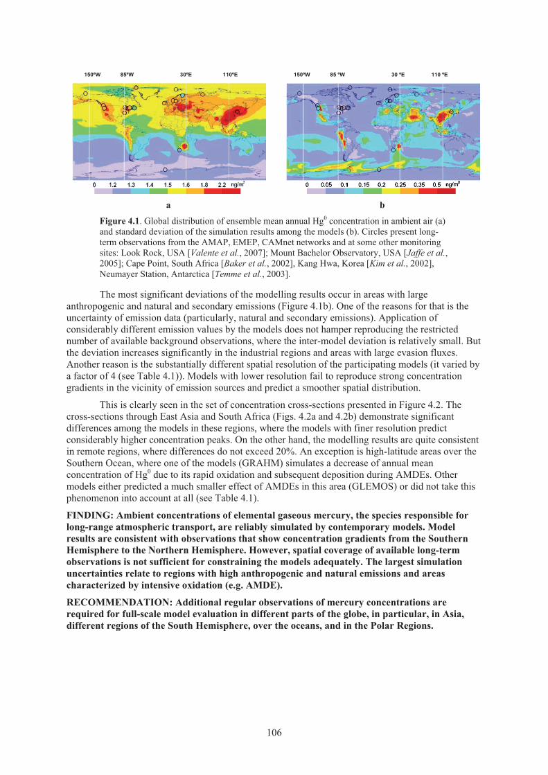
150ºW 85ºW 30ºE 110ºE

a

150ºW 85 ºW 30 ºE 110 ºE

b

Figure 4.1. Global distribution of ensemble mean annual Hg0 concentration in ambient air (a) and standard deviation of the simulation results among the models (b). Circles present long-term observations from the AMAP, EMEP, CAMnet networks and at some other monitoring sites: Look Rock, USA [Valente et al., 2007]; Mount Bachelor Observatory, USA [Jaffe et al.,2005]; Cape Point, South Africa [Baker et al., 2002], Kang Hwa, Korea [Kim et al., 2002], Neumayer Station, Antarctica [Temme et al., 2003].

The most significant deviations of the modelling results occur in areas with large anthropogenic and natural and secondary emissions (Figure 4.1b). One of the reasons for that is the uncertainty of emission data (particularly, natural and secondary emissions). Application of considerably different emission values by the models does not hamper reproducing the restricted number of available background observations, where the inter-model deviation is relatively small. But the deviation increases significantly in the industrial regions and areas with large evasion fluxes. Another reason is the substantially different spatial resolution of the participating models (it varied by a factor of 4 (see Table 4.1)). Models with lower resolution fail to reproduce strong concentration gradients in the vicinity of emission sources and predict a smoother spatial distribution.

This is clearly seen in the set of concentration cross-sections presented in Figure 4.2. The cross-sections through East Asia and South Africa (Figs. 4.2a and 4.2b) demonstrate significant differences among the models in these regions, where the models with finer resolution predict considerably higher concentration peaks. On the other hand, the modelling results are quite consistent in remote regions, where differences do not exceed 20%. An exception is high-latitude areas over the Southern Ocean, where one of the models (GRAHM) simulates a decrease of annual mean concentration of Hg0 due to its rapid oxidation and subsequent deposition during AMDEs. Other models either predicted a much smaller effect of AMDEs in this area (GLEMOS) or did not take this phenomenon into account at all (see Table 4.1).

FINDING: Ambient concentrations of elemental gaseous mercury, the species responsible for long-range atmospheric transport, are reliably simulated by contemporary models. Model results are consistent with observations that show concentration gradients from the Southern Hemisphere to the Northern Hemisphere. However, spatial coverage of available long-term observations is not sufficient for constraining the models adequately. The largest simulation uncertainties relate to regions with high anthropogenic and natural emissions and areas characterized by intensive oxidation (e.g. AMDE).

RECOMMENDATION: Additional regular observations of mercury concentrations are required for full-scale model evaluation in different parts of the globe, in particular, in Asia, different regions of the South Hemisphere, over the oceans, and in the Polar Regions.

106

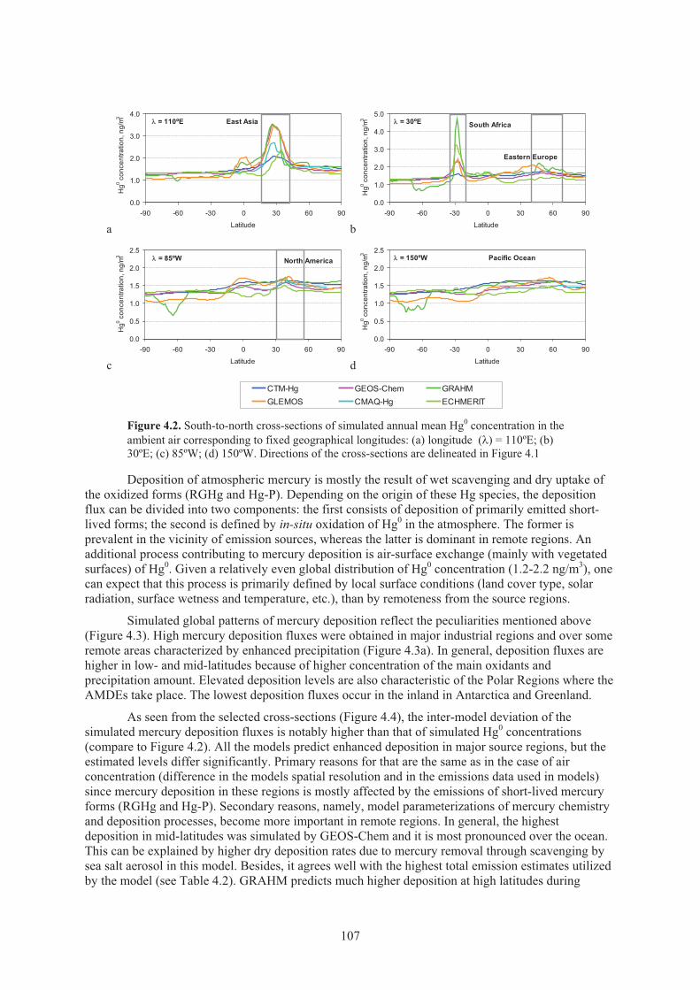
a b

c d

Figure 4.2. South-to-north cross-sections of simulated annual mean Hg0 concentration in the ambient air corresponding to fixed geographical longitudes: (a) longitude (�� = 110ºE; (b)30ºE; (c) 85ºW; (d) 150ºW. Directions of the cross-sections are delineated in Figure 4.1

Deposition of atmospheric mercury is mostly the result of wet scavenging and dry uptake of the oxidized forms (RGHg and Hg-P). Depending on the origin of these Hg species, the deposition flux can be divided into two components: the first consists of deposition of primarily emitted short-lived forms; the second is defined by in-situ oxidation of Hg0 in the atmosphere. The former is prevalent in the vicinity of emission sources, whereas the latter is dominant in remote regions. An additional process contributing to mercury deposition is air-surface exchange (mainly with vegetated surfaces) of Hg0. Given a relatively even global distribution of Hg0 concentration (1.2-2.2 ng/m3), one can expect that this process is primarily defined by local surface conditions (land cover type, solar radiation, surface wetness and temperature, etc.), than by remoteness from the source regions.

Simulated global patterns of mercury deposition reflect the peculiarities mentioned above (Figure 4.3). High mercury deposition fluxes were obtained in major industrial regions and over some remote areas characterized by enhanced precipitation (Figure 4.3a). In general, deposition fluxes are higher in low- and mid-latitudes because of higher concentration of the main oxidants and precipitation amount. Elevated deposition levels are also characteristic of the Polar Regions where the AMDEs take place. The lowest deposition fluxes occur in the inland in Antarctica and Greenland.

As seen from the selected cross-sections (Figure 4.4), the inter-model deviation of the simulated mercury deposition fluxes is notably higher than that of simulated Hg0 concentrations (compare to Figure 4.2). All the models predict enhanced deposition in major source regions, but the estimated levels differ significantly. Primary reasons for that are the same as in the case of air concentration (difference in the models spatial resolution and in the emissions data used in models) since mercury deposition in these regions is mostly affected by the emissions of short-lived mercury forms (RGHg and Hg-P). Secondary reasons, namely, model parameterizations of mercury chemistry and deposition processes, become more important in remote regions. In general, the highest deposition in mid-latitudes was simulated by GEOS-Chem and it is most pronounced over the ocean. This can be explained by higher dry deposition rates due to mercury removal through scavenging by sea salt aerosol in this model. Besides, it agrees well with the highest total emission estimates utilized by the model (see Table 4.2). GRAHM predicts much higher deposition at high latitudes during

0.0

1.0

2.0

3.0

4.0

-90 -60 -30 0 30 60 90

Latitude

Hg0 c

once

ntra

tion,

ng/

m3� = 110ºE East Asia

0.0

1.0

2.0

3.0

4.0

5.0

-90 -60 -30 0 30 60 90

Latitude

Hg0 c

once

ntra

tion,

ng/

m3 � = 30ºE

Eastern Europe

South Africa

0.0

0.5

1.0

1.5

2.0

2.5

-90 -60 -30 0 30 60 90

Latitude

Hg0 c

once

ntra

tion,

ng/

m3

North America� = 85ºW

0.0

0.5

1.0

1.5

2.0

2.5

-90 -60 -30 0 30 60 90

LatitudeH

g0 con

cent

ratio

n, n

g/m3

� = 150ºW Pacific Ocean

CTM-Hg GEOS-Chem GRAHMGLEMOS CMAQ-Hg ECHMERIT

107

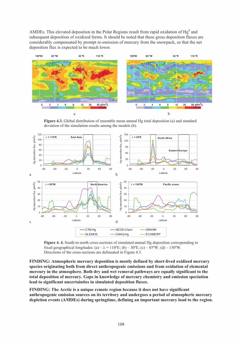
AMDEs. This elevated deposition in the Polar Regions result from rapid oxidation of Hg0 and subsequent deposition of oxidized forms. It should be noted that these gross deposition fluxes are considerably compensated by prompt re-emission of mercury from the snowpack, so that the net deposition flux is expected to be much lower.

150ºW 85 ºW 30 ºE 110 ºE

a

150ºW 85 ºW 30 ºE 110 ºE

b

Figure 4.3. Global distribution of ensemble mean annual Hg total deposition (a) and standard deviation of the simulation results among the models (b).

a b

c d

Figure 4. 4. South-to-north cross-sections of simulated annual Hg deposition corresponding to fixed geographical longitudes: (a) – � = 110ºE; (b) – 30ºE; (c) – 85ºW; (d) – 150ºW. Directions of the cross-sections are delineated in Figure 4.3.

FINDING: Atmospheric mercury deposition is mostly defined by short-lived oxidized mercury species originating both from direct anthropogenic emissions and from oxidation of elemental mercury in the atmosphere. Both dry and wet removal pathways are equally significant to the total deposition of mercury. Gaps in knowledge of mercury chemistry and emission speciation lead to significant uncertainties in simulated deposition fluxes.

FINDING: The Arctic is a unique remote region because it does not have significant anthropogenic emission sources on its territory and undergoes a period of atmospheric mercury depletion events (AMDEs) during springtime, defining an important mercury load to the region.

0

20

40

60

80

100

120

-90 -60 -30 0 30 60 90

Latitude

Hg

depo

sitio

n flu

x, g

/km2 /y East Asia� = 110ºE

0

30

60

90

120

150

-90 -60 -30 0 30 60 90

Latitude

Hg

depo

sitio

n flu

x, g

/km2 /y

South Africa� = 30ºE

Eastern Europe

0

10

20

30

40

50

-90 -60 -30 0 30 60 90

Latitude

Hg

depo

sitio

n flu

x, g

/km2 /y North America� = 85ºW

0

10

20

30

40

50

-90 -60 -30 0 30 60 90

Latitude

Hg

depo

sitio

n flu

x, g

/km2 /y Pacific ocean� = 150ºW

CTM-Hg GEOS-Chem GRAHMGLEMOS CMAQ-Hg ECHMERIT

108

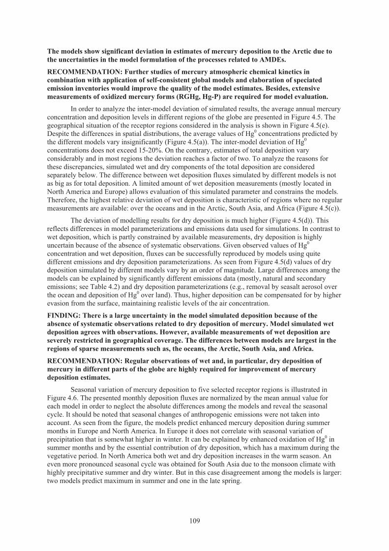
The models show significant deviation in estimates of mercury deposition to the Arctic due to the uncertainties in the model formulation of the processes related to AMDEs.

RECOMMENDATION: Further studies of mercury atmospheric chemical kinetics in combination with application of self-consistent global models and elaboration of speciated emission inventories would improve the quality of the model estimates. Besides, extensive measurements of oxidized mercury forms (RGHg, Hg-P) are required for model evaluation.

In order to analyze the inter-model deviation of simulated results, the average annual mercury concentration and deposition levels in different regions of the globe are presented in Figure 4.5. The geographical situation of the receptor regions considered in the analysis is shown in Figure 4.5(e). Despite the differences in spatial distributions, the average values of Hg0 concentrations predicted by the different models vary insignificantly (Figure 4.5(a)). The inter-model deviation of Hg0

concentrations does not exceed 15-20%. On the contrary, estimates of total deposition vary considerably and in most regions the deviation reaches a factor of two. To analyze the reasons for these discrepancies, simulated wet and dry components of the total deposition are considered separately below. The difference between wet deposition fluxes simulated by different models is not as big as for total deposition. A limited amount of wet deposition measurements (mostly located in North America and Europe) allows evaluation of this simulated parameter and constrains the models. Therefore, the highest relative deviation of wet deposition is characteristic of regions where no regular measurements are available: over the oceans and in the Arctic, South Asia, and Africa (Figure 4.5(c)).

The deviation of modelling results for dry deposition is much higher (Figure 4.5(d)). This reflects differences in model parameterizations and emissions data used for simulations. In contrast to wet deposition, which is partly constrained by available measurements, dry deposition is highly uncertain because of the absence of systematic observations. Given observed values of Hg0

concentration and wet deposition, fluxes can be successfully reproduced by models using quite different emissions and dry deposition parameterizations. As seen from Figure 4.5(d) values of dry deposition simulated by different models vary by an order of magnitude. Large differences among the models can be explained by significantly different emissions data (mostly, natural and secondary emissions; see Table 4.2) and dry deposition parameterizations (e.g., removal by seasalt aerosol over the ocean and deposition of Hg0 over land). Thus, higher deposition can be compensated for by higher evasion from the surface, maintaining realistic levels of the air concentration.

FINDING: There is a large uncertainty in the model simulated deposition because of the absence of systematic observations related to dry deposition of mercury. Model simulated wet deposition agrees with observations. However, available measurements of wet deposition are severely restricted in geographical coverage. The differences between models are largest in the regions of sparse measurements such as, the oceans, the Arctic, South Asia, and Africa.

RECOMMENDATION: Regular observations of wet and, in particular, dry deposition of mercury in different parts of the globe are highly required for improvement of mercury deposition estimates.

Seasonal variation of mercury deposition to five selected receptor regions is illustrated in Figure 4.6. The presented monthly deposition fluxes are normalized by the mean annual value for each model in order to neglect the absolute differences among the models and reveal the seasonal cycle. It should be noted that seasonal changes of anthropogenic emissions were not taken into account. As seen from the figure, the models predict enhanced mercury deposition during summer months in Europe and North America. In Europe it does not correlate with seasonal variation of precipitation that is somewhat higher in winter. It can be explained by enhanced oxidation of Hg0 in summer months and by the essential contribution of dry deposition, which has a maximum during the vegetative period. In North America both wet and dry deposition increases in the warm season. An even more pronounced seasonal cycle was obtained for South Asia due to the monsoon climate with highly precipitative summer and dry winter. But in this case disagreement among the models is larger: two models predict maximum in summer and one in the late spring.

109

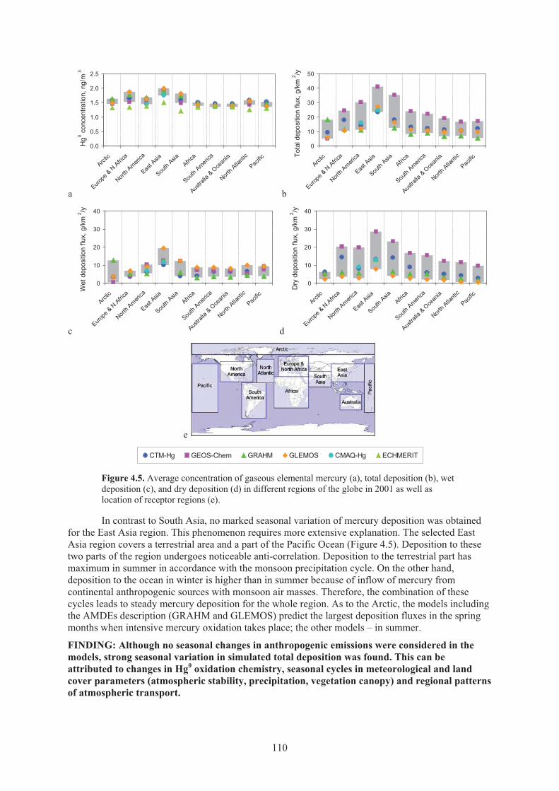
a b

c d

e

Figure 4.5. Average concentration of gaseous elemental mercury (a), total deposition (b), wet deposition (c), and dry deposition (d) in different regions of the globe in 2001 as well as location of receptor regions (e).

In contrast to South Asia, no marked seasonal variation of mercury deposition was obtained for the East Asia region. This phenomenon requires more extensive explanation. The selected East Asia region covers a terrestrial area and a part of the Pacific Ocean (Figure 4.5). Deposition to these two parts of the region undergoes noticeable anti-correlation. Deposition to the terrestrial part has maximum in summer in accordance with the monsoon precipitation cycle. On the other hand, deposition to the ocean in winter is higher than in summer because of inflow of mercury from continental anthropogenic sources with monsoon air masses. Therefore, the combination of these cycles leads to steady mercury deposition for the whole region. As to the Arctic, the models including the AMDEs description (GRAHM and GLEMOS) predict the largest deposition fluxes in the spring months when intensive mercury oxidation takes place; the other models – in summer.

FINDING: Although no seasonal changes in anthropogenic emissions were considered in the models, strong seasonal variation in simulated total deposition was found. This can be attributed to changes in Hg0 oxidation chemistry, seasonal cycles in meteorological and land cover parameters (atmospheric stability, precipitation, vegetation canopy) and regional patterns of atmospheric transport.

0.0

0.5

1.0

1.5

2.0

2.5

Arctic

Europe

& N.Afric

a

North A

merica

East A

sia

South

AsiaAfric

a

South

America

Austra

lia & O

cean

ia

North A

tlanti

c

Pacific

Hg0 c

once

ntra

tion,

ng/

m3

0

10

20

30

40

50

Arctic

Europe

& N

.Africa

North A

merica

East A

sia

South

AsiaAfric

a

South

America

Austra

lia &

Oce

ania

North A

tlanti

c

Pacific

Tota

l dep

ositi

on fl

ux, g

/km

2 /y

0

10

20

30

40

Arctic

Europe

& N

.Africa

North A

merica

East A

sia

South

AsiaAfric

a

South

America

Austra

lia &

Oce

ania

North A

tlanti

c

Pacific

Wet

dep

ositi

on fl

ux, g

/km

2 /y

0

10

20

30

40

Arctic

Europe

& N

.Africa

North A

merica

East A

sia

South

AsiaAfric

a

South

America

Austra

lia &

Oce

ania

North A

tlanti

c

Pacific

Dry

dep

ositi

on fl

ux, g

/km

2 /y

CTM-Hg GEOS-Chem GRAHM GLEMOS CMAQ-Hg ECHMERIT

110

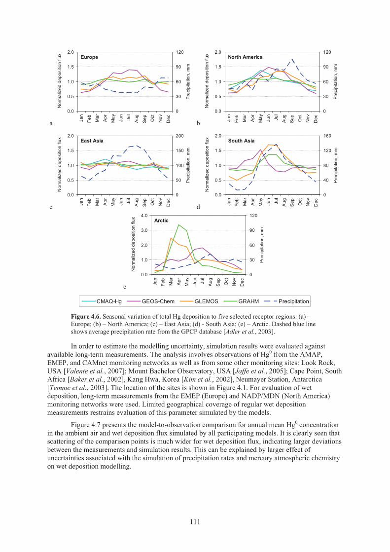
a b

c d

e

Figure 4.6. Seasonal variation of total Hg deposition to five selected receptor regions: (a) –Europe; (b) – North America; (c) – East Asia; (d) - South Asia; (e) – Arctic. Dashed blue line shows average precipitation rate from the GPCP database [Adler et al., 2003].

In order to estimate the modelling uncertainty, simulation results were evaluated against available long-term measurements. The analysis involves observations of Hg0 from the AMAP, EMEP, and CAMnet monitoring networks as well as from some other monitoring sites: Look Rock, USA [Valente et al., 2007]; Mount Bachelor Observatory, USA [Jaffe et al., 2005]; Cape Point, SouthAfrica [Baker et al., 2002], Kang Hwa, Korea [Kim et al., 2002], Neumayer Station, Antarctica [Temme et al., 2003]. The location of the sites is shown in Figure 4.1. For evaluation of wet deposition, long-term measurements from the EMEP (Europe) and NADP/MDN (North America) monitoring networks were used. Limited geographical coverage of regular wet deposition measurements restrains evaluation of this parameter simulated by the models.

Figure 4.7 presents the model-to-observation comparison for annual mean Hg0 concentration in the ambient air and wet deposition flux simulated by all participating models. It is clearly seen that scattering of the comparison points is much wider for wet deposition flux, indicating larger deviations between the measurements and simulation results. This can be explained by larger effect of uncertainties associated with the simulation of precipitation rates and mercury atmospheric chemistry on wet deposition modelling.

0.0

0.5

1.0

1.5

2.0

Jan

Feb

Mar

Apr

May Jun

Jul

Aug

Sep Oct

Nov

Dec

Nor

mal

ized

dep

ositi

on fl

u x

0

30

60

90

120

Pre

cipi

tatio

n, m

m

Europe

0.0

0.5

1.0

1.5

2.0

Jan

Feb

Mar

Apr

May Jun

Jul

Aug

Sep Oct

Nov

Dec

Nor

mal

ized

dep

ositi

on fl

u x

0

30

60

90

120

Pre

cipi

tatio

n, m

m

North America

0.0

0.5

1.0

1.5

2.0

Jan

Feb

Mar

Apr

May Jun

Jul

Aug

Sep Oct

Nov

Dec

Nor

mal

ized

dep

ositi

on fl

u x

0

50

100

150

200

Pre

cipi

tatio

n, m

m

East Asia

0.0

0.5

1.0

1.5

2.0

Jan

Feb

Mar

Apr

May Jun

Jul

Aug

Sep Oct

Nov

Dec

Nor

mal

ized

dep

ositi

on fl

u x

0

40

80

120

160

Pre

cipi

tatio

n, m

m

South Asia

0.0

1.0

2.0

3.0

4.0

Jan

Feb

Mar

Apr

May Jun

Jul

Aug

Sep Oct

Nov

Dec

Nor

mal

ized

dep

ositi

on fl

u x

0

30

60

90

120

Pre

cipi

tatio

n, m

m

Arctic

CMAQ-Hg GEOS-Chem GLEMOS GRAHM Precipitation

111

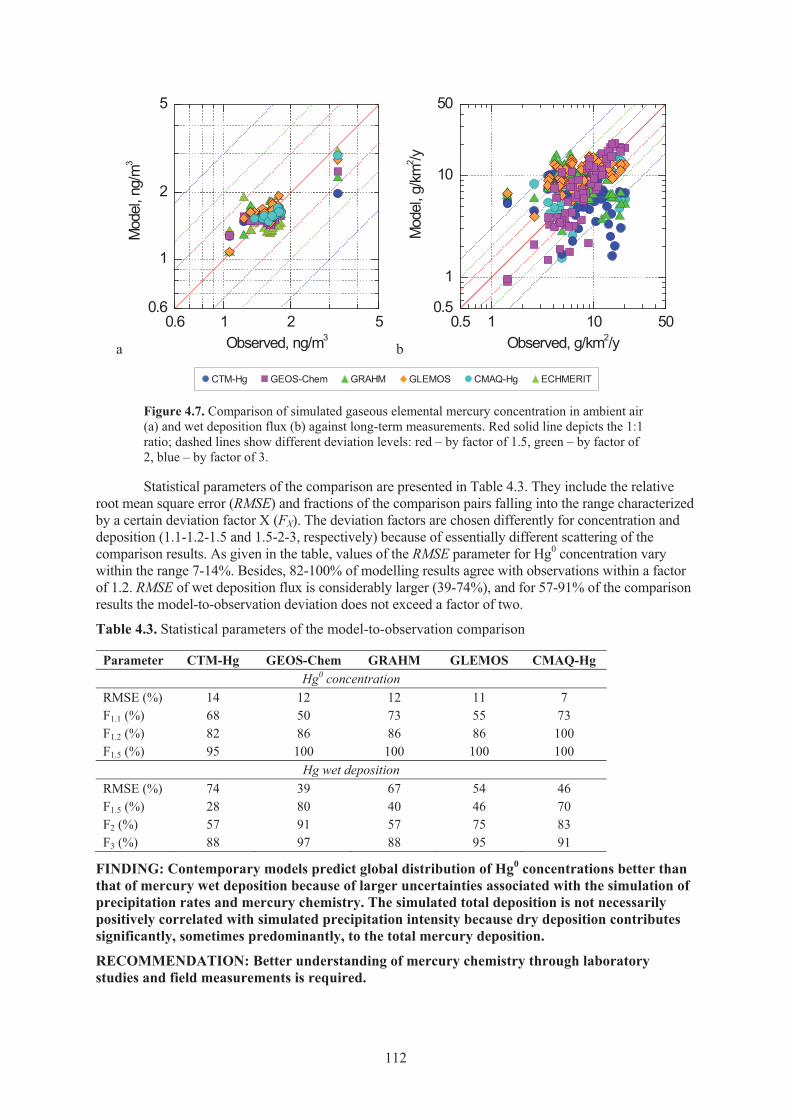
a b

Figure 4.7. Comparison of simulated gaseous elemental mercury concentration in ambient air (a) and wet deposition flux (b) against long-term measurements. Red solid line depicts the 1:1 ratio; dashed lines show different deviation levels: red – by factor of 1.5, green – by factor of 2, blue – by factor of 3.

Statistical parameters of the comparison are presented in Table 4.3. They include the relative root mean square error (RMSE) and fractions of the comparison pairs falling into the range characterized by a certain deviation factor X (FX). The deviation factors are chosen differently for concentration and deposition (1.1-1.2-1.5 and 1.5-2-3, respectively) because of essentially different scattering of the comparison results. As given in the table, values of the RMSE parameter for Hg0 concentration vary within the range 7-14%. Besides, 82-100% of modelling results agree with observations within a factor of 1.2. RMSE of wet deposition flux is considerably larger (39-74%), and for 57-91% of the comparison results the model-to-observation deviation does not exceed a factor of two.

Table 4.3. Statistical parameters of the model-to-observation comparison

Parameter CTM-Hg GEOS-Chem GRAHM GLEMOS CMAQ-HgHg0 concentration

RMSE (%) 14 12 12 11 7F1.1 (%) 68 50 73 55 73F1.2 (%) 82 86 86 86 100F1.5 (%) 95 100 100 100 100

Hg wet depositionRMSE (%) 74 39 67 54 46F1.5 (%) 28 80 40 46 70F2 (%) 57 91 57 75 83F3 (%) 88 97 88 95 91

FINDING: Contemporary models predict global distribution of Hg0 concentrations better than that of mercury wet deposition because of larger uncertainties associated with the simulation of precipitation rates and mercury chemistry. The simulated total deposition is not necessarily positively correlated with simulated precipitation intensity because dry deposition contributes significantly, sometimes predominantly, to the total mercury deposition.

RECOMMENDATION: Better understanding of mercury chemistry through laboratory studies and field measurements is required.

0.6 1 2 50.6

1

2

5

Mod

el, n

g/m

3

Observed, ng/m30.5 1 10 50

0.5

1

10

50

Mod

el, g

/km

2 /y

Observed, g/km2/y

CTM-Hg GEOS-Chem GRAHM GLEMOS CMAQ-Hg ECHMERIT

112

4.4. Intercontinental transport of mercurySediment and ice core data indicate that mercury deposition has increased significantly over the

past 150 years in both industrial and remote areas, which receive the majority of their inputs from long-range sources. In remote regions, increases in deposition of two to five times above preindustrial rates are reported [Engstrom and Swain, 1997; Fitzgerald et al., 1998; Fitzgerald et al., 2005; Lamborg et al., 2002; Lucotte et al., 1995; Schuster et al., 2002]. The measured increase occurs concurrently with industrialization, suggesting that anthropogenic sources are responsible [Biester et al., 2007].

Being a global pollutant with an atmospheric lifetime of 0.5-2 years, mercury emitted from anthropogenic and natural sources is subject to long-range transport. A majority of anthropogenic mercury emissions occur at mid-latitudes and circumpolar westerlies can transport the emissions from the source regions to other receptor regions. The South-North Hemispheric exchange is not as significant, as evidenced by the concentration gradient from the Northern Hemisphere to the Southern Hemisphere. Because current monitoring networks and field measurements of mercury concentration and deposition are scarce and not evenly distributed spatially, the data have limited capability in detecting the signals from intercontinental transport. Therefore, modelling assessments in a model domain that cover multiple source and receptor regions become an attractive evaluation approach to characterize the long-range transport. This section discusses the characteristics and earlier findings on intercontinental transport of mercury.

4.4.1. Characteristics of mercury intercontinental transport A number of studies have reported observational and modelling evidences of intercontinental

transport of atmospheric mercury. For example, observational analyses using Hg0 to CO concentration ratio as a chemical signature have shown that mercury plumes from East Asia can travel across the Pacific to the west coast of North America [Jaffe et al., 2005; Weiss-Penzias et al., 2007]. The concentration enhancement by the trans-Pacific plumes can be as high as 0.7 ng/m3 [Weiss-Penzias et al., 2006]. The transport pathway typically involves the lifting of mercury plumes to above the planetary boundary layer, followed by rapid atmospheric transport in the free troposphere. The transported plumes can reach ground level in the event of atmospheric subsidence at the receptor sites in another continent. Through this pathway, Asian plumes can be transported relatively undiluted to the Northeastern Pacific in about a week. The plumes are typically from large point sources that emit mercury at higher elevation and with higher temperatures [Friedli et al., 2004]. Springtime is found to be the most active period for trans-Pacific transport [Lin et al., 2006a; Reidmiller et al., 2009].Transport across the Atlantic is more complex and usually involves several mid-latitude cyclones and associated warm conveyor belts. Earlier measurements coupled with modelling analyses have also detected large industrial plumes coming out of the East Asian continent during the ACE-Asia campaign [Friedli et al., 2004; Friedli et al., 2007; Pan et al., 2006; Pan et al., 2008]. A number of global modelling efforts, [e.g.Seigneur et al., 2004; Strode et al., 2008; Travnikov, 2005] have also assessed the impact of the intercontinental transport of mercury.

Due to the large spatial scale of intercontinental transport, atmospheric models serve as an ideal tool for investigating the long-range transport of mercury. Two general approaches have been used in various studies. One is to investigate the source-receptor relationship, which quantifies the effect of an emission perturbation in a source region on the change of mercury concentration and deposition in the receptor regions. This is done by selectively reducing mercury emission in the source region by a certain percentage and allows models to quantitatively estimate its impact on mercury pollution in different receptor regions. The other approach is source attribution, which refers to estimating the percentage of contribution to mercury concentration and deposition in a receptor region caused by the emissions from various source regions. The source contribution calculations are typically made by "zeroing out" the emissions from multiple source regions. The contribution to mercury concentration and deposition from each source region is integrated based on model results to show the relative importance of mercury from different source regions. In source attribution studies, it is important that the model response to the emission changes is additive.

113

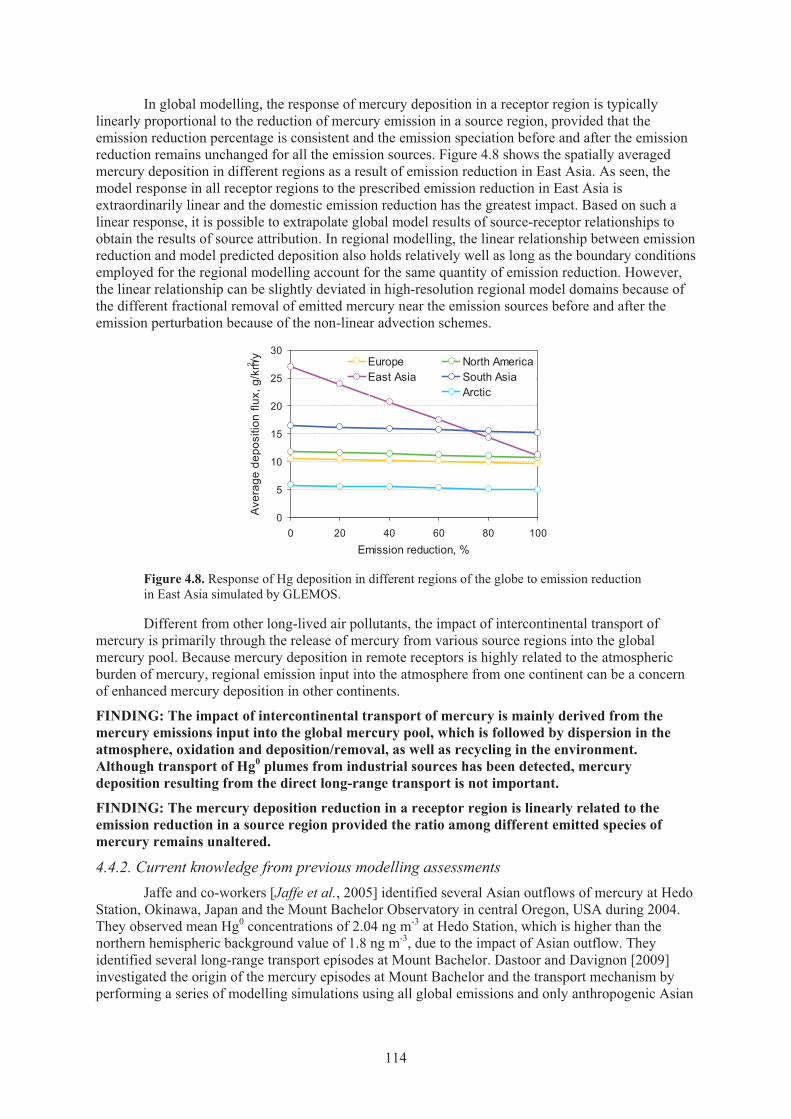
In global modelling, the response of mercury deposition in a receptor region is typically linearly proportional to the reduction of mercury emission in a source region, provided that the emission reduction percentage is consistent and the emission speciation before and after the emission reduction remains unchanged for all the emission sources. Figure 4.8 shows the spatially averaged mercury deposition in different regions as a result of emission reduction in East Asia. As seen, the model response in all receptor regions to the prescribed emission reduction in East Asia is extraordinarily linear and the domestic emission reduction has the greatest impact. Based on such a linear response, it is possible to extrapolate global model results of source-receptor relationships to obtain the results of source attribution. In regional modelling, the linear relationship between emission reduction and model predicted deposition also holds relatively well as long as the boundary conditions employed for the regional modelling account for the same quantity of emission reduction. However, the linear relationship can be slightly deviated in high-resolution regional model domains because of the different fractional removal of emitted mercury near the emission sources before and after the emission perturbation because of the non-linear advection schemes.

Figure 4.8. Response of Hg deposition in different regions of the globe to emission reduction in East Asia simulated by GLEMOS.

Different from other long-lived air pollutants, the impact of intercontinental transport of mercury is primarily through the release of mercury from various source regions into the global mercury pool. Because mercury deposition in remote receptors is highly related to the atmospheric burden of mercury, regional emission input into the atmosphere from one continent can be a concern of enhanced mercury deposition in other continents.

FINDING: The impact of intercontinental transport of mercury is mainly derived from the mercury emissions input into the global mercury pool, which is followed by dispersion in the atmosphere, oxidation and deposition/removal, as well as recycling in the environment. Although transport of Hg0 plumes from industrial sources has been detected, mercury deposition resulting from the direct long-range transport is not important.

FINDING: The mercury deposition reduction in a receptor region is linearly related to the emission reduction in a source region provided the ratio among different emitted species of mercury remains unaltered.

4.4.2. Current knowledge from previous modelling assessmentsJaffe and co-workers [Jaffe et al., 2005] identified several Asian outflows of mercury at Hedo

Station, Okinawa, Japan and the Mount Bachelor Observatory in central Oregon, USA during 2004. They observed mean Hg0 concentrations of 2.04 ng m-3 at Hedo Station, which is higher than the northern hemispheric background value of 1.8 ng m-3, due to the impact of Asian outflow. They identified several long-range transport episodes at Mount Bachelor. Dastoor and Davignon [2009]investigated the origin of the mercury episodes at Mount Bachelor and the transport mechanism by performing a series of modelling simulations using all global emissions and only anthropogenic Asian

0

5

10

15

20

25

30

0 20 40 60 80 100Emission reduction, %

Ave

rage

dep

ositi

on fl

ux, g

/km2 /y Europe North America

East Asia South Asia���� Arctic

114

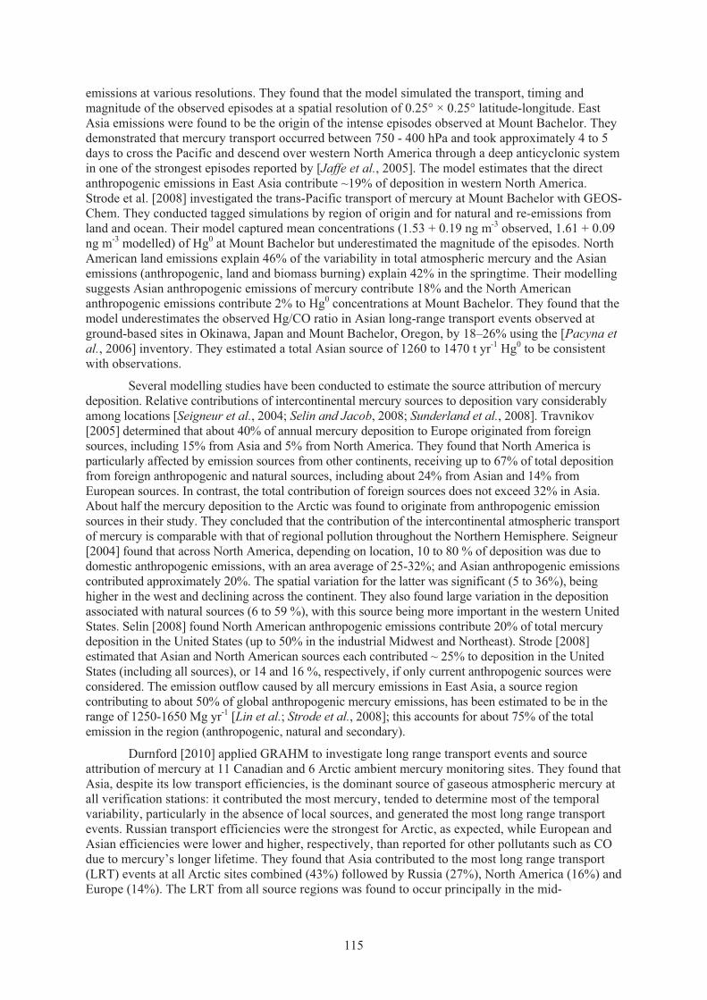
emissions at various resolutions. They found that the model simulated the transport, timing and magnitude of the observed episodes at a spatial resolution of 0.25° × 0.25° latitude-longitude. East Asia emissions were found to be the origin of the intense episodes observed at Mount Bachelor. They demonstrated that mercury transport occurred between 750 - 400 hPa and took approximately 4 to 5 days to cross the Pacific and descend over western North America through a deep anticyclonic system in one of the strongest episodes reported by [Jaffe et al., 2005]. The model estimates that the direct anthropogenic emissions in East Asia contribute ~19% of deposition in western North America.Strode et al. [2008] investigated the trans-Pacific transport of mercury at Mount Bachelor with GEOS-Chem. They conducted tagged simulations by region of origin and for natural and re-emissions from land and ocean. Their model captured mean concentrations (1.53 + 0.19 ng m-3 observed, 1.61 + 0.09 ng m-3 modelled) of Hg0 at Mount Bachelor but underestimated the magnitude of the episodes. North American land emissions explain 46% of the variability in total atmospheric mercury and the Asian emissions (anthropogenic, land and biomass burning) explain 42% in the springtime. Their modellingsuggests Asian anthropogenic emissions of mercury contribute 18% and the North American anthropogenic emissions contribute 2% to Hg0 concentrations at Mount Bachelor. They found that the model underestimates the observed Hg/CO ratio in Asian long-range transport events observed at ground-based sites in Okinawa, Japan and Mount Bachelor, Oregon, by 18–26% using the [Pacyna et al., 2006] inventory. They estimated a total Asian source of 1260 to 1470 t yr-1 Hg0 to be consistent with observations.

Several modelling studies have been conducted to estimate the source attribution of mercury deposition. Relative contributions of intercontinental mercury sources to deposition vary considerably among locations [Seigneur et al., 2004; Selin and Jacob, 2008; Sunderland et al., 2008]. Travnikov [2005] determined that about 40% of annual mercury deposition to Europe originated from foreign sources, including 15% from Asia and 5% from North America. They found that North America is particularly affected by emission sources from other continents, receiving up to 67% of total deposition from foreign anthropogenic and natural sources, including about 24% from Asian and 14% from European sources. In contrast, the total contribution of foreign sources does not exceed 32% in Asia. About half the mercury deposition to the Arctic was found to originate from anthropogenic emission sources in their study. They concluded that the contribution of the intercontinental atmospheric transport of mercury is comparable with that of regional pollution throughout the Northern Hemisphere. Seigneur [2004] found that across North America, depending on location, 10 to 80 % of deposition was due to domestic anthropogenic emissions, with an area average of 25-32%; and Asian anthropogenic emissions contributed approximately 20%. The spatial variation for the latter was significant (5 to 36%), being higher in the west and declining across the continent. They also found large variation in the deposition associated with natural sources (6 to 59 %), with this source being more important in the western United States. Selin [2008] found North American anthropogenic emissions contribute 20% of total mercury deposition in the United States (up to 50% in the industrial Midwest and Northeast). Strode [2008]estimated that Asian and North American sources each contributed ~ 25% to deposition in the United States (including all sources), or 14 and 16 %, respectively, if only current anthropogenic sources were considered. The emission outflow caused by all mercury emissions in East Asia, a source region contributing to about 50% of global anthropogenic mercury emissions, has been estimated to be in the range of 1250-1650 Mg yr-1 [Lin et al.; Strode et al., 2008]; this accounts for about 75% of the total emission in the region (anthropogenic, natural and secondary).

Durnford [2010] applied GRAHM to investigate long range transport events and source attribution of mercury at 11 Canadian and 6 Arctic ambient mercury monitoring sites. They found that Asia, despite its low transport efficiencies, is the dominant source of gaseous atmospheric mercury at all verification stations: it contributed the most mercury, tended to determine most of the temporal variability, particularly in the absence of local sources, and generated the most long range transport events. Russian transport efficiencies were the strongest for Arctic, as expected, while European and Asian efficiencies were lower and higher, respectively, than reported for other pollutants such as CO due to mercury’s longer lifetime. They found that Asia contributed to the most long range transport (LRT) events at all Arctic sites combined (43%) followed by Russia (27%), North America (16%) and Europe (14%). The LRT from all source regions was found to occur principally in the mid-

115

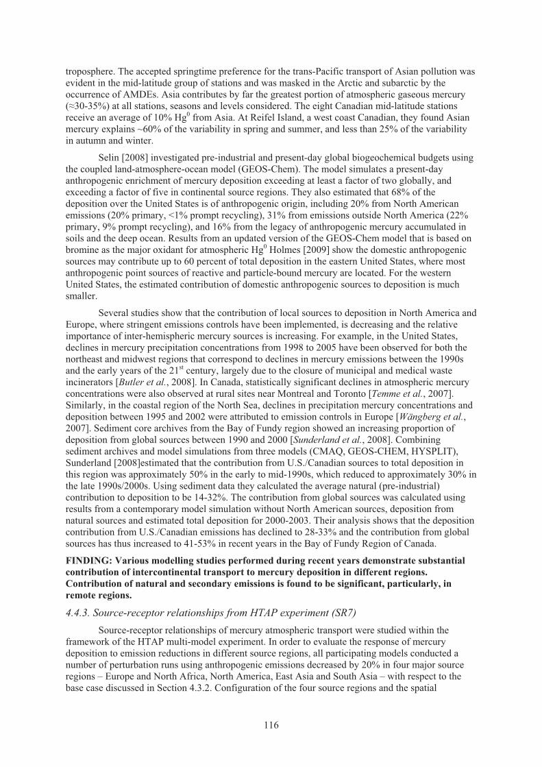
troposphere. The accepted springtime preference for the trans-Pacific transport of Asian pollution was evident in the mid-latitude group of stations and was masked in the Arctic and subarctic by the occurrence of AMDEs. Asia contributes by far the greatest portion of atmospheric gaseous mercury (#$�-35%) at all stations, seasons and levels considered. The eight Canadian mid-latitude stations receive an average of 10% Hg0 from Asia. At Reifel Island, a west coast Canadian, they found Asian mercury explains ~60% of the variability in spring and summer, and less than 25% of the variability in autumn and winter.

Selin [2008] investigated pre-industrial and present-day global biogeochemical budgets using the coupled land-atmosphere-ocean model (GEOS-Chem). The model simulates a present-day anthropogenic enrichment of mercury deposition exceeding at least a factor of two globally, and exceeding a factor of five in continental source regions. They also estimated that 68% of the deposition over the United States is of anthropogenic origin, including 20% from North American emissions (20% primary, <1% prompt recycling), 31% from emissions outside North America (22% primary, 9% prompt recycling), and 16% from the legacy of anthropogenic mercury accumulated in soils and the deep ocean. Results from an updated version of the GEOS-Chem model that is based on bromine as the major oxidant for atmospheric Hg0 Holmes [2009] show the domestic anthropogenic sources may contribute up to 60 percent of total deposition in the eastern United States, where most anthropogenic point sources of reactive and particle-bound mercury are located. For the western United States, the estimated contribution of domestic anthropogenic sources to deposition is much smaller.

Several studies show that the contribution of local sources to deposition in North America and Europe, where stringent emissions controls have been implemented, is decreasing and the relative importance of inter-hemispheric mercury sources is increasing. For example, in the United States, declines in mercury precipitation concentrations from 1998 to 2005 have been observed for both the northeast and midwest regions that correspond to declines in mercury emissions between the 1990s and the early years of the 21st century, largely due to the closure of municipal and medical waste incinerators [Butler et al., 2008]. In Canada, statistically significant declines in atmospheric mercury concentrations were also observed at rural sites near Montreal and Toronto [Temme et al., 2007].Similarly, in the coastal region of the North Sea, declines in precipitation mercury concentrations and deposition between 1995 and 2002 were attributed to emission controls in Europe [Wängberg et al.,2007]. Sediment core archives from the Bay of Fundy region showed an increasing proportion of deposition from global sources between 1990 and 2000 [Sunderland et al., 2008]. Combining sediment archives and model simulations from three models (CMAQ, GEOS-CHEM, HYSPLIT),Sunderland [2008]estimated that the contribution from U.S./Canadian sources to total deposition in this region was approximately 50% in the early to mid-1990s, which reduced to approximately 30% in the late 1990s/2000s. Using sediment data they calculated the average natural (pre-industrial) contribution to deposition to be 14-32%. The contribution from global sources was calculated using results from a contemporary model simulation without North American sources, deposition from natural sources and estimated total deposition for 2000-2003. Their analysis shows that the deposition contribution from U.S./Canadian emissions has declined to 28-33% and the contribution from global sources has thus increased to 41-53% in recent years in the Bay of Fundy Region of Canada.

FINDING: Various modelling studies performed during recent years demonstrate substantial contribution of intercontinental transport to mercury deposition in different regions. Contribution of natural and secondary emissions is found to be significant, particularly, in remote regions.

4.4.3. Source-receptor relationships from HTAP experiment (SR7)Source-receptor relationships of mercury atmospheric transport were studied within the

framework of the HTAP multi-model experiment. In order to evaluate the response of mercury deposition to emission reductions in different source regions, all participating models conducted a number of perturbation runs using anthropogenic emissions decreased by 20% in four major source regions – Europe and North Africa, North America, East Asia and South Asia – with respect to the base case discussed in Section 4.3.2. Configuration of the four source regions and the spatial

116

distribution of anthropogenic mercury emissions in 2000 according to Pacyna [2006] are shown in Figure 4.9(a). Figure 4.9(b) presents the relative contribution of the source regions to global anthropogenic mercury emission. This shows that almost 40% of the total global mercury emissions in 2000 originated in East Asia. It should be noted that one of the models (GEOS-Chem) used updated emissions data that are about 55% larger (see Table 4.2). Nevertheless, the relative contributions of the four source regions were effectively the same in the updated dataset.

a b

Figure 4.9. Global distribution of anthropogenic mercury emissions in 2000 (a) and the relative contribution of four source regions to the global mercury emission (b). Rectangles show location of the four source regions – Europe and North Africa, North America, East Asia and South Asia.

Figure 4.10 shows the simulated mercury deposition decrease in a number of regions of the Northern Hemisphere due to a 20% emission reduction in the selected source regions. The figure presents both average deposition decrease and spatial variation over a region. This is evident that reduction of anthropogenic emissions has the largest effect in the region of the emission origin. It is explained by the fact that a significant part of anthropogenic emissions is present as short-lived oxidized mercury forms (RGHg, Hg-P) which are not transported far from their emission sources. The highest average deposition response to reduction of domestic emissions is characteristic of East Asia (7-14%) and the lowest of North America (2-4%). It should be noted that the simulated deposition response to domestic emission reduction depends on the model spatial resolution: the higher model resolution the larger deposition response. An exception is regional CMAQ-Hg which is largely affected by conditions at the model domain boundary.

The effect of emission reduction in one region on mercury deposition in other regions is considerably smaller but in some cases can be essential. In general, the smallest effect on other regions is from the reduction of anthropogenic emissions in South Asia and North America. In these cases, the deposition decrease does not exceed 1%. The largest effect is from emission reduction in East Asia which leads to 2-4% decrease of deposition in other regions. This response is comparable to the effect of domestic emission reduction in North America. In contrast to local mercury deposition affected by the oxidized forms, the intercontinental transport is determined by long-lived Hg0 emitted from anthropogenic and natural sources. Therefore, the relative contribution of local sources and the intercontinental transport depends not only on total mercury emission in different regions but also on the emission speciation. In particular, larger emissions of Hg0 lead to enhanced export of regional emissions, whereas larger contribution of the oxidized forms results in higher local deposition.

FINDING: Changes in emissions in one region affect mercury concentration and deposition in another region proportionally to the magnitude of the source region contributions to the receptor region. The effect is larger for regions with lower local emissions. For example, 20% emission reduction in East Asia, Europe, North America, and South Asia separately results in 0.6-5.5%, 0.2-3.5%, 0.1-1.5%, 0.1-1.5% decrease of mercury deposition in other regions, respectively. The large contribution of natural sources and secondary emission of legacy mercury to deposition reduces the relative response of mercury deposition to the reduction in anthropogenic emissions. However, the response could be larger in the long-term perspective due to the lagged response of reduction of mercury recycling from Earth surfaces.

East Asia839 t/y (38%)

South Asia178 t/y (8%)

Europe & N.Africa

273 t/y (12%)North America144 t/y (7%)

Other756 t/y (35%)

117

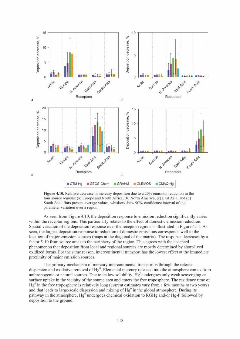
a b

c d

Figure 4.10. Relative decrease in mercury deposition due to a 20% emission reduction in the four source regions: (a) Europe and North Africa, (b) North America, (c) East Asia, and (d) South Asia. Bars present average values, whiskers show 90%-confidence interval of the parameter variation over a region.

As seen from Figure 4.10, the deposition response to emission reduction significantly varies within the receptor regions. This particularly relates to the effect of domestic emission reduction. Spatial variation of the deposition response over the receptor regions is illustrated in Figure 4.11. As seen, the largest deposition response to reduction of domestic emissions corresponds well to the location of major emission sources (maps at the diagonal of the matrix). The response decreases by a factor 5-10 from source areas to the periphery of the region. This agrees with the accepted phenomenon that deposition from local and regional sources are mostly determined by short-lived oxidized forms. For the same reason, intercontinental transport has the lowest effect at the immediate proximity of major emission sources.

The primary mechanism of mercury intercontinental transport is through the release, dispersion and oxidative removal of Hg0. Elemental mercury released into the atmosphere comes from anthropogenic or natural sources. Due to its low solubility, Hg0 undergoes only weak scavenging or surface uptake in the vicinity of the source area and enters the free troposphere. The residence time of Hg0 in the free troposphere is relatively long (current estimates vary from a few months to two years) and that leads to large-scale dispersion and mixing of Hg0 in the global atmosphere. During its pathway in the atmosphere, Hg0 undergoes chemical oxidation to RGHg and/or Hg-P followed by deposition to the ground.

0

5

10

15

Arctic

Europe

N. Ameri

ca

East A

sia

South

Asia

Receptors

Dep

ositi

on d

ecre

ase,

%

0

5

10

Arctic

Europe

N. Ameri

ca

East A

sia

South

Asia

Receptors

Dep

ositi

on d

ecre

ase,

%

0

5

10

15

20

Arctic

Europe

N. Ameri

ca

East A

sia

South

Asia

Receptors

Dep

ositi

on d

ecre

ase,

%

0

5

10

15

Arctic

Europe

N. Ameri

ca

East A

sia

South

Asia

Receptors

Dep

ositi

on d

ecre

ase,

%

CTM-Hg GEOS-Chem GRAHM GLEMOS CMAQ-Hg

118

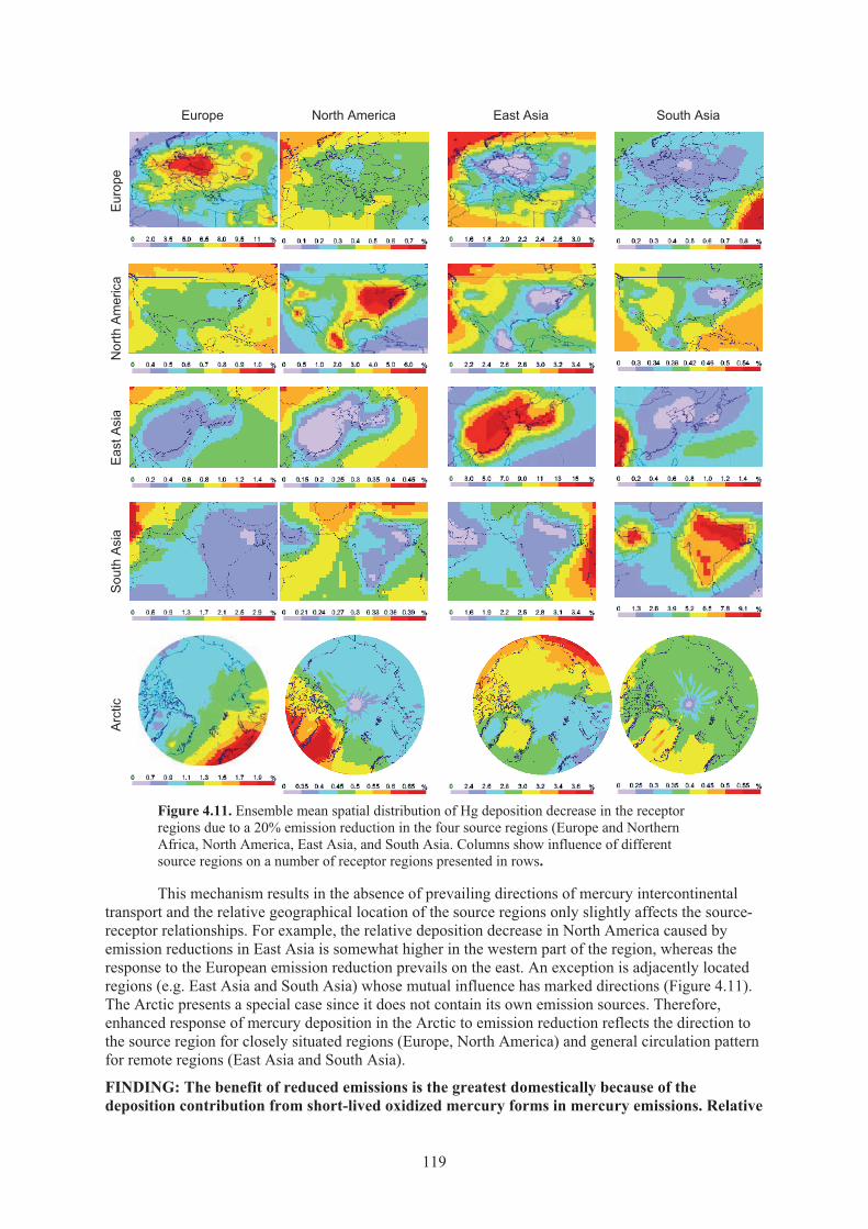
Europe North America East Asia South AsiaE

urop

eN

orth

Am

eric

aE

ast A

sia

Sou

th A

sia

Arc

tic

Figure 4.11. Ensemble mean spatial distribution of Hg deposition decrease in the receptor regions due to a 20% emission reduction in the four source regions (Europe and Northern Africa, North America, East Asia, and South Asia. Columns show influence of different source regions on a number of receptor regions presented in rows.

This mechanism results in the absence of prevailing directions of mercury intercontinental transport and the relative geographical location of the source regions only slightly affects the source-receptor relationships. For example, the relative deposition decrease in North America caused by emission reductions in East Asia is somewhat higher in the western part of the region, whereas the response to the European emission reduction prevails on the east. An exception is adjacently located regions (e.g. East Asia and South Asia) whose mutual influence has marked directions (Figure 4.11). The Arctic presents a special case since it does not contain its own emission sources. Therefore, enhanced response of mercury deposition in the Arctic to emission reduction reflects the direction to the source region for closely situated regions (Europe, North America) and general circulation pattern for remote regions (East Asia and South Asia).

FINDING: The benefit of reduced emissions is the greatest domestically because of the deposition contribution from short-lived oxidized mercury forms in mercury emissions. Relative

119

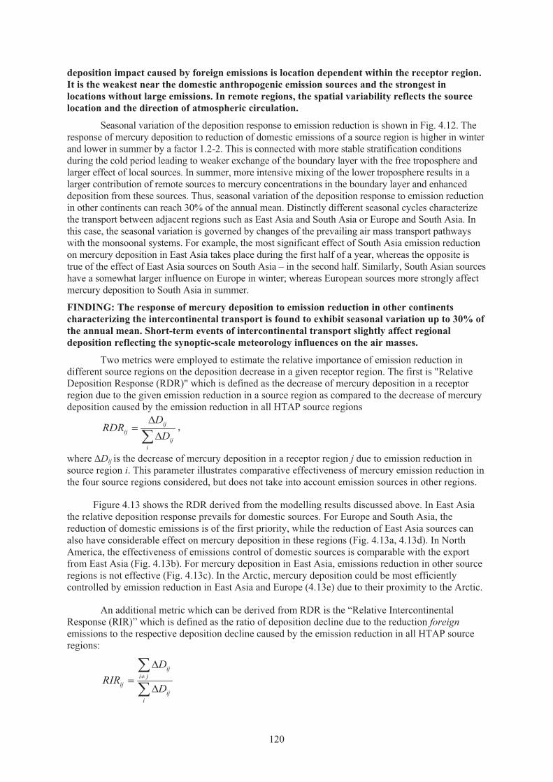
deposition impact caused by foreign emissions is location dependent within the receptor region. It is the weakest near the domestic anthropogenic emission sources and the strongest in locations without large emissions. In remote regions, the spatial variability reflects the source location and the direction of atmospheric circulation.

Seasonal variation of the deposition response to emission reduction is shown in Fig. 4.12. The response of mercury deposition to reduction of domestic emissions of a source region is higher in winter and lower in summer by a factor 1.2-2. This is connected with more stable stratification conditions during the cold period leading to weaker exchange of the boundary layer with the free troposphere and larger effect of local sources. In summer, more intensive mixing of the lower troposphere results in a larger contribution of remote sources to mercury concentrations in the boundary layer and enhanced deposition from these sources. Thus, seasonal variation of the deposition response to emission reduction in other continents can reach 30% of the annual mean. Distinctly different seasonal cycles characterize the transport between adjacent regions such as East Asia and South Asia or Europe and South Asia. In this case, the seasonal variation is governed by changes of the prevailing air mass transport pathways with the monsoonal systems. For example, the most significant effect of South Asia emission reduction on mercury deposition in East Asia takes place during the first half of a year, whereas the opposite is true of the effect of East Asia sources on South Asia – in the second half. Similarly, South Asian sources have a somewhat larger influence on Europe in winter; whereas European sources more strongly affect mercury deposition to South Asia in summer.

FINDING: The response of mercury deposition to emission reduction in other continents characterizing the intercontinental transport is found to exhibit seasonal variation up to 30% of the annual mean. Short-term events of intercontinental transport slightly affect regional deposition reflecting the synoptic-scale meteorology influences on the air masses.

Two metrics were employed to estimate the relative importance of emission reduction in different source regions on the deposition decrease in a given receptor region. The first is "Relative Deposition Response (RDR)" which is defined as the decrease of mercury deposition in a receptor region due to the given emission reduction in a source region as compared to the decrease of mercurydeposition caused by the emission reduction in all HTAP source regions

���

�

iij

ijij D

DRDR ,

where �Dij is the decrease of mercury deposition in a receptor region j due to emission reduction in source region i. This parameter illustrates comparative effectiveness of mercury emission reduction in the four source regions considered, but does not take into account emission sources in other regions.

Figure 4.13 shows the RDR derived from the modelling results discussed above. In East Asia the relative deposition response prevails for domestic sources. For Europe and South Asia, the reduction of domestic emissions is of the first priority, while the reduction of East Asia sources can also have considerable effect on mercury deposition in these regions (Fig. 4.13a, 4.13d). In North America, the effectiveness of emissions control of domestic sources is comparable with the export from East Asia (Fig. 4.13b). For mercury deposition in East Asia, emissions reduction in other source regions is not effective (Fig. 4.13c). In the Arctic, mercury deposition could be most efficiently controlled by emission reduction in East Asia and Europe (4.13e) due to their proximity to the Arctic.

An additional metric which can be derived from RDR is the “Relative Intercontinental Response (RIR)” which is defined as the ratio of deposition decline due to the reduction foreignemissions to the respective deposition decline caused by the emission reduction in all HTAP source regions:

��

�

��

iij

jiij

ij D

DRIR

120

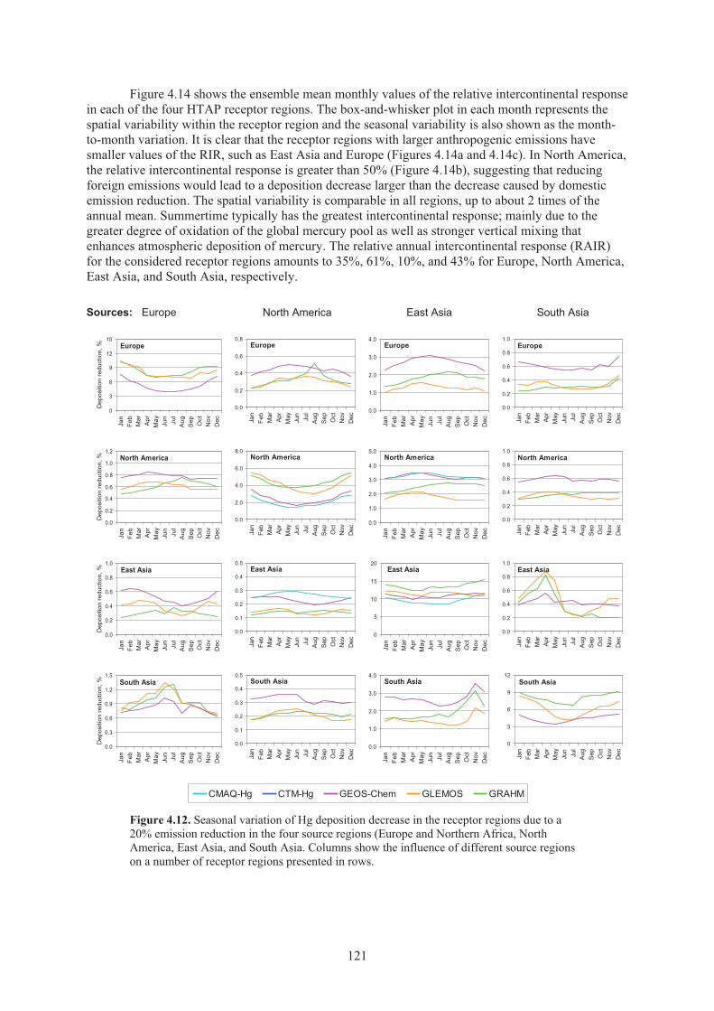
Figure 4.14 shows the ensemble mean monthly values of the relative intercontinental response in each of the four HTAP receptor regions. The box-and-whisker plot in each month represents the spatial variability within the receptor region and the seasonal variability is also shown as the month-to-month variation. It is clear that the receptor regions with larger anthropogenic emissions have smaller values of the RIR, such as East Asia and Europe (Figures 4.14a and 4.14c). In North America, the relative intercontinental response is greater than 50% (Figure 4.14b), suggesting that reducing foreign emissions would lead to a deposition decrease larger than the decrease caused by domestic emission reduction. The spatial variability is comparable in all regions, up to about 2 times of the annual mean. Summertime typically has the greatest intercontinental response; mainly due to the greater degree of oxidation of the global mercury pool as well as stronger vertical mixing that enhances atmospheric deposition of mercury. The relative annual intercontinental response (RAIR) for the considered receptor regions amounts to 35%, 61%, 10%, and 43% for Europe, North America, East Asia, and South Asia, respectively.

Sources: Europe North America East Asia South Asia

Figure 4.12. Seasonal variation of Hg deposition decrease in the receptor regions due to a 20% emission reduction in the four source regions (Europe and Northern Africa, North America, East Asia, and South Asia. Columns show the influence of different source regions on a number of receptor regions presented in rows.

0

3

6

9

12

15

Jan

Feb Mar

Apr

May

Jun

Jul

Aug

Sep Oct

Nov

Dec

Dep

ositi

on r

educ

tion,

% Europe

0.0

0.2

0.4

0.6

0.8

Jan

Feb

Mar

Apr

May

Jun

Jul

Aug

Sep Oct

Nov

Dec

Europe

0.0

1.0

2.0

3.0

4.0

Jan

Feb

Mar

Apr

May

Jun

Jul

Aug

Sep Oct

Nov

Dec

Europe

0.0

0.2

0.4

0.6

0.8

1.0

Jan

Feb

Mar

Apr

May

Jun

Jul

Aug

Sep Oct

Nov

Dec

Europe

0.0

0.2

0.4

0.6

0.8

1.0

1.2

Jan

Feb Mar

Apr

May

Jun

Jul

Aug

Sep Oct

Nov

Dec

Dep

ositi

on r

educ

tion,

% North America

0.0

2.0

4.0

6.0

8.0

Jan

Feb

Mar

Apr

May

Jun

Jul

Aug

Sep Oct

Nov

Dec

North America

0.0

1.0

2.0

3.0

4.0

5.0

Jan

Feb

Mar

Apr

May

Jun

Jul

Aug

Sep Oct

Nov

Dec

North America

0.0

0.2

0.4

0.6

0.8

1.0

Jan

Feb

Mar

Apr

May

Jun

Jul

Aug

Sep Oct

Nov

Dec

North America

0.0

0.2

0.4

0.6

0.8

1.0

Jan

Feb Mar

Apr

May

Jun

Jul

Aug

Sep Oct

Nov

Dec

Dep

ositi

on r

educ

tion,

% East Asia

0.0

0.1

0.2

0.3

0.4

0.5

Jan

Feb

Mar

Apr

May

Jun

Jul

Aug

Sep Oct

Nov

Dec

East Asia

0

5

10

15

20

Jan

Feb

Mar

Apr

May

Jun

Jul

Aug

Sep Oct

Nov

Dec

East Asia

0.0

0.2

0.4

0.6

0.8

1.0

Jan

Feb

Mar

Apr

May

Jun

Jul

Aug

Sep Oct

Nov

Dec

East Asia

0.0

0.3

0.6

0.9

1.2

1.5

Jan

Feb Mar

Apr

May

Jun

Jul

Aug

Sep Oct

Nov

Dec

Dep

ositi

on r

educ

tion,

% South Asia

0.0

0.1

0.2

0.3

0.4

0.5

Jan

Feb

Mar

Apr

May

Jun

Jul

Aug

Sep Oct

Nov

Dec

South Asia

0.0

1.0

2.0

3.0

4.0

Jan

Feb

Mar

Apr

May

Jun

Jul

Aug

Sep Oct

Nov

Dec

South Asia

0

3

6

9

12

Jan

Feb

Mar

Apr

May

Jun

Jul

Aug

Sep Oct

Nov

Dec

South Asia

CMAQ-Hg CTM-Hg GEOS-Chem GLEMOS GRAHM

121

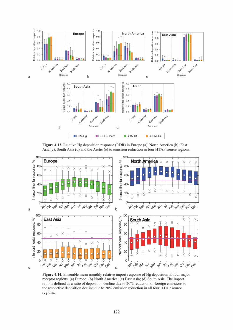
a b c

d e

Figure 4.13. Relative Hg deposition response (RDR) in Europe (a), North America (b), East Asia (c), South Asia (d) and the Arctic (e) to emission reduction in four HTAP source regions.

a b

c dFigure 4.14. Ensemble mean monthly relative import response of Hg deposition in four major receptor regions: (a) Europe; (b) North America; (c) East Asia; (d) South Asia. The import ratio is defined as a ratio of deposition decline due to 20% reduction of foreign emissions to the respective deposition decline due to 20% emission reduction in all four HTAP source regions.

0.0

0.2

0.4

0.6

0.8

1.0

Europe

N. Ameri

ca

East A

sia

South

Asia

Sources

Rel

ativ

e de

posi

tion

resp

onse

Europe

0.0

0.2

0.4

0.6

0.8

1.0

Europe

N. Ameri

ca

East A

sia

South

Asia

Sources

Rel

ativ

e de

posi

tion

resp

onse

North America

0.0

0.2

0.4

0.6

0.8

1.0

Europe

N. Ameri

ca

East A

sia

South

Asia

Sources

Rel

ativ

e de

posi

tion

resp

onse

East Asia

0.0

0.2

0.4

0.6

0.8

1.0

Europe

N. Ameri

ca

East A

sia

South

Asia

Sources

Rel

ativ

e de

posi

tion

resp

onse

South Asia

0.0

0.2

0.4

0.6

0.8

1.0

Europe

N. Ameri

ca

East A

sia

South

Asia

SourcesR

elat

ive

depo

sitio

n re

spon

se

Arctic

CTM-Hg GEOS-Chem GRAHM GLEMOS

Jan Feb

Mar Apr May Jun Jul Aug Sep Oct Nov Dec0

20

40

60

80

100Europe

Inte

rcon

tinen

tal r

espo

nse,

%

Jan

Feb

Mar Apr May Jun Ju

lAug Sep Oct Nov Dec

0

20

40

60

80

100North America

Inte

rcon

tinen

tal r

espo

nse,

%

Jan Feb

Mar Apr May Jun Jul Aug Sep Oct Nov Dec0

20

40

60

80

100East Asia

Inte

rcon

tinen

tal r

espo

nse,

%

Jan

Feb

Mar Apr May Jun Ju

lAug Sep Oct Nov Dec

0

20

40

60

80

100South Asia

Inte

rcon

tinen

tal r

espo

nse,

%

122

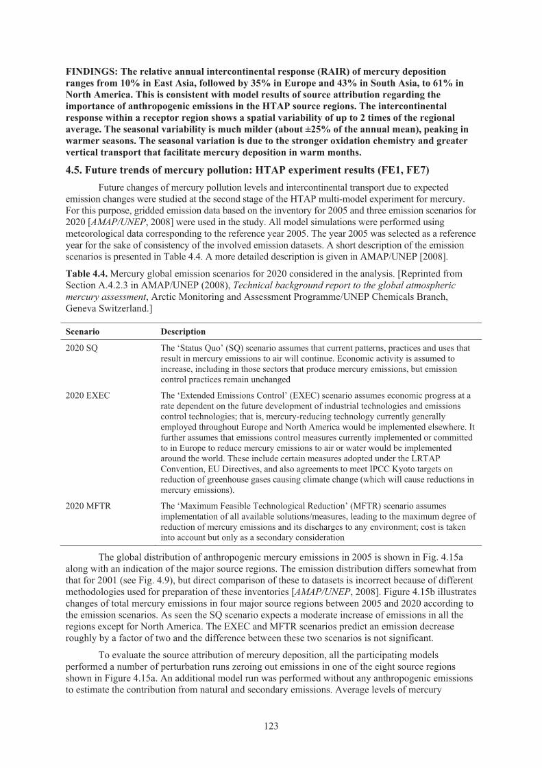
FINDINGS: The relative annual intercontinental response (RAIR) of mercury deposition ranges from 10% in East Asia, followed by 35% in Europe and 43% in South Asia, to 61% in North America. This is consistent with model results of source attribution regarding the importance of anthropogenic emissions in the HTAP source regions. The intercontinental response within a receptor region shows a spatial variability of up to 2 times of the regional average. The seasonal variability is much milder (about ±25% of the annual mean), peaking in warmer seasons. The seasonal variation is due to the stronger oxidation chemistry and greatervertical transport that facilitate mercury deposition in warm months.

4.5. Future trends of mercury pollution: HTAP experiment results (FE1, FE7)Future changes of mercury pollution levels and intercontinental transport due to expected

emission changes were studied at the second stage of the HTAP multi-model experiment for mercury. For this purpose, gridded emission data based on the inventory for 2005 and three emission scenarios for 2020 [AMAP/UNEP, 2008] were used in the study. All model simulations were performed using meteorological data corresponding to the reference year 2005. The year 2005 was selected as a reference year for the sake of consistency of the involved emission datasets. A short description of the emission scenarios is presented in Table 4.4. A more detailed description is given in AMAP/UNEP [2008].

Table 4.4. Mercury global emission scenarios for 2020 considered in the analysis. [Reprinted from Section A.4.2.3 in AMAP/UNEP (2008), Technical background report to the global atmospheric mercury assessment, Arctic Monitoring and Assessment Programme/UNEP Chemicals Branch, Geneva Switzerland.]

Scenario Description

2020 SQ The ‘Status Quo’ (SQ) scenario assumes that current patterns, practices and uses that result in mercury emissions to air will continue. Economic activity is assumed to increase, including in those sectors that produce mercury emissions, but emission control practices remain unchanged

2020 EXEC The ‘Extended Emissions Control’ (EXEC) scenario assumes economic progress at a rate dependent on the future development of industrial technologies and emissions control technologies; that is, mercury-reducing technology currently generally employed throughout Europe and North America would be implemented elsewhere. It further assumes that emissions control measures currently implemented or committed to in Europe to reduce mercury emissions to air or water would be implemented around the world. These include certain measures adopted under the LRTAP Convention, EU Directives, and also agreements to meet IPCC Kyoto targets on reduction of greenhouse gases causing climate change (which will cause reductions in mercury emissions).

2020 MFTR The ‘Maximum Feasible Technological Reduction’ (MFTR) scenario assumes implementation of all available solutions/measures, leading to the maximum degree of reduction of mercury emissions and its discharges to any environment; cost is taken into account but only as a secondary consideration

The global distribution of anthropogenic mercury emissions in 2005 is shown in Fig. 4.15a along with an indication of the major source regions. The emission distribution differs somewhat from that for 2001 (see Fig. 4.9), but direct comparison of these to datasets is incorrect because of different methodologies used for preparation of these inventories [AMAP/UNEP, 2008]. Figure 4.15b illustrates changes of total mercury emissions in four major source regions between 2005 and 2020 according to the emission scenarios. As seen the SQ scenario expects a moderate increase of emissions in all the regions except for North America. The EXEC and MFTR scenarios predict an emission decrease roughly by a factor of two and the difference between these two scenarios is not significant.

To evaluate the source attribution of mercury deposition, all the participating models performed a number of perturbation runs zeroing out emissions in one of the eight source regions shown in Figure 4.15a. An additional model run was performed without any anthropogenic emissions to estimate the contribution from natural and secondary emissions. Average levels of mercury

123

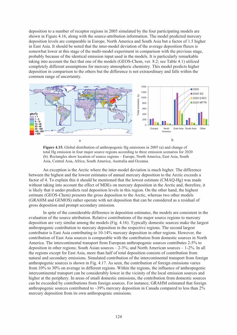
deposition to a number of receptor regions in 2005 simulated by the four participating models are shown in Figure 4.16, along with the source-attribution information. The model predicted mercury deposition levels are comparable in Europe, North America and South Asia but a factor of 1.5 higher in East Asia. It should be noted that the inter-model deviation of the average deposition fluxes issomewhat lower at this stage of the multi-model experiment in comparison with the previous stage, probably because of the identical emission input used in the models. It is particularly remarkable taking into account the fact that one of the models (GEOS-Chem, ver. 8.2; see Table 4.1) utilized completely different assumptions for mercury atmospheric chemistry. This model predicts higher deposition in comparison to the others but the difference is not extraordinary and falls within the common range of uncertainty.

a b

Figure 4.15. Global distribution of anthropogenic Hg emissions in 2005 (a) and change of total Hg emission in four major source regions according to three emission scenarios for 2020 (b). Rectangles show location of source regions – Europe, North America, East Asia, South Asia, Central Asia, Africa, South America, Australia and Oceania.

An exception is the Arctic where the inter-model deviation is much higher. The difference between the highest and the lowest estimates of annual mercury deposition to the Arctic exceeds a factor of 4. To explain this it should be mentioned that the lowest estimate (CMAQ-Hg) was made without taking into account the effect of MDEs on mercury deposition in the Arctic and, therefore, it is likely that it under-predicts real deposition levels in this region. On the other hand, the highest estimate (GEOS-Chem) presents the gross deposition to the Arctic, whereas two other models (GRAHM and GEMOS) rather operate with net deposition that can be considered as a residual of gross deposition and prompt secondary emission.

In spite of the considerable difference in deposition estimates, the models are consistent in the evaluation of the source attribution. Relative contributions of the major source regions to mercury deposition are very similar among the models (Fig. 4.16). Typically domestic sources make the largest anthropogenic contribution to mercury deposition in the respective regions. The second largest contributor is East Asia contributing to 10-14% mercury deposition in other regions. However, the contribution of East Asia sources is comparable with the contribution from domestic sources in North America. The intercontinental transport from European anthropogenic sources contributes 2-5% to deposition in other regions; South Asian sources – 2-3%; and North American sources – 1-2%. In all the regions except for East Asia, more than half of total deposition consists of contribution from natural and secondary emissions. Simulated contribution of the intercontinental transport from foreign anthropogenic sources is shown in Fig. 4.17. As seen, the contribution of foreign emissions varies from 10% to 30% on average in different regions. Within the regions, the influence of anthropogenic intercontinental transport can be considerably lower in the vicinity of the local emission sources and higher at the periphery. In areas of small domestic emissions, the contribution from domestic sources can be exceeded by contributions from foreign sources. For instance, GRAHM estimated that foreign anthropogenic sources contributed to ~39% mercury deposition in Canada compared to less than 2% mercury deposition from its own anthropogenic emissions.

0

200

400

600

800

1000

1200

1400

Europe NorthAmerica

East Asia South Asia Other

Tota

l em

issi

on, t

/y

2005

2020 SQ

2020 EXEC

2020 MFTR

124

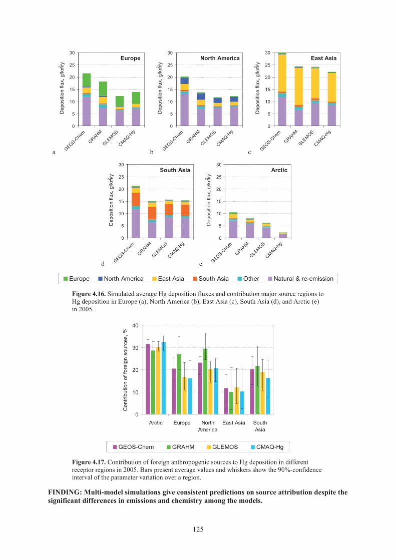
a b c

d e

Figure 4.16. Simulated average Hg deposition fluxes and contribution major source regions to Hg deposition in Europe (a), North America (b), East Asia (c), South Asia (d), and Arctic (e) in 2005.

Figure 4.17. Contribution of foreign anthropogenic sources to Hg deposition in different receptor regions in 2005. Bars present average values and whiskers show the 90%-confidence interval of the parameter variation over a region.

FINDING: Multi-model simulations give consistent predictions on source attribution despite the significant differences in emissions and chemistry among the models.

0

5

10

15

20

25

30

GEOS-Che

m

GRAHM

GLEMOS

CMAQ-Hg

Dep

ositi

on fl

ux, g

/km2 /y

Europe

0

5

10

15

20

25

30

GEOS-Che

m

GRAHM

GLEMOS

CMAQ-Hg

Dep

ositi

on fl

ux, g

/km2 /y

North America

0

5

10

15

20

25

30

GEOS-Che

m

GRAHM

GLEMOS

CMAQ-Hg

Dep

ositi

on fl

ux, g

/km2 /y

East Asia

0

5

10

15

20

25

30

GEOS-Che

m

GRAHM

GLEMOS

CMAQ-Hg

Dep

ositi

on fl

ux, g

/km2 /y

South Asia

0

5

10

15

20

25

30

GEOS-Che

m

GRAHM

GLEMOS

CMAQ-Hg

Dep

ositi

on fl

ux, g

/km2 /y

Arctic

Europe North America East Asia South Asia Other Natural & re-emission

0

10

20

30

40

Arctic Europe NorthAmerica

East Asia SouthAsia

Con

tribu

tion

of fo

reig

n so

urce

s, %

GEOS-Chem GRAHM GLEMOS CMAQ-Hg

125

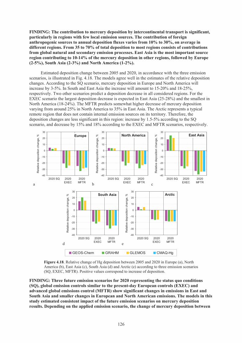
FINDING: The contribution to mercury deposition by intercontinental transport is significant, particularly in regions with few local emission sources. The contribution of foreign anthropogenic sources to annual deposition fluxes varies from 10% to 30%, on average in different regions. From 35 to 70% of total deposition to most regions consists of contributions from global natural and secondary emission processes. East Asia is the most important source region contributing to 10-14% of the mercury deposition in other regions, followed by Europe (2-5%), South Asia (2-3%) and North America (1-2%).

Estimated deposition change between 2005 and 2020, in accordance with the three emission scenarios, is illustrated in Fig. 4.18. The models agree well in the estimates of the relative deposition changes. According to the SQ scenario, mercury deposition in Europe and North America will increase by 3-5%. In South and East Asia the increase will amount to 15-20% and 18-25%, respectively. Two other scenarios predict a deposition decrease in all considered regions. For the EXEC scenario the largest deposition decrease is expected in East Asia (25-28%) and the smallest in North America (18-24%). The MFTR predicts somewhat higher decrease of mercury deposition varying from around 25% in North America to 35% in East Asia. The Arctic represents a typical remote region that does not contain internal emission sources on its territory. Therefore, the deposition changes are less significant in this region: increase by 1.5-5% according to the SQ scenario, and decrease by 15% and 18% according to the EXEC and MFTR scenarios, respectively.

a b c

d e

Figure 4.18. Relative change of Hg deposition between 2005 and 2020 in Europe (a), North America (b), East Asia (c), South Asia (d) and Arctic (e) according to three emission scenarios (SQ, EXEC, MFTR). Positive values correspond to increase of deposition.

FINDING: Three future emission scenarios for 2020 representing the status quo conditions (SQ), global emission controls similar to the present-day European controls (EXEC) and advanced global emissions control (MFTR) show significant changes in emissions in East and South Asia and smaller changes in European and North American emissions. The models in this study estimated consistent impact of the future emission scenarios on mercury deposition results. Depending on the applied emission scenario, the change of mercury deposition between

-40

-30

-20

-10

0

10

20

30

2020 SQ 2020EXEC

2020MFTR

Rel

ativ

e de

posi

tion

chan

ge, % Europe

-40

-30

-20

-10

0

10

20

30

2020 SQ 2020EXEC

2020MFTR

Rel

ativ

e de

posi

tion

chan

ge, % North America

-40

-30

-20

-10

0

10

20

30

2020 SQ 2020EXEC

2020MFTR

Rel

ativ

e de

posi

tion

chan

ge, % East Asia

-40

-30

-20

-10

0

10

20

30

2020 SQ 2020EXEC

2020MFTR

Rel

ativ

e de

posi

tion

chan

ge, % South Asia

-40

-30

-20

-10

0

10

20

30

2020 SQ 2020EXEC

2020MFTR

Rel

ativ

e de

posi

tion

chan

ge, %

Arctic

GEOS-Chem GRAHM GLEMOS CMAQ-Hg

126

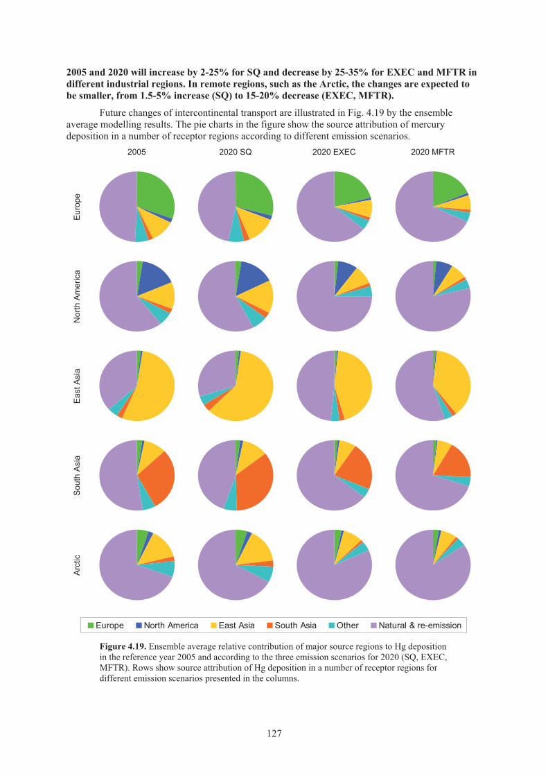
2005 and 2020 will increase by 2-25% for SQ and decrease by 25-35% for EXEC and MFTR in different industrial regions. In remote regions, such as the Arctic, the changes are expected to be smaller, from 1.5-5% increase (SQ) to 15-20% decrease (EXEC, MFTR).

Future changes of intercontinental transport are illustrated in Fig. 4.19 by the ensemble average modelling results. The pie charts in the figure show the source attribution of mercury deposition in a number of receptor regions according to different emission scenarios.

2005 2020 SQ 2020 EXEC 2020 MFTR

Eur

ope

Nor

th A

mer

ica

Eas

t Asi

aS

outh

Asi

aA

rctic

Figure 4.19. Ensemble average relative contribution of major source regions to Hg deposition in the reference year 2005 and according to the three emission scenarios for 2020 (SQ, EXEC, MFTR). Rows show source attribution of Hg deposition in a number of receptor regions for different emission scenarios presented in the columns.

Europe North America East Asia South Asia Other Natural & re-emission

127

In general, change of anthropogenic emissions leads to appropriate change of relative contributions of anthropogenic and natural sources to deposition in all regions. For example, the relative contribution of anthropogenic sources to mercury deposition in North America increases from 38% in 2005 to 41% for SQ and decreases to 26% and 20% for EXEC and MFTR, respectively. It should be noted that natural sources were expected to be unchanged for the future scenarios except for the dynamic evasion response of the ocean and prompt secondary emission from land applied in some models (GEOS-Chem, GRAHM).

A decrease of emissions from domestic sources results in a corresponding decrease of their contribution to mercury deposition to the region and an increase of the contribution of foreign sources from intercontinental transport. For example, the contribution of foreign sources (including natural and secondary emissions) to deposition in Europe will increase from 70% to 79% and 81% according to the EXEC and MFTR scenarios, respectively. Relative contributions of the source regions to mercury deposition to the Arctic, which does not contain internal sources, increases or decreases proportionally to each other in accordance with changes of anthropogenic emissions in these regions.

FINDING: Based on available mercury emission projections, the source-receptor relationships of anthropogenic emissions should not change greatly in the next 20 years. The direction of changes will depend on the assumptions of particular emission scenarios.

RECOMMENDATION: In light of the importance of natural and secondary emissions to the concentration and deposition in all regions under current and future anthropogenic emission scenarios, more studies are required for quantitative and mechanistic understanding of the emissions from various surfaces (soils, water, and vegetation).�4.6. Modelling uncertainty4.6.1. Sources of modelling uncertainty Uncertainties exist in multiple components of atmospheric mercury models, including the preparation of emission inventories and speciation, the treatment of natural emission or re-emission [Lin et al., 2005; Seigneur et al., 2004; Walcek et al., 2003], the mechanisms and kinetics of mercury chemistry in both gaseous and aqueous phases of the atmosphere [Ariya et al., 2009; Calvert and Lindberg, 2005; Gårdfeldt and Jonsson, 2003; Hynes et al., 2009; Pal and Ariya, 2004a; b; Ryaboshapko et al., 2002; Van Loon et al., 2000], the treatment of mercury deposition schemes [Lin et al., 2006a], the lack of knowledge in mercury-particulate interactions, and the choice of model grid spatial resolutions. For regional model simulation, additional uncertainty exists in the preparation of boundary conditions of various mercury species. These uncertainty issues are discussed in the following sections.

a) Mercury chemistry

One of the largest model uncertainties comes from the chemical mechanisms implemented in mercury models. The current understanding of atmospheric mercury chemistry and related kinetics is based on the extrapolation of limited laboratory investigations. The appropriateness of such extrapolation has been questioned [e.g.Calvert and Lindberg, 2005; Gårdfeldt and Jonsson, 2003]. The uncertainties in the gaseous mercury chemistry are mainly in two areas: (1) the uncertainty associated with the reported kinetic constants, and (2) the lack of deterministic product identification of mercury reactions, particularly for gaseous oxidation of Hg0. In addition, the temperature dependence of the mercury reactions are lacking in general. Several studies have discussed a number of possible reduction reactions for RGHg in the gaseous phase and in aqueous aerosols [Gårdfeldt and Jonsson, 2003; Lin et al., 2006a; Pongprueksa et al., 2008]. However, these reduction mechanisms require further experimental verification in the laboratory or in the field, and have not been implemented in models.

Experimental evidence has shown that oxidants such as O3 and OH can be important oxidants for the removal of Hg0 [Hall, 1995; Pal and Ariya, 2004a; b; Sommar et al., 2001; Sumner and Spicer,2005]. However, the studies of the reactions between Hg0 and O3/OH focused only on the first step of

128

the reaction sequences leading to RGHg and so may overestimate the conversion of Hg0 to RGHg [Ariya et al., 2008; Calvert and Lindberg, 2005; Goodsite et al., 2004]. And, the mechanistic insights are generally lacking [Ariya et al., 2009; Hynes et al., 2009].

For mercury model implementation, the kinetic uncertainty is especially troublesome for Hg0

oxidation by O3, since a wide range of rate constants have been reported:

� (4.2-49×10-19 cm3molecule-1s-1 by Schroeder et al.,[1991] using the data by [P’yankov, 1949];

� 3.0×10-20 cm3molecule-1s-1 by [Hall, 1995]; and � 7.5×10-19 cm3molecule-1s-1 by [Pal and Ariya, 2004b]).

The two most recent kinetic measurements show a range over a factor of 25. If the upper kinetic limit is used, ozone is the most important oxidant in the continental troposphere. However, if the lower limit is used, hydroxyl radical dominates the Hg0 oxidation according to the relatively consistent kinetic data reported by [Sommar et al., 2001](8.7×10-14 cm3molecule-1s-1, 2001) and [Pal and Ariya, 2004b] (9.0×10-14 cm3molecule-1s-1, 2004b). However, the occurrence of the Hg0+OHreaction in the atmosphere has been questioned, and an upper limit of the rate constant (1.2×10-13

cm3molecule-1s-1) obtained from using an alternative kinetic technique (laser-induced fluorescence spectroscopy) was reported [Bauer et al., 2003].

More recently, Calvert and Lindberg [2005] performed a kinetic re-evaluation of the two mechanisms by thermodynamic calculations and chemical kinetic modelling. They suggested that the oxidative removal of Hg0 by O3 may be significantly smaller than the laboratory kinetic predictions due to the possible dissociation of HgO in the atmosphere. The direct reaction between O3 and Hg0 to form HgO is endothermic and thus is not occurring in the atmosphere. However, mercury might still react with O3 to form an HgO3 intermediate that can react further, for example heterogeneously. Hg0

may also be transported to particles and oxidized by O3 in the particles [Munthe, 1992]. The reported rate constant for the Hg0+OH reaction may also be very much overestimated. Furthermore, since the oxidation of Hg0 by OH may be greatly attenuated by HgOH decomposition [Goodsite et al., 2004],the oxidation removal in the atmosphere is potentially unimportant [Calvert and Lindberg, 2005].These contradicting results complicate the model implementation.

The oxidation products of Hg0 have also not been clearly defined. Understanding the product distribution between gas and aerosol (i.e., RGHg vs. Hg-P) is important, since the deposition velocity and the removal mechanism of the mercury species vary greatly. For example, the deposition velocity of RGHg has been estimated as high as 7.6 cm s-1 with dry deposition as the primary removal pathway [Poissant et al., 2004]. Actual field measurements of RGHg are few, but those reported range from 1 to 5 cm s-1 , e.g., [Lindberg and Stratton, 1998; Zhang et al., 2009]. On the other hand, mercury associated with fine particulate matter (i.e., Hg-P) has a much smaller deposition velocity (usually < 0.1 cm/s; Xu and [Carmichael et al., 1998]) and mainly is removed by cloud scavenging and wet deposition.

The gas phase reaction of Hg0 with bromine (Br) is emerging as an important reaction in the global atmosphere. This reaction starts a sequence of reactions that eventually lead to RGHg. The reaction sequence is temperature dependent [Goodsite et al., 2004] and the fastest removal of Hg0 is observed under cold conditions such as those prevailing at the poles or in the upper part of the troposphere, whereas much longer lifetimes are found at warmer temperatures. In the background troposphere only small fluctuations in Hg0 concentrations are observed [Ebinghaus et al., 2002; Kim and Kim, 1996; Lindberg et al., 2007; Weiss-Penzias et al., 2003], which agrees well with a relatively long atmospheric lifetime of mercury obtained in a model study [Holmes et al., 2006]. Bromine atoms can be produced from a number of sources. One is through sea spray [Yang et al., 2005] in the marine boundary layer. A second source is refreezing leads (open water areas in sea ice or between sea ice and the shore) in Polar Regions during polar spring, where molecular bromine (Br2) is released from bromide-enriched sea-ice surfaces [Simpson et al., 2007]. Third, Br can be produced in the upper part of the troposphere from the photolysis of organo-bromides. However, a reliable modelling approach has yet to be developed in order to provide representative concentrations of Br and Br2 in the atmosphere.

129

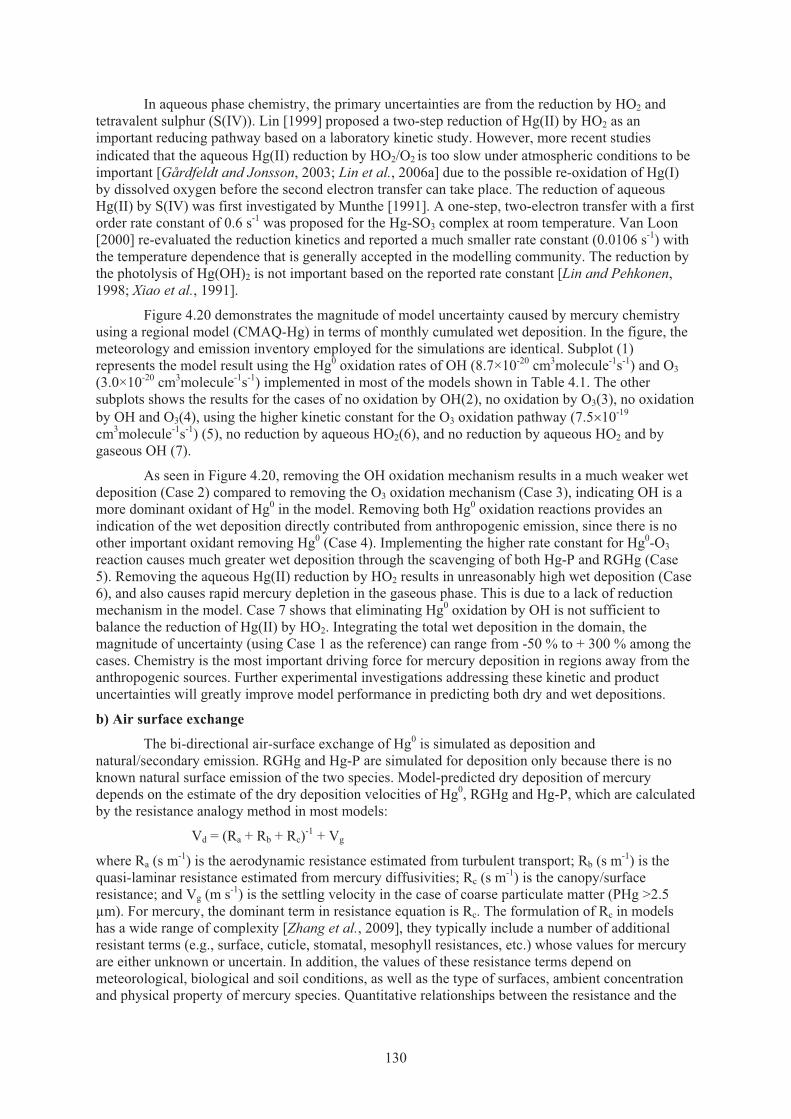
In aqueous phase chemistry, the primary uncertainties are from the reduction by HO2 and tetravalent sulphur (S(IV)). Lin [1999] proposed a two-step reduction of Hg(II) by HO2 as an important reducing pathway based on a laboratory kinetic study. However, more recent studies indicated that the aqueous Hg(II) reduction by HO2/O2

is too slow under atmospheric conditions to be important [Gårdfeldt and Jonsson, 2003; Lin et al., 2006a] due to the possible re-oxidation of Hg(I) by dissolved oxygen before the second electron transfer can take place. The reduction of aqueous Hg(II) by S(IV) was first investigated by Munthe [1991]. A one-step, two-electron transfer with a first order rate constant of 0.6 s-1 was proposed for the Hg-SO3 complex at room temperature. Van Loon [2000] re-evaluated the reduction kinetics and reported a much smaller rate constant (0.0106 s-1) with the temperature dependence that is generally accepted in the modelling community. The reduction by the photolysis of Hg(OH)2 is not important based on the reported rate constant [Lin and Pehkonen,1998; Xiao et al., 1991].

Figure 4.20 demonstrates the magnitude of model uncertainty caused by mercury chemistry using a regional model (CMAQ-Hg) in terms of monthly cumulated wet deposition. In the figure, the meteorology and emission inventory employed for the simulations are identical. Subplot (1) represents the model result using the Hg0 oxidation rates of OH (8.7×10-20 cm3molecule-1s-1) and O3(3.0×10-20 cm3molecule-1s-1) implemented in most of the models shown in Table 4.1. The other subplots shows the results for the cases of no oxidation by OH(2), no oxidation by O3(3), no oxidation by OH and O3(4), using the higher kinetic constant for the O3 oxidation pathway (7.5�10-19

cm3molecule-1s-1) (5), no reduction by aqueous HO2(6), and no reduction by aqueous HO2 and by gaseous OH (7).

As seen in Figure 4.20, removing the OH oxidation mechanism results in a much weaker wet deposition (Case 2) compared to removing the O3 oxidation mechanism (Case 3), indicating OH is amore dominant oxidant of Hg0 in the model. Removing both Hg0 oxidation reactions provides an indication of the wet deposition directly contributed from anthropogenic emission, since there is no other important oxidant removing Hg0 (Case 4). Implementing the higher rate constant for Hg0-O3reaction causes much greater wet deposition through the scavenging of both Hg-P and RGHg (Case 5). Removing the aqueous Hg(II) reduction by HO2 results in unreasonably high wet deposition (Case 6), and also causes rapid mercury depletion in the gaseous phase. This is due to a lack of reduction mechanism in the model. Case 7 shows that eliminating Hg0 oxidation by OH is not sufficient to balance the reduction of Hg(II) by HO2. Integrating the total wet deposition in the domain, the magnitude of uncertainty (using Case 1 as the reference) can range from -50 % to + 300 % among the cases. Chemistry is the most important driving force for mercury deposition in regions away from the anthropogenic sources. Further experimental investigations addressing these kinetic and product uncertainties will greatly improve model performance in predicting both dry and wet depositions.

b) Air surface exchange

The bi-directional air-surface exchange of Hg0 is simulated as deposition and natural/secondary emission. RGHg and Hg-P are simulated for deposition only because there is no known natural surface emission of the two species. Model-predicted dry deposition of mercury depends on the estimate of the dry deposition velocities of Hg0, RGHg and Hg-P, which are calculated by the resistance analogy method in most models:

Vd = (Ra + Rb + Rc)-1 + Vg

where Ra (s m-1) is the aerodynamic resistance estimated from turbulent transport; Rb (s m-1) is the quasi-laminar resistance estimated from mercury diffusivities; Rc (s m-1) is the canopy/surface resistance; and Vg (m s-1) is the settling velocity in the case of coarse particulate matter (PHg >2.5 μm). For mercury, the dominant term in resistance equation is Rc. The formulation of Rc in models has a wide range of complexity [Zhang et al., 2009], they typically include a number of additional resistant terms (e.g., surface, cuticle, stomatal, mesophyll resistances, etc.) whose values for mercury are either unknown or uncertain. In addition, the values of these resistance terms depend on meteorological, biological and soil conditions, as well as the type of surfaces, ambient concentration and physical property of mercury species. Quantitative relationships between the resistance and the

130

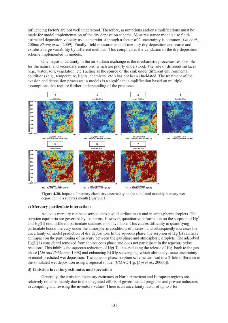
influencing factors are not well understood. Therefore, assumptions and/or simplifications must be made for model implementation of the dry deposition scheme. Most resistance models use field-estimated deposition velocity as a constraint, although a factor of 2 uncertainty is common [Lin et al.,2006a; Zhang et al., 2009]. Finally, field measurements of mercury dry deposition are scarce and exhibit a large variability by different methods. This complicates the validation of the dry deposition scheme implemented in models.

One major uncertainty in the air-surface exchange is the mechanistic processes responsible for the natural and secondary emissions, which are poorly understood. The role of different surfaces (e.g., water, soil, vegetation, etc.) acting as the source or the sink under different environmental conditions (e.g., temperature, lights, chemistry, etc.) has not been elucidated. The treatment of the evasion and deposition processes in models is a significant simplification based on multiple assumptions that require further understanding of the processes.

Figure 4.20. Impact of mercury chemistry uncertainty on the simulated monthly mercury wet deposition in a summer month (July 2001).

c) Mercury-particulate interactions

Aqueous mercury can be adsorbed onto a solid surface in air and in atmospheric droplets. The sorption equilibria are governed by isotherms. However, quantitative information on the sorption of Hg0

and Hg(II) onto different particulate surfaces is not available. This causes difficulty in quantifying particulate bound mercury under the atmospheric conditions of interest, and subsequently increases the uncertainty of model prediction of dry deposition. In the aqueous phase, the sorption of Hg(II) can have an impact on the partitioning of mercury between the gas phase and atmospheric droplets. The adsorbed Hg(II) is considered removed from the aqueous phase and does not participate in the aqueous redox reactions. This inhibits the aqueous reduction of Hg(II), thus reducing the release of Hg0 back to the gasphase [Lin and Pehkonen, 1998] and enhancing RGHg scavenging, which ultimately cause uncertainty in model-predicted wet deposition. The aqueous phase sorption scheme can lead to a 2-fold difference in the simulated wet deposition using a regional model (CMAQ-Hg, [Lin et al., 2006b]).

d) Emission inventory estimates and speciation

Generally, the emission inventory estimates in North American and European regions are relatively reliable, mainly due to the integrated efforts of governmental programs and private industries in compiling and revising the inventory values. There is an uncertainty factor of up to 3 for

1 432

5 6 7 8

1 432

5 6 7 8

131

anthropogenic emission sources depending on the source categories. Recently, several emission inventory re-assessments and field campaigns have provided more reliable estimates of mercury emissions in East Asia [Streets et al., 2005; Streets et al., 2009]. Nevertheless, significant uncertainties (usually underestimates) still remain in these estimates due to the lack or inaccuracy in reported emission data, stack measurements of mercury, and capture of mercury in control devices. The detailed anthropogenic emission uncertainties for each source category are presented in Section 3.4.

The secondary emissions from natural processes are highly uncertain, mainly due to the lack of a comprehensive, mechanistic description of the emission/evasion processes [Lindberg et al., 2005;Xin et al., 2007]. These emissions can be from various surfaces, including water, soils and vegetative surfaces. However, from an observational point of view, it is difficult to separate the primary emissions from natural sources from the secondary emissions. Recent isotopes studies suggested that an important fraction of mercury deposited to both terrestrial and aquatic surfaces are re-emitted[Lindberg et al., 2007]. The secondary emissions are similar in magnitude to the anthropogenic mercury emissions, especially in summer [Lindberg and Stratton, 1998; Mason and Sheu, 2002; Selin et al., 2007]. [Seigneur et al., 2004] estimated that the ratio of secondary emissions to deposition ranges from a lower limit of 33 % to an upper limit of 56%. On a global basis, there is an uncertainty factor of 4 in the estimate of secondary emissions [Mason, 2009]. More field and mechanistic studies of the emission processes from surfaces are clearly needed for better model parameterization.

The emission speciation of mercury has a profound impact on the simulated mercury deposition, especially near the emission sources. Hg0 is subject to long-range transport, while RGHg (and Hg-P to a lesser extent) deposit rapidly near the emission sources. The speciation of mercury emission depends on the fuel types and the use of emission control technology [Senior et al., 2000;Senior and Johnson, 2005]. Its characterization requires comprehensive in-stack measurements at the emission sources. In Europe and North America, the uncertainty of mercury emission speciation is relatively small since the fuel types and control devices are well documented, although some uncertainty for area source emissions still remains. In Asia, the speciation data are not readily available and caution should be used in interpreting model results of local deposition. With the continued implementation of air emission control technologies, mercury emission speciation in developing countries is likely to have major changes over time [Wang et al., 2009]. The natural and secondary emissions are dominated by Hg0.

e) Boundary conditions for regional modelling

Boundary conditions (BCs) represent the out-of-boundary transport input into the regional model domain. The BCs, particularly those of Hg0, have an important impact on the predicted concentration and deposition by regional models [Bullock et al., 2008; Pongprueksa et al., 2008].Pongprueksa [2008] found that varying Hg0 concentration from 0 to 2 ng m-3 in BC forces a strong linear increase in the simulated mercury concentration and total mercury deposition in a regional domain covering North America, and that the air in the domain can be replaced by the inflow from the boundary in about a week. Varying RGHg or Hg-P in BCs has an impact on the simulated dry and wet deposition near domain boundaries, typically within 5-20 grid cells from the boundary. The strong influence of BCs on the regional model results indicates that BCs must be carefully configured.Ideally, boundary conditions should be prepared based on network measurements of mercury concentrations. Boundary conditions regridded from global model results also serve as an acceptable alternative. However, the simulated deposition can vary considerably using different global model results as the lateral boundary, as shown in Figure 4.21. Using identical emission and meteorological data in the regional model simulations, the differences in the boundary conditions provided by the three global models (CTM, GEOS-CHEM and GRAHM) cause a 50% variability in the simulated dry deposition and a 30% variability in simulated wet deposition [Bullock et al., 2008].

f) Domain grid resolution

The effect of domain grid resolution on model results is two-fold. First, since models assume instantaneous mixing (thus dilution) of emitted pollutants in the receiving model grid cells, changes in the grid resolution directly influence the resulting dilution near the emission locations. In addition, the

132

change of spatial resolution may also result in different land-use classifications in the GIS data that lead to different dry deposition results [Pongprueksa et al., 2008]. An increase in the domain grid size dilutes the concentration of various mercury species. For Hg0, this dilution reduces the chemical oxidation rate and thus dry and wet deposition. For RGHg and Hg-P, the dilution decreases the tendency of dry deposition, since the deposition flux is proportional to the gaseous concentration. Because the air mercury concentration can be modified significantly near large emission sources, the effect of a grid resolution change is more important near the sources, due to both emission dilution and lower concentration of photochemical oxidants responsible for Hg0 oxidation. Pai [2000] tested the effects of grid resolution on the dry and wet deposition of mercury by varying the grid size from 100 km to 20 km in a regional northeast United States domain. They reported that the short-term peak dry deposition near emission sources can be increased by a factor of 2 in the 20-km domain. For simulations in coarser grids, implementation of plume-in-grid can provide a more realistic mercury concentration field near the emission points for modelling local mercury deposition.

Figure 4.21. The 2001 wet deposition (μg m-2 yr-1) as simulated by the CMAQ, REMSAD, and TEAM regional models using lateral boundary concentrations from the CTM-Hg, GEOS-Chem, and GRAHM global models. [Reprinted from Figure 10 in Bullock, O. R., Jr., et al. (2008), The North American Mercury Model Intercomparison Study (NAMMIS): Study description and model-to-model comparisons, Journal of Geophysical Research, 113(D17), D17310.]

FINDING: The largest uncertainties in model estimates of mercury deposition arise from the uncertainties in natural and re-emitted mercury, chemical mechanisms, reaction rates, partitioning of oxidized mercury in gas and particle phases, and dry deposition of Hg0.

RECOMMENDATION: There is a need for a more comprehensive measurement network and interoperable systems for mercury to constrain models and track mercury trends. This is particularly true for the measurement of dry deposition and speciated mercury concentration, especially in southern hemisphere. The development of analytical techniques for accurately quantifying dry deposition fluxes is critical. Better understanding of mercury chemistry in the atmosphere at different altitudes (particularly the gaseous phase oxidation mechanism and kinetics) and the mechanism of the evasion and deposition processes at the earth's surfaces are important. Advancement in field measurements capable of identifying the mercury compounds associated with RGHg is critical for verifying the chemical schemes used in models. More

133

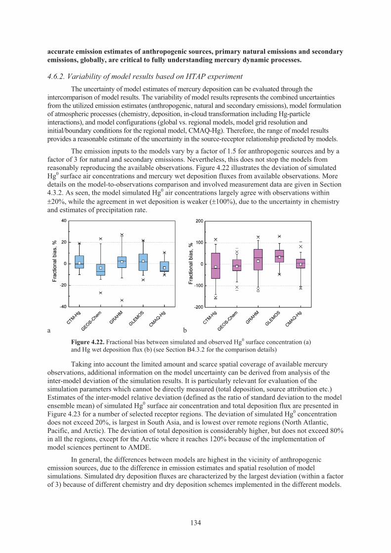
accurate emission estimates of anthropogenic sources, primary natural emissions and secondary emissions, globally, are critical to fully understanding mercury dynamic processes. 4.6.2. Variability of model results based on HTAP experiment

The uncertainty of model estimates of mercury deposition can be evaluated through the intercomparison of model results. The variability of model results represents the combined uncertainties from the utilized emission estimates (anthropogenic, natural and secondary emissions), model formulation of atmospheric processes (chemistry, deposition, in-cloud transformation including Hg-particle interactions), and model configurations (global vs. regional models, model grid resolution and initial/boundary conditions for the regional model, CMAQ-Hg). Therefore, the range of model results provides a reasonable estimate of the uncertainty in the source-receptor relationship predicted by models.

The emission inputs to the models vary by a factor of 1.5 for anthropogenic sources and by a factor of 3 for natural and secondary emissions. Nevertheless, this does not stop the models from reasonably reproducing the available observations. Figure 4.22 illustrates the deviation of simulated Hg0 surface air concentrations and mercury wet deposition fluxes from available observations. More details on the model-to-observations comparison and involved measurement data are given in Section 4.3.2. As seen, the model simulated Hg0 air concentrations largely agree with observations within �20%, while the agreement in wet deposition is weaker (�100%), due to the uncertainty in chemistry and estimates of precipitation rate.

a bFigure 4.22. Fractional bias between simulated and observed Hg0 surface concentration (a) and Hg wet deposition flux (b) (see Section B4.3.2 for the comparison details)

Taking into account the limited amount and scarce spatial coverage of available mercury observations, additional information on the model uncertainty can be derived from analysis of the inter-model deviation of the simulation results. It is particularly relevant for evaluation of the simulation parameters which cannot be directly measured (total deposition, source attribution etc.) Estimates of the inter-model relative deviation (defined as the ratio of standard deviation to the model ensemble mean) of simulated Hg0 surface air concentration and total deposition flux are presented in Figure 4.23 for a number of selected receptor regions. The deviation of simulated Hg0 concentration does not exceed 20%, is largest in South Asia, and is lowest over remote regions (North Atlantic, Pacific, and Arctic). The deviation of total deposition is considerably higher, but does not exceed 80% in all the regions, except for the Arctic where it reaches 120% because of the implementation of model sciences pertinent to AMDE.

In general, the differences between models are highest in the vicinity of anthropogenic emission sources, due to the difference in emission estimates and spatial resolution of model simulations. Simulated dry deposition fluxes are characterized by the largest deviation (within a factor of 3) because of different chemistry and dry deposition schemes implemented in the different models.

134

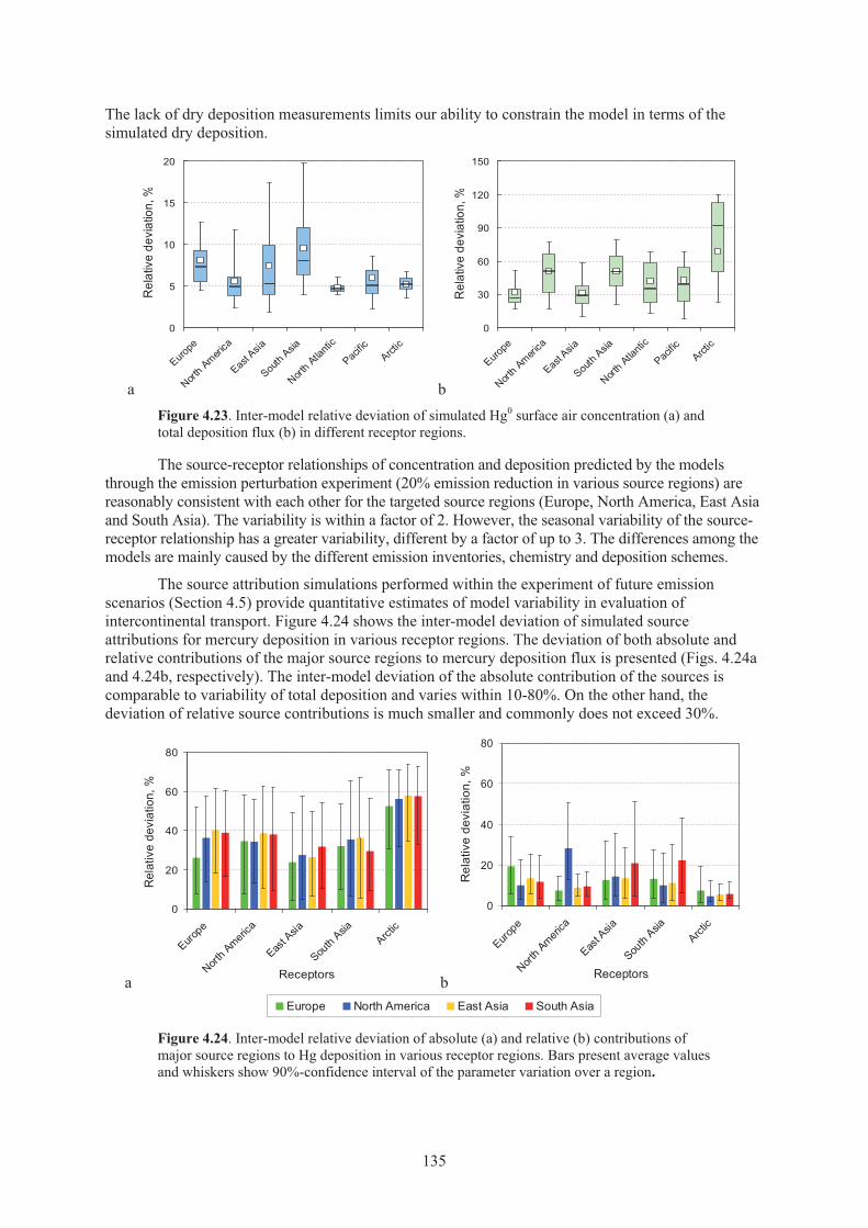
The lack of dry deposition measurements limits our ability to constrain the model in terms of the simulated dry deposition.

a bFigure 4.23. Inter-model relative deviation of simulated Hg0 surface air concentration (a) and total deposition flux (b) in different receptor regions.

The source-receptor relationships of concentration and deposition predicted by the models through the emission perturbation experiment (20% emission reduction in various source regions) are reasonably consistent with each other for the targeted source regions (Europe, North America, East Asia and South Asia). The variability is within a factor of 2. However, the seasonal variability of the source-receptor relationship has a greater variability, different by a factor of up to 3. The differences among the models are mainly caused by the different emission inventories, chemistry and deposition schemes.

The source attribution simulations performed within the experiment of future emission scenarios (Section 4.5) provide quantitative estimates of model variability in evaluation of intercontinental transport. Figure 4.24 shows the inter-model deviation of simulated source attributions for mercury deposition in various receptor regions. The deviation of both absolute and relative contributions of the major source regions to mercury deposition flux is presented (Figs. 4.24a and 4.24b, respectively). The inter-model deviation of the absolute contribution of the sources is comparable to variability of total deposition and varies within 10-80%. On the other hand, the deviation of relative source contributions is much smaller and commonly does not exceed 30%.

a b

Figure 4.24. Inter-model relative deviation of absolute (a) and relative (b) contributions of major source regions to Hg deposition in various receptor regions. Bars present average values and whiskers show 90%-confidence interval of the parameter variation over a region.

0

5

10

15

20

Europe

North A

merica

East A

sia

South

Asia

North A

tlanti

c

Pacific

Arctic

Rel

ativ

e de

viat

ion,

%

0

30

60

90

120

150

Europe

North A

merica

East A

sia

South

Asia

North A

tlanti

c

Pacific

Arctic

Rel

ativ

e de

viat

ion,

%

0

20

40

60

80

Europe

North A

merica

East A

sia

South Asia

Arctic

Receptors

Rel

ativ

e de

viat

ion,

%

0

20

40

60

80

Europe

North A

merica

East A

sia

South

AsiaArct

ic

Receptors

Rel

ativ

e de

viat

ion,

%

Europe North America East Asia South Asia

135

FINDING: The models represented in this study cover the exhaustive range of variability in emission estimates and in model formulations, therefore, the range of model results provides a reasonable estimate of uncertainty in predicted quantities. The magnitudes of model uncertainties range from 20%, for the simulated air concentration of Hg0, up to 80% for the simulated total deposition. However, the simulation results for the relative source attribution have a smaller uncertainty at about 30%. This also indicates that different models have consistent results in predicting the source-receptor relationships in relative terms.

4.7. Key findings and recommendations Process understanding and modelling uncertainties

FINDINGS: Numerous studies using mercury transport models have been conducted in the past two decades on both global and regional scales for a variety of tasks including understanding of mercury processes in the atmosphere, evaluation of mercury levels, and assessment of source-receptor relationships. In many cases, the models demonstrate satisfactory agreement with observations. However, considerable variability of the model results indicates essential gaps in knowledge of mercury atmospheric processes. In spite of the scientific uncertainties, mercury models have proven to be a useful tool for assessing mercury pollution.

FINDINGS: Ambient concentrations of elemental gaseous mercury, the species responsible for long-range atmospheric transport, are reliably simulated by contemporary models. Model results are consistent with observations that show similar concentration gradients from the Southern Hemisphere to the Northern Hemisphere. However, spatial coverage of available long-term observations is not sufficient for constraining the models adequately.

FINDINGS: Atmospheric mercury deposition is mostly defined by short-lived oxidized mercury species originating both from direct anthropogenic emissions and from oxidation of elemental mercury in the atmosphere. Both dry and wet removal pathways are equally significant to the total deposition of mercury. Gaps in our knowledge of mercury atmospheric chemistry andemission speciation lead to significant uncertainties in simulated deposition fluxes.

FINDINGS: There is a large uncertainty in the model simulated deposition because of the absence of systematic observations related to dry deposition of mercury. Model simulated wet deposition agrees with observations. However, available measurements of wet deposition are severely restricted in geographical coverage. The differences among models are largest in the regions of sparse measurements such as, the oceans, the Arctic, South Asia, and Africa.

FINDINGS: The Arctic is a unique remote region because it does not have anthropogenic emission sources on its territory and undergoes a period of the atmospheric mercury depletion events (AMDEs) during springtime, which define an important mercury load to the region. The models show significant deviation in estimates of mercury deposition to the Arctic due to the uncertainties in the model formulation of the processes related to AMDEs.

FINDINGS: The models represented in this study cover the exhaustive range of variability in emission estimates and in model formulations, therefore, the range of model results provides a reasonable estimate of uncertainty in predicted quantities. The magnitudes of model uncertainties range from 20%, for the simulated air concentration of Hg0, up to 80% for the simulated total deposition. However, the simulation results for the relative source attribution have a smaller uncertainty at about 30%. This also indicates that different models have consistent results in predicting the source-receptor relationships in relative terms.

RECOMMENDATIONS: There is a need for a comprehensive interoperable measurement network for mercury in the environment to constrain models and track future mercury trends. Extensive regular observations of speciated mercury concentrations are required for the full-scale model evaluation in different parts of the globe, in particular, in Asia, different regions of the Southern Hemisphere, over the oceans, and in the Polar Regions. Regular observations of wet and, in particular, dry deposition of mercury are highly required for the improvement of model formulation and mercury deposition estimates.

136

RECOMMENDATIONS: Better understanding of mercury chemistry through laboratory studies and field measurements are needed, particularly, for the gaseous and heterogeneous phase oxidation mechanisms, kinetics, and products under different atmospheric conditions. The studied chemical mechanisms can be evaluated by application of self-consistent global chemical transport models in combination with extensive observational data.

RECOMMENDATIONS: Reliable assessment of intercontinental or global-scale dispersion of mercury requires development of multi-media biogeochemical models that take into account the entire cycle of mercury in the environment. It is particularly relevant for evaluation of long-term trends, future scenarios and the impact of climate change on mercury pollution. This is also important since the main exposure pathway of mercury to humans occurs through its bioaccumulation in biota in the aquatic environment.

Intercontinental transport and source-receptor relationships

FINDINGS: The impact of intercontinental transport of mercury is mainly derived from the mercury emission input into the global mercury pool, which is followed by dispersion in the atmosphere, oxidation and deposition removal as well as recycling in the environment. Although transport of Hg0 plumes from industrial sources has been detected, mercury deposition resulting from direct long-range transport is not important.

FINDINGS: The contribution of mercury intercontinental transport is significant, particularly in regions with few local emission sources. The models provide consistent estimates of intercontinental transport and deposition. The contribution of foreign anthropogenic sources to annual deposition fluxes varies from 10% to 30% on average anywhere on the globe. From 35 to 70% of total deposition to most regions consists of deposition contributed by global natural and secondary emissions. East Asia is the most dominant source region contributing 10-14% mercury of the deposition in other regions, followed by contributions from Europe (2-5%), South Asia (2-3%) and North America (1-2%).

FINDINGS: Changes in emissions in one region affect mercury concentration and deposition in another region proportionally to the magnitude of source region’s contribution to the receptor region. For example, a 20% emission reduction in East Asia, Europe, South Asia, and North America separately results in 0.6-5.5%, 0.2-3.5%, 0.1-1.5% and 0.1-1.5% decrease of mercury deposition in other regions, respectively. The large contribution of natural sources and secondary emission of legacy mercury to deposition reduces the relative response of mercury deposition to the reduction in anthropogenic emissions. However, the response could be larger in the long-term perspective due to the lagged response of reduction of mercury recycling from planetary surfaces.

RECOMMENDATIONS: Model estimates of the effect of mercury intercontinental transport on regional pollution levels highly depend on the availability of reliable anthropogenic emissions data and, in particular, on speciation of mercury emissions. Therefore, further improvements of global mercury emission inventories are needed, including more accurate emission quantities, chemical speciation, as well as the temporal and spatial variation of the emissions.

RECOMMENDATIONS: In light of the importance of natural emission and secondary emissions for mercury concentration and deposition over the globe under current and future conditions, more studies are required for quantitative and mechanistic understanding of mercury emissions from various surfaces (soils, water, and vegetation).

Future changes of mercury pollution

FINDINGS: Three future emission scenarios for 2020, representing the status quo conditions (SQ), global emission controls similar to the present-day European controls (EXEC) and advanced global emissions control (MFTR), show significant changes in emissions in East and South Asia and smaller changes in European and North American emissions. The models in this study estimated consistent impact of the future emission scenarios on mercury deposition results. Depending on the applied emission scenario, the change of mercury deposition between

137

2005 and 2020 will increase by 2-25% for SQ and decrease by 25-35% for EXEC and MFTR in different industrial regions. In remote regions, such as the Arctic, the changes are expected to be smaller, from 1.5-5% increase (SQ) to 15-20% decrease (EXEC, MFTR).

FINDINGS: Based on available mercury emission projections, the source-receptor relationships of anthropogenic emissions is not expected to change significantly in the next 20 years. The direction of changes depend on the assumptions of particular emission scenarios.

RECOMMENDATIONS: Few available projections of mercury anthropogenic emissions restrict model estimates of mercury concentration and deposition changes in the future. More efforts are needed for elaboration of future mercury emission scenarios as well as the application of chemical transport models in evaluating future changes of mercury pollution levels.

ReferencesAdler, R. F., et al. (2003), The Version-2 Global Precipitation Climatology Project (GPCP) Monthly

Precipitation Analysis (1979–Present), Journal of Hydrometerology, 4(6): 1147-1167.

AMAP/UNEP (2008), Technical background report to the global atmospheric mercury assessment, 159 pp, Arctic Monitoring and Assessment Programme/UNEP Chemicals Branch, Geneva, Switzerland.

Ariya, P., et al. (2009), Mercury chemical transformation in the gas, aqueous, and heterogenous phases: State-of-the-art science and uncertainties in Mercury Fate and Transport in the Global Atmosphere: Emissions, Measurements, and Models, edited by N. Pirrone and R. Mason, 459-502 pp., Springer, New York.

Ariya, P. A., et al. (2004), The Arctic: a sink for mercury, Tellus Series B - Chemical and Physical Meteorology, 56: 397-403.

Ariya, P. A., et al. (2008), Gaseous elemental mercury in the ambient atmosphere: review of the application of theoretical calculations and experimental studies for determination of reaction coefficients and mechanisms with halogens and other reactants, in Advances in Quantum Chemistry, edited by J. R. Sabin, et al., 43-55 pp., Academic Press.

Baker, P. G. L., et al. (2002), Atmospheric mercury measurements at Cape Point, South Africa, Atmospheric Environment 36(14): 2459-2465.

Bauer, D., et al. (2003), Gas phase elemental mercury: a comparison of LIF detection techniques and study of the kinetics of reaction with the hydroxyl radical, Journal of Photochemistry and Photobiology A -Chemistry, 157: 247-256.

Bergan, T., and H. Rodhe (2001), Oxidation of elemental mercury in the atmosphere; constraints imposed by global scale modelling, Journal of Atmospheric Chemistry, 40(2): 191-212.

Biester, H., et al. (2007), Modeling the past atmospheric deposition of mercury using natural archives, Environmental Science & Technology, 41(14): 4851-4860.

Brooks, S. B., et al. (2006), The mass balance of mercury in the springtime arctic environment, Geophysical Research Letters, 33( L13812).

Bullock Jr, O. R., et al. (1998), Lagrangian modeling of mercury air emission, transport and deposition: an analysis of model sensitivity to emissions uncertainty, The Science of the Total Environment, 213(1-3): 1-12.

Bullock Jr., O. R., and K. A. Brehme (2002), Atmospheric mercury simulation using the CMAQ model: formulation description and analysis of wet deposition results, Atmospheric Environment, 36(13): 2135-2146.

Bullock, O. R., Jr., et al. (2008), The North American Mercury Model Intercomparison Study (NAMMIS): Study description and model-to-model comparisons, Journal of Geophysical Research, 113(D17310).

Bullock, O. R., Jr., et al. (2009), An analysis of simulated wet deposition of mercury from the North American Mercury Model Intercomparison Study, Journal of Geophysical Research, 114(D08301).

138

Butler, T. M., et al. (2008), The representation of emissions from megacities in global emission inventories, Atmospheric Environment, 42(4): 703-719.

Calvert, J. G., and S. E. Lindberg (2005), Mechanisms of mercury removal by O3 and OH in the atmosphere, Atmospheric Environment, 39: 3355-3367.

Carmichael, G. R., et al. (1998), Tropospheric ozone production and transport in the springtime in east Asia, Journal of Geophysical Research, 103(D10649).

Christensen, J. H., et al. (2004), Modelling of mercury in the Arctic with the Danish Eulerian Hemispheric Model, Atmospheric Chemistry & Physics, 4: 2251-2257.

Cohen, M. D., et al. (2004), Modelling the atmospheric transport and deposition of mercury to the Great Lakes, Environmental Research, 95: 247-265.

Dastoor, A. P., and Y. Larocque (2004), Global circulation of atmospheric mercury: a modelling study, Atmospheric Environment, 38(1): 147-161.

Dastoor, A. P., et al. (2008), Modeling dynamic exchange of gaseous elemental mercury at polar sunrise, Environmental Science & Technology, 42(14): 5183-5187.

Dastoor, A. P., and D. Davignon (2009), Global mercury modeling at Environment Canada, in Mercury Fate and Transport in the Global Atmosphere: Emissions, Measurements, and Models, edited by N. Pirrone and R. P. Mason, 519-531 pp., Springer, New York.

Durnford, D., et al. (2010), Long range transport of mercury to the Arctic and across Canada, Atmospheric Chemistry & Physics, 10: 6063-6086.

Ebinghaus, R., et al. (2002), Antarctic Springtime Depletion of Atmospheric Mercury, Environmental Science & Technology, 36(6): 1238–1244.

Engstrom, D. R., and E. B. Swain (1997), Recent declines in atmospheric mercury deposition in the upper midwest, Environmental Science & Technology, 31(4): 960–967.

Fitzgerald, W. F., et al. (1998), The case for atmospheric mercury contamination in remote areas, Environmental Science & Technology, 32(1): 1-7.

Fitzgerald, W. F., et al. (2005), Modern and historic atmospheric mercury fluxes in northern Alaska: Global sources and Arctic depletion, Environmental Science & Technology, 39(2): 557–568.

Friedli, H. R., et al. (2004), Mercury in the atmosphere around Japan, Korea, and China as observed during the 2001 ACE-Asia field campaign: Measurements, distributions, sources, and implications, Journal of Geophysical Research, 109: D19S25.

Friedli, H. R., et al. (2007), Mercury in vegetation and organic soil at an upland boreal forest site in Prince Albert National Park, Saskatchewan, Canada, Journal of Geophysical Research, 112: G01004.

Gårdfeldt, K., and M. Jonsson (2003), Is bimolecular reduction of HG(II) complexes possible in aqueous systems of environmental importance, Journal of Physical Chemistry, 107: 4478-4482.

Gbor, P. K., et al. (2006), Improved model for mercury emission, transport and deposition, AtmosphericEnvironment, 40(5): 973-983.

Goodsite, M. E., et al. (2004), A theoretical study of the oxidation of Hg-0 to HgBr2 in the troposphere, Environmental Science & Technology, 38: 1772-1776.

Hall, B. (1995), The gas phase oxidation of elemental mercury by ozone, Water, Air, and Soil Pollution, 80:301-315.

Hedgecock, I. M., et al. (2006), Integrated mercury cycling, transport and air-water exchange (MECAWEx) model, Journal of Geophysical Research 111: D20302.

Holmes, C. D., et al. (2006), Global lifetime of elemental mercury against oxidation by atomic bromine in the free troposphere, Geophysical Research Letters, 33(L20808).

Holmes, C. D., et al. (2009), Sources of deposition of reactive gaseous mercury in the marine atmosphere, Atmospheric Environment, 43(14): 2278-2285.

139

Holmes, C. D., et al. (2010), Global atmospheric model for mercury including oxidation by bromine atoms, atmospheric Chemistry and Physics Discussion, 10(8): 19845-19900.

Hynes, A. J., et al. (2009), Our current understanding of the major chemical and physical processes affecting mercury dynamics in the atmosphere and at the air-water/terrestrial interfaces, in Mercury Fate and Transport in the Global Atmosphere: Emissions, Measurements, and Models, edited by N. Pirrone and R. P. Mason, 427-458 pp., Springer, New York.

Jaffe, D. A., et al. (2005), Export of atmospheric mercury from Asia, Atmospheric Environment, 39(17): 3029-3038.

Jung, G., et al. (2009), The ECHMERIT model, in Mercury Fate and Transport in the Global Atmosphere: Emissions, Measurements, and Models, edited by N. Pirrone and R. P. Mason, 547-569 pp., Springer, New York.

Kallos, G., et al. (2001), Modelling framework for atmospheric mercury over the Mediterranean region: Model development and applications, Large-Scale Scientific Computing, 2179: 281-290.

Kim, K.-H., and M. Y. Kim (1996), Preliminary measurements of atmospheric mercury in mountainous regions of Korea, Journal of Environmental Science and Health - Part A Toxic/Hazardous Substances and Environmental Engineering 31(8): 2023-2032.

Kim, K. H., et al. (2002), The concentrations and fluxes of total gaseous mercury in a western coastal area of Korea during late March 2001, Atmospheric Environment, 36: 3413-3427.

Kirk, J. L., et al. (2006), Rapid reduction and reemission of mercury deposited into snowpacks during atmospheric mercury depletion events at Churchill, Manitoba, Canada, Environmental Science & Technology, 40(24): 7590–7596.

Lamborg, C. H., et al. (2002), Modern and historic atmospheric mercury fluxes in both hemispheres: Global and regional mercury cycling implications, Global Biogeochemical Cycles, 16(4): 1104-1114.

Lee, D. S., et al. (2001), Modelling atmospheric mercury transport and deposition across Europe and the UK, Atmospheric Environment, 35(32): 5455-5466.

Lin, C.-J., et al. (2005), Development of a processor in BEIS3 for estimating vegetative mercury emission in the continental United States, paper presented at Atmospheric Environment, 7th International Conference on Mercury as a Global Pollutant, 2005/12.

Lin, C.-J., et al. (2006a), Scientific uncertainties in atmospheric mercury models I: Model science evaluation, Atmospheric Environment, 40(16): 2911-2928.

Lin, C. J., and S. O. Pehkonen (1998), Two-phase model of mercury chemistry in the atmosphere, Atmospheric Environment, 32(14-15): 2543-2558.

Lin, C. J., and S. O. Pehkonen (1999), The chemistry of atmospheric mercury: a review, Atmospheric Environment, 33(13): 2067-2079.

Lin, C. J., et al. (2006b), Scientific uncertainties in atmospheric mercury models II: Sensitivity analysis in the CONUS domain, Atmospheric Environment, 41: 6544-6560.

Lin, C. J., et al. (2010), Estimating mercury emission outflow from East Asia using CMAQ-Hg, Atmospheric Chemistry and Physics, 10: 1853-1864.

Lin, X., and Y. Tao (2003), A numerical modelling study on regional mercury budget for eastern North America, Atmospheric Chemistry and Physics, 3: 535-548.

Lindberg, S. E., and W. J. Stratton (1998), Atmospheric mercury speciation: concentrations and behaviour of reactive gaseous mercury in ambient air, Environmental Science & Technology, 32(1): 49–57.

Lindberg, S. E., et al. (2002), Dynamic oxidation of gaseous mercury in the arctic troposphere at polar sunrise, Environmental Science & Technology, 36(6): 1245-1256.

Lindberg, S. E., et al. (2005), Gaseous methyl-and inorganic mercury in landfill gas from landfills in Florida, Minnesota, Delaware, and California, Atmospheric Environment, 39(2): 249-258.

140

Lindberg, S. E., et al. (2007), A synthesis of progress and uncertainties in attributing the sources of mercury in deposition, AMBIO: A Journal of the Human Environment, 36(1): 19-32.

Lucotte, M., et al. (1995), Anthropogenic mercury enrichment in remote lakes of northern Quebec (Canada), Water, Air, and Soil Pollution, 80(1-4): 467-476.

MacLeod, M., et al. (2005), A mass balance for mercury in the San Francisco Bay Area, Environmental science & technology, 39(17): 6721-6729.

Mason, R. P., and G.-R. Sheu (2002), Role of the ocean in the global mercury cycle, Global Biogeochemical Cycles, 16(4): 1093-1107.

Mason, R. P. (2009), Mercury emissions from natural processes and their importance in the global mercury cycle, in Mercury Fate and Transport in the Global Atmosphere: Emissions, Measurements, and Models, edited by N. Pirrone and R. P. Mason, 173-191 pp., Springer, Dordrecht.

Muir, D. C. G., et al. (2009), Spatial Trends and Historical Deposition of Mercury in Eastern and Northern Canada Inferred from Lake Sediment Cores, Environmental Science & Technology, 43(13): 4802-4809.

Munthe, J., et al. (1991), The aqueous reduction of divalent mercury by sulfite, Water, Air, and Soil Pollution, 56: 621-630.

Munthe, J. (1992), The aqueous oxidation of elemental mercury by ozone, Atmospheric Environment, 26: 1461-1468.

P’yankov, V. A. (1949), Kinetics of the reaction of mercury vapors with ozone, J. General Chem.(USSR), 19: 187-192.

Pacyna, E. G., et al. (2006), Global anthropogenic mercury emission inventory for 2000, Atmospheric Environment, 40(22): 4048-4063.

Pai, P., et al. (2000), A North American inventory of anthropogenic mercury emissions, Fuel Processing Technology, 65-66: 101-115.

Pal, B., and P. A. Ariya (2004a), Gas-phase HO center dot-initiated reactions of elemental mercury: Kinetics, product studies, and atmospheric implications, Environmental Science & Technology, 38: 5555-5566.

Pal, B., and P. A. Ariya (2004b), Studies of ozone initiated reactions of gaseous mercury: Kinetics, product studies, and atmospheric implications, Physical Chemistry Chemical Physics, 6: 572-579.

Pan, L., et al. (2006), Regional distribution and emissions of mercury in east Asia: A modeling analysis of Asian Pacific Regional Aerosol Characterization Experiment (ACE-Asia) observations, Journal of Geophysical Research 111: D07109.

Pan, L., et al. (2007), Top-down estimate of mercury emissions in China using four-dimensional variational data assimilation, Atmospheric Environment, 41(13): 2804-2819.

Pan, L., et al. (2008), A regional analysis of the fate and transport of mercury in East Asia and an assessment of major uncertainties, Atmospheric Environment, 42: 1144-1159.

Petersen, G., and J. Munthe (1995), Atmospheric mercury species over central and northern Europe. Model calculations and comparison with observations from the Nordic air and precipitation network for 1987 and 1988, Atmospheric Environment, 29(1): 47-67.

Petersen, G., et al. (1998), A comprehensive Eulerian modeling framework for airborne mercury species: Development and testing of the tropospheric chemistry module (TCM), Atmospheric Environment, 32(5): 829-843.

Poissant, L., et al. (2004), Mercury gas exchanges over selected bare soil and flooded sites in the bay St. Francois wetlands (Quebec, Canada), Atmospheric Environment, 38(25): 4205-4214.

Pongprueksa, P., et al. (2008), Scientific uncertainties in atmospheric mercury models III: Boundary and initial conditions, model grid resolution, and Hg(II) reduction mechanism, Atmospheric Environment, 42: 1828-1845.

Poulain, A. J., et al. (2007), Mercury distribution, partitioning and speciation in coastal vs. inland High Arctic snow, Geochimica et Cosmochimica Acta, 71(14): 3419-3431.

141

Reidmiller, D. R., et al. (2009), Interannual variability of long-range transport as seen at the Mt. Bachelor observatory, Atmospheric Chemistry and Physics, 9(2): 557-572.

Roustan, Y., and M. Bocquet (2006), Inverse modelling for mercury over Europe, Atmospheric Chemistry and Physics Discussions, 6(1): 795-838.

Ryaboshapko, A., et al. (2002), Comparison of mercury chemistry models, Atmospheric Environment, 36(24): 3881-3898.

Ryaboshapko, A., et al. (2007a), Intercomparison study of atmospheric mercury models: 1. Comparison of models with short-term measurements, Science of the Total Environment, 376(1-3): 228-240.

Ryaboshapko, A., et al. (2007b), Intercomparison study of atmospheric mercury models: 2. Modelling results vs. long-term observations and comparison of country deposition budgets, Science of the Total Environment, 376(2-3): 319-333.

Schroeder, W., et al. (1991), Transformation processes involving mercury species in the atmosphere — results from a literature survey, Water, Air, & Soil Pollution, 56(1): 653-666.

Schroeder, W. H., et al. (1998), Arctic springtime depletion of mercury, Nature, 394: 331-332.

Schuster, P., et al. (2002), Atmospheric mercury deposition during the last 270 years: A glacial ice core record of natural and anthropogenic sources, Environmental Science & Technology, 36(11): 2303-2310.

Seigneur, C., et al. (2001), Multiscale modeling of the atmospheric fate and transport of mercury, Journal of Geophysical Research, 106(D21): 27795-27809.

Seigneur, C., et al. (2003a), On the effect of spatial resolution on atmospheric mercury modeling, Science of the Total Environment, 304(1-3): 73-81.

Seigneur, C., et al. (2003b), Simulation of the fate and transport of mercury in North America, Journal De Physique Iv, 107: 1209-1212.

Seigneur, C., et al. (2004), Global source attribution for mercury deposition in the United States, Environmental Science & Technology, 38(2): 555-569.

Seigneur, C., et al. (2006), Atmospheric mercury chemistry: Sensitivity of global model simulations to chemical reactions, Journal of Geophysical Research, 111(D22306).

Seigneur, C., and K. Lohman (2008), Effect of bromine chemistry on the atmospheric mercury cycle, Journal of Geophysical Research, 113: D23309.

Selin, N. E., et al. (2007), Chemical cycling and deposition of atmospheric mercury: Global constraints from observations, Journal of Geophysical Research, 112: D02308.

Selin, N. E., and D. J. Jacob (2008), Seasonal and spatial patterns of mercury wet deposition in the United States: Constraints on the contribution from North American anthropogenic sources, Atmospheric Environment, 42(21): 5193-5204.

Selin, N. E. (2009), Global biogeochemical cycling of mercury: A review, Annual Review of Environment and Resources, 34: 43-63.

Senior, C. L., et al. (2000), Gas-phase transformations of mercury in coal-fired power plants, Fuel Processing Technology, 63(2-3): 197-213.

Senior, C. L., and S. A. Johnson (2005), Impact of carbon-in-ash on mercury removal across particulate control devices in coal-fired power plants, Energy and Fuels, 19(3): 859-863.

Sillman, S., et al. (2007), Reactive mercury in the troposphere: Model formation and results for Florida, the northeastern United States, and the Atlantic Ocean, Journal of Geophysical Research, 112: D23305.

Simpson, W., et al. (2007), Halogens and their role in polar boundary-layer ozone depletion, Atmospheric Chemistry and Physics 7: 4375-4418.

Sommar, J., et al. (2001), A kinetic study of the gas-phase reaction between the hydroxyl radical and atomic mercury, Atmospheric Environment, 35: 3049-3054.

142

Streets, D. G., et al. (2005), Anthropogenic mercury emissions in China, Atmospheric Environment, 39(40): 7789-7806.

Streets, D. G., et al. (2009), Mercury emissions from coal combustion in China, in Mercury Fate and Transport in the Global Atmosphere: Emissions, Measurements, and Models, edited by N. Pirrone and R. P. Mason, 51-65 pp., Springer, New York.

Strode, S. A., et al. (2008), Trans-Pacific transport of mercury, Journal of Geophysical Research, 113: D15305.

Sumner, A. L., and C. Spicer (2005), Dynamics of Mercury Pollution on Regional and Global Scales: Atmospheric Processes and Human Exposures around the World, edited by N. Pirrone and K. Mahaffey.

Sunderland, E. M., et al. (2008), Reconciling models and measurements to assess trends in atmospheric mercury deposition, Environmental Pollution, 156(2): 526-535.

Temme, C., et al. (2003), Distribution of mercury over the Atlantic Ocean in 1996 and 1999-2001, Atmospheric Environment, 37: 1889-1897.

Temme, C., et al. (2007), Trend, seasonal and multivariate analysis study of total gaseous mercury data from the Canadian Atmospheric Mercury Measurement Network (CAMNet), Atmospheric Environment 41: 5423-5441.

Travnikov, O. (2005), Contribution of the intercontinental atmospheric transport to mercury pollution in the Northern Hemisphere, paper presented at Atmospheric Environment, 7th International Conference on Mercury as a Global Pollutant, 2005/12.

Travnikov, O., and I. Ilyin (2009), The EMEP/MSC-E mercury modeling system, in Mercury Fate and Transport in the Global Atmosphere: Emissions, Measurements, and Models, edited by N. Pirrone and R. P. Mason, 571-587 pp., Springer, New York.

Valente, R. J., et al. (2007), Atmospheric mercury in the Great Smoky Mountains compared to regional and global levels, Atmospheric Environment, 41(9): 1861-1873.

Van Loon, L., et al. (2000), Reduction of the aqueous mercuric ion by sulfite: UV spectrum of HgSO3 and its intramolecular redox reaction, Journal of Physical Chemistry A, 104(8): 1621-1626.

Voudouri, A., and G. Kallos (2007), Validation of the integrated RAMS-Hg modelling system using wet deposition observations for eastern North America, Atmospheric Environment, 41: 5732-5745.

Walcek, C., et al. (2003), Preparation of mercury emissions inventory for eastern North America, Environmental Pollution, 123(3): 375-381.

Wang, Y., et al. (2009), Ozone air quality during the 2008 Beijing Olympics: Effectiveness of emission restrictions, Atmospheric Chemistry and Physics, 9: 5237-5251.

Wängberg, I., et al. (2007), Trends in air concentration and deposition of mercury in the coastal environment of the North Sea area, Atmospheric Environment, 41(12): 2612-2619.

Weiss-Penzias, P., et al. (2003), Gaseous elemental mercury in marine boundary layer: Evidence for rapid removal in anthropogenic pollution, Environmental Science & Technology, 37(17): 3755-3763.

Weiss-Penzias, P., et al. (2006), Observations of Asian air pollution in the free troposphere at Mount Bachelor observatory during the spring of 2004, Journal of Geophysical Research, 111(D10304).

Weiss-Penzias, P., et al. (2007), Quantifying Asian and biomass burning sources of mercury using the Hg/CO ratio in pollution plumes observed at the Mount Bachelor observatory, Atmospheric Environment, 41(21): 4366-4379.

Xiao, Z. F., et al. (1991), Sampling and determination of gaseous and particulate mercury in the atmosphere using gold-coated denuders, Water, Air, & Soil Pollution, 56(1): 141-151.

Xin, M., et al. (2007), Laboratory investigation of the potential for re-emission of atmospherically derived Hg from soils, Environmental Science & Technology, 41(14): 4946-4951.

Xu, X. H., et al. (2000), A sensitivity analysis on the atmospheric transformation and deposition of mercury in north-eastern USA, Science of the Total Environment, 259(1-3): 169-181.

143

Yang, X., et al. (2005), Tropospheric bromine chemistry and its impacts on ozone: A model study, Journal of Geophysical Research, 110: D23311.

Zhang, Q., et al. (2009), Satellite observations of recent power plant construction in Inner Mongolia, China, Geophysical Research Letters, 36: L15809.

144

Chapter 5 Impacts of Intercontinental Mercury Transport on

Human & Ecological Health Lead Author: Elsie Sunderland

Contributing Authors: Elizabeth Corbitt, Daniel Cossa, David Evers, Hans Friedli, David Krabbenhoft, Leonard Levin, Nicola Pirrone, Glenn Rice 5.1. Introduction

Both humans and wildlife are adversely affected by exposures to multiple chemical forms of mercury. For all three forms of mercury (divalent mercury – HgII, elemental mercury – Hg0, and methylmercury – MeHg) the severity of health impacts varies with the intensity and duration of exposure (i.e., the dose). Adverse human health effects range from those detectable only with specialized testing protocols to gross, clinically evident abnormalities, as well as death [Clarkson and Magos, 2006]. High levels of MeHg exposure cause a variety of negative health effects in humans and wildlife, including kidney and liver failure, endocrine disruption, reproductive abnormalities, neurodevelopmental delays and compromised cardiovascular health in adults [Clarkson and Magos, 2006; Mergler et al., 2007; Sheuhammer et al., 2007; Tan et al., 2009].

Neurological damage produced by concurrent exposure to multiple forms of mercury may produce additive or cumulative neurological damage [Mergler et al., 2007]. People living in artisanal mining areas with long-term environmental contamination in mining wastes are exposed concurrently to inorganic mercury vapour and MeHg. Within these regions, elevated MeHg exposures among fish-consuming workers and their families are attributable to bioaccumulation of MeHg in the aquatic food chain.

Human activity has enriched the atmospheric mercury reservoir and associated deposition to terrestrial and aquatic ecosystems by three to five times pre-industrial levels [Fitzgerald et al., 1998; Mason et al., 1994; Mason and Sheu, 2002; Pirrone et al., 2010; Selin et al., 2008]. Gaseous Hg0 accounts for the majority of atmospheric mercury, has an atmospheric lifetime of approximately one year, though it may change substantially with latitude and time of the year [Hedgecock and Pirrone, 2004], and distributes globally from its sources to the atmosphere [Selin et al., 2007]. HgII and particulate mercury species (Hg-P) are shorter-lived with a lifetime of days to a week and generally deposit closer to sources [Lin and Pehkonen, 1999]. Globally, anthropogenic emissions account for approximately one-third of the total releases of mercury to the atmosphere, with the remaining fraction divided between natural emission sources (crustal degassing, volcanoes, soil and oceanic emissions) and re-emission of historically deposited anthropogenic mercury [Pirrone et al., 1996; Pirrone et al., 2010; Selin et al., 2008].

In regions not impacted by industrial point sources of contamination, most human exposure to MeHg is through fish consumption [Mahaffey et al., 2009; Mahaffey et al., 2004; WHO, 1990]. For example, fish consumption patterns in the United States (U.S.) population are significantly correlated with blood mercury concentrations [Mahaffey et al., 2009; Mahaffey et al., 2004; Schober et al., 2003]. Because mercury is globally distributed, fish mercury concentrations in freshwater and marine ecosystems are impacted by a combination of local, long-range and historic sources. HgII from atmospheric deposition and other sources is converted to MeHg, the only mercury species that biomagnifies in aquatic food webs [Bloom, 1992; Wiener et al., 2003], by microbes in the water and sediments of wetlands, lakes, reservoirs, rivers, estuaries and oceans [Benoit et al., 2003; Cossa et al., 2009; Hammerschmidt and Fitzgerald, 2004; Louchouarn et al., 1993; Sunderland et al., 2004; Sunderland et al., 2009]. Larger and older higher trophic level fish species generally have higher MeHg tissue residues than smaller and younger lower trophic level organisms [Wiener et al., 2003]. Concentrations in top predator fish can be up to 10 million times as high as those in water [Chan et al., 2003; Kidd et al., 1995; Wiener et al., 2003]. MeHg levels in fish and shellfish reflect concentrations in their diet (prey items), the level of contamination in the system from which they

145

were harvested, and species specific physiological factors such as metabolism and growth rate [Doyon et al., 1998; Harris and Bodaly, 1998; Knightes et al., 2009; Mason et al., 2000].

5.1.1. Effects of methylmercury on childhood neurodevelopmental outcomes Three long-term studies have investigated MeHg impacts in children exposed prenatally with

continued exposure into adulthood. Two of these studies (based in the Faroe Islands and the Seychelles Islands) are ongoing, and the third, conducted in New Zealand, was completed in the 1980s [Axtell et al., 2000; Davidson et al., 1995; Davidson et al., 2006; Grandjean et al., 1992; Grandjean et al., 1994; Grandjean et al., 1997; Grandjean et al., 1998; Kjellstrom et al., 1989; Marsh et al., 1987; Murata et al., 1999; Myers et al., 1995; van Wijngaarden et al., 2006]. In the New Zealand cohort study, higher MeHg exposure was associated with lower scores on full-scale IQ, language development and gross-motor skills in children from three ethnic groups [Crump et al., 1998]. The Faroes study followed a cohort of more than 1000 singleton births in a population of frequent fish consumers that also periodically consumed whale meat and blubber [Grandjean et al., 1992; Grandjean et al., 1997; Murata et al., 1999]. Whale meat is known to contain mercury, while the blubber is contaminated with PCBs and other lipophilic persistent organic chemicals [Grandjean et al., 1992]. Neuropsychological tests administered at ages 7 and 14 years showed statistically significant indicators of poorer neurodevelopment with higher maternal MeHg exposure [Debes et al., 2006; Grandjean et al., 1997; Murata et al., 1999; Murata et al., 2004]. The Seychelles study included more than 800 infant-mother pairs and, in contrast to the New Zealand and Faroes studies, did not initially show a statistically significant association between maternal mercury exposures and postnatal neurodevelopment [Myers et al., 1995; Myers et al., 2003; van Wijngaarden et al., 2006]. Although fish species consumed by the Seychellois have tissue-mercury levels approximately one order of magnitude lower than those consumed by the other two populations, women participating in the Seychelles Islands study had a similar median maternal hair-mercury level [Myers et al., 1995]. After adjusting for maternal fish intake, a direct association between maternal MeHg exposure and poorer developmental scores has been reported for the first time in the Seychelles among a new cohort of children followed to 24 months of age [Strain et al., 2008].

5.1.2. Effects of methylmercury on cardiovascular outcomes in adults High exposures to MeHg have also been associated with heart disease risks in some

epidemiologic studies. Six different epidemiologic studies, which have been conducted in four different populations, have examined the relationship between MeHg exposures and the risk of heart attacks in humans. Studies in three of these epidemiological populations showed increased risks of heart attacks due to MeHg exposures, while the fourth did not.

Salonen et al. [1995] examined the association between hair mercury levels and first-time heart attacks risk in a prospective cohort study of 1,833 Finnish men aged 42−60 years at the beginning of the study. The mean follow-up period in this study was 5 years. When compared to subjects in the lower two exposure tertiles (hair mercury levels <2 μg g−1), the relative risks of fatal coronary heart disease and fatal or nonfatal heart attacks in subjects in the highest exposure tertile (hair mercury levels >2 μg g−1) were statistically significantly elevated. Additional analyses of the same cohort after longer follow-up times by Rissanen et al. [2000] and Virtanen et al. [2005] also reported increased levels of cardiovascular risks with increasing hair mercury levels. These two studies also showed that increased levels of two serum fatty acids derived from fish fatty acids decreased the magnitude of the relative risk of heart attacks associated with hair mercury levels.

Guallar et al. [2002] conducted a retrospective case-control study comprised of 684 nonfatal heart attack cases in Israeli and European males less than 70 years of age and 724 age-matched control males, with no history of myocardial infarction. Risks of first time heart attack were statistically significantly elevated in the fourth (toenail mercury concentrations 0.29–0.45 μg g-1) and fifth (toenail mercury concentrations >0.45 μg g-1) exposure quintiles.

Using a nested case-control design, Yoshizawa et al. [2002] evaluated the relationship between toenail mercury concentrations and coronary heart disease in U.S. male health professionals aged 40−75 years at study initiation. Through 5 years of study, Yoshizawa et al. [2002] identified 470

146

cases of coronary heart disease, which included fatal coronary heart disease, nonfatal heart attacks and coronary artery surgery. Control subjects, selected from members of the cohort who were still alive when a case was diagnosed, were matched for age and smoking status. The primary analysis showed no association between toenail mercury concentrations and the incidence of coronary heart disease, when comparing the highest and lowest toenail mercury quintiles. In a separate multivariate analysis (n = 220) that excluded cases from subjects likely exposed occupationally to inorganic mercury, the authors reported a non-significant but positive association between toenail mercury concentrations and nonfatal heart attacks and fatal coronary heart disease after adjusting for intake of fish fatty acids.

In a prospective nested case-control study, Hallgren et al. [2001] identified first-time heart attack cases (n = 78) among male and female participants in a community intervention program in Sweden. Control subjects, who had not reported a previous heart attack or stroke, were matched with cases by age and geographic region. Based on unadjusted results, the authors report a statistically significant decreased risk of first time heart attack associated with erythrocyte mercury levels, comparing the highest (>6 ng Hg/g erythrocyte) and lowest (<3 ng Hg/g erythrocyte) mercury exposure tertiles. In general, MeHg exposures in this study appear to be significantly lower than those reported in the other epidemiological studies that reported cardiovascular effects.

5.1.3. Safety reference doses Definitions of safety standards have been developed by various organizations, including the

European Commission in its Position Paper on Mercury and the World Health Organization (WHO), which are summarized elsewhere [Mergler et al., 2007; Pirrone et al., 2001]. For example, a U.S. National Research Council (NRC) committee [NRC, 2000] concluded that young children and children of women who consume fish during pregnancy are among the populations most at risk of adverse effects from current MeHg exposures. Other high-risk groups include tribal populations and various ethnic minorities who consume much larger quantities of fish than the general population [Mergler et al., 2007]. The U.S. NRC used dose-response relationships for neurodevelopmental effects from the Faroes, Seychelles and New Zealand studies to establish a safety reference dose (RfD) for methylmercury intake (0.1 μg/kg/day) in the U.S. from the lowest observed adverse effect blood mercury level of 58 μg/L and an uncertainty factor of 10 to account for sensitive populations. Generally, the U.S. Environmental Protection Agency (U.S. EPA) defines an RfD as the amount of a material that can be consumed on a daily basis for a lifetime by a population, including sensitive subpopulations, without expectation of adverse effect [Rice et al., 2003]. The NRC noted that deficiencies of the magnitude observed in the Faroes and New Zealand studies were likely to be associated with difficulty with vocabulary, verbal learning, attention, and motor functions, and concluded that children exposed at the levels reported in those studies are likely to struggle to keep up in class and may need special education, or other remedial help with school [NRC, 2000]. The U.S. EPA MeHg RfD has been used to derive biomonitoring comparison values considered to reflect exposures equivalent to the RfD; such as 1.2 μg/g (parts per million) mercury-in-hair concentration [Rice et al., 2003].

Differences among various agency assessments quantifying amounts of MeHg that produce adverse health effects are mainly related to the amounts of exposure doses considered to be without adverse effects (no observed adverse effect levels, NOAEL) rather than estimates of the minimum exposures producing adverse effects (lowest observed adverse effect level, LOAEL). To derive an RfD or other safety dose rate, the various agencies apply different uncertainty and modifying factors, fractional adjustments used, for example, to incorporate unsampled highly sensitive individuals. For example, the U.S. EPA applied an uncertainty factor of 10 to results from the Faroes population to account for variability and uncertainty within the human population [Rice et al., 2003]. By contrast, the Agency for Toxic Substances and Disease Registry (ATSDR) applied a factor of 4.5 for human variability and uncertainty into the sensitivity of the tests used in the Seychelles study, on which their assessment was based [ATSDR, 1999]. Governmental agencies representing a number of countries (such as Japan, U.S., New Zealand, Australia, UK, Canada, and those relying on the WHO) have developed MeHg intake levels to protect the public that range from 0.1 to 0.47 μg/kg/d [FSANZ, 2004; Health Canada, 2007; NRC, 2000; WHO, 2003].

147

FINDING: Maternal MeHg exposures can impair in utero development through a variety of mechanisms [Rice and Barone, 2000]. Children of women who are exposed to MeHg during pregnancy are at risk of adverse neurodevelopmental outcomes. Impacts of MeHg exposures on cardiovascular health are less certain.

RECOMMENDATION: Since fish are an important food resource benefiting human health, a long-term goal for public health protection should be reduction of MeHg concentrations in fish by reducing environmental concentrations rather than replacing fish in the diet by other foods.

5.2. Human and ecological mercury exposures attributable to intercontinental sources 5.2.1. Human exposure and safety standards

Various studies suggest that many populations and/or sub-populations exceed a body burden level of mercury as the result of fish consumption rates that are generally considered acceptable. For example, results from a study of pregnant women in Massachusetts, U.S. (Project Viva) indicated that approximately 10% of women exceeded a hair mercury level equivalent to the U.S. EPA RfD [Oken et al., 2005]. These results are similar to those observed in the U.S. National Health and Nutrition Examination Survey (NHANES), which showed that between 1999 and 2002 approximately 6% of women of childbearing age exceeded the U.S. EPA’s RfD for MeHg [Mahaffey et al., 2004]. Regional studies indicate that blood mercury levels in New York City adults are three times those of the national average [McKelvey et al., 2007]. Foreign-born Chinese in New York City had the highest blood mercury levels of all ethnic groups, with a geometric mean of 7.26 �g/L (exceeding the U.S. EPA RfD) [McKelvey et al., 2007]. Similar results have been observed within the Korean and Japanese communities in the Arsenic Mercury Intake Biometric Study (AMIBS), where many women within both communities exceed the MeHg RfD [Tsuchiya et al., 2008a; Tsuchiya et al., 2008b; Tsuchiya et al., 2009]. Further indication that mercury body burden levels in many individuals are exceeding those recommended comes from the Korean National Human Exposure and Bio-monitoring Examination in which one in three women and one in six children had hair-mercury levels exceeding 1 μg/g [Kim et al., 2008; Son et al., 2009]. Blood-mercury levels obtained for this examination, which was intended to reflect the general population of Korea, suggested that greater than 25% of the population have mercury intakes exceeding the U.S. EPA RfD [Kim et al., 2008; Son et al., 2009]. In addition, some studies have suggested that physiological differences among individuals and ethnic groups can alter the accumulation and potential toxicity of MeHg in the human body [Canuel et al., 2006].

In addition to fish consumption, production of rice and vegetables at contaminated sites may also be contributing to enhanced body burdens of MeHg in countries such as China [Zheng et al., 2007]. Several regional studies show that rice harvested from mercury-rich environments such as Guizhou in southwestern China are a significant contributor to overall mercury body burdens in the local population [Feng and Qiu, 2008; Qiu et al., 2008]. Mercury-contaminated rice is a growing concern in other areas such as the Philippines, where in some locations rice is grown in mercury-rich soils [Appleton et al., 2006]. For example, rice paddy fields along the Naboc River, Philippines have been irrigated by water from a contaminated river and mercury intake from rice for local residents exceeds one-third of their total exposure [Appleton et al., 2006]. The non-fish contributions to mercury exposure tend to be dominated by local rather than long-range sources of contamination. Thus, the remaining discussion presented here focuses on contributions of intercontinental sources to human exposure from fish consumption.

5.2.2. Fish consumption patterns and human exposures Fish MeHg levels depend on atmospheric loading rates, ecosystem-specific properties, and

food-web structure [Harris et al., 2007; Munthe et al., 2007]. Fish mercury concentrations vary both within and across species and tend to reflect contaminant levels in their ecosystems of origin (Figure 5.1). In higher trophic level organisms, virtually all (>95%) of the mercury is usually assumed to be MeHg based on previous analytical studies [Bloom, 1992]. Large, long-lived predatory fish such as king mackerel (Scomberomorus cavalla), bluefin tuna (Thunnus thynnus) and swordfish (Xiphias gladius) are generally highest in mercury [Sunderland, 2007]. Accordingly, many consumption

148

advisories recommend women of childbearing age and children limit or avoid these species. Changes in the amount of mercury present in ecosystems affect human and ecological exposure by altering the amounts of mercury in fish and shellfish consumed.

Individual seafood consumption choices also play a large role in determining exposures and resulting risks [Burger and Gochfeld, 2009; Carrington and Bolger, 2002; Stern et al., 2001]. Fish consumption patterns differ across geographic regions and vary according to traditional diets, recreational activities, and proximity to supply of fresh seafood products [Mahaffey et al., 2009; Moya, 2004]. Individual variability in mercury exposures across populations reflects these differences as well as the types and origins of seafood products consumed.

Figure 5. 1. Reported mercury concentrations (μg/g wet weight) in fish sold in the U.S. commercial market. [Data from: U.S. FDA, 2006].

Effectively managing MeHg risks requires information on the exposure pathway at both local and global scales. For example, although subsistence and recreational fishers may harvest and consume fish from local water bodies, most individuals obtain the majority of their fish from the commercial market, which combines locally harvested and imported species [Carrington et al., 2004; Groth, 2010; Sunderland, 2007]. For example, migratory pelagic marine species such as tuna and swordfish from the commercial market account for more than half of U.S. population-wide mercury intake (Figure 5.2). Most fish consumed globally are marine and estuarine species harvested from open ocean environments (see U.S. example Table 5.1). Thus, understanding the impacts of intercontinental mercury sources on the distribution of mercury in open-ocean environments is especially important.

Table 5.1. Sources of U.S. population-wide mercury exposure. Data from: [NMFS, 2007; Sunderland, 2007; UNFAO, 2007].

Harvesting Region Percent U.S. Hg Intake Fresh and farmed 14.9 Nearshore marine 7.9 North Atlantic Ocean (>55�N) 6.5 Atlantic Ocean (35�S to 55�N) 14.7 North Pacific Ocean (>30�N) 29.5 Pacific/Indian Oceans (40�S to 30�N) 25.4 Mediterranean Sea 1.0 Southern Ocean (>65�S) 0.1 Nearshore marine harvests are defined as those within 3 miles of coast. Farmed fish includes marine aquaculture.

0.0

0.20.4

0.6

0.8

1.01.2

1.4

1.6

Tile

fish

Sha

rk

Sw

ordf

ish

Ora

nge

Rou

ghy

Mar

lin

Tuna

-fres

h

Tuna

-can

ned

alb

Blu

efis

h

Gro

uper

, Roc

kfis

h

Sco

rpio

nfis

h

Hal

ibut

Sea

trou

t

Sab

lefis

h

Sna

pper

Lobs

ter

Mac

kere

l

Ska

te

Tuna

-can

ned

lght

Cod

Cro

aker

Squ

id

Whi

tefis

h

Pol

lock

Cra

b

149

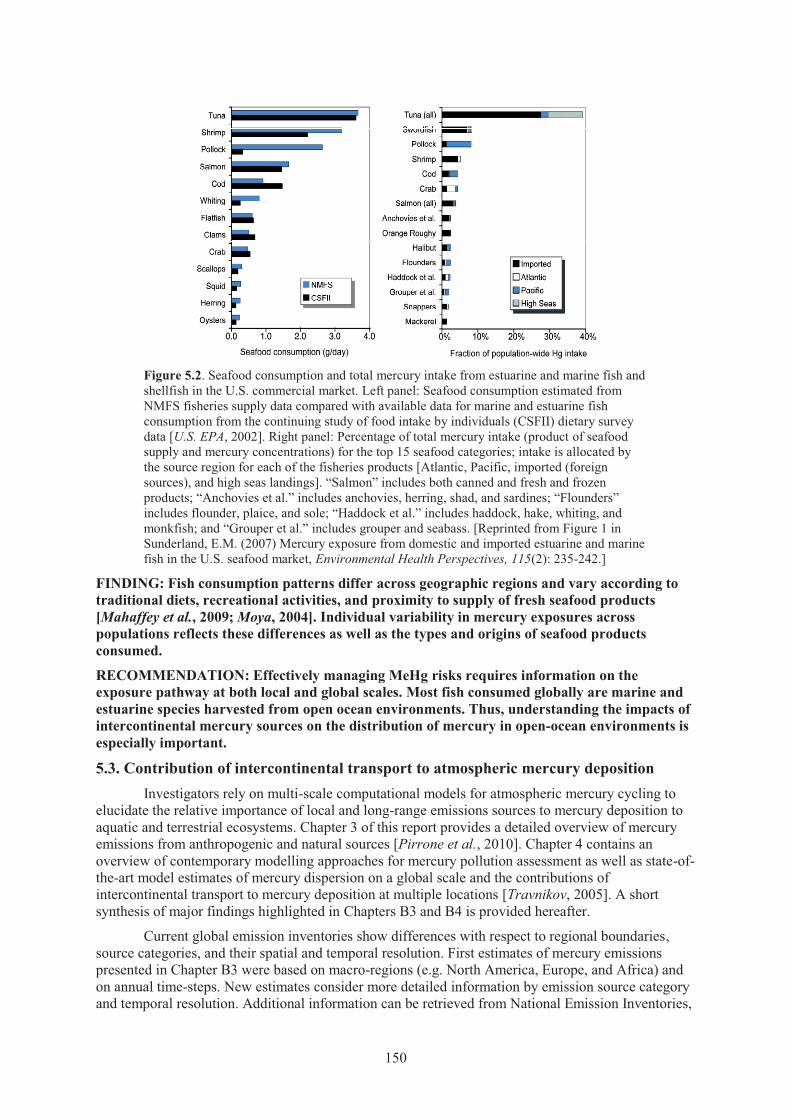
Figure 5.2. Seafood consumption and total mercury intake from estuarine and marine fish and shellfish in the U.S. commercial market. Left panel: Seafood consumption estimated from NMFS fisheries supply data compared with available data for marine and estuarine fish consumption from the continuing study of food intake by individuals (CSFII) dietary survey data [U.S. EPA, 2002]. Right panel: Percentage of total mercury intake (product of seafood supply and mercury concentrations) for the top 15 seafood categories; intake is allocated by the source region for each of the fisheries products [Atlantic, Pacific, imported (foreign sources), and high seas landings]. “Salmon” includes both canned and fresh and frozen products; “Anchovies et al.” includes anchovies, herring, shad, and sardines; “Flounders” includes flounder, plaice, and sole; “Haddock et al.” includes haddock, hake, whiting, and monkfish; and “Grouper et al.” includes grouper and seabass. [Reprinted from Figure 1 in Sunderland, E.M. (2007) Mercury exposure from domestic and imported estuarine and marine fish in the U.S. seafood market, Environmental Health Perspectives, 115(2): 235-242.]

FINDING: Fish consumption patterns differ across geographic regions and vary according to traditional diets, recreational activities, and proximity to supply of fresh seafood products [Mahaffey et al., 2009; Moya, 2004]. Individual variability in mercury exposures across populations reflects these differences as well as the types and origins of seafood products consumed.

RECOMMENDATION: Effectively managing MeHg risks requires information on the exposure pathway at both local and global scales. Most fish consumed globally are marine and estuarine species harvested from open ocean environments. Thus, understanding the impacts of intercontinental mercury sources on the distribution of mercury in open-ocean environments is especially important. 5.3. Contribution of intercontinental transport to atmospheric mercury deposition

Investigators rely on multi-scale computational models for atmospheric mercury cycling to elucidate the relative importance of local and long-range emissions sources to mercury deposition to aquatic and terrestrial ecosystems. Chapter 3 of this report provides a detailed overview of mercury emissions from anthropogenic and natural sources [Pirrone et al., 2010]. Chapter 4 contains an overview of contemporary modelling approaches for mercury pollution assessment as well as state-of-the-art model estimates of mercury dispersion on a global scale and the contributions of intercontinental transport to mercury deposition at multiple locations [Travnikov, 2005]. A short synthesis of major findings highlighted in Chapters B3 and B4 is provided hereafter.

Current global emission inventories show differences with respect to regional boundaries, source categories, and their spatial and temporal resolution. First estimates of mercury emissions presented in Chapter B3 were based on macro-regions (e.g. North America, Europe, and Africa) and on annual time-steps. New estimates consider more detailed information by emission source category and temporal resolution. Additional information can be retrieved from National Emission Inventories,

150

which are often based on measurements but are limited to anthropogenic sources. Nriagu and Pacyna [1988] published the first comprehensive estimate of anthropogenic mercury emissions on a global scale. Pirrone et al. [1996] subsequently published the first detailed overview of mercury emissions trends for each world region for the years 1983-1992, which was followed with a publication on mercury emissions and atmospheric deposition trends in North America for the period of 1850 to 1992 [Pirrone et al., 1998]. Later Pacyna and co-workers published an update for the year 2000 [Pacyna et al., 2006] along with an integration of emission source categories. Recently, a comprehensive overview of global emissions by source categories was provided by Pirrone et al. [2010], which considered new source categories and updated estimates for China, India and South Africa. Major findings discussed in Chapter B3 suggest an increase of total mercury emissions, which is not supported by the evidence that most countries have dramatically reduced trade in and consumption of mercury [UNEP, 2006]. Mercury supply in 1985 was near 6000 Mg that decreased to nearly 4000 Mg in 2006 [UNEP, 2006]. On the other hand, an increase in emissions was observed, which can be ascribed to the improvement of estimates by integrating new sources or by improving our knowledge on previously estimated sources.

Mercury is transported for long distances from the emission sources before it is removed through dry deposition and wet scavenging processes because it has an atmospheric lifetime of about a year, though this lifetime may change substantially with latitude and time of the year [Hedgecock and Pirrone, 2004]. Most anthropogenic mercury emissions occur at mid-latitudes where circumpolar westerlies can transport the emissions from the source regions to other receptor regions. South-North Hemispheric exchange is not as significant, as evidenced by the decreasing concentration gradient from the Northern Hemisphere to the Southern Hemisphere. Because current monitoring networks and field measurements of mercury concentrations and deposition are scarce and not evenly distributed spatially, existing data have limited capability to detect signals from intercontinental transport [Travnikov, 2005, chapter 4 - this report]. However, a recently approved research proposal by the European Commission, namely the Global Mercury Observation System (GMOS), will include 40 ground-based monitoring sites distributed worldwide, as well as aircraft and oceanographic measurement programs that will allow evaluation of the spatial distributions of mercury species taking into account the location of emission sources and atmospheric transport patterns with changing meteorological conditions (Chapter B2).

In contrast to other long-lived air pollutants, intercontinental transport of mercury can occur through two pathways: (1) Direct transport of an emitted mercury plume from one continent to another, and (2) input of a source region into the global mercury pool.

The first pathway typically involves the lifting of mercury plumes to above the planetary boundary layer, followed by rapid transport in the free troposphere. Transported plumes can reach ground level with atmospheric subsidence at a receptor site in another continent. Through this pathway, relatively undiluted Asian plumes can be transported to the northeastern Pacific in about a week. These plumes are typically from large point sources that emit mercury at higher elevation and with higher temperatures [Friedli et al., 2004]. Springtime is found to be the most active period for the trans-Pacific transport [Lin et al., 2006; Reidmiller et al., 2009]. Transport across the Atlantic is more complex and usually involves several mid-latitude cyclones and associated warm conveyor belts.

The other pathway for intercontinental mercury transport is through emissions that become part of the global mercury pool. Because mercury deposition in remote receptors is highly related to the atmospheric burden of mercury, regional emission input into the atmosphere from one continent can cause enhanced mercury deposition in other continents [Travnikov, 2005, chapter 4 - this report]. Major findings in Chapter B4 show that the contribution of mercury intercontinental transport is significant, particularly in regions with few local emission sources. The contribution of foreign anthropogenic sources to annual deposition fluxes varies from 10% to 30%, on average in different regions. In addition, between 35 to 70% of total deposition to most regions is from contributions from global natural sources and re-emission processes. East Asia is the most important source region contributing to 10-14% of the mercury deposited in other regions, followed by Europe (2-5%), South Asia (2-3%) and North America (1-2%).

151

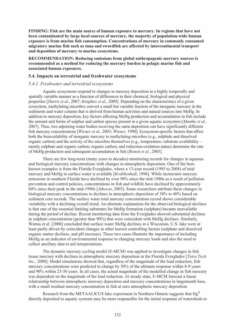
FINDING: Fish are the main source of human exposure to mercury. In regions that have not been contaminated by large local sources of mercury, the majority of population-wide human exposure is from marine fish consumption. Concentrations of mercury in commonly consumed migratory marine fish such as tuna and swordfish are affected by intercontinental transport and deposition of mercury to marine ecosystems.

RECOMMENDATION: Reducing emissions from global anthropogenic mercury sources is recommended as a method for reducing the mercury burden in pelagic marine fish and associated human exposures.

5.4. Impacts on terrestrial and freshwater ecosystems 5.4.1. Freshwater and terrestrial ecosystems

Aquatic ecosystems respond to changes in mercury deposition in a highly temporally and spatially variable manner as a function of differences in their chemical, biological and physical properties [Harris et al., 2007; Knightes et al., 2009]. Depending on the characteristics of a given ecosystem, methylating microbes convert a small but variable fraction of the inorganic mercury in the sediments and water column that is derived from human activities and natural sources into MeHg. In addition to mercury deposition, key factors affecting MeHg production and accumulation in fish include the amount and forms of sulphur and carbon species present in a given aquatic ecosystem [Munthe et al., 2007]. Thus, two adjoining water bodies receiving the same deposition can have significantly different fish mercury concentrations [Wiener et al., 2003; Wiener, 1990]. Ecosystem-specific factors that affect both the bioavailability of inorganic mercury to methylating microbes (e.g., sulphide and dissolved organic carbon) and the activity of the microbes themselves (e.g., temperature; substrate availability – mostly sulphate and organic carbon; organic carbon; and reduction-oxidation status) determine the rate of MeHg production and subsequent accumulation in fish [Benoit et al., 2003].

There are few long-term (many years to decades) monitoring records for changes in aqueous and biological mercury concentrations with changes in atmospheric deposition. One of the best-known examples is from the Florida Everglades, where a 13-year record (1995 to 2008) of total mercury and MeHg in surface water is available [Krabbenhoft, 1996]. While incinerator mercury emissions in southern Florida have declined by over 90% since the mid-1980s as a result of pollution prevention and control policies, concentrations in fish and wildlife have declined by approximately 60% since their peak in the mid-1990s [Atkeson, 2003]. Some researchers attribute these changes in biological mercury concentrations to declines in atmospheric deposition of 30% to 40% based on sediment core records. The surface water total mercury concentration record shows considerable variability with a declining overall trend. An alternate explanation for the observed biological declines is that one of the essential limiting substrates for MeHg formation (sulphate) became unavailable during the period of decline. Recent monitoring data from the Everglades showed substantial declines in sulphate concentration (greater than 90%) that were coincident with MeHg declines. Similarly, Watras et al. [2000] concluded that surface water MeHg declines in a Wisconsin, U.S. lake were at least partly driven by coincident changes in other known controlling factors (sulphate and dissolved organic matter declines, and pH increase). These two cases illustrate the importance of including MeHg as an indicator of environmental response to changing mercury loads and also the need to collect ancillary data to aid interpretations.

The dynamic mercury cycling model (E-MCM) was applied to investigate changes in fish tissue mercury with declines in atmospheric mercury deposition in the Florida Everglades [Tetra Tech Inc., 2000]. Model simulations showed that, regardless of the magnitude of the load reduction, fish mercury concentrations were predicted to change by 50% of the ultimate response within 8-9 years and 90% within 25-30 years. In all cases, the actual magnitude of the modelled change in fish mercury was dependent on the magnitude of the load reduction. At steady state, E-MCM forecast a linear relationship between atmospheric mercury deposition and mercury concentrations in largemouth bass, with a small residual mercury concentration in fish at zero atmospheric mercury deposition.

Research from the METAALICUS lake experiment in Northern Ontario suggests that HgII directly deposited to aquatic systems may be more responsible for the initial response of watersheds to

152

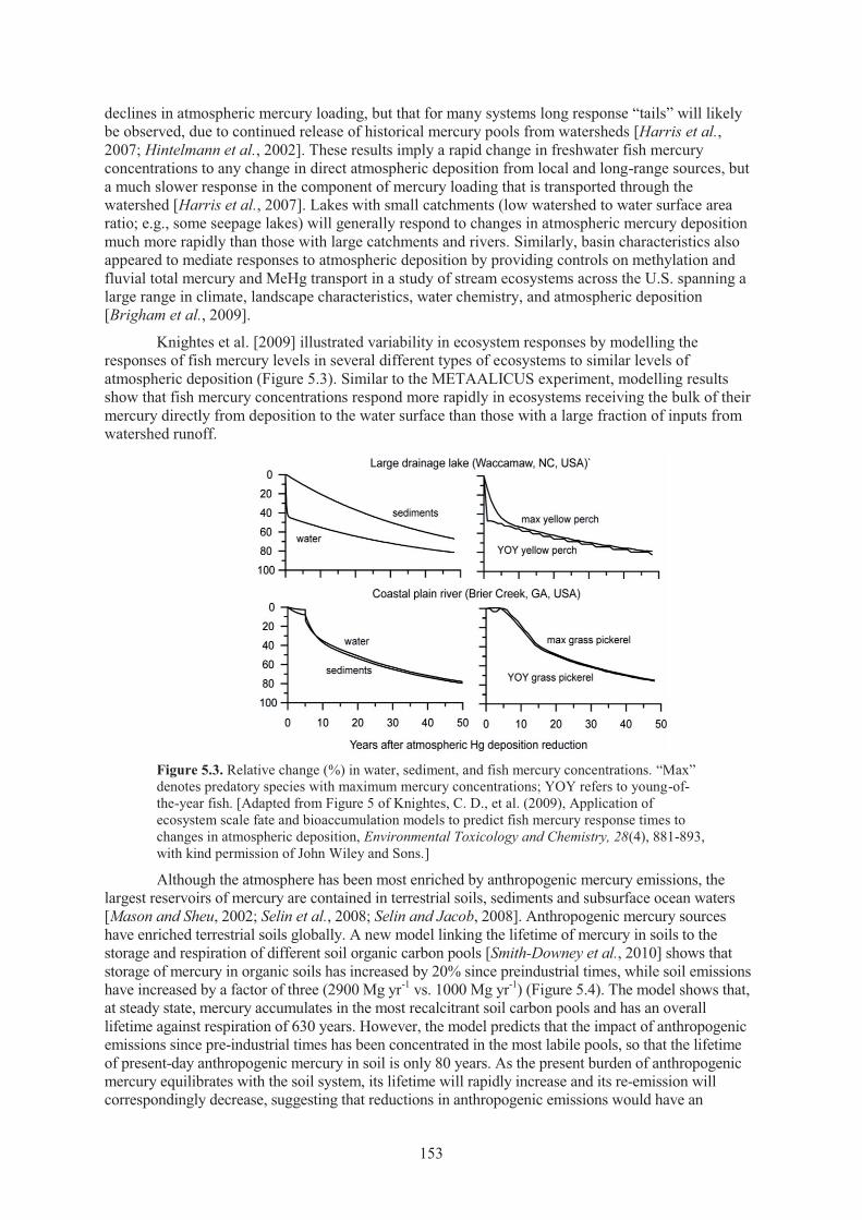
declines in atmospheric mercury loading, but that for many systems long response “tails” will likely be observed, due to continued release of historical mercury pools from watersheds [Harris et al., 2007; Hintelmann et al., 2002]. These results imply a rapid change in freshwater fish mercury concentrations to any change in direct atmospheric deposition from local and long-range sources, but a much slower response in the component of mercury loading that is transported through the watershed [Harris et al., 2007]. Lakes with small catchments (low watershed to water surface area ratio; e.g., some seepage lakes) will generally respond to changes in atmospheric mercury deposition much more rapidly than those with large catchments and rivers. Similarly, basin characteristics also appeared to mediate responses to atmospheric deposition by providing controls on methylation and fluvial total mercury and MeHg transport in a study of stream ecosystems across the U.S. spanning a large range in climate, landscape characteristics, water chemistry, and atmospheric deposition [Brigham et al., 2009].

Knightes et al. [2009] illustrated variability in ecosystem responses by modelling the responses of fish mercury levels in several different types of ecosystems to similar levels of atmospheric deposition (Figure 5.3). Similar to the METAALICUS experiment, modelling results show that fish mercury concentrations respond more rapidly in ecosystems receiving the bulk of their mercury directly from deposition to the water surface than those with a large fraction of inputs from watershed runoff.

Figure 5.3. Relative change (%) in water, sediment, and fish mercury concentrations. “Max” denotes predatory species with maximum mercury concentrations; YOY refers to young-of-the-year fish. [Adapted from Figure 5 of Knightes, C. D., et al. (2009), Application of ecosystem scale fate and bioaccumulation models to predict fish mercury response times to changes in atmospheric deposition, Environmental Toxicology and Chemistry, 28(4), 881-893, with kind permission of John Wiley and Sons.]

Although the atmosphere has been most enriched by anthropogenic mercury emissions, the largest reservoirs of mercury are contained in terrestrial soils, sediments and subsurface ocean waters [Mason and Sheu, 2002; Selin et al., 2008; Selin and Jacob, 2008]. Anthropogenic mercury sources have enriched terrestrial soils globally. A new model linking the lifetime of mercury in soils to the storage and respiration of different soil organic carbon pools [Smith-Downey et al., 2010] shows that storage of mercury in organic soils has increased by 20% since preindustrial times, while soil emissions have increased by a factor of three (2900 Mg yr-1 vs. 1000 Mg yr-1) (Figure 5.4). The model shows that, at steady state, mercury accumulates in the most recalcitrant soil carbon pools and has an overall lifetime against respiration of 630 years. However, the model predicts that the impact of anthropogenic emissions since pre-industrial times has been concentrated in the most labile pools, so that the lifetime of present-day anthropogenic mercury in soil is only 80 years. As the present burden of anthropogenic mercury equilibrates with the soil system, its lifetime will rapidly increase and its re-emission will correspondingly decrease, suggesting that reductions in anthropogenic emissions would have an

153

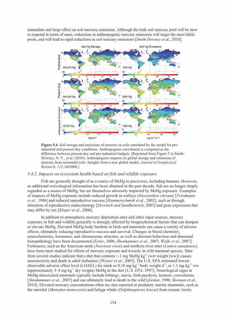
immediate and large effect on soil mercury emissions. Although the bulk soil mercury pool will be slow to respond in terms of mass, reductions in anthropogenic mercury emissions will target the most labile pools, and will lead to rapid reductions in soil mercury emissions [Smith-Downey et al., 2010].

Figure 5.4. Soil storage and emissions of mercury in soils simulated by the model for pre-industrial and present-day conditions. Anthropogenic enrichment is computed as the difference between present-day and pre-industrial budgets. [Reprinted from Figure 5 in Smith-Downey, N. V., et al. (2010), Anthropogenic impacts on global storage and emissions of mercury from terrestrial soils: Insights from a new global model, Journal of Geophysical Research, 115, G03008.]

5.4.2. Impacts on ecosystem health based on fish and wildlife exposure Fish are generally thought of as a source of MeHg to piscivores, including humans. However,

as additional toxicological information has been obtained in the past decade, fish are no longer simply regarded as a source of MeHg, but are themselves adversely impacted by MeHg exposure. Examples of impacts of MeHg exposure include reduced growth in walleye (Stizostedion vitreum) [Friedmann et al., 1996] and reduced reproductive success [Hammerschmidt et al., 2002], such as through alteration of reproductive endocrinology [Drevnick and Sandheinrich, 2003] and gene expression that may differ by sex [Klaper et al., 2006].

In addition to atmospheric mercury deposition rates and other input sources, mercury exposure in fish and wildlife generally is strongly affected by biogeochemical factors that can dampen or elevate MeHg. Elevated MeHg body burdens in birds and mammals can cause a variety of adverse effects, ultimately reducing reproductive success and survival. Changes in blood chemistry, neurochemistry, hormones, and chromosome structure, as well as aberrant behaviour and abnormal histopathology have been documented [Eisler, 2006; Sheuhammer et al., 2007; Wolfe et al., 2007]. Furbearers, such as the American mink (Neovison vison) and northern river otter (Lontra canadensis), have been most studied for effects of mercury exposure and toxicity in wild mammal species. Data from several studies indicate that a diet that contains � 1 mg MeHg kg-1 (wet weight [ww]) causes neurotoxicity and death in adult furbearers [Wiener et al., 2003]. The U.S. EPA estimated lowest observable adverse effect level (LOAEL) for mink as 0.18 mg kg-1 body weight d-1, or 1.1 mg kg-1 ww (approximately 3–4 mg kg-1 dry weight) MeHg in the diet [U.S. EPA, 1997]. Neurological signs in MeHg-intoxicated mammals typically include lethargy, ataxia, limb paralysis, tremors, convulsions, [Sheuhammer et al., 2007] and can ultimately lead to death in the wild [Jordan, 1990; Sleeman et al., 2010]. Elevated mercury concentrations often are also reported in predatory marine mammals, such as the narwhal (Monodon monoceros) and beluga whale (Delphinapterus leucas) from remote Arctic

154

locations, which are harvested for local human consumption and regularly exceed 1.0 μg/g (ww) in the muscle tissue and 100 μg/g (ww) in the liver [Dietz et al., 2000; Dietz et al., 2004; Wagemann et al., 1998]. Some species, such as the long-finned pilot whale (Globicephala melas), even exceed 3.0 μg/g (ww) in the muscle and 500 μg/g (ww) in the liver [Caurant et al., 1996].

Mercury concentrations are often measured in tissues such as eggs, blood, and feathers (primarily measured as total mercury with the premise that over 95% is MeHg). Based on a comprehensive egg dosing study for 26 species of birds, there is compelling evidence that species sensitivity to MeHg toxicity varies widely and that some species are up to 7 times more sensitive than others [Heinz et al., 2009]. Therefore, LOAELs for birds need to account for differences among species and future interests in using matrices that can be non-lethally sampled. Three broad categories of MeHg sensitivity for species with known LOAELs are based on foraging guilds. Piscivores are perhaps the most tolerant of toxic MeHg body burdens (seabirds more so than freshwater birds). Based on a robust study of a common loon (Gavia immer) breeding population in New England, LOAELs of 3.0 μg/g (ww) in blood, 1.3 μg/g (ww) in egg and 40.0 μg/g (fw) in feather were documented to produce 40% fewer fledged young [Evers et al., 2008]. A parallel, yet independent study in neighbouring regions demonstrated similar results [Burgess and Meyer, 2008]. The mallard (Anas platyrhynchos) with its broad, non-piscivorous diet is well-studied and its LOAELs are 0.74 μg/g (ww) in eggs [Heinz and Hoffman, 2003] and 9.0 μg/g (fresh weight) in feathers [Heinz, 1979]. Strictly invertivorous birds, such as many songbirds, likely have even lower LOAELs, and based on ongoing studies may be 2-3x lower than the mallard (BioDiversity Research Institute, unpublished data). Adverse dietary thresholds are challenging to develop for free-living birds, however, prey-loon mercury relationships developed from areas with paired sampling efforts indicate statistically significant reproductive harm to piscivorous birds foraging on >0.16 μg/g (ww, whole body total mercury, where 85% is MeHg) [Burgess and Meyer, 2008; Evers et al., 2008].

In addition to the taxonomic differences of MeHg exposure and sensitivity to MeHg toxicity that can be grouped according to foraging guilds, habitat type can be highly influential in MeHg production. Evers et al. [Evers et al., 2005] compiled a large database on mercury concentrations in birds from aquatic ecosystems in New England, New York, and eastern Canada (eastern Ontario to the Canadian Maritimes). Based on two indicator species, the belted kingfisher (Ceryle alcyon) and bald eagle (Haliaeetus leucocephalus), they found MeHg availability increased from marine, to estuarine and riverine systems, and was greatest in lake habitats. In general, lakes that receive relatively high atmospheric mercury loadings and are characterized by a high proportion of mercury sensitive scenarios, where methylation rates are relatively high (e.g., low-alkalinity, low-pH conditions; surface waters with large upstream or adjoining wetlands; waters with adjoining or upstream terrestrial areas subjected to flooding) pose the greatest risk for piscivorous wildlife. It is in these environments that trophic transfer of MeHg can bioaccumulate to harmful concentrations [Chen et al., 2005; Scheuhammer and Blancher, 1994; Wiener et al., 2003]. Headwater streams may have significantly higher MeHg concentrations than some lakes, based on comparisons of two-lined salamanders (Eurycea bislineata) [Bank et al., 2005] and northern crayfish (Orconectes virilis) [Pennuto et al., 2005].

Elevated environmental MeHg concentrations have recently been observed in a river floodplain in Massachusetts, U.S., indicating that terrestrial food-webs are also at risk for high levels of MeHg exposure. This research included paired sampling of avian piscivores and invertivores and demonstrated that invertivorous red-winged blackbirds (Aegolius phoenicius) can carry blood mercury levels up to an order of magnitude greater than associated pisivorous belted kingfishers [Evers et al., 2005] BioDiversity Research Institute, unpublished data]. Cristol et al. [2008] demonstrated that the likely primary mechanism for MeHg to biomagnify more in terrestrial food webs than strictly aquatic-based food webs is because of the ability of spiders to lengthen the trophic chain. These findings have generated a shift in understanding taxa and habitats most at risk from MeHg contamination and potential harm in ecosystems. Many species of wetland rails, shorebirds, and songbirds as well as mammalian invertivores, such as bats, are now known to be impacted by environmental mercury loads with anthropogenic origins (BioDiversity Research Institute, unpublished data).

155

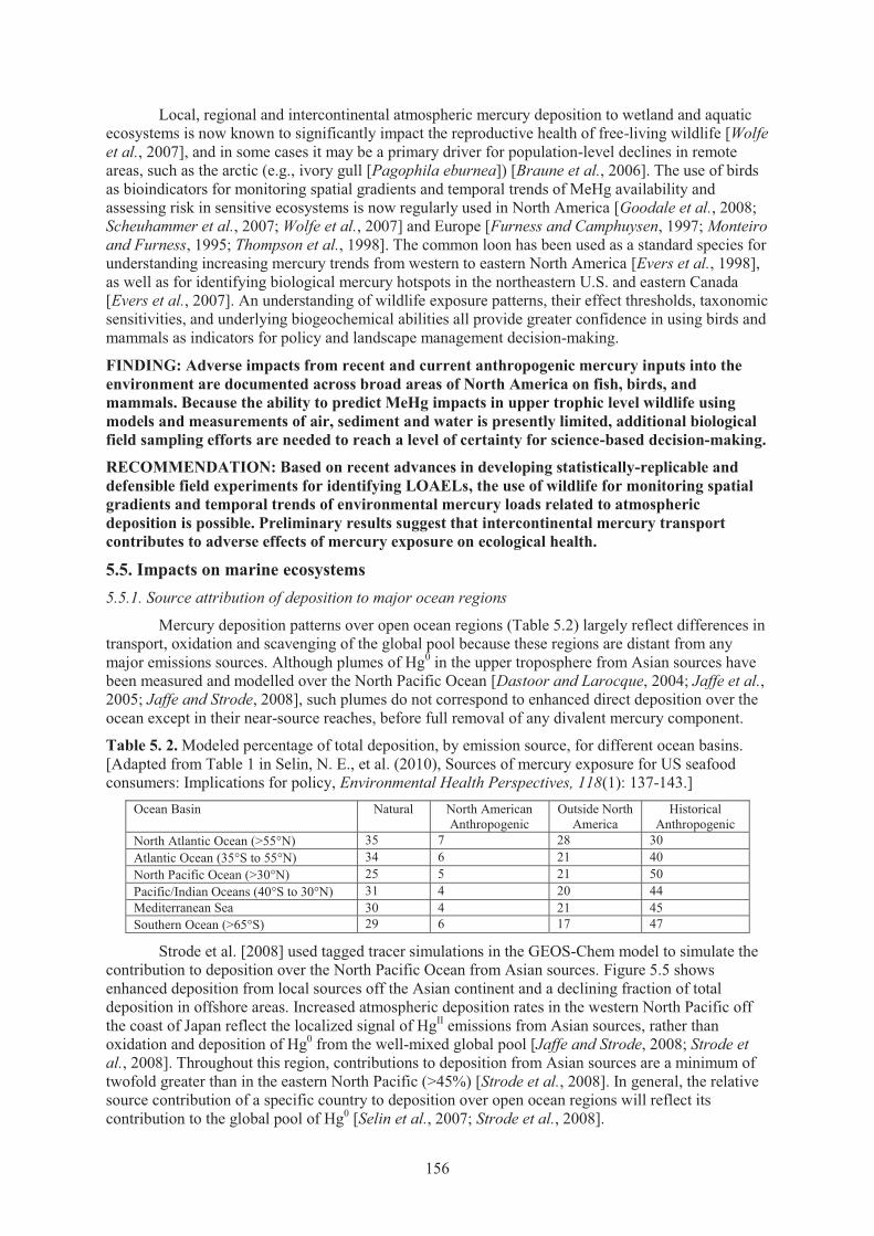
Local, regional and intercontinental atmospheric mercury deposition to wetland and aquatic ecosystems is now known to significantly impact the reproductive health of free-living wildlife [Wolfe et al., 2007], and in some cases it may be a primary driver for population-level declines in remote areas, such as the arctic (e.g., ivory gull [Pagophila eburnea]) [Braune et al., 2006]. The use of birds as bioindicators for monitoring spatial gradients and temporal trends of MeHg availability and assessing risk in sensitive ecosystems is now regularly used in North America [Goodale et al., 2008; Scheuhammer et al., 2007; Wolfe et al., 2007] and Europe [Furness and Camphuysen, 1997; Monteiro and Furness, 1995; Thompson et al., 1998]. The common loon has been used as a standard species for understanding increasing mercury trends from western to eastern North America [Evers et al., 1998], as well as for identifying biological mercury hotspots in the northeastern U.S. and eastern Canada [Evers et al., 2007]. An understanding of wildlife exposure patterns, their effect thresholds, taxonomic sensitivities, and underlying biogeochemical abilities all provide greater confidence in using birds and mammals as indicators for policy and landscape management decision-making.

FINDING: Adverse impacts from recent and current anthropogenic mercury inputs into the environment are documented across broad areas of North America on fish, birds, and mammals. Because the ability to predict MeHg impacts in upper trophic level wildlife using models and measurements of air, sediment and water is presently limited, additional biological field sampling efforts are needed to reach a level of certainty for science-based decision-making.

RECOMMENDATION: Based on recent advances in developing statistically-replicable and defensible field experiments for identifying LOAELs, the use of wildlife for monitoring spatial gradients and temporal trends of environmental mercury loads related to atmospheric deposition is possible. Preliminary results suggest that intercontinental mercury transport contributes to adverse effects of mercury exposure on ecological health.

5.5. Impacts on marine ecosystems 5.5.1. Source attribution of deposition to major ocean regions

Mercury deposition patterns over open ocean regions (Table 5.2) largely reflect differences in transport, oxidation and scavenging of the global pool because these regions are distant from any major emissions sources. Although plumes of Hg0 in the upper troposphere from Asian sources have been measured and modelled over the North Pacific Ocean [Dastoor and Larocque, 2004; Jaffe et al., 2005; Jaffe and Strode, 2008], such plumes do not correspond to enhanced direct deposition over the ocean except in their near-source reaches, before full removal of any divalent mercury component.

Table 5. 2. Modeled percentage of total deposition, by emission source, for different ocean basins. [Adapted from Table 1 in Selin, N. E., et al. (2010), Sources of mercury exposure for US seafood consumers: Implications for policy, Environmental Health Perspectives, 118(1): 137-143.]

Ocean Basin Natural North American Anthropogenic

Outside North America

Historical Anthropogenic

North Atlantic Ocean (>55�N) 35 7 28 30 Atlantic Ocean (35�S to 55�N) 34 6 21 40 North Pacific Ocean (>30�N) 25 5 21 50 Pacific/Indian Oceans (40�S to 30�N) 31 4 20 44 Mediterranean Sea 30 4 21 45 Southern Ocean (>65�S) 29 6 17 47

Strode et al. [2008] used tagged tracer simulations in the GEOS-Chem model to simulate the contribution to deposition over the North Pacific Ocean from Asian sources. Figure 5.5 shows enhanced deposition from local sources off the Asian continent and a declining fraction of total deposition in offshore areas. Increased atmospheric deposition rates in the western North Pacific off the coast of Japan reflect the localized signal of HgII emissions from Asian sources, rather than oxidation and deposition of Hg0 from the well-mixed global pool [Jaffe and Strode, 2008; Strode et al., 2008]. Throughout this region, contributions to deposition from Asian sources are a minimum of twofold greater than in the eastern North Pacific (>45%) [Strode et al., 2008]. In general, the relative source contribution of a specific country to deposition over open ocean regions will reflect its contribution to the global pool of Hg0 [Selin et al., 2007; Strode et al., 2008].

156

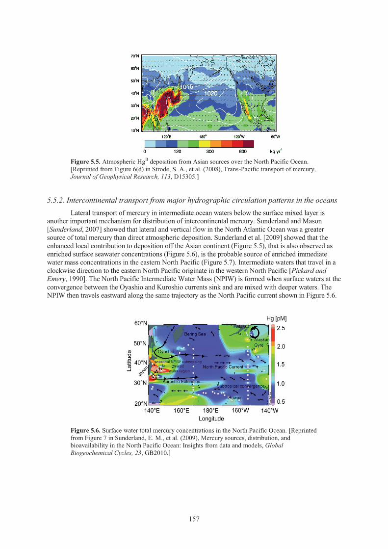
Figure 5.5. Atmospheric HgII deposition from Asian sources over the North Pacific Ocean. [Reprinted from Figure 6(d) in Strode, S. A., et al. (2008), Trans-Pacific transport of mercury, Journal of Geophysical Research, 113, D15305.]

5.5.2. Intercontinental transport from major hydrographic circulation patterns in the oceans Lateral transport of mercury in intermediate ocean waters below the surface mixed layer is

another important mechanism for distribution of intercontinental mercury. Sunderland and Mason [Sunderland, 2007] showed that lateral and vertical flow in the North Atlantic Ocean was a greater source of total mercury than direct atmospheric deposition. Sunderland et al. [2009] showed that the enhanced local contribution to deposition off the Asian continent (Figure 5.5), that is also observed as enriched surface seawater concentrations (Figure 5.6), is the probable source of enriched immediate water mass concentrations in the eastern North Pacific (Figure 5.7). Intermediate waters that travel in a clockwise direction to the eastern North Pacific originate in the western North Pacific [Pickard and Emery, 1990]. The North Pacific Intermediate Water Mass (NPIW) is formed when surface waters at the convergence between the Oyashio and Kuroshio currents sink and are mixed with deeper waters. The NPIW then travels eastward along the same trajectory as the North Pacific current shown in Figure 5.6.

Figure 5.6. Surface water total mercury concentrations in the North Pacific Ocean. [Reprinted from Figure 7 in Sunderland, E. M., et al. (2009), Mercury sources, distribution, and bioavailability in the North Pacific Ocean: Insights from data and models, Global Biogeochemical Cycles, 23, GB2010.]

157

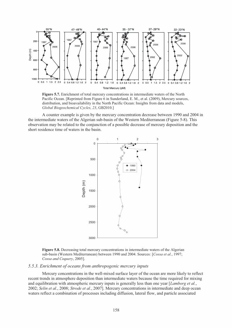
Figure 5.7. Enrichment of total mercury concentrations in intermediate waters of the North Pacific Ocean. [Reprinted from Figure 6 in Sunderland, E. M., et al. (2009), Mercury sources, distribution, and bioavailability in the North Pacific Ocean: Insights from data and models, Global Biogeochemical Cycles, 23, GB2010.]

A counter example is given by the mercury concentration decrease between 1990 and 2004 in the intermediate waters of the Algerian sub-basin of the Western Mediterranean (Figure 5-8). This observation may be related to the conjunction of a possible decrease of mercury deposition and the short residence time of waters in the basin.

Figure 5.8. Decreasing total mercury concentrations in intermediate waters of the Algerian sub-basin (Western Mediterranean) between 1990 and 2004. Sources: [Cossa et al., 1997; Cossa and Coquery, 2005].

5.5.3. Enrichment of oceans from anthropogenic mercury inputs Mercury concentrations in the well-mixed surface layer of the ocean are more likely to reflect

recent trends in atmosphere deposition than intermediate waters because the time required for mixing and equilibration with atmospheric mercury inputs is generally less than one year [Lamborg et al., 2002; Selin et al., 2008; Strode et al., 2007]. Mercury concentrations in intermediate and deep ocean waters reflect a combination of processes including diffusion, lateral flow, and particle associated

0

500

1000

1500

2000

2500

3000

0 1 2 3

Dep

th (m

)

1990

2004

158

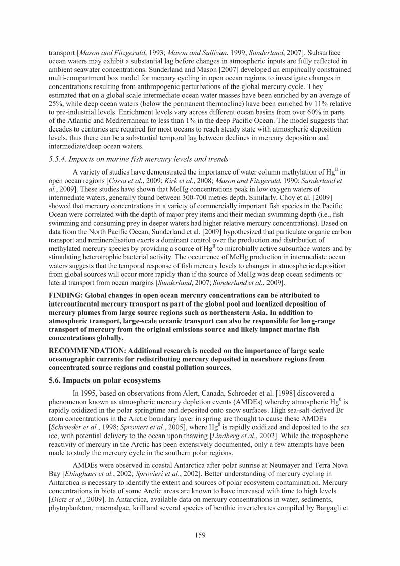
transport [Mason and Fitzgerald, 1993; Mason and Sullivan, 1999; Sunderland, 2007]. Subsurface ocean waters may exhibit a substantial lag before changes in atmospheric inputs are fully reflected in ambient seawater concentrations. Sunderland and Mason [2007] developed an empirically constrained multi-compartment box model for mercury cycling in open ocean regions to investigate changes in concentrations resulting from anthropogenic perturbations of the global mercury cycle. They estimated that on a global scale intermediate ocean water masses have been enriched by an average of 25%, while deep ocean waters (below the permanent thermocline) have been enriched by 11% relative to pre-industrial levels. Enrichment levels vary across different ocean basins from over 60% in parts of the Atlantic and Mediterranean to less than 1% in the deep Pacific Ocean. The model suggests that decades to centuries are required for most oceans to reach steady state with atmospheric deposition levels, thus there can be a substantial temporal lag between declines in mercury deposition and intermediate/deep ocean waters.

5.5.4. Impacts on marine fish mercury levels and trends A variety of studies have demonstrated the importance of water column methylation of HgII in

open ocean regions [Cossa et al., 2009; Kirk et al., 2008; Mason and Fitzgerald, 1990; Sunderland et al., 2009]. These studies have shown that MeHg concentrations peak in low oxygen waters of intermediate waters, generally found between 300-700 metres depth. Similarly, Choy et al. [2009] showed that mercury concentrations in a variety of commercially important fish species in the Pacific Ocean were correlated with the depth of major prey items and their median swimming depth (i.e., fish swimming and consuming prey in deeper waters had higher relative mercury concentrations). Based on data from the North Pacific Ocean, Sunderland et al. [2009] hypothesized that particulate organic carbon transport and remineralisation exerts a dominant control over the production and distribution of methylated mercury species by providing a source of HgII to microbially active subsurface waters and by stimulating heterotrophic bacterial activity. The occurrence of MeHg production in intermediate ocean waters suggests that the temporal response of fish mercury levels to changes in atmospheric deposition from global sources will occur more rapidly than if the source of MeHg was deep ocean sediments or lateral transport from ocean margins [Sunderland, 2007; Sunderland et al., 2009]. FINDING: Global changes in open ocean mercury concentrations can be attributed to intercontinental mercury transport as part of the global pool and localized deposition of mercury plumes from large source regions such as northeastern Asia. In addition to atmospheric transport, large-scale oceanic transport can also be responsible for long-range transport of mercury from the original emissions source and likely impact marine fish concentrations globally.

RECOMMENDATION: Additional research is needed on the importance of large scale oceanographic currents for redistributing mercury deposited in nearshore regions from concentrated source regions and coastal pollution sources.

5.6. Impacts on polar ecosystems In 1995, based on observations from Alert, Canada, Schroeder et al. [1998] discovered a

phenomenon known as atmospheric mercury depletion events (AMDEs) whereby atmospheric Hg0 is rapidly oxidized in the polar springtime and deposited onto snow surfaces. High sea-salt-derived Br atom concentrations in the Arctic boundary layer in spring are thought to cause these AMDEs [Schroeder et al., 1998; Sprovieri et al., 2005], where Hg0 is rapidly oxidized and deposited to the sea ice, with potential delivery to the ocean upon thawing [Lindberg et al., 2002]. While the tropospheric reactivity of mercury in the Arctic has been extensively documented, only a few attempts have been made to study the mercury cycle in the southern polar regions.

AMDEs were observed in coastal Antarctica after polar sunrise at Neumayer and Terra Nova Bay [Ebinghaus et al., 2002; Sprovieri et al., 2002]. Better understanding of mercury cycling in Antarctica is necessary to identify the extent and sources of polar ecosystem contamination. Mercury concentrations in biota of some Arctic areas are known to have increased with time to high levels [Dietz et al., 2009]. In Antarctica, available data on mercury concentrations in water, sediments, phytoplankton, macroalgae, krill and several species of benthic invertebrates compiled by Bargagli et

159

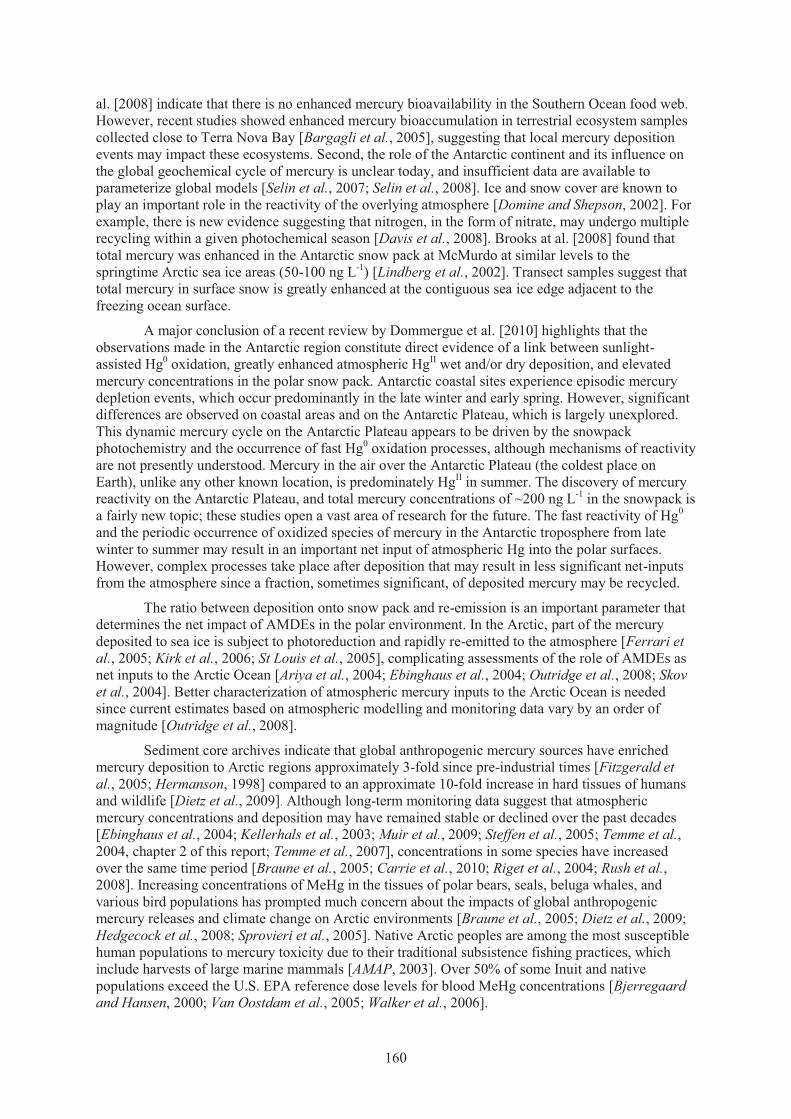
al. [2008] indicate that there is no enhanced mercury bioavailability in the Southern Ocean food web. However, recent studies showed enhanced mercury bioaccumulation in terrestrial ecosystem samples collected close to Terra Nova Bay [Bargagli et al., 2005], suggesting that local mercury deposition events may impact these ecosystems. Second, the role of the Antarctic continent and its influence on the global geochemical cycle of mercury is unclear today, and insufficient data are available to parameterize global models [Selin et al., 2007; Selin et al., 2008]. Ice and snow cover are known to play an important role in the reactivity of the overlying atmosphere [Domine and Shepson, 2002]. For example, there is new evidence suggesting that nitrogen, in the form of nitrate, may undergo multiple recycling within a given photochemical season [Davis et al., 2008]. Brooks at al. [2008] found that total mercury was enhanced in the Antarctic snow pack at McMurdo at similar levels to the springtime Arctic sea ice areas (50-100 ng L-1) [Lindberg et al., 2002]. Transect samples suggest that total mercury in surface snow is greatly enhanced at the contiguous sea ice edge adjacent to the freezing ocean surface.

A major conclusion of a recent review by Dommergue et al. [2010] highlights that the observations made in the Antarctic region constitute direct evidence of a link between sunlight-assisted Hg0 oxidation, greatly enhanced atmospheric HgII wet and/or dry deposition, and elevated mercury concentrations in the polar snow pack. Antarctic coastal sites experience episodic mercury depletion events, which occur predominantly in the late winter and early spring. However, significant differences are observed on coastal areas and on the Antarctic Plateau, which is largely unexplored. This dynamic mercury cycle on the Antarctic Plateau appears to be driven by the snowpack photochemistry and the occurrence of fast Hg0 oxidation processes, although mechanisms of reactivity are not presently understood. Mercury in the air over the Antarctic Plateau (the coldest place on Earth), unlike any other known location, is predominately HgII in summer. The discovery of mercury reactivity on the Antarctic Plateau, and total mercury concentrations of ~200 ng L-1 in the snowpack is a fairly new topic; these studies open a vast area of research for the future. The fast reactivity of Hg0 and the periodic occurrence of oxidized species of mercury in the Antarctic troposphere from late winter to summer may result in an important net input of atmospheric Hg into the polar surfaces. However, complex processes take place after deposition that may result in less significant net-inputs from the atmosphere since a fraction, sometimes significant, of deposited mercury may be recycled.

The ratio between deposition onto snow pack and re-emission is an important parameter that determines the net impact of AMDEs in the polar environment. In the Arctic, part of the mercury deposited to sea ice is subject to photoreduction and rapidly re-emitted to the atmosphere [Ferrari et al., 2005; Kirk et al., 2006; St Louis et al., 2005], complicating assessments of the role of AMDEs as net inputs to the Arctic Ocean [Ariya et al., 2004; Ebinghaus et al., 2004; Outridge et al., 2008; Skov et al., 2004]. Better characterization of atmospheric mercury inputs to the Arctic Ocean is needed since current estimates based on atmospheric modelling and monitoring data vary by an order of magnitude [Outridge et al., 2008].

Sediment core archives indicate that global anthropogenic mercury sources have enriched mercury deposition to Arctic regions approximately 3-fold since pre-industrial times [Fitzgerald et al., 2005; Hermanson, 1998] compared to an approximate 10-fold increase in hard tissues of humans and wildlife [Dietz et al., 2009]. Although long-term monitoring data suggest that atmospheric mercury concentrations and deposition may have remained stable or declined over the past decades [Ebinghaus et al., 2004; Kellerhals et al., 2003; Muir et al., 2009; Steffen et al., 2005; Temme et al., 2004, chapter 2 of this report; Temme et al., 2007], concentrations in some species have increased over the same time period [Braune et al., 2005; Carrie et al., 2010; Riget et al., 2004; Rush et al., 2008]. Increasing concentrations of MeHg in the tissues of polar bears, seals, beluga whales, and various bird populations has prompted much concern about the impacts of global anthropogenic mercury releases and climate change on Arctic environments [Braune et al., 2005; Dietz et al., 2009; Hedgecock et al., 2008; Sprovieri et al., 2005]. Native Arctic peoples are among the most susceptible human populations to mercury toxicity due to their traditional subsistence fishing practices, which include harvests of large marine mammals [AMAP, 2003]. Over 50% of some Inuit and native populations exceed the U.S. EPA reference dose levels for blood MeHg concentrations [Bjerregaard and Hansen, 2000; Van Oostdam et al., 2005; Walker et al., 2006].

160

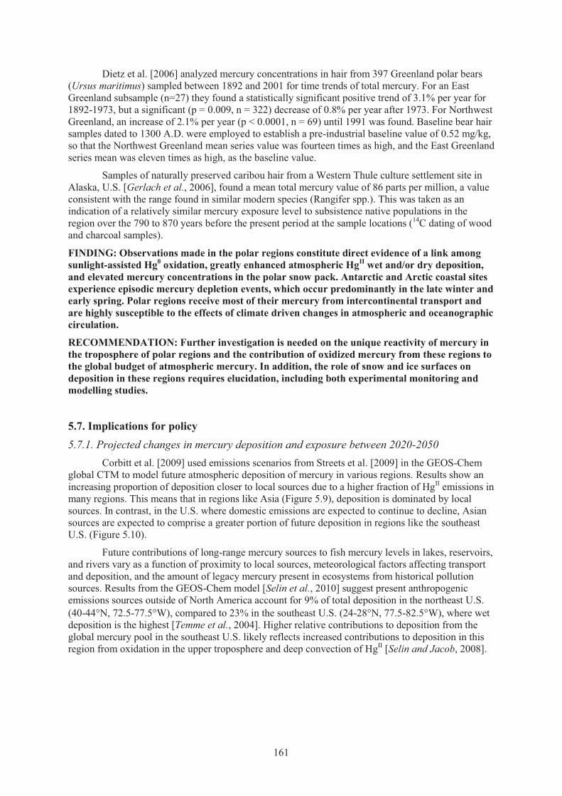
Dietz et al. [2006] analyzed mercury concentrations in hair from 397 Greenland polar bears (Ursus maritimus) sampled between 1892 and 2001 for time trends of total mercury. For an East Greenland subsample (n=27) they found a statistically significant positive trend of 3.1% per year for 1892-1973, but a significant (p = 0.009, n = 322) decrease of 0.8% per year after 1973. For Northwest Greenland, an increase of 2.1% per year (p < 0.0001, n = 69) until 1991 was found. Baseline bear hair samples dated to 1300 A.D. were employed to establish a pre-industrial baseline value of 0.52 mg/kg, so that the Northwest Greenland mean series value was fourteen times as high, and the East Greenland series mean was eleven times as high, as the baseline value.

Samples of naturally preserved caribou hair from a Western Thule culture settlement site in Alaska, U.S. [Gerlach et al., 2006], found a mean total mercury value of 86 parts per million, a value consistent with the range found in similar modern species (Rangifer spp.). This was taken as an indication of a relatively similar mercury exposure level to subsistence native populations in the region over the 790 to 870 years before the present period at the sample locations (14C dating of wood and charcoal samples).

FINDING: Observations made in the polar regions constitute direct evidence of a link among sunlight-assisted Hg0 oxidation, greatly enhanced atmospheric HgII wet and/or dry deposition, and elevated mercury concentrations in the polar snow pack. Antarctic and Arctic coastal sites experience episodic mercury depletion events, which occur predominantly in the late winter and early spring. Polar regions receive most of their mercury from intercontinental transport and are highly susceptible to the effects of climate driven changes in atmospheric and oceanographic circulation.

RECOMMENDATION: Further investigation is needed on the unique reactivity of mercury in the troposphere of polar regions and the contribution of oxidized mercury from these regions to the global budget of atmospheric mercury. In addition, the role of snow and ice surfaces on deposition in these regions requires elucidation, including both experimental monitoring and modelling studies.

5.7. Implications for policy 5.7.1. Projected changes in mercury deposition and exposure between 2020-2050 Corbitt et al. [2009] used emissions scenarios from Streets et al. [2009] in the GEOS-Chem global CTM to model future atmospheric deposition of mercury in various regions. Results show an increasing proportion of deposition closer to local sources due to a higher fraction of HgII emissions in many regions. This means that in regions like Asia (Figure 5.9), deposition is dominated by local sources. In contrast, in the U.S. where domestic emissions are expected to continue to decline, Asian sources are expected to comprise a greater portion of future deposition in regions like the southeast U.S. (Figure 5.10).

Future contributions of long-range mercury sources to fish mercury levels in lakes, reservoirs, and rivers vary as a function of proximity to local sources, meteorological factors affecting transport and deposition, and the amount of legacy mercury present in ecosystems from historical pollution sources. Results from the GEOS-Chem model [Selin et al., 2010] suggest present anthropogenic emissions sources outside of North America account for 9% of total deposition in the northeast U.S. (40-44�N, 72.5-77.5�W), compared to 23% in the southeast U.S. (24-28�N, 77.5-82.5�W), where wet deposition is the highest [Temme et al., 2004]. Higher relative contributions to deposition from the global mercury pool in the southeast U.S. likely reflects increased contributions to deposition in this region from oxidation in the upper troposphere and deep convection of HgII [Selin and Jacob, 2008].

161

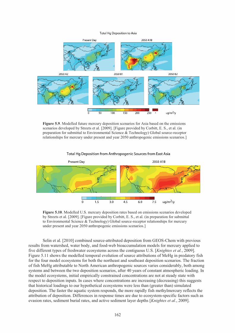
Figure 5.9. Modelled future mercury deposition scenarios for Asia based on the emissions scenarios developed by Streets et al. [2009]. [Figure provided by Corbitt, E. S., et al. (in preparation for submittal to Environmental Science & Technology) Global source-receptor relationships for mercury under present and year 2050 anthropogenic emissions scenarios.]

Figure 5.10. Modelled U.S. mercury deposition rates based on emissions scenarios developed by Streets et al. [2009]. [Figure provided by Corbitt, E. S., et al. (in preparation for submittal to Environmental Science & Technology) Global source-receptor relationships for mercury under present and year 2050 anthropogenic emissions scenarios.]

Selin et al. [2010] combined source-attributed deposition from GEOS-Chem with previous results from watershed, water body, and food-web bioaccumulation models for mercury applied to five different types of freshwater ecosystems across the contiguous U.S. [Knightes et al., 2009]. Figure 5.11 shows the modelled temporal evolution of source attributions of MeHg in predatory fish for the four model ecosystems for both the northeast and southeast deposition scenarios. The fraction of fish MeHg attributable to North American anthropogenic sources varies considerably, both among systems and between the two deposition scenarios, after 40 years of constant atmospheric loading. In the model ecosystems, initial empirically constrained concentrations are not at steady state with respect to deposition inputs. In cases where concentrations are increasing (decreasing) this suggests that historical loadings to our hypothetical ecosystems were less than (greater than) simulated deposition. The faster the aquatic system responds, the more rapidly fish methylmercury reflects the attribution of deposition. Differences in response times are due to ecosystem-specific factors such as evasion rates, sediment burial rates, and active sediment layer depths [Knightes et al., 2009].

162

International sources make up a larger fraction of MeHg in the southeast U.S. than the northeast U.S., reflecting their greater contribution to deposition; this conclusion is consistent with estimates of contributors to divalent mercury wet deposition there by Butler et al. [2007].

Figure 5.11. Temporal evolution of fish MeHg source attributions for various model lake ecosystems to deposition scenarios for northeast and southeast United States. Source: [Reprinted from Figure 1 in Selin, N. E., et al. (2010), Sources of mercury exposure for US seafood consumers: Implications for policy, Environmental Health Perspectives, 118(1): 137-143.]

5.7.2. Potential impacts of climate change on mercury deposition and exposures Variations in the regional and global mercury cycle among atmospheric, marine and terrestrial

ecosystems over time can occur due to changes in emissions of mercury and other atmospheric contaminants (e.g., nitrogen oxides and sulphur dioxide) as well as climate. Effects driven by climate change on the global mercury cycle can be classified as primary and secondary effects [Hedgecock and Pirrone, 2004; Pirrone and Mason, 2008]. Primary effects include an increase in air and sea temperatures, wind speeds and variation in precipitation patterns. Secondary effects are related to an increase in ozone (O3) concentration and aerosol loading, to a decrease of sea ice cover in the Arctic and changes in plant growth regimes. All these primary and secondary effects may act with different time scales and influence the atmospheric residence time of mercury and ultimately its dynamics from local to regional and global scale. The lifetime of elemental mercury is determined by the reactions which convert gaseous Hg0 to the readily scavenged gaseous HgII, which deposits much more rapidly. Major atmospheric oxidants of Hg0 are thought to be O3, hydroxyl radical (OH), and bromine (Br) in the continental boundary layer and Br and other reactive halogen species in the Marine Boundary Layer (MBL). There are exceptions to these generalizations however. It is known that in the Arctic halogens are very important for AMDEs; these are nevertheless seen at coastal sites and thus not far removed from the MBL. The other known exception is the Mediterranean Sea region, where very high O3 concentrations are seen, particularly during the summertime (when air quality standards are often exceeded) and OH proves to be a major Hg0 oxidant even in the MBL. The impact of increasing O3 concentrations in the atmosphere, including the boundary layer seen in some Intergovernmental Panel on Climate Change (IPCC) modelling scenarios, would therefore have an influence on the atmospheric oxidation rate of gaseous Hg0 , which in turn would influence mercury deposition both in

163

terms of dry and wet deposition. The nature of this influence is not, however, entirely clear and further modelling studies are needed to elucidate these effects.

Dramatic climate change has occurred in the Arctic over the past several decades that could help explain biological trends in mercury concentrations [Macdonald et al., 2005]. Mean air temperatures have increased by approximately 0.6�C per decade [Polyakov et al., 2002], summer ice cover in some areas of the Arctic Ocean has decreased by >50% [Kwok et al., 2009; Vinje et al., 1998; Vinje, 2001], the length of the ice melt season has increased [Ogi et al., 2008; Rigor et al., 2002], and freshwater and organic carbon discharges have increased for some Arctic rivers [McClelland et al., 2007; Peterson et al., 2002]. Impacts of such climate changes on ocean productivity [Ellingsen et al., 2008; Stein and Macdonald, 2004], species distributions [Wassmann et al., 2006], and foraging habitat [Laidre et al., 2004; Loseto et al., 2008b] could all affect the spatial and temporal patterns in biological mercury concentrations [Lockhart et al., 2005; Riget et al., 2004; Riget et al., 2005; Rush et al., 2008; Stern and Macdonald, 2005; Wagemann et al., 1995]. Some studies have postulated that increasing mercury concentrations in fish and marine mammals in recent decades could reflect changes in trophic dynamics and mercury bioaccumulation due to alterations in sea ice cover and organic carbon cycling [Loseto et al., 2008a; Macdonald et al., 2008; Outridge et al., 2008]. For example, stable isotope data indicate that polar bears with higher mercury burdens appear to be part of predominantly pelagic food chains compared to those deriving most of their nutrition from sympagic (ice-based) food webs [Horton et al., 2009].

As we enter an era of rapid climate change, resulting perturbations of the global mercury cycle will affect mercury mobilization and accumulation in various biogeochemical reservoirs and the rates of interspecies mercury conversion processes, especially mercury methylation. Climate-driven changes in mercury reservoirs and fluxes through increased forest fires, enhanced productivity in oceans, more rapid organic carbon decomposition in soils, and other processes have the potential to dramatically affect the allocation of mercury among various biogeochemical reservoirs, and the rate of MeHg formation and accumulation in the oceans [Booth and Zeller, 2005; Overpeck et al., 1990; Turetsky et al., 2006; Weidinmyer and Friedli, 2007]. As the climate warms, soil organic material turnover rates are likely to increase both as a result of increased respiration [Taneva et al., 2006] and wildfires [Spracklen et al., 2009]. This may mobilize the large mercury reservoir in soils, increasing atmospheric emissions and associated deposition to oceans. In marine ecosystems, microbial production of MeHg and associated biological uptake may be altered by enhanced heterotrophic bacterial activity associated with increased surface water productivity and organic carbon remineralisation, as well as future changes in ocean acidity. Observations show a link between surface water productivity, organic carbon remineralisation rates, and methylated mercury concentrations [Mason and Fitzgerald, 1993; Monperrus et al., 2007; Sunderland et al., 2009]. Increases in demineralised carbon and oxygen utilization are already being observed across different ocean basins [Emerson et al., 2004; Sabine et al., 2008] as well as changes in ocean acidity [Orr et al., 2005]. Other effects of climate change relevant to mercury cycling will include increased volatility from the ocean, reduction of sea ice cover, and changes in precipitation patterns.

5.7.3. Biomass burning as a present and future emission source Biomass burning has attracted increased attention because of the recent surge in wildfire

activity in Australia, the Mediterranean, Indonesia and California. These events have initiated analysis of past, current and future fire activities in global pyrogeography [Krawchuk et al., 2009], for the whole earth system [Bowman et al., 2009], as well as in fire behaviour changes and their regional to global climate dependence [Le Page et al., 2009; Westerling et al., 2006]. Under warming conditions due to climate change, projections are for larger, more intense, longer-lasting fires, often moving among different geographic areas. As an example, rapid temperature increases are expected for boreal forest areas [Randerson et al., 2006] that contain huge carbon and mercury pools, and thus portend large mercury releases.

The mercury emissions from biomass burning depend on the frequency and intensity of fires (wildfires, intentional burning) and the mercury content of the combusted fuel (i.e., vegetation and organic soil). The two components each vary dramatically by region and both are climate sensitive.

164

Mercury in vegetation and organic soil results from bidirectional fluxes connecting atmosphere, plants, organic soils, and hydrology [Driscoll et al., 2007; Gustin et al., 2008; Lindberg, 1996; St. Louis et al., 2001]. Mercury enters ecosystems mostly by wet and dry deposition of HgP, ionic (HgII) and gaseous Hg0 onto live vegetation and soil surfaces, and stomatic assimilation of Hg0 [Ericksen et al., 2003; Fay and Gustin, 2007; Frescholtz et al., 2003]. After deposition to the ground in throughfall or in decomposing leaves, needles, bark and dead wood (litterfall), the mercury is sequestered by reduced sulphur groups contained in the carbon pool [Skyllberg et al., 2003] and remains a component of the biogeochemical cycle.

During fires, essentially all mercury contained in leaves, needles, bark and small twigs, the plant parts that are burned and contain most of the mercury in the above ground fuel, is released. In severe fires, all or part of the mercury contained in organic soil may also be released. The speciation of the emitted mercury is dependent on many factors, mostly on the moisture content of the fuel: dry fuels emit Hg0 almost exclusively; green or wet fuels generate dense smoke, which includes up to 40% of the released mercury in particulate form (HgP). Since the life time of HgP is short (days) compared to the Hg0 (0.5 to 1 year), the speciation of the released mercury is critical because it determines the eventual deposition pattern.

Global and regional emissions of mercury from biomass burning are described in Section 3; emissions are estimated to amount to 675±240 Mg/y (average 1997-2006). Most striking in these estimates is the large spatial, seasonal and inter-annual variability. The indicated range reflects this variability as well as uncertainty, particularly that of the regional mercury emission factors. Although biomass burning emissions comprise only of 8% of the total global emission budget [Friedli et al., 2009], regional contributions from biomass burning can be significant. Biomass burning has long been recognized as a major source of variability in atmospheric chemistry and biogeochemical cycles, and, in particular, on the atmospheric concentrations of major pollutants and greenhouse gases [Crutzen and Andrae, 1990]. This is especially true in major biomass burning regions like Africa, South America and Oceania, where biomass burning contributions to atmospheric pollution are significantly larger, particularly in the dry season [Edwards et al., 2006].

The immediate biomass burning impact on humans is inhalation of smoke particles and gaseous toxicant, not from Hg0. The important impact is the contribution to the mercury available for bioconversion to MeHg and the subsequent bioaccumulation in the food web. The essential question is then: does enhanced mercury deposition from biomass burning elevate exposure risks in particular regions? A case study of biomass burning impacts on atmospheric mercury concentrations and deposition has been described for U.S. wildfires in July 2002 [Vijayaraghavan et al., 2008].

Biomass burning plumes are well-correlated with carbon monoxide (CO) [Friedli et al., 2009] and therefore CO simulations have been used as a proxy for mercury. CO from biomass burning has been modelled using tagged simulations from a chemical transport model called Model for Ozone and Related chemical Tracers [or MOZART4, see Emmons et al., 2009]). Emissions of CO from biomass burning were taken from the Global Emission Database version 2 (GFEDv2), consistent with the data used in Chapter B3. Figure 5.12 shows the percentage of surface CO from biomass burning to the total CO across four seasons for the year 2000 to 2006. The modelled relative contribution of biomass burning CO indicates the importance of biomass burning, especially in the Southern Hemisphere, where there is a significant impact during the dry biomass burning season (e.g., September to November). This is supported by studies showing that biomass burning emissions of CO (and other species) can be transported across the Southern Hemisphere [e.g. Edwards et al., 2006; Sinha et al., 2004]. There is therefore a potentially significant impact of biomass burning to Southern Hemisphere marine ecosystems where some highly productive fisheries are found [Watson et al., 2004].

165

Figure 5.12. Seasonal contribution of biomass burning (BMB) CO to total CO as derived from MOZART4 tagged CO simulations.

The release of mercury from biomass burning is partially under human control. Limiting the intentional burning of tropical and boreal forests would have two beneficial effects: reducing the amount of mercury releases to the atmosphere when burning and maintaining a sink for atmospheric mercury in vegetation and organic soils. Restricting the global release of anthropogenic mercury over time would reduce the vegetation/soil pools and thus the release potential in case of fires.

In summary, biomass burning currently accounts for about 8% of total global mercury emissions. Biomass burning is sensitive to warming trends: higher temperatures result in increased fire frequency, size and intensity and commensurate increased release of mercury. Important factors to consider in biomass burning and mercury are unique deposition patterns, and regions and periods where biomass burning mercury is a significant fraction of total deposition. This is particularly true during the Southern Hemisphere dry season in regions where fisheries are important. Studies are needed to model global mercury deposition from biomass burning trajectory plumes and to define the relationship between fishery ecology and biomass burning mercury depositions.

5.7.4. Future effectiveness of local and regional source emissions control

A detailed analysis of different emission reduction scenarios is reported in the Chapter B3 (Pirrone et al., this report). Specifically, for the target year of 2020, three emissions scenarios were considered:

� The “Status Quo” (SQ) scenario assumes that current patterns, practices and uses that result in mercury emissions to air will continue. Economic activity is assumed to increase, including in those sectors that produce mercury emissions, but emission control practices remain unchanged.

� The “Extended Emissions Control” (EXEC) scenario assumes economic progress at a rate dependent on the future development of industrial technologies and emissions control technologies; that is, mercury-reducing technology currently generally employed throughout Europe and North America would be implemented elsewhere. It further assumes that emissions control measures currently implemented or committed to in Europe to reduce mercury emissions to air or water would be implemented around the world. These include certain measures adopted under the LRTAP Convention, EU Directives, and also agreements to meet IPCC Kyoto targets on reduction of greenhouse gases causing climate change (which will cause reductions in mercury emissions).

166

� The “Maximum Feasible Technological Reduction” (MFTR) scenario assumes implementation of all available solutions/measures, leading to the maximum degree of reduction of mercury emissions and its discharges to any environment; cost is taken into account but only as a secondary consideration.

These emission scenarios were used as basis to model (Chapter B3, Travnikov et al., this report) the effectiveness of emission reduction on atmospheric deposition in the four HTAP selected regions. Major findings highlighted in Chapter B4 (Travnikov et al., chapter 4 - this report) show that the effect of emissions reduction in one region on mercury deposition in other regions is considerably smaller but in some cases can be essential. In general, the smallest effect on other regions is from the reduction of anthropogenic emissions in South Asia and North America. In these cases, the deposition decrease does not exceed 1%. The largest effect is from emission reduction in East Asia which leads to 2-4% decrease of deposition in other regions. This response is comparable to the effect of domestic emission reduction in North America. In contrast to local mercury deposition affected by the oxidized forms, the intercontinental transport is determined by long-lived Hg0 emitted from anthropogenic and natural sources. Therefore, relative contribution of local sources and the intercontinental transport depends not only on total mercury emission in different regions but also on the emission speciation. In particular, larger emissions of Hg0 lead to enhanced export of regional emissions, whereas larger contribution of the oxidized forms results in higher local deposition. In Chapter B4 (Travnikov et al., this report) three future emission scenarios for 2020 representing the status quo (SQ), global emission controls similar to present day European controls (EXEC) and advanced global emissions control (MFTR) were analysed. Major findings show significant changes in emissions in East and South Asia and smaller changes in European and North American emissions. Different models produce similar results, with minimum uncertainty, on the impact of future emissions scenarios. Change of mercury deposition between 2005 and 2020 will vary between 2-25% increase to 25-35% decrease in different industrial regions depending on emission scenarios. In remote regions, such as the Arctic, the changes are expected to be smaller – from 1.5-5% increase to 15-20% decrease.

References AMAP (2003), AMAP Assessment 2002: Human Health in the Arctic, 137 pp, Arctic Monitoring and

Assessment Programme, Oslo, Norway.

Appleton, J. D., et al. (2006), Impacts of mercury contaminated mining waste on soil quality, crops, bivalves, and fish in the Naboc River area, Mindanao, Philippines, Science of the Total Environment, 354(2-3): 198-211.

Ariya, P. A., et al. (2004), The Arctic: a sink for mercury, Tellus Series B - Chemical and Physical Meteorology, 56: 397-403.

Atkeson, T. (2003), The Everglades Mercury TMDL Pilot Study: Final Report, Florida Department of Environmental Protection, Tallahassee, FL. http://www.dep.state.fl.us/secretary/news/2003/nov/pdf/mercury_report_summary.pdf

ATSDR (1999), Toxicological Profile for Mercury, 676 pp, Agency for Toxic Substance and Disease Registry (ATSDR), U.S. Department of Health and Human Services, Atlanta, GA.

Axtell, C. D., et al. (2000), Association between methylmercury exposure from fish consumption and child development at five and a half years of age in the Seychelles Child Development Study: An evaluation of nonlinear relationships, Environmental Research, 84(2): 71-80.

Bank, M. S., et al. (2005), Mercury Bioaccumulation in Northern Two-lined Salamanders from Streams in the Northeastern United States, Ecotoxicology, 14(1-2): 181-191.

Bargagli, R., et al. (2005), Enhanced deposition and bioaccumulation of mercury in Antarctic terrestrial ecosystems facing a coastal polynya, Environmental Science & Technology, 39(21): 8150-8155.

Bargagli, R. (2008), Environmental contamination in Antarctic ecosystems, Science of the Total Environment, 400(1-3): 212-226.

167

Benoit, J. M., et al. (2003), Geochemical and biological controls over methylmercury production and degradation in aquatic systems, ACS Symposium Series, 835: 262-297.

Bjerregaard, P., and J. C. Hansen (2000), Organochlorines and heavy metals in pregnant women from the Disko Bay area in Greenland, Science of the Total Environment, 245(1-3): 195-202.

Bloom, N. S. (1992), On the chemical form of mercury in edible fish and marine invertebrate tissue, Canadian Journal of Fisheries and Aquatic Sciences, 49(5): 1010-1017.

Booth, S., and D. Zeller (2005), Mercury, food webs, and marine mammals: Implications of diet and climate change for human health, Environmental Health Perspectives, 113(5): 521-526.

Bowman, D. M. J. S., et al. (2009), Fire in the earth system, Science, 324(5926): 481-484.

Braune, B. M., et al. (2005), Persistent organic pollutants and mercury in marine biota of the Canadian Arctic: An overview of spatial and temporal trends, Science of The Total Environment, 351-352: 4-56.

Braune, B. M., et al. (2006), Elevated mercury levels in a declining population of ivory gulls in the Canadian Arctic, Marine Pollution Bulletin, 52(8): 5978-5982.

Brigham, M. E., et al. (2009), Mercury cycling in stream ecosystems. 1. Water column chemistry and transport, Environmental Science & Technology, 43(8): 2720-2725.

Brooks, S., et al. (2008), Springtime atmospheric mercury speciation in the McMurdo, Antarctica coastal region, Atmospheric Environment, 42(12): 2885-2893.

Burger, J., and M. Gochfeld (2009), Perceptions of the risks and benefits of fish consumption: Individual choices to reduce risk and increase health benefits, Environmental Research, 109(3): 343-349.

Burgess, N. M., and M. W. Meyer (2008), Methylmercury exposure associated with reduced productivity in common loons, Ecotoxicology, 17(2): 83-91.

Butler, T., et al. (2007), Regional precipitation mercury trends in the eastern USA 1998-2005, Atmospheric Environment, 42: 1582-1592.

Canuel, R., et al. (2006), New evidence on variations of human body burden of methylmercury from fish consumption, Environmental Health Perspectives, 114(2): 302-306.

Carrie, J., et al. (2010), Increasing contaminant burdens in Arctic Fish, Burbot (Lota lota) in a warming climate, Environmental Science & Technology, 44(1): 316-322.

Carrington, C., and M. Bolger (2002), An exposure assessment for methylmercury from seafood for consumers in the United States, Risk Analysis, 22(4): 689-699.

Carrington, C. D., et al. (2004), An intervention analysis for the reduction of exposure to methylmercury from the consumption of seafood by women of child-bearing age, Regulatory Toxicology and Pharmacology, 40(3): 272-280.

Caurant, F., et al. (1996), Mercury in pilot whales: Possible limits to the detoxification process, Science of the Total Environment, 186(1-2): 95-104.

Chan, H. M., et al. (2003), Impacts of mercury on freshwater fish-eating wildlife and humans, Human and Ecological Risk Assessment, 9(4): 867-883.

Chen, C., et al. (2005), Patterns of Hg bioaccumulation and transfer in aquatic food webs across multi-lake studies in the northeast US, Ecotoxicology, 14: 135-148.

Choy, C. A., et al. (2009), The influence of depth on mercury levels in pelagic fishes and their prey, Proceedings of the National Academy of Sciences of the United States of America, 106(33): 13865-13869.

Clarkson, T. W., and L. Magos (2006), The toxicology of mercury and its chemical compounds, Critical Reviews in Toxicology, 36(8): 609-662.

Corbitt, E. S., et al. (2009), Global source-receptor relationships for mercury under present and year 2050 anthropogenic emissions scenarios, American Geophysical Union, Fall Meeting 2009, 90(52).

168

Cossa, D., et al. (1997), The distribution and cycling of mercury species in the western Mediterranean, Deep Sea Research, Part II: Topical Studies in Oceanography, 44: 721-740.

Cossa, D., and M. Coquery (2005), The Mediterranean mercury anomaly, a geochemical or a biological issue, in The Mediterranean Sea. Handbook of Environmental Chemistry, edited by A. Saliot, 177-208 pp., Springer, New York.

Cossa, D., et al. (2009), The origin of methylmercury in open Mediterranean waters, Limnology and Oceanography, 54: 837-844.

Cristol, D. A., et al. (2008), The movement of aquatic mercury through terrestrial food webs, Science, 320(5874): 335-335.

Crump, K. S., et al. (1998), Influence of prenatal mercury exposure upon scholastic and psychological test performance: Benchmark analysis of a New Zealand cohort, Risk Analysis, 18(6): 701-713.

Crutzen, P. J., and M. O. Andrae (1990), Biomass burning in the tropics: Impact on atmospheric chemistry and biogeochemical cycles, Science, 250(4988): 1669-1678.

Dastoor, A. P., and Y. Larocque (2004), Global circulation of atmospheric mercury: a modelling study, Atmospheric Environment, 38: 147-161.

Davidson, P. W., et al. (1995), Longitudinal neurodevelopmental study of Seychellois children following in utero exposure to methylmercury from maternal fish ingestion: outcomes at 19 and 29 months, Neurotoxicology, 16(4): 677-688.

Davidson, P. W., et al. (2006), Prenatal methyl mercury exposure from fish consumption and child development: A review of evidence and perspectives from the Seychelles Child Development Study, Neurotoxicology, 27(6): 1106-1109.

Davis, D. D., et al. (2008), A reassessment of Antarctic plateau reactive nitrogen based on ANTO 2003 airborne and ground based measurements, Atmospheric Environment, 42(12): 2831-2848.

Debes, F., et al. (2006), Impact of prenatal methylmercury exposure on neurobehavioral function at age 14 years, Neurotoxicology and Teratology, 28(5): 536-547.

Dietz, R., et al. (2000), An assessment of selenium to mercury in Greenland marine animals, Science of the Total Environment, 245(1-3): 15-24.

Dietz, R., et al. (2004), Regional and inter annual patterns of heavy metals, organochlorines and stable isotopes in narwhals (Monodon monoceros) from West Greenland, Science of the Total Environment, 331(1-3): 83-105.

Dietz, R., et al. (2006), Trends in mercury in hair of Greenlandic polar bears (Ursus maritimus) during 1892-2001, Environmental Science & Technology, 40(4): 1120-1125.

Dietz, R., et al. (2009), Anthropogenic contributions to mercury levels in present-day Arctic animals-A review, Science of the Total Environment, 407(24): 6120-6131.

Domine, F., and P. B. Shepson (2002), Air-snow interactions and atmospheric chemistry, Science, 297(5586): 1506-1510.

Dommergue, A., et al. (2010), Overview of mercury measurements in the Antarctic troposphere, Atmospheric Chemistry and Physics, 10(7): 3309-3319.

Doyon, J.-F., et al. (1998), Different mercury bioaccumulation rates between sympatric populations of dwarf and normal lake whitefish (Coregonus clupeaformis) in the La Grande complex watershed, James Bay, Quebec, Biogeochemistry, 40: 203-216.

Drevnick, P. E., and M. Sandheinrich (2003), Effects of dietary methylmercury on reproductive endocrinology of fathead minnows, Environmental Science & Technology, 37(19): 4390-4396.

Driscoll, C. T., et al. (2007), Mercury contamination in forest and freshwater ecosystems in the Northeastern United States, BioScience, 57: 17-28.

Ebinghaus, R., et al. (2002), Antarctic Springtime Depletion of Atmospheric Mercury, Environmental Science & Technology, 36(6): 1238–1244.

169

Ebinghaus, R., et al. (2004), Springtime accumulation of atmospheric mercury in polar ecosystems, Journal De Physique Iv, 121: 195-208.

Edwards, D. P., et al. (2006), Satellite-observed pollution from Southern Hemisphere biomass burning, Journal of Geophysical Research, 111: D14312.

Eisler, R. (2006), Mercury Hazards to Living Organisms, CRC Press-Taylor & Francis Group, Boca Raton, FL.

Ellingsen, I. H., et al. (2008), Impact of climatic change on the biological production in the Barents Sea, Climatic Change, 87(1-2): 155-175.

Emerson, S., et al. (2004), Temporal trends in apparent oxygen utilization in the upper pycnocline of the North Pacific: 1980-2000, Journal of Oceanography, 60: 139-147.

Emmons, L. K., et al. (2009), Description and evaluation of the Model for Ozone and Related chemical Tracers, version 4, (MOZART-4), Geoscientific Model Development, 2: 1157-1213.

Ericksen, J. A., et al. (2003), Accumulation of atmospheric mercury in forest foliage, Atmospheric Environment, 37(12): 1613-1622.

Evers, D. C., et al. (1998), Geographic trends measured in common loon feathers and blood, Environmental Toxicology and Chemistry, 17: 173-183.

Evers, D. C., et al. (2005), Patterns and interpretation of mercury exposure in freshwater avian communities in Northeastern North America, Ecotoxicology, 14(1-2): 193-221.

Evers, D. C., et al. (2007), Biological mercury hotspots in the northeastern United States and southeastern Canada, BioScience, 57(1): 29-43.

Evers, D. C., et al. (2008), Adverse effects from environmental mercury loads on breeding common loons, Ecotoxicology, 17(2): 69-81.

Fay, L., and M. Gustin (2007), Assessing the influence of different atmospheric and soil mercury concentrations on foliar mercury concentrations in a controlled environment, Water Air and Soil Pollution, 181(1-4): 373-384.

Feng, X. B., and G. L. Qiu (2008), Mercury pollution in Guizhou, Southwestern China - An overview, Science of the Total Environment, 400(1-3): 227-237.

Ferrari, C. P., et al. (2005), Snow-to-air exchanges of mercury in an Arctic seasonal snow pack in Ny-Alesund, Svalbard, Atmospheric Environment, 39(39): 7633-7645.

Fitzgerald, W. F., et al. (1998), The case for atmospheric mercury contamination in remote areas, Environmental Science & Technology, 32(1): 1-7.

Fitzgerald, W. F., et al. (2005), Modern and historic atmospheric mercury fluxes in northern Alaska: Global sources and Arctic depletion, Environmental Science & Technology, 39(2): 557–568.

Frescholtz, T. F., et al. (2003), Assessing the source of mercury in foliar tissue of quaking aspen, Environmental Toxicology and Chemistry, 22(9): 2114-2119.

Friedli, H. R., et al. (2004), Mercury in the atmosphere around Japan, Korea, and China as observed during the 2001 ACE-Asia field campaign: Measurements, distributions, sources, and implications, Journal of Geophysical Research, 109: D19S25.

Friedli, H. R., et al. (2009), Mercury emissions from global biomass burning: spatial and temporal distribution, in Mercury Fate and Transport in the Global Atmosphere: Emissions, Measurements, and Models, edited by N. Pirrone and R. P. Mason, 193-221 pp., Springer, New York.

Friedmann, A. S., et al. (1996), Low levels of dietary methylmercury inhibit growth and gonadal development in juvenile walleye, Aquatic Toxicology, 35(3-4): 265-278.

FSANZ (2004), Mercury in Fish, Food Standards Australia New Zealand, http://www.foodstandards.gov.au/educationalmaterial/factsheets/factsheets2004/mercuryinfishfurther2394.cfm.

Furness, R. W., and K. Camphuysen (1997), Seabirds as monitors of the marine environment, ICES Journal of Marine Science, 54: 726-737.

170

Gerlach, S. C., et al. (2006), An exploratory study of total mercury levels in archaeological caribou hair from northwest Alaska, Chemosphere, 65: 1909-1914.

Goodale, M. W., et al. (2008), Marine foraging birds as bioindicators of mercury in the Gulf of Maine, EcoHealth, 5(4): 409-425.

Grandjean, P., et al. (1992), Impact of maternal seafood diet on fetal exposure to mercury, selenium, and lead, Archives of Environmental Health, 47(3): 185-195.

Grandjean, P., et al. (1994), Human-milk as a source of methylmercury exposure in infants, Environmental Health Perspectives, 102(1): 74-77.

Grandjean, P., et al. (1997), Cognitive deficit in 7-year-old children with prenatal exposure to methylmercury, Neurotoxicology and Teratology, 19(6): 417-428.

Grandjean, P., et al. (1998), Cognitive performance of children prenatally exposed to "safe" levels of methylmercury, Environmental Research, 77(2): 165-172.

Groth, E. (2010), Ranking the contributions of commercial fish and shellfish varieties to mercury exposure in the United States: Implications for risk communication, Environmental Research, 110: 226-236.

Guallar, E., et al. (2002), Mercury, fish oils, and the risk of myocardial infarction, New England Journal of Medicine, 347(22): 1747-1754.

Gustin, M. S., et al. (2008), An update on the natural sources and sinks of atmospheric mercury, Applied Geochemistry, 23(3): 482-493.

Hallgren, G. G., et al. (2001), Markers of high fish intake are associated with decreased risk of a first myocardial infarction, British Journal of Nutrition, 86: 397-404.

Hammerschmidt, C. R., et al. (2002), Effects of dietary methylmercury on reproduction of fathead minnows, Environmental Science & Technology, 36(5): 877-883.

Hammerschmidt, C. R., and W. F. Fitzgerald (2004), Geochemical controls on the production and distribution of methylmercury in near-shore marine sediments, Environmental Science and Technology, 38(5): 1487-1495.

Harris, R. C., and R. A. Bodaly (1998), Temperature, growth and dietary effects on fish mercury dynamics in two Ontario lakes, Biogeochemistry, 40: 175-187.

Harris, R. C., et al. (2007), Whole ecosystem study shows rapid fish-mercury response to changes in mercury deposition, Proceedings of the National Academy of Science, USA, 104: 16586-16591.

Health Canada (2007), Mercury: Your Health and the Environment, http://www.hc-sc.gc.ca/ewh-semt/pubs/contaminants/mercur/q57-q72-eng.php

Hedgecock, I., and N. Pirrone (2004), Chasing quicksilver: Modeling the atmospheric lifetime of Hg(0) in the marine boundary layer at various latitudes, Environmental Science and Technology, 38: 69-76.

Hedgecock, I. M., et al. (2008), Chasing quicksilver northward: mercury chemistry in the Arctic troposphere, Environmental Chemistry, 5(2): 131-134.

Heinz, G. H. (1979), Methylmercury - reproductive and behavioral effects on 3 generations of mallard ducks, Journal of Wildlife Management, 43(2): 394-401.

Heinz, G. H., and D. J. Hoffman (2003), Embryotoxic thresholds of mercury: Estimates from individual mallard eggs, Archives of Environmental Contamination and Toxicology, 44(2): 257-264.

Heinz, G. H., et al. (2009), Species differences in the sensitivity of avian embryos to methylmercury, Archives of Environmental Contamination and Toxicology, 56(1): 129-138.

Hermanson, M. H. (1998), Anthropogenic mercury deposition to arctic lake sediments, Water, Air and Soil Pollution, 101: 309-321.

Hintelmann, H., et al. (2002), Reactivity and mobility of new and old mercury deposition in a boreal forest ecosystem during the first year of the METAALICUS study, Environmental Science & Technology, 36(23): 5034–5040.

171

Horton, T. W., et al. (2009), Stable isotope food-web analysis and mercury biomagnification in polar bears (Ursus maritimus), Polar Research, 28(3): 443-454.

Jaffe, D. A., et al. (2005), Export of atmospheric mercury from Asia, Atmospheric Environment, 39(17): 3029-3038.

Jaffe, D. A., and S. Strode (2008), Sources, fate and transport of atmospheric mercury from Asia, Environmental Chemistry, 5(2): 121-126.

Jordan, D. (1990), Mercury contamination: Another threat to the Florida panther – Endangered Species. Tech. Bull., 1-2 pp, U.S. Fish and Wildlife Service, Washington, DC.

Kellerhals, M., et al. (2003), Temporal and spatial variability of total gaseous mercury in Canada: results from the Canadian Atmospheric Mercury Measurement Network (CAMNet), Atmospheric Environment, 37(7): 1003-1011.

Kidd, K., et al. (1995), The influence of trophic level as measured by delta-N-15 on mercury concentrations in fresh-water organisms, Water, Air, and Soil Pollution, 80(1-4): 1011-1015.

Kim, S. A., et al. (2008), Hair mercury concentrations of children and mothers in Korea: Implication for exposure and evaluation, Science of the Total Environment, 402(1): 36-42.

Kirk, J. L., et al. (2006), Rapid reduction and reemission of mercury deposited into snowpacks during atmospheric mercury depletion events at Churchill, Manitoba, Canada, Environmental Science & Technology, 40(24): 7590–7596.

Kirk, J. L., et al. (2008), Methylated mercury species in marine waters of the Canadian High and Sub Arctic, Environmental Science and Technology, 42(22): 8367-8373.

Kjellstrom, T. P., et al. (1989), Physical and mental development of children with prenatal exposure to mercury from fish: Stage II: Interviews and psychological tests at age 6, National Swedish Environmental Protection Board Report 3642, Solna, Sweden.

Klaper, R., et al. (2006), Gene expression changes related to endocrine function and decline in reproduction in fathead minnow (Pimephales promelas) after dietary methylmercury exposure, Environmental Health Perspectives, 114(9): 1337-1343.

Knightes, C. D., et al. (2009), Application of ecosystem scale fate and bioaccumulation models to predict fish mercury response times to changes in atmospheric deposition, Environmental Toxicology and Chemistry, 28(4): 881-893.

Krabbenhoft, D. P. (1996), Mercury Studies in the Florida Everglades. USGS Fact Sheet, FS-166-96, United States Geological Survey.

Krawchuk, M. A., et al. (2009), Global pyrogeography: The current and future distribution of wildfire, Plos One, 4(4).

Kwok, R., et al. (2009), Thinning and volume loss of the Arctic Ocean sea ice cover: 2003-2008, Journal of Geophysical Research, 114(C07005).

Laidre, K. L., et al. (2004), Seasonal narwhal habitat associations in the high Arctic, Marine Biology, 145(4): 821-831.

Lamborg, C. H., et al. (2002), A non-steady-state compartmental model of global-scale mercury biogeochemistry with interhemispheric atmospheric gradients, Geochimica et Cosmochimica Acta, 66(7): 1105-1118.

Le Page, Y. J., et al. (2009), Global fire activity patterns (1996–2006) and climatic influence: an analysis using the World Fire Atlas, Atmospheric Chemistry and Physics, 8(17): 1911-1924.

Lin, C. J., and S. O. Pehkonen (1999), The chemistry of atmospheric mercury: a review, Atmospheric Environment, 33(13): 2067-2079.

Lin, C. J., et al. (2006), Scientific uncertainties in atmospheric mercury models II: Sensitivity analysis in the CONUS domain, Atmospheric Environment, 41: 6544-6560.

172

Lindberg, S. E. (1996), Forests and the global biogeochemical cycle of mercury, in Global and Regional Mercury Cycles: Sources, Fluxes and Mass Balances, edited by W. Baeyens, 359-380 pp., Springer, New York.

Lindberg, S. E., et al. (2002), Dynamic oxidation of gaseous mercury in the arctic troposphere at polar sunrise, Environmental Science & Technology, 36(6): 1245-1256.

Lockhart, W. L., et al. (2005), Concentrations of mercury in tissues of beluga whales (Delphinapterus leucas) from several communities in the Canadian Arctic from 1981 to 2002, Science of the Total Environment, 351: 391-412.

Loseto, L. L., et al. (2008a), Linking mercury exposure to habitat and feeding behaviour in Beaufort Sea beluga whales, Journal of Marine Systems, 74: 1012-1024.

Loseto, L. L., et al. (2008b), Size and biomagnification: How habitat selection explains beluga mercury levels, Environmental Science & Technology, 42(11): 3982-3988.

Louchouarn, P., et al. (1993), Geochemistry of mercury in two hydroelectric reservoirs in Quebec, Canada, Canadian Journal of Fisheries and Aquatic Sciences, 50: 269-281.

Macdonald, R. W., et al. (2005), Recent climate change in the Arctic and its impact on contaminant pathways and interpretation of temporal trend data, Science of The Total Environment, 342(1-3): 5-86.

Macdonald, R. W., et al. (2008), The overlooked role of the ocean in mercury cycling in the Arctic, Marine Pollution Bulletin, 56(12): 1963-1965.

Mahaffey, K., et al. (2009), Adult women's blood mercury concentrations vary regionally in USA: Association with patterns of fish consumption (NHANES 1999-2004), Environmental Health Perspectives, 117(1): 47-53.

Mahaffey, K. R., et al. (2004), Blood organic mercury and dietary mercury intake: National Health and Nutrition Examination Survey, 1999 and 2000, Environmental Health Perspectives, 112(5): 562-670.

Marsh, D. O., et al. (1987), Fetal methylmercury poisoning: Relationship between concentration in single strands of maternal hair and child effects, Archives of Neurology, 44(10): 1017-1022.

Mason, R. P., and W. F. Fitzgerald (1990), Alkylmercury species in the equatorial Pacific, Nature, 347: 457-459.

Mason, R. P., and W. F. Fitzgerald (1993), The distribution and cycling of mercury in the equatorial Pacific Ocean, Deep-Sea Research Part 1: Oceanographic Research Papers, 40(9): 1897-1924.

Mason, R. P., et al. (1994), The biogeochemical cycling of elemental mercury: Anthropogenic influences, Geochimica et Cosmochimica Acta, 38(15): 3191-3198.

Mason, R. P., and K. A. Sullivan (1999), The distribution and speciation of mercury in the South and equatorial Atlantic, Deep-Sea Research II, 46: 937-956.

Mason, R. P., et al. (2000), Factors controlling the bioaccumulation of mercury, methylmercury, arsenic, selenium, and cadmium by freshwater invertebrates and fish, Archives of Environmental Contamination and Toxicology, 38: 283-297.

Mason, R. P., and G.-R. Sheu (2002), Role of the ocean in the global mercury cycle, Global Biogeochemical Cycles, 16(4): 1093-1107.

McClelland, J. W., et al. (2007), Recent changes in nitrate and dissolved organic carbon export from the upper Kuparuk River, North Slope, Alaska, Journal of Geophysical Research, 112: G04S60.

McKelvey, W., et al. (2007), A biomonitoring study of lead, cadmium, and mercury in the blood of New York city adults, Environmental Health Perspectives, 115(10): 1435-1441.

Mergler, D., et al. (2007), Methylmercury exposure and health effects in humans: A worldwide concern, Ambio, 36(1): 3-11.

Monperrus, M., et al. (2007), Mercury methylation, demethylation and reduction rates in coastal and marine surface waters of the Mediterranean Sea, Marine Chemistry, 107: 49-63.

173

Monteiro, L. R., and R. W. Furness (1995), Seabirds as monitors of mercury in the marine environment. (Originally published in Water, Air, and Soil Pollution 80: 851-870, 1995), in Mercury as a global pollutant, edited, 851-870 pp., Kluwer Academic Publishers; Kluwer Academic Publishers.

Moya, J. (2004), Overview of fish consumption rates in the United States, Human and Ecological Risk Assessment, 10(6): 1195-1211.

Muir, D. C. G., et al. (2009), Spatial Trends and Historical Deposition of Mercury in Eastern and Northern Canada Inferred from Lake Sediment Cores, Environmental Science & Technology, 43(13): 4802-4809.

Munthe, J., et al. (2007), Recovery of mercury-contaminated fisheries, AMBIO: A Journal of the Human Environment, 36(1): 33-44.

Murata, K., et al. (1999), Evoked potentials in Faroese children prenatally exposed to methylmercury, Neurotoxicology and Teratology, 21(4): 471-472.

Murata, K., et al. (2004), Delayed brainstem auditory evoked potential latencies in 14-year old children exposed to methylmercury, Journal of Pediatrics, 144(2): 177-183.

Myers, G. J., et al. (1995), A pilot neurodevelopmental study of Seychellois children following in utero exposure to methylmercury from a maternal fish diet, Neurotoxicology, 16(4): 629-638.

Myers, G. J., et al. (2003), Prenatal methylmercury exposure from ocean fish consumption in the Seychelles child development study, Lancet, 361(9370): 1686-1692.

NMFS (2007), Fisheries of the United States 2006, 119 pp, National Ocean and Atmospheric Administration, Silver Spring, Maryland.

NRC (2000), Toxicological Effects of Methylmercury, 368 pp, National Research Council, The National Academies, Washington, DC. http://books.nap.edu/catalog.php?record_id=9899#orgs

Nriagu, J. O., and J. M. Pacyna (1988), Quantitative assessment of worldwide contamination of air, water and soils by trace metals, Nature, 333(12): 134-139.

Ogi, M., et al. (2008), Summer retreat of Arctic sea ice: Role of summer winds, Geophysical Research Letters, 35(L24701).

Oken, E., et al. (2005), Maternal fish consumption, hair mercury, and infant cognition in a US cohort, Environmental Health Perspectives, 113(10): 1376-1380.

Orr, J., et al. (2005), Anthropogenic ocean acidification over the twenty-first century and its impact on calcifying organisms, Nature, 439: 681-686.

Outridge, P. M., et al. (2008), A mass balance inventory of mercury in the Arctic Ocean, Environmental Chemistry, 5(2): 89-111.

Overpeck, J., et al. (1990), Climate induced changes in forest disturbance and vegetation, Nature, 343(6253): 51-53.

Pacyna, E. G., et al. (2006), Global anthropogenic mercury emission inventory for 2000, Atmospheric Environment, 40(22): 4048-4063.

Pennuto, C. M., et al. (2005), Mercury in northern crayfish, Orconectes virilis (Hagen) in New England, USA, Ecotoxicology, 14(1-2): 149-162.

Peterson, B. J., et al. (2002), Increasing river discharge to the Arctic Ocean, Science, 298(5601): 2171-2173.

Pickard, G., and W. Emery (1990), Descriptive physical oceanography - 5th ed., 320 pp., Elsevier Science, Woburn, MA.

Pirrone, N., et al. (1996), Regional differences in worldwide emissions of mercury to the atmosphere, Atmospheric Environment, 30(17): 2981-2987.

Pirrone, N., et al. (1998), Historical atmospheric mercury emissions and depositions in North America compared to mercury accumulations in sedimentary records, Atmospheric Environment, 32(5): 929-940.

174

Pirrone, N., et al. (2001), EU Ambient Air Pollution by Mercury (Hg) - Position Paper on Mercury, European Commission Publisher, Office for Official Publications of the European Communitites, Brussels. ISBN 92-894-2053-7

Pirrone, N., and R. P. Mason (2008), Mercury Fate and Transport in the Global Atmosphere: Measurements, Models and Policy Implications, UNEP Global Mercury Partnership, Mercury Air Transport and Fate Research partnership area, Rome, Italy. http://www.cs.iia.cnr.it/UNEP-MFTP/index.htm

Pirrone, N., et al. (2010), Global mercury emissions to the atmosphere from anthropogenic and natural sources, Atmospheric Chemistry and Physics, 10(13): 5951-5964.

Polyakov, I. V., et al. (2002), Observationally based assessment of polar amplification of global warming, Geophysical Research Letters, 29(18): 1878-1881.

Qiu, G. L., et al. (2008), Methylmercury accumulation in rice (Oryza sativa L.) grown at abandoned mercury mines in Guizhou, China, Journal of Agricultural and Food Chemistry, 56(7): 2465-2468.

Randerson, J. T., et al. (2006), The impact of boreal forest fire on climate warming, Science, 314(5802): 1130-1132.

Reidmiller, D. R., et al. (2009), Interannual variability of long-range transport as seen at the Mt. Bachelor observatory, Atmospheric Chemistry and Physics, 9(2): 557-572.

Rice, D., and S. Barone (2000), Critical periods of vulnerability for the developing nervous system: Evidence from humans and animal models, Environmental Health Perspectives, 108(S3): 511-533.

Rice, D. C., et al. (2003), Methods and rationale for derivation of a reference dose for methylmercury by the US EPA, Risk Analysis, 23(1): 107-115.

Riget, F., et al. (2004), Levels and spatial and temporal trends of contaminants in Greenland biota: An updated review, Science of the Total Environment, 331(1-3): 29-52.

Riget, F., et al. (2005), Circumpolar pattern of mercury and cadmium in ringed seals, Science of the Total Environment, 351-352: 312-322.

Rigor, I. G., et al. (2002), Response of sea ice to the Arctic oscillation, Journal of Climate, 15(18): 2648-2663.

Rissanen, T., et al. (2000), Fish oil-derived fatty acids, docosahexaenoic acid and docosapentaenoic acid, and the risk of acute coronary events: The Kuopio ischaemic heart disease risk factor study, Circulation, 102: 2677-2679.

Rush, S. A., et al. (2008), Geographic distribution of selected elements in the livers of polar bears from Greenland, Canada and the United States, Environmental Pollution, 153(3): 618-626.

Sabine, C. L., et al. (2008), Decadal changes in Pacific carbon, Journal of Geophysical Research, 113: C07021.

Salonen, J. T., et al. (1995), Intake of mercury from fish, lipid peroxidation, and the risk of myocardial infarction and coronary, cardiovascular, and any death in eastern Finnish men, Circulation, 91: 645-655.

Scheuhammer, A. M., and P. B. Blancher (1994), Potential risk common loons (Gavia immer) from methylmercury exposure in acidified lakes, Hydrobiologia, 279/280: 445-455.

Scheuhammer, A. M., et al. (2007), Effects of environmental methylmercury on the health of wild birds, mammals, and fish, AMBIO: A Journal of the Human Environment, 36(1): 12-19.

Schober, S. E., et al. (2003), Blood mercury levels in U.S. women of childbearing age, Journal of American Medical Association, 289: 1667-1674.

Schroeder, W. H., et al. (1998), Arctic springtime depletion of mercury, Nature, 394: 331-332.

Selin, N. E., et al. (2007), Chemical cycling and deposition of atmospheric mercury: Global constraints from observations, Journal of Geophysical Research, 112: D02308.

Selin, N. E., et al. (2008), Global 3-D land-ocean-atmosphere model for mercury: Present-day versus preindustrial cycles and anthropogenic enrichment factors for deposition, Global Biogeochemical Cycles, 22: GB3099.

175

Selin, N. E., and D. J. Jacob (2008), Seasonal and spatial patterns of mercury wet deposition in the United States: Constraints on the contribution from North American anthropogenic sources, Atmospheric Environment, 42(21): 5193-5204.

Selin, N. E., et al. (2010), Sources of mercury exposure for US seafood consumers: Implications for policy, Environmental Health Perspectives, 118(1): 137-143.

Sheuhammer, A., et al. (2007), Effects of environmental methylmercury on the health of wild birds, mammals, and fish, Ambio, 36(1): 12-18.

Sinha, P., et al. (2004), Transport of biomass burning emissions from southern Africa, Journal of Geophysical Research, 109: D20204.

Skov, H., et al. (2004), Fate of elemental mercury in the Arctic during atmospheric mercury depletion episodes and the load of atmospheric mercury to the arctic, Environmental Science & Technology, 38(8): 2373-2382.

Skyllberg, U., et al. (2003), Distribution of mercury, methyl mercury and organic sulphur species in soil, soil solution and stream of a boreal forest catchment, Biogeochemistry, 64(1): 53-76.

Sleeman, J. M., et al. (2010), Mercury poisoning in a free-living Northern River Otter (Lontra canadensis), Journal of Wildlife Diseases, 46(3): 1035-1039.

Smith-Downey, N. V., et al. (2010), Anthropogenic impacts on global storage and emissions of mercury from terrestrial soils: Insights from a new global model Journal of Geophysical Research, 115: G03008.

Son, J. Y., et al. (2009), Blood levels of lead, cadmium, and mercury in the Korean population: Results from the Second Korean National Human Exposure and Bio-monitoring Examination, Environmental Research, 109(6): 738-744.

Spracklen, D. V., et al. (2009), Impacts of climate change from 2000 to 2050 on wildfire activity and carbonaceous aerosol concentrations in the western United States, Journal of Geophysical Research, 114: D20301.

Sprovieri, F., et al. (2002), Intensive atmospheric mercury measurements at Terra Nova Bay in Antarctica during November and December 2000, Journal of Geophysical Research, 107(D23): 4722-4729.

Sprovieri, F., et al. (2005), Oxidation of gaseous elemental mercury to gaseous divalent mercury during 2003 polar sunrise at Ny-Alesund, Environmental Science & Technology, 39(23): 9156-9165.

St Louis, V. L., et al. (2005), Some sources and sinks of monomethyl and inorganic mercury on Ellesmere island in the Canadian high Arctic, Environmental Science & Technology, 39(8): 2686-2701.

St. Louis, V., et al. (2001), Importance of the forest canopy to fluxes of methyl mercury and total mercury to boreal ecosystems, Environmental Science and Technology, 35: 3089-3098.

Steffen, A., et al. (2005), Mercury in the Arctic atmosphere: An analysis of eight years of measurements of GEM at Alert (Canada) and a comparison with observations at Amderma (Russia) and Kuujjuarapik (Canada), Science of The Total Environment, 342(1-3): 185-198.

Stein, R., and R. Macdonald (2004), The Organic Carbon Cycle in the Arctic Ocean, Springer-Verlag, Berlin.

Stern, A. H., et al. (2001), Mercury and methylmercury exposure in the New Jersey pregnant population, Archives of Environmental Health, 56(1): 4-10.

Stern, G. A., and R. W. Macdonald (2005), Biogeographic provinces of total and methyl mercury in zooplankton and fish from the Beaufort and Chukchi seas: Results from the SHEBA drift, Environmental Science & Technology, 39(13): 4707-4713.

Strain, J. J., et al. (2008), Associations of maternal long-chain polyunsaturated fatty acids, methyl mercury, and infant development in the Seychelles Child Development Nutrition Study, Neurotoxicology, 29(5): 776-782.

Streets, D. G., et al. (2009), Projections of global mercury emissions in 2050, Environmental Science & Technology, 43(8): 2983-2988.

Strode, S. A., et al. (2007), Air-sea exchange in the global mercury cycle, Global Biogeochemical Cycles, 21: GB1017.

176

Strode, S. A., et al. (2008), Trans-Pacific transport of mercury, Journal of Geophysical Research, 113: D15305.

Sunderland, E. M., et al. (2004), Speciation and bioavailability of mercury in well-mixed estuarine sediments, Marine Chemistry, 90: 91-105.

Sunderland, E. M. (2007), Mercury exposure from domestic and imported estuarine and marine fish in the US seafood market, Environmental Health Perspectives, 115(2): 235-242.

Sunderland, E. M., and R. P. Mason (2007), Human impacts on open ocean mercury concentrations, Global Biogeochemical Cycles, 21: GB4022.

Sunderland, E. M., et al. (2009), Mercury sources, distribution, and bioavailability in the North Pacific Ocean: Insights from data and models, Global Biogeochemical Cycles, 23: GB2010.

Tan, S. W., et al. (2009), The endocrine effects of mercury in humans and wildlife, Critical Reviews in Toxicology, 39(3): 228-269.

Taneva, L., et al. (2006), The turnover of carbon pools contributing to soil CO2 and soil respiration in a temperate forest exposed to elevated CO2 concentration, Global Change Biology, 12(6): 983-994.

Temme, C., et al. (2004), Time series analysis of long-term data sets of atmospheric mercury concentrations, Analytical and Bioanalytical Chemistry, 380(3): 493-501.

Temme, C., et al. (2007), Trend, seasonal and multivariate analysis study of total gaseous mercury data from the Canadian atmospheric mercury measurement network (CAMNet), Atmospheric Environment, 41: 5423-5441.

Tetra Tech Inc. (2000), Florida Pilot Mercury Total Maximum Daily Load (TMDL) Study: Application of the Everglades Mercury Cycling Model (E-MCM) to Site WCA 3A-15, 52 pp, United States Environmental Protection Agency and Florida Department of Environmental Protection.

Thompson, D. R., et al. (1998), Seabirds as biomonitors of mercury inputs to epipelagic and mesopelagic marine food chains, Science of the Total Environment, 213(1-3): 299-305.

Travnikov, O. (2005), Contribution of the intercontinental atmospheric transport to mercury pollution in the Northern Hemisphere, paper presented at Atmospheric Environment, 7th International Conference on Mercury as a Global Pollutant, 2005/12.

Tsuchiya, A., et al. (2008a), Fish intake guidelines: Incorporating n-3 fatty acid intake and contaminant exposure in the Korean and Japanese communities, American Journal of Clinical Nutrition, 88(6): 1706-1706.

Tsuchiya, A., et al. (2008b), Mercury exposure from fish consumption within the Japanese and Korean communities, Journal of Toxicology and Environmental Health - Part A - Current Issues, 71(15): 1019-1031.

Tsuchiya, A., et al. (2009), Longitudinal mercury monitoring within the Japanese and Korean Communities (United States): Implications for exposure determination and public health protection, Environmental Health Perspectives, 117(11): 1760-1766.

Turetsky, M., et al. (2006), Wildfires threaten mercury stocks in northern soils, Geophysical Research Letters, 33: L16403.

U.S. EPA (1997), Mercury Study Report to Congress Vol. VII: Characterization of Human Health and Wildlife Risks from Mercury Exposure in the United States, Office of Air Quality Planning and Standards and Office of Research and Development, Washington, DC. EPA-452/R-97-009

U.S. EPA (2002), Estimated per-capita fish consumption in the United States, 262 pp, U.S. Environmental Protection Agency, Washington, D.C. EPA-821-C-02-003

U.S. FDA (2006), Mercury Concentrations in Fish: FDA Monitoring Program (1990-2004), U.S. Food and Drug Administration, http://www.cfscan.fda.gov/~frf/seamehg2.html

UNEP (2006), Summary of supply, trade and demand information on mercury, Technical Report, Geneva, Switzerland.

UNFAO (2007), FAO Yearbook of Fisheries Statistics, Yearbook Summary Tables: Capture, Aquaculture and Commodity Fishery Statistics, Decided at, Rome, IT, June 02, 2008.

177

Van Oostdam, J., et al. (2005), Human health implications of environmental contaminants in Arctic Canada: A review, Science of The Total Environment, 351-352: 165-246.

van Wijngaarden, E., et al. (2006), Benchmark concentrations for methyl mercury obtained from the 9-year follow-up of the Seychelles child development study, Neurotoxicology, 27(5): 702-709.

Vijayaraghavan, K., et al. (2008), Effect of biomass fires on atmospheric mercury concentrations and deposition in the United States, in National Acid Deposition Program 2008 Technical Meeting, Madison, WI, October 14-16, 2008.

Vinje, T., et al. (1998), Monitoring ice thickness in Fram Strait, Journal of Geophysical Research, 103(C5): 10437-10449.

Vinje, T. (2001), Fram Strait ice fluxes and atmospheric circulation: 1950-2000, Journal of Climate, 14(16): 3508-3517.

Virtanen, J. K., et al. (2005), Mercury, fish oils, and risk of acute coronary events and cardiovascular disease, coronary heart disease, and all-cause mortality in men in eastern Finland, Arteriosclerosis Thrombosis and Vascular Biology, 25(1): 228-233.

Wagemann, R., et al. (1995), Arctic marine mammals as integrators and indicators of mercury in the Arctic, Water Air and Soil Pollution, 80(1-4): 683-693.

Wagemann, R., et al. (1998), Methylmercury and total mercury in tissues of arctic marine mammals, Science of the Total Environment, 218(1): 19-31.

Walker, J. B., et al. (2006), Maternal and umbilical cord blood levels of mercury, lead, cadmium, and essential trace elements in Arctic Canada, Environmental Research, 100(3): 295-318.

Wassmann, P., et al. (2006), Food webs and carbon flux in the Barents Sea, Progress in Oceanography, 71(2-4): 232-287.

Watras, C. J., et al. (2000), Decreasing mercury in northern Wisconsin: Temporal patterns in bulk precipitation and a precipitation-dominated lake, Environmental Science & Technology, 34(19): 4051-4057.

Watson, R., et al. (2004), Mapping global fisheries: Sharpening our focus, Fish and Fisheries, 5(2): 168-177.

Weidinmyer, C., and H. Friedli (2007), Mercury emissions from fires: An initial inventory for the United States, Environmental Science and Technology, 41(23): 8092-8098.

Westerling, A. L., et al. (2006), Warming and earlier spring increase western US forest wildfire activity, Science, 313(5789): 940-943.

WHO (1990), Methylmercury, World Health Organization, Geneva. Environmental Health Criteria 101.http://www.inchem.org/documents/ehc/ehc/ehc101.htm

WHO (2003), Joint FAO/WHO Expert Committee on Food Additives, World Health Organization, http://www.who.int/ipcs/food/jecfa/summaries/en/summary_61.pdf.

Wiener, J., et al. (2003), Ecotoxicology of mercury, in Handbook of Ecotoxicology, edited by D. Hoffman, et al., 407-461 pp., CRC Press, Boca Raton, FL.

Wiener, J. G. (1990), Enhanced bioaccumulation of mercury, cadmium and lead in low-alkalinity waters: An emerging problem, Environmental Toxicology and Chemistry, 9: 821-823.

Wolfe, M. F., et al. (2007), Wildlife Indicators, in Ecosystem Response to Mercury Contamination: Indicators of Change, edited by R. Harris, et al., 123-189 pp., Webster, NY.

Yoshizawa, K., et al. (2002), Mercury and the risk of coronary heart disease in men, New England Journal of Medicine, 347: 1755-1760.

Zheng, N., et al. (2007), Health risk of Hg Pb, Zn, and Cu to the inhabitants around Huludao Zinc Plant in China via consumption of vegetables, The Science of the Total Environment, 283: 81-89.

178

Chapter 6 Summary

Lead Authors: M. Hedgecock and Nicola Pirrone

Contributing Authors: Ashu Dastoor, Leonard Levin, Che-Jen Lin, Robert P. Mason, Elsie M. Sutherland, Oleg Travnikov

The previous chapters of this report give an overview of mercury (Hg) cycling in the environment (Chapter B1), a review of the environmental measurements of mercury to date (Chapter B2), an overview of the various types of mercury emissions to the atmosphere and their magnitude (Chapter B3), the results of the HTAP intercomparison of global and hemispheric mercury models (Chapter B4), and a summary of known environmental and health impacts of mercury, especially methylmercury (MeHg) (Chapter B5). Even though the authors of these chapters approached the problem of mercury in the environment from quite different starting points and perspectives, their findings, and associated recommendations, show a remarkable consensus in their identification of the major issues confronting the mercury research community. The research to date, described in the previous chapters shows that mercury transport on a hemispherical scale hinges on the magnitude or rate of the emission, reaction, deposition and re-emission of mercury. In addition, new research has begun to demonstrate the importance of large-scale oceanographic transport for inter-hemispheric transport (Chapter B5).

Although, the spatial distribution of emissions is very heterogeneous, the impact of mercury on ecosystem health is not only related to the magnitude of regional emissions. Importantly, mercury in the atmosphere is not in itself the primary cause for concern, given that elevated MeHg levels in food, primarily aquatic organisms and especially predatory and long-lived fish, is the main driver of health concerns. Therefore, the ambient atmospheric (and aquatic) mercury species concentrations, and fluxes are not sufficient in themselves to quantify risk. It has been observed in many studies that higher concentrations do not necessarily result in a higher exposure and impact [Knightes et al., 2009]. This primarily reflects the large differences in the potential for aquatic systems to convert inorganic mercury into MeHg. Thus, there is not a direct linear relationship across all aquatic ecosystems between the levels of mercury species in the air, and those in aquatic organisms.

The recommendations in the previous chapters can be summarised as: 1) the acknowledgement that there is a need for coordinated and detailed monitoring of mercury species, and that this would be best accomplished through the development of an integrated global mercury observation system; 2) the need to encourage the detailed investigation into atmospheric processes involving mercury, and in particular the oxidation of elemental mercury; 3) the need for a concerted effort using ad hoc experiments to determine more precisely, and understand the mechanisms controlling the rate of exchange of mercury at surfaces (in particular ocean surfaces); and 4) the need for investigation into the relationship between atmospheric mercury loading and fluxes, the resultant transformations of mercury within the aquatic systems and surrounding regions that lead to a build-up of MeHg, and MeHg concentrations within the food web.

Rather than reiterate the topic by topic exposition of mercury emissions, measurements, modelling and impacts as described so far in the proceeding chapters, in this chapter we focus on discussing the general recommendations and seek to illustrate how each of them provides components of the overall strategy toward the understanding of the global mercury problem. This may only be achieved through the resolution of the gaps in knowledge in each of the topics identified in the previous chapters, and in a clear identification of the dominant sources and recycling pathways of mercury at the Earth’s surface.

To give a general outline of the major recommendations, this chapter will focus on four major topics:

179

a) the need for and structure of a global mercury observation system, b) the required further investigations needed to better understand atmospheric reduction-oxidation

reactions, c) additional research related to the reaction and exchange of mercury species at

environmental/ecosystem interfaces, and d) the need for a better knowledge of the relationship between atmospheric mercury species

concentrations and fluxes, the resulting levels of mercury species in surface reservoirs, and the MeHg concentration in biota.

6.1 A Global Mercury Observation System The blueprint for a global mercury monitoring network was first proposed 15 years ago

[Fitzgerald, 1995] and there is still an obvious need [Keeler et al., 2009]. There have been efforts in the United States and elsewhere to promote this idea [i.e., Mason et al., 2005]]. The review of measurements to date (Chapter B2) clearly demonstrates, not only the almost total lack of measurements in the Southern Hemisphere, the scarcity of measurements over the major oceans, and the paucity of measurements at sites within the free troposphere, but also the lack of coordination among measurement campaigns [Sprovieri et al., 2010]. It is also clear that there is a relative absence of measurements in areas of recent major industrial development and developing countries, which are likely to emerge as the more important regions for anthropogenic emissions [Feng et al., 2009; Mukherjee et al., 2009; Streets et al., 2009]. The lack of a coordinated and globally diverse network seriously limits the level of confidence which can be placed in: 1) current emission estimates (natural and anthropogenic) over land and the ocean; 2) the current estimation of temporal and spatial trends in mercury concentration fields and change over time; and 3) the precision of modelling studies, because the evaluation of the modelling results is necessarily limited and requires a globally diverse dataset. Additionally, any network needs to link and combine atmospheric measurements and modelling with studies of the biogeochemical cycling and transformations in freshwaters and the ocean [Mason et al., 2005]]. If the impacts of changes in the biogeochemical cycle of mercury in a changing climate are to be identified, it is also imperative that the process of establishing a truly global mercury monitoring network begin very soon. As noted, any network must include observations on the ground (in the boundary layer), at different altitudes and latitudes, over water and in the Upper Troposphere - Lower Stratosphere (UTLS), as well as focused studies in aquatic systems.

6.1.1 Emissions The establishment of a global mercury monitoring network would provide the data necessary

to examine the currently available emission databases for anomalies and define areas where current emission estimates appear to be over- or underestimated. These new data would also provide a means to check the assumptions which are made concerning emission increases with increased industrialisation and economic development, particularly in south and east Asia. Additionally, such a network would provide a necessary constraint on the magnitude of areal emission estimates, as it is possible to use a combination of measurements and modelling to ascertain the relative importance of stationary anthropogenic, areal anthropogenic, and natural inputs, such as biomass burning, volcanoes and emissions from water/snow surfaces.

6.1.2 Modelling Our confidence in the performance of global modelling is dependent on the ability to test

model accuracy and precision; this will require a long-term, geographically widely distributed data set. Model evaluation is currently based on available measurements, which in terms of extended monitoring means North America, as well as some locations in Europe. In addition, field campaigns have collected short-term monitoring data from the Arctic and Antarctic campaigns, various ocean regions from shipboard collections, and across North America, Europe and Asia (Chapter B2). Reliable model evaluation is therefore almost entirely restricted to the northern hemisphere and, more specifically, with the exception of North America, it is also restricted to surface concentrations of elemental mercury. The only continuous monitoring of mercury in precipitation occurs in North America, and, as it is deposition from the atmosphere that is the major pathway for mercury from the

180

atmosphere to ecosystems, the evaluation of atmospheric mercury modelling deposition fields needs to be urgently addressed.

6.1.3 Exchange fluxes at environmental interfaces The measurement of deposition fluxes is important for impact assessment as well, as

comparison of deposition and emission estimates can allow for further constraint on the magnitude of these fluxes and on their rate of change over time. The relationship among MeHg concentrations in biota, mercury deposition fluxes, and ecosystem variables are not yet clear and are known to be variable across different ecosystem types. These relationships cannot even be properly parameterised for inclusion in models in some instances because not enough data are available to confirm notions and hypotheses or to perform statistical analyses to try to establish (1) whether relationships among given variables, fluxes and concentrations in biota exist, (2) that they are valid across ecosystems, and (3) that they are scientifically reasonable.

The requirements described above in the various fields of mercury environmental assessment show that an eventual global mercury monitoring network would need to meet a certain number of criteria to fulfill all the functions outlined for it, as discussed in recent publications [Keeler et al., 2009; Mason et al., 2005]. The network sites should be equipped to monitor not just elemental mercury but also oxidised or reactive gaseous mercury compounds and mercury associated with particulate matter. This is important because changes in the distribution among these fractions, and their variation over time, allows for the identification of pollution events and occurrences of localised oxidation phenomena, as well as potential source-receptor relationships. Also, their changes over time could be indicative of changes in emissions, the impact of changes in control technology, and other factors. Additionally, documenting their temporal trends is important. In order to begin to assess possible impacts and to seriously evaluate model performance, the measurement of at least the mercury content in wet deposition is fundamental. Event-by-event wet deposition measurements are important for regional modelling, but are not easily performed on a long-term basis. However, for global atmospheric models less highly temporally resolved measurements would suffice.

The measurement of dry deposition fluxes is fraught with difficulties and techniques to do so are in their infancy, as discussed later, where the necessity for measurement technique development for mercury species is discussed. For examination of air-water exchange, emissions from water surfaces also need to be quantified. The availability of meteorological data as well as ancillary chemical data (ozone, carbon monoxide, nitrogen oxides, sulphur dioxide, etc.) is also required in order to characterise the air masses being sampled and to help determine their prior history. This hindcasting information is vital both for modelling evaluation and emission inventory validation.

There is a very strong argument to base a global mercury monitoring network on an already existing monitoring network, rather than starting from scratch. There are worldwide monitoring networks such as the Global Atmospheric Watch (GAW) stations, as well as regional networks (such as EMEP in Europe and the MDN, NADP and CAMNet in North America), which could be used as a basis for an expanded network and whose capacity could be increased by the addition of more equipment. Additional sites may, however, also be warranted. The enhancement of the capacity of existing stations is clearly more straightforward logistically (manpower, electricity supply, etc.) as well as being economically more feasible.

While there is a clear need to focus on atmospheric measurements to understand emissions, transport, atmospheric reactions and fate, there is also the need to link these measurements to studies in the principal aquatic receptors where mercury methylation and MeHg bioaccumulation occurs. Such data are needed to demonstrate the links between changes in inputs to the atmosphere and that of MeHg in biota [Mason et al., 2005]. Otherwise, the network may not be able to properly inform managers and policy makers on the most important factors that can be changed to decrease human and wildlife exposure to MeHg.

The establishment of a mercury monitoring network, however, does leave unaddressed the questions of measurements in the open ocean and, with the exception of a few high altitude sites, measurements in the free troposphere. In the last three years a number of initiatives have been

181

undertaken with the aim of building a global monitoring network or even more ambitiously a global mercury observation system which would make integrated measurements on the ground, over the oceans and in the mid to upper troposphere. These activities are part of the GEO Task HE-09-02d “Global Monitoring Plan for Atmospheric Mercury” focussed on supporting the overarching objectives and goals of the GEOSS program1 and of the UNEP Global Partnership Area on Mercury Transport and Fate Research.2 In this framework, the European Commission has approved a very ambitious research project, the “Global Mercury Observation System” (GMOS), aiming to build an integrated system merging a ground-based monitoring network, over-water measurements program, and a tropospheric program.3 GMOS involves leading research institutions worldwide and will coordinate with existing programs and monitoring networks.

6.2 Atmospheric chemistry studies The importance of furthering our understanding of the reactions which convert elemental

mercury to oxidised mercury compounds cannot be overstressed. These reactions determine the distribution and deposition of mercury around the globe. In locations where such reactions are relatively slow, or counterbalanced by reactions which reduce oxidised mercury back to its elemental form, elemental mercury will persist and may then be transported great distances from its source. On the other hand, in locations where these reactions occur rapidly, such as during polar sunrise and over the marine boundary layer, deposition follows rapidly and a given source has a more immediate and local impact. This difference can be illustrated by comparing observations from Mount Bachelor, a mountain site near the west coast of the United States which measures elevated mercury mixing ratios originating from Asia and carried across the northern Pacific Ocean, and measurements in the Arctic where rapid oxidation of elemental mercury is seen episodically around the time of polar dawn. In the case of Arctic depletion events, it seems clear that the mercury oxidant is either the bromine radical or a bromine containing compound, as ozone is depleted at the same time as mercury. However, apart from these rather particular events, it is difficult to be certain whether ozone, the hydroxyl radical, or bromine-containing compounds are the major mercury oxidants. Measurement of reaction rates using conditions similar to those encountered in the atmosphere is difficult and as yet there is relatively little consensus on the rates, temperature dependence, and products of the reactions of mercury with these oxidants [Ariya et al., 2009; Hynes et al., 2009]. This applies to both experimental and theoretical studies. This clearly introduces an element of uncertainty into all modelling studies, as well as into the interpretation of field data and in the identification of mercury sources via source apportionment studies. Additionally, in the latter case, the uncertainty also arises because the mercury speciation characteristics of different mercury source categories are not always well-defined. Despite these mechanistic uncertainties, there is reasonable consistency in deposition estimates across global modelling studies (Chapter B4), allowing first order estimates of the contributions of anthropogenic mercury to different receptors.

The reduction of oxidised mercury compounds in the atmosphere, either in the gas phase or in cloud water droplets, is the opposite side of the coin of the oxidation problem. Sulphur dioxide and carbon monoxide have been suggested as possible reductants in the gas phase, as has hydroperoxyl (HO2) in the aqueous phase. The gas phase reductions are still hypotheses whereas laboratory studies suggest that Hg(II) is reduced to Hg(I) by HO2. However, it has been suggested that instead of undergoing further reduction to elemental mercury the Hg(I) is almost instantly oxidised back to Hg(II) by dissolved oxygen; a full discussion of this problem can be found in [Hynes et al., 2009].

One development which could help to shed light on this area would be a technique capable of identifying the oxidised gas phase mercury compounds actually present in the atmosphere, or collected during dry deposition flux measurements. However such a technique does not yet exist as is further discussed in the following section.

1 See http://www.earthobservation.org 2 See http://www.chem.unep.ch/mercury 3 See http://www.gmos.eu

182

6.3 Field measurements to determine mercury exchange fluxes at interfaces This is an extremely complex recommendation. Nonetheless, the magnitude of air-sea and air-

land (soil and vegetation) exchanges means that a major research effort is needed in this area. Mercury emissions from the world's oceans are estimated to be at least as great as anthropogenic emissions and possibly twice as great (Chapter B3) [Mason, 2009; Pirrone et al., 2009; 2010]]. Therefore, the oceans play a major role in the redistribution of mercury globally although clearly on time scales significantly longer than those associated with atmospheric transport [Sunderland and Mason, 2007]. Modelling efforts addressing these exchanges are continuously improving [Soerensen et al., 2010; Strode et al., 2007], but the model accuracy is still limited by lack of measurements of fluxes from the ocean, and by lack of study of the reduction-oxidation reactions occurring in surface waters and the major driving mechanisms. Mercury emissions from land surfaces occur via plant transpiration and directly from soils. Again, there have been some studies examining mechanisms [e.g. Friedli et al., 2001; Xia et al., 1998] and modelling efforts are providing interesting insights into the controls over these processes and the importance of recent inputs [Smith-Downey et al., 2010].

Among the factors influencing the rate at which mercury is emitted from surfaces are: temperature, concentration gradient between one medium and the other, wind speed, surface wetness in the case of soils, sunlight intensity, and biological activity.

It is thought that a part of the mercury deposited to surfaces is re-emitted fairly rapidly. This certainly seems to be the case after Arctic Mercury Depletion Events, and after wet deposition to bare soils, suggesting a rapid reduction process is taking place. Understanding the processes behind the emission and re-emission of mercury from terrestrial and marine surfaces will require a major effort to design instruments capable of rapid concentration determination, and, as mentioned above, ideally the capability to identify the mercury compounds which are being deposited and emitted. Surface emissions are predominantly elemental mercury. Thus, knowing the nature of the compounds being deposited, some of the chemical and physical variables associated with the surface under study, and the micrometeorological conditions, it may be possible to begin to form hypotheses regarding the actual processes taking place and investigate these further under laboratory conditions.

6.3.1 Emissions Increased understanding of the rate and variability of mercury exchange at surfaces has

implications for emissions budgets, modelling studies and impact assessments, including climate change. Until now global mercury budget estimates have been constrained by the dearth of measurements within soils, water, and air as well as our limited knowledge of anthropogenic emissions and the estimates of the rates of exchange among these environmental compartments. The only real measured exchange flux is mercury concentrations in rainfall. There have been some measurements of fluxes at the air-water, air-soil and air-snow interfaces [Mason, 2009; Pirrone et al., 2009]; however, there has always been the question of how generally applicable these measurements were. There are still a number of questions concerning the response of these fluxes to changes in environmental variables (meteorological, surface wetness, insolation, temperature differences, etc.). A greater understanding of these processes would permit more accurate global budget calculations and provide a greater capacity to estimate the changes in the dynamics of the mercury biogeochemical cycle as a result of a changing environment.

6.3.2 Modelling The importance of improved parameterisations of surface exchange processes in global and

regional modelling is enormous (Chapter B4). Emissions from oceans and from vegetation and land surfaces are either prescribed or parameterised in some fashion. A number of models take into account the quantity of mercury previously deposited in a model cell and use this to calculate the re-emissions. However, the actual processes which drive re-emission, including the initial reduction of the oxidised mercury and subsequent release as Hg(0) vapour, are uncertain at this stage and therefore cannot yet be included in a rigorous fashion. Notably, new mechanistic modelling is presently being performed for both terrestrial-atmospheric and air-sea exchange processes [Smith-Downey et al., 2010; Soerensen et al., 2010]. At present, the emission of mercury from natural sources is effectively

183

constrained by the known background concentrations and the north to south concentration gradient which exists on a global scale. Although this method is capable of reasonably estimating mercury deposition fluxes, it gives little insight into the actual processes occurring and severely limits the possibility of evaluating how these processes and the mercury biogeochemical cycle would respond to future climate scenarios.

6.3.3 Ecosystem Impacts Knowledge of processes and environmental characteristics driving the transformation of

inorganic mercury to MeHg in aquatic ecosystems and its uptake in food-chains is continuously improving (Chapter B5). Consumption of marine fish accounts for the majority of human exposure in most developed countries where occupational exposures are not large. Translating changes in environmental concentrations into trends in human exposure requires additional data on harvesting locations of fish consumed by various demographic groups in different countries. Preliminary analysis of data from the United States suggests that the majority of human exposure (67%) is from international fisheries that are harvested globally. Thus, inter-hemispheric transport of mercury occurs in the atmosphere and oceans as well as in food-distribution networks.

An improved understanding of the processes and mechanisms which underlie the exchange of mercury at environmental interfaces would also provide a starting point for linking atmospheric models and measurements to ecosystems where impacts are occurring. In addition, greater collaboration among health scientists, physical scientists and modellers is required for improving our quantitative understanding of the impacts of inter-hemispheric mercury transport and deposition on human exposures.

6.4 Improved measurement techniques 6.4.1 Atmospheric Mercury and Mercury Compounds

The concentrations of mercury and particularly mercury compounds (usually ten to a hundred times lower than that of elemental mercury in the atmosphere) in the environment are such that measuring them at all has presented a number of practical problems until recently. In spite of this there are now reliable commercial automatic elemental mercury analysers available. Unfortunately, the methods used to measure atmospheric mercury compounds (as opposed to elemental mercury) either in the gas phase or associated with particulate matter require that the sample be pyrolysed and the mercury content of the sample determined as elemental mercury which is relatively easy to quantify using absorbance or fluorescence spectroscopy. For research purposes it is now necessary to go beyond this point and begin to develop methods which are capable of distinguishing the individual compounds that make up the sum of oxidised gas phase and particulate phase mercury species. Given the concentrations, typically we are talking about thousands of molecules cm-3 of air at sea level temperature and pressure, where 1 cm3 of air would contain roughly 2.5 x 1019 molecules cm-3. This is, to say the least, a stringent requirement. Since there are now established techniques for other chemical species which can measure very low concentrations of very short-lived radicals, it is likely that progress can be made in this direction.

6.4.2 Emission speciation Although almost all mercury emissions from natural surfaces and from vegetation are

elemental mercury, this is most definitely not the case for anthropogenic emissions [Chapter B2, Pirrone et al., 2010]. Given the very different transport characteristics of elemental, gas phase oxidised, and particulate mercury it is important to have an understanding of the proportion of these emitted by anthropogenic sources, as this will determine the spatial scale of the impact of the emission source. The measurement of speciated emissions from anthropogenic sources would greatly improve the quality of emissions databases, which in turn would improve modelling capability and therefore deposition flux estimation, leading to improved estimates of mercury impacts on ecosystems. Although there have been measurements of the mercury species in emissions from a number of types of industrial installations, these were performed primarily in industrialised western countries and hence are influenced not only by the quality of the installations themselves (in terms of fuel

184

efficiency, for example) but also by the flue gas cleaning technology employed. It is not clear that the emission factors derived from these measurements are valid for installations in the rapidly developing industrial economies of other parts of the world. In particular, the waste incinerator source category is not always well characterized, in part due to the large heterogeneity in its fuel stock (Chapter B2). It is likely that, worldwide, the number of waste incinerators will increase over time as population and urbanization increase and the main alternative, landfills, becomes limited. In developed nations, waste incineration is likely to become an important source as other sources become more stringently regulated and technologies to extract pollutants from flue gases improve. Studies of speciated mercury emissions from incinerators should be a priority in the future.

6.4.3 Mercury Species Flux Measurements Deposition The determination of mercury fluxes at environmental interfaces is, as mentioned previously

in this chapter, one of the elements of the biogeochemical cycle of mercury which is a thorn in the side of those who wish to construct global mercury budgets, modellers, field campaign experimentalists and those whose research involves the investigation of the impact of mercury on ecosystem well-being. The only reliable mercury flux measurements available, with reasonably wide spatial and temporal scales, are those from the Mercury Deposition Network (Chapter B3), which has measured mercury concentrations in wet deposition in North America for a number of years. There are data available for Europe, but the limited number of stations which perform the measurements (all in northern Europe) means that the spatial coverage is much smaller and the climatological zones represented is more limited with respect to that in North America [Sprovieri et al., 2010].

Measurements of mercury in rainfall are necessary over a far wider geographical scale, and it is to be hoped that this would arise naturally with a global mercury monitoring network. Actions by individual nations to improve global measurements should become apparent with the increase in international mercury considerations (i.e., UNEP, GEO, GMOS). Dry deposition fluxes, particularly of reactive gaseous mercury species, are estimated to be the dominant flux mechanism in many parts of the world seasonally or annually, yet have no established measurement method to date. Techniques using surrogate surfaces are under development and testing but their efficiency has yet to be fully demonstrated. Measurements of dry deposition fluxes over water surfaces have yet to be undertaken, or a viable method developed.

Emissions As well as deposition, there are obviously emission fluxes from both marine (and lacustrine)

and terrestrial emissions. There are measurement data in the literature but they are relatively few and are campaign based. Until now the most common techniques used have employed chamber techniques, although there are possibilities of using relaxed eddy accumulation techniques [Skov et al., 2006]. Also, the recent development of cavity ring-down spectroscopy techniques for very rapid sub-nanogram m-3 detection have raised the possibility of using eddy covariance techniques to measure fluxes [Faïn et al., 2010].

Soil and water mercury concentration data With good reason, most measurements to date of the concentration of mercury in soil, soil

water, rivers, lakes, estuaries and marine environments have focussed on sites known to be contaminated or unusually rich in mercury, such as areas of cinnabar deposits. Improvement of the spatial coverage of soil and soil water mercury measurements (particularly if combined with deposition and emission flux measurements) would be valuable for both modelling and impact studies. Changes in mercury concentrations over space and time for the major oceans would also be of great interest, for emissions, transport, modelling, and impact studies. A long time series of measurements combined with data from a global atmospheric mercury modelling network would greatly enhance the ability to follow changes in the global mercury biogeochemical cycle as climate forcing changes, and provide the possibility to predict eventual consequences of climate change and / or emission change scenarios.

185

6.5 The Link among Air, Water and Biota Concentrations of Mercury As noted above, for mercury, it is not sufficient to examine just the atmospheric cycling, but it

is also necessary to quantify mercury cycling and transformation within the biosphere. Some of this necessitates considerations beyond the scope of HTAP, but requires comment because of the nature of mercury pollution impacts. The first sentence of the first chapter (Chapter B1) of this section of the HTAP report, states:

“While mercury (Hg) is globally distributed mainly through the atmosphere, it differs from other major atmospheric pollutants (e.g. ozone, particulates) in that its environmental impact is not directly related to the atmospheric burden.”

While the recommendations to this point have mostly directly addressed experimental or technological advances which would improve understanding of the emission to, the transport and transformation within, and the deposition from the atmosphere of mercury and its compounds, this last recommendation does not. For all the improvements that may be made in understanding the atmospheric cycling of mercury, it still remains fundamental that this understanding must be linked to the concentrations of MeHg found in biota, and in particular fish (Chapter B5).

Observation, or better, monitoring, of mercury in the atmosphere has allowed the identification of depletion events in the Arctic, which after some effort, led to the identification of bromine and bromine-containing compounds as atmospheric mercury oxidants. Observations of atmospheric mercury species in polluted atmospheres helps constrain the reaction rate of mercury with ozone and the hydroxyl radical. Similarly, studies in waters have lead to important insights and improved understanding. However, in most cases, such studies have not been well-linked. Therefore, an integral part of these recommendations is that any studies, to the extent possible, involve concurrent sampling of biota, the waters in which they reside, and the important processes involved in the transformations between inorganic mercury and MeHg. Focusing on sites where atmospheric mercury concentration and flux measurements are being made, should be a high priority.

6.6 Conclusions All the chapters in this mercury section of the report demonstrate the need for the

implementation of these four consensus recommendations,. With the proper commitment of common resources, these strategic goals would allow substantial progress in clarifying the details of environmental mercury cycling.

The need for international cooperation and coordination in the successful establishment of a long-term global mercury monitoring network is very clear and has been often stated in recent years. It is to be hoped that international bodies such as the United Nations Environment Programme, the Group on Earth Observations, the World Health Organization, and HTAP now will encourage national governments and their agencies to undertake the recommendations outlined in this section of the HTAP report.

The recommendations which refer to laboratory studies and to field studies rather than longer term monitoring networks, can provide starting points for national and international research support bodies to assess the importance and relevance of research proposals. The MDN in North America and a number of large European projects have served to highlight the scarcity of global data that was the fundamental message of this report and show that these initiatives have not been adequate to answer some of the fundamental questions regarding the hemispheric (let alone global) transport of mercury.

To give one example, it is generally agreed that the increase in coal combustion in south and southeast Asia in the last ten years means that mercury emissions hemispherically (and globally) have increased overall in spite of reductions in other areas. The long term mercury measurements at Mace Head on the west coast of Ireland, a background atmospheric monitoring station, show no evidence of this. The reason for this lack of direct trend evidence is unclear. Without further understanding of the link between source trends and measured levels of mercury concentrations or deposition, scientists will be unable to address with any certainty the response of the mercury cycle to large-scale environmental trends, such as climate change.

186

Prinect PDF Report 3.0.87 - 1 - 11.05.2011 08:39:25

Synthèse documentNom du fichier : 1122145_Couv_101_EngXXXX.pdfTitre : -Créé avec : Adobe InDesign CS4 (6.0.6)Application : Adobe PDF Library 9.0Auteur : -Créé le : 11.05.2011 08:08:45Modifié le : 11.05.2011 08:08:47Taille de fichier : 3.1 MByte / 3200.5 KByteGrossi-maigri : NonMode de conversion : -PDF/X Version : -Version PDF : 1.4Nombre de pages : 1Zone de support : 439.20 x 303.00 mmZone de rognage : 433.20 x 297.00 mm

Résumé Erreur AvertissementRéparé Info

Document - - - -PDF/X - - - -Pages - - - -Couleurs - - - -Polices - - - -Images - - - -Contenu - - 4 -

ContenuEpaisseur de trait 0.000 mm inférieure à la limite du trait fin 0.076 mmEpaisseur de trait 0.018 mm inférieure à la limite du trait fin 0.076 mmEpaisseur de trait 0.031 mm inférieure à la limite du trait fin 0.076 mmEpaisseur de trait 0.035 mm inférieure à la limite du trait fin 0.076 mm

Informations diversesSélections couleurs : 4

CMYK

Espaces colorimétriquesDeviceCMYK / DeviceGray

Polices : 4Arial-Black Type1 / Custom / Sous-groupe incorporéArial-BoldMT TrueType (CID) / Identity-H / Sous-groupe incorporéArial-BoldMT Type1 / Custom / Sous-groupe incorporéArialMT TrueType (CID) / Identity-H / Sous-groupe incorporé