1

INTRODUCTION

1.1 BACKGROUND

Urban air pollution has a significant impact on the chemistry of the atmosphere and thus

potentially on regional and global climate. Already, air pollution is a major issue in an increasing

number of megacities around the world, and new policies to address urban air pollution are likely

to be enacted in many developing countries irrespective of the participation of these countries in

any explicit future climate policies. The emissions of gases and microscopic particles (aerosols)

that are important in air pollution and climate are often highly correlated due to shared

generating processes. Most important among these processes is combustion of fossil fuels and

biomass which produces carbon dioxide (CO2), carbon monoxide (CO), nitrogen oxides (NOx),

volatile organic compounds (VOCs), black carbon (BC) aerosols, and sulfur oxides (SOx,

comprised of some sulfate aerosols, but mostly SO2 gas which subsequently forms white sulfate

aerosols).

In addition, the atmospheric lifecycles of common air pollutants such as CO, NOx and

VOCs, and of the climatically important methane (CH4) and sulfate aerosols, both involve the

fast photochemistry of the hydroxyl free radical (OH). Hydroxyl radicals are the dominant

“cleansing” chemical in the atmosphere, annually removing about 3.7 gigatons (1 gigaton = 1015

gm) of reactive trace gases from the atmosphere; this amount is similar to the total mass of

carbon removed annually from the atmosphere by the land and ocean combined (Ehhalt, 1999;

Prinn, 2003).

This paper is designed to show some of the major effects of specific global air pollutant

emission caps on climate. In other words, could future air pollution policies help to mitigate

future climate change or exacerbate it? For this purpose, we will need to consider carefully the

connections between the chemistry of the atmosphere and climate. These connections are

complex and their nonlinearity is exemplified by the fact that concentrations of ozone in urban

areas for a given level of VOC emissions tend to increase with increasing NOx emissions until a

critical CO-dependent or VOC-dependent NOx emission level is reached.

Above that critical level, ozone concentrations actually decrease with increasing NOx emissions

emphasizing the need for policies to consider CO, VOC and NOx emission reductions jointly

rather than independently.

2

1.2 STATEMENT OF PROBLEM

The effect of major environmental problems cannot be overemphasized. However, the

most worrisome of them all, as of now are Global Environmental ones. The problems created by

them are threat to both aquatic and terrestrial life and can be lead to their extinction. It ranges

from (air, water, and noise). Each problem has a linkage effect on the other which tends to

exacerbate the effects of other thus creating worry and concern for the environment.

Again, the menace of climate of climate change came to limelight in Nigeria when the

climate fluctuations cause incessant water shortages, increasing temperature, loss of soil fertility

and Shortage of food production amongst others. Each of these problems pose a lot to compound

livability of the environment.

Hence, the effect of air pollution encourages more health implications such as Malaria.

Measles, Yellow fever and Cholera.

1.3 JUSTFICATION OF THE PAPER

The atmospheric net of air surrounding the earth is very critical to man’s existence on the

planet. Air is reputed to be most fundamental among the basic essential of life. As a result of

several decades of tighter emission standard standards and closet monitoring, level of certain

types of air pollutants have decline in many developed countries. On the other hand the ambient

air pollution level is a growth problem in urban centers in many developing countries (Vinod

Misshra, 2003).

Several factors contribute to worsening air pollution levels in developing country cities,

including rapid population, increasing industrialization and rising demands for energy. Other

factors such as poor environmental regulation and less efficient technology also add to the

problem. (Vinod Misshra, 2003).

Under this condition, high volumes of a number of health-damaging air-borne pollutants

are generated through climate, resulting to high exposures to air pollution.

3

1.4 AIM AND OBJECTIVES

1.4.1 Aim

The term paper aimed at examines evidences of effect of climate as is it influence by air

pollution control.

1.4.2 Objectives

To identify and classify the evidence of effect of climate on air pollution.

To provide awareness and responsibility to the evidences and problems of climate change

To investigate the effect of climate on environmental quality.

To proffer measures for optimal mitigation of negative effect of air pollution climate.

1.5 SCOPE OF STUDY

This paper is designed to show some of the major effects of specific global air pollutant

emission caps on climate. In other words, could future air pollution policies help to mitigate

future climate change or exacerbate it? For this purpose, we will need to consider carefully the

connections between the chemistry of the atmosphere and climate.

1.6 METHODOLOGY

The data used for this term paper was mainly obtained through physical observation,

consultation of text books, news paper, journals and internet. Also relevant research works

concepts of environmental pollution were consulted for purpose of literature for more

understanding from various authors about the topics.

4

2.0 LITERATURE REVIEW

Arthur N and Alan H. Stranhler considered a pure and dry air in the lower atmosphere to

consist mainly of nitrogen (78.084% by volume), oxygen (20.946%) the remaining 0.975 is

Argon, Carbon dioxide, Neon, Helium, Xenon, Hydrogen, Methane and Nitrous Oxide in

decreasing order or percentage per volume.

But the activities from land, seas and the atmosphere itself interfere with the natural

consistency of these respective gases and therefore the purity of air which the sum total of these

gases in their natural constituents make up.

Quite often in the literature, the phrases air pollution and atmospheric pollution are used

synonymously. Air is defined as the mixture of gases that surround the earth and which we

breathe.

A.M. Macdonald (1974), in an allied perspective explained that air is the component of

the atmosphere. And atmosphere is defined as the gaseous envelop that surround the earth or any

of the heavenly bodies. The atmosphere extend several miles above the earth surface, with air

chief in the lowest atmosphere i.e. hemisphere which from the earth’s surface goes upward to an

altitude of about fifty miles (80Km). Thus, the dichotomy between the air and atmosphere is very

simple.

Uchegbu (1980) concluded that air pollution as the contamination of air with unwanted

gases, smokes, particles and other substances. He noted also that air pollution is waste resulting

from human activities such production of goods and generation of energy to heat our

environment.

2.1 A CHEMISTRY PRIMER

The ability of the lower atmosphere (troposphere) to remove most air pollutants depends

on complex chemistry driven by the relatively small amount of the sun’s ultraviolet light that

penetrates through the upper atmospheric (stratospheric) ozone layer (see: Ehhalt, 1999; Prinn,

2003). This chemistry is also driven by emissions of NOx, CO, CH4 and VOCs and leads to the

production of O3 and OH. Figure below reviews, with much simplification, the chemical

reactions involved (Prinn, 1994). The importance of this chemistry to climate change occurs

because it involves both climate-forcing greenhouse gases (H2O, CH4, O3) and air pollutants

(CO, NO, NO2). It also involves aerosols (H2SO4, HNO3, BC) that influence climate (through

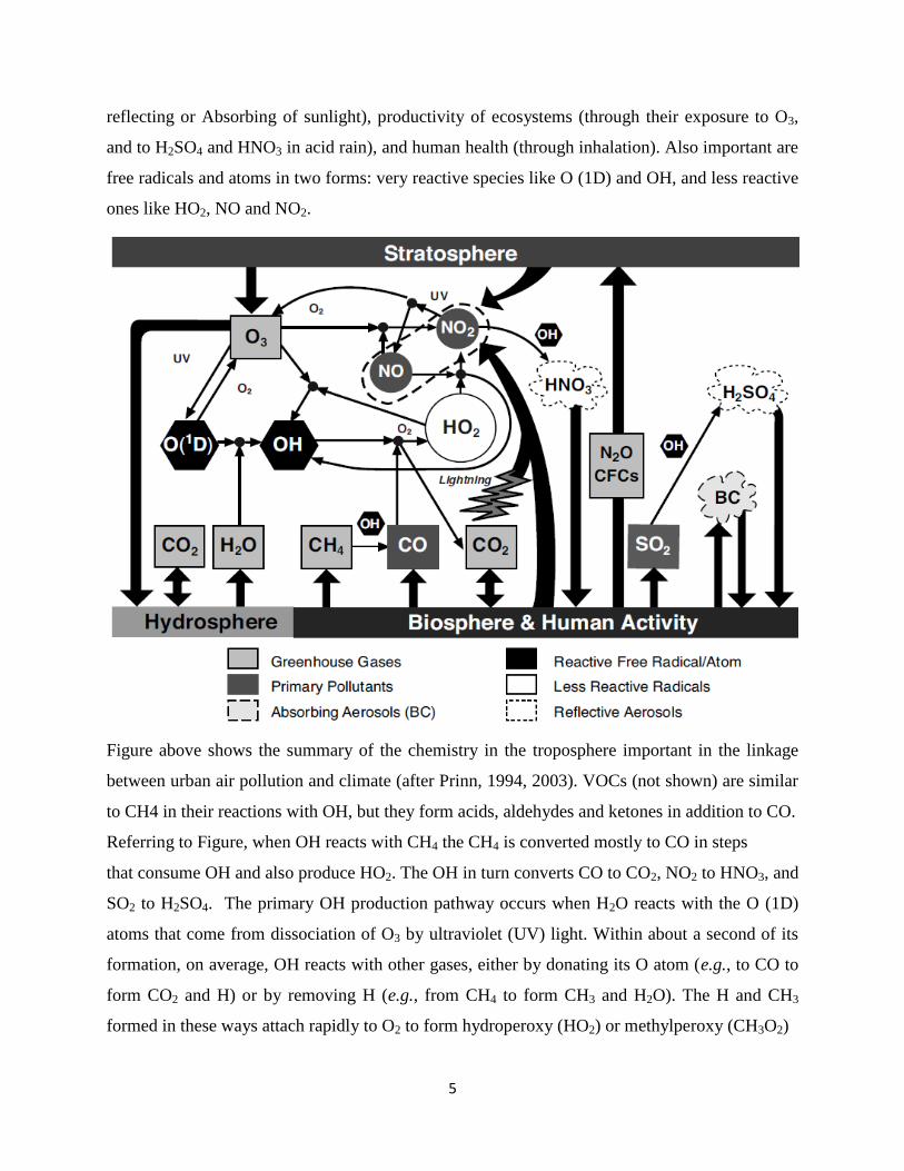
5

reflecting or Absorbing of sunlight), productivity of ecosystems (through their exposure to O3,

and to H2SO4 and HNO3 in acid rain), and human health (through inhalation). Also important are

free radicals and atoms in two forms: very reactive species like O (1D) and OH, and less reactive

ones like HO2, NO and NO2.

Figure above shows the summary of the chemistry in the troposphere important in the linkage

between urban air pollution and climate (after Prinn, 1994, 2003). VOCs (not shown) are similar

to CH4 in their reactions with OH, but they form acids, aldehydes and ketones in addition to CO.

Referring to Figure, when OH reacts with CH4 the CH4 is converted mostly to CO in steps

that consume OH and also produce HO2. The OH in turn converts CO to CO2, NO2 to HNO3, and

SO2 to H2SO4. The primary OH production pathway occurs when H2O reacts with the O (1D)

atoms that come from dissociation of O3 by ultraviolet (UV) light. Within about a second of its

formation, on average, OH reacts with other gases, either by donating its O atom (e.g., to CO to

form CO2 and H) or by removing H (e.g., from CH4 to form CH3 and H2O). The H and CH3

formed in these ways attach rapidly to O2 to form hydroperoxy (HO2) or methylperoxy (CH3O2)

6

free radicals which are relatively unreactive. If there is no way to rapidly recycle HO2 back to

OH, then levels of OH are kept relatively low. The addition of NOx emissions into the mix

significantly changes the chemistry. Specifically, a second pathway is created in which NO

reacts with HO2 to form NO2 and to reform OH. Ultraviolet light then decomposes NO2 to

produce O atoms (which attach to O2 to form O3) and reform NO. Hence NOx (the sum of NO

and NO2) is a catalyst which is not consumed in these reactions. The production rate of OH by

this secondary path in polluted air is about five times faster than the above primary pathway

involving O(1D) and H2O (Ehhalt, 1999). The reaction of NO with HO2 does not act as a sink for

HOx (the sum of OH and HO2) but instead determines the ratio of OH to HO2. Calculations for

polluted airs suggest that HO2 concentrations are about 40 times greater than OH (Ehhalt, 1999).

This is due mainly to the much greater reactivity of OH compared to HO2.

If emissions of air pollutants that react with OH, such as CO, VOCs, CH4, and SO2, are

increasing, then keeping all else constant, OH levels should decrease. This would increase the

lifetime and hence concentrations of CH4. However, increasing NOx emissions should increase

tropospheric O3 (and hence the primary source of OH), as well as increase the recycling rate of

HO2 to OH (the second source of OH). This OH increase should lower CH4 concentrations. Thus

changing the level of OH causes greenhouse gas, and thus climate, changes. Climate change will

also influence OH. Higher ocean temperatures should increase H2O in the lower troposphere and

thus increase OH production through its primary pathway. Higher atmospheric temperatures also

increase the rate of reaction of OH with CH4, decreasing the concentrations of both. Greater

cloud cover will reflect more solar ultraviolet light, thus decreasing OH, and vice versa.

Added to these interactions involving gases, are those involving aerosols. For example,

increasing SO2 emissions and/or OH concentrations should lead to greater concentrations of

sulfate aerosols which are a cooling influence. Accounting for all of these interactions, and other

related ones (e.g., Prinn, 2003), requires that a detailed interactive atmospheric chemistry and

climate model be used to assess the effects of air pollution reductions on climate.

7

2.2 INTEGRATED GLOBAL SYSTEM MODEL

For our calculations, we utilize the MIT Integrated Global System Model (IGSM). The IGSM

consists of a set of coupled sub-models of economic development and its associated emissions,

natural biogeochemical cycles, climate, air pollution, and natural ecosystems (Prinn et al., 1999;

Reilly et al., 1999; Webster et al., 2002, 2003). It is specifically designed to address key

questions in the natural and social sciences that are amenable to quantitative analysis and are

relevant to environmental policy.

Chemically and radiatively important trace gases and aerosols are emitted as a result of

human activity. The Emissions Prediction and Policy Analysis (EPPA) submodel incorporates

the major relevant demographic, economic, trade, and technical issues involved in these

emissions at the national and global levels. Natural emissions of these gases are also important

and are computed in the Natural Emissions Model (NEM) which is driven by IGSM predictions

of climate and ecosystem states around the world. The coupled atmospheric chemistry and

climate sub model is in turn driven by the combination of these anthropogenic and natural

emissions. This submodel includes atmospheric and oceanic chemistry and circulation, and land

hydrological processes. The atmospheric chemistry component has sufficient detail to include its

sensitivity to climate and different mixes of emissions, and to address the effects on climate of

policies proposed for control of air pollution and vice versa (Wang et al., 1998; Mayer et al.,

2000).

Global System Model (IGSM). Feedbacks between the component models that are

currently included, or proposed for inclusion in later versions, are shown as solid or dashed lines

respectively (adapted from Prinn et al., 1999). To simulate, the detailed chemical and dynamical

processes in current 3D urban air chemistry models (Mayer et al., 2000). For this purpose, the

emissions calculated in the EPPA submodel are divided into two parts: urban emissions which

are processed by the UAP submodel before entering the global chemistry/climate submodel, and

non-urban emissions which are input directly into the large-scale model. The UAP enables

simultaneous consideration of control policies applied to local air pollution and global climate. It

also provides the capability to assess the effects of air pollution on ecosystems, and to predict

levels of irritants important to human health in the growing number of megacities around the

world. The atmospheric and oceanic circulation components in the IGSM are simplified

compared to the most complex models available, but they capture the major processes and, with

8

appropriate parameter choices, can mimic quite well the zonal-average behavior of the complex

models (Sokolov and Stone, 1998; Sokolov et al., 2003). We use the version of the IGSM with

2D atmospheric and 2D oceanic sub models here, although the latest version has a 3D ocean to

capture better the deep ocean circulations that serve as heat and CO2 sinks (Kamenkovich et al.,

2002, 2003). The 2D/2D version we use here resolves separately the land and ocean (LO)

processes at each latitude and so is referred to as the 2D-LO-2D version.

The outputs from the coupled atmospheric chemistry and climate model then drive a

Terrestrial Ecosystems Model (TEM; Xiao et al., 1998) which calculates key vegetation

properties including production of vegetation mass, land-atmosphere CO2 exchanges, and soil

nutrient contents in 18 globally distributed ecosystems. TEM then feeds back its computed CO2

fluxes to the climate/atmospheric chemistry submodel, and its soil nutrient contents to NEM, to

complete the IGSM interactions. The current IGSM does not include treatment of black carbon

(BC) aerosols (see Figure 1). Detailed studies with a global 3D chemistry and climate model

indicate multiple, regionally variable and partially-offsetting, effects of BC on absorption and

reflection of sunlight, reflectivity of clouds, and the strength of lower tropospheric convection

(Wang, 2004). These detailed studies also suggest important BC-induced changes in the

geographic pattern of precipitation, not surprisingly since aerosols have important and complex

effects on cloud formation, and on whether clouds will even produce precipitation. Methods to

capture these effects in the IGSM are currently being explored. In light of the difficulty in

simulating these and other regional effects, the numerical results presented here are limited to

temperature and sea level effects, primarily at the global and hemispheric level.

2.3 NUMERICAL EXPERIMENTS

To investigate, at least qualitatively, some of the important potential impacts of controls

of air pollutants on temperature, we have carried out runs of the IGSM in which individual

pollutant emissions, or combinations of these emissions, are held constant from 2005 to 2100.

These are compared to a reference run (denoted “ref”) in which there is no explicit policy to

reduce greenhouse gas emissions (see Reilly et al., 1999; Webster et al., 2002).

Specifically, in five runs of the IGSM, we consider caps at 2005 levels of emissions of the

following air pollutants:

9

(1) NOx only (denoted “NOx cap”),

(2) CO plus VOCs only (denoted “CO/VOC cap”),

(3) SOx only (denoted “SOx cap”),

(4) Cases (1) and (2) combined (denoted “3 cap”),

(5) Cases (1), (2) and (3) combined (denoted “all cap”).

Cases (1) and (2) are designed to show the individual effects of controls on NOx and reactive

carbon gases (CO, VOC), although such individual actions are very unlikely. Case (3) addresses

further controls on emissions of sulfur oxides from combustion of fossil fuels and biomass, and

from industrial processes. Cases (4) and (5) address combinations more likely to be

representative of a real comprehensive air pollution control approach.

One important caveat in interpreting our results is that we are neglecting the effects of air

pollutant controls on: (a) the overall demand for fossil fuels (e.g., leading to greater efficiencies

in energy usage and/or greater demand for non-fossil energy sources), and (b), the relative mix of

fossil fuels used in the energy sector (i.e. coal versus oil versus gas). Consideration of these

effects, which may be very important, will require calculation in the EPPA model of the impacts

of NOx, CO, VOC and SOx emission reductions on the cost of using coal, oil, and gas. Such

calculations have not yet been included in the current global economic models (including EPPA)

used to address the climate issue. Such inclusion requires relating results from existing very

detailed studies of costs of meeting near-term air pollution control to the more aggregated

structure, and longer time horizon, of models used to examine climate policy.

The ratios of the emissions of NOx, CO/VOC, and SOx in the year 2100 to the reference

case in 2100 when their emissions are capped at 2005 levels. Because these chemicals are short-

lived (hours to several days for NOx, VOCs, and SOx, few months for CO), the effects of their

emissions are largely restricted to the hemispheres in which they are emitted (and for the

shortest-lived pollutants restricted to their source regions). Therefore shows hemispheric as well

as global emission ratios. For calibration, the reference global emissions of NOx, CO/VOC, and

SOx in 2100 are about 5, 2.5, and 1.5 times their 2000 levels. Global, northern hemispheric

(NH) and southern hemispheric (SH) emissions in the year 2100 of CO/VOC, NOx and SOx,

when they are capped at 2005 levels (CAP), are shown as ratios to emissions in the reference

(REF) case (no caps).

10

3.0 EFFECTS ON CONCENTRATIONS

The global and hemispheric average lower tropospheric concentrations of CH4,

O3, sulfate aerosols, and OH in each of the above five capping cases are shown as percentage

changes from the relevant global or hemispheric reference. From the major global effects of

capping SOx are to decrease sulfate aerosols and slightly increase OH (due to lower SO2 which

is an OH sink). Capping of NOx leads to decreases in O3 and OH and an increase in CH4 (caused

by the lower OH which is a CH4 sink). The CO and VOC cap increases OH and thus increases

sulfate (formed by OH and SO2) and decreases CH4. Note that CO and VOC changes have

opposing effects on O3 so the net changes when they are capped together are small.

Combining NOx, CO and VOC caps leads to an O3 decrease (driven largely by the NOx

decrease) and a slight increase in CH4 (the enhancement due to the NOx caps being partially

offset by the opposing CO/VOC caps). Finally, capping all emissions causes substantial lowering

of sulfate aerosols and O3 and a small increase in CH4.

The two hemispheres generally respond somewhat differently to these caps due to the short

air pollutant lifetimes and dominance of northern over southern hemispheric emissions. The

northern hemisphere contributes the most to the global averages and therefore responds

similarly. The southern hemisphere shows very similar decreases in sulfate aerosol from its

reference when compared to the northern hemisphere when either SOx or all emissions are

capped.

When compared to the southern hemisphere, the northern hemispheric ozone levels

decrease by much larger percentages below their northern hemisphere reference when either

NOx, NOx/CO/VOC, or all emissions are capped. Capping NOx emissions leads to significant

decreases in OH and thus increases in methane in both hemispheres (Figs. 4b and 4c). Because

methane has a long lifetime (about 9 years, Prinn et al., 2001) relative to the inter hemispheric

concentrations of climatically and chemically important species (CH4, O3, aerosols, OH) in the

five cases with capped emissions are shown as percent changes from their relevant global or

hemispheric average values in the reference case for the year 2100:

(a) Global-average;

(b) Southern hemispheric; and

11

(c) Northern hemispheric concentrations mixing time (about 1 to 2 years), its global

concentrations are influenced by OH changes in either hemisphere alone, or in both. Hence CH4

also increases in both hemispheres when NOx/CO/VOC or all emissions are capped even though

the OH decreases only occur in the northern hemisphere in these two cases.

3.1 EFFECTS ON ECOSYSTEMS

Effects of air pollution on the land ecosystem sink for carbon can be significant due to

reductions in ozone-induced plant damage ( Felzer et al., 2004). Net primary production (NPP,

the difference between plant photosynthesis and plant respiration), as well as net ecosystem

production (NEP, which is the difference between NPP and soil respiration plus decay, and

represents the net land sink), both increase when ozone decreases. This is evident in the case

where all pollutants are capped and ozone decreased by about 13% globally. The effect is even

greater when we assume that cropland and managed forests receive optimal levels of nitrogen

fertilizer (“with Fertilizer” case; Felzer et al., 2004).

The land sink (NEP) is increased by 30 to 49% or 0.6 to 0.9 gigatons of carbon (in CO2) in 2100

through the illustrated pollution caps ( 1 gigaton=1015

gm).

These ecosystem calculations do not include the additional positive effects on NPP and NEP

of decreased acid deposition and decreased exposure to SO2 and NO2 gas, that would result from

the pollution caps considered. They also do not include the negative effects on NPP and NEP of

decreasing nutrient nitrate and possibly sulfate deposition that also arise from these caps. Net

annual uptake of carbon by vegetation alone (net primary production) and vegetation

plus soils (net ecosystem production, the land carbon sink) for the NOx/SOx/CO plus VOC

capped (all cap) case is shown for the year 2100 as a percentage change from the reference case.

The results show the effects with optimal nitrogen use through fertilization on cropland (with

Fertilizer) or with levels of nitrogen in croplands assumed to be the same as those in equivalent

natural ecosystems (without Fertilizer).

3.2 ECONOMIC EFFECTS

If we could confidently value damages associated with climate change, we could estimate

the avoided damages in dollar terms resulting from reductions in temperature due to the lowered

level of atmospheric CO2 caused by the above increases in the land carbon sink achieved with

12

the ozone caps. We could similarly value the temperature changes due to caps in other pollutants

besides ozone. However monetary damage estimates suffer from numerous shortcomings (e.g.,

Jacoby, 2004). Felzer et al. (2004a, b) valued increases in carbon storage in ecosystems due to

decreased ozone exposure in terms of the avoided costs of fossil fuel CO2 reductions needed to

achieve an atmospheric stabilization target. The particular target they examined was 550 ppm

CO2. The above extra annual carbon uptake (due to avoided ozone damage) of 0.6 to 0.9

gigatons of carbon is only 2 to 4% of year 2100 reference projections of anthropogenic fossil

CO2 emissions (which reach nearly 25 gigatons year in 2100 according to Felzer et al.

However, as these authors point out, this small level of additional uptake can have a

surprisingly large effect on the cost of achieving a climate policy goal. Here we conduct a similar

analysis using a 5% discount rate, and adopting the policy costs associated with 550 ppm CO2

stabilization, to estimate the policy cost savings that would result from the increased carbon

uptake through 2100 in the “allcap” compared to the “ref” scenarios shown in Figure 5. The

savings are $2.5 (“without Fertilizer”) to $4.7 (“with Fertilizer”) trillion (1997 dollars). These

implied savings are 12 to 22% of the total cost of a 550ppm stabilization policy.

The disproportionately large economic value of the additional carbon uptake has two reasons.

One reason is that the fossil carbon reduction savings are cumulative; the total reference 2000-

2100 carbon uptake is 36 (without Fertilizer) and 75 (with Fertilizer) gigatons, or about 6 to 13

years of fossil carbon emissions at current annual rates. A second reason is that the additional

uptake avoids the highest marginal cost options. This assumes that the implemented policies

would be cost effective in the sense that the least costly carbon reduction options would be used

first, and more costly options would only be used later if needed. An important caveat here is

that, as shown in Felzer et al. (2004a,b), a carbon emissions reduction policy also reduces ozone

precursors so that an additional cap on these precursors associated with air pollution policy

results in a smaller additional reduction, and less avoided ecosystem damage. A pollution cap as

examined here, assuming there was also a 550ppm carbon policy in place, leads to only a 0.1 to

0.8 gigaton increase in the land sink in 2100 (compare 0.6 to 0.9 gigatons ) and a cumulative

2000-2100 increase of carbon uptake of 13 to 40 gigatons of carbon, which is about one-half of

the above increased cumulative uptake when the pollution cap occurs assuming there is no

climate policy.

13

3.3 EFFECTS ON TEMPERATURE AND SEA LEVEL

The impact of these various pollutant caps on global and hemispheric mean surface

temperature and sea level changes from 2000 to 2100 are shown in as percentages relative to the

global-average reference case changes of 2.7°C and 0.4 meters respectively. The largest

increases in temperature and sea level occur when SOx alone is capped due to the removal of

reflecting (cooling) sulfate aerosols. Because most SOx emissions are in the northern

hemisphere, the temperature increases are greatest there. For the NOx caps, temperature

increases in the southern hemisphere (driven by the CH4 increases), but decreases in the northern

hemisphere (due to the cooling effects of the O3 decreases exceeding the warming driven by the

CH4 increases). For CO and VOC reductions, there are small decreases in temperature driven by

the accompanying aerosol increases and CH4 reductions, with the greatest effects being in the

northern hemisphere where most of the CO and VOC emissions (and aerosol production) occur.

When NOx, CO, and VOCs are all capped, the nonlinearity in the system is evidenced by the fact

that the combined effects are not simple sums of the effects from the individual caps.

Effects of air pollution caps in the five capping cases on the global, northern hemispheric

and southern hemispheric average temperature increases, and the global sea level rise, between

2000 and 2100 are shown as percent changes from their average values (global or hemispheric)

in the reference case. Also shown are the equivalent results for the case where the enhanced sink

due to the ozone cap is included along with the caps on all pollutants. For this case, we assume

the average of the fertilized and non-fertilized sink enhancements from Figure 5.decreases and

aerosol increases (offset only slightly by CH4 increases) lead to even less warming and sea level

rise than obtained by adding the CO/VOC and NOx capping cases. Finally the capping of all

emissions yields temperature and sea level rises that are smaller but qualitatively similar to the

case where only SOx is capped, but the rises are greater than expected from simple addition of

the SOx-capped and CO/VOC/NOx-capped cases. Nevertheless, the capping of CO, VOC and

NOx serves to reduce the warming induced by the capping of SOx.

Note that these climate calculations omit the cooling effects of the CO2 reductions caused by the

lessening of the inhibition of the land sink by ozone. This omission is valid if we presume that

anthropogenic CO2 emissions, otherwise restricted by a climate policy, are allowed to increase to

compensate for these reductions. This was the basis for our economic analysis in the previous

section.

14

4.0 SUMMARY AND CONCLUSIONS

Hence to illustrate some of the impacts of air pollution policy on climate change, the

paper examined five highly idealized but informative scenarios for placing caps on emissions of

SOx, NOx, CO plus VOCs, NOx plus CO plus VOCs, and all of these pollutants combined.

These caps kept global emissions at 2005 levels through 2100 and their effects on climate were

compared to a reference run with no caps applied. Our purpose was not to claim that these

scenarios are in any way realistic or likely, but rather that they served to illustrate quite well the

complex interactions between air pollutant emissions and changes in temperature and sea level.

In general, placing caps on NOx alone, or NOx, CO and VOCs together, leads to lower

ozone levels, and thus less radiative forcing of climate change by this gas, and to less inhibition

by ozone of carbon uptake by ecosystems which also leads to less radiative forcing (this time by

CO2). Less radioactive forcing by these combined effects means less warming and less sea level

rise. Placing caps on NOx alone also leads to decreases in OH and thus increases in CH4.

These OH decreases and CH4 increases are lessened (but not reversed) when there are

simultaneous NOx, CO and VOC caps. Increases in CH4 lead to greater radiative forcing.

Placing caps on SOx leads to lower sulfate aerosols, less reflection of sunlight back to space by

these aerosols (direct effect) and by clouds seeded with these aerosols (indirect effect), and thus

to greater radiative forcing of climate change due to solar radiation. Enhanced radiative forcing

by these aerosol and CH4 changes combined leads to more warming and sea level rise. Hence

these impacts on climate of the pollutant caps partially cancel each other. Specifically, depending

on the capping case, the 2000-2100 reference global average climate changes are altered only by

+4.8 to –2.6% 13 (temperature) and +2.2 to –2.2 % (sea level).

Except for the NOx alone case, the alterations of temperature are of the same sign but

significantly greater in the northern hemisphere (where most of the emissions and emission

reductions occur) than in the southern hemisphere. Note that for the NOx alone caps, the

temperature decrease caused by ozone reductions is greater than the temperature increase driven

by methane increases in the northern hemisphere while the opposite is true in the southern

hemisphere. It is well established that urban air pollution control policies are beneficial for

human health and downwind ecosystems. As far as ancillary benefits are concerned, our

calculations suggest that air pollution policies may have only a small influence, either positive or

negative, on mitigation of global-scale climate change. However, even small contributions to

15

climate change mitigation can be disproportionately important in economic terms. This occurs

because, as we show in the case of increased carbon uptake, these effects mean that the highest

cost climate change mitigation measures, those occurring at the margin, can be avoided.

16

REFERENCES

Ehhalt, D.H., 1999: Gas phase chemistry of the troposphere. Topics in Physical Chemistry, 6: 21-

109.

Felzer, B., Kicklighter, D., Melillo, J., Wang, C., Zhuang, Q., and Prinn, R., 2004a: Effects of

ozone on net primary production and carbon sequestration in the conterminous United States

using a biogeochemistry model. Tellus B, 56: 230-248.

Felzer, B., Reilly, J., Melillo, J., Kicklighter, D., Wang, C., Prinn, R., Sarofim, M., and Zhuang,

Q.: 2004b: Past and future effects of ozone on net primary production and carbon sequestration

using a global biogeochemical model. MIT JPSPGC Report 103

(http://mit.edu/globalchange/www/MITJPSPGC_Rpt103.pdf); Climatic Change, in press Jacoby,

H.D., 2004: Informing climate policy given incommensurable benefits estimates. Global

Environmental Change Part A, 14(3): 287-279; MIT JPSPGC Reprint 2004-7.

Kamenkovich, I.V., Sokolov, A.P. and Stone, P., 2002: An efficient climate model with a 3D

ocean and

statistical-dynamical atmosphere. Climate Dynamics, 1: 585-598.

Kamenkovich, I.V., Sokolov, A.P. and Stone, P., 2003: Feedbacks affecting the response of the

thermohaline circulation to increasing CO2: A study with a model of intermediate complexity.

Climate Dynamics, 21: 119-130.

Mayer, M., Wang, C. Webster, M., and Prinn, R.G.: 2000. Linking local air pollution to global

chemistry

and climate. J. Geophysical Research, 105: 20,869-20,896.

Prinn, R.G., 1994, The interactive atmosphere: Global atmospheric-biospheric chemistry. Ambio,

23: 50-61.

Prinn, R.G., 2003: The cleansing capacity of the atmosphere. Annual Reviews Environment and

Resources, 28: 29-57.

Prinn, R.G., Huang, J., Weiss, R., Cunnold, D., Fraser, P., Simmonds, P., McCulloch, A., Harth,

C.,

Salameh, P., O’Doherty, S., Wang, R., Porter, L., and Miller, B., 2001: Evidence for substantial

variations of atmospheric hydroxyl radicals in the past two decades. Science, 292:1882-1888.

Prinn, R.G., Jacoby, H., Sokolov, A., Wang, C., Xiao, X., Yang, Z., Eckaus, R., Stone, P.,

Ellerman,

17

A.D., Melillo, J., Fitzmaurice, J., Kicklighter, D., Holian, G. and Liu, Y., 1999: Integrated

Global System Model for climate policy assessment: feedbacks and sensitivity studies. Climatic

Change, 41: 469-546.

Reilly, J., Prinn, R., Harnisch, J., Fitzmaurice, J., Jacoby, H., Kicklighter, D., Melillo, J., Stone.

Sokolov, A. and Wang, C., 1999: Multi-gas assessment of the Kyoto Protocol. Nature, 401: 549-

555.

Sokolov, A., and Stone, P., 1998: A flexible climate model for use in integrated assessments.

Climate Dynamics, 14: 291-303.

Sokolov, A., Forest, C.E. and Stone, P., 2003: Comparing oceanic heat uptake in AOGCM

transient climate change experiments. J. Climate, 16: 1573-1582.

Wang, C., Prinn, R. and Sokolov, A., 1998: A global interactive chemistry and climate model:

Formulation and testing. J. Geophysical Research, 103: 3399-3417.

Wang, C., 2004: A modeling study on the climate impacts of black carbon aerosols. J.

Geophysical Research, 109: D03106, doi: 10.1029/2003JD004084.

Webster, M.D., Babiker, M., Mayer, M., Reilly, J.M., Harnisch, J., Sarofim, M.C., and Wang, C.,

2002: Uncertainty in emissions projections for climate models. Atmospheric Environment, 36:

3659-3670.

Webster, M.D., Forest, C.E., Reilly, J.M., Babiker, M., Kicklighter, D., Mayer, M., Prinn, R.G.,

Sarofim,

M., Sokolov, A., Stone, P.H., and Wang, C., 2003: Uncertainty analysis of climate change and

policy response. Climatic Change, 61: 295-320.

Xiao, X., Melillo, J., Kicklighter, D., McGuire, A., Prinn, R., Wang, C., Stone, P. and Sokolov,

A., 1998: Transient climate change and net ecosystem production of the terrestrial biosphere.

Global Biogeochemical Cycles, 12: 345-360.