clean air plan - santa barbara county air pollution control
TRANSCRIPT
22000044 CClleeaann AAiirr PPllaann
Santa Barbara County’s plan to attain the state 1-hour ozone standard
FINAL December 2004
22000044 CClleeaann AAiirr PPllaann
Santa Barbara County’s plan to attain the state 1-hour ozone standard
Three Year Update to the 2001 Clean Air Plan – State 1-hour Ozone Standard
FINAL
December 2004
Santa Barbara County Santa Barbara County Air Pollution Control District Association of Governments 260 North San Antonio Road, Suite A 260 North San Antonio Road, Suite B Santa Barbara, California 93110 Santa Barbara, California 93110 www.sbcapcd.org www.sbcag.org (805) 961-8800 (805) 961-8900
BOARD OF DIRECTORS Supervisor Naomi Schwartz, First District Santa Barbara County Board of Supervisors
Mayor Bill Traylor City of Buellton
Supervisor Susan Rose, Second District Santa Barbara County Board of Supervisors
Mayor Richard Weinberg City of Carpinteria
Supervisor Gail Marshall, Third District Santa Barbara County Board of Supervisors
Mayor Cynthia Brock, Chair City of Goleta
Supervisor Joni Gray, Fourth District Santa Barbara County Board of Supervisors
Councilmember Carlos Aguilera City of Guadalupe
Supervisor Joe Centeno, Fifth District Santa Barbara County Board of Supervisors
Councilmember DeWayne Holmdahl City of Lompoc
Councilmember Dan Secord City of Santa Barbara
Councilmember Marty Mariscal City of Santa Maria
Mayor David Smyser, Vice-Chair City of Solvang
AIR POLLUTION CONTROL OFFICER
TERRY DRESSLER
BOARD OF DIRECTORS Supervisor Naomi Schwartz, First District, Chair Santa Barbara County Board of Supervisors
Mayor Bill Traylor City of Buellton
Supervisor Susan Rose, Second District Santa Barbara County Board of Supervisors
Mayor Richard Weinberg City of Carpinteria
Supervisor Gail Marshall, Third District Santa Barbara County Board of Supervisors
Councilmember Jack Hawxhurst City of Goleta
Supervisor Joni Gray, Fourth District Santa Barbara County Board of Supervisors
Mayor Sam Arca City of Guadalupe
Supervisor Joe Centeno, Fifth District Santa Barbara County Board of Supervisors
Mayor Dick DeWees, Vice-Chair City of Lompoc
Councilmember Dan Secord City of Santa Barbara
Councilmember Marty Mariscal City of Santa Maria
Mayor David Smyser City of Solvang
EXECUTIVE DIRECTOR JIM KEMP
22000044 CClleeaann AAiirr PPllaann
FINAL
December 2004
PROJECT MANAGEMENT
Tom Murphy, SBCAPCD Michael Powers, SBCAG
PRINCIPAL AUTHORS
Jim Damkowitch, SBCAG Jim Fredrickson, SBCAPCD
Douglas Grapple, SBCAPCD Joe Petrini, SBCAPCD
Tom Murphy, SBCAPCD Ron Tan, SBCAPCD
Vijaya Jammalamadaka, SBCAPCD
CONTRIBUTORS
Doug Allard, SBCAPCD (Retired) Bobbie Bratz , SBCAPCD
Mary Byrd, SBCAPCD Peter Cantle, SBCAPCD
Joel Cordes, SBCAPCD Terry Dressler, SBCAPCD
Gary Wissman, SBCAPCD
RESOLUTION OF THE BOARD OF DIRECTORS OF
THE SANTA BARBARA COUNTY
AIR POLLUTION CONTROL DISTRICT IN THE MATTER OF CERTIFYING THE ) RESOLUTION NO. 04 – 14 SUPPLEMENTAL ENVIRONMENTAL ) IMPACT REPORT AND ADOPTING THE ) 2004 CLEAN AIR PLAN ) _________________________________________ ) RECITALS WHEREAS: 1. The Santa Barbara County Air Pollution Control District ("District") is
currently classified as a nonattainment area for the state one-hour ozone standard;
2. Pursuant to the California Clean Air Act of 1988, the District is required to
update the 1991 Air Quality Attainment Plan, the 1994 Clean Air Plan, the 1998 Clean Air Plan
and the 2001 Clean Air Plan to attain the state one-hour ozone standard by the earliest
practicable date;
3. The District has prepared a 2004 Clean Air Plan to comply with the California
Clean Air Act update requirements;
4. The 2004 Clean Air Plan contains commitments by the Board for adoption of
specified regulations to control air pollution, and also includes commitments by the State of
California and the United States Environmental Protection Agency, and encourages certain
actions by other jurisdictions within Santa Barbara County;
5. Pursuant to the California Environmental Quality Act (“CEQA”), a
Supplemental Environmental Impact Report was prepared and circulated to address any potential
environmental impacts associated with the 2004 Clean Air Plan;
6. The Santa Barbara County Association of Governments (“SBCAG”), in a
noticed public hearing, considered and approved the Transportation Control Measures for the
2004 Clean Air Plan pursuant to the existing Memorandum of Understanding between the
District and SBCAG;
7. At their November 10, 2004 meeting, the Community Advisory Council
recommended that the Board adopt the 2004 Clean Air Plan;
8. The Community Advisory Council and the District have reviewed the emission
inventories developed for the 2004 Clean Air Plan and are alarmed by the magnitude of and the
growth in the emissions related to marine shipping;
9. The Community Advisory Council and the District recognize the relationship
between land use decisions and local air quality impacts.
THEREFORE, IT IS HEREBY RESOLVED THAT:
1. The Board hereby certifies that the Supplemental Environmental Impact
Report (Attachment 2) circulated for this 2004 Clean Air Plan has been completed in compliance
with CEQA and was presented to this Board and reviewed and considered prior to approving the
2004 Clean Air Plan, and that the final Supplemental Environmental Impact Report reflects the
Board’s independent judgment and analysis.
2. The Board hereby adopts the CEQA findings set forth in Attachment 3 and the
Mitigation Monitoring Plan contained in Attachment 2.
3. The Board hereby adopts the 2004 Clean Air Plan as provided to this Board on
October 21, 2004 and modified as set forth in Attachments 4 and 6 as the 2004 Clean Air Plan of
the District and finds that this Plan shall be the plan for purposes of compliance with the plan
update requirements of the California Clean Air Act.
4. The Board has reviewed the responses to comments received from the public
and interested agencies set forth in Chapter 8 (Attachment 6) and adopts those responses to
comments as findings of this Board. Additionally, the Board has reviewed the responses to
written comments received after the close of the public comment period set forth in Attachment
7 and adopts those responses as findings of this Board.
5. The Board commits to adopt the proposed regulations to control air pollution
required in the 2004 Clean Air Plan and the Board relies on the State of California and the
United States Environmental Protection Agency to fulfill the commitments referred to in the
Plan.
6. The Board recognizes the magnitude of and the projected growth in marine
shipping emissions and directs staff to continue all necessary and proper actions to influence the
United States Environmental Protection Agency to reduce the air quality impacts of emissions
from this significant federal source.
7. The Board encourages local governments to plan and design communities to
minimize motor vehicle miles traveled and trips.
8. The Board directs District staff to work with the Community Advisory Council
to evaluate tools to quantify emissions from indirect sources and return to the Board with
recommended options to mitigate emissions from such sources.
9. The Board authorizes the Chair to sign the letter (Attachment 8) transmitting
the 2004 Clean Air Plan to the California Air Resources Board. Additionally, the Board
authorizes the Control Officer to do all other acts necessary and proper to obtain approval of the
2004 Clean Air Plan by the California Air Resources Board.

TABLE OF CONTENTS Page #
i
EXECUTIVE SUMMARY Introduction...................................................................................................................EX-1
Why is this 2004 Plan being prepared?.........................................................................EX-2
What is new in this 2004 Plan Revision?......................................................................EX-2
How was this 2004 Plan Revision Prepared? ...............................................................EX-2
What are the health effects of ozone? ...........................................................................EX-3
Is air quality improving?...............................................................................................EX-3
How is attainment of state 1-hour ozone standard determined? ...................................EX-4
Does this 2004 Plan address any federal requirements?...............................................EX-4
What are the key state requirements that this 2004 Plan addresses? ............................EX-4
How has the emission inventory changed?...................................................................EX-5
Where does our human-generated air pollution come from?........................................EX-5
Has the overall control strategy changed? ....................................................................EX-5
Does the 2004 Plan show that we will attain the state 1-hour ozone standard? ...........EX-6
How does the adoption of this 2004 Plan impact rulemaking at the APCD?...............EX-6
CHAPTER 1 - INTRODUCTION 1.1 Purpose................................................................................................................. 1-1
1.2 Current State Planning Requirements.................................................................. 1-1
1.3 Summary of Attainment Planning Efforts ........................................................... 1-2
1.4 Plan Organization................................................................................................. 1-5
CHAPTER 2 - LOCAL AIR QUALITY 2.1 Introduction.......................................................................................................... 2-1
2.2 Climate of Santa Barbara County ........................................................................ 2-1
2.3 Air Quality Monitoring ........................................................................................ 2-4
2.4 State Ozone Exceedances .................................................................................... 2-4
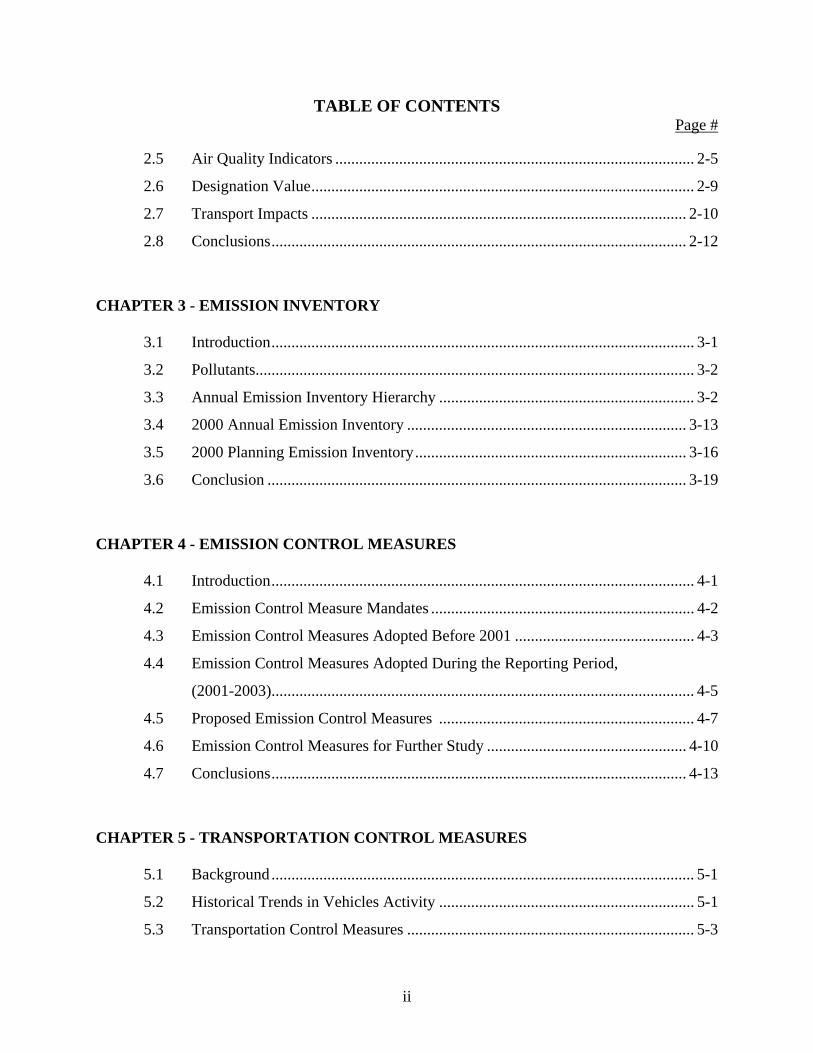
TABLE OF CONTENTS Page #
ii
2.5 Air Quality Indicators .......................................................................................... 2-5
2.6 Designation Value................................................................................................ 2-9
2.7 Transport Impacts .............................................................................................. 2-10
2.8 Conclusions........................................................................................................ 2-12
CHAPTER 3 - EMISSION INVENTORY 3.1 Introduction.......................................................................................................... 3-1
3.2 Pollutants.............................................................................................................. 3-2
3.3 Annual Emission Inventory Hierarchy ................................................................ 3-2
3.4 2000 Annual Emission Inventory ...................................................................... 3-13
3.5 2000 Planning Emission Inventory.................................................................... 3-16
3.6 Conclusion ......................................................................................................... 3-19
CHAPTER 4 - EMISSION CONTROL MEASURES 4.1 Introduction.......................................................................................................... 4-1
4.2 Emission Control Measure Mandates .................................................................. 4-2
4.3 Emission Control Measures Adopted Before 2001 ............................................. 4-3
4.4 Emission Control Measures Adopted During the Reporting Period,
(2001-2003).......................................................................................................... 4-5
4.5 Proposed Emission Control Measures ................................................................ 4-7
4.6 Emission Control Measures for Further Study .................................................. 4-10
4.7 Conclusions........................................................................................................ 4-13
CHAPTER 5 - TRANSPORTATION CONTROL MEASURES 5.1 Background.......................................................................................................... 5-1
5.2 Historical Trends in Vehicles Activity ................................................................ 5-1
5.3 Transportation Control Measures ........................................................................ 5-3
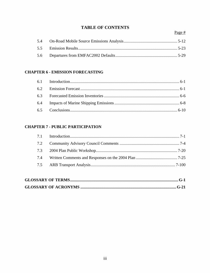
TABLE OF CONTENTS Page #
iii
5.4 On-Road Mobile Source Emissions Analysis.................................................... 5-12
5.5 Emission Results................................................................................................ 5-23
5.6 Departures from EMFAC2002 Defaults............................................................ 5-29
CHAPTER 6 - EMISSION FORECASTING 6.1 Introduction.......................................................................................................... 6-1
6.2 Emission Forecast ................................................................................................ 6-1
6.3 Forecasted Emission Inventories ......................................................................... 6-6
6.4 Impacts of Marine Shipping Emissions ............................................................... 6-8
6.5 Conclusions........................................................................................................ 6-10
CHAPTER 7 - PUBLIC PARTICIPATION 7.1 Introduction.......................................................................................................... 7-1
7.2 Community Advisory Council Comments .......................................................... 7-4
7.3 2004 Plan Public Workshop............................................................................... 7-20
7.4 Written Comments and Responses on the 2004 Plan ........................................ 7-25
7.5 ARB Transport Analysis.................................................................................. 7-100 GLOSSARY OF TERMS......................................................................................................... G-1
GLOSSARY OF ACRONYMS ............................................................................................. G-21
LIST OF TABLES Page #
iv
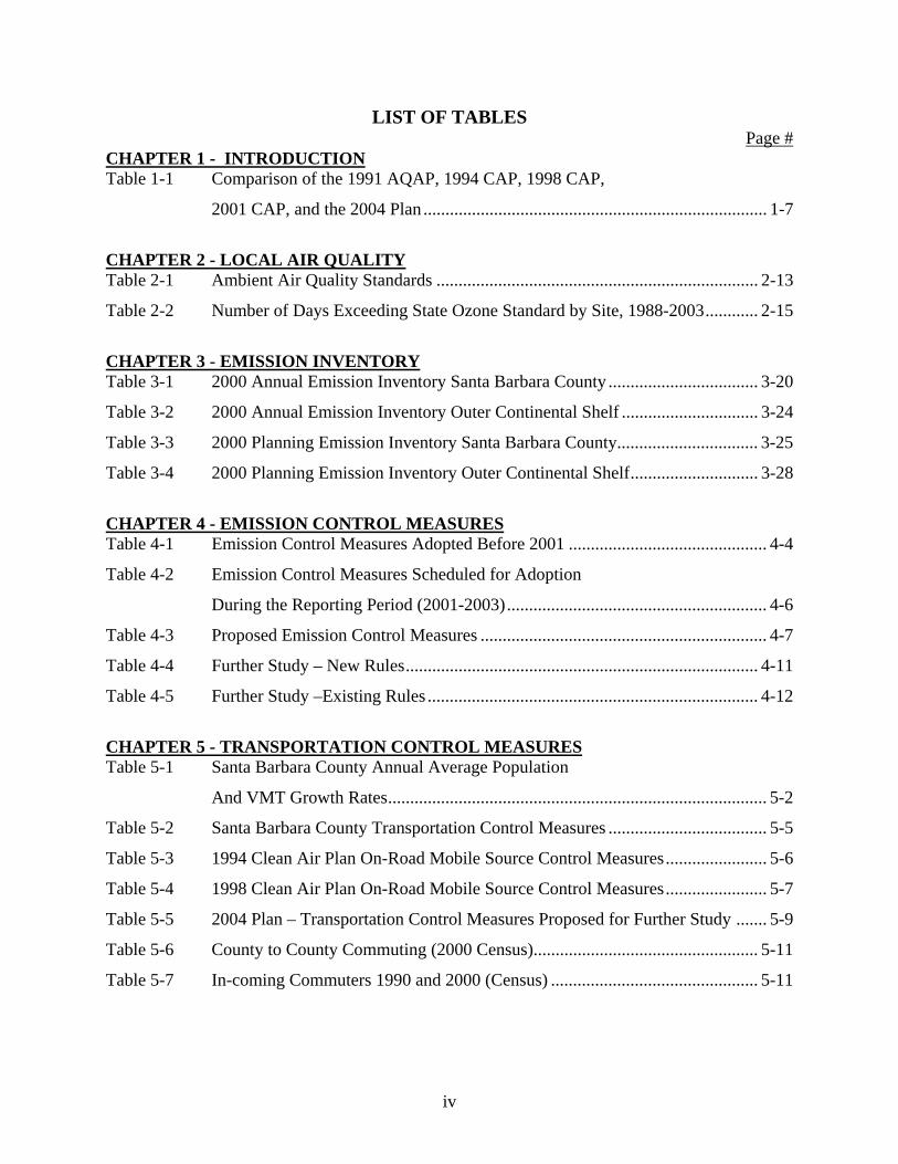
CHAPTER 1 - INTRODUCTION Table 1-1 Comparison of the 1991 AQAP, 1994 CAP, 1998 CAP,
2001 CAP, and the 2004 Plan .............................................................................. 1-7
CHAPTER 2 - LOCAL AIR QUALITY Table 2-1 Ambient Air Quality Standards ......................................................................... 2-13
Table 2-2 Number of Days Exceeding State Ozone Standard by Site, 1988-2003............ 2-15
CHAPTER 3 - EMISSION INVENTORY Table 3-1 2000 Annual Emission Inventory Santa Barbara County .................................. 3-20
Table 3-2 2000 Annual Emission Inventory Outer Continental Shelf ............................... 3-24
Table 3-3 2000 Planning Emission Inventory Santa Barbara County................................ 3-25
Table 3-4 2000 Planning Emission Inventory Outer Continental Shelf............................. 3-28
CHAPTER 4 - EMISSION CONTROL MEASURES Table 4-1 Emission Control Measures Adopted Before 2001 ............................................. 4-4
Table 4-2 Emission Control Measures Scheduled for Adoption
During the Reporting Period (2001-2003)........................................................... 4-6
Table 4-3 Proposed Emission Control Measures ................................................................. 4-7
Table 4-4 Further Study – New Rules................................................................................ 4-11
Table 4-5 Further Study –Existing Rules ........................................................................... 4-12
CHAPTER 5 - TRANSPORTATION CONTROL MEASURES Table 5-1 Santa Barbara County Annual Average Population
And VMT Growth Rates...................................................................................... 5-2
Table 5-2 Santa Barbara County Transportation Control Measures .................................... 5-5
Table 5-3 1994 Clean Air Plan On-Road Mobile Source Control Measures....................... 5-6
Table 5-4 1998 Clean Air Plan On-Road Mobile Source Control Measures....................... 5-7
Table 5-5 2004 Plan – Transportation Control Measures Proposed for Further Study ....... 5-9
Table 5-6 County to County Commuting (2000 Census)................................................... 5-11
Table 5-7 In-coming Commuters 1990 and 2000 (Census) ............................................... 5-11
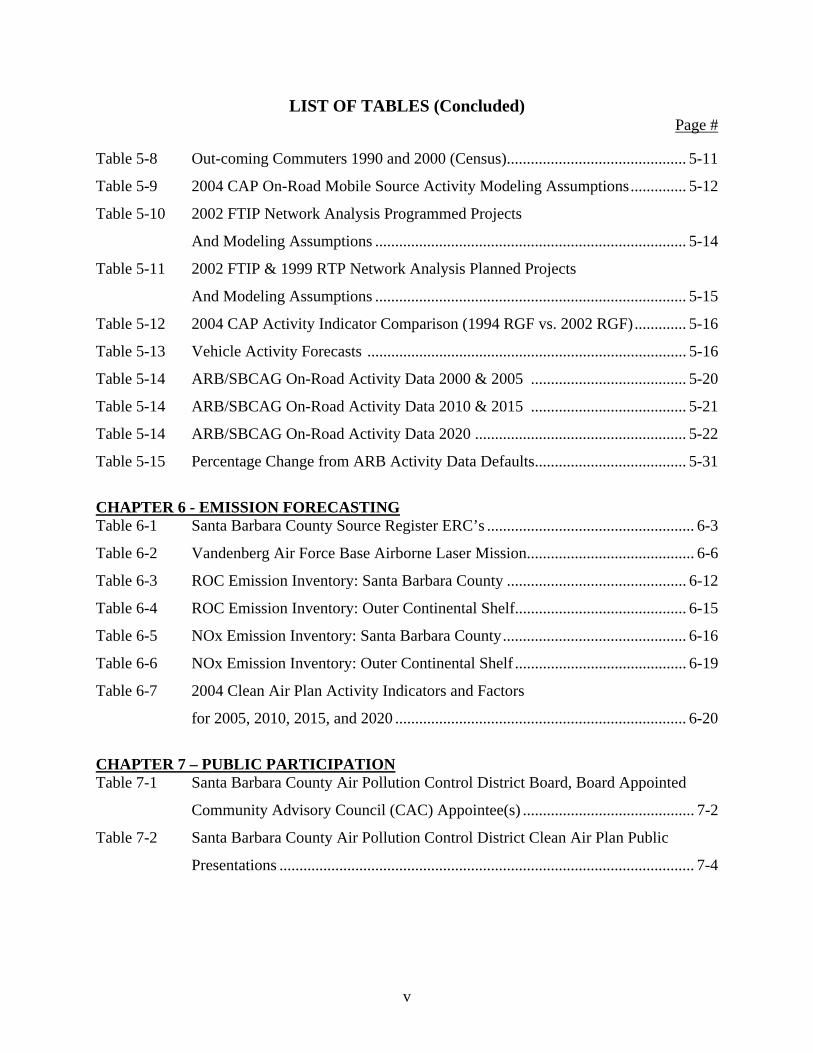
LIST OF TABLES (Concluded) Page #
v
Table 5-8 Out-coming Commuters 1990 and 2000 (Census)............................................. 5-11
Table 5-9 2004 CAP On-Road Mobile Source Activity Modeling Assumptions.............. 5-12
Table 5-10 2002 FTIP Network Analysis Programmed Projects
And Modeling Assumptions .............................................................................. 5-14
Table 5-11 2002 FTIP & 1999 RTP Network Analysis Planned Projects
And Modeling Assumptions .............................................................................. 5-15
Table 5-12 2004 CAP Activity Indicator Comparison (1994 RGF vs. 2002 RGF)............. 5-16
Table 5-13 Vehicle Activity Forecasts ................................................................................ 5-16
Table 5-14 ARB/SBCAG On-Road Activity Data 2000 & 2005 ....................................... 5-20
Table 5-14 ARB/SBCAG On-Road Activity Data 2010 & 2015 ....................................... 5-21
Table 5-14 ARB/SBCAG On-Road Activity Data 2020 ..................................................... 5-22
Table 5-15 Percentage Change from ARB Activity Data Defaults...................................... 5-31
CHAPTER 6 - EMISSION FORECASTING Table 6-1 Santa Barbara County Source Register ERC’s .................................................... 6-3
Table 6-2 Vandenberg Air Force Base Airborne Laser Mission.......................................... 6-6
Table 6-3 ROC Emission Inventory: Santa Barbara County ............................................. 6-12
Table 6-4 ROC Emission Inventory: Outer Continental Shelf........................................... 6-15
Table 6-5 NOx Emission Inventory: Santa Barbara County.............................................. 6-16
Table 6-6 NOx Emission Inventory: Outer Continental Shelf ........................................... 6-19
Table 6-7 2004 Clean Air Plan Activity Indicators and Factors
for 2005, 2010, 2015, and 2020 ......................................................................... 6-20
CHAPTER 7 – PUBLIC PARTICIPATION Table 7-1 Santa Barbara County Air Pollution Control District Board, Board Appointed
Community Advisory Council (CAC) Appointee(s) ........................................... 7-2
Table 7-2 Santa Barbara County Air Pollution Control District Clean Air Plan Public
Presentations ........................................................................................................ 7-4
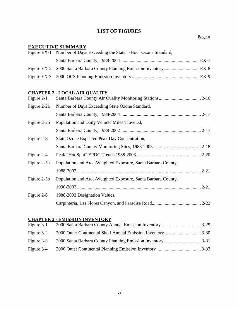
LIST OF FIGURES Page #
vi
EXECUTIVE SUMMARY Figure EX-1 Number of Days Exceeding the State 1-Hour Ozone Standard,
Santa Barbara County, 1988-2004....................................................................EX-7
Figure EX-2 2000 Santa Barbara County Planning Emission Inventory...............................EX-8
Figure EX-3 2000 OCS Planning Emission Inventory ..........................................................EX-9
CHAPTER 2 - LOCAL AIR QUALITY Figure 2-1 Santa Barbara County Air Quality Monitoring Stations.................................... 2-16
Figure 2-2a Number of Days Exceeding State Ozone Standard,
Santa Barbara County, 1988-2004..................................................................... 2-17
Figure 2-2b Population and Daily Vehicle Miles Traveled,
Santa Barbara County, 1988-2002..................................................................... 2-17
Figure 2-3 State Ozone Expected Peak Day Concentration,
Santa Barbara County Monitoring Sites, 1988-2003......................................... 2-18
Figure 2-4 Peak “Hot Spot” EPDC Trends 1988-2003 ....................................................... 2-20
Figure 2-5a Population and Area-Weighted Exposure, Santa Barbara County,
1988-2002 .......................................................................................................... 2-21
Figure 2-5b Population and Area-Weighted Exposure, Santa Barbara County,
1990-2002 .......................................................................................................... 2-21
Figure 2-6 1988-2003 Designation Values,
Carpinteria, Las Flores Canyon, and Paradise Road.......................................... 2-22
CHAPTER 3 - EMISSION INVENTORY Figure 3-1 2000 Santa Barbara County Annual Emission Inventory .................................. 3-29
Figure 3-2 2000 Outer Continental Shelf Annual Emission Inventory ............................... 3-30
Figure 3-3 2000 Santa Barbara County Planning Emission Inventory................................ 3-31
Figure 3-4 2000 Outer Continental Planning Emission Inventory ...................................... 3-32
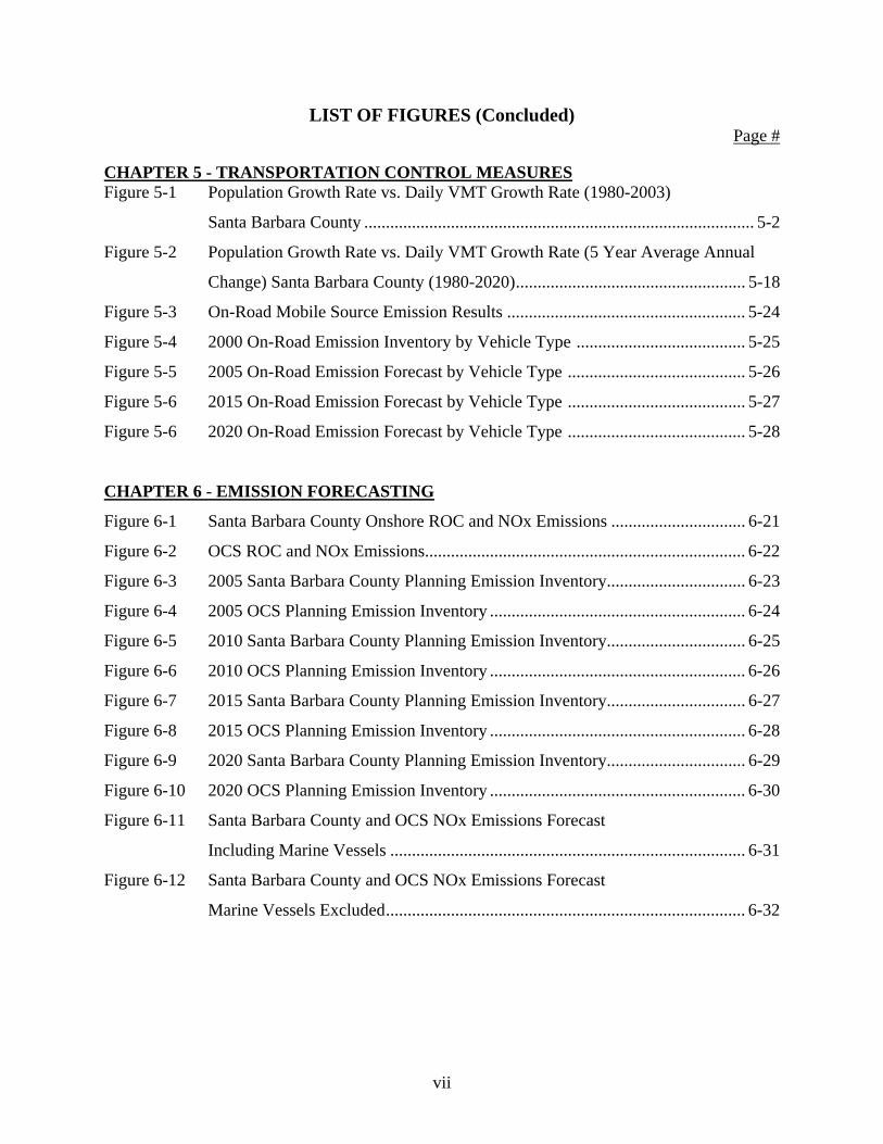
LIST OF FIGURES (Concluded) Page #
vii
CHAPTER 5 - TRANSPORTATION CONTROL MEASURES Figure 5-1 Population Growth Rate vs. Daily VMT Growth Rate (1980-2003)
Santa Barbara County .......................................................................................... 5-2
Figure 5-2 Population Growth Rate vs. Daily VMT Growth Rate (5 Year Average Annual
Change) Santa Barbara County (1980-2020)..................................................... 5-18
Figure 5-3 On-Road Mobile Source Emission Results ....................................................... 5-24
Figure 5-4 2000 On-Road Emission Inventory by Vehicle Type ....................................... 5-25
Figure 5-5 2005 On-Road Emission Forecast by Vehicle Type ......................................... 5-26
Figure 5-6 2015 On-Road Emission Forecast by Vehicle Type ......................................... 5-27
Figure 5-6 2020 On-Road Emission Forecast by Vehicle Type ......................................... 5-28
CHAPTER 6 - EMISSION FORECASTING
Figure 6-1 Santa Barbara County Onshore ROC and NOx Emissions ............................... 6-21
Figure 6-2 OCS ROC and NOx Emissions.......................................................................... 6-22
Figure 6-3 2005 Santa Barbara County Planning Emission Inventory................................ 6-23
Figure 6-4 2005 OCS Planning Emission Inventory ........................................................... 6-24
Figure 6-5 2010 Santa Barbara County Planning Emission Inventory................................ 6-25
Figure 6-6 2010 OCS Planning Emission Inventory ........................................................... 6-26
Figure 6-7 2015 Santa Barbara County Planning Emission Inventory................................ 6-27
Figure 6-8 2015 OCS Planning Emission Inventory ........................................................... 6-28
Figure 6-9 2020 Santa Barbara County Planning Emission Inventory................................ 6-29
Figure 6-10 2020 OCS Planning Emission Inventory ........................................................... 6-30
Figure 6-11 Santa Barbara County and OCS NOx Emissions Forecast
Including Marine Vessels .................................................................................. 6-31
Figure 6-12 Santa Barbara County and OCS NOx Emissions Forecast
Marine Vessels Excluded................................................................................... 6-32
EXECUTIVE SUMMARY
________________________
Introduction
Why is this 2004 Plan being prepared?
What is new in this 2004 Plan revision?
How was this 2004 Plan revision prepared?
What are the health effects of ozone?
Is air quality improving?
How is attainment of the state 1-hour ozone standard determined?
Does this 2004 Plan address any federal requirements?
What are the key state requirements that this 2004 Plan addresses?
How has the emission inventory changed?
Where does our human-generated air pollution come from?
Has the overall control strategy changed?
Does the 2004 Plan show that we will attain the state 1-hour ozone standard?
How does the adoption of this 2004 Plan impact rulemaking at APCD?
EX - 1
EXECUTIVE SUMMARY
INTRODUCTION
Air quality in Santa Barbara County continues to improve and 2004 was one of the cleanest years
on record. In fact, our air quality has improved to the point that the United States Environmental
Protection Agency (USEPA) has declared us an attainment area for the federal 1-hour ozone
standard. Meeting this milestone is clear evidence that Santa Barbara County residents are
breathing cleaner air. However, we do not yet comply with the state 1-hour ozone standard
which is more protective of public health. Therefore, this 2004 Clean Air Plan (2004 Plan) will
focus solely on the state 1-hour ozone standard and the associated planning requirements
mandated by the 1988 California Clean Air Act.
Continuing our progress toward clean air is a challenge that demands participation by the entire
community. A Clean Air Plan represents the blueprint for air quality improvement in Santa
Barbara County; the goals are to explain the complex interactions between emissions and air
quality, and to design the best possible emission control strategy in a cost-effective manner. This
2004 Plan represents a partnership among the Air Pollution Control District (APCD), the Santa
Barbara County Association of Governments (SBCAG), the California Air Resources Board
(ARB), the USEPA, local businesses, and the community at large to reduce pollution from all
sources: cars, trucks, industry, consumer products, and many more.
We have made remarkable progress in cleaning our air; the number of unhealthful air quality
days in Santa Barbara County has been reduced by more than 95 percent from 1988 to 2004
despite substantial increases in population and vehicle miles traveled. The community should be
proud of these accomplishments in reducing air pollution. This 2004 Plan reflects a commitment
to continue this progress and bring clean air to all of the residents of Santa Barbara County.
EX - 2
WHY IS THIS 2004 PLAN BEING PREPARED?
This 2004 Plan is being prepared to address California Clean Air Act mandates under Health and
Safety Code sections 40924 and 40925 that require that every three years areas update their clean air
plans to attain the state 1-hour ozone standard. More specifically, this 2004 Plan provides a three-
year update to the APCD’s 2001 Clean Air Plan. Previous plans developed to comply with the state
ozone standard include the1991 Air Quality Attainment Plan, the 1994 Clean Air Plan, and the 1998
Clean Air Plan.
WHAT IS NEW IN THIS 2004 PLAN REVISION?
Each clean air plan revision represents a snapshot in time, based on the most current information
available. This 2004 Plan is similar to the 2001 Clean Air Plan but includes significant new
information. Some key new elements are:
• Updated local air quality information (through 2004)
• An updated emission inventory (year 2000)
• An updated emission estimate of marine shipping emissions (year 2000)
• Updated future year emission estimates through 2020
• Identification of every feasible emission control measure as part of the overall
emission control strategy
HOW WAS THIS 2004 PLAN REVISION PREPARED?
APCD prepared this 2004 Plan in partnership with SBCAG, ARB, and USEPA. SBCAG provided
future growth projections, developed the transportation control measures, and estimated the on-road
mobile source emissions. ARB provided information on statewide mobile sources and consumer
product control measures. USEPA provided information on the status of the control efforts for
federally regulated sources.
EX - 3
To help provide important local policy and technical input on APCD clean air plans and rules, the
APCD Board of Directors established the Community Advisory Council. Starting in January of
2004, the CAC considered various components of this 2004 Plan at their monthly meetings. The
input provided by the Community Advisory Council was, on many occasions, directly incorporated
into this 2004 Plan. APCD staff also conducted public workshops to obtain direct public input on
the 2004 Plan.
WHAT ARE THE HEALTH EFFECTS OF OZONE?
Ozone can damage the respiratory system, causing inflammation, irritation, and symptoms such as
coughing and wheezing, and worsening of asthma symptoms. High levels of ozone are especially
harmful for children, people who exercise outdoors, older people, and people with asthma or other
respiratory problems. Ozone can harm the development of children’s lungs, and recent studies
suggest ozone plays a role in causing early childhood asthma. Ozone air pollution also hurts the
economy by increasing hospital visits and medical expenses, and loss of work time due to illness,
and by damaging crops, buildings, paint, and rubber.
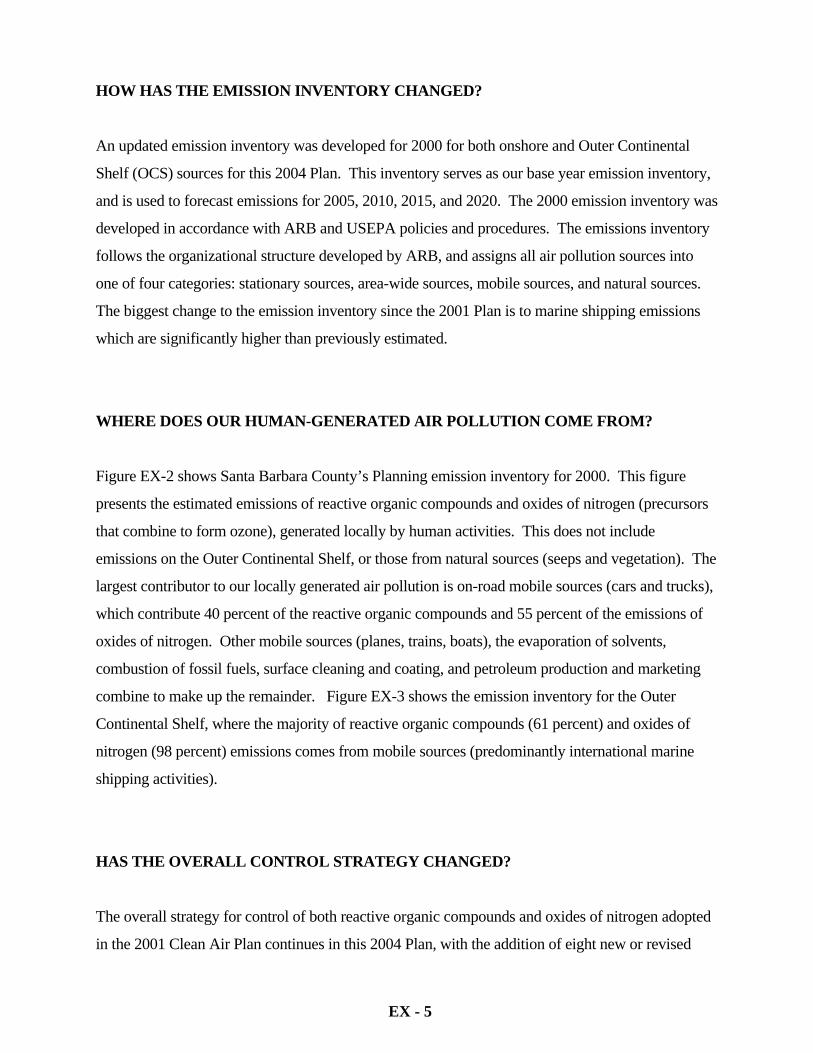
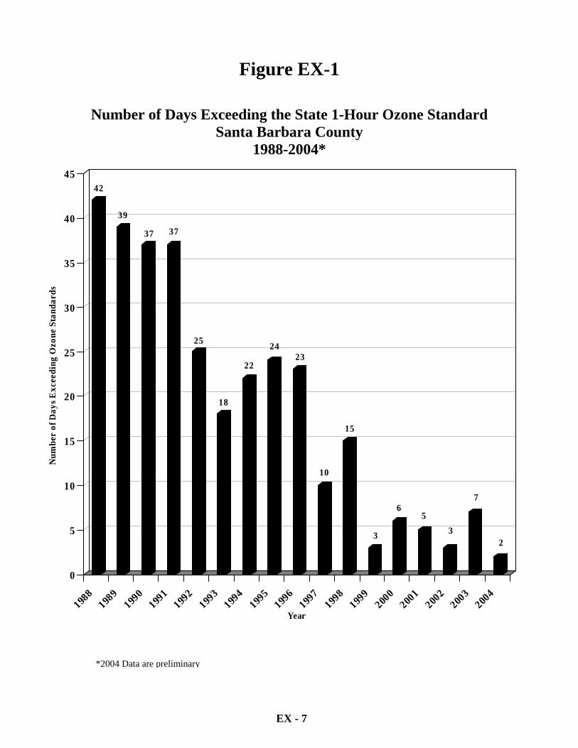
IS AIR QUALITY IMPROVING?
Figure EX-1 presents the number of state ozone exceedances in Santa Barbara County during the
period of 1988 to 2004. The most striking feature of Figure EX-1 is the dramatic decrease in the
number of state ozone exceedances since 1988, when the when the state standard was exceeded
on 42 days. In contrast, the state ozone standard was exceeded on only 2 days during 2004. A
clear declining trend in the number of state ozone exceedances is evident from 1988 through
1999. Since 1999 however, with a relatively low number of exceedances experienced in the
county, the trend is less discernable.
EX - 4
HOW IS ATTAINMENT OF THE STATE 1-HOUR OZONE STANDARD
DETERMINED?
Attainment of the state 1-hour ozone standard is determined using a statistical model developed by
the ARB that excludes extreme concentration events, which are not expected to occur more
frequently than once per year. This statistical concentration is commonly referred to as the
Expected Peak Day Concentration (EPDC). An area is considered to be in attainment of the state 1-
hour ozone standard if all monitoring stations have ozone concentrations less than 0.09 ppm, after
excluding those days with concentrations identified as extreme events.
DOES THIS 2004 PLAN ADDRESS ANY FEDERAL REQUIREMENTS?
This 2004 Plan does not address any specific federal planning requirements, as Santa Barbara
County was designated as an attainment area for the federal 1-hour ozone standard in 2003. All of
Santa Barbara County’s federal requirements are documented in the 2001 Clean Air Plan. The
USPEA has also designated the county as an attainment area for the federal 8-hour ozone standard,
although we only meet the attainment test by a very slim margin. A Clean Air Plan to implement
the new federal 8-hour standard is due by June 15, 2007, under USEPA’s Final Implementation
Rule (69 FR 23951).
WHAT ARE THE KEY STATE REQUIREMENTS THAT THIS 2004 PLAN
ADDRESSES?
The key requirements of the California Clean Air Act addressed in this 2004 Plan are the Triennial
Progress Report (H&SC Section 40924(b)) and the Triennial Plan Revision (H&SC Section
40925(a)). Additionally, this 2004 Plan must provide an annual five percent emission reduction of
ozone precursors, or, if this cannot be done, include every feasible measure as part of the emission
control strategy. Finally, state law requires this 2004 Plan to provide for attainment of the state
ambient air quality standards at the earliest practicable date (H&SC Section 40910).
EX - 5
HOW HAS THE EMISSION INVENTORY CHANGED?
An updated emission inventory was developed for 2000 for both onshore and Outer Continental
Shelf (OCS) sources for this 2004 Plan. This inventory serves as our base year emission inventory,
and is used to forecast emissions for 2005, 2010, 2015, and 2020. The 2000 emission inventory was
developed in accordance with ARB and USEPA policies and procedures. The emissions inventory
follows the organizational structure developed by ARB, and assigns all air pollution sources into
one of four categories: stationary sources, area-wide sources, mobile sources, and natural sources.
The biggest change to the emission inventory since the 2001 Plan is to marine shipping emissions
which are significantly higher than previously estimated.
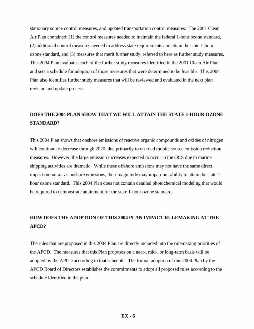
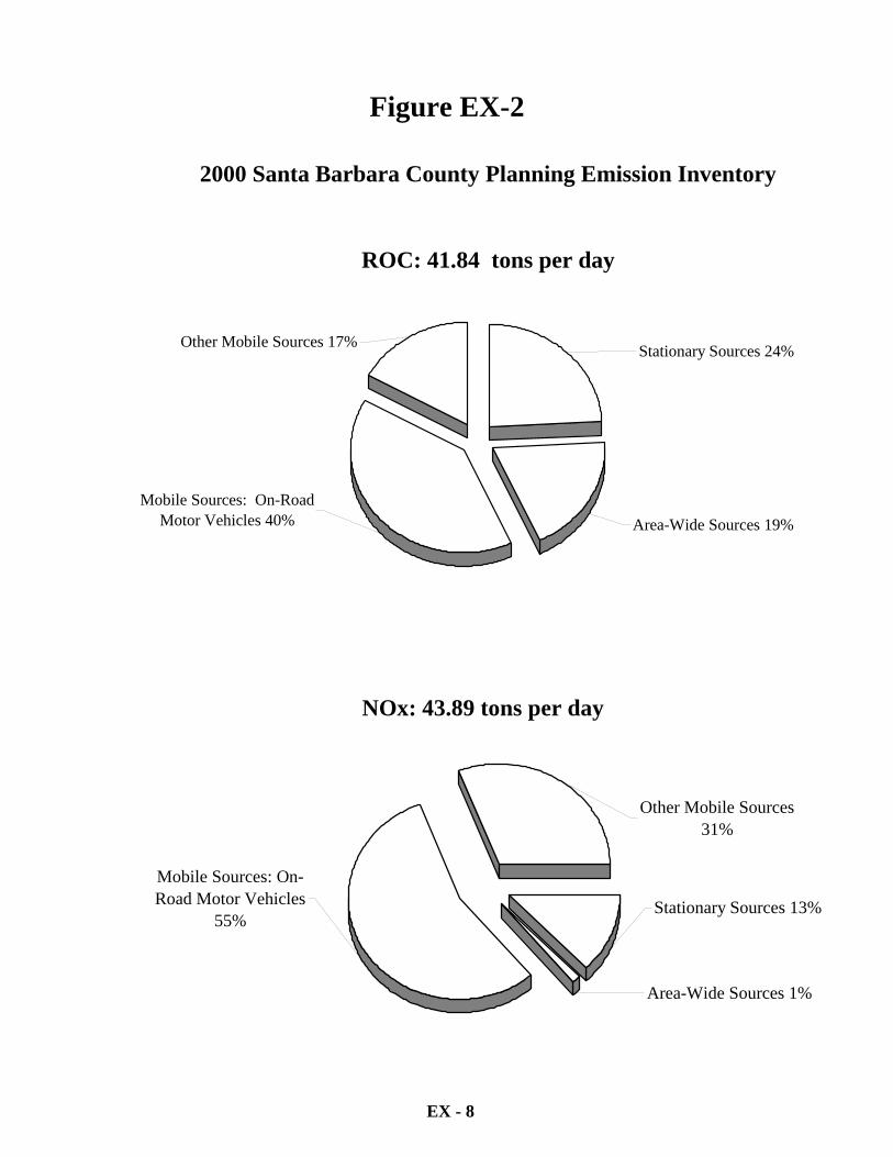
WHERE DOES OUR HUMAN-GENERATED AIR POLLUTION COME FROM?
Figure EX-2 shows Santa Barbara County’s Planning emission inventory for 2000. This figure
presents the estimated emissions of reactive organic compounds and oxides of nitrogen (precursors
that combine to form ozone), generated locally by human activities. This does not include
emissions on the Outer Continental Shelf, or those from natural sources (seeps and vegetation). The
largest contributor to our locally generated air pollution is on-road mobile sources (cars and trucks),
which contribute 40 percent of the reactive organic compounds and 55 percent of the emissions of
oxides of nitrogen. Other mobile sources (planes, trains, boats), the evaporation of solvents,
combustion of fossil fuels, surface cleaning and coating, and petroleum production and marketing
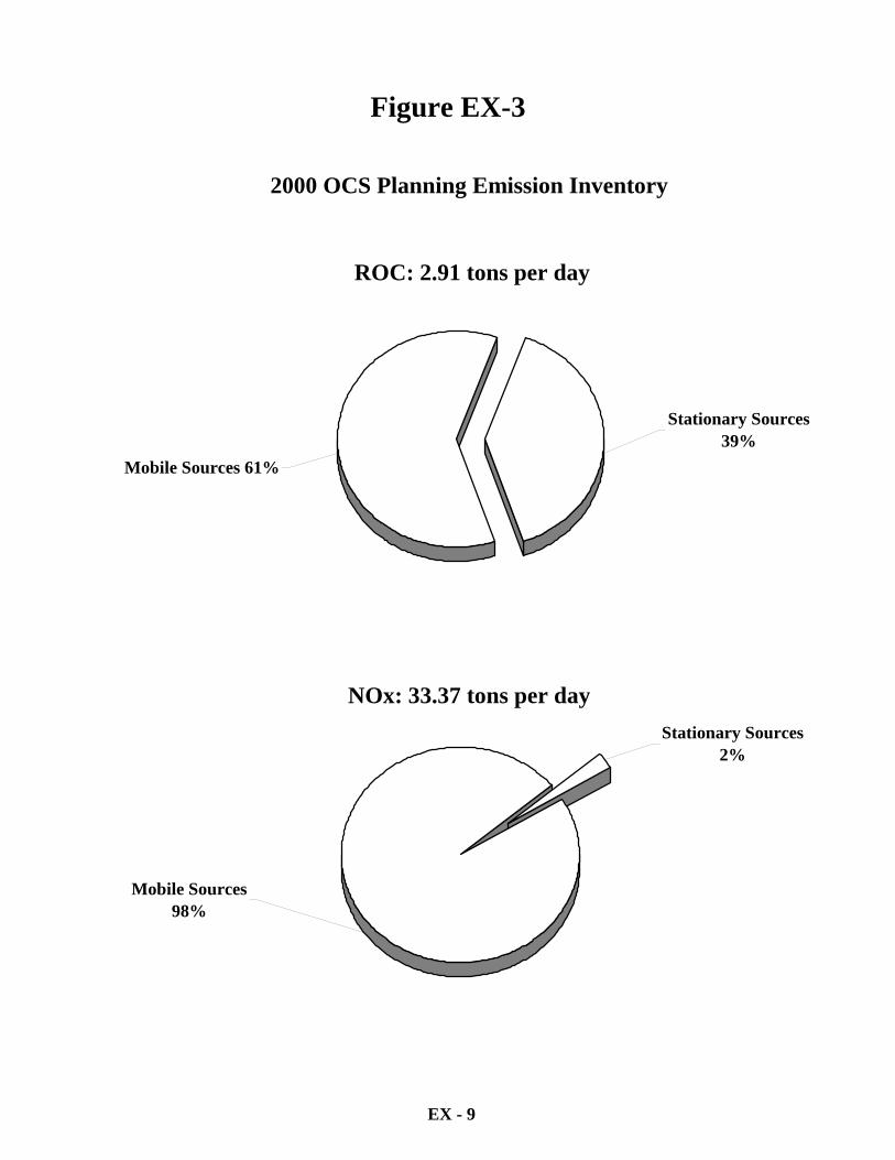
combine to make up the remainder. Figure EX-3 shows the emission inventory for the Outer
Continental Shelf, where the majority of reactive organic compounds (61 percent) and oxides of
nitrogen (98 percent) emissions comes from mobile sources (predominantly international marine
shipping activities).
HAS THE OVERALL CONTROL STRATEGY CHANGED?
The overall strategy for control of both reactive organic compounds and oxides of nitrogen adopted
in the 2001 Clean Air Plan continues in this 2004 Plan, with the addition of eight new or revised
EX - 6
stationary source control measures, and updated transportation control measures. The 2001 Clean
Air Plan contained: (1) the control measures needed to maintain the federal 1-hour ozone standard,
(2) additional control measures needed to address state requirements and attain the state 1-hour
ozone standard, and (3) measures that merit further study, referred to here as further study measures.
This 2004 Plan evaluates each of the further study measures identified in the 2001 Clean Air Plan
and sets a schedule for adoption of those measures that were determined to be feasible. This 2004
Plan also identifies further study measures that will be reviewed and evaluated in the next plan
revision and update process.
DOES THE 2004 PLAN SHOW THAT WE WILL ATTAIN THE STATE 1-HOUR OZONE
STANDARD?
This 2004 Plan shows that onshore emissions of reactive organic compounds and oxides of nitrogen
will continue to decrease through 2020, due primarily to on-road mobile source emission reduction
measures. However, the large emission increases expected to occur in the OCS due to marine
shipping activities are dramatic. While these offshore emissions may not have the same direct
impact on our air as onshore emissions, their magnitude may impair our ability to attain the state 1-
hour ozone standard. This 2004 Plan does not contain detailed photochemical modeling that would
be required to demonstrate attainment for the state 1-hour ozone standard.
HOW DOES THE ADOPTION OF THIS 2004 PLAN IMPACT RULEMAKING AT THE
APCD?
The rules that are proposed in this 2004 Plan are directly included into the rulemaking priorities of
the APCD. The measures that this Plan proposes on a near-, mid-, or long-term basis will be
adopted by the APCD according to that schedule. The formal adoption of this 2004 Plan by the
APCD Board of Directors establishes the commitments to adopt all proposed rules according to the
schedule identified in the plan.
EX - 7
42
39
37 37
25
18
22
2423
10
15
3
65
3
7
2
0
5
10
15
20
25
30
35
40
45
Num
ber
of D
ays E
xcee
ding
Ozo
ne S
tand
ards
1988
1989
1990
1991
1992
1993
1994
1995
1996
1997
1998
1999
2000
2001
2002
2003
2004
Year
Figure EX-1
Number of Days Exceeding the State 1-Hour Ozone Standard Santa Barbara County
1988-2004*
*2004 Data are preliminary
EX - 8
NOx: 43.89 tons per day
Stationary Sources 13%
Area-Wide Sources 1%
Mobile Sources: On-Road Motor Vehicles
55%
Other Mobile Sources31%
Figure EX-2
2000 Santa Barbara County Planning Emission Inventory
ROC: 41.84 tons per day
Stationary Sources 24%
Mobile Sources: On-Road Motor Vehicles 40%
Other Mobile Sources 17%
Area-Wide Sources 19%
EX - 9
2000 OCS Planning Emission Inventory
ROC: 2.91 tons per day
Stationary Sources39%
Mobile Sources 61%
NOx: 33.37 tons per day
Mobile Sources98%
Stationary Sources2%
Figure EX-3
CHAPTER 1
_____________________
INTRODUCTION
Purpose
Current State Planning Requirements
Summary of Attainment Planning Efforts
Plan Organization
1 - 1
1. INTRODUCTION
1.1 PURPOSE
The purpose of this 2004 Clean Air Plan (2004 Plan) is to chart a course of action that will ensure
clean, healthful air for the residents and environment of Santa Barbara County. Clean air is
fundamental to good public health; it enhances the environment and contributes to the attractiveness
of the area to residents, businesses, and visitors. Fortunately, our air quality has been improving
through the implementation of several air quality plans. These plans have been developed for Santa
Barbara County as required by both the 1988 California Clean Air Act (State Act) and the 1990
Federal Clean Air Act Amendments (Federal Act).
Santa Barbara County's air quality has historically violated both the state and federal ozone
standards. Ozone concentrations above these standards adversely affect public health, diminish the
production and quality of many agricultural crops, reduce visibility, and damage native and
ornamental vegetation. Since 1999, however, local air quality data show that every monitoring
location in Santa Barbara County complies with the federal 1-hour ambient air quality standard for
ozone. And on August 8, 2003, Santa Barbara County officially became an attainment area for the
federal 1-hour ozone standard.
While Santa Barbara County’s air quality has improved enough to be considered in attainment for
the federal 1-hour ozone standard, we do not yet comply with the more health protective state 1-
hour ozone standard. Therefore, this 2004 Plan will focus solely on the state 1-hour ozone standard
and the associated planning requirements mandated by the State Act.
1.2 CURRENT STATE PLANNING REQUIREMENTS
The California Clean Air Act requires that we report our progress in meeting state mandates and
revise our 1991 Air Quality Attainment Plan (1991 AQAP) to reflect changing conditions on a
triennial basis. There are two major items required to be in the triennial update (Sections 40924 and
1 - 2
40925 of the California Health and Safety Code): a Triennial Progress Report and a Triennial Plan
Revision. The Triennial Progress Report must assess the overall effectiveness of an air quality
program and the extent of air quality improvement resulting from the Plan. The Triennial Plan
Revision must correct for deficiencies in meeting the interim measures of progress and incorporate
new data or projections into the Plan.
The control strategy originally presented in the 1991 AQAP failed to produce the state mandated
five percent per year emission reductions, so the Plan was approved under the every feasible
measure option. The evaluation of every feasible measure was conducted for subsequent plans
developed in 1994, 1998, and 2001 and will be re-evaluated in this 2004 Plan. In addition to the
requirements that the State Act mandates for Santa Barbara County as a nonattainment area for the
state 1-hour ozone standard, we are also responsible for the impacts our air pollution has on areas
downwind of us. The State Act mandates that ARB identify air basins (or portions thereof) in
which transported air pollutants cause or contribute to violations of the state 1-hour ozone standard
in downwind areas and establish mitigation requirements commensurate with the level of
contribution.
This 2004 Plan examines the emission reductions achieved from existing and proposed regulations
with respect to every feasible measure and identifies measures for further study. It also examines
the change in emissions related to changes in population, industrial activity, vehicle use, and
provides updated emission inventories out to 2020. Finally, this plan evaluates local air quality
indictors and the impact of our local air pollution on areas downwind of us.
1.3 SUMMARY OF ATTAINMENT PLANNING EFFORTS
Several prior air quality plans have been prepared for Santa Barbara County. The first clean air plan
for Santa Barbara County was the 1979 Air Quality Attainment Plan (1979 AQAP) which was
updated in 1982. These two plans were prepared in response to mandates established by the Federal
Clean Air Act Amendments of 1977. At that time only the southern portion of the county, the
region south of the Santa Ynez Mountains, violated the federal 1-hour ozone standard. The 1982
1 - 3
update predicted attainment of the federal ozone standard by 1984, but acknowledged that the
county’s ability to attain the federal ozone standard was uncertain because pollution generated on
the OCS was not considered in the Plan.
The predicted attainment of the federal ozone standard did not occur. As a consequence, the
USEPA called for an update to the 1982 Air Quality Attainment Plan on March 17, 1986. On May
26, 1988, the USEPA issued a subsequent mandate that our planning efforts address air quality for
the entire county. This new mandate was issued in response to the failure of many regions of the
country to attain the federal 1-hour ozone standard by 1987. In response, the APCD prepared the
1989 Air Quality Attainment Plan (1989 AQAP), which was adopted by the APCD Board of
Directors in June of 1990 and was designed to bring the southern portion of the county into
attainment with the federal 1-hour ozone standard.
The APCD also prepared a 1991 Air Quality Attainment Plan (1991 AQAP). This plan was
required by the State Act to bring the entire county into attainment of the more health protective
California ozone standard. The APCD Board of Directors adopted the 1991 AQAP in December
1991 and ARB approved it in August 1992.
In 1990, Congress amended the federal Clean Air Act (Federal Act). The Federal Act required
Santa Barbara County, as a “moderate” nonattainment area, to submit a Rate-of-Progress Plan to the
USEPA by November 15, 1993, and an attainment demonstration by November 15, 1994. The
1994 Clean Air Plan (1994 CAP) that contained these required elements was adopted by the APCD
Board of Directors and formally submitted to the USEPA on November 15, 1994. The 1994 CAP
included: amendments to the 1993 Rate-of-Progress (1993 ROP) Plan; an attainment demonstration
of the federal ozone standard by 1996; a request for redesignation from a nonattainment area to an
attainment area for the federal ozone standard; and a plan to show maintenance of the federal ozone
standard through the year 2006. The 1994 CAP also provided a three-year update to the 1991
AQAP for the state ozone standard, as required by the State Act.
On January 8, 1997, the USEPA approved several elements of the 1994 CAP, including the
amendments to the 1993 Rate-of-Progress Plan, the base year emission inventory, and the control
1 - 4
strategy. USEPA did not approve the attainment demonstration element due to violations of the
federal 1-hour standard that occurred during 1994-1996. This element was withdrawn from the
1994 CAP submittal. Similarly, the USEPA never acted upon the maintenance plan element due to
the measured violations of the federal 1-hour ozone standard.
On December 10, 1997, the USEPA issued a final action finding that Santa Barbara County had not
attained the federal 1-hour ozone standard by the statutory attainment date for “moderate”
nonattainment areas of November 15, 1996. As a result, the entire Santa Barbara County
nonattainment area was reclassified as a “serious” nonattainment area by operation of federal law.
The USEPA action mandated that we continue progress toward the federal 1-hour ozone standard
through the development of a revised Clean Air Plan. The 1998 CAP was adopted by the APCD
Board of Directors on December 17, 1998, and forwarded by the ARB to the USEPA on March 19,
1999. The 1998 CAP addressed all the new federal planning requirements for “serious”
nonattainment areas and was approved by the USEPA on August 14, 2000. The 1998 CAP also
addressed the triennial plan revision and progress report requirements under the State Act.
Since 1999, local air quality data collected in Santa Barbara County showed that we had achieved
the federal 1-hour ozone standard. Achieving this milestone allowed us to request USEPA to
designate the county as an attainment area for this standard. The 2001 CAP was adopted by the
APCD Board of Directors on November 15, 2001 and subsequently amended on December 19,
2002. The 2001 CAP addressed all federal planning requirements for “maintenance plans” and
provided for ongoing attainment of the federal 1-hour ozone standard through the year 2015. The
plan was forwarded by the ARB to USEPA on February 21, 2002, formally approved by USEPA on
July 9, 2003, and became effective on August 8, 2003 with Santa Barbara County being officially
designated as an attainment area. The 2001 Plan also addressed the state triennial plan revision and
progress report requirements under the State Act.
A summary of Santa Barbara County’s planning activities that addressed state mandates is
presented in Table 1-1 beginning with the 1991 AQAP.
1 - 5
1.4 PLAN ORGANIZATION
Chapter 2, Local Air Quality, provides a summary of Santa Barbara County’s climatology, air
quality trends, and discusses the status of ARB’s re-assessment of our transport contributions to
neighboring air districts.
Chapter 3, Emission Inventory, establishes an emissions inventory for Santa Barbara County by
quantifying the emissions of reactive organic compounds and oxides of nitrogen for the year 2000.
This emission inventory is tailored to meet state requirements.
Chapter 4, Emission Control Measures, provides an overview of the APCD’s control measures in
relation to the “every feasible measure” requirement of the State Act. This chapter identifies the
status of each control measure in relation to state requirements.
Chapter 5, Transportation Control Measures, describes all transportation-related control measures,
and identifies their applicability to state requirements.
Chapter 6, Emission Forecasting, details the forecast procedures used to develop future year
emission inventories for 2005, 2010, 2015, and 2020.
Chapter 7, Public Participation, summarizes all public input received during the development of this
2004 Plan.
1 - 6
REFERENCES
California Health and Safety Code: 2004 Edition.
United States Public Law 101-549, Nov. 15, 1990 104 Stat.2399.
U.S. Environmental Protection Agency: Clean Air Act Reclassification; California Santa Barbara
Nonattainment Area; Ozone. December 10, 1997 (62 FR 65025-65030).
U.S. Environmental Protection Agency: Approval and Promulgation of State Implementation Plans;
California -- Santa Barbara. August 14, 2000 (65 FR 49499-49501).
U.S. Environmental Protection Agency: Approval and Promulgation of State Implementation Plans
and Designation of Areas for Air Quality Planning Purposes; 1-hour Ozone Standard for Santa
Barbara, CA. July 9, 2003 (68 FR 40789-40791).
1 - 7
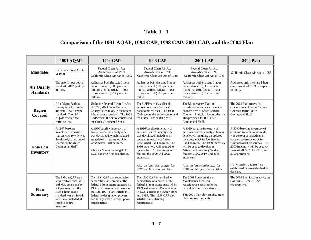
Table 1 - 1
Comparison of the 1991 AQAP, 1994 CAP, 1998 CAP, 2001 CAP, and the 2004 Plan
1991 AQAP 1994 CAP 1998 CAP 2001 CAP 2004 Plan
Mandates California Clean Air Act of 1988
Federal Clean Air Act Amendments of 1990
California Clean Air Act of 1988.
Federal Clean Air Act Amendments of 1990
California Clean Air Act of 1988
Federal Clean Air Act Amendments of 1990
California Clean Air Act of 1988 California Clean Air Act of 1988
Air Quality Standards
The state 1-hour ozone standard is 0.09 parts per million.
Addresses both the state 1-hour ozone standard (0.09 parts per million) and the federal 1-hour ozone standard (0.12 parts per million).
Addresses both the state 1-hour ozone standard (0.09 parts per million) and the federal 1-hour ozone standard (0.12 parts per million).
Addresses both the state 1-hour ozone standard (0.09 parts per million) and the federal 1-hour ozone standard (0.12 parts per million).
Addresses only the state 1-hour ozone standard (0.09 parts per million).
Region Covered
All of Santa Barbara County failed to attain the state 1-hour ozone standard. The 1991 AQAP covered the entire county.
Under the Federal Clean Air Act of 1990, all of Santa Barbara County failed to attain the federal 1-hour ozone standard. The 1994 CAP covers the entire county and the Outer Continental Shelf.
The USEPA re-classified the entire county as a “serious” nonattainment area. The 1998 CAP covers the entire county and the Outer Continental Shelf.
The Maintenance Plan and redesignation request covers the onshore area of Santa Barbara County. Emission Inventories are also provided for the Outer Continental Shelf.
The 2004 Plan covers the onshore area of Santa Barbara County and the Outer Continental Shelf.
Emission Inventory
A 1987 baseline inventory of emission sources countywide was developed, but excluded sources in the Outer Continental Shelf.
A 1990 baseline inventory of emission sources countywide was developed, which included an updated inventory of Outer Continental Shelf sources. Also, an "emission budget" for ROG and NOx was established.
A 1996 baseline inventory of emission sources countywide was developed, including an updated inventory of Outer Continental Shelf sources. The 1996 inventory will be used to update the 1990 emissions and to forecast the 1999 and 2005 emissions. Also, an "emission budget" for ROG and NOx was established.
A 1999 baseline inventory of emission sources countywide was developed, including an updated inventory of Outer Continental Shelf sources. The 1999 inventory will be used to develop an “attainment inventory” and to forecast 2005, 2010, and 2015 emissions. Also, an "emission budget" for ROG and NOx are re-established.
A 2000 baseline inventory of emission sources countywide was developed including an updated inventory of Outer Continental Shelf sources. The 2000 inventory will be used to forecast 2005, 2010, 2015, and 2020 emissions.
No “emission budgets” are established or re-established in the plan.
Plan Summary
The 1991 AQAP was required to reduce ROG and NOx emissions by 5% per year until the state 1-hour ozone standard was achieved, or to have included all feasible control measures.
The 1994 CAP was required to demonstrate attainment of the federal 1-hour ozone standard by 1996; document amendments to the 1993 ROP Plan; initiate the federal re-designation process; and satisfy state triennial update requirements.
The 1998 CAP is required to demonstrate attainment of the federal 1-hour ozone standard by 1999 and show a 24% reduction in ROG emissions between 1990 and 1999. This 1998 CAP also satisfies state planning requirements.
The 2001 Plan contains a Maintenance Plan and redesignation request for the federal 1-hour ozone standard.
This 2001 Plan also satisfies state planning requirements.
The 2004 Plan focuses solely on California Clean Air Act requirements.
CHAPTER 2
LOCAL AIR QUALITY
Introduction
Climate of Santa Barbara County
Air Quality Monitoring
State Ozone Exceedances
Air Quality Indicators
Designation Value
Transport Impacts
Conclusions
2-1
2. LOCAL AIR QUALITY
2.1 INTRODUCTION
This chapter provides the background for this 2004 Plan by presenting an overview of the
climate of Santa Barbara County, an assessment of local air quality trends using ARB-specified
indicators and a discussion of the impacts our air quality has on neighboring air districts. The
description of the climate of Santa Barbara County is important for understanding the factors
that influence air quality in the county, while the air quality indicator data are important for
assessing progress towards attainment of state ozone standards. The discussion on air pollution
transport summarizes the status of the California Air Resources Board (ARB) efforts to re-
assess the impacts that our air quality has on neighboring air districts.
The next section of this chapter, Section 2.2, discusses the local climate of Santa Barbara
County and the relationship of the climate to air quality. Santa Barbara County’s air quality
monitoring network is described in Section 2.3. A summary of state ozone exceedances
experienced in the county from 1988 through 2003 are highlighted in Section 2.4 while Section
2.5 summarizes air quality trends using air quality indicators. Section 2.6 discusses the State
Designation Value and its relation to the air quality indicators. Section 2.7 details air quality
transport and the ARB assessment of the potential impacts of the transport of emissions
generated in Santa Barbara County. Finally, Section 2.8 highlights the conclusions of this
chapter. For clarity, all tables and figures associated with this chapter will appear after the
conclusions.
2.2 CLIMATE OF SANTA BARBARA COUNTY
Santa Barbara County’s air quality is influenced by both local topography and meteorological
conditions. Surface and upper-level wind flow varies both seasonally and geographically in the
county and inversion conditions common to the area can affect the vertical mixing and
2-2
dispersion of pollutants. The prevailing wind flow patterns in the county are not necessarily
those that cause high ozone values. In fact, high ozone values are often associated with atypical
wind flow patterns. Meteorological and topographical influences that are important to air
quality in Santa Barbara County are as follows:
• Semi-permanent high pressure that lies off the Pacific Coast leads to limited rainfall
(around 18 inches per year), with warm, dry summers and relatively damp winters.
Maximum summer temperatures average about 70 degrees Fahrenheit near the coast and
in the high 80s to 90s inland. During winter, average minimum temperatures range from
the 40s along the coast to the 30s inland. Additionally, cool, humid, marine air causes
frequent fog and low clouds along the coast, generally during the night and morning
hours in the late spring and early summer. The fog and low clouds can persist for
several days until broken up by a change in the weather pattern.
• In the northern portion of the county (north of the ridgeline of the Santa Ynez
Mountains), the sea breeze (from sea to land) is typically northwesterly throughout the
year while the prevailing sea breeze in the southern portion of the county is from the
southwest. During summer, these winds are stronger and persist later into the night. At
night, the sea breeze weakens and is replaced by light land breezes (from land to sea).
The alternation of the land-sea breeze cycle can sometimes produce a "sloshing" effect,
where pollutants are swept offshore at night and subsequently carried back onshore
during the day. This effect is exacerbated during periods when wind speeds are low.
• The terrain around Point Conception, combined with the change in orientation of the
coastline from north-south to east-west can cause counterclockwise circulation (eddies)
to form east of the Point. These eddies fluctuate temporally and spatially, often leading
to highly variable winds along the southern coastal strip. Point Conception also marks
the change in the prevailing surface winds from northwesterly to southwesterly.
• Santa Ana winds are northeasterly winds that occur primarily during fall and winter, but
occasionally in spring. These are warm, dry winds blown from the high inland desert
2-3
that descend down the slopes of a mountain range. Wind speeds associated with Santa
Ana’s are generally 15-20 mph, though they can sometimes reach speeds in excess of 60
mph. During Santa Ana conditions, pollutants emitted in Santa Barbara, Ventura
County, and the South Coast Air Basin (the Los Angeles region) are moved out to sea.
These pollutants can then be moved back onshore into Santa Barbara County in what is
called a "post-Santa Ana condition." The effects of the post-Santa Ana condition can be
experienced throughout the county. Not all post-Santa Ana conditions, however, lead
to high pollutant concentrations in Santa Barbara County.
• Upper-level winds (measured at Vandenberg Air Force Base once each morning and
afternoon) are generally from the north or northwest throughout the year, but
occurrences of southerly and easterly winds do occur in winter, especially during the
morning. Upper-level winds from the south and east are infrequent during the summer.
When they do occur, they are usually associated with periods of high ozone levels.
Surface and upper-level winds can move pollutants that originate in other areas into the
county.
• Surface temperature inversions (0-500 ft) are most frequent during the winter, and
subsidence inversions (1000-2000 ft) are most frequent during the summer. Inversions
are an increase in temperature with height and are directly related to the stability of the
atmosphere. Inversions act as a cap to the pollutants that are emitted below or within
them and ozone concentrations are often higher directly below the base of elevated
inversions than they are at the earth’s surface. For this reason, elevated monitoring sites
will occasionally record higher ozone concentrations than sites at lower elevations.
Generally, the lower the inversion base height and the greater the rate of temperature
increase from the base to the top, the more pronounced effect the inversion will have on
inhibiting vertical dispersion. The subsidence inversion is very common during summer
along the California coast, and is one of the principal causes of air stagnation.
• Poor air quality is usually associated with "air stagnation" (high stability/restricted air
movement). Therefore, it is reasonable to expect a higher frequency of pollution events
2-4
in the southern portion of the county where light winds are frequently observed, as
opposed to the northern part of the county where the prevailing winds are usually strong
and persistent.
2.3 AIR QUALITY MONITORING
Both the federal and state Clean Air Acts identify pollutants of specific importance, which are
known as criteria pollutants. Ambient air quality standards are adopted by the ARB and the
USEPA to protect public health, vegetation, materials and visibility (Table 2-1). State standards
for ozone and both respirable (less than 10 microns -PM10) and fine (less than 2.5 microns –
PM2.5) particles are more stringent than federal standards.
Monitoring of ambient air pollutant concentrations is conducted by the ARB, APCD and
industry. Monitors operated by the ARB and APCD are part of the State and Local Air
Monitoring System (SLAMS). The SLAMS stations are located to provide local and regional
air quality information. Monitors operated by industry, at the direction of the APCD, are called
Prevention of Significant Deterioration (PSD) stations. PSD stations are required by the APCD
to ensure that new and modified sources under APCD permit do not interfere with the county’s
ability to attain or maintain air quality standards. Figure 2-1 shows the locations of all
monitoring stations in Santa Barbara County that are currently in operation.
2.4 STATE OZONE EXCEEDANCES
Figure 2-2a presents the number of state ozone exceedances in Santa Barbara County during
the period of 1988 to 2004. As shown in the figure, Santa Barbara County has experienced
between 2 and 42 days per year on which the state ozone standard was exceeded in the
county.
2-5
The most striking feature of Figure 2-2a is the dramatic decrease in the number of state ozone
exceedances since 1988, when the county experienced 42 days where the state standard was
exceeded. In contrast, there were only two days where the state ozone standard was
exceeded during 2004. A clear declining trend in the number of state ozone exceedances is
evident from 1988 through 1999. Since 1999, with the relatively low number of state 1-hour
ozone exceedances experienced in Santa Barbara County, the trend is less discernable.
The long-term declining trend in exceedance days has occurred concurrently with increases
in both population and daily vehicle miles traveled in Santa Barbara County (Figure 2-2b).
This shows that local, state and federal emission reduction programs have been effective in
improving air quality in Santa Barbara County despite significant increases in population and
vehicle miles traveled.
2.5 AIR QUALITY INDICATORS
The California Clean Air Act (CCAA) requires the ARB to evaluate and identify three air
quality related indicators for districts to use in assessing their progress toward attainment of
the State standards [Health and Safety Code section 39607(f)]. Districts are required to
assess their progress triennially and report to the ARB as part of the triennial plan revisions.
The assessment must address (1) the peak concentrations in the peak “hot spot” sub-area, (2)
the population-weighted average of the total exposure, and (3) the area-weighted average of
the total exposure (ARB Resolution 90-96, November 8, 1990).
2.5.1 Peak Concentration Indicators
As mentioned above, the ARB specifies the use of three air quality indicators to assess progress
toward attaining the state 1-hour ozone standard: peak “hot spot” indicator, population-weighted
exposure, and area-weighted exposure. These data were provided to us by the ARB on August
28, 2003, with the recommendation that we report improvement in air quality using the
2-6
Expected Peak Day Concentration (EPDC), and two exposure indicators (population-weighted
and area-weighted). 2003 exposure data are currently not available for trend analyses.
The peak “hot spot” indicator is assessed in terms of the EPDC. The EPDC is provided to
districts by the ARB for each monitoring site in the county and represents the maximum ozone
concentration expected to occur once per year, on average. The EPDC is useful for tracking air
quality progress at individual monitoring stations since it is relatively stable, thereby providing a
trend indicator that is not highly influenced by year-to-year changes in weather. Simply,
progress means the change or improvement in air quality over time that can be attributed to a
reduction in emissions rather than the influence of other factors, such as variable weather. The
EPDC is also used in the area designation process, which is described in Section 2.6.
The EPDC is calculated using ozone data for a three-year period (the summary year and the two
years proceeding the summary year). For example, the 2002 EPDC for a monitoring site uses
data from 2000, 2001 and 2002. The data that are used in the calculation are the daily
maximum one-hour concentrations. The EPDC is calculated using a complex statistical
procedure that analytically determines for each monitoring site the concentration that is
expected to recur at a rate of once per year.
Figure 2-3 presents 1988 through 2003 peak air quality indicators for monitoring sites in Santa
Barbara County. Note that data collection on Santa Rosa Island did not begin until 1996, thus
EPDC indicator data for that site does not start until 1998. Additionally, Santa Barbara data
terminate in 2000 since the station was offline for several months during 2001, but came back
online at the beginning of 2003. West Campus data end in 1998 when ozone data collected
terminated at that site.
Figure 2-3 shows that peak air quality indicators have declined significantly from 1988 levels at
all monitoring stations. 1999 EPDC values (based on 1997, 1998 and 1999 ozone data) fell
below the State standard at the GTC-B, Santa Ynez, El Capitan, Goleta, Lompoc HS&P and
Santa Barbara sites. The Carpinteria EPDC indicator dropped below the State ozone standard
in 2002 from earlier levels that were significantly above the standard. Additionally, the peak
2-7
indicators for the Las Flores Canyon, site fell below the state standard in 2003. The Paradise
Road monitoring site, while showing considerable improvement from earlier years, had an
EPDC values that remained above the standard during 2003.
As discussed previously, the ARB requires that district’s assess the peak “hot spot” subareas as
one method of determining progress toward meeting State air quality standards. Since 1988,
both the Paradise Road and Las Flores Canyon monitoring sites have experienced the most State
ozone exceedances in the county, and therefore can be considered hot spot locations (see Table
2-2). The Las Flores Canyon monitoring site had a maximum of 24 exceedances in 1990 with
no exceedances during 2002, while the number of State exceedances at the Paradise Road site
has ranged from 24 in 1988 to zero exceedances during 2000.
The EPDC indicators have improved significantly from earlier levels at both the Las Flores
Canyon and Paradise Road sites. The EPDC indicator was as high as 0.140 ppm during 1989
and 1990 at the Las Flores Canyon site decreasing to 0.092 ppm during 2003. At the Paradise
Road site, the peak indicator was as high as 0.125 ppm in 1989 and 1991, decreasing to 0.105
ppm by 2003. Figure 2-4 presents the overall EPDC trend improvement for both the Las Flores
Canyon and Paradise Road sites from 1988 to 2003. Based on the trendline, the overall EPDC
improvement for the Las Flores Canyon site from 1989 to 2003 is about 35%. The Paradise
Road EPDC trend improvement is about 20% for the period of 1988 to 2003.
In addition to assessing the longer-term trends, the ARB recommends that districts evaluate
changes in the EPDC indicator for the most recent three years of data and report any
improvement for those years. Between 2000 and 2003, the EPDC for the Las Flores Canyon
site decreased from 0.102 to 0.092 ppm, which translates to an improvement of about 7%. The
Paradise Road site EPDC dropped from 0.103 ppm to 0.100 ppm between 2000 and 2001 then
increased back to 0.105 during 2003. Peak indicators at other monitoring sites in Santa Barbara
County have also generally decreased between 2000 and 2002, although the El Capitan site
EPCD increased from 0.082 ppm to 0.086 ppm between 2000 and 2001 then decreased to 0.084
ppm in 2002.
2-8
The reduction in EPDC indicator data show that Santa Barbara County’s air quality has
improved significantly over the long-term. There have also been continued improvements at
several of the monitoring sites in the county, although the overall trend of countywide
exceedances has been less distinct over the last few years. Air quality improvement has led to
the reduction in the number of State ozone exceedances from 42 days in 1988 to as few as two
days in 2004.
2.5.2 Population and Area Exposure Indicators
Population and area exposure indicators are intended to provide an indication of the potential for
chronic adverse health impacts. Unlike the EPDC that tracks air quality progress at individual
monitoring sites, the population- and area-weighted exposure indicators consolidate hourly
ozone monitoring data from all sites within the county into a single exposure value. The result
is a value representing the average potential exposure in an area.
The population exposure indicator is based on the annual number of hours that ozone levels
were above the state standard. The exposure values are allocated to population on the basis of
census tracts and the distance of the various tracts to the air monitoring stations. The
population-weighted exposure indicators represent a composite of exposures at individual
locations that have been weighted to emphasize equally the potential exposure for each
individual in an area.
The area-weighted exposure value is similar to the population exposure except that it is based on
the area within each census tract rather than the population in each tract. The area-weighted
exposure indicator represents a composite of exposures at individual locations that have been
weighted to emphasize equally the potential exposure in all portions of the county.
Population- and area-weighted trends are presented in Figure 2-5a and 2-5b. These figures
show that both exposure indicators have decreased over time since 1988 (with the exception of
1989) and that indicator values have been very low during the last few years due to dramatic
improvement in air quality. It should be noted that high values during 1989, shown as spikes in
2-9
the trend data, are due to two specific ozone episodes in March and April of that year where
ozone concentrations were significantly higher than both federal and state standards. Due to
spikes in the data during 1989, exposure trend data for 1990 to 2000 are presented in a separate
figure (Figure 2-5b) with a more suitable scale to better display trends during that period.
These trends in the population- and area-weighted exposure data suggest that even with
population growth and natural fluctuations in weather, air quality has improved significantly
since 1988.
2.6 DESIGNATION VALUE
Designation values (DV) are used to determine whether an area is in or out of attainment of
applicable air quality standards. The designation value refers to the highest measured
concentration remaining at a given site after all measured concentrations affected by extreme
concentration events are excluded. In the area designation process, measured concentrations
that are higher than the calculated EPDC are identified as being affected by an extreme
concentration event (weather conditions conducive to high concentrations of ozone) and are not
considered violations of the State standard. If the highest designation value within an area does
not exceed the State standard, then the area can be considered in attainment for that pollutant.
For example, if the calculated EPDC for a site is 0.096 parts per million (ppm) and the four
highest measured ozone concentrations are 0.125, 0.113, 0.102 and 0.094 ppm, then the
designation value is equal to 0.10 ppm.. This is because the EPDC of 0.096 is first rounded to
0.10 to be consistent with the precision of the State standard, which is two decimal places, and
0.10 is the highest concentration measured (0.102 rounds down to 0.10) that is equal to or lower
than the rounded EPDC. The concentrations of 0.125 ppm (rounded to 0.13 ppm) and 0.113
ppm (rounded to 0.11 ppm) are higher than the rounded EPDC of 0.10 and are excluded as an
extreme concentrations and are not considered as the DV.
DV data for the period of 1988-2003 for Las Flores Canyon, Carpinteria and Paradise Road,
sites historically measuring the most ozone exceedances, are presented in Figure 2-6. Based on
2-10
these data, only the Paradise Road site remained out of compliance with the State ozone
standard during 2003.
2.7 TRANSPORT IMPACTS The State Act gives ARB the responsibility to assess the movement of air pollutants from one
air basin to another (referred to as “transport”) and the relative impacts on ozone
concentrations. The ARB must also establish mitigation requirements commensurate with
the level of contribution an upwind area has on a downwind area. While Section 2.2
discussed the impacts of pollution transported from the South Coast Air Basin on Santa
Barbara County, this section summarizes the status of ARB’s efforts to re-assess the impacts
that our air quality has on neighboring air districts.
The ARB staff assesses transport impacts by first identifying “transport couples” that consist
of an upwind area and a corresponding downwind area. These areas are generally defined
using air basin boundaries or portions thereof. Areas with similar geographic and weather
conditions are within the same air basin. Santa Barbara County is part of the South Central
Coast Air Basin, which also includes San Luis Obispo County and Ventura County. The
greater Los Angeles area is in the South Coast Air Basin. In addition to identifying upwind
and downwind relationships between air basins, the ARB is required to assess the degree of
impact. State law directs the ARB to determine if the contribution of transported pollution is
overwhelming, significant, inconsequential, or some combination.
The ARB determined through modeling of ozone episodes that occurred in the mid-1980’s
that under some conditions emissions generated in the South Central Coast Air Basin can
contribute to ozone exceedances occurring in the South Coast Air Basin. This led the ARB
to classify the South Central Coast Air Basin (excluding San Luis Obispo) as both a
significant and an inconsequential contributor to South Coast Air Basin ozone exceedances.
2-11
Recently, the ARB performed analyses of state ozone exceedances in the northwestern
portion of the South Coast Air Basin to determine whether emissions from the South Central
Coast Air Basin, particularly emissions generated in Santa Barbara and Ventura Counties,
continue to contribute to exceedances in the South Coast Air Basin. The ARB examined all
exceedances that occurred between 2000 and 2003 at monitoring sites located in Reseda and
Santa Clarita, northwest of downtown Los Angeles. In all, there were 263 State 1-hour
ozone exceedances between these two sites. Due to the large number of exceedance days, it
was not possible for the ARB to do an in-depth analysis of each day. Therefore, the ARB
used a screening approach to identify days that had the potential for transport from the Santa
Barbara area to the eastern South Coast Air Basin.
The ARB utilized two methods to screen potential Santa Barbara County to Reseda/Santa
Clarita transport days, and then applied a trajectory model to those days where screening
showed a potential for transport. The first method for screening exceedances was the
evaluation of weather conditions to determine if winds were conducive to transport.
Secondly, ozone, NOx and CO concentrations were plotted along with hourly wind speed
and direction for a 48-hour period to determine whether pollutants were transported into the
Reseda/Santa Clara area overnight or whether they were carried over from the day prior to
the exceedance day. After screening, a total of 14 exceedance days were evaluated with a
trajectory model.
While none of the trajectories backed into the urban Santa Barbara area, a few did back over
the Santa Barbara Channel and into the vicinity of Vandenberg Air Force Base. Emissions
from the Vandenberg area are a small fraction of overall county emissions, however, and are
unlikely to be sufficient enough to contribute to ozone exceedances in the Santa Clarita and
Reseda areas. Chapter 7 includes a more detailed explanation of the methodology used by
the ARB to determine Santa Barbara County’s transport contributions.
The ARB’s analyses suggest that there was a low potential for transport of ozone or ozone
precursors from Santa Barbara County into the Santa Clarita and Reseda area during the
period of 2000 through 2003 that could have contributed to any of the 263 state ozone
2-12
exceedances. The ARB has concluded, therefore, that transport from Santa Barbara County
into the South Coast has been inconsequential.
2.8 CONCLUSIONS
Although Santa Barbara County continues to violate the State ozone standard of 0.09 parts
per million, long-term EPDC indicator trend and exposure data show that air quality has
improved dramatically since 1988. Since 1999, with the relatively low number of State 1-
hour ozone exceecdances experienced in Santa Barbara County, the trend is less discernable.
As a result of overall trend improvement, however, the EPDC has decreased below the State
ozone standard at several sites within the county since 1988. This improvement in air quality
has decreased the number of days experiencing State ozone exceedances from 42 in 1988 to
just 2 in 2004.
The improvement in air quality is not only beneficial to Santa Barbara County, but may also
reduce our impact on neighboring counties. Since 1993, the South Central Coast Air Basin,
of which Santa Barbara is part of, has been classified by the ARB as both a significant and
inconsequential contributor to State ozone exceedances occurring in the neighboring South
Coast Air Basin. The ARB has recently performed updated analyses of exceedance days in
the South Coast Air Basin between 2000 and 2003 and found that the contribution of ozone
and ozone precursors from Santa Barbara County to each of the exceedances was
inconsequential.
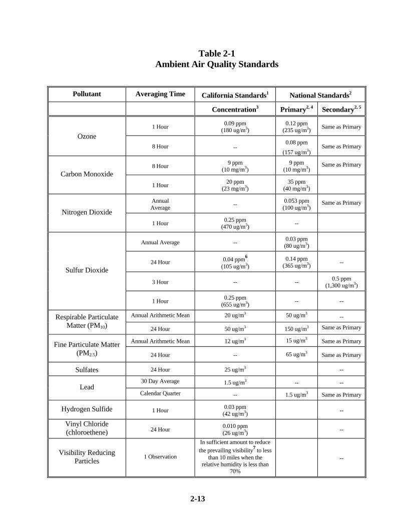
2-13
Table 2-1 Ambient Air Quality Standards
Pollutant Averaging Time California Standards1 National Standards2
Concentration3 Primary2, 4 Secondary2, 5
1 Hour 0.09 ppm (180 ug/m3)
0.12 ppm (235 ug/m3) Same as Primary
Ozone 8 Hour --
0.08 ppm
(157 ug/m3) Same as Primary
8 Hour 9 ppm (10 mg/m3)
9 ppm (10 mg/m3)
Same as Primary
Carbon Monoxide 1 Hour 20 ppm
(23 mg/m3) 35 ppm
(40 mg/m3)
Annual Average -- 0.053 ppm
(100 ug/m3) Same as Primary
Nitrogen Dioxide 1 Hour 0.25 ppm
(470 ug/m3) --
Annual Average -- 0.03 ppm (80 ug/m3)
24 Hour 0.04 ppm6 (105 ug/m3)
0.14 ppm (365 ug/m3) --
3 Hour -- -- 0.5 ppm (1,300 ug/m3)
Sulfur Dioxide
1 Hour 0.25 ppm (655 ug/m3) -- --
Annual Arithmetic Mean 20 ug/m3 50 ug/m3 -- Respirable Particulate Matter (PM10) 24 Hour 50 ug/m3 150 ug/m3 Same as Primary
Annual Arithmetic Mean 12 ug/m3 15 ug/m3 Same as Primary Fine Particulate Matter (PM2.5) 24 Hour -- 65 ug/m3 Same as Primary
Sulfates 24 Hour 25 ug/m3 --
30 Day Average 1.5 ug/m3 -- -- Lead
Calendar Quarter -- 1.5 ug/m3 Same as Primary
Hydrogen Sulfide 1 Hour 0.03 ppm (42 ug/m3) --
Vinyl Chloride (chloroethene) 24 Hour 0.010 ppm
(26 ug/m3) --
Visibility Reducing Particles 1 Observation
In sufficient amount to reduce the prevailing visibility7 to less
than 10 miles when the relative humidity is less than
70%
--
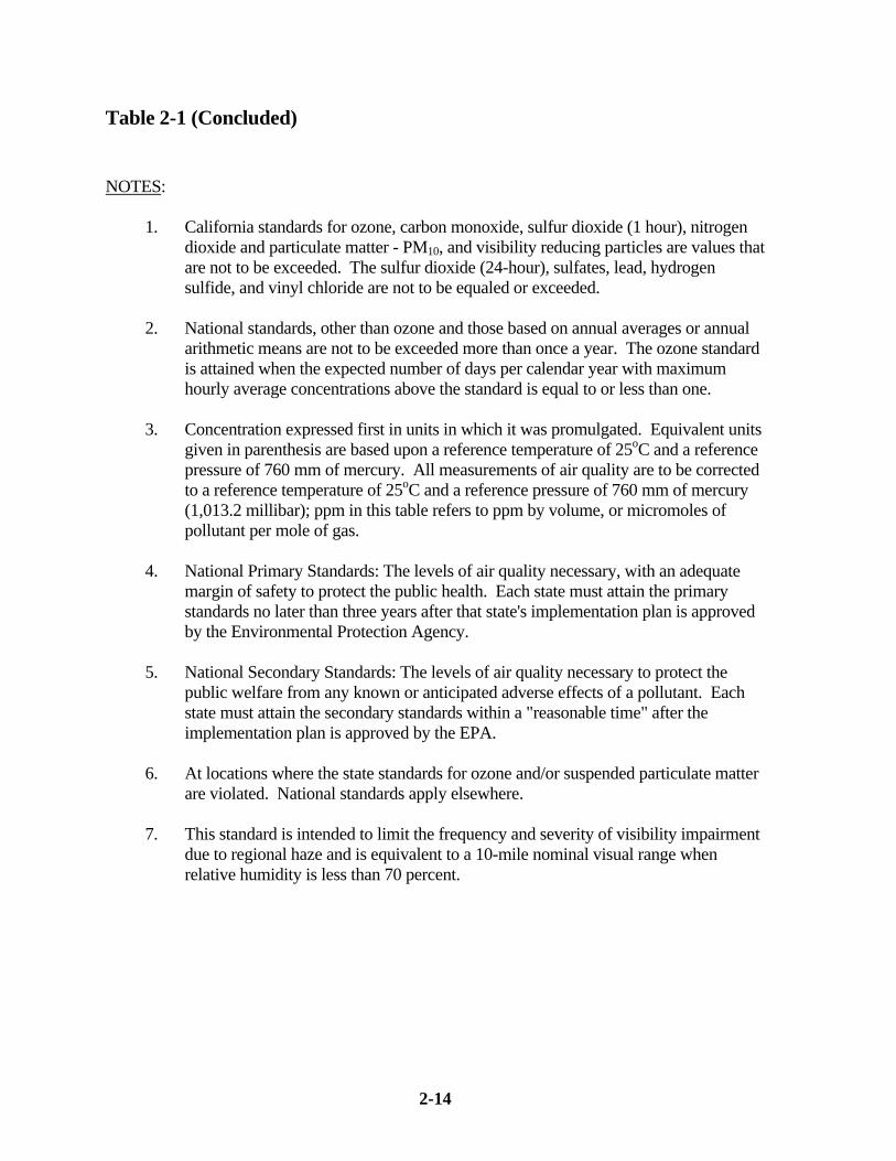
2-14
Table 2-1 (Concluded) NOTES:
1. California standards for ozone, carbon monoxide, sulfur dioxide (1 hour), nitrogen dioxide and particulate matter - PM10, and visibility reducing particles are values that are not to be exceeded. The sulfur dioxide (24-hour), sulfates, lead, hydrogen sulfide, and vinyl chloride are not to be equaled or exceeded.
2. National standards, other than ozone and those based on annual averages or annual
arithmetic means are not to be exceeded more than once a year. The ozone standard is attained when the expected number of days per calendar year with maximum hourly average concentrations above the standard is equal to or less than one.
3. Concentration expressed first in units in which it was promulgated. Equivalent units
given in parenthesis are based upon a reference temperature of 25oC and a reference pressure of 760 mm of mercury. All measurements of air quality are to be corrected to a reference temperature of 25oC and a reference pressure of 760 mm of mercury (1,013.2 millibar); ppm in this table refers to ppm by volume, or micromoles of pollutant per mole of gas.
4. National Primary Standards: The levels of air quality necessary, with an adequate
margin of safety to protect the public health. Each state must attain the primary standards no later than three years after that state's implementation plan is approved by the Environmental Protection Agency.
5. National Secondary Standards: The levels of air quality necessary to protect the
public welfare from any known or anticipated adverse effects of a pollutant. Each state must attain the secondary standards within a "reasonable time" after the implementation plan is approved by the EPA.
6. At locations where the state standards for ozone and/or suspended particulate matter
are violated. National standards apply elsewhere.
7. This standard is intended to limit the frequency and severity of visibility impairment due to regional haze and is equivalent to a 10-mile nominal visual range when relative humidity is less than 70 percent.
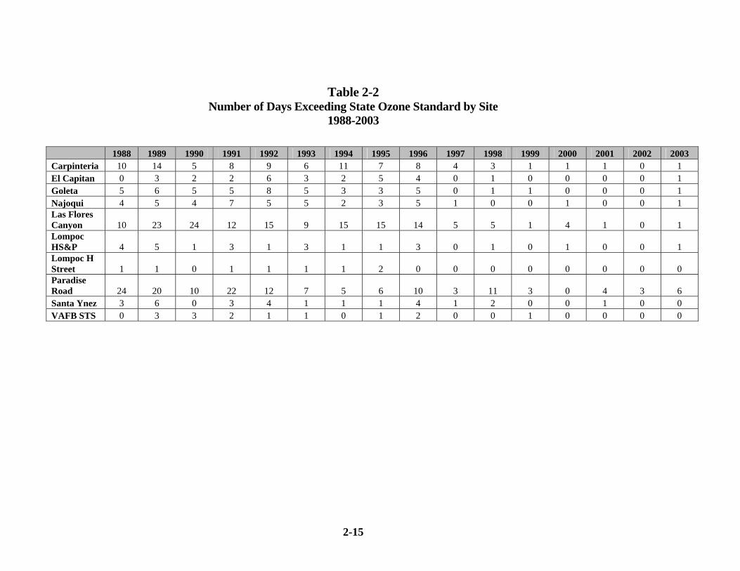
2-15
Table 2-2 Number of Days Exceeding State Ozone Standard by Site
1988-2003
1988 1989 1990 1991 1992 1993 1994 1995 1996 1997 1998 1999 2000 2001 2002 2003 Carpinteria 10 14 5 8 9 6 11 7 8 4 3 1 1 1 0 1 El Capitan 0 3 2 2 6 3 2 5 4 0 1 0 0 0 0 1 Goleta 5 6 5 5 8 5 3 3 5 0 1 1 0 0 0 1 Najoqui 4 5 4 7 5 5 2 3 5 1 0 0 1 0 0 1 Las Flores Canyon 10 23 24 12 15 9 15 15 14 5 5 1 4 1 0 1 Lompoc HS&P 4 5 1 3 1 3 1 1 3 0 1 0 1 0 0 1 Lompoc H Street 1 1 0 1 1 1 1 2 0 0 0 0 0 0 0 0 Paradise Road 24 20 10 22 12 7 5 6 10 3 11 3 0 4 3 6 Santa Ynez 3 6 0 3 4 1 1 1 4 1 2 0 0 1 0 0 VAFB STS 0 3 3 2 1 1 0 1 2 0 0 1 0 0 0 0
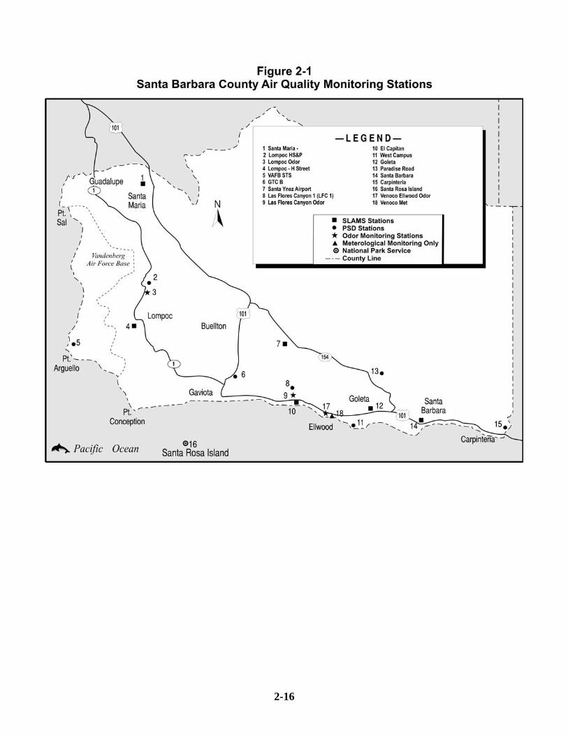
2-16
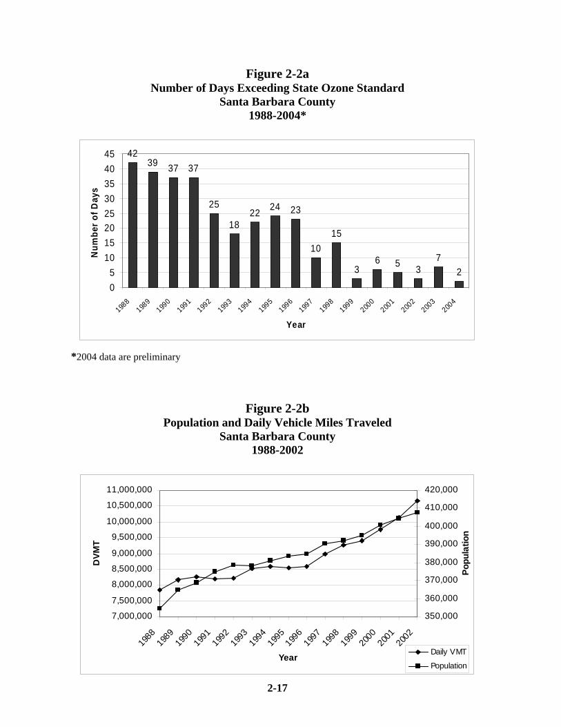
2-17
Figure 2-2a Number of Days Exceeding State Ozone Standard
Santa Barbara County 1988-2004*
4239 37 37
25
1822 24 23
1015
36 5 3
72
05
1015202530354045
1988
1989
1990
1991
1992
1993
1994
1995
1996
1997
1998
1999
2000
2001
2002
2003
2004
Year
Num
ber o
f Day
s
*2004 data are preliminary
Figure 2-2b Population and Daily Vehicle Miles Traveled
Santa Barbara County 1988-2002
7,000,000
7,500,000
8,000,000
8,500,000
9,000,000
9,500,000
10,000,000
10,500,000
11,000,000
1988
1989
1990
1991
1992
1993
1994
1995
1996
1997
1998
1999
2000
2001
2002
Year
DVM
T
350,000
360,000
370,000
380,000
390,000
400,000
410,000
420,000
Popu
latio
n
Daily VMT
Population
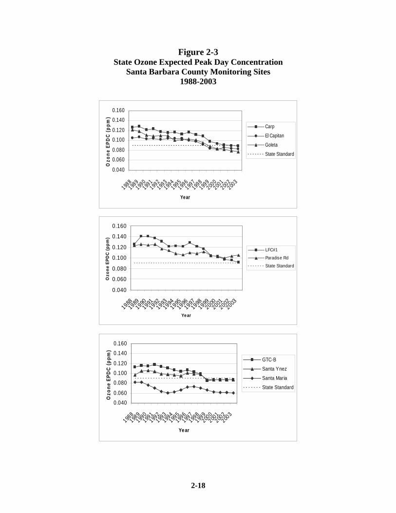
2-18
Figure 2-3 State Ozone Expected Peak Day Concentration
Santa Barbara County Monitoring Sites 1988-2003
0.040
0.060
0.080
0.100
0.120
0.140
0.160
1988198
9199
0199
1199
2199
3199
4199
5199
6199
7199
8199
9200
0200
1200
2200
3
Year
Ozo
ne E
PDC
(ppm
)
Carp
El Capitan
Goleta
State Standard
0.040
0.060
0.080
0.100
0.120
0.140
0.160
19881989
19901991
19921993
19941995
19961997
19981999
20002001
20022003
Year
Ozo
ne E
PDC
(ppm
)
LFC#1
Paradise Rd
State Standard
0.040
0.060
0.080
0.100
0.120
0.140
0.160
1988198
9199
0199
1199
2199
3199
4199
5199
6199
7199
8199
9200
0200
1200
2200
3
Year
Ozo
ne E
PDC
(ppm
)
GTC-B
Santa Ynez
Santa Maria
State Standard
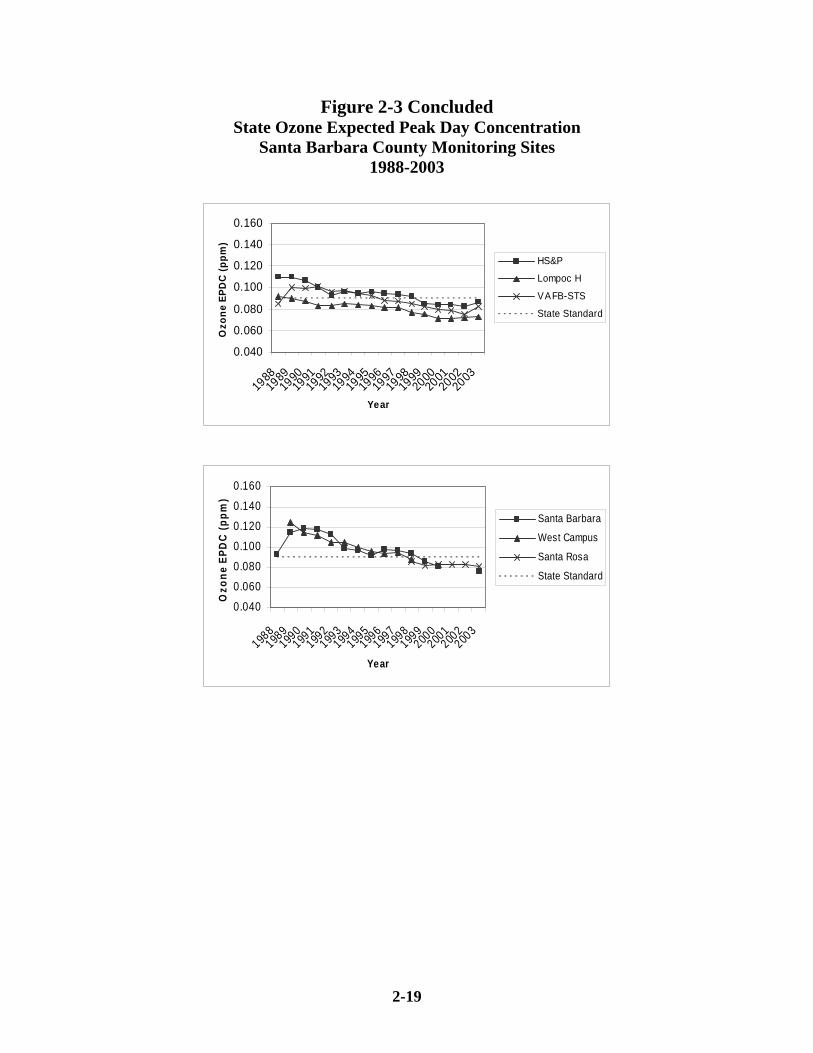
2-19
Figure 2-3 Concluded State Ozone Expected Peak Day Concentration
Santa Barbara County Monitoring Sites 1988-2003
0.040
0.060
0.080
0.100
0.120
0.140
0.160
198819
8919
9019
9119
9219
9319
9419
9519
9619
9719
9819
9920
0020
0120
0220
03
Year
Ozo
ne E
PDC
(ppm
)
HS&P
Lompoc H
VAFB-STS
State Standard
0.040
0.060
0.080
0.100
0.120
0.140
0.160
1988198
9199
0199
1199
2199
3199
4199
5199
6199
7199
8199
9200
0200
1200
2200
3
Year
Ozo
ne E
PDC
(ppm
)
Santa Barbara
West Campus
Santa Rosa
State Standard
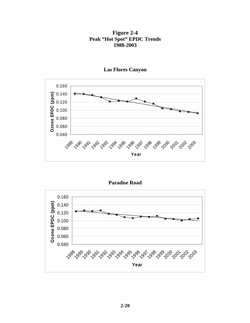
2-20
Figure 2-4 Peak “Hot Spot” EPDC Trends
1988-2003
Las Flores Canyon
0.040
0.060
0.080
0.100
0.120
0.140
0.160
19891990
19911992
19931994
19951996
19971998
19992000
20012002
2003
Year
Ozo
ne E
PDC
(ppm
)
Paradise Road
0.040
0.060
0.080
0.100
0.120
0.140
0.160
1988
1989
1990
1991
1992
1993
1994
1995
1996
1997
1998
1999
2000
2001
2002
2003
Year
Ozo
ne E
PDC
(ppm
)
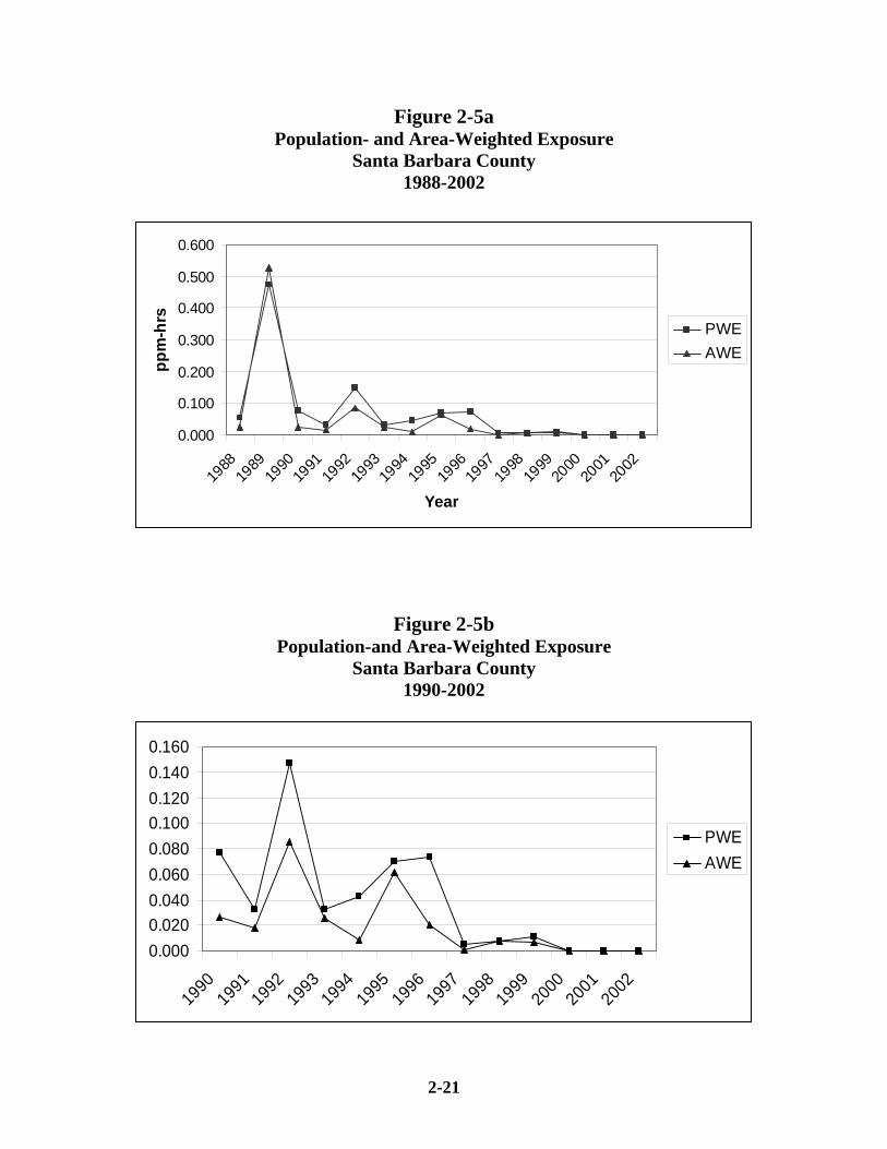
2-21
Figure 2-5a Population- and Area-Weighted Exposure
Santa Barbara County 1988-2002
0.000
0.100
0.200
0.300
0.400
0.500
0.600
1988
1989
1990
1991
1992
1993
1994
1995
1996
1997
1998
1999
2000
2001
2002
Year
ppm
-hrs
PWEAWE
Figure 2-5b Population-and Area-Weighted Exposure
Santa Barbara County 1990-2002
0.0000.0200.0400.0600.0800.1000.1200.1400.160
1990
1991
1992
1993
1994
1995
1996
1997
1998
1999
2000
2001
2002
PWEAWE
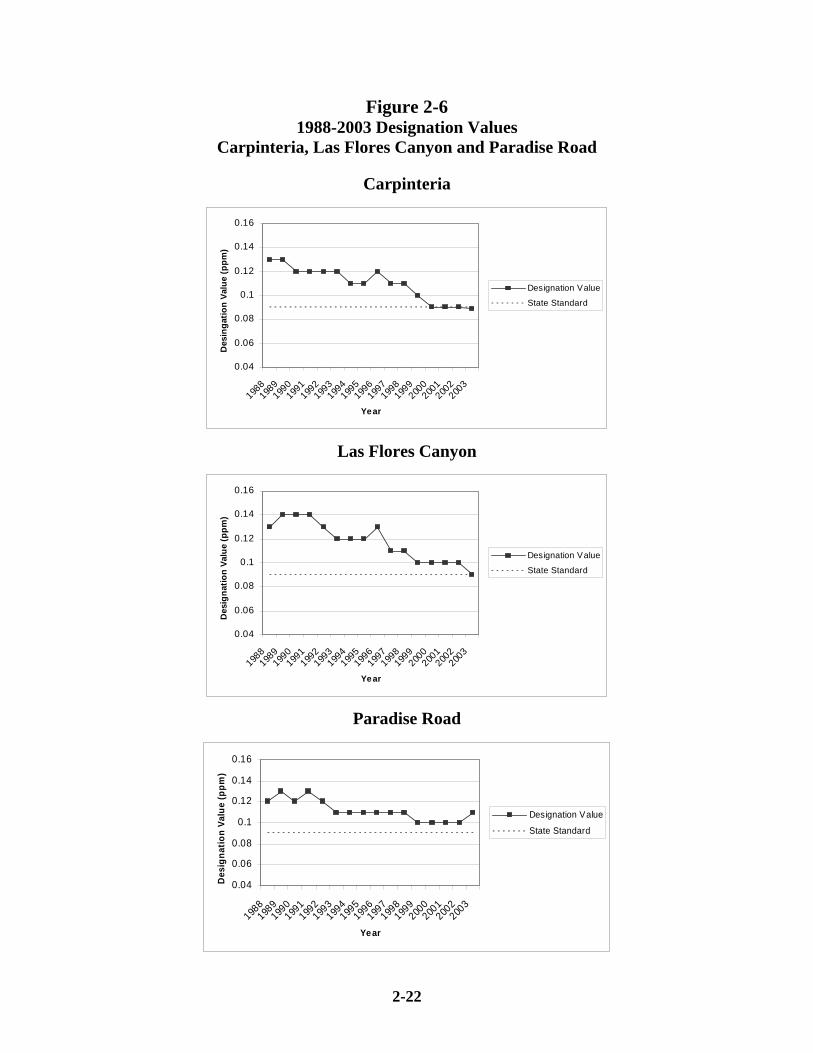
2-22
Figure 2-6 1988-2003 Designation Values
Carpinteria, Las Flores Canyon and Paradise Road
Carpinteria
0.04
0.06
0.08
0.1
0.12
0.14
0.16
1988198
9199
0199
1199
2199
3199
4199
5199
6199
7199
8199
9200
0200
1200
2200
3
Year
Des
inga
tion
Valu
e (p
pm)
Designation Value
State Standard
Las Flores Canyon
0.04
0.06
0.08
0.1
0.12
0.14
0.16
1988198
9199
0199
1199
2199
3199
4199
5199
6199
7199
8199
9200
0200
1200
2200
3
Year
Des
igna
tion
Valu
e (p
pm)
Designation Value
State Standard
Paradise Road
0.04
0.06
0.08
0.1
0.12
0.14
0.16
1988198
9199
0199
1199
2199
3199
4199
5199
6199
7199
8199
9200
0200
1200
2200
3
Year
Des
igna
tion
Valu
e (p
pm)
Designation Value
State Standard
CHAPTER 3
EMISSION INVENTORY
Introduction
Pollutants
Annual Emission Inventory Hierarchy
2000 Annual Emission Inventory
2000 Planning Emission Inventory
Conclusion
3 - 1
3. EMISSION INVENTORY
3.1 INTRODUCTION
This chapter describes the baseline emission inventory used in the development of this 2004
Clean Air Plan (2004 Plan). The emission inventory accounts for the types and amounts of
pollutants emitted from a wide variety of sources, including on-road motor vehicles and other
mobile sources, fuel combustion at industrial facilities, solvent and surface coating usage,
consumer product usage, and emissions from natural sources. The emission inventory is used to
describe and compare contributions from air pollution sources, evaluate control measures,
schedule rule adoptions, forecast future pollution, and prepare clean air plans.
The emission inventory is divided into two geographical regions: Santa Barbara County and the
Outer Continental Shelf (OCS). The Santa Barbara County emission inventory encompasses all
onshore sources of air pollution within Santa Barbara County and the State Tidelands (three
miles from the shoreline). The OCS emission inventory includes pollution sources 25 miles
beyond the State Tideland boundary offshore of Santa Barbara County.
The 2000 Annual Emission Inventory was derived from many sources including the APCD’s
Annual Emission Inventory Questionnaire and Annual Reports programs, the Santa Barbara
County Association of Governments, the California Air Resources Board, surveys from Santa
Barbara businesses, and other U.S., California, and Santa Barbara County government agencies.
Also included in this chapter is a modified version of the 2000 Annual Emission Inventory,
known as a “Planning Emission Inventory,” which will be used as the baseline to forecast
emissions for the years 2005, 2010, 2015, and 2020. Please refer to Chapter 6, Emission
Forecasting, for more discussion on how the 2000 Planning Emission Inventory is used to
forecast future emissions.
The Planning Emission Inventory is a modified subset of an Annual Emission Inventory and they
differ from each other in several ways. First, the creation of the Planning Emission Inventory
3 - 2
involves adjusting the Annual Emission Inventory to account for seasonal variation because most
exceedances of the state 1-hour ozone standard occur during the April to October ozone season.
This is commonly referred to as a summer seasonal inventory. Second, the emissions from
natural sources such as biogenics, oil and gas seeps, and wildfires that are part of the Annual
Emission Inventory are excluded from the Planning Emission Inventory since they are not
regulated or controlled through implementation of emission control measures. Finally, the
annual emissions in the Annual Emission Inventory are converted to daily emissions in the
Planning Emission Inventory.
This chapter presents both the 2000 Annual Emission Inventory and the 2000 Planning Emission
Inventory for both Santa Barbara County and the OCS. These inventories are presented in
Tables 3-1 to 3-4 and Figures 3-1 to 3-4.
3.2 POLLUTANTS
The Annual Emission Inventory and Planning Emission Inventory include two pollutants that
contribute to ozone formation, referred to as ozone precursors. These pollutants are reactive
organic compounds (ROC) and oxides of nitrogen (NOx). The definition of ROC used in this
plan is essentially equivalent to the USEPA's definition of Volatile Organic Compounds (VOC)
and ARB’s definition of Reactive Organic Gases (ROG), and does not include ethane, acetone or
perchloroethylene as reactive organic chemical species.
3.3 ANNUAL EMISSION INVENTORY HIERARCHY
The annual emission inventory is organized in a three-tiered hierarchy that categorizes all air
pollution sources. The first tier of this hierarchy contains four divisions: Stationary Sources
(individual facilities and aggregated point sources), Area-Wide Sources (geographically
dispersed area sources), Mobile Sources (both on-road vehicles and off-road sources) and
Natural Sources (not man-made). In the second tier, each of the four divisions is sub-divided
into major source categories. The third tier divides the major source categories into summary
categories
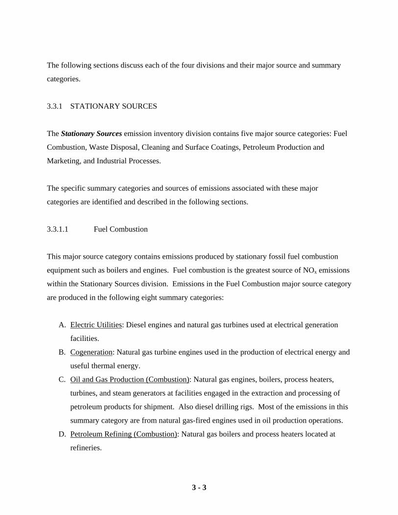
3 - 3
The following sections discuss each of the four divisions and their major source and summary
categories.
3.3.1 STATIONARY SOURCES
The Stationary Sources emission inventory division contains five major source categories: Fuel
Combustion, Waste Disposal, Cleaning and Surface Coatings, Petroleum Production and
Marketing, and Industrial Processes.
The specific summary categories and sources of emissions associated with these major
categories are identified and described in the following sections.
3.3.1.1 Fuel Combustion
This major source category contains emissions produced by stationary fossil fuel combustion
equipment such as boilers and engines. Fuel combustion is the greatest source of NOx emissions
within the Stationary Sources division. Emissions in the Fuel Combustion major source category
are produced in the following eight summary categories:
A. Electric Utilities: Diesel engines and natural gas turbines used at electrical generation
facilities.
B. Cogeneration: Natural gas turbine engines used in the production of electrical energy and
useful thermal energy.
C. Oil and Gas Production (Combustion): Natural gas engines, boilers, process heaters,
turbines, and steam generators at facilities engaged in the extraction and processing of
petroleum products for shipment. Also diesel drilling rigs. Most of the emissions in this
summary category are from natural gas-fired engines used in oil production operations.
D. Petroleum Refining (Combustion): Natural gas boilers and process heaters located at
refineries.
3 - 4
E. Manufacturing and Industrial: Most of the emissions in this summary category are from
diesel-fired engines and natural gas process heaters used in other industrial and
manufacturing activities such as: sand, rock, and gravel processing; concrete and asphalt
production; and mineral processing.
F. Food and Agricultural Processing: Diesel-fired engines used for agricultural irrigation.
G. Service and Commercial: Natural gas commercial space and water heaters and small
boilers and diesel-fired engines at non-industrial facilities.
H. Other (Fuel Combustion). Fuel combustion not accounted for in any other category.
3.3.1.2 Waste Disposal
This major source category contains emissions associated with wastewater treatment plants,
municipal landfills and incineration in five summary categories:
A. Sewage Treatment: Wastewater treatment plants and process gas flares.
B. Landfills: Landfill gas emissions from natural biodegradation and decomposition of
waste material at Class I & Class II landfill sites. Also waste gas flares.
C. Incinerators: Incinerators burning natural gas and process gas.
D. Soil Remediation: Contaminated soil clean-up sites.
E. Other (Waste Disposal). Waste disposal not accounted for in any other category.
3.3.1.3 Cleaning and Surface Coatings
This major source category consists entirely of evaporative ROC emissions from solvents and
coatings, in the following six summary categories:
A. Laundering: Use of petroleum-based solvents at dry cleaning facilities.
B. Degreasing: Cold cleaning of parts and materials at industrial and commercial facilities,
mostly using Isopropyl Alcohol and other degreasing solvents.
C. Coatings and Related Process Solvents: Automotive refinishing, metal parts, furniture
and wood product coatings and associated solvent and thinner use.
3 - 5
D. Printing: Inks, solvents and cleaning agents.
E. Adhesives and Sealants: Organic solvent-based and water-based adhesives and sealants
used in various commercial and industrial applications.
F. Other (Cleaning and Surface Coating): Solvents not accounted for in any other category.
3.3.1.4 Petroleum Production and Marketing
This major source emission category includes emissions resulting from the handling of
petroleum liquids and gases at petroleum extraction, processing, transport, and marketing
facilities. This category is comprised primarily of ROC emissions and is the most significant
source of ROC emissions in the Stationary Sources division. The emissions are produced from
processes in the following three summary categories:
A. Oil and Gas Production: Fugitive hydrocarbon emissions from oil wells, oil valves and
fittings, compressor seals, flanges, fixed and floating roof tanks, oil sumps, pits and well
cellars, glycol regenerator vents, tank car and truck loading operations, and combustion
emissions from vapor recovery flares at oil and gas extraction and processing facilities.
B. Petroleum Refining: Fugitive hydrocarbon emissions from valves, fittings, storage tanks
and loading racks at oil and gas production facilities.
C. Petroleum Marketing: Fugitive hydrocarbon emissions from crude oil storage tanks
affiliated with pipelines, and loading of marine vessels and tank cars and trucks with
crude oil, natural gas transmission losses, refined fuel vapor losses from underground
storage tanks, gasoline dispensing facilities, and bulk fuel storage plants.
3.3.1.5 Industrial Processes
The Industrial Processes major source category pertains to industries other than the petroleum
industry. Industrial Processes produce only a small fraction of the county's ROC and NOx
emissions. They include the following summary categories:
A. Chemical: Fiberglass operations and plastic product manufacturing.
3 - 6
B. Food and Agriculture: Wine fermentation and aging.
C. Mineral Processes: Crushed rock, diatomaceous earth processing, asphalt and cement
concrete production and limestone processing.
D. Metal Processes: There are no sources in Santa Barbara County for this category.
E. Wood and Paper: There are no sources in Santa Barbara County for this category.
F. Other (Industrial Processes): Aerospace operations (missile launches from Vandenberg
Air Force Base).
3.3.2 AREA-WIDE SOURCES
The Area-Wide Sources emission inventory division is composed entirely of emissions from
sources that are not subject to APCD permitting requirements. Emissions are geographically
dispersed throughout the county but are aggregated into two major source emission categories:
Solvent Evaporation and Miscellaneous Processes.
3.3.2.1 Solvent Evaporation
The Solvent Evaporation major source category consists entirely of evaporative ROC emissions
from consumer product use, architectural coatings, and pesticide use. The Solvent Evaporation
major source category includes the following four summary categories.
A. Consumer Products: Solvents used in antiperspirants, personal fragrance products, air
fresheners, automotive cleaners, household and bathroom cleaners, insecticides, barbecue
lighter fluid, aerosol paints, hair spray, rubbing alcohol, and laundry detergents.
B. Architectural Coatings and Related Process Solvents: Oil and water-based paints and
thinners used to paint commercial and residential buildings and other structures.
C. Pesticides/Fertilizers: Pesticides used in agricultural, structural and consumer product
applications.
D. Asphalt Roofing and Paving: Road oils, emulsified asphalt, and hot-mix asphalt.
3.3.2.2 Miscellaneous Processes
3 - 7
The emissions produced by miscellaneous processes are listed in the following 10 summary
categories:
A. Residential Fuel Combustion: Fuel combustion for cooking, space, and water heating
using natural gas, distillate oil, and liquified petroleum gas. Also wood stoves and
fireplaces.
B. Farming Operations: Tilling, harvest season operations and cattle feedlots.
C. Construction and Demolition: Residential, commercial and industrial building and
demolition, and road construction.
D. Paved Road Dust: Vehicular travel on paved roads, including freeways, major roads, and
local streets.
E. Unpaved Road Dust: Vehicular travel on unpaved roads, including city and county, farm
and federal land roads.
F. Fugitive Windblown Dust: Wind erosion of agricultural fields, pastures, and unpaved
roads.
G. Fires: Automobile and structural fires.
H. Waste Burning and Disposal: Burning of agricultural debris, weed abatement and range
management burning, prescribed forest management burning and fire fighting training.
I. Cooking: Commercial charbroiling.
J. Other (Miscellaneous Processes): Miscellaneous processes not accounted for in any
other category.
3.3.3 MOBILE SOURCES
The Mobile Sources emission inventory division contains emissions related to on-road motor
vehicles and a variety of off-road vehicles and equipment, including aircraft, recreational
vehicles and marine vessels. Mobile Sources consists of two major source categories: On-Road
Motor Vehicles and Other Mobile Sources.
3 - 8
The Mobile Sources emission inventory category contains most of the NOx emissions and
substantial amounts of the ROC emissions in the county’s onshore and offshore inventory.
3.3.3.1 On-Road Motor Vehicles
The On-Road Motor Vehicles emission inventory in the 2004 Plan was developed from ARB’s
EMFAC2002 model, which incorporates county-specific vehicle activity data generated by
SBCAG’s Santa Barbara Travel Model, ARB, and vehicle demographic data from the
Department of Motor Vehicles (DMV). SBCAG coordinates with CalTrans and the ARB to
estimate vehicle emissions by vehicle class.
The On-Road Motor Vehicles major source category includes gasoline and diesel light-duty
passenger vehicles (automobiles), gasoline and diesel light-duty trucks (pick-up trucks),
medium-duty trucks, light heavy-duty trucks, medium heavy-duty trucks, and heavy heavy-duty
trucks, motorcycles, heavy-duty gasoline and diesel buses, school buses, and motor homes. The
categories are described in more detail below:
A. Light Duty Passenger (LDA): Catalytic and non-catalytic converter-equipped gasoline
engine and diesel engine automobiles designed primarily for transportation and having a
design capacity of 12 persons or less.
B. Light Duty Trucks – 1 (LDT1): Catalytic and non-catalytic converter-equipped gasoline
engine and diesel engine trucks rated at less than or equal to 3,750 pounds gross vehicle
weight designed primarily for transportation of property but also includes Sport Utility
Vehicles (SUV).
C. Light Duty Trucks – 2 (LDT2): Catalytic and non-catalytic converter-equipped gasoline
engine and diesel engine trucks from 3,751 to 5,750 pounds gross vehicle weight
designed primarily for transportation of property but also includes Sport Utility Vehicles
(SUV).
D. Medium Duty Trucks (MDV): Catalytic and non-catalytic converter-equipped gasoline
engine and diesel engine trucks from 5,751 to 8,500 pounds gross vehicle weight. Some
larger SUV are included in this vehicle class.
3 - 9
E. Light Heavy Duty Gas Trucks – 1 (LHDV1): Catalytic and non-catalytic converter-
equipped gasoline engine trucks from 8,501 to 10,000 pounds gross vehicle weight.
F. Light Heavy Duty Gas Trucks – 2 (LHDV2): Catalytic and non-catalytic converter-
equipped gasoline engine trucks from 10,001 to 14,000 pounds gross vehicle weight.
G. Medium Heavy Duty Gas Trucks (MHDV): Catalytic and non-catalytic converter-
equipped gasoline engine trucks from 14,001 to 33,000 pounds gross vehicle weight.
H. Heavy Heavy Duty Gas Trucks (HHDV): Catalytic and non-catalytic converter-equipped
gasoline engine trucks from 33,001 to 60,000 pounds gross vehicle weight.
I. Light Heavy Duty Diesel Trucks – 1 (LHDV1): Diesel engine trucks from 8,501 to
10,000 pounds gross vehicle weight.
J. Light Heavy Duty Diesel Trucks – 2 (LHDV2): Diesel engine trucks from 10,001 to
14,000 pounds gross vehicle weight.
K. Medium Heavy Duty Diesel Trucks (MHDV): Diesel engine trucks from 14,001 to
33,000 pounds gross vehicle weight.
L. Heavy Heavy Duty Diesel Trucks (HHDV): Diesel engine trucks from 33,001 to 60,000
pounds gross vehicle weight.
M. Motorcycles (MCY): Non-catalytic converter equipped gasoline engines in vehicles with
not more than three wheels and weighing less than 1,500 pounds.
N. Heavy Duty Diesel Urban Buses (UB): Diesel engine buses typically used for municipal
transportation.
O. Heavy Duty Gas Urban Buses (UB): Gas engine buses typically used for municipal
transportation.
P. School Buses (SB).
Q. Motor Homes (MH).
3.3.3.2 Other Mobile Sources
The Other Mobile Sources category pertains to emission sources that do not produce their
emissions on roads and highways. These include ships, boats, airplanes, trains, residential utility
equipment, and construction and mining equipment. Although the ARB has the primary
3 - 10
responsibility for estimating the emissions from these categories, the APCD currently estimates
the emissions from ships, aircraft, and trains.
The ARB uses the model known as OFFROAD to calculate emissions from these categories.
The OFFROAD model consists of four main modules: population, activity, emissions, and
control factor. The base year equipment population is adjusted for growth and scrappage,
producing population distributions for specified calendar years through 2020. The statewide
population is allocated to each geographic region, including air basin and county. The base
emission factors are corrected for in-use and ambient conditions. The annual equipment
emissions are adjusted for seasonal and diurnal factors, producing the base emissions output.
Virtually all of the Other Mobile Source emissions are related to fuel combustion in engines. A
significant percentage of the NOx emissions come from marine vessels that operate in the State
Tidelands and the Outer Continental Shelf. The Other Mobile Sources category is divided into
seven summary categories:
A. Aircraft: Piston and jet powered commercial, civil, and military aircraft, and agricultural
crop dusting.
B. Trains: Diesel road hauling locomotives on the railway line linking the Los Angeles
area with the San Francisco Bay area.
C. Ships and Commercial Boats: A variety of large container ships, tankers, and cargo
vessels, both of US and foreign origin traversing the Santa Barbara Channel, gasoline
and diesel commercial fishing vessels, and crew and supply boats servicing offshore oil
production platforms.
D. Recreational Boats: Gasoline and diesel powered boats, determined by ARB’s
OFFROAD model. These emissions are divided equally between the Santa Barbara
County onshore (which includes the State Tidelands) and the Outer Continental Shelf.
E. Off-Road Recreational Vehicles: Four-wheel drive all-terrain and off-road passenger
vehicles, and off-road motorcycles, determined by ARB’s OFFROAD model.
F. Off-Road Equipment: Gasoline, diesel and LPG powered construction and industrial
equipment. Light duty equipment with engines less than 175 horsepower, such as
3 - 11
forklifts, mobile cranes, airport ground support equipment, portable generators,
compressors, and pumps. Heavy-duty non-farm equipment with engines greater than or
equal to 175 horsepower including construction equipment such as pavers, scrapers,
loaders and mining equipment. Diesel powered refrigeration units on trucks and trailers.
This category also includes emissions from lawn and garden equipment, which include
small horsepower two and four stroke utility engines driving chainsaws, lawn mowers,
leaf blowers, portable compressors and generators used in residential and commercial
applications. Lastly, there are emissions from oil drilling and workover, and military
tactical support equipment. The emissions from these categories are determined by
ARB’s OFFROAD model.
G. Farm Equipment: Gasoline and diesel heavy-duty farm equipment, including tractors,
mowers, combines and other mobile agricultural equipment. The emissions from these
categories are determined by ARB’s OFFROAD model.
Also within the Other Mobile Sources major source category is construction equipment. This
emission category is diverse in terms of equipment types and sizes, and includes gas and diesel
fired engines with horsepower ranges from under 15 to over 500 horsepower. Construction
emissions are estimated by the ARB for the APCD using the OFFROAD model in the summary
category Off-Road Equipment (Construction and Mining Equipment). Within this category,
construction emissions are aggregated with emissions from equipment used in mining
operations. This single category includes approximately 27 equipment types including pavers,
loaders, excavators, dozers, graders and tractors. The ARB, using the OFFROAD model,
estimated that about 1,646 tons per year of NOx, 183 tons per year of ROC and 1,146 tons per
year of CO were emitted from construction and mining equipment in 2000. Previous estimates
from the early- and mid-1990’s using statewide construction valuation permit data allocated to
the county level and construction permit data from SBCAG showed NOx emissions in the range
of 300 to 525 tons per year from construction equipment alone. Since current estimates of
construction emissions are aggregated with emissions from mining equipment, it is difficult to
determine whether these estimates compare favorably with previous estimates. Based on the
equipment types included in the Construction and Mining Equipment category along with
3 - 12
housing and population growth, however, it is reasonable to believe that current construction
emissions alone equal or exceed the high end of the range suggested from earlier estimates.
3.3.4 NATURAL SOURCES
The Natural Sources emission inventory division consists of emissions that are not man-made.
Emission estimates for these categories tend to be difficult to quantify with any degree of
certainty. Note that natural emissions are excluded from the Planning Emission Inventory.
3.3.4.1 Natural Sources
There are four summary categories of Natural Sources emissions:
A. Biogenic Sources: Emission estimates from natural vegetation are generated using the
Urban Airshed Model’s Biogenic Emission Inventory System (BEIS), a complex
regional model incorporating biomass types and distribution, plant species emission
factors and climate correction factors. Soil microorganisms contribute some NOx
emissions.
B. Geogenic Sources: Naturally occurring oil seeps and gas seeps located off the southern
coast of Santa Barbara County. Seep emissions flow out from subsurface sources on the
ocean floor, primarily in the State Tidelands, and exhibit a high degree of temporal and
spatial variability. We have worked in cooperation with the Institute of Crustal Studies
at the University of California at Santa Barbara to determine estimates of seep emissions
in the Santa Barbara Channel. The results of their research have been used in this
inventory.
C. Wildfires: Timber, grass and brush wildfires. This is different from the planned or
prescribed burn fires that are part of the Area-Wide Source division.
D. Windblown Dust.
Based on information presented in Sections 3.2 and 3.3, the 2000 Annual Emission Inventory
and the 2000 Planning Emission Inventory will be described in the following sections. These
3 - 13
two inventories will form the basis for determining emission reductions and forecasting future
inventories.
3.4 2000 ANNUAL EMISSION INVENTORY
The 2000 Santa Barbara County and the Outer Continental Shelf Annual Emission Inventory
document the current sources of ROC and NOx emissions, both in quantity and relative
contribution.
3.4.1 SANTA BARBARA COUNTY ANNUAL EMISSIONS
The 2000 Santa Barbara County Annual Emissions Inventory of ROC and NOx in tons per year
is presented in Table 3-1. The Santa Barbara County inventory represents onshore and State
Tidelands emission sources, and includes natural sources. Figure 3-1 shows each major source
category’s relative contribution for each pollutant during 2000. The largest sources of each
pollutant and their percent of contribution are as follows:
2000 Santa Barbara County ROC Annual Emissions: 44,348 tons
• 8% Stationary Sources: 3,667 tons
Primarily from Coatings and Process Solvents (Thinning and Cleanup Solvents),
Adhesives and Sealants, and Oil and Gas Production (Fugitives from Crude Oil Valves).
• 7% Area-Wide Sources: 3,064 tons
Primarily from Consumer Products, Pesticides & Fertilizers (Methyl Bromide), and
Architectural Coatings and Related Process Solvents (Thinning and Cleanup Solvents).
• 14% Mobile Sources – On-Road Motor Vehicles: 6,122 tons
Predominantly Light Duty Passenger cars, Light Duty Trucks, and Medium Duty Trucks.
• 6% Other Mobile Sources: 2,565 tons
Significant emissions are from Lawn and Garden Equipment, Fuel Storage and Handling,
Recreational Boats, and Farm Equipment (Diesel Agricultural Equipment).
• 65 % Natural Sources: 28,930 tons
3 - 14
Mostly Biogenic Sources with a significant contribution from Geogenic Sources.
2000 Santa Barbara County NOx Annual Emissions: 17,615 tons
• 12% Stationary Sources: 2,096 tons
Almost all from Oil and Gas Production (Natural Gas IC Engines), Manufacturing and
Industrial (Diesel IC Engines), Agricultural Irrigation (Diesel IC Engines).
• 2% Area-Wide Sources: 350 tons
Mostly Residential Fuel Combustion (Natural Gas Space and Water Heating).
• 50% Mobile Sources – On-Road Motor Vehicles: 8,890 tons
The majority from Light Duty Passenger cars, Light Duty Trucks, and Heavy Heavy
Duty Diesel Trucks.
• 28% Other Mobile Sources: 4,913 tons
Contributors are from Off-Road Equipment (Diesel Construction and Mining
Equipment), and Farm Equipment (Diesel Agricultural Equipment).
• 8% Natural Sources: 1,365 tons
Mostly from Biogenic Sources with some Wildfire (Timber and Brush) emissions.
In summary, Natural Sources (both Biogenic and Geogenic Sources) contribute the most ROC
emissions in the Annual Emission Inventory. On-Road Motor Vehicles, specifically Light Duty
Passenger, also produce large amounts of ROC emissions and most of the NOx emissions. On-
Road Motor Vehicles, Light Duty Trucks, and Other Mobile Sources, Off-Road Equipment and
Farm Equipment, also contribute large amounts of NOx emissions.
3.4.2 OCS ANNUAL EMISSIONS
The 2000 OCS emission inventory is presented in Table 3-2. The OCS emissions are
summarized separately from the onshore emission inventory for clarity. Figure 3-2 shows each
major source’s relative contribution for each pollutant during 2000. The largest sources of each
pollutant and their percent of contribution are discussed below.
3 - 15
2000 OCS ROC Annual Emissions: 3,067 tons
• 14% Stationary Sources: 417 tons
Primarily Oil and Gas Production (Fugitives from Crude Oil Valves).
• 21% Mobile Sources: 646 tons
Mostly Ships and Commercial Boats (Foreign Motor Ships).
• 65% Natural Sources: 2,004 tons
All from Geogenic Sources (Gas Seeps and Oil Seeps).
2000 OCS NOx Annual Emissions: 12,175 tons
• 2% Stationary Sources: 298 tons
Primarily Oil and Gas Production (Natural Gas Turbine IC Engines).
• 98% Mobile Sources: 11,876 tons
Predominantly Ships and Commercial Boats (Foreign Motor Ships).
It should be noted that the method used for determining emissions from marine shipping was
updated since the completion of the 2001 Clean Air Plan. The 1999 marine shipping inventory
that was included in the 2001 Clean Air Plan was calculated based on average horsepower
ratings for each ship type (e.g., cargo ships, container ships, auto carriers, etc.). In addition, the
types of marine vessels transiting off the coast of Santa Barbara County were derived by
assuming the same percentages of each vessel type as those departing or arriving from the north
out of or into the Port of Los Angeles - Long Beach. The fleet makeup and average horsepower
ratings for the 1999 inventory were obtained from the September 1999 report Marine Vessel
Emissions Inventory, Update to 1996 Report: Marine Vessel Emissions Inventory and Control
Strategies prepared by ARCADIS for the South Coast Air Quality Management District. Since
the preparation of the 1999 marine shipping inventory, we have acquired the Lloyds Registry of
Ships database that includes ship-specific horsepower ratings for marine vessels including those
transiting off the coast of Santa Barbara County.
3 - 16
In developing the 2000 marine shipping inventory, ship-specific data including ship name, ship
type, and cruising speed were obtained from the Marine Exchange of Los Angeles – Long Beach
Harbor. The 2000 marine shipping inventory is based on estimating emissions by utilizing the
ship-specific power consumption data for each ship that transited the coast of the county during
2000 rather than by using averages of power by ship type and assumed fleet makeup as was done
for the 1999 inventory. This methodology update has increased our current marine shipping
NOx emission estimates by about 4.1 tons per day over 1999 estimates. The significant increase
in marine shipping emissions from 1999 to 2000 is a direct result of our updated calculation
methodology as opposed to an increase in the level of marine shipping activity or the number of
vessel transits off our coast.
In summary, two thirds of the ROC emissions in the OCS are from Natural Sources, specifically
offshore oil seeps and gas seeps. Ships and Commercial Boats in transit, and Oil and Gas
Production, primarily offshore platform fugitive hydrocarbons, contribute the largest remaining
portions of ROC emissions to the OCS inventory. Ships and Commercial Boats also account for
almost all of the NOx emissions.
3.5 2000 PLANNING EMISSION INVENTORY
The 2000 Planning Emission Inventory was developed by modifying the Annual Emission
Inventory three significant ways. First, seasonal variations are factored into the Planning
Emission Inventory because most exceedances of the state ozone standard occur during the April
to October ozone season. Second, the Planning Emission Inventory excludes emissions from
natural sources such as biogenics, oil seeps and gas seeps, and wildfires, since they are not
regulated or controlled. Third, the emission values are converted from tons per year to tons per
day.
3.5.1 SANTA BARBARA COUNTY PLANNING EMISSION INVENTORY
3 - 17
Table 3-3 and Figure 3-3 shows each major source’s relative contribution for each pollutant
during 2000. The largest sources of each pollutant and their relative contribution are discussed
in the following section.
2000 Santa Barbara County ROC Planning Emissions: 41.84 tons per day
• 24% Stationary Sources: 10.05 tons per day
Primarily from Coatings and Process Solvents (Thinning and Cleanup Solvents),
Adhesives and Sealants, and from Oil and Gas Production (Fugitives from Crude Oil
Valves).
• 19% Area-Wide Sources: 7.94 tons per day
Primarily from Consumer Products, Pesticides & Fertilizers (Methyl Bromide), and
Architectural Coatings and Related Process Solvents (Thinning and Cleanup Solvents).
• 43% Mobile Sources – On-Road Motor Vehicles: 16.77 tons per day
Mostly from Light Duty Passenger cars, Light Duty Trucks, and Medium Duty Trucks.
• 18% Other Mobile Sources: 7.07 tons per day
Significant emissions are from Lawn and Garden Equipment, Fuel Storage and Handling,
Recreational Boats, and Farm Equipment (Diesel Agricultural Equipment).
2000 Santa Barbara County NOx Planning Emissions: 43.89 tons per day
• 13% Stationary Sources: 5.57 tons per day
Almost all from Oil and Gas Production (Natural Gas IC Engines), Manufacturing and
Industrial (Diesel IC Engines), Agricultural Irrigation (Diesel IC Engines).
• 1% Area-Wide Sources: 0.48 tons per day
Mostly Residential Fuel Combustion (Natural Gas Space and Water Heating).
• 55% Mobile Sources – On-Road Motor Vehicles: 24.36 tons per day
The majority from Light Duty Passenger cars, Light Duty Trucks, and Heavy-Heavy
Duty Diesel Trucks.
• 31% Other Mobile Sources: 13.48 tons per day
3 - 18
Contributions from Off-Road Equipment (Diesel Construction and Mining Equipment),
and Farm Equipment (Diesel Agricultural Equipment).
In summary, On-Road Motor Vehicles, specifically Light Duty Passenger cars and Light Duty
Trucks produce about two-thirds of the ROC emissions along with significant contributions from
Cleaning and Surface Coatings, Solvent Evaporation, and Petroleum Production and Marketing.
On-Road Motor Vehicles, primarily Light Duty Passenger cars, Light Duty Trucks, and Heavy,
Heavy Duty Diesel Trucks, along with the Other Mobile Source categories of Off-Road
Equipment and Farm Equipment, produce the majority of the NOx emissions.
3.5.2 OCS PLANNING EMISSION INVENTORY
The 2000 OCS Planning Emission Inventory is presented in Table 3-4. The OCS emissions are
summarized separately from the onshore emission inventory for clarity. Figure 3-4 shows each
major source’s relative contribution for each pollutant during 2000. The largest sources of each
pollutant and their percent of contribution are discussed as follows.
2000 OCS ROC Planning Emissions: 2.91 tons per day
• 39% Stationary Sources: 1.14 tons per day
Primarily Oil and Gas Production (Fugitives from Crude Oil Valves).
• 61% Mobile Sources: 1.77 tons per day
Mostly Ships and Commercial Boats (Foreign Motor Ships).
2000 OCS NOx Planning Emissions: 33.37 tons per day
• 2% Stationary Sources: 0.82 tons per day
Primarily Oil and Gas Production (Natural Gas Turbine IC Engines).
• 98% Mobile Sources: 32.55 tons per day
Predominantly Ships and Commercial Boats (Foreign Motor Ships).
3 - 19
In summary, the most significant contributors of ROC and NOx emissions to the 2000 Planning
Emission Inventory on the OCS are from Ships and Commercial Boats (Foreign Motor Ships).
3.6 CONCLUSION
In this chapter we have described how our emission inventories are categorized into Stationary
Sources, Area-Wide Sources, Mobile Sources and Natural Sources. The emphasis in the 2004
Plan is on the ozone precursors of ROC and NOx. We have also discussed the development of
the 2000 Annual Emission Inventory and 2000 Planning Emission Inventory for both Santa
Barbara County and the Outer Continental Shelf. These inventories provide the foundation for
this plan and are key elements to calculating emission reductions attributable to control measures
and for forecasting future emission inventories for 2005, 2010, 2015, and 2020.
The largest contributor of locally generated ROC and NOx emissions in both the Annual
Emission Inventory and Planning Emission Inventory is on-road motor vehicles. The most
significant source of NOx emissions in both the Annual Emission Inventory and the Planning
Emission Inventory for the Outer Continental Shelf is Other Mobile Sources (predominately
international marine shipping activities).
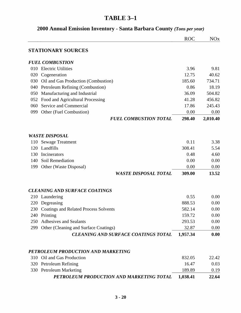
TABLE 3–1 2000 Annual Emission Inventory - Santa Barbara County (Tons per year)
ROC NOx
3 - 20
STATIONARY SOURCES FUEL COMBUSTION 010 Electric Utilities 3.96 9.81020 Cogeneration 12.75 40.62030 Oil and Gas Production (Combustion) 185.60 734.71040 Petroleum Refining (Combustion) 0.86 18.19050 Manufacturing and Industrial 36.09 504.82052 Food and Agricultural Processing 41.28 456.82060 Service and Commercial 17.86 245.43099 Other (Fuel Combustion) 0.00 0.00
FUEL COMBUSTION TOTAL 298.40 2,010.40 WASTE DISPOSAL 110 Sewage Treatment 0.11 3.38120 Landfills 308.41 5.54130 Incinerators 0.48 4.60140 Soil Remediation 0.00 0.00199 Other (Waste Disposal) 0.00 0.00
WASTE DISPOSAL TOTAL 309.00 13.52 CLEANING AND SURFACE COATINGS 210 Laundering 0.55 0.00220 Degreasing 888.53 0.00230 Coatings and Related Process Solvents 582.14 0.00240 Printing 159.72 0.00250 Adhesives and Sealants 293.53 0.00299 Other (Cleaning and Surface Coatings) 32.87 0.00
CLEANING AND SURFACE COATINGS TOTAL 1,957.34 0.00 PETROLEUM PRODUCTION AND MARKETING 310 Oil and Gas Production 832.05 22.42320 Petroleum Refining 16.47 0.03330 Petroleum Marketing 189.89 0.19
PETROLEUM PRODUCTION AND MARKETING TOTAL 1,038.41 22.64
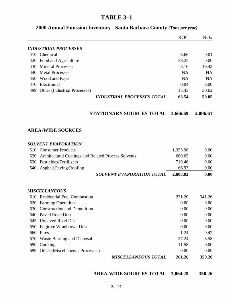
TABLE 3–1 2000 Annual Emission Inventory - Santa Barbara County (Tons per year)
ROC NOx
3 - 21
INDUSTRIAL PROCESSES 410 Chemical 6.66 0.01420 Food and Agriculture 38.25 0.00430 Mineral Processes 3.16 19.42440 Metal Processes NA NA450 Wood and Paper NA NA470 Electronics 0.04 0.00499 Other (Industrial Processes) 15.43 30.62
INDUSTRIAL PROCESSES TOTAL 63.54 50.05
STATIONARY SOURCES TOTAL 3,666.69 2,096.61
AREA-WIDE SOURCES
SOLVENT EVAPORATION 510 Consumer Products 1,355.98 0.00520 Architectural Coatings and Related Process Solvents 660.65 0.00530 Pesticides/Fertilizers 719.46 0.00540 Asphalt Paving/Roofing 66.93 0.00
SOLVENT EVAPORATION TOTAL 2,803.02 0.00 MISCELLANEOUS 610 Residential Fuel Combustion 221.20 341.26620 Farming Operations 0.00 0.00630 Construction and Demolition 0.00 0.00640 Paved Road Dust 0.00 0.00645 Unpaved Road Dust 0.00 0.00650 Fugitive Windblown Dust 0.00 0.00660 Fires 1.24 0.42670 Waste Burning and Disposal 27.24 8.58690 Cooking 11.58 0.00699 Other (Miscellaneous Processes) 0.00 0.00
MISCELLANEOUS TOTAL 261.26 350.26
AREA-WIDE SOURCES TOTAL 3,064.28 350.26
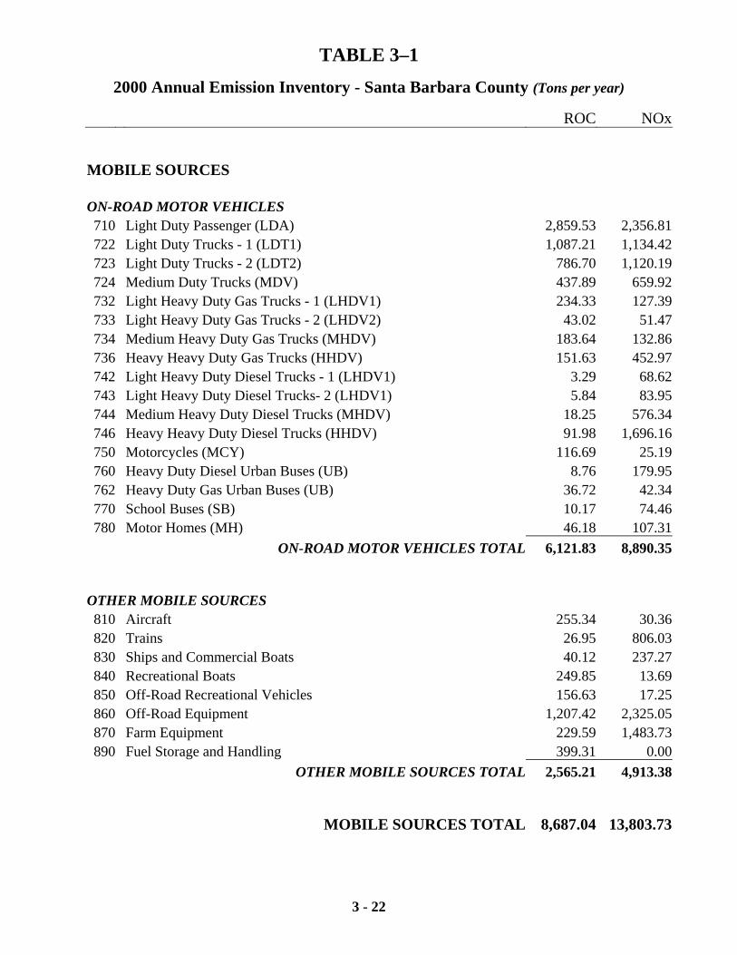
TABLE 3–1 2000 Annual Emission Inventory - Santa Barbara County (Tons per year)
ROC NOx
3 - 22
MOBILE SOURCES ON-ROAD MOTOR VEHICLES 710 Light Duty Passenger (LDA) 2,859.53 2,356.81722 Light Duty Trucks - 1 (LDT1) 1,087.21 1,134.42723 Light Duty Trucks - 2 (LDT2) 786.70 1,120.19724 Medium Duty Trucks (MDV) 437.89 659.92732 Light Heavy Duty Gas Trucks - 1 (LHDV1) 234.33 127.39733 Light Heavy Duty Gas Trucks - 2 (LHDV2) 43.02 51.47734 Medium Heavy Duty Gas Trucks (MHDV) 183.64 132.86736 Heavy Heavy Duty Gas Trucks (HHDV) 151.63 452.97742 Light Heavy Duty Diesel Trucks - 1 (LHDV1) 3.29 68.62743 Light Heavy Duty Diesel Trucks- 2 (LHDV1) 5.84 83.95744 Medium Heavy Duty Diesel Trucks (MHDV) 18.25 576.34746 Heavy Heavy Duty Diesel Trucks (HHDV) 91.98 1,696.16750 Motorcycles (MCY) 116.69 25.19760 Heavy Duty Diesel Urban Buses (UB) 8.76 179.95762 Heavy Duty Gas Urban Buses (UB) 36.72 42.34770 School Buses (SB) 10.17 74.46780 Motor Homes (MH) 46.18 107.31
ON-ROAD MOTOR VEHICLES TOTAL 6,121.83 8,890.35 OTHER MOBILE SOURCES 810 Aircraft 255.34 30.36820 Trains 26.95 806.03830 Ships and Commercial Boats 40.12 237.27840 Recreational Boats 249.85 13.69850 Off-Road Recreational Vehicles 156.63 17.25860 Off-Road Equipment 1,207.42 2,325.05870 Farm Equipment 229.59 1,483.73890 Fuel Storage and Handling 399.31 0.00
OTHER MOBILE SOURCES TOTAL 2,565.21 4,913.38
MOBILE SOURCES TOTAL 8,687.04 13,803.73
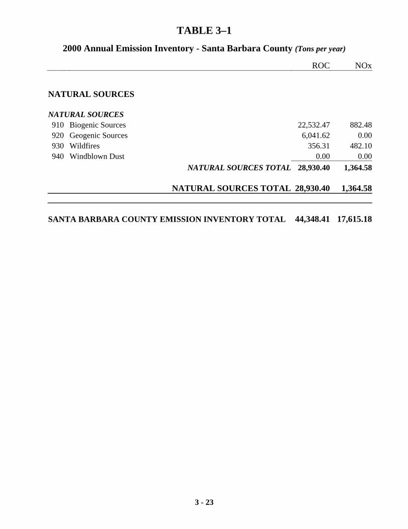
TABLE 3–1 2000 Annual Emission Inventory - Santa Barbara County (Tons per year)
ROC NOx
3 - 23
NATURAL SOURCES NATURAL SOURCES 910 Biogenic Sources 22,532.47 882.48920 Geogenic Sources 6,041.62 0.00930 Wildfires 356.31 482.10940 Windblown Dust 0.00 0.00
NATURAL SOURCES TOTAL 28,930.40 1,364.58
NATURAL SOURCES TOTAL 28,930.40 1,364.58
SANTA BARBARA COUNTY EMISSION INVENTORY TOTAL 44,348.41 17,615.18
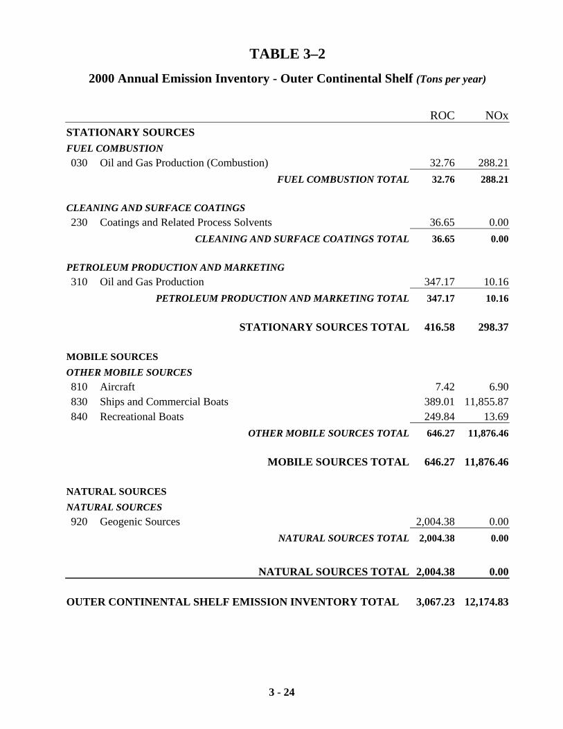
3 - 24
TABLE 3–2 2000 Annual Emission Inventory - Outer Continental Shelf (Tons per year)
ROC NOxSTATIONARY SOURCES FUEL COMBUSTION 030 Oil and Gas Production (Combustion) 32.76 288.21
FUEL COMBUSTION TOTAL 32.76 288.21
CLEANING AND SURFACE COATINGS 230 Coatings and Related Process Solvents 36.65 0.00
CLEANING AND SURFACE COATINGS TOTAL 36.65 0.00 PETROLEUM PRODUCTION AND MARKETING 310 Oil and Gas Production 347.17 10.16
PETROLEUM PRODUCTION AND MARKETING TOTAL 347.17 10.16 STATIONARY SOURCES TOTAL 416.58 298.37 MOBILE SOURCES OTHER MOBILE SOURCES 810 Aircraft 7.42 6.90830 Ships and Commercial Boats 389.01 11,855.87840 Recreational Boats 249.84 13.69
OTHER MOBILE SOURCES TOTAL 646.27 11,876.46 MOBILE SOURCES TOTAL 646.27 11,876.46 NATURAL SOURCES NATURAL SOURCES 920 Geogenic Sources 2,004.38 0.00
NATURAL SOURCES TOTAL 2,004.38 0.00
NATURAL SOURCES TOTAL 2,004.38 0.00 OUTER CONTINENTAL SHELF EMISSION INVENTORY TOTAL 3,067.23 12,174.83
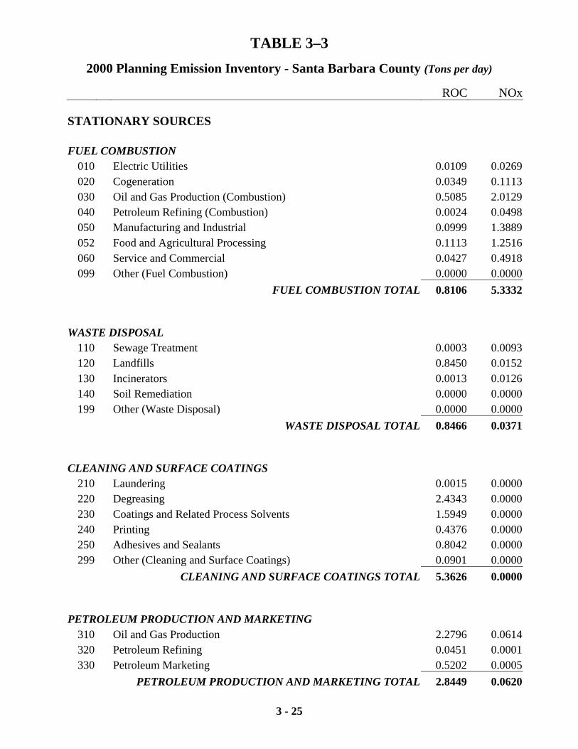
TABLE 3–3 2000 Planning Emission Inventory - Santa Barbara County (Tons per day)
ROC NOx
3 - 25
STATIONARY SOURCES
FUEL COMBUSTION 010 Electric Utilities 0.0109 0.0269020 Cogeneration 0.0349 0.1113030 Oil and Gas Production (Combustion) 0.5085 2.0129040 Petroleum Refining (Combustion) 0.0024 0.0498050 Manufacturing and Industrial 0.0999 1.3889052 Food and Agricultural Processing 0.1113 1.2516060 Service and Commercial 0.0427 0.4918099 Other (Fuel Combustion) 0.0000 0.0000
FUEL COMBUSTION TOTAL 0.8106 5.3332
WASTE DISPOSAL 110 Sewage Treatment 0.0003 0.0093120 Landfills 0.8450 0.0152130 Incinerators 0.0013 0.0126140 Soil Remediation 0.0000 0.0000199 Other (Waste Disposal) 0.0000 0.0000
WASTE DISPOSAL TOTAL 0.8466 0.0371
CLEANING AND SURFACE COATINGS 210 Laundering 0.0015 0.0000220 Degreasing 2.4343 0.0000230 Coatings and Related Process Solvents 1.5949 0.0000240 Printing 0.4376 0.0000250 Adhesives and Sealants 0.8042 0.0000299 Other (Cleaning and Surface Coatings) 0.0901 0.0000
CLEANING AND SURFACE COATINGS TOTAL 5.3626 0.0000
PETROLEUM PRODUCTION AND MARKETING 310 Oil and Gas Production 2.2796 0.0614320 Petroleum Refining 0.0451 0.0001330 Petroleum Marketing 0.5202 0.0005
PETROLEUM PRODUCTION AND MARKETING TOTAL 2.8449 0.0620
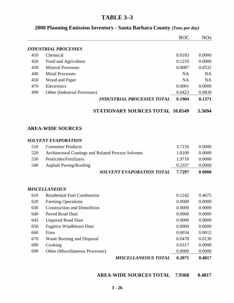
TABLE 3–3 2000 Planning Emission Inventory - Santa Barbara County (Tons per day)
ROC NOx
3 - 26
INDUSTRIAL PROCESSES 410 Chemical 0.0183 0.0000420 Food and Agriculture 0.1210 0.0000430 Mineral Processes 0.0087 0.0532440 Metal Processes NA NA450 Wood and Paper NA NA470 Electronics 0.0001 0.0000499 Other (Industrial Processes) 0.0423 0.0839
INDUSTRIAL PROCESSES TOTAL 0.1904 0.1371
STATIONARY SOURCES TOTAL 10.0549 5.5694
AREA-WIDE SOURCES SOLVENT EVAPORATION
510 Consumer Products 3.7150 0.0000520 Architectural Coatings and Related Process Solvents 1.8100 0.0000530 Pesticides/Fertilizers 1.9710 0.0000540 Asphalt Paving/Roofing 0.2337 0.0000
SOLVENT EVAPORATION TOTAL 7.7297 0.0000
MISCELLANEOUS 610 Residential Fuel Combustion 0.1242 0.4675620 Farming Operations 0.0000 0.0000630 Construction and Demolition 0.0000 0.0000640 Paved Road Dust 0.0000 0.0000645 Unpaved Road Dust 0.0000 0.0000650 Fugitive Windblown Dust 0.0000 0.0000660 Fires 0.0034 0.0012670 Waste Burning and Disposal 0.0478 0.0130690 Cooking 0.0317 0.0000699 Other (Miscellaneous Processes) 0.0000 0.0000
MISCELLANEOUS TOTAL 0.2071 0.4817
AREA-WIDE SOURCES TOTAL 7.9368 0.4817
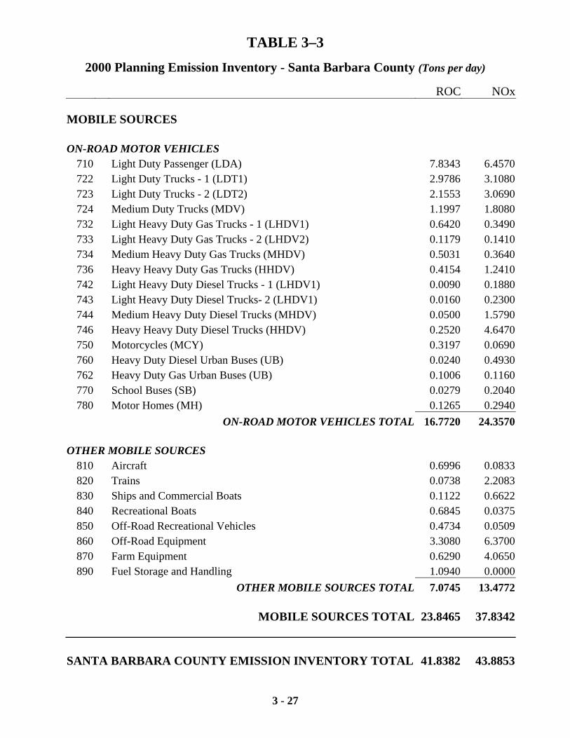
TABLE 3–3 2000 Planning Emission Inventory - Santa Barbara County (Tons per day)
ROC NOx
3 - 27
MOBILE SOURCES
ON-ROAD MOTOR VEHICLES 710 Light Duty Passenger (LDA) 7.8343 6.4570722 Light Duty Trucks - 1 (LDT1) 2.9786 3.1080723 Light Duty Trucks - 2 (LDT2) 2.1553 3.0690724 Medium Duty Trucks (MDV) 1.1997 1.8080732 Light Heavy Duty Gas Trucks - 1 (LHDV1) 0.6420 0.3490733 Light Heavy Duty Gas Trucks - 2 (LHDV2) 0.1179 0.1410734 Medium Heavy Duty Gas Trucks (MHDV) 0.5031 0.3640736 Heavy Heavy Duty Gas Trucks (HHDV) 0.4154 1.2410742 Light Heavy Duty Diesel Trucks - 1 (LHDV1) 0.0090 0.1880743 Light Heavy Duty Diesel Trucks- 2 (LHDV1) 0.0160 0.2300744 Medium Heavy Duty Diesel Trucks (MHDV) 0.0500 1.5790746 Heavy Heavy Duty Diesel Trucks (HHDV) 0.2520 4.6470750 Motorcycles (MCY) 0.3197 0.0690760 Heavy Duty Diesel Urban Buses (UB) 0.0240 0.4930762 Heavy Duty Gas Urban Buses (UB) 0.1006 0.1160770 School Buses (SB) 0.0279 0.2040780 Motor Homes (MH) 0.1265 0.2940
ON-ROAD MOTOR VEHICLES TOTAL 16.7720 24.3570
OTHER MOBILE SOURCES 810 Aircraft 0.6996 0.0833820 Trains 0.0738 2.2083830 Ships and Commercial Boats 0.1122 0.6622840 Recreational Boats 0.6845 0.0375850 Off-Road Recreational Vehicles 0.4734 0.0509860 Off-Road Equipment 3.3080 6.3700870 Farm Equipment 0.6290 4.0650890 Fuel Storage and Handling 1.0940 0.0000
OTHER MOBILE SOURCES TOTAL 7.0745 13.4772
MOBILE SOURCES TOTAL 23.8465 37.8342
SANTA BARBARA COUNTY EMISSION INVENTORY TOTAL 41.8382 43.8853
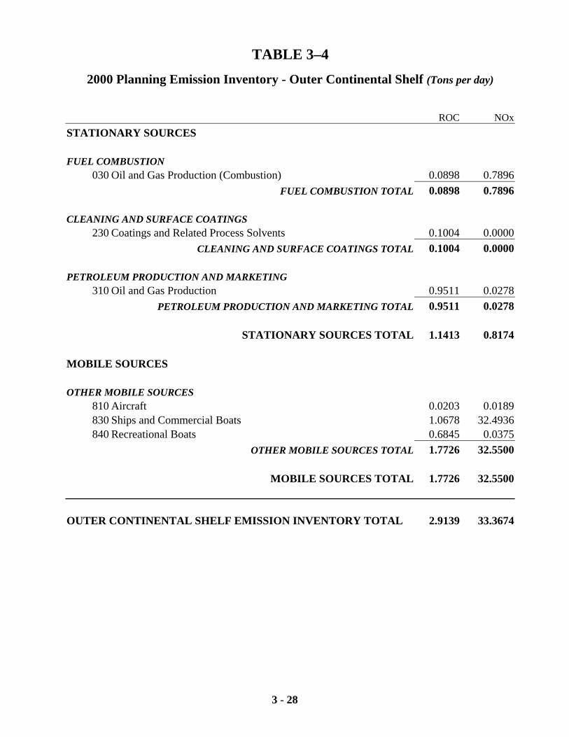
3 - 28
TABLE 3–4 2000 Planning Emission Inventory - Outer Continental Shelf (Tons per day)
ROC NOxSTATIONARY SOURCES FUEL COMBUSTION
030 Oil and Gas Production (Combustion) 0.0898 0.7896 FUEL COMBUSTION TOTAL 0.0898 0.7896 CLEANING AND SURFACE COATINGS
230 Coatings and Related Process Solvents 0.1004 0.0000 CLEANING AND SURFACE COATINGS TOTAL 0.1004 0.0000 PETROLEUM PRODUCTION AND MARKETING
310 Oil and Gas Production 0.9511 0.0278 PETROLEUM PRODUCTION AND MARKETING TOTAL 0.9511 0.0278
STATIONARY SOURCES TOTAL 1.1413 0.8174
MOBILE SOURCES OTHER MOBILE SOURCES
810 Aircraft 0.0203 0.0189830 Ships and Commercial Boats 1.0678 32.4936840 Recreational Boats 0.6845 0.0375
OTHER MOBILE SOURCES TOTAL 1.7726 32.5500
MOBILE SOURCES TOTAL 1.7726 32.5500 OUTER CONTINENTAL SHELF EMISSION INVENTORY TOTAL 2.9139 33.3674
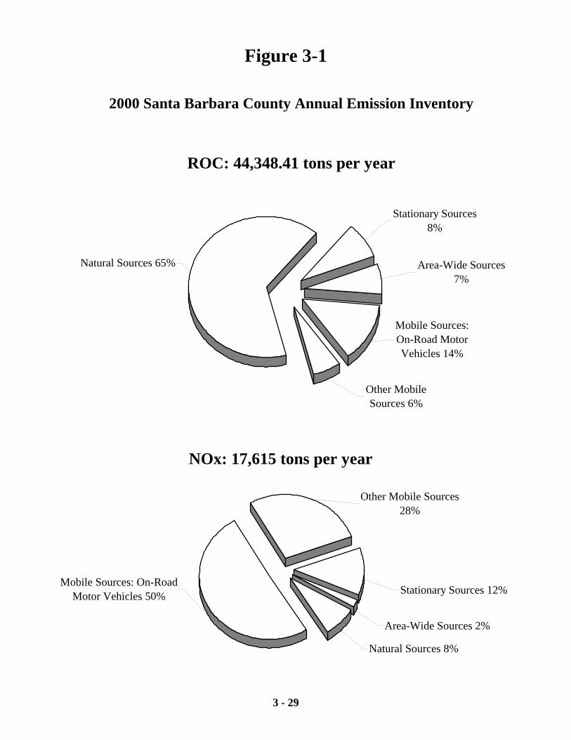
3 - 29
NOx: 17,615 tons per year
Other Mobile Sources28%
Mobile Sources: On-Road Motor Vehicles 50%
Natural Sources 8%
Stationary Sources 12%
Area-Wide Sources 2%
2000 Santa Barbara County Annual Emission Inventory
ROC: 44,348.41 tons per year
Mobile Sources: On-Road Motor Vehicles 14%
Area-Wide Sources 7%
Stationary Sources 8%
Other Mobile Sources 6%
Natural Sources 65%
Figure 3-1
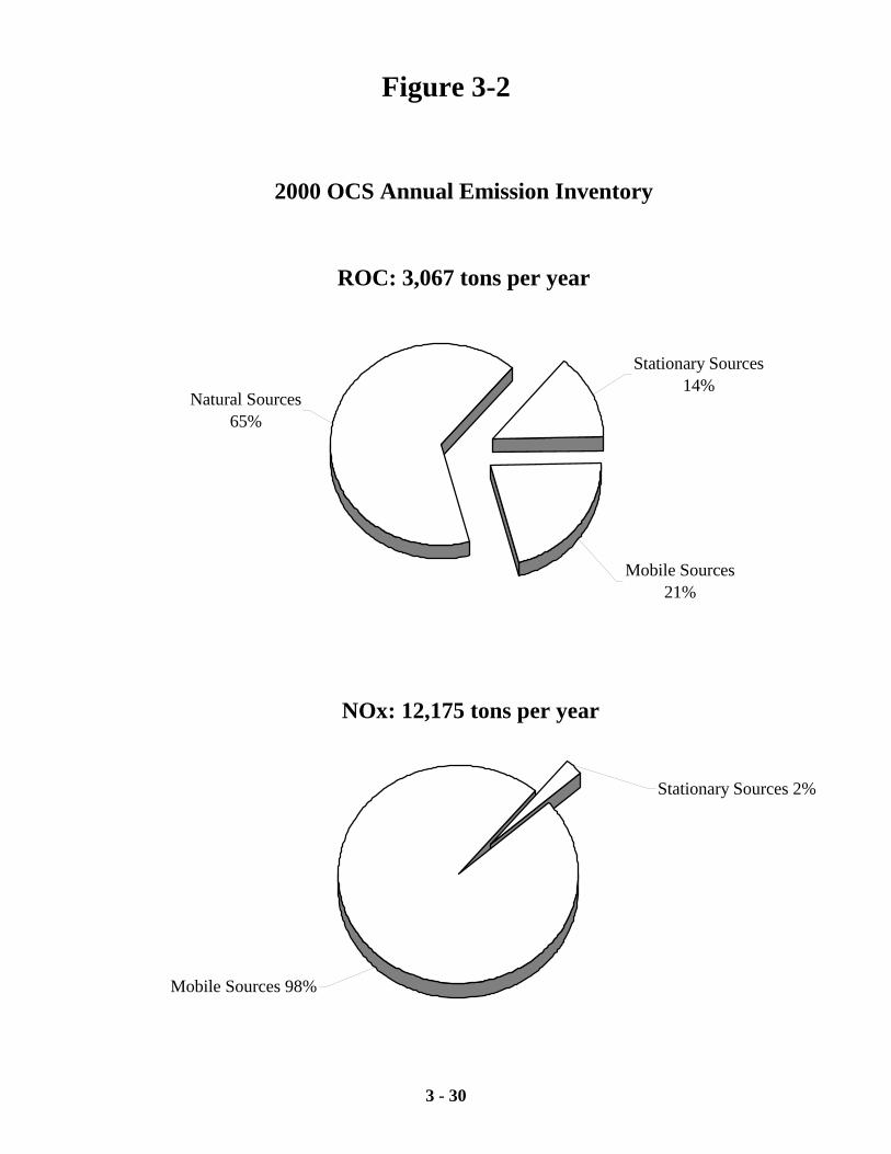
3 - 30
NOx: 12,175 tons per year
Stationary Sources 2%
Mobile Sources 98%
2000 OCS Annual Emission Inventory
ROC: 3,067 tons per year
Stationary Sources 14%
Mobile Sources 21%
Natural Sources 65%
Figure 3-2
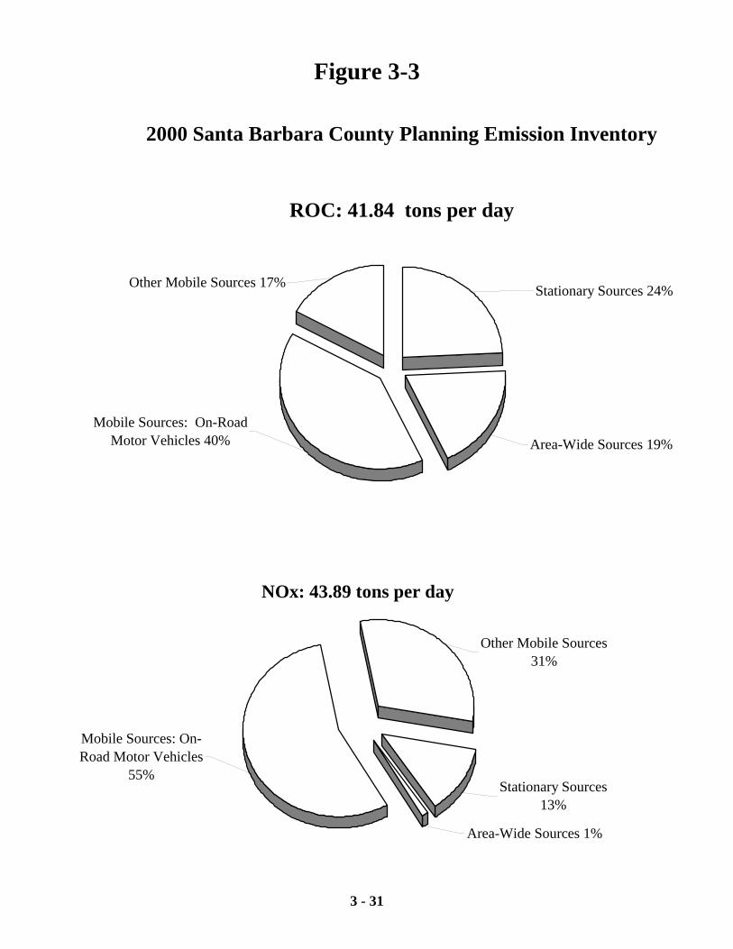
3 - 31
2000 Santa Barbara County Planning Emission Inventory
ROC: 41.84 tons per day
Stationary Sources 24%
Mobile Sources: On-Road Motor Vehicles 40%
Other Mobile Sources 17%
Area-Wide Sources 19%
NOx: 43.89 tons per day
Stationary Sources 13%
Area-Wide Sources 1%
Mobile Sources: On-Road Motor Vehicles
55%
Other Mobile Sources31%
Figure 3-3
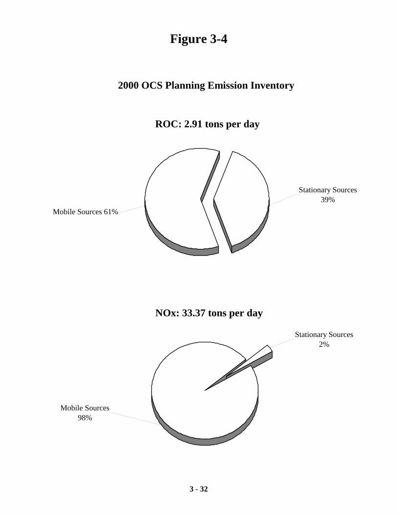
3 - 32
2000 OCS Planning Emission Inventory
ROC: 2.91 tons per day
Stationary Sources39%
Mobile Sources 61%
NOx: 33.37 tons per day
Mobile Sources98%
Stationary Sources2%
Figure 3-4
CHAPTER 4
__________________________________
EMISSION CONTROL MEASURES
Introduction
Emission Control Measure Mandates
Emission Control Measures Adopted Before 2001
Emission Control Measures Adopted During the
Reporting Period (2001 - 2003)
Proposed Emission Control Measures
Emission Control Measures for Further Study
Conclusions
4 - 1
4. EMISSION CONTROL MEASURES
4.1 INTRODUCTION
This chapter evaluates adopted and proposed stationary source control measures in order to
make progress toward attaining the state one-hour ozone standard and identifies additional
measures for further study. The APCD promulgates these ROC and NOx control measures to
meet the requirements in Section 40914 of the state Health and Safety Code. This chapter also
addresses the plan assessment and update requirements specified in Health and Safety Code
Sections 40924 and 40925. Chapter 5 discusses local transportation-related control measures.
The control measures presented in this chapter are founded on the following plans:
• 1989 Air Quality Attainment Plan
• 1991 Air Quality Attainment Plan
• 1993 Rate-Of-Progress Plan
• 1994 Clean Air Plan
• 1998 Clean Air Plan
• 2001 Clean Air Plan
Control measures are evaluated and classified as adopted, proposed, or further study, based on
an analysis of the measures applicability to Santa Barbara County, potential emission reductions,
and the implementation of similar measures in other areas of California. The following describes
the control measure classes:
• Adopted control measures are those that the APCD has formally adopted as APCD rules
for the purpose of attaining the state one-hour ozone standard. Table 4-1 lists the
control measures adopted before 2001 and Table 4-2 identifies the control measures
adopted or modified within the reporting period (2001 to 2003) for this 2004 Plan.
4 - 2
• Proposed control measures are those that the APCD plans to adopt for the purpose of
attaining the state one-hour ozone standard. These measures are scheduled as either
near-term (2004 - 2006), mid-term (2007 - 2009), or long-term (2010 - 2012). Table 4-3
shows the proposed control measures for this 2004 Plan.
• Further study measures are emission reduction techniques that the APCD plans to
investigate further before making a commitment to adopt them in our next triennial plan
update and revision. Tables 4-4 and 4-5 identify the control measures for further study.
Through a public process, the APCD Board of Directors adopts control measures as local rules.
Once the APCD Board adopts a rule, the APCD is responsible to ensure that the affected parties
comply with the rule. Some rules impose emission limits and other requirements on businesses
and industry. Other rules require manufacturers and retailers to comply with requirements that
limit emissions.
Section 4.2, Emission Control Measure Mandates, discusses the legal mandates that this
2004 Plan must address when evaluating and proposing emission control measures. Section 4.3
contains information on rules adopted before 2001 and Section 4.4 discusses the rules adopted or
modified during the reporting period (2001 - 2003) for this plan. Section 4.5, Proposed Control
Measures, includes details on the proposed new and modified control measures that the APCD
recommends for adoption. Rules slated for further study are discussed in Section 4.6.
4.2 EMISSION CONTROL MEASURE MANDATES
The air pollution control strategy identified in this chapter is proposed to meet the California
Clean Air Act requirements. No federal Clean Air Act requirements are addressed in this
2004 Plan. The 2001 Clean Air Plan addresses all applicable federal planning requirements for
Santa Barbara County.
Under Health and Safety Code Section 40914(b), each district in the state that is nonattainment
for the California one-hour ozone standard must demonstrate a five percent reduction in
4 - 3
emissions per year or adopt every feasible measure available to that district. The APCD has
taken the approach of evaluating and adopting every feasible measure since the 1991 AQAP
failed to produce the state mandated five percent per year emission reductions and was approved
by ARB under the every feasible measure option.
In addition, California Code of Regulations, Title 17, Section 70600(b)(4)(A) requires Santa
Barbara County to adopt every feasible measure in order in order to mitigate our downwind
impacts on ozone concentrations in the South Coast Air Basin. This is due to ARB analysis that
indicated the potential for significant contributions from Santa Barbara County to the South
Coast Air Basin. As discussed in Chapter 2, however, current ARB analysis indicates that the
Santa Barbara County upwind contributions to the South Coast Air Basin from 2000 to 2003
were inconsequential. Therefore, the transport requirements of Title 17 no longer apply in
addition to the every feasible measure requirements under Health and Safety Code Section
40914(b).
To ensure that the APCD has adopted or has proposed to adopt every feasible measure, staff:
1. Compared the APCD’s rules to rules of other California air districts using ARB’s
document titled, “Identification of Performance Standards,” April 1999, which evaluates
emission control measures adopted throughout the state.
2. Reviewed and considered information provided in the California Air Pollution Control
Officer Association document titled, “Potential All Feasible Measures,” September 2003.
4.3 EMISSION CONTROL MEASURES ADOPTED BEFORE 2001
Table 4-1 identifies the APCD emission control measures adopted before 2001.
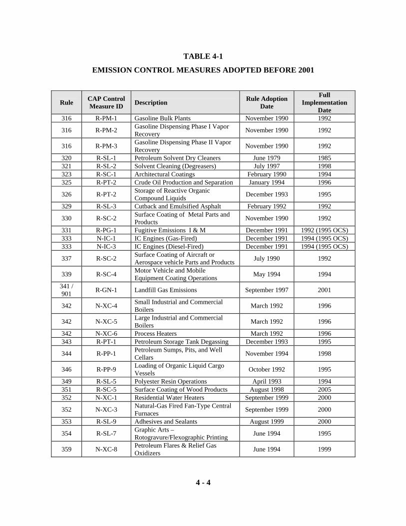
4 - 4
TABLE 4-1
EMISSION CONTROL MEASURES ADOPTED BEFORE 2001
Rule CAP Control Measure ID Description Rule Adoption
Date
Full Implementation
Date 316 R-PM-1 Gasoline Bulk Plants November 1990 1992
316 R-PM-2 Gasoline Dispensing Phase I Vapor Recovery November 1990 1992
316 R-PM-3 Gasoline Dispensing Phase II Vapor Recovery November 1990 1992
320 R-SL-1 Petroleum Solvent Dry Cleaners June 1979 1985 321 R-SL-2 Solvent Cleaning (Degreasers) July 1997 1998 323 R-SC-1 Architectural Coatings February 1990 1994 325 R-PT-2 Crude Oil Production and Separation January 1994 1996
326 R-PT-2 Storage of Reactive Organic Compound Liquids December 1993 1995
329 R-SL-3 Cutback and Emulsified Asphalt February 1992 1992
330 R-SC-2 Surface Coating of Metal Parts and Products November 1990 1992
331 R-PG-1 Fugitive Emissions I & M December 1991 1992 (1995 OCS) 333 N-IC-1 IC Engines (Gas-Fired) December 1991 1994 (1995 OCS) 333 N-IC-3 IC Engines (Diesel-Fired) December 1991 1994 (1995 OCS)
337 R-SC-2 Surface Coating of Aircraft or Aerospace vehicle Parts and Products July 1990 1992
339 R-SC-4 Motor Vehicle and Mobile Equipment Coating Operations May 1994 1994
341 / 901 R-GN-1 Landfill Gas Emissions September 1997 2001
342 N-XC-4 Small Industrial and Commercial Boilers March 1992 1996
342 N-XC-5 Large Industrial and Commercial Boilers March 1992 1996
342 N-XC-6 Process Heaters March 1992 1996 343 R-PT-1 Petroleum Storage Tank Degassing December 1993 1995
344 R-PP-1 Petroleum Sumps, Pits, and Well Cellars November 1994 1998
346 R-PP-9 Loading of Organic Liquid Cargo Vessels October 1992 1995
349 R-SL-5 Polyester Resin Operations April 1993 1994 351 R-SC-5 Surface Coating of Wood Products August 1998 2005 352 N-XC-1 Residential Water Heaters September 1999 2000
352 N-XC-3 Natural-Gas Fired Fan-Type Central Furnaces September 1999 2000
353 R-SL-9 Adhesives and Sealants August 1999 2000
354 R-SL-7 Graphic Arts – Rotogravure/Flexographic Printing June 1994 1995
359 N-XC-8 Petroleum Flares & Relief Gas Oxidizers June 1994 1999
4 - 5
As seen in Table 4-1, the APCD has adopted a wide range of control measures that reduced ROC
and NOx emissions both onshore and on the outer continental shelf.
4.4 EMISSION CONTROL MEASURES ADOPTED DURING THE REPORTING PERIOD (2001 - 2003)
The APCD is on schedule with adopting and implementing the proposed control measures
identified in the 2001 CAP, with the following exceptions:
• The modifications of control measures N-IC-1 and N-IC-3 (amended Rule 202, Permit
Exemptions, and amended Rule 333, Control of Emissions from Reciprocating Internal
Combustion Engines) has been delayed. The APCD anticipates accomplishing the
modifications to these control measures in the 2004 - 2006 term.
• The APCD decided to reclassify the proposed control measure (N-IC-2) for Gas-Fired
Turbines to be a further study control measure because the 2001 CAP identified no
emission reductions for the proposed measure.
During the 2001 - 2003 reporting period for this plan, the Board adopted modifications to Rule
323, Architectural Coatings, and the new Rule 360, Emissions of Oxide of Nitrogen from Large
Water Heaters and Small Boilers. The 2001 CAP identified the adoption of these proposed
control measures (R-SC-1 and N-XC-2) for the near-term period of 2001 - 2003 of the 2001
CAP.
Health and Safety Code Section 40924(b)(2) requires the APCD to identify the expected
emission reductions that were in the 2001 CAP and the current revised emission reductions for
each measure scheduled for adoption during the reporting period. Table 4-2 provides
information on the rules adopted during the 2001 to 2003 reporting period of this plan to fulfill
this requirement.
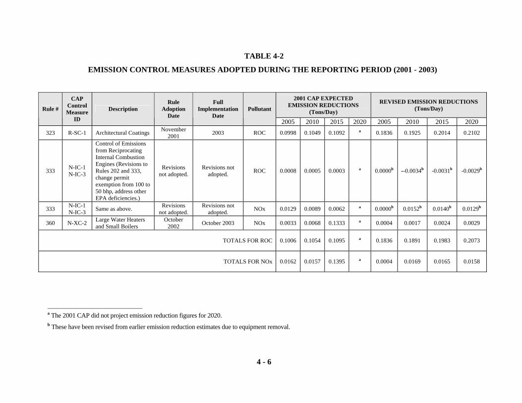
4 - 6
TABLE 4-2
EMISSION CONTROL MEASURES ADOPTED DURING THE REPORTING PERIOD (2001 - 2003)
2001 CAP EXPECTED EMISSION REDUCTIONS
(Tons/Day)
REVISED EMISSION REDUCTIONS (Tons/Day) Rule #
CAP Control Measure
ID
Description Rule
Adoption Date
Full Implementation
Date Pollutant
2005 2010 2015 2020 2005 2010 2015 2020 323 R-SC-1 Architectural Coatings November
2001 2003 ROC 0.0998 0.1049 0.1092 a 0.1836 0.1925 0.2014 0.2102
333 N-IC-1 N-IC-3
Control of Emissions from Reciprocating Internal Combustion Engines (Revisions to Rules 202 and 333, change permit exemption from 100 to 50 bhp, address other EPA deficiencies.)
Revisions not adopted.
Revisions not adopted. ROC 0.0008 0.0005 0.0003 a 0.0000b --0.0034b -0.0031b -0.0029b
333 N-IC-1 N-IC-3 Same as above. Revisions
not adopted. Revisions not
adopted. NOx 0.0129 0.0089 0.0062 a 0.0000b 0.0152b 0.0140b 0.0129b
360 N-XC-2 Large Water Heaters and Small Boilers
October 2002 October 2003 NOx 0.0033 0.0068 0.1333 a 0.0004 0.0017 0.0024 0.0029
TOTALS FOR ROC
0.1006 0.1054 0.1095 a 0.1836 0.1891 0.1983 0.2073
TOTALS FOR NOx
0.0162 0.0157 0.1395 a 0.0004 0.0169 0.0165 0.0158
a The 2001 CAP did not project emission reduction figures for 2020. b These have been revised from earlier emission reduction estimates due to equipment removal.
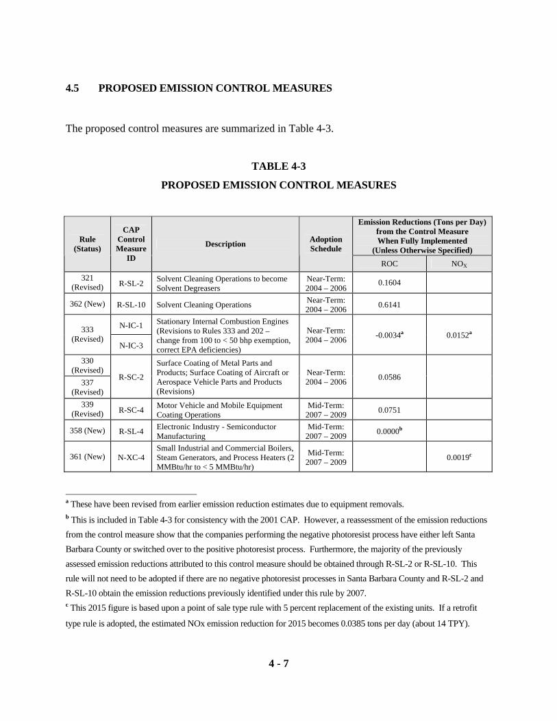
4 - 7
4.5 PROPOSED EMISSION CONTROL MEASURES
The proposed control measures are summarized in Table 4-3.
TABLE 4-3
PROPOSED EMISSION CONTROL MEASURES
Emission Reductions (Tons per Day)
from the Control Measure When Fully Implemented
(Unless Otherwise Specified) Rule
(Status)
CAP Control Measure
ID
Description Adoption Schedule
ROC NOX
321 (Revised) R-SL-2 Solvent Cleaning Operations to become
Solvent Degreasers Near-Term: 2004 – 2006
0.1604
362 (New) R-SL-10 Solvent Cleaning Operations Near-Term: 2004 – 2006 0.6141
N-IC-1 333 (Revised)
N-IC-3
Stationary Internal Combustion Engines (Revisions to Rules 333 and 202 – change from 100 to < 50 bhp exemption, correct EPA deficiencies)
Near-Term: 2004 – 2006 -0.0034a 0.0152a
330 (Revised)
337 (Revised)
R-SC-2
Surface Coating of Metal Parts and Products; Surface Coating of Aircraft or Aerospace Vehicle Parts and Products (Revisions)
Near-Term: 2004 – 2006 0.0586
339 (Revised) R-SC-4 Motor Vehicle and Mobile Equipment
Coating Operations Mid-Term:
2007 – 2009 0.0751
358 (New) R-SL-4 Electronic Industry - Semiconductor Manufacturing
Mid-Term: 2007 – 2009 0.0000b
361 (New) N-XC-4 Small Industrial and Commercial Boilers, Steam Generators, and Process Heaters (2 MMBtu/hr to < 5 MMBtu/hr)
Mid-Term: 2007 – 2009 0.0019c
a These have been revised from earlier emission reduction estimates due to equipment removals. b This is included in Table 4-3 for consistency with the 2001 CAP. However, a reassessment of the emission reductions from the control measure show that the companies performing the negative photoresist process have either left Santa Barbara County or switched over to the positive photoresist process. Furthermore, the majority of the previously assessed emission reductions attributed to this control measure should be obtained through R-SL-2 or R-SL-10. This rule will not need to be adopted if there are no negative photoresist processes in Santa Barbara County and R-SL-2 and R-SL-10 obtain the emission reductions previously identified under this rule by 2007. c This 2015 figure is based upon a point of sale type rule with 5 percent replacement of the existing units. If a retrofit
type rule is adopted, the estimated NOx emission reduction for 2015 becomes 0.0385 tons per day (about 14 TPY).
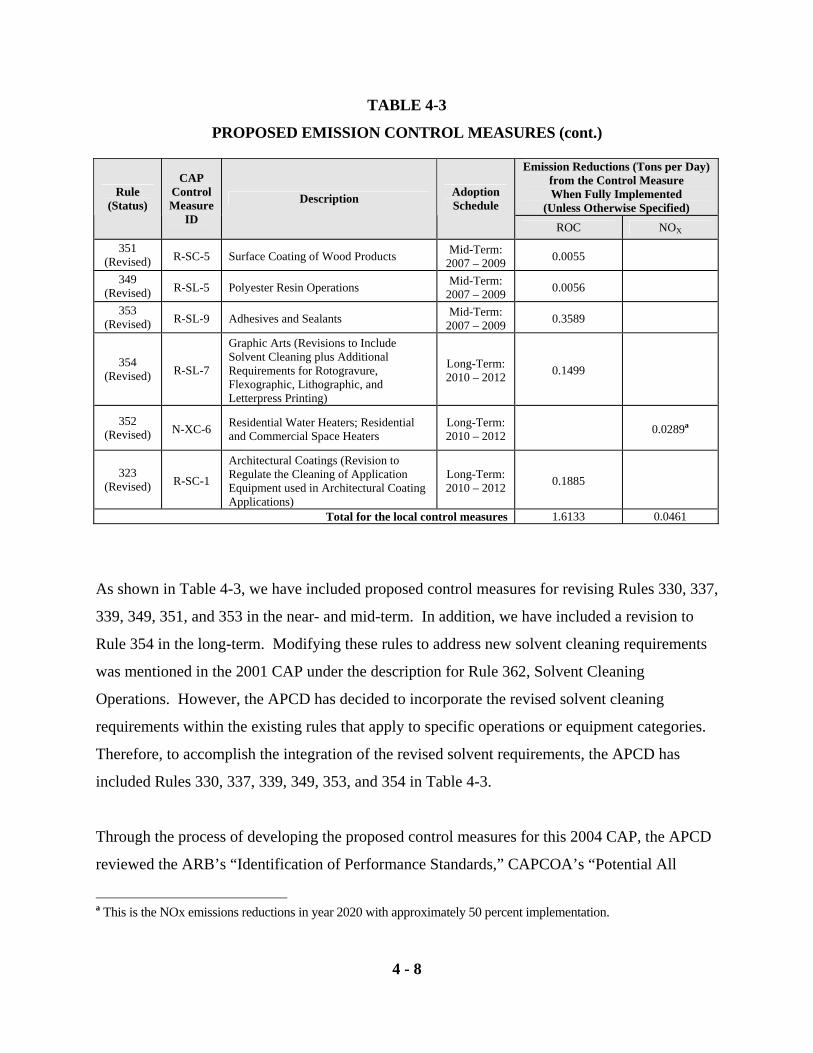
TABLE 4-3
PROPOSED EMISSION CONTROL MEASURES (cont.)
4 - 8
Emission Reductions (Tons per Day) from the Control Measure When Fully Implemented
(Unless Otherwise Specified) Rule
(Status)
CAP Control Measure
ID
Description Adoption Schedule
ROC NOX
351 (Revised) R-SC-5 Surface Coating of Wood Products Mid-Term:
2007 – 2009 0.0055
349 (Revised) R-SL-5 Polyester Resin Operations Mid-Term:
2007 – 2009 0.0056
353 (Revised) R-SL-9 Adhesives and Sealants Mid-Term:
2007 – 2009 0.3589
354 (Revised) R-SL-7
Graphic Arts (Revisions to Include Solvent Cleaning plus Additional Requirements for Rotogravure, Flexographic, Lithographic, and Letterpress Printing)
Long-Term: 2010 – 2012 0.1499
352 (Revised) N-XC-6 Residential Water Heaters; Residential
and Commercial Space Heaters Long-Term: 2010 – 2012 0.0289a
323 (Revised) R-SC-1
Architectural Coatings (Revision to Regulate the Cleaning of Application Equipment used in Architectural Coating Applications)
Long-Term: 2010 – 2012 0.1885
Total for the local control measures 1.6133 0.0461
a This is the NOx emissions reductions in year 2020 with approximately 50 percent implementation.
As shown in Table 4-3, we have included proposed control measures for revising Rules 330, 337,
339, 349, 351, and 353 in the near- and mid-term. In addition, we have included a revision to
Rule 354 in the long-term. Modifying these rules to address new solvent cleaning requirements
was mentioned in the 2001 CAP under the description for Rule 362, Solvent Cleaning
Operations. However, the APCD has decided to incorporate the revised solvent cleaning
requirements within the existing rules that apply to specific operations or equipment categories.
Therefore, to accomplish the integration of the revised solvent requirements, the APCD has
included Rules 330, 337, 339, 349, 353, and 354 in Table 4-3.
Through the process of developing the proposed control measures for this 2004 CAP, the APCD
reviewed the ARB’s “Identification of Performance Standards,” CAPCOA’s “Potential All
4 - 9
Feasible Measures,” and control measures adopted by other APCDs and AQMDs. Because of
the commitment to adopt control measures in the 2001 CAP, those measures are being carried
forward into this plan, with the addition of the rules mentioned above that contain solvent
cleaning requirement components. The 2001 CAP control measures are now listed in Table 4-3
as near-term or mid-term control measures.
As seen in Table 4-3, the following long-term control measures are being proposed for inclusion
into the plan:
1. Rule 354, R-SL-7, Graphic Arts – Staff propose revising the rule to be similar to the
South Coast AQMD Rule 1130, Graphic Arts, with the addition of the South Coast
AQMD Rule 1171, Solvent Cleaning Operations, solvent cleaning requirements
applicable to graphic arts operations. Notwithstanding that the 1991 AQAP identified
graphic arts as a proposed control measure, the APCD adopted the existing Rule 354 to
meet EPA reasonably available control technology requirements. The existing rule
resulted in very minimal emission reductions. A rule revision is necessary to raise the
requirements to an all feasible level of control.
The major changes would be to 1) increase the rule applicable to apply to lithographic
and letterpress printing, 2) eliminate the 300 pounds per month exemption, 3) establish
new standards for fountain solutions, adhesives, and porous flexographic printing ink, 4)
set a grams per liter limit on the cleaning of adhesive application equipment used in a
graphic arts operation, and 5) limit the grams per liter of solvent used for the cleaning of
various ink application equipment used in graphic arts operations. Concurrent with the
Rule 354 revision, the APCD will revise the Rule 202 permit exemptions to make the
printing exemptions similar to those in South Coast AQMD Rule 219.
2. Rule 352, N-XC-6, Natural Gas-Fired Fan-Type Central Furnaces and Residential Water
Heaters – The APCD proposes revising the rule to be similar to the South Coast AQMD
Rule 1121. This would result in decreasing the allowable NOx emissions for natural gas-
4 - 10
fired water heaters from 0.0930 to 0.0465 pounds per million British thermal units
(output). The rule will remain a point of sale type rule.
3. Rule 323, R-SC-1, Architectural Coatings – Staff propose a rule revision to incorporate
the South Coast AQMD Rule 1171 requirements for the cleaning of coatings application
equipment. This would result in use of low-ROC solvents for the cleaning of spray
application equipment.
4.6 EMISSION CONTROL MEASURES FOR FURTHER STUDY
Additional potential control measures and existing control measures that merit further study are
shown in Table 4-4 (Further Study – New Rules) and Table 4-5 (Further Study – Existing Rules).
Some of the further study control measures are being carried forward from the 2001 CAP.
Others were identified through reviews of the September 2003 CAPCOA, “Potential All Feasible
Measures Report,” the April 1999 CARB document, “Identification of Performance Standards,”
other APCD/AQMD rules, and Santa Barbara County Air Pollution Control District staff
suggestions.
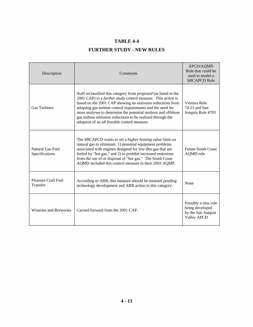
4 - 11
TABLE 4-4
FURTHER STUDY - NEW RULES
Description Comments
APCD/AQMD Rule that could be
used to model a SBCAPCD Rule
Gas Turbines
Staff reclassified this category from proposed (as listed in the 2001 CAP) to a further study control measure. This action is based on the 2001 CAP showing no emission reductions from adopting gas turbine control requirements and the need for more analyses to determine the potential onshore and offshore gas turbine emission reductions to be realized through the adoption of an all feasible control measure.
Ventura Rule 74.23 and San Joaquin Rule 4703
Natural Gas Fuel Specifications
The SBCAPCD wants to set a higher heating value limit on natural gas to eliminate: 1) potential equipment problems associated with engines designed for low-Btu gas that are fueled by "hot gas," and 2) to prohibit increased emissions from the use of or disposal of "hot gas." The South Coast AQMD included this control measure in their 2003 AQMP.
Future South Coast AQMD rule
Pleasure Craft Fuel Transfer
According to ARB, this measure should be retained pending technology development and ARB action in this category.
None
Wineries and Breweries Carried forward from the 2001 CAP.
Possibly a new rule being developed by the San Joaquin Valley APCD
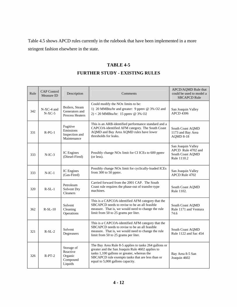
4 - 12
Table 4.5 shows APCD rules currently in the rulebook that have been implemented in a more
stringent fashion elsewhere in the state.
TABLE 4-5
FURTHER STUDY - EXISTING RULES
Rule CAP Control Measure ID Description Comments
APCD/AQMD Rule that could be used to model a
SBCAPCD Rule
342 N-XC-4 and N-XC-5
Boilers, Steam Generators and Process Heaters
Could modify the NOx limits to be: 1) 20 MMBtu/hr and greater: 9 ppmv @ 3% O2 and 2) < 20 MMBtu/hr: 15 ppmv @ 3% O2
San Joaquin Valley APCD 4306
331 R-PG-1
Fugitive Emissions Inspection and Maintenance
This is an ARB-identified performance standard and a CAPCOA-identified AFM category. The South Coast AQMD and Bay Area AQMD rules have lower thresholds for leaks.
South Coast AQMD 1173 and Bay Area AQMD 8-18
333 N-IC-3 IC Engines (Diesel-Fired)
Possibly change NOx limit for CI ICEs to 600 ppmv (or less).
San Joaquin Valley APCD Rule 4702 and South Coast AQMD Rule 1110.2
333 N-IC-1 IC Engines (Gas-Fired)
Possibly change NOx limit for cyclically-loaded ICEs from 300 to 50 ppmv.
San Joaquin Valley APCD Rule 4702
320 R-SL-1 Petroleum Solvent Dry Cleaners
Carried forward from the 2001 CAP. The South Coast rule requires the phase-out of transfer-type machines.
South Coast AQMD Rule 1102.
362 R-SL-10 Solvent Cleaning Operations
This is a CAPCOA-identified AFM category that the SBCAPCD needs to revise to be an all feasible measure. That is, we would need to change the rule limit from 50 to 25 grams per liter.
South Coast AQMD Rule 1171 and Ventura 74.6
321 R-SL-2 Solvent Degreasers
This is a CAPCOA-identified AFM category that the SBCAPCD needs to revise to be an all feasible measure. That is, we would need to change the rule limit from 50 to 25 grams per liter.
South Coast AQMD Rule 1122 and Sac 454
326 R-PT-2
Storage of Reactive Organic Compound Liquids
The Bay Area Rule 8-5 applies to tanks 264 gallons or greater and the San Joaquin Rule 4602 applies to tanks 1,100 gallons or greater, whereas the SBCAPCD rule exempts tanks that are less than or equal to 5,000 gallons capacity.
Bay Area 8-5 San Joaquin 4602
4 - 13
4.7 CONCLUSIONS
The APCD, SBCAG, county, cities, and ARB have developed a comprehensive air pollution
control strategy for Santa Barbara County. This strategy is updated in this 2004 CAP and
identifies every feasible measure available to make progress toward attainment of the state ozone
1-hour standard. Staff considered the ARB-identified performance standards, the CAPCOA-
identified potential all feasible measures, the commitments in the 2001 CAP, and other APCD
and AQMD rules to derive the proposed control measures and control measures for further study.
The 2004 CAP control measures include controls on all inventory categories contributing ROC
and NOx emissions: industrial processes, combustion sources, petroleum handling, solvent use,
consumer products, waste burning, and mobile sources. The control measures evaluated and
identified in this chapter, combined with the emissions reductions expected from on-road mobile
sources in Chapter 5, show that Santa Barbara County is making significant progress in reducing
emissions from sources subject to our control.
CHAPTER 5
TRANSPORTATION CONTROL MEASURES
Background
Historical Trends In Vehicle Activity
Transportation Control Measures
On-Road Mobile Source Emissions Analysis
Emission Results
Departures From EMFAC2002 Defaults
5 - 1
5. TRANSPORTATION CONTROL MEASURES
5.1 BACKGROUND
In June 1993, the boards of the Santa Barbara County Association of Governments and the Santa
Barbara County Air Pollution Control District jointly approved a Memorandum of
Understanding (MOU), which effectively placed the responsibility for developing the
transportation elements of the air quality plans with SBCAG. This MOU allows SBCAG to
assist the APCD in a cooperative effort towards meeting the APCD's responsibilities for
developing the transportation elements of its state and federal air quality plans. Under the MOU,
SBCAG is responsible for the development and analysis of the 2004 Plan on-road mobile source
emission estimates and transportation control measures (TCMs). SBCAG also provides the
APCD with socio-economic projections, which form the basis for many of the stationary and
area source growth forecasts for this 2004 Plan.
5.2 HISTORICAL TRENDS IN VEHICLE ACTIVITY
The State Act requires areas classified as having a "moderate" air quality classification for the state
one-hour ozone standard, such as Santa Barbara County, to track and meet the following
transportation performance standard: a substantial reduction in the rate of increase in passenger
vehicle trips and vehicle miles traveled (VMT).1 ARB has defined substantial reduction as holding
growth in VMT and trips to the same growth rate as population. For Santa Barbara County, this
would equate to reducing VMT growth rates by more than one half the growth rates experienced
during the 1980’s.
Figure 5-1 shows that the annual VMT growth rate since 1980 has been highly variable with many
peaks accompanied by negative growth occurring during the recession years of 1991 and 1995.
However, for 12 of the 16 years monitored since the passage of the California Clean Air Act in
1988, the annual VMT growth rate has exceeded the annual population growth rate in Santa Barbara
County. The figure also shows that the annual VMT growth rate over the last three years (2000-
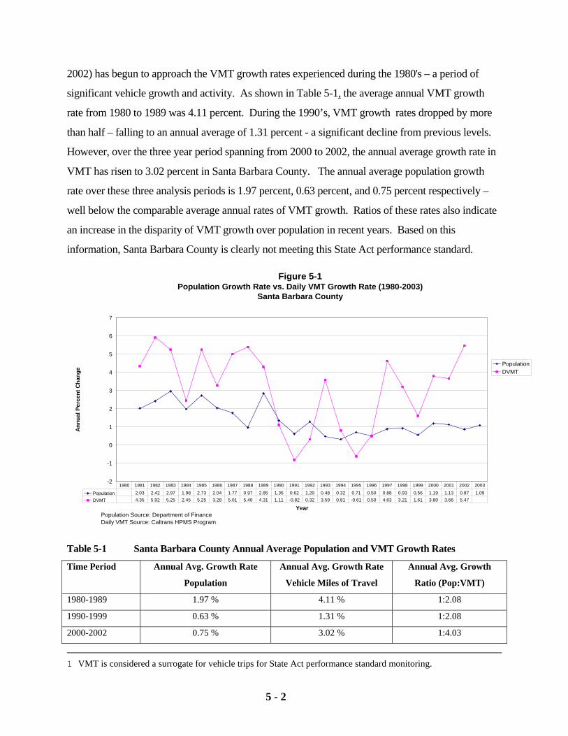
5 - 2
2002) has begun to approach the VMT growth rates experienced during the 1980's – a period of
significant vehicle growth and activity. As shown in Table 5-1, the average annual VMT growth
rate from 1980 to 1989 was 4.11 percent. During the 1990’s, VMT growth rates dropped by more
than half – falling to an annual average of 1.31 percent - a significant decline from previous levels.
However, over the three year period spanning from 2000 to 2002, the annual average growth rate in
VMT has risen to 3.02 percent in Santa Barbara County. The annual average population growth
rate over these three analysis periods is 1.97 percent, 0.63 percent, and 0.75 percent respectively –
well below the comparable average annual rates of VMT growth. Ratios of these rates also indicate
an increase in the disparity of VMT growth over population in recent years. Based on this
information, Santa Barbara County is clearly not meeting this State Act performance standard.
Figure 5-1Population Growth Rate vs. Daily VMT Growth Rate (1980-2003)
Santa Barbara County
-2
-1
0
1
2
3
4
5
6
7
Year
Ann
ual P
erce
nt C
hang
e
PopulationDVMT
Population 2.03 2.42 2.97 1.98 2.73 2.04 1.77 0.97 2.85 1.35 0.62 1.29 0.48 0.32 0.71 0.50 0.88 0.93 0.56 1.19 1.13 0.87 1.09DVMT 4.35 5.92 5.25 2.45 5.25 3.28 5.01 5.40 4.31 1.11 -0.82 0.32 3.59 0.81 -0.61 0.50 4.63 3.21 1.61 3.80 3.66 5.47
1980 1981 1982 1983 1984 1985 1986 1987 1988 1989 1990 1991 1992 1993 1994 1995 1996 1997 1998 1999 2000 2001 2002 2003
Population Source: Department of FinanceDaily VMT Source: Caltrans HPMS Program
Table 5-1 Santa Barbara County Annual Average Population and VMT Growth Rates
Time Period Annual Avg. Growth Rate
Population
Annual Avg. Growth Rate
Vehicle Miles of Travel
Annual Avg. Growth
Ratio (Pop:VMT)
1980-1989 1.97 % 4.11 % 1:2.08
1990-1999 0.63 % 1.31 % 1:2.08
2000-2002 0.75 % 3.02 % 1:4.03
1 VMT is considered a surrogate for vehicle trips for State Act performance standard monitoring.
5 - 3
5.3 TRANSPORTATION CONTROL MEASURES
TCMs are programs or activities that states and localities can implement to encourage the
traveling public to rely less on the automobile or to use the automobile more efficiently. TCMs
reduce emissions from on-road motor vehicles and trucks by: improving the existing
transportation system to allow motor vehicles to operate more efficiently; inducing people to
change their travel behavior to less polluting modes; or, ensuring emission control technology
improvements in the motor vehicle fleet are fully and expeditiously realized. TCMs address the
need for the traveling public to carefully consider: 1) the implications of continued reliance on
the single occupant vehicle as the major choice of commute trips; 2) the need to provide and
promote alternatives to single occupant vehicle travel; and, 3) the need to consider regulating
those factors which promote single occupant vehicle travel. While the greatest on-road mobile
source emission reductions (over 95 percent) are attributable to motor vehicle emission controls
established by federal and state laws and the natural attrition of older more polluting vehicles
(i.e., fleet turnover), TCMs should be considered as an integral part of air quality plans given
that they help meet multiple objectives (e.g., congestion relief, energy efficiency, etc.).
Table 5-2 summarizes the implementation characteristics of all currently adopted TCM
categories in the county. Identified are: the type of TCM; the adopting agency/agencies; the
agency/agencies responsible for implementing the TCM; the formal agreements between the
adopting and implementing agencies; and, how TCM implementation will be monitored and by
whom. All currently adopted TCMs except for T-18 (Alternative Fuels) are listed as TCMs by
EPA in Section 108(f) of the Federal Clean Air Act.
For state air quality planning purposes, control measures are classified as being adopted,
proposed, contingency, further study, or deleted. Adopted TCMs are those projects and
programs that the APCD has formally adopted and included in the federal State Implementation
Plan (SIP). These TCM projects/programs were developed as part the 1994 CAP and 1998 CAP
and are listed in Table 5-3 and Table 5-4 respectively. These measures meet the every feasible
control measure (Health and Safety Code, Section 40914(b)) provisions of the State Act.
All TCM's evaluated as part of the last triennial update (2001 CAP) are listed below.
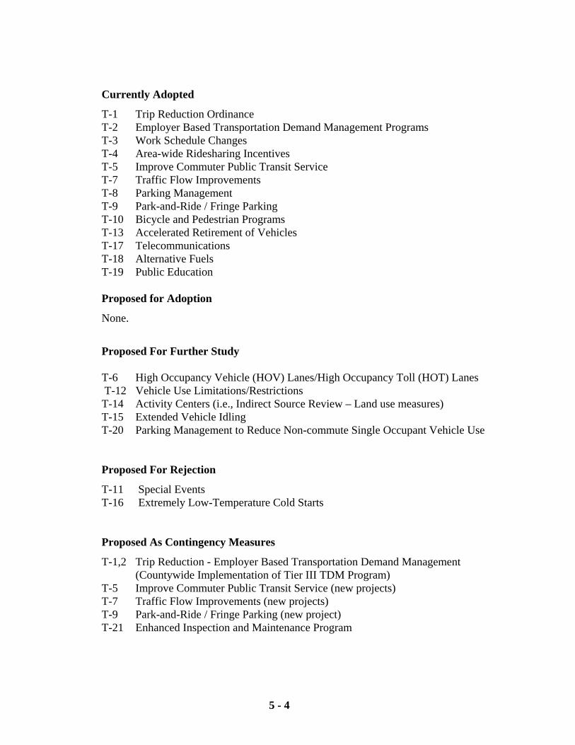
5 - 4
Currently Adopted
T-1 Trip Reduction Ordinance T-2 Employer Based Transportation Demand Management Programs T-3 Work Schedule Changes T-4 Area-wide Ridesharing Incentives T-5 Improve Commuter Public Transit Service T-7 Traffic Flow Improvements T-8 Parking Management T-9 Park-and-Ride / Fringe Parking T-10 Bicycle and Pedestrian Programs T-13 Accelerated Retirement of Vehicles T-17 Telecommunications T-18 Alternative Fuels
T-19 Public Education
Proposed for Adoption
None.
Proposed For Further Study T-6 High Occupancy Vehicle (HOV) Lanes/High Occupancy Toll (HOT) Lanes T-12 Vehicle Use Limitations/Restrictions T-14 Activity Centers (i.e., Indirect Source Review – Land use measures) T-15 Extended Vehicle Idling T-20 Parking Management to Reduce Non-commute Single Occupant Vehicle Use Proposed For Rejection
T-11 Special Events T-16 Extremely Low-Temperature Cold Starts Proposed As Contingency Measures
T-1,2 Trip Reduction - Employer Based Transportation Demand Management (Countywide Implementation of Tier III TDM Program)
T-5 Improve Commuter Public Transit Service (new projects) T-7 Traffic Flow Improvements (new projects) T-9 Park-and-Ride / Fringe Parking (new project) T-21 Enhanced Inspection and Maintenance Program
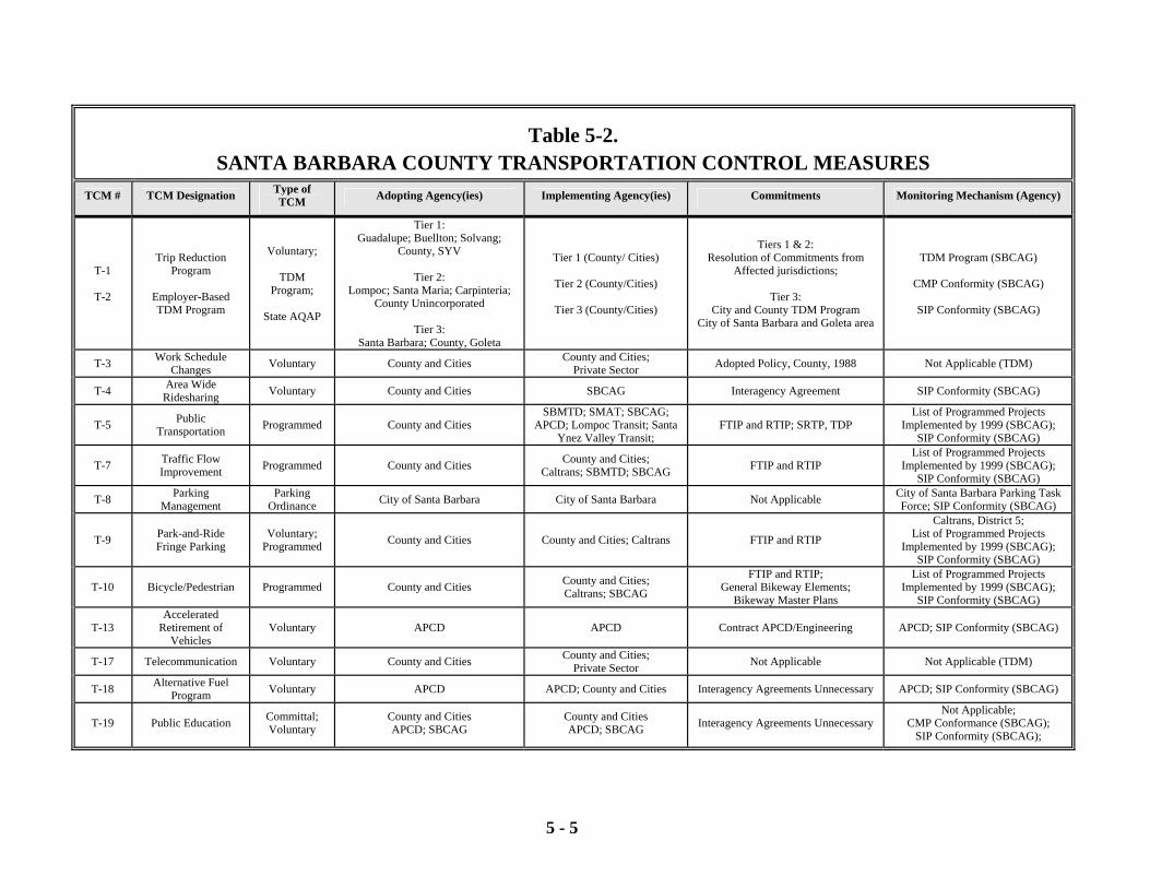
5 - 5
Table 5-2.
SANTA BARBARA COUNTY TRANSPORTATION CONTROL MEASURES TCM # TCM Designation Type of
TCM Adopting Agency(ies) Implementing Agency(ies) Commitments Monitoring Mechanism (Agency)
T-1
T-2
Trip Reduction Program
Employer-Based TDM Program
Voluntary;
TDM Program;
State AQAP
Tier 1: Guadalupe; Buellton; Solvang;
County, SYV
Tier 2: Lompoc; Santa Maria; Carpinteria;
County Unincorporated
Tier 3: Santa Barbara; County, Goleta
Tier 1 (County/ Cities)
Tier 2 (County/Cities)
Tier 3 (County/Cities)
Tiers 1 & 2: Resolution of Commitments from
Affected jurisdictions;
Tier 3: City and County TDM Program
City of Santa Barbara and Goleta area
TDM Program (SBCAG)
CMP Conformity (SBCAG)
SIP Conformity (SBCAG)
T-3 Work Schedule Changes Voluntary County and Cities County and Cities;
Private Sector Adopted Policy, County, 1988 Not Applicable (TDM)
T-4 Area Wide Ridesharing Voluntary County and Cities SBCAG Interagency Agreement SIP Conformity (SBCAG)
T-5 Public Transportation Programmed County and Cities
SBMTD; SMAT; SBCAG; APCD; Lompoc Transit; Santa
Ynez Valley Transit; FTIP and RTIP; SRTP, TDP
List of Programmed Projects Implemented by 1999 (SBCAG);
SIP Conformity (SBCAG)
T-7 Traffic Flow Improvement Programmed County and Cities County and Cities;
Caltrans; SBMTD; SBCAG FTIP and RTIP List of Programmed Projects
Implemented by 1999 (SBCAG); SIP Conformity (SBCAG)
T-8 Parking Management
Parking Ordinance City of Santa Barbara City of Santa Barbara Not Applicable City of Santa Barbara Parking Task
Force; SIP Conformity (SBCAG)
T-9 Park-and-Ride Fringe Parking
Voluntary; Programmed County and Cities County and Cities; Caltrans FTIP and RTIP
Caltrans, District 5; List of Programmed Projects
Implemented by 1999 (SBCAG); SIP Conformity (SBCAG)
T-10 Bicycle/Pedestrian Programmed County and Cities County and Cities; Caltrans; SBCAG
FTIP and RTIP; General Bikeway Elements;
Bikeway Master Plans
List of Programmed Projects Implemented by 1999 (SBCAG);
SIP Conformity (SBCAG)
T-13 Accelerated
Retirement of Vehicles
Voluntary APCD APCD Contract APCD/Engineering APCD; SIP Conformity (SBCAG)
T-17 Telecommunication Voluntary County and Cities County and Cities; Private Sector Not Applicable Not Applicable (TDM)
T-18 Alternative Fuel Program Voluntary APCD APCD; County and Cities Interagency Agreements Unnecessary APCD; SIP Conformity (SBCAG)
T-19 Public Education Committal; Voluntary
County and Cities APCD; SBCAG
County and Cities APCD; SBCAG Interagency Agreements Unnecessary
Not Applicable; CMP Conformance (SBCAG);
SIP Conformity (SBCAG);
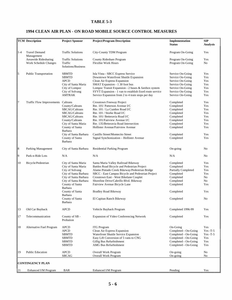
5 - 6
TABLE 5-3
1994 CLEAN AIR PLAN - ON ROAD MOBILE SOURCE CONTROL MEASURES
TCM Description Project Sponsor Project/Program Description Implementation SIP Status Analysis
1-4 Travel Demand Management
Traffic Solutions City-County TDM Program Program On-Going Yes
Areawide Ridesharing Traffic Solutions County Rideshare Program Program On-Going Yes Work Schedule Changes Traffic
Solutions/Business Flexibie Work Hours Program On-Going No
5 Public Transportation SBMTD Isla Vista - SBCC Express Service Service On-Going Yes
SBMTD Downtown Waterfront Shuttle Expansion Service On-Going Yes APCD Clean Air Express Expansion Service On-Going Yes City of Santa Maria SMAT Expansion - 1 30 foot bus Service On-Going Yes City of Lompoc Lompoc Transit Expansion - 2 buses & farebox system Service On-Going Yes City of Solvang SYVT Expansion - 1 van to establish fixed route service Service On-Going Yes AMTRAK Service Expansion from 2 to 4 train stops per day Service On-Going Yes
7 Traffic Flow Improvements Caltrans Crosstown Freeway Project Completed Yes County/Caltrans Rte. 101/ Patterson Avenue I/C Completed Yes SBCAG/Caltrans Rte. 101 / La Cumbre Road I/C Completed Yes SBCAG/Caltrans Rte. 101 / Storke Road I/C Completed Yes SBCAG/Caltrans Rte. 101/ Betteravia Road I/C Completed Yes County/Caltrans Rte. 101/Fairview Avenue I/C Completed Yes City of Santa Maria Rte. 135/Betteravia Road Intersection Completed Yes County of Santa
Barbara Hollister Avenue/Fairview Avenue Completed Yes
City of Santa Barbara Castillo Street/Montecito Street Completed Yes County of Santa
Barbara Signal Synchonization – Hollister Avenue Completed Yes
8 Parking Management City of Santa Barbara Residential Parking Program On-going No
9 Park-n-Ride Lots N/A N/A N/A No
10 Bicycle/Pedestrian City of Santa Maria Santa Maria Valley Railroad Bikeway Completed Yes
City of Santa Maria Battles Road Bicycle and Pedestrian Project Completed Yes City of Solvang Alamo Pintado Creek Bikeway/Pedestrian Bridge Partially Completed Yes City of Santa Barbara SBCC - East Campus Bicycle and Pedestrian Project Completed Yes City of Santa Barbara Crosstown East - West Bikelane Couplet Completed No City of Santa Barbara Shoreline Drive/Cabrillo Blvd. Bikeway Completed No County of Santa
Barbara Fairview Avenue Bicycle Lane Completed Yes
County of Santa Barbara
Bradley Road Bikeway Completed Yes
County of Santa Barbara
El Capitan Ranch Bikeway Completed No
13 Old Car Buyback APCD Vehicle Buyback Program Completed 1996-99 Yes
17 Telecommunication County of SB -
Probation Expansion of Video Conferencing Network Completed Yes
18 Alternative Fuel Program APCD ITG Program On-Going Yes
APCD Clean Air Express Expansion Completed - On-Going Yes -T-5 SBMTD Waterfront Shuttle Service Expansion Completed - On-Going Yes -T-5 SBMTD Easy Lift Conversion of 5 vans to CNG Completed - On-Going Yes SBMTD Gillig Bus Refurbishment Completed - On-Going Yes SBMTD AMG Bus Refurbishment Completed - On-Going Yes
19 Public Education APCD Overall Work Program On-going No SBCAG Overall Work Program On-going No
CONTINGENCY PLAN
21 Enhanced I/M Program BAR Enhanced I/M Program Pending Yes
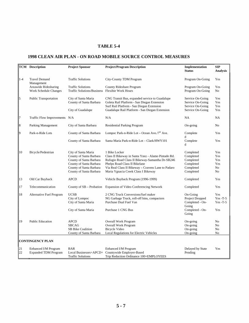
5 - 7
TABLE 5-4
1998 CLEAN AIR PLAN - ON ROAD MOBILE SOURCE CONTROL MEASURES
TCM Description Project Sponsor Project/Program Description Implementation SIP Status Analysis
1-4 Travel Demand Management
Traffic Solutions City-County TDM Program Program On-Going Yes
Areawide Ridesharing Traffic Solutions County Rideshare Program Program On-Going Yes Work Schedule Changes Traffic Solutions/Business Flexibie Work Hours Program On-Going No
5 Public Transportation City of Santa Maria CNG Transit Bus, expanded service to Guadalupe Service On-Going Yes County of Santa Barbara Goleta Rail Platform - San Diegan Extension Service On-Going Yes Surf Rail Platform - San Diegan Extension Service On-Going Yes City of Guadalupe Guadalupe Rail Platform - San Diegan Extension Service On-Going Yes
7 Traffic Flow Improvements N/A N/A NA NA
8 Parking Management City of Santa Barbara Residential Parking Program On-going No
9 Park-n-Ride Lots County of Santa Barbara Lompoc Park-n-Ride Lot – Ocean Ave./7th Ave. Completed
Yes
County of Santa Barbara Santa Maria Park-n-Ride Lot – Clark/HWY101 Completed
Yes
10 Bicycle/Pedestrian City of Santa Maria 1 Bike Locker Completed Yes
County of Santa Barbara Class II Bikeway in Santa Ynez - Alamo Pintado Rd. Completed Yes County of Santa Barbara Rufugio Road Class II Bikeway-Samantha Dr-SR246 Completed Yes County of Santa Barbara Phelps Road Class II Bikelane Completed Yes County of Santa Barbara Via Real Class II Bikeway – Cravens Lane to Padaro Completed No County of Santa Barbara Maria Ygnacia Creek Class I Bikeway Completed No
13 Old Car Buyback APCD Vehicle Buyback Program (1996-1999) Completed Yes
17 Telecommunication County of SB – Probation Expansion of Video Conferencing Network Completed Yes
18 Alternative Fuel Program UCSB 2 CNG Truck Conversions/fuel maker On-Going Yes City of Lompoc NG Garbage Truck, roll-off bins, compactors Project Dropped Yes -T-5 City of Santa Maria Purchase Dual Fuel Van Completed - On-
Going Yes -T-5
City of Santa Maria Purchase 1 CNG Bus Completed - On-Going
Yes
19 Public Education APCD Overall Work Program On-going No
SBCAG Overall Work Program On-going No SB Bike Coalition Bicycle Video On-going No County of Santa Barbara Local Regulations for Electric Vehicles On-going No
CONTINGENCY PLAN
21 Enhanced I/M Program BAR Enhanced I/M Program Delayed by State Yes 22 Expanded TDM Program Local Businesses+APCD+ Countywide Employer-Based Pending Traffic Solutions Trip Reduction Ordinance 100+EMPLOYEES
5 - 8
The TCM’s proposed for further study and as contingency measures under federal air quality
planning requirements (2001 Clean Air Plan) will form the basis for the 2004 CAP on-road
mobile source control strategy. Table 5-5 lists these measures and the process by which the
implementation feasibility will be assessed. The source of most measures included in Table 5-5
is the Highway 101 Deficiency Plan (SBCAG, June 2002). The potential air quality impacts of
the worsening Highway 101 congestion in the South Coast of Santa Barbara County was raised
as a major concern by the APCD’s Community Advisory Council and by members of the public
during the development of the 2001 CAP.
The Highway 101 Deficiency Plan is a multi-jurisdictional plan prepared as a result of the
growing congestion on Highway 101 within the South Coast (Ventura County Line to western
city limit of Goleta). The plan, adopted by local agencies and SBCAG, includes short-term
congestion relief improvements and commits the adopting agencies to complete the 101 In-
Motion Plan to provide long-term solutions to the growing congestion on Highway 101 within
the South Coast. The goal of the 101 In-Motion Plan is to thoroughly examine all the options
that will improve mobility on the South Coast for years to come rather than revisiting the
problem every funding cycle. It recognizes that no single option, including widening Highway
101, will solve the congestion problem for the long-term. The magnitude of the problem will
require a comprehensive plan with a range of both short and long term strategies to increase
vehicle capacity, reduce demand, improve management of the system, expand transportation
alternatives and change land use planning policies and decisions.
Exacerbating the demand for travel on Highway 101 in Santa Barbara County is the jobs-housing
imbalance that exists in the South Coast (Goleta, Santa Barbara, and Carpinteria) that serves to
foster long-distance commuting. The 2002 Commuter Survey funded by SBCAG was conducted
in order to provide an indication of the magnitude of intercity commute activity within Santa
Barbara County. This data indicates that 14 percent of the South Coast’s workforce comes from
Ventura County while another 11 percent drive from northern Santa Barbara County. This
suggests that well over 17,000 commuters are making long distance commutes to the South
Coast each weekday. Although now over ten-years old, 1990 Census data corroborates this
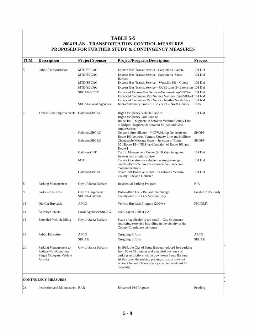
5 - 9
TABLE 5-5
2004 PLAN - TRANSPORTATION CONTROL MEASURES PROPOSED FOR FURTHER STUDY & CONTINGENCY MEASURES
TCM Description Project Sponsor Project/Program Description Process
5 Public Transportation MTD/SBCAG Express Bus Transit Service –Carpinteria–Goleta 101 Def
MTD/SBCAG Express Bus Transit Service –Carpinteria–Santa Barbara
101 Def
MTD/SBCAG Express Bus Transit Service – Westside SB – Goleta 101 Def MTD/SBCAG Express Bus Transit Service – UCSB Line 24 Extension 101 Def SBCAG/VCTC Enhanced Express Bus Service–Ventura–Carp/SB/Gol
Enhanced Commuter Rail Service Ventura Carp/SB/Gol Enhanced Commuter Rail Service North – South Cnty
101 Def 101 I-M 101 I-M
SBCAG/Local Agencies Inter-community Transit Bus Service – North County TDA
7 Traffic Flow Improvements Caltrans/SBCAG High Occupancy Vehicle Lane or High Occupancy Toll Lane on Route 101 – Segment 1: between Ventura County Line to Milpas. Segment 2: between Milpas and Glen Annie/Storke.
101 I-M
Caltrans/SBCAG Network Surveillance – CCTV&Loop Detectors on Route 101 between Ventura County Line and Hollister
SHOPP
Caltrans/SBCAG Changeable Message Signs – Junction of Route 101/Route 154 (N&S) and Junction of Route 101 and Route 1
SHOPP
Caltrans/CHP Traffic Management Center (in SLO) – integrated freeway and arterial control
101 Def
MTD Transit Operations – vehicle tracking/passenger counts/electronic fare collection/surveillance and /communications
101 Def
Caltrans/SBCAG Smart Call Boxes on Route 101 between Ventura County Line and Hollister
101 Def
8 Parking Management City of Santa Barbara Residential Parking Program N/A
9 Park-n-Ride Lots City of Carpinteria SBCAG/Caltrans
Park-n-Ride Lot – Bailard Interchange Countywide – SLO & Ventura Cnty
Funded 2005 Study
13 Old Car Buyback APCD Vehicle Buyback Program (2004+) ITG/DMV
14 Activity Centers Local Agencies/SBCAG See Chapter 7 2004 CAP
15 Extended Vehicle Idling City of Santa Barbara Scale of applicability too small – City Ordinance restricting extended bus idling in the vicinity of the County Courthouse continues.
19 Public Education APCD On-going Efforts APCD
SBCAG On-going Efforts SBCAG 20 Parking Management to
Reduce Non-Commute Single Occupant Vehicle Activity
City of Santa Barbara In 1999, the City of Santa Barbara reduced free parking from 90 to 75 minutes and extended the hours of parking restrictions within downtown Santa Barbara. At this time, the parking pricing structure does not account for vehicle occupancy (i.e., reduced cost for carpools).
CONTNGENCY MEASURES
21 Inspection and Maintenance BAR Enhanced I/M Program Pending
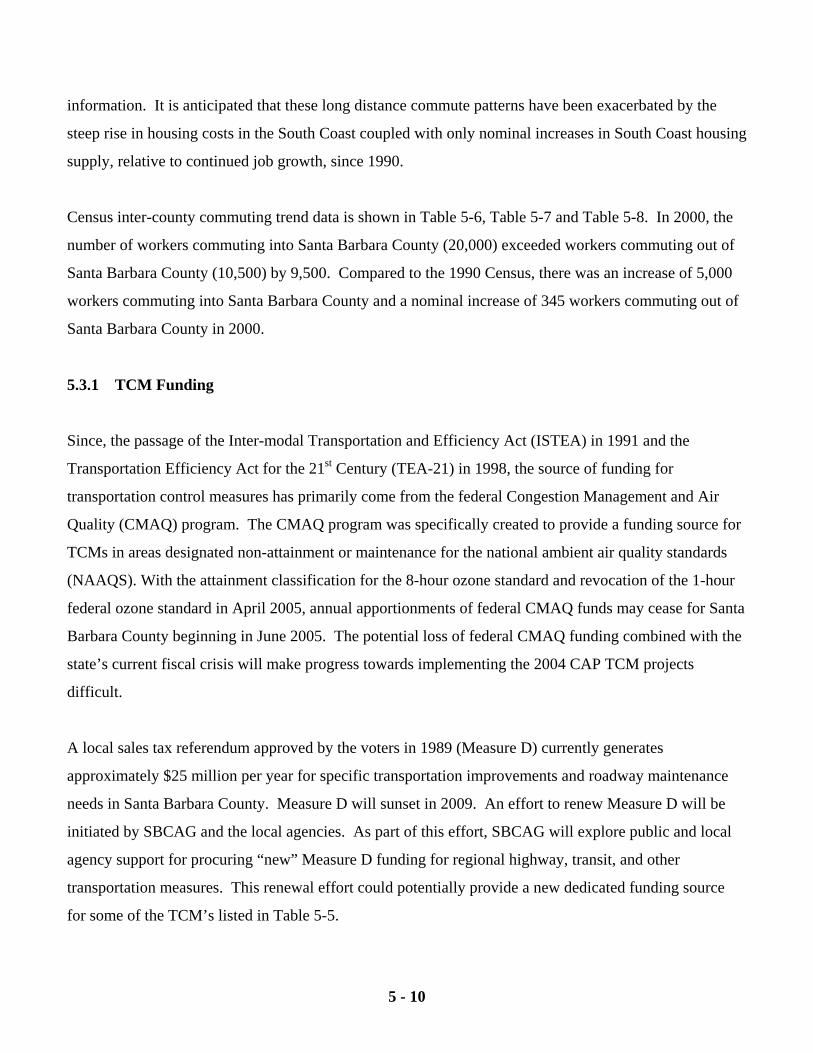
5 - 10
information. It is anticipated that these long distance commute patterns have been exacerbated by the
steep rise in housing costs in the South Coast coupled with only nominal increases in South Coast housing
supply, relative to continued job growth, since 1990.
Census inter-county commuting trend data is shown in Table 5-6, Table 5-7 and Table 5-8. In 2000, the
number of workers commuting into Santa Barbara County (20,000) exceeded workers commuting out of
Santa Barbara County (10,500) by 9,500. Compared to the 1990 Census, there was an increase of 5,000
workers commuting into Santa Barbara County and a nominal increase of 345 workers commuting out of
Santa Barbara County in 2000.
5.3.1 TCM Funding
Since, the passage of the Inter-modal Transportation and Efficiency Act (ISTEA) in 1991 and the
Transportation Efficiency Act for the 21st Century (TEA-21) in 1998, the source of funding for
transportation control measures has primarily come from the federal Congestion Management and Air
Quality (CMAQ) program. The CMAQ program was specifically created to provide a funding source for
TCMs in areas designated non-attainment or maintenance for the national ambient air quality standards
(NAAQS). With the attainment classification for the 8-hour ozone standard and revocation of the 1-hour
federal ozone standard in April 2005, annual apportionments of federal CMAQ funds may cease for Santa
Barbara County beginning in June 2005. The potential loss of federal CMAQ funding combined with the
state’s current fiscal crisis will make progress towards implementing the 2004 CAP TCM projects
difficult.
A local sales tax referendum approved by the voters in 1989 (Measure D) currently generates
approximately $25 million per year for specific transportation improvements and roadway maintenance
needs in Santa Barbara County. Measure D will sunset in 2009. An effort to renew Measure D will be
initiated by SBCAG and the local agencies. As part of this effort, SBCAG will explore public and local
agency support for procuring “new” Measure D funding for regional highway, transit, and other
transportation measures. This renewal effort could potentially provide a new dedicated funding source
for some of the TCM’s listed in Table 5-5.
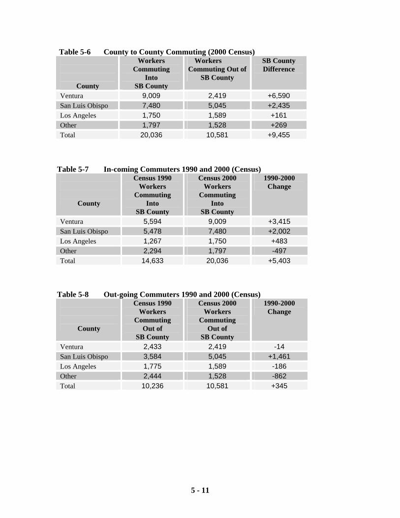
5 - 11
Table 5-6 County to County Commuting (2000 Census)
County
Workers Commuting
Into SB County
Workers Commuting Out of
SB County
SB County Difference
Ventura 9,009 2,419 +6,590 San Luis Obispo 7,480 5,045 +2,435 Los Angeles 1,750 1,589 +161 Other 1,797 1,528 +269 Total 20,036 10,581 +9,455
Table 5-7 In-coming Commuters 1990 and 2000 (Census)
County
Census 1990 Workers
Commuting Into
SB County
Census 2000 Workers
Commuting Into
SB County
1990-2000 Change
Ventura 5,594 9,009 +3,415 San Luis Obispo 5,478 7,480 +2,002 Los Angeles 1,267 1,750 +483 Other 2,294 1,797 -497 Total 14,633 20,036 +5,403
Table 5-8 Out-going Commuters 1990 and 2000 (Census)
County
Census 1990 Workers
Commuting Out of
SB County
Census 2000 Workers
Commuting Out of
SB County
1990-2000 Change
Ventura 2,433 2,419 -14 San Luis Obispo 3,584 5,045 +1,461 Los Angeles 1,775 1,589 -186 Other 2,444 1,528 -862 Total 10,236 10,581 +345
5 - 12
5.4 ON-ROAD MOBILE SOURCE EMISSIONS ANALYSIS
On-road emission estimates for this 2004 Plan were analyzed, in aggregate, using the ARB EMFAC2002
on-road emissions model. On-road mobile source emission forecasts were generated using the
EMFAC2002 model for 2000 (baseline year), 2005, 2010, 2015 and 2020. The transportation activity
data (e.g., regional vehicle miles of travel (VMT), regional vehicle trips, and VMT by speed class
distributions) generated by SBCAG’s Santa Barbara Travel Model provided the basis for the on-road
mobile source emission estimates contained in this plan. For the 2000 and 2010 emission forecasts, on-
road activity data was interpolated from the 1999, 2005 and 2015 model forecasts.
5.4.1 On-Road Activity Data Inputs
Table 5-9 lists the transportation and emissions modeling assumptions of the 2004 CAP on-road mobile
source emissions analysis.
Table 5-9 2004 CAP On-Road Mobile Source Activity Modeling Assumptions
Modeling Assumptions Information Source Socio-economic growth assumptions
(Housing & Employment)
1994 Regional Growth Forecast
(1990-2015) (SBCAG) Vehicle Activity Forecasts
(LDA, LDT, MDT, MCY)
Santa Barbara Travel Model - SYSTEM2
(1999, 2005, 2015) (SBCAG)
Vehicle Activity Forecasts
(HDDT, HDGT, UB, SBUS)
EMFAC2002 v2.2 April 03 (ARB)
ARB Default Activity
Infrastructure Improvements &
Schedules – Travel Model Networks
Programmed/Planned Projects–2002 FTIP SBCAG
2001 RTP SBCAG
VMT by Speed Class Distributions
(LDA, LDT, MDT, MCY)
Santa Barbara Travel Model - SYSTEM2
(1999, 2005, 2015) (SBCAG)
VMT by Speed Class Distributions
(HDDT, HDGT, UB, SBUS)
EMFAC2002 v2.2 April 03 (ARB)
ARB Default Activity
Emission Model EMFAC2002 v2.2 April 03 (ARB)
Vehicle Type/Technology and
Demographic Distributions
EMFAC2002 v2.2 April 03 (ARB/DMV)
5 - 13
Since 2001, SBCAG has been in the process of updating the Santa Barbara Travel Model using the
TRANSCAD software developed by Caliper Corporation. Although SBCAG anticipates completion and
of the model base year and forecasts by mid 2004, the need for a comprehensive review process of these
modeling products by SBCAG, Caltrans and ARB will preclude the use of the model in time for this
triennial update. In lieu of using the new travel model, past modeling performed by SBCAG using the
SYSTEM2 software was relied upon to provide the on-road activity data inputs (countywide VMT,
vehicle trips, and VMT by speed class distribution (SCD)) for this 2004 CAP.
The last modeling products produced by the SYSTEM2 model were a 1999 (base year) and 2005, 2015,
and 2020 forecasts. These modeling products were used for the transportation air quality conformity
assessments of SBCAG’s 2001 Regional Transportation Plan (RTP), SBCAG’s 2002 Federal
Transportation Improvement Programs (FTIP), and the 2001 Clean Air Plan (CAP). The coded
transportation networks for each forecast scenario reflect road improvement projects identified in the
2001 RTP and 2002 FTIP. Which model year scenarios (i.e., 2005, 2015 and 2020) include particular
projects was based on programmed and planned project scope and schedule information known at the
time of the 2002 FTIP. Table 5-10 and Table 5-11 include all regionally significant infrastructure
improvement projects currently programmed and planned in Santa Barbara County respectively. As a
result of the state fiscal crises and its impact on the flow of state transportation funds – some project
sponsors may have difficulty delivering projects consistent with modeling performed as part of the 2002
FTIP and 2001 RTP.
The socio-economic inputs (employment and households) that form the basis for the transportation model
used in the SYSTEM2 model were based on the SBCAG’s 1994 Regional Growth Forecast (RGF). The
1994 RGF forecasts population, housing, and employment growth in Santa Barbara County out to 2015.
The 2002 RGF, adopted March 2002, resulted in updates to the countywide forecasts for population,
housing, and employment. Table 5-12 provides a comparison for the socio-economic forecasts between
the 1994 RGF and the 2002 RGF. Differences between the forecasts for population, housing and
employment range between +/- one to four percent with the largest percent differences occurring in the
2015 out year. Although underestimating population and housing by four percent in 2015 is not
insignificant, it well within the error limitations of network travel models. Hence, use of the 1994 RGF is
considered reasonable for generating on-road activity estimates for emissions modeling.
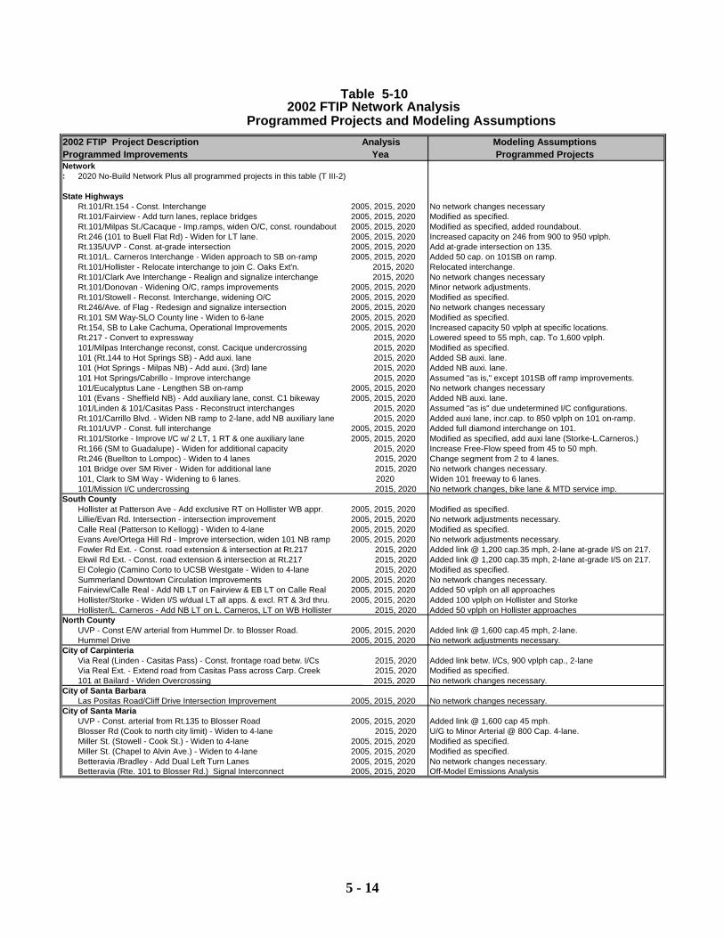
5 - 14
2002 FTIP Project Description Analysis Modeling AssumptionsProgrammed Improvements Yea Programmed ProjectsNetwork: 2020 No-Build Network Plus all programmed projects in this table (T III-2)
State Highways Rt.101/Rt.154 - Const. Interchange 2005, 2015, 2020 No network changes necessary Rt.101/Fairview - Add turn lanes, replace bridges 2005, 2015, 2020 Modified as specified. Rt.101/Milpas St./Cacaque - Imp.ramps, widen O/C, const. roundabout 2005, 2015, 2020 Modified as specified, added roundabout. Rt.246 (101 to Buell Flat Rd) - Widen for LT lane. 2005, 2015, 2020 Increased capacity on 246 from 900 to 950 vplph.Rt.135/UVP - Const. at-grade intersection 2005, 2015, 2020 Add at-grade intersection on 135. Rt.101/L. Carneros Interchange - Widen approach to SB on-ramp 2005, 2015, 2020 Added 50 cap. on 101SB on ramp. Rt.101/Hollister - Relocate interchange to join C. Oaks Ext'n. 2015, 2020 Relocated interchange. Rt.101/Clark Ave Interchange - Realign and signalize interchange 2015, 2020 No network changes necessary Rt.101/Donovan - Widening O/C, ramps improvements 2005, 2015, 2020 Minor network adjustments. Rt.101/Stowell - Reconst. Interchange, widening O/C 2005, 2015, 2020 Modified as specified. Rt.246/Ave. of Flag - Redesign and signalize intersection 2005, 2015, 2020 No network changes necessary Rt.101 SM Way-SLO County line - Widen to 6-lane 2005, 2015, 2020 Modified as specified. Rt.154, SB to Lake Cachuma, Operational Improvements 2005, 2015, 2020 Increased capacity 50 vplph at specific locations.Rt.217 - Convert to expressway 2015, 2020 Lowered speed to 55 mph, cap. To 1,600 vplph.
101/Milpas Interchange reconst, const. Cacique undercrossing 2015, 2020 Modified as specified. 101 (Rt.144 to Hot Springs SB) - Add auxi. lane 2015, 2020 Added SB auxi. lane.101 (Hot Springs - Milpas NB) - Add auxi. (3rd) lane 2015, 2020 Added NB auxi. lane.101 Hot Springs/Cabrillo - Improve interchange 2015, 2020 Assumed "as is," except 101SB off ramp improvements.101/Eucalyptus Lane - Lengthen SB on-ramp 2005, 2015, 2020 No network changes necessary 101 (Evans - Sheffield NB) - Add auxiliary lane, const. C1 bikeway 2005, 2015, 2020 Added NB auxi. lane.101/Linden & 101/Casitas Pass - Reconstruct interchanges 2015, 2020 Assumed "as is" due undetermined I/C configurations.Rt.101/Carrillo Blvd. - Widen NB ramp to 2-lane, add NB auxiliary lane 2015, 2020 Added auxi lane, incr.cap. to 850 vplph on 101 on-ramp.Rt.101/UVP - Const. full interchange 2005, 2015, 2020 Added full diamond interchange on 101. Rt.101/Storke - Improve I/C w/ 2 LT, 1 RT & one auxiliary lane 2005, 2015, 2020 Modified as specified, add auxi lane (Storke-L.Carneros.)Rt.166 (SM to Guadalupe) - Widen for additional capacity 2015, 2020 Increase Free-Flow speed from 45 to 50 mph.Rt.246 (Buellton to Lompoc) - Widen to 4 lanes 2015, 2020 Change segment from 2 to 4 lanes. 101 Bridge over SM River - Widen for additional lane 2015, 2020 No network changes necessary. 101, Clark to SM Way - Widening to 6 lanes. 2020 Widen 101 freeway to 6 lanes. 101/Mission I/C undercrossing 2015, 2020 No network changes, bike lane & MTD service imp.
South County Hollister at Patterson Ave - Add exclusive RT on Hollister WB appr. 2005, 2015, 2020 Modified as specified. Lillie/Evan Rd. Intersection - intersection improvement 2005, 2015, 2020 No network adjustments necessary. Calle Real (Patterson to Kellogg) - Widen to 4-lane 2005, 2015, 2020 Modified as specified. Evans Ave/Ortega Hill Rd - Improve intersection, widen 101 NB ramp 2005, 2015, 2020 No network adjustments necessary. Fowler Rd Ext. - Const. road extension & intersection at Rt.217 2015, 2020 Added link @ 1,200 cap.35 mph, 2-lane at-grade I/S on 217.Ekwil Rd Ext. - Const. road extension & intersection at Rt.217 2015, 2020 Added link @ 1,200 cap.35 mph, 2-lane at-grade I/S on 217.El Colegio (Camino Corto to UCSB Westgate - Widen to 4-lane 2015, 2020 Modified as specified. Summerland Downtown Circulation Improvements 2005, 2015, 2020 No network changes necessary. Fairview/Calle Real - Add NB LT on Fairview & EB LT on Calle Real 2005, 2015, 2020 Added 50 vplph on all approaches Hollister/Storke - Widen I/S w/dual LT all apps. & excl. RT & 3rd thru. 2005, 2015, 2020 Added 100 vplph on Hollister and Storke Hollister/L. Carneros - Add NB LT on L. Carneros, LT on WB Hollister 2015, 2020 Added 50 vplph on Hollister approaches
North County UVP - Const E/W arterial from Hummel Dr. to Blosser Road. 2005, 2015, 2020 Added link @ 1,600 cap.45 mph, 2-lane. Hummel Drive 2005, 2015, 2020 No network adjustments necessary.
City of Carpinteria Via Real (Linden - Casitas Pass) - Const. frontage road betw. I/Cs 2015, 2020 Added link betw. I/Cs, 900 vplph cap., 2-laneVia Real Ext. - Extend road from Casitas Pass across Carp. Creek 2015, 2020 Modified as specified. 101 at Bailard - Widen Overcrossing 2015, 2020 No network changes necessary.
City of Santa Barbara Las Positas Road/Cliff Drive Intersection Improvement 2005, 2015, 2020 No network changes necessary.
City of Santa Maria UVP - Const. arterial from Rt.135 to Blosser Road 2005, 2015, 2020 Added link @ 1,600 cap 45 mph. Blosser Rd (Cook to north city limit) - Widen to 4-lane 2015, 2020 U/G to Minor Arterial @ 800 Cap. 4-lane. Miller St. (Stowell - Cook St.) - Widen to 4-lane 2005, 2015, 2020 Modified as specified. Miller St. (Chapel to Alvin Ave.) - Widen to 4-lane 2005, 2015, 2020 Modified as specified. Betteravia /Bradley - Add Dual Left Turn Lanes 2005, 2015, 2020 No network changes necessary. Betteravia (Rte. 101 to Blosser Rd.) Signal Interconnect 2005, 2015, 2020 Off-Model Emissions Analysis
Programmed Projects and Modeling Assumptions 2002 FTIP Network Analysis
Table 5-10
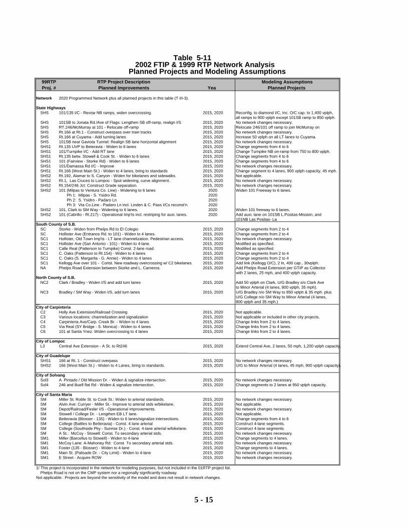
5 - 15
99RTP RTP Project Description Modeling Assumptions Proj. # Planned Improvements Yea Planned Projects
Network 2020 Programmed Network plus all planned projects in this table (T III-3).
State Highways SHS 101/135 I/C - Revise NB ramps, widen overcrossing. 2015, 2020 Reconfig. to diamond I/C, Inc. O/C cap. to 1,400 vplph,
all ramps to 900 vplph except 101SB ramp to 850 vplph.SHS 101SB to Jonata Rd./Ave of Flags: Lengthen SB off-ramp, realign I/S 2015, 2020 No network changes necessary. SHS RT.246/McMurray at 101 - Relocate off-ramp 2015, 2020 Relocate 246/101 off ramp to join McMurray on SHS Rt.166 at Rt.1 - Construct overpass over train tracks 2015, 2020 No network changes necessary. SHS Rt.166 at Cuyama - Add turning lanes 2015, 2020 Increase 50 vplph on all LT lanes to Cuyama. SHS 101SB near Gaviota Tunnel: Realign SB lane horizontal alignment 2015, 2020 No network changes necessary. SHS1 Rt.135 UVP to Beteravia - Widen to 6 lanes 2015, 2020 Change segments from 4 to 6 SHS1 101/Turnpike I/C - Add RT lane 2015, 2020 Change Turnpike NB on-ramp from 750 to 800 vplph.SHS1 Rt.135 betw. Stowell & Cook St. - Widen to 6 lanes 2015, 2020 Change segments from 4 to 6 SHS1 101 (Fairview - Storke Rd) - Widen to 6 lanes
2015, 2020 Change segments from 4 to 6
SHS1 101/Damassa Rd I/C - Improve 2015, 2020 No network changes necessary. SHS1 Rt.166 (West Main St.) - Widen to 4 lanes, bring to standards 2015, 2020 Change segment to 4 lanes, 900 vplph capacity, 45 mph.SHS2 Rt.192, Alamar to S. Canyon - Widen for bikelanes and sidewalks. 2015, 2020 Not applicable.SHS2 Rt.1, Las Cruces to Lompoc - Spot widening, curve alignment. 2015, 2020 No network changes necessary. SHS2 Rt.154/246 Jct: Construct Grade separation. 2015, 2020 No network changes necessary. SHS2 101 (Milpas to Ventura Co. Line) - Widening to 6 lanes 2020 Widen 101 Freeway to 6 lanes.
Ph 1: Milpas - S. Ysidro Rd. 2020 Ph 2: S. Ysidro - Padaro Ln 2020 Ph 3: Vta Co.Line - Padaro Ln incl. Linden & C. Pass I/Cs reconst'n. 2020
SHS2 101, Clark to SM Way - Widening to 6 lanes. 2020 Widen 101 freeway to 6 lanes. SHS2 101 (Cabrillo - Rt.217) - Operational Imp'ts incl. restriping for auxi. lanes. 2020 Add auxi. lane on 101SB L.Positas-Mission, and
101NB Las Positas- La South County of S.B.
SC Storke - Widen from Phelps Rd to El Colegio 2015, 2020 Change segments from 2 to 4 SC Hollister Ave (Entrance Rd. to 101) - Widen to 4 lanes. 2015, 2020 Change segments from 2 to 4 SC1 Hollister, Old Town Imp'ts - LT lane channelization. Pedestrian access. 2015, 2020 No network changes necessary. SC1 Hollister Ave (San Antonio - 101) - Widen to 4-lane. 2015, 2020 Modified as specified.SC1 Calle Real (Patterson to Turnpike) Const. 2-lane road. 2015, 2020 Modified as specified.SC1 C. Oaks (Patterson to Rt.154) - Widen to 4 lanes 2015, 2020 Change segments from 2 to 4 SC1 C. Oaks (S. Margarita - G. Annie) - Widen to 4 lanes 2015, 2020 Change segments from 2 to 4 SC1 Kellogg Ave over 101 - Const. New roadway overcrossing w/ C2 bikelanes. 2015, 2020 Add link (Kellogg O/C), 2 ln, 400 cap., 30vplph. NA Phelps Road Extension between Storke and L. Carneros. 2015, 2020 Add Phelps Road Extension per GTIP as Collector
with 2 lanes, 25 mph, and 400 vplph capacity. North County of S.B.
NC2 Clark / Bradley - Widen I/S and add turn lanes 2015, 2020 Add 50 vplph on Clark, U/G Bradley s/o Clark Ave
to Minor Arterial (4 lanes, 800 vplph, 35 mph). NC3 Bradley / SM Way - Widen I/S, add turn lanes 2015, 2020 U/G Bradley n/o SM Way to 850 vplph & 35 mph. plus
U/G College n/o SM Way to Minor Arterial (4 lanes, 800 vplph and 35 mph.)
City of Carpinteria C2 Holly Ave Extension/Railroad Crossing 2015, 2020 Not applicable.C3 Various locations: channelization and signalization 2015, 2020 Not applicable or included in other city projects. C4 Carpinteria Ave/Carp. Creek Br. - Widen to 4 lanes 2015, 2020 Change links from 2 to 4 lanes. C5 Via Real (SY Bridge - S. Monica) - Widen to 4 lanes 2015, 2020 Change links from 2 to 4 lanes. C6 101 at Santa Ynez: Widen overcrossing to 4 lanes 2015, 2020 Change links from 2 to 4 lanes.
City of Lompoc L3 Central Ave Extension - A St. to Rt246
2015, 2020 Extend Central Ave, 2 lanes, 50 mph, 1,200 vplph capacity.
City of Guadelupe SHS1 166 at Rt. 1 - Construct overpass
2015, 2020 No network changes necessary.
SHS2 166 (West Main St.) - Widen to 4 Lanes, bring to standards.
2015, 2020 U/G to Minor Arterial (4 lanes, 45 mph, 900 vplph capacity).
City of Solvang Sol3 A. Pintado / Old Mission Dr. - Widen & signalize intersection. 2015, 2020 No network changes necessary. Sol4 246 and Buell flat Rd - Widen & signalize intersection. 2015, 2020 Change segments to 2 lanes at 950 vplph capacity.
City of Santa Maria SM Miller St. Roble St. to Cook St.: Widen to arterial standards. 2015, 2020 No network changes necessary. SM Alvin Ave: Curryer - Miller St.- Improve to arterial stds w/bikelane. 2015, 2020 Not applicable.SM Depot/Railroad/Fesler I/S - Operational improvements. 2015, 2020 No network changes necessary. SM Stowell / College Dr. - Lengthen EB LT lane. 2015, 2020 Not applicable.SM Betteravia (Blosser - 135) - Widen to 6 lanes/signalize intersections. 2015, 2020 Change segments from 4 to 6 SM College (Battles to Betteravia) - Const. 4 lane arterial 2015, 2020 Construct 4-lane segments.SM College (Southside Pky - Sunrise Dr.) - Const. 4-lane arterial w/bikelane. 2015, 2020 Construct 4-lane segments.SM A St.: McCoy - Stowell: Const. To secondary arterial stds. 2015, 2020 No network changes necessary. SM1 Miller (Barcellus to Stowell) - Widen to 4-lane 2015, 2020 Change segments to 4 lanes. SM1 McCoy Lane: A-Mahoney Rd: Const. To secondary arterial stds. 2015, 2020 No network changes necessary. SM1 Foster (135 - Blosser) - Widen to 4-lane 2015, 2020 Change segments to 4 lanes. SM1 Main St. (Palisade Dr. - City Limit) - Widen to 4-lane 2015, 2020 No network changes necessary. SM1 E Street - Acquire ROW 2015, 2020 No network changes necessary.
1/ This project is incorporated in the network for modeling purposes, but not included in the 01RTP project list.
Phelps Road is not on the CMP system nor a regionally significantly roadway.Not applicable: Projects are beyond the sensitivity of the model and does not result in network changes.
2002 FTIP & 1999 RTP Network AnalysisPlanned Projects and Modeling Assumptions
Table 5-11
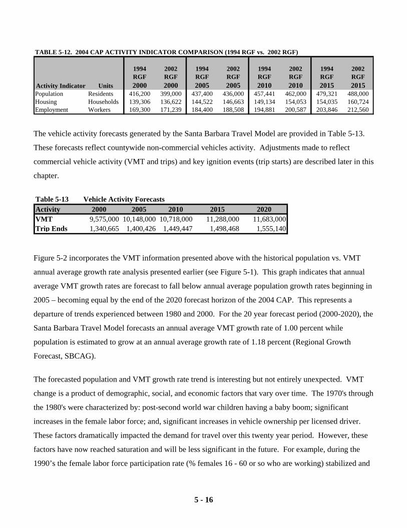
5 - 16
TABLE 5-12. 2004 CAP ACTIVITY INDICATOR COMPARISON (1994 RGF vs. 2002 RGF)
1994 2002 1994 2002 1994 2002 1994 2002RGF RGF RGF RGF RGF RGF RGF RGF
Activity Indicator Units 2000 2000 2005 2005 2010 2010 2015 2015Population Residents 416,200 399,000 437,400 436,000 457,441 462,000 479,321 488,000Housing Households 139,306 136,622 144,522 146,663 149,134 154,053 154,035 160,724Employment Workers 169,300 171,239 184,400 188,508 194,881 200,587 203,846 212,560 The vehicle activity forecasts generated by the Santa Barbara Travel Model are provided in Table 5-13.
These forecasts reflect countywide non-commercial vehicles activity. Adjustments made to reflect
commercial vehicle activity (VMT and trips) and key ignition events (trip starts) are described later in this
chapter.
Figure 5-2 incorporates the VMT information presented above with the historical population vs. VMT
annual average growth rate analysis presented earlier (see Figure 5-1). This graph indicates that annual
average VMT growth rates are forecast to fall below annual average population growth rates beginning in
2005 – becoming equal by the end of the 2020 forecast horizon of the 2004 CAP. This represents a
departure of trends experienced between 1980 and 2000. For the 20 year forecast period (2000-2020), the
Santa Barbara Travel Model forecasts an annual average VMT growth rate of 1.00 percent while
population is estimated to grow at an annual average growth rate of 1.18 percent (Regional Growth
Forecast, SBCAG).
The forecasted population and VMT growth rate trend is interesting but not entirely unexpected. VMT
change is a product of demographic, social, and economic factors that vary over time. The 1970's through
the 1980's were characterized by: post-second world war children having a baby boom; significant
increases in the female labor force; and, significant increases in vehicle ownership per licensed driver.
These factors dramatically impacted the demand for travel over this twenty year period. However, these
factors have now reached saturation and will be less significant in the future. For example, during the
1990’s the female labor force participation rate (% females 16 - 60 or so who are working) stabilized and
Table 5-13 Vehicle Activity Forecasts Activity 2000 2005 2010 2015 2020VMT 9,575,000 10,148,000 10,718,000 11,288,000 11,683,000 Trip Ends 1,340,665 1,400,426 1,449,447 1,498,468 1,555,140
5 - 17
has probably reached its peak; the post WWII baby boom generation has had their children; and, the
number of vehicles per licensed driver is near or at 1.0. Hence, it has been postulated by transportation
researchers that in the absence of “new” demographic and/or socio-economic changes, VMT growth in
the future should track more closely with overall population growth.
Social factors emerged in the 1990’s that impacted travel. Given the increase in dual income families,
more vehicle trips resulted (e.g., two working parents requiring two work trips instead of one; an added
trip to the day care center; a trip to the gym on the way to or from work etc.). Another potential factor in
future demand is the change in ethnic composition. At this time, change in ethnic composition and its
impact on travel is not well understood. The emergence of the Hispanic population can be seen in
elementary school enrollment data. This ethnic age cohort will age and turn into licensed drivers, but
their driving characteristics may differ from the past drivers that were dominated by the white ethnic
group. At this time, travel forecasting models do not account for ethnicity and its impact on travel
behavior.
Another economic trend that is impacting travel demand in Santa Barbara County is the high cost of
housing in the South Coast. With median housing costs over $1,000,000, many workers in the South
Coast are opting to buy more affordable homes in northern Santa Barbara County or Ventura County –
living further from the worksite and increasing VMT. The U.S. Census indicates that between 1990 and
2000, Santa Barbara County experienced approximately a 20 percent increase in the number of
commuters who must travel 30 minutes or more from within or to Santa Barbara County for work2. The
resulting jobs-housing imbalance that these housing costs have fostered may be a contributing factor to
VMT growth rates remaining twice as high as population growth between 1980 and 2000 and more
recently (2000-2002) four times higher (See Table 5-1).
As stated earlier, SBCAG will be updating the Santa Barbara Travel Model. Although the “new” travel
model would not be completed in time for this triennial update – it will be available for the next State Act
triennial update. Updated travel forecasts generated by the new model will replace those used for this
2004 CAP. These updated travel forecasts will result in different forecasted annual VMT growth rates
than those reported in the 2004 CAP.
2 This estimate includes inter-county commuting into Santa Barbara County from outside counties (e.g., Los Angeles, Ventura and San Luis Obispo) and implicitly assumes that these inter-county commutes require 30 minutes or more to achieve.
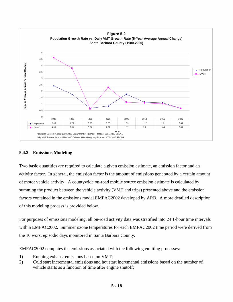
5 - 18
Figure 5-2Population Growth Rate vs. Daily VMT Growth Rate (5-Year Average Annual Change)
Santa Barbara County (1980-2020)
0
0.5
1
1.5
2
2.5
3
3.5
4
4.5
5
Year
5-Ye
ar A
vera
ge A
nnua
l Per
cent
Cha
nge
Population
DVMT
Population 2.43 1.79 0.68 0.85 1.79 1.17 1.1 0.69
DVMT 4.63 3.81 0.64 2.32 1.17 1.1 1.04 0.69
1985 1990 1995 2000 2005 2010 2015 2020
Population Source: Actual 1980-2000 Department of Finance; Forecast 2005-2020 SBCAGDaily VMT Source: Actual 1980-2000 Caltrans HPMS Program; Forecast 2005-2020 SBCAG
5.4.2 Emissions Modeling
Two basic quantities are required to calculate a given emission estimate, an emission factor and an
activity factor. In general, the emission factor is the amount of emissions generated by a certain amount
of motor vehicle activity. A countywide on-road mobile source emission estimate is calculated by
summing the product between the vehicle activity (VMT and trips) presented above and the emission
factors contained in the emissions model EMFAC2002 developed by ARB. A more detailed description
of this modeling process is provided below.
For purposes of emissions modeling, all on-road activity data was stratified into 24 1-hour time intervals
within EMFAC2002. Summer ozone temperatures for each EMFAC2002 time period were derived from
the 10 worst episodic days monitored in Santa Barbara County.
EMFAC2002 computes the emissions associated with the following emitting processes:
1) Running exhaust emissions based on VMT; 2) Cold start incremental emissions and hot start incremental emissions based on the number of
vehicle starts as a function of time after engine shutoff;
5 - 19
3) Diurnal emissions based on numbers of vehicles; 4) Hot soak emissions based on total numbers of vehicle starts; 5) Evaporative running losses based on VMT; and, 6) Resting loss emissions based on numbers of vehicles.
Depending on the activity data used, EMFAC2002 will produce two types of inventories, an annual
average inventory or a planning inventory. This 2004 Plan is based on a summer ozone season (April to
October) average daily emissions planning inventory. The latter is based on meteorological and activity
conditions that exist during peak episodic conditions for a given pollutant.
ARB distributions were used to allocate VMT and vehicle trips into 24 1-hour EMFAC2002 time periods.
To compute running emissions, each time period's VMT total was stratified into 13 speed classes (0 - 65
in 5 mile increments) and by vehicle classification. Hence, for the 13 vehicle classifications modeled by
EMFAC2002, there are 24 VMT by Speed Class Distributions (SCD), one for each time period.
The emissions associated with vehicle starts are accounted for in the EMFAC2002 model based on the
distribution of vehicle starts by vehicle classification, vehicle technology class, and operating mode. This
allows the model to compute emissions associated with vehicle starts and evaporative processes (for
ROC). EMFAC2002 adds these vehicle start and evaporative emissions to running emissions to compute
total on-road mobile source emissions.
As required by the EMFAC2002 model, vehicle trips were stratified into the following 13 vehicle
classifications: Light Duty Auto (LDA); Light Duty Truck (LDT1 & LDT2); Medium Duty Truck
(MDT); Light-Heavy Duty Truck (LHDT1 & LHDT2); Medium-Heavy Duty Truck (MHDT); Heavy-
Heavy Duty Truck (HHDT); Urban Bus (UB); School Bus (SBUS); Mobile Home (MH); Motorcycle
(MCY); and, Line Haul Vehicles (LHV – currently not used). The distribution of each vehicle by age
(model year), operating mode (e.g., cold start, hot start), and technology class (e.g. catalytic, non-
catalytic, diesel) was based on the most recent ARB distributions for Santa Barbara County. Vehicle age
distributions were based on 2000-2001 vehicle registration data for Santa Barbara County.
The EMFAC2002 activity data summaries for the 2000 baseline, and the 2005, 2010, 2015 and 2020
forecasts are provided in Table 5-14 through 5-18 respectively.
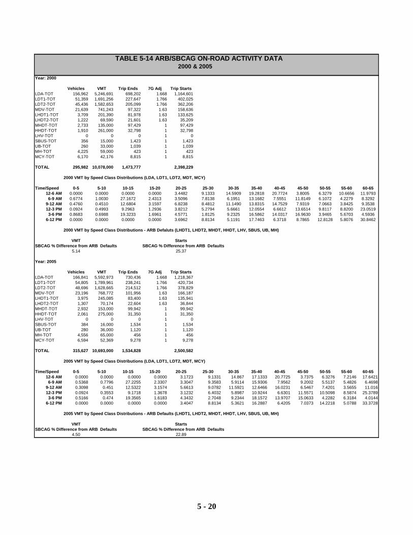
5 - 20
TABLE 5-14 ARB/SBCAG ON-ROAD ACTIVITY DATA 2000 & 2005
Year: 2000
Vehicles VMT Trip Ends 7G Adj Trip StartsLDA-TOT 156,962 5,246,691 698,202 1.668 1,164,601LDT1-TOT 51,359 1,691,256 227,647 1.766 402,025LDT2-TOT 45,436 1,582,653 205,099 1.766 362,206MDV-TOT 21,639 741,243 97,322 1.63 158,636LHDT1-TOT 3,709 201,390 81,978 1.63 133,625LHDT2-TOT 1,222 69,590 21,601 1.63 35,209MHDT-TOT 2,733 135,000 97,429 1 97,429HHDT-TOT 1,910 261,000 32,798 1 32,798LHV-TOT 0 0 0 1 0SBUS-TOT 356 15,000 1,423 1 1,423UB-TOT 260 33,000 1,039 1 1,039MH-TOT 4,225 59,000 423 1 423MCY-TOT 6,170 42,176 8,815 1 8,815
TOTAL 295,982 10,078,000 1,473,777 2,398,229
2000 VMT by Speed Class Distributions (LDA, LDT1, LDT2, MDT, MCY)
Time/Speed 0-5 5-10 10-15 15-20 20-25 25-30 30-35 35-40 40-45 45-50 50-55 55-60 60-6512-6 AM 0.0000 0.0000 0.0000 0.0000 3.4482 9.1333 14.5909 19.2818 20.7724 3.8005 6.3279 10.6656 11.97936-9 AM 0.6774 1.0030 27.1672 2.4313 3.5096 7.8138 6.1951 13.1682 7.5551 11.8149 6.1072 4.2279 8.3292
9-12 AM 0.4760 0.4510 12.6804 3.1597 6.8238 8.4812 11.1490 13.8315 14.7529 7.9319 7.0663 3.8425 9.353812-3 PM 0.0924 0.4993 9.2963 1.2936 3.8212 5.2794 5.6661 12.0554 6.6612 13.6514 9.8117 8.8200 23.0519
3-6 PM 0.8683 0.6988 19.3233 1.6961 4.5771 1.8125 9.2325 16.5862 14.0317 16.9630 3.9465 5.6703 4.59366-12 PM 0.0000 0.0000 0.0000 0.0000 3.6962 8.8134 5.1191 17.7463 6.3718 8.7865 12.8128 5.8076 30.8462
2000 VMT by Speed Class Distributions - ARB Defaluts (LHDT1, LHDT2, MHDT, HHDT, LHV, SBUS, UB, MH)
VMT StartsSBCAG % Difference from ARB Defaults SBCAG % Difference from ARB Defaults
5.14 25.37
Year: 2005
Vehicles VMT Trip Ends 7G Adj Trip StartsLDA-TOT 166,841 5,592,973 730,436 1.668 1,218,367LDT1-TOT 54,805 1,789,961 238,241 1.766 420,734LDT2-TOT 48,696 1,628,665 214,512 1.766 378,829MDV-TOT 23,196 768,772 101,956 1.63 166,187LHDT1-TOT 3,975 245,085 83,400 1.63 135,941LHDT2-TOT 1,307 70,174 22,604 1.63 36,844MHDT-TOT 2,932 153,000 99,942 1 99,942HHDT-TOT 2,061 275,000 31,350 1 31,350LHV-TOT 0 0 0 1 0SBUS-TOT 384 16,000 1,534 1 1,534UB-TOT 280 36,000 1,120 1 1,120MH-TOT 4,556 65,000 456 1 456MCY-TOT 6,594 52,369 9,278 1 9,278
TOTAL 315,627 10,693,000 1,534,828 2,500,582
2005 VMT by Speed Class Distributions (LDA, LDT1, LDT2, MDT, MCY)
Time/Speed 0-5 5-10 10-15 15-20 20-25 25-30 30-35 35-40 40-45 45-50 50-55 55-60 60-6512-6 AM 0.0000 0.0000 0.0000 0.0000 3.1723 9.1331 14.867 17.1333 20.7725 3.7375 6.3276 7.2146 17.64216-9 AM 0.5368 0.7796 27.2255 2.3307 3.3047 9.3583 5.9114 15.9306 7.9562 9.2002 5.5137 5.4826 6.4698
9-12 AM 0.3098 0.451 12.5322 3.1574 5.6613 9.0782 11.5921 12.6466 16.0231 6.5467 7.4201 3.5655 11.01612-3 PM 0.0924 0.3553 9.1718 1.3678 3.1232 6.4032 5.8987 10.9244 6.6301 11.5571 10.5098 8.5874 25.3789
3-6 PM 0.5166 0.474 19.3565 1.6183 4.3432 2.7048 9.2344 18.1572 13.9707 15.0633 4.2282 6.3184 4.01446-12 PM 0.0000 0.0000 0.0000 0.0000 3.4047 8.8134 5.3621 16.2887 6.4205 7.0373 14.2218 5.0788 33.3728
2005 VMT by Speed Class Distributions - ARB Defaults (LHDT1, LHDT2, MHDT, HHDT, LHV, SBUS, UB, MH)
VMT StartsSBCAG % Difference from ARB Defaults SBCAG % Difference from ARB Defaults
4.50 22.89
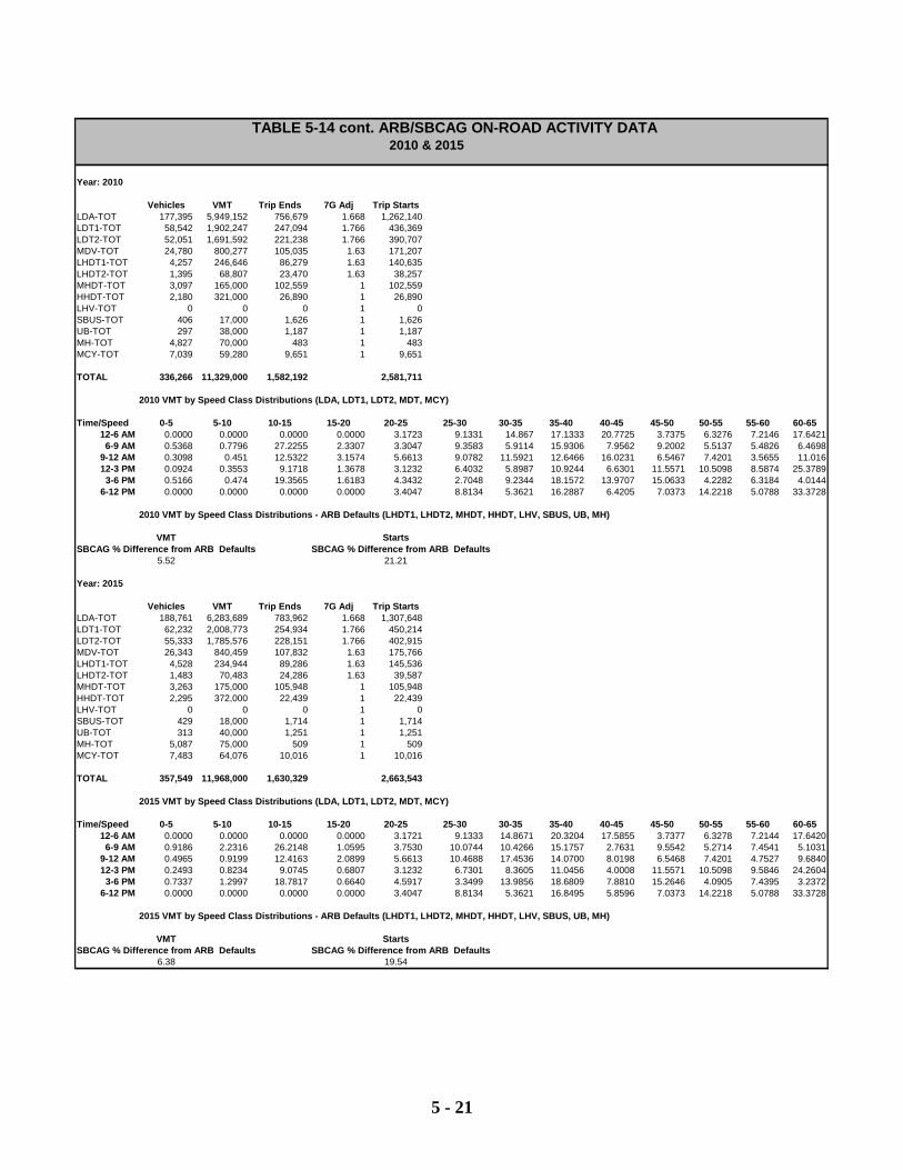
5 - 21
TABLE 5-14 cont. ARB/SBCAG ON-ROAD ACTIVITY DATA 2010 & 2015
Year: 2010
Vehicles VMT Trip Ends 7G Adj Trip StartsLDA-TOT 177,395 5,949,152 756,679 1.668 1,262,140LDT1-TOT 58,542 1,902,247 247,094 1.766 436,369LDT2-TOT 52,051 1,691,592 221,238 1.766 390,707MDV-TOT 24,780 800,277 105,035 1.63 171,207LHDT1-TOT 4,257 246,646 86,279 1.63 140,635LHDT2-TOT 1,395 68,807 23,470 1.63 38,257MHDT-TOT 3,097 165,000 102,559 1 102,559HHDT-TOT 2,180 321,000 26,890 1 26,890LHV-TOT 0 0 0 1 0SBUS-TOT 406 17,000 1,626 1 1,626UB-TOT 297 38,000 1,187 1 1,187MH-TOT 4,827 70,000 483 1 483MCY-TOT 7,039 59,280 9,651 1 9,651
TOTAL 336,266 11,329,000 1,582,192 2,581,711
2010 VMT by Speed Class Distributions (LDA, LDT1, LDT2, MDT, MCY)
Time/Speed 0-5 5-10 10-15 15-20 20-25 25-30 30-35 35-40 40-45 45-50 50-55 55-60 60-6512-6 AM 0.0000 0.0000 0.0000 0.0000 3.1723 9.1331 14.867 17.1333 20.7725 3.7375 6.3276 7.2146 17.64216-9 AM 0.5368 0.7796 27.2255 2.3307 3.3047 9.3583 5.9114 15.9306 7.9562 9.2002 5.5137 5.4826 6.4698
9-12 AM 0.3098 0.451 12.5322 3.1574 5.6613 9.0782 11.5921 12.6466 16.0231 6.5467 7.4201 3.5655 11.01612-3 PM 0.0924 0.3553 9.1718 1.3678 3.1232 6.4032 5.8987 10.9244 6.6301 11.5571 10.5098 8.5874 25.3789
3-6 PM 0.5166 0.474 19.3565 1.6183 4.3432 2.7048 9.2344 18.1572 13.9707 15.0633 4.2282 6.3184 4.01446-12 PM 0.0000 0.0000 0.0000 0.0000 3.4047 8.8134 5.3621 16.2887 6.4205 7.0373 14.2218 5.0788 33.3728
2010 VMT by Speed Class Distributions - ARB Defaults (LHDT1, LHDT2, MHDT, HHDT, LHV, SBUS, UB, MH)
VMT StartsSBCAG % Difference from ARB Defaults SBCAG % Difference from ARB Defaults
5.52 21.21
Year: 2015
Vehicles VMT Trip Ends 7G Adj Trip StartsLDA-TOT 188,761 6,283,689 783,962 1.668 1,307,648LDT1-TOT 62,232 2,008,773 254,934 1.766 450,214LDT2-TOT 55,333 1,785,576 228,151 1.766 402,915MDV-TOT 26,343 840,459 107,832 1.63 175,766LHDT1-TOT 4,528 234,944 89,286 1.63 145,536LHDT2-TOT 1,483 70,483 24,286 1.63 39,587MHDT-TOT 3,263 175,000 105,948 1 105,948HHDT-TOT 2,295 372,000 22,439 1 22,439LHV-TOT 0 0 0 1 0SBUS-TOT 429 18,000 1,714 1 1,714UB-TOT 313 40,000 1,251 1 1,251MH-TOT 5,087 75,000 509 1 509MCY-TOT 7,483 64,076 10,016 1 10,016
TOTAL 357,549 11,968,000 1,630,329 2,663,543
2015 VMT by Speed Class Distributions (LDA, LDT1, LDT2, MDT, MCY)
Time/Speed 0-5 5-10 10-15 15-20 20-25 25-30 30-35 35-40 40-45 45-50 50-55 55-60 60-6512-6 AM 0.0000 0.0000 0.0000 0.0000 3.1721 9.1333 14.8671 20.3204 17.5855 3.7377 6.3278 7.2144 17.64206-9 AM 0.9186 2.2316 26.2148 1.0595 3.7530 10.0744 10.4266 15.1757 2.7631 9.5542 5.2714 7.4541 5.1031
9-12 AM 0.4965 0.9199 12.4163 2.0899 5.6613 10.4688 17.4536 14.0700 8.0198 6.5468 7.4201 4.7527 9.684012-3 PM 0.2493 0.8234 9.0745 0.6807 3.1232 6.7301 8.3605 11.0456 4.0008 11.5571 10.5098 9.5846 24.2604
3-6 PM 0.7337 1.2997 18.7817 0.6640 4.5917 3.3499 13.9856 18.6809 7.8810 15.2646 4.0905 7.4395 3.23726-12 PM 0.0000 0.0000 0.0000 0.0000 3.4047 8.8134 5.3621 16.8495 5.8596 7.0373 14.2218 5.0788 33.3728
2015 VMT by Speed Class Distributions - ARB Defaults (LHDT1, LHDT2, MHDT, HHDT, LHV, SBUS, UB, MH)
VMT StartsSBCAG % Difference from ARB Defaults SBCAG % Difference from ARB Defaults
6.38 19.54
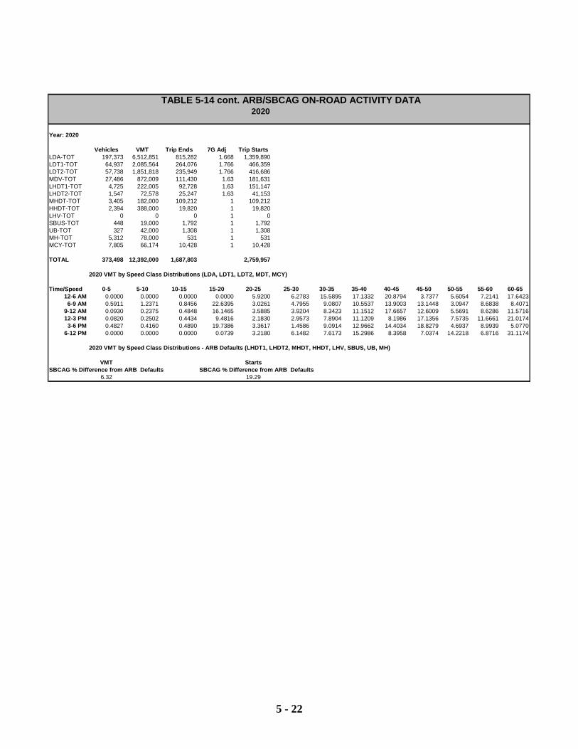
5 - 22
TABLE 5-14 cont. ARB/SBCAG ON-ROAD ACTIVITY DATA2020
Year: 2020
Vehicles VMT Trip Ends 7G Adj Trip StartsLDA-TOT 197,373 6,512,851 815,282 1.668 1,359,890LDT1-TOT 64,937 2,085,564 264,076 1.766 466,359LDT2-TOT 57,738 1,851,818 235,949 1.766 416,686MDV-TOT 27,486 872,009 111,430 1.63 181,631LHDT1-TOT 4,725 222,005 92,728 1.63 151,147LHDT2-TOT 1,547 72,578 25,247 1.63 41,153MHDT-TOT 3,405 182,000 109,212 1 109,212HHDT-TOT 2,394 388,000 19,820 1 19,820LHV-TOT 0 0 0 1 0SBUS-TOT 448 19,000 1,792 1 1,792UB-TOT 327 42,000 1,308 1 1,308MH-TOT 5,312 78,000 531 1 531MCY-TOT 7,805 66,174 10,428 1 10,428
TOTAL 373,498 12,392,000 1,687,803 2,759,957
2020 VMT by Speed Class Distributions (LDA, LDT1, LDT2, MDT, MCY)
Time/Speed 0-5 5-10 10-15 15-20 20-25 25-30 30-35 35-40 40-45 45-50 50-55 55-60 60-6512-6 AM 0.0000 0.0000 0.0000 0.0000 5.9200 6.2783 15.5895 17.1332 20.8794 3.7377 5.6054 7.2141 17.64236-9 AM 0.5911 1.2371 0.8456 22.6395 3.0261 4.7955 9.0807 10.5537 13.9003 13.1448 3.0947 8.6838 8.4071
9-12 AM 0.0930 0.2375 0.4848 16.1465 3.5885 3.9204 8.3423 11.1512 17.6657 12.6009 5.5691 8.6286 11.571612-3 PM 0.0820 0.2502 0.4434 9.4816 2.1830 2.9573 7.8904 11.1209 8.1986 17.1356 7.5735 11.6661 21.0174
3-6 PM 0.4827 0.4160 0.4890 19.7386 3.3617 1.4586 9.0914 12.9662 14.4034 18.8279 4.6937 8.9939 5.07706-12 PM 0.0000 0.0000 0.0000 0.0739 3.2180 6.1482 7.6173 15.2986 8.3958 7.0374 14.2218 6.8716 31.1174
2020 VMT by Speed Class Distributions - ARB Defaults (LHDT1, LHDT2, MHDT, HHDT, LHV, SBUS, UB, MH)
VMT StartsSBCAG % Difference from ARB Defaults SBCAG % Difference from ARB Defaults
6.32 19.29
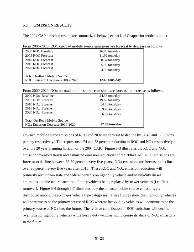
5 - 23
5.5 EMISSION RESULTS The 2004 CAP emission results are summarized below (see back of Chapter for model output). From 2000-2020, ROC on-road mobile source emissions are forecast to decrease as follows:
2000 ROC Baseline 16.80 tons/day 2005 ROC Forecast 11.92 tons/day 2010 ROC Forecast 2015 ROC Forecast 2020 ROC Forecast Total On-Road Mobile Source ROC Emission Decrease 2000 – 2020
8.34 tons/day 5.93 tons/day 4.35 tons/day 12.45 tons/day
From 2000-2020, NOx on-road mobile source emissions are forecast to decrease as follows:
2000 NOx Baseline 24.36 tons/day 2005 NOx Forecast 19.60 tons/day 2010 NOx Forecast 2015 NOx Forecast 2020 NOx Forecast Total On-Road Mobile Source NOx Emission Decrease 2000-2020
14.45 tons/day 9.76 tons/day 6.67 tons/day 17.69 tons/day
On-road mobile source emissions of ROC and NOx are forecast to decline by 12.45 and 17.69 tons
per day respectively. This represents a 74 and 73 percent reduction in ROC and NOx respectively
over the 20 year planning horizon of the 2004 CAP. Figure 5-3 illustrates the ROC and NOx
emission inventory trends and estimated emission reductions of the 2004 CAP. ROC emissions are
forecast to decline between 25-30 percent every five years. NOx emissions are forecast to decline
over 30 percent every five years after 2010. These ROC and NOx emission reductions will
primarily result from state and federal controls on light duty vehicle and heavy-duty diesel
emissions and the natural attrition of older vehicles being replaced by newer vehicles (i.e., fleet
turnover). Figure 5-4 through 5-7 illustrates how the on-road mobile source emissions are
distributed among the six major vehicle type categories. These figures show that light-duty vehicles
will continue to be the primary source of ROC whereas heavy-duty vehicles will continue to be the
primary source of NOx into the future. The relative contribution of ROC emissions will decline
over time for light duty vehicles while heavy duty vehicles will increase its share of NOx emissions
in the future.
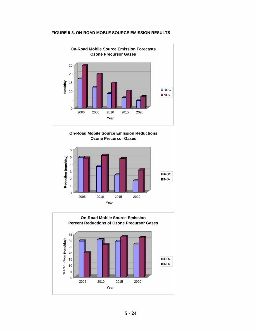
5 - 24
FIGURE 5-3. ON-ROAD MOBLE SOURCE EMISSION RESULTS
0
5
10
15
20
25to
ns/ d
ay
2000 2005 2010 2015 2020
Year
On-Road Mobile Source Emission Forecasts Ozone Precursor Gases
ROCNOx
0
1
2
3
4
5
6
Re d
ucti o
n ( to
n s/d
ay)
2005 2010 2015 2020
Year
On-Road Mobile Source Emission Reductions Ozone Precursor Gases
ROCNOx
0
5
10
15
20
25
30
35
% R
e duc
ti on
( ton s
/ day
)
2005 2010 2015 2020
Year
On-Road Mobile Source Emission Percent Reductions of Ozone Precursor Gases
ROCNOx
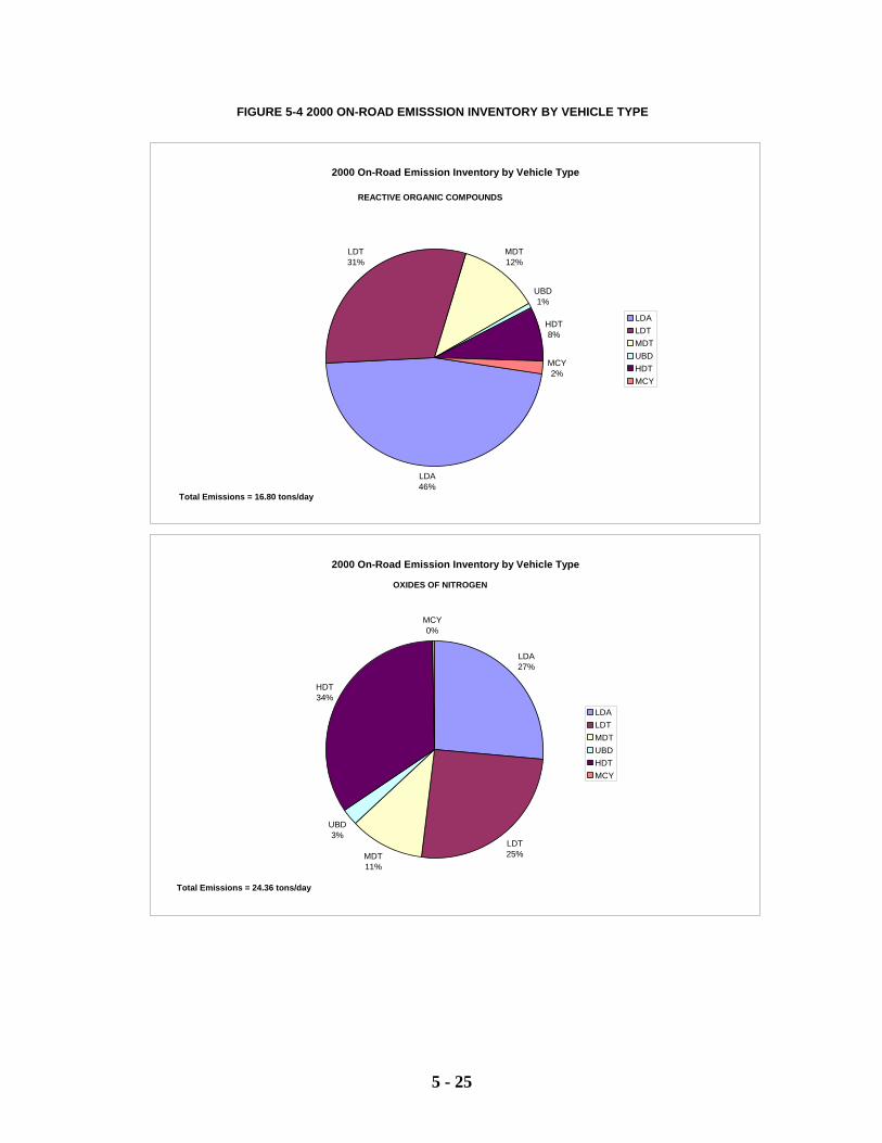
5 - 25
FIGURE 5-4 2000 ON-ROAD EMISSSION INVENTORY BY VEHICLE TYPE
2000 On-Road Emission Inventory by Vehicle Type
LDA46%
LDT31%
MDT12%
UBD1%
HDT8%
MCY2%
LDALDTMDTUBDHDTMCY
REACTIVE ORGANIC COMPOUNDS
Total Emissions = 16.80 tons/day
2000 On-Road Emission Inventory by Vehicle Type
LDA27%
LDT25%MDT
11%
UBD3%
HDT34%
MCY0%
LDALDTMDTUBDHDTMCY
OXIDES OF NITROGEN
Total Emissions = 24.36 tons/day
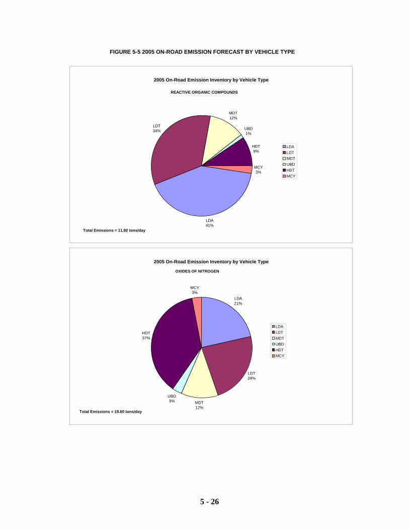
5 - 26
FIGURE 5-5 2005 ON-ROAD EMISSION FORECAST BY VEHICLE TYPE
2005 On-Road Emission Inventory by Vehicle Type
LDA41%
LDT34%
MDT12%
UBD1%
HDT9%
MCY3%
LDALDTMDTUBDHDTMCY
REACTIVE ORGANIC COMPOUNDS
Total Emissions = 11.92 tons/day
2005 On-Road Emission Inventory by Vehicle Type
LDA21%
LDT24%
MDT12%
UBD3%
HDT37%
MCY3%
LDALDTMDTUBDHDTMCY
OXIDES OF NITROGEN
Total Emissions = 19.60 tons/day

5 - 27
FIGURE 5-6 2015 ON-ROAD EMISSION FORECAST BY VEHICLE TYPE
2015 On-Road Emission Inventory by Vehicle Type
LDA31%
LDT38%
MDT15%
UBD2%
HDT10%
MCY4%
LDALDTMDTUBDHDTMCY
REACTIVE ORGANIC COMPOUNDS
Total Emissions = 5.90 tons/day
2015 On-Road Emission Inventory by Vehicle Type
LDA17%
LDT25%
MDT15%
UBD6%
HDT36%
MCY1%
LDALDTMDTUBDHDTMCY
OXIDES OF NITROGEN
Total Emissions = 9.75 tons/day
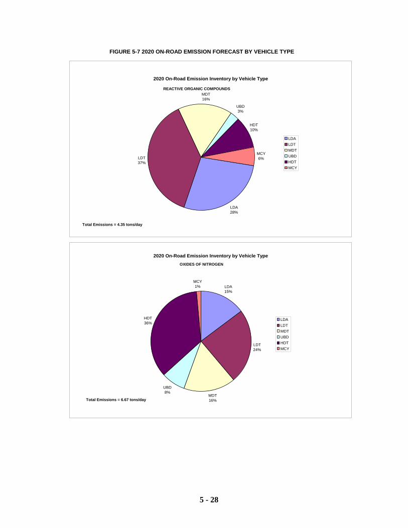
5 - 28
FIGURE 5-7 2020 ON-ROAD EMISSION FORECAST BY VEHICLE TYPE
2020 On-Road Emission Inventory by Vehicle Type
LDA28%
LDT37%
MDT16%
UBD3%
HDT10%
MCY6%
LDALDTMDTUBDHDTMCY
REACTIVE ORGANIC COMPOUNDS
Total Emissions = 4.35 tons/day
2020 On-Road Emission Inventory by Vehicle Type
LDA15%
LDT24%
MDT16%
UBD8%
HDT36%
MCY1%
LDALDTMDTUBDHDTMCY
OXIDES OF NITROGEN
Total Emissions = 6.67 tons/day
5 - 29
5.6 DEPARTURES FROM EMFAC2002 DEFAULTS
ARB approved the use of EMFAC2002 for purposes of on-road mobile source emission inventory
development in California in September 2002. As part of the development of the 2004 CAP,
several changes were also made to the vehicle activity data default values resident in the
EMFAC2002 model in order to more accurately reflect Santa Barbara County travel characteristics.
For each of the 2004 Clean Air Plan emission forecasts, adjustments were made to: vehicle
population, vehicle starts; and, vehicle miles of travel related to commercial vehicle activity. These
adjustments were agreed to by ARB and are consistent with how on-road mobile source emissions
were modeled as part of the federally approved 2001 Clean Air Plan. EMFAC2002 allows these
adjustments through its WIS (what-if-scenario) user-interface module. Justification for each of
these vehicle activity adjustments is provided below.
5.6.1 Vehicle Population
Vehicle population estimates in EMFAC2002 are based on an area’s county specific vehicle
registration data. One concern with this approach it that it effectively ignores the population of
vehicles that are operated within Santa Barbara County but are registered outside the county. This
is an issue for MPOs like SBCAG that have destination resort areas within its modeling domains
and/or experience a greater proportion of in-coming inter-county commuters. For instance, based
on 2000 U.S. Census data, Santa Barbara County experienced a daily net increase of 9,455
incoming commuters versus those leaving Santa Barbara County to go to work. Combined with the
influx of tourists, relying solely on county specific registration data would tend to underestimate the
number of vehicles actually operating within Santa Barbara County on a given weekday – thereby
underestimating the ROC and NOx emissions associated with these vehicles. Adjustments to the
LDA, LDT and MDT vehicle populations were made within EMFAC2002 based on maintaining the
VMT to vehicle population relationship (i.e., keeping the mileage accrual rates constant). The
VMT adjustment is described section 5.6.3.
5 - 30
5.6.2 Vehicle Starts
Departing from its predecessors3, the EMFAC2002 methodology for generating vehicle starts for
the LDA, LDT, and MDT vehicle types is now based solely on factoring an area’s county specific
vehicle registration data. There are two concerns that SBCAG has with respect to this approach.
1) It effectively ignores the contribution of internal visitor trips, i.e., trip starts from vehicles
that are registered outside the county. ARB is developing a county-to-county trip matrix
based on instrumented vehicle data to address these trips. However, this matrix is currently
not complete and will not be operational for this generation of EMFAC. This may be an
issue for MPOs like SBCAG that have destination resort areas within its modeling domains.
2) It creates an analytical disconnect between regional transportation network model output
and vehicle start emissions. This is especially problematic when making emission forecasts.
Relying on model defaults for vehicle starts makes EMFAC2002 insensitive to
present/future mode split/vehicle trip changes resulting from HOV facilities, new transit
services, transit fare policy changes, market based TCMs, traditional TCMs etc.
Based on these concerns, SBCAG revised the estimate of total countywide vehicle trip starts by
applying the EMFAC7G trip-end to vehicle start adjustment factors to SBCAG’s travel model
output for trip-ends. The revised vehicle start control totals were then input into EMFAC2002 and
allocated by vehicle type based on EMFAC2002’s existing activity data distribution percentages.
5.6.3 Commercial Vehicle Activity
Given that SBCAG travel model does not explicitly model commercial truck activity, a two-step
process was taken to appropriately augment SBCAG’s modeled VMT estimates with VMT from
heavy-duty gas trucks (HDGT), heavy-duty diesel trucks (HDDT) and urban diesel buses (UBD).
3 For EMFAC7F and MVEI7G, ARB accepted travel demand model activity estimates of trip ends, VMT, and VMT by speed class distributions from MPOs/RTPAs. In MVEI7G, vehicle trip ends as produced by the regional transportation planning agency network models (or statewide travel survey derived trip end estimates) were adjusted to vehicle starts. These adjustments were based on ARB instrumented vehicle surveys and appropriately allowed the estimate of vehicle emissions to capture non-destination trips (i.e., trip chaining activity) and short trips (e.g., ignition key events associated with shuffling cars at home or moving a car in a parking lot). Because the resulting trip start control totals for each vehicle type are factored from the trip end data, the nexus between vehicle start emissions with MPO travel model results was maintained.
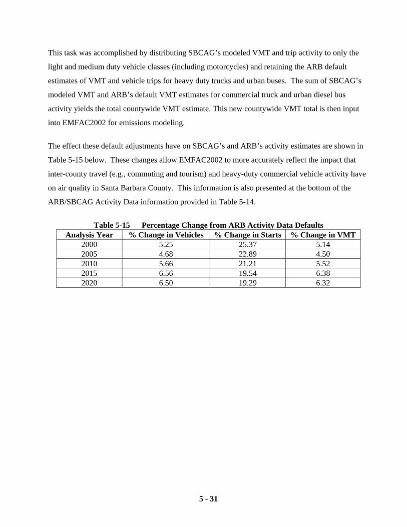
5 - 31
This task was accomplished by distributing SBCAG’s modeled VMT and trip activity to only the
light and medium duty vehicle classes (including motorcycles) and retaining the ARB default
estimates of VMT and vehicle trips for heavy duty trucks and urban buses. The sum of SBCAG’s
modeled VMT and ARB’s default VMT estimates for commercial truck and urban diesel bus
activity yields the total countywide VMT estimate. This new countywide VMT total is then input
into EMFAC2002 for emissions modeling.
The effect these default adjustments have on SBCAG’s and ARB’s activity estimates are shown in
Table 5-15 below. These changes allow EMFAC2002 to more accurately reflect the impact that
inter-county travel (e.g., commuting and tourism) and heavy-duty commercial vehicle activity have
on air quality in Santa Barbara County. This information is also presented at the bottom of the
ARB/SBCAG Activity Data information provided in Table 5-14.
Table 5-15 Percentage Change from ARB Activity Data Defaults
Analysis Year % Change in Vehicles % Change in Starts % Change in VMT 2000 5.25 25.37 5.14 2005 4.68 22.89 4.50 2010 5.66 21.21 5.52 2015 6.56 19.54 6.38 2020 6.50 19.29 6.32
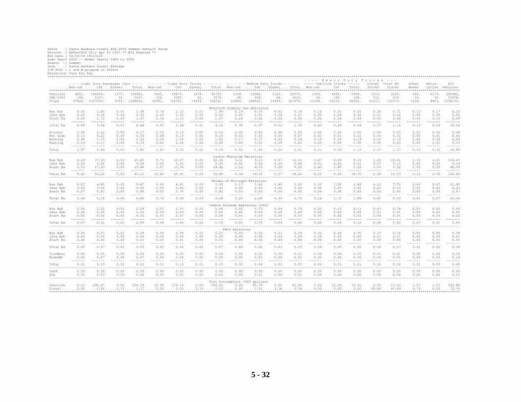
5 - 32
Title : Santa Barbara County Avg 2000 Summer Default Title Version : Emfac2002 V2.2 Apr 23 2003 ** WIS Enabled ** Run Date : 02/12/04 14:13:24 Scen Year: 2000 -- Model Years: 1965 to 2000 Season : Summer Area : Santa Barbara County Average I/M Stat : I and M program in effect Emissions: Tons Per Day ***************************************************************************************************************************************************************************************************************** - - - - H e a v y D u t y T r u c k s - - - - - - Light Duty Passenger Cars - - - - - - - - Light Duty Trucks - - - - - - - - - - Medium Duty Trucks - - - - ----- Gasoline Trucks ------ Diesel Total HD Urban Motor- All Non-cat Cat Diesel Total Non-cat Cat Diesel Total Non-cat Cat Diesel Total Non-cat Cat Total Trucks Trucks Buses cycles Vehicles **************************************************************************************************************************************************************************************************************** Vehicles 8651. 146934. 1377. 156962. 5445. 89473. 1878. 96795. 1439. 23968. 1163. 26570. 1354. 4554. 5908. 3316. 9224. 260. 6170. 295982. VMT/1000 108. 5107. 32. 5247. 126. 3087. 62. 3274. 28. 918. 66. 1012. 18. 140. 158. 312. 470. 33. 42. 10078. Trips 47826. 1107030. 9744. 1164600. 32981. 716391. 14859. 764231. 23644. 288832. 14993. 327470. 21438. 59225. 80662. 51411. 132073. 1039. 8815. 2398230. ---------------------------------------------------------------------------------------------------------------------------------------------------------------------------------------------------------------- Reactive Organic Gas Emissions Run Exh 0.65 1.82 0.01 2.48 0.74 1.23 0.01 1.99 0.19 0.55 0.02 0.76 0.14 0.31 0.45 0.26 0.71 0.13 0.17 6.23 Idle Exh 0.00 0.00 0.00 0.00 0.00 0.00 0.00 0.00 0.00 0.01 0.00 0.01 0.00 0.00 0.00 0.01 0.02 0.00 0.00 0.02 Start Ex 0.25 1.72 0.00 1.97 0.16 1.10 0.00 1.27 0.16 0.42 0.00 0.58 0.26 0.18 0.44 0.00 0.44 0.00 0.03 4.29 ------- ------- ------- ------- ------- ------- ------- ------- ------- ------- ------- ------- ------- ------- ------- ------- ------- ------- ------- ------- Total Ex 0.89 3.54 0.01 4.44 0.91 2.34 0.01 3.26 0.35 0.97 0.02 1.35 0.40 0.49 0.89 0.27 1.16 0.13 0.20 10.54 Diurnal 0.05 0.22 0.00 0.27 0.03 0.13 0.00 0.16 0.00 0.03 0.00 0.03 0.00 0.00 0.00 0.00 0.00 0.00 0.02 0.48 Hot Soak 0.12 0.22 0.00 0.33 0.08 0.15 0.00 0.23 0.02 0.05 0.00 0.07 0.01 0.01 0.02 0.00 0.02 0.00 0.01 0.65 Running 0.88 1.75 0.00 2.63 0.38 1.05 0.00 1.42 0.17 0.37 0.00 0.54 0.10 0.09 0.19 0.00 0.19 0.00 0.08 4.88 Resting 0.03 0.11 0.00 0.14 0.02 0.06 0.00 0.08 0.00 0.01 0.00 0.02 0.00 0.00 0.00 0.00 0.00 0.00 0.01 0.25 ------- ------- ------- ------- ------- ------- ------- ------- ------- ------- ------- ------- ------- ------- ------- ------- ------- ------- ------- ------- Total 1.97 5.84 0.01 7.82 1.41 3.72 0.01 5.14 0.55 1.44 0.02 2.01 0.51 0.59 1.10 0.27 1.37 0.13 0.32 16.80 ---------------------------------------------------------------------------------------------------------------------------------------------------------------------------------------------------------------- Carbon Monoxide Emissions Run Exh 8.29 37.33 0.03 45.65 9.75 32.57 0.05 42.38 3.31 9.13 0.07 12.51 3.67 5.69 9.36 1.25 10.61 1.10 2.21 114.47 Idle Exh 0.00 0.00 0.00 0.00 0.00 0.00 0.00 0.00 0.00 0.04 0.00 0.04 0.01 0.02 0.02 0.07 0.10 0.00 0.00 0.14 Start Ex 1.53 17.93 0.00 19.46 1.07 13.36 0.00 14.42 1.12 4.93 0.00 6.05 2.43 2.89 5.32 0.00 5.32 0.05 0.09 45.39 ------- ------- ------- ------- ------- ------- ------- ------- ------- ------- ------- ------- ------- ------- ------- ------- ------- ------- ------- ------- Total Ex 9.82 55.26 0.03 65.11 10.82 45.92 0.05 56.80 4.44 14.10 0.07 18.61 6.10 8.60 14.70 1.33 16.03 1.15 2.30 160.00 ---------------------------------------------------------------------------------------------------------------------------------------------------------------------------------------------------------------- Oxides of Nitrogen Emissions Run Exh 0.57 4.85 0.05 5.47 0.65 4.61 0.09 5.35 0.17 1.66 0.43 2.26 0.12 1.36 1.48 6.22 7.70 0.60 0.07 21.45 Idle Exh 0.00 0.00 0.00 0.00 0.00 0.00 0.00 0.00 0.00 0.00 0.00 0.00 0.00 0.00 0.00 0.23 0.23 0.00 0.00 0.23 Start Ex 0.07 0.91 0.00 0.98 0.05 0.78 0.00 0.83 0.03 0.43 0.00 0.45 0.04 0.36 0.40 0.00 0.40 0.00 0.00 2.67 ------- ------- ------- ------- ------- ------- ------- ------- ------- ------- ------- ------- ------- ------- ------- ------- ------- ------- ------- ------- Total Ex 0.64 5.76 0.05 6.46 0.70 5.39 0.09 6.18 0.20 2.08 0.43 2.72 0.16 1.72 1.88 6.45 8.33 0.61 0.07 24.36 ---------------------------------------------------------------------------------------------------------------------------------------------------------------------------------------------------------------- Carbon Dioxide Emissions (000) Run Exh 0.06 2.22 0.01 2.29 0.07 1.57 0.02 1.66 0.02 0.73 0.04 0.79 0.01 0.10 0.11 0.67 0.78 0.07 0.01 5.59 Idle Exh 0.00 0.00 0.00 0.00 0.00 0.00 0.00 0.00 0.00 0.00 0.00 0.00 0.00 0.00 0.00 0.01 0.01 0.00 0.00 0.01 Start Ex 0.01 0.10 0.00 0.11 0.01 0.07 0.00 0.08 0.01 0.03 0.00 0.03 0.00 0.00 0.01 0.00 0.01 0.00 0.00 0.22 ------- ------- ------- ------- ------- ------- ------- ------- ------- ------- ------- ------- ------- ------- ------- ------- ------- ------- ------- ------- Total Ex 0.07 2.31 0.01 2.40 0.08 1.64 0.02 1.74 0.03 0.76 0.04 0.82 0.02 0.10 0.12 0.68 0.80 0.07 0.01 5.83 ---------------------------------------------------------------------------------------------------------------------------------------------------------------------------------------------------------------- PM10 Emissions Run Exh 0.00 0.07 0.01 0.08 0.00 0.05 0.01 0.07 0.00 0.02 0.01 0.03 0.00 0.00 0.00 0.15 0.16 0.01 0.00 0.34 Idle Exh 0.00 0.00 0.00 0.00 0.00 0.00 0.00 0.00 0.00 0.00 0.00 0.00 0.00 0.00 0.00 0.01 0.01 0.00 0.00 0.01 Start Ex 0.00 0.01 0.00 0.01 0.00 0.01 0.00 0.01 0.00 0.00 0.00 0.00 0.00 0.00 0.00 0.00 0.00 0.00 0.00 0.02 ------- ------- ------- ------- ------- ------- ------- ------- ------- ------- ------- ------- ------- ------- ------- ------- ------- ------- ------- ------- Total Ex 0.00 0.07 0.01 0.09 0.01 0.06 0.01 0.07 0.00 0.02 0.01 0.03 0.00 0.00 0.00 0.16 0.17 0.01 0.00 0.36 TireWear 0.00 0.05 0.00 0.05 0.00 0.03 0.00 0.03 0.00 0.01 0.00 0.01 0.00 0.00 0.00 0.01 0.01 0.00 0.00 0.10 BrakeWr 0.00 0.07 0.00 0.07 0.00 0.04 0.00 0.05 0.00 0.01 0.00 0.01 0.00 0.00 0.00 0.00 0.01 0.00 0.00 0.14 ------- ------- ------- ------- ------- ------- ------- ------- ------- ------- ------- ------- ------- ------- ------- ------- ------- ------- ------- ------- Total 0.01 0.19 0.01 0.21 0.01 0.13 0.01 0.15 0.00 0.04 0.01 0.05 0.00 0.01 0.01 0.18 0.18 0.01 0.00 0.60 ---------------------------------------------------------------------------------------------------------------------------------------------------------------------------------------------------------------- Lead 0.00 0.00 0.00 0.00 0.00 0.00 0.00 0.00 0.00 0.00 0.00 0.00 0.00 0.00 0.00 0.00 0.00 0.00 0.00 0.00 SOx 0.00 0.03 0.00 0.04 0.00 0.02 0.00 0.03 0.00 0.01 0.00 0.01 0.00 0.00 0.00 0.06 0.06 0.00 0.00 0.15 ---------------------------------------------------------------------------------------------------------------------------------------------------------------------------------------------------------------- Fuel Consumption (000 gallons) Gasoline 9.21 246.97 0.00 256.18 10.08 176.16 0.00 186.25 3.44 80.39 0.00 83.84 3.02 12.00 15.02 0.00 15.02 1.57 1.03 543.88 Diesel 0.00 0.00 1.17 1.17 0.00 0.00 2.15 2.15 0.00 0.00 3.36 3.36 0.00 0.00 0.00 60.89 60.89 4.74 0.00 72.30 ****************************************************************************************************************************************************************************************************************
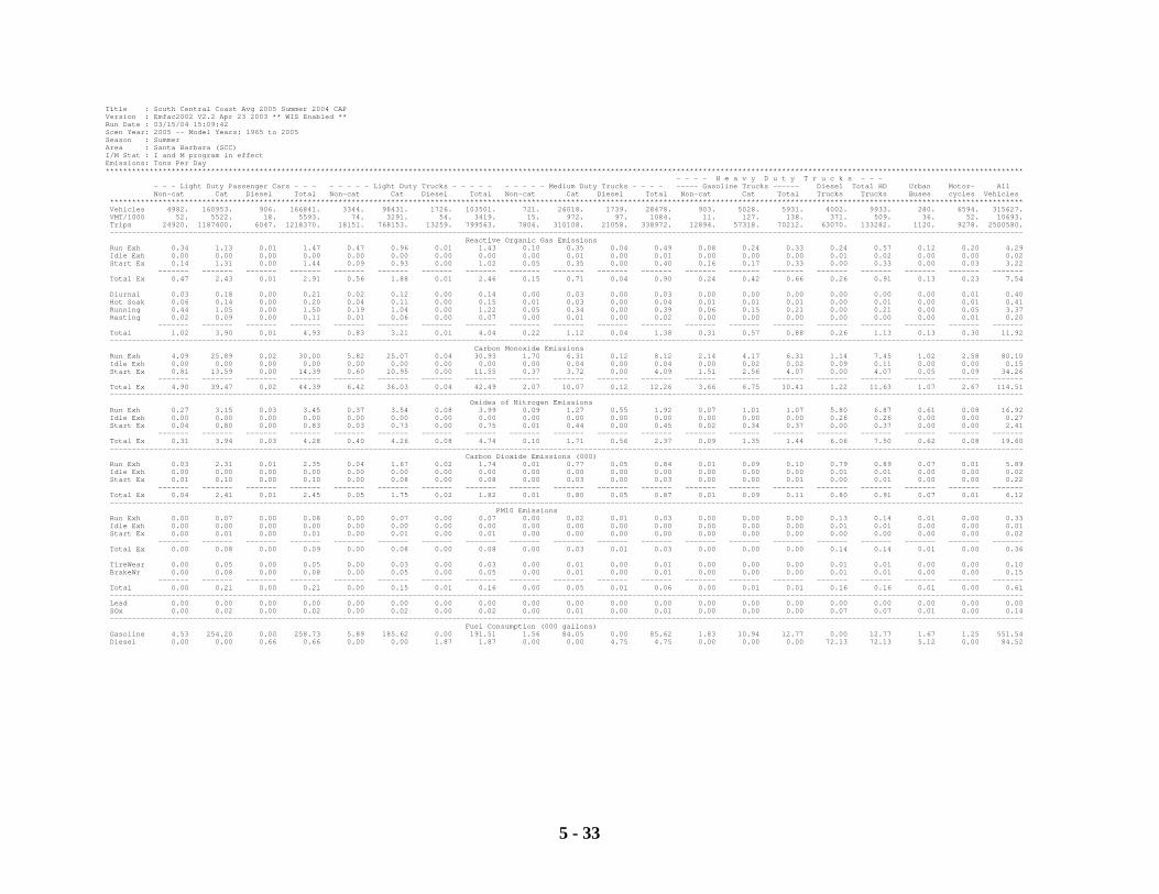
5 - 33
Title : South Central Coast Avg 2005 Summer 2004 CAP Version : Emfac2002 V2.2 Apr 23 2003 ** WIS Enabled ** Run Date : 03/15/04 15:09:42 Scen Year: 2005 -- Model Years: 1965 to 2005 Season : Summer Area : Santa Barbara (SCC) I/M Stat : I and M program in effect Emissions: Tons Per Day ***************************************************************************************************************************************************************************************************************** - - - - H e a v y D u t y T r u c k s - - - - - - Light Duty Passenger Cars - - - - - - - - Light Duty Trucks - - - - - - - - - - Medium Duty Trucks - - - - ----- Gasoline Trucks ------ Diesel Total HD Urban Motor- All Non-cat Cat Diesel Total Non-cat Cat Diesel Total Non-cat Cat Diesel Total Non-cat Cat Total Trucks Trucks Buses cycles Vehicles **************************************************************************************************************************************************************************************************************** Vehicles 4982. 160953. 906. 166841. 3344. 98431. 1726. 103501. 721. 26018. 1739. 28478. 903. 5028. 5931. 4002. 9933. 280. 6594. 315627. VMT/1000 52. 5522. 18. 5593. 74. 3291. 54. 3419. 15. 972. 97. 1084. 11. 127. 138. 371. 509. 36. 52. 10693. Trips 24920. 1187400. 6047. 1218370. 18151. 768153. 13259. 799563. 7806. 310108. 21058. 338972. 12894. 57318. 70212. 63070. 133282. 1120. 9278. 2500580. ---------------------------------------------------------------------------------------------------------------------------------------------------------------------------------------------------------------- Reactive Organic Gas Emissions Run Exh 0.34 1.13 0.01 1.47 0.47 0.96 0.01 1.43 0.10 0.35 0.04 0.49 0.08 0.24 0.33 0.24 0.57 0.12 0.20 4.29 Idle Exh 0.00 0.00 0.00 0.00 0.00 0.00 0.00 0.00 0.00 0.01 0.00 0.01 0.00 0.00 0.00 0.01 0.02 0.00 0.00 0.02 Start Ex 0.14 1.31 0.00 1.44 0.09 0.93 0.00 1.02 0.05 0.35 0.00 0.40 0.16 0.17 0.33 0.00 0.33 0.00 0.03 3.22 ------- ------- ------- ------- ------- ------- ------- ------- ------- ------- ------- ------- ------- ------- ------- ------- ------- ------- ------- ------- Total Ex 0.47 2.43 0.01 2.91 0.56 1.88 0.01 2.46 0.15 0.71 0.04 0.90 0.24 0.42 0.66 0.26 0.91 0.13 0.23 7.54 Diurnal 0.03 0.18 0.00 0.21 0.02 0.12 0.00 0.14 0.00 0.03 0.00 0.03 0.00 0.00 0.00 0.00 0.00 0.00 0.01 0.40 Hot Soak 0.06 0.14 0.00 0.20 0.04 0.11 0.00 0.15 0.01 0.03 0.00 0.04 0.01 0.01 0.01 0.00 0.01 0.00 0.01 0.41 Running 0.44 1.05 0.00 1.50 0.19 1.04 0.00 1.22 0.05 0.34 0.00 0.39 0.06 0.15 0.21 0.00 0.21 0.00 0.05 3.37 Resting 0.02 0.09 0.00 0.11 0.01 0.06 0.00 0.07 0.00 0.01 0.00 0.02 0.00 0.00 0.00 0.00 0.00 0.00 0.01 0.20 ------- ------- ------- ------- ------- ------- ------- ------- ------- ------- ------- ------- ------- ------- ------- ------- ------- ------- ------- ------- Total 1.02 3.90 0.01 4.93 0.83 3.21 0.01 4.04 0.22 1.12 0.04 1.38 0.31 0.57 0.88 0.26 1.13 0.13 0.30 11.92 ---------------------------------------------------------------------------------------------------------------------------------------------------------------------------------------------------------------- Carbon Monoxide Emissions Run Exh 4.09 25.89 0.02 30.00 5.82 25.07 0.04 30.93 1.70 6.31 0.12 8.12 2.14 4.17 6.31 1.14 7.45 1.02 2.58 80.10 Idle Exh 0.00 0.00 0.00 0.00 0.00 0.00 0.00 0.00 0.00 0.04 0.00 0.04 0.00 0.02 0.02 0.09 0.11 0.00 0.00 0.15 Start Ex 0.81 13.59 0.00 14.39 0.60 10.95 0.00 11.55 0.37 3.72 0.00 4.09 1.51 2.56 4.07 0.00 4.07 0.05 0.09 34.26 ------- ------- ------- ------- ------- ------- ------- ------- ------- ------- ------- ------- ------- ------- ------- ------- ------- ------- ------- ------- Total Ex 4.90 39.47 0.02 44.39 6.42 36.03 0.04 42.49 2.07 10.07 0.12 12.26 3.66 6.75 10.41 1.22 11.63 1.07 2.67 114.51 ---------------------------------------------------------------------------------------------------------------------------------------------------------------------------------------------------------------- Oxides of Nitrogen Emissions Run Exh 0.27 3.15 0.03 3.45 0.37 3.54 0.08 3.99 0.09 1.27 0.55 1.92 0.07 1.01 1.07 5.80 6.87 0.61 0.08 16.92 Idle Exh 0.00 0.00 0.00 0.00 0.00 0.00 0.00 0.00 0.00 0.00 0.00 0.00 0.00 0.00 0.00 0.26 0.26 0.00 0.00 0.27 Start Ex 0.04 0.80 0.00 0.83 0.03 0.73 0.00 0.75 0.01 0.44 0.00 0.45 0.02 0.34 0.37 0.00 0.37 0.00 0.00 2.41 ------- ------- ------- ------- ------- ------- ------- ------- ------- ------- ------- ------- ------- ------- ------- ------- ------- ------- ------- ------- Total Ex 0.31 3.94 0.03 4.28 0.40 4.26 0.08 4.74 0.10 1.71 0.56 2.37 0.09 1.35 1.44 6.06 7.50 0.62 0.08 19.60 ---------------------------------------------------------------------------------------------------------------------------------------------------------------------------------------------------------------- Carbon Dioxide Emissions (000) Run Exh 0.03 2.31 0.01 2.35 0.04 1.67 0.02 1.74 0.01 0.77 0.05 0.84 0.01 0.09 0.10 0.79 0.89 0.07 0.01 5.89 Idle Exh 0.00 0.00 0.00 0.00 0.00 0.00 0.00 0.00 0.00 0.00 0.00 0.00 0.00 0.00 0.00 0.01 0.01 0.00 0.00 0.02 Start Ex 0.01 0.10 0.00 0.10 0.00 0.08 0.00 0.08 0.00 0.03 0.00 0.03 0.00 0.00 0.01 0.00 0.01 0.00 0.00 0.22 ------- ------- ------- ------- ------- ------- ------- ------- ------- ------- ------- ------- ------- ------- ------- ------- ------- ------- ------- ------- Total Ex 0.04 2.41 0.01 2.45 0.05 1.75 0.02 1.82 0.01 0.80 0.05 0.87 0.01 0.09 0.11 0.80 0.91 0.07 0.01 6.12 ---------------------------------------------------------------------------------------------------------------------------------------------------------------------------------------------------------------- PM10 Emissions Run Exh 0.00 0.07 0.00 0.08 0.00 0.07 0.00 0.07 0.00 0.02 0.01 0.03 0.00 0.00 0.00 0.13 0.14 0.01 0.00 0.33 Idle Exh 0.00 0.00 0.00 0.00 0.00 0.00 0.00 0.00 0.00 0.00 0.00 0.00 0.00 0.00 0.00 0.01 0.01 0.00 0.00 0.01 Start Ex 0.00 0.01 0.00 0.01 0.00 0.01 0.00 0.01 0.00 0.00 0.00 0.00 0.00 0.00 0.00 0.00 0.00 0.00 0.00 0.02 ------- ------- ------- ------- ------- ------- ------- ------- ------- ------- ------- ------- ------- ------- ------- ------- ------- ------- ------- ------- Total Ex 0.00 0.08 0.00 0.09 0.00 0.08 0.00 0.08 0.00 0.03 0.01 0.03 0.00 0.00 0.00 0.14 0.14 0.01 0.00 0.36 TireWear 0.00 0.05 0.00 0.05 0.00 0.03 0.00 0.03 0.00 0.01 0.00 0.01 0.00 0.00 0.00 0.01 0.01 0.00 0.00 0.10 BrakeWr 0.00 0.08 0.00 0.08 0.00 0.05 0.00 0.05 0.00 0.01 0.00 0.01 0.00 0.00 0.00 0.01 0.01 0.00 0.00 0.15 ------- ------- ------- ------- ------- ------- ------- ------- ------- ------- ------- ------- ------- ------- ------- ------- ------- ------- ------- ------- Total 0.00 0.21 0.00 0.21 0.00 0.15 0.01 0.16 0.00 0.05 0.01 0.06 0.00 0.01 0.01 0.16 0.16 0.01 0.00 0.61 ---------------------------------------------------------------------------------------------------------------------------------------------------------------------------------------------------------------- Lead 0.00 0.00 0.00 0.00 0.00 0.00 0.00 0.00 0.00 0.00 0.00 0.00 0.00 0.00 0.00 0.00 0.00 0.00 0.00 0.00 SOx 0.00 0.02 0.00 0.02 0.00 0.02 0.00 0.02 0.00 0.01 0.00 0.01 0.00 0.00 0.00 0.07 0.07 0.01 0.00 0.14 ---------------------------------------------------------------------------------------------------------------------------------------------------------------------------------------------------------------- Fuel Consumption (000 gallons) Gasoline 4.53 254.20 0.00 258.73 5.89 185.62 0.00 191.51 1.56 84.05 0.00 85.62 1.83 10.94 12.77 0.00 12.77 1.67 1.25 551.54 Diesel 0.00 0.00 0.66 0.66 0.00 0.00 1.87 1.87 0.00 0.00 4.75 4.75 0.00 0.00 0.00 72.13 72.13 5.12 0.00 84.52
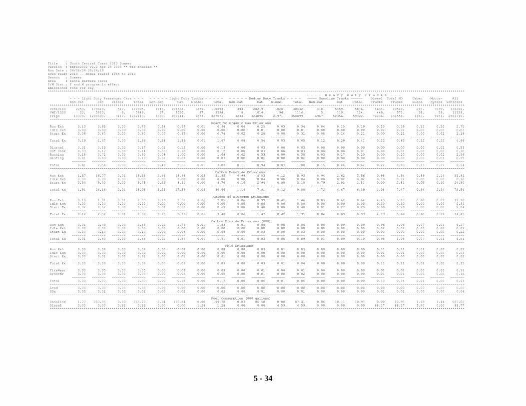
5 - 34
Title : South Central Coast 2010 Summer Version : Emfac2002 V2.2 Apr 23 2003 ** WIS Enabled ** Run Date : 04/06/04 08:24:18 Scen Year: 2010 -- Model Years: 1965 to 2010 Season : Summer Area : Santa Barbara (SCC) I/M Stat : I and M program in effect Emissions: Tons Per Day ***************************************************************************************************************************************************************************************************************** - - - - H e a v y D u t y T r u c k s - - - - - - Light Duty Passenger Cars - - - - - - - - Light Duty Trucks - - - - - - - - - - Medium Duty Trucks - - - - ----- Gasoline Trucks ------ Diesel Total HD Urban Motor- All Non-cat Cat Diesel Total Non-cat Cat Diesel Total Non-cat Cat Diesel Total Non-cat Cat Total Trucks Trucks Buses cycles Vehicles **************************************************************************************************************************************************************************************************************** Vehicles 2259. 174619. 517. 177395. 1746. 107568. 1279. 110593. 393. 28219. 1820. 30432. 418. 5459. 5876. 4634. 10510. 297. 7039. 336266. VMT/1000 20. 5920. 9. 5949. 37. 3520. 37. 3594. 8. 1014. 94. 1116. 5. 119. 124. 449. 573. 38. 59. 11329. Trips 10378. 1248640. 3117. 1262140. 8660. 809144. 9273. 827076. 3233. 324896. 21971. 350099. 6967. 52356. 59322. 72236. 131558. 1187. 9651. 2581710. ---------------------------------------------------------------------------------------------------------------------------------------------------------------------------------------------------------------- Reactive Organic Gas Emissions Run Exh 0.13 0.62 0.00 0.76 0.24 0.69 0.01 0.94 0.06 0.25 0.03 0.34 0.04 0.15 0.19 0.20 0.39 0.12 0.20 2.75 Idle Exh 0.00 0.00 0.00 0.00 0.00 0.00 0.00 0.00 0.00 0.01 0.00 0.01 0.00 0.00 0.00 0.02 0.02 0.00 0.00 0.03 Start Ex 0.06 0.85 0.00 0.90 0.05 0.69 0.00 0.74 0.02 0.28 0.00 0.31 0.08 0.14 0.21 0.00 0.21 0.00 0.02 2.19 ------- ------- ------- ------- ------- ------- ------- ------- ------- ------- ------- ------- ------- ------- ------- ------- ------- ------- ------- ------- Total Ex 0.19 1.47 0.00 1.66 0.28 1.39 0.01 1.67 0.08 0.54 0.03 0.65 0.12 0.29 0.41 0.22 0.63 0.12 0.22 4.96 Diurnal 0.01 0.15 0.00 0.17 0.01 0.12 0.00 0.13 0.00 0.03 0.00 0.03 0.00 0.00 0.00 0.00 0.00 0.00 0.01 0.33 Hot Soak 0.03 0.12 0.00 0.14 0.02 0.10 0.00 0.12 0.00 0.03 0.00 0.03 0.00 0.00 0.01 0.00 0.01 0.00 0.00 0.30 Running 0.18 0.72 0.00 0.90 0.08 1.00 0.00 1.08 0.02 0.33 0.00 0.35 0.03 0.17 0.20 0.00 0.20 0.00 0.02 2.56 Resting 0.01 0.09 0.00 0.10 0.01 0.07 0.00 0.07 0.00 0.02 0.00 0.02 0.00 0.00 0.00 0.00 0.00 0.00 0.01 0.19 ------- ------- ------- ------- ------- ------- ------- ------- ------- ------- ------- ------- ------- ------- ------- ------- ------- ------- ------- ------- Total 0.41 2.54 0.00 2.96 0.40 2.66 0.01 3.07 0.11 0.94 0.03 1.08 0.15 0.46 0.62 0.22 0.83 0.13 0.27 8.34 ---------------------------------------------------------------------------------------------------------------------------------------------------------------------------------------------------------------- Carbon Monoxide Emissions Run Exh 1.57 16.77 0.01 18.34 2.94 18.98 0.03 21.95 0.99 4.83 0.12 5.93 0.94 2.62 3.56 0.98 4.54 0.89 2.24 53.91 Idle Exh 0.00 0.00 0.00 0.00 0.00 0.00 0.00 0.00 0.00 0.04 0.00 0.04 0.00 0.02 0.02 0.10 0.12 0.00 0.00 0.16 Start Ex 0.34 9.40 0.00 9.73 0.29 8.41 0.00 8.70 0.16 2.94 0.00 3.10 0.79 2.03 2.81 0.00 2.81 0.05 0.10 24.50 ------- ------- ------- ------- ------- ------- ------- ------- ------- ------- ------- ------- ------- ------- ------- ------- ------- ------- ------- ------- Total Ex 1.91 26.16 0.01 28.08 3.23 27.39 0.03 30.66 1.14 7.81 0.12 9.08 1.72 4.67 6.39 1.08 7.47 0.94 2.34 78.56 ---------------------------------------------------------------------------------------------------------------------------------------------------------------------------------------------------------------- Oxides of Nitrogen Emissions Run Exh 0.10 1.91 0.01 2.03 0.19 2.61 0.06 2.85 0.06 0.99 0.42 1.46 0.03 0.62 0.64 4.43 5.07 0.60 0.09 12.10 Idle Exh 0.00 0.00 0.00 0.00 0.00 0.00 0.00 0.00 0.00 0.00 0.00 0.00 0.00 0.00 0.00 0.30 0.30 0.00 0.00 0.31 Start Ex 0.02 0.62 0.00 0.63 0.01 0.62 0.00 0.63 0.00 0.48 0.00 0.48 0.01 0.27 0.29 0.00 0.29 0.00 0.00 2.04 ------- ------- ------- ------- ------- ------- ------- ------- ------- ------- ------- ------- ------- ------- ------- ------- ------- ------- ------- ------- Total Ex 0.12 2.52 0.01 2.66 0.20 3.23 0.06 3.48 0.06 1.47 0.42 1.95 0.04 0.89 0.93 4.73 5.66 0.60 0.09 14.45 ---------------------------------------------------------------------------------------------------------------------------------------------------------------------------------------------------------------- Carbon Dioxide Emissions (000) Run Exh 0.01 2.43 0.00 2.45 0.02 1.79 0.01 1.83 0.01 0.80 0.05 0.86 0.00 0.09 0.09 0.96 1.06 0.07 0.01 6.27 Idle Exh 0.00 0.00 0.00 0.00 0.00 0.00 0.00 0.00 0.00 0.00 0.00 0.00 0.00 0.00 0.00 0.02 0.02 0.00 0.00 0.02 Start Ex 0.00 0.10 0.00 0.10 0.00 0.08 0.00 0.08 0.00 0.03 0.00 0.03 0.00 0.00 0.00 0.00 0.00 0.00 0.00 0.22 ------- ------- ------- ------- ------- ------- ------- ------- ------- ------- ------- ------- ------- ------- ------- ------- ------- ------- ------- ------- Total Ex 0.01 2.53 0.00 2.55 0.02 1.87 0.01 1.91 0.01 0.83 0.05 0.89 0.01 0.09 0.10 0.98 1.08 0.07 0.01 6.51 ---------------------------------------------------------------------------------------------------------------------------------------------------------------------------------------------------------------- PM10 Emissions Run Exh 0.00 0.08 0.00 0.08 0.00 0.08 0.00 0.08 0.00 0.03 0.01 0.03 0.00 0.00 0.00 0.11 0.11 0.01 0.00 0.32 Idle Exh 0.00 0.00 0.00 0.00 0.00 0.00 0.00 0.00 0.00 0.00 0.00 0.00 0.00 0.00 0.00 0.01 0.01 0.00 0.00 0.01 Start Ex 0.00 0.01 0.00 0.01 0.00 0.01 0.00 0.01 0.00 0.00 0.00 0.00 0.00 0.00 0.00 0.00 0.00 0.00 0.00 0.02 ------- ------- ------- ------- ------- ------- ------- ------- ------- ------- ------- ------- ------- ------- ------- ------- ------- ------- ------- ------- Total Ex 0.00 0.09 0.00 0.09 0.00 0.09 0.00 0.09 0.00 0.03 0.01 0.04 0.00 0.00 0.00 0.11 0.11 0.01 0.00 0.35 TireWear 0.00 0.05 0.00 0.05 0.00 0.03 0.00 0.03 0.00 0.01 0.00 0.01 0.00 0.00 0.00 0.01 0.02 0.00 0.00 0.11 BrakeWr 0.00 0.08 0.00 0.08 0.00 0.05 0.00 0.05 0.00 0.01 0.00 0.02 0.00 0.00 0.00 0.01 0.01 0.00 0.00 0.16 ------- ------- ------- ------- ------- ------- ------- ------- ------- ------- ------- ------- ------- ------- ------- ------- ------- ------- ------- ------- Total 0.00 0.22 0.00 0.22 0.00 0.17 0.00 0.17 0.00 0.06 0.01 0.06 0.00 0.00 0.00 0.13 0.14 0.01 0.00 0.61 ---------------------------------------------------------------------------------------------------------------------------------------------------------------------------------------------------------------- Lead 0.00 0.00 0.00 0.00 0.00 0.00 0.00 0.00 0.00 0.00 0.00 0.00 0.00 0.00 0.00 0.00 0.00 0.00 0.00 0.00 SOx 0.00 0.02 0.00 0.02 0.00 0.02 0.00 0.02 0.00 0.01 0.00 0.01 0.00 0.00 0.00 0.01 0.01 0.00 0.00 0.06 ---------------------------------------------------------------------------------------------------------------------------------------------------------------------------------------------------------------- Fuel Consumption (000 gallons) Gasoline 1.77 263.95 0.00 265.72 2.94 196.84 0.00 199.78 0.83 86.58 0.00 87.41 0.86 10.11 10.97 0.00 10.97 1.69 1.44 567.02 Diesel 0.00 0.00 0.32 0.32 0.00 0.00 1.28 1.28 0.00 0.00 4.59 4.59 0.00 0.00 0.00 88.17 88.17 5.40 0.00 99.77 ****************************************************************************************************************************************************************************************************************
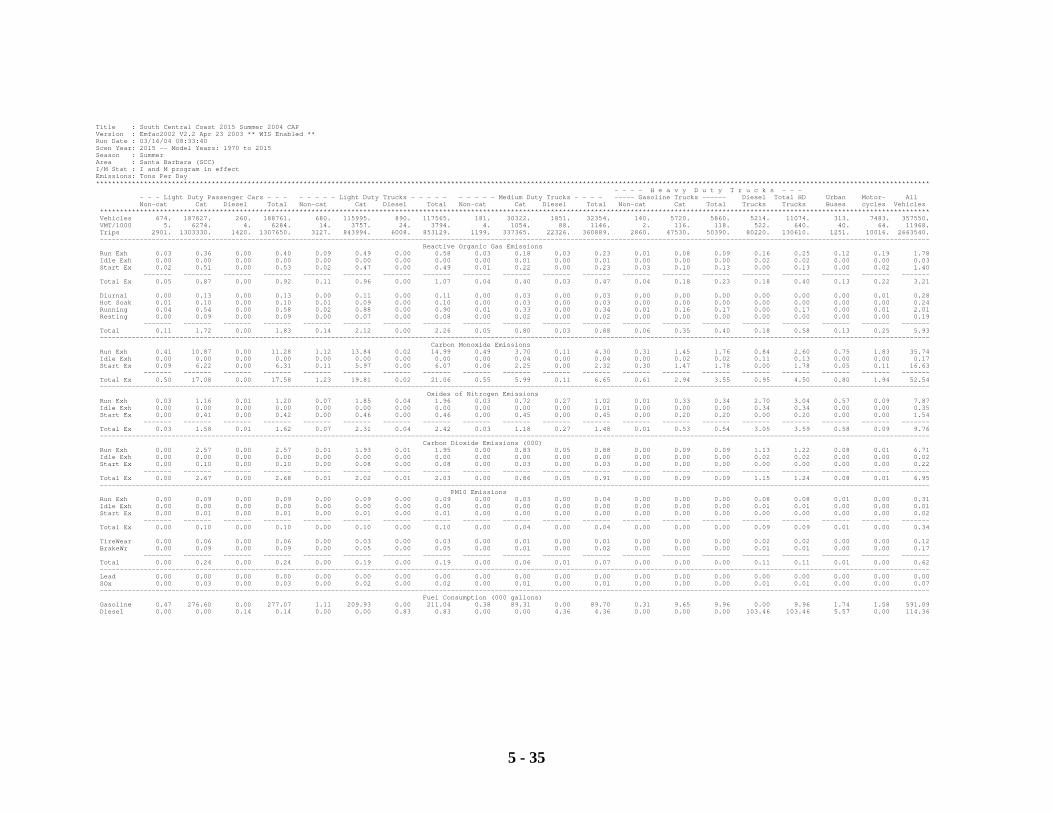
5 - 35
Title : South Central Coast 2015 Summer 2004 CAP Version : Emfac2002 V2.2 Apr 23 2003 ** WIS Enabled ** Run Date : 03/16/04 08:33:40 Scen Year: 2015 -- Model Years: 1970 to 2015 Season : Summer Area : Santa Barbara (SCC) I/M Stat : I and M program in effect Emissions: Tons Per Day ***************************************************************************************************************************************************************************************************************** - - - - H e a v y D u t y T r u c k s - - - - - - Light Duty Passenger Cars - - - - - - - - Light Duty Trucks - - - - - - - - - - Medium Duty Trucks - - - - ----- Gasoline Trucks ------ Diesel Total HD Urban Motor- All Non-cat Cat Diesel Total Non-cat Cat Diesel Total Non-cat Cat Diesel Total Non-cat Cat Total Trucks Trucks Buses cycles Vehicles **************************************************************************************************************************************************************************************************************** Vehicles 674. 187827. 260. 188761. 680. 115995. 890. 117565. 181. 30322. 1851. 32354. 140. 5720. 5860. 5214. 11074. 313. 7483. 357550. VMT/1000 5. 6274. 4. 6284. 14. 3757. 24. 3794. 4. 1054. 88. 1146. 2. 116. 118. 522. 640. 40. 64. 11968. Trips 2901. 1303330. 1420. 1307650. 3127. 843994. 6008. 853129. 1199. 337365. 22326. 360889. 2860. 47530. 50390. 80220. 130610. 1251. 10016. 2663540. ---------------------------------------------------------------------------------------------------------------------------------------------------------------------------------------------------------------- Reactive Organic Gas Emissions Run Exh 0.03 0.36 0.00 0.40 0.09 0.49 0.00 0.58 0.03 0.18 0.03 0.23 0.01 0.08 0.09 0.16 0.25 0.12 0.19 1.78 Idle Exh 0.00 0.00 0.00 0.00 0.00 0.00 0.00 0.00 0.00 0.01 0.00 0.01 0.00 0.00 0.00 0.02 0.02 0.00 0.00 0.03 Start Ex 0.02 0.51 0.00 0.53 0.02 0.47 0.00 0.49 0.01 0.22 0.00 0.23 0.03 0.10 0.13 0.00 0.13 0.00 0.02 1.40 ------- ------- ------- ------- ------- ------- ------- ------- ------- ------- ------- ------- ------- ------- ------- ------- ------- ------- ------- ------- Total Ex 0.05 0.87 0.00 0.92 0.11 0.96 0.00 1.07 0.04 0.40 0.03 0.47 0.04 0.18 0.23 0.18 0.40 0.13 0.22 3.21 Diurnal 0.00 0.13 0.00 0.13 0.00 0.11 0.00 0.11 0.00 0.03 0.00 0.03 0.00 0.00 0.00 0.00 0.00 0.00 0.01 0.28 Hot Soak 0.01 0.10 0.00 0.10 0.01 0.09 0.00 0.10 0.00 0.03 0.00 0.03 0.00 0.00 0.00 0.00 0.00 0.00 0.00 0.24 Running 0.04 0.54 0.00 0.58 0.02 0.88 0.00 0.90 0.01 0.33 0.00 0.34 0.01 0.16 0.17 0.00 0.17 0.00 0.01 2.01 Resting 0.00 0.09 0.00 0.09 0.00 0.07 0.00 0.08 0.00 0.02 0.00 0.02 0.00 0.00 0.00 0.00 0.00 0.00 0.00 0.19 ------- ------- ------- ------- ------- ------- ------- ------- ------- ------- ------- ------- ------- ------- ------- ------- ------- ------- ------- ------- Total 0.11 1.72 0.00 1.83 0.14 2.12 0.00 2.26 0.05 0.80 0.03 0.88 0.06 0.35 0.40 0.18 0.58 0.13 0.25 5.93 ---------------------------------------------------------------------------------------------------------------------------------------------------------------------------------------------------------------- Carbon Monoxide Emissions Run Exh 0.41 10.87 0.00 11.28 1.12 13.84 0.02 14.99 0.49 3.70 0.11 4.30 0.31 1.45 1.76 0.84 2.60 0.75 1.83 35.74 Idle Exh 0.00 0.00 0.00 0.00 0.00 0.00 0.00 0.00 0.00 0.04 0.00 0.04 0.00 0.02 0.02 0.11 0.13 0.00 0.00 0.17 Start Ex 0.09 6.22 0.00 6.31 0.11 5.97 0.00 6.07 0.06 2.25 0.00 2.32 0.30 1.47 1.78 0.00 1.78 0.05 0.11 16.63 ------- ------- ------- ------- ------- ------- ------- ------- ------- ------- ------- ------- ------- ------- ------- ------- ------- ------- ------- ------- Total Ex 0.50 17.08 0.00 17.58 1.23 19.81 0.02 21.06 0.55 5.99 0.11 6.65 0.61 2.94 3.55 0.95 4.50 0.80 1.94 52.54 ---------------------------------------------------------------------------------------------------------------------------------------------------------------------------------------------------------------- Oxides of Nitrogen Emissions Run Exh 0.03 1.16 0.01 1.20 0.07 1.85 0.04 1.96 0.03 0.72 0.27 1.02 0.01 0.33 0.34 2.70 3.04 0.57 0.09 7.87 Idle Exh 0.00 0.00 0.00 0.00 0.00 0.00 0.00 0.00 0.00 0.00 0.00 0.01 0.00 0.00 0.00 0.34 0.34 0.00 0.00 0.35 Start Ex 0.00 0.41 0.00 0.42 0.00 0.46 0.00 0.46 0.00 0.45 0.00 0.45 0.00 0.20 0.20 0.00 0.20 0.00 0.00 1.54 ------- ------- ------- ------- ------- ------- ------- ------- ------- ------- ------- ------- ------- ------- ------- ------- ------- ------- ------- ------- Total Ex 0.03 1.58 0.01 1.62 0.07 2.31 0.04 2.42 0.03 1.18 0.27 1.48 0.01 0.53 0.54 3.05 3.59 0.58 0.09 9.76 ---------------------------------------------------------------------------------------------------------------------------------------------------------------------------------------------------------------- Carbon Dioxide Emissions (000) Run Exh 0.00 2.57 0.00 2.57 0.01 1.93 0.01 1.95 0.00 0.83 0.05 0.88 0.00 0.09 0.09 1.13 1.22 0.08 0.01 6.71 Idle Exh 0.00 0.00 0.00 0.00 0.00 0.00 0.00 0.00 0.00 0.00 0.00 0.00 0.00 0.00 0.00 0.02 0.02 0.00 0.00 0.02 Start Ex 0.00 0.10 0.00 0.10 0.00 0.08 0.00 0.08 0.00 0.03 0.00 0.03 0.00 0.00 0.00 0.00 0.00 0.00 0.00 0.22 ------- ------- ------- ------- ------- ------- ------- ------- ------- ------- ------- ------- ------- ------- ------- ------- ------- ------- ------- ------- Total Ex 0.00 2.67 0.00 2.68 0.01 2.02 0.01 2.03 0.00 0.86 0.05 0.91 0.00 0.09 0.09 1.15 1.24 0.08 0.01 6.95 ---------------------------------------------------------------------------------------------------------------------------------------------------------------------------------------------------------------- PM10 Emissions Run Exh 0.00 0.09 0.00 0.09 0.00 0.09 0.00 0.09 0.00 0.03 0.00 0.04 0.00 0.00 0.00 0.08 0.08 0.01 0.00 0.31 Idle Exh 0.00 0.00 0.00 0.00 0.00 0.00 0.00 0.00 0.00 0.00 0.00 0.00 0.00 0.00 0.00 0.01 0.01 0.00 0.00 0.01 Start Ex 0.00 0.01 0.00 0.01 0.00 0.01 0.00 0.01 0.00 0.00 0.00 0.00 0.00 0.00 0.00 0.00 0.00 0.00 0.00 0.02 ------- ------- ------- ------- ------- ------- ------- ------- ------- ------- ------- ------- ------- ------- ------- ------- ------- ------- ------- ------- Total Ex 0.00 0.10 0.00 0.10 0.00 0.10 0.00 0.10 0.00 0.04 0.00 0.04 0.00 0.00 0.00 0.09 0.09 0.01 0.00 0.34 TireWear 0.00 0.06 0.00 0.06 0.00 0.03 0.00 0.03 0.00 0.01 0.00 0.01 0.00 0.00 0.00 0.02 0.02 0.00 0.00 0.12 BrakeWr 0.00 0.09 0.00 0.09 0.00 0.05 0.00 0.05 0.00 0.01 0.00 0.02 0.00 0.00 0.00 0.01 0.01 0.00 0.00 0.17 ------- ------- ------- ------- ------- ------- ------- ------- ------- ------- ------- ------- ------- ------- ------- ------- ------- ------- ------- ------- Total 0.00 0.24 0.00 0.24 0.00 0.19 0.00 0.19 0.00 0.06 0.01 0.07 0.00 0.00 0.00 0.11 0.11 0.01 0.00 0.62 ---------------------------------------------------------------------------------------------------------------------------------------------------------------------------------------------------------------- Lead 0.00 0.00 0.00 0.00 0.00 0.00 0.00 0.00 0.00 0.00 0.00 0.00 0.00 0.00 0.00 0.00 0.00 0.00 0.00 0.00 SOx 0.00 0.03 0.00 0.03 0.00 0.02 0.00 0.02 0.00 0.01 0.00 0.01 0.00 0.00 0.00 0.01 0.01 0.00 0.00 0.07 ---------------------------------------------------------------------------------------------------------------------------------------------------------------------------------------------------------------- Fuel Consumption (000 gallons) Gasoline 0.47 276.60 0.00 277.07 1.11 209.93 0.00 211.04 0.38 89.31 0.00 89.70 0.31 9.65 9.96 0.00 9.96 1.74 1.58 591.09 Diesel 0.00 0.00 0.14 0.14 0.00 0.00 0.83 0.83 0.00 0.00 4.36 4.36 0.00 0.00 0.00 103.46 103.46 5.57 0.00 114.36
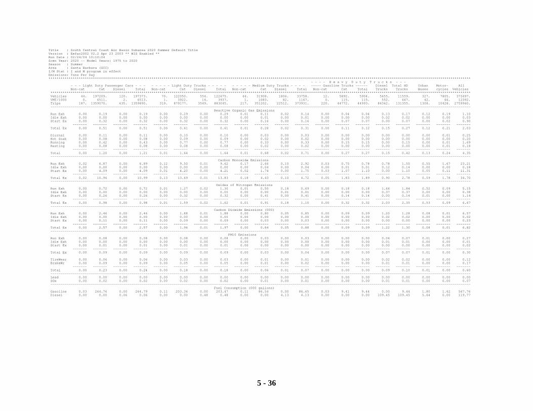
5 - 36
Title : South Central Coast Air Basin Subarea 2020 Summer Default Title Version : Emfac2002 V2.2 Apr 23 2003 ** WIS Enabled ** Run Date : 02/24/04 10:10:04 Scen Year: 2020 -- Model Years: 1975 to 2020 Season : Summer Area : Santa Barbara (SCC) I/M Stat : I and M program in effect Emissions: Tons Per Day ***************************************************************************************************************************************************************************************************************** - - - - H e a v y D u t y T r u c k s - - - - - - Light Duty Passenger Cars - - - - - - - - Light Duty Trucks - - - - - - - - - - Medium Duty Trucks - - - - ----- Gasoline Trucks ------ Diesel Total HD Urban Motor- All Non-cat Cat Diesel Total Non-cat Cat Diesel Total Non-cat Cat Diesel Total Non-cat Cat Total Trucks Trucks Buses cycles Vehicles **************************************************************************************************************************************************************************************************************** Vehicles 44. 197209. 120. 197373. 70. 122050. 554. 122675. 44. 31908. 1806. 33758. 12. 5892. 5904. 5655. 11559. 327. 7805. 373497. VMT/1000 0. 6511. 2. 6513. 1. 3922. 14. 3937. 1. 1083. 82. 1167. 0. 115. 115. 552. 667. 42. 66. 12392. Trips 187. 1359070. 635. 1359890. 319. 879177. 3549. 883045. 217. 351202. 22512. 373931. 220. 44772. 44993. 86362. 131355. 1308. 10428. 2759960. ---------------------------------------------------------------------------------------------------------------------------------------------------------------------------------------------------------------- Reactive Organic Gas Emissions Run Exh 0.00 0.19 0.00 0.19 0.00 0.29 0.00 0.29 0.01 0.11 0.02 0.14 0.00 0.04 0.04 0.13 0.17 0.12 0.19 1.10 Idle Exh 0.00 0.00 0.00 0.00 0.00 0.00 0.00 0.00 0.00 0.01 0.00 0.01 0.00 0.00 0.00 0.02 0.02 0.00 0.00 0.03 Start Ex 0.00 0.32 0.00 0.32 0.00 0.32 0.00 0.32 0.00 0.16 0.00 0.16 0.00 0.07 0.07 0.00 0.07 0.00 0.02 0.90 ------- ------- ------- ------- ------- ------- ------- ------- ------- ------- ------- ------- ------- ------- ------- ------- ------- ------- ------- ------- Total Ex 0.00 0.51 0.00 0.51 0.00 0.61 0.00 0.61 0.01 0.28 0.02 0.31 0.00 0.11 0.12 0.15 0.27 0.12 0.21 2.03 Diurnal 0.00 0.11 0.00 0.11 0.00 0.10 0.00 0.10 0.00 0.03 0.00 0.03 0.00 0.00 0.00 0.00 0.00 0.00 0.01 0.25 Hot Soak 0.00 0.08 0.00 0.08 0.00 0.09 0.00 0.09 0.00 0.02 0.00 0.02 0.00 0.00 0.00 0.00 0.00 0.00 0.00 0.20 Running 0.00 0.42 0.00 0.43 0.00 0.77 0.00 0.77 0.00 0.33 0.00 0.33 0.00 0.15 0.15 0.00 0.15 0.00 0.01 1.69 Resting 0.00 0.08 0.00 0.08 0.00 0.08 0.00 0.08 0.00 0.02 0.00 0.02 0.00 0.00 0.00 0.00 0.00 0.00 0.01 0.18 ------- ------- ------- ------- ------- ------- ------- ------- ------- ------- ------- ------- ------- ------- ------- ------- ------- ------- ------- ------- Total 0.00 1.20 0.00 1.21 0.01 1.64 0.00 1.64 0.01 0.68 0.02 0.71 0.00 0.27 0.27 0.15 0.42 0.13 0.24 4.35 ---------------------------------------------------------------------------------------------------------------------------------------------------------------------------------------------------------------- Carbon Monoxide Emissions Run Exh 0.02 6.87 0.00 6.89 0.12 9.50 0.01 9.62 0.17 2.66 0.10 2.92 0.03 0.75 0.78 0.78 1.55 0.55 1.67 23.21 Idle Exh 0.00 0.00 0.00 0.00 0.00 0.00 0.00 0.00 0.00 0.04 0.00 0.04 0.00 0.01 0.01 0.12 0.14 0.00 0.00 0.18 Start Ex 0.00 4.09 0.00 4.09 0.01 4.20 0.00 4.21 0.02 1.74 0.00 1.75 0.03 1.07 1.10 0.00 1.10 0.05 0.11 11.31 ------- ------- ------- ------- ------- ------- ------- ------- ------- ------- ------- ------- ------- ------- ------- ------- ------- ------- ------- ------- Total Ex 0.02 10.96 0.00 10.99 0.13 13.69 0.01 13.83 0.18 4.43 0.10 4.72 0.05 1.83 1.89 0.90 2.78 0.59 1.78 34.70 ---------------------------------------------------------------------------------------------------------------------------------------------------------------------------------------------------------------- Oxides of Nitrogen Emissions Run Exh 0.00 0.72 0.00 0.72 0.01 1.27 0.02 1.30 0.01 0.50 0.18 0.69 0.00 0.18 0.18 1.66 1.84 0.52 0.09 5.15 Idle Exh 0.00 0.00 0.00 0.00 0.00 0.00 0.00 0.00 0.00 0.00 0.01 0.01 0.00 0.00 0.00 0.37 0.37 0.00 0.00 0.38 Start Ex 0.00 0.26 0.00 0.26 0.00 0.32 0.00 0.32 0.00 0.41 0.00 0.41 0.00 0.14 0.14 0.00 0.14 0.01 0.00 1.14 ------- ------- ------- ------- ------- ------- ------- ------- ------- ------- ------- ------- ------- ------- ------- ------- ------- ------- ------- ------- Total Ex 0.00 0.98 0.00 0.98 0.01 1.59 0.02 1.62 0.01 0.91 0.18 1.10 0.00 0.32 0.32 2.03 2.35 0.53 0.09 6.67 ---------------------------------------------------------------------------------------------------------------------------------------------------------------------------------------------------------------- Carbon Dioxide Emissions (000) Run Exh 0.00 2.46 0.00 2.46 0.00 1.88 0.01 1.88 0.00 0.80 0.05 0.85 0.00 0.09 0.09 1.20 1.28 0.08 0.01 6.57 Idle Exh 0.00 0.00 0.00 0.00 0.00 0.00 0.00 0.00 0.00 0.00 0.00 0.00 0.00 0.00 0.00 0.02 0.02 0.00 0.00 0.02 Start Ex 0.00 0.11 0.00 0.11 0.00 0.09 0.00 0.09 0.00 0.03 0.00 0.03 0.00 0.00 0.00 0.00 0.00 0.00 0.00 0.23 ------- ------- ------- ------- ------- ------- ------- ------- ------- ------- ------- ------- ------- ------- ------- ------- ------- ------- ------- ------- Total Ex 0.00 2.57 0.00 2.57 0.00 1.96 0.01 1.97 0.00 0.84 0.05 0.88 0.00 0.09 0.09 1.22 1.30 0.08 0.01 6.82 ---------------------------------------------------------------------------------------------------------------------------------------------------------------------------------------------------------------- PM10 Emissions Run Exh 0.00 0.08 0.00 0.08 0.00 0.08 0.00 0.08 0.00 0.03 0.00 0.03 0.00 0.00 0.00 0.06 0.07 0.01 0.00 0.27 Idle Exh 0.00 0.00 0.00 0.00 0.00 0.00 0.00 0.00 0.00 0.00 0.00 0.00 0.00 0.00 0.00 0.01 0.01 0.00 0.00 0.01 Start Ex 0.00 0.01 0.00 0.01 0.00 0.01 0.00 0.01 0.00 0.00 0.00 0.00 0.00 0.00 0.00 0.00 0.00 0.00 0.00 0.02 ------- ------- ------- ------- ------- ------- ------- ------- ------- ------- ------- ------- ------- ------- ------- ------- ------- ------- ------- ------- Total Ex 0.00 0.09 0.00 0.09 0.00 0.09 0.00 0.09 0.00 0.03 0.00 0.04 0.00 0.00 0.00 0.07 0.07 0.01 0.00 0.30 TireWear 0.00 0.06 0.00 0.06 0.00 0.03 0.00 0.03 0.00 0.01 0.00 0.01 0.00 0.00 0.00 0.02 0.02 0.00 0.00 0.12 BrakeWr 0.00 0.09 0.00 0.09 0.00 0.05 0.00 0.05 0.00 0.01 0.00 0.02 0.00 0.00 0.00 0.01 0.01 0.00 0.00 0.17 ------- ------- ------- ------- ------- ------- ------- ------- ------- ------- ------- ------- ------- ------- ------- ------- ------- ------- ------- ------- Total 0.00 0.23 0.00 0.24 0.00 0.18 0.00 0.18 0.00 0.06 0.01 0.07 0.00 0.00 0.00 0.09 0.10 0.01 0.00 0.60 ---------------------------------------------------------------------------------------------------------------------------------------------------------------------------------------------------------------- Lead 0.00 0.00 0.00 0.00 0.00 0.00 0.00 0.00 0.00 0.00 0.00 0.00 0.00 0.00 0.00 0.00 0.00 0.00 0.00 0.00 SOx 0.00 0.02 0.00 0.02 0.00 0.02 0.00 0.02 0.00 0.01 0.00 0.01 0.00 0.00 0.00 0.01 0.01 0.00 0.00 0.07 ---------------------------------------------------------------------------------------------------------------------------------------------------------------------------------------------------------------- Fuel Consumption (000 gallons) Gasoline 0.03 264.76 0.00 264.79 0.11 203.36 0.00 203.47 0.11 86.54 0.00 86.65 0.03 9.41 9.44 0.00 9.44 1.80 1.62 567.76 Diesel 0.00 0.00 0.06 0.06 0.00 0.00 0.48 0.48 0.00 0.00 4.13 4.13 0.00 0.00 0.00 109.45 109.45 5.64 0.00 119.77
CHAPTER 6
EMISSION FORECASTING
Introduction
Emission Forecast
Emission Inventories
Impacts of Marine Shipping Emissions
Conclusions
6 - 1
6. EMISSION FORECASTING
6.1 INTRODUCTION
This chapter presents the four emission inventory forecasts used in the development of this 2004
Plan. These inventories are the 2005, 2010, 2015 and 2020 Planning Emission Inventory forecasts of
reactive organic compounds (ROC) and oxides of nitrogen (NOx) emissions in Santa Barbara
County and the Outer Continental Shelf (OCS), offshore of Santa Barbara County.
The 2005, 2010, 2015 and 2020 Planning Emission Inventory forecasts are based on the 2000
Planning Emission Inventory, which is described in Chapter 3, Emission Inventory. This 2000
Planning Emission Inventory is the base year for emission forecasting and was developed by
modifying the 2000 Annual Emission Inventory, (also described in Chapter 3). A Planning
Emission Inventory is essentially a modified subset of an Annual Emission Inventory and differs
from an Annual Emission Inventory in three ways. First, the creation of the Planning Emission
Inventory involves adjusting the Annual Emission Inventory to account for seasonal variation
because most exceedances of the state and federal 1-hour ozone standards occur during the April to
October ozone season. This is commonly referred to as a summer seasonal inventory. Second, the
emissions from natural sources such as biogenics, oil seeps and gas seeps, and wildfires are excluded
from the Planning Emission Inventory since they are not regulated or controlled through
implementation of emission control measures. Finally, the annual emissions in the Annual Emission
Inventory are converted to daily emissions in the Planning Emission Inventory.
6.2 EMISSION FORECAST
The 2000 Planning Emission Inventory is used to forecast emissions in order to determine whether
the emission control measures described in Chapters 4 and 5 of the 2004 Plan will reduce enough
emissions in order to attain the State 1-hour ozone standard, while accounting for the growth that is
6 - 2
expected in the county. The inventory approach to assessing progress assumes that if forecasted
inventories are below base level values, then the reductions will be sufficient enough to meet air
quality goals, particularly if an area is close to meeting the standard. It should be noted, however,
that there are uncertainties with regard to using the emission inventory approach since there is not
always a direct correlation between ozone precursor emissions and monitored ozone values.
Important factors such as weather conditions and the transport of pollution from other areas can
significantly influence local air quality and ozone concentrations. Photochemical modeling is often
used in lieu of the inventory approach; however, due to resource limitations the APCD is not able to
provide modeling analyses for this 2004 Plan.
To forecast future year emissions, estimates of the changes in the level of pollution producing
activities, known as “activity indicators”, are used to grow the 2000 Planning Emission Inventory.
In addition, emission reductions resulting from local control rules adopted by the APCD Board of
Directors and from statewide regulations adopted by the California Air Resources Board (ARB) are
estimated and accounted for in the future year forecasts.
Since we are using a 2000 emission inventory base year, future year forecasted emission inventories
must be adjusted to account for the most recent emission reduction credits (ERCs) that were in the
APCD Source Register during the 2nd quarter of 2004. ERC’s are previous reductions in emissions
that can be credited to allow increased emissions from a new or modified stationary source. USEPA
policy mandates that ERC’s must be treated as potential growth in forecast years. Total available
ERC’s in the Source Register for Santa Barbara County as of the 2nd quarter of 2004, were 0.2504
tons per day of ROC and 0.4191 tons per day of NOx. These total ERC values are included in the
emission forecast tables presented at the end of this chapter. A detailed list of each source that owns
these ERC’s are listed in Table 6-1.
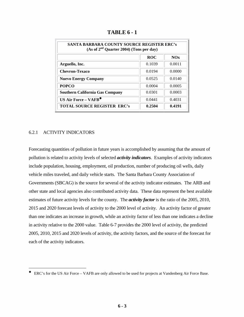
6 - 3
TABLE 6 - 1
SANTA BARBARA COUNTY SOURCE REGISTER ERC’s (As of 2nd Quarter 2004) (Tons per day)
ROC NOx Arguello, Inc. 0.1039 0.0011
Chevron-Texaco 0.0194 0.0000
Nuevo Energy Company 0.0525 0.0140
POPCO 0.0004 0.0005 Southern California Gas Company 0.0301 0.0003
US Air Force – VAFB 0.0441 0.4031 TOTAL SOURCE REGISTER ERC’s 0.2504 0.4191
6.2.1 ACTIVITY INDICATORS
Forecasting quantities of pollution in future years is accomplished by assuming that the amount of
pollution is related to activity levels of selected activity indicators. Examples of activity indicators
include population, housing, employment, oil production, number of producing oil wells, daily
vehicle miles traveled, and daily vehicle starts. The Santa Barbara County Association of
Governments (SBCAG) is the source for several of the activity indicator estimates. The ARB and
other state and local agencies also contributed activity data. These data represent the best available
estimates of future activity levels for the county. The activity factor is the ratio of the 2005, 2010,
2015 and 2020 forecast levels of activity to the 2000 level of activity. An activity factor of greater
than one indicates an increase in growth, while an activity factor of less than one indicates a decline
in activity relative to the 2000 value. Table 6-7 provides the 2000 level of activity, the predicted
2005, 2010, 2015 and 2020 levels of activity, the activity factors, and the source of the forecast for
each of the activity indicators.
ERC’s for the US Air Force – VAFB are only allowed to be used for projects at Vandenberg Air Force Base.
6 - 4
Note that the activity indicator for OCS Oil and Gas Production has been set to 1.0 or “no-growth.”
The recommendation to use a no-growth activity factor came from the Santa Barbara County Air
Pollution Control District Community Advisory Council after deliberation of what the future
projection of the OCS Production should be. The Community Advisory Council considered
potential OCS growth scenarios identified in the federal Minerals Management Service’s California
Offshore Oil and Gas Energy Resources (COOGER) study. The COOGER study presents several
scenarios of future growth for the OCS, including a “future baseline” scenario that projects existing
OCS platforms to decline steeply in production over the next fifteen years. The COOGER study also
presents scenarios that project substantial growth and development of future platforms from existing
undeveloped leases. The Council noted that, since any future oil and gas production on the OCS
will be required to be permitted under New Source Review/Prevention of Significant Deterioration
process, any potential increase in emissions must be offset to provide a net emission benefit from the
new OCS production activity. This would also ensure consistency of these future projects with this
Plan. Therefore, the Council recommended that the activity indicator for OCS Production should be
set to no-growth as a reasonable assumption of future oil and gas production emissions on the OCS.
An activity indicator was assigned to each Stationary Source and Area-Wide Source category
described in Chapter 3, with the exception of categories of On-Road Motor Vehicles and Other
Mobile Sources, Consumer Products and Architectural Coatings, which are derived from ARB’s
EMFAC2000 and OFFROAD Models, respectively. The ARB has provided the APCD with
emission forecasts for all of these source categories.
6.2.2 CONTROL MEASURES
The next step in forecasting future year emissions is to account for regulations and control measures
that have been previously implemented or that are scheduled for implementation. Emission
reductions are achieved through implementation of federal, state and local controls on a variety of
pollution sources, including Stationary Sources, Area-Wide Sources, and Mobile Sources.
6 - 5
The emissions from each source were reduced according to the expected efficiency of any control
measures that apply to that source, taking into account any existing level of control. Estimated
efficiencies take into account equipment (design) efficiencies, exemptions, phased implementations,
and expected rates of compliance (assumed to be a default 80%, as recommended in USEPA
guidelines). The resulting emissions after the application of control measures represent a seasonally
adjusted emission inventory forecast.
6.2.3 VANDENBERG AFB AIRBORNE LASER MISSION GROWTH ALLOWANCE
During the preparation of the 2001 Plan, Vandenberg Air Force Base (VAFB) requested that the
APCD include a General Conformity growth allowance into the 2001 Plan to account for an
Airborne Laser (ABL) Mission that may potentially come to VAFB. On November 15, 2001, the
APCD Board of Directors approved this request, with the condition that a portion of the emissions
from the ABL Mission be offset by withdrawing Emission Reduction Credits (ERC’s) from the
VAFB Source Register. Although General Conformity is not directly applicable to this 2004 Plan as
this Plan addresses only State planning requirements, projected ABL emissions are presented in this
Plan so that the inventory for VAFB is consistent with the 2001 Plan. Table 6-2 shows the
emissions from the ABL Mission estimated by VAFB, and the ERC’s required from VAFB required
to offset the ABL Mission. The remaining emissions from the ABL Mission are included as line
items in Tables 6-3 and 6-5.
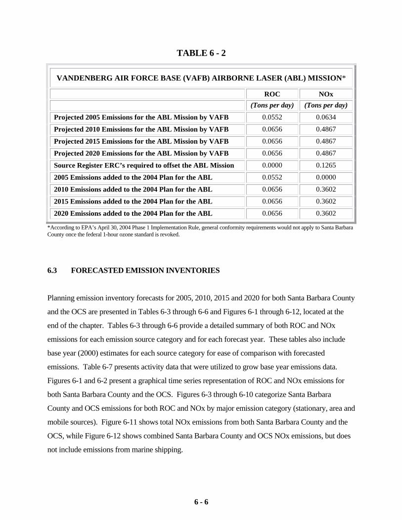
6 - 6
TABLE 6 - 2
VANDENBERG AIR FORCE BASE (VAFB) AIRBORNE LASER (ABL) MISSION*
ROC NOx (Tons per day) (Tons per day)
Projected 2005 Emissions for the ABL Mission by VAFB 0.0552 0.0634
Projected 2010 Emissions for the ABL Mission by VAFB 0.0656 0.4867
Projected 2015 Emissions for the ABL Mission by VAFB 0.0656 0.4867
Projected 2020 Emissions for the ABL Mission by VAFB 0.0656 0.4867
Source Register ERC’s required to offset the ABL Mission 0.0000 0.1265
2005 Emissions added to the 2004 Plan for the ABL 0.0552 0.0000
2010 Emissions added to the 2004 Plan for the ABL 0.0656 0.3602
2015 Emissions added to the 2004 Plan for the ABL 0.0656 0.3602
2020 Emissions added to the 2004 Plan for the ABL 0.0656 0.3602
*According to EPA’s April 30, 2004 Phase 1 Implementation Rule, general conformity requirements would not apply to Santa Barbara County once the federal 1-hour ozone standard is revoked.
6.3 FORECASTED EMISSION INVENTORIES
Planning emission inventory forecasts for 2005, 2010, 2015 and 2020 for both Santa Barbara County
and the OCS are presented in Tables 6-3 through 6-6 and Figures 6-1 through 6-12, located at the
end of the chapter. Tables 6-3 through 6-6 provide a detailed summary of both ROC and NOx
emissions for each emission source category and for each forecast year. These tables also include
base year (2000) estimates for each source category for ease of comparison with forecasted
emissions. Table 6-7 presents activity data that were utilized to grow base year emissions data.
Figures 6-1 and 6-2 present a graphical time series representation of ROC and NOx emissions for
both Santa Barbara County and the OCS. Figures 6-3 through 6-10 categorize Santa Barbara
County and OCS emissions for both ROC and NOx by major emission category (stationary, area and
mobile sources). Figure 6-11 shows total NOx emissions from both Santa Barbara County and the
OCS, while Figure 6-12 shows combined Santa Barbara County and OCS NOx emissions, but does
not include emissions from marine shipping.
6 - 7
The bar graph presented in Figure 6-1 shows that Santa Barbara County onshore NOx and ROC
emissions are expected to decrease continually through 2020. Total onshore ROC emissions are
forecasted to decrease from 41.84 tons per day in 2000 to 29.69 tons per day in 2020 representing a
29 percent decrease in emissions. Total onshore NOx emissions are projected to decrease from
43.89 tons per day in 2000 to 21.66 tons per day by 2020, about a 51 percent decrease in emissions.
On a source category basis, ROC emissions from onshore stationary sources are forecasted to
increase from 10.06 tons per day in 2000 to 11.49 tons per day in 2020 while NOx emissions from
onshore stationary sources are expected to increase from 5.57 tons per day in 2000 to 6.74 tons per
day in 2020. ROC emissions from area-wide sources are forecasted to increase from 7.94 tons per
day in 2000 to 10.16 tons per day in 2020. Area-wide NOx emissions are predicted to increase from
0.48 tons per day in 2000 to 1.23 tons per day by 2020.
The largest decreases in both onshore NOx and ROC emissions are attributable to decreased
emissions from on-road mobile sources. ROC emissions from onshore mobile sources are projected
to decrease from 23.85 tons per day in 2000 to 8.03 tons per day in 2020 (66 percent decrease),
while NOx emissions from on-road mobile sources are expected to decrease to13.69 tons per day by
2020 from 37.83 tons per day in 2000 (64 percent decrease).
Figure 6-2 presents forecasts for OCS ROC and NOx emissions. The figure shows that total
offshore ROC emissions are predicted to increase from 2.92 tons per day in 2000 to 3.36 tons per
day in 2020. Total offshore NOx emissions are anticipated to increase from 33.37 tons per day in
2000 to 65.59 tons per day in 2020. Mobile sources on the OCS, predominately marine shipping,
account for all of the anticipated growth in OCS ROC and NOx emissions. ROC emissions from
OCS mobile sources are expected to increase from 1.77 tons per day in 2000 to 2.22 tons per day in
2020, while OCS mobile source NOx emissions are forecasted to increase from 32.55 tons per day in
2000 to 64.77 tons per day in 2020.
6 - 8
As shown in Figure 6-3, mobile sources (on-road and other mobile sources) are forecasted to
account for 50 percent of total onshore ROC emissions and 81 percent of the onshore NOx
emissions in 2005. By 2020, mobile sources are predicted to account for 30 percent of the onshore
ROC emissions and 63 percent of the onshore NOx emissions as presented in Figure 6-9.
Although total onshore emissions of ROC and NOx from stationary and area sources increase only
slightly from 2005 to 2020, their relative contributions to overall onshore emissions increase
considerably due to significant reductions of both ROG and NOx emissions from on-road mobile
sources through the planning horizon. As displayed in figures 6-3 and 6-9, the relative percentage
of total ROC emissions from onshore stationary sources increases from 23 percent in 2005 to 31
percent in 2020, while NOx emissions from onshore stationary sources increases from 16 percent in
2005 to 31 percent of overall onshore inventory in 2020. Area wide ROC emissions are forecasted
to increase from 27 percent of total onshore emissions in 2005 to 39 percent of the total onshore
inventory by 2020. The projected contribution from area-wide NOx emissions increases from 3
percent in 2005 to 6 percent of the NOx inventory by 2020.
6.4 IMPACTS OF MARINE SHIPPING EMISSIONS
As discussed in the previous section, onshore Santa Barbara County emissions of ROC and NOx are
expected to decrease significantly by 2020, primarily from reductions in on-road mobile emissions
and through the implementation of the State Act’s every feasible measure requirements. While
Santa Barbara County onshore emissions are forecasted to substantially decrease during the planning
horizon, OCS NOx emissions are expected to dramatically increase from base year levels. These
increases in NOx emissions are the result of projected growth in marine shipping activities, which
are estimated to double from 2000 levels by 2020.
Figure 6-11 presents combined OCS and onshore NOx forecasts out to 2020. This figure clearly
illustrates that increases in NOx emissions from marine vessels will overwhelm stationary source
NOx reductions that will be achieved by implementing every feasible measure strategies and by
significant decreases in NOx from on-road mobile sources. Combined NOx emissions from onshore
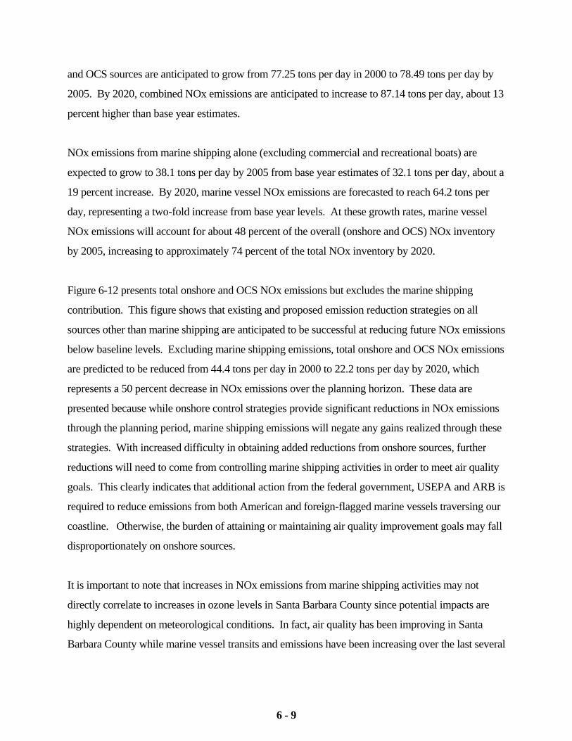
6 - 9
and OCS sources are anticipated to grow from 77.25 tons per day in 2000 to 78.49 tons per day by
2005. By 2020, combined NOx emissions are anticipated to increase to 87.14 tons per day, about 13
percent higher than base year estimates.
NOx emissions from marine shipping alone (excluding commercial and recreational boats) are
expected to grow to 38.1 tons per day by 2005 from base year estimates of 32.1 tons per day, about a
19 percent increase. By 2020, marine vessel NOx emissions are forecasted to reach 64.2 tons per
day, representing a two-fold increase from base year levels. At these growth rates, marine vessel
NOx emissions will account for about 48 percent of the overall (onshore and OCS) NOx inventory
by 2005, increasing to approximately 74 percent of the total NOx inventory by 2020.
Figure 6-12 presents total onshore and OCS NOx emissions but excludes the marine shipping
contribution. This figure shows that existing and proposed emission reduction strategies on all
sources other than marine shipping are anticipated to be successful at reducing future NOx emissions
below baseline levels. Excluding marine shipping emissions, total onshore and OCS NOx emissions
are predicted to be reduced from 44.4 tons per day in 2000 to 22.2 tons per day by 2020, which
represents a 50 percent decrease in NOx emissions over the planning horizon. These data are
presented because while onshore control strategies provide significant reductions in NOx emissions
through the planning period, marine shipping emissions will negate any gains realized through these
strategies. With increased difficulty in obtaining added reductions from onshore sources, further
reductions will need to come from controlling marine shipping activities in order to meet air quality
goals. This clearly indicates that additional action from the federal government, USEPA and ARB is
required to reduce emissions from both American and foreign-flagged marine vessels traversing our
coastline. Otherwise, the burden of attaining or maintaining air quality improvement goals may fall
disproportionately on onshore sources.
It is important to note that increases in NOx emissions from marine shipping activities may not
directly correlate to increases in ozone levels in Santa Barbara County since potential impacts are
highly dependent on meteorological conditions. In fact, air quality has been improving in Santa
Barbara County while marine vessel transits and emissions have been increasing over the last several
6 - 10
years. To fully understand the impacts of marine vessel emissions on county-wide ozone levels,
however, would require the use of photochemical modeling techniques. This would allow for an
evaluation of potential impacts from all sources of ozone precursors (ROC and NOx), both onshore
and offshore, and would also provide an assessment of the relative contribution of impacts from
marine vessel emissions on ozone concentrations. Since the resources and expertise required to
perform photochemical modeling are beyond our capabilities, we must defer the need for such an
exercise to the discretion of the ARB.
6.5 CONCLUSIONS
This chapter presents the 2005, 2010, 2015 and 2020 Planning Emission Inventory Forecasts. The
2000 Planning Emission Inventory is used as the basis to calculate the 2005, 2010, 2015 and 2020
forecasts.
ROC emissions from onshore stationary and area-wide sources are forecasted to increase over base
year levels by about 1.43 and 2.22 tons per day, respectively, by 2020. NOx emissions from onshore
stationary sources are anticipated to increase from base year levels by 1.17 tons per day by 2020,
while NOx increases over base year estimates are expected to be about 0.75 tons per day by 2020 for
onshore area-wide sources.
These small increases in ROC and NOx emissions from onshore stationary and area-wide sources
are significantly offset by emission reductions from onshore mobile sources. Baseline ROC
emissions from onshore mobile sources are predicted to decrease by nearly 16 tons per day by 2020,
while baseline NOx emissions are anticipated to decrease by about 24 tons per day by 2020.
Mobile sources account for the highest percentage of overall onshore ROC emissions until 2015,
when area-wide sources comprise the largest percentage contribution to the overall ROC onshore
inventory. Although there are substantial reductions of NOx emissions from mobile sources
through 2020, mobile sources are anticipated to comprise the largest portion of the total onshore
NOx inventory for each of the planning years.
6 - 11
While reductions of onshore ROC and NOx emissions are forecasted to occur through the planning
period due to existing and proposed emission reduction strategies, emissions from OCS sources are
predicted to increase dramatically over the same time horizon. These increases in NOx and ROC
emissions in the OCS are exclusively from significant growth that is forecasted for marine shipping.
Marine shipping NOx emissions are expected to double between 2000 and 2020. The increases in
marine vessel NOx emissions that are expected to occur will eliminate anticipated NOx emission
reductions from onshore sources. Without the contributions from this large uncontrolled source of
emissions, air quality in Santa Barbara County would clearly be improving. Further action from the
federal government, USEPA and the ARB will be required to reduce emissions from marine
shipping.
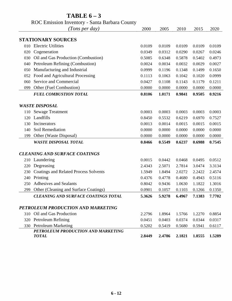
TABLE 6 – 3 ROC Emission Inventory - Santa Barbara County
(Tons per day) 2000 2005 2010 2015 2020
6 - 12
STATIONARY SOURCES 010 Electric Utilities 0.0109 0.0109 0.0109 0.0109 0.0109 020 Cogeneration 0.0349 0.0312 0.0290 0.0267 0.0246 030 Oil and Gas Production (Combustion) 0.5085 0.6348 0.5878 0.5402 0.4973 040 Petroleum Refining (Combustion) 0.0024 0.0034 0.0032 0.0029 0.0027 050 Manufacturing and Industrial 0.0999 0.1196 0.1348 0.1499 0.1650 052 Food and Agricultural Processing 0.1113 0.1063 0.1042 0.1020 0.0999 060 Service and Commercial 0.0427 0.1108 0.1143 0.1179 0.1211 099 Other (Fuel Combustion) 0.0000 0.0000 0.0000 0.0000 0.0000
FUEL COMBUSTION TOTAL 0.8106 1.0171 0.9841 0.9505 0.9216 WASTE DISPOSAL
110 Sewage Treatment 0.0003 0.0003 0.0003 0.0003 0.0003 120 Landfills 0.8450 0.5532 0.6219 0.6970 0.7527 130 Incinerators 0.0013 0.0014 0.0015 0.0015 0.0015 140 Soil Remediation 0.0000 0.0000 0.0000 0.0000 0.0000 199 Other (Waste Disposal) 0.0000 0.0000 0.0000 0.0000 0.0000
WASTE DISPOSAL TOTAL 0.8466 0.5549 0.6237 0.6988 0.7545 CLEANING AND SURFACE COATINGS
210 Laundering 0.0015 0.0442 0.0468 0.0495 0.0512 220 Degreasing 2.4343 2.5071 2.7814 3.0474 3.3134 230 Coatings and Related Process Solvents 1.5949 1.8494 2.0272 2.2422 2.4574 240 Printing 0.4376 0.4778 0.4680 0.4943 0.5116 250 Adhesives and Sealants 0.8042 0.9436 1.0630 1.1822 1.3016 299 Other (Cleaning and Surface Coatings) 0.0901 0.1057 0.1103 0.1266 0.1350
CLEANING AND SURFACE COATINGS TOTAL 5.3626 5.9278 6.4967 7.1383 7.7702 PETROLEUM PRODUCTION AND MARKETING
310 Oil and Gas Production 2.2796 1.8964 1.5766 1.2270 0.8854 320 Petroleum Refining 0.0451 0.0403 0.0374 0.0344 0.0317 330 Petroleum Marketing 0.5202 0.5419 0.5680 0.5941 0.6117
PETROLEUM PRODUCTION AND MARKETING TOTAL 2.8449 2.4786 2.1821 1.8555 1.5289

TABLE 6 – 3 ROC Emission Inventory - Santa Barbara County
(Tons per day) 2000 2005 2010 2015 2020
6 - 13
INDUSTRIAL PROCESSES
410 Chemical 0.0183 0.0205 0.0231 0.0257 0.0283 420 Food and Agriculture 0.1210 0.1298 0.1385 0.1473 0.1561 430 Mineral Processes 0.0087 0.0102 0.0115 0.0128 0.0141 440 Metal Processes NA NA NA NA NA 450 Wood and Paper NA NA NA NA NA 470 Electronics 0.0001 0.0002 0.0003 0.0002 0.0002 499 Other (Industrial Processes) 0.0423 0.0489 0.1147 0.0681 0.0681
INDUSTRIAL PROCESSES TOTAL 0.1904 0.2096 0.2881 0.2540 0.2667 STATIONARY SOURCES TOTAL 10.0551 10.1880 10.6884 10.8972 11.2418 AREA-WIDE SOURCES SOLVENT EVAPORATION
510 Consumer Products 3.7150 3.4570 3.6970 3.9630 4.3060 520 Architectural Coatings and Related Process Solvents 1.8100 1.6530 1.7030 1.7570 1.8100 530 Pesticides/Fertilizers 1.9710 1.8839 1.8479 1.8113 1.7756 540 Asphalt Paving/Roofing 0.2337 0.2742 0.3089 0.3436 0.3783
SOLVENT EVAPORATION TOTAL 7.7297 7.2682 7.5568 7.8749 8.2698 MISCELLANEOUS
610 Residential Fuel Combustion 0.1242 0.1334 0.1401 0.1462 0.1497 620 Farming Operations 0.0000 0.0000 0.0000 0.0000 0.0000 630 Construction and Demolition 0.0000 0.0000 0.0000 0.0000 0.0000 640 Paved Road Dust 0.0000 0.0000 0.0000 0.0000 0.0000 645 Unpaved Road Dust 0.0000 0.0000 0.0000 0.0000 0.0000 650 Fugitive Windblown Dust 0.0000 0.0000 0.0000 0.0000 0.0000 660 Fires 0.0034 0.0036 0.0038 0.0040 0.0041 670 Waste Burning and Disposal 0.0478 1.7000 1.6996 1.6992 1.6988 690 Cooking 0.0317 0.0340 0.0363 0.0386 0.0409 699 Other (Miscellaneous Processes) 0.0000 0.0000 0.0000 0.0000 0.0000
MISCELLANEOUS TOTAL 0.2071 1.8710 1.8799 1.8880 1.8936 AREA-WIDE SOURCES TOTAL 7.9368 9.1392 9.4367 9.7629 10.1634
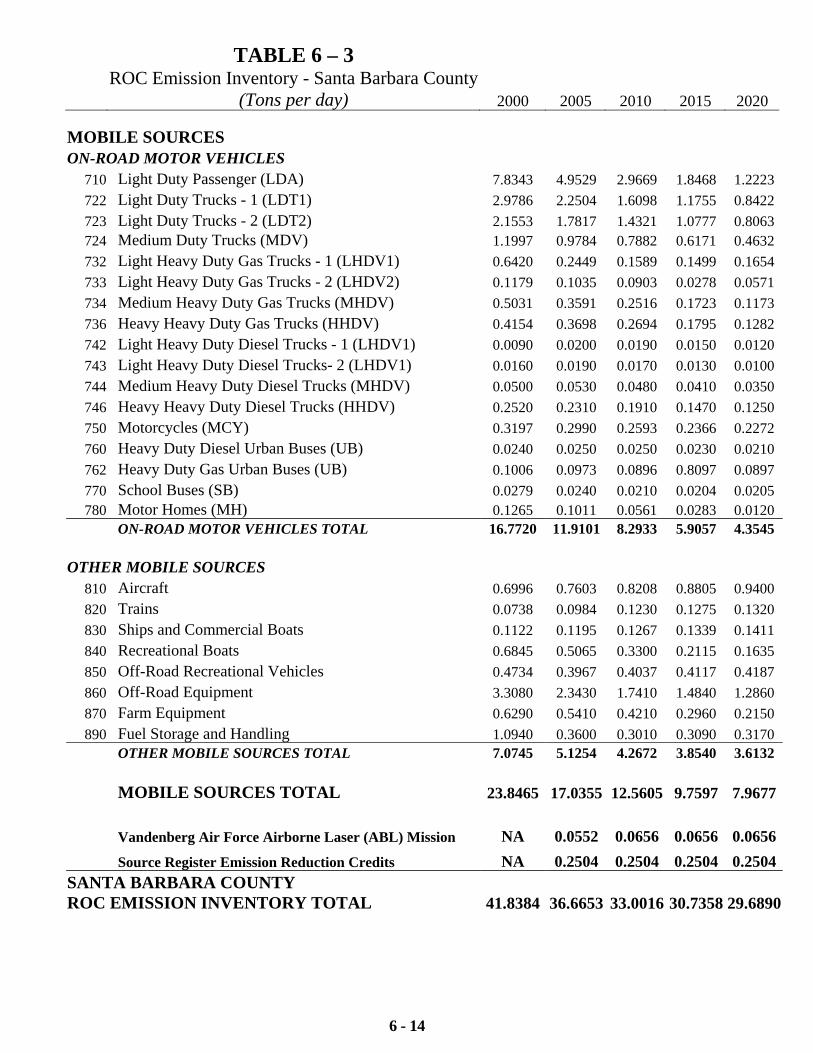
TABLE 6 – 3 ROC Emission Inventory - Santa Barbara County
(Tons per day) 2000 2005 2010 2015 2020
6 - 14
MOBILE SOURCES ON-ROAD MOTOR VEHICLES
710 Light Duty Passenger (LDA) 7.8343 4.9529 2.9669 1.8468 1.2223 722 Light Duty Trucks - 1 (LDT1) 2.9786 2.2504 1.6098 1.1755 0.8422 723 Light Duty Trucks - 2 (LDT2) 2.1553 1.7817 1.4321 1.0777 0.8063 724 Medium Duty Trucks (MDV) 1.1997 0.9784 0.7882 0.6171 0.4632 732 Light Heavy Duty Gas Trucks - 1 (LHDV1) 0.6420 0.2449 0.1589 0.1499 0.1654 733 Light Heavy Duty Gas Trucks - 2 (LHDV2) 0.1179 0.1035 0.0903 0.0278 0.0571 734 Medium Heavy Duty Gas Trucks (MHDV) 0.5031 0.3591 0.2516 0.1723 0.1173 736 Heavy Heavy Duty Gas Trucks (HHDV) 0.4154 0.3698 0.2694 0.1795 0.1282 742 Light Heavy Duty Diesel Trucks - 1 (LHDV1) 0.0090 0.0200 0.0190 0.0150 0.0120 743 Light Heavy Duty Diesel Trucks- 2 (LHDV1) 0.0160 0.0190 0.0170 0.0130 0.0100 744 Medium Heavy Duty Diesel Trucks (MHDV) 0.0500 0.0530 0.0480 0.0410 0.0350 746 Heavy Heavy Duty Diesel Trucks (HHDV) 0.2520 0.2310 0.1910 0.1470 0.1250 750 Motorcycles (MCY) 0.3197 0.2990 0.2593 0.2366 0.2272 760 Heavy Duty Diesel Urban Buses (UB) 0.0240 0.0250 0.0250 0.0230 0.0210 762 Heavy Duty Gas Urban Buses (UB) 0.1006 0.0973 0.0896 0.8097 0.0897 770 School Buses (SB) 0.0279 0.0240 0.0210 0.0204 0.0205 780 Motor Homes (MH) 0.1265 0.1011 0.0561 0.0283 0.0120
ON-ROAD MOTOR VEHICLES TOTAL 16.7720 11.9101 8.2933 5.9057 4.3545 OTHER MOBILE SOURCES
810 Aircraft 0.6996 0.7603 0.8208 0.8805 0.9400 820 Trains 0.0738 0.0984 0.1230 0.1275 0.1320 830 Ships and Commercial Boats 0.1122 0.1195 0.1267 0.1339 0.1411 840 Recreational Boats 0.6845 0.5065 0.3300 0.2115 0.1635 850 Off-Road Recreational Vehicles 0.4734 0.3967 0.4037 0.4117 0.4187 860 Off-Road Equipment 3.3080 2.3430 1.7410 1.4840 1.2860 870 Farm Equipment 0.6290 0.5410 0.4210 0.2960 0.2150 890 Fuel Storage and Handling 1.0940 0.3600 0.3010 0.3090 0.3170
OTHER MOBILE SOURCES TOTAL 7.0745 5.1254 4.2672 3.8540 3.6132 MOBILE SOURCES TOTAL 23.8465 17.0355 12.5605 9.7597 7.9677 Vandenberg Air Force Airborne Laser (ABL) Mission NA 0.0552 0.0656 0.0656 0.0656 Source Register Emission Reduction Credits NA 0.2504 0.2504 0.2504 0.2504SANTA BARBARA COUNTY ROC EMISSION INVENTORY TOTAL 41.8384 36.6653 33.0016 30.7358 29.6890
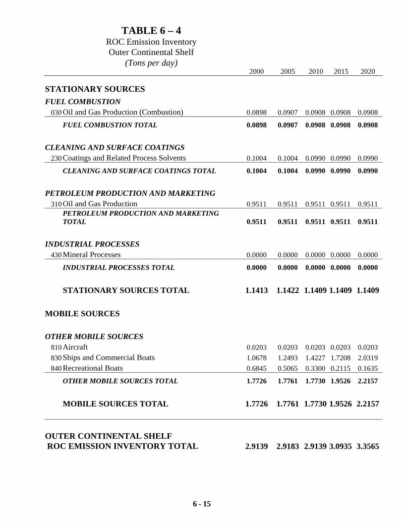
TABLE 6 – 4 ROC Emission Inventory Outer Continental Shelf
(Tons per day) 2000 2005 2010 2015 2020
6 - 15
STATIONARY SOURCES
FUEL COMBUSTION 030 Oil and Gas Production (Combustion) 0.0898 0.0907 0.0908 0.0908 0.0908
FUEL COMBUSTION TOTAL 0.0898 0.0907 0.0908 0.0908 0.0908
CLEANING AND SURFACE COATINGS 230 Coatings and Related Process Solvents 0.1004 0.1004 0.0990 0.0990 0.0990
CLEANING AND SURFACE COATINGS TOTAL 0.1004 0.1004 0.0990 0.0990 0.0990
PETROLEUM PRODUCTION AND MARKETING 310 Oil and Gas Production 0.9511 0.9511 0.9511 0.9511 0.9511
PETROLEUM PRODUCTION AND MARKETING TOTAL 0.9511 0.9511 0.9511 0.9511 0.9511
INDUSTRIAL PROCESSES 430 Mineral Processes 0.0000 0.0000 0.0000 0.0000 0.0000
INDUSTRIAL PROCESSES TOTAL 0.0000 0.0000 0.0000 0.0000 0.0000
STATIONARY SOURCES TOTAL 1.1413 1.1422 1.1409 1.1409 1.1409
MOBILE SOURCES
OTHER MOBILE SOURCES 810 Aircraft 0.0203 0.0203 0.0203 0.0203 0.0203 830 Ships and Commercial Boats 1.0678 1.2493 1.4227 1.7208 2.0319 840 Recreational Boats 0.6845 0.5065 0.3300 0.2115 0.1635
OTHER MOBILE SOURCES TOTAL 1.7726 1.7761 1.7730 1.9526 2.2157
MOBILE SOURCES TOTAL 1.7726 1.7761 1.7730 1.9526 2.2157
OUTER CONTINENTAL SHELF ROC EMISSION INVENTORY TOTAL 2.9139 2.9183 2.9139 3.0935 3.3565
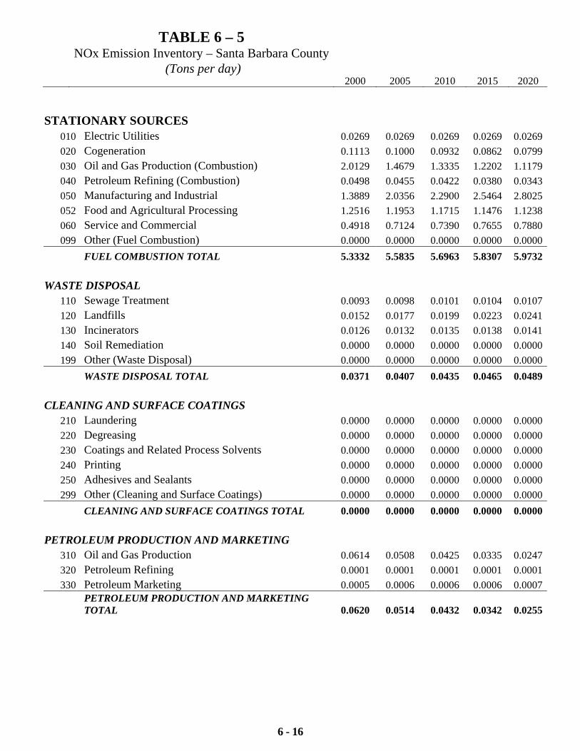
TABLE 6 – 5 NOx Emission Inventory – Santa Barbara County
(Tons per day) 2000 2005 2010 2015 2020
6 - 16
STATIONARY SOURCES
010 Electric Utilities 0.0269 0.0269 0.0269 0.0269 0.0269020 Cogeneration 0.1113 0.1000 0.0932 0.0862 0.0799030 Oil and Gas Production (Combustion) 2.0129 1.4679 1.3335 1.2202 1.1179040 Petroleum Refining (Combustion) 0.0498 0.0455 0.0422 0.0380 0.0343050 Manufacturing and Industrial 1.3889 2.0356 2.2900 2.5464 2.8025052 Food and Agricultural Processing 1.2516 1.1953 1.1715 1.1476 1.1238060 Service and Commercial 0.4918 0.7124 0.7390 0.7655 0.7880099 Other (Fuel Combustion) 0.0000 0.0000 0.0000 0.0000 0.0000
FUEL COMBUSTION TOTAL 5.3332 5.5835 5.6963 5.8307 5.9732 WASTE DISPOSAL
110 Sewage Treatment 0.0093 0.0098 0.0101 0.0104 0.0107120 Landfills 0.0152 0.0177 0.0199 0.0223 0.0241130 Incinerators 0.0126 0.0132 0.0135 0.0138 0.0141140 Soil Remediation 0.0000 0.0000 0.0000 0.0000 0.0000199 Other (Waste Disposal) 0.0000 0.0000 0.0000 0.0000 0.0000
WASTE DISPOSAL TOTAL 0.0371 0.0407 0.0435 0.0465 0.0489 CLEANING AND SURFACE COATINGS
210 Laundering 0.0000 0.0000 0.0000 0.0000 0.0000220 Degreasing 0.0000 0.0000 0.0000 0.0000 0.0000230 Coatings and Related Process Solvents 0.0000 0.0000 0.0000 0.0000 0.0000240 Printing 0.0000 0.0000 0.0000 0.0000 0.0000250 Adhesives and Sealants 0.0000 0.0000 0.0000 0.0000 0.0000299 Other (Cleaning and Surface Coatings) 0.0000 0.0000 0.0000 0.0000 0.0000
CLEANING AND SURFACE COATINGS TOTAL 0.0000 0.0000 0.0000 0.0000 0.0000 PETROLEUM PRODUCTION AND MARKETING
310 Oil and Gas Production 0.0614 0.0508 0.0425 0.0335 0.0247320 Petroleum Refining 0.0001 0.0001 0.0001 0.0001 0.0001330 Petroleum Marketing 0.0005 0.0006 0.0006 0.0006 0.0007
PETROLEUM PRODUCTION AND MARKETING TOTAL 0.0620 0.0514 0.0432 0.0342 0.0255
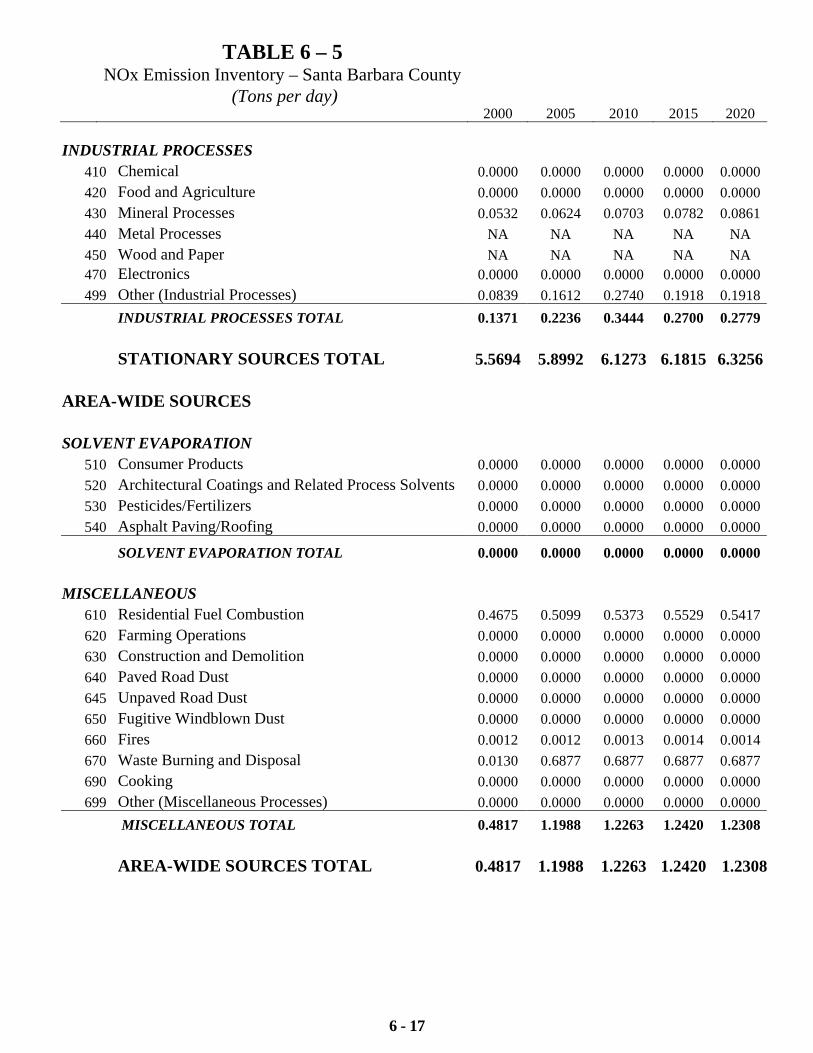
TABLE 6 – 5 NOx Emission Inventory – Santa Barbara County
(Tons per day) 2000 2005 2010 2015 2020
6 - 17
INDUSTRIAL PROCESSES 410 Chemical 0.0000 0.0000 0.0000 0.0000 0.0000420 Food and Agriculture 0.0000 0.0000 0.0000 0.0000 0.0000430 Mineral Processes 0.0532 0.0624 0.0703 0.0782 0.0861440 Metal Processes NA NA NA NA NA 450 Wood and Paper NA NA NA NA NA 470 Electronics 0.0000 0.0000 0.0000 0.0000 0.0000499 Other (Industrial Processes) 0.0839 0.1612 0.2740 0.1918 0.1918
INDUSTRIAL PROCESSES TOTAL 0.1371 0.2236 0.3444 0.2700 0.2779 STATIONARY SOURCES TOTAL 5.5694 5.8992 6.1273 6.1815 6.3256 AREA-WIDE SOURCES SOLVENT EVAPORATION
510 Consumer Products 0.0000 0.0000 0.0000 0.0000 0.0000520 Architectural Coatings and Related Process Solvents 0.0000 0.0000 0.0000 0.0000 0.0000530 Pesticides/Fertilizers 0.0000 0.0000 0.0000 0.0000 0.0000540 Asphalt Paving/Roofing 0.0000 0.0000 0.0000 0.0000 0.0000
SOLVENT EVAPORATION TOTAL 0.0000 0.0000 0.0000 0.0000 0.0000 MISCELLANEOUS
610 Residential Fuel Combustion 0.4675 0.5099 0.5373 0.5529 0.5417620 Farming Operations 0.0000 0.0000 0.0000 0.0000 0.0000630 Construction and Demolition 0.0000 0.0000 0.0000 0.0000 0.0000640 Paved Road Dust 0.0000 0.0000 0.0000 0.0000 0.0000645 Unpaved Road Dust 0.0000 0.0000 0.0000 0.0000 0.0000650 Fugitive Windblown Dust 0.0000 0.0000 0.0000 0.0000 0.0000660 Fires 0.0012 0.0012 0.0013 0.0014 0.0014670 Waste Burning and Disposal 0.0130 0.6877 0.6877 0.6877 0.6877690 Cooking 0.0000 0.0000 0.0000 0.0000 0.0000699 Other (Miscellaneous Processes) 0.0000 0.0000 0.0000 0.0000 0.0000
MISCELLANEOUS TOTAL 0.4817 1.1988 1.2263 1.2420 1.2308 AREA-WIDE SOURCES TOTAL 0.4817 1.1988 1.2263 1.2420 1.2308
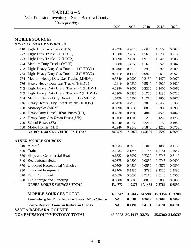
TABLE 6 – 5 NOx Emission Inventory – Santa Barbara County
(Tons per day) 2000 2005 2010 2015 2020
6 - 18
MOBILE SOURCES ON-ROAD MOTOR VEHICLES
710 Light Duty Passenger (LDA) 6.4570 4.2820 2.6600 1.6150 0.9820 722 Light Duty Trucks - 1 (LDT1) 3.1080 2.2650 1.5650 1.0730 0.7130 723 Light Duty Trucks - 2 (LDT2) 3.0690 2.4780 1.9180 1.3420 0.9050 724 Medium Duty Trucks (MDV) 1.8080 1.4750 1.1660 0.8520 0.5840 732 Light Heavy Duty Gas Trucks - 1 (LHDV1) 0.3490 0.2610 0.2930 0.2920 0.2800 733 Light Heavy Duty Gas Trucks - 2 (LHDV2) 0.1410 0.1110 0.0970 0.0810 0.0670 734 Medium Heavy Duty Gas Trucks (MHDV) 0.3640 0.2900 0.2160 0.1470 0.0970 736 Heavy Heavy Duty Gas Trucks (HHDV) 1.2410 0.9230 0.5540 0.2920 0.1620 742 Light Heavy Duty Diesel Trucks - 1 (LHDV1) 0.1880 0.3000 0.2220 0.1400 0.0960 743 Light Heavy Duty Diesel Trucks- 2 (LHDV1) 0.2300 0.2230 0.1720 0.1130 0.0720 744 Medium Heavy Duty Diesel Trucks (MHDV) 1.5790 1.5200 1.1770 0.7650 0.4870 746 Heavy Heavy Duty Diesel Trucks (HHDV) 4.6470 4.2910 3.3090 2.0450 1.3350 750 Motorcycles (MCY) 0.0690 0.0830 0.0890 0.0900 0.0930 760 Heavy Duty Diesel Urban Buses (UB) 0.4930 0.4980 0.4840 0.4520 0.4040 762 Heavy Duty Gas Urban Buses (UB) 0.1160 0.1200 0.1200 0.1240 0.1230 770 School Buses (SB) 0.2040 0.2230 0.2240 0.2150 0.1940 780 Motor Homes (MH) 0.2940 0.2540 0.1840 0.1210 0.0750
ON-ROAD MOTOR VEHICLES TOTAL 24.3570 19.5970 14.4500 9.7590 6.6690 OTHER MOBILE SOURCES
810 Aircraft 0.0833 0.0945 0.1016 0.1086 0.1155 820 Trains 2.2083 2.1345 2.1788 1.4151 1.4647 830 Ships and Commercial Boats 0.6622 0.6997 0.7370 0.7745 0.8119 840 Recreational Boats 0.0375 0.0800 0.0850 0.0745 0.0690 850 Off-Road Recreational Vehicles 0.0509 0.0529 0.0559 0.0579 0.0599 860 Off-Road Equipment 6.3700 5.5430 4.2730 3.1320 2.5830 870 Farm Equipment 4.0650 3.3830 2.7170 2.0140 1.5550 890 Fuel Storage and Handling 0.0000 0.0000 0.0000 0.0000 0.0000
OTHER MOBILE SOURCES TOTAL 13.4772 11.9875 10.1483 7.5764 6.6590 MOBILE SOURCES TOTAL 37.8342 31.5845 24.5983 17.3354 13.3280 Vandenberg Air Force Airborne Laser (ABL) Mission NA 0.0000 0.3602 0.3602 0.3602
Source Register Emission Reduction Credits NA 0.4191 0.4191 0.4191 0.4191 SANTA BARBARA COUNTY NOx EMISSION INVENTORY TOTAL 43.8853 39.1017 32.7311 25.5382 21.6637
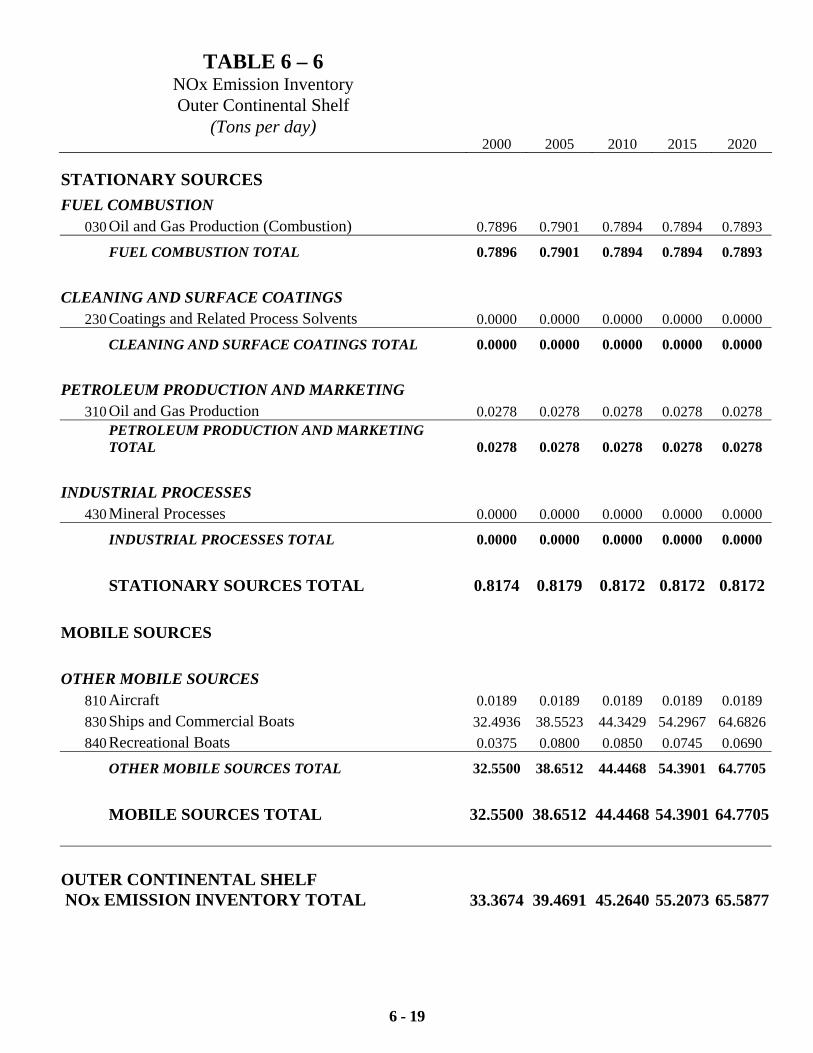
TABLE 6 – 6 NOx Emission Inventory Outer Continental Shelf
(Tons per day) 2000 2005 2010 2015 2020
6 - 19
STATIONARY SOURCES
FUEL COMBUSTION 030 Oil and Gas Production (Combustion) 0.7896 0.7901 0.7894 0.7894 0.7893
FUEL COMBUSTION TOTAL 0.7896 0.7901 0.7894 0.7894 0.7893
CLEANING AND SURFACE COATINGS 230 Coatings and Related Process Solvents 0.0000 0.0000 0.0000 0.0000 0.0000
CLEANING AND SURFACE COATINGS TOTAL 0.0000 0.0000 0.0000 0.0000 0.0000
PETROLEUM PRODUCTION AND MARKETING 310 Oil and Gas Production 0.0278 0.0278 0.0278 0.0278 0.0278
PETROLEUM PRODUCTION AND MARKETING TOTAL 0.0278 0.0278 0.0278 0.0278 0.0278
INDUSTRIAL PROCESSES 430 Mineral Processes 0.0000 0.0000 0.0000 0.0000 0.0000
INDUSTRIAL PROCESSES TOTAL 0.0000 0.0000 0.0000 0.0000 0.0000
STATIONARY SOURCES TOTAL 0.8174 0.8179 0.8172 0.8172 0.8172
MOBILE SOURCES
OTHER MOBILE SOURCES 810 Aircraft 0.0189 0.0189 0.0189 0.0189 0.0189 830 Ships and Commercial Boats 32.4936 38.5523 44.3429 54.2967 64.6826840 Recreational Boats 0.0375 0.0800 0.0850 0.0745 0.0690
OTHER MOBILE SOURCES TOTAL 32.5500 38.6512 44.4468 54.3901 64.7705
MOBILE SOURCES TOTAL 32.5500 38.6512 44.4468 54.3901 64.7705
OUTER CONTINENTAL SHELF NOx EMISSION INVENTORY TOTAL 33.3674 39.4691 45.2640 55.2073 65.5877
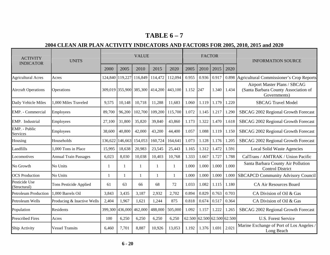
6 - 20
TABLE 6 – 7 2004 CLEAN AIR PLAN ACTIVITY INDICATORS AND FACTORS FOR 2005, 2010, 2015 and 2020
VALUE FACTOR ACTIVITY INDICATOR UNITS
2000 2005 2010 2015 2020 2005 2010 2015 2020
INFORMATION SOURCE
Agricultural Acres Acres 124,840 119,227 116,849 114,472 112,094 0.955 0.936 0.917 0.898 Agricultural Commissioner’s Crop Reports
Aircraft Operations Operations 309,019 355,900 385,300 414,200 443,100 1.152 247 1.340 1.434Airport Master Plans / SBCAG
(Santa Barbara County Association of Governments)
Daily Vehicle Miles 1,000 Miles Traveled 9,575 10,148 10,718 11,288 11,683 1.060 1.119 1.179 1.220 SBCAG Travel Model
EMP. - Commercial Employees 89,700 96,200 102,700 109,200 115,700 1.072 1.145 1.217 1.290 SBCAG 2002 Regional Growth Forecast
EMP. Industrial Employees 27,100 31,800 35,820 39,840 43,860 1.173 1.322 1.470 1.618 SBCAG 2002 Regional Growth Forecast EMP. - Public Services Employees 38,600 40,800 42,000 43,200 44,400 1.057 1.088 1.119 1.150 SBCAG 2002 Regional Growth Forecast
Housing Households 136,622 146,663 154,053 160,724 164,641 1.073 1.128 1.176 1.205 SBCAG 2002 Regional Growth Forecast
Landfills 1,000 Tons in Place 15,995 18,638 20,983 23,545 25,443 1.165 1.312 1.472 1.591 Local Solid Waste Agencies
Locomotives Annual Train Passages 6,023 8,030 10,038 10,403 10,768 1.333 1.667 1.727 1.788 CalTrans / AMTRAK / Union Pacific
No Growth No Units 1 1 1 1 1 1.000 1.000 1.000 1.000 Santa Barbara County Air Pollution Control District
OCS Production No Units 1 1 1 1 1 1.000 1.000 1.000 1.000 SBCAPCD Community Advisory Council Pesticide Use (Structural) Tons Pesticide Applied 61 63 66 68 72 1.033 1.082 1.115 1.180 CA Air Resources Board
Petroleum Production 1,000 Barrels Oil 3,843 3,435 3,187 2,932 2,702 0.894 0.829 0.763 0.703 CA Division of Oil & Gas Petroleum Wells Producing & Inactive Wells 2,404 1,967 1,621 1,244 875 0.818 0.674 0.517 0.364 CA Division of Oil & Gas
Population Residents 399,300 436,000 462,000 488,000 505,000 1.092 1.157 1.222 1.265 SBCAG 2002 Regional Growth Forecast
Prescribed Fires Acres 100 6,250 6,250 6,250 6,250 62.500 62.500 62.500 62.500 U.S. Forest Service
Ship Activity Vessel Transits 6,460 7,701 8,887 10,926 13,053 1.192 1.376 1.691 2.021 Marine Exchange of Port of Los Angeles / Long Beach
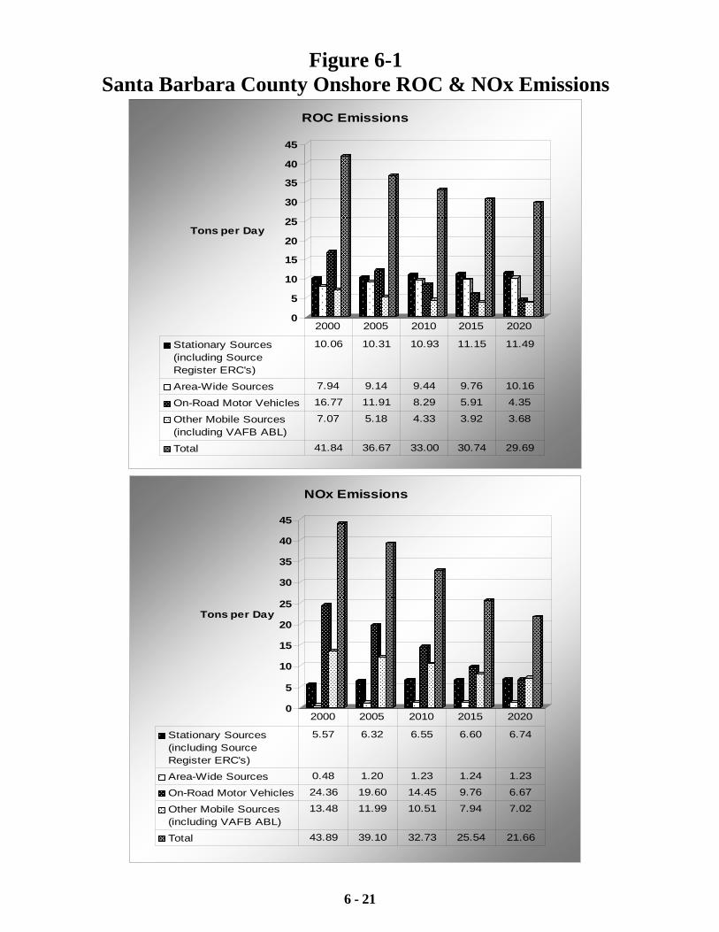
6 - 21
Figure 6-1 Santa Barbara County Onshore ROC & NOx Emissions
0
5
10
15
20
25
30
35
40
45
Tons per Day
ROC Emissions
Stationary Sources(including SourceRegister ERC's)
10.06 10.31 10.93 11.15 11.49
Area-Wide Sources 7.94 9.14 9.44 9.76 10.16
On-Road Motor Vehicles 16.77 11.91 8.29 5.91 4.35
Other Mobile Sources(including VAFB ABL)
7.07 5.18 4.33 3.92 3.68
Total 41.84 36.67 33.00 30.74 29.69
2000 2005 2010 2015 2020
0
5
10
15
20
25
30
35
40
45
Tons per Day
NOx Emissions
Stationary Sources(including SourceRegister ERC's)
5.57 6.32 6.55 6.60 6.74
Area-Wide Sources 0.48 1.20 1.23 1.24 1.23
On-Road Motor Vehicles 24.36 19.60 14.45 9.76 6.67
Other Mobile Sources(including VAFB ABL)
13.48 11.99 10.51 7.94 7.02
Total 43.89 39.10 32.73 25.54 21.66
2000 2005 2010 2015 2020
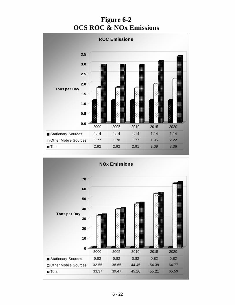
6 - 22
Figure 6-2 OCS ROC & NOx Emissions
0.0
0.5
1.0
1.5
2.0
2.5
3.0
3.5
Tons per Day
ROC Emissions
Stationary Sources 1.14 1.14 1.14 1.14 1.14
Other Mobile Sources 1.77 1.78 1.77 1.95 2.22
Total 2.92 2.92 2.91 3.09 3.36
2000 2005 2010 2015 2020
0
10
20
30
40
50
60
70
Tons per Day
NOx Emissions
Stationary Sources 0.82 0.82 0.82 0.82 0.82
Other Mobile Sources 32.55 38.65 44.45 54.39 64.77
Total 33.37 39.47 45.26 55.21 65.59
2000 2005 2010 2015 2020
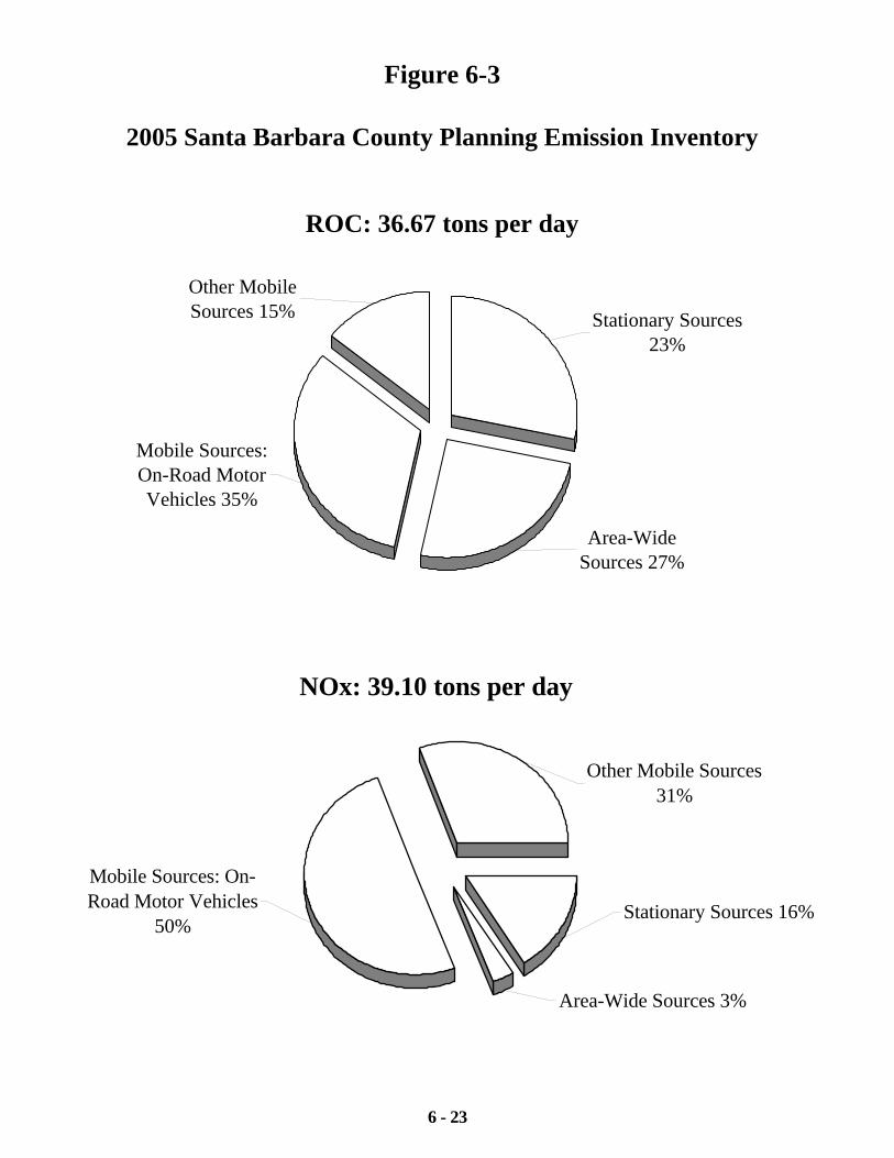
6 - 23
NOx: 39.10 tons per day
Stationary Sources 16%
Area-Wide Sources 3%
Mobile Sources: On-Road Motor Vehicles
50%
Other Mobile Sources31%
Figure 6-3
2005 Santa Barbara County Planning Emission Inventory
ROC: 36.67 tons per day
Mobile Sources: On-Road Motor Vehicles 35%
Other Mobile Sources 15% Stationary Sources
23%
Area-Wide Sources 27%
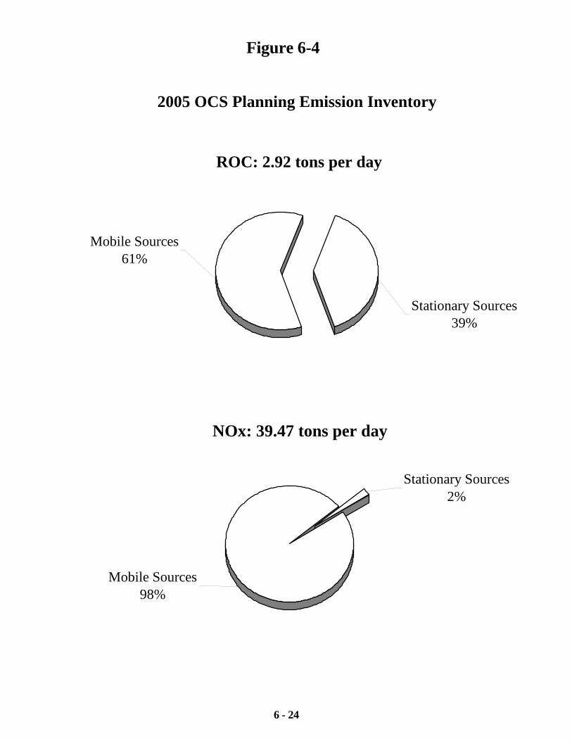
6 - 24
2005 OCS Planning Emission Inventory
ROC: 2.92 tons per day
Stationary Sources39%
Mobile Sources 61%
NOx: 39.47 tons per day
Mobile Sources98%
Stationary Sources2%
Figure 6-4
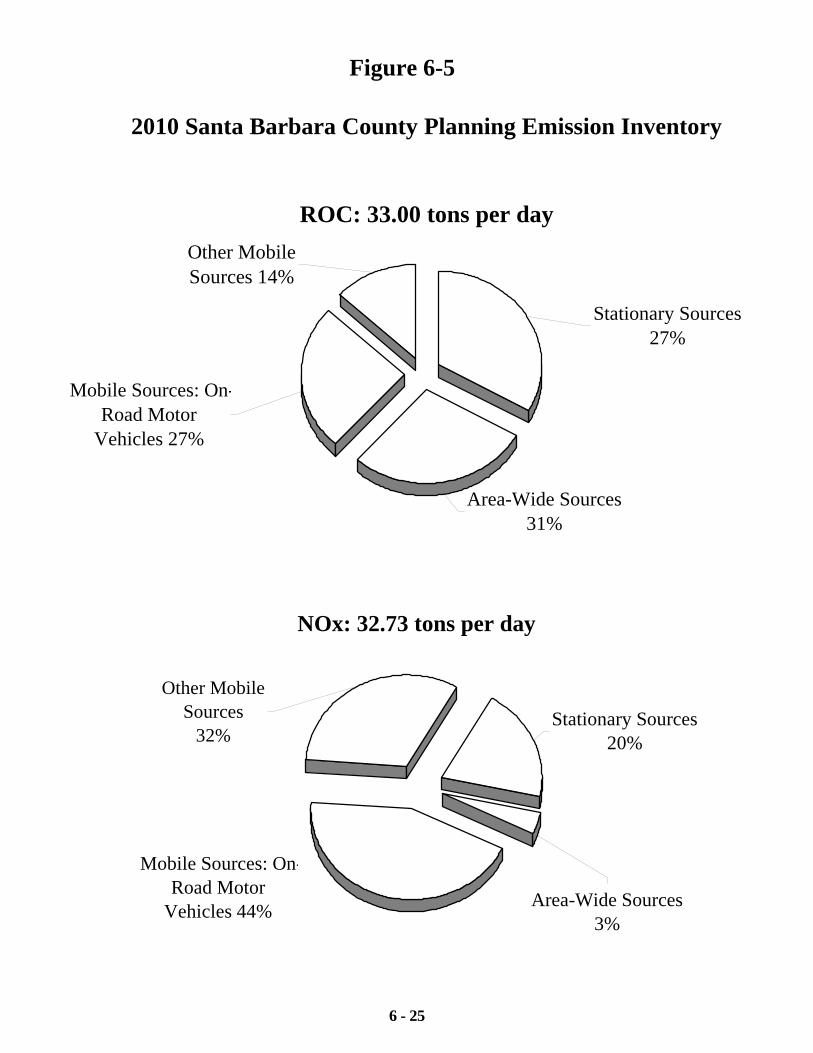
6 - 25
2010 Santa Barbara County Planning Emission Inventory
ROC: 33.00 tons per day
Area-Wide Sources 31%
Other Mobile Sources 14%
Mobile Sources: On-Road Motor
Vehicles 27%
Stationary Sources 27%
NOx: 32.73 tons per day
Stationary Sources 20%
Area-Wide Sources 3%
Mobile Sources: On-Road Motor
Vehicles 44%
Other Mobile Sources
32%
Figure 6-5
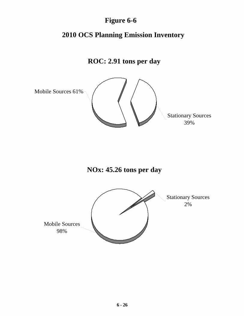
6 - 26
2010 OCS Planning Emission Inventory
ROC: 2.91 tons per day
Stationary Sources39%
Mobile Sources 61%
NOx: 45.26 tons per day
Mobile Sources98%
Stationary Sources2%
Figure 6-6
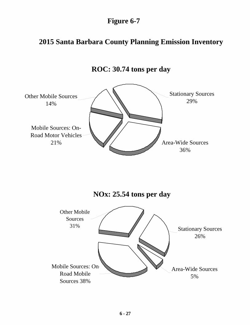
6 - 27
2015 Santa Barbara County Planning Emission Inventory
ROC: 30.74 tons per day
Stationary Sources 29%
Mobile Sources: On-Road Motor Vehicles
21%
Other Mobile Sources 14%
Area-Wide Sources 36%
NOx: 25.54 tons per day
Stationary Sources 26%
Area-Wide Sources 5%
Mobile Sources: On-Road Mobile Sources 38%
Other Mobile Sources
31%
Figure 6-7
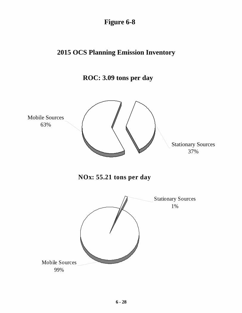
6 - 28
2015 OCS Planning Emission Inventory
ROC: 3.09 tons per day
Stationary Sources37%
Mobile Sources 63%
Figure 6-8
NOx: 55.21 tons per day
Stationary Sources1%
Mobile Sources 99%
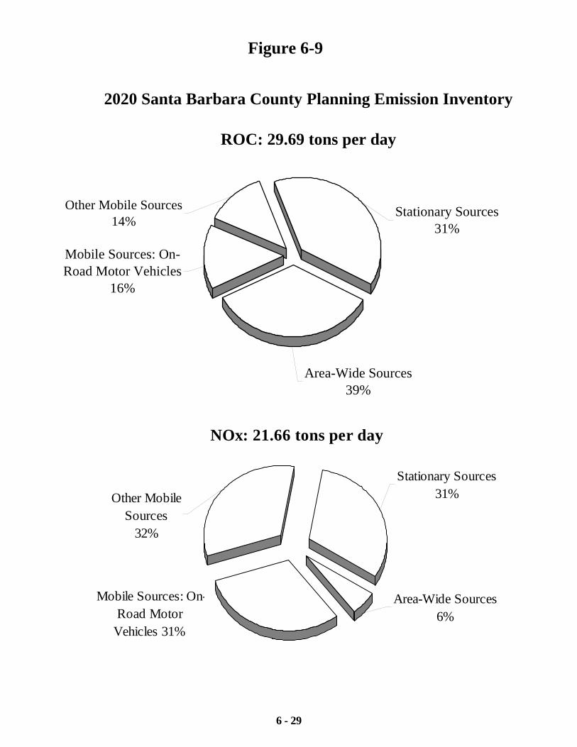
6 - 29
2020 Santa Barbara County Planning Emission Inventory
ROC: 29.69 tons per day
Stationary Sources 31%
Mobile Sources: On-Road Motor Vehicles
16%
Other Mobile Sources 14%
Area-Wide Sources 39%
NOx: 21.66 tons per day
Stationary Sources 31%
Area-Wide Sources 6%
Mobile Sources: On-Road Motor
Vehicles 31%
Other Mobile Sources
32%
Figure 6-9
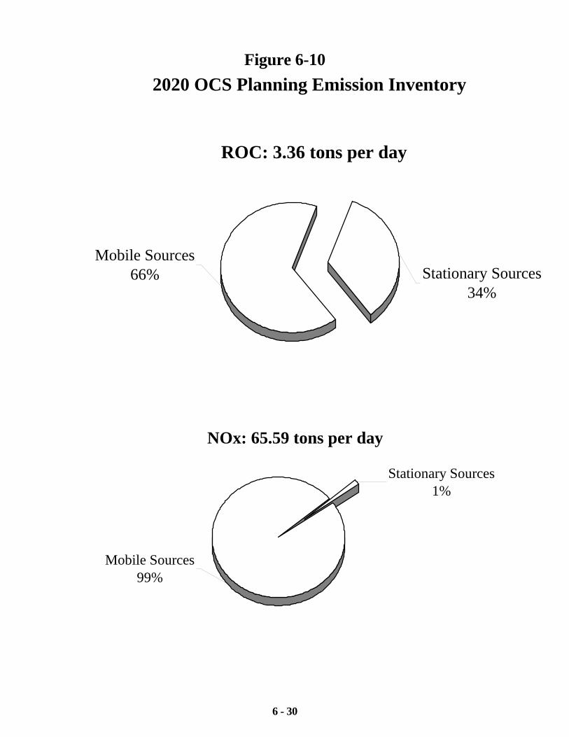
6 - 30
2020 OCS Planning Emission Inventory
ROC: 3.36 tons per day
Stationary Sources34%
Mobile Sources 66%
Figure 6-10
NOx: 65.59 tons per day
Mobile Sources99%
Stationary Sources1%
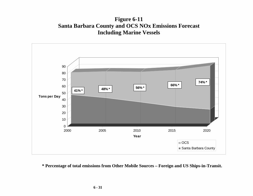
6 - 31
Figure 6-11 Santa Barbara County and OCS NOx Emissions Forecast
Including Marine Vessels
0
10
20
30
40
50
60
70
80
90
Tons per Day
2000 2005 2010 2015 2020Year
OCSSanta Barbara County
41% *66% *
56% *48% *
74% *
* Percentage of total emissions from Other Mobile Sources – Foreign and US Ships-in-Transit.
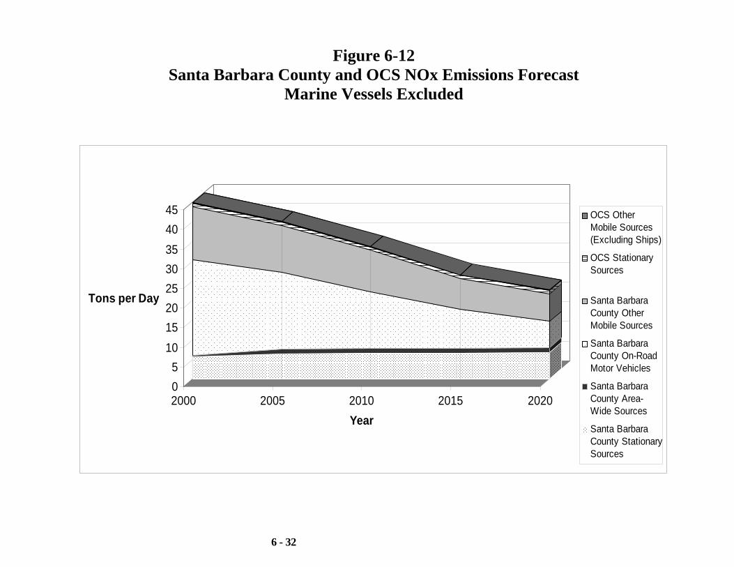
6 - 32
Figure 6-12 Santa Barbara County and OCS NOx Emissions Forecast
Marine Vessels Excluded
05
1015202530354045
Tons per Day
2000 2005 2010 2015 2020Year
OCS OtherMobile Sources(Excluding Ships)
OCS StationarySources
Santa BarbaraCounty OtherMobile Sources
Santa BarbaraCounty On-RoadMotor Vehicles
Santa BarbaraCounty Area-Wide Sources
Santa BarbaraCounty StationarySources
CHAPTER 7
PUBLIC PARTICIPATION
Introduction
Community Advisory Council Comments
2004 Plan Public Workshop
Written Comments and Responses on the 2004 Plan
ARB Transport Analysis
7 - 1
7. PUBLIC PARTICIPATION
7.1 INTRODUCTION
The public participation process used in the development of this 2004 Clean Air Plan (2004 Plan)
was implemented to assure that the demands of clean air placed on us by the plan are reasonable
and capable of being achieved. Also, it is important that members of the public, the regulated
industry, and government agencies, have an opportunity to provide input into shaping our present
and future strategies to clean the air.
A specific group of people has been organized to serve the goal of providing input on the
development of clean air plans. They are known as the Community Advisory Council. On
May 24, 1994, the Air Pollution Control District Board of Directors (Board) formed the
Community Advisory Council (CAC). The purpose of the CAC is to provide advice to the Air
Pollution Control Officer (APCO) and the Board in matters relating to attainment planning,
development and promulgation of air pollution control rules and other associated policy issues.
The CAC considers and renders advice on subjects submitted to them by the APCO, the Board,
CAC members, and the public. The CAC is chartered to consider issues related to air pollution
planning and rulemaking for which the Air Pollution Control District (APCD) has jurisdiction.
The CAC's deliberations and recommendations are to consider, to the extent feasible and
reasonable, the effects of APCD planning and rulemaking actions upon public health, the
economy, the costs to industry, and the public, along with conformance with the mandates of all
applicable local, state, and federal laws. The recommendations of the CAC are advisory in nature
and neither the APCO, nor the Board, are bound by CAC recommendations.
Each Board member can appoint two representatives to the CAC. The Board was directed to
select CAC members who contain a background related to community interest, professional
business, or technical experience. For example a CAC member could have a working knowledge
of land use planning, agriculture, petroleum production, medicine, engineering, transportation,
environmental conservation, public health, business, or education.
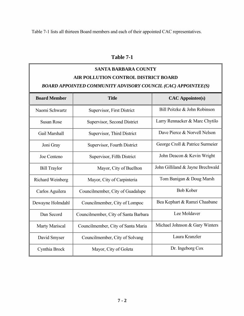
7 - 2
Table 7-1 lists all thirteen Board members and each of their appointed CAC representatives.
Table 7-1
SANTA BARBARA COUNTY
AIR POLLUTION CONTROL DISTRICT BOARD
BOARD APPOINTED COMMUNITY ADVISORY COUNCIL (CAC) APPOINTEE(S)
Board Member Title CAC Appointee(s)
Naomi Schwartz Supervisor, First District Bill Peitzke & John Robinson
Susan Rose Supervisor, Second District Larry Rennacker & Marc Chytilo
Gail Marshall Supervisor, Third District Dave Pierce & Norvell Nelson
Joni Gray Supervisor, Fourth District George Croll & Patrice Surmeier
Joe Centeno Supervisor, Fifth District John Deacon & Kevin Wright
Bill Traylor Mayor, City of Buellton John Gilliland & Jayne Brechwald
Richard Weinberg Mayor, City of Carpinteria Tom Banigan & Doug Marsh
Carlos Aguilera Councilmember, City of Guadalupe Bob Kober
Dewayne Holmdahl Councilmember, City of Lompoc Bea Kephart & Ramzi Chaabane
Dan Secord Councilmember, City of Santa Barbara Lee Moldaver
Marty Mariscal Councilmember, City of Santa Maria Michael Johnson & Gary Winters
David Smyser Councilmember, City of Solvang Laura Kranzler
Cynthia Brock Mayor, City of Goleta Dr. Ingeborg Cox
7 - 3
The APCD has specifically sought out input from the CAC on each element of the 2004 Plan as it
was being developed over the past year. Starting in January of 2004, APCD staff presented
specific portions of the 2004 Plan for the CAC to review and comment on. The CAC also
provided recommendations regarding policy and other key issues that altered the direction, and
ultimately enhanced the plan’s contents. The highlights of these CAC meetings and the
recommendations that occurred are listed in Section 7.2.
As part of the APCD's continuing commitment to solicit public participation and input into plan
development, public workshops were also conducted to present the concepts of the 2004 Plan and
the implications of its proposed control measures on the residents and business community of
Santa Barbara County. The focus of the public workshops was to allow public commentary on
the plan while allowing APCD and Santa Barbara County Association of Governments (SBCAG)
staff the opportunity to address concerns and answer questions regarding the plan and its
contents. The public comments received verbally during the workshops were responded to at that
time and are included in Section 7.4. Public notices announcing the date, time, and location of
the public workshops were published in area newspapers, including the Santa Barbara News
Press, the Santa Maria Times, and the Lompoc Record. A copy of the public notice can be can be
found at the end of this chapter.
The public notice announced that the 2004 Plan was available for public review. The public
comment period was from August 25, 2004 to September 24, 2004. A copy of all written
comments on the 2004 Plan that have been submitted by the public, along with the written
responses to these comments, is provided in Section 7.3.
Public presentations of the 2004 Plan were conducted at workshops, before the Board at public
hearings, and before the Community Advisory Council. A complete listing of all public
workshops and plan presentations is contained in Table 7-2.
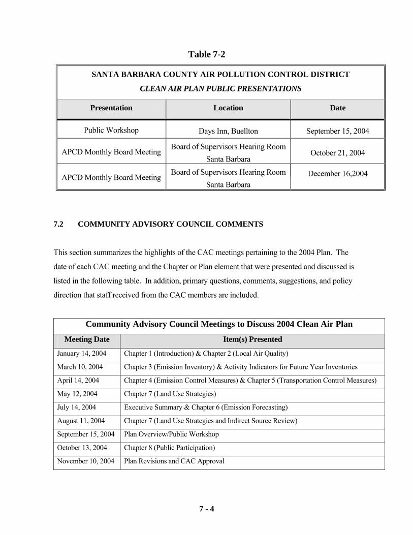
7 - 4
Table 7-2
SANTA BARBARA COUNTY AIR POLLUTION CONTROL DISTRICT
CLEAN AIR PLAN PUBLIC PRESENTATIONS
Presentation Location Date
Public Workshop Days Inn, Buellton September 15, 2004
APCD Monthly Board Meeting Board of Supervisors Hearing Room Santa Barbara
October 21, 2004
APCD Monthly Board Meeting Board of Supervisors Hearing Room Santa Barbara
December 16,2004
7.2 COMMUNITY ADVISORY COUNCIL COMMENTS
This section summarizes the highlights of the CAC meetings pertaining to the 2004 Plan. The
date of each CAC meeting and the Chapter or Plan element that were presented and discussed is
listed in the following table. In addition, primary questions, comments, suggestions, and policy
direction that staff received from the CAC members are included.
Community Advisory Council Meetings to Discuss 2004 Clean Air Plan
Meeting Date Item(s) Presented
January 14, 2004 Chapter 1 (Introduction) & Chapter 2 (Local Air Quality)
March 10, 2004 Chapter 3 (Emission Inventory) & Activity Indicators for Future Year Inventories
April 14, 2004 Chapter 4 (Emission Control Measures) & Chapter 5 (Transportation Control Measures)
May 12, 2004 Chapter 7 (Land Use Strategies)
July 14, 2004 Executive Summary & Chapter 6 (Emission Forecasting)
August 11, 2004 Chapter 7 (Land Use Strategies and Indirect Source Review)
September 15, 2004 Plan Overview/Public Workshop
October 13, 2004 Chapter 8 (Public Participation)
November 10, 2004 Plan Revisions and CAC Approval
7 - 5
January 14, 2004 Chapter 1: Introduction
Chapter 2: Local Air Quality
The APCD presented Chapter 1 (Introduction) and Chapter 2 (Local Air Quality) to the CAC.
There were no action items related to Chapter 1. The CAC made the following suggestion for
Chapter 2 that was incorporated in the draft Plan:
• The CAC recommended that Figure 2-2, which shows the number of state ozone
exceedances since 1988, also include a graphic showing trends in population and vehicle
miles traveled. This would provide an indication that while population and vehicle miles
are increasing, air quality is continuing to improve. See Figure 2-26 for added graphic.
March 10, 2004 Chapter 3: Emission Inventory
Discussion of Future Year Activity Indicators
The APCD presented the base year emission inventory (Chapter 3) to the CAC. The CAC
recommended the following:
• Under emissions summary categories, only present source types that are that are
consistent with facilities that we have in our county. The CAC suggested that it is not
necessary to provide facility types as examples if those types of businesses do not exist in
the county.
In addition, activity data used in emission forecasting were presented to the CAC so that the
activity factors could be discussed and refined prior to the development of Chapter 6 (Emission
Forecasting). The CAC provided the following comments and suggestions related to the
activity indicators:
• The CAC suggested that the activity indicator of irrigated acres is not a good proxy for
emission sources tied to agricultural operations. After further research, it was determined
that irrigated acres is a reasonable indicator for determining trends in agricultural related
activities.
• Two separate trends for the petroleum production indicator were presented to the CAC.
7 - 6
One trend showed a fairly rapid decline in production while the other showed a slower
decline in production over time. After some discussion, it was decided that the slower
declining trend in oil production represents the best scenario due to current trends in the
oil industry.
April 14, 2004 Chapter 4: Emission Control Measures
Chapter5: Transportation Control Measures
After an overview of both emission and transportation control measures, the CAC asked staff
to address the following items:
• Determine the current status on regulatory progress on pesticides and pesticide emissions
inventory in Santa Barbara County. In addition, the CAC requested that the APCD
determine the effectiveness of the statewide pesticide program.
• As part of a review of the external combustion lime/cement kiln further study measure,
the CAC suggested that staff look into work that was done by the state of Texas.
Information from the state of Texas was found not to apply to Santa Barbara County.
Additionally, staff will continue to research whether any applicable lime or cement kilns
are located in Santa Barbara County. If none are found, this further study measures will
be removed from consideration.
• Determine whether emission reduction credits from incentive programs such as Carl
Moyer are being incorporated in the OFFROAD and EMFAC models. Staff research
determined that neither EMFAC nor OFFROAD account for emission reductions from
incentive programs - ARB does not incorporate the reductions into these models.
• There should be greater detail in the Plan on the VMT growth rate and how to address
growth. In addition, state law requires public input on transportation control measure
(TCM) development. It was suggested that the planning process does not allow for public
participation of the TCM’s that are included in the Plan. SBCAG staff briefed the CAC
on 101 in Motion, a project with the objective of developing long-term solutions for
improving traffic congestion along the 101 corridor in the south coast of Santa Barbara
County. SBCAG suggested that input on TCM’s could be provided at 101 in Motion
7 - 7
workshops. The CAC asked staff to return with a report on the overall process for
developing the TCM’s.
May 12, 2004 Chapter 7: Land Use Strategies
For Chapter 7, the CAC made the following suggestions:
• Add a glossary of terms to the chapter.
• Provide a definition for “traditional neighborhood development.”
• Consider deleting sentence with Centers of Disease Control, which may be controversial.
• The policies of density should also include a discussion that densification requires that
there is enforcement of policies and ordinances such as noise and nuisance, and that there
is protection of privacy and affordability.
• There should be a more regional approach to the challenges of land use strategies by
bringing together representatives from air quality, water quality, agriculture, LAFCO
among others.
• There should be a focus on how to enhance implementation of land use concepts. This
should be done through collaboration with other planning agencies to incorporate these
concepts into their own planning programs.
• It was suggested by the CAC that an Indirect Source Review (ISR) subcommittee be
formed to address ISR challenges and build CAC consensus. A five-member CAC
subcommittee was formed and will meet with the APCD to discuss ISR issues and to
develop conceptual language for discussion with the entire CAC.
July 14, 2004 Executive Summary
Chapter 6: Emission Forecasting
• In the Executive Summary, add a question/answer section that explains how attainment of
the state 1-hour ozone standard is determined.
7 - 8
For Chapter 6, the CAC comments resulted in the following changes to the draft Plan:
• Added a discussion in the Chapter specifying that 90% marine shipping fleet that transited
the Santa Barbara coastline in 2000 was foreign flagged.
• The CAC recommended that mobile sources be broken-out in the emissions graphics to
show that marine vessels comprise a majority of the emissions.
In addition, the CAC made the following recommendations:
• It was suggested that a representative from Lois Capps’ office attend the 2004 Plan
adoption hearing to bring more attention to the challenges controlling emissions from
marine shipping.
• A recommendation was made that the APCD should look into forming a partnership with
UCSB’s remote sensing group to investigate the impacts of marine shipping on Santa
Barbara County.
August 11, 2004 Chapter 7: Land Use Strategies (ISR Program and Regulation
Concept)
• The CAC recommended that the APCD assess and develop as warranted and Indirect Source
Review Program/Regulation to minimize and mitigate air pollution from discretionary land
use entitlements. A section on Indirect Source Review will be included in Chapter 7. In
addition, under the goals of the ISR Program/Regulation, the CAC suggested that the term
“Smart Growth” be removed from the text since it is confusing and its deletion would make
the text more readable.
September 15, 2004 Plan Overview
A brief overview of the draft Plan was provided at this meeting. Comments received from CAC
members during the meeting are provided in the next section.
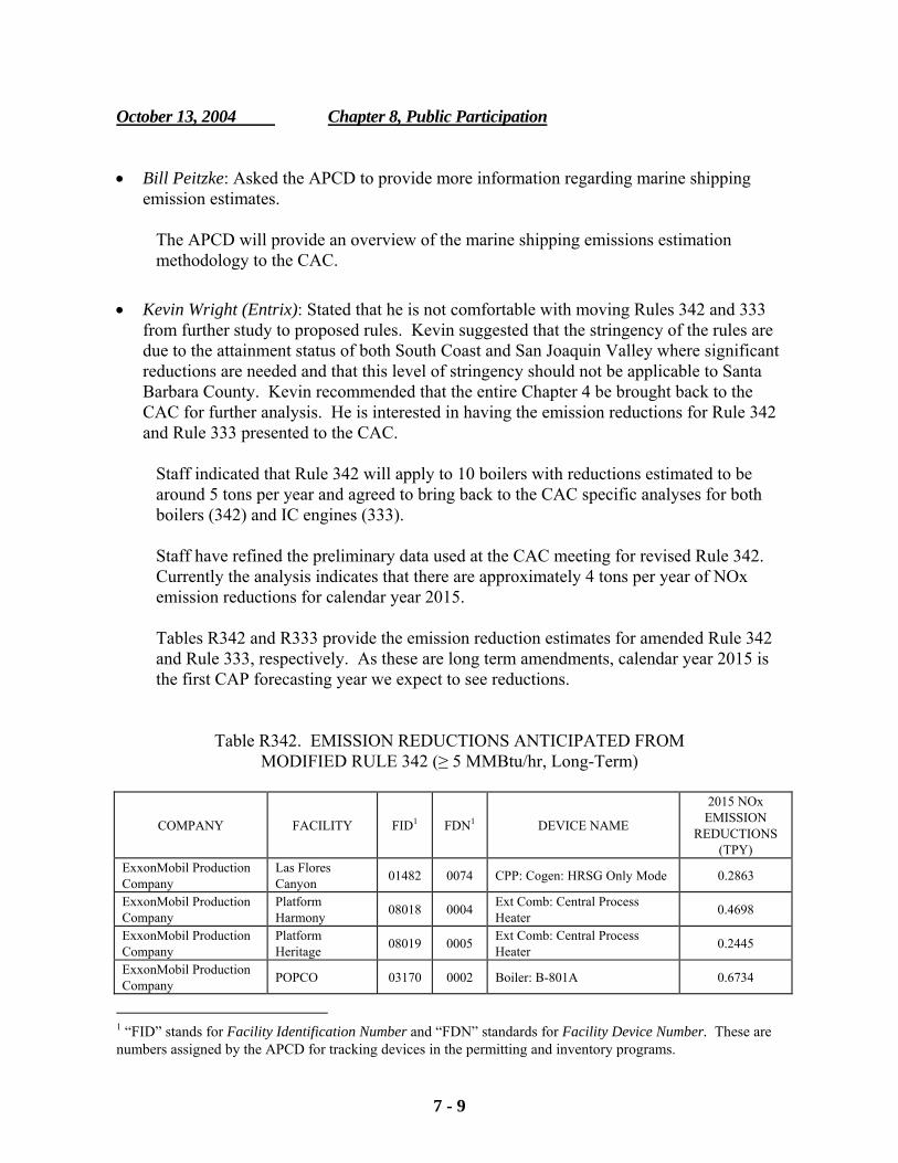
7 - 9
October 13, 2004 Chapter 8, Public Participation
• Bill Peitzke: Asked the APCD to provide more information regarding marine shipping emission estimates.
The APCD will provide an overview of the marine shipping emissions estimation methodology to the CAC.
• Kevin Wright (Entrix): Stated that he is not comfortable with moving Rules 342 and 333 from further study to proposed rules. Kevin suggested that the stringency of the rules are due to the attainment status of both South Coast and San Joaquin Valley where significant reductions are needed and that this level of stringency should not be applicable to Santa Barbara County. Kevin recommended that the entire Chapter 4 be brought back to the CAC for further analysis. He is interested in having the emission reductions for Rule 342 and Rule 333 presented to the CAC.
Staff indicated that Rule 342 will apply to 10 boilers with reductions estimated to be around 5 tons per year and agreed to bring back to the CAC specific analyses for both boilers (342) and IC engines (333).
Staff have refined the preliminary data used at the CAC meeting for revised Rule 342. Currently the analysis indicates that there are approximately 4 tons per year of NOx emission reductions for calendar year 2015. Tables R342 and R333 provide the emission reduction estimates for amended Rule 342 and Rule 333, respectively. As these are long term amendments, calendar year 2015 is the first CAP forecasting year we expect to see reductions.
Table R342. EMISSION REDUCTIONS ANTICIPATED FROM MODIFIED RULE 342 (≥ 5 MMBtu/hr, Long-Term)
COMPANY FACILITY FID1 FDN1 DEVICE NAME
2015 NOx EMISSION
REDUCTIONS (TPY)
ExxonMobil Production Company
Las Flores Canyon 01482 0074 CPP: Cogen: HRSG Only Mode 0.2863
ExxonMobil Production Company
Platform Harmony 08018 0004 Ext Comb: Central Process
Heater 0.4698
ExxonMobil Production Company
Platform Heritage 08019 0005 Ext Comb: Central Process
Heater 0.2445
ExxonMobil Production Company POPCO 03170 0002 Boiler: B-801A 0.6734
1 “FID” stands for Facility Identification Number and “FDN” standards for Facility Device Number. These are numbers assigned by the APCD for tracking devices in the permitting and inventory programs.
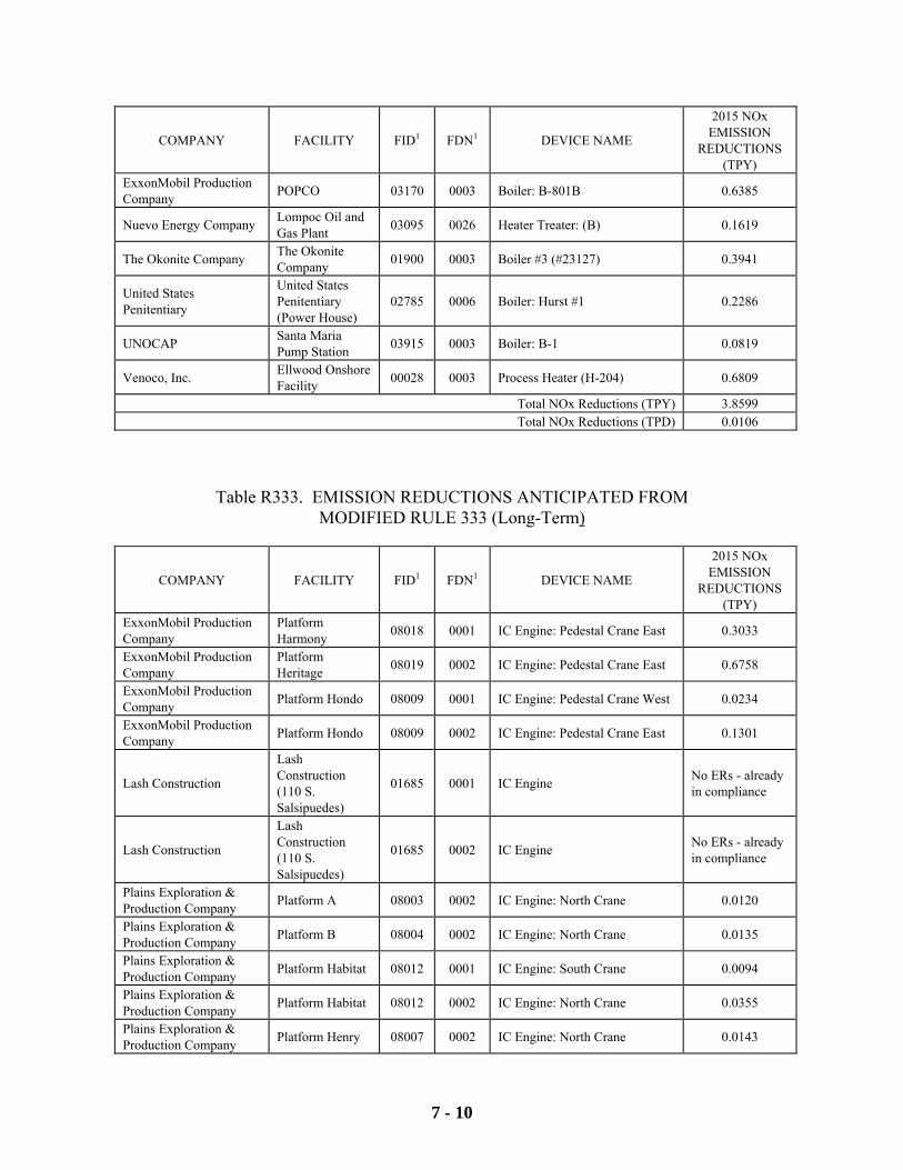
7 - 10
COMPANY FACILITY FID1 FDN1 DEVICE NAME
2015 NOx EMISSION
REDUCTIONS (TPY)
ExxonMobil Production Company POPCO 03170 0003 Boiler: B-801B 0.6385
Nuevo Energy Company Lompoc Oil and Gas Plant 03095 0026 Heater Treater: (B) 0.1619
The Okonite Company The Okonite Company 01900 0003 Boiler #3 (#23127) 0.3941
United States Penitentiary
United States Penitentiary (Power House)
02785 0006 Boiler: Hurst #1 0.2286
UNOCAP Santa Maria Pump Station 03915 0003 Boiler: B-1 0.0819
Venoco, Inc. Ellwood Onshore Facility 00028 0003 Process Heater (H-204) 0.6809
Total NOx Reductions (TPY) 3.8599 Total NOx Reductions (TPD) 0.0106
Table R333. EMISSION REDUCTIONS ANTICIPATED FROM MODIFIED RULE 333 (Long-Term)
COMPANY FACILITY FID1 FDN1 DEVICE NAME
2015 NOx EMISSION
REDUCTIONS (TPY)
ExxonMobil Production Company
Platform Harmony 08018 0001 IC Engine: Pedestal Crane East 0.3033
ExxonMobil Production Company
Platform Heritage 08019 0002 IC Engine: Pedestal Crane East 0.6758
ExxonMobil Production Company Platform Hondo 08009 0001 IC Engine: Pedestal Crane West 0.0234
ExxonMobil Production Company Platform Hondo 08009 0002 IC Engine: Pedestal Crane East 0.1301
Lash Construction
Lash Construction (110 S. Salsipuedes)
01685 0001 IC Engine No ERs - already in compliance
Lash Construction
Lash Construction (110 S. Salsipuedes)
01685 0002 IC Engine No ERs - already in compliance
Plains Exploration & Production Company Platform A 08003 0002 IC Engine: North Crane 0.0120
Plains Exploration & Production Company Platform B 08004 0002 IC Engine: North Crane 0.0135
Plains Exploration & Production Company Platform Habitat 08012 0001 IC Engine: South Crane 0.0094
Plains Exploration & Production Company Platform Habitat 08012 0002 IC Engine: North Crane 0.0355
Plains Exploration & Production Company Platform Henry 08007 0002 IC Engine: North Crane 0.0143
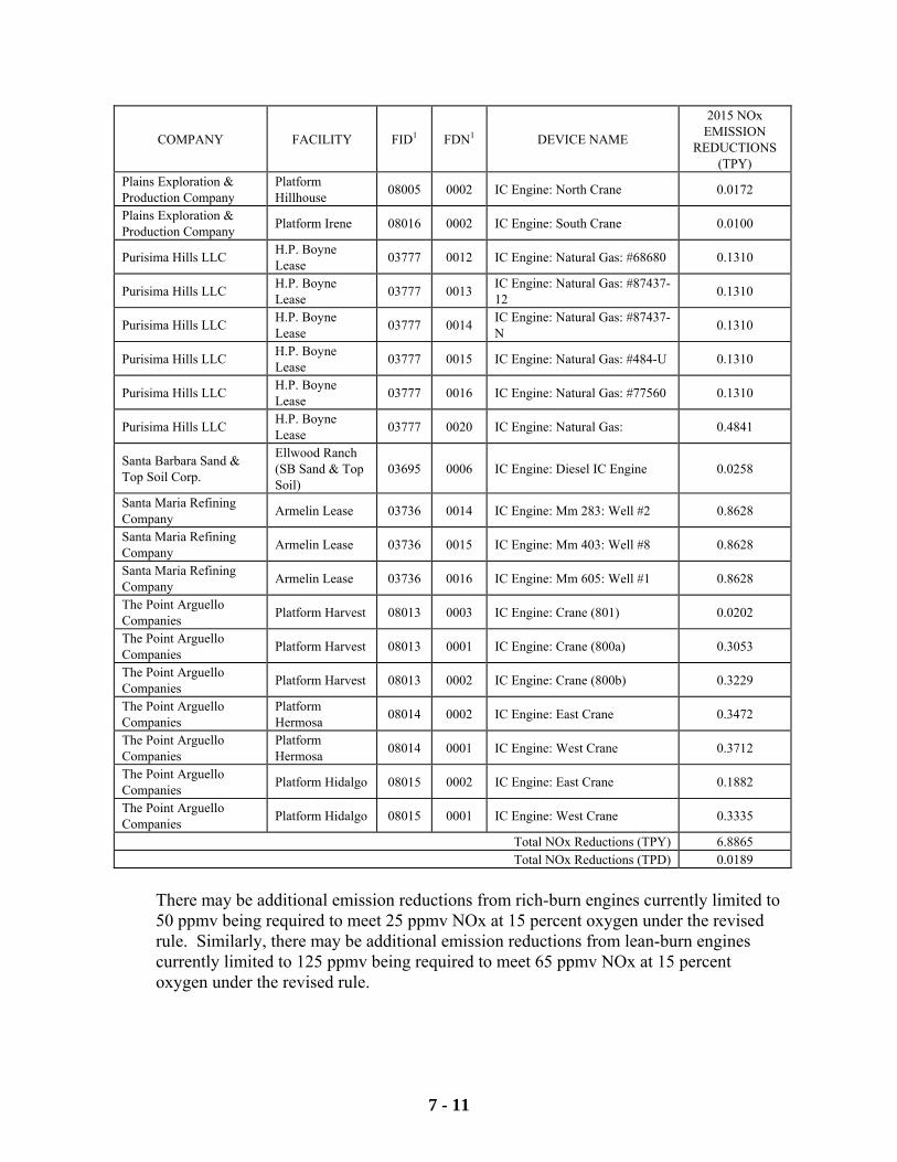
7 - 11
COMPANY FACILITY FID1 FDN1 DEVICE NAME
2015 NOx EMISSION
REDUCTIONS (TPY)
Plains Exploration & Production Company
Platform Hillhouse 08005 0002 IC Engine: North Crane 0.0172
Plains Exploration & Production Company Platform Irene 08016 0002 IC Engine: South Crane 0.0100
Purisima Hills LLC H.P. Boyne Lease 03777 0012 IC Engine: Natural Gas: #68680 0.1310
Purisima Hills LLC H.P. Boyne Lease 03777 0013 IC Engine: Natural Gas: #87437-
12 0.1310
Purisima Hills LLC H.P. Boyne Lease 03777 0014 IC Engine: Natural Gas: #87437-
N 0.1310
Purisima Hills LLC H.P. Boyne Lease 03777 0015 IC Engine: Natural Gas: #484-U 0.1310
Purisima Hills LLC H.P. Boyne Lease 03777 0016 IC Engine: Natural Gas: #77560 0.1310
Purisima Hills LLC H.P. Boyne Lease 03777 0020 IC Engine: Natural Gas: 0.4841
Santa Barbara Sand & Top Soil Corp.
Ellwood Ranch (SB Sand & Top Soil)
03695 0006 IC Engine: Diesel IC Engine 0.0258
Santa Maria Refining Company Armelin Lease 03736 0014 IC Engine: Mm 283: Well #2 0.8628
Santa Maria Refining Company Armelin Lease 03736 0015 IC Engine: Mm 403: Well #8 0.8628
Santa Maria Refining Company Armelin Lease 03736 0016 IC Engine: Mm 605: Well #1 0.8628
The Point Arguello Companies Platform Harvest 08013 0003 IC Engine: Crane (801) 0.0202
The Point Arguello Companies Platform Harvest 08013 0001 IC Engine: Crane (800a) 0.3053
The Point Arguello Companies Platform Harvest 08013 0002 IC Engine: Crane (800b) 0.3229
The Point Arguello Companies
Platform Hermosa 08014 0002 IC Engine: East Crane 0.3472
The Point Arguello Companies
Platform Hermosa 08014 0001 IC Engine: West Crane 0.3712
The Point Arguello Companies Platform Hidalgo 08015 0002 IC Engine: East Crane 0.1882
The Point Arguello Companies Platform Hidalgo 08015 0001 IC Engine: West Crane 0.3335
Total NOx Reductions (TPY) 6.8865 Total NOx Reductions (TPD) 0.0189
There may be additional emission reductions from rich-burn engines currently limited to 50 ppmv being required to meet 25 ppmv NOx at 15 percent oxygen under the revised rule. Similarly, there may be additional emission reductions from lean-burn engines currently limited to 125 ppmv being required to meet 65 ppmv NOx at 15 percent oxygen under the revised rule.
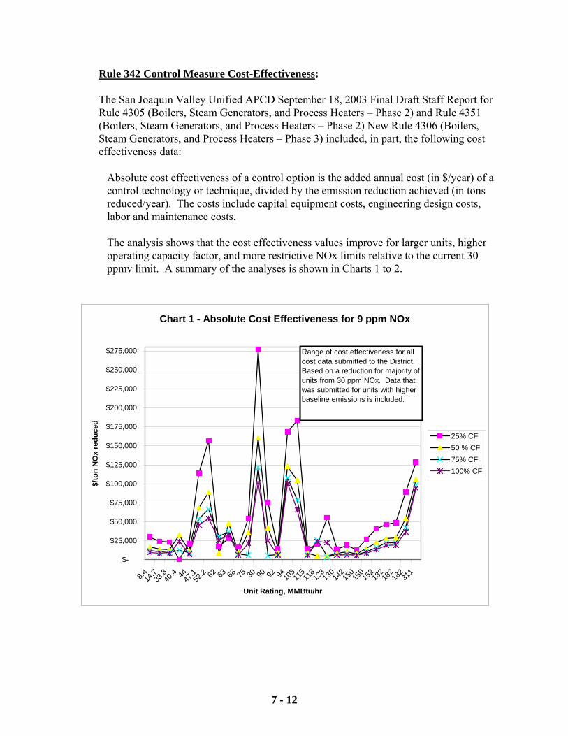
7 - 12
Rule 342 Control Measure Cost-Effectiveness: The San Joaquin Valley Unified APCD September 18, 2003 Final Draft Staff Report for Rule 4305 (Boilers, Steam Generators, and Process Heaters – Phase 2) and Rule 4351 (Boilers, Steam Generators, and Process Heaters – Phase 2) New Rule 4306 (Boilers, Steam Generators, and Process Heaters – Phase 3) included, in part, the following cost effectiveness data:
Absolute cost effectiveness of a control option is the added annual cost (in $/year) of a control technology or technique, divided by the emission reduction achieved (in tons reduced/year). The costs include capital equipment costs, engineering design costs, labor and maintenance costs. The analysis shows that the cost effectiveness values improve for larger units, higher operating capacity factor, and more restrictive NOx limits relative to the current 30 ppmv limit. A summary of the analyses is shown in Charts 1 to 2.
Chart 1 - Absolute Cost Effectiveness for 9 ppm NOx
$-
$25,000
$50,000
$75,000
$100,000
$125,000
$150,000
$175,000
$200,000
$225,000
$250,000
$275,000
8.414.733
.840
.4 4447.152
.2 62 63 68 75 80 90 92 94 10511
511
812
813
014
215
015
015
218
218
218
231
1
Unit Rating, MMBtu/hr
$/to
n N
Ox
redu
ced
25% CF50 % CF75% CF100% CF
Range of cost effectiveness for all cost data submitted to the District. Based on a reduction for majority of units from 30 ppm NOx. Data that was submitted for units with higher baseline emissions is included.
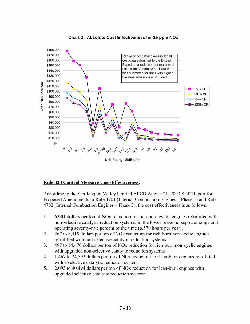
7 - 13
Chart 2 - Absolute Cost Effectiveness for 15 ppm NOx
$-$10,000$20,000$30,000$40,000$50,000$60,000$70,000$80,000$90,000
$100,000$110,000$120,000$130,000$140,000$150,000$160,000$170,000$180,000
5 5.5 5.9 7.4 8.4 8.9
10.20
612
.614
.714
.717
.133
.8 44 68 92 115
130
150
Unit Rating, MMBtu/hr
$/to
n N
Ox
redu
ced
25% CF50 % CF75% CF100% CF
Range of cost effectiveness for all cost data submitted to the District. Based on a reduction for majority of units from 30 ppm NOx. Data that was submitted for units with higher baseline emissions is included.
Rule 333 Control Measure Cost-Effectiveness:
According to the San Joaquin Valley Unified APCD August 21, 2003 Staff Report for Proposed Amendments to Rule 4701 (Internal Combustion Engines – Phase 1) and Rule 4702 (Internal Combustion Engines – Phase 2), the cost-effectiveness is as follows:
1. 6,901 dollars per ton of NOx reduction for rich-burn cyclic engines retrofitted with
non-selective catalytic reduction systems, in the lower brake horsepower range and operating seventy-five percent of the time (6,570 hours per year).
2. 267 to 8,415 dollars per ton of NOx reduction for rich-burn non-cyclic engines retrofitted with non-selective catalytic reduction systems.
3. 497 to 14,470 dollars per ton of NOx reduction for rich-burn non-cyclic engines with upgraded non-selective catalytic reduction systems.
4. 1,467 to 24,593 dollars per ton of NOx reduction for lean-burn engines retrofitted with a selective catalytic reduction system.
5. 2,093 to 40,494 dollars per ton of NOx reduction for lean-burn engines with upgraded selective catalytic reduction systems.
7 - 14
The San Joaquin Valley Unified APCD July 31, 1996 Cost Effectiveness Analyses of the Proposed Amendments to Rule 4701 (Internal Combustion Engines) indicates the cost effectiveness range for diesel engines meeting the 600 ppmv NOx at 15 percent oxygen limit is 330 to 6,001 dollars per ton of NOx reduction.
• George Croll (VAFB): Asked the APCD to break the reduction analysis for Rule 342
down by boiler size and determine the reductions if the exemption is from 5MMBtu to 2MMBtu.
For a breakdown on the reductions anticipated from modifying Rule 342, see the previous response, Table R342. The question mentions combustion units in the 2 to 5 MMBtu/hr range. Rule 342 covers boilers that are 5 million British thermal units per hour (MMBtu/hr) and greater. Proposed Rule 361 will regulate combustion equipment rated greater than (>) 2 but less than (<) 5 MM Btu/hr. Therefore, it appears that the request may have been meant to apply to Rule 361. Before presenting the breakdown for Rule 361, a quick summary of the combustion rules may be helpful.
Combustion units are, or will be, governed by the following APCD Rules based on the combustion equipment heat input rating:
• Rule 352: Below 75,000 Btu/hr • Rule 360: 75,000 Btu/hr up to and including 2 MMBtu/hr • Rule 361: > 2 MMBtu/hr to < 5 MMBtu/hr • Rule 342: 5 MMBtu/hr and greater
The APCD rules currently have a gap for combustion units > 2 MMBtu/hr and < 5 MMBtu/hr. Rule 361 is intended to close this gap so there will be regulations for combustion units in all size ranges.
Table R361 provides a breakdown of the point source inventory combustion units in the range of 2 to 5 MMBtu/hr. The rule is scheduled for adoption in the mid-term (2007 – 2009). Using a conservative approach, assuming the rule is adopted late 2009 with a one-year compliance deadline, calendar year 2015 is the first CAP forecasting year that we would expect to see a full year of emission reductions from the Rule 361.
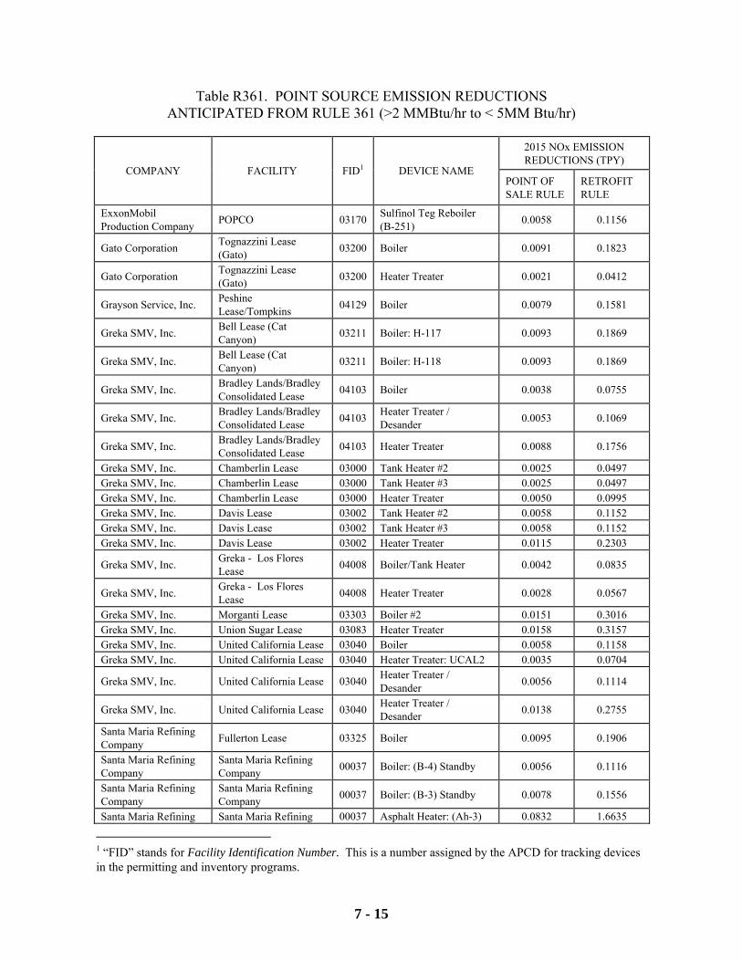
7 - 15
Table R361. POINT SOURCE EMISSION REDUCTIONS ANTICIPATED FROM RULE 361 (>2 MMBtu/hr to < 5MM Btu/hr)
2015 NOx EMISSION REDUCTIONS (TPY)
COMPANY FACILITY FID1 DEVICE NAME POINT OF SALE RULE
RETROFIT RULE
ExxonMobil Production Company POPCO 03170 Sulfinol Teg Reboiler
(B-251) 0.0058 0.1156
Gato Corporation Tognazzini Lease (Gato) 03200 Boiler 0.0091 0.1823
Gato Corporation Tognazzini Lease (Gato) 03200 Heater Treater 0.0021 0.0412
Grayson Service, Inc. Peshine Lease/Tompkins 04129 Boiler 0.0079 0.1581
Greka SMV, Inc. Bell Lease (Cat Canyon) 03211 Boiler: H-117 0.0093 0.1869
Greka SMV, Inc. Bell Lease (Cat Canyon) 03211 Boiler: H-118 0.0093 0.1869
Greka SMV, Inc. Bradley Lands/Bradley Consolidated Lease 04103 Boiler 0.0038 0.0755
Greka SMV, Inc. Bradley Lands/Bradley Consolidated Lease 04103 Heater Treater /
Desander 0.0053 0.1069
Greka SMV, Inc. Bradley Lands/Bradley Consolidated Lease 04103 Heater Treater 0.0088 0.1756
Greka SMV, Inc. Chamberlin Lease 03000 Tank Heater #2 0.0025 0.0497 Greka SMV, Inc. Chamberlin Lease 03000 Tank Heater #3 0.0025 0.0497 Greka SMV, Inc. Chamberlin Lease 03000 Heater Treater 0.0050 0.0995 Greka SMV, Inc. Davis Lease 03002 Tank Heater #2 0.0058 0.1152 Greka SMV, Inc. Davis Lease 03002 Tank Heater #3 0.0058 0.1152 Greka SMV, Inc. Davis Lease 03002 Heater Treater 0.0115 0.2303
Greka SMV, Inc. Greka - Los Flores Lease 04008 Boiler/Tank Heater 0.0042 0.0835
Greka SMV, Inc. Greka - Los Flores Lease 04008 Heater Treater 0.0028 0.0567
Greka SMV, Inc. Morganti Lease 03303 Boiler #2 0.0151 0.3016 Greka SMV, Inc. Union Sugar Lease 03083 Heater Treater 0.0158 0.3157 Greka SMV, Inc. United California Lease 03040 Boiler 0.0058 0.1158 Greka SMV, Inc. United California Lease 03040 Heater Treater: UCAL2 0.0035 0.0704
Greka SMV, Inc. United California Lease 03040 Heater Treater / Desander 0.0056 0.1114
Greka SMV, Inc. United California Lease 03040 Heater Treater / Desander 0.0138 0.2755
Santa Maria Refining Company Fullerton Lease 03325 Boiler 0.0095 0.1906
Santa Maria Refining Company
Santa Maria Refining Company 00037 Boiler: (B-4) Standby 0.0056 0.1116
Santa Maria Refining Company
Santa Maria Refining Company 00037 Boiler: (B-3) Standby 0.0078 0.1556
Santa Maria Refining Santa Maria Refining 00037 Asphalt Heater: (Ah-3) 0.0832 1.6635
1 “FID” stands for Facility Identification Number. This is a number assigned by the APCD for tracking devices in the permitting and inventory programs.
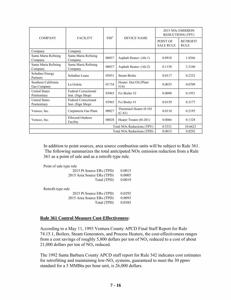
7 - 16
2015 NOx EMISSION REDUCTIONS (TPY)
COMPANY FACILITY FID1 DEVICE NAME POINT OF SALE RULE
RETROFIT RULE
Company Company Santa Maria Refining Company
Santa Maria Refining Company 00037 Asphalt Heater: (Ah-1) 0.0918 1.8366
Santa Maria Refining Company
Santa Maria Refining Company 00037 Asphalt Heater: (Ah-2) 0.1158 2.3160
Soladino Energy Partners Soladino Lease 03031 Steam Boiler 0.0117 0.2332
Southern California Gas Company La Goleta 01734 Heater: Hot Oil (Plant
#14) 0.0035 0.0709
United States Penitentiary
Federal Correctional Inst. (Sign Shop) 03965 Fci Boiler #2 0.0098 0.1951
United States Penitentiary
Federal Correctional Inst. (Sign Shop) 03965 Fci Boiler #1 0.0159 0.3177
Venoco, Inc. Carpinteria Gas Plant 00027 Therminol Heater H-101 (C-81) 0.0110 0.2195
Venoco, Inc. Ellwood Onshore Facility 00028 Heater Treater (H-201) 0.0066 0.1328
Total NOx Reductions (TPY) 0.5331 10.6623 Total NOx Reductions (TPD) 0.0015 0.0292
In addition to point sources, area source combustion units will be subject to Rule 361. The following summarizes the total anticipated NOx emission reduction from a Rule 361 as a point of sale and as a retrofit type rule.
Point of sale type rule
2015 Pt Source ERs (TPD) 0.0015 2015 Area Source ERs (TPD) 0.0005
Total (TPD) 0.0019
Retrofit type rule 2015 Pt Source ERs (TPD) 0.0292
2015 Area Source ERs (TPD) 0.0093 Total (TPD) 0.0385
Rule 361 Control Measure Cost-Effectiveness: According to a May 11, 1993 Ventura County APCD Final Staff Report for Rule 74.15.1, Boilers, Steam Generators, and Process Heaters, the cost-effectiveness ranges from a cost savings of roughly 5,800 dollars per ton of NOx reduced to a cost of about 21,000 dollars per ton of NOx reduced.
The 1992 Santa Barbara County APCD staff report for Rule 342 indicates cost estimates for retrofitting and maintaining low-NOx systems, guaranteed to meet the 30 ppmv standard for a 5 MMBtu per hour unit, is 26,000 dollars.
7 - 17
According to information from the Vandenberg Air Force Base ENVVEST program for two 4.25 MMBtu/hr boiler retrofits, the cost-effectiveness was about 6,000 dollars per ton of NOx reduced. In addition, data from the APCD’s Innovative Technology Group’s work on retrofitting nursery boilers in the 4 to 5 MMBtu/hr range indicates the cost-effectiveness ranged from about 3,000 to 4,000 dollars per ton of NOx reduced.
Note that the movement of amended Rules 333 and 342 from “Further Study” to “Rules Scheduled for Adoption” was based on direction from ARB (see letter from Robert Fletcher to Tom Murphy dated September 24, 2004 in Section 8.4). At the November 10, 2004 CAC meeting, a motion was made by the CAC to approve the Plan with the stipulation that the APCD contact the ARB to determine whether moving the rules back to further study would jeopardize ARB approval of the Plan. After discussion with the ARB, amended rules 333 and 342 will be moved back to “Further Study” from “Rules Scheduled for Adoption.” The information and analyses provided above on these rules is being retained in this chapter, however, for historical continuity of CAC and public input. • Marc Chytilo: Suggested that the APCD should prioritize rules by looking at the emission
inventory to see where emissions are greatest and propose rules based on where reductions are needed. Marc also suggested that we should look beyond what other districts are doing and more at available technologies.
Terry responded that all feasible measures are based on the most stringent rules throughout the state and that the South Coast AQMD rules are the most stringent in the nation. Additionally the South Coast AQMD has staff who can investigate new technologies.
• Marc Chytilo: Raised concerns that were expressed in his September 24, 2004 letter to
Jim Kemp (SBCAG) and Terry Dressler (APCD) regarding TCM’s, land use, and the general planning process (see section 8.4).
See APCD Response to Public Comments
• General CAC Discussion: A general discussion on potential TCMs took place that focused on alternative forms of transportation and transportation incentive programs. Suggested forms of alternative transportation included rail from north county to south county, van pools, shared cars, employer and self-propelled buses.
Jim Damkowitch said the alternative transportation control measures discussed by the CAC are currently being examined through the 101-in-Motion process.
• Dr. Inga Cox: Asked the APCD to provide Holzclaw’s reference in bibliography and to
provide a better explanation of the term “holistic”, which is included in Chapter 7.
The Holzclaw reference has been provided to Dr. Cox and “holistic” will be changed to “comprehensive” on page 7-1 of the plan.
7 - 18
November 10, 2004 Plan Revisions and CAC Approval
• Marc Chytilo: Suggested that ISR was not to be brought to the Board as a specific part of
the Plan but more as a rule.
ISR was intended to be part of the Plan as guidance and was never intended as a rule.
• Tom Banigan (NuSil): “Why have baseline ROC emissions increased from that last draft version of the Plan?”
The increase in ROC emissions from 39.46 tons per day to 41.84 tons per day is due to adding area source degreaser emissions that were inadvertently left out of previous estimates.
• John Gilliland (URS): “Why are there no VAFB boilers listed on pages 8-9 and 8-15?” The APCD will review its inventory to determine which boilers should be included in Table R342 and Table R361.
• Glenn Oliver (Plains Exploration): Some of the measures will affect sources that already provide emission reduction credits. Requiring more controls would then upset the offset efforts. Additionally, since emissions from certain sources are already low, further emission controls are not feasible.
The Planning process utilizes the current inventory in conjunction with the latest air quality monitoring data to determine whether we are making progress toward meeting air quality standards. If we don’t meet the standards, then we need to implement all feasible measures. The net air quality benefit is then accounted for in the emissions inventory through the permitting process.
• Doug Marsh: “Since rule 361 is currently proposed as a mid-term measure, how do we know which boilers will in existence by the time the rule is implemented?”
As a currently proposed mid-term rule, it is not possible to know which boilers will still be in existence at the time the rule is implemented. It will be necessary to wait until the next plan update to determine the population of devices that will be affected by the proposed rule.
• Larry Rennacker: “Did the APCD do cost-effectiveness analyses for Rule 342 and Rule 333?”
Cost effectiveness calculations are presented in the responses to comments made at the October 13, 2004 CAC meeting.
7 - 19
• George Croll (VAFB): “Can banked ERC’s be discounted?” Yes. The RACT offset discount applies if a rule is made more stringent.
• Doug Marsh: “Will proposed rules be going through the rulemaking process?” Yes. These rules will go through the standard rulemaking process including workshops and CAC discussion.
• Kevin Wright (Entrix): “If Rule 333 is proposed, how will RACT discounting apply and does the surplus go away once the Plan is adopted?”
ERC’s are available until the time a rule is adopted. As any ERCs derived from proposed rules could only generate short-term ERC’s, the APCD would not allow for their use in long-term projects. RACT discounting applies to available ERC’s if a rule becomes more stringent at a later date.
• Patrice Surmeier: “Doesn’t the diesel ATCM control internal combustion engines and if so why is Rule 333 needed?”
The diesel ATCM is particulate matter based and targets carcinogenic diesel exhaust, not criteria pollutants.
• General CAC Discussion: A motion was made to approve the Plan with the caveat that Rule 342 and Rule 333 be moved from “Rules Scheduled for Adoption” back to “Further Study”, and to provide the Board with a “Statement of Concern” written by CAC members regarding Chapter 7 and the significance of including TCM’s in the Plan.
The APCD has contacted the ARB to determine the ramifications of moving Rules 342 and 333 back to “Emission Control Measures for Further Study” from “Proposed Emission Control Measures.” Based on discussions with ARB, Rule 333 and Rule 342 will be moved back to “Emission Control Measures for Further Study Measures”, and doing so will not jeopardize ARB’s approval of the Plan. In addition, Marc Chytilo and Kevin Wright were nominated by the CAC to provide a “Statement of Concern” to the Board regarding Chapter 7 and the significance of Transportation Control Measures.
7 - 20
7.3 2004 PLAN PUBLIC WORKSHOP
This section summarizes all public comments and staff responses from the public workshop. The
public workshop was held on September 15, 2004 in Buellton in conjunction with the normally
scheduled CAC meeting. There were no members of the public present at the workshop and all
comments came from CAC members. Comments from the workshop/CAC meeting and the
responses to these comments are provided below.
Comments Received During September 15th Community Advisory Council Meeting • General CAC Discussion: A discussion ensued regarding the presentation of air quality
exceedance data and the appropriate time scale to use for the data. Some CAC members suggested that it may be more appropriate to only present exceedance data for the past five years to provide a snapshot of our recent trends while others felt that the current presentation of exceedance data is sufficient and gives a good overall indication of exceedance trends and air quality improvement.
• Lee Moldaver: “How did we get the message out to the regulated community regarding
the Plan workshop and the opportunity to provide comment on the draft Plan?”
The APCD informed the public of the workshop and of the opportunity to comment through mailing lists and through a public notice in local newspapers. In addition, the plan was provided to a number of sites, including local libraries, where the document could be reviewed by the public.
• Bill Peitzke: “CO2 emissions should be shown in the Plan, and what is the APCD doing to address CO2 emissions?”
The 2004 Plan is an state ozone attainment plan and does not cover CO2 emissions. The APCD will provide more information to the CAC on CO2 emissions at a future CAC meeting.
• John Gilliland (URS): “Will ERC’s from control measures be lost if a rule comes into
place after the Plan is approved?” If the APCD implements a rule that requires controls on equipment that were controlled
to create ERCs, the emission reductions are no longer surplus. If the control technique employed for ERCs over-controls emissions (e.g., has a higher control efficiency than the efficiency required by the rule), then Rule 806 would consider the emission reductions that go beyond the rule requirements as surplus emissions available for emission reduction credits.
7 - 21
• Dr. Inge Cox: “Why has the list of 22 potential further study measures that was provided at the April 14, 2004 CAC meeting been reduced to 12 measures in the Plan, and what was the process utilized to determine which further study measures are included in the Plan itself?”
Staff provided the two lists of further study measures at the April 14, 2004 CAC
meeting to show the broad number of measures that are being considered as potentially “all feasible measures.” At this CAC meeting, we discussed which ones out of the overall population of all feasible measures actually had sources with enough emissions to make it worthwhile to list them as a further study measure.
Staff reduced the initial further study lists by reviewing the control measure category
inventory and potential emission reductions. If a control measure had the potential to reduce NOx or ROC emissions by 10 tons per year or greater then we kept it in as a further study measure.
• George Croll (VAFB): Regarding increased NOx emissions from marine shipping: “Does
the net increase in NOx emissions from marine shipping have an impact on air quality?” Intuitively, any net increase in emissions will have an adverse impact on air quality.
Without photochemical modeling analyses, the extent of the impact due to the net increase in NOx emissions from marine shipping is difficult to determine.
• John Robinson: Suggested that the APCD should provide more information to the Board
of Directors highlighting the impacts of marine shipping on air quality. We have provided the Board information regarding marine shipping emissions and they
are aware of the magnitude of the challenge of controlling emissions from this significant source. We also plan to invite representatives of Lois Capps and Elton Gallegly to the December Plan adoption hearing so that they can further hear of the air quality challenges associated with marine shipping.
• Tom Banigan (NuSil Technology): “Why can emissions from marine shipping be
estimated, but potential emission impacts from the potential widening of 101 cannot be determined?”
SBCAG did provide an estimate of emissions from additional lanes to Route 101 as part
of the 2001 Clean Air Plan (Appendix C). They estimate that by adding additional lanes on Route 101 will result in approximately .25 tons per day or 62 tons per year of ROC and NOx combined. This calculation is somewhat “crude” as it does not consider the possible negative impact of induced travel growth as a result of widening, nor the inevitable worsening of congestion and greater vehicular emissions that will occur over time if the freeway is not widened due to slower vehicle speeds under congested conditions. A more complete analysis on the impacts of widening or not widening the 101 freeway will be developed as part of the 101 In-Motion process.
7 - 22
• John Gilliland (URS): “The 2001 federal Clean Air Plan shows that future emissions are projected to be less than base year emissions. The 2004 state triennial update, however, shows that future year emission estimates of NOx are higher than base year levels. Will this jeopardize the 2001 Plan and the ability to maintain compliance with the federal 1-hour standard?”
The APCD has contacted EPA and they are aware of our recent emission projections as
presented in the 2004 CAP. The primary reason that NOx emissions have increased from earlier estimates is that we were able to use actual horsepower data by individual ship rather than averages of horsepower by ship type in the emission calculations. This resulted in about a four ton per day increase in NOx emissions for the 2000 base year over the 1999 base year that was presented in the 2001 Plan. EPA, while concerned about net emission increases, did not indicate that the net increase in NOx emissions due to marine shipping would jeopardize the 2001 Plan. Additionally, there have been not violations of the federal 1-hour standard since 2000.
• Bill Peitzke: “Why not explore speed reduction to reduce emissions from marine shipping
in the Santa Barbara Channel?” While this is a good suggestion, there is argument among ship owners and operators
about which speed is optimal for emission reductions. Additionally, the shipping industry is faced with a demanding schedule that involves precise coordination of several other industry types including port services, rail and trucking. Finally, it would be difficult to enforce mandatory reductions and non-compliant marine vessels would have an unfair economic advantage over those that would comply with such a rule.
• Larry Rennacker: “What is the emission factor NOx used to determine marine shipping
emissions?” The NOx emission factors range from 16.02 g/kWh for auto carriers and 17.09 g/kWh
for container ships. These NOx emission factors assume that marine vessels meet International Maritime Organization (IMO) NOx emission standards.
• Larry Rennacker: “Did ARB look at the potential impacts of marine shipping during its
recent transport analysis?” Back trajectories performed by the ARB showed air parcels moving over the Santa
Barbara Channel prior to advecting into the Los Angeles area. It is not possible to determine from the analyses, however, whether emissions from ships transiting through the Santa Barbara Channel had an adverse impact on air quality in the Los Angeles Basin.
• Lee Moldaver: “Representatives from the offices of both Lois Capp’s and Elton Gallegly
should be invited to the Board Plan adoption hearing so that they can take notice of the marine shipping problem, which may induce increased action at the state level.”
7 - 23
The APCD will contact the offices of both representatives and invite them to the Board Hearing currently scheduled for December.
• Dr. Inga Cox: “Why is there a difference in the percentage of overall total NOx emissions
between the 2001 Plan and the 2004 Plan? NOx emission differences between the 2001 Plan and the 2004 Plan are primarily due to
the differences in methods used to calculate marine shipping emissions. NOx emissions from marine shipping in the 2001 Plan were based on average horsepower by ship type (e.g., auto carrier, container ship, etc.) while NOx emissions from marine shipping that is presented in the 2004 Plan are based on ship-specific horsepower data.
• Marc Chytilo (Law Offices of Marc Chytilo): Commented that there are technical
deficiencies in the Plan that need to be addressed. These deficiencies are as follows:
1. The Plan references two sections of the Health and Safety code, but not the appropriate section that pertains to state triennial updates.
The 2004 Plan references the appropriate sections of the Health and Safety code for this triennial update in the Executive Summary (H&SC Sections 40924 and 40925) and for our emission reduction strategy in Chapter 4 (H&SC Section 40914).
2. The Plan should address whether the San Joaquin Valley is a potential transport
couple and whether emissions from Santa Barbara County impact the southern San Joaquin Valley.
Transport analyses conducted by the ARB have shown that emissions from the San Joaquin Valley can have an impact on the northern portion of the South Central Coast Air Basin (which includes Santa Barbara, San Luis Obispo and Ventura Counties), primarily in northern San Luis Obispo County. The ARB, however, has not identified a South Central Coast Air Basin to San Joaquin Valley transport couple. Additionally, emissions generated in the San Joaquin Valley are considerably higher than those generated in Santa Barbara County. Given the prevailing meteorology and relatively low emissions compared to San Joaquin Valley, it is not likely that Santa Barbara County emissions contribute significantly to San Joaquin Valley exceedances.
3. There a no contingency measures within the Plan.
The suite of further study measures presented in Chapter 4 of the Plan can be considered contingency measures by ARB, if needed. Also, Chapter 5 has been revised to list Enhanced I/M as a contingency measures for the on-road mobile source side of the inventory.
7 - 24
4. There should be a discussion of VMT growth versus population growth and whether VMT growth will be reduced as population increases.
A discussion of VMT with respect to population growth can be found in Section 5.2 of the Plan.
• Kevin Wright (Entrix): “Will Rule 361 (Small Industrial and Commercial Boilers, Steam
Generators and Process Heaters – 2 MMBtu/hr to < 5 MMBtu/hr) be a point-of-sale or retrofit rule?”
Rule 361 is a mid-term rule that is scheduled to take effect in the 2007 to 2009
timeframe. Credits are being taken in the Plan by assuming that Rule 361 will be a point-of-sale rule. If during rule development, however, it is determined that a retrofit approach to Rule 361 is cost-effective, staff will bring this issue back to the CAC for discussion.
• Kevin Wright (Entrix): “Can ERC’s be claimed for further study measures, and will the
availability of ERC’s go away once the Plan is adopted?” Further study measures will remain available for ERC’s after the Plan is adopted. Any
ERC’s from further study measures are available until the time the rule is adopted. For proposed rules, however, credit cannot be taken once the Plan is adopted
Point-of-clarification: With respect to proposed rules, once a Plan is adopted, the APCD may consider the possibility of creating short-term Emission Reduction Credits that may be used for only short term projects. For example, if a proposed rule in an adopted Plan is not scheduled for implementation until 2010, the APCD may consider allowing short-term ERCs to be created and used by a project whose shut-down date is prior to 2010. As any ERCs derived from proposed rules could only generate short-term ERCs, the APCD would not allow for their use in long-term projects.
• Kevin Wright (Entrix): Commented that many of the further study measures proposed in
the Plan are measures implemented by the San Joaquin Valley, which is classified as an “Extreme” area by EPA, whereas Santa Barbara is in attainment for the federal 1-hour ozone standard. Mr. Wright added that it is not necessary to be as aggressive as San Joaquin Valley since Santa Barbara County is a federal attainment area.
We are required to implement every feasible control measure. Generally, this means that control measures adopted by other air districts are cost-effective and feasible. The measures identified in Tables 4-4 and 4-5 are slated for further study. Staff will perform additional analysis on these control measures to determine if they should be moved into the proposed control measure category. Cost-effectiveness and the environmental benefits from implementing the control measure will be considered during the further study analysis.

7 - 25
7.4 WRITTEN COMMENTS AND RESPONSES ON THE 2004 PLAN This section provides all written comments received on the 2004 Plan and accompanying APCD
staff responses to these comments.
7 - 26
March 18, 2004 e-mail From John Gilliland (URS) to Jim Damkowitch (SBCAG)
Jim. I would like to express my appreciation to you for taking time out of yours schedule to meet with me to discuss the APCD 2004 Clean Air Plan (CAP),Chapter 5. You provided informed answers that clarified issues and assisted my further understanding. Following is a brief summary of our discussion. 1. Does the CAP take into account emission reductions resulting from the California Air Resources Board (CARB) revisions to the portable equipment registration program (PERP)? You indicated that emission reductions associated with the PERP revisions are not incorporated into the APCD CAP because these emission sources are typically handled in the CARB off road emission model. Tom Murphy suggested I contact Joe Petrini and confirm this (Joe: Your thoughts? Are the emission reductions associated with the 2010 deadline accounted for in the CAP?) 2. Does the departure from EMFAC2002 Defaults affect the EPA-approved 2001 APCD CAP? You indicated that additional verbiage would be added clarifying that these changes will not affect the basic assumptions applied to the EMFAC 2002 Model and the APCD 2001 CAP. 3. Are emission reduction from control of internal combustion engines (ICEs) following CARB codification of the mobile airborne toxic control measures (ATCMs) accounted for in the EMFAC2002 modeling? You stated that if the ATCMs were final regulations, they would be incorporated into the model. ATCMs not codified as a final regulation are not included and could be incorporated when the EMFAC model is revised. If this revision does not occur by the next APCD triennial review, these emission reductions could be accounted for in an off model calculation. I would suggest that language be added indicating this because you or I may not be around in three years. 4. EMFAC2002 Output Sheets - Are Diesel Oxidation Catalysts accounted for in the CAP? You stated you needed to research this question and would hopefully have an answer available by the next CAC meeting.- Unfortunately, it appears that I have a scheduling conflict that may prevent my participation at the 14 Apr 04 CAC meeting. In the event that I am unable to attend, I would greatly appreciate it if you would inform members of the CAC of our discussion. If you have any questions, please do not hesitate to contact me. John D. Gilliland, URS Corporation (OFC) (805) 606-2068 (Cell) (805) 705-0273 [email protected] [email protected] [email protected]
7 - 27
LAW OFFICE OF MARC CHYTILO
ENVIRONMENTAL LAW
April 15, 2004 Mr. Terry Dressler, Control Officer Air Pollution Control District 260 N San Antonio Road, Suite A Santa Barbara, California 93110 Mr. Jim Kemp, Executive Director Santa Barbara County Association of Governments 260 N San Antonio Road, Suite B Santa Barbara, California 93110 By E-mail [email protected], [email protected]
RE: 2004 CAP TCM Plan
Dear Terry and Jim: At last night's APCD CAC meeting, I expressed concern that the draft TCM list proposed for the 2004 CAP was being developed without the benefit of an emissions reductions target. I further expressed concern that the District must undertake a specific TCM Planning process under State law. Finally, I stated that I supported a more extensive and expansive process for involving and including the public, transit operators, local municipalities, adjacent counties and other agencies in the process of identifying potential TCMs and scoping them so they would receive adequate consideration in the reasonably available control measure analysis process. The CAC was generally supportive of these concerns, so I write to describe more particularly the issues at hand. Health and Safety Code § 40717 establishes a clear mandate for Districts to establish the quantity of emissions reductions necessary from transportation sources necessary to attain the state standard. § 40717(b)(1). This language unquestionably applies to the 2004 CAP. §§ 40717(a); 40717(b)(3)(C). Other portions of the California Clean Air Act require attainment demonstrations and emissions reductions goals. See, for example, Health and Safety Code § 41503(b), describing the standards by which ARB is supposed to assess the CAP's adequacy. The fact that there is an exemption for District that cannot feasibly predict an attainment date does not eliminate that requirement unless the District and its CAP demonstrate this on the basis of substantial evidence. I was led to believe that the data from SCOS would enable ARB and local Districts to predict attainment dates, and since the District was required to model attainment of the federal one hour standard, addressing the state standard should represent a limited increment of additional work.
MARC CHYTILO P.O. Box 92233 • Santa Barbara, California 93190
Phone: (805) 682-0585 • Fax: (805) 682-2379 Email: [email protected]
7 - 28
Mssrs. Dressler and Kemp April 15, 2004 Page 2
In any case, the Transportation Sources Plan must be developed and "adopted" by the COG, or SBCAG, and then submitted to the District on a schedule adopted by the District. § 40717(b)(2). The District has a mandatory obligation to review and reject that plan if inadequate to achieve the emissions reductions requirement. § 40717(b)(3). In light of the broad public distrust in the "101 in Motion" process (many community representatives believe that the SBCAG Board of Directors has directed a particular outcome, a belief supported by the record), the TCM planning process is an important opportunity for public involvement in scoping potential TCMs. The APCD CAC had a lively discussion about potential transit measures, and staff recited that there are no shortage of creative ideas to address local congestion issues and different forms of transit. The California Clean Air Act recites that "Districts shall focus particular attention on reducing the emissions from transportation sources and areawide emissions sources." Health and Safety Code § 40910. I ask that the District and SBCAG create a robust public outreach process that includes the public, the various agencies that have expressed interest in public transit issues through the unmet transit needs process, transit operators and adjoining jurisdictions. Your agencies' duty is to consider all reasonably available transportation control measures, not simply adopt all feasible measures. § 40918(a)(3). The CAP must address means to achieve applicable performance standards. Id. Thank you for considering these views on this important topic. I hope that this will result in a renewed effort to identify and adopt TCMs that can overcome the challenges our community faces in achieving the state standard and addressing transportation needs of our community.
CC: Tom Murphy Jim Damkovich Bill Dillon
7 - 29
July 15, 2004 Memorandum From John Gilliland (URS)
Memorandum: Santa Barbara County Air Pollution Control District (APCD) Community Advisory Counsel
From: John D. Gilliland, CAC Member Date: 15 July 2004 Subject: 14 July 2004 Community Advisory Counsel Meeting Comments 1. I have reviewed the Executive Summary and Chapter 6, Emission Forecasting, to the Santa Barbara County Air Pollution Control District (APCD) State of California Clean Air Plan (SCCAP). The following comments and questions are provided: 2. Executive Summary:
a. Introduction:
(1) Request consideration from the APCD to include a discussion on the new federal 8-hour standard and its relationship to Santa Barbara County.
(2) Should this SCCAP add comments discussing the proposed California 8-hour
standard?
b. Does This 2004 Plan Address any Federal Requirements:
(1) Please include the federal authority citation at the end of the paragraph. 3. Chapter 6
a. Section 6.1 – Introduction: The APCD indicates that emissions from natural sources
are excluded from the Planning Emission Inventory (PEI) because they are unregulated. Is the APCD willing to consider including some biogenic sources such as oil and gas seeps, agricultural waste composting and range burning in APCD regulations and the PEI? Controlling these sources provides additional air quality improvement and provides industrial sources potential incentives to control emissions for the purposes of creating emission reduction credits.
b. Section 6.2.2 – Control Measures: Refer to the discussions regarding natural sources.
c. Section 6.2.3 – Vandenberg Air Force Base Airborne Laser Mission Growth Allowance: Can the APCD add a footnote to this discussion that indicates this requirement may be removed pending the revocation of the Federal one-hour standard.
7 - 30
d. Section 6.4 – Impacts of Marine Shipping Emissions: Is it possible for the APCD to determine the actual marine shipping for 2001, 2002, and 2003 to see how it tracks with the forecasted assumption? If the emissions are significantly different (either greater or less) is it possible to revise the forecast for this 2004 SCCAP or the 2007 SCCAP?
e. Section 6.4 – Impacts of Marine Shipping Emissions: The APCD stated that the burden of attaining or maintaining air quality improvement goals may fall disproportionately on onshore sources. Please add a discussion as to the ramifications to the APCD if the Board waives air quality improvement rules due to stakeholder input. Are state sanctions or other regulatory penalties mandated by CARB possible?
f. Table 6-5 – 2004 Clean Air Plan Activity Indicators and Factors for 2005, 2010, 2015 and 2020: Under the prescribed fires section, is the APCD willing to consider revising the baseline numbers to more accurately represent this section. Even though this very low activity took place in 2000, a review of previous years and post years indicates values more closely attuned to the 6,250 values. The value, as listed, provides an erroneous growth factor for this category.
g. Figure 6-11 - Santa Barbara County OCS NOx Emission Forecast Including Marine Vessels: This table clearly illustrates that the 2000 baseline year is less than the 2020-forecasted year. Is it possible for the APCD to receive Plan approval when the 2020 values are higher than the baseline year? 4. Thank you for the opportunity to provide comments.
JOHN D. GILLIAND
7 - 31
LAW OFFICE OF MARC CHYTILO
ENVIRONMENTAL LAW
September 24, 2004 Mr. Terry Dressler, Control Officer By Fax: (805) 961-8801 Air Pollution Control District And US Mail 260 N San Antonio Road, Suite A Santa Barbara, California 93110
Mr. Jim Kemp, Executive Director By Fax: (805) 961-8901 Santa Barbara County Association of Governments And US Mail 260 N San Antonio Road, Suite B Santa Barbara, California 93110
RE: 2004 CAP Comments
Dear Terry and Jim: As you know, I am gravely concerned that Santa Barbara County has proceeded headlong into the development of a `paper' state Clean Air Plan (CAP) which fails to address minimum legal requirements for this document and defers treatment of significant issues to a future time, at which point the problems will have become far more difficult to overcome. Please accept these comments on behalf of Our Children's Earth Foundation, an organization committed to improving air quality throughout California to meet the needs of all of our community, and in particular, the needs of children and other persons that are particularly sensitive to exposure to air pollution. I strongly encourage your agencies to withdraw the 2004 CAP and commence the analysis and processes identified in this letter of comment. Residents of Santa Barbara County are entitled to the public health protection required by California law – attainment of the California ambient air quality standards "as expeditiously as practicable." As drafted, the 2004 CAP fails in that fundamental purpose, with substantial adverse human health effects as a result. We deserve better.
1. Transportation Control Measures The CAP is deficient for failing to contain any transportation control measures, which the legislature intended should be a focus in each Clean Air Plan. The California Clean Air Act contains clear and express reference to a particular process that is required to identify and develop Transportation Control Measures (TCMs) in all air quality plans, including CAPS. The Santa Barbara County Air Pollution Control District (APCD) and. Santa Barbara County Association of Governments (SBCAG) have ignored that process entirely, and as a consequence, propose no new TCMs in the 2004 CAP. Your agencies' development of the 2004 CAP should be guided by the following admonition:
MARC CHYTILO P.O. Box 92233 • Santa Barbara, California 93190
Phone: (805) 682-0585 • Fax: (805) 682-2379 Email: [email protected]
7 - 32
Mssrs. Dressler and Kemp . September 24, 2004 Page 2
"In developing attainment plans and regulations to achieve this objective [of attainment by the `earliest practicable date'], districts shall consider the full spectrum of emission sources and focus particular attention on reducing emissions from transportation and areawide sources."
Health and Safety Code § 40910 (emphasis added). The planning emissions inventories in the 2004 CAP disclose that 81% of 2000 ROC emissions and 87% of NO,, emissions are from mobile and area sources. 3-17. The CAP, however, proposes only nominal progress in reducing emissions from these source categories, beyond the progress achieved by state tailpipe standards and a few rules developed by other Districts. The CAP fails to focus on these source categories, even though they are substantial elements of local emissions inventories. Further, growth in other sectors of the emissions inventory jeopardizes all emissions reductions contained in the plan. The 2004 CAP fails to "focus particular attention on reducing emissions from transportation and areawide sources." Although several SBC APCD SIPS and CAPs have contained chapters addressing land use strategies, growth associated with land use activities is a significant factor in future emissions inventories. The plans pay lip service to the issue, but the APCD and SBCAG are failing to act aggressively enough to assert these issues in the land use planning process throughout the county. The jobs-housing balance remains at an all-time high, and VMT continues to skyrocket. Despite vigorous debates within the County and virtually every municipal jurisdiction, the APCD remains at the edges of any such discussion, if not absent entirely. Further, the District and SBCAG have ignored the procedures required by Health and Safety Code § 40717 that would ensure that these issues are given proper focus. That statute is reproduced below, in its entirety.
Health and Safety Code § 40717. Adoption of plan for transportation control measures; Contents of plan
(a) A district shall adopt, implement, and enforce transportation control measures
for the attainment of state or federal ambient air quality standards to the extent necessary to comply with Section 40918, 40919, or 40920.
(b) A district which has entered into an agreement with a council of
governments or a regional agency to jointly develop a plan for transportation control measures shall develop the plan in accordance with all of the following:
(1) The district shall establish the quantity of emission reductions from
transportation sources necessary to attain state and federal ambient air standards.
7 - 33
Mssrs. Dressler and Kemp September 24, 2004 Page 3
(2) The council of governments or regional agency, in cooperation with the district and any other person or entity authorized by the council of governments or regional agency, shall develop and adopt a plan to control emissions from transportation sources which will achieve the emission reductions established under paragraph (1). The plan shall include, at a minimum, a schedule for implementing transportation control measures, identification of potential implementing agencies and any agreements entered into by agencies to implement portions of the plan, and procedures for monitoring the effectiveness of and compliance with the measures in the plan. The council of governments or regional agency shall submit the plan to the district for its adoption according to a reasonable schedule developed by the district in consultation with the council of governments or regional agency.
(3) Upon receipt of the plan submitted by the council of governments or
regional agency, the district shall review and approve or disapprove the plan in the following manner:
(A) The district shall review, adopt, and enforce the plan if it meets the
criteria established by the district pursuant to paragraph (1) and has been submitted pursuant to the schedule established under paragraph (2).
(B) If the district determines that the plan does not meet the criteria established
pursuant to paragraph (1), the district shall return the plan to the council of governments or regional agency with comments which identify the reasons the plan does not meet the criteria established pursuant to paragraph (1). Within 45 days, the council of governments or regional agency shall review the district's comments, revise the plan to meet the criteria established under paragraph (1), and resubmit the plan to the district. The district shall review and approve the revised plan if it meets the criteria established by the district pursuant to paragraph (1) and has been resubmitted to the district within 45 days.
(C) If the plan is not submitted pursuant to the schedule established under
paragraph (2), or if a plan revised by a council of governments or regional agency and resubmitted to a district pursuant to this subparagraph does not meet the criteria established under paragraph (1), the district shall develop, adopt, and enforce an alternative plan for transportation control measures.
(4) Whenever the district revises its establishment of the quantity of emission
reductions from transportation sources necessary to attain state and federal ambient air standards, the plan shall be revised, adopted, and enforced in accordance with paragraphs (1), (2), and (3).
7 - 34
Mssrs. Dressler and Kemp September 24, 2004 Page 4
(c) Subdivision (b) shall not apply to the Sacramento district. Chapter 10 (commencing with Section 40950) shall govern preparation and enforcement of that plan for transportation control measures for the Sacramento district.
(d) Notwithstanding subdivision (b), a district located in a county of the third
class shall develop a plan for transportation control measures as follows:
(1) The district, in consultation with the council of governments, shall develop, approve, and adopt criteria under which the plan shall be developed.
(2) The council of governments shall develop and adopt a plan for transportation
control measures which meets the criteria established by the district, and shall submit the plan to the district for its review and adoption according to a reasonable schedule developed by the district in consultation with the council of governments.
(3) Upon receipt of the plan submitted by the council of governments, the district
shall review and approve the plan if it meets the criteria established by the district pursuant to paragraph (1) and has been submitted pursuant to the schedule established under paragraph (2). If the district determines that the plan does not meet the criteria established pursuant to paragraph (1) or if the plan is not submitted pursuant to the schedule established under paragraph (2), the district shall develop and adopt an alternative plan for transportation control measures.
(e) A district may delegate any function with respect to the implementation of transportation control measures to any local agency, if all of the following conditions are met:
(1) The local agency submits to the district an implementation plan that
provides adequate resources to adopt and enforce the measures, and the district approves the plan.
(2) The local agency adopts and implements measures at least as stringent as
those in the district plan.
(3) The district adopts procedures to review the performance of the local agency in implementing the measures to ensure compliance with the district plan.
(4) Multiple site employers with more than one regulated worksite in the district
have the option of complying with the district rule and reporting directly to the
7 - 35
Mssrs. Dressler and Kemp September 24, 2004 Page 5
district. Employers that exercise this option shall be exempt from the local agency trip reduction measure.
(f) A district may revoke an authority granted under this section if it determines
that the performance of the local agency is in violation of this section or otherwise inadequate to implement the district plan.
(g) For purposes of this section, "transportation control measures" means any
strategy to reduce vehicle trips, vehicle use, vehicle miles traveled, vehicle idling, or traffic congestion for the purpose of reducing motor vehicle emissions.
(h) Nothing in this section shall preclude a local agency from implementing a
transportation control measure that exceeds the requirements imposed by an air pollution control district or an air quality management district if otherwise authorized by law.
The District and SBCAG have entered into an agreement for the joint development of a CAP, but have ignored the mandatory requirements of Health and Safety Code § 40717. For example, the District failed to develop an estimate of emissions reductions from transportation sources necessary for attainment. The California Clean Air Act does not necessarily require a complete, modeled attainment demonstration, but only an estimate. The CAP contains no estimate at all. Having previously raised this issue with the District and SBCAG, Exhibit 1. The District and SBCAG responded that: "While § 40717 mandates that areas quantify the emission reductions from transportation sources to attain state and federal standards, we do not have the photochemical modeling analysis to identify the targets for the state standard. Therefore, we are technically unable to fulfill the process identified under § 40717 and must default to the every feasible measure approach outlined in § 40914." Letter, Terry Dressler and Jim Kemp to Marc Chytilo, May 21, 2004, attached as Exhibit 2. There is no authority for the conclusion that the general responsibility of every District to utilize the process mandated by HSC § 40717 is preempted by § 40914's supplemental requirement that each District achieve a 5% annual emissions reduction. HSC § 40914 is clearly a description of one necessary element of a CAP, and does not override all other requirements of the California Clean Air Act, such as HSC § 40717. Further, it is difficult to determine that the District and SBCAG have employed all feasible transportation control measures in the absence of a meaningful and public effort to identify them. This office provided the District and SBCAG with an extensive list of reasonably available transportation control measures that have been employed in other parts of the country. See Exhibit 3, suggested TCMs to the 2001 maintenance plan. It is absurd to contend that the "101 in Motion" process serves as a surrogate for the 40717 process — the "101 in Motion" process is designed and intended to address traffic congestion on a single reach of highway, and was
7 - 36
Mssrs. Dressler and Kemp September 24, 2004 Page 6
authorized with the governing SBCAG Board's resolution and staff report referencing that lane widening w a s t h e project that the Board wanted to see as the outcome and product. Respectfully, the claims that the agencies are "unaware of a `broad public distrust' is disingenuous at best. SBCAG's board, controlled by a particular faction, was adamant as to the project that they expected to result and that they intended to approve from the "101 in Motion" process — widening of Highway 101. As evidence, on October 16, 2003, SBCAG staff revised the previously recommended policy concerning Highway 101 to read as follows, with strikethrough and italics in the original indicating stricken and added language:
"The implementation plan shall include result in a project or set of projects that will increase the capacity by adding lanes and reduce congestion on Highway 101."
SBCAG Staff Report, 10/16/2003, Agenda Item # 10, attached as Exhibit 4. The public testimony included numerous comments, including myself, decrying the mandating of a particular project as the outcome from this process. Lane widening is not a TCM, and no where else in the SBCAG Staff Report or "101 in Motion" process is the identification of TCMs specified as an objective.
The inadequacy of the agencies' TCM development process is evident in the result — not a single new TCM is proposed for adoption. Previously APCD staff expressed reservations about adding aggressive new TCMs to the federal SIP due to the requirement that these TCMs actually be implemented, regardless of changed circumstances. This argument does not apply to the State CAP, where there are apparently no consequences from a failure to implement. We note also that the District and EPA have each adopted guidance and/or rules allowing TCM substitution, and thus the nature of the commitment to adopt and implement a TCM is quite different from a stationary source control commitment.
It is apparent that the failure of the District and SBCAG to observe each of the § 40717 steps — identifying an emissions reductions target by the District; SBCAG developing a transportation sources plan that could achieve those emissions reductions; conducting a public hearing where the adequacy of that plan is considered; and the District either guiding SBCAG's development, or assuming itself the responsibility of developing and implementing the transportation sources plan — robbed the CAP TCM process of legitimacy or effectiveness. The agencies were placed on notice early in the process that this was an applicable requirement, Exhibit 1, yet they chose to ignore it. The breathing public, the adequacy of the 2004 CAP, and the direction of transportation in our communities, are the victims of this defiance.
Reasonably available transportation control measures include the following:
Commuter Choice: Adopt and staff a Commuter Choice program. This is an obvious program to adopt. Recent changes in state and federal tax law allow employers to offer employees parking
7 - 37
Mssrs. Dressler and Kemp September 24, 2004 Page 7
and transportation benefits as tax-exempt compensation, with greater incentives for parking cash-out and alternative commute options. Employees can receive up to $175 per month of their existing or new compensation tax free. This is truly "found money" for both employers and employees which offers a meaningful incentive to use alternative commuter options in a flexible and cohesive package. According to the International Council for Local Environmental Initiatives "[t]his simple act of uncovering parking subsidies and offering a choice can reduce solo car commuting by up to 22%." See http://www.iclei,org/cashout/. See also http://www.commuterchoice.com/. Community Car Programs: A number of communities in the United States and Europe have begun "community car" programs. In essence, this is a low cost, cooperative subscription car rental system allowing families to avoid many of the expenses of auto ownership while maintaining access to a car when specifically needed. Communities must be designed and operated to allow most daily functions to occur without needing a car. In some European cities (e.g., Zurich), community cars enjoy preferential parking privileges, enhancing their attractiveness. San Francisco has recently initiated a community car cooperative program. Linked to new residential design features enhancing the quality of communities that are not designed with the car as the first .priority, the community car concept may offer considerable benefits in encouraging more appropriate land uses Smart Growth Resources: Smart Growth Resources to land use planning officials. Our sprawling land use patterns cost local government in increased and inefficient services, destroy open space, increase auto dependence, waste personal economic resources and degrade quality of life. See, for example, Driven to Spend: How Sprawl and Lack of Transportation Choice Are Driving Up Family Transportation Costs, http://www.transact.org/. Land use planners in the County and cities lack a regional perspective and are largely ignorant of the environmental and social ramifications of ignoring air quality impacts and transportation alternatives in their review and planning processes.. This is one essential ingredient of sprawl. Your agencies must tackle this issue aggressively, or else decisions made in coming years will preclude an efficient future public transportation system and create continuing problems for our communities. Only your agencies are positioned to assemble and provide effective materials on "smart" planning for air quality and transportation perspectives and make strong recommendations for appropriate land use development patterns and design. While your agencies lack direct regulatory control, you can serve both as an important source of information, training and expertise to cities and the county. Bike projects: Design and implement a much more comprehensive bicycle system for the region. Develop and implement a continuous, connected bike lane system from each county line with an extensive bike lane network. Develop a bike lane network serving all medium and large schools to promote safe bike commuting to school. Complete a comprehensive network of bikeways,including: Class I (exclusive bike paths separated from roads), Class II (on-road striped bike lanes), Class III, (on-road shared, signed routes) and Bicycle Boulevards. Install bicycle route
7 - 38
Mssrs Dressler and Kemp September 24, 2004 Page 8
numbering with maps. Maintain effective and continuing review and improvement of safety problems and maintenance of all bikeways. Review and maintain highway and street standards including surface standards, bridge access, bike lane cleaning, illegally parked car intrusion elimination, and bicycle sensitive traffic signals.
Pedestrian Projects: The region lacks a comprehensive sidewalk system, and continues to design new development prioritizing vehicular, rather than pedestrian access. Areas within existing communities where existing and future land uses are conducive to pedestrian use should be subject to a master planning process to be designed and shaped to become more pedestrian-friendly over time as redevelopment and other improvements occur and as these communities and developments mature.
Recognize Induced Traffic and VMT: SBCAG should require future project-level analysis (and analysis of all private projects which require transportation infrastructure improvements to accommodate traffic increases) to include additional modeling that incorporates the principle of latent (induced) demand in its design. Recalibrate the travel model, using actual VMT from completed projects.
Comprehensive Public Transit Gap Analysis: Gaps in the County's public transit system make the use of a car a necessity for many people who would otherwise use the bus. A number of residents simply forgo travel to these areas, as the car is not an option, The CAP should include a public transportation gap analysis and strive to implement a comprehensive public transit system. Once a complete transit system is in place, each portion of the entire system will experience increased ridership.
Indirect Source Review: for all permitting actions that induce traffic, as recommended by the CAC.
Parking Management: increase the cost of parking in all urban areas to subsidize and increase the attractiveness of public transit.
TEA Restrictions to Enhance Transit and Smart Growth: Some communities in California have considered restricting certain portions of TEA-21 funds to communities which adhere to certain land use and transit performance standards. For example, the following policies could have application in Santa Barbara County:
A) A RTP investment policy prioritizing transportation projects that are coupled with transit, bicycle and pedestrian oriented development along transit corridors and nodes, and conditioning capacity increasing highway projects on the adoption of growth management plans that embody provisions for open space preservation and subregional agreement on a growth budget that does not overload either transportation infrastructure or other forms of infrastructure.
7 - 39
Mssrs. Dressler and Kemp September 24, 2004 Page 9
B) Condition funding and approval of projects serving large new trip generating land uses on a major reduction in drive-alone access to those projects. Such reductions shall be based on providing parking for fewer than the number of spaces ordinarily required, parking charges, cashing out employer paid employee parking, developer subsidies for transit access to the project, and other similar transportation measures. The effectiveness of demand management shall be guaranteed by an enforceable agreement to meet performance standards for access that reduce by some figure (half?) the number of drive alone trips and mandate the addition of further transportation incentives to meet performance goals if they are not met. C) Increased county-level transit ridership targets (necessitating increased investment in transit, increasing the cost effectiveness of transit investments, as well as encouraging land use jurisdictions to provide incentives to transit-supportive land use decisions). The TCM should reference achieving and maintaining a minimum modal split for transit, pedestrian and bike travel at specific milestone's, with If/Then consequences for each portion of the county at these points for not reaching the specified target. D) Fund h ighway expansions only within cities or sub-regions of the county where 80 percent of employees in businesses with over 5 employees are offered parking cash-out or commuter choices, and where parking is unbundled from rental housing and business rental/lease agreements. E) Allocate a certain percentage of discretionary funds exclusively to projects (both maintenance and capacity-expanding) in areas that meet specified smart growth criteria as is the practice in San Mateo (where transportation money is given to cities that approve dense housing near rail stations).
These policies build upon the use of TEA funds as incentives for smart growth principle utilization, as pioneered by Dr. John Holtzclaw, director of Sierra Club's Transportation Program. This approach has been determined to be legally appropriate upon scrutiny by the Air Resources Board. (K. Walsh, ARB General Counsel, to F. Chin, MTC, 10/26/1999).
EPA's Transportation Air Quality (TRAQ) Center provides state and local air quality regulators and transportation planners with access to critical information regarding transportation programs and mobile source incentive based programs, partnership opportunities, grant funding sources, useful contact names, and technical assistance. http://www.epa.gov/oms/transp.htm. Links from this page provide testimonials and experiences from other programs and references to EPA's emissions reductions quantification analysis for TCMs and land use strategies. See also The Surface Transportation Policy Project: http://www.transact.org/caldefault.htm. Finally, there is no evidence to support the CAP'S apparent conclusion that none of the list of further study transportation control measures could be feasibly implemented more immediately.
7 - 40
Mssrs. Dressler and Kemp . September 24, 2004 Page 10
2. VMT Growth The California Clean Air Act imposes several mandatory elements of a CAP. As a "moderate" area, Santa Barbara County's CAP must include:
"(a)(3) Reasonably available transportation control measures sufficient to substantially reduce the rate of increase in passenger vehicle trips and miles traveled per trip if the district contains an urbanized area with a population of 50,000 or more."
Health and Safety Code §. 40918(a)(3). As demonstrated by figure 2-2b, daily VMT is increasing at ever steeper rates. This reflects, although the CAP does not specifically address, increases in both trips taken and miles traveled per trip. The 2004 CAP is defective for posting gross VMT information and comparing it to population, rather than examining trip starts and trip length. Trip start data and average trip length are each available through the County's travel model, yet this information is omitted. The CAP should be revised to reflect the data that is relevant to addressing the standard imposed by the Act — trip starts and miles traveled per trip, and not merely VMT growth rates. Notwithstanding the use of misleading and different units, with zero transportation control measures, the CAP is obviously incompetent to address this requirement. Far from a "substantial reduction" in VMT growth, the CAP simply endorses business as usual, and offers no substantive evaluation or analysis of the source of the problem, instead merely reporting on past trends and concluding "Santa Barbara County is clearly not meeting this State act performance standard." Rather than merely reporting on "historical trends" as the summand total of the analysis, the CAP should more fully develop and articulate the basis for this failure and propose strategies and alternatives that could address the problem. Were a more complete and robust TCM review and development process undertaken, potential solutions to this problem might be under consideration.
3. Contingency measures The 2004 CAP lacks treatment of contingency measures as required by law. Health and Safety Code § 40915. Since the CAP predicts that emissions reductions will likely be overtaken by increased emissions from marine shipping, and revised estimates show increased marine shipping emissions than previously projected (in the 2001 maintenance plan) it is incumbent on the District to include a robust set of contingency measures to address the likely loss of progress towards attainment. Further, as the CAP reports the inability to achieve interim goals, such as control over VMT growth, contingency measures are necessary immediately to attempt to get the County back onto the path of attainment. Recent exceedences of both the state and federal 8 hour ozone standards is troubling, and may reflect a trend. If so, contingency measures should be
7 - 41
Mssrs. Dressler and Kemp . September 24, 2004 Page 11
implemented according to the 180 day deadline in Health and Safety Code § 40915. Their omission in unacceptable and jeopardizes the adequacy of the CAP.
4. Transport The 2004 CAP does not contain a complete analysis of air pollution transport to and from Santa Barbara County. It ignores the substantial effects of northern Santa Barbara County emissions on southern San Joaquin Valley air quality, in particular episodic emissions from Vandenberg Air Force Base activities. Previously, the APCD provided assurances that the SCOS data would allow an independent evaluation of transport to and from Santa Barbara County, but the CAP relies exclusively upon a canned ARB conclusion, then recites that it doesn't really matter since the state requirements for upwind Districts are so ineffectual that they mere require what is already required. Health and Safety Code § 40912 establishes the State's § 39610 "Transport Mitigation" control requirements as a floor, not a ceiling. Additional controls and emissions reductions are required of upwind Districts under state law "to reduce emissions originating in the District below the level at which violations of the state ambient air quality standards would occur in the absence of the transport contribution." Health and Safety Code § 40912. The 2004 CAP must use the SCOS data and ensure that Santa Barbara County meets this requirement.
5. Emissions Trends The draft 2004 CAP recognizes that marine shipping emissions, if uncontrolled, will actually exceed the projections made in the 2001 CAP and maintenance plan. The 2004 CAP fails to either develop methods of controlling these emissions or identify other sources that can provide additional emissions reductions to overcome the growth. Given the trend line for the emissions inventory, the CAP is inadequate to ever improve air quality to the point of attainment, and thus fails to reach attainment "as expeditiously as practicable." A number of new port projects in California threaten to further increase marine shipping emissions and impacts to Santa Barbara County. Ports in Long Beach are proposed to be expanded, and a series of new LNG terminals are under discussion. The District must become an active and forceful advocate in constraining these expansions and/or ensuring that air pollution impacts will be avoided or minimized.
6. The "All Feasible Measures" Analysis is a Race to the Bottom The control strategies in the 2004 CAP fall short of the level of aggressiveness required to attain the California ambient air quality standard for ozone. First to fall was an attainment demonstration, then the 5% annual emissions reductions became obsolete, and now the all feasible measures process has devolved into an arbitrary comparative process where no measure needs be considered unless it has been adopted in another District. Since all Districts prepare triennial CAPs and look no further than the list of control measures adopted by other Districts,
7 - 42
Mssrs. Dressler and Kemp . September 24, 2004 Page 12
few new control measures are developed. Thus the CAP all feasible measure process is largely an exercise with no meaningful benefit. This is elucidated in the statement that only rules adopted by other Districts will be considered, and references to other Districts that have been the least effective at controlling air pollution in the state. If Santa Barbara County elects to follow the footsteps of San Joaquin Valley in controlling air pollution, it is unlikely we will ever achieve and maintain the California ambient air quality standard for ozone. There is no explanation as to why control measures identified as reasonably available control measures should not be imposed prior to 2007 and 2010 — the Act requires attainment "as expeditiously as practicable" and that requires control strategies to be implemented "as expeditiously as practicable." A six year delay in identifying a known control measure for which a parallel rule already exists is not expeditious or acceptable. Given that "long term" control measures are 'scheduled for adoption until 2100-2012, it appears that the further study measures may not be adopted until after that time.. The 2004 CAP does not appear to actually include all feasible control measures for adoption or implementation, but rather puts them on a very generous schedule for eventual consideration. A further study measure carried forward from the 2001 maintenance plan, wineries and breweries, should be adopted and implemented promptly. This is a growing source category in Santa Barbara County that should be controlled expeditiously. The control measure vetting and winnowing process appears quite arbitrary. The CAC questioned why staff made various unilateral screening decisions rejecting control strategies without consulting that body for guidance. This "closed door" exercise taints the integrity of the control strategy selection process. The District should hold workshops that include the public and CAC in evaluating prospective sources and control strategies.
7. Construction Equipment Emissions Inventory Issues The 2004 CAP discloses that construction (and mining) equipment emissions are up to five times higher than previously estimated, as previously contended by commenter's counsel. 3-11. In light of the newfound significance of this emission category, the District must achieve a better characterization of the emissions from this category and develop strategies for their control, including alternatively fueled construction equipment and other mandatory mitigation measures for application by land use permitting jurisdictions.
8. Environmental Justice Issues There are continuing concerns that the District and SBCAG are ignoring environmental justice consequences of its actions. Public transit is an important community asset for low income and
7 - 43
Mssrs. Dressler and Kemp . September 24, 2004 Page 13
communities of color. The County has emphasized subscription, commuter transit services (which serve more affluent populations) to the detriment of scheduled services that serve the needs of our County's poor. The County lacks basic intercommunity service allowing a person to use public transit to move between many of our communities. Not only is it discriminatory; but it induces auto dependence and increased single occupancy vehicle emissions and VMT. Further, spiraling VMT and the related highway-based emissions from vehicle use disproportionately and increasingly affects housing adjacent to highways, which typically contains high percentages of low income and people of color. Intentionally or accidentally, the effect of the CAP and its related programs is to discriminate against low income communities and communities of color. The CAP should include a consideration and analysis of the environmental justice implications of its adoption and implementation. What is in the CAP is as important as what is not in the CAP, and means to avoid disproportionate impacts should be included as part of a environmental justice impact assessment. Thank you for considering our concerns on the 2004 CAP.
Attachments CC: Our Children's Earth Foundation
Tom Murphy Jim Damkovich
7 - 44
LAW OFFICE OF MARC CHYTILO
ENVIRONMENTAL LAW
April 15, 2004 Mr. Terry Dressler, Control Officer Air Pollution Control District 260 N San Antonio Road, Suite A Santa Barbara, California 93110
Mr. Jim Kemp, Executive Director Santa Barbara County Association of Governments 260 N San Antonio Road, Suite B Santa Barbara, California 93110
By E-mail - [email protected], [email protected]
RE: 2004 CAP TCM Plan
Dear Terry and Jim: At last night's APCD CAC meeting, I expressed concern that the draft TCM list proposed for the 2004 CAP was being developed without the benefit of an emissions reductions target. I further expressed concern that the District must undertake a specific TCM Planning process under State law.. Finally, I stated that I supported a more extensive and expansive process for involving and including the public, transit operators, local municipalities, adjacent counties and other agencies in the process of identifying potential TCMs and scoping them so they would receive adequate consideration in the reasonably available control measure analysis process. The CAC was generally supportive of these concerns, so I write to describe more particularly the issues at hand.
Health and Safety Code § 40717 establishes a clear mandate for Districts to establish the quantity of emissions reductions necessary from transportation sources necessary to attain the state standard. § 40717(b)(1). This language unquestionably applies to the 2004 CAP. §§ 40717(a); 40717(b)(3)(C). Other portions of the California Clean Air Act require attainment demonstrations and emissions reductions goals. See, for example, Health and Safety Code § . 41503(b), describing the standards by which ARB is supposed to assess the CAP's adequacy. The fact that there is an exemption for District that cannot feasibly predict an attainment date does not eliminate that requirement unless the District and its CAP demonstrate this on the basis of substantial evidence. I was led to believe that the data from SCOS would enable ARB and local Districts to predict attainment dates, and since the District was required to model attainment of the federal one hour standard, addressing the state standard should represent a limited increment of additional work.
MARC CHYTILO P.O. Box 92233 • Santa Barbara, California 93190
Phone: (805) 682.0585 • Fax: (805) 682.2379 Email: [email protected]
EXHIBIT 1
7 - 45
Mssrs. Dressler and Kemp April 15, 2004 Page 2 In any case, the Transportation Sources Plan must be developed and "adopted" by the COG, or SBCAG, and then submitted to the District on a schedule adopted by the District. § 40717(b)(2). The District has a mandatory obligation to review and reject that plan if inadequate to achieve the emissions reductions requirement. § 40717(b)(3). In light of the broad public distrust in the "101 in Motion" process (many community representatives believe that the SBCAG Board of Directors has directed a particular outcome, a belief supported by the record), the TCM planning process is' an important opportunity for public involvement in scoping potential TCMs. The APCD CAC had a lively discussion about potential transit measures, and staff recited that there are no shortage of creative ideas to address local congestion issues and different forms of transit. The California Clean Air Act recites that "Districts shall focus particular attention on reducing the emissions from transportation sources and areawide emissions sources." Health and Safety Code § 40910. I ask that the District and SBCAG create a robust public outreach process that includes the public, the various agencies that have expressed interest in public transit issues through the unmet transit needs process, transit operators and adjoining jurisdictions. Your agencies’ duty is to consider all reasonably available transportation control measures, not simply adopt all feasible measures. § 40918(a)(3). The CAP must address means to achieve applicable performance standards. Id. Thank you for considering these views on this important topic. I hope that this will result in a renewed effort to identify and adopt TCMs that can overcome the challenges our community faces in achieving the state standard and addressing transportation needs of our community.
Sincerely, /s/ Marc Chytilo CC: Tom Murphy Jim Damkowitch Bill Dillon
7 - 46
May 21, 2004 Marc Chytilo Law Office of Marc Chytilo P.O. Box 92233 Santa Barbara, CA 93190 Dear Mr. Chytilo: The Santa Barbara County Air Pollution Control District (APCD) and the Association of Governments (SBCAG) appreciate your interest in the development of the 2004 Clean Air Plan and specifically the on-road mobile source portion of the inventory. We share your enthusiasm for transportation control measure (TCM) planning and we believe that the cooperative planning process undertaken pursuant to our memorandum of' understanding complies with the intent of the applicable requirements in the Health and Safety Code. In your recent letter on this topic, you raise the following issues that we have responded to below:
• The 2004 Clean Air Plan is being developed without a specific emissions reductions target.
• There should be a more extensive and expansive process for identifying TCM's in the 2004 Clean Air Plan.
• The 2004 Clean Air Plan must address means to achieve applicable performance standards.
The fundamental state requirement that our planning process has focused on since the enactment of the California Clean Air Act is the five percent annual emission reduction requirement under Health and Safety Code § 40914. If an area can not meet the five percent reduction requirement, they must include every feasible measure in their plan to attain the state standard by the earliest practicable date. While § 40717 mandates that areas quantify the emission reductions from transportation sources to attain state and federal standards, we do not have the photochemical modeling analysis to identify the targets for the state standard. Therefore, we are technically unable to fulfill the process identified under § 40717 and must default to the every feasible measure approach outlined in § 40914. Even without the benefit of photochemical modeling, we believe that the progress we have made in cleaning our air (with significant emissions reductions from on-road mobile sources) clearly shows that our air quality planning process has been a success. According to our most recent air quality data, we have one monitoring station (Paradise Road) that violates, that state standard and only by a very slim margin. Back in 1990, we had ten monitoring stations that violated the state standard.
EXHIBIT 2
7 - 47
The origin of the TCM projects identified in the 2004 Clean Air Plan is from the previously adopted plans (1994 and 1998). As part of the development of these plans – a comprehensive process involving and including the public, transit operators, local municipalities, and other agencies was undertaken. We agree with your desire for an extensive and expansive process for identifying TCM's and believe that the current "101 in Motion"process represents a unique opportunity to engage in such an endeavor. W e are unaware of a "broad public distrust" in the process and encourage you to take advantage in this very important opportunity. Many of the further study measures identified in the 2004 Clean Air Plan will be evaluated by "101 in Motion" and we see this as an unparalleled opportunity for the public, transit operators, local municipalities, and other agencies to participate in developing transportation strategies to address congestion and air quality in Santa Barbara County. As § 40910 provides that it is the intent of the legislature to avoid redundant work, we view the "101 in Motion" process as the proper forum front which to evaluate existing and future TCM's in our most congested transportation corridor at this point in t ime . As Chapter 5 of the 2004 Clean Air Plan discusses, areas having "moderate" air pollution are required to track and provide reasonably available TCM's to provide a substantial reduction in the rate of increase in passenger trips and vehicle miles traveled (VMT). The ARB has further defined this "performance measure" as holding the growth in VMT to the same growth rate in population. The data presented in Chapter 5 shows that for 12 of the last 16 years, the annual VMT growth rate has exceeded the annual population growth rate in Santa Barbara County. Our ability to limit the growth rate of VMT to that of the local population is problematic due to many factors related to how and where we live and work in the region. This issue is also one that the "101 in Motion" process will consider and we encourage you to bring this issue to that forum. We hope that we have addressed your concerns and that you will take an active role in the "101 in Motion" process. If we find that the "101 in Motion" process was ineffective in evaluating TCM's or our local air quality is degrading, we will consider initiating another process to evaluate such measures. If you have any questions or comments, please call either Michael Powers at (805) 961-8910 or Tom Murphy at (805) 961-8857.
Sincerely,
Terry Dressler Jim Kemp Air Pollution Control Officer Executive Director Santa Barbara County Air Pollution Santa Barbara. County Association Control District of Goverments cc: Michael Powers, SBCAG
Tom Murphy, APCD Dennis Wade, ARB
7 - 48
LAW OFFICE OF MARC CHYTILO
ENVIRONMENTAL LAW
March 28, 2001
Mr. Bill Derrick, Executive Director Santa Barbara County Association of Governments 222 E. Anapamu Street, Suite 11 Santa Barbara, California 93101
Mr. Doug Allard, Control Officer Santa Barbara County Air Pollution Control District 26 Castilian Drive, Suite B-23 Santa Barbara, California 93117
RE: TCMs and Land Use Strategies for the 2001 Maintenance Plan and Regional Transportation Plan
Dear Bill and Doug:
As each of us has discussed, our County faces a growing mobile sources emissions inventory and shrinking stationary source emissions inventory. The severity of the future problem is exacerbated by substantial population and VMT growth projections. These factors mandate that your agencies take more serious steps to develop and implement more effective land use air pollution control strategies and transportation control measures (TCMs). At the March meeting of the APCD Community. Advisory Council (CAC), the CAC expressed a strong desire that your agencies address this issue in a more effective and comprehensive manner. This desire was stated by both public health advocates and stationary source representatives on the CAC.
As the Maintenance Plan is.being developed, I implore your agencies to consider a new suite of land use strategies and TCMs for inclusion in the upcoming Maintenance Plan and revised Regional Transportation Plan (RTP). Not only are new, popular and feasible TCMs and land use strategies available, but improved modeling allows a more realistic and meaningful assessment of the emissions reductions benefits of these measures. Projecting future population and VMT growth curves against either increased single occupancy vehicle automotive usage or wider-spread use of alternative transportation strategies discloses the necessity of developing alternatives to the single occupancy vehicle. This is particularly important in addressing the fine particulate matter ambient air quality standard and the upcoming "next generation" of state and federal ambient air quality standards. We are not out of the woods.
MARC CHYTILO P.O. Box 92233 • Santa Barbara, California 93190
Phone: (805) 682.0585 • Fax: (805) 682.2379 Email: [email protected]
EXHIBIT 3
7 - 49
TCM Suggestions March 28, 2001 Page 2
In order to stimulate your staff's discussion and consideration of options, below is a list of potential land use strategies and TCMs suggested for inclusion in the Maintenance Plan and RTP. I obtained most of my information about these strategies from various web sites and from experience in other communities. I trust that you will ensure that each suggestion receives careful consideration. Commuter Choice: Adopt and staff a Commuter Choice program. This is an obvious program to adopt. Recent changes in state and federal tax law allow employers to offer employees parking and transportation benefits as tax-exempt compensation, with greater incentives for parking cash-out and alternative commute options. Employees can receive up to $175 per month of their existing or new compensation tax free. This is truly "found money" for both employers and employees which offers a meaningful incentive to use alternative commuter options in a flexible and cohesive package. According to the International Council for Local Environmental Initiatives "[t]his simple act of uncovering parking subsidies and offering a choice can reduce solo car commuting by up to 22%." See http://www.iclei.org/cashout/. See also http://www.conzmuterchoice.com/. Guaranteed Ride Home Program: A locally missing element of all alternative transportation strategies is the guaranteed ride home program (and/or workplace loaner car) for individuals who must return home (or to their child's school) for emergencies or after hours when transit service may not be available. While typically administered through taxi companies, some communities have implemented "community car" programs, where an employer and/or employee can participate in cooperative car ownership to provide a "backup" for workers who need a car infrequently, but urgently, while at the workplace or on their personal time. Community Car Programs: A number of communities in the United States and Europe have begun "community car" programs. In essence, this is a low cost, cooperative subscription car rental system allowing families to avoid many of the expenses of auto ownership while maintaining access to a car when specifically needed. Communities must be designed and operated to allow most daily functions to occur without. needing a car. In some European cities (e.g., Zurich), community cars enjoy preferential parking privileges, enhancing their attractiveness. San Francisco has recently initiated a community car cooperative program. Linked to new residential design features enhancing the quality of communities that are not designed with the car as the first priority, the community car concept may offer considerable benefits in encouraging more appropriate land uses Smart Growth Resources: Smart Growth Resources to land use planning officials. Our sprawling land use patterns cost local government in increased and inefficient services, destroy open space, increase auto dependence, waste personal economic resources and degrade quality of life. See, for example, Driven to Spend: How Sprawl and Lack of Transportation Choice Are Driving Up Family Transportation Costs, http://www.transact.org/. Land use planners in the County and cities lack a regional perspective and are largely ignorant of the environmental and social ramifications of ignoring air quality impacts and transportation alternatives in their review and planning processes. This is one essential ingredient of sprawl. Your agencies must tackle this issue aggressively, or else decisions made in coming years will preclude an efficient future public transportation system and create
7 - 50
TCM Suggestions March 28, 2001 Page 3
continuing problems for our communities. Only your agencies are positioned to assemble and provide effective materials on "smart" planning for air quality and transportation perspectives and make strong recommendations for appropriate land use development patterns and design. While your agencies lack direct regulatory control, you can serve both as an important source of information, training and expertise to cities and the county. Bike projects: Design and implement a much more comprehensive bicycle system for the region. Develop and implement a continuous, connected bike lane system from each county line with an extensive bike lane network. Develop a bike lane network serving all medium and large schools to promote safe bike commuting to school. Complete a comprehensive network of bikeways, including: Class I (exclusive bike paths separated from roads), Class II (on-road striped bike lanes), Class III, (on-road shared, signed routes) and Bicycle Boulevards. Install bicycle route numbering with maps. Maintain effective and continuing review and improvement of safety problems and maintenance of all bikeways. Review and maintain highway and street standards including surface standards, bridge access, bike lane cleaning, illegally parked car intrusion elimination, and bicycle sensitive traffic signals. Pedestrian Projects: The region lacks a comprehensive sidewalk system, and continues to design new development prioritizing vehicular, rather than pedestrian access. Areas within existing communities where existing and future land uses are conducive to pedestrian use should be subject to a master planning process to be designed and shaped to become more pedestrian-friendly over time as . redevelopment and other improvements occur and as these communities and developments mature. Recognize Induced Traffic and VMT: SBCAG should require future project-level analysis (and analysis of all private projects which require transportation infrastructure improvements to accommodate traffic increases) to include additional modeling that incorporates the principle of latent (induced) demand in its design. Recalibrate the travel model, using actual VMT from completed projects. TEA Restrictions to Enhance Transit and Smart Growth: Some communities in California have considered restricting certain portions of TEA-21 funds to communities which adhere to certain land use and transit performance standards. For example, the following policies could have application in Santa Barbara County: 1) A RTP investment policy prioritizing transportation projects that are coupled with transit, bicycle and pedestrian oriented development along transit corridors and nodes, and conditioning capacity increasing highway projects on the adoption of growth management plans that embody provisions for open space preservation and subregional agreement on a growth budget that does not overload either transportation infrastructure or other forms of infrastructure. 2) Condition funding and approval of projects serving large new trip generating land uses on a major reduction in drive-alone access to those projects. Such reductions shall be based on providing
7 - 51
TCM Suggestions March 28, 2001 Page 4
parking for fewer than the number of spaces ordinarily required, parking charges, cashing out employer paid employee parking, developer subsidies for transit access to the project, and other similar transportation measures. The effectiveness of demand management shall be guaranteed by an enforceable agreement to meet performance standards for access that reduce by some figure (half?) the number of drive alone trips and mandate the *addition of further transportation incentives to meet performance goals if they are not met. 3) Increased county-level transit ridership targets (necessitating increased investment in transit, increasing the cost effectiveness of transit investments, as well as encouraging land use jurisdictions to incentivize transit-supportive land use decisions). The TCM should reference achieving and maintaining a minimum modal split for transit, pedestrian and bike travel at specific milestones, with If/Then consequences for each portion of the county at these points for not reaching the specified target. 4) Fund highway expansions only within cities or sub-regions of the county where 80 percent of employees in businesses with over 5 employees are offered parking cash-out or commuter choices, and where parking is unbundled from rental housing and business rental/lease agreements. 5) Allocate a certain percentage of discretionary funds exclusively to projects (both maintenance and capacity-expanding) in areas that meet specified smart growth criteria as is the practice in San Mateo (where transportation money is given to cities that approve dense housing near rail stations). These policies build upon the use of TEA funds as incentives for smart growth principle utilization, as pioneered by Dr. John Holtzclaw, director of Sierra Club's Transportation Program. This approach has been determined to be legally appropriate upon scrutiny by the Air Resources Board. (K. Walsh, ARB General Counsel, to F. Chin, MTC, 10/26/1999), EPA's Transportation Air Quality (IRAQ) Center provides state and local air quality regulators and transportation planners with access to critical information regarding transportation programs and mobile source incentive-based programs, partnership opportunities, giant funding sources, useful contact names, and technical assistance. http://www.epa.gov/oms/transp.htm. Links from this page provide testimonials and experiences from other programs and references to EPA's emissions reductions quantification analysis for TCMs and land use strategies. See also The Surface Transportation Policy Project; http://www.transact.org/ca/.default.htm. Environmental Justice Issues Transportation Equity issues are central to this process. SBCAG's environmental justice deficiency was noted by the Department of Transportation in the recent MPO certification review, and must be addressed aggressively. A suggested approach is the formation of a joint APCD-SBCAG Environmental Justice Committee comprised of community representatives that are supported and
7 - 52
TCM Suggestions March 28, 2001 Page 5
staffed by agency members. Funds should be available to reimburse qualifying (low-income) participants the lost income and costs of attendance to allow participation by transit-dependent community representatives. The Agencies should commit to create a consensus methodology for El impact equity analysis. This is a preliminary list with both some concrete suggestions and conceptual framework for addressing these issues. I hope this assists you and your staffs in evaluating TCMs in the Maintenance Plan and Regional Transportation Plan. I trust that you will ensure that these issues are given serious and careful consideration. Thank you.
Sincerely,
Marc Chytilo
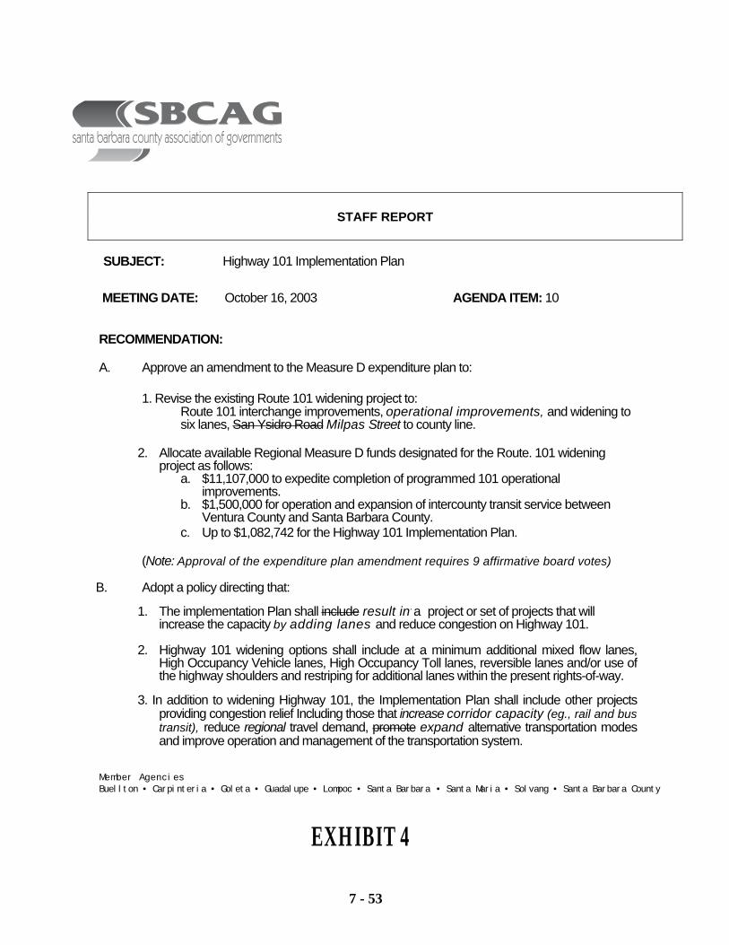
7 - 53
STAFF REPORT
SUBJECT: Highway 101 Implementation Plan
MEETING DATE: October 16, 2003 AGENDA ITEM: 10
RECOMMENDATION:
A. Approve an amendment to the Measure D expenditure plan to:
1. Revise the existing Route 101 widening project to: Route 101 interchange improvements, operational improvements, and widening to six lanes, San Ysidro Road Milpas Street to county line.
2. Allocate available Regional Measure D funds designated for the Route. 101 widening
project as follows: a. $11,107,000 to expedite completion of programmed 101 operational
improvements. b. $1,500,000 for operation and expansion of intercounty transit service between
Ventura County and Santa Barbara County. c. Up to $1,082,742 for the Highway 101 Implementation Plan.
(Note: Approval of the expenditure plan amendment requires 9 affirmative board votes)
B. Adopt a policy directing that:
1. The implementation Plan shall include result in. a project or set of projects that will
increase the capacity by adding lanes and reduce congestion on Highway 101.
2. Highway 101 widening options shall include at a minimum additional mixed flow lanes, High Occupancy Vehicle lanes, High Occupancy Toll lanes, reversible lanes and/or use of the highway shoulders and restriping for additional lanes within the present rights-of-way.
3. In addition to widening Highway 101, the Implementation Plan shall include other projects providing congestion relief Including those that increase corridor capacity (eg., rail and bus transit), reduce regional travel demand, promote expand alternative transportation modes and improve operation and management of the transportation system.
Member Agencies Buellton • Carpinteria • Goleta • Guadalupe • Lompoc • Santa Barbara • Santa Maria • Solvang • Santa Barbara County
EXHIBIT 4
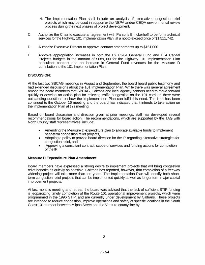
7 - 54
4. The implementation Plan shall include an analysis of alternative congestion relief projects which may be used in support of the NEPA and/or CEQA environmental review process during the next phases of project development.
C. Authorize the Chair to execute an agreement with Parsons Brinckerhoff to perform technical
services for the Highway 101 implementation Plan, at a not-to-exceed price of $1,511,742. D. Authorize Executive Director to approve contract amendments up to $151,000. E. Approve appropriation increases in both the FY 03-04 General Fund and LTA Capital
Projects budgets in the amount of $689,300 for the Highway 101 Implementation Plan consultant contract and an increase in General Fund revenues for the Measure D contribution to the 101 Implementation Plan.
DISCUSSION: At the last two SBCAG meetings in August and September, the board heard public testimony and had extended discussions about the 101 Implementation Plan. While there was general agreement among the board members that SBCAG, Caltrans and local agency partners need to move forward quickly to develop an action plan for relieving traffic congestion on the 101 corridor, there were outstanding questions on how the Implementation Plan can fulfill this need. The item has been continued to the October 16 meeting and the board has indicated that it intends to take action on the implementation Plan at this meeting. Based on board discussion and direction given at prior meetings, staff has developed several recommendations for board action. The recommendations, which are supported by the TAG with North County staff representatives, include:
• Amending the Measure D expenditure plan to allocate available funds to Implement near-term congestion relief projects,
• Adopting a policy to provide board direction for the IP regarding alternative strategies for congestion relief, and
• Approving a consultant contract, scope of services and funding actions for completion of the lP.
Measure D Expenditure Plan Amendment Board members have expressed a strong desire to implement projects that will bring congestion relief benefits as quickly as possible. Caltrans has reported, however, that completion of a freeway widening project will take more than ten years. The Implementation Plan will identify both short-term congestion relief projects that can be implemented quickly as well as longer term major capital improvement projects. At last month's meeting and retreat, the board was advised that the lack of sufficient STIP funding is jeopardizing timely completion of the Route 101 operational improvement projects, which were programmed in the 1996 STIP, and are currently under development by Caltrans. These projects are intended to reduce congestion, improve operations and safety at specific locations in the South Coast 101 corridor between Milpas Street and the Ventura county line by
2
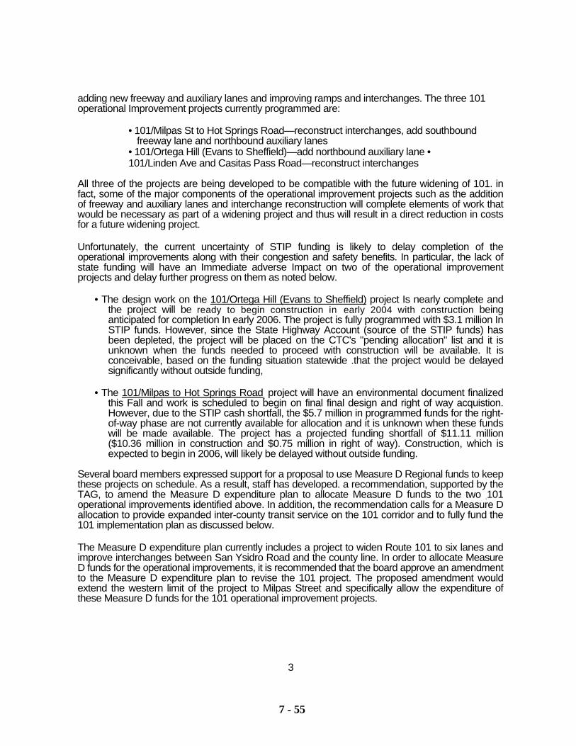
7 - 55
adding new freeway and auxiliary lanes and improving ramps and interchanges. The three 101 operational Improvement projects currently programmed are:
• 101/Milpas St to Hot Springs Road—reconstruct interchanges, add southbound freeway lane and northbound auxiliary lanes
• 101/Ortega Hill (Evans to Sheffield)—add northbound auxiliary lane • 101/Linden Ave and Casitas Pass Road—reconstruct interchanges
All three of the projects are being developed to be compatible with the future widening of 101. in fact, some of the major components of the operational improvement projects such as the addition of freeway and auxiliary lanes and interchange reconstruction will complete elements of work that would be necessary as part of a widening project and thus will result in a direct reduction in costs for a future widening project. Unfortunately, the current uncertainty of STIP funding is likely to delay completion of the operational improvements along with their congestion and safety benefits. In particular, the lack of state funding will have an Immediate adverse Impact on two of the operational improvement projects and delay further progress on them as noted below.
• The design work on the 101/Ortega Hill (Evans to Sheffield) project Is nearly complete and the project will be ready to begin construction in early 2004 with construction being anticipated for completion In early 2006. The project is fully programmed with $3.1 million In STIP funds. However, since the State Highway Account (source of the STIP funds) has been depleted, the project will be placed on the CTC's "pending allocation" list and it is unknown when the funds needed to proceed with construction will be available. It is conceivable, based on the funding situation statewide .that the project would be delayed significantly without outside funding,
• The 101/Milpas to Hot Springs Road, project will have an environmental document finalized this Fall and work is scheduled to begin on final final design and right of way acquistion. However, due to the STIP cash shortfall, the $5.7 million in programmed funds for the right-of-way phase are not currently available for allocation and it is unknown when these funds will be made available. The project has a projected funding shortfall of $11.11 million ($10.36 million in construction and $0.75 million in right of way). Construction, which is expected to begin in 2006, will likely be delayed without outside funding.
Several board members expressed support for a proposal to use Measure D Regional funds to keep these projects on schedule. As a result, staff has developed. a recommendation, supported by the TAG, to amend the Measure D expenditure plan to allocate Measure D funds to the two .101 operational improvements identified above. In addition, the recommendation calls for a Measure D allocation to provide expanded inter-county transit service on the 101 corridor and to fully fund the 101 implementation plan as discussed below. The Measure D expenditure plan currently includes a project to widen Route 101 to six lanes and improve interchanges between San Ysidro Road and the county line. In order to allocate Measure D funds for the operational improvements, it is recommended that the board approve an amendment to the Measure D expenditure plan to revise the 101 project. The proposed amendment would extend the western limit of the project to Milpas Street and specifically allow the expenditure of these Measure D funds for the 101 operational improvement projects.
3
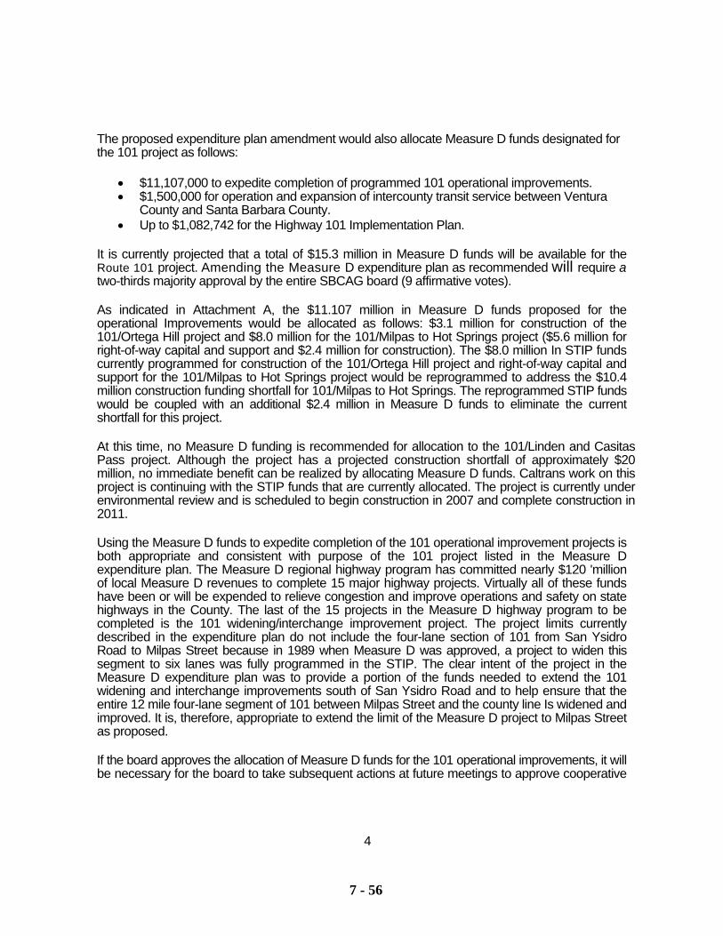
7 - 56
The proposed expenditure plan amendment would also allocate Measure D funds designated for the 101 project as follows:
• $11,107,000 to expedite completion of programmed 101 operational improvements. • $1,500,000 for operation and expansion of intercounty transit service between Ventura
County and Santa Barbara County. • Up to $1,082,742 for the Highway 101 Implementation Plan.
It is currently projected that a total of $15.3 million in Measure D funds will be available for the Route 101 project. Amending the Measure D expenditure plan as recommended will require a two-thirds majority approval by the entire SBCAG board (9 affirmative votes). As indicated in Attachment A, the $11.107 million in Measure D funds proposed for the operational Improvements would be allocated as follows: $3.1 million for construction of the 101/Ortega Hill project and $8.0 million for the 101/Milpas to Hot Springs project ($5.6 million for right-of-way capital and support and $2.4 million for construction). The $8.0 million In STIP funds currently programmed for construction of the 101/Ortega Hill project and right-of-way capital and support for the 101/Milpas to Hot Springs project would be reprogrammed to address the $10.4 million construction funding shortfall for 101/Milpas to Hot Springs. The reprogrammed STIP funds would be coupled with an additional $2.4 million in Measure D funds to eliminate the current shortfall for this project. At this time, no Measure D funding is recommended for allocation to the 101/Linden and Casitas Pass project. Although the project has a projected construction shortfall of approximately $20 million, no immediate benefit can be realized by allocating Measure D funds. Caltrans work on this project is continuing with the STIP funds that are currently allocated. The project is currently under environmental review and is scheduled to begin construction in 2007 and complete construction in 2011. Using the Measure D funds to expedite completion of the 101 operational improvement projects is both appropriate and consistent with purpose of the 101 project listed in the Measure D expenditure plan. The Measure D regional highway program has committed nearly $120 'million of local Measure D revenues to complete 15 major highway projects. Virtually all of these funds have been or will be expended to relieve congestion and improve operations and safety on state highways in the County. The last of the 15 projects in the Measure D highway program to be completed is the 101 widening/interchange improvement project. The project limits currently described in the expenditure plan do not include the four-lane section of 101 from San Ysidro Road to Milpas Street because in 1989 when Measure D was approved, a project to widen this segment to six lanes was fully programmed in the STIP. The clear intent of the project in the Measure D expenditure plan was to provide a portion of the funds needed to extend the 101 widening and interchange improvements south of San Ysidro Road and to help ensure that the entire 12 mile four-lane segment of 101 between Milpas Street and the county line Is widened and improved. It is, therefore, appropriate to extend the limit of the Measure D project to Milpas Street as proposed. If the board approves the allocation of Measure D funds for the 101 operational improvements, it will be necessary for the board to take subsequent actions at future meetings to approve cooperative
4
7 - 57
agreements with Caltrans for each of the projects. The agreements will outline the roles and responsibilities of each agency. In addition, SBCAG will need to seek approval by the CTC of a STIP amendment revising the programming amounts for each project as described in Attachment A. Providing local contributions to fund state highway improvement projects is quite common, particularly In self-help counties that have local transportation sales taxes. SBCAG's contribution of Measure D funds to the 101 operational improvement projects would have no effect on the county share amount of STIP funds that SBCAG will receive because these funds are allocated to regions based on a formula specified in statute. Staff and the TAG are also recommending that the. board allocate $1.5 million of the Measure D 101 project allocation for operation and expansion of the intercounty transit service currently provided by the Coastal Express. It was reported to the board at its retreat last month that this service is experiencing strong ridership growth (16% increase in FY 02-03) and productivity (farebox recovery ratio is currently 31%) . and it is believed that there is significant potential for expansion of current peak period and express service. Because the Coastal Express service provides direct congestion relief benefits by reducing peak hour auto trips on the South Coast 101., allocating the Measure D funds for this service should be considered. At the board retreat, staff reported that the CMAQ funding being used for the Coastal Express 3-year demonstration project will be exhausted along with the current APCD subsidy at the end of the current fiscal year. It is projected that beginning in FY 04-05, SBCAG will experience a shortfall of approximately $200,000 annually for its share of the Coastal Express operating costs (Ventura County Transportation Commission and SBCAG split the costs equally). Unless another funding source Is identified for SBCAG's share of the operating costs, the Coastal Express service will have to be terminated at the end of the pilot program next year. The recommended allocation of $1.5 million in' Measure D funds will allow the service to continue to operate for at least "6 more-years (until Measure D expires in 2009) and provide for an expansion of the service to include approximately 4 more weekday peak period round trips (11 weekday round trips are currently provided). Other funding options for subsidizing the Coastal Express are limited. Existing sources of transit funding including FTA 5307 urbanized area formula funds and TDA funds are already fully committed to existing transit services. CMAQ funds cannot be used after the 3-year pilot program is complete. The staff and TAG recommendations for allocating Measure D funds for operational improvements and transit services in the 101 corridor will provide several benefits as shown in the table below:
Project Status BenefitUS 101: Mllpas to Hot • Final EIR in November • Maintain current schedule Springs Road • Construction scheduled for • Initiate right of way delivery
2006 • Fully funds project • Ready to begin right of
way but no money in SHA
• Overall funding shortfall of $11.1 million
US 101: Ortega Hill — • Ready for advertisement; Begin construction in 2004 Evans to Sheffield no money in SHACoastal Express • On-going service showing • Maintain existing service
Increased ridership levels • Expand peak service in FY 04- Operating deficit beginning 05
In FY 04-05 • Reduce trips on 101 corridor US 101: Linden / In environmental review • No immediate direct benefit Casitas Interchanges Overall funding shortfall of
$20 million
5
7 - 58
The recommended Measure D expenditure plan amendment would allocate about $13.7 million o f t h e available funds fo r the 101 project leaving a balance of approximately $1.6 million. It is recommended that the remaining funds be reserved at this time to serve as a contingency amount for the 101 operational improvement projects. The reserve could be also be used for specific projects that come from the IP Including early implementation of low cost projects that can provide immediate congestion relief benefits, Policy Direction for the Implementation Plan One of the major concerns expressed by several board members is that the IP fails to reflect the necessity of adding new capacity to 101 to Improve traffic flow: While many members acknowledged the need to evaluate other strategies, they also stated that relieving congestion would require increasing the capacity of 101 by adding new lanes and that this must, therefore, be a mandatory component of the IP. Increasing frustration with the congestion and voter approval of Measure D in 1989--which includes a project to widen 101 south of San Ysidro Road–are cited as evidence of broad support for widening 101. As a result, some board members indicated that they may support the IP only if It includes a project to widen 101 as a mandatory component. Consequently, last month, staff and the TAG presented recommendations for board consideration that would provide policy direction for development of the IP. These recommendations are again being presented this month with some changes based on board comments and alternative language suggested by Councilmember Smyser at last month's meeting. The suggested language by Councilmember Smyser was as follows:
The Implementation Plan shall result in a project that will provide additional lanes and concurrently other capacity alternatives that may result in other projects to reduce congestion on Highway 101. The plan will also provide concurrently for the designation end release of Measure D funds for approved operational improvements
The policy direction recommended by staff and the TAG is included in Recommendation B. The revised language in B(1) states the board's intent that a project or projects to increase the capacity of 101 shall be the result of the IP and clarifies that increased capacity shall be provided by adding lanes. The board must not to preclude consideration of the many options for adding freeway lanes including traditional mixed flow lanes, high occupancy vehicle (carpool) lanes, high occupancy toll lanes, reversible lanes, etc. Consequently, recommendation B(2) identifies some of'these options for widening 101 and adding lanes that will be evaluated in the 1P. A successful long-range, comprehensive plan for relieving congestion must' also include projects other than adding freeway lanes. Recommendation B(3) states that the IP will include other projects that would increase the carrying capacity of the travel corridor such as bus or commuter rail transit, reduce travel demand, provide alternatives for peak period single-occupant auto trips and Improve the operation and management of the system. Finally, Recommendation B(4) states that the board intends to fully comply with CEQA and NEPA by using the IP to support a requirement to evaluate alternative congestion relief projects. Consultant Scope of Work Modifications At the September board meeting, staff and the TAG presented some recommended changes in the consultant scope of services to ensure that the IP addresses regional issues In Northern Santa Barbara County and Ventura County (these were presented as Recommendation B in the
6
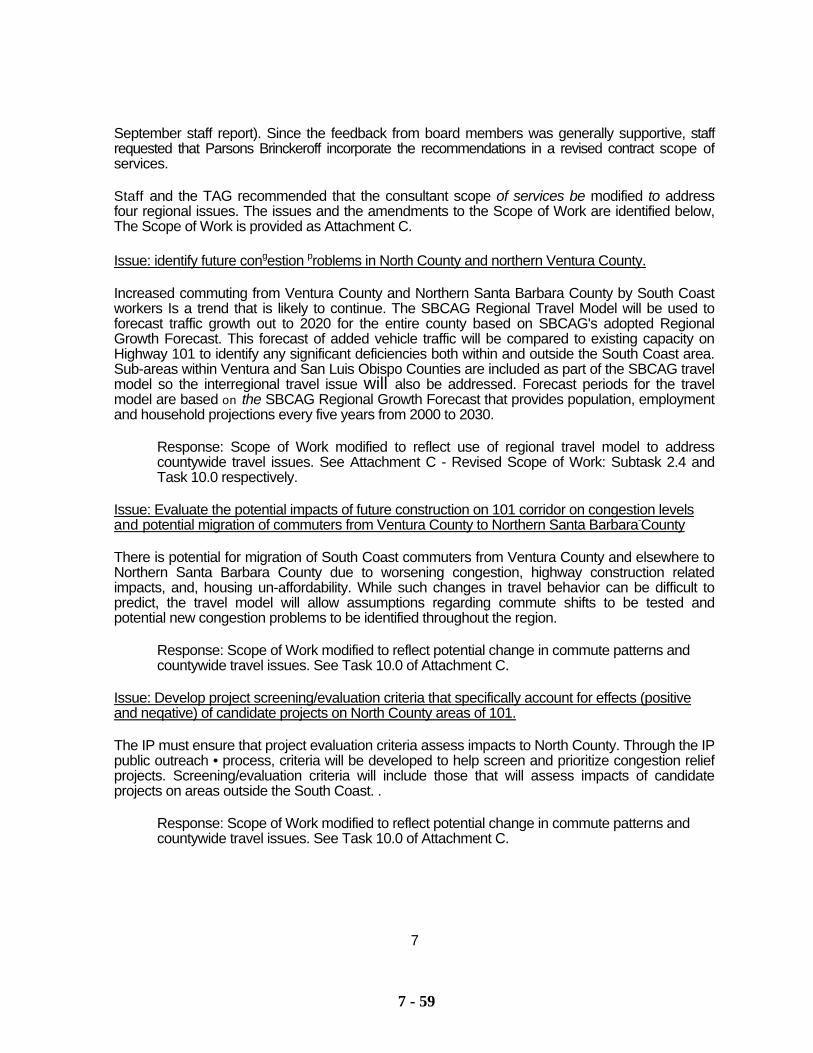
7 - 59
September staff report). Since the feedback from board members was generally supportive, staff requested that Parsons Brinckeroff incorporate the recommendations in a revised contract scope of services. Staff and the TAG recommended that the consultant scope of services be modified to address four regional issues. The issues and the amendments to the Scope of Work are identified below, The Scope of Work is provided as Attachment C. Issue: identify future congestion problems in North County and northern Ventura County. Increased commuting from Ventura County and Northern Santa Barbara County by South Coast workers Is a trend that is likely to continue. The SBCAG Regional Travel Model will be used to forecast traffic growth out to 2020 for the entire county based on SBCAG's adopted Regional Growth Forecast. This forecast of added vehicle traffic will be compared to existing capacity on Highway 101 to identify any significant deficiencies both within and outside the South Coast area. Sub-areas within Ventura and San Luis Obispo Counties are included as part of the SBCAG travel model so the interregional travel issue will also be addressed. Forecast periods for the travel model are based on the SBCAG Regional Growth Forecast that provides population, employment and household projections every five years from 2000 to 2030.
Response: Scope of Work modified to reflect use of regional travel model to address countywide travel issues. See Attachment C - Revised Scope of Work: Subtask 2.4 and Task 10.0 respectively.
Issue: Evaluate the potential impacts of future construction on 101 corridor on congestion levels and potential migration of commuters from Ventura County to Northern Santa Barbara-County There is potential for migration of South Coast commuters from Ventura County and elsewhere to Northern Santa Barbara County due to worsening congestion, highway construction related impacts, and, housing un-affordability. While such changes in travel behavior can be difficult to predict, the travel model will allow assumptions regarding commute shifts to be tested and potential new congestion problems to be identified throughout the region.
Response: Scope of Work modified to reflect potential change in commute patterns and countywide travel issues. See Task 10.0 of Attachment C.
Issue: Develop project screening/evaluation criteria that specifically account for effects (positive and neqative) of candidate projects on North County areas of 101. The IP must ensure that project evaluation criteria assess impacts to North County. Through the IP public outreach • process, criteria will be developed to help screen and prioritize congestion relief projects. Screening/evaluation criteria will include those that will assess impacts of candidate projects on areas outside the South Coast. .
Response: Scope of Work modified to reflect potential change in commute patterns and countywide travel issues. See Task 10.0 of Attachment C.
7
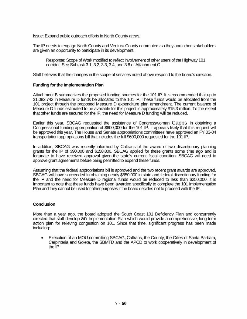
7 - 60
Issue: Expand public outreach efforts in North County areas.
The IP needs to engage North County and Ventura County commuters so they and other stakeholders are given an opportunity to participate in its development.
Response: Scope of Work modified to reflect involvement of other users of the Highway 101 corridor. See Subtask 3.1,.3.2, 3.3, 3.4, and 3.8 of Attachment C.
Staff believes that the changes in the scope of services noted above respond to the board's direction.
Funding for the Implementation Plan
Attachment B summarizes the proposed funding sources for the 101 IP. It is recommended that up to $1,082,742 in Measure D funds be allocated to the 101 IP. These funds would be allocated from the 101 project through the proposed Measure D expenditure plan amendment. The current balance of Measure D funds estimated to be available for this project is approximately $15.3 million. To the extent that other funds are secured for the IP, the need for Measure D funding will be reduced.
Earlier this year, SBCAG requested the assistance of Congresswoman Capps in obtaining a Congressional funding appropriation of $600,000 for the 101 IP. It appears likely that this request will be approved this year. The House and Senate appropriations committees have approved an FY 03-04 transportation appropriations bill that includes the full $600,000 requested for the 101 IP.
In addition, SBCAG was recently informed by Caltrans of the award of two discretionary planning grants for the IP of $90,000 and $158,800. SBCAG applied for these grants some time ago and is fortunate to have received approval given the state's current fiscal condition. SBCAG will need to approve grant agreements before being permitted to expend these funds.
Assuming that the federal appropriations bill is approved and the two recent grant awards are approved, SBCAG will have succeeded In obtaining nearly $850,000 in state and federal discretionary funding for the IP and the need for Measure D regional funds would be reduced to less than $250,000. it is Important to note that these funds have been awarded specifically to complete the 101 Implementation Plan and they cannot be used for other purposes if the board decides not to proceed with the IP.
Conclusion
More than a year ago, the board adopted the South Coast 101 Deficiency Plan and concurrently directed that staff develop an Implementation Plan which would provide a comprehensive, long-term action plan for relieving congestion on 101. Since that time, significant progress has been made including:
• Execution of an MOU committing SBCAG, Caltrans, the County, the Cities of Santa Barbara,
Carpinteria and Goleta, the SBMTD and the APCD to work cooperatively in development of the IP
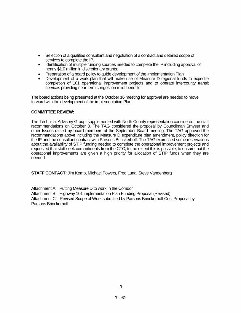
7 - 61
• Selection of a qualified consultant and negotiation of a contract and detailed scope of services to complete the IP.
• Identification of multiple funding sources needed to complete the IP including approval of nearly $1.0 million in discretionary grants.
• Preparation of a board policy to guide development of the Implementation Plan • Development of a work plan that will make use of Measure D regional funds to expedite
completion of 101 operational improvement projects and to operate intercounty transit services providing near-term congestion relief benefits
The board actions being presented at the October 16 meeting for approval are needed to move forward with the development of the implementation Plan. COMMITTEE REVIEW: The Technical Advisory Group, supplemented with North County representation considered the staff recommendations on October 3. The TAG considered the proposal by Councilman Smyser and other Issues raised by board members at the September Board meeting. The TAG approved the recommendations above including the Measure D expenditure plan amendment, policy direction for the IP and the consultant contract with Parsons Brinckerhoff. The TAG expressed some reservations about the availability of STIP funding needed to complete the operational improvement projects and requested that staff seek commitments from the CTC, to the extent this is possible, to ensure that the operational improvements are given a high priority for allocation of STIP funds when they are needed. STAFF CONTACT: Jim Kemp, Michael Powers, Fred Luna, Steve Vandenberg Attachment A: Putting Measure D to work In the Corridor Attachment B: Highway 101 implementation Plan Funding Proposal (Revised) Attachment C: Revised Scope of Work submitted by Parsons Brinckerhoff Cost Proposal by Parsons Brinckerhoff
9
7 - 62
Tom Murphy APCD Manager Technology and Environmental Assessment 260 N. San Antonio Rd. Suite A Santa Barbara, CA 93110 Comments Draft 2004 Clean Air Plan August 2004 Dear Mr. Murphy:
Here are my questions and comments for the above document: Pg 3-14 NOx annual emissions. Under mobile sources you cite 78% = 13,804 tons; in the 2001 Clean Air Plan (CAP) we had 80% = 15,319. We are dealing here with light duty passenger cars and trucks. How do you explain this reduction, if the traffic and gridlock in the freeways and streets is continuing to increase? Please comment.
Pg.4-4 table 4-1(2004 CAP) "Emissions control measures adopted before 2001" you dropped the ROC and NOx emission reduction that one can clearly see in the comparable table on pg 4-27 (2001 CAP). I suggest keeping the same format with the same headings and information from the 2001 Clean Air Plan. Why drop the future projections of ROC and NOx for 2005, 2010, and 2015? Pg 4-11 Table 4-4 Please add the Rule# to Gas turbines (363) Pg. 4-23 (2001 CAP) Liquefied Natural and Petroleum Gas Truck loading was deleted from in the 2001 Clean Air Plan. On March 3, 2004 a truck contracted by the Southern California Gas Co. spilled five gallons of mercaptan in Goleta near the Bacara Resort. The CAC was informed about the spill. This control measure should be reinstated and not deleted.
1 of 3
September 23, 2004
7 - 63
Pg 5-2 It would be helpful to have comparison charts from North and South County regarding population growth and VMT (Vehicle Mile Traveled).The source of your VMT is Caltrans. Did they take into account traffic originating in Santa Barbara County or are they counting traffic on the 101 freeway, a major thoroughfare for the entire state of California? Land use strategies: Higher density with fewer parking spaces does not mean fewer cars. To the contrary, higher density with inadequate parking affects adjacent residential areas as people who do not have places to park in their development will use the side streets leading to them. Sometimes they even will park on designed bike lanes, creating a danger to bicyclists as they have to use the street instead of their assigned safer lane. Pg. 7-8 paragraph 6e) needs correction "Discourage projects less than 20 housing units per gross acre". The Village Homes at Davis cited as an example by the Local Government Commission (LGC) have a density of 7.7 per acre, not 20 per acre. Where was the # 20 for the housing units per acre taken from? Public transportation has to be optimal and functional for people to leave their cars. Streets and thoroughfares should be built first. People living in California are dependent on their cars. They are still the preferred mode of transportation. SUV's are replacing cars and instead of carrying more passengers; we still see one person per vehicle. Building of large residential areas should be placed on hold until alternative routes or mode of transportation have been created if the LOS (level of service) of the existing streets is going to be degraded to a LOS D or F secondary to increased traffic generated by this homes.
2 of 3
7 - 64
Developments should not encroach on buffer areas of ESHA's (environmental sensitive habitats).
In Goleta the few open spaces left are already being eyed for development. Once you have paved over an area there is no going back. Infill development should not place residents or employees near sources of nuisance, dust, odors and accidental releases of toxic substances that could be lethal.
Why do the CMP (Congestion Mitigation Program) requirements state that a specific area should be zoned residential within one third of a mile of a rail transit station? We know NOx reacts with ammonia, moisture and other compounds to form nitric acid and related particles. Small particles penetrate into the lung and can cause respiratory disease such as emphysema, bronchitis and can aggravate existing heart disease.
Studies regarding the impact of ROC and NOx to populations near trains should be incorporated into this report. As part of the final document under a separate chapter I would like to see all the comments that we members of the CAC contributed for each chapter. This is part of the public record and should be shared.
3 of 3
7 - 65
7 - 66
7 - 67
7 - 68
7 - 69
7 - 70
7 - 71
7 - 72
7 - 73
7 - 74
APCD RESPONSE TO PUBLIC COMMENTS
• Comments From Marc Chytilo 1. Comment: Health and Safety Code Section 40717 Response: While the District and SBCAG have not performed photochemical modeling
to determine an emission reduction quantity necessary from transportation
sources to attain the state standard, the District and SBCAG have determined
the emissions reductions necessary for such sources by including in the CAP
all reasonably available and feasible TCM's. These TCM's in the CAP
constitute the District and SBCAG's determination of the emission
reductions necessary for this CAP to attain the state standard. These
reductions together with the substantial emission reductions achieved
through ARB's regulation of fuels and tail pipe emissions are achieving
significant reductions of emission from transportation sources. As explained
in the District/SBCAG letter to Marc Chytilo on May 21, 2004, the District
has made substantial progress toward attainment of the state standard since
1990, when 10 monitoring stations showed violations of the state standard.
In contrast, the most recent data show that only one station (Paradise)
violates the state standard and only by a slim margin. In light of this
progress and the very narrow margin of improvement needed to attain the
state standard, the District and SBCAG have determined that the emission
reduction necessary from transportation sources necessary to attain the state
standard are those that will be achieved from the implementation of all
feasible measures that have been included in the CAP. These reductions
together with the stationary source regulations should achieve the state
standard. The District will continue to monitor the air quality data and, if
necessary, make future adjustments to the CAP, including to TCM's, as
necessary to take further steps to achieve the state standard.
7 - 75
2. Comment: Transportation Control Measures Response: Table 5-2 in Chapter 5 (“Transportation Control Measures”) enumerates
thirteen currently adopted TCMs while Table 5-5 lists nine TCMs proposed
for further study. Seven projects identified in this list of nine for further
study TCMs have now either been implemented or are funded and
proceeding to implementation. The remaining projects are currently being
evaluated as part of a comprehensive study called the 101 In-Motion. The
latter is a $1.6 million study to identify a “solution package” of
projects/strategies to address congestion in the Highway 101 corridor in the
long term. Additionally one TCM has been proposed as a contingency
measure.
Commenter cites only the first SBCAG board directive regarding the 101 in
Motion process. The complete adopted policy direction from the SBCAG
board for the 101 in Motion process is as follows:
1) 101 in Motion shall result in a project or set of projects that will increase
the capacity by adding lanes and reduce congestion on Highway 101.
2) Highway 101 widening options shall include at a minimum additional
mixed flow lanes, High Occupancy Vehicle lanes, High Occupancy Toll
lanes, reversible lanes and/or use of the highway shoulders and re-striping
for additional lanes within the present rights-of-way.
3) In addition to widening Highway 101, 101 in Motion shall include other
projects providing congestion relief including those that increase corridor
capacity (e.g.., rail and bus transit), reduce regional travel demand, expand
alternative transportation modes and improve operation and management
of the transportation system.
4) 101 in Motion shall include an analysis of alternative congestion relief
projects which may be used in support of the NEPA and/or CEQA
environmental review process during the next phases of project
7 - 76
development.
The commenter is doubtful that the 101 in Motion process is one through
which TCMs could be developed and maintains that there remains a “broad
public distrust” of 101 in Motion process. However, through 101 in Motion,
a wide cross-section of community members as well as city, County,
Caltrans, APCD and MTD staff have jointly developed eight alternative
congestion relief packages one of which does include traditional mixed flow
lanes but others include TCMs such as high occupancy vehicle lanes
(standard and reversible), ramp metering, express transit, commuter rail,
limiting the number of all-day parking spaces, variable parking rates,
enhanced demand management strategies (flexible work schedules, reducing
bus/vanpool fares), and land use measures such as transit oriented
development. Additionally, the 101 in Motion process has also included an
extensive public outreach program – specifically to low income and minority
segments of our population. These efforts have been well received by the
public. And while there may remain a segment of the public which is
distrustful of the eventual outcome of 101 in Motion, the process does
represent the most inclusive and comprehensive effort to date for developing
meaningful TCMs. It should also be made clear that although a freeway
capacity enhancement will be part of the 101 In-Motion solution package,
this could take the form of HOV/HOT lanes and/or reversible HOV/HOT
lanes. The latter project types are federally recognized TCMs (CAAA
Section 108f), are listed as further study TCMs in the 2004 Clean Air Plan,
and are eligible for federal Congestion Mitigation and Air Quality (CMAQ)
program funds.
As a point of clarification APCD Rule 701, Transportation Conformity, does
not have a TCM substitution provision.
7 - 77
3. Comment: Suggested TCMs.
a) Commuter choice Response: SBCAG already has adopted (TCM 1-4) and staffs a similar program.
SBCAG’s Traffic Solutions Office implements a commuter based TDM
program countywide. Recent changes in state and federal tax law that allow
employers to offer employees parking and transportation benefits as tax-
exempt compensation, with greater incentives for parking cash-out and
alternative commute options has been aggressively marketed by the Traffic
Solutions Office. Copies of the tax code, samples and descriptions of the
various potential parking cash-out strategies and their estimated tax savings
are provided in the Employer Transportation Coordinator (ETC) Training
and Resource Guide. Similar information is posted on the Traffic Solutions
Web Site. In addition, SBCAG staff regularly recommends parking cash out
programs when reviewing/commenting on environmental documents for land
use projects that trigger the Congestion Management Program thresholds for
analysis.
SBCAG’s Traffic Solutions Office provides/implements the following
commuter based TDM programs and services:
• Employer Services: Including the development of a training and
resource manual, free consulting services, and a monthly newsletter geared towards informing employers about alternative transportation resources available to them and their employees.
• Carpool Matching: Provide free carpool matching services for
commuters interested in forming carpools. Matchlists can be e-mailed, mailed, faxed or telephoned to clients. In 2004/05, on-line instant carpool matchlists will be available through the Traffic Solutions website.
• Emergency Ride Home Program: Program providing a free ride home
to eligible alternative transportation commuters in the event of an unplanned personal emergency. This program is offered through a
7 - 78
partnership with employers (at no charge to employers). • New Vanpool Rider Rebate Program: Provides a $100 rebate to new
vanpoolers, after they join the vanpool for at least three months. • Vanpool Quick Start Program: Provides a 50 and 25 percent subsidy
for vanpool lease support for each new vanpool for the first and second months of operation respectively; $60 rebate for vanpool driver physical exams; lease support for new vanpools serving Downtown Santa Barbara commuters and aggressively assists in the formation of vanpool groups; and, a $400 subsidy for the San Marcos Pass Vanpool program paid for by San Marcos Golf Course.
• Amtrak Commuter Passes: Negotiated and market reduced rate passes
(monthly and 10-ride) for Central Coast commuters. • Coastal Express: Marketing and administrative support for the Coastal
Express bus service between Santa Barbara and Ventura counties. • Clean Air Express: Administration of the Clean Air Express commuter
bus service. • Bike to Work Day: Cooperative special event with the Santa Barbara
Bicycle Coalition held at seven locations countywide to promote and reward bicycle commuting.
• Rideshare Events: Countywide events designed to encourage
alternative transportation. • Pollution Prevention Week Partner: An annual educational campaign
about pollution and the strategies individuals and businesses can use to reduce pollution.
• Green Award Consortium: Annual award honoring the voluntary
environmental efforts of Santa Barbara county businesses. • Participates and supports the Santa Barbara Carfree Program designed
to encourage visitors to tour Santa Barbara without a car. • Kids Care for Clean Air Calendar: Cooperative educational project
with APCD showcasing children’s art about air pollution and transportation.
• Countywide Bike Map & Countywide Transit Map: Production and
distribution of both maps displaying bike and transit routes throughout Santa Barbara County.

7 - 79
• Website: Maintain an up-to-date website that includes information
about alternative transportation in Santa Barbara county, including on line applications for carpool matchlists and links to transportation service providers and resources.
• Downtown Santa Barbara Transportation Programs: Repackage and
renew the downtown alternative transportation programs, such as carpool parking, free bus passes, and bicycle lockers.
• School Programs: staff resources to promote alternative transportation
at schools, including bike and walk to school days, bicycle and pedestrian safety instruction, school pools, buses, and incentive programs for school children.
• Enhanced Employer Programs: Staff and financial resources to provide
and support employer-based telework and flexible schedule pilot programs.
b) Community Car Program
Response: Community car programs are of interest to SBCAG and the APCD. Such
programs have worked well in areas like the Bay Area where they have been
integrated with major transit hubs and where certain conditions exist such as
adequate density, severely limited on-street parking, limited and expensive
garage space etc. Although these conditions do not exist in Santa Barbara
County, SBCAG feels that there are applications for community car
programs that can be structured to promote alternative forms of
transportation. One such example is for new developments (e.g. large
residential developments) to offer a community car program coupled with
parking cash out options as a means to reduce residential parking
requirements. As reviewing agencies under CEQA, SBCAG and the APCD
will continue to consider community car programs a potential mitigation for
new developments of this scale.
SBCAG does feel that given the right conditions and program requirements,
some employer based car-sharing programs can be effective at promoting
alternative forms of transportation to work thereby reducing vehicle
7 - 80
emissions. One such program is being considered at UCSB. SBCAG has
met and discussed how such a program could be structured at UCSB in order
for it to compete for Congestion Mitigation and Air Quality (CMAQ) funds.
Given the lack of more favorable conditions for a more regional approach to
car sharing, SBCAG feels it is more prudent and protective of air quality to
assess the merit of employer based car-sharing programs on a case by case
basis.
c) Smart Growth Resources
Response: Both SBCAG and the APCD agree with your statements regarding the
importance of educating both local planners and the public on the importance
of better land use development and design. Hence, an entire chapter of the
2004 Clean Air Plan addresses the land use and air quality linkage. Chapter
7 provides examples of specific land use strategies; provides a list of
prospective transportation system management policies and programs that
local agencies can incorporate into general plans and circulation elements;
and, describes the process in terms of communication, coordination, and
monitoring that may be necessary to ensure that such policies if pursued will
produce the desired results. This chapter was purposely structured in this
“how to” fashion to be a resource for local agencies to use as they deem
appropriate.
While SBCAG has very limited direct responsibility for land use planning in
the region, there is increasing recognition of the need to effectively integrate
land use and transportation planning in order to 1) reduce the impact of
sprawl and consumption of land, 2) address the imbalance between jobs and
housing in different parts of the region, 3) limit the increase in travel
demand, and 4) minimize the need for major highway capacity
improvements.
SBCAG’s Overall Work Program for fiscal year 2004-05 includes several
7 - 81
activities designed to help inform decision-makers and provide a framework
for addressing these issues. These include upgrades to SBCAG’s travel
forecasting model, a continuing project to analyze alternative land use
futures in terms of their transportation implications and SBCAG’s recent
jobs/housing Interregional Partnership report. These activities will build
upon the Regional Growth Forecast anticipated to be updated in 2005/06 and
will also provide input to the update of the Regional Transportation Plan.
d) Bike projects
Response: The identification of a more comprehensive bicycle system for the region
was made and formalized with the adoption of The Regional Bikeway Plan
(SBCAG) in July of 1994. A primary goal of the study was to identify a
regional bikeway system which links the major population centers and,
within centers, major trip origins and destinations. Routes chosen for
inclusion on the regional bikeway system serve the needs of both commuters
and recreational riders. Completion of the regional bikeway network is a
transportation performance measure that is tracked and reported by SBCAG
during biennial updates of the Santa Barbara County Congestion
Management Program (see 2003 CMP). A full update of SBCAG’s Regional
Bikeway Plan is scheduled in 2004/05.
In August of 1998, the SBCAG board approved two new Regional
Transportation Plan policies regarding bikeways. First:
• Determine that projects supportive of the SBCAG Regional Bikeway
Study will be given priority for the use of bikeway funds. This policy is carried out as part of SBCAG’s project selection criteria for
state and federal funding program cycles. Priority is given to bikeway
projects (Class I or II) that fill or connect the SBCAG regional system of
routes as identified in the Regional Bikeway Study.
7 - 82
To help guarantee a funding source for the completion of the regional
bikeway system, the SBCAG board approved the second RTP policy:
• Establish goal to program a least 10% to TEA-21 flexible funds from
the Regional STP, CMAQ and TEA funds for these bikeway projects (i.e., regional bikeway system).
Upon completion of each federal funding cycle, SBCAG reports how the
flexible funds are distributed by project type. Historically, SBCAG has
programmed over 15% of ISTEA and TEA-21 flexible funds for bikeway
projects countywide.
Continuous review and improvement of safety problems and maintenance
including surface street standards, bridge access, and traffic control issues
are carried out by not only each respective local agency’s public works
department but by eight regional bike clubs throughout the county as well.
SBCAG’s Traffic Solutions Division disseminates the “official” Santa
Barbara County Bike Map on a continuous basis and tracks the number of
maps it gives out in its monthly newsletter. The Santa Barbara County Bike
Map includes a complete inventory of all designated Class I, Class II, and
Class III bikeways in the county. The Bike Maps also lists phone numbers
and contacts for regional bike clubs within the county and for reporting of
bikeway hazards, provides safety tips for cyclists, and lists all applicable
bike laws. SBCAG plans to include the taxonomy of bicycle signage in
future upgrades of the Bike Map. The taxonomy will help educate cyclists
on how to understand the various bicycle signs. Presently, all South County
jurisdictions use a consistent standardized taxonomy of signs. North County
jurisdictions have not coordinated bicycle signage efforts to date.
In conclusion, SBCAG/APCD believe that many if not all of the suggestions
for bike projects are already being addressed.
7 - 83
e) Pedestrian projects
Response: SBCAG agrees that pedestrian-friendly facilities need to be given greater
consideration in land use design and implementation. However, such
considerations continue to be under the purview of the cities and the county.
Chapter 7 of the 2004 Clean Air Plan provides examples of specific land use
strategies; provides a list of prospective transportation system management
policies and programs that local agencies can incorporate into general plans
and circulation elements; and, describes the process in terms of
communication, coordination, and monitoring that may be necessary to
ensure that such policies if pursued will produce the desired results. This
chapter was purposely structured in this “how to” fashion to be a resource for
local agencies to use as they deem appropriate.
The City of Santa Barbara is planning to develop a Pedestrian Facility Plan
that will identify a comprehensive sidewalk system. This will be the first
plan of its kind in Santa Barbara County.
A more regional issue that SBCAG is cognizant of and will continue to work
with Caltrans on is cross-highway pedestrian and bikeway access issues.
Given that Highway 101 can act as a barrier to pedestrian and bikeway cross-
highway movements, increasing attention to this issue is needed during the
design phase of new interchanges and interchange reconstruction projects.
f) Recognize induced traffic and VMT
Response: This is not a TCM but more of an air quality analysis consideration. SBCAG
did include a discussion of induced VMT in the 2001 RTP EIR and has
included a more in depth assessment using local traffic data in the Highway
101 Deficiency Plan (June, 2002). SBCAG does not advocate an “across the
board” treatment of induced vehicle activity as a result of transportation
infrastructure improvements. Current peer reviewed research and local data
7 - 84
strongly suggests that the magnitude of an induced effect is scale sensitive
(i.e., magnitude of travel time savings from the proposed improvement) and
dependent on the presence of several other land use and travel demand
characteristics and factors. Hence, consideration of latent demand should be
handled on a project-by-project basis.
All travel models – including SBCAG’s Santa Barbara Travel Model are
calibrated/validated using actual “ground truth” HPMS VMT data. Santa
Barbara County’s Highway Performance Monitoring System (HPMS)
sample size currently meets 90–10 precision limits (90-percent confidence
with 10-percent allowable error – or in other words there is the probability
that 90 times out of a 100 the error of a data element estimate will be no
greater or less than 10 percent of its true value). This ensures that the annual
HPMS VMT estimates for Santa Barbara County reflect VMT from currently
completed projects. Future land use projects are generically reflected in
SBCAG’s travel forecasts given that the model’s socio-economic input files
include growth in employment and housing levels for small geographical
units called Traffic Analysis Zones (TAZs). The source of the model’s
socio-economic data comes directly from SBCAG’s Regional Growth
Forecast. SBCAG monitors how well the Regional Growth Forecast tracks
actual growth in employment and housing.
g) Comprehensive Public Transit Gap
Response: A pilot transit project between Lompoc and Santa Maria has been funded by
SBCAG and local agencies and this intercommunity transit service is
scheduled to begin in 2004/05. Intercommunity transit exists between the
Ventura County and Santa Barbara County (Coastal Express), the Cities of
Santa Maria and Guadalupe (SMAT), and is also scheduled to begin service
connecting Santa Ynez Valley communities with southern Santa Barbara
County (SBMTD). Currently, regional commuter transit exists between San
7 - 85
Luis Obispo County and the Santa Maria area of Santa Barbara County
(SLORTA) and between northern Santa Barbara County and the South Coast
of Santa Barbara County (Clean Air Express). SBCAG will monitor the
success of these services to determine their cost-effectiveness and
opportunities to expand. In addition, an analysis of the effectiveness of
enhanced inter-city and inter-county public transit service to and from the
South Coast of Santa Barbara County will be studied as part of the 101 In-
Motion process.
h) Parking management
Response: Such strategies were considered as part of the 1995 101 Alternatives Study
but did not gain general public or political acceptance or support. Parking
management strategies to subsidize and increase public transit will again be
assessed as part of the 101 In-Motion process.
i) TEA Restrictions Response: This is an interesting concept. However, SBCAG staff feels that such
restrictions if desired by the Board would be more appropriate as RTP
policies rather than formal TCMs. Such policies do not easily lend
themselves to emission reduction quantification or tracking.
As stated previously (bike projects), to help guarantee a funding source for
the completion of the regional bikeway system, the SBCAG board approved
the following RTP policy:
• Establish goal to program a least 10% to TEA-21 flexible funds from
the Regional STP, CMAQ and TEA funds for these bikeway projects (i.e., regional bikeway system).
Upon completion of each federal funding cycle, SBCAG reports how the
flexible funds are distributed by project type. Historically, SBCAG has
programmed over 15% of ISTEA and TEA-21 flexible funds for bikeway
7 - 86
projects countywide.
It should also be mentioned that currently the following two flexible funding
programs (Federal Surface Transportation Program (STP) and Federal
Congestion Mitigation and Air Quality (CMAQ)) are subject to similar
restrictions within jurisdictions that are found to be in noncompliance with
the adopted Congestion Management Program for Santa Barbara County
(Section 65089.2 (C)(1) California Government Code).
4. Comment: Land Use Strategies Response: The APCD’s participation in land use activities rests with Community
Programs section. This section is responsible for reviewing and commenting
on environmental documents for development projects, recommending
mitigation measures to reduce a projects emissions profile as well as
representing the APCD on the County’s Subdivision Review Committee.
The APCD is also a member of a statewide group of air districts committed
to supporting and updating URBEMIS, an ARB-developed model which
calculates emissions from development projects. Finally, the APCD
provides training to County and city planning department staff on issues
relating to air quality and land use.
5. Comment: VMT Growth Response: Given that trip starts and average trip length are estimated using traffic
modeling rather than being measured in the field, they are not the most
appropriate statistics to assess historical trends in vehicle activity. Both EPA
and ARB recognize and advocate the use of “ground truth” vehicle activity
data generated as part of the federal Highway Performance Monitoring
System (HPMS) program for this purpose. This is footnoted on page 5-2 in
Chapter 5.

7 - 87
6. Comment: Contingency Measures Response: Chapter 5, Table 5-5 has been revised to list Enhanced Inspection and
Maintenance Program as a contingency measure. This is consistent with
previous Clean Air Plans transportation control measures as shown in Table
5-3 and Table 5-4.
7. Comment: Air Pollution Transport
Response: Transport analyses conducted by the ARB have shown that emissions from
the San Joaquin Valley can have an impact on the northern portion of the
South Central Coast Air Basin (which includes Santa Barbara, San Luis
Obispo and Ventura Counties), primarily in northern San Luis Obispo
County. The ARB, however, has not identified a South Central Coast Air
Basin to San Joaquin Valley transport couple. Additionally, emissions
generated in the San Joaquin Valley are considerably higher than those
generated in Santa Barbara County. Given the prevailing meteorology and
relatively low emissions compared to San Joaquin Valley, it is not likely that
Santa Barbara County emissions contribute significantly to San Joaquin
Valley exceedances.
8. Comment: Emissions Trends (marine shipping) Response: The APCD’s Innovative Technology Group, in concert with other coast air
districts, ARB, EPA and the federal Maritime Administration are
aggressively pursuing programs to reduce marine shipping emissions
through the application of control technologies such as fuel- water
emulsification. As EPA has preempted state and local jurisdictions insofar
as controls on marine vessels and as a majority of marine vessels transiting
our coast are foreign-flagged, progress is not as rapid as we would desire.
9. Comment: All Feasible Analysis Response: The basis for selecting all feasible measures has been the California Air
7 - 88
Pollution Control Officers Association’s Potential All Feasible Measures
report as well as ARB’s “Identification of Performance Standards for
Existing Stationary Sources”. The former document identifies the most
stringent measures adopted to date by California air districts. ARB considers
these two documents a sufficient basis from which to select all feasible
measures.
With respect to the concerns raised as to when certain measures will be
adopted, ARB concurs with the timeframes and measures selected.
10. Comment: Construction Emissions Response: We always strive to improve the accuracy of our emissions inventories and
control measures. 11. Comment: Environmental Justice Response: SBCAG and the APCD are both striving to properly address environmental
justice issues as part of our planning procedures and processes. SBCAG and
the APCD will continue to gauge and monitor whether the current forums
and public outreach process and technical analyses addresses environmental
justice issues.
• Comments From Dr. Ingeborg Cox
1. Comment: Reduction in mobile source emissions Response: The 2001 CAP is based on a 1999 baseline inventory while the 2004 CAP is
reporting a 2000 baseline inventory. Although there is greater on-road
activity in 2000 than in 1999, there are less vehicle emissions of ROC and
NOx. This is primarily the result of changes in ARB’s estimated rate of fleet
turnover (new vehicles being introduced into the fleet while older more
polluting vehicles being retired from the fleet).
7 - 89
2. Comment: Table 4-1 and future ROC and NOx projections Response: This Plan focuses on the triennial update and the Plan revision guidelines
that require us to examine measures proposed in the last three years and in
the future. Therefore, we did not quantify emission reductions from
previously adopted measures.
3. Comment: Add Rule # to Gas Turbines Response: Rule numbers are provided at the time a control measure is proposed as a
new rule. As the gas turbine control measure is in the Further Study
category and there is no existing gas turbine control rule, there is no rule
number.
4. Comment: LPG Truck Loading Control Measure Response: This control measure would have required balance systems to collect
displaced vapors during truck loading and unloading. It was deleted in the
2001 CAP because facilities are already equipped with vapor balance
systems as required by Title 58 of the National Fuel Gas Code and no further
ROC emission reductions would be realized. In any event, it would not have
prevented accidental spills as occurred near the Bacara resort.
5. Comment: VMT/Population growth and source of VMT data Response: While population estimates for Santa Barbara County can be reported by
sub-area, the “ground truth” VMT estimates from Caltrans can not. This
precludes generating population to VMT growth rates disaggregated by
north and south county. SBCAG’s new regional travel model will be able to
generate VMT estimates by sub-area. As such, future triennial updates can
report future growth rate comparisons of population and VMT by sub-area if
desired.
6. Comment: Land Use Strategies
7 - 90
Response: Research conducted by John Holtzclaw of the Sierra Club (“How Compact
Neighborhoods Affect Modal Choice – Two Examples”) indicates that auto
trips significantly increase when density falls below 20-25 units per acre.
Therefore the 2004 Plan recommends 20 units per acre.
7. Comment: Infill development Response: We agree that infill development should not place residents or employees
near sources of nuisance, dust, odors or accidental releases of toxic
substances. See Section 7.3.1, first paragraph.
8. Comment: CMP Requirements Response: The rational of zoning residential units within one third of a mile from rail
transit stations is to provide alternative transportation within a reasonable
walking distance of homes.
9. Comment: Include all comments in the Plan Response: All comments received and responses to them will be documented in Chapter
8 of the Plan. • Comments From the City of Goleta 1. Comment: The City of Goleta express a general concern that the recommendations
contained in this chapter constituted an unwarranted intrusions into local
land use authority and jurisdiction. Additionally the City of Goleta found the
policies relating to densification and parking, particularly troubling.
Response: Chapter 7 has been substantially revised to address the concerns expressed
by the City of Goleta and members of the APCD Board of Directors. It
should be noted that this chapter does not establish land use policies; rather
its purpose is to recommend that the air pollution impacts of growth be
minimized through land use policy. Communities can and should decide
7 - 91
which land use policies would ultimately result in the least negative effects
to air quality.
• Comments From the California Air Resources Board 1. Comment: Emission Inventory Response: We are addressing the 2004 Plan inventory categories identified by ARB
staff as differing from the estimates in the ARB data base. Additionally, we
will continue our coordination with SBCAG and ARB staff in preparing and
reviewing the new activity data in SBCAG travel model.
2. Comment: Control Strategy Recommendations Response: Natural Gas Fuel Specifications: Should it become necessary to adopt a
district-specific standard, we will certainly consider the efforts undertaken
by the CPUC, CEC and ARB.
Gas Turbines: At this time, we have concluded that adoption of a gas turbine
control measure will not result in any emission reductions and thus would
not be the most prudent use of our resources. We will continue a dialog with
ARB staff concerning the development of this control measure
Boilers, Steam Generators and Process Heaters and Stationary IC Engines:
Based on CAC recommendations and on subsequent discussion with ARB,
Rules 333 and 342 will remain as Further Study Measures.
Solvent Cleaning and Degreasing: When Rules 321 and 362 are revised, we
will consider incorporating rule limits consistent with All Feasible Measures.
3. Comment: VMT Growth Response: Comment noted. As stated, a sampling change in Caltrans Highway
Performance Monitoring System (HPMS) program did occur in 1999 (see
7 - 92
below). Although this change has had a positive effect on the veracity of
Santa Barbara County’s VMT estimates for the period 2000 to 2002, it does
represent a methodological departure from all previous historical VMT
estimates generated for our county. Also, causality associated with this
“trend” must be tempered by the fact that this is a short-term 3-year trend
that is being compared with two 10-year trends.
Prior to 2000, states could put all of the urban areas that contained more than
50,000 but less than 200,000 population - that were not in an NAAQS non-
attainment area - into a statewide “collective”. This enabled a state to
sample this collective as if it were just one urban area. Urban areas
(population >50000 and <200000) within NAAQS non-attainment areas
would still have to be sampled individually. Large urban areas (population
>200,000) would always have to be sampled individually whether or not they
were in an NAAQS non-attainment area (although all of the large urban
areas were in NAAQS non-attainment areas). At the time, this collective
included the urban areas of Chico, Redding-Anderson, Salinas, San Luis
Obispo, Santa Cruz, Seaside-Monterey, Watsonville, Yuma (the portion of
the urban area that's in California), along with Lompoc, Santa Barbara and
Santa Maria. Accordingly, Caltrans sampled this collective as though it were
a single urban area.
• Comments From John Gilliland’s July 15th Memo
1. Comment: The APCD indicates that emissions from natural sources are excluded from
the Planning Emission Inventory (PEI) because they are unregulated. Is the
APCD willing to consider including some biogenic sources such as oil and
gas seeps, agricultural waste composting and range burning in APCD
regulations and the PEI?
7 - 93
Response: We do not have any current plans to regulate natural sources, including those
you mention above. As you point out, emissions from natural sources are
excluded from the planning inventory since they are not regulated or
controlled through the implementation of control measures. The planning
inventory is a modified subset of the annual emission inventory developed by
adjusting the annual inventory to account for seasonal variation because most
ozone exceedances occur between April and October. Planning inventories
are created consistent with guidance from the Air Resources Board.
2. Comment: Vandenberg Air Force Base Airborne Laser Mission Growth Allowance: Can
the APCD add a footnote to this discussion that indicates this requirement
may be removed pending the repeal of the Federal one-hour standard?
3. Response: The emissions shown in the VAFB ABL Growth Allowance table are
included in the 2004 Plan for consistency with inventories specified in the
2001 Plan. We will footnote the ABL emissions table, however, to specify
that the requirement may be removed pending the repeal of the Federal 1-
hour standard.
Comment: Impacts of Marine Shipping: Is it possible for the APCD to determine the
actual marine shipping for 2001, 2002, and 2003 to see how it tracks with the
forecasted assumption? If the emissions are significantly different (either
greater or less) is it possible to revise the forecast for this 2004 SCCAP or
the 2007 SCCAP?
Response: Marine shipping forecasts are based on growth data from the 1999 report:
Marine Vessel Emissions Inventory, Update to 1996 Report: Marine Vessel
Emissions Inventory and Control Strategies prepared by ARCADIS fro the
South Coast Air Quality Management District.
NOx estimates from 2000 to 2002 are as follows (2003 inventory not yet
7 - 94
prepared): 2000: 11,512 tons per year 2001: 11,972 tons per year 2002: 12,940 tons per year These data show that 2002 NOx emissions were 12.4% higher than 2000
emissions. We have predicted about 19% growth from 2000 to 2005 in the
2004 Plan. Based on the short-term trends, our growth predictions appear
reasonable.
4. Comment: Impacts of Marine Shipping: The APCD stated that the burden of attaining
or maintaining air quality improvement goals may fall disproportionately on
onshore sources. Please add a discussion as to the ramifications to the local
jurisdictional authority if air quality improvement goals are waived for
onshore sources.
Response: The statement regarding disproportionate onshore responsibilities was made
to highlight the potential implications of the large increase in NOx emissions
anticipated from marine shipping. We are not aware of any state sanctions
that could be imposed by ARB if the Board waives air quality improvement
rules due to stakeholder input. The ARB does, however, have the legal
authority to mandate additional control measures if a district fails to achieve
interim goals or maintain adequate progress toward attainment.
5. Comment: 2004 Clean Air Plan Activity Indicators and Factors for 2005, 2010, 2015
and 2020: Under the prescribed fires section, is the APCD willing to
consider revising the baseline numbers to more accurately represent this
section. Even though this very low activity took place in 2000, a review of
previous years and post years indicates values more closely attuned to the
6,250 values. The value, as listed, provides an erroneous growth factor for
this category.
7 - 95
Response: Forecasts are prepared relative to baseline activity and adjusting real baseline
value to “fit” more closely with forecasts is not a good precedent. While
forecasted activity for prescribed fires for each of the planning years is
significantly higher than 2000 baseline levels, it shows the ratio of expected
activity (provided by the National Forest Service) to actual activity.
6. Comment: Santa Barbara County OCS NOx Emission Forecast Including Marine
Vessels: This table clearly illustrates that the 2000 baseline year is less than
the 2020-forecasted year. Is it possible for the APCD to receive Plan
approval when the 2020 values are higher than the baseline year?
Response: The ARB is fully aware of challenges of controlling emissions from marine
shipping and the implications that these emissions have on air quality goals.
The ARB has indicated, however, that projected emissions from marine
shipping should not jeopardize approval of the Plan. The APCD will
continue to work closely with the ARB and other agencies to determine
appropriate control strategies for marine shipping.
• Comments From John Gilliland’s March 18th Memo
1. Comment: EMFAC2002 Output Sheets - Are Diesel Oxidation Catalysts accounted for
in the CAP?
Response: Yes – indirectly. Future vehicle emission standards that are presently
adopted are reflected in EMFAC2002. EMFAC2002 is technology neutral
i.e., how the auto manufacturers meet these standards is left to them. Diesel
oxidation catalysts may be one such strategy to meet the emission standards
reflected in EMFAC2002.
7 - 96
May 21, 2004
Marc Chytilo Law Office of Marc Chytilo P.O. Box 92233 Santa Barbara, CA 93190
Dear Mr. Chytilo:
The Santa Barbara County Air Pollution Control District (APCD) and the Association of Governments (SBCAG) appreciate your interest in the development of the 2004 Clean Air Plan and specifically the on-road mobile source portion of the inventory. We share your enthusiasm for transportation control measure (TCM) planning and we believe that the cooperative planning process undertaken pursuant to our memorandum of understanding complies with the intent of the applicable requirements in the Health and Safety Code. In your recent letter on this topic, you raise the following issues that we have responded to below:
• The 2004 Clean Air Plan is being developed without a specific emissions reductions target.
• There should be a more extensive and expansive process for identifying TCM's in the 2004 Clean Air Plan.
• The 2004 Clean Air Plan must address means to achieve applicable performance standards.
The fundamental state requirement that our planning process has focused on since the enactment of the California Clean Air Act is the five percent annual emission reduction requirement under Health and Safety Code § 40914. If an area can not meet the five percent reduction requirement, they must include every feasible measure in their plan to attain the state standard by the earliest practicable date. While § 40717 mandates that areas quantify the emission reductions from transportation sources to attain state and federal standards, we do not have the photochemical modeling analysis to identify the targets for the state standard. Therefore, we are technically unable to fulfill the process identified under § 40717 and must default to the every feasible measure approach outlined in § 40914. Even without the benefit of photochemical modeling, we believe that the progress we have made in cleaning our air (with significant emissions reductions from on-road mobile sources) clearly shows that our air quality planning process has been a success. According to our most recent air quality data, we have one monitoring station (Paradise Road) that violates that state standard and only by a very slim margin. Back in 1990, we had ten monitoring stations that violated the state standard.
260 N San Antonio Road, Santa Barbara, California 93110 Terry Dressler Jim Kemp Air Pollution Control Officer SBCAG Executive Director 805.961.8800 805.961.8900
SBCAGSanta Barbara County
Air Pollution Control District
7 - 97
The origin of the TCM projects identified in the 2004 Clean Air Plan is from the previously adopted plans (1994 and 1998). As part of the development of these plans - a comprehensive process involving and including the public, transit operators, local municipalities, and other agencies was undertaken. We agree with your desire for an extensive and expansive process for identifying TCM's and believe that the current "101 in Motion" process represents a unique opportunity to engage in such an endeavor. We are unaware of a "broad public distrust" in the process and encourage you to take advantage in this very important opportunity. Many of the further study measures identified in the 2004 Clean Air Plan will be evaluated by "101 in Motion" and we see this as an unparalleled opportunity for the public, transit operators, local municipalities, and other agencies to participate in developing transportation strategies to address congestion and air quality in Santa Barbara County. As § 40910 provides that it is the intent of the legislature to avoid redundant work, we view the "101 in Motion" process as the proper forum from which to evaluate existing and future TCM's in our most congested transportation corridor at this point in time.
As Chapter 5 of the 2004 Clean Air Plan discusses, areas having "moderate" air pollution are required to track and provide reasonably available TCM's to provide a substantial reduction in the rate of increase in passenger trips and vehicle miles traveled (VMT). The ARB has further defined this "performance measure" as holding the growth in VMT to the same growth rate in population. The data presented in Chapter 5 shows that for 12 of the last 16 years, the annual VMT growth rate has exceeded the annual population growth rate in Santa Barbara County. Our ability to limit the growth rate of VMT to that of the local population is problematic due to many factors related to how and where we live and work in the region. This issue is also one that the "101 in Motion" process will consider and we encourage you to bring this issue to that forum.
We hope that we have addressed your concerns and that you will take an active role in the "101 in Motion" process. If we find that the "101 in Motion" process was ineffective in evaluating TCM's or our local air quality is degrading, we will consider initiating another process to evaluate such measures. If you have any questions or comments, please call either Michael Powers at (805) 961-8910 or Tom Murphy at (805) 961-8857.
Sincerely, Terry Dressler Jim Kemp Air Pollution Control Officer Executive Director Santa Barbara County Air Pollution Santa Barbara County Association Control District of Governments
cc: Michael Powers, SBCAG Tom Murphy,APCD Dennis Wade, ARB
7 - 98
July 26, 2004 Letter to Tom Banigan (NuSil Technology) Regarding Employment Trends July 26, 2004 Mr. Thomas P. Banigan 1150 Mark Avenue Carpinteria, CA 93013 Dear Tom, At the July 14, 2004 Community Advisory Council meeting, you provided an estimate that
approximately 4,000 jobs were lost in the industrial sector over the last five years and suggested that
the industrial employment activity indicator used in the 2004 Clean Air Plan may be trending in the
wrong direction, particularly in the short-term. Please note that industrial employment includes not
only jobs in manufacturing (durable and non-durable goods), but mining and construction as well.
These projections come directly from the Santa Barbara County Association of Governments
(SBCAG) Regional Growth Forecast 2000-2030 (RGF). The RGF was prepared with extensive
public participation and review, and was adopted by SBCAG’s Governing Board on March 21, 2002.
According to RGF data, industrial employment is expected to grow by about 4,700 jobs from 2000
to 2005.
We have researched your concerns further using the April 2004 UCSB Economic Outlook for Santa
Barbara County that shows about 2,220 industrial jobs were lost in Santa Barbara County during the
period of 2000 to 2003. During that timeframe, 2,275 jobs were lost in manufacturing alone,
although construction employment increased by 283 jobs in that period. From 2002 to 2003,
however, manufacturing employment increased by 200 jobs. Additionally, from 2002 to 2003,
construction employment gained 416 jobs, while mining employment, the smallest fraction of the
industrial sector, decreased by about 58 jobs. These data show that there was a net increase in
industrial employment of 558 jobs from 2002 to 2003.
The UCSB Economic Outlook data suggest that while there were net losses in manufacturing
7 - 99
employment from 2000 to 2003, total industrial employment may be trending upward as shown by
2002 to 2003 data. In addition, we believe that there will be significant increase in housing
construction, in particular due to considerable growth in the North County, which will translate to
further increases in construction employment over the next several years. Recent increases in
manufacturing and construction employment suggest that our industrial employment growth
projections and trends for 2005 are possible. As such, our emission growth projections for sources
tied to industrial employment will continue to reflect the industrial employment growth forecasts
presented in SBCAG’s 2000 RGF.
Should you have any questions, please do not hesitate to call me at 961-8894 or Brian Bresolin,
SBCAG’s Regional Analyst at 961-8909.
Sincerely, Joe Petrini Emission Inventory/Planning Specialist III Cc: Tom Murphy, APCD Brian Bresolin, SBCAG
7 - 100
7.5 ARB TRANSPORT ANALYSIS
7 - 101
7 - 102
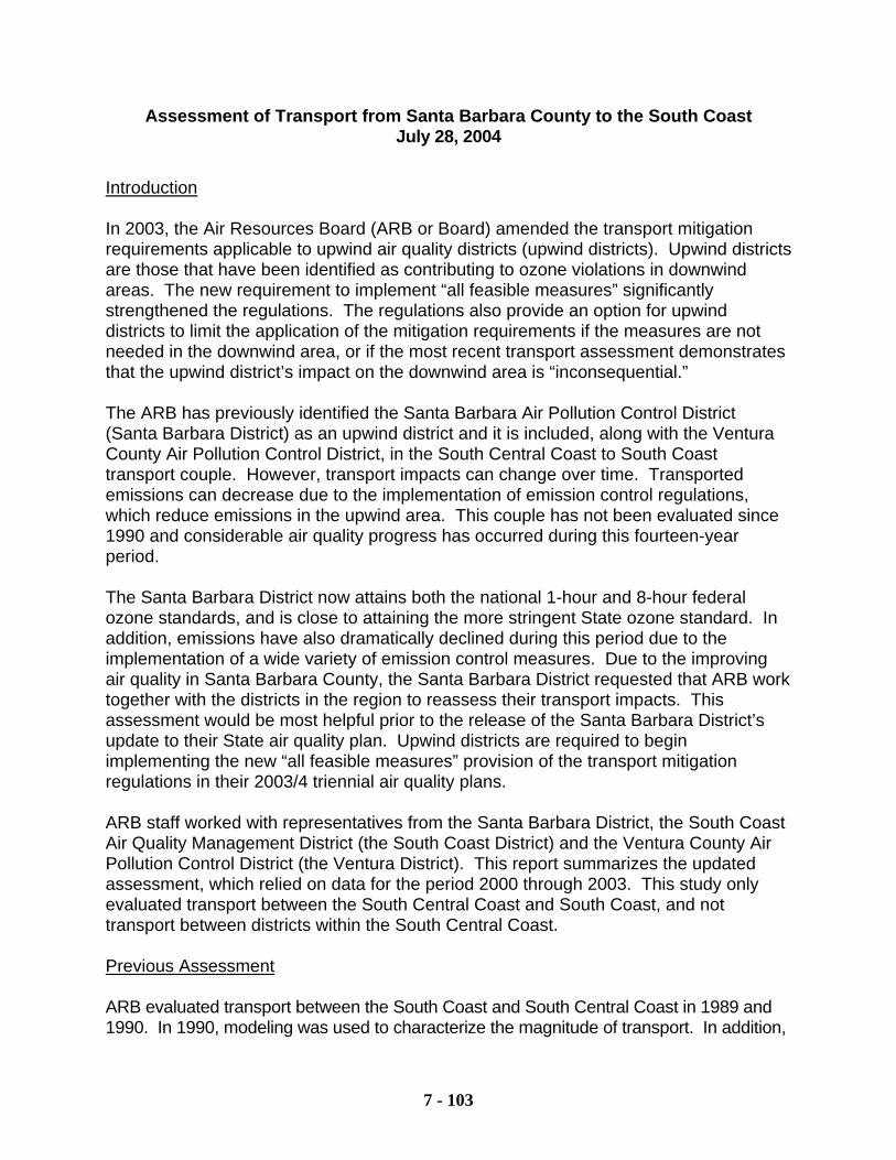
7 - 103
Assessment of Transport from Santa Barbara County to the South Coast July 28, 2004
Introduction In 2003, the Air Resources Board (ARB or Board) amended the transport mitigation requirements applicable to upwind air quality districts (upwind districts). Upwind districts are those that have been identified as contributing to ozone violations in downwind areas. The new requirement to implement “all feasible measures” significantly strengthened the regulations. The regulations also provide an option for upwind districts to limit the application of the mitigation requirements if the measures are not needed in the downwind area, or if the most recent transport assessment demonstrates that the upwind district’s impact on the downwind area is “inconsequential.” The ARB has previously identified the Santa Barbara Air Pollution Control District (Santa Barbara District) as an upwind district and it is included, along with the Ventura County Air Pollution Control District, in the South Central Coast to South Coast transport couple. However, transport impacts can change over time. Transported emissions can decrease due to the implementation of emission control regulations, which reduce emissions in the upwind area. This couple has not been evaluated since 1990 and considerable air quality progress has occurred during this fourteen-year period. The Santa Barbara District now attains both the national 1-hour and 8-hour federal ozone standards, and is close to attaining the more stringent State ozone standard. In addition, emissions have also dramatically declined during this period due to the implementation of a wide variety of emission control measures. Due to the improving air quality in Santa Barbara County, the Santa Barbara District requested that ARB work together with the districts in the region to reassess their transport impacts. This assessment would be most helpful prior to the release of the Santa Barbara District’s update to their State air quality plan. Upwind districts are required to begin implementing the new “all feasible measures” provision of the transport mitigation regulations in their 2003/4 triennial air quality plans. ARB staff worked with representatives from the Santa Barbara District, the South Coast Air Quality Management District (the South Coast District) and the Ventura County Air Pollution Control District (the Ventura District). This report summarizes the updated assessment, which relied on data for the period 2000 through 2003. This study only evaluated transport between the South Central Coast and South Coast, and not transport between districts within the South Central Coast. Previous Assessment ARB evaluated transport between the South Coast and South Central Coast in 1989 and 1990. In 1990, modeling was used to characterize the magnitude of transport. In addition,
7 - 104
over the last thirty years a number of researchers have evaluated transport between the southern portion of the South Central Coast Air Basin (Santa Barbara and Ventura Districts) and the South Coast Air Basin. The general consensus, as reported in ARB’s 1989 transport identification report, is that transport takes place in both directions, but transport is mostly from the South Coast Air Basin to the South Central Coast Air Basin. In 1990, ARB analyzed three ozone episodes that occurred in 1984 and 1985. An urban airshed model was used and incorporated data from the South Central Coast Cooperative Aerometric Monitoring Program (a field study). Two episodes were characterized as insignificant and the other as significant for transport from the South Central Coast to the South Coast. The two days characterized as insignificant, September 7, 1984 and September 13, 1985 had daily peak ozone levels of 0.14 and 0.11 ppm at Reseda, respectively. The September 17, 1984 ozone episode identified as significant had a peak ozone level of 0.16 ppm at Reseda. However, the 1990 ARB Staff Report concluded that while the couple included both Santa Barbara and Ventura as upwind districts, most of the transported mass most likely originated in Ventura County. Assessment Approach Transport of ozone and its precursors occurs when winds of sufficient speed, direction, and duration are present. Transport can take place near the surface (surface-level transport) or far above the surface (transport aloft). This assessment only considered the likelihood of surface level transport over land, and did not evaluate potential for surface level transport over the Santa Barbara Channel (channel) or transport aloft. Transport over the channel or offshore of the channel was not evaluated because both districts and ARB have very limited legal authority to control emission sources operating there. Specifically, the Santa Barbara and Ventura Districts only have authority over the stationary sources in the channel or offshore of the channel, and not marine shipping sources. Marine shipping sources represent over 90% of those emissions in the channel or offshore of the channel. Aloft transport is of concern for many areas of the State, and was considered for inclusion in this analysis. However, it was deemed not to be important for the transport couple under consideration. This is because there are very few emission sources within the onshore portion of either Santa Barbara or Ventura Counties with the potential to release emissions aloft. For example, based on one SCOS 1997 summer episode day emissions inventory for the Santa Barbara County, only 5% of the NOx emissions (1.8 tons per day) and only 1% of the ROG emissions (0.4 tons per day) are from stack-based sources. Aloft emissions of this magnitude were considered unlikely to contribute significantly to downwind ozone levels at the sites under consideration for this analysis. The characterization of transport is based on detailed analysis of one or more days when the ozone standard was violated in the downwind area. There are two basic approaches that are typically utilized to assess transport: (1) air quality modeling evaluations or (2) data analysis techniques. The modeling approach relies on large data sets gathered from special field studies. In contrast, the data analysis approach uses available data from air
7 - 105
quality monitoring and meteorological databases, along with emissions and population estimates, to assess transport. Regardless of which approach is used, the results of the analysis are used to label the magnitude of transport. Three labels are applied according to whether the ozone violation in the downwind area is predominately due to transport (overwhelming), local emissions (inconsequential), or a combination of both (significant). This current study evaluated transport for all State ozone exceedance days during the period 2000 through 2003. As has been done in prior studies, it would have been desirable to include a model-based assessment of transport for the days that were analyzed. The available modeling episodes for southern California (using the SCOS modeling domain, which includes Santa Barbara and Ventura Counties) are from 1997 and 1998. Development of other episodes is very resource intensive, and would have impacted SIP development efforts for central and northern California. Therefore, a number of air quality analysis methods were used to evaluate transport impacts for this current study. This study was conducted in several steps.
♦ Typical wind flow patterns were identified for the study area and the magnitude of the ozone air quality problem in the downwind area was identified;
♦ Screening analyses were conducted on all exceedance days to identify days with potential for transport;
♦ In-depth trajectory analyses were conducted on days identified as having weather conditions conducive to transport, which were identified in the step above;
♦ Population growth and change in emissions were evaluated in both upwind and downwind areas.
Study Area For this current analysis, the study area consisted of the two southern counties in the South Central Coast (Ventura and Santa Barbara) and a portion of the South Coast Air Basin, as shown in Figure 1. The downwind area in the South Coast is the western part of the San Fernando Valley and the Santa Clarita area. The Santa Clarita area is slightly north of the San Fernando Valley. The air monitoring sites representative of the downwind areas in this analysis are Reseda and Santa Clarita. These sites are closest to the boundary between the two air basins. If transport originated in the South Central Coast, one or both of these sites would be the most impacted. The Santa Barbara coastal strip is only a few miles wide and is bordered on the inland side by mountains that reach 4,000 feet. This narrow southern coastal strip of Santa Barbara County connects to the San Fernando Valley via the Oxnard Plain of Ventura County. The Oxnard Plain includes the cities of Ventura, Oxnard, and Camarillo. The San Fernando Valley is an inland valley within northwestern Los Angeles County and extends to the southeastern boundary of Ventura County. Still further inland and northward, the Santa Clara River Valley runs eastward from near the city of Ventura to Castaic and the Santa Clarita area that are located just north of the San Fernando
7 - 106
Valley. To the south of the San Fernando Valley, the 3,000 foot Santa Monica Mountain ridge slopes down to sea level at Point Mugu in Ventura County. Wind Flow Patterns Throughout the year, airflow patterns within the study area are dominated by a diurnal land-sea breeze pattern with strong on-shore winds most of the day and calm to weak offshore during the night. These sea breeze winds are generally from the southwest to west in the study area and are channeled by the coastal mountains. In addition, a portion of the onshore seabreeze in the Los Angeles coastal plain and the seabreeze from the Oxnard Plain converge in the San Fernando Valley. Under the seabreeze pattern, emissions transport is complex within the study area. In general, the onshore seabreeze blows emissions within the Oxnard Plain of Ventura County eastward into the interior valleys of Ventura County. Two other wind flow patterns can exist in the study area. These include a general pattern of winds from the south and weak to strong offshore winds associated with the Santa Ana pattern. Under these two patterns emissions transport is complex. As discussed above, there are a number of geographical barriers and wind flow patterns that limit the pathway that a parcel of air originating in Santa Barbara County could take. The three most likely pathways over land for emissions in the coastal Santa Barbara County area to transport into western Los Angeles County are listed below and shown in Figure 1:
♦ Santa Barbara County to Ventura County to Santa Clarita via the Santa Clara River Valley;
♦ Santa Barbara County to Ventura County to Reseda in the San Fernando Valley via Highway 118;
♦ Santa Barbara County to Ventura County to Reseda in the San Fernando Valley via Highway 101.
Air Quality There has been a growing concern over air quality at the Reseda and Santa Clarita downwind sites, which had 263 State 1-hour ozone exceedances from 2000 through 2003. The 2002 and 2003 ozone seasons were particularly severe in this portion of the South Coast, with an average of 85 and 55 days per year exceeding the State ozone standard at Santa Clarita and Reseda, respectively. Approximately 70% of the time when the South Coast experiences a State ozone exceedance anywhere in the basin, it also occurs at Santa Clarita. In addition, some of the highest peak level ozone levels that occurred in the South Coast during the last two years have been recorded at the Santa Clarita monitoring site. This includes ozone concentrations twice the level of the State standard. While the South Coast is classified as an extreme one-hour ozone nonattainment area and has more than enough emissions within the basin to cause these exceedances, it is also important to
7 - 107
evaluate whether transport is a contributing factor to poor ozone air quality in this region. If transport is a factor, it needs to be addressed through the implementation of the mitigation regulations. In contrast, the number of days when ozone standards are exceeded in Santa Barbara County has dropped dramatically. Santa Barbara County now attains both federal ozone standards. During the last three years, the Santa Barbara District, classified as a moderate nonattainment area, averaged only five days when the State ozone standard was exceeded. The average daily maximum ozone concentration for 2001-2003, using the mean of the top 30 days for the worst site, is now at the level of the State standard, with only a few days remaining that have peaks above the level of the State Standard. Ventura County, the other upwind district in this couple, has also seen significant air quality improvements. They now attain the federal 1-hour ozone standard, although they still exceed the more protective federal 8-hour ozone and State 1-hour ozone standards. Though they had an average of 32 State ozone exceedance days over the last three years, the number of exceedances has decreased by 141 percent since 1990. Screening Analyses In order to determine the transport impacts that the Santa Barbara District has on the South Coast Air Basin, there was a need to review all recent ozone exceedances at the downwind sites. As noted, there were 263 State 1-hour ozone exceedance days that occurred at Reseda and/or Santa Clarita between 2000-2003. Due to the large number of exceedance days, it was not possible to evaluate each exceedance day in-depth. Therefore, the approach used was to identify days with potential for transport, and then focus more in-depth analyses on these days. Multiple levels of screening methods were used to identify days with high transport potential. The screening methods employed were (1) evaluation of weather conditions, (2) conducting time series analysis, and (3) a review of the progression of the hour of the daily maximum ozone concentration. These screening methods are described below. The primary method for screening was an evaluation of weather conditions to determine if winds of sufficient speed, direction, and duration were present that would have been conducive to the transport of ozone or its precursors. For all 263 days, the wind speed and direction at the downwind sites (Reseda and Santa Clarita) were examined at the time of the daily maximum ozone concentration and up to six hours prior to the maximum ozone concentration. The goal was to identify days with persistent winds from the west, which could have resulted in transport from Santa Barbara and Ventura Counties. The second screening method was time series analysis. This analysis was applied to some of the days identified as having transport potential in the first screening step. The objective of this analysis is to determine whether weather conditions are conducive to transporting emissions on the prior day and remaining overnight to contribute to an exceedance on the next day. This analysis consists of plotting hourly ozone, NOx, and CO concentrations, along with hourly wind speed and direction for a 48-hour period at the
7 - 108
downwind site (Reseda and/or Santa Clarita sites). Hydrocarbon measurements were not available. However, CO was used instead to characterize the motor vehicle emissions behavior. The impact of transported emissions on the previous day would be indicated by persistent winds from the west along with high NOx and CO concentrations on the prior day, followed by calm winds and continued high NOx and CO concentrations on the next day. In other words, emissions transported into the area on the previous day remain to contribute to an ozone exceedance on the following day. Low winds on both days with high NOx and CO would suggest emissions are mostly local and transport was unlikely. The third screening method was a review of the progression of the hour of the daily maximum ozone concentration along a path beginning in Santa Barbara County through Ventura County to Reseda or Santa Clarita. If there is progression in the time of the peak ozone concentration along the path, this could be an indication that ozone was transported. However, this approach was not effective in identifying potential transport days, because of the intermediate precursor emissions in Ventura County, topography, and varying elevations of air monitoring sites along the path. Trajectory Analysis The screening procedure described above identified 12 potential transport days for the period 2000 through 2003. Ten of these days are for exceedances that occurred at Santa Clarita and two for Reseda. These 12 days, plus an additional 4 days with the highest daily maximum ozone concentration at Santa Clarita (0.18-0.19 ppm) in 2003, were chosen for in-depth study using trajectory analysis. The additional 4 days were not identified as having weather conditions conducive to transport during the screening analysis; however they were analyzed due to their high concentrations. The objective of a trajectory analysis is to identify the most likely source of emissions and the path those emissions took to result in an ozone exceedance at a downwind location. In other words, it is a pictorial analysis technique that estimates the path an air parcel took over a specified period of time. In a backward trajectory, the site location and site hour of the daily maximum ozone concentration are used as the starting point. From this point, the air parcel is backed up in time, based on an hourly set of wind data. Depending on whether a computer model or manual approach is used, the path of the air parcel is estimated using model generated hourly gridded wind fields or manually generated hourly airflow fields, respectively. The gridded wind and airflow fields are based on wind speed and direction at various sites in the study area. In a model, terrain barriers can be considered. However, they were not used in this analysis. In ARB staff’s opinion, the observed wind measurements already reflected the influence of terrain. Initially, back trajectories were manually constructed for the two Reseda and one Santa Clarita State ozone exceedance days which were identified in the screening process. This manual method has been used in previous ARB transport assessments. Back trajectories were manually drawn for these three days, due to the unavailability of a trajectory model at the early point in this assessment. Wind data (speed and direction) from approximately 21
7 - 109
weather monitoring stations within the study area were used to construct each manually drawn back trajectory. Wind data included four offshore buoy sites. The wind data were obtained from the U.S EPA–AIRS, CIMIS, and NOAA buoy databases. A total of about 90 weather data sites were available; however only 21 were used in this case due to the extensive time requirements to construct manually drawn back trajectories. Based on these trajectories, the ARB and districts determined those State ozone exceedances for the two Reseda days were the result of local emissions. However, the one Santa Clarita day warranted further analysis by a trajectory model. When the two dimensional (2-d) Caltech trajectory model became available, it was used to analyze the remaining Santa Clarita day. In addition, it was used to analyze the other 9 days identified in the screening process, along with the 4 days having the highest ozone concentration at Santa Clarita in 2003. Wind data (speed and direction) from approximately 90 weather monitoring stations within the study area were used to construct each 2-d trajectory. Wind data included six offshore buoy sites. The wind data were obtained from U.S EPA-AIRS, CIMIS, RAWS, NOAA buoy, and Plymouth State University databases. Typically, back trajectories are constructed beginning at the hour of the daily maximum ozone concentration. However, for each of the 14 days analyzed with the 2-d Caltech trajectory model, separate back trajectories were constructed for each hour when the State ozone standard was exceeded. The back trajectories extended back in time up to 44 hours depending on the hour of the State ozone exceedance. This was done to better characterize the weather conditions and likely pathways for emissions to be transported. Since all of the 14 exceedance days occurred at Santa Clarita, back trajectories beginning at Santa Clarita were constructed for these 14 days. In addition, because on 11 out of these 14 days there was also an exceedance at the Reseda site, back trajectories for these days were also constructed beginning at Reseda. In all, a total of 83 Reseda and 94 Santa Clarita back trajectories were completed using the 2-d Caltech trajectory model. In general, back trajectories from Santa Clarita indicated that emission contributions from Los Angeles County and Ventura County occurred at hours exceeding the State ozone standard on 10 of these 14 days. Four of these ten days had this emission contribution over multiple consecutive hours. As noted, there were also ozone exceedances at Reseda on 11 of these 14 days. Back trajectories at hours that exceeded the State ozone standard at Reseda on 7 of these 11 days indicated that emissions were limited to Los Angeles County. However, the remaining four days had contributions of emissions from Los Angeles County, along with Ventura County or Ventura County and the offshore area of Santa Barbara County. As discussed above, none of the back trajectories were similar to the transport paths shown in Figure 1; that is, they did not follow the paths all the way into Santa Barbara County or back into the Santa Barbara urban area from the Santa Barbara Channel. However, a few trajectories backed into the vicinity of Vandenberg Air Force Base from
7 - 110
the channel. However, this small area only represents approximately 1% of Santa Barbara County’s emissions (estimated 0.8 tons per day combined ROG and NOx emissions, see Tables 1 and 2) and less than 0.1% of Los Angeles County’s combined ROG and NOx emissions. Therefore, the emissions in the Vandenberg Air Force Base area are insufficient to have influenced ozone concentrations in the South Coast. It is also not located within the major population centers of Santa Barbara County. Emissions A comparison of emission trends over time will provide additional information on which to base an assessment of transport impacts. Emission estimates for ozone precursors were obtained for the current year and compared to 1985 emission estimates (the year of the ozone episode evaluated in 1990). These emission estimates are shown in Table 1 and Table 2 and the source of these emission estimates is discussed in detail in Attachment A. The ROG and NOx emission estimates are from the official ARB emission inventory in the 2004 Almanac. However, the emission estimates may not reflect the district’s most recent inventory in their air quality plans. Emissions in the upwind and downwind areas have declined significantly since 1985. The South Central Coast portion of Santa Barbara and Ventura Counties (onshore emissions) combined ROG and NOx emissions have declined by over 40%. Moreover, emissions decreased by 58% in the San Fernando Valley and the South Coast portion of Los Angeles County, although they are substantially higher than those emissions in either the South Central Coast portion of Ventura or Santa Barbara County. The Outer Continental Shelf (>3 to 25 miles offshore) portion of Santa Barbara County’s combined ROG and NOx emissions for ships (approximately 33 tons per day), which are uncontrollable by the Santa Barbara District, are approximately 25% of Santa Barbara County’s total combined ROG and NOx emissions. Thus, both the upwind and downwind areas have had steadily declining emissions since 1985. These declining emissions in Santa Barbara County suggest a lower potential for significant transport impact on the South Coast since the 1990 ozone transport assessment. Because Ventura County separates Santa Barbara County from the San Fernando Valley, these declining emissions suggest a much lower potential for transport impact from Santa Barbara County on the South Coast since the 1990 transport assessment. Declining emissions may also indicate a lowered potential for transport from Ventura County. The decline in emissions is expected to continue. This should continue to lower the potential for transport from the South Central Coast. Population A comparison of population in the study area over time will provide additional information on which to base an assessment of transport impacts. The population of Los Angeles County dwarfs that of either Santa Barbara or Ventura counties. The 2000 population of Los Angeles County exceeds 9 million, compared to 753,000 for Ventura County and 400,000 for Santa Barbara County. However, there has been significant population
7 - 111
growth along certain portions of the transport pathway, particularly in Ventura County. The Ventura County cities of Thousand Oaks, Oxnard, and Simi Valley are connected to Los Angeles County through commerce, jobs, and commute traffic. These cities experienced 11.1% to 19.5% population growth between 1990 and 2000. Santa Clarita grew at the even larger rate of 36.5%. In contrast, the City of Santa Barbara had a 4.7% increase in population. Transport Contribution This section links emission trends, population trends, air quality, and trajectory results together to assess the transport contribution. We look at these to assess the transport contribution from Santa Barbara County, Ventura County, and the South Coast. As discussed in the section of trajectories, no trajectory backed into the landmass of Santa Barbara County with significant emissions and population. However, the back trajectories did indicate a contribution from Ventura County and the South Coast. Of the 263 State ozone exceedance days at Reseda and/or Santa Clarita, there were no back trajectories that included a significant contribution from Santa Barbara County. However, back trajectory analysis identified 10 Santa Clarita days with emission contributions from Los Angeles County and Ventura County at hours exceeding the State ozone standard. Of these 10 Santa Clarita days, four days indicated significant emissions contribution from Ventura County due to multiple hours with back trajectories from the west. The back trajectories indicate that for three of these four days, the initial buildup of ozone concentrations reaching the State 1-hr exceedance level was due to emissions within the South Coast. However, this buildup reached a peak either during the hour that the wind direction shifted or two hours after the wind direction shifted and brought emissions from Ventura County. Ventura County emissions, along with local South Coast emissions, continued to be sufficient in maintaining ozone concentrations above the State standard one hour after the occurrence of the peak ozone concentration. The Ventura County contribution was evident upwind at Piru by the elevated ozone concentrations that included one day that exceeded the State 1-hour ozone standard. In addition, the back trajectories also indicated that the Ventura County emissions had built up in stagnant flow overnight or during the early morning hours of the exceedance day over urban areas on the Oxnard Plain or inland valley. When air stagnates over an emissions area, these emissions accumulate (buildup) dispersing very little. The stagnation of emissions over these urban areas suggests that a significant buildup of emissions occurred within Ventura County before arriving at Santa Clarita in the westerly sea breeze. This was evidenced by the high ozone concentrations upwind of Santa Clarita at Piru. On the fourth day, the back trajectories indicated that the initial buildup of ozone concentrations in the late morning was due to emissions within the South Coast. However, a wind direction shift at noon brought emissions from Ventura County over the next three hours. The back trajectories also indicated that these Ventura County
7 - 112
emissions had built up in stagnant airflow overnight in the Piru area prior to arriving at Santa Clarita in the westerly seabreeze. These emissions reaching Piru had come from urban areas in the northern Oxnard Plain (Ventura) and transported inland by seabreeze winds the previous day. In addition, elevated ozone concentrations upwind at Piru suggest that there was a significant contribution of Ventura County emissions during the three hour period. The combination of local South Coast emissions and transported Ventura County emissions resulted in 3 hours of ozone concentrations exceeding the State 1-hr ozone standard. The stagnation of air in Ventura County prior to reaching Santa Clarita, emissions from the urban areas in the Oxnard Plain and inland valley, and elevated ozone concentrations upwind of Santa Clarita at Piru suggest that Ventura County contributed to ozone exceedances at Santa Clarita. In addition, the large number of ROG and NOx emissions in Los Angeles County compared to the South Central Coast indicate that local emissions within the South Coast were sufficient to significantly contribute to the exceedances on these four days. Conclusions This study examined all 263 State ozone exceedance days for the period 2000 to 2003 that occurred at either the Reseda and/or Santa Clarita monitoring sites. Of these 263 days, analyses indicate that weather conditions on these days do not show transport of significant ozone precursors or ozone from the mainland portion of Santa Barbara County to either Santa Clarita or Reseda. Trajectory analyses indicate that contributions were from either the South Coast Air Basin or the South Coast Air Basin and Ventura County. In addition, emissions are continuing downward, and the magnitude of emissions makes transport of ozone precursors from the Santa Barbara County portion of the South Central Coast even less likely. This analysis supports a finding that the magnitude of transport during the last four years from Santa Barbara County to the South Coast has been inconsequential. In addition, this study did not find any basis for changing the transport classification for the Ventura County portion of the South Central Coast.
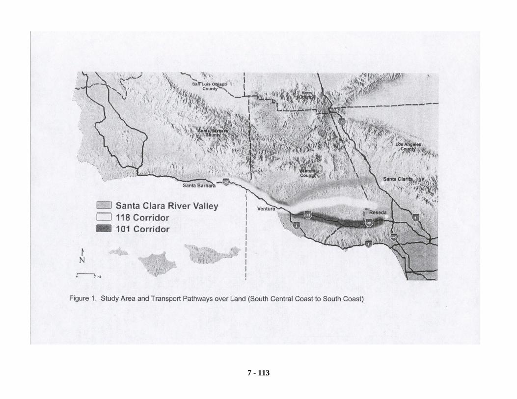
7 - 113
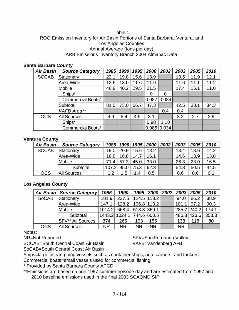
7 - 114
Table 1 ROG Emission Inventory for Air Basin Portions of Santa Barbara, Ventura, and
Los Angeles Counties Annual Average (tons per day)
ARB Emissions Inventory Branch 2004 Almanac Data
Santa Barbara County Air Basin Source Category 1985 1990 1995 2000 2002 2003 2005 2010 SCCAB Stationary 22.1 19.8 15.6 13.9 13.5 11.9 12.1 Area-Wide 12.6 13.0 11.6 11.9 11.6 11.1 11.2 Mobile 46.8 40.2 29.5 21.5 17.4 15.1 11.0 Ships* 0 0 Commercial Boats* 0.087 0.034 Subtotal 81.5 73.0 56.7 47.3 42.5 38.1 34.3 VAFB Area** 0.4 0.4 OCS All Sources 4.9 5.4 4.9 3.1 3.2 2.7 2.9 Ships* 0.98 1.10 Commercial Boats* 0.085 0.034
Ventura County Air Basin Source Category 1985 1990 1995 2000 2002 2003 2005 2010 SCCAB Stationary 19.0 20.9 15.6 13.2 13.4 13.6 14.2 Area-Wide 16.8 16.8 14.7 16.1 14.6 13.9 13.8 Mobile 71.4 57.3 45.0 33.0 26.8 23.0 16.5 Subtotal 107.2 95.0 75.3 62.3 54.8 50.5 44.5 OCS All Sources 1.2 1.5 1.4 0.5 0.6 0.6 0.1
Los Angeles County
Air Basin Source Category 1985 1990 1995 2000 2002 2003 2005 2010 SoCAB Stationary 281.9 227.5 124.5 118.2 94.0 86.2 88.9 Area-Wide 147.1 128.2 106.8 113.2 101.1 97.2 90.3 Mobile 1014.2 668.4 513.3 369.1 285.7 240.2 174.1 Subtotal 1443.2 1024.1 744.6 600.5 480.8 423.6 353.3 SFV** All Sources 374 265 193 155 133 118 80 OCS All Sources NR NR NR NR NR
Notes: NR=Not Reported SFV=San Fernando Valley SCCAB=South Central Coast Air Basin VAFB=Vandenberg AFB SoCAB=South Central Coast Air Basin Ships=large ocean-going vessels such as container ships, auto carriers, and tankers. Commercial boats=small vessels used for commercial fishing. * Provided by Santa Barbara County APCD **Emissions are based on one 1997 summer episode day and are estimated from 1997 and 2010 baseline emissions used in the final 2003 SCAQMD SIP
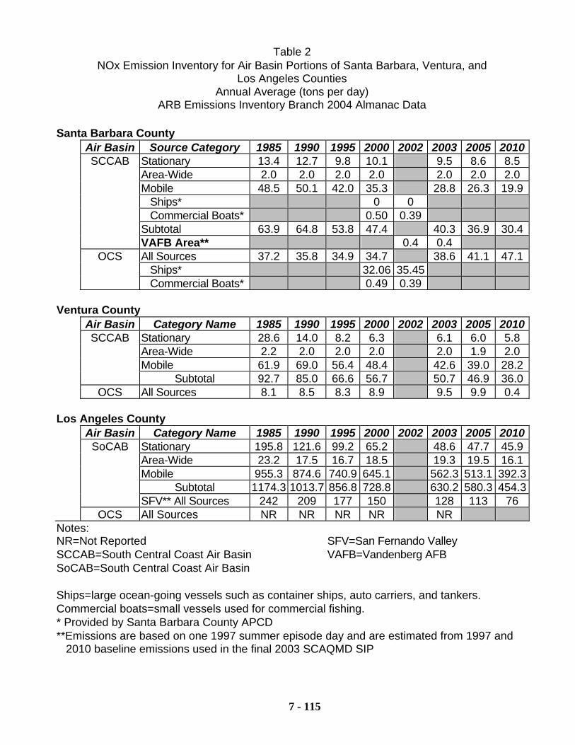
7 - 115
Table 2 NOx Emission Inventory for Air Basin Portions of Santa Barbara, Ventura, and
Los Angeles Counties Annual Average (tons per day)
ARB Emissions Inventory Branch 2004 Almanac Data
Santa Barbara County Air Basin Source Category 1985 1990 1995 2000 2002 2003 2005 2010 SCCAB Stationary 13.4 12.7 9.8 10.1 9.5 8.6 8.5 Area-Wide 2.0 2.0 2.0 2.0 2.0 2.0 2.0 Mobile 48.5 50.1 42.0 35.3 28.8 26.3 19.9 Ships* 0 0 Commercial Boats* 0.50 0.39 Subtotal 63.9 64.8 53.8 47.4 40.3 36.9 30.4 VAFB Area** 0.4 0.4 OCS All Sources 37.2 35.8 34.9 34.7 38.6 41.1 47.1 Ships* 32.06 35.45 Commercial Boats* 0.49 0.39
Ventura County Air Basin Category Name 1985 1990 1995 2000 2002 2003 2005 2010 SCCAB Stationary 28.6 14.0 8.2 6.3 6.1 6.0 5.8 Area-Wide 2.2 2.0 2.0 2.0 2.0 1.9 2.0 Mobile 61.9 69.0 56.4 48.4 42.6 39.0 28.2 Subtotal 92.7 85.0 66.6 56.7 50.7 46.9 36.0 OCS All Sources 8.1 8.5 8.3 8.9 9.5 9.9 0.4
Los Angeles County Air Basin Category Name 1985 1990 1995 2000 2002 2003 2005 2010 SoCAB Stationary 195.8 121.6 99.2 65.2 48.6 47.7 45.9 Area-Wide 23.2 17.5 16.7 18.5 19.3 19.5 16.1 Mobile 955.3 874.6 740.9 645.1 562.3 513.1 392.3 Subtotal 1174.3 1013.7 856.8 728.8 630.2 580.3 454.3 SFV** All Sources 242 209 177 150 128 113 76 OCS All Sources NR NR NR NR NR
Notes: NR=Not Reported SFV=San Fernando Valley SCCAB=South Central Coast Air Basin VAFB=Vandenberg AFB SoCAB=South Central Coast Air Basin
Ships=large ocean-going vessels such as container ships, auto carriers, and tankers. Commercial boats=small vessels used for commercial fishing. * Provided by Santa Barbara County APCD **Emissions are based on one 1997 summer episode day and are estimated from 1997 and 2010 baseline emissions used in the final 2003 SCAQMD SIP
7 - 116
ATTACHMENT A
EMISSIONS
We used annual average emission estimates for ROG and NOx from ARB’s 2004 Almanac web page for the years 1985, 1990, 1995, 2000, and 2003. These estimates covered Santa Barbara County, Ventura County, and Los Angeles County. In addition, we developed a ROG and NOx emissions inventory for the same years for the San Fernando Valley in order to have emissions estimates representing the Reseda and Santa Clarita area. The San Fernando Valley NOx and ROG emissions inventory were estimated by extracting emissions from grid cells in the SCOS97 modeling region. The emission estimates were based on emissions in the 1997 and 2010 baseline years for a Tuesday during the 1997 episode (August 5). These emission estimates were extracted from the final emission inventories used for the 2003 South Coast SIP photochemical modeling. San Fernando Valley ROG and NOx emissions for 1985, 1990, and 1995 were based on the ratio of San Fernando Valley to Los Angeles County emissions for the year 2000. Emissions for 2000 and 2003 were interpolated from the 1997 and 2010 baseline year emissions.
7 - 117
References
Air Resources Board, 1989: California Surface Wind Climatology. Staff Report prepared by the Technical Support Division, Air Resources Board, Sacramento, California, October 1989, reprinted January 1992. Air Resources Board, 1989: Proposed Identification of Districts Affected by Transported Air Pollutants which Contribute to Violations of the State Ambient Air Quality Standard for Ozone. Staff report prepared by the Technical Support Division, Air Resources Board, Sacramento, California, October 1989. Air Resources Board, 1990: Assessment and Mitigation of the Impacts of Transported Pollutants on Ozone Concentrations within California. Staff report prepared by the Technical Support Division and Office of Air Quality Planning and Liaison, Air Resources Board, Sacramento, California, June 1990. State of California, Department of Finance, Revised Historical City, County and State Population Estimates, 1991-2000, with 1990 and 2000 Census Counts.
Sacramento, California, March 2002 via DOF Website http://www.dof.ca.gov/HTML/DEMOGRAP/NewHist_E-4.XLS).
Air Resources Board, 2003: Initial Statement of Reasons for the Proposed Amendments to the Ozone Transport Mitigation Regulations. Staff report prepared by the Planning and Technical Support Division, Air Resources Board, Sacramento, California, April 2003. South Coast Air Quality Management District, 2003: Final 2003 Air Quality
Management Plan. Staff report prepared by the Air Resources Board, Sacramento, California, and the South Coast Air Quality Management District, Diamond Bar, California, August 2003.
7 - 118
PUBLIC NOTICE
Draft 2004 Clean Air Plan and Supplemental Environmental Impact Report Public Comment Period Starts August 25, 2004
SUMMARY: The Santa Barbara County Air Pollution Control District (APCD) has prepared a Draft 2004 Clean Air Plan and associated Draft Supplemental Environmental Impact Report. As required by the California Clean Air Act, the 2004 Clean Air Plan provides a three-year update to the 2001 Clean Air Plan. Previous plans developed to comply with the California Clean Air Act include the 1991 Air Quality Attainment Plan, the 1994 Clean Air Plan, and the 1998 Clean Air Plan. The 2004 Clean Air Plan includes previously adopted air pollution control measures and newly proposed and further study emission control measures. The 2004 Plan is not required to address any Federal Clean Air Act requirements. The 2004 Clean Air Plan will be submitted to the California Air Resources Board for approval. Pursuant to the California Environmental Quality Act (CEQA), the APCD has prepared a Draft Supplemental Environmental Impact Report for the 2004 Clean Air Plan. PUBLIC REVIEW: Beginning August 25, 2004, the Draft 2004 Clean Air Plan will be available for public review and comment for 30 days and the Draft Supplemental Environmental Impact Report will be available for review and comment for 45 days. Both documents will be available at public libraries in Santa Maria, Buellton, Lompoc, Goleta, Santa Barbara, and UCSB, and at the following four locations, and on the APCD website at www.sbcapcd.org:
1. Santa Barbara County APCD: 260 N. San Antonio Road, Suite A, Santa Barbara 2. Santa Barbara County Clerk’s Office: 123 E. Anapamu Street, Santa Barbara 3. Santa Barbara County 5th District Supervisors Office: 511 E. Lakeside Parkway, Santa Maria 4. Santa Barbara County Clerk’s Office: 401 E. Cypress, Suite 101, Lompoc
PUBLIC WORKSHOP: There will be a meeting of the APCD Community Advisory Council to consider the 2004 Clean Air Plan on Wednesday September 15, 2004 at 6:30 pm at the address below. Public comments can be provided on the Draft 2004 Clean Air Plan and the Draft Supplemental Environmental Impact Report at the Community Advisory Council meeting.
Wednesday, September 15, 2004 6:30 pm Days Inn: Windmill Room
114 East Highway 246, Buellton WRITTEN COMMENTS: Written comments on the Draft 2004 Clean Air Plan should be submitted to
Tom Murphy, APCD Manager, Technology and Environmental Assessment, o 260 N. San Antonio Rd, Suite A, Santa Barbara, CA 93110-1315. o Comments must be received by 5:00 PM on September 24, 2004.
Written comments on the Draft Supplemental Environmental Impact Report should be submitted to
Dr. Ron Tan, APCD Planning and Technology Supervisor, o 260 N. San Antonio Rd, Suite A, Santa Barbara, CA 93110-1315 o Comments must be received by 5:00 PM on October 11, 2004.
For more information, please contact Mr. Murphy at 805/961-8857 or Dr. Tan at 805/961-8812. Published SB News-Press, Lompoc Record, SM Times 8/25/04; SB Independent 8/26/04
7 - 119
NOTICE OF PUBLIC HEARING 2004 CLEAN AIR PLAN and SUPPLEMENTAL ENVIRONMENTAL IMPACT REPORT
Thursday, December 16, 2004 – Approximately 2:00pm Board of Supervisors Hearing Room
105 East Anapamu Street, Fourth Floor Santa Barbara, California 93101
The Santa Barbara County Air Pollution Control District will hold a public hearing to consider adoption of the proposed 2004 Clean Air Plan and certification of the Supplemental Environmental Impact Report (SCH No. 9103045) for the 2004 Clean Air Plan. SUMMARY: The Santa Barbara County Air Pollution Control District (APCD) has prepared a Draft 2004 Clean Air Plan and associated Draft Supplemental Environmental Impact Report. As required by the California Clean Air Act, the 2004 Clean Air Plan provides a three-year update to the 2001 Clean Air Plan. Previous plans developed to comply with the California Clean Air Act include the 1991 Air Quality Attainment Plan, the 1994 Clean Air Plan, and the 1998 Clean Air Plan. The 2004 Clean Air Plan includes previously adopted air pollution control measures and newly proposed and further study emission control measures. The 2004 Plan is not required to address any Federal Clean Air Act requirements. The 2004 Clean Air Plan will be submitted to the California Air Resources Board for approval. Pursuant to the California Environmental Quality Act (CEQA), the APCD has prepared a Supplemental Environmental Impact Report (SCH No. 91031045) for the 2004 Clean Air Plan. PUBLIC REVIEW: The Draft 2004 Clean Air Plan and Supplemental Environmental Impact Report are available at public libraries in Santa Maria, Buellton, Lompoc, Goleta, Santa Barbara, UCSB, on the APCD website at www.sbcapcd.org and at the following three locations: Air Pollution Control District 240 N. San Antonio Road Suite A Santa Barbara
Air Pollution Control District 301 E. Cook Street, Suite L Santa Maria
4th District Supervisors Office 401 E Cypress Suite 101 Lompoc
WRITTEN COMMENTS: Written comments on the 2004 Clean Air Plan should be submitted to Tom Murphy, APCD Division Manager, 240 N. San Antonio Road, Suite A, Santa Barbara, CA 93110-1315. In order to be included in the staff report for the Board’s action, comments must be received by 5:00 PM on November 29, 2004. For more information, please contact Mr. Murphy at (805) 961-8857.

G - 1
GLOSSARY OF TERMS
A Acute Health Effect: An adverse heath effect that occurs over a relatively short period of time, (e.g., minutes, or hours.) Adverse Health Effect: A health effect from exposure to air contaminants that may range from relatively mild temporary conditions, such as eye or throat irritation, shortness of breath, or headaches to permanent and serious conditions, such as birth defects, cancer or damage to lungs, nerves, liver, heart, or other organs. Aerosol: Particles of solid or liquid matter that can remain suspended in air from a few minutes to many months depending on the particle size and weight. Agricultural Burning: The intentional use of fire for vegetation management in areas such as agricultural fields, orchards, rangelands, and forests. The regulation of agricultural burning is described in the Agricultural Burning Guidelines, Title 17, California Code of Regulations. Air: So called “pure” air is a mixture of gases containing about 78 percent nitrogen, 21 percent oxygen, and less than one percent carbon dioxide, argon, and other inert gases, with varying amounts of water vapor. See also ambient air. Air Basin: A land area with generally similar meteorological and geographic conditions throughout. To the extent possible, air basin boundaries are defined along political boundary lines and include both the source and receptor areas. California is currently divided into 15 air basins. Santa Barbara County is located in the South Central Coast Air Basin, along with San Luis Obispo and Ventura Counties. Air District: A political body responsible for managing air quality on a regional or county basis. California is currently divided into 35 air districts. (See also air pollution control district). Air Monitoring: Sampling for and measuring of pollutants present in the atmosphere. Air Pollutant: Any foreign and/or natural substance that is discharged, released, or propagated into the atmosphere that may result in adverse effects on humans, animal, vegetation and/or materials. Also known as an air contaminant. Examples include but are not limited to smoke, charred paper, dust, soot, grime, carbon, fumes, gases, odors, particulate matter, acids, or any combination thereof. Air Pollution: Degradation of air quality resulting from unwanted chemicals or other materials occurring in the air. Air Pollution Control District (APCD): This is the local agency that has authority to regulate stationary, indirect, and area sources of air pollution and governing air quality issues. The APCD proposes and adopts local air pollution rules, enforces those rules, responds to air pollution related
G - 2
complaints, issues permits to polluting sources, inventories sources of air pollution emissions. An air pollution control board composed of elected officials governs the APCD. Air Quality Attainment Plan (AQAP): A comprehensive document required under the California Clean Air Act (Health and Safety Code Section 40910 et. seq.), which details the programs and control measures to be implemented for the purpose of reducing emissions. Emissions ultimately must be reduced to the extent that measured concentrations of pollutants in the air will not exceed California ambient air quality standards. Air Quality Index (AQI): The USEPA recently revised its method of reporting air quality and the associated health effects. The Air Quality Index replaces the Pollutant Standards Index (PSI) previously used to report air quality to the public. The AQI is a measure of air quality based on a percentage of the federal air quality standard: An AQI of 100 means the pollutant level is equal to the federal standard for that pollutant. An AQI below 100 means the air quality is better than the standard, and above 100 can be considered unhealthful. The higher the number, the more air pollution we are breathing. In Santa Barbara County, we report the AQI for ozone, based on the federal 8-hour standard. Ozone is the only pollutant for which we have recently violated a federal air quality standard. Air Quality Simulation Model: A computer program that simulates the transport, dispersion, and transformation of compounds emitted into the air and can project the relationship between emissions and air quality. Air Toxics: A generic term referring to a harmful chemical or group of chemicals in the air. Typically, substances that are especially harmful to health, such as those considered under EPA's hazardous air pollutant program or California's AB 1807 toxic air contaminant program, are considered to be air toxics. Technically, any compound that is in the air and has the potential to produce adverse health effects is an air toxic. Airborne Toxic Control Measure (ATCM): A type of control measure, adopted by the ARB (Health and Safety Code Section 39666 et seq.), which reduces emissions of toxic air contaminants from non-vehicular sources. Alternate Fuels: Any fuel used for vehicular sources other than standard gasoline or diesel fuels. These include ethanol, methanol, compressed natural gas, liquid petroleum gas and electricity. Alternative fuels are cleaner burning and help meet ARB's mobile and stationary emission standards. Ambient Air: The air that is in the troposphere and is subjected to meteorological and climatic change. Often used interchangeably with "outdoor" air. Ambient Air Quality Standard: Health and welfare based standards established by the state or federal government for clean outdoor air that identify the maximum acceptable average concentrations of air pollutants during a specified period of time. Ammonia (NH3): A pungent colorless gaseous compound of nitrogen and hydrogen that is very
G - 3
soluble in water and can easily be condensed into a liquid by cold and pressure. Ammonia reacts with NOx to form ammonium nitrate -- a major PM2.5 component in the Western United States. Anthropogenic Emissions: Emissions related to human activity or devices. Area-Wide Source: Stationary sources of pollution (e.g., water heaters, gas furnaces, fireplaces, and residential wood stoves) that are typically associated with homes and non-industrial sources. The emissions from these sources in themselves don’t emit a significant amount of emissions, but when considered collectively with other similar sources become significant. Arterial Streets: Streets designed to serve longer vehicle trips to, from, and within urban areas. Atmosphere: The gaseous mass or envelope surrounding the Earth. From ground level up, the atmosphere is further subdivided into the troposphere, stratosphere, mesosphere, and the thermosphere. Where air pollutants are emitted into a building not designed specifically as a piece of air pollution control equipment, such emission into the building shall be considered an emission into the atmosphere. Attainment: Achievement of air quality standards. Attainment Area: A geographic region, which is in compliance with the National and/or California Ambient Air Quality Standards for a criteria pollutant under the Federal Clean Air Act or California Clean Air Act. Attainment Plan: In general, a plan that details the emission reducing control measures and their implementation schedule necessary to attain air quality standards. In particular, the federal Clean Air Act requires attainment plans for nonattainment areas; these plans must meet several requirements, including requirements related to enforceability and adoption deadlines. Average Daily Emissions: Annual emissions divided by 365 (the number of days in a year).
B
Best Available Control Measure (BACM): A term used to describe the "best" measures (according to U.S. EPA guidance) for controlling small or dispersed sources of particulate matter and other emissions from sources such as roadway dust, woodstoves, and open burning. Best Available Control Technology (BACT): BACT is a term used to describe up-to-date methods, systems, techniques, and processes applied to new and modified sources of air pollution in order to achieve the most feasible air pollution emission control. BACT is a requirement stipulated in APCD Regulation VIII (New Source Review), in both Rule 802 (Nonattainment Review) and Rule 803 (Prevention of Significant Deterioration). Rule 802 governs the permitting of new and modified stationary sources of air pollution that emit pollutants for which the County has been designated as nonattainment for either the State or federal ambient air quality health standards. Rule 803 governs the permitting of new or modified stationary sources of attainment pollutants. Each of
G - 4
these two rules contains its own emission rate thresholds over which the BACT requirement is triggered. For sources permitted under Rule 802, BACT is the more stringent of:
a.) The most effective control device, emission unit, or technique that has been achieved in practice for the type of equipment comprising the stationary source; or
b.) The most stringent limitation contained in any State Implementation Plan; or c.) Any other emission control device or technique determined after public hearing to
technologically feasible and cost effective by the Control Officer. For sources permitted under Rule 803, BACT is an emission limitation based on the maximum degree of reduction for each pollutant that would be emitted from any new or modified stationary source. This is done on a case-by-case basis, taking into account energy, environment, and economic impacts and other costs. It also needs to be achievable for such a source or modification through application of production processes or available methods, systems, and techniques, including fuel cleaning or treatment or innovative fuel combustion techniques for control of such a pollutant. Best Available Mitigation Measures (BAMM): Design or operation measures that are directly related to the particular project, and are intended to reduce the number of vehicle trips. Best Available Retrofit Control Technology (BARCT): An emission limitation based on the maximum degree of reduction achievable by existing sources, taking into consideration environmental, energy and economic needs. Bicycle Master Plan: A formal city or county document that describes existing bicycle use, and sets out goals and actions that the government plans to do to increase bicycling as a means of travel. Biogenic Emissions: Biological sources such as plants and animals that emit air pollutants such as volatile organic compounds. Examples of biogenic sources include animal management operations, and oak and pine tree forests. (See also natural sources.). Bureau of Automotive Repair (BAR): An agency of the California Department of Consumer Affairs that manages the implementation of the motor vehicle Inspection and Maintenance Program.
C California Air Resources Board (ARB or CARB): The State's lead air quality agency consisting of an eleven-member board appointed by the Governor and several hundred employees. CARB is responsible for attainment and maintenance of the state and federal air quality standards, and is fully responsible for motor vehicle pollution control. CARB oversees county and regional air pollution management programs. California Ambient Air Quality Standards (CAAQS): A legal limit that specifies the maximum level and time of exposure in the outdoor air for a given air pollutant and which is protective of human health and public welfare (Health and Safety Code 39606b). CAAQSs are recommended
G - 5
by the California Office of Environmental Health Hazard Assessment and adopted into regulation by the CARB. CAAQSs are the standards, which must be met per the requirements of the California Clean Air Act (State Act). California Clean Air Act of 1988 (State Act): A California law passed in 1988, which provides the basis for air quality planning and regulation independent of federal regulations. A major element of the Act is the requirement that local air districts in violation of the CAAQS must prepare attainment plans which identify air quality problems, causes, trends, and actions to be taken to attain and maintain California's air quality standards by the earliest practicable date. California Environmental Protection Agency (Cal/EPA): A state government agency established in 1991 for unifying environmental activities related to public health protection in the State of California. There are six boards, departments, and offices under the organization of Cal/EPA including the California Air Resources Board (ARB), California Integrated Waste Management Board (IWMB), State Water Resources Control Board (SWRCB) and its nine Regional Water Quality Control Boards (RWQCB), Department of Pesticide Regulation (DPR), Department of Toxic Substances Control (DTSC), and Office of Environmental Health Hazard Assessment (OEHHA. The Cal/EPA boards, departments, and offices are directly responsible for implementing California environmental laws, or play a cooperative role with other regulatory agencies at regional, local, state, and federal levels. California Environmental Quality Act (CEQA): A California law, which sets forth a process for public agencies to make informed decisions on discretionary project approvals. The process aids decision-makers to determine whether any environmental impacts are associated with a proposed project. It requires environmental impacts associated with a proposed project to be eliminated or reduced, and that air quality mitigation measures are implemented. Carbon Monoxide (CO): A colorless, odorless, poisonous gas resulting from the incomplete combustion of fossil fuels. Over 80% of the CO emitted in urban areas is contributed by motor vehicles. CO interferes with the blood's ability to carry oxygen to the body's tissues and results in numerous adverse health effects. CO is a criteria air pollutant. This is one of the six pollutants for which there is a national ambient standard. (See Criteria Pollutants). Carl Moyer Fund: A multi-million dollar incentive grant program designed to encourage reduction of emissions from heavy-duty engines. The grants cover the additional cost of cleaner technologies for on-road, off-road, marine, locomotive and agricultural pump engines, as well as forklifts and airport ground support equipment. Car Share: A program organized by a public or private entity for the purpose of sharing the use of a number of vehicles between a number of individuals. For a nominal fee, the individual is able to reserve use of a vehicle as needed (usually by the hour), without actually being responsible for the maintenance, storage, insurance, etc. of the vehicle. Central Business District (CBD): The downtown business areas of cities, historically the central downtown area.
G - 6
Chlorofluorocarbons (CFCs): Any of a number of substances consisting of chlorine, fluorine, and carbon. CFCs are used for refrigeration, foam packaging, solvents, and propellants. They have been found to cause depletion of the atmosphere's ozone layer. Chronic Health Effect: An adverse health effect, which occurs over a relatively long period of time (e.g., months or years). Circulation Element: A plan adopted by a city or county to describe how people and goods should move. Commute: A home-to-work or work-to-home trip made regularly in connection with employment. Commute Alternatives: Carpooling, vanpooling, transit, bicycling, and walking as commute modes during peak period, as well as any Alternative Work Hours Program which results in the use of any mode of transportation for commuting outside of the peak periods. Compliance Efficiency: The percent of emission sources subject to a control measure that is in compliance with its requirements. EPA recommends that compliance efficiency is assumed to be 80 percent unless a District proves otherwise. Composite Efficiency: The efficiency value, which represents the actual effect of a control measure on a source category. Composite efficiency is calculated by finding the product of the control efficiency, percent implementation, the compliance efficiency, and the fraction of the source category affected. Compressed Natural Gas (CNG): An alternative fuel currently being demonstrated in motor vehicles in Santa Barbara County and considered one of the cleanest alternative fuels because of low hydrocarbon emissions. However, it does emit a significant quantity of nitrogen oxides. Compressed Work Schedules: Work schedules that compress the traditional 40-hour weekly work period into fewer than five days by adopting longer work day such as 4/40 (4-ten hour days), and 9/80 (8-nine hour and 1-eight hour days out of every ten work days). Conformity: A demonstration of whether a federally supported activity is consistent with the State Implementation Plan (SIP) -- per Section 176 (c) of the Clean Air Act. Transportation conformity refers to plans, programs, and projects approved or funded by the Federal Highway Administration or the Federal Transit Administration. General conformity refers to projects approved or funded by other federal agencies. Congestion: Traffic conditions on roads, highways, or freeways, which do not permit movement at optimal legal speeds. Congestion Management Program (CMP): A state mandated program (Government Code Section 65089a) that requires each county to prepare a plan to relieve congestion and reduce air pollution. The CMP is a comprehensive program designed to reduce auto-related congestion through provision of roadway improvements, travel demand management and coordinated land
G - 7
use planning among all local jurisdictions. The program is required of every county in California with an urbanized area of at least 50,000 people. The CMP is updated biennially. Congestion Mitigation and Air Quality Program (CMAQ): A program created by the Intermodal Surface Transportation and Efficiency Act (ISTEA) which provides funds for transportation plans and programs in areas that are currently not in attainment with the federal Clear Air Act for ozone or carbon monoxide. CMAQ-funded projects must contribute to the attainment of air quality standards by demonstrating a reduction in vehicular emissions. Consumer Products: Products such as detergents, cleaning compounds, polishes, lawn and garden products, personal care products, and automotive specialty products which are part of our everyday lives and, through consumer use, may produce air emissions which contribute to air pollution. Contiguous Property: Two or more parcels of land with a common boundary or that are separated solely by a public roadway or other public right-of-way. Contingency Measure: Contingency measures are statute-required back-up control measures to be implemented in the event of specific conditions. These conditions can include failure to meet interim milestone emission reduction targets or failure to attain or maintain the standard by the statutory attainment date. Both state and federal Clean Air Acts require that District plans include contingency measures. Control Efficiency: The percent of emissions that are controlled (i.e. not emitted) as a result of some control on a polluting device or process. Control Measure: A strategy to reduce the emissions of air pollution caused by a specific activity or related group of activities. An existing control measure is a measure, which is currently being implemented as a rule. A proposed for adoption control measure is a measure that the APCD will be mandated to make into a rule if the plan is approved by the Board. A further study control measure is a measure that has the potential of being proposed for adoption, but warrants further study. Corporate Average Fuel Economy: The sales-weighted average fuel economy of an automobile manufacturer's annual production; CAFE is also used to refer to the Federal law that mandates that automobile manufacturers meet minimum average fuel economy standards. Cost-Effectiveness: A cost per unit of emission reduction, which is lower than or equivalent to the maximum unit costs of the same emission reduction through the use of demonstrated Best Available Control Technology, calculated in current year dollars. Criteria Pollutants: The Federal Clean Air Act required the Environmental Protection Agency to set air quality standards for common and widespread pollutants after preparing “criteria documents” summarizing scientific knowledge on their characteristics and potential health and welfare effects. Today there are standards for six “criteria pollutants” for which State or National Ambient Air Quality Standards exist. These criteria pollutants include ozone, carbon monoxide, nitrogen dioxide, sulfur dioxide, lead, and suspended particulate matter (PM10 and PM2.5). The USEPA and CARB
G - 8
periodically review new scientific data and may propose revisions to the standards as a result.
D Design Value: For ozone, the state defines that a calculated design day is based on three years of data excluding: extreme values, values that result from exceptional events or values attributable to overwhelming transport from an upwind district. Under federal law, the design day for ozone (1-hour standard) is the fourth highest one-hour concentration experienced at an individual monitoring station during the past three years.
E
Electric Motor Vehicle: A motor vehicle, which uses a battery-powered electric motor as the basis of its operation. Such vehicles emit virtually no air pollutants. Hybrid electric motor vehicles may operate using both electric and gasoline powered motors. Emissions from hybrid electric motor vehicles are also substantially lower than conventionally powered motor vehicles. EMFAC: The Emission Factor model used by ARB to calculate on-road mobile vehicle emissions. Emission Budget: An emission "ceiling" for future transportation emissions that cannot be exceeded. Emission Factor: For stationary sources, the relationship between the amount of pollution produced and the amount of raw material processed or burned. For mobile sources, the relationship between the amount of pollution produced and the number of vehicle miles traveled. By using the emission factor of a pollutant and specific data regarding quantities of materials used by a given source, it is possible to compute emissions for the source. This approach is used in preparing an emissions inventory. Emission Forecasting: Estimating air pollutant emissions in future years using population, economic and control projections. Emission Inventory: An estimate of the amount of pollutants emitted from mobile, stationary, area-wide, and natural sources into the atmosphere over a specific period such as a day or a year. Emission Offsets: A rule-making concept whereby approval of a new or modified stationary source of air pollution is conditional on the reduction of emissions from other existing stationary sources of air pollution. These reductions are required in addition to reductions required by BACT. Emission Reductions: The amount of emissions that will be reduced due to the implementation of a control measure. Emission reductions can be calculated by finding the product of the emissions and the composite efficiency, while accounting for existing control.
G - 9
Emission Standard: The maximum amount of a pollutant that is allowed to be discharged from a polluting source such as an automobile or smoke stack. Employment Centers: Locations having a concentration of jobs or employment. Centers may vary in size and density, serving sub-regional or local markets, generally meeting the needs of the immediate population. Environmental Impact Report (EIR): A document discussing the potential adverse environmental impacts of a project required by the California Environmental Quality Act. Ethanol: A clear liquid derived from biomass (also known as "ethyl alcohol" or "grain alcohol"). Evaporative Emissions: Emissions from evaporating gasoline, which can occur during vehicle refueling, vehicle operation, and even when the vehicle is parked. Evaporative emissions can account for two-thirds of the hydrocarbon emissions from gasoline-fueled vehicles on hot summer days. Exceedance: Ambient pollutant concentrations measured above the applicable ambient air quality standards. Exhaust Gas Recirculation (EGR): An emission control method that involves recirculating exhaust gases from an engine back into the intake and combustion chambers. This lowers combustion temperatures and reduces NOx. Expected Peak Day Concentration (EPDC): A calculated value that represents the concentration expected to occur at a particular site once per year, on average. The calculation procedure uses measured data collected at the site during a three-year period. Measured concentrations that are higher than the EPDC are excluded from the state area designation process. Express service: Bus Service designed to connect high volume destinations, using the freeway where possible.
F
Facility: A structure, building, or operation that has one or more permitted pieces of equipment. Feasible: Feasibility is most frequently used in the context of "feasible" stationary source control measures. In this context, feasible means Best Available Retrofit Control Technology (see definition, above). Federal Clean Air Act (Federal Act): A federal law passed in 1970 and amended in 1977 and 1990, which forms the basis for the national air pollution control effort. Basic elements of the act include national ambient air quality standards for major air pollutants, air toxics standards, acid rain control measures, and enforcement provisions.
G - 10
Federal Implementation Plan (FIP): In the absence of an approved State Implementation Plan (SIP), a plan prepared by the EPA which provides measures that nonattainment areas must take to meet the requirements of the Federal Clean Air Act. Feeder service: Bus Service designed to connect low-density areas, usually residential, with trunk or other lines. Feeder services are quite similar to local service. Flexible Fuel Vehicle (FFV): A vehicle capable of operating on any combination of methanol, ethanol, and gasoline. Fraction Reactive Organic Gases (FROG): The weight fraction of reactive organic gases in emissions of total organic gases from a source. Fugitive Dust: Dust particles, which are introduced into the air through certain activities such as soil cultivation, off-road vehicles, or any vehicles operating on open fields or dirt roadways.
G
Gasoline Tolerant: A term used to describe vehicles that normally operate on methanol but can run on gasoline as well. Growth Management Plan: A plan for a given geographical region containing demographic projections (i.e., housing units, employment, and population) through some specified point in time, and which provides recommendations for local governments to better manage growth and reduce projected environmental impacts.
H
Hazardous Air Pollutant (HAP): An air pollutant listed under section 112 (b) of the federal Clean Air Act as particularly hazardous to health. Emission sources of hazardous air pollutants are identified by USEPA, and emission standards are set accordingly. Haze (Hazy): A phenomenon that results in reduced visibility due to the scattering of light caused by aerosols. Haze is caused in a large part by man-made air pollutants. Health-Based Standard (Primary Standard): A dosage of air pollution scientifically determined to protect against human health effects such as asthma, emphysema, and cancer. High Occupancy Vehicle (HOV): A vehicle which is transporting more than one person. HOV lanes are segments of roadway which are restricted to HOV vehicles. Highway Performance Monitoring System (HPMS): The Highway Performance Monitoring System (HPMS) is a federally mandated inventory system and planning study designed to assess the nation’s highway system. It maintains its authority through the following Codes of Federal Regulations: 23 CFR 420.105(b), 23 CFR 500.807(b), 40 CFR 51.452 (b)(2), 40 CFR
G - 11
93.130(b)(2), and Section 187 of the 1990 Clean Air Act Amendments (CAAA). It is used to provide data to the Environmental Protection Agency (EPA) to assist in monitoring air quality conformity and travel forecasts generated for federal air quality plans. Hybrid Electric Vehicle (HEV): Hybrid electric motor vehicles may operate using both electric and gasoline-powered motors. Emissions from hybrid electric motor vehicles are also substantially lower than conventionally powered motor vehicles. (See also Electric Motor Vehicle.) Hydrocarbons: Compounds containing various combinations of hydrogen and carbon atoms. They may be emitted into the air by natural sources (e.g., trees) and as a result of fossil and vegetative fuel combustion, fuel volatilization, and solvent use. Hydrocarbons are a major contributor to smog. (See also Reactive Organic Compounds). Hydrogen Sulfide (H2S): A colorless, flammable, poisonous compound having a characteristic rotten-egg odor. It is used in industrial processes and may be emitted into the air. 101 Def: Highway 101 Deficiency Plan adopted by SBCAG, June 2002. 101 I-M: Highway 101 In-Motion – $1.6 million study to identify long-term solutions to the congestion problems within the Highway 101 corridor in southern Santa Barbara County.
I
Incentives: Measures designed to encourage certain actions or behavior. These include inducements for the use of carpools, buses and other high-occupancy vehicles in place of single -occupant automobile travel. Examples include HOV lanes, preferential parking and financial incentives. Indirect Source: Any facility, building, structure, or installation, or combination thereof, which generates or attracts mobile source activity that results in emissions of any pollutant (or precursor) for which there is a state ambient air quality standard. Examples of indirect sources include employment sites, shopping centers, sports facilities, housing developments, airports, commercial and industrial development, and parking lots and garages. Indirect Source Control Program: Rules, regulations, local ordinances and land use controls, and other regulatory strategies of air pollution control districts or local governments used to control or reduce emissions associated with new and existing indirect sources. Indirect Source Review: A major component of an indirect source control program, which applies to new and modified indirect sources. Strategies for indirect source review include permit programs, review and comment on new and modified indirect source projects through the California Environmental Quality Act (CEQA) process, and coordination of air quality, transportation and land use policies through local government general plans. Indirect source review reduces emissions from new and modified sources through best available mitigation
G - 12
measures and additional offsite mitigation such as offsets and mitigation fees. Infill: Development that focuses on the rehabilitation or redevelopment of land within an existing urban or town boundary rather than the conversion of previously undeveloped open space. Inspection and Maintenance Program: A motor vehicle inspection program implemented by the California Bureau of Automotive Repair. The purpose of I&M is to reduce emissions by assuring that cars are running properly. It is designed to identify vehicles in need of maintenance and to assure the effectiveness of their emission control systems on a biennial basis. Enacted in 1979 and strengthened in 1990. (Also known as the "Smog Check" program.) Inversion: A layer of warm air in the atmosphere that prevents the rise of cooling air and traps pollutants beneath it. Intelligent Transportation System (ITS): Advanced electronic and information systems that can improve the safety, operational efficiency and productivity of the transportation system.
L
Lead: A gray-white metal that is soft, malleable, ductile, and resistant to corrosion. Sources of lead resulting in concentrations in the air include industrial sources and crustal weathering of soils followed by fugitive dust emissions. Health effects from exposure to lead include brain and kidney damage and learning disabilities. Lead is the only substance, which is currently listed as both a criteria air pollutant and a toxic air contaminant. Lead Agency: The public agency, which has the principal responsibility to carry out or approve a project. Level of Service (LOS): A measure of the congested level on a highway facility or intersection based primarily on the comparison between the facility's capacity and the speed and density of its traffic volume it carries. Increasing levels of congestion are designated along a scale from A to F. Light-Duty Vehicle (LDV): Any motor vehicle with a gross vehicle weight of 6000 pounds or less. Liquefied Petroleum Gas (LPG): A gaseous byproduct of petroleum refining that is compressed to a liquefied form for sales. LPG consists of butane, propane, or a mixture of the two, and of trace amounts of propylene and butylene. Local Agency: Any public agency other than a state or federal agency. Local Service: Service connecting residential areas with central business districts. Low Emission Vehicle (LEV): The LEV standards for passenger cars represent a 70 percent
G - 13
reduction in gasoline-equivalent hydrocarbon and a 50 percent reduction in NOX from ARB’s 1994 standards. Lowest Achievable Emission Rate (LAER): Under the Federal Clean Air Act, the rate of emissions that reflects (1) the most stringent emission limitation in the State Implementation Plan of any state for a given source unless the owner or operator demonstrates such limitations are not achievable; or (2) the most stringent emissions limitation achieved in practice, whichever is more stringent.
M
Maintenance Plan: In general, a plan that details the actions necessary to maintain air quality standards. In particular, the federal Clean Air Act requires maintenance plans for areas that have been redesignated as attainment areas. Memorandum of Understanding (MOU): The Santa Barbara Association of Governments (SBCAG) is the regional agency responsible for preparing regional transportation plans and programs. Most of these programs require the participation of cities, the county, and other affected local agencies. A number of these programs also have implications to regional air quality plans such as the Clean Air Plan. Since SBCAG currently works with cities and the county on regional transportation programs, and because of the close interaction between many of these programs and the regional air quality plan, the APCD and SBCAG have entered into a MOU. Within this MOU, SBCAG is charged with developing the transportation elements of the plan, especially the transportation control measures, which essentially seek to reduce the use of the single passenger automobile and are implemented by a number of local agencies such as local cities and the county. Methanol: A colorless, clear liquid derived from natural gas or coal (also known as "methyl alcohol" or "wood alcohol"). Methyl Tertiary Butyl Ether (MTBE): An ether compound added to gasoline to provide oxygen and enhance complete combustion. MTBE is being fazed out of California's gasoline. Mitigation: A change or alternative to the proposed project, which reduces or eliminates its significant adverse environmental impacts. Mitigation can be in the form of traditional offsets, transportation-based mitigation measures that are directly associated with the project under consideration, or mitigation fees to be used to secure off site mitigation. Mobile Source: Sources of air pollution such as automobiles, motorcycles, trucks, buses, off-road vehicles, boats and airplanes. (Contrast with stationary sources.) Model Rule: A generically formatted control measure, prepared as a guide for adoption by regulatory agencies. Model rules have no force of law until they are adopted by a regulatory agency. Historically, model rules were prepared by the California Air Resources Board and given to local Air Pollution Control Districts for their consideration. The model rule process was replaced by the suggested control measure process. (See Suggested Control Measure).
G - 14
Metropolitan Planning Organization (MPO): Under federal law, the organization designated by the governor as responsible for transportation planning and programming activities required under federal law in an urbanized area. It serves as the forum for cooperative decision making by a regional board made up of local elected officials. As the regions' designated MPO, SBCAG is responsible for development of the federal long range transportation plan and multi-year funding programs, and the selection and approval of transportation projects using federal funds.
N
National Ambient Air Quality Standards (NAAQS): Standards established by the United States EPA that apply for outdoor air throughout the country. There are two types of NAAQS. Primary standards set limits to protect public health and secondary standards set limits to protect public welfare Natural Sources: Non-manmade emission sources, including biological and geological sources, wildfires, and windblown dust. Net Emissions: The actual emissions occurring from a new or modified project after actual on site and off site mitigation, and other effective mitigation has been applied, as determined by the Air Pollution Control Officer. New Source Review (NSR): A program used in development of permits for new or modified industrial facilities which are in a nonattainment area, and which emit nonattainment criteria air pollutants. The two major requirements of NSR are Best Available Control Technology and Emission Offsets. Nitrogen Oxides (Oxides of Nitrogen, NOx): A general term pertaining to compounds of nitric acid (NO), nitrogen dioxide (NO2), and other oxides of nitrogen. Nitrogen oxides are typically created during combustion processes, and are major contributors to smog formation and acid deposition. NO2 is a criteria air pollutant, and may result in numerous adverse health effects; it absorbs blue light, resulting in a brownish-red cast to the atmosphere and reduced visibility. Nonattainment Area: A geographic area identified by the USEPA and/or ARB as not meeting either NAAQS or CAAQS standards for a given pollutant.
O
Opacity: The amount of light obscured by particle pollution in the atmosphere. Opacity is used as an indicator of changes in performance of particulate control systems. Outer Continental Shelf: The area of the Pacific Ocean extending twenty-five miles out to sea from the State Tidelands (which extends three miles from the coastline). Oxygenate: Any oxygen-rich substance added to gasoline to enhance octane and reduce carbon monoxide emissions.
G - 15
Ozone: A strong smelling, pale blue, reactive toxic chemical gas consisting of three oxygen atoms. It is a product of the photochemical process involving the sun's energy. Ozone exists in the upper atmosphere ozone layer as well as at the earth's surface. Ozone at the earth's surface causes numerous adverse health effects and is a criteria air pollutant. It is a major component of smog. Ozone Precursors: Chemicals such as reactive organic compounds and oxides of nitrogen, occurring either naturally or as a result of human activities, which contribute to the formation of ozone, a major component of smog.
P
Particulate Matter (PM): Any material, except pure water, that exists in the solid or liquid state in the atmosphere, such as soot, dust, smoke, fumes, and aerosols. The size of particulate matter can vary from coarse, wind-blown dust particles to fine particle combustion products. Particulate Matter less than 10 microns (PM10): A criteria air pollutant consisting of small particles with an aerodynamic diameter less than or equal to a nominal 10 microns (about 1/7 the diameter of a single human hair). Their small size allows them to make their way to the air sacs deep within the lungs where they may be deposited and result in adverse health effects. PM10 also causes visibility reduction. Particulate Matter less than 2.5 microns (PM2.5): A major air pollutant consisting of tiny solid or liquid particles, generally soot and aerosols. The size of the particles (2.5 microns or smaller, about 0.0001 inches or less) allows them to easily enter the air sacs deep in the lungs where they may cause adverse health effects, as noted in several recent studies. PM2.5 also causes visibility reduction. Peak Period/Peak Hour Demand: The time of most intensive use of a service or facility. In terms of travel, generally there is a morning and an afternoon peak on streets and highways. Permit: Written permission and authorization from a government agency that allows for the construction and/or operation of an emission generating facility or its equipment within certain specified limits or conditions. Photochemical: Of, relating to, or resulting from the chemical action of radiant energy, especially sunlight. Planning Inventory: Emissions inventory from which pollution from natural sources (e.g., seeps, vegetation) are excluded because they are currently not regulated by implementation of APCD rules. Precursor: Any directly emitted pollutant that, when released into the atmosphere, forms or causes to be formed or contributes to the formation of a secondary pollutant for which an ambient air quality standard has been adopted, or whose presence in the atmosphere will contribute to the violation of one or more ambient air quality standards.
G - 16
Prevention of Significant Deterioration (PSD): A program used in development of permits for new or modified industrial facilities in an area that is already in attainment. The intent is to prevent an attainment area from becoming a non-attainment area. This program, like NSR, can require BACT and, if a standard is projected to be exceeded, Emission Offsets. Public Transportation: Transportation service by bus, rail, airplane, and ship offered by an operator on a regular basis to the general public. Public Workshop: A workshop held by a public agency for the purpose of informing the public and obtaining its input on the development of a regulatory action or control measure by that agency.
R
Reactive Organic Compound (ROC): A reactive chemical gas, composed of hydrocarbons, that reacts with nitrogen oxides and contributes to the formation of ozone. Also known as Volative Organic Compounds (see VOC), or as Non-Methane Organic Compounds (NMOCs). The APCD considers all volatile compounds containing carbon except the following to be reactive: ethane, methane, carbon monoxide, carbon dioxide, carbonic acid, metallic carbides or carbonates, ammonium carbonates, methyl chloroform (TCA), methylene chloride (dichloromethane), CFC-11, CFC-12, HCFC-22, FC-23, CFC-113, CFC-114, CFC-115, HCFC-123, HCFC-134a, HCFC-141b, HCFC-142b. Reactive Organic Gases (ROG): See reactive organic compound. Reactivity: A measure of the tendency of a hydrocarbon species to react with nitrogen oxides to form atmospheric ozone. Reasonable Further Progress: Annual incremental reductions in emissions of the relevant air pollutant and its precursors required to ensure attainment of the applicable air quality standard by the applicable date. Reasonably Available Control Measures (RACM): A broadly defined term referring to technologies and other measures that can be used to control pollution. They include Reasonably Available Control Technology and other measures. In the case of PM10, RACM refers to approaches for controlling small or dispersed source categories such as road dust, woodstoves, and open burning. Reasonably Available Control Technology (RACT): Process changes and/or devices to minimize air pollution from mobile and stationary sources that are cost-effective and readily available. Reformulated Gasoline: Also called Cleaner Burning Gasoline (CBG). Gasoline with a different composition from conventional gasoline (e.g., lower aromatics content) that results in the production of lower levels of air pollutants.
G - 17
Regional Haze: The haze produced by a multitude of sources and activities, which emit fine particles and their precursors across a broad geographic area. National regulations require states to develop plans to reduce the regional haze that impairs visibility in national parks and wilderness areas. Residential Second Units (RSU): Residential Second Unit means one additional living unit on any one lot or parcel within a single-family residential zoning district containing a single family dwelling. Such residential second unit is further defined as a building, or portion thereof, that provides complete, independent living facilities for one or more persons and permanent provisions for living, sleeping, eating, cooking, and sanitation. Retrofit: Modification of a polluting device to make it less polluting. Ridesharing: A cooperative effort of two or more people to travel together. Examples are carpools, vanpools, bus pools, trains, and public transit. ROP Plan: The 1993 Rate-of-Progress Plan. The 1993 ROP Plan demonstrated that by 1996 existing and proposed control measures reduced emissions of reactive organic gases (ROG) to a level 15 percent below the 1990 baseline inventory.
S
Santa Maria Basin: An area of undersea oil reserves off the western coast of Santa Barbara County. Secondary Pollutants: Pollutants not emitted directly, but formed in the atmosphere through chemical reactions or transformation of other pollutants (e.g., ozone). Single Occupant Vehicle (SOV): A motor vehicle occupied by one employee for commute purposes, including motorcycles. Smog: A combination of smoke, ozone, hydrocarbons, nitrogen oxides, and other chemically reactive compounds which, under certain conditions of weather and sunlight, may result in a murky brown haze that causes adverse health effects. The primary contributor to smog in California is motor vehicles. Smog Check: A vehicle inspection and maintenance exam. Smog Check Program: (See Inspection and Maintenance Program.) Smoke: A form of air pollution consisting primarily of particulate matter (i.e., particles). Other components of smoke include gaseous air pollutants such as hydrocarbons, oxides of nitrogen, and carbon monoxide. Sources of smoke may include fossil fuel combustion, agricultural burning, and other combustion processes. Solvent: A substance that dissolves another to form a solution.
G - 18
Source: Something that produces air pollution emissions. Sources can be stationary or mobile, and anthropogenic or natural. South Coast Transit Plan (SCTP): A transit plan prepared by Santa Barbara MTD that describes extensive improvements to transit service throughout the South Coast. Sprawl: Dispersed development outside of compact urban and village centers along highways and in rural countryside. State Implementation Plan (SIP): A comprehensive plan prepared by each state, mandated by the federal Clean Air Act, which describes the existing air quality conditions and measures which will be taken to attain and maintain national ambient air quality standards. State Tidelands: The area of the Pacific Ocean within three miles of the shores of Santa Barbara County. Stationary Source: A non-mobile structure, building, facility, equipment installation or operation. Examples include oil production facilities, industrial coating operations, a rock crushing facility, and factories that use large amounts of solvents. A stationary source is classified as having a common production process, located on one or more adjacent properties, and is under the same or common ownership, operation, or control. (Contrast with mobile sources.) Stationary Source Control Measures: A control measure designed to limit the kind and amount of pollutants emitted from stationary sources. Street Furniture: Items that add interest and convenience to the pedestrian street environment including benches, planters, newsstands, drinking fountains, lighting fixtures and bike racks. Suggested Control Measure (SCM): A document upon which air pollution control rules and regulations can be based. The California Air Resources Board issues SCMs to provide guidance to districts in their consideration and development of rules and regulations. However, approval by the ARB of an SCM does not obligate the local districts to develop particular regulations for sources addressed by the SCM. Local districts have the latitude to develop regulations that are as stringent, more stringent, or less stringent than SCMs. The stringency of regulations that are developed by the local districts is usually based in part on the extent to which emissions reductions are needed to achieve compliance with the ambient air quality standards, in that district's area of jurisdiction, as well as other local considerations. The districts also consider the costs for achieving the emission reductions. Sulfur Dioxide (SO2): A strong smelling, colorless gas that is formed by the combustion of fossil fuels. Power plants, which may use coal or oil high in sulfur content, can be major sources of SO2. SO2 and other sulfur oxides contribute to the problem of acid deposition. SO2 is a criteria pollutant.
G - 19
T Telecommuting: Working at a location other than the conventional office. This place may be the home, or an office other than the employee's primary office. Telecommuting employees can communicate with their offices by telephone. Total Organic Gases (TOG): Reactive organic gases plus non-reactive organic gases. Toxic Air Contaminant: An air pollutant, identified in regulation by the ARB, which may cause or contribute to an increase in deaths or in serious illness, or which may pose a present or potential hazard to human health. TACs are considered under a different regulatory process (California Health and Safety Code Section 39650 et seq.) than pollutants subject to CAAQS. Health effects due to TACs may occur at extremely low levels, and it is typically difficult to identify levels of exposure, which do not produce adverse health effects. Transfer of Development Rights (TDR): Transfer of development rights refers to a method for protecting land by transferring the "rights to develop" from one area and giving them to another. What is actually occurring is a consensus to place conservation easements on property in agricultural areas while allowing for an increase in development densities or "bonuses" in other areas that are being developed. The costs of purchasing the easements are recovered from the developers who receive the building bonus. Transitional Low Emission Vehicle (TLEV): TLEV vehicle standards will be 50 percent less hydrocarbon emissions than 1993 model-year conventional gasoline vehicles. Transport: The act of emissions from one source being carried by wind to other locations. Transportation Control Measure (TCM): Any strategy to reduce vehicle trips, vehicle use, vehicle miles traveled, vehicle idling, or traffic congestion for the purpose of reducing motor vehicle emissions. TCMs can include encouraging the use of carpools and mass transit. TCM’s include both Transportation Demand Management and Transportation System Management measures. Transportation Demand Management (TDM): The implementation of measures, which encourage people to change their mode of travel, or not to make a trip at all, (e. g., ridesharing, pricing incentives, parking management and telecommuting.) Transportation System Management (TSM): The implementation of measures, which improve the efficiency of transportation infrastructure. Trip: A single or one direction vehicle movement.
U
Ultra Low Emission Vehicle (ULEV): ULEV standards would lower gasoline-equivalent hydrocarbon emissions by 85 percent, carbon monoxide by 50 percent, and NOX emissions by 50
G - 20
percent, from 1993 levels. United States Environmental Protection Agency (USEPA): The federal agency charged with setting policy and guidelines, and carrying out legal mandates for the protection of national interests in environmental resources. Urban Growth Boundary (UGB): Boundaries that delineate where development ends and open space begins.
V
Vapor Recovery Systems: Mechanical systems that collect and recover chemical vapors resulting from transfer of gasoline from operations such as tank-to-truck systems at refineries, tanker-to-pipeline systems at offshore oil operations, and pump-to-vehicle systems at gasoline stations. Vehicle Miles Traveled (VMT): VMT is the sum number of miles traveled by a given vehicle in a specified time period. This sum number of miles is sometimes estimated for the entire fleet of on road vehicles during a fixed period of time on a fixed expanse of highways. Violation: A number of measured exceedances of an applicable ambient air quality standard. Visibility: The distance that atmospheric conditions allow a person to see at a given time and location. Visibility reduction from air pollution is often due to the presence of sulfur and nitrogen oxides, as well as particulate matter. Volatile Organic Compound (VOC): This term is generally used similarly to the term "reactive organic compounds" but excludes ethane, which the federal government does not consider to be reactive. VOCs are hydrocarbon compounds that exist in the ambient air and contribute to the formation of smog and/or may themselves be toxic. VOCs often have an odor, and some examples include gasoline, alcohol, and the solvents used in paints.
Z Zero Emission Vehicle (ZEV): A vehicle, which will maintain zero emissions throughout its lifetime. Zoning. The public regulation of the use of land. It involves the adoption of ordinances that divide a community into various districts or zones. Each district allows certain uses of land within that zone, such as residential, commercial, or industrial. Typical zoning regulations address building height, bulk, lot area, setbacks, parking, signage, and density.
G - 21
GLOSSARY OF ACRONYMS APCD Air Pollution Control District APCO Air Pollution Control Officer API American Petroleum Institute AQAP Air Quality Attainment Plan ARB California Air Resources Board ATCM Air Toxic Control Measure ATV All Terrain Vehicle AVR Average Vehicle Ridership BACT Best Available Control Technology BAMM Best Available Mitigation Measures BAR Bureau of Automotive Repair BARCT Best Available Retrofit Control Technology BBLS Barrels BOPD Barrels of Oil Per Day Btu British thermal unit CAC Community Advisory Council Caltrans California Department of Transportation CAP Clean Air Plan CAPCOA California Air Pollution Control Officers Association CARB California Air Resources Board CCAA California Clean Air Act of 1988 CCC California Coastal Commission CEC California Energy Commission CEQA California Environmental Quality Act CES Category of Emission Source (for Area-Wide Sources) CFR Code of Federal Regulations CMAQ Congestion Mitigation and Air Quality CMP Congestion Management Program CNG Compressed Natural Gas CO Carbon Monoxide CO2 Carbon Dioxide District Santa Barbara County Air Pollution Control District DMV Department of Motor Vehicles DOG Department of Oil and Gas (California) DPR Department of Pesticide Regulation DVMT Daily Vehicle Miles of Travel EDS Statewide Emission Data System EIR Environmental Impact Report EPA Environmental Protection Agency (United States) ERC Emissions Reduction Credit ERF Environmental Research Foundation EtO Ethylene Oxide FCAA Federal Clean Air Act
G - 22
FCAAA Federal Clean Air Act Amendments FFV Flexible Fuel Vehicle FIP Federal Implementation Plan FMVCP Federal Motor Vehicle Control Program FROG Fraction Reactive Organic Gases FPM10 Fraction Particulate Matter Less Than 10 Microns in Diameter FTIP Federal Transportation Improvement Program FTP Federal Emissions Test Procedure GVR Gasoline Vapor Recovery H&SC Health & Safety Code HAP Hazardous Air Pollutant H2S Hydrogen Sulfide HC Hydrocarbons HDDT Heavy Duty Diesel Truck HDGT Heavy Duty Gas Truck HDT Heavy Duty Truck HDV Heavy Duty Vehicle HHDT Heavy-Heavy Duty Trucks (33,001 – 60,000 lbs) HOT High Occupancy Toll (Lane) HOV High Occupancy Vehicle (Lane) Hp Horsepower HPMS Highway Performance Monitoring System IC Internal Combustion IMPROVE Interagency Monitoring of Protected Visual Environments Program I&M Inspection and Maintenance IPM Integrated Pest Management IRTA Institute for Research & Technical Assistance ISTEA Intermodal Surface Transportation Efficiency Act ISR Indirect Source Review ITG Innovative Technology Group LAER Lowest Achievable Emission Rate LDA Light Duty Auto LDT Light Duty Truck (0 – 5,750 lbs) LDT1 Light Duty Truck (0 - 3,750 lbs) LDT2 Light Duty Truck (3,751 – 5,750 lbs) LDV Light Duty Vehicle (LDA, LDT1, LDT2) LEV Low Emission Vehicle LHDT1 Light-Heavy Duty Trucks (8,501 – 10,000 lbs) LHDT2 Light Heavy Duty Trucks (10,001 – 14,000 lbs) LHV Line Haul Vehicle (60,001 lbs +) LNG Liquefied Natural Gas LPG Liquefied Petroleum Gas M Thousand MCY Motorcycle MH Motor Homes
G - 23
MM Million M85 85 percent Methanol/15 percent Gasoline Fuel MDT Medium Duty Truck MDV Medium Duty Vehicle MHDT Medium Heavy Duty Trucks (14,001 – 33,000 lbs) MMBTU Million British Thermal Units MMSCFD Million Standard Cubic Feet Per Day MOU Memorandum of Understanding MSCF Thousand Standard Cubic Feet MTBE Methyl Tertiary-Butyl Ether MVFF Motor Vehicle Fueling Facility (Gas Station) MVRF Motor Vehicle Refurbishing Facility (Auto Body Repair Shop) MVIP Motor Vehicle Inspection Program NAAQS National Ambient Air Quality Standards NEPA National Environmental Policy Act NESHAPS National Emission Standards for Hazardous Air Pollutants NGL Natural Gas Liquids NMHC Non-Methane Hydrocarbons NO Nitric Oxide NO2 Nitrogen Dioxide NOX Oxides of Nitrogen NOV Notice of Violation NSPS New Source Performance Standards NSR New Source Review O3 Ozone OCS Outer Continental Shelf OVA Organic Vapor Analyzer PAM Photochemical Assessment Monitoring Station PAN Peroxyacyl Nitrate PC Passenger Cars (LDA) Pb Lead PM Particulate Matter PM10 Particulate Matter Less Than 10 Microns in Diameter ppb Parts Per Billion pphm Parts Per Hundred Million ppm Parts Per Million PSD Prevention of Significant Deterioration psi Pounds Per Square Inch PSI Pollution Standards Index psia Pounds Per Square Inch Absolute Pressure PVC Polyvinyl Chloride PVRV Pressure Vacuum Relief Valves RACT Reasonably Available Control Technology RHC Reactive Hydrocarbons - same as ROG RMD Resource Management Department (Santa Barbara County)
G - 24
ROC Reactive Organic Compounds - same as ROG ROG Reactive Organic Gases - same as ROC ROP Rate-of-Progress Plan RTP Regional Transportation Plan RVP Reid Vapor Pressure SARA Superfund Amendment and Reauthorization Act SBCAPCD Santa Barbara County Air Pollution Control District SBCAG Santa Barbara County Association of Governments SBMTD Santa Barbara Metropolitan Transportation District SBUS School Bus SCC Source Classification Code (for Stationary Sources) SCCAB South Central Coast Air Basin SCCCAMP South Central Coast Cooperative Aerometric Monitoring Program scf Standard Cubic Feet SCOS Southern California Ozone Study SCR Selective Catalytic Reduction SHOPP State Highway Operations and Protection Program SIC Standard Industrial Classification Code SIP State Implementation Plan SLAMS State and Local Air Monitoring Stations SO2 Sulfur Dioxide SO4 Sulfates SOX Oxides of Sulfur SOV Single-Occupant Vehicle SUV Sport Utility Vehicle TAC Toxic Air Contaminant TCM Transportation Control Measure TDA Transportation Development Act TDM Transportation Demand Management TEA-21 Transportation Efficiency Act for the 21st Century THC Total Hydrocarbons TLEV Transitional Low Emission Vehicle TMP Transportation Management Plan TOC Total Organic Compounds TOG Total Organic Gases TPD Tons Per Day TPY Tons Per Year TSM Transportation Systems Management TSP Total Suspended Particulates UAM Urban Airshed Model UB Urban Bus ug Microgram ug/m3 Micrograms Per Cubic Meter ULEV Ultra-Low Emission Vehicle USEPA United States Environmental Protection Agency

G - 25
UTM Universal Transverse Mercator VMT Vehicle Miles Traveled VOC Volatile Organic Compounds VRS Vapor Recovery System ZEV Zero Emission Vehicle