analysis of air pollution parameters using covariance function

DOI: 10.2478/eces-2020-0034 ECOL CHEM ENG S. 2020;27(4):555-565

Ignas DAUGELA1*, Jurate SUZIEDELYTE VISOCKIENE1 and Jonas SKEIVALAS1

ANALYSIS OF AIR POLLUTION PARAMETERS USING COVARIANCE FUNCTION THEORY

Abstract: The paper analyses the intensity changes of three pollution parameter vectors in space and time. The RGB raster pollution data of the Lithuanian territory used for the research were prepared according to the digital images of the Sentinel-2 Earth satellites. The numerical vectors of environmental pollution parameters CH4 (methane), NO2 (nitrogen dioxide) and for direct comparison O2 (oxygen gas) were used for the calculations. The covariance function theory was used to perform the analysis of intensity changes in digital vectors. Estimates of the covariance functions of the numerical vectors of pollution parameters and O2 or the auto-covariance functions of single vectors are calculated from random functions consisting of arrays of measurement parameters of all parameters vectors. Correlation between parameters vectors depends on the density of parameters and their structure. Estimates of covariance functions were calculated by changing the quantization interval on a time scale and using a compiled computer program using the Matlab procedure package. The probability dependence between the environmental pollution parameter vectors and trace gas of the territory in Lithuania and their change in time scale was determined.

Keywords: air pollution, methane, nitrogen dioxide, oxygen, correlation coefficients, covariance functions

Introduction

The effects of climate change are increasingly felt around the world: natural processes are changing, extreme meteorological and hydrological phenomena are increasing, rainfall patterns are changing, and glaciers are melting, ocean levels are rising, and so on. Average global temperature is higher by 0.8 °C when compared to pre-industrial levels. In order to avoid the adverse effects of irreversible climate change, global temperature must not rise more than 2 °C. However, no matter what adaptation and mitigation measures countries will take in the coming decades, the effects of climate change will continue to grow and worsen due to past changes and current greenhouse gas emissions. Therefore, it is necessary to monitor and predict. Emission of greenhouse gases, such as carbon dioxide (CO2) and methane (CH4), also nitrogen dioxide (NO2) and sulphur dioxide (SO2) into our environment receives the world's concern because it was considered responsible for the ever-increasing global temperature and the weather disasters [1-3]. That have a direct impact on the world's atmosphere. It is critical that effective identification and capture technologies be developed to reduce the amount of greenhouse gases into our environment. Global Monitoring for Environment and Security (GMES) is a joint initiative of the European Commission (EC) and the European Space Agency (ESA), designed to establish

1 Department Geodesy and Cadastre, Vilnius Gediminas Technical University, Sauletekio av. 11, LT-10223 Vilnius, Lithuania *Corresponding author: [email protected]

Ignas Daugela, Jurate Suziedelyte Visockiene and Jonas Skeivalas

556

a European capacity for the provision and use of operational monitoring information for environment and security applications [4]. Based on global observations, GMES services, provided essential information in three Earth-system domains (atmosphere, marine and land) and three cross-cutting domains (emergency management, security and climate change). The Space Component, led by ESA, comprises five types of new satellites called Sentinels, which are being developed by ESA specifically to meet the observational requirements of GMES services [5]. The GMES dedicated missions include the development of a series of two spacecraft of the Sentinel-1, Sentinel-2 and Sentinel-3 missions. For the analysis of pollution parameters, we will use Sentinel-2 mission which provides continuity to services relying on SPOT and LANDSAT multispectral high-resolution optical observations over global terrestrial surfaces. Sentinel-2 provides 13 spectral bands from the visible (VIS) and the near infra-red (NIR) to the short wave infra-red (SWIR) at different spatial resolution at the ground ranging from 10 to 60 m. The 4 bands at 10 m has: the classical blue (490 nm), green (560 nm), red (665 nm) and NIR (842 nm). It is dedicated to land applications. The 6 bands at 20 m: 4 narrow bands in the vegetation red edge spectral domain (705, 740, 775 and 865 nm) and 2 SWIR large bands (1610 nm and 2190 nm) dedicated to snow/ice/cloud detection, and to vegetation moisture stress assessment. The 3 bands at 60 m dedicated to atmospheric correction (443 nm for aerosols and 940 for water vapour) and cirrus detection (1380 nm) [6]. Sentinel Data are available in the Copernicus Open Access Hub for free [7]. The geometric and radiometric image quality present in the article [4]. The literature recommends the following wavelengths (λ) for gases detection [8-10] (Table 1).

Table 1

Spectral wavelengths of bands regions of study gases

Target gas λ [nm] Type of wavelengths

Spatial resolution of the Sentinel-2 data

[m] CH4

CO2 1542-1685 SWIR 20

NO2 760-905 VNIR/SWIR 10 O2 765-794 VNIR 20

Additionally, the authors of the article studying samples of data from the newest

Copernicus mission dedicated to monitoring our atmosphere, it is the Copernicus Sentinel-5, which was launched from October 2017. It is the result of close collaboration between ESA, the EC, the Netherlands Space Office, industry, data users and scientists. The mission (Sentinel-5P) consists of one satellite carrying the Tropospheric Monitoring Instrument (TROPOMI) [11, 12]. There are three levels data products. In the geophysical data Level-2 are products types: CO2, NO2, CH4 and others. Spatial resolution of data is 7×7 km. This data source is relevant for global gases situation analyses. The pixel size is too big and study area - Lithuania territory do not have the gases information inside of Sentinel-5P data. Apparently, gas concentration areas are smaller than data pixel size. In the literature, the authors find a remote sensing approach where various sensors are integrated into an unmanned aerial vehicle (UAV) [13, 14]. The UAV systems are characterized by low cost and rapid detection of methane gas leakage.

Every year Lithuanian national GHG (Greenhouse Gas) emissions report provides information on direct (CO2, CH4, N2O, HFC, SF6 and NF3) and indirect (CO, NO2,

Analysis of air pollution parameters using covariance function theory

557

NMLOJ, SO2) anthropogenic emissions by sources in Lithuania and absorption by absorbents (vegetation) [11]. The report gives the GHG as equivalent to CO2, as various GHG are estimated based on their global warming potential (GWP). The GWP of CO2 equals 1, CH4 - 25, N2O - 298, SF6 - 22800, NF3 - 17200 and so on. 2015 Lithuania accounted for 0.47 % of EU-wide GHG emissions. Germany had the highest emissions of 20.93 % of the EU total. Germany, the United Kingdom, France and Italy together accounted for 53.34 % of GHG emissions.

The authors propose to estimate gas quantities and concentrations by using auto-correlation and gas correlation (Image Cross-Correlation ICC) module based on RGB satellite image data of gas concentrations CH4, NO2, O2, and CO2. The correlation change of each pollution parameter and O2 on a time scale is determined depending on the change of time intervals, i.e. as the quantization interval changes. The magnitude of the correlation between all study parameters is affected by the image parameters pixel density and pixel brightness (intensity).

Aim of study work: Using the developed auto-correlation and cross-correlation algorithm, to determine the change and correlation of methane, nitrogen dioxide and oxygen concentration in the time scale in the images obtained by the remote sensing method.

Materials and methods

Test area

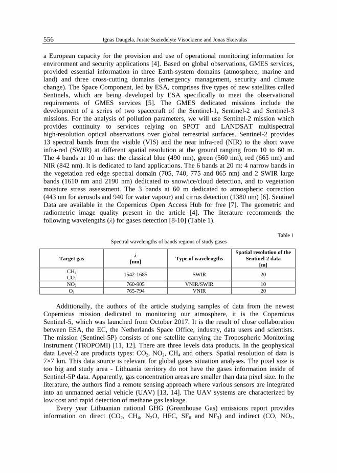
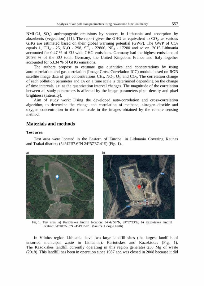
Test area were located in the Eastern of Europe; in Lithuania Covering Kaunas and Trakai districts (54°42'57.6"N 24°57'37.4"E) (Fig. 1).

a) b)

Fig. 1. Test area: a) Kariotiskes landfill location: 54°42′58″N, 24°57′33″E; b) Kazokiskes landfill

location: 54°48'25.0"N 24°49'15.0"E (Source: Google Earth)

In Vilnius region Lithuania have two large landfill sites (the largest landfills of unsorted municipal waste in Lithuania): Kariotiskes and Kazokiskes (Fig. 1). The Kazokiskes landfill currently operating in this region generates 230 Mg of waste (2018). This landfill has been in operation since 1987 and was closed in 2008 because it did


558

not meet modern environmental standards and was morally and technologically obsolete. More than 4 million cubic meters of unsorted rubbish have been accumulated. The closure work lasted 1.5 years. The garbage in the area of 30 ha is covered with special multi-layer constructions, a gas collection system is installed to prevent the release of toxic methane gas into the environment. In 2010, the first power plant in Lithuania to generate electricity from landfill gas was opened here. Similar projects are underway in other landfills in the region.

Kazokiskes landfill area is 27.1 ha (Fig. 1b). It operated from the 2007 year. This landfill replaced the closed Kariotiskes landfill. Landfill safety is ensured by EU-compliant measures: • A 0.5 m thick clay and high-density polyethylene geomembrane installed at the bottom

of the landfill ensures that pollutants do not enter the environment. • The filtrate formed in the landfill is collected in the drainage layer of granite gravel

and enters the filtrate pumping station through pipes. The collected filtrate is sent for treatment to wastewater treatment plants.

• Groundwater monitoring wells were installed around the landfill: four in the direction of groundwater flow, one upstream. Gas monitoring is also carried out in wells, buildings and on the landfill. Classical methods are used to monitor gas leaks in landfill areas, measured a couple of

times a year with a multi-channel analyser. The processes of gas accumulation and disintegration continue to take place in the closed landfill. It is important to monitor it continuously to avoid environmental consequences. Therefore, additional remote sensing studies have been made by authors in Kariotiskes landfill territory (Fig. 1a) [15].

Data acquisition

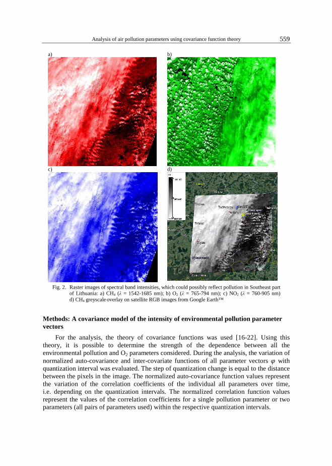
Transformed digital image vectors of environmental pollution parameters and O2 used for the study were prepared from satellite images. RGB-range CO2, NO2 and CH4 images data were obtained from Sentinel-2 mission MultiSpectral Instrument (MSI). Images needed were found through web interface of Copernicus Open Access Hub [7]. This interface allows choosing territory and check availability of data filtered by date, product type and cloud cover for example. Products were chosen by Central wavelength [nm] and Bandwidth [nm] to correspond to wavelengths of possible CO2, NO2 and CH4 reflectance. The radiometric resolution of the MSI instrument is stored in 12-bit system, enabling the image to be acquired over a range of 0 to 4095 potential light intensity values. The radiometric accuracy is less than 5 % (goal 3 %) [10, 11]. Then using Sentinel-2 Toolbox software package satellite images processed to be rasterized and particular colour applied in each case for grey-scaled intensity. In this study date of the images are 2019 May 12th and spatial resolution of bands are 10 meters and 20 meters covering roughly 109 x 109 km territory (see Fig. 2).

In Figure 2 λ (Lambda) - wavelength of spectral band. All three images cover the same territory Southeast part of Lithuania. That area covers two parts of major districts of Lithuania with various land uses. While the weather was partially cloudy, some matches between spectral bands are visible. While each colour is chosen artificially, instead of greyscale, it helps to make computations simultaneously in RGB model.


559

a) b)

c) d)

Fig. 2. Raster images of spectral band intensities, which could possibly reflect pollution in Southeast part of Lithuania: a) CH4 (λ = 1542-1685 nm); b) O2 (λ = 765-794 nm); c) NO2 (λ = 760-905 nm) d) CH4 greyscale overlay on satellite RGB images from Google Earth™

Methods: A covariance model of the intensity of environmental pollution parameter vectors

For the analysis, the theory of covariance functions was used [16-22]. Using this theory, it is possible to determine the strength of the dependence between all the environmental pollution and O2 parameters considered. During the analysis, the variation of normalized auto-covariance and inter-covariate functions of all parameter vectors � with quantization interval was evaluated. The step of quantization change is equal to the distance between the pixels in the image. The normalized auto-covariance function values represent the variation of the correlation coefficients of the individual all parameters over time, i.e. depending on the quantization intervals. The normalized correlation function values represent the values of the correlation coefficients for a single pollution parameter or two parameters (all pairs of parameters used) within the respective quantization intervals.


560

Each column of an image pixel matrix is understood as a single pixel intensity vector. The array of column-vectors of a matrix creates a transformed vector matrix �� of pixel intensity vectors of the transformed i-digital image. We obtain three matrices ��, of three parameters used to define pollution: CH4, O2 and NO2 pixel intensity vectors, where � = 1, 2, 3. Column-vectors of each matrix form the parametric vector of the whole matrix.

Theoretical model of covariance functions is based on the concept of stationary random function, considering that errors in field parameter measurements are random and possibly systematic, i.e. the mean of their errors �∆ = �� → 0 their variance �∆ = �� and the covariate function of the digital signals depends only on the difference in the arguments, i.e. from the quantization interval on the time scale.

Estimates of the covariance function of two numerical parametric vectors of the environmental pollution parameters or the auto-covariance function of a single parametric vector are calculated by spreading digital data vectors in the form of random functions. Discrete transformation is used to process digital signals [20, 23].

In the parametric vector φ of measurement data for each environmental pollution parameter the trend of measurement data for that vector was eliminated. We will consider the random function generated by the data of the vector of environmental pollution φ as stationary (in the broad sense), i.e. its mean the covariate function depends only on the difference τ of the arguments. The auto-covariance function of one random vector or the covariance function of two random vectors is written in [20-24]:

�� = � �� ∙ �� + �� (1)

or:

�� = 1� − � ! �� ∙ �� + �� ∙ "�

#$%

& (2)

where: �� = �' − �', �� = �( − �( - centered � vectors, when eliminated trend �,

� - vector parameter, � = ) × Δ - variable quantization interval, ) - number of units of measure, Δ - value of unit of measure, � - time, � - symbol of average.

Estimation of covariance function ��, �� based on the available data on the measurement of the pollution parameters shall be calculated as follows:

��, �� = ��, �)� = 1� − ) - ��./�

0$/

�1' (3)

where n - total number of discrete intervals (pixels). Formula (3) can be applied in the form of an auto-covariate or a covariate function.

When a function is auto-covariant, vectors φ'�� and φ(�� + �� are parts of single vectors, and when they are covariate, they are two different vectors. The estimate of the normalized covariate function is equal to:

3�, �)� = ��, �)��, �4� = ��, �)�

5�,( (4)

where ��, - estimate of the standard deviation of the random function. The formula (5) used to eliminate the trend of the digital measurement data vector:

�� = � − � (5)


561

where: �� - data vector, with trend eliminated; � - vector trend.

Estimation of the covariance matrix of the � - vector of environmental pollution parameters looks like this:

�,6��78 = 1� − 1 ��79 ��7 (6)

The estimate of the covariance matrix of the two vectors � and : of the environmental pollution parameters shall be written:

�, ;��7 , ��=> = 1� − 1 ��79 ��= (7)

where: ��7 , ��= - the dimensions of the vectors must be the same.

Estimates of covariance matrices �,6��78 and �, ;��7 , ��=> are reduced to estimates of

correlation coefficient 3,6��78 and 3, ;��7 , ��7= >:

3,6��78 = ��$'/(�,6��78��

$'/( (8)

3, ;��7 , ��= > = ��@$'/(�, ;��7 , ��=> ��@

$'( (9)

where ��, ��@ - estimates of the corresponding covariance matrices �,6��78 and

�, ;��7 , ��=> the diagonal matrices of the principal diagonal members.

The accuracy of the calculated correlation coefficients is defined by the standard deviation 5A, estimating its value according to the formula:

5A = 1√) �1 − C(� (10)

where: ) = 8,000; C - correlation coefficient. The highest estimate of the standard deviation is obtained when C the value is close to zero in this case as well 5A, = 0.01 when C ≈ 0.5 we get 5A, = 0.08.

Experimental results

Parameter vector measurement data was processed by compiled computer programs using Matlab 7 software package operators. The ) values of the quantization interval of normalized covariate functions vary from 1 to �/2 values, here � = 160,000 - number of values of each parametric vector for environmental pollution and O2. Normalized auto-covariance functions were calculated for each parametric vector �� estimate ��, �� and graphical expressions of 3 normalized auto-covariance functions were obtained. The quantization interval is plotted on the abscissa axes and the values of the normalized covariate functions (correlation coefficients) on the ordinates (Fig. 3).


562

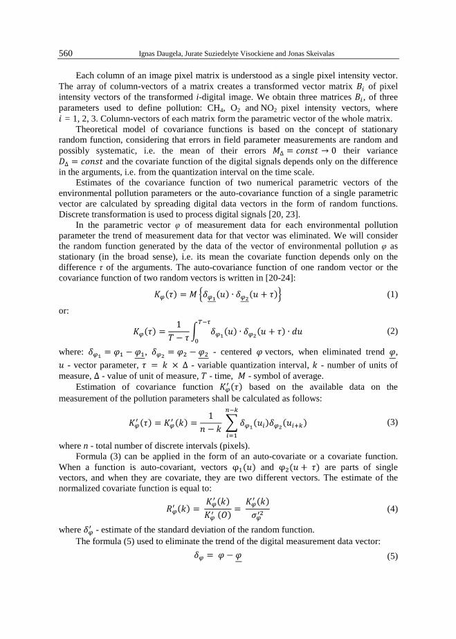
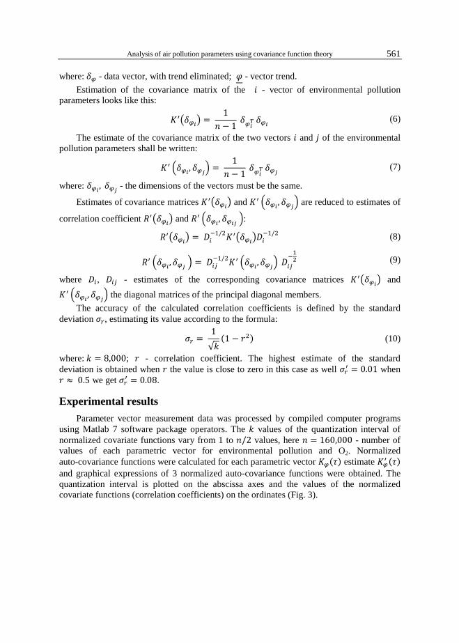
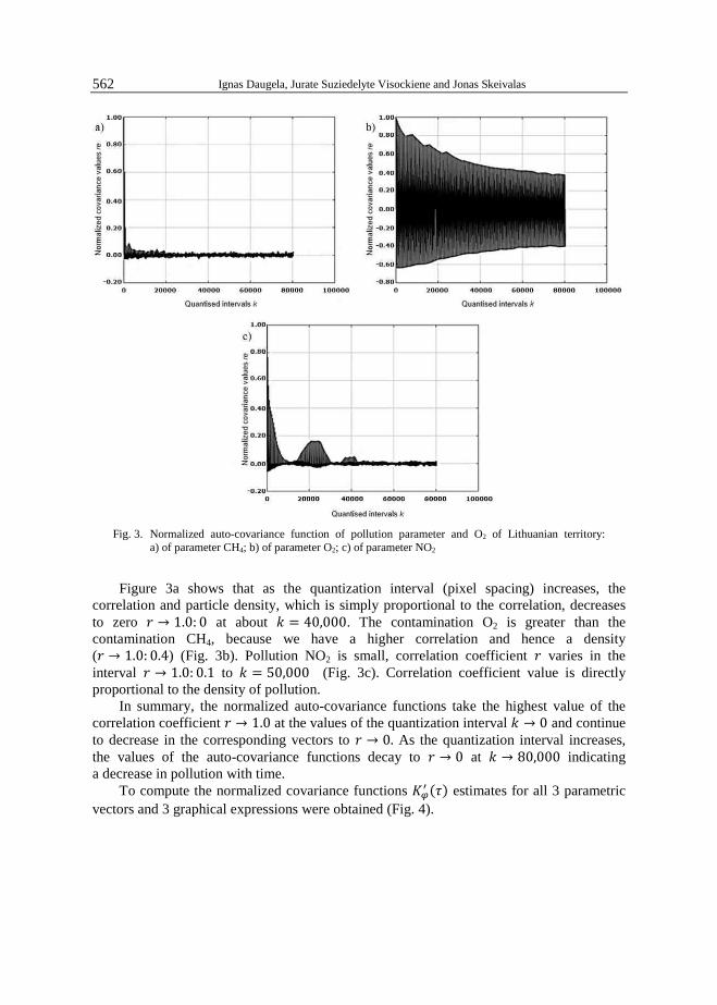
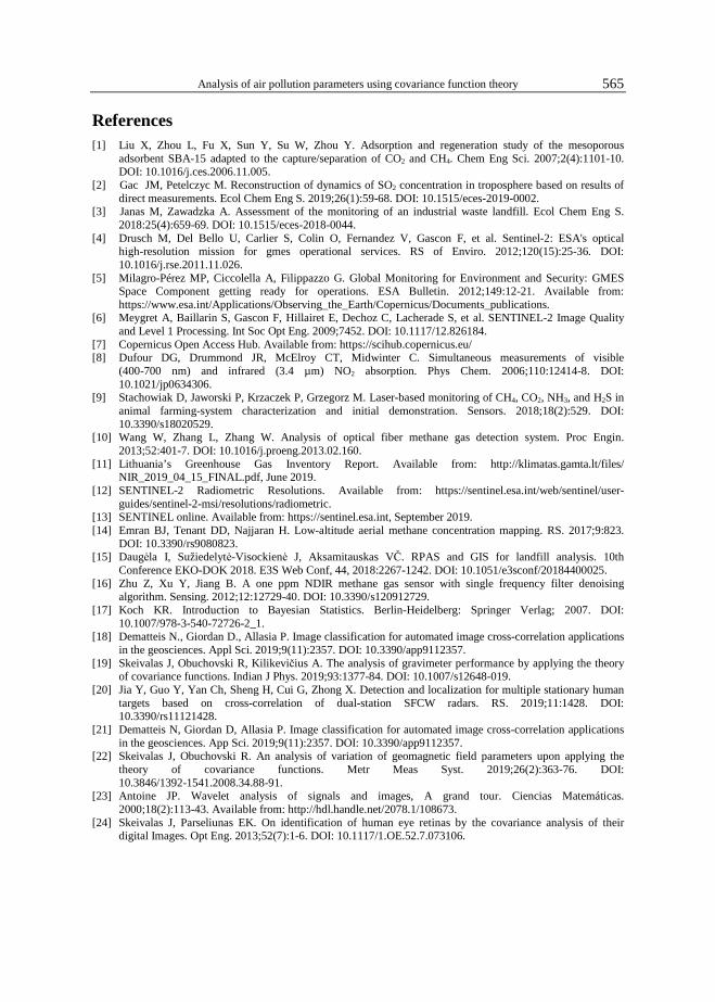
Fig. 3. Normalized auto-covariance function of pollution parameter and O2 of Lithuanian territory:

a) of parameter CH4; b) of parameter O2; c) of parameter NO2

Figure 3a shows that as the quantization interval (pixel spacing) increases, the correlation and particle density, which is simply proportional to the correlation, decreases to zero C → 1.0: 0 at about ) = 40,000. The contamination O2 is greater than the contamination CH4, because we have a higher correlation and hence a density (C → 1.0: 0.4) (Fig. 3b). Pollution NO2 is small, correlation coefficient C varies in the interval C → 1.0: 0.1 to ) = 50,000 (Fig. 3c). Correlation coefficient value is directly proportional to the density of pollution.

In summary, the normalized auto-covariance functions take the highest value of the correlation coefficient C → 1.0 at the values of the quantization interval ) → 0 and continue to decrease in the corresponding vectors to C → 0. As the quantization interval increases, the values of the auto-covariance functions decay to C → 0 at ) → 80,000 indicating a decrease in pollution with time.

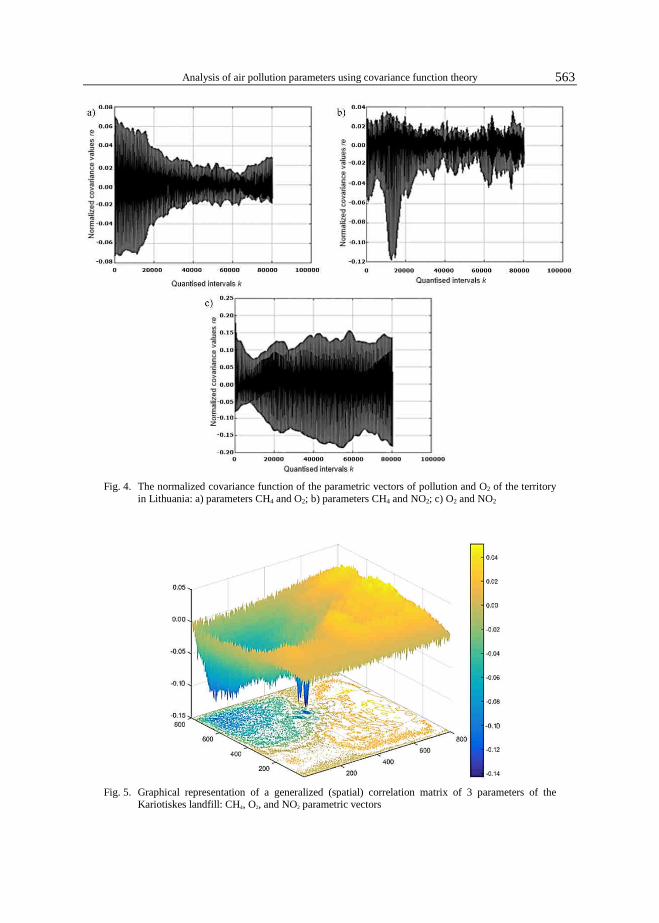
To compute the normalized covariance functions ��, �� estimates for all 3 parametric vectors and 3 graphical expressions were obtained (Fig. 4).


563

Fig. 4. The normalized covariance function of the parametric vectors of pollution and O2 of the territory

in Lithuania: a) parameters CH4 and O2; b) parameters CH4 and NO2; c) O2 and NO2

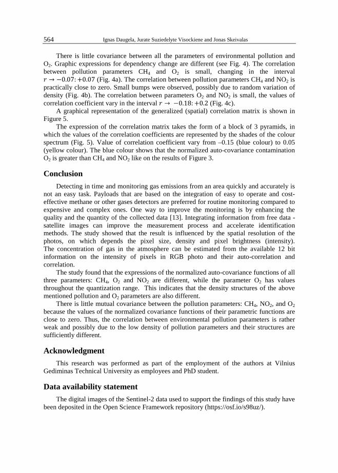
Fig. 5. Graphical representation of a generalized (spatial) correlation matrix of 3 parameters of the

Kariotiskes landfill: CH4, O2, and NO2 parametric vectors


564

There is little covariance between all the parameters of environmental pollution and O2. Graphic expressions for dependency change are different (see Fig. 4). The correlation between pollution parameters CH4 and O2 is small, changing in the interval C → −0.07: +0.07 (Fig. 4a). The correlation between pollution parameters CH4 and NO2 is practically close to zero. Small bumps were observed, possibly due to random variation of density (Fig. 4b). The correlation between parameters O2 and NO2 is small, the values of correlation coefficient vary in the interval C → −0.18: +0.2 (Fig. 4c).

A graphical representation of the generalized (spatial) correlation matrix is shown in Figure 5.

The expression of the correlation matrix takes the form of a block of 3 pyramids, in which the values of the correlation coefficients are represented by the shades of the colour spectrum (Fig. 5). Value of correlation coefficient vary from –0.15 (blue colour) to 0.05 (yellow colour). The blue colour shows that the normalized auto-covariance contamination O2 is greater than CH4 and NO2 like on the results of Figure 3.

Conclusion

Detecting in time and monitoring gas emissions from an area quickly and accurately is not an easy task. Payloads that are based on the integration of easy to operate and cost-effective methane or other gases detectors are preferred for routine monitoring compared to expensive and complex ones. One way to improve the monitoring is by enhancing the quality and the quantity of the collected data [13]. Integrating information from free data - satellite images can improve the measurement process and accelerate identification methods. The study showed that the result is influenced by the spatial resolution of the photos, on which depends the pixel size, density and pixel brightness (intensity). The concentration of gas in the atmosphere can be estimated from the available 12 bit information on the intensity of pixels in RGB photo and their auto-correlation and correlation.

The study found that the expressions of the normalized auto-covariance functions of all three parameters: CH4, O2 and NO2 are different, while the parameter O2 has values throughout the quantization range. This indicates that the density structures of the above mentioned pollution and O2 parameters are also different.

There is little mutual covariance between the pollution parameters: CH4, NO2, and O2 because the values of the normalized covariance functions of their parametric functions are close to zero. Thus, the correlation between environmental pollution parameters is rather weak and possibly due to the low density of pollution parameters and their structures are sufficiently different.

Acknowledgment

This research was performed as part of the employment of the authors at Vilnius Gediminas Technical University as employees and PhD student.

Data availability statement

The digital images of the Sentinel-2 data used to support the findings of this study have been deposited in the Open Science Framework repository (https://osf.io/s98uz/).


565

References [1] Liu X, Zhou L, Fu X, Sun Y, Su W, Zhou Y. Adsorption and regeneration study of the mesoporous

adsorbent SBA-15 adapted to the capture/separation of CO2 and CH4. Chem Eng Sci. 2007;2(4):1101-10. DOI: 10.1016/j.ces.2006.11.005.

[2] Gac JM, Petelczyc M. Reconstruction of dynamics of SO2 concentration in troposphere based on results of direct measurements. Ecol Chem Eng S. 2019;26(1):59-68. DOI: 10.1515/eces-2019-0002.

[3] Janas M, Zawadzka A. Assessment of the monitoring of an industrial waste landfill. Ecol Chem Eng S. 2018:25(4):659-69. DOI: 10.1515/eces-2018-0044.

[4] Drusch M, Del Bello U, Carlier S, Colin O, Fernandez V, Gascon F, et al. Sentinel-2: ESA's optical high-resolution mission for gmes operational services. RS of Enviro. 2012;120(15):25-36. DOI: 10.1016/j.rse.2011.11.026.

[5] Milagro-Pérez MP, Ciccolella A, Filippazzo G. Global Monitoring for Environment and Security: GMES Space Component getting ready for operations. ESA Bulletin. 2012;149:12-21. Available from: https://www.esa.int/Applications/Observing_the_Earth/Copernicus/Documents_publications.

[6] Meygret A, Baillarin S, Gascon F, Hillairet E, Dechoz C, Lacherade S, et al. SENTINEL-2 Image Quality and Level 1 Processing. Int Soc Opt Eng. 2009;7452. DOI: 10.1117/12.826184.

[7] Copernicus Open Access Hub. Available from: https://scihub.copernicus.eu/ [8] Dufour DG, Drummond JR, McElroy CT, Midwinter C. Simultaneous measurements of visible

(400-700 nm) and infrared (3.4 µm) NO2 absorption. Phys Chem. 2006;110:12414-8. DOI: 10.1021/jp0634306.

[9] Stachowiak D, Jaworski P, Krzaczek P, Grzegorz M. Laser-based monitoring of CH4, CO2, NH3, and H2S in animal farming-system characterization and initial demonstration. Sensors. 2018;18(2):529. DOI: 10.3390/s18020529.

[10] Wang W, Zhang L, Zhang W. Analysis of optical fiber methane gas detection system. Proc Engin. 2013;52:401-7. DOI: 10.1016/j.proeng.2013.02.160.

[11] Lithuania’s Greenhouse Gas Inventory Report. Available from: http://klimatas.gamta.lt/files/ NIR_2019_04_15_FINAL.pdf, June 2019.

[12] SENTINEL-2 Radiometric Resolutions. Available from: https://sentinel.esa.int/web/sentinel/user-guides/sentinel-2-msi/resolutions/radiometric.

[13] SENTINEL online. Available from: https://sentinel.esa.int, September 2019. [14] Emran BJ, Tenant DD, Najjaran H. Low-altitude aerial methane concentration mapping. RS. 2017;9:823.

DOI: 10.3390/rs9080823. [15] Daugėla I, Sužiedelytė-Visockienė J, Aksamitauskas VČ. RPAS and GIS for landfill analysis. 10th

Conference EKO-DOK 2018. E3S Web Conf, 44, 2018:2267-1242. DOI: 10.1051/e3sconf/20184400025. [16] Zhu Z, Xu Y, Jiang B. A one ppm NDIR methane gas sensor with single frequency filter denoising

algorithm. Sensing. 2012;12:12729-40. DOI: 10.3390/s120912729. [17] Koch KR. Introduction to Bayesian Statistics. Berlin-Heidelberg: Springer Verlag; 2007. DOI:

10.1007/978-3-540-72726-2_1. [18] Dematteis N., Giordan D., Allasia P. Image classification for automated image cross-correlation applications

in the geosciences. Appl Sci. 2019;9(11):2357. DOI: 10.3390/app9112357. [19] Skeivalas J, Obuchovski R, Kilikevičius A. The analysis of gravimeter performance by applying the theory

of covariance functions. Indian J Phys. 2019;93:1377-84. DOI: 10.1007/s12648-019. [20] Jia Y, Guo Y, Yan Ch, Sheng H, Cui G, Zhong X. Detection and localization for multiple stationary human

targets based on cross-correlation of dual-station SFCW radars. RS. 2019;11:1428. DOI: 10.3390/rs11121428.

[21] Dematteis N, Giordan D, Allasia P. Image classification for automated image cross-correlation applications in the geosciences. App Sci. 2019;9(11):2357. DOI: 10.3390/app9112357.

[22] Skeivalas J, Obuchovski R. An analysis of variation of geomagnetic field parameters upon applying the theory of covariance functions. Metr Meas Syst. 2019;26(2):363-76. DOI: 10.3846/1392-1541.2008.34.88-91.

[23] Antoine JP. Wavelet analysis of signals and images, A grand tour. Ciencias Matemáticas. 2000;18(2):113-43. Available from: http://hdl.handle.net/2078.1/108673.

[24] Skeivalas J, Parseliunas EK. On identification of human eye retinas by the covariance analysis of their digital Images. Opt Eng. 2013;52(7):1-6. DOI: 10.1117/1.OE.52.7.073106.