Computers & Graphics 36 (2012) 398–409

Contents lists available at SciVerse ScienceDirect

Computers & Graphics

0097-84

http://d

$If a

online

027.n Corr

E-m

bberger

journal homepage: www.elsevier.com/locate/cag

SMI 2012: Full Paper

Spectral computations on nontrivial line bundles$

Alexander Vais n, Benjamin Berger, Franz-Erich Wolter

Welfenlab, Division of Computer Graphics, Leibniz University of Hannover, 30167 Hannover, Germany

a r t i c l e i n f o

Article history:

Received 1 December 2011

Received in revised form

15 March 2012

Accepted 17 March 2012Available online 28 March 2012

Keywords:

Spectral geometry processing

Vector bundles

Computational topology

Laplace operator

Finite elements

93/$ - see front matter & 2012 Elsevier Ltd. A

x.doi.org/10.1016/j.cag.2012.03.027

pplicable, supplementary material from the

after the conference. Please see http://dx.d

esponding author.

ail addresses: vais@welfenlab.de, vais@gdv.un

@welfenlab.de (B. Berger), few@welfenlab.de

a b s t r a c t

Computing the spectral decomposition of the Laplace–Beltrami operator on a manifold M has proven

useful for applications such as shape retrieval and geometry processing. The standard operator acts on

scalar functions which can be identified with sections of the trivial line bundle M �R. In this work we

propose to extend the discussion to Laplacians on nontrivial real line bundles. These line bundles are in

one-to-one correspondence with elements of the first cohomology group of the manifold with Z2

coefficients. While we focus on the case of two-dimensional closed surfaces, we show that our method

also applies to surfaces with boundaries. Denoting by b the rank of the first cohomology group, there

are 2b different line bundles to consider and each of these has a naturally associated Laplacian that

possesses a spectral decomposition. Using our new method it is possible for the first time to compute

the spectra of these Laplacians by a simple modification of the finite element basis functions used in the

standard trivial bundle case. Our method is robust and efficient. We illustrate some properties of the

modified spectra and eigenfunctions and indicate possible applications for shape processing. As an

example, using our method, we are able to create spectral shape descriptors with increased sensitivity

in the eigenvalues with respect to geometric deformations and to compute cycles aligned to object

symmetries in a chosen homology class.

& 2012 Elsevier Ltd. All rights reserved.

1. Introduction

Curves, surfaces and solids are commonly used in computergraphics, computer vision and computer aided geometric design,where they serve as basic building blocks or data elements. Severalcontinuous and discrete representations exist and many algo-rithms have been proposed to operate on these representationsfor a variety of tasks or to convert between them. It is often usefulto view these objects within the framework of differential geome-try where they become instances of manifolds, with or withoutboundary. Loosely speaking, a manifold M is a space that locallylooks like the Euclidean space. In this setting it becomes possible totransfer the tools and techniques of multivariate calculus onto M

and to develop algorithms that benefit from the rich arsenal oftechniques available in this mathematical fundament.

In this paper we deal with the Laplace–Beltrami operator whichis the generalization of the Euclidean Laplacian. As in the Euclideancase it can be defined by Df :¼ �divrf , where rf is the gradient ofthe real-valued function f defined on the manifold M and div is thedivergence operator. We follow the above sign convention, making

ll rights reserved.

author(s) will be available

oi.org/10.1016/j.cag.2012.03.

i-hannover.de (A. Vais),

(F.-E. Wolter).

D a positive definite operator. The Laplace operator is abundantthroughout mathematics, physics and engineering. It plays animportant role in describing physical phenomena such as heatdiffusion and wave propagation. Moreover, in the context of shapeanalysis, the Laplace–Beltrami operator has proven useful for avariety of applications due to the fact that it captures importantgeometric and topological information about the shape representedby the manifold in an isometrically invariant way.

Solving the eigenvalue problem Df ¼ lf results in a sequenceof eigenvalues l1,l2, . . ., called spectrum of D and a sequence ofeigenfunctions f 1,f 2, . . . corresponding to the eigenvalues. Theeigenfunctions have the useful property that they are orthonor-mal with respect to the L2 inner product

ðf ,hÞ ¼

ZM

f ðxÞhðxÞ dM

and form a basis for the corresponding Hilbert space of functionsdefined on M. For rectangular or spherical manifolds M we obtainthe well-known Fourier bases and spherical harmonics, respectively.From this functional-analytic point of view, knowledge of theeigenvalues and eigenfunctions leads to an improved understandingof the Laplacian itself, since it becomes diagonal in the basis of itseigenfunctions. Intuitively this means that the action of D on afunction f can be described by the action of an infinite diagonalmatrix, the diagonal entries being the eigenvalues, on the infinitevector of coefficients describing f with respect to the eigenfunctionbasis, see e.g. [1]. The aforementioned decomposition of f provides a

A. Vais et al. / Computers & Graphics 36 (2012) 398–409 399

natural frequency decomposition for dealing with data on themanifold at different scales.

1.1. Related work and motivation

Laplacians in several computational discretizations, see e.g.[2–5], and their spectral decomposition have received muchattention in the geometric processing community.

Among the applications are shape and image retrieval using aprefix of the spectrum as a fingerprint or ‘‘Shape-DNA’’ [6–12],geometric signal processing operations [13–15], surface remesh-ing and parametrization [16–19], creating descriptors for shapematching [20–26], shape segmentation and registration [27,28],statistical shape analysis for medical studies [29–31] and sym-metry detection [32], just to mention a few. A survey of someapplications can be found in [33]. According to our knowledge theearliest research works employing Laplace (Beltrami) spectra asfingerprints for classification, retrieval and matching of shapesand images appears to have been done at the Welfenlab in theyears 1999–2001, cf. [11], for details see [12]. Theoretical back-ground is provided by a branch of mathematics known as spectralgeometry, in which several results have been obtained, relatinge.g. asymptotic expansions of fundamental solutions of the heatand wave equation with the geometry of the manifold, see e.g.[34–38].

In this paper we introduce numerical computations for Lapla-cian operators on nontrivial Euclidean line bundles over two-dimensional surfaces M. To motivate and explain the idea, con-sider first the one-dimensional simple case where M is the unitcircle S1 or equivalently the interval ½0;2p� with end pointsidentified. Any real-valued function f on M can be considered asa 2p-periodic function on R. The Laplace–Beltrami operatorbecomes D¼�d2=dx2 and the eigenvalue problem reads

�f 00ðxÞ ¼ lf ðxÞ, f ð0Þ ¼ f ð2pÞ, f 0ð0Þ ¼ f 0ð2pÞ:

The solutions in this case are easily obtained. The eigenvalues arelk :¼ k2 for any integer k and the corresponding eigenfunctionsare linear combinations of sinðkxÞ and cosðkxÞ. At this point,consider the question:

What happens if f is chosen 2p-antiperiodic?

This means the boundary conditions become

f ð0Þ ¼�f ð2pÞ, f 0ð0Þ ¼�f 0ð2pÞ:

It is easy to check that the eigenvalues are lk ¼ ðkþ12 Þ

2 and thecorresponding eigenfunctions are linear combinations of thefunctions sinððkþ 1

2ÞxÞ and cosððkþ 12ÞxÞ for integers k.

For higher-dimensional manifolds the spectral decompositionis not easily obtained since only very special metrics give rise toclosed form solutions via techniques such as separation of vari-ables [39]. Hence, numerical approximation methods, typicallybased on the finite element or finite difference schemes have tobe used.

Our goal is to study the generalization of the question above inthe situation where M is a two-dimensional manifold, focusing ona numerical approach based on the finite element method. Wewill show that our method also covers manifolds with bound-aries. Intuitively we have the freedom to choose if a function f onM has a sign-flip discontinuity when crossing a set of specificloops or paths on M. In order to discuss these matters on solidmathematical ground, it is appropriate to interpret the situationwithin the framework of vector bundles, where f becomes asmooth section of a certain vector bundle over M that incorpo-rates the sign flips in its transition functions, ultimately leading tomodifications in the discretized problems under consideration.

Similar discontinuities arise for example in the context of model-ing singularities occurring in global parametrization [17–19].

We note that analogous situations also commonly occur inphysics in the context of describing the wave function of fermio-nic particles, i.e. half-integer spin particles such as electrons,giving rise to the notion of spin structure. The choice of spinstructure is essential in defining the spinor bundle, the spinorLaplacian and the Dirac operator which is a square root of thespinor Laplacian. Recently, related concepts have made their wayinto applications in computer graphics and geometric modeling.In [40] an algorithm is presented that employs a quaternionicdiscrete Dirac operator for constructing conformal mappings ofsurfaces. This has applications such as distortion-minimizingtexture mapping and curvature-based shape editing. A key stepin the aforementioned algorithm is the computation of aneigenfunction of a modification of this discrete operator. Theauthors show that their discrete Dirac operator is related to aDirac operator in the continuous setting. For example they showthat it is locally equivalent to the standard Dirac operator for aspin 1

2 particle in the plane.While objects with simple topology like the Euclidean plane or

compact oriented surfaces of genus zero have essentially only onespin structure, it is known that there are several possible spinstructures for surfaces with more complicated topology and eachone induces a different spinor bundles, different Dirac operatorsand associated spectra. More precisely the possible spin struc-tures are in correspondence with elements of the first cohomol-ogy group H1

ðM,Z2Þ, see [41].In our case, we consider real line bundles, which are also in

one-to-one correspondence with elements of H1ðM,Z2Þ. However,

while the fiber of a spinor bundle is some representation of thespin group, typically C2, the fiber of our bundles is R. Thissimilarity suggests that the ideas presented here are applicableto more general settings, for example in order to compute thespectral decomposition of Dirac operators for different spinstructures.

1.2. Outline

In the following section we recall several notions and facts ofdifferential geometry and topology, focusing especially on theconcept of a vector bundle. The Laplace–Beltrami operator will beidentified with a Laplacian operator associated to the trivial linebundle over M. However, in general the trivial line bundle over M

is just one of the several different line bundles and for each ofthem an associated Laplacian exists.

In the third section we describe an algorithm that computesthe spectra of Laplacian operators associated naturally to any ofthese nontrivial vector bundles.

Afterwards we present results obtained using our method andgive examples, focusing on the differences that arise from thenontrivial bundles. We also validate our results against knownspectra and spectra computed by a different method for arestricted class of shapes, namely flat tori and tori of revolution.

Finally we give a conclusion and indicate possible applicationsand directions for future work.

2. Mathematical background

We review some of the terminology and notation that we willneed, avoiding technical details. For a comprehensive treatment,including formal definitions, we refer to textbooks on differentialgeometry and topology such as [42–44].

A vector bundle E over a manifold M is obtained by assigningto each point pAM a vector space Ep in a continuous way.

A. Vais et al. / Computers & Graphics 36 (2012) 398–409400

The dimension of the vector spaces is called rank of the bundleand vector bundles of rank one are called line bundles.

The simplest line bundle is the Cartesian product M �R whichassigns to each point a copy of the real numbers. This is the so-called trivial line bundle. However, not every line bundle is trivial:It is possible to assign to each point a copy of R such that theresulting bundle is not homeomorphic to M �R. Fig. 1 visualizestwo possible line bundles over the circle M :¼ S1. The first bundleis the trivial bundle which is topologically an infinite cylinder,although only a finite portion is shown in the figure. The secondbundle in the figure looks locally like a Cartesian product, whileglobally it is twisted like a Mobius strip of infinite width. Again,only a finite portion is shown.

A map s : M-E with the property that sðpÞAEp is called asection of E. The space of all smooth sections is denoted by GðEÞ.Sections of real line bundles are easy to visualize: Locally they canbe imagined as the graphs of real-valued functions. The red linesin Fig. 1 show sections of the trivial and nontrivial real linebundles over the circle.

Besides the line bundles, two very important vector bundlesassociated to a manifold are the tangent bundle TM which is thecollection of all tangent spaces, and the cotangent bundle TnM

which is the collection of vector spaces being dual to the tangentspaces. Sections of these bundles are the familiar vector fields anddifferential one-forms.

A useful concept for computations in vector bundles is thenotion of repers: A local reper or frame of E over U �M is acollection of sections e1, . . . ,ek such that for all pAU the vectorse1ðpÞ, . . . ,ekðpÞ form a basis of Ep. A reper is called global if thisproperty extends to all pAM.

Every vector bundle admits local repers. A vector bundleadmitting a global reper is trivial. Notice that for line bundles, areper consists of only one nonvanishing section.

Often, vector bundles come equipped with additional struc-tures, such as a fiber metric or a connection.

A fiber metric is a scalar product / � , �S : Ep � Ep/R dependingsmoothly on p. Vector bundles with such a fiber metric are calledEuclidean vector bundles. We will assume throughout this paper thatthe tangent bundle is Euclidean. In this case, its fiber metric is calleda Riemannian metric or metric tensor which is often denoted by g orby a matrix gij with respect to a local reper of TM. This allows us tomeasure lengths, angles and volumes on the manifold M.

A connection r on a vector bundle E is a differential operatorr : GðEÞ-GðE� TnMÞ that is R-linear and satisfies the Leibnizrule rðffÞ ¼f� df þ frf for any function f and any section f.Here d denotes the exterior derivative, mapping a real-valuedfunction to its differential, which is a real-valued one-form. Aconnection can be considered as an extension of this concept,mapping E-sections to E-valued one-forms.

The space of sections GðEÞ of an Euclidean vector bundlebecomes a Hilbert space by introducing the natural inner product

ðf,cÞ :¼Z

M/f,cS dM

The Riemannian metric on TM induces a fiber metric on TnM. Thefiber metric of E and the fiber metric of TnM induce a fiber metric

Fig. 1. Line bundles over the circle. (For interpretation of the references to color in

this figure legend, the reader is referred to the web version of this article.)

in the bundle E� TnM and therefore a natural inner product onthe space of E-valued one-forms. These inner products are neededin order to define the adjoint to r which is denoted by rn. Theadjointness property means that ðrf,aÞ ¼ ðf,rnaÞ for all sectionsf and all E-valued one-forms a. It is essential for deriving theweak variational formulation in the finite element method.

Using the connection and its adjoint, the Connection Laplacian

associated to r is defined by D :¼ rnr.The Laplace–Beltrami operator is defined by D¼ dnd where d

the differential and dn is its adjoint. It is a special case of aconnection Laplacian since d is a connection on the trivialEuclidean line bundle M �R.

2.1. Classification of Euclidean line bundles

Having identified the classical Laplace–Beltrami operator withthe connection Laplacian dnd of the trivial Euclidean line bundle,we can now proceed to consider other line bundles. To character-ize these, we will make use of some tools of algebraic topology,see Appendix A for a quick review and [44] for details.

According to the following classification theorem, which wecite from [45], the following objects are equivalent via appro-priate isomorphisms:

�

An Euclidean line bundle E over M. � An element x of the first cohomology group H1

ðM,Z2Þ.

� A two-sheeted cover r : ~M-M. � A homomorphism f : p1ðMÞ-Z2.

Any element xAH1ðM,Z2Þ of the cohomology group is com-

pletely characterized by its values on a basis. For a compact closedoriented surface of genus g, the rank of the first (co-)homologygroup is 2g. Therefore we choose a basis G¼ fg1, . . . ,g2gg of cycleswhose equivalence classes generate H1ðM,Z2Þ.

Intuitively we can identify a section of an Euclidean linebundle E with a real-valued function on M that does or does notflip sign when crossing a loop gi. We will encode this informationby a tuple ðG,wÞ where w is a Z2-valued vector of dimension 2g,setting wðiÞ ¼ 0 if no sign flip occurs across gi and setting wðiÞ ¼ 1 ifa sign flip occurs. In the latter case, we will call gi an active

generator. We will denote the corresponding Euclidean linebundle by EG,w.

More formally, we can construct the bundle as follows: Let f :p1ðMÞ-Z2 be a homomorphism. Let ~M be the universal coveringof M. Using f and interpreting the fundamental group as thegroup of deck transformations, we define an action of p1ðMÞ onthe trivial line bundle ~M �R via:

gð ~q,vÞ ¼ ðg ~q,ð�1ÞfðgÞvÞ for gAp1ðMÞ, ~qA ~M , vAR:

The bundle E :¼ ð ~M �RÞ=p1ðMÞ is an Euclidean line bundle overM. The connection r¼ d on M �R lifts to a connection on ~M �R

and induces a connection on E. This connection in turn induces aconnection Laplacian that acts locally just like the Laplace–Beltrami operator.

Note that a smooth section of E can be identified with asmooth real-valued function on a (two-sheeted) covering space ofM, provided that it satisfies the chosen symmetry or anti-symmetry conditions. Therefore not every function on the cover-ing space corresponds to a smooth section of the bundle.

3. Description of our algorithm

Our goal is the following: Given an Euclidean line bundle EG,wover M we want to compute the spectral decomposition of theassociated connection Laplacian.

A. Vais et al. / Computers & Graphics 36 (2012) 398–409 401

In order to carry out the numerical computation we prescribesign-flips across the loops in G similar to the sign flip that arose inthe boundary conditions in the motivating introductory exampleemploying the Mobius strip. The sign-flips are incorporated intothe finite element basis functions. The resulting spectrum doesnot depend on the specific choice of loops, but only on theelement xAH1

ðM,Z2Þ that the tuple ðG,wÞ represents.In the first subsection we determine the system of loops G,

which is a necessary preliminary step for the subsequent steps.Then we describe the classical finite element approach. Finally weintroduce the sign-flip modifications necessary in order toaccount for the nontrivial bundles.

3.1. Computing homology generators

We assume that our manifold is furnished with a triangulationðV ,E,FÞ where V is the set of vertices, E� V2 is the set of edges andF � V3 is the set of faces. The set of vertices together with theedges form a graph (V,E). The dual of this graph is obtained as thegraph ðF,En

Þ where En� F2 is given by all pairs of faces sharing an

edge in E. In the following, we identify E and En with each other.The problem of computing cycles on surfaces has been researchedbefore, see e.g. [46–49] and the references therein. For ourpurposes we apply the algorithm by Erickson and Whittlesey [47]:

1.

Compute a spanning tree T � E of the graph (V,E). 2. Compute a spanning tree Tn

� En of the dual graph ðF,EnÞ using

only edges not occurring in T.

3. Compute the set L of all edges not occurring in T or Tn. Each

edge eAL induces a cycle in T.

For a closed manifold of genus g, this algorithm yields a set of 2g

cycles that generate H1ðM,Z2Þ. It can be run with differentspanning trees to obtain different generators, though any set ofcycles generating the first homology group is sufficient for ourlater calculations.

3.2. Finite elements formulation

The general outline for applying a finite element computationto the the Laplacian eigenvalue problem dndf ¼ lf is obtained intwo steps: First, taking the inner product with an arbitrary testfunction j we obtain the equation:

ðdn df ,jÞ ¼ ðdf ,djÞ ¼ lðf ,jÞ 8j:

Here we exploited the adjointness property of the operators d anddn with respect to the inner products on functions and one-forms.This weak variational formulation is discretized by writing theunknown function f as a linear combination f ¼ f 1j1þ � � � f

NjN ofa collection ðjkÞ of suitable basis functions and solving thediscrete generalized eigenvalue problem

Af ¼ lBf , ð1Þ

where A and B are N�N matrices and f ¼ ðf kÞ is a vector of

dimension N. The entries of the matrices are computed byevaluating the inner products

Aij :¼

ZM/dji,djjS dM, Bij ¼

ZMjijj dM:

According to standard finite element constructions, see e.g.[50], the basis functions are constructed by piecing togetherpolynomials over the individual triangles in a triangulation of M

to yield functions with local support that satisfy the interpolationconditions jiðqjÞ ¼ dij on a set of N nodes ðqkÞ spaced regularly atthe vertices, on the edges and in the interior of the triangles. Thisestablishes a one-to-one correspondence between every node qk

and the basis function jk evaluating to one precisely at that nodeand to zero at all other nodes. Depending on where qk is located,the corresponding basis function is called a vertex, edge or bubblefunction, respectively.

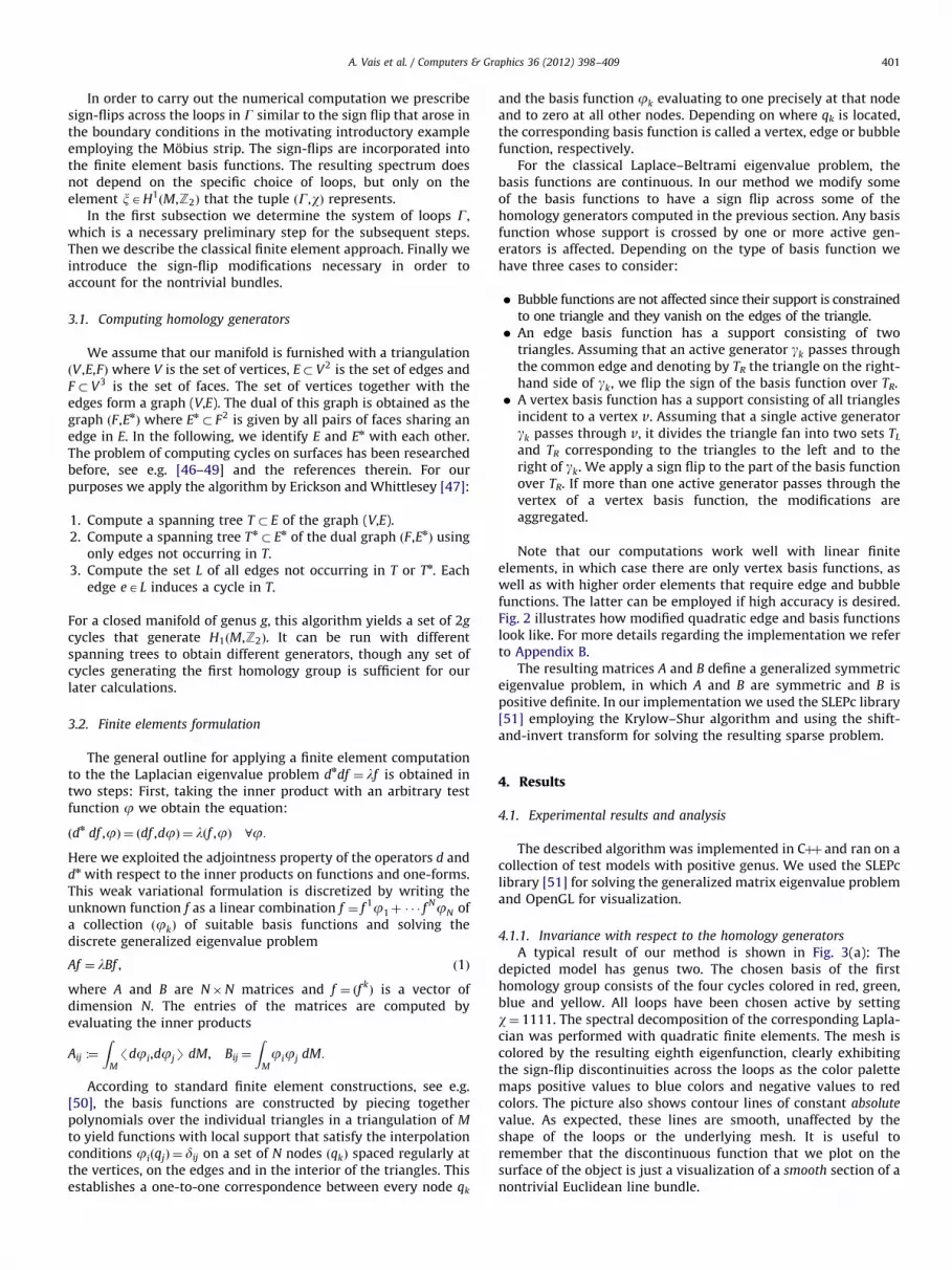
For the classical Laplace–Beltrami eigenvalue problem, thebasis functions are continuous. In our method we modify someof the basis functions to have a sign flip across some of thehomology generators computed in the previous section. Any basisfunction whose support is crossed by one or more active gen-erators is affected. Depending on the type of basis function wehave three cases to consider:

�

Bubble functions are not affected since their support is constrainedto one triangle and they vanish on the edges of the triangle. � An edge basis function has a support consisting of two

triangles. Assuming that an active generator gk passes throughthe common edge and denoting by TR the triangle on the right-hand side of gk, we flip the sign of the basis function over TR.

� A vertex basis function has a support consisting of all triangles

incident to a vertex v. Assuming that a single active generatorgk passes through v, it divides the triangle fan into two sets TL

and TR corresponding to the triangles to the left and to theright of gk. We apply a sign flip to the part of the basis functionover TR. If more than one active generator passes through thevertex of a vertex basis function, the modifications areaggregated.

Note that our computations work well with linear finiteelements, in which case there are only vertex basis functions, aswell as with higher order elements that require edge and bubblefunctions. The latter can be employed if high accuracy is desired.Fig. 2 illustrates how modified quadratic edge and basis functionslook like. For more details regarding the implementation we referto Appendix B.

The resulting matrices A and B define a generalized symmetriceigenvalue problem, in which A and B are symmetric and B ispositive definite. In our implementation we used the SLEPc library[51] employing the Krylow–Shur algorithm and using the shift-and-invert transform for solving the resulting sparse problem.

4. Results

4.1. Experimental results and analysis

The described algorithm was implemented in Cþþ and ran on acollection of test models with positive genus. We used the SLEPclibrary [51] for solving the generalized matrix eigenvalue problemand OpenGL for visualization.

4.1.1. Invariance with respect to the homology generators

A typical result of our method is shown in Fig. 3(a): Thedepicted model has genus two. The chosen basis of the firsthomology group consists of the four cycles colored in red, green,blue and yellow. All loops have been chosen active by settingw¼ 1111. The spectral decomposition of the corresponding Lapla-cian was performed with quadratic finite elements. The mesh iscolored by the resulting eighth eigenfunction, clearly exhibitingthe sign-flip discontinuities across the loops as the color palettemaps positive values to blue colors and negative values to redcolors. The picture also shows contour lines of constant absolute

value. As expected, these lines are smooth, unaffected by theshape of the loops or the underlying mesh. It is useful toremember that the discontinuous function that we plot on thesurface of the object is just a visualization of a smooth section of anontrivial Euclidean line bundle.

Fig. 2. Modified quadratic finite element basis functions. (a) Sign flip along edge basis function. (b) Sign flip along vertex basis function. (c) Double sign flip along vertex

basis function.

A. Vais et al. / Computers & Graphics 36 (2012) 398–409402

We point out, that it is not necessary to choose a nice basis ofloops, as any homology basis would suffice. The loops do not have tobe short or straight and they may even degenerate in the sense ofbeing locally parallel to other loops or to themselves, as long as thesign flip modifications are correctly applied in the FEM basis func-tions. The spectrum and the contour lines of absolute value will notbe affected by such changes. Any changes are purely due to the waythe active loops are positioned in relation to each other with respectto Z2 homology and there are precisely 22g different configurations.For example, Fig. 3(b) shows a different configuration of loops: Theyellow loop has been deformed, the blue loop has been moved downand the green loop switched from one handle to another. Thisconfiguration represents a different basis for the homology group. Itwould have been the same if the green loop had only been deformed.In order to account for the change in the homology basis, the red loophas been deactivated and the spectral decomposition was performedwith active yellow, green and blue loops. Despite all these changes,we obtain exactly the same spectrum and the same eighth eigenfunc-tion. Of course we would have obtained a different eighth eigenfunc-tion if we had chosen a different bundle.

4.1.2. Zero sets of nontrivial eigenfunctions

The zero sets of the eigenfunctions of the Laplace–Beltramioperator, sometimes also called nodal sets, have been used for

shape segmentation since they often identify privileged directionsrelated to the symmetries of the objects or capture surfaceprotrusions that are often well aligned with perceptual features,see [4,32]. Among all eigenfunctions, the first one correspondingto the lowest nonzero eigenvalue has been proven to be especiallyuseful, since it varies smoothly along the principal direction ofelongated objects [52,53] and in many cases its zero set alignswith a central symmetry of the object. This property has beenexploited for example in medical studies to detect the CorpusCallosum, an important structure in brain anatomy, located in themiddle between the left and right hemispheres of the whitematter surface [54].

Regarding the zero set of a section s on a nontrivial line bundleEG,w, we observe that this set, when interpreted as a chain, isclosed and homologous to the collection of active loops in G. Thisis seen as follows: Denote by d the zero set of s, denote by g theunion of active loops, assuming without loss of generality that allloops have been slightly deformed so they intersect only trans-versally. Identify s with a function ~s : M-R that has the sign-flipdiscontinuities when crossing the set g and let D be the subset ofM where ~s is positive. Interpreting g and d as 1-cycles and D as a2-chain, we have that D is bounded by gþd. Therefore g¼ d withrespect to Z2 homology.

Applying this observation to the eigenfunctions of the non-trivial bundle Laplacians, we can compute cycles that are geometry

Fig. 3. Example: two views of the same eigenfunction. (a) Plot of the eighth

eigenfunction on a genus two object. All loops are active. (b) Same computation

using a different set of loops. All loops except the red one are active. Notice that

the contour lines of absolute value are unaffected. (For interpretation of the

references to color in this figure legend, the reader is referred to the web version of

this article.)

Fig. 4. Zero sets of the first nontrivial eigenfunction for a genus 1 object. (a) Loops

in G. (b) Green loop active (handle loop). (c) Red loop active (tunnel loop). (d) Both

loops active. (e) Zoom-in on (d). (f) Trivial bundle. (For interpretation of the

references to color in this figure legend, the reader is referred to the web version of

this article.)

A. Vais et al. / Computers & Graphics 36 (2012) 398–409 403

aware in the above mentioned sense within any chosen homology class.The example in Fig. 4 shows the zero sets of the first eigenfunctionson all four bundles associated to a genus one kitten model. Thecomputations were performed using the two homology generatorsdepicted in Fig. 4(a). The nontrivial bundle cases are shown inFig. 4(b)–(d) while the classical trivial bundle case is shown inFig. 4(f) for comparison. Note that in general, the zero set need notbe connected or can have degeneracies. However, the latter typicallyappears only in perfectly symmetric situations that easily break upto yield paths as shown in Fig. 4(e). It is also possible to obtain longcycles that wrap around the surface in complicated ways withintheir respective homology class.

Concentrating on short cycles, we performed several experi-ments with the zero sets of the first eigenfunctions and obtainedresults similar to [49] who compute cycles aligned with theprincipal curvature direction fields on the surface or [48] whocompute short cycles that wrap around the handles and tunnelsof the surface. In our approach, we compute the zero sets of all22g�1 first eigenfunctions on the nontrivial bundles of an object

with genus g and sort these by total length. Then we pick out a set

of 2g cycles that are linearly independent. Fig. 5 shows the outputof this method for objects of genus one to four. We note that the

resulting loops, while not necessarily the shortest possible, do align

well with symmetries of the object.The obtained zero sets form cycles that are characteristic for

their respective homology class and depend on the intrinsicmetric of the surface. Therefore they can be used in the contextof shape analysis for objects with nontrivial topology. An exampleapplication emphasizing the use of characteristic cycles in med-ical shape analysis can be found in [55].

4.1.3. Comparison of the different spectra

By considering all combinations of loops that are active, weobtain prefixes of all 22g different spectra for a model with genusg. For the model in Fig. 3 we have g¼2 and the resulting sixteenspectra are shown in Fig. 7 indexed by the vectors w. Of thesespectra, only the bottom row, corresponding to the trivial bundlecould be computed before. The other fifteen spectra are new andwe will call them nontrivial spectra.

We note that the first eigenvalue is zero if and only if thebundle is trivial. This is easily seen as follows: If E is trivial, thenf :¼ 1 gives an eigenfunction for l¼ 0. Now, assume E is nottrivial, and f is an eigenfunction corresponding to l¼ 0. BecauseDf ¼ dn df ¼ 0, it follows that df¼0 and therefore f is locallyconstant. If the constant were not zero, then f would be a globallynonvanishing section which is a contradiction to E being non-trivial. So f must be zero everywhere, but this is a contradiction tof being an eigenfunction.

The existence of the nontrivial spectra suggests extensions ofconcepts such as Shape-DNA [6,7]. Considering the basic exampleof the Laplacian on a circle of circumference L, the eigenvaluesgiven by lk ¼o2

k for ok ¼ 2pk=L, kAZ indicate a dependence onthe circumference L. Intuitively, it is the necessity of an eigen-function to be periodic on the circle that selects these particularvalues for o. As discussed in the introduction, antiperiodicity orequivalently the choice of the nontrivial bundle results in a shift

Fig. 5. Homology generators calculated from the zero sets of the first eigenfunctions.

k = 1 k = 10

k = 20 k = 30

0 5 10 15 20 25 30trivial bundle

0

50

100

150

200

0 5 10 15 20 25 30tunnel loop active

0

50

100

150

200

0 5 10 15 20 25 30handle loop active

0

50

100

150

200

0 5 10 15 20 25 30both loops active

0

50

100

150

200

Fig. 6. Evolution of all four spectra for a deformation of the kitten model.

A. Vais et al. / Computers & Graphics 36 (2012) 398–409404

of the eigenvalues. Similar behavior manifests itself when con-sidering surfaces. As an example we created a deformation of thekitten model by thickening its tail over thirty time frames. The leftpart of Fig. 6 shows frame kAf1;10,20;30g of this sequence. Foreach frame we computed the lowest thirty eigenvalues of theclassical Laplace–Beltrami spectrum and the other three nontri-vial spectra as defined by activating all combinations of thehandle and tunnel loop, see Fig. 4(b) and 4(c). The resultingspectral curves are shown in the right part of Fig. 6. It isinteresting to note that some nontrivial spectra are more suscep-tible to the deformation. More precisely, the influence of thicken-ing a handle is reflected in the eigenvalues when introducingsign-flips across the corresponding tunnel loop. This property can

be exploited to generate more sensitive fingerprints in the context of

Shape-DNA by combining information from multiple spectra. It can

also be used to generate shape descriptors that are more sensitive to

deformation affecting a chosen homology class.

4.1.4. Behavior of the heat kernel signature

Considering the heat diffusion equation @f=@t¼�Df withgiven initial data f ðt,xÞ9t ¼ 0, it can be shown that the eigenvalueslk and the eigenfunctions fk of the Laplace–Beltrami operator Ddetermine the heat kernel

Htðx,yÞ :¼ e�tD ¼X1k ¼ 0

e�tlk f kðxÞf kðyÞ t40, x,yAM

also known as the fundamental solution of the heat equation.Knowing the heat kernel allows us to compute how the initial

heat distribution evolves with time, see e.g. [1,38]. IntuitivelyHtðx,yÞ describes the amount of heat obtained after time t at thepoint y if unit heat was initially concentrated at the point x fort¼0. The heat kernel can be used to define the so-called heatkernel signature Sðt,xÞ :¼ Htðx,xÞ, which was introduced in [21] asa multi-scale shape descriptor. The multi-scale nature is owed tothe fact that for small t the heat diffusion process is mostlyinfluenced by the local geometry of M while for large t it isinfluenced by large geometric features and the topology of themanifold. For example Sðt,xÞ becomes constant as t-1 since heateventually distributes uniformly over M.

Considering the heat diffusion equation on nontrivial bundleshas interesting implications: Imagine a point p located on a handleof M. After placing a heat source at p at the time t¼0, the heatbegins to diffuse around the handle. For a time parameter t40that is relevant in scale with respect to the diameter of the handle,the heat has enough time to diffuse to the points opposite to p onthe surface of the handle. If the nontrivial bundle E is defined byan active tunnel loop g on the handle, then, loosely speaking, heatcancels itself due to the sign flip across g and the handle coolsdown rapidly. An illustration of this phenomenon is shown inFig. 8 which depicts an object colored by the HKS function Sðt,xÞ atseveral instants of increasing time t, comparing the classical HKSwith the HKS derived from the Laplacian on a nontrivial bundle.

4.1.5. Extension to manifolds with boundary

In the discussion so far we assumed our manifold M to beclosed, i.e. @M¼ |. Our method generalizes easily for manifolds

Spectrum

00000 100 200 300 400

000100100100100000110101011010011010110001111011110111101111

Fig. 7. Spectra associated to the different bundles on the object in Fig. 3.

Fig. 8. Comparison of the heat kernel signature function on the trivial and a

nontrivial bundle. (a) Classical HKS. (b) Nontrivial bundle HKS.

A. Vais et al. / Computers & Graphics 36 (2012) 398–409 405

with boundary. Recall that Euclidean line bundles are classified byelements of the first cohomology group H1

ðM,Z2Þ. The Lefschetzduality theorem (see for example [56]) implies that there is anisomorphism between H1

ðM,Z2Þ and the first relative homologygroup H1ðM,@M,Z2Þ. In this relative homology, two 1-chains arehomologous if their difference is the boundary of a 2-chain plussome 1-chain on @M.

In order to compute a set of paths that generate H1ðM,@M,Z2Þ,we first apply the algorithm of Section 3.1, since, following aremark in [49], the algorithm remains correct by consideringevery boundary loop to enclose a hypothetical face whosegeometry need not be determined. If @M consists of b boundaryloops, we additionally compute b�1 paths that connect differentboundary loops. Again we can choose any paths, but for visualiza-tion we prefer short connections that are easily obtained with amodified Dijkstra algorithm.

Having obtained 2gþb�1 generators of H1ðM,@M,Z2Þ we canprescribe sign flips across each of them to define 22gþb�1 differentbundles. The Laplacian eigenvalue problem needs to be supple-mented with appropriate boundary conditions, such as Dirichletor Neumann, on each boundary loop.

An example is shown in Fig. 9. The object has genus three andthree boundary loops, yielding 2 � 3¼ 6 loops and 3�1¼ 2 pathswhich are all relative cycles that generate the first relativehomology group. Choosing all cycles active and applying Dirichletboundary conditions to the boundary loops we obtain eigenfunc-tions which typically look as shown in Fig. 9(b). Note that theboundary loops constitute contour lines of value zero in this case.

For Neumann boundary conditions the contour lines run ortho-gonal to the boundary loops as shown in Fig. 9(c).

4.2. Validation against known results

To demonstrate the correctness of our approach, we comparethe numerical output of our implementation to well-knownresults in special cases where the eigenvalue spectra are explicitlycomputable or at least computable using another approach. Wediscuss two cases: The flat torus and tori of revolution.

4.2.1. Flat torus

The flat torus of dimensions a and b is obtained by identifyingthe opposite sides of the rectangle ½0,a� � ½0,b�. Applying separa-tion of variables the problem can be reduced to two independentinstances of the one-dimensional circle case. The eigenvalues of Dfor w¼ ð0;0Þ are given by the expression

lm,n :¼ 4p2 m2

a2þ

n2

b2

� �

for m,nAN. The multiplicities are one for m¼ n¼ 0, two if eitherm¼0 or n¼0 but not both and four or higher in case m40,n40.

For wað0;0Þ the eigenvalue 0 disappears and the integers getshifted by 1

2 in case of a sign flip. In the case w¼ ð1;1Þ we obtain

lm,n :¼ 4p2 ðmþ12Þ

2

a2þðnþ1

2Þ2

b2

!:

We created a flat rectangle mesh with vertices on the bordersidentified according to the topology of the torus. The two-dimensional FEM computations were carried out using the sign-flipped basis functions. The resulting eigenvalues were found tocoincide within numerical tolerances with the eigenvaluesobtained using the above equations.

4.2.2. Surfaces of revolution

A surface of revolution generated by a progenitor curve ðx,zÞ :I-R2 is defined by the parametrization

Xðt,jÞ ¼ xðtÞ

cos jsin j

0

0B@

1CAþzðtÞ

0

0

1

0B@

1CA:

We assume the progenitor curve to be parametrized by arc-lengthand defined on the interval I¼ ½0,L�. In this case, the metric tensor

Fig. 9. Manifold with genus g¼3 and b¼3 boundaries. (a) Cut loops and paths. (b) An eigenfunction with Dirichlet boundary conditions. (c) An eigenfunction with

Neumann boundary conditions.

A. Vais et al. / Computers & Graphics 36 (2012) 398–409406

associated with the parametrization is

ðgijðt,jÞÞ ¼1 0

0 x2ðtÞ

!:

The metric is therefore captured by the volume element wðtÞ :¼ffiffiffiffiffiffiffiffiffiffiffiffidet g

p¼ xðtÞ which is a function of t alone. From the local

description of the Laplace–Beltrami operator we obtain

Df ¼�@2t f�

1

w2@2jf�

@tw

w@tf :

By separation of variables, the substitution f ðt,jÞ ¼ sinðbjÞuðtÞleads to the following differential equation for u:

�@tðw@tuÞþb2

wu¼ lwu:

In order to compute the eigenvalues of a genus one surface ofrevolution, we need to solve a sequence of Sturm–Liouvilleproblems, one for each possible value of b. The possible valuesof b and the boundary conditions are given by

b¼ kþwð1Þ

2, uð0Þ ¼ ð�1Þwð2ÞuðLÞ, @tuð0Þ ¼ ð�1Þwð2Þ@tuðLÞ

for nonnegative integers k. We created a torus of revolution andcarried out the computations for all four possible bundles usingthis approach. The Sturm–Liouville problems were solved using aone-dimensional finite element method in which the interval [0,L]is subdivided by a sequence of nodes t0 ¼ 0ot1o � � �otn ¼ L. Weidentify the nodes t0 and t1. For the antiperiodic boundarycondition wð2Þ ¼ 1 the sign flip was easily introduced into thebasis function associated to this node.

Similar to the flat case, we created a mesh for the torus ofrevolution and computed its eigenvalues using our modified two-dimensional finite elements, comparing the results with theeigenvalues obtained from the sequence of one-dimensional finiteelement computations. Again the results agree within numericaltolerances.

5. Conclusion and outlook

The proposed method generalizes the numerical computationof the spectral decomposition of the Laplace–Beltrami operatorfrom the trivial line bundle case to other nontrivial line bundles.This is achieved by adapting the finite element basis functions tothe topological structure of the bundles using appropriate signflips. Our method is applicable to models with nontrivial topologyas measured by a nonvanishing first cohomology group and isrobust and efficient. We gave experimental evidence and theore-tical substantiation of several interesting differences that arisedue to the choice of different bundles and indicated how thesecan be exploited for finding collections of cycles aligned with

object symmetries or used to extend classical shape descriptorssuch as the Shape-DNA or the heat kernel signature.

Based on the previous success of algorithms using differential-geometric notions, including the Laplace–Beltrami operator, wesuggest that our method can be considered as a first attempt tomake the additional machinery of bundles accessible to numericalcomputations in the context of shape processing.

Following the path of ideas outlined in this paper, researchcould proceed in several directions: First, application studies onthe behavior of the modified Laplacians should be conducted inorder to exploit the additional flexibility offered by them and toexplore other ways in which they can serve as useful buildingblocks in shape processing algorithms.

Second, it is possible to study the extension of the proposedmethod to three-dimensional manifolds, i.e. solids that arebounded by two-dimensional surfaces.

Third, it is possible to consider other differential operatorsaside from the Laplacians discussed here. Finally, it is interestingto generalize the computational discussion from real rank onebundles to other vector bundles and differential operators that acton their sections. Consider for example the set of isomorphismclasses of complex line bundles over a manifold M. It is knownthat these bundles are characterized by elements of the secondcohomology group H2

ðM,ZÞ with integer coefficients. Thereforewe obtain a different vector bundle for each nAZ, identifying theinteger zero with the trivial bundle M �C and the Euler char-acteristic of M with the tangent bundle TM, fitting vector fieldsnicely into this unifying view.

We reckon that the exploration of these issues from a compu-tational point of view will have several fruitful applications.

Acknowledgments

The authors would like to thank Dr. L. Habermann and H.Thielhelm for valuable comments. We also thank the AIM@SHAPEShape Repository for making accessible the 3D models used inthis paper.

Appendix A. Algebraic topology

Let M be a path-connected topological space. A continuousmap g : ½0;1�-M with gð0Þ ¼ gð1Þ ¼ p is called a loop with basepoint p. Two loops are called homotopic if one can be graduallydeformed into the other. The set of equivalence classes of loopswith a fixed base point is called the first fundamental group of M,denoted by p1ðM,pÞ.

A covering of M is a space ~M with a surjective local home-omorphism r : ~M-M. If ~M is simply connected, then it is called auniversal covering of M. A deck transformation is a homeomorphism

a

b

b

ap

M M

q aq

bq abq

Fig. A1. Fundamental group of the torus acting on its universal covering space by

deck transformations.

p1 p2

p3

R

T1

�T1�T1

�T2�T2

T2

p1 p3

p5

R

T1

T2

p2

p4p6

Fig. B1. Node numbering for a linear and for a quadratic element.

A. Vais et al. / Computers & Graphics 36 (2012) 398–409 407

h : ~M- ~M such that rJh¼ r. Using these notions, another geo-metric interpretation of the first fundamental group is given by thefact that it is isomorphic to the deck transformation group of theuniversal cover of M.

To visualize this construction, consider the torus M¼ S1� S1 as

shown in Fig. A1. Its fundamental group is generated by twoloops, denoted by a and b. Cutting the torus along these loopscreates a rectangle, the so-called fundamental domain. The uni-versal covering is the Euclidean plane ~M ¼R2, which is tiled withcopies of the fundamental domain. The fundamental group actson the points ~qA ~M by translation, sending ~q to the correspondingpoint in another copy of the fundamental domain.

Now, assume M is a manifold represented by a singularsimplicial complex and let R be an arbitrary ring. A k-chain is aformal linear combination of oriented k-simplices with coeffi-cients in the ring R. The set of k-chains form a group Ck underaddition. The boundary operator @k : Ck-Ck�1 is a linear operatorthat maps any oriented simplex to the chain consisting of itsappropriately signed oriented boundary simplices. A chain aACk

is called closed, or cycle, if @a¼ 0 and it is called exact if it can bewritten as a¼ @g for some gACkþ1. Any exact chain is closed as aconsequence of the fact that the boundary of a boundary is empty,i.e. @2 ¼ 0. Therefore the sequence of chain groups Ck with theboundary operators in between form a chain complex.

Now let Zk be the group of closed k-chains and let Bk be thegroup of exact k-cycles. Two cycles a,bAZk are called homolo-gous, if a�bABk. The k-th homology groups are the quotientgroups HkðM,RÞ :¼ Zk=Bk induced by this equivalence relation.

The set of homomorphisms from Hk to R form the k-thcohomology group Hk

ðM,RÞ. If R is a field, these homology andcohomology groups are finite-dimensional vector spaces and forour purposes it suffices to consider R¼Z2.

Appendix B. Implementation details

B.1. Construction of the FEM basis functions

The construction of the basis functions is carried out usingFEM techniques by piecing together polynomial functions onindividual triangles of the finite element mesh. The mesh can bethe original triangulation defining the object or a refined versionof it for higher accuracy computations. We summarize the typicalprocedure for the so-called nodal elements and refer to [50] fordetails.

Given a reference triangle R�R2, spanned by the verticesðu,vÞAfð0;0Þ,ð1;0Þ,ð0;1Þg, any real-valued polynomial functioncðu,vÞ has the form of a finite linear combination of monomialsuivj up to some degree. For the construction of a finite elementspace, one typically defines a set of polynomials c1, . . . ,cK byprescribing the interpolation conditions ciðpjÞ ¼ dij on a set oflocal nodes p1, . . . ,pK AR. These nodes can be chosen in anequidistant manner or they can be chosen as Fekete points forbetter numerical conditioning.

Every triangle T in a triangulation of M can be parametrizedover the reference triangle R by a map xT : R-T . Projecting the setof local nodes on R onto M using xT for all T, eliminatingduplicates and enumerating the resulting set of nodes, we obtaina set of global nodes q1, . . . ,qN AM.

Fig. B1 shows the situation for linear and quadratic finiteelements. Each figure shows the reference element R and thelocation of the local nodes as well as two triangles T1,T2 �M thatare parametrized over R via the maps xT1

, xT2and the locations of

the global nodes. Linear polynomial basis functions on R, definedby the above mentioned interpolation conditions, are given by theexpressions

c1 ¼ 1�u�v, c2 ¼ u, c3 ¼ v

while quadratic polynomial basis functions on R are given by

c1 ¼ 1�3uþ2u2�3vþ4uvþ2v2

c2 ¼ 4u�4u2�4uv

c3 ¼�uþ2u2

c4 ¼ 4uv

c5 ¼�vþ2v2

c6 ¼ 4v�4uv�4v2

Higher order finite element spaces are constructed in the sameway for higher accuracy computations, if desired.

In order to construct the global basis functions on M fromthese polynomials, we denote by aðT,kÞ the index i such thatqk ¼ xT ðpiÞ and assign to each global node qk a global basisfunction jk defined piecewise by

jk9T :¼ 7caðT,kÞJx�1T ðB:1Þ

for all triangles T that contain the node qk and by jk9T :¼ 0 forall other triangles. The sign choice depends on whether thebasis function is flipped on this triangle or not, as described inSection 3.2.

Everything discussed so far in the construction of the basisfunctions boils down to computing the entries of the matrices A

and B of the generalized eigenvalue problem in Eq. (1) byevaluating the integrals on the reference domain R. Using the

connectivity information given by a, the basis polynomials ci on R

and the metric coefficients gij :¼ /@ixT ,@jxTS we compute the

inverse metric coefficients ðgijÞ ¼ ðgijÞ�1, the volume element w :¼ffiffiffiffiffiffiffiffiffiffiffiffiffiffiffiffi

detðgijÞ

qand obtain by summing over the relevant triangles:

Akl ¼X

T

ZR

Xi,j

gij � 7@icaðT,kÞ � 7@jcaðT ,lÞ �w dR

A. Vais et al. / Computers & Graphics 36 (2012) 398–409408

Bkl ¼X

T

ZR7caðT ,kÞ � 7caðT ,lÞ �w dR

The integrals can be computed by numerical integration such asGauss–Legendre quadrature by computing a linear combinationof the integrand evaluated at a set of sample points in R withappropriate weights [57]. If the embedding of the triangulation is

planar, the maps xT are affine and their derivatives are constant.In this case the integrals can be evaluated exactly.

B.2. Determining the sign flips

In order to determine the sign flips, it is algorithmicallyconvenient to proceed as follows: we store with each triangle T

an array T:dof of length K that maps the local node numbers tothe global node numbers. More precisely we set T:dof½i� ¼ k ifaðT,kÞ ¼ i. With each triangle T we also store a bit-valued arrayT:flip of length K that indicates which sign flips occur. Fori¼ aðT ,kÞ the entry T:flip½i� determines the sign of jk9T in Eq.(B.1).

Initially, we set all flip bits to zero. Then, for each active loop gwe walk along its edges, looking at every triangle T adjacent to theright of g, and flip T:flip½i� for all local node numbers i thatcorrespond to the global node number of a node lying on g. Notethat the described implementation handles cases with more thanone loop passing through a vertex as shown in Fig. 2(c). It alsohandles cases in which more than one active loop passes throughthe same edge and the effects of the sign flips cancel.

References

[1] Rosenberg S. The Laplacian on a Riemannian manifold: an introduction toanalysis on manifolds. Cambridge University Press; 1997.

[2] Xu G. Discrete Laplace–Beltrami operators and their convergence. ComputAided Geometric Des 2004;21(8):767–84.

[3] Wardetzky M, Mathur S, Kalberer F, Grinspun E. Discrete Laplace operators:no free lunch. In: Proceedings of the eurographics symposium on geometryprocessing; 2007. p. 33–7.

[4] Reuter M, Biasotti S, Giorgi D, Patan�e G, Spagnuolo M. Discrete Laplace–Beltrami operators for shape analysis and segmentation. Comput Graphics2009;33(3):381–90.

[5] Alexa M, Wardetzky M. Discrete Laplacians on general polygonal meshes.ACM Trans Graphics 2011;30(4):102.

[6] Reuter M, Wolter F-E, Peinecke N. Laplace-spectra as fingerprints for shapematching. In: Proceedings of the ACM symposium on solid and physicalmodeling; 2005. p. 101–6.

[7] Reuter M, Wolter F-E, Peinecke N. Laplace–Beltrami spectra as shape DNA ofsurfaces and solids. Comput Aided Des 2006;38(4):342–66.

[8] Peinecke N, Wolter F-E, Reuter M. Laplace-spectra as fingerprints for imagerecognition. Comput Aided Des 2007;39(6):460–76.

[9] Peinecke N, Wolter F-E. Mass density Laplace-spectra for image recognition.In: Proceedings of the conference on cyberworlds. IEEE; 2007. p. 409–16.

[10] Wolter F-E, Blanke P, Thielhelm H, Vais A. Computational differentialgeometry contributions of the Welfenlab to GRK 615. In: Modelling, simula-tion and software concepts for scientific-technological problems. Lecturenotes in applied and computational mechanics, vol. 57. Springer; 2011. p.211–36.

[11] Wolter F-E, Friese K-I. Local and global geometric methods for analysisinterrogation, reconstruction, modification and design of shape. In: Proceed-ings of the computer graphics international. IEEE; 2000. p. 137–51. Alsoavailable as Welfenlab report No. 3. ISSN 1866-7996].

[12] Wolter F-E, Howind T, Altschaffel T, Reuter M, Peinecke N. Laplace-Spek-tra—Anwendungen in Gestalt- und Bildkognition. Available as WelfenlabReport no. 7. ISSN 1866-7996.

[13] Taubin G. A signal processing approach to fair surface design. In: Proceedingsof the computer graphics and interactive techniques. ACM; 1995. p. 351–8.

[14] Levy B. Laplace–Beltrami eigenfunctions: towards an algorithm that under-stands geometry. International conference on shape modeling andapplications.

[15] Vallet B, Levy B. Spectral geometry processing with manifold harmonics.Comput Graphics Forum 2008;27(2):251–60.

[16] Dong S, Bremer P, Garland M, Pascucci V, Hart J. Spectral surface quad-rangulation. ACM Trans Graphics 2006;25(3):1057–66.

[17] Tong Y, Alliez P, Cohen-Steiner D, Desbrun M. Designing quadrangulationswith discrete harmonic forms. In: Proceedings of the eurographics sympo-sium on geometry processing; 2006. p. 201–10.

[18] Kalberer F, Nieser M, Polthier K. Quadcover-surface parameterization usingbranched coverings. Comput Graphics Forum 2007;26(3):375–84.

[19] Bommes D, Zimmer H, Kobbelt L. Mixed-integer quadrangulation. ACM TransGraphics 2009;28(3):77.

[20] Rustamov R. Laplace–Beltrami eigenfunctions for deformation invariantshape representation. In: Belyaev A, Garland M, editors. Proceedings of theeurographics symposium on geometry processing; 2007. p. 225–33.

[21] Sun J, Ovsjanikov M, Guibas L. A concise and provably informative multi-scale signature based on heat diffusion. Comput Graphics Forum 2009;28(5):1383–1392.

[22] Bronstein MM, Kokkinos I. Scale-invariant heat kernel signatures for non-rigid shape recognition. In: Conference on computer vision and patternrecognition. IEEE; 2010. p. 1704–11.

[23] Ruggeri M, Patan G, Spagnuolo M, Saupe D. Spectral-driven isometry-invariant matching of 3D shapes. J Comput Vision 2010;89:248–65.

[24] Hildebrandt K, Schulz C, von Tycowicz C, Polthier K. Eigenmodes of surfaceenergies for shape analysis. In: Mourrain B, Schaefer S, Xu G, editors.Advances in geometric modeling and processing. Lecture notes in computerscience, vol. 6130. Springer; 2010. p. 296–314.

[25] Memoli F. Spectral Gromov–Wasserstein distances for shape matching. In:International conference on computer vision; 2009. p. 256–63.

[26] Bronstein A, Bronstein M, Kimmel R, Mahmoudi M, Sapiro G. A Gromov–Hausdorff framework with diffusion geometry for topologically robust non-rigid shape matching. J Comput Vision 2010;89(2):266–86.

[27] Reuter M. Hierarchical shape segmentation and registration via topologicalfeatures of Laplace–Beltrami eigenfunctions. J Comput Vision 2010;89:287–308.

[28] Hou T, Qin H. Robust dense registration of partial nonrigid shapes. IEEE TransVisualization Comput Graphics, preprint; 2011.

[29] Reuter M, Wolter F-E, Shenton M, Niethammer M. Laplace–Beltrami eigen-values and topological features of eigenfunctions for statistical shapeanalysis. Comput Aided Des 2009;41(10):739–55.

[30] Niethammer M, Reuter M, Wolter F-E, Bouix S, Peinecke N, Ko M-S, et al.Global medical shape analysis using the Laplace–Beltrami-spectrum. In:Conference on medical image computing and computer assisted intervention.

[31] Reuter M, Niethammer M, Wolter F-E, Bouix S, Shenton M. Global medicalshape analysis using the volumetric Laplace spectrum. In: Proceedings of theconference on cyberworlds. IEEE; 2007. p. 417–26.

[32] Ovsjanikov M, Sun J, Guibas L. Global intrinsic symmetries of shapes. ComputGraphics Forum 2008;27(5):1341–8.

[33] Zhang H, Van Kaick O, Dyer R. Spectral mesh processing. Comput GraphicsForum 2010;29(6):1865–94.

[34] Minakshisundaram S, Pleijel A. Some properties of the eigenfunctions of theLaplace-operator on Riemannian manifolds. Can J Math 1949;1:242–56.

[35] Varadhan SRS. On the behavior of the fundamental solution of the heatequation with variable coefficients. Commun Pure Appl Math 1967;20(2):431–455.

[36] Colin de Verdi�ere Y. Spectre du Laplacien et longueurs des geodesiquesperiodiques I. Compositio Math 1973;27:83–106.

[37] Duistermaat J. On the spectrum of positive elliptic operators and periodicbicharacteristics. In: Chazarain J, editor. Fourier integral operators and partialdifferential equations. Lecture notes in mathematics, vol. 459. Berlin,Heidelberg: Springer; 1975. p. 15–22.

[38] Molchanov SA. Diffusion processes and Riemannian geometry. Russ MathSurv 1975;30:1–63.

[39] Farlow SJ. Partial differential equations for scientists and engineers. DoverPublishing Inc.; 1993.

[40] Crane K, Pinkall U, Schroder P. Spin transformations of discrete surfaces. In:ACM transactions on graphics, vol. 30. ACM; 2011. p. 104.

[41] Lawson HB, Michelsohn M-L. Spin geometry. Princeton University Press;1994.

[42] do Carmo MP. Riemannian geometry. Boston: Birkhauser; 1992.[43] Frankel T. The geometry of physics: an introduction. Cambridge University

Press; 2011.[44] Hatcher A. Algebraic topology. Cambridge University Press; 2002.[45] Murdoch TA. Twisted-calibrations and the cone on the veronese surface. PhD

thesis, Rice University; 1988.[46] de Verdi�ere EC, Lazarus F. Optimal system of loops on an orientable surface.

Discrete Comput Geometry 2005;33(3):507–34.[47] Erickson J, Whittlesey K. Greedy optimal homotopy and homology genera-

tors. In: Proceedings of the ACM-SIAM symposium on discrete algorithms.SODA’05, Philadelphia, PA, USA: SIAM; 2005. p. 1038–46.

[48] Dey T, Li K, Sun J, Cohen-Steiner D. Computing geometry-aware handle andtunnel loops in 3D models. ACM Trans Graphics 2008;27(3):1–9.

[49] Diaz-Gutierrez P, Eppstein D, Gopi M. Curvature aware fundamental cycles.Comput Graphics Forum 2009;28(7):2015–24.

[50] Solin P. Partial differential equations and the finite element method. JohnWiley & Sons; 2005.

[51] Hernandez V, Roman JE, Vidal V. SLEPc: a scalable and flexible toolkit for thesolution of eigenvalue problems. ACM Trans Math Software 2005;31(3):351–362.

[52] Shi Y, Lai R, Krishna S, Sicotte N, Dinov I, Toga AW. Anisotropic Laplace–Beltrami eigenmaps: bridging Reeb graphs and skeletons. In: Computervision and pattern recognition workshop; 2008. p. 1–7.

[53] Shi Y, Morra J, Thompson P, Toga A. Inverse-consistent surface mapping withLaplace–Beltrami eigen-features. In: Information processing in medicalimaging. Springer; 2009. p. 467–78.

A. Vais et al. / Computers & Graphics 36 (2012) 398–409 409

[54] Lai R, Shi Y, Sicotte N, Toga A. Automated corpus callosum extraction viaLaplace–Beltrami nodal parcellation and intrinsic geodesic curvature flowson surfaces. In: Proceedings of the international conference on computervision.

[55] Xin S, He Y, Fu C, Wang D, Lin S, Chu W, et al. Euclidean Geodesic loopson high-genus surfaces applied to the morphometry of vestibular systems.

In: Medical Image Computing and Computer-Assisted Intervention—MICCAI;2011, p. 384–92.

[56] Edelsbrunner H, Harer J. Computational topology, an introduction. AmericanMathematical Society; 2010.

[57] Wandzura S, Xiao H. Symmetric quadrature rules on a triangle. ComputerMath Appl 2003;45(12):1829–40.