implementing efficient, portable computations for machine
TRANSCRIPT
Implementing Efficient, Portable Computations for MachineLearning
Matthew Walter Moskewicz
Electrical Engineering and Computer SciencesUniversity of California at Berkeley
Technical Report No. UCB/EECS-2017-37http://www2.eecs.berkeley.edu/Pubs/TechRpts/2017/EECS-2017-37.html
May 9, 2017
Copyright © 2017, by the author(s).All rights reserved.
Permission to make digital or hard copies of all or part of this work forpersonal or classroom use is granted without fee provided that copies arenot made or distributed for profit or commercial advantage and that copiesbear this notice and the full citation on the first page. To copy otherwise, torepublish, to post on servers or to redistribute to lists, requires priorspecific permission.
Acknowledgement
Research partially funded by DARPA Award Number HR0011-12-2-0016,plus ASPIRE and BAIR industrial sponsors and affiliates Intel, Google,Huawei, Nokia, NVIDIA, Oracle, and Samsung.
Implementing Ecient, Portable Computations for Machine Learning
by
Matthew W. Moskewicz
A dissertation submitted in partial satisfaction of the
requirements for the degree of
Doctor of Philosophy
in
Engineering–Electrical Engineering and Computer Sciences
in the
Graduate Division
of the
University of California, Berkeley
Committee in charge:
Professor Kurt Keutzer, Chair
Professor Sanjit Seshia
Professor Alper Atamturk
Professor Jonathan Ragan-Kelley
Spring 2017
Implementing Ecient, Portable Computations for Machine Learning
Copyright 2017
by
Matthew W. Moskewicz
1
Abstract
Implementing Ecient, Portable Computations for Machine Learning
by
Matthew W. Moskewicz
Doctor of Philosophy in Engineering–Electrical Engineering and Computer Sciences
University of California, Berkeley
Professor Kurt Keutzer, Chair
Computers are powerful tools which perform fast, accurate calculations over huge sets of data.
However, many layers of abstraction are required to use computers for any given task. Recent
advances in machine learning employ compute-intensive operations embedded in complex over-
all ows. Further, deployment of these systems must balance many concerns: accuracy, speed,
energy, portability, and cost. Currently, for each target, a good implementation of the needed
software layers requires many programmer-years of eort.
To address this, we explore new tools and methods to amplify programmer eort for machine
learning applications. In particular, we focus on portability and speed for machine learning oper-
ations, algorithms, and ows. Additionally, we wish to maintain accuracy and carefully control
the complexity of the overall software system.
First, we motivate our approach with a case study in developing libHOG, which provides high-
speed primitives for calculating image gradient histograms, where we achieve a 3.6X speedup
over the state of the art. Next, in DenseNet, we enable previously prohibitively slow multiscale
sliding window object detection using dense convolutional neural network features. Finally, we
propose our Boda framework for implementing articial neural network computations, based on
metaprogramming, specialization, and autotuning. In Boda, we explore in depth the development
of ecient convolution operations across various types of hardware. With only a few months of
eort, we achieve speed within 2X of the highly-tuned vendor library on NVIDIA Graphics Pro-
cessing Units (GPUs). Further, in only a few weeks, we achieve up to 30% eciency on Qualcomm
mobile GPUs, where no vendor library exists.
i
To my wife:
I don’t know how I could have ever accomplished this without your helpful advice and constant
berating me for lack of willpower.
PS: Kids, you own me big time.
ii
Contents
Contents ii
List of Figures vii
List of Tables ix
1 Introduction 11.1 Problem: Computation for Machine Learning . . . . . . . . . . . . . . . . . . . . . 2
1.1.1 Example Task; Introduction to Concerns and Problems . . . . . . . . . . . 3
1.1.2 Accuracy . . . . . . . . . . . . . . . . . . . . . . . . . . . . . . . . . . . . . 4
1.1.3 Speed . . . . . . . . . . . . . . . . . . . . . . . . . . . . . . . . . . . . . . . 5
1.1.4 Energy . . . . . . . . . . . . . . . . . . . . . . . . . . . . . . . . . . . . . . 6
1.1.5 Portability . . . . . . . . . . . . . . . . . . . . . . . . . . . . . . . . . . . . 7
1.1.6 Cost . . . . . . . . . . . . . . . . . . . . . . . . . . . . . . . . . . . . . . . 9
1.1.7 Key Research Questions . . . . . . . . . . . . . . . . . . . . . . . . . . . . 9
1.2 We Focus on GPUs for NN Computation . . . . . . . . . . . . . . . . . . . . . . . 11
1.2.1 Details of Current Approaches to NN Computation and Their Deciencies 12
1.2.2 GPU Programming for Numerical Applications . . . . . . . . . . . . . . . 12
1.2.3 Why not just use NVIDIA/cuDNN? . . . . . . . . . . . . . . . . . . . . . . 13
1.2.4 What would be the ideal situation for NN Computation? . . . . . . . . . . 13
1.3 Specic Motivating Problems and Trajectory of Research . . . . . . . . . . . . . . 14
1.3.1 Speed and Energy Ecient Histogram-of-Oriented-Gradients Calculations:
libHOG . . . . . . . . . . . . . . . . . . . . . . . . . . . . . . . . . . . . . . 14
1.3.2 Speed and Energy Ecient Dense, Multiscale Convolutional Neural Net
Features: DenseNet . . . . . . . . . . . . . . . . . . . . . . . . . . . . . . . 15
1.3.3 The Eect of the Rise of Neural Networks on Research Implementations . 17
1.4 Solution for implementing NN Computations: The Boda Framework . . . . . . . . 17
1.5 Thesis Contributions . . . . . . . . . . . . . . . . . . . . . . . . . . . . . . . . . . 18
1.6 Thesis Outline . . . . . . . . . . . . . . . . . . . . . . . . . . . . . . . . . . . . . . 19
2 Motivating Early Work : libHOG 202.1 Introduction . . . . . . . . . . . . . . . . . . . . . . . . . . . . . . . . . . . . . . . 20
iii
2.2 HOG Features and Detailed Motivation . . . . . . . . . . . . . . . . . . . . . . . . 21
2.3 libHOG Related Work . . . . . . . . . . . . . . . . . . . . . . . . . . . . . . . . . . 22
2.4 Background on HOG Features . . . . . . . . . . . . . . . . . . . . . . . . . . . . . 23
2.4.1 Single Image HOG . . . . . . . . . . . . . . . . . . . . . . . . . . . . . . . 23
2.4.2 Existing Implementation Details . . . . . . . . . . . . . . . . . . . . . . . . 24
2.4.3 Multiple Image HOG and Image Resizing . . . . . . . . . . . . . . . . . . . 25
2.5 Our Approach to HOG . . . . . . . . . . . . . . . . . . . . . . . . . . . . . . . . . 25
2.5.1 Gradient Computation . . . . . . . . . . . . . . . . . . . . . . . . . . . . . 26
2.5.2 Histogram Accumulation . . . . . . . . . . . . . . . . . . . . . . . . . . . . 28
2.5.3 Neighborhood Normalization . . . . . . . . . . . . . . . . . . . . . . . . . 30
2.5.4 Attempts at Fusion of Kernels . . . . . . . . . . . . . . . . . . . . . . . . . 30
2.6 Evaluation of libHOG . . . . . . . . . . . . . . . . . . . . . . . . . . . . . . . . . . 31
2.6.1 Speed and Energy . . . . . . . . . . . . . . . . . . . . . . . . . . . . . . . . 31
2.6.2 Accuracy . . . . . . . . . . . . . . . . . . . . . . . . . . . . . . . . . . . . . 31
2.7 libHOG Conclusions and Lessons Learned . . . . . . . . . . . . . . . . . . . . . . 32
2.7.1 Key Research Contributions of libHOG . . . . . . . . . . . . . . . . . . . . 32
2.7.2 Conclusions on the Specic Contributions of libHOG . . . . . . . . . . . . 33
2.7.3 Contributions of this Work to Dening our Research Trajectory . . . . . . 33
2.7.3.1 Issues with Core Implementation Eorts . . . . . . . . . . . . . 33
2.7.3.2 Issues with Packaging libHOG for Reuse in Research and Practice 34
2.7.4 Conclusions from libHOG that Dened our Research Trajectory . . . . . . 35
3 Bridge to Our Boda Framework: DenseNet 373.1 Introduction to DenseNet: Speeding up Neural-Network-based Object Detection . 37
3.2 DenseNet Related Work . . . . . . . . . . . . . . . . . . . . . . . . . . . . . . . . . 40
3.3 DenseNet CNN Feature Pyramids . . . . . . . . . . . . . . . . . . . . . . . . . . . 42
3.3.1 Multiscale Image Pyramids for CNNs . . . . . . . . . . . . . . . . . . . . . 43
3.3.2 Data Centering / Simplied RGB mean subtraction . . . . . . . . . . . . . 44
3.3.3 Aspect Ratios . . . . . . . . . . . . . . . . . . . . . . . . . . . . . . . . . . 44
3.3.4 Measured Speedup . . . . . . . . . . . . . . . . . . . . . . . . . . . . . . . 44
3.3.5 Straightforward Programming Interface . . . . . . . . . . . . . . . . . . . 44
3.4 Qualitative Evaluation of DenseNet . . . . . . . . . . . . . . . . . . . . . . . . . . 45
3.5 DenseNet Conclusions and Lessons Learned . . . . . . . . . . . . . . . . . . . . . 45
3.5.1 DenseNet Summary of Contributions . . . . . . . . . . . . . . . . . . . . . 47
3.5.2 Conclusions on Contributions of DenseNet . . . . . . . . . . . . . . . . . . 47
3.5.3 Issues with DenseNet that Informed our Research Trajectory . . . . . . . . 48
3.5.3.1 Feature Space Mapping and DenseNet-v2 . . . . . . . . . . . . . 48
3.5.3.2 Often Cited, Sometimes Re-implemented, Never Directly Used . 50
3.5.4 Conclusions From DenseNet that Shaped our Research Trajectory . . . . . 51
4 Background 534.1 What are Neural Networks? . . . . . . . . . . . . . . . . . . . . . . . . . . . . . . 53
iv
4.1.1 Deep and/or Convolutional NNs . . . . . . . . . . . . . . . . . . . . . . . . 53
4.1.2 Depth and NN Function Structure . . . . . . . . . . . . . . . . . . . . . . . 54
4.1.3 Branching NNs and Compute Graphs . . . . . . . . . . . . . . . . . . . . . 55
4.1.4 Introduction to Layer Functions . . . . . . . . . . . . . . . . . . . . . . . . 56
4.2 Groups of Numbers: ND-Arrays; relationship to Tensors, Images, and Matrices . . 57
4.2.1 Applying Functions to ND-Arrays . . . . . . . . . . . . . . . . . . . . . . . 59
4.2.2 ND-Arrays and Layer Functions . . . . . . . . . . . . . . . . . . . . . . . . 60
4.2.3 Discussion of Common Dimensions of ND-Arrays in NNs . . . . . . . . . 61
4.2.4 Spatial vs. Channel Dimensions in NNs . . . . . . . . . . . . . . . . . . . . 62
4.2.5 Aside on the Batch Dimension and Computation . . . . . . . . . . . . . . 63
4.3 Details of Neural Network Layer Functions . . . . . . . . . . . . . . . . . . . . . . 63
4.3.1 Activation Functions . . . . . . . . . . . . . . . . . . . . . . . . . . . . . . 64
4.3.2 Pooling Functions . . . . . . . . . . . . . . . . . . . . . . . . . . . . . . . . 65
4.3.3 Convolution Functions . . . . . . . . . . . . . . . . . . . . . . . . . . . . . 67
4.4 Machine Learning Terminology . . . . . . . . . . . . . . . . . . . . . . . . . . . . 69
4.4.1 Accuracy vs. Precision/Recall . . . . . . . . . . . . . . . . . . . . . . . . . 69
4.4.2 Precision/Recall tradeos, PR curves, and Fidelity . . . . . . . . . . . . . . 70
4.4.3 Overtting and Computation . . . . . . . . . . . . . . . . . . . . . . . . . 71
4.5 Training vs. Deployment . . . . . . . . . . . . . . . . . . . . . . . . . . . . . . . . 71
4.5.1 Computation for Training . . . . . . . . . . . . . . . . . . . . . . . . . . . 72
4.5.2 Batch Sizes in Training and Deployment . . . . . . . . . . . . . . . . . . . 73
4.5.3 Scale of Computation: One GPU or Many? . . . . . . . . . . . . . . . . . . 74
5 Boda Related Work 755.1 General Approaches to Implementing Computation . . . . . . . . . . . . . . . . . 76
5.1.1 Compilers (and their Languages) . . . . . . . . . . . . . . . . . . . . . . . 77
5.1.2 Libraries . . . . . . . . . . . . . . . . . . . . . . . . . . . . . . . . . . . . . 78
5.1.3 Templates/Skeletons . . . . . . . . . . . . . . . . . . . . . . . . . . . . . . 79
5.1.4 Frameworks . . . . . . . . . . . . . . . . . . . . . . . . . . . . . . . . . . . 80
5.1.5 Note on Autotuners . . . . . . . . . . . . . . . . . . . . . . . . . . . . . . . 80
5.2 Existing Flows for NN Computations . . . . . . . . . . . . . . . . . . . . . . . . . 81
5.3 Frameworks for Machine Learning . . . . . . . . . . . . . . . . . . . . . . . . . . . 82
5.3.1 TensorFlow . . . . . . . . . . . . . . . . . . . . . . . . . . . . . . . . . . . 82
5.3.1.1 Google Tensor Processing Unit (TPU) . . . . . . . . . . . . . . . 82
5.3.1.2 Google Accelerated Linear Algebra (XLA) . . . . . . . . . . . . . 83
5.3.2 Cae . . . . . . . . . . . . . . . . . . . . . . . . . . . . . . . . . . . . . . . 84
5.3.3 Nervana Neon . . . . . . . . . . . . . . . . . . . . . . . . . . . . . . . . . . 84
5.3.4 Theano . . . . . . . . . . . . . . . . . . . . . . . . . . . . . . . . . . . . . . 85
5.3.5 Other Frameworks . . . . . . . . . . . . . . . . . . . . . . . . . . . . . . . 85
5.4 Libraries . . . . . . . . . . . . . . . . . . . . . . . . . . . . . . . . . . . . . . . . . 86
5.4.1 BLAS Libraries . . . . . . . . . . . . . . . . . . . . . . . . . . . . . . . . . 86
5.4.2 cuDNN . . . . . . . . . . . . . . . . . . . . . . . . . . . . . . . . . . . . . . 86
v
5.4.3 Neon/NervanaGPU . . . . . . . . . . . . . . . . . . . . . . . . . . . . . . . 87
5.4.4 Greentea LibDNN and cltorch . . . . . . . . . . . . . . . . . . . . . . . . . 87
5.5 Compiler-like Approaches . . . . . . . . . . . . . . . . . . . . . . . . . . . . . . . 88
5.5.1 Halide . . . . . . . . . . . . . . . . . . . . . . . . . . . . . . . . . . . . . . 88
5.5.2 Latte . . . . . . . . . . . . . . . . . . . . . . . . . . . . . . . . . . . . . . . 89
6 Implementing Ecient NN Computations : The Boda Framework 906.1 Introduction to Boda . . . . . . . . . . . . . . . . . . . . . . . . . . . . . . . . . . . 90
6.2 Boda Background and Motivation . . . . . . . . . . . . . . . . . . . . . . . . . . . 92
6.2.1 Problem Statement and Motivation . . . . . . . . . . . . . . . . . . . . . . 94
6.2.2 Key Problems of Ecient GPU Convolutions . . . . . . . . . . . . . . . . . 95
6.2.3 NVIDIA and GPU Computation . . . . . . . . . . . . . . . . . . . . . . . . 96
6.2.4 Why Not Rely on Hardware Vendors for Software? . . . . . . . . . . . . . 97
6.3 Boda Approach . . . . . . . . . . . . . . . . . . . . . . . . . . . . . . . . . . . . . . 98
6.3.1 Justication for Metaprogramming . . . . . . . . . . . . . . . . . . . . . . 98
6.3.1.1 Intuition for Metaprogramming from Matrix-Matrix Multiply
Example . . . . . . . . . . . . . . . . . . . . . . . . . . . . . . . . 99
6.3.1.2 Benets of Metaprogramming for NN Convolutions . . . . . . . 100
6.3.2 Comparison with Libraries . . . . . . . . . . . . . . . . . . . . . . . . . . . 101
6.3.3 Specialization and Comparison with General-Purpose Compilation . . . . 102
6.3.4 Framework Structure . . . . . . . . . . . . . . . . . . . . . . . . . . . . . . 103
6.3.4.1 Programming Model Portability with CUCL . . . . . . . . . . . . 104
6.3.4.2 ND-Arrays . . . . . . . . . . . . . . . . . . . . . . . . . . . . . . 106
6.3.5 General Metaprogramming in Boda . . . . . . . . . . . . . . . . . . . . . . 106
6.3.6 Boda Metaprogramming vs. C++ Templates . . . . . . . . . . . . . . . . . 107
6.3.7 Details of Boda Metaprogramming for NN Convolutions . . . . . . . . . . 108
6.3.7.1 Detailed Technical Example . . . . . . . . . . . . . . . . . . . . . 110
6.3.7.2 Summary of Boda Metaprogramming . . . . . . . . . . . . . . . 112
6.3.8 Variant Selection and Autotuning . . . . . . . . . . . . . . . . . . . . . . . 112
6.3.9 Graph-level Optimizations . . . . . . . . . . . . . . . . . . . . . . . . . . . 114
6.3.10 Code Generation, Scheduling, and Execution . . . . . . . . . . . . . . . . . 114
6.4 Boda Results . . . . . . . . . . . . . . . . . . . . . . . . . . . . . . . . . . . . . . . 115
6.4.1 Programming model portability – OpenCL vs. CUDA . . . . . . . . . . . . 116
6.4.2 Tuning for Qualcomm Mobile GPUs . . . . . . . . . . . . . . . . . . . . . . 117
6.4.3 Easily Improving Eciency with Autotuning on New Platforms . . . . . . 118
6.4.4 Performance Portability on Dierent Targets . . . . . . . . . . . . . . . . . 119
6.5 Key Features of Boda’s Support for Regression Testing . . . . . . . . . . . . . . . . 120
6.5.1 Approximate Numerical Agreement for NN Calculations . . . . . . . . . . 121
6.5.2 Using ND-Array Digests to Compactly Store Known-Good Test Results . . 121
6.6 Boda Enables Productive Development of NN Operations . . . . . . . . . . . . . . 122
6.7 Summary of Boda’s Contributions . . . . . . . . . . . . . . . . . . . . . . . . . . . 124
vi
7 Summary, Conclusions, and Future Work 1277.1 Contributions . . . . . . . . . . . . . . . . . . . . . . . . . . . . . . . . . . . . . . 127
7.2 Conclusions: Answering Key Research Questions . . . . . . . . . . . . . . . . . . 129
7.3 Future Work . . . . . . . . . . . . . . . . . . . . . . . . . . . . . . . . . . . . . . . 130
7.3.1 Boda for Other Operations . . . . . . . . . . . . . . . . . . . . . . . . . . . 130
7.3.2 Boda on Other Hardware . . . . . . . . . . . . . . . . . . . . . . . . . . . . 130
7.3.3 Broader Scope of NN Computations . . . . . . . . . . . . . . . . . . . . . . 131
7.4 Final Thoughts . . . . . . . . . . . . . . . . . . . . . . . . . . . . . . . . . . . . . . 131
Bibliography 132
vii
List of Figures
1.1 Two example input/output pairs for the person-in-image example task. . . . . . . . . 3
1.2 NN as a stateless, deterministic function. . . . . . . . . . . . . . . . . . . . . . . . . . 3
1.3 NN function for Person-In-Image example task. . . . . . . . . . . . . . . . . . . . . . 4
1.4 Object detection example, using bounding boxes for localization. . . . . . . . . . . . . 15
1.5 Boda Framework Overview: Portable Deployment of NNs . . . . . . . . . . . . . . . . 18
2.1 Our fast, energy-ecient HOG pipeline. This produces Felzenszwalb [38] HOG
feature maps. We only show 3 HOG pyramid resolutions here, but a typical HOG
pyramid in [38] has 40 or more resolutions. . . . . . . . . . . . . . . . . . . . . . . . . 21
2.2 Per-image HOG feature computation high-level pseudo code . . . . . . . . . . . . . . 23
2.3 Scatter histogram code (baseline). This scatters data from the magnitude array to the
histogram. . . . . . . . . . . . . . . . . . . . . . . . . . . . . . . . . . . . . . . . . . . 29
2.4 Gather histogram code (our approach, which maintains a smaller working set). . . . 29
3.1 DenseNet multiscale feature pyramid calculation . . . . . . . . . . . . . . . . . . . . . 38
3.2 Sliding-window object recognition. A number of detection methods including De-
formable Parts Models (DPMs) and Poselets are built on pipelines like this. . . . . . . 39
3.3 Object Detection with R-CNN [37]: region proposals and CNN features. . . . . . . . . 41
3.4 Features independently computed on image regions. Here, we rst crop object pro-
posal regions from images, then compute features. This is the type of approach used
in R-CNN [37]. The regions were chosen arbitrarily, not taken from [80]. Also notice
that the regions used in this example are square, so no pixel warping is needed. . . . 46
3.5 Features computed on a full image. These features can be cropped to approximate
features for each object proposal region (rightmost panel). DenseNet is optimized for
this type of feature calculation. . . . . . . . . . . . . . . . . . . . . . . . . . . . . . . . 46
4.1 Neural Network as Linear Composition of Layers. . . . . . . . . . . . . . . . . . . . . 54
4.2 Neural network with branching. . . . . . . . . . . . . . . . . . . . . . . . . . . . . . . 56
4.3 Normal application of a function to an ND-Array with type matching the function’s
domain. . . . . . . . . . . . . . . . . . . . . . . . . . . . . . . . . . . . . . . . . . . . . 59
4.4 Automatic extension of per-slice function to an ND-Array with compatible higher-
dimensionality type. . . . . . . . . . . . . . . . . . . . . . . . . . . . . . . . . . . . . . 59
viii
4.5 Plots of the common tanh() and ReLU() activation functions. . . . . . . . . . . . . . . 64
4.6 10x10 pixel 3-channel (RGB) image split into 3 10x10 pixel 1-channel images. . . . . . 65
4.7 3x3 max-pooling and average-pooling applied to 10x10 pixel 1-channel (Red) image. . 66
4.8 Three examples of 3x3 convolutions applied to a 10x10 pixel 1-channel (Red) image. . 68
4.9 A typical NN convolution layer with stride 4, as might be found at the start of an
image-processing NN. . . . . . . . . . . . . . . . . . . . . . . . . . . . . . . . . . . . . 69
6.1 Position of Boda in productivity/eciency space. . . . . . . . . . . . . . . . . . . . . . 91
6.2 An illustration of a typical NN convolution (left) and the corresponding compute
graph fragment (right). . . . . . . . . . . . . . . . . . . . . . . . . . . . . . . . . . . . 93
6.3 Overall structure of Boda. . . . . . . . . . . . . . . . . . . . . . . . . . . . . . . . . . . 103
6.4 Boda ow: from compute graph to code. . . . . . . . . . . . . . . . . . . . . . . . . . . 106
6.5 Storage layout and execution ow of one work block of an example NN convolution. 111
6.6 Autotuning in Boda. . . . . . . . . . . . . . . . . . . . . . . . . . . . . . . . . . . . . . 113
6.7 OpenCL vs CUDA. Runtime on NVIDIA Titan-X (Maxwell) . . . . . . . . . . . . . . . 116
6.8 Comparison of Boda with cuDNNv5 on NVIDIA Titan-X . . . . . . . . . . . . . . . . 117
6.9 Initial vs. optimized results on Qualcomm Snapdragon 820 . . . . . . . . . . . . . . . 118
6.10 Manually-tuned and autotuned runtime on AMD R9-Nano (Fiji) . . . . . . . . . . . . 119
6.11 Autotuned runtime on NVIDIA Titan-X, AMD R9-Nano, and Qualcomm Snapdragon
820 . . . . . . . . . . . . . . . . . . . . . . . . . . . . . . . . . . . . . . . . . . . . . . 120
ix
List of Tables
2.1 Image Resizing with bi-linear interpolation. Comparison with related work.
This is simply “making 40 copies of a 640x480 input image at various resolutions."
Each experiment is the average of at least 100 runs. . . . . . . . . . . . . . . . . . . . 26
2.2 Gradient Computation. Comparison with related work. In the related work, only
FFLD uses multithreading. Where relevant, we report results with and without
OpenMP multithreading. (640x480 images, 10+30 pyramid resolutions.) . . . . . . . . 26
2.3 Histogram Accumulation, 640x480 images, 40 pyramid resolutions. . . . . . . . . . 29
2.4 Neighborhood Normalization, 640x480 images, 40 pyramid resolutions. . . . . . . 30
2.5 End-to-end HOG Eciency, 640x480 images, 40 pyramid resolutions. cuHOG re-
sults are claimed in [63]. All other results were produced by the authors of this
work. libHOG-L2-OpenMP-pipelined produces numerically identical re-
sults to voc-release5. . . . . . . . . . . . . . . . . . . . . . . . . . . . . . . . . . 31
2.6 Accuracy for PASCAL 2007 object detection using HOG implementations with De-
formable Parts Models [38]. . . . . . . . . . . . . . . . . . . . . . . . . . . . . . . . . . 32
6.1 List of benchmark convolution operations. KSZ: kernel X/Y window size; S: X/Y
stride; OC: # of output channels; B: # input images per batch . . . . . . . . . . . . . . 126
x
Acknowledgments
Firstly, I must thank my wife, SungSim Park, for her ongoing support (see also: dedication).
Then, in roughly authorship order, I would like to thank my co-authors: Great thanks go to my
MVP co-author for much of the work presented here: Forrest Iandola. Additionally, I would like to
thank Sergey Karayev, Ross Girshick, and Trevor Darrell, my co-authors on the DenseNet work,
and great sources of information on machine learning and computer vision. Any errors in those
departments are of course my own. Next, I would like to thank Ali Jannesari for his co-authorship
and support during the later part of our work on Boda. And, last-but-certainly-not-least, I thank
my stalwart research advisor, Kurt Keutzer, for his support over an undisclosed (but high) number
of years.
Additional thanks go to Piotr Dollár and Dennis Park for helpful discussions on HOG neigh-
borhood normalization and David Sheeld for his advice on HOG gradient computation.
Research partially funded by DARPA Award Number HR0011-12-2-0016, plus ASPIRE and
BAIR industrial sponsors and aliates Intel, Google, Huawei, Nokia, NVIDIA, Oracle, and Sam-
sung.
1
Chapter 1
Introduction
The popularity of neural networks (NNs) spans academia [1], industry [2], and popular cul-
ture [3]. Deep convolutional NNs have been applied to many image based machine learning
tasks and have yielded strong results [4]. Specic computer vision applications include object
detection [5], video classication [6], and human action recognition [7]. Both the sizes of the
data sets and amount of computing used by these approaches would have been impractical in the
not too distant past. Thus, it is often noted that these advances in machine learning were enabled
by various Big things: Big Data, Big Compute, Big Labeling (crowd-sourcing), and so on. In this
work, we focus on enabling the use of Big Compute for the practical application of NN-based
methods.
When we examine the notion of Big Compute more deeply and concretely, we nd that it is
embodied in complex, layered software systems. These systems bridge the gap between complex
compute hardware and the desired research or practical applications. Ideally, we could quickly
create software systems that adequately addressed all the needs of research and practice. How-
ever, this is not currently possible. Instead, such systems require substantial eort for initial
design and development. Further, the required eort is compounded by maintenance costs as-
sociated with continually shifting requirements. One area of particular interest and concern is
the ecient implementation of the computational primitives needed for neural network based
algorithms. Typically, for eciency, each hardware target requires a specialized implementa-
tion of certain computational primitives. In practice, it is often the lack of complete, ecient
software systems, not underlying hardware capability, that limits the viable combinations of use-
cases and platforms. Yet, it seems clear that the availability of hardware/software systems for
NN-based methods is critical for the continued success of the eld [8] [1]. Thus, there is both
a great challenge and great opportunity in the timely creation of the complex layered software
systems needed for the future success of machine learning.
The problems that this dissertation addresses are at the intersection of several domains. In
particular, approaching these issues requires at least some knowledge of machine learning, pro-
cessor design, software engineering, and algorithms. Further, almost all levels of the software
stack are relevant, from the hardware, though compilers and runtimes, and up to the user code
level. However, as a balance to this, not much depth of understanding is required in many of
CHAPTER 1. INTRODUCTION 2
these areas. As a general theme, this work is about cutting across many layers, and necessarily
such a tall approach will tend to be skinny. Otherwise, even with good layers of abstraction, the
scope of the work would be untenably broad. This is certainly a tradeo, as it is all to easy to
miss some important detail from one area or another as we hurry though them. However, it is the
claim of this work that some interesting results can only be discovered using such an approach.
Of course, we admit that, for all of the areas in which we tread, it is also important that others
research them in more detail. That is, we make no claim that our tall-skinny approach is exhaus-
tive, only that it is valuable. Later in this introduction, in Section 1.1.7, we detail the specic
key research questions we seek to answer. But, rst, we will dene the scope of problems and
concerns that we consider.
1.1 Problem: Computation for Machine LearningThe overall problem of creating software systems for machine learning is a very broad topic.
While our work will focus on a few specic concrete problems, the key guiding concerns we
address are fundamental: accuracy, speed, energy, portability, and cost. Depending on the use-
case, these concerns will have dierent constraints, priorities, and diculties. There will often be
hard constraints for one or more of these concerns. For example, on a mobile phone or wearable
device, energy-ecient computer vision is necessary to put research into production and enable
novel functionality. Next, consider the use of machine learning to enable autonomous vehicles. In
this case, human safety hinges on the ability to understand the environment in real-time under
tight energy, power, and price constraints. Once hard constraints are satised, any additional
gains in each area of concern yield additional value according to some application-specic utility
function. This function is often qualitative and only partially specied, reecting the real-world
risks and uncertainties of deploying technology. To better illustrate this, for each concern, we
will give a hypothetical scenario related to some current popular applications of neural networks.
In each example, we ask what utility improvement might result from a gain in one of our areas
of concern. These examples make it clear that gains related to each concern are important, but
that it is often hard to quantify their impact:
• Accuracy: What is aggregate value of avoided unnecessary biopsies if the area-under-curve
of a skin cancer classication system [9] increases from 0.92 to 0.94?
• Speed: How many new drugs can be discovered by reducing the time needed for compound
activity prediction [10] by 20%?
• Energy: If the energy required for machine translation [11] is reduced by 50%, what is the
overall eect on data center economics?
• Portability: What would be the market impact of enabling an algorithm to render video
in the style of famous painters [12] to run on processors deployed in more than 1 billion
mobile devices?
CHAPTER 1. INTRODUCTION 3
• Cost: How does one quantify the value (to both the manufacturer and society as a whole)
of reducing the price of a autonomous-driving system [13] by 10% below the maximum
protable production price?
Later in this section, we will pose our key research questions. But rst, we will broadly discuss
the scope of concerns and related problems that we consider.
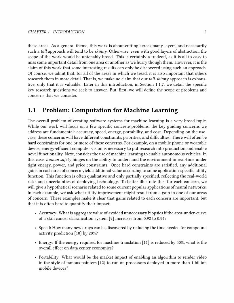
1.1.1 Example Task; Introduction to Concerns and ProblemsFor discussion and illustration, we introduce a machine learning task to use as a running example.
The task we choose is, given an input image, answer the question: “Is there a person in this
image?”
person-in-image? 0 person-in-image? 1
Figure 1.1: Two example input/output pairs for the person-in-image example task.
This specic example task, show in Figure 1.1, is a particular case of what is termed the imageclassication problem. In order to use a computer to perform this task, we require a computable
function that maps from images to a single Boolean value (i.e. person-in-image) that answers the
desired question. For simplicity, we will restrict our discussion here to stateless, deterministic
functions, as this is the common case in practice. In particular, we are interested in such functions
that arise in the context of using neural networks for machine learning problems such as our
example task.
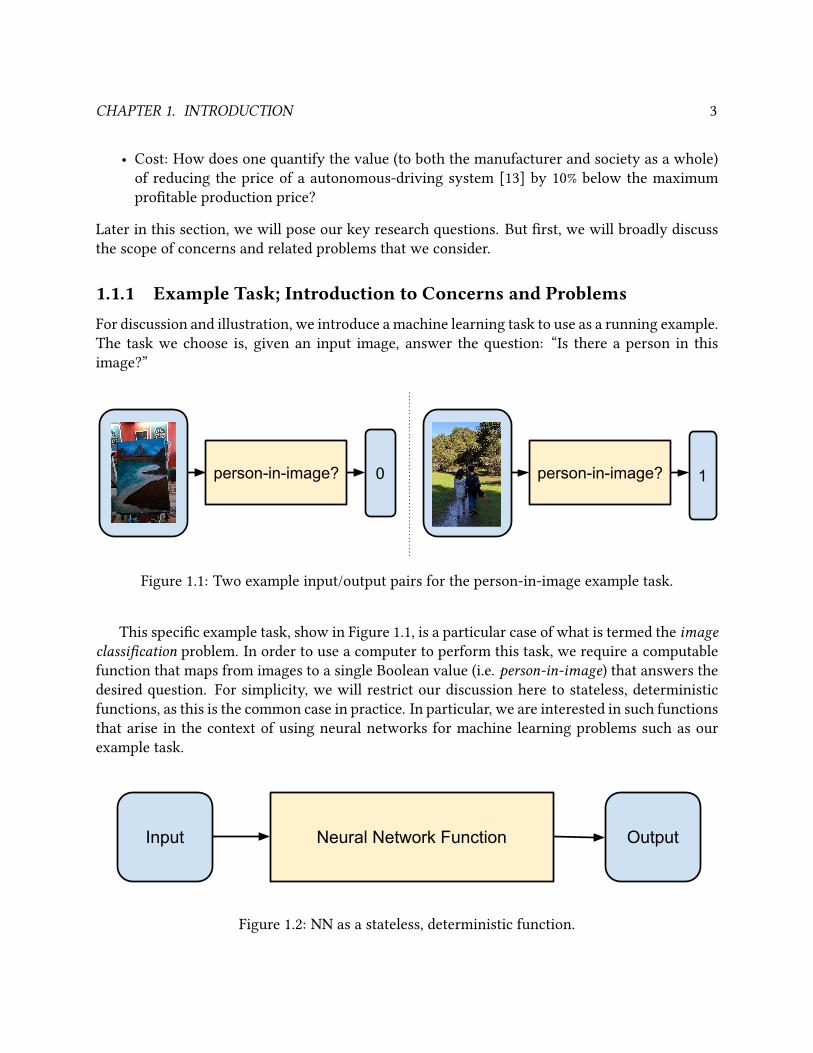
Neural Network FunctionInput Output
Figure 1.2: NN as a stateless, deterministic function.
CHAPTER 1. INTRODUCTION 4
In Figure 1.2, we illustrate this simple view of NNs, graphically showing the statementoutput =NNFunc (input ). The blue-rounded-rectangles denote values (each some xed, but unspecied
number of bits), and the yellow-squared-rectangle represents a function.
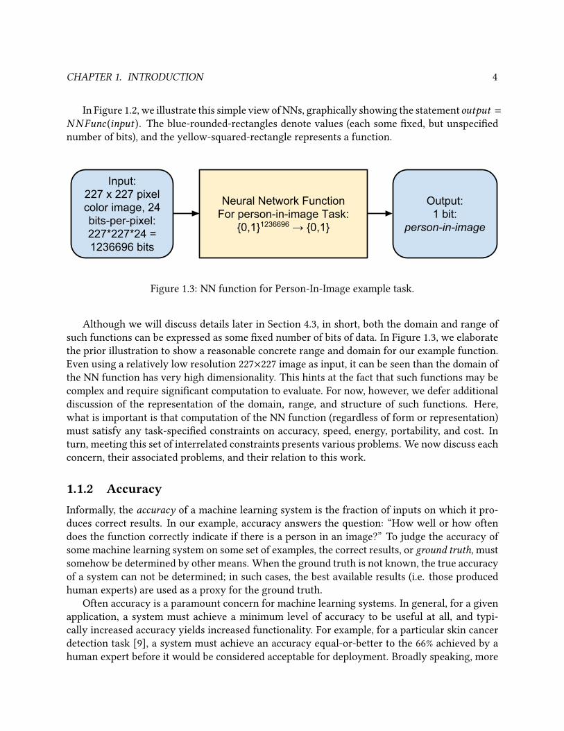
Neural Network FunctionFor person-in-image Task:
0,11236696 → 0,1
Input:227 x 227 pixel color image, 24 bits-per-pixel:227*227*24 = 1236696 bits
Output:1 bit:
person-in-image
Figure 1.3: NN function for Person-In-Image example task.
Although we will discuss details later in Section 4.3, in short, both the domain and range of
such functions can be expressed as some xed number of bits of data. In Figure 1.3, we elaborate
the prior illustration to show a reasonable concrete range and domain for our example function.
Even using a relatively low resolution 227×227 image as input, it can be seen than the domain of
the NN function has very high dimensionality. This hints at the fact that such functions may be
complex and require signicant computation to evaluate. For now, however, we defer additional
discussion of the representation of the domain, range, and structure of such functions. Here,
what is important is that computation of the NN function (regardless of form or representation)
must satisfy any task-specied constraints on accuracy, speed, energy, portability, and cost. In
turn, meeting this set of interrelated constraints presents various problems. We now discuss each
concern, their associated problems, and their relation to this work.
1.1.2 AccuracyInformally, the accuracy of a machine learning system is the fraction of inputs on which it pro-
duces correct results. In our example, accuracy answers the question: “How well or how often
does the function correctly indicate if there is a person in an image?” To judge the accuracy of
some machine learning system on some set of examples, the correct results, or ground truth, must
somehow be determined by other means. When the ground truth is not known, the true accuracy
of a system can not be determined; in such cases, the best available results (i.e. those produced
human experts) are used as a proxy for the ground truth.
Often accuracy is a paramount concern for machine learning systems. In general, for a given
application, a system must achieve a minimum level of accuracy to be useful at all, and typi-
cally increased accuracy yields increased functionality. For example, for a particular skin cancer
detection task [9], a system must achieve an accuracy equal-or-better to the 66% achieved by a
human expert before it would be considered acceptable for deployment. Broadly speaking, more
CHAPTER 1. INTRODUCTION 5
accuracy is always better, and each task will have some particular minimum-useful-accuracy and
accuracy-to-utility curve. See Chapter 12 of Deep Learning [14] for an overview of modern ma-
chine learning applications.
We will later provide minimal and sucient additional background details to concretely un-
derstand the concept of accuracy in machine learning as it applies to this work in Section 4.4. For
this work, we are mainly concerned with the more limited notion of maintaining accuracy. To
achieve this, it would be sucient to exactly compute whatever function we are given, in any way
we please. But, in practice, that condition is generally too constraining and impractical to strictly
satisfy. In particular, oating point arithmetic is approximate and does not yield equivalent re-
sults for dierent (but mathematically equivalent) orderings of operations. For more details on
oating point numbers and their issues, the reader is referred to Goldberg [15]. In part due to the
above issues with oating point, and more generally due to the diculty of program-equivalence-
checking [16] for numerical GPU programs, it does not seem practical to apply formal or other
methods to ensure general-case equivalence between algorithms. Thus, current practice is to
perform empirical accuracy evaluations on validation sets of inputs. Naturally, maintaining ac-
curacy on these sets is a necessary condition for doing so on all inputs. However, meeting only
this condition can lead to approximate or buggy algorithms with many types of intermediate
errors that do not happen to aect accuracy for the validation sets. As we will discuss in more
detail in Section 4.4.3, to use machine learning terminology, such results can be considered a type
of overtting. Since such problems are often due to real, signicant coding errors, it is clear that
it is undesirable for them to remain undetected. Such errors can cause rare random behavior,
crashes, or simply degrade the nal accuracy of any deployed system. Certainly, any methods
to help address this issue would improve development speed and overall software quality. Thus,
to the degree possible and practical, it is important to go beyond the necessary condition, and
attempt to at least approximately satisfy the sucient one. The key challenges are to:
• determine a good, suitable denition of approximate equivalence for NN functions, and
• develop methods to, with as much condence as is practical, verify such equivalence.
As a nal important note, any allowable compromises in accuracy often allow for signicant
improvements in all other concerns. However, in this work, we do not address the higher level
issues related to the design space of NN functions themselves. Other recent work gives these
issues a more comprehensive treatment [17].
1.1.3 SpeedThe time taken to process an image, or the speed of computation, is clearly an important prac-
tical consideration in all cases. In particular, in deployment use cases such as autonomous driv-
ing [13], systems such as pedestrian detection must run at real-time rates of at least 25 frames-per-
second [18]. However, exactly what level of speed is acceptable can vary considerably between
use cases. Of particular note is the dierence between training (creating new per-task functions)
CHAPTER 1. INTRODUCTION 6
and testing or deployment (using an already-created function for its intended task) use-cases,
which we explain in detail in Section 4.5.
A core freedom of algorithmic optimization is that, as long as the desired function is computed
correctly-enough, one is free to use any algorithm to do so. And, some algorithms can compute a
given function faster than others, yielding dierent levels of speed. In short, this is due either to
doing less work, or being able to do the same work more eciently on a given hardware target.
In this work, we mostly focus on the computational eciency aspect: doing the same set of work
faster. In this case, we treat the work to do, or set of computations, as relatively xed. The goal is
to organize the computation so it is well suited for a given device. So, for a given hardware target,
limited to the scope we consider, speed and computational eciency are mostly equivalent. For
a xed level of accuracy and xed general family of hardware targets, speed is typically tightly
coupled via tradeos to cost and energy. In particular, higher speed can often be traded o for:
• lower cost: by using a smaller/less-capable device of a similar type.
• lower energy: by running a device in a slower, but more energy ecient mode.
Due to these interrelations, we defer detailed discussion of the current problems with achieving
reasonable eciency until we have nished introducing all the remaining concerns. But in sum-
mary, getting reasonable speed/eciency for any given hardware target is a dicult, core problem
we address in this work. Currently, vendors appear to struggle greatly to achieve reasonable ef-
ciency for NN computations. They incur delays of many real-time years, and costs of dozens
of sta-years, to deliver inconsistent levels of support for NN computations. Thus, any methods
that reduce the latency and eort required to create complete, reasonably ecient systems to
support NN computations have immediate, clear value.
1.1.4 EnergyFirst, for completeness, we note that energy (e.g. Watt-hours or Joules) is power (e.g. Watts) inte-
grated over time. At a high level, energy is a simple concern: energy usage is always constrained,
and any computation must meet these constraints. In particular, as forecast over a decade ago,
power usage currently limits performance at all levels of computing [19]. From individual pack-
aged integrated circuits, to mobile devices, and up to entire datacenters, power usage bounds the
amount of parallel computation that is possible. For example, a typical smartphone has a bat-
tery that can hold 5 Watt-hours of energy, and can comfortably dissipate 1W on average [20].
This nite battery capacity places hard limits on the aggregate energy budget available for ma-
chine learning tasks between battery charges. For the Qualcomm Snapdragon 820, we bench-
marked that the GPU can achieve around 80 GFLOPS for single-precision matrix-matrix multiply
(SGEMM), using about 3W [21]. Given that such devices are generally hand-held, this repre-
sents close to the maximum reasonable sustained power dissipation achievable without burning
users. But, compared to the 3000 GFLOPS of SGEMM performance from a 235W NVIDIA K40m
GPU, this is clearly signicantly less available computing capacity [22]. And, even for the K40m,
CHAPTER 1. INTRODUCTION 7
performance is limited by power; these cards are designed to dissipate the maximum allowable
power for the servers in which they are typically installed.
Also, for datacenters, energy cost is a signicant component of total operating costs [23]. In
general, any methods that directly or indirectly yield lower energy usage for NN computations
will provide real and immediate benets on both mobile and server platforms. While we do not
attempt to comprehensively address the concern of energy in this work, there are several key
points to mention here. In particular, we nd a key empirical observation: for a given target,
more computationally ecient algorithms seem to always also be more energy ecient as well
(see Section 2.6). There are several intuitive reasons why this is sensible:
• Compute hardware has idle power : power usage that is weakly or not dependant how much
work is being done at any moment. Reducing runtime directly reduces energy used due to
this idle power.
• Often, given that the work to do is xed, the key reason one algorithm is faster than another
is that it performs less (or more ecient) communication. Since communication costs both
time and energy, avoiding it via better data reuse (or better data transfer) saves both.
So, in this work, our focus on good computational eciency conveniently also tends to yield
good energy eciency. However, note that tradeos between energy and speed might be quite
dierent on hardware outside the scope we consider here.
1.1.5 PortabilityFor software to be portable, it must run on multiple targets. Of course, if one could simply pick any
hardware device to use for each application, portability might be unnecessary. However, in gen-
eral, one does not have free choice of hardware platform. As discussed in detail in Section 1.2.3,
business needs, relationships, and strife (litigation) can limit choice of hardware platform and
thus provide critical motivation for having portable software. Specically, on each target, the
software must meet any constraints on accuracy, speed, energy, and other concerns. If only some
constraints are met, then we say the software is partially portable to that target. In particular:
• If constraints on accuracy are met, we term this functional portability. Strictly, functional
portability implies that a function should yield exactly the same result across targets. How-
ever, as discussed earlier, issues related to oating point arithmetic mean this is often not
strictly true, and we must settle for approximate agreement of results and intermediates.
• If constraints on speed are met, we term this performance portability. Often, in this case,
we are more concerned with compute and/or energy eciency, rather than absolute speed,
in order to normalize across absolute dierences in the computational capability of various
devices.
Currently, for NN computations on GPUs, portability is dicult to achieve. Firstly, even func-
tional portability can be dicult to achieve. Dierences in programming models, languages, and
CHAPTER 1. INTRODUCTION 8
use of target-specic features often preclude running code for one target on another. For exam-
ple, code written using NVIDIA’s proprietary programming model (CUDA) can only be run on
NVIDIA devices. Similarly, code written using recent versions of the competing industry stan-
dard programming model (OpenCL 2.0) can only be run on the hardware of the few vendors that
support it. This includes AMD and Qualcomm, but notably does not include NVIDIA. Then, even
when code is functionally portable, performance portability, for the types of NN computation al-
gorithms we consider, is simply absent. That is, ecient algorithms for one target are much less
ecient on others, as shown for example in our own results for NN computations in Section 6.4.
Typically, this is due to the fact that, for current GPU targets, computation and data movement
must be explicitly and carefully orchestrated in target-specic ways to achieve eciency [24].
In summary, it appears that the current set of layered abstractions employed on modern GPUs,
from hardware to compiler, simply do not enable performance portability for NN computations.
One might ask, why not simply deal with each hardware target separately to avoid portabil-
ity issues? In short, there are many downsides to reimplementing NN computations for every
target. At a high level, the notion of portability is only a means to an end: lowering development
costs. Development costs have various components; for example: initial development, testing,
and maintenance. Portability aims to reduce the aggregate time and eort spent on each of these
components across multiple targets compared with per-target development. Both initial devel-
opment and maintenance may require very skilled, scarce programming sta resources. Thus, if
portable approaches are feasible, supporting many targets via redundant eort is at best wasteful
of scarce resources and at worst impossible. Further, separate per-target implementations com-
plicate testing. If a high degree of condence of consistency and/or correctness across targets is
required, testing may become extremely time consuming.
Beyond simply increasing the development costs of implementing NN computations across
many targets, a lack of portable NN-computations impedes development at the application level
as well. In practice, the bulk of high-performance, high-eciency NN computation code cur-
rently resides inside highly tuned libraries. Such libraries are generally tuned for only a small
subset of targets – typically only those from a single vendor. As these libraries are developed
independently, they are often incompatible and support dierent sets of operations. Some plat-
forms might not even have NN computation libraries at all. And, even when a particular set of
operations is supported across some set of targets, per-operation relative speed can vary consid-
erably across platforms, making it dicult to portably meet application-level speed constraints.
These libraries are also generally dicult or impossible to extend, especially if it is desired to
support multiple targets at the application level.
In summary, an open, portable approach to implementing NN computations would help en-
sure compatibility and functional correctness across all platforms, both existing and new. Fur-
ther, such approaches encourage collaboration, which in turn helps ease both extensibility and
the ability to eciently target new hardware platforms. Finally, at the application level, having
a uniform interface and set of NN operations across targets would oer considerable portability
advantages.
CHAPTER 1. INTRODUCTION 9
1.1.6 CostThe cost of deploying an application on a given target has various components. Firstly, there is
the monetary price per unit for the needed hardware. In general, more capable hardware is more
expensive, because it requires:
• utilization of more silicon area (i.e. larger integrated circuits, which cost more to produce),
and/or
• fabrication in later, more expensive semiconductor process generations.
The more memory and processing power that is needed, the bigger and more costly the needed
computing hardware will be. In turn, this directly aects the nal physical size and cost of the
overall deployed system. To illustrate this, consider two similar NVIDIA GPUs, the GTX 1080
Ti and GTX 1060. They are both quite suitable for machine learning computations, and retail
for ∼$700 and ∼$250 respectively [25]. The GTX 1080 Ti oers a peak of 11.3 TFLOPS of single-
precision performance using 250W, whereas the GTX 1060 oers 5.1 TFLOPS using 120W [26].
Thus, at 45.2 and 42.5 GFLOPS/Watt respectively, and these products oer similar capabilities
per unit power. However, at 16.1 and 20.4 GFLOPS/$, the GTX 1060 has a signicant relative
advantage in terms of computation rate per dollar, and of course a much lower absolute cost.
So, the less ecient the software implementation of a given task is, the more that will have
spent on computing hardware to achieve a given level of speed. Conversely, increased speed
can also enable cost reduction by the same reasoning. So, enabling higher speed on one target,
or in particular higher energy or computational eciency, may enable choosing a lower-cost,
less-capable computing platform.
Also, there may be direct or indirect costs and risks associated with using a particular tar-
get. For example, there may be long-term legal or supply uncertainties associated with a given
vendor. Thus, portability is a key enabling force to reduce cost in the long term, via choice and
competition. Overall, our focuses on speed and portability in this work are natural enablers for
lower cost deployments.
1.1.7 Key Research QuestionsIn general, for all the concerns we have listed, it is easy to do well in one area of concern at
the expense of all others. Complementarily, experience has shown that it is simply not feasible
to achieve the state-of-art with respect to each concern simultaneously. So, naturally, the key
research questions we ask involve combinations of all our concerns. However, attempting to
consider all feasible design points with respect to our concerns would be an overwhelmingly
broad task. So, based on our above analysis, we choose to reduce the dimensionality of the design
space that we will consider:
• Accuracy: As mentioned in Section 1.1.2, we will focus on maintaining accuracy. Hence,
all scenarios we consider treat accuracy as xed, and we seek neither to improve accuracy
nor to make gains in other concerns by compromising it.
CHAPTER 1. INTRODUCTION 10
• Speed/Energy: As mentioned above in Sections 1.1.3 and 1.1.4, we simplify the space by
using computational eciency as a proxy for speed and energy.
• Portability: As will be discussed in Section 1.2, we constrain the scope of our eorts by
focusing on a specic type of computation hardware: GPUs.
• Cost: As discussed in 1.1.6, improvements in both portability and eciency can be realized
as improvements in cost, or at least as insurance to reduce the risk of incurring various
possible costs. We decompose cost into development costs (addressed by portability) and
deployment costs (addressed by eciency).
So, with this sharper focus, the main axis of our work becomes the tradeo between eciencyand portability for (correctly) implementing computations on GPUs. Then we ask, along this axis,
how much improvement over the state of the art is possible? As will be discussed in Section 1.2,
current practice heavily favors high eciency at the expense of portability. Specically, in Sec-
tion 1.2.2 we discuss how high eciency GPU implementations of NN computations require real-
time years of eort by teams including key, rare individuals. At the other end of the axis, there are
techniques that are somewhat portable, but commonly yield ∼25% or lower eciency [27]. Fur-
ther, even these portable approaches depend on the existence of optimized numerical libraries
for each platform. For NN computations, as we will discuss in Section 5.1, serial computation is
impractical, and ecient automated parallel compilation is absent. Hence, if a target lacks such
libraries, there is no practical fallback method for NN computations. Considering this state of
aairs, what is missing is an exploration of the middle region of the eciency/portability axis for
NN computations on GPUs.
But, in the end, what are reasonable eciency goals for code running on GPUs? Consider the
NVIDIA K40m (from the Kepler generation of NVIDIA hardware architectures), which has a peak
compute rate of 4.29 TFLOPS. In a detailed experiment, Nugteren [28] implements many itera-
tions of matrix-matrix multiplication (SGEMM) on this hardware, using both OpenCL and CUDA,
incrementally adding known optimizations. Their naive, initial version of SGEMM achieves only
∼3% eciency. Eventually, they achieve 36% eciency with their best version, using CUDA C. For
comparison, NVIDIA’s own cuBLAS library can do signicantly better, achieving ∼70% eciency
for matrix-matrix multiply (SGEMM) on this hardware, but still cannot reach 100% eciency, per-
haps due to fundamental limitations of the Kepler GPU architecture. Although it is application
dependant, our general engineering judgment based on our experience with GPU programming,
reinforced by vendor documentation on best practices [29], yields the following rules of thumb
for computational eciency on GPUs:
• Naive code is expected to yield <5% eciency.
• Achieving ∼30%-60% eciency is generally considered quite reasonable or good.
• Achieving more than 60% eciency often requires extreme measures, such as using assem-
bly language.
CHAPTER 1. INTRODUCTION 11
Note that the optimizations used in the above experiment (which targeted only a single input size
for SGEMM, N=2048) were developed over many years, and require continual adjustment for new
GPU architectures. Clearly, achieving even reasonable performance requires signicant manual
eort.
So, this suggests the following key research questions:
• Is possible to reduce the time taken to implement ecient neural net computations on new
GPU platforms from years to months?
• If so, for platforms where they apply, can we improve on the eciency of existing portable
(numerical library-based) approaches by at least 2X? That is, can we achieve ∼50% e-
ciency, which is generally about the best that can be expected for GPU code, short of using
assembly language?
• Then, for platforms with no libraries to build upon or compare with, can we achieve at least
25% eciency? This represents the low end of the expected eciency of optimized GPU
code, but is at least 5X better than what would be expected from naive code.
• In order to maintain accuracy during implementation and optimization, can we fully auto-
mate continuous numerical regression testing of NN computations for full ows with full
inputs?
In the immediately following section (Section 1.2), we raise further considerations with regard
to the use of GPUs for NN computation. Those wishing to immediately review our research
trajectory can skip ahead to Section 1.3.
1.2 We Focus on GPUs for NN ComputationModern Graphics Processing Units (GPUs) oer a tantalizing combination of general programma-
bility, high peak operation throughput, and high energy eciency. Due to this, GPUs are cur-
rently the dominant style of hardware used for NN computations. However, despite increasing
hardware exibility and software programming toolchain maturity, high eciency GPU pro-
gramming remains dicult. GPU vendors such as NVIDIA have spent enormous eort to write
special-purpose NN compute libraries. However, on other hardware targets, especially mobile
GPUs, such vendor libraries are not generally available. But, for the broad deployment of NN-
based applications, it is necessary to support many operations across many hardware targets.
Thus, the development of portable, open, high-performance, energy-ecient GPU code for NN
operations would enable broader deployment of NN-based algorithms.
CHAPTER 1. INTRODUCTION 12
1.2.1 Details of Current Approaches to NN Computation and TheirDeciencies
Considering all the interrelated concerns we will balance in this work, we now focus in more
detail on the problems associated with implementing computation for neural networks. Later, in
Section 4.3 we will provide more details on the exact details of NN computation we consider. Here,
we provide a general overview of the scope of the problem, current approaches to it, and their de-
ciencies with respect to the above concerns. As mentioned, GPUs are well suited to, or perhaps
have enabled, modern NN-based applications [30],[31]. Further, neural networks are emerging
as the primary approach for challenging applications in computer vision, natural language pro-
cessing, and human action recognition [7]. Originally, NN researchers leveraged existing dense
linear algebra (BLAS) libraries [22],[32] for NVIDIA GPUs to perform the bulk of computation.
The landmark BLAS-based NN implementation from Krizhevsky, cuda-convnet, was released in
2012-12 [30]. At the time, this approach oered a level of NN compute performance that far out-
paced any other commonly available CPU or GPU computing platform. In Section 6.2.3, we will
discuss in more detail the history that lead to NVIDIA’s dominant position in this area. But, look-
ing toward the future from that time, increasing attention has been given to pushing the envelope
of ecient GPU implementations of NN computation. Over several years, it became clear that,
rather than layering on BLAS libraries for NN computation, much more ecient special-purpose
libraries were possible. Yet, even given the high level of interest in the domain, and the signicant
speedups that were possible, the availability of such a library from NVIDIA took years. The rst
ocial release of NVIDIA’s NN computation library cuDNN [33] was not until 2014-09. Given
that, at a high level, the cuDNN library is only a special-case optimization of a few modestly
generalized BLAS functions, why did it take almost 2 years to release? To answer this question,
we must consider the current state of high-performance, high-eciency numerical programming
for GPUs. Then, we will consider if this state is desirable or acceptable, and what alternatives
might exist.
1.2.2 GPU Programming for Numerical ApplicationsGPUs oer a large amount of potential performance, but it is often not easily accessible. As a case
study, consider the development of the cuBLAS library. Early versions (up to 1.2) of the cuBLAS
library, released in 2007, could only achieve about 35% of the peak available computation (or 35%
computational eciency) for matrix-matrix multiplication on the hardware of that time. By 2008,
research eorts were able to greatly improve on this, with Volkov achieving >90% computational
eciency [34]. These improvements were subsequently integrated into cuBLAS, yielding the
tuned, performant library used by Krizhevsky for NN computations in 2011. Although details
are not public, it seems likely that cuDNN development followed a similar pattern. In 2011, re-
search by Catanzaro and co-authors demonstrated advanced techniques for high-eciency GPU
programming [35]. From that time until 2014, Catanzaro was employed by NVIDIA, roughly co-
inciding with the development timeframe of cuDNN. In both the case of cuBLAS and cuDNN, it
seems development required long-term eorts by key, perhaps nearly uniquely qualied, indi-
CHAPTER 1. INTRODUCTION 13
viduals to achieve good results. In short, only a very small number of programmers are capable
and willing to map new applications to GPUs, and even then the process often suers from high
complexity and low productivity. So, considering this, it is no surprise that the development of
cuDNN took almost 2 years. Thus, in practice, the bulk of high-performance, high-eciency
GPU code resides inside highly tuned, costly to develop libraries for a few specic task/platform
combinations.
1.2.3 Why not just use NVIDIA/cuDNN?Imagine that, for a given task, a high-performance vendor library exists for at least one platform.
Currently, for NN computation, that vendor is NVIDIA and the library is cuDNN [33]. So, why
not simply use NVIDIA’s platform and libraries for all NN computation applications and be sat-
ised? One reason is quite simple: in industrial use cases, choice of platform may be dictated
by business concerns. Further, those same business concerns may preclude dependence on any
single vendor. For example, the agship Samsung Galaxy S7 mobile phone shipped in two ver-
sions: one using a Samsung-proprietary Exynos 8890 System-on-Chip (SoC), the other using the
Qualcomm Snapdragon 820 [36] SoC. Neither of these SoCs contains NVIDIA GPUs or are other-
wise capable of running cuDNN. Further, NVIDIA, Qualcomm, and Samsung have engaged in a
long running patent dispute over GPU technologies. Based on the uncertainties associated with
such litigation, SoC and/or GPU alternatives are subject to constant change. Further, even once
a hardware platform is chosen, business needs may dictate the specic software tasks that must
be supported. Any research or practical application that requires operations that the vendor is
not willing or able to support in a timely manner will suer. Together, these uncertainties about
both target hardware and particular use-case create a strong pressure for portability: the ability
to quickly achieve reasonably performance for a variety of tasks across a variety of platforms. In
Section 6.2.4, we will discuss in more detail the issues of reliance on hardware vendors for NN
computation libraries. For now, the key point is that there are clear reasons to, at a minimum,
have reasonable alternatives to such reliance.
1.2.4 What would be the ideal situation for NN Computation?A key assertion of this work is as follows: To support ongoing research, development, and de-
ployment of systems that include NNs, it is desirable to nurture a diverse enabling ecosystem
of tools and approaches. In particular, it is desirable to support many hardware and software
platforms to enable new applications across many areas, including mobile, IoT, transportation,
medical, and others. Consider a use-case consisting of a specic combination of:
• a target computational device (i.e. a hardware architecture), and
• a graph of neural network primitives (i.e. a NN for some task).
Using existing common general-purpose computational primitives and libraries (e.g. BLAS) gen-
erally achieves only limited eciency [27]. Improving on such approaches requires tuning use-
CHAPTER 1. INTRODUCTION 14
case specic computational kernels for the desired target. Further, reliance on special-case tuned
vendor libraries is not always possible or desirable. In particular, for new uses cases, achieving
good computational eciency and/or meeting particular performance requirements is, in gen-
eral, dicult. As previously discussed, such eorts require months, or even years, of eort led
by very specialized programmers. Such programmers must be both capable of producing high-
eciency code for the target platform as well as being familiar with the details of the needed NN
computations. Such programmers are not common and thus their time is a very limited resource.
Ideally, tools and frameworks would exist to amplify the eorts of such programmers, helping
them easily tune multiple operations across multiple targets. Such a framework should address
all the concerns we have discussed. It should:
• Help maintain accuracy and correctness, the cornerstones of any robust NN computation
system.
• Achieve reasonable speed and eciency for all desired targets, as needed by use-cases.
• Enable portability, to reduce duplicated eorts (and thus development costs) across targets.
• Aid in meeting constants on energy and power usage.
• Oer paths to reduce the nal cost of deployment.
1.3 Specic Motivating Problems and Trajectory ofResearch
Neural networks are currently the dominant approach for many machine learning tasks. Further,
GPUs are the most common type of computing platform on which they are currently run. Hence,
addressing the above concerns when running NNs on GPUs is the focus of the framework that
represents the culmination of this work. However, our research trajectory began before neural
networks became dominant, and the basic concerns we address apply to both other machine
learning approaches and other target hardware platforms. In this section, we give an overview of
the two specic problems we addressed in our earlier research. These works served an important
role in dening and shaping the research trajectory that led to our key research questions and
our nal results. Then, to conclude this section, we briey discuss our observations on how the
modern rise of neural networks in machine learning has changed the landscape of implementing
machine learning computations.
1.3.1 Speed and Energy Ecient Histogram-of-Oriented-GradientsCalculations: libHOG
Prior to the widespread adoption of NNs for object detection, calculation of hand-designed fea-
tures such as Histograms-of-Oriented-Gradients (HOG) was commonly the rst step in machine-
CHAPTER 1. INTRODUCTION 15
learning pipelines operating on images. Even now, HOG features remain attractive in some sce-
narios due to their easily understood semantics and ease of computation. The initial motivation
for the nal proposed framework of this dissertation was rooted in our experience addressing
our core concerns for the task of computing HOG features on CPUs. While we achieved good
results in this work, various challenges we encountered highlighted opportunities to improve the
development process for such tasks. In particular, even though the scope of the task was rela-
tively small, writing and testing the relevant highly-tuned CPU code was very time consuming.
Further, deploying the resulting code in a form usable by the machine learning community was
problematic. Both the contributions of this work and the way in which it motivated our later
work will be discussed in Chapter 2.
1.3.2 Speed and Energy Ecient Dense, Multiscale ConvolutionalNeural Net Features: DenseNet
The rst task at which NNs rose to dominance in the modern era was image classication (as in
our example task). At that time, it was natural to attempt to leverage and extend image classi-
cation NNs to the more dicult task of object detection. For object detection, the task is not
simply to determine if a given type of object is in an image, but to localize all objects (of some
type) within an image.
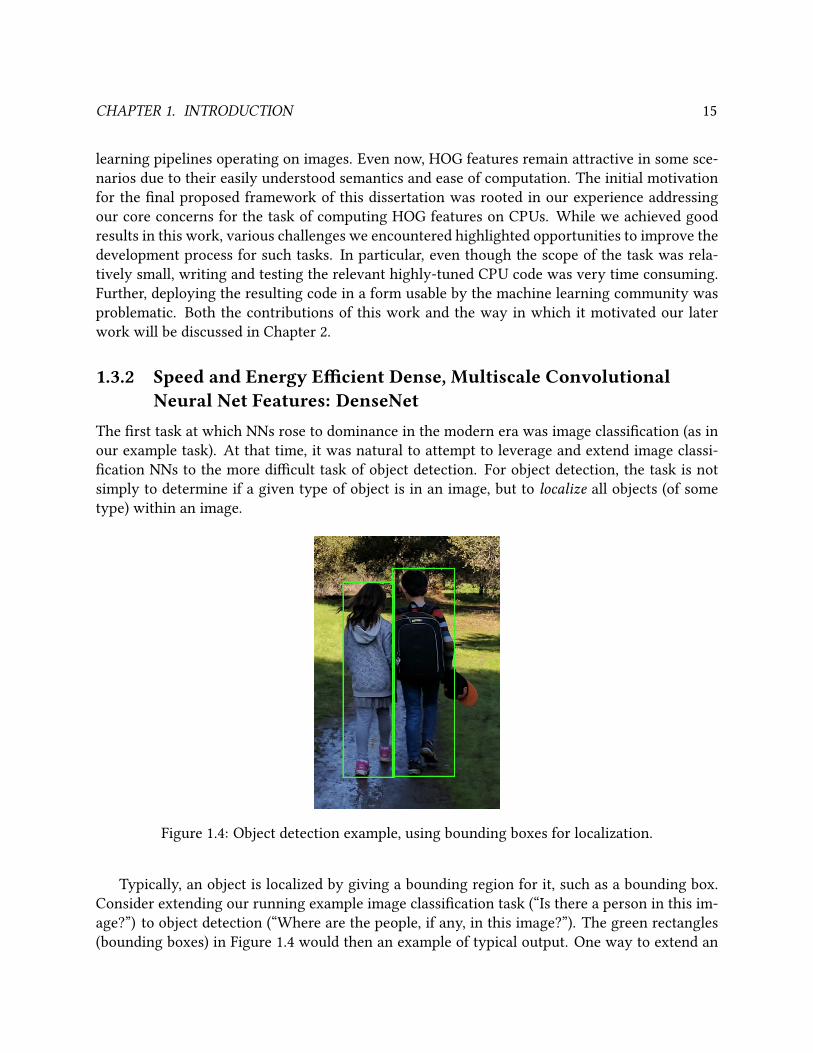
Figure 1.4: Object detection example, using bounding boxes for localization.
Typically, an object is localized by giving a bounding region for it, such as a bounding box.
Consider extending our running example image classication task (“Is there a person in this im-
age?”) to object detection (“Where are the people, if any, in this image?”). The green rectangles
(bounding boxes) in Figure 1.4 would then an example of typical output. One way to extend an
CHAPTER 1. INTRODUCTION 16
image classication method into an object detection method is to apply the classier at every re-
gion in the image that might contain an object. However, this method is prohibitively expensive
when applied to NN-based classiers. To reduce the overhead of this method, approaches such
as R-CNN [37] applied the NN-based classier only at a sparse set of object proposal regions from
the original image. However, such approaches were, while tractable for research, still quite com-
putationally intensive and too slow for use in various real-world applications. In our DenseNet
approach, we leveraged the fact that, even when object proposal regions are sparse, they share
much overlapping area. Thus, in our approach, we could calculate dense, multiscale NN features
for the entire input image in ∼1s. This is 10X faster than the time taken to evaluate the same fea-
tures for 2000 individual regions, as needed for approaches like R-CNN. This work is discussed
in detail in Chapter 3.
Unlike our prior work with libHOG, the DenseNet library focused more on issues of integra-
tion rather than tuning specic computations. While we achieved good results, the experience
of creating DenseNet highlighted certain problems related to integrating NN computations into
complex machine learning ows. In particular, it was dicult to cleanly encapsulate DenseNet
into a broadly usable library. The core calculations could be exposed fairly easily: the input
was the desired image for which to calculate features, and the output was a pyramid of dense-
NN-feature images, with one image per desired scale (i.e. a dense multiscale feature pyramid).
However, the mapping from regions in the original image to regions in the dense feature space
was complex and dependant on the specic NN that was used to generate the features. This
complicated both correctness testing of DenseNet as well as usage in existing machine learning
pipelines. This motivated a more holistic approach, where all stages of the pipeline could be
integrated within a single framework. In such a framework, issues related to mapping regions
between input and feature space (for localization) could be handled correctly and consistently
across pipeline stages. To experiment with this idea, we re-implemented DenseNet inside a pro-
totype vertical framework that included support for input, output, correctness testing, and visual
demonstrations. In this framework, we were able to perform extensive correctness testing that
was not possible in the prior implementation. It was indeed much easier to correctly manage
issues of input-to-feature-space conversions once all stages of the pipeline were contained in a
single framework. The key overall idea was that, even if such a framework would not generally
be used by machine learning researchers, it provides key benets to those that need to imple-ment the core operations needed for machine learning. That is, at the time, there was no exist-
ing platform suitable for the development and testing of libraries like DenseNet. Our prototype
framework proved the idea that it was indeed possible to rectify that lack of suitable platform.
Going forward, this prototype framework formed the foundation for the culminating project of
this dissertation.
CHAPTER 1. INTRODUCTION 17
1.3.3 The Eect of the Rise of Neural Networks on ResearchImplementations
As NNs have become more dominant in machine learning, a general shift in approach has become
evident. In the past, machine learning pipelines were often comprised of many dierent types of
operations, composed in an ad-hoc manner. For example, when working on libHOG, we observed
this pattern in DPM-based object detection ows [38]. Then, when working on DenseNet, we
observed this again when analyzing the implementation of R-CNN [37]. Dierent pipeline stages
were often implemented in dierent languages and frameworks. Then, stages were simply glued
together in whatever manner was expedient for research. Thus, optimization, testing, and real-
world deployment of such ows was quite problematic. Optimizing each individual stage would
potentially require re-implementation in high-performance languages. Worse, eciently gluing
together existing stages together could sometimes be intractable due to diering languages, data
formats, and approaches to parallelism. Often, the only feasible approach was to re-implement
many pipeline stages together into a new, cohesive ow, where all stages could be optimized and
tested together for a particular hardware target.
At the same time, we observed that NNs were replacing stage after stage in many ows.
Eventually, the state of the art for many tasks consisted of either one or several NNs with few
other types of operations [4]. Currently, progress for many machine learning tasks is achieved by
nding new types or structures of NNs rather than using new algorithms or approaches. Thus,
support for NN computation is increasingly important. Further, in the past, supporting ecient
computation for a single type of machine learning primitive could have only limited overall use-
fulness, since state-of-the-art machine pipelines would generally involve using many type of
operations. Now, however, just supporting ecient NN computations can be a key enabler for
overall ecient research and practical deployment. This motivates the culminating eort of this
work, our proposed framework for implementing ecient neural network computations, as dis-
cussed in Chapter 6. In the following, we briey introduce our proposed framework and how
we will use it to address our concerns and, though its development, answer our key research
questions.
1.4 Solution for implementing NN Computations: TheBoda Framework
After our work on libHOG and DenseNet, we considered all our concerns in the context of NN
computations. Then, with our key research questions in hand, we began work on the culminating
project of this dissertation, the Boda framework. Boda is an open-source, vertically-integrated
framework for developing and deploying NN computations. While we will discuss our approach
in more detail in Chapter 6, we give a brief introduction here.
CHAPTER 1. INTRODUCTION 18
820
Figure 1.5: Boda Framework Overview: Portable Deployment of NNs
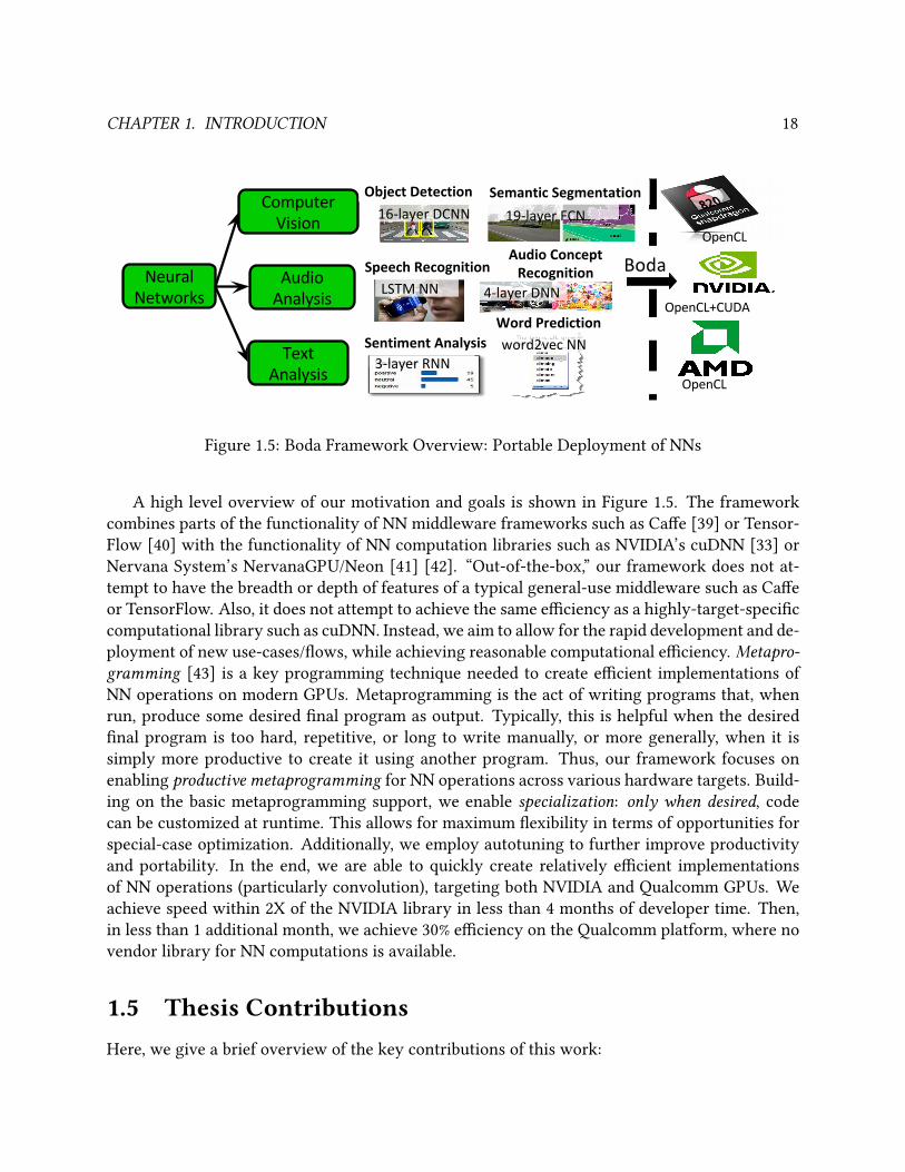
A high level overview of our motivation and goals is shown in Figure 1.5. The framework
combines parts of the functionality of NN middleware frameworks such as Cae [39] or Tensor-
Flow [40] with the functionality of NN computation libraries such as NVIDIA’s cuDNN [33] or
Nervana System’s NervanaGPU/Neon [41] [42]. “Out-of-the-box,” our framework does not at-
tempt to have the breadth or depth of features of a typical general-use middleware such as Cae
or TensorFlow. Also, it does not attempt to achieve the same eciency as a highly-target-specic
computational library such as cuDNN. Instead, we aim to allow for the rapid development and de-
ployment of new use-cases/ows, while achieving reasonable computational eciency. Metapro-gramming [43] is a key programming technique needed to create ecient implementations of
NN operations on modern GPUs. Metaprogramming is the act of writing programs that, when
run, produce some desired nal program as output. Typically, this is helpful when the desired
nal program is too hard, repetitive, or long to write manually, or more generally, when it is
simply more productive to create it using another program. Thus, our framework focuses on
enabling productive metaprogramming for NN operations across various hardware targets. Build-
ing on the basic metaprogramming support, we enable specialization: only when desired, code
can be customized at runtime. This allows for maximum exibility in terms of opportunities for
special-case optimization. Additionally, we employ autotuning to further improve productivity
and portability. In the end, we are able to quickly create relatively ecient implementations
of NN operations (particularly convolution), targeting both NVIDIA and Qualcomm GPUs. We
achieve speed within 2X of the NVIDIA library in less than 4 months of developer time. Then,
in less than 1 additional month, we achieve 30% eciency on the Qualcomm platform, where no
vendor library for NN computations is available.
1.5 Thesis ContributionsHere, we give a brief overview of the key contributions of this work:
CHAPTER 1. INTRODUCTION 19
• First, we developed libHOG [44], a library which implements ecient calculation of HOG
features on CPUs using SIMD parallelism. We achieved a 3X speedup over the state of the
art at that time.
• Then, we enabled previously prohibitively slow multiscale sliding window object detection
using dense convolutional neural network features inDenseNet [45], yielding a 10X or more
speedup over existing approaches.
• Finally, in our Boda framework, we explore in depth the development of ecient NN con-
volution operations across various types of hardware. With less than 4 months of eort, we
achieve speed within 2X of the highly-tuned vendor library on NVIDIA GPUs. With less
than a month of additional eort, we achieve up to 30% eciency on Qualcomm mobile
GPUs, where vendor libraries remain unreleased [46] [47]. In both cases, we provide both
details on our implementation and experimental results.
Now, we briey explain the overall outline of this work.
1.6 Thesis OutlineThe rest of this work is organized as follows:
• In Chapter 2, we discuss libHOG, a library for eciently computing Histogram-of-Oriented-
Gradient features, which provided initial motivation and direction to our work.
• In Chapter 3, we discuss DenseNet, a library for extracting dense, multiscale neural network
features. After the initial implementation of DenseNet, we then created a prototype of our
Boda framework as a proof-of-concept development aid.
• In Chapter 4, we review various background details concerning machine learning and nu-
merical computation as are relevant for ecient computation for neural networks.
• In Chapter 5 we review the related work for the core problems we address in Boda, including
various NN frameworks and computation libraries.
• In Chapter 6 we detail our culminating eort, our proposed Boda framework for eciently
implementing NN computations.
• Finally, we review the key conclusions of our research in Chapter 7.
20
Chapter 2
Motivating Early Work : libHOG
2.1 IntroductionNow, we discuss the development of libHOG, work that occurred early in our exploration of
computational eciency in computer vision. The motivating application for this work was ob-
ject detection using a technique called Deformable Parts Models or DPMs [38]. At the time, such
approaches were state of the art in terms of accuracy, but were also typically too slow and en-
ergy/compute intensive to consider using in practical embedded applications. So, with the end
goal of speeding up such ows, we performed performance analysis on a reference DPM-based
object detection ow. We found that one particularly slow and energy/compute intensive part of
the ow was the calculation of Histogram of Oriented Gradients (HOG) features from the input
image. We then used various techniques to optimize this portion of the ow. Further, along the
way, we encountered various issues that would inform our future work.
The rest of this chapter is organized as follows. First, in Section 2.2, we briey describe HOG
features and motivate our work. In Section 2.3, we survey other HOG computation methods
from the related literature. In Section 2.4 we review the general procedure for calculating HOG
features. In Section 2.5 we describe how we accelerate HOG computation. In Section 2.6, we
evaluate the overall speed and energy of libHOG and the accuracy of an object detector using
libHOG. Finally, in Section 2.7, we conclude with a summary of our contributions, a discussion of
issues that arose during our eorts, and our conclusions on them that informed our future work.
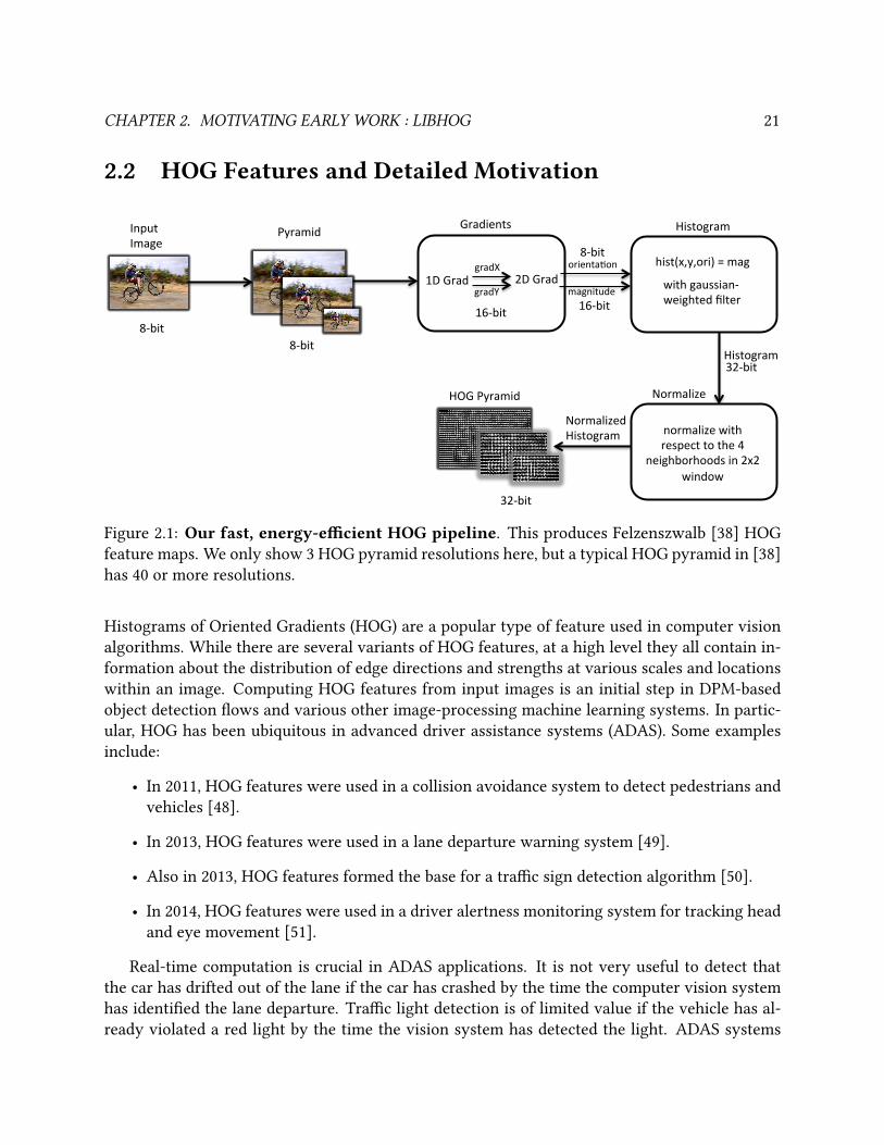
CHAPTER 2. MOTIVATING EARLY WORK : LIBHOG 21
2.2 HOG Features and Detailed Motivation
UC Berkeley
2"
End$to$end(pipeline(
Forrest"Iandola""""""""""""""""forres/@eecs.berkeley.edu"
88bit"88bit"
Input"Image"
Pyramid"Gradients"
1D"Grad"gradX"
gradY"
168bit"
TODO:"8 picture"of"gradX,"gradY"8 picture"of"magnitudes"
2D"Grad"orienta/on"
magnitude"168bit"
88bit"
Histogram"
hist(x,y,ori)"="mag"
328bit"Histogram"
with"gaussian8weighted"filter"
Normalize"
normalize"with"respect"to"the"4"
neighborhoods"in"2x2"window"
328bit"
Normalized"Histogram"
HOG"Pyramid"
Figure 2.1: Our fast, energy-ecient HOG pipeline. This produces Felzenszwalb [38] HOG
feature maps. We only show 3 HOG pyramid resolutions here, but a typical HOG pyramid in [38]
has 40 or more resolutions.
Histograms of Oriented Gradients (HOG) are a popular type of feature used in computer vision
algorithms. While there are several variants of HOG features, at a high level they all contain in-
formation about the distribution of edge directions and strengths at various scales and locations
within an image. Computing HOG features from input images is an initial step in DPM-based
object detection ows and various other image-processing machine learning systems. In partic-
ular, HOG has been ubiquitous in advanced driver assistance systems (ADAS). Some examples
include:
• In 2011, HOG features were used in a collision avoidance system to detect pedestrians and
vehicles [48].
• In 2013, HOG features were used in a lane departure warning system [49].
• Also in 2013, HOG features formed the base for a trac sign detection algorithm [50].
• In 2014, HOG features were used in a driver alertness monitoring system for tracking head
and eye movement [51].
Real-time computation is crucial in ADAS applications. It is not very useful to detect that
the car has drifted out of the lane if the car has crashed by the time the computer vision system
has identied the lane departure. Trac light detection is of limited value if the vehicle has al-
ready violated a red light by the time the vision system has detected the light. ADAS systems
CHAPTER 2. MOTIVATING EARLY WORK : LIBHOG 22
typically must run at a speed of at least 30 fps, and HOG feature calculation is only one of sev-
eral computations performed per frame. Therefore, it should come as a surprise that the fastest
publicly-available HOG implementation (FFLD [52]) runs at just 20 frames per second on rela-
tively powerful commodity CPUs. In this work, we propose libHOG, which runs at 70 fps on a
commodity CPU. This is fast enough for real-time usage in ADAS applications ranging from lane
identication to pedestrian and vehicle detection.
Energy eciency is also important in ADAS. While many DARPA Grand Challenge vehicles
used auxiliary generators to power multiple high-end computers, this approach is clearly un-
desirable for consumer automotive applications. In order to compare energy eciency across
implementations, one could consider simply measuring total system power during operation.
However, without normalization due to the diering frame rates of various implementations, to-
tal system power can be a misleading metric. Instead, we use the metric of energy per frame or
J/frame. Our libHOG implementation requires just 2.6 J/frame, which is 3.6x less energy than the
previous state-of-the-art.
Note that, although NN-based approaches are increasing displacing all other methods for ob-
ject detection, their high computational requirements remain a signicant impediment to prac-
tical deployment, and thus NN-based object detection is still too slow and/or energy intensive
for many ADAS applications. Thus, interest in HOG-based approaches, and possibly hybrid ap-
proaches, is expected to continue for some time.
2.3 libHOG Related WorkHistograms of Oriented Gradients (HOG), pioneered by Dalal and Triggs [53], are an extremely
widely-used type of hand-designed feature in computer vision. A number of HOG variants have
been developed over the years, such as Felzenszwalb HOG [38], Circular Fourier HOG [54], Mo-
tion Contour HOG [55], and Compressed HOG [56]. Felzenszwalb HOG is used in numerous
object recognition methods including Deformable Parts Models [38], Poselets [57], and Exem-
plar SVMs [58]. The main dierence between the Dalal HOG [53] and Felzenszwalb HOG [38]
is that Felzenszwalb HOG uses a special normalization scheme (see Section 2.5.3). The canoni-
cal reference implementation of Felzenszwalb HOG can be found in the voc-release5 [59]
Deformable Parts Model codebase. In particular, the core of that implementation resides in the
single source le features.cc. This implementation is included in numerous open-source
computer vision projects, such as frameworks for vehicle tracking [60].
In the literature, we have observed a few attempts to accelerate HOG feature computation.
Each of the following implementations produce Felzenszwalb HOG features. First, Dollár’sfhog [61]
exploits SIMD vector parallelism to run faster than the reference voc-release5 implementation.
Next, FFLD [52], [62] achieves speedups via outer-loop parallelism across image scales, but does
not employ SIMD parallelism. Finally, while Dollár and FFLD run on multicore CPUs,cuHOG [63]
runs on NVIDIA GPUs.
While we focus on Felzenszwalb HOG calculation, there is also some work on accelerating
Dalal HOG calculation. OpenCV [64] provides modestly optimized implementations of Dalal
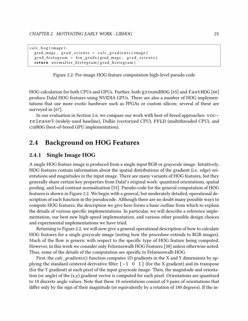
CHAPTER 2. MOTIVATING EARLY WORK : LIBHOG 23
c a l c _ h o g ( image ) :
grad_mags , g r a d _ o r i e n t s = c a l c _ g r a d i e n t s ( image )
g r a d _ h i s t o g r a m = b i n _ g r a d s ( grad_mags , g r a d _ o r i e n t s )
return n o r m a l i z e _ h i s t o g r a m ( g r a d _ h i s t o g r a m )
Figure 2.2: Per-image HOG feature computation high-level pseudo code
HOG calculation for both CPUs and GPUs. Further, both groundHOG [65] and fastHOG [66]
produce Dalal HOG features using NVIDIA GPUs. There are also a number of HOG implemen-
tations that use more exotic hardware such as FPGAs or custom silicon; several of these are
surveyed in [67].
In our evaluation in Section 2.6, we compare our work with best-of-breed approaches: voc-release5 (widely-used baseline), Dollár (vectorized CPU), FFLD (multithreaded CPU), and
cuHOG (best-of-breed GPU implementation).
2.4 Background on HOG Features
2.4.1 Single Image HOGA single HOG feature image is produced from a single input RGB or grayscale image. Intuitively,
HOG features contain information about the spatial distributions of the gradient (i.e. edge) ori-
entations and magnitudes in the input image. There are many variants of HOG features, but they
generally share certain key properties from Dalal’s original work: quantized orientations, spatial
pooling, and local contrast normalization [53]. Pseudo-code for the general computation of HOG
features is shown in Figure 2.2. We begin with a general, but moderately detailed, operational de-
scription of each function in the pseudocode. Although there are no doubt many possible ways to
compute HOG features, the description we give here forms a basic outline from which to explain
the details of various specic implementations. In particular, we will describe a reference imple-
mentation, our best new high-speed implementation, and various other possible design choices
and experimental implementations we have tried.
Returning to Figure 2.2, we will now give a general operational description of how to calculate
HOG features for a single grayscale image (noting how the procedure extends to RGB images).
Much of the ow is generic with respect to the specic type of HOG feature being computed.
However, in this work we consider only Felzenszwalb HOG Features [38] unless otherwise noted.
Thus, some of the details of the computation are specic to Felzenszwalb HOG.
First, the calc_дradients () function computes 1D gradients in the X and Y dimensions by ap-
plying the standard centered derivative lter [-1 0 1] (for the X gradient) and its transpose
(for the Y gradient) at each pixel of the input grayscale image. Then, the magnitude and orienta-
tion (or angle) of the (x,y) gradient vector is computed for each pixel. Orientations are quantized
to 18 discrete angle values. Note that these 18 orientations consist of 9 pairs of orientations that
dier only by the sign of their magnitude (or equivalently by a rotation of 180 degrees). If the in-
CHAPTER 2. MOTIVATING EARLY WORK : LIBHOG 24
put image is multi-channel (i.e. RGB as opposed to grayscale), calc_дradients () is called for each
color channel, and then for each pixel the maximum gradient value across color channels (and its
corresponding orientation) are selected and computation then proceeds as in the grayscale input
image case.
Next, the bin_дrads () function smoothly spatially bins the per-pixel gradient magnitudes and
orientations at a lower resolution than the original image. Typically, the resolution of the gradient
histogram is either 1/8 (or sometimes 1/4) that of the input image. Each histogram bin is formed
by an approximately-Gaussian weighted pooling over the 16x16 (or 8x8 in the 1/4 scale case)
window of gradient pixels centered over the bin.
Finally, the normalize_histoдram() function computes the nal per-bin output HOG fea-
tures using various local normalizations and combinations of the contents of the “raw” or un-
normalized gradient histogram just computed by bin_дrads (). Note that computation of the nal
features is independent for each bin. For each bin, we consider the 4 possible 2x2 sub-windows
of the 3x3 window of bins centered over that bin. Based on the total per-bin non-normalized
gradient energy in each of the 4 sub-windows we compute 4 local “directional” (+X+Y, +X-Y, -
X+Y, -X-Y) normalization factors. The average of these 4 directed normalization factors is the bin
normalization factor BNF . Then, a total of 31 features are computed as follows: 18 features are
computed by taking BNF times the 18 per-bin non-normalized gradient magnitudes; these are
termed the contrast-sensitive features. Next, 9 more features are formed by taking BNF times
the 9 sums of pairs of magnitudes of the 9 per-bin pairs of 180-degree-rotated orientations; these
are termed the contrast-insensitive features. Finally, the last 4 features are created by summing
recomputations of all 27 prior features using each of 4 “directional” bin-local normalization con-
stants individually instead of BNF .
2.4.2 Existing Implementation DetailsIn the following sections we will present tables that, for each specic stage of computing HOG
features, compare our new algorithm to various existing algorithms. However, here we rst
highlight the key overall design choices in the other HOG implementations that we have cited
and with which we will compare our computational eciency.
First, we consider the baseline/reference voc-release5 [59] HOG implementation. For
the most part, this implementation is a straight-forward standard C-programming-language elab-
oration of the above description. No SIMD or process/thread parallelism is used. A mix of 32-bit
f loat and 64-bitdouble datatypes are used. Gradient normalization uses the standard L2 norm. In
calc_дradients (), orientation quantization is accomplished by taking the dot product of the (x,y)
gradient vector with 18 reference orientation vectors and choosing the maximum. Inbin_дrads (),the gradient pixels are iterated over and added to each histogram bin that they inuence. We term
this a scatter style approach as illustrated in Figure 2.3.
Dollár’s fhog [61] implementation improves over voc-release5 primarily in its use of
SIMD parallelism. For determining the quantized gradient orientation, it uses an arccos () lookup-
table (or LUT). It also uses a scatter style bin_дrads (). The FFLD [52], [62] implementation uses
thread-level parallelism across image scales, but without SIMD parallelism. For determining the
CHAPTER 2. MOTIVATING EARLY WORK : LIBHOG 25
quantized gradient orientation, it uses an arctan() lookup-table (or LUT). Like the prior two
implementations, it also uses a scatter style bin_дrads (). cuHOG [63], as a GPU based imple-
mentation, uses GPU-style SIMT parallelism rather than the SIMD and coarse thread parallelism
used by the other (all CPU-based) algorithms discussed here. As it uses the CUDA programming
environment, it runs only on NVIDIA GPUs.
2.4.3 Multiple Image HOG and Image ResizingSo far, we have described how to compute HOG features for a single image. However, in practice it
is often desired to compute HOG features at many scales. This can be accomplished by computing
many HOG feature images from many scaled copies of an input image. Note that the computation
of HOG features is independent across scales. In this work, we primarily consider a common case
where 10+30 scales of a 640x480 size input image are desired. First, 30 1/8-bin-resolution HOG
feature images are computed from 30 progressively downsampled versions of the input image,
with 10 equally-logarithmically-spaced scales for every factor of 2 (octave) of downsampling.
Then, an additional 10 1/4-bin-resolution HOG feature images are computed from reusing the
rst 10 largest-scale copies of the input image. The resultant 10 HOG feature images are the
same size as would be the rst 10 1/8-bin-resolution HOG feature images computed from a 2X
upsampled version of the input image.
The HOG implementations in the related work (voc-release5, FFLD, and Dollár) each
have custom, from-scratch implementations of image resizing. There are also a number of o-
the-shelf image resizing implementations, found in libraries such as OpenCV [64] and Intel Per-
formance Primitives (IPP) [68]. In Table 2.1, we compare the speed of image pyramid computation
using OpenCV, IPP, and the HOG related work. For OpenCV and IPP, we show two variants: a
serial version, and a version with OpenMP parallelism across image scales. We found that the
image resizing functions in OpenCV and Intel Performance Primitives (IPP) are quite ecient. In
libHOG, we use the IPP image resizing function with parallelism across scales. One interesting
note is that the majority (∼80%) of the time spent on resizing is on the 10 largest image scales.
This is sensible since these largest scales contain ∼80% of the total pixels across all scales.
Additionally, while it is possible to exploit thread-level parallelism within a single image, as
with FFLD we also choose to exploit thread-level parallelism across scales by default.
2.5 Our Approach to HOGIn this section we explain our techniques to accelerate per-image HOG feature computation. As
per Figure 2.2, there are three major steps: gradient computation (calc_дradients ()), histogram
accumulation (bin_дrads ()), and normalization (normalize_histoдram()). To achieve high speed,
we follow two simple high level design principles: First, we wish to minimize memory trac to
avoid being bound by communication costs. Second, we wish to maximize vectorization to avoid
being bound by maximum rate at which computations can be issued.
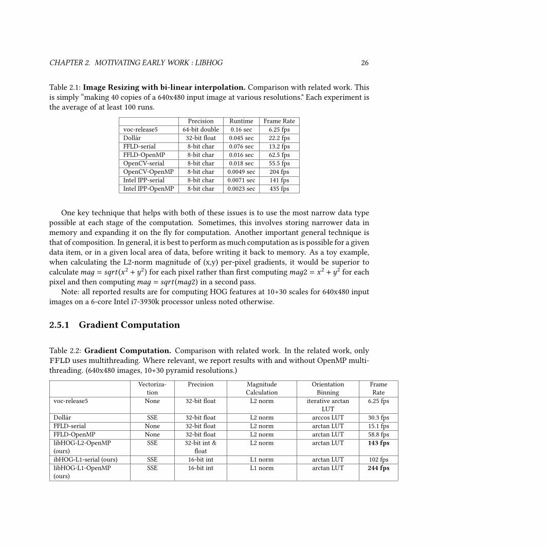
CHAPTER 2. MOTIVATING EARLY WORK : LIBHOG 26
Table 2.1: Image Resizing with bi-linear interpolation. Comparison with related work. This
is simply “making 40 copies of a 640x480 input image at various resolutions." Each experiment is
the average of at least 100 runs.
Precision Runtime Frame Rate
voc-release5 64-bit double 0.16 sec 6.25 fps
Dollár 32-bit oat 0.045 sec 22.2 fps
FFLD-serial 8-bit char 0.076 sec 13.2 fps
FFLD-OpenMP 8-bit char 0.016 sec 62.5 fps
OpenCV-serial 8-bit char 0.018 sec 55.5 fps
OpenCV-OpenMP 8-bit char 0.0049 sec 204 fps
Intel IPP-serial 8-bit char 0.0071 sec 141 fps
Intel IPP-OpenMP 8-bit char 0.0023 sec 435 fps
One key technique that helps with both of these issues is to use the most narrow data type
possible at each stage of the computation. Sometimes, this involves storing narrower data in
memory and expanding it on the y for computation. Another important general technique is
that of composition. In general, it is best to perform as much computation as is possible for a given
data item, or in a given local area of data, before writing it back to memory. As a toy example,
when calculating the L2-norm magnitude of (x,y) per-pixel gradients, it would be superior to
calculatemaд = sqrt (x2 +y2) for each pixel rather than rst computingmaд2 = x2 +y2for each
pixel and then computingmaд = sqrt (maд2) in a second pass.
Note: all reported results are for computing HOG features at 10+30 scales for 640x480 input
images on a 6-core Intel i7-3930k processor unless noted otherwise.
2.5.1 Gradient Computation
Table 2.2: Gradient Computation. Comparison with related work. In the related work, only
FFLD uses multithreading. Where relevant, we report results with and without OpenMP multi-
threading. (640x480 images, 10+30 pyramid resolutions.)
Vectoriza-
tion
Precision Magnitude
Calculation
Orientation
Binning
Frame
Rate
voc-release5 None 32-bit oat L2 norm iterative arctan
LUT
6.25 fps
Dollár SSE 32-bit oat L2 norm arccos LUT 30.3 fps
FFLD-serial None 32-bit oat L2 norm arctan LUT 15.1 fps
FFLD-OpenMP None 32-bit oat L2 norm arctan LUT 58.8 fps
libHOG-L2-OpenMP
(ours)
SSE 32-bit int &
oat
L2 norm arctan LUT 143 fps
ibHOG-L1-serial (ours) SSE 16-bit int L1 norm arctan LUT 102 fps
libHOG-L1-OpenMP
(ours)
SSE 16-bit int L1 norm arctan LUT 244 fps
CHAPTER 2. MOTIVATING EARLY WORK : LIBHOG 27
Calculating 1D gradients in X and Y. First, as noted in the resizing discussion, our im-
plementation stores the resized images using the same 8-bit unsigned integer values per-pixel-
per-color as the input image. Thus, the input pixels have a range of [0,255], and the resultant X
and Y derivatives have a range from [−255,255]. We choose the simple option of storing the X
and Y components of the gradient each as 16-bit signed integers. Thus, the input of the gradient
calculation is 1 byte per pixel, and the output is 2×2 = 4 bytes per pixel. To perform the actual
calculation, we rst load the input pixel data, widen it, and then compute the gradients using
128-bit-wide packed-16-bit-SIMD SSE (hereafter 128w16si) operations. This allows us to perform
8 concurrent arithmetic operations per CPU clock cycle.
We also considered using 256-bit AVX instructions. We wrote some HOG-like microbench-
marks in AVX, and we saw no speedup for AVX over SSE. We speculate that 128-bit SSE computa-
tion combined with OpenMP parallelism is sucient to saturate the available memory bandwidth.
Magnitude. Next, we use the X and Y gradients to compute the per-pixel gradient magnitude.
At this stage, our gradients are stored as 16-bit signed integers, albeit with a limited range of
[−255,255]. However, when computing the L2 norm, the expression дradX 2 + дradY 2can still
(just) overow a 16-bit integer, and current CPUs do not support vectorized 16-bit oating-point
math. Thus, we use 32-bit intermediates for the L2 magnitude calculation to avoid overow.
Additionally, although it has dierent semantics, we also chose to experiment with using
the L1 norm |дradX | + |дradY | instead of the L2 norm. The output range of this expression is
[0,510], which still easily ts within a 16-bit signed integer. For the L1 norm calculation we
again use 128w16si operations. Note: in our evaluation in Section 2.6, we will show that training
Deformable Parts Model object detectors on HOG features that use the L1 norm (for gradient
magnitudes) produces lower but similar accuracy to using the more typical L2 norm for gradient
magnitudes.
Handling RGB images. As previously mentioned, for RGB images we must calculate the
gradient for all three color channels and select the one with the maximum magnitude. Frustrat-
ingly, SSE instructions do not natively have the ability to compute the needed argmax opera-
tion across 3 channels. Thus, we implement our own vectorized argmax primitive, again using
128w16si operations. In summary, we iterate over the 3 per-channel magnitudes and compare
them against the largest magnitude seen so far for this pixel. If it is larger than the best seen
magnitude, we:
• replace the best seen magnitude with the current channel magnitude, and
• store the corresponding X and Y gradients from the current channel for later use.
Standard SIMD comparisons and bit-wise Boolean operations are used to perform these opera-
tions in a fully vectorized manner; consult the code for more details.
Orientation. The non-quantized gradient orientation for each pixel is dened asatan2(дradY ,дradX ).However, there does not currently exist a vectorized atan2 instruction. Also, atan2 is typically a
relatively expensive operation. Further, we need only the 18-levels-quantized angle, which allows
for various possible optimizations. Currently, we choose to use a modestly sized look-up table:
atan2[gradX][gradY]. Given that gradX and gradY both have a range of [−255,255], a
CHAPTER 2. MOTIVATING EARLY WORK : LIBHOG 28
LUT with 512×512 entries is sucient. Further, the elements of the table need only have a range
of [0,17] for the 18 quantized orientations, so 1 byte per entry is sucient. Thus, the total LUT
size is only 256 KB. We also experimented with using a directly vectorized version of the voc-
release5 orientation computation method, but determined that the LUT-based method was faster
to compute.
In Table 2.2, we compare our gradient (orientation and magnitude) computational eciency
with previous HOG implementations. We nd that our gradient implementation is 39x faster
than voc-release5 and 4.1x faster than the fastest known implementation.
2.5.2 Histogram AccumulationHistogram computation. Recall that the gradient histogram consists of both spatial binning
(at 1/8 or 1/4 the input image resolution) and orientation binning. We choose to iterate over the
spatial dimension rst. At each spatial location, the histogram to be computed by bin_дrads () has
18 orientation bins to ll in, one for each quantization level of the orientations; we term this set of
18 orientation bins a “spatial bin”. The contribution of each gradient pixel to each bin is weighted
by an approximately-Gaussian function centered over the spatial bin with a width of 8 (or 4 in
the 1/4 resolution case) pixels. The spatial bin includes only contributions from the 16x16 (or 8x8
in the 1/4 resolution case) gradient pixels nearest to its center; note that this range is somewhat
arbitrarily chosen, but the intent is that pixels further away would not signicantly contribute to
the bin due to having low weights as the Gaussian falls o. The actual weighting function used
is decomposable into the product of symmetric X and Y terms, and thus can be computed using
only a multiply and two lookups into a 16 (or 8 in the 1/4 resolution case) element LUT. Note that
we do not attempt to apply SIMD parallelism for this stage.
Optimization: gather instead of scatter. As previously mentioned, implementations like
voc-release5, FFLD, and Dollár use scatter-style histogram construction, as shown in
Figure 2.3. In our experiments, however, we found that using a gather-style method yielded
faster computation times, particularly in the multi-threaded case. Our theory is that the memory
accesses used by scatter-style histogram construction are the limiting factor for the speed of
bin_дrad () in the multi-threaded case, regardless of the level (over scales or within a single image)
at which multi-threading is used. For each gradient pixel, scatter-style histogram creation will
perform one write to each of the 2×2 = 4 spatial bins that include contributions from that pixel.
However, only one orientation bin in each spatial bin will be modied. The result is a stream
of sparse read-modify-write operations to the full set of 2×2×18 = 72 individual orientation
bins that may be aected by each pixel. In contrast, for the gather-style approach, we need
only a single spatial bin (of 18 orientation bins) as our output working set, and we will perform
all needed writes to it within a small time window (i.e. with good temporal locality of writes).
We illustrate the gather-style approach in Figure 2.4. While the gather-style approach needs an
input working set of 8×8×2 = 128 X/Y gradients, this set is read-only, has a simple access pattern,
and is substantially shared among spatial bins. Thus, overall it seems plausible that the gather-
style histogram signicantly reduces write overhead while not overly increasing read memory
bandwidth or cache pressure.
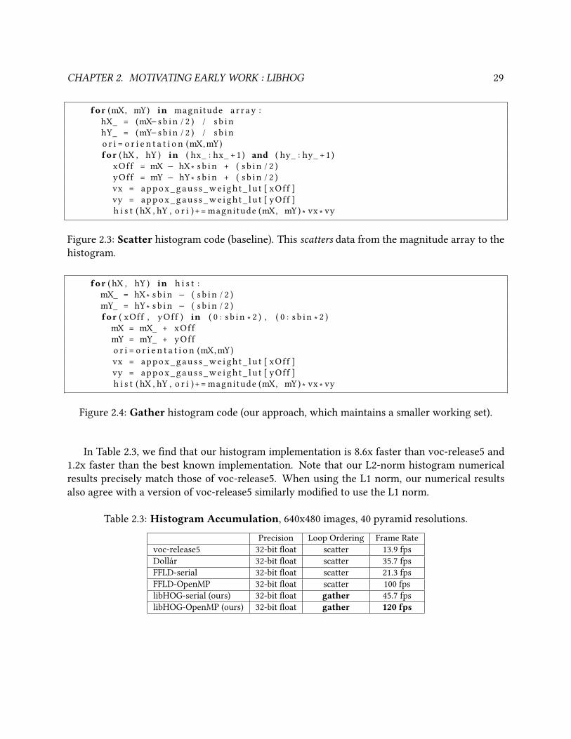
CHAPTER 2. MOTIVATING EARLY WORK : LIBHOG 29
for (mX, mY) in magnitude a r r a y :
hX_ = (mX− s b i n / 2 ) / s b i n
hY_ = (mY− s b i n / 2 ) / s b i n
o r i = o r i e n t a t i o n (mX, mY)
for ( hX , hY ) in ( hx_ : hx_ +1 ) and ( hy_ : hy_ +1 )
xOf f = mX − hX ∗ s b i n + ( s b i n / 2 )
yOf f = mY − hY ∗ s b i n + ( s b i n / 2 )
vx = a p p o x _ g a u s s _ w e i g h t _ l u t [ xOf f ]
vy = a p p o x _ g a u s s _ w e i g h t _ l u t [ yOf f ]
h i s t ( hX , hY , o r i )+= magnitude (mX, mY ) ∗ vx ∗ vy
Figure 2.3: Scatter histogram code (baseline). This scatters data from the magnitude array to the
histogram.
for ( hX , hY ) in h i s t :
mX_ = hX ∗ s b i n − ( s b i n / 2 )
mY_ = hY ∗ s b i n − ( s b i n / 2 )
for ( xOff , yOf f ) in ( 0 : s b i n ∗ 2 ) , ( 0 : s b i n ∗ 2 )
mX = mX_ + xOf f
mY = mY_ + yOff
o r i = o r i e n t a t i o n (mX, mY)
vx = a p p o x _ g a u s s _ w e i g h t _ l u t [ xOf f ]
vy = a p p o x _ g a u s s _ w e i g h t _ l u t [ yOf f ]
h i s t ( hX , hY , o r i )+= magnitude (mX, mY ) ∗ vx ∗ vy
Figure 2.4: Gather histogram code (our approach, which maintains a smaller working set).
In Table 2.3, we nd that our histogram implementation is 8.6x faster than voc-release5 and
1.2x faster than the best known implementation. Note that our L2-norm histogram numerical
results precisely match those of voc-release5. When using the L1 norm, our numerical results
also agree with a version of voc-release5 similarly modied to use the L1 norm.
Table 2.3: Histogram Accumulation, 640x480 images, 40 pyramid resolutions.
Precision Loop Ordering Frame Rate
voc-release5 32-bit oat scatter 13.9 fps
Dollár 32-bit oat scatter 35.7 fps
FFLD-serial 32-bit oat scatter 21.3 fps
FFLD-OpenMP 32-bit oat scatter 100 fps
libHOG-serial (ours) 32-bit oat gather 45.7 fps
libHOG-OpenMP (ours) 32-bit oat gather 120 fps
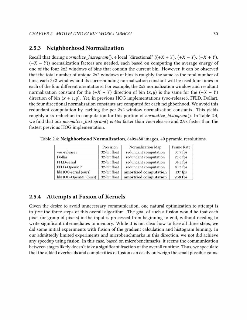
CHAPTER 2. MOTIVATING EARLY WORK : LIBHOG 30
2.5.3 Neighborhood NormalizationRecall that during normalize_histoдram(), 4 local “directional” ((+X + Y ), (+X − Y ), (−X + Y ),(−X − Y )) normalization factors are needed, each based on computing the average energy of
one of the four 2x2 windows of bins that contain the current bin. However, it can be observed
that the total number of unique 2x2 windows of bins is roughly the same as the total number of
bins; each 2x2 window and its corresponding normalization constant will be used four times in
each of the four dierent orientations. For example, the 2x2 normalization window and resultant
normalization constant for the (+X − Y ) direction of bin (x ,y) is the same for the (−X − Y )direction of bin (x + 1,y). Yet, in previous HOG implementations (voc-release5, FFLD, Dollár),
the four directional normalization constants are computed for each neighborhood. We avoid this
redundant computation by caching the per-2x2-window normalization constants. This yields
roughly a 4x reduction in computation for this portion of normalize_histoдram(). In Table 2.4,
we nd that our normalize_histoдram() is 66x faster than voc-release5 and 2.9x faster than the
fastest previous HOG implementation.
Table 2.4: Neighborhood Normalization, 640x480 images, 40 pyramid resolutions.
Precision Normalization Map Frame Rate
voc-release5 32-bit oat redundant computation 35.7 fps
Dollár 32-bit oat redundant computation 25.6 fps
FFLD-serial 32-bit oat redundant computation 34.5 fps
FFLD-OpenMP 32-bit oat redundant computation 83.3 fps
libHOG-serial (ours) 32-bit oat amortized computation 137 fps
libHOG-OpenMP (ours) 32-bit oat amortized computation 238 fps
2.5.4 Attempts at Fusion of KernelsGiven the desire to avoid unnecessary communication, one natural optimization to attempt is
to fuse the three steps of this overall algorithm. The goal of such a fusion would be that each
pixel (or group of pixels) in the input is processed from beginning to end, without needing to
write signicant intermediates to memory. While it is not clear how to fuse all three steps, we
did some initial experiments with fusion of the gradient calculation and histogram binning. In
our admittedly limited experiments and microbenchmarks in this direction, we not did achieve
any speedup using fusion. In this case, based on microbenchmarks, it seems the communication
between stages likely doesn’t take a signicant fraction of the overall runtime. Thus, we speculate
that the added overheads and complexities of fusion can easily outweigh the small possible gains.
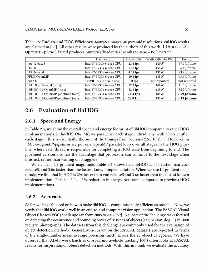
CHAPTER 2. MOTIVATING EARLY WORK : LIBHOG 31
Table 2.5: End-to-endHOGEciency, 640x480 images, 40 pyramid resolutions. cuHOG results
are claimed in [63]. All other results were produced by the authors of this work. libHOG-L2-OpenMP-pipelined produces numerically identical results to voc-release5.
Hardware Frame Rate Watts (idle: 86.8W) Energy
voc-release5 Intel i7-3930k 6-core CPU 2.44 fps 140W 57.4 J/frame
Dollár Intel i7-3930k 6-core CPU 5.88 fps 155W 26.4 J/frame
FFLD-serial Intel i7-3930k 6-core CPU 4.59 fps 137W 29.9 J/frame
FFLD-OpenMP Intel i7-3930k 6-core CPU 19.6 fps 185W 9.44 J/frame
cuHOG NVIDIA GTX560 GPU 20 fps not reported not reported
libHOG-L1-serial (ours) Intel i7-3930k 6-core CPU 12.3 fps 140W 11.3 J/frame
libHOG-L1-OpenMP (ours) Intel i7-3930k 6-core CPU 52.6 fps 185W 3.52 J/frame
libHOG-L1-OpenMP-pipelined (ours) Intel i7-3930k 6-core CPU 71.4 fps 185W 2.59 J/framelibHOG-L2-OpenMP-pipelined (ours) Intel i7-3930k 6-core CPU 58.8 fps 185W 3.15 J/frame
2.6 Evaluation of libHOG
2.6.1 Speed and EnergyIn Table 2.5, we show the overall speed and energy footprint of libHOG compared to other HOG
implementations. In libHOG-OpenMP, we parallelize each stage individually, with a barrier after
each stage – this is essentially the sum of the timings from Sections 2.5.1 to 2.5.3. However, in
libHOG-OpenMP-pipelined we put one OpenMP parallel loop over all stages in the HOG pipe-
line, where each thread is responsible for completing a HOG scale from beginning to end. The
pipelined version also has the advantage that processors can continue to the next stage when
nished, rather than waiting on stragglers.
When using L2 gradient magnitude, Table 2.5 shows that libHOG is 24x faster than voc-
release5, and 3.0x faster than the fastest known implementation. When we use L1 gradient mag-
nitude, we nd that libHOG is 29x faster than voc-release5 and 3.6x faster than the fastest known
implementation. This is a 3.0x - 22x reduction in energy per frame compared to previous HOG
implementations.
2.6.2 AccuracySo far, we have focused on how to make libHOG as computationally ecient as possible. Now, we
verify that libHOG works well in an end-to-end computer vision application. The PASCAL Visual
Object Classes (VOC) challenge ran from 2005 to 2012 [69]. A subset of the challenge tasks focused
on detecting the occurrence and bounding boxes of 20 types of objects (car, person, dog, ...) in 5000
realistic photographs. The datasets from this challenge are commonly used for the evaluation of
object detection methods. Generally, accuracy on the PASCAL datasets are reported in terms
of the single-number mean average precision (mAP) across the 20 object categories. We have
observed that ADAS work (such as on-road multivehicle tracking [60]) often looks at PASCAL
results for inspiration on object detection methods. With this in mind, we evaluate the accuracy
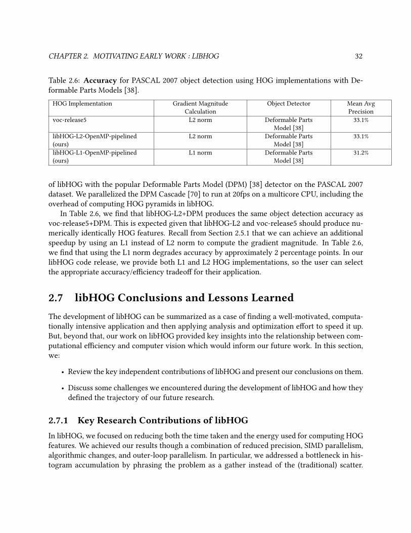
CHAPTER 2. MOTIVATING EARLY WORK : LIBHOG 32
Table 2.6: Accuracy for PASCAL 2007 object detection using HOG implementations with De-
formable Parts Models [38].
HOG Implementation Gradient Magnitude
Calculation
Object Detector Mean Avg
Precision
voc-release5 L2 norm Deformable Parts
Model [38]
33.1%
libHOG-L2-OpenMP-pipelined
(ours)
L2 norm Deformable Parts
Model [38]
33.1%
libHOG-L1-OpenMP-pipelined
(ours)
L1 norm Deformable Parts
Model [38]
31.2%
of libHOG with the popular Deformable Parts Model (DPM) [38] detector on the PASCAL 2007
dataset. We parallelized the DPM Cascade [70] to run at 20fps on a multicore CPU, including the
overhead of computing HOG pyramids in libHOG.
In Table 2.6, we nd that libHOG-L2+DPM produces the same object detection accuracy as
voc-release5+DPM. This is expected given that libHOG-L2 and voc-release5 should produce nu-
merically identically HOG features. Recall from Section 2.5.1 that we can achieve an additional
speedup by using an L1 instead of L2 norm to compute the gradient magnitude. In Table 2.6,
we nd that using the L1 norm degrades accuracy by approximately 2 percentage points. In our
libHOG code release, we provide both L1 and L2 HOG implementations, so the user can select
the appropriate accuracy/eciency tradeo for their application.
2.7 libHOG Conclusions and Lessons LearnedThe development of libHOG can be summarized as a case of nding a well-motivated, computa-
tionally intensive application and then applying analysis and optimization eort to speed it up.
But, beyond that, our work on libHOG provided key insights into the relationship between com-
putational eciency and computer vision which would inform our future work. In this section,
we:
• Review the key independent contributions of libHOG and present our conclusions on them.
• Discuss some challenges we encountered during the development of libHOG and how they
dened the trajectory of our future research.
2.7.1 Key Research Contributions of libHOGIn libHOG, we focused on reducing both the time taken and the energy used for computing HOG
features. We achieved our results though a combination of reduced precision, SIMD parallelism,
algorithmic changes, and outer-loop parallelism. In particular, we addressed a bottleneck in his-
togram accumulation by phrasing the problem as a gather instead of the (traditional) scatter.
CHAPTER 2. MOTIVATING EARLY WORK : LIBHOG 33
Overall, we were able to compute multiresolution HOG pyramids at a rate of 59 frames-per-
second for 640x480 images on a multicore CPU. This represented a 3X improvement in speed
and energy usage compared to the state of the art without compromising accuracy. Additionally,
we explored the tradeos of using L1 instead of L2 norms to compute gradients, which enabled
the use of smaller operands and thus allowed more SIMD parallelism. When using L1 norms,
we achieved a rate of 70 frames-per-second, increasing our speed and energy improvement over
the state of the art to 3.6X, at the price of some accuracy loss. Further, we packaged libHOG as
a drop-in replacement for the standard and commonly-used voc-release5 HOG calculation code.
We tested libHOG (using standard L2 norms) for equivalence and nal correctness in a full DPM
ow that normally uses the voc-release5 code. For the feature calculation portion of the ow, lib-
HOG ran at 59 frames-per-second and gave a 24X speed improvement and an 18X improvement
in per-frame energy usage over the voc-release5 reference code.
2.7.2 Conclusions on the Specic Contributions of libHOGHOG feature calculation is a core building block in numerous computer vision applications in-
cluding advanced driver assistance systems (ADAS). Further, real-time, energy-ecient compu-
tation is crucial to real-world deployability of such systems. However, prior to our work, existing
implementations of HOG feature calculation were both slow in absolute terms and inecient
in their use of computational resources (leaving room for optimization). The core independent
results and contributions of this work were released in our open-source HOG implementation,
libHOG. It is 3.0X - 29X faster (and 3.0X - 22X more energy-ecient) than previous HOG im-
plementations. We computed HOG pyramids at 71 fps, enabling ADAS applications like object
detection and lane detection to compute HOG pyramids in real-time.
2.7.3 Contributions of this Work to Dening our Research TrajectoryThis work was a good case study in optimizing a core operation for computer vision. There were
two categories of tasks involved in this eort:
• Performing the core analysis, implementation, optimization, and tuning of the operation at
hand.
• Packaging the results of our eort in a way usable by the computer vision community (i.e.
as a library).
While we achieved good results in the end, there were issues associated with both of these aspects
of our eorts. We will now discuss the issues we encountered and how they informed our future
work, organized by the above two categories.
2.7.3.1 Issues with Core Implementation Eorts
For the rst aspect, the core implementation work, we were hindered by a lack of tools and
frameworks in several ways:
CHAPTER 2. MOTIVATING EARLY WORK : LIBHOG 34
• Writing this type of highly-tuned code manually is time consuming, error prone, and di-
cult to maintain. This limited our ability to explore the design space and exploit special-case
optimizations.
• The existing ows and projects using HOG calculations were not well suited to the type
of development needed for optimization eorts. Thus, our work required a combination of
writing custom test harnesses and using existing ows in awkward ways. The net result
was reduced testing coverage and increased development time.
Our diculties informed our later eorts to build a vertical framework that would address these
issues. In particular:
• Support for metaprogramming was included in our framework to help reduce eort spent
manually writing low-level code. Metaprogramming and other framework features work
together to provide greater exibility to explore the space of possible implementation choices
and to enable the programmer to exploit special-case optimizations without undue eort
or complexity.
• Our framework was designed to include a full vertical slice of ows in which the operations
to implement are used. This allows for continuous, full testing during implementation.
Also, if desired, the vertical nature of the framework provides a smooth path to deploying
full systems without needing to integrate additional dependencies.
2.7.3.2 Issues with Packaging libHOG for Reuse in Research and Practice
The development of libHOG provided key insights into the overall software ecosystem for ma-
chine learning and computer vision research. In particular, the computer vision ows we exam-
ined had an ad-hoc combination of languages, frameworks and methodologies. As is common
in research [71], new functionality was layered over existing functionality in ways such that
resultant full codebases were dicult to understand or modify. While this approach to devel-
opment may be reasonable and justied in a research context, it often makes optimization and
replacement of any one part of a computer vision ow problematic. In general, an optimization
eort begins with the observation that some particular ow is too slow, or at least that it might
benet from being more ecient. However, just understanding how a typical research-quality
computer-vision software pipeline operates can be quite daunting. And, even when certain parts
of the ow are isolated as good targets for optimization, the interface between those parts and
the rest of the ow may not be clear. While it is often easy to get a single reference ow working
after some optimizations, it is generally unclear how such changes might aect other ows or
projects using similar (older, newer, or diverged) codebases.
Given that the barrier to entry for optimizing such ows is high, such work is less likely to be
performed. And, even in the cases where such optimizations are performed, the high diculty of
packaging and integrating such work can lead to low adoption in research and practice. Some-
times, optimizations only apply to narrow use-cases, and thus new ows are unable to use them.
CHAPTER 2. MOTIVATING EARLY WORK : LIBHOG 35
Other times, the cost for individual researchers to integrate such optimizations outweighs any
benets, especially if any particular optimization provides only limited benets in the context of
full ows (i.e. due to Amdahl’s law). The end result of this situation is that researchers can be
limited by needlessly slow software.
At the time when libHOG was created, this was a problem with no easy solutions in sight.
However, the rise of neural networks has oered various opportunities to reconsider this issue
and potentially make progress toward a solution, as will be discussed in Section 3.5.3.2.
2.7.4 Conclusions from libHOG that Dened our Research TrajectoryWhile computer vision researchers do not view computational eciency as their primary con-
cern, their work is fundamentally enabled by computation. Further, while it is only one of several
concerns, improvements in computational eciency can enable new lines of research. Comple-
mentarily, the lack of computational eciency can seriously limit research productivity. In this
work, we observed that computer vision researchers are often driven to attempt various opti-
mizations on their own. They hand-code critical operations in low-level performance languages
(such a C) or try to write custom code to exploit parallel hardware (such as GPUs or multicore
CPUs). But, their approaches to achieving high computational eciency often suer from a lack
of focus and engineering rigor. In turn, this leads to unreliability, sub-optimal speed, poor mod-
ularity/reusability, and poor maintainability of the resulting implementations. This gives an op-
portunity for contributions though research specically targeting computational eciency. But,
there are several key challenges that arise for any such research:
• Analysis and optimization of research-quality computer vision codebases can be quite dif-
cult.
• For any optimization work to have maximal impact, it must be general and well-packaged
enough for other researchers to easily use.
In the context of libHOG, the rst issue limited our ability to explore the full design space. While
we successfully focused our eort on the most critical aspects of HOG computation, there were
various other areas we wished to explore but were not able to due to productivity limitations.
For example, we did not attempt to apply SIMD optimizations to histogram binning or try to
develop our own image resizing routines. In this case, we were lucky that focused optimization
of a very small section of the overall operation (gradient calculation), when combined with a
reasonable-overall-quality unied implementation in a performance language, was enough to
achieve high overall speedup. But, in general, this is not the case, and the approach we used here
would not easily scale to optimization of more complex algorithms. Further, we were only able to
target a single hardware platform: multicore CPUs. It would have been desirable to support more
portability, but this was quite dicult to even contemplate given the development environments
and tools we had at our disposal. Further, potential deployment of a library that could use multiple
hardware targets introduces additional challenges we were not prepared to address at that time.
But, if we wished to consider a broader space of problems and hardware targets going forward, it
CHAPTER 2. MOTIVATING EARLY WORK : LIBHOG 36
was clear that we would need to nd ways to improve the productivity of such optimization and
deployment eorts. Similarly, while we were able to fairly cleanly package our work in a library,
we still struggled to achieve wide direct adoption of our work. Our conclusion is that there are
two key sub-issues with packaging and deployment:
• First, the benets of any library must exceed the eort required for researchers to integrate
and use it. In the case of libHOG, we are only optimizing a small portion of the overall
detection pipeline. Especially in research ows, speeding up HOG calculation alone may
give only a limited overall benet.
• Secondly, researchers often (but not always) want to modify various aspects of high-level
operations in their pipelines. Thus, any xed library for a high-level operation (such as
libHOG) can be too xed in terms of functionality and interface for research use.
As our research moved into the domain of ecient computation for neural networks, all these
issues became guideposts to inform and direct our future eorts.
37
Chapter 3
Bridge to Our Boda Framework:DenseNet
3.1 Introduction to DenseNet: Speeding upNeural-Network-based Object Detection
The modern era of high interest in neural networks (NNs) started with their successful application
to image classication. As per our running example from Section 1.1.1, image classication is the
task of determining if an image contains a certain type of object (at any location in the image).
In contrast, object detection (as introduced in Section 1.3.2) is the more dicult task of localizing
(i.e. putting a bounding box around) each instance of some type of object in an image. Given the
early success of NNs for image classication, it was natural to try to extend them to the more
general problem of object detection. However, early eorts in this direction were hampered by
the high computational requirements of NNs. So, as with libHOG, we analyzed this situation
and searched for research opportunities related to optimizing both existing and future NN-based
object detection ows.
In this chapter, we present the results of this eort: DenseNet, an open source system that
computes dense, multiscale features from the convolutional layers of a convolutional-NN-based
image classier. As with libHOG, while our work on DenseNet has independent research con-
tributions, it also taught us various lessons that informed our future work. In particular, while
our initial implementation approach yielded timely results, various challenges impeded our abil-
ity to build on that implementation. Thus, we later reimplemented our DenseNet approach in
a new prototype framework. This prototype became the base for our future work on the Bodaframework for implementing portable, ecient NN convolutions and other operations.
The rebirth of neural networks has led to profound improvements in the state-of-the-art
benchmark accuracy for various computer vision tasks. The key algorithms of the so-called “deep
learning” revolution can be traced back at least to the late 1980s [72]. However, the rise of big data
has led to huge labeled datasets (e.g. ImageNet [73] with >1M labeled images) for training and
evaluating image classication systems. Additionally, neural network frameworks such as Berke-
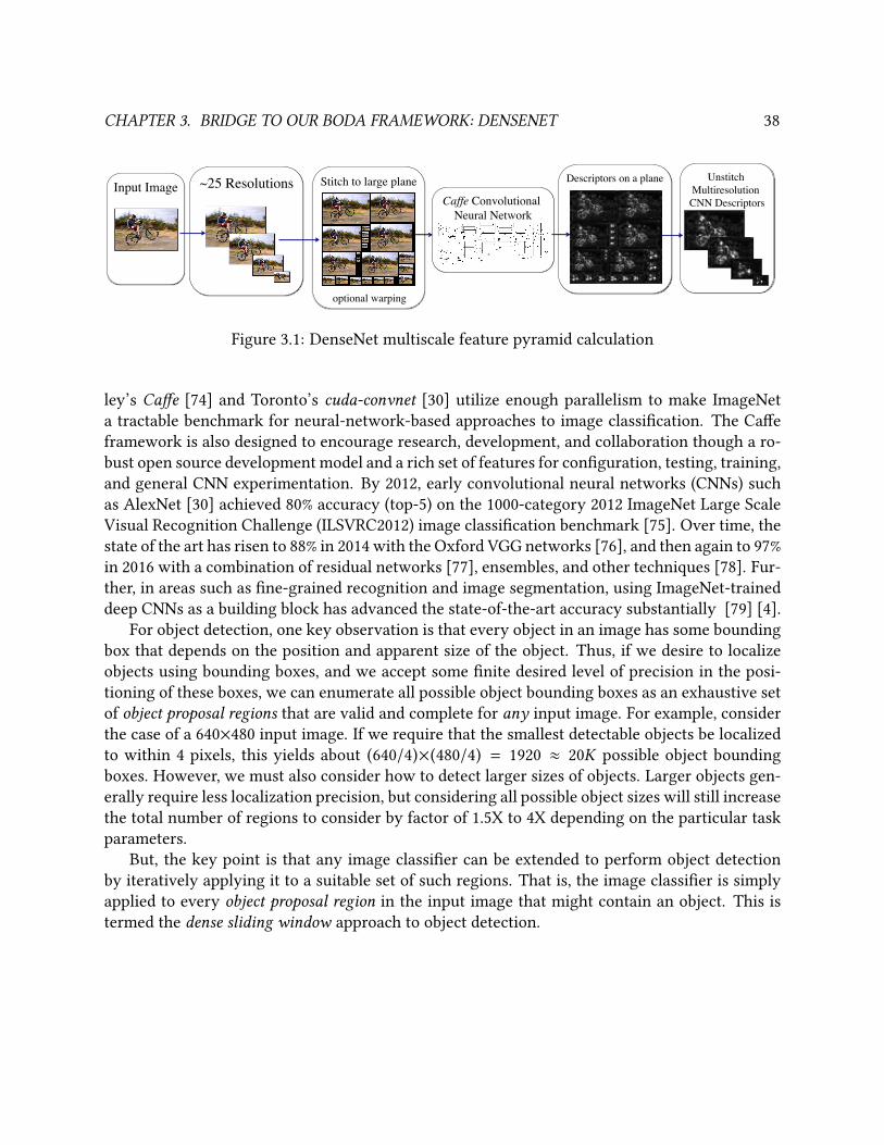
CHAPTER 3. BRIDGE TO OUR BODA FRAMEWORK: DENSENET 38
Unstitch Multiresolution CNN Descriptors!
Descriptors on a plane!Stitch to large plane!~25 Resolutions!Input Image!Caffe Convolutional !
Neural Network!
optional warping!
Figure 3.1: DenseNet multiscale feature pyramid calculation
ley’s Cae [74] and Toronto’s cuda-convnet [30] utilize enough parallelism to make ImageNet
a tractable benchmark for neural-network-based approaches to image classication. The Cae
framework is also designed to encourage research, development, and collaboration though a ro-
bust open source development model and a rich set of features for conguration, testing, training,
and general CNN experimentation. By 2012, early convolutional neural networks (CNNs) such
as AlexNet [30] achieved 80% accuracy (top-5) on the 1000-category 2012 ImageNet Large Scale
Visual Recognition Challenge (ILSVRC2012) image classication benchmark [75]. Over time, the
state of the art has risen to 88% in 2014 with the Oxford VGG networks [76], and then again to 97%
in 2016 with a combination of residual networks [77], ensembles, and other techniques [78]. Fur-
ther, in areas such as ne-grained recognition and image segmentation, using ImageNet-trained
deep CNNs as a building block has advanced the state-of-the-art accuracy substantially [79] [4].
For object detection, one key observation is that every object in an image has some bounding
box that depends on the position and apparent size of the object. Thus, if we desire to localize
objects using bounding boxes, and we accept some nite desired level of precision in the posi-
tioning of these boxes, we can enumerate all possible object bounding boxes as an exhaustive set
of object proposal regions that are valid and complete for any input image. For example, consider
the case of a 640×480 input image. If we require that the smallest detectable objects be localized
to within 4 pixels, this yields about (640/4)×(480/4) = 1920 ≈ 20K possible object bounding
boxes. However, we must also consider how to detect larger sizes of objects. Larger objects gen-
erally require less localization precision, but considering all possible object sizes will still increase
the total number of regions to consider by factor of 1.5X to 4X depending on the particular task
parameters.
But, the key point is that any image classier can be extended to perform object detection
by iteratively applying it to a suitable set of such regions. That is, the image classier is simply
applied to every object proposal region in the input image that might contain an object. This is
termed the dense sliding window approach to object detection.
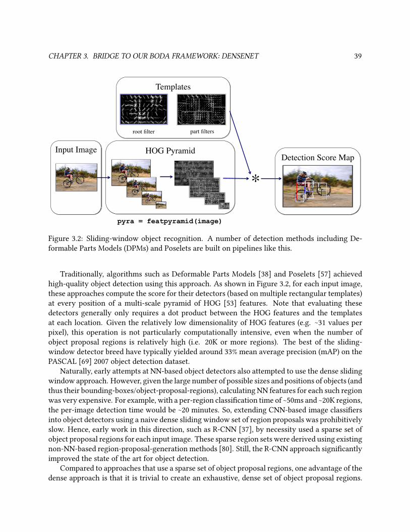
CHAPTER 3. BRIDGE TO OUR BODA FRAMEWORK: DENSENET 39
Ground Truth!
Detection!
Filter Placement!
Templates!
HOG Pyramid!Input Image!Detection Score Map!
!
pyra = featpyramid(image)
root filter! part filters!
*!
Figure 3.2: Sliding-window object recognition. A number of detection methods including De-
formable Parts Models (DPMs) and Poselets are built on pipelines like this.
Traditionally, algorithms such as Deformable Parts Models [38] and Poselets [57] achieved
high-quality object detection using this approach. As shown in Figure 3.2, for each input image,
these approaches compute the score for their detectors (based on multiple rectangular templates)
at every position of a multi-scale pyramid of HOG [53] features. Note that evaluating these
detectors generally only requires a dot product between the HOG features and the templates
at each location. Given the relatively low dimensionality of HOG features (e.g. ∼31 values per
pixel), this operation is not particularly computationally intensive, even when the number of
object proposal regions is relatively high (i.e. 20K or more regions). The best of the sliding-
window detector breed have typically yielded around 33% mean average precision (mAP) on the
PASCAL [69] 2007 object detection dataset.
Naturally, early attempts at NN-based object detectors also attempted to use the dense sliding
window approach. However, given the large number of possible sizes and positions of objects (and
thus their bounding-boxes/object-proposal-regions), calculating NN features for each such region
was very expensive. For example, with a per-region classication time of ∼50ms and ∼20K regions,
the per-image detection time would be ∼20 minutes. So, extending CNN-based image classiers
into object detectors using a naive dense sliding window set of region proposals was prohibitively
slow. Hence, early work in this direction, such as R-CNN [37], by necessity used a sparse set of
object proposal regions for each input image. These sparse region sets were derived using existing
non-NN-based region-proposal-generation methods [80]. Still, the R-CNN approach signicantly
improved the state of the art for object detection.
Compared to approaches that use a sparse set of object proposal regions, one advantage of the
dense approach is that it is trivial to create an exhaustive, dense set of object proposal regions.
CHAPTER 3. BRIDGE TO OUR BODA FRAMEWORK: DENSENET 40
However, as stated, depending on the desired density in position and scale, the number of region
proposals may become quite large. To avoid this issue, one can either reduce the number of
region proposals, decrease the time spent per region, or some combination of the two. In the
related work section, we consider various approaches that explore specic design points in this
space of options.
Of particular note for decreasing the time spent per region, the convolutional nature of CNNs
oers the potential to share signicant work between overlapping regions. However, in practice,
there are various challenges that complicate achieving this sharing. Specically, in this work
we consider what is necessary to eciently support the classication method of CNNs such as
AlexNet [30] over many possible region proposals for an image. In particular, we must address
the key issues of supporting per-region data centering, varied region sizes, and varied region
aspect ratios.
The remainder of this chapter is organized as follows: In Section 3.2, we review related
work on dense CNN features, particularly for object detection. Then, in Section 3.3 we propose
DenseNet, our approach to eciently computing pyramids of CNN features. Next, in Section 3.4,
we briey and qualitatively evaluate the correctness of our approach. Finally, in Section 3.5 we
present our conclusions. There, we include discussion about our second implementation of the
DenseNet method, DenseNet-v2, and the relationship of the entire DenseNet eort to shaping
our research trajectory.
3.2 DenseNet Related WorkCNNs for Object Detection. DetectorNet [81] performs sliding-window detection on a coarse
3-scale CNN pyramid. Due to the large receptive eld of CNN features, localization can be a
challenge for sliding-window detection based on CNNs. Toward rectifying this, DetectorNet adds
a procedure to rene the CNN for better localization. However, DetectorNet does not pretrain its
CNN on a large data corpus such as ImageNet, and this may be a limiting factor in its accuracy.
In fact, DetectorNet reported 30% mAP on PASCAL VOC 2007, less than the best HOG-based
methods.
OverFeat [82] generates dense, multi-scale CNN features suitable for object detection and clas-
sication for square regions. OverFeat does not consider the issue of non-square region proposals
as they are not necessary for their approaches to detection or classication. In our approach, we
support both the extraction of non-square regions of features as well as the higher level approach
of constructing multiple feature pyramids where, for each pyramid, the input has been warped to
a selected aspect ratio. While pre-compiled binaries for running the OverFeat CNN to create such
features using provided pre-trained CNN model parameters are provided, training code is explic-
itly not provided. Further, it is unclear how much of the source code for the rest of the OverFeat
system is available; some is part of the Torch [83] framework used by OverFeat. This lack of
openness hinders the usage of OverFeat as the basis for exploring the design space of CNN-based
detection algorithms, particularly for benchmark sets where no OverFeat-based detection results
are available (such as the PASCAL VOC benchmarks). Also, unlike the Cae system into which
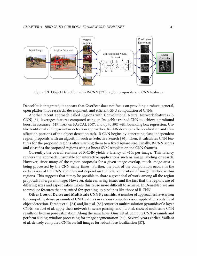
CHAPTER 3. BRIDGE TO OUR BODA FRAMEWORK: DENSENET 41
Per-Region!Descriptors!
Convolutional Neural Network!
Warped Regions!
Region Proposals!
HOG Pyramid!Input Image!
DenseNet: Efficient Object Detection with!! ! ! ! ! Deep ConvNet Feature Pyramids!
Forrest Iandola, Matt Moskewicz, Sergey Karayev, Ross Girshick, Yangqing Jia, !Kurt Keutzer, and Trevor Darrell!
Deformable Parts Model Detection!
1. P. Felzenszwalb, R. Girshick, D. McAllester, D. Ramanan. Object Detection with Discriminatively Trained Part Based Models. PAMI, 2010.!
2. H. Song, R. Girshick, T. Darrell. Discriminatively Activated Sparselets. ICML, 2013.!3. T. Dean, et al. (Google, Inc.) Fast, Accurate Detection of 100,000 Object Classes on a
Single Machine. CVPR, 2013.!4. C. Dubout and F. Fleuret. Exact Acceleration of Linear Object Detectors. ECCV, 2012.!5. F. Iandola, D. Sheffield, M. Anderson, P. Phothilimthana, and K. Keutzer.
Communication-Minimizing 2D Convolution in GPU Registers. ICIP, 2013.!6. H. Niknejad et al. On-Road Multivehicle Tracking Using Deformable Object Model and
Particle Filter With Improved Likelihood Estimation. IEEE Trans. Intell. Transportation. 2012.!
7. M. Andriluka et al. Vision based victim detection from unmanned aerial vehicles. IROS, 2010. !
References!
Input Image! Extract HOG feature descriptors !!
Feature matching with learned model!!!
Distance transform and scoring !
Structured grid!Histogram and!Convolution!
Structured grid!Convolution with !several filters!
Output Detections!!
Vector distance,!Structured grid!
…
Linear !Classifier!
pyra = featpyramid(image)
Input Image!
Figure 3.3: Object Detection with R-CNN [37]: region proposals and CNN features.
DenseNet is integrated, it appears that OverFeat does not focus on providing a robust, general,
open platform for research, development, and ecient GPU computation of CNNs.
Another recent approach called Regions with Convolutional Neural Network features (R-
CNN) [37] leverages features computed using an ImageNet-trained CNN to achieve a profound
boost in accuracy: 54% mAP on PASCAL 2007, and up to 59% with bounding box regression. Un-
like traditional sliding-window detection approaches, R-CNN decouples the localization and clas-
sication portions of the object detection task. R-CNN begins by generating class-independent
region proposals with an algorithm such as Selective Search [80]. Then, it calculates CNN fea-
tures for the proposed regions after warping them to a xed square size. Finally, R-CNN scores
and classies the proposed regions using a linear SVM template on the CNN features.
Currently, the overall runtime of R-CNN yields a latency of ∼10s per image. This latency
renders the approach unsuitable for interactive applications such as image labeling or search.
However, since many of the region proposals for a given image overlap, much image area is
being processed by the CNN many times. Further, the bulk of the computation occurs in the
early layers of the CNN and does not depend on the relative position of image patches within
regions. This suggests that it may be possible to share a great deal of work among all the region
proposals for a given image. However, data centering issues and the fact that the regions are of
diering sizes and aspect ratios makes this reuse more dicult to achieve. In DenseNet, we aim
to produce features that are suited for speeding up pipelines like those of R-CNN.
OtherUses of Dense andMultiscale CNNPyramids. A number of approaches have arisen
for computing dense pyramids of CNN features in various computer vision applications outside of
object detection. Farabet et al. [84] and Jiu et al. [85] construct multiresolution pyramids of 2-layer
CNNs. Farabet et al. apply their network to scene parsing, and Jiu et al. showed multiscale CNN
results on human pose estimation. Along the same lines, Giusti et al. compute CNN pyramids and
perform sliding-window processing for image segmentation [86]. Several years earlier, Vaillant
et al. densely computed CNNs on full images for robust face localization [87].
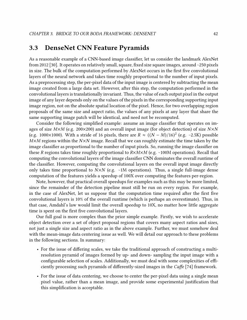
CHAPTER 3. BRIDGE TO OUR BODA FRAMEWORK: DENSENET 42
3.3 DenseNet CNN Feature PyramidsAs a reasonable example of a CNN-based image classier, let us consider the landmark AlexNet
from 2012 [30]. It operates on relatively small, square, xed size square images, around ∼250 pixels
in size. The bulk of the computation performed by AlexNet occurs in the rst ve convolutional
layers of the neural network and takes time roughly proportional to the number of input pixels.
As a preprocessing step, the per-pixel data of the input image is centered by subtracting the mean
image created from a large data set. However, after this step, the computation performed in the
convolutional layers is translationally invariant. Thus, the value of each output pixel in the output
image of any layer depends only on the values of the pixels in the corresponding supporting input
image region, not on the absolute spatial location of the pixel. Hence, for two overlapping region
proposals of the same size and aspect ratio, the values of any pixels at any layer that share the
same supporting image patch will be identical, and need not be recomputed.
Consider the following simplied example: assume an image classier that operates on im-
ages of size M×M (e.g. 200×200) and an overall input image (for object detection) of size N×N(e.g. 1000×1000). With a stride of 16 pixels, there are R ≈ ((N − M )/16)2 (e.g. ∼2.5K) possible
M×M regions within the N×N image. Recall that we can roughly estimate the time taken by the
image classier as proportional to the number of input pixels. So, running the image classier on
these R regions takes time roughly proportional to R×M×M (e.g. ∼100M operations). Recall that
computing the convolutional layers of the image classier CNN dominates the overall runtime of
the classier. However, computing the convolutional layers on the overall input image directly
only takes time proportional to N×N (e.g. ∼1M operations). Thus, a single full-image dense
computation of the features yields a speedup of 100X over computing the features per-region.
Note, however, that practical overall speedups for examples such as this may be more limited,
since the remainder of the detection pipeline must still be run on every region. For example,
in the case of AlexNet, let us suppose that the computation time required after the rst ve
convolutional layers is 10% of the overall runtime (which is perhaps an overestimate). Thus, in
that case, Amdahl’s law would limit the overall speedup to 10X, no matter how little aggregate
time is spent on the rst ve convolutional layers.
Our full goal is more complex than the prior simple example. Firstly, we wish to accelerate
object detection over a set of object proposal regions that covers many aspect ratios and sizes,
not just a single size and aspect ratio as in the above example. Further, we must somehow deal
with the mean-image data centering issue as well. We will detail our approach to these problems
in the following sections. In summary:
• For the issue of diering scales, we take the traditional approach of constructing a multi-
resolution pyramid of images formed by up- and down- sampling the input image with a
congurable selection of scales. Additionally, we must deal with some complexities of e-
ciently processing such pyramids of dierently-sized images in the Cae [74] framework.
• For the issue of data centering, we choose to center the per-pixel data using a single mean
pixel value, rather than a mean image, and provide some experimental justication that
this simplication is acceptable.
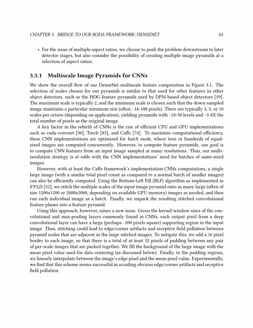
CHAPTER 3. BRIDGE TO OUR BODA FRAMEWORK: DENSENET 43
• For the issue of multiple aspect ratios, we choose to push the problem downstream to later
detector stages, but also consider the possibility of creating multiple image pyramids at a
selection of aspect ratios.
3.3.1 Multiscale Image Pyramids for CNNsWe show the overall ow of our DenseNet multiscale feature computation in Figure 3.1. The
selection of scales chosen for our pyramids is similar to that used for other features in other
object detectors, such as the HOG feature pyramids used by DPM-based object detectors [59].
The maximum scale is typically 2, and the minimum scale is chosen such that the down-sampled
image maintains a particular minimum size (often ∼16-100 pixels). There are typically 3, 5, or 10
scales per octave (depending on application), yielding pyramids with ∼10-50 levels and ∼3-8X the
total number of pixels as the original image.
A key factor in the rebirth of CNNs is the rise of ecient CPU and GPU implementations
such as cuda-convnet [30], Torch [83], and Cae [74]. To maximize computational eciency,
these CNN implementations are optimized for batch mode, where tens or hundreds of equal-
sized images are computed concurrently. However, to compute feature pyramids, our goal is
to compute CNN features from an input image sampled at many resolutions. Thus, our multi-
resolution strategy is at odds with the CNN implementations’ need for batches of same-sized
images.
However, with at least the Cae framework’s implementation CNNs computations, a single
large image (with a similar total pixel count as compared to a normal batch of smaller images)
can also be eciently computed. Using the Bottom-Left Fill (BLF) algorithm as implemented in
FFLD [52], we stitch the multiple scales of the input image pyramid onto as many large (often of
size 1200x1200 or 2000x2000, depending on available GPU memory) images as needed, and then
run each individual image as a batch. Finally, we unpack the resulting stitched convolutional
feature planes into a feature pyramid.
Using this approach, however, raises a new issue. Given the kernel/window sizes of the con-
volutional and max-pooling layers commonly found in CNNs, each output pixel from a deep
convolutional layer can have a large (perhaps ∼200 pixels square) supporting region in the input
image. Thus, stitching could lead to edge/corner artifacts and receptive eld pollution between
pyramid scales that are adjacent in the large stitched images. To mitigate this, we add a 16 pixel
border to each image, so that there is a total of at least 32 pixels of padding between any pair
of per-scale images that are packed together. We ll the background of the large image with the
mean pixel value used for data centering (as discussed below). Finally, in the padding regions,
we linearly interpolate between the image’s edge pixel and the mean pixel value. Experimentally,
we nd that this scheme seems successful in avoiding obvious edge/corner artifacts and receptive
eld pollution.
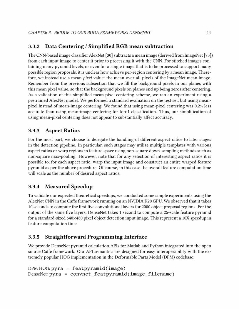
CHAPTER 3. BRIDGE TO OUR BODA FRAMEWORK: DENSENET 44
3.3.2 Data Centering / Simplied RGB mean subtractionThe CNN-based image classier AlexNet [30] subtracts a mean image (derived from ImageNet [73])
from each input image to center it prior to processing it with the CNN. For stitched images con-
taining many pyramid levels, or even for a single image that is to be processed to support many
possible region proposals, it is unclear how achieve per-region centering by a mean image. There-
fore, we instead use a mean pixel value: the mean-over-all-pixels of the ImageNet mean image.
Remember from the previous subsection that we ll the background pixels in our planes with
this mean pixel value, so that the background pixels on planes end up being zeros after centering.
As a validation of this simplied mean-pixel centering scheme, we ran an experiment using a
pretrained AlexNet model. We performed a standard evaluation on the test set, but using mean-
pixel instead of mean-image centering. We found that using mean-pixel centering was 0.2% less
accurate than using mean-image centering for top-1 classication. Thus, our simplication of
using mean-pixel centering does not appear to substantially aect accuracy.
3.3.3 Aspect RatiosFor the most part, we choose to delegate the handling of dierent aspect ratios to later stages
in the detection pipeline. In particular, such stages may utilize multiple templates with various
aspect ratios or warp regions in feature space using non-square down-sampling methods such as
non-square max-pooling. However, note that for any selection of interesting aspect ratios it is
possible to, for each aspect ratio, warp the input image and construct an entire warped feature
pyramid as per the above procedure. Of course, in this case the overall feature computation time
will scale as the number of desired aspect ratios.
3.3.4 Measured SpeedupTo validate our expected theoretical speedups, we conducted some simple experiments using the
AlexNet CNN in the Cae framework running on an NVIDIA K20 GPU. We observed that it takes
10 seconds to compute the rst ve convolutional layers for 2000 object proposal regions. For the
output of the same ve layers, DenseNet takes 1 second to compute a 25-scale feature pyramid
for a standard-sized 640×480 pixel object detection input image. This represent a 10X speedup in
feature computation time.
3.3.5 Straightforward Programming InterfaceWe provide DenseNet pyramid calculation APIs for Matlab and Python integrated into the open
source Cae framework. Our API semantics are designed for easy interoperability with the ex-
tremely popular HOG implementation in the Deformable Parts Model (DPM) codebase:
DPM HOG: pyra = featpyramid(image)DenseNet: pyra = convnet_featpyramid(image_filename)
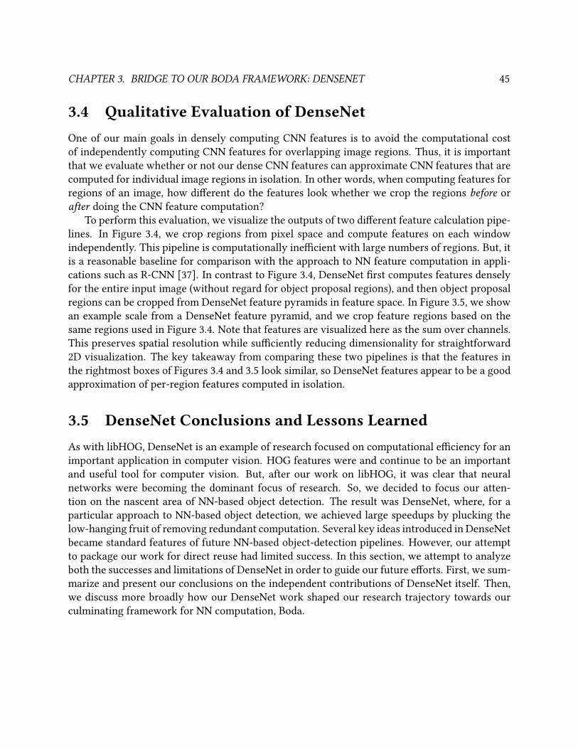
CHAPTER 3. BRIDGE TO OUR BODA FRAMEWORK: DENSENET 45
3.4 Qualitative Evaluation of DenseNetOne of our main goals in densely computing CNN features is to avoid the computational cost
of independently computing CNN features for overlapping image regions. Thus, it is important
that we evaluate whether or not our dense CNN features can approximate CNN features that are
computed for individual image regions in isolation. In other words, when computing features for
regions of an image, how dierent do the features look whether we crop the regions before or
after doing the CNN feature computation?
To perform this evaluation, we visualize the outputs of two dierent feature calculation pipe-
lines. In Figure 3.4, we crop regions from pixel space and compute features on each window
independently. This pipeline is computationally inecient with large numbers of regions. But, it
is a reasonable baseline for comparison with the approach to NN feature computation in appli-
cations such as R-CNN [37]. In contrast to Figure 3.4, DenseNet rst computes features densely
for the entire input image (without regard for object proposal regions), and then object proposal
regions can be cropped from DenseNet feature pyramids in feature space. In Figure 3.5, we show
an example scale from a DenseNet feature pyramid, and we crop feature regions based on the
same regions used in Figure 3.4. Note that features are visualized here as the sum over channels.
This preserves spatial resolution while suciently reducing dimensionality for straightforward
2D visualization. The key takeaway from comparing these two pipelines is that the features in
the rightmost boxes of Figures 3.4 and 3.5 look similar, so DenseNet features appear to be a good
approximation of per-region features computed in isolation.
3.5 DenseNet Conclusions and Lessons LearnedAs with libHOG, DenseNet is an example of research focused on computational eciency for an
important application in computer vision. HOG features were and continue to be an important
and useful tool for computer vision. But, after our work on libHOG, it was clear that neural
networks were becoming the dominant focus of research. So, we decided to focus our atten-
tion on the nascent area of NN-based object detection. The result was DenseNet, where, for a
particular approach to NN-based object detection, we achieved large speedups by plucking the
low-hanging fruit of removing redundant computation. Several key ideas introduced in DenseNet
became standard features of future NN-based object-detection pipelines. However, our attempt
to package our work for direct reuse had limited success. In this section, we attempt to analyze
both the successes and limitations of DenseNet in order to guide our future eorts. First, we sum-
marize and present our conclusions on the independent contributions of DenseNet itself. Then,
we discuss more broadly how our DenseNet work shaped our research trajectory towards our
culminating framework for NN computation, Boda.
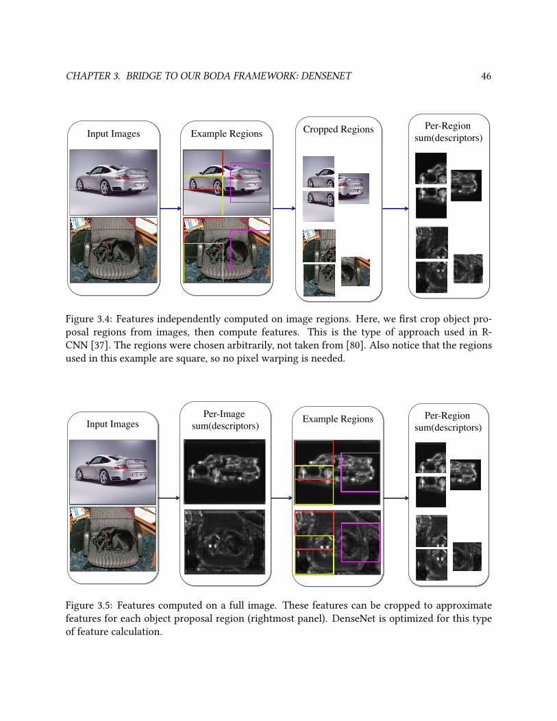
CHAPTER 3. BRIDGE TO OUR BODA FRAMEWORK: DENSENET 46
Input Images! Example Regions!
Per-Region sum(descriptors) !
Per-Region sum(descriptors) !
Cropped Regions!Input Images! Example Regions!
Per-Image sum(descriptors)!
Figure 3.4: Features independently computed on image regions. Here, we rst crop object pro-
posal regions from images, then compute features. This is the type of approach used in R-
CNN [37]. The regions were chosen arbitrarily, not taken from [80]. Also notice that the regions
used in this example are square, so no pixel warping is needed.
Input Images! Example Regions!
Per-Region sum(descriptors) !
Per-Region sum(descriptors) !
Cropped Regions!Input Images! Example Regions!
Per-Image sum(descriptors)!
Figure 3.5: Features computed on a full image. These features can be cropped to approximate
features for each object proposal region (rightmost panel). DenseNet is optimized for this type
of feature calculation.
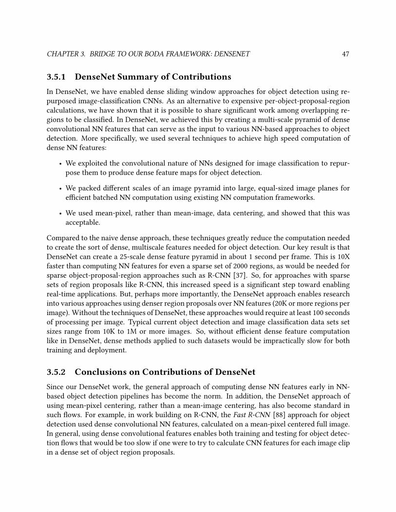
CHAPTER 3. BRIDGE TO OUR BODA FRAMEWORK: DENSENET 47
3.5.1 DenseNet Summary of ContributionsIn DenseNet, we have enabled dense sliding window approaches for object detection using re-
purposed image-classication CNNs. As an alternative to expensive per-object-proposal-region
calculations, we have shown that it is possible to share signicant work among overlapping re-
gions to be classied. In DenseNet, we achieved this by creating a multi-scale pyramid of dense
convolutional NN features that can serve as the input to various NN-based approaches to object
detection. More specically, we used several techniques to achieve high speed computation of
dense NN features:
• We exploited the convolutional nature of NNs designed for image classication to repur-
pose them to produce dense feature maps for object detection.
• We packed dierent scales of an image pyramid into large, equal-sized image planes for
ecient batched NN computation using existing NN computation frameworks.
• We used mean-pixel, rather than mean-image, data centering, and showed that this was
acceptable.
Compared to the naive dense approach, these techniques greatly reduce the computation needed
to create the sort of dense, multiscale features needed for object detection. Our key result is that
DenseNet can create a 25-scale dense feature pyramid in about 1 second per frame. This is 10X
faster than computing NN features for even a sparse set of 2000 regions, as would be needed for
sparse object-proposal-region approaches such as R-CNN [37]. So, for approaches with sparse
sets of region proposals like R-CNN, this increased speed is a signicant step toward enabling
real-time applications. But, perhaps more importantly, the DenseNet approach enables research
into various approaches using denser region proposals over NN features (20K or more regions per
image). Without the techniques of DenseNet, these approaches would require at least 100 seconds
of processing per image. Typical current object detection and image classication data sets set
sizes range from 10K to 1M or more images. So, without ecient dense feature computation
like in DenseNet, dense methods applied to such datasets would be impractically slow for both
training and deployment.
3.5.2 Conclusions on Contributions of DenseNetSince our DenseNet work, the general approach of computing dense NN features early in NN-
based object detection pipelines has become the norm. In addition, the DenseNet approach of
using mean-pixel centering, rather than a mean-image centering, has also become standard in
such ows. For example, in work building on R-CNN, the Fast R-CNN [88] approach for object
detection used dense convolutional NN features, calculated on a mean-pixel centered full image.
In general, using dense convolutional features enables both training and testing for object detec-
tion ows that would be too slow if one were to try to calculate CNN features for each image clip
in a dense set of object region proposals.
CHAPTER 3. BRIDGE TO OUR BODA FRAMEWORK: DENSENET 48
3.5.3 Issues with DenseNet that Informed our Research TrajectoryThe DenseNet approach was a natural evolution of existing object detection approaches at that
time, and has become a common building block in NN-based object detection. Indeed, in later
work by some DenseNet co-authors [5], it was shown that the older Deformable Parts Model
approach [38] to object detection could be formulated in terms of NNs, and thus could leverage
DenseNet-style NN features. However, in the course of the DenseNet work, two particular issues
shaped our continuing research trajectory going forward:
• Repurposing object-classication NNs for object-detection highlighted issues related to
mapping spatial coordinates across NN layers. These issues could only be incompletely
explored and addressed in the context of DenseNet, and motivated the reimplementation
of DenseNet within a custom vertical framework designed to help explore such issues.
• While the concepts of DenseNet were often cited and used various contexts, packaging
DenseNet for direct use in research and practice proved dicult. As with libHOG, it was
often the case that, for researchers, the integration costs exceeded the benets. This pro-
vided motivation to explore methods whereby such optimizations could be performed in a
manner that was more deployable in both research and practice.
We now explain in detail how these two issues tie DenseNet together with the overall body of
work presented in this dissertation.
3.5.3.1 Feature Space Mapping and DenseNet-v2
One of the key aspects of the DenseNet approach is the idea of repurposing convolutional-NN-
based image classiers for object detection. In this section, we will rst explain some key technical
details of this process. Then, we will discuss some of the challenges we encountered related to
this process, and how they informed our future work.
As will be discussed in Section 4.1.2, deep NNs transform an input image into dierent rep-
resentations layer-by-layer. For image classication, the spatial resolution of the nal output
layer must be a single pixel, since the classication task is to return a single Boolean value, is-X-in-image, for each entire input image. But, the input image has some nite image resolution,
such as X×Y = 227×227 as in our running example (introduced in Section 1.1.1). Typically, the
spatial resolution is gradually decreased layer-by-layer from the input to the nal output. Thus,
the outputs of intermediate layers will have intermediate spatial resolutions, progressively lower
than that of the input image. The two primary methods by which the spatial resolution decreases
from layer to layer are downsampling and padding-related-eects. Resolution reduction due to
downsampling is straightforward: some layers use strided convolution or pooling such that, for
each spatial dimension, they produce only 1 pixel of output for every 2 or 4 input pixels. Thus,
if the rst layer employs convolution with a stride of 4, the rst layer output will have spatial
resolution of about 227/4 ≈ 56. However, padding-related-eects are a bit more subtle. They
arise from the fact that, for each output point, convolution and pooling often have a kernel size
greater than one. So, unless some form of padding is employed, the spatial size of the output of
CHAPTER 3. BRIDGE TO OUR BODA FRAMEWORK: DENSENET 49
a convolution or pooling operation will also be reduced by one-less-than-the-size of that opera-
tion’s spatial window (i.e. its kernel size minus 1). For example, to rene our prior example, if
the rst layer has a stride of 4, no padding, and a convolution kernel size of 11, then resulting
spatial dimension will be exactly 55. In general, the spatial output size of a layer is calculated as
1 + (INSIZE + PAD − KERNELSZ )/STRIDE or 1 + (227 + 0 − 11)/4 in this case.
As a particularly important special case, if the kernel size is the same size as the entire input to
a given layer, and no padding is used, then the output of that layer will have a spatial resolution
of 1×1 (i.e. it will be a single pixel). This is commonly termed a fully-connected layer. Note
that, in this case, stride has no eect on the operation, since there is only a single output point
to compute. In fact, the stride for such layers may not even be specied, but can typically be
assumed to be 1 by default. After such a layer, all information that was previously distributed in
the spatial dimensions has been merged, so that the per-pixel feature space now represents the
entire input image.
Now, consider that case where a convolutional NN-based image classier is given an input
image larger than which it was designed for. In this case, the spatial dimensions at all layers,
including the output, will increase proportionally to the increase in the input image size. For
example, typically, the total end-to-end NN downsampling factor due to strided convolution and
pooling might be around 32X. Thus, for each 32 pixels added to the spatial dimensions of the
input, the output will increase in spatial size by 1. Intermediate layers will increase by 32, 16, 8,
4, 2, or 1 pixel(s), depending on how much stride-induced downsampling has accrued up to each
layer. But, in short, this method of using increased input image sizes is the basic method by which
dense features usable for localization (and thus object detection) are formed. However, the nal
relationship between regions of the input image and regions of intermediate layers is complex
and depends on the stride and padding applied at each layer. In DenseNet, this relationship was
not well understood or fully explored. In turn, this created uncertainly in:
• how to properly localize detection results corresponding to spatial sub-regions of interme-
diate NN layers.
• how to test that DenseNet was correctly calculating the deep NN features for any given
sub-region.
A desire to more fully study and understand this issue prompted reimplementing DenseNet in-
side a purpose-built vertical framework. In this new framework, termed DenseNet-v2, we were
able to fully understand and automate the mapping of spatial regions between layers of convo-
lutional NNs. Using these feature space mappings, we were able to perform various testing and
experiments that were not possible in the original DenseNet implementation. In particular, when
padding and strides were correctly controlled, we could quantitatively verify that the DenseNet-
calculated features corresponding to sub-regions of large images were numerically equivalent to
computing the same features for the sub-region directly. The lack of such quantitative correct-
ness testing was a signicant limitation of the original implementation, which we have rectied
in our reimplementation.
CHAPTER 3. BRIDGE TO OUR BODA FRAMEWORK: DENSENET 50
3.5.3.2 Often Cited, Sometimes Re-implemented, Never Directly Used
Over time, the research contributions of DenseNet are commonly cited by researchers in terms
such as “Our feature calculation is slow, but could be speed up using the methods of DenseNet.” As
with libHOG, DenseNet suered from a lack of direct research or practical adoption. As discussed
in Section 2.7.3.2, packaging research-quality optimization work so that it can be used by other
researchers, or perhaps even in real-world practice, is quite dicult. Certainly, such packaging
for direct use is not a requirement of such research. However, good packaging can only increase
the impact of a given piece of optimization research. Further, it is valid topic of research in and
of itself, and, in the context of the rise of NNs, it seems that are good opportunities to explore
this area. In particular, modern NN frameworks, including our Boda framework that we will
present in Chapter 6, allow for more portability and modularity with respect to implementing
core operations, such that:
• Optimizations of individual core operations can be performed more easily.
• Machine learning researchers can easily benet from optimization of small parts of their
ows without per-researcher overhead.
In the end, this avoids the situation where many individual optimizations are not adopted since
their individual eects on a given ow are not enough to warrant special eort to include them.
Thus, eventually, as all parts of a given ow are optimized, researchers and practical applications
can eventually see signicant overall speedups.
In our work, we embrace the higher levels of abstraction and modularity that are achieved by
using NN operations as pre-specied building blocks for larger systems. We envision an ecosys-
tem consisting of set of frameworks for neural network related activities, each geared toward
dierent tasks and goals. As long as these frameworks use a common layer of abstraction to
encapsulate lower-level computations, they will have an inherent level of compatibility. With
this in mind, the culminating framework of this dissertation is intended primarily to support the
development of new NN operations and the optimization of existing ones. However, once opera-
tions are developed or tuned, the clean, simple operation-level interface of functions acting over
xed-size groups of numbers (i.e. N-Dimensional-Arrays, or ND-Arrays) allows for reasonably
easy sharing of such eorts across frameworks. Further, as another feature of our framework,
we want to provide support for a wide range of deployment scenarios as well, giving users more
choices for practical deployments on various target platforms.
So, one goal of reimplementing DenseNet as DenseNet-v2 was as a prototype for this vision.
To further explore this concept, we extended DenseNet-v2 to include a full object detection pipe-
line. While such a system was not intended to give state-of-the-art results, it provided a testing
environment to evaluate our ideas about enabling more portable deployment of optimizations
such as DenseNet and the vision pipelines that would use them. In our framework, we were able
to use the same detection pipeline for both:
• Image classication, using the original unmodied convolutional NN, and
CHAPTER 3. BRIDGE TO OUR BODA FRAMEWORK: DENSENET 51
• Object detection, using an automatically repurposed version of the original NN (operating
on larger images).
The detection pipeline operates on ND-Arrays of NN features as input, without dependencies on
where the ND-Arrays came from. For multi-scale detection, the detection pipeline was simply
run on multiple ND-Arrays, one per scale. Thus, the detection pipeline is agnostic to all the
details of the implementation of DenseNet-style NN feature calculation. Internally, the feature
calculation stages in DenseNet-v2 were free to pack multiple scales into large images, perform NN
computations on the large images, and then unpack the resultant dense per-scale feature images,
with all this being transparent to the rest of the detection pipeline. This type of transparency
was not possible in the original DenseNet, due to the restrictions of working within existing
NN frameworks (such as Cae) that had no notion of using general ND-Arrays as an interface
between pipeline stages in a unied manner. In particular, the ability to map between spatial
regions of NN features at dierent scales and layers of abstraction was critical to enabling this
ow.
In summary, while DenseNet and DenseNet-v2 did not focus on direct optimization of core NN
computations, they explored key issues associated with composition and reuse of such operations.
The reimplementation work of DenseNet-v2 was a prototype, proof-of-concept, and foundation
for our future work on a more general framework for implementing, optimizing, and deploying
general NN computations.
3.5.4 Conclusions From DenseNet that Shaped our Research TrajectoryOne goal of DenseNet was to achieve direct use of our optimization research by speeding up the
relatively high-level operation of multiscale feature pyramid creation. DenseNet was packaged in
such a way that it could be used as a drop-in replacement for pipelines that previously used other
types of features, such as HOG features. However, computer vision researchers at the time had
other plans. Instead of retrotting other pipelines with NN features, they were more interested
in creating entire end-to-end systems using new congurations of NNs. In particular, they were
interested in creating NN-based systems that could be trained as a whole, rather than having
some xed-function, pre-trained, or separately trained components.
For example, consider the case of Fast R-CNN, which was the next iteration of the R-CNN ow
that DenseNet used as a model ow to target for optimization. After computing dense features at a
single scale, Fast R-CNN employs a Region-of-Interest (RoI) pooling layer. This RoI pooling layer
uses max-pooling to form xed-length features for each object proposal region, thus avoiding
the need for calculating dense NN features at multiple scales. Since this is a somewhat dierent
approach for handling multiple scales than the feature pyramid approach employed in DenseNet,
Fast R-CNN did not directly use the DenseNet library. This sort of change in approach, from one
iteration of a ow to the next, is common in computer vision. Thus, the optimization of very high-
level NN primitives, like the multi-scale feature pyramids of DenseNet, seems less than ideal, due
to the rapid current rate of progress in eld. Simply put, in the current climate, any high-level
NN operation in use today is likely to be modied or changed substantially by next year.
CHAPTER 3. BRIDGE TO OUR BODA FRAMEWORK: DENSENET 52
Again, we note that direct use of the artifacts of research is not a requirement to make a
good contribution. Further, for any optimization research, it is important to release a reference
implementation in any event. Such a reference implementation can be inspected, built on, or
used to replicate results. However, the impact of such usage alone falls short having the resultant
library directly used in research or practice. So, as we moved forward in our research trajectory,
we continued to consider this issue in the context of NNs.
Overall, when choosing our next optimization research target, we looked for an aspect of NN
computation that was:
• low-level enough to remain a commonly-used building block for a long time, and
• packageable in a way that the results of our optimizations could be directly used.
The increasing success of neural networks over the period from ∼2012-2017 suggests that NNs
have unprecedented current and future importance, far beyond the norm for any single technique.
Although the space of NN-based approaches is large, one can isolate a key set computational
primitives, particularly convolutions, that play a large role across many usages of NNs. However,
unlike the relatively easy to exploit opportunities for optimization of libHOG and DenseNet, the
optimization of NN convolutions is a signicantly more complex problem. In particular, it re-
quires high-diculty low-level GPU parallel programming. Both teaching and automating such
programming remain unsolved problems, and thus such tasks require signicant manual eort
by rare skilled programmers. However, with these challenges and complexities come opportu-
nities for research. In particular, one key concern we choose to focus on was that of portability.
Given the dicult of implementing ecient convolutions, it was no surprise that many reason-
able target hardware platforms had no such implementations. So, by steering our work toward
targeting such platforms, we aimed to increase the chance of real adoption of our work. That
is, if we can create reasonably ecient implementations for platforms that currently lack any
implementation, it creates signicant incentive for direct usage of our work.
In the following chapters, we will discuss our culminating contribution: the Boda framework
for ecient, productive implementation of NN computations. Briey revisiting our outline, the
remaining chapters are organized as follows:
• In Chapter 4, we review background details specically relevant for Boda.
• In Chapter 5 we isolate the core problem we will address in Boda and review the relevant
related work.
• Then, in Chapter 6 we present the Boda framework itself.
• Finally, we give our overall conclusions on all our work (libHOG, DenseNet, and Boda) in
Chapter 7.
53
Chapter 4
Background
As discussed in Chapter 1, the Boda framework addresses problems that span several domains.
In this chapter, we will give a summary and references for the needed background across all the
relevant areas. In the following chapters, we will refer back to the relevant sections of this chapter
when appropriate. Hence, especially to the degree the reader is familiar with various topics, this
chapter can be skipped, skimmed, and/or read later on an as-needed basis. Note that, for many
of the topics in this chapter, the 2016 book Deep Learning [14] is a good general (and currently
freely available online) reference, and we will cite specic chapters and sections in that work
throughout this chapter. Further, for general information on current trends and applications in
machine learning, a good starting reference is the short 2015 article by Jordan and Mitchell [89].
4.1 What are Neural Networks?Neural Networks, or perhaps more properly Articial Neural Networks, have a long history in
machine learning. Much of the terminology and conventions associated with the current state of
the eld are historical. Indeed, many terms serve mostly to distinguish current approaches from
historical ones. For an extensive historical overview of NNs as they pertain to this work, the
reader is encouraged to start with a focused survey such as that from Schmidhuber [1]. However,
in this work, we are mainly concerned with current practice. Conveniently, we can describe cur-
rent types of NNs relatively easily using basic concepts without much reference to their historical
development.
4.1.1 Deep and/or Convolutional NNsIn this work, we deal mainly with what are commonly termed Deep and/or Convolutional Neural
Networks (DNNs, CNNs, or DCNNs). Since these are commonly used terms in machine learning
literature, it is important to try understand what they typically mean. At a high level, both terms
can be dened simply:
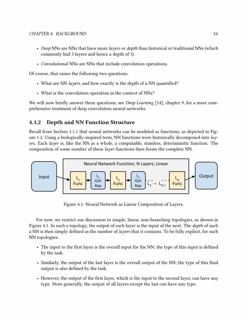
CHAPTER 4. BACKGROUND 54
• Deep NNs are NNs that have more layers or depth than historical or traditional NNs (which
commonly had 3 layers and hence a depth of 3).
• Convolutional NNs are NNs that include convolution operations.
Of course, that raises the following two questions:
• What are NN layers, and how exactly is the depth of a NN quantied?
• What is the convolution operation in the context of NNs?
We will now briey answer these questions; see Deep Learning [14], chapter 9, for a more com-
prehensive treatment of deep convolution neural networks.
4.1.2 Depth and NN Function StructureRecall from Section 1.1.1 that neural networks can be modeled as functions, as depicted in Fig-
ure 1.2. Using a biologically-inspired term, NN functions were historically decomposed into lay-ers. Each layer is, like the NN as a whole, a computable, stateless, deterministic function. The
composition of some number of these layer functions then forms the complete NN.
L3 → LN-1
Figure 4.1: Neural Network as Linear Composition of Layers.
For now, we restrict our discussion to simple, linear, non-branching topologies, as shown in
Figure 4.1. In such a topology, the output of each layer is the input of the next. The depth of such
a NN is then simply dened as the number of layers that it contains. To be fully explicit, for such
NN topologies:
• The input to the rst layer is the overall input for the NN; the type of this input is dened
by the task.
• Similarly, the output of the last layer is the overall output of the NN; the type of this nal
output is also dened by the task.
• However, the output of the rst layer, which is the input to the second layer, can have any
type. More generally, the output of all layers except the last can have any type.
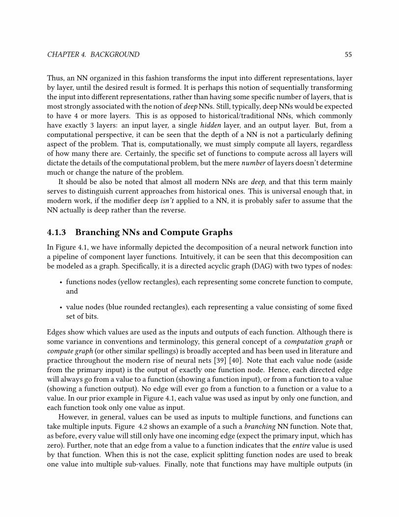
CHAPTER 4. BACKGROUND 55
Thus, an NN organized in this fashion transforms the input into dierent representations, layer
by layer, until the desired result is formed. It is perhaps this notion of sequentially transforming
the input into dierent representations, rather than having some specic number of layers, that is
most strongly associated with the notion of deep NNs. Still, typically, deep NNs would be expected
to have 4 or more layers. This is as opposed to historical/traditional NNs, which commonly
have exactly 3 layers: an input layer, a single hidden layer, and an output layer. But, from a
computational perspective, it can be seen that the depth of a NN is not a particularly dening
aspect of the problem. That is, computationally, we must simply compute all layers, regardless
of how many there are. Certainly, the specic set of functions to compute across all layers will
dictate the details of the computational problem, but the mere number of layers doesn’t determine
much or change the nature of the problem.
It should be also be noted that almost all modern NNs are deep, and that this term mainly
serves to distinguish current approaches from historical ones. This is universal enough that, in
modern work, if the modier deep isn’t applied to a NN, it is probably safer to assume that the
NN actually is deep rather than the reverse.
4.1.3 Branching NNs and Compute GraphsIn Figure 4.1, we have informally depicted the decomposition of a neural network function into
a pipeline of component layer functions. Intuitively, it can be seen that this decomposition can
be modeled as a graph. Specically, it is a directed acyclic graph (DAG) with two types of nodes:
• functions nodes (yellow rectangles), each representing some concrete function to compute,
and
• value nodes (blue rounded rectangles), each representing a value consisting of some xed
set of bits.
Edges show which values are used as the inputs and outputs of each function. Although there is
some variance in conventions and terminology, this general concept of a computation graph or
compute graph (or other similar spellings) is broadly accepted and has been used in literature and
practice throughout the modern rise of neural nets [39] [40]. Note that each value node (aside
from the primary input) is the output of exactly one function node. Hence, each directed edge
will always go from a value to a function (showing a function input), or from a function to a value
(showing a function output). No edge will ever go from a function to a function or a value to a
value. In our prior example in Figure 4.1, each value was used as input by only one function, and
each function took only one value as input.
However, in general, values can be used as inputs to multiple functions, and functions can
take multiple inputs. Figure 4.2 shows an example of a such a branching NN function. Note that,
as before, every value will still only have one incoming edge (expect the primary input, which has
zero). Further, note that an edge from a value to a function indicates that the entire value is used
by that function. When this is not the case, explicit splitting function nodes are used to break
one value into multiple sub-values. Finally, note that functions may have multiple outputs (in
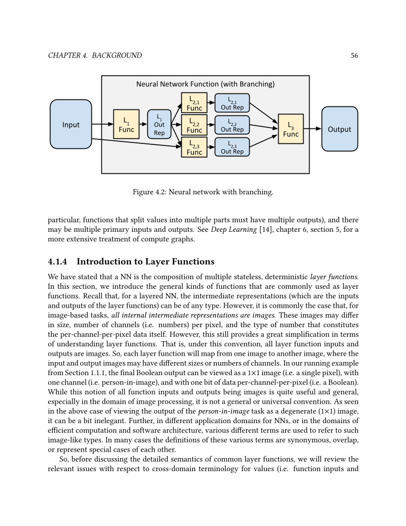
CHAPTER 4. BACKGROUND 56
Neural Network Function (with Branching)
InputOutput
L1
Func
L1
OutRep
L2,1
FuncL
2,1Out Rep
L3
Func
L2,2
FuncL
2,2Out Rep
L2,3
FuncL
2,3Out Rep
Figure 4.2: Neural network with branching.
particular, functions that split values into multiple parts must have multiple outputs), and there
may be multiple primary inputs and outputs. See Deep Learning [14], chapter 6, section 5, for a
more extensive treatment of compute graphs.
4.1.4 Introduction to Layer FunctionsWe have stated that a NN is the composition of multiple stateless, deterministic layer functions.In this section, we introduce the general kinds of functions that are commonly used as layer
functions. Recall that, for a layered NN, the intermediate representations (which are the inputs
and outputs of the layer functions) can be of any type. However, it is commonly the case that, for
image-based tasks, all internal intermediate representations are images. These images may dier
in size, number of channels (i.e. numbers) per pixel, and the type of number that constitutes
the per-channel-per-pixel data itself. However, this still provides a great simplication in terms
of understanding layer functions. That is, under this convention, all layer function inputs and
outputs are images. So, each layer function will map from one image to another image, where the
input and output images may have dierent sizes or numbers of channels. In our running example
from Section 1.1.1, the nal Boolean output can be viewed as a 1×1 image (i.e. a single pixel), with
one channel (i.e. person-in-image), and with one bit of data per-channel-per-pixel (i.e. a Boolean).
While this notion of all function inputs and outputs being images is quite useful and general,
especially in the domain of image processing, it is not a general or universal convention. As seen
in the above case of viewing the output of the person-in-image task as a degenerate (1×1) image,
it can be a bit inelegant. Further, in dierent application domains for NNs, or in the domains of
ecient computation and software architecture, various dierent terms are used to refer to such
image-like types. In many cases the denitions of these various terms are synonymous, overlap,
or represent special cases of each other.
So, before discussing the detailed semantics of common layer functions, we will review the
relevant issues with respect to cross-domain terminology for values (i.e. function inputs and
CHAPTER 4. BACKGROUND 57
outputs). In particular, we discuss a common and important way to organize groups of numbers
(including, but not limited to, images): N-Dimensional-Arrays or ND-Arrays. We also note the
meanings of several terms commonly used to refer to similar or synonymous concepts.
4.2 Groups of Numbers: ND-Arrays; relationship toTensors, Images, and Matrices
Recall that in our running example, the overall input to the task is a X×Y = 227×227 image.
We will now be more concrete about the exact encoding of the image. In particular, for each
image pixel, there are three color values, representing the pixel’s red, green, and blue intensities.
We will represent each intensity as an 8-bit unsigned integer, yielding 24-bits per pixel. Each
individual color intensity that constitutes the image can be referenced with three integer indices:
an x index in [0,227), a y index also in [0,227), and a c (which color channel: red, green, or
blue) index in [0,3). As a general convention, we assume that the range of an index starts at 0
unless otherwise stated. Thus, we more can compactly specify that the dimensions of the image
are X×Y×C = 227×227×3. Here, X, Y, and C name the dimensions, and 227, 227, and 3 are the
concrete sizes of those dimensions.
To generalize this organization beyond images, we use the concept of the N-Dimensional
Array, orND-Array: a collection of numbers with N indices/dimensions. In this work, we will deal
extensively with ND-Arrays, both in terms of dening the operational semantics of operations,
as well as using them as our key data type for implementing NN operations such as convolution.
For the most part, we use ND-Arrays in a manner consistent with existing literature and practice.
However, terminology and syntax for handling ND-Arrays varies considerably across libraries,
languages, and research domains. Luckily, ND-Arrays are a simple and intuitive concept, and the
level of understanding required for our purposes is relatively limited.
Conveniently, ND-Arrays can be used for most of the types of multiple-number aggregate
values (such as images) that we are concerned with in this work. A concrete ND-Array value
must have both a xed number of dimensions and a xed size (or length) in each dimension.
Thus, the total number of elements (numbers) in an ND-Array is the product of the sizes of the
dimensions. As with the image example above, we generally assume all ND-Array indices range
from 0 to the size of the corresponding dimension (exclusive).
Often, we discuss ND-Arrays where the dimensionality happens to be xed for some partic-
ular usage. In such cases, then either the N in ND-Array can be replaced with the specic value,
or a special term used to denote an ND-Array with that particular specic dimensionality can be
used. Here, we give examples of specic terminology and types associated with ND-Arrays of
dimensionality from zero to four:
• A 0D-Array, or a scalar, is a single number (and has no indices). For example, the intensity
of a single (grayscale or single-channel) pixel in a image is a scalar.
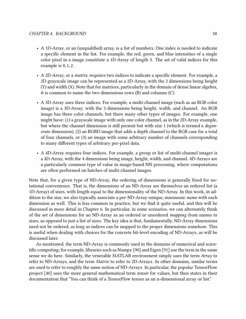
CHAPTER 4. BACKGROUND 58
• A 1D-Array, or an (unqualied) array, is a list of numbers. One index is needed to indicate
a specic element in the list. For example, the red, green, and blue intensities of a single
color pixel in a image constitute a 1D-Array of length 3. The set of valid indices for this
example is 0,1,2.
• A 2D-Array, or a matrix, requires two indices to indicate a specic element. For example, a
2D grayscale image can be represented as a 2D-Array, with the 2 dimensions being height
(Y) and width (X). Note that for matrices, particularly in the domain of dense linear algebra,
it is common to name the two dimensions rows (R) and columns (C).
• A 3D-Array uses three indices. For example, a multi-channel image (such as an RGB color
image) is a 3D-Array, with the 3 dimensions being height, width, and channel. An RGB
image has three color channels, but there many other types of images. For example, one
might have: (1) a grayscale image with only one color channel, as in the 2D-Array example,
but where the channel dimension is still present but with size 1 (which is termed a degen-erate dimension), (2) an RGBD image that adds a depth channel to the RGB case for a total
of four channels, or (3) an image with some arbitrary number of channels corresponding
to many dierent types of arbitrary per-pixel data.
• A 4D-Array requires four indices. For example, a group or list of multi-channel images is
a 4D-Array, with the 4 dimensions being image, height, width, and channel. 4D-Arrays are
a particularly common type of value in image-based NN processing, where computations
are often performed on batches of multi-channel images.
Note that, for a given type of ND-Array, the ordering of dimensions is generally xed for no-
tational convenience. That is, the dimensions of an ND-Array are themselves an ordered list (a
1D-Array) of sizes, with length equal to the dimensionality of the ND-Array. In this work, in ad-
dition to the size, we also typically associate a per-ND-Array-unique, mnemonic name with each
dimension as well. This is less common in practice, but we nd it quite useful, and this will be
discussed in more detail in Chapter 6. In particular, in some scenarios, we can alternately think
of the set of dimensions for an ND-Array as an ordered or unordered mapping from names to
sizes, as opposed to just a list of sizes. The key idea is that, fundamentally, ND-Array dimensions
need not be ordered, as long as indices can be mapped to the proper dimensions somehow. This
is useful when dealing with choices for the concrete bit-level encoding of ND-Arrays, as will be
discussed later.
As mentioned, the term ND-Array is commonly used in the domains of numerical and scien-
tic computing; for example, libraries such as Numpy [90] and Eigen [91] use the term in the same
sense we do here. Similarly, the venerable MATLAB environment simply uses the term Array to
refer to ND-Arrays, and the term Matrix to refer to 2D-Arrays. In other domains, similar terms
are used to refer to roughly the same notion of ND-Arrays. In particular, the popular TensorFlow
project [40] uses the more general mathematical term tensor for values, but then states in their
documentation that “You can think of a TensorFlow tensor as an n-dimensional array or list.”
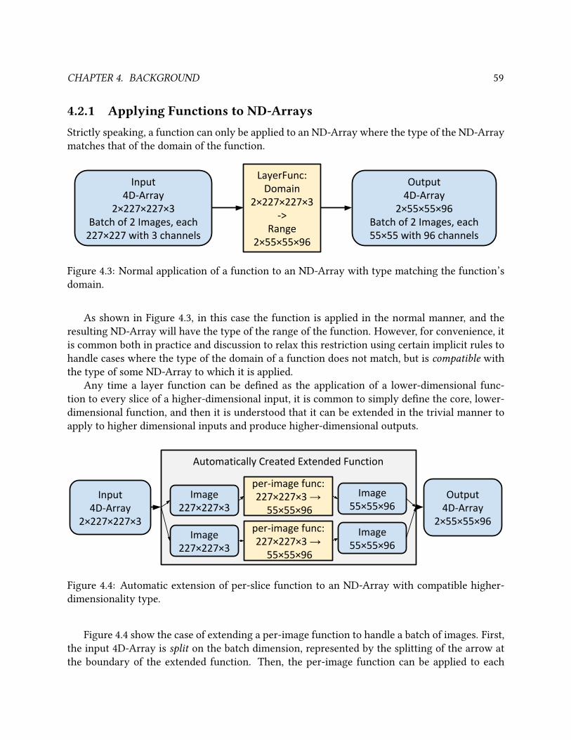
CHAPTER 4. BACKGROUND 59
4.2.1 Applying Functions to ND-ArraysStrictly speaking, a function can only be applied to an ND-Array where the type of the ND-Array
matches that of the domain of the function.
Input4D-Array
2×227×227×3Batch of 2 Images, each
227×227 with 3 channels
LayerFunc:Domain
2×227×227×3 ->
Range 2×55×55×96
Output4D-Array
2×55×55×96Batch of 2 Images, each 55×55 with 96 channels
Figure 4.3: Normal application of a function to an ND-Array with type matching the function’s
domain.
As shown in Figure 4.3, in this case the function is applied in the normal manner, and the
resulting ND-Array will have the type of the range of the function. However, for convenience, it
is common both in practice and discussion to relax this restriction using certain implicit rules to
handle cases where the type of the domain of a function does not match, but is compatible with
the type of some ND-Array to which it is applied.
Any time a layer function can be dened as the application of a lower-dimensional func-
tion to every slice of a higher-dimensional input, it is common to simply dene the core, lower-
dimensional function, and then it is understood that it can be extended in the trivial manner to
apply to higher dimensional inputs and produce higher-dimensional outputs.
Automatically Created Extended Function
Input4D-Array
2×227×227×3
per-image func:227×227×3 →
55×55×96
Output4D-Array
2×55×55×96per-image func:227×227×3 →
55×55×96
Image227×227×3
Image227×227×3
Image55×55×96
Image55×55×96
Figure 4.4: Automatic extension of per-slice function to an ND-Array with compatible higher-
dimensionality type.
Figure 4.4 show the case of extending a per-image function to handle a batch of images. First,
the input 4D-Array is split on the batch dimension, represented by the splitting of the arrow at
the boundary of the extended function. Then, the per-image function can be applied to each
CHAPTER 4. BACKGROUND 60
of these two images, in this case yielding two spatially smaller, 96-channel images. Finally, the
two 3D-Array outputs (images) are concatenated, as shown by the merging arrows, to form a
4D-Array output (a batch of the two images).
4.2.2 ND-Arrays and Layer FunctionsAs mentioned in Section 4.1.4, for the types of layers functions we deal with in this work, both
the domain and range are commonly and conveniently representable as ND-Arrays. Further,
particularly in image processing, the most common type of ND-Arrays are 4D-Arrays consisting
of batches of multi-channel images with 2 spatial dimensions (i.e. X/Y or width/height).
Generally, the batch index of a given image has no semantics. That is, the individual images in
these batches have no ordering. Further, all images in a batch are generally treated equivalently.
As discussed in Section 4.2.1, full-batch layer functions can be implicitly dened by specifying
a per-image function that maps from a 3D-Array to another 3D-Array (i.e. from a multi-channel
image to another multi-channel image). The full-batch layer function is then constructed by
slicing, applying the per-image layer function is to each input image, and then concatenating
the images to form the full 4D-Array (batch-of-multi-channel-images) output. Note that, in this
construction, clearly the number of images in the domain and range of the layer function will
always be identical.
Note that, in general, the number of spatial dimensions in an image can be more or less than
2. For example, tasks using volumetric data might use images with three spatial dimensions
(e.g. X/Y/Z or width/height/depth). Combined with a batch dimension, and multiple channels of
information per volumetric pixel (i.e. voxel), NNs for such tasks would thus use 5D-Arrays as
their input and intermediate types. Typically, the ND-Arrays used in NNs have:
• A channel dimension, whose size determines the dimensionality of the feature space at the
point in the NN where the ND-Array in question is used. May sometimes be omitted if the
per-sample data is a single value (i.e. a scalar).
• Some number of spatial dimensions that represent a space over which the features are de-
ned/distributed/sampled. May be omitted when the input consists of a single (at) feature
vector (i.e. a single sample). For example, there are commonly 2 or 3 spatial dimensions in
image-based applications (X, Y, and sometimes Z), and 2 dimensions in audio applications
(time and frequency).
• A batch dimension, so that multiple items of the basic task-input-type can be grouped to-
gether for more ecient computation (in implementation) or to specify the batching to
be used for a training algorithm (see Section 4.5). In short, batching allows for higher ef-
ciency due to increased opportunities to reuse data (primarily convolution lter values)
during computation. We will discuss this more in Sections 4.2.5 and 4.5.2.
While these cases cover much of present and historical usages, they are not exhaustive and there
are no strict rules or conventions on exactly what types of data can be used in NNs. To simplify
CHAPTER 4. BACKGROUND 61
discussion, we often neglect the batch dimension and consider only the per-image denition of
any given layer function. In such cases, we assume that when a batch/multi-image version of the
function is required, it is constructed by the method of Section 4.2.1.
For many types of inputs, the term spatial dimensions is a misnomer, as the spatial dimensions
can refer to sampling over time, frequencies, or other spaces. For example, a batch of (xed-
length) videos could be input to a NN as a 5D-Array: a batch dimension, a channel dimension
(i.e. the per-pixel RGB data), and 3 spatial dimensions: X, Y, and T (for time).
4.2.3 Discussion of Common Dimensions of ND-Arrays in NNsTaking aside the batch dimension, all other ND-Array dimensions together represent either:
• the per-task input type, or
• one of the internal representations into which the NN transforms the input.
That is, the product of the sizes of all non-batch dimensions for the ND-Array at the input rep-
resents the dimensionality of the domain of the overall task-level NN-function. Similarly, this
concept can be applied to every intermediate ND-Array in the NN, to give the dimensionality of
each intermediate representation in the NN. So, one might ask, why not simply use a (at) 1D-
Array as the basic data type for the input and intermediate representations? One reason is that,
if the input or internal representations have some natural structure that can be expressed using
ND-Arrays (such as 3D-Arrays for RGB images), it would seem sensible to use that representation
for clarity and convenience. In particular, many useful operations can be dened over particular
types of ND-Arrays, leveraging the additional metadata provided by organizing the data in an
ND-Array instead of a at 1D-Array. In the case of 2D images, as in our running example, the
use of two spatial dimensions derives from the common convention of using a uniform 2D grid
to sample light intensities in cameras. But, further, many forms of image processing are built on
this convention.
NNs are composed of many such operations which rely on understanding the structure of
the data on which they act. Such operations expect some set of spatial dimensions which are
treated dierently from any others. Usually, there is only a single catch-all non-spatial channeldimension, but this need not strictly be the case. Instead, it is generally only required that any
specic spatial dimensions required for a given operation be present. All other dimensions are
then ignored (i.e. attened or merged), and the entire ND-Array is treated as a set of at 1D-
Arrays of data attached to each point in the space dened by the spatial dimensions used by the
given operation. For example, downsampling an image by a set factor is a common operation that
can easily be performed on any image represented as a 3D array. Specically, consider a simple
image-downsample-by-2 operation. In general, such a resize might support any number of spatial
dimensions, but for this example, we will consider a 2D resize. In this case, any ND-Array that
has an X and Y dimension (in addition to any number of other dimensions) is an acceptable input.
The output ND-Array will have the same dimensions and dimension sizes as the input, except
that the sizes of the X and Y dimensions will be half that of the input. Note that, for simplicity,
CHAPTER 4. BACKGROUND 62
we assume that the input X and Y dimension sizes are evenly divisible by two. The semantics of
this downsize can be expressed as several steps:
• First, slice the input array for each pair of unique X and Y values, yielding per-pixel ND-
Arrays that have no X or Y dimension, but have all other dimensions unchanged.
• Then, these per-pixel values are grouped together in non-overlapping 2×2 windows, yield-
ing one group per output pixel. Recall that the output X and Y dimensions are both 1/2 the
size of the corresponding input dimension, so there will be 1/4 as many output pixels as
input pixels.
• Then, the per-output-pixel groups of 4 input pixels are element-wise averaged. Since this
operation is uniform over all elements of the per-pixel ND-Arrays, it does not depend on
their dimensionality, and can thus treat the 4 pieces of per-pixel data as at 1D-Arrays.
• Finally, the output per-pixel ND-Arrays are concatenated, with the output X and Y dimen-
sions inserted at their “original” locations, so that the output dimension order matches the
input.
4.2.4 Spatial vs. Channel Dimensions in NNsThere are cases where it is not clear if a given natural dimension of some input type should
be treated as a spatial dimension or folded into the channel dimension. This is particularly true
when the top level task is not a clear t for existing sets of operations in some NN framework. For
example, when processing audio data in the frequency domain, sampling over both the temporal
and frequency domains can be reasonably considered as either spatial dimensions or folded into
the channel dimension. Thus, if a given audio sample type (used as input for some NN task) had
20 frequency bins and 100 temporal samples, it could be treated as any of the following ND-Array
types:
• A 1D-Array with size 2000, with only a channel dimension, containing all temporal and
frequency data at.
• A 3D-Array with dimensions either 20×100×1 or 100×20×1, with two spatial dimensions
for time and frequency, and a degenerate (size 1) channel dimension (which holds the single
per-frequency-per-timeslice intensity). Depending on conventions and implementation is-
sues, the degenerate channel dimension might be omitted, as it does not impact the number
of ND-Array elements.
• A 2D-Array with dimensions 20×100, where the frequency sub-space of each sample is
considered spatial, but the temporal sub-space is folded into the channel dimension.
• Similarly, A 2D-Array with dimensions 100×20, where the temporal sub-space of each sam-
ple is considered spatial, but the frequency sub-space is folded into the channel dimension.
CHAPTER 4. BACKGROUND 63
Generally, which type is chosen will depend on the existing library of NN operations, how exible
they are with respect to dimension layout, and what operations are desired to be performed within
the NN. In this work, the net eect of such issues is that, across various NN tasks, we are likely
to see a diverse set of input sizes for many operations, as they may be applied in many dierent
scenarios.
4.2.5 Aside on the Batch Dimension and ComputationAs with the overall number of layers in a NN, neither the number of images in a batch, nor
even the existence of the batch dimension, signicantly eects the core computational problems
we must solve. For correctness, we must simply evaluate whatever per-image function we are
given for all images in the batch at each layer. However, in current implementation practice,
optimizations that depend on the size of the batch are more common and important than those
that depend on the number of NN layers. In particular, since all convolutional lters are reused
for each input, batching allows reusing lter values across images, which, if feasible, will lower
communication costs.
So, when we discuss the computation of layer functions over batches of inputs, two cases arise.
In the rst case, similar to how we dened the semantics of layer functions, we omit discussion
of the details of extending per-task-level-input (i.e. per-image in our example task) computation
over the batch dimension. Instead, we assume that simple iteration or similar methods are used
to extend the per-task-level-input implementation to multiple-input batches. However, in the
second case, we may explicitly consider and discuss performing our calculations across an entire
batch of inputs to expose additional opportunities for optimization.
4.3 Details of Neural Network Layer FunctionsHaving introduced the basic semantics and terminology for the values on which NN layer func-
tions operate, we now discuss in detail the semantics of some common layer functions. While
there is no particular denition or hard limit on what can constitute a layer function, there are var-
ious historical and current conventions. Generally, layer functions are relatively simple primitive
operations with well dened semantics. Typically, each is used in the context of many dierent
high-level machine learning tasks. Thus, they represent the building blocks from which per-task
NNs are created.
Focusing on image-based tasks (like our example task from Section 1.1.1), many historical and
current NNs can be realized using only three basic types of image-to-image layer functions:
• Activation: Apply a simple function to each per-channel-per-pixel value.
• Pooling: Combine nearby values.
• Convolution: Convolve a set of (given/constant) lters or kernels with the input image.
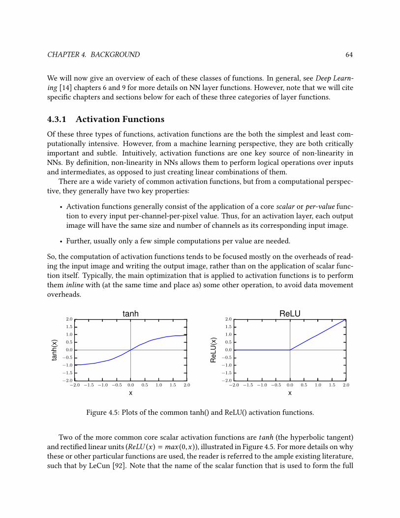
CHAPTER 4. BACKGROUND 64
We will now give an overview of each of these classes of functions. In general, see Deep Learn-ing [14] chapters 6 and 9 for more details on NN layer functions. However, note that we will cite
specic chapters and sections below for each of these three categories of layer functions.
4.3.1 Activation FunctionsOf these three types of functions, activation functions are the both the simplest and least com-
putationally intensive. However, from a machine learning perspective, they are both critically
important and subtle. Intuitively, activation functions are one key source of non-linearity in
NNs. By denition, non-linearity in NNs allows them to perform logical operations over inputs
and intermediates, as opposed to just creating linear combinations of them.
There are a wide variety of common activation functions, but from a computational perspec-
tive, they generally have two key properties:
• Activation functions generally consist of the application of a core scalar or per-value func-
tion to every input per-channel-per-pixel value. Thus, for an activation layer, each output
image will have the same size and number of channels as its corresponding input image.
• Further, usually only a few simple computations per value are needed.
So, the computation of activation functions tends to be focused mostly on the overheads of read-
ing the input image and writing the output image, rather than on the application of scalar func-
tion itself. Typically, the main optimization that is applied to activation functions is to perform
them inline with (at the same time and place as) some other operation, to avoid data movement
overheads.
−2.0 −1.5 −1.0 −0.5 0.0 0.5 1.0 1.5 2.0
x
−2.0
−1.5
−1.0
−0.5
0.0
0.5
1.0
1.5
2.0
tanh
(x)
tanh
−2.0 −1.5 −1.0 −0.5 0.0 0.5 1.0 1.5 2.0
x
−2.0
−1.5
−1.0
−0.5
0.0
0.5
1.0
1.5
2.0
ReL
U(x
)
ReLU
Figure 4.5: Plots of the common tanh() and ReLU() activation functions.
Two of the more common core scalar activation functions are tanh (the hyperbolic tangent)
and rectied linear units (ReLU (x ) =max (0,x )), illustrated in Figure 4.5. For more details on why
these or other particular functions are used, the reader is referred to the ample existing literature,
such that by LeCun [92]. Note that the name of the scalar function that is used to form the full
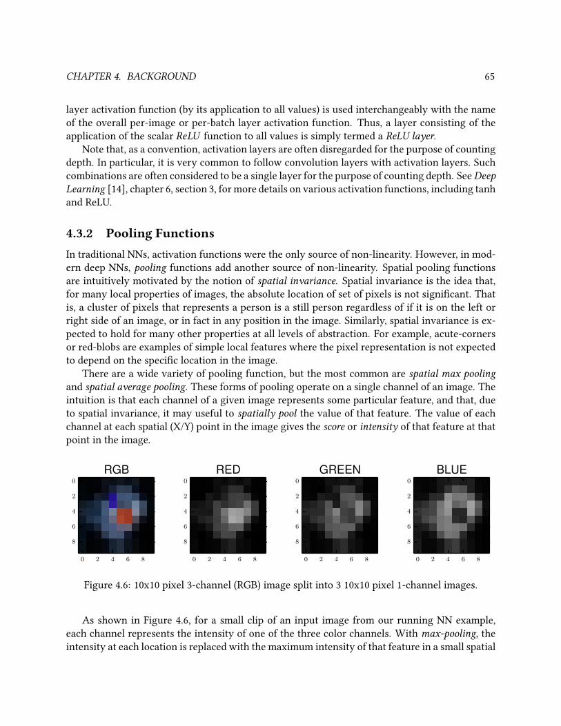
CHAPTER 4. BACKGROUND 65
layer activation function (by its application to all values) is used interchangeably with the name
of the overall per-image or per-batch layer activation function. Thus, a layer consisting of the
application of the scalar ReLU function to all values is simply termed a ReLU layer.Note that, as a convention, activation layers are often disregarded for the purpose of counting
depth. In particular, it is very common to follow convolution layers with activation layers. Such
combinations are often considered to be a single layer for the purpose of counting depth. SeeDeepLearning [14], chapter 6, section 3, for more details on various activation functions, including tanh
and ReLU.
4.3.2 Pooling FunctionsIn traditional NNs, activation functions were the only source of non-linearity. However, in mod-
ern deep NNs, pooling functions add another source of non-linearity. Spatial pooling functions
are intuitively motivated by the notion of spatial invariance. Spatial invariance is the idea that,
for many local properties of images, the absolute location of set of pixels is not signicant. That
is, a cluster of pixels that represents a person is a still person regardless of if it is on the left or
right side of an image, or in fact in any position in the image. Similarly, spatial invariance is ex-
pected to hold for many other properties at all levels of abstraction. For example, acute-corners
or red-blobs are examples of simple local features where the pixel representation is not expected
to depend on the specic location in the image.
There are a wide variety of pooling function, but the most common are spatial max poolingand spatial average pooling. These forms of pooling operate on a single channel of an image. The
intuition is that each channel of a given image represents some particular feature, and that, due
to spatial invariance, it may useful to spatially pool the value of that feature. The value of each
channel at each spatial (X/Y) point in the image gives the score or intensity of that feature at that
point in the image.
0 2 4 6 8
0
2
4
6
8
RGB
0 2 4 6 8
0
2
4
6
8
RED
0 2 4 6 8
0
2
4
6
8
GREEN
0 2 4 6 8
0
2
4
6
8
BLUE
Figure 4.6: 10x10 pixel 3-channel (RGB) image split into 3 10x10 pixel 1-channel images.
As shown in Figure 4.6, for a small clip of an input image from our running NN example,
each channel represents the intensity of one of the three color channels. With max-pooling, the
intensity at each location is replaced with the maximum intensity of that feature in a small spatial
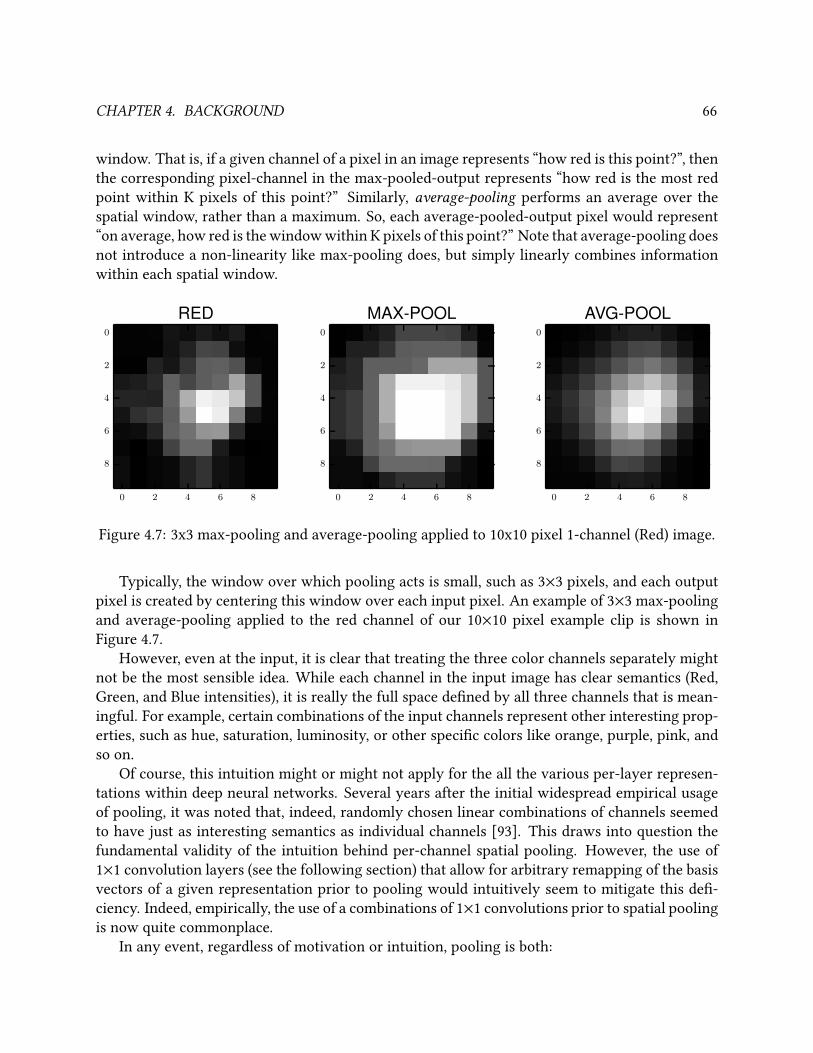
CHAPTER 4. BACKGROUND 66
window. That is, if a given channel of a pixel in an image represents “how red is this point?”, then
the corresponding pixel-channel in the max-pooled-output represents “how red is the most red
point within K pixels of this point?” Similarly, average-pooling performs an average over the
spatial window, rather than a maximum. So, each average-pooled-output pixel would represent
“on average, how red is the window within K pixels of this point?” Note that average-pooling does
not introduce a non-linearity like max-pooling does, but simply linearly combines information
within each spatial window.
0 2 4 6 8
0
2
4
6
8
RED
0 2 4 6 8
0
2
4
6
8
MAX-POOL
0 2 4 6 8
0
2
4
6
8
AVG-POOL
Figure 4.7: 3x3 max-pooling and average-pooling applied to 10x10 pixel 1-channel (Red) image.
Typically, the window over which pooling acts is small, such as 3×3 pixels, and each output
pixel is created by centering this window over each input pixel. An example of 3×3 max-pooling
and average-pooling applied to the red channel of our 10×10 pixel example clip is shown in
Figure 4.7.
However, even at the input, it is clear that treating the three color channels separately might
not be the most sensible idea. While each channel in the input image has clear semantics (Red,
Green, and Blue intensities), it is really the full space dened by all three channels that is mean-
ingful. For example, certain combinations of the input channels represent other interesting prop-
erties, such as hue, saturation, luminosity, or other specic colors like orange, purple, pink, and
so on.
Of course, this intuition might or might not apply for the all the various per-layer represen-
tations within deep neural networks. Several years after the initial widespread empirical usage
of pooling, it was noted that, indeed, randomly chosen linear combinations of channels seemed
to have just as interesting semantics as individual channels [93]. This draws into question the
fundamental validity of the intuition behind per-channel spatial pooling. However, the use of
1×1 convolution layers (see the following section) that allow for arbitrary remapping of the basis
vectors of a given representation prior to pooling would intuitively seem to mitigate this de-
ciency. Indeed, empirically, the use of a combinations of 1×1 convolutions prior to spatial pooling
is now quite commonplace.
In any event, regardless of motivation or intuition, pooling is both:
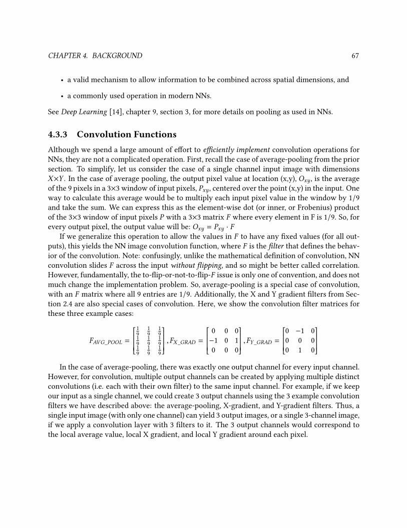
CHAPTER 4. BACKGROUND 67
• a valid mechanism to allow information to be combined across spatial dimensions, and
• a commonly used operation in modern NNs.
See Deep Learning [14], chapter 9, section 3, for more details on pooling as used in NNs.
4.3.3 Convolution FunctionsAlthough we spend a large amount of eort to eciently implement convolution operations for
NNs, they are not a complicated operation. First, recall the case of average-pooling from the prior
section. To simplify, let us consider the case of a single channel input image with dimensions
X×Y . In the case of average pooling, the output pixel value at location (x,y), Oxy , is the average
of the 9 pixels in a 3×3 window of input pixels, Pxy , centered over the point (x,y) in the input. One
way to calculate this average would be to multiply each input pixel value in the window by 1/9and take the sum. We can express this as the element-wise dot (or inner, or Frobenius) product
of the 3×3 window of input pixels P with a 3×3 matrix F where every element in F is 1/9. So, for
every output pixel, the output value will be: Oxy = Pxy · FIf we generalize this operation to allow the values in F to have any xed values (for all out-
puts), this yields the NN image convolution function, where F is the lter that denes the behav-
ior of the convolution. Note: confusingly, unlike the mathematical denition of convolution, NN
convolution slides F across the input without ipping, and so might be better called correlation.
However, fundamentally, the to-ip-or-not-to-ip-F issue is only one of convention, and does not
much change the implementation problem. So, average-pooling is a special case of convolution,
with an F matrix where all 9 entries are 1/9. Additionally, the X and Y gradient lters from Sec-
tion 2.4 are also special cases of convolution. Here, we show the convolution lter matrices for
these three example cases:
FAVG_POOL =
1
9
1
9
1
9
1
9
1
9
1
9
1
9
1
9
1
9
,FX_GRAD =
0 0 0
−1 0 1
0 0 0
,FY_GRAD =
0 −1 0
0 0 0
0 1 0
In the case of average-pooling, there was exactly one output channel for every input channel.
However, for convolution, multiple output channels can be created by applying multiple distinct
convolutions (i.e. each with their own lter) to the same input channel. For example, if we keep
our input as a single channel, we could create 3 output channels using the 3 example convolution
lters we have described above: the average-pooling, X-gradient, and Y-gradient lters. Thus, a
single input image (with only one channel) can yield 3 output images, or a single 3-channel image,
if we apply a convolution layer with 3 lters to it. The 3 output channels would correspond to
the local average value, local X gradient, and local Y gradient around each pixel.
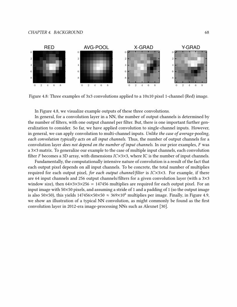
CHAPTER 4. BACKGROUND 68
0 2 4 6 8
0
2
4
6
8
RED
0 2 4 6 8
0
2
4
6
8
AVG-POOL
0 2 4 6 8
0
2
4
6
8
X-GRAD
0 2 4 6 8
0
2
4
6
8
Y-GRAD
Figure 4.8: Three examples of 3x3 convolutions applied to a 10x10 pixel 1-channel (Red) image.
In Figure 4.8, we visualize example outputs of these three convolutions.
In general, for a convolution layer in a NN, the number of output channels is determined by
the number of lters, with one output channel per lter. But, there is one important further gen-
eralization to consider. So far, we have applied convolution to single-channel inputs. However,
in general, we can apply convolution to multi-channel inputs. Unlike the case of average-pooling,each convolution typically acts on all input channels. Thus, the number of output channels for a
convolution layer does not depend on the number of input channels. In our prior examples, F was
a 3×3 matrix. To generalize our example to the case of multiple input channels, each convolution
lter F becomes a 3D array, with dimensions IC×3×3, where IC is the number of input channels.
Fundamentally, the computationally intensive nature of convolution is a result of the fact that
each output pixel depends on all input channels. To be concrete, the total number of multiplies
required for each output pixel, for each output channel/lter is IC×3×3. For example, if there
are 64 input channels and 256 output channels/lters for a given convolution layer (with a 3×3
window size), then 64×3×3×256 = 147456 multiplies are required for each output pixel. For an
input image with 50×50 pixels, and assuming a stride of 1 and a padding of 1 (so the output image
is also 50×50), this yields 147456×50×50 ≈ 369×106
multiplies per image. Finally, in Figure 4.9,
we show an illustration of a typical NN convolution, as might commonly be found as the rst
convolution layer in 2012-era image-processing NNs such as Alexnet [30].
CHAPTER 4. BACKGROUND 69
Input3-channel (RGB)(227x227)
Output96-channel(55x55)
96 Filters, each:3-channel (11x11)
Figure 4.9: A typical NN convolution layer with stride 4, as might be found at the start of an
image-processing NN.
See Deep Learning [14], chapter 9, section 1, for more details on convolution in NNs.
4.4 Machine Learning TerminologyAlthough the focus of this work is on computation, some familiarity with machine learning is re-
quired to understand how to ensure the correctness of our implementations. In this dissertation,
one of our key concerns is to concretely determine if an algorithm is maintaining accuracy, espe-
cially when its results are not identical to a reference. So, we must understand how accuracy is
measured in some detail. Let us return to our running example of person-in-image classication,
and discuss the basic needed terminology.
4.4.1 Accuracy vs. Precision/RecallEarlier, when we referred to accuracy, we used it in the general sense of “how well does this
function perform at this task?” However, when evaluating classication task performance, there
is a more specic quantitative set of metrics that are commonly employed. Concretely, in our
example from Section 1.1.1, let us assume for simplicity that each input image either has a person
or does not (neglecting corner cases). For a set of images, the images with a person are termed
positives, and the images with no person are termed negatives. If the total number of images is
N , then we use NPOS to refer to the number of positives, and NNEG to refer to the number of
negatives. Thus, there are four possible outcomes when running a given function on each image:
• The image has a person, and the function (correctly) outputs true. This is termed a truepositive. We refer to the number of such cases as NTP .
• The image has no person, and the function (correctly) outputs false. This is termed a truenegative. We refer to the number of such cases as NTN .
CHAPTER 4. BACKGROUND 70
• The image has a person, and the function (incorrectly) outputs false. This is termed a falsenegative. We refer to the number of such cases as NFN .
• The image has no person, and the function (incorrectly) outputs true. This is termed a falsepositive. We refer to the number of such cases as NFP .
For a given set of images, the results of running a function can be summarized using the metrics
precision and recall. Recall is dened as the ratio of true positives to all positives, or NTP/NPOS .
Thus, recall simply measures how many of images with a person were found. Note that a func-
tion which simply always returns true will have a perfect recall score of 1.0. Complementarily,
precision is dened as NTP/(NTP +NFP ); perfect precision is thus 1.0. Note that a function which
always returns true will have a precision of NTP/NP . Thus, in the case where most examples are
true, the trivial always-true function will have perfect recall and near-perfect precision. Such a
case is known as a class imbalance. In the case of binary classication (as in our example) where
there are only two classes, the convention is that the less common class should be the true case.
In this way, precision and recall form easy to interpret measures of how well a given function
performs binary classication. Finally, to reduce precision and recall to a single metric, the con-
cept of delity is often used. This is simply the (potentially weighted) harmonic mean of recall
and precision. The most common delity metric, or the F1 score, is the unweighted harmonic
mean: (2×recall×precision)/(recall + precision). For more details, see the work of Davis [94].
4.4.2 Precision/Recall tradeos, PR curves, and FidelityOften, a binary classication function is built from the composition of a real-valued classication
function and a threshold function. That is, the bulk of the computation is a function that maps
from images to a real value, typically normalized to be in the range [0,1]. This value represents
the condence of the function that the desired output value is true. There is no particular scale
assumed, only that higher values are more likely to be true. To get a nal binary result, a threshold
function is applied to the condence value. If the real value is less than the threshold, false is
returned; otherwise, true is returned. Note that choosing a threshold of 0.0 always yields the
always-true function, which has maximum recall. On the other hand, choosing a high threshold
will only return true when the condence is high. Thus, higher thresholds will tend to have lower
recall, but (potentially) higher precision. The choice of threshold is termed the operating point for
the classier. Depending on the use-case, dierent tradeos between recall and precision may
be desired. Thus, for a given real-valued classier, it is common to evaluate it at many operating
points by sweeping the threshold value from 0.0 to 1.0. Sometimes, for a given evaluation set of
inputs, every possible unique operating point is considered. Otherwise, some particular sampling
of thresholds is used. Then, after performing this sweep, a PR-curve graph is drawn, which shows
precision vs recall, and two common summary metrics are derived:
• The maximum delity operating point, dened as the point with highest with delity, using
the F1 score or similar metric.
CHAPTER 4. BACKGROUND 71
• The average precision or area-under-curve metrics, which are roughly equivalent modulo
interpolation of the precision in-between operating points.
Finally, when evaluating multiple classiers as a group with a single metric is desired, often the
mean average precision or mAP score is used. The mAP score is simply the mean of the average
precision (AP) scores of multiple classiers. For more details, see the work of Powers [95].
4.4.3 Overtting and ComputationIn machine learning, the term overtting refers to the case where a function:
• performs well on some input data used to create the function (termed training data)
• performs less well (or poorly) on other input data (termed validation or real-world data)
In such cases, the function is said to fail to generalize to new data that it has not previously
“seen” as part of the training data. For the most part, overtting is an issue that arises in the
process of creating functions, not when optimizing their computation. However, as previously
mentioned, eorts to optimize the computation of a given function can also create a form of
overtting. Rather than some abstract description of a computable function, the starting place
for optimization is often a reference algorithm from which the underlying function must be de-
duced. Checking that accuracy has been maintained is generally accomplished by checking the
accuracy of the optimized algorithm over some set of validation inputs. But, care must be taken
that any approximations or other deviations from the reference algorithm are valid in general.
That is, assume that some approximation scheme or set of optimizations is chosen out of many
possibilities. Further, assume that this was done by nding trying many schemes, and nding a
particular conguration that was both fast and performed well on the validation set. However,
such a scheme might then only work well for the validation set, which ts our above denition of
overtting. To combat this possibility, it is generally preferable to ensure good numerical agree-
ment among all algorithms to the degree possible and practical. Ideally, this includes not just the
nal output values of the function, but any comparable intermediate values as well. This gives
a higher degree of condence that the function to compute has not been substantially altered by
numerical issues. Thus, the approximate function should generalize beyond the validation set
as well as the original function. However, in current practice, such testing for numerical agree-
ment is often quite cumbersome, and is thus often neglected. For more details on Overtting and
related topics in machine learning, see Chapter 5, Section 2 of Deep Learning [14].
4.5 Training vs. DeploymentIn machine learning, one approach to creating a system that performs a particular task, given
some set of (hopefully correct-enough) input/output pairs, is termed supervised learning. Using
this method specically for nding a good NN function for a given task is commonly approached
using two steps:
CHAPTER 4. BACKGROUND 72
• First, a graph of parameterized layer functions is chosen. This graph is variously called
the NN architecture, the space of models, or the function structure. The parameters to be
xed to select a nal, concrete NN function (termed a model) for the task are called modelparameters. In particular, the model parameters include all the lters of any convolution
layers of the type described in Section 4.3.3. This process perhaps has no clear common
term in the literature; here we will refer to it as NN architecture design space exploration.
• Second, an optimization algorithm is run to determine good values for the model parame-
ters. This part of the process is termed training.
Then, once a system has been created, we term using it to perform the desired task deployment.For NNs, then, deployment consists of evaluating some existing, xed NN function.
As a general reference on the fundamentals of machine learning and training NNs, the reader
is referred to chapters 5 and 8 in Deep Learning [14]. As mentioned in Section 1.1.2, the issue of
NN architecture design space exploration is outside the scope of this dissertation. The reader is
referred to the recent work of Iandola [17] for details on this process.
So, from a computational standpoint as relevant for this dissertation, we split the space of
machine learning use-cases into the two remaining parts: training and deployment. For our proof-
of-concept use of Boda in Chapter 6, we focus on the deployment use-case. For deployment, we
must simply evaluate NN functions consisting of various layer functions, such as the common
types described in Section 4.3.
4.5.1 Computation for TrainingHowever, the training use-case is also of interest. In this section, we consider the ways in which
the computational requirements of training dier from those of deployment. In particular, we
consider the general ow of one common family of training procedures called stochastic gradientdescent or SGD. At a high level, such procedures consist of selecting some initial value for all
model parameters, and then repeatedly:
• Applying the current NN function (as determined by the current values of the model pa-
rameters) to a batch of inputs.
• Calculating the error of the current model for the current batch of inputs.
• Calculating the gradient of the error with respect to each model parameter.
• Using the per-model-parameter (error) gradients to adjust all model parameters slightly so
as to decrease the error (i.e. optimization by gradient decent).
From a computational standpoint, it can be seen that training involves both the application
of the NN function itself (as determined by the constantly changing model parameters), but also
the calculation of the gradient of the error with respect to the model parameters. Commonly,
an algorithm called backpropagation [96] is used to calculate the needed gradients. See Deep
CHAPTER 4. BACKGROUND 73
Learning [14], chapter 6, section 5, for a more modern treatment of backpropagation for general
NNs. Using that approach, the calculation of the gradient of convolutions is performed using
other convolutions. For an accessible explanation on the specic convolutions that result when
calculating the gradients of other of convolutions, see the tutorial of Gibiansky [97]. However, the
key point here is that the particular convolution operations required for the gradient calculation
may have quite dierent input sizes than their counterparts in the NN function itself. Thus, at
a minimum, they represent additional cases that may require tuning or optimization. Further, in
practice, they commonly happen to be at least somewhat more dicult to implement eciently
then their deployment counterparts, although there is no clear fundamental reason why this need
be true. This means that supporting NN computations for training is very similar to, but broader
than, just supporting NN computations for deployment.
4.5.2 Batch Sizes in Training and DeploymentOne important detail is that, in training, the error is calculated for a batch of inputs, not a sin-
gle input. Thus, the size of the batch is an important parameter that aects the optimization
algorithm. However, the nature of the model-parameter updates is such that it is permissible to
compute the outputs, errors, and model-parameter-error-gradients of each input individually, if
desired, and combine (via simple summation) the model-parameter-updates incrementally until
the batch is complete. Thus, computationally, we never need compute more inputs at the same
time than we desire. However, the reverse is not true: based on the details of the training proce-
dure, we may not process more inputs than have been requested for a training batch, because we
must actually update the model parameters (using the accumulated updates) between batches.
So, it should be noted that the batch size specied for training has important semantics, but does
not strictly determine the batch size that must be used for computation. Instead, it only places a
maximum on the batch size that may be used for computation.
As with training, there is no minimum batch size for deployment. If desirable for eciency,
each input can be computed individually. However, in general, more data reuse is possible with
larger batches, albeit generally at the price of needing additional intermediate storage space. In
deployment, the maximum batch size is eectively determined by the latency tolerance of the
application. The minimum input-to-output latency will always achieved by using a batch size of
1. However, if the application can tolerate some delay in the production of the output, it may be
permissible to wait for multiple inputs and process them in a batch. This will increase latency
due to:
• needing to wait for multiple inputs, and
• the fact that processing a larger batch should always take longer than processing a smaller
one.
For more details specically on batches and SGD, see Deep Learning [14], chapter 8, sections 1
and 3.
CHAPTER 4. BACKGROUND 74
4.5.3 Scale of Computation: One GPU or Many?When batch sizes are large, one method to improve speed is to divide batches across multiple
GPUs and process the resulting sub-batches in parallel. However, this practice is not generally
relevant for the deployment use-case, even when considering cloud-scale deployments. As men-
tioned in the prior section, multiple requests (where each request is one input) may be batched
together to improve overall eciency when the application permits the additional latency. At the
other extreme, it is possible to conceive of some extremely compute intensive application where
a latency advantage can be achieved by using multiple GPUs to service a single request. How-
ever, for typical current applications, it is wasteful to occupy an entire GPU with serving a single
request, let alone to distribute one request across GPUs. This can be seen in real world use-cases
such as at Baidu [2], where batching is performed only to increase eciency at the level of a sin-
gle GPU. In such cases, there is no advantage in waiting for 2N independent requests only to then
divide them into two batches of N requests to be processed by dierent GPUs. Instead, one should
wait for at most the number of requests needed to create a single ecient batch, and then pro-
cess that batch immediately. So, for current deployment scenarios, performance within a single
GPU (for optimal-or-smaller batch sizes) is typically the chief concern. In fact, even for training,
this still holds at the level of each individual GPU, but with additional concerns at a higher level
related to communication and synchronization between GPUs. In this dissertation, we do not
address these additional issues that arise when trying to distribute batches across multiple GPUs.
For more details on this topic, see the recent work of Iandola [17].
75
Chapter 5
Boda Related Work
In chapters 2 and 3, we have discussed both:
• the independent contributions of libHOG and DenseNet, as well as
• how they dened and shaped our research trajectory.
In both libHOG and DenseNet, we choose an important use case from machine learning, applied
analysis, and focused on optimization with respect to our motivating concerns: accuracy, speed,
energy, portability, and cost. In each case, we made signicant contributions and learned impor-
tant lessons about computation for machine learning. But, along the way, we encountered two
general categories of issues that limited the impact of our work:
• It was dicult to perform our optimization work directly in the context of the machine
learning ows we were trying to optimize.
• It was dicult to package our reference implementations in ways that allowed for practical
extension and reuse of our eorts.
After our work with DenseNet, it was natural and timely to pursue further research into ef-
cient computation for neural networks. Since then, the immense popularity and generality of
neural-network-based techniques in machine learning has shown no signs of decreasing. So,
considering both the successes and limitations of our prior work, we chose the problem of im-plementing neural network computations as our next research area. Based on our experience with
libHOG, we learned that optimizing high-level operations has clear advantages and drawbacks.
High-level machine-learning operations, such as the multi-scale HOG feature pyramid creation of
libHOG, may oer easy opportunities for optimization, due to the overheads and naive implemen-
tations of existing codebases. Further, they may oer simple high-level interfaces for deployment.
However, the resulting optimized code is can be too xed-function and brittle to integrate into
new projects, especially when the underlying machine-learning use models are rapidly evolving.
Thus, we choose to attempt to optimize low-level, rather than high-level, computing primitives.
Certainly, there is a similar danger that the computing primitives of today may be less useful
CHAPTER 5. BODA RELATED WORK 76
tomorrow. However, when considering neural networks in general, and convolutional neural
networks in particular, evidence and opinion points to their likely ongoing importance for many
years.
One consideration, however, is that optimizations to low-level operations tend to be better ad-
dressed by existing work. Thus, one must expect that the bar for useful contributions is higher;
the low hanging fruit is likely already plucked. Further, compared to our prior eorts, the imple-
mentation complexity of NN operations, such as convolution, is signicantly higher than that of
the gradient-histogram-creation of libHOG or the pyramid-creation of DenseNet. Thus, manag-
ing this complexity during the implementation process will be a signicant challenge.
But rst, given that we have specied the key problem we will consider, we now ask the
natural question: how well does existing work address this problem? For each approach, with
respect to all our concerns, what are its advantages and limitations?
Given that our concerns span many levels of abstraction, there are several broad categories
of related work to consider. In general, when using computers, there are many methods (and
combinations of methods) that can be used to bridge the gap between each application and the
underlying computer hardware. So, we will start with a brief, high-level overview of the overall
space of methods that can be used to create software systems. In particular, we consider the
general categories of libraries, compilers, and templates/skeletons. As we do this, we will note
examples of how each of these general techniques is currently being applied in the context of
NN computations. In general, we nd that, at a high level, all of the possible general approaches
to mapping computation are indeed in use for NN computation with varying degrees of success.
So, conveniently, for the most part we can focus our discussion on work that is specic to NN
computation and simultaneously cover most of the space of all approaches for general numerical
computation targeting GPUs.
As we discuss in detail the space of existing systems for NN computations, there are two
recurring motifs:
• Existing approaches oer high computational eciency or portability, but not both.
• Existing approaches with high computational eciency have high development costs.
For example, one hardware vendor, NVIDIA, has implemented a very ecient NN computa-
tion library (cuDNN). However, as we will discuss in Sections 6.2.3 and 6.2.4, the existence of this
single implementation does not address our full set of concerns. Instead, we seek an approach that
combines portability and reasonable computational eciency, while maintaining accuracy and
minimizing development costs. Overall, we nd that none of the existing approaches achieves
this balance that we seek.
5.1 General Approaches to Implementing ComputationIn this work, we focus on implementing computations on GPUs. Since GPUs are highly parallel
computational devices, this implies that we are interested in parallel computation. In fact, for
CHAPTER 5. BODA RELATED WORK 77
the computations we consider in this work, serial computation is simply not an option, as the
amount of computation to be performed is impractical without the application of parallelism.
For example, a neural network for image classication, as in our example of Section 1.1.1, can
easily require 90 billion operations per image [76] during training. Modern computer clock rates
are limited to around 5 billion cycles per second [98]. Thus, roughly speaking, a purely serial
computation would require ∼18 seconds per image. Common datasets for image classication
have 1M images [75]. Training a NN generally requires at least 10 passes over such datasets [99].
So, using serial computation would yield a training time of 180M seconds or 5.7 years.
Further, for the most part, we are concerned only with core computations, rather than full
complex pieces of software. Thus, while the space of possible historical and current mapping
strategies for serial and/or complex software is quite large, much of that space is not of signicant
concern for our work. For additional background material on the general problem of bridging
the implementation gap between application and hardware, the reader is referred to the work of
Chong [100], Catanzaro [35], and Gonina [101]. In particular, we need only be concerned with
methods that can eciently exploit parallelism for the NN operations we consider. Further, since
we do not have a complex system to map, we are less concerned with approaches whose benet
is in the management of such complexity.
5.1.1 Compilers (and their Languages)In general, the lowest level at which hardware can be programmed is with what is called as-sembly language. At this level, a sequence of very low level instructions is directly and explic-
itly given the to hardware [102]. These operations are at the granularity of moving individual
numbers between storage locations and performing individual mathematical operations between
several numbers. However, even this assembly-language/instruction level can include various
more complex operations, such as those that operate on multiple numbers in parallel. This is one
type of instruction level parallelism (ILP), and includes single-instruction-multiple-date (SIMD),
very-long-instruction-word (VLIW), and other types of instructions. Note that other types of ILP
involve the concurrent execution of multiple instructions. For more details on ILP, the reader is
referred to the work of Rau [103].
While it is tractable to write simple functions in assembly language, it can be very time
consuming, error prone, and lacks portability, leading to overall high development costs [104].
Thus, higher level languages are created to more compactly and conveniently describe compu-
tations [105]. Then, compilers translate these higher level languages to assembly language, pre-
serving the semantics of the computation as described by the programmer [106]. In addition to
preserving semantics, compilers are generally also tasked with nding optimized mappings that
minimize the time and/or memory consumed by a particular computation [107].
A stack of languages and compilers can be created by employing compilers that map from one
language to another. Over time, some languages have gained special status as a common ground
with which to express computations without reference to any specic computer. In particular,
the C language contains primitives that map well to the common data types and operations sup-
ported for all modern hardware [108]. Thus, C can easily describe the semantics of any given
CHAPTER 5. BODA RELATED WORK 78
computation. However, C is an inherently serial language that describes a single sequence of
primitive operations. So, the C description of any given computation only represents one validsequence of primitive operations that performs that computation. In general, it is dicult to map
from the C description of a computation to an ecient implementation for hardware that can
execute many operations in parallel [109].
For GPU programming, there are two primary languages: OpenCL [110] and CUDA [24]. Both
of these languages use C syntax and semantics to describe primitive computations and data move-
ment. However, unlike C, both OpenCL and CUDA but expose an abstract-but-explicit model of
the parallel capabilities of GPU hardware. Further, also unlike C, they expose details of the seg-
regated and non-homogeneous storage present in GPUs. This allows-and-requires the program-
mer to explicitly manage the parallel and heterogeneous nature of GPU computation and storage.
Unfortunately, OpenCL and CUDA happen to use totally dierent syntax for these GPU-specic
features, rendering them incompatible. However, for basic features, the two programming models
are mostly semantically compatible. But, considering more advanced features, CUDA generally
exposes hardware-specic functionality directly, whereas OpenCL (as a rule) hides, abstracts, or
simply ignores it.
OpenCL and CUDA are generally the lowest level of programming language that is recom-
mended for general use by GPU hardware vendors. For a given GPU, an assembly language inter-
face may or may not be provided. But, a key point is that, when compared with OpenCL/CUDA,
GPU assembly language generally does not present a substantially dierent abstraction of the
underlying GPU hardware. Still, if provided, GPU assembly language typically allows for ner
control of storage allocation (i.e. for registers), and sometimes exposes particular hardware prim-
itives, limitations, or capabilities that are abstracted away at the OpenCL/CUDA level.
In theory in is possible to create an ecient general-purpose compiler that maps from serial-
C to OpenCL, CUDA, or GPU assembly language directly. However, currently no general ap-
proaches to this problem achieve good eciency for the type of numerical computations we
consider in this work [109].
5.1.2 LibrariesThe concept of a library is quite simple. If there is way to clearly dene the inputs and outputs
of some operation (i.e. as a function), then this can be used to dene an interface boundary. So,
anytime one desires to perform the given operation, one need only call a pre-dened function
that matches this interface. A library is simply a collection of such functions delivered in a ready-
to-use form. In general, this means that the user of the function and the creator of the function are
insulated from each other. As long as they agree on the interface, they can each use any methods
they prefer on their side of the interface boundary. In particular, this means they are each free
to use the languages, compilers, and (other) libraries that they prefer. Hence, the term librarycan legitimately include a very wide range of approaches. In order to discuss this spectrum of
approaches, we dene an axis based on the usage of code generation techniques inside the library
boundary. As one end point, we dene a traditional library as a library that does not utilize
code generation in any form. Then, as more techniques are used inside the library boundary,
CHAPTER 5. BODA RELATED WORK 79
such as C++ templates or general metaprogramming (see the following section), we term it a
general library. Eventually, in cases where complex code generation and compilation ows are
used inside the library boundary, we instead consider such systems as frameworks with a library-like interface (see the section after the next). However, note that all libraries share the dening
characteristic of having a well-dened interface to perform specic operations. In the context of
NNs, NervanaGPU (Section 5.4.3) is an example of a library for NN computation. However, as
it uses code generation, it does not t our denition of a traditional library. In fact, it is worth
noting that there are no ecient NN libraries that t our denition of a traditional library. This
is not too surprising, since we use the notion of a traditional library to dene the extreme end of
a spectrum. However, since traditional libraries are, perhaps, the most common type of library
in general usage (i.e. at a broader scope than numerical computing for GPUs), this point is still
noteworthy.
5.1.3 Templates/SkeletonsIn the basic case, a library function takes some specic concrete types of data as input, performs
some xed operation over the input, and returns some xed type of data as output. For example, a
matrix-matrix multiplication function might take two 2D-Arrays of 32-bit oating point numbers
(of any valid sizes) as input, multiply them, and return a 2D Array of 32-bit oating point numbers
as a result. In order to enhance the performance of the library model in cases where the data types
or operation are not xed, various techniques can be used. One common technique is known as
templates, or sometimes historically as skeletons. In general, the idea is that some elements of
the implementation and/or interface of a library function become meta-level input parameters
to the function. Because it employs parameters-about-parameters and code-that-generates-code,
this technique falls into the general category of metaprogramming [43]. For example, a matrix-
matrix multiplication function might use a meta-parameter to set the bit-width and type (oating
or xed point) of numbers that it uses for input and output. Or, a sorting function might take
a snippet of C-code as a string parameter that represents the desired comparison semantics for
the sort. In general, the usage of such parameters will require that the function be compiled for
each set of meta-parameters. This can be accomplished either by pre-compilation of all desired
cases (i.e. to produce a xed library of functions), by compilation at the time when the code that
calls the function is compiled (e.g. C++ templates), or at runtime when the call to the function
is executed (e.g. runtime compilation in metaprogramming-based libraries and frameworks). For
NN computation, the convolution implementation inside cuda-convnet2 [111] (see Section 5.3.5)
is a good example of an archetypal template-based approach, using C++ templates and CUDA. We
will discuss metaprogramming in more detail in the context of our Boda framework in Section 6.3.
Also, we will specically discuss C++ templates in more detail in Section 6.3.6, in the context of
a direct comparison with our approach.
CHAPTER 5. BODA RELATED WORK 80
5.1.4 FrameworksFramework is a general catch-all term for approaches that don’t neatly t into the above cate-
gories. One common class of frameworks are those that implement a particular style of input in-
terface called a domain specic language orDSL. DSLs are languages that attempt to allow the easy
expression of computations associated with specic application areas. For example, SQL [112] is
a DSL for database operations, and HTML [113] is a DSL for web-page specication. For NNs,
rather than one specic DSL with agreed syntax and semantics, compute graphs (serialized in
various semi-compatible forms) serve the same role as DSLs do in other domains. Frameworks
associated with DSLs are typically vertical: they take programs in the DSL as input, and then
produce the output of running the program as output, without any intermediate steps.
Often, however, the boundary between the DSL and the framework itself is somewhat blurry,
and some classes of user are intended to modify the framework, and perhaps the DSL, in the
course of normal usage. A lack of xed, clear, or traditional interface boundaries, combined with
spanning vertically from DSL to execution, is typical of such approaches. Together, these are
important reasons to distinguish them from more modular and/or self-contained compilers, lan-
guages, and libraries. The SEJITS[114] family of frameworks are typical examples of this vertical-
framework approach. In particular, Latte (see Section 5.5.2) is an example of a SEJITS-style frame-
work for NN computations.
More broadly, there are a wide variety of frameworks for NN computation, with dierent
scopes and approaches. Some are examples of DSL-based frameworks, such as Cae and cuda-
convnet. Some of these have their own implementation of the needed operations (such as cuda-
convnet), but most use libraries for the actual NN computations. Other frameworks have wider
scope, and attempt to address a broad set of workows for machine learning, such as TensorFlow,
Torch, and Theano. We will discuss all these in detail in Section 5.3.
5.1.5 Note on AutotunersTypied by projects such as OpenTuner [115], autotuners are a general tool for optimization. In
general, an implementation of some computation may have tuning parameters. These are param-
eters that impact eciency, but where optimal or good values are not known, so they cannot
be xed. Generally, either the space of tuning parameter values is too large to manually search
over, or the optimal values may dier depending on hardware target or input classes that can not
be anticipated during implementation. In such cases, an autotuner can be used to automatically
explore the space of tuning parameters and select good values. We mention autotuners here to
be clear that, like compiler optimizations, we view them as an important piece of any approach
to implementing ecient computation. So, we would expect that any solution for ecient NN
computation might benet from using this general approach. However, as with DSLs, the there is
no single autotuner that is suitable all tasks. Projects like OpenTuner attempt to gather multiple
approaches to autotuning together, to encourage reuse. Considering the cases where details are
public, autotuners are not used in current implementations of NN computations. So, it seems
that an exploration of using autotuners for NN computation is needed. However, this rst re-
CHAPTER 5. BODA RELATED WORK 81
quires some approach to NN computation where autotuning is applicable, as autotuners are not
in themselves a method for implementing computations.
5.2 Existing Flows for NN ComputationsFor surveying existing approaches to NN computation, a good starting place is to consider gen-
eral frameworks for machine learning. These frameworks generally form the top level of the
abstraction stack, at least for research use cases. For each framework, we will consider both:
• The degree to which the framework’s current support for NN computation meets our re-
quirements.
• If the framework generally enables accurate, ecient, portable, productive development of
NN operations.
That is, we must consider both if each framework has already achieved the end goal of portable,
ecient NN computations, but also we must consider if it is suitable for the development such op-erations in the rst place. We will consider the second point on a case-by-case basis. For the
rst point, however, there is a general common pattern. When frameworks support native (i.e.
implemented inside the framework) NN computations, these implementations generally lack ef-
ciency. So, typically, current frameworks delegate ecient computation of NN computations to
libraries.
Hence, libraries for NN computation, in their various forms, are the second general area of
related work we consider. While such libraries may be quite ecient, they generally suer from
high development costs and low portability. Due to the variation across the dierent library
approaches, we will consider the specic details of each library on a case-by-case basis.
Finally, the last overall category of approaches to consider are compilers or compiler-like ap-
proaches. In general, NN computations are easy to express in high level languages. So, it would
be ideal to be able to take high-level, programmatic descriptions of NN operations and create
ecient low-level implementations directly. In many ways, the dierence between the library
and compiler approaches to computation can be more philosophical or stylistic than practical.
Typically, we consider an approach compiler-like if it has certain properties:
• If it aspires to generality, in particular by using simple code in a general programming
language to specify the semantics of operations.
• If it uses standard compiler frameworks (e.g. LLVM), techniques (e.g. syntax directed trans-
lation and optimization passes), and abstractions (e.g. internal representations or IRs) as
building blocks.
In general, note that there may be no clear line between these various categories of approaches,
and this is true in particular of compilers, compiler-like frameworks, and libraries that make use
of compiler-like techniques.
CHAPTER 5. BODA RELATED WORK 82
5.3 Frameworks for Machine LearningAs of early 2017, there are a large number of active, popular machine learning frameworks. Fur-
ther, if we consider lesser known, less active, or defunct frameworks, the number is even larger.
However, as stated, machine learning frameworks generally do not focus on having ecient inter-
nal implementations of NN operations, nor do they focus on the development of such operations.
Here, we focus on a selection of frameworks that oer novel combinations of features in regard
to the development of implementations of NN computations.
5.3.1 TensorFlowReleased in late 2015, TensorFlow [40] is a relatively recent but increasing popular brand of
machine-learning software from Google. According to the 40-author whitepaper from 2016: “Ten-
sorFlow is an interface for expressing machine learning algorithms, and an implementation for
executing such algorithms.” To further elaborate on this, the documentation states: “TensorFlow
programs are usually structured into a construction phase, that assembles a graph, and an ex-
ecution phase that uses a session to execute ops in the graph.” The graph referred to here is a
compute graph as introduced in Section 4.1.3. In summary, TensorFlow denes a format for com-
pute graphs suitable for expressing machine learning algorithms, and also for executing them. At
a high level, this is similar to other machine learning frameworks. Generally, the key goal of such
frameworks is to enable machine learning researchers to operate productively. So, speed is an
important concern, but portability is less so, since researchers are generally free to choose their
hardware platform. Thus, like most other current machine-learning frameworks, it is no surprise
that TensorFlow primarily supports NVIDIA as their platform, and uses NVIDIA’s cuDNN [33]
library for performing NN computations. TensorFlow also supports using Google’s cloud infras-
tructure for various use cases. However, beyond supporting mixes of CPUs and GPUs, details of
what hardware and software can used in this case are scant.
As mentioned, the TensorFlow branding is applied to many related projects at Google, and
this makes it dicult and perhaps misleading to discuss TensorFlow as if it was a single project.
Here, we discuss several of these.
5.3.1.1 Google Tensor Processing Unit (TPU)
Google claims to have developed a custom accelerator for neural network computations that it
calls the Google Tensor Processing Unit or TPU. Specic details on the properties and capabilities
of the TPU are not available. However, Google claims that the TPU provides much better NN
computing throughput per Watt than alternatives such as GPUs. Based on the minimal released
information, one might speculate that a single TPU, for certain use cases, provides similar NN
compute throughput to that of a ∼400W NVIDIA GPU, with some unknown (but claimed to be
as much as 10X) savings in power. The support for using TPUs in TensorFlow is not released,
though, so we can only speculate on the software development methods and costs of TPUs. Given
CHAPTER 5. BODA RELATED WORK 83
that both TPU hardware and software are only available to a single company (Google), portability
is a signicant concern with respect to the usage of TPUs.
5.3.1.2 Google Accelerated Linear Algebra (XLA)
By default, TensorFlow executes compute graphs primarily by calling various external library
functions for each function node in the graph. However, TensorFlow provides a new experimen-
tal (labeled as alpha-quality) approach to execute compute graphs. This project is called GoogleAccelerated Linear Algebra, or XLA. In summary, XLA inserts a compiler between the compute
graph and execution. Based on the description and stated goals of XLA, it clearly appears to fall
in the category of compiler-like approaches. The stated goals of XLA are to perform graph level
optimizations, including specializing computations for particular graph instances. Also, it wishes
to handle the general case of eciently executing complex operations specied as the combina-
tion of many simple primitives. For example, consider the case where a convolution is implicitly
specied using multiplies and adds (i.e. the graph equivalent of a C-nested-loop convolution).
XLA envisions that this graph could be executed as eciently as when the convolution is speci-
ed as a single monolithic high-level operation. However, achieving this in general (as opposed
to just using graph-pattern-matching to recognize specic high-level operations) would seem to
require solving the general problem of parallel compilation for GPUs.
Concrete released work using XLA to actually implement ecient NN computations on GPUs
in any form seems to be nascent or non-existent. Currently, XLA just calls out to cuDNN to
perform NN convolutions on GPUs, similar to the ow in non-XLA TensorFlow graph execution.
That is, XLA does not yet seem to have actual implementations of either:
• the idea of specialized per-graph convolutions, or
• the idea of eciently executing NN convolutions specied using compositions of low-level
primitives.
Further, while some documentation discusses portability to various platforms as a goal, it
appears that XLA currently only supports NVIDIA GPUs using CUDA as a backend language. So,
while XLA promises to support the sort of implementation work we are interested in, it is very
dicult to judge if it could actually be used to productively, eciently, and correctly perform
such development. Given that XLA is highly complex and embedded in TensorFlow, it certainly
does not seem to be a project focused on enabling development, but rather on speeding up end-
usage once suitable compiler technology for executing NN operations on GPUs is (somehow)
developed.
Considered from another view, XLA is actually very complimentary to, rather than competing
with, any work that nds ways to eciently implement NN convolutions on various targets.
The interface that XLA creates between the compute graph and execution is a good match for a
variety of complex, compiler-like techniques that operate on compute graphs. Thus, XLA enables
integration of such techniques into TensorFlow, regardless of how they are developed, allowing
CHAPTER 5. BODA RELATED WORK 84
their use by the entire TensorFlow ecosystem. As eluded to in Google’s stated motivation for
releasing XLA in such an early state, it is perhaps for just this reason that XLA exists.
5.3.2 CaeCae [39] was one of the earliest machine learning frameworks with a focus on using GPUs for
NN computations. It was derived from the earlier cuda-convnet [30] framework with additional
features and user interface enhancements. Both cuda-convnet and Cae can perform CNN con-
volutions internally by leveraging NVIDIA’s cuBLAS [22] matrix math (BLAS) library.
However, this BLAS-based approach to NN convolution limits achievable eciency in several
ways:
• It does not reuse input data for adjacent output pixels whose input windows overlap.
• It sometimes requires expensive input and output transformations to convert 4D-Arrays
into 2D matrices.
• It does not allow fusion of an activation function with the convolution operation.
Additionally, the underlying BLAS matrix-matrix multiply function(s) may not be well optimized
for the problem sizes required. Finally, other higher-level optimizations for convolutions, such as
Winograd convolution [116], require monolithic implementations and cannot leverage existing
BLAS kernels at all.
Cae’s original implementation of NN operations (including convolution) using BLAS primi-
tives is not substantially dierent from that in the cuda-convnet code from which it was derived.
Some amount of custom GPU programming is required to implement the data format conversions
needed for convolution, as well as to implement the other various NN operations with reason-
able eciently. However, overall, the amount of high-eciency GPU programming required for
Cae was limited. And, it was implemented by machine learning researchers with an eye to-
ward an expedient solution to their current problems. Overall, Cae is not designed to aid in the
implementation of NN computations, but just to use them.
In current common usage, Cae now uses the cuDNN library to perform computationally
expensive NN operations such as convolutions, rather than its own internal implementation. In
fact, Cae was the motivation for (and initial use case of) the cuDNN library.
5.3.3 Nervana NeonThe Neon framework was released in mid 2015 as a general purpose machine learning framework
with a focus on high performance for NVIDIA GPUs. Thus, it was unique among frameworks
in that it not only implemented the core computations of neural networks itself, but was able
to compete with and surpass the performance of NVIDIA’s vendor libraries. Note that the NN
computation part of Neon consists of a library called NevranaGPU [41] that was originally inde-
pendent but was later folded into Neon. We will discuss this library in more detail in Section 5.4
CHAPTER 5. BODA RELATED WORK 85
below. However, as a framework, Neon had no particular support for NN computation or de-
velopment of NN operations itself. It should also be noted that Nervana Systems, the company
that developed Neon, was acquired by Intel in 2016-09. Around that time, the key developer of
NervanaGPU left the company, and little development on NervanaGPU or Neon has occurred
since.
5.3.4 TheanoThe Theano [117] framework predates the modern rise of neural networks. The authors of
Theano describe it as a Python library for dening, optimizing, and eciently evaluating math-
ematical expressions involving multi-dimensional arrays. However, for executing NN computa-
tions on GPUs, Theano functions similarly to other compute-graph based frameworks. In partic-
ular, in standard practice, NN convolutions are handled by calling cuDNN functions. At a high
level, Theano seems like a potentially reasonable platform to input high-level descriptions of NN
operations and then generate ecient GPU code. However, currently, it appears that Theano
does not oer any specic support for either implementing NN computations or for creating ef-
cient GPU code. Also, Theano’s support for GPUs is focused on using CUDA to target NVIDIA
hardware, with only limited experimental support for OpenCL. So, despite Theano having the
sort of high-level ow from application to hardware that we would desire, there appears to be
little advantage in using Theano as a starting point for implementing ecient, portable NN com-
putations.
5.3.5 Other FrameworksMXNet is a second-generation machine learning framework from the authors of the prior CXXNET,
Minerva, and Purine frameworks [118]. Recently, MXNet has gained attention due to its adop-
tion by Amazon as a preferred framework. At a high level, it is a compute-graph based machine
learning framework similar to TensorFlow and others. Like Cae, it has a BLAS-based inter-
nal implementation of convolution. But, again as is common, the standard use model assumes
NVIDIA hardware and defers to the cuDNN library to perform ecient convolutions for GPUs.
Keras [119] is popular framework that operates as a wrapper on top of TensorFlow, Theano,
and MXNET. It has no specic features related to low-level NN Computation.
Microsoft CNTK is another general-purpose machine learning framework [120]. In particular,
they claim better support for distributed processing (using multiple systems with multiple GPUs
each) in their released, public code as compared to other frameworks. However, in terms of NN
computation, CNTK provides only an inecient internal reference implementation using BLAS,
and then defers to cuDNN for ecient computation.
The Torch [83] framework focuses on combining a lua-based frontend with a C/CUDA back-
end. It also places emphasis on a collaborative development model and a large library of primitive
operations. For NN operations, it employs an abstraction layer, where a broad set of NN opera-
tions is dened, and then these can be implemented by any number of independent backends. In
CHAPTER 5. BODA RELATED WORK 86
particular, bindings for cuDNN are provided, as well as an implementation based on BLAS prim-
itives, which in turn can be provided by various libraries. Given this library-interface approach,
the Torch framework somewhat distances itself from the details of implementing ecient NN
computations. Instead, it presents a clear interface that describes the operations that it needs,
and relies on the separate development of libraries that meet this interface. Later, in Section 5.4,
we will discuss one particular torch-based library for NN computations that is of direct interest:
cltorch [121]. Related to torch, the DXTK [122] framework provides a wrapper for torch that can
be used on android-based mobile platforms. DXTK focuses on various optimizations and trans-
formations of NNs, but simply defers to Torch for the execution of NNs themselves. In turn, Torch
(when running on android) uses a BLAS-library-based approach, yielding limited performance,
especially if no ecient BLAS library is available for the given hardware target.
As a successor to cuda-convnet, cuda-convnet2 [111] contains a custom CUDA implemen-
tation of NN convolution that does not require BLAS, and oers substantial improvements in
performance over the original cuda-convnet’s BLAS-based approach. Additionally, it serves as
a vehicle to demonstrate certain techniques for speeding up training for certain classes of NNs
for computer vision. The implementation of convolution in cuda-convnet2 specically targets
particular versions of NVIDIA hardware (Kepler) that were common in the 2012-2014 timeframe.
Further, the code is complex, poorly documented, and has not been signicantly updated since
mid 2014. Thus, while it is an open codebase with reasonable performance, it is dicult to extend,
and it shares similar portability issues as compared to NVIDIA’s vendor libraries.
5.4 Libraries
5.4.1 BLAS LibrariesNN Convolution can implemented on top of Basic Linear Algebra Subroutines (BLAS) library
calls. Here, we briey note some of the most common such BLAS library implementations for
GPUs. The NVIDIA vendor BLAS library is cuBLAS [22]. It currently oers near-theoretical-peak
performance on current NVIDIA hardware. However, it has taken a large amount of developer
eort to create and maintain, and has also required key contributions from the research com-
munity [34] to reach its current levels of performance. The OpenCL-based clBLAS [32] library
is supported by AMD and primarily targets AMD GPUs. The MAGMA [123] open-source BLAS
library targets GPUs using both CUDA and OpenCL. Note that, with the exception of cuBLAS
where implementation details are not public, all these libraries uses metaprogramming, ranging
from C++ templates in Magma to string-based code generation in clBLAS.
5.4.2 cuDNNNVIDIA’s popular cuDNN [33] library achieves much higher eciency than BLAS-based ap-
proaches [27]. In particular, it achieves close to (>90% of) the peak computational rate supported
by NVIDIA’s current Maxwell and Pascal generations of hardware. But, it is closed-source and
CHAPTER 5. BODA RELATED WORK 87
limited to NVIDIA hardware. Thus, it is not extensible to support new operations or to target
other hardware platforms. Further, the development of cuDNN was extremely expensive and
time consuming. Anecdotally, developing cuDNN required a large amount of engineering eort
by a team of specialized programmers, perhaps in total more than 15 sta-years to date.
Still, it forms a good baseline for speed comparisons. Matching the speed of cuDNN may be
very dicult, and not necessary for many applications. However, the quality of any implemen-
tation that cannot oer speed that is at least reasonably competitive with cuDNN is suspect. Al-
though details are not public, anecdotally, cuDNN has used C++ templates for metaprogramming
in the past, and presumably either continues to do so or uses other metaprogramming techniques.
5.4.3 Neon/NervanaGPUWith similar performance to cuDNN, a more open family of libraries based on an assembly-
language-level metaprogramming ow is embodied in Nervana System’s “Neon” framework [124] [42].
However, as with cuDNN, this approach is limited to NVIDIA hardware. One key advantage of
NervanaGPU is that the code is open source. However, it uses a Perl-based metaprogramming
system to generate low-level GPU assembly code for a custom-written, unocial/unsupported
GPU assembler. This extreme approach, while perhaps necessary to match the performance of
cuDNN, creates signicant hurdles to extending this approach for new operations or platforms.
5.4.4 Greentea LibDNN and cltorchAll of the above machine learning frameworks currently focus on NVIDIA hardware as the pri-
mary/default target, using the CUDA language and/or NVIDIA libraries. Recognizing the value of
portability, there have been several attempts to enable ecient NN computations on other plat-
forms. In particular, there are two projects that derive from early eorts to add OpenCL support
to the Cae framework: Greentea LibDNN [125] and cltorch [121]. Both projects originally used
BLAS-based approaches, but both have moved toward metaprogramming-based special-purpose
code generation for NN operations. These eorts have seen some level of success in target-
ing AMD GPUs, which are the main type of alternate hardware that is generally considered for
general-purpose use in machine learning. The overall eciency of these approaches is still cur-
rently relatively low, although it is unclear if this is due to the quality of the implementations
or to more fundamental limitations of AMD GPUs with respect to implementing NN convolu-
tions. However, since OpenCL can also target NVIDIA GPUs, we can consider the performance
of these approaches on NVIDIA hardware as well. Based on published results [121] [27], cltorch
and Greentea do not appear to be currently competitive with cuDNN on NVIDIA platforms. So,
either these approaches are not portable between AMD and NVIDIA, or the overall quality of the
implementations is not high. Also, it appears that neither project currently attempts to support
mobile GPUs, which is a key type of target to consider for future applications of neural networks.
In general, despite the use of the potentially-cross-platform OpenCL language, each project seems
focused on eciency only for a single target: AMD GPUs.
CHAPTER 5. BODA RELATED WORK 88
In terms of general approach, neither project oers any overall framework to support their
development. That is, both are independent libraries which rely on a hosting machine learning
framework (Cae and Torch respectively) for testing and development. While both include some
limited internal unit testing, they are not capable of independent autotuning or testing based on a
full machine learning ow. And, as neither Cae nor Torch is designed to aid in such development,
this development methodology impedes exploration of the full design space for NN operations.
In particular, it is dicult to experiment with autotuning and graph-level optimizations in the
context of Cae or Torch.
5.5 Compiler-like Approaches
5.5.1 HalideThe Halide [126] project describes itself as a “language designed to make it easier to write high-
performance image processing code on modern machines.” Halide targets a broad set of opera-
tions, pipelines, and hardware platforms. In general, Halide appears to focus more on issues of
fusing and scheduling multiple operations at the level of compute graphs, rather than focusing
on optimization of individual operations. One key element of Halide’s approach is to separate the
semantics of what is to be computed from the scheduling of that computation. This recognizes
the fact that scheduling of operations and data movement is perhaps the most challenging aspect
of creating high eciency implementations of numerical computations for modern computers.
Currently, usage of Halide for implementing NN operations seems to be at an early stage,
and absolute performance results on GPUs do not seem to be competitive with purpose-built
libraries. In particular, in 2016, eorts were made to automatically schedule operations using
Halide, including a few cases of NN calculations [127]. One of the two NN cases benchmarked in
that work is the deployment calculations for the VGG16(D) NN [76] for a batch of 4 images.
For this benchmark, results for running on GPUs are reported for three cases:
• a baseline case, described as what might be written by a novice Halide programmer,
• a manually-optimized-by-an-expert case, and
• a automatically-scheduled case.
Oddly, in this case, manual scheduling did not achieve gains over the baseline case runtime of 5s.
Automatic scheduling showed modest gains over manual scheduling, yielding a runtime of 3.8s.
This calculation requires ∼120GF and was run on an NVIDIA K40 with a peak compute rate of
4.3TF/s. So, we can calculate that the fastest result of 120GF/3.8s corresponds to a compute rate
of 32GF/s. This represents an absolute eciency of <1%.
However, the general techniques for at least modestly ecient (i.e. >= 10%) GPU implemen-
tations of NN convolutions using direct convolution (i.e. not using a BLAS library) are well
known [124] and not too dicult to implement for a skilled GPU programmer. So, we specu-
late that:
CHAPTER 5. BODA RELATED WORK 89
• Even for an expert-Halide-scheduler, the abstractions of Halide somehow make it dicult
to exercise the needed level of control over data movement and computation to achieve an
ecient implementation of convolution.
• Automated techniques, at least in the context of Halide, are also not able to match the
performance of skilled GPU programmers.
This suggests Halide is not currently well suited for developing or optimizing NN calculations
for GPUs, either manually or automatically. However, as was the case with TensorFlow XLA,
it may be quite reasonable to integrate any discovered techniques for implementing ecient
convolutions into Halide, where they may well be more generally useful.
5.5.2 LatteAnother compiler-style approach, Latte [128], also focuses on front-end generality and the ability
to support arbitrary NN code. However, it mainly targets Intel CPUs and accelerators, as opposed
to the more popular GPU platforms. Thus, the portability of the approach to a variety of plat-
forms, such as mobile GPUs and others, is questionable. Overall, Latte seems intended more as a
black-box solution for NN computations, rather than a framework for exploring and producing
such implementations in the rst place. Thus, like XLA and Halide, it may be a natural place to
embed various techniques for creating ecient implementations of NN operations, but it is not
focused on the initial development such techniques.
90
Chapter 6
Implementing Ecient NNComputations : The Boda Framework
6.1 Introduction to BodaAs discussed in Chapter 5, our research trajectory led us to consider the issue of implementing
low-level neural network computations. To summarize, NN operations are both important and
highly compute intensive, and thus are a well motivated area to study that was a good t for
our research agenda. In particular, after surveying the related work while considering all our
key concerns, we isolated a middle ground on the productivity-eciency axis as under-served
by existing approaches. Further, we felt that, going forward, portability and high development
costs would be key limiting issues for practical deployment of NN based technology (see Sec-
tion 1.2.3), and thus key concerns to address. So, we made it our goal to carve out a rectangle
at that point on the productivity-eciency Pareto frontier (see Figure 6.1). Or, to restate: our
goal was to enable the productive creation of ecient, portable, accurate implementations of NN
computations. But, there was clearly risk in this endeavor. To sum up our key questions from
Section 1.1.7: without too much compromise on eciency, can we address our concerns of porta-
bility and development cost? That is, any implementation of NN computations we might create
would also need to have reasonable speed and energy usage, limiting our ability to compromise
on computational eciency in pursuit of portability and productivity. GPU programming is dif-
cult, and achieving high eciency for the wide space input sizes for NN operations was surely
a large task [29] [24](see Section 1.1.7). Further, it would be important to maintain accuracy
throughout the development process. And, as we had learned, current NN frameworks were not
designed to aid in such implementation eorts (see Section 5.3). In this chapter, we present our
eorts to address our concerns, and, in doing so, to answer our key research questions.
Our practical starting point was the prototype framework we had developed as part of our
DenseNet eort (see Chapter 3). This prototype already had some support for the type of full-ow
(vertical) development cycle we desired: it could read inputs, execute a NN (using an external
NN framework), and compare the correctness of the outputs. So, our plan was to add support
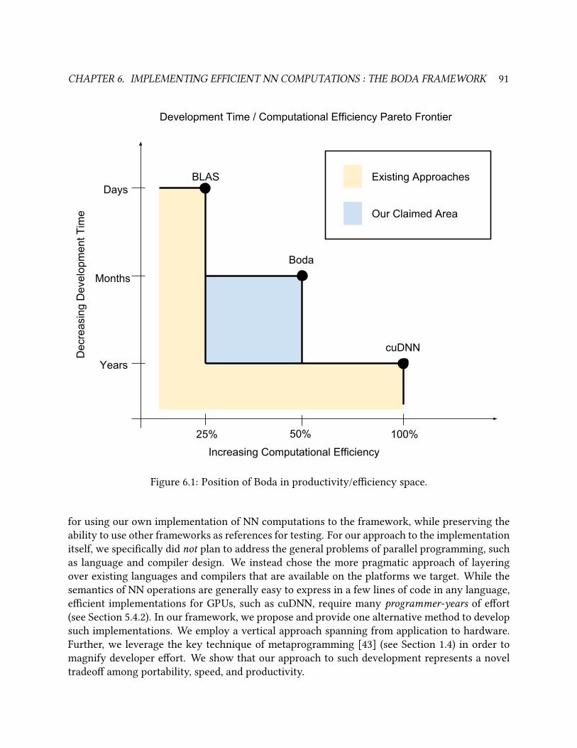
CHAPTER 6. IMPLEMENTING EFFICIENT NN COMPUTATIONS : THE BODA FRAMEWORK 91
Increasing Computational Efficiency
Dec
reas
ing
Dev
elop
men
t Tim
e
50%
Months
Years
25%
Days
100%
Boda
BLAS
cuDNN
Existing Approaches
Our Claimed Area
Development Time / Computational Efficiency Pareto Frontier
Figure 6.1: Position of Boda in productivity/eciency space.
for using our own implementation of NN computations to the framework, while preserving the
ability to use other frameworks as references for testing. For our approach to the implementation
itself, we specically did not plan to address the general problems of parallel programming, such
as language and compiler design. We instead chose the more pragmatic approach of layering
over existing languages and compilers that are available on the platforms we target. While the
semantics of NN operations are generally easy to express in a few lines of code in any language,
ecient implementations for GPUs, such as cuDNN, require many programmer-years of eort
(see Section 5.4.2). In our framework, we propose and provide one alternative method to develop
such implementations. We employ a vertical approach spanning from application to hardware.
Further, we leverage the key technique of metaprogramming [43] (see Section 1.4) in order to
magnify developer eort. We show that our approach to such development represents a novel
tradeo among portability, speed, and productivity.
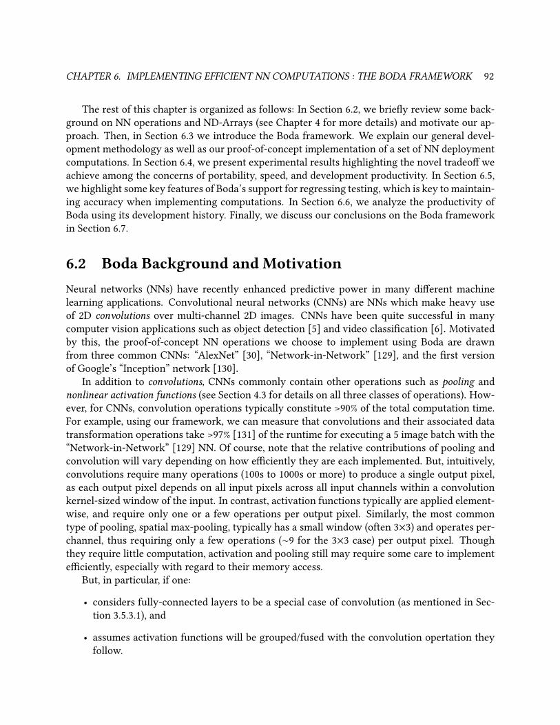
CHAPTER 6. IMPLEMENTING EFFICIENT NN COMPUTATIONS : THE BODA FRAMEWORK 92
The rest of this chapter is organized as follows: In Section 6.2, we briey review some back-
ground on NN operations and ND-Arrays (see Chapter 4 for more details) and motivate our ap-
proach. Then, in Section 6.3 we introduce the Boda framework. We explain our general devel-
opment methodology as well as our proof-of-concept implementation of a set of NN deployment
computations. In Section 6.4, we present experimental results highlighting the novel tradeo we
achieve among the concerns of portability, speed, and development productivity. In Section 6.5,
we highlight some key features of Boda’s support for regressing testing, which is key to maintain-
ing accuracy when implementing computations. In Section 6.6, we analyze the productivity of
Boda using its development history. Finally, we discuss our conclusions on the Boda framework
in Section 6.7.
6.2 Boda Background and MotivationNeural networks (NNs) have recently enhanced predictive power in many dierent machine
learning applications. Convolutional neural networks (CNNs) are NNs which make heavy use
of 2D convolutions over multi-channel 2D images. CNNs have been quite successful in many
computer vision applications such as object detection [5] and video classication [6]. Motivated
by this, the proof-of-concept NN operations we choose to implement using Boda are drawn
from three common CNNs: “AlexNet” [30], “Network-in-Network” [129], and the rst version
of Google’s “Inception” network [130].
In addition to convolutions, CNNs commonly contain other operations such as pooling and
nonlinear activation functions (see Section 4.3 for details on all three classes of operations). How-
ever, for CNNs, convolution operations typically constitute >90% of the total computation time.
For example, using our framework, we can measure that convolutions and their associated data
transformation operations take >97% [131] of the runtime for executing a 5 image batch with the
“Network-in-Network” [129] NN. Of course, note that the relative contributions of pooling and
convolution will vary depending on how eciently they are each implemented. But, intuitively,
convolutions require many operations (100s to 1000s or more) to produce a single output pixel,
as each output pixel depends on all input pixels across all input channels within a convolution
kernel-sized window of the input. In contrast, activation functions typically are applied element-
wise, and require only one or a few operations per output pixel. Similarly, the most common
type of pooling, spatial max-pooling, typically has a small window (often 3×3) and operates per-
channel, thus requiring only a few operations (∼9 for the 3×3 case) per output pixel. Though
they require little computation, activation and pooling still may require some care to implement
eciently, especially with regard to their memory access.
But, in particular, if one:
• considers fully-connected layers to be a special case of convolution (as mentioned in Sec-
tion 3.5.3.1), and
• assumes activation functions will be grouped/fused with the convolution opertation they
follow.
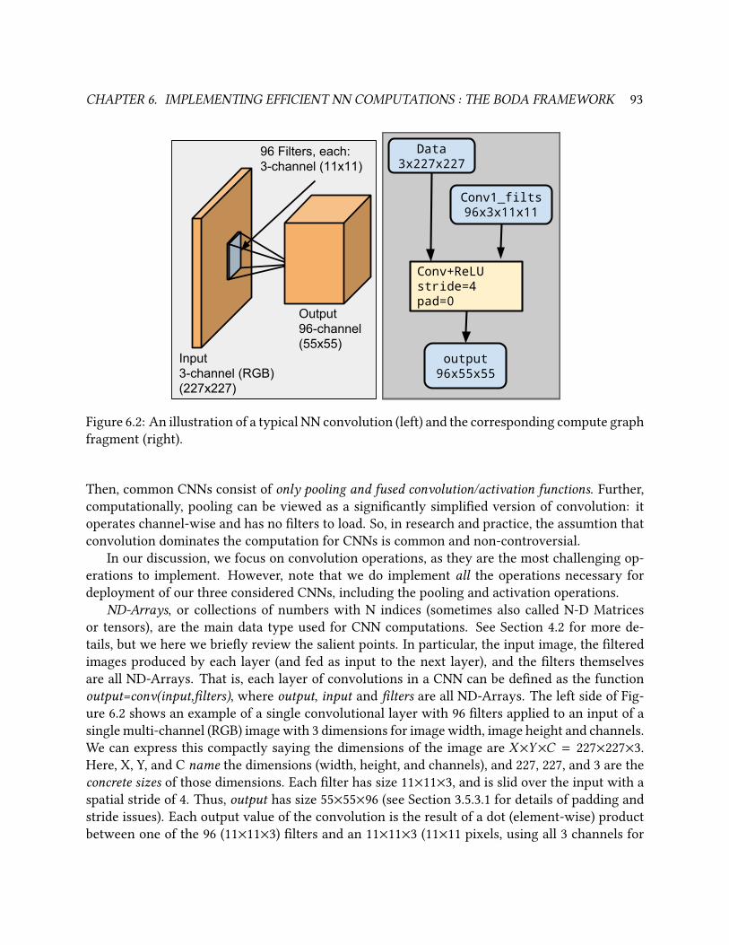
CHAPTER 6. IMPLEMENTING EFFICIENT NN COMPUTATIONS : THE BODA FRAMEWORK 93
Input3-channel (RGB)(227x227)
Output96-channel(55x55)
96 Filters, each:3-channel (11x11)
Data3x227x227
Conv1_filts96x3x11x11
output96x55x55
Conv+ReLUstride=4 pad=0
Figure 6.2: An illustration of a typical NN convolution (left) and the corresponding compute graph
fragment (right).
Then, common CNNs consist of only pooling and fused convolution/activation functions. Further,
computationally, pooling can be viewed as a signicantly simplied version of convolution: it
operates channel-wise and has no lters to load. So, in research and practice, the assumtion that
convolution dominates the computation for CNNs is common and non-controversial.
In our discussion, we focus on convolution operations, as they are the most challenging op-
erations to implement. However, note that we do implement all the operations necessary for
deployment of our three considered CNNs, including the pooling and activation operations.
ND-Arrays, or collections of numbers with N indices (sometimes also called N-D Matrices
or tensors), are the main data type used for CNN computations. See Section 4.2 for more de-
tails, but we here we briey review the salient points. In particular, the input image, the ltered
images produced by each layer (and fed as input to the next layer), and the lters themselves
are all ND-Arrays. That is, each layer of convolutions in a CNN can be dened as the function
output=conv(input,lters), where output, input and lters are all ND-Arrays. The left side of Fig-
ure 6.2 shows an example of a single convolutional layer with 96 lters applied to an input of a
single multi-channel (RGB) image with 3 dimensions for image width, image height and channels.
We can express this compactly saying the dimensions of the image are X×Y×C = 227×227×3.
Here, X, Y, and C name the dimensions (width, height, and channels), and 227, 227, and 3 are the
concrete sizes of those dimensions. Each lter has size 11×11×3, and is slid over the input with a
spatial stride of 4. Thus, output has size 55×55×96 (see Section 3.5.3.1 for details of padding and
stride issues). Each output value of the convolution is the result of a dot (element-wise) product
between one of the 96 (11×11×3) lters and an 11×11×3 (11×11 pixels, using all 3 channels for
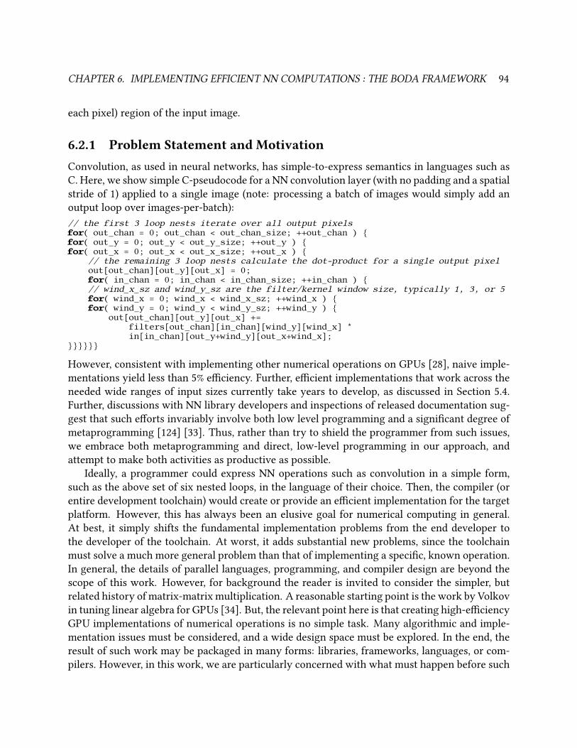
CHAPTER 6. IMPLEMENTING EFFICIENT NN COMPUTATIONS : THE BODA FRAMEWORK 94
each pixel) region of the input image.
6.2.1 Problem Statement and MotivationConvolution, as used in neural networks, has simple-to-express semantics in languages such as
C. Here, we show simple C-pseudocode for a NN convolution layer (with no padding and a spatial
stride of 1) applied to a single image (note: processing a batch of images would simply add an
output loop over images-per-batch):
// the first 3 loop nests iterate over all output pixelsfor( out_chan = 0; out_chan < out_chan_size; ++out_chan ) for( out_y = 0; out_y < out_y_size; ++out_y ) for( out_x = 0; out_x < out_x_size; ++out_x )
// the remaining 3 loop nests calculate the dot-product for a single output pixelout[out_chan][out_y][out_x] = 0;for( in_chan = 0; in_chan < in_chan_size; ++in_chan ) // wind_x_sz and wind_y_sz are the filter/kernel window size, typically 1, 3, or 5for( wind_x = 0; wind_x < wind_x_sz; ++wind_x ) for( wind_y = 0; wind_y < wind_y_sz; ++wind_y )
out[out_chan][out_y][out_x] +=filters[out_chan][in_chan][wind_y][wind_x] *in[in_chan][out_y+wind_y][out_x+wind_x];
However, consistent with implementing other numerical operations on GPUs [28], naive imple-
mentations yield less than 5% eciency. Further, ecient implementations that work across the
needed wide ranges of input sizes currently take years to develop, as discussed in Section 5.4.
Further, discussions with NN library developers and inspections of released documentation sug-
gest that such eorts invariably involve both low level programming and a signicant degree of
metaprogramming [124] [33]. Thus, rather than try to shield the programmer from such issues,
we embrace both metaprogramming and direct, low-level programming in our approach, and
attempt to make both activities as productive as possible.
Ideally, a programmer could express NN operations such as convolution in a simple form,
such as the above set of six nested loops, in the language of their choice. Then, the compiler (or
entire development toolchain) would create or provide an ecient implementation for the target
platform. However, this has always been an elusive goal for numerical computing in general.
At best, it simply shifts the fundamental implementation problems from the end developer to
the developer of the toolchain. At worst, it adds substantial new problems, since the toolchain
must solve a much more general problem than that of implementing a specic, known operation.
In general, the details of parallel languages, programming, and compiler design are beyond the
scope of this work. However, for background the reader is invited to consider the simpler, but
related history of matrix-matrix multiplication. A reasonable starting point is the work by Volkov
in tuning linear algebra for GPUs [34]. But, the relevant point here is that creating high-eciency
GPU implementations of numerical operations is no simple task. Many algorithmic and imple-
mentation issues must be considered, and a wide design space must be explored. In the end, the
result of such work may be packaged in many forms: libraries, frameworks, languages, or com-
pilers. However, in this work, we are particularly concerned with what must happen before such
CHAPTER 6. IMPLEMENTING EFFICIENT NN COMPUTATIONS : THE BODA FRAMEWORK 95
packaging can occur. That is, one of our key goals is to enable the initial algorithmic work and
exploration required to create ecient implementations. To summarize, let us say one believes
that a compiler or language should handle some general case of creating ecient numerical code
for some platform. However, in that case, it is still a prerequisite that it is known how to create
ecient code for such operations for the given platform in the rst place; Boda is a framework
designed to aid in that process.
That said, we note that, after an implementation is created, we are also concerned with de-
ployment for both research and practical use. Our vertical approach and focus on portability are
natural enablers for easy deployment. In particular, as required by our development approach,
Boda can be used to run Boda-created implementations inside full ows (as used for testing and
development) on multiple platforms without additional dependencies.
Now, with the above intuition in mind, we state our high-level task more generally and for-
mally: Given a NN and its inputs, eciently compute its outputs. Recall from Section 4.1.3 that
we can dene a NN as a directed acyclic compute graph of (stateless) functions and ND-Arrays.
Figure 6.2 shows an example of a convolution operation and its corresponding compute graph
fragment. We term the process of converting from some description of a NN to the corresponding
compute graph the NN front-end. In this work, as we are focused on the implementation of core
computations, we are NN front-end neutral; as long as a suitable compute graph can be produced,
any NN front-end can be used with our approach. Further, as mentioned earlier, while there are
various operations in the compute graph, convolution is the most computationally challenging.
So, much of our discussion here will focus on the details of implementing convolution.
After convolution, the next most complex operation we consider is pooling (see Section 4.3
for a detailed description of pooling). Compared to convolution, pooling is relatively simple,
not computationally intensive, and does not require signicant additional implementation eort
beyond what is already needed for convolution. In particular, the performance of pooling is gen-
erally limited by memory access to its inputs and outputs, rather than by computation. We nd
that, conveniently, the access pattern of pooling is reasonably eciently handled by the compiler
and hardware without signicant manual eort. While optimizations are no doubt possible, the
low overall contribution of pooling to total application runtime made optimization of pooling a
lower priority. While we still leverage specialization over the pooling window size, we were able
use a single version of our pooling code across all input sizes and hardware targets without issue.
The nal broad category of operations, activation functions, are purely memory bound and
operate element-wise. Their standalone implementations are trivial, but one key optimization is
fusing them into preceding operations, and thus avoiding memory access for them entirely.
6.2.2 Key Problems of Ecient GPU ConvolutionsWhen implementing convolutions across multiple types of GPUs, there are two categories of
problems. First, there are the fundamental challenges of implementing ecient convolutions
on any GPU. Second, recalling our discussion of the importance of portability in Section 1.1.5,
there are the issues that arise when targeting multiple GPUs. Together, the full set of high-level
problems we address with our approach are:
CHAPTER 6. IMPLEMENTING EFFICIENT NN COMPUTATIONS : THE BODA FRAMEWORK 96
• Incompatible GPU programming models across dierent hardware: OpenCL and CUDA.
• GPU-hardware-specic constraints: memory size and access methods, organization and
control of hardware execution primitives such as multiply-accumulate (MAC) instructions.
• Data movement: getting data from o-chip to compute units and back, considering the
sizes and bandwidths of all storage locations.
• Scheduling/Resource-Management/Parallelism: what computations happen when, where,
and how.
• Managing overheads: minimizing the use and impact of conditionals, control ow, and
indexing.
To the best of our knowledge, our approach is the rst to address these concerns in a unied,
vertical framework for implementing NN convolutions on GPUs. In Section 6.3, we will discuss
how our approach addresses each of these concerns using metaprogramming, autotuning, and
other techniques.
6.2.3 NVIDIA and GPU ComputationWhen Krizhevsky developed cuda-convnet in 2011, early in the modern rise of neural networks,
NVIDIA was the clear platform of choice for NN computation. However, it is worth noting that
this was no accident. NVIDIA had been developing their hardware and software with a focus on
high-throughput scientic and general purpose computing since roughly 2001 [132]. Certainly by
2005, it was clear that general-purpose-GPU (GP-GPU) programming was beginning to mature,
with GPUs outperforming CPUs on relatively complex linear algebra computations such as LU
factorization [133]. An important milestone was the release of version 1.0 of NVIDIA’s CUDA
development environment in 2007, which ocially promoted computation to a peer of graphics
at the interface level. So, use of NVIDIA GPUs for NN computing represents a 10-years-awaited
payo for NVIDIA’s bet on using GPUs for general purpose computing. NVIDIA shows every sign
of attempting to capitalize on this trend and continue to develop their capabilities in this area.
However, they seem clearly interested in maintaining and enhancing their market dominance,
rather than broadening the overall GPU compute market though increased competition.
In particular, let us consider the ongoing development of NVIDIA’s NN computation library,
cuDNN. Despite the large eort for its original creation, cuDNN is not a once-and-done endeavor.
Due to constantly changing hardware capabilities and software requirements, signicant ongoing
eort is required to maintain cuDNN. Over time, important improvements and new features have
continued to appear, with cuDNN v5 released 2016-04. These improvements and new features
generally track new developments in the ML community, but with a signicant real-time lag
of many months. Anecdotally, the reason for this long latency is simple: developing cuDNN
requires a large amount of engineering eort by a team of specialized programmers, perhaps in
total more than 15 sta-years to date. Given this history, it is unclear if it is even possible for
other vendors to compete with cuDNN using the same closed, single-vendor development model.
CHAPTER 6. IMPLEMENTING EFFICIENT NN COMPUTATIONS : THE BODA FRAMEWORK 97
Worse, it is unclear if NVIDIA itself can continue to support the ever growing set of use-cases
for NN computation. This highlights one of the issues with reliance on any single vendor for
critical parts of any software ecosystem. We now discuss this issue in more detail in the following
Section 6.2.4.
6.2.4 Why Not Rely on Hardware Vendors for Software?Here, we build on our prior discussion from Section 1.2.3 on the topic of vendor-supplied libraries
for computation. One general approach to the problem of ecient numerical computation is to
rely on individual hardware vendors to provide ecient implementations of all needed opera-
tions. However, this suers from several problems:
• It does not address the fundamental issues with creating ecient implementations (as listed
in Section 6.2.2), but only shifts them to hardware vendors.
• Vendors typically only support only their own hardware.
• Vendors may not provide timely support for all needed functions.
Despite focusing only on their own hardware and business-need-selected features, vendors have
still required many years (and anecdotally, many times that number of sta-years) to release NN
computation software packages. Further, to gain competitive advantages over each other, ven-
dors have incentive both to hide their eorts and provide unique functionality. The end result is
considerable duplicated eort and patchwork functionality across hardware targets. Worse, many
vendors may simply not have the motivation (due to lack of sucient perceived return on invest-
ment / market potential) or capability (due to lack of the rare skilled programmers capable of such
work) of delivering any robust software system at all. In short, all users, in research and business,
are at the ckle mercy of hardware vendors for the implementation of any needed functionality.
Some research users may have the luxury of working around these issues to some degree, due
to hardware and support subsidies from specic vendors. However, business customers may not
have such luxuries of platform choice and support, or may be (rightfully) hesitant to become too
dependant on specic hardware vendors. But, some dependence on hardware vendors is both
inevitable and perhaps desirable. Indeed, vendors should be expected to be adept at creating soft-
ware for their own hardware. That is, vendors have a privileged position to develop software
for their own hardware. They generally have proprietary access to some combination of tools,
hardware, software, knowledge, and experience. Yet, even with these advantages, vendors have
not been, as whole, able to deliver NN computation libraries in a timely manner. Thus, for a
healthy software ecosystem, reliance on vendors must be balanced with freedom, independence,
and competition. In particular, users should be able to:
• choose among multiple hardware vendors for each task, and
• have the freedom to modify and enhance the software systems they require.
CHAPTER 6. IMPLEMENTING EFFICIENT NN COMPUTATIONS : THE BODA FRAMEWORK 98
6.3 Boda ApproachIn this section, we will discuss our overall approach to implementing NN computations as embod-
ied in the Boda framework. At a high level, our vertically-integrated approach falls somewhere
between that of compilers and traditional libraries (see Section 5.1 for an overview of general
approaches to computation).
Like a library, Boda aims to help deliver ecient implementations of specic, predetermined
sets of operations. From an interface perspective, using a Boda-created implementation to actu-
ally perform NN computations feels similar to using a library. However, bear in mind that a main
goal of Boda is to help create ecient implementations in the rst place, not simply to deliver an
implementation with a library-like interface for later use.
The sorts of implementations that Boda helps to create are, by necessity, generally not a xed
set of functions that can be compiled and placed into a independent library. Instead, achieving
high eciency for operations such as NN convolutions requires the use of various metaprogram-
ming techniques, where functions dynamically generate and transform other functions. Boda
provides support for general-purpose metaprogramming and dynamic compilation, and thus acts
somewhat like a traditional compiler. However, compared to a full compiler, we do not aspire
to support general purpose programming, and we avoid all mandatory, pre-existing, already-
specied intermediary layers (such as the LLVM IR [134]) present in typical compilation ows.
Thus, we can avoid much of the complexity of full, general purpose compilers. Overall, using
this approach, we can achieve high eciency for the set of operations required for our applica-
tions of interest, while keeping overall complexity manageable.
6.3.1 Justication for MetaprogrammingAlthough powerful, metaprogramming is a technique to be used judiciously, due to the com-
plexity it adds to any implementation. In this section, we motivate the use of metaprogramming
for eciently implementing NN computations. Firstly, it should be noted that the notion that
metaprogramming is currently necessary for high eciency numerical computing on GPUs is
not particularly controversial, as seen from our survey of related work in Chapter 5. At the least,
empirically, all current libraries for ecient NN computing on GPUs use at least some form of
metaprogramming.
To illustrate this trend towards metaprogramming, let us consider the example of matrix-
matrix multiplication. In Volkov’s work in 2008, he focused on performance for large, square
matrices [34]. In this case, it was possible, albeit with great diculty, to hand-write a single
function with reasonable performance for a single GPU target. As can be seen in later work, var-
ious optimization were possible in the case of small and/or non-square matrices. However, these
optimizations required hard-coding problem sizes into the code, which is generally intractable
without metaprogramming [135]. Currently, it can be seen that use of metaprogramming tech-
niques is now quite common in GPU BLAS libraries [32] [136].
CHAPTER 6. IMPLEMENTING EFFICIENT NN COMPUTATIONS : THE BODA FRAMEWORK 99
6.3.1.1 Intuition for Metaprogramming from Matrix-Matrix Multiply Example
To gain a qualitative intuition as to why it is dicult to write a single version of an operation
to handle all possible inputs, let us consider the technical details of the case of matrix-matrix
multiplication. To simplify somewhat, let us consider just the case of a single, general matrix
multiplication:
C = AB
Where:
• A is an M×K matrix,
• B is a K×N matrix,
• and the result, C , is an M×N matrix.
The space of all possible input sizes for matrix-matrix multiply is dened by all possible values
of M , K , and N . That is, each point in Z+3
given by some value of the positive integers M , K , and
N represents a unique set of input sizes to handle. For dense linear algebra, the behavior of an
implementation of a function like matrix-matrix multiply, in terms of the sequence of primitive
operations it performs (e.g. loads, stores, multiplies, and adds), is fully determined by the sizes
of its inputs. That is, the actual values of the numbers in the input matrices will not (neglecting
corner cases) aect the computational eciency; only the sizes of the inputs are relevant. In the
case of square matrices, M = K = N , and the space of possible input sizes is reduced to one
dimension N . Further, nite GPU memory places an upper limit of ∼8196 on N , and sizes below
a certain minimum are often neglected as less interesting. In Volkov’s work, for square matrices
above a certain minimum size (perhaps 256), a single pre-compiled function can oer reasonable
performance over the entire space of input sizes (especially if all sizes are, for example, multiples
of 64). However, as mentioned, later work has shown that having input-size-specic code helps
optimize over the full space of possible input sizes [135]. In particular, in any case where one
of M , N , or K is much smaller than the others, or when (more generally) the ratios between the
three values span a large range (i.e. extreme aspect ratios), the behavior of the function becomes
qualitatively dierent:
• The relative and absolute needed amounts of dierent kinds of intermediate storage will
vary considerably.
• The ratios of computation and communication in dierent parts of the algorithm will vary.
• The relative contribution of overheads, such as those from looping and indexing, will vary.
Especially when any inputs sizes are small, this will lead to scenarios where it becomes more
critical to avoid various overheads. Typically, this is accomplished using metaprogramming to
unroll loops, avoid conditionals, or hard-code specic patterns and amounts of register usage.
Further, data that can be stored in shared local memory in one input-size-regime may t in reg-
isters in another regime, or require spilling to global memory in a third regime. In one regime,
CHAPTER 6. IMPLEMENTING EFFICIENT NN COMPUTATIONS : THE BODA FRAMEWORK 100
it may be important to unroll a loop somewhat (to reduce overhead), but not too much (to avoid
excessive register usage). In another regime, it might be important, and perhaps a simplica-
tion, to fully unroll the same loop. In yet a third regime, the loop might have only one iteration,
making it possible to simplify the code by removing the loop and all relevant indexing and setup
overheads.
To illustrate this issue, let us consider a simplied example. Let us assume that achieving 100%
computational eciency requires that the hardware perform a non-overhead calculation on every
cycle in every available computation unit (which is, in fact, quite close to true on modern GPUs).
Let us start with a loop that performs 1 non-overhead multiply instruction per iteration, and
further assume that the hardware requires 2 instructions to implement the needed logic for the
loop. Then, assuming the hardware performs 1 instruction per cycle, eciency for this loop will
be limited to 1/3 or ∼33% of the peak possible. So, in this case, unrolling the loop to performing
8 multiplies per iteration would raise the eciency of the loop to 8/10 or ∼80% (assuming a large
number of iterations). However, let as assume that each additional multiply added to the loop
requires an additional register for temporary storage, and that the hardware only has 16 registers
available for this loop. So, if we attempted to put 32 multiplies in the loop, to try to achieve
32/34 or ∼94% eciency, the compiler would need to add many loads/stores inside the loop due
to register spilling (needing to use bigger-but-slower storage to emulate extra registers). Not
only would this lower the percentage of instructions spent on multiplies, but would also incur
slowdowns due to accessing slower-than-registers storage, and eciency would perhaps drop to
<5%. But, however important these issues may be for matrix-matrix multiplication, we shall see
that they are magnied in the case of NN convolution.
6.3.1.2 Benets of Metaprogramming for NN Convolutions
Convolution (as used in NNs and shown in Figure 6.2) can be viewed as a generalization of matrix-
matrix multiplication. First, consider a C-pseudocode representation of the matrix-matrix multi-
ply example of the prior section:
// the first 2 loop nests iterate over all elements of Cfor( n = 0; n < N; ++n ) for( m = 0; m < M; ++m )
// the remaining loop nest calculates the dot-product for a single output elementC[m][n] = 0;for( k = 0; k < K; ++k )
C[m][n] += A[m][k] * B[k][n];
Then, recall the C-pseudocode for NN convolution from 6.2.1. Note that both functions iterate
over output elements in their outer set of loop nests, and then iterate over the elements of a dot-
product in their inner loop nests. In order to compute NN convolutions using matrix-matrix
multiply, we need only atten all the inner loops of convolution (which iterate over all values in
the lter and corresponding input window) and treat them as the K dimension, and then atten
the out_x and out_y dimensions and treat the combination as the M dimension.
Thus, many of the same algorithms and optimizations used for matrix-matrix multiplication
also apply to convolution [135]. However, instead of three integers (M, N, and K) as in the case of
CHAPTER 6. IMPLEMENTING EFFICIENT NN COMPUTATIONS : THE BODA FRAMEWORK 101
matrix-matrix multiplication, NN convolution has an input space dened by considerably more
(six or more) values. These consist of a mix of small/enumerated integers (e.g. padding, stride,
kernel size), large integers (e.g. input X and Y sizes, input and output number-of-channels), and
Booleans (e.g. “has activation function fused to output?”, see Section 6.3.9 for details on the fusion
of activation functions with convolutions). Thus, the dimensionality of the space of problem sizes
for convolution is both larger and more complex than that of matrix-matrix multiplication. Fur-
ther, dierent parts of this space may be qualitatively quite dierent in terms of the calculations
they perform. For example, the data reuse patterns for kernel sizes of 1 are quite dierent from
those for kernel sizes of 3, and then in turn the patterns for a size of 3 are quite dierent from
those for a size of 11. But, given that only a few sparse points in this space are needed for any
particular application, NN convolution can particularly benet from metaprogramming, where
(if needed), code can be specialized for each case.
6.3.2 Comparison with LibrariesThe need for metaprogramming does not, by itself, preclude the traditional library approach (as
dened in Section 5.1.2). In this section, we show how a traditional library-based approach is
insucient for NN computations.
As discussed earlier, metaprogramming can be used to create various versions of an operation
to handle dierent points in the operation’s space of input sizes. For NN convolutions, the number
of such needed versions can be quite high when considering all common scenarios in modern
NNs. In Table 6.1 (Section 6.4), we show all the unique convolution input sizes that we implement
for our proof-of-concept of Boda. From just the three NNs we considered, there are over 40 unique
convolution congurations spanning a wide range of input sizes. Further, this number is then
multiplied by the product of the number of input formats, output formats, and potential fusion
scenarios. For example, assume that N pre-compiled versions of a convolution are required to
cover the space of input congurations. So, it might be tractable to support 2 output formats and
2 fusions, yielding N×2×2 = 4N versions. But, extending this support to 2 output formats, 2
input formats, and 3 fusions, now N×2×2×3 = 12N versions are needed. Especially if N is large,
the size of a library that held all needed pre-compiled versions could quickly become impractical.
Worse, given the large and complex space of possible input sizes, one is faced with the unfortunate
choices of either:
• Attempting to eciently handle the entire space of possible input sizes.
• Attempting to guess what input congurations are likely to be encountered in the future.
• Spending additional optimization eort to reduce the number of functions needed to handle
various sets of input sizes while still preserving performance.
So, avoiding all these issues (and their attendant development and/or speed costs) is a key benet
of our per-input-size-compilation approach. As a note, it is sometimes desired to avoid run-time compilation in deployment use-cases. However, for a xed application, it is always possible
CHAPTER 6. IMPLEMENTING EFFICIENT NN COMPUTATIONS : THE BODA FRAMEWORK 102
to generate, as part of the application, an application-specic computation library containing all
needed functions for that particular application, and thus avoid runtime compilation. However,
this should not be confused with the notion of a traditional library, which is not application spe-
cic, and must handle all possible input sizes.
6.3.3 Specialization and Comparison with General-PurposeCompilation
In this section, we consider in more detail the concept of specialization (using metaprogram-
ming to tailor code for particular use-cases, as introduced in Section 1.4) and how it is used in
Boda. Along the way, we contrast this approach with that of a general purpose compiler (see
Section 5.1.1), and show how our approach sidesteps the unsolved problem of general-purpose
ecient parallel compilation.
One key to eciency and managing complexity in our approach is that, at runtime, we need
only handle the specic instances of operations needed for our applications. That is, unlike a
traditional library, we need not write and pre-compile code to handle the general cases of opera-
tions, and we are free to use all input-specic runtime information to aid in optimization. For the
types of NN computations we consider here, there are several key pieces of runtime information
we can exploit:
• Perhaps most importantly, for each operation, we need only handle the specic input sizes
and operational modes used.
• Additionally, for each use-case, we only need to handle the specic overall graph of opera-
tions used. So, this allows: (1) graph level optimizations such as fusions (see Section 6.3.9),
and (2) the use of optimized intermediate types.
Using SEJITS [114] terminology, we term this usage of runtime information to generate special-
case implementations of operations specialization. As discussed in the prior section, as the num-
ber of possible input sizes is very large, specialization of individual operations for each input size
is cumbersome and/or limited in the traditional library approach. However, compared to a gen-
eral purpose compiler, the types of program generation we need to perform are quite simple. The
expectation is that the generated functions will handle parallelism and data movement explicitly.
Thus, these problems need only be solved for the specic operations to be performed. In contrast,
a parallelizing compiler must solve these problems in general for some class of input programs.
While we believe our approach is perhaps the most productive way to achieve our particular
goals, we also realize the benets of the traditional library and compiler approaches as well. In
fact, we would argue that, as progress is made on the key problems of implementing ecient
GPU convolutions (using our approach), it is then natural to: (1) generalize the techniques and
embed them in a compiler, or (2) apply additional eort (and perhaps compromise speed) to allow
for a xed-library implementation.
Additionally, we mention here that there are certain compiler features that would have been
helpful to us during our eorts. In particular, in cases where the existing compiler heuristics were
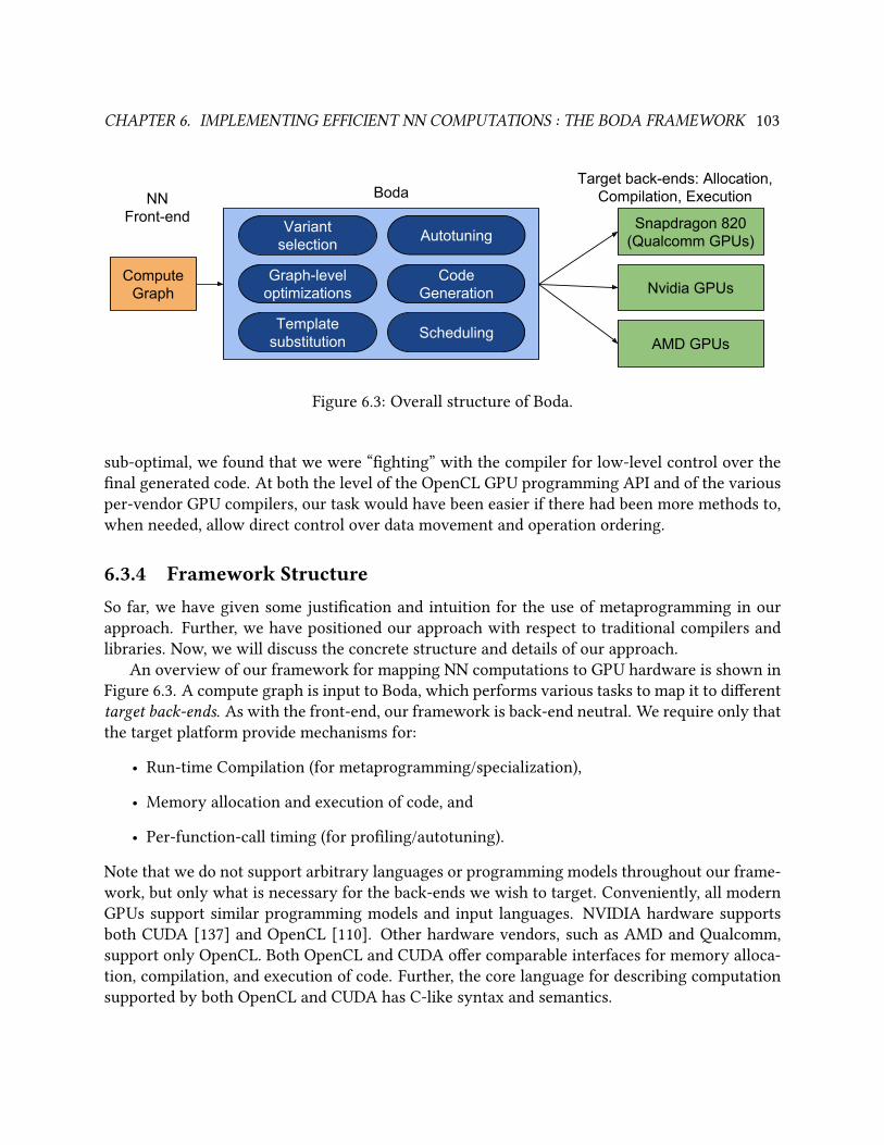
CHAPTER 6. IMPLEMENTING EFFICIENT NN COMPUTATIONS : THE BODA FRAMEWORK 103
NN Front-end
Target back-ends: Allocation, Compilation, ExecutionBoda
Compute Graph
Variant selection Autotuning
Graph-level optimizations
Scheduling
Code Generation
Template substitution
Snapdragon 820 (Qualcomm GPUs)
Nvidia GPUs
AMD GPUs
Figure 6.3: Overall structure of Boda.
sub-optimal, we found that we were “ghting” with the compiler for low-level control over the
nal generated code. At both the level of the OpenCL GPU programming API and of the various
per-vendor GPU compilers, our task would have been easier if there had been more methods to,
when needed, allow direct control over data movement and operation ordering.
6.3.4 Framework StructureSo far, we have given some justication and intuition for the use of metaprogramming in our
approach. Further, we have positioned our approach with respect to traditional compilers and
libraries. Now, we will discuss the concrete structure and details of our approach.
An overview of our framework for mapping NN computations to GPU hardware is shown in
Figure 6.3. A compute graph is input to Boda, which performs various tasks to map it to dierent
target back-ends. As with the front-end, our framework is back-end neutral. We require only that
the target platform provide mechanisms for:
• Run-time Compilation (for metaprogramming/specialization),
• Memory allocation and execution of code, and
• Per-function-call timing (for proling/autotuning).
Note that we do not support arbitrary languages or programming models throughout our frame-
work, but only what is necessary for the back-ends we wish to target. Conveniently, all modern
GPUs support similar programming models and input languages. NVIDIA hardware supports
both CUDA [137] and OpenCL [110]. Other hardware vendors, such as AMD and Qualcomm,
support only OpenCL. Both OpenCL and CUDA oer comparable interfaces for memory alloca-
tion, compilation, and execution of code. Further, the core language for describing computation
supported by both OpenCL and CUDA has C-like syntax and semantics.
CHAPTER 6. IMPLEMENTING EFFICIENT NN COMPUTATIONS : THE BODA FRAMEWORK 104
6.3.4.1 Programming Model Portability with CUCL
For portability across GPUs, one key issue is the incompatibility between the two main GPU
programming languages, OpenCL and CUDA (as introduced in Section 5.1.1). Any approach that
wishes to portably target both OpenCL and CUDA must somehow surmount this problem. In
particular, while CUDA and OpenCL share C as a base, they use dierent syntax for various GPU-
programming-specic concepts. But, importantly, the core computational semantics and parallel
programming models of OpenCL and CUDA are fairly compatible. Conveniently for our work on
implementing NN convolutions, this cross compatible core of functionality is mostly sucient
for our needs. So, as our solution, we start with the cross-compatible intersection of CUDA and
OpenCL and form a language we call CUCL. However, it should be noted from the start that CUCL
is not a new language in the normal sense of the word. Instead, it simply adds new features to
both OpenCL and CUDA that the programmer can use instead of OpenCL/CUDA specic ones.
So, to program in CUCL with Boda, an OpenCL or CUDA programmer need not learn anything
new to start working. However, if they use OpenCL or CUDA specic features, their code will
only work on the corresponding back-end. If, and only if, they desire portability, then they must
replace OpenCL/CUDA idioms with corresponding CUCL ones. The optional nature of CUCL
reects our overall pragmatic philosophy and approach, as will be discussed later in this section.
To summarize, in CUCL, we abstract away the syntactic dierences for the basic GPU pro-
gramming concepts shared by OpenCL and CUDA. For example, CUDA uses a special variable
threadIdx to allow each thread to determine its thread index. By contrast, OpenCL uses a
function named get_local_id() for a similar purpose. While the syntax and semantics
dier slightly between these two systems, common use cases can be easily be mapped to either
one. In CUCL, to handle the common case where threads are treated as a 1D array, we intro-
duce a new primitive LOC_ID_1D, which yields the current thread index as a single integer.
This CUCL primitive maps to get_local_id(0) in OpenCL and threadIdx.x in CUDA. For a
complete list of the current CUCL abstractions and their mappings to OpenCL and CUDA syntax,
see the relevant Boda source code [138] in the lesocl_util.cc (for OpenCL) andnvrtc_-util.cc (for CUDA).
In general, OpenCL lags behind CUDA in terms of supporting various GPU programming
features. Some of these features relate to hardware specic capabilities of NVIDIA GPUs. For
example, the warp-shue operation was exposed to CUDA users in CUDA version 4.2 in early
2012. However, as of 2017, no version of OpenCL explicitly exposes this operation, considering it
too low-level, even though by now many other vendors provide hardware primitives with simi-
lar functionality. Instead, as of the OpenCL 2.0 specication, released in mid 2013, just the most
common higher-level operations (such as reductions) that typically benet from warp shues
are exposed. In general, OpenCL chooses not to expose low-level hardware features, even when
they are necessary to achieve the best performance on a given hardware target. On non-NVIDIA
hardware, this is mitigated by the ability and willingness for vendors to expose vendor-specic
features though the OpenCL extension mechanism. On NVIDIA hardware, OpenCL support lags
behind that which is typical from other vendors, and so usage of hardware-specic features gen-
erally necessitates using CUDA.
CHAPTER 6. IMPLEMENTING EFFICIENT NN COMPUTATIONS : THE BODA FRAMEWORK 105
Further, considering the full software development stack, the CUDA Toolkit (or CUDA SDK)
tends to be more aggressive than OpenCL in terms of supporting additional features throughout
the toolchain. For example, CUDA oered dynamic parallelism as early as 2012, whereas the
OpenCL standard did not have such a concept until OpenCL 2.0 (in mid 2013). Note that while
the OpenCL 2.0 standard was released in mid 2013, at that point no hardware vendors supported
it. By 2014, only few GPU vendors supported OpenCL 2.0. Even by 2016, NVIDIA still did not
support OpenCL 2.0 on its own hardware. Thus, as with the warp-shue operation, the use
of CUDA is required to use dynamic parallelism on NVIDIA hardware. So, CUCL’s ability to
use either CUDA or OpenCL as a backend is helpful insurance when targeting both NVIDIA and
non-NVIDIA hardware, since usage of various target-specic optimizations on NVIDIA hardware
might (for no clear technical reason) require using CUDA.
Our framework is fairly pragmatic about this general situation. That is, Boda allows full free-
dom to implement portability at any level of abstraction. At the extreme low level of abstraction,
the user is free to add new primitives to CUCL. This is generally most useful for basic, low-level
features that can be supported across dierent hardware/languages with compatible semantics,
such as the LOC_ID_1D example above. At the extreme high level of abstraction, entirely dif-
ferent per-target implementations of some high level function (such as NN convolution) can be
used. Such per-target implementations would be free to use any back-end specic features they
desired, even perhaps inline assembly code. But, of course, the use of such back-end specic
features limits the portability of any code that uses them. Naturally, if portability is desired, and
per-target implementations are used, then the implementation eort will rise accordingly.
But, why not simply avoid any such back-end specic features, since the basic CUCL language
is easily able to express our needed computations? This brings us to the core fundamental issue
of performance portability. While it is convenient to share a common syntax and semantics for
computation (i.e. C) across targets, this ensures only functional equivalence. This is very helpful
for development, testing, and debugging. However, it does not address our goal of achieving higheciency across all back-ends. Currently, GPU compilers are unable to produce ecient runtime
code from high-level, portable descriptions of convolutions. So, we instead aim to minimize the
eort needed in order to optimize and specialize (to whatever degree in necessary) operations
of interest across our limited set of target back-ends. A key point is that, in general, it is not a
lack of ability to use back-end specic features that limits performance portability. That is, for
some operation to compute, we can generally nd some implementation in CUCL (or directly in
OpenCL) that is reasonably ecient on a given hardware target without using features such as
inline assembly or compiler intrinsics. However, CUCL (or OpenCL) code that is ecient on one
target is rarely ecient on another. In short, the main reason for this situation is that, for modern
GPUs, the ordering of computation and the movement of data must be explicitly and carefully
orchestrated in target-specic ways to achieve eciency. While these tasks might ideally be
handled by the compiler, it appears that the current set of layered abstractions employed on
modern GPUs, from hardware to compiler, do not give performance portability for the type of
computations we are interested in implementing. In summary, in the Boda framework, CUCL
is the functionally portable base on which we tackle this greater issue of performance portabilityusing metaprogramming and autotuning.
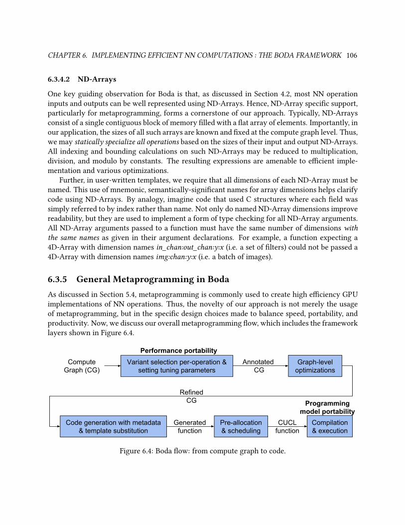
CHAPTER 6. IMPLEMENTING EFFICIENT NN COMPUTATIONS : THE BODA FRAMEWORK 106
6.3.4.2 ND-Arrays
One key guiding observation for Boda is that, as discussed in Section 4.2, most NN operation
inputs and outputs can be well represented using ND-Arrays. Hence, ND-Array specic support,
particularly for metaprogramming, forms a cornerstone of our approach. Typically, ND-Arrays
consist of a single contiguous block of memory lled with a at array of elements. Importantly, in
our application, the sizes of all such arrays are known and xed at the compute graph level. Thus,
we may statically specialize all operations based on the sizes of their input and output ND-Arrays.
All indexing and bounding calculations on such ND-Arrays may be reduced to multiplication,
division, and modulo by constants. The resulting expressions are amenable to ecient imple-
mentation and various optimizations.
Further, in user-written templates, we require that all dimensions of each ND-Array must be
named. This use of mnemonic, semantically-signicant names for array dimensions helps clarify
code using ND-Arrays. By analogy, imagine code that used C structures where each eld was
simply referred to by index rather than name. Not only do named ND-Array dimensions improve
readability, but they are used to implement a form of type checking for all ND-Array arguments.
All ND-Array arguments passed to a function must have the same number of dimensions withthe same names as given in their argument declarations. For example, a function expecting a
4D-Array with dimension names in_chan:out_chan:y:x (i.e. a set of lters) could not be passed a
4D-Array with dimension names img:chan:y:x (i.e. a batch of images).
6.3.5 General Metaprogramming in BodaAs discussed in Section 5.4, metaprogramming is commonly used to create high eciency GPU
implementations of NN operations. Thus, the novelty of our approach is not merely the usage
of metaprogramming, but in the specic design choices made to balance speed, portability, and
productivity. Now, we discuss our overall metaprogramming ow, which includes the framework
layers shown in Figure 6.4.
Annotated CG
Compute Graph (CG)
Refined CG
Variant selection per-operation & setting tuning parameters
Graph-level optimizations
Performance portability
Code generation with metadata & template substitution
Pre-allocation & scheduling
Compilation& execution
Programming model portability
Generatedfunction
CUCLfunction
Figure 6.4: Boda ow: from compute graph to code.
CHAPTER 6. IMPLEMENTING EFFICIENT NN COMPUTATIONS : THE BODA FRAMEWORK 107
We start with allowing the user to write only mildly restricted native GPU code in our CUD-
A/OpenCL subset language, CUCL. Compared to directly using CUDA or OpenCL, CUCL:
• provides language-neutral idioms to replace those from CUDA and OpenCL, and
• requires all ND-Array function arguments to be decorated with their dimension names, and
• requires access to ND-Array metadata (sizes, strides) to use a special template syntax:
%(myarray_mydim_size ).
Many simpler operations can be directly written as a single CUCL function template. To produce
OpenCL or CUDA functions from a CUCL function template, the framework: (1) replaces CUCL
idioms with OpenCL or CUDA ones, and (2) replaces references to ND-Array sizes and strides
with either (at the user’s explicit choice) (2a) constants for the specic input ND-Array sizes, or
(2b) references to dynamically-passed ND-Array metadata. Typically, we care most about the case
where the sizes are replaced with constants, as this gives the most possibility for optimizations
and therefor eciency. However, this does require instantiation of the given CUCL template for
every unique set of called argument sizes. Sometimes, for a given operation, this is unnecessary
for performance, and perhaps even creates prohibitive overhead due to having an excess number
of versions of a function. Thus, at the user’s selection, our framework also allows dynamically
passing the sizes and strides of ND-Arrays as automatically-generated function arguments. Note,
however, that CUCL code insulates the user from this issue, since the same syntax is used to refer
to ND-Array metadata regardless of if it is dynamic or static, allowing easy experimentation with
both methods for each function argument.
Then, for general metaprogramming support, we employ a string-template based approach,
using the framework’s host language (C++) to write code-generators that set the values of string
template variables inside CUCL function templates. Bear in mind that while the framework itself
and the code generators are written in C++, the GPU code is generated by C++ functions, not
written in C++ itself. We argue that our approach of writing a C++ program that generates CUCL
(i.e. C for GPUs) code is straightforward, and relatively easier to work with than, for example,
writing Perl to generate assembly (as in NervanaGPU, see Section 5.4.3). In particular, using C,
many constructs look roughly the same at the metacode and code levels. As will be shown shortly
in the example in Section 6.3.7, to statically unroll a loop, one simply moves the loop from the
code to the metacode, and “escapes” the body of the loop so as to print the code it previously
contained. In essence, we claim the similarity and compatibility between the metacode and code
languages eases the burden on the programmer to operate across both levels.
6.3.6 Boda Metaprogramming vs. C++ TemplatesOne common approach to metaprogramming is to use built-in language level metaprogramming
facilities. In particular, C++ templates are commonly used for high performance GPU metapro-
gramming with CUDA. However, C++ templates have the following disadvantages as compared
with the Boda approach:
CHAPTER 6. IMPLEMENTING EFFICIENT NN COMPUTATIONS : THE BODA FRAMEWORK 108
• C++ template support for OpenCL is only starting to become available.
• All C++ template programs must run at compile time, and thus cannot use run-time infor-
mation.
• Like Perl, C++ templates are a signicantly dierent language compared to C, and are gen-
erally considered dicult to use.
• C++ templates do not oer the practical ability to implement complex code generation
methods and heuristics at the meta level.
• C++ templates do not allow the ability to inspect the generated C level code for a given
instantiation in order to perform debugging and analysis.
6.3.7 Details of Boda Metaprogramming for NN ConvolutionsAs mentioned in Section 6.3.1.2, NN convolution can be viewed as generalized matrix-matrix
multiplication. In fact, in early approaches, NN convolution was often implemented using BLAS
(Basic Linear Algebra Subroutines) library SGEMM (Single-precision General Matrix-Matrix mul-
tiply) invocations for the bulk of the computation. But, as discussed in Chapter 5, the use of
special-purpose libraries for NN convolutions is currently the dominant approach. However, cre-
ating an ecient NN Convolution implementation is dicult, as it requires:
• writing large blocks of code consisting of many moves and/or multiplies,
• supporting many regimes of input sizes, and
• exercising ne-grained control over data storage and movement, and
• careful scheduling of all primitive operations, including storage blocking and loop tiling/un-
rolling.
All of these issues share a common solution: metaprogramming [43] (as introduced in Section 1.4).
With metaprogramming, one can easily write loops at the metacode level to generate long se-
quences of moves or multiplies. Multiple input regimes can be handled with metacode level case-
splits that do not incur runtime overhead. Finally, one can generate specic memory and register
indexing patterns without repetitive, error-prone manual eort. Where such details are public,
prior eorts have indeed uniformly used metaprogramming to varying degrees to address these
issues (see Section 5.4). At a high level, we choose to take a very general and exible approach to
metaprogramming. Rather than use some language-level metaprogramming facility, we choose to
directly write code generators in our framework’s host language of C++. We use our framework’s
native support for ND-Arrays at the metacode layer to (when desired) allow code generation to
exploit xed, exact sizes for all inputs and outputs. For example, when cooperatively loading data
across threads on a GPU, one must typically employ a loop with a conditional load. If there are Nthreads loadingW words, the loop must iterate dW /N e times. For each iteration, the load must
CHAPTER 6. IMPLEMENTING EFFICIENT NN COMPUTATIONS : THE BODA FRAMEWORK 109
be guarded on the condition that i ∗ N + thread_id <W . In CUCL, OpenCL, or CUDA, here is a
simplied version of how such a loop might appear:
for(int i = 0; i < ((W-1)/N)+1; ++i) int const ix = i*N + thread_id;if(ix<W)filts_buf[ix] = filts[ix];
However, if N and W are xed, we know we need exactly dW /N e individual loads. Further,
only the last load need be conditional, and then only if (W mod N ) is non-zero. In some cases,
just making W and N constant may allow the platform-specic compiler to unroll the loop and
eliminate unneeded conditionals without additional eort. We show our framework’s support
for this simple metaprogramming approach here, where we have replaced the W and N variables
with template variables that will be expanded to integer string constants:
#pragma unrollfor(int i = 0; i < ((%(W)-1)/%(N))+1; ++i)
int const ix = i*%(N) + thread_id;if(ix<%(W))filts_buf[ix] = filts[ix];
Further, in the event that W and N can be xed at compile time, even simpler metaprogramming
approaches (such as C++ templates, discussed in Section 6.3.6) might be sucient to handle this
case. However, note that for NN convolutions, it not easy to x such constants at compile time.
One alternate approach, that is compatible with static metaprogramming methods such as C++
templates, is tiling. In this method, operations are decomposed into tiles of xed, pre-determined
sizes with some additional code to handle remainders. While this is a reasonable and useful
approach that we also support, it is inconvenient and limiting for it to be the only viable technique.
Further, even in seemingly simple and ideal cases of loops with static bounds, we have ob-
served that the platform-specic compiler often does not successfully unroll the loop and remove
unneeded conditionals (we give an example later in this section). A burden of targeting multiple
hardware platforms is the variable quality of the OpenCL implementations, which can often in-
clude unpredictable or otherwise lacking optimization capabilities in the compiler. In such cases,
our framework allows us to smoothly and easily shift more complexity to the metacode level and
directly emit the sequence of desired loads. To do this, we move the loop to the metacode level,
and replace it entirely with a template variable in the CUCL code:
%(filts_buf_loads);
Then, at the metacode level, we write code to generate the needed sequence of loads, which is
similar in structure to the original loop:
string ix_str, load_str;for(int i = 0; i < ((W-1)/N)+1; ++i)
int const max_ix = i*N + (N-1);ix_str = str(i*N)+"+thread_id";load_str = "filts_buf["+ix_str+"]";load_str += "= filts["+ix_str+"];";if(max_ix >= W) // need bound check
load_str = "if("+ix_str+"<"+str(W)+ ")"+load_str+"";
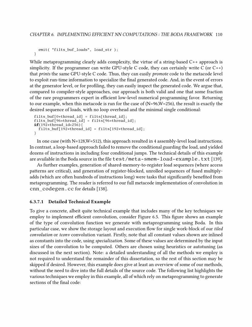
CHAPTER 6. IMPLEMENTING EFFICIENT NN COMPUTATIONS : THE BODA FRAMEWORK 110
emit( "filts_buf_loads", load_str );
While metaprogramming clearly adds complexity, the virtue of a string-based C++ approach is
simplicity. If the programmer can write GPU-style C code, they can certainly write C (or C++)
that prints the same GPU-style C code. Thus, they can easily promote code to the metacode level
to exploit run-time information to specialize the nal generated code. And, in the event of errors
at the generator level, or for proling, they can easily inspect the generated code. We argue that,
compared to compiler-style approaches, our approach is both valid and one that some fraction
of the rare programmers expert in ecient low-level numerical programming favor. Returning
to our example, when this metacode is run for the case of (N=96,W=256), the result is exactly the
desired sequence of loads, with no loop overhead and the minimal single conditional:
filts_buf[0+thread_id] = filts[thread_id];filts_buf[96+thread_id] = filts[96+thread_id];if(192+thread_id<256)
filts_buf[192+thread_id] = filts[192+thread_id];
In one case (with N=128,W=512), this approach resulted in 4 assembly-level load instructions.
In contrast, a loop-based approach failed to remove the conditional guarding the load, and yielded
dozens of instructions in including four conditional jumps. The technical details of this example
are available in the Boda source in the le test/meta-smem-load-example.txt [139].
As further examples, generation of shared-memory-to-register load sequences (where access
patterns are critical), and generation of register-blocked, unrolled sequences of fused multiply-
adds (which are often hundreds of instructions long) were tasks that signicantly beneted from
metaprogramming. The reader is referred to our full metacode implementation of convolution in
cnn_codegen.cc for details [138].
6.3.7.1 Detailed Technical Example
To give a concrete, albeit quite technical example that includes many of the key techniques we
employ to implement ecient convolution, consider Figure 6.5. This gure shows an example
of the type of convolution function we generate with metaprogramming using Boda. In this
particular case, we show the storage layout and execution ow for single work-block of our tiledconvolution or tconv convolution variant. Firstly, note that all constant values shown are inlined
as constants into the code, using specialization. Some of these values are determined by the input
sizes of the convolution to be computed. Others are chosen using heuristics or autotuning (as
discussed in the next section). Note: a detailed understanding of all the methods we employ is
not required to understand the remainder of this dissertation, so the rest of this section may be
skipped if desired. However, this example does give at least an overview of some of our methods,
without the need to dive into the full details of the source code. The following list highlights the
various techniques we employ in this example, all of which rely on metaprogramming to generate
sections of the nal code:
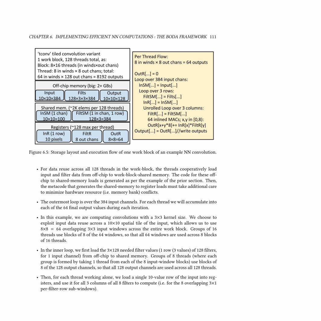
CHAPTER 6. IMPLEMENTING EFFICIENT NN COMPUTATIONS : THE BODA FRAMEWORK 111
Figure 6.5: Storage layout and execution ow of one work block of an example NN convolution.
• For data reuse across all 128 threads in the work-block, the threads cooperatively load
input and lter data from o-chip to work-block-shared memory. The code for these o-
chip to shared-memory loads is generated as per the example of the prior section. Then,
the metacode that generates the shared-memory to register loads must take additional care
to minimize hardware resource (i.e. memory bank) conicts.
• The outermost loop is over the 384 input channels. For each thread we will accumulate into
each of the 64 nal output values during each iteration.
• In this example, we are computing convolutions with a 3×3 kernel size. We choose to
exploit input data reuse across a 10×10 spatial tile of the input, which allows us to use
8×8 = 64 overlapping 3×3 input windows across the entire work block. Groups of 16
threads use blocks of 8 of the 64 windows, so that all 64 windows are used across 8 blocks
of 16 threads.
• In the inner loop, we rst load the 3×128 needed lter values (1 row (3 values) of 128 lters,
for 1 input channel) from o-chip to shared memory. Groups of 8 threads (where each
group is formed by taking 1 thread from each of the 8 input-window blocks) use blocks of
8 of the 128 output channels, so that all 128 output channels are used across all 128 threads.
• Then, for each thread working alone, we load a single 10-value row of the input into reg-
isters, and use it for all 3 columns of all 8 lters to compute (i.e. for the 8 overlapping 3×1
per-lter-row sub-windows).
CHAPTER 6. IMPLEMENTING EFFICIENT NN COMPUTATIONS : THE BODA FRAMEWORK 112
• For the remainder of the inner loop, we unroll 3 times over the columns of the lters.
• For each unrolling, we load 8 lter values (one per output channel) from shared memory
into registers, and perform 64 inlined multiply accumulates, one per output value. This
step is accumulating the result of an 8×8 outer product into the output registers.
• Finally, we write the 64 outputs directly from registers to o-chip memory.
Note that, to form a complete convolution, this work-block will be tiled out across the full input
and full number of output channels. So, it can eciently handle any convolution where the
number of output channels is near a multiple of 128, and the input can be approximately tiled
into 8×8 regions. However, these values are not xed, and were instead chosen by the metacode
to tile well for some desired full convolution. For some other case where these constants did
not yield a good tiling, a dierent version of convolution with dierent work-block geometry (or
using a dierent variant entirely) would be generated. But, overall, it can be seen that:
• We employ data reuse at the shared-memory and register levels, exploiting the specic data
reuse patterns of convolution.
• We choose computation/thread geometry to match the specic input sizes.
• We unroll loops to exploit data reuse in registers and register tiled computation.
6.3.7.2 Summary of Boda Metaprogramming
In summary, it is not easy to determine what sequences of C-level code will execute well on a
given platform, but our framework aims to make the process easier. Further, metaprogramming
allows the programmer to exploit run-time knowledge to make many values (such as sizes, strides,
loop bounds, and osets) constant, and to reduce the usage of loops and conditionals. Generally,
this allows the platform-specic compiler to generate more ecient binary code. But, perhaps
more importantly, when the compiler fails to automatically generate ecient code, metaprogram-
ming allows for the ability to emit very low-level code, so that the nal instruction sequence can
be carefully guided. This allows the ability to productively experiment with dierent compute
and memory access patterns. This can be done without needing to manually rewrite large sec-
tions of target-specic code. And, lest it be forgotten, the compiler need not be modied for
such experiments either, as long as it allows sucient control over detailed execution. Access to
detailed documentation, compiler source code, disassemblers and/or instruction-level proling
tools for each target platform make this process much more productive. However, it is perhaps
when such aids are not available that Boda’s ability to speed the cycle of experimentation is most
vital.
6.3.8 Variant Selection and AutotuningAs mentioned, NN Convolutions have a wide range of possible input sizes and parameters. It
is dicult to write a single function, even with metaprogramming, that runs well over a broad
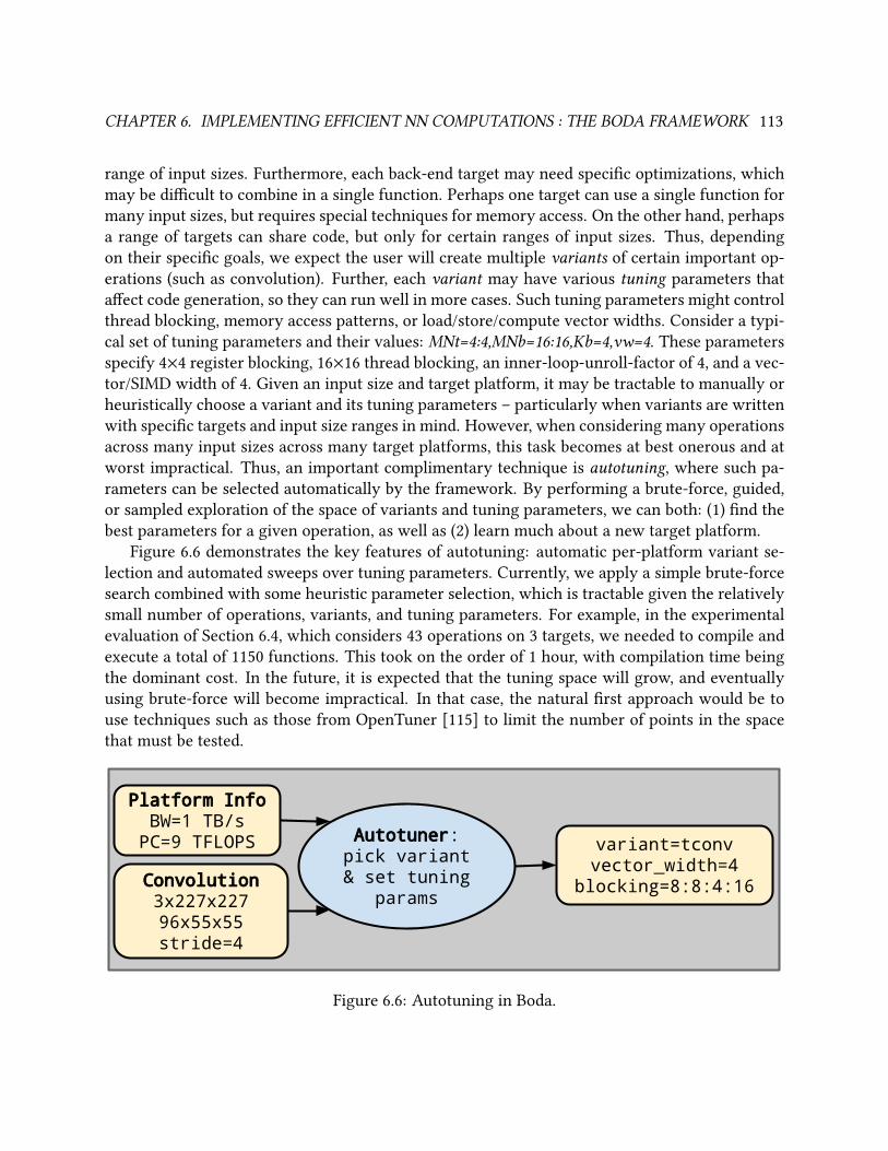
CHAPTER 6. IMPLEMENTING EFFICIENT NN COMPUTATIONS : THE BODA FRAMEWORK 113
range of input sizes. Furthermore, each back-end target may need specic optimizations, which
may be dicult to combine in a single function. Perhaps one target can use a single function for
many input sizes, but requires special techniques for memory access. On the other hand, perhaps
a range of targets can share code, but only for certain ranges of input sizes. Thus, depending
on their specic goals, we expect the user will create multiple variants of certain important op-
erations (such as convolution). Further, each variant may have various tuning parameters that
aect code generation, so they can run well in more cases. Such tuning parameters might control
thread blocking, memory access patterns, or load/store/compute vector widths. Consider a typi-
cal set of tuning parameters and their values: MNt=4:4,MNb=16:16,Kb=4,vw=4. These parameters
specify 4×4 register blocking, 16×16 thread blocking, an inner-loop-unroll-factor of 4, and a vec-
tor/SIMD width of 4. Given an input size and target platform, it may be tractable to manually or
heuristically choose a variant and its tuning parameters – particularly when variants are written
with specic targets and input size ranges in mind. However, when considering many operations
across many input sizes across many target platforms, this task becomes at best onerous and at
worst impractical. Thus, an important complimentary technique is autotuning, where such pa-
rameters can be selected automatically by the framework. By performing a brute-force, guided,
or sampled exploration of the space of variants and tuning parameters, we can both: (1) nd the
best parameters for a given operation, as well as (2) learn much about a new target platform.
Figure 6.6 demonstrates the key features of autotuning: automatic per-platform variant se-
lection and automated sweeps over tuning parameters. Currently, we apply a simple brute-force
search combined with some heuristic parameter selection, which is tractable given the relatively
small number of operations, variants, and tuning parameters. For example, in the experimental
evaluation of Section 6.4, which considers 43 operations on 3 targets, we needed to compile and
execute a total of 1150 functions. This took on the order of 1 hour, with compilation time being
the dominant cost. In the future, it is expected that the tuning space will grow, and eventually
using brute-force will become impractical. In that case, the natural rst approach would be to
use techniques such as those from OpenTuner [115] to limit the number of points in the space
that must be tested.
Convolution3x227x22796x55x55stride=4
Platform InfoBW=1 TB/s
PC=9 TFLOPS Autotuner:pick variant& set tuning
params
variant=tconvvector_width=4
blocking=8:8:4:16
Figure 6.6: Autotuning in Boda.
CHAPTER 6. IMPLEMENTING EFFICIENT NN COMPUTATIONS : THE BODA FRAMEWORK 114
6.3.9 Graph-level OptimizationsNext, we discuss graph-level optimizations: a critical but relatively simple part of our ow. In
particular, there are two important graph-level optimizations for NN compute graphs:
• Fusing of adjacent convolution and activation operations, and
• Inserting any needed data-format-conversion operations.
Convolution operations are commonly followed by the application of some element-wise activa-
tion function (see Section 4.3 for details on common types of activation functions). In some cases,
the overhead to read and re-write the output ND-Array to apply the activation function is signif-
icant. In these cases, one may inline the code for the activation function into the output-writing
portion of the convolution operation to avoid a read-modify-write of the output. While this may
increase the code size of the output-writing part of the convolution operation, it is generally still
favorable to do this, as activation functions such as ReLU add only a few instructions per existing
output store. So, our framework simply always performs this fusion when possible, using string
substitution to insert an application of the activation function for all output-value writes.
The second optimization, insertion of data-format-conversion operations, is necessary due to
the fact that some variants may use dierent layouts or padding of their input or output ND-
Arrays. That is, since we are able to freely choose the format of most internal ND-Arrays, we
can exploit this to achieve higher eciency within each variant. While the user must generally
manually pick data layouts chosen to work well for a given case, the framework’s support for
ND-Array access and metadata handling eases the burden of creating transformation functions
and experimenting with dierent layouts. Also, as long as dierent layouts are distinguished by
dierent ND-Array signatures (dierent dimension cardinality or naming), the framework can
error-check that all ND-Arrays are in the proper format prior to each operation. In many cases,
data-format-conversion operations can be inserted automatically, based on the context in which
an ND-Array is used.
6.3.10 Code Generation, Scheduling, and ExecutionOnce we have generated and compiled callable functions for each needed operation, we exe-
cute the compute graph. For this, we must rst perform operation scheduling and ND-Array
allocation. For compute graphs derived from our current proof-of-concept set of target applica-
tions, scheduling is not dicult. The bulk of execution time is spent on functions that can each
individually saturate the target hardware’s compute capacity by themselves. So, we need not
attempt to run multiple function nodes (from the graph) in parallel; any topological sort of the
compute graph yields a reasonable execution order. Further, for our current use cases, we are
generally not limited by GPU memory. Hence, we can employ a naive allocation strategy and
simply pre-allocate all ND-Arrays in the compute graph. However, with some additional work,
our framework should be easily capable of supporting more complex scheduling and allocation
policies if needed or desired. After allocation and scheduling, we issue the resultant sequence
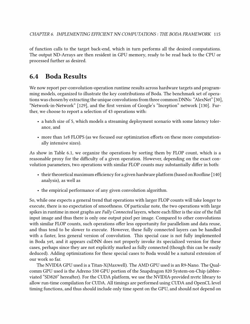
CHAPTER 6. IMPLEMENTING EFFICIENT NN COMPUTATIONS : THE BODA FRAMEWORK 115
of function calls to the target back-end, which in turn performs all the desired computations.
The output ND-Arrays are then resident in GPU memory, ready to be read back to the CPU or
processed further as desired.
6.4 Boda ResultsWe now report per-convolution-operation runtime results across hardware targets and program-
ming models, organized to illustrate the key contributions of Boda. The benchmark set of opera-
tions was chosen by extracting the unique convolutions from three common DNNs: “AlexNet” [30],
“Network-in-Network” [129], and the rst version of Google’s “Inception” network [130]. Fur-
ther, we choose to report a selection of 43 operations with:
• a batch size of 5, which models a streaming deployment scenario with some latency toler-
ance, and
• more than 1e8 FLOPS (as we focused our optimization eorts on these more computation-
ally intensive sizes).
As show in Table 6.1, we organize the operations by sorting them by FLOP count, which is a
reasonable proxy for the diculty of a given operation. However, depending on the exact con-
volution parameters, two operations with similar FLOP counts may substantially dier in both:
• their theoretical maximum eciency for a given hardware platform (based on Rooine [140]
analysis), as well as
• the empirical performance of any given convolution algorithm.
So, while one expects a general trend that operations with larger FLOP counts will take longer to
execute, there is no expectation of smoothness. Of particular note, the two operations with large
spikes in runtime in most graphs are Fully Connected layers, where each lter is the size of the full
input image and thus there is only one output pixel per image. Compared to other convolutions
with similar FLOP counts, such operations oer less opportunity for parallelism and data reuse,
and thus tend to be slower to execute. However, these fully connected layers can be handled
with a faster, less general version of convolution. This special case is not fully implemented
in Boda yet, and it appears cuDNN does not properly invoke its specialized version for these
cases, perhaps since they are not explicitly marked as fully connected (though this can be easily
deduced). Adding optimizations for these special cases to Boda would be a natural extension of
our work so far.
The NVIDIA GPU used is a Titan-X(Maxwell). The AMD GPU used is an R9-Nano. The Qual-
comm GPU used is the Adreno 530 GPU portion of the Snapdragon 820 System-on-Chip (abbre-
viated “SD820” hereafter). For the CUDA platform, we use the NVIDIA-provided nvrtc library to
allow run-time compilation for CUDA. All timings are performed using CUDA and OpenCL level
timing functions, and thus should include only time spent on the GPU, and should not depend on
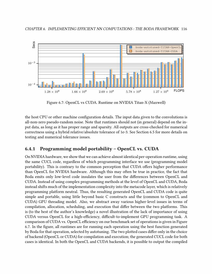
CHAPTER 6. IMPLEMENTING EFFICIENT NN COMPUTATIONS : THE BODA FRAMEWORK 116
1.28× 10⁸ 1.66× 10⁸ 2.69× 10⁸ 5.78× 10⁸ 1.27× 10⁹ FLOPS
10−4
10−3
Sec
s
boda-autotuned-TITAN-OpenCL
boda-autotuned-TITAN-CUDA
Figure 6.7: OpenCL vs CUDA. Runtime on NVIDIA Titan-X (Maxwell)
the host CPU or other machine conguration details. The input data given to the convolutions is
all-non-zero pseudo-random noise. Note that runtimes should not (in general) depend on the in-
put data, as long as it has proper range and sparsity. All outputs are cross-checked for numerical
correctness using a hybrid relative/absolute tolerance of 1e-3. See Section 6.5 for more details on
testing and numerical tolerance issues.
6.4.1 Programming model portability – OpenCL vs. CUDAOn NVIDIA hardware, we show that we can achieve almost identical per-operation runtime, using
the same CUCL code, regardless of which programming interface we use (programming model
portability). This is contrary to the common perception that CUDA oers higher performance
than OpenCL for NVIDIA hardware. Although this may often be true in practice, the fact that
Boda emits only low-level code insulates the user from the dierences between OpenCL and
CUDA. Instead of using complex programming methods at the level of OpenCL and CUDA, Boda
instead shifts much of the implementation complexity into the metacode layer, which is relatively
programming platform neutral. Thus, the resulting generated OpenCL and CUDA code is quite
simple and portable, using little beyond basic C constructs and the (common to OpenCL and
CUDA) GPU threading model. Also, we abstract away various higher-level issues in terms of
compilation, allocation, scheduling, and execution that dier between the two platforms. This
is (to the best of the author’s knowledge) a novel illustration of the lack of importance of using
CUDA versus OpenCL for a high-eciency, dicult-to-implement GPU programming task. A
comparison of CUDA vs. OpenCL eciency on our benchmark set of operations is given in Figure
6.7. In the gure, all runtimes are for running each operation using the best function generated
by Boda for that operation, selected by autotuning. The two plotted cases dier only in the choice
of backend (OpenCL or CUDA) for compilation and execution; the generated CUCL code for both
cases is identical. In both the OpenCL and CUDA backends, it is possible to output the compiled
CHAPTER 6. IMPLEMENTING EFFICIENT NN COMPUTATIONS : THE BODA FRAMEWORK 117
1.28× 10⁸ 1.66× 10⁸ 2.69× 10⁸ 5.78× 10⁸ 1.27× 10⁹ FLOPS
10−4
10−3
Sec
s
boda-autotuned-TITAN
NVIDIA-cuDNNv5-library
Figure 6.8: Comparison of Boda with cuDNNv5 on NVIDIA Titan-X
“binary” code (in this case, NVIDIA PTX portable assembly code). For several cases that were
inspected, the same CUCL source code yields the nearly the same PTX when compiled using
either OpenCL or CUDA. However, there are some minor dierences: the addressing modes and
internal LLVM compiler versions appear to slightly dier between NVIDIA’s internal OpenCL
and CUDA compilation ows. These issues, combined with normal runtime variation/noise, can
easily explain the remaining small dierences in runtime between the OpenCL and CUDA cases.
In order to gauge the overall quality of our results, in Figure 6.8, we compare to the most
highly tuned vendor CNN library that is available: cuDNN version 5. Note that Boda is particu-
larly slower in cases with 3x3 kernel sizes, where cuDNN is using Winograd convolution [116],
which is not yet implemented in Boda. A case study to determine the eort/speed tradeo of
implementing Winograd convolution in Boda is a key topic of future work. However, overall,
we are reasonably competitive, and even faster than the reference library in a few cases. This
is particularly impressive given that private sources indicate cuDNN to be the result of ∼15 sta
years of eort, whereas Boda comes close with only a few months of eort, and is portable to
other platforms as well (note: we perform a detailed productivity analysis later in Section 6.6).
6.4.2 Tuning for QualcommMobile GPUsIn Figure 6.9, the boda-initial values show the initial (poor) performance when running the
general-case fallback convolution variant on the SD820 platform. When starting work on this
platform, the general-case fallback variant was the only variant that could be run, since bugs
in the Qualcomm OpenCL implementation and portability issues (primarily related to usage of
shared memory and high register usage) prevented any of the existing optimized-for-NVIDIA
variants from running at all. The few missing bars in the boda-initial series denote cases where
even the simple fallback variant failed to compile or run. However, with a few weeks of eort, we
were able to create a new convolution variant that both worked around bugs in the Qualcomm
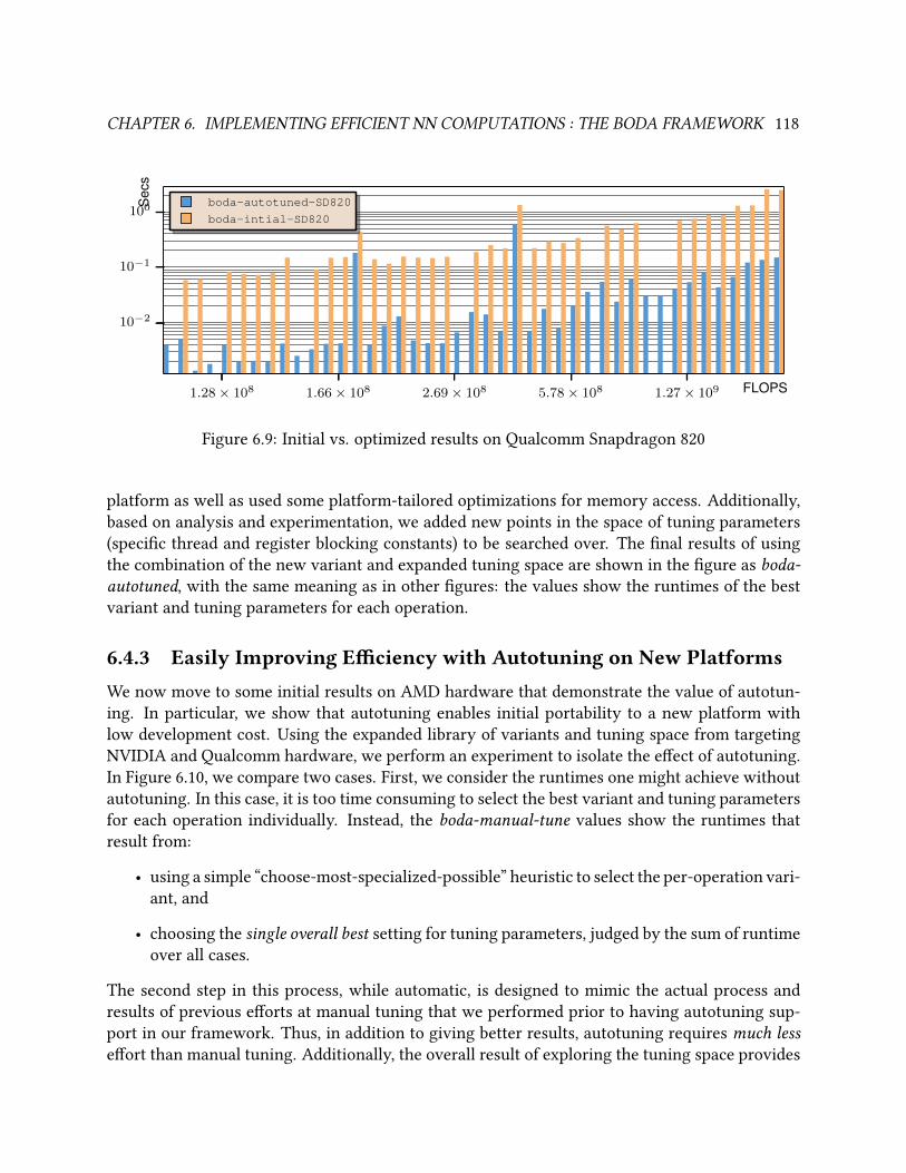
CHAPTER 6. IMPLEMENTING EFFICIENT NN COMPUTATIONS : THE BODA FRAMEWORK 118
1.28× 10⁸ 1.66× 10⁸ 2.69× 10⁸ 5.78× 10⁸ 1.27× 10⁹ FLOPS
10−2
10−1
100Sec
s
boda-autotuned-SD820
boda-intial-SD820
Figure 6.9: Initial vs. optimized results on Qualcomm Snapdragon 820
platform as well as used some platform-tailored optimizations for memory access. Additionally,
based on analysis and experimentation, we added new points in the space of tuning parameters
(specic thread and register blocking constants) to be searched over. The nal results of using
the combination of the new variant and expanded tuning space are shown in the gure as boda-autotuned, with the same meaning as in other gures: the values show the runtimes of the best
variant and tuning parameters for each operation.
6.4.3 Easily Improving Eciency with Autotuning on New PlatformsWe now move to some initial results on AMD hardware that demonstrate the value of autotun-
ing. In particular, we show that autotuning enables initial portability to a new platform with
low development cost. Using the expanded library of variants and tuning space from targeting
NVIDIA and Qualcomm hardware, we perform an experiment to isolate the eect of autotuning.
In Figure 6.10, we compare two cases. First, we consider the runtimes one might achieve without
autotuning. In this case, it is too time consuming to select the best variant and tuning parameters
for each operation individually. Instead, the boda-manual-tune values show the runtimes that
result from:
• using a simple “choose-most-specialized-possible” heuristic to select the per-operation vari-
ant, and
• choosing the single overall best setting for tuning parameters, judged by the sum of runtime
over all cases.
The second step in this process, while automatic, is designed to mimic the actual process and
results of previous eorts at manual tuning that we performed prior to having autotuning sup-
port in our framework. Thus, in addition to giving better results, autotuning requires much lesseort than manual tuning. Additionally, the overall result of exploring the tuning space provides
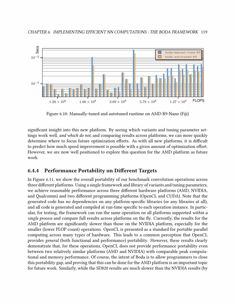
CHAPTER 6. IMPLEMENTING EFFICIENT NN COMPUTATIONS : THE BODA FRAMEWORK 119
1.28× 10⁸ 1.66× 10⁸ 2.69× 10⁸ 5.78× 10⁸ 1.27× 10⁹ FLOPS
10−3
10−2
Sec
s
boda-manual-tune-R9
boda-autotuned-R9
Figure 6.10: Manually-tuned and autotuned runtime on AMD R9-Nano (Fiji)
signicant insight into this new platform. By seeing which variants and tuning parameter set-
tings work well, and which do not, and comparing results across platforms, we can more quickly
determine where to focus future optimization eorts. As with all new platforms, it is dicult
to predict how much speed improvement is possible with a given amount of optimization eort.
However, we are now well positioned to explore this question for the AMD platform as future
work.
6.4.4 Performance Portability on Dierent TargetsIn Figure 6.11, we show the overall portability of our benchmark convolution operations across
three dierent platforms. Using a single framework and library of variants and tuning parameters,
we achieve reasonable performance across three dierent hardware platforms (AMD, NVIDIA,
and Qualcomm) and two dierent programming platforms (OpenCL and CUDA). Note that the
generated code has no dependencies on any platform-specic libraries (or any libraries at all),
and all code is generated and compiled at run-time specic to each operation instance. In partic-
ular, for testing, the framework can run the same operation on all platforms supported within asingle process and compare full results across platforms on the y. Currently, the results for the
AMD platform are signicantly slower than those on the NVIDIA platform, especially for the
smaller (lower FLOP count) operations. OpenCL is presented as a standard for portable parallel
computing across many types of hardware. This leads to a common perception that OpenCL
provides general (both functional and performance) portability. However, these results clearly
demonstrate that, for these operations, OpenCL does not provide performance portability even
between two relatively similar platforms (AMD and NVIDIA) with comparable peak computa-
tional and memory performance. Of course, the intent of Boda is to allow programmers to close
this portability gap, and proving that this can be done for the AMD platform is an important topic
for future work. Similarly, while the SD820 results are much slower than the NVIDIA results (by
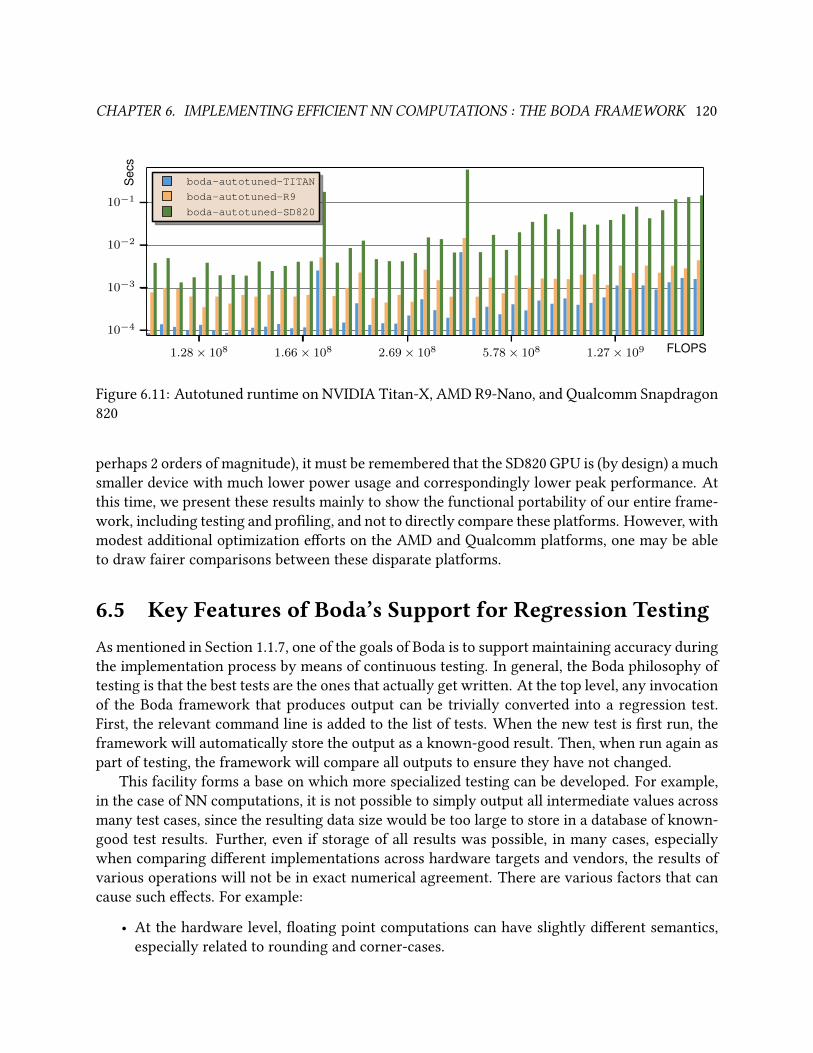
CHAPTER 6. IMPLEMENTING EFFICIENT NN COMPUTATIONS : THE BODA FRAMEWORK 120
1.28× 10⁸ 1.66× 10⁸ 2.69× 10⁸ 5.78× 10⁸ 1.27× 10⁹ FLOPS10−4
10−3
10−2
10−1
Sec
s
boda-autotuned-TITAN
boda-autotuned-R9
boda-autotuned-SD820
Figure 6.11: Autotuned runtime on NVIDIA Titan-X, AMD R9-Nano, and Qualcomm Snapdragon
820
perhaps 2 orders of magnitude), it must be remembered that the SD820 GPU is (by design) a much
smaller device with much lower power usage and correspondingly lower peak performance. At
this time, we present these results mainly to show the functional portability of our entire frame-
work, including testing and proling, and not to directly compare these platforms. However, with
modest additional optimization eorts on the AMD and Qualcomm platforms, one may be able
to draw fairer comparisons between these disparate platforms.
6.5 Key Features of Boda’s Support for Regression TestingAs mentioned in Section 1.1.7, one of the goals of Boda is to support maintaining accuracy during
the implementation process by means of continuous testing. In general, the Boda philosophy of
testing is that the best tests are the ones that actually get written. At the top level, any invocation
of the Boda framework that produces output can be trivially converted into a regression test.
First, the relevant command line is added to the list of tests. When the new test is rst run, the
framework will automatically store the output as a known-good result. Then, when run again as
part of testing, the framework will compare all outputs to ensure they have not changed.
This facility forms a base on which more specialized testing can be developed. For example,
in the case of NN computations, it is not possible to simply output all intermediate values across
many test cases, since the resulting data size would be too large to store in a database of known-
good test results. Further, even if storage of all results was possible, in many cases, especially
when comparing dierent implementations across hardware targets and vendors, the results of
various operations will not be in exact numerical agreement. There are various factors that can
cause such eects. For example:
• At the hardware level, oating point computations can have slightly dierent semantics,
especially related to rounding and corner-cases.
CHAPTER 6. IMPLEMENTING EFFICIENT NN COMPUTATIONS : THE BODA FRAMEWORK 121
• Sometimes, dierent high-level algorithms can be used to compute the same operation.
Again, due to the nature of oating-point calculations, one would not expect the results of
such dierent approaches to agree exactly.
• Even when nominally the same algorithm is used, dierences in operation ordering and
compiler optimizations can cause dierences in numerical results.
• Further, some algorithms may oer internal speed/precision tradeos. Diering choices
for these tradeos will of course yield dierent results.
6.5.1 Approximate Numerical Agreement for NN CalculationsFor the problem of dealing with approximate numerical comparison, Boda utilizes a hybrid abso-
lute/relative error metric, derived from the nature of NN calculations. For the results of a given
intermediate layer, values tend to span a limited range which includes zero. However, it is typi-
cally numbers with higher absolute values that are most semantically important. Thus, neither a
xed absolute error tolerance nor a relative tolerance works well in practice. For large values, a
relative error tolerance of between 0.001 and 0.00001 is generally appropriate. But, for small val-
ues near zero, much larger relative dierences are acceptable. In particular, for a NN layer with
outputs ranging from 0 to ∼1000, some values might be zero in the output of one implementation,
but have a small non-zero value in another, yielding a large relative dierence. Conveniently, it is
generally the case that NN calculations do not rely on precision for values with very small mag-
nitudes (i.e. large negative exponents). So, when comparing each value between known-good
and under-test implementations, we calculate a relative dierence, but clamp it to the maximum
absolute value of the two values being compared. Thus, as the values to compare become smaller
than the specied relative error tolerance, the tolerance becomes absolute instead of relative. See
the function min_sig_mag_rel_diff() in boda_base.cc for the exact implementa-
tion [138].
6.5.2 Using ND-Array Digests to Compactly Store Known-Good TestResults
For the problem of results being too large to store, Boda provides two solutions:
• When possible, Boda will run the reference and under-test implementations at the same
time, so that comparison between all known-good and under-test results can be performed
online.
• In addition, Boda will create digests of known-good ND-Arrays, where a sampling approach
is used to reduce the amount of data needed to later check approximate equivalence with
under-test ND-Arrays.
The digests consist of a moderately large set of variable length periodic-sampled checksums.
This approach allows both detecting changes anywhere in the results (like a hash), but also allows
CHAPTER 6. IMPLEMENTING EFFICIENT NN COMPUTATIONS : THE BODA FRAMEWORK 122
for approximate numerical comparison (like a simple checksum). For more details, see the class
nda_digest_T in boda_base.cc [138].
6.6 Boda Enables Productive Development of NNOperations
In the best case, measuring developer productivity is a dicult task [141]. For the case of im-
plementing ecient NN computations on GPUs, the problem is magnied. Globally, there are
only a few historical instances of such implementations [33] [41], and, as both were commercial
endeavors, details on their development processes are lacking. Similarly, it appears that very few
programmers are capable of addressing this type of problem, and it is hard to generalize about
programmer skills and preferences from such a small set. Still, from the release history of cuDNN
and Neon, we can at least infer that development took years in both cases. In Section 1.1.7, we
asked if it was possible to improve on this situation, and reduce development time from years to
months. When analyzing the development of Boda, we must decouple eort spent on the frame-
work itself from that spent actually implementing NN operations. However, these two activities
are, by design, closely coupled in Boda, and it is thus dicult (and perhaps not meaningful) to
make a hard distinction. Instead, work on Boda consists of a spectrum of development activities,
ranging from general framework support (which should be amortized fully over all operations
and targets) to specic optimizations for a given hardware/operation pair (for which all costs are
fully attributable to that specic operation and target). Here, we list the broad classes of Boda
development activity, ordered from general framework support to operation/target specic opti-
mizations. Near the center of the list, we draw a rough boundary between activities that are more
focused on general framework features versus those that are more focused on operation/target
specic optimizations:
• Boda’s support for ND-Arrays and compute graph handling is general, albeit with special
support for NNs. So, it should be useful for implementations of a wide range of operations
over ND-Arrays. Hence, eort related to these parts of the framework can (in theory) be
amortized over many targets and operations.
• Similarly, Boda’s support for autotuning is general, and can be amortized across all hard-
ware targets and operations.
• Boda’s support for testing has both general components as well as those that are more
operation specic. Thus, such eorts should be amortized across all hardware targets, but
only partially amortized across operations.
• Boda’s backends for OpenCL and CUDA are generally useful for running any compute
graph of functions over ND-Arrays on the respective programming platforms (assuming a
GPU-like target). Basic support for CPUs in the OpenCL backend would not be dicult to
add, but would not be useful without a full ow to generate ecient CPU code. Still, eorts
CHAPTER 6. IMPLEMENTING EFFICIENT NN COMPUTATIONS : THE BODA FRAMEWORK 123
for this portion of Boda are amortized across all OpenCL and CUDA targets and across all
operations.
– General/Specic Development Activity Boundary –
• Boda’s code generation and metaprogramming support is specialized both for GPUs as tar-
gets and for NN operations as the functions to compute. In general, adding new operations,
or new variants of existing operations, requires some eort at this level, but it is still par-
tially amortized across dierent operations.
• Boda requires some eort at the framework level to add new operations. But, this eort
is low when the new operations have similar interfaces to existing ones. And, the needed
eort is amortized across all variants of each operation, which includes any hardware-
target-specic variants.
• Each new operation requires a general-case reference/fallback implementation. Generally,
this can be shared across all hardware targets.
• If needed to meet eciency goals, each operation may require some amount of tuning
and optimization. This may require writing per-hardware-target variants, and/or variants
specialized for particular types of inputs. Eort for this category of development should be
fully attributed to the specic use-case that is being optimized.
When comparing against the development of cuDNN and Neon, the time spent in the last
category listed above gives the best case bound on the productivity improvement of using Boda.
In addition to a best case estimate, we also consider a reasonable worst case estimate that includes
all activities below the general/specic boundary line. This includes most of the development
eort that is at all related to the entire code generation ow, much of which can in theory be
reused across many platforms and operations. But, for now, it has only been used for our proof-
of-concept set of NN computations across three targets (NVIDIA, Qualcomm, and AMD). So, we
recognize that the degree of generality of these parts of Boda remains to be demonstrated.
In order to perform our analysis, we examine the entire development history of Boda on a
commit-by-commit basis, as provided by the version control system used for development (git).
Also, it should be noted that the primary developer for Boda was only working part-time on
development during this period, due to work, family, and academic commitments (Note: the
developer recommends avoiding such multitasking if possible). From the commit log, we derive
a summary timeline of development related to the implementation of NN operations in Boda
across the NVIDIA and Qualcomm platforms:
• 2015-05: Development using runtime compilation for NVIDIA begins with running a dot-
product example using the vendor-provided nvrtc (NVIDIA Run Time Compilation) library.
• 2015-06: A reference, general-case version of convolution targeting NVIDIA hardware is
developed, along with various related additions to the framework to support it.
CHAPTER 6. IMPLEMENTING EFFICIENT NN COMPUTATIONS : THE BODA FRAMEWORK 124
• 2015-07 though 2015-08: The two main optimized convolution variants (k1conv and tconv)
are developed, which improve speed by more than 2X over the Boda reference convolution
on our benchmark set (see Table 6.1), yielding our current best speed results on NVIDIA
hardware (see Figure 6.8).
• 2016-05: The entire development of Qualcomm-specic (conv-simd and tconv-simd) con-
volution variants occurred during this month, yielding our current best results for the Qual-
comm platform, which are roughly 10X better (see Figure 6.9) than the initial results we
achieved on that platform.
Considering the above timeline, it can be seen that it took 4 real-time months of part-time
eort to achieve our current results on the NVIDIA platform. However, the rst two months of
this period involved setting up our general run-time compilation ow for the NVIDIA platform,
as well as implementing a reference version of convolution. Note that, although the developer is
an experienced algorithmic and performance programmer, this was their rst attempt at both dy-
namic compilation and high-eciency numerical GPU programming. So, there was a signicant
learning curve to be climbed in the those rst few months. The second two months, however,
felt qualitatively quite productive. During this period, we developed, optimized, and tuned two
special-case variants of convolution for the NVIDIA platform. So, one can legitimately say that
only it took two months of part-time eort to move from a reference GPU convolution imple-
mentation to our current best (within 2X of the vendor library) results.
Finally, for our eorts on the Qualcomm platform, there were some signicant initial costs
associated with targeting an Android-OS based platform, as well as dealing with the quirks of
the Qualcomm OpenCL implementation. After this platform bootstrapping was complete, we
began our eort to improve eciency. Initially, it took some time and research to isolate the key
needed optimization for the Qualcomm platform: manual SIMD memory access. Still, including
this research, it only took a month of part-time eort to develop our nal optimized variants for
the Qualcomm platform.
In summary, Boda enabled the rapid development of reasonably eciency implementations
of NN convolutions for two GPU platforms in just a few months.
6.7 Summary of Boda’s ContributionsBy 2006, it was clear that parallel computing would be a critical challenge going forward [109].
More than ten years later, productive, ecient parallel programming still remains a challenging
task with no general solution, especially for GPUs [24]. Combined with the promise of modern,
compute-intensive machine learning [14], this makes enabling the productive creation of e-
cient, portable, accurate implementations of machine learning computations an important sub-
ject for research. While only a single facet of this broad issue, the implementation of just neural
network operations on GPUs is still a worthy challenge by itself, and has tractable scope for a
single research project. In this chapter, we have presented our answer to this challenge: the Boda
framework for productive implementation of ecient neural network computations.
CHAPTER 6. IMPLEMENTING EFFICIENT NN COMPUTATIONS : THE BODA FRAMEWORK 125
Taking a vertical approach spanning from high-level application to low-level programming,
we have presented several contributions:
• The Boda framework itself, which provides a novel unied methodology, based on metapro-
gramming and autotuning, for productive development of portable, ecient implementa-
tions of a broad class of numerical functions targeting GPUs or similar platforms.
• Metaprogramming with named ND-Arrays dimensions for improved productivity and type
checking.
• A proof-of-concept use of the framework to implement the core set of operations needed
for deploying three common image-processing neural networks (AlexNet, Network-in-
Network, and Inception-V1) across three dierent GPU targets.
• An experimental evaluation of the resulting implementation, including a comparison to a
highly-tuned vendor library.
Additionally, Boda provides a platform for future research, further experiments, and benchmark-
ing related to GPU portability and metaprogramming.
Our experimental results show that Boda eases the path to portable, ecient implementations.
In particular, we have shown how Boda’s metaprogramming and autotuning support enables pro-
gramming model and performance portability. On NVIDIA hardware, we achieve performance
competitive with the vendor library using either OpenCL or CUDA, demonstrating programming
model portability. On Qualcomm hardware, we show that we can quickly develop new variants
and otherwise tune our generated code to achieve reasonable performance on a mobile GPU. On
AMD hardware, we show that autotuning and proling pre-existing code on a new platform pro-
vides a good foundation for future platform-specic optimization eorts. Further, as an open,
vendor-neutral framework, we avoid dependencies on any specic hardware platforms or unex-
tensible vendor libraries. Thus, our framework provides a productive method for implementing
existing and new NN operations while targeting various hardware platforms. As a nal note,
the entire framework, including support for automated replication of all results presented here,
and the entire development history, is made available online as open source with a permissive
license [142].
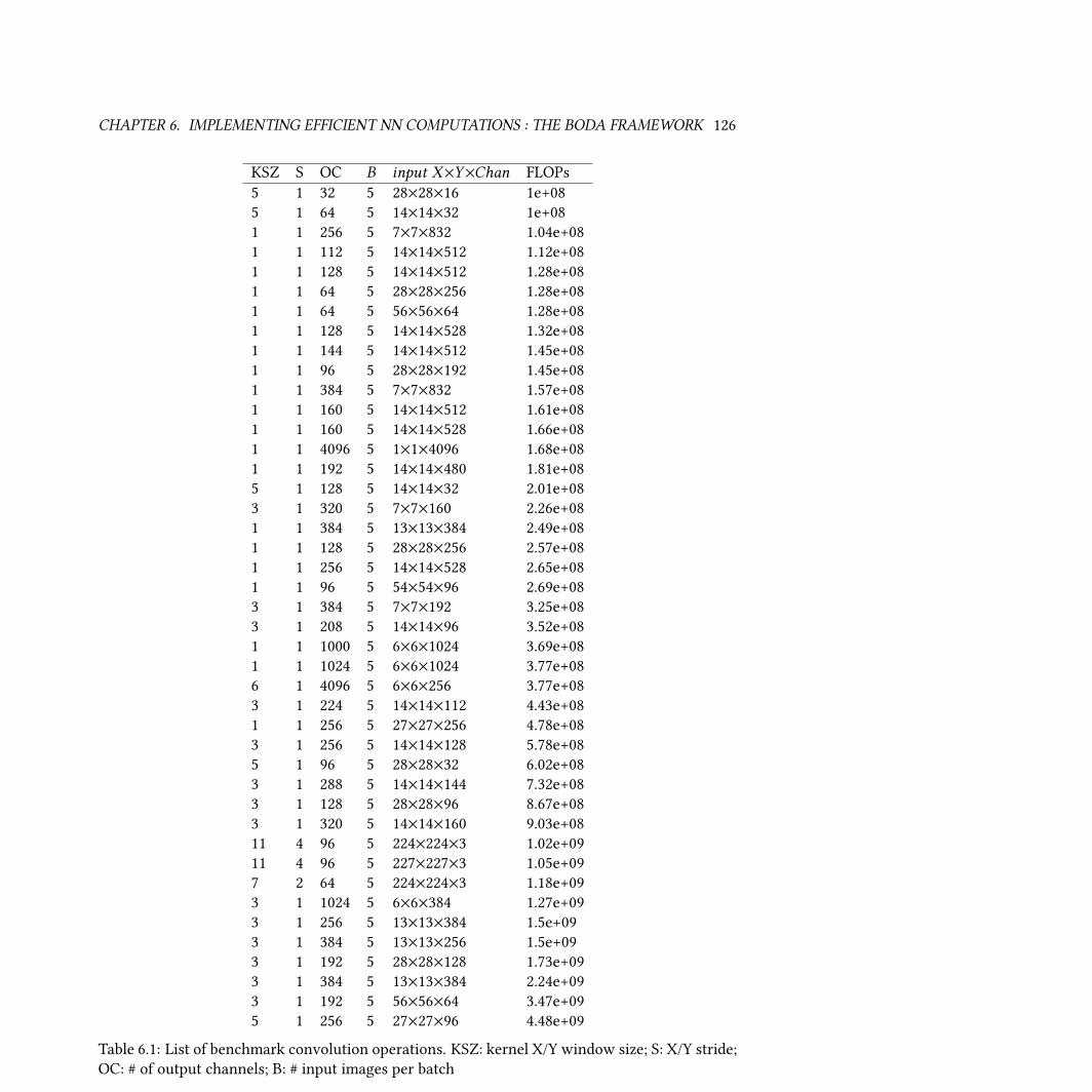
CHAPTER 6. IMPLEMENTING EFFICIENT NN COMPUTATIONS : THE BODA FRAMEWORK 126
KSZ S OC B input X×Y×Chan FLOPs
5 1 32 5 28×28×16 1e+08
5 1 64 5 14×14×32 1e+08
1 1 256 5 7×7×832 1.04e+08
1 1 112 5 14×14×512 1.12e+08
1 1 128 5 14×14×512 1.28e+08
1 1 64 5 28×28×256 1.28e+08
1 1 64 5 56×56×64 1.28e+08
1 1 128 5 14×14×528 1.32e+08
1 1 144 5 14×14×512 1.45e+08
1 1 96 5 28×28×192 1.45e+08
1 1 384 5 7×7×832 1.57e+08
1 1 160 5 14×14×512 1.61e+08
1 1 160 5 14×14×528 1.66e+08
1 1 4096 5 1×1×4096 1.68e+08
1 1 192 5 14×14×480 1.81e+08
5 1 128 5 14×14×32 2.01e+08
3 1 320 5 7×7×160 2.26e+08
1 1 384 5 13×13×384 2.49e+08
1 1 128 5 28×28×256 2.57e+08
1 1 256 5 14×14×528 2.65e+08
1 1 96 5 54×54×96 2.69e+08
3 1 384 5 7×7×192 3.25e+08
3 1 208 5 14×14×96 3.52e+08
1 1 1000 5 6×6×1024 3.69e+08
1 1 1024 5 6×6×1024 3.77e+08
6 1 4096 5 6×6×256 3.77e+08
3 1 224 5 14×14×112 4.43e+08
1 1 256 5 27×27×256 4.78e+08
3 1 256 5 14×14×128 5.78e+08
5 1 96 5 28×28×32 6.02e+08
3 1 288 5 14×14×144 7.32e+08
3 1 128 5 28×28×96 8.67e+08
3 1 320 5 14×14×160 9.03e+08
11 4 96 5 224×224×3 1.02e+09
11 4 96 5 227×227×3 1.05e+09
7 2 64 5 224×224×3 1.18e+09
3 1 1024 5 6×6×384 1.27e+09
3 1 256 5 13×13×384 1.5e+09
3 1 384 5 13×13×256 1.5e+09
3 1 192 5 28×28×128 1.73e+09
3 1 384 5 13×13×384 2.24e+09
3 1 192 5 56×56×64 3.47e+09
5 1 256 5 27×27×96 4.48e+09
Table 6.1: List of benchmark convolution operations. KSZ: kernel X/Y window size; S: X/Y stride;
OC: # of output channels; B: # input images per batch
127
Chapter 7
Summary, Conclusions, and Future Work
With recent advances in machine-learning, it appears that an era of pervasive machine-learning
in all aspects of life is imminent or, possibly, has already arrived, quietly working behind the
scenes in datacenters [143]. Implementing the ecient parallel computations upon which ma-
chine learning relies, however, is still an endeavor that needs signicant manual human eort.
And, although existing libraries eciently support some operations on some hardware, there will
always be new algorithms and hardware platforms to consider. So, in this work, we strive to am-
plify the eort of the few humans willing and able to work on such problems. In this chapter, we
will summarize all the contributions we have made in this work and consider the natural next
steps for future work.
7.1 ContributionsThis dissertation has several categories of contributions:
• Contributions related to libHOG and DenseNet, early work that motivated the Boda frame-
work,
• Contributions directly embodied in the Boda framework,
• Contributions related to performance experiments performed with the Boda framework.
• Contributions related to an analysis of developer productivity when using the Boda frame-
work.
First, we consider contributions are related to our early work that motivated and guided the
early design of the framework:
• Our rst project was libHOG [44]. Here, we sped up a key machine learning computation,
HOG feature pyramid calculation, on CPUs by 3X over the state of the art. To achieve this,
CHAPTER 7. SUMMARY, CONCLUSIONS, AND FUTURE WORK 128
we implemented a reasonably well engineered pipeline using reduced precision, SIMD par-
allelism, algorithmic changes, and outer-loop parallelism. However, we encountered var-
ious challenges associated with the development and deployment of libHOG. These pro-
vided inspiration for our later work and dened our research trajectory.
• Following the same theme, our next project was DenseNet [45]. There, we achieved a
10X speedup for the calculation of dense convolutional neural network feature pyramids.
This enabled multiscale sliding window object detection ows (over DenseNet features)
that were previously too slow to consider. Again, the implementation and deployment
challenges of this work shaped our research trajectory and motivated our future work.
In particular, after the initial implementation of DenseNet, we then reimplemented it as
DenseNet-v2, a prototype of what would become our Boda framework.
Then, moving to our nal project, we consider our contributions related to Boda framework
itself, the experiments we performed with it, and our productivity analysis of its development:
• In Boda, we have produced a framework that supports the development of ecient GPU
implementations of numeric operations on GPUs.
• As our proof-of-concept for Boda, we have presented the specic techniques we used to
achieve our best speed results for NN convolutions on NVIDIA and Qualcomm GPUs. We
achieved speed within 2X of the highly-tuned vendor library on NVIDIA GPUs, and did
so with only a few months of part-time eort. With a few additional weeks of eort, we
achieved up to 30% eciency on Qualcomm mobile GPUs, where vendor libraries for NN
computation remain unreleased [46].
• Further, we showed that the addition of an autotuning method into the framework im-
proved portability and development productivity. Using it, we showed initial results that
indicate our framework can yield reasonable performance on a new platform, AMD GPUs,
with minimal eort [47].
Finally, although it does not map one-to-one with to specic research contributions, another
way to organize our eorts is using our list of concerns. Organized by concern, our contributions
are:
• Speed contribution: In libHOG and DenseNet, we directly speed-up particular use-cases.
In Boda, our goal is to generally enable creating high eciency implementations across
dierent hardware targets and use cases, and we show a proof-of-concept of this approach
for implementing NN operations on GPUs.
• Accuracy contribution: In general, our focus for this concern is on maintaining accuracy
versus reference implementations. In both the second iteration of DenseNet and in Boda,
we provide advanced testing support, including numerical accuracy checking using both
golden results (ND-Array digests) and live full-ow per-ND-Array comparisons.
CHAPTER 7. SUMMARY, CONCLUSIONS, AND FUTURE WORK 129
• Energy contribution: As discussed in 1.1.4, for our targets (CPU and GPU), more speed
conveniently means less energy usage. So, our contributions in libHOG, DenseNet, and
Boda related to speed also yield improvements in energy usage.
• Portability contribution: As a key focus of Boda, we provide the CUCL language to al-
low programming model portability between OpenCL and CUDA, as well as leveraging
metaprogramming to deal with target-specic issues to enable performance portability.
• Cost contribution: As discussed in 1.1.5, more portability and more speed yield lower costs
for development and deployment.
7.2 Conclusions: Answering Key Research QuestionsLet us return to the key research questions we asked in Section 1.1.7. Now, at the conclusion of
our eorts, we can answer them:
• Is possible to reduce the time taken to implement ecient neural net computations on new
GPU platforms from years to months?
Yes. In Boda, we showed that, without reliance on any existing libraries, we can implement
ecient NN computations on several platforms. As discussed in Section 6.6, we needed only ∼2
months of eort to tune our NN convolutions for NVIDIA hardware. Then, we needed only ∼1
additional month to tune for Qualcomm GPUs.
• If so, for platforms where they apply, can we improve on the eciency of existing portable
(numerical library-based) approaches by at least 2X? That is, can we achieve ∼50% e-
ciency, which is generally about the best that can be expected for GPU code, short of using
assembly language?
Yes. For the NVIDIA platform, for our benchmark cases, we achieved roughly 50% peak eciency,
or 2X that which is achievable using BLAS libraries. Further, this is within a factor of 2 of the
performance of the vendor library cuDNN (which achieves near 100% eciency).
• Then, for platforms with no libraries to build upon or compare with, can we achieve at least
25% eciency? This represents the low end of the expected eciency of optimized GPU
code, but is at least 5X better than what would be expected from naive code.
Yes. For the Qualcomm SD820 platform, we achieve ∼%30 eciency. Since the SD820 lacks both
GPU NN computation and GPU BLAS libraries, comparison is dicult, and the maximum achiev-
able eciency is an open question. But, our results represent a solid lower-bound for what can
be achieved, and thus are a good benchmark for future eorts to compare against.
CHAPTER 7. SUMMARY, CONCLUSIONS, AND FUTURE WORK 130
• In order to maintain accuracy during implementation and optimization, can we fully auto-
mate continuous numerical regression testing of NN computations for full ows with full
inputs?
Partially. As discussed in Section 6.5, we enabled two methods: approximate testing using ND-
Array digests, and full live testing that requires being able to run reference and under-test calcu-
lations simultaneously. Neither option is perfect, but both represent a signicant improvement
on existing practice.
7.3 Future Work
7.3.1 Boda for Other OperationsWhile our current focus is on neural network operations, any numerical operations that operate
over ND-Arrays should be reasonably well supported by our approach. Thus, exploring the space
of such operations is a good subject for future work. In particular, signal processing, nancial
calculations, and scientic computation are all interesting areas where some applications use
GPUs to process data that is well represented using ND-Arrays [144].
7.3.2 Boda on Other HardwareWhile we have focused on GPUs, Boda’s vertical nature and unrestricted support for metapro-
gramming allow for extension to other parallel hardware targets. Natural candidates include
FPGAs, CPUs, hardware description languages, and DSPs. However, the tradeo for Boda’s ex-
ibility is that such extensions will require eort that is the sum of two parts:
• an amount proportional to how dierent each new platform is from the existing supported
ones (i.e. currently just GPUs), and
• an amount proportional to how many operations require signicant tuning for the new
platform.
Without actually performing such extensions, it is dicult to speculate on exactly how high these
costs might be for any particular set of operations on a new hardware target. However, many of
Boda’s features are clearly independent of both the operations to compute and hardware target,
such as:
• testing (to maintain accuracy),
• metaprogramming using ND-Arrays with named dimensions,
• compute graph creation and execution.
CHAPTER 7. SUMMARY, CONCLUSIONS, AND FUTURE WORK 131
So, even if much of the metacode and CUCL for particular operations must be rewritten for a new
hardware target, the basic scaolding provided by Boda provides a good starting point.
Also, we only had time to perform initial experiments on the AMD platform. It would be
natural to try to improve our results on this platform, and see what gains could be made with a
few months of eort. In particular, a key question is: can we achieve 50% eciency, as we did on
the NVIDIA platform?
7.3.3 Broader Scope of NN ComputationsWe believe the set of NN operations that we implemented is sucient to prove the concept of
Boda. However, the space of NN operations is very broad, and true practical deployment of Boda
would certainly require implementing more operations, or at least tuning for additional points in
the space of all possible convolutions. In particular, it would be sensible to examine the broader
space of NNs outside of CNNs, such as recurrent NNs and others (see Part 2 of Deep Learning for
a comprehensive list [14]).
7.4 Final ThoughtsWe believe that eciently implementing computations on parallel hardware will remain an im-
portant problem with no general solution for the foreseeable future. So, it is vital to research
tools and methods to continue to improve the ability for programmers to productively tackle
this issue. With each new application domain and each new generation of hardware, require-
ments shift, and new implementation challenges arise. In this work, we focused on the specic
challenges associated with performing neural network computations on modern GPU hardware.
In each of the three projects that constitute this dissertation (libHOG, DenseNet, and Boda),
we optimized an important machine learning operation. In Boda, we present a general framework
that embodies our vision for how to productively implement ecient computations for GPUs, and
we provided a proof-of-concept by implementing key NN operations on NVIDIA, Qualcomm, and
AMD GPUs. We look forward to extensions of Boda to other operations and hardware targets
in order to further demonstrate the value of our approach. Further, as Boda matures, we see it
moving from a research project to a legitimate alternative to vendor-supplied libraries for NN
computation in real-world practical deployments across a variety of hardware platforms.
132
Bibliography
[1] J. Schmidhuber, “Deep learning in neural networks: an overview”, Neural networks, vol.
61, pp. 85–117, 2015.
[2] D. Amodei, R. Anubhai, E. Battenberg, C. Case, J. Casper, B. Catanzaro, J. Chen, M. Chrzanowski,
A. Coates, G. Diamos, et al., “Deep speech 2: end-to-end speech recognition in english and
mandarin”, arXiv:1512.02595, 2015.
[3] D. Silver, A. Huang, C. J. Maddison, A. Guez, L. Sifre, G. Van Den Driessche, J. Schrit-
twieser, I. Antonoglou, V. Panneershelvam, M. Lanctot, et al., “Mastering the game of go
with deep neural networks and tree search”, Nature, vol. 529, no. 7587, pp. 484–489, 2016.
[4] A. Sharif Razavian, H. Azizpour, J. Sullivan, and S. Carlsson, “Cnn features o-the-shelf:
an astounding baseline for recognition”, in Proceedings of the IEEE Conference on ComputerVision and Pattern Recognition Workshops, 2014, pp. 806–813.
[5] R. Girshick, F. Iandola, T. Darrell, and J. Malik, “Deformable part models are convolutional
neural networks”, in Proceedings of the IEEE Conference on Computer Vision and PatternRecognition, 2015, pp. 437–446.
[6] A. Karpathy, G. Toderici, S. Shetty, T. Leung, R. Sukthankar, and L. Fei-Fei, “Large-scale
video classication with convolutional neural networks”, in Proceedings of the IEEE con-ference on Computer Vision and Pattern Recognition, 2014, pp. 1725–1732.
[7] S. Ji, W. Xu, M. Yang, and K. Yu, “3d convolutional neural networks for human action
recognition”, IEEE transactions on pattern analysis and machine intelligence, vol. 35, no. 1,
pp. 221–231, 2013.
[8] K.-S. Oh and K. Jung, “Gpu implementation of neural networks”, Pattern Recognition, vol.
37, no. 6, pp. 1311–1314, 2004.
[9] A. Esteva, B. Kuprel, R. A. Novoa, J. Ko, S. M. Swetter, H. M. Blau, and S. Thrun, “Dermatologist-
level classication of skin cancer with deep neural networks”, Nature, vol. 542, no. 7639,
pp. 115–118, 2017.
[10] G. E. Dahl, N. Jaitly, and R. Salakhutdinov, “Multi-task neural networks for qsar predic-
tions”, arXiv preprint arXiv:1406.1231, 2014.
[11] J. Chung, K. Cho, and Y. Bengio, “A character-level decoder without explicit segmentation
for neural machine translation”, arXiv preprint arXiv:1603.06147, 2016.
BIBLIOGRAPHY 133
[12] L. A. Gatys, A. S. Ecker, and M. Bethge, “A neural algorithm of artistic style”, arXiv preprintarXiv:1508.06576, 2015.
[13] C. Chen, A. Se, A. Kornhauser, and J. Xiao, “Deepdriving: learning aordance for direct
perception in autonomous driving”, in Proceedings of the IEEE International Conference onComputer Vision, 2015, pp. 2722–2730.
[14] I. Goodfellow, Y. Bengio, and A. Courville, “Deep learning”, Book in preparation for MIT
Press, 2016, [Online]. Available: http://www.deeplearningbook.org.
[15] D. Goldberg, “What every computer scientist should know about oating-point arith-
metic”, ACM Computing Surveys (CSUR), vol. 23, no. 1, pp. 5–48, 1991.
[16] M Leeser, J Ramachandran, T Wahl, and D Yablonski, “Opencl oating point software on
heterogeneous architectures–portable or not”, in Workshop on Numerical Software Veri-cation (NSV), 2012.
[17] F. Iandola, “Exploring the design space of deep convolutional neural networks at large
scale”, arXiv preprint arXiv:1612.06519, 2016.
[18] D. Geronimo, A. M. Lopez, A. D. Sappa, and T. Graf, “Survey of pedestrian detection for
advanced driver assistance systems”, IEEE transactions on pattern analysis and machineintelligence, vol. 32, no. 7, pp. 1239–1258, 2010.
[19] M. Horowitz and W. Dally, “How scaling will change processor architecture”, in Solid-State Circuits Conference, 2004. Digest of Technical Papers. ISSCC. 2004 IEEE International,IEEE, 2004, pp. 132–133.
[20] D. Ferreira, A. K. Dey, and V. Kostakos, “Understanding human-smartphone concerns: a
study of battery life”, in International Conference on Pervasive Computing, Springer, 2011,
pp. 19–33.
[21] M. Moskewicz, Boda framework core source code, master branch, sgemm benchmarking re-sults, https://github.com/moskewcz/boda/blob/master/src/doc/sgemm-notes.txt, [Online; accessed 04-April-2017], 2017.
[22] NVIDIA, Cublas, https://developer.nvidia.com/cublas, [Online; ac-
cessed 27-May-2016], 2016.
[23] K. Le, O. Bilgir, R. Bianchini, M. Martonosi, and T. D. Nguyen, “Managing the cost, energy
consumption, and carbon footprint of internet services”, ACM SIGMETRICS PerformanceEvaluation Review, vol. 38, no. 1, pp. 357–358, 2010.
[24] D. B. Kirk and W. H. Wen-Mei, Programming massively parallel processors: a hands-onapproach. Morgan Kaufmann, 2016.
[25] T. Dettmers, Which gpu for deep learning, http://timdettmers.com/2017/03/19/which-gpu-for-deep-learning/, [Online; accessed 04-April-2017],
2017.
BIBLIOGRAPHY 134
[26] Wikipedia, List of nvidia graphics processing units — wikipedia, the free encyclopedia, [On-
line; accessed 6-April-2017], 2017. [Online]. Available:\urlhttps://en.wikipedia.org/w/index.php?title=List_of_Nvidia_graphics_processing_units&oldid=773358079.
[27] S. Chintala, Convnet-benchmarks, https://github.com/soumith/convnet-benchmarks, [Online; accessed 4-April-2016], 2016.
[28] C. Nugteren, Tutorial: opencl sgemm tuning for kepler,https://cnugteren.github.io/tutorial/pages/page12.html, [Online; accessed 04-April-2017], 2014.
[29] NVIDIA, Cuda c best practices guide, http://docs.nvidia.com/cuda/cuda-c-best-practices-guide/, [Online; accessed 04-April-2017], 2017.
[30] A. Krizhevsky, I. Sutskever, and G. E. Hinton, “Imagenet classication with deep con-
volutional neural networks”, in Advances in neural information processing systems, 2012,
pp. 1097–1105.
[31] D. Ciregan, U. Meier, and J. Schmidhuber, “Multi-column deep neural networks for image
classication”, in Computer Vision and Pattern Recognition (CVPR), 2012 IEEE Conferenceon, IEEE, 2012, pp. 3642–3649.
[32] AMD et al., A software library containing blas functions written in opencl, https://github.com/clMathLibraries/clBLAS, [Online; accessed 31-May-2016],
2016.
[33] S. Chetlur, C. Woolley, P. Vandermersch, J. Cohen, J. Tran, B. Catanzaro, and E. Shelhamer,
“cuDNN: ecient primitives for deep learning”, arXiv:1410.0759, 2014.
[34] V. Volkov and J. W. Demmel, “Benchmarking gpus to tune dense linear algebra”, in HighPerformance Computing, Networking, Storage and Analysis, 2008. SC 2008. InternationalConference for, IEEE, 2008, pp. 1–11.
[35] B. Catanzaro, M. Garland, and K. Keutzer, “Copperhead: compiling an embedded data
parallel language”, ACM SIGPLAN Notices, vol. 46, no. 8, pp. 47–56, 2011.
[36] Qualcomm, Snapdragon 820 processor,https://www.qualcomm.com/products/snapdragon/processors/820, [Online; accessed 4-April-2016], 2016.
[37] R. Girshick, J. Donahue, T. Darrell, and J. Malik, “Rich feature hierarchies for accurate ob-
ject detection and semantic segmentation”, in Proceedings of the IEEE conference on com-puter vision and pattern recognition, 2014, pp. 580–587.
[38] P. F. Felzenszwalb, R. B. Girshick, D. McAllester, and D. Ramanan, “Object detection with
discriminatively trained part-based models”, IEEE transactions on pattern analysis and ma-chine intelligence, vol. 32, no. 9, pp. 1627–1645, 2010.
[39] Y. Jia, E. Shelhamer, J. Donahue, S. Karayev, J. Long, R. Girshick, S. Guadarrama, and T.
Darrell, “Cae: convolutional architecture for fast feature embedding”, in Proceedings ofthe 22nd ACM international conference on Multimedia, ACM, 2014, pp. 675–678.
BIBLIOGRAPHY 135
[40] M. Abadi, A. Agarwal, P. Barham, E. Brevdo, Z. Chen, C. Citro, G. S. Corrado, A. Davis,
J. Dean, M. Devin, et al., “Tensorow: large-scale machine learning on heterogeneous
distributed systems”, arXiv preprint arXiv:1603.04467, 2016.
[41] S. Gray and N. Systems,Nervana library for gpus,https://github.com/NervanaSystems/nervanagpu, [Online; accessed 4-April-2016], 2016.
[42] N. Systems, Fast, scalable, easy-to-use python based deep learning framework by nervanaâďć,https://github.com/NervanaSystems/neon, [Online; accessed 4-April-
2016], 2016.
[43] Wikipedia, Metaprogramming — wikipedia, the free encyclopedia, [Online; accessed 12-
April-2017], 2017. [Online]. Available: \urlhttps://en.wikipedia.org/w/index.php?title=Metaprogramming&oldid=773634179.
[44] F. N. Iandola, M. W. Moskewicz, and K. Keutzer, “libHOG: energy-ecient histogram of
oriented gradient computation”, in ITSC, 2015.
[45] F. Iandola, M. Moskewicz, S. Karayev, R. Girshick, T. Darrell, and K. Keutzer, “Densenet:
implementing ecient convnet descriptor pyramids”, arXiv preprint arXiv:1404.1869, 2014.
[46] M. Moskewicz, F. Iandola, and K. Keutzer, “Boda-rtc: productive generation of portable,
ecient code for convolutional neural networks on mobile computing platforms”, arXivpreprint arXiv:1606.00094, 2016.
[47] M. W. Moskewicz, A. Jannesari, and K. Keutzer, “A metaprogramming and autotuning
framework for deploying deep learning applications”, arXiv preprint arXiv:1611.06945,
2016.
[48] C. G. Keller, T. Dang, H. Fritz, A. Joos, C. Rabe, and D. M. Gavrila, “Active pedestrian safety
by automatic braking and evasive steering”, IEEE Transactions on Intelligent TransportationSystems, vol. 12, no. 4, pp. 1292–1304, 2011.
[49] H. Y. Yalic, A. S. Keceli, and A. Kaya, “On-board driver assistance system for lane departure
warning and vehicle detection”, International Journal of Electrical Energy, 2013.
[50] S. Salti, A. Petrelli, F. Tombari, N. Fioraio, and L. Di Stefano, “A trac sign detection
pipeline based on interest region extraction”, in Neural Networks (IJCNN), The 2013 Inter-national Joint Conference on, IEEE, 2013, pp. 1–7.
[51] A. Tawari, K. H. Chen, and M. M. Trivedi, “Where is the driver looking: analysis of head,
eye and iris for robust gaze zone estimation”, in Intelligent Transportation Systems (ITSC),2014 IEEE 17th International Conference on, IEEE, 2014, pp. 988–994.
[52] C. Dubout and F. Fleuret, Fd, http://www.dubout.ch/en/code/ffld.tar.gz, [Online; accessed 3-March-2017].
[53] N. Dalal and B. Triggs, “Histograms of oriented gradients for human detection”, in Com-puter Vision and Pattern Recognition, 2005. CVPR 2005. IEEE Computer Society Conferenceon, IEEE, vol. 1, 2005, pp. 886–893.
BIBLIOGRAPHY 136
[54] H. Skibbe and M. Reisert, “Circular fourier-hog features for rotation invariant object de-
tection in biomedical images”, in Biomedical Imaging (ISBI), 2012 9th IEEE InternationalSymposium on, IEEE, 2012, pp. 450–453.
[55] S. Köhler, M. Goldhammer, S. Bauer, K. Doll, U. Brunsmann, and K. Dietmayer, “Early
detection of the pedestrian’s intention to cross the street”, in Intelligent TransportationSystems (ITSC), 2012 15th International IEEE Conference on, IEEE, 2012, pp. 1759–1764.
[56] V. Chandrasekhar, G. Takacs, D. M. Chen, S. S. Tsai, Y. Reznik, R. Grzeszczuk, and B. Girod,
“Compressed histogram of gradients: a low-bitrate descriptor”, International journal ofcomputer vision, vol. 96, no. 3, pp. 384–399, 2012.
[57] L. Bourdev, S. Maji, and J. Malik, “Describing people: a poselet-based approach to attribute
classication”, in Computer Vision (ICCV), 2011 IEEE International Conference on, IEEE,
2011, pp. 1543–1550.
[58] T. Malisiewicz, A. Gupta, and A. A. Efros, “Ensemble of exemplar-svms for object detection
and beyond”, inComputer Vision (ICCV), 2011 IEEE International Conference on, IEEE, 2011,
pp. 89–96.
[59] P. F. Felzenszwalb, R. B. Girshick, D. A. McAllester, and D. Ramanan, voc-release5,https://people.eecs.berkeley.edu/~rbg/latent/index.html, [Online;
accessed 3-March-2017].
[60] H. T. Niknejad, A. Takeuchi, S. Mita, and D. McAllester, “On-road multivehicle tracking
using deformable object model and particle lter with improved likelihood estimation”,
IEEE Transactions on Intelligent Transportation Systems, vol. 13, no. 2, pp. 748–758, 2012.
[61] P. Dollár, Piotr’s Computer VisionMatlab Toolbox (PMT),https://pdollar.github.io/toolbox/, [Online; accessed 04-April-2017], 2017.
[62] C. Dubout and F. Fleuret, “Exact acceleration of linear object detectors”, Computer Vision–ECCV 2012, pp. 301–311, 2012.
[63] M. Pedersoli, J. Gonzalez, X.Hu, and X. Roca, “Towards a real-time pedestrian detec-
tion based only on vision”, Journal of Intelligent Transportation Systems, under review,
https://github.com/hushell/CUHOG.
[64] G. Bradski and A. Kaehler, Learning OpenCV: Computer vision with the OpenCV library. "
O’Reilly Media, Inc.", 2008.
[65] P. Sudowe and B. Leibe, “Ecient use of geometric constraints for sliding-window ob-
ject detection in video”, in International Conference on Computer Vision Systems, Springer,
2011, pp. 11–20.
[66] V. Prisacariu, I. Reid, et al., “Fasthog-a real-time gpu implementation of hog”, Departmentof Engineering Science, vol. 2310, no. 9, 2009.
[67] K. Mizuno, Y. Terachi, K. Takagi, S. Izumi, H. Kawaguchi, and M. Yoshimoto, “Architec-
tural study of hog feature extraction processor for real-time object detection”, in SignalProcessing Systems (SiPS), 2012 IEEE Workshop on, IEEE, 2012, pp. 197–202.
BIBLIOGRAPHY 137
[68] E. Stewart, Intel Integrated Performance Primitives: How to Optimize Software ApplicationsUsing Intel IPP. Intel Press, 2004.
[69] M. Everingham, L. Van Gool, C. K. Williams, J. Winn, and A. Zisserman, “The pascal
visual object classes (voc) challenge”, International journal of computer vision, vol. 88, no.
2, pp. 303–338, 2010.
[70] P. F. Felzenszwalb, R. B. Girshick, and D. McAllester, “Cascade object detection with de-
formable part models”, in Computer vision and pattern recognition (CVPR), 2010 IEEE con-ference on, IEEE, 2010, pp. 2241–2248.
[71] W. H. Brown, R. C. Malveau, H. W. McCormick, and T. J. Mowbray, AntiPatterns: refac-toring software, architectures, and projects in crisis. John Wiley & Sons, Inc., 1998, pp. 49–
53.
[72] Y. LeCun, B. Boser, J. S. Denker, D. Henderson, R. E. Howard, W. Hubbard, and L. D. Jackel,
“Backpropagation applied to handwritten zip code recognition”, Neural computation, vol.
1, no. 4, pp. 541–551, 1989.
[73] J. Deng, W. Dong, R. Socher, L.-J. Li, K. Li, and L. Fei-Fei, “Imagenet: a large-scale hierar-
chical image database”, in Computer Vision and Pattern Recognition, 2009. CVPR 2009. IEEEConference on, IEEE, 2009, pp. 248–255.
[74] Y. Jia and et al., Cae: an open source convolutional architecture for fast feature embedding,
http://caffe.berkeleyvision.org, [Online; accessed 04-April-2017], 2017.
[75] O. Russakovsky, J. Deng, H. Su, J. Krause, S. Satheesh, S. Ma, Z. Huang, A. Karpathy, A.
Khosla, M. Bernstein, A. C. Berg, and L. Fei-Fei, “ImageNet Large Scale Visual Recognition
Challenge”, International Journal of Computer Vision (IJCV), vol. 115, no. 3, pp. 211–252,
2015. doi: 10.1007/s11263-015-0816-y.
[76] K. Simonyan and A. Zisserman, “Very deep convolutional networks for large-scale image
recognition”, arXiv:1409.1556, 2014.
[77] K. He, X. Zhang, S. Ren, and J. Sun, “Deep residual learning for image recognition”, in Pro-ceedings of the IEEE Conference on Computer Vision and Pattern Recognition, 2016, pp. 770–
778.
[78] C. Szegedy, S. Ioe, V. Vanhoucke, and A. Alemi, “Inception-v4, inception-resnet and the
impact of residual connections on learning”, arXiv preprint arXiv:1602.07261, 2016.
[79] J. Donahue, Y. Jia, O. Vinyals, J. Homan, N. Zhang, E. Tzeng, and T. Darrell, “Decaf:
a deep convolutional activation feature for generic visual recognition.”, in Icml, vol. 32,
2014, pp. 647–655.
[80] J. R. Uijlings, K. E. Van De Sande, T. Gevers, and A. W. Smeulders, “Selective search for
object recognition”, International journal of computer vision, vol. 104, no. 2, pp. 154–171,
2013.
[81] C. Szegedy, A. Toshev, and D. Erhan, “Deep neural networks for object detection”, in
Advances in Neural Information Processing Systems, 2013, pp. 2553–2561.
BIBLIOGRAPHY 138
[82] P. Sermanet, D. Eigen, X. Zhang, M. Mathieu, R. Fergus, and Y. LeCun, “Overfeat: inte-
grated recognition, localization and detection using convolutional networks”, arXiv preprintarXiv:1312.6229, 2013.
[83] R. Collobert, K. Kavukcuoglu, and C. Farabet, “Torch7: a matlab-like environment for
machine learning”, in BigLearn, NIPS Workshop, 2011.
[84] C. Farabet, C. Couprie, L. Najman, and Y. LeCun, “Scene parsing with multiscale feature
learning, purity trees, and optimal covers”, arXiv preprint arXiv:1202.2160, 2012.
[85] M. Jiu, C. Wolf, G. Taylor, and A. Baskurt, “Human body part estimation from depth im-
ages via spatially-constrained deep learning”, Pattern Recognition Letters, vol. 50, pp. 122–
129, 2014.
[86] A. Giusti, D. C. Ciresan, J. Masci, L. M. Gambardella, and J. Schmidhuber, “Fast image scan-
ning with deep max-pooling convolutional neural networks”, in Image Processing (ICIP),2013 20th IEEE International Conference on, IEEE, 2013, pp. 4034–4038.
[87] R. Vaillant, C. Monrocq, and Y. Le Cun, “Original approach for the localisation of objects
in images”, IEE Proceedings-Vision, Image and Signal Processing, vol. 141, no. 4, pp. 245–
250, 1994.
[88] R. Girshick, “Fast r-cnn”, in Proceedings of the IEEE International Conference on ComputerVision, 2015, pp. 1440–1448.
[89] M. Jordan and T. Mitchell, “Machine learning: trends, perspectives, and prospects”, Sci-ence, vol. 349, no. 6245, pp. 255–260, 2015.
[90] S. v. d. Walt, S. C. Colbert, and G. Varoquaux, “The numpy array: a structure for ecient
numerical computation”, Computing in Science & Engineering, vol. 13, no. 2, pp. 22–30,
2011.
[91] Eigen, Eigen, http://eigen.tuxfamily.org, [Online; accessed 13-Febuary-
2017], 2017.
[92] Y. A. LeCun, L. Bottou, G. B. Orr, and K.-R. Müller, “Ecient backprop”, in Neural net-works: Tricks of the trade, Springer, 2012, pp. 9–48.
[93] C. Szegedy, W. Zaremba, I. Sutskever, J. Bruna, D. Erhan, I. Goodfellow, and R. Fergus,
“Intriguing properties of neural networks”, arXiv preprint arXiv:1312.6199, 2013.
[94] J. Davis and M. Goadrich, “The relationship between precision-recall and roc curves”, in
Proceedings of the 23rd international conference on Machine learning, ACM, 2006, pp. 233–
240.
[95] D. M. Powers, “Evaluation: from precision, recall and f-measure to roc, informedness,
markedness and correlation”, 2011.
[96] Y. Chauvin and D. E. Rumelhart, Backpropagation: theory, architectures, and applications.Psychology Press, 1995.
BIBLIOGRAPHY 139
[97] A. Gibiansky, Convolutional neural networks, http://andrew.gibiansky.com/blog/machine-learning/convolutional-neural-networks/, [On-
line; accessed 04-April-2017], 2017.
[98] A. Danowitz, K. Kelley, J. Mao, J. P. Stevenson, and M. Horowitz, “Cpu db: recording
microprocessor history”, Communications of the ACM, vol. 55, no. 4, pp. 55–63, 2012.
[99] H. B. Demuth, M. H. Beale, O. De Jess, and M. T. Hagan, Neural network design. Martin
Hagan, 2014.
[100] J. Chong, “Pattern-oriented application frameworks for domain experts to eectively uti-
lize highly parallel manycore microprocessors”, PhD thesis, University of California, Berke-
ley, 2010.
[101] E. Gonina, “A framework for productive, ecient and portable parallel computing”, PhD
thesis, University of California, Berkeley, 2013.
[102] D. A. Patterson, “Reduced instruction set computers”, Communications of the ACM, vol.
28, no. 1, pp. 8–21, 1985.
[103] B. R. Rau and J. A. Fisher, “Instruction-level parallel processing: history, overview, and
perspective”, The journal of Supercomputing, vol. 7, no. 1-2, pp. 9–50, 1993.
[104] C. Jones, “Software metrics: good, bad and missing”, Computer, vol. 27, no. 9, pp. 98–100,
1994.
[105] T. J. Bergin Jr and R. G. Gibson Jr, History of programming languages—II. ACM, 1996.
[106] D. S. Scott and C. Strachey, Toward a mathematical semantics for computer languages.Oxford University Computing Laboratory, Programming Research Group, 1971, vol. 1.
[107] R. P. Wilson, R. S. French, C. S. Wilson, S. P. Amarasinghe, J. M. Anderson, S. W. Tjiang,
S.-W. Liao, C.-W. Tseng, M. W. Hall, M. S. Lam, et al., “Suif: an infrastructure for research
on parallelizing and optimizing compilers”, ACM Sigplan Notices, vol. 29, no. 12, pp. 31–37,
1994.
[108] D. M. Ritchie, “The development of the c language”, ACM SIGPLAN Notices, vol. 28, no. 3,
pp. 201–208, 1993.
[109] K. Asanovic, R. Bodik, B. C. Catanzaro, J. J. Gebis, P. Husbands, K. Keutzer, D. A. Patter-
son, W. L. Plishker, J. Shalf, S. W. Williams, et al., “The landscape of parallel computing
research: A view from berkeley”, Technical Report UCB/EECS-2006-183, EECS Depart-
ment, University of California, Berkeley, Tech. Rep., 2006.
[110] J. E. Stone, D. Gohara, and G. Shi, “Opencl: a parallel programming standard for heteroge-
neous computing systems”, Computing in science & engineering, vol. 12, no. 3, pp. 66–73,
2010.
[111] A. Krizhevsky, “One weird trick for parallelizing convolutional neural networks”, arXivpreprint arXiv:1404.5997, 2014.
BIBLIOGRAPHY 140
[112] C. J. Date and H. Darwen, A Guide to the SQL Standard. Addison-Wesley New York, 1987,
vol. 3.
[113] D. Raggett, A. Le Hors, I. Jacobs, et al., “Html 4.01 specication”, W3C recommendation,
vol. 24, 1999.
[114] B. Catanzaro, S. Kamil, Y. Lee, K. Asanovic, J. Demmel, K. Keutzer, J. Shalf, K. Yelick,
and A. Fox, “Sejits: getting productivity and performance with selective embedded jit
specialization”, ProgrammingModels for Emerging Architectures, vol. 1, no. 1, pp. 1–9, 2009.
[115] J. Ansel, S. Kamil, K. Veeramachaneni, J. Ragan-Kelley, J. Bosboom, U.-M. O’Reilly, and
S. Amarasinghe, “Opentuner: an extensible framework for program autotuning”, in Pro-ceedings of the 23rd international conference on Parallel architectures and compilation, ACM,
2014, pp. 303–316.
[116] A. Lavin, “Fast algorithms for convolutional neural networks”, arXiv preprint arXiv:1509.09308,
2015.
[117] Theano Development Team, “Theano: A Python framework for fast computation of math-
ematical expressions”, arXiv e-prints, vol. abs/1605.02688, May 2016. [Online]. Available:
http://arxiv.org/abs/1605.02688.
[118] T. Chen, M. Li, Y. Li, M. Lin, N. Wang, M. Wang, T. Xiao, B. Xu, C. Zhang, and Z. Zhang,
“Mxnet: a exible and ecient machine learning library for heterogeneous distributed
systems”, arXiv preprint arXiv:1512.01274, 2015.
[119] F. Chollet, Keras, https://github.com/fchollet/keras, 2015.
[120] D. Yu, A. Eversole, M. Seltzer, K. Yao, Z. Huang, B. Guenter, O. Kuchaiev, Y. Zhang, F.
Seide, H. Wang, et al., “An introduction to computational networks and the computational
network toolkit”, Microsoft Technical Report MSR-TR-2014–112, 2014.
[121] H. Perkins, “Cltorch: a hardware-agnostic backend for the torch deep neural network
library, based on opencl”, arXiv preprint arXiv:1606.04884, 2016.
[122] N. Lane, S. Bhattacharya, A. Mathur, C. Forlivesi, and F. Kawsar, “Dxtk: enabling resource-
ecient deep learning on mobile and embedded devices with the deepx toolkit”, in Pro-ceedings of the 8th EAI International Conference on Mobile Computing, Applications andServices, ICST (Institute for Computer Sciences, Social-Informatics and Telecommunica-
tions Engineering), 2016, pp. 98–107.
[123] Y. Li, J. Dongarra, and S. Tomov, “A note on auto-tuning gemm for gpus”, ComputationalScience–ICCS 2009, pp. 884–892, 2009.
[124] A. Lavin, “maxDNN: an ecient convolution kernel for deep learning with maxwell gpus”,
arXiv:1501.06633, 2015.
[125] F. Tschopp, “Ecient convolutional neural networks for pixelwise classication on het-
erogeneous hardware systems”, arXiv preprint arXiv:1509.03371, 2015.
BIBLIOGRAPHY 141
[126] J. Ragan-Kelley, C. Barnes, A. Adams, S. Paris, F. Durand, and S. Amarasinghe, “Halide: a
language and compiler for optimizing parallelism, locality, and recomputation in image
processing pipelines”, ACM SIGPLAN Notices, vol. 48, no. 6, pp. 519–530, 2013.
[127] R. T. Mullapudi, A. Adams, D. Sharlet, J. Ragan-Kelley, and K. Fatahalian, “Automatically
scheduling halide image processing pipelines”, ACM Transactions on Graphics (TOG), vol.
35, no. 4, p. 83, 2016.
[128] L. Truong, R. Barik, E. Totoni, H. Liu, C. Markley, A. Fox, and T. Shpeisman, “Latte: a
language, compiler, and runtime for elegant and ecient deep neural networks”, in Pro-ceedings of the 37th ACM SIGPLAN Conference on Programming Language Design and Im-plementation, ACM, 2016, pp. 209–223.
[129] M. Lin, Q. Chen, and S. Yan, “Network in network”, arXiv preprint arXiv:1312.4400, 2013.
[130] C. Szegedy, W. Liu, Y. Jia, P. Sermanet, S. Reed, D. Anguelov, D. Erhan, V. Vanhoucke, and
A. Rabinovich, “Going deeper with convolutions”, arXiv:1409.4842, 2014.
[131] M. Moskewicz, Per-layer prole of nin, https://github.com/moskewcz/boda/blob/master/test/nin-profile-example.txt, [Online; ac-
cessed 14-April-2017], 2017.
[132] J. D. Owens, D. Luebke, N. Govindaraju, M. Harris, J. Krüger, A. E. Lefohn, and T. J. Purcell,
“A survey of general-purpose computation on graphics hardware”, in Computer graphicsforum, Wiley Online Library, vol. 26, 2007, pp. 80–113.
[133] N. Galoppo, N. K. Govindaraju, M. Henson, and D. Manocha, “Lu-gpu: ecient algo-
rithms for solving dense linear systems on graphics hardware”, in Proceedings of the 2005ACM/IEEE conference on Supercomputing, IEEE Computer Society, 2005, p. 3.
[134] C. Lattner and V. Adve, “Llvm: a compilation framework for lifelong program analysis
& transformation”, in Proceedings of the international symposium on Code generation andoptimization: feedback-directed and runtime optimization, IEEE Computer Society, 2004,
p. 75.
[135] M. J. Anderson, “A framework for composing high-performance opencl from python de-
scriptions”, PhD thesis, University of California, Berkeley, 2014.
[136] J. Dongarra, M. Gates, A. Haidar, J. Kurzak, P. Luszczek, S. Tomov, and I. Yamazaki, “Ac-
celerating numerical dense linear algebra calculations with gpus”, in Numerical Compu-tations with GPUs, Springer, 2014, pp. 3–28.
[137] NVIDIA, Cuda, https://developer.nvidia.com/cuda-zone, [Online;
accessed 01-Oct-2016], 2016.
[138] M. Moskewicz, Boda framework core source code, master branch, https://github.com/moskewcz/boda/blob/master/src, [Online; accessed 14-March-2017],
2017.
BIBLIOGRAPHY 142
[139] ——, Example of usingmetaprogramming for shared-memory load sequences on gpus,https://github.com/moskewcz/boda/blob/master/test/meta-smem-load-example.txt, [Online; accessed 14-April-2017], 2017.
[140] S. Williams, A. Waterman, and D. Patterson, “Rooine: an insightful visual performance
model for multicore architectures”, Communications of the ACM, vol. 52, no. 4, pp. 65–76,
2009.
[141] S. Moser and O. Nierstrasz, “The eect of object-oriented frameworks on developer pro-
ductivity”, Computer, vol. 29, no. 9, pp. 45–51, 1996.
[142] M. Moskewicz, Boda framework, https://github.com/moskewcz/boda,
[Online; accessed 14-March-2017], 2017.
[143] N. P. Jouppi, C. Young, N. Patil, D. Patterson, et al., “In-datacenter performance analysis
of a tensor processing unit”, Preprint; To appear at the 44th International Symposium onComputer Architecture (ISCA), 2017.
[144] J. Nickolls and W. J. Dally, “The gpu computing era”, IEEE micro, vol. 30, no. 2, 2010.