robustness versus accuracy in shock-wave computations

INTERNATIONAL JOURNAL FOR NUMERICAL METHODS IN FLUIDSInt. J. Numer. Meth. Fluids 2000; 33: 313–332

Robustness versus accuracy in shock-wave computations

Jeremie Gressiera,*,1 and Jean-Marc Moschettab,2

a ONERA DMAE BP 4025, 31055 Toulouse cedex 4, Franceb Ecole Nationale Superieure de l’Aeronautique et de l’Espace, 31400 Toulouse, France

SUMMARY

Despite constant progress in the development of upwind schemes, some failings still remain. Quirkrecently reported (Quirk JJ. A contribution to the great Riemann solver debate. International Journal forNumerical Methods in Fluids 1994; 18: 555–574) that approximate Riemann solvers, which share theexact capture of contact discontinuities, generally suffer from such failings. One of these is the odd–evendecoupling that occurs along planar shocks aligned with the mesh. First, a few results on some failingsare given, namely the carbuncle phenomenon and the kinked Mach stem. Then, following Quirk’s analysisof Roe’s scheme, general criteria are derived to predict the odd–even decoupling. This analysis is appliedto Roe’s scheme (Roe PL, Approximate Riemann solvers, parameters vectors, and difference schemes,Journal of Computational Physics 1981; 43: 357–372), the Equilibrium Flux Method (Pullin DI, Directsimulation methods for compressible inviscid ideal gas flow, Journal of Computational Physics 1980; 34:231–244), the Equilibrium Interface Method (Macrossan MN, Oliver. RI, A kinetic theory solutionmethod for the Navier–Stokes equations, International Journal for Numerical Methods in Fluids 1993; 17:177–193) and the AUSM scheme (Liou MS, Steffen CJ, A new flux splitting scheme, Journal ofComputational Physics 1993; 107: 23–39). Strict stability is shown to be desirable to avoid most of theseflaws. Finally, the link between marginal stability and accuracy on shear waves is established. Copyright© 2000 John Wiley & Sons, Ltd.

KEY WORDS: shock waves; stability analysis; upwind schemes

1. INTRODUCTION

One of the most common failings in compressible Euler computations is the carbunclephenomenon, which appears in the computation of blunt-body problems. This pathologicalbehavior has been commonly encountered in many high-speed flows, particularly when thebow shock is aligned with grid lines. In some situations, the carbuncle phenomenon is sobadly developed that the flow field downstream is very far from any engineering predictionor experimental data. Another failing, called the kinked Mach stem, occurs in unsteady

* Correspondence to: ONERA DMAE BP 4025, 31055 Toulouse cedex 4, France.1 E-mail: [email protected] E-mail: [email protected]

Copyright © 2000 John Wiley & Sons, Ltd.Recei6ed December 1998

Re6ised July 1999

J. GRESSIER AND J.-M. MOSCHETTA314

computations where shocks propagate along a wall. Before analyzing the way these failingsappear, some results are given on classical upwind schemes such as Roe’s scheme [19] orOsher’s scheme [13] and more recent schemes such as the AUSM scheme [10] and EFMO [12].These schemes have been selected because of their shock-capturing capabilities which makethem well-suited for the computation of high-speed flows.

The AUSM variant which has been used is one of the first variants proposed in theliterature, named as the Mach splitting version, and labeled AUSM-M in the present study.Additional computations have shown that AUSM-M produces nearly the same results as therecent AUSM+ variant [8].

EFMO results from Coquel’s Hybrid Upstream Splitting technique [2], which has beenapplied to the Equilibrium Flux Method (EFM) proposed by Pullin [16] and to Osher’sscheme. Proposed by Moschetta [12] it shares the robustness of EFM and the accuracy onshear and contact waves provided by Osher’s method.

In the first section, two classical failings of these schemes are described and variousnumerical explanations are reported and discussed. In Section 3, the odd–even decouplingproblem proposed by Quirk [17] is computed using various upwind methods, followed by ageneral linear stability analysis. Following Quirk [17] this linear stability analysis is applied toRoe’s scheme in Section 4 including the effect of Harten’s entropy fix. In Section 5, the linearstability analysis is applied to two kinetic schemes: EFM and EIM, taking advantage of thedifferentiability of their numerical functions. In Section 6, the particular behavior of theAUSM-M scheme (Mach-splitting variant) is analyzed and its damping properties are com-pared with the ones from Roe’s scheme. Finally, in Section 8, the stability analysis is appliedto the linearized form of a generic upwind scheme. The link between marginal stability andaccuracy on contact discontinuities is mathematically established. Furthermore, viscous com-putations are presented to quantify the effects of natural viscosity on these failings.

2. TWO CLASSICAL FAILINGS

Among well known failings in compressible Euler computations, some of them are stronglyconnected to the computation of shock waves. The most famous example is the carbunclephenomenon, which occurs in the bow shock ahead of blunt-body shapes in supersonic flows.Unexpected behavior of shock waves can also appear in unsteady computations. One suchbehavior is the kinked Mach stem, detailed in the following section.

According to recent results [4,7,17] most Riemann solvers (Roe, Osher) produce spurioussolutions, while Flux Vector Splitting (FVS) schemes yield a physical computation of shockwaves. Numerical results show that the Hybrid Upwind Splitting (HUS) technique [2], whichrestores the resolution of contact discontinuities, also makes the flaw appear [4].

2.1. The carbuncle phenomenon

Although FVS schemes are not affected by this problem, they cannot be used efficiently in theframework of the Navier–Stokes equations since their intrinsic dissipative mechanism tends toartificially broaden boundary layers. First, computations of the hypersonic flow around a

Copyright © 2000 John Wiley & Sons, Ltd. Int. J. Numer. Meth. Fluids 2000; 33: 313–332

ROBUSTNESS VS. ACCURACY IN SHOCK-WAVE COMPUTATIONS 315

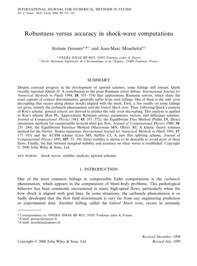
Figure 1. 80×160 computations of a forward-facing cylinder, M�=10, temperature contours.

forward-facing cylinder are presented. The freestream Mach number is 10. The computationalmesh is composed of 80×160 cells. In Figure 1(a), one cell over eight is presented for clarity.

First reported by Peery and Imlay [15] with Roe’s scheme, the carbuncle phenomenon is allthe more likely to show that the mesh is aligned with the detached bow shock. It consists ofa spurious stagnation point which moves the shock upstream along the symmetry axis. Thecarbuncle phenomenon is highly grid-dependent, but does not require a large number of pointsto appear. In certain cases, the numerical solution converges toward a steady solutionincluding the carbuncle phenomenon even though the residuals have come down to zeromachine accuracy. This means that, for a fixed space resolution, an unphysical solution of thesteady discretized Euler equations can be obtained with a consistent and stable conservativemethod. This conclusion is not in contradiction with the Lax–Wendroff theorem [6] since



when the grid is even more refined, unphysical solutions are more and more perturbed andeventually the computation fails to converge toward a steady solution.

According to the results shown in Figure 1, AUSM-M, HLLE [3] and EFM are the onlyschemes, among those included in this study, which naturally provide a physical calculationaround the stagnation line (Figure 1(c–d)). However, Pandolfi and D’Ambrosio [14] showedcomputations where the AUSM-M family yields perturbed contours downstream of the shock.These results are not surprising since the carbuncle phenomenon is highly grid-dependent.

The EIM scheme was not plotted: its lack of robustness prevents any attempt to computethis case without reaching negative pressures.

Osher’s scheme blows up in the first time steps for both natural (NO) and inverse ordering(IO) of the eigenvalues because of the severity of the initial freestream conditions. Steady statesolutions can still be reached by using another suitable scheme during the first time steps.

A steady solution can also be reached with Roe’s scheme by applying Harten’s entropy fix[5,7]. In principle, this fix should not be applied to the multiple eigenvalue l=u, because thatwould just be a convenient way to introduce a minimal amount of dissipation on shear waves.Indeed, the mathematical justification to modify the eigenvalues is simply to enforce asecond-law principle to the Euler equations in order to get rid of expansion shocks that mightotherwise appear. Thus, the entropy fix should only be applied on eigenvalues associated withsonic points such as l=u−a and l=u+a. If this is done, Roe’s scheme still develops thecarbuncle problem. However, if this fix is also applied to l=u the carbuncle disappearsprovided that a minimum value of Harten’s parameter has been used. Yet, there are twodrawbacks associated with this extended correction: (1) the exact resolution of shock waves islost, i.e. the entropy fix introduces an intermediate point in the resolution and (2) boundarylayers are significantly broadened when using a typical value for Harten’s entropy fix function,i.e. the exact resolution of contact waves is also lost. This entropy fix has also been discussedby Quirk [17] and Sanders et al. [20] who proposed an extension of this fix.

Because it is based upon the HUS technique, which provides the exact resolution of contactdiscontinuities, the EFMO scheme suffers from the same flaw as Osher’s scheme: the inverseordering develops the same unphysical protuberance as Roe’s scheme. With the naturalordering, the shape of the bow shock is not as badly affected, but the stagnation line remainsperturbed.

The fact that the EFM scheme is not affected by the carbuncle phenomenon suggests thata link should exist between the exact resolution of contact discontinuities (which has beenrestored in the EFMO scheme) and this flaw. This is confirmed by results obtained usingupwind schemes belonging to the HLL family. The restoration of the contact surface proposedby Toro et al. [21] and Batten et al. [1] in the HLL Riemann solver makes the flaw appear(HLLC scheme, Figure 1(h)), while the HLLE scheme [3] is not affected (Figure 1(g)). Similarresults with others members of the HLL Riemann solvers family are presented in Reference[14].

Based on numerical experiments, Liou [9] proposed a criterion on the mass flux dependen-cies to pressure difference. Similarly, Xu [23] proposed a more detailed explanation for theapparition of this anomalous phenomenon in the Riemann solvers family. On the other hand,the features of linear instability have been recently studied by Sanders et al. [20] and Robinetet al. [18]



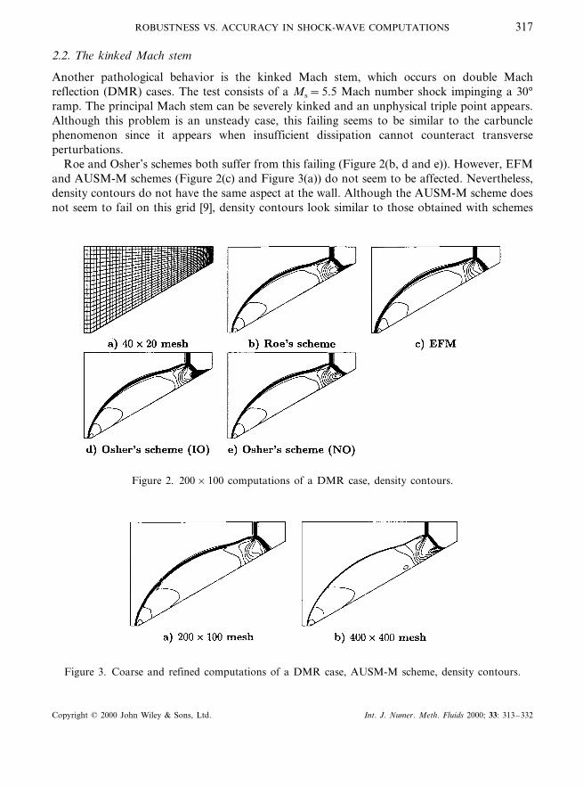
2.2. The kinked Mach stem

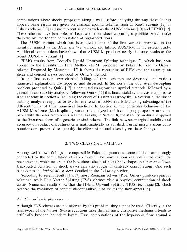
Another pathological behavior is the kinked Mach stem, which occurs on double Machreflection (DMR) cases. The test consists of a Ms=5.5 Mach number shock impinging a 30°ramp. The principal Mach stem can be severely kinked and an unphysical triple point appears.Although this problem is an unsteady case, this failing seems to be similar to the carbunclephenomenon since it appears when insufficient dissipation cannot counteract transverseperturbations.

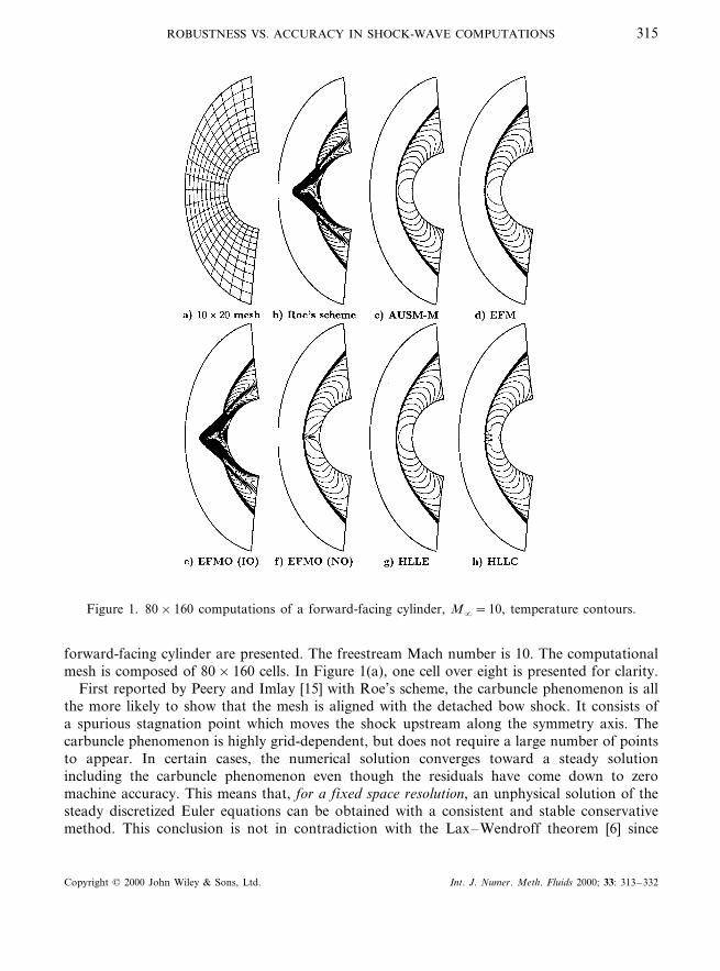
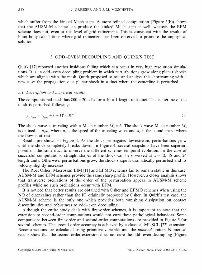
Roe and Osher’s schemes both suffer from this failing (Figure 2(b, d and e)). However, EFMand AUSM-M schemes (Figure 2(c) and Figure 3(a)) do not seem to be affected. Nevertheless,density contours do not have the same aspect at the wall. Although the AUSM-M scheme doesnot seem to fail on this grid [9], density contours look similar to those obtained with schemes

Figure 2. 200×100 computations of a DMR case, density contours.

Figure 3. Coarse and refined computations of a DMR case, AUSM-M scheme, density contours.



which suffer from the kinked Mach stem. A more refined computation (Figure 3(b)) showsthat the AUSM-M scheme can produce the kinked Mach stem as well, whereas the EFMscheme does not, even at this level of grid refinement. This is consistent with the results ofblunt-body calculations where grid refinement has been observed to promote the unphysicalsolution.

3. ODD–EVEN DECOUPLING AND QUIRK’S TEST

Quirk [17] reported another insidious failing which can occur in very high resolution simula-tions. It is an odd–even decoupling problem in which perturbations grow along planar shockswhich are aligned with the mesh. Quirk proposed to test and analyze this shortcoming with anew case: the propagation of a planar shock in a duct where the centerline is perturbed.

3.1. Description and numerical results

The computational mesh has 800×20 cells for a 40×1 length unit duct. The centerline of themesh is perturbed following:

yi, j mid=yj mid

+ (−1)i · 10−6 (1)

The shock wave is traveling with a Mach number Ms=6. The shock wave Mach number Ms

is defined as us/ar where us is the speed of the traveling wave and ar is the sound speed wherethe flow is at rest.

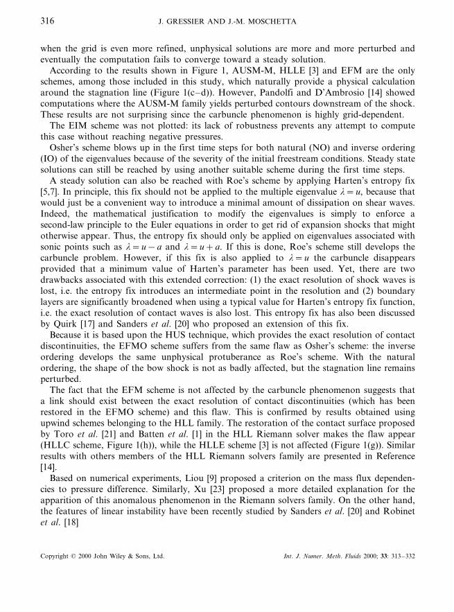
Results are shown in Figure 4. As the shock propagates downstream, perturbations growuntil the shock completely breaks down. In Figure 4, several snapshots have been superim-posed on the same duct to observe the different schemes temporal evolution. In the case ofsuccessful computations, straight shapes of the shock can be observed at x=12, 18 and 24length units. Otherwise, perturbations grow, the shock shape is dramatically perturbed and itsvelocity slightly increases.

The Roe, Osher, Macrossan EIM [11] and EFMO schemes fail to remain stable in this case.AUSM-M and EFM schemes provide the same sharp profile. However, a closer analysis showsthat transverse oscillations of the order of the perturbation appear in AUSM-M schemeprofiles while no such oscillations occur with EFM.

It is noticed that better results are obtained with Osher and EFMO schemes when using theNO of eigenvalues rather than the IO originally proposed by Osher. In Quirk’s test case, theAUSM-M scheme is the only one which provides both vanishing dissipation on contactdiscontinuities and robustness to odd–even decoupling.

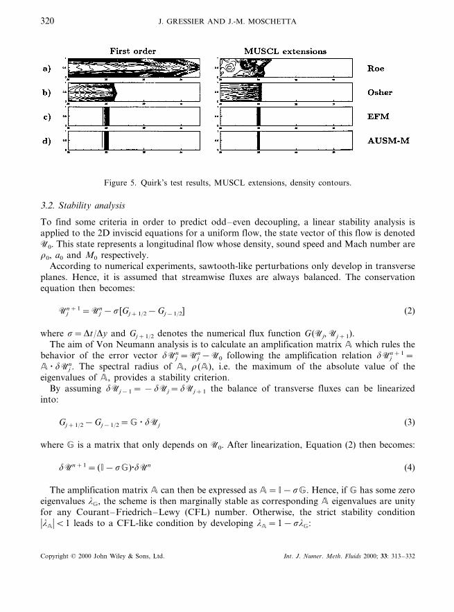
Although the entire study deals with first-order schemes, it is important to note that theextension to second-order computations would not cure these pathological behaviors. Somecomparisons between first-order and second-order computations are provided in Figure 5 forseveral schemes. The second-order accuracy is achieved by a classical MUSCL [22] extension.Reconstructions are calculated using primitive variables and the minmod limiter. Numericalresults show that the second-order extension does not cure the odd–even decoupling (Figure



Figure 4. Quirk’s test results, Mach number contours.

5(a–b)). Although the shock shape seems to be less perturbed, the computed solution stillremains unacceptable. On the other hand, the MUSCL extension does not trigger the failingeither (Figure 5(c–d)). These results support the choice of only considering first-order schemesin the following.



Figure 5. Quirk’s test results, MUSCL extensions, density contours.

3.2. Stability analysis

To find some criteria in order to predict odd–even decoupling, a linear stability analysis isapplied to the 2D inviscid equations for a uniform flow, the state vector of this flow is denotedU0. This state represents a longitudinal flow whose density, sound speed and Mach number arer0, a0 and M0 respectively.

According to numerical experiments, sawtooth-like perturbations only develop in transverseplanes. Hence, it is assumed that streamwise fluxes are always balanced. The conservationequation then becomes:

Ujn+1=Uj

n−s [Gj+1/2−Gj−1/2] (2)

where s=Dt/Dy and Gj+1/2 denotes the numerical flux function G(Uj, Uj+1).The aim of Von Neumann analysis is to calculate an amplification matrix A which rules the

behavior of the error vector dUjn=Uj

n−U0 following the amplification relation dUjn+1=

A · dUjn. The spectral radius of A, r(A), i.e. the maximum of the absolute value of the

eigenvalues of A, provides a stability criterion.By assuming dUj−1= −dUj=dUj+1 the balance of transverse fluxes can be linearized

into:

Gj+1/2−Gj−1/2=G · dUj (3)

where G is a matrix that only depends on U0. After linearization, Equation (2) then becomes:

dUn+1= (I−sG)·dUn (4)

The amplification matrix A can then be expressed as A=I−sG. Hence, if G has some zeroeigenvalues lG, the scheme is then marginally stable as corresponding A eigenvalues are unityfor any Courant–Friedrich–Lewy (CFL) number. Otherwise, the strict stability condition�lA�B1 leads to a CFL-like condition by developing lA=1−slG:



�lA�2= (1−sRe(lG))2+ (sIm(lG))2B1 (5a)

1+s(s �lG�2−2Re(lG))B1 (5b)

s �lG�2−2Re(lG)B0 (5c)

Hence, the following CFL-like condition provides a linearly stable scheme:

sB2Re(lG)

�lG�2 (6)

It should be pointed out that this criterion just comes from a stability analysis of a constantflow. The shock relations have not been considered in this approach.

4. ROE’S SCHEME ANALYSIS

Quirk [17] has already proposed an analysis of Roe’s scheme failure. The same assumptionswere used concerning streamwise fluxes, but only pressure and density perturbations wereconsidered.

In the present study, a similar analysis is performed using all components to describe theperturbed state vector. The interface flux of Roe’s scheme may be written as:

Gj+1/2=12

(Gj+Gj+1)−12

%k

a j+1/2k �l0 j+1/2

k �e j+1/2k (7)

where l0 k are the eigenvalues, ak the corresponding wave strengths and e k the correspondingright eigenvectors. More details and full expressions can be found in Reference [19].

4.1. Stability of odd–e6en perturbations

Since wave strengths are of the order of the perturbed quantities, the eigenvalues andeigenvectors which depend on Roe averaged state can be evaluated with the constant state U0.These assumptions lead to the following properties:

Gj−1=Gj+1 (8a)

a j−1/2k = −a j+1/2

k (8b)

l0 j−1/2k =l0 j+1/2

k (8c)

e j−1/2k = e j+1/2

k (8d)

The conservation Equation (2) can be developed and yields:



dUjn+1=dUj

n−2ny

ÁÃÃÃÄ

(dpn/a2)U0(dpn/a2)

r0 d6n

H0(dpn/a2)

ÂÃÃÃÅ

(9)

where 6y=sa0 can be interpreted as a CFL number. To extract an amplification matrix,Equation (9) can be expressed (assuming a0# a) as:

ÁÃÃÃÄ

dpdud6

dp

ÂÃÃÃÅ

n+1

=

ÁÃÃÃÄ

1 0 0 −2ny/a02

0 1 0 00 0 1−2ny 00 0 0 1−2ny

ÂÃÃÃÅ

ÁÃÃÃÄ

dr

dud6

dp

ÂÃÃÃÅ

n

(10)

This result shows that density and streamwise velocity errors are marginally stable since theyare associated with an amplification factor equal to one. Then, these perturbations are totallydriven by source terms which are not modeled here. In Quirk’s problem, source terms comefrom unbalanced fluxes along the perturbed centerline. The present analysis only describes thedevelopment of an initial perturbation.

Marginal stability confirms numerical experiments where odd–even decoupling does notdepend on the CFL number. This implies that the marginal stability property is an intrinsicmechanism directly dependent on the flux function definition.

4.2. Effects of the extended entropy fix

In the same way as it does for the carbuncle and the kinked Mach stem failings, an extensionof the true entropy fix can cure the odd–even decoupling failing. The extension consists ofapplying this fix to linear waves which govern shear and contact discontinuities. But this hasno mathematical or physical justification: it is just a convenient method to add a minimalamount of artificial dissipation. None of the true entropy fix (where the fix is only applied to69a eigenvalues) can cure Roe’s failure.

A similar stability analysis is performed with Roe’s scheme using the extended entropy fix.Absolute values of the eigenvalues of Equation (7) are replaced by Harten’s function [5] inwhich Harten’s parameter d0 is evaluated from the spectral radius according to d0=d(�60�+a0)where d is a problem-dependent tunable parameter. The present analysis is not affected by theuse of a more elaborate form of d0 [7] since d0 comes directly into the amplification matrix.

Referring to the previous analysis of the original version of Roe scheme (see Section 4.1),when the entropy fix is applied, the calculation now consists of replacing the eigenvalue �60� byd0. After the same calculation which has led to Equation (10), pressure and transverse velocityperturbations can be shown to remain stable under a CFL condition as observed in the lattercase. Amplification factors of density and streamwise velocity perturbations now become:�

1−2d0

a0

ny�

(11)

instead of 1 as in the latter analysis of Roe’s original scheme (without any fix).



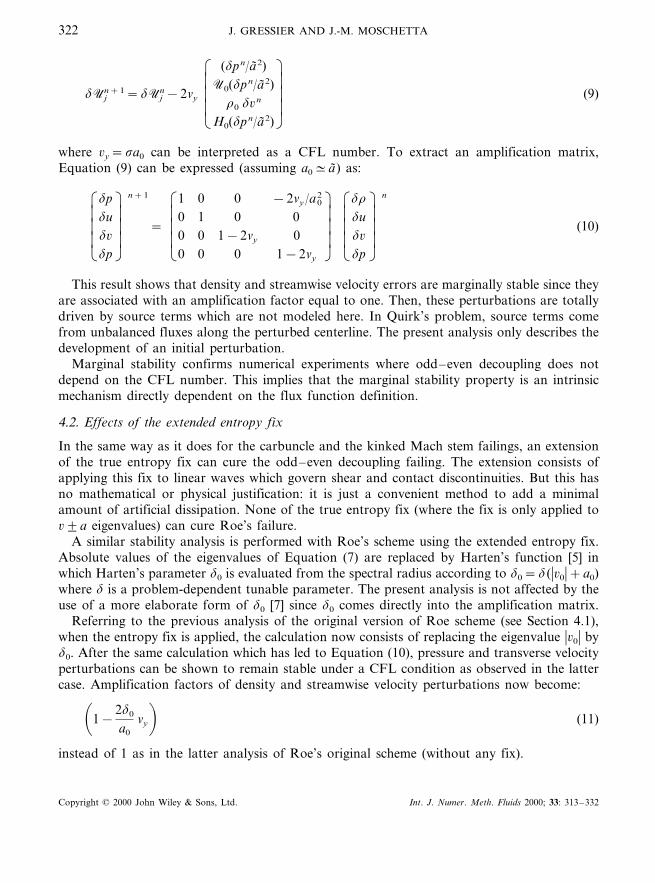
Figure 6. Effects of the extended entropy fix, Mach number contours.

Owing to the extended entropy fix, Roe’s scheme becomes stable under a CFL condition.Surprisingly, numerical results of Figure 6 show that a threshold (d#0.2) is necessary toremove the odd–even decoupling problem. Results of Figure 6(b) show the limits of thepresent analysis since linear stability condition is satisfied for d=0.1, i.e. r(A)B1, whileresults still indicate instability. At this point, further analysis taking into account the shockstructure and the contribution of streamwise fluxes is certainly needed.

Nevertheless, the stability analysis carried out for both versions of Roe’s scheme suggeststhat marginal stability is not a desirable property for upwind schemes.

5. EFM AND EIM SCHEMES ANALYSIS

Both EFM and EIM schemes interface flux share infinite differentiability with respect to theirleft and right states. Therefore, amplification matrix A can be directly calculated as a functionof the Jacobian matrices of the interface flux G(UL, UR). Conservation Equation (2) islinearized and A is evaluated via G as:

G=2� (G(UL

−(G(UR

�U0

(12)

5.1. EFM scheme

The EFM scheme amplification matrix is evaluated following Equation (12). Expressionsremain intricate but, by computing its determinant, matrix G can be shown to have no zeroeigenvalue. Hence, the EFM scheme is strictly stable under a CFL condition. This confirms thegood damping properties observed in numerical experiments.



5.2. EIM scheme

The same method can be used to evaluate the EIM scheme amplification matrix.It can be written via G as:

G=' 2

gp

ÁÃÃÃÃÃÃÃÃÃÄ

U− gM0

a0

0g

a02

M0a0U − gM02 0

gM0

a0

0 0 g+1 0

a02UC

g−1−gM0a0C 0 gC

ÂÃÃÃÃÃÃÃÃÃÅ

(13)

where g=g(g−1), U=1+g((g−1)/2)M02 and C=1+ ((g−1)/2)M0

2.Because of column vectors dependencies, G yields two zero eigenvalues. Indeed, the second

column is equal to −a0M0 times the fourth and the first is a2U/g times the fourth. Obviously,a third one is 2/gp(g+1). The trace of matrix G provides the fourth eigenvalue 2/gp(g+1). Finally, the complete set of eigenvalues is:

[0 ; 0 ; 2/gp(g+1) ; 2/gp(g+1)] (14)

Hence, A has two eigenvalues equal to one and, consequently, the EIM scheme is marginallystable. This is consistent with the numerical results (Figure 4(e)).

6. AUSM-M SCHEME ANALYSIS

Like Roe’s scheme, AUSM-M interface flux expressions are not differentiable around theconstant state U0. Properties of upwind functions in AUSM-M scheme are used. Forodd–even perturbations, one has:

dMj+1= −dMj=dMj−1 (15)

Hence, by first-order approximations,

Mj+1/2=M+(dMj)+M−(dMj+1)=0 (16a)

Mj−1/2=M+(dMj−1)+M−(dMj)=0 (16b)

pj+1/2=p+(dMj)+p−(dMj+1)=2p+(dMj) (16c)



pj−1/2=p+(dMj−1)+p−(dMj)=2p−(dMj) (16d)

Convective terms disappear in the conservation Equation (2). The pressure term is the only oneleft. It influences the transverse momentum equation following:

r0a0dMjn+1=r0a0dMj

n−2s [pj+ −pj

−] (17)

In the AUSM-M scheme, p9 can be linearized as p9=1/2p(193/2M). This leads to theamplification matrix:

ÁÃÃÃÄ

dr

dud6

dp

ÂÃÃÃÅ

n+1

=

ÁÃÃÃÃÃÄ

1 0 0 0

0 1 0 0

0 0 1−3g

ny 0

0 0 0 1

ÂÃÃÃÃÃÅ

ÁÃÃÃÄ

dr

dud6

dp

ÂÃÃÃÅ

n

(18)

The AUSM-M scheme is therefore also marginally stable. Nevertheless, numerical experimentsindicate that it does not suffer from odd–even decoupling. This result points out that marginalstability cannot be considered as a criterion to predict odd–even decoupling since it can leadeither to methods which are prone to develop the odd–even decoupling problem or to methodswhich will not amplify nor damp perturbations, such as the AUSM-M scheme.

7. DAMPING PROPERTIES

Although the AUSM-M and EFM schemes do not have the same amplification matrix sincethe EFM is strictly stable (under a CFL condition) and the AUSM-M is marginally stable,none of them suffer from odd–even decoupling in Quirk’s test. Nevertheless, the EFM isexpected to have better damping properties. This is confirmed by the following results.

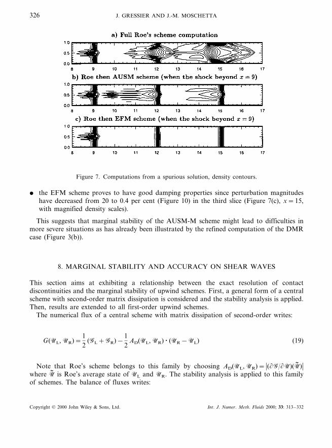
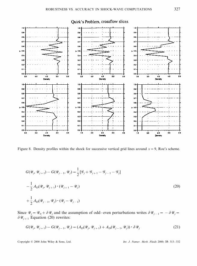
The moving shock is computed using Roe’s scheme until it has covered 9 length units(t=1.5). This unsteady solution is then used as an initial condition for the AUSM-M, EFMor Roe’s scheme as if the computation had not been interrupted. The three cases arerepresented in Figure 7, where the first slice (x=9) comes from the same computation. First,Figure 7 shows that the shock profile has already been greatly perturbed while using Roe’sscheme (Figure 7, x=9). Transverse snapshots show that density profiles suffer from oscilla-tions of 20 per cent magnitude (Figure 8). The three computations of Figure 7 show thedamping properties of these three schemes:

� an entire computation with Roe’s scheme fail since the shock profile has blown up atx=15;

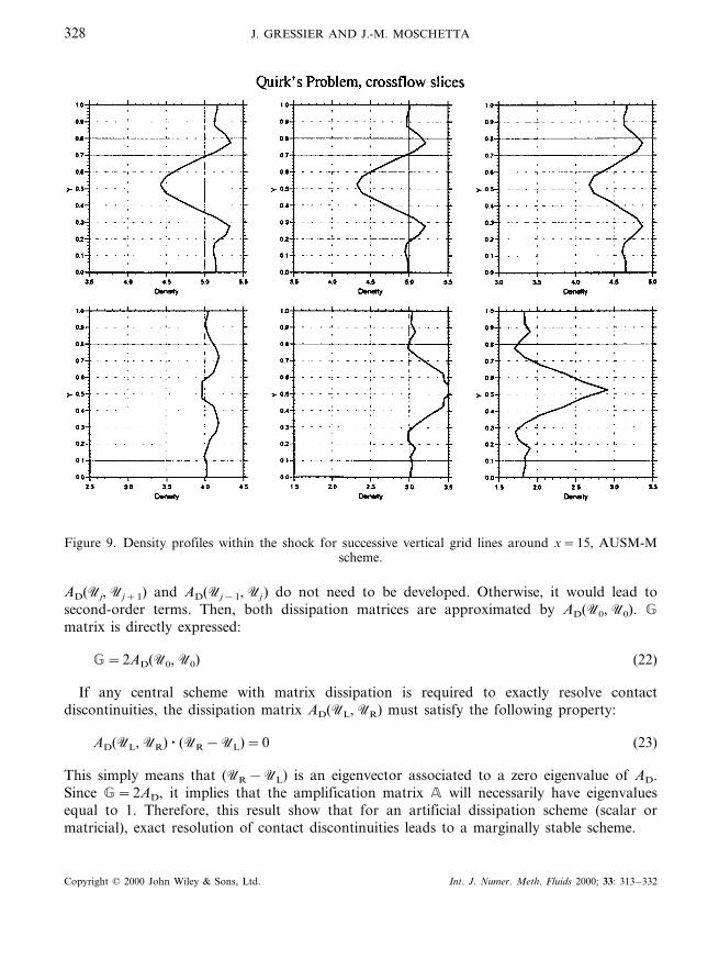
� the AUSM-M seems to cope with these initial conditions: perturbations are not amplifiedbut remain at 20 per cent magnitude (Figure 9) in the third slice (Figure 7(b), x=15);



Figure 7. Computations from a spurious solution, density contours.

� the EFM scheme proves to have good damping properties since perturbation magnitudeshave decreased from 20 to 0.4 per cent (Figure 10) in the third slice (Figure 7(c), x=15,with magnified density scales).

This suggests that marginal stability of the AUSM-M scheme might lead to difficulties inmore severe situations as has already been illustrated by the refined computation of the DMRcase (Figure 3(b)).

8. MARGINAL STABILITY AND ACCURACY ON SHEAR WAVES

This section aims at exhibiting a relationship between the exact resolution of contactdiscontinuities and the marginal stability of upwind schemes. First, a general form of a centralscheme with second-order matrix dissipation is considered and the stability analysis is applied.Then, results are extended to all first-order upwind schemes.

The numerical flux of a central scheme with matrix dissipation of second-order writes:

G(UL, UR)=12

(GL+GR)−12

AD(UL, UR) · (UR−UL) (19)

Note that Roe’s scheme belongs to this family by choosing AD(UL, UR)= �((G/(U)(U0 )�where U0 is Roe’s average state of UL and UR. The stability analysis is applied to this familyof schemes. The balance of fluxes writes:



Figure 8. Density profiles within the shock for successive vertical grid lines around x=9, Roe’s scheme.

G(Uj, Uj+1)−G(Uj−1, Uj)=12

[Gj+Gj+1−Gj−1−Gj ]

−12

AD(Uj, Uj+1) · (Uj+1−Uj) (20)

+12

AD(Uj−1, Uj) · (Uj−Uj−1)

Since Uj=U0+dUj and the assumption of odd–even perturbations writes dUj−1= −dUj=dUj+1 Equation (20) rewrites:

G(Uj, Uj+1)−G(Uj−1, Uj)= (AD(Uj, Uj+1)+AD(Uj−1, Uj)) · dUj (21)



Figure 9. Density profiles within the shock for successive vertical grid lines around x=15, AUSM-Mscheme.

AD(Uj, Uj+1) and AD(Uj−1, Uj) do not need to be developed. Otherwise, it would lead tosecond-order terms. Then, both dissipation matrices are approximated by AD(U0, U0). G

matrix is directly expressed:

G=2AD(U0, U0) (22)

If any central scheme with matrix dissipation is required to exactly resolve contactdiscontinuities, the dissipation matrix AD(UL, UR) must satisfy the following property:

AD(UL, UR) · (UR−UL)=0 (23)

This simply means that (UR−UL) is an eigenvector associated to a zero eigenvalue of AD.Since G=2AD, it implies that the amplification matrix A will necessarily have eigenvaluesequal to 1. Therefore, this result show that for an artificial dissipation scheme (scalar ormatricial), exact resolution of contact discontinuities leads to a marginally stable scheme.



Figure 10. Density profiles within the shock for successive vertical grid lines around x=15, EFMscheme.

Furthermore, any upwind scheme, after linearization, can be expressed as a central schemewith matrix dissipation. If the numerical flux is differentiable, the matrix AD can be directlycalculated with Jacobians of the numerical flux G :

AD=(G(UL

−(G(UR

(24)

Hence, previous results can be extended to all first-order schemes: if any upwind schemeprovides accuracy on contact waves then it is marginally stable. In other words, any upwindscheme cannot simultaneously satisfy both the following properties: exact resolution of contactdiscontinuities and strict stability.



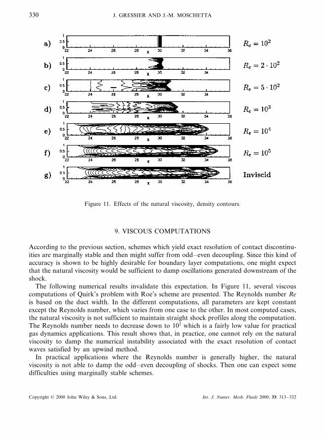
Figure 11. Effects of the natural viscosity, density contours.

9. VISCOUS COMPUTATIONS

According to the previous section, schemes which yield exact resolution of contact discontinu-ities are marginally stable and then might suffer from odd–even decoupling. Since this kind ofaccuracy is shown to be highly desirable for boundary layer computations, one might expectthat the natural viscosity would be sufficient to damp oscillations generated downstream of theshock.

The following numerical results invalidate this expectation. In Figure 11, several viscouscomputations of Quirk’s problem with Roe’s scheme are presented. The Reynolds number Reis based on the duct width. In the different computations, all parameters are kept constantexcept the Reynolds number, which varies from one case to the other. In most computed cases,the natural viscosity is not sufficient to maintain straight shock profiles along the computation.The Reynolds number needs to decrease down to 102 which is a fairly low value for practicalgas dynamics applications. This result shows that, in practice, one cannot rely on the naturalviscosity to damp the numerical instability associated with the exact resolution of contactwaves satisfied by an upwind method.

In practical applications where the Reynolds number is generally higher, the naturalviscosity is not able to damp the odd–even decoupling of shocks. Then one can expect somedifficulties using marginally stable schemes.



10. CONCLUDING REMARKS

The present analysis of odd–even decoupling has contributed to explain why Roe and EIMschemes fail in some situations. Applying the same analysis, the AUSM-M scheme althoughmarginally stable, is observed to pass successfully Quirk’s test. Nevertheless, this marginalbehavior is consistent with the observed propagation of perturbations from the centerlinealong crossflow planes, and with the failing of the AUSM-M scheme on some other cases suchas the DMR problem for high resolution computations.

Among the upwind methods considered in this study, the EFM scheme has been the onlyscheme which provides the desirable damping properties. Unfortunately, the EFM does notexactly resolve contact discontinuities. These features are shared by most FVS schemes [14]. Inorder to be used as a criterion, this analysis certainly needs to take into account perturbationsdue to source terms, the shock structure and streamwise fluxes contribution. Furthermore, theEFM scheme results reveal that strict stability is desirable to avoid these flaws.

The linear stability analysis has proved that any central scheme with matrix dissipationcannot simultaneously satisfy both properties, and the result is extended to any upwindscheme. In view of the proposed criteria and based upon the above-mentioned numericalobservations, strict stability and exact resolution of contact discontinuities are not compatible.This might have heavy consequences on the development of future algorithms for thecompressible Navier–Stokes equations, since natural viscosity cannot cure this flaw by itself.

APPENDIX A. NOMENCLATURE

sound speedaA amplification matrix

error vectordUG physical flux vector

numerical flux vectorGstagnation enthalpyHpressurePdensityr

spectral radius of Ar(A)velocity componentsu, 6

U state vector

Subscriptstransverse subscriptj

reference values0

Superscriptstime stepn

Roe average value�



REFERENCES

1. Batten P, Clarke N, Lambert C, Causon DM. On the choice of waves speeds for the HLLC Riemann solver.SIAM Journal on Scientific Computing 1997; 18(6): 1553–1570.

2. Coquel F, Liou MS. Hybrid Upwind Splitting (HUS) by a Field by Field Decomposition, NASA TM-106843,1995.

3. Einfeldt B, Munz CD, Roe PL, Sjogreen B. On Godunov-type methods near low densities. Journal ofComputational Physics 1991; 92: 273–295.

4. Gressier J, Moschetta J-M. On the Pathological Behavior of Upwind Schemes, AIAA Paper 98-0110, January1998.

5. Hirsch C. Numerical Computation of Internal and External Flows, Computational Methods for In6iscid and ViscousFlows (2nd ed.), vol. 2:. Wiley: New York, 1990.

6. Lax PD, Wendroff B. Systems of conservation laws. Communications on Pure and Applied Mathemathics 1960; 13:217–237.

7. Lin HC. Dissipations additions to flux difference splitting. Journal of Computational Physics 1995; 117: 20–27.8. Liou MS. Progress towards an Improved CFD Method: AUSM+ , AIAA Paper 95-1701 CP, 1995.9. Liou MS. Probing Numerical Fluxes: Mass Flux, Positivity and Entropy satisfying Property, AIAA Paper

97-2035, 1997.10. Liou MS, Steffen CJ. A new flux splitting scheme. Journal of Computational Physics 1993; 107: 23–39.11. Macrossan MN, Oliver RI. A kinetic theory solution method for the Navier–Stokes equations. International

Journal for Numerical Methods in Fluids 1993; 17: 177–193.12. Moschetta JM, Pullin DI. A robust low diffusive kinetic scheme for the Navier–Stokes equations. Journal of

Computational Physics 1997; 133(2): 193–204.13. Osher S, Chakravarthy S. Upwind schemes and boundary conditions with applications to Euler equations in

general geometries. Journal of Computational Physics 1983; 50: 447–481.14. Pandolfi M, D’Ambrosio D. Upwind methods and carbuncle phenomenon. In Computational Fluid Dynamics 98,

4th ECCOMAS, vol. 1. Wiley: New York, 1998.15. Peery KM, Imlay ST. Blunt body flow simulations. In AIAA Paper No. 88-2924, 1988.16. Pullin DI. Direct simulation methods for compressible inviscid ideal gas flow. Journal of Computational Physics

1980; 34: 231–244.17. Quirk JJ. A contribution to the great Riemann solver debate. International Journal for Numerical Methods in

Fluids 1994; 18: 555–574.18. Robinet J-Ch, Gressier J, Casalis G, Moschetta J-M. The carbuncle phenomenon: an intrinsic inviscid instability?

In 22nd ISSW, July, 1999.19. Roe PL. Approximate Riemann solvers, parameters vectors, and difference schemes. Journal of Computational

Physics 1981; 43: 357–372.20. Sanders R, Morano E, Druguet M-C. Multi-dimensional dissipation for upwind schemes: stability and applica-

tions to gas dynamics. Journal of Computational Physics 1998; 145: 511–537.21. Toro EF, Spruce M, Speares W. Restoration of the contact surface in the HLL-Riemann solver. Shock Wa6es

1994; 4: 25–34.22. van Leer B. Towards the ultimate conservative difference scheme V. A second-order sequel to Godunov’s method.

Journal of Computational Physics 1979; 32: 101–136.23. Xu K. VKI Lecture Series 1998-03, February, 1998.


robustness versus accuracy in shock-wave computations

Documents