Immaculate line bundles on toric varieties

Klaus Altmann Jarosław Buczyński Lars KastnerAnna-Lena Winz

29th August 2018

Abstract

We call a sheaf on an algebraic variety immaculate if it lacks any cohomology including thezero-th one, that is, if the derived version of the global section functor vanishes. Such sheavesare the basic tools when building exceptional sequences, investigating the diagonal property,or the toric Frobenius morphism.

In the present paper we focus on line bundles on toric varieties. First, we present a possib-ility of understanding their cohomology in terms of their (generalized) momentum polytopes.Then we present a method to exhibit the entire locus of immaculate divisors within the classgroup. This will be applied to the cases of smooth toric varieties of Picard rank two and threeand to those being given by splitting fans.

The locus of immaculate line bundles contains several linear strata of varying dimensions.We introduce a notion of relative immaculacy with respect to certain contraction morphisms.This notion will be stronger than plain immaculacy and provides an explanation of some ofthese linear strata.

Addresses:K. Altmann, altmann@math.fu-berlin.de, Institut für Mathematik, FU Berlin, Arnimalle 3, 14195 Berlin, Ger-manyJ. Buczyński, jabu@mimuw.edu.pl, Institute of Mathematics of the Polish Academy of Sciences, ul. Śniadeckich8, 00-656 Warsaw, Poland, and Faculty of Mathematics, Computer Science and Mechanics, University of Warsaw,ul. Banacha 2, 02-097 Warszawa, PolandL. Kastner kastner@math.fu-berlin.de, Institut für Mathematik, TU Berlin, Gebäude MA, Straße des 17. Juni136, 10623 Berlin, GermanyA.-L. Winz, anna-lena.winz@fu-berlin.de, Institut für Mathematik, FU Berlin, Arnimalle 3, 14195 Berlin, Ger-many.Keywords: toric variety, immaculate line bundle, splitting fan, toric varieties of Picard rank 3, primitive collec-tions.AMS Mathematical Subject Classification 2010: Primary: 14M25; Secondary: 14F05, 14F17, 52B20, 14L32.

Contents

I Introduction 2I.1 Exceptional sequences ask for immaculacy . . . . . . . . . . . . . . . . . . . . . . 2I.2 The situation on toric varieties . . . . . . . . . . . . . . . . . . . . . . . . . . . . 3I.3 Visualizing the cohomology of toric line bundles . . . . . . . . . . . . . . . . . . . 3I.4 Immaculate loci for toric varieties . . . . . . . . . . . . . . . . . . . . . . . . . . . 5I.5 Special situations . . . . . . . . . . . . . . . . . . . . . . . . . . . . . . . . . . . . 5

1

arX

iv:1

808.

0931

2v1

[m

ath.

AG

] 2

8 A

ug 2

018

II Differences of polytopes 7II.1 Removing open subsets . . . . . . . . . . . . . . . . . . . . . . . . . . . . . . . . . 7II.2 Compact approximation of open semialgebraic sets . . . . . . . . . . . . . . . . . 8II.3 Allowing common tail cones . . . . . . . . . . . . . . . . . . . . . . . . . . . . . . 9

III Toric geometry 10III.1 Basic toric notation . . . . . . . . . . . . . . . . . . . . . . . . . . . . . . . . . . . 10III.2 Toric cohomology . . . . . . . . . . . . . . . . . . . . . . . . . . . . . . . . . . . . 12III.3 Cohomology using polyhedra . . . . . . . . . . . . . . . . . . . . . . . . . . . . . 13

IV The immaculacy locus in Pic(X) 16IV.1 Immaculate line bundles . . . . . . . . . . . . . . . . . . . . . . . . . . . . . . . . 16IV.2 Relative immaculacy and affine spaces of immaculate line bundles . . . . . . . . . 17

V Immaculacy by avoiding temptations 21V.1 Temptations . . . . . . . . . . . . . . . . . . . . . . . . . . . . . . . . . . . . . . . 23V.2 Conditions on presence or absence of temptations . . . . . . . . . . . . . . . . . . 26

V.2.1 Monomials do not lead into temptation . . . . . . . . . . . . . . . . . . . . 26V.2.2 Faces are not tempting . . . . . . . . . . . . . . . . . . . . . . . . . . . . . 27V.2.3 Primitive collections delude . . . . . . . . . . . . . . . . . . . . . . . . . . 27

V.3 The cube . . . . . . . . . . . . . . . . . . . . . . . . . . . . . . . . . . . . . . . . 28

VI Toric manifolds with Picard rank two 30VI.1 Spotting smoothness via Gale duality . . . . . . . . . . . . . . . . . . . . . . . . . 30VI.2 Immaculate locus for Picard rank two . . . . . . . . . . . . . . . . . . . . . . . . 30

VII The immaculate locus for splitting fans 32VII.1 Primitive relations . . . . . . . . . . . . . . . . . . . . . . . . . . . . . . . . . . . 33VII.2 Temptation for splitting fans . . . . . . . . . . . . . . . . . . . . . . . . . . . . . . 33VII.3 The refined structure of the fan and the class map . . . . . . . . . . . . . . . . . 34VII.4 Generating immaculate seeds . . . . . . . . . . . . . . . . . . . . . . . . . . . . . 36

VIII The immaculate locus for Picard rank 3 38VIII.1 Classification by Batyrev . . . . . . . . . . . . . . . . . . . . . . . . . . . . . . . . 38VIII.2 Tempting Subsets . . . . . . . . . . . . . . . . . . . . . . . . . . . . . . . . . . . . 39VIII.3 Immaculate line bundles for Picard rank 3 . . . . . . . . . . . . . . . . . . . . . . 40

IX Computational aspects 44

References 46

I. Introduction

We work over an algebraically closed field k of any characteristic.

I.1. Exceptional sequences ask for immaculacy

A major tool for the process of understanding derived categories D(X) on an algebraic variety Xis full exceptional sequences “FES ” (F1, . . . ,Fk) of sheaves or complexes. That is, its members are

2

supposed to generate D(X) and, up to HomD(X)(Fi,Fi) = k, one asks for HomD(X)(Fi,Fj [p]) = 0for all shifts p ∈ Z and pairs i ≥ j. These conditions call to mind the shape of unitary uppertriangular matrices. If FES exist, then they provide a semi-orthogonal decomposition of D(X)into the simplest summands possible.Whenever the Fi are sheaves, then HomD(X)(Fi,Fj [p]) can alternatively be written as the

classical group ExtpOX (Fi,Fj). If, moreover, Fi are locally free, e.g. invertible sheaves, then thisequals Hp(X,F−1

i ⊗Fj). Thus, we require certain sheaves G = F−1i ⊗Fj to lack any cohomology,

including the seemingly innocent 0-th one:

RΓ(X,G) = 0.

We will call this property of a sheaf G immaculate, see Definition IV.1 in Subsection IV.1.We are going to focus on invertible sheaves on smooth, projective varieties X with RΓ(OX) = k.

So, when looking for exceptional sequences of line bundles, the case i = j yielding G = OX isalready taken care of. That is, whenever we have sufficiently good knowledge of the locus ofimmaculate sheaves within the Picard or class group Cl(X), then we can freely use its elementsGν = OX(Dν) as building blocks to mount exceptional sequences via Fi := OX(

∑iν=2Dν). The

defining property of the vanishing Ext groups can then be understood as asking consecutive sumsof the Dν to be immaculate, too.The comparison of the shape of several FES can shed light on several features of the given

variety X. Thus, the shape of the tool box of immaculate line bundles should serve as a richinvariant. In addition, immaculate line bundles appear in different contexts. In [Ach15] they areexploited to show a characterisation of toric varieties in terms of Frobenius splitting property.In [PSP08] they are used to study the diagonal property of smooth projective varieties (see forinstance [PSP08, Thm 4]). For a surface of general type, the property of immaculacy of linebundles is relevant to the spectral theory [KZ17].

I.2. The situation on toric varieties

Suppose thatX is a smooth, projective toric variety. The main result in this context is Kawamata’sproof of the existence of FES of sheaves on smooth, projective toric Deligne-Mumford stacks, see[Kaw06, Kaw13]. An earlier conjecture of King about the existence of full, strongly exceptional(Ext≥1(Fi,Fj) = 0 for all i, j) sequences of line bundles was disproved in [HP06], [Mic11]. But,when abstaining from the additional property “strong”, it is still an open question whether smooth,projective toric varieties admit FES of line bundles, let alone provide an understanding of whichequivariant divisors represented by which abstract polyhedra will form those sequences. The onlyrather general, positive result is that of [CM04, Theorem 4.12] where the existence of those se-quences was established for splitting fans, see Subsection VII. From a different viewpoint, thiswas reproven for a special case in [Cra11].Another remarkable result can be found in [HP11]. There, the authors start with an arbitrary,

that is, not necessarily toric, smooth complete rational surface and show that FES of line bundlesdo always exist. But the interesting point is that these sequences can easily be transformed intoa cycle of divisors imitating the toric situation, that is, to each FES one can associate a toricsurface materialising this sequence.

I.3. Visualizing the cohomology of toric line bundles

In the present paper, we keep the notion of exceptional sequences in the background. Instead, fora given projective (often smooth) toric variety we are just interested in the immaculacy property

3

of divisor classes. Classically, the cohomology of a reflexive rank one sheaf, that is, of a Weildivisor on a toric variety X can be expressed in terms of special polyhedral complexes whosevertices are some rays of the fan Σ of X. In particular, the complexes live in NR = N ⊗R, whereN is the lattice of one parameter subgroups of the torus acting on X.We propose a different point of view on the cohomology of toric Q-Cartier Weil divisors. We

will make it literally visible in terms of polytopes in the dual space MR. As usual, one writesMR = M ⊗R with M = Hom(N,Z) being the monomial lattice of the acting torus T . Since eachQ-Cartier Weil divisor can be decomposed into a difference D = D+ − D− of nef (or even Q-ample) ones, this means that the T -invariant among them can be encoded by a pair of polytopes(∆+,∆−), see Subsection III.3 for more details and the more general situation of semi-projectivevarieties.Polytopes form a cancellative semigroup under Minkowski addition. In this context, the pair

(∆+,∆−) represents the formal difference

D = ∆+ −∆−

within the Grothendieck group of generalized polytopes. On the other hand, each T -invariantWeil divisor D leads to a (possibly empty) polytope of sections ∆(D) ⊆ MR. Its lattice pointsparametrize the monomial basis of Γ(X,OX(D)). If D is nef, then the pair consisting of ∆+ :=∆(D) and ∆− := 0 can be used to represent D. For general D being represented by some(∆+,∆−), one can still recover the polytope of sections as

∆(D) = {r ∈MR | ∆− + r ⊆ ∆+},

cf. Remark III.9. This can be visualized as a kind of a materialized shadow of the abstractdifference ∆+ −∆−.So it is quite a surprising fact that, after using the formal difference ∆+ −∆− and its shadow

∆(D), the cohomology of D = ∆+ − ∆− can be understood by a third flavour, namely by thenaive and original meaning of the set theoretic differences of these polytopes.

Theorem I.1. On a projective toric variety X the cohomology groups Hi(X,OX(D)) are M -graded, and for each m ∈ M , the homogeneous component of degree m equals H̃

i−1(∆− \ (∆+ −

m),k). Here ∆+ −m means the shift by m of ∆+ in M ⊗ R.

See Example III.12 for an illustration of this claim. The theorem is stated more generally asTheorem III.6 in the context of semi-projective toric varieties. It implies that the immaculacyof D = (∆+,∆−) can be measured by the fact whether ∆− \ (∆+ −m) is k-acyclic for all shiftsm ∈M . See Subsection IV.1 for a discussion of the notion of being k-acyclic.Besides its elementary geometric nature, the description of sheaf cohomology via the defining

polyhedra in the vector space MR also has another advantage. It allows one to think about ageneralization to the more general setup of Okounkov bodies, as introduced in [LM09]: after fixinga complete flag of subspaces in an arbitrary (not necessarily toric) smooth projective variety X,convex polytopes of sections ∆(L) are assigned to each invertible sheaf L. Thus, a description ofCartier divisors D via pairs of polytopes (∆+,∆−) is possible, and one can ask for the relationbetween Hi(X,OX(D)), and the cohomology of the set theoretic differences ∆− \(∆+−m). Sincein especially nice situations the Okounkov bodies induce a toric degeneration of X, see [And13],semi continuity suggests that the latter might serve as an upper bound for the first.

4

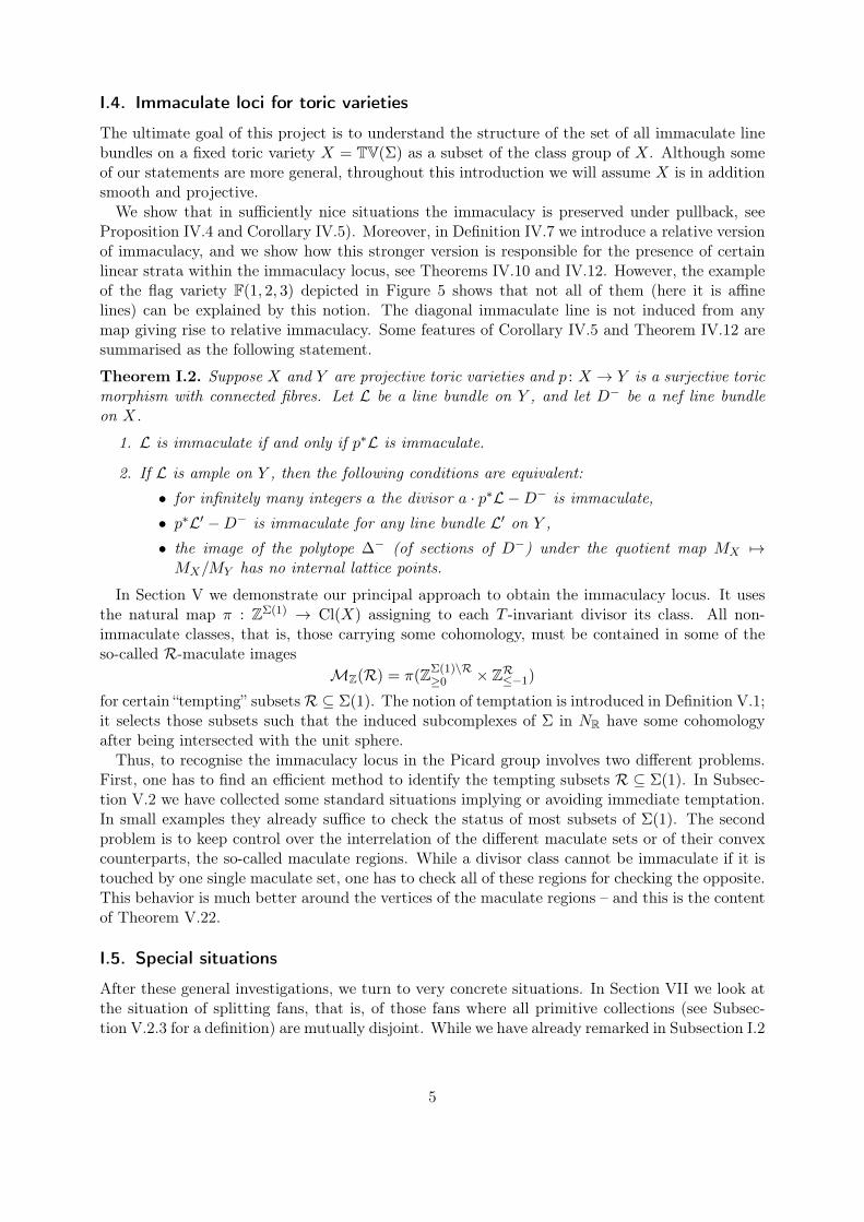
I.4. Immaculate loci for toric varieties

The ultimate goal of this project is to understand the structure of the set of all immaculate linebundles on a fixed toric variety X = TV(Σ) as a subset of the class group of X. Although someof our statements are more general, throughout this introduction we will assume X is in additionsmooth and projective.We show that in sufficiently nice situations the immaculacy is preserved under pullback, see

Proposition IV.4 and Corollary IV.5). Moreover, in Definition IV.7 we introduce a relative versionof immaculacy, and we show how this stronger version is responsible for the presence of certainlinear strata within the immaculacy locus, see Theorems IV.10 and IV.12. However, the exampleof the flag variety F(1, 2, 3) depicted in Figure 5 shows that not all of them (here it is affinelines) can be explained by this notion. The diagonal immaculate line is not induced from anymap giving rise to relative immaculacy. Some features of Corollary IV.5 and Theorem IV.12 aresummarised as the following statement.

Theorem I.2. Suppose X and Y are projective toric varieties and p : X → Y is a surjective toricmorphism with connected fibres. Let L be a line bundle on Y , and let D− be a nef line bundleon X.

1. L is immaculate if and only if p∗L is immaculate.

2. If L is ample on Y , then the following conditions are equivalent:

• for infinitely many integers a the divisor a · p∗L −D− is immaculate,

• p∗L′ −D− is immaculate for any line bundle L′ on Y ,

• the image of the polytope ∆− (of sections of D−) under the quotient map MX 7→MX/MY has no internal lattice points.

In Section V we demonstrate our principal approach to obtain the immaculacy locus. It usesthe natural map π : ZΣ(1) → Cl(X) assigning to each T -invariant divisor its class. All non-immaculate classes, that is, those carrying some cohomology, must be contained in some of theso-called R-maculate images

MZ(R) = π(ZΣ(1)\R≥0 × ZR≤−1)

for certain “tempting” subsetsR ⊆ Σ(1). The notion of temptation is introduced in Definition V.1;it selects those subsets such that the induced subcomplexes of Σ in NR have some cohomologyafter being intersected with the unit sphere.Thus, to recognise the immaculacy locus in the Picard group involves two different problems.

First, one has to find an efficient method to identify the tempting subsets R ⊆ Σ(1). In Subsec-tion V.2 we have collected some standard situations implying or avoiding immediate temptation.In small examples they already suffice to check the status of most subsets of Σ(1). The secondproblem is to keep control over the interrelation of the different maculate sets or of their convexcounterparts, the so-called maculate regions. While a divisor class cannot be immaculate if it istouched by one single maculate set, one has to check all of these regions for checking the opposite.This behavior is much better around the vertices of the maculate regions – and this is the contentof Theorem V.22.

I.5. Special situations

After these general investigations, we turn to very concrete situations. In Section VII we look atthe situation of splitting fans, that is, of those fans where all primitive collections (see Subsec-tion V.2.3 for a definition) are mutually disjoint. While we have already remarked in Subsection I.2

5

that the existence of FES is known for this class, we understand this situation from a differentviewpoint – namely by describing the entire locus of immaculate line bundles. The main result iscontained in Theorem VII.12, A special case of this class is the smooth, projective toric varietiesof Picard rank 2. We have decided to treat these varieties in a separate section. On the one hand,the result can be described in a very clear manner – we did this in Theorem VI.2 – and serves asa concrete example to illustrate the more general situation of Section VII. On the other, it is agood starting point for the much tougher situation of Picard rank 3 coming in Section VIII.Without going into details of the notation, the highlights of the results in Sections VI–VIII can

be summarised in the following theorem:

Theorem I.3. Suppose X is a smooth projective toric variety.

• If the Picard rank of X is 2 and X is not a product of projective spaces, then the set ofimmaculate line bundles in the Picard group forms a union of finitely many parallel (infinite)lines (arising as in Theorem I.22 from a projection p : X → P`1−1) and two bounded triangles.

• If the fan of X is a splitting fan, in particular X = Xk = P(L1⊕ · · · ⊕L`k) for line bundlesLi on a smaller splitting fan variety Xk−1, then set of immaculate line bundles contains thepullbacks of immaculate line bundles from Xk−1, their Serre duals, and a family of `k − 1hyperplanes arising as in Theorem I.22 from the projection p : Xk → Xk−1. Moreover,for sufficiently “general” choices of Li, these are all immaculate line bundles on X (seeTheorem VII.12 for the exact phrasing of the sufficiently “general” condition).

• If the Picard rank of X is 3 and X does not have a splitting fan, then the set of immaculateline bundles contains a collection of parallel lines (parametrised by lattice points in the unionof two parallelograms), and a finite collection of bounded line segments. For sufficientlygeneral (see Proposition VIII.7) choices of such X, these are all immaculate line bundles.

The article concludes with Section IX, which briefly treats the computational aspects of theapproach.Throughout the paper the theory will be illustrated by one running example. We call it the

hexagon example since Σ equals the normal fan of a lattice hexagon in R2. The associated toricvariety is the del Pezzo surface of degree 6, which equals the blowing up of P2 in three points. Inparticular, it has Picard rank 4 which makes it possible to demonstrate many possible featuresexplicitly. The example is spread under the names Example III.2, III.12, IV.6, IV.16, V.2, V.9,V.13, V.16, V.19, and V.25. In addition, its immaculate locus and exceptional sequences can becompletely recovered from computer calculations, which are summarised in Section IX.

Acknowledgements

The project was initiated by the work within the DerivedTV group during the special semesterat the Fields Institute in 2016. In particular, we would like to thank Jenia Tevelev and BarbaraBolognese for interesting discussions and the Fields Institute for hosting us. Many thanks alsoto Piotr Achinger, Weronika Buczyńska, Oskar Kędzierski, and Mateusz Michałek for discussingseveral issues concerning exceptional sequences and immaculate line bundles. Buczyński is par-tially supported by Polish National Science Center (NCN), project 2013/11/D/ST1/02580 and bya scholarship of Polish Ministry of Science. Kastner is supported by the Collaborative ResearchCentre TRR195 of the German research foundation (DFG SFB/Transregio 195).

6

II. Differences of polytopes

In Section III.3 we will encode invertible sheaves on projective toric varieties by pairs of poly-topes. Then, the cohomology of these sheaves will be expressed by the differences of shifts of thepolytopes. Hence, we will start with gathering some general remarks about this construction.

II.1. Removing open subsets

Fix a real vector space, e.g. Rd with the Euclidean topology. In this subsection we will show thatcertain subsets of Rd are homotopy equivalent. In fact, in most statements below, for A ⊂ B ⊂ Rdwe will show that A is a strong deformation retract of B. Recall, that a retract is a continuous mapr : B → A, such that r|A = idA, and a strong deformation retract is a retract which is homotopicto the identity idB in a way that preserves A, that is there exists continuous H : B × [0, 1]→ B,such that H|A×[0,1](a, t) = a, H(·, 0) = idB, and H(·, 1) : B → A is the retract of B to A. Wewill mostly use the standard “strong deformation”, that is, once we have defined r, the standarddefinition of H is H(b, t) = tb+(1−t)r(b). Note that this requires that the interval between b andr(b) is contained in B, which will often be guaranteed by some sort of convexity. This standardway of defining H will allow us to glue together several such homotopies.For a convex subset P ⊂ Rd, by its span we mean the smallest affine subspace containing P .

The relative interior P ◦ of P is its interior as a subset of its span. Analogously, the relativeboundary ∂P is the boundary of P within spanP . Note that every convex subset of Rd containsan open subset of its span, so the relative interior of non-empty P is never empty either.

Lemma II.1. Let P ⊂ Rd be a compact convex subset and let Q ⊂ Rd be an open convex subset.If P ∩Q 6= ∅, then (∂P ) \Q is a strong deformation retract of P \Q.

Proof. Since Q is open and P ∩ Q 6= ∅, there exists a point p0 ∈ P ◦ ∩ Q. Define the retractr : P \ {p0} → ∂P by r(p) to be the unique point on the boundary ∂P that is contained in thesemiline originating at p0 and passing through p. Since P and Q are convex, the standard strongdeformation map H is well defined, showing the claim.

We adapt the convention that polyhedra are intersections of finitely many closed halfspaces,polytopes denote bounded hence compact polyhedra, that the empty set is a (−1)-dimensionalface of every convex polytope, and that each P is a face of itself. In particular, polytopes andpolyhedra are always convex. A proper face is any face that is not ∅ or P . By a (finite) polytopalcomplex we mean a finite collection Ξ of compact convex polytopes in Rd satisfying the usualconditions:

• if P ∈ Ξ, then every face of P is in Ξ, and

• if P1, P2 ∈ Ξ, then P1 ∩ P2 is a face of both P1 and P2.

Note that the support of a polytopal complex Ξ, supp Ξ :=⋃{P : P ∈ Ξ} ⊂ Rd is compact. A

convex polytope P gives rise to a natural polytopal complex {F : F is a face of P}, whose supportis P .For a polytopal complex Ξ ⊂ Rd, and a convex subset Q ⊂ Rd we denote by C(Ξ, Q) the

polytopal complexC(Ξ, Q) = {F ∈ Ξ | F ∩Q = ∅} .

If P ⊂ Rd is a convex polytope, then this gives rise to the special case

C(P,Q) = {F | F is its face, and F ∩Q = ∅} .

7

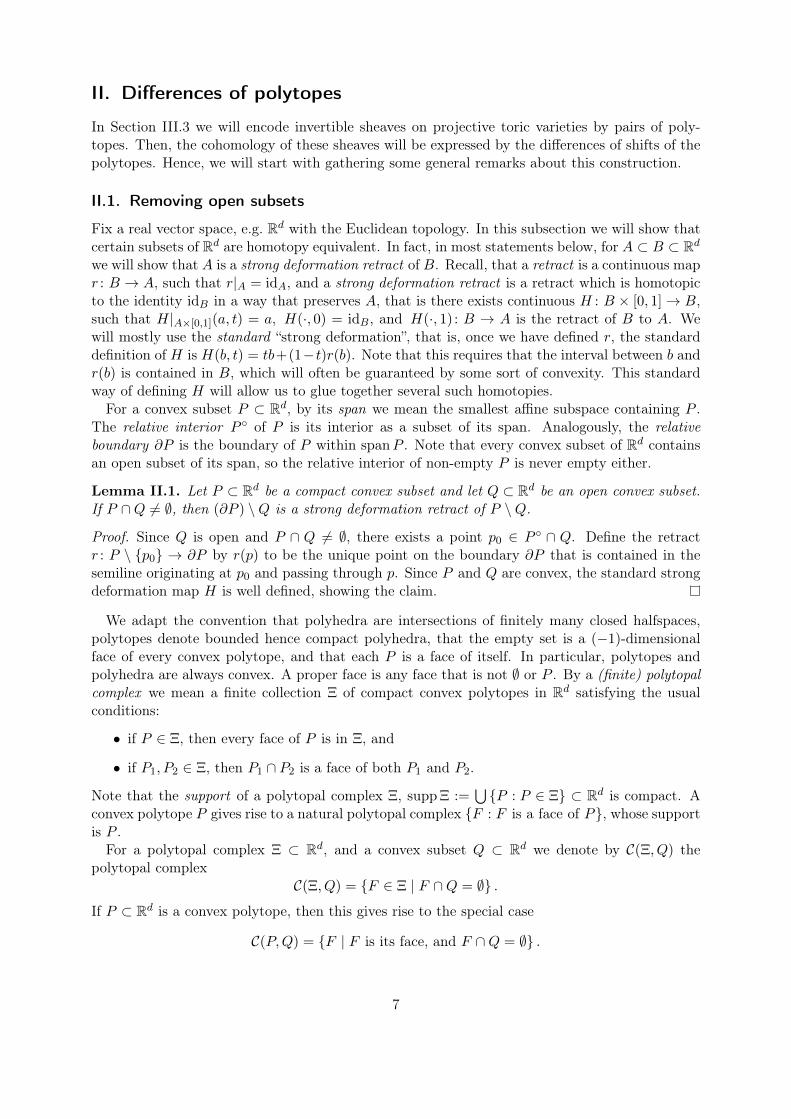
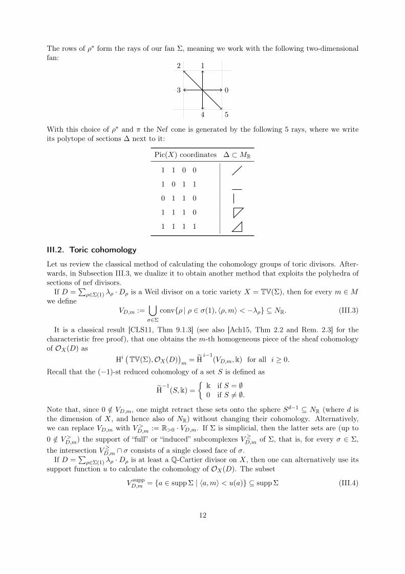
For example, for

P

Qwe get as C(P,Q).

This leads to an analogue of Lemma II.1 for P replaced with a polytopal complex.

Proposition II.2. Let Ξ be a polytopal complex and Q an open convex set. Then supp C(Ξ, Q)is a strong deformation retract of (supp Ξ) \Q.

Proof. We argue by induction on the number of elements (faces) of Ξ. If Q ∩ supp Ξ = ∅, orequivalently, C(Ξ, Q) = Ξ, then there is nothing to prove. So suppose P ∈ Ξ is such that P∩Q 6= ∅and assume that P has maximal possible dimension among such faces. Then there is no otherface F ∈ Ξ that intersects the relative interior P ◦. In particular, Ξ′ := Ξ \ {P} is a polytopalcomplex, such that supp Ξ′∩P = ∂P . By the inductive assumption, supp C(Ξ, Q) = supp C(Ξ′, Q)is a strong deformation retract of (supp Ξ′) \Q.It remains to show, that (supp Ξ′) \Q is a strong deformation retract of (supp Ξ) \Q. But this

follows directly by applying Lemma II.1.

II.2. Compact approximation of open semialgebraic sets

Now we will discuss a way of replacing a semialgebraic set in Rd with a homotopy equivalentsubset that is additionally closed in Rd.

Proposition II.3. Suppose X ⊂ Rd is a compact semialgebraic subset of Rd. Let φ : Rd → R bea continuous, piecewise polynomial function. Denote by φ>0 := φ−1((0,∞)) the set of points thatare mapped to the positive axis, and for ε ∈ R define φ≥ε := φ−1([ε,∞)). Then there exists a realnumber c > 0 such that for all 0 < ε ≤ c the intersection X ∩ φ≥ε is a strong deformation retractof X ∩ φ>0.

Proof. We may and will assume that X is contained in φ≥0. We use the Whitney stratificationof X, see for example [Tho69] or [Kal05]. We argue by restricting to one stratum of X at atime. When c is sufficiently small, then the strata whose closures do not intersect φ0 := φ−1(0)are contained in X ∩ φ≥ε. Hence the homotopy does not move these strata. The strata that arecontained in φ0 are neither existent in X ∩ φ≥ε nor X ∩ φ>0. Hence it is enough to consider thestrata whose closures intersect φ0, but are not contained in φ0. Let M be such a stratum, andsuppose that M has a maximal dimension among all such strata.Define M<ε ⊂M to be the intersection M ∩ φ−1(0, ε). Similar to the proof of Proposition II.2,

we can find a strong deformation retract ofM∩φ>0 onto (∂M∩φ>0)∪(M∩φ≥ε) = M \M<ε. Thenwe replace X with X ′ = X \ (M<ε ∪ φ0), and we can argue inductively to show the claim.

Suppose Q ⊂ Rd is a (compact) polytope defined by affine inequalities φi(v) ≥ 0 for i ∈{1, . . . , k}. Let ε > 0 be a positive real number. Then the ε-widening of Q (with respect to thecollection of inequalities {φi(v) ≥ 0 | i ∈ {1, . . . , k}}) is the set:

Q>−ε :={v ∈ Rd | ∀i φi(v) > −ε

}.

Note that Q>−ε is open and contains Q. The shape of Q>−ε may depend on the choice of theinequalities defining Q, but we will ignore this dependence in our notation, as it will be irrelevantto our statements.

8

Lemma II.4. Suppose P,Q ⊂ Rd are two polytopes. Then there exists a positive constant c > 0,such that for all 0 < ε ≤ c, the difference P \ Q>−ε is a strong deformation retract of P \ Q.Similarly, if Ξ is a polytopal complex, then supp Ξ \ Q>−ε is a strong deformation retract ofsupp Ξ \Q for sufficiently small ε.

Proof. Suppose Q = {φi(v) ≥ 0 | i ∈ {1, . . . , k}}. If the intersection Q ∩ P is empty, then thestatement is easy, just choose c such that P ∩Q>−c = ∅. So assume otherwise Q ∩ P 6= ∅ and fixa point v ∈ Q ∩ P . For any x ∈ P \Q consider the unique line `x passing through x and v. Let

cx = − 1

min {φi(y) | i ∈ {1, . . . , k} , y ∈ `x ∩ P}.

Note that cx > 0 and the set {cx | x ∈ P \Q} is closed, as its values are equal to those onsupp C(P,Q), which is compact. So let c = min {cx | x ∈ P \Q} and choose 0 < ε ≤ c. Then forevery x ∈ P \ Q the line `x has non-empty intersection with the compact set P \ Q>−ε. Definethe retract as x 7→ r(x) = v + λx(x − v) where λx = min {λ : λ ≥ 0, v + λx(x− v) ∈ P \Q>−ε}.The standard homotopy H(x, t) = tx+ (1− t)r(x) gives the desired strong deformation.Note that in the above arguments, r and H preserve faces of P , in the sense, that if F is a

(closed) face of P , and rF and HF are the retract and its deformation as above, but defined forF , then rF = rP |F and HF = HP |F×[0,1]. Thus, they glue well to define the appropriate retractand its strong deformation of supp Ξ \Q>−ε onto supp Ξ \Q.

As a collorary we have an analogue of Proposition II.2 and Lemma II.1 for polytopes Q:

Lemma II.5. Let Ξ ⊂ Rd be a polytopal complex, and let Q ⊂ Rd be a polytope. Then supp C(Ξ, Q)is a strong deformation retract of supp Ξ \ Q. In particular, if P ⊂ Rd is a polytope, thensupp C(P,Q) is a strong deformation retract of P \Q.

Proof. This is a combination of Lemma II.4 and Proposition II.2, together with an observationthat C(Ξ, Q) = C(Ξ, Q>−ε) for sufficiently small ε > 0.

Corollary II.6. Let P,Q ⊂ Rd be two polytopes and assume their intersection is nonempty. Then∂P \Q is homotopy equivalent to P \Q.

Proof. The complex of P consists of all faces of ∂P and in addition P . Since Q ∩ P 6= ∅, thecomplexes C(P,Q) and C(∂P,Q) are equal. Therefore, by Lemma II.5 both P \Q and ∂P \Q arehomotopy equivalent to supp C(P,Q) = supp C(∂P,Q).

II.3. Allowing common tail cones

Finally, we conclude this section with an argument that reduces considerations of homotopy typesof differences of (closed) polyhedra to the case of (compact) polytopes. A simplifying assumptionis that the polyhedra have the same tail cone. Recall that tail(P ) := {v ∈ Rd | P + v ⊆ P} is thepolyhedral cone indicating the unbounded directions of a polyhedron P .

Proposition II.7. Suppose P ⊂ Rd is a polyhedron with a pointed tail cone and Q ⊂ Rd is apolyhedron or the interior of a polyhedron with the same tail cone tailQ = tailP . Then thereexists a sequence of linear forms H1, . . . ,Hk and sufficiently large numbers t1, . . . , tk ∈ R, suchthat the truncated difference

Trunc(P \Q) := (P \Q) ∩⋂i

{Hi ≤ ti}

is compact and a strong deformation retract of P \Q.

9

Proof. Proceeding inductively on the number of rays of the common tail cone, we may assumethat there are polyhedra P ′ and Q′ with tailP ′ = tailQ′ not containing a certain ray ρ such thatP = P ′ + ρ and Q = Q′ + ρ. We choose a linear form H with H(ρ) > 0 that is non-positive ontailP ′ = tailQ′. Then there exists a real number t such that both P ′ and Q′ are contained in thehalfplane {H < t}. It follows that (P \ Q) ∩ {H ≤ t} is a strong deformation retract of P \ Q.Indeed, the map rρ : Rd → {H ≤ t} projecting along ρ does the job.

As a conclusion, we remark that the homotopy equivalences, such as that in Lemma II.5, arevalid also for polyhedra with common tail cones.

III. Toric geometry

The main subject of our paper is to investigate a toric variety X and its immaculacy locuswithin Cl(X). For this we will make use of the classical method of calculating the cohomology ofequivariant line bundles from the fan in NR. However, after introducing the usual toric notationin Subsection III.1, we will provide an alternative method using the momentum polyhedra in MRin Subsection III.3. It is appropriate to make the cohomology of equivariant line bundles or itsabsence visible.

III.1. Basic toric notation

All our toric varieties are normal. Our main references for dealing with toric varieties are [CLS11,Ful93, KKMSD73]. We denote by N the lattice of one-parameter subgroups of the torus actingon the toric variety, and by M the monomial lattice. Throughout Σ denotes a fan in N andX = TV(Σ) the corresponding toric variety. Occasionally, if there is more than one toric varietyinvolved, we may add a subscript NX , MX , ΣX ,. . . . For a cone σ in NR = N ⊗R orMR = M ⊗Rwe denote the dual cone in MR or NR, respectively, by σ∨ .The set of all cones of dimension k of a fan Σ is denoted Σ(k). Similarly, for a cone σ, by

σ(k) we mean the set of all faces of dimension k. In general, every cone σ generates a unique fanconsisting of all faces of σ, and the fan will be denoted by the same letter σ. In order to reduce thenotation, we will follow the standard convention to denote rays (one dimensional strictly convexlattice cones) and their primitive lattice generators by the same letter, usually ρ.We will frequently assume that our toric variety X is semiprojective, that is that it is projective

over an affine (toric) variety. This means that the fan of X has a convex support supp Σ ⊆ NR.Another assumption simplifying the notation in the proofs is that X has no torus factors. Inparticular, (with both these assumptions) the fan Σ is generated by cones of dimension equal todimX.Every Weil divisor on X is linearly equivalent to a torus invariant divisor D =

∑ρ∈Σ(1) λρ ·

Dρ with Dρ := orb(ρ). If in addition D is Q-Cartier, then there exists a continuous functionu : supp Σ→ R, which is linear on the cones of Σ, and such that u(ρ) = −λρ for every ρ ∈ Σ(1).In particular, for every maximal cone σ ∈ Σ there is a unique uσ ∈ MQ, such that u|σ = 〈·, uσ〉.We call u the support funtion of D. The divisor D is Cartier if and only if each uσ is containedin the lattice M .The polyhedron of sections ∆ = ∆(D) ⊂MR of an equivariant Weil divisor D is defined by its

inequalities:∆ = {r ∈MR | 〈ρ, r〉 ≥ −λρ for all ρ ∈ Σ(1)} .

10

The name was derived from the fact that ∆∩M provides a (monomial) basis of the global sectionsof OX(D). If D is in addition Q-Cartier, then we can describe it also as an intersection of shiftedcones that depend on the support function u:

∆ =⋂

σ maximal cone of Σ

(uσ + σ∨

).

A Q-Cartier Weil divisor D on a semiprojective toric variety X of dimension d is nef if andonly if its support function u is concave, that is, for all a, b ∈ supp Σ and for all 0 ≤ t ≤ 1, wehave u(ta + (1 − t)b) ≥ tu(a) + (1 − t)u(b). Equivalently, if a ∈ σ for some σ ∈ Σ(d), then forevery σ′ ∈ Σ(d) we have: 〈a, uσ〉 ≤ 〈a, uσ′〉. Another way to understand nefness is that all uσare contained in ∆; in fact, the set of its vertices equals the set {uσ}. Note that some of the uσmight coincide. Moreover, in contrast to the projective case treated, e.g., in [CLS11, (4.2)], forsemiprojective X, the polyhedron ∆ is no longer compact but has (supp Σ)∨ ⊆ MR as its tailcone. Nevertheless, one may still recover the support function of a nef divisor from its polyhedron∆ by

u(a) = min〈a,∆〉 := min{〈a, r〉 | r ∈ ∆}.

Note that the minimum is well-defined for a ∈ supp Σ = (tail ∆)∨.A fan Σ in NR ∼= Rd gives rise to a map ρ : ZΣ(1) → N , which takes the basis element indexed

by a ray of Σ to the corresponding primitive element on that ray in N . If the underlying toricvariety X = TV(Σ) has no torus factors, then the cokernel of ρ is finite. For simplicity, we alwaysassume that this is the case. If, moreover, X is smooth, then ρ is surjective. We denote the kernelby K, and we obtain a short exact sequence

0 // K // ZΣ(1) ρ // N.

It is well known that the so-called Gale dual of this sequence yields

0 Cl(X)oo DivT (X)πoo M

ρ∗oo 0,oo (III.1)

where DivT (X) =(ZΣ(1)

)∗ denotes the group of torus invariant Weil divisors on X. Note thatCl(X) may have torsion, which corresponds to the torsion of the cokernel of ρ. The anticanonicalclass of X is −KX = π(1). The set of effective classes is EffZ(X) = π

(ZΣ(1)≥0

), although often

we really consider the effective cone EffR(X) = π(RΣ(1)≥0

), where π is now considered as the map

RΣ(1) → Cl(X)⊗ R.

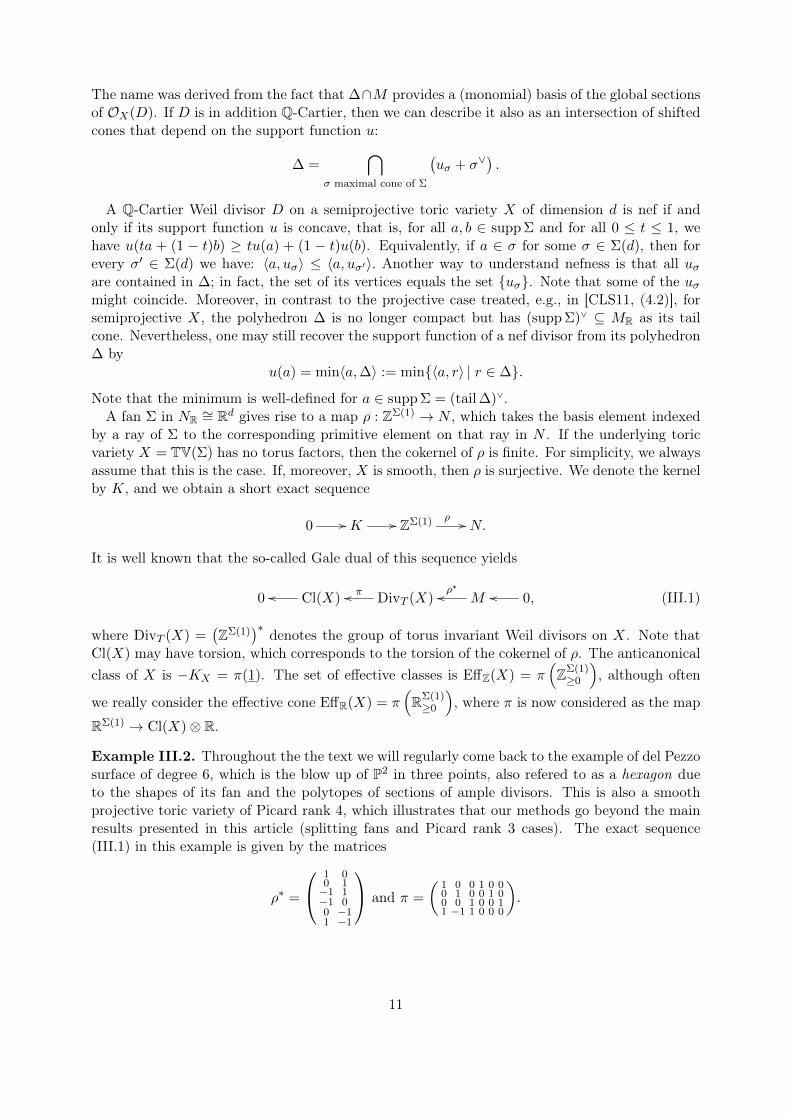
Example III.2. Throughout the the text we will regularly come back to the example of del Pezzosurface of degree 6, which is the blow up of P2 in three points, also refered to as a hexagon dueto the shapes of its fan and the polytopes of sections of ample divisors. This is also a smoothprojective toric variety of Picard rank 4, which illustrates that our methods go beyond the mainresults presented in this article (splitting fans and Picard rank 3 cases). The exact sequence(III.1) in this example is given by the matrices

ρ∗ =

1 00 1−1 1−1 00 −11 −1

and π =

(1 0 0 1 0 00 1 0 0 1 00 0 1 0 0 11 −1 1 0 0 0

).

11

The rows of ρ∗ form the rays of our fan Σ, meaning we work with the following two-dimensionalfan:

0

12

3

4 5

With this choice of ρ∗ and π the Nef cone is generated by the following 5 rays, where we writeits polytope of sections ∆ next to it:

Pic(X) coordinates ∆ ⊂MR

1 1 0 0

1 0 1 1

0 1 1 0

1 1 1 0

1 1 1 1

III.2. Toric cohomology

Let us review the classical method of calculating the cohomology groups of toric divisors. After-wards, in Subsection III.3, we dualize it to obtain another method that exploits the polyhedra ofsections of nef divisors.If D =

∑ρ∈Σ(1) λρ ·Dρ is a Weil divisor on a toric variety X = TV(Σ), then for every m ∈ M

we defineVD,m :=

⋃σ∈Σ

conv{ρ | ρ ∈ σ(1), 〈ρ,m〉 < −λρ} ⊆ NR. (III.3)

It is a classical result [CLS11, Thm 9.1.3] (see also [Ach15, Thm 2.2 and Rem. 2.3] for thecharacteristic free proof), that one obtains the m-th homogeneous piece of the sheaf cohomologyof OX(D) as

Hi(TV(Σ),OX(D)

)m

= H̃i−1

(VD,m, k) for all i ≥ 0.

Recall that the (−1)-st reduced cohomology of a set S is defined as

H̃−1

(S, k) =

{k if S = ∅0 if S 6= ∅.

Note that, since 0 /∈ VD,m, one might retract these sets onto the sphere Sd−1 ⊆ NR (where d isthe dimension of X, and hence also of NR) without changing their cohomology. Alternatively,we can replace VD,m with V >

D,m := R>0 · VD,m. If Σ is simplicial, then the latter sets are (up to0 /∈ V >

D,m) the support of “full” or “induced” subcomplexes V ≥D,m of Σ, that is, for every σ ∈ Σ,the intersection V ≥D,m ∩ σ consists of a single closed face of σ.If D =

∑ρ∈Σ(1) λρ ·Dρ is at least a Q-Cartier divisor on X, then one can alternatively use its

support function u to calculate the cohomology of OX(D). The subset

V suppD,m = {a ∈ supp Σ | 〈a,m〉 < u(a)} ⊆ supp Σ (III.4)

12

contains V >D,m as a strong deformation retract. One can easily prove this using homotopies as

in Subsection II.1. See [CLS11, Theorem 9.1.3] for a slightly weaker claim. Actually, in the original[KKMSD73, p.42], it was exactly the sets V supp

D,m which were used to describe Hi(TV(Σ),OX(D)

)m.

III.3. Cohomology using polyhedra

From now on we assume X to be a semiprojective toric variety, in particular it is quasiprojective.Let Y be a projective toric variety containing X as an open torus invariant subset. Fix a torusinvariant ample Cartier divisor L on Y such that L+KY is effective, where KY = −

∑ρ∈ΣY (1)Dρ

is the canonical divisor of Y . Then the piecewise linear function ‖ · ‖ := −u corresponding to Lis a norm on the vector space NR. The closed balls centred at 0 with respect to this norm areconvex polytopes, whose vertices are on rays of ΣY .Since X is quasiprojective, every Q-Cartier Weil divisor is a difference of nef divisors: D =

D+ −D−, with both D+ and D− nef Q-Cartier Weil [CLS11, Thm 6.3.22(a)]. Thus every suchCartier divisor on X = TV(Σ) is (non-uniquely) represented by a pair of polyhedra (∆+,∆−)sharing the same tail cone |Σ|∨ ⊆ MR. Polyhedra form a semigroup under Minkowski addition.Restricting to polyhedra with a fixed tail cone, one ensures that this semigroup is cancellative.In this context, the pair (∆+,∆−) represents the formal difference D = ∆+ − ∆− within theGrothendieck group of generalized polyhedra.The goal of this section is to reinterprete the toric cohomology in terms of this pair of polyhedra.

Lemma III.5. Let X be a semiprojective toric variety with no torus factors and D = D+ −D−be a Q-Cartier Weil divisor on X with D+ and D− nef. Assume that ∆+ and ∆− are theassociated polyhedra of D+ and D− and denote by u the support function of D. Then the setsV suppD,0 = {a ∈ supp Σ | u(a) > 0} ⊆ supp Σ and ∆− \∆+ are homotopy equivalent.

Proof. Let u± be the support functions of the nef divisors D±. For each full-dimensional σ ∈ Σ wedenote by u+

σ ∈ ∆+ and u−σ ∈ ∆− the unique vertices minimising 〈a, •〉 on the respective polytopesfor a ∈ intσ, hence for all a ∈ σ. Thus, for a ∈ σ, we have min〈a,∆±〉 = 〈a, u±σ〉 = u±(a).Moreover, we can write

V suppD,0 = {a ∈ supp Σ | u−(a) < u+(a)}.

Since V suppD,0 ⊆ NR and ∆− \ ∆+ ⊆ MR are contained in mutually dual spaces, we are going to

compare these two sets via the following incidence set:

W := {(a, r) ∈ V suppD,0 × (∆− \∆+)

∣∣ 〈a, r〉 < u+(a)}.

It comes with two natural, surjective projections

WpVvvvv

p∆

** **NR ⊇ V supp

D,0 ∆− \∆+ ⊆MR,

with contractible fibers: Let us start with checking the map pV . If a ∈ V suppD,0 , then there is a cone

σ ∈ Σ containing a, and we obtain that

p−1V (a) ∼= {r ∈ ∆− \∆+ | 〈a, r〉 < 〈a, u+

σ 〉} = {r ∈ ∆− | 〈a, r〉 < 〈a, u+σ 〉}.

Obviously, the latter is a convex set. However, it is non-empty, too. The reason is that the facta ∈ V supp

D,0 (together with a ∈ σ) implies that min〈a,∆−〉 < 〈a, u+σ 〉. We turn to the second map

p∆. Fixing an element r ∈ ∆− \∆+ ⊆ ∆− we have

p−1∆ (r) ∼= {a ∈ V supp

D,0 | 〈a, r〉 < u+(a)} = {a ∈ NR | 〈a, r〉 < min〈a,∆+〉}.

13

Again, the latter is a convex set and, because r /∈ ∆+, it is non-empty, too.Now, the idea is to apply results around the Vietoris mapping theorem. We are going to use the

stronger version from [Sma57]. Taking into account Whitehead’s theorem, the criterion of Smalesays that a proper surjective continuous map f : X → Y between two CW complexes X ⊂ Rnand Y ⊂ Rm is a homotopy equivalence if its fibers f−1(y) (for all y ∈ Y ) are contractible andlocally contractible.Since our maps pV and p∆ are not proper yet, we will replace the three objects in the above

diagram with homotopy equivalent gadgets which are all compact. Recall the notions of sufficientlylarge truncation Trunc(∆−) of ∆− as in Proposition II.7 and the ε-widening (∆+)>−ε as inSubsection II.2. For any R > 0 and any sufficiently small ε > 0 we consider the following threecompact sets:

V suppD,0 (R, ε) := {a ∈ supp Σ | u(a) ≥ ε and ‖a‖ ≤ R} ,W (R, ε) :=

{(a, r) ∈ supp Σ× Trunc(∆−) | 〈a, r〉 ≤ u+(a)− ε, u(a) ≥ ε, and ‖a‖ ≤ R

}, and

Trunc(∆−) \ (∆+)>−ε.

By the results from Section II.1 these are homotopy equivalent to VD,0, W , and ∆− \∆+, respect-ively (see Lemma II.4, Propositions II.3 and II.7). We need to carefully choose the inequalitiesused in the ε-widening so that the projection W (R, ε) → Trunc(∆−) \ (∆+)>−ε is well definedand surjective. Then with the same arguments as above we show that the fibres of projectionsW (R, ε) → V supp

D,0 (R, ε) and W (R, ε) → Trunc(∆−) \ (∆+)>−ε are non-empty convex polytopes.Thus by the criterion of Smale, the projection maps are homotopy equivalences, and consequently,VD,0 is homotopy equivalent to ∆− \∆+.

Theorem III.6. Let X be a semiprojective toric variety and D = D+ − D− be a Q-CartierWeil divisor on X with D+ and D− nef. Denote by ∆+ and ∆− the polyhedra of D+ and D−,respectively. Then Hi(X,O(D)) =

⊕m∈M H̃

i−1(∆− \ (∆+ −m),k).

Proof. We will show that Hi(X,O(D))m = H̃i−1

(∆− \ (∆+ − m), k). From Subsection III.2together with Lemma III.5 we obtain this claim for m = 0.For general m ∈M we define D(m) := D+div(xm) = D+

∑a∈Σ(1)〈a,m〉 ·Da. Compared with

D, its associated sheaf is twisted with OX(m) := OX(

div(xm))

= x−m ·OX . Since the polyhedra∆± encode, for each affine chart, the minimal generators of the sheaves OX(D±), this means thatthe divisor D(m) is represented by the pair (∆+−m,∆−) or, equivalently, by (∆+,∆−+m). Inparticular, for the support functions we have uD(m) = uD −m. Thus, VD(m),0 = VD,m.

Remark III.7. Note that the presentation of a toric divisor D = D+ −D− as a difference of nefdivisors is by far not unique. Thus, one of the consequences of Theorem III.6 is that the reducedcohomology of the difference of polyhedra is independent of the choice of this presentation. Inparticular, choosing a suitable semiprojective toric variety X, for any three rational polyhedra∆0,∆1,∆2 in MR with the same tail cone, the differences ∆1 \∆2 and (∆1 + ∆0) \ (∆2 + ∆0) arehomotopy equivalent.

Remark III.8. Suppose X is a projective toric variety and D is a Q-Cartier Weil divisor on X.Observe that despite that there are at most finitely many degrees m for which Hi(O(D))m 6= 0,in the definitions of VD,m and V supp

D,m it is not immediately clear, which m ∈ M can potentiallylead to nonzero cohomology. Instead, the description in Theorem III.6 provides such a criterion.If ∆− and ∆+ + m are disjoint, then the difference is contractible. We will elaborate more onthis criterion in a follow up article about related computational issues.

14

Remark III.9. Let the Q-Cartier Weil divisor D be encoded by the pair of polyhedra (∆+,∆−).Then, the polyhedron of sections ∆(D) mentioned in Subsection III.1 can be recovered as

∆(D) =⋂r∈∆−

(∆+ − r) = {r ∈MR | ∆− + r ⊆ ∆+}.

Example III.10. If D is a nef divisor on a projective toric variety X, one can choose ∆− = {0},and then the formula from Remark III.9 implies ∆ = ∆(D) = ∆+. Thus for r ∈ ∆ the set∆− \ (∆+ − r) is empty (thus only has 1-dimensional (−1)st cohomology), or for r /∈ ∆ theset ∆− \ (∆+ − r) is a single point, hence it has no reduced cohomology at all. Therefore,h0(X,O(D)) = #(∆ ∩M) and Hi(X,O(D)) = 0 for all i > 0.

Example III.11. If on the other hand −D is a nef divisor, then ∆+ = {0}, and ∆− is thepolytope of −D. Let i = dim ∆−. Thus for r ∈ − relint ∆− the set ∆− \ (∆+ − r) is homotopicto a sphere of dimension i − 1, while for r /∈ − relint ∆− the set ∆− \ (∆+ − r) is contractible.Therefore, hi(X,O(D)) = #(relint ∆− ∩M) and Hj(X,O(D)) = 0 for all j 6= i.

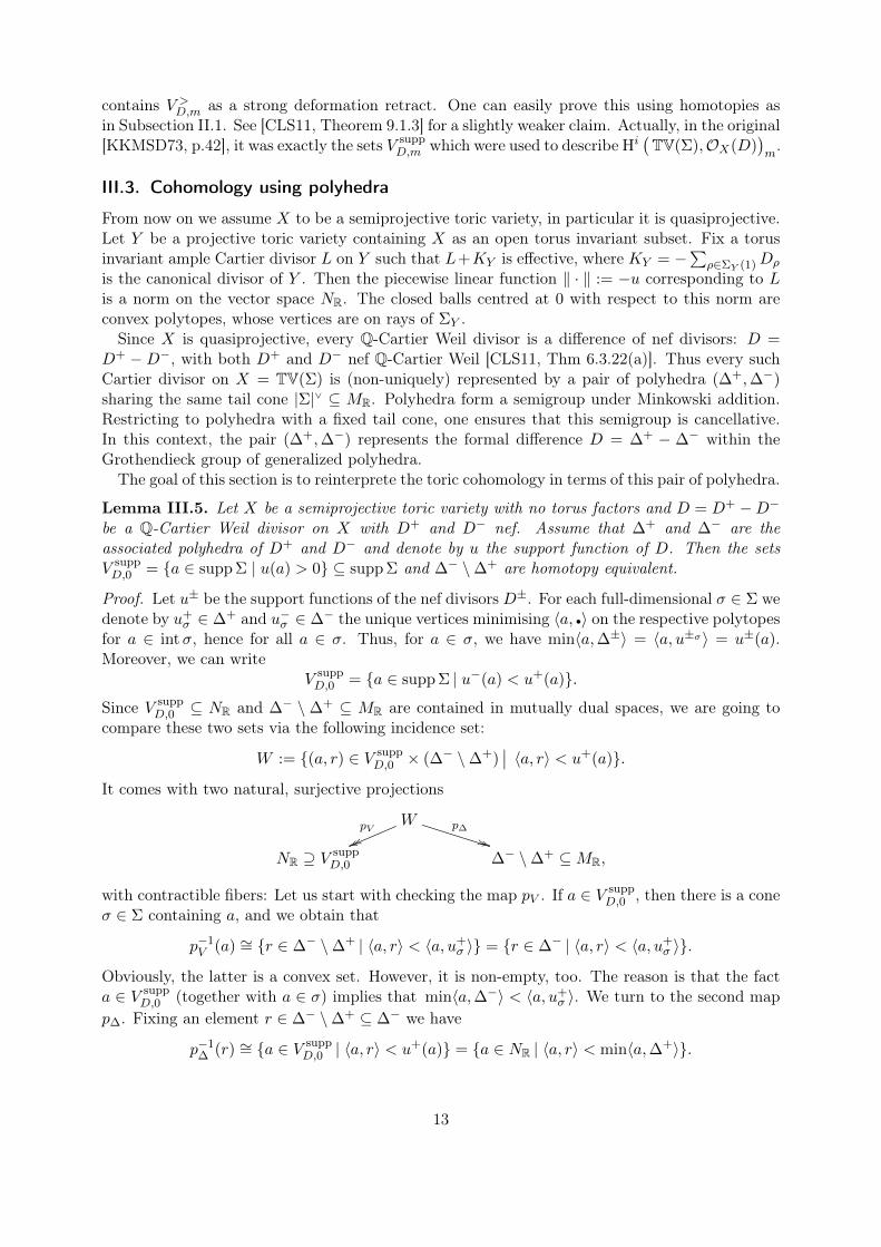
−1

−1

1

VD,0 ρ2

ρ1

ρ3

Figure 1: The fan of X = P2 \ [0, 0, 1], the divisor D = −Dρ1 − Dρ2 + Dρ3 ' OX(−1), and thecomplex VD,0 consisting of 2 points responsible for H1(OX(D))0 6= 0.

The claim of Theorem III.6 does not hold for quasiprojective toric varieties, that are not semi-projective. To see this, consider X = P2 \ {[0, 0, 1]} and let D ' OX(−1) be the negative ofthe hyperplane divisor. Then D+ ' 0 and D− ' OX(1), the polytopes are a point and a basictriangle, respectively. Thus ∆− \ (∆+ − m) is always non-empty and contractible, hence thedifference never has any reduced cohomologies. But H1(OX(−1)) 6= 0 as shown on Figure 1.

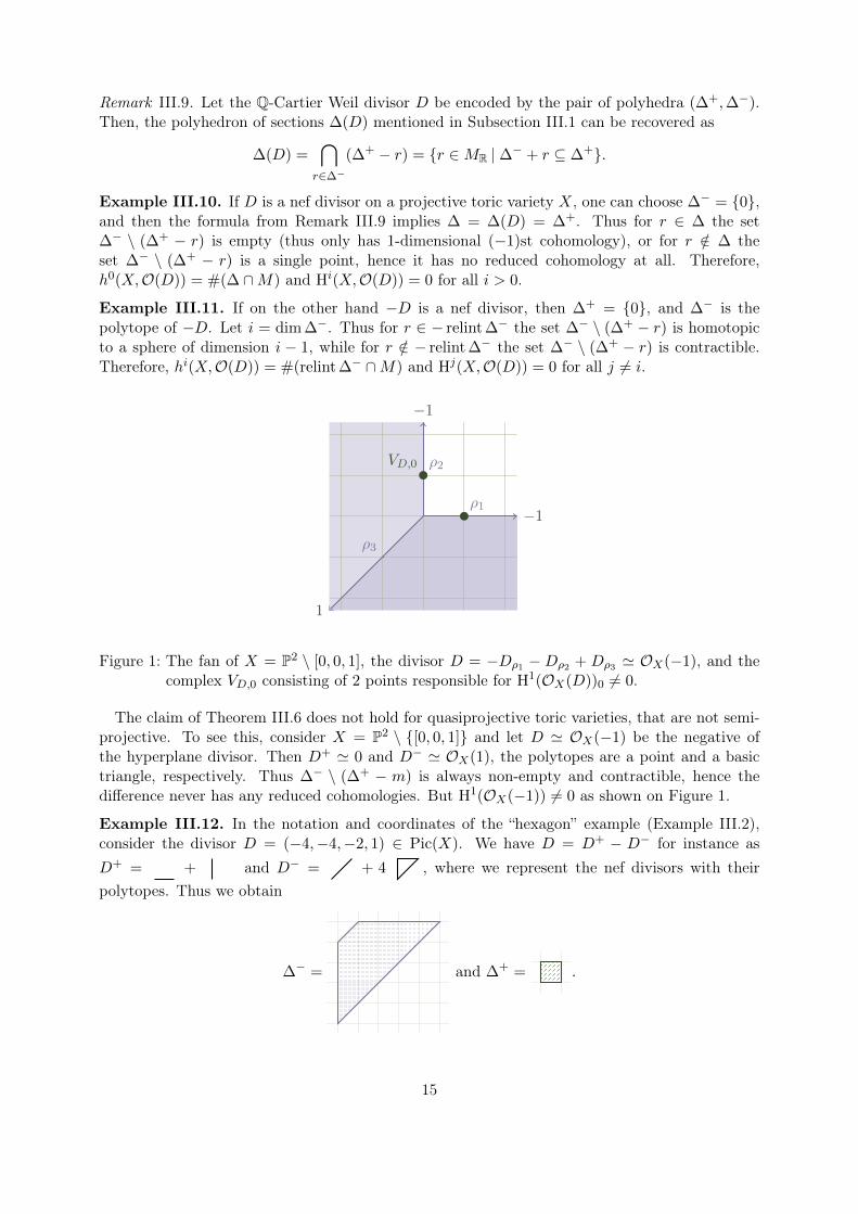
Example III.12. In the notation and coordinates of the “hexagon” example (Example III.2),consider the divisor D = (−4,−4,−2, 1) ∈ Pic(X). We have D = D+ − D− for instance asD+ = + and D− = + 4 , where we represent the nef divisors with theirpolytopes. Thus we obtain

∆− = and ∆+ = .

15

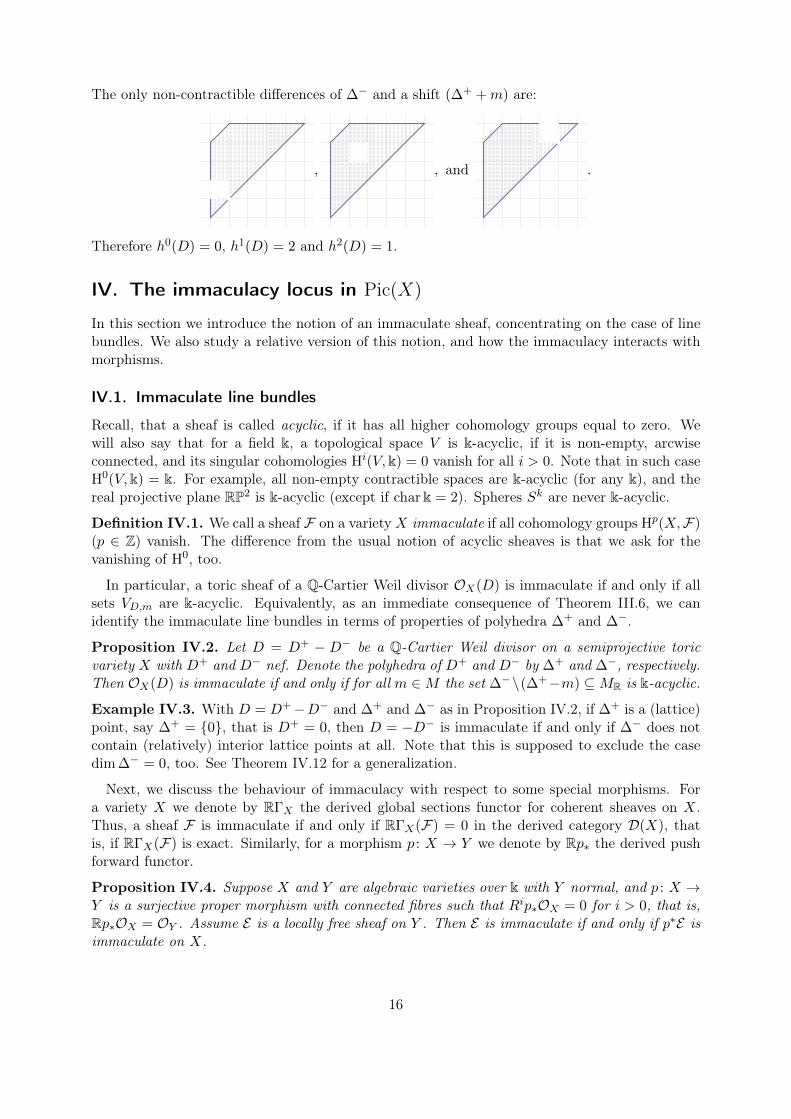
The only non-contractible differences of ∆− and a shift (∆+ +m) are:

, , and .

Therefore h0(D) = 0, h1(D) = 2 and h2(D) = 1.

IV. The immaculacy locus in Pic(X)

In this section we introduce the notion of an immaculate sheaf, concentrating on the case of linebundles. We also study a relative version of this notion, and how the immaculacy interacts withmorphisms.

IV.1. Immaculate line bundles

Recall, that a sheaf is called acyclic, if it has all higher cohomology groups equal to zero. Wewill also say that for a field k, a topological space V is k-acyclic, if it is non-empty, arcwiseconnected, and its singular cohomologies Hi(V,k) = 0 vanish for all i > 0. Note that in such caseH0(V,k) = k. For example, all non-empty contractible spaces are k-acyclic (for any k), and thereal projective plane RP2 is k-acyclic (except if char k = 2). Spheres Sk are never k-acyclic.

Definition IV.1. We call a sheaf F on a varietyX immaculate if all cohomology groups Hp(X,F)(p ∈ Z) vanish. The difference from the usual notion of acyclic sheaves is that we ask for thevanishing of H0, too.

In particular, a toric sheaf of a Q-Cartier Weil divisor OX(D) is immaculate if and only if allsets VD,m are k-acyclic. Equivalently, as an immediate consequence of Theorem III.6, we canidentify the immaculate line bundles in terms of properties of polyhedra ∆+ and ∆−.

Proposition IV.2. Let D = D+ − D− be a Q-Cartier Weil divisor on a semiprojective toricvariety X with D+ and D− nef. Denote the polyhedra of D+ and D− by ∆+ and ∆−, respectively.Then OX(D) is immaculate if and only if for all m ∈M the set ∆−\(∆+−m) ⊆MR is k-acyclic.

Example IV.3. With D = D+−D− and ∆+ and ∆− as in Proposition IV.2, if ∆+ is a (lattice)point, say ∆+ = {0}, that is D+ = 0, then D = −D− is immaculate if and only if ∆− does notcontain (relatively) interior lattice points at all. Note that this is supposed to exclude the casedim ∆− = 0, too. See Theorem IV.12 for a generalization.

Next, we discuss the behaviour of immaculacy with respect to some special morphisms. Fora variety X we denote by RΓX the derived global sections functor for coherent sheaves on X.Thus, a sheaf F is immaculate if and only if RΓX(F) = 0 in the derived category D(X), thatis, if RΓX(F) is exact. Similarly, for a morphism p : X → Y we denote by Rp∗ the derived pushforward functor.

Proposition IV.4. Suppose X and Y are algebraic varieties over k with Y normal, and p : X →Y is a surjective proper morphism with connected fibres such that Rip∗OX = 0 for i > 0, that is,Rp∗OX = OY . Assume E is a locally free sheaf on Y . Then E is immaculate if and only if p∗E isimmaculate on X.

16

Figure 2: The church of the Immaculate Conception of Blessed Virgin Mary in Warsaw. Theshape of the roof resembles an illustration of a line bundle.

Proof. This follows from RΓY E = RΓY (Rp∗p∗E) = RΓX(p∗E).

The assumptions of Proposition IV.4 are satisfied in the typical setting of the morphisms arisingfrom the Minimal Model Program.

Corollary IV.5. Suppose X and Y are toric varieties, and p : X → Y is a surjective toricprojective morphism with connected fibres, that is a toric projective morphism corresponding to asurjective map of one-parameter subgroups lattices NX → NY . Assume E is a locally free sheafon Y . Then E is immaculate if and only if p∗E is immaculate.

Proof. To apply Proposition IV.4 we must ensure that Rip∗OX = 0 for i > 0. For this, we mayassume that Y is affine and have to check that Hi(OX) = 0. Since p is projective, the support ofthe fan ΣX of X is a convex cone. Thus for m ∈ MX the m-th grading of Hi(OX) is calculatedby V supp

0,m = {a ∈ supp ΣX | 〈a,m〉 < 0} which is convex, hence either contractible or empty.

Example IV.6. In the notation of Example III.2 (“hexagon”), consider the divisor

D = (−2,−2,−2,−2) = −2 .

It is a pullback of the immmaculate line bundle OP2(−2) under the blow-down map to P2 (con-tracting three disjoint exceptional divisors), thus D is also immaculate.

IV.2. Relative immaculacy and affine spaces of immaculate line bundles

The main goal of this subsection is to explain the occurrence of some infinite families of immaculateline bundles. For this we present a more restrictive notion than plain immaculacy, which leads toa construction of such families.

Definition IV.7. Suppose p : X → Y is a morphism of algebraic varieties. We say that a sheafF on X is p-immaculate if the direct image sheaves Rip∗F vanish in all cohomological degreesi ∈ Z, that is, if Rp∗F = 0 is exact.

17

Clearly, a sheaf on X is immaculate if and only if it is p-immaculate for the map p : X → {∗}.Moreover, for any map p : X → Y , the equality RΓX = RΓY ◦Rp∗ implies that each p-immaculatesheaf is automatically immaculate. And, finally, it is a consequence of cohomology and base changethat for a flat morphism the relative immaculacy of locally free sheaves can be checked fiberwise:

Proposition IV.8. Suppose that p : X → Y is a flat proper morphism of algebraic varieties. LetE be a locally free sheaf on X and for y ∈ Y denote by Xy := f−1(y) the fiber of y. Then E isp-immaculate if and only if Ey := E|Xy is immaculate for every closed point y.

Proof. If E|Xy is immaculate for every closed point y, then the functions y 7→ dim Hi(Xy, E|Xy)are constantly equal to 0, on closed points. Hence, by semicontinuity [Mum08, Cor. 1 in Sect. 5,p. 50], they are also zero on non-closed points. Thus by the implication (i) =⇒ (ii) in [Mum08,Cor. 2 in Sect. 5, pp. 50–51], the sheaf Rip∗(E) is locally free and zero at every point of Y , thatis Rip∗(E) = 0.If E is p-immaculate, then for sufficiently large i the equivalent conditions of [Mum08, Cor. 2 in

Sect. 5, pp. 50–51] are satisfied, hence by the last paragraph of that corollary the map Ri−1p∗(E)⊗κ(y) → Hi−1(Xy, E|Xy) is an isomorphism. Moreover, Ri−1p∗(E) = 0, hence the condition (ii) issatisfied for a smaller value of i and hence also condition (i) is satisfied. Going down with i, weeventually get the claim.

Proposition IV.9. Suppose that X and Y are varieties and p : X → Y is a morphism. Assumethat F is a p-immaculate coherent sheaf on X. Then, for any locally free sheaf E on Y , the sheafF ⊗ p∗E is p-immaculate, hence immaculate.

Proof. The projection formula implies Rip∗(F ⊗ p∗E) = Rip∗F ⊗ E and the latter is zero by thedefinition of a p-immaculate sheaf.

While the previous claims followed from rather standard arguments, it is quite nice that, in theprojective setting, also the converse of the above statement holds true:

Theorem IV.10. Suppose X and Y are varieties, p : X → Y is a morphism, and Y is projective.Assume F is a coherent sheaf on X, and L is an ample line bundle on Y . Then the followingconditions are equivalent.

(a) F is p-immaculate,

(b) for any locally free sheaf E on Y the sheaf F ⊗ p∗E is immaculate,

(c) for any Cartier divisor D on Y the sheaf F ⊗OX(p∗D) is immaculate,

(d) for any integer k > 0 the sheaf F ⊗ p∗L⊗k is immaculate.

Proof. The implication (a) =⇒ (b) is shown in Proposition IV.9. The implications (b) =⇒ (c) =⇒(d) are clear. Thus we only have to show (d) =⇒ (a).By the derived projection formula (Rp∗F) ⊗ L⊗k ' Rp∗(F ⊗ p∗L⊗k) in D(Y ). Applying the

derived global sections functor RΓY we obtain that

RΓY (Rp∗F ⊗ L⊗k))q.is.' (RΓY ◦ Rp∗)(F ⊗ p∗L⊗k) = RΓX(F ⊗ L⊗k) = 0

by our assumption in (d). The entries in the second table, that is, in the E2 layer of the spectralsequence for RΓY (Rp∗F ⊗ L⊗k)) are Hi(Y, Rjp∗F ⊗ L⊗k) for varying i, j.

18

By Serre vanishing, for sufficiently large k, we have Hi(Rjp∗F ⊗ L⊗k) = 0 for all i > 0 and allj. Hence for such k the spectral sequence stabilises immediately and thus (since it converges to0) also the H0 row is identically zero. That is H0(Rjp∗F ⊗ L⊗k) = 0 for all sufficiently large k.Hence Rjp∗F is a coherent sheaf on a projective variety Y , whose corresponding graded moduleis zero for all sufficiently large degrees. Therefore, still for all j, the sheaves Rjp∗F are identicallyzero by [Har77, Exercise II.5.9(c)], which is the content of (a).

We now switch our attention back to toric varieties. Our goal is to reinterprete p-immaculacyand apply Theorem IV.10 in terms of toric geometry. The following statement captures ourmain reason to study the cohomology of divisors on semiprojective varieties, despite that we areprincipally interested in projective varieties. For a projective toric morphism X → Y , we canrestrict to an open affine subset of Y , and our theory still works, despite that we no longer livein the projective world. Technically, the following characterization of p-immaculacy differs fromthe characterisation of plain immaculacy in Proposition IV.2 just by enlarging the tail cones.

Proposition IV.11. Suppose p : X → Y is a toric map of semiprojective toric varieties, andlet p∗ : MY → MX be the corresponding map of monomial lattices. Let D be a Q-Cartier Weildivisor on X and write D = D+ − D− as a difference of nef divisors, as usual. Then OX(D)is p-immaculate if and only if for all maximal cones σ in the fan of Y and for all m ∈ MX thedifference (∆− + p∗(σ∨)) \ (∆+ + p∗(σ∨)−m) is k-acyclic.

Proof. Let ΣY be the fan of Y and for a maximal cone σ ∈ Σ(dimY ) denote by Uσ the openaffine subset of Y corresponding to σ. By [Har77, Prop. III.8.5] the sheaf OX(D) is p-immaculateif and only if Hi(Op−1(Uσ)(D)) = 0 for all i and for all σ ∈ ΣY (dimY ). Equivalently, for all σ therestriction of D to p−1(Uσ) is immaculate. The restriction of D+ to p−1(Uσ) is still nef and thepolyhedron of the restriction is equal to ∆+ + p∗(σ∨). Anologous statements hold for D− and∆−. Therefore, the claim follows from Proposition IV.2 applied to each p−1(Uσ) separately.

A sublattice M ′ ⊂ M is saturated if M ∩M ′R = M ′ (the intersection is taken in MR). Fora rational polyhedron ∆ ⊂ MR define its linear sublattice span to be the smallest saturatedsublattice M ′ ⊂ M containing a translate of ∆. Therefore ∆ ⊂ m + M ′R for any m ∈ ∆, anddim ∆ = dimM ′.The following theorem can be interpreted as a relative version of Example IV.3.

Theorem IV.12. Assume X is a projective toric variety, D− is a nef Q-Cartier Weil divisor,and D′ is a nef Cartier divisor on X. Suppose ∆− and ∆′ are their respective polytopes, and letM ′ ⊂ M be the linear sublattice span of ∆′. Let Y be the projective toric variety correspondingto ∆′ and p : X → Y be the natural map of toric varieties. Then the following conditions areequivalent.

(1) For all integers a the divisors aD′ −D− are immaculate on X.

(2) For infintely many integers a the divisors aD′ −D− are immaculate.

(3) The image of ∆− under the projection ϕ : MR → MR/M ′R

=(M/M ′)⊗ R has no lattice

points in the relative interior.

(4) The divisor −D− is p-immaculate.

19

Proof. The implication (1) =⇒ (2) is clear.To show (2) =⇒ (3) we consider two cases, positive or negative. That is, among the integers

a such that Da := aD′ − D− is immaculate, there exists a subsequence either of positive aiconverging to +∞ or of negative ai converging to −∞.In the positive case, suppose by contradiction, that there exist an interior lattice point of

ϕ(∆−). Replacing ∆− with its translate (and D− with a linearly equivalent divisor) if necessary,we may assume that, say, 0 ∈ relintϕ(∆−). Choosing a subsequence if necessary, assume thatevery |ai|∆′ has a lattice point mi ∈ M in the relative interior such that the distance (withrespect to any fixed norm on MR) of mi to the boundary ∂(|ai|∆′) converges to +∞. A nefdecomposition of Dai = aiD

′ −D− is exactly D+ai = aiD

′ and D−ai = D−. By Proposition IV.2for any i the difference ∆− \ (ai∆

′ −mi) is k-acyclic. Since ∆− is compact, taking ai very largewe have ∆− \ (ai∆

′−mi) = ∆− \M ′R. By the criterion of [Sma57], the restricted projection mapϕ : ∆−\M ′R → ϕ(∆′)\{0} is a homotopy equivalence, a contradiction, since the first one ∆−\M ′Ris k-acyclic, and the latter one ϕ(∆−)\{0} is either homeomorphic to a sphere (if dimϕ(∆−) > 0)or empty (if ϕ(∆−) = {0}).In the negative case, the nef decomposition of Dai is D+

ai = 0 and D−ai = D− − aiD′. By

Example IV.3 for any ai the Minkowski sum ∆− + |ai|∆′ has no lattice points in the relativeinterior. Taking |ai| very large, we see that there are no lattice points in the relative interior of∆− +M ′R. Equivalently, there is no (relative) interior lattice point in ϕ(∆−). This concludes theproof of (2) =⇒ (3).Next we prove (3) =⇒ (1). Assume (by shifting ∆′ if necessary) that ∆′ ⊆ M ′R, that is, that

ϕ(∆′) equals 0 ∈M/M ′ . Assume a is a nonnegative integer. We must show that

• the Minkowski sum ∆−+a∆′ has no interior lattice points (hence −D−−aD′ is immaculate),and

• ∆− \ (a∆′ −m) is contractible and non-empty for all m ∈ M (hence −D− + aD′ has nocohomology in degree m).

The first claim is straightforward: Such an interior lattice point would be mapped to an interiorlattice point of ϕ(∆−), which is impossible by the assumptions of (3). Also the second claim is easy.Let P := (a∆′−m)∩∆−, which is a convex set contained in ∆− such that ∆−\(a∆′−m) = ∆−\P .Since ∆′ is contained inM ′R, also a∆′ ⊂M ′R, and consequently P ⊂M ′R−m. If ϕ(−m) = ϕ(P ) /∈ϕ(∆−), then P is disjoint with ∆− and ∆− \ P = ∆−, which is contractible and non-empty asclaimed. Since ϕ(∆−) has no interior lattice points, it remains to consider ϕ(−m) ∈ ∂(ϕ(∆−))and, consequently, P ⊂ ∂∆−. So the difference is nonempty and by Corollary II.6 it is homotopicto ∂∆− \ P , which is contractible (a sphere with a convex disc taken out).To show (1)⇐⇒ (4) note that D′ = p∗L for an ample line bundle L on Y . We apply the

implications (d) =⇒ (a) =⇒ (c) of Theorem IV.10.

The following examples obey the notation of Theorem IV.12.

Example IV.13. If ∆′ is full dimensional, that is if D′ is big, then there is no antinef divisorwhich is p-immaculate, as in this case, M ′ is the whole lattice M , and ϕ(∆−) is a point, thushaving an interior lattice point by definition.

Example IV.14. If ∆′ is just a point, then M ′ = 0 and the question becomes whether ∆−

contains any interior lattice points, as already discussed in Example IV.3.

20

Example IV.15. If ∆′ has codimension one, then M ′ is a hyperplane. The divisor −D− isp-immaculate if ∆− cannot be divided by integral shifts of M ′. In case D− is in addition Cartier,this is equivalent to

max〈∆−,M ′〉 −min〈∆−,M ′〉 ≤ 1,

where we think of the hyperplane M ′ ⊂M as a primitive element of N dual to the hyperplane.

Example IV.16. In the hexagon case (Example III.2), let D′ = (1, 1, 0, 0) so that ∆′ = , and

let D− = (1, 1, 1, 0) so that ∆− = . Then all combinations aD′−D− = (a−1, a−1,−1, 0) areimmaculate. Other lines of immaculate divisors on this surface are listed in Table 2 in Section IX.

V. Immaculacy by avoiding temptations

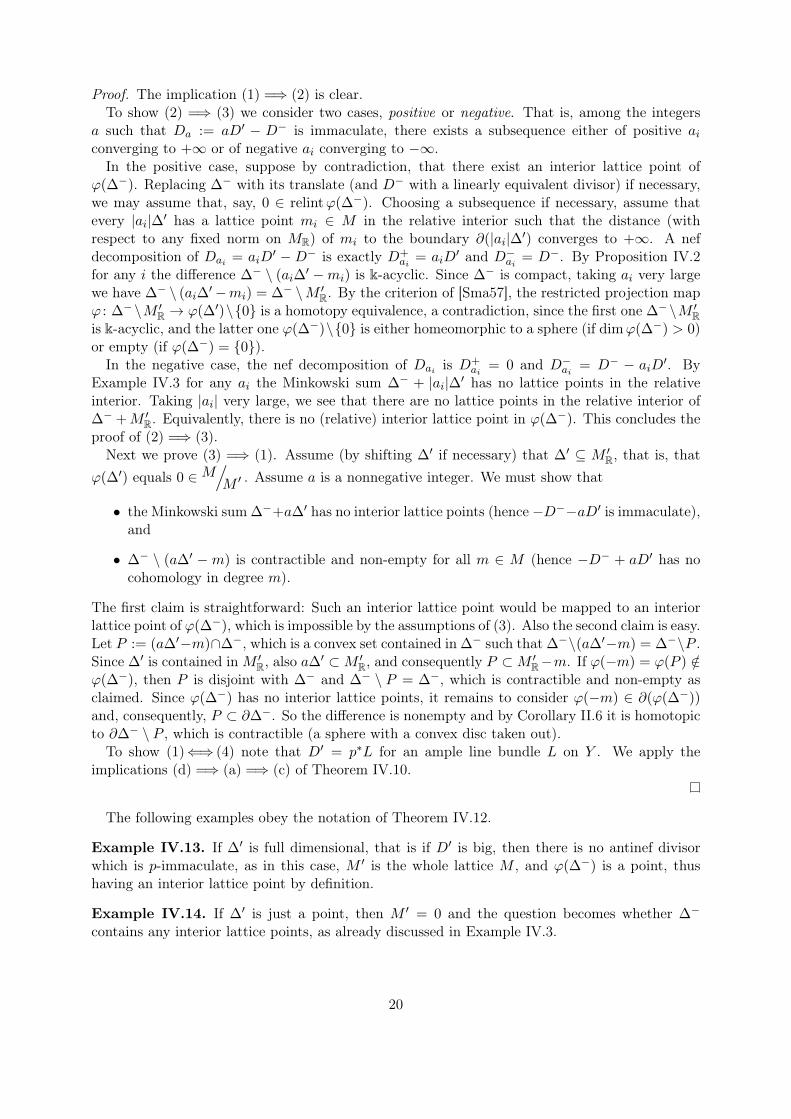
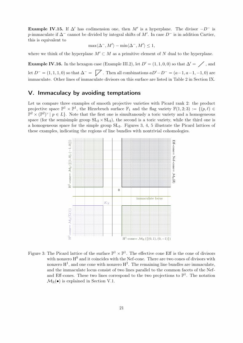
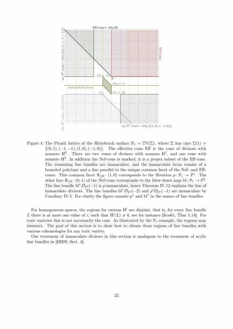
Let us compare three examples of smooth projective varieties with Picard rank 2: the productprojective space P1 × P1, the Hirzebruch surface F1 and the flag variety F(1, 2; 3) := {(p, `) ∈P2 × (P2)∨ | p ∈ L}. Note that the first one is simultanously a toric variety and a homogeneousspace (for the semisimple group SL2×SL2), the second is a toric variety, while the third one isa homogeneous space for the simple group SL3. Figures 3, 4, 5 illustrate the Picard lattices ofthese examples, indicating the regions of line bundles with nontrivial cohomologies.

Eff-cone=

Nef-cone=

MR

(∅)

0

H1-c

one=M

R({

(1,0

),(−

1,0

)})

H1-cone=MR ({(0, 1), (0,−1)})H2-c

one=M

R(Σ

(1))

KX

immaculate locus

Figure 3: The Picard lattice of the surface P1 × P1. The effective cone Eff is the cone of divisorswith nonzero H0 and it coincides with the Nef-cone. There are two cones of divisors withnonzero H1, and one cone with nonzero H2. The remaining line bundles are immaculate,and the immaculate locus consist of two lines parallel to the common facets of the Nef-and Eff-cones. These two lines correspond to the two projections to P1. The notationMR(•) is explained in Section V.1.

21

Eff-cone=MR(∅)

0

Nef-cone

anH

1-c

one=M

R({

(0,1

),(−

1,−

1)}

)

an H1-cone=MR({(1, 0), (−1, 0)})

the

H2-c

one=M

R(Σ

(1))

KX

immaculate locus

OP1 (−1)

OP2 (−1)

OP2 (−2)

Figure 4: The Picard lattice of the Hirzebruch surface F1 = TV(Σ), where Σ has rays Σ(1) ={(0, 1), (−1,−1), (1, 0), (−1, 0)}. The effective cone Eff is the cone of divisors withnonzero H0. There are two cones of divisors with nonzero H1, and one cone withnonzero H2. In addition the Nef-cone is marked; it is a proper subset of the Eff-cone.The remaining line bundles are immaculate, and the immaculate locus consist of abounded polytope and a line parallel to the unique common facet of the Nef- and Eff-cones. This common facet R≥0 · (1, 0) corresponds to the fibration p : F1 → P1. Theother face R≥0 · (0, 1) of the Nef-cone corresponds to the blow-down map bl : F1 → P2.The line bundle bl∗OP2(−1) is p-immaculate, hence Theorem IV.12 explains the line ofimmaculate divisors. The line bundles bl∗OP2(−2) and p∗OP1(−1) are immaculate byCorollary IV.5. For clarity the figure ommits p∗ and bl∗ in the names of line bundles.

For homogeneous spaces, the regions for various Hi are disjoint, that is, for every line bundleL there is at most one value of i, such that Hi(L) 6= 0, see for instance [Kos61, Thm 5.14]. Fortoric varieties this is not necessarily the case. As illustrated by the F1 example, the regions mayintersect. The goal of this section is to show how to obtain these regions of line bundles withvarious cohomologies for any toric variety.Our treatment of immaculate divisors in this section is analogous to the treatment of acylic

line bundles in [BH09, Sect. 4].

22

0

Eff-cone=

Nef-cone

H1-cone

H1-cone

H2-c

one

H2-cone

H3-c

one

KX

immaculate locus

Figure 5: The Picard lattice of the threefold flag variety F(1, 2, 3). The effective cone Eff is thecone of divisors with nonzero H0 and it coincides with Nef-cone. There are two conesof divisors with nonzero H1, two cones with nonzero H2, and one cone with nonzero H3.The remaining line bundles are immaculate, and the immaculate locus consists of threelines. The diagonal is not parallel to joined faces of the Nef- and Eff-cones, that is, itis not predicted by a contraction.

V.1. Temptations

Let X = TV(Σ) be a toric variety with no torus factors. For any subset R ⊆ Σ(1) we defineV >(R) ⊂MR, similar to V >

D,0 as in Section III.2:

V >(R) := R>0 ·

(⋃σ∈Σ

conv(R∩ σ(1))

).

Moreover define V ≥(R) as the complex of cones {cone(R∩ σ(1)) | σ ∈ Σ} in MR, so that

suppV ≥(R) = V >(R) ∪ {0} .

In fact, V >(R) = V >−

∑ρ∈RDρ,0

and analogously for V ≥. Thus, as in Section III.2, if Σ is in

addition simplicial, then V ≥(R) is a full (“induced”) subcomplex of Σ generated by R.

Definition V.1. We call R ⊆ Σ(1) tempting if the geometric realization V >(R) of V ≥(R) \ {0}admits some reduced cohomology, that is if it is not k-acyclic.

23

Example V.2. Following with our “hexagon” example (see notation in Example III.2), the fanΣ of this surface has the following 34 tempting subsets R ⊆ Σ(1):

∅, {0, 2}, {0, 3}, {0, 4}, {1, 3}, {1, 4}, {1, 5}, {2, 4}, {2, 5}, {3, 5}, {0, 1, 3}, {0, 1, 4},{0, 2, 3}, {0, 2, 4}, {0, 2, 5}, {0, 3, 4}, {0, 3, 5}, {1, 2, 4}, {1, 2, 5}, {1, 3, 4},

{1, 3, 5}, {1, 4, 5}, {2, 3, 5}, {2, 4, 5}, {0, 1, 2, 4}, {0, 1, 3, 4}, {0, 1, 3, 5}, {0, 2, 3, 4},{0, 2, 3, 5}, {0, 2, 4, 5}, {1, 2, 3, 5}, {1, 2, 4, 5}, {1, 3, 4, 5}, {0, 1, 2, 3, 4, 5}.

As in Section III.1 we denote both natural maps ZΣ(1) → Cl(X) and RΣ(1) → Cl(X)⊗R by π.

Definition V.3. Let R ⊆ Σ(1) be a subset. Then, we denote the images

MZ(R) := π(ZΣ(1)\R≥0 × ZR≤−1

),

MR(R) := π(RΣ(1)\R≥0 × RR≤−1

).

IfR is tempting as defined above, thenMZ(R) is called theR-maculate set of Cl(X), respectively,MR(R) is the R-maculate region of Cl(X)⊗ R.

Remark V.4. Suppose the fan Σ is complete. The empty set R = ∅ yields MR(∅) = Eff(X).Moreover, Alexander duality implies that switching between R and Σ(1) \R does not change thetemptation status. After applyingM, the relation between the subsetsMZ(R) andMZ(Σ(1)\R)of Cl(X) becomes Serre duality in X = TV(Σ).

The integral sets MZ(R) ⊆ Cl(X) reflect more precisely the properties we need, but the realregions MR(R) are easier to control and they already contain a lot of information. Note thatunder the natural map κ : Cl(X)→ Cl(X)⊗R, [D] 7→ [D]⊗1, the R-maculate set is mapped intothe R-maculate region, that is κ : MZ(R)→MR(R). In other words, the preimage κ−1MR(R)in Cl(X) containsMZ(R), or, slightly incorrect,MZ(R) ⊆MR(R) ∩ Cl(X). We will encounterseveral situations when κ−1MR(R) andMZ(R) are either equal or not equal, depending on thesaturation of respective cones.

Proposition V.5. Suppose X = TV(Σ) is a toric variety with no torus factors.

(i) Let R ⊆ Σ(1) be a subset, and suppose [D] ∈ Cl(X) is a class of a Weil divisor D on X.Then [D] belongs toMZ(R) if and only if D is linearly equivalent to some

∑ρ∈Σ(1) λρ ·Dρ

with λρ ∈ Z and R = {ρ ∈ Σ(1) | λρ < 0}.

(ii) Again, let R ⊆ Σ(1), and suppose [D] ∈ Cl(X) is a class of a Weil divisor D on X.Then [D]R ∈ Cl(X) ⊗ R belongs to MR(R), if and only if D is Q-linearly equivalent to∑

ρ∈Σ(1) λρ ·Dρ (for rational λρ) with R = {ρ ∈ Σ(1) | λρ < 0}.

(iii) If R ⊆ Σ(1) is tempting, then for any i such that H̃i−1

(V >(R), k) 6= 0 and any Weil divisor[D] ∈MZ(R), we have Hi(OX(D)) 6= 0.

(iv) A rank one reflexive sheaf OX(D) for [D] ∈ Cl(X) is immaculate if and only if D /∈⋃R=temptingMZ(R).

(v) A rank one reflexive sheaf OX(D) such that [D]R /∈⋃R=temptingMR(R) is immaculate.

This statement should be compared with [BH09, Prop. 4.3 and 4.5].

24

Proof. The divisor D of (i) or (ii) belongs toMZ(R) orMR(R) if and only if it is an image underπ of ZΣ(1)\R

≥0 ×ZR≤−1 or RΣ(1)\R≥0 ×RR≤−1, respectively. The kernel of π is the set of principal torus

invariant divisors, hence the claim holds.To see (iii), take [D] ∈ MZ(R), and a linearly equivalent D′ =

∑ρ∈Σ(1) λρ · Dρ = D(m)

as in (i). Then by [CLS11, Thm 9.1.3] the appropriate cohomology group is Hi(OX(D))m =Hi(OX(D′))0 6= 0.If D is immaculate, then it is not in

⋃R=temptingMZ(R) by (iii). Conversely, if D is not immacu-

late, then pick a linearly equivalent divisor∑

ρ∈Σ(1) λρ · Dρ which has non-trivial cohomologiesin degree 0 ∈ M . By [CLS11, Thm 9.1.3] the set R = {ρ ∈ Σ(1) | λρ < 0} is tempting and[D] ∈MZ(R), concluding the proof of (iv).Finally, (v) follows from (iv), since [D] ∈MZ(R) implies [D]R ∈MR(R).

It is not always true, that [D]R ∈ MR(R) implies [D] ∈ MZ(R) as the following exampleshows.

Example V.6. Let X = TV(Σ) = P(2, 3, 5), the weighted projective plane with weights 2, 3, 5.Consider the Q-Cartier Weil divisor D ' OX(1) which can be written as the difference Dρ2−Dρ1 .Then D is immaculate, but [D]R ∈MR(R) for R = ∅ (corresponding to the EffR-cone).

This leads to the following definition:

Definition V.7. A divisor D is really immaculate (or R-immaculate), if

[D]R ∈ Cl(X)⊗ R \⋃

R=tempting

MR(R).

Thus Example V.6 shows a simple case of an immaculate Weil divisor that is not really im-maculate. In Example VII.8 we construct a line bundle on a smooth toric projective variety withthe same property. Up to the zero-th cohomology group, the concept of really immaculate divisorhere is an analogue of the strongly acyclic line bundle in [BH09, Def. 4.4].

Definition V.8. The immaculate loci of X are

ImmZ(X) = Cl(X) \⋃

R⊂Σ(1), R is tempting

MZ(R), and

ImmR(X) = κ−1

(Cl(X)⊗ R) \⋃

R⊂Σ(1), R is tempting

MR(R)

⊂ Cl(X),

where κ : Cl(X)→ Cl(X)⊗ R is the natural map [D] 7→ [D]⊗ 1 = [D]R.

Thus ImmZ(X) is the collection of all immaculate divisors. By Proposition V.5(v) all thedivisors in ImmR(X) are immaculate, that is ImmR(X) ⊂ ImmZ(X). More precisely, ImmR(X)is the set of all really immaculate divisors as in Definition V.7.

Example V.9. In contrast to Examples V.6 and VII.8, we can see that in the case of the hexagon(Example III.2), all immaculate line bundles are really immaculate. This follows since the matrixπ defining the map (ZΣ(1))∗ → Pic(X) is totally unimodular.

Example V.10. We illustrate Proposition V.5 with the example of the Hirzebruch surface Fa =TV(Σa). The special cases a = 0 and a = 1 are presented in the Figures 3 and 4, respectively.

25

More general cases are explained in Subsection VI.2 — our surface case corresponds to `1 = `2 = 2there.The Gale transform, that is the map π, is given by the matrix

π =

(1 1 0 −a0 0 1 1

).

The associated rays of the fan Σa are given by the matrix

ρ =

(0 −a 1 −11 −1 0 0

).

If we denote the four columns, that is the rays, by ρ1, . . . , ρ4, then the tempting subsets of Σa(1)are just ∅, Σa(1), R1 = {ρ1, ρ2}, and R2 = {ρ3, ρ4}. The corresponding maculate regions are

MR(∅) = cone⟨(1, 0), (0, 1), (−a, 1)

⟩= cone

⟨(1, 0), (−a, 1)

⟩,

MR(Σa(1)) = (a− 2,−2) + cone⟨(−1, 0), (a,−1)

⟩,

MR(R1) = (−2, 0) + cone⟨(−1, 0), (0, 1), (−a, 1)

⟩= (−2, 0) + cone

⟨(−1, 0), (0, 1)

⟩,

MR(R2) = (a,−2) + cone⟨(1, 0), (0,−1)

⟩.

The lattice points within the complement of the union of these four regions consist of the line(∗,−1) and, if a ≥ 1, the two isolated points (−1, 0) and (a − 1,−2). In the degenerate case ofa = 0, there is an additional line (−1, ∗), see Figure 3. Here, all immaculate divisors are reallyimmaculate.

V.2. Conditions on presence or absence of temptations

In this section we describe straightforward criteria that imply that a given subset of rays istempting or it is nontempting. The upshot is that, for all sets R ⊆ Σ(1) covered by one of theseclaims, one does not need to look at the topology of V >(R) = suppV ≥(R) \ {0}.

V.2.1. Monomials do not lead into temptation

The first criterion is similar to the boundedness condition in [HKP06, Prop. 2].

Proposition V.11. Suppose X = TV(Σ) is a complete toric variety and R ⊂ Σ(1) is a temptingsubset. Denote by ρ∗ : MR → RΣ(1) the natural embedding of the principal torus invariant divisorsinto all torus invariant divisors. Then

ρ∗(MR) ∩(RΣ(1)\R≥0 × RR≤0

)= {0} .

Proof. Suppose on the contrary, that (ρ∗)−1(RΣ(1)\R≥0 × RR≤0

)is a positive dimensional cone τ ⊂

MR. Consider the divisor D =∑

%∈R−D%. Since R is tempting, the divisor has non-zerocohomologies in degree −m for all m ∈ τ ∩M . Thus, the cohomology groups

⊕dimXi=0 Hi(D) are

infinitely dimensional, a contradiction with the completeness of X.

Example V.12. Consider the Hirzebruch surface Fa as in Example V.10, and suppose a > 0.Then out of 16 subsets of {ρ1, ρ2, ρ3, ρ4}, only six survive the test provided by Proposition V.11.Namely, these are the four tempting subsets as listed in Example V.10, and {ρ4} and its comple-ment {ρ1, ρ2, ρ3} having the property of the associated cone intersecting M in just {0}.

26

Example V.13. In the “hexagon” case (see Examples III.2 and V.2), Proposition V.11 showsthat the following 18 out of 64 = 26 subsets of Σ(1) are non-tempting:

{0, 1} , {0, 5} , {1, 2} , {2, 3} , {3, 4} , {4, 5} , {0, 1, 2} , {0, 1, 5} , {0, 4, 5} , {1, 2, 3} ,{2, 3, 4} , {3, 4, 5} , {0, 1, 2, 3} , {0, 1, 2, 5} , {0, 1, 4, 5} , {0, 3, 4, 5} , {1, 2, 3, 4} , {2, 3, 4, 5} .

V.2.2. Faces are not tempting

Proposition V.14. Suppose X = TV(Σ) is a complete toric variety and σ ∈ Σ is any cone (ora proper subfan with strictly convex support). Then the subsets R = σ(1) ⊂ Σ(1) and Σ(1) \ Rare not tempting.

Proof. The complex V >(R) is equal to the convex set σ \ {0}, hence it is contractible. ByAlexander duality (see Remark V.4) the complement is also not tempting.

Example V.15. For the Hirzebruch surface Fa, only the four tempting subsets fail this test. Allthe other subsets are either faces or complements of faces.

Example V.16. According to Proposition V.14, in the “hexagon” case (see Examples III.2, V.2),the following 24 subsets of Σ(1) are non-tempting: all single element subsets {i}, all consecutivetwo elements subsets {i, i+ 1}, and their complements (which have either four or five elements),which are all faces or their complements. Moreover, considering also three consecutive elements{i, i+ 1, i+ 2} (which are rays of a subfan with a strictly convex support), we obtain 30 subsets,which are all the non-tempting subsets of Σ(1). Alternatively, the three element subsets can beunderstood from Example V.13.

V.2.3. Primitive collections delude

A primitive collection of a simplicial fan Σ is a “minimal non-face”, that is, a subset of raysR ⊂ Σ(1), such that the cone spanned by R is not in Σ, but the cone spanned by R \ {ρ} is inΣ for every ρ ∈ R. More generally, a subset R ⊂ Σ(1) of any fan is a primitive collection, if R isnot contained in any single cone of Σ, but every proper subset is. See [Bat91], [CvR09] for moredetails and explanations why this notion is important and relevant to projective toric varieties,see also Section VII.1.

Proposition V.17. Suppose X = TV(Σ) is a complete simplicial toric variety with no torusfactors. Let R ⊂ Σ(1) be either empty or a primitive collection. Then R and its complement aretempting.

Proof. If R = ∅ or R = Σ(1), then the claim is clear, so suppose R is a primitive collection,that is, a subset which is does not generate a cone of Σ, but all its proper subsets do generatesuch cones. By Alexander duality it is enough to prove that R = {ρ1, . . . , ρk} is tempting. Sinceevery ray belongs to Σ, we have k ≥ 2. We distinguish between two cases: either R is linearilyindependent or not.If R is linearily independent, then V := spanRR is k-dimensional, and R+ :=

∑kj=1 R≥0 · ρj

is a k-dimensional simplicial cone in V which does not belong to Σ. On the other hand, itsboundary ∂R+ is a subcomplex of Σ; it is exactly the complex V ≥(R) as in Section V.1. Thus,|V ≥(R)| \ {0} = |∂R+| \ {0} is homotopy equivalent to a sphere Sk−2. In particular, it is notk-acyclic.

27

On the other hand, suppose R is linearly dependent. Since R is a primitive collection, all thecones generated by R \ {ρj} are necessarily simplicial. In particular, V := spanRR is (k − 1)-dimensional, and each R\{ρj} spans a full-dimensional cone in V that belongs to Σ. Thus, thesecones generate V ≥(R), and this is a complete fan in V which (up to R-linear change of coordinates)looks like the Pk−1-fan in Rk−1. Again, V >(R) = |V ≥(R)| \ {0} is homotopy equivalent to Sk−2,hence it is not k-acyclic.

Example V.18. For the Hirzebruch surface Fa, all tempting subsets are predicted by Proposi-tion V.17. That is all four of them are either empty, or Σ(1), or a primitive collection.

Example V.19. Proposition V.17 applied to the hexagon example (see Examples III.2, V.2),implies that the following 20 subsets are tempting:

∅, {0, 2} , {0, 3} , {0, 4} , {1, 3} , {1, 4} , {1, 5} , {2, 4} , {2, 5} , {3, 5} , {0, 1, 2, 4} , {0, 1, 3, 4} ,{0, 1, 3, 5} , {0, 2, 3, 4} , {0, 2, 3, 5} , {0, 2, 4, 5} , {1, 2, 3, 5} , {1, 2, 4, 5} , {1, 3, 4, 5} ,Σ(1).

V.3. The cube

Throughout this subsection we will assume X = TV(Σ) is a complete and simplicial toric variety.Let R ⊆ Σ(1) be an arbitrary, not necessarily tempting subset. This gives rise to a vertex

v(R) := −(0Σ(1)\R, 1R) of the cube W spanned by all points of RΣ(1) with 0/− 1 coordinates. Itis the only vertex of the polyhedral cone RΣ(1)\R

≥0 × RR≤−1, that is, the class of the correspondingdivisor DR := −

∑ρ∈RDρ is the most prominent element of the R-maculate region MR(R) :=

π(RΣ(1)\R≥0 × RR≤−1

)introduced in Definition V.3.

We have discussed in Proposition V.5 that the temptation of R implies the maculacy of DR.In the following we will show in Theorem V.22 that for [DR] ∈ Cl(X) this is the only source ofdisgrace.

Lemma V.20. Suppose X = TV(Σ) is a complete simplicial toric variety, and R ⊆ Σ(1) isan arbitrary subset. Let m ∈ M \ {0}. Then the complex V >

DR,m(or VDR,m) from (III.3) in

Subsection III.2 is contractible and non-empty.

Proof. We prove a slightly more general claim. Let Σ be a simplicial, complete fan, letm ∈M\{0}and S ⊆ Σ(1) such that

{ρ ∈ Σ(1) | 〈ρ,m〉 < 0} ⊆ S ⊆ {ρ ∈ Σ(1) | 〈ρ,m〉 ≤ 0} ,

then the pointed full subcomplex 〈S〉 \ {0} ⊂ Σ is contractible and non-empty: First, since thecohomology of 〈S〉\{0} is stable under small perturbations of the position of the rays from Σ(1), wemay move those from Σ(1)∩m⊥ into the open halfspaces (m < 0) or (m > 0) depending on whetherthey belong to S or if they do not, respectively. Hence, we may assume that Σ(1) ∩ m⊥ = ∅,that is, that S = [m< 0] ∩ Σ(1) = [m≤ 0] ∩ Σ(1). But now, the proof follows from the fact that〈S〉 is a deformation retract of the (m ≤ 0) part of the geometric realization of Σ, that is, of(supp Σ) ∩ (m ≤ 0). This is a closed half space which stays cohomologically trivial even afterremoving the origin.

Remark V.21. Note that full subcomplex generated by S = [m< 0] ∩ Σ(1) equals V ≥0,m for thezero divisor. Its contractibility for m 6= 0 is reflected by the fact that the structure sheaf is almostimmaculate.

As an immeadiate corollary of Lemma V.20 we obtain

28

Theorem V.22. Suppose X = TV(Σ) is a complete simplicial toric variety, and R ⊆ Σ(1) is asubset. It gives rise to the divisor DR := −

∑ρ∈RDρ.

(i) Let D =∑

ρ∈Σ(1) λρDρ be a Weil divisor linearly equivalent to DR. Then either D = DR,or RD := {ρ ∈ Σ(1) | λρ < 0} is not tempting.

(ii) If DR is not immaculate, then R is tempting, DR is the only divisor from ZΣ(1)\R≥0 × ZR≤−1

that maps to [DR] under π, and R is the only tempting set containing [DR] ∈ Cl(X) in itsmaculate regionMR(R).

(iii) Non-tempting R lead to immaculate [DR], and the class map π is injective on the maculatevertices of the cube W .

Proof. (i) If D 6= DR, then there is an m ∈ M \ {0} such that DR = D − div(xm) = D(−m).Thus, as in the proof of Theorem III.6, we obtain VD,0 = VDR(m), 0 = VDR,m. The latter iscohomologically trivial by Lemma V.20, and the first is generated by RD.(ii) Since [DR] is maculate, there must be a tempting R′ such that [DR] ∈ MZ(R′), that is

there is a divisor D with [D] = [DR] and RD = R′. By (i) this implies D = DR, that is RD = R.(iii) This is just a reformulation of (ii).

Remark V.23. Immaculate divisors on X do always exist: By Proposition V.14, there exist non-tempting subsets induced from cones. Other possibilities to produce such subsets arise fromLemma V.20 – just takeR := Σ(1)∩[m < 0] for somem ∈M \{0}. In any case, the correspondingvertex of the cube is immaculate by Theorem V.22(iii).

Example V.24. We work with the Hirzebruch surface X = Fa, and we follow the coordinatesand notation of Example V.10. The cube W is 4-dimensional, so that it has 16 vertices. Theycorrespond to subsets I ⊆ {ρ1, ρ2, ρ3, ρ4}, and only four of them are tempting. These temptingones lead to the four different images

(0, 0) = −π(0000), (0,−2) = −π(1100), (a,−2) = −π(0011), (−2 + a,−2) = −π(1111)

in Z2 = Cl(Fa) = Cl(Fa). The remaining twelve are

(−1, 0) = −π(1000) = −π(0100), (−1 + a,−2) = −π(1011) = −π(0111),(−1,−1) = −π(1010) = −π(1001), (−1 + a,−1) = −π(1001) = −π(0101)

(appearing twice) and, with single occurrence,

(0,−1) = −π(0010), (a,−1) = −π(0001), (−2,−1) = −π(1110), (−2 + a,−1) = −π(1101).

Thus, the two isolated points of the immaculate locus plus two points from the immaculate linecould have been guessed from the non-injectivity of π alone. More precisely, it is caused by(1,−1, 0, 0) ∈ kerπ, which corresponds to the second row of the matrix ρ describing the fan.

Example V.25. In the notation of Examples III.2 and V.2 (the hexagon) the image of [−1, 0]-cube in Pic(X)⊗R is a lattice polytope P with 46 vertices and 54 lattice points. 34 of the verticescome from the 34 tempting vertices of the cube. The remaining 12 vertices of P are images of12 non-tempting vertices of the cube. The 8 lattice points in P that are not vertices (including2 interior points), are images of the remaining 18 non-tempting vertices of the cube, each with arepetition (the two interior lattice points appear three times each as images of the vertices of thecube, the other points appear twice each). In particular, the cube produces 20 immaculate linebundles on X.

29

VI. Toric manifolds with Picard rank two

We commence this section with recalling a well-known fact about smoothness of toric varietiesin terms of Gale duality. Then we study our first family of examples, that is smooth completetoric varieties of Picard rank 2. Such varieties are described in [Kle88], and we can classify allthe immaculate line bundles on them.

VI.1. Spotting smoothness via Gale duality

While working with fans having only few generators, the Gale transform becomes the essential toolto investigate their combinatorial structure. We recall an argument showing that this instrument,considered for abelian groups instead of vector spaces, can spot smoothness, too. Let

0 // Kι // Zn ρ // N // 0

be an exact sequence of free abelian groups with d := rkN . This situation gives rise to the Galetransform being just the dual sequence

0 K∗oo Zn∗ι∗oo N∗oo 0.oo

Denote by Zd ⊆ Zn and Z(n−d)∗ ⊆ Zn∗ the orthogonal subgroups being generated by {e1, . . . , ed}and {ed+1, . . . , en}, respectively.

Proposition VI.1. The determinant of {ρ(e1), . . . , ρ(ed)} equals, maybe up to sign, the determ-inant of {ι∗(ed+1), . . . , ι∗(en)}.

Proof. Assuming that the restriction ρ|Zd : Zd → N has a finite cokernel C (which is equivalentto ρ|Zd being injective or to Qd ρ→ N ⊗Q being an isomorphism), we obtain

0��

0��

Zd��

Zdρ��

0 // Kι // Zn ρ //

��N //

��0

0 // Kι // Zn−d ρ //

��

C //

��

0

0 0

Dualizing the bottom row yields coker(Z(n−d)∗ ι∗→ K∗

)= Ext1Z(C,Z). That is, the cokernels of

Zd in N and of Z(n−d)∗ in K∗ have the same order.

VI.2. Immaculate locus for Picard rank two

After illustrating the general method for classifiying immaculate line bundles in Section V, wecompletely describe the immaculate loci in a specific case. Explicitly, this section is devoted tosmooth (complete) toric varieties of Picard rank 2.Investigating Gale duals leads to the well-known classification of the combinatorial type of

d-dimensional, simple, convex polytopes with d + 2 vertices – they are (4`1−1 × 4d−`1+1)∨ forsome `1 = 2, . . . , d, where 4r means the r-dimensional simplex and (. . .)∨ denotes the dual of apolytope. This is a special case of the situation we will meet in Subsection VII.2.

30

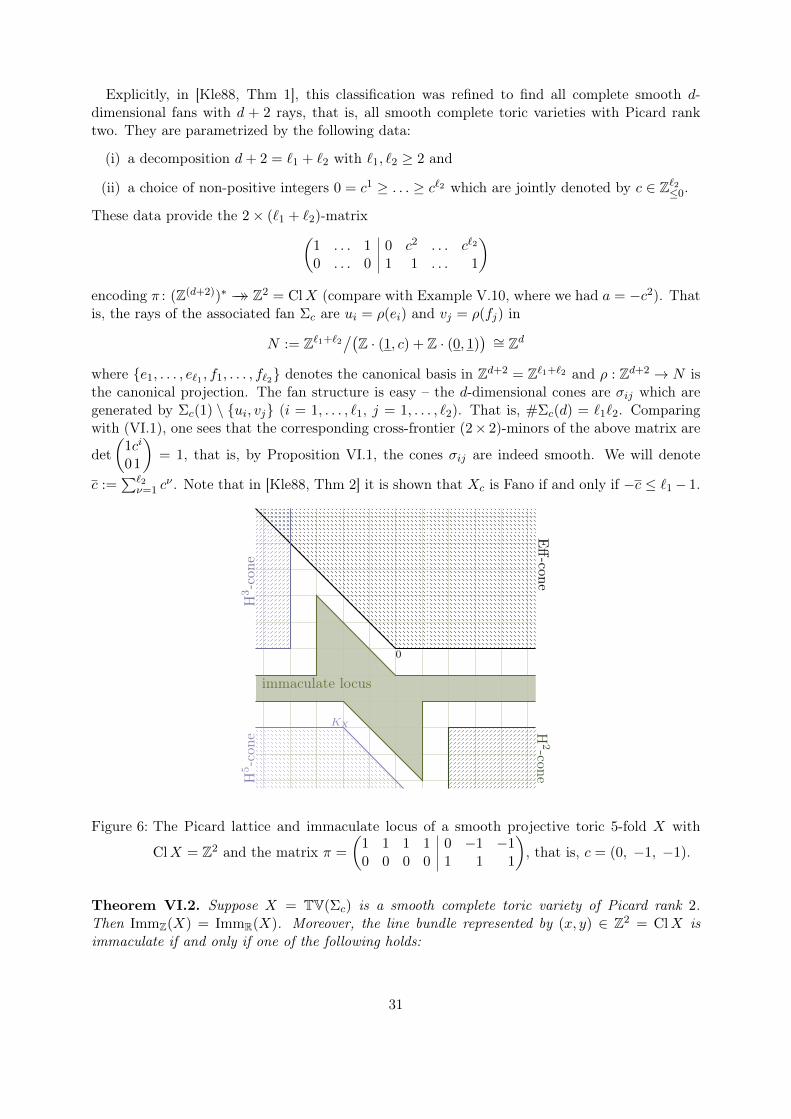
Explicitly, in [Kle88, Thm 1], this classification was refined to find all complete smooth d-dimensional fans with d + 2 rays, that is, all smooth complete toric varieties with Picard ranktwo. They are parametrized by the following data:

(i) a decomposition d+ 2 = `1 + `2 with `1, `2 ≥ 2 and

(ii) a choice of non-positive integers 0 = c1 ≥ . . . ≥ c`2 which are jointly denoted by c ∈ Z`2≤0.

These data provide the 2× (`1 + `2)-matrix(1 . . . 1 0 c2 . . . c`2

0 . . . 0 1 1 . . . 1

)encoding π : (Z(d+2))∗ →→ Z2 = ClX (compare with Example V.10, where we had a = −c2). Thatis, the rays of the associated fan Σc are ui = ρ(ei) and vj = ρ(fj) in

N := Z`1+`2/(

Z · (1, c) + Z · (0, 1)) ∼= Zd

where {e1, . . . , e`1 , f1, . . . , f`2} denotes the canonical basis in Zd+2 = Z`1+`2 and ρ : Zd+2 → N isthe canonical projection. The fan structure is easy – the d-dimensional cones are σij which aregenerated by Σc(1) \ {ui, vj} (i = 1, . . . , `1, j = 1, . . . , `2). That is, #Σc(d) = `1`2. Comparingwith (VI.1), one sees that the corresponding cross-frontier (2× 2)-minors of the above matrix are

det

(1ci

01

)= 1, that is, by Proposition VI.1, the cones σij are indeed smooth. We will denote

c :=∑`2

ν=1 cν . Note that in [Kle88, Thm 2] it is shown that Xc is Fano if and only if −c ≤ `1− 1.

Eff-cone

0

H3-con

eH

2-coneH5-con

e

KX

immaculate locus

Figure 6: The Picard lattice and immaculate locus of a smooth projective toric 5-fold X with

ClX = Z2 and the matrix π =

(1 1 1 1 0 −1 −10 0 0 0 1 1 1

), that is, c = (0, −1, −1).

Theorem VI.2. Suppose X = TV(Σc) is a smooth complete toric variety of Picard rank 2.Then ImmZ(X) = ImmR(X). Moreover, the line bundle represented by (x, y) ∈ Z2 = ClX isimmaculate if and only if one of the following holds:

31

• −`2 < y < 0 or

• y ≥ 0 and −`1 < x < c`2y or

• y ≤ −`2 and 0 > x+ c > c`2(y + `2)− `1.Note that the second and the third case in the theorem are Serre dual to one another, while

the first item is self-dual. The first item is a bunch of (horizontal) affine lines of the same typeas in Theorem IV.12, corresponding to p-immaculate line bundles (0,−1), . . . , (0,−`2 + 1), wherep : X → P`1−1 is the natural projection. If c = 0, that is, if X ' P`1−1 × P`2−1, then the divisorsappearing in the second and third item form parts of the lines corresponding to the other projectionX → P`2−1. Otherwise, c`2 < 0, and there are only finitely many line bundles in the second andthird items (the inequalities define triangles). The special case of `1 = `2 = 2 is illustrated onFigure 4, and another case of a 5-fold is on Figure 6. Points of the form (−1, 0), . . . , (−`1 + 1, 0)are always contained in the second item (independently of c). Later, in the more general setupof Section VII, these points, together with the lines from the first item, will form the “generatingseeds” in the sense of Definition VII.9.

Proof of Theorem VI.2. The only tempting subsets of Σc(1) are ∅, U = {u1, . . . , u`1}, V ={v1, . . . , v`2} and Σc(1) = U t V . We proceed along the lines of Example V.10 and calculatethe maculate loci:

MR(∅) = cone⟨(1, 0), (c`2 , 1)

⟩,

MR(Σc(1)) = (−c− `1,−`2) + cone⟨(−1, 0), (−c`2 ,−1)

⟩,

MR(U) = (−`1, 0) + cone⟨(−1, 0), (0, 1)

⟩,

MR(V ) = (−c,−`2) + cone⟨(1, 0), (0,−1)

⟩.

Note that for every maculate R ⊂ Σc(1), the tail cone in the above locus is smooth and theprimitive generators of rays are all in the image of the set ZΣ(1)\R

≥0 × ZR≤−1. Thus, the map

ZΣ(1)\R≥0 × ZR≤−1 →MR(R) ∩Cl(X) is surjective, i.e.MZ(R) =MR(R) ∩Cl(X). It follows that

ImmZ(X) = ImmR(X) and the explicit description of the immaculate locus follows by an explicitcalculation of the inequalities of the cones above, and by taking the complement in Cl(X).

Proposition VI.3. Suppose as above that X = TV(Σc) is a smooth complete toric variety of Pi-card rank 2. If L is a line bundle on X such that Hi(X,L) 6= 0, then i ∈ {0, `1 − 1, `2 − 1,dimX}.Proof. As in the previous proof, the only tempting subsets are ∅, U , V and U t V . Each of themleads to line bundles with nontrivial cohomology in one of the degrees: dimX, `2 − 1, `1 − 1 or0, respectively. Thus no other Hi can be non-zero.

VII. The immaculate locus for splitting fans

In this section we apply the theory of Section V to the case of splitting fans and calculate theessential part of the immaculate locus of line bundles in this setup. Let X = TV(Σ) be a smoothcomplete toric variety. Recall from Subsection V.2.3 that a primitive collection of a (smooth,hence simplicial) fan Σ is another word for a “minimal non-face”. We say Σ is a splitting fan, ifthe primitive collections of Σ are pairwise disjoint. This is equivalent to an existence of a chainΣ = Σk, . . . ,Σ1 of fans such that TV(Σ1) = Pn and TV(Σi+1) → TV(Σi) is a toric split bundle,that is a projectivisation of a direct sum of toric line bundles (see [Bat91, Cor. 4.4]). In particular,all such X are projective. Note that every smooth complete toric variety with Picard rank twosatisfies this property with k = 2, see Subsection VI.2.

32

VII.1. Primitive relations

In this subsection we recall the notion of the primitive relation associated to a primitive collectionand express all such relations for a splitting fan. We also give a lower bound on the numberof primitive collections and characterise the splitting fans as those smooth complete fans thathave the least possible primitive collections, with respect to that lower bound. Having in mindthe application to splitting fans, which are smooth by definition, we restrict our presentation ofprimitive relations to the smooth case, following [Bat91]. See [CvR09, §1.3] for a more generaltreatment.Let Σ be a fan of a smooth complete toric variety X. Recall that #Σ(1) = rk Cl(X) + dimX.

For every primitive collection P ⊆ Σ(1) we denote eP :=∑

ρ∈P eρ, where the eρ ∈ ZΣ(1) is thebasis element corresponding to ρ, which under the natural map ZΣ(1) → N is mapped to theprimitive generator of the corresponding ray. We denote by σ(P) (called the “focus of P”) theunique cone σ ∈ Σ such that the image of eP in N is contained in intσ ⊂ NR. It leads to a uniqueelement f(P) ∈ Zσ(P)(1)

≥1 with eP − f(P) ∈ ker(ZΣ(1) → N). (Here, by convention, Z∅≥1 = {0}.)The expression eP − f(P) is called the primitive relation associated to P. As an element ofCl(X)∗, it represents a class of 1-cycles.In [Bat91, Prop. 3.1] it is shown that P ∩ σ(P) = ∅, that is the elements of P are not among

the generators of σ(P). Moreover, if Σ is projective, then there exists a primitive collection Pwith σ(P) = 0, see [Bat91, Prop. 3.2 and Thm 4.3].

Proposition VII.1. Let X = TV(Σ) be a complete toric variety. Then every ray of Σ is con-tained in some primitive collection. If X is in addition Q-factorial, then the number of primitivecollections is at least the rank of Cl(X). Moreover, if X is smooth, then equality holds if and onlyif Σ is a splitting fan.

Proof. Let {P1, . . . , . . .Pk} be the primitive collections of Σ. For each ρ ∈ Σ(1) there exists acone τ ∈ Σ such that τ(1) ∪ {ρ} is not contained in any cone of Σ (otherwise, Σ would not becomplete). Thus ρ is also contained in a minimal set of this type. This proves

⋃ki=1 Pi = Σ(1) as

claimed.Let X be Q-factorial. For each i = 1, . . . , k we choose a ρi ∈ Pi. Then, Σ(1) \ {ρ1, . . . , ρk} does

not contain any of the primitive collections, hence it generates a cone in Σ. Thus,

(dimX + rk Cl(X))− k = #Σ(1)− k ≤ # (Σ(1) \ {ρ1, . . . , ρk}) ≤ dimX.

If there is some overlap, say Pi∩Pj 6= ∅, then we might choose ρi = ρj , thus the above inequalitieseven yield rk Cl(X) ≤ k− 1. On the other hand, if all Pi are pairwise disjoint, then we know thatthe facets of Σ look like tki=1(Pi \ {ρi}), in particular, #Σ(1)− k = dimX.

VII.2. Temptation for splitting fans

Here we assume X is a smooth toric projective variety of dimension d whose fan Σ is a splittingfan. We will first identify all of the tempting subsets R ⊆ Σ(1). Later in Section VII.3 we willinvestigate the associated π-imagesMR(R) orMZ(R) as introduced in Definition V.3.Let Σ(1) = P1t. . .tPk be the decomposition into primitive collections of lengths `1, . . . , `k ≥ 2,

respectively. Thus, maximal cones σ ∈ Σ(d) correspond to maximal subsets of Σ(1) not containingany entire set Pi (i = 1, . . . , k). This establishes a bijection

P1 × . . .× Pk∼−→ Σ(d), (p1, . . . , pk) 7→ Σ(1) \ {p1, . . . , pk}.

33

In particular, Σ is combinatorially equivalent to the normal fan of

� = �({1, . . . , k}) := 4`1−1 × . . .×4`k−1

where 4`−1 denotes the (`− 1)-dimensional simplex with ` vertices. In particular, we know that#Σ(1) =

∑ki=1 `i, d =

∑ki=1(`i−1), #Σ(d) =

∏ki=1 `i, and, in compliance with Proposition VII.1,

rk(ClX) = #Σ(1)− d = k.Now, the essential point is that the temptation of a subset R ⊆ Σ(1) depends only on the

combinatorial structure of Σ. The finer structure, the true shape of the fan reflected by the mapsρ : ZΣ(1) → N or π : ZΣ(1) → Cl(X), does matter only for the second step of turning the temptingsets R into the maculate regionsMR(R).

Lemma VII.2. If Σ is a splitting fan with the decomposition Σ(1) = P1 t . . .tPk into primitivecollections Pi, then the tempting subsets of Σ(1) are R(J) :=

⋃j∈J Pj with J ⊆ {1, . . . , k}.

Proof. Instead of the complex (suppV ≥(R)) \ {0} ⊆ supp Σ \ {0} ∼ Sd−1 we consider itsdual version G(R) built as the union of all (closed) facets G(ρ) < � dual to ρ ∈ R. Clearly,suppV ≥(R)\{0} is homotopy equivalent to G(R), thus one is k-acyclic if and only if the other is.A subset J ⊆ {1, . . . , k} defines a splitting � = �(J)×�({1, . . . , k}\J) and accordingly we haveG(R(J)) = ∂�(J)×�({1, . . . , k} \ J), which is not k-acyclic. Thus every set R(J) is tempting.On the other hand, suppose that, for some j, the set R ⊂ Σ(1) does not contain the whole

Pj , but at least one element of Pj . We claim G(R) is contractible. Indeed, if, without loss ofgenerality, j = 1, then we split off � = 4`1−1 ×�(2, . . . , k). Let f < 4`1−1 be the (non-empty)face corresponding to the subset R ∩ P1 ⊂ P1 and pick a standard strong deformation retract4`1−1 → f . Then G(R) can be retracted to the contractible f × �(2, . . . , k) by gluing togetherthe retractions of the contributing faces: each of the faces is either of the form 4`1−1 × F forsome face F < �(2, . . . , k) or of the form F ′ × �(2, . . . , k) for a face F ′ < 4`1−1 containing f .Note that the image of any face of the latter type is just all of f × �(2, . . . , k), hence G(R) iscontractible.

Remark VII.3. The 2k different sets J ⊆ {1, . . . , k} yield 2k tempting setsR(J), hence 2k maculateregionsMR(R(J)) within the k-dimensional space Cl(X) ⊗ R ∼= Rk. This looks a little like thestructure of 2k octants in this space, but we will see that typically the octants are “leaning”, andthey may intersect as illustrated on Figures 4 and 6.

Proposition VII.4. Let X = TV(Σ) with Σ a splitting fan with k primitive collections, and Lbe a line bundle on X such that Hi(X,L) 6= 0, then i ∈

{∑j∈J(`j − 1)

}J⊂{1,...,k}

.

Proof. In the previous proof we have seen that R(J) leads to the non-k-acyclic G(R(J)) =∂�(J) × �({1, . . . , k} \ J). For cohomological considerations we can now focus on the first part∂�(J) = ∂

(∏j∈J 4`j−1

). Thus we have the boundary of a polytope of dimension

∑j∈J(`j − 1),

so R(J) is homotopy equivalent to a (∑

j∈J(`j − 1)− 1)-dimensional sphere.

VII.3. The refined structure of the fan and the class map

We have treated the combinatorial structure of the splitting fan Σ in the previous section. Herewe concentrate on the more refined information, specifically, we focus on the detailed structure ofthe class map π : ZΣ(1) → Cl(X), where X = TV(Σ).

34

Write Σ(1) =⊔ki=1 Pi the decomposition of the rays into the disjoint sets of primitive collections.

In [Bat91, Corollary 4.4], Batyrev has proved that X can be obtained via a sequence of projectiva-tions of decomposable bundles. Within the fan language this means that we can assume that thereis a sequence of fans Σ = Σk, . . . ,Σ1,Σ0 = 0 in abelian groups N = Nk →→ . . .→→ N1 →→ N0 = 0such that the focus σ(Pj) = 0 in Nj and Nj−1 = Nj/ spanPj . The fans Σj in Nj are splittingwith Σj(1) = tji=1Pi, and they admit subfans Σ̃j−1 ⊂ Σj such that ψj : Nj →→ Nj−1 induces anisomorphism Σ̃j−1

∼→ Σj−1 (piecewise linear on the geometric realizations) and Σj consist of thesums of cones from Σ̃j−1 and proper subsets of Pj .With `i = #Pi, this explicit structure of Σ can be translated into the fact that π is a triangular

block matrix

π =

1 c12 . . . c1k

0 1 . . . c2k...

.... . .

...0 0 . . . 1

(VII.5)

with k rows and k blocks of columns of thickness `j (j = 1, . . . , k). While 1 denotes (1, 1, . . . , 1)

with `j entries, we have cij ∈ Z`j≤0. If needed, its entries will be denoted by cνij ∈ Z≤0 (i < j, ν =1, . . . , `j). Every row encodes a primitive relation, hence each cij has at least one zero entry (thesupport of ci• is supposed to be a face, that is to not contain any full Pj).Proposition VII.6. Each matrix π in a triangular block form as in (VII.5) with cij ∈ Z`j and`j ≥ 2 for all j gives rise to a smooth splitting fan of dimension d :=

∑ki=1(`i − 1).

Proof. We argue inductively on the number of rows k (and, at the same time, the number ofblocks of columns). For k = 1 there is nothing to prove, so assume that Σk−1 is a splitting fanobtained from π′, a matrix with last row and last block of columns removed from π. For eachν ∈ {1, . . . , `k} let Lν be the line bundle on Xk−1 = TV(Σk−1) corresponding to the point cν∗k inClXk−1. Then X = P(

⊕`kν=1 Lν) is the desired smooth toric variety.

Note that the smootheness of the variety TV(Σ) associated to the matrix π can also be deriveddirectly from the method of Subsection VI.1. The co-facets of the fan Σ give rise to choosingone column of π in every block. But this yields an upper triangular matrix with only 1 as thediagonal entries. Hence, the determinant equals 1, too.

Example VII.7. A simple case to have in mind is k = 2. The matrix of π is(1 . . . 1 0 c2 . . . c`2

0 . . . 0 1 1 . . . 1

)=

(1 c0 1

)It covers the case of Hirzebruch surfaces. In Subsection VI.2 we have discussed the immaculatelocus of this matrix in detail.

Example VII.8. Consider the following smooth projective three dimensional toric variety X =TV(Σ) = P(OY (−2, 0)⊕OY (0,−2)), where Y = P1× P1, and OY (i, j) := OP1(i)�OP1(j). Thenthe fan Σ is a splitting fan with matrix

π =

1 1 0 0 −2 00 0 1 1 0 −20 0 0 0 1 1

.

The line bundle represented by

π((0, 0, 0, 0, 1

2 ,12))

= (−1,−1, 1) ∈ Cl(X)

is immaculate but not really immaculate (in the sense of Definition V.7).

35

VII.4. Generating immaculate seeds

We fix a format ` := (`1, . . . , `k) of splitting fans, that is a block format of the associated matrixπ. We understand c, that is the entries cij ∈ Z`j≤0 of π, as coordinates of the “moduli space” ofsplitting fans Σ(`, c) of this fixed format `. All these fans share the same combinatorial type – thatof the normal fan of � := 4`1−1 × . . .×4`k−1, see Section VII.2. Similarily, the associated toricvarieties share the same Picard group. Since we use the primitive relations for the rows of π, wehave even distinguished coordinates leading to a simultaneous identification ClTV(Σ(`, c)) = Zk.This makes it possible to compare the immaculate loci of different Σ(`, c) sharing the same `.Now, the basic idea is simple: For special c, e.g. c = 0, the immaculate locus is large – but it

becomes smaller for growing |c| := −c. Roughly speaking, we will show that this shrinking of theimmaculate locus becomes stationary, and we are going to calculate the limit.There is, however, a technical obstacle. The center of symmetry KX/2 arising from Serre

duality moves with c. Thus, it is not the whole immaculate locus that becomes stationary – thisworks only for some generating seed. That is, there is a certain subset of Zk which is immaculatefor all Σ(`, c) and which generates (via some operations/reflections corresponding to successiveSerre dualities) the full immaculate locus if −c is sufficiently large.

Definition VII.9. We call Seed(`) :=⋃kj=1

(Zj−1×{−1, . . . ,−(`j − 1)}× 0k−j

)the “generating

immaculate seed” for ` in Zk.

Recall the integral matrix expression

π = π(`, c) =

1 c12 . . . c1k0 1 . . . c2k...

.... . .

...0 0 . . . 1

from Section VII.3 with non-positive entries within the vectors cij . For fixed i, j ∈ {1, . . . , k} weset cij :=

∑`jν=1 c

νij ∈ Z≤0. Moreover, denote

vj := (c1j , . . . , cj−1, j , `j , 0) ∈ (Zj × 0) ⊆ Zk.

Depending on c, we can now define the operator enlarging a given seed in Zk:

Definition VII.10. For a given subset G ⊆ Zk we define its c-hull as the smallest set 〈G〉c ⊇ Gsatisfying the following recursive property: If a ∈ 〈G〉c ∩ (Zj × 0k−j) for some j = 0, . . . , k − 1,then so is the shift a− vj+1 ∈ 〈G〉c.Note that a − vj+1 ∈ Zj × {−`j+1} × 0k−j−1. Hence, building 〈G〉c out of G can be done by

enlarging 〈G〉c successively with increasing j.

Remark VII.11. Note that Serre duality replaces a ∈ Zk with −a −∑k

i=1 vi. As we will see, wecan also use Serre duality on the level of the smaller varieties TV(Σj). Thus the shift a − vj+1

is obtained by a “double Serre duality”: First we dualise in TV(Σj) obtaining −a−∑j

i=1 vi, andthen we dualize in TV(Σj+1) to get the shift −(−a−

∑ji=1 vi)−

∑j+1i=1 vi from Definition VII.10.

These definitions of Seed(`) and the hull operations allow to describe the locus of immaculateline bundles for “general” c. Recall the notions of maculate regions from Definition V.3, andimmaculate loci from Definition V.8.

Theorem VII.12. Fix ` and let c be a parameter leading to a matrix π = π(`, c) with theassociated splitting fan Σ = Σ(`, c). Then:

36

(i) Seed(`) ⊆ ImmR(Σ(`, c)) for all c, that is the generating seeds are really immaculate.

(ii) Both the loci ImmZ(Σ) and ImmR(Σ) are closed under the c-hull operation.

(iii) For “general” c, the immaculate loci are both equal to the minimal set satisfying the above.That is, ImmZ(Σ(`, c)) = ImmR(Σ(`, c)) = 〈Seed(`)〉c.

More precisely, a sufficient condition for “general” in (iii) is that for each j = 1, . . . , k − 1 thevector cj,j+1 ∈ Z`j+1 has at least two entries differing by more than `j.

Proof. Consider the sequence of projections X = Xk → Xk−1 → Xk−2 → · · · → X1 = P`1−1 andthe corresponding fans Σ = Σk,Σk−1,Σk−2, . . . ,Σ1, such that Xj+1 = P(Ej), where Ej is a splitvector bundle over Xj = TV(Σj). We argue by induction on the Picard number k. If k = 1, thenX ' P`1−1, Seed(`) = Imm(Σ1) = {−1,−2, . . . ,−(`1 − 1)} ⊂ Z ' ClX, v1 = −`1, and the shiftin the definition of c-hull operation is irrelevant since 0 is not a generating seed. Thus there isnothing to prove in this case.So suppose that the statement holds for Picard number at most k − 1 and denote by p the

projection p : X = P(Ek−1) → Xk−1. To present a description of the maculate regions, werecognize the vectors vj (for j = 1, . . . , k) defined above as the building blocks of the π-imagesof the “maculate vertices of the cube” (see Section V.3). The associated tail cones are built fromthe polyhedral cones

Cj := 〈(cν1j , . . . , cνj−1, j , 1, 0) | ν = 1, . . . , `j〉 ⊆ (Rj × 0) ⊆ Rk = Cl(X)⊗ R.

Note that vj is the sum of the generators of Cj . The maculate regions are now parametrized byJ ⊆ {1, . . . , k} and equal

MR(RJ) =∑

j /∈J Cj +∑

j∈J(−vj − Cj).

We claim the elements (∗, . . . , ∗, j) ∈ Zk−1 × {j} ⊂ Zk with j = −1, . . . ,−(`k − 1) are alwaysreally immaculate. Indeed, the vectors vj and the cones Cj for j = 1, . . . , k− 1 have zero as theirlast entries. The last entry of vk is `k, and the last entries of the generators of Ck are always 1.Thus, any point in a maculate coneMR(RJ) has either the last entry at least 0 or at most −`k.We turn our attention to the points of the form (∗, . . . , ∗, 0) ∈ Zk−1 × {0} ⊂ Zk. We remark

that those line bundles are exactly the pullbacks of line bundles on Xk−1. Thus Corollary IV.5 isrelevant here, if we restrict the attention to p∗(ImmZ(Xk−1)) ⊂ ImmZ(X). Instead, our argumenthere is stronger, about the really immaculate locus. If k ∈ J , thenMR(RJ) ∩ (Zk−1 × {0}) = ∅.Thus, those J are never a source of maculacy for points with the last coordinate 0. On the otherhand, if k /∈ J , thenMR(RJ) ∩ (Zk−1 × {0}) =MR(RJ) andMR denotes the maculate regionwith respect to π resulting from π by deleting the last row and the last block of columns. Inparticular, π corresponds to the fan Σk−1.Therefore, by the inductive assumption, all the generating seeds are really immaculate conclud-

ing the proof of (i). Moreover, the inductive assumption together with Alexander/Serre duality(see Remarks V.4, VII.11, and Corollary IV.5) show that both loci ImmZ(X) and ImmR(X) areclosed under c-hull operation, proving (ii). The induction and the above discussion also show (iii)for points of the form (∗, . . . , ∗, j) for −`k < j ≤ 0. By Alexander/Serre duality (or the shift fromthe definition of c-hull), the case of j = −`k is also proved: if a = (∗, . . . , ∗,−`k), then a is (really)immaculate if and only if its shift a− vk ∈ Zk−1 × 0 is (really) immaculate.The duality also swaps the points of the form (∗, . . . , ∗,≥ 1) ∈ Zk−1 × Z≥1 ⊂ Zk with those

of the form (∗, . . . , ∗,≤ −(`k + 1)). Therefore, to complete the proof of (iii) it remains to show

37

that no line bundle whose class in Cl(X) is a = (∗, . . . , ∗,≥ 1) is immaculate. We must show thisunder the assumptions that (iii) holds for Xk−1 and ck−1,k has two entries differing by more than`k−1, say, |c1

k−1,k − c2k−1,k| > `k−1.

As before, RJ -maculacy can only go along with k /∈ J . Let ak be the last coordinate of a andconsider two vectors bν = a − ak · (cν1k, . . . , cνk−1, k, 1) ∈ Zk−1 × 0 for ν = 1 or 2. The differencebetween the (k − 1)-st coordinates of b1 and b2 is at least `k−1 + 1. Using (iii) for Xk−1, sinceall immaculate line bundles for Xk−1 have the last coordinate in the set {−`k−1, . . . , 0}, at leastone of b1 or b2 is not immaculate. Say b1 is not immaculate. Let J ⊂ {1, . . . , k − 1} be thesubset such that b1 ∈MZ(RJ). ThenMZ(RJ) is the sum ofMZ(RJ) and the monoid generatedby (cν1k, . . . , c

νk−1, k, 1). Therefore a = b1 + ak · (c1

1k, . . . , c1k−1, k, 1) ∈ MZ(RJ) and a cannot be

immaculate.

We remark that for non-general values of c the conclusion of (iii) needs not to hold, see forexample Figure 6.

VIII. The immaculate locus for Picard rank 3

In this section we finally make everything concrete in the case of Picard rank 3. We first reviewthe classification of Batyrev, and then describe the tempting subsets of rays. Finally, we list a lotof immaculate line bundles and prove (similarly to Theorem VII.12) that for sufficiently generalparameters the listed ones are all immaculate line bundles.

VIII.1. Classification by Batyrev

In [Bat91] a classification of smooth, projective toric varieties of Picard rank three is given byusing its primitive collections. See also [CvR09].

Proposition VIII.1 ([Bat91, Thm 5.7]). If Σ is a complete, regular d-dimensional fan with d+3generators, then the number of primitive collections of its generators is equal to 3 or 5.

In the case that there are exactly three primitive collections the fan Σ is a splitting fan byProposition VII.1. Thus the associated toric variety is isomorphic to a projectivisation of adecomposable bundle over a smooth toric variety of smaller dimension and Picard rank two. Inparticular, Theorem VII.12 provides a valid description of the immaculate loci in this case.Therefore, for the rest of this section we are going to assume that X is a smooth variety of

Picard rank 3, which has exactly five primitive collections. Following [Bat91] we give a moreprecise description of the fan. There is a decomposition of the rays Σ(1) into five disjoint subsetsJα and the primitive collections are given by Jα ∪ Jα+1 for α ∈ Z/

5Z .

Proposition VIII.2 ([Bat91, Thm 6.6]). Let us denote Jα = Jα ∪ Jα+1, where α ∈ Z/5Z ,

J0 = {v1, . . . , vp0}, J1 = {y1, . . . , yp1}, J2 = {z1, . . . , zp2}, J3 = {t1, . . . , tp3}, J4 = {u1, . . . , up4},

and p0+· · ·+p4 = d+3. Then any complete regular d-dimensional fan Σ with the set of generatorsΣ(1) =

⋃Jα and five primitive collections Jα can be described up to a symmetry of the pentagon

38

by the following primitive relations with non-negative integral coefficients c2, . . . , cp2, b1, . . . bp3:

p0∑i=1

vi +

p1∑i=1

yi −p2∑i=2

cizi −p3∑i=1

(bi + 1)ti = 0,

p1∑i=1

yi +

p2∑i=1

zi −p4∑i=1

ui = 0,

p2∑i=1

zi +

p3∑i=1

ti = 0,

p3∑i=1

ti +

p4∑i=1

ui −p1∑i=1

yi = 0,

p4∑i=1

ui +

p0∑i=1

vi −p2∑i=2

cizi −p3∑i=1

biti = 0.

It looks less scary if we write those equations as a matrix whose rows indicate the five primitiverelations. This matrix consists of five blocks of columns of sizes p0, . . . , p4. By 0 = (0, 0, . . . , 0)and 1 = (1, 1, . . . , 1) we mean row vectors of the appropriate size to fit into the indicated block.Denoting c = (0, c2, . . . , cp2) ∈ Zp2

≥0 and b = (b1, . . . , bp3) ∈ Zp3

≥0, the primitive relation matrixlooks like

1 1 −c −(b+ 1) 00 1 1 0 −10 0 1 1 00 −1 0 1 11 0 −c −b 1

.

VIII.2. Tempting Subsets

As above, we suppose X = TV(Σ) is a smooth projective toric variety of dimension d and Picardrank 3, whose fan Σ has five primitive relations.For finding the immaculate line bundles the first step is to find the tempting subsets of Σ(1).

We have seen in Proposition V.17 that the primitive collections, their complements, the emptyset and the full subset Σ(1) are tempting.

Lemma VIII.3. The only tempting subsets are primitive collections, their complements, theempty set and the full subset Σ(1).

Proof. Let R be a non-empty tempting subset, which is not equal to Σ(1). Then R and Σ(1) \Rdo not span cones in Σ by Proposition V.14. It follows that there exist two primitive collectionsP, P ′, with P ⊆ R ⊆ Σ(1) \ P ′. In the notation as above we obtain

Jα ∪ Jα+1 ⊆ R ⊆ Jβ+2 ∪ Jβ+3 ∪ Jβ+4

for some α, β ∈ Z/5Z . This already implies that β = α± 2:

Jα ∪ Jα+1 ⊆ R ⊆ Jα−1 ∪ Jα ∪ Jα+1, orJα ∪ Jα+1 ⊆ R ⊆ Jα ∪ Jα+1 ∪ Jα+2.

For brevity we denote by J•, respectively, either Jα−1 or Jα+2. So the only question is, what isR∩ J•. If we show the intersection is empty or the whole J•, the proof will be completed.

39

Denote by R• := R ∩ J•, and assume conversely that the R• is not equal to ∅ or J•, andconsider Jα ∪R•. This set does not contain any primitive collection, thus it is a face. The sameholds for Jα+1 ∪ R•. Hence R is the union of two faces which intersect in a common face R•.This implies that R is not tempting.

Proposition VIII.4. Suppose as above that X is a smooth projective toric variety of Picard rank3 with five primitive collections Ji of lengths pi. If L is a line bundle on X such that Hi(X,L) 6= 0,then i ∈ {0, pα + pα+1 − 1, pα−1 + pα−2 + pα−3 − 2, dimX}

α∈Z/5Z

.

Proof. The tempting subset Σ(1) and ∅ lead to line bundles with nontrivial cohomology in degrees0 and dimX respectively.Along the lines of the proof of Proposition V.17 we see that the complement of the primitive

collection Jα leads to line bundles with nontrivial cohomology in degree pα + pα+1 − 1, and theprimitive collection itself to line bundles with nonvanishing cohomology in degree pα−1 + pα−2 +pα−3 − 2. Since there are no other tempting subsets, there cannot occure other degrees.

VIII.3. Immaculate line bundles for Picard rank 3

We can calculate the immaculate line bundles as described in Proposition V.5. For this we haveto consider π(ZΣ(1)\R

≥0 × ZR≤−1) for all maculate R where π is given as the transpose of the mapembedding the kernel of the ray map into ZΣ(1). This can be realized by selecting a Z-basis outof the rows of the matrix of primitive relations presented at the end of Subsection VIII.1. Pickingits first, second and fourth row, we obtain

π =

1 1 −c −(b+ 1) 00 1 1 0 −10 −1 0 1 1

.

These are the primitive relations that, being understood as classes of 1-cycles, correspond tothe rays of the Mori cone which in this case is a three-dimensional simplicial cone.

Remark VIII.5. (i) For all parameters b, c, the matrix π leads to a smooth fan of Picard rank 3.This means the converse of Proposition VIII.2, and it follows from Subsection VI.1: The3-minors with respect to the columns chosen from the blocks (α, α+ 1, α+ 3) for α ∈ Z/5Zare always 1.

(ii) It is straightforward (although tedious) to check that for all 12 tempting subsets R ⊂ Σ(1)the tail cone of the respective maculate regionMR(R) is either a smooth cone or a cone with4 rays which do also form its Hilbert basis (the latter is the case for J3 ∪ J4 if cp2 < b1 + 1,for J4 ∪ J0 if b1 > 0, and for their respective complements).

(iii) From (ii) it follows that, independent of the parameters b, c, we always have thatMZ(R) =MR(R) ∩ PicX and thus ImmZ(X) = ImmR(X).

We will distinguish three classes (F), (A), (B) of line bundles which will become the main herosfor the immaculate locus presented in Proposition VIII.7. To locate these classes in Z3 we will usethe horizontal projection (x, y, z) 7→ (y, z) and start with some geography on the target space.

40

Definition VIII.6. Denote by P1 and P2 the following two planary parallelograms P1, P2:

P1 = conv((p1 − p2 − p3 + 2, p1 − 1), (−p1, p1 − 1),(−p2 + p4, −p3 − p4 + 1), (p3 + p4 − 2, −p3 − p4 + 1)),

P2 = conv((−p1 − p2 + 1, p1 + p2 − 2), (p4 − 1, −p4),(−p1 − p2 + 1, p1 − p3), (p4 − 1, −p2 − p3 − p4 + 2))

They are depicted in blue and red in Figure 7, and we will be interested in their union. Note thefollowing two special cases:

• If p2 = 1, then P2 ⊂ P1 and the simplified vertices of P1 are:

(p1 − p3 + 1, p1 − 1), (−p1, p1 − 1), (p4 − 1, −p3 − p4 + 1), (p3 + p4 − 2, −p3 − p4 + 1)

• If p3 = 1, then P1 ⊂ P2 and the simplified vertices of P2 are:

(−p1 − p2 + 1, p1 + p2 − 2), (−p1 − p2 + 1, p1 − 1), (p4 − 1, −p4), (p4 − 1, −p2 − p4 + 1)

Now we can describe the three classes of our immaculate candidates. They consist of entire“horizontal” lines or line segments, that are parallel to the x-axis:

• Full horizontal lines (F). This class consists of the union of the (infinite) lines (∗, y, z)with (y, z) ∈ P1∪P2 (including the boundary). Note that it does not depend on the valuesof b and c and it is self dual with respect to Serre duality: here the canonical divisor is(−p0 − p1 + p3 + c+ b, −p1 − p2 + p4, p1 − p3 − p4).

• Line segments of Type (A). This class consists of finite horizontal segments Iy (describedbelow) located over the diagonal (∗, y, −y). Denote Dx,y = (x, −y, y), and for anyy ∈ [−p3 − p4 + 1, p1 + p2 − 1] let

Iy := {Dx,y | x0(y) ≤ x ≤ x1(y)}

be the set of lattice points on the segment with x coordinate varying from x0(y) to x1(y).The values of x0(y), x1(y) and the number of elements of Iy is in Table 1. Notice that theydo not depend on b or c, as in the case of type (F).

• Line segments of Type (B). The segments of this type depend on p2 and p3 via theparallelograms P1 and P2 elaborated in Definition VIII.6.

– If p2, p3 ≥ 2, then this type consist of just one horizontal segment whose projectionto the (y, z)-plane is located left and above the intersection of the upper edges of theparallelograms P1 and P2, see the point marked as B on Figure 7. The line segmentcontains p0 − 1 immaculate line bundles with coordinates

([−p0 − p1 + c+ 1,−p1 + c− 1], −p1 − p2, p1),

where c :=∑ci.

– If p2 = 1, then the points of Type (B) consist of p3 horizontal line segments, eachcontaining p0 − 1 immaculate line bundles. The coordinates are

([−p0 − p1 + 1,−p1 − 1], −p1 − p2 − y, p1)

for y ∈ [0, p3 − 1]. On Figure 8 their projections onto (y, z) plane are indicated by theletter B. Roughly speaking, their projections are at each lattice point directly abovethe upper edge of the parallelogram P1,

41

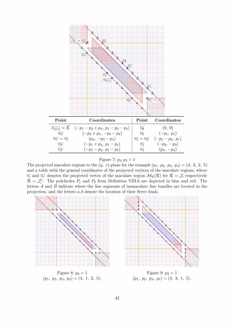
vΣ(1)

v∅

v0c

v0

v1c = v3

v1 = v3c

v2c

v2

v4c

v4

B

b

A

A

A

A

A

A

A

A

A

A

A

A

A

a

a

a

a

a

a

a

a

a

a

a

a

a

Point Coordinates Point Coordinates

vΣ(1) = K (−p1 − p2 + p4, p1 − p3 − p4) v∅ (0, 0)

v0c (−p2 + p4, −p3 − p4) v0 (−p1, p1)v1c = v3 (p4, −p3 − p4) v1 = v3c (−p1 − p2, p1)v2c (−p1 + p4, p1 − p4) v2 (−p2, −p3)v4c (−p1 − p2, p1 − p3) v4 (p4, −p4)

Figure 7: p2, p3 > 1The projected maculate regions to the (y, z)-plane for the example (p1, p2, p3, p4) = (4, 3, 2, 5)and a table with the general coordinates of the projected vertices of the maculate regions, wherevi and vic denotes the projected vertex of the maculate region MR(R) for R = Ji respectivelyR = J ci . The polyhedra P1 and P2 from Definition VIII.6 are depicted in blue and red. Theletters A and B indicate where the line segments of immaculate line bundles are located in theprojection, and the letters a, b denote the location of their Serre duals.

B B

b b

A

A

A

A

A

A

A

A

A

A

A

a

a

a

a

a

a

a

a

a

a

a

Figure 8: p2 = 1(p1, p2, p3, p4) = (4, 1, 2, 5).

B

B

B

b

b

b

A

A

A

A

A

A

A

A

A

A

A

A

a

a

a

a

a

a

a

a

a

a

a

a

Figure 9: p3 = 1(p1, p2, p3, p4) = (4, 3, 1, 5).

42

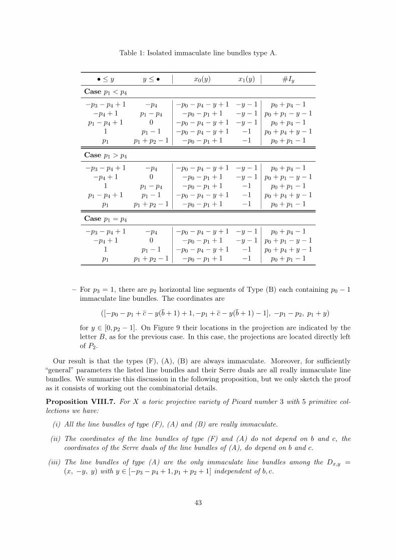
Table 1: Isolated immaculate line bundles type A.

• ≤ y y ≤ • x0(y) x1(y) #Iy

Case p1 < p4

−p3 − p4 + 1 −p4 −p0 − p4 − y + 1 −y − 1 p0 + p4 − 1−p4 + 1 p1 − p4 −p0 − p1 + 1 −y − 1 p0 + p1 − y − 1

p1 − p4 + 1 0 −p0 − p4 − y + 1 −y − 1 p0 + p4 − 11 p1 − 1 −p0 − p4 − y + 1 −1 p0 + p4 + y − 1p1 p1 + p2 − 1 −p0 − p1 + 1 −1 p0 + p1 − 1

Case p1 > p4

−p3 − p4 + 1 −p4 −p0 − p4 − y + 1 −y − 1 p0 + p4 − 1−p4 + 1 0 −p0 − p1 + 1 −y − 1 p0 + p1 − y − 1

1 p1 − p4 −p0 − p1 + 1 −1 p0 + p1 − 1p1 − p4 + 1 p1 − 1 −p0 − p4 − y + 1 −1 p0 + p4 + y − 1

p1 p1 + p2 − 1 −p0 − p1 + 1 −1 p0 + p1 − 1

Case p1 = p4

−p3 − p4 + 1 −p4 −p0 − p4 − y + 1 −y − 1 p0 + p4 − 1−p4 + 1 0 −p0 − p1 + 1 −y − 1 p0 + p1 − y − 1

1 p1 − 1 −p0 − p4 − y + 1 −1 p0 + p4 + y − 1p1 p1 + p2 − 1 −p0 − p1 + 1 −1 p0 + p1 − 1

– For p3 = 1, there are p2 horizontal line segments of Type (B) each containing p0 − 1immaculate line bundles. The coordinates are

([−p0 − p1 + c− y(b+ 1) + 1,−p1 + c− y(b+ 1)− 1], −p1 − p2, p1 + y)

for y ∈ [0, p2 − 1]. On Figure 9 their locations in the projection are indicated by theletter B, as for the previous case. In this case, the projections are located directly leftof P2.

Our result is that the types (F), (A), (B) are always immaculate. Moreover, for sufficiently“general” parameters the listed line bundles and their Serre duals are all really immaculate linebundles. We summarise this discussion in the following proposition, but we only sketch the proofas it consists of working out the combinatorial details.

Proposition VIII.7. For X a toric projective variety of Picard number 3 with 5 primitive col-lections we have:

(i) All the line bundles of type (F), (A) and (B) are really immaculate.

(ii) The coordinates of the line bundles of type (F) and (A) do not depend on b and c, thecoordinates of the Serre duals of the line bundles of (A), do depend on b and c.

(iii) The line bundles of type (A) are the only immaculate line bundles among the Dx,y =(x, −y, y) with y ∈ [−p3 − p4 + 1, p1 + p2 + 1] independent of b, c.

43

(iv) For b, c large enough, that is max(bp3 , cp2) ≥ p0 + p1 + max(p2, p3) + p4 and if p2 6= 1additionally cp2 ≥ p0 − 1 and for p3 6= 1 the additional condition that bp3 − b1 ≥ p0 − 1, theonly (really) immaculate line bundles are the previously mentioned and their Serre duals.

Sketch of proof. For proving all of those statements we will consider the ”horizontal” projectionof the Picard group and in particular of the twelve maculate regions to the y, z-plane. Figures 7,8 and 9 illustrate the situation, for the cases p2, p3 > 1 and p2 = 1, p3 = 1 respectively.

• (F) Full horizontal lines. If the projected divisorD is not in any of the projected maculatecones MR(R), then all the divisors in the line parallel to the kernel of the projection areimmaculate.

• Line segments of Type (A). Given a divisor Dx,y we want to know whether it is im-maculate. Thus we want to know whether there is an R such that Dx,y ∈ MR(R). Weanalyse the projected situation. We know that if D /∈ MR(R), then D /∈ MR(R). Thiseliminates a large number of candidate R’s. Various situations that can occur are depictedin the aforementioned figures.

Once we have identified the candidate R’s we do a case analysis for the y-coordinate.

• Line Segments of Type (B). The proof essentially proceeds in the same manner as forthe isolated points of type (A), by working out the combinatorial details of the situation.

IX. Computational aspects

In this section we want to highlight the computational advantages of immaculate line bundles andmaculate regions. All of these objects and conditions give rise to nice combinatorial algorithms.Throughout the development of this paper we have implemented these in polymake and they areavailable on githublink as a polymake ([GJ00]) extension. The combinatorial nature of thesealgorithms makes them very fast, as opposed to many algorithms from commutative algebra. Thisstresses the main computational advantage of working with toric varieties. We will give a shortsketch of the resulting algorithms.Immaculacy of a line bundle can be checked from its representation as a difference of nef

divisors. Thus we want to check all differences ∆− \ (∆+ −m), for any m ∈ M , for k-acyclicity,via Proposition IV.2. But it is actually enough to check only finitely many m, since both ∆− and∆+ are compact and thus they only intersect for finitely many shifts. Using Proposition II.2, wejust need to consider ∆− as a polytopal complex and remove any face intersecting ∆+ −m non-trivially, for those finitely many m. Homology computation of the resulting polytopal complexis already built in polymake and many other software frameworks for combinatorial software aswell.Next we want to find the tempting R ⊆ Σ[1]. The easiest way is to brute force this by checking

any subset of rays and then compute the homology. One can also imagine a more sophisticatedapproach by considering sub-diagrams of the Hasse diagram of Σ. So far this has never been abottleneck in our examples, though in case this happens, results of Subsection V.2 might be ofuse.From the collection of all tempting R we can finally compute the immaculate locus ImmR(X),

or rather the lattice points thereof. We only need to compute the intersection of all complements

44

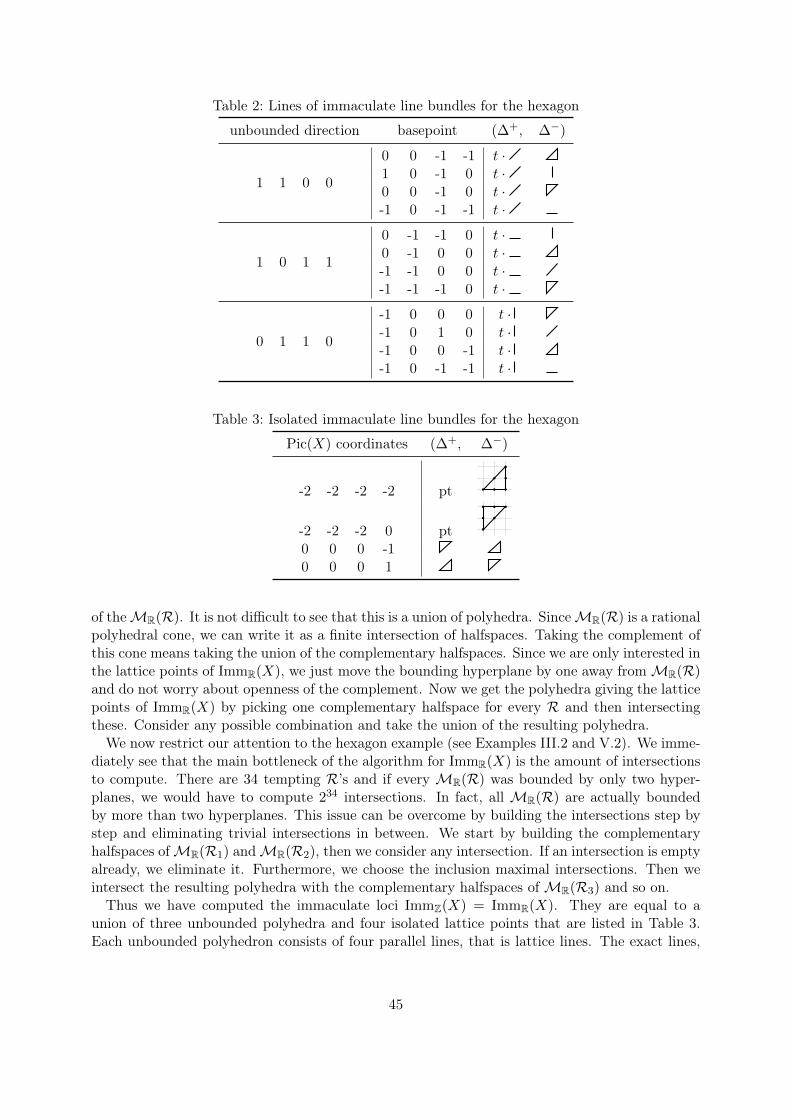
Table 2: Lines of immaculate line bundles for the hexagon

unbounded direction basepoint (∆+, ∆−)

1 1 0 0

0 0 -1 -1 t ·1 0 -1 0 t ·0 0 -1 0 t ·-1 0 -1 -1 t ·

1 0 1 1

0 -1 -1 0 t ·0 -1 0 0 t ·-1 -1 0 0 t ·-1 -1 -1 0 t ·

0 1 1 0

-1 0 0 0 t ·-1 0 1 0 t ·-1 0 0 -1 t ·-1 0 -1 -1 t ·

Table 3: Isolated immaculate line bundles for the hexagon

Pic(X) coordinates (∆+, ∆−)

-2 -2 -2 -2 pt

-2 -2 -2 0 pt0 0 0 -10 0 0 1

of theMR(R). It is not difficult to see that this is a union of polyhedra. SinceMR(R) is a rationalpolyhedral cone, we can write it as a finite intersection of halfspaces. Taking the complement ofthis cone means taking the union of the complementary halfspaces. Since we are only interested inthe lattice points of ImmR(X), we just move the bounding hyperplane by one away fromMR(R)and do not worry about openness of the complement. Now we get the polyhedra giving the latticepoints of ImmR(X) by picking one complementary halfspace for every R and then intersectingthese. Consider any possible combination and take the union of the resulting polyhedra.We now restrict our attention to the hexagon example (see Examples III.2 and V.2). We imme-

diately see that the main bottleneck of the algorithm for ImmR(X) is the amount of intersectionsto compute. There are 34 tempting R’s and if every MR(R) was bounded by only two hyper-planes, we would have to compute 234 intersections. In fact, all MR(R) are actually boundedby more than two hyperplanes. This issue can be overcome by building the intersections step bystep and eliminating trivial intersections in between. We start by building the complementaryhalfspaces ofMR(R1) andMR(R2), then we consider any intersection. If an intersection is emptyalready, we eliminate it. Furthermore, we choose the inclusion maximal intersections. Then weintersect the resulting polyhedra with the complementary halfspaces ofMR(R3) and so on.Thus we have computed the immaculate loci ImmZ(X) = ImmR(X). They are equal to a

union of three unbounded polyhedra and four isolated lattice points that are listed in Table 3.Each unbounded polyhedron consists of four parallel lines, that is lattice lines. The exact lines,

45

Table 4: Exceptional sequences of line bundles for the hexagon

D0 = [0, 0, 0, 0]

D1 D2 D3 D4 D5

-2 -1 -1 -1 -1 -2 -1 0 -2 -2 -1 -1 -2 -2 -1 0 -1 -1 -2 -1-1 -1 -1 -1 -2 -2 -1 -1 -1 -1 -2 -1 -2 -1 -2 -2 -1 -2 -2 -1-1 -1 -1 -1 -2 -1 -1 -1 -2 -2 -1 -1 -1 -1 -2 -1 -2 -1 -2 -2-1 -1 -1 -1 -2 -1 -1 -1 -1 -2 -1 0 -2 -2 -1 -1 -1 -1 -2 -1-1 -1 -1 -1 -1 -1 -1 0 -2 -1 -1 -1 -1 -2 -1 0 -1 -1 -2 -1-1 -1 0 0 -2 -1 -1 -1 -1 -2 -1 0 -2 -2 -1 -1 -2 -2 -1 0-1 -1 0 0 -1 -1 -1 -1 -2 -1 -1 -1 -1 -2 -1 0 -2 -2 -1 -1-1 -1 0 0 -1 -1 -1 -1 -1 -1 -1 0 -2 -1 -1 -1 -1 -2 -1 0-1 -1 0 0 -1 0 -1 -1 -1 -1 -1 -1 -1 -1 -1 0 -2 -1 -1 -1-1 -1 0 0 -1 0 -1 -1 0 -1 -1 0 -1 -1 -1 -1 -1 -1 -1 0-1 -1 0 0 0 0 -1 -1 -1 0 -1 -1 0 -1 -1 0 -1 -1 -1 -1-1 -1 0 0 0 0 -1 -1 0 0 -1 0 -1 0 -1 -1 0 -1 -1 0-1 0 0 -1 -1 -1 -1 -1 -2 -1 -1 -1 -2 -2 -1 -1 -2 -1 -2 -2-1 0 0 -1 -1 -1 0 0 -1 -1 -1 -1 -2 -1 -1 -1 -2 -2 -1 -1-1 0 0 -1 -1 -1 0 0 -1 0 -1 -1 -1 -1 -1 -1 -2 -1 -1 -1-1 0 0 -1 -1 -1 0 0 0 0 -1 -1 -1 0 -1 -1 -1 -1 -1 -1-1 0 0 -1 -1 0 0 0 -1 -1 0 0 -1 0 -1 -1 -2 -1 -1 -1-1 0 0 -1 0 -1 0 0 -1 -1 0 0 -1 -1 -1 -1 -2 -2 -1 -1-1 0 0 -1 0 -1 0 0 -1 -1 0 0 0 0 -1 -1 -1 -1 -1 -1

together with their polytopes (∆+,∆−) are depicted in Table 2. Each pair of quadruples of linesintersects in four points.Now it is easy to compute all exceptional sequences that are contained in the projection of the

cube π([−1, 0]6) ⊆ Cl(X). One just collects the lattice points in the projected cube and thenruns a depth first search. There are 228 exceptional sequences of length six in the projected cube.Under the group action on the hexagon these 228 exceptional sequences correspond to 19 orbitsof size 12. In Table 4 we list one representative from each orbit. Note that we do not need to usethe four isolated points for these exceptional sequences. This is different than in the case of thesplitting fans, for example the Picard rank 2 case (see [CM04]).

References

[Ach15] Piotr Achinger. A characterization of toric varieties in characteristic p. Int. Math.Res. Not. IMRN, (16):6879–6892, 2015.

[And13] Dave Anderson. Okounkov bodies and toric degenerations. Math. Ann., 356(3):1183–1202, 2013.

[Bat91] Victor V. Batyrev. On the classification of smooth projective toric varieties. TohokuMath. J. (2), 43(4):569–585, 1991.

46

[BH09] Lev Borisov and Zheng Hua. On the conjecture of King for smooth toric Deligne-Mumford stacks. Adv. Math., 221(1):277–301, 2009.

[CLS11] David A. Cox, John B. Little, and Henry K. Schenck. Toric varieties. Providence,RI: American Mathematical Society (AMS), 2011.

[CM04] L. Costa and R.M. Miró-Roig. Tilting sheaves on toric varieties. Math. Z.,248(4):849–865, 2004.

[Cra11] Alastair Craw. Quiver flag varieties and multigraded linear series. Duke Math. J.,156(3):469–500, 2011.

[CvR09] David A. Cox and Christine von Renesse. Primitive collections and toric varieties.Tohoku Math. J. (2), 61(3):309–332, 2009.

[Ful93] William Fulton. Introduction to toric varieties. The 1989 William H. Roever lecturesin geometry. Princeton, NJ: Princeton University Press, 1993.

[GJ00] Ewgenij Gawrilow and Michael Joswig. polymake: a framework for analyzing con-vex polytopes. In Polytopes—combinatorics and computation (Oberwolfach, 1997),volume 29 of DMV Sem., pages 43–73. Birkhäuser, Basel, 2000.

[Har77] Robin Hartshorne. Algebraic geometry. Springer-Verlag, New York, 1977. GraduateTexts in Mathematics, No. 52.

[HKP06] M. Hering, A. Küronya, and S. Payne. Asymptotic cohomological functions of toricdivisors. Adv. Math., 207(2):634–645, 2006.

[HP06] Lutz Hille and Markus Perling. A counterexample to King’s conjecture. Compos.Math., 142(6):1507–1521, 2006.

[HP11] Lutz Hille and Markus Perling. Exceptional sequences of invertible sheaves on ra-tional surfaces. Compos. Math., 147(4):1230–1280, 2011.

[Kal05] V. Yu. Kaloshin. A geometric proof of the existence of Whitney stratifications.Mosc. Math. J., 5(1):125–133, 2005.

[Kaw06] Yuriro Kawamata. Derived categories of toric varieties. Mich. Math. J., 54(3):517–535, 2006.

[Kaw13] Yujiro Kawamata. Derived categories of toric varieties. II. Mich. Math. J., 62(2):353–363, 2013.

[KKMSD73] G. Kempf, Finn Faye Knudsen, D. Mumford, and B. Saint-Donat. Toroidal embed-dings. I. Lecture Notes in Mathematics, Vol. 339. Springer-Verlag, Berlin-New York,1973.

[Kle88] Peter Kleinschmidt. A classification of toric varieties with few generators. Aequa-tiones Math., 35(2-3):254–266, 1988.

[Kos61] Bertram Kostant. Lie algebra cohomology and the generalized Borel-Weil theorem.Ann. Math. (2), 74:329–387, 1961.

47

[KZ17] Viktor S. Kulikov and Alexander Zheglov. Amazing examples of nonrational smoothspectral surfaces. arXiv:1710.05991, 2017.

[LM09] Robert Lazarsfeld and Mircea Mustaţă. Convex bodies associated to linear series.Ann. Sci. Éc. Norm. Supér. (4), 42(5):783–835, 2009.

[Mic11] Mateusz Michałek. Family of counterexamples to King’s conjecture. C. R. Math.Acad. Sci. Paris, 349(1-2):67–69, 2011.

[Mum08] David Mumford. Abelian varieties, volume 5 of Tata Institute of Fundamental Re-search Studies in Mathematics. Published for the Tata Institute of FundamentalResearch, Bombay; by Hindustan Book Agency, New Delhi, 2008. With appendicesby C. P. Ramanujam and Yuri Manin, Corrected reprint of the second (1974) edition.

[Orl92] D.O. Orlov. Projective bundles, monoidal transformations, and derived categoriesof coherent sheaves. Russ. Acad. Sci., Izv., Math., 41(1):1, 1992. available at http://www.mi.ras.ru/~orlov/papers/1992_Izv_Math.pdf.

[PSP08] Piotr Pragacz, Vasudevan Srinivas, and Vishwambhar Pati. Diagonal subschemesand vector bundles. Pure Appl. Math. Q., 4(4, Special Issue: In honor of Jean-PierreSerre. Part 1):1233–1278, 2008.

[Sma57] Stephen Smale. A Vietoris mapping theorem for homotopy. Proc. Amer. Math. Soc.,8:604–610, 1957.

[Tho69] R. Thom. Ensembles et morphismes stratifiés. Bull. Amer. Math. Soc., 75:240–284,1969.

48