nc calabi-yau orbifolds in toric varieties with discrete torsion
TRANSCRIPT

arX
iv:h
ep-t
h/02
1016
7v1
17
Oct
200
2
UFR-HEP/02-11
NC Calabi-Yau Orbifolds in Toric Varieties
with Discrete Torsion
A. Belhaj∗, and E.H. Saidi†
Lab/UFR-High Energy Physics, Faculty of Sciences, Rabat, Morocco.
February 1, 2008
Abstract
Using the algebraic geometric approach of Berenstein et al (hep-th/005087 and hep-th/009209) and methods of toric geometry, we study non commutative (NC) orbifolds ofCalabi-Yau hypersurfaces in toric varieties with discrete torsion. We first develop a new
way of getting complex d mirror Calabi-Yau hypersurfaces H∗d∆ in toric manifolds M
∗(d+1)∆
with a C∗r action and analyze the general group of the discrete isometries of H∗d∆ . Then
we build a general class of d complex dimension NC mirror Calabi-Yau orbifolds wherethe non commutativity parameters θµν are solved in terms of discrete torsion and toric
geometry data of M(d+1)∆ in which the original Calabi-Yau hypersurfaces is embedded.
Next we work out a generalization of the NC algebra for generic d dimensions NC Calabi-Yau manifolds and give various representations depending on different choices of theCalabi-Yau toric geometry data. We also study fractional D-branes at orbifold points.We refine and extend the result for NC (T 2 ×T 2 ×T 2)/(Z2 × Z2) to higher dimensionaltorii orbifolds in terms of Clifford algebra.
Key words: Toric geometry, mirror symmetry, orbifolds of Calabi-Yau hypersurfaces with
discrete torsion, non commutative geometry, fractional D-branes.

Contents
1 Introduction 2
2 Toric geometry of CY Manifolds 4
2.1 Toric realization of CY manifolds . . . . . . . . . . . . . . . . . . . . . . . . . 4
2.2 Solving the mirror constraint eqs . . . . . . . . . . . . . . . . . . . . . . . . . 7
2.3 More on the mirror CY geometry . . . . . . . . . . . . . . . . . . . . . . . . . 10
3 Discrete Symmetries and CY Orbifolds 11
3.1 P d+1 projective spaces . . . . . . . . . . . . . . . . . . . . . . . . . . . . . . . 11
3.1.1 Explicit construction of bµ weights . . . . . . . . . . . . . . . . . . . . 12
3.1.2 Complex Deformations . . . . . . . . . . . . . . . . . . . . . . . . . . 13
3.2 WP d+1 weighted projective spaces . . . . . . . . . . . . . . . . . . . . . . . . . 14
4 NC Toric CY Manifolds 15
4.1 Algebraic geometric approach for CY . . . . . . . . . . . . . . . . . . . . . . . 15
4.2 NC toric CY orbifolds . . . . . . . . . . . . . . . . . . . . . . . . . . . . . . . 16
4.2.1 Matrix representations for projective spaces . . . . . . . . . . . . . . 17
4.2.2 Solution for weighted projective spaces . . . . . . . . . . . . . . . . . . 20
4.2.3 Fractional Branes . . . . . . . . . . . . . . . . . . . . . . . . . . . . . 22
5 Link with the BL Construction 23
5.1 More on the NC quintic . . . . . . . . . . . . . . . . . . . . . . . . . . . . . . 25
5.2 Comments on lower dimension CY manifolds . . . . . . . . . . . . . . . . . . 26
6 NC Elliptic Manifolds 27
6.1 Solution I . . . . . . . . . . . . . . . . . . . . . . . . . . . . . . . . . . . . . . 30
6.2 Solution II . . . . . . . . . . . . . . . . . . . . . . . . . . . . . . . . . . . . . . 31
7 Conclusion 31
1

1 Introduction
Non-commutative (NC) geometry plays an interesting role in the context of string theory [1]
and in compactification of the Matrix model formulation of M-theory on NC torii [?], which
has opened new lines of research devoted to the study NC quantum field theories [8]; see also
[9-23]. In the context of string theory, NC geometry is involved whenever an antisymmetric
B-field is turned on. For example, in the study of the ADHM construction D(p−4)/Dp brane
systems (p > 3) [24], the NC version of the Nahm construction for monopoles [25] and in the
study of tachyon condensation using the so called GMS approach [26], see also[27-31].
More recently efforts have been devoted to go beyond the particular NC Rdθ, NC Td
θ geome-
tries [29-37]. A special interest has been given to build NC Calabi-Yau manifolds containing
the commutative ones as subalgebras and a development has been obtained for the case of orb-
ifolds of Calabi-Yau hypersurfaces. The key point of this construction, using a NC algebraic
geometric method [38], see also [39, 40], is based on solving non commutativity in terms of dis-
crete torsion of the orbifolds. In this regards, there are two ways one may follow to construct
this extended geometry. (i) A constrained approach using purely geometric analysis, which
we are interested in this paper. (ii) Crossed product algebra based on the techniques of the
fibre bundle and the discrete group representations. For the first way, it has been shown that
the T 2×T 2×T 2
Z2×Z2, orbifold of the product of three elliptic curves with torsion, embedded in the C6
complex space, defines a NC Calabi-Yau threefolds [39] having a remarkable interpretation in
terms of string states. Moreover on the fixed planes of this NC threefolds, branes fractionate
and local complex deformations are no more trivial. This constrained method was also applied
successfully to Calabi-Yau hypersurfaces described by homogeneous polynomials with discrete
symmetries including K3 and the quintic as particular geometries [39, 40, 41, 42, 43]. NC alge-
braic geometric approach for building NC Calabi-Yau manifolds has very remarkable features
and is suspected to have deep connections both with the intrinsic properties of toric varieties
[44, 45, 46] and the R matrix of Yang-Baxter equations of quantum spaces [47, 48, 49].
In this study we extend the Berenstein and Leigh ( BL for short) construction for NC
Calabi-Yau manifolds with discrete torsion by considering d dimensional complex Calabi-
Yau orbifolds embedded in (d + 1) complex toric manifolds and using toric geometry method
[50, 51, 52, 53]. In particular, we build a general class of d complex dimension non commutative
mirror Calabi-Yau orbifolds for which the non commutativity parameters θµν are solved in
terms of discrete torsion and toric geometry data of dual polytopes ∆(Md). To establish these
results, we will proceed in three steps:
2

(i) We consider pairs of mirror Calabi-Yau hypersurfaces Hd∆ and H∗d
∆ respectively embedded
in the toric manifolds Md+1∆ and M
∗(d+1)∆ , where ∆ is their attached polyhedron; and develop a
manner of handling these spaces by working out the explicit solution for the so called Yα = Πk+1i=1
x<Vi,V
∗α >
i invariants of the C∗r actions and their mirrors yi = Πk∗
I=1 z<V ∗
I,Vi>
I . The construction
we will give here is a new one; it is based on pushing further the solving of the Calabi-Yau
constraint eqs regarding the invariants under the C∗r toric actions. Aspects of this analysis
may be approached with the analysis of [53, 54], but the novelty is in the manner we treat
the C∗r invariants. Then we fix our attention on H∗d∆ described by the zero of a homogeneous
polynomial P∆(z) of degree D and explore the general form of the group of discrete symmetries
Γ of H∗d∆ using the toric geometry data qa
i ; Vi ; 1 ≤ i ≤ k + 1; 1 ≤ a ≤ r; d = (k − r) of
the polyedron ∆.
(ii) We show that for the special region in the moduli space where complex deformations are
set to zero, the polynomials P∆ defining the Calabi-Yau hypersurfaces have a larger group
of discrete symmetries Γ0 containing as a subgroup the usual Γcd one; Γcd ⊂ Γ0. We treat
separately the two corresponding orbifolds O0 and Ocd and study their link to each other.
(iii) Finally we construct the NC extension of the Calabi-Yau hypersurfaces by first deriving
the right constraint equations, then solve non commutativity in terms of discrete torsion and
toric geometry data of the variety.
This method can be applied to higher dimensional NC torii orbifolds extending the result of
NC (T 2×T 2×T 2)/(Z2 × Z2) Calabi-Yau threefolds. In this case, the general solution is given
in terms of d-dimensional Clifford algebra.
The organization of this paper is as follows: In section 2, we review the main lines of
Calabi-Yau hypersurfaces using toric geometry methods. Then we develop a method of getting
complex d Calabi-Yau mirror coset manifolds Ck+1/C∗r , k−r = d, as hypersurfaces in WP d+1,
by solving the yi inavriants of mirror geometry in terms of invariants of the C∗ action of the
weighted projective space and the toric geometry data of Ck+1/C∗r. In section 3, we explore
the general form of discrete symmetries of the mirror hypersurface using their toric geometry
data. Then we discuss orbifolds of toric Calabi-Yau hypersurfaces. In section 4, we build
the corresponding NC toric Calabi-Yau algebras using the algebraic geometry approach of
[38, 39]. Then we work out explicitly the matrix realizations of these algebras using toric
geometry ideas. In section 5, we give the link with the BL construction while in section 6 we
give the generalization of the NC T 2×T 2×T 2
Z2×Z2orbifold to
(T 2)⊗(2k+1)
Z2k
2
, k ≥ 1, where (T 2)⊗(2k+1)
is realized by (2k+1) elliptic curves embedded in C(4k+2) complex space. Our construction,
which generalizes that of [39] given by k = 1, involves non commuting operators satisfying the
3

2k dimensional Clifford algebra. We end this paper by giving our conclusion.
2 Toric geometry of CY Manifolds
2.1 Toric realization of CY manifolds
The simplest (d+1)-complex dimension toric manifold, which we denote as Md+1 , is given by
the usual complex projective space P d+1 = Cd+2 − 0d+2/C∗ [55, 56, 57]. One can also build
Md+1 varieties by considering the (k +1)-dimensional complex spaces Ck+1, parameterized by
the complex coordinates x = (x1, x2, x3, ..., xk+1), and r toric actions Ta acting on the xi’s
as;
Ta : xi → xi
(
λqai
a
)
. (2.1)
Here the λa’s are r non zero complex parameters and qai are integers defining the weights of
the toric actions Ta. Under these actions, the xi’s form a set of homogeneous coordinates
defining a (d + 1) complex dimensional coset manifold Md+1 = (Ck+1)/C∗r with dimension
d = (k − r).
More generally, toric manifolds may be thought of as the coset space (Ck+1 −P)/C∗rwith
P a given subset of Ck+1 defined by the C∗r action and a chosen triangulation. P generalizes
the standard 0k+1 = (0, 0, 0, ..., 0) singlet subset that is removed in the case of P k. One
of the beautiful features of toric manifolds is their nice geometric realization known as the
toric geometry representation. The toric data of this realization are encoded in a polyhedron
∆ generated by (k + 1) vertices carrying all geometric informations on the manifold. These
data are stable under C∗r actions and are useful in the geometric engineering method of 4D
N = 2 supersymmetric quantum field theory in particular in the building of the basic (d + 1)
gauge invariant coordinates system uI of the (Ck+1 −P)/C∗r coset manifold in terms of the
homogeneous coordinates xi [50, 51, 52, 53, 55].
In toric geometry, (d+1) complex manifolds Md+1 are generally represented by an integral
polytope ∆ spanned by (k + 1) vertices Vi of the standard lattice Zd+1. These vertices fulfill
r relations given by:k+1∑
i=1
qai Vi = 0, a = 1, ..., r, (2.2)
and are in one to correspondence with the r actions of C∗r on the complex coordinates xi
eq(2.1). In the above relation, the qai integers are the same as in eq(2.1) and are interpreted,
in the N = 2 gauged linear sigma model language, as the U(1)r gauge charges of the xi
4

complex field variables of two dimensional N = 2 chiral multiplets [56-62]. They are also
known as the entries of the Mori vectors describing the intersections of complex curves Ca and
divisors Di of Md+1 [63, 64, 65].
Submanifolds N of Md+1 may be also studied by using the ∆ toric data qa
i , Vi of the
original manifold. An interesting example of Md+1 subvarieties is given by the d complex
dimension Calabi-Yau manifolds Hd defined as hypersurfaces in Md+1
as follows [53]:
p(x1, x2, x3, ..., xk+1) =∑
I
bI
k+1∏
i=1
x<Vi,V
∗I
>
i = 0, (2.3)
together with the Calabi-Yau condition
k+1∑
i=1
qai = 0, a = 1, ..., r. (2.4)
The V ∗I ’s appearing in the relation (2.3) are vertices in the dual polytope ∆∗ of ∆; their scalar
product with the Vi’s is positive, < Vi, V∗I > ≥ 0. For convenience, we will set from now on
< Vi, V∗I >= nI
i . The bI coefficients are complex moduli describing the complex structure of
Hd; their number is given by the Hodge number h(d−1,1)(Hd
). Using the nIi integers, the d
dimensional hypersurfaces Hd in Md+1
eq(2.3) read as
∑
I
bI
k+1∏
i=1
xnI
ii = 0. (2.5)
At this stage it is interesting to make some remarks regarding the above relation . At first
sight, one is tempted to make a correspondence between this relation and the hypersurface eq
used in [39] and take it as the starting point to build NC Calabi-Yau manifolds a la Berenstein
et al. However this is not so obvious; first because the polynomial (2.5) is not a homogeneous
one and second even though one wants to try to bring it to a homogeneous form, one has
to specify the toric data q∗AI ; V ∗I of the polyhedron ∆∗; mirror to qa
i ; Vi data of ∆. The
mirror data satisfy similar relations as (2.2) and (2.4) namely:
k∗+1∑
I=1
q∗AI = 0 A = 1, ..., r∗, (2.6)
k∗+1∑
I=1
q∗AI V ∗I = 0 A = 1, ..., r∗
together with k+1−r = k∗+1−r∗ = d. Moreover setting YI = Πk+1i=1 x
nIi
i , the above polynomial
becomes a linear combination of the YI gauge invariants as∑
I bI YI = 0. This relation can
5

however be rewritten in terms of the (d+1) dimensional generator basis Yα; 1 ≤ α ≤ (d+1)
as follows
1 +d+1∑
α=1
bαYα +k∗+1∑
I=d+2
bI YI = 0, (2.7)
where the remaining YI invariants, that is the set YI ; (d + 2) ≤ I ≤ (k∗ + 1) are determined
by solving the following Calabi-Yau constraint eqs
k∗+1∏
I=1
Yq∗AI
I = 1; A = 1, ..., r∗. (2.8)
To realize the relation (2.7) as a homogeneous polynomial describing the hypersurfaces Hd
with the desired properties, in particular the Calab-Yau condition, one has to solve the above
constraint eqs. Though this derivation can apriori be done using (2.8), we will not proceed in
that way. What we will do instead is to use the so called mirror Calabi-Yau manifolds Hd∗ and
derive its homogeneous description. The point is that the mirror geometry has some specific
features and constraint eqs that involve directly the toric data qai ; Vi of the ∆ polyhedron
contrary to the original hypersurfaces Hd which involve the q∗AI ; V ∗
I data of ∆∗. Once the
rules of getting the Hd∗ homogeneous hypersurfaces are defined, one can also reconsider the
analysis of Hd by starting from the relations (2.7-8), use the ∆∗ toric data and perform similar
analysis to that we will be developing herebelow.
Under mirror symmetry, toric manifolds M(d+1) and Calabi-Yau hypersurfaces Hd
are
mapped to M(d+1)∗ and Hd∗
respectively. They are obtained by exchanging the roles of
complex and Kahler structures in agreement with the Hodge relations
h(d−1,1)(Hd) = h(1,1)(Hd∗
), (2.9)
h(1,1)(Hd) = h(d−1,1)(Hd∗
),
and similarly for M(d+1) and M
(d+1)∗ [64-67]. In practice the building of M
(d+1)∗ and so
Hd∗ is achieved by using the vertices V ∗
I of the convex hull spanned by the V ∗α . Following
[66, 67, 68, 69, 70, 71, 72], mirror Calabi-Yau manifolds Hd∗ is given by the zero of the
polynomial
p(z1, z2, ..., zk∗+1) =k+1∑
i=1
ai
k∗+1∏
I=1
(
znI
i
I
)
, (2.10)
where the zI ’s are the mirror coordinates. The C∗r∗ actions of M(d+1)∗ act on the zI ’s as
zI → zIλq∗AI
I , (2.11)
6

with q∗AI as in eq(2.6). The ai’s are the complex structure of the mirror Calabi-Yau manifold
Hd∗ ; they describe also the Kahler deformations of Hd
. An interesting feature of the relation
(2.10) is its representation in terms of the (k +1) invariants yi = Πk∗+1I=1
(
zmI
i
I
)
under the C∗r∗
actions of Md∗ ; i.e:
k+1∑
i=1
aiyi = 0, (2.12)
together with the r following constraint eqs of the mirror geometry
k+1∏
i=1
(
yqai
i
)
= 1, a = 1, ..., r. (2.13)
These eqs involve (k + 1) variables yi, not all of them independent since they are subject to
(r+1) conditions ( r from eqs(2.13) and one from (2.12)) leading indeed to the right dimension
of Hd∗ . Eqs(2.12-13) will be our starting point towards building NC alabi-Yau manifolds using
the Berenstein et al approach. Before that let us put these relations into a more convenient
form.
2.2 Solving the mirror constraint eqs
As shown on the above eqs, not all the yi’s are independent variables, only (d+1) of them do.
In what follows we shall fix this redundancy by using a coordinate patch of the (d+1) weighted
projective spaces WP d+1 parameterized by the system of variables uα, 1 ≤ α ≤ (d + 1); ud+2.
In the coordinate patch ud+2 = 1, the uα variables behave as (d + 1) independent gauge in-
variants parameterizing the coset manifold[
(Cd+2)/C∗]
∼[
(Ck+1)/C∗r]
. The r remaining
yi’s are given by monomials of the uα’s. A nice way of getting the relation between yi’s
and uα’s is inspired from the analysis [53, 54]; it is based on introducing the following system
Ni; 1 ≤ i ≤ (k + 1) of (d+1) dimensional vectors of integer entries (Ni)α =< Vi, V∗α >≡ nα
i .
From eq(2.2), it is not difficult to see that:
k+1∑
i=1
qai Ni = 0, a = 1, ..., r; α = 1, ..., d + 1, (2.14)
or equivalently:k+1∑
i=1
qai n
αi = 0, a = 1, ..., r; α = 1, ..., d + 1. (2.15)
Note that the introduction of the system (Ni)α ≡ nαi ; 1 ≤ i ≤ (k + 1) has a remarkable
interpretation; it describes the complex deformations of Hd∗ and by the correspondence (2.9)
7

the Kahler ones of Hd. Observe also that shifting the Ni’s by a constant vector, say t0,
eq(2.14) remains invariant due to the Calabi-Yau condition (2.4). Therefore the Vi vertices
of eqs(2.2) can be solved by a linear combination of Ni and t0; Vi = Ni + at0. Having these
relations in mind, we can use them to reparametrize the yi invariants in terms of the (d + 2)
generators uµ (ud+2 arbitrary) as follows
yi = u(n1
i−1)1 u
(n2i −1)
2 ...u(nd+1
i−1)
d+1 u(nd+2
i−1)
d+2 =d+2∏
µ=1
u(nµi −1)
α , (2.16)
y0 = 1 ⇔ (nα0 − 1) = 0, ∀α = 1, ..., d + 2. (2.17)
Note that Πk+1i=1 (y
qai
i ) = 1 is automatically satisfied due to eqs(2.14) and(2.15). Note also the
nd+2i integers are extra quantities introduced for later use; they should not be confused with
the nαi ; 1 ≤ α ≤ d + 1 entries of Ni. Putting the relations (2.16-17) back into eq(2.12), we
get an equivalent way of writing eq(2.10), namely:
a01 +k+1∑
i=1
aiu(n1
i−1)1 u
(n2i−1)
2 ...u(nd+1
i−1)
d+1 u(nd+2
i−1)
d+2 = 0. (2.18)
The main difference between this relation and eq(2.10) is that the above one involve (d + 2)
variables only, contrary to the case of eq (2.10) which rather involve (d + r∗ + 1) coordinates;
that is r∗ variables in more. Eq (2.18) is then a relation where the C∗r∗ symmetries on the
zI ’s eq(2.11) are completely fixed. Indeed starting from eq (2.10), it is not difficult to rederive
eq (2.18) by working in the remarkable coordinate patch U = (z1, z2,..., zd+2,1, 1, ..., 1) ,
which is isomorphic to a weighted projective space WP d+1(δ1,...,δd+2)
with a weight vector δµ =
(δ1, ..., δd+2). In this way of viewing things, the yi variables may be thought of as gauge
invariants under the projective action WP d+1(δ1,...,δd+2)
and consequently the Calabi-Yau manifold
(2.18) as a hypersurface in WP d+1(δ1,...,δd+2)
described by a homogeneous polynomial p(u1, ..., ud+2)
embedded of degree D =∑d+2
µ=1 δµ. Thus, under the projective action uµ −→ λδµ uµ, the
monomials yi = Πd+2µ=1
(
u(nµ
i −1)µ
)
transform as yiλΣµ(δµ(nµ
i−1)) and so the following constraint
eqs should hold,
d+2∑
µ=1
δµ = D, (2.19)
d+2∑
µ=1
δµnµi = D. (2.20)
These relations show that the nµi integers can be solved in terms of the partitions dµ
i of the
degree D of the homogeneous polynomial p(u1, ..., ud+2). Indeed from∑d+2
µ=1 dµi = D, one sees
8
that nµi =
dµi
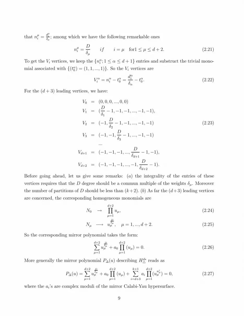
δµ; among which we have the following remarkable ones
nµi =
D
δµ
if i = µ for1 ≤ µ ≤ d + 2. (2.21)
To get the Vi vertices, we keep the nαi ; 1 ≤ α ≤ d + 1 entries and substruct the trivial mono-
mial associated with (tα0 ) = (1, 1, ..., 1). So the Vi vertices are
V αi = nα
i − tα0 =dα
i
δα
− tα0 . (2.22)
For the (d + 3) leading vertices, we have:
V0 = (0, 0, 0, ..., 0, 0)
V1 = (D
δ1
− 1,−1,−1, ...,−1,−1),
V2 = (−1,D
δ2
− 1,−1, ...,−1,−1) (2.23)
V3 = (−1,−1,D
δ3
− 1, ...,−1,−1)
...
Vd+1 = (−1,−1,−1, ...,D
δd+1− 1,−1),
Vd+2 = (−1,−1,−1, ...,−1,D
δd+2− 1).
Before going ahead, let us give some remarks: (a) the integrality of the entries of these
vertices requires that the D degree should be a commun multiple of the weights δµ. Moreover
the number of partitions of D should be less than (k+2). (b) As far the (d+3) leading vertices
are concerned, the corresponding homogeneous monomials are
N0 →d+2∏
µ=1
uµ, (2.24)
Nµ −→ uDδµµ , µ = 1, ..., d + 2. (2.25)
So the corresponding mirror polynomial takes the form:
d+2∑
µ=1
uDδµµ + a0
d+2∏
µ=1
(uµ) = 0. (2.26)
More generally the mirror polynomial P∆(u) describing Hd∗ reads as
P∆(u) =d+2∑
µ=1
uDδµµ + a0
d+2∏
µ=1
(uµ) +k+1∑
i=d+3
ai
d+2∏
µ=1
(uni
µµ ) = 0, (2.27)
where the ai’s are complex moduli of the mirror Calabi-Yau hypersurface.
9

2.3 More on the mirror CY geometry
Here we further explore the relations between the realizations (2.10) and (2.27) of the mirror
Calabi-Yau manifolds. In particular, we give an explicit derivation of the weights δµ involved
in the polynomials (2.27) in terms of the Calabi-Yau qai charges. To do so, first of all recall
that under the projective action
uµ −→ λδµuµ, (2.28)
the polynomial P∆(u) behaves as P∆(λδµu) = λDP∆(u) leaving the zero locus invariant. Using
the identity∑d+2
µ=1 δµ = D, one may reinterpret the Calabi-Yau condition (2.4) or equivaletly
by introducing r integers pa
d+2∑
µ=1
r∑
a=1
paqaµ = −
k+1∑
i=d+3
r∑
a=1
paqai ,
by thinking about it as
δµ =r∑
a=1
paqaµ (2.29)
D =k+1∑
i=d+3
δi = −k+1∑
i=d+3
r∑
a=1
paqai . (2.30)
For instance, for ordinary projective spaces P k, we can use the generalization of the transfor-
mation introduced in [39]; namely
uµ −→ ωQaµuµ,
ud+2 −→ ud+2, (2.31)
where ,roughly speaking, ω is a D − th root of unity. This transformation leaves P∆(u)
invariant as far as the Qaµ’s obey the Calabi-Yau condition Σd+1
µ=1Qaµ = 0 and Qa
d+2 = 0, in
agreement with the choice of the coordinate patch ud+2 = 1. Next by appropriate choice
of λ, we can compare both the transformations(2.28) and (2.31) as well as their actions on
the monomials yi = Πd+2µ=1
(
u(nµ
i −1)µ
)
respectively given by yi −→ yiωΣµδµ(nµ
i −1) and yi −→ yi
ωΣµQaµ(nµ
i −1). Invariance under these actions lead to eqs (2.19-20), and their toric geometry
equations analogue
d+2∑
µ=1
Qaµ = 0 modulo (D) (2.32)
d+2∑
µ=1
Qaµn
µi = 0; modulo (D) . (2.33)
10

Comparing these eqs with eqs(2.32-33) and (2.19-20), one gets the following relation between
the Qaµ and qa
i charges of the original manifold
Qaµ =
qaµ +
1
d + 2
k∑
i=d+3
qai
; modulo (D) (2.34)
As the isometries of eqs(2.26-27) will be involved in the study of the NC hypersurface Calabi-
Yau orbifolds, let us derive general form of these isometries using geometry toric data. We will
distinguish between two cases: (i) the group of isometries Γ0 leaving eq(2.26) invariant. (ii)
its subgroup Γcd of discrete symmetries of eq(2.27). commuting with complex deformations.
3 Discrete Symmetries and CY Orbifolds
To determine the discrete symmetries of the Calabi-Yau homogeneous hypersurfaces, let us
derive the general groups Γ0 and Γcd of transformations leaving eqs(2.26) and (2-27) invariants:
Γ = gω | gW : uµ → gω(uµ) = u′µ = uµ (W)bµ ; P∆(u′) = P∆(u) , (3.1)
where
Wbµ = Πd+2ν=1
[
(ων)aν
µ
]
and where bµ1≤µ≤d+2 is a (d + 2) dimensional vector weight and aνµ are their entries. They
will be determined by symmetry requirements and the Calabi-Yau toric geometry data. As
the solutions we will build depend on the weights δµ, we will distinguish hereafter the P d+1
and WP d+1 spaces; a matter of illustrating the idea and the techniques we will be using.
3.1 P d+1 projective spaces
The crucial point to note here is that because of the equality δ1 = δ2 = ... = δd+2 = 1, the D
degree of the polynomials P∆(u) is equal to (d + 2) and so the constraint eq (2.20) reduces to:∑d+2
µ=1 nµi = (d+2) for any value of the i index. Putting back δµ = 1 in eqs (2.26), one sees that
invariance under Γ0 of the first terms ud+2µ shows that a natural solution is given by taking
ω1 = ω2 = ... = ωd+1 = ω = exp i( 2πd+2
) and then ωbµ = exp i 2πd+2
bµ. However, invariance of the
term∏d+2
µ=1( uµ) under the change (3.1), implies that bµ should satisfy the following constraint
equationd+2∑
µ=1
bµ = 0, modulo (d+2) . (3.2)
11
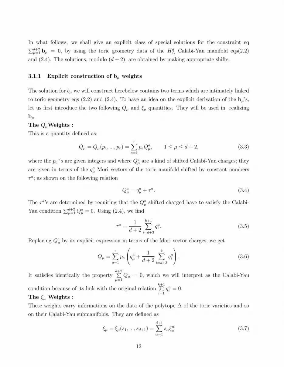
In what follows, we shall give an explicit class of special solutions for the constraint eq∑d+2
µ=1 bµ = 0, by using the toric geometry data of the Hd Calabi-Yau manifold eqs(2.2)
and (2.4). The solutions, modulo (d + 2), are obtained by making appropriate shifts.
3.1.1 Explicit construction of bµ weights
The solution for bµ we will construct herebelow contains two terms which are intimately linked
to toric geometry eqs (2.2) and (2.4). To have an idea on the explicit derivation of the bµ’s,
let us first introduce the two following Qµ and ξµ quantities. They will be used in realizing
bµ.
The QµWeights :
This is a quantity defined as:
Qµ = Qµ(p1, ..., pr) =r∑
a=1
paQaµ, 1 ≤ µ ≤ d + 2, (3.3)
where the pa′s are given integers and where Qa
µ are a kind of shifted Calabi-Yau charges; they
are given in terms of the qaµ Mori vectors of the toric manifold shifted by constant numbers
τa; as shown on the following relation
Qaµ = qa
µ + τa. (3.4)
The τa’s are determined by requiring that the Qaµ shifted charged have to satisfy the Calabi-
Yau condition∑d+2
µ=1 Qaµ = 0. Using (2.4), we find
τa =1
d + 2
k+1∑
i=d+3
qai . (3.5)
Replacing Qaµ by its explicit expression in terms of the Mori vector charges, we get
Qµ =r∑
a=1
pa
qaµ +
1
d + 2
k∑
i=d+3
qai
. (3.6)
It satisfies identically the propertyd+2∑
µ=1Qµ = 0, which we will interpret as the Calabi-Yau
condition because of its link with the original relationk+1∑
i=1qai = 0.
The ξµ Weights :
These weights carry informations on the data of the polytope ∆ of the toric varieties and so
on their Calabi-Yau submanifolds. They are defined as
ξµ = ξµ(s1, ..., sd+1) =d+1∑
α=1
sαξαµ (3.7)
12

where the sα’s are integers and where ξαµ are defined in terms of the toric data of Md+1
as
follows
ξαµ =
r∑
a=1
pa
qaµn
αµ +
1
d + 2
k+1∑
i=d+3
qai n
αi
. (3.8)
Like for the Qµ weights, one can check here also that the sumd+2∑
µ=1ξµ vanishes identically due
to the constraint equation(2.15).
The bµ Weights :
A class of solutions for bµ based on the Calabi-Yau toric geometry data (2.2) and (2.4), may
be given by a linear combination of the Qµ and ξµ weights as shown herebelow:
bµ = m1Qµ + m2ξµ, (3.9)
where m1and m2 are integers modulo (d + 2). Moreover setting bµ =∑d+2
ν=1 aνµ and
Qαµ = Qa
µ for α = 1, ..., r;
Qαµ = 0 for α = (r + 1), ..., (d + 2), (3.10)
while Qαµ = Qa
µ for r ≥ d + 1, we can rewrite the above solutions as follows:
aνµ = m1Q
νµ + m2ξ
νµ. (3.11)
Therefore, the general transformations of the Γ0(Pd+1) group of discrete isometries are given
by the change (3.1) with bµ vector weights depending on (r + d + 1) = k integers; namely r
integers pa and (d + 1) integers sα.
3.1.2 Complex Deformations
To get the discrete symmetries of the full Calabi-Yau homogeneous complex hypersurface
including the complex deformations eq(2.27), one should solve more complicated constraint
relations which we give hereafter. Under Γcd of transformations eq(2.27), the complex defor-
mations of the Calabi-Yau manifold P∆(u) are stable provided the bµ weights satisfy eq(3.2)
but also the following constraint eqs:
d+2∑
µ=1
bµnνµ = 0, (3.12)
where the nνµ ’s are as in eq(2.27). A particular solution of these constraint eqs is given by
taking bµ = Qµ that is m1 = 1 and m2 = 0. Indeed replacing bµ by its expression(3.9) and
13

putting back into the above relation, we get by help of the identity (2.20),
d+2∑
µ=1
r∑
a=1
pa(qaµ + τa)nν
µ
=r∑
a=1
pa
d+2∑
µ=1
qaµnν
µ + (d + 2)τa
=r∑
a=1
pa
d+2∑
µ=1
qaµnν
µ +k∑
i=d+3
qai n
νµ
= 0. (3.13)
For m1, m2 6= 0, the relation bµ = m1Qµ + m2ξµ cease to be a solution of the constraint
eq(3.12). Therefore Γcd is a subgroup of Γ0. It depends on the pa integers and involves the
Calabi-Yau condition only.
3.2 WP d+1 weighted projective spaces
The previous analysis made for the case of P d+1 applies as well for WP d+1. Starting from
eq(2.26) and making the change (3.1), invariance requirement leads to take the ωµ group
parameters as ωµ = exp i2πδµ
Dand the aν
µ coefficients constrained as
d+2∑
ν=1
δνaνµ = 0, modulo δµ
d+2∑
µ=1
aνµ = 0. (3.14)
Following the same reasoning as before, one can write down a class of solution, with integer
entries, in terms of the previous weights as follows
aνµ = (δν)−1
[
m1Qνµ + m2ξ
νµ
]
, (3.15)
where Qνµ and ξν
µ are as in eq (3.11). In case where the complex deformations of eq(2.27) are
taken into account, the discrete symmetry group is no longer the same since the constraint
eq(3.13) is now replaced by the following one
d+2∑
µ=1
aνµn
iµ = 0, ∀ ν = 1, ..., (d + 2). (3.16)
Like in the projective case where the δµ’s are equal to one, the solutions for the aνµ integers
are given by eq(3.15) with m1 6= 0 and m2 = 0. To conclude this section, one should note that
the group of discrete isometries Γcd ⊂ Γ0 of the Calabi-Yau hypersurfaces including complex
deformations is intimately related to the Calabi-Yau condition.
14

4 NC Toric CY Manifolds
Before exposing our results regarding NC toric Calabi-Yau’s, let us begin this section by
reviewing briefly the BL idea of building NC orbifolds of Calabi-Yau hypersurface.
4.1 Algebraic geometric approach for CY
Roughly speaking, given a d dimensional a Calabi-Yau manifold Xd described algebraically
by a complex equation p(zi) = 0 with a group Γ of discrete isometries. Taking the quotient of
Xd, by the action of the finite group Γ
Γ : zi → gzig−1, g ∈ Γ (4.1)
such that the two following conditions are fulfilled p(zi) polynomial and the (d, 0) holomorphic
from are invaraints. The latter condition is equivalently to the vanishing the first Chern class
c1 = 0. Using the discrete torsion, one can build the NC extensions of the orbifold,(
Xd
Γ
)
ncas
follows. The coordinate zi’s are replaced by matrix operators Zi satisfying
ZiZj = θijZjZi, (4.2)
Invariance of p(zi) requires that the parameter θij ’s to be in the discrete group Γ. Moreover,
the Calabi-Yau condition imposes the extra constraint equation
∏
i
θij = 1, ∀j 6= i, (4.3)
In this case of the quintic, embedded in a P 5 projective space described by the homogeneous
polynomial p(z1, ..., z5) of degree 5:
p(zi) = z51 + z5
2 + z53 + z5
4 + z55 + a0
5∏
1=1
zi = 0. (4.4)
The group Γ acts as zi −→ zi ωQai where ω5 = 1 and where the Qa
i vectors are
Q1i = (1,−1, 0, 0, 0),
Q2i = (1, 0,−1, 0, 0), (4.5)
Q3i = (1, 0, 0,−1, 0).
In the coordinate patch U = (z1, z2, z3, z4); z5 = 1, eq(4.5) reduces to
1 + z51 + z5
2 + z53 + z5
4 + a0
4∏
j=1
zj = 0. (4.6)
15

The local NC algebra Anc describing the NC version of equation(4.5) is obtained by associating
to z5 the matrix z5I5 and to each holomorphic variable zi a 5× 5 matrix Zi satisfying the BL
algebra
Z1Z2 = αZ2Z1, Z1Z3 = α−1βZ3Z1,
Z1Z4 = β−1Z4Z1, Z2Z3 = αγZ3Z2, (4.7)
Z2Z4 = γ−1Z4Z2, Z3Z4 = βγZ4Z3
where α, β and γ are fifth roots of unity. The centre of this algebra Z(Anc) = I5, Z5ν , Π
4ν=1Zν,
that is,
[
Zµ, Z5ν
]
= 0,[
Zµ, Π4ν=1Zν
]
= 0, (4.8)
According to the Schur lemma, one can set Z5ν = I5z
5ν and Π4
ν=1Zν = I5Π4ν=1zν and so the
centre coincide with the equation of the quintic. In what follows we extend this analysis to
NC toric Calabi-Yau orbifolds.
4.2 NC toric CY orbifolds
Following the same lines as [38, 39, 40, 41, 42] and using the discrete symmetry group Γ, one
can build the orbifolds O = Hd∗ / Γ of the Calabi Yau hypersurface and work out their non
commutative extensions Onc. The main steps in the building of Onc may summarized as fol-
lows: First start from the Calabi-Yau hypersurfaces Hd∗ eqs(2.26-27) and fix a coordinate pach
of WP d+1, say ud+2 = 1. Then impose the identification under the discrete automorphisms
(3.1) defining Hd∗ /Γ. The NC extension of this orbifold is obtained as usual by extending the
commutative algebra Ac of functions on Hd∗ / Γ to a NC one Anc ∼ Onc. In this algebra, the
uµ coordinates are replaced by matrix operators Uµ satisfying the algebraic relations
UµUν = θµνUνUµ, ν > µ = 1, ..., d + 1, (4.9)
where the θµν non commutativity parameters obey the following constraint relations
θµνθνµ = 1, (4.10)
(θµν)Dδν = 1, (4.11)
d+1∏
µ=1
(θµν) = 1 (4.12)
16

as far as eq(2.26) is concerned that is in the region of the moduli space where the complex
moduli ai are zero (i = 1, . . .). However, in the general case where the ai’s are non zero we
should have moreover:d+1∏
µ=1
(
θnα
µµν
)
= 1; α = 1, ..., d + 1. (4.13)
Let us comment briefly these constraint relations. Eq(4.11) reflects that the parameters θνµ
are just the inverse of θµν and can be viewed as describing deformations away from the identity
suggesting by the occasion that they may be realized as
θµν = exp ηµν
, where ηµν = −ηνµ is the infinitesimal version of the non commutativity parameter. The
constraint (4.12-13) reflect just the remarkable property according to which UDδνν and Πd+2
µ=1 (Uµ)
are elements in the centre Z(Anc) of the non commutative algebra Anc,i.e;
[
Uµ, UDδνν
]
= 0, (4.14)[
Uµ, Πd+2ν=1 (Uν)
]
= 0. (4.15)
Finally, the constraint eqs(4.14), obtained by requiring[
Uµ, Πd+2ν=1
(
Unα
µν
)]
= 0, describe the
compatibility between non commutativity and deformations of the complex structure of the
Calabi-Yau hypersurfaces.
In what follows we shall solve the above constraint equations (4.11-14) in terms of toric
geometry data of the toric variety in which the mirror geometry is embedded. Since these
solutions depend on the weight vector δ we will consider two cases; δµ = 1 for all values of µ
and δµ taking general numbers eqs(2.20).
4.2.1 Matrix representations for projective spaces
The analysis we have developed so far can be made more explicit by computing the NC algebras
associated to the Calabi-Yau hypersurface orbifolds with discrete torsion. In this regards, a
simple and instructive class of solutions of the above constraint eqs may be worked in the
framework of the P d+1 ordinary projective spaces. To do this, consider a d complex dimension
Calabi-Yau homogeneous hypersurfaces in P d+1 namely,
ud+21 + ud+2
2 + ud+23 + ud+2
4 + . . . + ud+2d+2 + a0
d+2∏
µ=1
uµ = 0, (4.16)
17
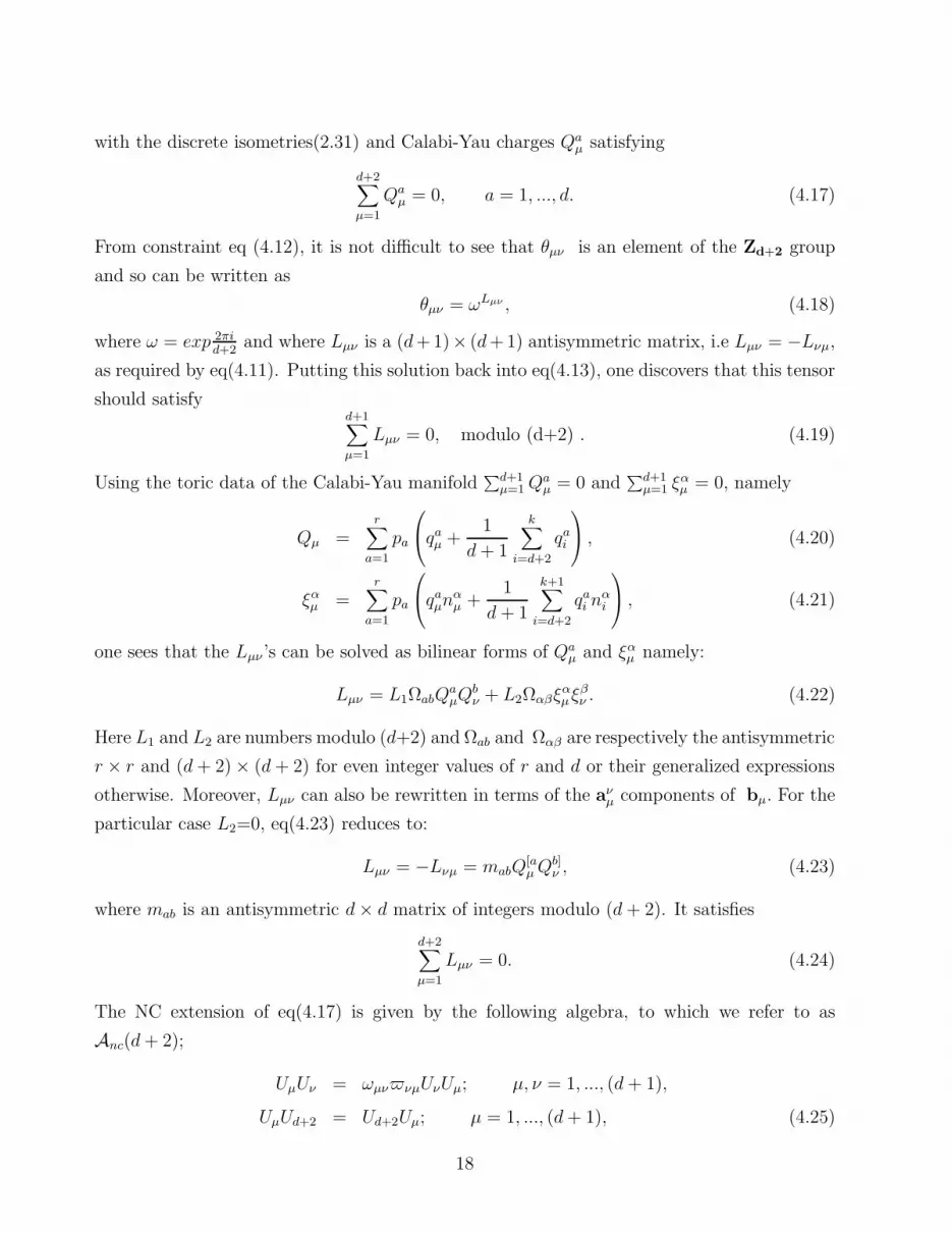
with the discrete isometries(2.31) and Calabi-Yau charges Qaµ satisfying
d+2∑
µ=1
Qaµ = 0, a = 1, ..., d. (4.17)
From constraint eq (4.12), it is not difficult to see that θµν is an element of the Zd+2 group
and so can be written as
θµν = ωLµν , (4.18)
where ω = exp 2πid+2
and where Lµν is a (d+1)× (d+1) antisymmetric matrix, i.e Lµν = −Lνµ,
as required by eq(4.11). Putting this solution back into eq(4.13), one discovers that this tensor
should satisfyd+1∑
µ=1
Lµν = 0, modulo (d+2) . (4.19)
Using the toric data of the Calabi-Yau manifold∑d+1
µ=1 Qaµ = 0 and
∑d+1µ=1 ξα
µ = 0, namely
Qµ =r∑
a=1
pa
qaµ +
1
d + 1
k∑
i=d+2
qai
, (4.20)
ξαµ =
r∑
a=1
pa
qaµn
αµ +
1
d + 1
k+1∑
i=d+2
qai n
αi
, (4.21)
one sees that the Lµν ’s can be solved as bilinear forms of Qaµ and ξα
µ namely:
Lµν = L1ΩabQaµQ
bν + L2Ωαβξα
µξβν . (4.22)
Here L1 and L2 are numbers modulo (d+2) and Ωab and Ωαβ are respectively the antisymmetric
r × r and (d + 2) × (d + 2) for even integer values of r and d or their generalized expressions
otherwise. Moreover, Lµν can also be rewritten in terms of the aνµ components of bµ. For the
particular case L2=0, eq(4.23) reduces to:
Lµν = −Lνµ = mabQ[aµ Qb]
ν , (4.23)
where mab is an antisymmetric d × d matrix of integers modulo (d + 2). It satisfies
d+2∑
µ=1
Lµν = 0. (4.24)
The NC extension of eq(4.17) is given by the following algebra, to which we refer to as
Anc(d + 2);
UµUν = ωµννµUνUµ; µ, ν = 1, ..., (d + 1),
UµUd+2 = Ud+2Uµ; µ = 1, ..., (d + 1), (4.25)
18

where µν is the complex conjugate of ωµν . The latters are realized in terms of the Calabi-Yau
charges data as follows:
ωµν = exp i(
2π
d + 2mabQ
aµQb
ν
)
= ωmabQaµQb
ν . (4.26)
Using the propriety d+2µν = 1 and
∏
µµν = 1, one can check that the center of the algebra
(4.26) is given by the
Z(Anc) = λ1Ud+21 + λ2U
d+22 + . . . + λd+1U
d+2d+1 + λd+2Id+2 +
d+1∏
µ=1
Uµ. (4.27)
Schur lemma implies that this matrix equation can be written
Z(Anc) = p(u1, u2, . . . , ud+1)Id+2. (4.28)
To determine the explicit expression of p(u1, u2, . . . , ud+1), let us discuss in what follow the
matrix irreducible representations of the NC Calabi-Yau algebra for a regular point. In the
next subsection we will give the representation for the fixed points, where the representation
becomes reducible and corresponds to fractional branes.
Finite dimensional representations of the algebra (4.26) are given by matrix subalgebras
Mat [n(d + 2), C], the algebra of n(d + 2) × n(d + 2) complex matrices, with n = 1, 2, ....
Computing the determinant of both sides of eqs(4.26)
det (UµUν) = (ωµννµ)Ddet (UνUµ) = det (UνUµ), (4.29)
the dimension D of the representation to be such that:
(ωµννµ)D = 1. (4.30)
Using the identity (4.19), one discovers that D is a multiple of (d + 2). We consider the
fundamental (d + 2)× (d + 2) matrix representation obtained by introducing the following set
Q;Pαab; a, b = 1, ..., d
of matrices:
Pαab= diag(1, αab,α
2ab, ..., α
d+1ab ); Q =
0 0 0 . . . 11 0 0 . . . 00 1 0 . . . 0. . . . . . .. . . . . . .0 0 0 . 1 0 00 0 0 . . 1 0
(4.31)
19

where αab = wmab satisfying αd+2ab = 1. From these expressions, it is not difficult to see that
the
Q;Pαab; a, b = 1, ..., d
matrices obey the algebra:
PαPβ = Pαβ
Pd+2α = 1, (4.32)
Qd+2 = 1.
Using the following identities
Pnµ
αµQmµ = αnµmµ
µ QmµPnµ
αµ, (4.33)
(
Pnµαµ
Qmµ
) (
Pnναν
Qmν
)
= αnimνµ α−mµnν
ν
(
Pnναν
Qmν
) (
Pnναµ
Qmµ
)
, (4.34)
one can check that the Uµ operators can be realized as
Uµ = uµ
d∏
a,b=1
(
PQa
µαabQ
Qµb)
, (4.35)
where uµ are C-number which should be thought of as in (4.17). From the Calabi-Yau condi-
tion, one can also check that the above representation satisfy
Ud+2µ = ud+2
µ Id+2
d+1∏
µ=1
Uµ = Id+2
d+1∏
µ=1
uµ
. (4.36)
Putting these relations back into (4.29), one finds that the polynomial p(uµ) is nothing but
the eq (4.17) of the Calabi-Yau hypersurface.
4.2.2 Solution for weighted projective spaces
In the case of weighted projective spaces with a weight vector δ =(δ1, ..., δd+2); the degree D
of the Calabi-Yau polynomials and the corresponding Ni vertices are respectively given by
eqs(2.19-20) and (2.24-25). Note that integrality of the vertex entries requires that D should
be the smallest commun multiple of the weights δµ; that is Dδµ
an integer. Following the same
reasoning as for the case of the projective space, one can work out a class of solutions of the
constraint eqs(4.11-13) in terms of powers of ωµ. We get the result
θµν = exp i2π
[
(δν)Lµν
D
]
, (4.37)
20

where Lµν is as in eq(4.23). Instead of being general, let us consider a concrete example dealing
with the analogue of the quintic in the weighted projective space WP4δ1,δ2,δ3,δ4,δ5
. In this case
the Calabi-Yau hypersurface,∑5
µ=1 uDδµµ + a0
∏5µ=1 (uµ) = 0; which for the example δ1 = 2 and
δ2 = δ3 = δ4 = δ5 = 1, reduces to:
u31 + u6
2 + u63 + u6
4 + u65 + a0
5∏
µ=1
(uµ) = 0. (4.38)
This polynomial has discrete isometries acting on the homogeneous coordinates uµ as:
uµ → uµζa
νµ
µ µ = 1, ..., 5, (4.39)
with ζ31 = 1 while ζ6
µ = ω6 = 1; i.e ζ1 = ω2 and ζµ = ω and where the aνµ are consistent with the
Calabi-Yau condition. In the coordinate patch uµ1≤4 with u5 = 1, the equations defining the
NC geometry of the Calabi-Yau (4.39) with discrete torsion, upon using the correspondence
u → U , are given by the algebra (5.1) where the θµν parameters should obey now the following
constraint eqs:
θ3µ1 = 1, µ = 2, 3, 4,
θ6µν = 1, ν 6= 1, µ (4.40)
4∏
µ=1
θνµ = 1, ∀ν
θµνθνµ = 1, ∀µ, ν.
Setting θµν as θµν = ωLµν the constraints on Lµν read as:
Lµν = −Lνµ integers modulo 6,
Lµ1 = even modulo 6. (4.41)
Particular solutions of this geometry may be obtained by using antisymmetric bilinears of aνµ.
Straightforward calculations show that, for pµ = 1, Lµν is given by the following 4× 4 matrix:
Lµν =
0 k1 − k3 −k1 + k2 k3 − k2
−k1 + k3 0 k1 −k3
k1 − k2 −k1 0 k2
−k3 + k2 k3 −k2 0
(4.42)
where the kµ integers are such that kµ − kν ≡ 2rµν ∈ 2Z.
The NC algebra associated with eq(4.39) reads, in terms of ωµ = ωkµ and µ = ω−kµ, as
21

follows:
U1U2 = ω13U2U1, U1U3 = 1ω2U3U1,
U1U4 = ω32U4U1, U2U3 = ω1U3U2, (4.43)
U2U4 = 3U4U2, U3U4 = ω2U4U3.
Furthermore taking α = ω13, β = ω23 and γ = ω3, one discovers an extension of the BL
NC algebra( 4.4); the difference is that now the deformation parameters are such that:
α3 = β3 = γ6 = 1. (4.44)
4.2.3 Fractional Branes
Here we study the fractional branes corresponding to reducible representations at singular
points. To illustrate the idea, we give a concrete example concerning the mirror geometry in
terms of the Pd+1 projective space. First note that the Anc(d+2) (4.37) corresponds to regular
points of NC Calabi-Yau. This solution is irreducible and the branes do not fractionate. A
similar solutions may be worked out as well for fixed points where we have fractional branes.
We focus our attention on the orbifold of the eight-tic, namely,
u81 + u8
2 + . . . + u88 + a0
8∏
µ=1
uµ = 0, (4.45)
with the discrete isometries Z68 and Calabi-Yau charges Qa
µ
Q1µ = (1,−1, 0, 0, 0, 0, 0, 0)
Q2µ = (1, 0,−1, 0, 0, 0, 0, 0)
Q3µ = (1, 0, 0,−1, 0, 0, 0, 0)
Q4µ = (1, 0, 0, 0,−1, 0, 0, 0) (4.46)
Q5µ = (1, 0, 0, 0, 0,−1, 0, 0)
Q6µ = (1, 0, 0, 0, 0, 0,−1, 0).
The corresponding NC algebra is deduced from the general one given in (4.26). At regular
points, the matrix theory representation of this algebra is irreducible as shown on eqs (4.37).
However, the situation is more subtle at fixed points where representations are reducible. One
way to deal with the singularity of the orbifold with respect to Z68 is to interpret the algebra
as describing a Z38 orbifold with Z3
8 discrete torsions having singularities in codimension four.
22

Starting from eqs(4.26) and choosing matrix coordinates U5, U6 and U7 in the centre of the
algebra by setting
(ωµννµ) = 1, for µ = 5, 6, 7, 8; ∀ν = 1, ..., 8, (4.47)
the algebra reduces to
U1U2 = α1α2U2U1
U1U3 = α−11 α3U3U1
U1U4 = α−12 α−1
3 U4U1 (4.48)
U2U3 = α1U3U2
U2U4 = α2U4U2,
U3U4 = α3U4U3
and all remaining other relations are commuting. In these equations, the αµ ’s are such
that α8µ = 1; these are the phases Z3
8. At the singularity where the u1, u2, u3, and u4
moduli of eq(4.37) go to zero, one ends with the familiar result for orbifolds with discrete
torsion. Therefore the D-branes fractionate in the codimension four singularities of the eight-
tic geometry.
5 Link with the BL Construction
In this section we want to rederive the results of [39] concerning NC quintic using the analysis
developed in section 3 and 4. Recall that in the coordinate patch uµ1≤4 and u5 = 1,
the defining equations of NC geometry of the quintic with discrete torsion, upon using the
correspondence u → U , are given by the following operators algebra.
UµUν = θµνUνUµ, ν > µ = 1, ..., 4, (5.1)
where the θµν ’s are non zero complex parameters. As the monomials U5µ and
∏5µ=1 (Uµ) are
commuting with all the Uµ ’s , we have also
[
Uν , U5µ
]
= 0,
Uν ,4∏
µ=1
Uµ
= 0. (5.2)
23

Compatibility between eqs (5.1-2) gives constraint relations on θµν ’s namely
θ5νµ = 1, (5.3)
4∏
µ=1
θνµ = 1, ∀ν (5.4)
θµνθνµ = 1; θµ5 = 1, ∀µ, ν. (5.5)
To establish the link between our way of doing and the construction of [41], it is interesting to
note that the analysis of [41] corresponds in fact to a special representation of the formalism
we developed so far. The idea is summarized as follows: First start from eq(3.1), which reads
for the quintic as:
uµ → uµωbµ, (5.6)
where the bµ weights, bµ =∑5
ν=1 aνµ, µ = 1, . . . , 5, are such that
5∑
ν=1
bµ = 0. (5.7)
This relation, interpreted as the Calabi-Yau condition, can be solved in different ways. A way
to do is to set the bµ weights as
bµ = (p1 + p2 + p3,−p1,−p2,−p3, 0), (5.8)
or equivalently by taking the weight components bνµ as:
aνµ =
p1 p2 p3 0 0−p1 0 0 0 00 −p2 0 0 00 0 −p3 0 00 0 0 0 0
, (5.9)
where pa are integers modulo 5. More general solutions can be read from eqs (4.23) by following
the same method. The next step is to take θµν = expi(2π5Lµν) with Lµν as follows:
Lµν = m12
(
a1µa
2ν − a1
νa2µ
)
− m23
(
a2µa
3ν − a2
νa3µ
)
+ m13
(
a1µa
3ν − a1
νa3µ
)
, (5.10)
where m12 = k1, m23 = k2 and m13 = k3 are integers modulo 5. For pµ = 1, we get
Lµν =
0 k1 − k3 −k1 + k2 k3 − k2
−k1 + k3 0 k1 −k3
k1 − k2 −k1 0 k2
−k3 + k2 k3 −k2 0
, (5.11)
24

and so the NC quintic algebra reads:
U1U2 = ωk1−k3U2U1, U1U3 = ω−k1+k2U3U1,
U1U4 = ωk3−k2U4U1, U2U3 = ωk1U3U2, (5.12)
U2U4 = ω−k3U4U2, U3U4 = ωk2U4U3.
Setting ωµ = ωkµ and µ = ω−kµ , the above relations become:
U1U2 = ω13U2U1, U1U3 = 1ω2U3U1,
U1U4 = ω32U4U1, U2U3 = ω1U3U2, (5.13)
U2U4 = 3U4U2, U3U4 = ω2U4U3.
Now taking α = ω13, β = ω23 and γ = ω3, one discovers exactly the BL algebra eqs(4.8).
5.1 More on the NC quintic
As we mentioned, the solution given by eqs(5.8-9) is in fact a special realization of the BL
algebra (4.8). One can also write down other representations of the NC quintic; one of them
is based on taking aνµ as:
aνµ =
p1 0 p3 0 0−2p1 p2 0 0 0p1 −2p2 p3 0 00 p2 −2p3 0 00 0 0 0 0
. (5.14)
The corresponding bµ weight vector is then:
bµ = (p1 + p3,−2p1 + p2, p1 − 2p2 + p3, p2 − 2p3; 0), (5.15)
with pa’s are integers modulo 5. As one sees this is a different solution from that given in
eq(5.8-9) as the corresponding Γ group of isometries acts differently on the uµ variables leading
then to a different orbifold with discrete torsion. Note that setting pµ = 1, the aνµ weights are
nothing but the Mori vectors of the blow up of the the A2 affine singularity of K3, used in
the geometric engineering method of 4D N = 2 superconformal theories embedded in type II
superstrings.
Setting pµ = 1 and using equations (5.10) and (5.14), the anti-symmetric Lµν matrix reads as:
Lµν =
0 k1 + k2 + 2k3 −2k1 − 2k2 k1 + k2 − 2k3
−k1 − k2 − 2k3 0 3k1 − k2 − 2k3 −2k1 + 2k2 + 4k3
2k1 + 2k2 −3k1 + k2 + 2k3 0 k1 − 3k2 − 2k3
−k1 − k2 + 2k3 2k1 − 2k2 − 4k3 −k1 + 3k2 + 2k3 0
(5.16)
25

where the k1, k2 and k3 are integers modulo 5. The new algebra describing the NC quintic
reads, in terms of the ωµ and ν generators of the Z35 , as follows:
U1U2 = ω1ω2ω23U2U1, U1U3 = 2
122U3U1,
U1U4 = ω1ω223U4U1, U2U3 = ω3
1223U3U2, (5.17)
U2U4 = 21ω
22ω
43U4U2, U3U4 = ω1
32
23U4U3.
Setting α = ω1ω2ω23, β = 12ω
23 and γ = ω2
122
43, one discovers, once again, the BL algebra
(4.7). Therefore eq(5.9) and eq(5.14) give two representations of the BL algebra.
5.2 Comments on lower dimension CY manifolds
The analysis we developed so far applies to complex d dimension homogeneous hypersurfaces
with discrete torsion; d ≥ 2. We have discussed the cases d ≥ 3; here we want to complete
this study for lower dimension Calabi-Yau manifolds namely K3 and the elliptic curve. These
are very special cases which deserves some comments. For the K3 surface in CP 3, we have
u41 + u4
2 + u43 + u4
3 + a0
4∏
µ=1
uµ = 0, (5.18)
This is a quartic polynomial with a Z4 × Z4 symmetry acting on the ui variables as:
uµ → wQaµuµ, (5.19)
where w4 = 1 and where aaµ are integers satisfying the Calabi-Yau condition
4∑
µ=1Qa
µ = 0.
Choosing Qaµ as,
Q1µ = (1,−1, 0, 0)
Q2µ = (1, 0,−1, 0) (5.20)
the 3 × 3 matrix Lµν reads as
Lµν =
0 k −k−k 0 kk −k 0
. (5.21)
Therefore the NC K3 algebra reads as:
U1U2 = U2U1ei 2πk
4 ,
U1U3 = U3U1e−i 2πk
4 ,
26

U1U4 = U4U1, (5.22)
U2U3 = U3U2ei 2πk
4 ,
U2U4 = U4U2,
U3U4 = U4U3.
where k is an integer modulo 4. Note that one gets similar results by making other choices of
Qai such as,
Q1µ = (1,−2, 1, 0)
Q2µ = (1, 1,−2, 0). (5.23)
More general results may also be written down for K3 embedded in WP(δ1,δ2,δ3,δ4). In the case
of the one dimensional elliptic fiber given by a cubic in P 2
u31 + u3
2 + u33 + a0
3∏
µ=1
uµ = 0, (5.24)
the constraint equations defining non commutativity are trivially solved. They show that
Lµν = 0 and so θ12 = 1 leading then to a commutative geometry. NC geometries involving
elliptic curves can be constructed; the idea is to consider orbifolds of products of elliptic curves.
More details are exposed in the following section. Related ideas with fractional branes will be
considered as well.
6 NC Elliptic Manifolds
In this section we want refine the study of the NC Calabi-Yau hypersurface defined in terms
of orbifolds of elliptic curves. The original idea of this construction was introduced first in
[39]; see also [73], in connection with the NC orbifold T 6
Z22. The method is quite similar to that
discussed for the quintic and generalized Calabi-Yau geometries in sections 4 and 5. To start
consider the following elliptic realization of T 2n+2
Γ; that is T 2n+2 is represented by the product
of (n + 1) elliptic curves (T 2)⊗(2k+1)
where n = 2k. Each elliptic curve is given in Weierstrass
form as:
y2µ = xµ(xµ − 1)(xµ − aµ), µ = 1, ..., n + 1, (6.1)
with a point added at infinity µ = 1, ..., n+1. The system (xµ, yµ); µ = 1, ..., n+1 defines
the complex coordinates of C2n+2 space and aµ are (n + 1) complex moduli. For later use, we
introduce the algebra Ac of holomorphic functions on T 2n+2. This is a commutative algebra
27

generated by monomials in the xµ’s and yµ’s with the conditions eqs(6.1). The discrete group
Γ acts on xµ’s and yµ’s as:
xµ → x′µ = xµ,
yµ → y′µ = yµω
Qµ, (6.2)
where ω is an element of the discrete group Γ and where Qµ are integers which should be
compared with eq(4.24). Note that if one is requiring that eqs(6.1) to be invariant under Γ,
then ω2 should be equal to one that is ω = ±1. If one requires moreover that the monomial∏n+1
µ=1 yµ or again the holomorphic ((n+1), 0) form dy1 ∧ dy2....∧ dyn+1, to be invariants under
the orbifold action, it follows then that∏n+1
µ=1 ωQµ = ωΣµQµ = 1. This is equivalent to
n+1∑
µ=1
Qµ = 0, modulo 2 (6.3)
defines the Calabi-Yau condition for the orbifold T 2n+2
Γ. Therefore the Γ discrete group is given
by Γ = (Z2)⊗n. Following the discussion we made in section 4, this equation can also be
rewritten asn+1∑
µ=1
Qaµ = 0, modulo 2; a = 1, ..., n. (6.4)
The four fixed points of the orbifold for each two torus T 2 are located at (xµ = 0, 1, aµ; yµ = 0)
and the point at infinity; i.e (xµ = ∞; yµ = ∞). This later can be brought to a fixed finite
point by working in another coordinate patch related to the old one by using the change of
variables:
yµ → y′µ =
yµ
x2µ
xµ → x′µ =
1
xµ
. (6.5)
The NC version of the orbifold T 2n+2
Γis obtained by substituting the usual commuting xµ and
yµ variables by the matrix operators Xµ and Yµ respectively. These matrix operators satisfy
the folowing NC algebra structure:
YµYν = θµνYνYµ, (6.6)
XµXν = XνXµ, (6.7)
XµYν = YνXµ, (6.8)
with
YµY2ν = Y 2
ν Yµ, (6.9)
28
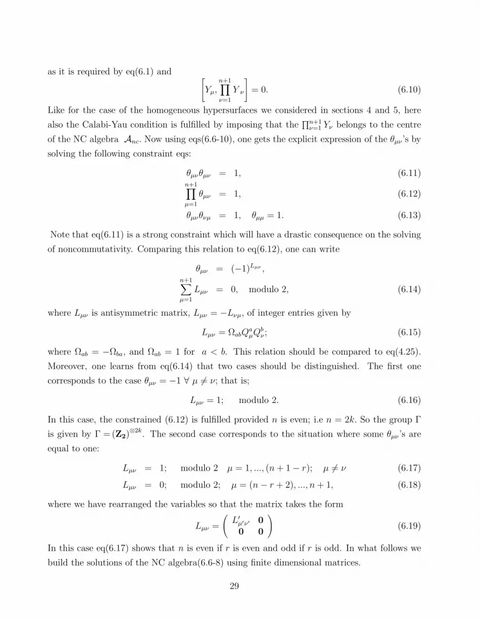
as it is required by eq(6.1) and[
Yµ,n+1∏
ν=1
Y ν
]
= 0. (6.10)
Like for the case of the homogeneous hypersurfaces we considered in sections 4 and 5, here
also the Calabi-Yau condition is fulfilled by imposing that the∏n+1
ν=1 Yν belongs to the centre
of the NC algebra Anc. Now using eqs(6.6-10), one gets the explicit expression of the θµν ’s by
solving the following constraint eqs:
θµνθµν = 1, (6.11)n+1∏
µ=1
θµν = 1, (6.12)
θµνθνµ = 1, θµµ = 1. (6.13)
Note that eq(6.11) is a strong constraint which will have a drastic consequence on the solving
of noncommutativity. Comparing this relation to eq(6.12), one can write
θµν = (−1)Lµν ,n+1∑
µ=1
Lµν = 0, modulo 2, (6.14)
where Lµν is antisymmetric matrix, Lµν = −Lνµ, of integer entries given by
Lµν = ΩabQaµQ
bν ; (6.15)
where Ωab = −Ωba, and Ωab = 1 for a < b. This relation should be compared to eq(4.25).
Moreover, one learns from eq(6.14) that two cases should be distinguished. The first one
corresponds to the case θµν = −1 ∀ µ 6= ν; that is;
Lµν = 1; modulo 2. (6.16)
In this case, the constrained (6.12) is fulfilled provided n is even; i.e n = 2k. So the group Γ
is given by Γ = (Z2)⊗2k. The second case corresponds to the situation where some θµν ’s are
equal to one:
Lµν = 1; modulo 2 µ = 1, ..., (n + 1 − r); µ 6= ν (6.17)
Lµν = 0; modulo 2; µ = (n − r + 2), ..., n + 1, (6.18)
where we have rearranged the variables so that the matrix takes the form
Lµν =
(
L′µ′ν′ 0
0 0
)
(6.19)
In this case eq(6.17) shows that n is even if r is even and odd if r is odd. In what follows we
build the solutions of the NC algebra(6.6-8) using finite dimensional matrices.
29

6.1 Solution I
Replacing the relation (6.16) back into in eqs(6.6-8), the non commutativity algebra, which
reads as:
YµYν = −YνYµ, (6.20)
YµY2ν = Y 2
ν Yµ (6.21)
XµXν = XνXµ, (6.22)
XµYν = YνXµ, (6.23)
may be realized in terms of 2k × 2k matrices of the space of matrices M(2k, C). These are
typical relations naturally solved by using the 2k dimensional Clifford algebra generated by
the basis system Γı, µ = 1, ..., 2k:
Γµ, Γν = 2δµν ,
Γi, Γ2k+1 = 0, (6.24)
where Γ2k+1 =∏2k
i=1 Γi. We therefore have:
Yµ = bµΓµ, µ = 1, ..., 2k, (6.25)
Y2k+1 = b0Γ2k+1, (6.26)
Xµ = xµI2k (6.27)
where the bµ’s are complex scalars. This solution has remarkable features: (i) After choosing
a hermitian Γ matrices representation, one can see at the fixed planes, where 2k variables
among the (2k+1) yµ’s act by zero and all others zero, that there exists a multiplicity of
inequivalent representations for each set of roots xµ of the Weierstrass forms. Therefore, one
can get 2k distinct NC points, as there are 2k irreducibles representations corresponding to 2k
eigenvalues of the non zero matrix variable and so the branes fractionate on the singularity.
(ii) The non-commutative points of the singular planes are then seen to be a 2k cover of the
commutative singular plane, which is a (CP 1)⊗k. The 2k cover is branched around the four
points xk = 0, 1, ak,∞ and hence the NC points form an elliptic manifold T 2k of the form
eq(6.1). Around each of these four points, there is a (Z2) monodromy of the representations,
which is characteristic of the local singularity as measuring the effect of discrete torsion.
30

6.2 Solution II
Putting the relations (6.17) back into in eqs(6.6-8), the resulting NC algebra depends on the
integer r and reads as:
YµYν = −YνYµ, µ, ν = 1, ..., (n + 1 − r). (6.28)
YµYν = YνYµ, µ, ν = (n + 2 − r), ..., (n + 1), (6.29)
YµY2ν = Y 2
ν Yµ, µ = 1, ..., (n + 1), (6.30)
XµXν = XνXµ, (6.31)
XµYν = YνXµ. (6.32)
For r = 2s even, irreducible representations of this algebra are given, in terms of 2k−s × 2k−s
matrices of the space M(2k−s, C), by the 2(k − s) dimensional Clifford algebra. The result is:
Yµ = bµΓµ, i = 1, ..., 2(k − s), (6.33)
Y2(k−s)+1 = b0
2(k−s)∏
µ=1
Γµ, (6.34)
Yµ = yµI2k−s, i = 2(k − s + 1), ..., (2k + 1), (6.35)
Xµ = xµI2k−s. (6.36)
In the end of this section, we would like to note that this analysis could be extended to a
general case initiated in [73], where the elliptic curves are replaced by K3 surfaces. This
might be applied to the resolution of orbifold singularities in the moduli space of certain
models, describing a D2 brane wrapped n times over the fiber of an elliptic K3, as follows [74]
M1,n = Sym(K3) =K3⊗n
Sn
. (6.37)
Here M1,n denotes the moduli space of a D2-brane with charges (1, n) and Sn is the group of
permutation of n elements.
7 Conclusion
In this paper we have studied the NC version of Calabi-Yau hypersurface orbifolds using
the algebraic geometry approach of [40,41] combined with toric geometry method of complex
31

manifolds. Actually this study extends the analysis on the NC Calabi-Yau manifolds with
discrete torsion initiated in [41] and expose explicitly the solving of non commutativity in
terms of toric geometry data. Our main results may be summarized as follows:
(1) First we have developed a method of getting d complex Calabi-Yau mirror coset man-
ifolds Ck+1/C∗r , k − r = d, as hypersurfaces in WP d+1. The key idea is to solve the yi
inavriants (2.12-13) of mirror geometry in terms of invariants of the C∗ action of the weighted
projective space and the toric data of Ck+1/C∗r. As a matter of facts, the above men-
tioned mirror Calabi-Yau spaces are described by homogeneous polynomials P∆(u) of degree
D =∑d+2
µ=1 δµ =∑d+2
µ=1
∑ra=1 paq
aµ, where δµ are projective weights of the C∗ action, qa
µ entries
of the well known Mori vectors and the pa’s are given integers. Then we have determined the
general group Γ of discrete isometries of P∆(u). We have shown by explicit computation that
in general one should distinguish two cases Γ0 and Γcd. First Γ0 is the group of isometries
of the hypersurface∑d+2
µ=1 uDδµµ + a0
∏d+2µ=1 (uµ) = 0, generated by the changes u′
µ = uµ (W)bµ
where the weight vector bµ is given by the sum of Qµ and ξµ respectively associated with
the Calabi-Yau charges and the vertices data of the toric manifold Md+1 . In case where the
complex deformations are taken into account (see eq(2.27)), the symmetry group reduces to
the subgroup Γcd generated by the changes u′µ = uµ (W)bµ where now bµ has no ξµ factor.
(2) Using the above results and the algebraic geometry approach, we have developed a
method of building NC Calabi-Yau orbifolds in toric manifolds. Non commutativity is solved
in terms of the discrete torsion and bilinears of the weight vector aνµ; see eq(3.11). Among our
results, we have worked out several matrix representations of the NC quintic algebra obtained
in [41] by using various Calabi-Yau toric geometry data. We have also given the generaliza-
tion of these results to higher dimensional Calabi-Yau hypersurface orbifolds and derived the
explicit form of the non commutative D-tic orbifolds.
(3) We have extended to higher complex dimension Calabi-Yau’s realized as toric orbifold
of type T 4k+2
Γwith discrete torsion. Due to constraint eqs on non commutativity, we have
shown that in the elliptic realization of the two torii factors, Γ is constrained to be equal to
Z2k
2, the real dimension should be 2k + 2 and non commutativity is solved in terms of the 2k
dimensional Clifford algebra. We have also discussed the fractional brane which correspond
to reducible representations of toric Calabi-Yau algebras.
Acknowledgments
One of us (AB) is very grateful to J. McKay and A. Sebbar for discussion, encouragement,
and scientific helps. He would like also to thank J.J. Manjarın and P. Resco for earlier collab-
32

oration on this subject. This work is partially supported by PARS, programme de soutien a
la recherche scientifique; Universite Mohammed V-Agdal, Rabat.
References
[1] E. Witten, Noncommutative Geometry and String Field Theory, Nucl. Phys. B268 (1986)
253.
[2] A. Connes, M.R. Douglas et A. Schwarz, JHEP 9802, 003 (1998), hep-th/9711162.
[3] A. Konechny, A. Schwarz, Introduction to M(atrix) theory and noncommutative geometry,
hep-th/0012145.
[4] M.R. Douglas, C. Hull, D-branes and the Noncommutative Torus, JHEP 9802 (1998)
008.
[5] W. Taylor, Lectures On D-Branes, Gauge Theory and M(atrices), hep-th/9801182.
W. Taylor, The M(atrix) model of M-theory, hep-th/0002016.
[6] A. Sen, D0 branes on T n and matrix theory, Adv. Theor. Math. Phys. 2, 51 (1998),
hep-th/9709220.
[7] N. Nekrasov and A. Schwarz, Commun Math. Phys 198(1998) 689-703, hep-th/9802068.
[8] N. Seiberg and E. Witten, JHEP 9909(1999) 032, hep-th/990814.
[9] A. P. Polychronakos, Flux tube solutions in noncommutative gauge theories, Phys.Lett.
B495 (2000) 407-412, hep-th/0007043.
[10] D. J. Gross, N. A. Nekrasov, Solitons in Noncommutative Gauge Theory, JHEP 0103
(2001) 044, hep-th/0010090.
[11] M. R. Douglas, N. A. Nekrasov, Noncommutative Field Theory, hep-th/0106048.
[12] D.J. Gross, N. A. Nekrasov, Solitons in Noncommutative Gauge Theory, JHEP 0103
(2001) 044, hep-th/0010090.
[13] D. J. Gross, N. A. Nekrasov, Dynamics of Strings in Noncommutative Gauge Theory,
JHEP 0010 (2000) 021, hep-th/0007204.
33

[14] D. J. Gross, N. A. Nekrasov, Monopoles and Strings in Noncommutative Gauge Theory,
JHEP 0007 (2000) 034, hep-th/0005204.
[15] A. Belhaj, M. Hssaini, E. L. Sahraoui, E. H. Saidi, CGC. 18(2001) 2339-2358,
hep-th/0007137.
[16] D.J. Gross, V.Periwal, String field theory, non-commutative Chern-Simons theory and
Lie algebra cohomology, JHEP 0108 (2001) 008, hep-th/0106242.
[17] Z. Guralnik, J.Troost, Aspects of Gauge Theory on Commutative and Noncommutative
Tori, JHEP 0105 (2001) 022, hep-th/0103168.
[18] D. Berenstein, R. G. Leigh, Observations on non-commutative field theories in coordinate
space,hep-th/0102158.
[19] A. Khare, M. B. Paranjape, Solitons in 2+1 Dimensional Non-Commutative Maxwell
Chern-Simons Higgs Theories, JHEP 0104 (2001) 002, hep-th/0102016.
[20] A.Armoni, R.Minasian, S. Theisen, On non-commutative N=2 super Yang-Mills,
Phys.Lett. B513 (2001) 406-412, hep-th/0102007.
[21] D.Berenstein, V.Jejjala, R.G. Leigh, Non-Commutative Moduli Spaces, Dielectric Tori
and T-duality, Phys.Lett. B493 (2000) 162-168, hep-th/0006168.
[22] J. Ganor, A.Yu. Mikhailov, N.Saulina, Constructions of Non Commutative Instantons on
T 4 and K3, Nucl.Phys. B591 (2000) 547-583, hep-th/0007236.
[23] J. M. Maldacena, J. G. Russo, Large N Limit of Non-Commutative Gauge Theories,
JHEP 9909 (1999) 025, hep-th/9908134.
[24] N. A. Nekrasov, Trieste lectures on solitons in noncommutative gauge theories,
hep-th/0011095.
[25] D. Bak, Deformed Nahm Equation and a Noncommutative BPS Monopole, Phys. Lett.
B471 (1999) 149, hep-th/9910135.
[26] R. Gopakumar, S.Minwalla, A. Strominger, Noncommutative Solitons, JHEP 0005 (2000)
020, hep-th/0003160.
[27] R. Gopakumar, M. Headrick, M. Spradlin, On Noncommutative Multi-solitons,
hep-th/0103256.
34
[28] M. Aganagic, R.Gopakumar, S. Minwalla, A. Strominger, Unstable Solitons in Noncom-
mutative Gauge Theory, JHEP 0104 (2001) 001, hep-th/0009142.
[29] I. Bars, H. Kajiura, Y. Matsuo, T. Takayanagi, Tachyon Condensation on Noncommuta-
tive Torus, Phys.Rev. D63 (2001) 086001, hep-th/0010101.
[30] A. Sen, Some Issues in Non-commutative Tachyon Condensation, JHEP 0011 (2000)035,
hep-th/0009038.
[31] E. M. Sahraoui, E.H. Saidi, Solitons on compact and noncompact spaces in large noncom-
mutativity, CQG 18(2001) 3339-3358, hep-th/0012259.
[32] B. R. Greene, C. I. Lazaroiu, Piljin Yi, D-particles on T 4/Zn orbifolds and their resolu-
tions, Nucl.Phys. B539 (1999) 135-165,hep-th/9807040.
[33] A. Konechny, A. Schwarz, Moduli spaces of maximally supersymmetric solutions
on noncommutative tori and noncommutative orbifolds, JHEP 0009 (2000) 005,
hep-th/0005174.
[34] A. Konechny, A. Schwarz, Compactification of M(atrix) theory on noncommutative
toroidal orbifolds, Nucl.Phys. B591 (2000) 667-684, hep-th/9912185.
[35] E. J. Martinec, G.Moore,Noncommutative Solitons on Orbifolds, hep-th/0101199.
[36] E. M. Sahraoui, E.H. Saidi, D-branes on Noncommutative Orbifolds, hep-th/0105188.
[37] K. Ichikawa, Solution Generating Technique for Noncommutative Orbifolds,
hep-th/0109131.
[38] D.Berenstein, V.Jejjala, R. G. Leigh, Marginal and Relevant Deformations of N=4 Field
Theories and Non-Commutative Moduli Spaces of Vacua, Nucl.Phys. B589 (2000), 196-
248, hep-th/0005087.
[39] D.Berenstein, R. G. Leigh, Phys.Lett. B499 (2001) 207-214, hep-th/0009209.
[40] D. Berenstein, R. G. Leigh, Resolution of Stringy Singularities by Non-commutative Al-
gebras, JHEP 0106 (2001) 030, hep-th/0105229.
[41] H. Kim, C.-Y. Lee, Noncommutative K3 surfaces, hep-th/0105265.
[42] A. Belhaj and E. H, Saidi, On Non Commutative Calabi-Yau Hypersurfaces, Phys.Lett.
B523 (2001) 191-198, hep-th/0108143.
35

[43] E. H, Saidi, NC Geometry and Discrete Torsion Fractional Branes:I ,hep-th/0202104.
[44] W. Fulton, Introduction to Toric varieties, Annals of Math. Studies, No .131, Princeton
University Press, 1993.
[45] N.C. Leung and C. Vafa; Adv .Theo . Math. Phys 2(1998) 91, hep-th/9711013.
[46] A. Belhaj, E.H Saidi, Toric Geometry, Enhanced non Simply Laced Gauge Symmetries
in Superstrings and F-theory Compactifications, hep-th/0012131.
[47] A.Lorek, W. B. Schmidke, J. Wess, SUq(2) covariant R matrices for reducible represen-
tations, Lett. Math.Phys. 31 (1994)279.
[48] J. Wess, q-Deformed Heisenberg Algebras, math-ph/9910013.
[49] A. Sebbar, Quatum screening and Canonical q-de Rham Cocyles, Com. Math.Phys
198,283-309(1998).
[50] S. Katz, P. Mayr and C. Vafa, Adv, Theor. Math. Phys 1(1998)53.
[51] P. Mayr, N=2 of Gauge theories, Lectures presented at Spring school on superstring
theories and related matters, ICTP, Trieste, Italy, (1999).
[52] A. Belhaj, A. E. Fallah , E. H, Saidi, CQG 16 (1999)3297-3306.
[53] A. Belhaj, A. E. Fallah , E. H, Saidi, CQG 17 (2000)515-532.
[54] A. Belhaj, F-theory Duals of M-theory on G2 Manifolds from Mirror Symmetry,
hep-th/0207208.
[55] A. Belhaj, On geometric engineering of supersymmetric gauge theories, the proceedings
of Workshop on Noncommutative Geometry, Superstrings and Particle Physics, Rabat,
Morocco, 2000, hep-ph/0006248.
[56] E. Witten, Nucl Phys B403(1993)159-22, hep-th/9301042.
[57] K. Hori, A. Iqbal, C.Vafa, D-Branes And Mirror Symmetry, hep-th/0005247.
[58] M. Aganagic and C. Vafa, Mirror Symmetry, D-branes and Counting Holomorphic Discs,
hep-th/0012041.
[59] M. Aganagic, C. Vafa, Mirror Symmetry and a G2 Flop, hep-th/0105225.
36

[60] M. Aganagic, A. Klemm, C. Vafa, Disk Instantons, Mirror Symmetry and the Duality
Web, hep-th/0105045.
[61] P. Mayr, N=1 Mirror Symmetry and Open/Closed String Duality, hep-th/0108229.
[62] A. Belhaj, Mirror Symmetry and Landau Ginzburg Calabi-Yau Superpotentials in F-theory
Compactifications, J.Phys. A35 (2002) 965-984, hep-th/0112005
[63] P.Candelas, H. Skarke, F-theory, SO(32) and Toric Geometry, Phys.Lett. B413 (1997)
63-69.
[64] A.C. Avram, M. Kreuzer, M. Mandelberg, H. Skarke, The web of Calabi-Yau hypersurfaces
in toric varieties, Nucl.Phys. B505 (1997) 625-640, hep-th/9703003.
[65] M. Kreuzer, Strings on Calabi-Yau spaces and Toric Geometry, Nucl.Phys.Proc.Suppl.
102 (2001) 87-93, hep-th/0103243.
[66] D. R. Morrison, M. R. Plesser, Nucl.Phys.B440,1995,279-354, hep-th/9412236.
[67] B. R. Greene, D. R. Morrison , M.R. Plesser, Commun.Math.Phys.173.559-598,1995,
hep-th/9402119.
[68] S. Ferrara, J. Harvey, A. Strominger, and C. Vafa, Second Quantized Mirror Symmetry,
Phys. Lett. B361 (1995) 59–65, hep-th/9505162.
[69] A. Strominger, S.-T. Yau, and E. Zaslow, Mirror Symmetry is T-Duality,
hep-th/9606040.
[70] P. Berglund, P. Mayr, Heterotic String/F-theory Duality from Mirror Symmetry,
Adv.Theor.Math.Phys. 2 (1999) 1307-1372, hep-th/9811217.
[71] T.-M. Chiang, A. Klemm, S.-T. Yau, E. Zaslow, Local Mirror Symmetry: Calculations
and Interpretations, Adv.Theor.Math.Phys. 3 (1999) 495-565, hep-th/9903053.
[72] S. Hosono, Local Mirror Symmetry and Type IIA Monodromy of Calabi-Yau manifolds,
Adv.Theor.Math.Phys. 4 (2001) 335-376, hep-th/0007071.
[73] A. Belhaj, J.J. Manjarin, P. Resco, Non-Commutative Orbifolds of K3 Surfaces,
hep-th/0207160.
[74] C. Vafa, Lectures on Strings and Dualities, Published in “Trieste 1996, High energy
physics and cosmology” hep-th/9702201.
37