Preprint typeset in JHEP style. - HYPER VERSION MIT-CTP-3184

hep-th/

Toric Duality as Seiberg Duality and Brane

Diamonds

Bo Feng1, Amihay Hanany1, Yang-Hui He1 and Angel M. Uranga2 ∗

1 Center for Theoretical Physics,Massachusetts Institute of Technology,Cambridge, MA 02139, USA.

2 TH Division, CERNCH-1211 Geneva 23, Switzerland

fengb, hanany, yhe@ctp.mit.edu, Angel.Uranga@cern.ch

Abstract: We use field theory and brane diamond techniques to demonstrate that Toric

Duality is Seiberg duality. This resolves the puzzle concerning the physical meaning of Toric

Duality as proposed in our earlier work. Furthermore, using this strong connection we arrive

at three new phases which can not be thus far obtained by the so-called “Inverse Algorithm”

applied to partial resolution of C3/(ZZ3 × ZZ3). The standing proposals of Seiberg duality as

diamond duality in the work by Aganagic-Karch-Lust-Miemiec are strongly supported and

new diamond configurations for these singularities are obtained as a byproduct. We also

make some remarks about the relationships between Seiberg duality and Picard-Lefschetz

monodromy.

∗Research supported in part by the CTP and the LNS of MIT and the U.S. Department of Energyunder cooperative research agreement # DE-FC02-94ER40818. A. H. is also supported by an A. P. SloanFoundation Fellowship, the Reed Fund and a DOE OJI award. Y.-H. H. is also supported by the PresidentialFellowship of M.I.T. A. M. U. is supported by the TH Division, CERN

Contents

1. Introduction

Witten’s gauge linear sigma approach [1] to N = 2 super-conformal theories has provided

deep insight not only to the study of the phases of the field theory but also to the un-

derstanding of the mathematics of Geometric Invariant Theory quotients in toric geometry.

Thereafter, the method was readily applied to the study of the N = 1 supersymmetric gauge

theories on D-branes at singularities [3, 4, 5, 6]. Indeed the classical moduli space of the

gauge theory corresponds precisely to the spacetime which the D-brane probes transversely.

In light of this therefore, toric geometry has been widely used in the study of the moduli

space of vacua of the gauge theory living on D-brane probes.

The method of encoding the gauge theory data into the moduli data, or more specif-

ically, the F-term and D-term information into the toric diagram of the algebraic variety

describing the moduli space, has been well-established [3, 4]. The reverse, of determining

the SUSY gauge theory data in terms of a given toric singularity upon which the D-brane

probes, has also been addressed using the method partial resolutions of abelian quotient

singularities. Namely, a general non-orbifold singularity is regarded as a partial resolution

of a worse, but orbifold, singularity. This “Inverse Procedure” was formalised into a linear

optimisation algorithm, easily implementable on computer, by [7], and was subsequently

checked extensively in [8].

One feature of the Inverse Algorithm is its non-uniqueness, viz., that for a given toric

singularity, one could in theory construct countless gauge theories. This means that there

are classes of gauge theories which have identical toric moduli space in the IR. Such a salient

feature was dubbed in [7] as toric duality. Indeed in a follow-up work, [9] attempted to

analyse this duality in detail, concentrating in particular on a method of fabricating dual

theories which are physical, in the sense that they can be realised as world-volume theories

on D-branes. Henceforth, we shall adhere to this more restricted meaning of toric duality.

Because the details of this method will be clear in later examples we shall not delve

into the specifics here, nor shall we devote too much space reviewing the algorithm. Let us

1

highlight the key points. The gauge theory data of D-branes probing Abelian orbifolds is

well-known (see e.g. the appendix of [9]); also any toric diagram can be embedded into that

of such an orbifold (in particular any toric local Calabi-Yau threefold D can be embedded

into C3/(ZZn × ZZn) for sufficiently large n. We can then obtain the subsector of orbifold

theory that corresponds the gauge theory constructed for D. This is the method of “Partial

Resolution.”

A key point of [9] was the application of the well-known mathematical fact that the

toric diagram D of any toric variety has an inherent ambiguity in its definition: namely any

unimodular transformation on the lattice on which D is defined must leave D invariant. In

other words, for threefolds defined in the standard lattice ZZ3, any SL(3;C) transformation

on the vector endpoints of the defining toric diagram gives the same toric variety. Their

embedding into the diagram of a fixed Abelian orbifold on the other hand, certainly is

different. Ergo, the gauge theory data one obtains in general are vastly different, even

though per constructio, they have the same toric moduli space.

What then is this “toric duality”? How clearly it is defined mathematically and yet how

illusive it is as a physical phenomenon. The purpose of the present writing is to make the

first leap toward answering this question. In particular, we shall show, using brane setups,

and especially brane diamonds, that known cases for toric duality are actually interesting

realisations of Seiberg Duality. Therefore the mathematical equivalence of moduli spaces for

different quiver gauge theories is related to a real physical equivalence of the gauge theories

in the far infrared.

The paper is organised as follows. In Section 2, we begin with an illustrative example of

two torically dual cases of a generalised conifold. These are well-known to be Seiberg dual

theories as seen from brane setups. Thereby we are motivated to conjecture in Section 3

that toric duality is Seiberg duality. We proceed to check this proposal in Section 4 with all

the known cases of torically dual theories and have successfully shown that the phases of the

partial resolutions of C3/(ZZ3 × ZZ3) constructed in [7] are indeed Seiberg dual from a field

theory analysis. Then in Section 6 we re-analyse these examples from the perspective of brane

diamond configurations and once again obtain strong support of the statement. From rules

used in the diamond dualisation, we extracted a so-called “quiver duality” which explicits

Seiberg duality as a transformation on the matter adjacency matrices. Using these rules we

are able to extract more phases of theories not yet obtained from the Inverse Algorithm. In

a more geometrical vein, in Section 7, we remark the connection between Seiberg duality

and Picard-Lefschetz and point out cases where the two phenomena may differ. Finally we

finish with conclusions and prospects in Section 8.

2

While this manuscript is about to be released, we became aware of the nice work [34],

which discusses similar issues.

2. An Illustrative Example

We begin with an illustrative example that will demonstrate how Seiberg Duality is realised

as toric duality.

2.1. The Brane Setup

The example is the well-known generalized conifold described as the hypersurface xy = z2w2

in C4, and which can be obtained as a ZZ2 quotient of the famous conifold xy = zw by the

action z → −z, w → −w. The gauge theory on the D-brane sitting at such a singularity

can be established by orbifolding the conifold gauge theory in [18], as in [19]. Also, it can

be derived by another method alternative to the Inverse Algorithm, namely performing a

T-duality to a brane setup with NS-branes and D4-branes [19, 20]. Therefore this theory

serves as an excellent check on our methods.

The setup involves stretching D4 branes (spanning 01236) between 2 pairs of NS and NS′

branes (spanning 012345 and 012389, respectively), with x6 parameterizing a circle. These

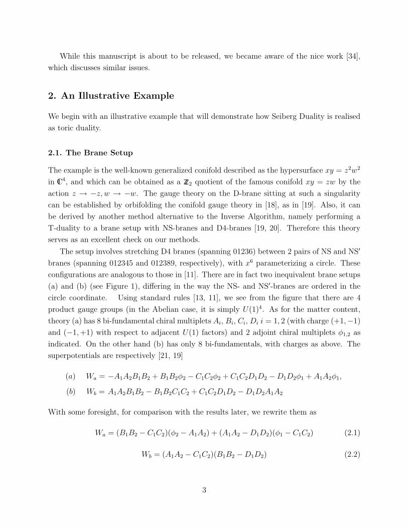
configurations are analogous to those in [11]. There are in fact two inequivalent brane setups

(a) and (b) (see Figure 1), differing in the way the NS- and NS′-branes are ordered in the

circle coordinate. Using standard rules [13, 11], we see from the figure that there are 4

product gauge groups (in the Abelian case, it is simply U(1)4. As for the matter content,

theory (a) has 8 bi-fundamental chiral multiplets Ai, Bi, Ci, Di i = 1, 2 (with charge (+1,−1)

and (−1,+1) with respect to adjacent U(1) factors) and 2 adjoint chiral multiplets φ1,2 as

indicated. On the other hand (b) has only 8 bi-fundamentals, with charges as above. The

superpotentials are respectively [21, 19]

(a) Wa = −A1A2B1B2 +B1B2φ2 − C1C2φ2 + C1C2D1D2 −D1D2φ1 + A1A2φ1,

(b) Wb = A1A2B1B2 − B1B2C1C2 + C1C2D1D2 −D1D2A1A2

With some foresight, for comparison with the results later, we rewrite them as

Wa = (B1B2 − C1C2)(φ2 −A1A2) + (A1A2 −D1D2)(φ1 − C1C2) (2.1)

Wb = (A1A2 − C1C2)(B1B2 −D1D2) (2.2)

3

AA

B

B

CC

D

Dφ1

φ2

NS NS NS

NSNS’

NS’

NS’NS’

(a) (b)

Figure 1: The two possible brane setups for the generalized conifold xy = z2w2. They are relatedto each other passing one NS-brane through an NS’-brane. Ai, Bi, Ci,Di i = 1, 2 are bifundamentalswhile φ1, φ2 are two adjoint fields.

2.2. Partial Resolution

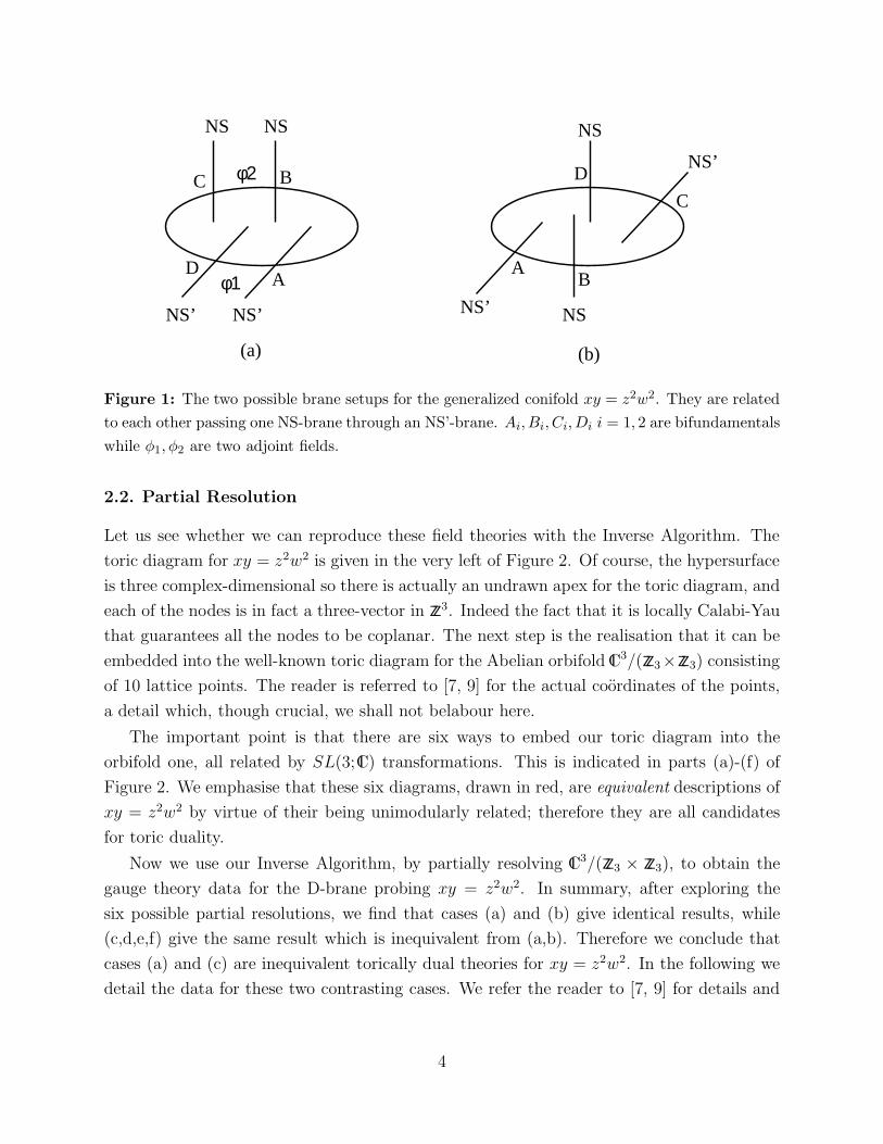
Let us see whether we can reproduce these field theories with the Inverse Algorithm. The

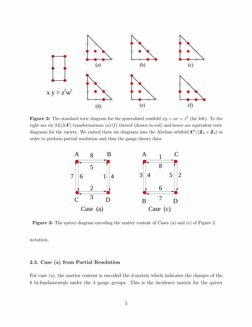
toric diagram for xy = z2w2 is given in the very left of Figure 2. Of course, the hypersurface

is three complex-dimensional so there is actually an undrawn apex for the toric diagram, and

each of the nodes is in fact a three-vector in ZZ3. Indeed the fact that it is locally Calabi-Yau

that guarantees all the nodes to be coplanar. The next step is the realisation that it can be

embedded into the well-known toric diagram for the Abelian orbifold C3/(ZZ3×ZZ3) consisting

of 10 lattice points. The reader is referred to [7, 9] for the actual coordinates of the points,

a detail which, though crucial, we shall not belabour here.

The important point is that there are six ways to embed our toric diagram into the

orbifold one, all related by SL(3;C) transformations. This is indicated in parts (a)-(f) of

Figure 2. We emphasise that these six diagrams, drawn in red, are equivalent descriptions of

xy = z2w2 by virtue of their being unimodularly related; therefore they are all candidates

for toric duality.

Now we use our Inverse Algorithm, by partially resolving C3/(ZZ3 × ZZ3), to obtain the

gauge theory data for the D-brane probing xy = z2w2. In summary, after exploring the

six possible partial resolutions, we find that cases (a) and (b) give identical results, while

(c,d,e,f) give the same result which is inequivalent from (a,b). Therefore we conclude that

cases (a) and (c) are inequivalent torically dual theories for xy = z2w2. In the following we

detail the data for these two contrasting cases. We refer the reader to [7, 9] for details and

4

(a) (b) (c)

(d) (e) (f)

x y = z w2 2

Figure 2: The standard toric diagram for the generalized conifold xy = uv = z2 (far left). To theright are six SL(3;C) transformations (a)-(f) thereof (drawn in red) and hence are equivalent toricdiagrams for the variety. We embed these six diagrams into the Abelian orbifold C3/(ZZ3 × ZZ3) inorder to perform partial resolution and thus the gauge theory data.

A

B

C

D

1

8

5 23 4

6

7

A B

C D

1 4

2

3

67

5

8

Case (c)Case (a)

Figure 3: The quiver diagram encoding the matter content of Cases (a) and (c) of Figure 2.

notation.

2.3. Case (a) from Partial Resolution

For case (a), the matter content is encoded the d-matrix which indicates the charges of the

8 bi-fundamentals under the 4 gauge groups. This is the incidence matrix for the quiver

5

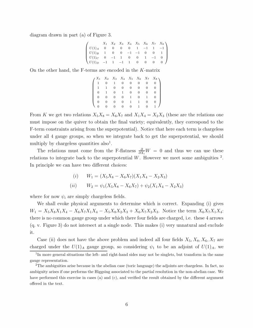
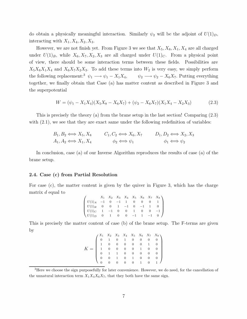
diagram drawn in part (a) of Figure 3.X1 X2 X3 X4 X5 X6 X7 X8

U(1)A 0 0 0 0 1 −1 1 −1

U(1)B 1 0 0 −1 −1 0 0 1

U(1)C 0 −1 1 0 0 1 −1 0

U(1)D −1 1 −1 1 0 0 0 0

On the other hand, the F-terms are encoded in the K-matrix

X1 X2 X3 X4 X5 X6 X7 X8

1 0 1 0 0 0 0 0

1 1 0 0 0 0 0 0

0 1 0 1 0 0 0 0

0 0 0 0 1 0 1 0

0 0 0 0 1 1 0 0

0 0 0 0 0 1 0 1

From K we get two relations X5X8 = X6X7 and X1X4 = X2X3 (these are the relations one

must impose on the quiver to obtain the final variety; equivalently, they correspond to the

F-term constraints arising from the superpotential). Notice that here each term is chargeless

under all 4 gauge groups, so when we integrate back to get the superpotential, we should

multiply by chargeless quantities also1.

The relations must come from the F-flatness ∂∂Xi

W = 0 and thus we can use these

relations to integrate back to the superpotential W . However we meet some ambiguities 2.

In principle we can have two different choices:

(i) W1 = (X5X8 −X6X7)(X1X4 −X2X3)

(ii) W2 = ψ1(X5X8 −X6X7) + ψ2(X1X4 −X2X3)

where for now ψi are simply chargeless fields.

We shall evoke physical arguments to determine which is correct. Expanding (i) gives

W1 = X5X8X1X4 − X6X7X1X4 − X5X8X2X3 + X6X7X2X3. Notice the term X6X7X1X4:

there is no common gauge group under which there four fields are charged, i.e. these 4 arrows

(q. v. Figure 3) do not intersect at a single node. This makes (i) very unnatural and exclude

it.

Case (ii) does not have the above problem and indeed all four fields X5, X8, X6, X7 are

charged under the U(1)A gauge group, so considering ψ1 to be an adjoint of U(1)A, we1In more general situations the left- and right-hand sides may not be singlets, but transform in the same

gauge representation.2The ambiguities arise because in the abelian case (toric language) the adjoints are chargeless. In fact, no

ambiguity arises if one performs the Higgsing associated to the partial resolution in the non-abelian case. Wehave performed this exercise in cases (a) and (c), and verified the result obtained by the different argumentoffered in the text.

6

do obtain a physically meaningful interaction. Similarly ψ2 will be the adjoint of U(1)D,

interacting with X1, X4, X2, X3.

However, we are not finish yet. From Figure 3 we see that X5, X8, X1, X4 are all charged

under U(1)B, while X6, X7, X2, X3 are all charged under U(1)C . From a physical point

of view, there should be some interaction terms between these fields. Possibilities are

X5X8X1X4 and X6X7X2X3. To add these terms into W2 is very easy, we simply perform

the following replacement:3 ψ1 −→ ψ1 −X1X4, ψ2 −→ ψ2 −X6X7. Putting everything

together, we finally obtain that Case (a) has matter content as described in Figure 3 and

the superpotential

W = (ψ1 −X1X4)(X5X8 −X6X7) + (ψ2 −X6X7)(X1X4 −X2X3) (2.3)

This is precisely the theory (a) from the brane setup in the last section! Comparing (2.3)

with (2.1), we see that they are exact same under the following redefinition of variables:

B1, B2 ⇐⇒ X5, X8 C1, C2 ⇐⇒ X6, X7 D1, D2 ⇐⇒ X2, X3

A1, A2 ⇐⇒ X1, X4 φ2 ⇐⇒ ψ1 φ1 ⇐⇒ ψ2

In conclusion, case (a) of our Inverse Algorithm reproduces the results of case (a) of the

brane setup.

2.4. Case (c) from Partial Resolution

For case (c), the matter content is given by the quiver in Figure 3, which has the charge

matrix d equal to X1 X2 X3 X4 X5 X6 X7 X8

U(1)A −1 0 −1 1 0 0 0 1

U(1)B 0 0 1 −1 0 −1 1 0

U(1)C 1 −1 0 0 1 0 0 −1

U(1)D 0 1 0 0 −1 1 −1 0

This is precisely the matter content of case (b) of the brane setup. The F-terms are given

by

K =

X1 X2 X3 X4 X5 X6 X7 X8

0 1 0 1 0 0 0 0

1 0 0 0 0 0 1 0

1 0 0 0 0 1 0 0

0 1 1 0 0 0 0 0

0 0 1 0 1 0 0 0

0 0 0 0 0 1 0 1

3Here we choose the sign purposefully for later convenience. However, we do need, for the cancellation of

the unnatural interaction term X1X4X6X7, that they both have the same sign.

7

From it we can read out the relations X1X8 = X6X7 and X2X5 = X3X4. Again there are

two ways to write down the superpotential

(i) W1 = (X1X8 −X6X7)(X3X4 −X2X5)

(ii) W2 = ψ1(X1X8 −X6X7) + ψ2(X3X4 −X2X5)

In this case, because X1, X8, X6, X7 are not charged under any common gauge group, it is

impossible to include any adjoint field ψ to give a physically meaningful interaction and so

(ii) is unnatural. We are left the superpotential W1. Indeed, comparing with (2.2), we see

they are identical under the redefinitions

A1, A2 ⇐⇒ X1, X8 B1, B2 ⇐⇒ X3, X4

C1, C2 ⇐⇒ X6, X7 D1, D2 ⇐⇒ X2, X5

Therefore we have reproduced case (b) of the brane setup.

What have we achieved? We have shown that toric duality due to inequivalent embed-

dings of unimodularly related toric diagrams for the generalized conifold xy = z2w2 gives

two inequivalent physical world-volume theories on the D-brane probe, exemplified by cases

(a) and (c). On the other hand, there are two T-dual brane setups for this singularity, also

giving two inequivalent field theories (a) and (b). Upon comparison, case (a) (resp. (c)) from

the Inverse Algorithm beautifully corresponds to case (a) (resp. (b)) from the brane setup.

Somehow, a seemingly harmless trick in mathematics relates inequivalent brane setups. In

fact we can say much more.

3. Seiberg Duality versus Toric Duality

As follows from [11], the two theories from the brane setups are actually related by Seiberg

Duality [10], as pointed out in [19] (see also [12, 22]. Let us first review the main features of

this famous duality, for unitary gauge groups.

Seiberg duality is a non-trivial infrared equivalence of N = 1 supersymmetric field the-

ories, which are different in the ultraviolet, but flow the the same interacting fixed point in

the infrared. In particular, the very low energy features of the different theories, like their

moduli space, chiral ring, global symmetries, agree for Seiberg dual theories. Given that

toric dual theories, by definition, have identical moduli spaces, etc , it is natural to propose

a connection between both phenomena.

The prototypical example of Seiberg duality is N = 1 SU(Nc) gauge theory with Nf

vector-like fundamental flavours, and no superpotential. The global chiral symmetry is

8

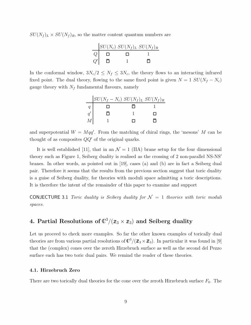
SU(Nf )L × SU(Nf )R, so the matter content quantum numbers are

SU(Nc) SU(Nf )L SU(Nf )R

Q 1

Q′ 1

In the conformal window, 3Nc/2 ≤ Nf ≤ 3Nc, the theory flows to an interacting infrared

fixed point. The dual theory, flowing to the same fixed point is given N = 1 SU(Nf − Nc)

gauge theory with Nf fundamental flavours, namely

SU(Nf −Nc) SU(Nf )L SU(Nf )R

q 1

q′ 1

M 1

and superpotential W = Mqq′. From the matching of chiral rings, the ‘mesons’ M can be

thought of as composites QQ′ of the original quarks.

It is well established [11], that in an N = 1 (IIA) brane setup for the four dimensional

theory such as Figure 1, Seiberg duality is realised as the crossing of 2 non-parallel NS-NS′

branes. In other words, as pointed out in [19], cases (a) and (b) are in fact a Seiberg dual

pair. Therefore it seems that the results from the previous section suggest that toric duality

is a guise of Seiberg duality, for theories with moduli space admitting a toric descriptions.

It is therefore the intent of the remainder of this paper to examine and support

CONJECTURE 3.1 Toric duality is Seiberg duality for N = 1 theories with toric moduli

spaces.

4. Partial Resolutions of C3/(ZZ3 × ZZ3) and Seiberg duality

Let us proceed to check more examples. So far the other known examples of torically dual

theories are from various partial resolutions of C3/(ZZ3×ZZ3). In particular it was found in [9]

that the (complex) cones over the zeroth Hirzebruch surface as well as the second del Pezzo

surface each has two toric dual pairs. We remind the reader of these theories.

4.1. Hirzebruch Zero

There are two torically dual theories for the cone over the zeroth Hirzebruch surface F0. The

9

X

Y

X

Y

��������

��������

��������

��������

��������

��������

������������

������������

A B

DC

������

������

��������

��������

���������

���������

��������

��������

BA 5, 9

6, 10D C

2, 41, 3 7, 8, 11, 12

i 12

i 22

i 21

i 11Case I

Quiver Diagram

Case II

Toric DiagramToric Diagram Quiver Diagram

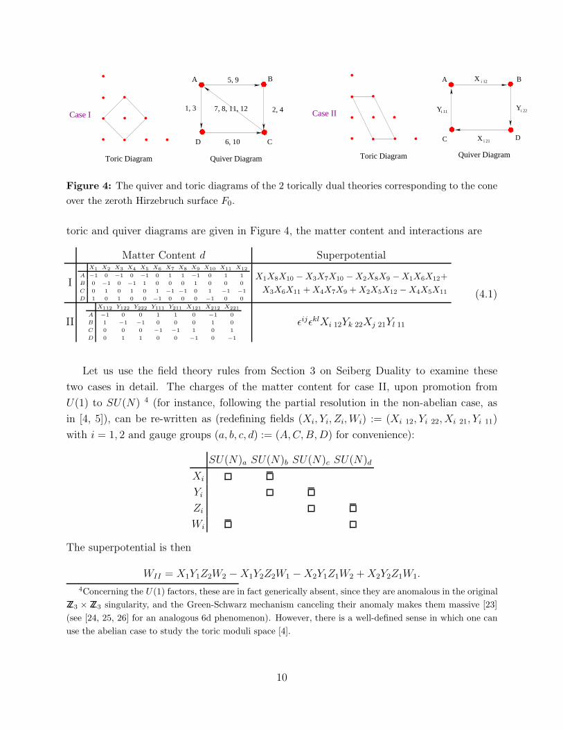
Figure 4: The quiver and toric diagrams of the 2 torically dual theories corresponding to the coneover the zeroth Hirzebruch surface F0.

toric and quiver diagrams are given in Figure 4, the matter content and interactions are

Matter Content d Superpotential

I

X1 X2 X3 X4 X5 X6 X7 X8 X9 X10 X11 X12A −1 0 −1 0 −1 0 1 1 −1 0 1 1

B 0 −1 0 −1 1 0 0 0 1 0 0 0

C 0 1 0 1 0 1 −1 −1 0 1 −1 −1

D 1 0 1 0 0 −1 0 0 0 −1 0 0

X1X8X10 −X3X7X10 −X2X8X9 −X1X6X12+X3X6X11 + X4X7X9 + X2X5X12 −X4X5X11

II

X112 Y122 Y222 Y111 Y211 X121 X212 X221A −1 0 0 1 1 0 −1 0

B 1 −1 −1 0 0 0 1 0

C 0 0 0 −1 −1 1 0 1

D 0 1 1 0 0 −1 0 −1

εijεklXi 12Yk 22Xj 21Yl 11

(4.1)

Let us use the field theory rules from Section 3 on Seiberg Duality to examine these

two cases in detail. The charges of the matter content for case II, upon promotion from

U(1) to SU(N) 4 (for instance, following the partial resolution in the non-abelian case, as

in [4, 5]), can be re-written as (redefining fields (Xi, Yi, Zi,Wi) := (Xi 12, Yi 22, Xi 21, Yi 11)

with i = 1, 2 and gauge groups (a, b, c, d) := (A,C,B,D) for convenience):

SU(N)a SU(N)b SU(N)c SU(N)d

Xi

Yi

Zi

Wi

The superpotential is then

WII = X1Y1Z2W2 −X1Y2Z2W1 −X2Y1Z1W2 +X2Y2Z1W1.

4Concerning the U(1) factors, these are in fact generically absent, since they are anomalous in the originalZZ3 × ZZ3 singularity, and the Green-Schwarz mechanism canceling their anomaly makes them massive [23](see [24, 25, 26] for an analogous 6d phenomenon). However, there is a well-defined sense in which one canuse the abelian case to study the toric moduli space [4].

10

Let us dualise with respect to the a gauge group. This is a SU(N) theory with Nc =

N and Nf = 2N (as there are two Xi’s). The chiral symmetry is however broken from

SU(2N)L×SU(2N)R to SU(N)L×SU(N)R, which moreover is gauged as SU(N)b×SU(N)d.

Ignoring the superpotential WII , the dual theory would be:

SU(N)a′ SU(N)b SU(N)c SU(N)d

qi

Yi

Zi

q′iMij

(4.2)

We note that there are Mij giving 4 bi-fundamentals for bd. They arise from the Seiberg

mesons in the bi-fundamental of the enhanced chiral symmetry SU(2N) × SU(2N), once

decomposed with respect to the unbroken chiral symmetry group. The superpotential is

W ′ = M11q1q′1 −M12q2q

′1 −M21q1q

′2 +M22q2q

′2.

The choice of signs in W ′ will be explained shortly.

Of course, WII is not zero and so give rise to a deformation in the original theory, anal-

ogous to those studied in e.g. [21]. In the dual theory, this deformation simply corresponds

to WII rewritten in terms of mesons, which can be thought of as composites of the original

quarks, i.e., Mij = WiXj. Therefore we have

WII = M21Y1Z2 −M11Y2Z2 −M22Y1Z1 +M12Y2Z1

which is written in the new variables. The rule for the signs is that e.g. the field M21 appears

with positive sign in WII , hence it should appear with negative sign in W ′, and analogously

for others. Putting them together we get the superpotential of the dual theory

W dualII = WII +W ′ =

M11q1q′1 −M12q2q

′1 −M21q1q

′2 +M22q2q

′2 +M21Y1Z2 −M11Y2Z2 −M22Y1Z1 +M12Y2Z1

(4.3)

Upon the field redefinitions

M11 → X7 M12 → X8 M21 → X11 M22 → X12

q1 → X4 q2 → X2 q1′ → X9 q2′ → X5

Y1 → X6 Y2 → X10 Z1 → X1 Z2 → X3

we have the field content (4.2) and superpotential (4.3) matching precisely with case I in

(4.1). We conclude therefore that the two torically dual cases I and II obtained from partial

resolutions are indeed Seiberg duals!

11

������������

������������

���������

���������

��������

��������

���������

���������

������������

������������

������������������������������������������������������������������������������������������������

������������������������������������������������������������������������������������������������

������������������������������������������������������������������������

������������������������������������������������������������������������

������������������������������������������������������������������������������������������������

������������������������������������������������������������������������������������������������

��������������������������������������������������������������������������������������������������������������������������������������������������������������������������������������������������������������������������������������������������������������������������

��������������������������������������������������������������������������������������������������������������������������������������������������������������������������������������������������������������������������������������������������������������������������

����������������������������������������������������������������������������������������������������������������������������������������������������������������

����������������������������������������������������������������������������������������������������������������������������������������������������������������

7, 11

3, 5

64

2

9D C

BE

A

10

8, 12, 13

1 ������������

������������

������������

������������

������������

������������

���������

���������

���������

���������

1

2,5

34

6

7

98,10

11

B

CD

E

A

Case I

Toric Diagram Quiver Diagram Toric Diagram Quiver Diagram

Case II

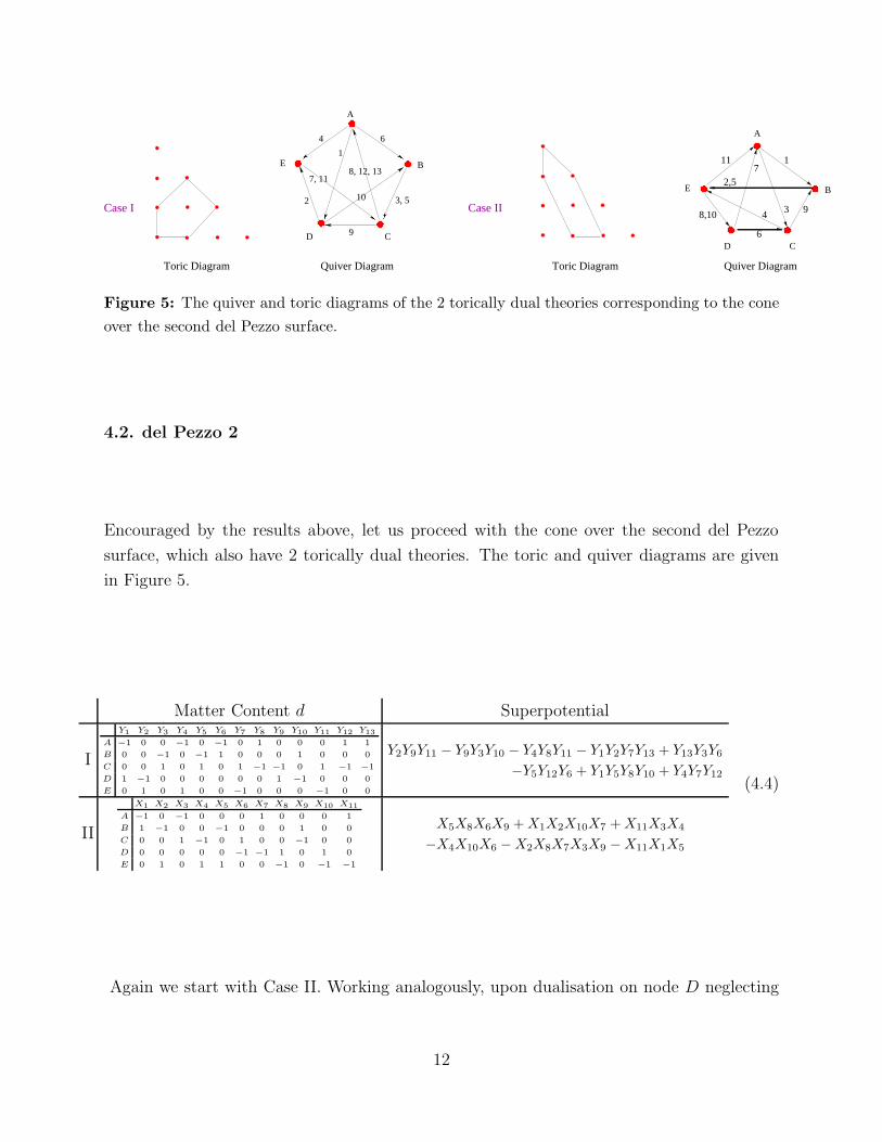
Figure 5: The quiver and toric diagrams of the 2 torically dual theories corresponding to the coneover the second del Pezzo surface.

4.2. del Pezzo 2

Encouraged by the results above, let us proceed with the cone over the second del Pezzo

surface, which also have 2 torically dual theories. The toric and quiver diagrams are given

in Figure 5.

Matter Content d Superpotential

I

Y1 Y2 Y3 Y4 Y5 Y6 Y7 Y8 Y9 Y10 Y11 Y12 Y13A −1 0 0 −1 0 −1 0 1 0 0 0 1 1

B 0 0 −1 0 −1 1 0 0 0 1 0 0 0

C 0 0 1 0 1 0 1 −1 −1 0 1 −1 −1

D 1 −1 0 0 0 0 0 0 1 −1 0 0 0

E 0 1 0 1 0 0 −1 0 0 0 −1 0 0

Y2Y9Y11 − Y9Y3Y10 − Y4Y8Y11 − Y1Y2Y7Y13 + Y13Y3Y6

−Y5Y12Y6 + Y1Y5Y8Y10 + Y4Y7Y12

II

X1 X2 X3 X4 X5 X6 X7 X8 X9 X10 X11A −1 0 −1 0 0 0 1 0 0 0 1

B 1 −1 0 0 −1 0 0 0 1 0 0

C 0 0 1 −1 0 1 0 0 −1 0 0

D 0 0 0 0 0 −1 −1 1 0 1 0

E 0 1 0 1 1 0 0 −1 0 −1 −1

X5X8X6X9 + X1X2X10X7 + X11X3X4

−X4X10X6 −X2X8X7X3X9 −X11X1X5

(4.4)

Again we start with Case II. Working analogously, upon dualisation on node D neglecting

12

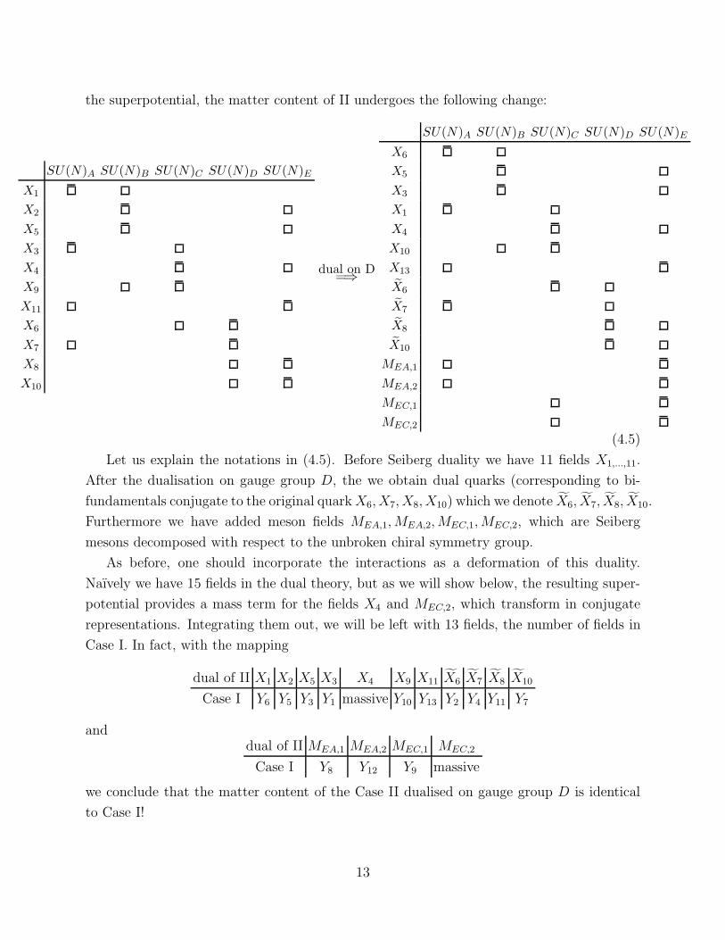
the superpotential, the matter content of II undergoes the following change:

SU(N)A SU(N)B SU(N)C SU(N)D SU(N)EX1

X2

X5

X3

X4

X9

X11

X6

X7

X8

X10

dual on D=⇒

SU(N)A SU(N)B SU(N)C SU(N)D SU(N)EX6

X5

X3

X1

X4

X10

X13

X6

X7

X8

X10

MEA,1

MEA,2

MEC,1

MEC,2

(4.5)

Let us explain the notations in (4.5). Before Seiberg duality we have 11 fields X1,...,11.

After the dualisation on gauge group D, the we obtain dual quarks (corresponding to bi-

fundamentals conjugate to the original quarkX6, X7, X8, X10) which we denote X6, X7, X8, X10.

Furthermore we have added meson fields MEA,1,MEA,2,MEC,1,MEC,2, which are Seiberg

mesons decomposed with respect to the unbroken chiral symmetry group.

As before, one should incorporate the interactions as a deformation of this duality.

Naıvely we have 15 fields in the dual theory, but as we will show below, the resulting super-

potential provides a mass term for the fields X4 and MEC,2, which transform in conjugate

representations. Integrating them out, we will be left with 13 fields, the number of fields in

Case I. In fact, with the mapping

dual of II X1 X2 X5 X3 X4 X9 X11 X6 X7 X8 X10

Case I Y6 Y5 Y3 Y1 massive Y10 Y13 Y2 Y4 Y11 Y7

anddual of II MEA,1 MEA,2 MEC,1 MEC,2

Case I Y8 Y12 Y9 massive

we conclude that the matter content of the Case II dualised on gauge group D is identical

to Case I!

13

Let us finally check the superpotentials, and also verify the claim that X4 and MEC,2

become massive. Rewriting the superpotential of II from (4.4) in terms of the dual variables

(matching the mesons as composites MEA,1 = X8X7, MEA,2 = X10X7, MEC,1 = X8X6,

MEC,2 = X10X6), we have

WII = X5MEC,1X9 +X1X2MEA,2 +X11X3X4

−X4MEC,2 −X2MEA,1X3X9 −X11X1X5.

As is with the previous subsection, to the above we must add the meson interaction terms

coming from Seiberg duality, namely

Wmeson = MEA,1X7X8 −MEA,2X7X10 −MEC,1X6X8 +MEC,2X6X10,

(notice again the choice of sign in Wmeson). Adding this two together we have

W dualII = X5MEC,1X9 +X1X2MEA,2 +X11X3X4

−X4MEC,2 −X2MEA,1X3X9 −X11X1X5

+MEA,1X7X8 −MEA,2X7X10 −MEC,1X6X8 +MEC,2X6X10.

Now it is very clear that both X4 and MEC,2 are massive and should be integrated out:

X4 = X6X10, MEC,2 = X11X3.

Upon substitution we finally have

W dualII = X5MEC,1X9 +X1X2MEA,2 +X11X3X6X10 −X2MEA,1X3X9

−X11X1X5 +MEA,1X7X8 −MEA,2X7X10 −MEC,1X6X8,

which with the replacement rules given above we obtain

W dualII = Y3Y9Y10 + Y6Y5Y12 + Y13Y1Y2Y7 − Y5Y1Y10Y8

−Y13Y6Y3 + Y8Y4Y11 − Y12Y4Y7 − Y9Y2Y11.

This we instantly recognise, by referring to (4.4), as the superpotential of Case I.

In conclusion therefore, with the matching of matter content and superpotential, the two

torically dual cases I and II of the cone over the second del Pezzo surface are also Seiberg

duals.

14

5. Brane Diamonds and Seiberg Duality

Having seen the above arguments from field theory, let us support that toric duality is Seiberg

duality from yet another perspective, namely, through brane setups. The use of this T-dual

picture for D3-branes at singularities will turn out to be quite helpful in showing that toric

duality reproduces Seiberg duality.

What we have learnt from the examples where a brane interval picture is available (i.e.

NS- and D4-branes in the manner of [13]) is that the standard Seiberg duality by brane

crossing reproduces the different gauge theories obtained from toric arguments (different

partial resolutions of a given singularity). Notice that the brane crossing corresponds, under

T-duality, to a change of the B field in the singularity picture, rather than a change in the

singularity geometry [19, 12]. Hence, the two theories arise on the world-volume of D-branes

probing the same singularity.

Unfortunately, brane intervals are rather limited, in that they can be used to study

Seiberg duality for generalized conifold singularities, xy = wkwl. Although this is a large

class of models, not many examples arise in the partial resolutions of C3/(ZZ3 × ZZ3). Hence

the relation to toric duality from partial resolutions cannot be checked for most examples.

Therefore it would be useful to find other singularities for which a nice T-dual brane

picture is available. Nice in the sense that there is a motivated proposal to realize Seiberg

duality in the corresponding brane setup. A good candidate for such a brane setup is brane

diamonds, studied in [14].

Reference [27] (see also [28, 29]) introduced brane box configurations of intersecting

NS- and NS’-branes (spanning 012345 and 012367, respectively), with D5-branes (spanning

012346) suspended among them. Brane diamonds [14] generalized (and refined) this setup

by considering situations where the NS- and the NS’-branes recombine and span a smooth

holomorphic curve in the 4567 directions, in whose holes D5-branes can be suspended as soap

bubbles. Typical brane diamond pictures are as in figures in the remainder of the paper.

Brane diamonds are related by T-duality along 46 to a large set of D-branes at singu-

larities. With the set of rules to read off the matter content and interactions in [14], they

provide a useful pictorial representation of these D-brane gauge field theories. In particular,

they correspond to singularities obtained as the abelian orbifolds of the conifold studied in

Section 5 of [19], and partial resolutions thereof. Concerning this last point, brane diamond

configurations admit two kinds of deformations: motions of diamond walls in the directions

57, and motions of diamond walls in the directions 46. The former T-dualize to geometric

sizes of the collapse cycles, hence trigger partial resolutions of the singularity (notice that

15

2

2

3

1 3

44

4

3 11

4 4

44

4

3 3

1

2’

2’

1 1

3

Diamond (Seiberg)Dual

(II)(I)

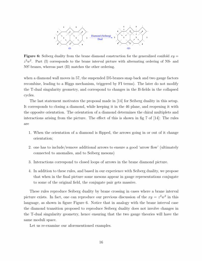
Figure 6: Seiberg duality from the brane diamond construction for the generalized conifold xy =z2w2. Part (I) corresponds to the brane interval picture with alternating ordering of NS- andNS′-branes, whereas part (II) matches the other ordering.

when a diamond wall moves in 57, the suspended D5-branes snap back and two gauge factors

recombine, leading to a Higgs mechanism, triggered by FI terms). The later do not modify

the T-dual singularity geometry, and correspond to changes in the B-fields in the collapsed

cycles.

The last statement motivates the proposal made in [14] for Seiberg duality in this setup.

It corresponds to closing a diamond, while keeping it in the 46 plane, and reopening it with

the opposite orientation. The orientation of a diamond determines the chiral multiplets and

interactions arising from the picture. The effect of this is shown in fig 7 of [14]: The rules

are

1. When the orientation of a diamond is flipped, the arrows going in or out of it change

orientation;

2. one has to include/remove additional arrows to ensure a good ‘arrow flow’ (ultimately

connected to anomalies, and to Seiberg mesons)

3. Interactions correspond to closed loops of arrows in the brane diamond picture.

4. In addition to these rules, and based in our experience with Seiberg duality, we propose

that when in the final picture some mesons appear in gauge representations conjugate

to some of the original field, the conjugate pair gets massive.

These rules reproduce Seiberg duality by brane crossing in cases where a brane interval

picture exists. In fact, one can reproduce our previous discussion of the xy = z2w2 in this

language, as shown in figure Figure 6. Notice that in analogy with the brane interval case

the diamond transition proposed to reproduce Seiberg duality does not involve changes in

the T-dual singularity geometry, hence ensuring that the two gauge theories will have the

same moduli space.

Let us re-examine our aforementioned examples.

16

2

1

1

2

3

4

3

4

(II) x y = z w22

Z Quotient2

2

1

1 1

1

2 2

2

Z Quotient2

2

1 3

4

3

4

1

2(I) Conifold x y = z w

(III) Cone over F0

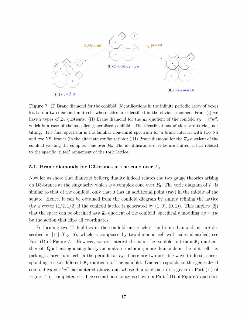
Figure 7: (I) Brane diamond for the conifold. Identifications in the infinite periodic array of boxesleads to a two-diamond unit cell, whose sides are identified in the obvious manner. From (I) wehave 2 types of ZZ2 quotients: (II) Brane diamond for the ZZ2 quotient of the conifold xy = z2w2,which is a case of the so-called generalised conifold. The identifications of sides are trivial, nottilting. The final spectrum is the familiar non-chiral spectrum for a brane interval with two NSand two NS’ branes (in the alternate configuration); (III) Brane diamond for the ZZ2 quotient of theconifold yielding the complex cone over F0. The identifications of sides are shifted, a fact relatedto the specific ‘tilted’ refinement of the toric lattice.

5.1. Brane diamonds for D3-branes at the cone over F0

Now let us show that diamond Seiberg duality indeed relates the two gauge theories arising

on D3-branes at the singularity which is a complex cone over F0. The toric diagram of F0 is

similar to that of the conifold, only that it has an additional point (ray) in the middle of the

square. Hence, it can be obtained from the conifold diagram by simply refining the lattice

(by a vector (1/2, 1/2) if the conifold lattice is generated by (1, 0), (0, 1)). This implies [2])

that the space can be obtained as a ZZ2 quotient of the conifold, specifically modding xy = zw

by the action that flips all coordinates.

Performing two T-dualities in the conifold one reaches the brane diamond picture de-

scribed in [14] (fig. 5), which is composed by two-diamond cell with sides identified, see

Part (I) of Figure 7. However, we are interested not in the conifold but on a ZZ2 quotient

thereof. Quotienting a singularity amounts to including more diamonds in the unit cell, i.e.

picking a larger unit cell in the periodic array. There are two possible ways to do so, corre-

sponding to two different ZZ2 quotients of the conifold. One corresponds to the generalized

conifold xy = z2w2 encountered above, and whose diamond picture is given in Part (II) of

Figure 7 for completeness. The second possibility is shown in Part (III) of Figure 7 and does

17

2

1 3

4

3

4

1

2

1 3

4

3

4

1

2’

2’Diamond (Seiberg)

Dual

(II)(I)

W1

X2

X1

W2

Y1

Y2

Z1

Z2

X6

X4

X12 X7

X10

X2

X8

X1 X5

X3

X11

X9

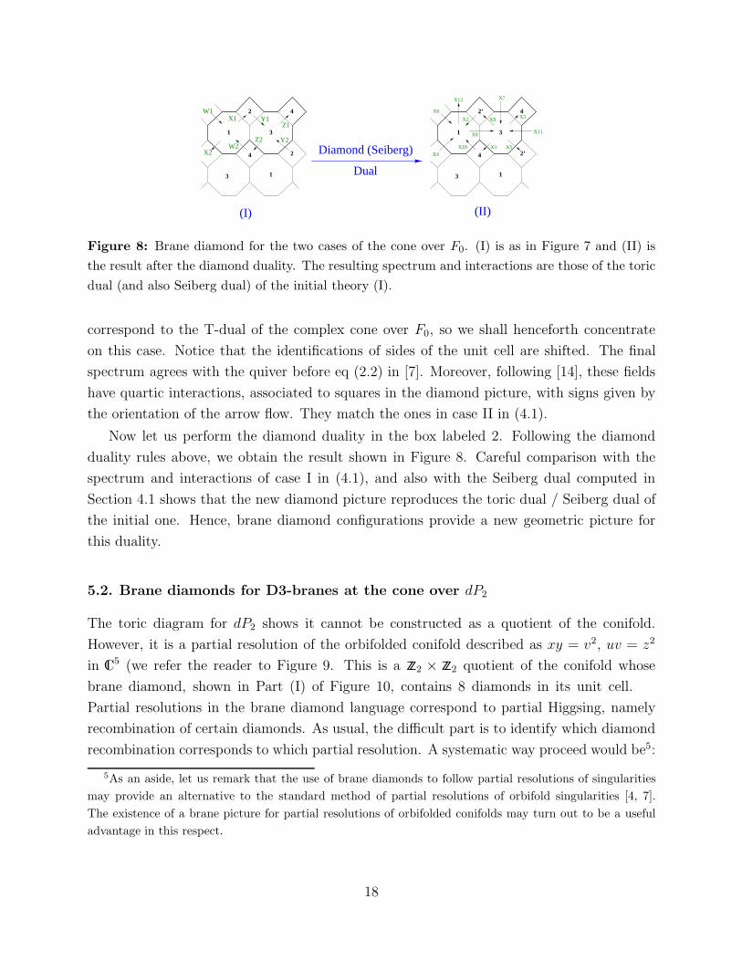
Figure 8: Brane diamond for the two cases of the cone over F0. (I) is as in Figure 7 and (II) isthe result after the diamond duality. The resulting spectrum and interactions are those of the toricdual (and also Seiberg dual) of the initial theory (I).

correspond to the T-dual of the complex cone over F0, so we shall henceforth concentrate

on this case. Notice that the identifications of sides of the unit cell are shifted. The final

spectrum agrees with the quiver before eq (2.2) in [7]. Moreover, following [14], these fields

have quartic interactions, associated to squares in the diamond picture, with signs given by

the orientation of the arrow flow. They match the ones in case II in (4.1).

Now let us perform the diamond duality in the box labeled 2. Following the diamond

duality rules above, we obtain the result shown in Figure 8. Careful comparison with the

spectrum and interactions of case I in (4.1), and also with the Seiberg dual computed in

Section 4.1 shows that the new diamond picture reproduces the toric dual / Seiberg dual of

the initial one. Hence, brane diamond configurations provide a new geometric picture for

this duality.

5.2. Brane diamonds for D3-branes at the cone over dP2

The toric diagram for dP2 shows it cannot be constructed as a quotient of the conifold.

However, it is a partial resolution of the orbifolded conifold described as xy = v2, uv = z2

in C5 (we refer the reader to Figure 9. This is a ZZ2 × ZZ2 quotient of the conifold whose

brane diamond, shown in Part (I) of Figure 10, contains 8 diamonds in its unit cell.

Partial resolutions in the brane diamond language correspond to partial Higgsing, namely

recombination of certain diamonds. As usual, the difficult part is to identify which diamond

recombination corresponds to which partial resolution. A systematic way proceed would be5:

5As an aside, let us remark that the use of brane diamonds to follow partial resolutions of singularitiesmay provide an alternative to the standard method of partial resolutions of orbifold singularities [4, 7].The existence of a brane picture for partial resolutions of orbifolded conifolds may turn out to be a usefuladvantage in this respect.

18

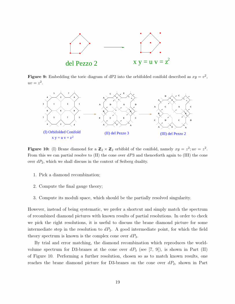
del Pezzo 2 x y = u v = z2

Figure 9: Embedding the toric diagram of dP2 into the orbifolded conifold described as xy = v2,uv = z2.

2

1 1

2

3

4

5

6

7

8

3

4

8

7 5

44

5 7

x y = u v = z2

A

EC

D

B

F

EC

A

A

B

E

A F A

C

DA

B

A

A

B

A A

C

C

D DC

C

E

E

D C

(I) Orbifolded Conifold (III) del Pezzo 2(II) del Pezzo 3

Figure 10: (I) Brane diamond for a ZZ2 × ZZ2 orbifold of the conifold, namely xy = z2;uv = z2.From this we can partial resolve to (II) the cone over dP3 and thenceforth again to (III) the coneover dP2, which we shall discuss in the context of Seiberg duality.

1. Pick a diamond recombination;

2. Compute the final gauge theory;

3. Compute its moduli space, which should be the partially resolved singularity.

However, instead of being systematic, we prefer a shortcut and simply match the spectrum

of recombined diamond pictures with known results of partial resolutions. In order to check

we pick the right resolutions, it is useful to discuss the brane diamond picture for some

intermediate step in the resolution to dP2. A good intermediate point, for which the field

theory spectrum is known is the complex cone over dP3.

By trial and error matching, the diamond recombination which reproduces the world-

volume spectrum for D3-branes at the cone over dP3 (see [7, 9]), is shown in Part (II)

of Figure 10. Performing a further resolution, chosen so as to match known results, one

reaches the brane diamond picture for D3-branes on the cone over dP2, shown in Part

19

(III) of Figure 10. More specifically, the spectrum and interactions in the brane diamond

configuration agrees with those of case I in (4.4).

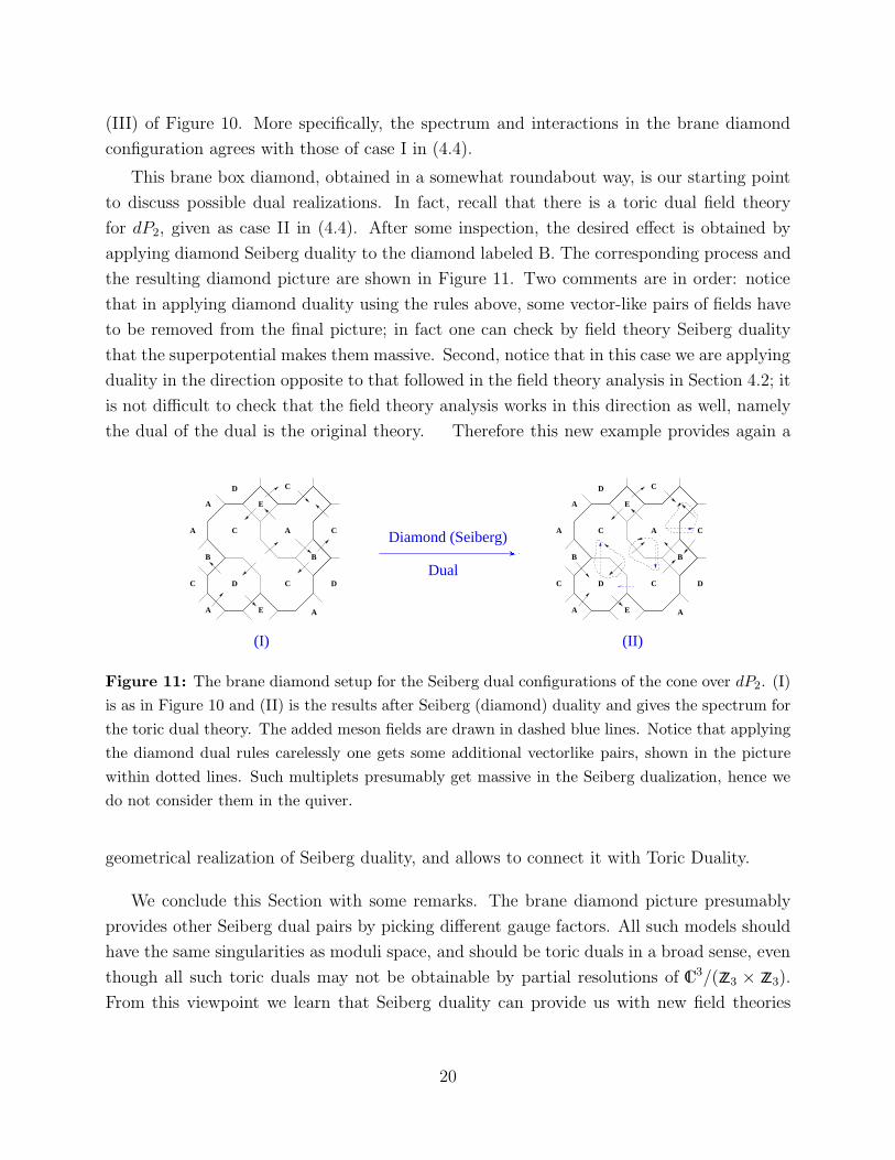
This brane box diamond, obtained in a somewhat roundabout way, is our starting point

to discuss possible dual realizations. In fact, recall that there is a toric dual field theory

for dP2, given as case II in (4.4). After some inspection, the desired effect is obtained by

applying diamond Seiberg duality to the diamond labeled B. The corresponding process and

the resulting diamond picture are shown in Figure 11. Two comments are in order: notice

that in applying diamond duality using the rules above, some vector-like pairs of fields have

to be removed from the final picture; in fact one can check by field theory Seiberg duality

that the superpotential makes them massive. Second, notice that in this case we are applying

duality in the direction opposite to that followed in the field theory analysis in Section 4.2; it

is not difficult to check that the field theory analysis works in this direction as well, namely

the dual of the dual is the original theory. Therefore this new example provides again a

Diamond (Seiberg)

Dual

(II)(I)

A

B

A

A

B

A A

C

C

D DC

C

E

E

D C

A

B

A

A

B

A A

C

C

D DC

C

E

E

D C

Figure 11: The brane diamond setup for the Seiberg dual configurations of the cone over dP2. (I)is as in Figure 10 and (II) is the results after Seiberg (diamond) duality and gives the spectrum forthe toric dual theory. The added meson fields are drawn in dashed blue lines. Notice that applyingthe diamond dual rules carelessly one gets some additional vectorlike pairs, shown in the picturewithin dotted lines. Such multiplets presumably get massive in the Seiberg dualization, hence wedo not consider them in the quiver.

geometrical realization of Seiberg duality, and allows to connect it with Toric Duality.

We conclude this Section with some remarks. The brane diamond picture presumably

provides other Seiberg dual pairs by picking different gauge factors. All such models should

have the same singularities as moduli space, and should be toric duals in a broad sense, even

though all such toric duals may not be obtainable by partial resolutions of C3/(ZZ3 × ZZ3).

From this viewpoint we learn that Seiberg duality can provide us with new field theories

20

and toric duals beyond the reach of present computational tools. This is further explored in

Section 7.

A second comment along the same lines is that Seiberg duality on nodes for which Nf 6=2Nc will lead to dual theories where some gauge factors have different rank. Taking the

theory back to the ‘abelian’ case, some gauge factors turn out to be non-abelian. Hence, in

these cases, even though Seiberg duality ensures the final theory has the same singularity

as moduli space, the computation of the corresponding symplectic quotient is beyond the

standard tools of toric geometry. Therefore, Seiberg duality can provide (‘non-toric’) gauge

theories with toric moduli space.

6. A Quiver Duality from Seiberg Duality

If we are not too concerned with the superpotential, when we make the Seiberg duality

transformation, we can obtain the matter content very easily at the level of the quiver

diagram. What we obtain are rules for a so-called “quiver duality” which is a rephrasing

of the Seiberg duality transformations in field (brane diamond) theory in the language of

quivers. Denote (Nc)i the number of colors at the ith node, and aij the number of arrows

from the node i to the j (the adjacency matrix) The rules on the quiver to obtain Seiberg

dual theories are

1. Pick the dualisation node i0. Define the following sets of nodes: Iin := nodes having

arrows going into i0; Iout := those having arrow coming from i0 and Ino := those

unconnected with i0. The node i0 should not be included in this classification.

2. Change the rank of the node i0 fromNc toNf−Nc where Nf is the number of vector-like

flavours, Nf =∑

i∈Iin

ai,i0 =∑

i∈Iout

ai0,i

3. Reverse all arrows going in or out of i0, therefore

adualij = aji if either i, j = i0

4. Only arrows linking Iin to Iout will be changed and all others remain unaffected.

5. For every pair of nodes A, B, A ∈ Iout and B ∈ Iin, change the number of arrows aAB

to

adualAB = aAB − ai0AaBi0 for A ∈ Iout, B ∈ Iin.

If this quantity is negative, we simply take it to mean −adual arrow go from B to A.

21

These rules follow from applying Seiberg duality at the field theory level, and therefore are

consistent with anomaly cancellation. In particular, notice the for any node i ∈ Iin, we have

replaced ai,i0Nc fundamental chiral multiplets by −ai,i0(Nf − Nc) +∑

j∈Ioutai,i0ai0,j which

equals −ai,i0(Nf − Nc) + ai,i0Nf = ai,i0Nc, and ensures anomaly cancellation in the final

theory. Similarly for nodes j ∈ Iout.

It is straightforward to apply these rules to the quivers in the by now familiar examples

in previous sections.

In general, we can choose an arbitrary node to perform the above Seiberg duality rules.

However, not every node is suitable for a toric description. The reason is that, if we start

from a quiver whose every node has the same rank N , after the transformation it is possible

that this no longer holds. We of course wish so because due to the very definition of the

C∗ action for toric varieties, toric descriptions are possible iff all nodes are U(1), or in the

non-Abelian version, SU(N). If for instance we choose to Seiberg dualize a node with 3N

flavours, the dual node will have rank 3N −N = 2N while the others will remain with rank

N , and our description would no longer be toric. For this reason we must choose nodes with

only 2Nf flavors, if we are to remain within toric descriptions.

One natural question arises: if we Seiberg-dualise every possible allowed node, how many

different theories will we get? Moreover how many of these are torically dual? Let we

re-analyse the examples we have thus far encountered.

6.1. Hirzebruch Zero

Starting from case (II) of F0 (recall Figure 4.1) all of four nodes are qualified to yield toric

Seiberg duals (they each have 2 incoming and 2 outgoing arrows and hence Nf = 2N).

Dualising any one will give to case (I) of F0. On the other hand, from (I) of F0, we see

that only nodes B,D are qualified to be dualized. Choosing either, we get back to the

case (II) of F0. In another word, cases (I) and (II) are closed under the Seiberg-duality

transformation. In fact, this is a very strong evidence that there are only two toric phases

for F0 no matter how we embed the diagram into higher ZZk × ZZk singularities. This also

solves the old question [7, 9] that the Inverse Algorithm does not in principle tell us how

many phases we could have. Now by the closeness of Seiberg-duality transformations, we

do have a way to calculate the number of possible phases. Notice, on the other hand, the

existence of non-toric phases.

22

6.2. del Pezzo 0,1,2

Continuing our above calculation to del Pezzo singularities, we see that for dP0 no node is

qualified, so there is only one toric phase which is consistent with the standard result [9] as a

resolution OIP2(−1) →C3/ZZ3. For dP1, nodes A,B are qualified (all notations coming from

[9]), but the dualization gives back to same theory, so it too has only one phase.

For our example dP2 studied earlier (recall Figure 4.4), there are four points A,B,C,D

which are qualified in case (II). Nodes A,C give back to case (II) while nodes B,D give rise

to case (I) of dP2. On the other hand, for case (I), three nodes B,D,E are qualified. Here

nodes B,E give case (II) while node D give case (I). In other words, cases (I) and (II) are

also closed under the Seiberg-duality transformation, so we conclude that there too are only

two phases for dP2, as presented earlier.

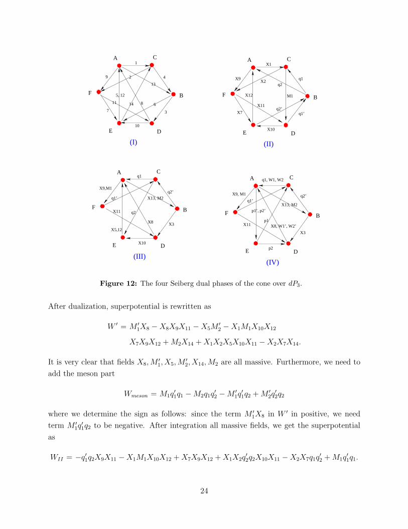
6.3. The Four Phases of dP3

Things become more complex when we discuss the phases of dP3. As we remarked before,

due to the running-time limitations of the Inverse Algorithm, only one phase was obtained

in [9]. However, one may expect this case to have more than just one phase, and in fact

a recent paper has given another phase [17]. Here, using the closeness argument we give

evidence that there are four (toric) phases for dP3. We will give only one phase in detail.

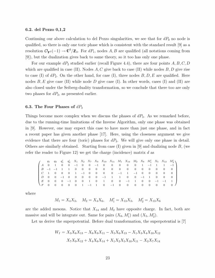
Others are similarly obtained. Starting from case (I) given in [9] and dualizing node B, (we

refer the reader to Figure 12) we get the charge (incidence) matrix d as

q1 q2 q′1 q′2 X1 X2 X7 X9 X10 X11 M1 X14 M2 X8 M ′1 X5 X12 M ′

2

A 0 1 0 0 −1 0 0 −1 0 0 0 0 0 1 −1 1 1 −1

B −1 −1 1 1 0 0 0 0 0 0 0 0 0 0 0 0 0 0

C 1 0 0 0 1 −1 0 0 0 0 −1 1 −1 0 0 0 0 0

D 0 0 −1 0 0 0 0 0 −1 1 1 0 0 −1 1 0 0 0

E 0 0 0 −1 0 0 1 0 1 0 0 −1 1 0 0 −1 −1 1

F 0 0 0 0 0 1 −1 1 0 −1 0 0 0 0 0 0 0 0

where

M1 = X4X3, M2 = X4X6, M ′1 = X13X3, M ′

2 = X13X6

are the added mesons. Notice that X14 and M2 have opposite charge. In fact, both are

massive and will be integrate out. Same for pairs (X8,M′1) and (X5,M

′2).

Let us derive the superpotential. Before dual transformation, the superpotential is [7]

WI = X3X8X13 −X8X9X11 −X5X6X13 −X1X3X4X10X12

X7X9X12 +X4X6X14 +X1X2X5X10X11 −X2X7X14

23

���

���

���

���

������

������

����

���

���

����

F

9

8

A

E D10

7

11

B

C

5, 12

1

42

14

13

6

3

(I)

���

���

������

������

���

���

��������

������

������

��������

F

A

E D

B

C

(II)

q1

��������

����

����

���

���

����

������

������

F

A

E D

B

C

(III)

q1

������

������

������

������

���

���

����

���

���

����

F

A

E D

B

C

(IV)

q1’

X1

X7

X9

X10

X12 M1

q2

q2’X11

X2

q1’

q2’

X5,12X3X8

X9,M1

X10

X11 q2

X13, M2

q1, W1, W2

q1’q2’

X3

X8, W1’, W2’

X9, M1

p1’, p2’

X11p1

X13, M2

p2

Figure 12: The four Seiberg dual phases of the cone over dP3.

After dualization, superpotential is rewritten as

W ′ = M ′1X8 −X8X9X11 −X5M

′2 −X1M1X10X12

X7X9X12 +M2X14 +X1X2X5X10X11 −X2X7X14.

It is very clear that fields X8,M′1, X5,M

′2, X14,M2 are all massive. Furthermore, we need to

add the meson part

Wmeson = M1q′1q1 −M2q1q

′2 −M ′

1q′1q2 +M ′

2q′2q2

where we determine the sign as follows: since the term M ′1X8 in W ′ in positive, we need

term M ′1q

′1q2 to be negative. After integration all massive fields, we get the superpotential

as

WII = −q′1q2X9X11 −X1M1X10X12 +X7X9X12 +X1X2q′2q2X10X11 −X2X7q1q

′2 +M1q

′1q1.

24

The charge matrix now becomes

q1 q2 q′1 q′2 X1 X2 X7 X9 X10 X11 M1 X12

A 0 1 0 0 −1 0 0 −1 0 0 0 1

B −1 −1 1 1 0 0 0 0 0 0 0 0

C 1 0 0 0 1 −1 0 0 0 0 −1 0

D 0 0 −1 0 0 0 0 0 −1 1 1 0

E 0 0 0 −1 0 0 1 0 1 0 0 −1

F 0 0 0 0 0 1 −1 1 0 −1 0 0

This is in precise agreement with [17]; very re-assuring indeed!

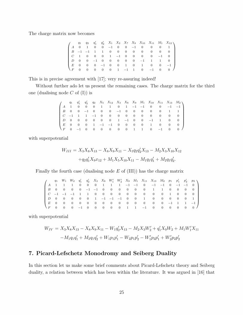
Without further ado let us present the remaining cases. The charge matrix for the third

one (dualising node C of (I)) is

q1 q′1 q′2 q2 X5 X12 X3 X8 X9 M1 X10 X11 X13 M2

A 1 0 0 0 1 1 0 1 −1 −1 0 0 −1 −1

B 0 0 −1 0 0 0 −1 0 0 0 0 0 1 1

C −1 1 1 −1 0 0 0 0 0 0 0 0 0 0

D 0 0 0 0 0 0 1 −1 0 0 −1 1 0 0

E 0 0 0 1 −1 −1 0 0 0 0 1 0 0 0

F 0 −1 0 0 0 0 0 0 1 1 0 −1 0 0

with superpotential

WIII = X3X8X13 −X8X9X11 −X5q2q′2X13 −M2X3X10X12

+q2q′1X9x12 +M1X5X10X11 −M1q1q

′1 +M2q1q

′2.

Finally the fourth case (dualising node E of (III)) has the charge matrix

q1 W1 W2 q′1 q′2 X3 X8 W ′1 W ′

2 X9 M1 X11 X13 M2 p1 p′1 p′2 p2

A 1 1 1 0 0 0 1 1 1 −1 −1 0 −1 −1 0 −1 −1 0

B 0 0 0 0 −1 −1 0 0 0 0 0 0 1 1 0 0 0 0

C −1 −1 −1 1 1 0 0 0 0 0 0 0 0 0 1 0 0 0

D 0 0 0 0 0 1 −1 −1 −1 0 0 1 0 0 0 0 0 1

E 0 0 0 0 0 0 0 0 0 0 0 0 0 0 −1 1 1 −1

F 0 0 0 −1 0 0 0 0 0 1 1 −1 0 0 0 0 0 0

with superpotential

WIV = X3X8X13 −X8X9X11 −W1q′2X13 −M2X3W

′2 + q′1X9W2 +M1W

′1X11

−M1q1q′1 +M2q1q

′2 +W1p1p

′1 −W2p1p

′2 −W ′

1p2p′1 +W ′

2p2p′2

7. Picard-Lefschetz Monodromy and Seiberg Duality

In this section let us make some brief comments about Picard-Lefschetz theory and Seiberg

duality, a relation between which has been within the literature. It was argued in [16] that

25

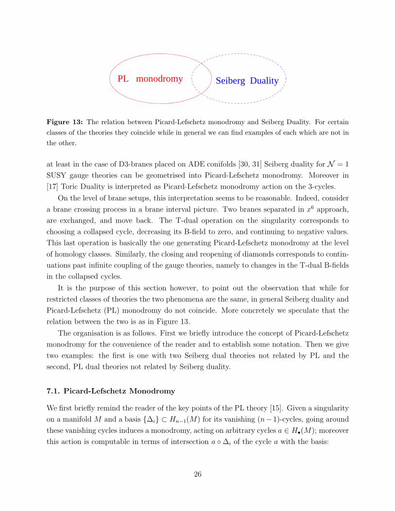
PL monodromy Seiberg Duality

Figure 13: The relation between Picard-Lefschetz monodromy and Seiberg Duality. For certainclasses of the theories they coincide while in general we can find examples of each which are not inthe other.

at least in the case of D3-branes placed on ADE conifolds [30, 31] Seiberg duality for N = 1

SUSY gauge theories can be geometrised into Picard-Lefschetz monodromy. Moreover in

[17] Toric Duality is interpreted as Picard-Lefschetz monodromy action on the 3-cycles.

On the level of brane setups, this interpretation seems to be reasonable. Indeed, consider

a brane crossing process in a brane interval picture. Two branes separated in x6 approach,

are exchanged, and move back. The T-dual operation on the singularity corresponds to

choosing a collapsed cycle, decreasing its B-field to zero, and continuing to negative values.

This last operation is basically the one generating Picard-Lefschetz monodromy at the level

of homology classes. Similarly, the closing and reopening of diamonds corresponds to contin-

uations past infinite coupling of the gauge theories, namely to changes in the T-dual B-fields

in the collapsed cycles.

It is the purpose of this section however, to point out the observation that while for

restricted classes of theories the two phenomena are the same, in general Seiberg duality and

Picard-Lefschetz (PL) monodromy do not coincide. More concretely we speculate that the

relation between the two is as in Figure 13.

The organisation is as follows. First we briefly introduce the concept of Picard-Lefschetz

monodromy for the convenience of the reader and to establish some notation. Then we give

two examples: the first is one with two Seiberg dual theories not related by PL and the

second, PL dual theories not related by Seiberg duality.

7.1. Picard-Lefschetz Monodromy

We first briefly remind the reader of the key points of the PL theory [15]. Given a singularity

on a manifold M and a basis {∆i} ⊂ Hn−1(M) for its vanishing (n−1)-cycles, going around

these vanishing cycles induces a monodromy, acting on arbitrary cycles a ∈ H•(M); moreover

this action is computable in terms of intersection a ◦∆i of the cycle a with the basis:

26

THEOREM 7.1 The monodromy group of a singularity is generated by the Picard-Lefschetz

operators hi, corresponding to a basis {∆i} ⊂ Hn−1 of vanishing cycles. In particular for

any cycle a ∈ Hn−1 (no summation in i)

hi(a) = a+ (−1)n(n+1)

2 (a ◦∆i)∆i.

More concretely, the PL monodromy operator hi acts as a matrix (hi)jk on the basis ∆j :

hi(∆j) = (hi)jk∆k.

Next we establish the relationship between this geometric concept and a physical inter-

pretation. According geometric engineering, when a D-brane wraps a vanishing cycle in the

basis, it give rise to a simple factor in the product gauge group. Therefore the total number

of vanishing cycles gives the number of gauge group factors. Moreover, the rank of each

particular factor is determined by how many times it wraps that cycle.

For example, an original theory with gauge group∏jSU(Mj) is represented by the brane

wrapping the cycle∑jMj∆j . Under PL monodromy, the cycle undergoes the transformation

∑j

Mj∆j =⇒∑j

Mj(hi)jk∆k.

Physically, the final gauge theory is∏kSU(

∑j Mj(hi)jk).

The above shows how the rank of the gauge theory changes under PL. To determine the

theory completely, we also need to see how the matter content transforms. In geometric

engineering, the matter content is given by intersection of these cycles ∆j . Incidentally, our

Inverse Algorithm gives a nice way and alternative method of computing such intersection

matrices of cycles.

Let us take a = ∆j , then

hi(∆j) = ∆j + (∆j ◦∆i)∆i.

This is particularly useful to us because (∆j ◦∆i), as is well-known, is the anti-symmetrised

adjacency matrix of the quiver (for a recent discussion on this, see [17]). Indeed this intersec-

tion matrix of (the blowup of) the vanishing homological cycles specifies the matter content

as prescribed by D-branes wrapping these cycles in the mirror picture. Therefore we have

(∆j ◦∆i) = [aji] := aji − aij for j 6= i and for i = j, we have the self-intersection numbers

(∆i ◦∆i). Hence we can safely write (no summation in i)

∆dualj = hi(∆j) = ∆j + [aji]∆i (7.1)

27

for aji the quiver (matter) matrix when Seiberg dualising on the node i; we have also used

the notation [M ] to mean the antisymmetrisation M − M t of matrix M . Incidentally in

the basis prescribed by {∆i}, we have the explicit form of the Picard-Lefschetz operators in

terms of the quiver matrix (no summation over indices): (hi)jk = δjk + [aji]δik.

From (7.1) we have

[adualjk ] := ∆dual

j ◦∆dualk = (∆j + [aji]∆i) ◦ (∆k + [aki]∆i)

= [ajk] + [aki][aji] + [aji][aik] + [aji][aki]∆i ◦∆i

= [ajk] + ci[aij ][aki]

(7.2)

where ci := ∆i ◦∆i, are constants depending only on self-intersection.

We observe that our quiver duality rules obtained from field theory (see beginning of

Section 6) seem to resemble (7.2), i. e. when ci = 1 and j, k 6= i. However the precise relation

of trying to reproduce Seiberg duality with PL theory still remains elusive.

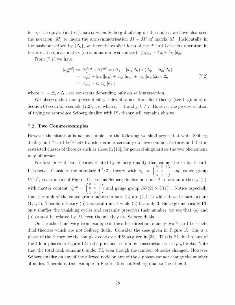
7.2. Two Counterexamples

However the situation is not as simple. In the following we shall argue that while Seiberg

duality and Picard-Lefschetz transformations certainly do have common features and that in

restricted classes of theories such as those in [16], for general singularities the two phenomena

may bifurcate.

We first present two theories related by Seiberg duality that cannot be so by Picard-

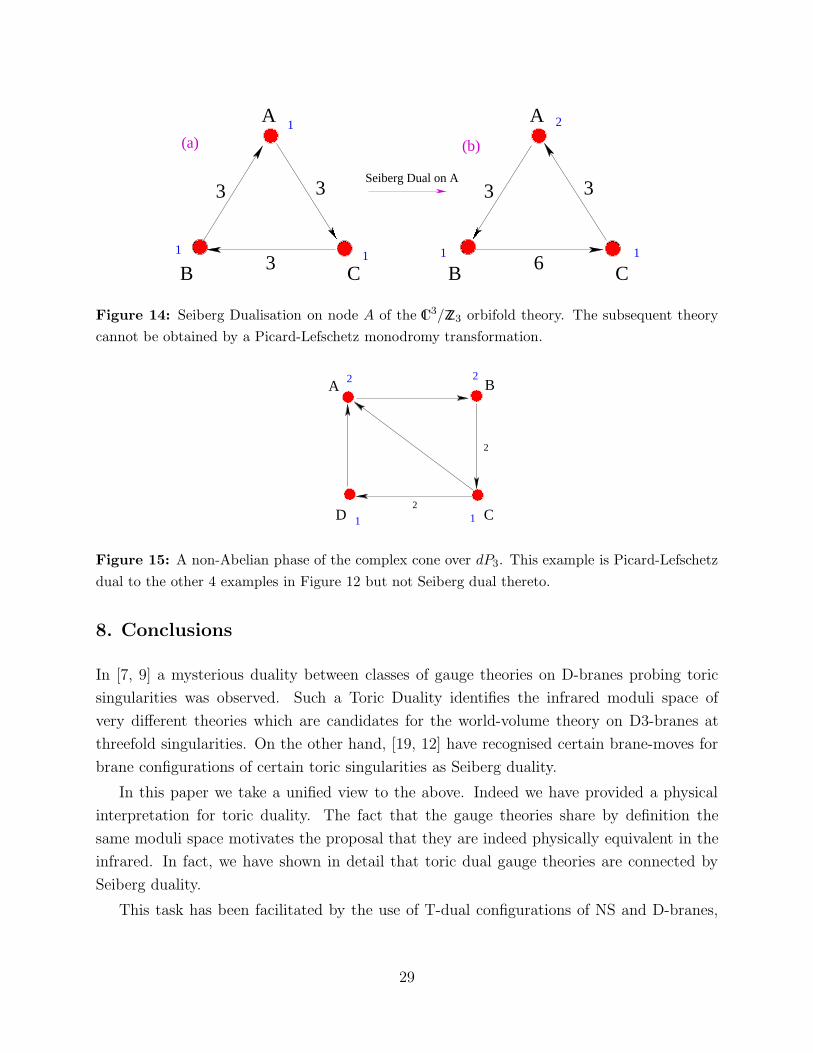
Lefschetz. Consider the standard C3/ZZ3 theory with aij =

(0 0 3

3 0 0

0 3 0

)and gauge group

U(1)3, given in (a) of Figure 14. Let us Seiberg-dualise on node A to obtain a theory (b),

with matter content adualij =

(0 3 0

0 0 6

3 0 0

)and gauge group SU(2) × U(1)2. Notice especially

that the rank of the gauge group factors in part (b) are (2, 1, 1) while those in part (a) are

(1, 1, 1). Therefore theory (b) has total rank 4 while (a) has only 3. Since geometrically PL

only shuffles the vanishing cycles and certainly preserves their number, we see that (a) and

(b) cannot be related by PL even though they are Seiberg duals.

On the other hand we give an example in the other direction, namely two Picard-Lefschetz

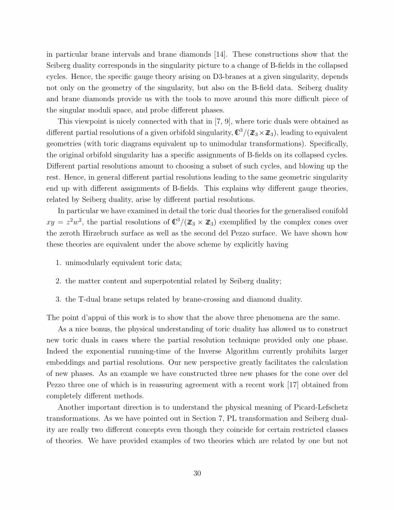
dual theories which are not Seiberg duals. Consider the case given in Figure 15, this is a

phase of the theory for the complex cone over dP3 as given in [33]. This is PL dual to any of

the 4 four phases in Figure 12 in the previous section by construction with (p, q)-webs. Note

that the total rank remains 6 under PL even though the number of nodes changed. However

Seiberg duality on any of the allowed node on any of the 4 phases cannot change the number

of nodes. Therefore, this example in Figure 15 is not Seiberg dual to the other 4.

28

���������

���������

���������

���������

��������

��������

������

������

���������

���������

��������������������������������������������������������������������������������������������������������������������������������������������

��������������������������������������������������������������������������������������������������������������������������������������������

A

CB 3

33

���������

���������

���������

���������

��������

��������

������

������

������

������������

������������������������������������������������������������������������������������������������������������������������

������������������������������������������������������������������������������������������������������������������������������

A

CB

33

6

1

1 1 1

2

1

Seiberg Dual on A

(a) (b)

Figure 14: Seiberg Dualisation on node A of the C3/ZZ3 orbifold theory. The subsequent theorycannot be obtained by a Picard-Lefschetz monodromy transformation.

������������

������������

������

������

��������

��������

��������

��������

BA

D C

2 2

11

2

2

Figure 15: A non-Abelian phase of the complex cone over dP3. This example is Picard-Lefschetzdual to the other 4 examples in Figure 12 but not Seiberg dual thereto.

8. Conclusions

In [7, 9] a mysterious duality between classes of gauge theories on D-branes probing toric

singularities was observed. Such a Toric Duality identifies the infrared moduli space of

very different theories which are candidates for the world-volume theory on D3-branes at

threefold singularities. On the other hand, [19, 12] have recognised certain brane-moves for

brane configurations of certain toric singularities as Seiberg duality.

In this paper we take a unified view to the above. Indeed we have provided a physical

interpretation for toric duality. The fact that the gauge theories share by definition the

same moduli space motivates the proposal that they are indeed physically equivalent in the

infrared. In fact, we have shown in detail that toric dual gauge theories are connected by

Seiberg duality.

This task has been facilitated by the use of T-dual configurations of NS and D-branes,

29

in particular brane intervals and brane diamonds [14]. These constructions show that the

Seiberg duality corresponds in the singularity picture to a change of B-fields in the collapsed

cycles. Hence, the specific gauge theory arising on D3-branes at a given singularity, depends

not only on the geometry of the singularity, but also on the B-field data. Seiberg duality

and brane diamonds provide us with the tools to move around this more difficult piece of

the singular moduli space, and probe different phases.

This viewpoint is nicely connected with that in [7, 9], where toric duals were obtained as

different partial resolutions of a given orbifold singularity, C3/(ZZ3×ZZ3), leading to equivalent

geometries (with toric diagrams equivalent up to unimodular transformations). Specifically,

the original orbifold singularity has a specific assignments of B-fields on its collapsed cycles.

Different partial resolutions amount to choosing a subset of such cycles, and blowing up the

rest. Hence, in general different partial resolutions leading to the same geometric singularity

end up with different assignments of B-fields. This explains why different gauge theories,

related by Seiberg duality, arise by different partial resolutions.

In particular we have examined in detail the toric dual theories for the generalised conifold

xy = z2w2, the partial resolutions of C3/(ZZ3 × ZZ3) exemplified by the complex cones over

the zeroth Hirzebruch surface as well as the second del Pezzo surface. We have shown how

these theories are equivalent under the above scheme by explicitly having

1. unimodularly equivalent toric data;

2. the matter content and superpotential related by Seiberg duality;

3. the T-dual brane setups related by brane-crossing and diamond duality.

The point d’appui of this work is to show that the above three phenomena are the same.

As a nice bonus, the physical understanding of toric duality has allowed us to construct

new toric duals in cases where the partial resolution technique provided only one phase.

Indeed the exponential running-time of the Inverse Algorithm currently prohibits larger

embeddings and partial resolutions. Our new perspective greatly facilitates the calculation

of new phases. As an example we have constructed three new phases for the cone over del

Pezzo three one of which is in reassuring agreement with a recent work [17] obtained from

completely different methods.

Another important direction is to understand the physical meaning of Picard-Lefschetz

transformations. As we have pointed out in Section 7, PL transformation and Seiberg dual-

ity are really two different concepts even though they coincide for certain restricted classes

of theories. We have provided examples of two theories which are related by one but not

30

the other. Indeed we must pause to question ourselves. For those which are Seiberg dual

but not PL related, what geometrical action does correspond to the field theory transforma-

tion. On the other hand, perhaps more importantly, for those related to each other by PL

transformation but not by Seiberg duality, what kind of duality is realized in the dynamics

of field theory? Does there exists a new kind of dynamical duality not yet uncovered??

Acknowledgements

We would like to extend our sincere gratitude to Amer Iqbal for discussions. Moreover, Y.-

H. H. would like to thank A. Karch for enlightening discussions. A. M. U. thanks M. Gonzalez

for encouragement and kind support.

References

[1] E. Witten, “Phases of N = 2 theories in two dimensions”, hep-th/9301042.

[2] P. Aspinwall, “Resolution of Orbifold Singularities in String Theory,” hep-th/9403123.

[3] Michael R. Douglas, Brian R. Greene, and David R. Morrison, “Orbifold Resolution by D-Branes”, hep-th/9704151.

[4] D. R. Morrison and M. Ronen Plesser, “Non-Spherical Horizons I”, hep-th/9810201.

[5] J. Park, R. Rabadan, A. M. Uranga, “Orientifolding the conifold”, Nucl.Phys. B570 (2000)38-80, hep-th/9907086.

[6] Chris Beasley, Brian R. Greene, C. I. Lazaroiu, and M. R. Plesser, “D3-branes on partialresolutions of abelian quotient singularities of Calabi-Yau threefolds,” hep-th/9907186.

[7] Bo Feng, Amihay Hanany and Yang-Hui He, “D-Brane Gauge Theories from Toric Singularitiesand Toric Duality,” Nucl. Phys. B 595, 165 (2001), hep-th/0003085.

[8] Tapobrata Sarkar, “D-brane gauge theories from toric singularities of the form C3/Γ andC4/Γ,” hep-th/0005166.

[9] Bo Feng, Amihay Hanany, Yang-Hui He, “Phase Structure of D-brane Gauge Theories andToric Duality”, hep-th/0104259.

[10] N. Seiberg, “Electric-Magnetic Duality in Supersymmetric Non-Abelian Gauge Theories,” hep-th/9411149, Nucl.Phys. B435 (1995) 129-146.

31

[11] S. Elitzur, A. Giveon, D. Kutasov, “Branes and N=1 Duality in String Theory,” Phys.Lett.B400 (1997) 269-274, hep-th/9702014.

[12] R. von Unge, “Branes at Generalized Conifolds and Toric Geometry,” hep-th/9901091, JHEP9902 (1999) 023.

[13] Amihay Hanany, Edward Witten, “Type IIB Superstrings, BPS Monopoles, And Three-Dimensional Gauge Dynamics,” Nucl.Phys. B492 (1997) 152-190, hep-th/9611230.

[14] M. Aganagic, A. Karch, D. Lust, A. Miemiec, ‘Mirror symmetries for brane configurations andbranes at singularities’, Nucl. Phys. B569 (2000) 277, hep-th/9903093.

[15] V. I. Arnold, S. M. Gusein-Zade and A. N. Varchenko, “Singularities of Differentiable Maps,”Vols I and II, Birkhauser, 1988.

[16] K. Ito, “Seiberg’s duality from monodromy of conifold singularity,” Phys. Lett. B 457, 285(1999), hep-th/9903061.

[17] Amihay Hanany, Amer Iqbal, “Quiver Theories from D6-branes via Mirror Symmetry,” hep-th/0108137.

[18] Igor R. Klebanov, Edward Witten, “Superconformal field theory on three-branes at a Calabi-Yau singularity”, Nucl. Phys. B536 (1998) 199, hep-th/9807080.

[19] Angel M. Uranga, “Brane configurations for branes at conifolds”, JHEP 9901 (1999) 022,hep-th/9811004.

[20] Keshav Dasgupta, Sunil Mukhi, “Brane constructions, conifolds and M theory”, Nucl. Phys.B551 (1999) 204, hep-th/9811139.

[21] Ofer Aharony, Amihay Hanany, “Branes, superpotentials and superconformal fixed points”,Nucl. Phys. B504 (1997) 239, hep-th/9704170.

[22] Angel M. Uranga, “From quiver diagrams to particle physics”, hep-th/0007173.

[23] L.E. Ibanez, R. Rabadan, A.M. Uranga, “Anomalous U(1)’s in type I and type IIB D = 4,N=1 string vacua”, Nucl. Phys. B542 (1999) 112, hep-th/9808139.

[24] Augusto Sagnotti, “A Note on the Green-Schwarz mechanism in open string theories”, Phys.Lett. B294 (1992) 196, hep-th/9210127.

[25] Michael R. Douglas, Gregory Moore, “D-branes, quivers, and ALE instantons”, hep-th/9603167.

32

[26] Kenneth Intriligator, “RG fixed points in six-dimensions via branes at orbifold singularities”,Nucl. Phys. B496 (1997) 177, hep-th/9702038.

[27] Amihay Hanany, Alberto Zaffaroni, “On the realization of chiral four-dimensional gauge the-ories using branes”, JHEP 9805 (1998) 001, hep-th/9801134.

[28] Amihay Hanany, Matthew J. Strassler, Angel M. Uranga, “Finite theories and marginal oper-ators on the brane”, JHEP 9806 (1998) 011, hep-th/9803086.

[29] Amihay Hanany, Angel M. Uranga, “Brane boxes and branes on singularities”, JHEP 9805(1998) 013, hep-th/9805139.

[30] Steven Gubser, Nikita Nekrasov, Samson Shatashvili, “Generalized conifolds and 4-Dimensional N=1 SuperConformal Field Theory”, JHEP 9905 (1999) 003, hep-th/9811230.

[31] Esperanza Lopez, “A Family of N=1 SU(N)k theories from branes at singularities”, JHEP9902 (1999) 019, hep-th/9812025.

[32] Steven S. Gubser, Igor R. Klebanov, “Baryons and domain walls in an N=1 superconformalgauge theory”, Phys. Rev. D58 (1998) 125025, hep-th/9808075.

[33] Amihay Hanany, Amer Iqbal, work in progress.

[34] C. Beasley and M. R. Plesser, “Toric Duality is Seiberg Duality”, hep-th/0109053.

33