relative algebro-geometric stabilities of toric manifolds

RELATIVE ALGEBRO-GEOMETRIC STABILITIES OF TORIC MANIFOLDS

NAOTO YOTSUTANI AND BIN ZHOU

ABSTRACT. In this paper, we study the relative Chow and K-stability of toric manifolds.First, we give a criterion for relative K-stability and instability of toric Fano manifolds. Thereduction of relative Chow stability on toric manifolds will be investigated by the Hibert-Mumford criterion in two ways. One is to consider the criterion for the maximal torusaction and its weight polytope. Then we obtain a reduction by the strategy of Ono [32],which fits into the relative GIT stability detected by Szekelyhidi. The other way is to usethe criterion for C×-actions and Chow weights associated to toric degenerations followingDonaldson and Ross-Thomas [12, 34]. In the end, we determine the relative K-stability ofall toric Fano threefolds and present counter-example for relatively K-stable manifold, butwhich is asymptotically relatively Chow unstable.

1. INTRODUCTION

The well known Yau-Tian-Donaldson conjecture asserts that a compact complex po-larized manifold (X,L) admits canonical metrics(Kahler-Einstein metrics, constant scalarcurvature (cscK) metrics, and extremal metrics, etc) in 2πc1(L) if and only if the underly-ing manifold is stable in the sense of Geometric Invariant Theory. Among various notionsof stabilities, K-stability and Chow stability are the most widely studied. Many authors usethe term polystablity rather than stablity, since the former agrees better with the notions inGIT. Throughout this paper, we use the latter for simplicity.

The conception of K-stability was first introduced by Tian [38] in the study of the exis-tence of Kahler-Einstein metrics in the first Chern class (if it is positive) on a Kahler mani-fold. Later, Donaldson extended it to general polarized varieties [12] and made a conjectureon the relation between K-stability and the existence of constant scalar curvature Kahlermetrics. More generally, for the existence of extremal metrics, the definition of K-stabilitywas extended by Szekelyhidi [37] to Kahler classes with the non-vanishing Futaki invariantand was called relative K-stability. Meanwhile, the conception of Chow stability is alsosignificant in Kahler geometry. Again, let (X,L) be a polarized manifold. Let Aut(L)be the bundle automorphism group. Since Aut(L) contains C× as a subgroup which actsas fiber-wise multiplications, we define Aut(X,L) by Aut(L)/C×. In [11] Donaldsonshowed that the existence of a cscK metric in 2πc1(L) implies asymptotic Chow stabilityof (X,L) if Aut(X,L) is discrete. At this point, Arezzo and Loi conjectured that Donald-son’s result would hold even if Aut(X,L) is not discrete [1, Conjecture 1]. Donaldson’sresult was generalized by Mabuchi [24], with the assumption on Aut(X,L) replaced bythe condition of vanishing higher order Futaki invariants. With these remarkable progress,

Date: February 26, 2016.Key words and phrases. Extremal metrics, K-stability, Chow stability, toric manifold.The second author was supported partially by ARC grant DE120101167, NSFC grants No. 11571018 and

11331001.1

2 NAOTO YOTSUTANI AND BIN ZHOU

the verification of the stabilities is drawing more and more attentions. In general, this is acomplicated problem since one has to study an infinite number of possible degenerationsof the manifold. In this paper, we shall discuss the stabilities of toric manifolds.

For toric manifolds, a well-understood reduced version of the relative K-stability on themoment polytope is believed to be equivalent to the existence of extremal metrics [12, 44].The conjecture has been confirmed on toric surfaces [13, 14, 7].

Let (X,L) be a polarized toric manifold. In [12], Donaldson reduced K-stability of2πc1(L) to the positivity of a linear functional defined on the moment polytope ∆ associ-ated to (X,L). The functional was generalized for the relative K-stability, given by [44]

(1.1) L∆(u) =

∫∂∆

u dσ −∫∆

(S + θ∆)u dx

where S is the average of the scalar curvature and θ∆ is the normalized potential functionof the extremal vector field V [17]. Note that this functional corresponds to the modifiedFutaki invariant in [37]. Then by [12, 44], ∆ is relative K-stable if and only if L∆ ispositive for all nontrivial convex functions on ∆. A further reduction in dimension 2 isthat for the positivity of L∆, it suffices to consider only simple piecewise linear convexfunctions on ∆ instead of all convex functions [12, 42]. In higher dimensions, a sufficientcondition on verifying the relative K-stability was given by [44]. When X is a Fano n-foldand L is the anti-canonical bundle, S = n and the condition is

(1.2) ∥θ∆∥ := sup∆θ∆ ⩽ 1.

The condition has been verified to hold on all toric Fano surfaces. They also asked whetherthe condition (1.2) holds for higher dimension or not. On the other hand, it is also inter-esting to determine the instability of toric Fano manifolds. By a simple observation andtogether with (1.2), we have

Theorem 1.1. Assume ∆ is the moment polytope of a toric Fano manifold and θ∆ =n∑

i=1

aixi + c, where ai, c ∈ R. Let ∆− = {x ∈ ∆|1− θ∆ < 0}.

(a) If ∆− = ∅, i.e. θ∆ < 1 on ∆, then ∆ is relatively strongly K-stable;(b) If ∆− = ∅ and satisfies

(1.3) 1− c <

∫∆−(1− θ∆)

2 dx

Vol(∆−),

then there exists a convex function u, s.t. L∆(u) < 0. In particular, if 0 ∈ ∆−, it is unstable.

An immediate application of the criterion is to determine all the relative K-stable toricFano threefolds as well as unstable ones. Remark that condition θ∆ ≡ 0 is equivalent to thatthe Futaki invariant vanishes, since the extremal vector field is dual to the Futaki invariantwith respect to generalized Killing forms [17]. Note that there are 18 deformation classesof toric Fano threefolds (See Section 2.1). Among all toric Fano threefolds, CP 3, B4, C3,C5 and F1 have the vanishing Futaki invariant, so the condition (1.2) is naturally true. Bycomputation with Theorem 1.1, we have

Theorem 1.2. Let X be a toric Fano threefold. We assume that the Futaki invariant of Xdoes not vanish. Then X is relative K-stable in toric sense in the anti-canonical class ifand only if X is one of the following: B2, B3, C1, C4, E3, E4 and F2.

RELATIVE ALGEBRO-GEOMETRIC STABILITIES OF TORIC MANIFOLDS 3

It is known that all toric Fano surfaces admit extremal metrics in the anti-cannonicalclass [6, 8]. The instability tells us counter-examples appear in dimension 3.

Corollary 1.3. If X is one of B1, C2, D1, D2, E1 and E2, then X does not admit extremalmetrics in its first Chern class.

On the other hand, the reduction of Chow stability is also an interesting problem. Anatural idea is to use the Hibert-Mumford criterion. Ono [32] studied Chow stability of toricmanifolds by considering the maximal torus action and its weight polytope. He obtained areduction by adapting Gelfand-Kapranov-Zelevinsky’s theory of Chow polytopes [19, 21].He also defined a notion of the relative Chow semistability in toric sense. In this paper, weintroduce a refinement of this notion so that it fits naturally into a picture of the relativeGIT stability detected by Szekelyhidi [36, Chapter 1]. We would like to point out that inthe statement of the results we only consider toric manifolds, but most of them hold forgeneral toric varieties.

Let N = dimH0(X,L)− 1 and TCN = CN+1 ∩ SL(C, N + 1). Let { a1, . . . , aN+1 } be

all the lattice points in ∆. We define θ∆ by

θ∆ =

N+1∑j=1

θ∆(aj)

N + 1.

To describe the relative Chow stability, we define Rn-valued functions d∆ and θ∆ by

d∆ : ∆ ∩ (Z)n −→ R, d∆(a) = 1 and

θ∆ : ∆ ∩ (Z)n −→ R, θ∆(a) = θ∆(a)− θ∆

respectively.

Theorem 1.4. A polarized toric manifold (X,L) is relatively TCN -semistable if and only if

there exists s ∈ R such that

(1.4)N+1∑j=1

aj + sN+1∑j=1

(θ∆(aj)− θ∆)aj =N + 1

Vol(∆)

∫∆

x dx

and

(1.5)(n+ 1)!Vol(∆)

N + 1

(d∆ + sθ∆

)∈ Ch(∆),

where Ch(∆) is the Chow polytope of X .

Furthermore, the asymptotic relative Chow stability can be reduced to the positivity ofQ∆(i, g) for all piecewise linear concave functions (see (3.9)). To distinguish the con-cepts, we call (X,L) is asymptotically relatively Chow stable in toric sense if for i ≫ 0,Q∆(i, g) > 0 for all nontrivial piecewise linear concave functions; and is asymptoticallyrelatively weakly Chow stable in toric sense, or asymptotically relatively Chow stable fortoric degenerations if for i ≫ 0, Q∆(i, g) > 0 for all nontrivial rational piecewise linearconcave functions. Concerning on relation between Chow and K-stabilities, we have

Theorem 1.5. If a polarized toric manifold (X,L) is asymptotically relatively Chow semistablein toric sense, then it is relatively K-semistable in toric sense.


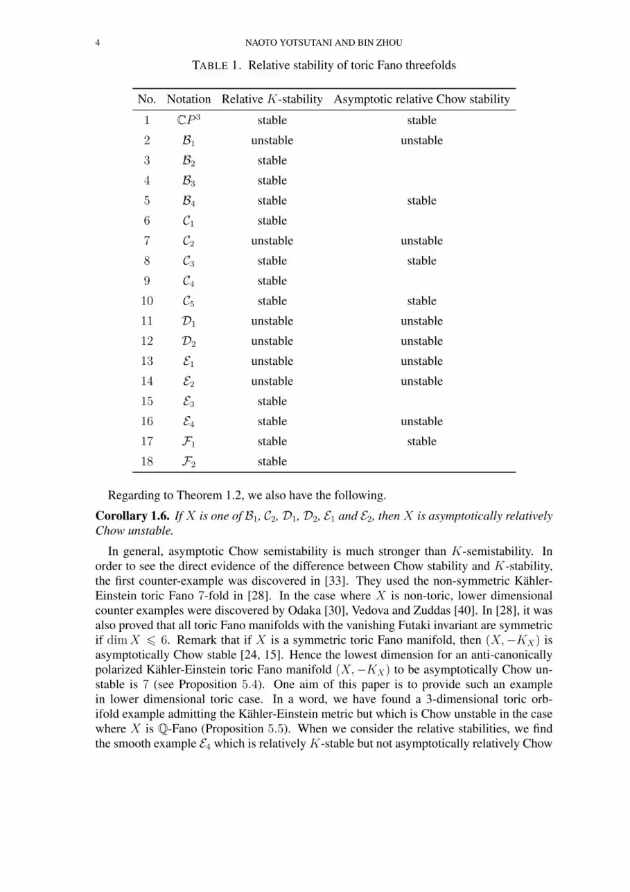
TABLE 1. Relative stability of toric Fano threefolds

No. Notation Relative K-stability Asymptotic relative Chow stability

1 CP 3 stable stable

2 B1 unstable unstable

3 B2 stable

4 B3 stable

5 B4 stable stable

6 C1 stable

7 C2 unstable unstable

8 C3 stable stable

9 C4 stable

10 C5 stable stable

11 D1 unstable unstable

12 D2 unstable unstable

13 E1 unstable unstable

14 E2 unstable unstable

15 E3 stable

16 E4 stable unstable

17 F1 stable stable

18 F2 stable

Regarding to Theorem 1.2, we also have the following.

Corollary 1.6. If X is one of B1, C2, D1, D2, E1 and E2, then X is asymptotically relativelyChow unstable.

In general, asymptotic Chow semistability is much stronger than K-semistability. Inorder to see the direct evidence of the difference between Chow stability and K-stability,the first counter-example was discovered in [33]. They used the non-symmetric Kahler-Einstein toric Fano 7-fold in [28]. In the case where X is non-toric, lower dimensionalcounter examples were discovered by Odaka [30], Vedova and Zuddas [40]. In [28], it wasalso proved that all toric Fano manifolds with the vanishing Futaki invariant are symmetricif dimX ⩽ 6. Remark that if X is a symmetric toric Fano manifold, then (X,−KX) isasymptotically Chow stable [24, 15]. Hence the lowest dimension for an anti-canonicallypolarized Kahler-Einstein toric Fano manifold (X,−KX) to be asymptotically Chow un-stable is 7 (see Proposition 5.4). One aim of this paper is to provide such an examplein lower dimensional toric case. In a word, we have found a 3-dimensional toric orb-ifold example admitting the Kahler-Einstein metric but which is Chow unstable in the casewhere X is Q-Fano (Proposition 5.5). When we consider the relative stabilities, we findthe smooth example E4 which is relatively K-stable but not asymptotically relatively Chow


stable (Proposition 5.7). The asymptotic Chow stability of CP 3, B4, C3, C5, F1 followsfrom [33]. Hence, we list all the determined stability of toric Fano threefolds in this paperin Table 1. Note that the stabilities are all in toric sense. It is an interesting question tocomplete the table, i.e., to determine the rest stabilities in the blank.

In [34], Ross-Thomas gave a description of Chow stability by using the Hilbert-Mumfordcriterion for the C×-actions induced by test configurations [12]. Inspired by this idea, wegive an alternative reduction of the relative Chow stability of toric manifolds in Section 4.One can see that the Chow weight coincides with Q∆(i, ·).

This paper is organized as follows. Section 2 is a brief review of toric varieties and thereduction of relative K-stability on toric manifolds which will be used at later stages in thepaper. We also prove Theorem 1.1. In Sections 3 and 4 we shall discuss the two ways ofreduction of the relative Chow stability of toric manifolds. In Section 5, we present variousexamples for the stabilities considered in the paper. We compute normalized potentialson toric Fano threefolds and verify the relative K-stability or instablity in Section 5.1.We also provide an example of K-stable toric Fano orbifold X which is Chow unstablein dimX = 3. Finally, we discuss the asymptotic relative Chow stability of toric Fanothreefolds. The computational results for θ∆ and ∆− are listed in Table 3.

Acknowledgements. The first author would like to thank Professors Y. Nakagawa, Y. Sanoand A. Higashitani for their valuable comments and discussions. In particular, Higashitanisuggested us use toric package [5] for our computations.

2. PRELIMINARIES

2.1. Toric varieties. We review some of notations of toric varieties. Let M be a latticeof rank n, N = Hom(M,Z) the Z-dual of M . Let MR (resp. NR) denote the R-vectorspace M ⊗Z R ∼= Rn (resp. N ⊗Z R ∼= Rn). Let Σ denote a complete fan in NR. The k-dimensional cones of Σ form a set Σ(k). Let σ be a cone in Σ. The associated affine schemeUσ := Spec C[M ∩ σ∨] is called the affine toric variety. Then Σ defines the toric varietyX := X(N,Σ) by constructing the disjoint union of the affine toric varieties Uσ, where oneglues Uσ1 and Uσ2 along the open subvarietiy Uσ1∩σ2 for σ1, σ2 ∈ Σ. We generally definea toric variety X as an irreducible complex algebraic normal variety containing a torus T n

Cas a Zariski open subset such that the action of T n

C on itself extends to an algebraic actionof T n

C on X .Let ∆ ⊆ MR be a rational n-dimensional polytope with 0 ∈ Int∆. We define the dual

polytope ∆◦ ⊆ NR by

∆◦ := { a ∈ NR | ⟨a, b⟩ ⩾ −1 for all b ∈ ∆ } ,which is also a rational n-dimensional polytope with 0 ∈ Int∆◦. We denote a face F of∆◦ by F ≤ ∆◦. The fan N∆ := { pos(F ) | F ≤ ∆◦ } is called the normal fan of ∆, wherepos(F ) is the linear positive hull of F . For a rational polytope ∆ ⊆ MR, we define theassociated toric variety by X∆ := X(N,N∆).

The discussion on examples (Section 5) will focus on toric Fano threefolds. We recallthe related notations here. See [10] and [27] for more details.

Definition 2.1. A complex normal variety X is said to be Fano variety if X is projectiveand the anti-canonical divisor −KX is an ample Q-Cartier divisor, i.e., a multiple of −KX

is ample Cartier.


Definition 2.2. Let ∆◦ ⊆ NR be an n-dimensional lattice polytope which contains theorigin in its interior. Then ∆◦ is called a canonical Fano polytope if Int∆◦ ∩ N = {0 }.Furthermore, ∆◦ is called a Fano polytope if the vertices of any facet of ∆◦ form a Z-basisof the lattice N .

Then there is the following fundamental result.

Proposition 2.3. [27, Proposition 2.3.7] There is a bijective correspondence between iso-morphism classes of Fano polytopes (resp. canonical Fano polytopes) and smooth toricFano varieties (resp. toric Fano varieties with canonical singularities).

Here and hereafter we call a smooth toric Fano variety a toric Fano manifold throughoutthe paper.

Let X be a complex normal variety. Recall that X is called Q-factorial if any Weildivisor is Q-Cartier. For the toric case, we have a well-known description in terms of aFano polytope. A polytope is called simplicial if any facet is a simplex. It was shown thatsimplicial Fano polytopes correspond uniquely up to isomorphism to Q-factorial toric Fanovarieties (see Proposition 2.3.12 in [27]). Since a toric variety X has only finite quotientsingularities (that is, X is an orbifold) if and only if the associated fan Σ is simplicial,Q-factorial toric Fano varieties are toric Fano orbifolds.

In [22], Kasprzyk classified 3-dimensional toric Fano varieties at worst canonical sin-gularities. There are 12, 190 Q-factorial toric Fano varieties X up to isomorphism. In thecase whenX is smooth, 3-dimensional toric Fano manifolds (i.e., toric Fano threefolds) areclassified by Batyrev [2] and K. Watanabe and M. Watanabe [41] independently. There are18 deformation classes of toric Fano threefolds, that is, CP 3, B1, B2, B3, B4 = CP 2×CP 1,C1, C2, C3 = CP 1 ×CP 1 ×CP 1, C4, C5 = CPCP 1×CP 1(O⊕O(1,−1)), D1, D2, E1, E2, E3,E4, F1 = CP 1 × (CP 2 ♯ 3CP 2) and F2. Note that we use the same notation as in [2]. Itis well-known that each toric Fano threefold is obtained from CP 3 by a series of blow-upsand blow-downs along torus invariant subvarieties. Furthermore, we can specify the cor-responding moment polytopes ∆ associated to anti-canonical polarization of all toric Fanothreefolds (see Table 2 in the end of the paper). These classification results are availableonline at [46, 29].

2.2. Reduction of relative K-stability. In this subsection, we recall the reduction of theFutaki invariant and the related materials on toric manifolds. We also present the formulaeto determine the normalized potential θ∆ of the extremal vector field in symplectic coordi-nate and criterions for relative K-stability and instablity.

First we recall the Futaki invariant and the extremal vector field. Let (X,ωg) be a com-pact Kahler manifold. Let Aut0(X) be the identity component of the holomorphisms groupof X and Autr(X) be the reductive part of Aut0(X). Then Autr(X) is the complexificationof a maximal compact subgroup K of Autr(X). We denote the Lie algebra of Autr(X)by ηr(X), which induces a set of holomorphic vector fields on X . Let v ∈ ηr(X) sothat its imaginary part generates a one-parameter compact subgroup of K. Then if theKahler form ωg is K-invariant, that is, invariant under the group K, there exists a uniquereal-valued function θv (called normalized potential of v) such that

(2.1) ivωg =√−1∂θv(ωg), and

∫X

θv(ωg)ωng

n!= 0.


For simplicity, we denote the set of such potentials θv by Ξωg . Then the Futaki invariant onηr can be written as

(2.2) F (v) = −∫X

θv(ωg)(S(ωg)− S)ωng

n!.

In [17], Futaki and Mabuchi defined the extremal vector field, V = gij(proj(S(ωg)))j∂∂zi

in ηr(X) for the Kahler class [ωg], where proj(S(ωg)) is the L2-inner projection of thescalar curvature of ωg to Ξωg . In fact, they showed that V is independent of the choice ofK-invariant metrics in [ωg], and its potential is uniquely determined by the bilinear form

(2.3) F (v) = −∫X

θv(ωg)θV (ωg)ωng

n!, ∀ v ∈ ηr(X).

Now we consider the reduction on polarized toric manifolds. Assume that (X,L) is atoric manifold polarized by a line bundle L. Choose an (S1)n-invariant Kahler metric gwith ωg ∈ 2πc1(L). The open dense orbit of the complex torus action T n

C in X inducesa ‘global’ coordinates (z1, ..., zn) ∈ (C×)n. Denote the affine logarithmic coordinateswi = log zi = yi+

√−1ηi. Then ωg is determined by a uniformly convex function φ which

depends only on y1, ..., yn ∈ Rn in the coordinates (w1, ......, wn), namely

(2.4) ωg = 2√−1∂∂φ

on (C×)n. As is well-known, the moment map can be given by Dφ and the image by∆ = Dφ(Rn) is a polytope. We denote by xi = ∂φ

∂yi, i = 1, ..., n the symplectic coordinates.

Note that in the affine logarithm coordinates (w1, ..., wn), { ∂∂wi

, i = 1, ..., n} is a basis ofthe Lie algebra of T n

C as a complex Lie subalgebra of the Lie algebra of holomorphic vectorfields on X . The following lemma was given in [44] on how to determine the potential ofthe extremal vector field in symplectic coordinates through the Futaki invariant.

Lemma 2.4. Let g be an (S1)n-invariant metric on X . Assume V is the extremal vectorfield and θV (ωg) be the normalized potential associated to ωg by (2.1). Then there are2n-numbers ai and ci such that

θV (ωg) =n∑

i=1

ai(xi + ci) := θ∆,

where x = (xi) = Dφ ∈ ∆. Moreover ai and ci are determined uniquely by 2n-equations,

1

(2π)nF (

∂

∂wi

) = −∫∆

(n∑

j=1

aj(xj + cj)

)(xi + ci)dx, i = 1, ..., n,(2.5) ∫

∆

(xi + ci)dx = 0, i = 1, ..., n.(2.6)

The relative K-stability on toric manifolds can be reduced to the positivity of the linearfunctional

(2.7) L∆(u) =

∫∂∆

u dσ −∫∆

(S + θ∆)u dx

for convex functions. We recall [12, 37, 44]


Definition 2.5. A toric manifold (X∆, L∆) is called relatively K-semistable for toric de-generations if L∆(u) ⩾ 0 for all rational piecewise linear convex functions. Furthermore,it is called relatively weakly K-stable in toric sense or relatively K-stable for toric degen-erations when L∆(u) = 0 if and only if u is a linear function.

When proving the existence of cscK metrics on toric surfaces [13, 14], Donaldson intro-duced a stronger notion, called strong K-stability. Let ∆∗ be the union of the interior of ∆and the interiors of its co-dimension 1 faces. Denote

C1 = {u | u is convex on ∆∗ and∫∂∆

u <∞}.

The linear functional L∆ is well defined in C1.

Definition 2.6. (X∆, L∆) is called relatively strongly K-stable in toric sense if L∆(u) ⩾ 0for all convex functions in C1 and L∆(u) = 0 if and only if u is a linear function.

Note that L∆(u) is invariant when adding an affine linear function to u. Without lossof generality, we assume 0 lies in the interior of ∆. Hence, it suffices to consider convexfunctions normalized at 0 in the sense that infx∈∆ u(x) = u(0) = 0.

When X is a toric Fano manifold, it is observed in [44] that

(2.8) L∆(u) =

∫∆

(n∑

i=1

xiui − u

)+ (1− θ∆)u dx

for C1 functions by an integration by parts from (2.7). Here ui = ∂u∂xi

. By approximation,it is easy to see that (2.8) can also be used for the computation of L∆(u) for piecewise C1

functions. As can be seen from (2.8), the positivity of L∆ relies heavily on the positivity of1− θ∆. Assume θ∆ =

∑ni=1 aixi + c. Then we shall prove Theorem 1.1.

Proof of Theorem 1.1. (a) is obvious [44]. We only need to consider (b). If 1 − θ∆ < 0,i.e. ∆− = ∆, it is obvious that all simple piecewise linear convex functions of the form

max{n∑

i=1

bixi, 0} will destabilize ∆. So we assume 1− θ∆ = 0 intersects the interior of ∆.

Letu = max{−(1− θ∆), 0}.

Thenn∑

i=1

xiui − u =

{1− c, x ∈ ∆−;

0, x ∈ ∆ \∆−.

Hence,

L∆(u) = (1− c)Vol(∆−)−∫∆−

(1− θ∆)2 dx.

The theorem follows. □Although the condition in this theorem is not sharp, but we will see in Section 5 that this

criterion can determine all the stable toric Fano threefolds and many fourfolds.

3. RELATIVE CHOW STABILITY OF TORIC MANIFOLDS

In this section, we consider relative Chow stability of polarized toric manifolds.


3.1. Notions of Chow stabilities. We first recall various notions of Chow stabilities. Werefer to the monograph [16] by Futaki for more general concept of Chow stability in Kahlergeometry. In [23, 25], Mabuchi defined the notion of relative Chow stability in order toconsider the existence problem of extremal Kahler metrics. A historical background ofrelative GIT stability was detected by Szekelyhidi [36, Chapter 1].

Let G be a reductive algebraic group and V be a finite dimensional complex vectorspace. Suppose that G acts linearly on V. Let us denote a nonzero vector v∗ in V whichis a representative of v = [v∗] ∈ P(V). According to GIT, we call v∗ is G-semistable ifthe closure of the G-orbit OG(v

∗) does not contain the origin. Furthermore, v∗ is G-stableif OG(v

∗) is closed. We call v∗ is G-unstable if v∗ is not G-semistable. Analogously,v ∈ P(V) is said to be G-semistable (resp. stable, unstable) if any representative of v isG-semistable (resp. stable, unstable).

To feature relative stability, following [36, Chapter 1], we consider a compact torus T inG, and denote its Lie algebra by t. Then we define subalgebras of g by

gT = {α ∈ g | [α, β] = 0 for all β ∈ t } ,gT⊥ = {α ∈ gT | ⟨α, β⟩ = 0 for all β ∈ t }

where ⟨·, ·⟩ is a rational invariant inner product. We denote the corresponding subgroup byGT and GT⊥ .

Definition 3.1. [36] Let T be a torus inG fixing the point v. Then v is said to be semistable(resp. stable, unstable) relative to T if it is GT⊥-semistable (resp. stable, unstable).

The Hilbert-Mumford criterion says that v ∈ P(V) is G-semistable if and only if v isH-semistable for each maximal algebraic torus H ⊂ G [9, p.137]. Hence, it is importantto consider when a reductive group G is isomorphic to an algebraic torus. In this case, theabove stabilities can be described by the weight polytopes of the actions as follows. Letχ(G) denote the character group of G. Then χ(G) consists of algebraic homomorphismsχ : G −→ C×. If we fix an isomorphism G ∼= (C×)N+1, we may express each χ as aLaurent monomial

χ(t1, . . . , tN+1) = ta11 · · · taN+1

N+1 , ti ∈ C×, ai ∈ Z.

Thus, there is the identification between χ(G) and ZN+1:

χ = (a1, . . . , aN+1) ∈ ZN+1.

Then it is well-known that V decomposes under the action of G into weight spaces

V =⊕

χ∈χ(G)

Vχ, Vχ := { v∗ ∈ V | t · v∗ = χ(t) · v∗, t ∈ G } .

Definition 3.2. Let v∗ ∈ V \ {0 } be a nonzero vector in V with

v∗ =∑

χ∈χ(G)

vχ, vχ ∈ Vχ.

The weight polytope of v∗ (with respect to G-action) is the convex lattice polytope inχ(G)⊗ R ∼= RN+1 defined by

NG(v∗) := Conv {χ ∈ χ(G) | vχ = 0 } ⊆ RN+1.


Then the Hilbert-Mumford criterion can be restated as the following proposition. It givescombinatorial description whether a given point is G-semistable (resp. G-stable) or not.

Proposition 3.3. [9, Theorem 9.2] Let V, G and v∗ be as above. Then v∗ is G-semistableif and only if NG(v

∗) contains the origin. Moreover, v∗ is G-stable if and only if NG(v∗)

contains the origin in its interior.

In the relative stability setting, we also have

Proposition 3.4. [36, Theorem 1.5.1] The point v is relatively semistable (resp. stable)if and only if the orthogonal projection of the origin onto the minimal affine subspacecontaining NG(v

∗) is in NG(v∗) (resp, relintNG(v

∗)).

Now we take the subtorus H of G which is the maximal torus of SL(N +1,C) given by

H = { (t1, . . . , tN , (t1 · · · tN)−1) | ti ∈ C×, 1 ⩽ i ⩽ N } ∼= (C×)N .

Considering the projection

πH : χ(G)⊗ R ∼= RN+1 −→ χ(H)⊗ R ∼= RN

(φ1, . . . , φN+1) 7−→ (φ1 − φN+1, . . . , φN − φN+1),

we observe that πH(NG(v∗)) = NH(v

∗). Hence we have the following.

Proposition 3.5. [32, Proposition 2.4] v∗ is H-semistable exactly if

NG(v∗) ∩ SpanR { (1, . . . , 1) } = ∅ in RN+1.

Remark 3.6. Setting W = SpanR { (1, . . . , 1) }, we observe that the perpendicular sub-space W⊥ of W in RN+1 is spanned by

β1 = (1,−1, 0, . . . , 0), β2 = (1, 0,−1, 0, . . . , 0), . . . , βN = (1, 0, . . . , 0,−1).

Thus the projection πH is written as

πH : RN+1 −→ RN

φ = (φ1, . . . , φN+1) 7−→ (⟨φ, β1⟩ , . . . , ⟨φ, βN⟩).We will generalize this argument to the relative stability in the next section.

Next we define the Chow form and Chow stability of irreducible projective varieties.See [19, 43] for more details. Let X ⊂ CPN be an n-dimensional irreducible complexprojective variety of degree d. Recall that the Grassmann variety G(k,CPN) parameterizesk-dimensional projective linear subspaces of CPN . The associated hypersurface of X ⊂CPN is the subvariety in G(N − n− 1,CPN) which is given by

ZX := {W ∈ G(N − n− 1,CPN) | W ∩X = ∅ } .The fundamental properties of ZX can be summarized as follows (see [19], p.99):

(a) ZX is irreducible,(b) Codim ZX = 1 (that is, ZX is a divisor in G(N − n− 1,CPN)),(c) degZX = d in the Plucker coordinates, and(d) ZX is given by the vanishing of a section R∗

X ∈ H0(G(N − n− 1,CPN),O(d)).We call R∗

X the Chow form of X . Note that R∗X can be determined up to a multiplicative

constant. Let V := H0(G(N−n−1,CPN),O(d)) andRX ∈ P(V) be the projectivizationof R∗

X . We call RX the Chow point of X . Since we have the natural action of G =SL(N + 1,C) into P(V), we can define stabilities of RX as follows.


Definition 3.7. LetX ⊂ CPN be an irreducible, n-dimensional complex projective variety.Then X is said to be Chow semistable (resp. stable, unstable) if the Chow point RX of Xis SL(N + 1,C)-semistable (resp. stable, unstable).

Definition 3.8. Let (X,L) be a polarized variety. For i ∈ Z, let Ψi : X −→ P(H0(X,Li)∗)be the Kodaira embedding.

(1) (X,L) is said to be Chow semistable (resp. stable, unstable) if Ψ(X) ⊂ P(H0(X,L)∗)is Chow semistable (resp. stable, unstable).

(2) (X,L) is called asymptotically Chow semistable (resp. stable) if there is an i0 suchthat Ψi(X) ⊂ P(H0(X,Li)∗) is Chow semistable (resp. stable) for each i ⩾ i0.

We say that (X,L) is asymptotically Chow unstable if it is not asymptotically Chowsemistable.

As is similar to K-stability and relative K-stability, we consider relative Chow stabilitywhen the Futaki invariant does not vanish, i.e., the extremal vector field V is nontrivial.Choose T the one-parameter subgroup induced by V . Hence, T also acts into P(V).

Definition 3.9. LetX ⊂ CPN be an irreducible, n-dimensional complex projective variety.Then X is said to be relatively Chow semistable (resp. stable, unstable) if the Chow pointRX of X is semistable (resp. stable, unstable) relative to T .

Definition 3.10. Let (X,L) be a polarized variety. For i ∈ Z, let Ψi : X −→ P(H0(X,Li)∗)be the Kodaira embedding.

(1) (X,L) is said to be relatively Chow semistable (resp. stable, unstable) if Ψ(X) ⊂P(H0(X,L)∗) is relatively Chow semistable (resp. stable, unstable).

(2) (X,L) is called asymptotically relatively Chow semistable (resp. stable) if there isan i0 such that Ψi(X) is relatively Chow semistable (resp. stable) for each i ⩾ i0.

We say that (X,L) is asymptotically relatively Chow unstable if it is not asymptoticallyrelatively Chow semistable.

For an n-dimensional irreducible projective variety X ⊂ CPN , the weight polytope ofR∗

X∈ H0(G(N − n− 1,CPN),O(d)) with respect to the action (C×)N+1 ⊂ GL(N+1,C)of diagonal matrices is called Chow polytope of X , and is denoted by Ch(X). See [19,Chapter 6] for more details.

3.2. Reduction on toric manifolds. We reduce the relative Chow stability of toric mani-folds by developing an idea in [31, 32].

Let ∆ ⊆ MR be an n-dimensional Delzant lattice polytope. It is well-known that thereis the bijective correspondence between n-dimensional lattice polytope ∆ and compacttoric variety with a (C×)n-equivariant very ample line bundle (X∆, L∆). We consider the(relative) Chow stability of X∆ ⊂ CPN , N = dim(H0(X∆, L∆))− 1.

Setting G = (C×)N+1, we only consider the specific maximal torus

TC∆ := G ∩ SL(N + 1,C).

We view the Lie algebra of TC∆ as a subalgebra of sl(N +1,C) by considering the traceless

part. The inner product ⟨, ⟩ on sl(N + 1,C) is given by ⟨A,B⟩ = Tr(AB). Since G is thealgebraic torus consisting of diagonal matrices, TC

∆ is given by

TC∆ ↪→ (C×)N+1

(t1, . . . , tN) 7−→ (t1, . . . , tN , (t1 · · · tN)−1).


In particular, TC∆∼= (C×)N . Let Ch(∆) denote the Chow polytope of X∆ ⊂ CPN . Recall

that X∆ ↪→ CPN is Chow semistable w.r.t TC∆-action if and only if

Ch(∆) ∩ SpanR { (1, . . . , 1) } = ∅ in RN+1

by Proposition 3.3 and Proposition 3.5. In the literature of Gelfand-Kapranov-Zelevinsky’stheory, the Chow polytope Ch(∆) coincides with the secondary polytope [21]. In particu-lar, it is known that the affine span of the secondary polytope is given by the following.

Proposition 3.11. [19, Chapter 7, Proposition 1.11] Let φ = (φ1, . . . , φN+1) be a point inthe affine hull of Ch(∆) in χ(G)⊗ R ∼= RN+1. Then

N+1∑j=1

φj = (n+ 1)!Vol(∆),(3.1)

N+1∑j=1

φjaj = (n+ 1)!

∫∆

x dx.(3.2)

Here x = (x1, . . . , xn) and ∆ ∩M = { a1, . . . , aN+1 } is all the lattice points in ∆.

Now we shall consider relative Chow semistability as follows. Let V be the extremalvector field on X∆ and θ∆ be the potential function in Section 2 and λ ∈ χ(G)∗ be theone-parameter subgroup induced by V . Then λ is given in TC

∆ by

λ : C× ↪→ G

t 7−→(t(θ∆(a1)−θ∆), . . . , t(θ∆(aN+1)−θ∆)

),

where

θ∆ =

N+1∑j=1

θ∆(aj)

N + 1.

Let us take for T the image of λ, i.e., T = {λ(t) | t ∈ C× }. We define a two dimensionalsubspace in RN+1 by

W := SpanR { (1, . . . , 1), ((θ∆ (a1)− θ∆), . . . , (θ∆ (aN+1)− θ∆)) } .

Let β1, . . . , βN−1 ∈ RN+1 be the basis of the subspace perpendicular to W. Note that GT⊥

is isomorphic to (C×)N−1. Considering the projection

πGT⊥ : χ(G)⊗ R ∼= RN+1 −→ χ(GT⊥)⊗ R ∼= RN−1

φ = (φ1, . . . , φN+1) 7−→ (⟨φ, β1⟩, . . . , ⟨φ, βN−1⟩),

we observe that NGT⊥ (RX∆

) = πGT⊥ (NG(RX∆

)) ⊂ RN−1.To describe the relative Chow stability, we define Rn-valued functions d∆ and θ∆ by

d∆ : ∆ ∩ (Z)n −→ R, d∆(a) = 1 and

θ∆ : ∆ ∩ (Z)n −→ R, θ∆(a) = θ∆(a)− θ∆

respectively. Then we have the following.


Theorem 3.12. The Chow form of X∆ ↪→ CPN+1 is GT⊥-semistable if and only if thereexists s ∈ R such that

(3.3)N+1∑j=1

aj + sN+1∑j=1

(θ∆(aj)− θ∆)aj =N + 1

Vol(∆)

∫∆

x dx,

and

(3.4)(n+ 1)!Vol(∆)

N + 1

(d∆ + sθ∆

)∈ Ch(∆).

Proof. By definition, our assumption is equivalent to 0 ∈ NGT⊥ (RX∆

). By the projectionabove, it is equivalent to W ∩ Ch(∆) = ∅, that is, there exist s1, s2 ∈ R such that

(3.5) s1d∆ + s2θ∆ ∈ Ch(∆).

By (3.1) and the factN+1∑j=1

θ∆(aj) = 0, we have

s1 =(n+ 1)!Vol(∆)

N + 1.

(3.3) follows from (3.2). □

Remark 3.13. This theorem extends Ono’s description of Chow semistability [31, 32] torelative case. The reader should bear in mind that we only consider a special case of themaximal torus action.

With Theorem 3.12 and Proposition 3.3, we have

Definition 3.14. We callX∆ is relatively Chow semistable in toric sense if (3.4) is satisfied;it is called relatively Chow stable in toric sense if

(3.6)(n+ 1)!Vol(∆)

N + 1

(d∆ + sθ∆

)∈ Int(Ch(∆)).

3.3. Asymptotic relative Chow semistability. In this subsection, we develop the argu-ment of relative Chow semistability to the case of asymptotic stability.

Let ∆ and X∆ be as above. Let us denote the Ehrhart polynomial of ∆ by E∆(t). It hasdegree n = dim∆ and satisfies

E∆(i) = Card(i∆ ∩ Zn) = Card(∆ ∩ (Z/i)n))

for all i ∈ Z+. Moreover, by Ehrhart Theorem, E∆(t) has the form

E∆(t) = Vol(∆)tn +Vol(∂∆)

2tn−1 + · · ·+ 1.

Now for any i ∈ Z+, following [32], we replace ∆ in the last subsection by i∆ andN + 1 by E∆(i). Then G = (C×)E∆(i) and we consider the maximal torus TC

i∆ := G ∩SL(E∆(i),C). The character group of (C×)E∆(i) is identified with

{i∆ ∩ Zn → Z} ∼= {∆ ∩ (Z/i)n → Z} ∼= ZE∆(i).


For future convenience, we denote χ(G)⊗ R and χ(G)⊗Q by

W (i∆) = {i∆ ∩ Zn → R} ∼= {∆ ∩ (Z/i)n → R} ∼= RE∆(i) and

W (i∆)Q = {i∆ ∩ Zn → Q} ∼= {∆ ∩ (Z/i)n → Q} ∼= QE∆(i)

respectively. As in [19, p.220], we identifyW (i∆) with its dual space by the scalar product

⟨φ, ψ⟩ =∑

a∈∆∩(Z/i)nφ(a)ψ(a).

Correspondingly, we define

θi∆ =

∑a∈∆∩(Z/i)n

θ∆(a

i)

E∆(i)

and functions

di∆ : ∆ ∩ (Z/i)n −→ R, di∆(a) = 1 and

θi∆ : ∆ ∩ (Z/i)n −→ R, θi∆(a) =θ∆(a)− θi∆

i.

in W (i∆). Note that∫i∆

x dx = in+1

∫∆

x dx, hence we have the following.

Definition 3.15. We call (X∆, L∆) is asymptotically relatively Chow semistable in toricsense if there is an i0 such that for each i ⩾ i0, there exists si, such that

(3.7)∑

a∈∆∩(Z/i)nia+ si

∑a∈∆∩(Z/i)n

(θ∆(a)− θi∆)a =iE∆(i)

Vol(∆)

∫∆

x dx,

and

(3.8)in(n+ 1)!Vol(∆)

E∆(i)

(di∆ + siθi∆

)∈ Ch(i∆).

The asymptotic relative Chow semistability can be related to relative K-semistabilitythrough Gelfand-Kapranov-Zelevinsky’s theory on triangulations, A-Resultants and sec-ondary polytopes of ∆ [19, Chapter 7-8]. For this purpose, we recall some notations. For afixed φ ∈ W (i∆), let

Gφ = the convex hull of∪

a∈∆∩(Z/i)n{(a, t) | t ⩽ φ(a)} ⊂MR × R ∼= Rn+1.

Then we define a piecewise linear function gφ : ∆ −→ R by

gφ(x) = max{t | (x, t) ∈ Gφ}.The upper boundary of Gφ can be regarded as the graph of gφ. Furthermore, gφ has thefollowing properties.

Lemma 3.16 ([19] p.221, Lemma 1.9). For any φ ∈ W (i∆),(a) the function gφ is concave.(b) we have the equality

max{⟨φ, ψ⟩ | ψ ∈ Ch(i∆)} = in(n+ 1)!

∫∆

gφ dx.


Also we denote

PL(∆, i) = {gφ | φ ∈ W (i∆)}, PL(∆, i)Q = {gφ | φ ∈ W (i∆)Q}.

Proposition 3.17. For each i ∈ Z+, the Chow form of (X∆, Li∆) is relatively TC

i∆-semistableif and only if

(3.9) Q∆(i, g) = E∆(i)

∫∆

g dx− Vol(∆)∑

a∈∆∩(Z/i)n

(1 + siθi∆(a)

)g(a) ⩾ 0

for all g ∈ PL(∆, i) where si is the constant given by Definition 3.15. In addition, it isrelatively TC

i∆-stable if the equality holds only if g is an affine linear function.

Proof. The proof is similar to [32]. One can see that the condition (3.8) holds if and onlyif the following condition holds:

(3.10) max{⟨φ, ψ⟩ | ψ ∈ Ch(i∆)} ⩾ in(n+ 1)!Vol(∆)

E∆(i)⟨φ, 1 + siθi∆⟩

for all φ ∈ W (i∆). By applying Lemma 3.16 to (3.10), we obtain (3.9). □

We also state the following necessary condition of relative Chow semistability for lateruse.

Corollary 3.18. Let ∆ ⊆ MR be a simple lattice polytope. If (X∆, Li∆) is relatively Chow

semistable for an i ∈ Z+, then there exists si such that (3.7) holds; If (X∆, L∆) is asymp-totically relatively Chow semistable, then for any i ∈ Z+, there exists si such that (3.7)holds.

Remark 3.19. This necessary condition also implies Q∆(i, g) = 0 when g is affine linear.It is clear that (3.7) is an over-determined linear system since there is only one parametersi, but n equations. Hence, one can expect to find counter-examples from polytopes whichare not symmetric with respect to x1, ..., xn. When V = 0, this condition becomes

(3.11)∑

a∈∆∩(Z/i)na =

E∆(i)

Vol(∆)

∫∆

x dx

which is originally founded by Ono in [31]. Recall that the lattice point sum polynomial isthe Rn-valued polynomial s∆(t) such that

s∆(i) =∑

a∈∆∩(Z/i)na =

1

i

∑a∈i∆∩Zn

a

for all i ∈ Z+. It is known that s∆(t) has the form

(3.12) s∆(t) = tn∫∆

x dx+tn−1

2

∫∂∆

xdσ + . . .

similarly to the Ehrhart polynomial (see [27, Proposition 5.5.2]). Taking into considerationthat one can define the lattice point sum polynomial s∆(t) for any simple lattice polytopes(i.e., every vertex is the intersection of precisely n facets), we readily see that (3.11) holdsfor the associated polarized toric orbifold. We shall use this result in the proof of Proposi-tion 5.5.


3.4. Asymptotic relative Chow semistability implies relativeK-semistability. It is knownthat asymptotic Chow semistability implies K-semistability [34]. Here we show an ana-logue for relative setting in toric case. For proving Theorem 1.5, we need the followinglemma.

Lemma 3.20. si in (3.7) satisfies si = −12+O(i−1).

Proof. Note that si is determined by (3.7). By∫∆

θ∆ dx = 0 and Lemma 3.3 of [44], we

have

θi∆ =in−1

2E∆(i)

∫∂∆

θ∆dσ +O(in−2),

∑a∈∆∩(Z/i)n

ia = in+1

∫∆

x dx+in

2

∫∂∆

x dσ +O(in−1), and

∑a∈∆∩(Z/i)n

θV (a)a = in∫∆

θ∆x dx+O(in−1).

Then (3.7) is written as

iE∆(i)

∫∆

x dx = Vol(∆)

(in+1

∫∆

x dx+in

2

∫∂∆

x dσ +O(in−1)

)+siVol(∆) ·

[in∫∆

θ∆x dx+O(in−1)−in∫∆x dx+O(in−1)

E∆(i)

(in−1

2

∫∂∆

θ∆ dσ +O(in−2)

)].

Comparing the coefficient of in, we conclude that

Vol(∆)

[1

2

∫∂∆

x dσ + si

∫∆

θ∆x dx

]=

1

2Vol(∂∆)

∫∆

x dx.

Since θ∆ is the potential function of the extremal vector field, it holds∫∂∆

xk dσ −∫∆

(Vol(∂∆)

Vol(∆)+ θ∆

)xk dx = 0 for k = 1, ..., n.

Hence we have si = −12+O(i−1). □

Now we prove Theorem 1.5.

Proof of Theorem 1.5. First we observe that for any i ∈ Z+ and g ∈ PL(∆, i)Q, by Lemma3.20,

Q∆(i, g) =E∆(i)

∫∆

g dx− Vol(∆)∑

a∈∆∩(Z/i)n

(−θV (a)− θi∆

2i+ 1 +O(i−2)

)g(a)

=

(Vol(∆)in +

Vol(∂∆)

2in−1 +O(in−2)

)∫∆

g dx

+ in−1Vol(∆)

∫∆

θV − θi∆2

g dx+O(in−2)

−(inVol(∆)

∫∆

g dx+in−1Vol(∆)

2

∫∂∆

g dσ +O(in−2)

)


Note that θi∆ = O(i−1), then

Q∆(i, g) = −Vol(∆)

2

[∫∂∆

g dσ −∫∆

(Vol(∂∆)

Vol(∆)+ θ∆

)g dx

]in−1 +O(in−2)

= −Vol(∆)

2L∆(g)i

n−1 +O(in−2).

Next we show the result as follows. By our assumption, there is an i0 ∈ Z+ such that(3.8) holds for each i ⩾ i0. It implies

Q∆(i, g) ⩾ 0

for any i ⩾ i0 and g ∈ PL(∆, i)Q. Note that for any rational piecewise linear convexfunction u, there exists r ∈ Z+, such that −ru ∈ PL(∆, i)Q. From the above observation

Q∆(i,−ru) =Vol(∆)

2L∆(u)r

n−1in−1 +O(in−2).

The assertion follows. □

4. REDUCTION OF RELATIVE CHOW STABILITY: AN ALTERNATIVE APPROACH

The (asymptotic) Chow stability can also be described through the Chow weight of C×-actions induced by test configurations [12, 34]. In this section, we derive an alternative re-duction of relative Chow stability of toric manifolds by investigating the normalized weightin [34] for toric degenerations.

First, we recall the notion of test configuration [12].

Definition 4.1. A test configuration for a polarized scheme (X,L) is a polarized scheme(X,L) with:

• a C×-action and a proper flat morphism π : X → C which is C×-equivariant forthe usual action on C,

• a C×-equivariant line bundle L → X which is ample over all fibers of π such thatfor z = 0, (X,L) is isomorphic to (Xz,Lz), Lz = L|Xz .

A test configuration is called product if X = X × C, and trivial if in addition the C× actsonly on C.

It is shown in [34] that for any i ∈ Z+, the data of a test configuration for (X,Li) gives aone-parameter subgroup of GL(H0(X,Li),C) and vice versa. Let (X0,L0) be the centralfiber. For any K ∈ Z+, let k = Ki. Let dk = dimH0(X,Lk) and w(k) = w(Ki) be thetotal weight of the induced C×-action onH0(X0,L

K0 ). As in [34], we define the normalized

weight wi,k by

(4.1) wi,k = w(k)idi − w(i)kdk.

By general algebraic theory, wi,k is a polynomial of degree n+ 1 in k for k ≫ 0. Write

wi,k =n+1∑j=1

ej(i)kj.

Then the leading term en+1(i)in+1(n + 1)! is the Chow weight. Then by using the Hibert-

Mumford criterion for the C×-actions, Chow stability is described as follows.


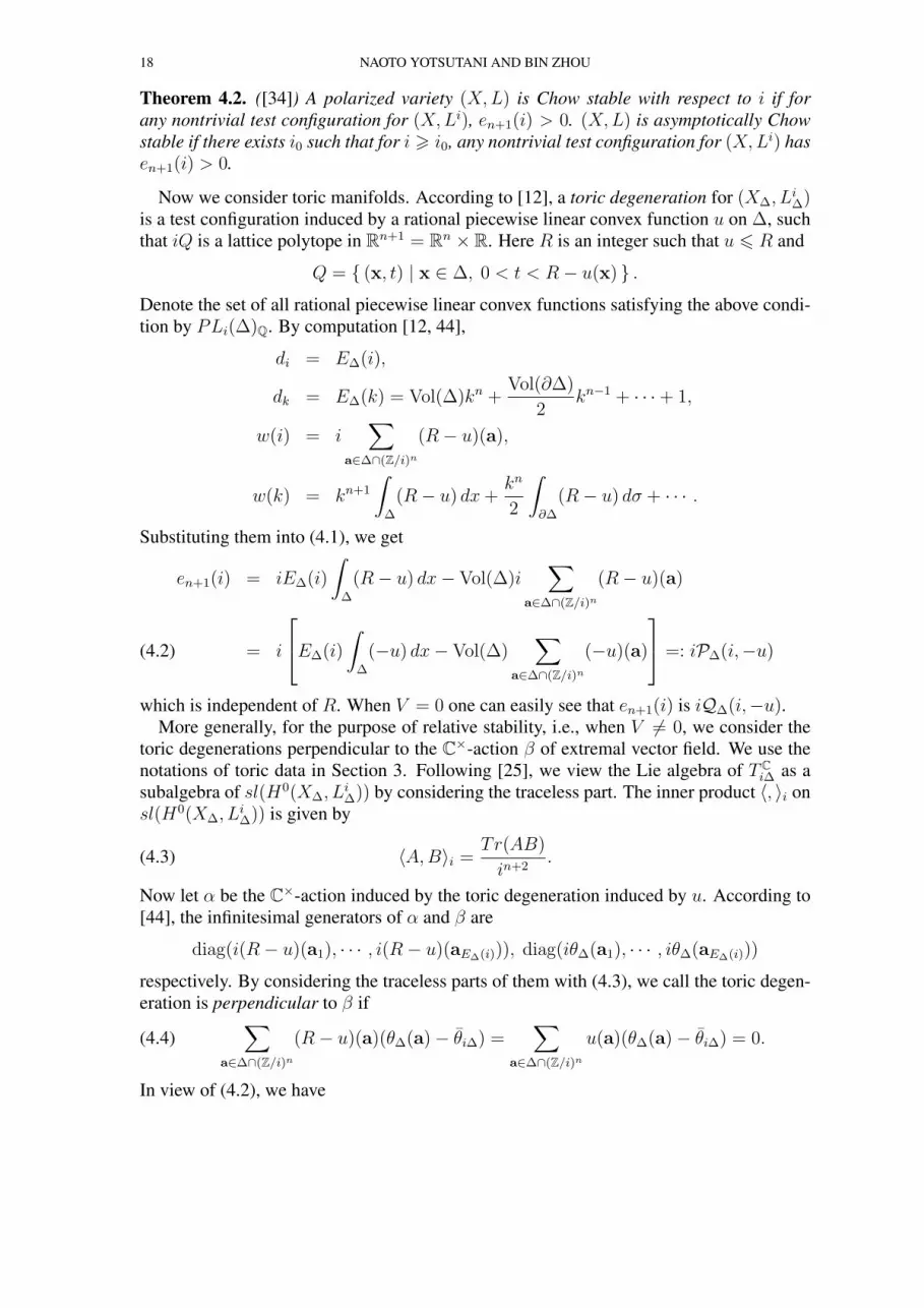
Theorem 4.2. ([34]) A polarized variety (X,L) is Chow stable with respect to i if forany nontrivial test configuration for (X,Li), en+1(i) > 0. (X,L) is asymptotically Chowstable if there exists i0 such that for i ⩾ i0, any nontrivial test configuration for (X,Li) hasen+1(i) > 0.

Now we consider toric manifolds. According to [12], a toric degeneration for (X∆, Li∆)

is a test configuration induced by a rational piecewise linear convex function u on ∆, suchthat iQ is a lattice polytope in Rn+1 = Rn × R. Here R is an integer such that u ⩽ R and

Q = { (x, t) | x ∈ ∆, 0 < t < R− u(x) } .

Denote the set of all rational piecewise linear convex functions satisfying the above condi-tion by PLi(∆)Q. By computation [12, 44],

di = E∆(i),

dk = E∆(k) = Vol(∆)kn +Vol(∂∆)

2kn−1 + · · ·+ 1,

w(i) = i∑

a∈∆∩(Z/i)n(R− u)(a),

w(k) = kn+1

∫∆

(R− u) dx+kn

2

∫∂∆

(R− u) dσ + · · · .

Substituting them into (4.1), we get

en+1(i) = iE∆(i)

∫∆

(R− u) dx− Vol(∆)i∑

a∈∆∩(Z/i)n(R− u)(a)

= i

E∆(i)

∫∆

(−u) dx− Vol(∆)∑

a∈∆∩(Z/i)n(−u)(a)

=: iP∆(i,−u)(4.2)

which is independent of R. When V = 0 one can easily see that en+1(i) is iQ∆(i,−u).More generally, for the purpose of relative stability, i.e., when V = 0, we consider the

toric degenerations perpendicular to the C×-action β of extremal vector field. We use thenotations of toric data in Section 3. Following [25], we view the Lie algebra of TC

i∆ as asubalgebra of sl(H0(X∆, L

i∆)) by considering the traceless part. The inner product ⟨, ⟩i on

sl(H0(X∆, Li∆)) is given by

(4.3) ⟨A,B⟩i =Tr(AB)

in+2.

Now let α be the C×-action induced by the toric degeneration induced by u. According to[44], the infinitesimal generators of α and β are

diag(i(R− u)(a1), · · · , i(R− u)(aE∆(i))), diag(iθ∆(a1), · · · , iθ∆(aE∆(i)))

respectively. By considering the traceless parts of them with (4.3), we call the toric degen-eration is perpendicular to β if

(4.4)∑

a∈∆∩(Z/i)n(R− u)(a)(θ∆(a)− θi∆) =

∑a∈∆∩(Z/i)n

u(a)(θ∆(a)− θi∆) = 0.

In view of (4.2), we have


Definition 4.3. A polarized toric manifold (X∆, L∆) is called asymptotically relativelyChow semistable for toric degenerations if there exists i0 ∈ Z+, such that when i ⩾ i0, forany u ∈ PLi(∆)Q satisfying (4.4), P∆(i, u) ⩽ 0. Furthermore, it is called asymptoticallyrelatively Chow stable for toric degenerations, or asymptotically relatively weakly Chowstable in toric sense when P∆(i, u) = 0 if and only if u is a linear function.

Remark 4.4. The sign differs from (3.9) because we consider convex functions here, whilein (3.9) g is a concave function.

The necessary condition (3.7) for asymptotic relative Chow semistability in last sectioncan also be recovered as follows. We consider the projection of the toric degeneration of uonto the perpendicular space. Let

u = u−

∑a∈∆∩(Z/i)n

u(a)(θ∆(a)− θi∆)∑a∈∆∩(Z/i)n

(θ∆(a)− θi∆)2

(θ∆ − θi∆).

Then u induces a toric degeneration perpendicular to β. By (4.2), we have

P∆(i, u) = E∆(i)

∫∆

u dx− Vol(∆)∑

a∈∆∩(Z/i)nu(a)

= E∆(i)

∫∆

u dx− Vol(∆)∑

a∈∆∩(Z/i)n(1 + siθi∆(a))u(a)

= Q∆(i, u),

where

(4.5) si =iθi∆E∆(i)∑

a∈∆∩(Z/i)n(θ∆(a)− θi∆)

2.

In the above deduction, we used the normalization condition∫∆θ∆ dx = 0. For j =

1, ..., n, substituting u = xj and −xj into the above, we obtain condition (3.7). It is alsoeasy to see that in (3.7), if the si exists, it can be given by (4.5).

Remark 4.5. By the above computation, one can see the definition for asymptotic relativeChow stability in Definition 4.3 is equivalent to the negativity of Q∆(i, u) for all u ∈PLi(∆)Q as in Proposition 3.17.

5. EXAMPLES

Finally we provide many interesting examples which will support our understanding ofstabilitities. Here we will mainly concern on toric Fano manifolds.

5.1. RelativeK-stability of toric Fano threefolds. In this section, we shall determine thepotential θ∆ of the extremal vector field V of toric Fano threefolds in symplectic coordi-nates and verify the relative K-stability or instability by Theorem 1.1.

By Lemma 5.1, if a holomorphic vector field V is given by V =n∑

i=1

ai∂

∂wi

in the

affine logarithm coordinates (w1, . . . , wn), then the potential function θ∆ in symplectic


coordinates is given by θ∆ =n∑

i=1

aixi + c for some constant c. There are several ways

to compute θ∆. The most general one is to use the linear functional in (2.7). In order todetermine constants ai and c, one can solve the n+ 1-linear system

(5.1) L∆(1) = 0, L∆(xi) = 0 for i = 1, . . . , n.

This method works for general polarizations.In Fano case, we have a more efficient algorithm. According to [3], φ in (2.4) can be

given by

(5.2) φ = log

(m∑i=1

e⟨p(i),y⟩

),

where p(1), ..., p(m) are the vertices of ∆. This formula implies

(5.3) |φ+ log det(φij)| <∞.

For the sake of computing the Futaki invariant, we recall another normalization on thepotentials of holomorphic vector fields. Let v be a holomorphic vector field on X andθ′v(ωg) be the potential function determined by

(5.4) ivωg =√−1∂θ′v(ωg), and

∫X

θ′v(ωg)ehgωng

n!= 0.

According to [39], the above θ′v satisfies

θ′v = −∆θ′v − v(hg),

where ∆ is the Laplacian. Then the Futaki invariant can be given by

(5.5) F (v) :=

∫X

v(hg)ωn = −

∫X

θ′vωn.

Lemma 5.1. Assume the holomorphic vector field is given by

v =n∑

i=1

aizi∂

∂zi=

n∑i=1

ai∂

∂wi

,

where ai ∈ R, i = 1, ..., n. Then we have θ′v(ωg) =∑n

i=1 aixi in the symplectic coordi-nates. In particular, θ′ ∂

∂wi

(ωg) = xi, i = 1, ..., n.

Proof. By (2.4), θ′v(ωg) = 2v(φ) + c on (C×)n for some c ∈ Rn. Furthermore,

θ′v(ωg) = 2n∑

i=1

ai∂φ

∂zi+ c =

n∑i=1

ai∂φ

∂yi+ c.

Write (C×)n = (S1)n × Rn. By (5.3), hg = −φ− log det(φij) on Rn, hence we have∫X

θ′v(ωg)ehgωng

n!= C

∫Rn

(n∑

i=1

∂φ

∂yi+ c

)e−φ dy, i = 1, 2, · · · , n

for some constant C. Note that∫Rn

∂φ

∂yie−φ dy = −

∫Rn

∂e−φ

∂yidy = 0.


Then c = 0 under the normalization (5.4). □

By (5.5) and the above lemma, we can compute the Futaki invariant in symplectic coor-dinates by

(5.6) F (v) = −(2π)2∫∆

θ′vdx.

The first step of the algorithm is to determine a1, ..., an by (5.6) and Lemma 2.4. Then

(5.7) c = − 1

Vol(∆)

∫∆

∑i

aixi dx

by the normalization condition. An alternative method to compute a1, ..., an was also givenby Nakagawa. He gave a combinatorial formula for the Futaki invariants and generalizedKilling forms of toric Fano orbifolds in [26]. As an application, he computed the extremalvector field in the anti-canonical class on a toric Fano manifold X with dimX ⩽ 4. Inorder to prove Theorem 1.2, we shall use his result on toric Fano threefolds (or fourfolds)directly.

The main goal of this section is to prove the following proposition.

Proposition 5.2. Let X be a toric Fano threefold with anti-canonical polarization.

(a) If X = B2, then X is relatively strongly K-stable in toric sense in the anti-canonical class.

(b) If X = B1, then X is relatively K-unstable in its first Chern class.

Once Proposition 5.2 has been proved, other cases are similar and further details are leftto the reader1. In Table 1 and Table 3 we give the list of all results proved in Theorem 1.2.

Proof. (a) Let ei (i = 1, 2, 3) be the standard basis of N ∼= Z3. Let Σ be the complete fanin NR ∼= R3 whose 1-dimensional cones are given by Σ(1) = {σ1, σ2, σ3, σ4, σ5 } where

σ1 = Cone(e1), σ2 = Cone(e2), σ3 = Cone(e3),

σ4 = Cone(−e3), and σ5 = Cone(−e1 − e2 − e3).

Then the associated toric manifold X is CP (OCP 2 ⊕ OCP 2(1)) and the correspondingpolytope ∆ ⊆MR is determined by

∆ ={(x1, x2, x3) ∈ R3 | 1 + x1 ⩾ 0, 1 + x2 ⩾ 0, 1 + x3 ⩾ 0, 1− x3 ⩾ 0,

1− x1 − x2 − x3 ⩾ 0 } .

Hence Vol(∆) = 283

. Let V ∈ ηc(X) be the extremal vector field in the anti-canonical classand θ∆ be the potential function of V in symplectic coordinates. Then

θ∆ =3∑

i=1

aixi + c

1In the practical computation we used packages (i) Normaliz and (ii) Polymake. These packages areavailable at [5] and [20] respectively.


with a1 = a2 = 0 and a3 = −7097

for some constant c. (See [26], Section 6, Table 2). Since

we have∫∆

x3 = −2, we conclude that

c = −−(∫

∆−70

97x3 dx

)Vol(∆)

=70

97· (−2) · 3

28= −15

97

by (5.7). Thus θ∆ = −7097x3 − 15

97and

∆− = { (x1, x2, x3) ∈ ∆ | −112

97− 70

97x3 ⩾ 0 } = ∅.

This implies ∥θ∆∥ < 1, that is, X satisfies the condition (1.2). The assertion is verified.(b) Let Σ be the complete fan in NR ∼= R3 whose 1-dimensional cones are given by Σ(1) ={σ1, . . . , σ5 } where

σ1 = Cone(e1), σ2 = Cone(e2), σ3 = Cone(e3),

σ4 = Cone(−e3), and σ5 = Cone(−e1 − e2 − 2e3).

Then we readily see that X = CP (OCP 2 ⊕OCP 2(2)) and

∆ = Conv { e∗3 − e∗2, 4e∗1 − e∗2 − e∗3, −e∗1 − e∗2 − e∗3, e

∗3 − e∗1 − e∗2, 4e

∗2 − e∗1 − e∗3, e

∗3 − e∗1 } ,

where e∗i is the dual basis of ei. Then Vol(∆) = 313

and

θ∆ =3∑

i=1

aixi + c with (a1, a2, a3) =

(0, 0,−620

349

)

for some constant c. Since we find∫∆

x3 = −4, we obtain c = −240349

. Hence we conclude

θ∆ = −620349x3 − 240

349and

∆− = { (x1, x2, x3) ∈ ∆ | −589

349− 620

349x3 ⩾ 0 }

= Conv

4e∗1 − e∗2 − e∗3,3910e∗1 − e∗2 − 19

20e∗3, −e∗1 − e∗2 − 19

20e∗3

−e∗1 + 3910e∗2 − 19

20e∗3, −e∗1 − e∗2 − e∗3, −e∗1 + 4e∗2 − e∗3

.

Thus

(5.8) Vol(∆−) =7351

12000.

Now we shall verify the condition (1.3). First we note that∫∆−

x3 dx = −96197

4and

∫∆−

x23 dx =1828273

5.

Hence one can see that∫∆−

(1− θ∆)2 dx =

∫∆−

(589

349+

620

349x3

)2

dx =1475918766336271

1461612000.

Plugging this and (5.8) into (1.3), we obtain the desired result because 1− c = 589349

. □


Remark 5.3. It is also interesting to ask if the method in Section 5.1 can determine alltoric Fano fourfolds. However, we have some technical difficulties on computing (1.3).That is, the the vertices of ∆− can be very complicated which leads to the overflow of thesoftware Normaliz when we compute the term

∫∆−(1− θ∆)

2dx while some of them arestill computable. For example, the toric Fano fourfolds B5 has

∆− = Conv

{(−2

3,−1, 11

3,−1), (−2

3,−1,−1, 11

3), (−1,−1, 4,−1), (−1,−1, 11

3,−1)

(−1,−23, 11

3,−1), (−1,−1,−1, 4), (−1,−1,−1, 11

3), (−1,−2

3,−1, 11

3)

}with 8 vertices, and hence condition (1.3) has been verified. Meanwhile, D4 has

∆− = Conv{(−31276

9769,−1,−1, 5869

9769), . . . , (31276

9769,−1, 41045

9769, 58699769

)}

with 8 vertices which makes impossible to check (1.3). Apart from this, our computationshows that the stability of all computable ones can be determined by Theorem 1.1. Thatis among all toric Fano fourfolds (124 deformation classes), there are 52 types of relativeK-stable ones, 15 types of relative K-unstable ones, and 57 types of undistinguishableones. We expect that the 57 types of undistinguishable ones can be settled by using moreadvanced software or improvement of the criterion in Thereom 1.1.

5.2. Relative Chow stability. We study (relatively) Chow unstable examples of toric Fanomanifolds. First, we recall the example founded by Nill and Paffenholz [28] which isisomorphic to P(OW ⊕ OW (−1,−1,−1, 2)) =: XNP where W = (CP 1)3 × CP 3. XNP

is the non-symmetric Kahler-Einstein toric Fano 7-fold. In [33], Ono, Sano and Yotsutanishowed that (XNP,−KXNP

) is asymptotically Chow unstable. Later Yotsutani observedthat XNP is Chow unstable w.r.t. −KXNP

(i.e., i = 1) using (3.11). Meanwhile, Nill andPaffenholz [28] also proved that all toric Kahler-Einstein Fano manifolds are symmetric ifdimX ⩽ 6. It is known that if X is a symmetric toric Fano manifold, then (X,−KX) isasymptotically Chow stable. Hence we have the following.

Proposition 5.4 ([28], [33]). The lowest dimension for an anti-canonically polarized Kahler-Einstein toric Fano manifold (X,−KX) to be (asymptotically) Chow unstable is 7.

However, in the case whereX is a Fano orbifold, such an example appears in dimX = 3.

Proposition 5.5. There is a Kahler-Einstein toric Fano orbifold X with dimX = 3 whichis Chow unstable w.r.t. (−KX)

2.

Our strategy is the following. For any toric Fano orbifold X with the associated sim-plicial Fano polytope ∆◦ ⊆ NR, X admits the Kahler-Einstein metric if and only if theFutaki invariant of X vanishes by Shi-Zhu’s result [35]. Let W(X) be the Weyl group ofAut(X) with respect to the maximal torus and NW(X)

R be the W(X)-invariant subspaceof NR. For a given simplicial Fano polytope ∆◦, it is known that

∑v∈V(∆◦) v ∈ N

W(X)R

(see [27, Chapter 5]). Here V(∆◦) denotes the set of vertices of ∆◦. Hence if we finda toric Fano orbifold with the vanishing Futaki invariant satisfying

∑v∈V(∆◦) v = 0, this

will be a candidate of our desired example because X is symmetric when and only whenN

W(X)R = {0 }. Among all 12, 190 3-dimensional toric Fano orbifolds (i.e., Q-factorial

toric Fano varieties), there are 42 toric Fano orbifolds with the vanishing Futaki invariant.Of these 42 toric Fano orbifolds, there is the only one example such that the correspondingsimplicial canonical Fano polytope satisfies

∑v∈V(∆◦) v = 0. Thus our problem can be


deduced to the computation of (3.11) for the dual moment polytope ∆ ⊆MR of this exam-ple. Remark that the Gorenstein index jX is given by minimal k such that k∆ is a latticepolytope for a fixed canonical Fano polytope ∆◦ ⊆ NR [27, Proposition 2.3.2].

Proof of Proposition 5.5. Again we use the same notation in the proof of Proposition 5.2.We consider the 3-dimensional canonical Fano polytope2

∆◦ := Conv { e1 − e2 − 2e3, e2 + 3e3, e1 + e2 + 3e3, e1 + 2e2 + 4e3, e2,−2e1 − 2e2 − 3e3 } .The vertices of the dual polytope ∆ are

−1

2e∗1 +

5

2e∗2 − e∗3, e

∗1 − e∗2, 2e

∗2 − e∗3,

1

2e∗2 −

1

2e∗3,−e∗1,−e∗1 − e∗2 +

1

2e∗3,

3

2e∗1 − e∗2,−e∗2 + e∗3.

Thus ∆ is the simple polytope and jX∆= 2. Setting ∆ := 2∆, we compute the Chow

weight of ∆. We readily see that

E∆(i) = 12i3 + 9i2 + 3i+ 1, Vol(∆) = 12,

∫∆

x dx = (0, 0, 0)

and ∑a∈∆∩Z3

a = (0, 1,−1),∑

a∈2∆∩Z3

a = (0, 3,−3),∑

a∈3∆∩Z3

a = (0, 6,−6)

hold. Thus we haves∆(i) =

i+ 1

2(0, 1,−1)

by (3.12) (cf. [31, Lemma 3.5]). In particular,∫∆

x dx = (0, 0, 0) and∫∂∆

x dσ = (0, 0, 0)

hold. This implies that ∫∂∆

x dσ − Vol(∂∆)

Vol(∆)

∫∆

x dx = (0, 0, 0)

i.e., the Futaki invariant vanishes. However obviously,∑a∈∆∩Z3

a =E∆(1)

Vol(∆)

∫∆

x dx.

By (3.11), we conclude that the 2-Gorenstein toric Fano variety (X∆, (−KX∆)2) is Chow

unstable. □In [4], Berman proved that a Q-Fano variety X admitting Kahler-Einstein metrics is

K-stable. Hence we have the following.

Corollary 5.6. The example in Proposition 5.5 is K-stable but asymptotically Chow un-stable.

Next, we consider the general case with the nontrivial Futaki invariant. We see that asmooth counter-example appears in dimX = 3.

Proposition 5.7. LetX be a toric Fano threefold which is isomorphic to E4. Then (X,−KX)is relatively K-stable but it is asymptotically relatively Chow unstable.

2ID number in the database [46] is 530571.


Proof. It suffices to see that (3.7) is not satisfied. The corresponding 3-dimensional momentpolytope is listed in Table 2. Thus we have

E∆(i) =20

3i3 + 10i2 +

16

3i+ 1 and

∫∆

x dx =

(−7

8,5

12,5

24

).

In particular,∑a∈∆∩Z3

a = (−4, 2, 1) and s1∑

a∈∆∩Z3

(θ∆(a)−θ∆)a = s1

(−11134272

1816885,1079424

363377,539712

363377

)holds. Thus there is no s1 which satisfies (3.7). The assertion is verified. □


TABLE 2. Toric Fano threefolds

No. Notation The moment polytope ∆

1 CP 3 Conv

{(−1−1−1

),

(−1−13

),

(−13−1

),

(3−1−1

)}

2 B1 Conv

{(0−11

),

(4−1−1

),

(−1−1−1

),

(−1−11

),

(−14−1

),

(−101

)}

3 B2 Conv

{(1−11

),

(3−1−1

),

(−1−1−1

),

(−1−11

),

(−13−1

),

(−111

)}

4 B3 Conv

{(2−10

),

(2−1−1

),

(−12−1

),

(−1−1−1

),

(−120

),

(−1−13

)}

5 B4 Conv

{(2−11

),

(2−1−1

),

(−1−1−1

),

(−1−11

),

(−12−1

),

(−121

)}

6 C1 Conv

{(0−11

),

(2−1−1

),

(22−1

),

(001

),

(−12−1

),

(−101

),

(−1−1−1

),

(−1−11

)}

7 C2 Conv

{(0−11

),

(2−1−1

),

(20−1

),

(001

),

(−13−1

),

(−111

),

(−1−1−1

),

(−1−11

)}

8 C3 Conv

{(1−11

),

(1−1−1

),

(11−1

),

(111

),

(−11−1

),

(−111

),

(−1−1−1

),

(−1−11

)}

9 C4 Conv

{(2−11

),

(2−1−1

),

(01−1

),

(011

),

(−11−1

),

(−111

),

(−1−1−1

),

(−1−11

)}

10 C5 Conv

{(0−11

),

(2−1−1

),

(20−1

),

(021

),

(−10−1

),

(−121

),

(−1−1−1

),

(−1−11

)}

11 D1 Conv

{(010

),

(01−1

),

(3−1−1

),

(11−1

),

(−1−13

),

(−1−1−1

),

(−10−1

),

(−102

)}

12 D2 Conv

{(011

),

(01−1

),

(2−1−1

),

(21−1

),

(−1−12

),

(−1−1−1

),

(−10−1

),

(−102

)}


No. Notation The moment polytope ∆

13 E1 Conv

{(1−1−1

),

(1−11

),

(010

),

(100

),

(10−1

),

(01−1

),

(−11−1

),

(−111

),

(−1−13

),

(−1−1−1

)}

14 E2 Conv

{(1−1−1

),

(1−10

),

(011

),

(100

),

(10−1

),

(01−1

),

(−11−1

),

(−112

),

(−1−12

),

(−1−1−1

)}

15 E3 Conv

{(1−1−1

),

(1−11

),

(011

),

(101

),

(10−1

),

(01−1

),

(−111

),

(−11−1

),

(−1−11

),

(−1−1−1

)}

16 E4 Conv

{(1−10

),

(1−1−1

),

(01−1

),

(10−1

),

(101

),

(012

),

(−11−1

),

(−112

),

(−1−1−1

),

(−1−10

)}

17 F1 Conv

{(01−1

),

(011

),

(11−1

),

(10−1

),

(101

),

(111

),

(0−11

),

(0−1−1

),

(−1−1−1

),

(−1−11

),

(−101

),

(−10−1

)}

18 F2 Conv

{(012

),

(01−1

),

(112

),

(101

),

(10−1

),

(11−1

),

(0−1−1

),

(0−10

),

(−1−10

),

(−1−1−1

),

(−10−1

),

(−101

)}


TAB

LE

3.θ ∆

and∆

onto

ric

Fano

thre

efol

ds

No.

Not

atio

nθ ∆

=∑ 3 i=

1aix

i+c

∆−

1CP

3≡

0∅

2B 1

−620

349x3−

240

349

Con

v

{(4 −1

−1) ,( 39 1

0 −1

−19

20

) ,( −1 −1

−19

20

) ,( −1 39

10

−19

20

) ,( −1 −1

−1) ,( −1 4 −

1

)}

3B 2

−70

97x3−

15

97

∅

4B 3

−20

43x1−

20

43x2−

5 43

∅

5B 4

≡0

∅

6C 1

−260

219x3−

80

219

∅

7C 2

−7600

17787x1−

17750

17787x3−

4868

17787

Con

v

( −981

1520

−1

−1

) , −981

1520

4021

1520

−1

, −1

10111

3550

−3011

3550

,( −1 3 −1) ,( −

1−1

−3011

3550

) ,( −1 −1

−1

) 8

C 3≡

0∅

9C 4

−6 11x2−

1 11

∅

10C 5

≡0

∅

11D

199600

467581x1−

627000

467581x2−

213939

467581

Con

v

48388

18165

−12058

18165

−1

,( 1363

2490

−1

3617

2490

) ,( 3 −1

−1

) ,( 1363

2490

−1

−1

)


No.

Not

atio

nθ ∆

∆−

12D

2219420

650251x1−

318320

650251x2−

62565

650251

Con

v

{(2

−1489

1730

−1

) ,( 4288

2385

−1

−1903

2385

) ,( 2 −1

−1

) ,( 4288

2385

−1

−1

)}

13E 1

−17020

19651x1−

17020

19651x2−

6845

19651

Con

v

{( −103

185

−1

−1

) ,( −103

185

−1

473

185

) ,( −1

−103

185

−1

) ,( −1

−103

185

473

185

) ,( −1 −1 3

) ,( −1 −1

−1

)}

14E 2

−2646160

2735927x1−

982960

2735927x2−

692905

2735927

Con

v

{( −13897

15035

−1

−1

) ,( −13897

15035

−1

28932

15035

) ,( −1

−4447

5585

−1

) ,( −1

−4447

5585

2

) ,( −1 −1 2

) ,( −1 −1

−1

)}

15E 3

−168

409x1−

168

409x2−

32

409

∅

16E 4

−34208

78995x1+

7936

78995x2−

24929

394975

∅

17F

1≡

0∅

18F

236

67x2−

5 67

∅


REFERENCES

[1] C. Arezzo and A. Loi, Moment maps, scalar curvature and quantization of Kahler manifolds. Comm.Math. Phys. 246 (2004), 543-559.

[2] V. V. Batyrev, Troidal Fano 3-folds. Math. USSR-Izv. 19 (1982), 13-25. Izv. Akad. Nauk SSSR 45 (1981),704-717.

[3] V. V. Batyrev and E. N Selivanova, Einstein-Kahler metrics on symmetric toric Fano manifolds. J. ReineAngew. Math. 512 (1999), 225-236.

[4] R. Berman, K-stability of Q-Fano varieties admitting Kahler-Einstein metrics. Invent. Math. 203 (2016),973-1025.

[5] W. Bruns, B. Ichim, T. Romer and C. Soger, Normaliz. Algorithms for rational cones and affine monoids.Available at http://www.math.uos.de/normaliz.

[6] E. Calabi, Extremal Kahler metrics, Seminar on differential geometry, Ann. of Math Studies, PrincetonUniv. Press, 102 (1982), 259-290.

[7] B.H. Chen, A.M. Li and L. Sheng, Extremal metrics on toric surfaces. arXiv:1008.2607.[8] X. X. Chen, C. Lebrun and B. Weber, On conformally Kahler-Einstein manifolds. J. Amer. Math. Soc.

21 (2008), 1137-1168.[9] I. Dolgachev, Lectures on invariant theory. London Mathematical Society Lecture Note Series, 296.

Cambridge University Press, Cambridge, 2003.[10] O. Debarre, Fano varieties, Higher dimensional varieties and rational points. Budapest, 2001, Bolyai

Society Mathematical Studies 12, 93-132. Springer, Berlin 2003.[11] S.K. Donaldson, Scalar curvature and projective embeddings, I. J. Diff. Geom. 59 (2001), 479-522.[12] S.K. Donaldson, Scalar curvature and stability of toric varieties. J. Diff. Geom. 62 (2002), 289-349.[13] S.K. Donaldson, Extremal metrics on toric surfaces: a continuity method. J. Diff. Geom. 79 (2008),

389-432.[14] S.K. Donaldson, Constant scalar curvature metrics on toric surfaces. Geom. Funct. Anal. 19 (2009),

83-136.[15] A. Futaki, Asymptotic Chow semi-stability and integral invariants. Int. J. Math. 15 (2004), 967-979.[16] A. Futaki, Asymptotic Chow stability in Kahler geometry. Fifth International Congress of Chinese Math-

ematicians. Part 1, 2, 139-153, AMS/IP Stud. Adv. Math., 51, pt. 1, 2, Amer. Math. Soc., Providence, RI,2012.

[17] A. Futaki and T. Mabuchi, Bilinear forms and extremal Kahler vector fields associated with Kahlerclass. Math. Ann. 301 (1995), 199-210.

[18] A. Futaki, H. Ono and Y. Sano, Hilbert series and obstructions to asymptotic semistability. Adv. Math.226 (2011), 254-284.

[19] I. M. Gelfand, M. M. Kapranov, and A. V. Zelevinsky, Discriminants, resultants, and multidimensionaldeterminants. Mathematics: Theory & Applications. Birkhauser Boston Inc., Boston, MA, 1994.

[20] E. Gawrilow and M. Joswig, Polymake Version 2.9.8-Convex polytopes, polyhedra, simpli-cial complexes, matroids, fans, and tropical objects, Available at wwwopt.mathematik.tu-darmstadt.de/polymake/doku.php, 1997-present.

[21] M. M. Kapranov, B. Sturmfels and A. V. Zelevinsky, Chow polytopes and general resultants. DukeMath. J. 67 (1992), 189-218.

[22] A. M. Kasprzyk, Canonical toric Fano threefolds. Canad. J. Math. 62 (2010), 1293-1309.[23] T. Mabuchi, Stability of extremal Kahler manifolds. Osaka J. Math. 41 (2004), 563-582.[24] T. Mabuchi, An energy-theoretic approach to the Hitchin-Kobayashi correspondence for manifolds. I.

Invent. Math. 159 (2005), 225-243.[25] T. Mabuchi, Relative stability and extremal metrics. J. Math. Soc. Japan 66 (2014), 535-563.[26] Y. Nakagawa, Combinatorial formulae for Futaki characters and generalized killing forms of toric

Fano orbifolds. The Third Pacific Rim Geometry Conference (Seoul, 1996), 223-260, Monogr. Geom.Topology, 25, Int. Press, Cambridge, MA, 1998.

[27] B. Nill, Gorenstein toric Fano varieties. Dissertation, Universitat Tubingen, 2005. Available athttp://tobias-lib.uni-tuebingen.de/volltexte/2005/1888

[28] B. Nill and A. Paffenholz, Examples of Kahler-Eisntein toric Fano manifolds associated to non-symmetric reflexive polytopes. Beitr. Algebra. Geom 52 (2011), 297-304.


[29] M. Obro, An algorithm for the classification of smooth Fano polytopes. arXiv:0704.0049 (2007).[30] Y. Odaka, The Calabi conjecture and K-stability. Int. Math. Res. Not. IMRN 2012, 2272-2288.[31] H. Ono, A necessary condition for Chow semistability of polarized toric manifolds. J. Math. Soc. Japan.

63 (2011), 1377-1389.[32] H. Ono, Algebro-geometric semistability of polarized toric manifolds. Asian J. Math. 17 (2013), 609-

616.[33] H. Ono, Y. Sano and N. Yotsutani, An example of an asymptotically Chow unstable manifold with

constant scalar curvature. Ann. Inst. Fourier (Grenoble) 62 (2012), 1265-1287.[34] J. Ross and R. Thomas, A study of the Hilbert-Mumford criterion for the stability of projective varieties.

J. Alg. Geom. 16 (2007), 201-255.[35] Y. Shi and X. Zhu, Kahler-Ricci solitons on toric Fano orbifolds. Math. Zeit. 271 (2012), 1241-1251.[36] G. Szekelyhidi, Extremal metrics and K-stability. Dissertation, Imperial college, London, (2006),

arXiv:0611002.[37] G. Szekelyhidi, Extremal metrics and K-stability. Bull. London Math. Soc. 39 (2007), 76-84.[38] G. Tian, Kahler-Einstein metrics with positive scalar curvature. Invent. Math. 130 (1997), 1-39.[39] G. Tian and X.H. Zhu, A new holomorphic invariant and uniqueness of Kahler-Ricci solitons. Comm.

Math. Helv. 77 (2002), 297-325.[40] A.D. Vedova and F. Zuddas, Scalar curvature and asymptotic Chow stability of projective bundles and

blowups. Trans. Amer. Math. Soc. 364 (2012), 6495-6511.[41] K. Watanabe and M. Watanabe, The classification of Fano 3-folds with torus embeddings. Tokyo J.

Math. 5 (1982), 37-48.[42] X. J. Wang and B. Zhou, Existence and nonexistence of extremal metrics on toric Kahler manifolds.

Adv. Math. 226 (2011), 4429-4455.[43] N. Yotsutani, Facets of secondary polytopes and Chow stability of toric varieties. To appear in Osaka J.

Math Vol. 53, (2016).[44] B. Zhou and X.H. Zhu, Relative K-stability and modified K-energy on toric manifolds. Adv. Math. 219

(2008), 1327-1362.[45] B. Zhou and X.H. Zhu, K-stability on toric manifolds. Proc. Amer. Math. Soc. 136 (2008), 3301-3307.[46] Graded Ring Database, http://grdb.lboro.ac.uk/forms/toricsmooth.

SCHOOL OF MATHEMATICAL SCIENCES AT FUDAN UNIVERSITY, SHANGHAI, 200433, P. R. CHINAE-mail address: [email protected]

SCHOOL OF MATHEMATICAL SCIENCES, PEKING UNIVERSITY, BEIJING, 100871, P. R. CHINA; ANDMATHEMATICAL SCIENCES INSTITUTE, THE AUSTRALIAN NATIONAL UNIVERSITY, CANBERRA, ACT2601, AUSTRALIA.

E-mail address: [email protected]; [email protected]

relative algebro-geometric stabilities of toric manifolds

Documents