on the chiral ring of calabi-yau hypersurfaces in toric varieties
TRANSCRIPT
arX
iv:m
ath/
0010
318v
1 [
mat
h.A
G]
31
Oct
200
0
ON THE CHIRAL RING OF CALABI-YAU HYPERSURFACES IN
TORIC VARIETIES
ANVAR R. MAVLYUTOV
Contents
0. Introduction 11. Semiampleness 32. Toric hypersurfaces 83. Polynomial part of the chiral ring 114. Non-polynomial part of the chiral ring 145. Toric and residue parts of cohomology 206. Cohomology of semiample regular hypersurfaces 247. The chiral ring for anticanonical hypersurfaces 38References 41
0. Introduction
In nonlinear sigma models (see Appendix B.2 in [CK] on physical theories) thereare two twisted theories, the A-model and the B-model. Mirror symmetry is anisomorphism between the A-model and the B-model for a pair of two distinct Calabi-Yau threefolds V and V with Kahler structures. One consequence of mirror sym-metry is an isomorphism between the quantum cohomology on ⊕p,qH
p,q(V ) and thechiral ring of the B-model ⊕p,qH
p(V ,∧qTV ), which implies the equality of thecorresponding correlation functions (Yukawa couplings). These correlation func-tions describe interactions between strings. From a mathematical point of view,knowledge about the B-model Yukawa coupling and the equality with the A-modelYukawa coupling of the mirror manifold produces enumerative information on thismirror manifold. One important construction widely used in physics and mathe-matics is the Batyrev mirror construction in toric varieties (see [B2]).
In this paper we study the chiral ring ⊕pHp(X,∧pTX) (this is actually a subring
of the whole chiral ring) for quasismooth hypersurfaces X in complete simplicialtoric varieties. In particular, we completely describe the chiral ring⊕pH
p(X,∧pTX)in the case of 3-dimensional Calabi-Yau hypersurfaces. This applies to the mirrorsymmetric hypersurfaces in Batyrev’s construction.
The following is an outline of the paper. We begin in Section 1 with a reviewof notation and general facts from toric geometry. For complete toric varieties, thenotions of semiample, nef (numerically effective) and generated by global sectionsare equivalent for invertible sheaves (divisors). Geometry and intersection theory
1991 Mathematics Subject Classification. Primary: 14M25.Key words and phrases. Toric varieties, mirror symmetry, chiral ring.
1
2 ANVAR R. MAVLYUTOV
associated with big (the self-intersection number is positive) and nef divisors wasstudied in [M]. Here, we generalize those results to all semiample divisors. Suchdivisors on complete toric varieties naturally produce a surjective morphism of theambient space onto another complete toric variety. Moreover, this construction isunique with certain conditions relating semiample divisors to ample divisors on thenew toric variety. We also show that a proper birational morphism of toric varietiesinduces a natural graded homomorphism of the coordinate rings. For a semiampledivisor, this gives an isomorphism of rings in the degree of the divisor.
Section 2 uses the results of Section 1 to describe the geometry of semiampleregular (transversal to orbits) hypersurfaces in complete toric varieties. We get astratification of such hypersurfaces in terms of nondegenerate affine hypersurfacescohomology of which has been studied in [B1]. We also review some facts abouthypersurfaces in complete simplicial toric varieties. In particular, we recall from[M] the relationship between the Jacobian ring R(f) (resp., R1(f)) and the middlecohomology Hd−1(X) of a quasismooth (resp., big and nef regular) hypersurface Xin a d-dimensional complete simplicial toric variety. The ring R1(f) has been usedin [M] to describe the middle cohomology of a 3-dimensional big and nef regularhypersurface completely.
In Section 3, we introduce the (Zariski) p-th exterior power ∧pTX of the tangentsheaf for an arbitrary orbifold X , which is defined similarly to the sheaf Ωp
X ofZariski p-forms (see [CK, A.3]). Then we show that for a quasismooth hypersurfaceX of degree β there is a ring homomorphism R(f)∗β → H∗(X,∧∗TX) (the latteris our notation for ⊕pH
p(X,∧pTX)). Also, with respect to this homomorphismthe map between R(f) and the middle cohomology of a quasismooth hypersurfaceis a morphism of modules. In the Calabi-Yau case the situation is especially nicebecause we get an injective ring homomorphism R1(f)∗β → H∗(X,∧∗TX) (we callR1(f)∗β the polynomial part of the chiral ring because its graded piece inH1(X, TX)should correspond to polynomial infinitesimal deformations for a minimal Calabi-Yau X (see [CK])).
According to the above terminology, in Section 4, we study the non-polynomialpart of the chiral ring complementary to the polynomial part. We construct newelements in H∗(X,∧∗TX) for a big and nef quasismooth hypersurface X , and inthe case of a minimal Calabi-Yau these elements in H1(X, TX) should correspondto non-polynomial deformations. The new elements are represented by a mapfrom some quotient Rσ(f) of the Jacobian ring to H∗(X,∧∗TX), and this map isactually a morphism of modules with respect to the ring homomorphism R(f)∗β →H∗(X,∧∗TX). We also calculate some vanishing cup products of the new elements.The new part of H∗(X,∧∗TX) has its analogue in the middle cohomologyHd−1(X)of the hypersurface. This is also given by a map from certain graded pieces ofRσ(f) to Hd−1(X). We show that this map is morphism of modules with respectto R(f)∗β → H∗(X,∧∗TX).
In Section 5, we describe the toric part of cohomology of a semiample regularhypersurface. This part is the image of cohomology of the ambient space, while itscomplement, called the residue part, comes from the residues of rational differen-tial forms with poles along the hypersurface. We show that the cohomology of asemiample regular hypersurface is a direct sum of its toric and residue parts.
Section 6 studies the middle cohomology of a big and nef regular hypersurface.We provide a better and more general description of the middle cohomology thanthe one given for 3-dimensional hypersurfaces in [M]. Here, we use a new ringRσ
1 (f),
ON THE CHIRAL RING OF CALABI-YAU HYPERSURFACES IN TORIC VARIETIES 3
analogous to the ring R1(f). An algebraic description of the middle cohomologycan be used in the Calabi-Yau case to compute the product structure on the chiralring.
In Section 7, we consider semiample anticanonical regular hypersurfaces. Suchhypersurfaces are Calabi-Yau, implying that their chiral ring is isomorphic to themiddle cohomology. Using the description of Section 6, we have a partial descriptionof the space H∗(X,∧∗TX) in terms of R1(f) and Rσ
1 (f). We show that this partis a subring of the chiral ring. This subring is the whole H∗(X,∧∗TX) in the caseof Calabi-Yau threefolds. The product structure of the polynomial part R1(f) isin Section 3, while the product of two different elements from R1(f) and Rσ
1 (f)is in Section 4. We describe the nontrivial product structure on the spaces Rσ
1 (f)in terms of triple products. Since H∗(X,∧∗TX) and the described subring have anondegenerate pairing, induced by the cup product on the middle cohomology, onecan recover the chiral ring structure completely on these spaces.
Acknowledgments. I am very grateful to David Cox for his support and valuablecomments. Parts of this work were inspired by some notes of David Cox and DavidMorrison whose results we include in Section 3.
1. Semiampleness
In this section we first review some basic facts and notation, and then generalizethe geometric construction of [M] associated with semiample divisors on completetoric varieties. We show that a semiample divisor naturally produces a surjectivemorphism of the ambient space onto another complete toric variety. This construc-tion is unique with certain conditions which relate the semiample divisor to anample divisor on the new toric variety. At the end of this section we show that aproper birational morphism of toric varieties gives a natural graded homomorphismof the homogeneous coordinate rings of the varieties. We apply this to the mapsassociated with semiample divisors.
Let M be a lattice of rank d, then N = Hom(M,Z) is the dual lattice; MR
(resp. NR) denotes the R-scalar extension of M (resp. of N). The symbol PΣ
stands for a d-dimensional toric variety associated with a finite rational fan Σ inNR. A toric variety PΣ is a disjoint union of its orbits by the action of the torusT = N ⊗C∗ that sits naturally inside PΣ. Each orbit Tσ is a torus correspondingto a cone σ ∈ Σ. The closure of each orbit Tσ is again a toric variety denoted V (σ).
We use Σ(k) for the set of all k-dimensional cones in Σ; in particular, Σ(1) =ρ1, . . . , ρn is the set of 1-dimensional cones in Σ with the minimal integral gen-erators e1, . . . , en, respectively. Each 1-dimensional cone ρi corresponds to a torusinvariant divisor Di in PΣ.
A torus invariant Weil divisor D =∑n
i=1 aiDi determines a convex polyhedron
∆D = m ∈MR : 〈m, ei〉 ≥ −ai for all i ⊂MR.
Each Weil divisor D gives a reflexive sheaf OPΣ(D), whose sections over U ⊂ PΣ
are the rational functions f such that div(f)+D ≥ 0 on U . When D =∑n
i=1 aiDi
is Cartier, there is a support function ψD : NR → R that is linear on each coneσ ∈ Σ and determined by some mσ ∈M :
ψD(ei) = 〈mσ, ei〉 = −ai for all ei ∈ σ.
4 ANVAR R. MAVLYUTOV
When PΣ is complete, the polyhedron ∆D of a torus invariant Weil divisor isbounded and called polytope. Also, the line bundle OPΣ(D), corresponding to aCartier divisor D, is generated by global sections if and only if ψD is convex.
We call a Cartier divisor D on a complete toric variety PΣ semiample if OPΣ(D)is generated by global sections.
Remark 1.1. This definition is consistent with the one in [EV, § 5] used in a non-toric context for projective varieties, because an invertible sheaf L on a completetoric variety is generated by global sections iff some positive power Lk is generatedby global sections.
Theorem 1.6 in [M] shows: OPΣ(D) is generated by global sections is equivalentto the condition that the divisor D is nef (numerically effective). Therefore, thenotions of semiample and nef are equivalent for divisors on complete toric varieties.
Following [EV, § 5], a semiample divisor D on PΣ also has the Iitaka dimension:
κ(D) := κ(OPΣ(D)) = dimφD(PΣ),
where φD : PΣ −→ P(H0(PΣ, OPΣ(D))) is the map defined by the sections ofthe line bundle OPΣ(D). The possible values for this characteristic are κ(D) =0, . . . ,dimPΣ. Moreover, the Exercise on page 73 in [F1, Section 3.4] shows thatκ(D) for a torus invariant D is exactly the dimension of the associated polytope∆D. It will be convenient for us to introduce the following notion.
Definition 1.2. A semiample divisor D on a complete toric variety PΣ is calledi-semiample if the Iitaka dimension κ(D) = i.
Remark 1.3. In [M] we called a Cartier divisor D semiample if OPΣ(D) is gener-ated by global sections and the intersection number (Dd) > 0. In fact, such divisorshave the maximal Iitaka dimension κ(D) = dimPΣ. In the common terminology,they correspond to big ((Dd) > 0) and nef, and, according to the above definition,we should call them d-semiample with d = dimPΣ.
All ample divisors on PΣ are semiample and have the Iitaka dimension equalto dimPΣ. Our goal is to show that semiample divisors give rise to a naturalgeometric construction connected with ample divisors. Let D =
∑nk=1 akDk be
an i-semiample divisor on PΣ with the convex support function ψD. For each d-dimensional cone σ ∈ Σ there is a unique mσ ∈ M such that ψD(v) = 〈mσ, v〉 forall v ∈ σ. Glue together the maximal dimensional cones in Σ with the same valuemσ. The glued set τ(mσ) is a convex rational polyhedral cone. Indeed, let v be inthe convex hull of τ(mσ), then ψD(v) ≤ 〈mσ, v〉, by the convexity of the supportfunction. On the other hand, v is lying in some d-dimensional cone, where thevalue of ψD is determined by m′ ∈M . Hence, ψD(ek) = 〈mσ, ek〉 ≤ 〈m′, ek〉 for allgenerators ek from the set τ(mσ). Since v is a positive linear combination of somegenerators lying in τ(mσ), we get 〈mσ, v〉 ≤ 〈m′, v〉 = ψD(v). Therefore, the gluedset τ(mσ) coincides with its convex hull. The new cones τ(mσ) are not necessarilystrongly convex, but they all contain the same linear subspace
τ(mσ) ∩ (−τ(mσ)) = v ∈ NR : ψD(−v) = −ψD(v). (1)
To see the equality note that 〈mσ, w〉 ≥ ψD(w) for any w, by the convexity of thesupport function. Therefore, for v in the right-hand side of (1), we have 〈mσ,−v〉 ≥ψD(−v) = −ψD(v) ≥ −〈mσ, v〉 implying that v ∈ τ(mσ) ∩ (−τ(mσ)). The other
ON THE CHIRAL RING OF CALABI-YAU HYPERSURFACES IN TORIC VARIETIES 5
way is obvious. From here we get that the linear space in (1) consists of v ∈ NR suchthat 〈mσ, v〉 is the same for all σ. Since OPΣ(D) is generated by global sections, thepolytope ∆D is the convex hull of mσ. Therefore, the dimension of (1) is exactlyd− i. If ∆D contains the origin, this linear space can be obtained as the orthogonalcomplement of the polytope.
Denote by N ′ = v ∈ N : ψD(−v) = −ψD(v) a sublattice of N , we also get thequotient lattice ND := N/N ′. Then the i-dimensional linear space N ′
Ris a support
of a complete fan Σ′ filled up by the cones of the fan Σ contained in N ′R. The
quotient sets τ(mσ)/N ′R
in (ND)R
are strongly convex polyhedral cones and formanother complete fan ΣD. Thus, we get the following picture: there is a naturalexact sequence of lattices
0 −→ N ′ −→ N −→ ND −→ 0
compatible with the fans Σ′, Σ and ΣD, giving rise to toric morphisms
PΣ′ν−→ PΣ
π−→ PΣD.
Let us note that linearly equivalent semiample divisors D produce the same con-struction. The complete toric variety PΣ′ is mapped into an open toric subvarietyPΣ′ ⊂ PΣ given by the subfan Σ′ ⊂ Σ of all cones that lie in N ′
R. Section 2.1 in
[F1] shows that the above sequence of toric morphisms induces a trivial fibrationover the maximal dimensional torus TΣD
:= ND ⊗ C∗ of PΣD:
PΣ′ν−→ PΣ′
π−→ TΣD.
We next show that the above construction is unique in a certain sense. Usinga standard description of a toric morphism, we can see that the toric subvarietiesV (γ) ⊂ PΣ of dimension i, such that γ ∈ Σ(d−i) and γ ⊂ N ′
R, map birationally onto
PΣD. As in [F1, Section], let us restrict the semiample divisor D =
∑nk=1 akDk
to V (γ). Using the linear equivalence, we can assume that the origin is one ofthe vertices of the polytope ∆D. In this case, equation (1) implies that ak = 0for ρk ⊂ N ′
R(equivalently, ψD = 0 on N ′
R), whence V (γ) is not contained in
the support of D. Therefore, we get a Weil divisor D · V (γ) in the Chow groupAi−1(V (γ)) representing the Cartier divisor D|V (γ). Its support function ψD·V (γ)
is represented by ψD which descends to the quotient space (ND)R
= NR/N′R. The
latticeMD := N ′⊥∩M is the dual of ND, and the polytope ∆D contained in (MD)R
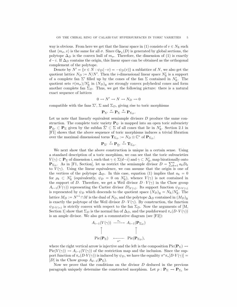
is exactly the polytope of the Weil divisor D · V (γ). By construction, the functionψD·V (γ) is strictly convex with respect to the fan ΣD. Now the arguments of [M,Section 1] show that ΣD is the normal fan of ∆D, and the pushforward π∗(D ·V (γ))is an ample divisor. We also get a commutative diagram (see [F2]):
Ai−1(V (γ))π∗−−−−→ Ai−1(PΣD
)x
x
Pic(PΣ) ←−−−−π∗
Pic(PΣD),
where the right vertical arrow is injective and the left is the composition Pic(PΣ) −→Pic(V (γ)) −→ Ai−1(V (γ)) of the restriction map and the inclusion. Since the sup-port function of π∗(D·V (γ)) is induced by ψD, we have the equality π∗π∗[D·V (γ)] =[D] in the Chow group Ad−1(PΣ).
Now we prove that the conditions on the divisor D deduced in the previousparagraph uniquely determine the constructed morphism. Let p : PΣ −→ PΣ1 be
6 ANVAR R. MAVLYUTOV
a surjective morphism of complete toric varieties arising from a surjective homo-morphism of lattices p : N −→ N1 which maps the fan Σ into Σ1. The kernel ofp is a sublattice N2 ⊂ N . It is not difficult to see that a cone of Σ is either ly-ing in the space (N2)R
or its relative interior has no intersection with this space.Hence, the space (N2)R
is a support of a complete fan Σ2 filled up by those conesof Σ lying in (N2)R
. The toric subvarieties V (γ) corresponding to γ ∈ Σ(d − k)(k := dimPΣ1), contained in (N2)R
, are the only ones mapping birationally ontoPΣ1 . Suppose now that we have an i-semiample (torus invariant) divisor D on PΣ
such that p∗[D ·V (γ)] is ample and p∗p∗[D ·V (γ)] = [D] for some V (γ), γ ∈ Σ(d−k),which maps birationally onto PΣ1 . Then the polytope of the divisor p∗(D · V (γ))has dimension equal to dimPΣ1 . On the other hand, the support function of D isinduced by the support function of p∗(D · V (γ)), implying that the polytopes ofthese divisors is the same set in M ∩N⊥
2 . Therefore, the dimension of PΣ1 is i, andthe fan Σ1 coincides with ΣD constructed before. Thus, we proved the following.
Theorem 1.4. Let [D] ∈ Ad−1(PΣ) be an i-semiample divisor class on a completetoric variety PΣ of dimension d. Then, there exists a unique complete toric varietyPΣD
with a surjective morphism π : PΣ −→ PΣD, corresponding to a map of Σ
into ΣD, such that π∗[D · V (γ)] is ample and π∗π∗[D · V (γ)] = [D] for some closedtoric subvariety V (γ) ⊂ PΣ, γ ∈ Σ, which maps birationally onto PΣD
. Moreover,dimPΣD
= i, and the fan ΣD is the normal fan of ∆D for a torus invariant D.
Remark 1.5. The fan ΣD is canonical with respect to the equivalence relation onthe divisors. Therefore, it will sometimes be convenient for us to use the notationΣβ := ΣD for a semiample divisor class β = [D] ∈ Ad−1(PΣ).
While a restriction of a semiample divisor D on PΣ to a closed toric subvariety isagain a semiample divisor, the Iitaka dimension of the restricted divisor may change.Let us investigate this problem. If D is an i-semiample divisor on PΣ, then, bythe above theorem, we have a unique toric morphism π : PΣ −→ PΣD
, arisingfrom a homomorphism π : NR −→ (ND)
Rmapping Σ into ΣD. This morphism
encodes information about the structure of the variety PΣ. The Iitaka dimensionof the semiample divisor D · V (σ) on V (σ), σ ∈ Σ, can be determined in thefollowing way. The complete toric variety V (σ) is mapped onto a closed subvarietyV (σ0) ⊂ PΣD
such that the cone σ0 ∈ ΣD is the smallest that contains π(σ). Weclaim that this induced map π : V (σ) −→ V (σ0) is exactly the one associated withthe semiample divisor D · V (σ). To prove this we will verify the conditions whichuniquely determine such a morphism. As in the theorem above, let V (γ) be suchthat π∗[D · V (γ)] is ample and π∗π∗[D · V (γ)] = [D], and let V (γ′) ⊂ V (σ) be aclosed toric subvariety mapping birationally onto V (σ0). By the projection formula(see [F2]), we get
π∗[D · V (γ′)] = π∗[(π∗π∗[D · V (γ)]) · V (γ′)]
= π∗[D · V (γ)] · π∗[V (γ′)] = π∗[D · V (γ)] · V (σ0)
in the Chow group of the toric variety V (σ0). Since π∗[D · V (γ)] is ample, thedivisor class π∗[D · V (γ′)] is ample as well. The other condition for the semiampledivisor D · V (σ) also follows:
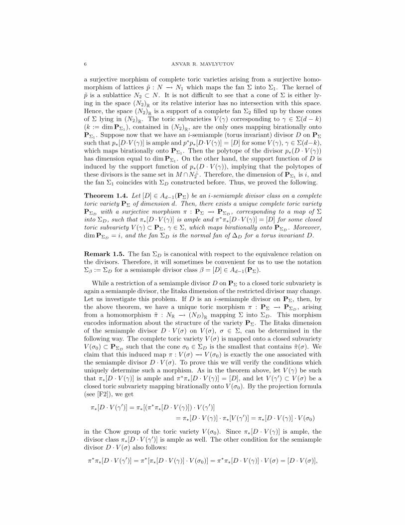
π∗π∗[D · V (γ′)] = π∗[π∗[D · V (γ)] · V (σ0)] = π∗π∗[D · V (γ)] · V (σ) = [D · V (σ)],
ON THE CHIRAL RING OF CALABI-YAU HYPERSURFACES IN TORIC VARIETIES 7
where we used the commutative diagram
Pic(PΣD)
π∗
−−−−→ Pic(PΣ)y
y
Pic(V (σ0))π∗
−−−−→ Pic(V (σ)).
Thus, by the uniqueness part of Theorem 1.4, we get the next result.
Proposition 1.6. Let [D] ∈ Ad−1(PΣ) be an i-semiample divisor class on PΣ withthe associated morphism π : PΣ −→ PΣD
arising from a map of the fan Σ into ΣD.Then, for σ ∈ Σ, the restriction [D · V (σ)] is a k-semiample divisor class on V (σ)with k = i−dim(σ0) = dimV (σ0), where σ0 ∈ ΣD is the smallest cone that containsthe image of σ. Moreover, the induced map π : V (σ) −→ V (σ0) is the one associatedwith the semiample divisor class [D · V (σ)].
This proposition says that the maps associated with the semiample divisors arecompatible with the restrictions.
Any toric variety PΣ has a homogeneous coordinate ring S(Σ) = C[x1, . . . , xn]with variables x1, . . . , xn corresponding to the irreducible torus invariant divi-sors D1, . . . , Dn. This ring is graded by the Chow group Ad−1(PΣ), assigning[∑n
i=1 aiDi] to deg(∏n
i=1 xai
i ). For a Weil divisor D on PΣ, there is an isomorphismH0(PΣ, OPΣ(D)) ∼= S(Σ)α, where α = [D] ∈ Ad−1(PΣ). If D is torus invariant, themonomials in S(Σ)α correspond to the lattice points of the associated polyhedron∆D.
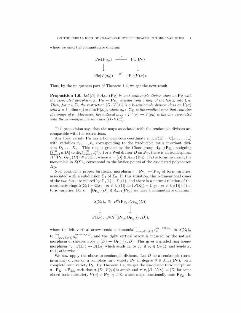
Now consider a proper birational morphism π : PΣ1 −→ PΣ2 of toric varieties,associated with a subdivision Σ1 of Σ2. In this situation, the 1-dimensional conesof the two fans are related by Σ2(1) ⊂ Σ1(1), and there is a natural relation of thecoordinate rings S(Σ1) = C[xk : ρk ∈ Σ1(1)] and S(Σ2) = C[yk : ρk ∈ Σ2(1)] of thetoric varieties. For α = [OPΣ1
(D)] ∈ Ad−1(PΣ1) we have a commutative diagram:
S(Σ1)α∼= H0(PΣ1 , OPΣ1
(D))y
y
S(Σ2)π∗α∼=H0(PΣ2 , OPΣ2
(π∗D)),
where the left vertical arrow sends a monomial∏
ρk∈Σ1(1)x
ak+〈m,ek〉k in S(Σ1)α
to∏
ρk∈Σ2(1) yak+〈m,ek〉k , and the right vertical arrow is induced by the natural
morphism of sheaves π∗OPΣ1(D) −→ OPΣ2
(π∗D). This gives a graded ring homo-
morphism π∗ : S(Σ1) −→ S(Σ2) which sends xk to yk, if ρk ∈ Σ2(1), and sends xk
to 1, otherwise.We now apply the above to semiample divisors. Let D be a semiample (torus
invariant) divisor on a complete toric variety PΣ in degree β ∈ Ad−1(PΣ). on acomplete toric variety PΣ, By Theorem 1.4, we get the associated toric morphismπ : PΣ → PΣD
such that π∗[D · V (γ)] is ample and π∗π∗[D · V (γ)] = [D] for someclosed toric subvariety V (γ) ⊂ PΣ, γ ∈ Σ, which maps birationally onto PΣD
. In
8 ANVAR R. MAVLYUTOV
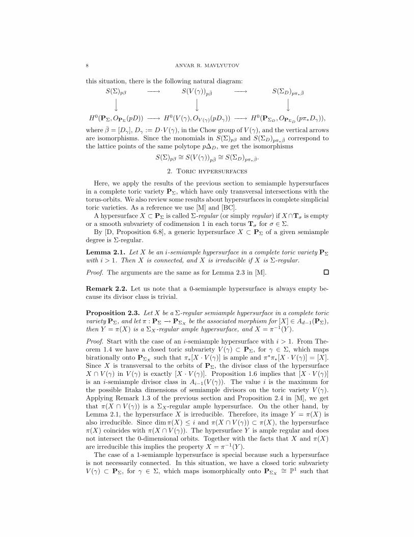
this situation, there is the following natural diagram:
S(Σ)pβ −−→ S(V (γ))pβ −−→ S(ΣD)pπ∗βyy
y
H0(PΣ, OPΣ(pD)) −−→ H0(V (γ), OV (γ)(pDγ)) −−→ H0(PΣD, OPΣD
(pπ∗Dγ)),
where β = [Dγ ], Dγ := D ·V (γ), in the Chow group of V (γ), and the vertical arrowsare isomorphisms. Since the monomials in S(Σ)pβ and S(ΣD)pπ∗β correspond tothe lattice points of the same polytope p∆D, we get the isomorphisms
S(Σ)pβ∼= S(V (γ))pβ
∼= S(ΣD)pπ∗β.
2. Toric hypersurfaces
Here, we apply the results of the previous section to semiample hypersurfacesin a complete toric variety PΣ, which have only transversal intersections with thetorus-orbits. We also review some results about hypersurfaces in complete simplicialtoric varieties. As a reference we use [M] and [BC].
A hypersurfaceX ⊂ PΣ is called Σ-regular (or simply regular) if X∩Tσ is emptyor a smooth subvariety of codimension 1 in each torus Tσ for σ ∈ Σ.
By [D, Proposition 6.8], a generic hypersurface X ⊂ PΣ of a given semiampledegree is Σ-regular.
Lemma 2.1. Let X be an i-semiample hypersurface in a complete toric variety PΣ
with i > 1. Then X is connected, and X is irreducible if X is Σ-regular.
Proof. The arguments are the same as for Lemma 2.3 in [M].
Remark 2.2. Let us note that a 0-semiample hypersurface is always empty be-cause its divisor class is trivial.
Proposition 2.3. Let X be a Σ-regular semiample hypersurface in a complete toricvariety PΣ, and let π : PΣ −→ PΣX
be the associated morphism for [X ] ∈ Ad−1(PΣ),then Y = π(X) is a ΣX-regular ample hypersurface, and X = π−1(Y ).
Proof. Start with the case of an i-semiample hypersurface with i > 1. From The-orem 1.4 we have a closed toric subvariety V (γ) ⊂ PΣ, for γ ∈ Σ, which mapsbirationally onto PΣX
such that π∗[X · V (γ)] is ample and π∗π∗[X · V (γ)] = [X ].Since X is transversal to the orbits of PΣ, the divisor class of the hypersurfaceX ∩ V (γ) in V (γ) is exactly [X · V (γ)]. Proposition 1.6 implies that [X · V (γ)]is an i-semiample divisor class in Ai−1(V (γ)). The value i is the maximum forthe possible Iitaka dimensions of semiample divisors on the toric variety V (γ).Applying Remark 1.3 of the previous section and Proposition 2.4 in [M], we getthat π(X ∩ V (γ)) is a ΣX -regular ample hypersurface. On the other hand, byLemma 2.1, the hypersurface X is irreducible. Therefore, its image Y = π(X) isalso irreducible. Since dimπ(X) ≤ i and π(X ∩ V (γ)) ⊂ π(X), the hypersurfaceπ(X) coincides with π(X ∩ V (γ)). The hypersurface Y is ample regular and doesnot intersect the 0-dimensional orbits. Together with the facts that X and π(X)are irreducible this implies the property X = π−1(Y ).
The case of a 1-semiample hypersurface is special because such a hypersurfaceis not necessarily connected. In this situation, we have a closed toric subvarietyV (γ) ⊂ PΣ, for γ ∈ Σ, which maps isomorphically onto PΣX
∼= P1 such that
ON THE CHIRAL RING OF CALABI-YAU HYPERSURFACES IN TORIC VARIETIES 9
π∗[X · V (γ)] is ample and π∗π∗[X · V (γ)] = [X ]. It follows from Proposition 1.6and Remark 2.2 that the image Y = π(X) is contained in the 1-dimensional torusof PΣX
∼= P1. The preimage π−1(Y ) of this finite set can be easily seen fromthe description of the toric morphism π in Section 1. This morphism is a trivialfibration over the 1-dimensional torus of PΣX
, and each point of π(X) gives exactlyone irreducible component of π−1(Y ) which is actually a complete toric variety.
On the other hand, each point of π(X) came from an irreducible component ofX ⊂ π−1(Y ). Hence, X = π−1(Y ). This gives an isomorphism π : X ∩ V (γ) ∼=π(X). Thus, π(X) is a ΣX -regular ample hypersurface.
Remark 2.4. If, in addition, we assume in this proposition thatX is an anticanon-ical hypersurface in PΣ, then X is big and PΣX
is a Fano toric variety associatedto a reflexive polytope, and this corresponds to the construction in [B2].
Let Y be an ample regular hypersurface in a complete toric variety PΣ. Ahypersurface in the torus T ⊂ PΣ isomorphic to the affine hypersurface Y ∩T inT is called nondegenerate. Cohomology of such hypersurfaces has been studied in[DK] and [B2].
Lemma 2.5. [DK] Let Z be a nondegenerate affine hypersurface in the torus T,then the natural map Hi(T)→ Hi(Z), induced by the inclusion, is an isomorphismof Hodge structures for i < dimT− 1 and an injection for i = dimT− 1.
Using the standard description of a toric morphism, from Proposition 2.3 weget a stratification of an i-semiample regular hypersurface X ⊂ PΣ in terms ofnondegenerate affine hypersurfaces:
X ∩Tσ∼= (π(X) ∩Tσ0)× (C∗)l, (2)
where π : PΣ −→ PΣXis the associated morphism, l = d − i + dim σ0 − dimσ,
d = dimPΣ, and σ0 ∈ ΣX is the smallest cone containing the image of σ ∈ Σ.From here on, we assume that P := PΣ denotes a complete simplicial toric vari-
ety. In this case, [BC] shows that homogeneous polynomials in S := S(Σ) determinehypersurfaces in P. In terms of the coordinate ring S, a regular hypersurface in P
defined by a homogeneous polynomial f ∈ Sβ is characterized by the condition thatx1(∂f/∂x1), . . . , xn(∂f/∂xn) do not vanish simultaneously on P (see [C2, Proposi-tion 5.3]). A more general class of hypersurfaces in P called quasismooth is definedby a similar condition that ∂f/∂x1, . . . , ∂f/∂xn do not vanish simultaneously onP (see [BC]).
We also like to mention the following fact.
Proposition 2.6. An anticanonical quasismooth hypersurface X in a Gorensteincomplete simplicial toric variety P is Calabi-Yau.
Proof. A quasismooth hypersurface is an orbifold (see [BC]), and for a (d − 1)-
dimensional orbifold X Calabi-Yau means that Ωd−1X ≃ OX and Hi(X,OX) = 0
for i = 1, . . . , d − 2 (see [CK, A.2]). The arguments of the proof that anti-canonical implies Calabi-Yau are the same as in [C3]: use the adjunction formula
Ωd−1X ≃ Ωd
P(X) ⊗ OX , the isomorphism OP(−X) ≃ Ωd
Pand the exact sequence
0 −→ OP(−X) −→ OP −→ OX −→ 0.
10 ANVAR R. MAVLYUTOV
Definition 2.7. [BC] Fix an integer basis m1, . . . ,md for the lattice M . Thengiven subset I = i1, . . . , id ⊂ 1, . . . , n, denote det(eI) = det(〈mj , eik
〉1≤j,k≤d),dxI = dxi1 ∧ · · · ∧ dxid
and xI =∏
i/∈I xi. Define the d-form Ω by the formula
Ω =∑
|I|=d
det(eI)xIdxI ,
where the sum is over all d element subsets I ⊂ 1, . . . , n.Let X ⊂ P be a quasismooth (not necessarily Cartier) hypersurface defined by
f ∈ Sβ. For A ∈ S(a+1)β−β0(here, β0 =
∑ni=1 deg(xi)), consider a rational d-form
ωA := AΩ/fa+1 ∈ H0(P,ΩdP((a+ 1)X)).
This form gives a class in Hd(P \X), and by the residue map
Res : Hd(P \X)→ Hd−1(X)
we get Res(ωA) ∈ Hd−1(X).
Remark 2.8. The residue map and the residues of rational differential forms withpoles along a regular hypersurface are well defined even if the toric variety is notsimplicial (see the proof of Theorem 3.7 in [DK] and Remark 6.4 in [B2]).
Definition 2.9. [BC] Given f ∈ Sβ, we have the Jacobian ideal J(f) in S gener-ated by the partial derivatives ∂f/∂x1, . . . , ∂f/∂xn, the ideal
J0(f) = 〈x1(∂f/∂x1), . . . , xn(∂f/∂xn)〉and the ideal quotient (see [CLO, p. 193]) J1(f) = J0(f) : x1 · · ·xn. These give theJacobian ring R(f) = S/J(f), R0(f) = S/J0(f) and R1(f) = S/J1(f) graded bythe Chow group Ad−1(P).
In [M] we have shown that the induced maps
Res(ω )d−1−q,q : R(f)(q+1)β−β0→ Hq(X,Ωd−1−q
X )
(sending A to the Hodge component Res(ωA)d−1−q,q) for a quasismooth hypersur-face X ⊂ P and, respectively,
Res(ω )d−1−q,q : R1(f)(q+1)β−β0→ Hq(X,Ωd−1−q
X )
for a big and nef regular hypersurface are well defined. There we also studied therelationship between the multiplicative structure on R(f) (resp., R1(f)) and thecup product on the middle cohomology of a quasismooth (resp., big and nef regular)hypersurface in P. From Theorem 4.4 [M] we have the following description of themiddle cohomology of big and nef regular hypersurfaces X ⊂ PΣ:
Hd−1−q,q(X) ∼= R1(f)(q+1)β−β0
⊕( n∑
i=1
ϕi!Hd−2−q,q−1(X ∩Di)
), (3)
where ϕi! are the Gysin maps for ϕi : X∩Di → X . In the case, when the dimensionof the ambient space is 4 we have (see [M, Theorem 5.2]):
Theorem 2.10. Let X ⊂ PΣ, dimPΣ = 4, be a big and nef regular hypersurfacedefined by f ∈ Sβ. Then there is a natural isomorphism
H3−q,q(X) ∼= R1(f)(q+1)β−β0
⊕( ⊕
σ∈ΣX (2)
(R1(fσ)qβσ−βσ0)n(σ)
),
ON THE CHIRAL RING OF CALABI-YAU HYPERSURFACES IN TORIC VARIETIES 11
where n(σ) is the number of cones ρi such that ρi ⊂ σ and ρi /∈ ΣX(1), and where fσ
is the polynomial of degree βσ, defining the ample hypersurface π(X)∩V (σ) ⊂ V (σ)(here, π : PΣ −→ PΣX
is the associated morphism), and βσ0 is the degree of the
anticanonical divisor on the 2-dimensional toric variety V (σ).
3. Polynomial part of the chiral ring
Here we show that for a quasismooth hypersurface X of degree β there is a ho-momorphism between R(f)∗β and the chiral ring H∗(X,∧∗TX). We will also showthat R1(f)∗β is a subring of the chiral ring for a semiample anticanonical regularhypersurface X ⊂ P (which is Calabi-Yau). This subring may be called “poly-nomial” because its graded piece in H1(X, TX) should correspond to polynomialinfinitesimal deformations of X performed in the toric variety P (see [CK]).
Let ΩpX be the sheaf of Zariski p-forms on an orbifold X (see Appendix A.3 in
[CK]). We can also define ∧pTX := (ΩpX)∗ = HomOX
(ΩpX , OX) for an orbifold X .
We call this the (Zariski) p-th exterior power of the tangent sheaf of X . For p = 1this sheaf is isomorphic to the usual tangent sheaf ΘX , by Proposition A.4.1 in[CK]. When X is smooth, ∧pTX coincides with the standard exterior power sheaf.Moreover, if j : Xo ⊂ X is the inclusion of the smooth locus ofX , then the argumentin the proof of Proposition 3.10 in [Od] shows that j∗(
∧pΘXo
) = ∧pTX . One canuse the same argument to prove Ωp
X ≃ (∧pTX)∗ and that ΩpX is isomorphic to the
dual (∧p ΘX)∗ of the usual p-th exterior power of ΘX , whence ∧pTX ≃ (
∧p ΘX)∗∗.In particular, we also have the natural maps of sheaves ∧pTX ⊗ ∧qTX → ∧p+qTX
and ∧pTX ⊗ ΩqX → Ωq−p
X .Let X ⊂ P be a quasismooth hypersurface defined by f ∈ Sβ , which is an
orbifold as we know from [BC]. By definition of quasismooth, we get an open coverU = Uini=1 of P, where Ui = x ∈ P : fi(x) 6= 0 and fi denotes the partialderivative ∂f/∂xi.
Definition 3.1. Denote ∂i0...ip= ∂
∂xi0∧· · ·∧ ∂
∂xipfor an ordered subset i0, . . . , ip
in 1, . . . , n. Then given A ∈ Spβ, set
(γA)i0...ip=
(−1)p2/2A〈∂i0...ip
, df〉fi0 · · · fip
i0...ip
,
where 〈 , 〉 denotes the contraction (the extra factor of (−1)p2/2 which is√−1 for
odd p is added to make convenient commutative diagrams later).
This defines a Cech cocycle, giving its class in Hp(U|X ,∧pTX). Indeed, (γA)i0...ip
is homogeneous of degree 0 and is a cochain in Cp(U|X ,∧pTX) by the exact sequence
0→ ∧pTXo−→ i∗ ∧p TPo
i∗df−−−→ ∧p−1TXo⊗OXo
(X)
(where i : X ⊂ P is the inclusion, Po is the smooth locus of P such thatXo = Po∩X(see [Hi, §4, p. 55])), and because of 〈〈∂i0...ip
, df〉, df〉 = 0 since df ∧ df = 0. Onthe other hand, it is straightforward to verify that
(γA)i0...ip=
(−1)p2/2A
fi0 · · · fip
p∑
j=0
(−1)jfij∂
i0...ij ...ip
i0...ip
vanishes under the Cech coboundary map Cp(U|X ,∧pTX) → Cp+1(U|X ,∧pTX).One can actually show that (γA)i0...ip
is a coboundary in Cp(U|X , i∗ ∧p TP).
12 ANVAR R. MAVLYUTOV
For A ∈ Spβ let γA ∈ Hp(X,∧pTX) be the image of the Cech cocycle (γA)i0...ip
under the natural map Hp(U|X ,∧pTX)→ Hp(X,∧pTX). And we get a well definedmap γ : R(f)∗β → H∗(X,∧∗TX) because of the following statement.
Lemma 3.2. If A ∈ J(f)pβ , then the cocycle (γA)i0...ipis a Cech coboundary in
Cp(U|X ,∧pTX).
Proof. If A ∈ J(f)pβ , then we can assume that A is a multiple of one of the partialderivatives fk = ∂f/∂xk. We have
fk
〈∂i0...ip, df〉
fi0 · · · fip
=
p∑
j=0
(−1)jfk∂i0...ij ...ip
fi0 · · · fij· · · fip
=
p∑
j=0
(−1)j〈∂k, df〉∂i0...ij ...ip
fi0 · · · fij· · · fip
−p∑
j=0
(−1)j∂k ∧ 〈∂i0...ij ...ip
, df〉
fi0 · · · fij· · · fip
=
p∑
j=0
(−1)j〈∂
ki0...ij ...ip, df〉
fi0 · · · fij· · · fip
,
where the second sum after the second equality is identically zero. Hence, it followsthat (γA)i0...ip
is in the image of the Cech coboundary map Cp−1(U|X ,∧pTX) →Cp(U|X ,∧pTX).
We now study the compatibility of the multiplication in the Jacobian ring R(f)and the cohomology ring H∗(X,∧∗TX). The cocycle (γA)i0...ip
(up to an extrafactor) and the calculations in the next two theorems are essentially due to D. Coxand D. Morrison.
Theorem 3.3. Let X ⊂ P be a quasismooth hypersurface defined by f ∈ Sβ. Themap R(f)∗β → H∗(X,∧∗TX), assigning γA to a polynomial A, is a ring homomor-phism.
Proof. We need to show that γA ∪ γB = γAB for A ∈ Spβ and B ∈ Sqβ . Similar to
[CaG, page 63], the cup product γA ∪ γB is represented by the Cech cocycle
(−1)pq
(−1)p2/2A〈∂i0...ip
, df〉 ∧ (−1)q2/2B〈∂ip...ip+q, df〉
fi0 · · · fip+q· fip
i0...ip+q
.
Note that
〈∂i0...ip, df〉 ∧ 〈∂ip...ip+q
, df〉 =p∑
j=0
(−1)jfij∂
i0...ij ...ip∧
p+q∑
l=p
(−1)l−pfil∂
ip...il...ip+q
= fip
p+q∑
j=0
(−1)jfij∂
i0...ij ...ip= fip
〈∂i0...ip+q, df〉, (4)
where we used ∂ip∧ ∂ip
= 0. Hence the result follows.
The middle cohomology of a quasismooth hypersurface X ⊂ P is a module overH∗(X,∧∗TX) with respect to the natural cup product
Hp(X,∧pTX)⊗Hq(X,Ωd−1−qX )
∪−→ Hp+q(X,Ωd−1−p−qX ).
From the previous section we know that there is a natural map
Res(ω )d−1−q,q : R(f)(q+1)β−β0−→ Hq(X,Ωd−1−q
X ).
We normalize this map as [ωA] = (−1)q/2q!Res(ωA)d−1−q,q (where we assume(−1)q/2 = (
√−1)q) to show that this gives a morphism of modules R(f)(∗+1)β−β0
→H∗(X,Ωd−1−∗
X ).
ON THE CHIRAL RING OF CALABI-YAU HYPERSURFACES IN TORIC VARIETIES 13
Theorem 3.4. Let X ⊂ P be a quasismooth hypersurface defined by f ∈ Sβ. Thenthe diagram
R(f)pβ ⊗R(f)(q+1)β−β0−−→ R(f)(p+q+1)β−β0
γ ⊗[ω ]
y [ω ]
y
Hp(X,∧pTX)⊗Hq(X,Ωd−1−qX )
∪−−→ Hp+q(X,Ωd−1−p−qX )
commutes, where the top arrow is induced by the multiplication. When X ⊂ P is ad-semiample regular hypersurface the same diagram commutes with R1(f)(∗+1)β−β0
in place of R(f)(∗+1)β−β0.
Proof. From Theorem 3.3 in [M] we know that [ωB] = (−1)q/2q!Res(ωB)d−1−q,q,for B ∈ S(q+1)β−β0
, is represented by the Cech cocycle
(−1)d−1+(q(q+2)/2)
BKiq
· · ·Ki0Ω
fi0 · · · fiq
i0...iq
∈ Hq(U|X ,Ωd−1−qX ),
where Ki is the contraction operator (∂/∂xi)y. Therefore, for A ∈ Spβ the cup
product γA ∪ [ωB] is represented by the Cech cocycle
(−1)p2/2A〈∂i0...ip
, df〉fi0 · · · fip
y
(−1)d−1+(q(q+2)/2)BKip+q· · ·Kip
Ω
fip· · · fip+q
i0...ip+q
.
But note that
〈∂i0...ip, df〉yKip+q
· · ·KipΩ =
p∑
j=0
(−1)jfij∂
i0...ij ...ipyKip+q
· · ·KipΩ
= (−1)pfip∂i0...ip−1yKip+q
· · ·KipΩ = (−1)p+pqfip
Kip+q· · ·Ki0Ω.
Since (−1)p2/2 · (−1)q(q+2)/2 · (−1)p+pq = (−1)(p+q)(p+q+2)/2 we obtain γA ∪ [ωB ] =[ωAB], whence the diagram commutes.
For an anticanonical quasismooth hypersurface X in a Gorenstein toric varietyP (by Proposition 2.6, X is Calabi-Yau) the situation is especially nice. In this
case the natural product ∧pTX ⊗Ωd−1X → Ωd−1−p
X induced by the contraction is an
isomorphism since Ωd−1X ≃ OX and Ωd−1−p
X ≃ HomOX(Ωp
X ,Ωd−1X ) (see [CK, A.3]),
so that the cup product with [ω1] corresponding to 1 ∈ S0 (β = β0 because ofanticanonical) gives
∪ [ω1] : Hp(X,∧pTX) ∼= Hp(X,Ωd−1−pX ). (5)
For regular hypersurfaces this implies:
Theorem 3.5. Let X ⊂ P be a semiample anticanonical regular hypersurface de-fined by f ∈ Sβ. Then the map γ : R1(f)∗β → H∗(X,∧∗TX) is an injective ringhomomorphism.
Proof. The map is a well defined ring homomorphism by Theorems 3.3, 3.4 and(5), while the injectivity follows from Theorem 4.4 in [M].
Later we will need to use the following result.
14 ANVAR R. MAVLYUTOV
Lemma 3.6. Let j : L −→ K be a morphism of orbifolds, and let a ∈ Hp(K,∧qTK)
be such that j∗a = η∗a for some a under the maps
Hp(K,∧qTK)j∗−→ Hp(L, j∗ ∧q TK)
η∗
←− Hp(L,∧qTL).
Then j∗(a ∪ b) = a ∪ j∗b for b ∈ Hr(K,ΩsK).
Proof. The map j∗ decomposes as H∗(K,Ω∗K)
j∗−→ H∗(L, j∗Ω∗K)
η∗−→ H∗(L,Ω∗L).
Therefore,
j∗(a ∪ b) = η∗j∗(a ∪ b) = η∗(j∗a ∪ j∗b) = η∗(η∗a ∪ j∗b) = a ∪ η∗j∗b = a ∪ j∗b,
where we use the projection formula.
4. Non-polynomial part of the chiral ring
This section studies the non-polynomial part of the chiral ring which is com-plementary to the polynomial part. We will construct new cocycles representingelements in H∗(X,∧∗TX) for a big and nef quasismooth hypersurface X ⊂ PΣ. InSection 7 we will see that these elements with R1(f)β span H1(X, TX) for a semi-ample anticanonical regular hypersurface X ⊂ PΣ (dimPΣ 6= 1, 3). This meansthat we have found all cocycles corresponding to non-polynomial infinitesimal de-formations for a minimal Calabi-Yau X (see [CK]).
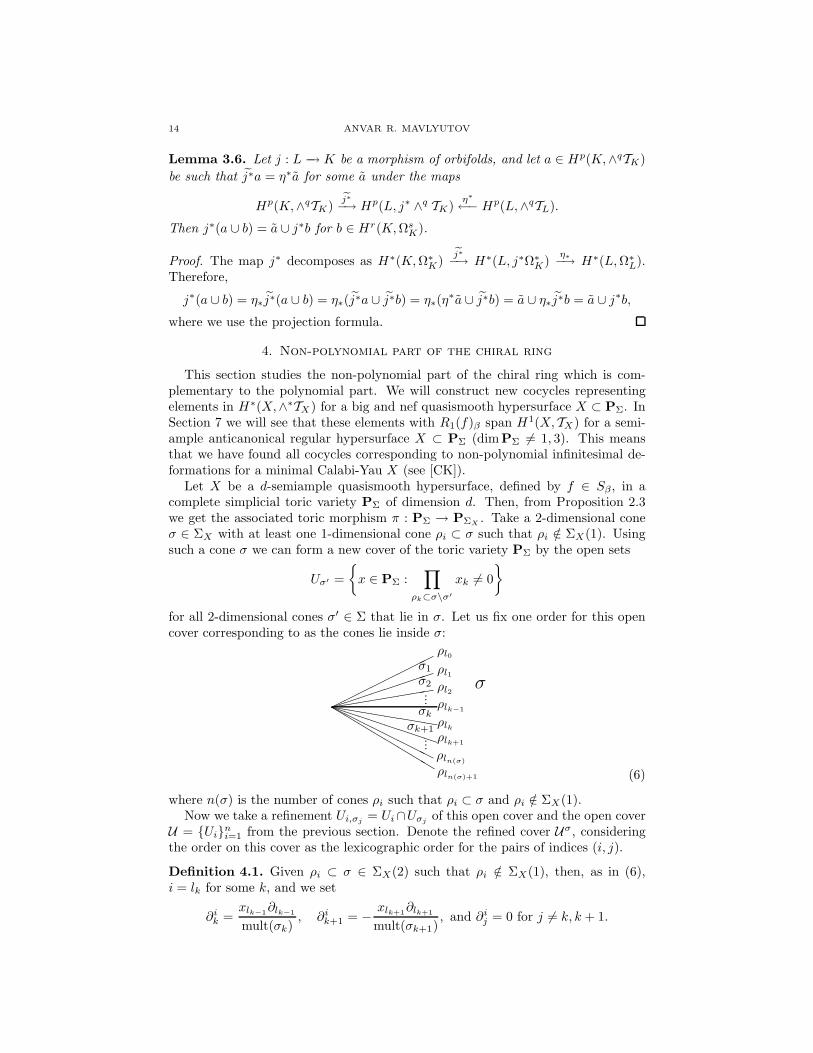
Let X be a d-semiample quasismooth hypersurface, defined by f ∈ Sβ, in acomplete simplicial toric variety PΣ of dimension d. Then, from Proposition 2.3we get the associated toric morphism π : PΣ → PΣX
. Take a 2-dimensional coneσ ∈ ΣX with at least one 1-dimensional cone ρi ⊂ σ such that ρi /∈ ΣX(1). Usingsuch a cone σ we can form a new cover of the toric variety PΣ by the open sets
Uσ′ =
x ∈ PΣ :
∏
ρk⊂σ\σ′
xk 6= 0
for all 2-dimensional cones σ′ ∈ Σ that lie in σ. Let us fix one order for this opencover corresponding to as the cones lie inside σ:
ρl0
σ1 ρl1
σ2
(((((((( ρl2p
p
p ρlk−1σkρlk
hhhhhhhhσk+1
PP
PP
PP
PPρlk+1
σ
p
p
p
ρln(σ)
HH
HH
HH
HH
bb
bb
bb
bb ρln(σ)+1 (6)
where n(σ) is the number of cones ρi such that ρi ⊂ σ and ρi /∈ ΣX(1).Now we take a refinement Ui,σj
= Ui∩Uσjof this open cover and the open cover
U = Uini=1 from the previous section. Denote the refined cover Uσ, consideringthe order on this cover as the lexicographic order for the pairs of indices (i, j).
Definition 4.1. Given ρi ⊂ σ ∈ ΣX(2) such that ρi /∈ ΣX(1), then, as in (6),i = lk for some k, and we set
∂ik =
xlk−1∂lk−1
mult(σk), ∂i
k+1 = − xlk+1∂lk+1
mult(σk+1), and ∂i
j = 0 for j 6= k, k + 1.
ON THE CHIRAL RING OF CALABI-YAU HYPERSURFACES IN TORIC VARIETIES 15
For A ∈ Sβσ1
(here, βσ1 :=
∑ρk⊂σ deg(xk)), define
(γiA)(i0,j0),(i1,j1) =
A∏
ρk⊂σ xk
( 〈∂i1 ∧ ∂ij1, df〉
fi1
−〈∂i0 ∧ ∂i
j0, df〉
fi0
)
(i0,j0),(i1,j1)
.
Lemma 4.2. In the definition, (γiA)(i0,j0),(i1,j1) is a Cech cocycle in C1(Uσ|X , TX).
Proof. By the arguments after Definition 3.1, (γiA)(i0,j0),(i1,j1) is a cocycle class in
H1(Uσ|X , TX). The only thing that we need to check in addition is that it is welldefined on the given cover, which follows easily from the following two observations.LetX be equivalent to a torus invariant divisorD =
∑nk=1 akDk with the associated
polytope ∆D and the support function ψD. Since ψD is linear on σ and determines
ak, a monomial∏n
k=1 xak+〈m,ek〉k (in xljflj ) with m ∈ ∆D is divisible by xlj implies
that ak + 〈m, ek〉 > 0 for all ρk ⊂ σ such that ρk /∈ ΣX(1). In particular, such amonomial is divisible by xi. On the other hand, we have an identity on PΣ:
xlk−1∂lk−1
mult(σk)+
xlk+1∂lk+1
mult(σk+1)=
mult(σk + σk+1)
mult(σk)mult(σk+1)xlk∂lk , (7)
where σk and σk+1 are the two cones contained in σ and containing ρi (the identitycorresponds to an Euler vector field (see [BC, Remark 3.10]) coming from the rela-tion of the cone generators mult(σk+1)elk−1
+ mult(σk)elk+1= mult(σk + σk+1)elk
(see [D, Section 8.2])).
Remark 4.3. Finding the above cocycle is far from obvious, but Propositions 6.3,6.4, 6.6 with Theorem 4.11 and equation (5) show how this comes up in the caseof Calabi-Yau threefolds from the description of the middle cohomology in Theo-rem 2.10.
Next we generalize the cocycles from Definition 4.1.
Definition 4.4. Let ρi ⊂ σ ∈ ΣX(2) be such that ρi /∈ ΣX(1). Given A ∈S(p−1)β+βσ
1, βσ
1 =∑
ρk⊂σ deg(xk), and an index set I = (i0, j0), . . . , (ip, jp),define
(γiA)I =
(−1)(p−1)2/2A∏
ρk⊂σ xk
∑
I=I\(ik,jk)
(−1)k〈∂i0...ip−1
∧ ∂ijp−1
, df〉fi0· · · fip−1
I
,
where the sum is over the ordered sets
I = (i0, j0), . . . , (ip−1, jp−1) = (i0, j0), . . . , (ik, jk), . . . , (ip, jp).
Similar to the proof of Lemma 4.2, this also determines a cocycle class inHp(Uσ|X ,∧pTX). Denoting its image in Hp(X,∧pTX) by γi
A, we get a map
γi : S(p−1)β+βσ1→ Hp(X,∧pTX),
when ρi \ 0 lies in the relative interior of a 2-dimensional cone σ ∈ ΣX .
Lemma 4.5. If A ∈ 〈J(f), xi〉(p−1)β+βσ1
and p > 1 or A ∈ 〈xi〉βσ1, then γi
A = 0.
16 ANVAR R. MAVLYUTOV
Proof. If A is divisible by xi, then (γiA)I is clearly a Cech coboundary, by Defini-
tion 4.4. Assume p > 1 and A ∈ J(f)(p−1)β+βσ1
is a multiple of one of the partialderivatives fs. Similar to the proof of Lemma 3.2, we have
fs〈∂i0...ip−1∧ ∂i
jp−1, df〉
(∏
ρk⊂σ xk)fi0· · · fip−1
≡p−1∑
l=0
(−1)l〈∂
si0...il...ip−1
∧ ∂ijp−1
, df〉
(∏
ρk⊂σ xk)fi0· · · fil
· · · fip−1
≡∑
˜I=I\(il,jl)
(−1)l〈∂
si0...ip−2∧ ∂i
˜jp−2
, df〉
(∏
ρk⊂σ xk)f˜i0· · · f˜ip−2
(the sum is over the ordered sets ˜I = (i0, j0), . . . , (il, jl), . . . , (ip−1, jp−1)) modulowell defined expressions on the open set Ui0,σj0
∩· · ·∩Uip−1,σjp−1
, because 〈∂ijp−1
, df〉is divisible by xi and because of equation (7). On the other hand, there is an identity
∑
I=I\(ik,jk)
(−1)k∑
˜I=I\(il,jl)
(−1)l〈∂
si0...ip−2∧ ∂i
˜jp−2
, df〉
f˜i0· · · f˜ip−2
= 0,
since the square of a coboundary map is zero. This shows that (γiA)I is a Cech
coboundary for A ∈ J(f).
Definition 4.6. Given f ∈ Sβ, let J i(f) be the ideal in S generated by the Jaco-bian ideal J(f) and xi. Then we get the quotient ring Ri(f) = S/J i(f) graded bythe Chow group Ad−1(PΣ).
Lemma 4.5 shows that there are well defined maps γi : Ri(f)(p−1)β+βσ1→
Hp(X,∧pTX), for p > 1, and γi : (S/〈xi〉)βσ1→ H1(X, TX). Note, however, that
a monomial∏
ρl 6⊂σ xl
∏nl=1 x
(p−1)al+〈m,el〉l in 〈xk〉(p−1)β+βσ
1(with ρk ⊂ σ) corre-
sponds to m ∈ M satisfying the inequalities (p − 1)al + 〈m, el〉 ≥ −1 for ρl ⊂ σ,l 6= k, and (p − 1)ak + 〈m, ek〉 ≥ 0. Since the support function, corresponding toβ = [
∑ni=1 aiDi], is linear on σ and determines ai, it follows from a relation of the
cone generators that (p−1)ai + 〈m, ei〉 ≥ 0 and, consequently, the above monomialis divisible by xi, for all ρi ⊂ σ such that ρi /∈ ΣX(1). Therefore, for all such ρi theideal J i(f) is the same as
Jσ(f) := 〈J(f), xk : ρk ⊂ σ〉in the degree (p− 1)β + βσ
1 . Hence, we define Rσ(f) = S/Jσ(f).The cocycle (γi
A)I in Definition 4.4 came from the proof of the following theorem.
Theorem 4.7. Let X ⊂ PΣ be a d-semiample quasismooth hypersurface definedby f ∈ Sβ. Then, for q > 1, the diagram
R(f)pβ ⊗Rσ(f)(q−1)β+βσ1−−→ Rσ(f)(p+q−1)β+βσ
1
γ ⊗γi
y γi
y
Hp(X,∧pTX)⊗Hq(X,∧qTX)∪−−→ Hp+q(X,∧p+qTX)
commutes, where βσ1 =
∑ρk⊂σ deg(xk) and the top arrow is induced by the multi-
plication. For q = 1 the diagram commutes with (S/〈xi〉)βσ1
in place of Rσ(f)βσ1.
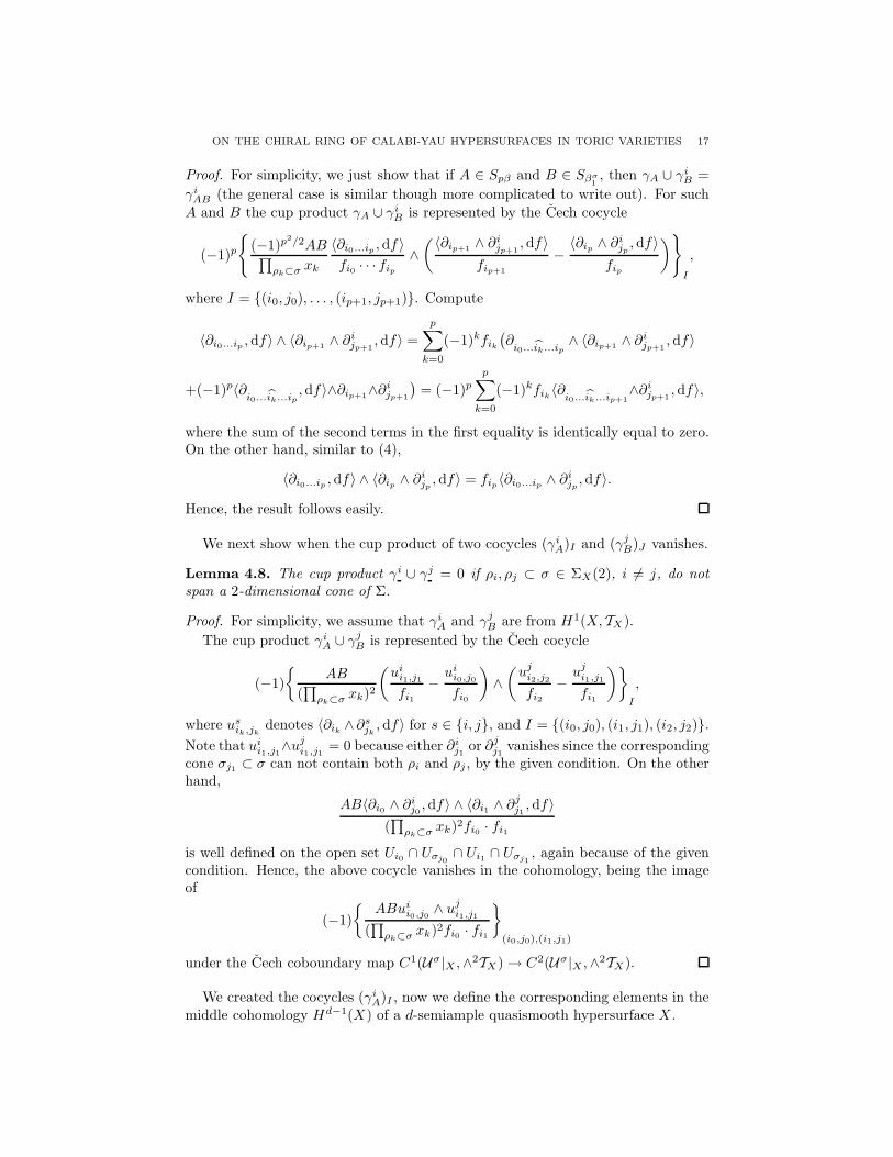
ON THE CHIRAL RING OF CALABI-YAU HYPERSURFACES IN TORIC VARIETIES 17
Proof. For simplicity, we just show that if A ∈ Spβ and B ∈ Sβσ1, then γA ∪ γi
B =
γiAB (the general case is similar though more complicated to write out). For such
A and B the cup product γA ∪ γiB is represented by the Cech cocycle
(−1)p
(−1)p2/2AB∏
ρk⊂σ xk
〈∂i0...ip, df〉
fi0 · · · fip
∧( 〈∂ip+1 ∧ ∂i
jp+1, df〉
fip+1
−〈∂ip∧ ∂i
jp, df〉
fip
)
I
,
where I = (i0, j0), . . . , (ip+1, jp+1). Compute
〈∂i0...ip, df〉 ∧ 〈∂ip+1 ∧ ∂i
jp+1, df〉 =
p∑
k=0
(−1)kfik
(∂
i0...ik...ip∧ 〈∂ip+1 ∧ ∂i
jp+1, df〉
+(−1)p〈∂i0...ik...ip
, df〉∧∂ip+1∧∂ijp+1
)= (−1)p
p∑
k=0
(−1)kfik〈∂
i0...ik...ip+1∧∂i
jp+1, df〉,
where the sum of the second terms in the first equality is identically equal to zero.On the other hand, similar to (4),
〈∂i0...ip, df〉 ∧ 〈∂ip
∧ ∂ijp, df〉 = fip
〈∂i0...ip∧ ∂i
jp, df〉.
Hence, the result follows easily.
We next show when the cup product of two cocycles (γiA)I and (γj
B)J vanishes.
Lemma 4.8. The cup product γi ∪ γj = 0 if ρi, ρj ⊂ σ ∈ ΣX(2), i 6= j, do notspan a 2-dimensional cone of Σ.
Proof. For simplicity, we assume that γiA and γj
B are from H1(X, TX).
The cup product γiA ∪ γ
jB is represented by the Cech cocycle
(−1)
AB
(∏
ρk⊂σ xk)2
(ui
i1,j1
fi1
−ui
i0,j0
fi0
)∧(uj
i2,j2
fi2
−uj
i1,j1
fi1
)
I
,
where usik,jk
denotes 〈∂ik∧∂s
jk, df〉 for s ∈ i, j, and I = (i0, j0), (i1, j1), (i2, j2).
Note that uii1,j1∧u
ji1,j1
= 0 because either ∂ij1 or ∂j
j1vanishes since the corresponding
cone σj1 ⊂ σ can not contain both ρi and ρj , by the given condition. On the otherhand,
AB〈∂i0 ∧ ∂ij0 , df〉 ∧ 〈∂i1 ∧ ∂j
j1, df〉
(∏
ρk⊂σ xk)2fi0 · fi1
is well defined on the open set Ui0 ∩ Uσj0∩ Ui1 ∩ Uσj1
, again because of the givencondition. Hence, the above cocycle vanishes in the cohomology, being the imageof
(−1)
ABui
i0,j0 ∧ uji1,j1
(∏
ρk⊂σ xk)2fi0 · fi1
(i0,j0),(i1,j1)
under the Cech coboundary map C1(Uσ|X ,∧2TX)→ C2(Uσ|X ,∧2TX).
We created the cocycles (γiA)I , now we define the corresponding elements in the
middle cohomology Hd−1(X) of a d-semiample quasismooth hypersurface X .
18 ANVAR R. MAVLYUTOV
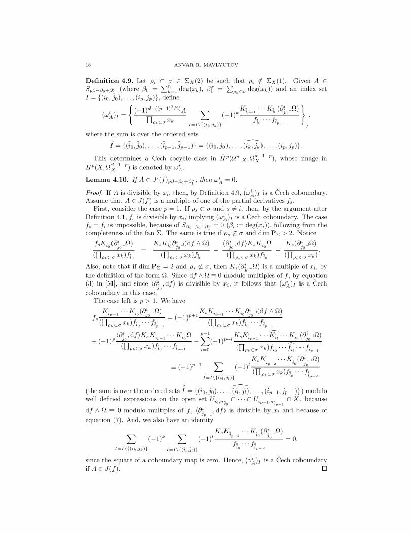
Definition 4.9. Let ρi ⊂ σ ∈ ΣX(2) be such that ρi /∈ ΣX(1). Given A ∈Spβ−β0+βσ
1(where β0 =
∑nk=1 deg(xk), βσ
1 =∑
ρk⊂σ deg(xk)) and an index set
I = (i0, j0), . . . , (ip, jp), define
(ωiA)I =
(−1)d+((p−1)2/2)A∏
ρk⊂σ xk
∑
I=I\(ik,jk)
(−1)kKip−1
· · ·Ki0(∂i
j0yΩ)
fi0· · · fip−1
I
,
where the sum is over the ordered sets
I = (i0, j0), . . . , (ip−1, jp−1) = (i0, j0), . . . , (ik, jk), . . . , (ip, jp).
This determines a Cech cocycle class in Hp(Uσ|X ,Ωd−1−pX ), whose image in
Hp(X,Ωd−1−pX ) is denoted by ωi
A.
Lemma 4.10. If A ∈ J i(f)pβ−β0+βσ1, then ωi
A = 0.
Proof. If A is divisible by xi, then, by Definition 4.9, (ωiA)I is a Cech coboundary.
Assume that A ∈ J(f) is a multiple of one of the partial derivatives fs.First, consider the case p = 1. If ρs ⊂ σ and s 6= i, then, by the argument after
Definition 4.1, fs is divisible by xi, implying (ωiA)I is a Cech coboundary. The case
fs = fi is impossible, because of Sβi−β0+βσ1
= 0 (βi := deg(xi)), following from thecompleteness of the fan Σ. The same is true if ρs 6⊂ σ and dimPΣ > 2. Notice
fsKi0(∂i
j0yΩ)
(∏
ρk⊂σ xk)fi0
=KsKi0
∂ij0
y(df ∧ Ω)
(∏
ρk⊂σ xk)fi0
−〈∂i
j0, df〉KsKi0
Ω
(∏
ρk⊂σ xk)fi0
+Ks(∂
ij0
yΩ)
(∏
ρk⊂σ xk).
Also, note that if dimPΣ = 2 and ρs 6⊂ σ, then Ks(∂ij0
yΩ) is a multiple of xi, by
the definition of the form Ω. Since df ∧ Ω ≡ 0 modulo multiples of f , by equation(3) in [M], and since 〈∂i
j0, df〉 is divisible by xi, it follows that (ωi
A)I is a Cech
coboundary in this case.The case left is p > 1. We have
fs
Kip−1· · ·Ki0
(∂ij0
yΩ)
(∏
ρk⊂σ xk)fi0· · · fip−1
= (−1)p+1KsKip−1
· · ·Ki0∂i
j0y(df ∧ Ω)
(∏
ρk⊂σ xk)fi0· · · fip−1
+ (−1)p〈∂i
j0, df〉KsKip−1
· · ·Ki0Ω
(∏
ρk⊂σ xk)fi0· · · fip−1
−p−1∑
l=0
(−1)p+lKsKip−1
· · · Kil· · ·Ki0
(∂ij0
yΩ)
(∏
ρk⊂σ xk)fi0· · · fil
· · · fip−1
≡ (−1)p+1∑
˜I=I\(il,jl)
(−1)lKsK˜ip−2
· · ·K˜i0(∂i
˜j0
yΩ)
(∏
ρk⊂σ xk)f˜i0· · · f˜ip−2
(the sum is over the ordered sets ˜I = (i0, j0), . . . , (il, jl), . . . , (ip−1, jp−1)) modulowell defined expressions on the open set Ui0,σj0
∩ · · · ∩ Uip−1,σjp−1
∩ X , because
df ∧ Ω ≡ 0 modulo multiples of f , 〈∂ijp−1
, df〉 is divisible by xi and because of
equation (7). And, we also have an identity
∑
I=I\(ik,jk)
(−1)k∑
˜I=I\(il,jl)
(−1)lKsK˜ip−2
· · ·K˜i0(∂i
˜j0
yΩ)
f˜i0· · · f˜ip−2
= 0,
since the square of a coboundary map is zero. Hence, (γiA)I is a Cech coboundary
if A ∈ J(f).
ON THE CHIRAL RING OF CALABI-YAU HYPERSURFACES IN TORIC VARIETIES 19
The last lemma shows that there is a well defined map
ωi : Ri(f)pβ−β0+βσ1→ Hp(X,Ωd−1−p
X ).
Since pβ is d-semiample, multiplying a monomial in 〈xk〉pβ−β0+βσ1
(for ρk ⊂ σ) by∏ρl 6⊂σ xl and applying the argument in the proof of Lemma 4.2, we get a monomial
divisible by all xi corresponding to ρi ⊂ σ such that ρi /∈ ΣX(1). Therefore, for allsuch ρi the ideal J i(f) is the same as Jσ(f) in the degree pβ − β0 + βσ
1 .The cocycle (ωi
A)I came from the proof of the following result.
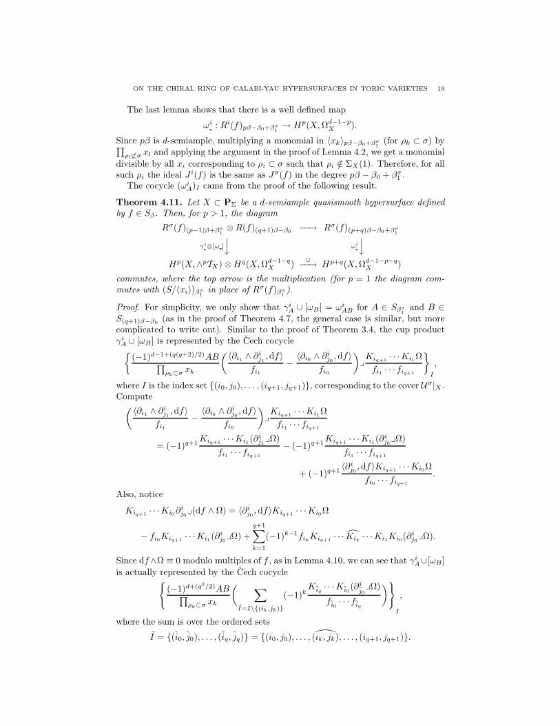
Theorem 4.11. Let X ⊂ PΣ be a d-semiample quasismooth hypersurface definedby f ∈ Sβ. Then, for p > 1, the diagram
Rσ(f)(p−1)β+βσ1⊗R(f)(q+1)β−β0
−−→ Rσ(f)(p+q)β−β0+βσ1
γi⊗[ω ]
y ωi
y
Hp(X,∧pTX)⊗Hq(X,Ωd−1−qX )
∪−−→ Hp+q(X,Ωd−1−p−qX )
commutes, where the top arrow is the multiplication (for p = 1 the diagram com-mutes with (S/〈xi〉)βσ
1in place of Rσ(f)βσ
1).
Proof. For simplicity, we only show that γiA ∪ [ωB] = ωi
AB for A ∈ Sβσ1
and B ∈S(q+1)β−β0
(as in the proof of Theorem 4.7, the general case is similar, but morecomplicated to write out). Similar to the proof of Theorem 3.4, the cup productγi
A ∪ [ωB] is represented by the Cech cocycle
(−1)d−1+(q(q+2)/2)AB∏ρk⊂σ xk
( 〈∂i1 ∧ ∂ij1 , df〉
fi1
−〈∂i0 ∧ ∂i
j0 , df〉fi0
)y
Kiq+1 · · ·Ki1Ω
fi1 · · · fiq+1
I
,
where I is the index set (i0, j0), . . . , (iq+1, jq+1), corresponding to the cover Uσ|X .Compute( 〈∂i1 ∧ ∂i
j1 , df〉fi1
−〈∂i0 ∧ ∂i
j0 , df〉fi0
)y
Kiq+1 · · ·Ki1Ω
fi1 · · · fiq+1
= (−1)q+1Kiq+1 · · ·Ki1(∂
ij1yΩ)
fi1 · · · fiq+1
− (−1)q+1Kiq+1 · · ·Ki1(∂
ij0yΩ)
fi1 · · · fiq+1
+ (−1)q+1〈∂i
j0, df〉Kiq+1 · · ·Ki0Ω
fi0 · · · fiq+1
.
Also, notice
Kiq+1 · · ·Ki0∂ij0y(df ∧ Ω) = 〈∂i
j0 , df〉Kiq+1 · · ·Ki0Ω
− fi0Kiq+1 · · ·Ki1(∂ij0yΩ) +
q+1∑
k=1
(−1)k−1fikKiq+1 · · · Kik
· · ·Ki1Ki0(∂ij0yΩ).
Since df∧Ω ≡ 0 modulo multiples of f , as in Lemma 4.10, we can see that γiA∪[ωB]
is actually represented by the Cech cocycle
(−1)d+(q2/2)AB∏ρk⊂σ xk
( ∑
I=I\(ik,jk)
(−1)kKiq· · ·Ki0
(∂ij0
yΩ)
fi0· · · fiq
)
I
,
where the sum is over the ordered sets
I = (i0, j0), . . . , (iq, jq) = (i0, j0), . . . , (ik, jk), . . . , (iq+1, jq+1).
20 ANVAR R. MAVLYUTOV
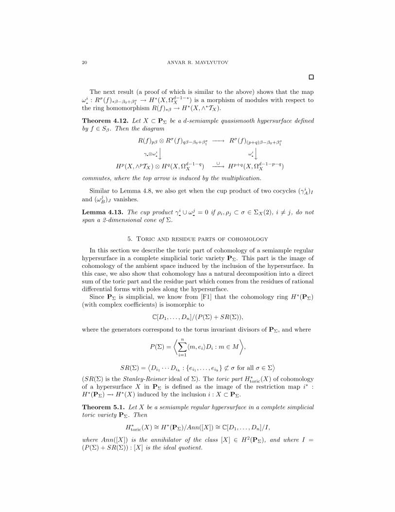
The next result (a proof of which is similar to the above) shows that the map
ωi : Rσ(f)∗β−β0+βσ1→ H∗(X,Ωd−1−∗
X ) is a morphism of modules with respect tothe ring homomorphism R(f)∗β → H∗(X,∧∗TX).
Theorem 4.12. Let X ⊂ PΣ be a d-semiample quasismooth hypersurface definedby f ∈ Sβ. Then the diagram
R(f)pβ ⊗Rσ(f)qβ−β0+βσ1−−→ Rσ(f)(p+q)β−β0+βσ
1
γ ⊗ωi
y ωi
y
Hp(X,∧pTX)⊗Hq(X,Ωd−1−qX )
∪−−→ Hp+q(X,Ωd−1−p−qX )
commutes, where the top arrow is induced by the multiplication.
Similar to Lemma 4.8, we also get when the cup product of two cocycles (γiA)I
and (ωjB)J vanishes.
Lemma 4.13. The cup product γi ∪ ωj = 0 if ρi, ρj ⊂ σ ∈ ΣX(2), i 6= j, do notspan a 2-dimensional cone of Σ.
5. Toric and residue parts of cohomology
In this section we describe the toric part of cohomology of a semiample regularhypersurface in a complete simplicial toric variety PΣ. This part is the image ofcohomology of the ambient space induced by the inclusion of the hypersurface. Inthis case, we also show that cohomology has a natural decomposition into a directsum of the toric part and the residue part which comes from the residues of rationaldifferential forms with poles along the hypersurface.
Since PΣ is simplicial, we know from [F1] that the cohomology ring H∗(PΣ)(with complex coefficients) is isomorphic to
C[D1, . . . , Dn]/(P (Σ) + SR(Σ)),
where the generators correspond to the torus invariant divisors of PΣ, and where
P (Σ) =
⟨ n∑
i=1
〈m, ei〉Di : m ∈M⟩,
SR(Σ) =⟨Di1 · · ·Dik
: ei1 , . . . , eik 6⊂ σ for all σ ∈ Σ
⟩
(SR(Σ) is the Stanley-Reisner ideal of Σ). The toric part H∗toric(X) of cohomology
of a hypersurface X in PΣ is defined as the image of the restriction map i∗ :H∗(PΣ) −→ H∗(X) induced by the inclusion i : X ⊂ PΣ.
Theorem 5.1. Let X be a semiample regular hypersurface in a complete simplicialtoric variety PΣ. Then
H∗toric(X) ∼= H∗(PΣ)/Ann([X ]) ∼= C[D1, . . . , Dn]/I,
where Ann([X ]) is the annihilator of the class [X ] ∈ H2(PΣ), and where I =(P (Σ) + SR(Σ)) : [X ] is the ideal quotient.
ON THE CHIRAL RING OF CALABI-YAU HYPERSURFACES IN TORIC VARIETIES 21
Proof. We need to show that ker(i∗ : H∗(PΣ) −→ H∗(X)) coincides with ker(∪[X ] :H∗(PΣ) −→ H∗+2(PΣ)). Since ∪[X ] = i!i
∗ (where i! is the Gysin map), this isequivalent to ker(i!) ∩ im(i∗) = 0 in Hp(X) for all p. Using an induction on thedimension of the hypersurface, we will show a stronger statement:
Hp(X) = im(i∗)⊕ ker(i!) for all p. (8)
If dimX = 0, then PΣ = P1. In this case, the compositionH0(P1)i∗−→ H0(X)
i!−→H2(P1) is clearly an isomorphism, and (8) follows.
Let dimX = d− 1 > 0. For all odd p, Hp(X) = ker(i!) and equation (8) holdsbecause Hodd(PΣ) vanishes. So we can assume that p is even.
We show first that Hp(X) = im(i∗) + ker(i!). The Gysin spectral sequence (see[M, Section 4]) gives an exact sequence
⊕nk=1H
p−2(X ∩Dk) −→ Hp(X) −→ GrWp Hp(X ∩T) −→ 0.
Also, by the Gysin exact sequence (see [DK, Theorem 3.7]), we get
0 −→ Hp+1(PΣ \X)Res−−→ Hp(X)
i!−→ Hp+2(PΣ) (9)
for even p. Hence, Res(Hp+1(PΣ \X)) = ker(i!). We claim that the composition
Hp+1(PΣ \X)Res−−→ Hp(X) −→ GrW
p Hp(X ∩T) (10)
is a surjective map for p > 0. If [X ] is an i-semiample divisor class, then weget the associated morphism π : PΣ −→ PΣX
, and the ample regular hypersurfaceY = π(X) in PΣX
, by Proposition 2.3. The statement is trivial for p 6= i − 1because, in this case,
GrWp Hp(X ∩T) ∼= GrW
p Hp((Y ∩TΣX)× (C∗)d−i) = 0 (11)
(where TΣXis the maximal torus of PΣX
), by equation (2) and the Kunnethisomorphism theorem with Lemma 2.5. For p = i − 1, consider the followingcommutative diagram:
Hi(PΣ \X)Res−−→ Hi−1(X) −−→ Hi−1(X ∩T)
xx
x
Hi(PΣX\ Y )
Res−−→ Hi−1(Y ) −−→ Hi−1(Y ∩TΣX),
where the vertical arrows are induced by the morphism π. The right vertical arrowdescends to an isomorphism
π∗ : GrWi−1H
i−1(Y ∩TΣX) ∼= GrW
i−1Hi−1(X ∩T) (12)
which follows from equation (2), the Kunneth isomorphism and Lemma 2.5. Onthe other hand, the proof of Theorem 4.4 in [M] and Remark 2.8 show that theweight space Wi−1H
i−1(Y ∩ TΣX) lies in the image of the composition of maps
on the bottom of the diagram. Thus, we have shown that the composition (10) is
surjective for all p > 0. Hence, ker(i!) in Hp(X) maps onto GrWp Hp(X ∩T). Since
22 ANVAR R. MAVLYUTOV
GrWp Hp(T) = 0 for p > 0, we get the commutative diagram:
⊕nk=1H
p(Dk) −−→ Hp+2(PΣ) −−→ 0xi!
xi!
⊕nk=1H
p−2(X ∩Dk) −−→ Hp(X) −−→ GrWp Hp(X ∩T) −−→ 0
xi∗xi∗
⊕nk=1H
p−2(Dk) −−→ Hp(PΣ) −−→ 0,
where the rows are exact sequences arising from the Gysin spectral sequence. Chas-ing this diagram and using the induction assumption (8) for the semiample regularhypersurfaces X ∩ Dk ⊂ Dk, we can see that Hp(X) is spanned by ker(i!) andim(i∗) for all p > 0. Let us show this in the case p = 0. If X is connected,then i∗ : H0(PΣ) −→ H0(X) is an isomorphism of 1-dimensional spaces, whenceH0(X) = im(i∗). By Lemma 2.1, we are left to consider the case when X is a1-semiample hypersurface. We use another commutative diagram:
H0(PΣ)i∗−−→ H0(X)
i!−−→ H2(PΣ)xπ∗
xπ∗
xπ∗
H0(PΣX) −−→ H0(Y ) −−→ H2(PΣX
).
The propertyX = π−1(Y ) from Proposition 2.3 gives an isomorphism π∗ : H0(Y ) −→H0(X). Using the diagram and the fact PΣX
∼= P1, we deduce H0(X) = im(i∗) +ker(i!).
To prove (8) it suffices now to show that im(i∗) and ker(i!) have complementarydimensions in Hp(X). From equation (9) we get dimker(i!) = hp+1(PΣ \X). Theexact sequence of cohomology with compact supports
Hp(PΣ)i∗−→ Hp(X) −→ Hp+1
c (PΣ \X) −→ 0
also gives dim im(i∗) = hp(X)− hp+1c (PΣ \X) for even p. Since Hp(X) = im(i∗) +
ker(i!), the inequalities
hp+1c (PΣ \X) ≤ hp+1(PΣ \X) (13)
hold for all even p. By Poincare duality, we have the equalities hp+1c (PΣ \ X) =
h2d−p−1(PΣ \X), hp+1(PΣ \X) = h2d−p−1c (PΣ \X). Applying them to (13), we
geth2d−p−1(PΣ \X) ≤ h2d−p−1
c (PΣ \X)
for all even p. Hence, all these inequalities are equalities, and equation (8) follows.The proof by induction is finished.
Remark 5.2. We should note that the above nontrivial result or its equivalenthas been used without a proof for smooth Calabi-Yau hypersurfaces (complete in-tersections) in many papers (e.g., [B3, Proposition 8.1], [HLY, Section 3.4], [St,Section 9]; cup product induces a nondegenerate pairing on the toric part—[CK,Lemma 8.6.11], [Gi, Introduction]). In the case of ample quasismooth hypersur-faces, this follows directly from the Hard-Lefschetz theorem. It is an open questionwhether Theorem 5.1 holds in general for smooth or quasismooth semiample hy-persurfaces.
ON THE CHIRAL RING OF CALABI-YAU HYPERSURFACES IN TORIC VARIETIES 23
Remark 5.3. An interesting equality follows from the proof of Theorem 5.1:
hp(PΣ \X) = hpc(PΣ \X) for odd p.
If X is ample, these Hodge numbers vanish for p away from the middle dimensiond. But in the semiample case they are nontrivial in general.
As a consequence of the above proof, we have a direct sum decompositionHp(X) = im(i∗) ⊕ ker(i!) for a semiample regular hypersurface. By the Gysinexact sequence, the kernel of the Gysin map is exactly the image of the residuemap. Therefore, it is natural to introduce the following.
Definition 5.4. The residue part H∗res(X) of cohomology of a quasismooth hyper-
surface X in a complete simplicial toric variety PΣ is defined as the image of theresidue map Res : H∗+1(PΣ \X) −→ H∗(X).
Remark 5.5. The residue part H∗res(X) is isomorphic to the primitive cohomology
PH∗(X) defined in [BC] by the exact sequence
H∗(PΣ) −→ H∗(X) −→ PH∗(X) −→ 0.
For a semiample regular hypersurface X in a complete simplicial toric varietyPΣ we have
H∗(X) = H∗toric(X)⊕H∗
res(X).
Theorem 5.1 described the toric part. Note that
H∗toric(X) ∪H∗
res(X) ⊂ H∗res(X),
since i!(i∗a ∪ b) = a ∪ i!b = 0 for b ∈ ker(i!), by the projection formula. Therefore,
the residue part is a submodule of H∗(X) over the ring H∗toric(X).
Finally, we suggest an algorithmic approach to computing the residue part ofcohomology. As in the proof of Theorem 5.1, the Gysin spectral sequence gives thecommutative diagram:
0 0 0x
xx
⊕nk=1H
p−2res (X ∩Dk) −→ Hp
res(X) −→ GrWp PHp(X ∩T) −→ 0
xx
x⊕n
k=1Hp−2(X ∩Dk) −→ Hp(X) −→ GrW
p Hp(X ∩T) −→ 0x
xx
⊕nk=1H
p−2(Dk) −→ Hp(PΣ) −→ GrWp Hp(T) −→ 0,
(14)
where the columns and the rows are exact, and where PHp(X ∩T) is defined, asin [B1, Definition 3.13], by the exact sequence
H∗(T) −→ H∗(X ∩T) −→ PH∗(X ∩T) −→ 0.
The hypersurfaces X∩Dk in Dk are semiample regular of lower dimension, and thespace GrW
p PHp(X∩T) can be described in terms of cohomology of a nondegenerateaffine hypersurface, again, using the proof of Theorem 5.1. Therefore, this providesa way to calculate Hp
res(X).
24 ANVAR R. MAVLYUTOV
6. Cohomology of semiample regular hypersurfaces
In this section we continue the study of the cohomology of semiample regu-lar hypersurfaces which was initiated in [M, Section 4]. Applying the algorithmicapproach of the previous section, we will compute the residue part of the middle co-homology of a big and nef regular hypersurface X . In particular, we will generalizethe description in equation (3) and Theorem 2.10. An algebraic description of themiddle cohomology is important because, in the Calabi-Yau case, this is isomorphicto the chiral ring H∗(X,∧∗TX), by equation (5). In terms of this description, oneshould be able to compute the product structure of the chiral ring. Here, we alsocompute the nontrivial cup products γi
A ∪ωjB of elements constructed in Section 4.
Let X be a d-semiample regular hypersurface, defined by f ∈ Sβ , in a completesimplicial toric variety PΣ. Our goal is to relate ωi
A, defined in Section 4, to thedescription of the middle cohomology of X given in equation (3). First, we definenew Cech cocycles, representing elements in Hd−3(X ∩Di).
Definition 6.1. Given σ ∈ ΣX(2) with the ordered integral generators el0 andeln(σ)+1
as in (6), introduce a (d− 2)-form
Ωσ =xl0xln(σ)+1
Kln(σ)+1Kl0Ω
mult(σ)∏
ρk⊂σ xk.
Then, for A ∈ S(p+1)β−β0+βσ1
and ρi ⊂ σ such that ρi /∈ ΣX(1), define
(ωiA)I = (−1)p2/2
AKip
· · ·Ki0Ωσ
fi0 · · · fip
I
,
where I is the index set i0, . . . , ip.
Consider a rational (d− 2)-form
(AΩσ/fp+1) ∈ H0(Di,Ω
d−2Di
((p+ 1)Xi)),
where Xi := X ∩ Di (we will use both notations). By the residue map we getRes(AΩσ/f
p+1) ∈ Hd−3(X∩Di). The next statement shows that up to a constant,(ωi
A)I is a Cech cocycle which represents this residue.
Proposition 6.2. Let X ⊂ PΣ be a d-semiample regular hypersurface defined byf ∈ Sβ. Given ρi ⊂ σ ∈ ΣX(2) such that ρi /∈ ΣX(1), and A ∈ S(p+1)β−β0+βσ
1,
then, under the natural map
Hp(U|X∩Di,Ωd−3−p
X∩Di)→ Hp(X ∩Di,Ω
d−3−pX∩Di
) ∼= Hd−3−p,p(X ∩Di),
the Hodge component Res(AΩσ/fp+1)d−3−p,p is represented by the Cech cocycle
(−1)d−3+(p(p+1)/2)
p!
AKip
· · ·Ki0Ωσ
fi0 · · · fip
I
∈ Cp(U|X∩Di,Ωd−3−p
X∩Di).
Proof. The proof of this is similar to the proof of Theorem 3.3 in [M] (see also[CaG]). We only need to show that
df ∧Ωσ ≡ 0 modulo multiples of f and xi. (15)
ON THE CHIRAL RING OF CALABI-YAU HYPERSURFACES IN TORIC VARIETIES 25
Note
df ∧ Ωσ = df ∧xl0xln(σ)+1
Kln(σ)+1Kl0Ω
mult(σ)∏
ρk⊂σ xk=xl0xln(σ)+1
Kln(σ)+1Kl0(df ∧ Ω)
mult(σ)∏
ρk⊂σ xk
−xl0fl0xln(σ)+1
Kln(σ)+1Ω
mult(σ)∏
ρk⊂σ xk+xl0xln(σ)+1
fln(σ)+1Kl0Ω
mult(σ)∏
ρk⊂σ xk.
The first summand is divisible by f , because df ∧Ω ≡ 0 modulo multiples of f , asin Lemma 4.10, and because f is not divisible by any variable xk, correspondingto ρk ⊂ σ, since X is regular. The sum of the other two terms is a multiple of xi,because, by the argument after Definition 4.1, xljflj are divisible by all variablesxk, corresponding to the cones ρk ⊂ σ not contained in ΣX(1), and because of anEuler identity similar to (7). Hence, equation (15) follows.
We also verify that (ωiA)I is a Cech cocycle. The Cech coboundary of (ωi
A)I is
(−1)p2/2
A
p+1∑
k=0
(−1)kfikKip+1 · · · Kik
· · ·Ki0Ωσ
fi0 · · · fip+1
I
.
On the other hand,
p+1∑
k=0
(−1)kfikKip+1 · · · Kik
· · ·Ki0Ωσ = Kip+1 · · ·Ki0(df ∧ Ωσ)
− (−1)p+2df ∧Kip+1 · · ·Ki0Ωσ.
Applying equation (15) and df = 0 on X , we can see that the image of (ωiA)I under
the Cech coboundary map is zero.
Denote by ωiA the image of the cocycle (ωi
A)I in Hp(X ∩ Di,Ωd−3−pX∩Di
). In the
next step we show a relation between ωiA and ωi
A.
Proposition 6.3. Let X ⊂ PΣ be a d-semiample regular hypersurface defined byf ∈ Sβ. Then ϕi!ω
iA = ωi
A, where ϕi! is the Gysin map for ϕi : X ∩Di → X.
Proof. It suffices to show that ϕi!ωiA, for A ∈ Spβ−β0+βσ
1, is represented by the
Cech cocycle (ωiA)I .
The Gysin map ϕi! we can compute, using the following commutative diagram
0 −→ Cp(Vσ,Ωd−1−pX ) −→ Cp(Vσ,Ωd−1−p
X (logXi))Res−−→ Cp(Vσ
i ,Ωd−2−pX∩Di
)x
xx
0 −→ Cp−1(Vσ,Ωd−1−pX ) −→ Cp−1(Vσ,Ωd−1−p
X (logXi))Res−−→ Cp−1(Vσ
i ,Ωd−2−pX∩Di
),
where the vertical arrows are the Cech coboundary maps, Vσ denotes the opencover Uσ|X , and the cover Vσ
i is the restriction Vσ|Xi, Xi = X ∩Di. By the residue
map, the cocycle (ωiA)I is lifted to the cochain
ψI = (−1)(p−1)2/2
AKip−1
· · ·Ki0Ωσ
fi0· · · fip−1
∧n∑
k=1
〈mj0, ek〉
dxk
xk
I
in Cp−1(Vσ,Ωd−1−pX (logXi)), where I is the index set (i0, j0), . . . , (ip−1, jp−1),
corresponding to the cover Vσ, and where mj0∈ MR, for σj0
⊃ ρi generated by
ei and es, satisfies 〈mj0, ei〉 = 1, 〈mj0
, es〉 = 0, and mj0= 0 in all other cases.
26 ANVAR R. MAVLYUTOV
Appropriately, this can be obtained, using some affine open cover on X , where
X ∩Di is given by∏n
k=1 x〈m,ek〉k = 0 up to some multiplicity (we omit the details).
The image of ψI under the Cech coboundary map should represent ϕi!ωiA. Using
the diagram, we can see that changing of ψI by a cochain in Cp−1(Vσ,Ωd−1−pX ) does
not affect the image. Notice that ψI is equivalent to
(−1)(p−1)2/2
AKip−1
· · ·Ki0
fi0· · · fip−1
(Ωσ ∧
n∑
k=1
〈mj0, ek〉
dxk
xk
)
I
modulo some cochain in Cp−1(Vσ,Ωd−1−pX ). Assume for a moment that
(Ωσ ∧
n∑
k=1
〈mj0, ek〉
dxk
xk
)− (−1)d
∂ij0
yΩ∏
ρk⊂σ xk(16)
is well defined on Uσj0. Then ψI is actually equivalent to
(−1)d+((p−1)2/2)
AKip−1
· · ·Ki0
fi0· · · fip−1
( ∂ij0
yΩ∏
ρk⊂σ xk
)
I
modulo some cochain in Cp−1(Vσ,Ωd−1−pX ). The image of this under the Cech
coboundary map is clearly (ωiA)I . We are left to show that (16) is well defined
on Uσj0. The case σj0
6⊃ ρi is trivial because mj0= 0 and ∂i
j0= 0. The cases
left are j0 = k, k + 1 for i = lk as in (6); we only check the case j0 = k (then〈mj0
, elk−1〉 = 0, ∂i
j0= xlk−1
∂lk−1/(mult(σk)), the other case is similar. It is enough
to verify that multiples of (dxi)/xi cancel each other in the difference (16). Wedefined Ω =
∑|I|=d det(eI)xIdxI ; note that the multiples of (dxi)/xi in (16) are
( ∑
|J|=d−2
(det(el0,ln(σ)+1∪J)
mult(σ)− (−1)d det(elk−1∪J∪i)
mult(σk)
)xJdxJ∏ρk⊂σ xk
)∧ dxi
xi,
where the sum is over all (d − 2)-element subsets J ⊂ 1, . . . , n. Interchangingi = lk with the ordered set lk−1 ∪ J in det(elk−1∪J∪i) and using the relationsof the cone generators (see [D, Section 8.2])
elk
mult(σk)=
mult(σ0,k)elk−1
mult(σk)mult(σ0,k−1)− el0
mult(σ0,k−1),
mult(σ)elk−1
mult(σ0,k−1)mult(σk−1,n(σ)+1)=
eln(σ)+1
mult(σk−1,n(σ)+1)+
el0
mult(σ0,k−1),
where σs,t denotes the cone generated by els and elt , we get that the multiples of(dxi)/xi in (16) cancel each other. The proposition is proved.
The last proposition shows the relation of ωiA to the description of the middle
cohomology of X given in equation (3). But we also need to understand the relationof ωi
A to the description of the cohomology in Theorem 2.10. For this, we will haveto consider some toric subvarieties of codimension 2 in PΣ, and to study the relationof some quotients of the homogeneous coordinate rings of these toric subvarietiesand PΣ. This work will culminate in Theorem 6.7, which generalizes Theorem 2.10.
As in [M, Section 5], we consider a 2-dimensional cone σ′ ∈ Σ contained inσ ∈ ΣX(2) and containing ρi (in the notation of (6), we have i = lk and σ′ = σk
or σk+1), and let S(V (σ′)) = C[xγ′ : σ′ ⊂ γ′ ∈ Σ(3)] be the coordinate ring of the
ON THE CHIRAL RING OF CALABI-YAU HYPERSURFACES IN TORIC VARIETIES 27
(d−2)-dimensional complete simplicial toric variety V (σ′) ⊂ PΣ. From Lemma 1.4in [M], it follows that Xσ′ := X ∩ V (σ′) (we will use both notations) has a positiveself-intersection number inside V (σ′), implying Xσ′ is a big and nef hypersurface.We have a natural commutative diagram:
S∗β∼= H0(PΣ, OPΣ(∗X))
ϕ∗σ′
y ϕ∗σ′
y
S(V (σ′))∗βσ′∼=H0(V (σ′), OV (σ′)(∗Xσ′)),
where βσ′ ∈ Ad−3(V (σ′)) is the restriction of β, and the vertical arrows are therestriction maps induced by the inclusion ϕσ′ : V (σ′) ⊂ PΣ. To describe thevertical arrow on the left one first has to restrict a Cartier divisor D =
∑nk=1 akDk
(as in [F1, Section 5.1], assuming that ak = 0 for ρk ⊂ σ′) in degree β to V (σ′):
D|V (σ′) =∑
γ′
ak(γ′)mult(σ′)
mult(γ′)V (γ′),
where the sum is over all γ′ ∈ Σ(3) spanned by σ′ and a generator ek(γ′). Then
a monomial∏n
k=1 xqak+〈m,ek〉k in Sqβ with m ∈ σ′⊥ is sent by the restriction
map ϕ∗σ′ to
∏γ′ x
qaγ′+〈m,eγ′ 〉
γ′ , where aγ′ = ak(γ′)mult(σ′)/mult(γ′) and eγ′ =
ek(γ′)mult(σ′)/mult(γ′); if m /∈ σ′⊥, the monomial is sent to 0. Hence, we cansee that the restriction map S∗β −→ S(V (σ′))∗βσ′ is surjective, and its kernel is theideal in S∗β generated by all variables xk such that ρk ⊂ σ, by the argument in theproof of Lemma 4.2. Therefore, we have an isomorphism:
ϕ∗σ′ : (S/〈xk : ρk ⊂ σ〉)∗β
∼= S(V (σ′))∗βσ′ . (17)
If X is defined by f ∈ Sβ, then the restriction of f , denoted by fσ′ , determinesexactly the hypersurface Xσ′ ⊂ V (σ′).
We also have a natural map
S(p+1)β−β0+βσ1−→ H0(Di,Ω
d−2Di
((p+ 1)Xi)), (18)
sending A to the rational (d− 2)-form (AΩσ/fp+1) considered after Definition 6.1.
Let us determine the restriction of this form with respect to the map
H0(Di,Ωd−2Di
((p+ 1)Xi))ϕ∗
i,σ′−−−→ H0(V (σ′),Ωd−2V (σ′)((p+ 1)Xσ′)),
induced by the inclusion ϕi,σ′ : V (σ′) ⊂ Di. The form Ω in Definition 2.7 isdetermined up to ±1, depending on the choice of the basis for the lattice M . Wehave fixed one basis m1, . . . ,md, but it is always possible to find another basismσ
1 , . . . ,mσd , for σ ∈ ΣX(2), so that the corresponding Ω is the same as before and
mσ1 , . . . ,m
σd−2 form a basis for the lattice M ∩σ⊥. With the new choice of the basis,
the proof of Proposition 9.5 in [BC] shows that
Ω =
n∏
k=1
xk
( n∑
k=1
〈mσ1 , ek〉
dxk
xk
)∧ · · · ∧
( n∑
k=1
〈mσd , ek〉
dxk
xk
).
28 ANVAR R. MAVLYUTOV
Using this, we compute
Ωσ =xl0xln(σ)+1
Kln(σ)+1Kl0Ω
mult(σ)∏
ρk⊂σ xk
=
∏ρk 6⊂σ xk
mult(σ)ed−1,d
( n∑
k=1
〈mσ1 , ek〉
dxk
xk
)∧ · · · ∧
( n∑
k=1
〈mσd−2, ek〉
dxk
xk
),
where ed−1,d denotes (〈mσd−1, el0〉〈mσ
d , eln(σ)+1〉 − 〈mσ
d , el0〉〈mσd−1, eln(σ)+1
〉). By the
properties of mult(σ) in [D, Section 8], we can see that ed−1,d/mult(σ) is ±1. Therewere two (reverse to each other) possibilities of labeling the generators of σ whenwe chose the order in (6). In further calculations we assume such a choice of ρl0
and ρln(σ)+1that ed−1,d/mult(σ) = 1. Set tσj =
∏nk=1 x
〈mσj ,ek〉
k , then tσ1 , . . . , tσd−2 are
the coordinates on the torus Tσ′ . In terms of the homogeneous coordinates xγ′ on
V (σ′), the affine coordinates tσj are identified with∏
γ′ x〈mσ
j ,eγ′ 〉
γ′ . Hence,
ϕ∗i,σ′
(AΩσ
fp+1
)= ϕ∗
i,σ′
(A∏
ρk 6⊂σ xk
fp+1
dtσ1tσ1∧ · · · ∧
dtσd−2
tσd−2
)
=ϕ∗
σ′(A∏
ρk 6⊂σ xk)
fp+1σ′
(∑
γ′
〈mσ1 , eγ′〉dxγ′
xγ′
)∧ · · · ∧
(∑
γ′
〈mσd−2, eγ′〉dxγ′
xγ′
)
=ϕ∗
σ′(A∏
ρk 6⊂σ xk)
(∏
γ′ xγ′)fp+1σ′
ΩV (σ′),
where, as in Definition 2.7, ΩV (σ′) is the (d − 2)-form on the toric variety V (σ′),corresponding to the basis mσ
1 , . . . ,mσd−2. A monomial in S(p+1)β−β0+βσ
1with β =
[∑n
k=1 akDk] corresponds to a lattice point m, satisfying the inequalities (p+1)ak+〈m, ek〉 ≥ 0, for ρk ⊂ σ, and (p + 1)ak + 〈m, ek〉 ≥ 1, for ρk 6⊂ σ. Then, by theearlier explicit description of ϕ∗
σ′ , we can see that the restriction ϕ∗σ′ (A
∏ρk 6⊂σ xk)
is a polynomial in S(V (σ′))(p+1)βσ′ , divisible by∏
γ′ xγ′ . Therefore, we get the
following commutative diagram
S(p+1)β−β0+βσ1
−−−−→ H0(Di,Ωd−2Di
((p+ 1)Xi)
ϕ∗σ′
y ϕ∗i,σ′
y
S(V (σ′))(p+1)βσ′−βσ′
0−−−−→ H0(V (σ′),Ωd−2
V (σ′)((p+ 1)Xσ′)),
where βσ′
0 := deg(∏
γ′ xγ′) ∈ Ad−3(V (σ′)) is the anticanonical degree, and the
horizontal arrows are given by (18) and a similar one sending a polynomial A to the
form (AΩV (σ′)/fp+1σ′ ). Recall from Section 2 that for the hypersurface Xσ′ ⊂ V (σ′)
we have the residue map
Res : S(V (σ′))(p+1)βσ′−βσ′
0−→ Hp(X,Ωd−3−p
X∩V (σ′)),
sending a polynomial B to the Hodge component Res(ωB)d−3−p,p. As in Section 3,denote [ωB] = (−1)p/2p!Res(ωB)d−3−p,p. By the naturality of the residue map andProposition 6.2, we obtain the following result.
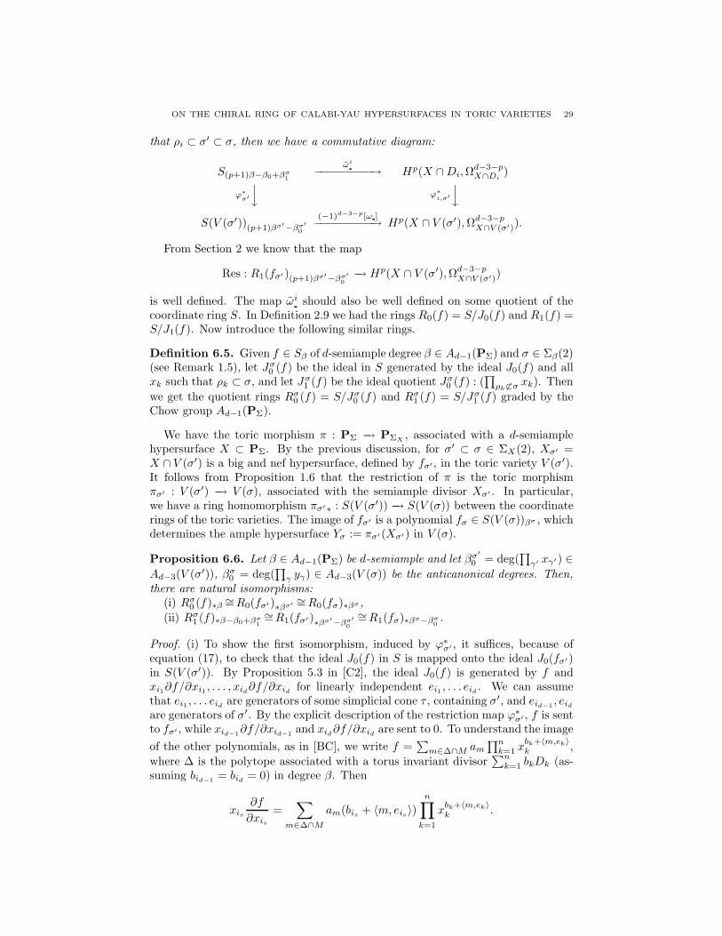
Proposition 6.4. Let X ⊂ PΣ be a d-semiample regular hypersurface defined byf ∈ Sβ. Given ρi ⊂ σ ∈ ΣX(2) such that ρi /∈ ΣX(1), and given σ′ ∈ Σ(2) such
ON THE CHIRAL RING OF CALABI-YAU HYPERSURFACES IN TORIC VARIETIES 29
that ρi ⊂ σ′ ⊂ σ, then we have a commutative diagram:
S(p+1)β−β0+βσ1
ωi
−−−−−−−−−→ Hp(X ∩Di,Ωd−3−pX∩Di
)
ϕ∗σ′
y ϕ∗i,σ′
y
S(V (σ′))(p+1)βσ′−βσ′
0
(−1)d−3−p[ω ]−−−−−−−−−→ Hp(X ∩ V (σ′),Ωd−3−pX∩V (σ′)).
From Section 2 we know that the map
Res : R1(fσ′)(p+1)βσ′−βσ′
0−→ Hp(X ∩ V (σ′),Ωd−3−p
X∩V (σ′))
is well defined. The map ωi should also be well defined on some quotient of thecoordinate ring S. In Definition 2.9 we had the rings R0(f) = S/J0(f) and R1(f) =S/J1(f). Now introduce the following similar rings.
Definition 6.5. Given f ∈ Sβ of d-semiample degree β ∈ Ad−1(PΣ) and σ ∈ Σβ(2)(see Remark 1.5), let Jσ
0 (f) be the ideal in S generated by the ideal J0(f) and allxk such that ρk ⊂ σ, and let Jσ
1 (f) be the ideal quotient Jσ0 (f) : (
∏ρk 6⊂σ xk). Then
we get the quotient rings Rσ0 (f) = S/Jσ
0 (f) and Rσ1 (f) = S/Jσ
1 (f) graded by theChow group Ad−1(PΣ).
We have the toric morphism π : PΣ −→ PΣX, associated with a d-semiample
hypersurface X ⊂ PΣ. By the previous discussion, for σ′ ⊂ σ ∈ ΣX(2), Xσ′ =X ∩ V (σ′) is a big and nef hypersurface, defined by fσ′ , in the toric variety V (σ′).It follows from Proposition 1.6 that the restriction of π is the toric morphismπσ′ : V (σ′) −→ V (σ), associated with the semiample divisor Xσ′ . In particular,we have a ring homomorphism πσ′∗ : S(V (σ′)) −→ S(V (σ)) between the coordinaterings of the toric varieties. The image of fσ′ is a polynomial fσ ∈ S(V (σ))βσ , whichdetermines the ample hypersurface Yσ := πσ′ (Xσ′) in V (σ).
Proposition 6.6. Let β ∈ Ad−1(PΣ) be d-semiample and let βσ′
0 = deg(∏
γ′ xγ′) ∈Ad−3(V (σ′)), βσ
0 = deg(∏
γ yγ) ∈ Ad−3(V (σ)) be the anticanonical degrees. Then,there are natural isomorphisms:
(i) Rσ0 (f)∗β
∼=R0(fσ′ )∗βσ′ ∼=R0(fσ)∗βσ ,
(ii) Rσ1 (f)∗β−β0+βσ
1
∼=R1(fσ′)∗βσ′−βσ′
0
∼=R1(fσ)∗βσ−βσ0.
Proof. (i) To show the first isomorphism, induced by ϕ∗σ′ , it suffices, because of
equation (17), to check that the ideal J0(f) in S is mapped onto the ideal J0(fσ′)in S(V (σ′)). By Proposition 5.3 in [C2], the ideal J0(f) is generated by f andxi1∂f/∂xi1 , . . . , xid
∂f/∂xidfor linearly independent ei1 , . . . eid
. We can assumethat ei1 , . . . eid
are generators of some simplicial cone τ , containing σ′, and eid−1, eid
are generators of σ′. By the explicit description of the restriction map ϕ∗σ′ , f is sent
to fσ′ , while xid−1∂f/∂xid−1
and xid∂f/∂xid
are sent to 0. To understand the image
of the other polynomials, as in [BC], we write f =∑
m∈∆∩M am
∏nk=1 x
bk+〈m,ek〉k ,
where ∆ is the polytope associated with a torus invariant divisor∑n
k=1 bkDk (as-suming bid−1
= bid= 0) in degree β. Then
xis
∂f
∂xis
=∑
m∈∆∩M
am(bis+ 〈m, eis
〉)n∏
k=1
xbk+〈m,ek〉k .
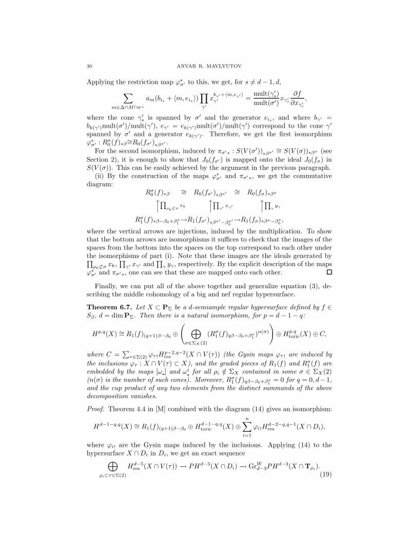
30 ANVAR R. MAVLYUTOV
Applying the restriction map ϕ∗σ′ to this, we get, for s 6= d− 1, d,
∑
m∈∆∩M∩σ⊥
am(bis+ 〈m, eis
〉)∏
γ′
xbγ′+〈m,eγ′ 〉
γ′ =mult(γ′s)
mult(σ′)xγ′
s
∂f
∂xγ′s
,
where the cone γ′s is spanned by σ′ and the generator eis, and where bγ′ =
bk(γ′)mult(σ′)/mult(γ′), eγ′ = ek(γ′)mult(σ′)/mult(γ′) correspond to the cone γ′
spanned by σ′ and a generator ek(γ′). Therefore, we get the first isomorphismϕ∗
σ′ : Rσ0 (f)∗β
∼=R0(fσ′ )∗βσ′ .
For the second isomorphism, induced by πσ′∗ : S(V (σ′))∗βσ′ ∼= S(V (σ))∗βσ (see
Section 2), it is enough to show that J0(fσ′) is mapped onto the ideal J0(fσ) inS(V (σ)). This can be easily achieved by the argument in the previous paragraph.
(ii) By the construction of the maps ϕ∗σ′ and πσ′∗, we get the commutative
diagram:Rσ
0 (f)∗β∼= R0(fσ′)∗βσ′ ∼= R0(fσ)∗βσ
x∏
ρk 6⊂σxk
x∏
γ′ xγ′
x∏
γyγ
Rσ1 (f)∗β−β0+βσ
1→R1(fσ′)∗βσ′−βσ′
0→R1(fσ)∗βσ−βσ
0,
where the vertical arrows are injections, induced by the multiplication. To showthat the bottom arrows are isomorphisms it suffices to check that the images of thespaces from the bottom into the spaces on the top correspond to each other underthe isomorphisms of part (i). Note that these images are the ideals generated by∏
ρk 6⊂σ xk,∏
γ′ xγ′ and∏
γ yγ , respectively. By the explicit description of the mapsϕ∗
σ′ and πσ′∗, one can see that these are mapped onto each other.
Finally, we can put all of the above together and generalize equation (3), de-scribing the middle cohomology of a big and nef regular hypersurface.
Theorem 6.7. Let X ⊂ PΣ be a d-semiample regular hypersurface defined by f ∈Sβ, d = dimPΣ. Then there is a natural isomorphism, for p = d− 1− q:
Hp,q(X) ∼= R1(f)(q+1)β−β0⊕( ⊕
σ∈ΣX (2)
(Rσ1 (f)qβ−β0+βσ
1)n(σ)
)⊕Hp,q
toric(X)⊕ C,
where C =∑
τ∈Σ(2) ϕτ !Hp−2,q−2res (X ∩ V (τ)) (the Gysin maps ϕτ ! are induced by
the inclusions ϕτ : X ∩ V (τ) ⊂ X), and the graded pieces of R1(f) and Rσ1 (f) are
embedded by the maps [ω ] and ωi for all ρi /∈ ΣX contained in some σ ∈ ΣX(2)(n(σ) is the number of such cones). Moreover, Rσ
1 (f)qβ−β0+βσ1
= 0 for q = 0, d−1,and the cup product of any two elements from the distinct summands of the abovedecomposition vanishes.
Proof. Theorem 4.4 in [M] combined with the diagram (14) gives an isomorphism:
Hd−1−q,q(X) ∼= R1(f)(q+1)β−β0⊕Hd−1−q,q
toric (X)⊕n∑
i=1
ϕi!Hd−2−q,q−1res (X ∩Di),
where ϕi! are the Gysin maps induced by the inclusions. Applying (14) to thehypersurface X ∩Di in Di, we get an exact sequence
⊕
ρi⊂τ∈Σ(2)
Hd−5res (X ∩ V (τ)) −→ PHd−3(X ∩Di) −→ GrW
d−3PHd−3(X ∩Tρi
).(19)
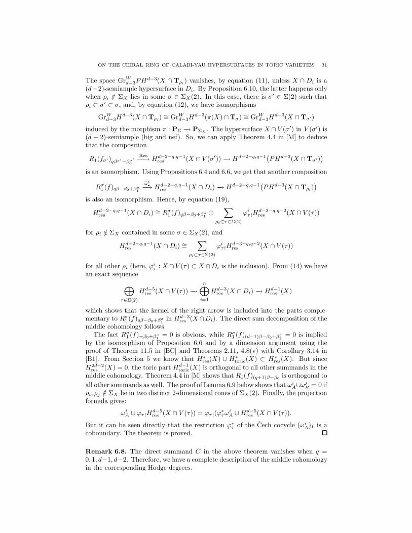
ON THE CHIRAL RING OF CALABI-YAU HYPERSURFACES IN TORIC VARIETIES 31
The space GrWd−3PH
d−3(X ∩ Tρi) vanishes, by equation (11), unless X ∩ Di is a
(d−2)-semiample hypersurface in Di. By Proposition 6.10, the latter happens onlywhen ρi /∈ ΣX lies in some σ ∈ ΣX(2). In this case, there is σ′ ∈ Σ(2) such thatρi ⊂ σ′ ⊂ σ, and, by equation (12), we have isomorphisms
GrWd−3H
d−3(X ∩Tρi) ∼= GrW
d−3Hd−3(π(X) ∩Tσ) ∼= GrW
d−3Hd−3(X ∩Tσ′)
induced by the morphism π : PΣ −→ PΣX. The hypersurface X ∩ V (σ′) in V (σ′) is
(d − 2)-semiample (big and nef). So, we can apply Theorem 4.4 in [M] to deducethat the composition
R1(fσ′)qβσ′−βσ′
0
Res−−→ Hd−2−q,q−1res (X ∩ V (σ′)) −→ Hd−2−q,q−1
(PHd−3(X ∩Tσ′)
)
is an isomorphism. Using Propositions 6.4 and 6.6, we get that another composition
Rσ1 (f)qβ−β0+βσ
1
ωi
−→ Hd−2−q,q−1res (X ∩Di) −→ Hd−2−q,q−1
(PHd−3(X ∩Tρi
))
is also an isomorphism. Hence, by equation (19),
Hd−2−q,q−1res (X ∩Di) ∼= Rσ
1 (f)qβ−β0+βσ1⊕
∑
ρi⊂τ∈Σ(2)
ϕiτ !H
d−3−q,q−2res (X ∩ V (τ))
for ρi /∈ ΣX contained in some σ ∈ ΣX(2), and
Hd−2−q,q−1res (X ∩Di) ∼=
∑
ρi⊂τ∈Σ(2)
ϕiτ !H
d−3−q,q−2res (X ∩ V (τ))
for all other ρi (here, ϕiτ : X ∩ V (τ) ⊂ X ∩Di is the inclusion). From (14) we have
an exact sequence
⊕
τ∈Σ(2)
Hd−5res (X ∩ V (τ)) −→
n⊕
i=1
Hd−3res (X ∩Di) −→ Hd−1
res (X)
which shows that the kernel of the right arrow is included into the parts comple-mentary to Rσ
1 (f)qβ−β0+βσ1
in Hd−3res (X ∩Di). The direct sum decomposition of the
middle cohomology follows.The fact Rσ
1 (f)−β0+βσ1
= 0 is obvious, while Rσ1 (f)(d−1)β−β0+βσ
1= 0 is implied
by the isomorphism of Proposition 6.6 and by a dimension argument using theproof of Theorem 11.5 in [BC] and Theorems 2.11, 4.8(v) with Corollary 3.14 in[B1]. From Section 5 we know that H∗
res(X) ∪ H∗toric(X) ⊂ H∗
res(X). But since
H2d−2res (X) = 0, the toric part Hd−1
toric(X) is orthogonal to all other summands in themiddle cohomology. Theorem 4.4 in [M] shows that R1(f)(q+1)β−β0
is orthogonal to
all other summands as well. The proof of Lemma 6.9 below shows that ωiA∪ω
jB = 0 if
ρi, ρj /∈ ΣX lie in two distinct 2-dimensional cones of ΣX(2). Finally, the projectionformula gives:
ωiA ∪ ϕτ !H
d−5res (X ∩ V (τ)) = ϕτ !(ϕ
∗τω
iA ∪Hd−5
res (X ∩ V (τ)).
But it can be seen directly that the restriction ϕ∗τ of the Cech cocycle (ωi
A)I is acoboundary. The theorem is proved.
Remark 6.8. The direct summand C in the above theorem vanishes when q =0, 1, d−1, d−2. Therefore, we have a complete description of the middle cohomologyin the corresponding Hodge degrees.
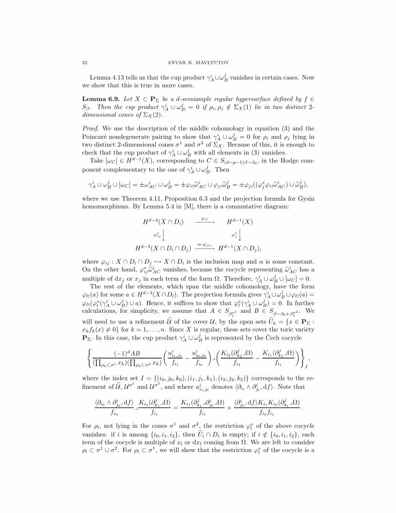
32 ANVAR R. MAVLYUTOV
Lemma 4.13 tells us that the cup product γiA∪ω
jB vanishes in certain cases. Now
we show that this is true in more cases.
Lemma 6.9. Let X ⊂ PΣ be a d-semiample regular hypersurface defined by f ∈Sβ. Then the cup product γi
A ∪ ωjB = 0 if ρi, ρj /∈ ΣX(1) lie in two distinct 2-
dimensional cones of ΣX(2).
Proof. We use the description of the middle cohomology in equation (3) and the
Poincare nondegenerate pairing to show that γiA ∪ ωj
B = 0 for ρi and ρj lying intwo distinct 2-dimensional cones σ1 and σ2 of ΣX . Because of this, it is enough tocheck that the cup product of γi
A ∪ ωjB with all elements in (3) vanishes.
Take [ωC ] ∈ Hd−1(X), corresponding to C ∈ S(d−p−1)β−β0, in the Hodge com-
ponent complementary to the one of γiA ∪ ω
jB. Then
γiA ∪ ωj
B ∪ [ωC ] = ±ωiAC ∪ ωj
B = ±ϕi!ωiAC ∪ ϕj !ω
jB = ±ϕj !((ϕ
∗jϕi!ω
iAC) ∪ ωj
B),
where we use Theorem 4.11, Proposition 6.3 and the projection formula for Gysinhomomorphisms. By Lemma 5.4 in [M], there is a commutative diagram:
Hd−3(X ∩Di)ϕi!−−−−→ Hd−1(X)
ϕ∗ij
y ϕ∗j
y
Hd−3(X ∩Di ∩Dj)α·ϕji!−−−−→ Hd−1(X ∩Dj),
where ϕij : X ∩Di ∩ Dj → X ∩ Di is the inclusion map and α is some constant.On the other hand, ϕ∗
ij ωiAC vanishes, because the cocycle representing ωi
AC has a
multiple of dxj or xj in each term of the form Ω. Therefore, γiA ∪ ω
jB ∪ [ωC ] = 0.
The rest of the elements, which span the middle cohomology, have the formϕl!(a) for some a ∈ Hd−3(X ∩Dl). The projection formula gives γi
A∪ωjB ∪ϕl!(a) =
ϕl!(ϕ∗l (γ
iA ∪ ω
jB) ∪ a). Hence, it suffices to show that ϕ∗
l (γiA ∪ ω
jB) = 0. In further
calculations, for simplicity, we assume that A ∈ Sβσ1
1and B ∈ S
β−β0+βσ2
1. We
will need to use a refinement U of the cover U , by the open sets Uk = x ∈ PΣ :xkfk(x) 6= 0 for k = 1, . . . , n. Since X is regular, these sets cover the toric variety
PΣ. In this case, the cup product γiA ∪ ω
jB is represented by the Cech cocycle
(−1)dAB
(∏
ρk⊂σ1 xk)(∏
ρk⊂σ2 xk)
(ui
i1,j1
fi1
−ui
i0,j0
fi0
)y
(Ki2(∂
jk2
yΩ)
fi2
−Ki1(∂
jk1
yΩ)
fi1
)
I
,
where the index set I = (i0, j0, k0), (i1, j1, k1), (i2, j2, k2) corresponds to the re-
finement of U , Uσ1
and Uσ2
, and where uiit,jt
denotes 〈∂it∧ ∂i
jt, df〉. Note that
〈∂i0 ∧ ∂ij0, df〉
fi0
y
Ki1(∂jk1
yΩ)
fi1
=Ki1(∂
jk1
y∂ij0
yΩ)
fi1
+〈∂i
j0, df〉Ki1Ki0(∂
jk1
yΩ)
fi0fi1
.
For ρl, not lying in the cones σ1 and σ2, the restriction ϕ∗l of the above cocycle
vanishes: if i is among i0, i1, i2, then Ui ∩ Di is empty; if i /∈ i0, i1, i2, eachterm of the cocycle is multiple of xl or dxl coming from Ω. We are left to considerρl ⊂ σ1 ∪ σ2. For ρl ⊂ σ1, we will show that the restriction ϕ∗
l of the cocycle is a
ON THE CHIRAL RING OF CALABI-YAU HYPERSURFACES IN TORIC VARIETIES 33
Cech coboundary; the other case is similar. Compute
(ui
i1,j1
fi1
−ui
i0,j0
fi0
)y
(Ki2(∂
jk2
yΩ)
fi2
−Ki1(∂
jk1
yΩ)
fi1
)
=∑
I=I\(is,js,ks)
(−1)s
(Ki1(∂j
k1y(∂i
j0− ∂i
j1)yΩ)
fi1
+〈∂i
j0, df〉Ki1
Ki0(∂j
k0yΩ)
fi0fi1
).
Using this, we can see that the restriction ϕ∗l (γ
iA ∪ ωj
B) is represented by a Cechcoboundary because of the following observations. The polynomial 〈∂i
j0, df〉 is
divisible by xl. If ρl 6⊂ σ1jt
, then the restricted open set Uσ1jt
∩Dl is empty. If σ1j0
and σ1j1
contain ρl, then Ki1(∂i
j0− ∂i
j1)yΩ is either 0 or divisible by xl because of
equation (7). Thus, the restriction ϕ∗l (γ
iA ∪ ωj
B) = 0, and the result follows.
At this point, let us summarize our calculations of the cup productsH∗(X,∧∗TX)
with the middle cohomology H∗(X,Ωd−1−∗X ) for d-semiample regular hypersur-
faces. We have the elements in H∗(X,∧∗TX) represented by γ , γi (with ρi ly-ing in some σ ∈ ΣX(2) such that ρi /∈ ΣX), and the corresponding elements in
H∗(X,Ωd−1−∗X ) represented by ω , ωi. Theorem 3.4 provides γA ∪ ωB = ωAB,
while Theorems 4.11 and 4.12 have γA ∪ ωiB = ωi
AB and γiA ∪ ωB = ωi
AB. Lem-
mas 4.13 and 6.9 tell us that the cup product γiA∪ωj
B = 0, for i 6= j, unless ρi and ρj
span a 2-dimensional cone of Σ. Thus, for the constructed elements inH∗(X,∧∗TX)
and H∗(X,Ωd−1−∗X ), we are missing only the cup products γi
A ∪ ωjB when ρi and
ρj (i may be equal to j) span a cone of Σ contained in some 2-dimensional cone ofΣX .
First, we consider the nontrivial cup products γiA ∪ ω
jB lying in Hd−1(X,OX),
which is isomorphic to R1(f)dβ−β0 , by Theorem 6.7. We note here that the inclusion
µ : R1(f)dβ−β0
∏n
k=1xk−−−−−−→ R0(f)dβ (20)
induced by the multiplication is an isomorphism because the dimensions of thespaces is the same number (of the interior integral points of a polytope ∆ corre-sponding to β) by the isomorphism R1(f)dβ−β0 = H0,d−1(Hd−1(X ∩ T)) of [M,Theorem 4.4], by [DK, Section 5.8], and by [BC, Theorem 11.5] with [B2, Corol-lary 3.14]. The cup product should be represented by a polynomial in the abovespaces.
Proposition 6.10. Let X ⊂ PΣ be a d-semiample regular hypersurface defined byf ∈ Sβ, and denote
Gσ(f) :=xsfsxtft
∏ρk 6⊂σ xk
mult(σ)∏
ρk⊂σ xk∈ S2β+β0−2βσ
1
for σ ∈ ΣX(2) spanned by ρs and ρt. Given A ∈ S(p−1)β+βσ1, B ∈ S(d−1−p)β−β0+βσ
1,
then(i) for ρi = ρlk /∈ ΣX , as in (6), contained in σ ∈ ΣX(2):
γiA ∪ ωi
B =mult(σk + σk+1)[ωµ−1(ABGσ(f))]
mult(σk)mult(σk+1)in Hd−1(X,OX),
34 ANVAR R. MAVLYUTOV
(ii) for ρi, ρj /∈ ΣX which span a 2-dimensional cone σ′ ∈ Σ contained in σ ∈ΣX(2):
γiA ∪ ωj
B = − [ωµ−1(ABGσ(f))]
mult(σ′)in Hd−1(X,OX).
Proof. To simplify the proof we assume that p = 1.(i) After a simple modification it follows that the cup product γi
A ∪ ωiB is repre-
sented by the cocycle
(−1)d+((d−3)2/2)AB
(∏
ρk⊂σ xk)2
∑
I=I\(ik,jk)
(−1)k〈∂i0∧ ∂i
j0, df〉
fi0
y
Kid−2· · ·Ki1
(∂ij1
yΩ)
fi1· · · fid−2
I
,
where I = (i0, j0), . . . , (id−1, jd−1) is the index set corresponding to the open sets
Uik(defined in Lemma 6.9) and Uσjk
. Note that
AB
(∏
ρk⊂σ xk)2
〈∂i0∧ ∂i
j0, df〉
fi0
y
Kid−2· · ·Ki1
(∂ij1
yΩ)
fi1· · · fid−2
=(−1)d−1AB
(∏
ρk⊂σ xk)2
(〈∂i
j0, df〉
Kid−2· · ·Ki0
(∂ij1
yΩ)
fi0· · · fid−2
+Kid−2
· · ·Ki1(∂i
j1y∂i
j0yΩ)
fi1· · · fid−2
).
The first summand is well defined on the corresponding open set: if i ∈ i0, . . . , id−2,then xi 6= 0 on the open set; otherwise, 〈∂i
j0, df〉Kid−2
· · ·Ki0(∂i
j1yΩ) is a multiple
of (xi)2. Therefore, the corresponding sum in the above cocycle forms a Cech
coboundary, and γiA ∪ ωi
B is represented by
(−1)1+((d−3)2/2)AB
(∏
ρk⊂σ xk)2
∑
I=I\(ik,jk)
(−1)kKid−2
· · ·Ki1(∂i
j1y∂i
j0yΩ)
fi1· · · fid−2
I
.
By Proposition 5.3 in [C2], the polynomials xr0fr0 , . . . , xrd−1frd−1
do not vanishsimultaneously on X if er0 , . . . , erd−1
are linearly independent. We can always findsuch generators so that er0 = el0 and er1 = eln(σ)+1
as in (6). Since the open sets
x ∈ PΣ : xrkfrk6= 0 cover the toric variety, we can assume that the first index in
I takes only the ordered values r0, . . . , rd−1. In this case, it is not difficult to checkthat the above cocycle is different by a coboundary from
(−1)1+((d−3)2/2)AB
(∏
ρk⊂σ xk)2
∑
I=I\(ik,jk)
(−1)kαI
Kid−2· · ·Ki1
(∂lk+1y∂lk−1
yΩ)
fi1· · · fid−2
mult(σk)mult(σk+1)
I
,
where
αI =
−1 if i0 = i1 = r2, j0 ≤ k < k + 1 ≤ j1−1 if i0 = r1, i1 = r2, j1 ≥ k + 1
1 if i0 = r0, i1 = r2, j1 ≤ k0 in all other cases.
Using the Euler identities in the proof of Proposition 6.3, the last cocycle convertsto
mult(σk + σk+1)
mult(σk)mult(σk+1)
(−1)(d−3)2/2ABxl0fl0xln(σ)+1
fln(σ)+1
mult(σ)(∏
ρk⊂σ xk)2Kid−1
· · ·Ki0Ω
fi0 · · · fid−1
I
.
ON THE CHIRAL RING OF CALABI-YAU HYPERSURFACES IN TORIC VARIETIES 35
This cocycle represents
mult(σk + σk+1)[ωµ−1(ABGσ(f))]
mult(σk)mult(σk+1)
in Hd−1(X,OX).(ii) Similar to the proof of the previous part and Lemma 6.9, the cup product
γiA ∪ ω
jB is represented by the following cocycle:
(−1)1+((d−3)2/2)AB
(∏
ρk⊂σ xk)2
∑
I=I\(ik,jk)
(−1)kKid−2
· · ·Ki1(∂j
j1y(∂i
j0− ∂i
j1)yΩ)
fi1· · · fid−2
I
.
The 1-dimensional cones ρi and ρj span one of the 2-dimensional cones σk ⊂ σ asin in (6). The cocycle differs by a coboundary from
(−1)1+((d−3)2/2)AB
(∏
ρk⊂σ xk)2
∑
I=I\(ik,jk)
(−1)kαI
−Kid−2· · ·Ki1
(∂lky∂lk−1yΩ)
fi1· · · fid−2
mult(σk)2
I
,
where αI is the same as in part (i). The Euler identities show that this represents
−[ωµ−1(ABGσ(f))]
mult(σk)∈ Hd−1(X,OX).
The restriction maps ϕ∗l , induced by the inclusions ϕl : X ∩ Dl → X , give
some information about the nontrivial cup products γiA ∪ωi
B in Hd−1(X). We willuse this in Section 7 to calculate nontrivial triple products on the chiral ring ofanticanonical hypersurfaces.
Proposition 6.11. Let X ⊂ PΣ be a d-semiample regular hypersurface defined byf ∈ Sβ, and let, as in (6), ρi = ρlk /∈ ΣX be in some σ ∈ ΣX(2). Then, forA ∈ Spβ+βσ
1and B ∈ Sqβ−β0+βσ
1,
(i) ϕ∗lk±1
(γiA ∪ ωi
B) = ±ϕ∗lk±1
(ωi
ABHσi,±1
(f)
), where Hσ
i,±1(f) is a polynomial in
Sβ−βσ1
equal to√−1xlk±1
flk±1/(mult(σk,k±1)
∏ρk⊂σ xk) at xlk = 0 and xlk±1
= 0,where σs,t denotes the cone spanned by ρls and ρlt.
(ii) ϕ∗i (γ
iA ∪ ωi
B) = ϕ∗i
(ωi
ABHσi(f)
), where Hσ
i (f) is a polynomial in Sβ−βσ1
equal
to √−1xlk+1
flk+1
mult(σk,k+1)∏
ρk⊂σ xk−
√−1xlk−1
flk−1
mult(σk−1,k)∏
ρk⊂σ xk
with xi = xlk−1= xlk+1
= 0.
Proof. For simplicity, we assume that A ∈ Sβσ1
and B ∈ Sβ−β0+βσ1. The cup
product γiA ∪ ωi
B is represented by the Cech cocycle:
(−1)dAB
(∏
ρk⊂σ xk)2
(ui
i1,j1
fi1
−ui
i0,j0
fi0
)y
(Ki2(∂
jk2
yΩ)
fi2
−Ki1(∂
jk1
yΩ)
fi1
)
I
,(21)
36 ANVAR R. MAVLYUTOV
where uiik,jk
denotes 〈∂ik∧ ∂i
jk, df〉, and I = (i0, j0), (i1, j1), (i2, j2) is the index
set. Compute
〈∂i0 ∧ ∂ij0 , df〉
fi0
y
Ki1(∂ij1yΩ)
fi1
=Ki1(∂
ij1y∂
ij0yΩ)
fi1
+〈∂i
j0 , df〉Ki1Ki0(∂ij1yΩ)
fi0fi1
=Ki0(∂
ij1
y∂ij0
yΩ)
fi0
+〈∂i
j1, df〉Ki1Ki0(∂
ij0
yΩ)
fi0fi1
+Ki1Ki0(∂
ij1
y∂ij0
y(df ∧Ω)
fi0fi1
≡Ki0(∂
ij1
y∂ij0
yΩ)
fi0
+〈∂i
j1, df〉Ki1Ki0(∂
ij0
yΩ)
fi0fi1
,
where, as in Lemma 4.10, we used df ∧ Ω ≡ 0 modulo multiples of f . Hence, thecup product γi
A ∪ ωiB is represented by the Cech cocycle
(−1)dAB
(∏
ρk⊂σ xk)2
∑
I=I\(is,js)
(−1)s
(Ki0(∂i
j1y∂i
j0yΩ)
fi0
+〈∂i
j1, df〉Ki1
Ki0(∂i
j0yΩ)
fi0fi1
)
I
.
For part (i), consider the restriction ϕ∗lk±1
of this cocycle. Note that the open
set Uσj∩ Dlk±1
is empty, if σj does not contain ρlk±1, and that ∂i
j = 0, if the
corresponding cone σj does not contain ρi. Using this and ∂ij ∧ ∂i
j = 0, we get that
the restriction ϕ∗lk±1
of γiA ∪ ωi
B is represented by
±√−1
(−1)d+(1/2)AB
(∏
ρk⊂σ xk)2
∑
I=I\(is,js)
(−1)s xlk±1flk±1
mult(σk,k±1)
Ki1Ki0
(∂ij0
yΩ)
fi0fi1
I
,(22)
where the index set I corresponds to the restricted open cover Uσ|X∩Dlk±1, and
where σk,k±1 is the cone generated by elk and elk±1. Notice that this cocycle is
similar to the restriction ϕ∗lk±1
(ωiC) for some polynomial C. The problem here is
that xlk±1flk±1
is not necessarily divisible by∏
ρk⊂σ xk. So some work is required toget the correct polynomial. Let X be linearly equivalent to a torus invariant divisorD =
∑nk=1 bkDk with the associated polytope ∆ = ∆D given by the conditions
bl + 〈m, el〉 ≥ 0 . Then we can write f =∑
m∈∆∩M amxD(m), where xD(m) denotes∏n
l=1 xbl+〈m,el〉l . Note that
xlk±1flk±1
=∑
m∈∆∩M
am(blk±1+ 〈m, elk±1
〉)xD(m).
If blk±1+ 〈m, elk±1
〉 = 0, then the corresponding monomial xD(m) is not presentin xlk±1
flk±1. On the other hand, if blk±1
+ 〈m, elk±1〉 > 1, then the multiple of
the corresponding monomial xD(m) in (22) vanishes, since ∂ij0
= ∓xlk±1∂lk±1
or 0.
By the argument in the proof of Lemma 4.2, blk±1+ 〈m, elk±1
〉 = 1 implies thatbl + 〈m, el〉 > 0 for all ρl ⊂ σ such that ρl /∈ ΣX(1). If bi + 〈m, ei〉 > 1, themultiple of the monomial xD(m) in (22) forms a coboundary. Therefore, only themonomials xD(m) in xlk±1
flk±1, satisfying blk±1
+〈m, elk±1〉 = 1 and bi+〈m, ei〉 = 1,
have a nontrivial contribution in the Cech cocycle (22). For all such monomials,it follows from the relations of the cone generators in the proof of Proposition 6.3that bs + 〈m, es〉 > 0 with s = l0, ln(σ)+1. Hence, the monomials are divisible by∏
ρk⊂σ xk. Thus, ϕ∗lk±1
(γiA ∪ ωi
B) = ±ϕ∗lk±1
(ωi
ABHσi,±1
(f)
), where Hσ
i,±1(f) is the
ON THE CHIRAL RING OF CALABI-YAU HYPERSURFACES IN TORIC VARIETIES 37
polynomial
∑
m
√−1∑
m amxD(m)
mult(σk,k±1)∏
ρk⊂σ xk
with the sum over all m ∈ ∆ ∩M , satisfying the equalities blk±1+ 〈m, elk±1
〉 = 1
and bi + 〈m, ei〉 = 1. This is the same as√−1xlk±1
flk±1/(mult(σk,k±1)
∏ρk⊂σ xk)
evaluated at xi = 0 and xlk±1= 0.
In part (ii) we will need to use the refinement U of the cover U defined inLemma 6.9. From (21) we get that the cup product γi
A ∪ ωiB is represented by the
Cech cocycle
(−1)dAB
(∏
ρk⊂σ xk)2
∑
I=I\(is,js)
(−1)s
(Ki1(∂i
j1y∂i
j0yΩ)
fi1
+〈∂i
j0, df〉Ki1
Ki0(∂i
j1yΩ)
fi0fi1
)
I
,
where the index set I = (i0, j0), (i1, j1), (i2, j2) corresponds to the refinement of
U and Uσ|X . Notice
Ki1(∂ij1
y∂ij0
yΩ)
fi1
−Ki2(∂
ij1
y∂ij0
yΩ)
fi2
=〈∂i
j0, df〉Ki2Ki1(∂
ij1
yΩ)
fi1fi2
−〈∂i
j1, df〉Ki2Ki1(∂
ij0
yΩ)
fi1fi2
−Ki2Ki1(∂
ij1
y∂ij0
y(df ∧ Ω)
fi1fi2
≡〈∂i
j0, df〉Ki2Ki1(∂
ij1
yΩ)
fi1fi2
−〈∂i
j1, df〉Ki2Ki1(∂
ij0
yΩ)
fi1fi2
,
since df ∧ Ω ≡ 0 modulo multiples of f . Using this, we compute
AB
(∏
ρk⊂σ xk)2
∑
I=I\(is,js)
(−1)s
(Ki1(∂i
j1y∂i
j0yΩ)
fi1
+〈∂i
j0, df〉Ki1
Ki0(∂i
j1yΩ)
fi0fi1
)
=∑
I=I\(is,js)
(−1)sAB〈∂i
j0, df〉Ki1
Ki0((∂i
j1− ∂i
j0)yΩ)
(∏
ρk⊂σ xk)2fi0fi1
+ABKi2((∂
ij0∧ ∂i
j1− ∂i
j0∧ ∂i
j2+ ∂i
j1∧ ∂i
j2)yΩ)
(∏
ρk⊂σ xk)2fi2
+AB〈∂i
j1 , df〉(∏
ρk⊂σ xk)2
(Ki2Ki0(∂
ij0yΩ)
fi0fi2
−Ki1Ki0(∂
ij0yΩ)
fi0fi1
−Ki2Ki1(∂
ij0yΩ)
fi1fi2
)
+AB(〈∂i
j0 , df〉+ 〈∂ij1 , df〉)
(∏
ρk⊂σ xk)2
( ∑
I=I\(is,js)
(−1)sKi1
Ki0(∂i
j0yΩ)
fi0fi1
).
It is not difficult to see that the first summand produces a coboundary. The openset Uσj
∩Di is empty unless σj contains ρi. Therefore, applying the restriction ϕ∗i ,
we can assume that the second component of the index (i0, j0) takes only valueslk−1 or lk+1. In this case, ∂i
j0∧ ∂i
j1− ∂i
j0∧ ∂i
j2+ ∂i
j1∧ ∂i
j2(and the corresponding
summand in the cocycle) vanishes. The third summand also ends up contributing
38 ANVAR R. MAVLYUTOV
zero:
AB〈∂ij1, df〉
(∏
ρk⊂σ xk)2
(Ki2Ki0(∂
ij0
yΩ)
fi0fi2
−Ki1Ki0(∂
ij0
yΩ)
fi0fi1
−Ki2Ki1(∂
ij0
yΩ)
fi1fi2
)
=AB〈∂i
j1, df〉
(∏
ρk⊂σ xk)2
( 〈∂ij0, df〉Ki2Ki1Ki0Ω
fi0fi1fi2
+Ki2Ki1Ki0∂
ij0
y(df ∧ Ω)
fi0fi1fi2
)
≡AB〈∂i
j0, df〉〈∂i
j1, df〉
(∏
ρk⊂σ xk)2Ki2Ki1Ki0Ω
fi0fi1fi2
.
If i is among i0, i1, i2, then this restricts to an empty set since Ui ∩Di is empty.In the opposite case, this gives 0 under the restriction since xi or dxi is present ineach term of Ω. Thus, the restriction ϕ∗
i (γiA ∪ ωi
B) is represented by the cocycle
(−1)dAB(〈∂i
j0, df〉+ 〈∂i
j1, df〉)
(∏
ρk⊂σ xk)2
∑
I=I\(is,js)
(−1)sKi1
Ki0(∂i
j0yΩ)
fi0fi1
I
,
where the index set I now corresponds to the open cover Uσ|X∩Di. However, the
last calculation shows that if j0 coincides with j1, then the expression in the abovecocycle vanishes on the given open set. Hence, this cocycle is the same as
(−1)dAB
(∏
ρk⊂σ xk)2
(xlk−1
flk−1
mult(σk)− xlk+1
flk+1
mult(σk+1)
) ∑
I=I\(is,js)
(−1)sKi1
Ki0(∂i
j0yΩ)
fi0fi1
I
.
By the arguments similar to part (i), one can show that this coincides with therestriction ϕ∗
i
(ωi
ABHσi(f)
), where Hσ
i (f) is equal to
√−1xlk+1
flk+1
mult(σk,k+1)∏
ρk⊂σ xk−
√−1xlk−1
flk−1
mult(σk−1,k)∏
ρk⊂σ xk
at xlk = xlk−1= xlk+1
= 0.
Remark 6.12. In the anticanonical case β = β0 the polynomials Hσi,±1(f), Hσ
i (f)
of the above proposition can be written in a simpler form. Let D =∑n
k=1Dk
be the anticanonical divisor with the associated polytope ∆ := ∆D. For f =∑m∈∆∩M amx
D(m) and σ ∈ ΣX(2), denote
Hσ(f) :=√−1
∑
m∈σ⊥∩∆∩M
amxD(m)
∏ρk⊂σ xk
.
Then Hσi,±1(f) = Hσ(f)/mult(σk,k±1) and
Hσi (f) =
(1
mult(σk+1)− 1
mult(σk)
)Hσ(f).
7. The chiral ring for anticanonical hypersurfaces
Here, we will apply the results of the previous sections to explicitly describe asubring of the chiral ring H∗(X,∧∗TX), coming from the graded pieces of R1(f)and Rσ
1 (f), for semiample anticanonical regular hypersurfaces. By Proposition 2.6,such hypersurfaces are Calabi-Yau. The description of the chiral ring is completefor Calabi-Yau threefolds.
ON THE CHIRAL RING OF CALABI-YAU HYPERSURFACES IN TORIC VARIETIES 39
Let PΣ be a complete simplicial toric variety, and let X ⊂ PΣ be a big and nefregular hypersurface defined by f ∈ Sβ . From Theorem 6.7, we know the followingpart of the middle cohomology of X :
[ω ]⊕ (⊕iωi) : R1(f)(∗+1)β−β0
⊕( ⊕
σ∈ΣX (2)
(Rσ
1 (f)∗β−β0+βσ1
)n(σ)
)→ Hd−1−∗,∗(X).
Now suppose that β is the anticanonical degree β0. In this case, the isomorphism(5) and Theorems 3.4, 4.11 give us:
Theorem 7.1. Let X ⊂ PΣ be a semiample anticanonical regular hypersurfacedefined by f ∈ Sβ. Then there is a natural inclusion
γ ⊕ (⊕iγi) : R1(f)∗β ⊕
( ⊕
σ∈ΣX (2)
(Rσ
1 (f)(∗−1)β+βσ1
)n(σ)
)→ H∗(X,∧∗TX),
where the sum ⊕iγi is over ρi ⊂ σ ∈ ΣX(2) such that ρi /∈ ΣX and n(σ) is the
number of such cones. Also, Rσ1 (f)(q−1)β+βσ
1= 0 for q = 0, d− 1.
Remark 7.2. The map given by γ ⊕ (⊕iγi) is an isomorphism onto Hq(X,∧qTX)
if q = 0, 1, d − 2, d − 1 and d 6= 1, 3. In particular, for semiample anticanonicalregular hypersurfaces of dimension 3, we get a complete description of the chiralring.
We claim that the part of H∗(X,∧∗TX) given in the above theorem is a sub-ring. Let us describe the product structure on this part. First, note that the ring⊕pH
p(X,∧pTX) is commutative. Theorems 3.3, 4.7, Lemmas 4.8, 6.9 and equation
(5) give us all information about the ring structure except for the products γiA∪γ
jB
when ρi and ρj span a cone of Σ contained in some 2-dimensional cone σ ∈ ΣX . For
such ρi and ρj , we first show that γiA ∪ ω
jB is in the part of the middle cohomology
represented by [ω ]⊕ (⊕kωk). It is easy to see that γi
A ∈ H∗(X,∧∗TX) can be liftedto γ in H∗(PΣ,∧∗TPΣ) with respect to the maps of Lemma 3.6. Using this lemma,for h ∈ Hd−1(PΣ), we have
γiA ∪ ωj
B ∪ i∗h = ±γiA ∪ i∗h ∪ ωj
B = ±i∗(γ ∪ h) ∪ ωjB = 0
since the toric part is orthogonal to the residue part in the middle cohomology.
Similarly, ϕ∗τγ
iA = η∗γi
A for a corresponding γiA ∈ H∗(X ∩ V (τ),∧∗TX∩V (τ)), τ ∈
Σ(2). Therefore, for h′ ∈ Hd−5(X ∩ V (τ)),
γiA∪ωj
B∪ϕτ !h′ = ϕτ !(ϕ
∗τ (γi
A∪ωjB)∪h′ = ϕτ !(γ
iA∪ϕ∗
τωjB∪h′) = ±ϕτ !(γ
iA∪h′)∪ω
jB = 0
where we use the projection formula for Gysin homomorphisms and Theorem 6.7.Hence, by the same Theorem and because of the nondegenerate pairing on themiddle cohomology, the cup product γi
A∪ωjB lies in the space given by [ω ]⊕(⊕kω
k).
By the isomorphism (5), the cup product γiA ∪ γ
jB is in the part of the chiral ring
described in Theorem 7.1. Thus, this part is a subring of H∗(X,∧∗TX).Since X is Calabi-Yau, we have natural isomorphisms
Hd−1(X,∧d−1TX) ∼= Hd−1(X,OX) ∼= H0(X,Ωd−1X ) ∼= C.
The cup product on the middle cohomology induces a nondegenerate pairing on thechiral ring and its subring represented by γ ⊕ (⊕kγ
k). Therefore, one can recoverthe product structure of the subring, knowing the triple products on this subring.
40 ANVAR R. MAVLYUTOV
Because of Lemmas 4.8 and 6.9 it suffices to consider the product of three elementsγi
A ∪ γjB ∪ γl
C ∈ Hd−1(X,∧d−1TX) in the cases i = j = l and i = j with l suchthat ρi, ρl span a 2-dimensional cone of Σ contained in some σ ∈ ΣX(2). For this,compute
(γiA ∪ γi
B ∪ γiC ∪ [ω1]) ∪ [ω1] = εγi
A ∪ ωiB ∪ ωi
C = εγiA ∪ ωi
B ∪ ϕi!ωiC
= εϕi!(ϕ∗i (γ
iA ∪ ωi
B) ∪ ωiC) = εϕi!((ϕ
∗i ω
iABHσ
i(f)) ∪ ωi
C)
= εωiABHσ
i(f) ∪ ϕi!ω
iC = εωi
ABHσi(f) ∪ ωi
C = (γiABHσ
i(f) ∪ ωi
C) ∪ [ω1]
=mult(σk + σk+1)[ωµ−1(ABCHσ
i(f)Gσ(f))] ∪ [ω1]
mult(σk)mult(σk+1),
where we used Propositions 6.3, 6.11, 6.10 and the projection formula for Gysinhomomorphisms, and where ε is a sign depending on the degree of C. Similarly, inthe other case (as in (6), ρi = ρlk):
(γiA ∪ γi
B ∪ γlk±1
C ∪ [ω1]) ∪ [ω1] = εγiA ∪ ωi
B ∪ ωlk±1
C = εγiA ∪ ωi
B ∪ ϕlk±1 !ω
lk±1
C
= εϕlk±1 !(ϕ∗
lk±1(γi
A ∪ ωiB) ∪ ωlk±1
C ) = ±εϕlk±1 !((ϕ∗
lk±1ωi
ABHσi,±1
(f)) ∪ ωlk±1
C )
= ±εωiABHσ
i,±1(f) ∪ ω
lk±1
C = ±(γiABHσ
i,±1(f) ∪ ω
lk±1
C ) ∪ [ω1]
= ∓[ωµ−1(ABCHσ
i,±1(f)Gσ(f))] ∪ [ω1]
mult(σk,k±1).
Since there is an isomorphism ∪[ω1] : Hd−1(X,OX) ∼= Hd−1(X,Ωd−1X ), from the
above calculation we get an explicit product structure on the chiral ring.
Theorem 7.3. Let X ⊂ PΣ be a semiample anticanonical regular hypersurfacedefined by f ∈ Sβ. Then, under the identifications of Theorem 7.1, we have
(i) γA ∪ γB = γAB,(ii) γA ∪ γi
B = γiAB,
(iii) γiA ∪ γ
jB = 0, i 6= j, unless ρi and ρj span a cone of Σ contained in a
2-dimensional cone of ΣX ,(iv) for ρi = ρlk /∈ ΣX , as in (6), contained in σ ∈ ΣX(2) and A,B ∈
Rσ1 (f)(∗−1)β+βσ
1such that AB ∈ Rσ
1 (f)(d−3)β+2βσ1,
γiA ∪ γi
B =mult(σk + σk+1)γµ−1(ABGσ(f))
mult(σk)mult(σk+1)in Hd−1(X,∧d−1TX),
where the map µ and Gσ(f) ∈ S3β−2βσ1
are defined in (20) and Proposition 6.10,
(v) for ρi, ρj /∈ ΣX which span a 2-dimensional cone σ′ ∈ Σ contained in σ ∈ΣX(2) and A,B as in (iv),
γiA ∪ γj
B = −γµ−1(ABGσ(f))
mult(σ′)in Hd−1(X,∧d−1TX),
(vi) for ρi = ρlk as in (6) and A,B,C ∈ Rσ1 (f)(∗−1)β+βσ
1such that ABC ∈
Rσ1 (f)(d−4)β+3βσ
1,
γiA ∪ γi
B ∪ γiC =
(mult(σk)−mult(σk+1))mult(σk + σk+1)γµ−1(ABCHσ(f)Gσ(f))
(mult(σk)mult(σk+1))2,
where Hσ(f) ∈ Sβ−βσ1
is defined in Remark 6.12,
ON THE CHIRAL RING OF CALABI-YAU HYPERSURFACES IN TORIC VARIETIES 41
(vii) for ρi = ρlk as in (6) and A,B,C as in (vi),
γiA ∪ γi
B ∪ γlk±1
C = ∓γµ−1(ABCHσ(f)Gσ(f))
mult(σk,k±1)2,
where σk,k±1 denotes the cone spanned by ρi and ρlk±1.
Remark 7.4. If the multiplicities of the 2-dimensional cones of the fan Σ, lyinginside a cone of ΣX(2), are equal to 1, then γi
A ∪ γiB ∪ γi
C = 0 in part (vi) of theabove theorem. In particular, this holds for the minimal Calabi-Yau hypersurfacesin [B2].
References
[B1] V. V. Batyrev, Variations of the mixed Hodge structure of affine hypersurfaces in algebraictori, Duke Math. J., 69 (1993), 349–409.
[B2] , Dual polyhedra and mirror symmetry for Calabi-Yau hypersurfaces in toric vari-eties, J. Algebraic Geometry 6 (1994), 493–535.
[B3] , “Quantum cohomology rings of toric manifolds” in Journees de GeometrieAlgebrique d’Orsay (Orsay, 1992), Asterisque No. 218, (1993), 9–34.
[BC] V. V. Batyrev and D. A. Cox, On the Hodge structure of projective hypersurfaces in toricvarieties, Duke Math. J. 75 (1994), 293–338.
[CaG] J. Carlson and P. Griffiths, “Infinitesimal variations of Hodge structure and the globalTorelli problem” in Journees de Geometrie Algebrique d’Angers, juillet 1979, Sijthoff andNordhoff, Alphen aan den Rijn, Germantown, Md., 1980, pp. 51–76.
[C1] D. Cox, The homogeneous coordinate ring of a toric variety, J. Algebraic Geom. 4 (1995),17–50.
[C2] , Toric residues, Ark. Mat., 34 (1996), 73–96.[C3] , “Recent developments in toric geometry” in Algebraic Geometry (Santa Cruz,
1995), Proc. Sympos. Pure Math. 62, Part 2, Amer. Math. Soc., Providence, 1997, 389–436.
[CK] D. Cox and S. Katz, Algebraic Geometry and Mirror Symmetry, Math. Surveys Monogr.68, Amer. Math. Soc., Providence, 1999.
[CLO] D. Cox, J. Little, and D. O′Shea, Ideals, Varieties and Algorithms, Springer-Verlag, New-York, 1992.
[D] V. Danilov, The geometry of toric varieties, Russian Math. Surveys 33 (1978), 97–154.[DK] V. Danilov and A. Khovanskii, Newton polyhedra and an algorithm for computing Hodge-
Deligne numbers, Math. USSR-Izv. 29 (1987), 279–298.[EV] H. Esnault, E. Viehweg, Lectures on vanishing theorems, Birkhauser-Basel-Boston, 1992.[F1] W. Fulton, Introduction to toric varieties, Princeton Univ. Press, Princeton, NJ, 1993.[F2] , Intersection theory, 2nd ed., Springer-Verlag, Berlin, 1998.[Gi] A. Givental, “A mirror theorem for toric complete intersections” in Topological field theory,
primitive forms and related topics (Kyoto, 1996), 141–175, Progr. Math., 160, BirkhauserBoston, Boston, MA, 1998.
[Hi] F. Hirzebruch, Topological methods in Algebraic Geometry, 3rd ed., Springer-Verlag,Berlin-Heidelberg-New York, 1966.
[HLY] S. Hosono, B. H. Lian and S.-T. Yau, GKZ-generalized hypergeometric systems in mirrorsymmetry of Calabi-Yau hypersurfaces, Comm. Math. Phys. 182 (1996), no. 3, 535–577.
[M] A. R. Mavlyutov, Semiample hypersurfaces in toric varieties, Duke Math. J. 101 (2000),85–116.
[Od] T. Oda, Convex Bodies and Algebraic geometry, Springer-Verlag, Berlin, 1988.[PS] C. Peters and J. Steenbrink, “Infinitesimal variations of Hodge structure and the generic
Torelli problem for projective hypersurfaces (after Carlson, Donagi, Green, Griffiths, Har-ris)” in Classification of Algebraic and Analytic Manifolds (Katata 1982), Progr. Math.
39, Birkhauser, Boston, 1983, 399–463.[St] J. Stienstra, “Resonant hypergeometric systems and mirror symmetry” in Integrable sys-
tems and algebraic geometry (Kobe/Kyoto, 1997), 412–452, World Sci. Publishing, RiverEdge, NJ, 1998.
42 ANVAR R. MAVLYUTOV
Department of Mathematics & Statistics, University of Massachusetts, Amherst,
MA, 01003, USA
E-mail address: [email protected]