on the vacuum structure of type ii string compactifications on calabi–yau spaces with h-fluxes

arX

iv:h

ep-t

h/00

1221

3v2

19

Jan

2001

HU-EP-00/58

AEI-2000-84

hep-th/0012213

On the Vacuum Structure of Type II String Compactifications

on Calabi-Yau Spaces with H-Fluxes

Gottfried Curioa, Albrecht Klemma, Dieter Lusta and Stefan Theisenb1

aHumboldt-Universitat zu Berlin, Institut fur Physik, D-10115 Berlin, GermanybMax-Planck-Institut fur Gravitationsphysik, D-14476 Golm,

ABSTRACT

We discuss the vacuum structure of type IIA/B Calabi-Yau string compactifications to

four dimensions in the presence of n-form H-fluxes. These will lift the vacuum degeneracy

in the Calabi-Yau moduli space, and for generic points in the moduli space, N = 2

supersymmetry will be broken. However, for certain ‘aligned’ choices of the H-flux vector,

supersymmetric ground states are possible at the degeneration points of the Calabi-

Yau geometry. We will investigate in detail the H-flux induced superpotential and the

corresponding scalar potential at several degeneration points, such as the Calabi-Yau

large volume limit, the conifold loci, the Seiberg-Witten points, the strong coupling

point and the conformal points. Some emphasis is given to the question whether partial

supersymmetry breaking can be realized at those points. We also relate the H-flux

induced superpotential to the formalism of gauged N = 2 supergravity. Finally we point

out the analogies between the Calabi-Yau vacuum structure due to H-fluxes and the

attractor formalism of N = 2 black holes.

December 2000

1 email: aklemm,curio,[email protected], [email protected]

http://arXiv.org/abs/hep-th/0012213v2

http://arXiv.org/abs/hep-th/0012213

1 Introduction

In this paper we will discuss the vacuum structure of type II strings on Calabi-Yau three-

folds with internal n-form H-fluxes turned on. In general, the effect of non-vanishing

H-fluxes is that they lift the vacuum degeneracy in the Calabi-Yau moduli space. In fact,

as already discussed in [1, 2, 3, 4], at generic points in the Calabi-Yau moduli space, non-

trivial Ramond and/or Neveu-Schwarz n-form H-fluxes generally break N = 2 space-time

supersymmetry completely, unless their contribution to the vacuum energy is balanced by

other background fields, such as the dilaton field in heterotic string compactifications [5].

However N = 2 or N = 1 supersymmetric vacua can be found at certain corners in the

moduli space, where the Calabi-Yau geometry is degenerate. We will consider several

degeneration points of the Calabi-Yau geometry, such as the large volume limit, the

Calabi-Yau conifold point, the Seiberg-Witten limit and the strong coupling singularity.

However as soon as one abandons these special points, supersymmetry will be in general

broken. E.g. going away from the classical large radius limit, type IIA world-sheet

instanton corrections to the prepotential imply a non-degenerate period vector such that

supersymmetry gets broken [4]. In addition, there might be the possibility for unbroken

supersymmetry in case the contribution of the Ramond fluxes is balanced by the NS-

fluxes, as we will discuss at the end of the paper.

Turning on n-form H-fluxes on the six-dimensional Calabi-Yau space corresponds to a

gauging of certain hypermultiplet isometries in the low-energy N = 2 supergravity action

and leads to a non-vanishing scalar potential in four dimensions which lifts the previous

vacuum degeneracy [1, 2]. Alternatively the H-fluxes can be described by a non-trivial

superpotentialW in four dimensions, which is expressed in terms of N = 1 chiral fields [3].

Specifically, it turns out that the superpotential is simply given by the symplectic scalar

product of the (dilaton dependent) H-flux vector with the N = 2 period vector Ξ, which

is a function of the complex scalars residing in the N = 2 vector multiplets.2 In this way

the superpotential is closely tied up to the Calabi-Yau geometry, since the period vector

Ξ corresponds to the various geometric cycles of the Calabi-Yau space. The question of

supersymmetry breaking is then intimately related to the question whether the H-fluxes

are turned on in the directions of the vanishing cycles of the Calabi-Yau spaces (aligned

case) or not (misaligned case). For the aligned situations, the degeneration points in

the Calabi-Yau geometry are attractor points where supersymmetry is unbroken and the

potential exhibits a (local) minimum of zero energy. On the other hand, in case of H-fluxes

which are misaligned with respect to a particular vanishing cycle, supersymmetry will be

2Related types of Calabi-Yau superpotentials were discussed before in [6].

1

broken at the degeneration points in the Calabi-Yau geometry. Therefore the question

which degeneration point corresponds to a supersymmetric ground state depends crucially

on the chosen H-fluxes.

In this paper we will first show that the gauging of N = 2 supergravity due to H-fluxes

leads to the superpotential of [3]. Subsequently we will discuss in detail the vacuum

structure of type II Calabi-Yau compactifications with H-flux induced superpotential.

The paper is organized as follows. In the next section we shortly review those aspects

of N = 2 special geometry, which we need for our discussion, as well as the derivation

of the symplectic invariant superpotential from the gauged hypermultiplet couplings.

Analyzing the structure of the gravitino mass matrix which follows from the H-flux

induced superpotential we will see that partial supersymmetry breaking from N = 2 to

N = 1 supersymmetry [7, 8] is a priori possible in case the flux vector is complex which

means that Ramond as well as NS fluxes have to be turned on. However treating the type

IIB dilaton field as a dynamical variable N = 2 supersymmetry will be either unbroken or

completely broken at the minimum of the scalar potential. Therefore at the degeneration

points with aligned fluxes in the Calabi-Yau geometry, the full N = 2 supersymmetry is

unbroken. Finally, at the end of sect. 2, we point out that the superpotential formalism

due to internal H-fluxes is closely related to N = 2 black holes and the so called attractor

formalism [9, 10]. In fact, when computing the supersymmetric points in the effective

supergravity action one has to solve precisely the same equations which determine the

scalar fields at the horizon of the N = 2 black holes. This means that the supersymmetric

ground states with H-fluxes are the attractor points of the N = 2 black holes.

In sect. 3 we discuss in detail the vacuum structure of type II compactifications with

non-trivial Ramond H-fluxes turned on. We focus on the special points in the Calabi-Yau

moduli spaces where the H-fluxes are aligned with the vanishing cycles. We will see that

the correct identification of the vanishing cycles might be quite subtle, as in the case of

the Seiberg-Witten limit. We should note that while our discussion will concentrate on

specific Calabi-Yau compactifications, qualitatively the results will be generic, i.e. they

are also valid for compactifications on other CY manifolds with the same type of special

points in their moduli space.

In chapter 4 we discuss changes of the above scenarios in case NS H-fluxes are turned on.

Studying one simple example we see that supersymmetric vacua might be possible away

from the special points discussed before.

In the appendix we give additional details about the minimization of the potential in the

perturbative heterotic limit with general flux vectors.

2

Related issues of H-fluxes in M-theory and type II compactifications on Calabi-Yau four-

folds were discussed in [11] and [12], respectively.

2 The superpotential from H-fluxes

2.1 Special geometry and vector couplings

The self-couplings of (Abelian) vector multiplets of N = 2 supersymmetric Yang-Mills

theory are completely specified by a holomorphic function F (X) of the complex scalar

components of the NV vector multiplets. With local supersymmetry this function de-

pends on one additional, unphysical scalar field, which incorporates the graviphoton.

Including this field, the Abelian gauge group is G = U(1)NV +1. The couplings of the

vectors are now encoded in a function F (X) of the complex scalars XI , I = 0, . . . , NV .

F (X) is holomorphic and homogeneous of degree two.

More abstractly, the special geometry [13, 14] of the Kahler manifold M parameterized

by the NV physical scalars is defined in terms of 2(NV + 1) covariantly holomorphic

sections LI , MI of a bundle L⊗V where L is a line bundle and V is a Sp(2(NV + 1),Z)-

bundle; i.e. DALI = (∂A − 1

2∂AKV (z, z))LI = 0, and likewise for the MI . Here KV (z, z)

is the Kahler potential, and the physical scalars zA, A = 1, . . . , NV are intrinsic complex

coordinates on the moduli space MV = SK(NV ), which is a special Kahler space of

complex dimension NV . The sections are assembled into a symplectic vector V :

V =

(

LI

MI

)

, (2.1)

MV is defined by the constraint

〈V , V 〉 ≡ V TΩV = −i, (2.2)

with Ω the invariant symplectic metric

Ω =

(

0 1

−1 0

)

. (2.3)

Given XI and FI , one may define an holomorphic period vector Ξ,

Ξ(z) =

(

XI(z)

FI(z)

)

, (2.4)

via

XI(z) = e−12KV (z,z) LI , FI(z) = e−

12KV (z,z)MI , (2.5)

3

Via the constraint (2.2) the Kahler potential can be expressed as

KV (z, z) = − log(

iXI(z)FI(z) − iXI(z)FI(z))

= − log(iΞ†ΩΞ) . (2.6)

Invariance under Sp(2NV + 2) transformations is manifest.

If det(∂iXI , XI) 6= 0, there exists a holomorphic, homogeneous prepotential F (X) such

that FI = ∂F (X)/∂XI . In this case the XI are good local homogeneous coordinates on

MV ; they are algebraically independent, i.e. ∂IXJ = δJI . The existence of a prepotential

is a basis-dependent statement. There exists, however, always a symplectic basis (XI , FI)

such that FI = ∂IF (X).

One important example which after a symplectic transformation leads to algebraically

dependent periods is given by a prepotential which is linear in one of the sections, say in

X1:

F (X) = t1G(X0, Xa) +H(X0, Xa). (2.7)

Here we have defined t1 = X1/X0 and G, H are functions of X0 and Xa (a = 2, . . . , NV )

only. Then F1 = G/X0 is independent of X1, and after the symplectic transformation

X1 → X1 = F1 the new XI are algebraically dependent.

If a prepotential exists for the basis (XI , FI), we can introduce inhomogeneous coordi-

nates tA on MV which are defined as3

tA =XA

X0, X0 6= 0 , A = 1, . . . , NV . (2.8)

In this parameterization the Kahler potential is [15]

KV (t, t) = − log(

2(F + F) − (tA − tA)(FA − FA))

, (2.9)

where F(z) = i(X0)−2F (X).

2.2 Hypermultiplet Couplings and superpotential

2.2.1 Gauged N = 2 supergravity

Now consider the N = 2 supergravity couplings including NH hypermultiplets qi as

additional matter fields [18]. Together with the NV vector multiplets the moduli space

is locally, at generic points in the moduli space, a product space of the form

M = SK(NV ) ⊗Q(NH), (2.10)

3Later we will also use inhomogeneous coordinates T A = −iXA

X0 .

4

where the hypermultiplet moduli space MH = Q(NH) is a quaternionic space of real

dimension 4NH . The coupling of the hypermultiplet scalars qi to the vectormultiplets XI

arises from gauging the Abelian isometries of Q. This means that the hypermultiplets

are charged with respect to the gauge group G = U(1)NV +1. The gauging is done by

introducing NV + 1 Killing vectors kiI(q) on MH which correspond to the (field depen-

dent) Abelian charges of the hypermultiplets. This means that one defines the following

covariant derivatives

∇µqi = ∂µq

i + kiIAIµ . (2.11)

The Killing vectors kiI can be determined in terms of a SU(2) triplet of real Killing

prepotentials P xI as follows

kiIΩxij = −(∂jP

xI + ǫzyzωyjP

zI ) , (2.12)

where ωx is a SU(2) connection and Ωx its curvature.

The gauging of the hypermultiplet isometries generically implies non-vanishing masses of

the two N = 2 gravitini, whose mass matrix is:

SAB =i

2eKV /2 (σx)A

C ǫBC P xI (q) XI(z) =

i

2(σx)A

C ǫBC P xI (q) LI . (2.13)

We now rewrite the coupling of the N = 2 hypermultiplets to the vector multiplets in

N = 1 language. The coupling with x = 3 corresponds to N = 1 D-terms while those

with x = 1, 2 to F-terms, i.e. they are equivalent to a N = 1 superpotential.

From now on we are interested in situations where all P 3I = 0. To derive the superpo-

tential let us introduce the following functions eI :

eI = e−KH/2(P 1I + iP 2

I ) . (2.14)

Then the N = 1 superpotential is

W (z, q) = eI(q)XI(z), (2.15)

where the zA and also the qi now denote N = 1 chiral superfields. We will now motivate

(2.15).

The N = 1 supergravity action can be expressed in terms of the generalized Kahler

function

G = KV (z, z) +KH(q, q) + log |W (z, q)|2. (2.16)

The scalar potential is

v = eG(

GAGBGAB +GiGG

i − 3)

, (2.17)

5

and the N = 1 gravitino mass

m3/2 = eG/2 = eK/2|W |. (2.18)

The introduction of the superpotential eq.(2.15) is largely based on the fact that the

mass of the N = 1 gravitino in eq.(2.18) agrees with one of the two mass eigenvalues of

the two N = 2 gravitini in eq.(2.13):

SAB =i

2e(KV +KH)/2

(−W + 2i Im(eI) XI 0

0 W

)

(2.19)

Indeed, one eigenvalue agrees with (2.18). However for complex eI and mI the mass of

the second gravitino is in general different.

2.2.2 Symplectic covariance

Since the superpotential eq.(2.15) only contains the periods XI but not the dual periods

FI , it is clear that the gravitino masses so far are not invariant under symplectic Sp(2NV +

2,Z) transformations. One can achieve full symplectic invariance by introducing magnetic

prepotentials P xI [2]. These can be thought of as giving the relevant hypermultiplets also

a magnetic charge with respect to the Abelian gauge group U(1)NV +1, which can be done

by introducing magnetic Killing vectors kiI . It then follows that the electric/magnetic

prepotentials (P xI , P

xI) as well as the corresponding Killing vectors (kiI , kiI) transform as

vectors under Sp(2NV + 2).

In analogy with the eI in eq.(2.14) we introduce the complex magnetic functions

mI = e−KH/2(P 1I + iP 2I) . (2.20)

Then the eI and the mI build a symplectic vector H of the form

H =

(

mI

eI

)

, (2.21)

and the superpotential is given by the symplectic invariant scalar product between H

and Ξ:

W (z, q) = 〈H,Ξ〉 = eI(q)XI(z) −mI(q)FI(X

I(z)), (2.22)

The N = 1 gravitino mass can be simply written as:

m3/2 = e(KV +KH)/2|〈H,Ξ〉| . (2.23)

Finally, the symplectic invariant N = 2 gravitino mass matrix is

SAB =i

2e(KV +KH)/2

(

W + 2i Im(eI) XI + 2i Im(mI) FI 0

0 W

)

(2.24)

6

Actually, the symplectic transformations act on the two vectors (P 1I , P

1I) =

eKH/2(Re eI ,Re mI) and (P 2I , P

2I) = eKH/2(Im eI , Im mI). This means that one can

always perform symplectic transformations such that, e.g., (P 1I , P

1I) is purely electric.

In addition, (P 2I , P

I2) can be also made purely electric by a further symplectic transfor-

mations in case these two vectors are local w.r.t. each other, i.e. if

P × P ≡ P 1I P

2I − P 1IP 2I = 0 . (2.25)

If (2.25) holds the superpotential can be always brought to the form eq.(2.15). On the

other hand, if P × P 6= 0, i.e. if there exist hypermultiplets with mutually non-local

electric/magnetic U(1) charges, the superpotential necessarily contains both XI and

FI fields in any basis. Of course, it is not possible to write down a Lorentz invariant

microscopic gauged N = 2 supergravity action which contains hypermultiplets with

mutually non-local electric/magnetic charges. But this case will be of interest for us

below, when we investigate points in the Calabi-Yau moduli spaces where electric and

dual (magnetic) cycles, which mutually intersect, degenerate (Argyres Douglas points).

Here the superpotential will contain both XI and FI . We will assume that while a

local action without additional auxiliary degrees of freedom does not exist for the non-

local Argyres-Douglas points, the effective superpotential and the corresponding gravitino

mass formulas do provide a valid description for the massless fields.

2.2.3 The ground state of the theory – the question of partial supersymmetry

breaking

The ground state of the theory is determined by the requirement that the scalar potential

is minimized with respect to all scalar fields:

dv

dzA= 0,

dv

dqi= 0 → zA = zA|min, qi = qi|min. (2.26)

N = 1 supersymmetry is unbroken at the minimum of the potential if the auxiliary fields

are zero

hA = GABeG/2∂BG = GAB|W | eK/2(

∂BK +1

W∂BW

)

= 0,

hı = GıjeG/2∂jG = Gıj |W | eK/2(

∂jK +1

W∂jW

)

= 0. (2.27)

In supergravity, supersymmetric minima of v generally lead to a negative vacuum energy.

In order to find minima of v with v|min = 0 plus unbroken N = 1 supersymmetry, all four

terms in eqs.(2.27) like GAB|W |eK/2∂BK etc. must be separately zero. If GABeK/2∂BK,

7

GıjeK/2∂jK, and GABeK/2, GıjeK/2 are finite this leads to the conditions:

W |min = 0, ∂AW |min = 0, ∂iW |min = 0. (2.28)

If these conditions are satisfied, N = 2 supersymmetry is either partially broken to

N = 1 or unbroken, depending on the eigenvalues of the gravitino mass matrix eq.(2.19).

Specifically, if the eI and mI are real at a N = 1 minimum, or if eK/2|min = 0, then

both mass eigenvalues in eq.(2.19) are zero, and the full N = 2 supersymmetry will be

unbroken.

On the other hand, partial supersymmetry breaking to N = 1 supersymmetry is possible

if some of the eI or mI are complex. In addition, according to [8], the existence of

minima with partial supersymmetry breaking requires that there exists a symplectic

basis in which the periods XI are algebraically dependent.

2.3 The superpotential from type IIB 3-form Fluxes

2.3.1 Calabi-Yau compactification

In type IIB compactifications on a Calabi-Yau threefold M the superpotential eq.(2.15)

arises from turning on flux for NS and R three-form field strength H(3)NS and H

(3)R [3].

The low energy spectrum consists, in addition to the N = 2 gravitational multiplet with

the graviphoton, of NV = h2,1 vector multiplets and NH = h1,1 + 1 hypermultiplets.

Turning on the internal H-flux manifests itself in the 4-dimensional effective Lagrangian

as a superpotential of the form

W =∫

Ω ∧ (τH(3)NS +H

(3)R ), (2.29)

where Ω is the holomorphic 3-form on the Calabi-Yau space and τ the complex type

IIB couplings constant. This superpotential is closely related to NS5 resp. D5 branes

wrapped around 3-cycles C(3) in the Calabi-Yau space. In the four-dimensional effective

theory the wrapped 5-branes correspond to domain walls whose BPS tension is the jump

∆W of the superpotential across the wall.

In order to bring eq.(2.29) to the form (2.15) one expands the 3-cycles dual to the H-fluxes

in terms of the basis vectors (AI , BI) of H3(M,Z) as

τC(3)NS + C(3)

R = eI(τ)AI −mI(τ)BI , (2.30)

where eI(τ) and mI(τ) are defined as

eI(τ) = e1Iτ + e2I , mI(τ) = m1Iτ +m2I . (2.31)

8

The integer symplectic vectors (e1I , m1I) and (e2I , m

2I) are the quantized flux values of the

NS resp. R 3-form fields through the 3-cycles. Then the superpotential (2.29) becomes

[3]

W =∫

C(3)R

Ω + τ∫

C(3)NS

Ω = WR + τWNS = eI(τ)XI −mI(τ)FI ,

WR = e2IXI −m2IFI ,

WNS = e1IXI −m1IFI ; (2.32)

here XI =∫

AI Ω and FI =∫

BIΩ. Similar superpotentials were already discussed in

[6]. This superpotential W is Sp(2NV + 2,Z) invariant. Under the type IIB S-duality

transformations τ → aτ+bcτ+d

it transforms with modular weight −1,

W → W

cτ + d, (2.33)

provided that (H(3)NS, H

(3)R ), or equivalently (e1I , e

2I) and (m1I , m2I) transform as vectors

under SL(2,Z).

2.3.2 The scalar potential and the question of partial supersymmetry break-

ing

Next we have to determine the Kahler potential and the scalar potential, which receives

contributions from the scalar fields in both, vector and hypermultiplets. On the hyper-

multiplet side we are dealing with the complex dilaton field τ and Y = (vol(CY))1/3 + i a,

the volume of the Calabi-Yau space and its axionic partner a, plus possibly other complex

fields qi. We assume that the vacuum expectation values of the qi are zero and thus we

can neglect them in the following discussion; we are mainly interested in the contribu-

tions of τ and Y to the Kahler potential. We work from now on in the weak coupling

limit, i.e. τ → ∞ and in the large volume limit, i.e. Y → ∞. In these two limits the

Kahler potential is explicitly known :

K = KV +KH , KH = − log(1

2i(τ − τ )) − 3 log(Y + Y ). (2.34)

The function G = K + log |W |2 is invariant under SL(2,Z)τ .

Since the superpotential (2.32) does not depend on the field Y , the contribution of Y

to the scalar potential v has precisely the effect to cancel the negative vacuum energy.

Specifically, the scalar potential now is

v = eG(

GAGAGAB +GτGτG

τ τ)

. (2.35)

9

Supersymmetric minima of v require that the auxiliary fields h Since the superpo-

tential does not depend on Y and on the other hypermultiplets qi, the conditions

DYW = DqiW = 0 imply W = 0, and therefore the conditions of unbroken local N = 1

supersymmetry turn into the conditions of unbroken global N = 1 supersymmetry, which

read:dW

dzA= 0,

dW

dτ= 0, W = 0. (2.36)

Using the specific form eq.(2.32) of W these conditions turn into

WNS = 0, WR = 0,dWR

dzA+ τ

dWNS

dzA= 0. (2.37)

Let us now consider the question of partial supersymmetry breaking and compute

the gravitino mass matrix (2.19) for the H-flux induced superpotential (2.32). With

(2.32,2.34) the gravitino mass matrix (2.24) becomes

SAB =i

2(τ − τ)1/2(Y + Y )3/2eKV /2

(−W + 2i Imτ WNS 0

0 W

)

. (2.38)

We see that a priori partial supersymmetry breaking (one vanishing eigenvalue) is only

possible in the presence of NS fluxes and Im(τ) 6= 0. However if we treat τ as a dynamical

field we have to require that dW/dτ = 0 and hence WNS = 0. Therefore, as soon as we are

searching for N = 1 supersymmetric vacua, with dW/dτ = 0, both gravitino eigenvalues

are zero and the theory is N = 2 supersymmetric. In other words, partial supersymmetry

breaking seems to be impossible in connection with the H-flux induced superpotential

eq.(2.32); supersymmetry is either completely broken, or supersymmetric minima always

preserve full N = 2 supersymmetry.

2.3.3 The type IIB superpotential from gauged N = 2 supergravity

Comparing the superpotential eq.(2.32) with the general expressions in the previous

section, we can derive the following electric and magnetic Killing prepotentials for the

hypermultiplet fields (τ = τ1 + iτ2):

P 1I = eKH/2 Im eI =

τ1/22

(Y + Y )3/2e1I ,

P 2I = eKH/2 Re eI =

1

τ1/22 (Y + Y )3/2

(τ1e1I − e2I),

P 1I = eKH/2 Im mI =τ

1/22

(Y + Y )3/2m1I ,

P 2I = eKH/2 Re mI =1

τ1/22 (Y + Y )3/2

(τ1m1I −m2I). (2.39)

10

Similar as in [2] these prepotentials should be obtained from the electric resp. magnetic

gauging of the hypermultiplets Y and q = (S,C0), where the complex dilaton field S

is the NS component of q, and C0 its complex Ramond component. Gauging in an

SL(2,Z) invariant way two particular isometries of the hypermultiplet moduli space

MH = SU(2, 1)/SU(2) × U(1) will lead to the Killing prepotential (2.39)4. Note that

the condition that the electric and magnetic charges are mutually local is equivalent to

the locality of the Ramond and NS flux vectors, i.e.∫

H(3)NS ∧H(3)

R ∼ m × e = m1Ie2I −m2Ie1I = 0. (2.40)

As we will discuss in the last section, some special H-fluxes which do not satisfy this

constraint can also lead to supersymmetric vacua.

2.4 The superpotential from type IIA fluxes

Consider now type IIA compactification on the mirror Calabi-Yau space W with Hodge

numbers h2,1(W ) = h1,1(M) and h1,1(W ) = h2,1(M). The number of vectormultiplets is

NV = h1,1(W ), and the number of hypermultiplets is NH = h2,1(W ) + 1. The type IIA

superpotential can be obtained performing the mirror map on the type IIA superpotential

eq.(2.32). Since the IIA mirror configuration to the wrapped IIB NS 5-branes is unknown,

we discuss the case of turning on Ramond fluxes only. The mirror flux of H(3)R corresponds

to fluxes of the IIA Ramond fields H(6)R , H

(4)R and H

(2)R which are dual to 0,2 and 4-cycles

on W , plus one other flux term corresponding to the 6-cycle, W itself.

We will define the IIA flux vectors with respect to the integral basis Ξ∞ (see sect. 3.1).

Then the IIA superpotential is [3]

W =∫

W(H

(6)R + J ∧H(4)

R + J ∧ J ∧H(2)R +m0 J ∧ J ∧ J) =

= e0 +∫

C(2)R

J +∫

C(4)R

J ∧ J + m0∫

WJ ∧ J ∧ J, (2.41)

where J is the Kahler class of W . The corresponding domain walls are due to D2-

branes, living in the uncompactified space, D4-branes wrapped around the 2-cycles C(2)R ,

D6-branes wrapped around C(4)R and D8-branes wrapped around the entire CY-space W .

Next we choose a basis JA (A = 1, . . . h1,1) for H2(W,Z),

C(2)R = eAJ

A, (2.42)

as well as a dual basis JA for H4(W,Z) (JA ∧ JA = Ω ∧ Ω, no sum on A)

C(4)R = mAJA. (2.43)

4We acknowledge discussions with G. Dall’Agata and J. Louis.

11

The integers eA and mA are the quantized fluxes of H(4)R and H

(2)R through the 4- and

2-cycles, respectively. Then the type IIA superpotential (2.41) can be written in homo-

geneous coordinates as

W = eIXI −mIFI , (2.44)

where we have replaced the e0 by e0X0. Therefore the classical IIA periods X0, XA are

associated with the 0- and 2-cycles of W , whereas the periods FA and F0 correspond to

the 4- and 6-cycles. The integers (eI , mI) transform as a vector under Sp(2h1,1(W )+2,Z).

2.5 Relation between the superpotential due to Ramond fluxes and N = 2

black holes and attractor mechanism

The above discussion of the superpotential due to internal fluxes has a close relationship

to extremal black hole solutions in N = 2 supergravity, which we will now exhibit. We

will show that the supersymmetry condition hA = 0 (see eq.(2.27)) is formally analogous

to the attractor equations which determines the values of the scalar fields at the horizon

of N = 2 supersymmetric black holes.

Consider N = 2 BPS states, whose masses are equal to the central charge Z of the N = 2

supersymmetry algebra. The magnetic/electric charge vector of the BPS states is defined

as

pI =1

2π

∫

S2F I ,

qJ =1

2π

∫

S2GJ , (2.45)

where F I and GJ are the electric and magnetic Abelian field strengths in four dimensions.

In terms of the charge vector Q = (pI , qI) and the period vector V the BPS masses are

[19]:

M2BPS = |Z|2 = |〈Q, V 〉|2 = eKV |qIXI(z) − pIFI(z)|2 ≡ eKV |M(z)|2. (2.46)

Extremal N = 2 black holes solution leave half of the supersymmetries unbroken. They

are BPS states. In type II string theory they can be constructed as D-branes wrapped

around the internal CY cycles, where the wrapping numbers corresponds to the electric

and magnetic charges. Specifically in type IIB, the black holes arise from wrapped D3-

branes around 3-cycles, whereas in type IIA black holes originate from wrapping D6, D4,

D2 and D0-branes over the cycles of the respective dimensions.

Near the horizon the values of the moduli fields, and thus the value of the central charge,

are strongly restricted by the presence of full N = 2 supersymmetry. In [9] it was

12

proved that this implies that the central charge becomes extremal on the horizon. As

a consequence, independent of their asymptotic values, at the horizon the moduli are

uniquely determined in terms of the magnetic/electric charges pI and qI . This is called

the attractor mechanism. The value of the central charge at the horizon is related to the

Hawking-Bekenstein entropy viaSπ

= |Zhor|2 . (2.47)

In order to obtain the attractor values of the moduli at the horizon for extremal N = 2

black holes, one has to determine the extremal value of the central charge in moduli

space. This implies

∂A|Z| = 0 ↔ DAM = 0 . (2.48)

These equations are difficult to solve in general. They are, however, equivalent to the

following set of algebraic equations [9]

Z V − Z V = iQ . (2.49)

Several solutions of these equations in the context of Calabi-Yau black holes were dis-

cussed in [20, 21].

Comparing the extremal black holes with the N = 1 supergravity action we get the

following formal correspondence between the BPS masses of the N = 2 black holes and

the N = 1 superpotential,

M ∼= W, with q ∼= e, p ∼= m, (2.50)

as well as the correspondence between the black hole entropy and the gravitino masses,

SπeKH ∼= m2

3/2. (2.51)

The extremization of the central charges at the horizon, eqs.(2.48) and (2.49), corre-

sponds to the condition of vanishing auxiliary fields DAW = 0, i.e. to unbroken N = 1

supersymmetry. The condition m23/2 = 0 is equivalent to dealing with an extremal black

hole with vanishing entropy. Therefore the supersymmetric points of the effective su-

pergravity action precisely correspond to the attractor points of the N = 2 black holes.

These observations will turn out to be useful to find explicitly the points of preserved

N = 1 supersymmetry, since the equations DAW = 0 can be translated into the following

equation for the symplectic vectors V and H :

eKV /2(W V −W V ) = iH . (2.52)

13

3 Type II Vacua with Ramond Fluxes

In this section we will consider type IIB compactifications with all NS 3-form fields turned

off. Then the superpotential (2.22) does not depend on the scalar fields of the universal

hypermultiplet. It also means that the fluxes are mutually local. The condition of having

unbroken supersymmetry at the minimum of the scalar potential then has solutions only

at subsets of the boundary of the moduli space [3, 4].

3.1 Type II compactifications on Calabi-Yau threefolds

Let us review the aspects of the geometry which will be relevant for the discussion of fluxes

and the question of supersymmetry breaking. The vector moduli space is completely

geometrical in the type IIB compactification on Calabi-Yau threefolds M .5 This special

Kahler manifold arises as the moduli space of complex structure deformations of M for

the type IIB string compactification on M . By mirror symmetry, it is equivalent to the

complexified Kahler structure deformation space on the mirror W of M , which describes

the type IIA string vector moduli space on W .

Let us now investigate the basis of the fluxes in type IIA/B compactifications. In type

IIB compactifications on M the fluxes of the 3−form field strengths H(3)R and H

(3)NS are

w.r.t. an integral symplectic basis of H3(M). Following [23, 24] we will find such an

integral symplectic basis for the periods, or equivalently a basis for H3(M,Z) at the

point of maximal unipotent monodromy, which corresponds in the mirror W to the

large volume limit (RA)2 → ∞. At this point, which is at zA = 0 in the coordinates

used in [24], one has a unique analytic period, normalized to X0 = 1 + O(z), and

m = dim(H1(M,Θ)) = h2,1(M) logarithmic periods XA, which provide natural special

Kahler coordinates tA = XA

X0 = 12πi

log(zA)+σA, where σA = O(z) and tA := BA+ i(RA)2.

The prepotential F , which is homogeneous of degree two in the periods XI , is (qA =

exp(2πitA))

F = −CABCXAXBXC

3!X0+ nAB

XAXB

2+ cAX

AX0 − iχζ(3)

2(2π)3(X0)2 + (X0)2f(q)

= (X0)2F = X20

[

−CABCtAtBtC

3!+ nAB

tAtB

2+ cAt

A − iχζ(3)

2(2π)3+ f(q)

]

. (3.1)

It defines an integral basis for the periods in the following way (note that in the following

5For a review on string vacua with N = 2 supersymmetry see [22]

14

the periods FI are ordered in a different way compared to eq.(2.4))6

Ξ∞ =

X0

XA

∂F∂XA

∂F∂X0

= X0

1

tA

∂F∂tA

2F − tA∂AF

= X0

1

tA

−CABC

2tBtC + nABt

B + cA + ∂Af(q)CABC

3!tAtBtC + cAt

A − iχζ(3)(2π)3

+ O(q)

.

(3.2)

In the type IIA interpretation CABC =∫

W JAJBJC ≥ 0 are the classical intersec-

tion numbers, where JA are (1, 1)-forms in H2(W,Z), which span the Kahlercone,

cA = 124

∫

W c2JA7. In type IIA the q expansion of F around the large volume is a

world sheet instanton expansion. The explicit form f(q) can be determined by mirror

symmetry using the type IIB compactification on M .

Note that the point qA = 0, ∀ A corresponds, by mirror symmetry, to a very singular

configuration of M (it degenerates to intersecting hyperplanes), i.e. from the Type IIB

perspective the large volume limit of W corresponds to a complex structure degeneration

of M , where partial susy breaking might occur. Away from this point, in a generic

direction in the complex structure moduli space, M is regular and we do not expect any

unbroken supersymmetry. Going away from the supersymmetric groundstate world-sheet

instantons on the mirror W will break supersymmetry [4], but the dynamics generically

drives the theory back to its supersymmetric vacuum.

Interesting effects may also occur at other singular points on the moduli space of M ,

like the conifold points. Here one particular IIB 3-cycle A1 shrinks to zero size, i.e.

X1IIB → 0. However that does not correspond to a shrinking type IIA 2-cycle. Rather

the whole quantum volume of W , i.e. the period F0, vanishes [1]. In the next section we

will discuss this and other degeneration points in the Calabi-Yau moduli space.

In the type IIA interpretation of the period vector Ξ, tA scales as the third root of the

volume of the threefold W . This relates via (2.46) the first entry of (3.2) to the D0-mass,

the next m entries to the BPS masses of the wrapped D2-branes, followed by the masses

of the m D4 and finally the last entry to the D6-brane wrapped around the whole Calabi-

Yau manifold W 8. This identification of the basis of H3(M,Z) and⊕3i=0H

i,i(W,Z) maps

6This basis is unique up to integral symplectic transformations. E.g. a slightly more complicated

choice has been made in [23], which amounts to a shift of the CA by an integer. Odd CABC requires

that some of the nAB ∈ Z \ 0 to get an integer monodromy around zA = 0. Using mirror symmetry

and the expression for the D4-brane charge one can determine nAB as the integral of JA ∧ JB against

i∗c1(D) (i : D → W ) where D is the divisor dual to JA ∧ JB [40, 41, 42].7Note that, up to the nAB, the data needed to specify (3.2) are those which give the topological

classification of the three-fold W as it follows from a theorem of C.T.C. Wall.8The moduli space of the D0-brane, W itself, has been identified with the moduli space of the D3-

15

a IIB RR 3−form H(3)R to a linear combination in ⊕3

i=0Hi,iR of type IIA RR forms.

3.2 Points in the moduli space corresponding to a nonsingular CY

In the absence of HNS, all cycles can be chosen to be A-cycles, say A1 and A2. It

is assumed that the periods XI =∫

AIΩ can serve as homogeneous coordinates in the

moduli space, in particular that they are algebraically independent, ∂XI

∂XJ = δIJ . If eKGAB

(cf. eq.(2.27)) is finite at the point in the moduli space under consideration then the

condition for unbroken supersymmetry is W = 0 and DAW = (∂A + KA)W = 0 ∀A.

This is equivalent to W = dW = 0. Here the derivatives are w.r.t. the inhomogeneous

coordinates tA = XA

X0 . For a superpotential of the form (2.32) this is equivalent to

dW = ∂W∂XI dXI = 0 and requires that HR = 0.

When could X fail to be a suitable parametrization for the complex structure moduli

space? In fact this happens even at points parametrizing non-singular Calabi-Yau mani-

folds. Let us consider for example the mirror of the sextic W = 2x30+∑4i=1 x

6i−ψ

∏4i=0 xi =

0 in P(2, 1, 1, 1, 1) discussed in [17, 10]. With the data χ = −204, CAAA = 3 and∫

c2J = 42 we find an integral basis Ξ∞ at the point of maximal unipotent monodromy

z = 1(6ψ)6

= 0 from (3.1,3.2). This can be analytically continued to ψ = 0. Here we find

a basis of solutions Ξ0 = (w2, w1, w0, w5) with

w0 = −iπ4

35

∞∑

n=1

e5niπ

6

sin πn6

Γ(n)Γ4(

1 − n3

)

Γ4(

1 − n6

)

(

6ψ

213

)n

, wk = w0(e2πik

6 ψ) . (3.3)

The transformation matrix Ξ∞ = NΞ0 is

N =

−1 −1 1 1

0 0 −3 0

0 −3 3 0

3 0 −9 −6

. (3.4)

It follows from this that X = 6X1 + 3F1 − 9X0 − 2F0 = cψ2 + O(ψ3) 9 is not a good

coordinate for the moduli space and with W = X, W = dW = 0 can be fulfilled.

However, we see that due to the degeneration of the factor eK ∼ 1|ψ|2 (the metric stays

finite) the scalar potential does not vanish10

V = eKGψψ|DψW |2 = c+ O(|ψ|2) , (3.5)

brane on the special Lagrangian torus (in M) fibered over the S3, which vanishes at the generic conifold

[26].9 c = iπ4210/3

9√

3Γ( 1

3 )Γ( 2

3 )10c = 8π2

177147√

3Γ2( 1

3 )Γ6( 2

3 )Γ16( 5

6 )

16

and supersymmetry is broken.

The periods at a generic point ψ0 of the moduli space are all power series in the defor-

mation parameter a = ψ − ψ0 of the Calabi-Yau space. For simplicity consider a one

parameter family h11 = 1 and with Ramond fluxes only. We may choose a new variable

a as a fractional power of a so that only integer powers of a appear in the periods. Let

us be concrete and consider the generic expansion of the periods around the point a = 0

Ξk =∞∑

n=0

ck,nan, (3.6)

where generically all coefficients ck,n are non-zero. Iff at the point a = 0 the first two

coefficients ck,n, n = 0, 1, of the periods would be linear dependent over the rational

numbers, then we could pick a flux whose dual XA is not a good variable of the moduli

space at a = 0, i.e. X ∼ a2 + O(a3). More precisely, if X = xkΞk, the xk have to satisfy

2h11+2∑

k=1

xkck,n = 0, n = 0, 1 (3.7)

For the statement that all choices of A-cycles lead to good algebraically independent

coordinates to hold11 the ratios xk

xlshould be irrational for all k, l. Clearly the above

equation can be solved for xk ∈ C. An interesting question is whether it can be solved for

xk ∈ R. In this case it would be possible to select fluxes with “large” integer coefficients

which would lead with an arbitrary precision to a supersymmetric vacuum at the point

a = 0. To check this we plotted

det

Re(c10) . . .Re(c40)

Im(c10) . . . Im(c40)

Re(c11) . . .Re(c41)

Im(c11) . . . Im(c41)

(3.8)

for the quintic hypersurface in P4 and found that is vanishes only at the orbifold point,

which implies that there is not even approximate supersymmetry for any choice of RR

fluxed for a generic quintic.

3.3 Overview over the degenerate cases

As already emphasized, supersymmetry will be broken at generic points in the Calabi-

Yau moduli space. However there is in fact the chance that supersymmetric minima

exist at those points where the Calabi-Yau space degenerates. These points correspond

11The infinitesimal Torelli Theorem implies only that there is one choice of h2,1 + 1 cycles, whose

periods can serve as good homogeneous parameters.

17

to limits where certain cycles of the Calabi-Yau space shrink to zero size (resp. grow to

infinity). As we will see these degenerate points will correspond to supersymmetric vacua

in case the flux vectors are precisely aligned along the directions of the vanishing cycles.

Let us analyze the situation in more detail. Suppose that we are considering a superpo-

tential of the form W = e1X1, where e.g. in type IIA, X1 corresponds to a two-cycle,

X1 =∫

C(2)1J and the flux is due to a non-vanishing four-form H

(4)R : e1 =

∫

C(4)1H

(4)R . Then,

at a generic point in the moduli space, where X1 6= 0, the condition W = dW = 0 implies

that H(4)R = 0, i.e. non-vanishing flux necessarily breaks supersymmetry. On the other

hand, in case the two-cycle vanishes, X1 → 0, the condition W = 0 is automatically

satisfied. Moreover the metric factor eKG11 vanishes in many examples at the points

where X1 = 0. Hence (2.27) is also satisfied. We will show in the following that the

degeneration points also correspond to minima of the scalar potential, which means that

they are supersymmetric ground states of the theory. As mentioned already, the values of

the scalar fields at these points precisely agree with the attractor points in the context of

supersymmetric black holes. So it is quite natural to assume that the compactification is

dynamically driven to the attractor points in case we turn on H-fluxes which are aligned

along vanishing cycles.

Before we proceed let us first give a brief overview over the degenerate cases with vanish-

ing cycles in the IIA moduli space and the corresponding Ramond fluxes which are turned

on. For simplicity consider for the moment a model with h1,1 = 2; the corresponding two

moduli are S = −iX1/X0 and T = −iX2/X0. In the large volume ReS,ReT ≫ 1 and

ReS > ReT limit, where F ∼ iST 2, we have the following correspondences (we assume

that the CY is a K3 fibration over a P1b base; the K3 fiber contains a second P1, denoted

by P1f):

X0 ⇐⇒ vol(C(0)),

X1 ∼ iS ⇐⇒ vol(C(2)1 ) ∼ vol(P1

b),

X2 ∼ iT ⇐⇒ vol(C(2)2 ) ∼ vol(P1

f),

F1 ∼ i∂F

∂S∼ T 2 ⇐⇒ vol(C(4)

1 ) ∼ vol(K3),

F2 ∼ i∂F

∂T∼ ST ⇐⇒ vol(C(4)

2 ),

F0 ∼ iST 2 ⇐⇒ vol(C(6)) ∼ vol(CY ). (3.9)

Here C(d) is a cycle of real dimension d. vol(C(0)) is a constant and C(4)2 is a four-cycle which

contains the base P1b and the P1

f . All volumes are meant to be complexified volumes. In

18

the following the aligned fluxes will correspond to the vanishing cycles. However other,

non-aligned choices are of course also possible and will be mentioned in the sects. 3.4-3.9.

(i) The perturbative heterotic limit

This is simply the limit where, in the heterotic dual, we turn off all instanton effects, i.e.

S → ∞. Therefore, comparing with (3.9) we see that the cycles C(2)1 , C(4)

2 , C(6) become

large, which can be alternatively interpreted to mean that the remaining cycles C(0), C(2)2

and C(4)1 vanish. Turning on the aligned fluxes e0, e2 and m1, the superpotential takes

the form

W = e0X0 + e2X

2 +m1F1 . (3.10)

Note that the periods X2 and F1 (and X0 = 1 anyway) do not vanish. The superpotential

is zero at the minimum, and dW = 0, nevertheless supersymmetry will be unbroken

because of the eK factor, cf. the discussion before (2.28).

(ii) The large volume limit

In this limit all IIA Kahler moduli are large: S → ∞, T → ∞. This can be interpreted

as having X0 as vanishing cycle. Using the aligned flux e0, one derives the following

superpotential

W = e0X0 . (3.11)

(iii) The conifold limit

The conifold limit is the limit where one of the IIB three-cycles C(3)IIB shrinks to zero size.

As already observed in [1], this conifold limit corresponds in IIA compactification to the

limit where the entire quantum six-volume of the CY vanishes, i.e.

F0 → 0. (3.12)

Hence we turn on the aligned flux m0, and the superpotential takes the form

W = m0F0. (3.13)

(iv) The field theory Seiberg-Witten limit

In this limit non-perturbative monopoles or dyons become massless [27]. In case of

massless monopoles, u → 1 corresponding to aD → 0, in the notation of [27]. The string

interpretation of this situation is a double scaling limit, namely the intersection of the

19

conifold limit with the large S limit, which can be regarded as going to the u-plane.

Hence we expect (actually more cycles vanish, see sect. 3.7)

F0 → 0,1

2F1 + iX2 → 0. (3.14)

(The first line in this equation describes the conifold limit, whereas the second line

corresponds to going to the u-plane divisor.) The corresponding superpotential with

aligned fluxes will turn out to be

W = m0F0 +m(F1 + 2iX2). (3.15)

Finally, vanishing dyon masses correspond to u → −1, aD− a → 0. Since the sum of the

dyon electric/magnetic charges plus the monopole charges equals the W±–boson charges,

we can conclude that

F0 −X0 +1F1 → 0,

1

2F1 + iX2 → 0. (3.16)

The superpotential is

W = −m0(2F0 − 2X0 + F1) +m1(F1 + 2iX2) . (3.17)

(v) The strong coupling limit

The strong coupling singularity [28] is an example of a degeneration where two intersect-

ing cycles shrink to zero size. In case of non-vanishing NS and Ramond fluxes this degen-

eration leads to a situation in which the fluxes are non-local w.r.t. each other. To be spe-

cific consider a type IIA compactification on the Calabi-Yau manifold P4(1, 1, 2, 8, 12||24)

with h1,1 = 3 and h2,1 = 243 which is an elliptic fibration over the Hirzebruch surface F2.

The three vector moduli are S, the volume of the P1 basis of F2, U , the volume of the

P1 fiber of F2, and T , the volume of the elliptic fiber E. At the strong coupling point

S = 0 the following two cycles with non-trivial intersection number shrink to zero size:

vol(C(2)S ) → 0 ⇐⇒ S → 0,

vol(C(4)S ) − 1

2vol(C(4)

U ) → 0 ⇐⇒ FS −1

2FU → 0, (3.18)

where C(2)i ∩C(2)

j = δij . At this point a U(1) gauge group is enhanced to SU(2), and also

an SU(2) adjoint hypermultiplet becomes massless. Hence the corresponding (N = 2)

β-function vanishes. The superpotential with aligned fluxes is then

W = ieSS + im(2FS − FU) . (3.19)

20

3.4 The IIA large volume limit and the perturbative heterotic limit

3.4.1 The classical heterotic limit

In this section we consider the classical heterotic limit, or equivalently in IIA language

the limit where the base of the K3 fibration is large (see the appendix for more details),

i.e. S → ∞. In this limit the prepotential is

F = i(X0)2S(T aηabTb + 1), (3.20)

where S = −iX1/X0, T a = −iXa/X0. The corresponding period vector is then (X0 = 1)

(XI , FI) = (1, iS, iT a;−iST aηabT b + iS, T aηabTb, 2SηabT

b).

As discussed before, we want to choose the H-fluxes aligned with the directions of the

vanishing cycles X0, Xa and F1. This leads to the following non-vanishing fluxes e0, ea,

mS, and the superpotential takes the following form:

W = e0 −mST aηabTb + ieaT

a , (3.21)

where e0 = e0 −ms. The N = 2 supersymmetric zero energy ground state, W = 0 and

eK2 DW = 0, is obtained for the following (attractor) values of the (real) moduli:

eaTa = 0, e0 −mST aηabT

b = 0, S = ∞ . (3.22)

On the other hand, for finite S supersymmetry is completely broken.

To be concrete, let us investigate in more detail the corresponding scalar potential for

the STU model, assuming, for simplicity, that the three moduli are real:

v =e20 + (mS)2T 2U2 + e2TT

2 + e2UU2

2STU(3.23)

In the directions of T and U this scalar potential has its minima at the N = 2 super-

symmetry preserving points

Tmin = −eUeTUmin, Umin = ±

√

− e0eTmSeU

, (3.24)

where we need − eT e0mSeU

> 0 for real moduli fields, as we assumed here. In the direction of

the S-field the scalar potential has no minimum, but has a run-away behavior, v ∼ 1/S,

which drives the S-field to infinity.

The classical field theory limit is naturally contained in this discussion. This is the limit,

where we turn off all field theory quantum effects, and the perturbative W±–bosons

become massless. In string theory, this limit corresponds to a double scaling limit,

21

namely to S → ∞ together with T → U . Specifically, within the STU model this limit

is achieved by choosing e0 = mS = 0 and eT = −eU in the superpotential eq.(3.21), i.e.

W = ieT (T − U). The corresponding minima are at the line T = U , where the classical

gauge group is enhanced to SU(2).

In summary, using the classical heterotic prepotential and turning on aligned fluxes one

finds supersymmetric minima with vanishing potential for finite Ta and infinite S. In

fact, for S → ∞, the whole N = 2 supersymmetry is restored.

3.4.2 The large volume limit

In this limit all Kahler moduli tA are large, Im(tA) → ∞, which means that all rational

instantons are suppressed. The prepotential is determined by the intersections numbers

CABC and has the form

F IIA = −1

6CABC

XAXBXC

X0, (3.25)

where the IIA Kahler moduli are defined as tA = XA/X0 (Imt > 0). The Kahler potential

is in this limit

K = − log

(

i

6CABC(tA − tA)(tB − tB)(tC − tC)

)

. (3.26)

Let us first discuss the case of aligned fluxes, i.e. e0 is the only non-vanishing flux,

which leads to the superpotential W = e0X0. This case is essentially contained in the

discussion of the previous section (see eq.(3.23)). The scalar potential can be computed

in a straightforward manner (see also [1]):

v = 4 e20 eK ∼ (e0)

2

vol(CY ). (3.27)

This potential has no extrema for finite values of tA, but it shows the characteristic run-

away behavior, which drives all moduli to infinity, where supersymmetry is unbroken.

As an alternative let us consider a choice of Ramond fluxes which are not aligned with

the vanishing cycle C(0). Specifically, we decide to turn on the flux e0 and all fluxes mA,

which correspond to the 4-cycles C(4)A . The superpotential is now

W = X0(e0 +1

2mACABCt

BtC). (3.28)

The conditions for preserving supersymmetry in the sector of the fields tA, hA = 0, are

then solved, using the attractor equations (2.52), by the following values of the moduli

[21]:

tASusy = −imA

√

− 6e0CABCmAmBmC

. (3.29)

22

(We haven chosen e0 < 0 and mA > 0.) Consistency with the large volume limit requires

−e0 ≫ mA.

For the gravitino mass m23/2 = eG at the points (3.29) we find

m23/2|Susy = 2

√

−e0CABC

6mAmBmC . (3.30)

Note that this expression is identical to the entropy Sπ

of classical Calabi-Yau black hole

solutions which are due mA D4-branes, wrapped around the CY 4-cycles, plus e0 D0

branes. Since CABCmAmBmC 6= 0, m3/2 is non-zero.

Analyzing the scalar potential it turns out that the points (3.29) are indeed extrema of

v; at these extrema the potential has the value:

v|Susy = 2

√

−e0CABC

6mAmBmC . (3.31)

Although the auxiliary fields hA are zero at the extrema of v, supersymmetry is never-

theless broken in the sector of the hypermultiplets τ and Y . This comes from the fact

that W 6= 0 at the points (3.29), and hence hτ , hY 6= 0.

To be more specific about the nature of the extrema of v, let us compute v for the STU

model with CSTU = 1 and all other CABC = 0 for real moduli S, T, U :

v =e20 + (m1)2T 2U2 + (m2)2S2U2 + (m3)2S2T 2

2S T U. (3.32)

We see that this potential indeed possesses a minimum at the points eq.(3.29). Therefore

the model with non-aligned fluxes exhibits a stable non-supersymmetric ground state

with positive scalar potential at its minimum. On the other hand, since the moduli tA

at the minimum of the potential are large (for−e0 ≫ mA) but not infinite, one should

also discuss the contribution of the exponentially suppressed instanton terms to the

prepotential, where we expect that the minima of the potential are shifted by corrections

of the order e−tA

.

3.5 The conifold locus

In this section we want to explore the vacuum structure of a type IIB compactification

near the conifold locus in the moduli space. The generic conifold locus is the co-dimension

one locus in M, where in M a cycle, say A1, with the topology of S3 vanishes, while

the remaining 3-cycles stay finite. More precisely the Calabi-Yau space M exhibits a

nodal singularity, i.e. it is described locally by the eq.∑4i=1 ǫ

2i = µ. For µ → 0 the real

23

part of this local equation describes the vanishing S3. In the vicinity of a conifold point,

X1 =∫

A1Ω → 0, an additional hypermultiplet, the ground state of a singly wrapped

3−brane around A1, with mass proportional to |X1| becomes light [29]. It is charged

w.r.t. to the U(1)NV gauge symmetry of the vector multiplets12. Related N = 2 black

hole solutions at the conifold locus were considered before in [29, 30].

In the following we will discuss the simplest situation with periods X i =∫

AiΩ, i = 0, 1

and the dual periods Fi =∫

Bi Ω (with Ai ∩ Bj = δji ), where X1 vanishes at the conifold

locus and the other periods remain finite. So at the conifold we have

µ :=X1

X0= 0 . (3.33)

In addition, if the 3-fold is transported along a closed loop around the conifold locus the

period F1 undergoes a monodromy transformation, given by the Lefshetz formula

F1 → F1 +X1 , (3.34)

while all other periods have trivial monodromy. Therefore the periods near the conifold

have the expansion13 F1 =∑2i=0 c

(i)1 µ

i + X1(µ)2πi

log(µ) + O(µ3), X1 = cµ + O(µ2), F0 =∑2i=0 c

(i)0 µ

i + O(µ3) and X0 =∑2i=0 c

0(i)µ

i + O(µ3) and near µ = 0 the prepotential can

be expanded as

F = −i (X0)2

(

a+c2

4πµ2 log µ+ bµ + (analytic terms)

)

. (3.35)

It is easy to see that the Kahler potential is finite at the conifold point:

e−KV = 4 Im a. (3.36)

In contrast, the internal moduli space metric logarithmically diverges at the conifold

point:

Kµµ = − log |µ| 1

2Ima. (3.37)

In the type IIA mirror compactification on the mirror quintic W the conifold point for

M corresponds to the limit where the entire quantum volume of W shrinks to zero size,

whereas the other cycles stay finite [23]. χ = −200,∫

c2J = 50 and n11 = 1 [23] fixes

the integral basis (3.2). Using the relation µ = 1 − 55z, where z is the variable at the

12E.g. it corresponds to a magnetic monopole or dyon in the effective gauge theory, whereas its

effective supergravity description is given as a massless black hole.13For the field theory interpretation it is essential that c

(0)i 6= 0, otherwise a magnetically as well as an

electrically charged particle become massless at µ = 0. The O(µn) parts are fixed by the Picard-Fuchs

equation.

24

large complex structure point z = 0 [24], c turns out to be√

52πi

and one can fix the c(j)I ,

j = 1, 2 so that after analytic continuation14 X∞,0 = −F1, X∞,1 = −F0, F

∞1 = X0 and

F∞0 = X1. One checks that XI , FI satisfy the integrability conditions for the existence

of the prepotential and determines the constants in F : a = 0.517061 + i.04500226 and

b = 0. Even for this choice of coordinates in one parameter models the constant a is not

universal, as we find for the sextic in P(1, 1, 1, 1, 2) a = .147507 i, but b = 0 for all one

moduli cases.

For hypersurfaces in toric varieties with an arbitrary number of moduli we find that the

S3 vanishing at the principal discriminant [24] corresponds via mirror symmetry always

to the quantum volume F∞0 .

Consider the case where the flux that is aligned with the vanishing cycle of the conifold

point is turned on. In type IIB the corresponding superpotential is

W = e1µ. (3.38)

Since W = 0 but ∂W/∂µ = e1 6= 0 at the conifold point, one might expect that the coni-

fold point does not correspond to a supersymmetric ground state with vanishing scalar

potential. However this conclusion is not correct in the context of supergravity, since

the Kahler metric diverges at the conifold point. In fact, the corresponding supergravity

scalar potential in the vicinity of the conifold point,

v = |Wµ|2eKK−1µµ = − e21

log |µ|2 , (3.39)

has a supersymmetry preserving minimum at µ = 0 with v = 0. Hence µ is attracted to

the conifold point [1].

This ground state of supergravity is not changed if also the additional light hypermultiplet

is included into the superpotential at the conifold point [3]:

W = e1µ + µφφ . (3.40)

Now the supersymmetric, stationary points of v are at W = 0 and dW = 0, which leads

again to µ = 0 and in addition to φφ = −e1, as discussed in [3].

3.6 Colliding conifold loci

Next we study the situation where two conifold loci meet. (This corresponds to an A2

singularity, cf. below. The generalization to An singularities is straightforward.) To be

14To six significant digits, they are c(0)1 = 1.07073, c

(1)1 = −.0247076, c

(2)1 = .0566403, c

(0)0 = 6.79502−

7.11466i, c(1)0 = 1.01660 − .829217i, c

(2)0 = .711623 − .580451i, c0

(0) = 1.29357i, c0(1) = −.150767i and

c0(2) = .777445i.

25

concrete we consider the mirror of the X18(1, 1, 1, 6, 9) Calabi-Yau hypersurface, a two

parameter model where two conifold loci meet [43]. Many aspects of the generalization

to the meeting of several conifold loci are straightforward. X18(1, 1, 1, 6, 9) is an elliptic

fibration over P2 and the mirror manifold may be defined by

P = x181 + x18

2 + x183 + x3

4 + x25 − 3Φx6

2x62x

63 − 6

23 Ψx1x2x3x4x5 = 0 , (3.41)

with the orbifold action Z18 × Z18: (x1 7→ x1 exp 2πi18, x2 7→ x2 exp(172πi

18)) (x1 7→

x1 exp 2πi18, x3 7→ x3 exp(172πi

18)) on the coordinates. The canonical large complex structure

coordinates are [24]

z1 = − Φ

Ψ6, l1 = (0, 0, 0, 2, 3, 1,−6),

z2 = − 1

Φ3, l2 = (1, 1, 1, 0, 0,−3, 0) . (3.42)

Here the li are the generators of the Mori cone, which identify the complex coordinates

of the mirror near zi = 0 as log(z1)2πi

∼ tE , log(z2)2πi

∼ tP1 , with the Kahler parameter tE

of X18(1, 1, 1, 6, 9) measuring the size of the elliptic fiber and tP1 measuring the size a

P1 in the base P2. We find the discriminant by solving ∂P∂xi

= P = 0 for Φ, Ψ and xi.

The principal discriminant is the solution where all xi 6= 0. We find x5 = 3(Ψx1x2x3)3,

x4 = 613 (Ψx1x2x3)

2, x181 = x18

2 = x183 6= 0 and

∆con1 = 1 − (Ψ6 + Φ)3 = 0 . (3.43)

A second solution is x4 = x5 = 0, x181 = x18

2 = x183 6= 0 and

∆con2 = 1 − Φ3 = 0 . (3.44)

Near Ψ = 0 and Φ = 1, where ∆con1 = ∆con2 = 0, the local expansion of the manifold is

ǫ21 + ǫ22 + ǫ23 + ǫ34 = aǫ4 + b , (3.45)

the three-dimensional version of an A2 singularity. In particular we have two S31 and S3

2

with S31 ∩ S3

2 = 1, but as three is odd we have S3i ∩ S3

i = 0.

In the z coordinates we have, up to irrelevant factors, ∆con1 = 1− 3z1 + 3z21 − (1 + z2)z

31

and ∆con2 = 1 + z2, so the conifolds collide at the two points (z±1 = 12± i

6

√3, z2 = −1).

At these points we can solve the Picard-Fuchs equation in the variables x1 = (1− z1z±

) and

x2 = 1+z21− z1

z±

. We get, as expected, two unique vanishing solutions Xcc,1 = x1 + O(x2) =∫

S31Ω and Xcc,2 = x1x2+O((x1x2)

2) =∫

S32Ω with dual periods F cc

1 = 12πiXcc,1 log(Xcc,1)+

a1 + holom. =∫

T 31

Ω and F cc2 = 1

2πiXcc,2 log(Xcc,2) + a2 + holom. =

∫

T 32

Ω. Further we

26

can see, in this case by analytic continuation, that T 31 ∩T 3

2 = 0 and furthermore that the

remaining two periods Xcc,0, F cc0 start with a constant term. This implies that to leading

order the Weil-Petersson-metric near the conifold is

Gxi,xj= −

(

c1 log(|x1|) 0

0 c2 log(|x2|)

)

, (3.46)

with c1, c2 > 0. The relation between Xcci and the periods at infinity can be obtained via

analytic continuation. One finds Xcc,1 ∝ F∞0 and Xcc,2 ∝ F∞

E − 3F∞P1 −X∞,0. It follows

that we can turn on fluxes which lead to a superpotential W = n1Xcc,1 + n2X

cc,2 and a

scalar potential which is in leading order

v = −a1n2

1

log(|x1|)− a2

n22

log(|x2|), (3.47)

where a1, a2 > 0. Note that we have chosen the flux vector such that it fixes the minimum

of the potential in the moduli space at complex codimension two.

3.7 The Seiberg-Witten limit

In the type II geometry, the Seiberg-Witten SU(2) theory emerges at the blow up in

the moduli space, which resolves the tangency of the weak coupling divisor y ∝ e−S = 0

and the generic conifold locus. The simplest situation where this geometry arises is for

the 2 moduli K3 fibration examples studied in [25, 24, 16]. A schematic picture of the

moduli space for this type of models can be found in Fig. 4 of [25]. As shown in Fig.

1 below we will use a slightly different resolution of the tangency of ∆con and y = 0

than refs. [25, 16]. The advantage is that this resolution splits the monopole and the

dyon point, which is important when writing down the superpotential. Furthermore

the SW-monodromy group is embedded in the simplest possible way in the Calabi-Yau

monodromy group. In [4] model independent general expressions for the scalar potential

have been obtained at the Seiberg-Witten point. Here we will derive the scalar potential

for a specific model.

In particular, for the well studied degree 12 hypersurface in P(1, 1, 2, 2, 6) we have CTTT =

4, CSTT = 2, zero otherwise, and∫

W c2JT = 52,∫

W c2JS = 24 and χ = −252. Here we

denote the Kahler class measuring the complex volume of the P1 basis of the K3 fibration

by S and the square root of the complex volume of the K3 by T . The integral basis is fixed

by (3.2). The connection to the canonical large complex structure variables is given by the

leading order relations zt ∝ e−T , zs ∝ e−S. We use the same rescaled complex structure

variables as in [24], x = 1728zt and y = 4zs. The order two tangency between the conifold

divisor ∆con = ∆con+ ∆con

− =(

(1 − x) + x√y) (

(1 − x) − x√y)

= (1 − x)2 − yx2 = 0

27

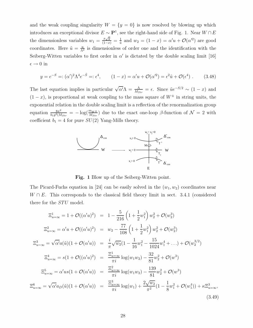
and the weak coupling singularity W = y = 0 is now resolved by blowing up which

introduces an exceptional divisor E ∼ P1, see the right-hand side of Fig. 1. Near W ∩Ethe dimensionless variables w1 =

x√y

(1−x) = 1u

and w2 = (1 − x) = α′u + O(α′2) are good

coordinates. Here u = uΛ2 is dimensionless of order one and the identification with the

Seiberg-Witten variables to first order in α′ is dictated by the double scaling limit [16]

ǫ→ 0 in

y = e−S =: (α′)2Λ4e−S =: ǫ4, (1 − x) = α′u+ O(α′2) = ǫ2u+ O(ǫ4) . (3.48)

The last equation implies in particular√α′Λ = Λ

MStr= ǫ. Since ue−S/2 ∼ (1 − x) and

(1 − x), is proportional at weak coupling to the mass square of W± in string units, the

exponential relation in the double scaling limit is a reflection of the renormalization group

equation 8π2

b1g2(MStr= − log(

mW±

MStr) due to the exact one-loop β-function of N = 2 with

coefficient b1 = 4 for pure SU(2) Yang-Mills theory.

con∆

con∆

x = 0+

x = 0-

W

∆ con

w = x =02 2

T

T

M

2

W

E

-

+

T -

+

w = 01

Fig. 1 Blow up of the Seiberg-Witten point.

The Picard-Fuchs equation in [24] can be easily solved in the (w1, w2) coordinates near

W ∩ E. This corresponds to the classical field theory limit in sect. 3.4.1 (considered

there for the STU model.

Ξ1u=∞ = 1 + O((α′u)2) = 1 − 5

216

(

1 +1

2w2

1

)

w22 + O(w3

2)

Ξ2u=∞ = α′u+ O((α′u)2) = w2 −

77

108

(

1 +1

2w2

1

)

w22 + O(w3

2)

Ξ3u=∞ =

√α′a(u)(1 + O(α′u)) =

i

π

√w2(1 −

1

16w2

1 −15

1024w4

1 + . . .) + O(w3/22 )

Ξ4u=∞ = s(1 + O((α′u)2) =

Ξ1u=∞πi

log(w1w2) −32

81w2

2 + O(w3)

Ξ5u=∞ = α′us(1 + O(α′u)) =

Ξ2u=∞πi

log(w1w2) −139

81w2

2 + O(w3)

Ξ6u=∞ =

√α′aD(u)(1 + O(α′u)) =

Ξ3u=∞πi

log(w1) +2√w2

π2(1 − 1

8w2

1 + O(w41)) + κΞ3

u=∞,

(3.49)

28

with κ = iπ(3 log(2) − 1). Classical gauge group enhancement to SU(2) occurs at a = 0

where the period Ξ3u=∞ vanishes.

Near the conifold branch ∆con+ ∩E, x+ = 1−x

x√y−1 = u−1 and x2 = (1−x) = α′u+O(α′2)

are good coordinates. Near the branch ∆con− ∩ E we may chose x− = 1−x

x√y

+ 1 = u + 1

and x2 = (1 − x) = α′u + O(α′2). The leading terms of the above basis in the (x+, x2)

coordinates near ∆con+ ∩ E read15

Ξ1mon = 1 + O((α′u)2) = 1 − 5

144

(

1 +2

3x+

)

x22 + O(x3

2)

Ξ2mon = α′u+ O((α′u)2) = x2 −

77

72

(

1 +2

3x+

)

x22 + O(x3

2)

Ξ3mon =

√α′a(u)(1 + O(α′u)) =

iΞ6mon

2πlog(x+) +

√2x2

iπ2(1 − 46

81x2 + O(x2)) + δΞ6

mon

Ξ4mon = s(1 + O((α′u)2) =

Ξ1mon

πilog(x2) −

1

πilog(1 − x+) + O(x2

2)

Ξ5mon = α′us(1 + O(α′u)) =

Ξ2mon

πilog(x2) −

x2

πilog(1 − x+) + O(x2

2)

Ξ6mon =

√α′aD(u)(1 + O(α′u)) =

1√2π

√x2(x+ +

9

32x2

+ +75

256x3

+ + . . .) + O(x322 ),

(3.50)

with δ = 1 + 3i(1−2 log(2))π

. Note that s = 2πiS ∝ 2πig2

and −S = log(y).

In this simple model we can give, at least numerically, a complete account of how the

periods in the Seiberg-Witten field theory limit are related to the ones in the large

complex structure basis, in which our flux choices are made, by calculating the trans-

formation matrix16 Ξu=∞ = Ξmon = NΞ∞, where the basis at infinity is as in (3.2),

Ξ∞ ∝ (1, t, s, ∂sF, ∂tF, 2F − s∂sF − t∂tF )

N =

0 iA+B 0 A−B2

0 0

0 iB 0 B2

0 0

1 0 0 −12

0 0

0 v2 + iA−B A−BA−B

2+ iv1 − iA+B

2−A−B

2

0 v3 + iB B B2

+ iv4iB2

B2

0 0 0 0 0 1

(3.51)

with A± = 136π4 (5π

4 ± 12Γ8(

34

)

), B = − π3√

3

Γ4( 34)

, v1 ≈ −4.0767326, v2 ≈ −16.409393,

v3 ≈ −69.6002844 and v4 ≈ −8.61884321. From the third and last line in N one sees

15Note that w1/21 w

1/22 = (x+ + 1)1/2w

1/22 =

√α′Λ, has to be factored out from the solutions on the

right to obtain the Seiberg-Witten expansions.16Explicit results for this Calabi-Yau manifold had already been obtained by W. Lerche and P. Mayr

(unpublished notes).

29

that the periods, which contain the Seiberg-Witten periods in the normalization17 (a ∼12Λsw

√2u, aD ∼ 2i

πa log(u)), have intersection 1 so we can make them dual in a symplectic

basis, but because of the entry −12

not in an integral symplectic basis.

The monodromy in the above basis around x+ = 0 can be identified directly with

the Seiberg-Witten monopole monodromy M(0,1) while the combination of monodromies

around w2 = 0 and w1 = 0 give the the Seiberg-Witten monodromy around infinity

M∞ = MT−12

M∞ =

1 0 0 0 0 0

0 1 0 0 0 0

0 0 −1 0 0 0

0 0 0 1 0 0

0 0 0 0 1 0

0 0 4 0 0 −1

M(0,1) =

1 0 0 0 0 0

0 1 0 0 0 0

0 0 1 0 0 −1

0 0 0 1 0 0

0 0 0 0 1 0

0 0 0 0 0 1

. (3.52)

It is a check on N that these are integral in the basis (3.2) and can be identified with

M(0,1) = T and M∞ = A−1TAT in the notation of [16]. Similarly, the monodromy around

x− gives M(−1,1) = M−1(0,1)M∞.

Let us first discuss the superpotential which arises in the classical field theory limit,

W = nΞu=∞ ∼ n√α′a , (3.53)

which vanishes at the point of classical gauge group enhancement. Using the third row

of the matrix N , we see that

Ξ3u=∞ = X0

∞ − i

2

∂F

∂S(3.54)

and hence the superpotential becomes

W = n(1 − i

2

∂F

∂S) =

n

2(1 − T 2) . (3.55)

This superpotential matches exactly with the superpotential in (3.10) after setting e0 =

−2m1 = n and e2 = 0.

Let us now go to the point where the monopole becomes massless. We first discuss

the field theory expectations and assume as in [3] that there is flux such that the field

theory superpotential behaves in leading order at the Seiberg-Witten point as W ∼ mu

[27]. This corresponds to a mass term for the adjoint scalar, which breaks N = 2 to

N = 1. Roughly speaking, such a potential should be generated by a flux that has m

17Note that Λ is rescaled by a numerical factor of order one, Λ = πi√

2Λsw.

30

“units” on Ξ2mon, i.e. W = mX2

mon. The superpotential has dimension three and since

the parameters x+, x2 are dimensionless it reads in natural units as

W =m

(α′)32

X2mon ∼ m

(α′)32

x2 + O(x2) . (3.56)

Under the double scaling limit it behaves hence as W ∼ mMstrΛ2u.

In the N = 1 field theory one expects h vacua with a mass gap, where h is the dual

Coxeter number of the gauge group. At each vacuum there is a superpotential

Wk = wke−S/h , (3.57)

where wh = 1, k = 0, . . . , h− 1 and S = 1g2

. Indeed we find that Ξ2mon ∼ x2 and from the

period Ξ4mon we learn that x2 ∼ e−

S2 , so that the string embedding delivers precisely the

right behavior of the superpotential.

The main issue will be the degeneration of the factor eKGxixj and whether the the scalar

potential drives the theory towards the Seiberg-Witten point. With the inverse of N

N−1 =

C −C+12

0 0 0

iC −iC− 0 0 0 0

C + iu3 C+ + iu4 0 C −C+12

2C −2C+ 0 0 0 0

u1 + 2iC u2 − 2iC− 0 −2iC 2iC− 0

0 0 0 0 0 1

(3.58)

where C =√

3π2Γ( 3

4)4

and C± =√

372Γ( 3

4)4

(5π4 ± 12Γ(34)8), u1 ≈ 5.5157560, u2 ≈ −.05616975,

u3 ≈ .1051578 and u4 ≈ .263801, we find that the Kahler factor eK diverges at E ∩∆con+

as

eK =1

2

π

π(2u3 + u1) − 4C log(|x2|)− Re(x2)a− 4C2πRe(x+)

(π(2u3 + u1) − 4C log(|x2|))2+ O(x2) , (3.59)

with a = π(2u3C− − C(2u4 + u2) + C+u1). To leading order the inverse metric is

Gxixj = 4π2Cπ(2u3 + C) − 4C log(|x2|)

6 log(2) − log(|x+|)

( 1|x2| −

√

x2

x2

−√

x2

x2|x2|

)

. (3.60)

The scalar potential, to leading order in (x+, x2), is

v = m2 2π3

(α′)2

(

|x2|2[

π2(u1 + 2u3)2 + 16C2 log(|x2|)2 − 8πC(2u3 + 1) log(|x2|)

]

−

4(Im(x2))2[

2C(2C + π(u1 + 2u3)) − 8C2 log(|x2|)]

)

×(

|x2|(

6 log(2) − log(|x+|))(

π(u1 + 2u3) − 4C log(|x2|))2)−1

. (3.61)

31

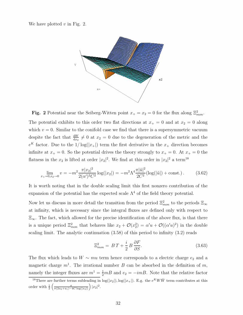
We have plotted v in Fig. 2.

x2

x+

V

x2

Fig. 2 Potential near the Seiberg-Witten point x+ = x2 = 0 for the flux along Ξ2mon.

The potential exhibits to this order two flat directions at x+ = 0 and at x2 = 0 along

which v = 0. Similar to the conifold case we find that there is a supersymmetric vacuum

despite the fact that dWdx2

6= 0 at x2 = 0 due to the degeneration of the metric and the

eK factor. Due to the 1/ log(|x+|) term the first derivative in the x+ direction becomes

infinite at x+ = 0. So the potential drives the theory strongly to x+ = 0. At x+ = 0 the

flatness in the x2 is lifted at order |x2|2. We find at this order in |x2|2 a term18

limx+=0,x2→0

v = −m2 π|x2|22(α′)2C2

log(|x2|) = −m2Λ4π|u|22C2

(log(|u|) + const.) . (3.62)

It is worth noting that in the double scaling limit this first nonzero contribution of the

expansion of the potential has the expected scale Λ4 of the field theory potential.

Now let us discuss in more detail the transition from the period Ξ2mon to the periods Ξ∞

at infinity, which is necessary since the integral fluxes are defined only with respect to

Ξ∞. The fact, which allowed for the precise identification of the above flux, is that there

is a unique period Ξ2mon that behaves like x2 + O(x2

2) = α′u + O((α′u)2) in the double

scaling limit. The analytic continuation (3.58) of this period to infinity (3.2) reads

Ξ2mon = B T +

i

2B∂F

∂S. (3.63)

The flux which leads to W ∼ mu term hence corresponds to a electric charge e2 and a

magnetic charge m1. The irrational number B can be absorbed in the definition of m,

namely the integer fluxes are m1 = 12mB and e2 = −imB. Note that the relative factor

18There are further terms subleading in log(|x2|), log(|x+|). E.g. the eKWW term contributes at this

order with 12

(

ππ(2u3+u1)−4C log(|x2|)

)

|x2|2.

32

between the flux vector entries is i/2. This means that the superpotential W = mu

cannot be generated by a Ramond flux alone. Specifically, whereas m1 is a real Ramond

flux, the electric flux e2, which corresponds to the field T , is purely imaginary and hence

is generated by a NS flux, where we have chosen the complex field τ to be imaginary,

τ = i.

This choice of fluxes can be compared to previous discussions in the literature on this

issue. First, the identification of the flux direction as ∂F∂S

∼ u in [3] ignores the mixing by

the analytic continuation. Second, the above identification has no zero-brane charge as in

[4]. This is explained by the fact that the basis used here differs by a integral symplectic

transformation relative to the one used in [4], i.e. our charge definitions are different.

If we just turn on the flux m0 the leading behaviour of the scalar potential is

v = − π

2(α′)2(log(|x+|) + 6 log(2)). (3.64)

This drives the theory to the conifold line, where the potential vanishes .

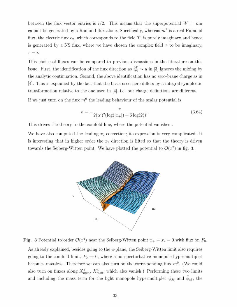
We have also computed the leading x2 correction; its expression is very complicated. It

is interesting that in higher order the x2 direction is lifted so that the theory is driven

towards the Seiberg-Witten point. We have plotted the potential to O(x2) in fig. 3.

x2

x+

V

x2

Fig. 3 Potential to order O(x2) near the Seiberg-Witten point x+ = x2 = 0 with flux on F0.

As already explained, besides going to the u-plane, the Seiberg-Witten limit also requires

going to the conifold limit, F0 → 0, where a non-perturbative monopole hypermultiplet

becomes massless. Therefore we can also turn on the corresponding flux m0. (We could

also turn on fluxes along X3mon, X

5mon, which also vanish.) Performing these two limits

and including the mass term for the light monopole hypermultiplet φM and φM , the

33

superpotential becomes

W = −m0F0 +m(

i∂F

∂S+ 2T

)

+ F0φM φM . (3.65)

Minimization of the corresponding potential will relate the vev of the monopole hyper-

multiplet φM to the vector moduli fields u and S.

Let us briefly comment on the possibility of partial supersymmetry breaking from N = 2

to N = 1 at the Seiberg-Witten point. As explained in [3] partial supersymmetry

breaking is possible in the rigid field theory limit after freezing out the S-field. From

the local supergravity perspective partial supersymmetry breaking seems possible since

the flux vector e2 is imaginary, as soon as we freeze out the hypermultiplet τ . Then the

difference in the mass eigenvalue of the two gravitini is proportional to 2mBT . But if

we treat τ as a dynamical field, the minimization of the potential with respect to τ will

make partial supersymmetry breaking impossible, as explained before.

3.8 The strong coupling limit and the role of the β-function.

The heterotic dilaton s corresponds in the dual K3 fibered Calabi-Yau spaces to the

complexified volume of the P1 base. Its dependence on its mirror dual complex structure

modulus is governed by an universal differential equation (θ = y ddy

, y = 4zs) (see e.g.

[24][

θ2 − y

4θ(θ +

1

2)]

Ξ = 0 , (3.66)

with three regular singular points at y = (0, 1,∞). Eq. (3.66) implies, that if the other

moduli of the Calabi-Yau zi are set to 0, the complexified volume s is given by

s =1

πarctan(

√

y − 1) . (3.67)

In particular at y = 1 the period ratio s vanishes with ws = 1−y as s = 1π

√ws∑∞n=0

wns

2n+1.

In the heterotic string this corresponds to the strong coupling limit. We therefore refer

to the ws = 1 − y = 0 locus in the moduli space as strong coupling divisor. Inside

the Calabi-Yau one finds a divisor F which is a rational fibration with the P1 as fiber

and a genus g curve Cg as base. If the fiber P1 vanishes, F collapses to Cg and branes

wrapped on P1 yield in type IIA compactifications charged massless vector multiplets,

which complete the U(1) vector multiplet s to a SU(2) vector multiplet. The square root

branch cut√ws will generate the Weyl reflection as monodromy. Holomorphic one-forms

of Cg lead to additional matter multiplets, likewise in the adjoint representation [28].

We will investigate superpotentials at the strong coupling singularity. An example is

the X12(1, 1, 2, 2, 6) model discussed in the last section. The curve Cg is the vanishing

34

locus of the first two variables and is hence represented by X6(1, 1, 3). By the adjunction

formula g = (2 − χ)/2 = 1 − (1+J)2(1+3J)6J2·3(1+6J)

|J2 = 2. With two hypermultiplets in the

adjoint representation the coupling grows with the scale.

At the point (x = 1728zt, y) = (0, 1) we have in the (zt, ws = 1 − y) coordinates the

solutions

Ξ1s = 1 +

5

72zt + O(2)

Ξ2s =

1

2πi

(

Ξ1s log(zt) +

1

2zt +

1

2log(1 − ws) + O(2)

)

=:1

2πi

(

Ξ1s log(zt) + Σ1

)

Ξ3s =

i

π

√ws

(

arctan(√−ws)

i√ws

+5

216ztws + O(2)

)

= a(ws) + O(zt)

Ξ4s =

Ξ3s

2πilog(ztws) −

√ws

2π2(

5

18ws + O(2)) = aD + O(zt)

Ξ5s =

1

2π2

(

Ξ1s log(zt)

2 + 2Σ1 log(zt) − ws +13

18x+ O(2)

)

=:1

2π2

(

Ξ1s log(zt)

2 + 2Σ1 log(zt) + Σ2

)

Ξ6s =

2

3(2πi)3(Ξ1

s log(zt)3 + 3Σ1 log(zt)

2 + 3Σ2 log(zt) − 6ws + O(2)).

(3.68)

This basis is related to the basis at zt = zs = 0 by the matrix Π∞ = NstrΠs with (cf.

footnote 16)

Nstr =

1 0 0 0 0 0

ib0 1 −12

0 0 0

0 0 1 0 0 0

2b1 −4ib0 0 1 0 0

b1 −2ib0 ib312

1 0

−ib2 b4 0 −ib0 0 1

, (3.69)

Here b0 = log(2)2π

and b1 ≈ 1.09550, b2 ≈ 1.00245, b3 ≈ .20799 and b4 ≈ 2.14233.

We consider a flux on the vanishing period Ξ3s = s, which generates a superpotential

W = ns (3.70)

and find the potential in leading order in (zt, ws)

v =n2π

(α′)2(2πb3 − 2 log(|ws||zt|) − 2)+ O(1) . (3.71)

This potential exhibits a similar logarithmic behaviour as the one at the conifold or the

pure SU(2) point. Its value is zero at ws = 0 and at x = 0. This value represents a local

35

minimum and the theory is strongly (by an infinite slope) attracted to ws = 0 = x = 0.The log(|ws||zt|) dependence is due to the non-vanishing of the β-function of the gauge

coupling constant. We thus expect a qualitative new behaviour of the scalar potential at

conformal points where the β-function vanishes.

3.9 The conformal points

We can study the situation with vanishing β-function in the X24(1, 1, 2, 8, 12) K3 fibra-

tion. Here Cg is obtained, as before, by setting to zero the first two variables, which yields

X12(1, 4, 6). Note that this curve has the Z2 singular point X6(2, 3). The Euler number

is obtained by combining the adjunction formula with the Riemann-Hurwitz formula:

χ(Cg) = (1+J)(1+4J)(1+6J)12J4·6(1+12J)

|J2 − 1/2 + 1 · 1 = 0. Hence there is g = 1 hypermultiplet and

the spectrum is conformal.

Recall that the above CY space M with Euler number χ = −480 exhibits several fibration

structures. On the one hand it is an elliptic fibration over the Hirzebruch surface F2,

which is itself a rational fibration with fiber P1U and base P1

S. At the same time the

CY space is a K3 fibration over the same base, hence the identification of the heterotic

dilaton with S. We have as Kahler classes S, the size of the base P1S, U = U − T

the size of the fiber P1U and T = T the size of a curve in the elliptic fiber. Hence

we have the nonvanishing intersections19 CTTT = 8, CSTT = 2, CUTT = 4, CSTU = 1,

CTUU = 2,∫

c2JT = 92,∫

c2JS = 24 and∫

c2JU = 36. This fixes the integral basis. The

mirror manifold W has the following discriminant (we have rescaled x = 432zt, y = 4zs,

y = 4zu)

∆s∆A∆B = (1 − y)[(1 − z)2 − yz2][((1 − x)2 − z)2 − yz2] (3.72)

which consists of three factors. ∆A,∆B are conifold loci. At z = 1, y = 0, ∆B 6= 0

there is a weakly coupled SU(2) without matter [16]. We will be interested in the

SU(2) with an adjoint hypermultiplet, i.e. with a conformal spectrum, which arises at

y = 1, ∆A 6= 0 6= ∆B, e.g. at y = 1, x = z = 0. To understand the role of the

hypermultiplets it is interesting to contrast this model with the more generic realization

of the X24(1, 1, 2, 8, 12) CY, which is given by an elliptic fibration over F0. As discussed

in [36] both models are in the same moduli space. However in the X24(1, 1, 2, 8, 12)

model the scalars in one hypermultiplet20 are set to a special value, which allows for

19Quantities with the tilde refer here to the heterotic spacetime moduli of T 2 in the compactification

on K3 × T 2, i.e. U is the complex structure modulus of T 2 and T its Kahler modulus.20This is the hypermultiplet related to the three-cycle which consists of the base P

1 and a one-cycle

on the elliptic fiber.

36

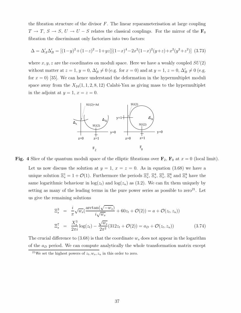
the fibration structure of the divisor F . The linear reparameterisation at large coupling

T → T , S → S, U → U − S relates the classical couplings. For the mirror of the F0

fibration the discriminant only factorizes into two factors:

∆ = ∆′A∆′

B = [(1−y)2+(1−z)2−1+yz][(1−x)4−2x2(1−x)2(y+z)+x2(y2+z2)] (3.73)

where x, y, z are the coordinates on moduli space. Here we have a weakly coupled SU(2)

without matter at z = 1, y = 0, ∆′B 6= 0 (e.g. for x = 0) and at y = 1, z = 0, ∆′

B 6= 0 (e.g.

for x = 0) [35]. We can hence understand the deformation in the hypermultiplet moduli

space away from the X24(1, 1, 2, 8, 12) Calabi-Yau as giving mass to the hypermultiplet

in the adjoint at y = 1, x = z = 0.

z=0 z=0

y=0y=0

z=1 z=1

y=1∆s

∆A∆A’

SU(2)

SU(2)+Ad SU(2)

SU(2)

F2

F0

Fig. 4 Slice of the quantum moduli space of the elliptic fibrations over F2, F0 at x = 0 (local limit).

Let us now discuss the solution at y = 1, x = z = 0. As in equation (3.68) we have a

unique solution Ξ1s = 1 + O(1). Furthermore the periods Ξ2

s, Ξ4s, Ξ5

s, Ξ6s and Ξ8

s have the

same logarithmic behaviour in log(zt) and log(zu) as (3.2). We can fix them uniquely by

setting as many of the leading terms in the pure power series as possible to zero21. Let

us give the remaining solutions

Ξ3s =

i

π

√ws(

arctan(√−ws)

i√ws

+ 60zt + O(2)) = a + O(zt, zu))

Ξ7s =

X3s

2πilog(zt) −

√ws

2π2(312zt + O(2)) = aD + O(zt, zu)) (3.74)

The crucial difference to (3.68) is that the coordinate ws does not appear in the logarithm

of the aD period. We can compute analytically the whole transformation matrix except

21We set the highest powers of zt, ws, zu in this order to zero.

37

one numerical constant

Nstr =

1 0 0 0 0 0 0 0

0 1 0 0 0 0 0 0

0 0 1 0 0 0 0 0

iA 0 −12

1 0 0 0 0

B− −4iA 0 −2iA 1 0 0 0

1 −iA 0 0 0 12

1 0

2 −2iA 0 0 0 1 0 0

C B+ 0 2 0 −iA 0 1

, (3.75)

where A = log(2)2π

, B± = 236± a

(2πi)2, a = .4804525 and C = 63i

2ζ(3)π3 +2iA. We see from this

matrix that the flux generating

W = nΞs = nS (3.76)

is an integral Ramond-Flux w.r.t. the basis at large volume.

The scalar potential is extremely complicated. The behaviour near zt = zu = ws = 0 is

determined by

v ∼p0

8 + p18

√

|ws| + p19

q9 + q10 ,(3.77)

where pid and qd are generic homogeneous polynomials in (log(|zt|), log(|zu|)) of the indi-

cated degree d. In particular the leading logarithmic term

v ∼ −2π4 log(|zu|) + 9 log(|zt|)

log(|zu|)2 + 6 log(|zt|) log(|z3|) + 9 log(|zt|)2(3.78)

is independent of ws. The potential has a minimum at zt = 0 as well as at zu = 0 with

vanishing energy. For fixed values of zt, zu the potential can be analyzed to 10-th order

in√ws and we found a series v ∼ ∑

i=0 ai(zt, zu)(|ws|)i2 whose coefficients ai go to zero if

zt or zu goes to zero.

Similarly to the situation above (3.74), where two periods vanish with a square root,

it was found in [31] at the point w = 0, where tensionless strings arise, that two dual

periods occur which start with w16 and w

56 . Therefore we expect for fluxes aligned with

a vanishing direction a similar behavior of the scalar potential in the direction of w, i.e.

a power series in wn6 with n ∈ Z.

4 Type II Vacua with Non-vanishing Ramond and NS Fluxes

In sect. 3.7 on the discussion of the Seiberg-Witten limit NS-fluxes have already emerged.

We now want to study in little more detail the possible effects of non-vanishing NS-fluxes

38

for the vacuum structure of type IIB strings. Since the superpotential is covariant under

the type IIB SL(2,Z) duality symmetry (see eq.(2.33)), the scalar potential is invariant

under this symmetry. Hence we expect to find non-trivial minima, where the field τ is

stabilized. The following discussion will be performed in the STU model, where we can

solve the minimization conditions explicitly. As we will see now, some of our previous

conclusions concerning the vector multiplets are modified by the presence of NS fluxes.

In particular it seems possible that the contribution of the R fluxes is precisely balanced

by the NS fluxes, such that supersymmetric minima of the scalar potential are possible

at non-degenerate points in the CY moduli space, i.e. at finite value for the S-field. It is

worth pointing out that in the example we are going to discuss the NS and Ramond flux

vectors are non-local w.r.t. each other. Nevertheless we will find that the ground state

of the model is fully N = 2 supersymmetric.

For simplicity we consider the perturbative heterotic prepotential with only three moduli

S, T and U and S → ∞: F = i(X0)2STU . After the symplectic transformation

S → FS , FS → −S (4.1)

the period vector has the form

(XI , FI) = (1,−TU, iT, iU,−iSTU, iS, SU, ST ) . (4.2)

One recognizes that the periods XI are algebraically dependent. Now we choose the flux

vectors such that all electric NS fluxes and also all magnetic Ramond fluxes are zero, i.e.

e1I = m2I = 0. In addition, in order to be able to balance the R fluxes against the NS

fluxes we choose them to be parallel, i.e. we impose the following condition:

e2I/p = (l2,−n2, n1,−l1), m1I/q = (−n2, l2,−l1, n1) . (4.3)

In fact, these two flux vectors are mutually non-local, m × e = m1Ie2I − m2Ie1I =

−2pq(l1n1 + l2n2) 6= 0. With this choice the superpotential becomes

W = (p+ iqSτ)(l2 − il1U + in1T − n2UT ), (4.4)

It is straightforward to see that the scalar potential has a N = 2 supersymmetry preserv-

ing minimum with zero cosmological constant; specifically the supersymmetry conditions,

WS = WT = WU = Wτ = 0, and W = 0, (4.5)

have the following solution:

Tmin =

√

l1l2n1n2

, Umin =

√

l2n1

l1n2, Smin τmin = i

p

q. (4.6)

So we see that supersymmetry preserving solutions are possible for finite heterotic dilaton

field S, as well as for finite type IIB dilaton τ . Insisting on large S and on large τ implies

that one has to ensure that p≫ q.

39

5 Summary

In this paper we have provided a detailed investigation of the vacuum structure of type

IIA/B compactifications on Calabi-Yau spaces in the presence of H-fluxes. These H-fluxes

lift the vacuum degeneracy in the Calabi-Yau moduli space. For aligned fluxes, local min-

ima of the scalar potential with space-time supersymmetry and vanishing cosmological

constant are found at several degeneration points of the Calabi-Yau space. However par-

tial supersymmetry at these minima seems to be impossible in local supergravity due

to the dilaton dependence of the effective superpotential, such that the degeneration

points always exhibit full N = 2 supersymmetry. Away from the degeneration points

supersymmetry is generically broken, and we expect in general local minima of the scalar

potential with broken supersymmetry. We also examined the vacuum structure of some

Calabi-Yau spaces (quintic, sextic) at certain rational, but non-singular points of enlarged

symmetry (Gepner points), and found that there are no supersymmetric solutions at this

points. However at the moment we cannot completely exclude supersymmetric vacua at

non-singular, rational points for other Calabi-Yau spaces.

This discussion can be extended in several ways. For example it would be interesting to

map the type IIA/B H-fluxes to dual heterotic or type I string compactifications. There

the H-fluxes will correspond to background electric or magnetic fields in the internal

directions [32]22 (for non-supersymmetric string compactifications with background F-

fields see [33]). Similarly it would be nice to see [32] how the type IIA/B H-fluxes at the

Calabi-Yau singularities can be mapped to dual brane configurations using the duality

[34] between the Calabi-Yau geometrical engineering and the Hanany-Witten approach.

Acknowledgements

We would like to thank Jan Louis for many valuable discussions and for collaboration

on the initial stage of this project. Discussions with K. Behrndt, G. Dell‘ Agata and

G. Lopes-Cardoso are also acknowledged. This work is supported by the European

Commission RTN programme HPRN-CT-2000-00131 and by GIF - the German-Israeli

Foundation for Scientific Research. D.L. and S.T. thank the Erwin-Schroedinger-Institute

in Vienna, where this project was started, for hospitality.

22This was already conjectured for the flux related to X0 in [1].

40

Appendix: The perturbative heterotic limit with general flux vector

In this appendix we like to solve in some detail the conditions of unbroken supersymmetry

within the perturbative heterotic limit for general flux vector (eI , mI). The corresponding

prepotential is given in eq.(3.20). After the symplectic transformation (4.1) the period

vector has the form

(XI ; FI) = (1,−T aηabT b, iT a;−iST aηabT b, iS, 2SηabT b). (5.1)

One recognizes that the periods XI are algebraically dependent. The symplectic trans-

formation (4.1) exchanges the IIA 2-cycle C(2)1 ∼ vol(P 1

b ) by its dual 4-cycle C(4)1 , namely

the whole K3-fibre. This amounts in exchanging H(4)R by H

(2)R in the S-field direction

and vice versa, and we denote the corresponding fluxes as

e1 = m1, m1 = e1. (5.2)

Seen from the heterotic point of view, the symplectic basis eq.(5.1) is the most natural

one since XI are the perturbative periods associated to the electric U(1), whereas the FI

are the non-perturbative magnetic U(1) periods.

For simplicity consider the case of only three moduli fields S, T and U . The classical

period vector is then

(XI , FI) = (1,−TU, iT, iU,−iSTU, iS, SU, ST ) . (5.3)

The holomorphic superpotential is then given as

W = e0 + e1TU + ie2T + ie3U + im0STU + im1S −m2SU −m3ST, (5.4)

and the Kahler potential take the well known form

K = − log[

(S + S)(T + T )(U + U)]

. (5.5)

In order to keep the notation as simple as possible we will omit from now on in this

chapter the tilde on e1 and m1.

The perturbative duality transformations SL(2,Z)T ⊗ SL(2,Z)U) × ZT↔U2 act as sym-

plectic transformations on the period vector as

XI

FI

→ Γ

XI

FI

=

U 0

0 UT,−1

XI

FI

. (5.6)

41

The generalized Kahler function eG = eK |W |2 is invariant under symplectic transforma-

tions (5.6) provided the quantum numbers are redefined by (mI ,−eI) → (mI ,−eI)ΓT .

Note that under the modular transformations SL(2,Z)T ⊗ SL(2,Z)U the superpoten-

tial transforms as a modular function of modular weight -1, as required for the modular

invariance of G [37]:

T → aT − ib

icT + d: W → W

icT + d. (5.7)

Now let us look for points of which preserve N = 1 supersymmetry, i.e. we look for

solutions of the equation

DaW = 0 → eK/2 (KaW +Wa) = 0 , a = S, T, U . (5.8)

This problem was already solved [20] using the attractor equations (2.52), and the full

solution of (5.8) is

SSusy = ie ·m〈m,m〉 +

√

√

√

√

〈e, e〉〈m,m〉 −

(e ·m)2

〈m,m〉2 ,

TSusy = ie′ ·m′

〈m′, m′〉 +

√

√

√

√

〈e′, e′〉〈m′, m′〉 −

(e′ ·m′)2

〈m′, m′〉2 ,

USusy = ie′′ ·m′′

〈m′′, m′′〉 +

√

√

√

√

〈e′′, e′′〉〈m′′, m′′〉 −

(e′′ ·m′′)2

〈m′′, m′′〉2 , (5.9)

where

〈e, e〉 = 2e0e1 + 2e2e3 ,

〈m,m〉 = 2m0m1 + 2m2m3 ,

e ·m = e0m0 + e1m

1 + e2m2 + e3m

3 . (5.10)

The exchange symmetries S ↔ T and S ↔ U map the vectors e,m to vectors e′, m′ and

e′′, m′′.

The function eG at the supersymmetric point (5.9) takes then the following value

m23/2|Susy = eG|Susy =

√

〈e, e〉〈m,m〉 − (e ·m)2 = 〈m,m〉ReS|Susy . (5.11)

From (5.11) one can easily read off that supersymmetric minima of the scalar potential v

with v = 0 at the minimum, i.e. W |Susy = eG|Susy = 0, are possible for certain choices of

fluxes. The first possibility for solving these two conditions is given by choosing parallel

electric and magnetic fluxes:

eI/p = (l2,−n2, n1,−l1), mI/q = (−n2, l2,−l1, n1) . (5.12)

42

This implies that

〈e, e〉 = −2p2nT l ,

〈m,m〉 = −2q2nT l ,

e ·m = −2pqnT l . (5.13)

With this choice the superpotential is

W = (p+ iqS)(l2 − il1U + in1T − n2UT ), (5.14)

and therefore eG|Susy = 0. However for this class of solutions ReS is zero, so one is driven

to strong coupling which is not consistent with assumption of having a large S-field.

The second class of supersymmetric solutions is given by only four non–vanishing flux

quantum numbers, namely the cases of purely electric (mI = 0) and purely magnetic

(eI = 0) charges. In both cases the moduli TSusy and USusy are generically finite. For

consistency we have to require in addition that Smin = ∞. This constraint is satisfied for

the purely electric solutions with mI = 0. This is precisely the case with aligned fluxes

and superpotential eq.(3.21). On the other hand the case with eI = 0 would imply strong

coupling with SSusy = 0.

Next let us consider the effects of one-loop corrections h(T a) to the heterotic prepotential.

Due to the required embedding of the perturbative T -duality group into the N = 2

symplectic transformations, it follows [38, 39] that the heterotic one-loop prepotential

h(T a) must obey well-defined transformation rules under this group. This becomes clear

if one considers the action of the one-loop T-duality transformations on the period vector

(5.1):

XI

iFI

→ Γ1−loop

XI

iFI

=

U 0

V UT,−1

XI

iFI

. (5.15)

where the matrix V encodes the quantum corrections. Therefore the one-loop transfor-

mation rule of symplectic quantum numbers implied by the general formula (m,−e) →(m,−e)ΓT is

e→ UT,−1e− Vm, m→ Um . (5.16)

It follows that the superpotential W is still transforms with modular weight -1 under

SL(2,Z)T and SL(2,Z)U .

In the presence of the heterotic one loop correction h(T a) the period vector eq.(5.1) will

43

be modified as follows:

(XI ; FI)|1−loop = (1, T aηabTb, iT a; iS, iST aηabT

b + 2ih(T a) − iT a∂h

∂T a,−ST a +

∂h

∂T a)

(5.17)

One recognizes, that the periods XI do not receive any quantum corrections and are

still algebraically dependent. Hence the superpotential with aligned fluxes is the same

as in the classical case eq.(3.21), and we therefore expect the same vacuum structure as

in the classical limit for aligned fluxes. The one-loop quantum corrections only result

in a simple modification of the Kahler potential which can be absorbed by the invariant

dilaton field Sinvar [38]. This field Sinvar is the true coupling constant at one loop, and

eK1−loop/2 is proportional to S−1invar.

Let us consider in a little bit more detail the complete superpotential

W = eIXI +mIFI |1−loop, (5.18)

which includes the one-loop term h(T a) in FI |1−loop. The supersymmetry equations

DaW = 0, W = 0 will still allow for non-trivial solutions which however cannot be

expressed any more in closed form like in eq.(5.9) for non-vanishing mI . Nevertheseless

one can derive an all order expression for m3/2 at the supersymmetric, stationary points,

as it was proven in the context of N = 2 black hole solutions. This expression has simply

the form

m23/2|Susy = eG|Susy = πReSinvar〈m,m〉 , (5.19)

where for the case of NV − 1 fields T a, 〈m,m〉 is defined as

〈m,m〉 = m0m1 +maηabmb. (5.20)

(〈m,m〉 is an invariant of the T-duality group SO(2, NV − 1,Z).) Thus the influence of

all perturbative one-loop effects to the superpotential is contained in ReSinvar. Hence,

demanding eG|min = 0 at ReSinvar = ∞, one has to set again 〈m,m〉 = 0.

References

[1] J. Polchinski and A. Strominger, Phys. Lett. B388 (1996) 736, hep-th/9510227.

[2] J. Michelson, Nucl. Phys. B495 (1997) 127, hep-th/9610151.

[3] T.R. Taylor and C. Vafa, Phys. Lett. B474 (2000) 130, hep-th/9912152.

[4] P. Mayr, Nucl. Phys. B593 (2000) 99, hep-th/0003198.

44





[5] A. Strominger, Nucl. Phys. B274 (1986) 274.

[6] S. Ferrara, C. Kounnas, D. Lust and F. Zwirner, Nucl. Phys. B365 (1991) 431.

[7] I. Antoniadis, H. Partouche and T.R. Taylor, Phys. Lett. B372 (1996) 83, hep-

th/9512006.

[8] S. Ferrara, L. Girardello and M. Porrati, Phys. Lett. B366 (1996) 155, hep-

th/9510074;

S. Ferrara, L. Girardello and M. Porrati, Phys. Lett. B376 (1996) 275, hep-

th/9512180.

[9] S. Ferrara and R. Kallosh, Phys. Rev. D54 (1996) 1514, hep-th/9602136;

S. Ferrara and R. Kallosh, Phys. Rev. D54 (1996) 1525, hep-th/9603090.

[10] G. Moore, Attractors and arithmetic, hep-th/9807056;

G. Moore, Arithmetic and attractors, hep-th/9807087.

[11] S. Gukov, C. Vafa and E. Witten, Nucl. Phys. B584 (2000) 69, hep-th/9906070;

S. Gukov, Nucl. Phys. B574 (2000) 169, hep-th/9911011.

[12] M. Haack, J. Louis and M. Marquart, Type IIA and heterotic string vacua in D = 2,

hep-th/0011075.

[13] B. de Wit and A. Van Proeyen, Nucl. Phys. B 245 (1984) 89.

[14] S. Ferrara and A. Strominger, in Strings ’89, eds. R. Arnowitt, R. Bryan, M.J. Duff,

D.V. Nanopoulos and C.N. Pope (World Scientific, 1989), p. 245;

A. Strominger, Commun. Math. Phys. 133 (1990) 163;

L.J. Dixon, V.S. Kaplunovsky and J. Louis, Nucl. Phys. B329 (1990) 27;

P. Candelas and X.C. de la Ossa, Nucl. Phys. B355 (1991) 455;

L. Castellani, R. D’ Auria and S. Ferrara, Phys. Lett. B 241 (1990) 57; Cl.Q. Grav.

7 (1990) 1767;

R. D’Auria, S. Ferrara and P. Fre, Nucl. Phys. B359 (1991) 705;

B. de Wit and A. Van Proeyen, in Quaternionic Structures in Mathematics and

Physics, ILAS/FM-6/1996 (Sissa, Trieste) hep-th/9505097; Nucl. Phys. B (Proc.

Suppl.) 45B,C (1996) 196.

[15] B. de Wit, P. G. Lauwers, R. Philippe, S.–Q. Su and A. Van Proeyen, Phys. Lett.

134B (1984) 37.

45















[16] S. Kachru, A. Klemm, W. Lerche, P. Mayr and C. Vafa, Nucl. Phys. B459 (1996)

537, hep-th/9506112 .

[17] A. Klemm and S. Theisen, Nucl. Phys. B389 (1993) 153, hep-th/9205041; A. Font,

Nucl. Phys. B391 (1993) 358, hep-th/9203084.

[18] L. Andrianopoli, M. Bertolini, A. Ceresole, R. D’Auria, S. Ferrara and P. Fre, Nucl.

Phys. B476 (1996) 397, hep-th/9603004.

[19] A. Ceresole, R. D’Auria, S. Ferrara and A. Van Proeyen, Nucl. Phys. B444 (1995)

92, hep-th/9502072.

[20] G. L. Cardoso, D. Lust and T. Mohaupt, Phys. Lett. B388 (1996) 266, hep-

th/9608099.

[21] K. Behrndt, G. Lopes Cardoso, B. de Wit, R. Kallosh, D. Lust and T. Mohaupt,

Nucl. Phys. B488 (1997) 236, hep-th/9610105.

[22] D. Lust, String vacua with N = 2 supersymmetry in four dimensions, hep-

th/9803072.

[23] P. Candelas, X. C. de la Ossa, P. S. Green and L. Parkes, Nucl. Phys. B359 (1991)

21.

[24] S. Hosono, A. Klemm, S. Theisen and S.-T. Yau, Commun. Math. Phys. 167 (1995)

301, hep-tn/9308122 and Nucl. Phys. B433, 501 (1995), hep-th/9406055 .

[25] P. Candelas, X. C. de la Ossa, A. Font, S. Katz and D. Morrison, Nucl. Phys. B416

(1994) 481, hep-th/9308083.

[26] A. Strominger, S.-T. Yau and E. Zaslow, Nucl. Phys. B479 (1996) 243, hep-

th/9606040.

[27] N. Seiberg and E. Witten, Nucl. Phys. B426 (1994) 19, hep-th/9407087.

[28] A. Klemm and P. Mayr, Nucl. Phys. B469 (1996) 37, hep-th/9601014;

S. Katz, D. Morrison and M.R. Plesser, Nucl. Phys. B477 (1996) 105, hep-

th/9601108.

[29] A. Strominger, Nucl. Phys. B451 (1995) 96, hep-th/9504090.

[30] K. Behrndt, D. Lust and W. Sabra, Phys. Lett. B418 (1998) 303, hep-th/9708065.

46











http://arXiv.org/abs/hep-tn/9308122











[31] A. Klemm, P. Mayr and C. Vafa, BPS states of exceptional non-critical strings,

hep-th/9607139.

[32] Work in progress.

[33] C. Bachas, A way to break supersymmetry, hep-th/9503030;

R. Blumenhagen, L. Gorlich, B. Kors and D. Lust, JHEP 0010 (2000) 006, hep-

th/0007024;

R. Blumenhagen, L. Gorlich, B. Kors and D. Lust, Magnetic flux in toroidal type I

compactifications, hep-th/0010198;

C. Angelantonj, I. Antoniadis, E. Dudas and A. Sagnotti, Phys. Lett. B489 (2000)

223, hep-th/0007090;

C. Angelantonj and A. Sagnotti, Type-I vacua and brane transmutation, hep-

th/0010279;

G. Aldazabal, S. Franco, L.E. Ibanez, R. Rabadan and A.M. Uranga, Chiral string

compactifications from intersecting branes, hep-th/0011073.

[34] A. Karch, D. Lust and D. Smith, Nucl. Phys. B533 (1998) 348, hep-th/9803232.

[35] S. Katz, A. Klemm and C. Vafa, Nucl. Phys. B497 (1997) 173, hep-th/9609239 .

[36] D. R. Morrison and Cumrun Vafa, Nucl.Phys. B476 (1996) 437-469, hep-th/9603161.

[37] S. Ferrara, D. Lust, A. Shapere and S. Theisen, Phys. Lett. B225 (1989) 363;

A. Font, L.E. Ibanez, D. Lust and F. Quevedo, Phys. Lett. B245 (1990) 401.

[38] B. de Wit, V. Kaplunovsky, J. Louis and D. Lust, Nucl. Phys. B451 (1995) 53,

hep-th/9504006.

[39] I. Antoniadis, S. Ferrara, E. Gava, K. S. Narain and T. R. Taylor, Nucl. Phys.

B447 (1995) 35, hep-th/9504034.

[40] D.-E. Diaconescu and C. Romelsberger, Nucl.Phys. B574 (2000) 245, hep-

th/9910172.

[41] S. Hosono, Local Mirror Symmetry and Type IIA Monodromy of Calabi-Yau mani-

folds, Adv. Theor. Math. Phys. 4 (2000), hep-th/0007071.

[42] P. Mayr, Phases of Supersymmetric D-branes on Kahler Manifolds and the McKay

correspondence, hep-th/0010223.

[43] P. Candelas, A. Font, S. Katz and D. R. Morrison, Nucl. Phys. B429 (1994) 626,

hep-th/9403187.

47




















on the vacuum structure of type ii string compactifications on calabi–yau spaces with h-fluxes

Documents