threshold corrections and symmetry enhancement in string compactifications
TRANSCRIPT
arX
iv:h
ep-t
h/94
1220
9v2
31
Jan
1995
HUB-IEP-94/50
hep-th/9412209
THRESHOLD CORRECTIONS AND SYMMETRY ENHANCEMENT IN
STRING COMPACTIFICATIONS
Gabriel Lopes Cardoso, Dieter Lust
Humboldt Universitat zu Berlin
Institut fur Physik
D-10115 Berlin, Germany1
and
Thomas Mohaupt
DESY-IfH Zeuthen
Platanenallee 6
D-15738 Zeuthen, Germany2
ABSTRACT
We present the computation of threshold functions for Abelian orbifold com-
pactifications. Specifically, starting from the massive, moduli-dependent
string spectrum after compactification, we derive the threshold functions as
target space duality invariant free energies (sum over massive string states).
In particular we work out the dependence on the continuous Wilson line mod-
uli fields. In addition we concentrate on the physically interesting effect that
at certain critical points in the orbifold moduli spaces additional massless
states appear in the string spectrum leading to logarithmic singularities in
the threshold functions. We discuss this effect for the gauge coupling thresh-
old corrections; here the appearance of additional massless states is directly
related to the Higgs effect in string theory. In addition the singularities in the
threshold functions are relevant for the loop corrections to the gravitational
coupling constants.
1e-mail addresses: [email protected], [email protected]
BERLIN.DE2e-mail address: [email protected]
1 Introduction
Four-dimensional string models possibly provide a consistent description of all known
interactions including gravity. At energy scales small compared to the typical string
scale Mstring, which is directly related to the Planck mass MPlanck = O(1019 GeV), it
is convenient to use an effective Lagrangian for the light string modes φL where the
effect of the heavy string modes φH is integrated out. Based on several motivations,
the main area of research in this context is on four-dimensional string vacua with N =
1 space-time supersymmetry, implying that the effective string interactions are of the
form of an N = 1 supergravity-matter action. Studying four-dimensional string vacua
with space-time supersymmetry, it turns out that infinitely many of them are connected
by continuous deformations of the underlying two-dimensional conformal field theory,
parametrized by coupling constants called moduli, collectively denoted by Ti. At the
level of the effective supergravity action, and neglecting non-perturbative effects, moduli
are described by massless scalar fields with flat potential, whose vacuum expectation
values parametrize the continuous deformations. The moduli play a very important role
in the effective action, since various coupling constants among the matter fields like the
tree-level Yukawa couplings [1, 2] or the loop corrections to the gauge and gravitational
coupling constants [3]-[19] are moduli dependent functions. Specifically, the one-loop
moduli dependence of the gauge and gravitational coupling constants arises from σ-
model and Kahler anomalies [5, 7, 8, 10] and from integrating out the infinite tower of
massive string modes with moduli dependent masses.
The moduli spaces M of four-dimensional string theories have a very interesting and
rich structure. First, as it is true for many known compactification schemes of the
ten-dimensional heterotic string, the underlying superconformal field theory is invariant
under the target space duality symmetries (see [20]) which act on the the moduli as
discrete reparametrizations. These target space duality transformations act in general
non-trivially on the infinite massive spectrum φH , in the sense that states with different
quantum numbers (e.g. discrete internal momentum and winding numbers) are mapped
onto each other. Consequently, integrating out the massive spectrum φH implies that
certain low energy couplings are given in terms of automorphic functions of the corre-
sponding duality group. This observation can provide very useful informations about the
structure of the effective low-energy supergravity action, in particular when combined
with some analyticity arguments of holomorphic coupling functions [21].
A second very interesting feature of the string moduli spaces comes from the fact that
at certain critical points Pc in the moduli spaces a finite number of additional massless
1
states may appear in the moduli-dependent string spectrum, which are otherwise massive
at generic points in M. We will call these states φ′H . Very often, at Pc these fields
correspond to additional holomorphic spin one currents on the world sheet. Then the
gauge symmetry of the four-dimensional string is enlarged which is nothing else than the
stringy version of the well known Higgs effect. The role of the Higgs fields is now taken
by moduli fields. The field-theoretical formulation of the stringy Higgs effect, i.e. the
correct coupling of the relevant moduli to the gauge bosons, was investigated in [22, 23]
for the case of the standard Z3 orbifold [24, 25].
The appearance of additional massless fields at some critical points Pc in M implies that
the description of the string compactification by an low-energy effective action contains
discontinuities, since near the critical points the fields φ′H should be kept as light de-
grees of freedom and should not be integrated out from the spectrum. In other words,
when integrating over all massive fields including φ′H the effective action may acquire
singularities at the critical points Pc. Let us make this more clear by considering as an
example the one loop running of a gauge coupling constant in the low-energy field theory.
The one-loop running coupling constant at a scale p is given by (neglecting Kahler and
σ-model anomalies)
1
g2(p2)=
1
g2(M2string)
+b
16π2log
M2string
p2+
|∆(Ti)|216π2
, (1.1)
where b is the one-loop β-function coefficient of the light modes φL and ∆(Ti) is the
moduli-dependent threshold correction of the heavy string modes. ∆(Ti) can be re-
garded as the suitably regularized free energy [26, 27] of all massive modes, ∆(Ti) ∝log detM2
φH(Ti), where the MφH
(Ti)’s are the moduli-dependent masses of the heavy
modes. Clearly, if this sum contains also states φ′H which become massless at Pc, ∆(Ti)
possesses a singularity at Pc. As we will discuss in detail, the masses of φ′H are generically
of the form Mφ′H(Ti) ∝ (Ti−Pc) (here, Ti is one specific ‘critical’ modulus). Thus we see
that ∆(Ti) exhibits a logarithmic singularity of the form
∆ → n log(Ti − Pc), (1.2)
where n accounts for the degeneracy of states which become massless at Pc. In order to
get finite threshold corrections ∆(Ti) over the whole moduli space it is useful to separate
in eq.(1.1) the contribution of the states φ′H from the states φH which are always massive.
Then eq.(1.1) can be written as
1
g2(p2)=
1
g2(M2string)
+b
16π2log
M2string
p2+
b′
16π2log |Ti − Pc|2 +
|∆(Ti)|216π2
. (1.3)
2
Here b′ is the contribution of the states φ′H to the β-function coefficient, and ∆(Ti) does
not contain the states φ′H . Thus the logarithmic singularity in the moduli Ti is nothing
else than the threshold effect of φ′H with (intermediate) mass scale Mφ′
H(Ti) ∝ (Ti −Pc).
This discussion was entirely based on field theoretical arguments. As already discussed
in [28], in string theory these threshold functions are given in terms of automorphic
functions of the underlying target space duality group with the appropriate singularity
structure. In fact, since in string theory there is generically an infinite number of states
which may become massless at duality equivalent points in M (at one particular point in
M only a finite number of states can become massless) the relevant automorphic func-
tions possess singularities at an infinite number of points being related by discrete duality
transformations. In this paper we will calculate explicitly these divergent threshold func-
tions which are related to the discontinuities in the string spectrum and to the stringy
Higgs effect. To be specific we concentrate on Abelian orbifold compactifications of the
ten-dimensional heterotic string. We will discuss the dependence of the threshold cor-
rections as functions of the moduli associated with the six-dimensional orbifold, denoted
by T and U , as well as of the socalled Wilson line moduli [29] which take values in the
heterotic gauge group. The orbifold moduli T , U (metric and antisymmetric tensor) will
be relevant for the discussion of the Higgs effect in the compactification sector; here the
relevant automorphic functions will be given in terms of the absolute modular invariant
function j. On the other hand, the Wilson line moduli are responsible for the Higgs
effect in the heterotic gauge group. This is of rather phenomenological importance since
the Wilson line Higgs field may break some GUT gauge group to the gauge group of the
standard model. Moreover it may be even possible to identify some of the Wilson line
moduli with the supersymmetric standard model Higgs fields H1 and H2.
Our paper is organized as follows. In sections 2 and 3 we discuss the structure of the
gauge groups in orbifold compactifications as a function of the various moduli fields. In
section 4 we compute the masses of the generically massive fields. Some of these masses
become zero at certain fixed points in the orbifold moduli spaces. Here we will use the
results of our previous paper [30] where we have determined the moduli spaces plus the
target space duality transformations in the presence of Wilson line moduli. In sections
5, 6 and 7 we will apply the results of section 4 to compute the target space free energies
as (infinite) sums over the massive string states. Finally we will explain the relation of
these free energies to the string threshold corrections. We will display the dependence of
the threshold corrections in terms of T and U as well as in terms of the generic Wilson
line moduli. A discussion of this is provided in section 8.
3
2 Gauge groups in orbifold compactifications with continuous Wilson lines
In this section we will start to discuss the moduli dependence of the gauge group of an
orbifold compactification. We will concentrate on the so called gauge sector here, whereas
the compactification sector will be studied in the next section. Our aim is to determine
the unbroken gauge group in the presence of the most general continuous Wilson lines
compatible with a given twist. For a certain class of twists the minimal and therefore
generic gauge groups are easily determined, and we describe the method for determining
them. The results are listed in tables given at the end of this paper. We also point out
under which circumstances this method fails to give the minimal gauge groups, in which
case it only yields a lower bound on these minimal gauge groups, that is not saturated.
For these cases, in which a more detailed analysis is necessary, we outline how one has
to proceed in order to determine the generic gauge groups.
2.1 Wilson lines in the Narain model
Since many properties of an orbifold model can be understood easily in terms of the
underlying Narain model [31, 32], let us first recall how the gauge group of a toroidal
compactification depends on the Wilson line moduli [33]. We will concentrate on the
so called gauge sector which is generated by the sixteen extra left–moving worldsheet
bosons X(z) := XIL(z), I = 1, . . . , 16.
There are sixteen chiral conserved currents ∂XIL(z) on the worldsheet. These can be
combined with the right–moving ground state, which is an N = 4 space time vector
supermultiplet, to give a U(1)16 N = 4 gauge theory. For special values of the moduli
the Narain lattice Γ = Γ22,6 contains vectors of the form
P = (pL;pR) = (v, 06; 06) ∈ Γ, p2L = v2 = 2. (2.1)
Then there are extra conserved currents exp(iv · X(z)), leading to vertex operators for
massless charged gauge bosons with charges v = (vI), thus extending the gauge group
to a rank 16 reductive non–abelian Lie group
G(16) = G(l) ⊗ U(1)16−l (2.2)
where G(l) is semi–simple and has rank l.
As discussed in [33] these extended symmetries can be described in the following way.
Every vector P ∈ Γ of the Narain lattice can be written as
P = qI lI + niki +miki, (2.3)
4
where the integers qI , ni and mi are the charge, winding and momentum quantum num-
bers, I = 1, . . . , 16, i = 1, . . . , 6. The standard basis vectors are [34]
lI =(eI ,−
1
2(eI ·Ai)e
i;−1
2(eI ·Ai)e
i), (2.4)
ki =(Ai, (4Gij +Dij)
1
2ei;Dij
1
2ei)
(2.5)
and
ki =(016,
1
2ei;
1
2ei), (2.6)
where
Dij = 2(Bij −Gij −
1
4Ai · Aj
). (2.7)
This basis is a function of the moduli
Gij = Gji ∈M(6, 6,R), Bij = −Bji ∈M(6, 6,R), Ai ∈ R16 (2.8)
of the Narain model, namely the metric and the axionic background field and the Wilson
lines. eI are basis vectors of a selfdual sixteen dimensional lattice Γ16 (the E8 ⊗E8 root
lattice or the SO(32) root lattice extended by the spinor weights of one chirality), and
the ei are a basis of the dual Λ∗ of the compactification lattice.
Vectors of the form (2.1) have quantum numbers such that qIC(16)IJ qJ := qTC(16)q = 2,
where C(16) is the lattice metric of Γ16 and nimi := nTm = 0. 3 The Wilson lines Ai
must be chosen such that
v · Ai ∈ Z (2.9)
where v = qIeI . Then
P = qI lI + (v · Ai)ki = (v, 06; 06) (2.10)
is a Narain vector with v2 = qTC(16)q = 2. If one sets for example Ai = 0, then all roots
of the lattice Γ16 are in the Narain lattice and therefore the generic gauge group U(1)16 is
extended to E8 ⊗E8 or SO(32), depending on the choice of Γ16. Other solutions, which
have as gauge groups all possible maximal rank regular reductive subgroups of E8 ⊗ E8
and SO(32) were constructed in [33].
Finally note that a small deformation δAi of the Wilson lines, if it destroys some of the
conditions v · Ai ∈ Z, acts on the lattice as a deformation
(v, 06; 06) → (v,w;w) (2.11)
with w = −12(v · δAi)e
i, which makes the corresponding state acquire a mass α′
2M2 =
w2 in a smooth way. This is a version of the stringy Higgs effect [23].3More generally all possible extra massless states correspond to Narain vectors with quantum numbers
satisfying qT C(16)q + 2nT m = 2. This is a consequence of the mass formula as we will recall in section
5. A second subclass of this set will be the subject of the next section.
5
2.2 Definition of the orbifold
We can now proceed to extend this to the untwisted sector of an orbifold compactification.
First of all one has to select a Narain lattice with some symmetry that can be modded out.
Our reference lattice will be the one with vanishing Wilson lines, which therefore factorises
as Γ22;6 = Γ16 ⊕ Γ6;6. For definiteness, Γ16 will be the E8 ⊗E8 lattice. Then, we have to
specify the twist action on Γ16 and Γ6;6. Whereas the twist action on Γ6;6 is defined by
choosing one of the 18 twists θ of the compactification lattice Λ that lead to N = 1 space
time supersymmetry [35], the twist on Γ16 will be a Weyl twist (inner automorphism) θ′ of
E8 ⊗E8. The total twist Θ = (θ′, θ, θ) of the Narain lattice is constrained by world sheet
modular invariance [36]. The level matching conditions worked out in [36] restrict the
eigenvalues of Θ. In this paper we will not present a classification of ZN Weyl orbifolds.
Instead we will take one of the E8 as a hidden sector and assume that the Weyl twist in
this sector has been chosen in such a way that it cancels the WS modular anomalies of
the internal twist and of the Weyl twist in the first E8. The orbifold model defined this
way still has some Wilson line moduli left. In order to be compatible with the twist the
Wilson lines must satisfy [29, 37]
θJIAJj = AIiθij (2.12)
where AIj is a matrix containing the components of the Wilson lines and θJI , θij are the
matrices of the gauge and of the internal twist with respect to the lattice bases eI and
ei of Γ16 and Λ∗ respectively. Wilson line moduli do exist if an eigenvalue appears both
in the gauge twist and in the internal twist. More precisely, if a complex conjugated pair
of eigenvalues (a real eigenvalue) appears d times in the gauge twist and d′ times in the
internal twist, this then leads to 2dd′ (dd′) real moduli [30, 37].
2.3 Minimal gauge groups in the presence of Wilson lines
Let us now work out the gauge groups for Weyl twists of a E8 in the presence of generic
continuous Wilson lines. The basic idea is the following. All Weyl twists of E8 are
induced by twists that have a nontrivial action on some sublattice N . This sublattice
can be chosen to be the root lattice of a regular semi–simple subalgebra. The twist
action on the sublattice can then be described by a so called Carter diagram, which can
be thought of as a generalization of the well known Dynkin diagram [38]. In fact most
Weyl twists of E8 are induced by Coxeter twists of regular subalgebras and in this case
the Carter diagram is identical with the Dynkin diagram of this subalgebra. To get all
inequivalent Weyl twist one has to add a few twists of subalgebras, which are not Coxeter
6
twists. These are then described by Carter diagrams that are not Dynkin diagrams. For
more details on Carter diagrams and their relation to Weyl twists see [39] and [40].
Given the sublattice N on which the twist acts non–trivially one has to look for the
largest complementary sublattice I on which it acts trivially. That means that I is
defined by
E8 ⊃ N ⊕ I (2.13)
together with
(E8 ⊃ N ⊕ I and I ′ ⊃ I) =⇒ I ′ = I. (2.14)
If we now decompose E8 into conjugacy classes with respect to N⊕I, a familiar procedure
used in covariant lattice models, we get schematically that
E8 = (N , 0) + (0, I) +∑
i
(Wi(N ),Wi(I)) (2.15)
This means that there are three types of lattice vectors, namely those belonging to the
sublattices N and I and those which have a non–vanishing projection onto both N and
I. For a review of lattice techniques see [41].
Using this decomposition the effect of switching on continuous Wilson lines becomes
quite obvious. If we assume for the moment that that all eigenvalues of the gauge twist
also appear in the internal twist, which is true for all Z3, Z4, Z′6 and Z7 orbifolds, then
the Wilson lines will take arbitrary values in 〈N 〉R. Thus for any generic choice of the
Wilson lines only states corresponding to lattice vectors in (0, I) are massless. Note
that these states are automatically twist invariant. Therefore the gauge group of the
orbifold contains at least a semi–simple group corresponding to the roots of the lattice I.
However, the rank of this group is not a priori guaranteed to be 8−dim(N ). This follows
from the fact that the subgroup, to which E8 is broken, need not to be semi–simple
but only reductive, that is there can be U(1) factors around. On the other hand, when
considering the action of the twist on the Cartan subalgebra, one knows that dim(N )
Cartan generators are not invariant under the twist and are therefore projected out,
whereas 8 − dim(N ) are invariant under the twist. Therefore, the rank of the unbroken
gauge group is 8 − dim(N ) and the gauge group itself is given by
GI ⊗ U(1)8−dim(N )−rk(GI) (2.16)
where GI is the semi-simple Lie group associated to the roots of the lattice I.
Decompositions of the form N ⊕ I can easily be found using the formalism of extended
Dynkin diagrams [42]. There are, however, cases where the decomposition is not unique.
This is not in contradiction with I being maximal, because ⊃ is a partial ordering
7
relation, only. It is well known that it happens in a few number of cases that the twist
of the full algebra does not only depend on the isomorphic type of the subalgebra that is
twisted, but also on the precise embedding [38]. This is easily illustrated by the following
example, namely by decomposing E8 into cosets with respect to A81 and then taking the
A41 Coxeter twist. From the decompostion one sees that, depending on the choice of
the A1’s, one has that I = D4 or I = A41. These twists are known as A4 I
1 and A4 II1 ,
respectively.
Fortunately, we can use the results of the classification of conjugacy classes of the Weyl
group, which is equivalent to the classification of Weyl twist modulo conjugation, for
determining the minimal gauge groups. In his work [38] Carter gives, for all twists, the
decompositions of the root system, which specify the group GI . Then, according to
(2.16), all one has to do is to add some U(1) factors, if necessary. We have listed all
the minimal gauge groups that can appear in the context of N = 1 supersymmetric ZN
orbifold compactifications.
Note, however, that we have so far assumed that the Wilson lines are really allowed
to take values in all of 〈N 〉R. But this is not the case if an eigenvalue of the gauge
twist does not appear in the internal twist. The simplest example for this is provided
by the A3 Coxeter twist which has, as a lattice twist, the eigenvalues ωi, i = 1, 2, 3
where ω = exp(2πi/4). This can be combined with a Z8 twist of the internal space
with eigenvalues Ωk, k = 1, 2, 3, 5, 6, 7, where Ω = exp(2πi/8). Since θ does not have
the eigenvalue −1, there are no Wilson lines taking values in the −1 eigenspace of θ′.
Therefore, the minimal gauge group is larger then the expected SO(10). A detailed
analysis shows that the unbroken gauge group is the non–simply laced group SO(11).
Note that this is not in contradiction with the twist being defined through a Weyl twist of
E8, because an inner automorphism of the full group may be an outer one of a subgroup.
Therefore, breaking to non–regular subgroups is possible, if Wilson lines are turned on.
In these cases, which include many of the Z6 and Z8, and most of the Z12 and Z′12
orbifolds, our list only provides a lower bound on the gauge group that is not saturated.
Note that the analysis to be performed in order to get the minimal gauge group is, in
these cases, the same as the one one has to use in order to get intermediate gauge groups,
that is gauge groups that are neither minimal nor maximal. A combination of counting
and embedding arguments as used in [37] is in many cases sufficent to determine the
gauge group.
The maximal gauge groups which appear for vanishing Wilson lines have been described
in [40]. Here the gauge group of the torus modes is E8 and therefore all the three classes
8
of vectors in the decomposition are present. In order to determine the gauge group of
the orbifold one has to form twist invariant combinations of the states corresponding
to lattice vectors in (N , 0) and (Wi(N ),Wi(I)), because these vectors transform non–
trivially under the twist. For convenience we have included the results of [40] in our
table.
The table is organized as follows. We list all twists that have order 2, 3, 4, 6, 7, 8 or 12
and can therefore appear in the context of N = 1 orbifolds. We quote the conjugacy
class of the twist and its name from [38]. So, a Coxeter twist in the subalgebra X
is called X, whereas the non–Coxeter twists, if they are needed, are called X(ai). If
the twist depends on the embedding of the subalgebra, then the inequivalente choices
are labeled by XI , XII , . . .. Next, we list the order of the twist. An asteriks is put
on those numbers, where the order of the Lie algebra twist is twice the order of the
corresponding lattice twist, following [40]. We also list the non–trivial eigenvalues of the
twist, because they specify the structure of the untwisted moduli space [30]. Actualy,
we list the corresponding powers of the N -th primitive root of unity where N is the
order of the twist. The eigenvalues of the Coxeter twists have been calculated using their
relation to the ranks of the inequivalent Casimir operators, whereas the eigenvalues of
non–Coxeter twists are quoted from [39]. Then we give the minimal gauge groups, by
taking the semi–simple part from [38] and adding U(1)s if needed. Finally, we also quote
the maximal gauge groups from [40].
3 Extended gauge groups from the compactification sector
In this section we will discuss the enhancement of the gauge group occuring in the
compactification (also called internal) sector of Narain compactifications and Narain
orbifolds. We will also take into account the effect of continuous Wilson lines on this
enhancement.
In the toroidal case, the generic gauge symmetries come from the twelve conserved chiral
world sheet currents ∂X iL(z) and ∂X i
R(z) corresponding to the left- and right–moving
parts of the six internal coordinates. Thus, the generic gauge group coming from the
compactification sector is U(1)6L⊗U(1)6
R. The six gauge bosons of the U(1)6R are gravipho-
tons, that is they are part of an N = 4 gravitational supermultiplet, whereas the other
six gauge bosons belong to N = 4 vector multiplets.
In order to break the extended N = 4 supersymmetry toN = 1 one must break the U(1)6R
completely. This is done by every twist that doesn’t have 1 as an eigenvalue. To preserve
9
the minimal N = 1 supersymmetry, the twist must be in the subgroup SU(3) ⊂ SO(6)
[25]. This leads to the classification [35] of N = 1 twists.
Since the twist acts in a left - right symmetric way the U(1)6L is automatically also
broken completely. There are, however, similarly to the gauge sector, special values
of the moduli for which one has extra conserved currents. Let us discuss this for the
untwisted model first. The additional massless gauge bosons are related to Narain vectors
P = qI lI + niki + miki with quantum numbers qI = 0, nimi := nTm = 1. In order to
extend the generic gauge group U(1)6L to G(l) ⊗U(1)6−l, where G(l) is a rank l ≤ 6 semi–
simple simply laced Lie group with Cartan matrix Cij , i, j = 1, . . . , l, the moduli must
satisfy the relations [33]
Ai · Aj + 4Gij = Cij (3.1)
and
4Bij = Cij modulo 2. (3.2)
This implies that Dij ∈ Z and moreover the vectors
P(i) =(p
(i)L ;p
(i)R
)= ki −Dijk
j = (Ai, 2ei; 06) (3.3)
are in the Narain lattice. The vectors ei = Gijej are basis vectors of the compactification
lattice Λ. Since Cij is a Cartan matrix, (p(i)L )2 = 2 and therefore the p
(i)L are a set of
simple roots of G(l).
For vanishing Wilson lines the conditions (3.1), (3.2) reduce to the more special conditions
for points of extended gauge symmetry that are known from [34]. Note that an extended
gauge group is compatible with, at least, small deformations of the Wilson lines, because
their effect can be compensated by tuning the metric.
In the orbifold case, the moduli are further restricted by the condition of compatibility
with a given twist. These conditions are, in the absence of discrete background fields,
given by (2.12) and
Dijθjk = θ ji Djk (3.4)
where
Dij = 2(Bij −Gij −
1
4Ai · Aj
)(3.5)
and θ ji , θij are the matrices of the internal twist with respect to lattice bases of the
compactification lattice Λ and its dual [37].
As an example, let us discuss the compactification on a 2-torus T2. There are two rank
two semi–simple simply laced Lie algebras, namely A1 ⊕ A1 and A2 with corresponding
gauge groups SU(2)2 and SU(3). These enhanced gauge groups occur at special points
10
in the moduli space. Let us in the following first consider the case of vanishing Wilson
lines. The special points of enhanced gauge symmetries are determined by equations
(3.1) and (3.2). For the maximal enhancement of the gauge group to SU(2)2 or SU(3),
these equations do completely fix the moduli Gij and Bij, up to discrete transformations.
Introducing complex moduli T and U ,
T = 2(√
G− iB12
), U =
1
G11
(√G− iG12
), (3.6)
where Gij , Bij, i, j = 1, 2 are the real moduli of the 2 - torus, these conditions can be
expressed as
U = T = 1 (3.7)
and
U = T = eiπ/6 (3.8)
for a maximal enhancement to A1 ⊕ A1 and A2, respectively [23]. Note that in these
equations we have restricted ourselves to the critical points of the standard fundamental
domain. If one allows for an abelian factor, then one can also have the gauge group
SU(2) ⊗ U(1). Inspection of equations (3.1) and (3.2) shows that, in this case, not all
of the moduli are fixed by these equations, but that two real moduli parameters are left
unfixed. These two parameters can be taken to be one of the two radii of the T2 as well as
the angle between these two radii. In terms of the complex moduli T and U , this means
that the extended gauge group SU(2)⊗U(1) occurs for points in moduli space for which
U = T . Note that this complex subspace U = T contains the two points (3.7) and (3.8)
of maximally extended symmetry. For generic values U 6= T , the toroidal gauge group is
given by U(1)2.
Let us now discuss the enhancement of the gauge group in the context of orbifold com-
pactifications for which the underlying internal 6-torus decomposes into a T6 = T2 ⊕ T4.
For concreteness, let us study the effect on this enhancement of a Z2 acting on the 2-torus
T2. This is the situation encountered in a Z4-orbifold, for instance. The Z2 twist, given
by the reflection −I2, doesn’t put any additional constraints on the four real moduli Gij
and Bij and on their complex version U and T . Therefore, the moduli space associated
with the T2 is the same as in the toroidal case. As is well known from one–dimensional
compactifications, the enhanced (SU(2)) and the generic (U(1)) gauge groups get bro-
ken to SU(2) → U(1) and U(1) → ∅ by the Z2-twist, respectively. Thus, in the case
of the Z2-twist acting on the internal T2, the gauge groups for the points U = T = 1,
exp(iπ/6) 6= U = T 6= 1 and U 6= T in moduli space are given by U(1)k with k = 2, 1, 0,
respectively.
11
Something more interesting happens at the SU(3) symmetric point U = T = exp(iπ/6)
in the orbifold case. The Z2-twist on T2 can be decomposed into
− I2 = W1C−1D (3.9)
where W1, C and D are the first Weyl reflection, the Coxeter twist and the diagram
automorphism of A2, respectively. Therefore the twist acts as an outer automorphism
and breaks the SU(3) to the maximal non–regular subgroup SU(2). Thus, we have found
a bosonic realization of the conformal embedding SU(2)k=4 ⊂ SU(3)k=1 and expect that
the SU(2) is realized at the higher level k = 4 in order to have central charge c = 2.
Indeed, a direct calculation of the OPE of the twist–invariant combinations of conserved
currents shows that there is a SU(2) current algebra at level k = 4.
Note that this phenomenon of rank reduction and simultaneous increase of the level is
also quite generically present in the gauge sector because, as mentioned in the previous
section, a Weyl twist of the E8 will often act as an outer automorphism of a subalgebra
left unbroken by Wilson lines. Take as an example the SU(3)3 model obtained in [43]
through switching on Wilson line moduli. By inspection of the vertex operators given in
[43] one easily sees that the algebra of the corresponding deformed untwisted model is
SO(8)1, like in some of the models described in [37]. Therefore all these models should
be bosonic realizations of the conformal embedding SU(3)3 ⊂ SO(8)1.
The points of extended gauge symmetry are fixed points under some transformation
belonging to the modular group SO(2, 2,Z). There is a remarkable relation between the
order of that transformation and the number of extra massless gauge bosons. Namely,
we will now show, for a two–dimensional torus compactification and for its Z2 and Z3
orbifolds, that
order of fixed point = (order of twist) × (number of extra gauge bosons) (3.10)
We will present here the case of the two–dimensional torus and its Z2 orbifold. The Z3
orbifold will be discussed at the end of this section.
The modular group of both the torus compactification and its Z2 orbifold is, in the
absence of Wilson lines, the group SO(2, 2,Z). This group has four generators, which we
can take to be S, T ,D2,R as defined in [20]. S and T generate the subgroup SL(2,Z) ⊂SO(2, 2,Z), which is the subgroup of orientation preserving basis changes in Λ, whereas
R is the reflection of the first coordinate and D2 is the factorized duality in the second
coordinate. Note that there is a second SL(2,Z) subgroup which commutes with the first
one. It is generated by S ′ = D2SD2 and T ′ = D2T D2. Whereas T ′ is the axionic shift
symmetry, S ′ is almost the full duality D = D1D2, namely S ′ = SD. Note that D1, which
12
is the factorized duality transformation of the first coordinate, is not an independent
generator of the group because P := RS permutes the two coordinates and therefore
D1 = PD2P. See [20] for a detailed discussion. The explicit matrices given there specify
the linear action of the modular group SO(2, 2,Z) on the quantum numbers.
The group SO(2, 2,Z) acts non–faithfully and fractionally linear on the moduli. The
faithfull transformation group PSO(2, 2,Z) is known to be generated by the transforma-
tions [50]
S : (U, T ) → (1
U, T ) T : (U, T ) → (U + i, T ) (3.11)
R : (U, T ) → (U, T ), M : (U, T ) → (T, U). (3.12)
Note that as a consequence of our definition of the U modulus with G11 in the de-
nominator, we had to rearrange the generators as: S = S, T = ST S, R = R and
M = RSD2, in order to achieve that the transformations take their standard form. The
well known subgroups SL(2,Z)U and SL(2,Z)T are generated by S, T and S ′ = MSM,
T ′ = MT M respectively.
We can now prove the statement given above. The extended gauge groups SU(2)⊗U(1),
SU(2)2 and SU(3) appear at the points U = T 6= 1, eiπ/6, U = T = 1 and U = T = eiπ/6.
These are fixed points of the transformations M, MS and MT S which have the orders
2, 4 and 6 respectively. By formally taking the twist to be the identity here, we see
that equation (3.10) holds, because the orders of the fixed point transformations are
equal to the numbers of extra massless gauge bosons appearing at these points. This can
moreover be extended to the point at infinity, which is a fixed point of order ∞ under
the translation MT . Since the limit U, T → ∞ describes the decompactification of the
torus, infinitely many Kaluza– Klein states become massless there, as predicted by the
order of the fixed point [28].
In the Z2 orbifold the critical points are the same, but since one must form twist invariant
combinations the numbers of extra massless gauge bosons is divided by the order of the
twist. Therefore equation (3.10) holds as well. The case of the Z3 orbifold will be
discussed below.
Let us now switch on Wilson lines in the Z2 orbifold model discussed above. As already
argued above in terms of the real moduli, any extended gauge group can be preserved by
an appropriate tuning of the moduli of the compactification sector. All we have to add
here is the prescription of this tuning in terms of the complex moduli. We will do this
for the case of two complex Wilson line moduli B,C associated with the internal 2-torus
13
T2. The B,C moduli are [30]
B =1
G11
(A11
√G−A21G12 + A22G11 + i(−A11G12 + A12G11 −A21
√G))
C =1
G11
(A11
√G+ A21G12 −A22G11 + i(−A11G12 + A12G11 + A21
√G)). (3.13)
The T modulus now reads
T = 2
(√G(1 +
1
4
Aµ1Aµ1
G11) − i(B12 +
1
4Aµ
1Aµ1G12
G11− 1
4Aµ
1Aµ2)
)(3.14)
whereas the U modulus is not modified. Here Aµi denotes the µ-th component of the
i-th Wilson line with respect to an orthonormal frame, µ, i = 1, 2.
States which become massless for generic U = T (where the orbifold gauge group is
SU(2) ⊗ U(1) → U(1)) stay massless when Wilson lines are turned on. Thus, no tuning
of the complex moduli U and T is necessary. In order to have the maximally extended
gauge group SU(2)2 → U(1)2, the original condition T = U = 1 is, in the presence of
Wilson lines, replaced by
T = U =
√
1 +BC
2(3.15)
whereas in order to have SU(3) → SU(2), the new condition is given by
T = U =i
2+
√3
4+BC
2. (3.16)
This follows from the discussion of the zeros of the mass formula, which will be presented
in section 6.
Consider, as another example, a Z3 orbifold defined by the Coxeter twist of the A2 root
lattice. Here, the moduli have to be restricted in order to be compatible with the twist.
In terms of complex moduli one has to set U = 12(√
3 + i) = eiπ/6 and C = 0, whereas
T and B =:√
3A remain moduli. Clearly, the SU(3) point (U = T = eiπ/6) is in the Z3
moduli space, and at this special point in moduli space the toroidal gauge group SU(3)
is broken to U(1)2. For generic T , the toroidal gauge group is U(1)2, whereas there is no
leftover gauge group in the orbifold case. Note again that the product of twist order and
number of extra massless states in the orbifold model equals the order of the fixed point
with respect to the modular group of the untwisted model, namely 3 · 2 = 6. No tuning
of T is required to preserve the SU(3) → U(1)2 gauge group in the presence of Wilson
lines. The condition for having an extended gauge symmetry is that T = eiπ/6, whereas
B =:√
3A is arbitrary.
Since the U and the C modulus are frozen to discrete values, the modular group of the Z3
orbifold is smaller than the one of the untwisted model. In the case of vanishing Wilson
14
lines the modular group is obviously SU(1, 1,Z) ≃ SL(2,Z)T with generators S ′ and T ′
as defined above. The point T = eiπ/6 of extended U(1)2 symmetry is a fixed point under
T ′S ′, which is a transformation of order 3. This reduction of the order, as compared to
the modular group of the untwisted model, is due to the fact that the transformation
M, which is of order 2, is not in the reduced modular group SU(1, 1,Z).
4 Mass formulae for SO(p+ 2, 2) and SU(m+ 1, 1) cosets
In this chapter we show that in the case of a factorizing 2–torus T2, the moduli dependent
part of the mass formula for the untwisted sector of an N = 1 orbifold can be written
as |M|2/Y . M is a holomorphic function of the moduli and depends on the quantum
numbers. Y is a real analytic function of the moduli, only, and is related to the Kahler
potential by K = − log Y .
4.1 Torus compactifications and the SO(22, 6) coset
Let us first recall that the mass formula for the heterotic string compactified on a torus
isα′
2M2 = NL +NR +
1
2(p2
L + p2R) − 1 (4.1)
and that physical states must also satisfy the level matching condition
α′
2M2
L := NL +1
2p2L − 1
!= NR +
1
2p2R =:
α′
2M2
R. (4.2)
Here, we have absorbed the normal ordering constant of the NS sector into the definition
of the right moving number operator and restricted ourselves to states surviving the GSO
projection. Thus NR has an integer valued spectrum in both the NS and the R sector.
Substituting the second equation into the mass formula yields
α′
2M2 = p2
R + 2NR. (4.3)
Our aim is to make the moduli dependence of the mass explicit.
The first step is to express pR in terms of the quantum numbers qI , ni, mj and the real
moduli Gij, Bij ,Ai. This can be done by expanding the Narain vector P = (pL;pR) ∈ Γ
in terms of the lattice basis lI , ki, kj (2.4) - (2.6),
P = qI lI + niki +mjkj (4.4)
15
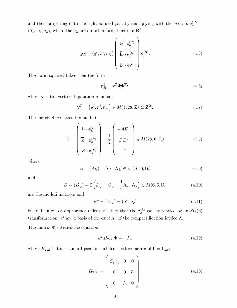
and then projecting onto the right handed part by multiplying with the vectors e(R)µ =
(016, 06, eµ), where the eµ are an orthonormal basis of R6
pR = (qI , ni, mj)
lI · e(R)µ
ki · e(R)µ
kj · e(R)µ
e(R)µ . (4.5)
The norm squared takes then the form
p2R = vTΦΦTv (4.6)
where v is the vector of quantum numbers,
vT =(qI , ni, mj
)∈M(1, 28,Z) ≃ Z28. (4.7)
The matrix Φ contains the moduli
Φ =
lI · e(R)µ
ki · e(R)µ
kj · e(R)µ
=1
2
−AE∗
DE∗
E∗
∈M(28, 6,R) (4.8)
where
A = (AIi) = (eI ·Ai) ∈M(16, 6,R) (4.9)
and
D = (Dij) = 2(Bij −Gij −
1
4Ai · Aj
)∈M(6, 6,R) (4.10)
are the moduli matrices and
E∗ = (Eiν) = (ei · eν) (4.11)
is a 6–bein whose appearence reflects the fact that the e(R)µ can be rotated by an SO(6)
transformation. ei are a basis of the dual Λ∗ of the compactification lattice Λ.
The matrix Φ satisfies the equation
ΦTH22,6 Φ = −I6, (4.12)
where H22,6 is the standard pseudo–euclidean lattice metric of Γ = Γ22;6:
H22,6 =
C−1(16) 0 0
0 0 I6
0 I6 0
, (4.13)
16
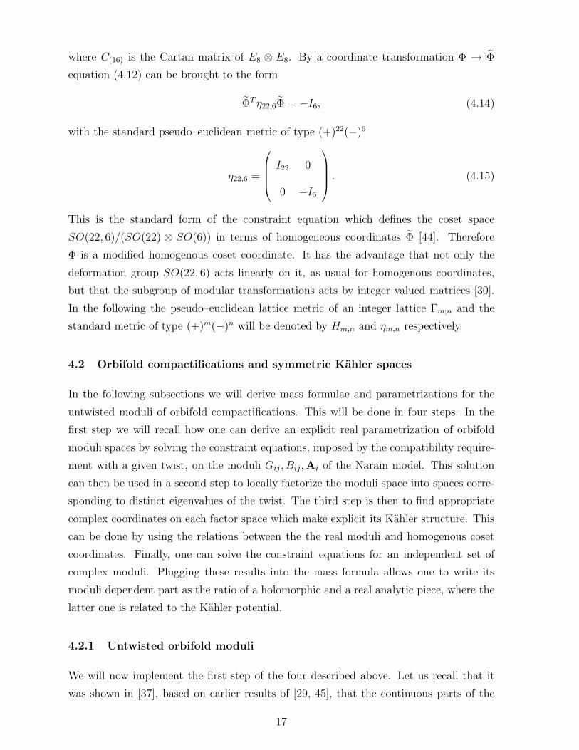
where C(16) is the Cartan matrix of E8 ⊗ E8. By a coordinate transformation Φ → Φ
equation (4.12) can be brought to the form
ΦT η22,6Φ = −I6, (4.14)
with the standard pseudo–euclidean metric of type (+)22(−)6
η22,6 =
I22 0
0 −I6
. (4.15)
This is the standard form of the constraint equation which defines the coset space
SO(22, 6)/(SO(22) ⊗ SO(6)) in terms of homogeneous coordinates Φ [44]. Therefore
Φ is a modified homogenous coset coordinate. It has the advantage that not only the
deformation group SO(22, 6) acts linearly on it, as usual for homogenous coordinates,
but that the subgroup of modular transformations acts by integer valued matrices [30].
In the following the pseudo–euclidean lattice metric of an integer lattice Γm;n and the
standard metric of type (+)m(−)n will be denoted by Hm,n and ηm,n respectively.
4.2 Orbifold compactifications and symmetric Kahler spaces
In the following subsections we will derive mass formulae and parametrizations for the
untwisted moduli of orbifold compactifications. This will be done in four steps. In the
first step we will recall how one can derive an explicit real parametrization of orbifold
moduli spaces by solving the constraint equations, imposed by the compatibility require-
ment with a given twist, on the moduli Gij , Bij,Ai of the Narain model. This solution
can then be used in a second step to locally factorize the moduli space into spaces corre-
sponding to distinct eigenvalues of the twist. The third step is then to find appropriate
complex coordinates on each factor space which make explicit its Kahler structure. This
can be done by using the relations between the the real moduli and homogenous coset
coordinates. Finally, one can solve the constraint equations for an independent set of
complex moduli. Plugging these results into the mass formula allows one to write its
moduli dependent part as the ratio of a holomorphic and a real analytic piece, where the
latter one is related to the Kahler potential.
4.2.1 Untwisted orbifold moduli
We will now implement the first step of the four described above. Let us recall that it
was shown in [37], based on earlier results of [29, 45], that the continuous parts of the
17
background fields Gij, Bij,Ai must satisfy the equations
Dijθjk = θ ji Djk, AIjθ
jk = θ JI AJk (4.16)
where θ ji , θjk and θ JI are the matrices of the internal twist θ and of the gauge twist θ′
with respect to the lattice bases ei, ei and eI of the lattices Λ, Λ∗ and Γ16. Although θ
and θ′ are orthogonal maps their matrices with respect to non–orthonormal lattice bases
are not. Thus, it is convenient to express equations (4.16) in terms of orthonormal bases
eµ and eM of R6 and R16, before solving them [45, 37]. The transformations between
the lattice and orthonormal frames is given by n–bein matrices E∗ = (Eiν) := (ei · eν),
E = (Eiν) := (ei · eν), E = (EIM) = (eI · eM), etc. Note that orthonormal bases are
”selfdual”, eM = eM , eµ = eµ, whereas lattice bases are (generically) not: eI 6= eI ,
ei 6= ei. Therefore Eiµ = E µi 6= Ei
µ. A useful relation to be used later is E∗ = ET,−1.
One complication is that the metric moduli drop out of the D–matrix when written with
respect to an orthonormal frame, because eµ ·eν = δµν and therefore (see below for details
of the transformation)
Dµν = 2(Bµν − δµν −
1
4Aµ · Aν
)(4.17)
Instead, they are now contained in the 6–bein E which is sensitive to deformations of Λ.
To study the effect of lattice deformations let us fix a reference lattice Λ and introduce
a deformation map S (or better a family of deformation maps) which maps it to Λ
S : Λ → Λ : ei → ei = S ji ej =⇒ Gij = ei · ej → Gij = ei · ej (4.18)
This is compatible with the twist θ : ei → θ ji ej if
S ji θ
kj = θ ji S
kj . (4.19)
In order to transform equations (4.16) and (4.19) into the orthonormal frame we will
have to work out some formulae. Consider therefore the deformation described in terms
of the eµ
S : eµ → e′µ = S ν
µ eν =⇒ eµ · eν = δµν → e′µ · e′
ν =: Gµν 6= δµν (4.20)
Thus, a compactification on Λ with background metric δµν can be reinterpreted as a
compactification on a fixed lattice Λ in a deformed background Gµν . Noting that
S νµ = e′
µ · eν = e′µ · eν =: Sµν and Sµν := e′µ · eν = GµνSµν (4.21)
and defining S∗ = (Sµν), S = (S νµ ) we have that S∗ = ST,−1.
Next we introduce a fixed (moduli independent) coordinate transformation which con-
nects the orthonormal basis eµ to the lattice basis ei of the reference lattice Λ:
ei = T µi eµ ⇒ T µ
i = ei · eµ (4.22)
18
This matrix and its inverse T iµ = eµ · e i connect the deformation matrices by
S νµ = T i
µ Sji T
νj (4.23)
Therefore, the matrix T µi also connects the deformed orthonormal basis e′
µ to the de-
formed lattice basis ei:
ei = T µi e′
µ ⇒ T µi = ei · e′µ = ei · eµ. (4.24)
The relations between the four n–bein matrices E νi , T
µi , S
ji , S
νµ and the four bases ei, ei,
eµ, e′µ are summarized by
E νi = S j
i Tνj = T µ
i Sνµ (4.25)
which shows that S ji and S ν
µ relate the undeformed lattice basis ei and the orthonormal
basis eµ to their images ei, eµ under the deformation S, whereas T describes a fixed
coordinate transformation relating ei to eµ and ei to e′µ. E is a family of coordinate
transformations relating the moving frame ei to the fixed orthonormal frame eµ. Equation
(4.25) shows that E can be factorised into a moduli–dependent piece and a moduli–
independent one in two different ways.
We can now use the n–bein matrices and transform the equations (4.16), (4.19) into the
orthonormal bases. In order to do this we have to introduce the transformed moduli
matrices
Dµν = E iµDijE
jν = T i
µDijTjν , AMν = E I
MAIjEjν = E I
MAIjTjν , S ν
µ = T iµ S
ji T
νj (4.26)
and the transformed twist matrices
θ νµ = E iµθ
ji E
νj = T i
µ θji T
νj , θµν = Eµ
iθijE
jν = T µi θ
ijT
jν , θ NM = E I
MθJI E N
J . (4.27)
Note that these relations are consistent thanks to (4.19). Since eµ, eM are orthonormal
bases it follows that
θ νµ = θµν =: θµν and θ NM =: θMN (4.28)
are orthogonal matrices.
Using the formulae derived above we find that equations (4.16), (4.19) are equivalent to
θMNANν = AMµθµν , θµνDνρ = Dµνθνρ, θµνSνρ = Sµνθνρ. (4.29)
The orthonormal bases can be chosen such that the twists θ, θ′ take their real standard
forms, with nonvanishing 2×2 blocks along the diagonal. A slight modification will turn
out to be useful in order to display the coset structure. Namely, we will group together
19
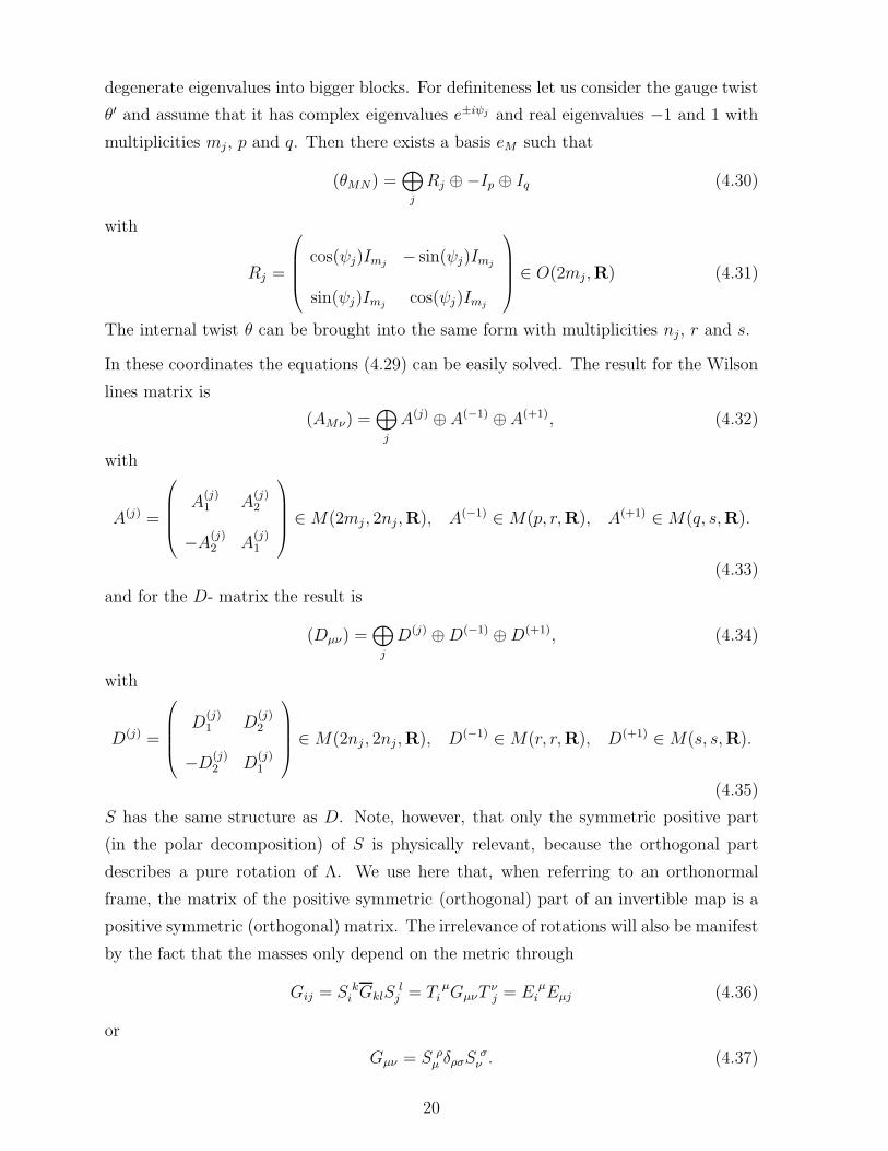
degenerate eigenvalues into bigger blocks. For definiteness let us consider the gauge twist
θ′ and assume that it has complex eigenvalues e±iψj and real eigenvalues −1 and 1 with
multiplicities mj , p and q. Then there exists a basis eM such that
(θMN) =⊕
j
Rj ⊕−Ip ⊕ Iq (4.30)
with
Rj =
cos(ψj)Imj− sin(ψj)Imj
sin(ψj)Imjcos(ψj)Imj
∈ O(2mj,R) (4.31)
The internal twist θ can be brought into the same form with multiplicities nj, r and s.
In these coordinates the equations (4.29) can be easily solved. The result for the Wilson
lines matrix is
(AMν) =⊕
j
A(j) ⊕A(−1) ⊕A(+1), (4.32)
with
A(j) =
A(j)1 A
(j)2
−A(j)2 A
(j)1
∈M(2mj , 2nj,R), A(−1) ∈M(p, r,R), A(+1) ∈M(q, s,R).
(4.33)
and for the D- matrix the result is
(Dµν) =⊕
j
D(j) ⊕D(−1) ⊕D(+1), (4.34)
with
D(j) =
D(j)1 D
(j)2
−D(j)2 D
(j)1
∈M(2nj , 2nj,R), D(−1) ∈ M(r, r,R), D(+1) ∈M(s, s,R).
(4.35)
S has the same structure as D. Note, however, that only the symmetric positive part
(in the polar decomposition) of S is physically relevant, because the orthogonal part
describes a pure rotation of Λ. We use here that, when referring to an orthonormal
frame, the matrix of the positive symmetric (orthogonal) part of an invertible map is a
positive symmetric (orthogonal) matrix. The irrelevance of rotations will also be manifest
by the fact that the masses only depend on the metric through
Gij = S ki GklS
lj = T µ
i GµνTνj = E µ
i Eµj (4.36)
or
Gµν = S ρµ δρσS
σν . (4.37)
20
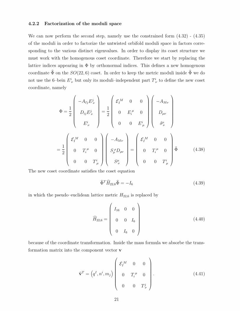
4.2.2 Factorization of the moduli space
We can now perform the second step, namely use the constrained form (4.32) - (4.35)
of the moduli in order to factorize the untwisted orbifold moduli space in factors corre-
sponding to the various distinct eigenvalues. In order to display its coset structure we
must work with the homogenous coset coordinate. Therefore we start by replacing the
lattice indices appearing in Φ by orthonormal indices. This defines a new homogenous
coordinate Φ on the SO(22, 6) coset. In order to keep the metric moduli inside Φ we do
not use the 6–bein Eiν but only its moduli–independent part T iν to define the new coset
coordinate, namely
Φ =1
2
−AIjEjν
DijEjν
Eiν
=1
2
E MI 0 0
0 E µi 0
0 0 Eiµ
−AMν
Dµν
δµν
=1
2
E MI 0 0
0 T µi 0
0 0 T iµ
−AMν
S ρµDρν
Sµν
=
E MI 0 0
0 T µi 0
0 0 T iµ
Φ (4.38)
The new coset coordinate satisfies the coset equation
ΦT H22,6Φ = −I6 (4.39)
in which the pseudo–euclidean lattice metric H22,6 is replaced by
H22,6 =
I16 0 0
0 0 I6
0 I6 0
(4.40)
because of the coordinate transformation. Inside the mass formula we absorbe the trans-
formation matrix into the component vector v
vT =(qI , ni, mj
)
E MI 0 0
0 T µi 0
0 0 T jν
. (4.41)
21
such that
vTφ = vT φ. (4.42)
Now we can use the block–diagonal form of the A, D and S matrices and permute the
rows and columns of Φ such that it becomes block–diagonal
Φ →⊕
j
φ(j) ⊕ φ(−1) ⊕ φ(+1) (4.43)
with
φ(j) =1
2
−A(j)
S(j)D(j)
(S(j))T,−1
∈M(2mj + 2nj, 2nj,R) (4.44)
and a similar expression for φ(−1) ∈M(p + r, r,R) and φ(+1) ∈M(q + s, s,R).
In the coset equation (4.39) this permutation results in replacing
H22,6 →⊕
j
H2mj+2nj ,2nj⊕ Hp+r,r ⊕ Hq+s,s, (4.45)
which makes manifest the factorization into factors corresponding to the distinct eigen-
values of the twist.
Again we can keep the mass formula form–invariant by absorbing this permutation into
the components v. Note, however, that the underlying lattice will not have a correspond-
ing decomposition, because a generic lattice vector has nonvanishing projections onto
more than one eigenspace. Therefore the mass formula will not factorize for all states,
but only for those having quantum numbers which live in only one of the eigenspaces.
Before we proceed to discuss the irreducible factors in the decomposition, let us recall
from [25] that N = 1 space time supersymmetry requires θ to have no eigenvalue +1 and
the eigenvalue −1 can only have multiplicities 0 or 2. Therefore s = 0 and either r = 0
or r = 2. This implies that Φ(+1) does not appear. More generally, if some eigenvalue
does only appear in θ (θ′) but not in θ′ (θ) this gives rise to vanishing rows in the Wilson
line matrix and therefore also in the rearranged Φ. They correspond to directions of the
Narain lattice which possess no deformations.
4.2.3 Real eigenvalues and the SO(p+ 2, 2) coset
We will now study the subspace which corresponds to the real twist eigenvalue −1 and
is parametrized by φ(−1). For the later discussion of modular symmetries it is convenient
22
to go one step back and to introduce a lattice basis in this sector. More precisely (see
[30]) we can find a sublattice Γp+2,2 of the Narain lattice Γ22,6 on which the twist Θ acts
as −Ip+4. Note, however, that this lattice is only a sublattice but not a direct factor,
which means that there is no decomposition Γ22,6 = Γp+2,2 ⊕ · · ·, but only a sublattice
Γp+2,2⊕· · · ⊂ Γ22,6. We will now consider those states that have non–vanishing quantum
numbers lying in Γp+2,2 only.
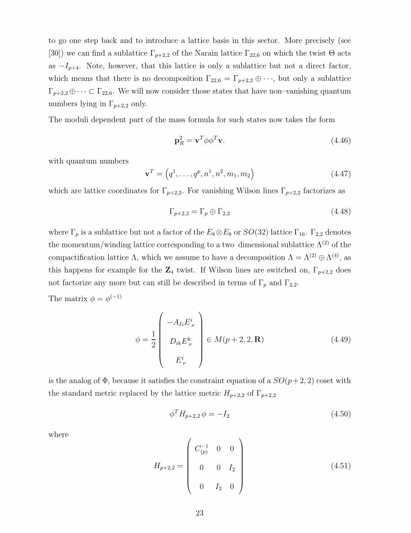
The moduli dependent part of the mass formula for such states now takes the form
p2R = vTφφTv. (4.46)
with quantum numbers
vT =(q1, . . . , qp, n1, n2, m1, m2
)(4.47)
which are lattice coordinates for Γp+2,2. For vanishing Wilson lines Γp+2,2 factorizes as
Γp+2,2 = Γp ⊕ Γ2,2 (4.48)
where Γp is a sublattice but not a factor of the E8⊗E8 or SO(32) lattice Γ16. Γ2,2 denotes
the momentum/winding lattice corresponding to a two–dimensional sublattice Λ(2) of the
compactification lattice Λ, which we assume to have a decomposition Λ = Λ(2) ⊕Λ(4), as
this happens for example for the Z4 twist. If Wilson lines are switched on, Γp+2,2 does
not factorize any more but can still be described in terms of Γp and Γ2,2.
The matrix φ = φ(−1)
φ =1
2
−AIiEiν
DikEkν
Eiν
∈M(p + 2, 2,R) (4.49)
is the analog of Φ, because it satisfies the constraint equation of a SO(p+2, 2) coset with
the standard metric replaced by the lattice metric Hp+2,2 of Γp+2,2
φTHp+2,2 φ = −I2 (4.50)
where
Hp+2,2 =
C−1(p) 0 0
0 0 I2
0 I2 0
(4.51)
23
and C(p) is the lattice metric of Γp.
In order to introduce complex coordinates and to make explicit the Kahler structure of
the SO(p + 2, 2) coset, we will now transform equation (4.51) into its standard form.
This can be done in two steps. The first step consists in converting the lattice indices
I, J, . . . = 1, . . . , p which refer to a lattice basis of Γp, into orthonormal indices M,N, . . .
as well as converting the lattice indices i, j, . . . = 1, 2, which refer to lattice bases of Λ2
(as lower indices) and of Λ∗2 (as upper indices), into orthonormal indices µ, ν. This is
done in a similar way to the one discussed in the last subsection, and one arrives at the
coordinate φ = φ(−1) introduced already there.
The second step for bringing equation (4.51) into its canonical form consists in replacing
the metric Hp+2,2 by the standard metric ηp+2,2. This is achieved by
vT φ = vT φ (4.52)
with
φ =
Ip 0 0
0 1√2I2
1√2I2
0 1√2I2 − 1√
2I2
φ , vT = vT
Ip 0 0
0 1√2I2
1√2I2
0 1√2I2 − 1√
2I2
(4.53)
In terms of the real moduli we have that
φ =1
2
−A
1√2(SD + ST,−1)
1√2(SD − ST,−1)
(4.54)
with A = A(−1), etc.
The new homogenous coset coordinate φ satisfies the standard coset relation
φTηp+2,2 φ = −I2. (4.55)
Recall that ηp+2,2 is the standard metric of type (+)p+2(−)2.
We can now introduce complex coset coordinates by [44]
φ =
φ1(1) φ1
(2)
......
φp+4(1) φp+4
(2)
∈M(p + 4, 2,R) −→ φc =
φ1(1) + i φ1
(2)
...
φp+4(1) + i φp+4
(2)
∈M(p + 4, 1,C)
(4.56)
24
The complex coordinate φc satisfies the equations
φ+c ηp+2,2 φc = −2, φTc ηp+2,2 φc = 0 (4.57)
and is therefore the standard complex homogenous coordinate on the SO(p+ 2, 2) coset
[44]. Note that we can replace vT φ by vTφc in the mass formula, because
p2R = vT φφT v = vTφcφ
+c v = |vTφc|2 (4.58)
Thus the moduli dependent part of the mass is proportional to the norm squared of a
complex number.
Our next step towards the derivation of the mass formula is to solve the complex con-
straint equations in terms of unconstrained complex coordinates and to make explicit the
Kahler structure of the moduli space and the Kahler potential. This procedure is well
known both in the mathematical [44] and in the physics [27] literature. We will use first
the physicists approach and then explain the relation to the results in the mathematical
literature.
A bounded realization
One way of solving the constraint equations is to first extract a scale factor√Y from
the coordinates, where Y is a positive, real analytic functions of the moduli. It turns
out that this function is closely related to the Kahler potential [27]. In terms of the new
variables y ∈ Cp+4
y =√Y φc (4.59)
the constraints readp+2∑
i=1
|yi|2 − |yp+3|2 − |yp+4|2 = −2Y (4.60)
andp+2∑
i=1
y2i − y2
p+3 − y2p+4 = 0 (4.61)
One can now take the first p+ 2 variables as the independent ones and express the other
two in terms of them [27]
yi = zi, i = 1, . . . , p+ 2, yp+3 =1
2
1 +
p+2∑
i=1
z2i
, yp+4 =
i
2
1 −
p+2∑
i=1
z2i
(4.62)
This solves equation (4.61). Defining z = (zi) ∈ Cp+2 we see that equation (4.60) yields
that
Y = Yb =1
4
(1 + (zTz)(zTz) − 2zTz
). (4.63)
25
Solution (4.63) is SO(p+ 2) symmetric.
The domain defined by Y > 0 has two connected components, which is readily seen from
|zTz| = 1 ⇒ Y = 0. Choosing |zTz| < 1 defines a bounded open domain in Cp+2, called
a complex polydisc,
PDp+2 = z ∈ Cp+2| |zTz| < 1 and 1 + (zTz)(zTz) − 2zTz > 0 (4.64)
which provides the standard bounded realization of the SO(p + 2, 2) coset [44]. The
domain possesses a Kahler metric, with Kahler potential [46]
K = − log Yb. (4.65)
An unbounded realization
Another useful parametrization is defined by taking y = (y1, . . . , , yp+1, yp+3) as indepen-
dent variables. Setting [27, 30]
yp+2 = −i1 − 1
4
−
p+1∑
i=1
y2i + y2
p+3
, yp+4 = i
1 +
1
4
−
p+1∑
i=1
y2i + y2
p+3
(4.66)
solves the rescaled constraint equations with
Y = Yu =1
4
(yp+3 + yp+3)
2 −p+1∑
i=1
(yi + yi)2
. (4.67)
This solution is SO(p+ 1, 1) symmetric.
Again, Y > 0 has two connected components, because yp+3 + yp+3 → 0 implies Y → 0.
Taking for definiteness yp+3 + yp+3 > 0 we get the unbounded open domain
Lp+1,1+ + i Rp+2 := y ∈ Cp+2| (yp+3 +yp+3)
2−p+1∑
i=1
(yi+yi)2 > 0, yp+3 +yp+3 > 0 (4.68)
which differs by a factor of i from the one used in the mathematical literature [44]. Note
that the imaginary part of y is unconstrained whereas the real part lives in the forward
light cone of a p + 2 dimensional Minkowski space.
Using the holomorphic transformation between the two parametrizations given in [48] we
know that
K = − log Yu (4.69)
also is a Kahler potential.
26
Another unbounded realization
For applications one prefers to rearrange the complex moduli y in terms of a T and
an U modulus and additional complex Wilson line moduli Bk, Ck. Then, for vanishing
Wilson lines, one is left with an SO(2, 2) coset which factorizes into two SU(1, 1) cosets
parametrised by the T and the U modulus. To do this one has to set (generalizing the
treatment of SO(4, 2) cosets [27, 30])
T = yp+1 + yp+3, 2U = yp+3 − yp+1, Bk = y2k−1 − iy2k, Ck = y2k−1 + iy2k (4.70)
with k = 1, . . . , r. If p is even, then r = p2. If p is odd, r = p−1
2and then there is one
additional unpaired complex coordinate
A = yp (4.71)
In terms of the new moduli, the Yu function now reads
Yu =1
2(T + T )(U + U) − 1
4
r∑
k=1
(Bk + Ck)(Ck +Bk) −1
4(A+ A)2 (4.72)
For completeness, let us display how the yi look in terms of the new moduli
y1 =1
2(B1 + C1), y2 =
i
2(B1 − C1), . . . , and yp = A, if p is odd
yp+1 =1
2(T − 2U), yp+2 = −i
(1 − 1
4(2TU −
∑
k
BkCk − A2)
)
yp+3 =1
2(T + 2U), yp+4 = i
(1 +
1
4(2TU −
∑
k
BkCk − A2)
)(4.73)
Let us now comment on several special cases. First, by setting all of the Wilson moduli
to zero, Bk = Ck = A = 0, one obtains the Kahler potential for a SO(2, 2) coset,
which factorizes into two SU(1, 1) cosets parametrised by the U and the T modulus,
respectively. Again, Y > 0 has two connected components, and U and T have been
defined in such a way, that the condition yp+3 + yp+3 > 0 implies that they both have a
positive real part, as usual.
Next, by inspection of the Kahler potential, one sees that, for a fixed value of
k, T, U,Bk, Ck parametrize a subspace which is a SO(4, 2) coset. Likewise T, U,A
parametrize a SO(3, 2) coset. Note also that by setting Bk = Ck one can truncate a
SO(4, 2) coset to a SO(3, 2) coset. Moreover, for even p = 2m we can eliminate half of
the moduli by setting U + U = r1 and (Bk +Ck)(Bk +Ck) = r2AkAk, with real positive
27
constants r1,2 and thus truncate the SO(p+ 2, 2) coset to a SU(m+ 1, 1) coset. This is
obvious from the fact that Y then takes the form
Y =1
2r1(T + T ) − 1
4r2∑
k
AkAk (4.74)
which leads to the Kahler potential of a SU(m+ 1, 1) coset.
The mass formula
Having found various parametrizations y =√Y φc with y = y(z), y(y) or y =
y(T, U,Bk, CK , A) of the coset, we can substitute each of them into the mass formula
with the result that
p2R =
|vTy|2Y
. (4.75)
Therefore the mass squared can be written as the ratio of the square of the norm of a
chiral mass M = vTy, which is a holomorphic function of the moduli and contains the
dependence on the quantum numbers, and of a real analytic positive function Y , which
is related to a Kahler potential by K = − log Y .
Let us recall that this expression is invariant under the group of target space modular
transformations. To be precise we will consider here the modular group of the sublattice
Γp+2,2 only. The connection of this group with the full modular group was discussed
in the extended version of our paper [30]. A general lattice vector P ∈ Γp+2,2 can be
decomposed as
P = vAE MA (m)eM , A,M = 1, . . . , p+ 4. (4.76)
Here v = (vA) denotes the set of all components with respect to a lattice basis of Γp+2,2
and eM an orthonormal basis. The p+ 4 bein E MA (m) connecting the two bases contains
the dependence on the moduli m = (T, U,Bk, Ck, A). Note that in [30] the full p + 4
bein (E MA ) was denoted by φ, a symbol that we now use for the right moving part (E i
A)
of it. Note also that we discussed the full Narain lattice there, but these considerations
also apply to sublattices. Now a modular transformation consists of acting with a matrix
Ω−1 ∈ SO(p+ 2, 2,Z) on the quantum numbers,
v → Ω−1v, (4.77)
while simultanously transforming the moduli m→ m′ such that P is invariant [49, 30].
As we discussed in some detail in [30] the modular group can be interpreted as a discrete
subgroup of the deformation group SO(p+ 2, 2) and therefore, the transformation of the
moduli is given by the left action of this discrete subgroup on the SO(p + 2, 2) coset.
28
Starting from this observation we then showed how the concrete transformation laws of
the moduli can be worked out.
We can now combine this with the results of this section to deduce the general form of the
transformation of Y and M. First we know that Y only depends on the moduli, but not
on the quantum numbers, and that it is related to the Kahler potential by K = − log Y .
Since the moduli are holomorphic coset coordinates, and modular transformations result
from the left action of SO(p+ 2, 2) on its coset, which is a symmetric Kahler manifold,
K must transform by a Kahler transformation
K → K + F + F , (4.78)
where F is a holomorphic function of the moduli. Therefore Y → e−F−FY . But since by
construction P = (pL;pR) and therefore p2R are invariant, this implies
M → e−FM (4.79)
Examples: The SO(4, 2), SO(3, 2) and SO(2, 2) mass formulae
Let us illustrate the formalism with a concrete example, namely a 2–torus with 2 two–
component Wilson lines turned on. This leads to a SO(4, 2) coset. The reference com-
pactification lattice is chosen to be the A1 ⊕ A1 root lattice. We also have to chose a
two–dimensional sublattice of the E8⊕E8 lattice and, again, we take it to be A1⊕A1. Let
us work out, step by step, the transformations of the quantum numbers v. To implement
the first step v → v, we need the matrices
(E MI ) = (T µ
i ) =
√2 0
0√
2
, (T iµ) =
1√2
0
0 1√2
(4.80)
in order to convert the lattice basis of our reference lattice to an orthonormal one (with
respect to the Euclidean scalar product)
vT = (q1, q2, n1, n2, m1, m2) =
(√2q1,
√2q2,
√2n1,
√2n2,
1√2m1,
1√2m1
)(4.81)
Note that we have written all of the indices as lower ones for simplicity. In a second
step, we have to switch to a basis which is also orthonormal with respect to the pseudo–
euclidean metric. This gives
vT = (q1, q2, n1, n2, m1, m2) =(√
2q1,√
2q2, n1 +1
2m1, n2 +
1
2m2, n1 −
1
2m1, n2 −
1
2m2
)
(4.82)
29
Next, let us use the solution (4.73) of the coset equations for the case p = 2 with U, T,B, C
as independent variables. Then the chiral mass is given by
M =6∑
i=1
viyi = −i(m2 − im1U + in1T − n2(TU − 1
2BC)
+i√2q1(B + C) − 1√
2q2(B − C) ) (4.83)
Using the mass formula (4.75), with the Kahler potential for p = 2 inserted in it, then
gives the following mass formula for an SO(4, 2) coset
p2R =
|m2 − im1U + in1T − n2(TU − 12BC) + i√
2q1(B + C) − 1√
2q2(B − C)|2
12(T + T )(U + U) − 1
4(B + C)(B + C)
(4.84)
The mass formula for a SO(3, 2)-coset can now be gotten from (4.83) in a straightforward
way. Namely, this time we have to choose a one–dimensional sublattice of Γ16 which we
take to be the first of the two A1 lattices of the former example. Now, the two real
Wilson lines will have one component only. Setting the second components to zero
A2i = 0, i = 1, 2 implies B = C. Note that this is a consistent truncation, because B−Cis the coefficent of q2 in (4.84). The mass formula then reads
iM = m2 − im1U + in1T + n2(−UT +1
2B2) + i
√2 q1B (4.85)
The mass formula for a SO(2, 2)-coset is obtained by setting B = C = 0, yielding [27]
iM = m2 − im1U + in1T − n2UT (4.86)
4.2.4 Complex eigenvalues and the SU(m+ 1, 1) coset
We will now discuss the moduli subspace corresponding to complex eigenvalues. We
will, however, restrict ourselves to the case of a non–degenerate rightmoving complex
eigenvalue, ni = 1. In geometrical terms this means that we again focus on a two torus
with Wilson line moduli switched on, but this time with the twist on this subsector acting
as a rotation and not as a reflection. As in the case of the SO(p + 2, 2) coset, one can
step by step repeat the procedure given there for introducing a new homogenous coset
coordinate φ satisfying
φTη2m+2,2φ = −I2. (4.87)
In this case, however, one has to take into account that only half of the components of φ
are independent. This can be done in the following way. After a suitable reordering of
the components
φ′ = P φ, v′T = vTP−1 (4.88)
30
via
P =
Im 0 0 0 0 0
0 0 I2 0 0 0
0 0 0 0 I2 0
0 Im 0 0 0 0
0 0 0 I2 0 0
0 0 0 0 0 I2
(4.89)
one finds that φ′ has the form
φ′ =
φ′1 φ′
2
−φ′2 φ′
1
(4.90)
This effectively leads to the replacement η2m+2,2 → ηm+1,1 ⊕ ηm+1,1 in (4.87). Then, by
introducing the complex coordinate
φc = φ′1 + i φ′
2 ∈M(m+ 2, 1,C) (4.91)
one finds that φc satisfies the relation
φ+c ηm+1,1φc = −1 (4.92)
characterizing the coset SU(m+ 1, 1)/ (SU(m+ 1)⊗U(1)) [44]. Finally, one also has to
introduce complex quantum numbers by
vi(c) = v′i + iv′m+2+i, i = 1, . . . , m+ 2 (4.93)
in order to be able to rewrite the mass formula as
p2R = v′Tφ′φ′Tv′ = |vT(c)φc|2 (4.94)
A bounded realization
Since the homogenous coset coordinate φc is again a complex vector (and not a matrix) we
can proceed as in the last subsection. First we introduce rescaled coordinates yi =√Y φic,
i = 1, . . . , m+ 2 and obtain the equation
m+1∑
i=1
yiyi − ym+2ym+2 = −Y. (4.95)
31
Let us introduce unconstrained coordinates z = (zi, z), i = 1, . . . , m by
yi = zi, i = 1, . . . , m, ym+1 = z, ym+2 = 1. (4.96)
This solves (4.92) with
Y = Yb = 1 − zTz. (4.97)
Note that Y > 0 implies that 1 − zTz > 0. Therefore we have found a realization of the
coset by the bounded open domain [44]
Dm+1 = z ∈ Cm+1| 1 − zTz > 0 (4.98)
and the standard Kahler potential for this realization is [46]
K = − log Yb. (4.99)
Comparing to standard projective coordinates (which are also known to provide a solution
to the constraints [44])
Zi :=φicφm+2c
=yi
ym+2= zi, i = 1, . . . , m, Zm+1 :=
φm+1c
φm+2c
=ym+1
ym+2= z (4.100)
we see that those are identical to the zi, z.
An unbounded realization
Again, we would like to have another, unbounded representation in terms of a T
modulus parametrizing a SU(1, 1) coset and additional complex Wilson line moduli
Ai, i = 1, . . . , m. The yi =√Y φic are now given by
yi = Ai, i = 1, . . . , m, ym+1 =1
2(T − 1), ym+2 =
1
2(T + 1). (4.101)
This solves (4.92) with
Y = Yu =1
2(T + T ) −
m∑
i=1
AiAi (4.102)
Clearly we have found an unbounded realization, because the imaginary part of T , for
example, is not constrained at all, whereas the real part can be arbitrarily large.
There is a second way of connecting the bounded and the unbounded realization. Namely
one can start with the bounded realization and then introduce T and Ai by the map
z → T =1 − z
1 + z, zi → Ai :=
zi1 + z
(4.103)
32
For vanishing Wilson lines this reduces to the standard map from the open unit disc onto
the right half plane
D1 = z ∈ C| |z| < 1 → H = T ∈ C|T + T > 0. (4.104)
Substituting the transformation (4.103) into K ′ = − log Yu yields
K ′ = − log
(1 − zz −
m∑
i=1
zizi
)+ log
(|1 + z|2
)(4.105)
which differs from K = − log Yb by a Kahler transformation. Note that, when relating
z, zi and T,Ai by equating (4.101) and (4.96), this is equivalent to relating them by
(4.103) modulo this Kahler transformation.
The mass formula
Again, the mass formula is given by the ratio of the square of the chiral mass and the
function Y
p2R =
|vT(c)y|2Y
(4.106)
where y and Y are functions of the complex moduli T,Ai, i = 1, . . . , m.
Again this expression is invariant under the group of modular transformations. The
relevant group SU(m + 1, 1,Z) is a subgroup of the group SO(p + 2, 2,Z), namely the
normalizer with respect to the ZN group generated by the twist [49]. Recall that these
groups explictly depend on the reference lattice, so we did not make this explicit in our
notation. For the same reasons as discussed before in the case of SO(p+ 2, 2) cosets, Y
and the chiral mass M transform as
Y → e−F−FY, M → e−FM, (4.107)
where F is a holomorphic function of the moduli.
Example: The SU(2, 1) and SU(1, 1) mass formulae
We will again illustrate the general procedure with a concrete example, a two dimensional
Z3 orbifold with one independent two–component Wilson line. This time we take both
the reference compactification lattice and the sublattice of Γ16 to be A2 root lattices.
Both the internal and the gauge twist are taken to be the A2 Coxeter twist.
Now the transformation matrices from the lattice to the orthonormal basis are given by
(E MI ) = (T µ
i ) =
√2 0
− 1√2
√32
, (Ei
µ) =
1√2
16
√6
0 13
√6
(4.108)
33
The transformed quantum numbers are given by
vT = (q1, q2, n1, n2, m1, m2) =
√
2q1 −1√2q2,
√3
2q2,
√2n1 −
1√2n2,
√3
2n2,
1√2m1,
1
6
√6m1 +
1
3
√6m2 ) (4.109)
Diagonalizing the pseudo–euclidean lattice metric yields
vT = (√
2q1 −1√2q2,
√3
2q2, n1 −
1
2n2 +
1
2m1,
1
2
√3n2 +
1
6
√3m1 +
1
3
√3m2,
n1 −1
2n2 −
1
2m1,
1
2
√3n2 −
1
6
√3m1 −
1
3
√3m2) (4.110)
Next, we have to reorder the components v → v′ and finally complexify them, v′ → vc.
Introducing the complex quantum numbers
qc =√
2q1 −1√2q2 + i
√3
2q2,
nc = n1 −1
2n2 +
1
2m1 + i
√3
2(n2 +
1
3m1 +
2
3m2)
mc = n1 −1
2n2 −
1
2m1 + i
√3
2(n2 −
1
3m1 −
2
3m2) (4.111)
yields that
vT(c) = (qc, nc, mc) (4.112)
Therefore, the chiral mass (setting y1 = y) is given by
M =3∑
i=1
vi(c)yi = qcy+nc1
2(T−1)+mc
1
2(T+1) = qcy+
1
2(nc+mc)T+
1
2(mc−nc) (4.113)
giving raise to the mass formula
p2R =
|qcy + 12(nc +mc)T + 1
2(mc − nc)|2
12(T + T ) − yy
(4.114)
We now proceed to show that one can get the mass formula (4.114) of an SU(2, 1) coset
by a suitable truncation of the one for the SO(4, 2) coset given in (4.84). To do this
truncation correctly, one has to take two things into account. First, the lattice Λ must
be proportional to the A2 root lattice in order to have the A2 Coxeter twist as a lattice
automorphism. This freezes the U modulus to the value U = 12(√
3 + i), while T is still
arbitrary. Secondly, one has to choose inside the E8 ⊕ E8 lattice a sublattice with the
appropriate symmetry. Taking an A2 sublattice amounts to setting
(q1, q2) = (√
2q1 −1√2q2,
√3
2q2) (4.115)
34
in (4.81). Also note that the Wilson line moduli have to be fixed to B =√
3A, C = 0
[30].
Specializing in this way, the chiral mass given in (4.83) turns into
M =
√3
2qcA +
1
2(mc + nc)T +
√3
2(mc − nc) (4.116)
with the complex quantum numbers as defined above. The mass formula (4.84) then
turns into
p2R =
|√
32qcA + 1
2(mc + nc)T +
√3
2(mc − nc)|2√
3(12(T + T ) −
√3
4AA)
(4.117)
Equation (4.114) is then indeed obtained from (4.117) by rescaling T by a factor 1/√
3
and by setting y = A2.
And finally, when switching off the complex Wilson line A, A = 0, one arrives at the
wellknown mass formula for a SU(1, 1)-coset
M =i
2
((mc + nc)T +
√3(mc − nc)
)(4.118)
5 Target space modular invariant orbits of massive untwisted states
Massive untwisted states play an important role in the context of 1-loop corrections
to gauge and gravitational couplings [3]-[6], [8]-[19], [26, 27, 55] in ZN -orbifold models.
These states give rise to moduli dependent threshold corrections, which are given in terms
of automorphic functions of the modular group under consideration [5, 11, 26, 27]. We
will thus focus on massive untwisted states in the following.
We will assume that the internal 6-torus factorises into T6 = T2 ⊕ T4 and that the
lattice twist θ acts on the 2-torus T2 as a Z2-twist. We will then focus on the SO(p +
2, 2)-coset space associated with the T2 and discuss its mass formula. That is, we will
consider those massive untwisted states which have non-vanishing quantum numbers
vT = (q1, ..., qp, n1, n2, m1, m2) in the Narain sublattice Γp+2,2 ⊂ Γ22,6, as discussed in
section 4.2.3. We will, in addition, also allow these massive untwisted states to carry non-
vanishing quantum numbers in an orthogonal sublattice Γ20−p,4 with Γp+2,2 ⊕ Γ20−p,4 ⊂Γ22,6.
Recall that the level matching condition for physical states in the heterotic string reads
p2L − p2
R = 2(NR + 1 −NL) + P2R − P2
L (5.1)
35
where (pL;pR) ∈ Γp+2,2 and (PL;PR) ∈ Γ20−p,4. The mass formula for physical states
can then be written as
α′
2M2 = p2
R + P2R + 2NR (5.2)
The untwisted states associated with the Narain sublattice Γp+2,2 do, on the other hand,
satisfy
p2L − p2
R = 2nTm+ qTCq (5.3)
where C denotes the lattice metric of the sublattice Γp of the E8 ⊕ E8 lattice Γ16, as
explained in section 4.2.3. Then, equating (5.1) and (5.3) yields
p2L − p2
R = 2(NR +1
2P2R + 1 −NL − 1
2P2L) = 2nTm+ qTCq (5.4)
We have shown in section 4.2.3 that for a SO(p+ 2, 2)-coset p2R can be written as
p2R =
|M|2Y
(5.5)
where Y is related to the Kahler potential byK = − log Y , and where M is a holomorphic
function of the complex coordinates for the SO(p+ 2, 2)-coset. From the study of a few
examples in the past [11, 26, 27], it is expected that a prominent role in threshold
corrections to gauge and gravitational couplings is going to be played by those massive
untwisted states which satisfy 2NR + P2R = 0, so that
α′
2M2 = p2
R =|M|2Y
(5.6)
Thus, we will in the following only consider untwisted states for which 2NR + P2R = 0.
Then, (5.4) turns into
p2L − α′
2M2 = 2(1 −NL − 1
2P2L) = 2nTm+ qTCq (5.7)
Note that, for any given 2NL+P2L, the orbit 2nTm+qTCq = 2(1−NL− 1
2P2L) is invariant
under modular SO(p+ 2, 2,Z)-transformations. Let us now consider the following cases:
a) first, consider untwisted states for which NL = 0,P2L = 0. This defines an orbit for
which
2nTm+ qTCq = 2 (5.8)
This is the orbit which is relevant for the discussion of the stringy Higgs effect. It
can namely happen [23] that at certain finite points in the fundamental region of the
36
moduli space certain (otherwise) massive states precisely become massless, M2 = 0.
Then, at these special points in moduli space one has that p2L = 2, and, hence, one has
additional massless gauge bosons in the spectrum as well as additional massless scalar
fields. These additional massless gauge bosons enhance the gauge group of the underlying
two-dimensional Z2-orbifold. This enhancement can give rise to an additional SU(2), as
discussed in section 3. Thus, it it crucial to take into account orbit (5.8) when discussing
1-loop corrections to gauge couplings associated with the enhanced gauge group of the
compactification sector of the orbifold. Similarly, orbit (5.8) must also be taken into
account when discussing threshold corrections to gravitational couplings.
b) now consider untwisted states for which 2NL+P2L = 2. This defines an orbit for which
p2L = p2
R and, hence,
2nTm+ qTCq = 0 (5.9)
An example is provided by setting NL = 0,P2L = 2. Then, take P2
L = 2 to be a vector
in the root lattice of the gauge group G′ which is not affected by the moduli associated
with Γp+2,2. For instance, G′ can be taken to be the E ′8 in the hidden sector left unbroken
when turning on Wilson lines. Then, the orbit given in (5.9) is the relevant one for the
discussion of threshold corrections for this type of gauge couplings in the presence of
Wilson lines.
For untwisted states with quantum numbers q = 0, (5.9) obviously reduces down to
nTm = 0. This reduced orbit is not invariant under general modular SO(p + 2, 2,Z)-
transformations anymore, but it is still invariant under modular transformations belong-
ing to the subgroup SL(2,Z)T ⊗ SL(2,Z)U ⊂ SO(p+ 2, 2,Z). This reduced orbit is the
one which has been discussed quite extensively in the literature [26, 27, 11] in the context
of (2, 2)ZN -orbifold theories. In this context, it is well known that there are no finite
points in the fundamental region of the (T, U)-moduli space where (otherwise) massive
states might become massless. Indeed, by setting [27] n1 = r1s2, n2 = s1s2, m1 = −r2s1
and m2 = r1r2, it follows that p2R = 2
( |r1+is1U |2U+U
) ( |r2+is2T |2T+T
). This shows that it is only
in the large radius limit, namely at T = ∞ with U fixed (and vice-versa), that states
(Kaluza-Klein states) become massless. This is in manifest contrast to what happens for
the orbit discussed in a).
c) finally, consider untwisted states for which 2NL + P2L ≥ 4. Inspection of (5.7) shows
that there aren’t any points, finite or otherwise, in moduli space for which M2 = 0, since
then p2L < 0, which isn’t allowed.
Hence, it is only for the orbits a) and b) that it can happen that massive states become
massless at some special points in the fundamental region of moduli space. Threshold
37
corrections to couplings should then exhibit a singular behaviour at precisely those points
in moduli space. Thus, it appears that the interesting physics contained in threshold
corrections is associated with orbits a) and b). This is then why we will be focussing on
orbits a) and b) in the following.
It was shown [11, 27] in the context of threshold corrections to the E6 and E ′8 gauge
couplings in (2, 2)ZN -orbifold theories, that it is of relevance to consider the quantity∑orbit logM. There, the relevant orbit is the reduced orbit discussed in case b), given
by nTm = 0, q = 0. Indeed, when suitably regularised [27],∑nTm=0,q=0 logM|reg =
log (η−2(T )η−2(U)), this quantity is precisely the object appearing in these threshold
corrections. In the context of threshold corrections to gravitational couplings, on the
other hand, one should apriori consider both the orbits a) and b). We will thus introduce
the following quantities for cases a) and b), respectively
∆0 =1
L0
∑
2nTm+qT Cq=2
logM
∆1 =1
L1
∑
2nTm+qT Cq=0
logM (5.10)
It is implied in (5.10) that a regularisation procedure should exist for turning these for-
mal expressions into meaningful ones. This regularisation procedure should be com-
patible with the transformation property of logM under modular SO(p + 2, 2,Z)-
transformations. Thus, each of the these ∆i, i = 0, 1, is expected to be expressed in
terms of automorphic functions of the modular group SO(p+ 2, 2,Z). The constants Li
are such so as to ensure that, under the subgroup of SL(2,Z)T,U -transformations, each
of the exp ∆i has a modular weight of −1.
Now consider the case when all Wilson lines have been turned off. As will be discussed
in detail in the next section, ∆0 should contain a term of the form
∆0 ∝ log (j(T ) − j(U))r η(T )−2 η(U)−2 + . . . (5.11)
where r denotes some non-zero integer and where j(T ) denotes the absolute modular
invariant function. We will explain that such a term should arise when summing over all
the states lying on the orbit nTm = 1, q = 0. The singular behaviour of this term at the
points in the fundamental region where T = U reflects the fact that (otherwise) massive
states become massless at these points in moduli space, as discussed in section 3. The
role of the eta-terms in (5.11) is to ensure the correct transformation property of exp ∆0
under SL(2,Z)T,U -transformations.4
4 As stated above, we have made the important assumption that the regularisation procedure used in
38
∆1, on the other hand, will contain a term of the form
∆1 ∝ log η(T )−2 η(U)−2 + . . . (5.12)
As shown in [27], this term arises when summing over all massive states for which nTm =
0, q = 0.
As discussed above, all the physically interesting information relevant to the threshold
corrections to gravitational couplings should be contained in ∆0 and in ∆1. These grav-
itational threshold corrections should then, for the case of vanishing Wilson moduli, be
proportional to
∆0 + ∆1 ∝ α log(j(T ) − j(U)) + β logη(T )−2 η(U)−2 (5.13)
where the constants α and β have to be determined from an appropriate string scattering
amplitude calculation. We will, in the next sections, study ∆0 and ∆1 in detail. We will,
in particular, also study the effect of non-vanishing Wilson moduli on (5.13). The last
section will be devoted to a discussion of threshold corrections to gauge and gravitational
couplings.
Note that the analogous result to (5.13) for a SU(m+ 1, 1)-coset can be obtained by an
appropriate truncation of the mass formula (5.6) for a SO(2m+ 2, 2)-coset, as discussed
in section 4.2.4.
6 Automorphic functions for the orbit 2nTm+ qTCq = 2
In this section we will consider massive untwisted states possessing NL = 0,P2L = 0.
Then the associated modular invariant orbit is defined by
2nTm+ qTCq = 2 (6.1)
It can happen that certain massive states, characterised by a set of quantum numbers
satisfying (6.1), become massless at special points in moduli space. Then, at these
special points one has that p2L = 2, and, hence, there are some additional massless states
corresponding to massless gauge bosons. Thus, orbit (6.1) is of big relevance for the
stringy Higgs-effect.
(5.10) respects both holomorphicity and modular covariance. Otherwise additional terms transforming
inhomogenously under modular transformations might appear on the r.h.s. of (5.11). Such additional
terms do not exhibit singular behaviour in the fundamental region, and so their appearance would not
change the singular behaviour of ∆0.
39
We will in the following try to construct automorphic functions for the orbit (6.1). We
will, for concretenesss, first consider a SO(4, 2)-coset associated with an internal 2-torus
T2. At the end of this section, by making use of the truncation procedure given in section
4.2.4, we will also discuss automorphic functions for a SU(2, 1)-coset.
Consider the quantity ∆0 introduced in (5.10). Taking into account that the Cartan
matrix C for the Narain sublattice Γ4;2 under consideration reads C = 2diag(1, 1), yields
(5.10) as
∆0 ∝∑
nTm+q2=1
logM
=∑
nTm=1 , q=0
logM +∑
nTm=0 , q2=1
logM +∑
nTm=−1 , q2=2
logM + . . . (6.2)
where we have rewritten the sum over all the states laying on the SO(4, 2,Z)-invariant
orbit nTm+ q2 = 1 into a sum over SL(2,Z)T,U -invariant orbits nTm = constant. Then,
(6.2) can be conveniently written as
∆0 ∝∑
q2≥0
∆0,q2 = ∆0,0 + ∆0,1 + . . . (6.3)
where
∆0,0 =∑
nTm=1,q=0
logM , ∆0,1 =∑
nTm=0,q2=1
logM (6.4)
Each of the exp ∆0,q2 should carry a definite modular weight under SL(2,Z)T,U -
transformations. The complete exp ∆0 should then have a modular weight of −1.
We begin by studying the case where the Wilson lines B and C have been switched off.
We will later generalise our results to the case of non-vanishing Wilson lines.
As already mentioned, there is an enhancement of the gauge group of the model at some
special points in the (T, U)-moduli space. The relevant untwisted states are the ones for
which q1 = q2 = 0, nTm = 1. For these states the mass formula (4.83) reduces to
M = m2 − im1U + in1T − n2UT (6.5)
Note that we have redefined the chiral mass M by an irrelevant overall phase factor for
convenience. Let us first discuss the issue of enhancement of the gauge group in the
context of a two-dimensional toroidal model. We will then, in a second step, discuss it
in the context of the two-dimensional Z2-orbifold. At generic values for the moduli T
and U the gauge group of the two-dimensional torus T2 under consideration is given by
G = U(1) ⊗ U(1). At special points in the (T, U)-moduli space, namely for i) T = U ,
40
ii) T = U = 1 and iii) T = U = ρ = eiπ6 , this generic gauge group is enhanced to i)
G = SU(2) ⊗ U(1), ii) SU(2) ⊗ SU(2) and iii) G = SU(3) [23], as we discussed in some
detail in section 3.
Let us consider case i) first. Setting T = U turns (6.5) into
M = m2 + i(n1 −m1)T − n2T2 (6.6)
Then, the holomorphic mass (6.6) vanishes for the following 2 untwisted states
m1 = n1 = ±1 , m2 = n2 = 0 (6.7)
Note that these states satisfy nTm = 1. Thus, they are precisely the 2 states correspond-
ing to the 2 additional gauge bosons which enhance the gauge group to G = SU(2)⊗U(1)
at the points where T = U .
Next, consider case ii). Setting T = U = 1 turns (6.6) into
M = m2 − n2 + i(n1 −m1) (6.8)
In addition to the 2 states (6.7) there are now 2 additional ones
m2 = n2 = ±1 , m1 = n1 = 0 (6.9)
satisfying nTm = 1, for which the holomorphic mass (6.8) vanishes. These 2 states
correspond to the 2 additional massless gauge bosons which further enhance the gauge
group from G = SU(2) ⊗ U(1) to G = SU(2) ⊗ SU(2).
Finally, consider case iii). Inserting T = U = eiπ6 into (6.6) yields
M =1
2
(2m2 − n2 − n1 +m1 + i
√3(n1 −m1 − n2)
)(6.10)
The holomorphic mass (6.10) vanishes not only for the states (6.7), but also for the
following 4 additional states satisfying nTm = 1
m2 = n2 = 1 : m1 = −1 , n1 = 0 or m1 = 0 , n1 = 1
m2 = n2 = −1 : m1 = 0 , n1 = −1 or m1 = 1 , n1 = 0 (6.11)
These 4 additional massless states correspond again to 4 additional massless gauge bosons
which enhance the gauge group to G = SU(3). Thus, the ratio of additional massless
gauge bosons for the cases i)-iii) is given by 1:2:3. Note that there is an infinite set of
states with dual transformed quantum numbers, whose masses vanish at the transformed
critical points.
41
The enhancement of the gauge group for the Z2-orbifold occurs at the same points in
moduli space as in the toroidal case. The associated gauge groups are, however, smaller,
since one has to project out all the non-twist invariant states. The resulting gauge groups
are then, for the cases i)-iii), given by i)U(1), ii)U(1)⊗U(1) iii) SU(2) at level k = 4, as
discussed in section 3. Thus, the ratio of additional massless gauge bosons is, as in the
toroidal case, given by 1:2:3.
Now, what do the individual ∆0,q2 given in (6.4) look like? First consider ∆0,0. It
is defined in terms of a sum over all the states laying on the orbit nTm = 1, q = 0.
As shown above, this is precisely the orbit for which some of the massive states become
massless at the special points i)-iii) in the fundamental region of the (T, U)-moduli space.
Thus, at each of these special points ∆0,0 has to exhibit a logarithmic singularity. The
order of this singularity should be determined by the number of states which become
massless at these special points. As shown above, the ratio of additional massless states
at the special points i)-iii) is 1:2:3. Thus, the order of the zeros of exp ∆0,0 should be
1:2:3 for the points i)-iii). According to well-known theorems of modular functions [51],
the order of the zeros and of the poles, together with the modular weights (possibly
leading to non-trivial multiplier systems), determine a modular function in a unique way.
Applying this to the above case yields that
exp ∆0,0 ∝ (j(T ) − j(U))r η(T )−2 η(U)−2 (6.12)
where r denotes some non-zero integer. j(T ) denotes the absolute modular invariant
function.5 The formal definition (6.4) of ∆0,0 implies that ∆0,0 has to carry a modular
weight of −1 under SL(2,Z)T,U -transformations. This explains the presence of the eta-
terms in (6.12), which indeed ensure that exp ∆0,0 transforms with modular weight of −1
under SL(2,Z)T,U -transformations. Furthermore, exp ∆0,0, as given in (6.12), obviously
vanishes for T = U . For T in the vicinity of U one has that j(T )− j(U) = j′(U)(T −U).
For T ∼ U = 1 one finds that j(T ) − j(U) = 12j′′(1)(T − 1)2, because of j′(1) = 0.
And, finally, for T ∼ U = ρ one has that j(T ) − j(U) = 13!j′′′(ρ)(T − ρ)3, because
j′(ρ) = j′′(ρ) = 0. Thus, the ansatz j(T )− j(U) does indeed reflect the ratio 1:2:3 in the
order of the zeros of exp ∆0,0. This observation is just a reflection of the fact that the
order of the zeros of the j-function is determined by the order of the fixed points of the
duality group; this order is proportional to the number of massless states at the fixed
points, as proven in (3.10).
5In (6.12) we have ignored possible additional multiplicative terms of the type exp f(T, U) with
f(T, U) exhibiting regular behaviour inside the fundamental region. Such terms might be necessary in
order to reproduce the correct asymptotic behaviour of ∆0,0 as T, U → ∞ [58].
42
Comparing (6.4) with (6.12), on the other hand, gives that
∆0,0 =∑
nTm=1
log(m2 − im1U + in1T − n2UT )
= log(j(T ) − j(U))r η(T )−2 η(U)−2 + . . . (6.13)
for some non-zero integer r. In (6.13) a regularisation of the infinite sum is implied. Thus,
(6.13) yields a representation of j(T )r η(T )−2 as a regularised sum (of chiral masses) over
all the states on the orbit nTm = 1, q = 0. It would be very interesting to prove this
directly by explicitly performing the sum. To our knowledge such a representation is
unknown in the literature. The dots in (6.13) stand for additional terms which are
regular inside the fundamental region of the T, U-moduli space (see footnote 5).
Let us now switch on the Wilson lines B and C and discuss the resulting modifications to
(6.13). We will, unfortunately, have to restrict ourselves to the case where B and C are
small, that is, we will work to lowest non-trivial order in B and C, only. When switching
on Wilson lines, ∆0,0 becomes equal to
∆0,0 =∑
nTm=1
logm2 − im1U + in1T + n2(−UT +1
2BC) (6.14)
as can be seen from (4.83). Then, a suitable ansatz for the modification to (6.13) is, to
lowest order in BC, given by
∆0,0 = log(j(T ) − j(U) +
1
2BC X(T, U)
)r+ log
(η(T )−2 η(U)−2 +
1
2BC Y (T, U)
)
+ . . . (6.15)
where X(T, U) and Y (T, U) will be determined in the following. Let us first dis-
cuss the modification to the (j(T ) − j(U))-term given by X(T, U). Under SL(2,Z)U -
transformations [17, 30]
U → αU − iβ
iγU + δ, T → T − iγ
2
BC
iγU + δ, αδ − βγ = 1
B → B
iγU + δ, C → C
iγU + δ(6.16)
it follows that, to lowest order in BC,
j(T ) − j(U) → j(T ) − j(U) − iγ
2
BC
iγU + δj′(T ) (6.17)
Then, if one requires that j(T ) − j(U) + 12BCX(T, U) should be invariant under
SL(2,Z)T,U -transformations (6.16), one obtains that X(T, U) has to transform as
X(T, U) → (iγU + δ)2 X(T, U) + iγ(iγU + δ) j′(T ) (6.18)
43
Similarly it follows that, under SL(2,Z)T -transformations, X(T, U) has to transform to
lowest order in BC as
X(T, U) → (iγT + δ)2 X(T, U) − iγ(iγT + δ) j′(U) (6.19)
Note that, in addition, X(T, U) has to vanish at T = U . Only then does ∆0,0 again
become singular at T = U . This has to be the case because, as discussed in section 3, the
enhancement of the gauge group still occurs at T = U when Wilson lines are switched on.
Indeed, when inserting (6.7) into (6.14) it follows that ∆0,0 has a singularity at T = U .
Similarly, when inserting (6.9) into (6.14) shows that another singularity of ∆0,0 occurs
at T = U =√
1 + BC2
. And finally, when inserting (6.11) into (6.14) yields yet another
singularity of ∆0,0 at T = U = i2+√
34
+ BC2
, thus substanciating our claims in section 2.
All these requirements do not uniquely specify X(T, U), however. The following X(T, U)
satisfies all the above requirements
X(T, U) = ∂U log η2(U) j′(T ) − ∂T log η2(T ) j′(U) + a (j(T ) − j(U)) η4(T )η4(U)
+ O((BC)2) (6.20)
where a is an arbitrary constant which cannot be determined alone by symmetry ar-
guments. Note that the first term in (6.20) transforms inhomogenously as in (6.19),
whereas the second term in (6.20) transforms homogenously with modular weight 2 un-
der SL(2,Z)T,U -transformations.6
One can now try to determine the function Y (T, U) in a similar manner [17] by demanding
that η(T )−2 η(U)−2 + 12BC Y (T, U) should transform with modular weight of −1 under
SL(2,Z)T,U -transformations. Then, one has to require Y (T, U) to transform as [17]
Y (T, U) → (iγU + δ)Y (T, U) + iγη−2(U)∂T η−2(T ) (6.21)
under SL(2,Z)U -transformations as well as [17]
Y (T, U) → (iγT + δ)Y (T, U) + iγη−2(T )∂Uη−2(U) (6.22)
under SL(2,Z)T -transformations. These transformation laws do, however, not uniquely
specify Y (T, U). The following Y (T, U) transforms appropriately up to corrections of
6This is, strictly speaking, not quite correct. We have ignored the issue of field-independent phases
φ = φ(α, β, γ, δ), which arise when performing modular transformations. These phases, also called
multiplier systems, show up in the transformation laws of the Wilson line moduli B and C as well as in
the transformation law of the eta-function. Thus, in order to really construct the appropriate function
X(T, U), care needs to be taken of all the different multiplier systems appearing in the transformation
laws.
44
order (BC)2
Y (T, U) = −η(T )−2 η(U)−2 ∂T log η2(T ) ∂U log η2(U) + b η2(T ) η2(U) + · · · (6.23)
where b denotes an arbitrary constant which cannot be determined alone by symmetry
arguments. Note that the first term [17] in (6.23) transforms inhomogenously under
SL(2,Z)T,U -transformations, whereas the second term in (6.23) transforms homogenously
with modular weight 1.7 Hence, it follows from (6.15) that the BC-corrected exp ∆0,0 is
given by
exp ∆0,0 ∝ (j(T ) − j(U))r η(T )−2 η(U)−2
+1
2BC rX(T, U)(j(T ) − j(U))r−1η(T )−2 η(U)−2
+1
2BC Y (T, U)(j(T ) − j(U))r (6.24)
with X(T, U) and Y (T, U) given by (6.20) and (6.23), respectively.
Next, let us discuss ∆0,1 in the presence of Wilson lines. The sum now runs over all the
states for which nTm = 0, q2 = 1. This set of states can be divided into two subsets. The
first subset consists of the 4 states n = m = 0, q2 = 1, whereas the second subset consists
of all the states for which (n,m) 6= (0, 0), q2 = 1. Then, it follows from (4.83) that
∆0,1 = 2 log(B + C) + 2 log(B − C) +∑
(n,m)6=(0,0),q2=1
logM + const (6.25)
The first two terms in (6.25) are the contribution arising from the 4 states n = m =
0, q2 = 1. When turning off the Wilson lines, these 4 states become massless, thus
giving rise to logarithmic singularities in ∆0,1, as required. The last term in (6.25),∑
(n,m)6=(0,0),q2=1 logM, can be written as
∑
(n,m)6=(0,0),q2=1
logM =∑
(n,m)6=(0,0)
logM +i√2(B + C)
+∑
(n,m)6=(0,0)
logM − i√2(B + C) +
∑
(n,m)6=(0,0)
logM +1√2(B − C)
+∑
(n,m)6=(0,0)
logM − 1√2(B − C) (6.26)
where
M = m2 − im1U + in1T + n2(−UT +1
2BC) (6.27)
7We have, again, ignored the issue of multiplier systems appearing in the transformation laws given
above.
45
Then, expanding (6.26) to lowest order in B and C yields that
∑
(n,m)6=(0,0),q2=1
logM = 4
∑
(n,m)6=(0,0)
log(m2 − im1U + in1T − n2UT )
+1
2BC
∑
(n,m)6=(0,0)
n2
(m2 − im1U + in1T − n2UT )
+ 2 B C∑
(n,m)6=(0,0)
1
(m2 − im1U + in1T − n2UT )2(6.28)
As we will show in the next section, the terms in the big bracket in (6.28) give, when
suitably regularised, rise to ∑
(n,m)6=(0,0)
log(m2 − im1U + in1T − n2UT ) +BC
2
n2
(m2 − im1U + in1T − n2UT ) |reg
= log(η(T )−2 η(U)−2 − 1
2BC η(T )−2 η(U)−2 ∂T log η2(T ) ∂U log η2(U)
)(6.29)
Furthermore, (6.28) should not exhibit any singular behaviour at finite points in the
fundamental region of moduli space, and it should transform appropriately under
SL(2,Z)T,U -transformations. Together with (6.29) this then restricts (6.28), to lowest
order in B and C, to be given by8
∑
(n,m)6=(0,0),q2=1
logM = 4 log(η(T )−2 η(U)−2
− 1
2BC η(T )−2 η(U)−2 ∂T log η2(T ) ∂U log η2(U)
)+ cBCη(T )4 η(U)4 (6.30)
where c is an arbitrary constant which cannot be fixed by symmetry considerations
alone. Note that the last term in (6.30) is invariant under SL(2,Z)T,U -transformations.9
Equation (6.30) can also be written as
∑
(n,m)6=(0,0),q2=1
logM = 4 log(η(T )−2 η(U)−2 +
1
2BC Y (T, U)
)(6.31)
with Y given in (6.23). Inserting (6.31) into (6.25) yields that
∆0,1 = p log(B + C) + p log(B − C)
+ t log(η(T )−2 η(U)−2 +
1
2BC Y (T, U)
)+ const (6.32)
8Holomorphic regularisation of the last term in (6.28) yields∑
(n,m) 6=(0,0)1
(m2−im1U+in1T−n2UT )2 ∝G2(T )G2(U). The holomorphically regularised Eisenstein function G2(T ), however, transforms inho-
mogenously under SL(2,Z)T -transformations. We thus suspect that the procedure given in (6.28) for
computing ∆0,1 is too naive.9Ignoring again complications due to the appearance of multiplier systems.
46
with appropriate constants p and t. Note that each of the factors in exp ∆0,1 transforms
with modular weight of −1 under SL(2,Z)T,U -transformations.
Inserting (6.15) and (6.32) into (6.2) yields that
∆0 ∝ r log(j(T ) − j(U) +
1
2BC
(∂U log η2(U) j′(T ) − ∂T log η2(T ) j′(U)
))
+ t log(η(T )−2 η(U)−2 − 1
2BCη(T )−2 η(U)−2 ∂T log η2(T ) ∂U log η2(U)
)
+ b BC η4(T ) η4(U) + p log(B + C) + p log(B − C) + . . . (6.33)
where, again, p, r, t and b denote some appropriate constants. Note that each of the
terms in (6.33) is either invariant or the logarithm of a term transforming with weight
of −1 under modular SL(2,Z)-transformations. Also note that, up to quadratic order
in B and C, the terms given in (6.33) are the only ones one can write down which can
exhibit singular behaviour at finite points in the moduli space. At these points, otherwise
massive states become massless, thus inducing this singular behaviour. The terms in
(6.33) represent possible threshold corrections terms which one should find in calculations
of the running of gauge and gravitational couplings in orbifolds with Z2-sectors. In that
context, the coefficients p, r, t and b are related to beta-function coefficients as well as to
Kahler and σ-model anomaly coefficients. This will be discussed in the last section of this
paper. Finally, note that the terms given in (6.33) transform appropriately under modular
SL(2,Z)T,U -transformations, but not under additional transformations belonging to the
full modular SO(4, 2,Z)-group. The dots in (6.33) stand for additional contributions,
which we haven’t computed, whose role is to restore the proper transformation behaviour
of ∆0 under full SO(4, 2,Z)-transformations.
Finally, let as look at the SU(2, 1)-coset discussed in section 4.2.4, which was based on
an A2-root lattice. Applying the truncation U = 12(√
3 + i), C = 0, B =√
3A to (6.33)
yields that
∆0 ∝ r log j(T ) + t log η(T )−2 + p logA + const+ . . . (6.34)
where we have used that j(U = ρ) = 0. The dots in (6.34) stand for additional terms
whose role is to restore the proper transformation behaviour of (6.34) under transforma-
tions belonging to the full modular SU(2, 1,Z)-group.
47
7 Automorphic functions for the orbit 2nTm+ qTCq = 0
In this section we will consider massive untwisted states possessing 2NL+P2L = 2. Then,
the associated modular invariant orbit is defined by
2nTm+ qTCq = 0 (7.1)
Let us again look at the example of an SO(4, 2)-coset, for concreteness. As in the previous
section, by taking into account that the Cartan matrix C for the Narain sublattice Γ4;2
under consideration reads C = 2diag(1, 1), then yields (5.10) as
∆1 ∝∑
nTm+q2=0
logM =∑
nTm=0 , q=0
logM +∑
nTm=−1 , q2=1
logM + . . . (7.2)
where we have rewritten the sum over all the states laying on the SO(4, 2,Z)-invariant
orbit nTm+ q2 = 0 into a sum over SL(2,Z)T,U -invariant orbits nTm = constant.
Let us consider the term∑nTm=0 , q=0 logM in (7.2). That is, let us consider massive
untwisted states for which q1 = q2 = 0, nTm = 0 and (n,m) 6= 0. For these states the
mass formula (4.83) reduces to
M = m2 − im1U + in1T + n2(−UT +1
2BC) (7.3)
Expanding to lowest order in B and C yields
∑
nTm=0 , q=0
logM =∑
(n,m)6=0
log(m2 − im1U + in1T − n2UT )
+1
2BC
∑
(n,m)6=0
n2
(m2 − im1U + in1T − n2UT )+ O((BC)2) (7.4)
Introducing a set of integers r1, r2, s1 and s2 [27] subject to nTm = 0, (n,m) 6= 0,
m2 = r1 r2 , n2 = s1 s2 , m1 = −r2 s1 , n1 = r1 s2 (7.5)
allows one to rewrite (7.4) as
∑
nTm=0 , q=0
logM =∑
(r1,s1)6=(0,0)
log(r1 + is1U) +∑
(r2,s2)6=(0,0)
log(r2 + is2T )
+1
2BC (
∑
(r1,s1)6=(0,0)
s1
r1 + is1U)(
∑
(r2,s2)6=(0,0)
s2
r2 + is2T)
+ O((BC)2) (7.6)
48
and, hence, as
∑
nTm=0 , q=0
logM =∑
(r1,s1)6=(0,0)
log(r1 + is1U) +∑
(r2,s2)6=(0,0)
log(r2 + is2T )
− 1
2BC (∂U
∑
(r1,s1)6=(0,0)
log(r1 + is1U)) (∂T∑
(r2,s2)6=(0,0)
log(r2 + is2T ))
+ O((BC)2) (7.7)
Using that upon regularisation,∑
(r1,s1)6=(0,0) log(r1 + is1U) = log η−2(U) [26, 27], allows
one to rewrite (7.7) as
∑
nTm=0 , q=0
logM = log(η−2(U)η−2(T )
)− 1
2BC ∂U log η−2(U) ∂T log η−2(T )
+ O((BC)2) (7.8)
This can also be written as
∑
nTm=0 , q=0
logM = log(η−2(U)η−2(T )(1 − 1
2BC ∂U log η2(U) ∂T log η2(T ))
)
+ O((BC)2) (7.9)
Inserting (7.9) into (7.2) yields that
∆1 ∝ log(η−2(U)η−2(T )(1 − 1
2BC ∂U log η2(U) ∂T log η2(T ))
)+ . . . (7.10)
This result agrees with the one given in [17], which was obtained by requiring exp ∆1
to transform with weight −1 under SL(2,Z)T,U -transformations [17]. Note that ∆1 also
has to transform appropriately under additional SO(4, 2,Z)-transformations. The dots
in (7.10) stand for additional contributions, which we haven’t computed, whose role is to
restore the proper transformation behaviour of ∆1 under transformations belonging to
the full modular SO(4, 2,Z)-group.
8 Threshold corrections
In this section, we will discuss 1-loop corrections to gauge and gravitational couplings in
the context of (0, 2)ZN -orbifold compactifications. We will begin by reviewing some well-
known facts about effective gauge couplings in locally N = 1 supersymmetric effective
quantum field theories (EQFT).
Consider first the case of a locally supersymmetric EQFT with gauge group G = ⊗Ga
where the light charged particles are exactly massless, and where the massive charged
49
fields decouple at some scale, say MX . Then, at energy scales p2 ≪ M2X , the 1-loop
corrected low energy gauge couplings are given by [3, 4, 5, 8, 57]
1
g2a(p
2)=
1
g2a(M
2X)
+ba
16π2log
M2X
p2+
∆a
16π2(8.1)
where ba is the coefficient of the 1-loop N = 1 β-function, βa = bag3a16π2 , computed from
the massless charged spectrum of the theory. ba describes the running between M2X and
p2 ≪ M2X and is given by ba = −3c(Ga) +
∑CTa(rC). Here, c(Ga) denotes the quadratic
Casimir of the gauge group and the sum is over chiral matter superfields transforming
under some representation r of the gauge group Ga. Also, Ta(r) = Trr(T2(a)), where T(a)
denotes a generator of Ga. ∆a, on the other hand, determines the boundary conditions
for the running gauge couplings at M2X and is given by
∆a =
(caK − 2
∑
r
Ta(r) log det gr
)+ ∆a (8.2)
The massive charged fields, which have been integrated out, contribute a finite threshold
correction ∆a to the low energy gauge coupling. There are, however, also contributions to
∆a from the massless modes in the theory. They too need to be taken into account when
discussing effective couplings. These massless contributions arise due to non-vanishing
Kahler and σ-model anomalies [5, 8, 9, 10, 57], present in generic supergravity-matter
systems, and they are given by the term caK − 2∑rTa(r) log det gr in (8.2). Here, ca =
−c(Ga) +∑CTa(rC), and gr denotes the σ-model metric of the massless subsector of the
matter fields in the representation r.
Next consider the case where some gauge or matter particles do have small masses of the
order MI ≪ MX . In a regime where M2I ≪ p2 ≪ M2
X , all interactions can be described
in terms of a massless EQFT, whereas for p2 ≪ M2I there is another EQFT given in
terms of the truly massless fields, only [57]. We will assume that, at the threshold scale
MI , supersymmetry remains unbroken whereas the gauge group G = ⊗Ga is sponta-
neoulsy broken down to G. Let us consider one such factor Ga and assume that it gets
spontaneously broken down to Ga → Ga = ⊗iGa,i. Let us then discuss the running of
the coupling ga,i(p2) of one such subgroup Ga,i. In order to simplify the notation, we
will, in the following, simply denote this subgroup Ga,i by Ga and its associated coupling
constant ga,i by ga. At low energies, p2 ≪ M2I , the effective gauge coupling g2
a(p2) is
given as [55, 57]
1
g2a(p
2)=
1
g2a(M
2I )
+ba
16π2log
M2I
p2+
1
16π2
(caK − 2
∑
r
Ta(r) log det gr
)(8.3)
50
where the coefficients ba = −3c(Ga) +∑
C
Ta(rC) and ca = −c(Ga) +∑
C
Ta(rC) are now
determined only in terms of the truly massless fields transforming under Ga. Here, C
denotes a truly massless chiral superfield transforming under some representation rC of
the unbroken gauge group Ga. Above the thresholdMI , the running of the gauge coupling
is determined by the gauge group Ga. Hence, ga(M2I ) is given by
1
g2a(M
2I )
=1
g2a(M
2X)
+ba
16π2log
M2X
M2I
+∆a
16π2(8.4)
Here, ba describes the running between MX and MI and is given by ba = −3c(Ga) +∑CTa(rC), where the sum runs over all the light chiral matter superfields charged under
Ga. ∆a denotes the contribution from all the massive charged states which decouple at
MX .
It is useful to note that the running of the gauge coupling between MX andMI can also be
described in terms of the light fields which are charged under the gauge group Ga. Above
the threshold MI all of these light fields are effectively massless. Thus, they all contribute
to the running and therefore, at least for regular embeddings, ba can also be written as
ba = −3c(Ga) − 3∑VTa(rV ) +
∑CTa(rC). Here, rV and rC denote the representation of
a light vector multiplet and of a light chiral multiplet, respectively. As an example,
consider the breaking of Ga = SU(5) down to SU(3) ⊗ SU(2)⊗ U(1). Decomposing the
adjoint representation of SU(5) into representations of SU(3) ⊗ SU(2), 24 = (8, 1) +
(1, 3) + (1, 1) + (3, 2) + (3, 2), yields that c(SU(5)) = c(SU(3)) + 4TSU(3)(3) = 10.
Decomposing 5 = (3, 1) + (1, 2) yields that TSU(5)(5) = TSU(3)(3) = 1. More generally,∑CTSU(5)(rC) =
∑CTSU(3)(rC), and it follows then indeed that bSU(5) = −3c(SU(3)) −
3∑VTSU(3)(rV ) +
∑CTSU(3)(rC).
We now turn to string theory and consider orbifolds with N = 2 spacetime sectors. The
reason for this is as follows. Explicit string scattering amplitude calculations of threshold
corrections to gauge [4, 6, 11, 13, 17, 19] and gravitational [15] couplings in the context of
(2, 2)ZN -orbifold compactifications show that a non-trivial moduli dependence of these
thresholds only arises if the orbifold point twist group P contains a subgroup P that, by
itself, would produce an orbifold with N = 2 spacetime supersymmetry. Furthermore,
if the underlying T6 torus factorises into T6 = T2 ⊕ T4, where the T2 remains untwisted
under the action of P, then the moduli dependent threshold corrections associated with
this T2 are invariant under Γ = SL(2,Z)T,U . We will, in the following, stick to those
(0, 2)ZN -orbifolds for which T6 = T2 ⊕ T4 with the untwisted plane lying in T2, and we
will derive formulae for the gauge and gravitational threshold corrections associated with
this untwisted plane T2. As an example one can think of a Z4-orbifold, for which P is
51
the Z2 generated by θ = θ2 = (Ω2,Ω,Ω), where Ω = eπi.
Let us consider the case where the gauge group G = ⊗Ga in the observable sector of
the (2, 2)ZN -orbifold gets broken to a subgroup G by turning on Wilson moduli. Thus,
the Wilson moduli act as Higgs fields. Let us assume that this breaking takes place
when turning on Wilson moduli B and C associated with the T2 (in the decomposition
T6 = T2 ⊕ T4). We will now determine the running of the gauge couplings in both
the hidden and the observable sectors from equations (8.1), (8.3) and (8.4). We will
throughout this section be working to lowest order in the Wilson moduli B and C.
As a consequence, the results given below will only be invariant under the subgroup
SO(2, 2,Z) of the modular group SO(4, 2,Z). Also, for notational simplicity we will not
include the Kac-Moody level ka into the equations below. The tree-level gauge couplings
in the observable and hidden sectors are given by g−2a (M2
string) = g−2E′
8
(M2string) = S+S
2. In
the case of vanishing Wilson lines B and C, the σ-model metric gC of a charged matter
field/ twisted modulus C exhibits the following dependence on the moduli T, U , namely
gC =((T + T )(U + U)
)nC , where nC denotes the modular weight of C. In the presence
of Wilson lines B and C one then expects the σ-model metric gC to be given by
gC =((T + T )(U + U) − 1
2(B + C)(C + B)
)nC
(8.5)
Let us first discuss the running, in the presence of Wilson lines B and C, of the gauge
couplings associated with the part of the gauge group which is not affected by turning
on B and C. For concreteness, take this to be the case for the E ′8 in the hidden sector.
Of the orbits discussed in section 5, there is one orbit which is the relevant one for the
discussion of threshold corrections to gE′
8, namely the orbit 2nTm + qTCq = 0. As also
discussed in section 5, there are no finite points in the fundamental region of moduli
space for which the massive states on this orbit might become massless and, hence, no
additional threshold scales. Thus, for this case the only relevant threshold scale is given
by MX = Mstring. Inspection of (7.10) shows that the threshold corrections ∆E′
8should
be given by
∆E′
8= −αE′
8log
(|η(U)η(T )|4|1 − 1
2BC ∂U log η2(U) ∂T log η2(T )|−2
)(8.6)
where αE′
8= −c(E ′
8) [8]. Inserting K = − log((T + T )(U + U) − 1
2(B + C)(C + B)
)
and (8.6) into (8.1) and (8.2) yields that
1
g2E′
8
(p2)=
S + S
2+
bE′
8
16π2log
M2string
p2
− αE′
8
16π2log
((T + T )(U + U) − 1
2(B + C2)(C + B)
)
52
− αE′
8
16π2log
(|η(U)η(T )|4|1 − 1
2BC ∂U log η2(U) ∂T log η2(T )|−2
)(8.7)
where bE′
8= −3c(E ′
8). Note that we have not yet taken into account the Green-Schwarz
mechanism. The Green-Schwarz mechanism can remove an amount δGS from the above
[7, 8]. It might, in addition, also remove a modular invariant function [56], yielding
1
g2E′
8
(p2)=
Y
2+
bE′
8
16π2log
M2string
p2
− (αE′
8− δGS)
16π2log
((T + T )(U + U) − 1
2(B + C2)(C + B)
)
− (αE′
8− δGS)
16π2log
(|η(U)η(T )|4|1 − 1
2BC ∂U log η2(U) ∂T log η2(T )|−2
)
(8.8)
where
Y = S + S − δGS
8π2 log((T + T )(U + U) − 1
2(B + C)(C + B)
)+ (modular inv. function).
The effective gauge coupling (8.8) has to be invariant under modular SL(2,Z)T,U transfor-
mations. The quantity Y is invariant, when taking into account that the dilaton acquires
a non-trivial transformation behaviour [8, 55] at the 1-loop level under SL(2,Z)T,U -
transformations, that is S → S − 18π2 δGS log(iγU + δ) under (6.16), etc. Then it indeed
follows that (8.8) is invariant under SL(2,Z)T,U -transformations.
Next, let us look at the running of the gauge coupling constants in the observable sector.
Consider a non-abelian factor Ga and assume that it gets broken down to Ga = ⊗iGa,i
when turning on the Wilson moduli B and C. Let us then discuss the running of the
coupling ga,i(p2) of one such subgroup Ga,i. In order to simplify the notation, we will, in
the following, simply denote this subgroup Ga,i by Ga and its associated coupling constant
ga,i by ga. This time, the relevant orbit is the one for which nTm = 0, q2 = 1. Inspection of
(6.32) shows that there are now 3 threshold scales in the presence of non-vanishing Wilson
lines B and C, namely MX = Mstring,MI = |B + C|Mstring and M ′I = |B − C|Mstring.
10
We will in the following set B = C for simplicity. Then the discussion simplifies and
the remaining 2 threshold scales are given by MX = Mstring,MI = |B + C|Mstring.
Furthermore, it follows from (8.5) that for B = C
caK − 2∑
r
Ta(r) log det gr = −αa log((T + T )(U + U) − 1
2(B + B)2
)(8.9)
where αa = −c(Ga) +∑
C
Ta(rC)(1 + 2nC). Inspection of (6.32), on the other hand, shows
10 All moduli are taken to be dimensionless.
53
that the threshold corrections ∆a should be given by
∆a = −αa log(|η(T )η(U)|4|1 − 1
2B2∂U log η2(U)∂T log η2(T ) + rB2η4(T )η4(U)|−2
)
(8.10)
where r denotes an unknown coefficient which cannot be determined by symmetry
considerations alone. αa can either be written in terms of the gauge group Ga as
αa = −c(Ga) +∑CTa(rC)(1 + 2nC), or in terms of the unbroken gauge group Ga as
αa = −c(Ga)−∑VTa(rV ) +
∑CTa(rC)(1 + 2nC). Here the nC denote the modular weights
of the light chiral superfields. Then, it follows from (8.3) and (8.4) that the effective
gauge coupling associated with the unbroken subgroup Ga is given by
1
g2a(p
2)=
S + S
2+
ba16π2
logM2
string
p2+
(ba − ba)
16π2log |B|2
− αa16π2
log((T + T )(U + U) − 1
2(B + B2)
)
− αa16π2
log(|η(T )η(U)|4|1 − 1
2B2∂U log η2(U)∂T log η2(T )
+ rB2η4(T )η4(U)|−2)
(8.11)
r denotes a constant which cannot be determined by symmetry. Note that we have not
yet taken into account the Green-Schwarz mechanism. The Green-Schwarz mechanism
can, again, remove an amount δGS from the above [7, 8] and possibly also a modular
invariant function [56], yielding
1
g2a(p
2)=
Y
2+
ba16π2
logM2
string
p2+
(ba − ba)
16π2log |B|2
− (αa − δGS)
16π2log
((T + T )(U + U) − 1
2(B + B2)
)
− (αa − δGS)
16π2log
(|η(T )η(U)|4|1 − 1
2B2∂U log η2(U)∂T log η2(T )
+ rB2η4(T )η4(U)|−2)
(8.12)
where Y = S + S − δGS
8π2 log((T + T )(U + U) − 1
2(B + B2)
)+ (modular inv. function).
The quantity Y is invariant under SL(2,Z)T,U -transformations, as discussed above. Re-
quiring (8.12) also to be invariant under SL(2,Z)T,U -transformations (6.16) leads to the
following restriction on the spectrum
ba − ba = αa − αa (8.13)
54
which can be rewritten as
∑
V
Ta(rV ) = −∑
C
nC Ta(rC) +∑
C
nC Ta(rC) (8.14)
Restrictions of a similar type on the spectrum where already considered in [55].
For completeness, let us consider the case of vanishing Wilson lines B = C = 0. Then,
equation (8.12) turns into
1
g2a(p
2)=
Y
2+
ba16π2
logM2
string
p2
− (αa − δGS)
16π2log
((T + T )(U + U)
)
− (αa − δGS)
16π2log
(|η(T )η(U)|4
)(8.15)
where Y = S + S− δGS
8π2 log((T + T )(U + U)
)+ (modular inv. function). This describes
the running of the gauge coupling associated with the unbroken group Ga [4, 5, 6, 8].
An example resembling the above situation is provided by a Z4-orbifold of the type
T6 = T2 ⊕ T4. In the (2, 2) case, the gauge group in the observable sector is given
by G = E6 ⊗ SU(2) ⊗ U(1). Now consider turning on complex Wilson lines B = C
associated with the T2. Then, the E6 ⊗ U(1) gets broken down to an SO(8) ⊗ U(1)′,
whereas the SU(2) remains intact. At energies below M2I , p
2 ≪ M2I , the running of
the gauge coupling gSO(8) is determined in terms of the truly massless representations of
SO(8). At energies above M2I , on the other hand, the running is determined in terms of
the light representations of E6.
Let us now consider a (2, 2)ZN -orbifold model with N = 2 spacetime supersymmetry.
Let us again assume that the internal torus factorises as T6 = T2 ⊕ T4, and that the
T2 is not twisted under the action of the internal twist, thus leading to a model with
N = 2 spacetime supersymmetry. Let us discuss the threshold corrections to the gauge
couplings associated with the gauge group of the internal T2. As discussed extensively in
section 6, the orbit relevant to the discussion of the threshold corrections to these gauge
couplings is given by nTm = 1, q2 = 0. Then, inspection of (6.13) shows that a different
threshold scale MI = |j(T ) − j(U)|Mstring arises in this context besides MX = Mstring.
For points where T = U in the (T, U)-moduli space, the generic gauge group U(1)⊗U(1)
gets enlarged to SU(2) ⊗ U(1), because 2 additional N = 2 vector multiplets become
massless at these points. At generic values in the (T, U)-moduli space, the running of
one such effective U(1)-gauge coupling should, in analogy to (8.11), be given by
1
g2U(1)(p
2)=
1
g2tree
+bU(1)
16π2log
M2string
p2+
(bU(1) − bU(1))
16π2log |j(T ) − j(U)|2
55
− αU(1)
16π2log(T + T )(U + U)|η(T )η(U)|4 (8.16)
Here, the N = 2 β-function coefficient bU(1) vanishes, bU(1) = 0, since there are no
massless hyper multiplets in the theory, which are charged under the U(1). The running
above the threshold scale MI is determined in terms of the N = 2 β-function coefficient
bU(1) associated with the light charged multiplets in the theory. Then, bU(1) is given by
bU(1) = bU(1) + 2bN=2vec = 2bN=2
vec , where bN=2vec denotes the N = 2 β-function coefficient for
one N = 2 vector multiplet. This is so, because at energies above the threshold MI the 2
additional N = 2 vector multiplets are effectively massless. Finally, the coefficient αU(1)
is related to the N = 2 β-function coefficient [4] as αU(1) = bU(1) = 0. Note that (8.16) is
manifestly invariant under modular SL(2,Z)T,U -transformations11 and also that we have
ignored a possible removal due to the Green-Schwarz mechanism.
Finally, at points where T = U 6= 1, ρ there is no threshold scale MI anymore and the
running of the effective SU(2) coupling is simply given by
1
g2SU(2)(p
2)=
1
g2tree
+bSU(2)
16π2log
M2string
p2− αSU(2)
16π2log(T + T )2|η(T )|8 (8.17)
Here, bSU(2) = −2c(SU(2)) denotes the N = 2 β-function coefficient associated with the
massless N = 2 SU(2)-vector multiplet in the theory. αSU(2) is again related to bSU(2) [4]
by αSU(2) = bSU(2).
Let us now turn to the discussion of moduli dependent threshold corrections to gravita-
tional couplings in the context of (0, 2)ZN - orbifold theories. As in the gauge case, we
will stick to those orbifolds for which the underlying T6 torus factorises into T6 = T2 ⊕T4
and we will discuss the moduli dependent threshold corrections associated with this T2.
The gravitational coupling we will be considering in the following is the one associated
with a C2 in the low energy effective action of (0, 2)ZN -compactifications of the het-
erotic string, L = −12R + 1
41
g2gravC2 + 1
4ΘgravRmnpqRmnpq + 1
ρ2R2mn + 1
σ2R2. Here, C2
denotes the square of the Weyl tensor Cmnpq. The conventional choice [52, 53, 54] for
the tree-level couplings to quadratic gravitational curvature terms is taken to be the one
where 1g2grav
= −12
1ρ2
= 32
1σ2 = S+S
2. Then, in the gravitational sector, the dilaton only
couples to the Gauss-Bonnet combination GB = C2 − 2R2mn + 2
3R2 at the tree-level,
L = −12R + 1
4ℜS GB + 1
4ℑS RmnpqRmnpq.
Let us first consider the running of the gravitational coupling g2grav in the context of
(2, 2)ZN -orbifold models with gauge group G (B = C = 0). In analogy to the gauge case11As discussed in footnote (4), we have ignored the issue of appearance of additional non covariant
terms. This will be discussed in [58]. Note that such additional terms do not change the singular
behaviour of (8.16).
56
(8.11), and ignoring a possible removal by the Green-Schwarz mechanism for the time
being, the running is, in the presence of a threshold p2 ≪M2I ≪M2
X = M2string, given by
1
g2grav(p
2)=
S + S
2+bgrav16π2
logM2
I
p2− bgrav
16π2log
M2I
M2string
− αgrav16π2
log(T + T )(U + U) − αgrav16π2
log |η(T )η(U)|4 (8.18)
As already discussed, at the points in the (T, U)-moduli space where T = U , the gauge
group occuring in the compactification sector of the model becomes enhanced to U(1)
because an additionalN = 2 vector multiplet becomes massless. Thus, the threshold scale
MI is to be identified withMI = |j(T )−j(U)|Mstring, as discussed above. Equation (8.18)
describes the running of g2grav at generic points in the (T, U)-moduli space. The 1-loop
β-function coefficient bgrav describes the running at low momenta p2 ≪ M2I and is thus
determined in terms of the truly massless modes in the theory. The 1-loop β-function
coefficient bgrav describes the running between MI and Mstring and is thus determined
in terms of all the light modes in the theory. Above the threshold MI there is only
one additional light multiplet around, namely the additional N = 2 vector multiplet.
Decomposing this N = 2 vector multiplet into one N = 1 vector multiplet and one
N = 1 chiral multiplet, it follows that bgrav − bgrav = δVgrav + δCgrav, where δVgrav and δCgrav
denote the gravitational 1-loop β-function coefficient for an N = 1 vector and chiral
multiplet, respectively. bgrav − bgrav is also proportional to the trace anomaly coefficient
of this additional N = 2 vector multiplet. The coefficient αgrav denotes the contribution
from the truly massless modes due to non-vanishing Kahler and σ-model anomalies, and
is given by [9, 16] αgrav = 124
(21+1−dimG+γM +∑
C
(1+2nC)), where the sum now runs
over all the massless chiral matter/twisted moduli fields C with modular weight nC , see
equation (8.5). γM denotes the contribution from the untwisted modulinos. For the case
that there is no Green-Schwarz mechanism for the T2 under consideration, αgrav is also
computed [15] to be αgrav = bN=2grav , where bN=2
grav denotes the trace anomaly contribution
to C2 of all the truly massless N = 2 multiplets in the associated N = 2-orbifold with
gauge group G generated by P, Tmm = − 1(4π)2
bN=2grav C2. This was checked explicitly for the
example of a Z4-orbifold in [16]. Finally, the coefficient αgrav denotes the contribution
from all the massive states which decouple at Mstring and is also given by αgrav = bN=2grav
[15].
Inserting all of this into (8.18) yields
1
g2grav(p
2)=
S + S
2+bgrav16π2
logM2
string
p2− (δVgrav + δCgrav)
16π2log |j(T ) − j(U)|2
57
− αgrav16π2
log(T + T )(U + U)|η(T )η(U)|4 (8.19)
which is manifestly invariant under modular SL(2,Z)T,U -transformations. If one also
takes the Green-Schwarz mechanism into account, then (8.19) gets, in analogy to the
gauge case, modified to
1
g2grav(p
2)=
Y
2+bgrav16π2
logM2
string
p2− (δVgrav + δCgrav)
16π2log |j(T ) − j(U)|2
− (αgrav − δGS)
16π2log(T + T )(U + U)|η(T )η(U)|4 (8.20)
where Y = S + S − δGS
8π2 log((T + T )(U + U) − 12(B + B)2) + (modular inv. function),
as pointed out by Kaplunovsky [56]. Note that (8.20) is again invariant under modular
SL(2,Z)-transformations.
The running of the effective gravitational coupling ggrav at the points where T = U 6= 1, ρ
is, on the other hand, given as follows. Since T = U , there is no additional threshold
scale MI , and thus it follows from (8.20) that
1
g2grav(p
2)=
Y
2+bgrav16π2
logM2
string
p2− (αgrav + α− δGS)
16π2log(T + T )2|η(T )|8
(8.21)
where now Y = S+ S− δGS
8π2 log((T + T )2 − 12(B+ B)2)+ (modular inv. function). Here,
α denotes the contribution to the Kahler and σ-model anomalies due to the additional
N = 2 vector multiplet which has become massless at T = U 6= 1, ρ. Since a N = 2
vector multiplet can be decomposed into a N = 1 vector multiplet and into a N = 1
chiral multiplet C, it follows that α = 124
(−1 + 1 + 2nc) = − 224
, which is precisely twice
the trace anomaly of one N = 2 vector multiplet. Note that, in the associated N = 2
orbifold generated by P , the gauge group associated with the internal T2 gets enhanced
from U(1) ⊗ U(1) to SU(2) ⊗ U(1) at T = U , resulting in 2 additional N = 2 vector
multiplets. Thus, α is indeed equal to the additional trace anomaly contribution in the
associated N = 2 orbifold generated by P . The coefficients bgrav and αgrav are the same
as in the previous case of generic T and U values.
Next, consider turning on Wilson lines B and C. Let us again set B = C, for simplicity.
This introduces a new threshold scale M ′I = |B|Mstring into the game, at which the gauge
group G of the model gets broken down to some subgroup H , thus changing the spectrum
of the massless multiplets in the theory. Consider first the generic case where T 6= U .
The resulting changes to (8.19) read
1
g2grav(p
2)=
S + S
2+bgrav,H16π2
logM2
string
p2+
(bgrav,H − bgrav,G)
16π2log |B|2
58
− (δVgrav + δCgrav)
16π2log |j(T ) − j(U)
+1
2B2
(∂U log η2(U) j′(T ) − ∂T log η2(T ) j′(U)
)|2
− αgrav,H16π2
log((T + T )(U + U) − 1
2(B + B)2
)
− αgrav,G16π2
log |η(U)η(T )|4|1 − 1
2B2 ∂U log η2(U) ∂T log η2(T )
+ r B2 η4(T ) η4(U)|−2 (8.22)
The coefficient bgrav,H describes the running of the coupling constant at low energies
and is thus determined entirely by the truly massless modes of the theory with gauge
group H . Above the threshold M ′I the running is described by bgrav,G, which is now
determined by all the light modes in the theory. αgrav,H denotes the contribution from
the truly massless fields to the Kahler and σ-model anomalies, and should thus be given
by αgrav,H = 124
(21 + 1 − dimH + γM +∑C(1 + 2nC)), where the sum goes over all
the truly massless chiral matter/twisted moduli multiplets. Finally, αgrav,G describes the
contribution of all the massive states which decouple at Mstring and should thus still be
given as before by αgrav,G = bN=2grav . As explained in section 6, r denotes a constant which
cannot be determined by symmetry arguments. Note that all of the orbits discussed in
section 5 are relevant for the gravitational case.
If a possible Green-Schwarz removal is taken into account, then (8.22) turns into
1
g2grav(p
2)=
Y
2+bgrav,H16π2
logM2
string
p2+
(bgrav,H − bgrav,G)
16π2log |B|2
− (δVgrav + δCgrav)
16π2log |j(T ) − j(U)
+1
2B2
(∂U log η2(U) j′(T ) − ∂T log η2(T ) j′(U)
)|2
− (αgrav,H − δGS)
16π2log
((T + T )(U + U) − 1
2(B + B)2
)
− (αgrav,G − δGS)
16π2log |η(U)η(T )|4|1 − 1
2B2 ∂U log η2(U) ∂T log η2(T )
+ r B2 η4(T ) η4(U)|−2 (8.23)
where Y = S+ S− δGS
8π2 log((T + T )(U + U)− 12(B+ B)2)+ (modular inv. function) [56].
The effective coupling (8.23) should be invariant under modular SL(2,Z)T,U transforma-
tions, which leads to the requirement that
bgrav,H − bgrav,G = αgrav,H − αgrav,G (8.24)
59
Finally, let us discuss the running in the presence of a Wilson line B for the case where
T = U 6= 1, ρ. When taking into account the Green-Schwarz mechanism, the running
(8.21) is modified to
1
g2grav(p
2)=
Y
2+
(bgrav,H + δVgrav + δCgrav)
16π2log
M2string
p2+
(bgrav,H − bgrav,G)
16π2log |B|2
− (αgrav,H + α− δGS)
16π2log
((T + T )2 − 1
2(B + B)2
)
− (αgrav,G + α− δGS)
16π2log |η(T )|8|1 − 1
2B2 (∂T log η2(T ))2 + r B2 η8(T )|−2
(8.25)
where Y = S + S − δGS
8π2 log((T + T )2 − 12(B + B)2) + (modular inv. function) [56]. The
coefficients are all given in the above discussion.
9 Conclusions
In this paper we have computed string threshold corrections from the massive string spec-
trum for Abelian orbifold compactifications. Our discussion contains two main results
which were not obtained before in the literature. First, we derive from the massive spec-
trum the dependence of the threshold functions on the continuous Wilson line moduli at
least for small values of these fields. Second, we derive the threshold functions also for
those gauge groups whose massless charged spectrum is enlarged at certain points in the
orbifold moduli spaces. In terms of target space free energies these thresholds correspond
to summation orbits which were neglected in previous considerations. This discussion
includes the stringy Higgs effect, i.e. that a gauge group gets spontaneously broken to
some subgroup when the moduli take values away from the critical points in the moduli
space. Then the corresponding threshold functions possess logarithmic singularities at
the critical points in M. This also happens for the gravitational threshold corrections
since the whole spectrum contributes to the loop corrections of the gravitational coupling
constants. We have shown that if the appearance of the additional massless states is re-
lated to the six-dimensional orbifold, the correct singularity structure of the threshold
functions is provided by the absolute modular invariant function j. (This result was
already anticipated in [28] in quite general terms.) For the case that the enlargement of
the massive spectrum is associated with the Wilson line fields, one encounters logarith-
mic singularities in these fields. (The leading Wilson line singularities in the threshold
functions were discussed in [55, 59] by using renormalization group arguments.)
60
Our results can be applied in various ways. First, the complete moduli dependence of
the threshold functions is relevant for several soft supersymmetry breaking parameters
after breaking of local N = 1 supersymmetry. In particular, the Wilson line dependence
is important for the µ-problem [17, 60, 61]. Second one can use the threshold corrections
for the non-perturbative gaugino condensation mechanism in the hidden gauge sector.
Specifically, if the hidden gauge group is spontaneosly broken by Wilson line moduli,
the effective superpotential depends on these fields; thus one can determine the non-
perturbatively fixed vacuum expectation values of these fields. Even more interesting
effects may happen if the discontinuities in the spectrum related to the six-dimensional
orbifold enter the non-perturbative superpotential. This might be the case when con-
sidering non-perturbative superpotential by gravitational instantons [62], since in this
case the gravitational threshold corrections are most likely to be relevant for the non-
perturbative dynamics. Then the non-perturbative superpotential will contain also the
absolute modular invariant function j, and the vacuum structure of the moduli depends
on the singularities of the threshold functions in an interesting way [28]. Finally, these
types of superpotentials are also important for the formation of domain walls and other
topological objects, as discussed in [63, 64].
Acknowledgement
We would like to thank V. Kaplunovsky, J. Louis and C. Kounnas for fruitful discus-
sions. We understand that V. Kaplunovsky, C. Kounnas and E. Kiritsis have also been
considering the influence of the enhanced symmetry points on threshold corrections.
61
References
[1] S. Hamidi and C. Vafa, Nucl. Phys. B279 (1987) 465.
[2] L. Dixon, D. Friedan, E.Martinec and S. Shenker, Nucl. Phys. B282 (1987) 13.
[3] V. Kaplunovsky, Nucl. Phys. B307 (1988) 145.
[4] L. J. Dixon, V. S. Kaplunovsky and J. Louis, Nucl. Phys. B355 (1991) 649.
[5] J. Louis, PASCOS 1991 Proceedings, P. Nath ed., World Scientific 1991.
[6] I. Antoniadis, K. S. Narain and T. R. Taylor, Phys. Lett. B267 (1991) 37.
[7] G. L. Cardoso and B. A. Ovrut, Nucl. Phys. B369 (1992) 351.
[8] J. P. Derendinger, S. Ferrara, C. Kounnas and F. Zwirner, Nucl. Phys. B372 (1992)
145.
[9] L. E. Ibanez and D. Lust, Nucl. Phys. B382 (1992) 305.
[10] G. L. Cardoso and B. A. Ovrut, Nucl. Phys. B392 (1993) 315.
[11] P. Mayr and S. Stieberger, Nucl. Phys. B407 (1993) 725.
[12] P. Mayr and S. Stieberger, Nucl. Phys. B412 (1994) 502.
[13] D. Bailin, A. Love, W. A. Sabra and S. Thomas, Mod. Phys. Lett. A9 (1994) 67.
[14] D. Bailin, A. Love, W. A. Sabra and S. Thomas, Phys. Lett. B320 (1994) 21.
[15] I. Antoniadis, E. Gava and K. S. Narain, Nucl. Phys. B383 (1992) 93.
[16] G. L. Cardoso, D. Lust and B. A. Ovrut, hep-th-9410056, HUB-IEP-94/20, UPR-
634T.
[17] I. Antoniadis, E. Gava, K. S. Narain and T. R. Taylor, hep-th-9405024, NUB-3084,
IC/94/72, CPTH-A282.0194.
[18] C. Kounnas and E. Kiritsis, hep-th-9410212, CERN-TH.7471/94, LPTENS-94/29.
[19] I. Antoniadis and T. R. Taylor, hep-th-9411218, CPTH-C335-1094.
[20] A. Giveon, M. Porrati and E. Rabinovici, Phys. Rept. 244 (1994) 77, hep–th 9401139.
[21] S. Ferrara, D. Lust, A. Shapere and S. Theisen, Phys. Lett. B225 (1989) 363.
62
[22] M. Dine, P. Huet and N. Seiberg, Nucl. Phys. B322 (1989) 301.
[23] L. E. Ibanez, W. Lerche, D. Lust and S. Theisen, Nucl. Phys. B352 (1991) 435.
[24] L. Dixon, J. Harvey, C. Vafa and E. Witten, Nucl. Phys. B261 (1985) 678.
[25] L. Dixon, J. Harvey, C. Vafa and E. Witten, Nucl. Phys. B274 (1986) 285.
[26] H. Ooguri and C. Vafa, Nucl. Phys. B361 (1991) 469.
[27] S. Ferrara, C. Kounnas, D. Lust and F. Zwirner, Nucl. Phys. B365 (1991) 431.
[28] M. Cvetic, A. Font, L. E. Ibanez, D. Lust and F. Quevedo, Nucl. Phys. B361 (1991)
194.
[29] L. E. Ibanez, H. P. Nilles and F. Quevedo, Phys. Lett. B192 (1987) 332.
[30] G. Lopes Cardoso, D. Lust and T. Mohaupt, hep-th-9405002, DESY 94-080, HUB-
IEP-94/6.
[31] K. S. Narain, Phys. Lett. B169 (1986) 41.
[32] K. S. Narain, M. Sarmadi and E. Witten, Nucl. Phys. B279 (1987) 369.
[33] T. Mohaupt, Int. Jour. Mod. Phys. A8 (1993) 3529.
[34] P. Ginsparg, Phys. Rev. D35 (1987) 648.
[35] J. Erler and A. Klemm, Comm. Math. Phys. 153 (1993) 579.
[36] K. S. Narain, M. Sarmadi and C. Vafa, Nucl. Phys. B356 (1991) 163.
[37] T. Mohaupt, Int. Jour. Mod. Phys. A9 (1994) 4637.
[38] R. W. Carter, Comp. Math. 25 (1972) 1.
[39] A. N. Schellekens and N. P. Warner, Nucl. Phys. B308 (1988) 397.
[40] T. J. Hollowood and R. G. Myhill, Int. Jour. Mod. Phys. A3 (1988) 899.
[41] W. Lerche, A. N. Schellekens and N. P. Warner, Phys. Rept. 177 (1989) 1.
[42] R. N. Cahn, Semi–Simple Lie Algebras and Their Representations, Benjamin and
Cummings, 1984.
[43] A. Font, L. E. Ibanez and F. Quevedo, Nucl. Phys. B345 (1990) 389.
63
[44] R. Gilmore, Lie Groups, Lie Algebras and some of Their Applications. Wiley–
Interscience, New York, 1974.
[45] J. Erler, D. Jungnickel, J. Lauer, Phys. Rev. D45 (1992) 3651.
[46] E. Calabi, E. Vesentini, Ann. Math. 71 (1960) 472.
[47] S. Helgason, Differential Geometry, Lie Groups, and Symmetric Spaces, Academic
Press 1978.
[48] S. Ferrara, C. Kounnas, Porrati and F. Zwirner, Nucl. Phys. B318 (1989) 75.
[49] M. Spalinski, Phys. Lett. B275 (1992) 47.
[50] R. Dijkgraaf, H. Verlinde and E. Verlinde, proceedings of Perspectives in String
Theory, Copenhagen, 1987.
[51] N. Koblitz, Introduction to Elliptic Curves and Modular Forms, Springer-Verlag,
1993.
[52] B. Zwiebach, Phys. Lett. B156 (1985) 315.
[53] D. J. Gross and J. H. Sloan, Nucl. Phys. B291 (1987) 41.
[54] A. A. Tseytlin, Phys. Lett. B176 (1986) 92.
[55] D. Lust and C. Munoz, Phys. Lett. B279 (1992) 272.
[56] V. Kaplunovsky, private communication.
[57] V. Kaplunovsky and J. Louis, Nucl. Phys. 422 (1994) 57.
[58] B. de Wit, V. Kaplunovsky, J. Louis and D. Lust, work in progress.
[59] B. de Carlos, J. A. Casas and C. Munoz, Phys. Lett. B263 (1991) 248.
[60] G. F. Giudice and A. Masiero, Phys. Lett. B206 (1988) 480.
[61] J. A. Casas and C. Munoz, Phys. Lett. B306 (1993) 288.
[62] Y. Park, M. Srednicki and A. Strominger, Phys. Lett. B244 (1990) 393.
[63] M. Cvetic, F. Quevedo and S.-J. Rey, Phys. Rev. Lett. 67 (1991) 1836.
[64] M. Cvetic, S.Griffies and H. H. Soleng, Phys. Rev. D48 (1993) 2613.
64
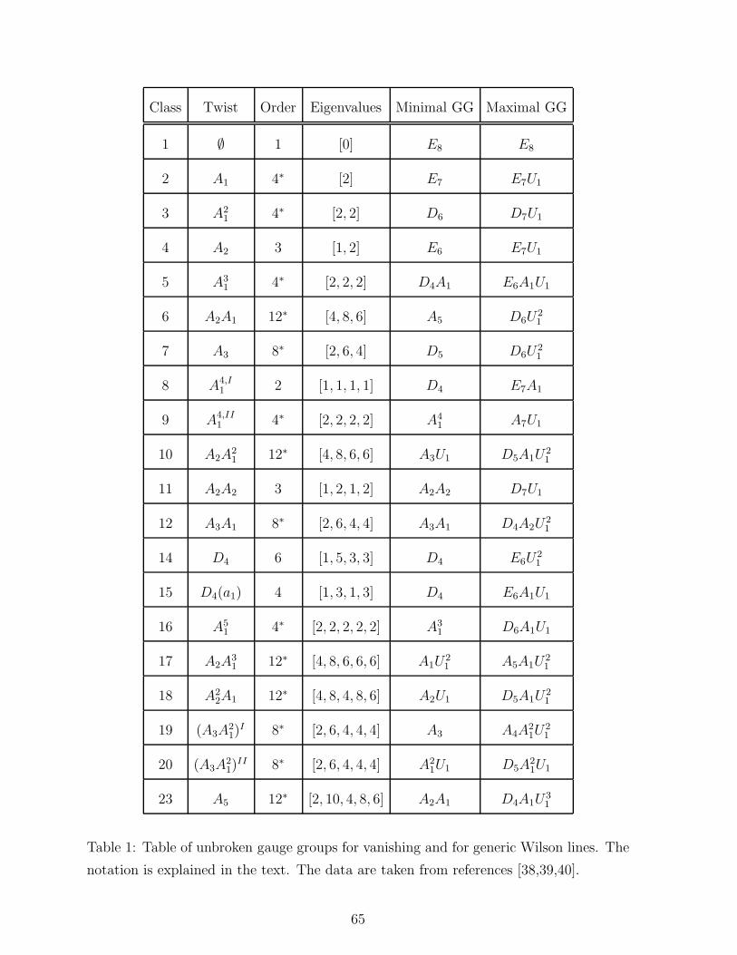
Class Twist Order Eigenvalues Minimal GG Maximal GG
1 ∅ 1 [0] E8 E8
2 A1 4∗ [2] E7 E7U1
3 A21 4∗ [2, 2] D6 D7U1
4 A2 3 [1, 2] E6 E7U1
5 A31 4∗ [2, 2, 2] D4A1 E6A1U1
6 A2A1 12∗ [4, 8, 6] A5 D6U21
7 A3 8∗ [2, 6, 4] D5 D6U21
8 A4,I1 2 [1, 1, 1, 1] D4 E7A1
9 A4,II1 4∗ [2, 2, 2, 2] A4
1 A7U1
10 A2A21 12∗ [4, 8, 6, 6] A3U1 D5A1U
21
11 A2A2 3 [1, 2, 1, 2] A2A2 D7U1
12 A3A1 8∗ [2, 6, 4, 4] A3A1 D4A2U21
14 D4 6 [1, 5, 3, 3] D4 E6U21
15 D4(a1) 4 [1, 3, 1, 3] D4 E6A1U1
16 A51 4∗ [2, 2, 2, 2, 2] A3
1 D6A1U1
17 A2A31 12∗ [4, 8, 6, 6, 6] A1U
21 A5A1U
21
18 A22A1 12∗ [4, 8, 4, 8, 6] A2U1 D5A1U
21
19 (A3A21)I 8∗ [2, 6, 4, 4, 4] A3 A4A
21U
21
20 (A3A21)II 8∗ [2, 6, 4, 4, 4] A2
1U1 D5A21U1
23 A5 12∗ [2, 10, 4, 8, 6] A2A1 D4A1U31
Table 1: Table of unbroken gauge groups for vanishing and for generic Wilson lines. The
notation is explained in the text. The data are taken from references [38,39,40].
65
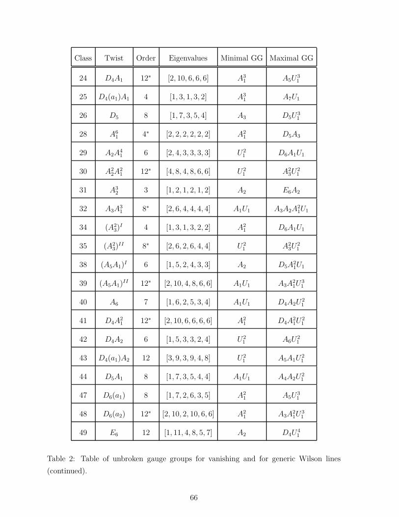
Class Twist Order Eigenvalues Minimal GG Maximal GG
24 D4A1 12∗ [2, 10, 6, 6, 6] A31 A5U
31
25 D4(a1)A1 4 [1, 3, 1, 3, 2] A31 A7U1
26 D5 8 [1, 7, 3, 5, 4] A3 D5U31
28 A61 4∗ [2, 2, 2, 2, 2, 2] A2
1 D5A3
29 A2A41 6 [2, 4, 3, 3, 3, 3] U2
1 D6A1U1
30 A22A
21 12∗ [4, 8, 4, 8, 6, 6] U2
1 A23U
21
31 A32 3 [1, 2, 1, 2, 1, 2] A2 E6A2
32 A3A31 8∗ [2, 6, 4, 4, 4, 4] A1U1 A3A2A
21U1
34 (A23)I 4 [1, 3, 1, 3, 2, 2] A2
1 D6A1U1
35 (A23)II 8∗ [2, 6, 2, 6, 4, 4] U2
1 A23U
21
38 (A5A1)I 6 [1, 5, 2, 4, 3, 3] A2 D5A
21U1
39 (A5A1)II 12∗ [2, 10, 4, 8, 6, 6] A1U1 A3A
21U
31
40 A6 7 [1, 6, 2, 5, 3, 4] A1U1 D4A2U21
41 D4A21 12∗ [2, 10, 6, 6, 6, 6] A2
1 D4A21U
21
42 D4A2 6 [1, 5, 3, 3, 2, 4] U21 A6U
21
43 D4(a1)A2 12 [3, 9, 3, 9, 4, 8] U21 A5A1U
21
44 D5A1 8 [1, 7, 3, 5, 4, 4] A1U1 A4A2U21
47 D6(a1) 8 [1, 7, 2, 6, 3, 5] A21 A5U
31
48 D6(a2) 12∗ [2, 10, 2, 10, 6, 6] A21 A3A
21U
31
49 E6 12 [1, 11, 4, 8, 5, 7] A2 D4U41
Table 2: Table of unbroken gauge groups for vanishing and for generic Wilson lines
(continued).
66
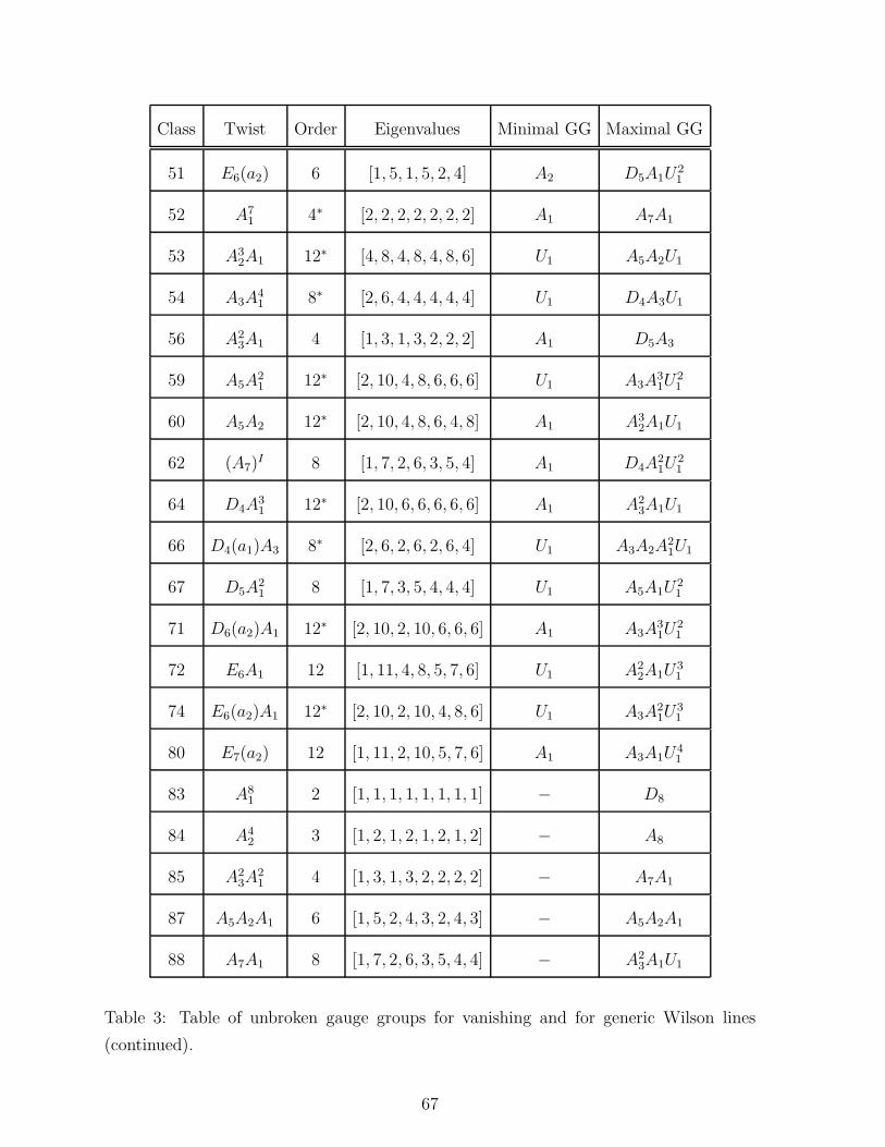
Class Twist Order Eigenvalues Minimal GG Maximal GG
51 E6(a2) 6 [1, 5, 1, 5, 2, 4] A2 D5A1U21
52 A71 4∗ [2, 2, 2, 2, 2, 2, 2] A1 A7A1
53 A32A1 12∗ [4, 8, 4, 8, 4, 8, 6] U1 A5A2U1
54 A3A41 8∗ [2, 6, 4, 4, 4, 4, 4] U1 D4A3U1
56 A23A1 4 [1, 3, 1, 3, 2, 2, 2] A1 D5A3
59 A5A21 12∗ [2, 10, 4, 8, 6, 6, 6] U1 A3A
31U
21
60 A5A2 12∗ [2, 10, 4, 8, 6, 4, 8] A1 A32A1U1
62 (A7)I 8 [1, 7, 2, 6, 3, 5, 4] A1 D4A
21U
21
64 D4A31 12∗ [2, 10, 6, 6, 6, 6, 6] A1 A2
3A1U1
66 D4(a1)A3 8∗ [2, 6, 2, 6, 2, 6, 4] U1 A3A2A21U1
67 D5A21 8 [1, 7, 3, 5, 4, 4, 4] U1 A5A1U
21
71 D6(a2)A1 12∗ [2, 10, 2, 10, 6, 6, 6] A1 A3A31U
21
72 E6A1 12 [1, 11, 4, 8, 5, 7, 6] U1 A22A1U
31
74 E6(a2)A1 12∗ [2, 10, 2, 10, 4, 8, 6] U1 A3A21U
31
80 E7(a2) 12 [1, 11, 2, 10, 5, 7, 6] A1 A3A1U41
83 A81 2 [1, 1, 1, 1, 1, 1, 1, 1] − D8
84 A42 3 [1, 2, 1, 2, 1, 2, 1, 2] − A8
85 A23A
21 4 [1, 3, 1, 3, 2, 2, 2, 2] − A7A1
87 A5A2A1 6 [1, 5, 2, 4, 3, 2, 4, 3] − A5A2A1
88 A7A1 8 [1, 7, 2, 6, 3, 5, 4, 4] − A23A1U1
Table 3: Table of unbroken gauge groups for vanishing and for generic Wilson lines
(continued).
67
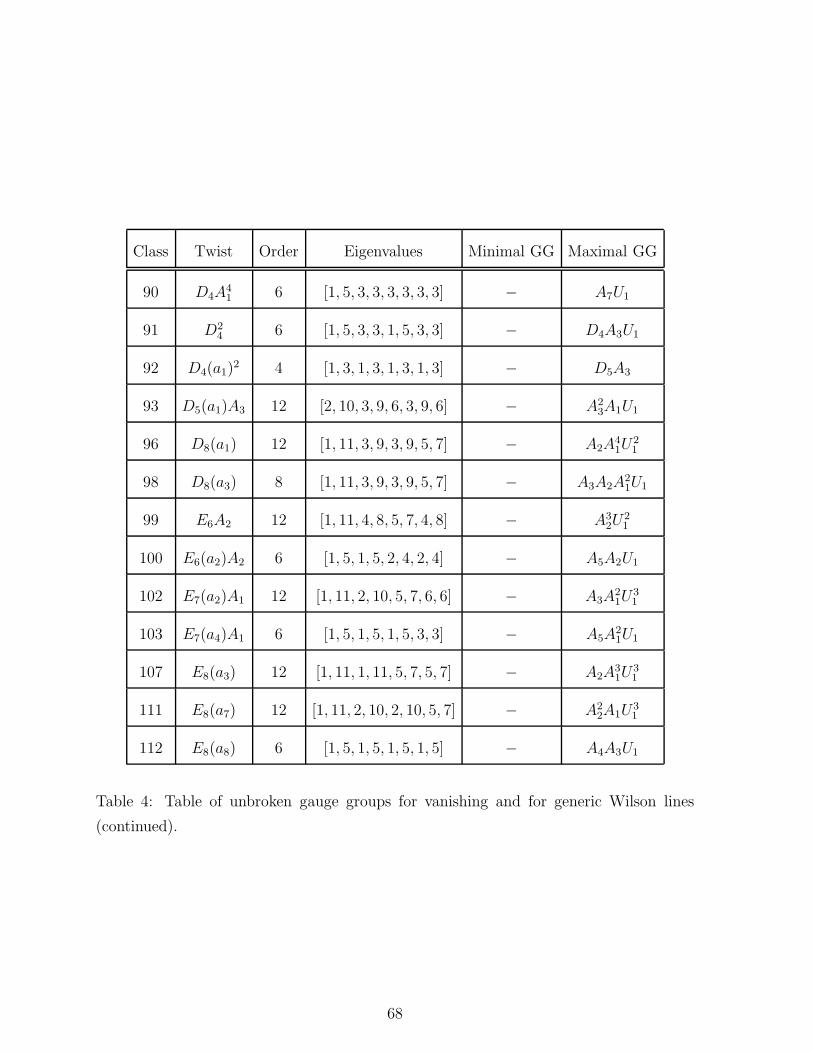
Class Twist Order Eigenvalues Minimal GG Maximal GG
90 D4A41 6 [1, 5, 3, 3, 3, 3, 3, 3] − A7U1
91 D24 6 [1, 5, 3, 3, 1, 5, 3, 3] − D4A3U1
92 D4(a1)2 4 [1, 3, 1, 3, 1, 3, 1, 3] − D5A3
93 D5(a1)A3 12 [2, 10, 3, 9, 6, 3, 9, 6] − A23A1U1
96 D8(a1) 12 [1, 11, 3, 9, 3, 9, 5, 7] − A2A41U
21
98 D8(a3) 8 [1, 11, 3, 9, 3, 9, 5, 7] − A3A2A21U1
99 E6A2 12 [1, 11, 4, 8, 5, 7, 4, 8] − A32U
21
100 E6(a2)A2 6 [1, 5, 1, 5, 2, 4, 2, 4] − A5A2U1
102 E7(a2)A1 12 [1, 11, 2, 10, 5, 7, 6, 6] − A3A21U
31
103 E7(a4)A1 6 [1, 5, 1, 5, 1, 5, 3, 3] − A5A21U1
107 E8(a3) 12 [1, 11, 1, 11, 5, 7, 5, 7] − A2A31U
31
111 E8(a7) 12 [1, 11, 2, 10, 2, 10, 5, 7] − A22A1U
31
112 E8(a8) 6 [1, 5, 1, 5, 1, 5, 1, 5] − A4A3U1
Table 4: Table of unbroken gauge groups for vanishing and for generic Wilson lines
(continued).
68