Post

Scri

pt⟩ p

roce

ssed

by

the

SLA

C/D

ESY

Lib

rari

es o

n 14

Jun

199

5.H

EP-

TH

-950

6091

CERN-TH-7528/95

IASSNS-HEP-94/106

OSU-M-94-3hep-th/9506091

Mirror Symmetry and the Moduli Space for

Generic Hypersurfaces in Toric Varieties

Per Berglund

School of Natural Sciences

Institute for Advanced Study

Princeton, NJ 08540, USA

Sheldon Katz

Department of Mathematics

Oklahoma State University

Stillwater, OK 74078, USA

and

Albrecht Klemm

Theory Division, CERN

CH-1211 Geneva 23, Switzerland

The moduli dependence of (2; 2) superstring compacti�cations based on Calabi{

Yau hypersurfaces in weighted projective space has so far only been investigatedfor Fermat-type polynomial constraints. These correspond to Landau-Ginzburg

orbifolds with c = 9 whose potential is a sum of A-type singularities. Here we

consider the generalization to arbitrary quasi-homogeneous singularities at c = 9.

We use mirror symmetry to derive the dependence of the models on the com-

plexi�ed K�ahler moduli and check the expansions of some topological correlationfunctions against explicit genus zero and genus one instanton calculations. Asan important application we give examples of how non-algebraic (\twisted") de-

formations can be mapped to algebraic ones, hence allowing us to study the full

moduli space. We also study how moduli spaces can be nested in each other,thus enabling a (singular) transition from one theory to another. Following the

recent work of Greene, Morrison and Strominger we show that this corresponds

to black hole condensation in type II string theories compacti�ed on Calabi-Yau

manifolds.

CERN-TH-7528/95

6/95

Email: berglund@guinness.ias.edu, katz@math.okstate.edu, klemm@nxth04.cern.ch

1. Motivation and Outline of the Strategy

The study of the moduli dependence of two-dimensional conformal �eld theories is

essential for understanding the symmetries and the vacuum structure of the critical string.

For conformal �eld theories with extended N = 2 superconformal symmetry remarkable

progress in this question was made after realizing the similarity of this problem with the

geometrical problem of the variation of the complex structure [1]. This implies that the

(topological) correlation functions are related to solutions of Fuchsian di�erential equa-

tions and have natural modular properties with respect to the four-dimensional spacetime

moduli [2]. Closed string compacti�cations with N = 1 spacetime supersymmetry actually

require an extension of the conformal symmetry to a global N = 2 superconformal symme-

try for the right moving modes on the worldsheet; heterotic compacti�cations with E8�E6

gauge group are based on a left-right symmetric (N; �N ) = (2; 2) superconformal internal

sectors with c = �c = 9. The truly marginal operators, which preserve the (2; 2) structure,

in these phenomenologically motivated string compacti�cations come in two equivalent

types related to the left-right chiral (c; c) states and the left anti-chiral, right chiral (a; c)

states of the (2; 2) theory [3] 1. The two types of states form two rings whose structure

constants depend only on one type of moduli respectively; our convention will be to iden-

tify the (c; c) ring with the complex structure deformations (also known as the B-model

in the language of topological �eld theory [5]) and the (a; c) ring with deformations of the

complexi�ed K�ahler structure (the A-model in the topological sigma model) of the target

space X, a Calabi{Yau threefold.

Unlike the dependence of the theory on the complexi�ed K�ahler structure, which

contains the information about the holomorphic instantons on X, the geometrical problem

of complex structure deformations is a well studied subject in classical geometry [6]. This

fact and the equivalent structure of the two rings from the point of view of the (2; 2)

theory, which is the origin of mirror symmetry [3,7], has motivated the key trick to solve

both sectors; to �nd a geometrical object X� yielding the identical (2; 2) theory in such a

way that the deformations of the complexi�ed K�ahler structure onX (X�) can be identi�ed

with the complex structure deformations on X� (X). If this holds for X and X�, the two

manifolds form a so called mirror pair.

Before going on let us brie y recall the phenomenological implications of the above.

The physical (normalized) Yukawa couplings can in principle be computed since we know

1 These marginal operators are in one to one correspondence with the 27 and �27 of E6. There

is yet a third class, namely the marginal operators which correspond to 1. They could potentially

enlarge the set of moduli �elds. They correspond to deformations of the tangent bundle of the

Calabi{Yau manifold in question, X , and are given byH1(X;EndTX). We will focus our attention

to the traditional space of (2; 2) preserving deformations. However, see [4] for some recent work.

1

the metric on the moduli space for both the complex structure and the K�ahler structure

deformations; the latter thanks to mirror symmetry. In addition, as was �rst pointed out

by Bershadsky et. al. [8] and recently ampli�ed by Kaplunovsky and Louis [9], threshold

corrections to gauge couplings in the four-dimensional e�ective �eld theory can be inferred

from the detailed knowledge of the singularity structure of the moduli space.

Recently it has become clear that the moduli spaces of Calabi-Yau manifolds might

play an essential role already when writing down a consistent four dimensional N = 2

supergravity theory, independently of whether one believes that it arises as a low energy

e�ective theory from string compacti�cation or not. In the work of Seiberg and Witten

[10] the moduli space of four dimensional pure SU(2) Super-Yang-Mills theory with global

N = 2 supersymmetry is governed by rigid special geometry, and due to the consistency

condition of the positive kinetic terms uniquely it can be identi�ed with the moduli space

of a torus2. Similarly, the moduli space of N = 2 supergravity is known to exhibit non-

rigid special geometry [13] and a natural geometrical object associated to this structure is

a Calabi-Yau threefold. Indeed, in a recent paper, Kachru and Vafa [14] give examples of

heterotic stringy realizations of [10].

The classi�cation of N = 2 SCFT with c < 3 follows an A-D-E scheme which has,

via the Landau-Ginzburg (LG) approach [15], a beautiful relation to the singularities of

modality zero [16]. Superstring compacti�cations with N = 1 spacetime supersymmetry

can be constructed by taking suitable tensor products of these models such that c = 9,

adding free theories for the uncompacti�ed spacetime degrees of freedom including the

gauge degrees of freedom in the left-moving sector, and implementing a generalized GSO-

projection [17].

The program for solving the full moduli dependence of the (2; 2) theory and checking

the instanton predictions has so far been studied only for theories based on tensor products

of the A-series [18,19,20,21,22]. (For a rather di�erent approach than the one pursued here,

using the linear sigma model, see [23], following the original mirror symmetry construction

by Greene and Plesser [24].) Geometrically they can be identi�ed with hypersurfaces of

Fermat-type in weighted projective spaces X = f~x 2 P4(~w)jP

5

i=1 xnii = 0g. These cases

are however only a very tiny subset of all transversal quasi-homogeneous singularities or

Landau-Ginzburg potentials with singularity index � = 3=2, which correspond to rational

N = 2 SCFT with c = 9. Theories of this general type have been classi�ed in [25]. Here

we develop the methods to treat these generic quasi-homogeneous potentials involving

arbitrary combinations of A-D-E invariants as well as new types of singularities.

2 The positivity condition is solved in this approach by the second Riemann inequality for the

period lattice. In general, from lattices of dimension six on, not every such such structure, which

de�nes an abelian variety, comes from a geometric curve; this is known as Schottky problem.

Families of curves however that generalize[10] for the SU(N) series have been identi�ed [11,12].

2

Already the �rst step, to �nd the geometrical object X�, is more tricky for the general

case. For models with A, Dk; k � 3 and/or E invariants one has always the simpli�cation,

that the complex structure moduli space of X� is the restriction of the moduli space of X

to the invariant subsector with respect to a discrete group H; in other words X� ' X=H

(modulo desingularizations). Therefore in these cases one in e�ect only needs to consider

the restricted complex structure deformation of the original manifoldX itself. The general

case, however, requires the construction of a new variety. The following two approaches to

that problem will become relevant for our calculation.

i) For models which admit a description in terms of Fermat-type polynomials Batyrev

has suggested a method of constructing the pair X and X� as hypersurfaces in toric

varieties de�ned by a pair of re exive simplices [26,27], see also [28]. It was later no-

ticed [22,29,30] that this method applies also to general quasi-homogeneous hypersurfaces

and can be used to construct all the mirror manifolds for the hypersurfaces in P4(~w) which

where classi�ed in [25].

ii) An alternative approach [31,32] starts from the following symmetry consideration.

The LG-theory P is de�ned by a transversal potential p(x1; : : : ; x5) quasi-homogeneous

of degree d with respect to the weights wi, i.e. p(�w1x1; : : : ; �

w5x5) = �dp(x1; : : : ; x5).

The potential has an invariance group G(P) whose elements act on the coordinates by

phase multiplication xi ! xi exp( i). The GSO-projection onto integral charge states is

implemented in the internal sector by orbifoldization with respect to a subgroup ZZd 2 G(P)

acting by xi ! xi exp(2�iwi

d) [17]. The string compacti�cation based on the internal sector

P=ZZd has a simple geometrical interpretation. Namely the compact part of the target space

is given by X = f~x 2 P4(~w)jp(x1; : : : ; x5) = 0g. Any orbifold with respect to a group H

with ZZd � H � G(P) andQ

5

i=1 exp(�i) = 1 for all � 2 H, leads likewise to a consistent

string compacti�cation. The compact part of the target space is now X=(H=ZZd). It now

follows from general arguments [33] that the orbifoldO with respect to an abelian groupH,

will have a dual symmetry group Gq(O) called the quantum symmetry, which is isomorphic

to H and manifest in the operator algebra of the twisted states of O. In the case of the

above orbifold O = P=ZZd all (a; c) states belong to the twisted states and Gq(O) �= ZZd.

On the other hand the operator algebra of the invariant (c; c) states is determined by

Gg(O) = G(P)=ZZd, the so called geometrical symmetry group. To exchange the role of the

(c; c) and the (a; c) ring and to construct a mirror pair one therefore tries to construct two

orbifolds O and O� in which the geometrical symmetry and the quantum symmetry are

exchanged, i.e. Gg(O) �= Gq(O�) and Gq(O) �= Gg(O

�). As was recognized in [31] N = 2

models based on tensor products of minimal models always have a symmetry groupH with

ZZd � H � G(P) such that ~ZZd = G(P)=H and the quantum symmetry and the geometrical

symmetry are in fact exchanged for the pair O = P=ZZd, O� = P=H.

3

For general LG-models such an H need not exist. In [32] the authors present a

generalization3 of the argument of [31] and consider a LG-potentials p(x1; : : : ; xr), which

is transversal for a polynomial con�guration with r monomials, i.e. p =Pr

i=1Xv(i) with

v(i) vectors of exponents and Xv(i) := xv(i)

1

1� � �x

v(i)rr , v

(i)j 2 N0. Then one can consider

the \transposed" polynomial p =Pr

i=1 Yv(i) , where the new exponent vectors v(i) are

de�ned by v(i)r = v

(r)i . It follows from the transversality condition [25] that all monomials

Xv(i) in p as well as the transposed monomials in p have the form xnii xj , with i, j not

necessarily di�erent. Using this one can see that G(P) �= G(P) and it was argued in

[32] that there exists a groupH with ZZd � H � G(P) such that Gq(P=ZZd) �= Gg(P=H) and

Gg(P=ZZd) �= Gq(P=H). In fact the transposition rule also holds for many non-transverse

polynomials [30], where it was also shown to be consistent with approach i).

In section 2 we will brie y review the construction of Calabi{Yau hypersurfaces in toric

varieties, heavily relying on the methods introduced in [22]. In particular we will introduce

the Batyrev-Cox homogeneous coordinate ring [37] which will simplify the construction of

the period vector as well as the Picard-Fuchs equation associated to it. To generalize this

approach to cases which have no ordinary LG-description, i.e. where no description as

hypersurface in P4(~w) or orbifolds thereof is available, we develop methods to derive the

Picard-Fuchs equations directly from the combinatorial data of the dual polyhedron ��.4

In section 3.1 we then consider generalized hypersurfaces in P4(~w) with two K�ahler

moduli. We use the constructions (i); (ii) to derive the Picard-Fuchs equations for the pe-

riod integrals in order to study the complex structure deformations of X�. It is convenient

to follow �rst (ii) and use P=H as a representation of X�. Then one can apply the stan-

dard Dwork-Katz-Gri�ths [38,39,40] reduction formulas adapted to weighted projective

spaces for the derivation of the di�erential equations. From this information we calculate

the number of holomorphic instantons of genus zero and genus one on X. A detailed check

of these predictions will be presented in the section 4, where we also note that the discrep-

ancy between the Mori cones a�ects the nature of the large complex structure limit, but

does not a�ect the validity of the instanton expansions.

The construction of [32] allows one to obtain X� for the majority of the LG-potentials

in [25]. It fails however for LG-potentials for which a transversal con�guration requires

3 Contrary to the original mirror symmetry construction [24], there is no supporting argument

at the level of the underlying conformal �eld theory, since the exact N = 2 SCFT theory is not

known. However, the calculation here, the a�rmative check of the elliptic genus [34] as well as

the chiral ring [35] suggests that this is true. Moreover, Morrison and Plesser have a promising

approach to providing such an argument.[36]4 As usual, the Mori cone of the associated toric variety enters in a crucial way. We observe

that the Mori cone of the Calabi{Yau hypersurface may be strictly smaller than the Mori cone of

the toric variety.

4

more than r monomials; in that case, Batyrev's approach will apply, as shown in [22,30].

We consider therefore in section 3.2 such a case. It turns out that if we restrict to a

suitable non-transversal con�guration involving r terms (where r = 4+1 in our case since

the hypersurfaces are embedded in a toric variety of dimension four) and consider the

transposed polynomial P=H as before, we get an orbifold of a non-transversal hypersurface

X� in P4(~w), which can be conveniently used to derive the set of di�erential equations

of Fuchsian type. The latter reproduce the topological couplings and at least to lowest

order the genus zero instantons of X, see section 4. This approach can be justi�ed by

translating the operator identities, which hold modulo the ideal of P (equations of motions),

to the Laurent-monomials and derivatives of the Laurent-polynomial and using the partial

di�erentiation rule of section (3.1).

In section 5 we apply the techniques developed in the earlier sections to study some new

phenomena. Given a toric variety based on a polyhedron �, we construct new re exive

polyhedra. In 5.1 we give examples of re exive polyhedra, which are not associated to

hypersurfaces in P4(~w) and apply the methods outlined in section 2 to get the Picard-Fuchs

equations also in this case. In section 5.2, we the study the phenomenon of embedding

the moduli space of one Calabi{Yau space into the moduli space of another Calabi{Yau

space and develop a quite general strategy for constructing an algebraic realization of

the space of deformations (section 5.3). The latter approach removes, what is sometimes

described as the \twisted sector problem" in the physics literature. Finally, in section 6

we will discuss the general validity of the computation and give an algorithm for which,

in principle, a model with any number of moduli can be solved. We also brie y comment

on the connection with the recent developments in type II string theory compacti�ed on

Calabi-Yau manifolds.

2. General construction of Picard{Fuchs equations for Calabi{Yau hypersur-

faces in toric varieties

Let us start by giving a brief review of the existing methods by which the the Picard{

Fuchs equations are obtained. For more details, see [22].

Given a weighted projective space P4(~w) we construct the Newton polyhedron, �,

as the convex hull (shifted by (�1;�1;�1;�1;�1)) of the most general polynomial p of

degree d =P

5

i=1wi,

� = Conv

fn 2 ZZ5j

5Xi=1

niwi = 0; ni � �18ig

!; (2:1)

which lies in a hyperplane in IR5 passing through the origin. For any set of weights which

admits a transverse polynomial, it has been shown in [30] that the Newton polyhedron is

5

re exive, yielding a toric variety birational to P4(~w). (Re exivity in these cases has been

checked independently by the third author.) The polar polyhedron, ��, is given by

�� = Conv (fm 2 ��j < n;m >� �1; 8n 2 �g) (2:2)

where �� is the dual lattice to � = fn 2 ZZ5jP

5

i=1 niwi = 0g. We can identify �ve vertices,

v�(i) ; i = 1; : : : ; 5 satisfying the linear relation [29]

5Xi=1

ki � v�(i) = 0 : (2:3)

When k1 = 1 we have

v�(1) = (�k2;�k3;�k4;�k5) ; v�(i+1) = ei ; i = 1; : : : ; 4 ; (2:4)

where the ei are the standard basis elements in ZZ4.

We are interested in studying hyperplane sections, X�, of the toric variety P�� , given

by

P =X

i2��\��

ai�i =X

i2��\��

Yj

Y��(i)

j

j (2:5)

The claim [26] is that hypersurfaces X 2 P4(~w) and X� 2 P�� are mirror partners. An

alternative way is to specify an �etale map Y (y) to the homogeneous coordinates (y1 : : : : :

y5) of a suitable four dimensional weighted projective space P4(~w) (this map is actually

only �etale on the respective tori), which identi�es (2.5) in P�� with the hypersurface

de�ned by an ordinary polynomial constraint p = (y1y2y3y4y5)P (Y (y)) = 0 in this P4(~w).

Note that in general P4(~w) 6= P4(~w) In fact if we set ai = 0; i 6= 1; : : : ; 5 then (2.5) reduces

to the transposed polynomial p0(yi), of p0; here p0(xi) de�nes a (possibly non-transverse)

hypersurface in P4(~w), see ii) in the previous section. Note that the map Y (y) is in general

not one-to-one, but rather there is an automorphism which is isomorphic to H the group

which we need to divide by in order to make fp(yi) = 0g=H the mirror of a hypersurface

in P4(~w) described by p = 0. (For a more detailed account of the correspondence between

the toric construction and the transposition scheme, see [29,30].)

Yet a third way of identifying the hyperplane section in P�� is to use the homogeneous

coordinate ring de�ned by Batyrev and Cox [37]. To each of the vertices, �(i) in � we

associate a coordinate xi. As for a homogeneous coordinate in a weighted projective space,

each xi has a weight, or rather a multiple weight, given by positive linear relations among

the �(i). However, for our purposes it is enough to note that to each vertex in the polar

polytope, ��, corresponds a monomial �j in terms of the xi;

�j =X

i2�\�

< (v(i); 1); (v(j)�; 1) > : (2:6)

6

Thus, P =P

j2��\�� ai�i de�nes a hyperplanes section in P�� . Note that if we were to

restrict to a particular set of �ve vertices in � one can show P reduces to p de�ned above

through the �etale map [29,30]. In the examples we will mostly be using the second and

third representation, but that is only as a matter of convenience; all results can be derived

using Batyrev's original set of coordinates (2.5).

The next step is to �nd the generators of the Mori cone as they are relevant in studying

the large complex structure limit; recall that the Mori cone is dual to the K�ahler cone.

Given �� we have to specify a particular triangulation; more precisely a star subdivision of

�� from the interior point ��(0). In general this triangulation is not unique. In particular

there may exist more than one subdivision which admits a K�ahler resolution, i.e. there is

more than one Calabi{Yau phase [41]; see section 3 for examples.

Once a particular subdivision is picked an algorithm for constructing the generators

of the Mori cone is as follows:5

i) Extend ��(i) to ���(i) = (1; ��(i))

ii) Consider every pair (Sk; Sl) of four-dimensional simplices in the star subdivision of

�� which have a common three-dimensional simplex si = Sk \ Sl.

iii) Find for all such pairs the unique linear relationP

6

i=1 l(k;l)i ���(i) = 0 among the six

points ��(i) of Sl [ Sk in which the l(k;l)i are minimal integers and the coe�cients of

the two points in (Sk [ Sl) n (Sl \ Sk) are non-negative.

iv) Find the minimal integer vectors l(i) by which every l(k;l) can be expressed as positive

integer linear combination. These are the generators of the Mori cone.

Next we derive the Picard-Fuchs equation for X� from the residue expression for the

periods. There are two residue forms for the periods; the Laurent polynomial (2.5) or the

transposed polynomial from the �etale map, both of which we will use for the derivation.

The �rst one reads [27]

�i(a0; : : : ; ap) =

Z�i

!

P; i = 1; : : : ; 2(h2;1 + 1); (2:7)

where �i 2 H4(T nX) (T is the algebraic torus associated to the toric variety [27]), and

! = dY1Y1

^dY2Y2

^dY3Y3

^dY4Y4

. Alternatively, we can write the following expression for the

periods in terms of the transposed polynomial p = 0, [40]

�i(a0; : : : ; ap) =

Z

Z�i

!

p; i = 1; : : : ; 2(h2;1 + 1) : (2:8)

5 This algorithm is equivalent to the one described by Oda and Park [42], but is simpler to

apply.

7

Here ! =P

5

i=1(�1)iwiyidy1 ^ : : : ^ cdyi ^ : : : ^ dy5; �i is an element of H3(X;ZZ) and a

small curve around p = 0 in the 4-dimensional embedding space. Note that by performing

a change of variables as dictated by the �etale map one can show that (2.7) is equivalent

to (2.8). Symmetry considerations now make the derivation of the Picard-Fuchs equations

a short argument. The linear relations between the points ��� (i) = (�� (i); 1) in the extended

dual polyhedron ��� as expressed by the l(i) translates into relations among the �i,

Lk(�i) = 0 : (2:9)

However, from the de�nition of �i, the (2.9) are equivalent to

Lk(@ai )�j = 0 : (2:10)

Finally, due to the (C�)5-invariance of �j(ai) we choose the following combinations as the

coordinates relevant in the large complex structure limit [27]

zk = (�1)l(k)

0

Yi

al(k)

i

i : (2:11)

They will lead directly to the large K�ahler structure limit at zk = 0 at which the mon-

odromy is maximal unipotent [43]. Thus, using �i = zidzi, eq. (2.10) is readily transformed

to6

Lk(�i; zi)�j = 0 : (2:12)

However, the above system (2.12) has in general more than 2(h2;1 + 1) solutions as

can be seen by studying the number of solutions to the indicial problem. This can be

resurrected in the following two ways. On one hand, one can try to factorize the set

of di�erential operators Lk in order to reproduce operators of lower order; for examples

see [22] and section 3.1. Alternatively, we can derive the di�erential operators by the more

standard manipulations of the residuum expressions (2.7) and (2.8). In particular, there

exist relations of order n based on the use of the ideal @yi p,7,

�k(@yi p; �j ; yi) = 0 : (2:13)

This impliesR

R�i

�!pn+1 = 0. We can use the partial integration rule

m(y)@yi p

pn+1 = 1

n

@yim(y)

pn

under the integral sign (2.8), which follows from the fact that @yi

�m(y)pn

�! is exact, pro-

vided the integral over both sides of the above equation makes sense as periods, which is

6 For historical reasons we rescale also the periods and use �i =1

a0�i. This brings the system

of di�erential equations in the form, �rst discussed by Gelfand-Kapranov and Zelevinskii [44].7 There are in general many ways of obtaining relations such as the one below. From a technical

point of view, it is preferable to use the ideal in such away that the use of the partial integration

rule becomes trivial.

8

the case if m(y)@yi p is homogeneous of degree dn, see e.g. [45,19]. In analogy to (2.9)

and (2.10) we get a di�erential equation satis�ed by the period vector,

Lk(�i; zi)�j = 0 : (2:14)

It is clear that (2.13) can be used analogously in (2.7). To be more precise �i = YiddYi

and the partial integration rule, which due to the measure ! of (2.7) now reads8 m(Y )diPPn =

1

n�1

(di+n�2)m(Y )

Pn�1 . Also this integration rule is valid only if the integral (2.7) over both

sides makes sense as periods, which is the case if the points associated to m(Y )diP are

in (n � 1)�� and the ones associated to (di + n � 2)m(Y ) are in (n � 2)��, where k��

denotes the polyhedron �� scaled by k.

It should be obvious from the �rst and the last derivation of the Picard-Fuchs equation,

that the �etale map and the transposed polynomial are auxiliary constructions. Their

virtue is to introduce a suitable grading which facilitate the calculations. All relevant data

however can be obtained directly from the polyhedron �� and (2.7).

Finally, from the sets of operators (Lk ; Lk) one then has to select the set of operators

(Lk) which will reproduce the relevant ring structure. Unfortunately, we do not know of

a general recipe for how this is done, and at present we have to resort to a case by case

study, see section 3.

With the relevant set of operators at hand (Lk) we are now ready to compute the

Yukawa couplings, the mirror map and then the instanton expansion. Schematically the

procedure is as follows. (For more details, see [22,46].) One �rst �nds solutions, wj, of the

Picard-Fuchs system (Lk� = 0) with maximally unipotent monodromy at zi = 0. Then

the at coordinates are given by tj = wj=w0 where w0 is the power series solution at

zi = 0. From the (Lk) one can derive linear relations among the Yukawa couplings Kzizjzk

and their derivatives. Thus rather than using the explicit solutions, and a knowledge of an

integral symplectic basis, we derive the Yukawa couplings (up to an overall normalization)

directly from the di�erential operators. This also gives us the discriminant locus, �, i.e.

the codimension one set where the Calabi{Yau hypersurface X� is singular.

From the Picard-Fuchs operators, we can also determine the intersection numbers up

to a normalization as the coe�cients of the unique degree three element in

C[�i]=f limzi!0

Lkg :

The normalization may be �xed by the intersection of

KJ1J1J1 :=

ZX

J1 ^ J1 ^ J1 =

dQ

5

i=1wi

!n30; (2:15)

8 The indexing of the di is such that diQ

jY

��(k)

j

j = (1� h�(i) ; ��(k)i)Q

jY

��(k)

j

j .

9

where n0 is the least common multiple of the orders of all �xpoints in X. Alternatively,

by considering the restriction to a one-parameter subspace of the moduli space of complex

structure deformations spanned by the deformation corresponding to the interior point

in ��, one can directly compute (2.15) [47].

With both the Yukawa couplings and the at coordinates at hand it is then straight-

forward to map our results to that of the Yukawa coupling as a function of the K�ahler

moduli in X, the hypersurface in P4(~w). The details of this are standard and can be found

in [22,46]. Here we only record the result;

K~ti~tj~tk(~t) =

1

w2

0

Xl;m;n

@xl

@~ti

@xm

@~tj

@xn

@~tkKzlzmzn ; (2:16)

where the ~ti corresponds to an integral basis of H1;1(X;ZZ) and are related to the at

coordinates by an integral similarity transformation. Finally, by expanding (2.16) in terms

of the variables qi = exp(2�i~ti), we can read o� the invariants of the rational curves

N(fnlg),

K~ti~tj~tk(~t) = K0

ijk +Xni

N(fnlg)ninjnk

1�Q

l qnll

Yl

qnll : (2:17)

It is well-known that there are no corrections to the Yukawa couplings at higher genus.

Still it is interesting to note that invariants of elliptic curves (genus one) can be studied

by means of the following index F top1

[8],

Ftop1

= log

"�1

!0

�5��=12@(zi)

@(ti)f(z)

#+ const: (2:18)

where f is a holomorphic function with singularities only at singular points on X and so

is related to the discriminant locus. Thus, we make the ansatz

f(z) = (Yj

�rjj )Yi

zsii ; (2:19)

with the si �xed by using the following asymptotic relation (valid at the large radius limit)

limt;�t!1

F1 = �2�i

12

Xi

(ti + �ti)

Zc2Ji : (2:20)

In (2.19) the product over the j is taken over the components �j of the discriminant locus.

The rj are determined by knowing some of the lowest order invariants of the elliptic curves;

see the examples for more details.

10

3. Examples

3.1. Non-Fermat hypersurfaces in P4 with two moduli

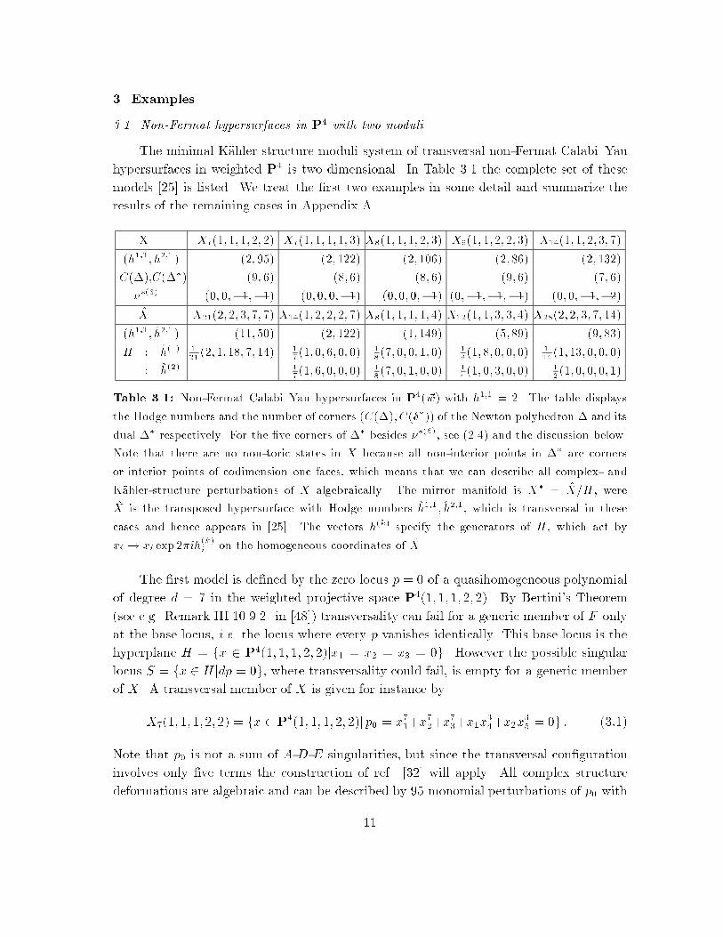
The minimal K�ahler structure moduli system of transversal non-Fermat Calabi{Yau

hypersurfaces in weighted P4 is two dimensional. In Table 3.1 the complete set of these

models [25] is listed. We treat the �rst two examples in some detail and summarize the

results of the remaining cases in Appendix A.

X X7(1; 1; 1; 2; 2) X7(1; 1; 1; 1; 3) X8(1; 1; 1; 2; 3) X9(1; 1; 2; 2; 3) X14(1; 1; 2; 3; 7)

(h1;1; h2;1) (2; 95) (2; 122) (2; 106) (2; 86) (2; 132)

C(�);C(��) (9; 6) (8; 6) (8; 6) (9; 6) (7; 6)

��(6) (0; 0;�1;�1) (0; 0; 0;�1) (0; 0; 0;�1) (0;�1;�1;�1) (0; 0;�1;�2)

X X21(2; 2; 3; 7; 7) X14(1; 2; 2; 2; 7) X8(1; 1; 1; 1; 4) X12(1; 1; 3; 3; 4) X28(2; 2; 3; 7; 14)

(h1;1; h2;1) (11; 50) (2; 122) (1; 149) (5; 89) (9; 83)

H : h(1) 1

21(2; 1; 18; 7; 14) 1

7(1; 0; 6; 0; 0) 1

8(7; 0; 0; 1; 0) 1

9(1; 8; 0; 0; 0) 1

14(1; 13; 0; 0; 0)

: h(2) 1

7(1; 6; 0; 0; 0) 1

8(7; 0; 1; 0; 0) 1

4(1; 0; 3; 0; 0) 1

2(1; 0; 0; 0; 1)

Table 3.1: Non-Fermat Calabi{Yau hypersurfaces in P4(~w) with h1;1 = 2. The table displays

the Hodge numbers and the number of corners (C(�); C(��)) of the Newton polyhedron � and its

dual �� respectively. For the �ve corners of �� besides ��(6), see (2.4) and the discussion below.

Note that there are no non-toric states in X because all non-interior points in �� are corners

or interior points of codimension one faces, which means that we can describe all complex- and

K�ahler-structure perturbations of X algebraically. The mirror manifold is X� = X=H , were

X is the transposed hypersurface with Hodge numbers h1;1; h2;1, which is transversal in these

cases and hence appears in [25]. The vectors h(k) specify the generators of H , which act by

xi ! xi exp 2�ih(k)

i on the homogeneous coordinates of X .

The �rst model is de�ned by the zero locus p = 0 of a quasihomogeneous polynomial

of degree d = 7 in the weighted projective space P4(1; 1; 1; 2; 2). By Bertini's Theorem

(see e.g. Remark III.10.9.2. in [48]) transversality can fail for a generic member of F only

at the base locus, i.e. the locus where every p vanishes identically. This base locus is the

hyperplane H = fx 2 P4(1; 1; 1; 2; 2)jx1 = x2 = x3 = 0g. However the possible singular

locus S = fx 2 Hjdp = 0g, where transversality could fail, is empty for a generic member

of X. A transversal member of X is given for instance by

X7(1; 1; 1; 2; 2) = fx 2 P4(1; 1; 1; 2; 2)j p0 = x71+x7

2+x7

3+x1x

3

4+x2x

3

5= 0g : (3:1)

Note that p0 is not a sum of A-D-E singularities, but since the transversal con�guration

involves only �ve terms the construction of ref. [32] will apply. All complex structure

deformations are algebraic and can be described by 95 monomial perturbations of p0 with

11

elements of R = C[x1; : : : ; x5]=f@x1p0; : : : ; @x5p0g. The canonical resolution X of the hy-

persurface X has two elements in H2(X); one corresponds to the divisor associated to the

generating element of Pic(X) and a second one stems from the exceptional divisor, which

is introduced by the resolution of the Z2-singularity.

Returning to P4(1; 1; 1; 2; 2), we see that � has nine corners whose components read

�(1) = (�1;�1;�1; 2); �(2) = (�1;�1;�1;�1); �(3) = (0;�1;�1; 2)

�(4) = (6;�1;�1;�1); �(5) = (�1; 0;�1; 2); �(6) = (�1; 6;�1;�1)

�(7) = (�1;�1; 2;�1); �(8) = (0;�1; 2;�1); �(9) = (�1; 0; 2;�1)

(3:2)

in a convenient basis for the sublattice � 2 ZZ5 within the hyperplane: e1 = (�1; 1; 0; 0; 0),

e2 = (�1; 0; 1; 0; 0), e3 = (�2; 0; 0; 1; 0) and e4 = (�2; 0; 0; 0; 1). Beside the corners, �

contains 1 lattice point in the interior, 20 lattice points on codimension 1 faces, 54 lattice

points on codimension 2 and 36 lattice points on codimension 3 faces. One can pick 95

monomials corresponding to 4 of the corners, the internal point and the 90 points on

codimension 2 and 3 faces as representatives of R.

Since we know that the weights wi at hand admits a transverse polynomial the poly-

hedron � is re exive [30]. Its dual �� has six corners, whose components in the basis of

the dual lattice �� are given below

��(1) = (�1;�1;�2;�2); ��(2) = (1; 0; 0; 0); ��(3) = (0; 1; 0; 0);

��(4) = (0; 0; 1; 0); ��(5) = (0; 0; 0; 1); ��(6) = (0; 0;�1;�1):(3:3)

Beside these corners, the point ��(0) = (0; 0; 0; 0) is the only integral point in ��. In all

cases where w1 = 1 we can chose the lattice such that ��(1) = (�w2;�w3;�w4;�w5) and

��(i) is as above for i = 2; : : : ; 5. In all cases considered here, there is only the additional

corner ��(6). It is always the case that ��(0) is an additional integral point of ��. It is in

fact the only additional integral point except in the case of P4(1; 1; 2; 3; 7). In that case

� contains the point (0; 0; 0;�1); but this plays essentially no role since it is the interior

point of a codimension 1 face. Hence it is su�cient to only list ��(6) for the other cases,

see Table 3.1.

Using (3.3) and (2.5) the Laurent polynomial of �� is given by

P =Xi

ai�i = a0 + a11

Y1Y2Y2

3Y 2

4

+ a2 Y1 + a3 Y2 + a4 Y3 + a5 Y4 + a61

Y3Y4: (3:4)

The �etale map is given by

Y1 =y62

y1y3y4; Y2 =

y63

y1y2y4y5; Y3 =

y24

y1y2y3y5; Y4 =

y25

y1y2y3y4(3:5)

which leads to a polynomial constraint

p =

6Xi=0

ai�i � a1y7

1y4 + a2y

7

2y5 + a3y

7

3+ a4y

3

4+ a5y

3

5+ a0y1y2y3y4y5 + a6(y1y2y3)

3; (3:6)

12

which is quasihomogeneous of degree d = 21 with respect to the weights of P4(2; 2; 3; 7; 7).

In fact p0 = y71y4 + y7

2y5 + y7

3+ y3

4+ y3

5is the transposed polynomial of p0 in (3.1) and

the symmetry, which is identi�ed in (3.5) corresponds exactly to the symmetry group H �

(Z21 : 2; 1; 18; 7; 14), which has to be modded out from the con�guration X21(2; 2; 3; 7; 7)

to obtain the mirror [32] of the con�guration X7(1; 1; 1; 2; 2). Note also that the family

X21(2; 2; 3; 7; 7) admits 50 independent complex structure perturbations (which are all

algebraic) but the terms of (3.6) are the only invariant terms under the H symmetry

group.

The boundary of �� in (3.3) consists of 9 three dimensional simplices and joining each

of these simplices with the origin ��(0) we get a unique star subdivision of �� into 9 four

dimensional simplices. Application of the algorithm for constructing the generators of the

Mori cone described in the previous section leads to

l(1) = (�3; 0; 0; 0; 1; 1; 1); l(2) = (�1; 1; 1; 1; 0; 0;�2): (3:7)

Note that the Mori cone of P�� coincides with the Mori cone of X in this example, as

well as in all examples treated so far [22,46]; see however sections 3.2, 4 and Appendix A

for models where this is not true. From the general discussion in section 2 this allows us

to determine the relevant coordinates in the large complex structure limit, see (2.11), as

z1 = �a4a5a6a30

and z2 = �a1a2a3a0a

26

.

From the relations �30��4�5�6 = 0 and �2

6�0 � �1�2�3 = 0, where the �i are de�ned

by (3.4) or equivalently by (3.6), we get two third order di�erential operators satis�ed by

all periods @3a0 � @a4@a5@a6 = 0 and @2a6@a0 � @a1@a2@a3 = 0. This is readily transformed

in the good variables (2.11)

L1 = �21(2�2 � �1) + (3�1 + �2 � 2)(3�1 + �2 � 1)(3�1 + �2)z1

L2 = �32� (3�1 + �2)(2�2 � �1 � 2)(2�2 � �1 � 1)z2:

(3:8)

A short consideration of the indicial problem reveals that it has nine solutions. The six

periods however are solutions of a system, which consists of a third and a second order

di�erential operator. As in many examples in [46] the second order di�erential can be

obtained in this case rather simply by factoring 7L2 � 27L1 = (3�1 + �2)L2 with

L2 = 9�21� 21�1�2 + 7�2

2� 27z1

2Yi=1

(3�1 + �2 + i)� 7z2

1Yi=0

(2�2 � �1 + i): (3:9)

As Picard-Fuchs system we may choose this operator and say L1 = L2.

Instead of using the factorization we may derive e.g. the second order di�erential

operator from the vanishing of

� =a1a2�1�2�3a1a6�1�6�3a2a6�2�6�3a0a6�0�6�27z1a2

0�20�7z2a

2

6�26�

9a4a6

a0(y1y2y3y4)

2@y5 p+3a6

�a2

a0y21y92y23+ y4(y1y2y3)

3

�@y4 p�

a1a2

a0(y1y2)

6@y3 p

(3:10)

13

which impliesR

R�i

�!p3

= 0. After the partial integration we get from the last three

terms of � the contribution 3a62

R

R�i

�6!p2

. Replacing all �i by derivatives with respect to

the ai and transforming to the zi variables yields (3.9)It is clear that (3.10) can be used

analogously in (2.7), to obtain the second order di�erential relation. To be more precise �

transforms into the variables Yi as

� =a1a2�1�2�3a1a6�1�6�3a2a6�2�6�3a0a6�0�6�27z1a2

0�20�7z2a

2

6�26�

9a4a6

a0

1

Y4d1P + 3a6

�a2

a0

Y1

Y3Y4+

1

Y3Y4

�d7P �

a1a2

a0

1

Y2Y2

3Y 2

4

d6P = 0 ;(3:11)

where d1 = (1 � �1 ��2 � �3 + 2�4), d7 = (1 � �1 ��2 + 2�3 ��4), d6 = (1 ��1 +

6�2 ��3 ��4) and �i = YiddYi

. Using the partial integration rule yields again (3.9).

From the Picard-Fuchs operators, we �rst determine the intersection numbers up to

a normalization which we get from (2.15). Hence KJ1J1J1 = 14, KJ1J1J2 = 7, KJ1J2J2 = 3

and KJ2J2J2 = 0. Secondly, we derive the general discriminant locus

� = (1�27z1)3�z2(8�675z1+71442z

2

1�16z2+1372z1z2�453789z

2

1z2+823543z

2

1z22)

(3:12)

and the Yukawa couplings in our normalization

K111 =(14�112z2+324z1+729z

2

1�2213z1z2�1323z

2

1z2+224z

2

2+4116z1z

2

2)

z31�

K112 =(7� 135z1�1458z

2

1�56z2+1284z1z2+3969z

2

1z2+112z

2

2�2744z1z

2

2)

z21z2�

K122 =(3� 162z1+2187z

2

1�26z2+1629z1z2�11907z

2

1z2+56z

2

2�3773z1z

2

2)

z1z2

2�

K222 =z1(�11 + 1161z1 + 35721z2

1+ 28z2 � 3087z1z2)

z32�

:

(3:13)

Finally, the number of rational curves is obtained by an expansion of (3.13) around zi = 0;

the result is recorded in Table 3.2.

To obtain the invariants for the elliptic curves we �rst note thatRXc2J1 = 68 andR

Xc2J2 = 36. Using the ansatz (2.18) and the asymptotic relation (2.20) one obtains

s1 = �20=3; s2 = �4. The invariants of the elliptic curves still contain r0, e.g. ne0;1 =

�(1=3)(2 + 12r0). We will see in section 4.1 that this invariant vanishes, which �xes

r0 = �(1=6). This allows us to obtain the other invariants of the elliptic curves, see

Table 3.2. In fact, we will see later that ne0;1 = 0 for all of our two parameter models, which

will allow us to determine r0 in each case. We always obtain r0 = �1=6, which supports

the conjecture [49], [46] that the exponent is universally �(1=6) for the component of the

discriminant parameterizing nodal hypersurfaces. An intriguing possible explanation of

14

this phenomenon based on consideration of black hole states of the type II string has been

given in [50]. These instanton predictions will be discussed in section four. The successful

check provides a very detailed veri�cation that the con�guration X21(2; 2; 3; 7; 7) modded

out by H ' (ZZ21 : 2; 1; 18; 7; 14) is in fact the correct mirror con�guration.

ni;j j = 0 j = 1 j = 2 j = 3 j = 4 j = 5 j = 6

nr0;j 0 �2 0 8j > 1

ne0;j 0 8j

nr1;j 177 178 3 5 7 9 11

ne1;j 0 8j

nr2;j 177 20291 �177 �708 �1068 �1448 1880

ne2;j 0 0 0 0 0 9 68

nr3;j 186 317172 332040 44790 75225 110271 157734

ne3;j 3 4 181 534 885 �177 �11161

nr4;j 177 2998628 73458379 794368 �4468169 �7157586 �11253268

ne4;j 0 �356 316802 �60844 �121684 �81636 857218

nr5;j 177 21195310 3048964748 3122149716 243105088 396368217 676476353

ne5;j 0 �40582 21251999 26695536 16380749 23269402 �21423697

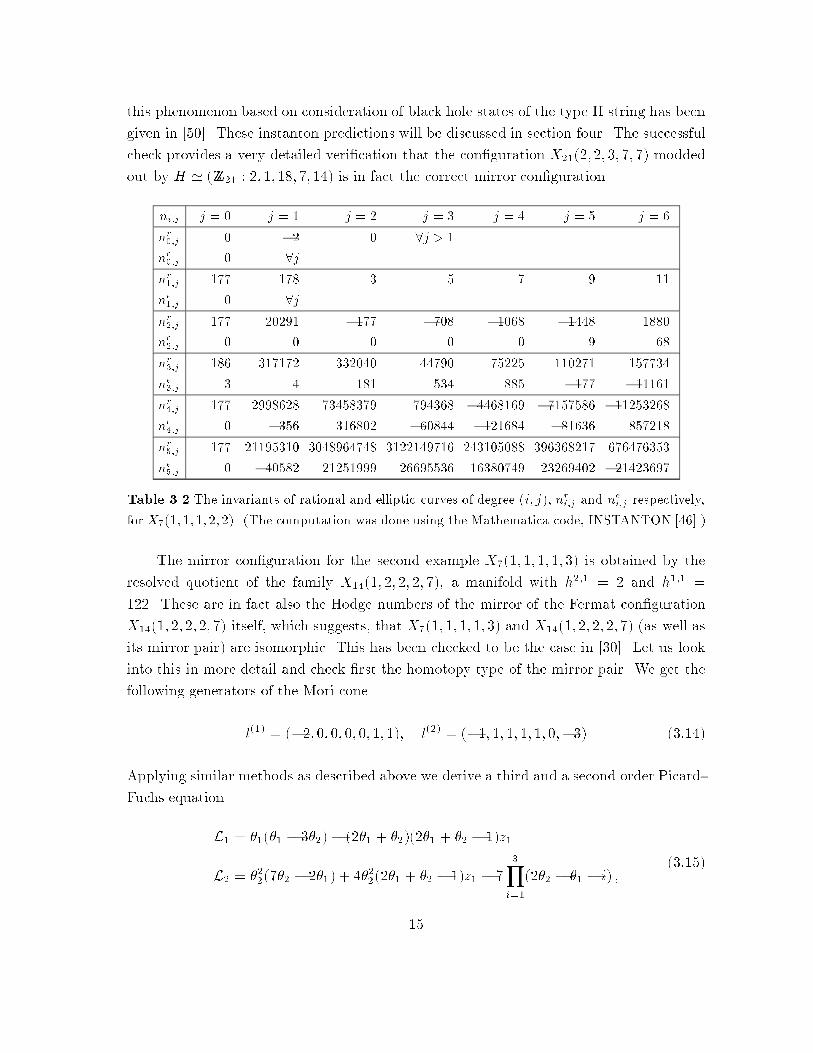
Table 3.2 The invariants of rational and elliptic curves of degree (i; j), nri;j and nei;j respectively,

for X7(1; 1; 1; 2; 2). (The computation was done using the Mathematica code, INSTANTON [46].)

The mirror con�guration for the second example X7(1; 1; 1; 1; 3) is obtained by the

resolved quotient of the family X14(1; 2; 2; 2; 7), a manifold with h2;1 = 2 and h1;1 =

122. These are in fact also the Hodge numbers of the mirror of the Fermat con�guration

X14(1; 2; 2; 2; 7) itself, which suggests, that X7(1; 1; 1; 1; 3) and X14(1; 2; 2; 2; 7) (as well as

its mirror pair) are isomorphic. This has been checked to be the case in [30]. Let us look

into this in more detail and check �rst the homotopy type of the mirror pair. We get the

following generators of the Mori cone

l(1) = (�2; 0; 0; 0; 0; 1; 1); l(2) = (�1; 1; 1; 1; 1; 0;�3) (3:14)

Applying similar methods as described above we derive a third and a second order Picard-

Fuchs equation

L1 = �1(�1 � 3�2) � (2�1 + �2)(2�1 + �2 � 1)z1

L2 = �22(7�2 � 2�1) + 4�2

2(2�1 + �2 � 1)z1 � 7

3Yi=1

(2�2 � �1 � i) ;(3:15)

15

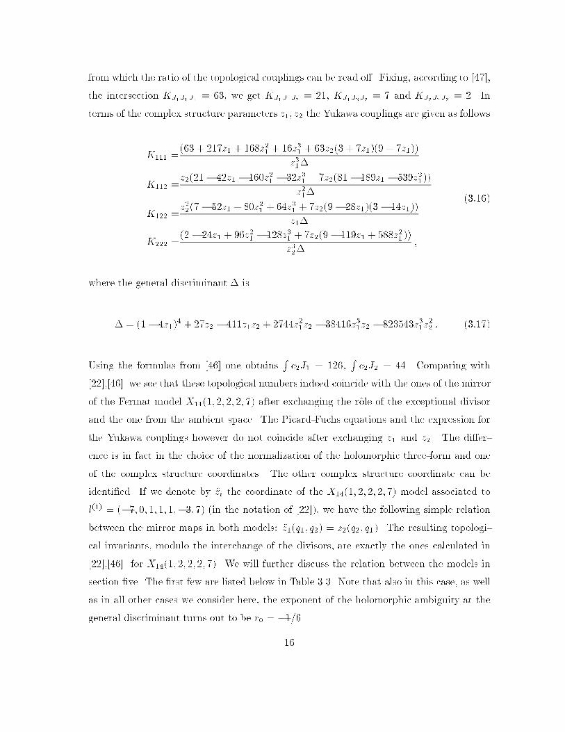
from which the ratio of the topological couplings can be read o�. Fixing, according to [47],

the intersection KJ1J1J1 = 63, we get KJ1J1J2 = 21, KJ1J2J2 = 7 and KJ2J2J2 = 2. In

terms of the complex structure parameters z1; z2 the Yukawa couplings are given as follows

K111 =(63 + 217z1 + 168z2

1+ 16z3

1+ 63z2(3 + 7z1)(9 + 7z1))

z31�

K112 =z2(21� 42z1 � 160z2

1� 32z3

1+ 7z2(81 � 189z1 � 539z2

1))

z21�

K122 =z22(7� 52z1 + 80z2

1+ 64z3

1+ 7z2(9� 28z1)(3 � 14z1))

z1�

K222 =(2 � 24z1 + 96z2

1� 128z3

1+ 7z2(9� 119z1 + 588z2

1))

z32�

;

(3:16)

where the general discriminant � is

� = (1� 4z1)4 + 27z2 � 411z1z2 + 2744z2

1z2 � 38416z3

1z2 � 823543z3

1z22: (3:17)

Using the formulas from [46] one obtainsRc2J1 = 126,

Rc2J2 = 44. Comparing with

[22],[46] we see that these topological numbers indeed coincide with the ones of the mirror

of the Fermat model X14(1; 2; 2; 2; 7) after exchanging the role of the exceptional divisor

and the one from the ambient space. The Picard-Fuchs equations and the expression for

the Yukawa couplings however do not coincide after exchanging z1 and z2. The di�er-

ence is in fact in the choice of the normalization of the holomorphic three-form and one

of the complex structure coordinates. The other complex structure coordinate can be

identi�ed. If we denote by ~zi the coordinate of the X14(1; 2; 2; 2; 7) model associated to

l(1) = (�7; 0; 1; 1; 1;�3; 7) (in the notation of [22]), we have the following simple relation

between the mirror maps in both models: ~z1(q1; q2) = z2(q2; q1). The resulting topologi-

cal invariants, modulo the interchange of the divisors, are exactly the ones calculated in

[22],[46] for X14(1; 2; 2; 2; 7). We will further discuss the relation between the models in

section �ve. The �rst few are listed below in Table 3.3. Note that also in this case, as well

as in all other cases we consider here, the exponent of the holomorphic ambiguity at the

general discriminant turns out to be r0 = �1=6.

16

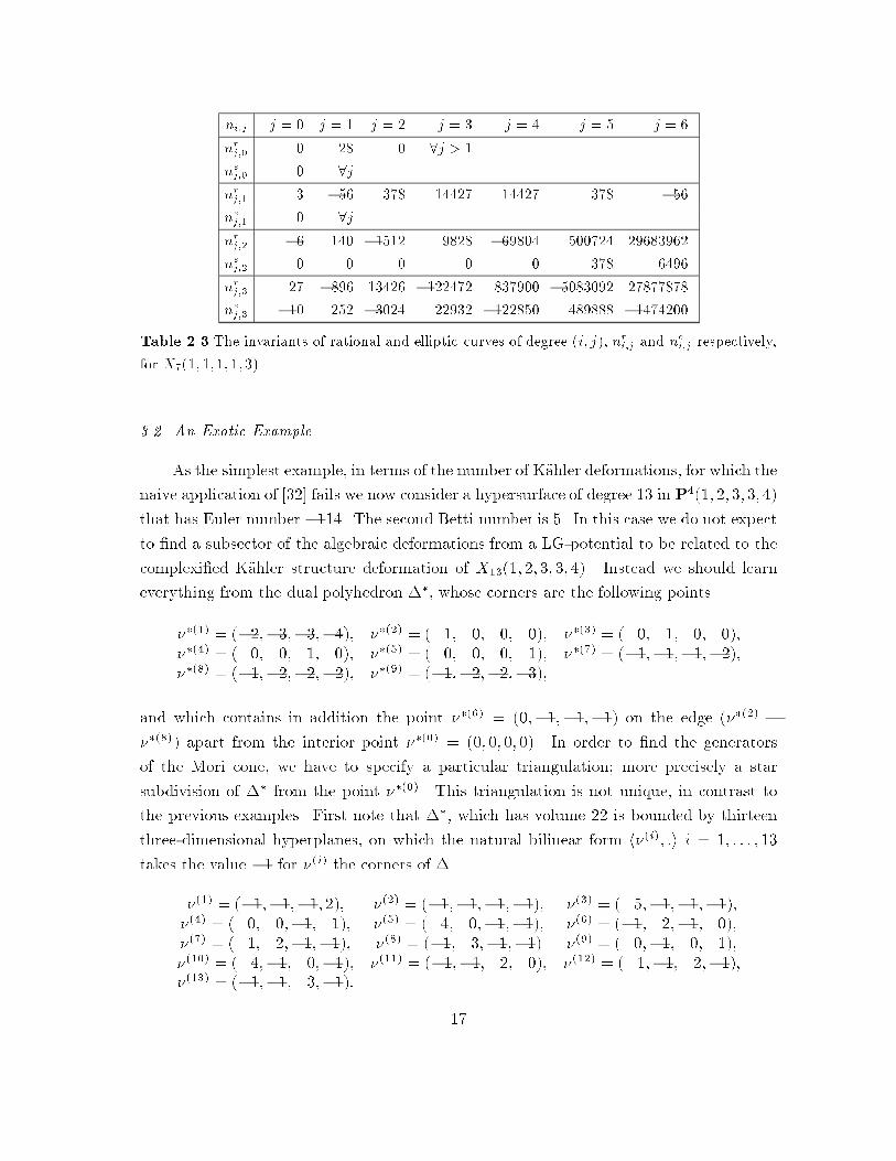
ni;j j = 0 j = 1 j = 2 j = 3 j = 4 j = 5 j = 6

nrj;0 0 28 0 8j > 1

nej;0 0 8j

nrj;1 3 �56 378 14427 14427 378 �56

nej;1 0 8j

nrj;2 �6 140 �1512 9828 �69804 500724 29683962

nej;2 0 0 0 0 0 378 6496

nrj;3 27 �896 13426 �122472 837900 �5083092 27877878

nej;3 �10 252 �3024 22932 �122850 489888 �1474200

Table 2.3 The invariants of rational and elliptic curves of degree (i; j), nri;j and nei;j respectively,

for X7(1; 1; 1; 1; 3).

3.2. An Exotic Example

As the simplest example, in terms of the number of K�ahler deformations, for which the

naive application of [32] fails we now consider a hypersurface of degree 13 in P4(1; 2; 3; 3; 4)

that has Euler number �114. The second Betti number is 5. In this case we do not expect

to �nd a subsector of the algebraic deformations from a LG-potential to be related to the

complexi�ed K�ahler structure deformation of X13(1; 2; 3; 3; 4). Instead we should learn

everything from the dual polyhedron ��, whose corners are the following points

��(1) = (�2;�3;�3;�4); ��(2) = ( 1; 0; 0; 0); ��(3) = ( 0; 1; 0; 0);

��(4) = ( 0; 0; 1; 0); ��(5) = ( 0; 0; 0; 1); ��(7) = (�1;�1;�1;�2);

��(8) = (�1;�2;�2;�2); ��(9) = (�1;�2;�2;�3);

and which contains in addition the point ��(6) = (0;�1;�1;�1) on the edge (��(2) �

��(8)) apart from the interior point ��(0) = (0; 0; 0; 0). In order to �nd the generators

of the Mori cone, we have to specify a particular triangulation; more precisely a star

subdivision of �� from the point ��(0). This triangulation is not unique, in contrast to

the previous examples. First note that ��, which has volume 22 is bounded by thirteen

three-dimensional hyperplanes, on which the natural bilinear form h�(i); :i i = 1; : : : ; 13

takes the value �1 for �(i) the corners of �

�(1) = (�1;�1;�1; 2); �(2) = (�1;�1;�1;�1); �(3) = ( 5;�1;�1;�1);

�(4) = ( 0; 0;�1; 1); �(5) = ( 4; 0;�1;�1); �(6) = (�1; 2;�1; 0);

�(7) = ( 1; 2;�1;�1); �(8) = (�1; 3;�1;�1) �(9) = ( 0;�1; 0; 1);

�(10) = ( 4;�1; 0;�1); �(11) = (�1;�1; 2; 0); �(12) = ( 1;�1; 2;�1);�(13) = (�1;�1; 3;�1):

17

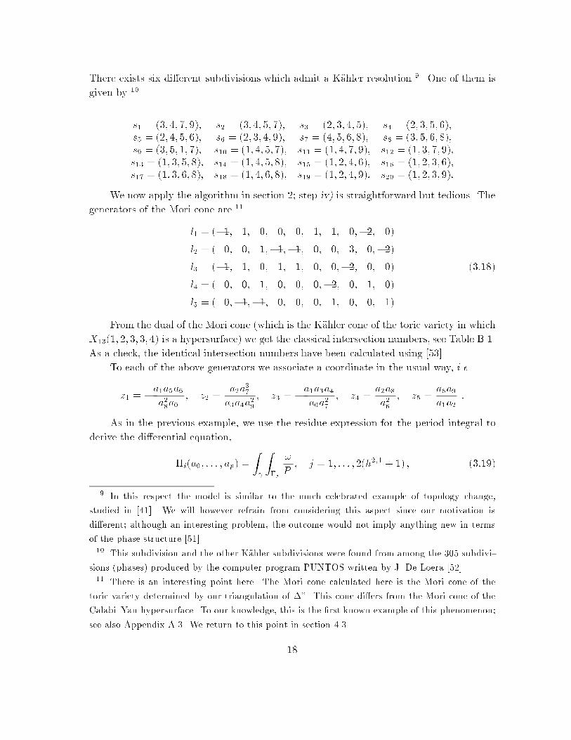
There exists six di�erent subdivisions which admit a K�ahler resolution 9. One of them is

given by 10

s1 = (3; 4; 7; 9); s2 = (3; 4; 5; 7); s3 = (2; 3; 4; 5); s4 = (2; 3; 5; 6);s5 = (2; 4; 5; 6); s6 = (2; 3; 4; 9); s7 = (4; 5; 6; 8); s8 = (3; 5; 6; 8);

s9 = (3; 5; 1; 7); s10 = (1; 4; 5; 7); s11 = (1; 4; 7; 9); s12 = (1; 3; 7; 9);

s13 = (1; 3; 5; 8); s14 = (1; 4; 5; 8); s15 = (1; 2; 4; 6); s16 = (1; 2; 3; 6);

s17 = (1; 3; 6; 8); s18 = (1; 4; 6; 8); s19 = (1; 2; 4; 9); s20 = (1; 2; 3; 9):

We now apply the algorithm in section 2; step iv) is straightforward but tedious. The

generators of the Mori cone are 11

l1 = (�1; 1; 0; 0; 0; 1; 1; 0;�2; 0)

l2 = ( 0; 0; 1;�1;�1; 0; 0; 3; 0;�2)

l3 = (�1; 1; 0; 1; 1; 0; 0;�2; 0; 0)

l4 = ( 0; 0; 1; 0; 0; 0;�2; 0; 1; 0)

l5 = ( 0;�1;�1; 0; 0; 0; 1; 0; 0; 1)

(3:18)

From the dual of the Mori cone (which is the K�ahler cone of the toric variety in which

X13(1; 2; 3; 3; 4) is a hypersurface) we get the classical intersection numbers, see Table B.1.

As a check, the identical intersection numbers have been calculated using [53].

To each of the above generators we associate a coordinate in the usual way, i.e.

z1 = �a1a5a6

a28a0

; z2 =a2a

3

7

a3a4a2

9

; z3 = �a1a3a4

a0a2

7

; z4 =a2a8

a26

; z5 =a6a9

a1a2:

As in the previous example, we use the residue expression for the period integral to

derive the di�erential equation,

�i(a0; : : : ; ap) =

Z

Z�j

!

P; j = 1; : : : ; 2(h2;1 + 1) ; (3:19)

9 In this respect the model is similar to the much celebrated example of topology change,

studied in [41]. We will however refrain from considering this aspect since our motivation is

di�erent; although an interesting problem, the outcome would not imply anything new in terms

of the phase structure [51].10 This subdivision and the other K�ahler subdivisions were found from among the 305 subdivi-

sions (phases) produced by the computer program PUNTOS written by J. De Loera [52].11 There is an interesting point here. The Mori cone calculated here is the Mori cone of the

toric variety determined by our triangulation of ��. This cone di�ers from the Mori cone of the

Calabi{Yau hypersurface. To our knowledge, this is the �rst known example of this phenomenon;

see also Appendix A.3. We return to this point in section 4.3.

18

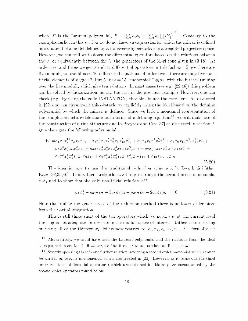
where P is the Laurent polynomial, P =P

i ai�i �P

i aiQ

j Y��(i)

j

j . Contrary to the

examples earlier in this section we do not have an expression for which the mirror is de�ned

as a quotient of a model de�ned by a transverse hypersurface in a weighted projective space.

However, we can still write down the di�erential operators based on the relations between

the �i or equivalently between the li, the generators of the Mori cone given in (3.18). At

order two and three we get 6 and 13 di�erential operators in this fashion. Since there are

�ve moduli, we would need 10 di�erential equations of order two|there are only �ve non-

trivial elements of degree 2, but 5 � 6=2 = 15 \monomials" �i�j , with the indices running

over the �ve moduli, which give ten relations. In most cases (see e.g. [22,46]) this problem

can be solved by factorization, as was the case in the previous example. However, one can

check (e.g. by using the code INSTANTON) that this is not the case here. As discussed

in [22] one can circumvent this obstacle by explicitly using the ideal based on the de�ning

polynomial by which the mirror is de�ned. Since we lack a monomial representation of

the complex structure deformations in terms of a de�ning equation12, we will make use of

the construction of a ring structure due to Batyrev and Cox [37] as discussed in section 2.

One then gets the following polynomial

W =a1x1x13

2x3x8x13 + a2x

6

3x4x

5

5x27x9x

5

10x212+ a3x4x5x

3

6x37x48+ a4x9x10x

3

11x312x413+

a5x3

1x24x6x

2

9x11 + a6x1x

4

2x43x4x

3

5x7x9x

3

10x12 + a7x

6

2x6x7x

2

8x11x12x

2

13+

a8x2

1x82x23x4x5x9x10 + a9x

9

2x33x25x7x8x

2

10x12x13 + a10x1 : : : x13

(3:20)

The idea is now to use the traditional reduction scheme �a la Dwork{Gri�ths{

Katz [38,39,40]. It is rather straightforward to go through the second order monomials,

�i�j and to show that the only non-trivial relation is13

a1�2

9+ a0�1�7 + 3a5�0�6 + a6�1�9 + 2a8�1�5 = 0: (3:21)

Note that unlike the generic case of the reduction method there is no lower order piece

from the partial integration.

This is still three short of the ten operators which we need, i.e. at the current level

the ring is not adequate for describing the moduli space of interest. Rather than insisting

on using all of the thirteen xi, let us now restrict to x1; x2; x5; x8; x11, i.e. formally set

12 Alternatively, we could have used the Laurent polynomial and the relations from the ideal

as explained in section 2. However, we �nd it easier to use method outlined below.13 Strictly speaking there is one further relation involving a second order monomial which cannot

be written as �i�j , a phenomenon which was treated in [22]. However, as it turns out the third

order relations (di�erential operators) which are obtained in this way are encompassed by the

second order operators found below.

19

the remaining xi = 1. Renaming these yi; i = 1; : : : ; 5 the Batyrev-Cox potential is then

reduced to

~W =a1y1y13

2y4 + a2y

5

3+ a3y3y

4

4+ a4y

3

5+ a5y

3

1y5+

a0y1y2y3y4y5 + a6y1y4

2y33+ a7y

6

2y24y5 + a8y

2

1y82y3 + a9y

9

2y23y4 :

(3:22)

Note that the �rst �ve terms can be thought of as obtained from a transposition of a

degenerate potential for the original model, degenerate because we need to add extra terms

in order to make it transversal; this was indeed the reason why the above xi were chosen.

Since the xi correspond to points in �, choosing the �ve xi corresponds to refraining from

resolving the singularities of X, the existence of which the remaining xi are based on.

Finally, let us then consider the following three monomials

�6�8; �27; �0�7 ; (3:23)

which are the among the �fteen �i�j ; i; j = 0; 6; :::; 9 which do not appear in any of the pre-

vious relations at second order among the �i�j . By vigorous application of the ideal, @ ~W ,

it is possible in all three cases to arrive at non-trivial relations of second order involving

only monomials of the form �i�j . This completes the story; together with the operators

obtained from the Mori cone, (3.18), and (3.21) it can be shown that the triple intersec-

tion numbers on the original toric variety P4(1; 2; 3; 3; 4) are reproduced, see Table B.1.

Note that they di�er from those we would compute from the K�ahler cone of the manifold

X14(1; 2; 3; 3; 4), see the discussion in section 4.3. In Table B.2 we record the lowest order

instanton corrections, some of which are veri�ed in the following section.

4. Veri�cations.

In this section we geometrically explain some of the instanton numbers computed in

the earlier sections.

4.1. P4(1; 1; 1; 2; 2)

The �rst step is to desingularize P4(1; 1; 1; 2; 2). This has already been accomplished

implicitly in (3.3) by the presence of the vector ��(6), since the other 5 vectors in (3.3)

determine the toric fan forP4(1; 1; 1; 2; 2). However, we prefer to use an explicit calculation.

P4(1; 1; 1; 2; 2) is singular along the P1 de�ned by x1 = x2 = x3 = 0. We desingularize

by using an auxiliary P2 with coordinates (y1; y2; y3) and de�ne

~P4 � P4(1; 1; 1; 2; 2) �P2

20

by the equations

xiyj = xjyi; i; j = 1; 2; 3: (4:1)

The exceptional divisor is just P1 �P2, where the two projective spaces have coordinates

(x4; x5) and (y1; y2; y3) respectively. The proper transform of a general degree 7 hyper-

surface X is seen to intersect the exceptional divisor in a surface de�ned by a polynomial

f(x4; x5; y1; y2; y3) which is cubic in the x's and linear in the y's. This can be seen by

direct calculation, the essential point being the presence of monomials cubic in x4; x5 and

linear in x1; x2; x3 in an equation for X. The �bers of the projection of this surface to P1

are lines; thus the desingularized Calabi{Yau manifold ~X contains a ruled surface with P1

as a base.

This fact was noticed and pointed out to us by D.R. Morrison. Other examples of

Calabi{Yau manifolds containing ruled surfaces parameterized by curves of higher genus

have been studied in [46] and in [21]. The presence of a ruled surface with P1 as base

yields di�erent and interesting geometry; this has in part motivated us to calculate the

instanton numbers for this example.

To understand this ruled surface, we �rst think of P1 �P2 as the projective bundle

P(O3) on P1 (see [54] for notation). Writing f = f1(x)y1 + f2(x)y2 + f3(x)y3, we see

that f is determined by the three fi; these can be identi�ed with a map O(�3) ! O3;

the cokernel of a generic such map is O(1)�O(2). So the exceptional divisor of X is just

P(O(1) � O(2)). Rational ruled surfaces such as this are very well understood [54]. We

quickly review the relevant points.

Let B denote the rank 2 bundle O(a) � O(b) on P1 for some integers a � b. The

abstract rational ruled surface P(B) is isomorphic to the Hirzebruch surface Fb�a; this

surface is characterized by the minimum value of C2 for C a section of the ruled surface,

the minimum being a� b. The section achieving this minimum is even unique if a < b.

H2(P(B)) is generated by two classes|a hyperplane class H and the �ber f . The

cohomologyH0(mH+nf) is calculated form � 0 as H0(P1;Symm(B)O(n)). The space

of curves in the classmH+nf is parameterized by the projectivization of this vector space.

We also note the intersection numbers H2 = a + b; H � f = 1; f2 = 0. In our case, this

gives

H2 = 3; H � f = 1; f2 = 0: (4:2)

We also note that the curve of minimum self intersection is in the class H � 2f .

In particular, if any families of rational curves are of this type, and are parameter-

ized by Pr, then its contribution to the Gromov-Witten invariant for this type of curve

is (�1)r(r + 1) by [21]. Later, we will also need that if a family of rational curves is

parameterized by a smooth curve of genus g, then its contribution to the Gromov-Witten

invariant is 2g � 2.

21

The classes J1 and J2 are interpreted as the classes given by the zeros of quadratic

and linear polynomials, respectively. Since all linear polynomials vanish along x1 = x2 =

x3 = 0, and therefore along the exceptional divisor E after the blowup, we conclude that

J1 = 2J2 +E.

To compute nri;j , we note that if i < 2j and if C � J1 = i; C � J2 = j, then C � E =

i�2j < 0, which implies that a component of C must be contained in E. So in this case we

are often reduced to understanding curves in E. Next, we need to observe that J1jE ' f

and J2jE ' H.

In the case of nr0;j for j � 1, we see inductively that all of these curves lie in E. For

these curves C, we have that (thought of as a curve in the ruled surface E) C � f = 0 and

C �H = j. The �rst equation and (4.2) say that C must be a �ber; in that case, necessarily

C �H = 1, so j=1. If j = 1, then we have

H0(P(B); f) ' H0(P1;O(1)) 'C2

so the curves are parameterized by P1 and nr0;1 = �2. We have also shown that nr

0;j = 0

for j � 2.

For nr1;j with j � 2, these curves C are again contained in E (at this point, it is clear

that a component is contained in E; but we will check later that all such curves are entirely

contained in E).

We have C � f = 1 and C �H = j, which implies that C is of type H + (j � 3)f . In

addition, C � f = 1 implies that C is a section or the union of a section and �bers, hence

is rational. Finally, H0(P(B);H + (j � 3)f) is isomorphic to

H0(P1; B O(j � 3)) = H0(P1;O(j � 2) �O(j � 1));

which has dimension 2j � 1. So the curves are parameterized by a projective space of

dimension 2j � 2. This gives n1;j = 2j � 1 for j � 2.

Note in passing that we have also shown that nej;k = 0 for j = 0; 1, since only rational

curves arise as sections or �bers. In fact, for all of our two parameter models we note

that for exactly the same reason as given above, a curve C of type (0; 1) necessarily lies in

the exceptional divisor E. In each case, E is an explicitly given rational surface, and by

consideration of the possible curves on E, the condition C � J2 = 1 is either not possible

or forces C to be rational. Either way, we get ne0;1 = 0, justifying the procedure given in

section 3.1 for determining r0.

Consider ne2;5. These curves are contained in E by the now-familiar argument. Since

C � f = 2 and C �H = 5, we get that C is in the class 2H � f . This is a family of elliptic

curves, and is parameterized by a P8. This gives ne2;5 = 9. The general curve in the class

2H + bf is elliptic only for b = �1. This leads quickly to the conclusion that ne2;j = 0 for

j 6= 5.

22

We can make further veri�cations (and �nish an earlier argument) by using J2. The

three linear forms which are the sections of J2 give a map to P2. Actually, we study this

by means of the map g : ~P4 ! P2 given by projection onto (y1; y2; y3); the map on the

Calabi{Yau hypersurface ~X is given by restriction. The �bers of g are isomorphic to P2;

in fact ~P4 can be constructed as the projective bundle P(O2 � O(2)) on P2. The O2

corresponds to the coordinates x4; x5; the O(2) arises because y1; y2; y3 can be rescaled in~P4 independent of x4; x5. Like all projective bundles, this one comes with a tautological

rank 1 quotient, the bundle of linear forms in the �bers. In this case, it turns out to be J1.

That is, there is a map g�(O2 �O(2))! J1. The hypersurface ~X is in the class 3J1 + J2.

This says that �bers of g, restricted to the hypersurface of interest, are plane cubic curves.

The �bers are readily seen to be of type (3; 0).

We are now equipped to compute nr1;0. If C � J2 = 0, then C is contained in a �ber of

g. The condition C � J1 = 1 says that C is a line. Hence we must enumerate points of P2

with the property that the cubic �ber factors into a line and a conic. In particular, there

is a 1-1 correspondence between lines and conics; hence nr1;0 = nr

2;0.

The technique is standard [55]. We form the Grassmann bundle G = Gr2(O2�O(2))

of lines in the �bers of g. Note that dim(G) = 4. There is a projection map � : G! P2.

On G, there is a canonical rank 2 bundle Q, the bundle of linear forms on these lines.

The equation of ~X induces a section of the rank 4 bundle Sym3(Q) ��O(1). The line

is contained in ~X if and only if this section vanishes at the corresponding point of G. So

we must calculate c4(Sym3(Q) ��O(1)). This is immediately calculated to be 177 using

Schubert [53].

Turning to nr1;1, we note that C � J1 = 1 and C � J2 = 1 implies that a component of

C is contained in E. There are two cases: either C � E, or C is a union of a curve of type

(1; 0) and a curve of type (0; 1) (we have already seen that the latter curve is a �ber of E).

In the former case, C �f = 1 and C �H = 1 implies that C is in the class H�2f . Since

H0(P(B);H � 2f) is 1 dimensional, there is only one curve of this type, contributing 1 to

nr0;1. Alternatively, note that (H � 2f)2 = �1, the minimum value; hence C is unique.

If on the other hand C = C 0[C 00 with C 0 of type (1; 0), then C 0�E = C 0�(J1�2J2) = 1.

For C to be connected, C 00 must be the unique �ber f containing the unique point of

intersection on C 0 and E. So each curve of type (1; 0) yields a degenerate instanton (see

appendix to [8]) of type (1; 1).

Putting these two cases together, we see that nr1;1 = nr

1;0 + 1 = 178.

Returning to the �nal details of nr1;j for j � 2, we see that if C were not contained in

E, then it would have to be a union

C = C 0 [ C1 [ : : : [ Cj

where C 0 has type (1; 0) and the Ci have type (0; 1). But C 0 meets E in just one point,

so there is no way to add on j �bers and obtain a connected curve. So this case does not

occur, as asserted earlier.

23

Next, ne3;0 is easy; these are the elliptic cubic curves in the �bers of g. But the

general �bers of g are elliptic cubic curves. So these curves are parameterized by P2;

hence ne3;0 = 3,

The calculation of nr3;0 is more intricate. Here we must study the rational cubic curves

in the �bers of g. A cubic curve is rational only if it is singular. So we investigate the locus

of singular cubic curves. This is seen to be a plane curve of degree 36. But this curve is

singular. In fact, the curve has nodes at each of the 177 cubics that we found earlier that

factor into a line and a conic. This is because such curves have 2 singularities, which can

be smoothed independently, yielding 2 distinct tangent directions in the space of singular

curves. In addition, there are 216 cusps.14

It will be illuminating to generalize this situation before continuing the calculation.

We suppose that we have a family of nodal elliptic curves with parameter space of curve B

of arithmetic genus pa, containing � nodes and � cusps. The nodes parameterize 2-nodal

elliptic curves (which necessarily split up into 2 smooth rational curves, meeting twice),

and the cusps parameterize cuspidal curves. In our example, pa = (36�1)(35�1)=2 = 595,

while � = 177 and � = 216.

Resolving the singularities of B, we get a curve ~B of genus pa � � � �; and the

computation from [21] shows that we must make a correction for the cusps, �nally obtaining

the Gromov-Witten invariant c1(1( ~B)) � � = 2(pa � � � �) � 2 � �, which simpli�es to

2pa � 2� � 3�� 2. In our example, this gives nr3;0 = 186.

This is not coincidentally the negative of the Euler characteristic of the target space ~X.

We calculate the Euler characteristic by decomposing ~X. Again we generalize, assuming

that there is a map f : ~X ! S, where S is a smooth complex surface. We suppose that

the general �ber of f is a smooth elliptic curve, while over some curve B contained in the

surface, the �ber degenerates in the manner described above. We keep the notation pa; �; �

as before.

We divide S into four pieces: S�B, the complement of the nodes and cusps in B, the

nodes, and the cusps. We can then divide ~X into four corresponding pieces, the inverse

images of these four pieces via f . We will calculate the Euler characteristic of these four

pieces.

We start the calculation by a preliminary calculation on B. We obtain a node by

pinching a 1-cycle to a point, and a cusp by pinching two 1-cycles. If we then remove the

resulting singularities, we compute that the Euler characteristic of the complement of the

nodes and cusps in B is 2� 2pa + � + 2�� (� + �), which simpli�es to 2� 2pa + �.

14 The statements about the degree and number of cusps can for instance be checked by the

standard technique of considering pairs (C; p) where C is one of the cubic curves and p 2 C, then

projecting onto C. The Schubert code for these calculations is available upon request.

24

We also need to observe that the Euler characteristic of a smooth elliptic curve, the

nodal curves, the 2-nodal curves, and the cuspidal curves have respective Euler character-

istics 0; 1; 2; 2.

We can obtain the Euler characteristic of each piece by multiplying the Euler char-

acteristics of the base and the �ber, then summing over all pieces. The result is

0 + (2 � 2pa + �)(1) + �(2) + �(2), which simpli�es to 2 � 2pa + 2� + 3�. This is plainly

the negative of the Gromov-Witten invariant obtained above. This phenomenon occurs in

several of the the examples discussed in [22,46].

For ne3;1, we claim that a curve C with C �J1 = 3 and C �J2 = 1 is reducible. Suppose

it were irreducible. Then J2 restricts to a degree 1 bundle on C, which has a 1 dimensional

space of global sections. Since J2 has a 3 dimensional space of global sections (spanned

by y1; y2; y3), the kernel of the restriction map is at least 2 dimensional. This constrains

C to lie in a �ber of g. But we have already noted that the �bers of g are of type (3; 0),

so this is impossible. Looking at our prior discussion of curves of type (a; b) with a � 3

and b � 1, we see that the only possibility is C = C1 [ C2, where the Ci are of type (3; 0)

and (0; 1) respectively. Such curves are parameterized by E|take the �ber f through the

point p 2 E union the �ber of g through the image of p in P2. Since c2(E) = 4, this gives

ne3;1 = 4.

Finally, we can easily see that n4;0 = n5;0 = 177. For each of the 177 line-conic pairs,

we have two families of degenerate instantons. These are analyzed by the method in the

appendix to [8]; since our situation is simpler, we will content ourselves with sketching the

construction. The �rst consists of maps from P1 to the conic, with lines bubbling o� at

each of the two nodes. These are degenerate instantons of type (4; 0). The other family

comes from maps from P1 to the line, with conics bubbling o� at each of the nodes. These

are degenerate instantons of type (5; 0).

One can in fact verify that there is a non-zero contribution to ni;0 for all i by using

stable maps [56] as the method to compactify the space of instantons. All stable maps

needed will restrict to degree 1 maps on each irreducible component.

If i = 3k, we can take a tree C = C1 [ � � � [Ck of rational curves, and map the inter-

section points of the components to the nodes of any of the nodal cubic curves described

above, with the rule that if Cj�1 maps to one branch of a nodal cubic near p = Cj�1 \Cj ,

then Cj maps to the other branch near p.

If i = 3k + 1, we take C = C1 [ � � � [ C2k+1, mapping C2j�1 to one of the lines found

above, and mapping C2j to the intersecting conic. Each Cl�1 \Cl maps to one of the two

intersection points of a line and a conic. If l < 2k + 1, then Cl \ Cl+1 maps to the other

intersection point.

The case i = 3k + 2 is similar, this time mapping C2j�1 to conics and C2j to lines.

25

4.2. P4(1; 1; 1; 1; 3)

We desingularize the weighted projective space in this case by using an auxiliary P3

with coordinates (y1; y2; y3; y4) and de�ne

~P4 � P4(1; 1; 1; 1; 3) �P3

by the equations

xiyj = xjyi; i = 1; : : : ; 4:

The exceptional locus is clearly a copy of P3. The proper transform of a general degree

7 hypersurface is seen to intersect this locus in a linear hypersurface, i.e. a projective

plane. This can be seen by direct calculation, the essential point being the presence of the

monomials xix2

5for i = 1; : : : ; 4 which are linear in the variables x1; : : : ; x4.

Now J1 and J2 are respectively the classes of degree 3 and degree 1 polynomials. This

leads to the equality J1 = 3J2 + E, where E is the class of the exceptional P2. So if a

curve C with C � Ji = ai and a1 < 3a2, then a component of C necessarily lies on E.

To compute nr0;j , we see that these curves lie on E, and have degree j as a curve on

E. Since lines are parameterized by P2, we get nr0;1 = 3. Since conics are parameterized

by P5, we get nr0;2 = �6. Elliptic curves are similar; the lowest degree possible is cubic,

so ne0;j = 0 for j = 1; 2, while ne

0;3 = �10 since plane cubics are parameterized by a P9.

To compute nr1;0, we note that a curve C with C � J2 = 0 maps to a point under the

projection to P3, since the projection map is de�ned by the sections of J2. We write the

equation of the proper transform of the hypersurface as f7(y)+f4(y)x5+f1(y)x2

5, where the

fj(y) are homogeneous polynomials of degree j in y1; : : : ; y4. The 28 values of y for which

f7(y) = f4(y) = f1(y) = 0 yield a P1 in the hypersurface (since x5 may be arbitrary); this

curve is easily seen to have J1-degree 1. This gives nr1;0 = 28. This geometry also implies

that nri;0 = 0 for i > 1. Each such curve C satis�es C �E=C �J1�3C �J2 = 1, so that C\E

is a point p. We can get reducible curves with C �J1 = 1 and C �J2 = 1 (resp: 2) by taking

the union of C with a line (resp. a conic) in E passing through p. Since lines (resp. conics)

passing through p are parameterized by P1 (resp. P4), we get nr1;1 = 28(�2) = �56 and

nr1;2 = 28(5) = 140. Also, we can construct rational curves of type (2; 1) by taking a pair

of curves of type (1; 0) and taking their union with the unique line in E passing through

the respective intersection points of these two curves with E. Thus nr2;1 =

�28

2

�= 378.

Irreducible elliptic curves C of type (5; 2) satisfy C �E = �1, so these lie on E. Such

curves do not exist, since we know that the plane curves in E have type (0; j) for some j.

The only possible reducible curves are obtained as follows. Consider one of the rational

curves C1 of type (5; 1). These meet E in 2 points, which may be joined by the unique

line C2 (of type (0; 1)) meeting these points. The curve C = C1 [C2 is of type (5; 2), and

is elliptic. This veri�es ne5;2 = nr

5;1.

26

Considering elliptic curves of type (i; 3) for i < 9, we see that such curves have a

component contained in E. We see that if i < 5, this component must be one of the (0; 3)

elliptic curves considered above, and there are i additional components, each rational

curves of type (1; 0). This gives nei;3 =�28

i

�� (�1)i�1(10 � i), since plane cubics passing

through i �xed points are parameterized by a P9�i. These are in agreement with the

invariants produced from the instanton expansion. This does not hold for 5 � i < 9, due

to the presence of reducible elliptic curves containing a rational component of type (5; 1).

4.3. P4(1; 2; 3; 3; 4)

We start by describing the geometry of the toric variety P�� , especially its K�ahler

cone. It will be convenient in the sequel to consult the following table.

��(1) (�2;�3;�3;�4) 1 0 1 0 �1

��(2) (1; 0; 0; 0) 0 1 0 1 �1

��(3) (0; 1; 0; 0) 0 �1 1 0 0

��(4) (0; 0; 1; 0) 0 �1 1 0 0��(5) (0; 0; 0; 1) 1 0 0 0 0

��(6) (0;�1;�1;�1) 1 0 0 �2 1

��(7) (�1;�1;�1;�2) 0 3 �2 0 0

��(8) (�1;�2;�2;�2) �2 0 0 1 0��(9) (�1;�2;�2;�3) 0 �2 0 0 1

(4:3)

Here, the �ve columns on the right come from the representation of the Mori cone

found in (3.18) (the �rst coordinate of the earlier representation, corresponding to the

origin, is not needed in the current context). This representation gives a basis for the

divisor class group of the toric variety; the coordinates of the classes of the divisors Di

given by the equations xi = 0 (corresponding to the edges ��(i)) can be read o� horizontally

in the above.

Now we �nd the edges of the K�ahler cone by taking the dual basis (recall that the

K�ahler cone is dual to the Mori cone). We �nd linear combinations of the generators

D1; : : : ;D9 such that in the coordinates given by the corresponding rows, we get the �ve

standard basis vectors of Z5. There are many ways of expressing these in terms of the Di;

here is one choice.

J1 = D5

J2 = D2 +D5 +D6 +D8

J3 = D2 +D3 +D5 +D6 +D8

J4 = 2D5 +D8

J5 = 3D5 +D6 + 2D8

27

Toric varieties can also be described as quotients of torus actions. We see that the

toric variety P�� is naturally identi�ed with (C9� F )=C�

5,15 where

F = fx2 = x7 = 0g [ fx2 = x8 = 0g [ fx5 = x9 = 0g [ fx6 = x7 = 0g [ fx6 = x9 = 0g

[fx7 = x8 = 0g [ fx8 = x9 = 0g [ fx1 = x2 = x5 = 0g [ fx1 = x3 = x4 = 0g

[fx3 = x4 = x6 = 0g [ fx3 = x4 = x8 = 0g [ fx1 = x5 = x6 = 0g:

The only singular point of the toric variety P�� is the point x2 = x3 = x4 = x9 = 0

corresponding to the determinant 3 cone spanned by ��(2); ��(3); ��(4); ��(9). Since the

general Calabi{Yau hypersurface X misses this point, X is smooth.

We now identify the classes of curves C1 : : : ; C5 which generate the Mori cone. These

curves by de�nition are dual to the divisors Ji via the intersection pairing. The intersection

numbers Ci � Dj can be read from the last �ve columns of (4.3), at least up to a scalar

multiple of each column. If the intersection number is negative, then necessarily Ci is

contained in Dj . So we see that C1 : : : C5 are respectively contained in the divisor D8, the

empty set D3 \D4 \D9, the divisor D7, the divisor D6, and the curve D1 \D2.

We immediately observe that the Mori cone of X di�ers from the Mori cone of the

toric variety, since C2 is not present on X. For comparison, the locus x3 = x4 = x9 = 0 is a

curve on the toric variety P�� , whose intersection numbers with the Di are given by 1=3 of

the corresponding column of (4.3). The fractional intersection numbers are not surprising,

since C2 passes through the singular point ofP�� . The fact thatD3\D4\D9 has dimension

less than 1 is to be expected on dimensional grounds; but can be veri�ed conclusively by

explicitly writing down the general equation for X, substituting x3 = x4 = x9 = 0, and

noting that vanishing of the remaining term would imply that the point is contained in

the disallowed set F . So this set is in fact empty.

We next set out to identify the Mori cone of X. Consider the class of a curve of

type C =P

i aiCi. In the sequel, we will sometimes call this a curve of type (a1; : : : ; a5).

Suppose that this is the class of an e�ective curve on X. We claim that

a1 � 0; a3 � a2 � 0; a4 � 0; a5 � 0: (4:4)

The inequalities C �Ji � 0 hold because C is an e�ective curve on P�� and the Ji are in the

K�ahler cone. But C � Ji = ai. Now suppose that a2 > a3. Without loss of generality, we

may assume that C is irreducible. Then C �D3 = C �D4 = a3�a2 < 0. Thus C � D3\D4.

We have already seen that D3 \D4 \D9 is empty. The intersection of D3 \D4 with any

15 This and other calculations in this section were performed using an extensive collection of

Maple procedures for toric varieties which has been written jointly by the second author and

S.A. Str�mme; a modi�ed version of these will appear in the next release of Schubert.

28

of D1; D6; or D8 is empty as well, by consideration of the locus F . So we only have to

show that C �Di < 0 for at least one of i = 1; 6; 8; 9. But the system of inequalities in the

ai deduced from the inequalities C �Di � 0 for i = 1; 6; 8; 9 together with ai � 0 is readily

seen to be inconsistent, justifying (4.4).

To show that the system (4.4) indeed de�nes the Mori cone, we �rst note that it is

a simplicial cone spanned by C1; C2 + C3; C3; C4; C5. So it su�ces to show that all of

these are classes of a curve on X. We denote these classes by ~C1; : : : ; ~C5.

Let ~Ji; i = 1; : : : ; 5 be the dual basis of divisors (which will turn out to be the

generators of the K�ahler cone of X). This gives explicitly ~Ji = Ji for i = 1; 2; 4; 5, and~J3 = J3 � J2 = D3.

We have already seen that if the respective curves ~C1; ~C3; ~C4 exist, they lie in the

divisors D8; D7; D6 and ~C5 lies in the curve D1\D2. By the same reasoning, we see that~C2 lies in the divisor D9.

Let Ji denote the wall of the K�ahler cone obtained by taking non-negative linear

combinations of all of the ~Jk except ~Ji. According to [57], these walls consist of divisor

classes which contract ~Ci (i.e. the divisors intersect each curve in the locus trivially). Let

us �nd these loci. First, we identify all curves xi = xj = 0 which meet the divisors in Ji

trivially. We may ignore the curves which are components of F . Direct calculation gives

1 (x3 = x8 = 0) [ (x4 = x8 = 0)

2 (x3 = x9 = 0) [ (x4 = x9 = 0)

3 (x5 = x7 = 0) [ (x7 = x9 = 0)

4 (x1 = x6 = 0) [ (x3 = x6 = 0) [ (x4 = x6 = 0) [ (x5 = x6 = 0)5 (x1 = x2 = 0)

The above table identi�es interesting curves, which leads to the following results.

The divisors of J1 blow down the �bers of a base point free pencil on x8 = 0 generated

by x3; x4 (base point free since x3 = x4 = x8 = 0 is a component of F ). The �bers are

calculated to be rational curves of type (1; 0; 0; 0; 0). This veri�es n1;0;0;0;0 = �2 and

nj;0;0;0;0 = 0 for j > 1.

The divisors of J2 blow down the �bers of a base point free pencil on x9 = 0 generated

by (x3; x4) (while x3 = x4 = x9 = 0 is non-empty on P�� since it is not a component

of F , it is in fact empty on X). The �bers are calculated to be rational curves of type

(0; 1; 1; 0; 0). This veri�es n0;1;1;0;0 = �2 and n0;j;j;0;0 = 0 for j > 1.

Similarly, the divisors of J3 blow down the �bers of a base point free pencil on x7 = 0

generated by x5; x9. Note that while (x5; x9) scale di�erently, the description of x7 = 0 as

a toric variety shows that x5 = 0 and x9 = 0 are linearly equivalent on x7 = 0. The �bers

are calculated to be rational curves of type (0; 0; 1; 0; 0). This veri�es n0;0;1;0;0 = �2 and

n0;0;j;0;0 = 0 for j > 1.

The divisors of J4 blow down the �bers of the base point free pencil on x6 = 0

generated by (x3; x4). The �bers are calculated to be rational curves of type (0; 0; 0; 1; 0).

29

This veri�es n0;0;0;1;0 = �2 and n0;0;0;j;0 = 0 for j > 1. Note that the curves x1 = x6 = 0

and x5 = x6 = 0 are actually disconnected unions of 3 and 4 �bers respectively, so

contribute nothing new.

The divisors of J5 blow down the curve x1 = x2 = 0, which is easily seen to have

three irreducible connected components, each of which is of type (0; 0; 0; 0; 1). This veri�es

n0;0;0;0;1 = 3 and n0;0;0;0;j = 0 for j > 1.

We can also verify several other numbers. For example, degenerate instantons can be

formed by taking the unions of transversely intersecting irreducible rational curves which

have no closed loops (hence still have genus 0). Here is a short list.

Each of the 3 curves of type (0; 0; 0; 0; 1) meets each of x6 = 0 and x9 = 0 once. So

there is a unique �ber of either or both of these surfaces that can be joined to each of these

3 curves to get a rational curve (a glance at F shows that x6 = 0 and x9 = 0 are disjoint).

This veri�es n0;0;0;1;1 = n0;1;1;0;1 = n0;1;1;1;1 = 3.

Now consider the curve C given by x7 = x9 = 0. This is one of the J3-exceptional

curves already considered, so is of type (0; 0; 1; 0; 0). The curve C meets each of the

exceptional �bers of type (0; 1; 1; 0; 0) on x9 = 0 in one point, so can be joined to each of

these �bers. We again get a family of curves parameterized by P1. This veri�es n0;1;2;0;0 =

�2. Now each of the 3 curves of type (0; 0; 0; 0; 1) can be joined to a unique element of

this family; and then again a unique �ber of x6 = 0 can be joined afterwards. This veri�es

n0;1;2;0;1 = n0;1;2;1;1 = 3.

Note also that the �brations on x6 = 0 and x8 = 0 are de�ned by the same pencil

(x3; x4), and that the corresponding �bers meet in one point. Taking unions again gives a

family of curves parameterized by P1. Then each of the 3 curves of type (0; 0; 0; 0; 1) can

be joined to precisely one of these, yielding a rational curve (each such curve meets x6 = 0

once but is disjoint from x8 = 0). This veri�es n1;0;0;1;0 = �2 and n1;0;0;1;1 = 3.

We next observe that curves of type (0; 2; 3; 0; 0) are restrictions to x9 = 0 of the

divisors linearly equivalent to J2. These restrictions are parameterized by P3 (explicitly,

the divisors are de�ned by linear combinations of x23x7; x3x4x7; x

2

4x7; x2x5x6x8). This

gives n0;2;3;0;0 = �4. Each of the 3 curves of type (0; 0; 0; 0; 1) meets x9 = 0 in one point;

the divisors of J2 passing through this point (the only ones that can be joined to get a

connected curve) are parameterized by P2. This gives n0;2;3;0;1 = 3 � 3 = 9. Similarly

we can add on two curves (which restricts divisors of J2 to a P1) or all three (uniquely

specifying the divisor of J2). This veri�es n0;2;3;0;2 = 3 � (�2) = �6 and n0;2;3;0;3 = 1,

while n0;2;3;0;j = 0 for j > 3.

Finally we observe that curves of type (0; 3; 4; 0; 0) are restrictions to x9 = 0 of the divi-

sors linearly equivalent to J2 + J3. These restrictions are parameterized by P5 (explicitly,

the divisors are de�ned by linear combinations of f3(x3; x4)x7; x2x3x5x6x8; x2x4x5x6x8,

and x1x2

5x6x

2

8, where f3(x3; x4) is a homogeneous cubic; note that when restricted to

X \ (x9 = 0), the last monomial becomes a linear combination of the others). This gives

30

n0;3;4;0;0 = �6, and proceeding as before, we also get n0;3;4;0;1 = 3 � 5 = 15; n0;3;4;0;2 =

3 � (�4) = �12, and n0;3;4;0;3 = 3.

The calculation of the Mori cone of X shows that the true large complex structure

coordinates are q1; q2q3; q3; q4; q5. In other words, the boundary divisor q3 = 0 in the moduli

space constructed from toric geometry gets blown down, slightly changing the geometry of

the large complex structure limit. The instanton expansions remain valid, the only change

being that we get the more precise result that the instanton expansions must be power

series in q1; q2q3; q3; q4; q5, agreeing with our calculations.

5. Applications and Generalizations

5.1. Non-Landau{Ginzburg cases

The classi�cation of the three dimensional polyhedra appears as the natural gener-

alization of the work of [25]. We will not solve this complicated combinatorial problem

here, but rather give the �rst examples of re exive pairs of polyhedra, which do not come

from the list of [25] nor from moddings of the examples in that list [58]. The impor-

tant observation in �nding such examples is the fact that one can systematically modify

a given polyhedron by moving one corner to a new position, in such a fashion that the

new polyhedron remains re exive. We can then use the general methods for determining

the Picard-Fuchs equations for re exive polyhedra, which were developed in the previous

section.

As an example of this phenomenon let us consider some of the two moduli models

of table 3.1 and move one of the vertices to a new position without destroying re ex-

ivity. In table 5.1 we list models constructed by moving the point ��(1) such that the

resulting Calabi-Yau spaces have h11 < 4. In a) � c), the original location for ��(1) is

(�k2;�k3;�k4;�k5), see (2.4). There are no such natural coordinates for the model in

table 5.1.d); a choice of coordinates has been made here.16

16 We are grateful to Maximilian Kreuzer for checking that the models marked with a star in

table 5.1 do not appear as a result of various moddings [58] of the models in [25].

31

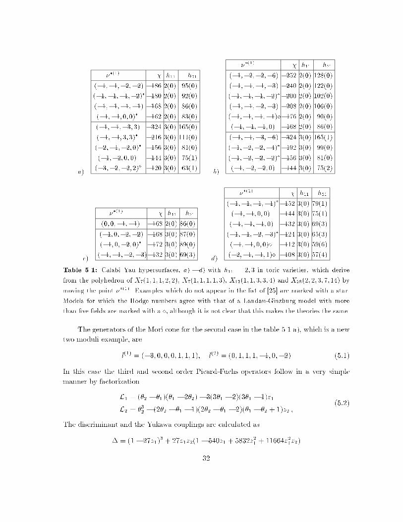
a)

��(1) � h11 h21

(�1;�1;�2;�2) �186 2(0) 95(0)

(�1;�1;�1;�2)��180 2(0) 92(0)

(�1;�1;�1;�1) �168 2(0) 86(0)

(�1;�1; 0; 0)� �162 2(0) 83(0)

(�1;�1;�3; 3) �324 3(0) 165(0)

(�1;�1; 3; 3)� �216 3(0) 111(0)

(�2;�1;�2; 0)� �156 3(0) 81(0)

(�1;�2; 0; 0) �144 3(0) 75(1)

(�3;�2;�2; 2)� �120 3(0) 63(1)b)

��(1) � h11 h21

(�1;�2;�2;�6) �252 2(0) 128(0)

(�1;�1;�1;�3) �240 2(0) 122(0)

(�1;�1;�1;�2)��200 2(0) 102(0)

(�1;�1;�2;�3) �208 2(0) 106(0)

(�1;�1;�1;�1)��176 2(0) 90(0)

(�1;�1;�1; 0) �168 2(0) 86(0)

(�1;�1;�3;�6) �324 3(0) 165(1)

(�1;�2;�2;�4)��192 3(0) 99(0)

(�1;�2;�2;�2)��156 3(0) 81(0)

(�1;�2;�2; 0) �144 3(0) 75(2)

c)

��(1) � h11 h21

(0; 0;�1;�1) �168 2(0) 86(0)

(�1; 0;�2;�2) �168 3(0) 87(0)

(�1; 0;�2; 0)� �172 3(0) 89(0)

(�1;�1;�2;�3)�132 3(0) 69(3)d)

��(1) � h11 h21

(�1;�1;�1;�1)��152 3(0) 79(1)

(�1;�1; 0; 0) �144 3(0) 75(1)

(�1;�1;�1; 0) �132 3(0) 69(3)

(�1;�1;�2;�3)��124 3(0) 65(3)

(�1;�1; 0; 0)� �112 3(0) 59(6)

(�2;�1;�1; 1)� �108 3(0) 57(4)

Table 5.1: Calabi{Yau hypersurfaces, a) � d) with h11 = 2; 3 in toric varieties, which derive

from the polyhedron of X7(1; 1; 1; 2; 2), X7(1; 1; 1; 1; 3), X12(1; 1; 3; 3; 4) and X28(2; 2; 3; 7; 14) by

moving the point ��(1). Examples which do not appear in the list of [25] are marked with a star.

Models for which the Hodge numbers agree with that of a Landau-Ginzburg model with more

than �ve �elds are marked with a �, although it is not clear that this makes the theories the same.

The generators of the Mori cone for the second case in the table 5.1.a), which is a new

two moduli example, are

l(1) = (�3; 0; 0; 0; 1; 1; 1); l(2) = (0; 1; 1; 1;�1; 0;�2) (5:1)

In this case the third and second order Picard-Fuchs operators follow in a very simple

manner by factorization

L1 = (�2 � �1)(�1 � 2�2) � 3(3�1 � 2)(3�1 � 1)z1

L2 = �32� (2�2 � �1 � 1)(2�2 � �1 � 2)(�1 � �2 + 1)z2 ;

(5:2)

The discriminant and the Yukawa couplings are calculated as

� = (1 � 27z1)3 + 27z1z2(1� 540z1 + 5832z2

1+ 11664z2

1z2)

32

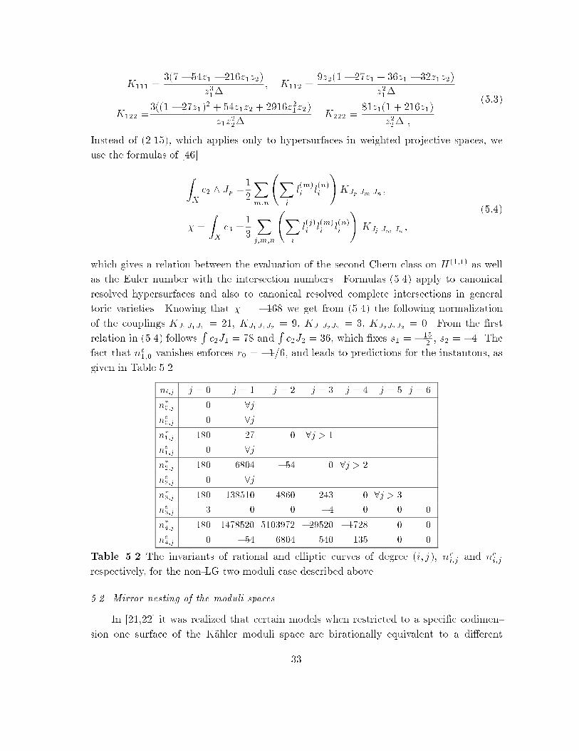
K111 =3(7 � 54z1 � 216z1z2)

z31�

; K112 =9z2(1� 27z1 + 36z1 � 32z1z2)

z21�

K122 =3((1 � 27z1)

2 + 54z1z2 + 2916z21z2)

z1z2

2�

K222 =81z1(1 + 216z1)

z22� ;

(5:3)

Instead of (2.15), which applies only to hypersurfaces in weighted projective spaces, we

use the formulas of [46]

ZX

c2 ^ Jp =1

2

Xm;n

Xi

l(m)

i l(n)i

!KJp Jm Jn ;

� =

ZX

c3 =1

3

Xj;m;n

Xi

l(j)i l

(m)

i l(n)i

!KJj Jm Jn ;

(5:4)

which gives a relation between the evaluation of the second Chern class on H(1;1) as well

as the Euler number with the intersection numbers. Formulas (5.4) apply to canonical

resolved hypersurfaces and also to canonical resolved complete intersections in general

toric varieties. Knowing that � = �168 we get from (5.4) the following normalization

of the couplings KJ1J1J1 = 21, KJ1J1J2 = 9, KJ1J2J2 = 3, KJ2J2J2 = 0. From the �rst

relation in (5.4) followsRc2J1 = 78 and

Rc2J2 = 36, which �xes s1 = � 15

2, s2 = �4. The

fact that ne1;0 vanishes enforces r0 = �1=6, and leads to predictions for the instantons, as

given in Table 5.2.

ni;j j = 0 j = 1 j = 2 j = 3 j = 4 j = 5 j = 6

nr0;j 0 8j

ne0;j 0 8j

nr1;j 180 27 0 8j > 1

ne1;j 0 8j

nr2;j 180 6804 �54 0 8j > 2

ne2;j 0 8j

nr3;j 180 138510 4860 243 0 8j > 3

ne3;j 3 0 0 �4 0 0 0

nr4;j 180 1478520 5103972 �29520 �1728 0 0

ne4;j 0 �54 6804 540 135 0 0

Table 5.2 The invariants of rational and elliptic curves of degree (i; j), nri;j and nei;jrespectively, for the non-LG two moduli case described above.

5.2. Mirror nesting of the moduli spaces

In [21,22] it was realized that certain models when restricted to a speci�c codimen-

sion one surface of the K�ahler moduli space are birationally equivalent to a di�erent

33

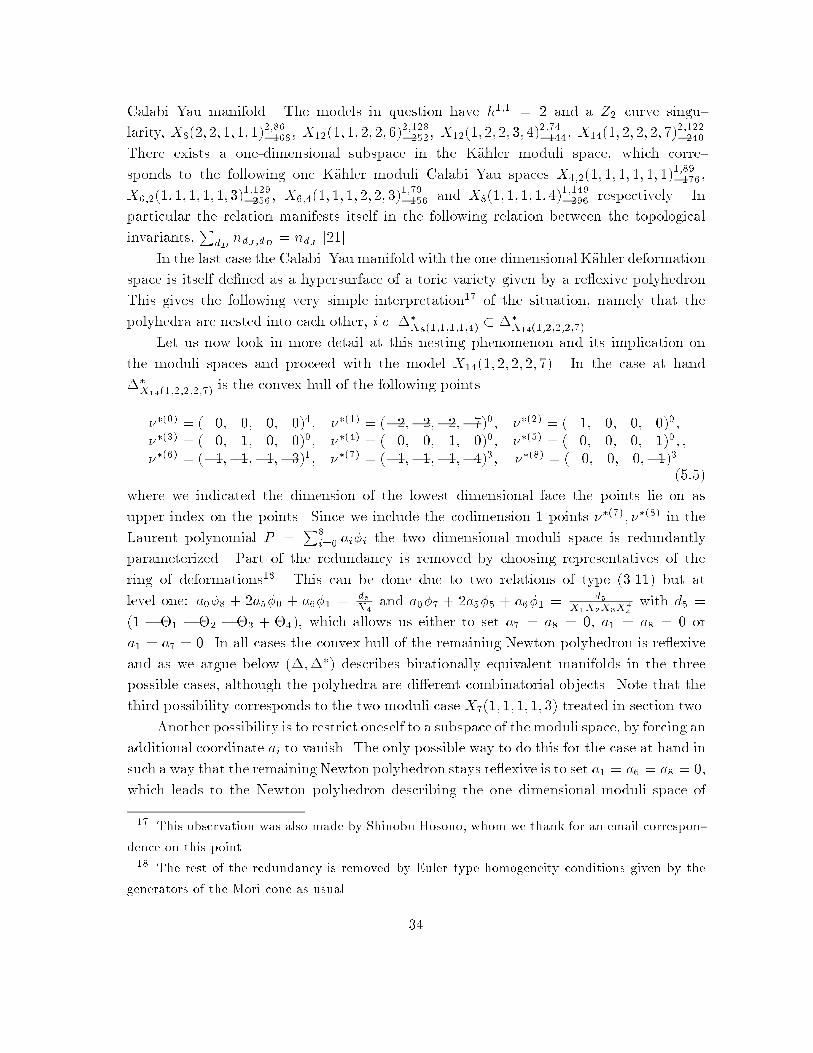
Calabi{Yau manifold. The models in question have h1;1 = 2 and a Z2 curve singu-

larity, X8(2; 2; 1; 1; 1)2;86�168

, X12(1; 1; 2; 2; 6)2;128�252

, X12(1; 2; 2; 3; 4)2;74�144

, X14(1; 2; 2; 2; 7)2;122�240

There exists a one-dimensional subspace in the K�ahler moduli space, which corre-

sponds to the following one K�ahler moduli Calabi{Yau spaces X4;2(1; 1; 1; 1; 1; 1)1;89�176

,

X6;2(1; 1; 1; 1; 1; 3)1;129�256

, X6;4(1; 1; 1; 2; 2; 3)1;79�156

and X8(1; 1; 1; 1; 4)1;149�296

respectively. In

particular the relation manifests itself in the following relation between the topological

invariants,P

dDndJ ;dD = ndJ [21].

In the last case the Calabi{Yau manifold with the one dimensional K�ahler deformation

space is itself de�ned as a hypersurface of a toric variety given by a re exive polyhedron

This gives the following very simple interpretation17 of the situation, namely that the

polyhedra are nested into each other, i.e. ��X8(1;1;1;1;4)� ��X14(1;2;2;2;7)

.

Let us now look in more detail at this nesting phenomenon and its implication on

the moduli spaces and proceed with the model X14(1; 2; 2; 2; 7). In the case at hand

��X14(1;2;2;2;7)is the convex hull of the following points

��(0) = ( 0; 0; 0; 0)4; ��(1) = (�2;�2;�2;�7)0; ��(2) = ( 1; 0; 0; 0)0;

��(3) = ( 0; 1; 0; 0)0; ��(4) = ( 0; 0; 1; 0)0; ��(5) = ( 0; 0; 0; 1)0;

��(6) = (�1;�1;�1;�3)1; ��(7) = (�1;�1;�1;�4)3; ��(8) = ( 0; 0; 0;�1)3;

(5:5)

where we indicated the dimension of the lowest dimensional face the points lie on as

upper index on the points. Since we include the codimension 1 points ��(7); ��(8) in the

Laurent polynomial P =P

8

i=0 ai�i the two dimensional moduli space is redundantly

parameterized. Part of the redundancy is removed by choosing representatives of the

ring of deformations18. This can be done due to two relations of type (3.11) but at

level one: a0�8 + 2a5�0 + a6�1 = d5X4

and a0�7 + 2a5�5 + a6�1 = d5X1X2X3X

44

with d5 =

(1 � �1 � �2 � �3 + �4), which allows us either to set a7 = a8 = 0, a1 = a8 = 0 or

a1 = a7 = 0. In all cases the convex hull of the remaining Newton polyhedron is re exive

and as we argue below (�;��) describes birationally equivalent manifolds in the three

possible cases, although the polyhedra are di�erent combinatorial objects. Note that the

third possibility corresponds to the two moduli case X7(1; 1; 1; 1; 3) treated in section two.

Another possibility is to restrict oneself to a subspace of the moduli space, by forcing an

additional coordinate ai to vanish. The only possible way to do this for the case at hand in

such a way that the remaining Newton polyhedron stays re exive is to set a1 = a6 = a8 = 0,

which leads to the Newton polyhedron describing the one dimensional moduli space of

17 This observation was also made by Shinobu Hosono, whom we thank for an email correspon-

dence on this point.18 The rest of the redundancy is removed by Euler type homogeneity conditions given by the

generators of the Mori cone as usual.

34

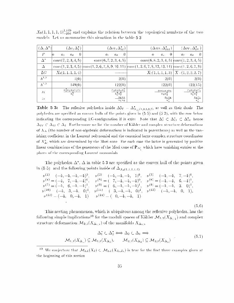
X8(1; 1; 1; 1; 4)1;149�296

and explains the relation between the topological numbers of the two

models. Let us summarize this situation in the table 5.3.

(�;��) (�I ;��

I ) (�II ;��

II ) (�III ;��

III ) (�IV ;��

IV )

P a1 = a6 = a8 = 0 a1 = a8 = 0 a1 = a7 = 0 a7 = a8 = 0

�� conv(7; 2; 3; 4; 5) conv(6; 7; 2; 3; 4; 5) conv(6; 8; 2; 3; 4; 5) conv(1; 2; 3; 4; 5)

� conv(1; 2; 3; 4; 5) conv(1; 2; 6; 7; 8; 9; 10; 11) conv(1; 2; 6; 7; 8; 12; 13; 14) conv(1; 2; 6; 7; 8)

LG X8(1; 1; 1; 1; 4) ��� X7(1; 1; 1; 1; 3) X14(1; 2; 2; 2; 7)

h1;1 1(0) 2(0) 2(0) 2(0)

h2;1 149(0) 122(0) 122(0) 122(15)

z1a45a2a3a4a7

a80

a2a3a4a46

a40a37

�a2a3a4a6a0a

38

�a2a3a4a

76

a70a31

z2 �a5a7a0a6

a6a8a20

a1a5a26

Table 5.3: The re exive polyhedra inside ��

IV = ��

X14(1;2;2;2;7)as well as their duals. The

polyhedra are speci�ed as convex hulls of the points given in (5.5) and (5.2), with the row below

indicating the corresponding LG-con�guration if it exits. Note that ��

I � ��

II � ��

IV hence

�IV � �II � �I . Furthermore we list the number of K�ahler and complex structure deformations

of X� (the number of non-algebraic deformations is indicated in parentheses) as well as the van-

ishing coe�cient in the Laurent polynomial and the canonical large complex structure coordinates

of X�

�, which are determined by the Mori cone. For each case the latter is generated by positive

linear combinations of the generators of the Mori cone of P��

1which have vanishing entries at the

places of the corresponding Laurent monomials.

The polyhedra ��, � in table 5.3 are speci�ed as the convex hull of the points given

in (5.5) and the following points inside of �X8(1;1;1;1;4)

�(1) = (�1;�1;�1;�1)0; �(2) = (�1;�1;�1; 1)0; �(3) = (�1;�1; 7;�1)0;

�(4) = (�1; 7;�1;�1)0; �(5) = ( 7;�1;�1;�1)0; �(6) = (�1;�1; 6;�1)1;�(7) = (�1; 6;�1;�1)1; �(8) = ( 6;�1;�1;�1)1; �(9) = (�1;�1; 3; 0)1;

�(10) = (�1; 3;�1; 0)1; �(11) = ( 3;�1;�1; 0)1; �(12) = (�1;�1; 0; 1);

�(13) = (�1; 0;�1; 1) �(14) = ( 0;�1;�1; 1)

:(5:6)

This nesting phenomenon, which is ubiquitous among the re exive polyhedra, has the

following simple implications19 for the moduli spaces of K�ahlerM1;1(X�1;2) and complex

structure deformationM2;1(X�1;2) of the manifolds X�1;2

��1� ��

2() �2 � �1 =)

M1;1(X�1) �M1;1(X�2); M2;1(X�2) �M2;1(X�1): (5:7)

19 We conjecture that M2;1(Xd) � M2;1(Xd1;d2 ) is true for the �rst three examples given at

the beginning of this section.

35

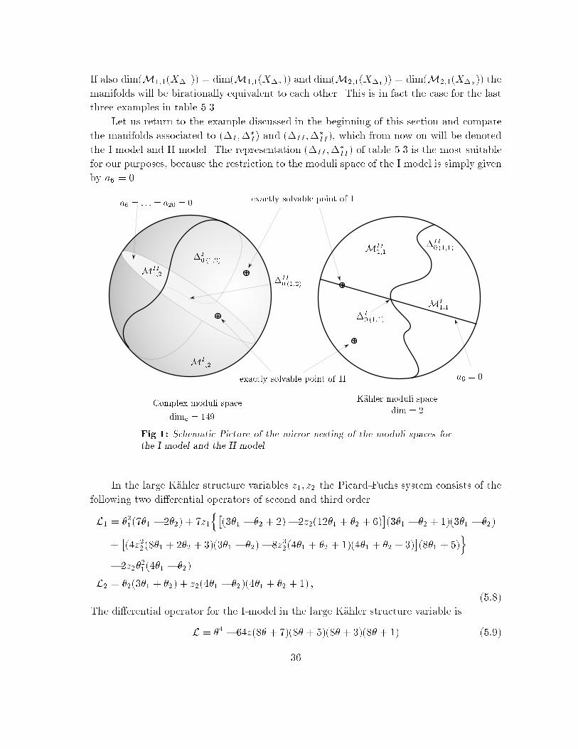
If also dim(M1;1(X�1)) = dim(M1;1(X�2

)) and dim(M2;1(X�1)) = dim(M2;1(X�2

)) the

manifolds will be birationally equivalent to each other. This is in fact the case for the last

three examples in table 5.3.

Let us return to the example discussed in the beginning of this section and compare

the manifolds associated to (�I;��

I) and (�II;��

II), which from now on will be denoted

the I model and II model. The representation (�II;��

II) of table 5.3 is the most suitable

for our purposes, because the restriction to the moduli space of the I model is simply given

by a6 = 0.

a6 = 0

MII1;1

�II0 (1;1)

MI1;1

�I0 (1;1)

MII1;2

�II0 (1;2)

MI1;2

a6 = : : : = a20 = 0

K�ahler moduli spaceComplex moduli space

�I0 (1;2)

dimc = 149

exactly solvable point of I

exactly solvable point of II

dim = 2

Fig.1: Schematic Picture of the mirror nesting of the moduli spaces for

the I model and the II model

In the large K�ahler structure variables z1; z2 the Picard-Fuchs system consists of the

following two di�erential operators of second and third order

L1 = �21(7�1 � 2�2) + 7z1

n�(3�1 � �2 + 2)� 2z2(12�1 + �2 + 6)

�(3�1 � �2 + 1)(3�1 � �2)

+�(4z2

2(8�1 + 2�2 + 3)(3�1 � �2) � 8z3

2(4�1 + �2 + 1)(4�1 + �2 + 3)

�(8�1 + 5)

o� 2z2�

2

1(4�1 � �2)

L2 = �2(3�1 + �2) + z2(4�1 � �2)(4�1 + �2 + 1) ;

(5:8)

The di�erential operator for the I-model in the large K�ahler structure variable is

L = �4 � 64z(8� + 7)(8� + 5)(8� + 3)(8� + 1) (5:9)

36

Let us then transform to the new variables (a; b)

a8 =a2a3a4a

4

5a7

a80

= z1z4

2= z; b8 =

a2a3a4a8

6

a45a7

=z1

z42

(5:10)

in which the limit b! 0 corresponds to restricting the K�ahler moduli space of the II-model

to the K�ahler moduli space of the I-model. The general discriminants of I and II read in

this parametrisation

�II0(1;1) =a

3(1 � 216a8) + a2b(3 � 7 � 215a8) + ab2(3� 7 � 41 � 210a8) + b3(1 � 5 � 7 � 29a8)

+ a4b4(7 � 23a2b� 7 � 32ab2 � 2 � 3 � 7 � 11 � 67a3 + 33b3 + 77a7b4)

�I0;(1;1) = lim

b!0

v�II0(1;1) = a3(1� 216a8):

(5:11)

The (unnormalized) Yukawa couplings of the II-model are

K111 =1

a3�II0(1;1)

�26a2(24a+32 � 5b)+74a4b5(26a2�225ab+32b2)+b2(22661a+19 � 41b))

K112 =1

a2�II0(1;1)

�26a2 + 2237ab + 3 � 31b2 + 73a4b3(210a3 + 263a2b � 2211ab2 + 32b3)

�K122 =

1

a�II0(1;1)

�(22a � 5b) + 72a4b(214a4 + 21011a3b + 273a2b2 + 32b4)

�K222 =

7a

b�II0(1;1)

�22(1� 216a8) + a3b(214a4 + 20103 � 29a3b� 275a2b2 � 2223ab3 + 32b4)

�:

(5:12)

We note that as b ! 0, both K112 and K122 stay �nite (and in particular non-zero)

while K222 blows up as 1=b. Comparison with [59] would indicate that b = 0 corresponds

to a conifold point; this will indeed be shown below. Also, limb!0K111 = 210=�I0(1;1)

which agrees with the result obtained by a direct computation on the I model [20].

Let us comment further on the limit b ! 0 of the II model and the corre-

spondence with model I. From table 5.3 we read o� that the II model has homoge-

neous coordinates (y2; y3; : : : ; y7) which are identi�ed by two C� actions with exponents

(1; 1; 1; 0; 4;�3) and (0; 0; 0; 1;�1; 1), corresponding to the generators of the Mori cone,

l(1) = (�4; 1; 1; 1; 0; 4;�3) and l(2) = (�1; 0; 0; 0; 1;�1; 1). The values of the yi are re-

stricted so that we cannot have y2 = y3 = y4 = y5 = 0 or y5 = y7 = 0 (the combinatorics

leading to this conclusion is identical to that which leads to the calculation of the numer-

ators of the entries for z1 and z2 in table 5.3). Consider the vector function

(y2; : : : ; y7) 7! (y2; y3; y4; y6y7; y5y6): (5:13)

37

Consideration of the C� actions shows that this gives a well de�ned map from the II model

to P(1; 1; 1; 1; 4), which blows down the divisor y6 = 0 to a codimension 2 subset. This

map is precisely the one that contracts the second generator of the Mori cone, as indicated

by the �1 in the corresponding coordinate of l(2). The hyperplane class of P(1; 1; 1; 1; 4)

pulls back to J1. So we are in a similar situation to that in the �rst paper of [21], obtaining

the relation Xj

ni;j(II) = ni(P(1; 1; 1; 1; 4)); (5:14)

where the spaces in parentheses indicate the space for which the Gromov-Witten invariants

are calculated.

It is also interesting to analyze the singularities resulting from the blow down (5.13). In

the coordinates (x1; : : : ; x5) of P4(1; 1; 1; 1; 4), the form of our map shows that the image of

the II model is a degree 8 hypersurface containing the surface x4 = x5 = 0. The situation is

now entirely analogous to that studied by Greene, Morrison and Strominger [60]. The octic

equation has the form x4f+x5g = 0, where f and g have degrees 4 and 7. This Calabi-Yau

is singular at the 28 points x4 = x5 = f = g = 0, having conifold singularities (nodes).

There are correspondingly 28 vanishing cycles on a nearby smooth octic hypersurface,

which, when compactifying the type IIB string on the Calabi-Yau in question, give rise to

28 hypermultiplets which become light as we approach our hypersurface. The 28 vanishing

cycles sum to zero, as they are bounded by the complement of 28 balls in the surface

x4 = x5 = 0. By the argument in [60], we check that this is consistent with h2;1 decreasing

by 27 from 149 to 122, while h1;1 increases by 1 from 1 to 2 as we perform this conifold

transition.

5.3. Construction of algebraic realizations of the deformation ring

It is a well-known fact that in certain situations not all of the K�ahlermoduli space can

be described by toric divisors of X. Similarly, the deformation of the de�ning equation of a

hypersurface X� in a toric variety P4

�� is in general not su�cient to describe the complex

structure moduli space of X. More precisely, there are non-toric divisors in X when [26]Xcodimension ��=2; ��2��

l0(��)l0(�) (5:15)

is non-zero. In a similar fashion, whenXcodimension �=2; ��2�

l0(�)l0(��) (5:16)

is non-zero there are non-algebraic deformations of the complex structure of X. l0(�) and

l0(��) is the number of interior points in a face � and �� respectively, where � and �� are

38

dual faces; if � 2 � is an n-dimensional face given by the set of vertices f�i1 ; : : : ; �ikg then

the dual face, �� 2 �� is an 3� n dimensional face given by,

�� = fy 2 �� j (y; �i1 ) = : : : ; (y�ik ) = �1g ; (5:17)

where (��)� = ��. We would like to propose a method by which we under certain circum-

stances can circumvent this problem such that either all of the non-toric divisors in (5.15)

or the non-algebraic deformations of the complex structure in (5.16), can be treated by

the methods described in section 2.

Let us assume that there exists a set of points f~�j1 ; : : : ~�jrg in codimension 1 faces of

�; we will consider the situation in (5.15). In a number of examples which we have studied

we have found that it was then possible to promote �ji 2 �, given by (5.15), to vertices,

while at the same time removing the previous vertices of �. This also implies that the ~�ji

become points in dimension 2 faces. After all this procedure will result in new polyhedra~�� and ~� such that

~�� � �� ; ~� � � : (5:18)

Hence, as we remove points coming from (5.15) we at the same time increase the contribu-

tion from (5.16), i.e. there are more points in codimension 2 faces of ~� and so the number

of non-algebraic deformations of the complex structure has increased. Repeated applica-

tion of this procedure will then have completely removed the contribution from (5.15).

The same can be applied to (5.16) with the obvious changes in the above discussion.

Unfortunately, we do not know at this point how general the above idea is.

Let us now consider an example, X12(1; 1; 1; 3; 6), in which a non-algebraic sector

occurs in the K�ahler structure moduli space. Batyrev's original construction leads to the

A-representation of the model, where �A is the convex hull of

�(1) = (�1;�1;�1;�1)0; �(2) = (�1;�1;�1; 1)0; �(3) = (�1;�1; 3;�1)0;�(4) = (�1; 11;�1;�1)0; �(5) = ( 11;�1;�1;�1)0:

(5:19)

The non-algebraic state is related to the fact that the point ��(6) in the dual polyhedra

��A

��(0) = ( 0; 0; 0; 0)4; ��(1) = (�1;�1;�3;�6)0; ��(2) = ( 1; 0; 0; 0)0;

��(3) = ( 0; 1; 0; 0)0; ��(4) = ( 0; 0; 1; 0)0; ��(7) = ( 0; 0; 0; 1)0;��(6) = ( 0; 0;�1;�2)2; ��(11) = ( 0; 0; 0;�1)3

;

(5:20)

lies on a face conv(��(1); ��(2); ��(3)), whose dual conv(�(2); �(3)) is not empty, but contains

the point ~�(3) = (�1;�1; 1; 0). The dimension of the cohomologies are h2;1 = 165(0) and

h1;1 = 3(1), i.e. in the A-representation, we have an algebraic description of M2;1 but not

of M1;1. We hence cut �A in a way, which turns �(3) into a corner, i.e. by replacing �(3)

39

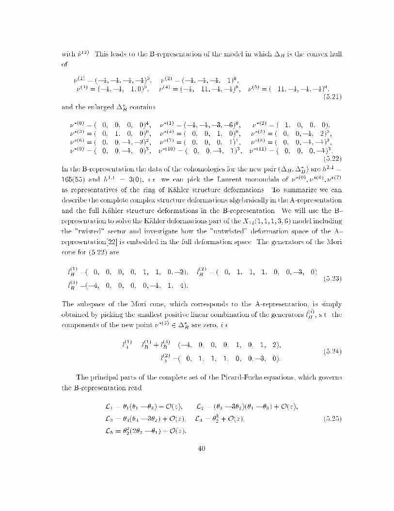
with ~�(3). This leads to the B-representation of the model in which �B is the convex hull

of

�(1) = (�1;�1;�1;�1)0; �(2) = (�1;�1;�1; 1)0;

�(3) = (�1;�1; 1; 0)0; �(4) = (�1; 11;�1;�1)0; �(5) = ( 11;�1;�1;�1)0:(5:21)

and the enlarged ��B contains

��(0) = ( 0; 0; 0; 0)4; ��(1) = (�1;�1;�3;�6)0; ��(2) = ( 1; 0; 0; 0);

��(3) = ( 0; 1; 0; 0)0; ��(4) = ( 0; 0; 1; 0)0; ��(5) = ( 0; 0;�1; 2)0;

��(6) = ( 0; 0;�1;�2)2; ��(7) = ( 0; 0; 0; 1)1; ��(8) = ( 0; 0;�1;�1)3;

��(9) = ( 0; 0;�1; 0)3; ��(10) = ( 0; 0;�1; 1)3; ��(11) = ( 0; 0; 0;�1)3:(5:22)

In the B-representation the data of the cohomologies for the new pair (�B;��

B) are h2;1 =

165(55) and h1;1 = 3(0), i.e. we can pick the Laurent monomials of ��(0); ��(6); ��(7)

as representatives of the ring of K�ahler structure deformations. To summarize we can

describe the complete complex structure deformations algebraically in the A-representation

and the full K�ahler structure deformations in the B-representation. We will use the B-

representation to solve the K�ahler deformations part of theX12(1; 1; 1; 3; 6) model including

the "twisted" sector and investigate how the "untwisted" deformation space of the A-

representation[22] is embedded in the full deformation space. The generators of the Mori

cone for (5.22) are

l(1)

B =( 0; 0; 0; 0; 1; 1; 0;�2); l(2)

B = ( 0; 1; 1; 1; 0; 0;�3; 0)

l(3)

B =(�4; 0; 0; 0; 0;�1; 1; 4):(5:23)

The subspace of the Mori cone, which corresponds to the A-representation, is simply

obtained by picking the smallest positive linear combination of the generators l(i)B , s.t. the

components of the new point ��(5) 2 ��B are zero, i.e.

l(1)

A = l(1)

B + l(3)

B =(�4; 0; 0; 0; 1; 0; 1; 2);

l(2)

A =( 0; 1; 1; 1; 0; 0;�3; 0):(5:24)

The principal parts of the complete set of the Picard-Fuchs equations, which governs

the B-representation read

L1 = �1(�1 � �3) +O(z); L2 = (�3 � 3�2)(�1 � �3) +O(z);

L3 = �3(�3 � 3�2) +O(z); L4 = �32+O(z);

L5 = �22(2�2 � �1) +O(z):

(5:25)

40

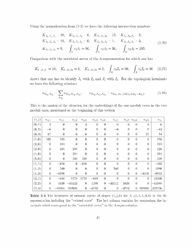
Using the normalization from (5.4) we have the following intersection numbers

KJ1;J1;J1 = 18; KJ1;J1;J2 = 6; KJ1;J1;J8 = 18; KJ1;J2;J2 = 2;

KJ1;J3;J3 = 18; KJ1;J2;J3 = 6; KJ2;J2;J3 = 1; KJ2;J3;J3 = 3;

KJ3;J3;J3 = 9;

ZX

c2J1 = 96;

ZX

c2J2 = 36;

ZX

c2J3 = 102:

(5:26)

Comparison with the untwisted sector of the A-representation for which one has

KI1;I1;I1 = 18; KI1;I1;I2 = 6; KI1;I2;I2 = 2;

ZX

c2I1 = 96;

ZX

c2I2 = 36 (5:27)

shows that one has to identify J1 with I1 and J2 with I2. For the topological invariants

we have the following relations

ndI1 ;dI2 =XdJ3

ndJ1 ;dJ2 ;dJ3 ; ndJ1 ;dJ2 ;dJ3 = ndJ1 ;dJ2 ;(3dJ2+dJ1�dJ3 ): (5:28)

This is the analog of the situation for the embeddings of the one moduli cases in the two

moduli ones, mentioned at the beginning of this section.

(i; j) nij0 nij1 nij2 nij3 nij4 nij5 nij6 nij7 nij8 nij9 nij

(0; 1) 3 0 0 3 0 0 0 0 0 0 6

(0; 2) �6 0 0 0 0 0 �6 0 0 0 �12

(0; 3) 27 0 0 0 0 0 0 0 0 27 54

(1; 0) 108 108 0 0 0 0 0 0 0 0 216

(2; 0) 0 324 0 0 0 0 0 0 0 0 324

(3; 0) 0 108 108 0 0 0 0 0 0 0 216

(4; 0) 0 0 324 0 0 0 0 0 0 0 324

(5; 0) 0 0 108 108 0 0 0 0 0 0 216

(1; 1) 0 �216 0 �216 0 0 0 0 0 0 �432

(1; 2) 0 540 0 0 0 0 540 0 0 0 1080

(1; 3) 0 �3456 0 0 0 0 0 0 0 �3456 �6912

(2; 1) 0 �648 5778 5778 �648 0 0 0 0 0 10260

(2; 2) 0 1620 �23112 0 1296 0 �23112 1620 0 0 �41688

(2; 3) 0 �10368 202986 0 �3240 0 0 �3240 0 202986 378756

Table 5.4 The invariants of rational curves of degree (i; j; k) for X12(1; 1; 1; 3; 6) in the B-

representation including the "twisted state". The last column contains for comparison the in-

variants which correspond to the "untwisted sector" in the A-representation.

41

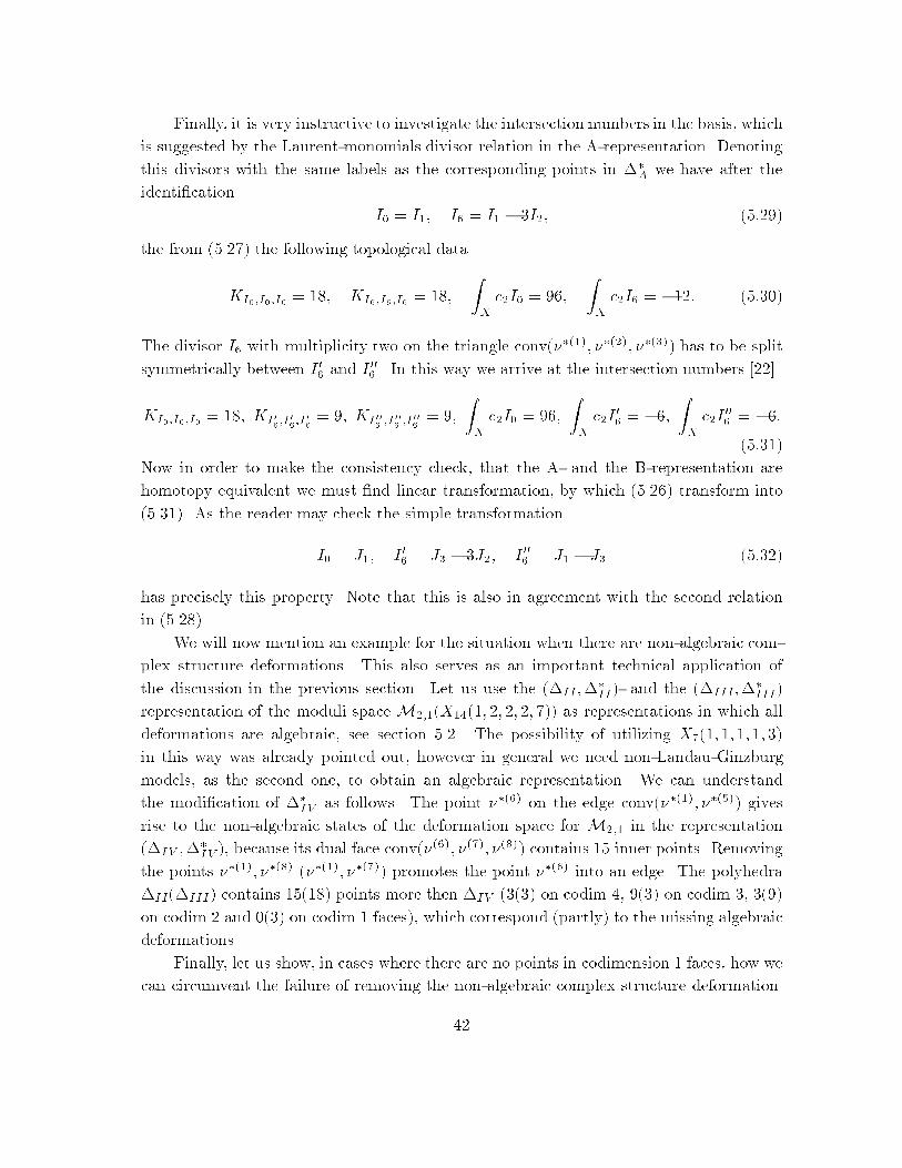
Finally, it is very instructive to investigate the intersection numbers in the basis, which

is suggested by the Laurent-monomials divisor relation in the A-representation. Denoting

this divisors with the same labels as the corresponding points in ��A we have after the

identi�cation

I0 = I1; I6 = I1 � 3I2; (5:29)

the from (5.27) the following topological data

KI0;I0;I0 = 18; KI6;I6;I6 = 18;

ZX

c2I0 = 96;

ZX

c2I6 = �12: (5:30)

The divisor I6 with multiplicity two on the triangle conv(��(1); ��(2); ��(3)) has to be split

symmetrically between I 06and I 00

6. In this way we arrive at the intersection numbers [22]

KI0;I0;I0 = 18; KI06;I0

6;I0

6= 9; KI006 ;I

00

6 ;I00

6= 9;

ZX

c2I0 = 96;

ZX

c2I0

6= �6;

ZX

c2I00

6= �6:

(5:31)

Now in order to make the consistency check, that the A- and the B-representation are

homotopy equivalent we must �nd linear transformation, by which (5.26) transform into

(5.31). As the reader may check the simple transformation

I0 = J1; I 06= J3 � 3J2; I 00

6= J1 � J3 (5:32)

has precisely this property. Note that this is also in agreement with the second relation

in (5.28).

We will now mention an example for the situation when there are non-algebraic com-

plex structure deformations. This also serves as an important technical application of

the discussion in the previous section. Let us use the (�II;��

II)- and the (�III;��

III)

representation of the moduli space M2;1(X14(1; 2; 2; 2; 7)) as representations in which all

deformations are algebraic, see section 5.2. The possibility of utilizing X7(1; 1; 1; 1; 3)

in this way was already pointed out, however in general we need non-Landau-Ginzburg

models, as the second one, to obtain an algebraic representation. We can understand

the modi�cation of ��IV as follows. The point ��(6) on the edge conv(��(1); ��(5)) gives

rise to the non-algebraic states of the deformation space for M2;1 in the representation

(�IV ;��

IV ), because its dual face conv(�(6); �(7); �(8)) contains 15 inner points. Removing

the points ��(1); ��(8) (��(1); ��(7)) promotes the point ��(6) into an edge. The polyhedra

�II(�III) contains 15(18) points more then �IV (3(3) on codim 4, 9(3) on codim 3, 3(9)

on codim 2 and 0(3) on codim 1 faces), which correspond (partly) to the missing algebraic

deformations.

Finally, let us show, in cases where there are no points in codimension 1 faces, how we

can circumvent the failure of removing the non-algebraic complex structure deformation.

42

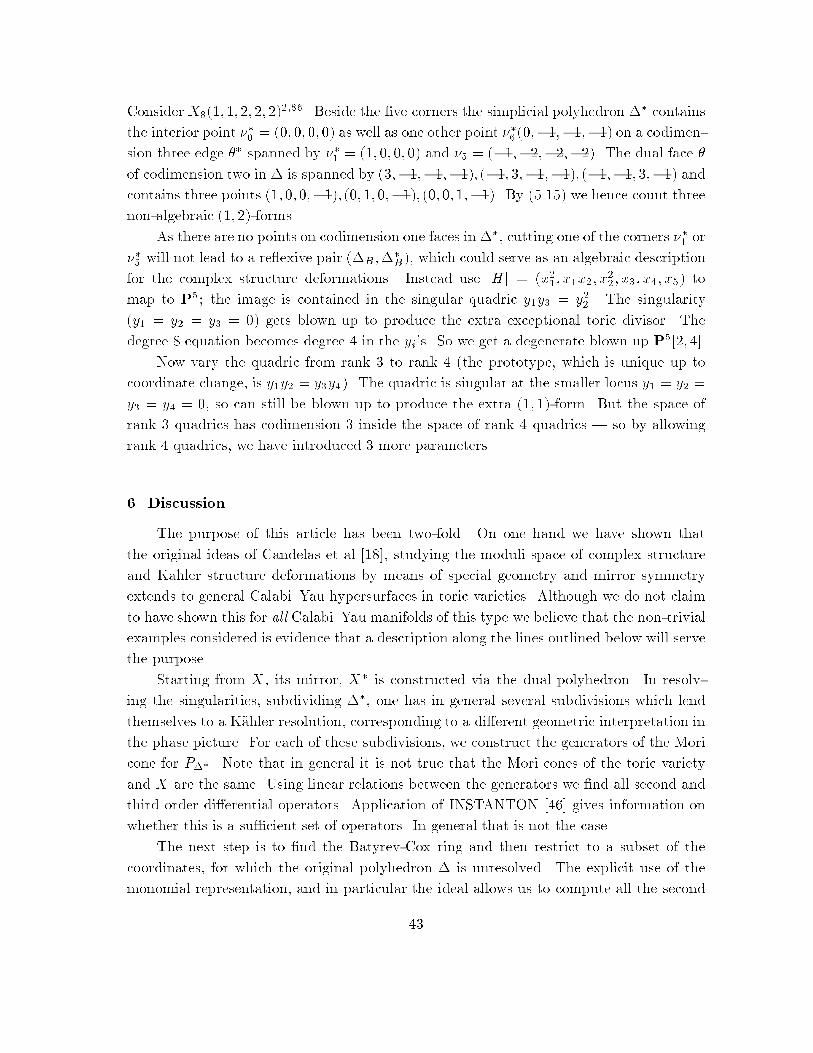
Consider X8(1; 1; 2; 2; 2)2;86. Beside the �ve corners the simplicial polyhedron �� contains

the interior point ��0= (0; 0; 0; 0) as well as one other point ��

6(0;�1;�1;�1) on a codimen-

sion three edge �� spanned by ��1= (1; 0; 0; 0) and �5 = (�1;�2;�2;�2). The dual face �

of codimension two in � is spanned by (3;�1;�1;�1); (�1; 3;�1;�1); (�1;�1; 3;�1) and

contains three points (1; 0; 0;�1); (0; 1; 0;�1); (0; 0; 1;�1). By (5.15) we hence count three

non-algebraic (1; 2)-forms.

As there are no points on codimension one faces in ��, cutting one of the corners ��1or

��5will not lead to a re exive pair (�B;�

�

B), which could serve as an algebraic description

for the complex structure deformations. Instead use jHj = (x21; x1x2; x

2

2; x3; x4; x5) to

map to P5; the image is contained in the singular quadric y1y3 = y22. The singularity

(y1 = y2 = y3 = 0) gets blown up to produce the extra exceptional toric divisor. The

degree 8 equation becomes degree 4 in the yi's. So we get a degenerate blown up P5[2; 4].

Now vary the quadric from rank 3 to rank 4 (the prototype, which is unique up to

coordinate change, is y1y2 = y3y4). The quadric is singular at the smaller locus y1 = y2 =

y3 = y4 = 0, so can still be blown up to produce the extra (1; 1)-form. But the space of

rank 3 quadrics has codimension 3 inside the space of rank 4 quadrics | so by allowing

rank 4 quadrics, we have introduced 3 more parameters.

6. Discussion

The purpose of this article has been two-fold. On one hand we have shown that

the original ideas of Candelas et al [18], studying the moduli space of complex structure

and Kahler structure deformations by means of special geometry and mirror symmetry

extends to general Calabi{Yau hypersurfaces in toric varieties. Although we do not claim

to have shown this for all Calabi{Yau manifolds of this type we believe that the non-trivial

examples considered is evidence that a description along the lines outlined below will serve

the purpose.

Starting from X, its mirror, X� is constructed via the dual polyhedron. In resolv-

ing the singularities, subdividing ��, one has in general several subdivisions which lend

themselves to a K�ahler resolution, corresponding to a di�erent geometric interpretation in

the phase picture. For each of these subdivisions, we construct the generators of the Mori

cone for P�� . Note that in general it is not true that the Mori cones of the toric variety

and X are the same. Using linear relations between the generators we �nd all second and

third order di�erential operators. Application of INSTANTON [46] gives information on

whether this is a su�cient set of operators. In general that is not the case.

The next step is to �nd the Batyrev-Cox ring and then restrict to a subset of the

coordinates, for which the original polyhedron � is unresolved. The explicit use of the

monomial representation, and in particular the ideal allows us to compute all the second

43

order relations. Although in the example studied in section 3 this turned out to be suf-

�cient, we believe that it will not be so for the general situation. Rather, we need to

consider order three monomials and then reapply the reduction method. Collecting all of

the order two and order three operators constructed in this way, one will be able to �rst

show that the classical intersection numbers agree with the above computation. Finally,

the instanton contributions can (in principle) be computed to arbitrary multidegree of the

rational curve.

There is an alternative approach to the method described here which is under investi-

gation. It appears that the principal parts of the Picard-Fuchs operators can be deduced

from the topological couplings directly. This would be a consequence of mirror symmetry if

mirror symmetry could be established for Batyrev's construction via dual polyhedra. It is

more likely that the result about the principal parts can be proven directly within a purely

mathematical framework. It can be checked that the principal parts of all the second and

third order operators in this paper may be derived much more easily by the method under

investigation. At present however, this method is less powerful since its correctness rests

on the validity of at least one conjecture.

Using these methods we have presented some new ways of exploring the moduli space.

Given a toric variety represented in terms of a re exive polyhedron, �, we may alter � with

the requirement that the new polytope, ~� is re exive. In such a fashion new theories can

be constructed as hypersurfaces in toric varieties based on ~�, taking a �rst step towards a

classi�cation of all re exive polyhedra, and hence further enlarge the class of N = 2 SCFT.

(Recall that the toric description is equivalent to the N = 2 supersymmetric gauged linear

sigma model [51,41], where the latter is believed to have non-trivial �xed point in the

IR-limit.) A less severe alteration of � such that the Hodge numbers do not change for

the hypersurfaces in question can still result in interesting phenomena. In some cases it

is possible to �nd a ~�( ~��) such that all the K�ahler (complex) structure deformations

can be described algebraically. Thus, we can study the moduli space for all deformations

including the so called twisted deformations. At this point it is not clear how general this

phenomenon is; we know of twisted complex structure deformations which seems to allude

the above prescription. Finally, given a � we can choose to embed the hypersurface in a

variety of ways, and in particular restricting to (singular) hypersurfaces which however in

their own right correspond to smooth (possibly after some desingularization) Calabi{Yau

manifolds. It may be that it is possible to understand all hypersurfaces in toric varieties as

special points in a moduli space. Naively, although the process in going from one theory

to another is singular this may provide us with a better understanding of the theories at

hand. However, in light of the recent developments in understanding conifold transitions

in type IIB string theories in terms of condensation of black holes [61,60]; though, rather

than being singular the transition is smooth when the e�ect of the massless black holes

44

are properly taken into account. Indeed, we �nd that the transition between model I and

II in section 5.2 can be explained in perfect analogy with [60].

Related to this is the recent evidence of a spacetime duality between type II string

theory compacti�ed on Calabi-Yau manifolds and that of compacti�cation of the heterotic

string on K3� T 2 [62]. It would be interesting to see if it is possible to �nd the heterotic

dual corresponding to the type of Calabi-Yau compacti�cations discussed in this paper.

On the other hand, with the improved knowledge of the moduli space of heterotic

string vacua one could try to make some �rst modest steps in probing the phenomenological

implications. Apart from the well-known Yukawa couplings the moduli dependence of the

threshold corrections to the gauge couplings in string theory (as well as in the e�ective

quantum �eld theory) [9] have come to be understood. We have computed the corrections

for the two parameter models studied in this article (as was done for some Fermat-type

models in [21,22]), and since the techniques at hand allows us to �nd the Picard-Fuchs

equation (and its solutions) for any model, similarly the threshold corrections can be

computed for any Calabi{Yau hypersurface for which our method applies. Finally, it is

interesting to note that so many quantities only depend on the massless part of the theory,

or can be deduced from the massless sector. One may wonder what other non-trivial

properties can be computed in a similar fashion.

Acknowledgments: It is a pleasure to thank D.R. Morrison and M.R. Plesser for useful

discussions. P.B. was supported by the DOE grant DE-FG02-90ER40542 and acknowl-

edges the hospitality of the Theory Division, CERN and Aspen Center for Physics where

this work was initiated. S.K. was supported by NSF grant DMS-9311386. A.K. thanks

Maximilian Kreuzer, Wolfgang Lerche, Bong Lian, Stefan Theisen, Shing-Tung Yau and

especially Shinobu Hosono for discussions and comments.

45

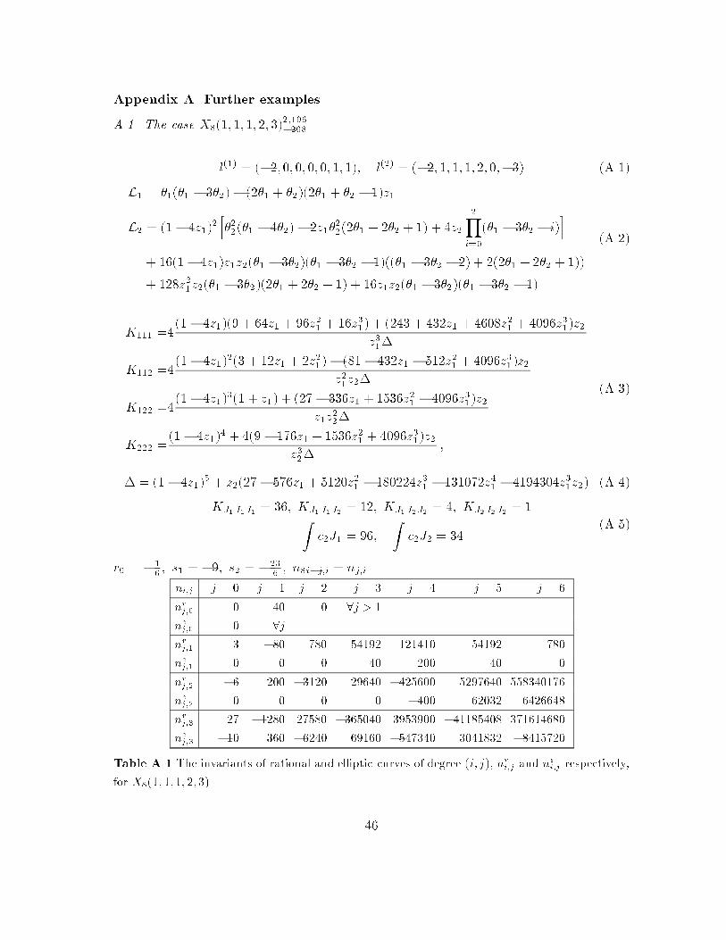
Appendix A. Further examples

A.1. The case X8(1; 1; 1; 2; 3)2;106�208

l(1) = (�2; 0; 0; 0; 0; 1; 1); l(2) = (�2; 1; 1; 1; 2; 0;�3) (A.1)

L1 = �1(�1 � 3�2)� (2�1 + �2)(2�1 + �2 � 1)z1

L2 = (1� 4z1)2

h�22(�1 � 4�2) � 2z1�

2

2(2�1 + 2�2 + 1) + 4z2

2Yi=0

(�1 � 3�2 � i)i

+ 16(1� 4z1)z1z2(�1 � 3�2)(�1 � 3�2 � 1)((�1 � 3�2 � 2) + 2(2�1 + 2�2 + 1))

+ 128z21z2(�1 � 3�2)(2�1 + 2�2 + 1) + 16z1z2(�1 � 3�2)(�1 � 3�2 � 1)

(A.2)

K111 =4(1� 4z1)(9 + 64z1 + 96z2

1+ 16z3

1) + (243 + 432z1 + 4608z2

1+ 4096z3

1)z2

z31�

K112 =4(1� 4z1)

2(3 + 12z1 + 2z21) � (81� 432z1 � 512z2

1+ 4096z3

1)z2

z21z2�

K122 =4(1� 4z1)

3(1 + z1) + (27� 336z1 + 1536z21� 4096z3

1)z2

z1z2

2�

K222 =(1� 4z1)

4 + 4(9 � 176z1 + 1536z21+ 4096z3

1)z2

z32�

;

(A.3)

� = (1� 4z1)5 + z2(27� 576z1 + 5120z2

1� 180224z3

1� 131072z4

1� 4194304z3

1z2) (A.4)

KJ1J1J1 = 36; KJ1J1J2 = 12; KJ1J2J2 = 4; KJ2J2J2 = 1Zc2J1 = 96;

Zc2J2 = 34

(A.5)

r0 = �1

6; s1 = �9; s2 = �23

6; n8i�j;i = nj;i

ni;j j = 0 j = 1 j = 2 j = 3 j = 4 j = 5 j = 6

nrj;0 0 40 0 8j > 1

nej;0 0 8j

nrj;1 3 �80 780 54192 121410 54192 780

nej;1 0 0 0 40 200 40 0

nrj;2 �6 200 �3120 29640 �425600 5297640 558340176

nej;2 0 0 0 0 �400 62032 6426648

nrj;3 27 �1280 27580 �365040 3953900 �41185408 371614680

nej;3 �10 360 �6240 69160 �547340 3041832 �8415720

Table A.1 The invariants of rational and elliptic curves of degree (i; j), nri;j and nei;j respectively,

for X8(1; 1; 1; 2; 3).

46

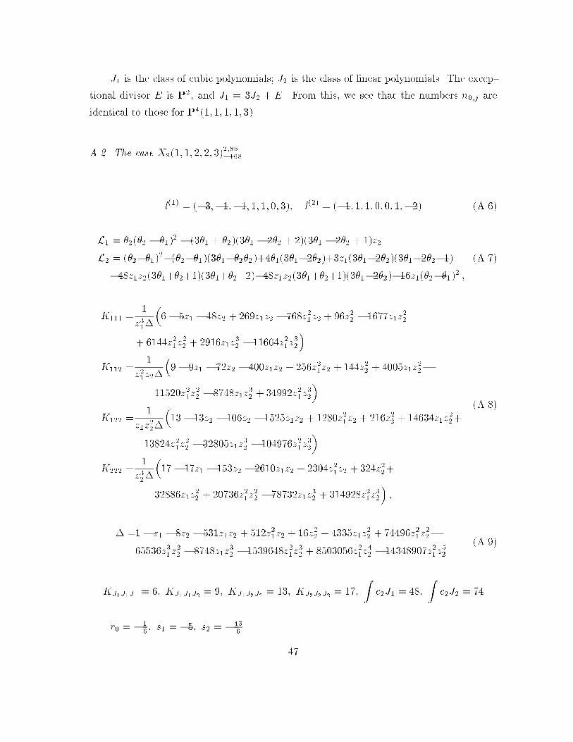
J1 is the class of cubic polynomials; J2 is the class of linear polynomials. The excep-

tional divisor E is P2, and J1 = 3J2 + E. From this, we see that the numbers n0;j are

identical to those for P4(1; 1; 1; 1; 3).

A.2. The case X9(1; 1; 2; 2; 3)2;86�168

l(1) = (�3;�1;�1; 1; 1; 0; 3); l(2) = (�1; 1; 1; 0; 0; 1;�2) (A.6)

L1 = �2(�2 � �1)2� (3�1 + �2)(3�1 � 2�2 + 2)(3�1 � 2�2 + 1)z2

L2 = (�2��1)2�(�2��1)(3�1��2�2)+4�1(3�1�2�2)+3z1(3�1�2�2)(3�1�2�2�1)

�48z1z2(3�1+�2+1)(3�1+�2+2)�48z1z2(3�1+�2+1)(3�1�2�2)�16z1(�2��1)2 ;

(A.7)

K111 =1

z31�

�6� 5z1 � 48z2 + 269z1z2 � 768z2

1z2 + 96z2

2� 1677z1z

2

2

+ 6144z21z22+ 2916z1z

3

2� 11664z2

1z32

�K112 =

1

z21z2�

�9� 9z1 � 72z2 � 400z1z2 + 256z2

1z2 + 144z2

2+ 4005z1z

2

2�

11520z21z22� 8748z1z

3

2+ 34992z2

1z32

�K122 =

1

z1z2

2�

�13� 13z1 � 106z2 � 1525z1z2 + 1280z2

1z2 + 216z2

2+ 14634z1z

2

2+

13824z21z22� 32805z1z

3

2� 104976z2

1z32

�K222 =

1

z32�

�17� 17z1 � 153z2 � 2610z1z2 + 2304z2

1z2 + 324z2

2+

32886z1z2

2+ 20736z2

1z22� 78732z1z

3

2+ 314928z2

1z32

�;

(A.8)

� =1� z1 � 8z2 � 531z1z2 + 512z21z2 + 16z2

2+ 4335z1z

2

2+ 74496z2

1z22�

65536z31z22� 8748z1z

3

2� 1539648z2

1z32+ 8503056z2

1z42� 14348907z2

1z52

(A.9)

KJ1J1J1 = 6; KJ1J1J2 = 9; KJ1J2J2 = 13; KJ2J2J2 = 17;

Zc2J1 = 48;

Zc2J2 = 74

r0 = �1

6; s1 = �5; s2 = �43

6

47

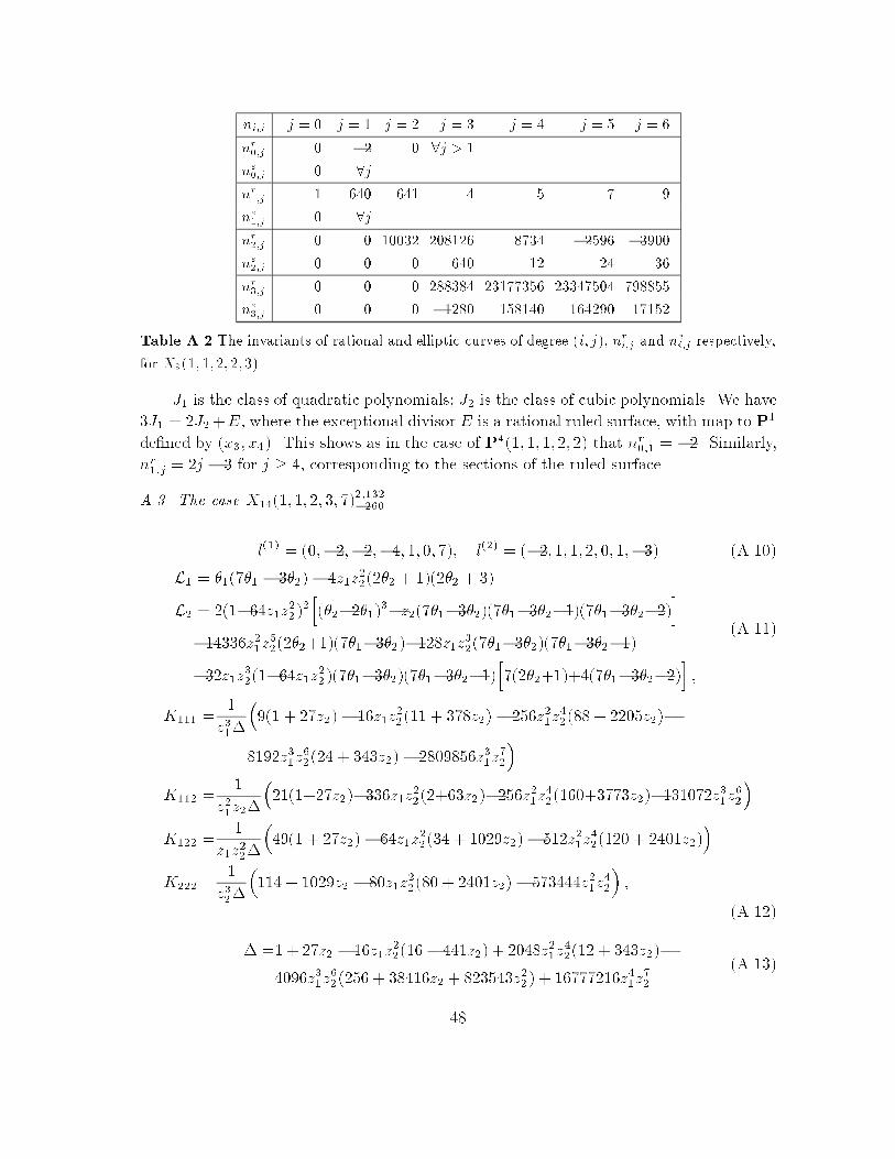
ni;j j = 0 j = 1 j = 2 j = 3 j = 4 j = 5 j = 6

nr0;j 0 �2 0 8j > 1

ne0;j 0 8j

nr1;j 1 640 641 4 5 7 9

ne1;j 0 8j

nr2;j 0 0 10032 208126 8734 �2596 �3900

ne2;j 0 0 0 640 12 24 36

nr3;j 0 0 0 288384 23177356 23347504 798855

ne3;j 0 0 0 �1280 158140 164290 17152

Table A.2 The invariants of rational and elliptic curves of degree (i; j), nri;j and nei;j respectively,

for X9(1; 1; 2; 2; 3).

J1 is the class of quadratic polynomials; J2 is the class of cubic polynomials. We have

3J1 = 2J2+E, where the exceptional divisor E is a rational ruled surface, with map to P1

de�ned by (x3; x4). This shows as in the case of P4(1; 1; 1; 2; 2) that nr0;1 = �2. Similarly,

nr1;j = 2j � 3 for j � 4, corresponding to the sections of the ruled surface.

A.3. The case X14(1; 1; 2; 3; 7)2;132�260

l(1) = (0;�2;�2;�4; 1; 0; 7); l(2) = (�2; 1; 1; 2; 0; 1;�3) (A.10)

L1 = �1(7�1 � 3�2) � 4z1z2

2(2�2 + 1)(2�2 + 3)

L2 = 2(1�64z1z2

2)2h(�2�2�1)

3�z2(7�1�3�2)(7�1�3�2�1)(7�1�3�2�2)

i�14336z2

1z52(2�2+1)(7�1�3�2)�128z1z

3

2(7�1�3�2)(7�1�3�2�1)

�32z1z3

2(1�64z1z

2

2)(7�1�3�2)(7�1�3�2�1)

h7(2�2+1)+4(7�1�3�2�2)

i;

(A.11)

K111 =1

z31�

�9(1 + 27z2)� 16z1z

2

2(11 + 378z2) � 256z2

1z42(88 + 2205z2)�

8192z31z62(24 + 343z2) � 2809856z3

1z72

�K112 =

1

z21z2�

�21(1+27z2)�336z1z

2

2(2+63z2)�256z

2

1z42(160+3773z2)�131072z

3

1z62

�K122 =

1

z1z2

2�

�49(1 + 27z2) � 64z1z

2

2(34 + 1029z2)� 512z2

1z42(120 + 2401z2)

�K222 =

1

z32�

�114 + 1029z2 � 80z1z

2

2(80 + 2401z2) � 573444z2

1z42

�;

(A.12)

� =1 + 27z2 � 16z1z2

2(16� 441z2) + 2048z2

1z42(12 + 343z2)�

4096z31z62(256 + 38416z2 + 823543z2

2) + 16777216z4

1z72

(A.13)

48

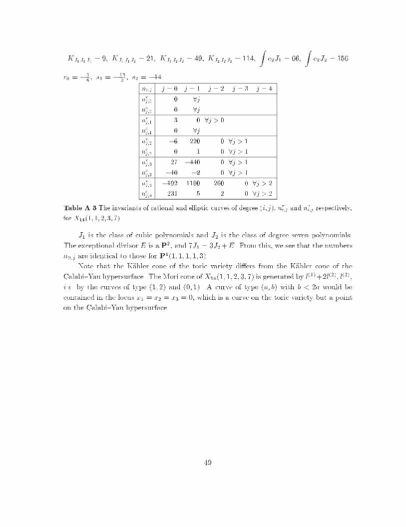
KJ1J1J1 = 9; KJ1J1J2 = 21; KJ1J2J2 = 49; KJ2J2J2 = 114;

Zc2J1 = 66;

Zc2J2 = 156

r0 = �1

6; s1 = �

13

2; s2 = �14

ni;j j = 0 j = 1 j = 2 j = 3 j = 4

nrj;0 0 8j

nej;0 0 8j

nrj;1 3 0 8j > 0

nej;1 0 8j

nrj;2 �6 220 0 8j > 1

nej;2 0 1 0 8j > 1

nrj;3 27 �440 0 8j > 1

nej;3 �10 �2 0 8j > 1

nrj;4 �192 1100 260 0 8j > 2

nej;4 231 5 2 0 8j > 2

Table A.3 The invariants of rational and elliptic curves of degree (i; j), nri;j and nei;j respectively,

for X14(1; 1; 2; 3; 7).

J1 is the class of cubic polynomials and J2 is the class of degree seven polynomials.

The exceptional divisor E is a P2, and 7J1 = 3J2+E. From this, we see that the numbers

n0;j are identical to those for P4(1; 1; 1; 1; 3).

Note that the K�ahler cone of the toric variety di�ers from the K�ahler cone of the

Calabi{Yau hypersurface. The Mori cone of X14(1; 1; 2; 3; 7) is generated by l(1)+2l(2); l(2),

i.e. by the curves of type (1; 2) and (0; 1). A curve of type (a; b) with b < 2a would be

contained in the locus x1 = x2 = x3 = 0, which is a curve on the toric variety but a point

on the Calabi{Yau hypersurface.

49

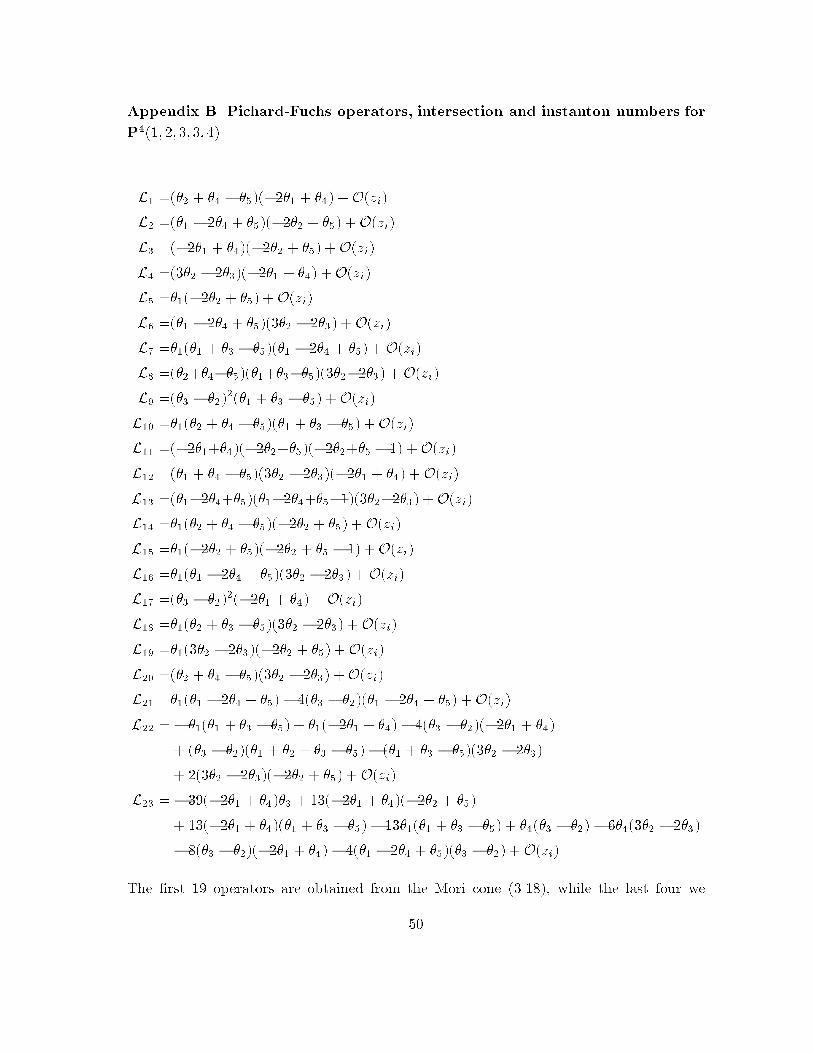
Appendix B. Pichard-Fuchs operators, intersection and instanton numbers for

P4(1; 2; 3; 3; 4)

L1 =(�2 + �4 � �5)(�2�1 + �4) +O(zi)

L2 =(�1 � 2�4 + �5)(�2�2 + �5) +O(zi)

L3 =(�2�1 + �4)(�2�2 + �5) +O(zi)

L4 =(3�2 � 2�3)(�2�1 + �4) +O(zi)

L5 =�1(�2�2 + �5) +O(zi)

L6 =(�1 � 2�4 + �5)(3�2 � 2�3) +O(zi)

L7 =�1(�1 + �3 � �5)(�1 � 2�4 + �5) +O(zi)

L8 =(�2+�4��5)(�1+�3��5)(3�2�2�3) +O(zi)

L9 =(�3 � �2)2(�1 + �3 � �5) +O(zi)

L10 =�1(�2 + �4 � �5)(�1 + �3 � �5) +O(zi)

L11 =(�2�1+�4)(�2�2+�5)(�2�2+�5 � 1) +O(zi)

L12 =(�1 + �4 � �5)(3�2 � 2�3)(�2�1 + �4) +O(zi)

L13 =(�1�2�4+�5)(�1�2�4+�5�1)(3�2�2�3) +O(zi)

L14 =�1(�2 + �4 � �5)(�2�2 + �5) +O(zi)

L15 =�1(�2�2 + �5)(�2�2 + �5 � 1) +O(zi)

L16 =�1(�1 � 2�4 + �5)(3�2 � 2�3) +O(zi)

L17 =(�3 � �2)2(�2�1 + �4) +O(zi)

L18 =�1(�2 + �3 � �5)(3�2 � 2�3) +O(zi)

L19 =�1(3�2 � 2�3)(�2�2 + �5) +O(zi)

L20 =(�2 + �4 � �5)(3�2 � 2�3) +O(zi)

L21 =�1(�1 � 2�4 + �5)� 4(�3 � �2)(�1 � 2�4 + �5) +O(zi)

L22 =� �1(�1 + �3 � �5) + �1(�2�1 + �4) � 4(�3 � �2)(�2�1 + �4)

+ (�3 � �2)(�1 + �2 + �3 � �5)� (�1 + �3 � �5)(3�2 � 2�3)

+ 2(3�2 � 2�3)(�2�2 + �5) +O(zi)

L23 =� 39(�2�1 + �4)�3 + 13(�2�1 + �4)(�2�2 + �5)

+ 13(�2�1 + �4)(�1 + �3 � �5)� 13�1(�1 + �3 � �5) + �4(�3 � �2) � 6�4(3�2 � 2�3)

� 8(�3 � �2)(�2�1 + �4) � 4(�1 � 2�4 + �5)(�3 � �2) +O(zi)

The �rst 19 operators are obtained from the Mori cone (3.18), while the last four we

50

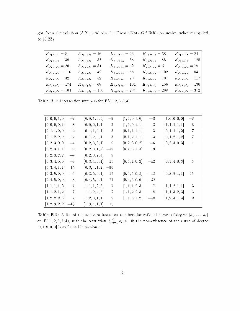
got from the relation (3.21) and via the Dwork-Katz-Gri�th's reduction scheme applied

to (3.23).

KJ1J1J1 = 8 KJ1J1J2 = 16 KJ1J2J2 = 26 KJ2J2J2 = 38 KJ1J1J3 = 24

KJ1J2J3 = 39 KJ2J2J3 = 57 KJ1J3J3 = 58 KJ2J3J3 = 85 KJ3J3J3 = 125

KJ1J1J4 = 20 KJ1J2J4 = 34 KJ2J2J4 = 52 KJ1J3J4 = 51 KJ2J3J4 = 78

KJ3J3J4 = 116 KJ1J4J4 = 42 KJ2J4J4 = 68 KJ3J4J4 = 102 KJ4J4J4 = 84

KJ1J1J5 = 32 KJ1J2J5 = 52 KJ2J2J5 = 78 KJ1J3J5 = 78 KJ2J3J5 = 117

KJ3J3J5 = 174 KJ1J4J5 = 68 KJ2J4J5 = 104 KJ3J4J5 = 156 KJ4J4J5 = 136

KJ1J5J5 = 104 KJ2J5J5 = 156 KJ3J5J5 = 234 KJ4J5J5 = 208 KJ5J5J5 = 312

Table B.1: Intersection numbers for P4(1; 2; 3; 3; 4).

[0; 0; 0; 1; 0] �2 [0; 0; 1; 0; 0] �2 [1; 0; 0; 1; 0] � 2 [1; 0; 0; 0; 0] �2

[0; 0; 0; 0; 1] 3 [0; 0; 0; 1; 1] 3 [1; 0; 0; 1; 1] 3 [1; 1; 1; 1; 1] 3

[0; 1; 1; 0; 0] �2 [0; 1; 1; 0; 1] 3 [0; 1; 1; 1; 1] 3 [0; 1; 1; 1; 2] 7

[0; 1; 2; 0; 0] �2 [0; 1; 2; 0; 1] 3 [0; 1; 2; 1; 1] 3 [0; 1; 2; 1; 2] 7

[0; 2; 3; 0; 0] �4 [0; 2; 3; 0; 1] 9 [0; 2; 3; 0; 2] �6 [0; 2; 3; 0; 3] 1

[0; 2; 3; 1; 1] 9 [0; 2; 3; 1; 2] �18 [0; 2; 3; 1; 3] 9

[0; 2; 3; 2; 2] �6 [0; 2; 3; 2; 3] 9

[0; 3; 4; 0; 0] �6 [0; 3; 4; 0; 1] 15 [0; 3; 4; 0; 2] �12 [0; 3; 4; 0; 3] 3

[0; 3; 4; 1; 1] 15 [0; 3; 4; 1; 2] �36

[0; 3; 5; 0; 0] �6 [0; 3; 5; 0; 1] 15 [0; 3; 5; 0; 2] �12 [0; 3; 5; 1; 1] 15

[0; 4; 5; 0; 0] �8 [0; 4; 5; 0; 1] 21 [0; 4; 6; 0; 0] �32

[1; 1; 1; 1; 2] 7 [1; 1; 1; 2; 2] 7 [1; 1; 1; 2; 3] 7 [1; 1; 2; 1; 1] 3

[1; 1; 2; 1; 2] 7 [1; 1; 2; 2; 2] 7 [1; 1; 2; 2; 3] 8 [1; 1; 3; 2; 3] 3

[1; 2; 2; 2; 3] 7 [1; 2; 3; 1; 1] 9 [1; 2; 3; 1; 2] �18 [1; 2; 3; 1; 3] 9

[1; 2; 3; 2; 2] �18 [1; 3; 4; 1; 1] 15

Table B.2: A list of the non-zero instanton numbers for rational curves of degree [a1; : : : ; a5]

on P4(1; 2; 3; 3; 4), with the restrictionP

5

i=1ai � 10; the non-existence of the curve of degree

[0; 1; 0; 0; 0] is explained in section 4.

51

References

[1] S. Ferrara and A. Strominger, in the Proceedings of the Strings '89 workshop, College

Stattion, 1989;

A. Strominger, Commun. Math. Phys. 133 (1990) 163;

P. Candelas and X. de la Ossa, Nucl. Phys. B355 (1991) 455.

[2] L. Dixon, V. Kaplunovsky and J. Louis, Nucl. Phys. B329 (1990) 27.

[3] W. Lerche, C. Vafa and N. Warner, Nucl. Phys. B324 (1989) 427.

[4] J. Distler and S. Kachru, Duality of (0,2) String Vacua, hep-th/9501111.

[5] E. Witten, Mirror Manifolds And Topological Field Theory, in Essays on Mirror

Manifolds, (ed. S.-T. Yau), Int. Press, Hong Kong, 1992 p. 120{158, hep-th/9112056.

[6] E.g. K. Kodaira, Complex Manifolds and Deformations of Complex Structure

(Springer Verlag 1985).

[7] L. Dixon: in Superstrings, Uni�ed Theories and Cosmology 1987, eds. G. Furlan et al.

(World Scienti�c, Singapore, 1988) p. 67{127.

[8] M. Bershadsky, S. Cecotti, H. Ooguri and C. Vafa (with an appendix by S. Katz),

Nucl. Phys. B405 (1993) 279, hep-th/9302103.

[9] V. Kaplunovsky and J. Louis, On Gauge Couplings in String Theory, hep-th/9502077.

[10] Seiberg and Witten, Nucl. Phys. B426 (1994) 19-52, Erratum-ibid. Nucl. Phys. B430

(1994) 485-486

[11] A. Klemm, W. Lerche, S. Theisen and S. Yankielowicz Phys. Lett. B 344 (1995) 169-

175, HEP-TH/9411048 and On The Monodromies Of N = 2 Supersymmetric Yang-

Mills Theory, HEP-TH/9412158, P. C. Argyres and A. E. Faraggi The Vacuum Struc-

ture and Spectrum of N = 2 Supersymmetric SU(n) Gauge Theory HEP-TH/9411057

[12] A. Klemm, W. Lerche, S. Theisen, Nonperturbative E�ective Actions of N = 2 Su-

persymmetric Gauge Theories. CERN-TH-95-104 HEP-TH/9505150

[13] A. Ceresole, R. D'Auria, S. Ferrara, A. Van Proeyen, On Electromagnetic Duality

In Locally Supersymmetric N = 2 Yang-Mills Theory. CERN-TH-7510-94, HEP-

TH/9412200 and Duality Transformations in Supersymmetric Yang-Mills-Theories

Coupled to Supergravity CERN-TH-7547-94, HEP-TH/9502072

[14] S. Kachru and C. Vafa, Exact Results for N=2 Compacti�cations of Heterotic Strings,

hep-th/9505105.

[15] E. Martinec, Phys. Lett. 217B (1989) 431, C. Vafa and N. P. Warner, Phys. Lett.

218B (1989) 51.

[16] V. I. Arnol'd, V. A. Vasil'ev, V. V. Goryunov and O. V. Lyashko, Singularities Local

and Global Theory in Dynamical Systems, Enc. Math. Sc. Vol 6, Ed. V. I. Arnold,

(1991) Springer, Heidelberg.

[17] D. Gepner, Phys. Lett. 199B (1987) 380, Nucl. Phys. B296 (1988) 757, Nucl. Phys.

52

B311 (1988) 191;

C. Vafa, Mod. Phys. Lett. A4 (1989) 1169.

[18] P. Candelas, X. De la Ossa, P. Green and L. Parkes, Nucl. Phys. B359 (1991) 21.

[19] D. Morrison, Picard-Fuchs Equations and Mirror Maps for Hypersurfaces, in Essays

on Mirror Manifolds, ed. S.-T. Yau, (Int. Press, Hong Kong, 1992), hep-th/9111025.

[20] A. Klemm and S. Theisen, Nucl. Phys. B389 (1993) 153, hep-th/9205041; Theor.

Math. Phys. 95 (1993) 583, hep-th/9210142;

A. Font, Nucl. Phys. B391 (1993) 358, hep-th/9203084.

[21] P. Candelas, X. de la Ossa, A. Font, S. Katz and D. Morrison, Nucl. Phys. B416

(1994) 481, hep-th/9308083;

P. Candelas, A. Font, S. Katz and D. Morrison, Nucl. Phys. B429 (1994) 626, hep-

th/9403187.

[22] S. Hosono, A. Klemm, S. Theisen and S.-T. Yau: Mirror Symmetry, Mirror Map and

Applications to Calabi{Yau Hypersurfaces, HUTMP-93/0801, LMU-TPW-93-22, to

be published in Commun. Math. Phys., hep-th/9308122.

[23] D.R. Morrison and M.R. Plesser, Summing the Instantons: QuantumCohomology and

Mirror Symmetry in Toric Varieties, hep-th/9412236.

[24] B. Greene and R. Plesser, Nucl. Phys. B338 (1990) 15.

[25] A. Klemm and R. Schimmrigk, Nucl. Phys. B411 (1994) 559, hep-th/9204060;

M. Kreuzer and H. Skarke, Nucl. Phys. B388 (1993) 113, hep-th/9205004.

[26] V. Batyrev, Journal Alg. Geom. 3 (1994) 493, alg-geom/9310003.

[27] V. Batyrev, Duke Math. Journ., 69 (1993) 349

[28] S.-S. Roan: Int. J. Math 2 (1991) 439

[29] P.Berglund and S. Katz, Mirror Symmetry Constructions: A Review to appear in

Essays of Mirror Manifolds II (Ed. S. T. Yau), hep-th/9406008.

[30] P. Candelas, X. de la Ossa and S. Katz: Mirror Symmetry for Calabi{Yau Hypersur-

faces in Weighted P4 and an Extension of Landau-Ginzburg Theory, IASSNS-HEP-

94/100,NEIP-94-009, OSU-M-93-3, UTTG-25-93, hep-th/9412117.

[31] B. Greene and R. Plesser, in the Proceedings of PASCOS '91, Boston 1991, hep-

th/9110014.

[32] P. Berglund and T. H�ubsch, Nucl. Phys. B393 (1993) 377, hep-th/9201014.

[33] R. Dijkgraaf, E. Verlinde, H. Verlinde and C. Vafa, Commun. Math. Phys. 123 (1989)

485.

[34] P. Berglund and M. Henningson, Nucl. Phys. B433 (1995) 311, hep-th/9401029; see

also On the Elliptic Genus and Mirror Symmetry to appear in Essays of Mirror Sym-

metry II, eds. B. Greene and S.T. Yau, hep-th/9406045.

[35] M. Kreuzer, Phys. Lett. 328B (1994) 312, hep-th/9402114.

[36] D.R. Morrison and M.R. Plesser, work in progress.

53

[37] V. Batyrev and D. Cox, Duke Math. Journ. 74 (1994) 293, alg-geom/9306011.

[38] B. Dwork, Ann. of Math. (2) 80 (1964) 227.

[39] N. Katz, Publ. Math. I.H.E.S. 35 (1968) 71.

[40] P. Gri�ths, Ann. of Math. 90 (1969) 460.

[41] P.S. Aspinwall, B.R. Greene and D.R. Morrison, Nucl. Phys. B416 (1994) 414, hep-

th/9309097.

[42] T. Oda and H. S. Park, Tohoku Math. J. 43 (1991) 375.

[43] D. Morrison, Amer. Math. Soc. 6 (1993) 223; Compacti�cations of Moduli spaces

inspired by mirror symmetry DUK-M-93-06, alg-geom/9304007.

[44] I. M. Gel'fand, A. V. Zelevinkii and M. M. Kapranov, Functional Anal. Appl. 23 2

(1989) 12, English trans. 94.

[45] W. Lerche, D. J. Smit and N. P. Warner, Nucl. Phys. B372 (1992) 87, hep-th/9108013.

[46] S. Hosono, A. Klemm, S. Theisen and S.-T. Yau, Nucl. Phys. B433 (1995) 501, hep-

th/9406055.

[47] P. Berglund and S. Katz, Nucl. Phys. B420 (1994) 289, hep-th/9311014.

[48] R. Hartshorne,Algebraic Geometry, Grad. Texts in Mathematics 52, (Springer Verlag,

Heidelberg 1977).

[49] P.S. Aspinwall and D.R. Morrison: Phys. Lett. 334B (1994) 79, hep-th/9406032.

[50] C. Vafa, A Stringy Test of the Fate of the Conifold, HUTP-95/A014, hep-th/9505023.

[51] E. Witten, Nucl. Phys. B403 (1993) 159, hep-th/9301042.

[52] J. De Loera, Triangulations of Polytopes and Computational Algebra, Ph.D. thesis,

Cornell University, in preparation.

[53] S. Katz and S.A. Str�mme, Schubert: a Maple package for intersection theory. Avail-

able by anonymous ftp from ftp.math.okstate.edu or linus.mi.uib.no, cd pub/schubert.

[54] D. Eisenbud and J. Harris, Proc. Symp. Pure Math. 46 Part I (1987) 3.

[55] A. Altman and S. Kleiman, Comp. Math. 34 (1977) 3.

[56] M. Kontsevich,Enumeration of Rational Curves via Torus Actions, alg-geom/9405035.

[57] P.M.H. Wilson, Inv. Math. 107 (1992) 561.

[58] M. Kreuzer and H. Starke, Nucl. Phys. B405 (1993) 305, hep-th/9211047 and hep-

th/9412033; A. Niemeier, Klassi�zierung von Calabi{Yau-Stringkompakti�zierungen

durch N = 2-superkonforme LG-Theorien, Diploma Thesis, TU-Munich (1993)

[59] P. Candelas, A. Font, S. Katz and D. Morrison, Nucl. Phys. B429 (1994) 626, hep-

th/9403187.

[60] B.R. Greene, D.R. Morrison and A. Strominger, Black Hole Condensation and the

Uni�cation of String Vacua, hep-th/9504145.

[61] A. Strominger,Massless Black Holes and Conifolds in String Theory, hep-th/9504090.

[62] S. Ferrara, J. A. Harvey, A. Strominger and C. Vafa, Second-Quantized Mirror Sym-

metry, hep-th/9505162.

54