Journal of Statistical Physics, Vol. 45, Nos. 1/2, 1986

The Wall Theorem for Elastic Moduli

F. B a v a u d I

Received March 3, 1986

New expressions for the elastic moduli of a classical system are derived. They involve only the two-point correlation function and the derivative of the one- point correlation function, both only on the boundary of the system. These expressions, valid for any interaction derivable from a potential, are proved from a mechanical point of view by generalizing the virial theorem of Clausius, and from a statistical point of view by a direct method that constitutes an alter- native to Green's dilatation method.

KEY WORDS: Wall theorem; viriat theorem; correlation functions; pressure; stress tensor; elastic moduli; compressibility; Lam6 coefficients.

1. I N T R O D U C T I O N

Pressure is defined either as the mean force exerted by the colliding par- ticles on a boundary element of a system, or as the derivative of the free energy with respect to a deformation; it is then one of the few physical quantities that can be directly defined either f rom a mechanical or a statistical point of view. The mechanical approach leads, via the virial theorem of Clausius (5) applied to a constrained system, (1~ to the wall theorem, P = PwallkT. On the other hand, in the statistical framework, the virial expression for the pressure (s/ is obtained by the dilation method of Green(7); this method can be extended to the elastic modulus tensor and therefore allows us to write "virial" expressions for, e.g., the inverse com- pressibility and the Lam6 coefficients (1'17'18) (we prefer to speak of "bulk" expressions, since the evaluat ion of such quantities necessitates knowledge of correlat ion functions up to the order 2n on the whole domain occupied by the system interacting th rough n-body forces).

1Ecole Polytechnique F6d6rale de Lausanne, Institut de Physique Th6orique, CH-1015 Lausanne, Switzerland.

171

0022-4715/86/1000-0171505.00/0 �9 1986 Plenum Publishing Corporation

172 Bavaud

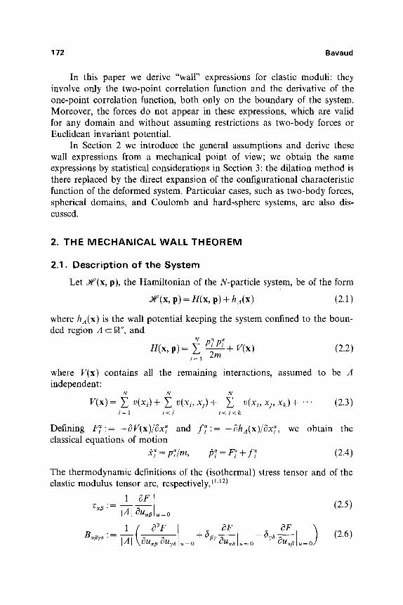
In this paper we derive "wall" expressions for elastic moduli: they involve only the two-point correlation function and the derivative of the one-point correlation function, both only on the boundary of the system. Moreover, the forces do not appear in these expressions, which are valid for any domain and without assuming restrictions as two-body forces or Euclidean invariant potential.

In Section 2 we introduce the general assumptions and derive these wall expressions from a mechanical point of view; we obtain the same expressions by statistical considerations in Section 3: the dilation method is there replaced by the direct expansion of the configurational characteristic function of the deformed system. Particular cases, such as two-body forces, spherical domains, and Coulomb and hard-sphere systems, are also dis- cussed.

2. T H E M E C H A N I C A L W A L L T H E O R E M

2.1. Description of the System

Let ~;4~ p), the Hamiltonian of the N-particle system, be of the form

2r p) = H(x, p) + hA(X) (2.1)

where hA(X) is the wall potential keeping the system confined to the boun- ded region A ~Rv, and

H(x, p )= '̂~ P~P~+ V(x) (2.2) i:~1 2m

where V(x) contains all the remaining interactions, assumed to be A independent:

N N N

V(x)= ~ v(xi)+ ~ v(xi, xfl+ ~ v(xi, xj, xk )+. . . (2.3) i = l i<] i < j < k

Defining FT:=-~V(x) /~x~ and f~:=-~hA(x)/OxT, we obtain the classical equations of motion

5c~ = p~/m, [~ = F~ + f~ (2.4)

The thermodynamic definitions of the (isothermal) stress tensor and of the elastic modulus tensor are, respectively, (~'~2)

1 OF (2.5) ~ := IAI c3-u--~ 2=0

( O--ZF 6 OF OF B~6 := ]A] \eu,r ,=0 + e~ ~--~6 ,=o-6~~ 0--~ ,=o) (2.6)

Wall Theorem for Elastic Modul i 173

Here F is the Helmholtz free energy and u~ is the displacement gradient tensor describing the deformation:

x '~ = ( 6 ~ + u ~ ) x ~ = : D ~ x ~ (2.7)

The evaluation of (2.5) and (2.6) in the canonical ensemble leads to (1)

1 %~ = ~-7< T~p ) (2.8)

1

+ aS, < T~a > - a,a < T~ e >) (2.9)

with

~ N

T ~ "= - P' p{ E FTx{ (2.10) m i = 1 i = 1

N 1 N 0F~i

�9 ~ ~ 6 e ~ p T P ~ ) - ~ x ~ g x ~ Ox~ (2.11) W~Ta = ~1 m ((~aP~P~ + 6~aPe p~ + i = i , j

In (2.8) and (2.9), the brackets indicate the canonical average, with

exp[ - f lH(x , p)] ZA(x) (2.12)

as the (unnormalized) probability density, where

N

zAx) = 1-] zAxi) i = l

ZA(Xi) = Xi r A

Now, in order to obtain a mechanical formulation for r ~ and B ~ a , the ensemble average is replaced by the time average along a phase space tra- jectory. The explicit form of ha(x) can be determined by considering ha(x) as an external potential: then (2.12) must be equivalent to exp[-fl~4~ p)], which leads to

N

ha(x) = - k T ~ In ZA(xi) (2.14) i = 1

Instead of (2.14), the most obvious choice would be to impose elastic collisions with the wall. But it is easy to see that h A would then be propor-

174 Bavaud

tional to the square of the velocity [which gives some insight about the origin of the factor kT appearing in (2.14)]; on the other hand, the statistical ensemble corresponding to this situation is the microcanonical one, and nothing ensures that (2.9) remains true in that ensemble (see, e.g., Refs. 1 and 17, where new terms appear when the canonical description is replaced by the grand canonical one).

Equation (2.14) is formal in the sense that it contains the logarithm of a distribution; however, all derivations can be made rigorous if )~A(X~) is considered as the limit of a continuous function (see, e.g., Ref. 10). In what follows, we shall take

f~ = kT C)ZA(X~) (2.15) ?X7

as the force exerted by the wall on the particle i.

2.2. Der ivat ion of the Wal l Expressions

f~ is a distribution whose support is the wall ~A. On the other hand, straighforward evaluation of (2.8) and (2.9) requires the knowledge of F~ on the whole domain. The program consists now in replacing F~ by f~, i.e., in transforming bulk expressions into wall expressions. The famous virial theorem of Clausius (5) fulfills exactly this task; let us repeat the argument: we define

N

N ~ : = ~ p~[x~ (2.16) i = 1

N

C~'= ~ f~x~ (2.17) i = l

Relations (2.4) and (2.10) lead to

fi/~ = --T~a + C~ (2.18)

Since N~ is a bounded observable, the time average of its derivative is zero; consequently,

(T~,,~)t= (C~,~), (2.19)

where the brackets now represent time averages. On the other hand, we get from (2.15)

Wall Theorem for Elastic Moduli 175

(C=e) =k T al.a(x~) x~ , 1 Ox~

= k T f dx ~)~a(x) xenl(x ) Ox =

= - kTfaA da~ x~n~(x) (2.20)

Here nl(x) := (~_~N~I ~(X- Xi))t is the one-point correlation function and da~ represents the ~ component of the outward-oriented surface element of c3A. An integration by parts and Stokes' theorem lead to the last expression of (2.20), which is the wall formulation for the stress tensor. When n~(x) is constant on OA, we get

,=a(A) = -6~aP(A) (2.21)

P(A ) = kTn, (OA) (2.22)

Equation (2.22) is the well-known wall theorem for the pressure, and con- stitutes the straightforward generalization to nonideal systems of the kinetic equation of state for the ideal gas. Equation (2.22) was derived by Lebowitz, (1~ using the virial theorem, by Fisher, (6~ who compared the virial expansion of the pressure and of the wall density, and by Siegert and Meeron, (17) in the particular case of a spherical domain with arguments similar to those of Section 3.

It remains to transform the bulk expression (2.9) of B~a(A) into a wall expression. This is done by the two identities

( W~a ), = fl ( T~r T,a ), - fl ( T~ C~a ), - b~ ( C~a ), (2.23)

( L ~ C , a ) , = (C~,~C,a)t+~5~akT(C,,~),+kT x x. r (2.24) , axe~

To get (2.23), we start from

0 = ~(T~eN~a ) = (J '~pN~,a) , - (L,~T,a) ,+(L#C~a)t (2.25)

Replacing the relevant observables by their explicit expressions (2.10), (2.11), (2.16), and (2.17) and using (2.19), we get (2.23) under the hypothesis that kinetic and configurational degrees of freedom are uncorrelated, in the sense that

(A(x) p~ p~)t = 3~,~kT(A(x))t (2.26)

822/45/1-2-i2

176 Bavaud

In the same way

o=Id (N~C'6))t=-(T~C~6)t+~C~C~)t+(N~C~6)t (2.27)

leads to (2.24). Equations (2.9), (2.23), and (2.24) allow us to write

1 N

6~a(C~) - &~a( C ~ ) ] (2.28)

Equation (2.28) constitutes the wall formulation for the elastic modulus tensor. Proceeding as in (2.20), we get its expression in terms of correlation functions:

B~.ya(A)=~A] I--faA da~x faA d~yn~(x, y) x~x~

anl(x) - faA d~ x~x ~ ~x ~

+ 6~6 faA dCX~xX3n~(x)--367 faA da~ x6nl(x)] (2.29)

Here

nf(x, y) := n2(x, y)--nl(x) nl(y) (2.30)

n2(x, y)"= gJ(x- xi) 6(y-- xj) (2.31) \ i ~ j

Equation (2.29) contains many interesting features: its evaluation necessitates only the two-point correlation function and the derivative of the one-point correlation function, both only on the boundary OA of the domain. Moreover, the potential V(x) does not appear in this expression, which is valid without assuming restrictions such as two-body forces or Euclidean invariance. This wall theorem for elastic moduli can greatly sim- plify numerical work in a computer simulation: the traditional bulk version given by (2.9) (see, e.g., Refs. 1, 17, and 18) requires knowledge of the correlation functions up to order 2n on the whole domain A for a system interacting with n-body forces.

Wall Theorem for Elastic Moduli 177

3. THE STATIST ICAL W A L L T H E O R E M

In this section, we derive the wall expressions for r ~ and B~6 by purely statistical arguments. The only difference between these two procedures lies in the fact that in formulas (2.20) and (2.29) time-averaged correlation functions must be replaced by ensemble-averaged ones.

The canonical partition function is

1 d Q(N, A, f l )=N! h ~ f p dx ZA(X) exp[-- fill(x, p)] (3.1)

A well-known trick (~'7) consists in absorbing in H(x, p) the deformation A --* A' by the change of variables x' = Dx and p' = D ltrp of Jacobian 1, where D is defined in (2.7). This procedure leads to bulk expressions for z~p and B~av6.

The alternative we shall develop here is to work directly with ZA'(X): when its derivatives appear under an integral, integration by parts allows us to apply Stokes' theorem, leaving a boundary contribution only. We use

XA,(x,) = ZDA(Xi) = ZA(D-lxi) (3.2)

and

(3.3)

Equations (3.2) and (3.3) imply

~)~A'(Xi) u = O a)~A(Xi) Ou~ = ax~ x~

au~ ouv~ ,,= o ax~ ax~ ax~

(3.4)

%~, ezA(__yx,) xf (3.5)

The derivatives of the free energy

F(N, A', T)= - k T l n Q(N, A', T) (3.6)

with respect to the displacement gradients are now computed by the method described above. %~ and B~Bv~ are obtained by (2.5) and (2.6); the final results are, as claimed before,

"c~fl(A) -- k.~ fc~A do: xfltU/l (x) (3,7)

178 Bavaud

kT

fa Onl(x) - d ~ xex ~ a gx r

+~5~a faa &r~xxflnl(x)--c~ foA d~7~ xanl(x) ] (3.8)

ensemble where the correlation functions are now to be considered as averages.

It is easy to obtain bulk expressions for %~ and B~B~a from (3.7) and (3.8) by using the BBGKY hierarchy: taking, e.g., the stress tensor in the case of two-body forces, we get

(3.9)

kT "c~fl(A)= ---~ L dx[ (~flnl(x)-{-Xfl~Illl(x)lox ~ J

We recognize in (3.9) the well-known virial expression for the pressure. The bulk expression for B~a(A) is obtained in a similar way.

Remarks

1. When V(x) contains two-body translation-invariant interactions only, we get

faa nf(x, y) = --Onl(x)/3x ~ (3.10) da~

[(3.10) is proved by applying the BBGKY hierarchy to both sides). The elastic modulus tensor can then be written in the more compact form

kT

- a=a%e(A) + 6e,%a(A ) (3.11)

2, In a recent paper, Powles et aL O4) considered A as the ball B(0, R) of radius R centered at the origin; by evaluating

kT fa dcr~ xZnl(x), [B(O, r)] B(O,r) r<.R

Wall Theorem for Elastic Moduli 179

either directly, or by using the BBGKY hierarchy, they obtained the iden- tity

v IB(0, r)] -i=1 xrfrO(r-[xi[) (3.12)

where p(r) is the local density at distance r and p(r) is the mean density inside B(0, r). Equation (3.12) is then interpreted as defining P(r), the local pressure at distance r.

3. For hard sphere systems, the wall theorem was obtained by Left and Coopersmith (11) by direct computation of the correlation function na(x) in the one-dimensional case, and by Reiss et al., (15) who considered the work of formation of a cavity in the system. For such systems the con- tact theorem holds, (8~

P= pkT + k T a v 1c3s n2(O, a) (3.13) ,AV

where [ag2v] is the surface of the v-dimensional unit ball, a is the diameter of the hard spheres, and n2(0, a) is the contact value of the distribution function. Equation (3.13) follows in straightforward way from the ther- modynamic limit of (3.9), and is therefore to be considered as a bulk expression. However, there is an analogy between the contact and the wall theorems in the sense that they are both direct consequences of the same singularity in the particle-particle and particle-wall interactions, respec- tively.

4. Systems with periodic boundary conditions possess no boundary, and the potential V(x) is, by construction, A-dependent; therefore the virial theorem cannot be applied (see, e.g., Ref. 2, p. 9, for a definition of the pressure in such systems).

5. The one-component plasma is constituted by charged particles interacting by Coulomb forces inside a neutralizing homogeneous bath. There are three possible deformations of such a system (and consequently, three different pressures and elastic moduli):

(i) The bath is left underformed.

(ii) The bath is deformed, keeping its total charge fixed.

(iii) The bath is deformed, keeping its density fixed.

The three choices correspond, respectively, to the so-called virial, thermal, and mechanical pressures, as discussed in Refs. 4 and 13. The V(x) as given by (2.2) is of course A-independent in the case (i) only, and therefore the density of the particles at the wall determines the "virial" pressure. Bonomi

180 Bavaud

et al. (3) studied by computer simulation the density profile near the wall for a one-dimensional, one-component plasma. Jancovici (9) calculated exactly in two dimensions the density near the wall and its dependence on a possible total charge excess, for kT= e2/2.

6. When the domain A is B(0, R), the v-dimensional ball of radius R centered at the origin, it is easy to check from symmetry considerations that the elastic modulus tensor, as given by (3.8), can be written as

(3.14)

Here the Lam6 coefficients 2 and / , are, respectively, the bulk and the shear modulus. They are related to the isothermal compressibility )iT

ZT ~ := --]A[ ~3P(A)/~(A) (3.15)

by

• T 1 ~- ,~ -{- (2/v) # (3.16)

where v is the dimension of the system. The form (3.14) implies that the system is isotropic. However, it must be realized that such an isotropy does not exclude solid phases; it means simply that the possible anisotropic pure phases have been averaged in all directions, leading to an effective isotropic elastic modulus tensor. (Recall that a pure phase is an equilibrium state which cannot be written as a convex combination of different equilibrium states; see, e.g., Ref. 16). In the following, we shall assume for simplicity that the potential is a two-body one. We shall now give the expressions for g71 and # in the cases v = 1, 2, 3; we get from (3.11):

For v = 3

Xr = "5 kTrcR3 d7 sin 7(cos 7 - 1) n5(cos 7) (3.17)

1 f/ #=-~kTrcR 3 dgs inT ( -3cos27+2eosT+l )n f ( cosT ) (3.18)

For v = 2

1 2 2= Z~ 1 =-~kTR fo dT(cos 7 - 1) n~(cos 7) (3.19)

1 r2rc #=-~kTR2Jo d 7 ( - 2 cos2 7 + cos 7 + 1) n[(cos 7) (3.20)

Wall Theorem for Elastic Moduli 181

F o r v = 1

Z r 1 = - k T L n r 2 ( L / 2 , - L / 2 ) (3.21)

In (3.17)-(3.20), have wri t ten n f ( x , y ) - n ~ ( e o s 7), where y is the angle between x and y. In (3.21), whose phys ica l i n t e rp re t a t ion is obvious , we

put A = [ - L / Z , L /Z] .

F o r m u l a s (3.17) and (3.19), which give the inverse compress ibi l i ty , are in full ag reement with fo rmula (8.11) of Ref. 17 when (3.10) is used.

F o r the ideal gas, where n~(x , y ) = - p / I A [, the above formulas lead to

�9 ~ = Z T 1 = p k T , /~=0 (3.22)

Equa t ions (3.18) and (3.20) cons t i tu te sum rules for fluids in the sense that /~ = 0 implies tha t n r ( cos 7) mus t be o r t h o g o n a l to the re levant weight fac-

tor.

R E F E R E N C E S

1. F. Bavaud, P. Choquard, and J,-R. Fontaine, J. Stat. Phys. 42:621 (1986). 2. B. J. Berne, Statistical Mechanics (Plenum Press, New York, 1977), Part B, p. 9. 3. E. Bonomi, E. Jamin, and M. R. Feix, Phys. Lett. 70A:199 (1979). 4. P. Choquard, P. Favre, and C. Gruber, J. Stat. Phys. 23:405 (1980). 5. R. Clausius, Phil Mag. 40:122 (1870). 6. I. Z. Fisher, The Statistical Theory of Liquids (Hindustan Publishing Corporation, 1964),

p. 117. 7. H. S. Green, Proc. Phys. Soc. A 189:103 (1947). 8. T. L. Hill, Statistical Mechanics (McGraw-Hill, New York, 1956), p. 190 and 216. 9. B. Jancovici, J. Phys. Lett. (Paris) 42:L-223 (1981).

10. J. L. Lebowitz, Phys. Fluids 3:64 (1960). 11. H. S. Left and M. H. Coopersmith, J. Math. Phys. 8:306 (1966). 12. F. D. Murnaghan, Am. J. Math. 49:235 (1937). 13. M. Navet, E. Jamin, and M. R. Feix, J. Phys. Lett. 41:L-69 (1980). 14. J. G. Powles, G. Rickayzen, and M. L. Williams, J. Chem. Phys. 83:293 (1985). 15. H. Reiss, H. L. Frisch, and J. L. Lebowitz, J, Chem. Phys. 31:369 (1959). 16. D. Ruelle, Statistical Mechanics (Benjamin, New York, 1969), p. 162. 17. A. Siegert and E. Meeron, J. Math. Phys. 7:741 (1966). 18. D. R. Squire, A. C. Holt, and W. G. Hoover, Physica 42:388 (1969).