teodorescu transform decomposition of multivector fields on fractal hypersurfaces
TRANSCRIPT

Contents
Editorial Introduction . . . . . . . . . . . . . . . . . . . . . . . . . . . . . . . . . . . . . . . . . . . . . . . . . . . . ix
R. Abreu-Blaya, J. Bory-Reyes and T. Moreno-GarcıaTeodorescu Transform Decomposition of Multivector Fieldson Fractal Hypersurfaces
1. Introduction . . . . . . . . . . . . . . . . . . . . . . . . . . . . . . . . . . . . . . . . . . . . . . . . . . . . . . . . . 12. Preliminaries . . . . . . . . . . . . . . . . . . . . . . . . . . . . . . . . . . . . . . . . . . . . . . . . . . . . . . . . 3
2.1. Clifford algebras and multivectors . . . . . . . . . . . . . . . . . . . . . . . . . . . . . . 32.2. Clifford analysis and harmonic multivector fields . . . . . . . . . . . . . . . . 42.3. Fractal dimensions and Whitney extension theorem . . . . . . . . . . . . . 5
3. Jump problem and monogenic extensions . . . . . . . . . . . . . . . . . . . . . . . . . . . . 64. K-Multivectorial case. Dynkin problem and harmonic extension . . . . . . 95. Example . . . . . . . . . . . . . . . . . . . . . . . . . . . . . . . . . . . . . . . . . . . . . . . . . . . . . . . . . . . . . 10
5.1. The curve of B. Kats . . . . . . . . . . . . . . . . . . . . . . . . . . . . . . . . . . . . . . . . . . . 115.2. The surface Γ∗ . . . . . . . . . . . . . . . . . . . . . . . . . . . . . . . . . . . . . . . . . . . . . . . . . 115.3. The function u∗ . . . . . . . . . . . . . . . . . . . . . . . . . . . . . . . . . . . . . . . . . . . . . . . . 135.4. Proof of properties a) · · · e) . . . . . . . . . . . . . . . . . . . . . . . . . . . . . . . . . . . . . 13References . . . . . . . . . . . . . . . . . . . . . . . . . . . . . . . . . . . . . . . . . . . . . . . . . . . . . . . . . . . 15
F. Brackx, N. De Schepper and F. SommenMetric Dependent Clifford Analysis with Applications to Wavelet Analysis
1. Introduction . . . . . . . . . . . . . . . . . . . . . . . . . . . . . . . . . . . . . . . . . . . . . . . . . . . . . . . . . 172. The metric dependent Clifford toolbox . . . . . . . . . . . . . . . . . . . . . . . . . . . . . . . 21
2.1. Tensors . . . . . . . . . . . . . . . . . . . . . . . . . . . . . . . . . . . . . . . . . . . . . . . . . . . . . . . . . 212.2. From Grassmann to Clifford . . . . . . . . . . . . . . . . . . . . . . . . . . . . . . . . . . . . 242.3. Embeddings of Rm . . . . . . . . . . . . . . . . . . . . . . . . . . . . . . . . . . . . . . . . . . . . . 302.4. Fischer duality and Fischer decomposition . . . . . . . . . . . . . . . . . . . . . . 322.5. The Euler and angular Dirac operators . . . . . . . . . . . . . . . . . . . . . . . . . 362.6. Solid g-spherical harmonics . . . . . . . . . . . . . . . . . . . . . . . . . . . . . . . . . . . . . 432.7. The g-Fourier transform . . . . . . . . . . . . . . . . . . . . . . . . . . . . . . . . . . . . . . . . 45
3. Metric invariant integration theory . . . . . . . . . . . . . . . . . . . . . . . . . . . . . . . . . . 493.1. The basic language of Clifford differential forms . . . . . . . . . . . . . . . . 49
vi Contents
3.2. Orthogonal spherical monogenics . . . . . . . . . . . . . . . . . . . . . . . . . . . . . . . 553.2.1. The Cauchy-Pompeiu formula . . . . . . . . . . . . . . . . . . . . . . . . . . . . . . . . 553.2.2. Spherical monogenics . . . . . . . . . . . . . . . . . . . . . . . . . . . . . . . . . . . . . . . . 57
4. The radial g-Clifford-Hermite polynomialsand associated CCWT . . . . . . . . . . . . . . . . . . . . . . . . . . . . . . . . . . . . . . . . . . . . . . . 594.1. The radial g-Clifford-Hermite polynomials . . . . . . . . . . . . . . . . . . . . . . 594.2. The g-Clifford-Hermite wavelets . . . . . . . . . . . . . . . . . . . . . . . . . . . . . . . . 624.3. The g-Clifford-Hermite Continuous Wavelet Transform . . . . . . . . . . 63References . . . . . . . . . . . . . . . . . . . . . . . . . . . . . . . . . . . . . . . . . . . . . . . . . . . . . . . . . . . 66
P. Dewilde and Sh. ChandrasekaranA Hierarchical Semi-Separable Moore-Penrose Equation Solver
1. Introduction . . . . . . . . . . . . . . . . . . . . . . . . . . . . . . . . . . . . . . . . . . . . . . . . . . . . . . . . . 692. HSS representations . . . . . . . . . . . . . . . . . . . . . . . . . . . . . . . . . . . . . . . . . . . . . . . . . 713. Preliminaries . . . . . . . . . . . . . . . . . . . . . . . . . . . . . . . . . . . . . . . . . . . . . . . . . . . . . . . . 734. HSS row absorption procedure . . . . . . . . . . . . . . . . . . . . . . . . . . . . . . . . . . . . . . . 76
Complexity calculation . . . . . . . . . . . . . . . . . . . . . . . . . . . . . . . . . . . . . . . . . 785. An HSS Moore-Penrose reduction method . . . . . . . . . . . . . . . . . . . . . . . . . . . 796. Discussion and conclusions . . . . . . . . . . . . . . . . . . . . . . . . . . . . . . . . . . . . . . . . . . . 83
Acknowledgements . . . . . . . . . . . . . . . . . . . . . . . . . . . . . . . . . . . . . . . . . . . . . . . . . . 84References . . . . . . . . . . . . . . . . . . . . . . . . . . . . . . . . . . . . . . . . . . . . . . . . . . . . . . . . . . . 84
Methods from Multiscale Theory and Wavelets Applied to Nonlinear Dynamics
1. Introduction . . . . . . . . . . . . . . . . . . . . . . . . . . . . . . . . . . . . . . . . . . . . . . . . . . . . . . . . . 872. Connection to signal processing and wavelets . . . . . . . . . . . . . . . . . . . . . . . . 883. Motivating examples, nonlinearity . . . . . . . . . . . . . . . . . . . . . . . . . . . . . . . . . . . 90
MRAs in geometry and operator theory . . . . . . . . . . . . . . . . . . . . . . . . 923.1. Spectrum and geometry: wavelets, tight frames, and
Hilbert spaces on Julia sets . . . . . . . . . . . . . . . . . . . . . . . . . . . . . . . . . . . . . 923.1.1. Background . . . . . . . . . . . . . . . . . . . . . . . . . . . . . . . . . . . . . . . . . . . . . . . . . . 923.1.2. Wavelet filters in nonlinear models . . . . . . . . . . . . . . . . . . . . . . . . . . . 953.2. Multiresolution analysis (MRA) . . . . . . . . . . . . . . . . . . . . . . . . . . . . . . . . 963.2.1. Pyramid algorithms and geometry . . . . . . . . . . . . . . . . . . . . . . . . . . . . 983.3. Julia sets from complex dynamics . . . . . . . . . . . . . . . . . . . . . . . . . . . . . . 99
4. Main results . . . . . . . . . . . . . . . . . . . . . . . . . . . . . . . . . . . . . . . . . . . . . . . . . . . . . . . . . 1004.1. Spectral decomposition of covariant representations:
projective limits . . . . . . . . . . . . . . . . . . . . . . . . . . . . . . . . . . . . . . . . . . . . . . . . 1075. Remarks on other applications . . . . . . . . . . . . . . . . . . . . . . . . . . . . . . . . . . . . . . . 111
Acknowledgements . . . . . . . . . . . . . . . . . . . . . . . . . . . . . . . . . . . . . . . . . . . . . . . . . . 122References . . . . . . . . . . . . . . . . . . . . . . . . . . . . . . . . . . . . . . . . . . . . . . . . . . . . . . . . . . . 122
D.E. Dutkay and P.E.T. Jorgensen
Contents vii
K. GustafsonNoncommutative Trigonometry
1. Introduction . . . . . . . . . . . . . . . . . . . . . . . . . . . . . . . . . . . . . . . . . . . . . . . . . . . . . . . . . 127
2. The first (active) period 1966–1972 . . . . . . . . . . . . . . . . . . . . . . . . . . . . . . . . . . 128
3. The second (intermittent) period 1973–1993 . . . . . . . . . . . . . . . . . . . . . . . . . 131
4. The third (most active) period 1994–2005 . . . . . . . . . . . . . . . . . . . . . . . . . . . . 133
5. Related work: Discussion . . . . . . . . . . . . . . . . . . . . . . . . . . . . . . . . . . . . . . . . . . . . 140
6. Noncommutative trigonometry: Outlook . . . . . . . . . . . . . . . . . . . . . . . . . . . . . 1426.1. Extensions to matrix and operator algebras . . . . . . . . . . . . . . . . . . . . . 1436.2. Multiscale system theory, wavelets, iterative methods . . . . . . . . . . . 1466.3. Quantum mechanics . . . . . . . . . . . . . . . . . . . . . . . . . . . . . . . . . . . . . . . . . . . . 148
References . . . . . . . . . . . . . . . . . . . . . . . . . . . . . . . . . . . . . . . . . . . . . . . . . . . . . . . . . . . 150
H. HeyerStationary Random Fields over Graphs and Related Structures
1. Introduction . . . . . . . . . . . . . . . . . . . . . . . . . . . . . . . . . . . . . . . . . . . . . . . . . . . . . . . . . 157
2. Second-order random fields . . . . . . . . . . . . . . . . . . . . . . . . . . . . . . . . . . . . . . . . . . 1582.1. Basic notions . . . . . . . . . . . . . . . . . . . . . . . . . . . . . . . . . . . . . . . . . . . . . . . . . . . 1582.2. Spatial random fields with orthogonal increments . . . . . . . . . . . . . . . 1592.3. The Karhunen representation . . . . . . . . . . . . . . . . . . . . . . . . . . . . . . . . . . . 161
3. Stationarity of random fields . . . . . . . . . . . . . . . . . . . . . . . . . . . . . . . . . . . . . . . . . 1633.1. Graphs, buildings and their associated polynomial structures . . . 1633.1.1. Distance-transitive graphs and Cartier polynomials . . . . . . . . . . . 1633.1.2. Triangle buildings and Cartwright polynomials . . . . . . . . . . . . . . . 1643.2. Stationary random fields over hypergroups . . . . . . . . . . . . . . . . . . . . . . 1653.3. Arnaud-Letac stationarity . . . . . . . . . . . . . . . . . . . . . . . . . . . . . . . . . . . . . . 168
References . . . . . . . . . . . . . . . . . . . . . . . . . . . . . . . . . . . . . . . . . . . . . . . . . . . . . . . . . . . 171
M.W. Wong and H. ZhuMatrix Representations and Numerical Computations of Wavelet Multipliers
1. Wavelet multipliers . . . . . . . . . . . . . . . . . . . . . . . . . . . . . . . . . . . . . . . . . . . . . . . . . . 173
2. The Landau-Pollak-Slepian operator . . . . . . . . . . . . . . . . . . . . . . . . . . . . . . . . . 175
3. Frames in Hilbert spaces . . . . . . . . . . . . . . . . . . . . . . . . . . . . . . . . . . . . . . . . . . . . . 176
4. Matrix representations of wavelet multipliers . . . . . . . . . . . . . . . . . . . . . . . . . 179
5. Numerical computations of wavelet multipliers . . . . . . . . . . . . . . . . . . . . . . . 180
References . . . . . . . . . . . . . . . . . . . . . . . . . . . . . . . . . . . . . . . . . . . . . . . . . . . . . . . . . . . 182

viii Contents
J. Zhao and L. Peng
than 2-dimensional Euclidean Group with Dilations
1. Introduction . . . . . . . . . . . . . . . . . . . . . . . . . . . . . . . . . . . . . . . . . . . . . . . . . . . . . . . . . 1832. Clifford algebra-valued admissible wavelet transform . . . . . . . . . . . . . . . . . 1843. Examples of Clifford algebra-valued admissible wavelets . . . . . . . . . . . . . . 188
Acknowledgement . . . . . . . . . . . . . . . . . . . . . . . . . . . . . . . . . . . . . . . . . . . . . . . . . . . 189References . . . . . . . . . . . . . . . . . . . . . . . . . . . . . . . . . . . . . . . . . . . . . . . . . . . . . . . . . . . 189
Clifford Algebra-valued Admissible Wavelets Associated to More
Quand sur l’Arbre de la Connaissanceune idee est assez mure, quelle voluptede s’y insinuer, d’y agir en larve,
et d’en precipiter la chute!
(Cioran, Syllogismes de l’amertume,[11, p. 145])
Editorial Introduction
Daniel Alpay
This volume contains a selection of papers on the topics of Clifford analysis andwavelets and multiscale analysis, the latter being understood in a very wide sense.That these two topics become more and more related is illustrated for instanceby the book of Marius Mitrea [19]. The papers considering connections betweenClifford analysis and multiscale analysis constitute more than half of the presentvolume. This is maybe the specificity of this collection of articles, in comparisonwith, for instance, the volumes [12], [7], [13] or [18].
The theory of wavelets is mathematically rich and has many practical appli-cations. From a mathematical point of view it is fascinating to realize that most,if not all, of the notions arising from the theory of analytic functions in the openunit disk (in another language, the theory of discrete time systems) have coun-terparts when one replaces the integers by the nodes of a homogeneous tree. Fora review of the mathematics involved we recommand the paper of G. Letac [16].More recently, and motivated by the works of Basseville, Benveniste, Nikoukhahand Willsky (see [6], [8], [5]) the editor of this volume together with Dan Volokshowed that one can replace the complex numbers by a C∗-algebra built from thestructure of the tree, and defined point evaluations with values in this C∗-algebraand a corresponding “Hardy space” in which Cauchy’s formula holds. The pointevaluation could be used to define in this context the counterpart of classical no-tions such as Blaschke factors. See [3], [2]. Applications include for instance theFBI fingerprint database, as explained in [15] and recalled in the introduction ofthe paper of Duktay and Jorgensen in the present volume, and the JPEG2000image compression standard.
It is also fascinating to realize that a whole function theory, different fromthe classical theory of several complex variables, can be developed when (say,in the quaternionic context) one considers the hypercomplex variables and theFueter polynomials and the Cauchy–Kovalevskaya product, in place of the classicalpolynomials in three independent variables; see [10], [14]. Still, a lot of inspirationcan be drawn from the classical case, as illustrated in [1].
x D. Alpay
The volume consists of eight papers, and we now review their contents:
Classical theory: The theory of second order stationary processes indexed by thenodes of a tree involves deep tools from harmonic analysis; see [4], [9]. Some ofthese aspects are considered in the paper of H. Heyer, Stationary random fieldsover graphs and related structures. The author considers in particular Karhunen–type representations for stationary random fields over quotient spaces of variouskinds.
Nonlinear aspects: In the paper Teodorescu transform decomposition of multivec-tor fields on fractal hypersurfaces R. Abreu-Blaya, J. Bory-Reyes and T. Moreno-Garcıa consider Jordan domains with fractal boundaries. Clifford analysis toolsplay a central role in the arguments. In Methods from multiscale theory andwavelets applied to nonlinear dynamics by D. Dutkay and P. Jorgensen some newapplications of multiscale analysis are given to a nonlinear setting.
Numerical computational aspects: In the paper A Hierarchical semi-separableMoore–Penrose equation solver, Patrick Dewilde and Shivkumar Chandrasekaranconsider operators with hierarchical semi-separable (HSS) structure and considertheir Moore–Penrose representation. The HSS forms are close to the theory of sys-tems on trees, but here the multiresolution really represents computation states.In the paper Matrix representations and numerical computations of wavelet mul-tipliers, M.W. Wong and Hongmei Zhu use Weyl–Heisenberg frames to obtainmatrix representations of wavelet multipliers. Numerical examples are presented.
Connections with Clifford analysis: Such connections are studied in the paperMetric Dependent Clifford Analysis with Applications to Wavelet Analysis by F.Brackx, N. De Scheppe and F. Sommen and in the paper Clifford algebra-valuedAdmissible Wavelets Associated to more than 2-dimensional Euclidean Group withDilations by J. Zhao and L. Peng, the authors study continuous Clifford algebrawavelet transforms, and they extend to this case the classical reproducing kernelproperty of wavelet transforms; see, e.g., [17, p. 73] for the latter.
Connections with operator theory: G. Gustafson, in noncommutative trigonome-try, gives an account of noncommutative operator geometry and its applicationsto the theory of wavelets.
References
[1] D. Alpay, M. Shapiro, and D. Volok. Rational hyperholomorphic functions in R4. J.Funct. Anal., 221(1):122–149, 2005.
[2] D. Alpay and D. Volok. Interpolation et espace de Hardy sur l’arbre dyadique: le casstationnaire. C.R. Math. Acad. Sci. Paris, 336:293–298, 2003.
[3] D. Alpay and D. Volok. Point evaluation and Hardy space on a homogeneous tree.Integral Equations Operator Theory, 53:1–22, 2005.
[4] J.P. Arnaud. Stationary processes indexed by a homogeneous tree. Ann. Probab.,22(1):195–218, 1994.

Editorial Introduction xi
[5] M. Basseville, A. Benveniste, and A. Willsky. Multiscale autoregressive processes.Rapport de Recherche 1206, INRIA, Avril 1990.
[6] M. Basseville, A. Benveniste, and A. Willsky. Multiscale statistical signal processing.In Wavelets and applications (Marseille, 1989), volume 20 of RMA Res. Notes Appl.Math., pages 354–367. Masson, Paris, 1992.
[7] J. Benedetto and A. Zayed, editors. Sampling, wavelets, and tomography. Appliedand Numerical Harmonic Analysis. Birkhauser Boston Inc., Boston, MA, 2004.
[8] A. Benveniste, R. Nikoukhah, and A. Willsky. Multiscale system theory. IEEE Trans.Circuits Systems I Fund. Theory Appl., 41(1):2–15, 1994.
[9] W. Bloom and H. Heyer. Harmonic analysis of probability measures on hypergroups,volume 20 of de Gruyter Studies in Mathematics. Walter de Gruyter & Co., Berlin,1995.
[10] F. Brackx, R. Delanghe, and F. Sommen. Clifford analysis, volume 76. Pitman re-search notes, 1982.
[11] E.M. Cioran. Syllogismes de l’amertume. Collection idees. Gallimard, 1976. Firstpublished in 1952.
[12] C.E. D’Attellis and E.M. Fernandez-Berdaguer, editors. Wavelet theory and har-monic analysis in applied sciences. Applied and Numerical Harmonic Analysis.Birkhauser Boston Inc., Boston, MA, 1997. Papers from the 1st Latinamerican Con-ference on Mathematics in Industry and Medicine held in Buenos Aires, November27–December 1, 1995.
[13] L. Debnath. Wavelet transforms and their applications. Birkhauser Boston Inc.,Boston, MA, 2002.
[14] R. Delanghe, F. Sommen, and V. Soucek. Clifford algebra and spinor valued func-tions, volume 53 of Mathematics and its applications. Kluwer Academic Publishers,1992.
[15] M.W. Frazier. An introduction to wavelets through linear algebra. UndergraduateTexts in Mathematics. Springer-Verlag, New York, 1999.
[16] G. Letac. Problemes classiques de probabilite sur un couple de Gel′fand. In Analyticalmethods in probability theory (Oberwolfach, 1980), volume 861 of Lecture Notes inMath., pages 93–120. Springer, Berlin, 1981.
[17] S. Mallat. Une exploration des signaux en ondelettes. Les editions de l’Ecole Poly-technique, 2000.
[18] Y. Meyer, editor. Wavelets and applications, volume 20 of RMA: Research Notes inApplied Mathematics, Paris, 1992. Masson.
[19] M. Mitrea. Clifford wavelets, singular integrals, and Hardy spaces, volume 1575 ofLecture Notes in Mathematics. Springer-Verlag, Berlin, 1994.
Daniel AlpayDepartment of MathematicsBen–Gurion University of the NegevPOB 653Beer-Sheva 84105, Israele-mail: [email protected]
Operator Theory:Advances and Applications, Vol. 167, 1–16c© 2006 Birkhauser Verlag Basel/Switzerland
Teodorescu Transform Decomposition ofMultivector Fields on Fractal Hypersurfaces
Ricardo Abreu-Blaya, Juan Bory-Reyes and Tania Moreno-Garcıa
Abstract. In this paper we consider Jordan domains in real Euclidean spacesof higher dimension which have fractal boundaries. The case of decomposinga Holder continuous multivector field on the boundary of such domains isobtained in closed form as sum of two Holder continuous multivector fieldsharmonically extendable to the domain and to the complement of its closurerespectively. The problem is studied making use of the Teodorescu transformand suitable extension of the multivector fields. Finally we establish equivalentcondition on a Holder continuous multivector field on the boundary to be thetrace of a harmonic Holder continuous multivector field on the domain.
Mathematics Subject Classification (2000). Primary: 30G35.
Keywords. Clifford analysis, Fractals, Teodorescu-transform.
1. Introduction
Clifford analysis, a function theory for Clifford algebra-valued functions in Rn
satisfying D u = 0, with D denoting the Dirac operator, was built in [10] and atthe present time becomes an independent mathematical discipline with its owngoals and tools. See [12, 18, 19] for more information and further references.
In [2, 3, 17], see also [4, 8] it is shown how Clifford analysis tools offer a lotof new brightness in studying the boundary values of harmonic differential formsin the Hodge-de Rham sense that are in one to one correspondence with the so-called harmonic multivector fields in Rn. In particular, the case was studied ofdecomposing a Holder continuous multivector field Fk on a closed (Ahlfors-David)regular hypersurface Γ, which bounds a domain Ω ⊂ R
n, as a sum of two Holdercontinuous multivector fields F±
k harmonically extendable to Ω and Rn \ (Ω ∪ Γ)respectively. A set of equivalent assertions was established (see [2], Theorem 4.1)which are of a pure function theoretic nature and which, in some sense, are replac-ing Condition (A) obtained by Dynkin [13] in studying the analogous problem forharmonic k-forms. For the case of C∞-hypersurfaces Σ and C∞-multivector fields
2 R. Abreu-Blaya, J. Bory-Reyes and T. Moreno-Garcıa
Fk, it is revealed in [3] the equivalence between Dynkin’s condition (A) and theso-called conservation law ((CL)-condition)
υ ∂ωFk = Fk∂ω υ, (1)
where υ denotes the outer unit normal vector on Σ and ∂ω stands for the tangentialDirac operator restrictive to Σ.
In general, a Holder continuous multivector field Fk admits on Γ the previ-ously mentioned harmonic decomposition if and only if
HΓFk = FkHΓ, (2)
where HΓ denotes the Hilbert transform on Γ
HΓu(x) :=2
An
∫Σ
x− y
|y − x|n υ(y)(u(y)− u(x))dHn(y) + u(x)
The commutation (2) can be viewed as an integral form of the (CL)-condition.Moreover, a Holder continuous multivector field Fk is the trace on Γ of a harmonicmultivector field in Ω if and only if HΓFk = Fk. An essential role in proving theabove results is played by the Cliffordian Cauchy transform
CΣu(x) :=1
An
∫Σ
x− y
|y − x|n υ(y)u(y)dHn(y)
and, in particular, by the Plemelj-Sokhotski formulas, which are valid for Holdercontinuous functions on regular hypersurfaces in Rn, see [1, 6].
The question of the existence of the continuous extension of the Clifford–Cauchy transform on a rectifiable hypersurface in Rn which at the same time sat-isfies the so-called Ahlfors–David regularity condition is optimally answered in [9].
What would happen with the above-mentioned decomposition for a continu-ous multivector field if we replace the considered reasonably nice domain with onewhich has a fractal boundary?
The purpose of this paper is to study the boundary values of harmonic multi-vector fields and monogenic functions when the hypersurface Γ is a fractal. Fractalsappear in many mathematical fields: geometric measure theory, dynamical system,partial differential equations, etc. For example, in [25] some unexpected and in-triguing connections has been established between the inverse spectral problem forvibrating fractal strings in R
n and the famous Riemann hypothesis.In this paper we treat mainly four kinds of problems: Let Ω be an open
bounded domain of Rn having as a boundary a fractal hypersurface Γ.
I) (Jump Problem) Let u be a Holder continuous Clifford algebra-valued func-tion on Γ. Under which conditions can one represent u as a sum
u = U+ + U−, (3)
where the functions U± are monogenic in Ω+ := Ω and Ω− := Rn \Ω respec-tively?
Teodorescu Transform Decomposition 3
II) Let u be a Holder continuous Clifford algebra-valued function on Γ. Underwhich conditions is u the trace on Γ of a monogenic function in Ω±?
III) (Dynkin’s type Problem) Let Fk be a Holder continuous multivector field onΓ. Under which conditions Fk can be decompose as a sum
Fk = F+k + F−
k , (4)
where F±k are harmonic multivector fields in Ω±, respectively?
IV) Let Fk be a Holder continuous multivector field on Γ. Under which conditionsis Fk the trace on Γ of a harmonic multivector field in Ω±?
2. Preliminaries
We thought it to be helpful to recall some well-known, though not necessarilyfamiliar basic properties in Clifford algebras and Clifford analysis and some basicnotions about fractal dimensions and Whitney extension theorem as well.
2.1. Clifford algebras and multivectors
Let R0,n (n ∈ N) be the real vector space Rn endowed with a non-degeneratequadratic form of signature (0, n) and let (ej)n
j=1 be a corresponding orthogonalbasis for R0,n. Then R0,n, the universal Clifford algebra over R0,n, is a real linearassociative algebra with identity such that the elements ej, j = 1, . . . , n, satisfythe basic multiplication rules
e2j = −1, j = 1, . . . , n;
eiej + ejei = 0, i = j.
For A = i1, . . . , ik ⊂ 1, . . . , n with 1 ≤ i1 < i2 < · · · < ik ≤ n, put eA =ei1ei2 · · · eik
, while for A = ∅, e∅ = 1 (the identity element in R0,n). Then (eA :A ⊂ 1, . . . , n) is a basis for R0,n. For 1 ≤ k ≤ n fixed, the space R
(k)0,n of k vectors
or k-grade multivectors in R0,n, is defined by
R(k)0,n = spanR(eA : |A| = k).
Clearly
R0,n =n∑
k=0
⊕R(k)0,n.
Any element a ∈ R0,n may thus be written in a unique way as
a = [a]0 + [a]1 + · · ·+ [a]n
where [ ]k : R0,n −→ R(k)0,n denotes the projection of R0,n onto Rk
0,n. Notice that forany two vectors x and y, their product is given by
xy = x • y + x ∧ y
4 R. Abreu-Blaya, J. Bory-Reyes and T. Moreno-Garcıa
where
x • y =12(xy + yx) = −
n∑j=1
xjyj
is – up to a minus sign – the standard inner product between x and y, while
x ∧ y =12(xy − yx) =
∑i<j
eiej(xiyj − xjyi)
represents the standard outer product between them.
More generally, for a 1-vector x and a k-vector Yk, their product xYk splitsinto a (k − 1)-vector and a (k + 1)-vector, namely:
xYk = [xYk]k−1 + [xYk]k+1.
The inner and outer products between x and Yk are then defined by
x • Yk = [xYk]k−1 and x ∧ Yk = [xYk]k+1. (5)
For further properties concerning inner and outer products between multivectors,we refer to [12].
2.2. Clifford analysis and harmonic multivector fields
Clifford analysis offers a function theory which is a higher dimensional analogueof the function theory of holomorphic functions of one complex variable.
Consider functions defined in Rn, (n > 2) and taking values in the Cliffordalgebra R0,n. Such a function is said to belong to some classical class of functionsif each of its components belongs to that class.
In Rn we consider the Dirac operator:
D :=n∑
j=1
ej∂xj ,
which plays the role of the Cauchy Riemann operator in complex analysis.Due to D2 = −∆, where ∆ being the Laplacian in R
n the monogenic functionsare harmonic.
Suppose Ω ⊂ Rn is open, then a real differentiable R0,n-valued function fin Ω is called left (right) monogenic in Ω if Df = 0 (resp. fD = 0) in Ω. Thenotion of left (right) monogenicity in Rn provides a generalization of the conceptof complex analyticity to Clifford analysis.
Many classical theorems from complex analysis could be generalized to higherdimensions by this approach. Good references are [10, 12]. The space of left mono-genic functions in Ω is denoted by M(Ω). An important example of a two-sidedmonogenic function is the fundamental solution of the Dirac operator, given by
e(x) =1
An
x
|x|n , x ∈ Rn \ 0.
Teodorescu Transform Decomposition 5
Hereby An stands for the surface area of the unit sphere in Rn. The function
e(x) plays the same role in Clifford analysis as the Cauchy kernel does in complexanalysis.
Notice that if Fk is a k-vector-valued function, i.e.,
Fk =∑|A|=k
eAFk,A ,
then, by using the inner and outer products (5), the action of D on Fk is given by
DFk = D • Fk +D ∧ Fk (6)
As DFk = Fk D with D = −D and Fk = (−1)k(k+1)
2 Fk, it follows that if Fk is leftmonogenic, then it is right monogenic as well. Furthermore, in view of (6), Fk isleft monogenic in Ω if and only if Fk satisfies in Ω the system of equations
D • Fk = 0D ∧ Fk = 0.
(7)
A k-vector-valued function Fk satisfying (7) in Ω is called a harmonic (k-grade)multivector field in Ω.
The following lemma will be much useful in what follows.
Lemma 2.1. Let u be a real differentiable R0,n-valued function in Ω admitting thedecomposition
u =n∑
k=0
[u]k.
Then u is two-sided monogenic in Ω if and only if [u]k is a harmonic multivectorfield in Ω, for each k = 0, 1, . . . , n.
2.3. Fractal dimensions and Whitney extension theorem
Before stating the main result of this subsection we must define the s-dimensionalHausdorff measure. Let E ⊂ R
n then the Hausdorff measure Hs(E) is defined by
Hs(E) := limδ→0
inf ∞∑
k=1
(diam Bk)s : E ⊂ ∪k Bk, diam Bk < δ,
where the infimum is taken over all countable δ-coverings Bk of E with open orclosed balls. Note that Hn coincides with the Lebesgue measure Ln in R
n up to apositive multiplicative constant.
Let E be a bounded set in Rn. The Hausdorff dimension of E, denoted byH(E), is the infimum of the numbers s ≥ 0 such that Hs(E) <∞. For more detailsconcerning the Hausdorff measure and dimension we refer the reader to [14, 15].Frequently, see [25], the box dimension is more appropriated dimension than theHausdorff dimension to measure the roughness of E.
Suppose M0 denotes a grid covering Rn and consisting of n-dimensionalcubes with sides of length 1 and vertices with integer coordinates. The gridMk is
6 R. Abreu-Blaya, J. Bory-Reyes and T. Moreno-Garcıa
obtained fromM0 by division of each of the cubes inM0 into 2nk different cubeswith side length 2−k. Denote by Nk(E) the minimum number of cubes of the gridMk which have common points with E.
The box dimension (also called upper Minkowski dimension, see [20, 21, 22,23]) of E ⊂ Rn, denoted by M(E), is defined by
M(E) = lim supk→∞
log Nk(E)k log(2)
,
if the limit exists.The box dimension and Hausdorff dimension can be equal (e.g., for the so-
called (n − 1)-rectifiable sets, see [16]) although this is not always valid. For setswith topological dimension n− 1 we have n− 1 ≤ H(E) ≤ M(E) ≤ n. If the set Ehas H(E) > n− 1, then it is called a fractal set in the sense of Mandelbrot.
Let E ⊂ Rn be closed. Call C0,ν(E), 0 < ν < 1, the class of R0,n-valuedfunctions satisfying on E the Holder condition with exponent ν.
Using the properties of the Whitney decomposition of Rn \ E (see [26], p.174) the following Whitney extension theorem is obtained.
Theorem 2.1 (Whitney Extension Theorem). Let u ∈ C0,ν(E), 0 < ν < 1. Thenthere exists a compactly supported function u ∈ C0,ν(Rn) satisfying
(i) u|E = u|E,(ii) u ∈ C∞(Rn \E),(iii) |Du(x)| ≤ Cdist(x,E)ν−1 for x ∈ Rn \E
3. Jump problem and monogenic extensions
In this section, we derive the solution of the jump problem as well as the problemof monogenically extension of a Holder continuous functions in Jordan domains.We shall work with fractal boundary data. Recall that Ω ⊂ Rn is called a Jordandomain (see [21]) if it is a bounded oriented connected open set whose boundaryis a compact topological hypersurface.
In [22, 23] Kats presented a new method for solving the jump problem, whichdoes not use contour integration and can thus be used on nonrectifiable and frac-tal curves. A natural multidimensional analogue of such method was adapted im-mediately within Quaternionic Analysis in [1]. Continuing along the same lines apossible generalization for n > 2 could also be envisaged. The jump problem (3) inthis situation was considered by the authors in [6, 7]. They were able to show thatfor u ∈ C0,ν(Γ), when the Holder exponent ν and the box dimension m := M(Γ)of the surface Γ satisfy the relation
ν >mn
, (8)
then a solution of (3) can be given by the formulas
U+(x) = u(x) + TΩDu(x), U−(x) = TΩDu(x)

Teodorescu Transform Decomposition 7
where TΩ is the Teodorescu transform defined by
TΩv(x) = −∫Ω
e(y − x)v(y)dLn(y).
For details regarding the basic properties of Teoderescu transform, we refer thereader to [19].
It is essential here that under condition (8) D(u|Ω) is integrable in Ω withany degree not exceeding n−m
1−ν (see [7]), i.e., under condition (8) it is integrablewith certain exponent exceeding n. At the same time, TΩDu satisfies the Holdercondition with exponent 1− n
p . Therefore we have TΩDu ∈ C0,µ(Rn) with
µ <nν −mn−m
.
When condition (8) is violated then some obstructions can be constructed as weshall see through an example in Section 5.
In the sequel we assume ν and m to be connected by (8). We now returnto the problem (II) of extending monogenically a Holder continuous R0,n-valuedfunction.
For the remainder of this paper let Ω := Ω+ be a Jordan domain in Rn withboundary Γ := ∂Ω+, by Ω− we denote the complement domain of Ω+ ∪ Γ.
Let u ∈ C0,ν(Γ). If Γ is some kind of reasonably nice boundary, then theclassical condition HΓu = u (HΓu = −u) is sufficient (and in this case also neces-sary!) for u to be the trace of a left monogenic function in Ω+ (Ω−). Of course, ifΓ is fractal, then the operator HΓ loses its usual meaning but the problem (II) re-mains still meaningful. The key idea here is to indicate how the Hilbert transformcould be replaced by the restriction to Γ of the Teodorescu transform so that theletter plays similar role of the former TΩ+ , but the restriction to Γ of the last oneis needed. Obviously our situation is much more general and seems to have beenoverlooked by many authors.
Theorem 3.1. Let u ∈ C0,ν(Γ). If u is the trace of a function U ∈ C0,ν(Ω+ ∪ Γ) ∩M(Ω+), then
TΩ+Du|Γ = 0 (9)
Conversely, if (9) is satisfied, then u is the trace of a function U ∈ C0,µ(Ω+∪Γ)∩M(Ω+), for some µ < ν.
Proof. The proof of the first part involves a mild modification of the proof of lemma1 in [24]. Let U∗ = u−U . Let Qk be the union of cubes of the netMk intersectingΓ. Denote Ωk = Ω+ \Qk, ∆k = Ω+ \ Ωk and denote by Γk the boundary of Ωk.
By the definition of m, for any ε > 0 there is a constant C(ε) such thatNk(Γ) ≤ C(ε)2k(m+ε). Then,
Hn−1(Γk) ≤ 2nC(ε)2k(m−n+1+ε)
8 R. Abreu-Blaya, J. Bory-Reyes and T. Moreno-Garcıa
As usual, the letters C, C1, C2 stand for absolute constants. Since U∗ ∈ C0,ν(Γ),U∗|Γ = 0 and any point of Γk is distant from Γ by no more than C1 · 2−k, then wehave
maxy∈Γk
|U∗(y)| ≤ C2 2−νk.
Consequently, for x ∈ Ω−, s = dist(x, Γ)
|∫Γk
e(y − x)υ(y)U∗(y)dHn−1(y)| ≤ 2n
sn−1C22−νkC(ε)2k(m−n+1+ε)
= C2C(ε)2n
sn−12k(m−n+1−ν+ε).
Under condition (8) the right-hand side of the above inequality tends to zero ask →∞. By Stokes formula we have∫
Ω
e(y − x)DU∗(y)dLn(y) = limk→∞
(∫∆k
+∫Ωk
)e(y − x)DU∗(y)dLn(y)
= limk→∞
(∫∆k
e(y − x)DU∗(y)dLn(y)−∫Γk
e(y − x)υ(y)U∗(y)dHn−1(y)) = 0.
ThereforeTΩ+Du|Γ = TΩ+DU |Γ = 0.
The second assertion follows directly by taking U = u + TΩ+Du.
For Ω− the following analogous result can be obtained.
Theorem 3.2. Let u ∈ C0,ν(Γ). If u is the trace of a function U ∈ C0,ν(Ω− ∪ Γ) ∩M(Ω−), and U(∞) = 0, then
TΩ+Du|Γ = −u(x) (10)
Conversely, if (9) is satisfied, then u is the trace of a function U ∈ C0,µ(Ω−∪Γ)∩M(Ω−) and U(∞) = 0, for some µ < ν.
Remark 3.1. To be more precise, under condition (9) (resp. (10)) the functionu + TΩ+Du (TΩ+Du) is a monogenic extension of u to Ω+ (Ω−) which belongs toC0,µ(Ω+ ∪ Γ) (resp. C0,µ(Ω− ∪ Γ)) for any
µ <nν −mn−m
.
On the other hand, one can state quite analogous results for the case of consider-ing (right) monogenic extensions. For that it is only necessary to replace in bothconditions (9) and (10) TΩ+Du|Γ by uDTΩ+ |Γ, where for a R0,n-valued function f
fTΩ(x) := −∫Ω
f(y)e(y − x)dLn(y).
Teodorescu Transform Decomposition 9
Theorem 3.3. If U ∈ C0,ν(Ω+∪Γ)∩M(Ω+) has trace u := U |Γ. Then the followingassertions are equivalent:
(i) U is two-sided monogenic in Ω+
(ii) TΩ+Du|Γ = uDTΩ+ |ΓProof. That (i) implies (ii) follows directly from Theorem 3.1 and its right-handside version. Assume (ii) is satisfied. Since U is (left) monogenic in Ω+, then byTheorem 3.1 we have
TΩ+Du|Γ = uDTΩ+ |Γ = 0.
The second equality implies the existence of a function U∗ which is (right) mono-genic in Ω+ and such that U∗|Γ = u. Put w = U − U∗, then ∆w = 0 in Ω+ andw|Γ = 0. By the classical Dirichlet problem we conclude that U = U∗ in Ω+, whichmeans that U is two-sided monogenic in Ω+.
4. K-Multivectorial case. Dynkin problem and harmonic extension
We are now in a position to treat the solvability of the problem (III) and problem(IV) stated in the introduction.
Theorem 4.1. Let Fk ∈ C0,ν(Γ) be a k-grade multivector field. If TΩ+DFk|Γ isk-vector-valued, i.e., if
[TΩ+DFk|Γ]k±2 = 0, (11)
then the problem (III) is solvable.
Proof. From the solution of the jump problem we have that the functions F+ :=Fk + TΩ+DFk and F− := TΩ+DFk are monogenic in Ω+ and Ω− respectively, andsuch that on Γ
F+ − F− = Fk.
Moreover, conditions (11) leads to∆[F±]k±2 = 0, in Ω±[F±]k±2|Γ = 0.
Then, by the classical Dirichlet problem we have [F±]k±2 ≡ 0 in Ω±, i.e., thefunctions F± are harmonic k-grade multivector fields in Ω±.
Theorems 3.1 and 4.1 yield the answer to problem (IV):
Theorem 4.2. Let Fk ∈ C0,ν(Γ). If Fk is the trace of a multivector field inC0,ν(Ω+ ∪ Γ) and harmonic in Ω+, then
TΩ+DFk|Γ = 0 (12)
Conversely, if (12) is satisfied, then Fk is the trace of a multivector field inC0,µ(Ω+ ∪ Γ), µ < ν, and harmonic in Ω+.

10 R. Abreu-Blaya, J. Bory-Reyes and T. Moreno-Garcıa
We would like to mention that all the above theorems in Section 3 and Section4 can be formally rewritten using surface integration. For that it is enough toemploy one of the definitions of integration on a fractal boundary of a Jordandomain, proposed in [20, 21, 24], which is fully discussed in a forthcoming paper[5] by the same authors.
In this more general sense, the Borel-Pompeiu formula allows us to recover asense for the Cauchy transforms on fractal boundaries, and consequently, all thepreviously proved sufficient (or necessary) conditions would look like in the smoothcontext.
Finally we wish to note that, as has been pointed out in [2, 8, 11], thereis a closed relation between the harmonic multivector fields and the harmonicdifferential forms in the sense of Hodge-deRham. Then, the results in Section 4can be easily adapt to the Hodge-deRahm system theory.
5. Example
Theorem 5.1. For any m ∈ [n− 1, n) and 0 < ν ≤ mn there exists an hypersurface
Γ∗ such that M(Γ∗) = m and a function u∗ ∈ C0,ν(Γ∗), such that the jump problem(3) has no solution.
For simplicity we restrict ourselves to surfaces in the 3-dimensional space R3.In [22] a low-dimensional analogue of the above theorem was proved for complex-valued functions and curves in the plane. Our construction is essentially a higher-dimensional extension of Kats’s idea with some necessary modifications.
To prove the theorem we construct a surface Γ∗ ⊂ R3 with box dimensionm which bounds a bounded domain Ω+ and a function u∗ with the followingproperties:
a) The surface Γ∗ contains the origin of coordinates, and any piece of Γ∗ notcontaining this point has finite area.
b) u∗ ∈ C0,ν(Ω+), where ν is any given number in the interval (0, m3 ], u∗(x) = 0
for x ∈ Rn \ Ω+.c) Du∗(x) is bounded outside of any neighborhood of zero, Du∗(x) ∈ Lp, where
p > 1.d) There exist constants ϑ < 2 and C > 0 such that
|TΩ+Du∗(x)| ≤ C|x|−ϑ.
e) There exist constants b > 0, C, such that
[TΩ+Du∗(−x1e1)]1 ≥ b ln(1x1
) + C, 0 < x1 ≤ 1.
To prove these properties we shall adapt the arguments from [22]. For the sake ofbrevity several rather technical steps will be omitted.
Proof of Theorem 5.1. Accept for the moment the validity of these properties andsuppose that (3) has a solution Φ for the surface Γ∗ and function u∗. We then
Teodorescu Transform Decomposition 11
consider the functionU∗(x) = u∗(x) + TΩ+Du∗(x)
and put Ψ = U∗(x)− Φ(x). By c) DU∗ ∈ Lp, p > 1, then
DU∗(x) = D(u∗(x) + TΩ+Du∗(x)) = Du∗(x)−Du∗(x) = 0
and U∗ is monogenic in the domains Ω±. On the other hand, since Du∗(x) isbounded outside of any neighborhood of zero, then it follows that U∗ has limitingvalues U±∗ (z) at each point of Γ∗ \ 0. Moreover U+∗ (z) − U−∗ (z) = u(z) forz ∈ Γ∗ \ 0 and U∗(∞) = 0. Hence the function Ψ is continuous in Γ∗ \ 0 and itis also monogenic in R3 \ Γ∗. Then, from a) and the multidimensional Painleve’sTheorem proved in [1] it follows that Ψ is monogenic in R3 \ 0. Next, by d) wehave |Ψ(x)| ≤ C|x|−ϑ which implies that the singularity at the point 0 is removable(see [10]). Hence, Ψ is monogenic in R3 and Ψ(∞) = 0. By Liouville theorem wehave Ψ(x) ≡ 0 and U∗(x) must be also a solution of (3) which contradicts e).
5.1. The curve of B. Kats
For the sake of clarity we firstly give a sketch of the Kats’s construction, which isborrowed from Reference [22], and leave the details to the reader. The constructionis as follows: Fix a number β ≥ 2 (compare with [22]) and denote Mn = 2[nβ].Suppose aj
nMn
j=0 are points dividing the interval In = [2−n, 2−n+1] into Mn equal
parts: a0n = 2−n+1, a1
n = 2−n+1 − 2−n
Mn, etc. Denote by Λn the curve consisting of
the vertical intervals [ajn, aj
n+i2−n], j = 1, . . . , Mn−1, the intervals of the real axis[a2j
n , a2j−1n ], j = 1, . . . , Mn
2 , and the horizontal intervals [a2j+1n + i2−n, a2j
n + i2−n],j = 1, . . . , Mn
2 − 1. Then he defined Λβ =⋃∞
n=1 Λn and constructed the closedcurve γ0 consisting of the intervals [0, 1 − i], [1 − i, 1] and the curve Λβ . Katsshowed that M(γ0) = 2β
1+β .
5.2. The surface Γ∗Denote by σ0 the closed plane domain bounded by the curve γ0 lying on the planex3 = 0 of R
3, and let Γ0 be the boundary of the three-dimensional closed domain
Ω0 :=
σ0 + λe3, −12≤ λ ≤ 1
2
.
Next we define the surface Γβ as the boundary of the closed cut domain
Ωβ := Ω0 ∩ 2x3 − x1 ≤ 0 ∩ 2x3 + x1 ≥ 0As it can be appreciated, the surface Γβ is composed of four plane pieces belongingto the semi-space x2 < 0 and the upper ‘cover’ T := Γβ ∩x2 ≥ 0. Denote by Tn
the piece of T generated by the curve Λn. Then we have T =⋃∞
n=1 Tn.We consider the covering of T by cubes of the grid Mk. All the sets Tk+1,
Tk+2, . . . , are covered by two cubes of this grid. Another two cubes cover Tk.Denote by ρn the distance between the vertical intervals of the curve Λn, i.e.ρn = 2−n
Mn= 2−n−[nβ]. To cover the sides of Tn not more than 23k−3n+1 cubes are
necessary when 2−k ≥ ρn. When 2−k < ρn, to cover the sides which are parallel
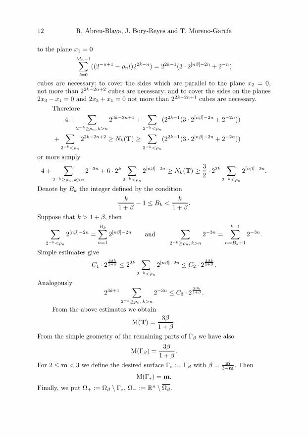
12 R. Abreu-Blaya, J. Bory-Reyes and T. Moreno-Garcıa
to the plane x1 = 0Mn−1∑
l=0
((2−n+1 − ρnl)22k−n) = 22k−1(3 · 2[nβ]−2n + 2−n)
cubes are necessary; to cover the sides which are parallel to the plane x2 = 0,not more than 22k−2n+2 cubes are necessary; and to cover the sides on the planes2x3 − x1 = 0 and 2x3 + x1 = 0 not more than 22k−2n+1 cubes are necessary.
Therefore
4 +∑
2−k≥ρn, k>n
23k−3n+1 +∑
2−k<ρn
(22k−1(3 · 2[nβ]−2n + 2−2n))
+∑
2−k<ρn
22k−2n+2 ≥ Nk(T) ≥∑
2−k<ρn
(22k−1(3 · 2[nβ]−2n + 2−2n))
or more simply
4 +∑
2−k≥ρn, k>n
2−3n + 6 · 2k∑
2−k<ρn
2[nβ]−2n ≥ Nk(T) ≥ 32· 22k
∑2−k<ρn
2[nβ]−2n.
Denote by Bk the integer defined by the conditionk
1 + β− 1 ≤ Bk <
k
1 + β.
Suppose that k > 1 + β, then∑2−k<ρn
2[nβ]−2n =Bk∑
n=1
2[nβ]−2n and∑
2−k≥ρn, k>n
2−3n =k−1∑
n=Bk+1
2−3n.
Simple estimates give
C1 · 23βk1+β ≤ 22k
∑2−k<ρn
2[nβ]−2n ≤ C2 · 23βk1+β .
Analogously23k+1
∑2−k≥ρn, k>n
2−3n ≤ C3 · 23βk1+β .
From the above estimates we obtain
M(T) =3β
1 + β.
From the simple geometry of the remaining parts of Γβ we have also
M(Γβ) =3β
1 + β.
For 2 ≤m < 3 we define the desired surface Γ∗ := Γβ with β = m3−m . Then
M(Γ∗) = m.
Finally, we put Ω+ := Ωβ \ Γ∗, Ω− := Rn \ Ωβ .
Teodorescu Transform Decomposition 13
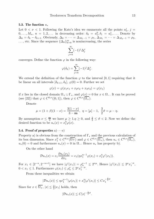
5.3. The function u∗Let 0 < ν < 1. Following the Kats’s idea we enumerate all the points aj
n, j =0, . . . , Mn, n = 1, 2, . . . in decreasing order: δ0 = a0
1, δ1 = a11, . . . . Denote by
∆k = δk − δk+1. Obviously, ∆0 = · · · = ∆M1−1 = ρ1, ∆M1 = · · · = ∆M2−1 = ρ2,. . . , etc. Since the sequence ∆k∞k=0 is nonincreasing, the series
∞∑j=k
(−1)j∆νj
converges. Define the function ϕ in the following way:
ϕ(δk) =∞∑
j=k
(−1)j∆νj .
We extend the definition of the function ϕ to the interval [0, 1] requiring that itbe linear on all intervals [δk+1, δk], ϕ(0) = 0. Further we set
ϕ(x) = ϕ(x1e1 + x2e2 + x3e3) = ϕ(x1)
if x lies in the closed domain Ω+ ∪ Γ∗, and ϕ(x) = 0 for x ∈ Ω−. It can be proved(see [22]) that ϕ ∈ C0,ν([0, 1]), then ϕ ∈ C0,ν(Ω+).
Denote
µ = (1 + β)(1 − ν) =3(1− ν)3−m
, η = [µ]− 1,32ϑ = µ− η.
By assumption ν ≤ m3 we have µ ≥ 1,η ≥ 0, and 2
3 ≤ ϑ < 2. Now we define thedesired function to be u∗(x) = xη
1ϕ(x).
5.4. Proof of properties a) · · · e)Property a) is obvious from the construction of Γ∗ and the previous calculation ofits box dimension. Since xη
1 ∈ C0,ν(Ω+) and ϕ ∈ C0,ν(Ω+), then u∗ ∈ C0,ν(Ω+),u∗(0) = 0 and furthermore u∗(x) = 0 in Ω−. Hence u∗ has property b).
On the other hand
Du∗(x) = e1∂u∗(x1)
∂x1= e1(ηxη−1
1 ϕ(x1) + xη1ϕ′(x1)).
For x1 ∈ [2−n, 2−n+1] we have |ϕ′(x1)| = ρν−1n ≤ 2nµ. Hence |ϕ′(x1)| ≤ 2µx−µ
1 ,0 < x1 ≤ 1. Furthermore ϕ(x1) ≤ ρν
n ≤ 2µx1−µ1 .
From these inequalities we obtain
|Du∗(x)| ≤ ηxη−11 |ϕ(x1)|+ xη
1 |ϕ′(x1)| ≤ Cx− 3
2 ϑ1 .
Since for x ∈ Ω+, |x| ≤ 32 |x1| holds, then
|Du∗(x)| ≤ C|x|− 32 ϑ.

14 R. Abreu-Blaya, J. Bory-Reyes and T. Moreno-Garcıa
Obviously, Du∗(x) ∈ Lp for p ≤ 2ϑ . Since 2
3 ≤ ϑ < 2 we obtain Du∗(x) ∈ Lp forsome p > 1. Hence property c) follows. The same estimate proves property d). Infact,
|x|ϑ|TΩ+Du∗(x)| = 14π|∫
Ω+
|y − x− y|ϑ(x− y)Du∗(y)|y − x|3 dL3(y)|
≤ 14π|∫
Ω+
|y − x− y|ϑDu∗(y)|y − x|2 dL3(y)|
≤ C(∫
Ω+
|y − x|ϑ−2|Du∗(y)|dL3(y) +∫
Ω+
|y|ϑ|Du∗(y)||y − x|2 dL3(y)).
Using Holder inequality the two last integrals can be bounded by a constant Cindependent of x, which proves property d). To prove e) we firstly note that
TΩ+(Du∗)(x) = ηTΩ+(e1(ηxη−11 ϕ(x1))(x) + TΩ+(e1x
η1ϕ′(x1))(x).
Since ϕ(0) = 0 and ϕ ∈ C0,ν(Ω+), then xη−11 ϕ(x) ∈ Lp(Ω+) for some p > 3
TΩ+(e1(ηxη−11 ϕ(x1))(x) is bounded.
In order to estimate TΩ+(e1xη1ϕ′(x1))(x) we split it as
TΩ+(e1xη1ϕ′(x1))(x) = TP(e1x
η1ϕ
′(x1))(x) +∞∑
n=0
TΠn(e1xη1ϕ′(x1))(x)
where
P = x : 0 ≤ x1 ≤ 1, −x1 ≤ x2 ≤ 0, −12x1 ≤ x3 ≤
12x1
and
Πn = x : δ2n+1 ≤ x1 ≤ δ2n, 0 ≤ x2 ≤ h2n, −12x1 ≤ x3 ≤
12x1
h0 = h1 = · · · = hM12 −1
= 2−1, hM12
= · · · = hM22 −1
= 2−2, . . . .
Since P has piecewise smooth boundary ∂P and u∗ ∈ C0,ν(Ω+) , then in virtue ofthe Borel-Pompeiu formula and the Holder boundedness of the Cauchy transformC∂P u∗ (see [1, 7], for instance), we have that TPDu∗(x) is bounded and thenTP(e1x
η1ϕ′(x1))(x) is also bounded.
The arguments used to state the lower bound for
[∞∑
n=0
TΠn(e1xη1ϕ′(x1))(x)]1
are rather technical and follow essentially the same Kats procedure. After that weobtain
[TΩ+Du∗(−x1e1)]1 ≥ C + b
∞∑k=0
2k(2ϑ−1)
(2kx1 + 1)2, b > 0, x1 ∈ (0, 1].
Teodorescu Transform Decomposition 15
Since∞∑
k=0
2k(2ϑ−1)
(2kx1 + 1)2≥
∞∫0
dt
(2tx1 + 1)2=
∞∫0
2−2tdt
(x1 + 2−t)2≥ ln 2 ln
1x1
then we obtain the desired inequality e).
References
[1] R. Abreu and J. Bory: Boundary value problems for quaternionic monogenic func-tions on non-smooth surfaces. Adv. Appl. Clifford Algebras, 9, No.1, 1999: 1–22.
[2] R. Abreu, J. Bory, R. Delanghe and F. Sommen: Harmonic multivector fields andthe Cauchy integral decomposition in Clifford analysis. BMS Simon Stevin, 11, No1, 2004: 95–110.
[3] R. Abreu, J. Bory, R. Delanghe and F. Sommen: Cauchy integral decomposition ofmulti-vector-valued functions on hypersurfaces. Computational Methods and Func-tion Theory, Vol. 5, No. 1, 2005: 111–134
[4] R. Abreu, J. Bory, O. Gerus and M. Shapiro: The Clifford/Cauchy transform witha continuous density; N. Davydov’s theorem. Math. Meth. Appl. Sci, Vol. 28, No. 7,2005: 811–825.
[5] R. Abreu, J. Bory and T. Moreno: Integration of multi-vector-valued functions overfractal hypersurfaces. In preparation.
[6] R. Abreu, D. Pena, J. Bory: Clifford Cauchy Type Integrals on Ahlfors-David RegularSurfaces in R
m+1. Adv. Appl. Clifford Algebras 13 (2003), No. 2, 133–156.
[7] R. Abreu, J. Bory and D. Pena: Jump problem and removable singularities for mono-genic functions. Submitted.
[8] R. Abreu, J. Bory and M. Shapiro: The Cauchy transform for the Hodge/deRhamsystem and some of its properties. Submitted.
[9] J. Bory and R. Abreu: Cauchy transform and rectifiability in Clifford Analysis. Z.Anal. Anwend, 24, No 1, 2005: 167–178.
[10] F. Brackx, R. Delanghe and F. Sommen: Clifford analysis. Research Notes in Math-ematics, 76. Pitman (Advanced Publishing Program), Boston, MA, 1982. x+308 pp.ISBN: 0-273-08535-2 MR 85j:30103.
[11] F. Brackx, R. Delanghe and F. Sommen: Differential Forms and/or MultivectorFunctions. Cubo 7 (2005), no. 2, 139–169.
[12] R. Delanghe, F. Sommen and V. Soucek: Clifford algebra and spinor-valued func-tions. A function theory for the Dirac operator. Related REDUCE software by F.Brackx and D. Constales. With 1 IBM-PC floppy disk (3.5 inch). Mathematics andits Applications, 53. Kluwer Academic Publishers Group, Dordrecht, 1992. xviii+485pp. ISBN: 0-7923-0229-X MR 94d:30084.
[13] E. Dyn’kin: Cauchy integral decomposition for harmonic forms. Journal d’AnalyseMathematique. 1997; 37: 165–186.
[14] Falconer, K.J.: The geometry of fractal sets. Cambridge Tracts in Mathematics, 85.Cambridge University Press, Cambridge, 1986.
16 R. Abreu-Blaya, J. Bory-Reyes and T. Moreno-Garcıa
[15] Feder, Jens.: Fractals. With a foreword by Benoit B. Mandelbrot. Physics of Solidsand Liquids. Plenum Press, New York, 1988.
[16] H. Federer: Geometric measure theory. Die Grundlehren der mathematischen Wis-senschaften, Band 153, Springer-Verlag, New York Inc.,(1969) New York, xiv+676pp.
[17] J. Gilbert, J. Hogan and J. Lakey: Frame decomposition of form-valued Hardy spaces.In Clifford Algebras in analysis and related topics, Ed. J. Ryan CRC Press, (1996),Boca Raton, 239–259.
[18] J. Gilbert and M. Murray: Clifford algebras and Dirac operators in harmonic anal-ysis. Cambridge Studies in Advanced Mathematics 26, Cambridge, 1991.
[19] K. Gurlebeck and W. Sprossig: Quaternionic and Clifford Calculus for Physicistsand Engineers. Wiley and Sons Publ., 1997.
[20] J. Harrison and A. Norton: Geometric integration on fractal curves in the plane.Indiana University Mathematical Journal, 4, No. 2, 1992: 567–594.
[21] J. Harrison and A. Norton: The Gauss-Green theorem for fractal boundaries. DukeMathematical Journal, 67, No. 3, 1992: 575–588.
[22] B.A. Kats: The Riemann problem on a closed Jordan curve. Izv. Vuz. Matematika,27, No. 4, 1983: 68–80.
[23] B.A. Kats: On the solvability of the Riemann boundary value problem on a fractalarc. (Russian) Mat. Zametki 53 (1993), no. 5, 69–75; translation in Math. Notes 53(1993), No. 5-6, 502–505.
[24] B.A. Kats: Jump problem and integral over nonrectifiable curve. Izv. Vuz. Matem-atika 31, No. 5, 1987: 49–57.
[25] M.L. Lapidus and H. Maier: Hypothese de Riemann, cordes fractales vibrantes et con-jecture de Weyl-Berry modifiee. (French) [The Riemann hypothesis, vibrating fractalstrings and the modified Weyl-Berry conjecture] C.R. Acad. Sci. Paris Ser. I Math.313 (1991), no. 1, 19–24. 1991.
[26] E.M. Stein: Singular integrals and differentiability properties of functions. PrincetonMath. Ser. 30, Princeton Univ. Press, Princeton, N.J. 1970.
Ricardo Abreu-BlayaFacultad de Informatica y MatematicaUniversidad de Holguin, Cubae-mail: [email protected]
Juan Bory-ReyesDepartamento of MatematicaUniversidad de Oriente, Cubae-mail: [email protected]
Tania Moreno-GarcıaFacultad de Informatica y MatematicaUniversidad de Holguin, Cubae-mail: [email protected]
Operator Theory:Advances and Applications, Vol. 167, 17–67c© 2006 Birkhauser Verlag Basel/Switzerland
Metric Dependent Clifford Analysis withApplications to Wavelet Analysis
Fred Brackx, Nele De Schepper and Frank Sommen
Abstract. In earlier research multi-dimensional wavelets have been construct-ed in the framework of Clifford analysis. Clifford analysis, centered aroundthe notion of monogenic functions, may be regarded as a direct and elegantgeneralization to higher dimension of the theory of the holomorphic functionsin the complex plane. This Clifford wavelet theory might be characterized asisotropic, since the metric in the underlying space is the standard Euclideanone.
In this paper we develop the idea of a metric dependent Clifford analy-sis leading to a so-called anisotropic Clifford wavelet theory featuring waveletfunctions which are adaptable to preferential, not necessarily orthogonal, di-rections in the signals or textures to be analyzed.
Mathematics Subject Classification (2000). 42B10; 44A15; 30G35.
Keywords. Continuous Wavelet Transform; Clifford analysis; Hermite polyno-mials.
1. Introduction
During the last fifty years, Clifford analysis has gradually developed to a com-prehensive theory which offers a direct, elegant and powerful generalization tohigher dimension of the theory of holomorphic functions in the complex plane.Clifford analysis focuses on so-called monogenic functions, which are in the sim-ple but useful setting of flat m-dimensional Euclidean space, null solutions of theClifford-vector valued Dirac operator
∂ =m∑
j=1
ej∂xj ,
where (e1, . . . , em) forms an orthogonal basis for the quadratic space Rm underly-ing the construction of the real Clifford algebra Rm. Numerous papers, conferenceproceedings and books have moulded this theory and shown its ability for appli-cations, let us mention [2, 15, 18, 19, 20, 24, 25, 26].

18 F. Brackx, N. De Schepper and F. Sommen
Clifford analysis is closely related to harmonic analysis in that monogenicfunctions refine the properties of harmonic functions. Note for instance that eachharmonic function h(x) can be split as h(x) = f(x)+ x g(x) with f , g monogenic,and that a real harmonic function is always the real part of a monogenic one, whichdoes not need to be the case for a harmonic function of several complex variables.The reason for this intimate relationship is that, as does the Cauchy-Riemannoperator in the complex plane, the rotation-invariant Dirac operator factorizes them-dimensional Laplace operator.
A highly important intrinsic feature of Clifford analysis is that it encompassesall dimensions at once, in other words all concepts in this multi-dimensional theoryare not merely tensor products of one dimensional phenomena but are directlydefined and studied in multi-dimensional space and cannot be recursively reducedto lower dimension. This true multi-dimensional nature has allowed for amongothers a very specific and original approach to multi-dimensional wavelet theory.
Wavelet analysis is a particular time- or space-scale representation of func-tions, which has found numerous applications in mathematics, physics and engi-neering (see, e.g., [12, 14, 21]). Two of the main themes in wavelet theory arethe Continuous Wavelet Transform (abbreviated CWT) and discrete orthonormalwavelets generated by multiresolution analysis. They enjoy more or less oppositeproperties and both have their specific field of application. The CWT plays ananalogous role as the Fourier transform and is a successful tool for the analysisof signals and feature detection in signals. The discrete wavelet transform is theanalogue of the Discrete Fourier Transform and provides a powerful technique for,e.g., data compression and signal reconstruction. It is only the CWT we are aimingat as an application of the theory developed in this paper.
Let us first explain the idea of the one dimensional CWT. Wavelets constitutea family of functions ψa,b derived from one single function ψ, called the motherwavelet, by change of scale a (i.e., by dilation) and by change of position b (i.e.,by translation):
ψa,b(x) =1√a
ψ
(x− b
a
), a > 0, b ∈ R.
In wavelet theory some conditions on the mother wavelet ψ have to be imposed.We request ψ to be an L2-function (finite energy signal) which is well localizedboth in the time domain and in the frequency domain. Moreover it has to satisfythe so-called admissibility condition:
Cψ :=∫ +∞
−∞
|ψ(u)|2|u| du < +∞,
where ψ denotes the Fourier transform of ψ. In the case where ψ is also in L1, thisadmissibility condition implies ∫ +∞
−∞ψ(x) dx = 0.
Metrodynamics with Applications to Wavelet Analysis 19
In other words: ψ must be an oscillating function, which explains its qualificationas “wavelet”.
In practice, applications impose additional requirements, among which agiven number of vanishing moments:∫ +∞
−∞xn ψ(x) dx = 0, n = 0, 1, . . . , N.
This means that the corresponding CWT:
F (a, b) = 〈ψa,b, f〉
=1√a
∫ +∞
−∞ψ
(x− b
a
)f(x) dx
will filter out polynomial behavior of the signal f up to degree N , making itadequate at detecting singularities.
The CWT may be extended to higher dimension while still enjoying the sameproperties as in the one-dimensional case. Traditionally these higher-dimensionalCWTs originate as tensor products of one-dimensional phenomena. However alsothe non-separable treatment of two-dimensional wavelets should be mentioned(see [1]).
In a series of papers [4, 5, 6, 7, 9, 10] multi-dimensional wavelets have beenconstructed in the framework of Clifford analysis. These wavelets are based onClifford generalizations of the Hermite polynomials, the Gegenbauer polynomials,the Laguerre polynomials and the Jacobi polynomials. Moreover, they arise as spe-cific applications of a general theory for constructing multi-dimensional Clifford-wavelets (see [8]). The first step in this construction method is the introductionof new polynomials, generalizing classical orthogonal polynomials on the real lineto the Clifford analysis setting. Their construction rests upon a specific Cliffordanalysis technique, the so-called Cauchy-Kowalewskaia extension of a real-analyticfunction in Rm to a monogenic function in Rm+1. One starts from a real-analyticfunction in an open connected domain in Rm, as an analogon of the classical weightfunction. The new Clifford algebra-valued polynomials are then generated by theCauchy-Kowalewskaia extension of this weight function. For these polynomialsa recurrence relation and a Rodrigues formula are established. This Rodriguesformula together with Stokes’s theorem lead to an orthogonality relation of thenew Clifford-polynomials. From this orthogonality relation we select candidatesfor mother wavelets and show that these candidates indeed may serve as kernelfunctions for a multi-dimensional CWT if they satisfy certain additional condi-tions.
The above sketched Clifford wavelet theory may be characterized as isotropicsince the metric in the underlying space is the standard Euclidean one for which
e2j = −1, j = 1, . . . , m
andejek = −ekej , 1 ≤ j = k ≤ m,

20 F. Brackx, N. De Schepper and F. Sommen
leading to the standard scalar product of a vector x =∑m
j=1 xjej with itself:
〈x, x〉 =m∑
j=1
x2j . (1.1)
In this paper we develop the idea of a metric dependent Clifford analysis leadingto a so-called anisotropic Clifford wavelet theory featuring wavelet functions whichare adaptable to preferential, not necessarily orthogonal, directions in the signalsor textures to be analyzed. This is achieved by considering functions taking theirvalues in a Clifford algebra which is constructed over Rm by means of a symmetricbilinear form such that the scalar product of a vector with itself now takes theform
〈x, x〉 =m∑
j=1
m∑k=1
gjkxjxk. (1.2)
We refer to the tensor gjk as the metric tensor of the Clifford algebra considered,and it is assumed that this metric tensor is real, symmetric and positive definite.This idea is in fact not completely new since Clifford analysis on manifolds withlocal metric tensors was already considered in, e.g., [13], [18] and [23], while in[17] a specific three dimensional tensor leaving the third dimension unaltered wasintroduced for analyzing two dimensional signals and textures. What is new isthe detailed development of this Clifford analysis in a global metric dependentsetting, the construction of new Clifford-Hermite polynomials and the study ofthe corresponding Continuous Wavelet Transform. It should be clear that thispaper opens a new area in Clifford analysis offering a framework for a new kindof applications, in particular concerning anisotropic Clifford wavelets. We have inmind constructing specific wavelets for analyzing multi-dimensional textures orsignals which show more or less constant features in preferential directions. Forthat purpose we will have the orientation of the fundamental (e1, . . . , em)-frameadapted to these directions resulting in an associated metric tensor which willleave these directions unaltered.
The outline of the paper is as follows. We start with constructing, by meansof Grassmann generators, two bases: a covariant one (ej : j = 1, . . . , m) anda contravariant one (ej : j = 1, . . . , m), satisfying the general Clifford algebramultiplication rules:
ejek + ekej = −2gjk and ejek + ekej = −2gjk, 1 ≤ j, k ≤ m
with gjk the metric tensor. The above multiplication rules lead in a natural wayto the substitution for the classical scalar product (1.1) of a vector x =
∑mj=1 xjej
with itself, a symmetric bilinear form expressed by (1.2). Next we generalize allnecessary definitions and results of orthogonal Clifford analysis to this metric de-pendent setting. In this new context we introduce for, e.g., the concepts of Fischerinner product, Fischer duality, monogenicity and spherical monogenics. Similar tothe orthogonal case, we can also in the metric dependent Clifford analysis decom-pose each homogeneous polynomial into spherical monogenics, which is referred
Metrodynamics with Applications to Wavelet Analysis 21
to as the monogenic decomposition. After a thorough investigation in the met-ric dependent context of the so-called Euler and angular Dirac operators, whichconstitute two fundamental operators in Clifford analysis, we proceed with the in-troduction of the notions of harmonicity and spherical harmonics. Furthermore, weverify the orthogonal decomposition of homogeneous polynomials into harmonicones, the so-called harmonic decomposition. We end Section 2 with the definitionand study of the so-called g-Fourier transform, the metric dependent analogue ofthe classical Fourier transform.
With a view to integration on hypersurfaces in the metric dependent setting,we invoke the theory of differential forms. In Subsection 3.1 we gather some basicdefinitions and properties concerning Clifford differential forms. We discuss, e.g.,fundamental operators such as the exterior derivative and the basic contractionoperators; we also state Stokes’s theorem, a really fundamental result in mathe-matical analysis. Special attention is paid to the properties of the Leray and sigmadifferential forms, since they both play a crucial role in establishing orthogonalityrelations between spherical monogenics on the unit sphere, the topic of Subsec-tion 3.2.
In a fourth and final section we construct the so-called radial g-Clifford-Hermite polynomials, the metric dependent analogue of the radial Clifford-Hermitepolynomials of orthogonal Clifford analysis. For these polynomials a recurrenceand orthogonality relation are established. Furthermore, these polynomials turnout to be the desired building blocks for specific wavelet kernel functions, the so-called g-Clifford-Hermite wavelets. We end the paper with the introduction of thecorresponding g-Clifford-Hermite Continuous Wavelet Transform.
2. The metric dependent Clifford toolbox
2.1. Tensors
Let us start by recalling a few concepts concerning tensors. Assume in Euclideanspace two coordinate systems (x1, x2, . . . , xN ) and (x1, x2, . . . , xN ) given.
Definition 2.1. If (A1, A2, . . . , AN ) in coordinate system (x1, x2, . . . , xN ) and(A1, A2, . . . , AN ) in coordinate system (x1, x2, . . . , xN ) are related by the trans-formation equations:
Aj =N∑
k=1
∂xj
∂xkAk , j = 1, . . . , N,
then they are said to be components of a contravariant vector.

22 F. Brackx, N. De Schepper and F. Sommen
Definition 2.2. If (A1, A2, . . . , AN ) in coordinate system (x1, x2, . . . , xN ) and(A1, A2, . . . , AN ) in coordinate system (x1, x2, . . . , xN ) are related by the trans-formation equations:
Aj =N∑
k=1
∂xk
∂xjAk, j = 1, . . . , N,
then they are said to be components of a covariant vector.
Example. The sets of differentials dx1, . . . , dxN and dx1, . . . , dxN transformaccording to the chain rule:
dxj =N∑
k=1
∂xj
∂xkdxk, j = 1, . . . , N.
Hence (dx1, . . . , dxN ) is a contravariant vector.
Example. Consider the coordinate transformation(x1, x2, . . . , xN
)=(x1, x2, . . . , xN
)A
with A = (ajk) an (N ×N)-matrix. We have
xj =N∑
k=1
xkajk or equivalently xj =
N∑k=1
∂xj
∂xkxk,
which implies that (x1, . . . , xN ) is a contravariant vector.
Definition 2.3. The outer tensorial product of two vectors is a tensor of rank 2.There are three possibilities:• the outer product of two contravariant vectors (A1,...,AN ) and (B1,...,BN)
is a contravariant tensor of rank 2:
Cjk = AjBk
• the outer product of a covariant vector (A1, . . . , AN ) and a contravariantvector (B1, . . . , BN ) is a mixed tensor of rank 2:
Ckj = AjB
k
• the outer product of two covariant vectors (A1, . . . , AN ) and (B1, . . . , BN ) isa covariant tensor of rank 2:
Cjk = AjBk.
Example. The Kronecker-delta
δkj =
1 if j = k
0 otherwise
is a mixed tensor of rank 2.

Metrodynamics with Applications to Wavelet Analysis 23
Example. The transformation matrix
ajk =
∂xj
∂xk, j, k = 1, . . . , N
is also a mixed tensor of rank 2.
Remark 2.4. In view of Definitions 2.1 and 2.2 it is easily seen that the transfor-mation formulae for tensors of rank 2 take the following form:
Cjk = AjBk =N∑
i=1
∂xj
∂xiAi
N∑=1
∂xk
∂xB
=N∑
i=1
N∑=1
∂xj
∂xi
∂xk
∂xAiB =
N∑i=1
N∑=1
∂xj
∂xi
∂xk
∂xCi
and similarly
Ckj =
N∑i=1
N∑=1
∂xi
∂xj
∂xk
∂xC
i , Cjk =N∑
i=1
N∑=1
∂xi
∂xj
∂x
∂xkCi.
Definition 2.5. The tensorial contraction of a tensor of rank p is a tensor of rank(p−2) which one obtains by summation over a common contravariant and covariantindex.
Example. The tensorial contraction of the mixed tensor Cjk of rank 2 is a tensor
of rank 0, i.e., a scalar:N∑
j=1
Cjj = D,
while the tensorial contraction of the mixed tensor Cjki of rank 3 yields a con-
travariant vector:N∑
j=1
Cjkj = Dk.
Definition 2.6. The inner tensorial product of two vectors is their outer productfollowed by contraction.
Example. The inner tensorial product of the covariant vector (A1, . . . , AN ) and thecontravariant vector (B1, . . . , BN ) is the tensor of rank 0, i.e., the scalar given by:
N∑j=1
AjBj = C.
24 F. Brackx, N. De Schepper and F. Sommen
2.2. From Grassmann to Clifford
We consider the Grassmann algebra Λ generated by the basis elements (j , j =1, . . . , m) satisfying the relations
j k + k j = 0 1 ≤ j, k ≤ m.
These basis elements form a covariant tensor (1, 2, . . . , m) of rank 1.Next we consider the dual Grassmann algebra Λ+ generated by the dual
basis (+j , j = 1, . . . , m), forming a contravariant tensor of rank 1 and satisfyingthe Grassmann identities:
+j +k + +k +j = 0 1 ≤ j, k ≤ m. (2.1)
Duality between both Grassmann algebras is expressed by:
j +k +
+kj = δk
j . (2.2)
Note that both the left- and right-hand side of the above equation is a mixedtensor of rank 2.
Now we introduce the fundamental covariant tensor gjk of rank 2. It is as-sumed to have real entries, to be positive definite and symmetric:
gjk = gkj , 1 ≤ j, k ≤ m.
Definition 2.7. The real, positive definite and symmetric tensor gjk is called themetric tensor.
Its reciprocal tensor (a contravariant one) is given by
gjk =1
det(gjk)Gjk,
where Gjk denotes the cofactor of gjk. It thus satisfiesm∑
=1
gjgk = δjk.
In what follows we will use the Einstein summation convention, i.e., summationover equal contravariant and covariant indices is tacitly understood.
With this convention the above equation expressing reciprocity is written as
gjgk = δjk.
Definition 2.8. The covariant basis (+j , j = 1, . . . , m) for the Grassmann algebra
Λ+ is given by+j = gjk+k.
This covariant basis shows the following properties.
Proposition 2.9. One has
+j
+k +
+k
+j = 0 and j
+k +
+k j = gjk ; 1 ≤ j, k ≤ m.

Metrodynamics with Applications to Wavelet Analysis 25
Proof. By means of respectively (2.1) and (2.2), we find
+j
+k +
+k
+j = gj+gkt+t + gkt+tgj+
= gjgkt(+
+t +
+t+) = 0
and
j +k +
+k j = jgkt+t + gkt+tj = gkt(j +t + +tj)
= gktδtj = gkj = gjk.
Remark 2.10. By reciprocity one has:
+k = gkj
+j .
Definition 2.11. The contravariant basis (j , j = 1, . . . , m) for the Grassmannalgebra Λ is given by
j = gjkk.
It shows the following properties.
Proposition 2.12. One has
j k + k j = 0 and j +k + +k j = gjk.
Proof. A straightforward computation yields
j k + k j = gjgktt + gkttg
j
= gjgkt(t + t) = 0
and
j +k + +kj = gj+k + +kgj
= gj(+k +
+k)
= gjδk = gjk.
Remark 2.13. By reciprocity one has:
k = gkj j .
Now we consider in the direct sum
spanC1, . . . , m ⊕ spanC+1 , . . . , +mtwo subspaces, viz. spanCe1, . . . , em and spanCem+1, . . . , e2m where the newcovariant basis elements are defined by
ej = j − +j , j = 1, . . . , m
em+j = i(j + +j ), j = 1, . . . , m.
Similarly, we consider the contravariant reciprocal subspaces spanCe1, . . . , emand spanCem+1, . . . , e2m given by
ej = j − +j , j = 1, . . . , mem+j = i(j + +j), j = 1, . . . , m.

26 F. Brackx, N. De Schepper and F. Sommen
The covariant basis shows the following properties.
Proposition 2.14. For 1 ≤ j, k ≤ m one has:(i) ejek + ekej = −2gjk
(ii) em+jem+k + em+kem+j = −2gjk
(iii) ejem+k + em+kej = 0.
Proof. A straightforward computation leads to
(i) ejek + ekej = (j − +j )(k −
+k ) + (k −
+k )(j −
+j )
= j k − j +k −
+j k +
+j
+k + kj − k
+j −
+k j +
+k
+j
= (j k + k j) + (+j
+k +
+k
+j )− (j
+k +
+k j)− (
+j k + k
+j )
= −gjk − gkj = −2gjk,
(ii) em+jem+k + em+kem+j
= −(j + +j )(k +
+k )− (k +
+k )(j +
+j )
= −j k − j +k −
+j k −
+j
+k − k j − k
+j −
+k j −
+k
+j
= −(j +k +
+k j)− (
+j k + k
+j )
= −gjk − gkj = −2gjk
and(iii) ejem+k + em+kej
= i(j − +j )(k +
+k ) + i(k +
+k )(j −
+j )
= ij k + ij +k − i+j k − i+j
+k + ik j − ik
+j + i+k j − i+k
+j
= i(j k + k j)− i(+j
+k +
+k
+j ) + i(j
+k +
+k j)− i(
+j k + k
+j )
= igjk − igkj = 0.
As expected, both e-bases are linked to each other by means of the metrictensor gjk and its reciprocal gjk.
Proposition 2.15. For j = 1, . . . , m one has(i) ej = gjkek and ek = gkje
j
(ii) em+j = gjkem+k and em+k = gkjem+j.
Proof.
(i) ej = j −
+j = gjkk − gjk
+k
= gjk(k − +k ) = gjkek
(ii) em+j = i(j +
+j) = igjk(k + +k )
= gjkem+k.
By combining Propositions 2.14 and 2.15 we obtain the following propertiesof the contravariant e-basis.

Metrodynamics with Applications to Wavelet Analysis 27
Proposition 2.16. For 1 ≤ j, k ≤ m one has(i) ejek + ekej = −2gjk
(ii) em+jem+k + em+kem+j = −2gjk
(iii) ejem+k + em+kej = 0.
The basis (e1, . . . , em) and the dual basis (e1, . . . , em) are also linked to eachother by the following relations.
Proposition 2.17. For 1 ≤ j, k ≤ m one has(i) eje
k + ekej = −2δkj
(ii) em+jem+k + em+kem+j = −2δk
j
(iii) ejem+k + em+kej = 0
(iv)∑
j ejej =
∑j ejej = −m
(v) 12
∑jej, e
j = −m
(vi)∑
j [ej , ej] = 0
(vii)∑
j em+jem+j =
∑j em+jem+j = −m
(viii) 12
∑jem+j, e
m+j = −m
(ix)∑
j [em+j , em+j] = 0.
Proof. A straightforward computation yields
(i) ejek + ekej = ejg
ktet + gktetej = gkt(ejet + etej)
= gkt(−2gjt) = −2δkj
(ii) em+jem+k + em+kem+j = em+jg
ktem+t + gktem+tem+j
= gkt(em+jem+t + em+tem+j)
= gkt(−2gjt) = −2δkj
(iii) ejem+k + em+kej = ejg
ktem+t + gktem+tej
= gkt(ejem+t + em+tej) = 0
(iv)m∑
j=1
ejej =
m∑j=1
ej
m∑i=1
gjiei =∑i,j
gijejei
=12
∑i,j
gijejei +12
∑i,j
gijejei =12
∑i,j
gijejei +12
∑j,i
gjieiej
=12
∑i,j
gijejei +12
∑i,j
gij(−ejei − 2gij) = −∑i,j
gijgij
= −∑
i
δii = −(1 + . . . + 1) = −m.
By means of (i) we also havem∑
j=1
ejej =m∑
j=1
(−ejej − 2) = m− 2m = −m.
28 F. Brackx, N. De Schepper and F. Sommen
(v) Follows directly from (iv).(vi) Follows directly from (iv).(vii) Similar to (iv).(viii) Follows directly from (vii).(ix) Follows directly from (vii).
Finally we consider the algebra generated by either the covariant basis (ej :j = 1, . . . , m) or the contravariant basis (ej : j = 1, . . . , m) and we observe thatthe elements of both bases satisfy the multiplication rules of the complex Cliffordalgebra Cm:
ejek + ekej = −2gjk, 1 ≤ j, k ≤ m
andejek + ekej = −2gjk, 1 ≤ j, k ≤ m.
A covariant basis for Cm consists of the elements eA = ei1ei2 . . . eihwhere A =
(i1, i2, . . . , ih) ⊂ 1, . . . , m = M is such that 1 ≤ i1 < i2 < . . . < ih ≤ m.Similarly, a contravariant basis for Cm consists of the elements eA = ei1ei2 . . . eih
where again A = (i1, i2, . . . , ih) ⊂ M is such that 1 ≤ i1 < i2 < . . . < ih ≤ m. Inboth cases, taking A = ∅, yields the identity element, i.e., e∅ = e∅ = 1.
Hence, any element λ ∈ Cm may be written as
λ =∑A
λAeA or as λ =∑A
λAeA with λA ∈ C.
In particular, the space spanned by the covariant basis (ej : j = 1, . . . , m) or thecontravariant basis (ej : j = 1, . . . , m) is called the subspace of Clifford-vectors.
Remark 2.18. Note that the real Clifford-vector α = αjej may be considered asthe inner tensorial product of a contravariant vector αj with real elements witha covariant vector ej with Clifford numbers as elements, which yields a tensor ofrank 0. So the Clifford-vector α is a tensor of rank 0; in fact it is a Clifford number.
In the Clifford algebra Cm, we will frequently use the anti-involution calledHermitian conjugation, defined by
e†j = −ej, j = 1, . . . , m
andλ† =
(∑A
λAeA
)† =∑A
λcAe†A,
where λcA denotes the complex conjugate of λA. Note that in particular for a real
Clifford-vector α = αjej : α† = −α .The Hermitian inner product on Cm is defined by
(λ, µ) = [놵]0 ∈ C,
where [λ]0 denotes the scalar part of the Clifford number λ. It follows that forλ ∈ Cm its Clifford norm |λ|0 is given by
|λ|20 = (λ, λ) = [λ†λ]0.
Metrodynamics with Applications to Wavelet Analysis 29
Finally let us examine the Clifford product of the two Clifford-vectorsα = αjej and β = βjej:
αβ = αjejβkek = αjβkejek
=12αjβkejek +
12αjβk(−ekej − 2gjk)
= −gjkαjβk +12αjβk(ejek − ekej).
It is found that this product splits up into a scalar part and a so-called bivectorpart:
α β = α • β + α ∧ β
with
α • β = −gjkαjβk =12(α β + β α) =
12α, β
the so-called inner product and
α ∧ β =12αjβk(ejek − ekej) =
12αjβk[ej, ek] =
12[α, β]
the so-called outer product.In particular we have that
ej • ek = −gjk, 1 ≤ j, k ≤ m
ej ∧ ej = 0, j = 1, . . . , m
and similarly for the contravariant basis elements:
ej • ek = −gjk, 1 ≤ j, k ≤ m
ej ∧ ej = 0, j = 1, . . . , m.
The outer product of k different basis vectors is defined recursively
ei1 ∧ ei2 ∧ · · · ∧ eik=
12(ei1(ei2 ∧ · · · ∧ eik
) + (−1)k−1(ei2 ∧ · · · ∧ eik)ei1
).
For k = 0, 1, . . . , m fixed, we then call
Ckm =
λ ∈ Cm : λ =
∑|A|=k
λA ei1 ∧ ei2 ∧ · · · ∧ eik, A = (i1, i2, . . . , ik)
the subspace of k-vectors ; i.e., the space spanned by the outer products of k dif-ferent basis vectors. Note that the 0-vectors and 1-vectors are simply the scalarsand Clifford-vectors; the 2-vectors are also called bivectors.
30 F. Brackx, N. De Schepper and F. Sommen
2.3. Embeddings of Rm
By identifying the point (x1, . . . , xm) ∈ Rm with the 1-vector x given by
x = xjej ,
the space Rm is embedded in the Clifford algebra Cm as the subspace of 1-vectors R1
m of the real Clifford algebra Rm. In the same order of ideas, a point(x0, x1, . . . , xm) ∈ Rm+1 is identified with a paravector x = x0 + x in R0
m ⊕ R1m.
We will equip Rm with a metric by defining the scalar product of two basisvectors through their dot product:
〈ej , ek〉 = −ej • ek = gjk, 1 ≤ j, k ≤ m
and by putting for two vectors x and y:
〈x, y〉 = 〈ejxj , ekyk〉 = 〈ej , ek〉xjyk = gjkxjyk.
Note that in this way 〈 . , . 〉 is indeed a scalar product, since the tensor gjk issymmetric and positive definite. Also note that in particular
‖x‖2 = 〈x, x〉 = gjkxjxk = −x • x = −x2 = |x|20 .
We also introduce spherical coordinates in Rm by:
x = rω
withr = ‖x‖ =
(gjkxjxk
)1/2 ∈ [0, +∞[ and ω ∈ Sm−1,
where Sm−1 denotes the unit sphere in Rm:
Sm−1 =ω ∈ R
1m ; ‖ω‖2 = −ω2 = gjkωjωk = 1
.
Now we introduce a new basis for Rm ∼= R
1m consisting of eigenvectors of the
matrix G = (gjk), associated to the metric tensor gjk. As (gjk) is real-symmetric,there exists an orthogonal matrix A ∈ O(m) such that
AT GA = diag(λ1, . . . , λm)
with λ1, . . . , λm the positive eigenvalues of G. We put
(Ej) = (ej)A.
We expect the basis (Ej : j = 1, . . . , m) to be orthogonal, since Ej (j = 1, . . . , m)are eigenvectors of the matrix G.
If (xj) and (Xj) are the column matrices representing the coordinates of xwith respect to the bases (ej) and (Ej) respectively, then we have
x = (ej)(xj) = (Ej)(Xj) = (ej)A(Xj)
and(xj) = A(Xj) or (Xj) = AT (xj).
Metrodynamics with Applications to Wavelet Analysis 31
Hence
〈x, y〉 = (xj)T G(yj) = (Xj)T AT GA(Y j)
= (Xj)T diag(λ1, . . . , λm) (Y j) =∑
j
λjXjY j .
In particular we find, as expected:
〈Ej , Ek〉 = 0, j = k and 〈Ej , Ej〉 = λj , j = 1, . . . , m.
Involving the Clifford product we obtain
Ej, Ek = 2Ej • Ek = −2〈Ej, Ek〉 = 0, j = k
andEj , Ej = 2Ej • Ej = −2〈Ej , Ej〉 = −2λj, j = 1, . . . , m
and so for all 1 ≤ j, k ≤ m
EjEk + EkEj = −2λjδjk.
Finally if we put
ηj
=Ej√λj
(j = 1, . . . , m),
we obtain an orthonormal frame in the metric dependent setting:
〈ηj, η
k〉 = δjk; 1 ≤ j, k ≤ m.
In what follows, (x′j) denotes the column matrix containing the coordinates of xwith respect to this orthonormal frame, i.e.,
x =∑
j
x′j ηj
=∑
j
〈ηj, x〉 η
j.
It is clear that the coordinate sets (Xj) and (x′j) are related as follows:
(Xj) = P−1(x′j) or (x′j) = P (Xj)
withP = diag(
√λ1, . . . ,
√λm).
Hence we also have
(xj) = AP−1(x′j) and (x′j) = PAT (xj).
Finally, note that in the x′j -coordinates, the inner product takes the followingform
〈x, y〉 =∑
j
x′jy′j .
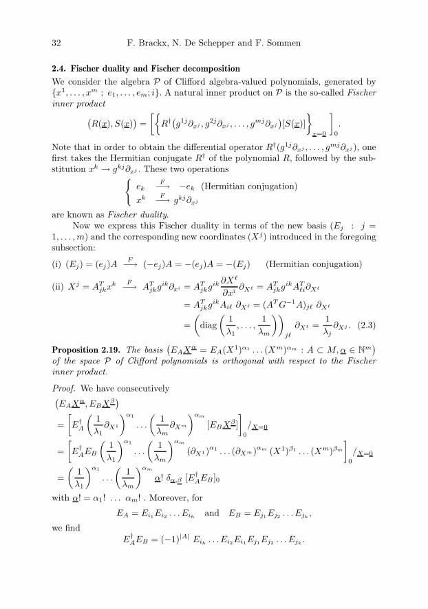
32 F. Brackx, N. De Schepper and F. Sommen
2.4. Fischer duality and Fischer decomposition
We consider the algebra P of Clifford algebra-valued polynomials, generated byx1, . . . , xm ; e1, . . . , em; i. A natural inner product on P is the so-called Fischerinner product(
R(x), S(x))
=[
R†(g1j∂xj , g2j∂xj , . . . , gmj∂xj
)[S(x)]
x=0
]0
.
Note that in order to obtain the differential operator R†(g1j∂xj , . . . , gmj∂xj ), onefirst takes the Hermitian conjugate R† of the polynomial R, followed by the sub-stitution xk → gkj∂xj . These two operations
ekF−→ −ek (Hermitian conjugation)
xk F−→ gkj∂xj
are known as Fischer duality.Now we express this Fischer duality in terms of the new basis (Ej : j =
1, . . . , m) and the corresponding new coordinates (Xj) introduced in the foregoingsubsection:
(i) (Ej) = (ej)AF−→ (−ej)A = −(ej)A = −(Ej) (Hermitian conjugation)
(ii) Xj = ATjkxk F−→ AT
jkgik∂xi = ATjkgik ∂X
∂xi∂X = AT
jkgikATi∂X
= ATjkgikAi ∂X = (AT G−1A)j ∂X
=(
diag(
1λ1
, . . . ,1
λm
))j
∂X =1λj
∂Xj . (2.3)
Proposition 2.19. The basis(EAXα = EA(X1)α1 . . . (Xm)αm : A ⊂ M, α ∈ Nm
)of the space P of Clifford polynomials is orthogonal with respect to the Fischerinner product.
Proof. We have consecutively(EAXα, EBXβ
)=[E†
A
(1λ1
∂X1
)α1
. . .
(1
λm∂Xm
)αm
[EBXβ ]]0
/X=0
=[E†
AEB
(1λ1
)α1
. . .
(1
λm
)αm
(∂X1)α1 . . . (∂Xm)αm (X1)β1 . . . (Xm)βm
]0
/X=0
=(
1λ1
)α1
. . .
(1
λm
)αm
α! δα,β [E†AEB ]0
with α! = α1! . . . αm! . Moreover, for
EA = Ei1Ei2 . . . Eihand EB = Ej1Ej2 . . . Ejk
,
we findE†
AEB = (−1)|A| Eih. . . Ei2Ei1Ej1Ej2 . . . Ejk
.
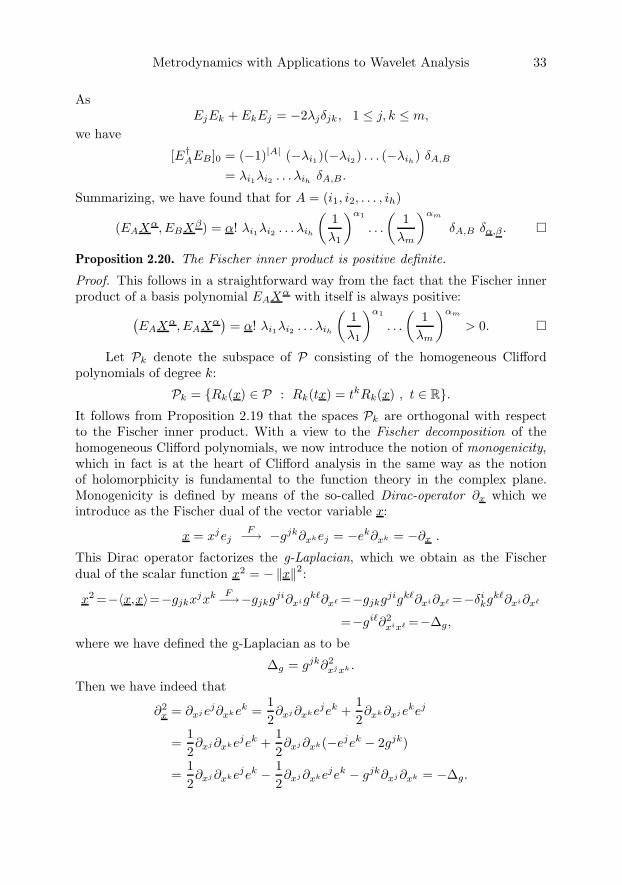
Metrodynamics with Applications to Wavelet Analysis 33
AsEjEk + EkEj = −2λjδjk, 1 ≤ j, k ≤ m,
we have
[E†AEB]0 = (−1)|A| (−λi1)(−λi2 ) . . . (−λih
) δA,B
= λi1λi2 . . . λihδA,B.
Summarizing, we have found that for A = (i1, i2, . . . , ih)
(EAXα, EBXβ) = α! λi1λi2 . . . λih
(1λ1
)α1
. . .
(1
λm
)αm
δA,B δα,β .
Proposition 2.20. The Fischer inner product is positive definite.
Proof. This follows in a straightforward way from the fact that the Fischer innerproduct of a basis polynomial EAXα with itself is always positive:(
EAXα, EAXα)
= α! λi1λi2 . . . λih
(1λ1
)α1
. . .
(1
λm
)αm
> 0.
Let Pk denote the subspace of P consisting of the homogeneous Cliffordpolynomials of degree k:
Pk = Rk(x) ∈ P : Rk(tx) = tkRk(x) , t ∈ R.It follows from Proposition 2.19 that the spaces Pk are orthogonal with respectto the Fischer inner product. With a view to the Fischer decomposition of thehomogeneous Clifford polynomials, we now introduce the notion of monogenicity,which in fact is at the heart of Clifford analysis in the same way as the notionof holomorphicity is fundamental to the function theory in the complex plane.Monogenicity is defined by means of the so-called Dirac-operator ∂x which weintroduce as the Fischer dual of the vector variable x:
x = xjejF−→ −gjk∂xkej = −ek∂xk = −∂x .
This Dirac operator factorizes the g-Laplacian, which we obtain as the Fischerdual of the scalar function x2 = −‖x‖2:
x2 =−〈x,x〉=−gjkxjxk F−→−gjkgji∂xigk∂x =−gjkgjigk∂xi∂x =−δikgk∂xi∂x
=−gi∂2xix =−∆g,
where we have defined the g-Laplacian as to be
∆g = gjk∂2xjxk .
Then we have indeed that
∂2x = ∂xj ej∂xkek =
12∂xj ∂xkejek +
12∂xk∂xj ekej
=12∂xj ∂xkejek +
12∂xj ∂xk(−ejek − 2gjk)
=12∂xj ∂xkejek − 1
2∂xj ∂xkejek − gjk∂xj ∂xk = −∆g.

34 F. Brackx, N. De Schepper and F. Sommen
We also mention the expression for the Dirac operator in the orthonormal frameintroduced at the end of Subsection 2.3.
Lemma 2.21. With respect to the orthonormal frame ηj
(j = 1, . . . , m), the Diracoperator takes the form
∂x =∑
j
∂x′j ηj.
Proof. For the sake of clarity, we do not use the Einstein summation convention.We have consecutively
∂x =∑
j
∂xj ej =∑j,k
∂xj gjkek =∑j,k,t
∂xj gjkEtATtk
=∑
t
⎛⎝∑j,k
ATtkgjk∂xj
⎞⎠Et.
By means of (2.3) this becomes
∂x =∑
t
1λt
∂XtEt =∑
t
∂x′tηt.
Definition 2.22.
(i) A Cm-valued function F (x1, . . . , xm) is called left monogenic in an open re-gion of Rm if in that region
∂x[F ] = 0.
(ii) A Cm-valued function F (x0, x1, . . . , xm) is called left monogenic in an openregion of Rm+1 if in that region
(∂x0 + ∂x)[F ] = 0.
Here ∂x0 + ∂x is the so-called Cauchy-Riemann operator.The notion of right monogenicity is defined in a similar way by letting act
the Dirac operator or the Cauchy-Riemann operator from the right.Note that if a Clifford algebra-valued function F is left monogenic, then its
Hermitian conjugate F † is right monogenic, since ∂†x = −∂x.
Similar to the notion of spherical harmonic with respect to the Laplace op-erator we introduce the following fundamental concept.
Definition 2.23.
(i) A (left/right) monogenic homogeneous polynomial Pk ∈ Pk is called a(left/right) solid inner spherical monogenic of order k.
(ii) A (left/right) monogenic homogeneous function Qk of degree −(k + m − 1)in Rm \ 0 is called a (left/right) solid outer spherical monogenic of order k.
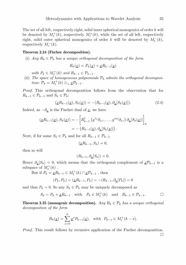
Metrodynamics with Applications to Wavelet Analysis 35
The set of all left, respectively right, solid inner spherical monogenics of order k willbe denoted by M+
(k), respectively M+r (k), while the set of all left, respectively
right, solid outer spherical monogenics of order k will be denoted by M− (k),
respectively M−r (k).
Theorem 2.24 (Fischer decomposition).
(i) Any Rk ∈ Pk has a unique orthogonal decomposition of the form
Rk(x) = Pk(x) + xRk−1(x)
with Pk ∈M+ (k) and Rk−1 ∈ Pk−1.
(ii) The space of homogeneous polynomials Pk admits the orthogonal decomposi-tion: Pk = M+
(k)⊕⊥ xPk−1.
Proof. This orthogonal decomposition follows from the observation that forRk−1 ∈ Pk−1 and Sk ∈ Pk:
(xRk−1(x), Sk(x)) = −(Rk−1(x), ∂x[Sk(x)]). (2.4)
Indeed, as −∂x is the Fischer dual of x, we have
(xRk−1(x), Sk(x)) = −[R†
k−1
(g1j∂xj , . . . , gmj∂xj
)∂x[Sk(x)]
]0
= −(Rk−1(x), ∂x[Sk(x)]
).
Next, if for some Sk ∈ Pk and for all Rk−1 ∈ Pk−1
(xRk−1, Sk) = 0,
then so will(Rk−1, ∂x[Sk]) = 0.
Hence ∂x[Sk] = 0, which means that the orthogonal complement of xPk−1 is asubspace of M+
(k) .But if Pk = xRk−1 ∈M+
(k) ∩ xPk−1 , then
(Pk, Pk) = (xRk−1, Pk) = −(Rk−1, ∂x[Pk]) = 0
and thus Pk = 0. So any Sk ∈ Pk may be uniquely decomposed as
Sk = Pk + xRk−1 with Pk ∈M+ (k) and Rk−1 ∈ Pk−1.
Theorem 2.25 (monogenic decomposition). Any Rk ∈ Pk has a unique orthogonaldecomposition of the form
Rk(x) =k∑
s=0
xsPk−s(x), with Pk−s ∈M+ (k − s).
Proof. This result follows by recursive application of the Fischer decomposition.
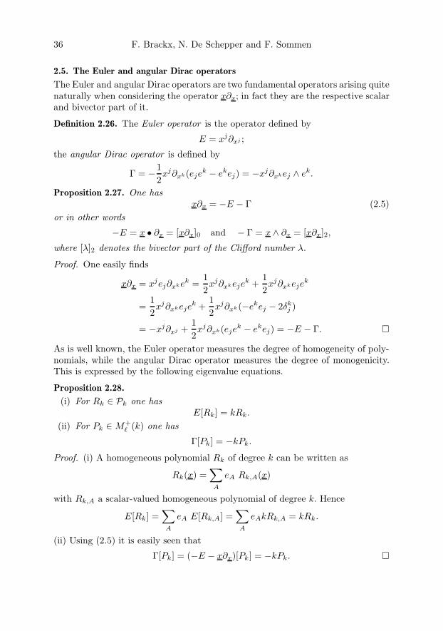
36 F. Brackx, N. De Schepper and F. Sommen
2.5. The Euler and angular Dirac operators
The Euler and angular Dirac operators are two fundamental operators arising quitenaturally when considering the operator x∂x; in fact they are the respective scalarand bivector part of it.
Definition 2.26. The Euler operator is the operator defined by
E = xj∂xj ;
the angular Dirac operator is defined by
Γ = −12xj∂xk(eje
k − ekej) = −xj∂xkej ∧ ek.
Proposition 2.27. One hasx∂x = −E − Γ (2.5)
or in other words
−E = x • ∂x = [x∂x]0 and − Γ = x ∧ ∂x = [x∂x]2,
where [λ]2 denotes the bivector part of the Clifford number λ.
Proof. One easily finds
x∂x = xjej∂xkek =12xj∂xkeje
k +12xj∂xkeje
k
=12xj∂xkeje
k +12xj∂xk(−ekej − 2δk
j )
= −xj∂xj +12xj∂xk(eje
k − ekej) = −E − Γ.
As is well known, the Euler operator measures the degree of homogeneity of poly-nomials, while the angular Dirac operator measures the degree of monogenicity.This is expressed by the following eigenvalue equations.
Proposition 2.28.
(i) For Rk ∈ Pk one hasE[Rk] = kRk.
(ii) For Pk ∈M+ (k) one has
Γ[Pk] = −kPk.
Proof. (i) A homogeneous polynomial Rk of degree k can be written as
Rk(x) =∑A
eA Rk,A(x)
with Rk,A a scalar-valued homogeneous polynomial of degree k. Hence
E[Rk] =∑A
eA E[Rk,A] =∑A
eAkRk,A = kRk.
(ii) Using (2.5) it is easily seen that
Γ[Pk] = (−E − x∂x)[Pk] = −kPk.
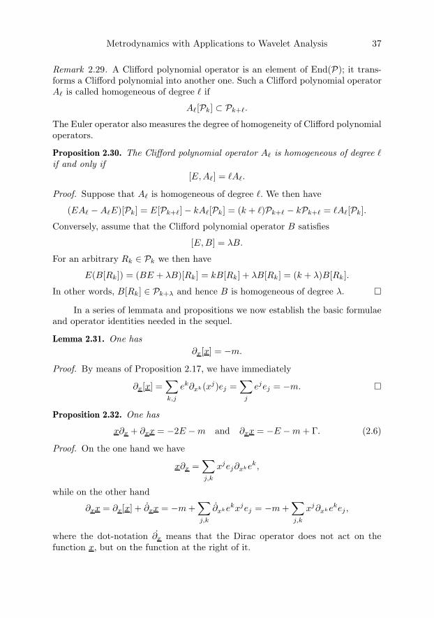
Metrodynamics with Applications to Wavelet Analysis 37
Remark 2.29. A Clifford polynomial operator is an element of End(P); it trans-forms a Clifford polynomial into another one. Such a Clifford polynomial operatorA is called homogeneous of degree if
A[Pk] ⊂ Pk+.
The Euler operator also measures the degree of homogeneity of Clifford polynomialoperators.
Proposition 2.30. The Clifford polynomial operator A is homogeneous of degree if and only if
[E, A] = A.
Proof. Suppose that A is homogeneous of degree . We then have
(EA −AE)[Pk] = E[Pk+]− kA[Pk] = (k + )Pk+ − kPk+ = A[Pk].
Conversely, assume that the Clifford polynomial operator B satisfies
[E, B] = λB.
For an arbitrary Rk ∈ Pk we then have
E(B[Rk]) = (BE + λB)[Rk] = kB[Rk] + λB[Rk] = (k + λ)B[Rk].
In other words, B[Rk] ∈ Pk+λ and hence B is homogeneous of degree λ.
In a series of lemmata and propositions we now establish the basic formulaeand operator identities needed in the sequel.
Lemma 2.31. One has∂x[x] = −m.
Proof. By means of Proposition 2.17, we have immediately
∂x[x] =∑k,j
ek∂xk(xj)ej =∑
j
ejej = −m.
Proposition 2.32. One has
x∂x + ∂xx = −2E −m and ∂xx = −E −m + Γ. (2.6)
Proof. On the one hand we have
x∂x =∑j,k
xjej∂xkek,
while on the other hand
∂xx = ∂x[x] + ∂xx = −m +∑j,k
∂xkekxjej = −m +∑j,k
xj∂xkekej ,
where the dot-notation ∂x means that the Dirac operator does not act on thefunction x, but on the function at the right of it.

38 F. Brackx, N. De Schepper and F. Sommen
Adding both equalities yields
x∂x + ∂xx = −m +∑j,k
xj∂xk(ejek + ekej)
= −m− 2∑j,k
xj∂xkδkj = −m− 2E.
Using (2.5) this becomes
∂xx = −x∂x − 2E −m = E + Γ− 2E −m = Γ− E −m.
Propositions 2.27 and 2.32 yield some nice additional results. The first corollaryfocuses on an interesting factorization of the g-Laplacian.
Corollary 2.33. One has
∆g = (E + m− Γ)1||x||2 (E + Γ).
Proof. By means of (2.5) and (2.6), we obtain
∆g = −∂2x = ∂x
x2
||x||2 ∂x = ∂x x1||x||2 x ∂x
= (E + m− Γ)1||x||2 (E + Γ).
Also the polynomials xPk are eigenfunctions of the angular Dirac operator.
Corollary 2.34. For any Pk ∈M+ (k) one has:
Γ[xPk] = (k + m− 1)xPk.
Proof. By means of (2.6) we obtain
x∂x[xPk] = x(−E −m + Γ)[Pk]
= x(−k −m− k)Pk = (−2k −m)xPk.
Using (2.5) and the fact that xPk ∈ Pk+1 gives
(−2k −m)xPk = −(E + Γ)[xPk] = −(k + 1)xPk − Γ[xPk].
HenceΓ[xPk] = (k + m− 1)xPk.
Lemma 2.35. One has(i) ∂xj [r] =
1rgjkxk , j = 1, . . . , m
(ii) ∂x[r] =x
r.

Metrodynamics with Applications to Wavelet Analysis 39
Proof. A straightforward computation yields
(i) ∂xj [r] = ∂xj
[(gikxixk
)1/2]
=12(gikxixk
)−1/2(gjkxk + gijx
i)
=12
1r2gjkxk =
1rgjkxk
(ii) ∂x[r] = ej∂xj [r] =1rejgjkxk =
1rekxk =
x
r.
Now it is easily proved that the angular Dirac operator only acts on the angularcoordinates, whence its name.
Lemma 2.36. One has(i) E[r] = r(ii) x∂x[r] = −r(iii) Γ[r] = 0.
Proof. By means of the previous Lemma we easily find
(i) E[r] = xj∂xj [r] = xj 1rgjkxk =
1rr2 = r.
(ii) x∂x[r] = xx
r= −r2
r= −r.
(iii) Γ[r] = −(x∂x + E)[r] = −(−r + r) = 0.
This enables us to prove the following eigenvalue equations.
Theorem 2.37. One has(i) E[xsPk] = (s + k)xsPk
(ii) Γ[x2sPk] = −kx2sPk
(iii) Γ[x2s+1Pk] = (k + m− 1)x2s+1Pk.
Proof. (i) Follows immediately from the fact that xsPk ∈ Ps+k .(ii) By means of the previous Lemma we find
Γ[x2sPk] = x2sΓ[Pk] = −kx2sPk.
(iii) Similarly we have
Γ[x2s+1Pk] = x2sΓ[xPk] = (k + m− 1)x2s+1Pk.
The previous Theorem combined with (2.6) yields the following result.
Theorem 2.38. One has∂x[xsPk] = Bs,k xs−1Pk
with
Bs,k =
−s for s even,
−(s− 1 + 2k + m) for s odd.
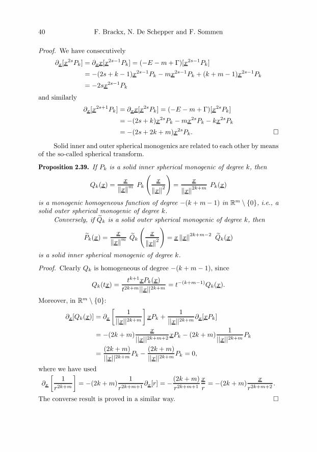
40 F. Brackx, N. De Schepper and F. Sommen
Proof. We have consecutively
∂x[x2sPk] = ∂xx[x2s−1Pk] = (−E −m + Γ)[x2s−1Pk]
= −(2s + k − 1)x2s−1Pk −mx2s−1Pk + (k + m− 1)x2s−1Pk
= −2sx2s−1Pk
and similarly
∂x[x2s+1Pk] = ∂xx[x2sPk] = (−E −m + Γ)[x2sPk]
= −(2s + k)x2sPk −mx2sPk − kx2sPk
= −(2s + 2k + m)x2sPk.
Solid inner and outer spherical monogenics are related to each other by meansof the so-called spherical transform.
Proposition 2.39. If Pk is a solid inner spherical monogenic of degree k, then
Qk(x) =x
‖x‖m Pk
(x
‖x‖2
)=
x
‖x‖2k+mPk(x)
is a monogenic homogeneous function of degree −(k + m− 1) in Rm \ 0, i.e., asolid outer spherical monogenic of degree k.
Conversely, if Qk is a solid outer spherical monogenic of degree k, then
Pk(x) =x
‖x‖m Qk
(x
‖x‖2
)= x ‖x‖2k+m−2
Qk(x)
is a solid inner spherical monogenic of degree k.
Proof. Clearly Qk is homogeneous of degree −(k + m− 1), since
Qk(tx) =tk+1xPk(x)
t2k+m||x||2k+m= t−(k+m−1)Qk(x).
Moreover, in Rm \ 0:
∂x[Qk(x)] = ∂x
[1
||x||2k+m
]xPk +
1||x||2k+m
∂x[xPk]
= −(2k + m)x
||x||2k+m+2xPk − (2k + m)
1||x||2k+m
Pk
=(2k + m)||x||2k+m
Pk −(2k + m)||x||2k+m
Pk = 0,
where we have used
∂x
[1
r2k+m
]= −(2k + m)
1r2k+m+1
∂x[r] = − (2k + m)r2k+m+1
x
r= −(2k + m)
x
r2k+m+2.
The converse result is proved in a similar way.
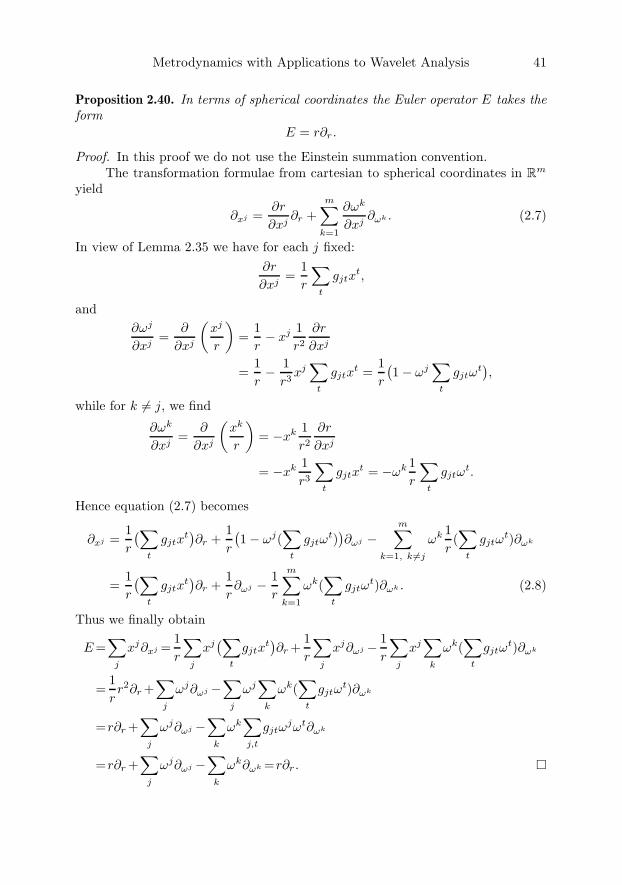
Metrodynamics with Applications to Wavelet Analysis 41
Proposition 2.40. In terms of spherical coordinates the Euler operator E takes theform
E = r∂r .
Proof. In this proof we do not use the Einstein summation convention.The transformation formulae from cartesian to spherical coordinates in R
m
yield
∂xj =∂r
∂xj∂r +
m∑k=1
∂ωk
∂xj∂ωk . (2.7)
In view of Lemma 2.35 we have for each j fixed:∂r
∂xj=
1r
∑t
gjtxt,
and∂ωj
∂xj=
∂
∂xj
(xj
r
)=
1r− xj 1
r2
∂r
∂xj
=1r− 1
r3xj∑
t
gjtxt =
1r
(1− ωj
∑t
gjtωt),
while for k = j, we find
∂ωk
∂xj=
∂
∂xj
(xk
r
)= −xk 1
r2
∂r
∂xj
= −xk 1r3
∑t
gjtxt = −ωk 1
r
∑t
gjtωt.
Hence equation (2.7) becomes
∂xj =1r
(∑t
gjtxt)∂r +
1r
(1− ωj(
∑t
gjtωt))∂ωj −
m∑k=1, k =j
ωk 1r(∑
t
gjtωt)∂ωk
=1r
(∑t
gjtxt)∂r +
1r∂ωj − 1
r
m∑k=1
ωk(∑
t
gjtωt)∂ωk . (2.8)
Thus we finally obtain
E =∑
j
xj∂xj =1r
∑j
xj(∑
t
gjtxt)∂r +
1r
∑j
xj∂ωj − 1r
∑j
xj∑
k
ωk(∑
t
gjtωt)∂ωk
=1rr2∂r +
∑j
ωj∂ωj −∑
j
ωj∑
k
ωk(∑
t
gjtωt)∂ωk
=r∂r +∑
j
ωj∂ωj −∑
k
ωk∑j,t
gjtωjωt∂ωk
=r∂r +∑
j
ωj∂ωj −∑
k
ωk∂ωk =r∂r .
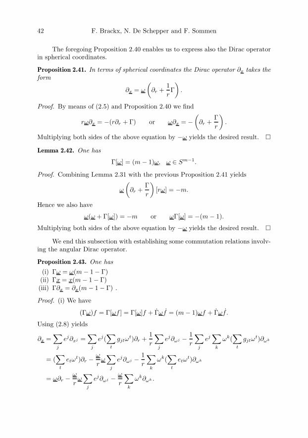
42 F. Brackx, N. De Schepper and F. Sommen
The foregoing Proposition 2.40 enables us to express also the Dirac operatorin spherical coordinates.
Proposition 2.41. In terms of spherical coordinates the Dirac operator ∂x takes theform
∂x = ω
(∂r +
1rΓ)
.
Proof. By means of (2.5) and Proposition 2.40 we find
rω∂x = −(r∂r + Γ) or ω∂x = −(
∂r +Γr
).
Multiplying both sides of the above equation by −ω yields the desired result.
Lemma 2.42. One has
Γ[ω] = (m− 1)ω, ω ∈ Sm−1.
Proof. Combining Lemma 2.31 with the previous Proposition 2.41 yields
ω
(∂r +
Γr
)[rω] = −m.
Hence we also have
ω(ω + Γ[ω]) = −m or ωΓ[ω] = −(m− 1).
Multiplying both sides of the above equation by −ω yields the desired result.
We end this subsection with establishing some commutation relations involv-ing the angular Dirac operator.
Proposition 2.43. One has(i) Γω = ω(m− 1− Γ)(ii) Γx = x(m− 1− Γ)(iii) Γ∂x = ∂x(m− 1− Γ) .
Proof. (i) We have
(Γω)f = Γ[ωf ] = Γ[ω]f + Γωf = (m− 1)ωf + Γωf.
Using (2.8) yields
∂x =∑
j
ej∂xj =∑
j
ej(∑
t
gjtωt)∂r +
1r
∑j
ej∂ωj − 1r
∑j
ej∑
k
ωk(∑
t
gjtωt)∂ωk
= (∑
t
etωt)∂r −
ω
rω∑
j
ej∂ωj − 1r
∑k
ωk(∑
t
etωt)∂ωk
= ω∂r −ω
rω∑
j
ej∂ωj − ω
r
∑k
ωk∂ωk .
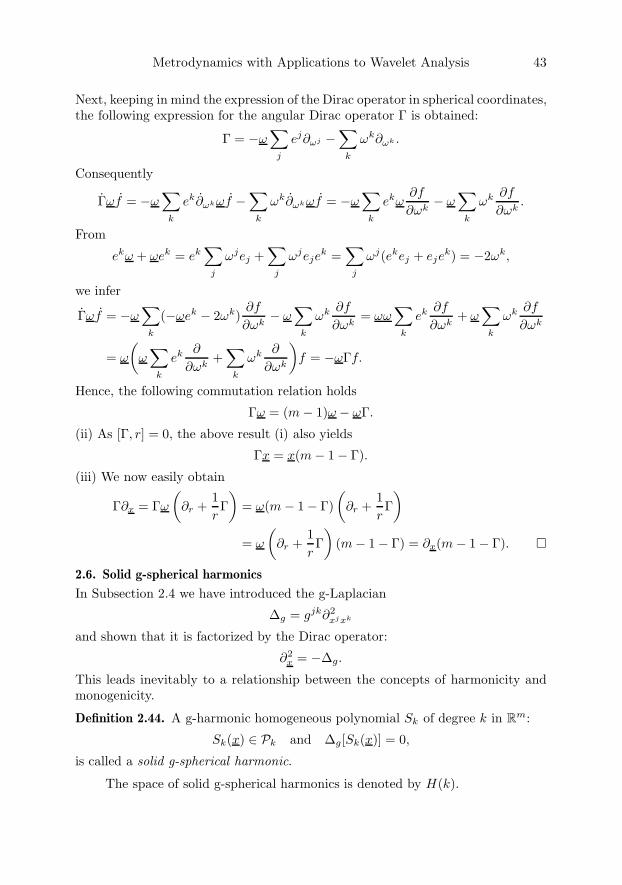
Metrodynamics with Applications to Wavelet Analysis 43
Next, keeping in mind the expression of the Dirac operator in spherical coordinates,the following expression for the angular Dirac operator Γ is obtained:
Γ = −ω∑
j
ej∂ωj −∑
k
ωk∂ωk .
Consequently
Γωf = −ω∑
k
ek∂ωkωf −∑
k
ωk∂ωkωf = −ω∑
k
ekω∂f
∂ωk− ω
∑k
ωk ∂f
∂ωk.
From
ekω + ωek = ek∑
j
ωjej +∑
j
ωjejek =
∑j
ωj(ekej + ejek) = −2ωk,
we infer
Γωf = −ω∑
k
(−ωek − 2ωk)∂f
∂ωk− ω
∑k
ωk ∂f
∂ωk= ωω
∑k
ek ∂f
∂ωk+ ω
∑k
ωk ∂f
∂ωk
= ω
(ω∑
k
ek ∂
∂ωk+∑
k
ωk ∂
∂ωk
)f = −ωΓf.
Hence, the following commutation relation holds
Γω = (m− 1)ω − ωΓ.
(ii) As [Γ, r] = 0, the above result (i) also yields
Γx = x(m− 1− Γ).
(iii) We now easily obtain
Γ∂x = Γω
(∂r +
1rΓ)
= ω(m− 1− Γ)(
∂r +1rΓ)
= ω
(∂r +
1rΓ)
(m− 1− Γ) = ∂x(m− 1− Γ).
2.6. Solid g-spherical harmonics
In Subsection 2.4 we have introduced the g-Laplacian
∆g = gjk∂2xjxk
and shown that it is factorized by the Dirac operator:
∂2x = −∆g.
This leads inevitably to a relationship between the concepts of harmonicity andmonogenicity.
Definition 2.44. A g-harmonic homogeneous polynomial Sk of degree k in Rm:
Sk(x) ∈ Pk and ∆g[Sk(x)] = 0,
is called a solid g-spherical harmonic.
The space of solid g-spherical harmonics is denoted by H(k).
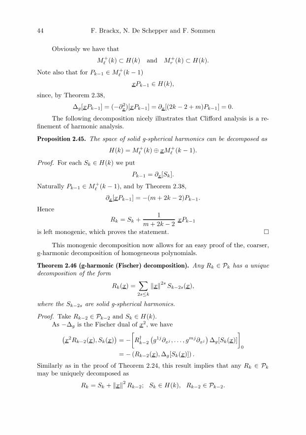
44 F. Brackx, N. De Schepper and F. Sommen
Obviously we have that
M+ (k) ⊂ H(k) and M+
r (k) ⊂ H(k).
Note also that for Pk−1 ∈M+ (k − 1)
xPk−1 ∈ H(k),
since, by Theorem 2.38,
∆g[xPk−1] = (−∂2x)[xPk−1] = ∂x[(2k − 2 + m)Pk−1] = 0.
The following decomposition nicely illustrates that Clifford analysis is a re-finement of harmonic analysis.
Proposition 2.45. The space of solid g-spherical harmonics can be decomposed as
H(k) = M+ (k)⊕ xM+
(k − 1).
Proof. For each Sk ∈ H(k) we put
Pk−1 = ∂x[Sk].
Naturally Pk−1 ∈M+ (k − 1), and by Theorem 2.38,
∂x[xPk−1] = −(m + 2k − 2)Pk−1.
Hence
Rk = Sk +1
m + 2k − 2xPk−1
is left monogenic, which proves the statement.
This monogenic decomposition now allows for an easy proof of the, coarser,g-harmonic decomposition of homogeneous polynomials.
Theorem 2.46 (g-harmonic (Fischer) decomposition). Any Rk ∈ Pk has a uniquedecomposition of the form
Rk(x) =∑2s≤k
‖x‖2sSk−2s(x),
where the Sk−2s are solid g-spherical harmonics.
Proof. Take Rk−2 ∈ Pk−2 and Sk ∈ H(k).As −∆g is the Fischer dual of x2, we have(
x2Rk−2(x), Sk(x))
= −[R†
k−2
(g1j∂xj , . . . , gmj∂xj
)∆g[Sk(x)]
]0
= − (Rk−2(x), ∆g[Sk(x)]) .
Similarly as in the proof of Theorem 2.24, this result implies that any Rk ∈ Pk
may be uniquely decomposed as
Rk = Sk + ‖x‖2 Rk−2; Sk ∈ H(k), Rk−2 ∈ Pk−2.

Metrodynamics with Applications to Wavelet Analysis 45
Recursive application of the above result then indeed yields:
Rk(x) =∑2s≤k
‖x‖2sSk−2s(x) with Sk−2s ∈ H(k − 2s).
We end this subsection with the introduction of the so-called g-Laplace-Beltrami-operator.
We start from the decomposition of the g-Laplacian established in Corollary2.33 and pass on to spherical coordinates:
∆g = (r∂r + m− Γ)1r2
(r∂r + Γ)
= r∂r1r2
(r∂r + Γ) +m
r2(r∂r + Γ)− Γ
1r2
(r∂r + Γ)
= r(−2)1r3
(r∂r + Γ) +1r∂r(r∂r + Γ) +
m
r∂r +
m
r2Γ− Γ
1r∂r −
1r2
Γ2
= −2r∂r −
2r2
Γ +1r∂r + ∂2
r +1r∂rΓ +
m
r∂r +
m
r2Γ− 1
r∂rΓ−
1r2
Γ2
= ∂2r +
(m− 1)r
∂r +1r2
[(m− 2)Γ− Γ2]
or finally
∆g = ∂2r +
m− 1r
∂r +1r2
∆∗g,
where we have put∆∗
g =((m− 2)− Γ
)Γ.
The operator ∆∗g is called the g-Laplace-Beltrami operator. Note that this operator
commutes with the angular Dirac operator:
[Γ, ∆∗g] = 0.
It follows that also the g-Laplace operator commutes with the angular Dirac op-erator:
[Γ, ∆g] = 0.
2.7. The g-Fourier transform
Let h be a positive function on Rm. Then we consider the Clifford algebra-valuedinner product
〈f, g〉 =∫
Rm
h(x) f †(x) g(x) dxM
where dxM stands for the Lebesgue measure on Rm; the associated norm thenreads
‖f‖2 = [〈f, f〉]0.The unitary right Clifford-module of Clifford algebra-valued measurable functionson Rm for which ‖f‖2 <∞ is a right Hilbert-Clifford-module which we denote byL2(Rm, h(x) dxM ).

46 F. Brackx, N. De Schepper and F. Sommen
In particular, taking h(x) ≡ 1, we obtain the right Hilbert-module of square inte-grable functions:
L2
(R
m, dxM)
=
f : Lebesgue measurable in Rm for which
‖f‖2 =(∫
Rm
|f(x)|20 dxM
)1/2
<∞
.
Naturally, L1
(Rm, dxM
)denotes the right Clifford-module of integrable functions:
L1
(R
m, dxM)
=
f : Lebesgue measurable in Rm for which
‖f‖1 =∫
Rm
|f(x)|0 dxM <∞
.
Now we define a g-Fourier transform on L1(Rm, dxM )-functions, which by aclassical argument may be extended to L2(Rm, dxM ).
This g-Fourier transform of f , denoted by Fg[f ], is defined by:
Fg[f ](y) =(
1√2π
)m ∫Rm
exp (−i〈x, y〉) f(x) dxM
=(
1√2π
)m ∫Rm
exp (−igjkxjyk) f(x1, . . . , xm) dxM .
To show that this definition is meaningful in this metric dependent context, it isimmediately checked how this g-Fourier transform behaves with respect to mul-tiplication with the variable x and, by duality, with respect to the action of theDirac operator.
Proposition 2.47. The g-Fourier transform Fg satisfies:
(i) the multiplication rule: Fg[xf(x)](y) = i∂y Fg[f(x)](y);
(ii) the differentiation rule: Fg[∂xf(x)](y) = iy Fg[f(x)](y).
Proof. We have consecutively
(i) Fg[xf(x)](y) =∑
j
ej
(1√2π
)m ∫Rm
exp (−i〈x, y〉) xj f(x) dxM
=∑j,k
gjkek
(1√2π
)m ∫Rm
exp (−i〈x, y〉) xj f(x) dxM
=∑
k
ek
(1√2π
)m ∫Rm
exp (−i〈x, y〉)∑
j
gjkxj f(x) dxM
=∑
k
ek
(1√2π
)m ∫Rm
i∂yk
[exp (−i〈x, y〉)
]f(x) dxM
= i∂y Fg[f(x)](y).
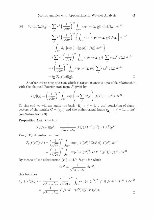
Metrodynamics with Applications to Wavelet Analysis 47
(ii) Fg[∂xf(x)](y) =∑
j
ej
(1√2π
)m ∫Rm
exp (−i〈x, y〉) ∂xj [f(x)] dxM
=∑
j
ej
(1√2π
)m ∫Rm
∂xj
[exp (−i〈x, y〉) f(x)
]dxM
−∫
Rm
∂xj
[exp (−i〈x, y〉)
]f(x) dxM
= i
∑j
ej
(1√2π
)m ∫Rm
exp (−i〈x, y〉)∑
k
gjkyk f(x) dxM
= i
(1√2π
)m ∫Rm
exp (−i〈x, y〉)∑
k
ekyk f(x) dxM
= iy Fg[f(x)](y).
Another interesting question which is raised at once is a possible relationshipwith the classical Fourier transform F given by
F [f ](y) =(
1√2π
)m ∫Rm
exp
⎛⎝−i∑
j
xjyj
⎞⎠ f(x1, . . . , xm) dxM .
To this end we will use again the basis (Ej : j = 1, . . . , m) consisting of eigen-vectors of the matrix G = (gjk) and the orthonormal frame (η
j: j = 1, . . . , m)
(see Subsection 2.3).
Proposition 2.48. One has
Fg[f(xj)](yj) =1√
λ1 . . . λm
F [f(AP−1(x′j))](PAT (yj)).
Proof. By definition we have
Fg[f(xj)](yj) =(
1√2π
)m ∫Rm
exp(−i((xj)T G(yj))
)f(xj) dxM
=(
1√2π
)m ∫Rm
exp(−i((xj)T GAP−1(y′j))
)f(xj) dxM .
By means of the substitution (xj) = AP−1(x′j) for which
dxM =1√
λ1 . . . λm
dx′M ,
this becomes
Fg[f(xj)](yj) =1√
λ1 . . . λm
(1√2π
)m ∫Rm
exp (−i(x′j)T (y′j)) f(AP−1(x′j)) dx′M
=1√
λ1 . . . λm
F [f(AP−1(x′j))](PAT (yj)).
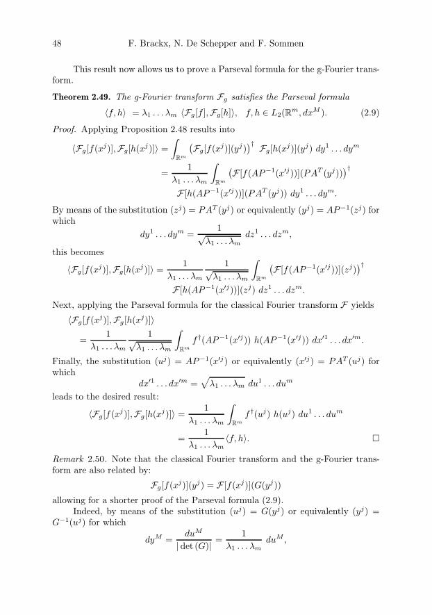
48 F. Brackx, N. De Schepper and F. Sommen
This result now allows us to prove a Parseval formula for the g-Fourier trans-form.
Theorem 2.49. The g-Fourier transform Fg satisfies the Parseval formula
〈f, h〉 = λ1 . . . λm 〈Fg[f ],Fg[h]〉, f, h ∈ L2(Rm, dxM ). (2.9)
Proof. Applying Proposition 2.48 results into
〈Fg[f(xj)],Fg[h(xj)]〉 =∫
Rm
(Fg[f(xj)](yj)
)† Fg[h(xj)](yj) dy1 . . . dym
=1
λ1 . . . λm
∫Rm
(F [f(AP−1(x′j))](PAT (yj))
)†F [h(AP−1(x′j))](PAT (yj)) dy1 . . . dym.
By means of the substitution (zj) = PAT (yj) or equivalently (yj) = AP−1(zj) forwhich
dy1 . . . dym =1√
λ1 . . . λm
dz1 . . . dzm,
this becomes
〈Fg[f(xj)],Fg[h(xj)]〉 =1
λ1 . . . λm
1√λ1 . . . λm
∫Rm
(F [f(AP−1(x′j))](zj)
)†F [h(AP−1(x′j))](zj) dz1 . . . dzm.
Next, applying the Parseval formula for the classical Fourier transform F yields
〈Fg[f(xj)],Fg[h(xj)]〉
=1
λ1 . . . λm
1√λ1 . . . λm
∫Rm
f †(AP−1(x′j)) h(AP−1(x′j)) dx′1 . . . dx′m.
Finally, the substitution (uj) = AP−1(x′j) or equivalently (x′j) = PAT (uj) forwhich
dx′1 . . . dx′m =√
λ1 . . . λm du1 . . . dum
leads to the desired result:
〈Fg[f(xj)],Fg[h(xj)]〉 =1
λ1 . . . λm
∫Rm
f †(uj) h(uj) du1 . . . dum
=1
λ1 . . . λm〈f, h〉.
Remark 2.50. Note that the classical Fourier transform and the g-Fourier trans-form are also related by:
Fg[f(xj)](yj) = F [f(xj)](G(yj))
allowing for a shorter proof of the Parseval formula (2.9).Indeed, by means of the substitution (uj) = G(yj) or equivalently (yj) =
G−1(uj) for which
dyM =duM
| det (G)| =1
λ1 . . . λmduM ,
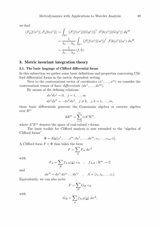
Metrodynamics with Applications to Wavelet Analysis 49
we find
〈Fg[f(xj)],Fg[h(xj)]〉 =∫
Rm
(F [f(xj)](G(yj))
)† F [h(xj)](G(yj)) dyM
=1
λ1 . . . λm
∫Rm
(F [f(xj)](uj)
)† F [h(xj)](uj) duM
=1
λ1 . . . λm〈f, h〉.
3. Metric invariant integration theory
3.1. The basic language of Clifford differential forms
In this subsection we gather some basic definitions and properties concerning Clif-ford differential forms in the metric dependent setting.
Next to the contravariant vector of coordinates (x1, . . . , xm) we consider thecontravariant tensor of basic differentials (dx1, . . . , dxm).
By means of the defining relations:
dxjdxj = 0, j = 1, . . . , m
dxjdxk = −dxkdxj , j = k, j, k = 1, . . . , m,
these basic differentials generate the Grassmann algebra or exterior algebraover Rm
ΛRm =
m∑r=0
⊕ΛrR
m,
where ΛrRm denotes the space of real-valued r-forms.The basic toolkit for Clifford analysis is now extended to the “algebra of
Clifford forms”
Φ = Algx1, . . . , xm; dx1, . . . , dxm; e1, . . . , em; i.A Clifford form F ∈ Φ thus takes the form
F =∑A
FA dxA
withFA =
∑B
fA,B(x) eB , fA,B : Rm → C
anddxA = dxi1dxi2 . . . dxir , A = (i1, i2, . . . , ir).
Equivalently, we can also write
F =∑B
GB eB
withGB =
∑A
fA,B(x) dxA.

50 F. Brackx, N. De Schepper and F. Sommen
The exterior derivative d is defined by means of the following axioms: for aC1-form F ∈ Φ one has
(A1) d(xjF ) = dxjF + xj dF(A2) d(dxjF ) = −dxjdF(A3) d(ejF ) = ej dF.
We also have the property d2 = 0 and with respect to the local coordinate system,d may be expressed as:
d = ∂xj dxj .
Hence for a C1-form F =∑
A FA dxA we have
dF =∑A
∑j
∂xj [FA] dxjdxA.
We also mention the following basic result, perhaps the most fundamental andmost intriguing theorem in mathematical analysis.
Theorem 3.1 (Stokes’s theorem). Let Σ be an oriented k-surface in Rm and F a
continuously differentiable (k − 1)-form. Then one has:∫∂Σ
F =∫
Σ
dF.
Next we define the basic contraction operators, determined by the relations(C1) ∂xj(xkF ) = xk ∂xjF(C2) ∂xj(dxkF ) = δk
j F − dxk∂xjF .
Note that, due to (C2), the contraction operators ∂xj are in fact a kind of de-rivative with respect to the generators dxj . They are sometimes called fermionicderivatives.
The Dirac contraction operator is given by
∂x = ej∂xj.
Before discussing the notion of directional derivative and Lie derivative, wemust point out a subtle difference between vector fields and Clifford vector fields.In differential geometry an operator of the form
v = vj(x) ∂xj , vj : Rm → C (3.1)
is called a ”vector field with components vj”, whereas a Clifford vector field hasthe form
v = vj(x) ej , vj : Rm → C.
For a survey paper on differential forms versus multi-vector functions, see [3].Moreover, in Clifford analysis one may even consider vector fields (3.1) with
Cm-valued components vj , which leads to several new interesting possibilities.First of all, given a Clifford vector field
v = vj(x) ∂xj , vj : Rm → Cm,
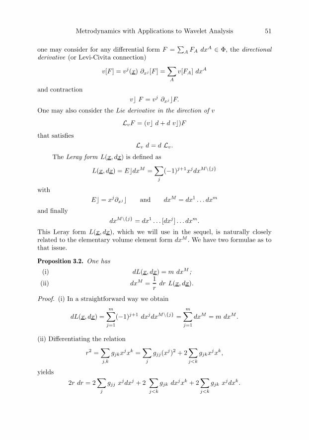
Metrodynamics with Applications to Wavelet Analysis 51
one may consider for any differential form F =∑
A FA dxA ∈ Φ, the directionalderivative (or Levi-Civita connection)
v[F ] = vj(x) ∂xj [F ] =∑A
v[FA] dxA
and contractionv F = vj ∂xjF.
One may also consider the Lie derivative in the direction of v
LvF = (v d + d v)F
that satisfiesLv d = d Lv.
The Leray form L(x, dx) is defined as
L(x, dx) = EdxM =∑
j
(−1)j+1xjdxM\j
withE = xj∂xj and dxM = dx1 . . . dxm
and finallydxM\j = dx1 . . . [dxj ] . . . dxm.
This Leray form L(x, dx), which we will use in the sequel, is naturally closelyrelated to the elementary volume element form dxM . We have two formulae as tothat issue.
Proposition 3.2. One has
(i) dL(x, dx) = m dxM ;
(ii) dxM =1r
dr L(x, dx).
Proof. (i) In a straightforward way we obtain
dL(x, dx) =m∑
j=1
(−1)j+1 dxjdxM\j =m∑
j=1
dxM = m dxM .
(ii) Differentiating the relation
r2 =∑j,k
gjkxjxk =∑
j
gjj(xj)2 + 2∑j<k
gjkxjxk,
yields
2r dr = 2∑
j
gjj xjdxj + 2∑j<k
gjk dxjxk + 2∑j<k
gjk xjdxk.

52 F. Brackx, N. De Schepper and F. Sommen
Hence we have
r dr L(x, dx)
=∑
j
gjj xj dxj
(∑i
(−1)i+1xidxM\i)
+∑j<k
gjk xk dxj
(∑i
(−1)i+1xi dxM\i)
+∑j<k
gjk xj dxk
(∑i
(−1)i+1xidxM\i)
=∑
j
gjj (xj)2 (−1)j+1dxjdxM\j +∑j<k
gjk xkxj (−1)j+1 dxjdxM\j
+∑j<k
gjk xjxk (−1)k+1 dxkdxM\k
=∑
j
gjj (xj)2dxM +∑j<k
gjk xkxjdxM +∑j<k
gjk xjxkdxM
=
⎛⎝∑j
gjj (xj)2 + 2∑j<k
gjk xjxk
⎞⎠ dxM
= r2 dxM ,
which proves the statement. It is clear that the Leray form is homogeneous of degree m, i.e., it transforms
likeL(λx, d(λx)
)= L(λx, λdx + xdλ) = λm L(x, dx).
Hence, we define the associated Leray form of degree 0:
L(ω, dω) :=L(x, dx)
rm, ω ∈ Sm−1,
so that, by Proposition 3.2
dxM = rm−1 dr L(ω, dω).
The last differential form needed, is the so-called sigma form σ(x, dx), de-fined as
σ(x, dx) = ∂x dxM =∑
j
(−1)j+1ejdxM\j
and we shall see that it can be interpreted as the oriented surface element on ahypersurface.
A first auxiliary property reads as follows.
Lemma 3.3. One hasdσ(x, dx) = 0.
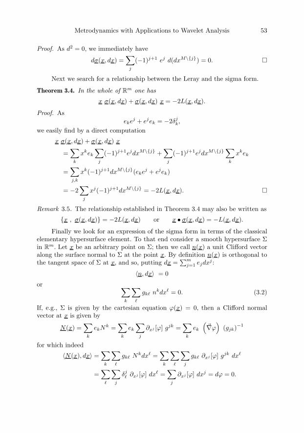
Metrodynamics with Applications to Wavelet Analysis 53
Proof. As d2 = 0, we immediately have
dσ(x, dx) =∑
j
(−1)j+1 ej d(dxM\j) = 0.
Next we search for a relationship between the Leray and the sigma form.
Theorem 3.4. In the whole of Rm one has
x σ(x, dx) + σ(x, dx) x = −2L(x, dx).
Proof. Asekej + ejek = −2δj
k,
we easily find by a direct computation
x σ(x, dx) + σ(x, dx) x
=∑
k
xkek
∑j
(−1)j+1ejdxM\j +∑
j
(−1)j+1ejdxM\j ∑k
xkek
=∑j,k
xk(−1)j+1dxM\j(ekej + ejek)
= −2∑
j
xj(−1)j+1dxM\j = −2L(x, dx).
Remark 3.5. The relationship established in Theorem 3.4 may also be written as
x , σ(x, dx) = −2L(x, dx) or x • σ(x, dx) = −L(x, dx).
Finally we look for an expression of the sigma form in terms of the classicalelementary hypersurface element. To that end consider a smooth hypersurface Σin Rm. Let x be an arbitrary point on Σ; then we call n(x) a unit Clifford vectoralong the surface normal to Σ at the point x. By definition n(x) is orthogonal tothe tangent space of Σ at x, and so, putting dx =
∑mj=1 ejdxj :
〈n, dx〉 = 0
or ∑k
∑
gk nkdx = 0. (3.2)
If, e.g., Σ is given by the cartesian equation ϕ(x) = 0, then a Clifford normalvector at x is given by
N(x) =∑
k
ekNk =∑
k
ek
∑j
∂xj [ϕ] gjk =∑
k
ek
(∇ϕ
)(gjk)−1
for which indeed
〈N(x), dx〉 =∑
k
∑
gk Nkdx =∑
k
∑
∑j
gk ∂xj [ϕ] gjk dx
=∑
∑j
δj ∂xj [ϕ] dx =
∑j
∂xj [ϕ] dxj = dϕ = 0.

54 F. Brackx, N. De Schepper and F. Sommen
Note that N(x) is not a unit vector since
‖N(x)‖2 = 〈N(x), N(x)〉 =∑
j
∑k
gjk N jNk
=∑
j
∑k
∑t
∑s
gjk ∂xt [ϕ] gtj ∂xs [ϕ] gsk
=∑
k
∑t
∑s
δtk ∂xt [ϕ] ∂xs [ϕ] gsk =
∑t
∑s
∂xt [ϕ] ∂xs [ϕ] gst
and hence
n(x) =
∑k
∑j ek ∂xj [ϕ] gjk(∑
k
∑j ∂xk [ϕ] ∂xj [ϕ] gjk
)1/2.
Now it may be proved that the sigma form is also orthogonal to the tangent spaceor, equivalently, that the sigma form lies along the surface normal at the pointconsidered.
Proposition 3.6. Let Σ be a smooth hypersurface and n(x) a unit normal Cliffordvector at x ∈ Σ, then
n(x) ∧ σ(x, dx) = 0.
Proof. By definition we have
n(x) ∧ σ(x, dx) =
(∑k
eknk
)∧
⎛⎝∑j
(−1)j+1ejdxM\j
⎞⎠=
⎛⎝∑k,t
gkt etnk
⎞⎠ ∧⎛⎝∑
j
(−1)j+1ejdxM\j
⎞⎠=∑
k
nk∑t,j
(−1)j+1gkt et ∧ ej dxM\j. (3.3)
Note that the above expression is a Clifford bivector; furthermore, as ej ∧ ej = 0,only the terms with t = j remain.
Take such a t and j fixed with, for example, t < j and consider the coefficientof the bivector et ∧ ej .
In view of the anti-commutativity of the outer product
et ∧ ej = −ej ∧ et,
this coefficient takes the form∑k
nk (−1)j+1gkt dxM\j −∑
k
nk (−1)t+1gkj dxM\t.
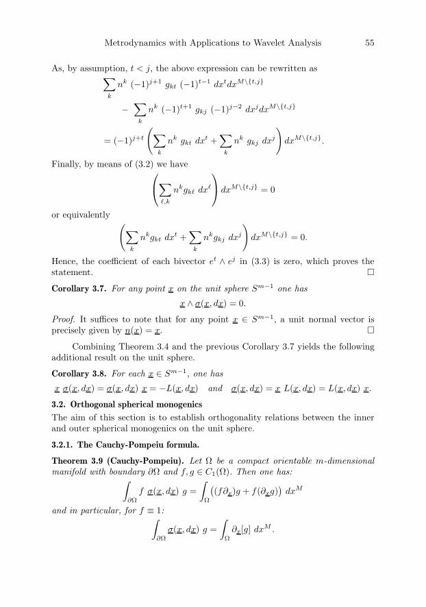
Metrodynamics with Applications to Wavelet Analysis 55
As, by assumption, t < j, the above expression can be rewritten as∑k
nk (−1)j+1 gkt (−1)t−1 dxtdxM\t,j
−∑
k
nk (−1)t+1 gkj (−1)j−2 dxjdxM\t,j
= (−1)j+t
(∑k
nk gkt dxt +∑
k
nk gkj dxj
)dxM\t,j.
Finally, by means of (3.2) we have⎛⎝∑,k
nkgk dx
⎞⎠ dxM\t,j = 0
or equivalently (∑k
nkgkt dxt +∑
k
nkgkj dxj
)dxM\t,j = 0.
Hence, the coefficient of each bivector et ∧ ej in (3.3) is zero, which proves thestatement. Corollary 3.7. For any point x on the unit sphere Sm−1 one has
x ∧ σ(x, dx) = 0.
Proof. It suffices to note that for any point x ∈ Sm−1, a unit normal vector isprecisely given by n(x) = x.
Combining Theorem 3.4 and the previous Corollary 3.7 yields the followingadditional result on the unit sphere.
Corollary 3.8. For each x ∈ Sm−1, one has
x σ(x, dx) = σ(x, dx) x = −L(x, dx) and σ(x, dx) = x L(x, dx) = L(x, dx) x.
3.2. Orthogonal spherical monogenics
The aim of this section is to establish orthogonality relations between the innerand outer spherical monogenics on the unit sphere.
3.2.1. The Cauchy-Pompeiu formula.
Theorem 3.9 (Cauchy-Pompeiu). Let Ω be a compact orientable m-dimensionalmanifold with boundary ∂Ω and f, g ∈ C1(Ω). Then one has:∫
∂Ω
f σ(x, dx) g =∫
Ω
((f∂x)g + f(∂xg)
)dxM
and in particular, for f ≡ 1:∫∂Ω
σ(x, dx) g =∫
Ω
∂x[g] dxM .

56 F. Brackx, N. De Schepper and F. Sommen
Proof. Taking into account that the sigma form is an (m − 1)-form, for whichmoreover dσ(x, dx) = 0 (see Lemma 3.3), we have
d(f σ(x, dx) g) = d(f σ(x, dx)
)g + (−1)m−1f σ(x, dx) dg
= df σ(x, dx) g + (−1)m−1f σ(x, dx) dg
=∑
j
∂xj [f ] dxj σ(x, dx) g
+ (−1)m−1 f σ(x, dx)(∑
j
dxj ∂xj [g]). (3.4)
Now for each j = 1, 2, . . . , m fixed, we obtain
dxj σ(x, dx) = dxj(∑
k
(−1)k+1ekdxM\k)
=∑
k
(−1)k+1ekdxjdxM\k
=∑
k
(−1)k+1ek(−1)j−1dxM δj,k = ejdxM
and similarly
σ(x, dx) dxj =∑
k
(−1)k+1ekdxM\kdxj =∑
k
(−1)k+1ek(−1)m−jdxMδj,k
= (−1)m+1ejdxM .
Hence, (3.4) becomes
d(f σ(x, dx) g) =∑
j
∂xj [f ] ejg dxM + f∑
j
ej∂xj [g] dxM
= (f∂x)g dxM + f(∂xg) dxM .
Consequently, by means of Stokes’s theorem (Theorem 3.1) we indeed obtain∫∂Ω
f σ(x, dx) g =∫
Ω
d(f σ(x, dx) g)
=∫
Ω
[(f∂x)g + f(∂xg)] dxM .
The Cauchy-Pompeiu formula immediately yields the following fundamental result.
Corollary 3.10 (Cauchy’s theorem). Let Ω be a compact orientable m-dimensionalmanifold with boundary ∂Ω. If f is right monogenic in Ω and g is left monogenicin Ω, one has: ∫
∂Ω
f σ(x, dx) g = 0.
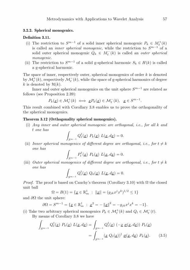
Metrodynamics with Applications to Wavelet Analysis 57
3.2.2. Spherical monogenics.
Definition 3.11.
(i) The restriction to Sm−1 of a solid inner spherical monogenic Pk ∈ M+ (k)
is called an inner spherical monogenic, while the restriction to Sm−1 of asolid outer spherical monogenic Qk ∈ M−
(k) is called an outer sphericalmonogenic.
(ii) The restriction to Sm−1 of a solid g-spherical harmonic Sk ∈ H(k) is calleda g-spherical harmonic.
The space of inner, respectively outer, spherical monogenics of order k is denotedbyM+
(k), respectivelyM− (k), while the space of g-spherical harmonics of degree
k is denoted by H(k).Inner and outer spherical monogenics on the unit sphere Sm−1 are related as
follows (see Proposition 2.39):
Pk(x) ∈M+ (k) ⇐⇒ xPk(x) ∈M−
(k), x ∈ Sm−1.
This result combined with Corollary 3.8 enables us to prove the orthogonality ofthe spherical monogenics.
Theorem 3.12 (Orthogonality spherical monogenics).
(i) Any inner and outer spherical monogenic are orthogonal, i.e., for all k andt one has ∫
Sm−1Q†
t(x) Pk(x) L(x, dx) = 0.
(ii) Inner spherical monogenics of different degree are orthogonal, i.e., for t = kone has ∫
Sm−1P †
t (x) Pk(x) L(x, dx) = 0.
(iii) Outer spherical monogenics of different degree are orthogonal, i.e., for t = kone has ∫
Sm−1Q†
t(x) Qk(x) L(x, dx) = 0.
Proof. The proof is based on Cauchy’s theorem (Corollary 3.10) with Ω the closedunit ball
Ω = B(1) = x ∈ R1m : ‖x‖ = (gjkxjxk)1/2 ≤ 1
and ∂Ω the unit sphere:
∂Ω = Sm−1 = x ∈ R1m : x2 = −‖x‖2 = −gjkxjxk = −1.
(i) Take two arbitrary spherical monogenics Pk ∈ M+ (k) and Qt ∈M−
(t).By means of Corollary 3.8 we have∫
Sm−1Q†
t(x) Pk(x) L(x, dx) =∫
Sm−1Q†
t(x) (−x σ(x, dx)) Pk(x)
=∫
Sm−1(x Qt(x))† σ(x, dx) Pk(x). (3.5)
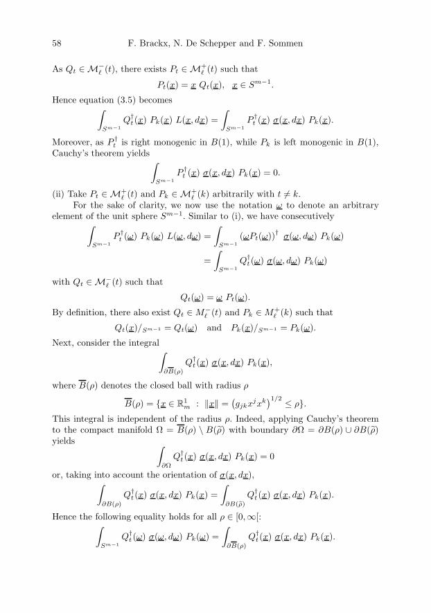
58 F. Brackx, N. De Schepper and F. Sommen
As Qt ∈M− (t), there exists Pt ∈ M+
(t) such that
Pt(x) = x Qt(x), x ∈ Sm−1.
Hence equation (3.5) becomes∫Sm−1
Q†t(x) Pk(x) L(x, dx) =
∫Sm−1
P †t (x) σ(x, dx) Pk(x).
Moreover, as P †t is right monogenic in B(1), while Pk is left monogenic in B(1),
Cauchy’s theorem yields∫Sm−1
P †t (x) σ(x, dx) Pk(x) = 0.
(ii) Take Pt ∈M+ (t) and Pk ∈M+
(k) arbitrarily with t = k.For the sake of clarity, we now use the notation ω to denote an arbitrary
element of the unit sphere Sm−1. Similar to (i), we have consecutively∫Sm−1
P †t (ω) Pk(ω) L(ω, dω) =
∫Sm−1
(ωPt(ω))† σ(ω, dω) Pk(ω)
=∫
Sm−1Q†
t(ω) σ(ω, dω) Pk(ω)
with Qt ∈M− (t) such that
Qt(ω) = ω Pt(ω).
By definition, there also exist Qt ∈M− (t) and Pk ∈M+
(k) such that
Qt(x)/Sm−1 = Qt(ω) and Pk(x)/Sm−1 = Pk(ω).
Next, consider the integral∫∂B(ρ)
Q†t(x) σ(x, dx) Pk(x),
where B(ρ) denotes the closed ball with radius ρ
B(ρ) = x ∈ R1m : ‖x‖ =
(gjkxjxk
)1/2 ≤ ρ.This integral is independent of the radius ρ. Indeed, applying Cauchy’s theoremto the compact manifold Ω = B(ρ) \ B(ρ) with boundary ∂Ω = ∂B(ρ) ∪ ∂B(ρ)yields ∫
∂Ω
Q†t(x) σ(x, dx) Pk(x) = 0
or, taking into account the orientation of σ(x, dx),∫∂B(ρ)
Q†t(x) σ(x, dx) Pk(x) =
∫∂B(ρ)
Q†t(x) σ(x, dx) Pk(x).
Hence the following equality holds for all ρ ∈ [0,∞[:∫Sm−1
Q†t (ω) σ(ω, dω) Pk(ω) =
∫∂B(ρ)
Q†t(x) σ(x, dx) Pk(x).
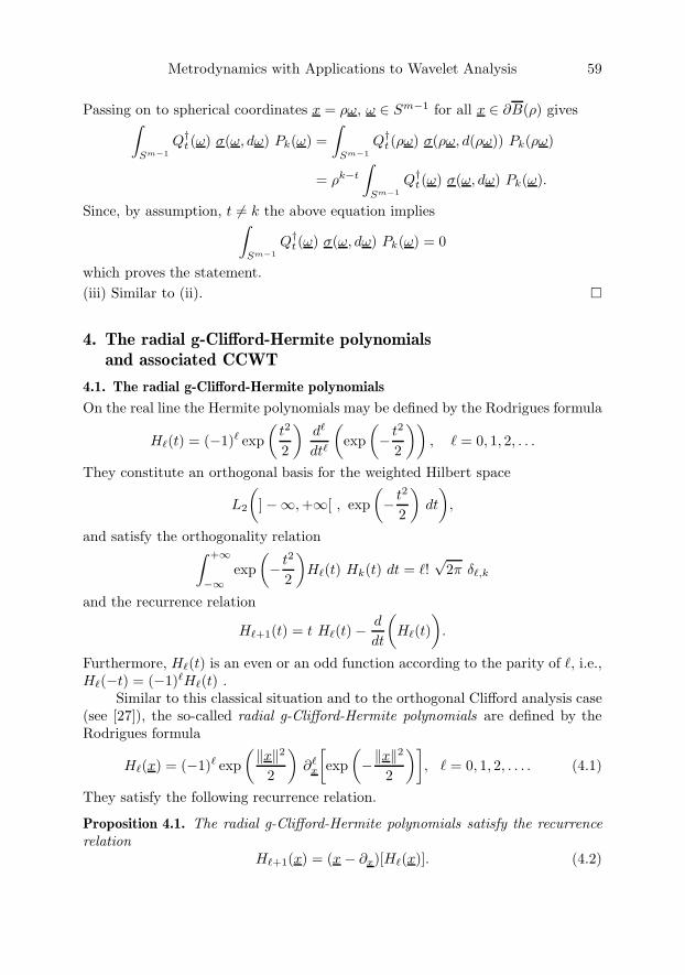
Metrodynamics with Applications to Wavelet Analysis 59
Passing on to spherical coordinates x = ρω, ω ∈ Sm−1 for all x ∈ ∂B(ρ) gives∫Sm−1
Q†t (ω) σ(ω, dω) Pk(ω) =
∫Sm−1
Q†t(ρω) σ(ρω, d(ρω)) Pk(ρω)
= ρk−t
∫Sm−1
Q†t(ω) σ(ω, dω) Pk(ω).
Since, by assumption, t = k the above equation implies∫Sm−1
Q†t(ω) σ(ω, dω) Pk(ω) = 0
which proves the statement.(iii) Similar to (ii).
4. The radial g-Clifford-Hermite polynomialsand associated CCWT
4.1. The radial g-Clifford-Hermite polynomials
On the real line the Hermite polynomials may be defined by the Rodrigues formula
H(t) = (−1) exp(
t2
2
)d
dt
(exp
(− t2
2
)), = 0, 1, 2, . . .
They constitute an orthogonal basis for the weighted Hilbert space
L2
(]−∞, +∞[ , exp
(− t2
2
)dt
),
and satisfy the orthogonality relation∫ +∞
−∞exp
(− t2
2
)H(t) Hk(t) dt = !
√2π δ,k
and the recurrence relation
H+1(t) = t H(t)−d
dt
(H(t)
).
Furthermore, H(t) is an even or an odd function according to the parity of , i.e.,H(−t) = (−1)H(t) .
Similar to this classical situation and to the orthogonal Clifford analysis case(see [27]), the so-called radial g-Clifford-Hermite polynomials are defined by theRodrigues formula
H(x) = (−1) exp(‖x‖2
2
)∂
x
[exp
(−‖x‖
2
2
)], = 0, 1, 2, . . . . (4.1)
They satisfy the following recurrence relation.
Proposition 4.1. The radial g-Clifford-Hermite polynomials satisfy the recurrencerelation
H+1(x) = (x − ∂x)[H(x)]. (4.2)

60 F. Brackx, N. De Schepper and F. Sommen
Proof. As
∂x
[exp
(‖x‖2
2
)]= ∂x
[exp
(−x2
2
)]= exp
(−x2
2
)(−1
2
)(−2x) = x exp
(‖x‖2
2
),
we have consecutively
∂x[H(x)] = (−1) ∂x
[exp
(‖x‖2
2
)]∂
x
[exp
(−‖x‖
2
2
)]+ (−1) exp
(‖x‖2
2
)∂+1
x
[exp
(−‖x‖
2
2
)]= x (−1) exp
(‖x‖2
2
)∂
x
[exp
(−‖x‖
2
2
)]−H+1(x)
= x H(x)−H+1(x)
which proves the statement. The recurrence relation (4.2) allows for a straightforward computation of somelower dimensional g-Clifford-Hermite polynomials:
H0(x) = 1
H1(x) = x
H2(x) = x2 + m = −‖x‖2 + m
H3(x) = x3 + (m + 2)x = x (−‖x‖2 + m + 2)
H4(x) = x4 + 2(m + 2)x2 + m(m + 2) = ‖x‖4 − 2(m + 2) ‖x‖2 + m(m + 2)etc.
Note that H(x) is a polynomial of degree in the variable x = xjej, that H2(x)only contains even powers of x and is scalar-valued, while H2+1(x) only containsodd powers and is vector-valued.
By means of the Rodrigues formula (4.1) and the Cauchy-Pompeiu formula(Theorem 3.9) we obtain the following orthogonality relation.
Theorem 4.2. The radial g-Clifford-Hermite polynomials H(x) are mutually or-thogonal in Rm with respect to the weight function exp
(− ‖x‖2
2
), i.e., for = t one
has ∫Rm
H† (x) Ht(x) exp
(−‖x‖
2
2
)dxM = 0.
Proof. Suppose that < t; the case > t follows by Hermitian conjugation.As H(x) is a polynomial of degree in x, it is sufficient to show that for
each t ∈ N and < t:∫Rm
x Ht(x) exp(−‖x‖
2
2
)dxM = 0.
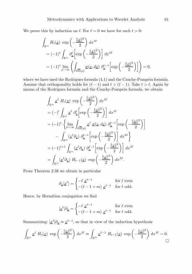
Metrodynamics with Applications to Wavelet Analysis 61
We prove this by induction on . For = 0 we have for each t > 0:∫Rm
Ht(x) exp(−‖x‖
2
2
)dxM
= (−1)t
∫Rm
∂tx
[exp
(−‖x‖
2
2
)]dxM
= (−1)t limρ→∞
(∫∂B(ρ)
σ(x, dx) ∂t−1x
[exp
(−‖x‖
2
2
)])= 0,
where we have used the Rodrigues formula (4.1) and the Cauchy-Pompeiu formula.Assume that orthogonality holds for (− 1) and t > (− 1). Take t > . Again bymeans of the Rodrigues formula and the Cauchy-Pompeiu formula, we obtain:∫
Rm
x Ht(x) exp(−‖x‖
2
2
)dxM
= (−)t
∫Rm
x ∂tx
[exp
(−‖x‖
2
2
)]dxM
= (−1)t
lim
ρ→∞
∫∂B(ρ)
x σ(x, dx) ∂t−1x
[exp
(−‖x‖
2
2
)]−
∫Rm
(x∂x) ∂t−1x
[exp
(−‖x‖
2
2
)]dxM
= (−1)t+1
∫Rm
(x∂x) ∂t−1x
[exp
(−‖x‖
2
2
)]dxM
=∫
Rm
(x∂x) Ht−1(x) exp(−‖x‖
2
2
)dxM .
From Theorem 2.38 we obtain in particular
∂x[x] =
− x−1 for even−(− 1 + m) x−1 for odd.
Hence, by Hermitian conjugation we find
[x]∂x =
− x−1 for even−(− 1 + m) x−1 for odd.
Summarizing: [x]∂x ≈ x−1, so that in view of the induction hypothesis∫Rm
x Ht(x) exp(−‖x‖
2
2
)dxM ≈
∫Rm
x−1 Ht−1(x) exp(−‖x‖
2
2
)dxM = 0.
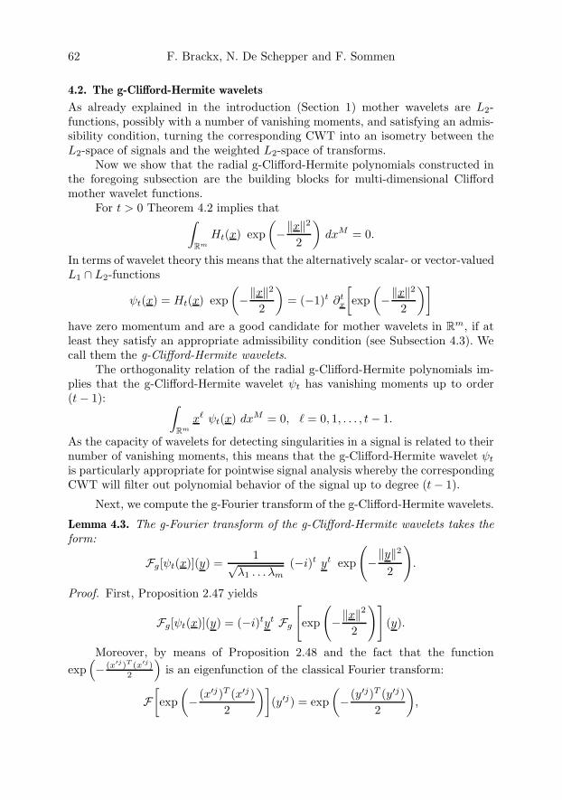
62 F. Brackx, N. De Schepper and F. Sommen
4.2. The g-Clifford-Hermite wavelets
As already explained in the introduction (Section 1) mother wavelets are L2-functions, possibly with a number of vanishing moments, and satisfying an admis-sibility condition, turning the corresponding CWT into an isometry between theL2-space of signals and the weighted L2-space of transforms.
Now we show that the radial g-Clifford-Hermite polynomials constructed inthe foregoing subsection are the building blocks for multi-dimensional Cliffordmother wavelet functions.
For t > 0 Theorem 4.2 implies that∫Rm
Ht(x) exp(−‖x‖
2
2
)dxM = 0.
In terms of wavelet theory this means that the alternatively scalar- or vector-valuedL1 ∩ L2-functions
ψt(x) = Ht(x) exp(−‖x‖
2
2
)= (−1)t ∂t
x
[exp
(−‖x‖
2
2
)]have zero momentum and are a good candidate for mother wavelets in Rm, if atleast they satisfy an appropriate admissibility condition (see Subsection 4.3). Wecall them the g-Clifford-Hermite wavelets.
The orthogonality relation of the radial g-Clifford-Hermite polynomials im-plies that the g-Clifford-Hermite wavelet ψt has vanishing moments up to order(t− 1): ∫
Rm
x ψt(x) dxM = 0, = 0, 1, . . . , t− 1.
As the capacity of wavelets for detecting singularities in a signal is related to theirnumber of vanishing moments, this means that the g-Clifford-Hermite wavelet ψt
is particularly appropriate for pointwise signal analysis whereby the correspondingCWT will filter out polynomial behavior of the signal up to degree (t− 1).
Next, we compute the g-Fourier transform of the g-Clifford-Hermite wavelets.
Lemma 4.3. The g-Fourier transform of the g-Clifford-Hermite wavelets takes theform:
Fg[ψt(x)](y) =1√
λ1 . . . λm
(−i)t yt exp
(−‖y‖2
2
).
Proof. First, Proposition 2.47 yields
Fg[ψt(x)](y) = (−i)tyt Fg
[exp
(−‖x‖
2
2
)](y).
Moreover, by means of Proposition 2.48 and the fact that the functionexp
(− (x′j)T (x′j)
2
)is an eigenfunction of the classical Fourier transform:
F[exp
(− (x′j)T (x′j)
2
)](y′j) = exp
(− (y′j)T (y′j)
2
),

Metrodynamics with Applications to Wavelet Analysis 63
we obtain consecutively
Fg
[exp
(−‖x‖
2
2
)](y) = Fg
[exp
(−〈x, x〉
2
)](y) = Fg
[exp
(− (xj)T G(xj)
2
)](yj)
=1√
λ1 . . . λm
F[exp
(− (AP−1(x′j))T G (AP−1(x′j))
2
)](PAT (yj))
=1√
λ1 . . . λm
F[exp
(− (x′j)T (x′j)
2
)](PAT (yj))
=1√
λ1 . . . λm
exp(− (PAT (yj))T PAT (yj)
2
)=
1√λ1 . . . λm
exp(− (yj)T G(yj)
2
)=
1√λ1 . . . λm
exp(−〈y, y〉
2
)=
1√λ1 . . . λm
exp
(−‖y‖2
2
).
Hence, we indeed have
Fg[ψt(x)](y) =1√
λ1 . . . λm
(−i)t yt exp
(−‖y‖2
2
).
4.3. The g-Clifford-Hermite Continuous Wavelet Transform
In order to introduce the corresponding g-Clifford-Hermite CWT, we consider, stillfor t > 0, the continuous family of wavelets
ψa,bt (x) =
1am/2
ψt
(x− b
a
),
with a ∈ R+ the dilation parameter and b ∈ Rm the translation parameter. Theg-Clifford-Hermite CWT (g-CHCWT) applies to functions f ∈ L2(Rm, dxM ) by
Tt[f ](a, b) = Ft(a, b) = 〈ψa,bt , f〉 =
∫Rm
(ψ
a,bt (x)
)†f(x) dxM
=1
am/2
∫Rm
exp(−‖x− b‖2
2a2
) (Ht
(x− b
a
))†f(x) dxM .
This definition can be rewritten in the frequency domain as
Ft(a, b) = λ1 . . . λm 〈Fg[ψa,bt ],Fg[f ]〉
= λ1 . . . λm
∫Rm
(Fg[ψ
a,bt ](y)
)†Fg[f ](y) dyM . (4.3)
The Fourier transform of the continuous family of wavelets:
Fg[ψa,bt ](y) =
(1√2π
)m ∫Rm
exp (−i〈x, y〉) 1am/2
ψt
(x− b
a
)dxM ,
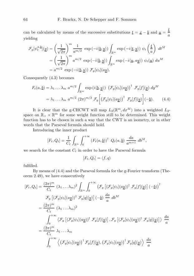
64 F. Brackx, N. De Schepper and F. Sommen
can be calculated by means of the successive substitutions t = x − b and u =t
ayielding
Fg[ψa,bt ](y) =
(1√2π
)m 1am/2
exp (−i〈b, y〉)∫
Rm
exp (−i〈t, y〉) ψt
(t
a
)dtM
=(
1√2π
)m
am/2 exp (−i〈b, y〉)∫
Rm
exp (−i〈u, ay〉) ψt(u) duM
= am/2 exp (−i〈b, y〉) Fg[ψt](ay).
Consequently (4.3) becomes
Ft(a, b) = λ1 . . . λm am/2
∫Rm
exp (i〈b, y〉)(Fg[ψt](ay)
)† Fg[f ](y) dyM
= λ1 . . . λm am/2 (2π)m/2 Fg
[(Fg[ψt](ay)
)† Fg[f ](y)](−b). (4.4)
It is clear that the g-CHCWT will map L2(Rm, dxM ) into a weighted L2-space on R+ × Rm for some weight function still to be determined. This weightfunction has to be chosen in such a way that the CWT is an isometry, or in otherwords that the Parseval formula should hold.
Introducing the inner product
[Ft, Qt] =1Ct
∫Rm
∫ +∞
0
(Ft(a, b))† Qt(a, b)da
am+1dbM ,
we search for the constant Ct in order to have the Parseval formula
[Ft, Qt] = 〈f, q〉
fulfilled.By means of (4.4) and the Parseval formula for the g-Fourier transform (The-
orem 2.49), we have consecutively
[Ft, Qt] =(2π)m
Ct(λ1 . . . λm)2
∫Rm
∫ +∞
0
(Fg
[(Fg[ψt](ay))† Fg[f ](y)
](−b)
)†Fg
[(Fg[ψt](ay))† Fg[q](y)
](−b)
da
adbM
=(2π)m
Ct(λ1 . . . λm)2∫ +∞
0
⟨Fg
[(Fg[ψt](ay))† Fg[f ](y)
],Fg
[(Fg[ψt](ay))† Fg[q](y)
]⟩ da
a
=(2π)m
Ctλ1 . . . λm∫ +∞
0
⟨(Fg[ψt](ay)
)†Fg[f ](y),(Fg[ψt](ay)
)† Fg[q](y)⟩ da
a
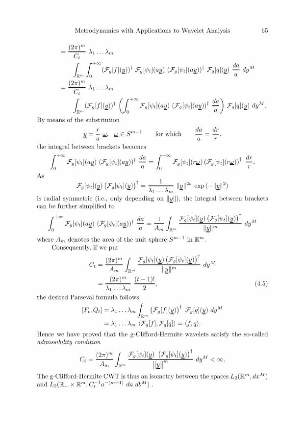
Metrodynamics with Applications to Wavelet Analysis 65
=(2π)m
Ctλ1 . . . λm∫
Rm
∫ +∞
0
(Fg[f ](y))† Fg[ψt](ay) (Fg[ψt](ay))† Fg[q](y)da
adyM
=(2π)m
Ctλ1 . . . λm∫
Rm
(Fg[f ](y))†(∫ +∞
0
Fg[ψt](ay) (Fg[ψt](ay))†da
a
)Fg[q](y) dyM .
By means of the substitution
y =r
aω, ω ∈ Sm−1 for which
da
a=
dr
r,
the integral between brackets becomes∫ +∞
0
Fg[ψt](ay) (Fg[ψt](ay))†da
a=∫ +∞
0
Fg[ψt](rω) (Fg[ψt](rω))†dr
r.
AsFg[ψt](y)
(Fg[ψt](y)
)† =1
λ1 . . . λm‖y‖2t exp (−‖y‖2)
is radial symmetric (i.e., only depending on ‖y‖), the integral between bracketscan be further simplified to∫ +∞
0
Fg[ψt](ay) (Fg[ψt](ay))†da
a=
1Am
∫Rm
Fg[ψt](y)(Fg[ψt](y)
)†‖y‖m dyM
where Am denotes the area of the unit sphere Sm−1 in Rm.Consequently, if we put
Ct =(2π)m
Am
∫Rm
Fg[ψt](y)(Fg[ψt](y)
)†‖y‖m dyM
=(2π)m
λ1 . . . λm
(t− 1)!2
, (4.5)
the desired Parseval formula follows:
[Ft, Qt] = λ1 . . . λm
∫Rm
(Fg[f ](y)
)† Fg[q](y) dyM
= λ1 . . . λm 〈Fg[f ],Fg[q]〉 = 〈f, q〉.Hence we have proved that the g-Clifford-Hermite wavelets satisfy the so-calledadmissibility condition
Ct =(2π)m
Am
∫Rm
Fg[ψt](y)(Fg[ψt](y)
)†∥∥y∥∥m dyM <∞.
The g-Clifford-Hermite CWT is thus an isometry between the spaces L2(Rm, dxM )and L2(R+ × Rm, C−1
t a−(m+1) da dbM ) .
66 F. Brackx, N. De Schepper and F. Sommen
References
[1] J.-P. Antoine, R. Murenzi, P. Vandergheynst and Syed Twareque Ali, Two-Dimen-sional Wavelets and their Relatives, Cambridge University Press, Cambridge, 2004.
[2] F. Brackx, R. Delanghe and F. Sommen, Clifford Analysis, Pitman Publishers(Boston-London-Melbourne, 1982).
[3] F. Brackx, R. Delanghe and F. Sommen, Differential Forms and/or Multi-vectorFunctions, CUBO A Mathematical Journal 7 (2005), no. 2, 139–169.
[4] F. Brackx, N. De Schepper and F. Sommen, The Bi-axial Clifford-Hermite Contin-uous Wavelet Transform, Journal of Natural Geometry 24 (2003), 81–100.
[5] F. Brackx, N. De Schepper and F. Sommen, The Clifford-Gegenbauer Polynomialsand the Associated Continuous Wavelet Transform, Integral Transform. Spec. Funct.15 (2004), no. 5, 387–404.
[6] F. Brackx, N. De Schepper and F. Sommen, The Clifford-Laguerre ContinuousWavelet Transform, Bull. Belg. Math. Soc. - Simon Stevin 11(2), 2004, 201–215.
[7] F. Brackx, N. De Schepper and F. Sommen, Clifford-Jacobi Polynomials and theAssociated Continuous Wavelet Transform in Euclidean Space (accepted for publi-cation in the Proceedings of the 4th International Conference on Wavelet Analysisand Its Applications, University of Macau, China, 2005).
[8] F. Brackx, N. De Schepper and F. Sommen, New multivariable polynomials andtheir associated Continuous Wavelet Transform in the framework of Clifford Analysis(submitted for publication in the Proceedings of the International Conference onRecent trends of Applied Mathematics based on partial differential equations andcomplex analysis, Hanoi, 2004).
[9] F. Brackx and F. Sommen, Clifford-Hermite Wavelets in Euclidean Space, Journalof Fourier Analysis and Applications 6, no. 3 (2000), 299–310.
[10] F. Brackx and F. Sommen, The Generalized Clifford-Hermite Continuous WaveletTransform, Advances in Applied Clifford Algebras 11(S1), 2001, 219–231.
[11] P. Calderbank, Clifford analysis for Dirac operators on manifolds-with-boundary,Max Planck-Institut fur Mathematik (Bonn, 1996).
[12] C.K. Chui, An Introduction to Wavelets, Academic Press, Inc., San Diego, 1992.
[13] J. Cnops, An introduction to Dirac operators on manifolds, Birkhauser Verlag (Basel,2002).
[14] I. Daubechies, Ten Lectures on Wavelets, SIAM, Philadelphia, 1992.
[15] R. Delanghe, F. Sommen and V. Soucek, Clifford Algebra and Spinor-Valued Func-tions, Kluwer Academic Publishers (Dordrecht, 1992).
[16] D. Eelbode and F. Sommen, Differential Forms in Clifford Analysis (accepted forpublication in the Proceedings of the International Conference on Recent trends ofApplied Mathematics based on partial differential equations and complex analysis,Hanoi, 2004).
[17] M. Felsberg, Low-Level Image Processing with the Structure Multivector, PhD-thesis,Christian-Albrechts-Universitat, Kiel, 2002.
[18] J. Gilbert and M. Murray, Clifford Algebras and Dirac Operators in Harmonic Anal-ysis, Cambridge University Press (Cambridge, 1991).
Metrodynamics with Applications to Wavelet Analysis 67
[19] K. Gurlebeck and W. Sprossig, Quaternionic analysis and elliptic boundary valueproblems, Birkhauser Verlag (Basel, 1990).
[20] K. Gurlebeck and W. Sprossig, Quaternionic and Clifford Calculus for Physicistsand Engineers, John Wiley & Sons (Chichester etc., 1997).
[21] G. Kaiser, A Friendly Guide to Wavelets, Birkhauser Verlag (Boston, 1994).
[22] G. Kaiser, private communication.
[23] N. Marchuk, The Dirac Type Tensor Equation in Riemannian Spaces, In: F. Brackx,J.S.R. Chisholm and V. Soucek (eds.), Clifford Analysis and Its Applications, KluwerAcademic Publishers (Dordrecht-Boston-London, 2001).
[24] M. Mitrea, Clifford Wavelets, Singular Integrals and Hardy Spaces, Lecture Notes inMathematics 1575, Springer-Verlag (Berlin, 1994).
[25] T. Qian, Th. Hempfling, A. McIntosh and F. Sommen (eds.), Advances in Analysisand Geometry: New Developments Using Clifford Algebras, Birkhauser verlag (Basel-Boston-Berlin, 2004).
[26] J. Ryan and D. Struppa (eds.), Dirac operators in analysis, Addison Wesley LongmanLtd, (Harlow, 1998).
[27] F. Sommen, Special Functions in Clifford analysis and Axial Symmetry. Journal ofMath. Analysis and Applications 130 (1988), no. 1, 110–133.
Fred Brackx, Nele De Schepper and Frank SommenClifford Research GroupDepartment of Mathematical AnalysisFaculty of Engineering – Faculty of SciencesGhent UniversityGalglaan 2B-9000 Gent, Belgium
e-mail: [email protected]: [email protected]: [email protected]
Operator Theory:Advances and Applications, Vol. 167, 69–85c© 2006 Birkhauser Verlag Basel/Switzerland
A Hierarchical Semi-separableMoore-Penrose Equation Solver
Patrick Dewilde and Shivkumar Chandrasekaran
Abstract. The main result of the present paper is a method to transform amatrix or operator which has a hierarchical semi-separable (HSS) represen-tation into a URV (Moore-Penrose) representation in which the operators Uand V represent collections of efficient orthogonal transformations and theblock upper matrix R still has the HSS form. The paper starts with an in-troduction to HSS-forms and a survey of a recently derived multi resolutionrepresentation for such systems. It then embarks on the derivation of the mainingredients needed for a Moore-Penrose reduction of the system while keepingthe HSS structure. The final result is presented as a sequence of efficient algo-rithmic steps, the efficiency resulting from the HSS structure that is preservedthroughout.
Mathematics Subject Classification (2000). Primary: 65F; Secondary: 15A.
Keywords. Hierarchically semi-separable systems, hierarchically quasi-separ-able systems, Moore-Penrose inverse, structured matrices.
1. Introduction
Many physical systems are modeled by systems of differential equations, integralequations or combinations of them. Solving these systems requires discretizationof the equations and leads to large systems of algebraic equations. In the caseof systems governed by linear equations, the resulting system of equations willbe linear as well and can be solved either directly or iteratively, involving a pre-conditioner and a Lanczos-type recursion. In the case of non-linear systems, thediscretized system will be non-linear as well and an iterative procedure has to beset up to find the solution. Such a procedure is, e.g., of the ‘Newton-Raphson’type and would in turn require the solution of a system of linear equations, nowinvolving a differential such as a Jacobian. In all cases the resulting systems tend tolead to matrices of very large dimensions, even for fairly small problems, so thatsolvers using standard numerical procedures quickly run out of steam. Luckily,many systems exhibit quite a bit of structure that can be exploited to make the
70 P. Dewilde and Sh. Chandrasekaran
solver more efficient. In the case of a discretized system for a differential equation,the resulting matrix structure will be very sparse, as only entries correspondingto nearby points will be different from zero. In this case, the matrix-vector multi-plication can be efficiently executed. Iterative methods are well suited to exploitthis fact, but they are dependent on a low-complexity approximant of the inverseof the original system, the so-called preconditioner. Approximate solutions of thesystem can be iteratively constructed via low-complexity calculations, providedthe pre-conditioner exhibits the necessary structure.
In the case of integral equations, it has been remarked by Gohberg, Kailathand Koltracht [9] and Rokhlin [12] that low rank approximations of the integralkernel lead to large submatrices of low rank in the resulting system of equations.Exploiting this structure which was termed ‘Semi-Separable’ leads to solution pro-cedures that are linear in the size of the matrix and quadratic in the size of theapproximation. A systematic method to obtain such low rank approximations wasproposed by Greengard and Rokhlin [10] and is known as the Fast MultipoleMethod. These original approaches suffered from numerical problems as the use ofbackward stable orthogonal transformations in this context was not yet well un-derstood. The introduction of time-varying system theory to model the system ofequations [13] provided for the necessary structure to allow for more general typesof transformations than those used by the original authors cited. A survey of thesetechniques can be found in the book [6]. Based on these ideas, the Semi-Separablestructure was extended to a more generic form called ‘Quasi-Separable’ and nu-merically stable system solvers were developed for this structure by a number ofauthors [8, 3, 7].
Although these developments lead to a satisfactory and useful theory, it wasalso evident that they did not exploit the structural properties of most physicalsystems sufficiently. Two examples may suffice to illustrate this point. In the caseof a partial differential equation in 3D space, discretization coordinates will havethree indices, say i, j, k, and interaction between values in close-by points maybe expected. To construct the interaction matrix, each discretization coordinatehas to be assigned a single index. In case of a regular grid of dimension N3, theindex assignment would run as i + Nj + N2k and the resulting matrix wouldhave a hierarchical structure consisting of a diagonal bands of blocks of dimensionN2 each consisting of diagonal bands of blocks of dimension N , which in turnconsist of scalar diagonal bands. The Semi-Separable or Quasi-Separable theoryis insufficient to handle such types of matrices, it gets a good grip only on thetop level of the hierarchy, while the structure of the lower hierarchical levels isgreatly disturbed [5]. Also in the case of the multipole method and assuming thedistribution of ‘objects’ handled by the method in 3D space to be fairly general(assuming of course that the multipole assumption holds as well), a similar problemwill arise: many submatrices will be of low rank, but they will have a ‘hierarchicalordering’, restricting the applicability of the Semi-Separable method.
In the present paper we deal with an intermediate structure which has a nicehierarchical (or equivalently multi-resolution) structure and is capable to cope
Hierarchical Semi-separable Equation Solver 71
with the problem mentioned in the previous paragraph. The structure was firstpresented in [4], and a few solvers for it were presented [11]. In particular, [2] showshow the structure can be reduced to a sparse, directly solvable system, using a statespace model of intermediate variables, much as was done for the Semi- or Quasi-separable case. In contrast to the latter the state-space model turns out to have ahierarchical (multi-resolution) structure, which can efficiently be exploited. Thesestraight solvers assume the original system to be square non-singular, allowing forpartial recursive elimination of unknowns and recursive back-substitutions as thealgorithm proceeds. In the present paper we propose a new, backward stable solverthat finds the Moore-Penrose solution for a general system of equations, namelya system that is not assumed to be square, non-singular. Our goal is to obtainthe same order of numerical complexity as the straight solvers, but now for theMoore-Penrose case.
2. HSS representations
The Hierarchical Semi-Separable representation of a matrix A is a layered repre-sentation of the multi-resolution type, indexed by the hierarchical level. At the toplevel 1, it is a 2× 2 block matrix representation of the form:
A =[
A1;1,1 A1;1,2
A2;2,1 A2;2,2
](2.1)
in which we implicitly assume that the ranks of the off-diagonal blocks is lowso that they can be represented by an ‘economical’ factorization (‘H ’ indicatesHermitian transposition, for real matrices just transposition), as follows:
A =[
D1;1 U1;1B1;1,2VH1;2
U1;2B1;2,1VH1;1 D1;2
]. (2.2)
The second hierarchical level is based on a further but similar decomposition ofthe diagonal blocks, respect. D1;1 and D1;2:
D1;1 =[
D2:1 U2;1B2;1,2VH2;2
U2;2B2;2,1VH2;1 D2;2
],
D1;2 =[
D2;3 U2;3B2;3,4VH2;4
U2;4B2;4,3VH2;3 D2;4
] (2.3)
for which we have the further level compatibility assumption
span(U1;1) ⊂ span([
U2;1
0
])⊕ span
([0
U2;2
]), (2.4)
span(V1;1) ⊂ span([
V2;1
0
])⊕ span
([0
V2;2
])etc . . . (2.5)
This spanning property is characteristic for the HSS structure, it is a kind ofhierarchical ‘Lanczos’ property and allows a substantial improvement on the nu-merical complexity as a multiplication with higher level structures always can be
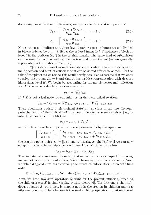
72 P. Dewilde and Sh. Chandrasekaran
done using lower level multiplications, using so called ‘translation operators’
U1;i =[
U2;2i−1R2;2i−1
U2;2iR2;2i
], i = 1, 2, (2.6)
V1;i =[
V2;2i−1W2;2i−1
V2;2iW2;2i
], i = 1, 2. (2.7)
Notice the use of indices: at a given level i rows respect. columns are subdividedin blocks indexed by 1, . . . , i. Hence the ordered index (i; k, ) indicates a block atlevel i in the position (k, ) in the original matrix. The same kind of subdivisioncan be used for column vectors, row vectors and bases thereof (as are generallyrepresented in the matrices U and V ).
In [2] it is shown how this multilevel structure leads to efficient matrix-vectormultiplication and a set of equations that can be solved efficiently as well. For thesake of completeness we review this result briefly here. Let us assume that we wantto solve the system Ax = b and that A has an HSS representation with deepesthierarchical level K. We begin by accounting for the matrix-vector multiplicationAx. At the leave node (K; i) we can compute
gK;i = V HK;ixK;i.
If (k; i) is not a leaf node, we can infer, using the hierarchical relations
gk;i = V Hk;ixk;i = WH
k+1;2i−1gk+1;2i−1 + WHk+1;2igk+1;2i.
These operations update a ‘hierarchical state’ gk;i upwards in the tree. To com-pute the result of the multiplication, a new collection of state variables fk;i isintroduced for which it holds that
bk;i = Ak;i,i + Uk;ifk;i
and which can also be computed recursively downwards by the equations[fk+1;2i−1
fk+1;2i
]=[
Bk+1;2i−1,2igk+1;2i + Rk+1;2i−1fk,i
Bk+1;2i,2i−1gk+1;2i−1 + Rk+1;2ifk;i
],
the starting point being f0; = [], an empty matrix. At the leaf level we can nowcompute (at least in principle - as we do not know x) the outputs from
bK;i = DK;ixK;i + UK;ifK;i.
The next step is to represent the multiplication recursions in a compact form usingmatrix notation and without indices. We fix the maximum order K as before. Nextwe define diagonal matrices containing the numerical information, in breadth firstorder:
D = diag[DK;i]i=1,...,K , W = diag[(W1;i)i=1,2, (W2;i)i=1···4, . . . ], etc . . .
Next, we need two shift operators relevant for the present situation, much asthe shift operator Z in time-varying system theory [6]. The first one is the shift-down operator Z↓ on a tree. It maps a node in the tree on its children and is anilpotent operator. The other one is the level exchange operator Z↔. At each level
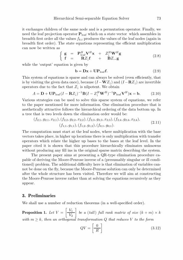
Hierarchical Semi-separable Equation Solver 73
it exchanges children of the same node and is a permutation operator. Finally, weneed the leaf projection operator Pleaf which on a state vector which assembles inbreadth first order all the values fk;i produces the values of the leaf nodes (again inbreadth first order). The state equations representing the efficient multiplicationcan now be written as
g = PHleafV
Hx + ZH↓ WHg
f = RZ↓f + BZ↔g(2.8)
while the ‘output’ equation is given by
b = Dx + UPleaf f . (2.9)
This system of equations is sparse and can always be solved (even efficiently, thatis by visiting the given data once), because (I−WZ↓) and (I−RZ↓) are invertibleoperators due to the fact that Z↓ is nilpotent. We obtain
A = D + UPleaf(I −RZ↓)−1B(I − ZH↓ WH)−1PleafVH)x = b. (2.10)
Various strategies can be used to solve this sparse system of equations, we referto the paper mentioned for more information. One elimination procedure that isaesthetically attractive follows the hierarchical ordering of the data bottom up. Ina tree that is two levels down the elimination order would be:
(f2;1, g2;1, x2;1), (f2;2, g2;2, x2;2), (f2;3, g2;3, x2;3), (f2;4, g2;4, x2;4),
(f1;1, g1;1), (f1;2, g1;2), (f0;1, g0;1).(2.11)
The computation must start at the leaf nodes, where multiplication with the basevectors takes place, in higher up locations there is only multiplication with transferoperators which relate the higher up bases to the bases at the leaf level. In thepaper cited it is shown that this procedure hierarchically eliminates unknownswithout producing any fill ins in the original sparse matrix describing the system.
The present paper aims at presenting a QR-type elimination procedure ca-pable of deriving the Moore-Penrose inverse of a (presumably singular or ill condi-tioned) problem. The additional difficulty here is that elimination of variables can-not be done on the fly, because the Moore-Penrose solution can only be determinedafter the whole structure has been visited. Therefore we will aim at constructingthe Moore-Penrose inverse rather than at solving the equations recursively as theyappear.
3. Preliminaries
We shall use a number of reduction theorems (in a well-specified order).
Proposition 1. Let V =[
V1
V2
]be a (tall ) full rank matrix of size (k + m) × k
with m ≥ k, then an orthogonal transformation Q that reduces V to the form
QV =[
0R
](3.12)

74 P. Dewilde and Sh. Chandrasekaran
with R square non-singular exists and can be chosen of the form
Q =[
w1 −LHwH2
w2 I − w2KwH2
](3.13)
in which w1 = V1R−1, w2 = V2R
−1, K is a hermitian matrix that satisfies
I − w2KwH2 = (I − w2w
H2 )1/2 (3.14)
and L a unitary matrix that satisfies
(I −KwH2 w2) = w1L. (3.15)
Proof. The theorem claims the existence of K and L implicitly. If V1 happens to beinvertible, then this is straightforward, the difficulty is when V1 is not invertible,we use an implicit proof to cover the general case. R is defined as a square matrixthat satisfies
V H1 V1 + V H
2 V2 = RHR (3.16)
and its non-singularity follows from the non-singularity assumption on V . Next let
w1 = V1R−1 and w2 = V2R
−1, then w =[
w1
w2
]is isometric, wH
1 w1 is contractive
and an eigenvalue decomposition
wH1 w1 = v1σ
2vH1 (3.17)
can be chosen such that the positive diagonal matrix σ satisfies 0 ≤ σ ≤ I. Sincew1 is square, a unitary u1 will exist such that w1 = u1σvH
1 (the proof goes as inthe proof of the SVD). Next, wH
2 w2 = I−wH1 w1 and an eigenvalue decomposition
for it isv1(I − σ2)vH
1 . (3.18)
Since w2 is tall by assumption, there will exist u2 isometric such that
w2 = u2(I − σ2)1/2vH1 . (3.19)
It is now easy to verify directly that
Q =[
u1σvH1 −u1(I − σ2)1/2uH
2
u2(I − σ2)1/2vH1 I − u2(I − σ)uH
2
](3.20)
is a unitary matrix. Putting K = v(I +σ)−1vH and L = vuH1 produces the desired
form of Q. The converse check that any Q with the given form is unitary is alsoimmediate by direct verification.
The theorem shows that a unitary matrix close to identity (where ‘close’means ‘the difference is a low rank matrix’) can be constructed that reduces a tallmatrix to a small triangular matrix. In Numerical Analysis one traditionally uses‘Householder transformations’ for this purpose, the transformation presented herehas the advantage that its determinant can be controlled more easily.
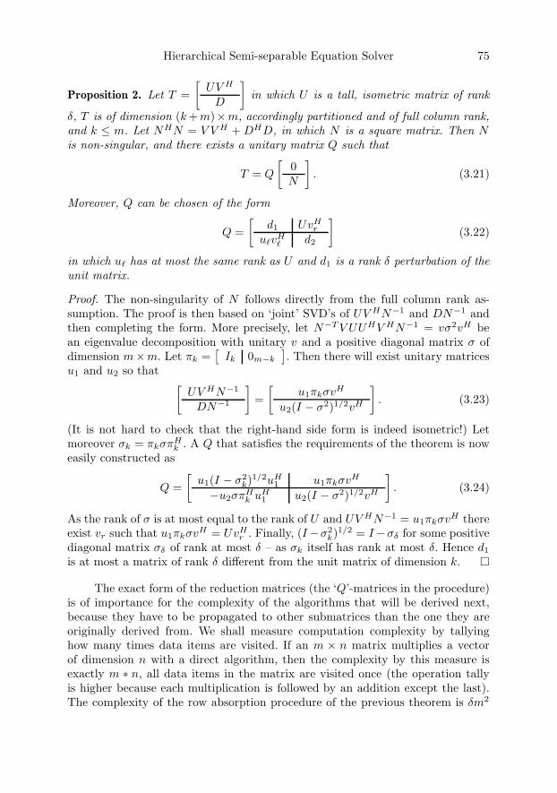
Hierarchical Semi-separable Equation Solver 75
Proposition 2. Let T =[
UV H
D
]in which U is a tall, isometric matrix of rank
δ, T is of dimension (k +m)×m, accordingly partitioned and of full column rank,and k ≤ m. Let NHN = V V H + DHD, in which N is a square matrix. Then Nis non-singular, and there exists a unitary matrix Q such that
T = Q
[0N
]. (3.21)
Moreover, Q can be chosen of the form
Q =[
d1 UvHr
uvH d2
](3.22)
in which u has at most the same rank as U and d1 is a rank δ perturbation of theunit matrix.
Proof. The non-singularity of N follows directly from the full column rank as-sumption. The proof is then based on ‘joint’ SVD’s of UV HN−1 and DN−1 andthen completing the form. More precisely, let N−T V UUHV HN−1 = vσ2vH bean eigenvalue decomposition with unitary v and a positive diagonal matrix σ ofdimension m×m. Let πk =
[Ik 0m−k
]. Then there will exist unitary matrices
u1 and u2 so that [UV HN−1
DN−1
]=[
u1πkσvH
u2(I − σ2)1/2vH
]. (3.23)
(It is not hard to check that the right-hand side form is indeed isometric!) Letmoreover σk = πkσπH
k . A Q that satisfies the requirements of the theorem is noweasily constructed as
Q =[
u1(I − σ2k)1/2uH
1 u1πkσvH
−u2σπHk uH
1 u2(I − σ2)1/2vH
]. (3.24)
As the rank of σ is at most equal to the rank of U and UV HN−1 = u1πkσvH thereexist vr such that u1πkσvH = UvH
r . Finally, (I−σ2k)1/2 = I−σδ for some positive
diagonal matrix σδ of rank at most δ – as σk itself has rank at most δ. Hence d1
is at most a matrix of rank δ different from the unit matrix of dimension k.
The exact form of the reduction matrices (the ‘Q’-matrices in the procedure)is of importance for the complexity of the algorithms that will be derived next,because they have to be propagated to other submatrices than the one they areoriginally derived from. We shall measure computation complexity by tallyinghow many times data items are visited. If an m × n matrix multiplies a vectorof dimension n with a direct algorithm, then the complexity by this measure isexactly m ∗ n, all data items in the matrix are visited once (the operation tallyis higher because each multiplication is followed by an addition except the last).The complexity of the row absorption procedure of the previous theorem is δm2

76 P. Dewilde and Sh. Chandrasekaran
where δ is the number of columns in the U or V matrix, because the result can be
obtained through a QR factorization on the matrix[
V H
D
].
4. HSS row absorption procedure
Our next goal is to derive a so-called ‘HSS row absorption’ matrix – one of themain ingredients in the HSS Moore-Penrose reduction process. Starting point isthe form ⎡⎣ w1v
H w2v
Hr
d1 urvHr
uvH d2
⎤⎦ (4.25)
in which we assume the top entries to be ‘skinny’, i.e., of low rank compared tothe dimensions of the matrix (this assumption is not used explicitly but underliesthe usefulness of the procedure – as discussed above, the HSS compatibility has tobe preserved!). We introduce a somewhat simplified notation, whenever clear fromthe context we drop the level indication. E.g., in the above matrix, the notationUr and U1;r or U1;1 would be equivalent. The goal of the procedure is to reducethe matrix to a row independent HSS form using orthogonal transformations.Important in the reduction procedure are the properties of the overall orthogonalreducing matrix, namely which block entries in it have an HSS form and whichare ‘skinny’ – i.e., have low rank of the same order as the rank of the top entriesto be absorbed. The procedure uses the properties derived in the first section.
Step 1. Find orthogonal q so that[q11 q12
q21 q22
] [w2
ur
]=[
r0
](4.26)
with r square non-singular and q22 close to a unit matrix, and apply the transfor-mation to the original after embedding:[
qI
]⎡⎣ w1vH w2v
Hr
d1 urvHr
uvH d2
⎤⎦ =
⎡⎣ q11w1vH + q12d1 rvH
r
q21w1vH + q22d1 0
uvH d2
⎤⎦ . (4.27)
Letd′1 = q21w1v
H + q22d1 (4.28)
the product of a lower level form (d1) with a ‘skinny’ perturbation of the unitmatrix (q22) followed by a ‘skinny’ additive perturbation (q21w1v
H ). The new
look of the matrix is, after an exchange of block-rows⎡⎣ d′1 0q11w1v
H + q12d1 rvH
r
uvH d2
⎤⎦ (4.29)
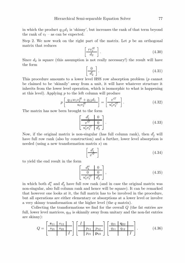
Hierarchical Semi-separable Equation Solver 77
in which the product q12d1 is ‘skinny’, but increases the rank of that term beyondthe rank of v – as can be expected.
Step 2. We now work on the right part of the matrix. Let p be an orthogonalmatrix that reduces [
rvHr
d2
]. (4.30)
Since d2 is square (this assumption is not really necessary!) the result will havethe form [
0d′2
]. (4.31)
This procedure amounts to a lower level HSS row absorption problem (p cannotbe claimed to be ‘skinnily’ away from a unit, it will have whatever structure itinherits from the lower level operation, which is isomorphic to what is happeningat this level). Applying p to the left column will produce
p
[q11w1v
H + q12d1
uvH
]=[
v′T
u′v
′T
]. (4.32)
The matrix has now been brought to the form⎡⎣ d′1 0v′T 0
u′v
′T d′2
⎤⎦ . (4.33)
Now, if the original matrix is non-singular (has full column rank), then d′2 willhave full row rank (also by construction) and a further, lower level absorption isneeded (using a new transformation matrix s) on[
d′1v′T
](4.34)
to yield the end result in the form⎡⎣ d′′1 00 0
u′v
′T d′2
⎤⎦ , (4.35)
in which both d′′1 and d′2 have full row rank (and in case the original matrix wasnon-singular, also full column rank and hence will be square). It can be remarkedthat however one looks at it, the full matrix has to be involved in the procedure,but all operations are either elementary or absorptions at a lower level or involvea very skinny transformation at the higher level (the q matrix).
Collecting the transformations we find for the overall Q (the fat entries arefull, lower level matrices, q22 is skinnily away from unitary and the non-fat entriesare skinny):
Q =
⎡⎣ s11 s12
s21 s22
I
⎤⎦⎡⎣ Ip11 p12
p21 p22
⎤⎦⎡⎣ q21 q22
q11 q12
I
⎤⎦ . (4.36)
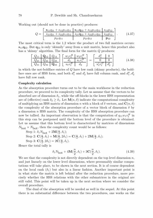
78 P. Dewilde and Sh. Chandrasekaran
Working out (should not be done in practice) produces:
Q =
⎡⎣ s11q21 + s12p11q11 s11q22 + s12p11q12 s12p12
s21q21 + s22p11q12 s21q22 + s22p11q22 s22p12
p21q11 p21q12 p22
⎤⎦ . (4.37)
The most critical term is the 1,2 where the product of two full matrices occurs:s11q22. But q22 is only ‘skinnily’ away from a unit matrix, hence this product alsohas a ‘skinny’ algorithm. The final form for the matrix Q produces:⎡⎣ Q11 Q12 Q13
Q21 Q22 Q23
Q31 Q32 Q33
⎤⎦⎡⎣ w1vH w2v
Hr
d1 urvHr
uvH d2
⎤⎦ =
⎡⎣ d′′1 00 0
u′v
′T d′2
⎤⎦ (4.38)
in which the not-boldface entries of Q have low rank (skinny products), the bold-face ones are of HSS form, and both d′′1 and d′2 have full column rank, and d′′1 , d′2have full row rank.
Complexity calculation
As the absorption procedure turns out to be the main workhorse in the reductionprocedure, we proceed to its complexity tally. Let us assume that the vectors to beabsorbed are of dimension δ1, while the off-blocks in the lower HSS representationare of (effective) rank δ2 ≥ δ1. Let M(n, δ) indicate the computational complexityof multiplying an HSS matrix of dimension n with a block of δ vectors, and C(n, δ)the complexity of the absorption procedure of a vector block of dimension δ bya dimension n HSS matrix. The complexity of the HSS absorption procedure cannow be tallied. An important observation is that the computation of q11w1v
H in
this step can be postponed until the bottom level of the procedure is obtained.Let us assume that this bottom level is characterized by matrices of dimensionsNbot ×Nbot, then the complexity count would be as follows:
Step 1: δ1Nbot + 2M(n2 , δ1);
Step 2: C(n2 , δ1) + M(n
2 , 2δ1) = C(n2 , δ1) + 2M(n
2 , δ1);Step 3: C(n
2 , 2δ1) = 2C(n2 , δ1).
Hence the total tally is
δ1Nbot + 4M(n
2, δ1) + 3C(
n
2, δ1). (4.39)
We see that the complexity is not directly dependent on the top level dimension n,and just linearly on the lower level dimensions, where presumably similar compu-tations will take place, to be shown in the next section. It is of course dependenton the local rank (δ1) but also in a linear fashion. Another important point isin what state the matrix is left behind after the reduction procedure, more pre-cisely whether the HSS relations with the other submatrices in the original arestill valid. This point will be taken up in the next section where we consider theoverall procedure.
The dual of the absorption will be needed as well in the sequel. At this pointthere is no substantial difference between the two procedures, one works on the
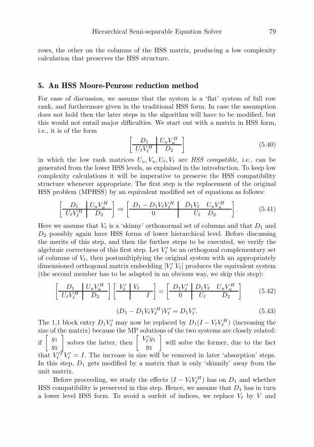
Hierarchical Semi-separable Equation Solver 79
rows, the other on the columns of the HSS matrix, producing a low complexitycalculation that preserves the HSS structure.
5. An HSS Moore-Penrose reduction method
For ease of discussion, we assume that the system is a ‘flat’ system of full rowrank, and furthermore given in the traditional HSS form. In case the assumptiondoes not hold then the later steps in the algorithm will have to be modified, butthis would not entail major difficulties. We start out with a matrix in HSS form,i.e., it is of the form [
D1 UuV Hu
UVH D2
](5.40)
in which the low rank matrices Uu, Vu, U, V are HSS compatible, i.e., can begenerated from the lower HSS levels, as explained in the introduction. To keep lowcomplexity calculations it will be imperative to preserve the HSS compatibilitystructure whenever appropriate. The first step is the replacement of the originalHSS problem (MPHSS) by an equivalent modified set of equations as follows:[
D1 UuV Hu
UVH D2
]⇒
[D1 −D1VV
H D1V UuV H
u
0 U D2
]. (5.41)
Here we assume that V is a ‘skinny’ orthonormal set of columns and that D1 andD2 possibly again have HSS forms of lower hierarchical level. Before discussingthe merits of this step, and then the further steps to be executed, we verify thealgebraic correctness of this first step. Let V ′
be an orthogonal complementary setof columns of V, then postmultiplying the original system with an appropriatelydimensioned orthogonal matrix embedding [V ′
V] produces the equivalent system(the second member has to be adapted in an obvious way, we skip this step):[
D1 UuV Hu
UVH D2
] [V ′
V
I
]=[
D1V′ D1V UuV H
u
0 U D2
](5.42)
(D1 −D1VVH )V ′
= D1V′ . (5.43)
The 1,1 block entry D1V′ may now be replaced by D1(I − VV
H ) (increasing the
size of the matrix) because the MP solutions of the two systems are closely related:
if[
y1
y2
]solves the latter, then
[V ′
y1
y2
]will solve the former, due to the fact
that V ′T V ′
= I. The increase in size will be removed in later ‘absorption’ steps.In this step, D1 gets modified by a matrix that is only ‘skinnily’ away from theunit matrix.
Before proceeding, we study the effects (I − VVH ) has on D1 and whether
HSS compatibility is preserved in this step. Hence, we assume that D1 has in turna lower level HSS form. To avoid a surfeit of indices, we replace V by V and

80 P. Dewilde and Sh. Chandrasekaran
express the lower level HSS form again with the same notation as before:
D1 ←[
D1 UrVHr
UVH D2
]. (5.44)
Furthermore, because of the HSS relations, we have
V =[
V1
V2
]=[
VW
VrWr
](5.45)
(which could also be expressed as
V =[
V
Vr
][
W
Wr
](5.46)
in which the W ’s are assumed tall matrices, and the indicates pointwise multi-plication of block entries – assuming matching dimensions of course). We find asresult for this operation[
D1 − (D1V1 + UrVHr V2)V H
1 UrVHr − (D1V1 + UrV
Hr V2)V H
2
UVH − (UV
H V1 + D2V2)V H
1 D2 − (UVH V1 + D2V2)V H
2
]. (5.47)
We see that the ranks of the off-diagonal terms have not increased, but the col-umn basis has changed, and it may be useful to keep the original column vectorsalthough they may not amount to a basis (they are able to generate the columnvectors though). Taking this conservative approach we may write the result so faras [
D′1 [Urn Ur]WH
rnV Hr
[Un U]WHnV H
D′2
](5.48)
in which ⎧⎪⎪⎪⎪⎪⎪⎪⎪⎪⎪⎨⎪⎪⎪⎪⎪⎪⎪⎪⎪⎪⎩
Urn = D1V1
D′1 = D1 − (Urn + UrV
Hr V2)V H
1
WHrn =
[−WH
r
I − V Hr V2W
Hr
]D′
2 = D2 − (Un + UVH V1)V H
2
Un = D2V2
WHn =
[−WH
I − V H V1W
H
](5.49)
all quantities that can now be computed at the lowest level, and are either ‘skinny’or ‘skinny’ updates.
Going back to the original procedure, the same strategy can now be appliedto the rightmost block in eq. 5.42, this produces:⎡⎣ U1;rV
H1;r,3 U1,rV
H1;r,4
D2;3 U2;rVH2;r
U2;VH2; D2;4
⎤⎦[ V ′2; V2; 00 0 I
]
=
⎡⎢⎣ U1;rVH1;r,3V
′2; U1;rV
H1;r,3V2; U1;rV
H1;r,4
D2;3(I − V2;VH2;)V
′2; D2;3V2; U2;rV
H2;r
0 U2; D2;4
⎤⎥⎦ .
(5.50)
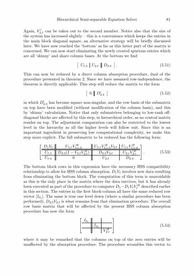
Hierarchical Semi-separable Equation Solver 81
Again, V ′2, can be taken out to the second member. Notice also that the size of
the system has increased slightly – this is a convenience which keeps the entries inthe main block diagonal square, an alternative strategy will be briefly discussedlater. We have now reached the ‘bottom’ as far as this latter part of the matrix isconcerned. We can now start eliminating the newly created spurious entries whichare all ‘skinny’ and share column bases. At the bottom we find[
U,4 U2; D2;4
]. (5.51)
This can now be reduced by a direct column absorption procedure, dual of theprocedure presented in theorem 2. Since we have assumed row-independence, thetheorem is directly applicable. This step will reduce the matrix to the form[
0 D′2;4
](5.52)
in which D′2;4 has become square non-singular, and the row basis of the submatrix
on top have been modified (without modification of the column basis), and thisby ‘skinny’ calculations. Notice that only submatrices belonging to low-rank off-diagonal blocks are affected by this step, in hierarchical order, as no central matrixresides on top. The adjustment computation can also be restricted to the lowestlevel in the hierarchy as all the higher levels will follow suit. Since this is animportant ingredient in preserving low computational complexity, we make thisstep more explicit. The full submatrix to be reduced has the following form:⎡⎣ D1V U1;rV
H1;r,3 U1;rV
H1;r,3V2; U1;rV
H1;r,4
U,3 D2;3(I − V2;VH2;) D2;3V2; U2;rV
H2;r
U,4 0 U2; D2;4
⎤⎦ . (5.53)
The bottom block rows in this expression have the necessary HSS compatibilityrelationship to allow for HSS column absorption. D1V involves new data resultingfrom eliminating the bottom block. The computation of this term is unavoidableas this is the only place in the matrix where the data survives, but it has alreadybeen executed as part of the procedure to computer D1−D1VV
H described earlier
in this section. The entries in the first block-column all have the same reduced rowvector [Iδ1 ]. The same is true one level down (where a similar procedure has beenperformed), D2;3V2; is what remains from that elimination procedure. The overallrow basis matrix that will be affected by the present HSS column absorptionprocedure has now the form ⎡⎣ Iδ1
Iδ2
V H2;r
⎤⎦ (5.54)
where it may be remarked that the columns on top of the zero entries will beunaffected by the absorption procedure. The procedure scrambles this vector to
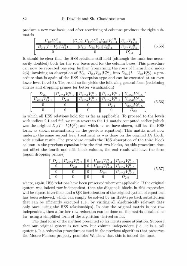
82 P. Dewilde and Sh. Chandrasekaran
produce a new row basis, and after reordering of columns produces the right sub-matrix⎡⎢⎣ U1;rV
H1;r,3 [D1V U1;rV
H1;r,3V2;]V
′,H2;r.4 U1;rV
′H1;r,5
D2;3(I − V2;VH2;) [U.3 D2;3V2;]V ′H
2;r,4 U2;rV′H2;r,5
0 0 D′2;4
⎤⎥⎦ . (5.55)
It should be clear that the HSS relations still hold (although the rank has neces-sarily doubled) both for the row bases and for the column bases. This procedurecan now be repeated one step further (concerning the rows of hierarchical index2;3), involving an absorption of [U3 D2;3V2;]V ′H
2;r,4 into D2;3(I − V2;VH2;), a pro-
cedure that is again of the HSS absorption type and can be executed at an evenlower level (level 3). The result so far yields the following general form (redefiningentries and dropping primes for better visualization)⎡⎢⎢⎣
D2;1 U2;r,1VH2;r,2 U1;r,1V
H2;r,3 U1;r,1V
H1;r,4 U1;r,1V
H1;r,5
U2;,2VH2;,1 D2;2 U1;r,2V
H2;r,3 U1;r,2V
H1;r,4 U1;r,2V
H1;r,5
0 0 0 D2;4 U2;r,3VH2;r,5
0 0 0 0 D2;5
⎤⎥⎥⎦ (5.56)
in which all HSS relations hold for as far as applicable. To proceed to the levelswith indices 2;1 and 2;2, we must revert to the 1;1 matrix computed earlier (whichwas the original D1(I − VV
H ), and which, as we have shown, still has the HSS
form, as shown schematically in the previous equation). This matrix must nowundergo the same second level treatment as was done on the original D2 block,with similar result. The procedure entails the HSS absorption of the third blockcolumn in the previous equation into the first two blocks, As this procedure doesnot affect the fourth and fifth block column, the end result will have the form(again dropping primes)⎡⎢⎢⎣
D2;1 U2;r,1VH2;r,2 0 U1;r,1V
H1;r,4 U1;r,1V
H1;r,5
0 D2;2 0 U1;r,2VH1;r,4 U1;r,2V
H1;r,5
0 0 0 D2;4 U2;r,3VH2;r,5
0 0 0 0 D2;5
⎤⎥⎥⎦ (5.57)
where, again, HSS relations have been preserved wherever applicable. If the originalsystem was indeed row independent, then the diagonals blocks in this expressionwill be square invertible, and a QR factorization of the original system of equationshas been achieved, which can simply be solved by an HSS-type back substitutionthat can be efficiently executed (i.e., by visiting all algebraically relevant dataonly once, using the HSS relationships). In case the original matrix is not rowindependent, then a further row reduction can be done on the matrix obtained sofar, using a simplified form of the algorithm derived so far.
The dual form of the method presented so far merits some attention. Supposethat our original system is not row- but column independent (i.e., it is a tallsystem). Is a reduction procedure as used in the previous algorithm that preservesthe Moore-Penrose property possible? We show that this is indeed the case.
Hierarchical Semi-separable Equation Solver 83
Proposition 3. Let [D1 UuV H
u
UVH D2
](5.58)
be given as the top-level of a column independent HSS representation in which thematrices Di, i = 1, 2 are HSS compatible, and in which Uu is isometric. Then anequivalent Moore-Penrose system is given by⎡⎣ (I − UuUH
u )D1 0UH
u D1 V Hu
UVH D2
⎤⎦ . (5.59)
Proof. The proof follows from the following two observations:1. Let U ′
u be an isometric matrix whose columns span the orthogonal comple-ment of the (column) range of Uu. Then
U ′Hu D1 = U ′H
u (I − UuUHu )D1; (5.60)
2. if V H is an isometric matrix then the system V HAx = b is equivalent to thesystem Ay = V b in the sense that if y solves the Moore-Penrose problem ofthe latter, then x=y is the Moore-Penrose solution of the former.
The required transformation now follows from the identity⎡⎣ U ′Hu
UHu
I
⎤⎦[ D1 UuV Hu
UVH D2
]=
⎡⎣ U ′Hu D1 0
UHu D1 V H
u
UVH D2
⎤⎦ . (5.61)
An application of the properties mentioned above allows one to eliminate U ′Hu so
that the modification of the entries only involves the product UHu D1, which can
efficiently be relegated to the lower hierarchical level.
Notice that just as before the HSS relations remain in place. We can summa-rize the procedures in the following conceptual theorem. In the formulation ‘URV-type’ means: using orthogonal transformation on the rows (for the U -factor) andthe columns (for the V factor).
Theorem 1. A matrix represented in HSS form can be constructively reduced toa non-singular block upper matrix in HSS form using efficient, HSS compatibletransformations of the URV type.
6. Discussion and conclusions
A number of observations seem relevant:1. the HSS form of an invertible matrix is stable under inversion, it is not too
hard to prove that the inverse of such a matrix has an HSS representationof the same complexity as the original. However, an efficient algorithm tocompute it has not been presented yet to our knowledge. The present papergoes some way towards this end, it shows at least that the URV form can be
84 P. Dewilde and Sh. Chandrasekaran
computed efficiently. The result even extends to non-invertible matrices andtheir Moore-Penrose inverse;
2. the theoretical results presented in this paper have not been tested numeri-cally. This will be done in the near future;
3. as mentioned in the introduction, the HSS form is not as generally availableas one would wish. 1D and 2D scattering problems can be brought into theform through the use of multipole theory. For 3D problems, the reduction isfar from evident. Here also we are still lacking a good reduction theory. Thesame can be said about finite element systems: for 1D and 2D cases there isa forthcoming reduction possible as is indicated in the thesis of T. Pals [11];
4. another interesting but as yet unsolved problem is the determination of (closeto optimal) preconditioners in HSS form; rank reductions in the HSS formwould amount to multi-resolution approximations;
5. the representation for HSS forms discussed in the introduction amounts toa ‘system theory on a tree’ much as is the case for the multi-resolution the-ory of Alpay and Volok [1]. However, the representations are fundamentallydifferent: in our case the system theory represents computational states, i.e.,intermediate data as they are stored in a hierarchical computation, while inthe Alpay-Volok case, the states parallel the multi-resolution, a higher upstate consists of a summary or average of lower lying states. Although thestates have therefore very different semantics, from a system theoretical pointof view they are states indexed by a tree and hence operators acting on thesestates will have similar effects. In particular, the shift operator and its adjointas well as the level exchange operator presented in the introductory sectionhave the same meaning in both theories (the definition of these operatorsdiffer somewhat due to different normalizations). A major difference, how-ever, is that in our case the state space structure is not uniform, while inthe Alpay-Volok it is, so that the system in their case can be advantageouslyreduced to a sequentially semi-separable form.
Acknowledgements
The authors wish to thank a number of colleagues for discussions and interactionswith them on the general theme of HSS systems, to wit Alle-Jan van der Veen,Ming Gu, Timoghy Pals, W. Lyons and Zhifeng Sheng.
References
[1] D. Alpay and D. Volok. Point evaluation and hardy space on a homogeneous tree.Integral Equations and Operator Theory, vol 53 (2005), pp. 1–22.
[2] S. Chandrasekaran, P. Dewilde, M. Gu, W. Lyons, and T. Pals. A fast solver for hssrepresentations via sparse matrices. In Technical Report. Delft University of Tech-nology, August 2005.
Hierarchical Semi-separable Equation Solver 85
[3] S. Chandrasekaran, M. Gu, and T. Pals. A fast and stable solver for smooth recur-sively semi-separable systems. In SIAM Annual Conference, San Diego and SIAMConference of Linear Algebra in Controls, Signals and Systems, Boston, 2001.
[4] S. Chandrasekaran, M. Gu, and T. Pals. Fast and stable algorithms for hierarchicallysemi-separable representations. In Technical Report. University of California at SantaBarbara, April 2004.
[5] P. Dewilde, K. Diepold, and W. Bamberger. A semi-separable approach to a tridi-agonal hierarchy of matrices with application to image flow analysis. In ProceedingsMTNS, 2004.
[6] P. Dewilde and A.-J. van der Veen. Time-varying Systems and Computations.Kluwer, 1998.
[7] P. Dewilde and A.-J. van der Veen. Inner-outer factorization and the inversion of lo-cally finite systems of equations. Linear Algebra and its Applications, page to appear,2000.
[8] Y. Eidelman and I. Gohberg. On a new class of structured matrices. Notes distributedat the 1999 AMS-IMS-SIAM Summer Research Conference, Structured Matrices inOperator Theory, Numerical Analysis, Control, Signal and Image Processing, 1999.
[9] I. Gohberg, T. Kailath, and I. Koltracht. Linear complexity algorithms for semisep-arable matrices. Integral Equations and Operator Theory, 8:780–804, 1985.
[10] L. Greengard and V. Rokhlin. A fast algorithm for particle simulations. J. Comp.Phys., 73:325–348, 1987.
[11] T. Pals. Multipole for Scattering Computations: Spectral Discretization, Stabiliza-tion, Fast Solvers. PhD thesis, Department of Electrical and Computer Engineering,University of California, Santa Barbara, 2004.
[12] V. Rokhlin. Applications of volume integrals to the solution of pde’s. J. Comp. Phys.,86:414–439, 1990.
[13] A.J. van der Veen. Time-varying lossless systems and the inversion of large structured
matrices. Archiv f. Elektronik u. Ubertragungstechnik, 49(5/6):372–382, September1995.
Patrick DewildeDepartment of Electrical EngineeringDelft University of TechnologyDelft, The Netherlandse-mail: [email protected]
Shivkumar ChandrasekaranDepartment of Electrical and Computer EngineeringUniversity of CaliforniaSanta Barbara, CA 93106-9560, USAe-mail: [email protected]
Operator Theory:Advances and Applications, Vol. 167, 87–126c© 2006 Birkhauser Verlag Basel/Switzerland
Methods from Multiscale Theory and WaveletsApplied to Nonlinear Dynamics
Dorin Ervin Dutkay and Palle E.T. Jorgensen
Abstract. We show how fundamental ideas from signal processing, multiscaletheory and wavelets may be applied to nonlinear dynamics.
The problems from dynamics include iterated function systems (IFS),dynamical systems based on substitution such as the discrete systems builton rational functions of one complex variable and the corresponding Juliasets, and state spaces of subshifts in symbolic dynamics. Our paper serves tomotivate and survey our recent results in this general area. Hence we leaveout some proofs, but instead add a number of intuitive ideas which we hopewill make the subject more accessible to researchers in operator theory andsystems theory.
Mathematics Subject Classification (2000). 42C40, 42A16, 43A65, 42A65.
Keywords. Nonlinear dynamics, martingale, Hilbert space, wavelet.
1. Introduction
In the past twenty years there has been a great amount of interest in the theory ofwavelets, motivated by applications to various fields such as signal processing, datacompression, tomography, and subdivision algorithms for graphics. (Our latestcheck on the word “wavelet” in Google turned up over one million and a halfresults, 1,590,000 to be exact.) It is enough here to mention two outstandingsuccesses of the theory: JPEG 2000, the new standard in image compression, andthe WSQ (wavelet scalar quantization) method which is used now by the FBIto store its fingerprint database. As a mathematical subject, wavelet theory hasfound points of interaction with functional and harmonic analysis, operator theory,ergodic theory and probability, numerical analysis and differential equations. Withthe explosion of information due to the expansion of the internet, there came aneed for faster algorithms and better compression rates. These have motivated theresearch for new examples of wavelets and new wavelet theories.
Research supported in part by the National Science Foundation.
88 D.E. Dutkay and P.E.T. Jorgensen
Recent developments in wavelet analysis have brought together ideas fromengineering, from computational mathematics, as well as fundamentals from rep-resentation theory. This paper has two aims: One to stress the interconnections,as opposed to one aspect of this in isolation; and secondly to show that the funda-mental Hilbert space ideas from the linear theory in fact adapt to a quite wide classof nonlinear problems. This class includes random-walk models based on martin-gales. As we show, the theory is flexible enough to allow the adaptation of pyramidalgorithms to computations in the dynamics of substitution theory as it is usedin discrete dynamics; e.g., the complex dynamics of Julia sets, and of substitutiondynamics.
Our subject draws on ideas from a variety of directions. Of these direc-tions, we single out quadrature-mirror filters from signal/image processing. High-pass/low-pass signal processing algorithms have now been adopted by pure mathe-maticians, although they historically first were intended for speech signals, see [55].Perhaps unexpectedly, essentially the same quadrature relations were rediscoveredin operator-algebra theory, and they are now used in relatively painless construc-tions of varieties of wavelet bases. The connection to signal processing is rarelystressed in the math literature. Yet, the flow of ideas between signal processingand wavelet math is a success story that deserves to be told. Thus, mathematicianshave borrowed from engineers; and the engineers may be happy to know that whatthey do is used in mathematics.
Our presentation serves simultaneously to motivate and to survey a numberof recent results in this general area. Hence we leave out some proofs, but insteadwe add a number of intuitive ideas which we hope will make the subject moreaccessible to researchers in operator theory and systems theory. Our theoremswith full proofs will appear elsewhere. An independent aim of our paper is topoint out several new and open problems in nonlinear dynamics which could likelybe attacked with the general multiscale methods that are the focus of our paper.
The first section presents background material from signal processing andfrom wavelets in a form which we hope will be accessible to operator theorists, andto researchers in systems theory. This is followed by a presentation of some moti-vating examples from nonlinear dynamics. They are presented such as to allow theconstruction of appropriate Hilbert spaces which encode the multiscale structure.Starting with a state space X from dynamics, our main tool in the constructionof a multiscale Hilbert space H(X) is the theory of random walk and martingales.The main section of our paper serves to present our recent new and joint results.
2. Connection to signal processing and wavelets
We will use the term “filter” in the sense of signal processing. In the simplestcase, time is discrete, and a signal is just a numerical sequence. We may be actingon a space of signals (sequences) using the operation of Cauchy product; and theoperations of down-sampling and up-sampling. This viewpoint is standard in the
Multiscale Theory and Wavelets in Nonlinear Dynamics 89
engineering literature, and is reviewed in [19] (see also [10] and [63]) for the benefitof mathematicians.
A numerical sequence (ak) represents a filter, but it is convenient, at thesame time, also to work with the frequency-response function. By this we meansimply the Fourier series (see (3.3) below) corresponding to the sequence (ak).This Fourier series is called the filter function, and in one variable we view itas a function on the one-torus. (This is using the usual identification of periodicfunctions on the line with functions on the torus.) The advantage of this dualapproach is that Cauchy product of sequences then becomes pointwise product offunctions.
We will have occasion to also work with several dimensions d, and then ourfilter function represents a function on the d-torus. While signal processing algo-rithms are old, their use in wavelets is of more recent vintage. From the theory ofwavelets, we learn that filters are used in the first step of a wavelet construction,the so-called multiresolution approach. In this approach, the problem is to con-struct a function on R or on Rd which satisfies a certain renormalization identity,called the scaling equation, and we recall this equation in two versions (2.2) and(3.2) below. The numbers (ak) entering into the scaling equation turn out to be thevery same numbers the signal processing engineers discovered as quadrature-mirrorfilters.
A class of wavelet bases are determined by filter functions. We establish aduality structure for the category of filter functions and classes of representationsof a certain C∗-algebra. In the process, we find new representations, and we provea correspondence which serves as a computational device. Computations are donein the sequence space 2, while wavelet functions are in the Hilbert space L2(R),or some other space of functions on a continuum. The trick is that we choosea subspace of L2(R) in which computations are done. The choice of subspaceis dictated by practical issues such as resolution in an image, or refinement offrequency bands.
We consider non-abelian algebras containing canonical maximal abelian sub-algebras, i.e., C(X) where X is the Gelfand space, and the representations definemeasures µ on X . Moreover, in the examples we study, it turns out that X is anaffine iterated function system (IFS), of course depending on the representation.In the standard wavelet case, X may be taken to be the unit interval. FollowingWickerhauser et al. [30], these measures µ are used in the characterization andanalysis of wavelet packets.
Orthogonal wavelets, or wavelet frames, for L2(Rd
)are associated with
quadrature-mirror filters (QMF), a set of complex numbers which relate the dyadicscaling of functions on R
d to the Zd-translates. In the paper [53], we show that
generically, the data in the QMF-systems of wavelets are minimal, in the sensethat it cannot be nontrivially reduced. The minimality property is given a geo-metric formulation in 2
(Zd); and it is then shown that minimality corresponds
to irreducibility of a wavelet representation of the Cuntz algebra ON . Our result isthat this family of representations of ON on 2
(Zd)
is irreducible for a generic set
90 D.E. Dutkay and P.E.T. Jorgensen
of values of the parameters which label the wavelet representations. Since MRA-wavelets correspond to representations of the Cuntz algebras ON , we then get, asa bonus, results about these representations.
Definition 2.1. (Ruelle’s operators.) Let (X, µ) be a finite Borel measure space, andlet r : X → X be a finite-to-one mapping of X onto itself. (The measure µ will beintroduced in Section 4 below, and it will be designed so as to have a certain stronginvariance property which generalizes the familiar property of Haar measure in thecontext of compact groups.) Let V : X → [0,∞) be a given measurable function.We then define an associated operator R = RV , depending on both V and theendomorphism r, by the following formula
RV f(x) =1
# r−1(x)
∑r(y)=x
V (y)f(y), f ∈ L1(X, µ). (2.1)
Each of the operators RV will be referred to as a Ruelle operator, or a transitionoperator; and each RV clearly maps positive functions to positive functions. (Whenwe say “positive” we do not mean “strictly positive”, but merely “non-negative”.)
We refer to our published papers/monographs [54, 40, 45] about the spectralpicture of a positive transition operator R (also called the Ruelle operator, or thePerron–Frobenius–Ruelle operator). Continuing [18], it is shown in [54] that a gen-eral family of Hilbert-space constructions, which includes the context of wavelets,may be understood from the so-called Perron–Frobenius eigenspace of R. Thiseigenspace is studied further in the book [19] by Jorgensen and O. Bratteli; seealso [55]. It is shown in [54] that a scaling identity (alias refinement equation)
ϕ (x) =√
N∑k∈Z
akϕ (Nx− k) (2.2)
may be viewed generally and abstractly. Variations of (2.2) open up for a varietyof new applications which we outline briefly below.
3. Motivating examples, nonlinearity
In this paper we outline how basic operator-theoretic notions from wavelet theory(such as the successful multiresolution construction) may be adapted to certainstate spaces in nonlinear dynamics. We will survey and extend our recent paperson multiresolution analysis of state spaces in symbolic shift dynamics X(A), andon a class of substitution systems X(r) which includes the Julia sets; see, e.g., ourpapers [42, 43, 44, 45]. Our analysis of these systems X starts with considerationof Hilbert spaces of functions on X . But already this point demands new tools.So the first step in our work amounts to building the right Hilbert spaces. Thatpart relies on tools from both operator algebras, and from probability theory (e.g.,path-space measures and martingales).

Multiscale Theory and Wavelets in Nonlinear Dynamics 91
First we must identify the appropriate measures on X , and secondly, wemust build Hilbert spaces on associated extension systems X∞, called generalizedsolenoids.
The appropriate measures µ on X will be constructed using David Ruelle’sthermodynamical formalism [71]: We will select our distinguished measures µ onX to have minimal free energy relative to a certain function W on X . The rela-tionship between the measures µ on X and a class of induced measures on theextensions X∞ is based on a random-walk model which we developed in [44], suchthat the relevant measures on X∞ are constructed as path-space measures on pathswhich originate on X . The transition on paths is governed in turn by a given andprescribed function W on X .
In the special case of traditional wavelets, W is the absolute square of a so-called low-pass wavelet filter. In these special cases, the wavelet-filter functionsrepresent a certain system of functions on the circle T = R/Z which we outlinebelow; see also our paper [45]. Even our analysis in [45] includes wavelet baseson affine Cantor sets in Rd. Specializing our Julia-set cases X = X(r) to thestandard wavelet systems, we get X = T, and the familiar approach to waveletsystems becomes a special case.
According to its original definition, a wavelet is a function ψ ∈ L2(R) thatgenerates an orthonormal basis under the action of two unitary operators: thedilation and the translation. In particular,
U jT kψ | j, k ∈ Z must be an orthonormal basis for L2(R), where
Uf(x) =1√2f(x
2
), T f(x) = f(x− 1), f ∈ L2(R), x ∈ R. (3.1)
One of the effective ways of getting concrete wavelets is to first look fora multiresolution analysis (MRA), that is to first identify a suitable telescopingnest of subspaces (Vn)n∈Z of L2(R) that have trivial intersection and dense union,Vn = UVn−1, and V0 contains a scaling function ϕ such that the translates of ϕform an orthonormal basis for V0.
The scaling function will necessarily satisfy an equation of the form
Uϕ =∑k∈Z
akT kϕ, (3.2)
called the scaling equation (see also (2.2)).To construct wavelets, one has to choose a low-pass filter
m0(z) =∑k∈Z
akzk (3.3)
and from this obtain the scaling function ϕ as the fixed point of a certain cascadeoperator. The wavelet ψ (mother function) is constructed from ϕ (a father function,or scaling function) with the aid of two closed subspaces V0, and W0. The scalingfunction ϕ is obtained as the solution to a scaling equation (3.2), and its integral

92 D.E. Dutkay and P.E.T. Jorgensen
translates generates V0 (the initial resolution), and ψ with its integral translatesgeneratingW0 := V1V0, where V1 is the next finer resolution subspace containingthe initial resolution space V0, and obtained from a one-step refinement of V0.
Thus the main part of the construction involves a clever choice for the low-pass filter m0 that gives rise to nice orthogonal wavelets.
MRAs in geometry and operator theory
Let X be a compact Hausdorff space, and let r : X → X be a finite-to-one contin-uous endomorphism, mapping X onto itself. As an example, r = r(z) could be arational mapping of the Riemann sphere, and X could be the corresponding Juliaset; or X could be the state space of a subshift associated to a 0-1 matrix.
Due to work of Brolin [25] and Ruelle [72], it is known that for these examples,X carries a unique maximal entropy, or minimal free-energy measure µ also calledstrongly r-invariant; see Lemma 4.3 (ii), and equations (4.20) and (4.27)–(4.28)below. For each point x ∈ X , the measure µ distributes the “mass” equally on thefinite number of solutions y to r(y) = x.
We show that this structure in fact admits a rich family of wavelet bases. Nowthis will be on a Hilbert space which corresponds to L2(R) in the familiar case ofmultiresolution wavelets. These are the wavelets corresponding to scaling x to Nx,by a fixed integer N , N ≥ 2. In that case, X = T, the circle in C, and r(z) = zN .So even in the “classical” case, there is a “unitary dilation” from L2(X) to L2(R)in which the Haar measure on T “turns into” the Lebesgue measure on R.
Our work so far, on examples, shows that this viewpoint holds promise forunderstanding the harmonic analysis of Julia sets, and of other iteration systems.In these cases, the analogue of L2(R) involves quasi-invariant measures µ∞ on aspace X∞, built from X in a way that follows closely the analogue of passing fromT to R in wavelet theory. But µ∞ is now a path-space measure. The translationsby the integers Z on L2(R) are multiplications in the Fourier dual. For the Juliaexamples, this corresponds to the coordinate multiplication, i.e., multiplicationby z on L2(X, µ), a normal operator. We get a corresponding covariant systemon X∞, where multiplication by f(z) is unitarily equivalent to multiplication byf(r(z)). But this is now on the Hilbert space L2(X∞), and defined from the path-space measure µ∞. Hence all the issues that are addressed since the mid-1980’sfor L2(R)-wavelets have analogues in the wider context, and they appear to revealinteresting spectral theory for Julia sets.
3.1. Spectrum and geometry: wavelets, tight frames, andHilbert spaces on Julia sets
3.1.1. Background. Problems in dynamics are in general irregular and chaotic,lacking the internal structure and homogeneity which is typically related to groupactions. Lacking are the structures that lie at the root of harmonic analysis, i.e.,the torus or Rd.
Chaotic attractors can be viewed simply as sets, and they are often lackingthe structure of manifolds, or groups, or even homogeneous manifolds. Therefore,
Multiscale Theory and Wavelets in Nonlinear Dynamics 93
the “natural” generalization, and question to ask, then depends on the point ofview, or on the application at hand.
Hence, many applied problems are typically not confined to groups; examplesare turbulence, iterative dynamical systems, and irregular sampling. But there aremany more. Yet harmonic analysis and more traditional MRA theory begins withRd, or with some such group context.
The geometries arising in wider contexts of applied mathematics might beattractors in discrete dynamics, in substitution tiling problems, or in complexsubstitution schemes, of which the Julia sets are the simplest. These geometriesare not tied to groups at all. And yet they are very algorithmic, and they invitespectral-theoretic computations.
Julia sets are prototypical examples of chaotic attractors for iterative discretedynamical systems; i.e., for iterated substitution of a fixed rational function r(z),for z in the Riemann sphere. So the Julia sets serve beautifully as a testing groundfor discrete algorithms, and for analysis on attractors. In our papers [44], [42] weshow that multiscale/MRA analysis adapts itself well to discrete iterative systems,such as Julia sets, and state space for subshifts in symbolic dynamics. But so farthere is very little computational harmonic analysis outside the more traditionalcontext of R
d.
Definition 3.1. Let S be the Riemann sphere, and let r : S → S be a rational mapof degree greater than one. Let rn be the nth iteration of r, i.e., the nth iteratedsubstitution of r into itself. The Fatou set F (r) of r is the largest open set U inS such that the sequence rn, restricted to U , is a normal family (in the sense ofMontel). The Julia set X(r) is the complement of F (r).
Moreover, X(r) is known to behave (roughly) like an attractor for the discretedynamical system rn. But it is more complicated: the Julia set X(r) is the locusof expanding and chaotic behavior; e.g., X(r) is equal to the closure of the set ofrepelling periodic points for the dynamical system rn in S.
In addition, X = X(r) is the minimal closed set X , such that |X | > 2, andX is invariant under the branches of r−1, the inverses of r.
While our prior research on Julia sets is only in the initial stages, there isalready some progress. We are especially pleased that Hilbert spaces of martingaleshave offered the essential framework for analysis on Julia sets. The reason is thatmartingale tools are more adapted to irregular structures than are classical Fouriermethods.
To initiate a harmonic analysis outside the classical context of the tori andof Rd, it is thus natural to begin with the Julia sets. Furthermore, the Julia setsare already of active current research interest in geometry and dynamical systems.
But so far, there are only sporadic attempts at a harmonic analysis for Juliasets, let alone the more general geometries outside the classical context of groups.Our prior work should prepare us well for this new project. Now, for Julia-setgeometries, we must begin with the Hilbert space. And even that demands newideas and new tools.
94 D.E. Dutkay and P.E.T. Jorgensen
To accommodate wavelet solutions in the wider context, we built new Hilbertspaces with the use of tools from martingale theory. This is tailored to applicationswe have in mind in geometry and dynamical systems involving Julia sets, fractals,subshifts, or even more general discrete dynamical systems.
The construction of solutions requires a combination of tools that are some-what non-traditional in the subject.
A number of wavelet constructions in pure and applied mathematics have acommon operator-theoretic underpinning. It may be illustrated with the followingoperator system: H some Hilbert space; U : H → H a unitary operator; V : T →U (H) a unitary representation. Here T is the 1-torus, T = R/Z, and U (H) is thegroup of unitary operators in H.
The operator system satisfies the identity
V (z)−1UV (z) = zU, z ∈ T. (3.4)
Definition 3.2. We say that U is homogeneous of degree one with respect to thescaling automorphisms defined by V (z) | z ∈ T if (3.4) holds. In addition, Umust have the spectral type defined by Haar measure. We say that U is homoge-neous of degree one if it satisfies (3.4) for some representation V (z) of T.
In the case of the standard wavelets with scale N , H = L2 (R), where inthis case the two operators U and T are the usual N -adic scaling and integraltranslation operators; see (3.1) above giving U for the case N = 2.
If V0 ⊂ H is a resolution subspace, then V0 ⊂ U−1V0. SetW0 := U−1V0V0,Q0 := the projection onto W0, Qk = U−kQ0U
k, k ∈ Z, and
V (z) =∞∑
k=−∞zkQk, z ∈ T. (3.5)
Then it is easy to check that the pair (U, V (z)) satisfies the commutation iden-tity (3.4).
Let (ψi)i∈I be a Parseval frame in W0. ThenUkTnψi
∣∣ i ∈ I, k, n ∈ Z
(3.6)
is a Parseval frame for H. (Recall, a Parseval frame is also called a normalizedtight frame.)
Turning the picture around, we may start with a system (U, V (z)) which sat-isfies (3.4), and then reconstruct wavelet (or frame) bases in the form (3.6). To dothis in the abstract, we must first understand the multiplicity function calculatedfor Tn | n ∈ Z when restricted to the two subspaces V0 andW0. But such a mul-tiplicity function may be be defined for any representation of an abelian C∗-algebraacting on H which commutes with some abstract scaling automorphism (V (z)).
This technique can be used for the Hilbert spaces associated to Julia sets, toconstruct wavelet (and frame) bases in this context.

Multiscale Theory and Wavelets in Nonlinear Dynamics 95
3.1.2. Wavelet filters in nonlinear models. These systems are studied both in thetheory of symbolic dynamics, and in C∗-algebra theory, i.e., for the Cuntz–Kriegeralgebras.
It is known [25, 71] that, for these examples, X carries a unique maximalentropy, or minimal free-energy measure µ. The most general case when (X, r)admits a strongly r-invariant measure is not well understood.
The intuitive property of such measures µ is this: For each point x in X , µdistributes the “mass” equally on the finite number of solutions y to r(y) = x. Thenµ is obtained by an iteration of this procedure, i.e., by considering successively thefinite sets of solutions y to rn(y) = x, for all n = 1, 2, . . . ; taking an average, andthen limit. While the procedure seems natural enough, the structure of the convexset K(X, r) of all the r-invariant measures is worthy of further study. For the casewhen X = T the circle, µ is unique, and it is the Haar measure on T.
The invariant measures are of interest in several areas: in representation the-ory, in dynamics, in operator theory, and in C∗-algebra theory. Recent work ofDutkay–Jorgensen [43, 44, 42] focuses on special convex subsets of K(X, r) andtheir extreme points. This work in turn is motivated by our desire to constructwavelet bases on Julia sets.
Our work on K(X, r) extends what is know in traditional wavelet analysis.While linear wavelet analysis is based on Lebesgue measure on Rd, and Haarmeasure on the d-torus Td, the nonlinear theory is different, and it begins withresults from geometric measure theory: We rely on results from [25], [60], [50],and [61]. And our adaptation of spectral theory in turn is motivated by work byBaggett et al. in [8, 7].
Related work reported in [61] further ties in with exciting advances on graphC∗-algebras pioneered by Paul Muhly, Iain Raeburn and many more in the C∗-algebra community; see [8], [10], [14], [20], [21], [31], [38] [65], [66], [68].
In this section, we establish specific basis constructions in the context of Juliasets, function systems, and self-similar operators.
Specifically, we outline a construction of a multiresolution/wavelet analysisfor the Julia set X of a given rational function r(z) of one complex variable, i.e.,X = Julia(r). Such an analysis could likely be accomplished with some kind ofwavelet representation induced by a normal operator T which is unitarily equiva-lent to a function of itself. Specifically, T is unitarily equivalent to r(T ), i.e.,
UT = r(T )U , for some unitary operator U in a Hilbert space H. (3.7)
Even the existence of these representations would seem to be new and significantin operator theory.
There are consequences and applications of such a construction: First wewill get the existence of a finite set of some special generating functions mi onthe Julia set X that may be useful for other purposes, and which are ratherdifficult to construct by alternative means. The relations we require for a system

96 D.E. Dutkay and P.E.T. Jorgensen
m0, . . . , mN−1 of functions on X(r) are as follows:
1N
∑y∈X(r)r(y)=x
mi(y)mj(y)h(y) = δi,jh(x) for a.e. x ∈ X(r), (3.8)
where h is a Perron–Frobenius eigenfunction for a Ruelle operator R defined onL∞(X(r)). Secondly, it follows that for each Julia set X , there is an infinite-dimensional group which acts transitively on these systems of functions. The gen-erating functions on X we are constructing are analogous to the more familiarfunctions on the circle T which define systems of filters in wavelet analysis. Infact, the familiar construction of a wavelet basis in H = L2(R) is a special case ofour analysis.
In the standard wavelet case, the rational function r is just a monomial, i.e.,r(z) = zN where N is the number of frequency bands, and X is the circle T in thecomplex plane. The simplest choice of the functions m0, . . . , mN−1 and h in thiscase is mk(z) = zk, z ∈ T, 0 ≤ k ≤ N − 1, and h(z) ≡ 1, z ∈ T. This representsprevious work by many researchers, and also joint work between Jorgensen andBratteli [19].
Many applied problems are typically not confined to groups; examples areturbulence, iterative dynamical systems, and irregular sampling. But there aremany more.
Even though attractors such as Julia sets are highly nonlinear, there areadaptations of the geometric tools from the analysis on R to the nonlinear setting.
The adaptation of traditional wavelet tools to nonlinear settings begins withan essential step: the construction of an appropriate Hilbert space; hence the mar-tingales.
Jorgensen, Bratteli, and Dutkay have developed a representation-theoreticduality for wavelet filters and the associated wavelets, or tight wavelet frames.It is based on representations of the Cuntz algebra ON (where N is the scalenumber); see [19], [39], [44], [53]. As a by-product of this approach they get infinitefamilies of inequivalent representations of ON which are of independent interestin operator-algebra theory.
The mathematical community has long known of operator-theoretic power inFourier-analytic issues, e.g., Rieffel’s incompleteness theorem [68] for Gabor sys-tems violating the Nyquist condition, cf. [34]. We now feel that we can address anumber of significant problems combining operator-theoretic and harmonic analy-sis methods, as well as broadening and deepening the mathematical underpinningsof our subject.
3.2. Multiresolution analysis (MRA)
One reason various geometric notions of multiresolution in Hilbert space (startingwith S. Mallat) have proved useful in computational mathematics is that theseresolutions are modeled on the fundamental concept of dyadic representation ofthe real numbers; or more generally on some variant of the classical positional
Multiscale Theory and Wavelets in Nonlinear Dynamics 97
representation of real numbers. In a dyadic representation of real numbers, theshift corresponds to multiplication by 2−1.
The analogue of that in Hilbert space is a unitary operator U which scalesfunctions by 2−1. If the Hilbert space H is L2(R), then a resolution is a closedsubspace V0 in H which is invariant under U with the further property that therestriction of U to V0 is a shift operator. Positive and negative powers of U thenscale H into a nested resolution system indexed by the integers; and this lets ussolve algorithmic problems by simply following the standard rules from numbertheory.
However, there is no reason at all that use of this philosophy should berestricted to function spaces on the line, or on Euclidean space. Other geometricstructures from discrete dynamics admit resolutions as well.
Most MRA, Fourier multiresolution analysis (FMRA) and generalized mul-tiresolution analysis (GMRA) wavelet constructions in pure and applied math-ematics have a common operator-theoretic underpinning. Consider the operatorsystem (H, U, V (z)) from (3.4) above.
Proposition 3.3. Once the system (H, U, V ) is given as in (3.4), a scale of closedsubspaces Vn (called resolution subspaces) may be derived from the spectral sub-spaces of the representation T z → V (z), i.e., subspaces (Vn)n∈Z
such thatVn ⊂ Vn+1, ⋂
Vn = 0,⋃Vn is dense in H,
and UVn ⊂ Vn−1.
Conversely, if these spaces (Vn) are given, then V (z) defined by equation(3.5) can be shown to satisfy (3.4) if
Q0 = the orthogonal projection onto U−1V0 V0,
and Qn = U−nQ0Un, n ∈ Z.
As a result we note the following criterion.
Proposition 3.4. A given unitary operator U in a Hilbert space H is part of somemultiresolution system (Vn) for H if and only if U is homogeneous of degree onewith respect to some representation V (z) of the one-torus T.
In application the spaces Vn represent a grading of the entire Hilbert spaceH, and we say that U scales between the different levels. In many cases, thisoperator-theoretic framework serves to represent structures which are similar upto scale, structures that arise for example in the study of fractional Brownianmotion (FBM ). See, e.g., [59], which offers a Hilbert-space formulation of FBMbased on a white-noise stochastic integration.
Moreover, this can be done for the Hilbert spaceH = L2 (X∞, µ∞) associatedwith a Julia set X . As a result, we get wavelet bases and Parseval wavelets in thiscontext.
This is relevant for the two mentioned classes of examples, Julia sets X(r),and state spaces X(A) of substitutions or of subshifts. Recall that the translations
98 D.E. Dutkay and P.E.T. Jorgensen
by the integers Z on L2(R) are multiplication in the Fourier dual. For the Juliasets, this corresponds to coordinate multiplication, i.e., multiplication by z on theHilbert space L2(X, µ), consequently a normal operator. The construction willinvolve Markov processes and martingales.
Thus, many of the concepts related to multiresolutions in L2(R) have ana-logues in a more general context; moreover, they seem to exhibit interesting con-nections to the geometry of Julia sets.
3.2.1. Pyramid algorithms and geometry. Several of the co-authors’ recent projectsinvolve some variant or other of the Ruelle transfer operator R, also called theRuelle–Perron–Frobenius operator. In each application, it arises in a wavelet-likesetting. But the settings are different from the familiar L2(R)-wavelet setup: oneis for affine fractals, and the other for Julia sets generated from iteration dynamicsof rational functions r(z).
Thus, there are two general themes in this work. In rough outline, they arelike this:(1) In the paper [45], Dutkay and Jorgensen construct a new class of wavelets
on extended fractals based on Cantor-like iterated function systems, e.g., themiddle-third Cantor set. Our Hilbert space in each of our constructions isseparable. For the fractals, it is built on Hausdorff measure of the same (frac-tal) dimension as the IFS-Cantor set in question. In the paper [45], we furtherintroduce an associated Ruelle operator R, and it plays a central role. For ourwavelet construction, there is, as is to be expected, a natural (equilibrium)measure ν which satisfies νR = ν, i.e., a left Perron–Frobenius eigenvector. Itcorresponds to the Dirac point-measure on the frequency variable ω = 0 (i.e.,low-pass) in the standard L2(R)-wavelet setting. It turns out that our mea-sures ν for the IFS-Cantor sets are given by infinite Riesz products, and theyare typically singular and have support = the whole circle T. This part ofour research is related to recent, completely independent, work by Benedettoet al. on Riesz products.
(2) A second related research direction is a joint project in progress with OlaBratteli, where we build wavelets on Hilbert spaces induced by Julia sets ofrational functions r(z) of one complex variable. Let r be a rational function ofdegree at least 2, and let X(r) be the corresponding Julia set. Then there is afamily of Ruelle operators indexed by certain potentials, and a correspondingfamily of measures ν on X(r) which satisfy νR = ν, again with the measures νplaying a role somewhat analogous to the Dirac point-mass on the frequencyvariable ω = 0, for the familiar L2(R)-MRA wavelet construction.
Independently of Dutkay–Jorgensen [45], John Benedetto and his co-authors EricaBernstein and Ioannis Konstantinidis [12] have developed a new Fourier/infinite-product approach to the very same singular measures that arise in the study in[45]. The motivations and applications are different. In [45] the issue is waveletson fractals, and in [12], it is time-frequency duality.
Multiscale Theory and Wavelets in Nonlinear Dynamics 99
In this second class of problems, the measures ν are far less well understood;and yet, if known, they would yield valuable insight into the spectral theory ofr-iteration systems and the corresponding Julia sets X(r).
3.3. Julia sets from complex dynamics
Wavelet-like constructions are just under the surface in the following brief sketchof problems. The projects all have to do with the kind of dynamical systems Xalready mentioned; and Ω is one of the standard probability spaces. The space Xcould be the circle, or a torus, or a solenoid, or a fractal, or it could be a Julia setdefined from a rational map in one complex variable. More generally, consider mapsr of X onto X which generate some kind of dynamics. The discussion is restrictedto the case when for each x in X , the pre-image r−1(x) is assumed finite. Usingthen a construction of Kolmogorov, it can be seen that these systems X admituseful measures which are obtained by a limit construction and by averaging overthe finite sets r−1(x); see, e.g., Jorgensen’s new monograph [52] and Proposition4.18 for more details.
We list three related problems:
(1) Operator algebras: A more systematic approach, along these lines, to crossedproducts with endomorphisms. For example, trying to capture the frameworkof endomorphism-crossed products introduced earlier by Bost and Connes[16].
(2) Dynamics: Generalization to the study of onto-maps, when the number andnature of branches of the inverse is more complicated; i.e., where it variesover X , and where there might be overlaps.
(3) Geometry: Use of more detailed geometry and topology of Julia sets, in thestudy of the representations that come from multiplicity considerations. TheDutkay–Jorgensen paper [45] on fractals is actually a special case of Julia-setanalysis. (One of the Julia sets X from the above is a Cantor set in the usualsense, e.g., the Julia set of r(z) = 2z − 1/z; or r(z) = z2 − 3.)
A main theme will be Hilbert spaces built on Julia sets X (r) built in turn onrational functions r (z) in one complex variable. In the case when r is not a mono-mial, say of degree N ≥ 2, we construct N functions mi, i = 0, 1, . . . , N − 1, onX (r) which satisfy a set of quadratic conditions (3.8) analogous to the axiomsthat define wavelet filters. We have done this, so far, using representation theory,in special cases. But our results are not yet in a form where they can be used incomputations. By using results on the Hausdorff dimension of Julia sets, it wouldalso be interesting to identify inequivalent representations, both in the case whenthe Julia set X is fixed but the functions vary, and in the case when X varies.
Moreover, we get an infinite-dimensional “loop group” G = G(X, N) actingtransitively on these sets of functions mi. The group G consists of measurablefunctions from X into the group UN of all unitary N by N complex matrices.In particular, our method yields information about this group. Since X can be
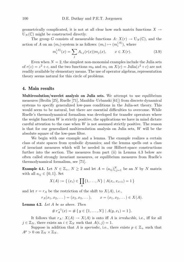
100 D.E. Dutkay and P.E.T. Jorgensen
geometrically complicated, it is not at all clear how such matrix functions X →UN (C) might be constructed directly.
The group G consists of measurable functions A : X(r) → UN (C), and theaction of A on an (mi)-system is as follows: (mi) → (m(A)
i ), where
m(A)i (x) =
∑j
Ai,j(r(x))mj(x), x ∈ X(r). (3.9)
Even when N = 2, the simplest non-monomial examples include the Julia setsof r(z) = z2 + c, and the two functions m0 and m1 on X(c) = Julia(z2 + c) are notreadily available by elementary means. The use of operator algebras, representationtheory seems natural for this circle of problems.
4. Main results
Multiresolution/wavelet analysis on Julia sets. We attempt to use equilibriummeasures (Brolin [25], Ruelle [71], Mauldin–Urbanski [61]) from discrete dynamicalsystems to specify generalized low-pass conditions in the Julia-set theory. Thiswould seem to be natural, but there are essential difficulties to overcome. WhileRuelle’s thermodynamical formalism was developed for transfer operators wherethe weight function W is strictly positive, the applications we have in mind dictatecareful attention to the case when W is not assumed strictly positive. The reasonis that for our generalized multiresolution analysis on Julia sets, W will be theabsolute square of the low-pass filter.
We begin with one example and a lemma. The example realizes a certainclass of state spaces from symbolic dynamics; and the lemma spells out a classof invariant measures which will be needed in our Hilbert-space constructionsfurther into the section. The measures from part (ii) in Lemma 4.3 below areoften called strongly invariant measures, or equilibrium measures from Ruelle’sthermodynamical formalism, see [71].
Example 4.1. Let N ∈ Z+, N ≥ 2 and let A = (aij)Ni,j=1 be an N by N matrix
with all aij ∈ 0, 1. Set
X(A) := (xi) ∈∏N
1, . . . , N | A(xi, xi+1) = 1
and let r = rA be the restriction of the shift to X(A), i.e.,
rA(x1, x2, . . . ) = (x2, x3, . . . ), x = (x1, x2, . . . ) ∈ X(A).
Lemma 4.2. Let A be as above. Then
# r−1A (x) = # y ∈ 1, . . . , N | A(y, x1) = 1 .
It follows that rA : X(A) → X(A) is onto iff A is irreducible, i.e., iff for allj ∈ ZN , there exists an i ∈ ZN such that A(i, j) = 1.
Suppose in addition that A is aperiodic, i.e., there exists p ∈ Z+ such thatAp > 0 on ZN × ZN .
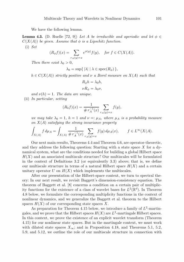
Multiscale Theory and Wavelets in Nonlinear Dynamics 101
We have the following lemma.
Lemma 4.3. (D. Ruelle [72, 9]) Let A be irreducible and aperiodic and let φ ∈C(X(A)) be given. Assume that φ is a Lipschitz function.
(i) Set(Rφf)(x) =
∑rA(y)=x
eφ(y)f(y), for f ∈ C(X(A)).
Then there exist λ0 > 0,
λ0 = sup |λ| | λ ∈ spec(Rφ) ,h ∈ C(X(A)) strictly positive and ν a Borel measure on X(A) such that
Rφh = λ0h,
νRφ = λ0ν,
and ν(h) = 1. The data are unique.(ii) In particular, setting
(R0f)(x) =1
# r−1A (x)
∑rA(y)=x
f(y),
we may take λ0 = 1, h = 1 and ν =: µA, where µA is a probability measureon X(A) satisfying the strong invariance property∫
X(A)
f dµA =∫
X(A)
1# r−1
A (x)
∑rA(y)=x
f(y) dµA(x), f ∈ L∞(X(A).
Our next main results, Theorems 4.4 and Theorem 4.6, are operator-theoretic,and they address the following question: Starting with a state space X for a dy-namical system, what are the conditions needed for building a global Hilbert spaceH(X) and an associated multiscale structure? Our multiscales will be formulatedin the context of Definitions 3.2 (or equivalently 3.3) above; that is, we defineour multiscale structure in terms of a natural Hilbert space H(X) and a certainunitary operator U on H(X) which implements the multiscales.
After our presentation of the Hilbert-space context, we turn to spectral the-ory: In our next result, we revisit Baggett’s dimension-consistency equation. Thetheorem of Baggett et al. [8] concerns a condition on a certain pair of multiplic-ity functions for the existence of a class of wavelet bases for L2(Rd). In Theorem4.8 below, we formulate the corresponding multiplicity functions in the context ofnonlinear dynamics, and we generalize the Baggett et al. theorem to the Hilbertspaces H(X) of our corresponding state spaces X .
As preparation for Theorem 4.15 below, we introduce a family of L2-martin-gales, and we prove that the Hilbert spaces H(X) are L2-martingale Hilbert spaces.In this context, we prove the existence of an explicit wavelet transform (Theorem4.15) for our nonlinear state spaces. But in the martingale context, we must workwith dilated state spaces X∞; and in Proposition 4.18, and Theorems 5.1, 5.2,5.9, and 5.12, we outline the role of our multiscale structure in connection with
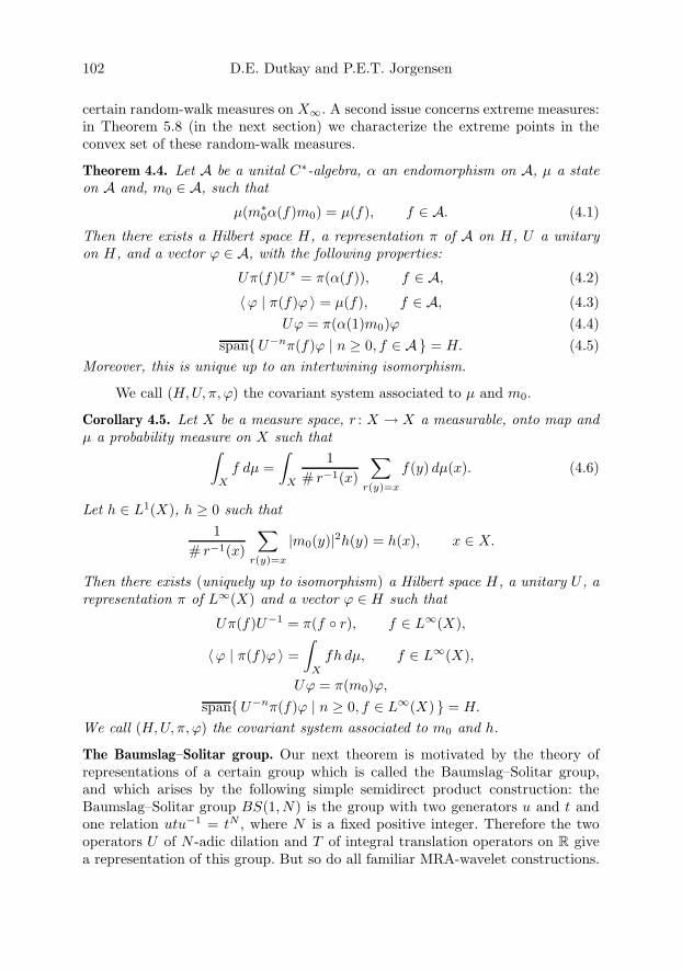
102 D.E. Dutkay and P.E.T. Jorgensen
certain random-walk measures on X∞. A second issue concerns extreme measures:in Theorem 5.8 (in the next section) we characterize the extreme points in theconvex set of these random-walk measures.
Theorem 4.4. Let A be a unital C∗-algebra, α an endomorphism on A, µ a stateon A and, m0 ∈ A, such that
µ(m∗0α(f)m0) = µ(f), f ∈ A. (4.1)
Then there exists a Hilbert space H, a representation π of A on H, U a unitaryon H, and a vector ϕ ∈ A, with the following properties:
Uπ(f)U∗ = π(α(f)), f ∈ A, (4.2)
〈ϕ | π(f)ϕ 〉 = µ(f), f ∈ A, (4.3)Uϕ = π(α(1)m0)ϕ (4.4)
spanU−nπ(f)ϕ | n ≥ 0, f ∈ A = H. (4.5)Moreover, this is unique up to an intertwining isomorphism.
We call (H, U, π, ϕ) the covariant system associated to µ and m0.
Corollary 4.5. Let X be a measure space, r : X → X a measurable, onto map andµ a probability measure on X such that∫
X
f dµ =∫
X
1# r−1(x)
∑r(y)=x
f(y) dµ(x). (4.6)
Let h ∈ L1(X), h ≥ 0 such that1
# r−1(x)
∑r(y)=x
|m0(y)|2h(y) = h(x), x ∈ X.
Then there exists (uniquely up to isomorphism) a Hilbert space H, a unitary U , arepresentation π of L∞(X) and a vector ϕ ∈ H such that
Uπ(f)U−1 = π(f r), f ∈ L∞(X),
〈ϕ | π(f)ϕ 〉 =∫
X
fh dµ, f ∈ L∞(X),
Uϕ = π(m0)ϕ,
spanU−nπ(f)ϕ | n ≥ 0, f ∈ L∞(X) = H.
We call (H, U, π, ϕ) the covariant system associated to m0 and h.
The Baumslag–Solitar group. Our next theorem is motivated by the theory ofrepresentations of a certain group which is called the Baumslag–Solitar group,and which arises by the following simple semidirect product construction: theBaumslag–Solitar group BS(1, N) is the group with two generators u and t andone relation utu−1 = tN , where N is a fixed positive integer. Therefore the twooperators U of N -adic dilation and T of integral translation operators on R givea representation of this group. But so do all familiar MRA-wavelet constructions.
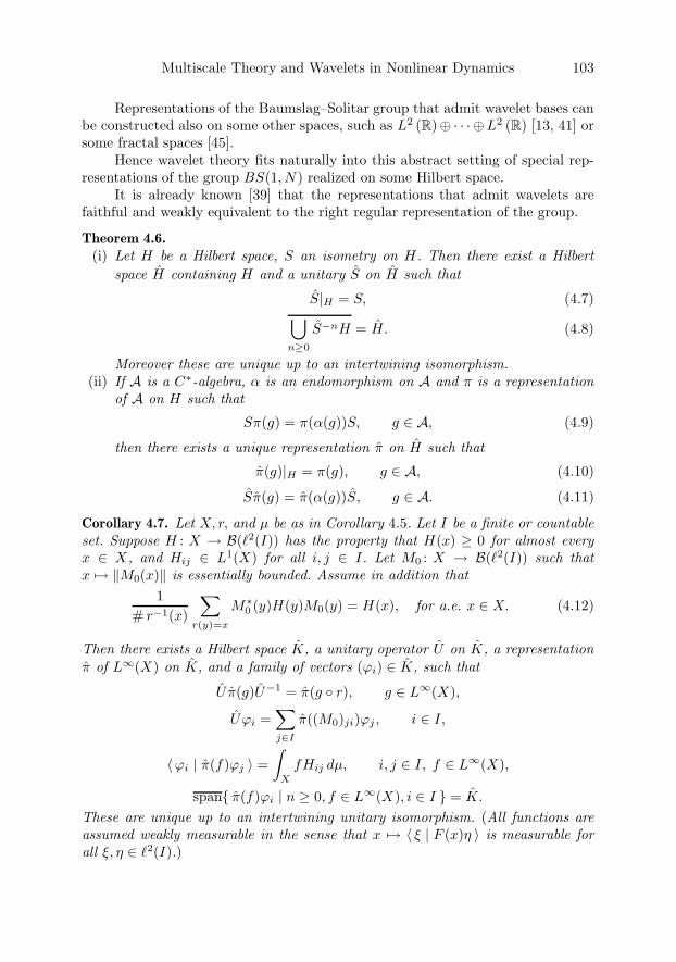
Multiscale Theory and Wavelets in Nonlinear Dynamics 103
Representations of the Baumslag–Solitar group that admit wavelet bases canbe constructed also on some other spaces, such as L2 (R)⊕ · · · ⊕L2 (R) [13, 41] orsome fractal spaces [45].
Hence wavelet theory fits naturally into this abstract setting of special rep-resentations of the group BS(1, N) realized on some Hilbert space.
It is already known [39] that the representations that admit wavelets arefaithful and weakly equivalent to the right regular representation of the group.
Theorem 4.6.(i) Let H be a Hilbert space, S an isometry on H. Then there exist a Hilbert
space H containing H and a unitary S on H such that
S|H = S, (4.7)⋃n≥0
S−nH = H. (4.8)
Moreover these are unique up to an intertwining isomorphism.(ii) If A is a C∗-algebra, α is an endomorphism on A and π is a representation
of A on H such that
Sπ(g) = π(α(g))S, g ∈ A, (4.9)
then there exists a unique representation π on H such that
π(g)|H = π(g), g ∈ A, (4.10)
Sπ(g) = π(α(g))S, g ∈ A. (4.11)
Corollary 4.7. Let X, r, and µ be as in Corollary 4.5. Let I be a finite or countableset. Suppose H : X → B(2(I)) has the property that H(x) ≥ 0 for almost everyx ∈ X, and Hij ∈ L1(X) for all i, j ∈ I. Let M0 : X → B(2(I)) such thatx → ‖M0(x)‖ is essentially bounded. Assume in addition that
1# r−1(x)
∑r(y)=x
M∗0 (y)H(y)M0(y) = H(x), for a.e. x ∈ X. (4.12)
Then there exists a Hilbert space K, a unitary operator U on K, a representationπ of L∞(X) on K, and a family of vectors (ϕi) ∈ K, such that
U π(g)U−1 = π(g r), g ∈ L∞(X),
Uϕi =∑j∈I
π((M0)ji)ϕj , i ∈ I,
〈ϕi | π(f)ϕj 〉 =∫
X
fHij dµ, i, j ∈ I, f ∈ L∞(X),
span π(f)ϕi | n ≥ 0, f ∈ L∞(X), i ∈ I = K.
These are unique up to an intertwining unitary isomorphism. (All functions areassumed weakly measurable in the sense that x → 〈 ξ | F (x)η 〉 is measurable forall ξ, η ∈ 2(I).)

104 D.E. Dutkay and P.E.T. Jorgensen
Suppose now that H is a Hilbert space with an isometry S on it and with anormal representation π of L∞(X) on H that satisfies the covariance relation
Sπ(g) = π(g r)S, g ∈ L∞(X). (4.13)
Theorem 4.6 shows that there exists a Hilbert space H containing H , a uni-tary S on H and a representation π of L∞(X) on H such that
(Vn := S−n(H))n form an increasing sequence of subspaces with dense union,
S|H = S,
π|H = π,
Sπ(g) = π(g r)S.
Theorem 4.8.(i) V1 = S−1(H) is invariant for the representation π. The multiplicity functions
of the representation π on V1, and on V0 = H, are related by
mV1(x) =∑
r(y)=x
mV0(y), x ∈ X. (4.14)
(ii) If W0 := V1 V0 = S−1H H, then
mV0(x) + mW0(x) =∑
r(y)=x
mV0(y), x ∈ X. (4.15)
Proof. Note that S maps V1 to V0, and the covariance relation implies that therepresentation π on V1 is isomorphic to the representation πr : g → π(g r) onV0. Therefore we have to compute the multiplicity of the latter, which we de-note by mr
V0.
By the spectral theorem there exists a unitary isomorphism J : H(= V0) →L2(X, mV0 , µ), where, for a multiplicity function m : X → 0, 1, . . . ,∞, we usethe notation
L2(X, m, µ) := f : X → ∪x∈XCm(x) | f(x) ∈ C
m(x),
∫X
‖f(x)‖2 dµ(x) <∞.
In addition J intertwines π with the representation of L∞(X) by multiplicationoperators, i.e.,
(Jπ(g)J−1(f))(x) = g(x)f(x), g ∈ L∞(X), f ∈ L2(X, mV0 , µ), x ∈ X.
Remark 4.9. Here we are identifying H with L2(X, mV0 , µ) via the spectral repre-sentation. We recall the details of this representation H f → f ∈ L2(X, mV0 , µ).
Recall that any normal representation π ∈ Rep(L∞(X), H) is the orthogonalsum
H =∑⊕
k∈C
[π(L∞(X))k], (4.16)
Multiscale Theory and Wavelets in Nonlinear Dynamics 105
where the set C of vectors k ∈ H is chosen such that• ‖k‖ = 1,
• 〈 k | π(g)k 〉 =∫
X
g(x)vk(x)2 dµ(x), for all k ∈ C;
• 〈 k′ | π(g)k 〉 = 0, g ∈ L∞(X), k, k′ ∈ C, k = k′; orthogonality.
The formula (4.16) is obtained by a use of Zorn’s lemma. Here, v2k is the Radon-
Nikodym derivative of 〈 k | π(·)k 〉 with respect to µ, and we use that π is assumednormal.
For f ∈ H , setf =
∑⊕
k∈C
π(gk)k, gk ∈ L∞(X)
andf =
∑⊕
k∈C
gkvk ∈ L2µ(X, 2(C)).
Then Wf = f is the desired spectral transform, i.e.,
W is unitary,
Wπ(g) = M(g)W,
and‖f(x)‖2 =
∑k∈C
|gk(x)vk(x)|2.
Indeed, we have∫X
‖f(x)‖2 dµ(x) =∫
X
∑k∈C
|gk(x)|2vk(x)2 dµ(x) =∑k∈C
∫X
|gk|2v2k dµ
=∑k∈C
⟨k | π(|gk|2)k
⟩=∑k∈C
‖π(gk)k‖2 =
∥∥∥∥∥∑⊕
k∈C
π(gk)k
∥∥∥∥∥2
H
= ‖f‖2H .
It follows in particular that the multiplicity function m(x) = mH(x) is
m(x) = # k ∈ C | vk(x) = 0 .Setting
Xi := x ∈ X | m(x) ≥ i , i ≥ 1,
we see thatH
∑⊕L2(Xi, µ) L2(X, m, µ),
and the isomorphism intertwines π(g) with multiplication operators.
Returning to the proof of the theorem, we have to find the similar form forthe representation πr. Let
m(x) :=∑
r(y)=x
mV0(y), x ∈ X. (4.17)
106 D.E. Dutkay and P.E.T. Jorgensen
Define the following unitary isomorphism:
L : L2(X, mV0 , µ)→ L2(X, m, µ),
(Lξ)(x) =1√
# r−1(x)(ξ(y))r(y)=x.
(Note that the dimensions of the vectors match because of (4.17).) This operatorL is unitary. For ξ ∈ L2(X, mV0 , µ), we have
‖Lξ‖2L2(X,mV0 ,µ) =∫
X
‖Lξ(x)‖2 dµ(x)
=∫
X
1# r−1(x)
∑r(y)=x
‖ξ(y)‖2 dµ(x)
=∫
X
‖ξ(x)‖2 dµ(x).
And L intertwines the representations. Indeed, for g ∈ L∞(X),
L(g r ξ)(x) = (g(r(y))ξ(y))r(y)=x = g(x)L(ξ)(x).
Therefore, the multiplicity of the representation πr : g → π(g r) on V0 is m, andthis proves (i).(ii) follows from (i).
Conclusions. By definition, if k ∈ C,
〈 k | π(g)k 〉 =∫
X
g(x)vk(x)2 dµ(x), and
〈 k | πr(g)k 〉 =∫
X
g(r(x))vk(x)2 dµ(x) =∫
X
g(x)1
# r−1(x)
∑r(y)=x
vk(x)2 dµ(x);
and so
mr(x) = # k ∈ C |∑
r(y)=x
vk(y)2 > 0
=∑
r(y)=x
# k ∈ C | vk(y)2 > 0 =∑
r(y)=x
m(y).
Let Cm(x) := k ∈ C | vk(x) = 0 . Then we showed that
Cm(x) =⋃
y∈X,r(y)=x
Cm(y)
and that Cm(y) ∩ Cm(y′) = ∅ when y = y′ and r(y) = r(y′) = x. SettingH(x) = 2(Cm(x)), we have
H(x) = 2(Cm(x)) =∑⊕
r(y)=x
2(Cm(y)) =∑⊕
r(y)=x
H(y).

Multiscale Theory and Wavelets in Nonlinear Dynamics 107
4.1. Spectral decomposition of covariant representations: projective limits
We give now a different representation of the construction of the covariant systemassociated to m0 and h.
We work in either the category of measure spaces or topological spaces.
Definition 4.10. Let r : X → X be onto, and assume that # r−1(x) < ∞ for allx ∈ X . We define the projective limit of the system:
Xr← X
r← X · · · → X∞ , (4.18)
asX∞ := x = (x0, x1, . . . ) | r(xn+1) = xn, for all n ≥ 0 .
Let θn : X∞ → X be the projection onto the nth component:
θn(x0, x1, . . . ) = xn, (x0, x1, . . . ) ∈ X∞.
Taking inverse images of sets in X through these projections, we obtain a sigma-algebra on X∞, or a topology on X∞.
We have an induced mapping r : X∞ → X∞ defined by
r(x) = (r(x0), x0, x1, . . . ), and with inverse r−1(x) = (x1, x2, . . . ). (4.19)
so r is an automorphism, i.e., r r−1 = idX∞ and r−1 r = idX∞ .Note that
θn r = r θn = θn−1,
Consider a probability measure µ on X that satisfies∫X
f dµ =∫
X
1# r−1(x)
∑r(y)=x
f(y) dµ(x). (4.20)
For m0 ∈ L∞(X), define
(Rξ)(x) =1
# r−1(x)
∑r(y)=x
|m0(y)|2ξ(y), ξ ∈ L1(X). (4.21)
We now resume the operator theoretic theme of our paper, that of extendinga system of operators in a given Hilbert space to a “dilated” system in an ambientor extended Hilbert space; the general idea being that the dilated system acquiresa “better” spectral theory; for example, contractive operators dilate to unitaryoperators in the extended Hilbert space; and similarly, endomorphisms dilate toautomorphisms. This of course is a general theme in operator theory; see e.g.,[10] and [38]. But in our present setting, there is much more structure than themere Hilbert space geometry: We must adapt the underlying operator theory tothe particular function spaces and measures at hand. The next theorem (Theorem4.13) is key to the understanding of the dilation step as it arises in our contextof multiscale theory. It takes into consideration how we arrive at our functionspaces by making dynamics out of the multiscale setting. Hence, the dilations weconstruct take place at three separate levels as follows:
108 D.E. Dutkay and P.E.T. Jorgensen
• dynamical systems,
(X, r, µ) endomorphism → (X∞, r, µ), automorphism ;
• Hilbert spaces,
L2(X, h dµ)→ (Rm0h = h)→ L2(X∞, µ);
• operators,
Sm0 isometry → U unitary (if m0 is non-singular),
M(g) multiplication operator →M∞(g).
Definition 4.11. A function m0 on a measure space is called singular if m0 = 0 ona set of positive measure.
In general, the operators Sm0 on H0 = L2(X, h dµ), and U on L2(X∞, µ),may be given only by abstract Hilbert-space axioms; but in our martingale repre-sentation, we get the following two concrete formulas:
(Sm0ξ)(x) = m0(x)ξ(r(x)), x ∈ X, ξ ∈ H0,
(Uf)(x) = m0(x0)f(r(x)), x ∈ X∞, f ∈ L2(X∞, µ).
Definition 4.12. Let X , r, µ, and W be given as before. Recall r : X → X is afinite-to-one map onto X , µ is a corresponding strongly invariant measure, andW : X → [0,∞) is a measurable weight function. We define the correspondingRuelle operator R = RW , and we let h be a chosen Perron–Frobenius–Ruelleeigenfunction. From these data, we define the following sequence of measures ωn
on X . (Our presentation of a wavelet transform in Theorem 4.15 will depend onthis sequence.) For each n, the measure ωn is defined by the following formula:
ωn(f) =∫
X
Rn(fh) dµ, f ∈ L∞(X). (4.22)
To build our wavelet transform, we first prove in Theorem 4.13 below thateach of the measure families (ωn) defines a unique W -quasi-invariant measure µ onX∞. In the theorem, we take W := |m0|2, and we show that µ is quasi-invariantwith respect to r with transformation Radon-Nikodym derivative W .
Theorem 4.13. If h ∈ L1(X), h ≥ 0 and Rh = h, then there exists a uniquemeasure µ on X∞ such that
µ θ−1n = ωn, n ≥ 0.
We can identify functions on X with functions on X∞ by
f(x0, x1, . . . ) = f(x0), f : X → C.
Under this identification,d(µ r)
dµ= |m0|2. (4.23)
Multiscale Theory and Wavelets in Nonlinear Dynamics 109
Theorem 4.14. Suppose m0 is non-singular, i.e., it does not vanish on a set ofpositive measure. Define U on L2(X∞, µ) by
Uf = m0f r, f ∈ L2(X∞, µ),
π(g)f = gf, g ∈ L∞(X), f ∈ L2(X∞, µ),ϕ = 1.
Then (L2(X∞, µ), U, π, ϕ) is the covariant system associated to m0 and h as inCorollary 4.5. Moreover, if Mgf = gf for g ∈ L∞(X∞, µ) and f ∈ L2(X∞, µ),then
UMgU−1 = Mgr.
The Hilbert space L2(X∞, µ) admits a different representation as an L2-mar-tingale Hilbert space. Let
Hn := f ∈ L2(X∞, µ) | f = ξ θn, ξ ∈ L2(X, ωn) .Then Hn form an increasing sequence of closed subspaces which have dense union.
We can identify the functions in Hn with functions in L2(X, ωn), by
in(ξ) = ξ θn, ξ ∈ L2(X, ωn).
The definition of µ makes in an isomorphism between Hn and L2(X, ωn).Define
H :=
(ξ0, ξ1, . . . )∣∣∣ ξn ∈ L2(X, ωn), R(ξn+1h) = ξnh, sup
n
∫X
Rn(|ξn|2h) dµ <∞
with the scalar product
〈 (ξ0, ξ1, . . . ) | (η0, η1, . . . ) 〉 = limn→∞
∫X
Rn(ξnηnh) dµ.
Theorem 4.15. The map Φ: L2(X∞, µ)→ H defined by
Φ(f) = (i−1n (Pnf))n≥0,
where Pn is the projection onto Hn, is an isomorphism. The transform Φ satisfiesthe following three conditions, and it is determined uniquely by them:
ΦUΦ−1(ξn)n≥0 = (m0 rn ξn+1)n≥0,
Φπ(g)Φ−1(ξn)n≥0 = (g rn ξn)n≥0,
Φϕ = (1, 1, . . . ).
Theorem 4.16. There exists a unique isometry Ψ: L2(X∞, µ)→ H such that
Ψ(ξ θn) = U−nπ(ξ)Unϕ, ξ ∈ L∞(X, µ).
Ψ intertwines the two systems, i.e.,
ΨU = UΨ, Ψπ(g) = π(g)Ψ, for g ∈ L∞(X, µ), Ψϕ = ϕ.
Theorem 4.17. Let (m0, h) be a Perron–Ruelle–Frobenius pair with m0 non-singu-lar.

110 D.E. Dutkay and P.E.T. Jorgensen
(i) For each operator A on L2(X∞, µ) which commutes with U and π, there existsa cocycle f , i.e., a bounded measurable function f : X∞ → C with f = f r,µ-a.e., such that
A = Mf , (4.24)and, conversely each cocycle defines an operator in the commutant.
(ii) For each measurable harmonic function h0 : X → C, i.e., Rm0h0 = h0, with|h0|2 ≤ ch2 for some c ≥ 0, there exists a unique cocycle f such that
h0 = E0(f)h, (4.25)
where E0 denotes the conditional expectation from L∞(X∞, µ) to L∞(X, µ),and conversely, for each cocycle the function h0 defined by (4.25) is harmonic.
(iii) The correspondence h0 → f in (ii) is given by
f = limn→∞
h0
h θn (4.26)
where the limit is pointwise µ-a.e., and in Lp(X∞, µ) for all 1 ≤ p <∞.
The final result in this section concerns certain path-space measures, indexed bya base space X . Such a family is also called a process: it is a family of positiveRadon measures Px, indexed by x in the base space X . Each Px is a measure on theprobability space Ω which is constructed from X by the usual Cartesian product,i.e., countably infinite Cartesian product of X with itself. The Borel structure onΩ is generated by the usual cylinder subsets of Ω. Given a weight function Won X , the existence of the measures Px comes from an application of a generalprinciple of Kolmogorov.
Let X be a metric space and r : X → X an N to 1 map. Denote by τk : X →X , k ∈ 1, . . . , N, the branches of r, i.e., r(τk(x)) = x for x ∈ X , the sets τk(X)are disjoint and they cover X .
Let µ be a measure on X with the property
µ =1N
N∑k=1
µ τ−1k . (4.27)
This can be rewritten as∫X
f(x) dµ(x) =1N
N∑k=1
∫X
f(τk(x)) dµ(x), (4.28)
which is equivalent also to the strong invariance property.Let W , h ≥ 0 be two functions on X such that
N∑k=1
W (τk(x))h(τk(x)) = h(x), x ∈ X. (4.29)
Denote by Ω the multi-index set
Ω := ΩN :=∏N
1, . . . , N.

Multiscale Theory and Wavelets in Nonlinear Dynamics 111
Also we define
W (n)(x) := W (x)W (r(x)) · · ·W (rn−1(x)), x ∈ X.
The final result in this section concerns certain path-space measures. In thiscontext each measure Px is a measure on Ω. We will return to a more generalvariant of these path-space measures in Theorem 5.12 in the next section. Thiswill be in the context of a system (X, r, V ) where r : X → X is a give finite toone endomorphism, and W : X → [0,∞) is a measurable weight function. In thiscontext the measures (Px) are indexed by a base space X , and they are measureson the projective space X∞ built on (X, r), see Definition 4.10. The family (Px) isalso called a process: each Px is a positive Radon measure on X∞, and X∞ maybe thought of as a discrete path space.
The Borel structure on Ω, and on X∞, is generated by the usual cylindersubsets. Given a weight function W on X , the existence of the measures Px := PW
x
comes from an application of a general principle of Kolmogorov.
Proposition 4.18. For every x ∈ X there exists a positive Radon measure Px on Ωsuch that, if f is a bounded measurable function on X which depends only on thefirst n coordinates ω1, . . . , ωn, then∫
Ω
f(ω) dPx(ω)
=∑
ω1,...,ωn
W (n)(τωnτωn−1 · · · τω1(x))h(τωnτωn−1 · · · τω1(x))f(ω1, . . . , ωn). (4.30)
5. Remarks on other applications
Wavelet sets. Investigate the existence and construction of wavelet sets and el-ementary wavelets and frames in the Julia-set theory, and the corresponding in-terpolation theory, and their relationships to generalized multiresolution analysis(GMRA). The unitary system approach to wavelets by Dai and Larson [32] dealtwith systems that can be very irregular. And recent work by Olafsson et al. showsthat wavelet sets can be essential to a basic dilation-translation wavelet theoryeven for a system where the set of dilation unitaries is not a group.
The renormalization question. When are there renormalizable iterates of r in arith-metic progression, i.e., when are there iteration periods n such that the systemrkn, k ∈ N may be renormalized, or rescaled to yield a new dynamical system ofthe same general shape as that of the original map r(z)?
Since the scaling equation (2.2) from wavelet theory is a renormalization,our application of multiresolutions to the Julia sets X(r) of complex dynamicssuggests a useful approach to renormalization in this context. The drawback ofthis approach is that it relies on a rather unwieldy Hilbert space built on X(r),or rather on the projective system X(r)∞ built in turn over X(r). So we are left
112 D.E. Dutkay and P.E.T. Jorgensen
with translating our Hilbert-space-theoretic normalization back to the direct andgeometric algorithms on the complex plane.
General and rigorous results from complex dynamics state that under addi-tional geometric hypotheses, renormalized dynamical systems range in a compactfamily.
The use of geometric tools from Hilbert space seems promising for renormal-ization questions (see, e.g., [64], [15], [23], and [74]) since notions of repetition upto similarity of form at infinitely many scales are common in the Hilbert-spaceapproach to multiresolutions; see, e.g., [35]. And this self-similarity up to scaleparallels a basic feature of renormalization questions in physics: for a variety of in-stances of dynamics in physics, and in telecommunication [64, 15, 20], we encounterscaling laws of self-similarity; i.e., we observe that a phenomenon reproduces itselfon different time and/or space scales.
Self-similar processes are stochastic processes that are invariant in distribu-tion under suitable scaling of time and/or space (details below!) Fractional Brown-ian motion is perhaps the best known of these, and it is used in telecommunicationand in stochastic integration. While the underlying idea behind this can be tracedback to Kolmogorov, it is only recently, with the advent of wavelet methods, thatits computational power has come more into focus, see, e.g., [64]. But at the sametime, this connection to wavelet analysis is now bringing the operator-theoreticfeatures in the subject to the fore.
In statistics, we observe that fractional Brownian motion (a Gaussian pro-cess B(t) with EB(t) = 0, and covariance EB(t)B(s) given by a certainh-fractional law) has the property that there is a number h such that, for all a,the two processes B(at) and ahB(t) have the same finite-dimensional distribu-tions. The scaling feature of fractional Brownian motion, and of its correspondingwhite-noise process, is used in telecommunication, and in stochastic integration;and this connection has been one of the new and more exciting domains of appli-cations of wavelet tools, both pure and applied (Donoho, Daubechies, Meyer, etc.[35, 33, 63]).
This is a new direction of pure mathematics which makes essential contactwith problems that are not normally investigated in the context of harmonic anal-ysis.
In our proofs, we take advantage of our Hilbert-space formulation of thenotion of similarity up to scale, and the use of scales of closed subspaces Vn ina Hilbert space H. The unitary operator U which scales between the spaces mayarise from a substitution in nonlinear dynamics, such as in the context of Juliasets [11]; it may “scale” between the sigma-algebras in a martingale [36, 37, 75];it may be a scaling of large volumes of data (see, e.g., [1]); it may be the scalingoperation in a fractional Brownian motion [64, 59]; it may be cell averages in finiteelements [29]; or it may be the traditional dyadic scaling operator in H = L2(R)in wavelet frame analysis [28, 29].
Once the system (H, (Vn), U) is given, then it follows that there is a unitaryrepresentation V of T in H which defines a grading of operators on H. Moreover
Multiscale Theory and Wavelets in Nonlinear Dynamics 113
U then defines a similarity up to scale precisely when U has grade one, see (3.4)for definition. We also refer to the papers [4, 10] for details and applications ofthis notion in operator theory.
The general idea of assigning degrees to operators in Hilbert space has servedas a powerful tool in other areas of mathematical physics (see, e.g., [3], [22]; and[16] on phase transition problems); operator theory [5, 4, 38, 2]; and operatoralgebras; see, e.g., [31, 73, 24].
Our research, e.g., [43], in fact already indicates that the nonlinear problemssketched above can be attacked with the use of our operator-theoretic framework.
Wavelet representations of operator-algebraic crossed products. The constructionof wavelets requires a choice of a low-pass filter m0 ∈ L∞(T) and of N − 1 high-pass filters mi ∈ L∞(T) that satisfy certain orthogonality conditions. As shownin [17], these choices can be put in one-to-one correspondence with a class ofcovariant representations of the Cuntz algebra ON . In the case of an arbitrary N -to-one dynamical system r : X → X , the wavelet construction will again involvea careful choice of the filters, and a new class of representations is obtain. Thequestion here is to classify these representations and see how they depend on thedynamical system r. A canonical choice of the filters could provide an invariantfor the dynamical system.
In a recent paper [47], the crossed-product of a C∗-algebra by an endomor-phism is constructed using the transfer operator. The required covariant relationsare satisfied by the operators that we introduced in [43], [44].
There are two spaces for these representations: one is the core space of themultiresolution V0 = L2(X, µ). Here we have the abelian algebra of multiplicationoperators and the isometry S : f → m0 f r. Together they provide representationsof the crossed product by an endomorphism. The second space is associated to adilated measure µ on the solenoid of r, L2(X∞, µ) (see [43], [44]). The isometryS is dilated to a unitary S which preserves the covariance. In this case, we aredealing with representations of crossed products by automorphisms.
Thus we have four objects interacting with one another: crossed products byendomorphisms and their representations, and crossed products by automorphismsand its representations on L2(X, µ).
The representations come with a rich structure given by the multiresolution,scaling function and wavelets. Therefore their analysis and classification seemspromising.
KMS-states and equilibrium measures. In [48], the KMS states on the Cuntz–Pimsner algebra for a certain one-parameter group of automorphisms are obtainedby composing the unique equilibrium measure on an abelian subalgebra (i.e., themeasure which is invariant to the transfer operator) with the conditional expec-tation. These results were further generalized in [58] for expansive maps and theassociated groupoid algebras.
As we have seen in [45] for the case when r(z) = zN , the covariant representa-tions associated to some low-pass filter m0 are highly dependent on the equilibrium
114 D.E. Dutkay and P.E.T. Jorgensen
measure ν. As outlined above, we consider here an expansive dynamical systembuilt on a given finite-to-one mapping r : X → X , and generalizing the familiarcase of the winding mapping z → zN on T. In our r : X → X context, we thenstudy weight functions V : X → [0,∞). If the zero-set of V is now assumed finite,we have so far generalized what is known in the z → zN case. Our results take theform of a certain dichotomy for the admissible Perron–Frobenius–Ruelle measures,and they fit within the framework of [58]. Hence our construction also yields covari-ant representations and symmetry in the context of [58]. Our equilibrium measuresin turn induce the kind of KMS-states studied in [58].
The results of [58] and [48] restrict the weight function (in our case repre-sented by the absolute square of the low-pass filter, |m0|2) to being strictly pos-itive and Holder continuous. These restrictions are required because of the formof the Ruelle–Perron–Frobenius theorem used, which guarantees the existence anduniqueness of the equilibrium measure.
However, the classical wavelet theory shows that many interesting examplesrequire a “low-pass condition”, m0(1) =
√N , which brings zeroes for |m0|2.
Our martingale approach is much less restrictive than the conditions of [58]:it allows zeroes and discontinuities. Coupled with a recent, more general form ofRuelle’s theorem from [49], we hope to extend the results of [58] and be able to findthe KMS states in a more general case. Since the existence of zeroes can implya multiplicity of equilibrium measures (see [41], [19]) a new phenomenon mightoccur such as spontaneously breaking symmetry.
For each KMS state, one can construct the GNS representation. Interest-ing results are known [65] for the subshifts of finite type and the Cuntz–Kriegeralgebra, when the construction yields type IIIλ AFD factors.
The natural question is what type of factors appear in the general case ofr : X → X . Again, a canonical choice for the low-pass filter can provide invariantsfor the dynamical system.
Historically, von-Neumann-algebra techniques have served as powerful toolsfor analyzing discrete structures. Our work so far suggests that the iterationsystems (X, r) will indeed induce interesting von-Neumann-algebra isomorphismclasses.
Dimension groups. We propose to use our geometric algorithms [20, 21] for decidingorder isomorphism of dimension groups for the purpose of deciding isomorphismquestions which arise in our multiresolution analysis built on Julia sets. The projectis to use the results in [20] to classify substitution tilings in the sense of [66], [67].
Equilibrium measures, harmonic functions for the transfer operator, and infiniteRiesz products. In [19], [41], for the dynamical system z → zN , we were able tocompute the equilibrium measures, the fixed points of the transfer operator andits ergodic decomposition by analyzing the commutant of the covariant represen-tations associated to the filter m0. In [43], [44] we have shown that also in thegeneral case there is a one-to-one correspondence between harmonic functions forthe transfer operator and the commutant. Thus an explicit form of the covariant
Multiscale Theory and Wavelets in Nonlinear Dynamics 115
representation can give explicit solutions for the eigenvalue problem Rm0h = h,which are of interest in ergodic theory (see [9]).
In some cases, the equilibrium measures are Riesz products (see [45]); theseare examples of exotic measures which arise in harmonic analysis [12, 46, 56, 6,69, 14, 26, 27, 57, 62, 70]. The wavelet-operator-theoretic approach may providenew insight into their properties.
Non-uniqueness of the Ruelle–Perron–Frobenius data. A substantial part of thecurrent literature in the Ruelle–Perron–Frobenius operator in its many guisesis primarily about conditions for uniqueness of KMS; so that means no phasetransition. This is ironic since Ruelle’s pioneering work was motivated by phase-transition questions, i.e., non-uniqueness.
In fact non-uniqueness is much more interesting in a variety of applications:That is when we must study weight functions W in the Ruelle operator R = RW
when the standard rather restrictive conditions on W are in force. The much cele-brated Ruelle theorem for the transition operator R gives existence and uniquenessof Perron–Frobenius data under these restrictive conditions. But both demandsfrom physics, and from wavelets, suggest strong and promising research interestin relaxing the stringent restrictions that are typical in the literature, referring toassumptions on W . There is a variety of exciting possibilities. They would give usexistence, but not necessarily uniqueness in the conclusion of a new Ruelle-typetheorem.
Induced measures. A basic tool in stochastic processes (from probability theory)involves a construction on a “large” projective space X∞, based on some marginalmeasure on some coordinate space X . Our projective limit space X∞ will beconstructed from a finite branching process.
Let A be a k × k matrix with entries in 0, 1. Suppose every column in Acontains an entry 1.
Set X(A) :=
(ξi)i∈N ∈∏
N1, . . . , k
∣∣ A(ξi, ξi+1) = 1
and
rA(ξ1, ξ2, . . . ) = (ξ2, ξ3, . . . ) for ξ ∈ X(A).
Then rA is a subshift, and the pair (X(A), rA) satisfies our conditions.It is known [72] that, for each A, as described, the corresponding system
rA : X(A) → X(A) has a unique strongly rA-invariant probability measure, ρA,i.e., a probability measure on X(A) such that ρA R1 = ρA, where R1 is definedas in (5.1) below.
We now turn to the connection between measures on X and an associatedfamily of induced measures on X∞, and we characterize those measures X∞ whichare quasi-invariant with respect to the invertible mapping r, where X∞ := x =(x0, x1, . . . ) ∈
∏N0
X | r(xn+1) = xn , r(x) = (r(x0), x0, x1, . . . ).In our extension of measures from X to X∞, we must keep track of the
transfer from one step to the next, and there is an operator which accomplishes

116 D.E. Dutkay and P.E.T. Jorgensen
this, Ruelle’s transfer operator
RW f(x) =1
# r−1(x)
∑r(y)=x
W (y)f(y), f ∈ L1(X, µ). (5.1)
In its original form it was introduced in [72], but since that, it has found a varietyof applications, see e.g., [9]. For use of the Ruelle operator in wavelet theory, werefer to [54] and [41].
The Hilbert spaces of functions on X∞ will be realized as a Hilbert spacesof martingales. This is consistent with our treatment of wavelet resolutions asmartingales. This was first suggested in [51] in connection with wavelet analysis.
In [43], we studied the following restrictive setup: we assumed that X carriesa probability measure µ which is strongly r-invariant. By this we mean that∫
X
f dµ =∫
X
1# r−1(x)
∑y∈X,r(y)=x
f(y) dµ(x), f ∈ L∞(X). (5.2)
If, for example X = R/Z, and r(x) = 2x mod 1, then the Haar measure onR/Z = Lebesgue measure on [0, 1) is the unique strongly r-invariant measure on X .
Suppose the weight function V is bounded and measurable. Then define R =RV , the Ruelle operator, by formula (5.1), with V = W .
Theorem 5.1. ([43]) Let r : X → X and X∞(r) be as described above, and supposethat X has a strongly r-invariant measure µ. Let V be a non-negative, measurablefunction on X, and let RV be the corresponding Ruelle operator.
(i) There is a unique measure µ on X∞(r) such that
(a) µ θ−10 µ (set h = d(µθ−1
0 )
dµ ),(b)
∫X f dµ θ−1
n =∫
X RnV (fh) dµ, n ∈ N0.
(ii) The measure µ on X∞(r) satisfies
d(µ r)dµ
= V θ0, (5.3)
andRV h = h. (5.4)
If the function V : X → [0,∞) is given, we define
V (n)(x) := V (x)V (r(x)) · · · V (rn−1(x)),
and set dµn := V (n)dµ0. Our result states that the corresponding measure µ onX∞(r) is V -quasi-invariant if and only if
dµ0 = (V dµ0) r−1. (5.5)
Theorem 5.2. Let V : X → [0,∞) be B-measurable, and let µ0 be a measure on Xsatisfying the following fixed-point property
dµ0 = (V dµ0) r−1. (5.6)
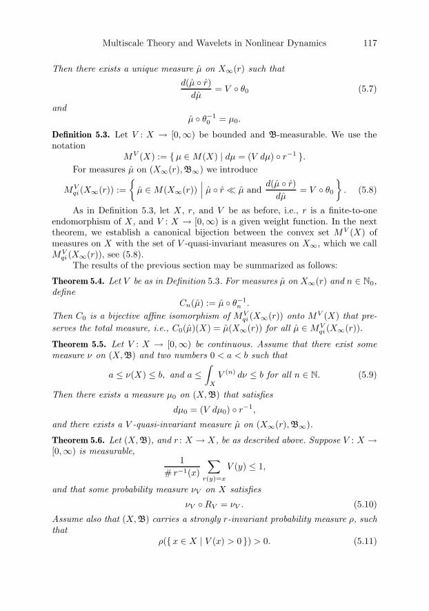
Multiscale Theory and Wavelets in Nonlinear Dynamics 117
Then there exists a unique measure µ on X∞(r) such thatd(µ r)
dµ= V θ0 (5.7)
andµ θ−1
0 = µ0.
Definition 5.3. Let V : X → [0,∞) be bounded and B-measurable. We use thenotation
MV (X) := µ ∈M(X) | dµ = (V dµ) r−1 .For measures µ on (X∞(r), B∞) we introduce
MVqi (X∞(r)) :=
µ ∈M(X∞(r))
∣∣∣ µ r µ andd(µ r)
dµ= V θ0
. (5.8)
As in Definition 5.3, let X , r, and V be as before, i.e., r is a finite-to-oneendomorphism of X , and V : X → [0,∞) is a given weight function. In the nexttheorem, we establish a canonical bijection between the convex set MV (X) ofmeasures on X with the set of V -quasi-invariant measures on X∞, which we callMV
qi (X∞(r)), see (5.8).The results of the previous section may be summarized as follows:
Theorem 5.4. Let V be as in Definition 5.3. For measures µ on X∞(r) and n ∈ N0,define
Cn(µ) := µ θ−1n .
Then C0 is a bijective affine isomorphism of MVqi (X∞(r)) onto MV (X) that pre-
serves the total measure, i.e., C0(µ)(X) = µ(X∞(r)) for all µ ∈MVqi (X∞(r)).
Theorem 5.5. Let V : X → [0,∞) be continuous. Assume that there exist somemeasure ν on (X, B) and two numbers 0 < a < b such that
a ≤ ν(X) ≤ b, and a ≤∫
X
V (n) dν ≤ b for all n ∈ N. (5.9)
Then there exists a measure µ0 on (X, B) that satisfies
dµ0 = (V dµ0) r−1,
and there exists a V -quasi-invariant measure µ on (X∞(r), B∞).
Theorem 5.6. Let (X, B), and r : X → X, be as described above. Suppose V : X →[0,∞) is measurable,
1# r−1(x)
∑r(y)=x
V (y) ≤ 1,
and that some probability measure νV on X satisfies
νV RV = νV . (5.10)
Assume also that (X, B) carries a strongly r-invariant probability measure ρ, suchthat
ρ( x ∈ X | V (x) > 0 ) > 0. (5.11)
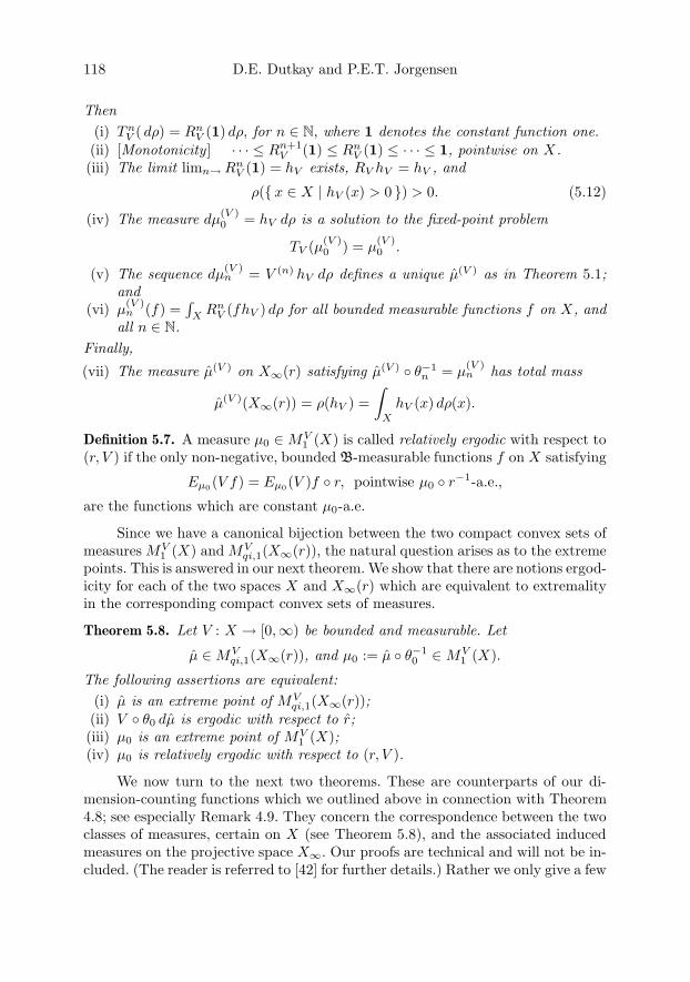
118 D.E. Dutkay and P.E.T. Jorgensen
Then(i) T n
V ( dρ) = RnV (1) dρ, for n ∈ N, where 1 denotes the constant function one.
(ii) [Monotonicity] · · · ≤ Rn+1V (1) ≤ Rn
V (1) ≤ · · · ≤ 1, pointwise on X.(iii) The limit limn→ Rn
V (1) = hV exists, RV hV = hV , and
ρ( x ∈ X | hV (x) > 0 ) > 0. (5.12)
(iv) The measure dµ(V )0 = hV dρ is a solution to the fixed-point problem
TV (µ(V )0 ) = µ
(V )0 .
(v) The sequence dµ(V )n = V (n) hV dρ defines a unique µ(V ) as in Theorem 5.1;
and(vi) µ
(V )n (f) =
∫X Rn
V (fhV ) dρ for all bounded measurable functions f on X, andall n ∈ N.
Finally,
(vii) The measure µ(V ) on X∞(r) satisfying µ(V ) θ−1n = µ
(V )n has total mass
µ(V )(X∞(r)) = ρ(hV ) =∫
X
hV (x) dρ(x).
Definition 5.7. A measure µ0 ∈MV1 (X) is called relatively ergodic with respect to
(r, V ) if the only non-negative, bounded B-measurable functions f on X satisfying
Eµ0 (V f) = Eµ0(V )f r, pointwise µ0 r−1-a.e.,
are the functions which are constant µ0-a.e.
Since we have a canonical bijection between the two compact convex sets ofmeasures MV
1 (X) and MVqi,1(X∞(r)), the natural question arises as to the extreme
points. This is answered in our next theorem. We show that there are notions ergod-icity for each of the two spaces X and X∞(r) which are equivalent to extremalityin the corresponding compact convex sets of measures.
Theorem 5.8. Let V : X → [0,∞) be bounded and measurable. Let
µ ∈MVqi,1(X∞(r)), and µ0 := µ θ−1
0 ∈MV1 (X).
The following assertions are equivalent:(i) µ is an extreme point of MV
qi,1(X∞(r));(ii) V θ0 dµ is ergodic with respect to r;(iii) µ0 is an extreme point of MV
1 (X);(iv) µ0 is relatively ergodic with respect to (r, V ).
We now turn to the next two theorems. These are counterparts of our di-mension-counting functions which we outlined above in connection with Theorem4.8; see especially Remark 4.9. They concern the correspondence between the twoclasses of measures, certain on X (see Theorem 5.8), and the associated inducedmeasures on the projective space X∞. Our proofs are technical and will not be in-cluded. (The reader is referred to [42] for further details.) Rather we only give a few
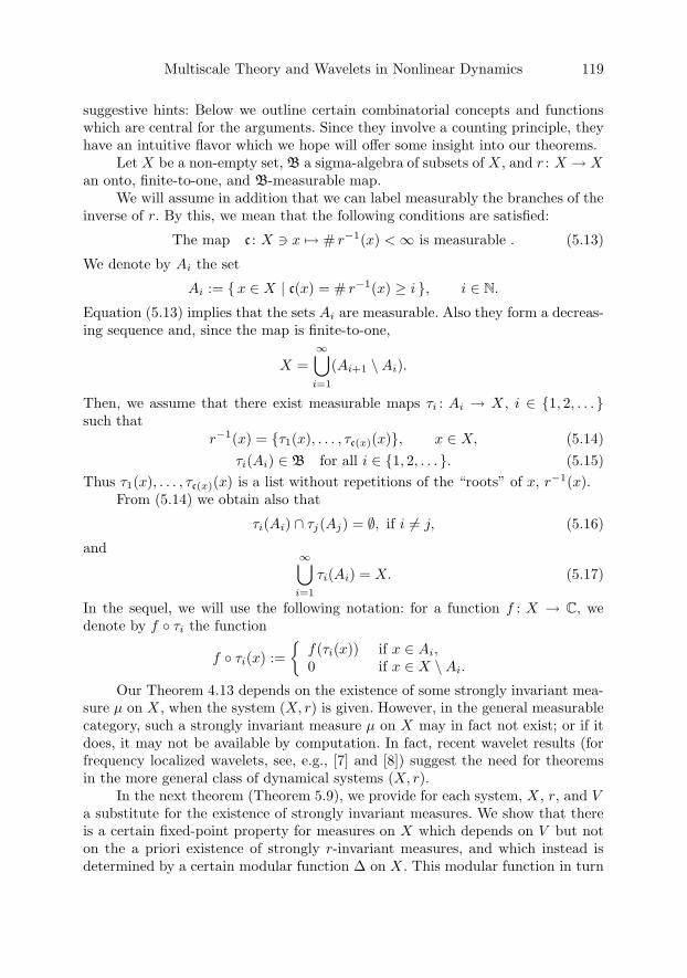
Multiscale Theory and Wavelets in Nonlinear Dynamics 119
suggestive hints: Below we outline certain combinatorial concepts and functionswhich are central for the arguments. Since they involve a counting principle, theyhave an intuitive flavor which we hope will offer some insight into our theorems.
Let X be a non-empty set, B a sigma-algebra of subsets of X , and r : X → Xan onto, finite-to-one, and B-measurable map.
We will assume in addition that we can label measurably the branches of theinverse of r. By this, we mean that the following conditions are satisfied:
The map c : X x → # r−1(x) <∞ is measurable . (5.13)
We denote by Ai the set
Ai := x ∈ X | c(x) = # r−1(x) ≥ i , i ∈ N.
Equation (5.13) implies that the sets Ai are measurable. Also they form a decreas-ing sequence and, since the map is finite-to-one,
X =∞⋃
i=1
(Ai+1 \Ai).
Then, we assume that there exist measurable maps τi : Ai → X , i ∈ 1, 2, . . .such that
r−1(x) = τ1(x), . . . , τc(x)(x), x ∈ X, (5.14)τi(Ai) ∈ B for all i ∈ 1, 2, . . .. (5.15)
Thus τ1(x), . . . , τc(x)(x) is a list without repetitions of the “roots” of x, r−1(x).From (5.14) we obtain also that
τi(Ai) ∩ τj(Aj) = ∅, if i = j, (5.16)
and ∞⋃i=1
τi(Ai) = X. (5.17)
In the sequel, we will use the following notation: for a function f : X → C, wedenote by f τi the function
f τi(x) :=
f(τi(x)) if x ∈ Ai,0 if x ∈ X \Ai.
Our Theorem 4.13 depends on the existence of some strongly invariant mea-sure µ on X , when the system (X, r) is given. However, in the general measurablecategory, such a strongly invariant measure µ on X may in fact not exist; or if itdoes, it may not be available by computation. In fact, recent wavelet results (forfrequency localized wavelets, see, e.g., [7] and [8]) suggest the need for theoremsin the more general class of dynamical systems (X, r).
In the next theorem (Theorem 5.9), we provide for each system, X , r, and Va substitute for the existence of strongly invariant measures. We show that thereis a certain fixed-point property for measures on X which depends on V but noton the a priori existence of strongly r-invariant measures, and which instead isdetermined by a certain modular function ∆ on X . This modular function in turn
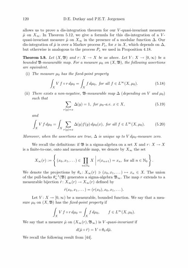
120 D.E. Dutkay and P.E.T. Jorgensen
allows us to prove a dis-integration theorem for our V -quasi-invariant measuresµ on X∞. In Theorem 5.12, we give a formula for this dis-integration of a V -quasi-invariant measure µ on X∞ in the presence of a modular function ∆. Ourdis-integration of µ is over a Markov process Px, for x in X , which depends on ∆,but otherwise is analogous to the process Px we used in Proposition 4.18.
Theorem 5.9. Let (X, B) and r : X → X be as above. Let V : X → [0,∞) be abounded B-measurable map. For a measure µ0 on (X, B), the following assertionsare equivalent.
(i) The measure µ0 has the fixed-point property∫X
V f r dµ0 =∫
X
f dµ0, for all f ∈ L∞(X, µ0). (5.18)
(ii) There exists a non-negative, B-measurable map ∆ (depending on V and µ0)such that ∑
r(y)=x
∆(y) = 1, for µ0-a.e. x ∈ X, (5.19)
and∫X
V f dµ0 =∫
X
∑r(y)=x
∆(y)f(y) dµ0(x), for all f ∈ L∞(X, µ0). (5.20)
Moreover, when the assertions are true, ∆ is unique up to V dµ0-measure zero.
We recall the definitions: if B is a sigma-algebra on a set X and r : X → Xis a finite-to-one, onto and measurable map, we denote by X∞ the set
X∞(r) :=
(x0, x1, . . . ) ∈
∏n∈N0
X
∣∣∣∣ r(xn+1) = xn, for all n ∈ N0
.
We denote the projections by θn : X∞(r) (x0, x1, . . . ) → xn ∈ X. The unionof the pull-backs θ−1
n (B) generates a sigma-algebra B∞. The map r extends to ameasurable bijection r : X∞(r)→ X∞(r) defined by
r(x0, x1, . . . ) = (r(x0), x0, x1, . . . ).
Let V : X → [0,∞) be a measurable, bounded function. We say that a mea-sure µ0 on (X, B) has the fixed-point property if∫
X
V f r dµ0 =∫
X
f dµ0, f ∈ L∞(X, µ0).
We say that a measure µ on (X∞(r), B∞) is V -quasi-invariant if
d(µ r) = V θ0 dµ.
We recall the following result from [44].
Multiscale Theory and Wavelets in Nonlinear Dynamics 121
Theorem 5.10. There exists a one-to-one correspondence between measures µ0
on X with the fixed-point property and V -quasi-invariant measures µ on X∞(r),given by
µ0 = µ θ−10 .
Proposition 5.11. Let (X, B), r : X → X and be as above, and let D : X → [0,∞)be a measurable function with the property that∑
r(y)=x
D(y) = 1. (5.21)
Denote by D(n) the product of compositions
D(n) := D ·D r · · · · ·D rn−1, n ∈ N, D(0) := 1. (5.22)
Then for each x0 ∈ X, there exists a Radon probability measure Px0 on Ωx0 suchthat, if f is a bounded measurable function on Ωx0 which depends only on the firstn coordinates x1, . . . , xn, then∫
Ωx0
f(ω) dPx0(ω) =∑
rn(xn)=x0
D(n)(xn)f(x1, . . . , xn). (5.23)
Theorem 5.12. Let (X, B), r : X → X and V : X → [0,∞) be as above. Let µ0
be a measure on (X, B) with the fixed-point property (5.18). Let ∆: X → [0, 1] bethe function associated to V and µ0 as in Theorem 5.9, and let µ be the uniqueV -quasi-invariant measure on X∞(r) with
µ θ−10 = µ0,
as in Theorem 5.10. For ∆ define the measures Px0 as in Proposition 5.11. Then,for all bounded measurable functions f on X∞(r),∫
X∞(r)
f dµ =∫
X
∫Ωx0
f(x0, ω) dPx0(ω) dµ0(x0). (5.24)
Hausdorff measure and wavelet bases. In this problem we propose wavelet bases inthe context of Hausdorff measure of fractional dimension between 0 and 1. Whileour fractal wavelet theory has points of similarity that it shares with the standardcase of Lebesgue measure on the line, there are also sharp contrasts.
It is well known that the Hilbert spaces L2(R) has a rich family of orthonormalbases of the following form: ψj,k(x) = 2j/2ψ(2jx− k), j, k ∈ Z, where ψ is a singlefunction ∈ L2(R). Take for example Haar’s function ψ(x) = χI(2x) − χI(2x − 1)where I = [0, 1] is the unit interval. Let C be the middle-third Cantor set. Thenthe corresponding indicator function ϕC := χC satisfies the scaling identity (see(2.2)), ϕC(x
3 ) = ϕC(x) + ϕC(x− 2).In [45] we use this as the starting point for a multiresolution construction in
a separable Hilbert space built with Hausdorff measure, and we identify the twomother functions which define the associated wavelet ONB.
Since both constructions, the first one for the Lebesgue measure, and thesecond one for the Hausdorff version (dx)s, arise from scaling and subdivision, it

122 D.E. Dutkay and P.E.T. Jorgensen
seems reasonable to expect multiresolution wavelets also in Hilbert spaces con-structed on the scaled Hausdorff measures Hs which are basic for the kind ofiterated function systems which give Cantor constructions built on scaling andtranslations by lattices.
Acknowledgements
The authors gratefully acknowledge constructive discussions with Richard Gundyand Roger Nussbaum. Further, we are pleased to thank Brian Treadway for helpwith TEX, with style files, and with proofreading. And especially for making a num-ber of very helpful suggestions. Both authors have benefited from discussions withthe members of our NSF Focused Research Group (DMS-0139473), “Wavelets,Frames, and Operator Theory,” especially from discussions with Larry Baggett,John Benedetto, David Larson, and Gestur Olaffson. The second named author isgrateful for helpful discussions and suggestions from Kathy Merrill, Wayne Law-ton, Paul Muhly, Judy Packer, Iain Raeburn, and Wai-Shing Tang. Several ofthese were participants and organizers of an August 4–7, 2004, Wavelet Workshop(“Functional and harmonic analysis of wavelets and frames”) at The National Uni-versity of Singapore (NUS). And we benefited from inspiration and enlighteningdiscussions with this workshop as well. The second named author is grateful tothe hosts at NUS in Singapore for support and generous hospitality in August of2004. Finally, we thank Daniel Alpay for inviting us to write this paper, and forencouragements.
References
[1] P. Abry, P. Flandrin, M.S. Taqqu, and D. Veitch, Wavelets for the analysis, esti-mation, and synthesis of scaling data, Self-Similar Network Traffic and PerformanceEvaluation (K. Park and W. Willinger, eds.), Wiley-Interscience, New York, 2000,pp. 39–88.
[2] D. Alpay, A. Dijksma, and J. Rovnyak, A theorem of Beurling-Lax type for Hilbertspaces of functions analytic in the unit ball, Integral Equations Operator Theory 47(2003), no. 3, 251–274.
[3] H. Araki, The work of Alain Connes, Fields Medallists’ lectures, World Sci. Ser. 20thCentury Math., vol. 5, World Scientific, River Edge, NJ, 1997, pp. 329–336.
[4] W. Arveson, The Dirac operator of a commuting d-tuple, J. Funct. Anal. 189 (2002),no. 1, 53–79.
[5] , Four lectures on noncommutative dynamics, Advances in Quantum Dynam-ics (South Hadley, MA, 2002) (G.L. Price, B.M. Baker, P.E.T. Jorgensen, and P.S.Muhly, eds.), Contemp. Math., vol. 335, American Mathematical Society, Provi-dence, RI, 2003, pp. 1–55.
[6] S. Avdonin and W. Moran, Ingham-type inequalities and Riesz bases of divided dif-ferences, Int. J. Appl. Math. Comput. Sci. 11 (2001), no. 4, 803–820, Mathematicalmethods of optimization and control of large-scale systems (Ekaterinburg, 2000).
Multiscale Theory and Wavelets in Nonlinear Dynamics 123
[7] L.W. Baggett, P.E.T. Jorgensen, K.D. Merrill, and J.A. Packer, Construction ofParseval wavelets from redundant filter systems, J. Math. Phys. 46 (2005), no. 8.doi:10.1063/1.1982768
[8] , An analogue of Bratteli-Jorgensen loop group actions for GMRA’s, Wavelets,Frames, and Operator Theory (College Park, MD, 2003) (C. Heil, P.E.T. Jorgensen,and D.R. Larson, eds.), Contemp. Math., vol. 345, American Mathematical Society,Providence, 2004, pp. 11–25.
[9] V. Baladi, Positive Transfer Operators and Decay of Correlations, World Scientific,River Edge, NJ, Singapore, 2000.
[10] J.A. Ball and V. Vinnikov, Functional models for representations of the Cuntz al-gebra, Operator Theory, Systems Theory and Scattering Theory: MultidimensionalGeneralizations, (D. Alpay and V. Vinnikov, eds.), Oper. Theory Adv. Appl., vol.157, Birkhauser, Basel, 2005, pp. 1–60.
[11] A.F. Beardon, Iteration of Rational Functions: Complex Analytic Dynamical Sys-tems, Graduate Texts in Mathematics, vol. 132, Springer-Verlag, New York, 1991.
[12] J.J. Benedetto, E. Bernstein, and I. Konstantinidis, Multiscale Riesz products andtheir support properties, Acta Appl. Math. 88 (2005), no. 2, 201–227.
[13] S. Bildea, D.E. Dutkay, and G. Picioroaga, MRA super-wavelets, New York J. Math.11 (2005), 1–19.
[14] A. Bisbas, A multifractal analysis of an interesting class of measures, Colloq. Math.69 (1995), no. 1, 37–42.
[15] L. Blum, Computing over the reals: Where Turing meets Newton, Notices Amer.Math. Soc. 51 (2004), no. 9, 1024–1034.
[16] J.-B. Bost and A. Connes, Hecke algebras, type III factors and phase transitions withspontaneous symmetry breaking in number theory, Selecta Math. (N.S.) 1 (1995),411–457.
[17] O. Bratteli and P.E.T. Jorgensen, Isometries, shifts, Cuntz algebras and multireso-lution wavelet analysis of scale N , Integral Equations Operator Theory 28 (1997),382–443.
[18] , Iterated function systems and permutation representations of the Cuntz al-gebra, Mem. Amer. Math. Soc. 139 (1999), no. 663.
[19] , Wavelets through a Looking Glass: The World of the Spectrum, Applied andNumerical Harmonic Analysis, Birkhauser, Boston, 2002.
[20] O. Bratteli, P.E.T. Jorgensen, K.H. Kim, and F. Roush, Decidability of the isomor-phism problem for stationary AF-algebras and the associated ordered simple dimen-sion groups, Ergodic Theory Dynam. Systems 21 (2001), 1625–1655, corrigendum:22 (2002), 633.
[21] , Computation of isomorphism invariants for stationary dimension groups,Ergodic Theory Dynam. Systems 22 (2002), 99–127.
[22] O. Bratteli and D.W. Robinson, Operator Algebras and Quantum Statistical Mechan-ics, 2nd ed., vol. II, Springer-Verlag, Berlin–New York, 1996.
[23] B. Brenken, and P.E.T, Jorgensen, A family of dilation crossed product algebras, J.Operator Theory 25, (1991), 299–308.

124 D.E. Dutkay and P.E.T. Jorgensen
[24] J. Brodzki, A. Connes, and D. Ellwood, Polarized modules and Fredholm modules,Mat. Fiz. Anal. Geom. 2 (1995), no. 1, 15–24.
[25] H. Brolin, Invariant sets under iteration of rational functions, Ark. Mat. 6 (1965),103–144 (1965).
[26] G. Brown, Riesz products and generalized characters, Proc. London Math. Soc. (3)30 (1975), 209–238.
[27] G. Brown and W. Moran, Products of random variables and Kakutani’s criterion fororthogonality of product measures, J. London Math. Soc. (2) 10 (1975), no. part 4,401–405.
[28] A. Cohen and R.D. Ryan, Wavelets and Multiscale Signal Processing, Applied Math-ematics and Mathematical Computation, vol. 11, Chapman & Hall, London, 1995.
[29] Albert Cohen, Numerical Analysis of Wavelet Methods, Studies in Mathematics andits Applications, vol. 32, North-Holland Publishing Co., Amsterdam, 2003.
[30] R.R. Coifman, Y. Meyer, and V. Wickerhauser, Numerical harmonic analysis, Es-says on Fourier Analysis in Honor of Elias M. Stein (Princeton, 1991) (C. Fefferman,R. Fefferman, and S. Wainger, eds.), Princeton Mathematical Series, vol. 42, Prince-ton University Press, Princeton, NJ, 1995, pp. 162–174.
[31] A. Connes, Noncommutative Geometry, Academic Press, San Diego, 1994.
[32] X. Dai and D.R. Larson, Wandering vectors for unitary systems and orthogonalwavelets, Mem. Amer. Math. Soc. 134 (1998), no. 640, viii+68.
[33] I. Daubechies, B. Han, A. Ron, and Z. Shen, Framelets: MRA-based constructionsof wavelet frames, Appl. Comput. Harmon. Anal. 14 (2003), no. 1, 1–46.
[34] I. Daubechies, H.J. Landau, and Z. Landau, Gabor time-frequency lattices and theWexler-Raz identity, J. Fourier Anal. Appl. 1 (1995), no. 4, 437–478.
[35] D.L. Donoho, Renormalizing experiments for nonlinear functionals, Festschrift forLucien Le Cam, Springer, New York, 1997, pp. 167–181.
[36] J.L. Doob, Application of the theory of martingales, Le Calcul des Probabilites et sesApplications, Colloques Internationaux du Centre National de la Recherche Scien-tifique, no. 13, Centre National de la Recherche Scientifique, Paris, 1949, pp. 23–27.
[37] , Notes on martingale theory, Proc. 4th Berkeley Sympos. Math. Statist. andProb., Vol. II, University of California Press, Berkeley, CA, 1961, pp. 95–102.
[38] R.G. Douglas and G. Misra, Quasi-free resolutions of Hilbert modules, Integral Equa-tions Operator Theory 47 (2003), no. 4, 435–456.
[39] D.E. Dutkay, Low-pass filters and representations of the Baumslag-Solitar group,preprint, University of Iowa, 2004, http://www.arxiv.org/abs/math.CA/0407344.To appear in the Transactions of Amer. Math. Soc.
[40] , Harmonic analysis of signed Ruelle transfer operators, J. Math. Anal. Appl.273 (2002), 590–617.
[41] , The wavelet Galerkin operator, J. Operator Theory 51 (2004), no. 1, 49–70.
[42] D.E. Dutkay and P.E.T. Jorgensen, Disintegration of projective measures, Proc.Amer. Math. Soc., to appear, http://arxiv.org/abs/math.CA/0408151.
[43] , Martingales, endomorphisms, and covariant systems of operators in Hilbertspace, J. Operator Theory, to appear, http://arXiv.org/abs/math.CA/0407330.
Multiscale Theory and Wavelets in Nonlinear Dynamics 125
[44] , Hilbert spaces of martingales supporting certain substitution-dynamical sys-tems, Conform. Geom. Dyn. 9 (2005), 24–45.
[45] , Wavelets on fractals, preprint, University of Iowa, 2003,http://arXiv.org/abs/math.CA/0305443, to appear in Rev. Mat. Iberoamericana.
[46] Paul Erdos, On the smoothness properties of a family of Bernoulli convolutions,Amer. J. Math. 62 (1940), 180–186.
[47] R. Exel, A new look at the crossed-product of a C∗-algebra by an endomorphism,Ergodic Theory Dynam. Systems 23 (2003), no. 6, 1733–1750.
[48] , KMS states for generalized gauge actions on Cuntz-Krieger algebras (anapplication of the Ruelle-Perron-Frobenius theorem), Bull. Braz. Math. Soc. (N.S.)35 (2004), no. 1, 1–12.
[49] A. Fan and Y. Jiang, On Ruelle-Perron-Frobenius operators. I. Ruelle theorem,Comm. Math. Phys. 223 (2001), no. 1, 125–141.
[50] Alexandre Freire, Artur Lopes, and Ricardo Mane, An invariant measure for rationalmaps, Bol. Soc. Brasil. Mat. 14 (1983), no. 1, 45–62.
[51] R.F. Gundy, Two remarks concerning wavelets: Cohen’s criterion for low-pass filtersand Meyer’s theorem on linear independence, The Functional and Harmonic Anal-ysis of Wavelets and Frames (San Antonio, 1999) (L.W. Baggett and D.R. Larson,eds.), Contemp. Math., vol. 247, American Mathematical Society, Providence, 1999,pp. 249–258.
[52] P.E.T. Jorgensen, Analysis and Probability: Wavelets, Signals, Fractals, Grad. Textsin Math., vol. 234, Springer-Verlag, New York, to appear 2006.
[53] , Minimality of the data in wavelet filters, Adv. Math. 159 (2001), no. 2,143–228, with an appendix by Brian Treadway.
[54] , Ruelle operators: Functions which are harmonic with respect to a transferoperator, Mem. Amer. Math. Soc. 152 (2001), no. 720.
[55] , Matrix factorizations, algorithms, wavelets, Notices Amer. Math. Soc. 50(2003), no. 8, 880–894, http://www.ams.org/notices/200308/200308-toc.html.
[56] J.-P. Kahane, Sur la distribution de certaines series aleatoires, Colloque de Theoriedes Nombres (Univ. Bordeaux, Bordeaux, 1969), Bull. Soc. Math. France, Mem. No.25, Soc. Math. France Paris, 1971, pp. 119–122.
[57] Y. Katznelson, Integrales de produits de Riesz, C. R. Acad. Sci. Paris Ser. I Math.305 (1987), 67–69.
[58] A. Kumjian and J. Renault, KMS states on C∗-algebras associated to expansive maps,preprint 2003.
[59] T. Lindstrøm, Fractional Brownian fields as integrals of white noise, Bull. LondonMath. Soc. 25 (1993), no. 1, 83–88.
[60] R. Mane, On the uniqueness of the maximizing measure for rational maps, Bol. Soc.Brasil. Mat. 14 (1983), no. 1, 27–43.
[61] R.D. Mauldin and M. Urbanski, Graph Directed Markov Systems: Geometry andDynamics of Limit Sets, Cambridge Tracts in Mathematics, vol. 148, CambridgeUniversity Press, Cambridge, 2003.
126 D.E. Dutkay and P.E.T. Jorgensen
[62] Y. Meyer, Produits de Riesz generalises, Seminaire d’Analyse Harmonique, 1978–1979, Publications Mathematiques d’Orsay 79, vol. 7, Universite de Paris-Sud, Fac-ulte Des Sciences-Mathematiques, Orsay, 1979, pp. 38–48.
[63] , The role of oscillations in some nonlinear problems, European Congress ofMathematics, Vol. I (Barcelona, 2000), Progr. Math., vol. 201, Birkhauser, Basel,2001, pp. 75–99.
[64] Y. Meyer, F. Sellan, and M.S. Taqqu, Wavelets, generalized white noise and fractionalintegration: The synthesis of fractional Brownian motion, J. Fourier Anal. Appl. 5(1999), no. 5, 465–494.
[65] R. Okayasu, Type III factors arising from Cuntz–Krieger algebras, Proc. Amer. Math.Soc. 131 (2003), no. 7, 2145–2153.
[66] C. Radin, Global order from local sources, Bull. Amer. Math. Soc. (N.S.) 25 (1991),335–364.
[67] , Miles of Tiles, Student Mathematical Library, vol. 1, American Mathemat-ical Society, Providence, 1999.
[68] M.A. Rieffel, von Neumann algebras associated with pairs of lattices in Lie groups,Math. Ann. 257 (1981), no. 4, 403–418.
[69] F. Riesz, Uber die Fourierkoeffizienten einer stetigen Funktion von beschrankterSchwankung, Math. Z. 2 (1918), 312–315.
[70] G. Ritter, On Kakutani’s dichotomy theorem for infinite products of not necessarilyindependent functions, Math. Ann. 239 (1979), 35–53.
[71] D. Ruelle, Thermodynamic formalism, Encyclopedia of Mathematics and Its Appli-cations, vol. 5, Addison-Wesley Publishing Co., Reading, Mass., 1978.
[72] , The thermodynamic formalism for expanding maps, Comm. Math. Phys.125 (1989), no. 2, 239–262.
[73] G. Skandalis, Geometrie non commutative d’apres Alain Connes: la notion de tripletspectral, Gaz. Math. (2002), no. 94, 44–51.
[74] A. Volberg, and P. Yuditskii, Noncommutative Perron-Frobenius-Ruelle theorem,two-weight Hilbert transform, and almost periodicity, preprint,arxiv:math.SP/0408259, 2004.
[75] S.G. Williams (ed.), Symbolic Dynamics and Its Applications, Proceedings of Sym-posia in Applied Mathematics, vol. 60, American Mathematical Society, Providence,RI, 2004.
Dorin Ervin DutkayDepartment of MathematicsRutgers UniversityNew Brunswick, NJ 08901, USAe-mail: [email protected]
Palle E.T. JorgensenDepartment of MathematicsThe University of IowaIowa City, IA 52242, USAe-mail: [email protected]
Operator Theory:Advances and Applications, Vol. 167, 127–155c© 2006 Birkhauser Verlag Basel/Switzerland
Noncommutative Trigonometry
Karl Gustafson
Abstract. A unified account of a noncommutative operator trigonometry orig-inated in 1966 by this author and its further developments and applicationsto date will be given within a format of a historical trace. Applications towavelet and multiscale theories are included. A viewpoint toward possiblefuture enlargement will be fostered.
Mathematics Subject Classification (2000). 15A18, 47A05, 65N12, 65N55,62H12, 81Q10.
Keywords. noncommutative operator trigonometry; antieigenvalue; linear al-gebra; quantum mechanics; statistics; numerical analysis; wavelets; multiscalesystems; iterative methods.
1. Introduction
The purpose of this paper is to provide a unified account for the first time of a non-commutative trigonometry which this author initiated in 1966. This noncommu-tative operator trigonometry involves notions of antieigenvalues and antieigenvec-tors, terms which I introduced for entities which arise naturally within the theory,and which carry interest in their own right. Applications of this noncommutativetrigonometry to date include, roughly and chronologically: perturbation of opera-tor semigroups, positivity of operator products, Markov processes, Rayleigh-Ritztheory, numerical range, normal operators, convexity theory, minimum residualand conjugate gradient solvers, Richardson and relaxation schemes, wavelets, do-main decomposition and multilevel methods, control theory, scattering theory,preconditioning and condition number theory, statistical estimation and efficiency,canonical correlations, Bell’s inequalities, quantum spin systems, and quantumcomputing. Further development and applications are expected.
The outline of the paper is as follows. In Section 2, we describe the first pe-riod, 1966–1972, from which all of the key notions came. These were all due to thisauthor. In Section 3, I describe the second period 1973 to 1993, in which my own
128 K. Gustafson
research interests were mainly elsewhere, but during which two of my Ph.D. stu-dents, D. Rao and M. Seddighin, made contributions to the theory. In Section 4, Idescribe the third and most active period, 1994 to 2005, during which I applied thisnoncommutative trigonometry to most of the application areas described above.
The format of the paper will be chronological and historical. It is my beliefthat this noncommutative operator trigonometry will eventually become an estab-lished chapter of linear algebra. Thus, to that end, I want to expose its overallscope and geometrical content here. For archival purposes I have attempted to listall of my publications [1–60] on this noncommutative trigonometry to date. Veryfew other mathematicians have embraced this theory or contributed to it, but I willmention some in Section 5. To help the reader’s overall perspective and interest,I will at times add some commentary, even of a personal nature. Thus the styleof this account will not discriminate between grammatical person, i.e., I, we, one,this author, and will just use whichever seems appropriate within local context.
Full detail would require writing a book. In fact we have published two books[26] and [29] which contain significant chapters dealing with this noncommutativeoperator trigonometry. But both of those books were written in 1995 and there hasbeen considerable new development and interesting applications in the ten yearssince then. Nonetheless I will often refer to those books when possible to keep theexposition here within space and time bounds.
Finally, it is my hope that by providing this unified account, I have fostered aviewpoint which will enable future enlargement of this theory and its applications.In particular, from time to time I will remind or emphasize that this theory, fromits beginning, has been: noncommutative. Of course it contains the commutativecase, but it is much more valuable for noncommuting operators. To me, operatortheory has always been noncommutative. Operators A and B should always be firstapproached as not commuting with each other. In most engineering applications,there would be no dynamics and the structures would all fall down were theirgoverning linear systems commutative. In a metaphysical sense, then, I wouldlike this paper to provide a take-off point into a more abstract conceptual framesomewhat akin to that of noncommutative geometry. Section 6 contains a fewpreliminary results and remarks toward that goal.
2. The first (active) period 1966–1972
In [1], my first published mathematics paper, I contributed to the perturbationtheory of linear operators. One of the important theorems there is one originallyfound in Hilbert space independently by T. Kato and F. Rellich. Here is a Banachspace version. Let G(1, 0) denote the densely defined infinitesimal generators Aof a contraction semigroup Zt on a Banach space X . Additively perturb A bya regular perturbation B, i.e., domain D(B) ⊃ D(A), which is relatively small:||Bx|| <= a||x||+ b||Ax|| for some b < 1. Then A + B is also in G(1, 0), i.e., A + B
Noncommutative Trigonometry 129
generates a contraction semigroup, iff A + B is dissipative: Re [(A + B)x, x] <= 0for all x in D(A). Here [y, x] denotes any semi-inner-product on the Banach space.
I wanted a general multiplicative perturbation theorem and obtained thefollowing: see [2]–[7] for details and related developments. Let A be a generator inG(1, 0) and let B be bounded on X and strongly accretive: Re [Bx, x] >= m||x||2for all x, m > 0. Then BA is in G(1, 0), i.e., BA generates a contraction semigroup,iff BA is dissipative: Re [BAx, x] <= 0 for all x in D(A).
Thus I arrived in 1966 at the core issue from which the noncommutativeoperator trigonometry to be exposed in this paper arose: when is dissipativitypreserved in an operator composition of an accretive operator B with a dissipativeoperator A? It occurred to me to try to answer this question in a way similar tothat by which I had proved the rest of the just stated multiplicative perturbationtheorem: reduce it to the Kato–Rellich additive perturbation theorem. Inserting afree parameter ε > 0, which will not alter whether or not εBA is a generator or not,one writes εBA = A+(εB−I)A and one notes that ||(εB−I)Ax|| <= ||εB−I||||Ax||implies by the Kato–Rellich Theorem that (εB − I)A is an acceptable additiveperturbation provided that b ≡ ||εB − I|| < 1 for some ε > 0. Indeed one findsthat the norm curve ||εB − I|| dips below 1 for an interval (0, εc) whenever B isstrongly accretive. Applying the same additive decomposition to the multiplicativeperturbation in the semi-inner-product, one finds
Re[εBAx, x] = Re[εB − I)Ax, x] + Re[Ax, x]<= ||εB − I||||Ax||||x|| + Re[Ax, x]
(2.1)
from which one obtains the sufficient condition for εBA, hence BA, to be dissipa-tive:
minε>0||εB − I|| <= inf
x∈D(A)x =0
Re[(−A)x, x]||Ax||||x|| . (2.2)
As A being dissipative is the same as −A being accretive, it is easier to reposethe result (2.2) as follows, and for simplicity, let us now just restrict attention toa Hilbert space X and its usual inner product. Define for accretive A
µ1(A) ≡ infx∈D(A)
x =0
Re〈Ax, x〉||Ax||||x|| ≡ cosφ(A) (2.3)
and let ν1(B) denote minε ||εB−I|| for accretive B. Then when ν1(B) <= µ1(A), BAwill be accretive. The intuition for calling µ1(A) a cosφ(A) is rather immediate.On the other hand, I puzzled on the entity ν1(B) for awhile and decided that ittoo must be trigonometric. This I showed in 1968 in [6] by a min-max argument,see also [11]. The result is that one can define for bounded accretive A and −∞ <ε <∞ the entity
ν1(A) ≡ minε||εA− I|| ≡ sinφ(A). (2.4)
130 K. Gustafson
The result of [6] is then: cos2 φ(A) + sin2 φ(A) = 1. This important result gave mean operator trigonometry.
I emphasize that one does not have this operator (noncommutative) trigonom-etry until one has sinφ(A). One needs both a cosine and a sine to develop atrigonometry. I also emphasize that although of course these results contain thecommutative cases too, they are not as interesting. See [3], [4], [5] for how com-mutative situations often become trivial or may be resolved by other means.
Thus from (2.2) the condition for the multiplicative perturbation BA to gen-erate a contraction semigroup became
sin φ(B) <= cosφ(A). (2.5)
However, I was a little disappointed that my theory was now restricting itselfto bounded B (I like unbounded operators). So Gunter Lumer and I extendedresults (but not the trigonometry) to include unbounded B [12]. Bruce Calvertand I obtained results for nonlinear semigroups [13]. Ken-iti Sato and I extendedboth additive and multiplicative perturbation results to positivity preserving (e.g.,real-valued Markov) semigroups [9]. These papers contained no trigonometry.
In [8] Bruno Zwahlen and I showed that all unbounded densely defined ac-cretive operators A in a Hilbert space, have cosφ(A) = 0. This finding, althoughof interest in itself in distinguishing unbounded and bounded operators geometri-cally, really disappointed me because it meant that the perturbation criteria (2.2)was not useful when the semigroup generator A was unbounded in a Hilbert space.
However, the trigonometry itself seemed interesting, so when invited to theUCLA Symposium on Inequalities in 1969, see the book of [11], I presented themain results there. I decided to call µ1(A) the first antieigenvalue of A becauseit measured the greatest turning angle of A: just the opposite geometrical effectfrom that of an eigenvalue, which measures the stretching effect of a vector whichis turned not at all by A. Real antieigenvalues, Imaginary antieigenvalues, Totalantieigenvalues, and Higher antieigenvalues were defined, and the min-max resultcos2 φ(A) + sin2 φ(A) = 1 exposed. Only mentioned in [11] but not detailed wasthe Euler equation
2||Ax||2||x||2(ReA)x− ||x||2Re〈Ax, x〉A∗Ax − ||Ax||2Re〈Ax, x〉x = 0 (2.6)
which is the functional derivative of (2.3) and which must be satisfied by any firstantieigenvector. This equation is also satisfied by all eigenvectors of A when A isselfadjoint or normal. Thus (2.6) may be regarded as a significant extension of theRayleigh-Ritz variational theory for eigenvalues. For A a symmetric n×n positivedefinite matrix, I established that
cosφ(A) =2√
λ1λn
λ1 + λn, sinφ(A) =
λn − λ1
λn + λ1(2.7)
and that the first antieigenvectors are the pair
x± = ±(
λn
λ1 + λn
)1/2
x1 +(
λ1
λ1 + λn
)1/2
xn (2.8)
Noncommutative Trigonometry 131
where λ1 is the smallest eigenvalue, with normalized eigenvector x1, and λn is thelargest eigenvalue, with normalized eigenvector xn.
To fix ideas, let A =[
9 00 16
], then by (2.7) and (2.8) we have the operator
turning angle φ(A) = 16.2602 and the two antieigenvectors (not normalized here)x+ = (4, 3) and x− = (−4, 3).
The papers [1]-[13] constitute the initial period during which I originatedthis theory of antieigenvalues and antieigenvectors and operator turning angles.In retrospect, I was fortunate that my motivating original question, that of mul-tiplicative perturbation of semigroup generators, brought forth both cosφ(A) andsin φ(A), of necessity. And in that application, the operator compositions BA arethoroughly noncommutative.
Commentary. One will notice common ingredients of the important min-max result[6], [11] proof in my proof [10] of the Toeplitz-Hausdorff Theorem for the convexityof the numerical range W (A). That is why I include [10] in this list [1]–[60].
3. The second (intermittent) period 1973–1993
A year sabbatical 1971–72 to the Theoretical Physics Institute at the University ofGeneva and the Ecole Polytechnique Federale in Lausanne, where the research in-terests were principally quantum scattering theory and bifurcation theory, respec-tively, brought to an end my initial contributions to the operator trigonometry.However, my Ph.D. student Duggirala Rao found a connection to a 1969 paper bythe noted Russian mathematician M.G. Krein. See my survey [25] for more detailsabout Krein’s work. Also together Rao and I looked at the operator trigonometrymore generally within the context of the numerical range W (AB). From this re-sulted the 1977 paper [14]. It should be noted that most of the issues dealt within that paper are thoroughly noncommutative. In particular, some generalizationsof the sufficient condition (2.5) were obtained. Also the accretivity of the productT 2 (admittedly commutative, but for an unbounded operator T ) was consideredwithin the framework of sesquilinear forms. Also I wrote an invited paper [15]related to [1] in 1983. The main concerns there centered on domains of perturbedunbounded operators.
Then with Ph.D. student Morteza Seddighin, we extended related 1980 re-sults of Chandler Davis, with emphasis on the Re and Total antieigenvalue theoryfor normal operators. This resulted in the two papers [16] and [18] in 1989 and1993, respectively. I will elaborate a bit on these developments in Section 5. Re-cently Seddighin and I returned [59] to this theory and resolved some shortcomingsin [16], [18] and also some incomplete statements in Davis’ analysis. In particularwe completely resolved an issue which I called “possible zero denominators” whicharose from our use of LaGrange multiplier techniques in [16], [18].
132 K. Gustafson
An important event of interest which occurred during this rather inactive (asconcerns the operator trigonometry) period, was an invitation to speak at a con-ference [17] on convexity in Dubrovnik, Yugoslavia, in June 1990. The organizersespecially asked me to speak about my semigroup and antieigenvalue results from20 years earlier! This I did. Relately, although not immediately obvious, in 1978several engineering departments had asked me to offer courses on computationalpartial differential equations, especially computational fluid dynamics. This I did,from 1978 to 1990. One learns working in that field that 70% of supercomputingtime is spent on linear solvers. In particular, in such research I had used somesteepest descent and conjugate gradient scheme computations and had learned ofthe basic convergence rate bound
E(xk+1)<=(
1− 4λ1λn
(λ1 + λn)2
)E(xk). (3.1)
Here E(x) is the error 〈(x − x∗), A(x − x∗)〉/2, x∗ the true solution. This boundalso occurs in a key way in some parts of optimization theory. Immediately frommy operator trigonometric expressions (2.7) I knew that what (3.1) really meant,geometrically, was trigonometric:
E(xk+1)<= sin2 φ(A)E(xk). (3.2)
Although (3.1) was known as a form of the Kantorovich inequality, nowhere in thenumerical nor in the optimization literature did I find this important geometricalresult: that gradient and conjugate gradient convergence rates are fundamentallytrigonometric. That is, they are a direct reflection of the elemental fact of A’smaximum turning angle φ(A). The known conjugate gradient convergence rate,by the way, becomes, trigonometrically written now,
E(xk) <= 4(sinφ(A1/2))2kE(x0). (3.3)
See [19] where I published this result (3.3) for conjugate gradient convergence.And I first announced the steepest descent result (3.2) at the 1990 Dubrovnikconference [17].
Summarizing, the period 1973–1993 was one of low, almost nonexistent, pri-ority for the operator trigonometry. Countervailingly, I was very occupied withlearning some computational linear algebra. In addition to a significant numberof publications with four Ph.D. students which I produced in the departments ofAerospace Engineering, Civil Engineering, Chemical Engineering, and ElectricalEngineering, I had also been asked to be the only mathematician in a seven de-partment successful attempt to bring a $22 million Optoelectronic Computing Sys-tems Engineering Research Center to the University of Colorado. I was in chargeof algorithms, especially those to be implemented on a large optoelectronic neuralnetwork. This activity took most of my research time in the interval 1988–1993.
But what I learned from this, essentially engineering, research in this period1978–1993, accrued to produce later dividends for the operator trigonometry, as Iwill discuss in the next Section. Furthermore, I had worked with physicists at the
Noncommutative Trigonometry 133
Solvay Institute of Professor Ilya Prigogine in Brussels during the period 1978–2000, and what I learned there also was indirectly of great importance later forthe operator trigonometry, as I will recount later.
Commentary. There are three interesting and related vignettes coming out of theDubrovnik meeting in June 1990.
First, as I flew in from Vienna, sitting beside me was a lovely coed of a jointAmerican–Yugoslavian family, returning from UCLA. She whispered detailed pre-dictions to me of a coming war, and why. I didn’t know if I should believe her. Butthe guards who rather roughly shook us down as we departed the airplane at theDubrovnik airport, added credence to her admonitions. This was several monthsbefore the war actually broke out. Where was the U.S. intelligence community?
Second, I knew that my discovery of the fundamental direct trigonometricmeaning of the Kantorovich inequality, viz., as it occurs in (3.1)–(3.3), wouldbe of general importance. So I intentionally put it into the proceedings of theDubrovnik meeting. Then I waited. War broke out. I may have been the onlymeeting participant who truly was concerned as to whether the Proceedings wouldin fact appear. Somehow, the editors (Caslav Stanojevic and Olga Hadzic) didmanage to publish a Proceedings, and hence my contribution [17], out of NoviSad, Yugoslavia.
Third, I submitted the paper [19] in 1993, a paper essentially invited bythe organizers of a 1992 numerical range conference to which I had been unableto go. In the manuscript [19] I cited the paper [17] in the Yugoslavian meetingProceedings, and its result. Certainly those proceedings were not very accessibleto the general public. A couple of months later I received a very confidentialfax from a rather secretive-sounding commercial agency, wanting a copy of myYugoslavian paper, citing it as such, and offering to pay me a sum ($25 or $65,I cannot remember) for the paper. I was to send the copy of my paper to thecommercial firm’s address. They said they were getting the paper from me forsome client who was to remain unnamed. This is probably the strangest “preprintrequest” I have ever received. In any case, I did not comply.
4. The third (most active) period 1994–2005
Following a disastrous (in my opinion) and illegal (in my opinion) split of ourmathematics department into separate applied mathematics and pure mathematicsin 1990, I had to decide which to join. Caught directly in the middle and with onefoot in each subject, I chose (for moral and legality reasons, in my opinion) tostay in the pure mathematics department. Within two years it became clear to methat I had been“closed out” of any future meaningful applied research teams andapplied Ph.D. students and applied grants for work of the kind I described in thesection above. A second happening was the retirement conference here for my verygood friend and matrix theory expert, John Maybee (now deceased). Similar tothe conference volume of LMA in which [19] appeared, a LAA conference volume
134 K. Gustafson
for John was planned. Having just gone back to the operator trigonometry in [17]and [19], I decided to specialize the operator trigonometry to matrix trigonometry[22] in the paper for John. Simultaneously there was a retirement volume of LAAfor Chandler Davis, and I put more antieigenvalue theory into that paper [20].These three papers [19], [20], [22] signalled a return to the operator trigonometryas a higher priority.
Meanwhile, I presented my new operator-trigonometric results [21] for cer-tain iterative linear solvers, at a 1994 computational linear algebra conferencehere in Colorado. I and my students had presented several multigrid solvers re-search applied to computational fluid dynamics at these famous Copper Mountain–Breckenridge numerical conferences earlier in the 1980’s. But my presentation in1994 received a cold shoulder. My impression was that no one there understoodmy theory. This impression has been enhanced, by the way, at some other confer-ences of the same community. However, I was then invited to the Nijmegen 1996numerical conference and my results were published there [24], [27].
Moreover, at about the same time I had been invited by Hans Schneiderto contribute to the Wielandt volume [25]. It was Schneider who pointed outWielandt’s (partial) operator trigonometry to me, of which I had been unaware.See my discussion in [25]. Also I had given six invited lectures in Japan in 1995.These resulted in the 1996 book [23] which then became the wider-distributed1997 book [29]. Also Duggirala Rao and I had decided in 1990 to write a book onNumerical Range. That book [26] appeared in 1997. Both of those books containaccounts of the operator trigonometry. As well, the Encyclopedia [28] sought adescription of antieigenvalue theory.
In summary, due to the (political) defaulting of me out of research sponsoredby the applied mathematics community, plus the welcoming of me by the moremathematical linear algebra community, I was able to accelerate research on myoperator trigonometry, which became of benefit to both communities! The tran-sition period is reflected in the publications [19]–[30] from 1994 into 1998. Whatare some of the main results?
I have already mentioned in Section 3 above the convergence ratio for steepestdescent and conjugate gradient solvers above, which came earlier. An importantsubsequent paper is [27]. There, in particular, I show that the very basic Richardsonscheme, is trigonometric. That had never been realized before. In more detail, theRichardson iteration can be written as xk+1 = xk + α(b−Axk) and I showed that
αoptimal = εm = Re〈Ax+, x+〉||Ax+||2
, ρoptimal = sin φ(A) (4.1)
where αoptimal is the optimal (relaxation) choice and where ρoptimal is the optimalconvergence rate. In (4.1) εm is the operator-trigonometric value that gives yousin φ(A) in (2.4), and x+ denotes either of A’s antieigenvectors x±. Beyond thisfundamental albeit basic Richardson scheme, in [27] I also show that the knownconvergence rates for the more sophisticated schemes GCR, PCG, Orthomin, CGN,

Noncommutative Trigonometry 135
CGS, BCG, GM–RES, are all to some extent, operator trigonometric. I also ob-tained in [27] the first geometrical (read: trigonometric) understandings of theconvergence of the schemes Jacobi, SOR, SSOR, Uzawa, Chebyshev algorithms.
In addition, at the conference of [24], I was introduced to the AMLI (algebraicmultilevel iteration) theory, and I was able to quickly establish connections to myoperator trigonometry. This is reported in [27] and here is a summary. Consider anested sequence of finite element meshes
Ω ⊃ Ω−1 ⊃ · · · ⊃ Ωk0 (4.2)
and let V, V−1, . . . , Vk0 be corresponding finite element spaces for a finite elementmethod applied to a second order elliptic boundary value problem. In particular,for a chosen discretization level , let V1 and V2 be finite element subspaces of V
such that V1 ∩ V2 = 0. Let a(u, v) be the symmetric positive definite energy innerproduct on the Sobolev space H1(Ω) corresponding to the given elliptic operator.
Let
γ = supu∈V1,v∈V2
a(u, v)(a(u, v) · a(v, v))1/2
(4.3)
be the resulting C.B.S. (Cauchy–Bunyakowsky–Schwarz) constant. For hierarchicalfinite element basis functions one uses a finite element symmetric-matrix partition-ing
A =[
A11 A12
A21 A22
](4.4)
which has the property that the spectral radius ρ(A−1/211 A12A
−1/222 ) equals the
C.B.S. constant (4.3). In the AMLI schemes one then likes to “precondition” byD−1 where D is the block diagonal portion of A in (4.4). From these and otherconsiderations I was able to show the following result: γ = sin φ(D−1A), and theAMLI interlevel amplification factors are all fundamentally trigonometric.
In a following paper [36], I worked out many details of the operator trigonom-etry of these iterative methods for the so-called model problem: the Dirichletboundary value problem on the unit square in two dimensions. I refer the readerto [36] for details. In particular, there is a powerful scheme, especially valuable andefficient for the numerical solution of parabolic PDE problems but also compet-itive for elliptic problems, called ADI (alternating-direction-implicit). I was ableto reveal in [36] that a beautiful sequence of operator sub-angles underlies andexplains the dramatic speed-up of ADI when it is employed in its semi-iterativeformulation: the optimizing parameter is allowed to change with each iteration.Then the convergence rate bounds possess an interesting recursive relationshipd(α, β, 2q) = d
(√αβ, α+β
2 , q).
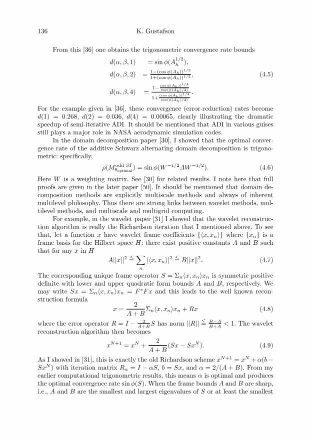
136 K. Gustafson
From this [36] one obtains the trigonometric convergence rate bounds
d(α, β, 1) = sin φ(A1/2h ),
d(α, β, 2) = 1−(cos φ(Ah))1/2
1+(cos φ(Ah))1/2 , (4.5)
d(α, β, 4) =1− cos φ(Ah))1/4
cos(φ(Ah)/2)
1+(cos φ(Ah))1/4
cos(φ(Ah)/2)
.
For the example given in [36], these convergence (error-reduction) rates becomed(1) = 0.268, d(2) = 0.036, d(4) = 0.00065, clearly illustrating the dramaticspeedup of semi-iterative ADI. It should be mentioned that ADI in various guisesstill plays a major role in NASA aerodynamic simulation codes.
In the domain decomposition paper [30], I showed that the optimal conver-gence rate of the additive Schwarz alternating domain decomposition is trigono-metric: specifically,
ρ(Modd SIθoptimal
) = sinφ(W−1/2AW−1/2). (4.6)
Here W is a weighting matrix. See [30] for related results. I note here that fullproofs are given in the later paper [50]. It should be mentioned that domain de-composition methods are explicitly multiscale methods and always of inherentmultilevel philosophy. Thus there are strong links between wavelet methods, mul-tilevel methods, and multiscale and multigrid computing.
For example, in the wavelet paper [31] I showed that the wavelet reconstruc-tion algorithm is really the Richardson iteration that I mentioned above. To seethat, let a function x have wavelet frame coefficients 〈x, xn〉 where xn is aframe basis for the Hilbert space H : there exist positive constants A and B suchthat for any x in H
A||x||2 <=∑
n
|〈x, xn〉|2 <= B||x||2. (4.7)
The corresponding unique frame operator S = Σn〈x, xn〉xn is symmetric positivedefinite with lower and upper quadratic form bounds A and B, respectively. Wemay write Sx = Σn〈x, xn〉xn = F ∗Fx and this leads to the well known recon-struction formula
x =2
A + BΣn〈x, xn〉xn + Rx (4.8)
where the error operator R = I − 2A+B S has norm ||R|| <= B−A
B+A < 1. The waveletreconstruction algorithm then becomes
xN+1 = xN +2
A + B(Sx− SxN ). (4.9)
As I showed in [31], this is exactly the old Richardson scheme xN+1 = xN + α(b−SxN ) with iteration matrix Rα = I − αS, b = Sx, and α = 2/(A + B). From myearlier computational trigonometric results, this means α is optimal and producesthe optimal convergence rate sin φ(S). When the frame bounds A and B are sharp,i.e., A and B are the smallest and largest eigenvalues of S or at least the smallest
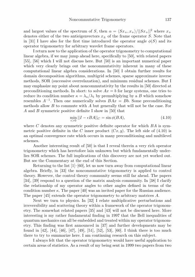
Noncommutative Trigonometry 137
and largest values of the spectrum of S, then α = 〈Sx+, x+〉/||Sx+||2 where x+
denotes either of the two antieigenvectors x± of the frame operator S. Note thatin [31] I have also for the first time introduced the operator angle φ(S) and itsoperator trigonometry for arbitrary wavelet frame operators.
I return now to the application of the operator trigonometry to computationallinear algebra, if we may jump ahead here, specifically to [50], with related papers[55], [56] which I will not discuss here. But [50] is an important numerical paperwhich very clearly brings out the noncommutativity inherent in many of thesecomputational linear algebra considerations. In [50] I obtain further results fordomain decomposition algorithms, multigrid schemes, sparse approximate inversemethods, SOR (successive overrelaxation), and minimum residual schemes. But Imay emphasize my point about noncommutativity by the results in [50] directed atpreconditioning methods. In short: to solve Ax = b for large systems, one tries toreduce its condition number κ = λn/λ1 by premultiplying by a B which somehowresembles A−1. Then one numerically solves BAx = Bb. Some preconditioningmethods allow B to commute with A but generally that will not be the case. ForA and B symmetric positive definite I show in [50] that
minε>0||I − εBA||C = sinφ(BA), (4.10)
where C denotes any symmetric positive definite operator for which BA is sym-metric positive definite in the C inner product 〈Cx, y〉. The left side of (4.10) isan optimal convergence rate which occurs in many preconditioning and multilevelschemes.
Another interesting result of [50] is that I reveal therein a very rich operatortrigonometry which has heretofore lain unknown but which fundamentally under-lies SOR schemes. The full implications of this discovery are not yet worked out.But see the Commentary at the end of this Section.
Returning to the list [1]–[60], let us now turn away from computational linearalgebra. Briefly, in [33] the noncommutative trigonometry is applied to controltheory. However, the control theory community seems still far ahead. The papers[34], [39] respond to a question of the matrix analysis community. In [38] I clarifythe relationship of my operator angles to other angles defined in terms of thecondition number κ. The paper [40] was an invited paper for the Russian audience.The paper [45] extends the operator trigonometry to arbitrary matrices A.
Next we turn to physics. In [32] I relate multiplicative perturbations andirreversibility and scattering theory within a framework of the operator trigonom-etry. The somewhat related papers [35] and [43] will not be discussed here. Moreinteresting is my rather fundamental finding in 1997 that the Bell inequalities ofquantum mechanics can all be embedded and treated within my operator trigonom-etry. This finding was first announced in [37] and further developments may befound in [42], [44], [46], [47], [49], [51], [52], [53], [60]. I think there is too muchthere to try to summarize here. I am continuing research on this subject.
I always felt that the operator trigonometry would have useful application tocertain areas of statistics. As a result of my being sent in 1999 two papers from two
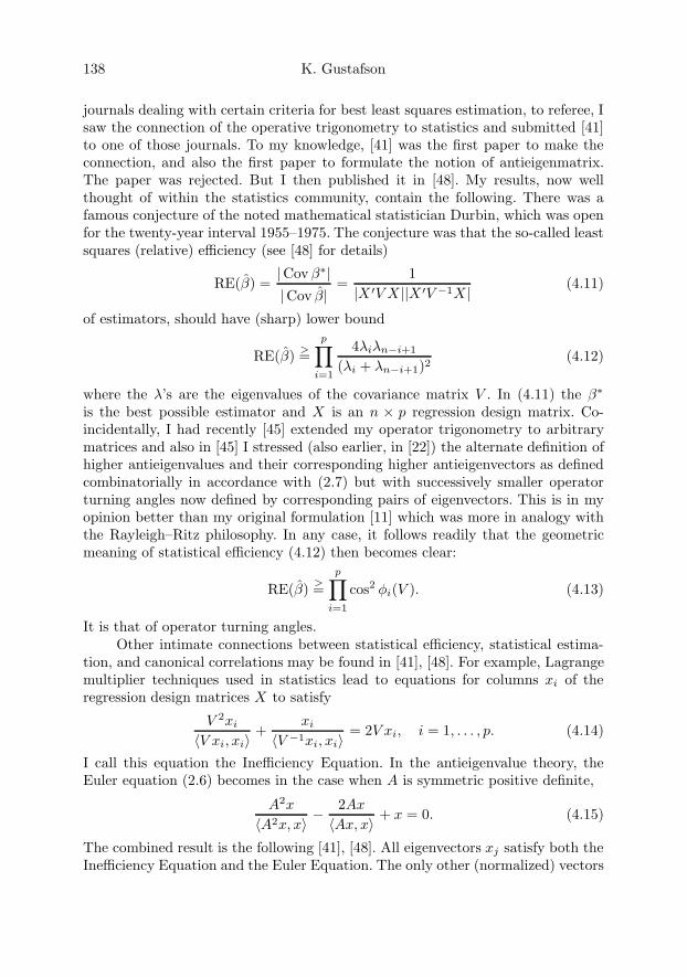
138 K. Gustafson
journals dealing with certain criteria for best least squares estimation, to referee, Isaw the connection of the operative trigonometry to statistics and submitted [41]to one of those journals. To my knowledge, [41] was the first paper to make theconnection, and also the first paper to formulate the notion of antieigenmatrix.The paper was rejected. But I then published it in [48]. My results, now wellthought of within the statistics community, contain the following. There was afamous conjecture of the noted mathematical statistician Durbin, which was openfor the twenty-year interval 1955–1975. The conjecture was that the so-called leastsquares (relative) efficiency (see [48] for details)
RE(β) =|Cov β∗||Cov β|
=1
|X ′V X ||X ′V −1X | (4.11)
of estimators, should have (sharp) lower bound
RE(β) >=p∏
i=1
4λiλn−i+1
(λi + λn−i+1)2(4.12)
where the λ’s are the eigenvalues of the covariance matrix V . In (4.11) the β∗
is the best possible estimator and X is an n × p regression design matrix. Co-incidentally, I had recently [45] extended my operator trigonometry to arbitrarymatrices and also in [45] I stressed (also earlier, in [22]) the alternate definition ofhigher antieigenvalues and their corresponding higher antieigenvectors as definedcombinatorially in accordance with (2.7) but with successively smaller operatorturning angles now defined by corresponding pairs of eigenvectors. This is in myopinion better than my original formulation [11] which was more in analogy withthe Rayleigh–Ritz philosophy. In any case, it follows readily that the geometricmeaning of statistical efficiency (4.12) then becomes clear:
RE(β) >=p∏
i=1
cos2 φi(V ). (4.13)
It is that of operator turning angles.Other intimate connections between statistical efficiency, statistical estima-
tion, and canonical correlations may be found in [41], [48]. For example, Lagrangemultiplier techniques used in statistics lead to equations for columns xi of theregression design matrices X to satisfy
V 2xi
〈V xi, xi〉+
xi
〈V −1xi, xi〉= 2V xi, i = 1, . . . , p. (4.14)
I call this equation the Inefficiency Equation. In the antieigenvalue theory, theEuler equation (2.6) becomes in the case when A is symmetric positive definite,
A2x
〈A2x, x〉 −2Ax
〈Ax, x〉 + x = 0. (4.15)
The combined result is the following [41], [48]. All eigenvectors xj satisfy both theInefficiency Equation and the Euler Equation. The only other (normalized) vectors
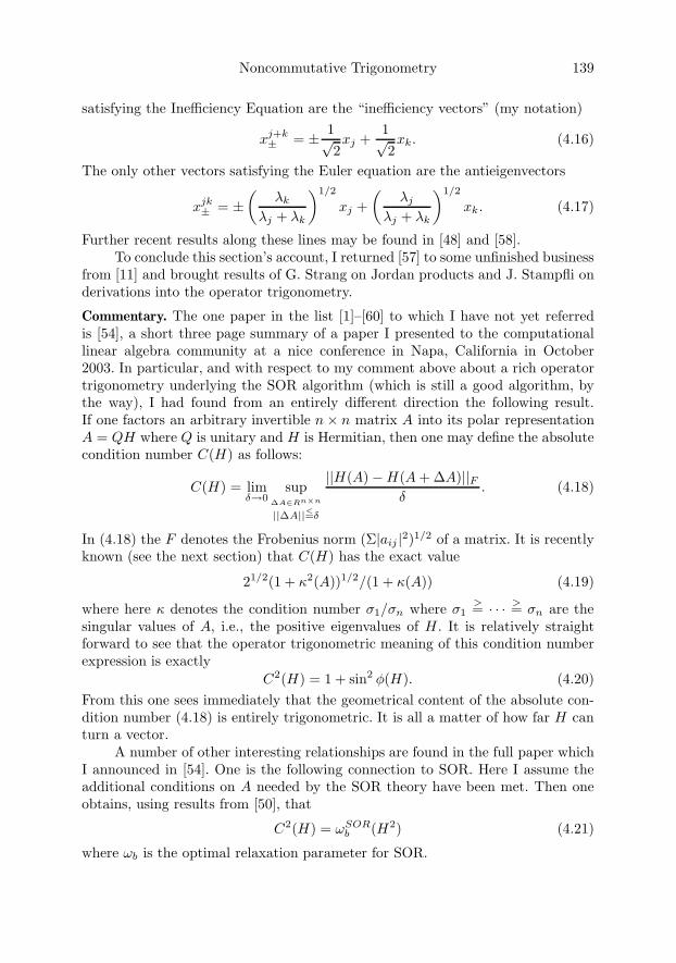
Noncommutative Trigonometry 139
satisfying the Inefficiency Equation are the “inefficiency vectors” (my notation)
xj+k± = ± 1√
2xj +
1√2xk. (4.16)
The only other vectors satisfying the Euler equation are the antieigenvectors
xjk± = ±
(λk
λj + λk
)1/2
xj +(
λj
λj + λk
)1/2
xk. (4.17)
Further recent results along these lines may be found in [48] and [58].To conclude this section’s account, I returned [57] to some unfinished business
from [11] and brought results of G. Strang on Jordan products and J. Stampfli onderivations into the operator trigonometry.
Commentary. The one paper in the list [1]–[60] to which I have not yet referredis [54], a short three page summary of a paper I presented to the computationallinear algebra community at a nice conference in Napa, California in October2003. In particular, and with respect to my comment above about a rich operatortrigonometry underlying the SOR algorithm (which is still a good algorithm, bythe way), I had found from an entirely different direction the following result.If one factors an arbitrary invertible n× n matrix A into its polar representationA = QH where Q is unitary and H is Hermitian, then one may define the absolutecondition number C(H) as follows:
C(H) = limδ→0
sup∆A∈Rn×n
||∆A||<=δ
||H(A)−H(A + ∆A)||Fδ
. (4.18)
In (4.18) the F denotes the Frobenius norm (Σ|aij |2)1/2 of a matrix. It is recentlyknown (see the next section) that C(H) has the exact value
21/2(1 + κ2(A))1/2/(1 + κ(A)) (4.19)
where here κ denotes the condition number σ1/σn where σ1>= · · · >= σn are the
singular values of A, i.e., the positive eigenvalues of H . It is relatively straightforward to see that the operator trigonometric meaning of this condition numberexpression is exactly
C2(H) = 1 + sin2 φ(H). (4.20)From this one sees immediately that the geometrical content of the absolute con-dition number (4.18) is entirely trigonometric. It is all a matter of how far H canturn a vector.
A number of other interesting relationships are found in the full paper whichI announced in [54]. One is the following connection to SOR. Here I assume theadditional conditions on A needed by the SOR theory have been met. Then oneobtains, using results from [50], that
C2(H) = ωSORb (H2) (4.21)
where ωb is the optimal relaxation parameter for SOR.
140 K. Gustafson
Apparently this full paper from [54] is too theoretical for the computationallinear algebra community and it rests, so far, unpublished. Perhaps the most in-teresting result from my analysis therein concerns the notion of antieigenmatrix, aconcept I first introduced in the statistics paper [41]. Therefore, in Section 6 hereI will construct an antieigenmatrix which achieves the C(H) limit in (4.18), i.e.,which attains the bounds (4.19) and (4.20).
5. Related work: Discussion
I have already mentioned above the early independent work of M.G. Krein [61] andWielandt [62], both of whom however failed to see the important entity minε ||εA−I|| and thus missed sin φ(A) and thus were not led to an operator trigonometry.My 1968 min-max theorem [6] was extended in 1971 by Asplund and Ptak [63] andbecause of their result (general failure of the min-max theorem for Banach spaces),I did not further pursue the Banach space context, even though I had mentionedit in 1969, see [11], p. 116. Later congenial discussions with V. Ptak confirmedto me that he did not know of my 1968 publication [6], but I had intimatelydiscussed my min-max result with E. Asplund, who was quite excited about it,at the 1969 UCLA meetings from which finally came the 1972 book in which myantieigenvalues paper [11] appeared. In 1971 P. Hess [64] extended our result [8]that cosφ(A) = 0 for unbounded accretive operators. As we observed in [16], thatneed no longer be the case in certain Banach spaces.
But my first encounter with really relevant outside interest in my operatortrigonometry theory came from Chandler Davis [65] who invited me to Toronto in1981 to discuss the subject. Through Davis I also learned of the results by Mirman[66] for the calculation of antieigenvalues. I also learned for the first time that inmy 1960’s work I had rediscovered Kantorovich’s inequality [67]. However, as Ihave emphasized elsewhere in this account: no-one, including Kantorovich, hadseen the natural operator angle which I had found in my equivalent formulationsof the inequality. As mentioned earlier, the reader may see [20] for further rela-tionships to Davis’ theory of shells of Hilbert space operators. For a recent surveyof many inequalities as they relate to Kantorovich’s inequality and to other issuesin statistics, see [68].
Following my 1999 paper [41], which first established the connection betweenmy operator trigonometry and statistics, and which circulated but was rejected bythe journal Metrika but which I then successfully published in 2002 in [48], andperhaps due to the authors of [68] including in their widely circulated 1999 draftsof [68] some explicit mention of my antieigenvalue theory, Khatree [69], [70], [71]published three papers somewhat parallel to [41], [48] but more from the statisticsviewpoint. There had also been a little earlier interest in my antieigenvalue theoryby mathematicians in India, see [72]. At the 14th IWMS Conference in Auckland inMarch 2005, I enjoyed thoroughly agreeable discussions with the noted mathemat-

Noncommutative Trigonometry 141
ical statistician C.R. Rao, who has fully embraced [73] my operator trigonometryas it applies to various considerations in statistics.
The same cannot be said of the computational linear algebra community.When I first presented my application of the operator trigonometry to conver-gence rates for iterative linear solvers at the Colorado Conference on IterativeMethods at Breckenridge, Colorado in April 1994, a colleague from Texas whoknew and appreciated some of my earlier work [74] on finite element methods,quietly took me aside and gave me his opinion that no-one there would under-stand nor appreciate this noncommutative operator trigonometry as it applied totheir matrices. Indeed, my full paper [21] was rejected by a SIAM journal from theconference. I then published my results in [24] and [27]. At the 1996 conferenceof [24] a very well known computational linear algebraist from Germany at mypresentation asked me “but can you produce a better algorithm?” Someone else,more supportive, later pointed out to me that my questioner, although a greatauthority and author of several excellent books on computational linear algebra,had never himself “produced a better algorithm.” Nevertheless, I do respect thatviewpoint in that field of scientific endeavor: producing a better algorithm is thename of the game. It is more important than a better theory, which in my opinion,I have indeed produced.
So to my knowledge, I know of no work on this noncommutative trigonometryby others within the computational matrix algebra community. However, some,e.g., Martin Gutknecht in Zurich and Owe Axelsson in Nijmegen and Michele Benziin Atlanta, among others, are genuinely appreciative of the theoretical contributionmy geometrical viewpoint makes to the overall theory of iterative and multilevelmethods. Some day, one of us may use this noncommutative matrix trigonometryto produce a faster or more accurate algorithm.
Within the quantum mechanics community, there has been great interest inmy successful embedding of much of the Bell inequality theory into my noncommu-tative trigonometry. This has been clearly evidenced when I presented my recentresults at many top-level conferences on the foundations of quantum mechanicsin Europe and in the USA. However, to my knowledge, no-one and no group haspushed my results further. One reason for that is there are so many other importantissues surrounding and related to Bell’s inequalities and the foundations of quan-tum mechanics that must also be dealt with, many of an endlessly confoundingand mysterious nature. Concerning the partial application of the noncommutativetrigonometry to quantum computing I outlined in [46], more work needs to bedone.
M. Seddighin has recently returned to the Re and Total antieigenvalue theoryand has advanced our results of [16], [18] in his papers [75], [76], [77]. Our recentjoint paper [59] grew out of those investigations. However it remains my feelingthat one needs a better theory for arbitrary matrices than that provided by myoriginal 1969 formulation of Real, Imaginary, and Total antieigenvalues.
When working on the optoelectronic neural networks, in 1992 my Ph.D. stu-dent Shelly Goggin and I implemented an angular version of the famous machine
142 K. Gustafson
learning algorithm called Backpropagation. We called our algorithm Anglepropand a brief summary of the simulations may be found in [78].
The C(H) result (4.19) referred to in the previous section is in [79]. I willcome back to this in the next section.
Generally I cannot cite full literature here, which must be obtained from eachpaper and each area of application. One of the original treatments and still a goodbook for the ADI and other iterative algorithms is that of Varga [80]. However,the computational linear algebra literature has exploded in the last thirty yearsdue to the availability of large scale computing. Of course the statistics literatureand the quantum mechanics literature are also enormous.
Our interest in wavelets actually began with the stochastic processes paper[81], from which we developed a theory of Time operators. From our formulationof a Time operator for Kolmogorov Systems, I. Antoniou and I saw in 1991 thatwavelets were wandering vectors: this discovery is documented in our NATO pro-posal [82]. I mention this here because at about the same time, others, e.g., see [83],also noticed this fact. For us it was natural from the beginning, because we were atthat time working with the Sz. Nagy–Foias dilation theory [84], where wanderingvectors occur on page 1. However, due to a number of more immediate tasks, wedid not get around to publishing our results on wavelets until the papers [85], [86],[87], [88], although I did mention our results in the earlier books [23], [29].
In particular, we showed that every wavelet multisolution analysis (MRA)has naturally associated to it a Time operator T whose age eigenstates are thewavelet detail subspaces Wn. The natural setting of the Haar’s wavelet is thatof an eigenbasis canonically conjugate to the Haar detail refinement. The Timeoperator of the wavelet may be regarded as a (position) multiplication operator,equivalent under appropriate transform to a first order (momentum) differentialoperator.
Commentary. As concerns the resistance I sometimes encounter when bringing myoperator trigonometry into a new domain of endeavor, I remember a discussionI once had with the late and renowned physicist (e.g., see [89]) Joseph Jauch inSwitzerland in 1972. He mused that the influential mathematician Paul Halmospossessed and practiced a clever tactic: apply the same key insight or philosoph-ical viewpoint to a variety of situations. As a result, no one could really beatHalmos at his game. There may be some parallel in the way in which the operatortrigonometry has been developed.
6. Noncommutative trigonometry: Outlook
After I returned to this noncommutative operator trigonometry about a dozenyears ago, the circumstances more or less described in Section 4, it became clearto me that it possessed the joint potentials for both further application and furthertheoretical development. During these last dozen years in which I have been ableto develop these joint potentials, it has become clear to me that I cannot do it all
Noncommutative Trigonometry 143
myself. Toward the future enlargement of this theory and its applications, in thefollowing three subsections I will indicate three fruitful future directions: OperatorAlgebras, Multiscale System Theory, and Quantum Mechanics.
6.1. Extensions to matrix and operator algebras
First, I would like to prove the result [90] announced in [54], and described in thecommentary at the end of Section 4, heretofore unpublished, that an antieigenma-trix can be found which attains the maximum turning which we now understand(4.18) to mean. The notion of antieigenmatrix was first, to my knowledge, pre-sented in my 1999 preprint [41]. However, it must be said the statisticians hadalready implicitly for many years had such antieigenmatrices lurking within theirinequalities, although they did not see the geometry, hence they could not seethe concept. Perhaps elsewhere I will try to elaborate all the places where suchantieigenmatrices were already implicitly hiding in statistics.
In any case, to construct an antieigenmatrix for (4.18), I will follow here veryclosely and use the analysis of [79], where (4.19) was shown. The reader will needto consult [79] carefully to check all entities that I will use now.
There are two key steps in the proof in [79]. First it is shown that C(H) =||H ′(A)||F where H ′(A) is the Frechet derivative. From this it follows by use ofthe implicit function theorem that in a neighborhood of A one has
H ′(A)∆A = ∆H = V KV T
= V (Γ2 B + ΓT2 BT )V T
(6.1)
where Γ2 = [σi/(σi + σj)], B = U∆AV , A has singular value decompositionA = UΣV T , H = V ΣV T , and where denotes Hadamard product. The secondkey step, [79] Appendix, is to show that from considerations involving the structureof Γ2 and ΓT
2 , one has
C(H) = ||H ′(A)||F = max||B||F =1 ||Γ2 B + ΓT2 BT ||F
=√
2maxi<j
√1+(σi/σj)2
1+σi/σj
(6.2)
from which the condition number bound (4.19) follows.We may now connect to the dynamics of the operator trigonometry by seeking
a ∆A which represents a maximal turning in the sense of the operator trigonometryand which attains the absolute condition number C(H) of A. In other words,we seek an ‘antieigenmatrix’. The Frobenius norm being unitarily invariant andrecalling that ∆A = UT BV T , it is easier to work with B as seen from (6.1) above.The following shows that C(H) is exactly caused by such a sought maximal turningantieigenmatrix.

144 K. Gustafson
Proposition 6.1. The absolute condition number C(H) of the absolute factor H ofthe matrix A = QH is attained by
B =
⎡⎢⎢⎢⎢⎣0 · · · 0 σ1
(σ21+σ2
n)1/2
......
0 0σn
(σ21+σ2
n)1/2 0 · · · 0
⎤⎥⎥⎥⎥⎦ . (6.3)
Proof. Following [79] and from (4.18) and (6.1), one has
C(H) = ||H ′(A)||F = sup||∆A||F =1
||H ′(A)∆A||F = sup||B||F =1
||2Re(Γ2 B)||F . (6.4)
However, rather than use the Hadamard product Γ2 B formulation, we preferto directly maximize ||K||F from (6.1). Recall that K = V T ∆HV = [kij ] wherekij = (σibij + σjbji)/(σi + σj). The way we wish to think is the following: ∆Arunning through all directions is the same as B running through all directions fromwhich we may look at all resulting symmetric K within which the data (the givenmatrix A’s singular values) is already incorporated. First suppose B is symmetric.Then kij = bij and ||∆H ||F = ||K||F = ||B||F = 1 so such B are not interesting. Alittle thought and experimentation then led to the candidate B of (6.3). Considerfirst the 2× 2 case and the matrix
K =
[b11
σ1b12+σ2b21σ1+σ2
σ2b21+σ1b12σ2+σ1
b22
]. (6.5)
We wish to maximize the expression
b211 + b2
22 +2(σ1b12 + σ2b21)2
(σ1 + σ2)2(6.6)
subject to the constraint
b211 + b2
22 + b212 + b2
21 = 1. (6.7)
We may take b211 = b2
22 = 0 and letting x = b12 and y = b21 we may maximize theexpression f(x) = σ1x + σ2(1− x2)1/2, from which
x =κ
(1 + κ2)1/2, y =
1(1 + κ2)1/2
(6.8)
where κ = σ1/σ2 (K(A) in the notation of [79]) is the condition number of A.From (6.6) and (6.8) we have
||K||2F =2
(σ1 + σ2)2(σ1κ + σ2)2
1 + κ2=
2(σ21 + σ2
2)(σ1 + σ2)2
= C2(H). (6.9)
The n× n situation is the same (choose all bij = 0 except b1n and bn1 as given in(6.3)). Thus B of (6.3) enables K hence ∆A to attain C(H).

Noncommutative Trigonometry 145
We may obtain a deeper geometrical clarification as follows.
Corollary 6.2. With the B of (6.3), the matrix K has turning angle φ(H2) on theantieigenvectors x± of H2.
Proof. We recall (2.8) that the (normalized) antieigenvectors of H2, i.e., thosevectors most turned by H2, are
x± = ± σ1(σ2
1+σ2n)1/2 xn + σn
(σ21+σ2
n)1/2 x1
= 1(σ2
1+σ2n)1/2 (±σ1, 0, . . . , 0, σn)T
(6.10)
where x1 and xn are the eigenvectors corresponding to σ1 and σn, respectively.Noting that K is the symmetric matrix with all kij = 0 except for
k1n = kn1 =σ1κ + σn
(1 + κ2)1/2(σ1 + σn)=
(σ21 + σ2
n)1/2
(σ1 + σn)(6.11)
and since ||x+|| = 1, we find
〈Kx+, x+〉||Kx+||||x+||
=2σ1σn(σ2
1 + σ2n)−1/2(σ1 + σn)−1
(σ2n + σ2
1)1/2(σ1 + σn)−1=
2σ1σn
σ21 + σ2
n
(6.12)
which is (see (2.7)) exactly cosφ(H2). For x− it is the same. Thus K, although not a positive definite matrix, nonetheless turns the anti-
eigenvectors x± of H2 = A∗A in the same (maximal) way that H2 does, and thisis what causes B, which is constructed from H2 antieigenvectors, to attain C(H).
A more complete presentation [90] of this attainment of C(H) by antieigen-matrices, and related considerations, will hopefully be published elsewhere. A nat-ural remaining question is: characterize all of the antieigenmatrices which achievethe maximum turning angle.
But beyond presenting these results here which are new, we see that we haveillustrated that the noncommutative operator trigonometry can be extended fromgeometrical action on vectors to geometrical action on matrices. In other words,in the future, hopefully to algebras of operators. If possible, it will be desirable tokeep Hilbert space structures in the formulation, for trigonometry to be most nat-ural needs a Euclidean geometry. The use of the Frobenius norm does do this sinceit has an inner product tr(AB∗). On the other hand, the Frobenius norm is not aninduced norm and ||I||F =
√n means that the key entity (2.4) will have to be mod-
ified. These are preliminary, tentative thoughts only, as also will be the following.Much of C∗ and W ∗ algebra tries to use commutativity when possible, if not,
then commutators, if not, then commutants, or centers. But even when matricesor operators do not commute, one has the often times very useful fact that thespectra σ(AB) and σ(BA) are the same (for invertible operators, and differingonly by ±0 in the general case). This fact should somehow be regarded as a keyinvariant in future noncommutative trigonometries. This is a vague statement. Butfor example, when A and B are positive selfadjoint operators, and do not commute,then BA is not even normal, yet σ(BA) is real and just from this spectrum one candefine some parts of a (noncommutative) operator trigonometry. Then (e.g., see

146 K. Gustafson
[55]) one can find a whole family of positive selfadjoint operators C for which BAbecomes positive selfadjoint in the C inner product. In this latter situation, we havea very comfortable, intuitive operator trigonometry, resembling the original one.
6.2. Multiscale system theory, wavelets, iterative methods
As is well known and as I mentioned in Section 4, there are strong links betweenwavelet methods, multilevel numerical methods, and multigrid and multiscale com-puting. I would like to elaborate that theme here. In particular, I want to advancethe notion that Iterative methods should be added to this list, or at least placedinto strong conjunction with these topics.
As I described in Section 4, at the Jackson, Wyoming Iterative Methodsconference in 1997 (reported in [31]), I showed that the wavelet reconstructionalgorithm, which had been developed independently by the wavelet community,was just the classical Richardson Iterative method. That method goes back to 1910[91]. Now, in addition we know [31] the optimal wavelet reconstruction algorithmconvergence rate to be operator trigonometric: sinφ(S), where S is the frameoperator. So wavelet reconstruction is both iterative and trigonometric.
Domain decomposition methods and multigrid numerical methods are clearlyimportant multiscale methods. However, until the important analysis of Griebeland Oswald [92], it was not known that domain decomposition and multigridmethods could be placed within the context of Jacobi iterative methods. Becausemy operator trigonometric analysis applies to Jacobi methods, I could then placedomain decomposition and multigrid methods into the noncommutative trigonom-etry. For more details see [30, 50].
The dramatic convergence improvements of the ADI semi-iterative methodsdescribed in Section 4 are clearly multiscale. So therefore are the underlying in-trinsic noncommutative trigonometric subangles [36]. I should mention that to myknowledge, there is not yet a full theoretical understanding of the very importantADI schemes and their later derivatives. You can see the difficulties from the excel-lent early analysis of Varga [80]. You can see that only a commutative situation iseasily analyzed. There is a very interesting noncommutative trigonometry of ADIwaiting to be understood. The same can be said for the important SOR methodcombined with iterative refinement on a sequence of grids, see the preliminarydiscussion and results in [50].
For the PDE Dirichlet–Poisson model problem, a grid noncommutative trigo-nometry was worked out in [36]. The discretized operator Ah had turning angleφ(Ah) = π/2− πh, where h is the grid size. One will find in [36] also a discussionof how an operator mesh trigonometry shows that the performance of an iterativemethod on a grid of mesh size h depends upon the operator trigonometry on thefiner mesh size h/2. This phenomenon is an aspect of interesting general identitieswithin the operator trigonometry. For example [27],
sinφ(A1/2) =sin φ(A)
1 + cosφ(A)(6.13)
Noncommutative Trigonometry 147
for symmetric positive definite matrices A. Such power-of-two refinement relationsare reminiscent of those of the dilations in wavelet multiresolutions. Another suchscale relation from [90] is inherent in the absolute condition number C(H) dis-cussed in Section 6.1 above:
C2(H) =2 sinφ(H)sin φ(H2)
. (6.14)
To date I have only cared about such identities as they relate to specific theoreticalor numerical applications.
A general theme could be stated philosophically as follows. All multiscale,multigrid, wavelet theories and behaviors are inherently spectral. So is my oper-ator trigonometry of antieigenvalues and antieigenvectors. Eigenvalues take youfrom largest to smallest scale in your model. Instead of a vibration or numericalgrid based range of scales, which correspond to an eigenvalue spectral decomposi-tion, the antieigenvalues and antieigenvectors correspond to physical or numericalturning angle scales.
Turning to another subject, our theory of wavelets as stochastic processes [23,29, 82, 85, 86, 87, 88] is inherently multiscale, but in quite a different sense. Thestochastic processes and Kolmogorov dynamical systems may be seen as basedupon a sequence of increasing σ-algebras of increasingly rich underlying eventspaces. These are sometimes called filtrations in the stochastic literature, e.g., see[93], [94]. This type of stochastic event-multiscale is related to coarse-graining instatistical physics, and to conditional expectations in general. The Time operatorof wavelets which we obtained [82,88], although motivated by mixing processes, isvery much spectral. See my analysis in the recent paper [95], where I take it allback to a cyclic vector.
Our approach to wavelets in the above mentioned papers, although originallymotivated by our work in statistical mechanics, can also be described as thatof “representation-free theory of shifts,” e.g., the Bernoulli shifts of dynamicalsystems theory being just one representation. In retrospect and as now connectedto wavelet multiresolutions, we dealt first with the shift V (the dilation in wavelets)via its wandering subspaces Wn, before dealing with the translations. This enabledour getting the Time operator of wavelets. The conventional wavelet theory doesnot do that. Following our approach, Kubrusly and Levan [96], [97] showed thatwith respect to an orthonormal wavelet ψ ∈ L2(R), any f ∈ L2(R) is the sum ofits layers of detail over all time shifts. This contrasts with the conventional waveletview of f as the sum of its layers over all scales. Thus one may write
f(x) =∑m
∑n
〈f, ψm,n〉ψm,n(x) =∑
n
∑m
〈f, ψm,n〉ψm,n. (6.15)
I could describe this result as a kind of Fubini theorem, holding in the absenceof the usual assumptions of absolute summability. More such results are to beexpected from our point of view [87] of wavelets.
148 K. Gustafson
6.3. Quantum mechanics
Much of the current interest (and funding) for research on multiscale theory isthe need in engineering applications to bring quantum mechanical effects intothe modelling which has heretofore been only classical. I know this from manyannecdotal conversations with my engineering colleagues. The applications rangefrom chip design to aerodynamics. Each of those applications is a subject untoitself and will not be dealt with here. The considerations and needs are usuallyboth physical and numerical.
Instead, I want to address quantum mechanics at a more fundamental level.As I mentioned briefly in Section 4, in [37, 42, 44, 46, 47, 49, 51, 52, 53, 60] I havefound fundamental connections of the noncommutative trigonometry to quantummechanics. There is too much in those papers to fully describe here, but let meat least delineate the issues and papers for bibliographical sake. Then I want toannounce a new result here.
In [37, 42, 44, 47, 51, 52, 53] I was able to place the celebrated Bell in-equality theory into the context of the noncommutative trigonometry. This wasa completely new contribution to the foundations of physics. In particular, frommy viewpoint, one cannot argue ‘nonlocality’ on the basis of violation of Bell’sinequalities. See the papers for more details.
In [46] I develop preliminary aspects of the noncommutative trigonometryfor quantum computing. To treat the unitary operators one encounters there,it becomes clear that I need a better complex-valued noncommutative operatortrigonometry. That is to say, the general operator trigonometry which I developedin [45] for arbitrary operators A, by writing them in polar form A = U |A| andthen defining an operator trigonometry for them in terms of the known operatortrigonometry for |A|, is not sufficient. Granted, quantum mechanics fundamentalsoften ignore phase when dealing just with probabilities. But for quantum comput-ing, one cannot ignore phase.
In [49] I connect the noncommutative trigonometry to elementary particlephysics. In particular, I showed that CP violation may be seen as a certain slightlyunequal weighting of the CP antieigenvectors. The setting is that of Kaon sys-tems and the decay of neutral mesons into charged pions. In particular, I showedthat CP eigenstates are strangeness total antieigenvectors. CP violation is seen asantieigenvector-breaking.
Finally, I wish to turn to the famous quantum Zeno’s paradox [98]. I wasinvolved in its initial formulations in 1974 and a summary of the state of affairsmay be found in [60], see also [99]. Mathematically and briefly, one is confrontedwith questions of the existence and nature of operator limits such as
s- limn→∞(EeitHE)n (6.16)
where (roughly) E is (for example) a projection operator corresponding to a phys-ical measuring apparatus, and H is a quantum mechanical Hamiltonian governinga wave packet evolution. When E is in the spectral family of H , i.e., when E
Noncommutative Trigonometry 149
and H commute, all the issues are trivial, or otherwise may be dealt with instraightforward fashion. But in the physically interesting case when E and H donot commute, very interesting mathematical unbounded operator domain ques-tions arise. Several enlightened physicists pushed me to return to these issues. Aclarification, essentially known to me in 1974 but not published, is the following[60,99].
Lemma 6.3. Let H be an unbounded selfadjoint operator and let E be an orthogonalprojection. Then the domain D(HE) is dense iff EH is closeable. In that case,
(HE)∗ = EH ⊃ EH (6.17)
is defined, with domain at least as large as D(H). Generally (EHE)∗ = EHEwhenever EH is closeable. Furthermore the polar factors satisfy
|EH | = (HE2H)1/2, |HE| ⊃ (EH2E)1/2 (6.18)
Here HE2H denotes (EH)∗EH.
Most of the recent papers by physicists on the Zeno issues, theory, and ap-plications, fail to understand these unbounded noncommutative operator consid-erations. The critical rigor is not seen or at best is just glossed over or ignored.Another approach, that of Misra and Sudarshan originally [98], was to go to theHeisenberg picture and only work with the density matrix (bounded operators).Even there one eventually must assume operator limits such as (6.16).
Recently, in pondering some of these Bell, Zeno, or other related issues inthe foundations of quantum mechanics, I found [100] the following operator theo-retic characterization of quantum mechanical reversibility in terms of what I shallcall domain regularity preservation. I have never seen this theorem elsewhere. Ibelieve it to be fundamental to the understanding of quantum probability in theSchrodinger picture. I include it here because I see it as truly multiscale.
Theorem 6.4. A unitary group Ut necessarily exactly preserves its infinitesimalgenerator’s domain D(H). That is, Ut maps D(H) one to one onto itself, at everyinstant −∞ < t <∞.
The proof of Theorem 6.4 is not hard (I give two proofs in [100]) and theresult is quite evident, once one sees it. Its application to quantum mechanics isdramatic: a quantum mechanical evolution must at all times be able to simulta-neously account for each wave function probability upon which the Hamiltoniancan act before one is entitled to draw any conclusions about the overall evolvingprobabilities. Not one probability can be lost.
A converse is the following [100]. Let Zt be a contraction semigroup on aHilbert space H such that Zt maps D(A) one to one onto D(A). Here A is theinfinitesimal generator of the semigroup Zt. Then Zt on the graph Hilbert spaceHA can be extended to a group Z−t = Z−1
t .What Theorem 6.4 means is that in unitary quantum mechanical evolutions,
one cannot lose any of the totality of detail embodied in the totality of wave
150 K. Gustafson
functions ψ in D(H). It is quite interesting to think about how much ‘mixingaround’ of the D(H) probabilities the evolution can do. That is a multiscale andeven interscale concept.
References
[1] K. Gustafson, A Perturbation Lemma, Bull. Amer. Math. Soc. 72 (1966), 334–338.
[2] K. Gustafson, Positive Operator Products, Notices Amer. Math. Soc. 14 (1967),Abstract 67T-531, p. 717. See also Abstracts 67T-340, 67T-564, 67T-675.
[3] K. Gustafson, A Note on Left Multiplication of Semi-group Generators, Pacific J.Math. 24 (1968a), 463–465.
[4] K. Gustafson, The Angle of an Operator and Positive Operator Products, Bull.Amer. Math. Soc. 74 (1968b), 488–492.
[5] K. Gustafson, Positive (noncommuting) Operator Products and Semigroups, Math.Zeitschrift 105 (1968c), 160–172.
[6] K. Gustafson, A min–max Theorem, Amer. Math Soc. Notices 15 (1968d), p. 799.
[7] K. Gustafson, Doubling Perturbation Sizes and Preservation of Operator Indices inNormed Linear Spaces, Proc. Camb. Phil. Soc. 98 (1969a), 281–294.
[8] K. Gustafson, On the Cosine of Unbounded Operators, Acta Sci. Math. 30 (1969b),33–34 (with B. Zwahlen).
[9] K. Gustafson, Some Perturbation Theorems for Nonnegative Contraction Semi-groups, J. Math. Soc. Japan 21 (1969c), 200–204 (with Ken-iti Sato).
[10] K. Gustafson, A Simple Proof of the Toeplitz–Hausdorff Theorem for Linear Oper-ators, Proc. Amer. Math. Soc. 25 (1970), 203–204.
[11] K. Gustafson, Anti-eigenvalue Inequalities in Operator Theory, Inequalities III (O.Shisha, ed.), Academic Press (1972a), 115–119.
[12] K. Gustafson, Multiplicative Perturbation of Semigroup Generators, Pac. J. Math.41 (1972b), 731–742 (with G. Lumer).
[13] K. Gustafson, Multiplicative Perturbation of Nonlinear m-accretive Operators, J.Funct. Anal. 10 (1972c), 149–158 (with B. Calvert).
[14] K. Gustafson, Numerical Range and Accretivity of Operator Products, J. Math.Anal. Applic. 60 (1977), 693–702 (with D. Rao).
[15] K. Gustafson, The RKNG (Rellich, Kato, Nagy, Gustafson) Perturbation Theoremfor Linear Operators in Hilbert and Banach Space, Acta Sci. Math. 45 (1983), 201–211.
[16] K. Gustafson, Antieigenvalue Bounds, J. Math. Anal. Applic. 143 (1989), 327–340(with M. Seddighin).
[17] K. Gustafson, Antieigenvalues in Analysis, Fourth International Workshop in Anal-ysis and its Applications, Dubrovnik, Yugoslavia, June 1–10, 1990 (C. Stanojevicand O. Hadzic, eds.), Novi Sad, Yugoslavi (1991), 57–69.
[18] K. Gustafson, A Note on Total Antieigenvectors, J. Math. Anal. Applic. 178 (1993),603–611 (with M. Seddighin).
[19] K. Gustafson, Operator Trigonometry, Linear and Multilinear Algebra 37 (1994a),139–159.
Noncommutative Trigonometry 151
[20] K. Gustafson, Antieigenvalues, Lin. Alg. and Applic. 208/209 (1994b), 437–454.
[21] K. Gustafson, Computational Trigonometry, Proc. Colorado Conf. on IterativeMethods, Vol. 1 (1994c), p. 1.
[22] K. Gustafson, Matrix Trigonometry, Lin. Alg. and Applic. 217 (1995), 117–140.
[23] K. Gustafson, Lectures on Computational Fluid Dynamics, Mathematical Physics,and Linear Algebra, Kaigai Publishers, Tokyo, Japan (1996a), 169 pp.
[24] K. Gustafson, Trigonometric Interpretation of Iterative Methods, Proc. Conf. Al-gebraic Multilevel Iteration Methods with Applications, (O. Axelsson, B. Polman,eds.), Nijmegen, Netherlands, June 13–15, (1996b), 23–29.
[25] K. Gustafson, Commentary on Topics in the Analytic Theory of Matrices, Section23, Singular Angles of a Square Matrix, Collected Works of Helmut Wielandt 2 (B.Huppert and H. Schneider, eds.), De Gruyters, Berlin (1996c), 356–367.
[26] K. Gustafson, Numerical Range: The Field of Values of Linear Operators and Ma-trices, Springer, Berlin, (1997a), pp. 205 (with D. Rao).
[27] K. Gustafson, Operator Trigonometry of Iterative Methods, Num. Lin Alg. withApplic. 34 (1997b), 333–347.
[28] K. Gustafson, Antieigenvalues, Encyclopaedia of Mathematics, Supplement 1,Kluwer Acad. Publ., Dordrecht, (1997c), 57.
[29] K. Gustafson, Lectures on Computational Fluid Dynamics, Mathematical Physics,and Linear Algebra, World Scientific, Singapore, (1997d), pp. 178.
[30] K. Gustafson, Domain Decomposition, Operator Trigonometry, Robin Condition,Contemporary Mathematics 218 (1998a), 455–560.
[31] K. Gustafson, Operator Trigonometry of Wavelet Frames, Iterative Methods inScientific Computation (1998b), 161–166; (J. Wang, M. Allen, B. Chen, T.Mathew, eds.), IMACS Series in Computational and Applied Mathematics 4, NewBrunswick, NJ.
[32] K. Gustafson, Semigroups and Antieigenvalues, Irreversibility and Causality–Semi-groups and Rigged Hilbert Spaces, (A. Bohm, H. Doebner, P. Kielanowski, eds.),Lecture Notes in Physics 504, Springer, Berlin, (1998c), pp. 379–384.
[33] K. Gustafson, Operator Trigonometry of Linear Systems, Proc. 8th IFAC Sym-posium on Large Scale Systems: Theory and Applications, (N. Koussoulas, PGroumpos, eds.), Patras, Greece, July 15–17, (1998d), 950–955. (Also publishedby Pergamon Press, 1999.)
[34] K. Gustafson, Symmetrized Product Definiteness? Comments on Solutions 19-5.1–19-5.5, IMAGE: Bulletin of the International Linear Algebra Society 21 (1998e),22.
[35] K. Gustafson, Antieigenvalues: An Extended Spectral Theory, Generalized Func-tions, Operator Theory and Dynamical Systems, (I. Antoniou, G. Lumer, eds.),Pitman Research Notes in Mathematics 399, (1998f), 144–149, London.
[36] K. Gustafson, Operator Trigonometry of the Model Problem, Num. Lin. Alg. withApplic. 5 (1998g), 377–399.
[37] K. Gustafson, The Geometry of Quantum Probabilities, On Quanta, Mind, andMatter: Hans Primas in Context, (H. Atmanspacher, A. Amann, U. Mueller–Herold,eds.), Kluwer, Dordrecht (1999a), 151–164.
152 K. Gustafson
[38] K. Gustafson, The Geometrical Meaning of the Kantorovich–Wielandt Inequalities,Lin. Alg. and Applic. 296 (1999b), 143–151.
[39] K. Gustafson, Symmetrized Product Definiteness: A Further Comment, IMAGE:Bulletin of the International Linear Algebra Society 22 (1999c), 26.
[40] K. Gustafson, A Computational Trigonometry and Related Contributions by Rus-sians Kantorovich, Krein, Kaporin, Computational Technologies 4 (No. 3) (1999d),73–83, (Novosibirsk, Russia).
[41] K. Gustafson, On Geometry of Statistical Efficiency, (1999e), preprint.
[42] K. Gustafson, The Trigonometry of Quantum Probabilities, Trends in Contempo-rary Infinite-Dimensional Analysis and Quantum Probability, (L. Accardi, H. Kuo,N. Obata, K. Saito, S. Si, L. Streit, eds.), Italian Institute of Culture, Kyoto (2000a),159–173.
[43] K. Gustafson, Semigroup Theory and Operator Trigonometry, Semigroups of Oper-ators: Theory and Applications, (A.V. Balakrisnan, ed.), Birkhauser, Basel (2000b),131–140.
[44] K. Gustafson, Quantum Trigonometry, Infinite-Dimensional Analysis, QuantumProbability, and Related Topics 3 (2000c), 33–52.
[45] K. Gustafson, An Extended Operator Trigonometry, Lin. Alg. & Applic. 319(2000d), 117–135.
[46] K. Gustafson, An Unconventional Linear Algebra: Operator Trigonometry, Uncon-ventional Models of Computation, UMC’2K, (I. Antoniou, C. Calude, M. Dinneen,eds.), Springer, London (2001a), 48–67.
[47] K. Gustafson, Probability, Geometry, and Irreversibility in Quantum Mechanics,Chaos, Solitons and Fractals 12 (2001b), 2849–2858.
[48] K. Gustafson, Operator Trigonometry of Statistics and Econometrics, Lin. Alg. andApplic. 354 (2002a), 151–158.
[49] K. Gustafson, CP-Violation as Antieigenvector-Breaking, Advances in ChemicalPhysics 122 (2002b), 239–258.
[50] K. Gustafson, Operator Trigonometry of Preconditioning, Domain Decomposi-tion, Sparse Approximate Inverses, Successive Overrelaxation, Minimum ResidualSchemes Num. Lin Alg. with Applic. 10 (2003a), 291–315.
[51] K. Gustafson, Bell’s Inequalities, Contributions to the XXII Solvay Conference onPhysics, (A. Borisov, ed.), Moscow–Izhevsk, ISC, Moscow State University (ISBN:5-93972-277-6) (2003b), 501–517.
[52] K. Gustafson, Bell’s Inequality and the Accardi–Gustafson Inequality, Foundationsof Probability and Physics-2, (A. Khrennikov, ed.) Vaxjo University Press, Sweden(2003c), 207–223.
[53] K. Gustafson, Bell’s Inequalities, The Physics of Communication, Proceedings ofthe XXII Solvay Conference on Physics, (I. Antoniou, V. Sadovnichy, H. Walther,eds.), World Scientific (2003d), 534–554.
[54] K. Gustafson, Preconditioning, Inner Products, Normal Degree, 2003 InternationalConference on Preconditioning Techniques for Large Sparse Matrix Problems inScientific and Industrial Applications, (E. Ng, Y. Saad, W.P. Tang, eds.), Napa,CA, 27–29, October (2003e), pp. 3.

Noncommutative Trigonometry 153
[55] K. Gustafson, An Inner Product Lemma, Num. Lin. Alg. with Applic. 11 (2004a),649–659.
[56] K. Gustafson, Normal Degree, Num. Lin. Alg. with Applic. 11 (2004b), 661–674.
[57] K. Gustafson, Interaction Antieigenvalues, J. Math Anal. Applic. 299 (2004c), 174–185.
[58] K. Gustafson, The Geometry of Statistical Efficiency, Research Letters Inf. Math.Sci. 8 (2005a), 105–121.
[59] K. Gustafson, On the Eigenvalues Which Express Antieigenvalues, International J.of Mathematics and Mathematical Sciences 2005:10 (2005b), 1543–1554. (with M.Seddighin).
[60] K. Gustafson, Bell and Zeno, International J. of Theoretical Physics 44 (2005c),1931–1940.
[61] M. Krein, Angular Localization of the Spectrum of a Multiplicative Integral in aHilbert Space, Funct. Anal. Appl. 3 (1969), 89–90.
[62] H. Wielandt, Topics in the Analytic Theory of Matrices, University of WisconsinLecture Notes, Madison, (1967).
[63] E. Asplund and V. Ptak, A Minmax Inequality for Operators and a Related Nu-merical Range, Acta Math. 126 (1971), 53–62.
[64] P. Hess, A Remark on the Cosine of Linear Operators, Acta Sci Math. 32 (1971),267–269.
[65] C. Davis, Extending the Kantorovich Inequalities to Normal Matrices, Lin. Alg.Appl. 31 (1980), 173–177.
[66] B.A. Mirman, Antieigenvalues: Method of Estimation and Calculation, Lin. Alg.Appl. 49 (1983), 247–255.
[67] L. Kantorovich, Functional Analysis and Applied Mathematics, Uspekhi Mat. Nauk3 No. 6 (1948), 89–185.
[68] S. Drury, S. Liu, C.Y. Lu, S. Puntanen, and G.P.H. Styan, Some Comments onSeveral Matrix Inequalities with Applications to Canonical Correlations: HistoricalBackground and Recent Developments, Sankhya: The Indian J. of Statistics 64,Series A, Pt. 2 (2002), 453–507.
[69] R. Khatree, On Calculation of Antiegenvalues and Antieigenvectors, J. Interdisci-plinary Math 4 (2001), 195–199.
[70] R. Khatree, On Generalized Antieigenvalue and Antieigenmatrix of order r, Amer.J. of Mathematical and Management Sciences 22 (2002), 89–98.
[71] R. Khatree, Antieigenvalues and Antieigenvectors in Statistics, J. of StatisticalPlanning and Inference 114 (2003), 131–144.
[72] K.C. Das, M. Das Gupta, K. Paul, Structure of the Antieigenvectors of a StrictlyAccretive Operator, International J. of Mathematics and Mathematical Sciences 21(1998), 761–766.
[73] C.R. Rao, Anti-eigen and Anti-singular Values of a Matrix and Applications toProblems in Statistics, Research Letters Inf. Math. Sci. 2005:10 (2005), 53–76.
[74] K. Gustafson, R. Hartman, Divergence-free Bases for Finite Element Schemes inHydrodynamics, SIAM J. Numer. Analysis 20 (1983), 697–721.

154 K. Gustafson
[75] M. Seddighin, Antieigenvalues and Total Antieigenvalues of Normal Operators, J.Math. Anal. Appl. 274 (2002), 239–254.
[76] M. Seddighin, Antieigenvalue Inequalities in Operator Theory, International J. ofMathematics and Mathematical Sciences (2004), 3037–3043.
[77] M. Seddighin, On the Joint Antieigenvalues of Operators in Normal Subalgebras, J.Math. Anal. Appl. (2005), to appear.
[78] K. Gustafson, Distinguishing Discretization and Discrete Dynamics, with Applica-tion to Ecology, Machine Learning, and Atomic Physics, in Structure and Dynamicsof Nonlinear Wave Phenomena, (M. Tanaka, ed.), RIMS Kokyuroku 1271, Kyoto,Japan (2002c), 100–111.
[79] F. Chaitin–Chatelin, S. Gratton, On the Condition Numbers Associated with thePolar Factorization of a Matrix, Numerical Linear Algebra with Applications 7(2000), 337–354.
[80] R. Varga, Matrix Iterative Analysis, Prentice Hall, NJ, (1962).
[81] K. Gustafson, B. Misra, Canonical Commutation Relations of Quantum Mechanicsand Stochastic Regularity, Letters in Math. Phys. 1 (1976), 275–280.
[82] K. Gustafson, I. Antoniou, Wavelets and Kolmogorov Systems,http://www.auth.gr/chi/PROJECTSWaveletsKolmog.html, (2004).
[83] X. Dai, D.R. Larson, Wandering Vectors for Unitary Systems and OrthogonalWavelets, Amer. Math. Soc. Memoirs 640, Providence, RI, (1998).
[84] B. Sz. Nagy, C. Foias, Harmonic Analysis of Operators in Hilbert Space, NorthHolland, Amsterdam, (1970).
[85] I. Antoniou, K. Gustafson, Haar Wavelets and Differential Equations, DifferentialEquations 34 (1998), 829–832.
[86] K. Gustafson, Wavelets as Stochastic Processes, Workshop on Wavelets andWavelet-based Technologies, (M. Kobayashi, S. Sakakibara, M. Yamada, eds.),IBM-Japan, Tokyo, October 29–30, (1998h), 40–43.
[87] I. Antoniou, K. Gustafson, Wavelets and Stochastic Processes, Mathematics andComputers in Simulation 49 (1999), 81–104.
[88] I. Antoniou, K. Gustafson, The Time Operator of Wavelets, Chaos, Solitons andFractals 11 (2000), 443–452.
[89] J.M. Jauch, Foundations of Quantum Mechanics, Addison–Wesley, Reading, MA,(1968).
[90] K. Gustafson, The Geometrical Meaning of the Absolute Condition Number of theHermitian Polar Factor of a Matrix, (2004d), preprint.
[91] L.F. Richardson, The Approximate Arithmetical Solution by Finite Differencesof Physical Problems Involving Differential Equations with an Application to theStresses in a Masonry Dam, Phil. Trans. Roy. Soc. London A242 (1910), 307–357.
[92] M. Griebel, P. Oswald, On the Abstract Theory of Additive and MultiplicativeSchwarz Algorithms, Numerische Mathematik 70 (1995), 163–180.
[93] P. Kopp, Martingales and Stochastic Integrals, Cambridge University Press, Cam-bridge (1984).
[94] R. Dudley, Real Analysis and Probability, Chapman & Hall, New York (1989).
Noncommutative Trigonometry 155
[95] K. Gustafson, Continued Fractions, Wavelet Time Operators, and Inverse Prob-lems, Rocky Mountain J. Math 33 (2003f), 661–668.
[96] N. Levan, C. Kubrusly, A Wavelet “time-shift-detail” Decomposition, Math. Com-put. Simulation 63 (2003), 73–78.
[97] N. Levan, C. Kubrusly, Time-Shifts Generalized Multiresolution Analysis overDyadic-scaling Reducing Subspaces, International J. Wavelets, Multiresolution andInformation Processing 2 (2004), 237–248.
[98] B. Misra, G. Sudarshan, The Zeno’s Paradox in Quantum Theory, J. of Mathemat-ical Physics 18 (1977), 756–763.
[99] K. Gustafson, The Quantum Zeno Paradox and the Counter Problem, Foundationsof Probability and Physics-2 (A. Khrennikov, ed.), Vaxjo University Press, Sweden(2003g), 225–236.
[100] K. Gustafson, Reversibility and Regularity (2004), preprint, to appear, InternationalJ. of Theoretical Physics (2006).
Karl GustafsonDepartment of MathematicsUniversity of ColoradoBoulder, CO 80309-0395, USAe-mail: [email protected]

Operator Theory:Advances and Applications, Vol. 167, 157–171c© 2006 Birkhauser Verlag Basel/Switzerland
Stationary Random Fields overGraphs and Related Structures
Herbert Heyer
Abstract. The concept of a stationary random field can be extended fromthe classical situation to a more general set up by letting the time parameterrun through groups, homogeneous spaces or hypergroups. In the present ex-position the author is concerned with spectral representations for stationaryrandom fields over these algebraic-topological structures.
Mathematics Subject Classification (2000). Primary: 60G60. Secondary:43A62.
Keywords. generalized random fields, hypergroups.
1. Introduction
Stationary random fields over trees and buildings can be efficiently studied bylooking at the algebraic-topological structure of such configurations. In their work[10] of 1989 R. Lasser and M. Leitner introduced the notion of stationary randomfields over a commutative hypergroup, in particular over a double coset space G//Harising from a Gelfand pair (G, H) consisting of a locally compact group G and acompact subgroup H of G. These authors put emphasis on some statistical prob-lems, in particular on the estimation of the mean of stationary random sequences.Much earlier the hypergroup approach to stationary random functions over homo-geneous spaces of the form G/H had been of significant interest to probabilists. Abroad discussion of the theory in the case that G/H admits a Riemannian structurecan be found in the paper [9] of R. Gangolli published in 1967. The first attemptto deal with stationary random functions over discrete homogeneous spaces G/Hwhich appear as graphs or buildings goes back to J.P. Arnaud and G. Letac [3]who in 1984 gave a Karhunen representation in the case of a homogeneous tree. Itis the aim of the present exposition to compare the approaches to stationary ran-dom fields over the discrete spaces G//H and G/H and to pinpoint the technicaldifferences in obtaining Karhunen-type representations.
158 H. Heyer
In Chapter 1 we recapitulate the basics on second-order random fields leadingto the classical Karhunen representation. Chapter 2 is devoted to stationary ran-dom fields over graphs and their corresponding polynomial hypergroups. Arnaud’sKarhunen isometry contained in his work [2] of 1994 is considered to supplementsection 8.2 of the monograph [4].
For the notation applied one observes that Z, R denote the sets of integersand reals respectively. For a measurable space (E, E), M(E) = M(E, E) standsfor the set of measures on (E, E), εx denoting the Dirac measure in x ∈ E.As usual L2
K(E, E, µ) symbolizes the space of µ-square integrable functions on
(E, E) with values in K = C or R. Occasionally E will be chosen to be theBorel-σ-algebra B(E) of a topological space E. For such E, C(E) is the space ofcontinuous functions on E. The upper b and the lower + attached to M and Crefer to boundedness and positivity respectively.
2. Second-order random fields
2.1. Basic notions
A stochastic process (Ω, A, P, X(t) : t ∈ T ) on a probability space (Ω, A, P)with parameter set T and state space C is called a (second-order) random fieldover T if X(t) ∈ L2
C(Ω, A, P) for every t ∈ T . In the sequel we shall view such a
process as a mapping t → X(t) from T into the space L2C(Ω, A, P). Along with a
random field X over T we define its mean function
t → m(t) : = E(X(t))
and covariance kernel
(s, t) → C(s, t) : = C(X(s), X(t))
= E[(X(s) − m(s))(X(t) − m(t))]
on T and T × T respectively. A random field X over T is said to be centeredprovided m ≡ 0.
Given a random field X over T one notes that its covariance kernel C is apositive form on T × T in the sense that(a) C(t, s) = C(s, t) for all (s, t) ∈ T and(b) for each n ≥ 1, (t1, . . . , tn) ∈ T n and (c1, . . . , cn) ∈ Cn,
n∑i, j = 1
cicj C(ti, tj) ≥ 0.
It is one of the first significant facts in the theory of random fields that givenfunctions m : T → R and C : T × T → R such that for every n ≥ 1 andevery (t1, . . . , tn) ∈ T n the matrix (C(ti, tj))i, j=1,..., n is symmetric and positive,there exists a Gaussian process (Ω, A, P, X(t) : t ∈ T ) whose finite-dimensionaldistribution P(X(t1),..., X(tn)) is the normal distribution
N((m(ti))i=1,..., n,(C(ti, tj))i, j =1,..., n) (for n ≥ 1).
Stationary Random Fields over Graphs 159
2.2. Spatial random fields with orthogonal increments
Let (E, E, µ) denote a σ-finite measure space. We consider the parameter set T := A ∈ E : µ(A) < ∞. Then the random field Z over T is called a spatialrandom field (over T ) with orthogonal increments and base µ provided the mappingA → Z(A) satisfies the following conditions:
(a) Z(∅) = 0.(b) For A, B ∈ T with A ∩ B = ∅,
Z(A ∪ B) = Z(A) + Z(B).
(c) For A, B ∈ T we have that
C(Z(A), Z(B)) = µ(A ∩ B).
Z is said to be centered if Z(A) is a centered random variable for all A ∈ T .
Examples of spatial random fields with orthogonal increments
(1) Spatial Poisson random fields with intensity measure µ.They are defined for a given σ-finite measure space (E, E, µ) and a Markovkernel Z from a probability space (Ω, A, P) to (E, E) as processes
(Ω, A, P, Z(A) : A ∈ T )
with parameter set T = A ∈ E : µ(A) < ∞ and state space
Z+ ⊂ R : = R ∪ −∞, +∞
having the following properties(a) For each n ≥ 1 and sequences A1, . . . , An of pairwise disjoint sets in
T, Z(A1), . . . , Z(An) is a sequence of independent random variables.(b) For each A ∈ T the random variable ω → Z(ω, A) admits the distribution
PZ(A) = Π(µ(A)) = e−µ(A)∑k ≥ 0
µ(A)k
k !εk.
(2) Spatial Gaussian random fields with independent increments and base µ.They are easily constructed by the method described in Section 2.1. In fact,given a σ-finite measure µ on the measurable space (E, E) one observes thatthe mapping
(A, B) → C(A, B) : = µ(A ∩ B)
from T × T into R is symmetric and positive and hence that for any n ≥ 1and any sequence A1, . . . , An of pairwise disjoint sets in T the matrix(C(Ai, Aj))i, j =1,..., n is symmetric and positive. Then there exists a centeredrandom field (Ω, A, P, Z(A) : A ∈ T ) with parameter set T : = A ∈E : µ(A) < ∞ and state space R such that
P(Z(A1),..., Z(An)) = N(0, (C(Ai, Aj))i, j = 1,..., n).

160 H. Heyer
Subexamples.(2.1) For the choices E : = R
d, E : = B(E) and µ : = d-dimensionalLebesgue measure one obtains the Brownian field.
(2.1.1) If d = 1, the process (Ω, A, P, X(t) : t ∈ R+) with X(t) : =Z([0, t]) for all t ∈ R+ appears to be Brownian motion in R.
Now, let Z be a spatial random field over T with orthogonal increments and base
µ. For f =m∑
i = 1
ai1Ai and g =n∑
j =1
bj1Bj in the space V of step functions in
L2C(E, E, µ) we obtain∫
fgdµ = C
⎛⎝ m∑i =1
ai Z(Ai),n∑
j =1
bj Z(Bj)
⎞⎠ .
LetHZ
C : = 〈Z(A) : A ∈ T 〉−
denote the Hilbert space generated by the random variables Z(A)(A ∈ T ). Clearly,
HZC ⊃
m∑
i = 1
ai Z(Ai) : ai ∈ C, Ai ∈ T, i = 1,, . . . , m; m ≥ 1
.
From the fact that V − = L2C(E, E, µ) follows the subsequent
Theorem. There exists a unique isometry
L2C(E, E, µ) → HZ
C
extending the mapping1A → Z(A) = : Z(1A)
defined on the subset 1A : A ∈ T of L2C(E, E, µ).
For every f ∈ L2C(E, E, µ)
Z(f) =∫
fdZ
is called the stochastic integral of f with respect to Z. Obviously, Z(f) is centeredfor f ∈ L2
C(E, E, µ), and
C(Z(f), Z(g)) =∫
fgdµ
whenever f, g ∈ L2C(E, E, µ).
Examples of stochastic integrals.(1) Let Z be a spatial Poisson random field with intensity µ. Then the random
field A → Z1(A) : = Z(A)− µ is centered, and
Z1(f) = Z(f)− µ(f) =∫
fdZ −∫
fdµ
for all f ∈ L2C(E, E, µ).

Stationary Random Fields over Graphs 161
(2) Let Z be a centered spatial Gaussian random field with base µ. Then
Z(f) ∈ HZR ,
hence Z(f) is a Gaussian random variable with
PZ(f) = N(0, µ(f))
for all f ∈ L2R(E, E, µ).
2.3. The Karhunen representation
An important result on random fields is their stochastic integral representationwith respect to a spatial random field with orthogonal increments. Our expositionfollows that of D. Ducunha-Castelle and M. Duflo in their book [8] of 1986.
Theorem. Let T be an arbitrary set, and let (E, E, µ) be some measure space. Fora given mapping a : T × E → C with a(t, ·) ∈ L2
C(E, E, µ) whenever t ∈ T we
define a mapping C : T × T → C by
C(s, t) : =∫
E
a(s, x)a(t, x)µ(dx)
for all s, t ∈ T .Let X be a centered random field over T with covariance kernel C. Then
there exists a spatial random field A → Z(A) over U : = A ∈ E : µ(A) < ∞with orthogonal increments and base µ such that
X(t) =∫
E
a(t, x)Z(·, dx)
for all t ∈ T . Moreover, the following statements are equivalent:(i) HX
C= HZ
C.
(ii) 〈a(t, ·) : t ∈ T 〉− = L2C(E, E, µ).
Remark. The statements of the theorem indicate the general task to be taken uponce one wishes to establish the Karhunen isometry: At first one has to providethe mapping a satisfying condition (ii); secondly the spatial random field Z has tobe constructed admitting
(s, t) →∫
E
a(s, x) a(t, x) µ(dx)
as its covariance kernel.The idea of the proof of the theorem admittedly well-known is worthwhile to
be reproduced (from [8]).
E(| X(t)−X(s) | 2) =∫
E
| a(t, x)− a(s, x) | 2 µ(dx)
valid for all s, t ∈ T implies that a(t, ·) = a(s, ·) µ − a.s. if and only if X(t) =X(s) P− a.s.. Now let K denote the Hilbert space 〈a(t, ·) : t ∈ T 〉− generatedin L2
C(E, E, µ) by the functions a(t, ·) (t ∈ T ).
162 H. Heyer
The mapping
a(t, ·) → X(t)
has a unique extension to an isometry ψ : K → HXC
.
Assume now that K = L2C(E, E, µ). Then 1A ∈ L2
R(E, E, µ) for all A ∈ U.
We put
Z(A) : = ψ(1A)
for all A ∈ U and see that A → Z(A) is a spatial random field over U withorthogonal increments and base µ. But then ψ is an isometry from L2
R(E, E, µ)
onto HZC
taking 1A into Z(A) for all A ∈ U. From
X(t) = ψ(a(t, ·)) =∫
E
a(t, x)Z(·, dx) (t ∈ T )
we conclude that HXC⊂ HZ
C. But Z(A) ∈ HX
C, since µ(A) < ∞ for all A ∈ E,
hence HXC
= HZC
.In the case that K ⊂
+L2
C(E, E, µ) we consider the orthogonal decomposition
of K in L2C(E, E, µ) with
K⊥ : = 〈a(t′, ·) : t′ ∈ T ′, 〉−,
where T ′ ∩ T = ∅. We introduce
C(s, t) : =∫
E
a(s, x) a(t, x) µ(dx)
for all s, t ∈ T ∪ T ′, with C(s, t) : = 0 whenever s ∈ T, t ∈ T ′, a random fieldt → X(t) as a mapping T ′ → L2
C(Ω ′, A ′, P ′) with covariance kernel C restricted
to T ′ × T ′, and a random field t → Y (t) as a mapping
T ∪ T ′ → L2C(Ω × Ω ′, A ⊗ A ′, P ⊗ P
′)
defined by
Y (t)(ω, ω′) : =
X(t)(ω) if t ∈ TX(t)(ω′) if t ∈ T ′.
Applying the previously discussed case to the random field Y over T ∪ T ′
and identifying Y with its projection t → X(t) from T into L2C(Ω ′, A ′, P ′) we
obtain that
X(t) =∫
E
a(t, x)Z(·, dx)
whenever t ∈ T . Here,
HZC∼= L2
C(E, E, µ)
and HXC∼= K, hence HX
C⊂+
HZC
.
Stationary Random Fields over Graphs 163
3. Stationarity of random fields
3.1. Graphs, buildings and their associated polynomial structures
3.1.1. Distance-transitive graphs and Cartier polynomials. Let Γ be an infinitegraph which is locally finite in the sense that each vertex admits only finitelymany neighbors. By G : = Aut(Γ) we denote the group of bijections f : Γ → Γsuch that the images of neighbors remain neighbors under f . We assume that(A) G operates transitively on G, i.e., for s, t ∈ Γ there exists g ∈ G such that
g(s) = t.Given 0 (= t0) ∈ Γ and the stabilizer H : = H0 of 0 one obtains a home-omorphism gH → g(t0) from G/H onto Γ. It follows that the double cosetspace K : = G//H can be identified with the set ΓH of orbits under theaction of H on Γ. On the other hand it is shown that K is a discrete spaceadmitting a convolution ∗ in M b(K) induced by the convolution in M b(G).Now we make an additional assumption.
(B) Γ is distance-transitive, i.e. for the natural distance d in Γ defined for s, t ∈ Γas the minimal length d(s, t) of paths connecting s and t, we require that forall s, t, u, v ∈ Γ with d(s, t) = d(u, v) there exists g ∈ G satisfying g(s) = uand g(t) = v.
It follows that H operates transitively on
ΓHn : = t ∈ Γ : d(t, 0) = n (n ∈ Z+).
In fact, every orbit in ΓH is given by exactly one ΓHn . Next one shows that
K : = G//H is isomorphic to Z+, and the convolution ∗ in M b(K) carries over toM b(Z+) via
εm ∗ εn =∑k ≥ 0
g(m, n, k)εk,
where the coefficients g(m, n, k) are ≥ 0 (m, n, k ∈ Z+). Defining the sequence(Qn)n∈Z+ of polynomials on R by⎧⎨⎩
Q0 ≡ 1,Q1(x) = c1x + c2 for all x ∈ R (c1, c2 ∈ R, c1 > 0), andQ1Qn = g(1, n, n + 1)Qn +1 + g(1, n, n)Qn + g(1, n, n− 1)Qn− 1 (n ≥ 1),
Favard’s theorem yields an orthogonal sequence admitting the nonnegative lin-earization
QmQn =∑k ≥ 0
g(m, n, k)Qk (m, n ∈ Z+). (∗)
Finally we apply MacPherson’s theorem which says that under the assump-tions (A) and (B) Γ is a standard graph Γ(a, b) for all a, b ≥ 2 with the definingproperty that at every vertex of Γ there are attached a copies of a complete graphwith b vertices.
Applying this standardization (Qn)n∈Z+ appears to be the sequence (Qa,bn )
of Cartier polynomials satisfying (∗) with coefficients involving only the numbers
164 H. Heyer
a and b. These coefficients can be explicitly calculated, and they specify the con-volution ∗(Qa,b
n ) in M b(Z+). The resulting convolution structure (Z+, ∗(Qa,bn ) will
be later identified as the Cartier hypergroup attached to the distance-transitivegraph Γ.
For detailed arguments concerning the above discussion see, e.g., [5] and [13].
Special case. For the choices a : = q + 1 with q ≥ 1 and b : = 2 (Z+, ∗(Qa,bn ))
becomes the Arnaud-Dunau hypergroup (Z+, ∗(Qqn)) attached to the homogeneous
tree Γq of order q (see [4], D 1.1.7).
3.1.2. Triangle buildings and Cartwright polynomials. A triangle building can beviewed as a simplicial complex # consisting of vertices, edges and triangles suchthat any two triangles are connected by a gallery of triangles. It will be assumedthat(A) the graph formed by the vertices and edges of # is locally finite.
To every v in the set Γ of vertices of # there is associated its type τ(v) ∈0, 1, 2 by the property that any triangle has a vertex of each type.
In the sequel we shall restrict ourselves to thick triangular buildings # whichenjoy the property that each edge of # belongs to the same number q + 1 oftriangles. q is said to be the order of #. From now on we only sketch what hasbeen detailed in the papers [11] and [7].
For u, v ∈ Γ there exists a subcomplex A of # with u, v ∈ # such that Ais isomorphic to a Euclidean plane tessellated by equilateral triangles. Moreover,there are unique elements m, n ∈ Z+ and rays (u0 = u, u1, . . . , un), (u′
0 =u, u′
1, . . . , u′m) in A with d(un, v) = m, d(u′
m, v) = n and τ(ui+1) = τ(ui) + 1 (mod 3), τ(u′
i+1) = τ(u′i) − 1 ( mod 3) (i ≥ 1) respectively. Since m, n are
independent of A, for u ∈ Γ and m, n ∈ Z+ the set Sn,m(u) consisting of allv ∈ Γ having the described properties is well defined and is such that v ∈ Sn,m(u)if and only if u ∈ Sm,n(v).
Let G denote the group Autq(Γ) of automorphisms g of Γ which are type-rotating in the sense that there is a cg ∈ 0, 1, 2with τ(g(u)) ≡ τ(u)+ cg (mod 3)for all u ∈ Γ.
Then the stabilizer H : = H0 of any fixed 0 = v0 ∈ Γ acts on Sn,m(o) forevery n, m ∈ Z+. Under the assumption that(B) G acts transitively on Γ, and H acts transitively on each Sn,m(o)we obtain the identifications
G//H ∼= Sn,m(o) : n, m ∈ Z+ ∼= Z2+.
Now, the method exposed in 3.1.1 yields a convolution ∗ in M b(Z2+) described
in terms of a sequence (Qqm,n)(m,n)∈Z2
+of orthogonal polynomials on C2 admitting
a nonnegative linearization analogous to (∗) of the form
Qqm,n Qq
k,l =∑
(r,s)∈Z2+
g((m, n), (k, l), (r, s))Qqr,s.
Stationary Random Fields over Graphs 165
The convolution structure (Z2+, ∗ (Qq
m,n)) attached to the given triangularbuilding # =: #q will later be made precise as the Cartwright hypergroup oforder q.
For an explicit calculation of the Cartwright polynomials see [11].
Special case. Let q be a prime power and let F be a local field with residual fieldof order q and valuation v. We consider the set Y : = x ∈ F : v(x) ≥ 0and fix y ∈ Y with v (y) = 1. A lattice L in V : = F 3 is any Y -submodule ofV consisting of elements of the form a1v1 + a2v2 + a3v3 with a1, a2, a3 ∈ Y ,where v1, v2, v3 is an F -basis of V . Lattices L, L′ in V are said to be equivalentif L′ = wL for some w ∈ F . The equivalence classes [L] of lattices L in V formthe set of vertices ΓF of a building #F , whose triangles consist of distinct vertices[L1], [L2], [L3] satisfying the inclusions L1 ⊃ L2 ⊃ L3 ⊃ wL1. It can be shownthat the group G : = PGL(3, F ) acts on #F by left multiplication as a group oftype-rotating automorphisms, and the stabilizer H0 of any vertex 0 = u0 of thegraph ΓF acts transitively on each of the sets Sn,m(0) (n, m ∈ Z+). For a proofof the latter fact see [6].
3.2. Stationary random fields over hypergroups
Hypergroups are locally compact spaces K admitting a continuous convolution(µ, ν) → µ ∗ ν in the Banach space M b(K) such that the convolution εx ∗ εy
for x, y ∈ K is a probability measure with compact (not necessarily singleton)support, and such that the axioms of. C.F. Dunkl, R.I. Jewett and R. Spector aresatisfied. For the entire set of axioms and an extensive presentation of the theorysee [4]. Here we just note that there is an involution µ → µ− in M b(K) and aneutral element εe for some distinguished e ∈ K. A hypergroup (K, ∗) is calledcommutative provided εx ∗ εy = εy ∗ εx for all x, y ∈ K.
Any analytic study on hypergroups relies on the notion of the generalizedtranslation of an admissible function f on K try an element x ∈ K defined by
f(x ∗ y) : = T xf(y) : =∫
K
f(z)εx ∗ εy(dz)
whenever y ∈ K.
Some analysis on a commutative hypergroup
1. On K there exists a unique translation invariant measure ωK ∈ M+(K)\0,called the Haar measure of K.
2. The set of characters of K consisting of all continuous mappings χ : K →D : = z ∈ C :| z | ≤ 1 such that
T xχ(y−) = χ(x)χ(y)
for all x, y ∈ K, together with the compact open topology becomes a locallycompact space K∧, the dual of K.

166 H. Heyer
3. There is an injective Fourier-Stiehltjes transform µ → µ on M b(K), whereµ is given by
µ(χ) : =∫
χ(x)µ(dx)
whenever χ ∈ K∧.4. The Fourier transform f → f establishes an isometric isomorphism
L2(K, ωK) → L2(K∧, πK),
where the measure πK ∈ M+(K∧) serves as the Plancherel measure associ-ated with the Haar measure ωK of K.
One observes that in general K∧ is not a hypergroup (with respect to pointwisecomposition), and that the support of πK can be strictly smaller than K∧.
Clearly, any locally compact group is a hypergroup, and in the case of Abeliangroups properties 2. to 4. do not present the obstacles mentioned.
Examples of commutative hypergroups(1) If (G, H) is a Gelfand pair in the sense that the algebra of H-biinvariant func-
tions in L1(G, B(G), ωG) (ωG denoting the Haar measure of G) is commuta-tive, then K : = G//H is a commutative hypergroup (K, ∗) with convolution∗ given by
εHxH ∗ εHyH =∫
H
εHxhyH ωH(dh),
involution HxH → Hx−1H , neutral element H = HeH (e denoting theneutral element of G) and Haar measure
ωK =∫
G
εHxH ωG(dx).
(1.1) The choice (G, H) with H = e yields the case K = G of an Abelianlocally compact group.
(1.2) In 3.1.1 we introduced the Cartier hypergroup (Z+, ∗(Qa,bn )) as (K, ∗) with
K : = G//H and G/H ∼= Γ. Its Haar measure is given by
ωk(k) =1
g(k, k, 0)= a(a− 1)k−1(b − 1)k
for all k ∈ Z+. Moreover,
K∧ ∼= x ∈ R : (Qa,bn (x)) is bounded
can be identified with the interval [−s1, s1], where s1 satisfying the inequal-ities −s1 ≤ −1 < 1 ≤ s1 can be computed in terms of a and b, and thePlancherel measure πK admits a density with respect to Lebesgue measureλ restricted to [−1, 1] (depending on a, b).
(1.3) For the Cartwright hypergroup (Z2+, ∗(Qq
m,n)) of 2.1.2 we have the identifica-tion with (K, ∗), where K : = G//H and G/H is isomorphic to the graph Γattached to the given triangle building. One notes that the involution of K is
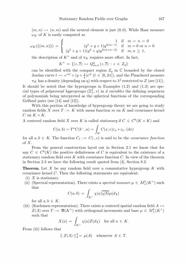
Stationary Random Fields over Graphs 167
(m, n) → (n, m) and the neutral element is just (0, 0). While Haar measureωK of K is easily computed as
ωK((m, n)) =
⎧⎨⎩1 if m = n = 0
(q2 + q + 1)q2(m−1) if m = 0 or n = 0(q2 + q + 1)(q2 + q)q2(m+n−2) if m, n ≥ 1,
the description of K∧ and of πK requires more effort. In fact,
K∧ = (z, z) → Qqm,n (z, z) : z ∈ Zq
can be identified with the compact region Zq in C bounded by the closedJordan curve t → ezit + (q + 1
q )eit (t ∈ [0, 2π]), and the Plancherel measureπK has a density (depending on q) with respect to λ2 restricted to Z (see [11]).
It should be noted that the hypergroups in Examples (1.2) and (1.3) are spe-cial types of polynomial hypergroups (Zd
+, ∗) in d variables the defining sequencesof polynomials being interpreted as the spherical functions of the correspondingGelfand pairs (see [14] and [12]).
With this portion of knowledge of hypergroup theory we are going to studyrandom fields X over T : = K with mean function m on K and covariance kernelC on K ×K.
A centered random field X over K is called stationary if C ∈ Cb(K ×K) and
C(a, b) = T aC(b−, a) =∫
K
C(x, e)εa ∗ εb−(dx)
for all a, b ∈ K. The function C1 : = C(·, e) is said to be the covariance functionof X .
From the general construction layed out in Section 2.1 we know that forany C ∈ Cb(K) the positive definiteness of C is equivalent to the existence of astationary random field over K with covariance function C. In view of the theoremin Section 2.3 we have the following result quoted from [4], Section 8.2.
Theorem. Let X be any random field over a commutative hypergroup K withcovariance kernel C. Then the following statements are equivalent:
(i) X is stationary.(ii) (Spectral representation). There exists a spectral measure µ ∈ M b
+(K∧) suchthat
C(a, b) =∫
K∧χ(a)χ(b)µ(dχ)
for all a, b ∈ K.(iii) (Karhunen representation). There exists a centered spatial random field A →
Z(A) over T : = B(K∧) with orthogonal increments and base µ ∈ M b+(K∧)
such thatX(a) =
∫K∧
χ(a)Z(dχ) for all a ∈ K.
From (iii) follows that
|| Z(A) || 22 = µ(A) whenever A ∈ T.

168 H. Heyer
The theorem applies to double coset spaces arising from Gelfand pairs (G, H),in particular to the following
Special cases
(1) G : = Aut(Γ) for a distance-transitive graph Γ : = Γ(a, b) and H : = H0 forsome 0 : = t0 ∈ Γ (see 3.1.1).
(2) G : = Autq(Γ) for the graph Γ of vertices of a triangle building #q andH : = H0 for some 0 : = v0 ∈ Γ (see 3.1.2).
3.3. Arnaud-Letac stationarity
Let Γ : = Γq denote a homogeneous tree of order q ≥ 1 (see 3.1.1, Special case). Acentered random field X over T : = Γ with covariance kernel C is called stationary(in the sense of Arnaud-Letac) if there exists a mapping ϕ : → R such that
C(s, t) = ϕ(d(s, t))
where s, t ∈ Γ.Clearly, the distribution of X (as a measure on the path space CΓ) is invariant
under the action of Aut(Γ).Given a stationary random field X over Γ we want to establish an isometry
HXC (Γ) : = 〈X(t) : t ∈ Γ〉− → L2
C(E, E, µ)
for some measure space (E, E, µ), where µ is related to the real spectral measureµX of X . In order to motivate the construction due to J.-P. Arnaud ([2]) we referto two very special situations (see [3]).(1) For q = 1 Karhunen’s approach yields the choices E : = T : = R/Z, E : =
B(T) and µ equal to the spectral measure µX of the random field X over Z.The desired isometry is given by
X(n) → χn,
where ϑ → χn(ϑ) is the character of T defined for n ∈ Z. The correspondingspectral representation reads as
C(X(m), X(n)) =∫
T
ei m ϑe−i nϑµ(dϑ)
valid for all m, n ∈ Z.We observe in this special situation that the distribution of X is invariant underthe commutative group of translations of T. The situation of a noncommutativeinvariance group as it appears, e.g., for Riemannian symmetric pairs (G, H) ismore difficult to handle as can be seen in the case of the homogeneous spaceG/H = S2 : = t ∈ R3 : || t ||= 1.(2) Let X be a centered random field over S2 with state space R having covari-
ance kernel C. We assume that there exists a continuous function ϑ : I : =[−1, 1] → R satisfying
C(s, t) = ϑ(〈s, t〉)
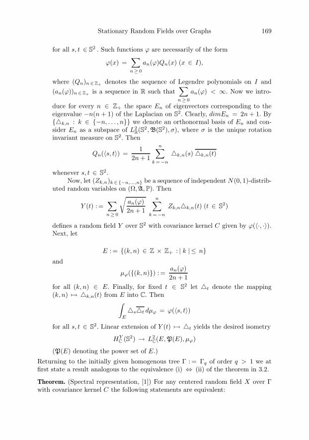
Stationary Random Fields over Graphs 169
for all s, t ∈ S2 . Such functions ϕ are necessarily of the form
ϕ(x) =∑n≥ 0
an(ϕ)Qn(x) (x ∈ I),
where (Qn)n∈Z+ denotes the sequence of Legendre polynomials on I and(an(ϕ))n ∈Z+ is a sequence in R such that
∑n≥ 0
an(ϕ) < ∞. Now we intro-
duce for every n ∈ Z+ the space En of eigenvectors corresponding to theeigenvalue −n(n + 1) of the Laplacian on S2. Clearly, dimEn = 2n + 1. By#k,n : k ∈ −n, . . . , n we denote an orthonormal basis of En and con-sider En as a subspace of L2
R(S2, B(S2), σ), where σ is the unique rotation
invariant measure on S2. Then
Qn(〈s, t〉) =1
2n + 1
n∑k =−n
#k,n(s) #k,n(t)
whenever s, t ∈ S2.Now, let (Zk,n)k ∈−n,...,n be a sequence of independent N(0, 1)-distrib-
uted random variables on (Ω, A, P). Then
Y (t) : =∑n≥ 0
√an(ϕ)2n + 1
n∑k =−n
Zk,n#k,n(t) (t ∈ S2)
defines a random field Y over S2 with covariance kernel C given by ϕ(〈·, ·〉).Next, let
E : = (k, n) ∈ Z × Z+ : | k | ≤ nand
µϕ((k, n)) : =an(ϕ)2n + 1
for all (k, n) ∈ E. Finally, for fixed t ∈ S2 let #t denote the mapping(k, n) → #k,n(t) from E into C. Then∫
E
#s#t dµϕ = ϕ(〈s, t〉)
for all s, t ∈ S2. Linear extension of Y (t) → #t yields the desired isometry
HYC (S2) → L2
C(E, P(E), µϕ)
(P(E) denoting the power set of E.)
Returning to the initially given homogenous tree Γ : = Γq of order q > 1 we atfirst state a result analogous to the equivalence (i) ⇔ (ii) of the theorem in 3.2.
Theorem. (Spectral representation, [1]) For any centered random field X over Γwith covariance kernel C the following statements are equivalent:
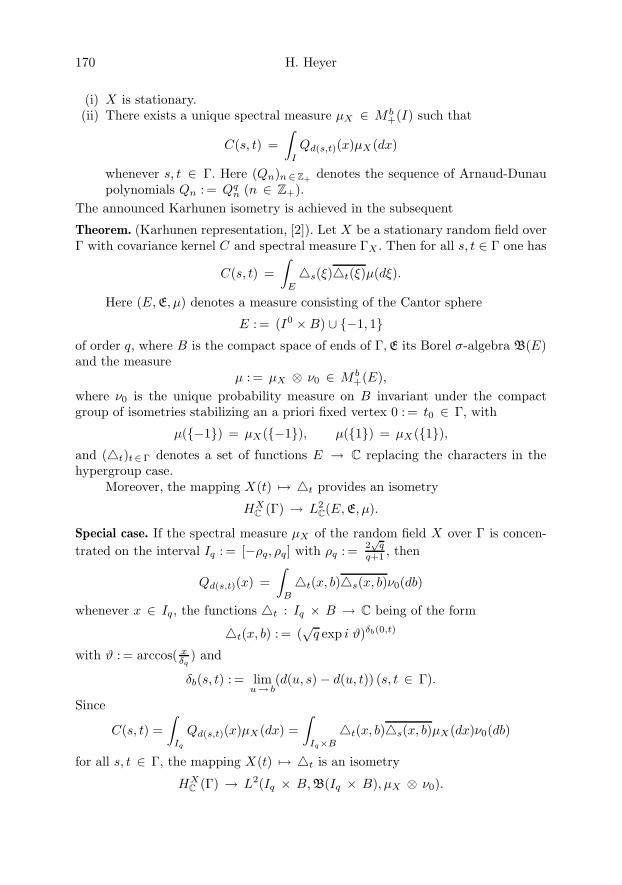
170 H. Heyer
(i) X is stationary.(ii) There exists a unique spectral measure µX ∈ M b
+(I) such that
C(s, t) =∫
I
Qd(s,t)(x)µX (dx)
whenever s, t ∈ Γ. Here (Qn)n∈Z+ denotes the sequence of Arnaud-Dunaupolynomials Qn : = Qq
n (n ∈ Z+).The announced Karhunen isometry is achieved in the subsequent
Theorem. (Karhunen representation, [2]). Let X be a stationary random field overΓ with covariance kernel C and spectral measure ΓX . Then for all s, t ∈ Γ one has
C(s, t) =∫
E
#s(ξ)#t(ξ)µ(dξ).
Here (E, E, µ) denotes a measure consisting of the Cantor sphere
E : = (I0 ×B) ∪ −1, 1of order q, where B is the compact space of ends of Γ, E its Borel σ-algebra B(E)and the measure
µ : = µX ⊗ ν0 ∈ M b+(E),
where ν0 is the unique probability measure on B invariant under the compactgroup of isometries stabilizing an a priori fixed vertex 0 : = t0 ∈ Γ, with
µ(−1) = µX(−1), µ(1) = µX(1),and (#t)t∈Γ denotes a set of functions E → C replacing the characters in thehypergroup case.
Moreover, the mapping X(t) → #t provides an isometry
HXC (Γ) → L2
C(E, E, µ).
Special case. If the spectral measure µX of the random field X over Γ is concen-trated on the interval Iq : = [−ρq, ρq] with ρq : = 2
√q
q+1 , then
Qd(s,t)(x) =∫
B
#t(x, b)#s(x, b)ν0(db)
whenever x ∈ Iq, the functions #t : Iq × B → C being of the form
#t(x, b) : = (√
q exp i ϑ)δb(0,t)
with ϑ : = arccos( xδq
) and
δb(s, t) : = limu→ b
(d(u, s)− d(u, t)) (s, t ∈ Γ).
Since
C(s, t) =∫
Iq
Qd(s,t)(x)µX(dx) =∫
Iq×B
#t(x, b)#s(x, b)µX(dx)ν0(db)
for all s, t ∈ Γ, the mapping X(t) → #t is an isometry
HXC (Γ) → L2(Iq × B, B(Iq × B), µX ⊗ ν0).
Stationary Random Fields over Graphs 171
References
[1] J.-P. Arnaud: Fonctions spheriques et fonctions definies positives sur l’arbre ho-mogene. C. R. Acad. Sci. Paris 290, Serie A (1980) 99–101
[2] J.-P. Arnaud: Stationary processes indexed by a homogeneous tree. The Annals ofProbability Vol. 22, no. 1 (1994), 195–218
[3] J.-P. Arnaud, G. Letac: La formule de representation spectrale d’un processusgaussien stationnaire sur un arbre homogene. Publication du Laboratoire de Statis-tique et Probabilites de l’Universite Paul Sabatier, no. 1 (1985), 1–11
[4] W.R. Bloom, H. Heyer: Harmonic Analysis of Probability Measures on Hyper-groups. Walter de Gruyter 1995
[5] P. Cartier: Harmonic analysis on trees. Proc. Symp. Pure Math. 26 (1976), 419–424
[6] D.I. Cartwright, W. Mlotkowski: Harmonic analysis for groups acting on tri-angle buildings. J. Austral. Math. Soc. 56 (1994), 345–383
[7] D.I. Cartwright, W. Woess: Isotropic random walks in a building of type Ad.Math. Z. 247 (2004), 101–135
[8] D. Dacunha-Castelle, M. Duflo: Probability and Statistics. Volume II. Springer-Verlag 1986
[9] R. Gangolli: Positive definite kernels on homogeneous spaces and certain stochasticprocesses related to Levy’s Brownian motion of serveral parameters. Ann. Inst. H.Poincare Sect. B (N.S.) 3 (1967), 121–226
[10] R. Lasser, M. Leitner: Stochastic processes indexed by hypergroups I. J. Theoret.Probab. 2, no. 3 (1989), 301–311
[11] M. Lindlbauer, M. Voit: Limit theorems for isotropic random walks on trianglebuildings. J. Austral. Math. Soc. 73 (2002), 301–333
[12] A.M. Mantero, A. Zappa: Spherical functions and spectrum of the Laplace oper-ators on buildings of rank 2. Boll. Unione Mat. Ital. VII Ser., B 8 (1994), 419–475
[13] M. Voit: Central limit theorems for random walks on 0 that are associated withorthogonal polynomials. J. Multivariate Analysis 34 (1990), 290–322
[14] Hm. Zeuner: Polynomial hypergroups in several variables. Arch. Math. 58 (1992),425–434
Herbert HeyerMathematisches InstitutEberhard-Karls-Universitat TubingenAuf der Morgenstelle 10D-72076 Tubingen, Germanye-mail: [email protected]
Operator Theory:Advances and Applications, Vol. 167, 173–182c© 2006 Birkhauser Verlag Basel/Switzerland
Matrix Representations and NumericalComputations of Wavelet Multipliers
M.W. Wong and Hongmei Zhu
Abstract. Weyl-Heisenberg frames are used to obtain matrix representationsof wavelet multipliers. Simple test cases are used to illustrate the numericalcomputations of wavelet multipliers by means of the corresponding truncatedmatrices.
Mathematics Subject Classification (2000). Primary: 47G10, 47G30, 65T50,65T60.
Keywords. Wavelet multipliers, Weyl-Heisenberg frames, admissible wavelets.
1. Wavelet multipliers
Let π be the unitary representation of the additive group Rn on L2(Rn) defined by
(π(ξ)u)(x) = eix·ξu(x), x, ξ ∈ Rn,
for all functions u in L2(Rn). The following two results can be found in the paper[4] by He and Wong.
Theorem 1.1. Let ϕ ∈ L2(Rn) ∩L∞(Rn) be such that ‖ϕ‖L2(Rn) = 1. Then for allfunctions u and v in the Schwartz space S,
(2π)−n
∫Rn
(u, π(ξ)ϕ)L2(Rn)(π(ξ)ϕ, v)L2(Rn)dξ = (ϕu, ϕv)L2(Rn).
Theorem 1.2. Let σ ∈ L∞(Rn) and let ϕ be any function in L2(Rn) ∩ L∞(Rn)such that ‖ϕ‖L2(Rn) = 1. If, for all functions u in S, we define Pσ,ϕu by
(Pσ,ϕu, v)L2(Rn) = (2π)−n
∫Rn
σ(ξ)(u, π(ξ)ϕ)L2(Rn)(π(ξ)ϕ, v)L2(Rn)dξ, v ∈ S,
(1.1)
This research has been supported by the Natural Sciences and Engineering Research Council ofCanada.
174 M.W. Wong and Hongmei Zhu
then(Pσ,ϕu, v)L2(Rn) = ((ϕTσϕ)u, v)L2(Rn), u, v ∈ S, (1.2)
where Tσ is the pseudo-differential operator with constant coefficients or Fouriermultiplier given by
(Tσu)(x) = (2π)−n/2
∫Rn
eix·ξσ(ξ)u(ξ) dξ, u ∈ S. (1.3)
The Fourier transform u of u in (1.3), also denoted by Fu, is chosen to bethat defined by
u(ξ) = (2π)−n/2
∫Rn
e−ix·ξu(x) dx, ξ ∈ Rn.
The inverse Fourier transform v of a function v in S, also denoted by F−1v, isthen given by
v(x) = (2π)−n/2
∫Rn
eix·ξv(ξ) dξ, x ∈ Rn.
Let σ ∈ L∞(Rn). Then the linear operator Pσ,ϕ : L2(Rn) → L2(Rn), defined by(1.2) for all functions u and v in S, is in fact a bounded linear operator, andcan be considered as a variant of a localization operator corresponding to thesymbol σ and the admissible wavelet ϕ studied in the book [12] by Wong. Had the“admissible wavelet” ϕ been replaced by the function ϕ0 on Rn given by
ϕ0(x) = 1, x ∈ Rn,
the equation (1.1) would have been a resolution of the identity formula and theoperator Pσ,ϕ0 would have been a usual pseudo-differential operator with con-stant coefficients or a Fourier multiplier. This is the rationale for calling the linearoperator Pσ,ϕ : L2(Rn)→ L2(Rn) a wavelet multiplier.
Wavelet multipliers arise naturally as filters in signal analysis and have beenstudied extensively and systematically in Chapters 19–21 of the book [12] by Wong,the paper [13] by Wong and Zhang, and the Ph.D. dissertation [14] by Zhang.
We need in this paper another representation of the wavelet multiplier ϕTσϕas a Hilbert-Schmidt operator on L2(Rn).
Theorem 1.3. Let σ ∈ L1(Rn) ∩L2(Rn) ∩L∞(Rn) and let ϕ ∈ L2(Rn) ∩L∞(Rn).If we let K be the function on Rn × Rn defined by
K(x, y) = ϕ(x)k(x − y)ϕ(y), x, y ∈ Rn,
wherek = (2π)−n/2σ,
then K ∈ L2(Rn × Rn) and
((ϕTσϕ)f)(x) =∫
Rn
K(x, y) f(y) dy, x ∈ Rn.
In particular, ϕTσϕ is a Hilbert-Schmidt operator.

Wavelet Multipliers 175
Proof. Since k ∈ L∞(Rn),∫Rn
∫Rn
|K(x, y)|2dx dy =∫
Rn
∫Rn
|ϕ(x)|2|k(x− y)|2|ϕ(y)|2dx dy
≤ ‖k‖2L∞(Rn)‖ϕ‖4L2(Rn) <∞.
Now, for all functions f in L2(Rn),
(k ∗ f)∧ = (2π)n/2kf = σf
and hencek ∗ f = (σf)∨ = Tσf.
Therefore for all functions in L2(Rn), we get
((ϕTσϕ)f)(x) = ϕ(x)(k ∗ (ϕf))(x)
=∫
Rn
ϕ(x)k(x − y)ϕ(y) f(y) dy
=∫
Rn
K(x, y) f(y) dy
for all x in Rn.
The motivation for this paper comes from a desire to develop “efficient” nu-merical methods for the computations of pseudo-differential operators studied inthe books [10, 11] by Wong, among others. As wavelet multipliers are very simple,but not trivial, pseudo-differential operators, they serve very well as test cases forany proposed numerical methods. The aim of this paper is to obtain matrix repre-sentations of wavelet multipliers using Theorem 1.3 and Weyl-Heisenberg frames.We first show in Section 2 that wavelet multipliers are natural and importantpseudo-differential operators in their own right by recalling succinctly the fact inthe book [12] to the effect that the well-known Landau-Pollak-Slepian operator isa wavelet multiplier. In Section 3, we give a brief recapitulation on the generaltheory of frames in Hilbert spaces and then we reconstruct the Weyl-Heisenbergframe, which is used in Section 4 to obtain matrix representations of waveletmultipliers. Some simple test cases are then used in Section 5 to illustrate thenumerical computations of wavelet multipliers by implementing MATLAB 7.0 onthe corresponding truncated matrices.
2. The Landau-Pollak-Slepian operator
Let Ω and T be positive numbers. Then we define the linear operators PΩ :L2(Rn)→ L2(Rn) and QT : L2(Rn)→ L2(Rn) by
(PΩf)∧(ξ) =
⎧⎨⎩ f(ξ),
0,
|ξ| ≤ Ω,
|ξ| > Ω,
176 M.W. Wong and Hongmei Zhu
and
(QT f)(x) =
⎧⎨⎩ f(x),
0,
|x| ≤ T,
|x| > T,
for all functions f in L2(Rn). Then it is easy to see that PΩ : L2(Rn) → L2(Rn)and QT : L2(Rn)→ L2(Rn) are self-adjoint projections. In signal analysis, a signalis a function f in L2(Rn). Thus, for all functions f in L2(Rn), the function QT PΩfcan be considered to be a filtered signal. Therefore it is of interest to compare theenergy ‖QT PΩf‖2L2(Rn) of the filtered signal QT PΩf with the energy ‖f‖2L2(Rn) ofthe original signal f . In fact, we can prove that
sup
‖QT PΩf‖2L2(Rn)
‖f‖2L2(Rn)
: f ∈ L2(Rn), f = 0
= ‖PΩQT PΩ‖∗,
where ‖ ‖∗ is the norm in the C∗-algebra of all bounded linear operators on L2(Rn).The bounded linear operator PΩQT PΩ : L2(Rn) → L2(Rn) alluded to in
the context of filtered signals is called the Landau-Pollak-Slepian operator. Seethe fundamental papers [5, 6] by Landau and Pollak, [7, 8] by Slepian and [9] bySlepian and Pollak for more detailed information.
The following theorem tells us that the Landau-Pollak-Slepian operator is infact a wavelet multiplier.
Theorem 2.1. Let ϕ be the function on Rn defined by
ϕ(x) =
⎧⎨⎩1√
µ(BΩ),
0,
|x| ≤ Ω,
|x| > Ω,
where µ(BΩ) is the volume of BΩ, and let σ be the characteristic function on BT ,i.e,
σ(ξ) =
⎧⎨⎩ 1,
0,
|ξ| ≤ T,
|ξ| > T.
Then the Landau-Pollak-Slepian operator PΩQT PΩ : L2(Rn) → L2(Rn) is uni-tarily equivalent to a scalar multiple of the wavelet multiplier ϕTσϕ : L2(Rn) →L2(Rn). In fact,
PΩQT PΩ = µ(BΩ)F−1(ϕTσϕ)F .
Details on the Landau-Pollak-Slepian operator can be found in Chapter 20of the book [12] by Wong.
3. Frames in Hilbert spaces
Frames, usually attributed to Duffin and Schaeffer [3] in the context of nonhar-monic series, are alternatives to orthonormal bases for Hilbert spaces.

Wavelet Multipliers 177
Let xj∞j=1 be a sequence in a separable, complex and infinite-dimensionalHilbert space X . We denote the inner product and norm in X by ( , ) and ‖ ‖respectively. Suppose that there exist positive constants A and B such that
A‖x‖2 ≤∞∑
j=1
|(x, xj)|2 ≤ B‖x‖2, x ∈ X.
Then we call xj∞j=1 a frame for X with frame bounds A, B with the understand-ing that A is the lower frame bound and B is the upper frame bound. The frameis said to be tight if A = B. The frame is called an exact frame if it is no longer aframe whenever an element is removed from it.
Of particular relevance for us in this paper are tight frames with frame bounds1,1. This is due to the following theorem.
Theorem 3.1. Let xj∞j=1 be a tight frame with frame bounds 1,1. Then
x =∞∑
j=1
(x, xj)xj , x ∈ X.
It is clear from Theorem 3.1 that a tight frame with frame bounds 1,1 providesan expansion, which is formally the same as that given by an orthonormal basis.
Frames and their applications abound in the literature. See, for instance, thebook [1] by Christensen in this connection.
We need the following result in the paper [2] by Daubechies, Grossmann andMeyer. Since the proof is not difficult, we include a proof for the sake of beingself-contained.
Theorem 3.2. Let g ∈ L2(R) and let a and b be positive numbers such that we canfind positive numbers A and B for which
A ≤∑n∈Z
|g(x + na)|2 ≤ B (3.1)
for almost all x in R, andsupp(g) ⊆ I,
where I is some interval with length 2πb . Then MmbTnag : m, n ∈ Z is a frame
for L2(R) with frame bounds 2πAb and 2πB
b .
Proof. Let n ∈ Z. Thensupp(f(Tnag)) ⊆ In,
where In = x − na : x ∈ I. By (3.1), g ∈ L∞(R). So, f(Tnag) ∈ L2(In). Now,√b
2π Emb : m ∈ Z
is an orthonormal basis for L2(In), where
Emb(x) = eimbx, x ∈ R.
178 M.W. Wong and Hongmei Zhu
So,
∑m∈Z
∣∣∣∣∣∣(
f(Tnag),
√b
2πEmb
)L2(R)
∣∣∣∣∣∣2
= ‖f(Tnag)‖2L2(R) =∫ ∞
−∞|f(x)|2|g(x+na)|2dx.
Therefore ∑m∈Z
∣∣(f(Tnag), Em)L2(R)
∣∣2 =2π
b
∫ ∞
−∞|f(x)|2|g(x + na)|2dx.
Thus, ∑m,n∈Z
∣∣(f, MmbTnag)L2(R)
∣∣2 =∑
m,n∈Z
∣∣(f(Tnag), Emb)L2(R)
∣∣2=
∑n∈Z
∑m∈Z
∣∣(f(Tnag), Emb)L2(R)
∣∣2=
2π
b
∑n∈Z
∫ ∞
−∞|f(x)|2 |g(x + na)|2dx
=2π
b
∫ ∞
−∞|f(x)|2
∑n∈Z
|g(x + na)|2dx.
So, by (3.1),
2πA
b‖f‖2L2(R) ≤
∑m,n∈Z
∣∣(f, MmbTnag)L2(R)
∣∣2 ≤ 2πB
b‖f‖2L2(R)
and the proof is complete.
Corollary 3.3. Let g ∈ L2(R) be such that∑n∈Z
|g(x + 2πn)|2 = 1
for almost all x in R and
supp(g) ⊆ [0, 1].
Then M2πmT2πng : m, n ∈ Z is a tight frame for L2(R) with frame bounds 1,1.
Remark 3.4. The frames in Theorem 3.2 and Corollary 3.3 are generated fromone single function g in L2(R) by translations and modulations. As such, they areintimately related to the Weyl-Heisenberg group in signal analysis and hence theyare known as Weyl-Heisenberg frames. The functions g generating the frames arecalled the admissible windows or wavelets. An admissible wavelet g for the tightframe in Corollary 3.3 can be given by g = χ[0,1].
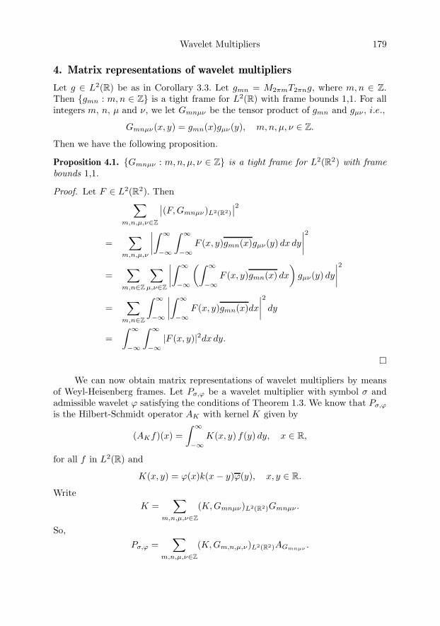
Wavelet Multipliers 179
4. Matrix representations of wavelet multipliers
Let g ∈ L2(R) be as in Corollary 3.3. Let gmn = M2πmT2πng, where m, n ∈ Z.Then gmn : m, n ∈ Z is a tight frame for L2(R) with frame bounds 1,1. For allintegers m, n, µ and ν, we let Gmnµν be the tensor product of gmn and gµν , i.e.,
Gmnµν(x, y) = gmn(x)gµν(y), m, n, µ, ν ∈ Z.
Then we have the following proposition.
Proposition 4.1. Gmnµν : m, n, µ, ν ∈ Z is a tight frame for L2(R2) with framebounds 1,1.
Proof. Let F ∈ L2(R2). Then∑m,n,µ,ν∈Z
∣∣(F, Gmnµν)L2(R2)
∣∣2=
∑m,n,µ,ν
∣∣∣∣∫ ∞
−∞
∫ ∞
−∞F (x, y)gmn(x)gµν(y) dx dy
∣∣∣∣2
=∑
m,n∈Z
∑µ,ν∈Z
∣∣∣∣∫ ∞
−∞
(∫ ∞
−∞F (x, y)gmn(x) dx
)gµν(y) dy
∣∣∣∣2
=∑
m,n∈Z
∫ ∞
−∞
∣∣∣∣∫ ∞
−∞F (x, y)gmn(x)dx
∣∣∣∣2 dy
=∫ ∞
−∞
∫ ∞
−∞|F (x, y)|2dx dy.
We can now obtain matrix representations of wavelet multipliers by meansof Weyl-Heisenberg frames. Let Pσ,ϕ be a wavelet multiplier with symbol σ andadmissible wavelet ϕ satisfying the conditions of Theorem 1.3. We know that Pσ,ϕ
is the Hilbert-Schmidt operator AK with kernel K given by
(AKf)(x) =∫ ∞
−∞K(x, y) f(y) dy, x ∈ R,
for all f in L2(R) and
K(x, y) = ϕ(x)k(x − y)ϕ(y), x, y ∈ R.
WriteK =
∑m,n,µ,ν∈Z
(K, Gmnµν)L2(R2)Gmnµν .
So,
Pσ,ϕ =∑
m,n,µ,ν∈Z
(K, Gm,n,µ,ν)L2(R2)AGmnµν .
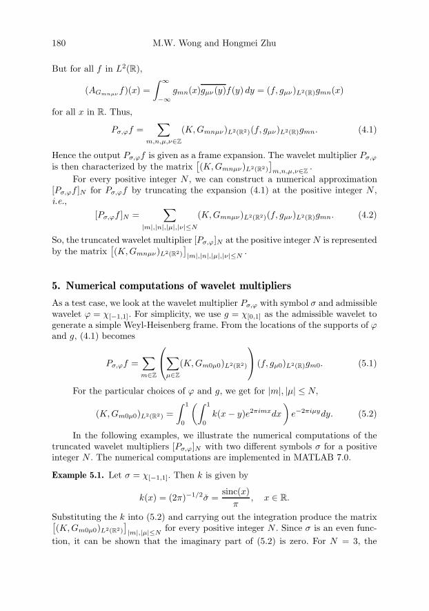
180 M.W. Wong and Hongmei Zhu
But for all f in L2(R),
(AGmnµν f)(x) =∫ ∞
−∞gmn(x)gµν(y)f(y) dy = (f, gµν)L2(R)gmn(x)
for all x in R. Thus,
Pσ,ϕf =∑
m,n,µ,ν∈Z
(K, Gmnµν)L2(R2)(f, gµν)L2(R)gmn. (4.1)
Hence the output Pσ,ϕf is given as a frame expansion. The wavelet multiplier Pσ,ϕ
is then characterized by the matrix[(K, Gmnµν)L2(R2)
]m,n,µ,ν∈Z
.
For every positive integer N , we can construct a numerical approximation[Pσ,ϕf ]N for Pσ,ϕf by truncating the expansion (4.1) at the positive integer N ,i.e.,
[Pσ,ϕf ]N =∑
|m|,|n|,|µ|,|ν|≤N
(K, Gmnµν)L2(R2)(f, gµν)L2(R)gmn. (4.2)
So, the truncated wavelet multiplier [Pσ,ϕ]N at the positive integer N is representedby the matrix
[(K, Gmnµν)L2(R2)
]|m|,|n|,|µ|,|ν|≤N
.
5. Numerical computations of wavelet multipliers
As a test case, we look at the wavelet multiplier Pσ,ϕ with symbol σ and admissiblewavelet ϕ = χ[−1,1]. For simplicity, we use g = χ[0,1] as the admissible wavelet togenerate a simple Weyl-Heisenberg frame. From the locations of the supports of ϕand g, (4.1) becomes
Pσ,ϕf =∑m∈Z
⎛⎝∑µ∈Z
(K, Gm0µ0)L2(R2)
⎞⎠ (f, gµ0)L2(R)gm0. (5.1)
For the particular choices of ϕ and g, we get for |m|, |µ| ≤ N,
(K, Gm0µ0)L2(R2) =∫ 1
0
(∫ 1
0
k(x− y)e2πimxdx
)e−2πiµydy. (5.2)
In the following examples, we illustrate the numerical computations of thetruncated wavelet multipliers [Pσ,ϕ]N with two different symbols σ for a positiveinteger N . The numerical computations are implemented in MATLAB 7.0.
Example 5.1. Let σ = χ[−1,1]. Then k is given by
k(x) = (2π)−1/2σ =sinc(x)
π, x ∈ R.
Substituting the k into (5.2) and carrying out the integration produce the matrix[(K, Gm0µ0)L2(R2)
]|m|,|µ|≤N
for every positive integer N . Since σ is an even func-tion, it can be shown that the imaginary part of (5.2) is zero. For N = 3, the
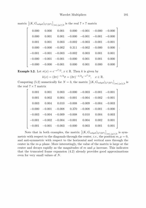
Wavelet Multipliers 181
matrix[(K, Gm0µ0)L2(R2)
]|m|,|µ|≤3
is the real 7× 7 matrix⎡⎢⎢⎢⎢⎢⎢⎢⎢⎢⎢⎢⎢⎢⎢⎢⎣
0.000 0.000 0.001 0.000 −0.001 −0.000 −0.000
0.000 0.001 0.001 −0.000 −0.001 −0.001 −0.000
0.001 0.001 0.003 −0.002 −0.003 −0.001 −0.001
0.000 −0.000 −0.002 0.311 −0.002 −0.000 0.000
−0.001 −0.001 −0.003 −0.002 0.003 0.001 0.001
−0.000 −0.001 −0.001 −0.000 0.001 0.001 0.000
−0.000 −0.000 −0.001 0.000 0.001 0.000 0.000
⎤⎥⎥⎥⎥⎥⎥⎥⎥⎥⎥⎥⎥⎥⎥⎥⎦.
Example 5.2. Let σ(x) = e−x2/2, x ∈ R. Then k is given by
k(x) = (2π)−1/2σ = (2π)−1/2e−x2/2, x ∈ R.
Computing (5.2) numerically for N = 3, the matrix[(K, Gm0µ0)L2(R2)
]|m|,|µ|≤3
isthe real 7× 7 matrix⎡⎢⎢⎢⎢⎢⎢⎢⎢⎢⎢⎢⎢⎢⎢⎢⎣
0.001 0.001 0.003 −0.000 −0.003 −0.001 −0.001
0.001 0.002 0.004 −0.001 −0.004 −0.002 −0.001
0.003 0.004 0.010 −0.008 −0.009 −0.004 −0.003
−0.000 −0.001 −0.008 0.370 −0.008 −0.001 −0.000
−0.003 −0.004 −0.009 −0.008 0.010 0.004 0.003
−0.001 −0.002 −0.004 −0.001 0.004 0.002 0.001
−0.001 −0.001 −0.003 −0.000 0.003 0.001 0.001
⎤⎥⎥⎥⎥⎥⎥⎥⎥⎥⎥⎥⎥⎥⎥⎥⎦.
Note that in both examples, the matrix[(K, Gm0µ0)L2(R2)
]|m|,|µ|≤3
is sym-metric with respect to the diagonals through the center, i.e., the position m, µ = 0,and anti-symmetric with respect to the horizontal and vertical axes through thecenter in the m-µ plane. More interestingly, the value of the matrix is large at thecenter and decays rapidly as the magnitudes of m and µ increase. This indicatesthat the truncated frame expansion (4.2) already provides good approximationseven for very small values of N .
182 M.W. Wong and Hongmei Zhu
References
[1] O. Christensen, An Introduction to Frames and Riesz Bases, Birkhauser, 2003.
[2] I. Daubechies, A. Grossmann and Y. Meyer, Painless nonorthogonal expansions, J.Math. Phys. 27 (1986), 1271–1283.
[3] R.J. Duffin and A.C. Schaeffer, A class of nonharmonic Fourier series, Trans. Amer.Math. Soc. 72 (1952), 341–366.
[4] Z. He and M.W. Wong, Wavelet multipliers and signals, J. Austral. Math. Soc. Ser.B 40 (1999), 437–446.
[5] H.J. Landau and H.O. Pollak, Prolate spheroidal wave functions, Fourier analysisand uncertainty II, Bell Syst. Tech. J. 40 (1961), 65–84.
[6] H.J. Landau and H.O. Pollak, Prolate spheroidal wave functions, Fourier analysisand uncertainty III, Bell Syst. Tech. J. 41 (1962), 1295–1336.
[7] D. Slepian, On bandwidth, Proc IEEE 64 (1976), 292–300.
[8] D. Slepian, Some comments on Fourier analysis, uncertainty and modelling, SIAMRev. 25 (1983), 379–393.
[9] D. Slepian and H.O. Pollak, Prolate spheroidal wave functions, Fourier analysis anduncertainty I, Bell Syst. Tech. J. 40 (1961), 43–64.
[10] M.W. Wong, Weyl Transforms, Springer-Verlag, 1998.
[11] M.W. Wong, An Introduction to Pseudo-Differential Operators, Second Edition,1999.
[12] M.W. Wong, Wavelet Transforms and Localization Operators, Birkhauser, 2002.
[13] M.W. Wong and Z. Zhang, Trace class norm inequalities for wavelet multipliers,Bull. London Math. Soc. 34 (2002), 739–744.
[14] Z. Zhang, Localization Operators and Wavelet Multipliers, Ph.D. Dissertation, YorkUniversity, 2003.
M.W. Wong and Hongmei ZhuDepartment of Mathematics and StatisticsYork University4700 Keele StreetToronto, Ontario M3J 1P3, Canadae-mail: [email protected]: [email protected]
Operator Theory:Advances and Applications, Vol. 167, 183–190c© 2006 Birkhauser Verlag Basel/Switzerland
Clifford Algebra-valued Admissible WaveletsAssociated to More than 2-dimensionalEuclidean Group with Dilations
Jiman Zhao and Lizhong Peng
Abstract. In this paper, we consider the Clifford algebra-valued admissiblewavelets, which are associated to more than 2-dimensional Euclidean groupwith Dilations. We give an explicit characterization of the admissibility con-dition in terms of the Fourier transform, study the properties of this kind ofwavelet transform, also give a family of admissible wavelets.
Mathematics Subject Classification (2000). Primary: 42B10, 44A15.
Keywords. Wavelets, Clifford algebra.
1. Introduction
There are two branches in wavelet theory: admissible (or continuous) wavelet trans-form and discrete orthogonal wavelets generated by multiresolution analysis. In theclassical case, Grossman and Morlet ([6]) introduced the wavelet transform in theone-dimensional case, where the group G is the affine group ax+b. After this thereare many papers about admissible wavelets and decomposition of function spaceassociated with the group SL(2, R) ([7], [8], [10]). In ([9]), Murenzi generalizedthis to more than one dimension.
In Clifford analysis, by using Clifford algebra, L. Andersson, B. Jawerthand M. Mitrea constructed higher-dimensional discrete orthogonal wavelets, see[1]. As for Clifford-valued admissible wavelets, in their paper (see [3], [4], [5]),Brackx and Sommen studied the radial and generalized Clifford-Hermite contin-uous wavelet transforms in Rn. In ([13]), quaternion-valued admissible waveletshave been characterized. In this paper, we consider the Clifford algebra-valued ad-missible wavelets, give an explicit characterization of the admissibility conditionin terms of Fourier transform, we also give a family of admissible wavelets.
Research supported by NNSF of China No.10471002 and 973 project of China G1999075105.

184 J. Zhao and L. Peng
Now we give an overview of some basic facts which are concerned with Cliffordanalysis ([2]).
The real Clifford algebra Rn over Rn is defined as:
Rn = ∑
I⊆1,2,...,nxIeI : xI ∈ R
where e1, . . . , en is an orthogonal basis of Rn, and eI = ei1ei2 · · · eikwith I =
i1, i2, . . . , ik, i1 < i2 < · · · < ik.The non-commutative multiplication in the Clifford algebra Rn is given by:
eiej + ejei = −2δi,j, i, j = 1, 2, . . . , n
An involution on Rn is defined by
eI = eik· · · ei1 , eij = −eij .
A Rn-valued function f(x1, · · · , xn) is called left monogenic in an open regionΩ of Rn, if:
Df(x) =n∑
j=1
ej(∂
∂xj)f(x) = 0,
where D =∑n
j=1 ej( ∂∂xj
) is the Dirac operator in Rn. We call Mk the Cliffordmodule of the left monogenic homogeneous polynomials of degree k, its dimensionis given by
dimMk =(m + k − 2)!(m− 2)!k!
Definition Let Rn be a real Clifford algebra. A Clifford module L2(Rn, Rn) is de-noted by
L2(Rn, Rn) =
f : Rn → Rn, f =
∑I
fIeI∣∣∣ (∑I
‖fI‖2L2(Rn)
) 12
<∞, fI ∈ L2(Rn), ∀I
.
The inner product of L2(Rn, Rn) is denoted by
(f, g) =∫
Rn
f(x)g(x)dx.
2. Clifford algebra-valued admissible wavelet transform
Let n > 2, think about the inhomogeneous group IG(n) = [R+ × SO(n)] ⊗ Rn,the group law of IG(n) is given by
v, bv′, b′ = vv′, vb′ + b,where v = ar, a > 0, r ∈ SO(n), b ∈ Rn. The group IG(n) is a non-unimodular Liegroup with: left Haar measure a−(n+1)dadrdb.
Clifford Algebra-valued Admissible Wavelets 185
First we define a nature unitary representation of IG(n) in L2(Rn, Rn). Westart by considering the operators corresponding to three types of operations thatconstitute IG(n).
Given a function φ ∈ L2(Rn, Rn), we define:
(T bφ)(x) = φ(x− b), x, b ∈ Rn, (unitary shift operator)
Daφ(x) = a−n2 φ(a−1x), (unitary dilation operator),
Rrφ(x) = φ(r−1x), x ∈ Rn, (unitary rotation operator).
Like the classical case, we have the following commutation relations:
T bDa = DaTba ,
RrDa = DaRr,
then we construct the operator
Ua,r,b = T bDaRr,
with action
Ua,r,bφ(x) = a−n2 φ(a−1r−1(x− b)).
For convenience, we denote Ua,r,bφ(x) = φa,r,b(x), then it is easy to check thatUa,r,b is a representation of IG(n) in L2(Rn, Rn).
By the Fourier transform, we have
φa,r,b∧(ξ) = a
n2 e−ib·ξφ(ar−1ξ).
Like the classical case, we can prove that this representation is irreducible.Now we define the operator Wψ on L2(Rn, Rn) by
L2(Rn, Rn) → L2(IG(n), Rn, a−(n+1)dadrdb)
f(x) → Wψf(a, r, b)
where
Wψf(a, r, b) = (ψa,r,b, f)L2(Rn,Rn). (1)
By direct calculation, we have
Wψf(a, r, b) = an2 (ψ(ar−1(·))f(·))∧(−b). (2)
The inner product of L2(IG(n), a−(n+1)dadrdb) is defined as follows:
〈f, g〉L2(IG(n),Rn) =∫
IG(n)
f(a, r, b)g(a, r, b)a−(n+1)dadrdb, (3)
then the space L2(IG(n), a−(n+1)dadrdb) becomes a right Hilbert Rn-module.
186 J. Zhao and L. Peng
In order to get the reproducing formula like in the classical case, we calculatethe 〈Wpsif, Wψg〉L2(IG(n),Rn). Using (1), (2), (3), we have
〈Wψf, Wψg〉 =∫ +∞0
∫SO(n)
∫Rn Wψf(a, r, b)Wψg(a, r, b)a−(n+1)dadrdb
=∫ +∞0
∫SO(n)
∫Rn (Wψf)
∧(a, r, ξ)(Wψg)∧(a, r, ξ)a−(n+1)dadrdξ
=∫ +∞0
∫SO(n)
∫Rn anf ψ(ar−1(ξ))ψ(ar−1(ξ))g(ξ)a−(n+1)dadrdξ
=∫
Rn f(ξ)(∫ +∞0
∫SO(n)
ψ(ar−1(ξ))ψ(ar−1(ξ))a−1dadr)g(ξ)dξ
=∫
Rn f(ξ)(∫ +∞0
∫SO(n)
ψ(aη)ψ(aη)a−1dadη)g(ξ)dξ
=∫
Rn f(ξ)∫
Rn ψ(aη)ψ(aη)|η|−ndηg(ξ)dξ
(4)
On the other hand, by (1), (3), we have
〈Wψf, Wψg)〉 =∫ +∞0
∫SO(n)
∫Rn Wψf(a, r, b)Wψg(a, r, b)a−(n+1)dadrdb
=∫
IG(n)Wψf(a, r, b)
∫Rn ψa,r,b(x)g(x)dxa−(n+1)dadrdb
=∫
Rn(∫
IG(n)Wψf(a, r, b)ψa,r,b(x)a−(n+1)dadrdb)g(x)dx
= (∫
IG(n)ψa,r,b(·)Wψf(a, r, b)a−(n+1)dadrdb, g).
(5)
Denote
Cψ =∫
Rn
ψ(ξ)ψ(ξ)|ξ|n dξ,
then by (4) and (5), we get
〈Wψf, Wψg〉 =∫
Rn
Cψ f(ξ)g(ξ)dξ = (Cψf, g),
thus
Cψf(x) =∫
IG(n)
ψa,r,b(x)Wψf(a, r, b)a−(n+1)dadrdb
holds in the weak sense.So the reproducing formula holds if and only if Cψ is the inverse Clifford
number.We call
Cψ =∫
Rn
ψ(ξ)ψ(ξ)|ξ|n dξ is the inverse Clifford number, (6)
the admissible condition, and call ψ the admissible wavelet if it satisfies the ad-missible condition (6), call the corresponding transform Wψ admissible wavelettransform.
Clifford Algebra-valued Admissible Wavelets 187
Denote
AW = ψ ∈ L2(Rn, Rn), Cψ =∫
Rn
ψ(ξ)ψ(ξ)|ξ|n dξ is the inverse Clifford number,
(7)and denote an “inner product” in AW as follows:
〈ψ, ϕ〉AW =∫
Rn
ψ(ξ)ϕ(ξ)|ξ|n dξ.
The AW here is different from the one in [13], there the AW is a quaternionmodule, while in this paper the AW is not a linear space.
The wavelet transform has the following properties: From (4) and (5), we canget the following theorem.
Theorem 1. For f(x), g(x) ∈ L2(Rn, Rn), and ψ, ϕ ∈ AW,
〈Wψf, Wϕg〉L2(IG(n),Rn,a−(n+1)dadrdb) = (〈ψ, ϕ)〉AW f, g)L2(Rn,Rn).
From Theorem 1, we know the continuous wavelet transform is an isometry,and we also get the reproducing formula.
Theorem 2. (Reproducing formula) Let f(x) ∈ L2(Rn, Rn), ψ ∈ AW, then
f(x) = C−1ψ
∫ +∞
0
∫SO(n)
∫Rn
ψa,r,bWψf(a, r, b)ψ(x)a−(n+1)dadrdb.
Proof. By (4) and (5), we can get the conclusion in the weak sense.Denote Aψ = Wψf(x) : f ∈ L2(Rn, Rn), ψ ∈ AW, then Aψ is a Hilbert
space with reproducing kernel.
Theorem 3. (Reproducing kernel)Let K(a, r, a′, r′) be the reproducing kernel of Aψ, then
K(a, r, b, a′, r′, b) = c−1ψ (ψa′,r′,b′ , ψa,rb).
Proof. From Theorem 2, we get
Wψf(a′, r′, b′)
= c−1ψ
∫Rn(
∫IG(n) ψa′,r′,b′(x)ψa,r,b(x)Wψf(a, r, b)a−(n+1)dadrdb)dx
= c−1ψ
∫IG(n)
(∫
Rn ψa′,r′,b′(x)ψa,r,b(x)dx)Wψf(a, r, b)a−(n+1)dadrdb.
So we have the reproducing kernel
K(a, r, b, a′, r′, b) = c−1ψ (ψa′,r′,b′ , ψa,rb).
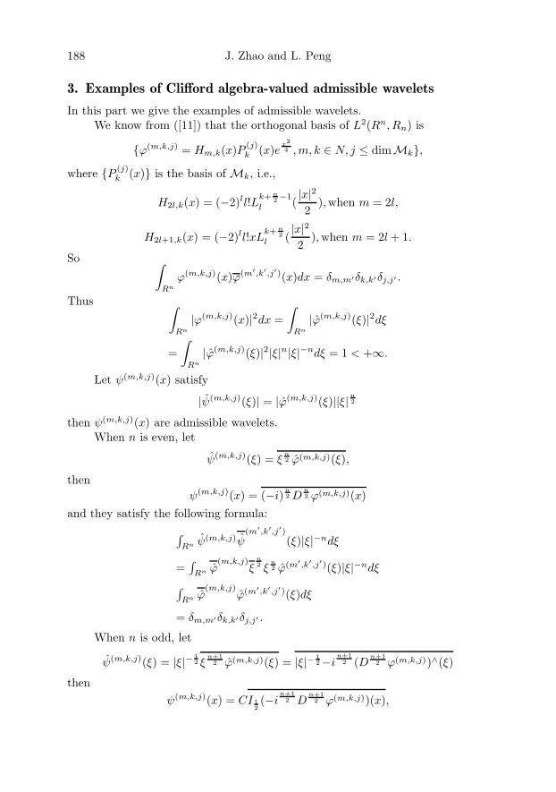
188 J. Zhao and L. Peng
3. Examples of Clifford algebra-valued admissible wavelets
In this part we give the examples of admissible wavelets.We know from ([11]) that the orthogonal basis of L2(Rn, Rn) is
ϕ(m,k,j) = Hm,k(x)P (j)k (x)e
x24 , m, k ∈ N, j ≤ dimMk,
where P (j)k (x) is the basis ofMk, i.e.,
H2l,k(x) = (−2)ll!Lk+ n2 −1
l (|x|22
), when m = 2l,
H2l+1,k(x) = (−2)ll!xLk+ n
2l (
|x|22
), when m = 2l + 1.
So ∫Rn
ϕ(m,k,j)(x)ϕ(m′,k′,j′)(x)dx = δm,m′δk,k′δj,j′ .
Thus ∫Rn
|ϕ(m,k,j)(x)|2dx =∫
Rn
|ϕ(m,k,j)(ξ)|2dξ
=∫
Rn
|ϕ(m,k,j)(ξ)|2|ξ|n|ξ|−ndξ = 1 < +∞.
Let ψ(m,k,j)(x) satisfy
|ψ(m,k,j)(ξ)| = |ϕ(m,k,j)(ξ)||ξ|n2
then ψ(m,k,j)(x) are admissible wavelets.When n is even, let
ψ(m,k,j)(ξ) = ξn2 ϕ(m,k,j)(ξ),
thenψ(m,k,j)(x) = (−i)
n2 D
n2 ϕ(m,k,j)(x)
and they satisfy the following formula:∫Rn ψ(m,k,j)ψ
(m′,k′,j′)(ξ)|ξ|−ndξ
=∫
Rn ϕ(m,k,j)
ξn2 ξ
n2 ϕ(m′,k′,j′)(ξ)|ξ|−ndξ∫
Rn ϕ(m,k,j)
ϕ(m′,k′,j′)(ξ)dξ
= δm,m′δk,k′δj,j′ .
When n is odd, let
ψ(m,k,j)(ξ) = |ξ|− 12 ξ
n+12 ϕ(m,k,j)(ξ) = |ξ|− 1
2−in+1
2 (Dn+12 ϕ(m,k,j))∧(ξ)
thenψ(m,k,j)(x) = CI 1
2(−i
n+12 D
n+12 ϕ(m,k,j))(x),
Clifford Algebra-valued Admissible Wavelets 189
where C is a real number,
Iα(f)(x) = πn2 2αΓ(
α
2)Γ(
n− α
2)−1 ∫
Rn
|x− y|−n+αf(y)
is the Riesz potential ([12]).In this case, ψ(m,k,j) also satisfy the following formula.∫
Rn
ψ(m,k,j)ψ(m′,k′,j′)
(ξ)|ξ|−ndξ = δm,m′δk,k′δj,j′
DenoteAm,k,j = Wψ(m,k,j)f(a, r, b) : f ∈ L2(Rn, Rn).
We have the following property.
Theorem 4. For Wψ(n,k,i)f(a, r, b) ∈ Am,k,i and Wψ(m′,k′,i′)g(a, r, b) ∈ Am′,k′,i′ ,
〈Wψ(m,k,i)f, Wψ(m′,k′,i′)g〉L2(IG(n),Rn,a−(n+1)dadrdb) = δm,m′δk,k′δi,i′ (f, g)L2(Rn,Rn)
Proof. We use Theorem 1 to prove the result. Both Am,k,i and Am′,k′,i′ are orthog-onal subspaces of L2(IG(n), Rn, a−(n+1)dadrdb). But we cannot get the orthogo-nal decomposition of L2(IG(n), Rn, a−(n+1)dadrdb) (like in [14]), since the groupIG(n) is large in this case (n > 2).
Acknowledgement
The authors wish to thank Professor Heping Liu for giving useful information.
References
[1] L. Andersson, B. Jawerth and M.Mitrea, The Cauchy singular integral operatorand Clifford wavelets, in: Wavelets: mathematics and applications, CRC Press, J.J.Benedetto and M.W. Frazier (eds.), 1994, 525–546.
[2] F. Brackx, R. Delanghe, F. Sommen, Clifford analysis, Pitman Publ., 1982.
[3] F. Brackx, F. Sommen, Clifford-Hermite Wavelets in Euclidean Space, J. FourierAnal. Appl., 6(3)(2000), pp. 209–310.
[4] F. Brackx, F. Sommen, The continuous wavelet transform in Clifford analysis, in Clif-ford Analysis and Its Applications, NATO ARW Series, F.Brackx, JSR. Chisholm,V.Soucek eds., Kluwer Acad. Publ., Dordrecht, The Netherlands, 2001, pp. 9–26.
[5] F. Brackx, F. Sommen, The generalized Clifford-Hermite continuous wavelet trans-form, Advances in Applied Clifford Algebras, 11 (2001), pp. 219–231.(Proceedingsof the Cetraro conference in October 1998).
[6] A. Grossman, J. Morlet, Decomposition of Hardy functions into square integrablewavelets of constant shape, SIAM J. Math. Anal., 15 (1984), 723–736.
[7] Q.T. Jiang, L.Z. Peng, Wavelet transform and Toeplitz-Hankel type operators, Math.Scand., 70 (1992), 247–264.
[8] Q.T. Jiang L.Z.Peng, Toeplitz and Hankel type operators on the upper half-plane,Integral Eqns. Op. Th., 15 (1992), 744–767.
190 J. Zhao and L. Peng
[9] R. Murenzi, Wavelet Transforms Associated to the n-dimensional Euclidean Groupwith Dilations, in Wavelet, Time-Frequency Methods and Phase Space (ed. Combes.J.), 1989, Boston-London: Jones and Bartlett Publishers.
[10] T. Paul. Functions analytic on the half plane as quantum mechanical states, J. Math.Phys., 25 (1984), 3252–3263.
[11] F. Sommen, Special functions in Clifford analysis and Axial Symmetry, Journal ofMathematical and Applications, 130, 110–133 (1988).
[12] E.M. Stein, G. Weiss, On theory of Hp spaces, Acta Math., 103, 1960.
[13] J.M. Zhao, L.Z. Peng, Quaternion-valued admissible Wavelets Associated with the2-dimensional Euclidean Group with Dilations, J. Nat. Geom., 20 (2001), pp. 21–32.
[14] J.M. Zhao, L.Z. Peng, Quaternion-valued Admissible Wavelets and Orthogonal De-composition of L2(IG(2), H), submitted.
Jiman ZhaoSchool of Mathematical SciencesBeijing Normal UniversityBeijing 100875, P.R. Chinae-mail: [email protected]
Lizhong PengLMAM, School of Mathematical SciencesPeking UniversityBeijing 100080, P.R.Chinae-mail: [email protected]