sar imaging of fractal surfaces
TRANSCRIPT
630 IEEE TRANSACTIONS ON GEOSCIENCE AND REMOTE SENSING, VOL. 50, NO. 2, FEBRUARY 2012
SAR Imaging of Fractal SurfacesGerardo Di Martino, Member, IEEE, Daniele Riccio, Senior Member, IEEE, and Ivana Zinno
Abstract—A complete theoretical model for synthetic apertureradar (SAR) imaging of natural surfaces is introduced in thispaper. The topography of the natural scenes is described viamodels derived from fractal geometry; scattering evaluationsare performed via fractal scattering models appropriate to theemployed fractal scene description. Scattering contributions arecombined according to the SAR image impulse response function.The power spectral density of appropriate cuts of the SAR im-age are evaluated in closed form in terms of the surface fractalparameters. Our theoretical model is here conceptually assessed,analytically derived, graphically validated, numerically verified,and also tested on simulated SAR images. The introduced modelallows defining innovative postprocessing inverse techniques toretrieve fractal parameters directly from SAR images.
Index Terms—Electromagnetic scattering, fractals, radar imag-ing, synthetic aperture radar (SAR).
I. INTRODUCTION
ANALYSIS of microwave images of natural surfaces is atopic of increasing interest as a consequence of recent
developments in remote sensing systems. Modern radars con-tinuously supply us with high-resolution images of the Earth;moreover, they are also unveiling details of other planets andmoons in the solar system that were never monitored before byany other remote sensing tool. This scenario suggests develop-ing new techniques to analyze radar images of natural areas. Asa matter of fact, by means of low-resolution images, it was onlypossible to identify large-scale features of an observed scene(e.g., presence of mountains and shape of reliefs); conversely,by means of high-resolution images, it is not only possible toimprove the resolution at which we monitor the environment,but, at least in principle, we are now able to extract value addedinformation of natural areas, presenting a much more precisephysical meaning, thus providing physical-based informationthat cannot be trivially deduced from the input data. Thisactivity can be very useful for a wide range of applications, e.g.,prevention and monitoring of environmental disasters [1], [2],land classification (extraction of morphological features, landuse, etc.) [3], rural planning, and so on.
Manuscript received November 19, 2010; revised March 21, 2011 andJune 21, 2011; accepted July 3, 2011. Date of publication August 18, 2011;date of current version January 20, 2012. This work was supported by theAgenzia Spaziale Italiana (ASI) within the COSMO-SkyMed AO Project1200 “Exploitation of fractal scattering models for COSMO-SkyMed imagesinterpretation,” and Project 2202 “Buildings Feature Extraction from SingleSAR Images: Application to COSMO-SkyMed High Resolution SAR Images.”
The authors are with the Dipartimento di Ingegneria Biomedica, Elet-tronica e delle Telecomunicazioni, Università di Napoli Federico II, 80125Napoli, Italy (e-mail: [email protected]; [email protected];[email protected]).
Digital Object Identifier 10.1109/TGRS.2011.2161997
In this paper, we deal with the fundamental issue of recover-ing value added information from the analysis of the behaviorof single amplitude-only SAR images of natural scenes; thus,our method is conceived for supporting almost real-time appli-cations in Earth monitoring and analysis from any interplane-tary mission. We propose an analytical method for estimationof surface roughness fractal parameters based on the powerspectral density (PSD) behavior of SAR images along the rangedirection. Such a method uses both reliable electromagnetic-based scattering models and radar models to get the value addedinformation from the SAR images.
In the existing literature, there is a general lack of algo-rithms allowing the estimation of meaningful topographicalparameters of natural surfaces from their radar image. This isdue to the absence of a reliable direct model for microwaveimaging of natural surfaces. A candidate direct model shouldoriginate automatic inverse procedures that should not requiresupervision of a SAR expert. In addition, the inverse procedureshould be general purpose, i.e., applicable to any type of SARimages, thus coping with the new generation of SAR sensors(e.g., Cosmo-SkyMed, TerraSAR-X) that exhibit extremely var-ied characteristics in terms of resolutions, configurations, andoperational modes (strip-map, spot-light, scansar); therefore,the available images can be each very different, making theinformation extraction procedure not immediate nor trivial.Consequently, none of the existing approaches to the problemcan be assumed to be reliable for a general-purpose application[4]. More specifically, most of the already published worksproposing a theoretical approach to this argument suffer froman inadequate choice of the scattering functions used to de-scribe the electromagnetic phenomenon as unveiled by the ir-radiation diagrams of heuristic type that are usually considered[5]–[8]. Alternatively, some works adopt empirical approachesto retrieve significant parameters of the observed surface start-ing from the texture of the relevant radar image, but the lackof a physical analytical model of SAR images to be used forinversion purposes leads these works to lose in generality andapplicability, requiring supervision on behalf of an expert [9],[10]. Other works model the image formation mechanism viaa nonminimal number of multiple-scale parameters and so,once more, are not definitively well suited as a basis for thedevelopment of inversion techniques [11], [12].
The main objective of this paper is to provide, for natural sur-faces, a radar imaging model, which is stochastic and analytical.As a matter of fact, the SAR image of any natural area can beseen as the image of an element of the ensemble (a particularrealization) of the stochastic process describing the observedsurface: this viewpoint is convenient because we are mainlyinterested in the knowledge of compact statistical parameters ofa natural surface, i.e., the parameters of the stochastic process
0196-2892/$26.00 © 2011 IEEE
DI MARTINO et al.: SAR IMAGING OF FRACTAL SURFACES 631
to which the surface belongs as an element of the ensemble,rather than in its complete deterministic behavior, which isspecific of the particular realization of the stochastic process ofinterest. In other words, for many applications involving spatialscales not very large with respect to the image resolution, itis more interesting to know some compact parameters (dimen-sional numbers) describing the surface roughness (e.g., fractaldimension and topothesy, or standard deviation and correlationlength) more than its deterministic point-by-point behavior (i.e.,a function of two independent variables). To accomplish thistask, we need to evaluate the statistical characterization of theacquired image and relate it to that of the observed surface. Inthis paper, the second-order statistics of the image are evaluatedin closed form, thus providing the basis for the enforcement ofinversion techniques, leading to the estimation of the surfaceparameters directly from the radar image.
A reliable radar image modeling requires appropriate de-scriptions for both the observed surface and the backscatteredfield. Fractal models are widely recognized as the best onesto qualitatively and quantitatively describe the geometry ofnatural surfaces with a minimum number of independent pa-rameters [13]–[15]. In addition to these geometrical models,fractal scattering models have been developed to properly rep-resent the interaction between the electromagnetic signal andthe fractal surface [16]–[18]. Therefore, we use a completelyfractal approach for both geometrical and electromagneticissues.
In the next section, we present the rationale of the imagingmodel, i.e., we derive the relation linking the SAR image tothe radar reflectivity and to the electromagnetic backscatteredfield. In particular, we find that the reflectivity, in the smallslope regime for the surface, is linearly dependent only on theground-range partial derivative of the surface. Therefore, inSection II, the link between the SAR image and the derivative ofthe imaged surface is provided. In Section III, the geometricaland electromagnetic models used in the paper are introduced.We describe the model used for the observed surface, i.e.,the fractional Brownian motion (fBm) fractal model, and weevaluate the analytical expression of its topographic derivativeprocess relevant to the ground-range direction. Then, we eval-uate in closed form the power spectral densities of this topo-graphic derivative process of two cuts of the surface directed,respectively along azimuth and ground-range directions. Fi-nally, we deal with the electromagnetic problem, presenting thefundamentals of the adopted scattering model, the fractal smallperturbation method (SPM), and, exploiting the general resultsobtained in Section II, we evaluate the reflectivity function as afunction of the partial derivatives of the considered surface inthe SPM case. In Section IV, by exploiting the results obtainedin the previous sections, we present the complete imagingmodel: we provide the complete statistical characterization ofthe SAR image in terms of the surface fractal parameters. Inparticular, we find that the PSD of the ground-range cut ofthe amplitude SAR image exhibits, in an appropriate range ofspatial frequencies, a power-law behavior, while that of theazimuth cut has a more involved expression. Key considerationsabout the retrieving of the fractal parameters directly from theamplitude SAR image are also presented. To validate the theo-
retical results, a large numerical setup is presented in Section V.In particular, a completely fractal elaboration chain, that makesalso use of tools previously developed by some of the authorsof this paper [19], is worked out: a canonical fractal surface ofcontrolled fractal parameters is generated to provide the inputto a SAR simulator [20]. The simulator supplies the relevantSAR raw signal, which, after standard processing, provides thesimulated SAR image. We consider both the case of absenceof speckle and the case of speckled images. To all theseimages, we apply an algorithm, based on a linear regressionon the range spectrum of the image, to retrieve the topographicfractal dimension of an observed region. Experimental results,obtained under the hypotheses formulated in the theoreticalsections, show a very good agreement with the analytical ones.Furthermore, several fractal maps obtained by extracting thelocal fractal dimension from a canonical simulated SAR imageare presented in Section V. Significant conclusions are reportedin Section VI.
II. IMAGING MODEL
The direct imaging model links the morphological features(topography at a wide range of scales) and the dielectric prop-erties of a surface (inputs) to the relevant SAR image (output).
In this section, we present the direct imaging model fora SAR sensor. We split the overall model into two majorelements. The first element links the SAR image to the scenereflectivity; the second element links the reflectivity to thescene parameters via a scattering model. In this section, acontinuous representation for the SAR image is assumed forthe first part of the following analysis: this (formal) choice isdone to emphasize our model behavior and stress the meaningof the obtained results. Then, the sampled counterpart of actual(bandlimited) SAR images is discussed.
To attain an analytical direct model for the first element,we consider a linear relationship for the SAR image i that isa filtered version of the reflectivity function depending on theresolutions of the sensor [21]
i(x′, r′) =
∫ ∫γ(x, r)sinc
[ π
∆x(x′ − x)
]
× sinc[ π
∆r(r′ − r)
]dxdr (2.1)
where x and r, as well as x′ and r′, represent azimuth and slantrange, respectively; γ(x, r) is the 2-D reflectivity pattern of thescene and includes the phase factor exp(−j(4π/λ)r); λ is theelectromagnetic wavelength; and ∆x and ∆r are the azimuthand slant-range SAR geometric resolutions, respectively.
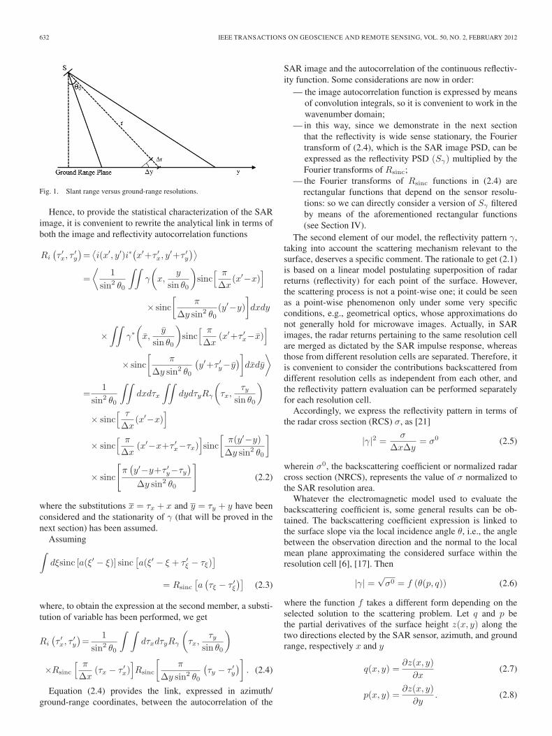
Equation (2.1) is computed by employing the slant-rangecoordinate. It is convenient to reconsider it by means of itsground-range counterpart y. Let us define the reflectivity mapin the cylindrical coordinate system (x, r, θ). Assuming that thelocal incidence angle coincides with the sensor look angle θ0,the ground-range coordinate and the ground-range resolutioncan be calculated by simple trigonometric computations: y =r ∗ sin θ0 and ∆y = ∆r/ sin θ0 (see Fig. 1) [21].
632 IEEE TRANSACTIONS ON GEOSCIENCE AND REMOTE SENSING, VOL. 50, NO. 2, FEBRUARY 2012
Fig. 1. Slant range versus ground-range resolutions.
Hence, to provide the statistical characterization of the SARimage, it is convenient to rewrite the analytical link in terms ofboth the image and reflectivity autocorrelation functions
Ri
(τ ′x, τ
′y
)=⟨i(x′, y′)i∗
(x′+τ ′x, y
′+τ ′y)⟩
=
⟨1
sin2 θ0
∫∫γ
(x,
y
sin θ0
)sinc
[ π
∆x(x′−x)
]
× sinc
[π
∆y sin2 θ0(y′−y)
]dxdy
×∫∫
γ∗(x,
y
sin θ0
)sinc
[ π
∆x(x′+τ ′x−x)
]
× sinc
[π
∆y sin2 θ0
(y′+τ ′y−y
)]dxdy
⟩
=1
sin2 θ0
∫∫dxdτx
∫∫dydτyRγ
(τx,
τysin θ0
)
× sinc[ τ
∆x(x′−x)
]
× sinc[ π
∆x(x′−x+τ ′x−τx)
]sinc
[π(y′−y)
∆y sin2 θ0
]
× sinc
[π(y′−y+τ ′y−τy
)∆y sin2 θ0
](2.2)
where the substitutions x = τx + x and y = τy + y have beenconsidered and the stationarity of γ (that will be proved in thenext section) has been assumed.
Assuming∫dξsinc [a(ξ′ − ξ)] sinc
[a(ξ′ − ξ + τ ′ξ − τξ)
]= Rsinc
[a(τξ − τ ′ξ
)](2.3)
where, to obtain the expression at the second member, a substi-tution of variable has been performed, we get
Ri
(τ ′x, τ
′y
)=
1
sin2 θ0
∫ ∫dτxdτyRγ
(τx,
τysin θ0
)
×Rsinc
[ π
∆x(τx − τ ′x)
]Rsinc
[π
∆y sin2 θ0
(τy − τ ′y
)]. (2.4)
Equation (2.4) provides the link, expressed in azimuth/ground-range coordinates, between the autocorrelation of the
SAR image and the autocorrelation of the continuous reflectiv-ity function. Some considerations are now in order:
— the image autocorrelation function is expressed by meansof convolution integrals, so it is convenient to work in thewavenumber domain;
— in this way, since we demonstrate in the next sectionthat the reflectivity is wide sense stationary, the Fouriertransform of (2.4), which is the SAR image PSD, can beexpressed as the reflectivity PSD (Sγ) multiplied by theFourier transforms of Rsinc;
— the Fourier transforms of Rsinc functions in (2.4) arerectangular functions that depend on the sensor resolu-tions: so we can directly consider a version of Sγ filteredby means of the aforementioned rectangular functions(see Section IV).
The second element of our model, the reflectivity pattern γ,taking into account the scattering mechanism relevant to thesurface, deserves a specific comment. The rationale to get (2.1)is based on a linear model postulating superposition of radarreturns (reflectivity) for each point of the surface. However,the scattering process is not a point-wise one; it could be seenas a point-wise phenomenon only under some very specificconditions, e.g., geometrical optics, whose approximations donot generally hold for microwave images. Actually, in SARimages, the radar returns pertaining to the same resolution cellare merged as dictated by the SAR impulse response, whereasthose from different resolution cells are separated. Therefore, itis convenient to consider the contributions backscattered fromdifferent resolution cells as independent from each other, andthe reflectivity pattern evaluation can be performed separatelyfor each resolution cell.
Accordingly, we express the reflectivity pattern in terms ofthe radar cross section (RCS) σ, as [21]
|γ|2 =σ
∆x∆y= σ0 (2.5)
wherein σ0, the backscattering coefficient or normalized radarcross section (NRCS), represents the value of σ normalized tothe SAR resolution area.
Whatever the electromagnetic model used to evaluate thebackscattering coefficient is, some general results can be ob-tained. The backscattering coefficient expression is linked tothe surface slope via the local incidence angle θ, i.e., the anglebetween the observation direction and the normal to the localmean plane approximating the considered surface within theresolution cell [6], [17]. Then
|γ| =√σ0 = f (θ(p, q)) (2.6)
where the function f takes a different form depending on theselected solution to the scattering problem. Let q and p bethe partial derivatives of the surface height z(x, y) along thetwo directions elected by the SAR sensor, azimuth, and groundrange, respectively x and y
q(x, y) =∂z(x, y)
∂x(2.7)
p(x, y) =∂z(x, y)
∂y. (2.8)
DI MARTINO et al.: SAR IMAGING OF FRACTAL SURFACES 633
The local incidence angle can be formally expressed as afunction of the partial derivatives p and q, in fact its cosine canbe evaluated as the scalar product between the propagation unitvector and the surface normal unit vector, i.e.,
θ = cos−1
(p sin θ0 + cos θ0√
p2 + q2 + 1
). (2.9)
In the hypothesis of a small slope regime for the surface, aMcLaurin series expansion of the function f(θ(p, q)) in (2.6)with respect to p and q can be performed: to the first order, weobtain a linear function of the partial derivative p only; as amatter of fact, from (2.9), it is clear that the derivative of θ withrespect to q is proportional to q itself, implying that the linearterm in q of the McLaurin expansion is zero.
Therefore, the modulus of the reflectivity function |γ(x, y)|,is, in a first-order approximation, linearly linked only to thepartial derivative p of the surface
|γ(x, y)|=f (θ(p, q))=a0 + a1p(x, y) + o(p, q) (2.10)
a0=f (θ(p=0, q=0)) a1=∂f (θ(p, q))
∂p
∣∣∣∣p=0q=0
(2.11)
a0 and a1 being the coefficients of the McLaurin series expan-sion, whose expressions depend on the specific scattering modelthat is adopted. In particular, these coefficients are functionof the look angle of the sensor, which is then an importantparameter for the determination of the validity limits of theproposed linear model. Finally, we note that the obtained resulthighlights a key property of SAR—and, more in general, ofside-looking radars—imaging behavior, showing a clear math-ematical definition of a preferential imaging direction due totheir particular acquisition geometry.
The result in (2.10) is valid independently of the selectedscattering function f(θ(p, q)), hence it holds for whateverelectromagnetic model (which can be evaluated analytically inclosed form) is chosen and it presents reasonably a general va-lidity, given the small slope regime for the observed surface. InSection III-B, the coefficients of the McLaurin series expansion,a0 and a1, are evaluated in closed form for a specific scatteringfunction, the SPM one.
The above reported analysis can be assumed as a clear andvalid foundation to assess the statistical characterization ofthe image. Usually, this characterization must be derived froma single amplitude SAR image, and we cannot set aside thespeckle phenomenon, the multiplicative noise affecting SARimages: for the sake of a theoretical analysis, we can considerthe speckle as part of the reflectivity. As a matter of fact, radarsingle-look images hold small-scale spatial properties (corre-sponding to high wavenumber spectral properties) dominatedby the speckle effect. A theoretical and quantitative analysisof the speckle is not the objective of this paper, and it will beone of the main future developments of this work. Anyway,some hints are provided in Section V-B. Now, a comment aboutthe bandwidths of the reflectivity and of the SAR acquisitionsystem is in order.
Due to the scattering mechanism, the reflectivity functionholds a finite (spatial frequency) bandwidth: the minimum
wavenumber being related to the (inverse of the) size of theilluminated area, the maximum one being related to the (inverseof the) electromagnetic wavelength. Due to the role played bythe SAR system, the SAR image holds a different but still finitebandwidth: the minimum wavenumber being related to the(inverse of the) size of the considered area, the maximum onebeing related to the (inverse of the) SAR resolution. Therefore,the image autocorrelation function depends on the SAR reso-lutions: so we look for the analytical relationship between thereflectivity function (sampled according to SAR resolutions)and the parameters of the observed surface. Hence, we oughtto work with a two-scale model for the surface description: theobserved surface is locally approximated by square plane facetswith dimension equal to that of the resolution cells; over theseplane facets, a microscopic roughness is superimposed so thatthe electromagnetic field backscattered from each resolutioncell can be evaluated. Hence, the individual returns from eachresolution cell are dictated by the microscopic scale (belowresolution cell) roughness, while the overall image textureis related to the macroscopic scale (above resolution cell)roughness.
III. FRACTAL MODELS
To obtain the spectral behavior of the reflectivity pattern asacquired by a sensor of prescribed resolution, it is fundamentalto describe both the geometry of the surface and the electro-magnetic field backscattered from it.
A. Geometrical Model
It is widely recognized that fractal geometry is the bestcandidate to describe the irregularity and the roughness ofnatural scenes. Among the fractal models, we make use ofthe regular stochastic fBm process to describe natural surfaces[13]–[17]. It can be defined in terms of the correspondingincrement process: the 2-D stochastic process z(x, y) describesan isotropic (mathematical) fBm surface if, for every x, y, x′, y′,all belonging to R, the increment process z(x, y)− z(x′, y′)satisfies the following relation:
Pr{z(x, y)− z(x′, y′) < ζ
}=
1√2πsτH
ζ∫−∞
exp
(− ζ2
2s2τ2H
)dζ
τ =
√(x− x′)2 + (y − y′)2 (3.1)
wherein H is the Hurst coefficient(0 < H < 1) and s is the in-cremental standard deviation of surface, measured in [m(1−H)],i.e., the standard deviation evaluated for increments at unitarydistance. The parameter s is related to a characteristic lengthof the fBm surface, called topothesy T [m] by the relation s =T (1−H). Topothesy is the distance over which chords joiningpoints on the surface have a root mean square slope equal tounity.
The Hurst coefficient, H , is related to the fractal dimensionthrough the expression
D = 3−H. (3.2)
634 IEEE TRANSACTIONS ON GEOSCIENCE AND REMOTE SENSING, VOL. 50, NO. 2, FEBRUARY 2012
Note that, while the fBm process is nonstationary, the incrementprocess is wide sense stationary [17].
The PSD of the topographic 2-D isotropic fBm process—inspite of the complexity of the derivation of its expression,involving the evaluation of the spectrum of a nonstationaryprocess, for instance obtained through Wigner-Ville or waveletanalysis [17], [22], [23]—exhibits an appropriate power-lawbehavior
S(k) = S0k−α (3.3)
wherein k =√k2x + k2y is the wavenumber and kx and ky are
its components along the azimuth and ground-range directions,respectively; S0 and α are the spectral parameters, related to thespatial ones by the following relationships [17]:
S0 =2H+1Γ2(1 +H) sin(πH)s2 (3.4)
α =2 + 2H = 8− 2D (3.5)
Γ(·) being the Gamma function.The PSD of a topographic 1-D fBm profile (that coincides
with a 1-D cut of an fBm surface) is also introduced
S(k) = S ′0k
−α′(3.6)
wherein k is the wavenumber and S ′0 and α′ are the spectral
parameters in the 1-D case
S ′0 =
πH
cos(πH)
1
Γ(1− 2H)s2 (3.7)
α′ =1 + 2H = 5− 2D. (3.8)
Note that the spectra of natural surfaces present a power-lawbehavior over a wide range of spatial scales [24]–[26].
Therefore, the application of the model to observable quan-tities (surfaces) leads us to use physical (bandlimited) fBms.By definition, for physical (bandlimited) fBms the above rela-tionships are still valid in the corresponding spatial scales orspectral bandwidths.
In Section II, we have shown that the stochastic characteri-zation of the SAR image involves use of the partial derivativesof the sensed surface. The formal derivative of an fBm profileis defined as fractional Gaussian noise (fGn) [23], [27], and itsPSD is proportional to that of the fBm profile multiplied by k2
[23], [27]
SfGn(k) ∝1
|k|2H−1. (3.9)
However, SAR images present a finite spatial extent and arediscretized according to a nonzero lag sampling. Hence, appli-cation to SAR images requires the definition of bandlimitedstochastic processes, whose analytical form depends on thespecific bandlimiting procedure applied. To get a closed formexpression for the SAR image power spectrum, it is mandatoryto consider the role of the resolution cell; this is convenientalso because it allows working with a two-scale model forthe surface. In this context, we want to study the canonicalcase of a fractal surface, with the same fractal parameters at
all the scales of interest for the sensor. In fact, a SAR sensordiscriminates between scales lower and greater than the reso-lution cell size. Therefore, in our case the surface descriptionwithin the resolution cell is introduced as a microscopic fractalroughness superimposed to a plane facet (having the dimensionof the resolution cell) approximating the scene of interest; themacroscopic surface description at the resolution cell scale,which is related to the applied bandlimiting procedure, is thenrequired to evaluate the PSD of interest.
Actually, to cope with the nondifferentiability of the fBmprocess, a smoothed version of the original fBm process can beintroduced [27]; this is a filtered version of the original surface,obtained by multiplying it by a differentiable test function ϕ:the test function support is, for the time being, set equal to[0, εx]× [0, εy], εx, and εy being related to the SAR resolutionsin azimuth and ground range, respectively. Thus, we set
ϕ(x, y) =
{1
εxεyif (x, y) ∈ [0, εx]× [0, εy]
0 otherwise
zϕ(x, y) =
∞∫∫−∞
z(x′, y′)ϕ(x− x′, y − y′)dx′dy′
=1
εxεy
x∫x−εx
y∫y−εy
z(x′, y′)dx′dy′. (3.10)
A comment on the relevance of the partial derivatives ofthe observed surface in imaging theory is in order. Theseare of clear physical meaning, providing information on theasymmetry in the SAR data structure with respect to the xand y directions, intuitively consistent with the existence of apreferential direction of sight of SAR sensors.
In fact, as we have seen in the previous section, the reflec-tivity function, in a first-order approximation, depends onlyon the partial derivative of the surface with respect to theground-range coordinate, as can be seen from (2.10). Moreover,we note that the functional zϕ(x, y) presented in (3.10) canbe seen as a distribution [27]. Hence, for our surface, thepartial derivative with respect to the ground-range directionzp(x, y; εy) can be defined using the theory of distributions,i.e., moving the derivation from the process z(x, y) to the testfunction ϕ(x, y)[28], thus obtaining
zp(x, y; εy, εx)
∆=
∂z(x, y)
∂y=
∞∫∫−∞
z(x′, y′)∂ϕ
∂y(x−x′, y−y′)dx′dy′
=1
εxεy
x∫x−εx
∞∫−∞
z(x′, y′) [δ(y−y′)−δ(y−εy−y′)] dy′dx′
=1
εxεy
x∫x−εx
[z(x′, y)−z(x′, y−εy)] dx′. (3.11)
Hence, zp(x, y; εy) is linearly related to the fBm incre-ment process, and it is, for this reason, wide sense stationary.
DI MARTINO et al.: SAR IMAGING OF FRACTAL SURFACES 635
Therefore, the autocorrelation function of the partial derivativeprocess zp(x, y) can be evaluated starting from the correlationbetween two increments of the fBm original process
Rzp(τx, τy; εy)
=〈zp(x, y; εy)zp(x+τx, y+τy; εy)〉
=
⟨1
(εxεy)2
x∫x−εx
[z(x′, y)−z(x′, y−εy)]dx′
×x∫
x−εx
[z(x′′+τx, y+τy)
−z(x′′+τx, y+τy−εy)]dx′′〉
=1
(εxεy)2
x∫x−εx
x∫x−εx
〈[z(x′, y)z(x′′+τx, y+τy)
−z(x′, y)z(x′′+τx, y+τy−εy)
−z(x′, y−εy)z(x′′+τx, y+τy)
+z(x′, y−εy)
× z(x′′+τx, y+τy−εy)]〉× dx′dx′′= (3.12)
wherein τx and τy are space lags in the azimuth and ground-range direction, respectively
τx =
√(x− x′)2; τy =
√(y − y′)2. (3.13)
Considering that the autocorrelation of an fBm is givenby [17]
〈z(r)z(r′)〉 = T 2(1−H)
2
(|r|2H + |r′|2H − |r′ − r|2H
)(3.14)
substituting (3.14) in (3.12), we get
Rzp(τx, τy; εy)
=s21
(εxεy)2
x∫x−εx
x∫x−εx
[∣∣τ2x+(τy+εy)2∣∣H
+∣∣τ2x+(τy−εy)
2∣∣H
− 2∣∣τ2x+τ2y
∣∣H] dx′dx′′
=s2ε−2y
[∣∣τ2x+(τy+εy)2∣∣H
+∣∣τ2x+(τy−εy)
2∣∣H−2
∣∣τ2x+τ2y∣∣H] . (3.15)
The autocorrelation function in (3.15) allows the evaluationof the 2-D power spectrum. However, in imaging theory (and inparticular for a SAR sensor which is characterized by differentspatial resolutions along azimuth and range), a more meaning-ful role is played by the power density spectra of cuts (alongazimuth and ground range) of the image. Analytical expressions
for these spectra are here evaluated via a Fourier transform ofthe azimuth and ground-range cuts of the 2-D autocorrelationfunction reported in (3.15): as a matter of fact, (3.15) shows thatzp is wide sense stationary and the Wiener–Kintchine theoremcan be applied.
— For a ground-range cut, from (3.13), we get
Rp(τy; εy) =Rzp(τx = 0, τy; εy)
=1
2s2ε2H−2
y
[(|τy|εy
+ 1
)2H
− 2
∣∣∣∣ τyεy∣∣∣∣2H
+
(|τy|εy
− 1
)2H]2
(3.16)
leading to [19], [29]
Sp(ky; εy) = 2s2ε−1+2Hy Γ(1 + 2H)
× sin(πH) [1− cos (|ky|εy)]1
(|ky|εy)1+2H. (3.17)
In this case, the autocorrelation function Rp and the PSDSp of the derivative process match exactly with those
introduced for a 1-D profile [19].Moreover, it is interesting and useful to evaluate Sp
defined as the limit of Sp for kyεy → 0
Sp(ky) = s2Γ(1 + 2H) sin(πH)1
|ky|2H−1. (3.18)
In (3.18), Sp(ky) provides an asymptotic evaluation andis amenable to meaningful interpretation and applica-tion: for every ky , it is analytically obtained by reducingthe support of the test function; alternatively, for everyεy , i.e., for actual radar resolutions, it approximates thelow spatial wavenumbers regime of the estimated PSD.
— For the azimuth cut, from (3.15), we get
Rp(τx; εy) =Rzp(τx, τy = 0; εy)
= s2ε−2y
[∣∣τ2x + ε2y∣∣H − |τx|2H
]. (3.19)
Evaluation of the corresponding PSD was never donebefore and is introduced hereafter in this paper. Also,in this case, it requires resorting to generalized Fouriertransforms; for the first term of (3.19), we get [29]
∞∫−∞
∣∣τ2x + ε2y∣∣H e−ikxτxdτx
=2(
32+H)√πε
( 12+H)
y KH+ 12(|kx|εy) 1
|kx|12+H
Γ(−H)(3.20)
and for the second term, we obtain [19], [29]
∞∫−∞
|τx|2He−ikxτx = 2Γ(1 + 2H) sin(πH)1
|kx|1+2H. (3.21)
636 IEEE TRANSACTIONS ON GEOSCIENCE AND REMOTE SENSING, VOL. 50, NO. 2, FEBRUARY 2012
Thus, we can evaluate in closed form the PSD of zp(x, y)for an azimuth cut of the surface
Sp(kx; εy)
= s2ε−1+2Hy
2
( 32+H)√πKH+ 1
2(|kx|εy) 1
(|kx|εy)12+H
Γ(−H)
+ 2Γ(1 + 2H)
× sin(πH)1
(|kx|εy)1+2H
(3.22)
where Kv(·) is the modified Bessel function of secondtype of fractional order v.
To point out the asymptotical spectral behavior ofthe aforementioned spectrum, we can express the func-tion KH+(1/2)(|kx|εy) through a power series expansionaround the value kx = 0 stopped to the first order [29]
KH+ 12(|kx|εy)
= 2−32−H (|kx|εy)
12+H
[1 +
(|kx|εy)2
(6 + 4H)
]Γ
(−1
2−H
)+ 2−
12+H (|kx|εy)−
12−H
×[1 +
(|kx|εy)2
(2− 4H)
]Γ
(1
2+H
). (3.23)
Therefore, substituting (3.23) in (3.22), we obtain thefollowing expression of the spectrum:
Sp(kx; εy)
= s2ε2H−1y
×{√
πΓ(− 1
2 −H)
Γ(−H)+
√πΓ
(− 1
2 −H)
2(2H)Γ(−H)(|kx|εy)2
+
√π21+2HΓ
(12 +H
)(1− 2H)Γ(−H)
1
(|kx|εy)2H−1
+
[√π21+2HΓ
(12 +H
)Γ(−H)
+ 2Γ(1 + 2H) sin(πH)
]
× 1
(|kx|εy)2H+1
}. (3.24)
Expression (3.24) can be simplified by consideringthat [29]
√πΓ
(12 +H
)Γ(−H)
= −2−2HΓ(1 + 2H) sin(πH) (3.25)
so (3.24) can be written as
Sp(kx; εy) = s2ε2H−1y
{√πΓ
(− 1
2 −H)
Γ(−H)
+
√πΓ
(− 1
2 −H)
4HΓ(−H)(|kx|εy)2
−2Γ(1 + 2H) sin(πH)
2− 4H
× 1
(|kx|εy)2H−1
}. (3.26)
The introduced formulas deserve some significant consid-erations. First of all, different from the case of the ground-range cut, the spectrum of the partial derivative process forthe azimuth cut does not show a power-law behavior, not evenasymptotically.
Owing to the radar preferential direction of sight, in the caseof a range profile, we are considering the derivative along thesame direction of the performed cut; this implies that the spec-trum of the derivative process inherits the correlation propertiesof successive increments of the fBm profile. Conversely, for anazimuth profile, such considerations are not valid anymore: inthis case, we are considering the derivative in the ground-rangedirection whereas the profile originates from an azimuth cut ofthe surface, so the properties of the derivative process is notdirectly linked to the profile behavior.
B. Electromagnetic Model
To evaluate the reflectivity pattern γ, we need an appropriatescattering model taking into account the specific geometricalcharacterization used for the observed scene. Hence, we mustconsider the interaction between the electromagnetic field andthe fractal surface by means of an appropriate fractal scatteringmodel tailored to the case at hand. The candidate scatteringmodel should lead to a closed form solution for the reflectivityfunction (and for the backscattering coefficient). For roughsurfaces, only approximate solutions are available, each solu-tion being valid under appropriate roughness and illuminationconditions [16]–[18]. In this paper, we use the SPM whichprovides the simplest expression for the NRCS and shows arange of validity adequate to SAR applications.
The NRCS for the SPM model in the fractal case is [16], [17]
σ0mn = 4κ3 cos4 θ|βmn|2
S0
(2κ sin θ)2+2H(3.27)
wherein κ is the electromagnetic wavenumber; βmn, account-ing for the incident and reflected fields polarization, is afunction of both the dielectric constant of the surface and thelocal incidence angle θ [17]; S0 and H are the surface fractalparameters introduced in the first part of this section. Note thatwith the considered model, we are able to deal only with thecopolarized case.
Now, it is possible to use the results presented in Section II toobtain an expression of the reflectivity function as a function ofthe partial derivatives of the surface. In particular, substitutingthe expression of cos θ provided in (2.9) and the correspondingexpression of sin θ into (3.27) and taking into account that theterm |βmn|2 can be considered constant with θ in the angularinterval of interest in the copolarized case, the NRCS can bethen expressed as
σ0 = A0
((cos θ0 + p sin θ0)
2
p2 + q2 + 1
)2
×((sin θ0 − p cos θ0)
2 + q2
p2 + q2 + 1
)−(1+H)
(3.28)
wherein
A0 =S0κ
1−2H |βmn|222H
. (3.29)
DI MARTINO et al.: SAR IMAGING OF FRACTAL SURFACES 637
Therefore, |γ(x, y)|, which is related to σ0 by (2.5), can beevaluated as
|γ(x, y)| = f (θ(p, q))
=√A0
((cos θ0 + p sin θ0)
2
p2 + q2 + 1
)
×((sin θ0 − p cos θ0)
2 + q2
p2 + q2 + 1
)− (1+H)2
. (3.30)
Performing the McLaurin series expansion of the expressionin (3.30), we obtain the coefficients a0 and a1 [see (2.10)]relevant to the SPM scattering function
|γ(x, y)|∼=a0+a1p
=√A0
{cos2 θ0 sin
−(1+H) θ0+cos θ0 sin−H θ0
×[2+(1+H) cos2 θ0 sin
−2 θ0]p}
(3.31)
wherein p is characterized in the first part of this section.Therefore, in the case of interest, the coefficients a0 and a1,and in turn the validity limits of the proposed model, depend onthe considered look angle and on the fractal parameters of theobserved surface.
IV. STOCHASTIC CHARACTERIZATION OF THE SAR IMAGE
Exploiting the results obtained in the previous sections, thecomplete statistical characterization of a SAR image is pre-sented in this section.
According to the theoretical results presented in the previoussections, provided that the slopes of the surface are sufficientlylow, the image is linearly dependent on the partial derivativeprocess zp, whose expression is given in (3.11). Hence, the im-age inherits the same statistical characterization of the processzp(x, y), i.e., it is Gaussian distributed with µ = a0 and σ =a1s∆yH−1, as we can deduce combining (2.10) and (3.11).
A discussion is now in order on the role of εx and εy ,defining the support of the kernel ϕ mentioned in the previoussection, which formally determines the effective bandwidth ofthe imaging system whenever applied to the fractal surfaces. Asfar as the bandwidth is concerned, our model implies dealingwith two, somehow implicit, band-limiting procedures thatcan be conveniently formalized as two filtering steps that wenow explicitly discuss. First of all, the electromagnetic fieldimpinging on the rough surface performs a low-pass filteringon the surface according to the electromagnetic wavelengthλ. Then, the obtained smoothed process is filtered accordingto the sensor impulse response (2.1), and spatial scales lowerthan the resolution one are discarded. In our case, assuming xand y as coordinates in azimuth and ground-range directions,respectively, and ∆x and ∆y as the corresponding sensorresolutions, we can consider, being ∆x,∆y � λ, directly thesecond filtering step and we can take εx and εy coincident withthe azimuth and ground-range resolutions.
Considering the expression of the SAR image autocorrela-tion function [see (2.2)] and applying the Wiener-Kintchinetheorem, we can now provide the power density spectra for a
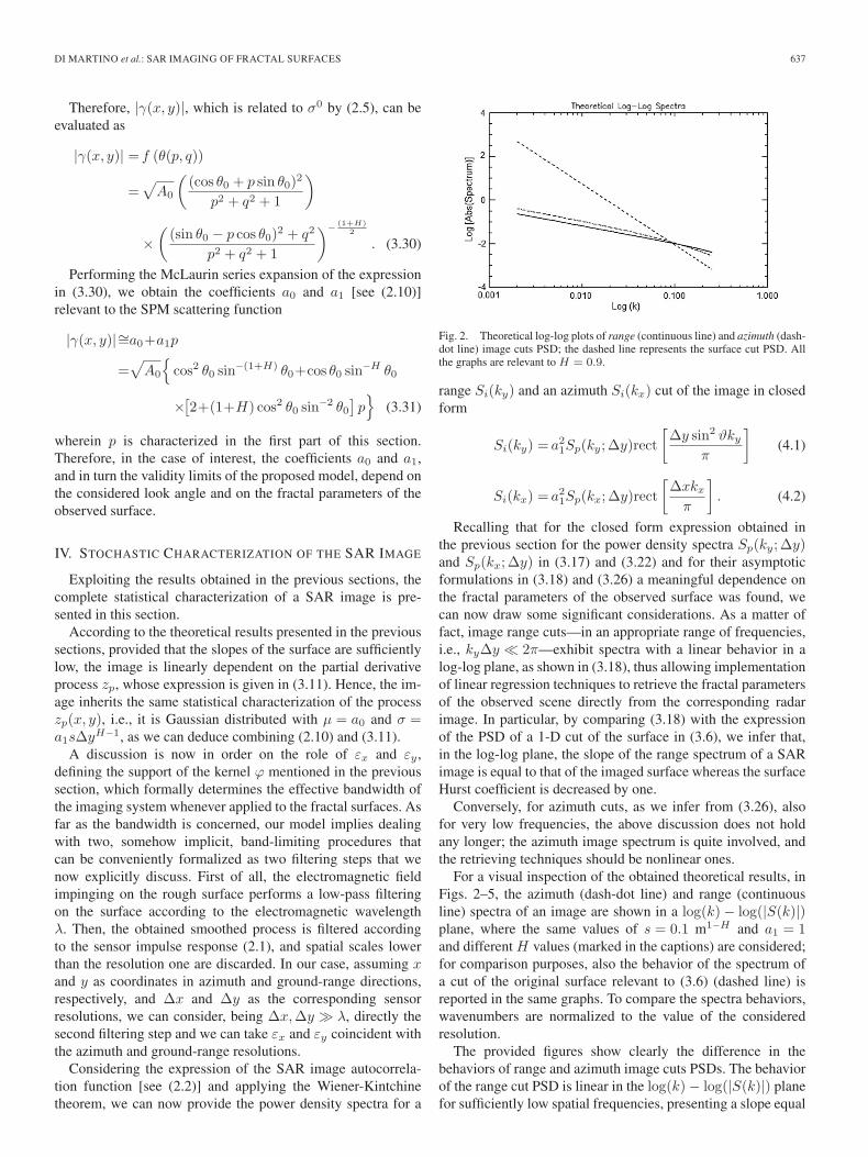
Fig. 2. Theoretical log-log plots of range (continuous line) and azimuth (dash-dot line) image cuts PSD; the dashed line represents the surface cut PSD. Allthe graphs are relevant to H = 0.9.
range Si(ky) and an azimuth Si(kx) cut of the image in closedform
Si(ky) = a21Sp(ky; ∆y)rect
[∆y sin2 ϑky
π
](4.1)
Si(kx) = a21Sp(kx; ∆y)rect
[∆xkxπ
]. (4.2)
Recalling that for the closed form expression obtained inthe previous section for the power density spectra Sp(ky; ∆y)and Sp(kx; ∆y) in (3.17) and (3.22) and for their asymptoticformulations in (3.18) and (3.26) a meaningful dependence onthe fractal parameters of the observed surface was found, wecan now draw some significant considerations. As a matter offact, image range cuts—in an appropriate range of frequencies,i.e., ky∆y � 2π—exhibit spectra with a linear behavior in alog-log plane, as shown in (3.18), thus allowing implementationof linear regression techniques to retrieve the fractal parametersof the observed scene directly from the corresponding radarimage. In particular, by comparing (3.18) with the expressionof the PSD of a 1-D cut of the surface in (3.6), we infer that,in the log-log plane, the slope of the range spectrum of a SARimage is equal to that of the imaged surface whereas the surfaceHurst coefficient is decreased by one.
Conversely, for azimuth cuts, as we infer from (3.26), alsofor very low frequencies, the above discussion does not holdany longer; the azimuth image spectrum is quite involved, andthe retrieving techniques should be nonlinear ones.
For a visual inspection of the obtained theoretical results, inFigs. 2–5, the azimuth (dash-dot line) and range (continuousline) spectra of an image are shown in a log(k)− log(|S(k)|)plane, where the same values of s = 0.1 m1−H and a1 = 1and different H values (marked in the captions) are considered;for comparison purposes, also the behavior of the spectrum ofa cut of the original surface relevant to (3.6) (dashed line) isreported in the same graphs. To compare the spectra behaviors,wavenumbers are normalized to the value of the consideredresolution.
The provided figures show clearly the difference in thebehaviors of range and azimuth image cuts PSDs. The behaviorof the range cut PSD is linear in the log(k)− log(|S(k)|) planefor sufficiently low spatial frequencies, presenting a slope equal
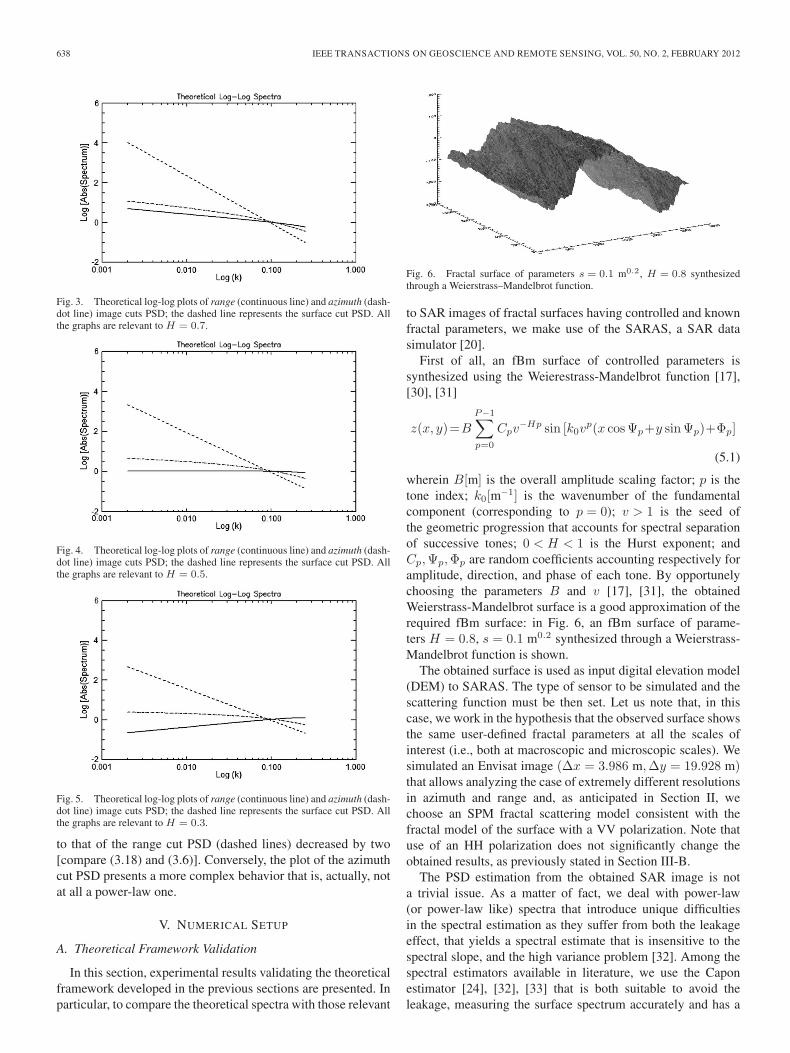
638 IEEE TRANSACTIONS ON GEOSCIENCE AND REMOTE SENSING, VOL. 50, NO. 2, FEBRUARY 2012
Fig. 3. Theoretical log-log plots of range (continuous line) and azimuth (dash-dot line) image cuts PSD; the dashed line represents the surface cut PSD. Allthe graphs are relevant to H = 0.7.
Fig. 4. Theoretical log-log plots of range (continuous line) and azimuth (dash-dot line) image cuts PSD; the dashed line represents the surface cut PSD. Allthe graphs are relevant to H = 0.5.
Fig. 5. Theoretical log-log plots of range (continuous line) and azimuth (dash-dot line) image cuts PSD; the dashed line represents the surface cut PSD. Allthe graphs are relevant to H = 0.3.
to that of the range cut PSD (dashed lines) decreased by two[compare (3.18) and (3.6)]. Conversely, the plot of the azimuthcut PSD presents a more complex behavior that is, actually, notat all a power-law one.
V. NUMERICAL SETUP
A. Theoretical Framework Validation
In this section, experimental results validating the theoreticalframework developed in the previous sections are presented. Inparticular, to compare the theoretical spectra with those relevant
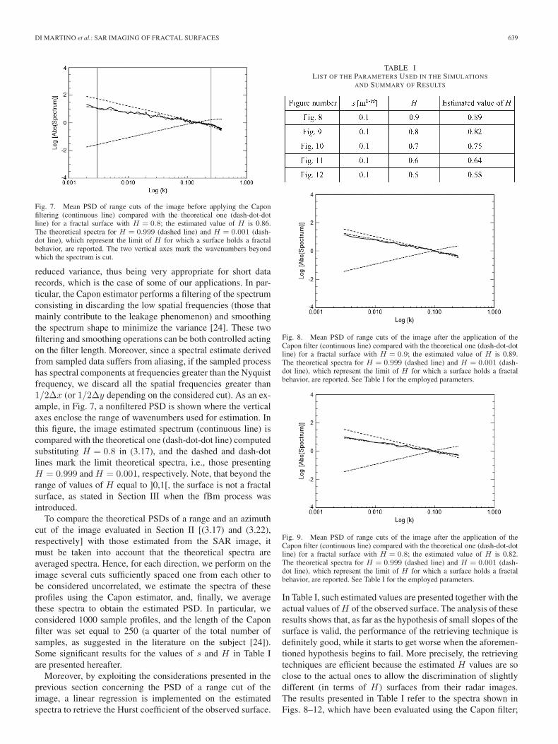
Fig. 6. Fractal surface of parameters s = 0.1 m0.2, H = 0.8 synthesizedthrough a Weierstrass–Mandelbrot function.
to SAR images of fractal surfaces having controlled and knownfractal parameters, we make use of the SARAS, a SAR datasimulator [20].
First of all, an fBm surface of controlled parameters issynthesized using the Weierestrass-Mandelbrot function [17],[30], [31]
z(x, y)=B
P−1∑p=0
Cpv−Hp sin [k0v
p(x cosΨp+y sinΨp)+Φp]
(5.1)
wherein B[m] is the overall amplitude scaling factor; p is thetone index; k0[m−1] is the wavenumber of the fundamentalcomponent (corresponding to p = 0); v > 1 is the seed ofthe geometric progression that accounts for spectral separationof successive tones; 0 < H < 1 is the Hurst exponent; andCp,Ψp,Φp are random coefficients accounting respectively foramplitude, direction, and phase of each tone. By opportunelychoosing the parameters B and v [17], [31], the obtainedWeierstrass-Mandelbrot surface is a good approximation of therequired fBm surface: in Fig. 6, an fBm surface of parame-ters H = 0.8, s = 0.1 m0.2 synthesized through a Weierstrass-Mandelbrot function is shown.
The obtained surface is used as input digital elevation model(DEM) to SARAS. The type of sensor to be simulated and thescattering function must be then set. Let us note that, in thiscase, we work in the hypothesis that the observed surface showsthe same user-defined fractal parameters at all the scales ofinterest (i.e., both at macroscopic and microscopic scales). Wesimulated an Envisat image (∆x = 3.986 m,∆y = 19.928 m)that allows analyzing the case of extremely different resolutionsin azimuth and range and, as anticipated in Section II, wechoose an SPM fractal scattering model consistent with thefractal model of the surface with a VV polarization. Note thatuse of an HH polarization does not significantly change theobtained results, as previously stated in Section III-B.
The PSD estimation from the obtained SAR image is nota trivial issue. As a matter of fact, we deal with power-law(or power-law like) spectra that introduce unique difficultiesin the spectral estimation as they suffer from both the leakageeffect, that yields a spectral estimate that is insensitive to thespectral slope, and the high variance problem [32]. Among thespectral estimators available in literature, we use the Caponestimator [24], [32], [33] that is both suitable to avoid theleakage, measuring the surface spectrum accurately and has a
DI MARTINO et al.: SAR IMAGING OF FRACTAL SURFACES 639
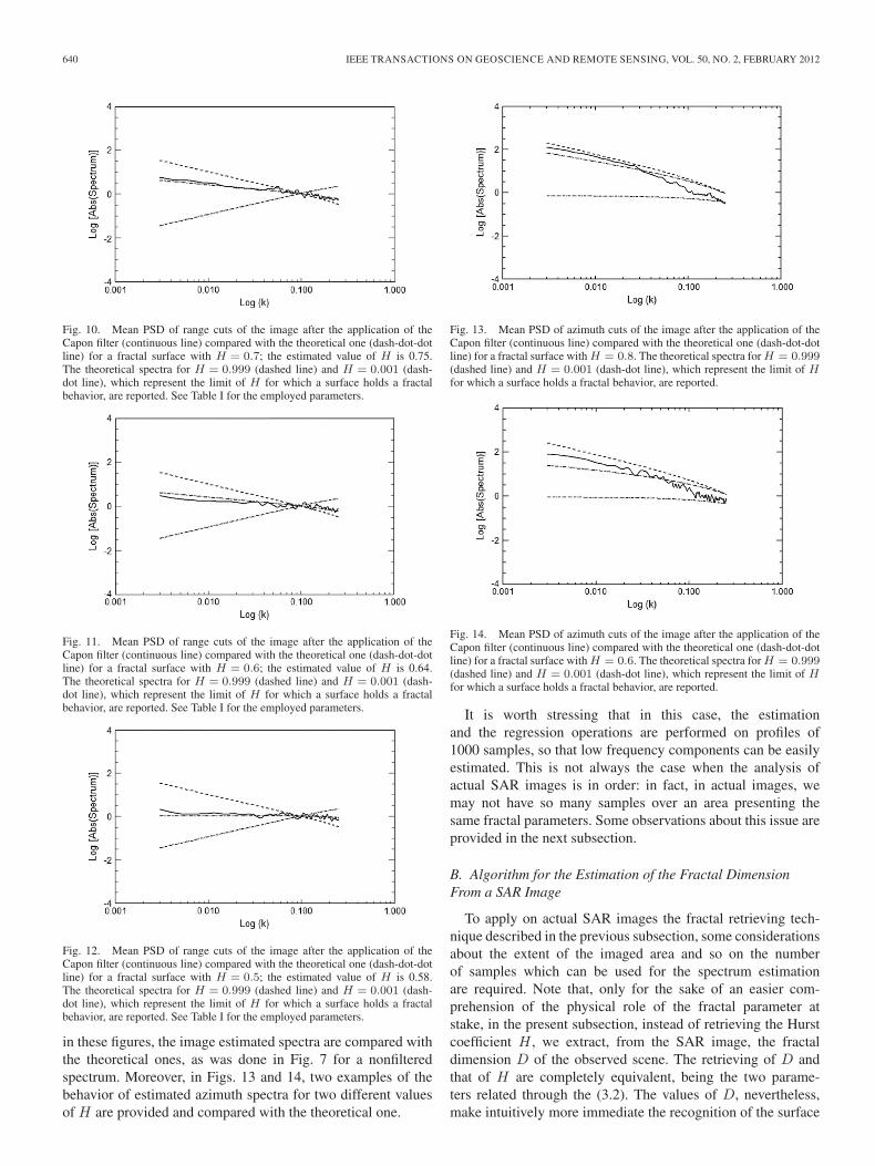
Fig. 7. Mean PSD of range cuts of the image before applying the Caponfiltering (continuous line) compared with the theoretical one (dash-dot-dotline) for a fractal surface with H = 0.8; the estimated value of H is 0.86.The theoretical spectra for H = 0.999 (dashed line) and H = 0.001 (dash-dot line), which represent the limit of H for which a surface holds a fractalbehavior, are reported. The two vertical axes mark the wavenumbers beyondwhich the spectrum is cut.
reduced variance, thus being very appropriate for short datarecords, which is the case of some of our applications. In par-ticular, the Capon estimator performs a filtering of the spectrumconsisting in discarding the low spatial frequencies (those thatmainly contribute to the leakage phenomenon) and smoothingthe spectrum shape to minimize the variance [24]. These twofiltering and smoothing operations can be both controlled actingon the filter length. Moreover, since a spectral estimate derivedfrom sampled data suffers from aliasing, if the sampled processhas spectral components at frequencies greater than the Nyquistfrequency, we discard all the spatial frequencies greater than1/2∆x (or 1/2∆y depending on the considered cut). As an ex-ample, in Fig. 7, a nonfiltered PSD is shown where the verticalaxes enclose the range of wavenumbers used for estimation. Inthis figure, the image estimated spectrum (continuous line) iscompared with the theoretical one (dash-dot-dot line) computedsubstituting H = 0.8 in (3.17), and the dashed and dash-dotlines mark the limit theoretical spectra, i.e., those presentingH = 0.999 and H = 0.001, respectively. Note, that beyond therange of values of H equal to ]0,1[, the surface is not a fractalsurface, as stated in Section III when the fBm process wasintroduced.
To compare the theoretical PSDs of a range and an azimuthcut of the image evaluated in Section II [(3.17) and (3.22),respectively] with those estimated from the SAR image, itmust be taken into account that the theoretical spectra areaveraged spectra. Hence, for each direction, we perform on theimage several cuts sufficiently spaced one from each other tobe considered uncorrelated, we estimate the spectra of theseprofiles using the Capon estimator, and, finally, we averagethese spectra to obtain the estimated PSD. In particular, weconsidered 1000 sample profiles, and the length of the Caponfilter was set equal to 250 (a quarter of the total number ofsamples, as suggested in the literature on the subject [24]).Some significant results for the values of s and H in Table Iare presented hereafter.
Moreover, by exploiting the considerations presented in theprevious section concerning the PSD of a range cut of theimage, a linear regression is implemented on the estimatedspectra to retrieve the Hurst coefficient of the observed surface.
TABLE ILIST OF THE PARAMETERS USED IN THE SIMULATIONS
AND SUMMARY OF RESULTS
Fig. 8. Mean PSD of range cuts of the image after the application of theCapon filter (continuous line) compared with the theoretical one (dash-dot-dotline) for a fractal surface with H = 0.9; the estimated value of H is 0.89.The theoretical spectra for H = 0.999 (dashed line) and H = 0.001 (dash-dot line), which represent the limit of H for which a surface holds a fractalbehavior, are reported. See Table I for the employed parameters.
Fig. 9. Mean PSD of range cuts of the image after the application of theCapon filter (continuous line) compared with the theoretical one (dash-dot-dotline) for a fractal surface with H = 0.8; the estimated value of H is 0.82.The theoretical spectra for H = 0.999 (dashed line) and H = 0.001 (dash-dot line), which represent the limit of H for which a surface holds a fractalbehavior, are reported. See Table I for the employed parameters.
In Table I, such estimated values are presented together with theactual values of H of the observed surface. The analysis of theseresults shows that, as far as the hypothesis of small slopes of thesurface is valid, the performance of the retrieving technique isdefinitely good, while it starts to get worse when the aforemen-tioned hypothesis begins to fail. More precisely, the retrievingtechniques are efficient because the estimated H values are soclose to the actual ones to allow the discrimination of slightlydifferent (in terms of H) surfaces from their radar images.The results presented in Table I refer to the spectra shown inFigs. 8–12, which have been evaluated using the Capon filter;
640 IEEE TRANSACTIONS ON GEOSCIENCE AND REMOTE SENSING, VOL. 50, NO. 2, FEBRUARY 2012
Fig. 10. Mean PSD of range cuts of the image after the application of theCapon filter (continuous line) compared with the theoretical one (dash-dot-dotline) for a fractal surface with H = 0.7; the estimated value of H is 0.75.The theoretical spectra for H = 0.999 (dashed line) and H = 0.001 (dash-dot line), which represent the limit of H for which a surface holds a fractalbehavior, are reported. See Table I for the employed parameters.
Fig. 11. Mean PSD of range cuts of the image after the application of theCapon filter (continuous line) compared with the theoretical one (dash-dot-dotline) for a fractal surface with H = 0.6; the estimated value of H is 0.64.The theoretical spectra for H = 0.999 (dashed line) and H = 0.001 (dash-dot line), which represent the limit of H for which a surface holds a fractalbehavior, are reported. See Table I for the employed parameters.
Fig. 12. Mean PSD of range cuts of the image after the application of theCapon filter (continuous line) compared with the theoretical one (dash-dot-dotline) for a fractal surface with H = 0.5; the estimated value of H is 0.58.The theoretical spectra for H = 0.999 (dashed line) and H = 0.001 (dash-dot line), which represent the limit of H for which a surface holds a fractalbehavior, are reported. See Table I for the employed parameters.
in these figures, the image estimated spectra are compared withthe theoretical ones, as was done in Fig. 7 for a nonfilteredspectrum. Moreover, in Figs. 13 and 14, two examples of thebehavior of estimated azimuth spectra for two different valuesof H are provided and compared with the theoretical one.
Fig. 13. Mean PSD of azimuth cuts of the image after the application of theCapon filter (continuous line) compared with the theoretical one (dash-dot-dotline) for a fractal surface with H = 0.8. The theoretical spectra for H = 0.999(dashed line) and H = 0.001 (dash-dot line), which represent the limit of Hfor which a surface holds a fractal behavior, are reported.
Fig. 14. Mean PSD of azimuth cuts of the image after the application of theCapon filter (continuous line) compared with the theoretical one (dash-dot-dotline) for a fractal surface with H = 0.6. The theoretical spectra for H = 0.999(dashed line) and H = 0.001 (dash-dot line), which represent the limit of Hfor which a surface holds a fractal behavior, are reported.
It is worth stressing that in this case, the estimationand the regression operations are performed on profiles of1000 samples, so that low frequency components can be easilyestimated. This is not always the case when the analysis ofactual SAR images is in order: in fact, in actual images, wemay not have so many samples over an area presenting thesame fractal parameters. Some observations about this issue areprovided in the next subsection.
B. Algorithm for the Estimation of the Fractal DimensionFrom a SAR Image
To apply on actual SAR images the fractal retrieving tech-nique described in the previous subsection, some considerationsabout the extent of the imaged area and so on the numberof samples which can be used for the spectrum estimationare required. Note that, only for the sake of an easier com-prehension of the physical role of the fractal parameter atstake, in the present subsection, instead of retrieving the Hurstcoefficient H , we extract, from the SAR image, the fractaldimension D of the observed scene. The retrieving of D andthat of H are completely equivalent, being the two parame-ters related through the (3.2). The values of D, nevertheless,make intuitively more immediate the recognition of the surface
DI MARTINO et al.: SAR IMAGING OF FRACTAL SURFACES 641
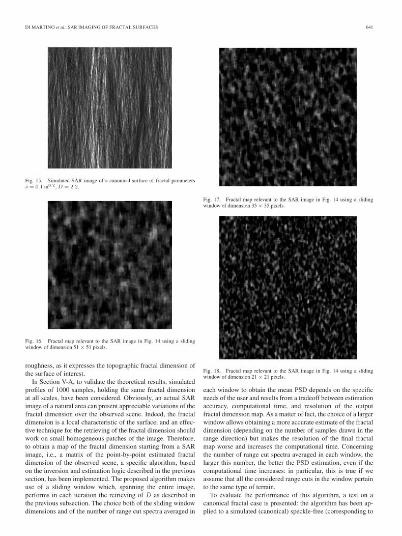
Fig. 15. Simulated SAR image of a canonical surface of fractal parameterss = 0.1 m0.2, D = 2.2.
Fig. 16. Fractal map relevant to the SAR image in Fig. 14 using a slidingwindow of dimension 51 × 51 pixels.
roughness, as it expresses the topographic fractal dimension ofthe surface of interest.
In Section V-A, to validate the theoretical results, simulatedprofiles of 1000 samples, holding the same fractal dimensionat all scales, have been considered. Obviously, an actual SARimage of a natural area can present appreciable variations of thefractal dimension over the observed scene. Indeed, the fractaldimension is a local characteristic of the surface, and an effec-tive technique for the retrieving of the fractal dimension shouldwork on small homogeneous patches of the image. Therefore,to obtain a map of the fractal dimension starting from a SARimage, i.e., a matrix of the point-by-point estimated fractaldimension of the observed scene, a specific algorithm, basedon the inversion and estimation logic described in the previoussection, has been implemented. The proposed algorithm makesuse of a sliding window which, spanning the entire image,performs in each iteration the retrieving of D as described inthe previous subsection. The choice both of the sliding windowdimensions and of the number of range cut spectra averaged in
Fig. 17. Fractal map relevant to the SAR image in Fig. 14 using a slidingwindow of dimension 35 × 35 pixels.
Fig. 18. Fractal map relevant to the SAR image in Fig. 14 using a slidingwindow of dimension 21 × 21 pixels.
each window to obtain the mean PSD depends on the specificneeds of the user and results from a tradeoff between estimationaccuracy, computational time, and resolution of the outputfractal dimension map. As a matter of fact, the choice of a largerwindow allows obtaining a more accurate estimate of the fractaldimension (depending on the number of samples drawn in therange direction) but makes the resolution of the final fractalmap worse and increases the computational time. Concerningthe number of range cut spectra averaged in each window, thelarger this number, the better the PSD estimation, even if thecomputational time increases: in particular, this is true if weassume that all the considered range cuts in the window pertainto the same type of terrain.
To evaluate the performance of this algorithm, a test on acanonical fractal case is presented: the algorithm has been ap-plied to a simulated (canonical) speckle-free (corresponding to
642 IEEE TRANSACTIONS ON GEOSCIENCE AND REMOTE SENSING, VOL. 50, NO. 2, FEBRUARY 2012
TABLE IISTATISTICS OF THE FRACTAL MAPS (SPECKLE-FREE CASE)
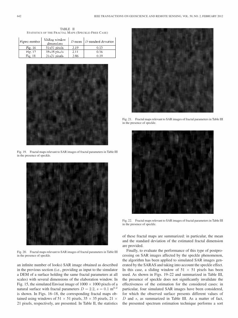
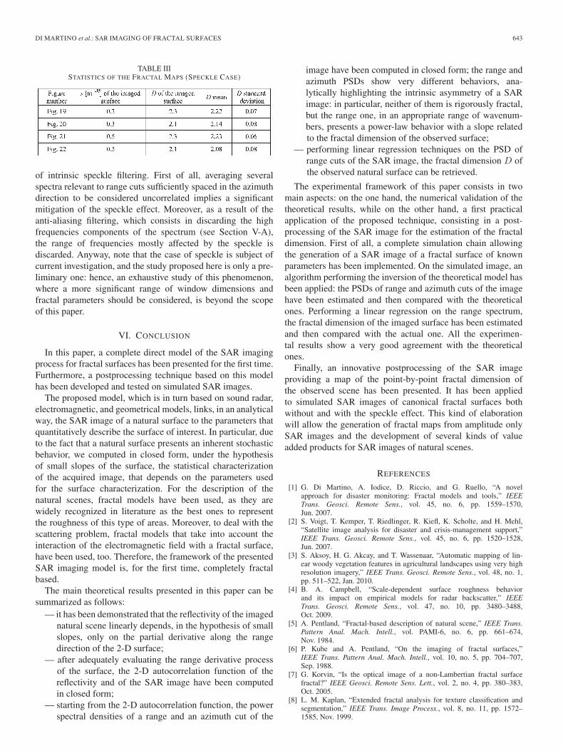
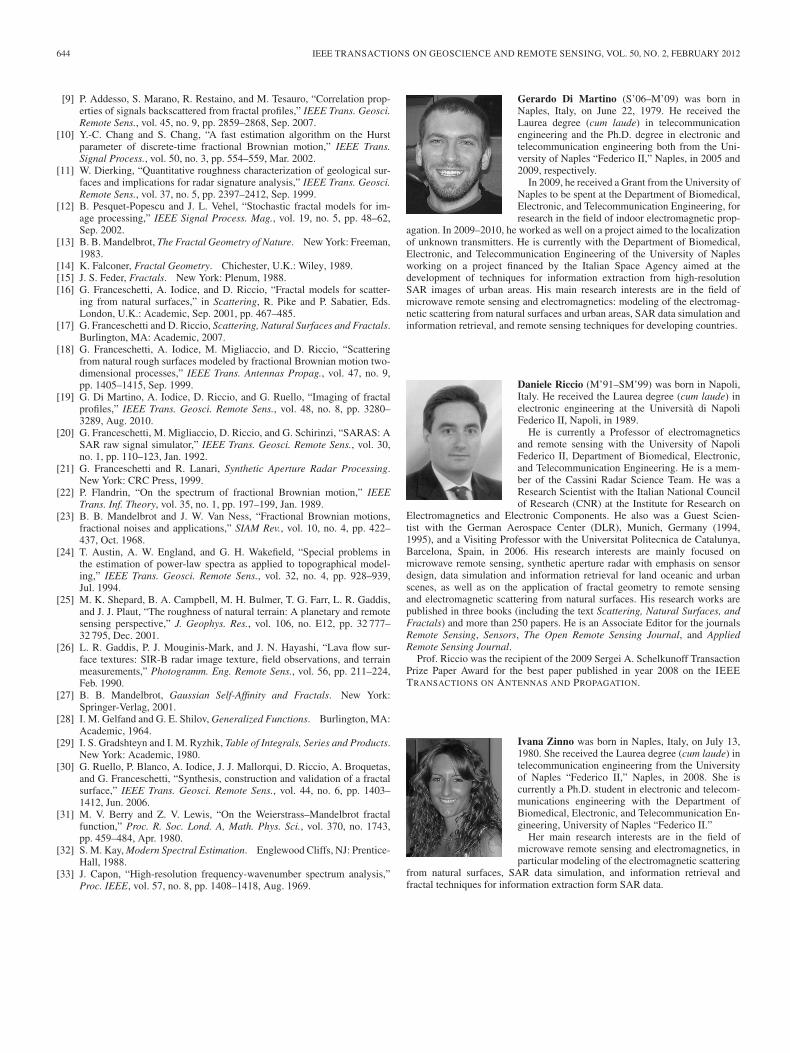
Fig. 19. Fractal maps relevant to SAR images of fractal parameters in Table IIIin the presence of speckle.
Fig. 20. Fractal maps relevant to SAR images of fractal parameters in Table IIIin the presence of speckle.
an infinite number of looks) SAR image obtained as describedin the previous section (i.e., providing as input to the simulatora DEM of a surface holding the same fractal parameters at allscales) with several dimensions of the elaboration window. InFig. 15, the simulated Envisat image of 1000 × 1000 pixels of anatural surface with fractal parameters D = 2.2, s = 0.1 m0.2
is shown. In Figs. 16–18, the corresponding fractal maps ob-tained using windows of 51 × 51 pixels, 35 × 35 pixels, 21 ×21 pixels, respectively, are presented. In Table II, the statistics
Fig. 21. Fractal maps relevant to SAR images of fractal parameters in Table IIIin the presence of speckle.
Fig. 22. Fractal maps relevant to SAR images of fractal parameters in Table IIIin the presence of speckle.
of these fractal maps are summarized: in particular, the meanand the standard deviation of the estimated fractal dimensionare provided.
Finally, to evaluate the performance of this type of postpro-cessing on SAR images affected by the speckle phenomenon,the algorithm has been applied to simulated SAR images gen-erated by the SARAS and taking into account the speckle effect.In this case, a sliding window of 51 × 51 pixels has beenused. As shown in Figs. 19–22 and summarized in Table III,the presence of speckle does not significantly invalidate theeffectiveness of the estimation for the considered cases: inparticular, four simulated SAR images have been considered,for which the observed surface presents different values ofD and s, as summarized in Table III. As a matter of fact,the presented spectrum estimation technique performs a sort
DI MARTINO et al.: SAR IMAGING OF FRACTAL SURFACES 643
TABLE IIISTATISTICS OF THE FRACTAL MAPS (SPECKLE CASE)
of intrinsic speckle filtering. First of all, averaging severalspectra relevant to range cuts sufficiently spaced in the azimuthdirection to be considered uncorrelated implies a significantmitigation of the speckle effect. Moreover, as a result of theanti-aliasing filtering, which consists in discarding the highfrequencies components of the spectrum (see Section V-A),the range of frequencies mostly affected by the speckle isdiscarded. Anyway, note that the case of speckle is subject ofcurrent investigation, and the study proposed here is only a pre-liminary one: hence, an exhaustive study of this phenomenon,where a more significant range of window dimensions andfractal parameters should be considered, is beyond the scopeof this paper.
VI. CONCLUSION
In this paper, a complete direct model of the SAR imagingprocess for fractal surfaces has been presented for the first time.Furthermore, a postprocessing technique based on this modelhas been developed and tested on simulated SAR images.
The proposed model, which is in turn based on sound radar,electromagnetic, and geometrical models, links, in an analyticalway, the SAR image of a natural surface to the parameters thatquantitatively describe the surface of interest. In particular, dueto the fact that a natural surface presents an inherent stochasticbehavior, we computed in closed form, under the hypothesisof small slopes of the surface, the statistical characterizationof the acquired image, that depends on the parameters usedfor the surface characterization. For the description of thenatural scenes, fractal models have been used, as they arewidely recognized in literature as the best ones to representthe roughness of this type of areas. Moreover, to deal with thescattering problem, fractal models that take into account theinteraction of the electromagnetic field with a fractal surface,have been used, too. Therefore, the framework of the presentedSAR imaging model is, for the first time, completely fractalbased.
The main theoretical results presented in this paper can besummarized as follows:
— it has been demonstrated that the reflectivity of the imagednatural scene linearly depends, in the hypothesis of smallslopes, only on the partial derivative along the rangedirection of the 2-D surface;
— after adequately evaluating the range derivative processof the surface, the 2-D autocorrelation function of thereflectivity and of the SAR image have been computedin closed form;
— starting from the 2-D autocorrelation function, the powerspectral densities of a range and an azimuth cut of the
image have been computed in closed form; the range andazimuth PSDs show very different behaviors, ana-lytically highlighting the intrinsic asymmetry of a SARimage: in particular, neither of them is rigorously fractal,but the range one, in an appropriate range of wavenum-bers, presents a power-law behavior with a slope relatedto the fractal dimension of the observed surface;
— performing linear regression techniques on the PSD ofrange cuts of the SAR image, the fractal dimension D ofthe observed natural surface can be retrieved.
The experimental framework of this paper consists in twomain aspects: on the one hand, the numerical validation of thetheoretical results, while on the other hand, a first practicalapplication of the proposed technique, consisting in a post-processing of the SAR image for the estimation of the fractaldimension. First of all, a complete simulation chain allowingthe generation of a SAR image of a fractal surface of knownparameters has been implemented. On the simulated image, analgorithm performing the inversion of the theoretical model hasbeen applied: the PSDs of range and azimuth cuts of the imagehave been estimated and then compared with the theoreticalones. Performing a linear regression on the range spectrum,the fractal dimension of the imaged surface has been estimatedand then compared with the actual one. All the experimen-tal results show a very good agreement with the theoreticalones.
Finally, an innovative postprocessing of the SAR imageproviding a map of the point-by-point fractal dimension ofthe observed scene has been presented. It has been appliedto simulated SAR images of canonical fractal surfaces bothwithout and with the speckle effect. This kind of elaborationwill allow the generation of fractal maps from amplitude onlySAR images and the development of several kinds of valueadded products for SAR images of natural scenes.
REFERENCES
[1] G. Di Martino, A. Iodice, D. Riccio, and G. Ruello, “A novelapproach for disaster monitoring: Fractal models and tools,” IEEETrans. Geosci. Remote Sens., vol. 45, no. 6, pp. 1559–1570,Jun. 2007.
[2] S. Voigt, T. Kemper, T. Riedlinger, R. Kiefl, K. Scholte, and H. Mehl,“Satellite image analysis for disaster and crisis-management support,”IEEE Trans. Geosci. Remote Sens., vol. 45, no. 6, pp. 1520–1528,Jun. 2007.
[3] S. Aksoy, H. G. Akcay, and T. Wassenaar, “Automatic mapping of lin-ear woody vegetation features in agricultural landscapes using very highresolution imagery,” IEEE Trans. Geosci. Remote Sens., vol. 48, no. 1,pp. 511–522, Jan. 2010.
[4] B. A. Campbell, “Scale-dependent surface roughness behaviorand its impact on empirical models for radar backscatter,” IEEETrans. Geosci. Remote Sens., vol. 47, no. 10, pp. 3480–3488,Oct. 2009.
[5] A. Pentland, “Fractal-based description of natural scene,” IEEE Trans.Pattern Anal. Mach. Intell., vol. PAMI-6, no. 6, pp. 661–674,Nov. 1984.
[6] P. Kube and A. Pentland, “On the imaging of fractal surfaces,”IEEE Trans. Pattern Anal. Mach. Intell., vol. 10, no. 5, pp. 704–707,Sep. 1988.
[7] G. Korvin, “Is the optical image of a non-Lambertian fractal surfacefractal?” IEEE Geosci. Remote Sens. Lett., vol. 2, no. 4, pp. 380–383,Oct. 2005.
[8] L. M. Kaplan, “Extended fractal analysis for texture classification andsegmentation,” IEEE Trans. Image Process., vol. 8, no. 11, pp. 1572–1585, Nov. 1999.
644 IEEE TRANSACTIONS ON GEOSCIENCE AND REMOTE SENSING, VOL. 50, NO. 2, FEBRUARY 2012
[9] P. Addesso, S. Marano, R. Restaino, and M. Tesauro, “Correlation prop-erties of signals backscattered from fractal profiles,” IEEE Trans. Geosci.Remote Sens., vol. 45, no. 9, pp. 2859–2868, Sep. 2007.
[10] Y.-C. Chang and S. Chang, “A fast estimation algorithm on the Hurstparameter of discrete-time fractional Brownian motion,” IEEE Trans.Signal Process., vol. 50, no. 3, pp. 554–559, Mar. 2002.
[11] W. Dierking, “Quantitative roughness characterization of geological sur-faces and implications for radar signature analysis,” IEEE Trans. Geosci.Remote Sens., vol. 37, no. 5, pp. 2397–2412, Sep. 1999.
[12] B. Pesquet-Popescu and J. L. Vehel, “Stochastic fractal models for im-age processing,” IEEE Signal Process. Mag., vol. 19, no. 5, pp. 48–62,Sep. 2002.
[13] B. B. Mandelbrot, The Fractal Geometry of Nature. New York: Freeman,1983.
[14] K. Falconer, Fractal Geometry. Chichester, U.K.: Wiley, 1989.[15] J. S. Feder, Fractals. New York: Plenum, 1988.[16] G. Franceschetti, A. Iodice, and D. Riccio, “Fractal models for scatter-
ing from natural surfaces,” in Scattering, R. Pike and P. Sabatier, Eds.London, U.K.: Academic, Sep. 2001, pp. 467–485.
[17] G. Franceschetti and D. Riccio, Scattering, Natural Surfaces and Fractals.Burlington, MA: Academic, 2007.
[18] G. Franceschetti, A. Iodice, M. Migliaccio, and D. Riccio, “Scatteringfrom natural rough surfaces modeled by fractional Brownian motion two-dimensional processes,” IEEE Trans. Antennas Propag., vol. 47, no. 9,pp. 1405–1415, Sep. 1999.
[19] G. Di Martino, A. Iodice, D. Riccio, and G. Ruello, “Imaging of fractalprofiles,” IEEE Trans. Geosci. Remote Sens., vol. 48, no. 8, pp. 3280–3289, Aug. 2010.
[20] G. Franceschetti, M. Migliaccio, D. Riccio, and G. Schirinzi, “SARAS: ASAR raw signal simulator,” IEEE Trans. Geosci. Remote Sens., vol. 30,no. 1, pp. 110–123, Jan. 1992.
[21] G. Franceschetti and R. Lanari, Synthetic Aperture Radar Processing.New York: CRC Press, 1999.
[22] P. Flandrin, “On the spectrum of fractional Brownian motion,” IEEETrans. Inf. Theory, vol. 35, no. 1, pp. 197–199, Jan. 1989.
[23] B. B. Mandelbrot and J. W. Van Ness, “Fractional Brownian motions,fractional noises and applications,” SIAM Rev., vol. 10, no. 4, pp. 422–437, Oct. 1968.
[24] T. Austin, A. W. England, and G. H. Wakefield, “Special problems inthe estimation of power-law spectra as applied to topographical model-ing,” IEEE Trans. Geosci. Remote Sens., vol. 32, no. 4, pp. 928–939,Jul. 1994.
[25] M. K. Shepard, B. A. Campbell, M. H. Bulmer, T. G. Farr, L. R. Gaddis,and J. J. Plaut, “The roughness of natural terrain: A planetary and remotesensing perspective,” J. Geophys. Res., vol. 106, no. E12, pp. 32 777–32 795, Dec. 2001.
[26] L. R. Gaddis, P. J. Mouginis-Mark, and J. N. Hayashi, “Lava flow sur-face textures: SIR-B radar image texture, field observations, and terrainmeasurements,” Photogramm. Eng. Remote Sens., vol. 56, pp. 211–224,Feb. 1990.
[27] B. B. Mandelbrot, Gaussian Self-Affinity and Fractals. New York:Springer-Verlag, 2001.
[28] I. M. Gelfand and G. E. Shilov, Generalized Functions. Burlington, MA:Academic, 1964.
[29] I. S. Gradshteyn and I. M. Ryzhik, Table of Integrals, Series and Products.New York: Academic, 1980.
[30] G. Ruello, P. Blanco, A. Iodice, J. J. Mallorqui, D. Riccio, A. Broquetas,and G. Franceschetti, “Synthesis, construction and validation of a fractalsurface,” IEEE Trans. Geosci. Remote Sens., vol. 44, no. 6, pp. 1403–1412, Jun. 2006.
[31] M. V. Berry and Z. V. Lewis, “On the Weierstrass–Mandelbrot fractalfunction,” Proc. R. Soc. Lond. A, Math. Phys. Sci., vol. 370, no. 1743,pp. 459–484, Apr. 1980.
[32] S. M. Kay, Modern Spectral Estimation. Englewood Cliffs, NJ: Prentice-Hall, 1988.
[33] J. Capon, “High-resolution frequency-wavenumber spectrum analysis,”Proc. IEEE, vol. 57, no. 8, pp. 1408–1418, Aug. 1969.
Gerardo Di Martino (S’06–M’09) was born inNaples, Italy, on June 22, 1979. He received theLaurea degree (cum laude) in telecommunicationengineering and the Ph.D. degree in electronic andtelecommunication engineering both from the Uni-versity of Naples “Federico II,” Naples, in 2005 and2009, respectively.
In 2009, he received a Grant from the University ofNaples to be spent at the Department of Biomedical,Electronic, and Telecommunication Engineering, forresearch in the field of indoor electromagnetic prop-
agation. In 2009–2010, he worked as well on a project aimed to the localizationof unknown transmitters. He is currently with the Department of Biomedical,Electronic, and Telecommunication Engineering of the University of Naplesworking on a project financed by the Italian Space Agency aimed at thedevelopment of techniques for information extraction from high-resolutionSAR images of urban areas. His main research interests are in the field ofmicrowave remote sensing and electromagnetics: modeling of the electromag-netic scattering from natural surfaces and urban areas, SAR data simulation andinformation retrieval, and remote sensing techniques for developing countries.
Daniele Riccio (M’91–SM’99) was born in Napoli,Italy. He received the Laurea degree (cum laude) inelectronic engineering at the Università di NapoliFederico II, Napoli, in 1989.
He is currently a Professor of electromagneticsand remote sensing with the University of NapoliFederico II, Department of Biomedical, Electronic,and Telecommunication Engineering. He is a mem-ber of the Cassini Radar Science Team. He was aResearch Scientist with the Italian National Councilof Research (CNR) at the Institute for Research on
Electromagnetics and Electronic Components. He also was a Guest Scien-tist with the German Aerospace Center (DLR), Munich, Germany (1994,1995), and a Visiting Professor with the Universitat Politecnica de Catalunya,Barcelona, Spain, in 2006. His research interests are mainly focused onmicrowave remote sensing, synthetic aperture radar with emphasis on sensordesign, data simulation and information retrieval for land oceanic and urbanscenes, as well as on the application of fractal geometry to remote sensingand electromagnetic scattering from natural surfaces. His research works arepublished in three books (including the text Scattering, Natural Surfaces, andFractals) and more than 250 papers. He is an Associate Editor for the journalsRemote Sensing, Sensors, The Open Remote Sensing Journal, and AppliedRemote Sensing Journal.
Prof. Riccio was the recipient of the 2009 Sergei A. Schelkunoff TransactionPrize Paper Award for the best paper published in year 2008 on the IEEETRANSACTIONS ON ANTENNAS AND PROPAGATION.
Ivana Zinno was born in Naples, Italy, on July 13,1980. She received the Laurea degree (cum laude) intelecommunication engineering from the Universityof Naples “Federico II,” Naples, in 2008. She iscurrently a Ph.D. student in electronic and telecom-munications engineering with the Department ofBiomedical, Electronic, and Telecommunication En-gineering, University of Naples “Federico II.”
Her main research interests are in the field ofmicrowave remote sensing and electromagnetics, inparticular modeling of the electromagnetic scattering
from natural surfaces, SAR data simulation, and information retrieval andfractal techniques for information extraction form SAR data.