1

SAR Calibration aided by Permanent ScatterersD. D’Aria(1), A. Ferretti(2), A. Monti Guarnieri(3), S. Tebaldini(3).

(1) ARESYS, Piazza Leonardo Da Vinci, 32 - 20133 Milano - Italy(2) Tele-Rilevamento Europa (TRE), Via V. Colonna 7, 20149 Milano, Italy

(3) Dipartimento di Elettronica ed Informazione - Politecnico di MilanoPiazza Leonardo Da Vinci, 32 - 20133 Milano - Italy

Abstract— We propose a calibration method suitable for a setof repeated SAR acquisitions, that uses both absolute calibrateddevices (like corner reflectors) and stable targets identified in thescene (the Permanent Scatterers, PS). Precisely the role of thePS is to extend the initial calibration sequence by monitoring theradiometric stability of the system throughout the whole missionlifespan. At a first step, this paper approaches the problem of PS-based normalization by an iterative Maximum Likelihood methodthat exploits the stack of complex interferometric SAR images.Two solutions are given based on different assumptions on thePS phases. As a second step, the merging of these estimateswith the available calibration information is discussed. Resultsachieved by experimental acquisitions are shown in two differentSAR systems: a C-band Space Borne (SB) SAR and a KU-bandGround Based (GB) one.

I. INTRODUCTION

Radiometric calibration of SAR image is a fundamentalissue in modern Synthetic Aperture RADAR: its achievementallows the proper exploitation of the backscatter coefficient inmany applications [1], [2]. The objective is to estimate theoverall system gain, including the transmitter, the receiver, thepropagation and the processor. Such a goal is usually achievedby exploiting an internal calibration scheme that monitors theacquisition system, and by using calibrated targets in the scene,like corner reflectors and transponders. The manufacturing anddeployment of such devices are quite expensive, and so it istheir maintenance throughout the whole mission. The purposeof the present paper is to provide a scheme for SAR calibrationthat integrates information coming from these external devices,maintained only for a short time, and those of the targetsin the scene that are intrinsically stable, the PS [3]. The PSphase stability has been exploited ever since for interferometricapplications, however the interest in this paper is to exploit thePS amplitude stability to monitor the slightest change in thesystematic gain.

The existence and the properties of such PSs is welldocumented in a widespread and rich literature, like in [3], [4],[5], [6], [7], [8]: a short summary with the definition of thePS model is in the appendix. For our purposes, each PS is likea stable calibrator, a corner reflector with unknown RADARcross section and with a quality that can be estimated by therepeated observations. The accuracy of the technique followsafter averaging several independent measures, where typicalPS densities in urban areas can be as high as 500 per square km[3], [7], in C-band and for a medium resolution (5×20 m). PSshave also been found also in rural areas, in volcanic calderas

[4], and even in boreal forests at P-band [8], ensuring theapplication of the technique in different contests. Moreover ithas been shown that the life-time span of such targets extendsseveral years [7]. In order to be able to distinguish betweensystem and scene changes, we will limit to those PS that areinsensitive, or reacts randomly, to changes like rain, moistureetc. As an example, we exclude homogeneous scenes of baresoil.

The typical scenario for a Space Borne SAR system isthe exploitation of the commissioning phase, when severalexternal calibration sites are available. This information will beused to monitor and calibrate the PS series. We will show thatit is not strictly necessary to have simultaneous acquisitionson the reference calibrators and the PSs, provided that thesystem ensures a good radiometric stability in short time, thatis usually expected at the beginning of life. The ubiquity of thePSs will then allow to construct a wide set of calibration sites(say in rocky areas, towns etc) distributed all over the earth,that does not demand for committing special acquisitions thatwould interfere with the operations. This very same calibrationscheme applies to other SAR systems, like for the GroundBased SAR, where a single scene can be monitored for timeextent up to several months [9], [10].

The paper is organized as follows. The next section intro-duces the PS based normalization. The method exploits aniterative solution of the Maximum Likelihood estimate forthe image gains, based on the PS model in the appendix. Inparticular we propose two estimators: one is phase-blind, ornon-coherent, whereas the other exploits a parametric modelfor the PS phases. In both cases, we derive the detection for thePSs, based on the Generalized Likelihood Ratio Test (GLRT)[11]. We show that this test leads to an index that includes asparticular cases the dispersion index, in the non-coherent case,and the ensemble coherence, in the case of linear phase model,both of them heuristically introduced in [3]. The accuracy ofthe estimate of the normalized gains is then evaluated as afunction of the number of PS and their quality.

In section III we study the integration of the PSs-basedinformation with the external calibrators, whereas in sectionIV, we provide experimental results achieved by the proposedPSCal. In particular we investigate the absolute calibration ofERS-2 SAR mission, for a six years time span, by combiningtwo different PS-sites, one of them with transponders infor-mation available in some acquisitions. In the same section, weprovide results achieved by exploiting the coherent approachon a set of Ground Based (GB) RADAR observations.

II. NORMALIZATION BY PERMANENT SCATTERERS

The geometry of a typical SAR acquisition system byrepeated observations is shown in Fig 1. The figure refers tothe Space Borne (SB) case, where the sensor repeats a setof NI observations by the same geometry. In particular weassume that the variation in the look and squint angles (θ, ψ)by which each target is observed, is small enough to neglectchanges in the target’s RCS.

The goal of this PS-based analysis is to identify and exploitthe largest number of stable targets available within an image.Moreover, as we can be interested in monitoring space variantgains, like due to changes in the antenna gain pattern, we needthe area exploited on the ground to be as small as possible.

The comprehensive block diagram of the PSCal techniqueis shown in Fig. 2. The technique is made by two majorsteps: a PS-based normalization of the stack of data, shownin the shaded block of the figure and discussed here, and thecalibration of the stack, that is discussed in section III.

We then assume a stack of say NI vignettes (small images),and NP targets that are stable in the whole stack. The goal isto retrieve the set of NI − 1 differential gains, with respect toone, that will be conventionally assumed to be unitary.

s1

s s

2

Ψ

NI

P1

Ψ

θ

P2

PN

P

Fig. 1. Typical geometry of the repeat-pass Space Borne system.

The model for the observations, the complex amplitude ofthe target PP in the image n, is derived from the PS modelin the appendix (32):

yn(Pp) = an · (bp exp (jφn,p) + wn,p) (1)

where an is the gain of the n-th vignette to be estimated, bpthe amplitude of the p-th PS, φn,p the phase of the p-th PSin the n-th vignette and wn,p the noise that accounts for thequality of the PS itself. In the following, we will assume wn,pto be complex, normal, circular distributed with zero meanand variance v(p), independent by the acquisition itself.

In summary, we have NT = NI ·NP complex observationsand NI − 1 images gains to be retrieved, we may assume for

PS detection

Images’ gains estimation

PS amplitudes and noise

variances, estimation

SLC coarsely calibrated & coregistered stack

External calibrators measures

PS

Norm

aliz

ation

ConvergenceNO

YES

Calibrated SLC stack

Absolute gains computation

Normalized SLC stack

PS

Norm

aliz

ation

Fig. 2. Schematic block diagram of the proposed PSCal technique forabsolute SAR calibration.

example a1 = 1. The amplitudes and the phases of the PSand the noise covariances represent an added set of nuisanceparameters.

Let us rephrase the model (1) in a compact matrix formu-lation:

y = x + wa (2)

where x is a column vector size [NT = NI ·NP , 1] :

x = (b⊗ a) · φ (3)

b =[b1 . . . bNP

]Ta =

[a1 = 1 . . . aNI

]Tthe apex “T ” standing for transposition, and the symbols “⊗”and “·” respectively for the Kronecker and the Hadamarddot products. Finally, the column vector φ [NT , 1] in (3) isobtained by vectorizing the phase field φn,p. The noise vectorwa introduced in (2) can be assumed normal, circular, zero-mean, independently distributed with non stationary variance,a2(i) · v(p):

fw (wa) = N(0, Cw) =exp

(−w∗

aC−1wa

)πNT |C|

C= diag2(a)⊗ diag([

v(1) . . . . . . v(Np)]T)

(4)

The log-likelihood of the complex observations can be ex-pressed as follows:

L (y|x,C) = − (y − x)∗ C−1 (y − x)− log |C| (5)

= 2 Re(y∗C−1x

)− y∗C−1y − x∗C−1x− log |C| ,

having omitted a constant that is irrelevant for the maximiza-tion. Eventually, by taking advantage of the non-correlationof noise, C in (4) being diagonal, we get the following

expression:

L=2Y −NI∑i=1

NP∑p=1

y2a(i, p)

a2(i)v(p)−NI

NP∑p=1

(b2(p)v(p)

+ log (v(p)))

− 2NPNI∑i=1

log (a(i)) (6)

where Y = Re

{NI∑i=1

1a(i)

NP∑p=1

b(p)v(p)

y∗(i, p) exp(j (φ(p, i))

}(7)

ya(i, p) being the amplitude of the p-th target in the i-th imageand xa(i) the i− th element of |x|.

In the following two sections we will derive two differentestimators basing on different models for the PS phases.

A. Non coherent estimate

We make here the hypothesis that PS phases are completelyunknown. This could be the case when the phase error withrespect to the model in (33), is much larger than 2π. Nonethe-less we can still achieve a phase-free estimate for the gains,a, by first maximizing the log-likelihood (7) with respect tothe unknown phases:

φ = arg maxφ

{Re

NI∑i=1

1a(i)

NP∑p=1

b(p)v(p)

y∗(i, p) exp(jφ(i, p))

}and then replacing the solution:

φ(i, p) = − arg {y(i, p)} , (8)

back into (7). We get the following expression for the log-likelihood:

L=2NI∑i=1

1a(i)

NP∑p=1

b(p)ya(i, p)v(p)

−NI∑i=1

NP∑p=1

y2a(i, p)

a2(i)v(p)(9)

−NINP∑p=1

(b2(p)v(p)

− log (v(p)))− 2NP

NI∑i=1

log (a(i))

The maximization of L with respect to the remaining un-knowns, the sets of parameters a, b, v, is a non linear problemthat demands for a joint exploitation of the whole space whichspans a dimensionality NI × NP × (NI − 1), with a largecomputational cost. However we follow the iterative approachproposed in [12], [13], that holds provided that the initialsolution is close enough to the optimum. This assumption findsa justification in the internal calibration capabilities providedby modern SAR instruments, that are enough to ensure anaccuracy < 1 dB, at least in their initial life [14], [15].

The algorithm is detailed within the shaded block in theblock diagram of Fig.2. Each iteration starts from an initialset of gains, ak−1(the apex defining the iteration step), anduses those gains to estimates the PS amplitudes and the noisevariances for each PS: bk, vk. These values are then usedto refine the estimate of the gains, ak and then start a newiteration. The iterations stop at convergence, ak ≈ ak−1.

The PS amplitudes are obtained by nulling the derivative of

log-likelihood (9):

∂L(y|{ak−1

}, {b}, {v}

)∂bp

= 0 p = 1 . . . NP

that leads to the solution:

bk(p) =1NI

NI∑i=1

ya(i, p)ak−1(i)

, µk(p) (10)

where we have introduced the definition of the term µ toremind that b corresponds to the sampled estimator of themean of the data (normalized as from the previous step).

In turn, we exploit the PS amplitudes to derive the noisepowers:

∂L(y|{a0},{b1}, {v}

)∂vp

= 0 p = 1 . . . NP

that leads to the solution:

vk(p) = Ek−1y (p)−

(µk(p)

)2, σ2

k(p) (11)

where Ek−1y (p) is the power of the p-th target in the pre-

normalized data:

Eky (p) =1NI

NI∑i=1

y2a(i, p)

(ak(i))2(12)

Here again we have introduced the notation σ2 to remind thatthe ML estimate v corresponds to the sampled estimator ofthe variance.

Finally, we conclude the iteration by providing the estimateof the set of gains:

∂L (y| {a} , {b} , {v})∂ai

= 0 for i = 2 . . . NI

The estimate of the gain that maximizes L is the largest ofthe two solutions of the following equation:

NPa2(i) +

NP∑p=1

b(p) · ya(i, p)v(p)

a(i)−NP∑p=1

y2a(i, p)v(p)

= 0 (13)

B. Non coherent detection

The detection of those targets that are effectively PS (andnot pure noise) is a crucial step for the estimator and forthe convergence of algorithm, as only a minority of all thetargets actually behaves as PSs [3]. We perform the detectionaccording to the Likelihood Ratio Test (LRT), for the binaryclassification between the event H0 the absence of the target,and H1 the presence of the target [11]. The LR for each targetP is defined as follows:

Λp =L (y|H1, {a} , {b} , {v})

L (y|H0, {a} , {b = 0}, {v})≶H0H1

VT (14)

where VT is a proper threshold that can be selected based on acompromise between the two possible error, the false positiveand the missing detection. We exploit (5) to express the LR

as follows:

Λp =exp

(− (y − x)H C−1 (y − x)

)a

πN |C|πN |C|

exp (yHC−1y)= exp

(−(xHC−1x−2 Re

(yHC−1x

)))(15)

This depends on both the noise variance and the imagesamplitudes, that are unknown. These are replaced by their MLestimate, according to the Generalized LRT approach [11].Eventually we evaluate (9) for the p-th target:

xHC−1x=NIb2(p)v(p)

(16a)

2 Re(yHC−1x

)= 2NI

b2(p)v((p)

(16b)

Notice that we have omitted the prefix with the iterationnumber for simplicity. If we combine (15) with (16a,16b) weget the following expression:

Λp = NIb2(p)v((p)

= NIµ2(p)

σ2(p)≶H0H1

VT (17)

The GRLT leads to the same figure of merit heuristicallyproposed in [3], and there defined as dispersion index:

DI =µ(p)σ(p)

Thus, we can say that the detection proposed in [3] isequivalent to the GRLT one here discussed at the first step,whereas in the further steps, the detection improves as a betterknowledge of the image gains and the noise variances areexploited.

We can however express the threshold in a different way bycombining (10) and (11):

ΛpNI

=µ2(p)

Ey(p)− µ2(p)Ey(p)µ2(p)

=NI

Λp+ 1

that leads to the equivalent thresholding:

µ(p)√Ey(p)

=(1 +D−2

I

)−0.5≶H0H1

γN (18)

where γN =

√1

1 +NIV−1T

(19)

The left hand term in (18) is just the normalized correlationcoefficient between the data and the model. A good featureis that 0 ≤ γN ≤ 1, where the two extremes correspondrespectively to select all the targets, or only those with infiniteSNR (thus no target). The probabilities of false alarm andmissing detection for the single PS are plotted in the first threeimages in Fig. 3 for different values of the threshold, γN , andachieved by Monte Carlo simulations of the model in (1) fordifferent number of images, NI .

The figure can be exploited for both fixing the threshold andfor estimating the performances of the technique as a function

Fig. 3. Plots of the probability of false alarm and missing PS detection fordifferent SNR. Upper three plots: non-coherent detection, for different numberof images, NI . Lower three plots: coherent detection. The horizontal axis isthe correlation coefficient: γN for the non-coherent approach and γC for thecoherent one.

of the number of images and the target quality. As an example,if we accept a probability of false alarm of 20%, we noticethat we miss a PS with SNR=8 dB for 50% of the times inthe case of NI =5 images, whereas if we exploit 20 images,this happens for a target whose SNR is greater than 4 dB.

C. Coherent estimate

So far we have assumed that the PS phases are completelyrandom from acquisition to acquisition. Instead, if we providea structured model for the phases, we can get better perfor-mances in terms of capability of distinguishing the PS fromthe case of pure noise. We assume here a parametric modelthat generalizes the linear phase model in (33), by replacingϕ = ϕ(Θ) (where Θ is the set of parameters) in (7). We firstsolve the ML in (6) for the phases’ parameters:

Θ = arg max

{∣∣∣∣∣NI∑i=1

y∗(i)a(i)

· exp (jϕ(Θ)))

∣∣∣∣∣}

(20)

Then we define the following term:

YM =

∣∣∣∣∣NI∑i=1

y∗(i)a(i)

· exp(jϕ(Θ))

)∣∣∣∣∣that can be replaced back into (6. We get:

L =

2∑p

b(p)v(p)YM (p)−

∑p

∑i

y2a(i,p)

a2(i)v(p)

−NI∑p

(b2(p)v(p) + log (v(p))

)− 2NP

∑i log (a(i))

We maximize the log-likelihood by means of the same iterativescheme as in the previous section. The set of gains is stillestimated according to (13), whereas for the target amplitudesand the noise variances, we have to replace (10) and (11) withthe following:

b(p) =1NI

∣∣∣∣∣NI∑i=1

y(i)a(i)

exp(−jϕ(Θ))

)∣∣∣∣∣ , µ(p) (21)

vk(p) =1NI

NI∑i=1

NP∑p=1

y2a(i, p)a2(i)

− 1NI

NP∑p=1

Y 2M (p)

= Ey(p)− µ2(p) , σ2(p) (22)

D. Coherent detection

The detection for the coherent estimate is achieved in thesame way as for the non-coherent case. We compute the GLRTtest by exploiting the estimate of the target amplitude in thecomplex case. We get from (21):

µ(p)√Ey(p)

=

∣∣∣∣∣ 1NI

NI∑i=1

y(i)a(i) · exp

(−jϕ(Θ))

)∣∣∣∣∣√Ey

≶H0H1

γC (23)

This expression generalizes (18) for the complex case, pre-cisely the left-hand term is the absolute value of normalizedcorrelation between the complex data and the model. Inprinciple, this PS detection needs a calibrated set of data,therefore it should be iterated. However (23) suggests a phase-based detection, that is obtained by ignoring the amplitudefluctuations, under the assumptions of large SNR. Therefore, ifwe assume the amplitude to be stable and we define the phasesof the data as φy(i, p), (23) can be expressed as follows:∣∣∣∣∣ 1

NI

NI∑i=1

exp(j(φy(i, p)− ϕ(Θ))

)∣∣∣∣∣2

≶H0H1

γC (24)

This index, that generalizes the concept of the PS ensemblecoherence defined in [3], has been exploited with success in theGround Based (GB) SAR case to provide a one-step detectionof the PS.

A case of interest is the following linear phase model:

ϕ(i, p) = θ0(p) + θ1(p) · t(i) (25)

t(i) being the time of the i-th acquisition, and θ0, θ1 theconstant phase term, and the linear coefficient. In that case, theestimate of the target amplitude in (21) becomes the maximum

of the absolute value of the Fourier Transform of the pre-calibrated data:

µc = maxθ1

{1NI

∣∣∣∣∣NI∑i=1

y(i)a(i)· exp (−jθ1 · t(i))

∣∣∣∣∣}

=1NI

Ya(f0)

where we used capitals for Fourier Transforms, and f0 is thefrequency of the argument of the maximum. The GRLT for thelinear model can be very efficiently evaluated in the frequencydomain:

|Ya(f0)|√1NI

∑k

|Ya(fk)|2≶H0H1

γC (26)

The performances of the detection according to the GLRTfor the linear phase model (25), evaluated basing on MonteCarlo simulations, are plotted in Fig. 3 in the same conditionsassumed for the non-coherent detection. The gain achieved bythis technique is remarkable: as an example, if we assume atarget with SNR=10 dB and a false alarm pfa =0.1 we geta missing detection rate pmd = 0.1 by exploiting NI = 20images with the non coherent approach, whereas with thecoherent approach we get a much better detection: pmd = 0.02by exploiting 1/4th of the images, NI = 5. The reason of suchimprovement appear quite evident if we compare (23) with thecorrespondent non-coherent expression in (18). In fact, in thecoherent case the expected target amplitude is compared withthe absolute value of the coherent summation of the noisycontributions, whereas in the non-coherent case, the singlenoisy measures are first detected and then averaged, enhancingmuch more the noise level at the detector.

E. Accuracy

The evaluation of the accuracy of the two estimators (thecoherent and the non-coherent one) is a complex task dueto the number of parameters involved. However we can havea first order approximation by assuming that the noise power,and the amplitude of the PS itself are known a-priori, as well asthe linear rate for the coherent case. This allows us for a quickmonodimensional evaluation of the Cramer Rao Bound (CRB).Such result is to be used as a rough evaluation of performancesof the technique in some typical scenario, and not to get theaccuracy relative to a specific experiment. However, in thelatter case, a numerical evaluation of the CRB is suggested.

The assumption of known noise variance allows us tomodify the model (1) as follows:

yn(Pp) = an · bp exp (jφn,p) + wn,p (27)

The log-likelihood of the observation is expressed as follows:

L=Y −NI∑i=1

NP∑p=1

y2a(i, p)v(p)

−NI∑i=1

NP∑p=1

a2(i)b2(p)v(p)

−NINP∑p=1

log v(p)

where Y = 2 Re

{NI∑i=1

NP∑p=1

a(i)b(p)v(p)

y∗(i, p) exp(j (φ(p, i))

}

This would lead to the following non-coherent gain estimate:

ai=

∑p

b(p)v−1(p) · ya(i, p)∑p

b2(p)v−1(p)=

∑p

SNR(p) · ya(i, p)b−1(p)∑p

SNR(p)

(28)

where SNR(p) = b(p)v−1(p)

that is suited to a simple interpretation in that the amplitudeof the image is the weighted average of each pixel normalizedby the PS amplitude itself. The weights are proportional to thequality of the PS in terms of SNR.

The CRB of the estimate of a is then obtained by itsdefinition:

σ2CRB = −

(E

[(∂2L(a)da2

)]∣∣∣∣a=ai

)−1

that leads to:

σ2CRB =

1

2NP∑p=1

b2(p)v(p)

=1

2NP∑p=1

SNR(p)

σ2CRB =

1Np

12SNR0

(29)

where SNR0 is the average of the SNRs of the detected PSs.The factor two accounts for the fact that half of the noisepower is attributed to the in-phase component, that affectsthe amplitude (for large SNR), and half to the quadraturecomponent, that affects the phase. The term N−1

p comes fromthe average of independent measured an states that the standarddeviation of the PS-normalization improves with the squareroot of the number of PS.

The radiometric accuracy is obtained by its definition

ρRAD = 10 log10

(1 +

σ2 [a]a2

)= 10 log10

(1 +

12NP

σ2w

a2

)= 10 log10

(1 +

12NP

SNR−10

)This expression descends from (27) and applies, in theory, forboth the coherent and the non-coherent approaches. Howeverwe suggest the non-coherent estimation (28), that, being phase-free, is insensitive with respect to model errors. Nonethelesswe can still choose to apply it to the targets detected by eitherof the two approaches, or even a combination of the two.

III. ABSOLUTE CALIBRATION

The set of gains estimated by the PS normalization are to bemultiplied by a constant term to get the absolute calibrationof the image stack. The straightforward way to derive thisconstant is a linear regression between the series of theexternal calibrated measures, say g(tm) (where tm is the timeof the measure), and the set of PS-derived normalized gains,a(ti). The estimate of the constant is trivial when the externalcalibration measures are simultaneous with say a subset of the

PS-based estimates, say tn. In those cases we write for thatsubset:

g(tn) ≈ k0 · a(tn) (30)

where k0 is the absolute calibration constant. The sign ”≈”suggests the Least Square approximation for k:

k0 =∑g(n)a(n)∑a2(n)

However, we may assume that the two sequences are notsimultaneous, say g(tm), and a(tm+∆tm) . This makes sensein space-borne missions, when the calibration site and the PSsite are in different position, but may be observed in the sameorbit, say few minutes apart. In this case we will still exploit(30), and select the PS series closest in time, by assuming thatthe system is enough stable in ∆tm,or at least, that errors arerandom.

As a final remark, we observe that the simultaneous pres-ence of two very different set of calibrators allows for each oftwo controlling the other, resulting in a qualification of bothsystems.

IV. EXPERIMENTAL RESULTS

We report here experimental results achieved by processingboth Space Borne and Ground Based systems, precisely theERS-2 system for the former case and the IBIS-L system(a commercial device by Ingegneria Dei Sistemi, IDS), forthe latter. The selection of a spaceborne and a ground basedsystems was done in order to test very different conditions, interms of wavelength, image size, time intervals. For a morecomplete comparison, the principal parameters of such systemsare listed in Tab. I.

TABLE ITYPICAL PARAMETERS OF A SB SAR (ERS-2) AND A GB SAR (IBIS-L)

ParameterSpace Borne

ERS-2Ground Based

IBIS-LWavelength, λ 5.6 cm 1.7 cmBandwidth, B 18 MHz 400 MHzSynthetic aperture length, Ls 4 km 2 mSlant Range interval 900-940 km 0-4 kmAzimuth extent strip ±300

A. Validation by ERS-2 data

The ERS-2 mission in particularly suited for the vali-dation of the proposed PSCal approach. The scenario wasthat discussed in section III, where two sites correspondingto the geographic locations of Milano-IT and Flevoland-NLwere selected, and in the second one there were three ESAtransponders for the precise absolute calibration of the wholesystem. The parameters of the test sites are summarized inTab. II, notice that more than 80 acquisitions were exploitedfor a time span of six years.

The location of the PS and the transponders are superposedon the averaged SAR amplitude images in Fig. 4.

In order to assess the convergence of the algorithm, Fig.5.a plots the ratio between gain estimated at the different

TABLE IIPARAMETERS OF THE TEST SITES USED FOR THE VALIDATION.

Test site Milano Flevoland TessinaSensor ERS-2 ERS-2 IBIS-LAcquisition dates 1995-2000 1995-2001 23/6/06 16:40

24/6/06 14:20Number of images 40 46 218Image size (range, azimuth) 60x100km 60x100km 1000x400mNumber of PS 110000 66000 36500Normal Baseline spread std 500 m 560 m 0Temporal Baseline spread std 1.6 years 1.4 years 5 hoursDoppler Centroid spread std 50 Hz 120 Hz -

Fig. 4. Average reflectivity maps for the two ERS-2 test sites used for thePS calibration validation: Flevoland (left) and Milano (right). The location ofthe PS is marked with red dots. The labels on the Flevoland image marks thelocation of the ESA transponders.

steps and its final estimate for each image. The initial wasassumed unitary for all the images, thus we ignored theinternal calibration information, leading to a spread of about3 dB. This spread is due to a progressive decay in ERS-2transmitted power of ∼0.66 dB/year, that is however wellmonitored by the internal calibration information (see [15]).Nonetheless, convergence was achieved within a few steps,less than 5 for both datasets. Notice that the large number ofimages, more than forty, avoided any problem even with thenon-coherent detection, in fact, the false alarm rate estimatedby Monte Carlo for NI = 40 is pfa < 10−4, completelynegligible. In order to assess the accuracy of the technique,we have estimated the dispersion of the gains (in dB), byperforming estimates of 10 different sub-sets, each of themwith a variable number of PS ranging from 500 to 10000.Fig. 5.b plots the standard deviation of the gains. In order toprovide a comparison, we have derived the approximation ofthe deviation of the gain in dB starting from the CRB in (29),that is

σadB = 4.3 · σCRB =4.3√

2NPSNR0

(31)

and we notice that the two plots fits fairly well for SNR0 = 6dB. If we compute the statistics as in Fig. 3 with the mean SNRjust found, and we add a further margin of 3 dB to account forthe initial calibration error, we notice that for NI > 10 imageswe provide detection of the stable targets, say with pfa <0.3 and pmd < 0.7 (threshold γ = 0.93), this interval wouldcorrespond to approximately one year in the ERS-2 life, or 4months in the SENTINEL-1 case. Instead, if we use a coherentdetection, e.g. by compensation the phases in (33) accordingto [3], we would get far better performances, i.e. pfa < 0.08and pcd > 0.93 with half of that images, i.e. NI > 5, andexploiting a threshold γC = 0.7. This observation supports

Fig. 5. Left: plots of the values of the normalized gain for each imageat the different iteration, measured for both Flevoland and Milano datasets.Right: plots of the standard deviation of the gains (in dB), as a function of thenumber of PSs. Continuous line: estimate made by averaging ten sets. Dottedline: approximated Cramer Rao Bound, computed for SNR0 = 9 dB.

the use of corner or transponder for the commissioning phaseonly.

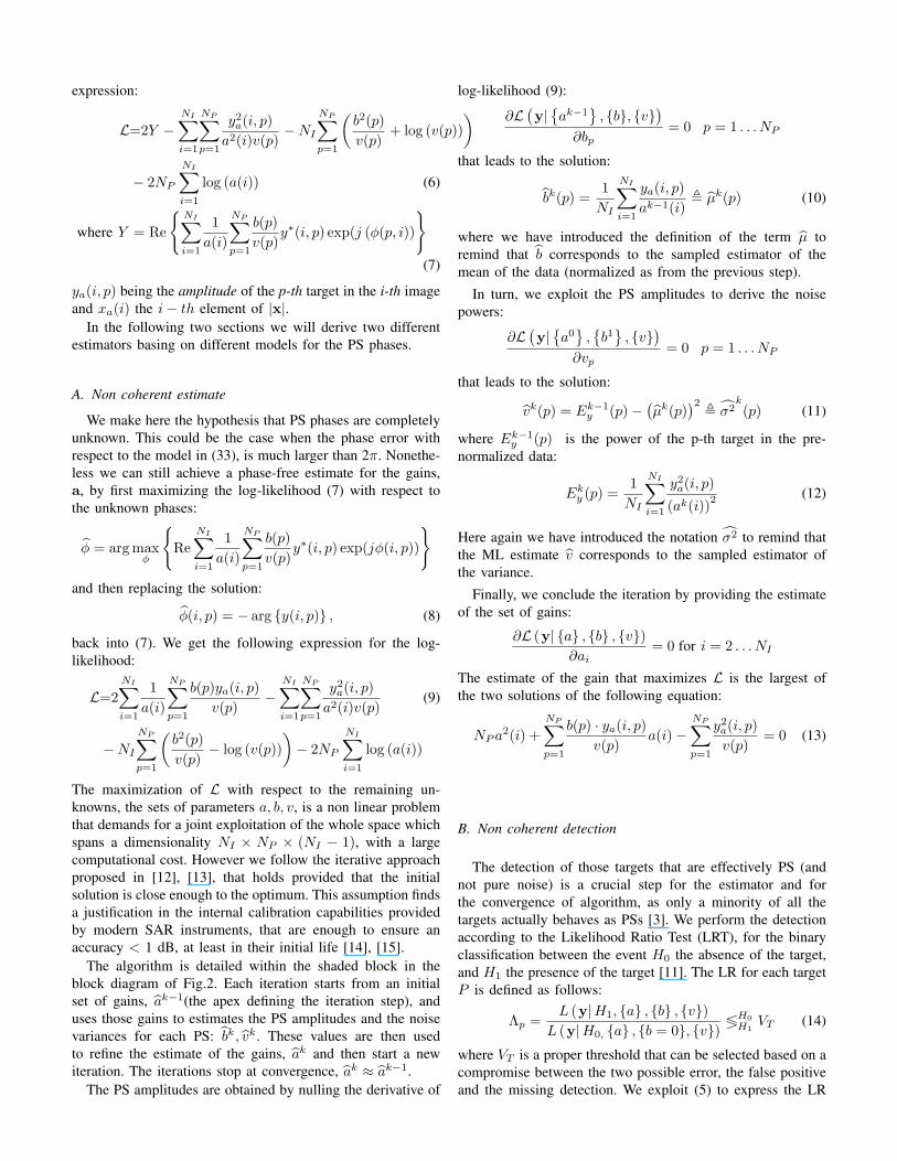
The major result of the technique, that is the absolutecalibration sequence, has been plotted in Fig. 6.a for the setof the PS measures. The sequence has been shifted to 0 in thefirst sample only for visualization. It is remarkable how bothtwo series were able to predict the ERS-2 power decay, and thegains estimated by images acquired in slightly different time,but very different location and orbit, matches tightly. In orderto provide a better evaluation, the sequence of the PS and theESA transponders have been superposed after detrending forthe ERS power decay in the plot of Fig. 6.b. In the plot, therewere a few cases when one of the three transponders in thesame image gave measures much different from the other two,and this happens for each one of the transponder, even if it ismuch more frequent for TR2.

In the plot, a sensible dispersion of the estimated systemgain by both the PS and the transponders is found close tothe end of the series, in 2000. The reason is to be foundin the solar activity that has a maximum at that age. For adraft comparison, Fig. 7 plots the sunspots numbers (courtesyof SWO-NOAA) measured for each month superposed withthe absolute value of the PSCal gain in both Flevoland andMilano. We observe that, when the solar activity is close toits minimum, in 1997, the estimated gains are dispersed in lessthan 0.1 dB, whereas the dispersion increases when movingat periods of higher solar activity, and there is a noticeablecorrelation between the most dispersed gains and the peaks inthe sunspots.

We emphasize the fact that the 0.1 dB dispersion is thecombination of both the system gain fluctuation, due not onlyto the solar activity, and thus the PSCal accuracy may be nottoo far from the very theoretical value 0.006 dB predicted by(31) for 66000 of PS. However, for a better comparison, weanalyzed the series where the three transponders in Flevolandgave consensus, when measures were dispersed in less thansay half of a dB. There were only seven of such imagesfrom the original 46, and they are represented in Fig. 8.

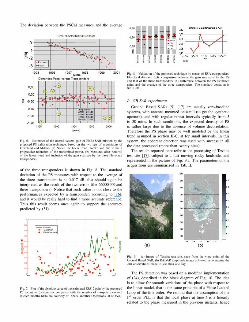
The deviation between the PSCal measures and the average

Fig. 6. Estimates of the overall system gain of ERS2-SAR mission by theproposed PS calibration technique, based on the two sets of acquisitions ofFlevoland and Milano. (a) Notice the linear trend, known and due to the aprogressive reduction of the transmitted power. (b) Measures after removalof the linear trend and inclusion of the gain estimate by the three Flevolandtransponders.

of the three transponders is shown in Fig. 8. The standarddeviation of the PS measures with respect to the average ofthe three transponders is ∼ 0.017 dB, that should again beinterpreted as the result of the two errors (the 66000 PS andthree transponders). Notice that such value is not close to theperformances expected by a transponder, according to [16],and it would be really hard to find a more accurate reference.Thus this result seems once again to support the accuracypredicted by (31).

1995 1996 1997 1998 1999 2000 20010

0.1

0.2

0.3

0.4

0.5

0.6

0.7

0.8

0.9

1

abs(

gain

) dB

0

200

# S

unsp

ots

SunspotsPScal MilanPScal Flevoland

Fig. 7. Plot of the absolute value of the estimated ERS-2 gain by the proposedPS technique (detrended), compared with the number of sunspots measuredat each months (data are courtesy of Space Weather Operations, at NOAA).

-0,20

0,30

PScal

-0,70

[dB

]

22/12/95

05/04/96

01/11/96

01/01/97

30/05/97

30/01/98

17/09/99

PScal

TR1

TR2

TR3

[dB]

Fig. 8. Validation of the proposed technique by means of ESA transponders,Flevoland data set. Left: comparison between the gain measured by the PSand that of the three transponders. (b) Difference between the PS-estimatedgains and the average of the three transponders. The standard deviation is0.017 dB.

B. GB SAR experiments

Ground Based SARs [5], [17] are usually zero-baselinesystems, with antenna mounted on a rail (to get the syntheticaperture), and with regular repeat intervals typically from 5to 30 mins. In such conditions, the expected density of PSis rather large due to the absence of volume decorrelation.Therefore the PS phase may be well modeled by the lineartrend assumed in section II-C, at for small intervals. In thissystem, the coherent detection was used with success in allthe data processed (more than twenty sites).

The results reported here refer to the processing of Tessinatest site [17], subject to a fast moving rocky landslide, andrepresented in the picture of Fig. 9.a. The parameters of theacquisitions are summarized in Tab. II.

Fig. 9. (a) Image of Tessina test site, seen from the view point of theGround Based SAR, (b) RADAR amplitude image achieved by averaging the218 observations made in less than one day.

The PS detection was based on a modified implementationof (24), described in the block diagram of Fig. 10. The ideais to allow for smooth variations of the phase with respect tothe linear model, that is the same principle of a Phase-LockedLoop of the first order. We remind that the assumption of theIst order PLL is that the local phase at time t is a linearlyrelated to the phase measured in the previous instants, hence

the model in (25) [18]. However, we extended this model tobe non-causal, that led to replace the closed loop with thescheme in Fig. 10. The instantaneous frequency estimator used20 samples (corresponding to approximately 100 mins), forwhich good performances can be achieved according to theplots in Fig. 3. A total of more than 30000 PS were detected

∠

∫

Low pass

filter

+

-

+

+)(ˆ tϕy(t)

Phase comparator

2πt∫

Instantaneous

frequency

estimator )(ˆ tf i

2πt

Fig. 10. Block diagram of the algorithm used to estimate the phase of eachPS in the GB RADAR.

in an area of 1 km, range, × 400 m, azimuth: that large numberis due to the absence of clutter in the rocky landslides area.

In order to compare the coherent and the non-coherentapproach, we have computed a 2D histogram of all the PSsas a function of both the estimated complex coherence, in (26)and the estimated dispersion of the amplitudes, in (17). Theresult, shown in Fig. 11.a, provides a clear evidence of thesuperior performances of the coherent detection with respectto the non-coherent one. This is a straight consequence ofthe model assumed in the appendix, as it is shown in Fig.11.b, that represents the same 2D histogram of Fig. 11.a,but achieved from a simulation of the ideal PS model. Theevidence of the figure is that the best targets are characterizedby high values in both indexes, however a significant part ofthe stable targets could not be identified basing on the noncoherent detection. This is indeed the major outcome of thetechnique in the GB case, where the interest is much more inthe detection of the PSs and the images, than the actual imageset normalization. Notwithstanding, the gains estimated by the

.3 .4 .5 .6 .7 .8 .9 1

2

4

6

8

10

0.894

0.970

0.986

0.992

0.995

(a) (b).3 .4 .5 .6 .7 .8 .9 1

Fig. 11. Bidimensional histogram of the number of stable targets PS in thecase of Tessina site, (a), and by a simulation according to the PS model inthe appendix, (b), assuming a uniform distributions of PS with the quality.Horizontal axes: estimated complex coherence, γC . Vertical axes is quoted inboth the estimated dispersion index and the estimated amplitude correlation,γN .

PS based calibration are plotted in Fig. 12, and compared withthe measures of the mean eco power. In this case we didnot have any calibrated reflector to compare with, therefore

we rely just in the intrinsic stability of the system, and itsinternal calibration. It is anyhow interesting to notice that thegain variations measured by the PS technique are in the orderof ±0.2dB at most, whereas the echo power changes of ±1dB,with fluctuations correlated with the scene conditions. Noticefor example the average increase of clutter by 2 dB from 9am to 1 pm, that is not at all found in the PS measures.

-1

-0.5

0

0.5

1

1.5

dB

Mean eco power

Mean PS power

18:00 9:07 13:19

0 200 400 600 800 1000 1200 1400-1

Acquisition times [mins]

Fig. 12. Estimate of the amplitude of each image in Tessina test site madeby averaging all the samples (mean echo power) and by the PS calibration.

V. CONCLUSIONS

A technique has been discussed to provide the radiometriccalibration of a stack of SAR images by exploiting the naturalstable targets (PS) in the image themselves and a set ofabsolutely calibrated images. The technique is subject to (1)the availability of repeated-pass images, like for differentialinterferometric applications, and (2) the presence of a suitablenumber of long-term coherent and independent targets inthe scene, that in turn excludes coarse resolution systems[19]. This second limit does not apply for global observationsystems, like the SB SAR, however, it can affect GB SARacquisitions, like in the case of pure vegetation, or for veryhomogenous scenes (like bare soil), and particularly for smallobservation times.

Two different estimators have been discussed, one that im-plements a coherent phase-based detection of the PSs and theother an incoherent amplitude-based one. The first approachis able to detect much more targets, and requires less images,say more than five, leading to very quick boot-strap that canexploit the commissioning phase in spaceborne missions. Onthe other hand the non coherent estimator is much simpler andmore robust in presence of fast phase fluctuations, or errordue to non-compensated atmospheric phase screen, and thuscomplement the first. The PSCal method is then completedby merging the PS-based estimates with external measures bya regression of the two series, whereby the regression errorqualifies both series.

The technique has been validated with two set of ERS-2 dataset, and an accuracy better of 0.017 dB (standarddeviation) was measured by using as reference the average ofthree transponders. Moreover, a gain dispersion < 0.1 dB wasnoticed in acquisitions in the period of low solar activity (oneyear). In the GB case, a system stability better than 0.2 dB wasfound, to be compared with the average clutter fluctuations ofmore than 2 dB.

Such PSs based calibration approach is characterized byits intrinsic robustness, due to the consensus of many naturaltargets. The technique paves the road for the development ofsystems able to perform very accurate and frequent verificationand calibration of the system gain, the antenna pattern and thefull polarimetric information, including Faraday rotations evenin a dual-polarized system, as well as the geometric accuracy.

VI. ACKNOWLEDGMENT

The authors wish to thank the European Space Agency andin particular B. Rosich and for providing the ERS-2 data setsand for supporting the development of the technique. Likewise,they wish to thank G. Bernardini and P. Ricci of Ingegneria DeiSistemi for the Tessina dataset. Special thanks to D. Giudicifor the fine tuning of the processor and the PSCal code andto P. Rizzoli for the testing on ERS-2 datasets. Finally, theauthors wish to thank F. Rocca for his inputs and the fruitfuldiscussions.

APPENDIX

The model of a set of SAR observations of the samePermanent (or coherent) Scatterer is formulated in [3] asfollows:

s(n) = b exp(jφ(n)) + w(n) (32)φ(n) = φ0 + k

TbN (n)q + kvbT (n)v + α(n) + e(n) (33)

where b is the amplitude of the PS, φ the phase and w anoise terms, that corresponds to the contribution of thermalnoise and clutter variation, and may be assumed as normal,circular distributed. The PS phase, in turn, is expressed asresultant of the following contributions:

- the target’s phase measured in correspondence of thereference image (or master), φ0;

- a contribution due to the target elevation, q, scaledproportionally to the normal baseline bN between the n-thimage and the master. The constant scale term, k

T, depends

on the parameters of the RADAR and the geometry. The linearrelation holds if the elevation is much smaller than the targetrange;

- a linear motion, modeling a deformation with rate kv , andproportional to the time interval bT (n) (or temporal baseline)between the n-th image and the master;

- a term modeling the propagation disturbances, α(n), anddefined as Atmospheric Phase Screen (APS);

- a residual noise term, e(n).Notice that this model leads to a good PS provided that both

the noise terms w(n) and e(n) are small.We can show that these terms adds up together under that

assumption, in fact let us introduce the noise term v definedas follows:

v = w exp(−jφ)

The circular property of complex noise ensure that the statis-tics of v are the same of w. Therefore we can express the dataas follows:

s = b exp(jφ) + w = (b+ v) exp(jφ)= (b+ vr + jvi) exp(jφ) (34)

vr and vi being the real and imaginary components. Further-more, for large signal to noise ratio, v = σ2

w � A2

∠(s) = φ+ arctan(

vib+ vr

)' φ+

vib

This proves the equivalence between the noise terms w (32)and the e in (33). This property, that is a direct consequence ofthe very simple model (32), states that the amplitude stabilityimplies the phase stability and vice versa that is indeed acrucial point in the Interferometric PS technique, in [3], andalso for our applications. We have observed in processingmany GB SAR datasets that the model is very reliable, asonly in a few cases we find a small amount of targets that arestable in amplitude and not in phase.

This result implies that the propagation disturbances can behandled like clutter or thermal noise, provided that the error issmall, that is really the case assessed by the many interferomet-ric PS processing reported in literature. The basic assumptionunderneath the model is then that the target keeps its coherencefor a long term, at least longer than the observation interval.The coherence computed according to (32):

γnm =E [s(n)s∗(m)]√

E[|s(n)|2

]E[|s(m)|2

]=

1

1 + σ2w

A2

E [exp(je)] exp(jφnm)

=1

1 + SNR−1exp

(12σ2e

)exp(jφnm)

where φnm = φn − φm

As an example, the Fig. 13.a draws the coherence matrixmeasured in a rocky area in Tessina, that represents a PS as itscoherence is constant, high and stable throughout the wholeexperiment, despite the weather conditions (rain during night).On the opposite, the coherence of a vegetated target is shownin Fig. 13.b: notice that coherence is low even in the shorttime. The histogram of coherence in Tessina test site, in Fig.11 has a mode of about γ = 0.996, that corresponds to a phasestandard deviation of 0.1 rad, and this justify the high qualityof the medium PS, a verification that the two models (32) and(34) are to be retained equivalent.

In summary, a PS may well be considered as a point target,a corner reflector, in presence of thermal and clutter noise.The Signal-to-Noise-Ratio defines the PS quality.

REFERENCES

[1] Anthony Freeman. SAR calibration: An overview. IEEE Transactionson Geoscience and Remote Sensing, 30(6):1107–1121, November 1992.

[2] H Laur, P Bally, P Meadows, J Sanchez, B Schaettler, E Lopinto, andD Esteban. Derivation of the backscattering coefficient σ0 in ESAERS SAR PRI products. Technical Report ES-TN-RS-PM-HL09, ESA,September 2002. Issue 2, Rev. 5d.

[3] Alessandro Ferretti, Claudio Prati, and Fabio Rocca. Permanent scat-terers in SAR interferometry. IEEE Transactions on Geoscience andRemote Sensing, 39(1):8–20, January 2001.

[4] Andy Hooper, Howard Zebker, Paul Segall, and Bert Kampes. A newmethod for measuring deformation on volcanoes and other non-urbanareas using InSAR persistent scatterers. Geophysical Research Letters,31:L23611, doi:10.1029/2004GL021737, December 2004.

50 100 150 200

20

40

60

80

100

120

140

160

180

200

0

0.1

0.2

0.3

0.4

0.5

0.6

0.7

0.8

0.9

Coherent target

(a) (b)

Vegetation (brush)

18:07

09:01

13:19

Fig. 13. Correlation matrixes measured by GB SAR, Tessina test site. Axesare sorted by acquisition time. (a) A rocky area, behaving like a PS. (b) Avegetated target (brush) in the same dataset.

[5] Linhsia Noferini, Massimiliano Pieraccini, Deniele Mecatti, Guido Luzi,Carlo Atzeni, Andrea Tamburini, and Massimo Broccolato. Permanentscatterers ananlysis for atmospheric correction in ground-based SARinterferometry. IEEE Transactions on Geoscience and Remote Sensing,43(7):1459–1471, July 2005.

[6] Timothy H Dixon, Falk Amelung, Alessandro Ferretti, Fabrizio Novali,Fabio Rocca, Roy Dokka, Giovanni Sella, Sang-Wan Kim, ShimonWdowinski, and Dean Whitman. Space geodesy: Subsidence andflooding in New Orleans. Nature, 441:587–588, June 2006.

[7] D. Perissin and A. Ferretti. Urban-target recognition by means ofrepeated spaceborne sar images. Geoscience and Remote Sensing, IEEETransactions on, 45(12):4043–4058, Dec. 2007.

[8] S. Tebaldini. On the role of phase stability in sar multi-baselineapplications. Geoscience and Remote Sensing, IEEE Transactions on,Submitted.

[9] G Antonello, N Casagli, P Farina, L Guerri, D Leva an G Nico, andD Tarchi. SAR interferometry monitoring of landslides on the strombolivolcano. In Third International Workshop on ERS SAR Interferometry,‘FRINGE03’, Frascati, Italy, 1-5 Dec 2003, 2003.

[10] D. Mecatti, L. Noferini, G. Macaluso, M. Pieraccini, G. Luzi, C. Atzeni,and A. Tamburini. Remote sensing of glacier by ground-based radarinterferometry. pages 4501–4504, July 2007.

[11] Harry L Van Trees. Detection, Estimation, and Modulation Theory, PartI. John Wiley & Sons, New York, 1968.

[12] Davide D’Aria, Alessandro Ferretti, Davide Giudici, AndreaMonti Guarnieri, Paola Rizzoli, and Fabio Rocca. Tecnica per lacalibrazione radiometrica di sensori SAR. Patent, No., 2008.

[13] Davide Giudici, Andrea Monti Guarnieri, Paola Rizzoli, and FabioRocca. Permanent scatterers for sar sensor calibration. In EuropeanConference on Synthetic Aperture Radar, Friedrichshafen, Germany, 2–5 June 2008, pages 1–4, 2008.

[14] B Rosich, PJ Meadows, A. Monti Guarnieri, D D’Aria, M Tranfaglia,M Santuari, and I. Navas. Review of ASAR performance and productquality evolution after 5 years of operations. In ESA ENVISAT Sympo-sium, Montreux, Switzerland, 23–27 April 2007, page 6 pp, 2007.

[15] P Meadows, B Rosich, A Pilgrim, and M Tranfaglia. ERS-2 SARperformance and product evolution. In ESA ENVISAT Symposium,Montreux, Switzerland, 23–27 April 2007, page 6 pp, 2007.

[16] H Jackson, I Sinclair, and S Tam. ENVISAT ASAR precision transpon-ders. In CEOS SAR Workshop, Toulouse, France, 26-29 October 1999,page ., 1999.

[17] G Bernardini, D D’Aria, A Monti Guarnieri, F Rocca, and P Ricci.Impact of atmospheric phase screen and target decorrelation of groundbased SAR differential interferometry. In European Conference onSynthetic Aperture Radar, Friedrichshafen, Germany, 2–5 June 2008,pages 1–4, 2008.

[18] John Wiley and Sons Ltd, editors. Communication Systems, 4th ed. NewYork, 2001.

[19] A Monti Guarnieri. ScanSAR interferometric monitoring using the PStechnique. In ERS/ENVISAT Symposium, Gothenburg, Sweden, 16–20October 2000, page 7, March 2001.