bistatic sar atr

ELECTRO-MAGNETIC REMOTE SENSING DEFENCE TECHNOLOGY CENTRE (EMRS-DTC)

Bistatic SAR ATR

A.K. Mishra and B. Mulgrew

Abstract: With the present revival of interest in bistatic radar systems, research in that area hasgained momentum. Given some of the strategic advantages for a bistatic configuration, and tech-nological advances in the past few years, large-scale implementation of the bistatic systems is ascope for the near future. If the bistatic systems are to replace the monostatic systems (at least par-tially), then all the existing usages of a monostatic system should be manageable in a bistaticsystem. A detailed investigation of the possibilities of an automatic target recognition (ATR) facil-ity in a bistatic radar system is presented. Because of the lack of data, experiments were carried outon simulated data. Still, the results are positive and make a positive case for the introduction of thebistatic configuration. First, it was found that, contrary to the popular expectation that the bistaticATR performance might be substantially worse than the monostatic ATR performance, the bistaticATR performed fairly well (though not better than the monostatic ATR). Second, the ATR per-formance does not deteriorate substantially with increasing bistatic angle. Last, the polarimetricdata from bistatic scattering were found to have distinct information, contrary to expert opinions.Along with these results, suggestions were also made about how to stabilise the bistatic-ATR per-formance with changing bistatic angle. Finally, a new fast and robust ATR algorithm (developed inthe present work) has been presented.

1 Introduction

As per the standard definition [1], the original radar systemswere bistatic, as they had physically separated transmittersand receivers. Soon, monostatic radars replaced them,because of the ease of design and compactness. Recently,there has been a revived interest in bistatic radars. This isbecause of a range of strategic advantages of a bistatic con-figuration as compared with its monostatic counterpart [2].Second, a bistatic configuration is the first step towards a mul-tistatic configuration, which may confer additional oper-ational and strategic advantages like the netted radar system[3].From the user point of view, replacing an existing mono-

static system should be justified by an equally apt radarsystem, which can handle the existing usages and offerother added advantages. One such usage of primary import-ance in most of the existing airborne (monostatic) radarsystems is the facility of automatic target recognition(ATR) (to various degrees of autonomy). In the recentyears some studies have come out in the open literature,describing object recognition using passive radars [4, 5].Passive radars are, strictly speaking, bistatic radars.However, there has been no work in the open literaturereporting ATR algorithms for airborne bistatic syntheticaperture radar (SAR)-based ATR. In the present work, wehave dealt with this problem of bistatic ATR using airborneSAR images. There are quite a few novelties involved inthis work. First of all, a study of bistatic ATR in itself isof huge practical importance and is a novel work in itself.

# The Institution of Engineering and Technology 2007

doi:10.1049/iet-rsn:20060160

Paper first received 29th November 2006 and in revised form 28th August 2007

The authors are with Institute for Digital Communication (IDCOM), Universityof Edinburgh, Edinburgh, UK

E-mail: [email protected]

IET Radar Sonar Navig., 2007, 1, (6), pp. 459–469

Looking at the present level of bistatic radar develop-ment, there was a lack of database to carry out these ATRexercises. The second novelty of the current work involvesthe development of the setup for the generation of syntheticbistatic SAR-signature database.As the data were generated synthetically, the data of all

different combinations of polarisations were simulated. Inlooking for the information content in the bistatic multipolardata, it was found that the bistatic multipolar data containinformation about the target, in contrast to what has beenpredicted by some researchers [6].Finally, a new algorithm for ATR has been developed,

based on a principal component analysis (PCA)-basednearest neighbour (NN) approach, which being simple andextremely fast, is expected to be of practical importance [7].The paper is arranged as follows. Section 2 consists of a

brief overview of a generic SAR ATR system. This is fol-lowed by a discussion of the challenges involved in devel-oping bistatic SAR ATR, in Section 3. In Section 4, wediscuss the algorithms used in the present work, and the par-ameters on which to compare the monostatic and the bistaticATR results. The next section deals with the basis on whichwe looked for information in bistatic multipolar data.Finally, we present the results. This is followed by thesection where discussions on the limitations of the presentstudy are presented. The paper ends with a discussion ofthe major conclusions.

2 SAR ATR: an overview

There has been a great deal of research in the field of radar-based ATR systems. This is mainly because of the all-weather and covert abilities of a radar system, and theincreasing image-resolution possible using SAR-imaging.The complexities in this field are numerous. The way aradar image is generated makes SAR image recognitionproblem different from the general optical image recog-nition problem. The process of SAR image formation of a

459

target or a scene is a sensitive function of the range of thesystem and scene parameters. Hence, the ATR algorithmsneed to be extremely robust to any variation in theimaging system and scene parameters. To add to the com-plexity, the strategic nature of the usage demands a muchlower acceptable error-in-classification level than that isacceptable in many other classification exercises. There isalso the problem of getting decent training data, whichcan be both expensive and time consuming. There are afew reports handling end-to-end SAR ATR exercises inthe open literature [8, 9], and many other diverseapproaches towards handling exclusively the task of targetrecognition. Some of the reports with excellent ATR per-formance reported have used a range of classification algor-ithms, starting from simple template matching [9] andGaussian-modelled Bayesian approach [10] to those invol-ving more involved algorithms such as the support vectormachine approaches [11].

3 Bistatic SAR ATR experiments: challenges andanswers

One of the basic requirements of any target classificationexercise is the database of target signatures, on which thealgorithms are to be tested. For the stand-alone problemof monostatic ATR-algorithm development, there is awidely accepted archive of SAR images of a widevariety of targets [12]. Unlike the monostatic counter-part, in the bistatic case there are no datasets in thepublic domain, which could be used in validation andanalysis of any classification algorithm. This was amajor challenge for the present work. Even thoughthere are some field-generated bistatic SAR images,they were not exhaustive enough to be used in an ATRexercise. As the next best alternative, an electro mag-netic modelling tool [13] was used to model targetsand to generate a database of bistatic SAR image clips(A target clip is the SAR image of the target, with theimage of the target at the centre of the image. In an auto-matic target recognition exercise, after the detectionstage, a particular part of the original SAR image ofthe scene is taken for further processing. This part ofthe SAR image, with the target at its centre, is termedas the target-clip. In the present work, only the classifi-cation problem is handled. Hence, the inputs taken arethe target image clips. Though no clipping operation isdone, for convention, the word target clip is usedthrough out.) [14].In modelling the targets (military land vehicles), only

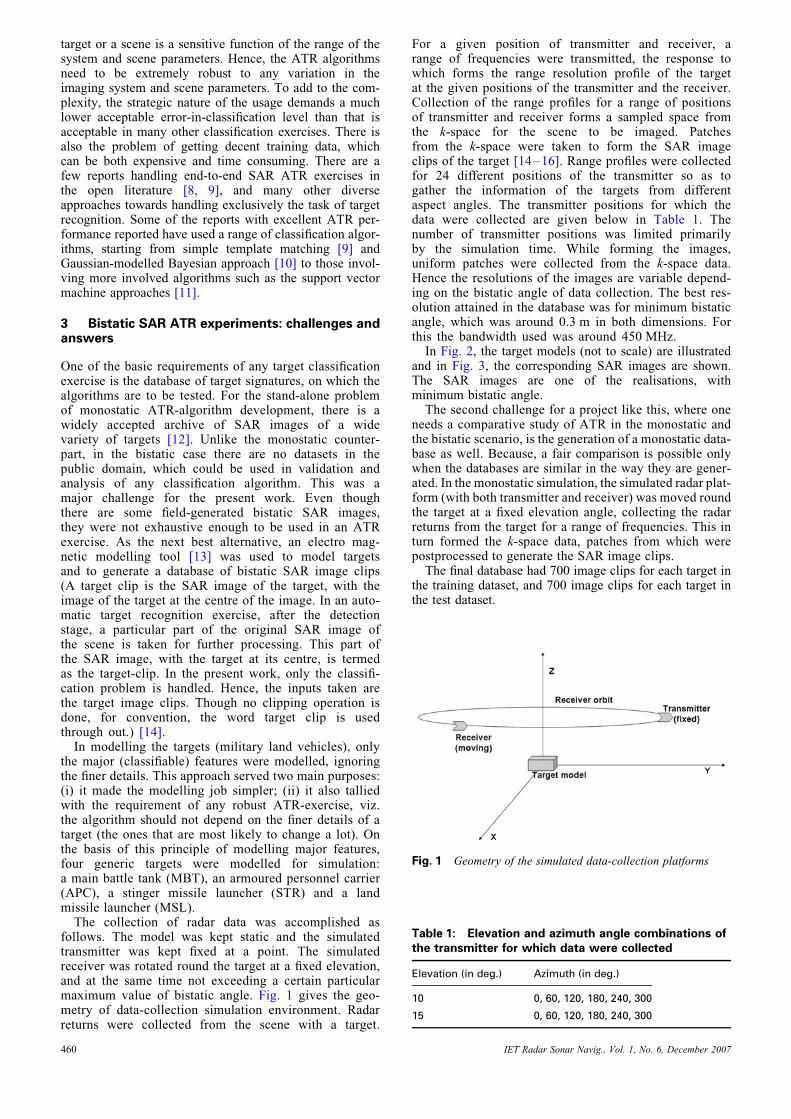
the major (classifiable) features were modelled, ignoringthe finer details. This approach served two main purposes:(i) it made the modelling job simpler; (ii) it also talliedwith the requirement of any robust ATR-exercise, viz.the algorithm should not depend on the finer details of atarget (the ones that are most likely to change a lot). Onthe basis of this principle of modelling major features,four generic targets were modelled for simulation:a main battle tank (MBT), an armoured personnel carrier(APC), a stinger missile launcher (STR) and a landmissile launcher (MSL).The collection of radar data was accomplished as

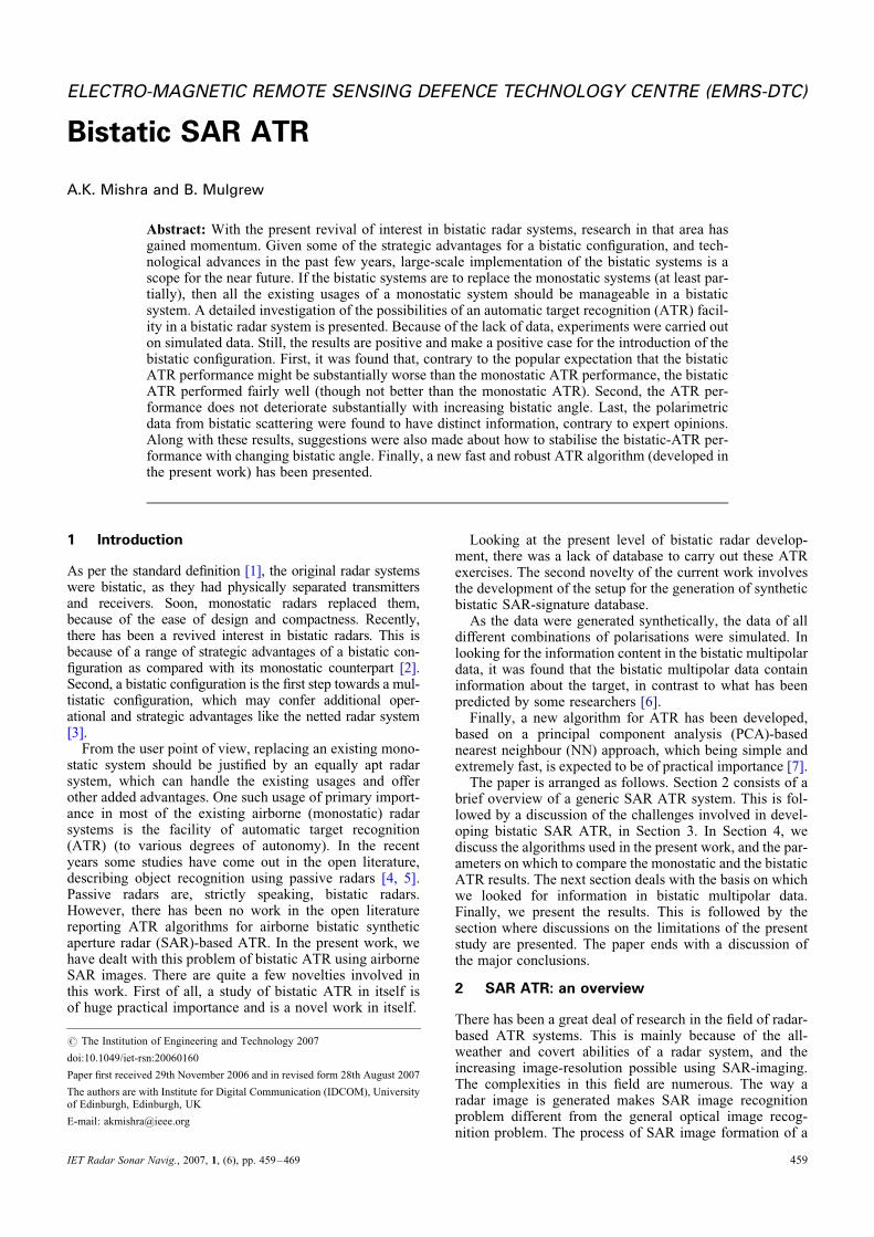
follows. The model was kept static and the simulatedtransmitter was kept fixed at a point. The simulatedreceiver was rotated round the target at a fixed elevation,and at the same time not exceeding a certain particularmaximum value of bistatic angle. Fig. 1 gives the geo-metry of data-collection simulation environment. Radarreturns were collected from the scene with a target.

460

For a given position of transmitter and receiver, arange of frequencies were transmitted, the response towhich forms the range resolution profile of the targetat the given positions of the transmitter and the receiver.Collection of the range profiles for a range of positionsof transmitter and receiver forms a sampled space fromthe k-space for the scene to be imaged. Patchesfrom the k-space were taken to form the SAR imageclips of the target [14–16]. Range profiles were collectedfor 24 different positions of the transmitter so as togather the information of the targets from differentaspect angles. The transmitter positions for which thedata were collected are given below in Table 1. Thenumber of transmitter positions was limited primarilyby the simulation time. While forming the images,uniform patches were collected from the k-space data.Hence the resolutions of the images are variable depend-ing on the bistatic angle of data collection. The best res-olution attained in the database was for minimum bistaticangle, which was around 0.3 m in both dimensions. Forthis the bandwidth used was around 450 MHz.In Fig. 2, the target models (not to scale) are illustrated

and in Fig. 3, the corresponding SAR images are shown.The SAR images are one of the realisations, withminimum bistatic angle.The second challenge for a project like this, where one

needs a comparative study of ATR in the monostatic andthe bistatic scenario, is the generation of a monostatic data-base as well. Because, a fair comparison is possible onlywhen the databases are similar in the way they are gener-ated. In the monostatic simulation, the simulated radar plat-form (with both transmitter and receiver) was moved roundthe target at a fixed elevation angle, collecting the radarreturns from the target for a range of frequencies. This inturn formed the k-space data, patches from which werepostprocessed to generate the SAR image clips.The final database had 700 image clips for each target in

the training dataset, and 700 image clips for each target inthe test dataset.

Fig. 1 Geometry of the simulated data-collection platforms

Table 1: Elevation and azimuth angle combinations ofthe transmitter for which data were collected

Elevation (in deg.) Azimuth (in deg.)

10 0, 60, 120, 180, 240, 300

15 0, 60, 120, 180, 240, 300

IET Radar Sonar Navig., Vol. 1, No. 6, December 2007

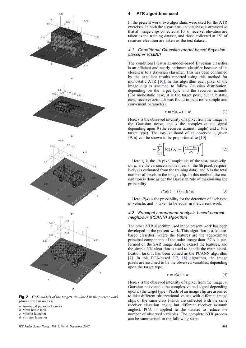
Fig. 2 CAD models of the targets simulated in the present work(dimensions in metres)

a Armoured personnel carrierb Main battle tankc Missile launcherd Stringer launcher


4 ATR algorithms used

In the present work, two algorithms were used for the ATRexercises. In both the algorithms, the database is arranged sothat all image clips collected at 108 of receiver elevation aretaken as the training dataset, and those collected at 158 ofreceiver elevation are taken as the test dataset.

4.1 Conditional Gaussian-model-based Bayesianclassifier (CGBC)

The conditional Gaussian-model-based Bayesian classifieris an efficient and nearly optimum classifier because of itscloseness to a Bayesian classifier. This has been confirmedby the excellent results reported using this method formonostatic ATR [10]. In this algorithm each pixel of theimage clip is assumed to follow Gaussian distribution,depending on the target type and the receiver azimuth(For monostatic case, it is the target pose, but in bistaticcase, receiver azimuth was found to be a more simple andconvenient parameter).

r ¼ s(u, a)þ w (1)

Here, r is the observed intensity of a pixel from the image, wthe Gaussian noise, and s the complex-valued signaldepending upon u (the receiver azimuth angle) and a (thetarget type). The log-likelihood of an observed r, givenfu, ag can be shown to be proportional to [10]

�XNi¼1

log (si)þri � mi

si

� �2" #

(2)

Here ri is the ith pixel amplitude of the test-image-clip,si, mi are the variance and the mean of the ith pixel, respect-ively (as estimated from the training data), and N is the totalnumber of pixels in the image-clip. In this method, the rec-ognition is done as per the Bayesian rule of maximising theprobability

P(ajr) ¼ P(rja)P(a) (3)

Here, P(a) is the probability for the detection of each typeof vehicle, and is taken to be equal in the current work.

4.2 Principal component analysis based nearestneighbour (PCANN) algorithm

The other ATR algorithm used in the present work has beendeveloped in the present work. This algorithm is a feature-based classifier, where the features are the approximateprincipal components of the radar image data. PCA is per-formed on the SAR image data to extract the features, andthe simple NN algorithm is used to handle the main classi-fication task. It has been coined as the PCANN algorithm[7]. In this PCA-based [17, 18] algorithm, the imagepixels are assumed to be the observed variables, dependingupon the target type.

r ¼ s(a)þ w (4)

Here, r is the observed intensity of a pixel from the image, wGaussian noise and s the complex-valued signal dependingupon a (the target type). Pixels of an image clip are assumedto take different observational values with different imageclips of the same class (which are collected with the samereceiver elevation angle, but different receiver azimuthangles). PCA is applied to the dataset to reduce thenumber of observed variables. The complete ATR processcan be summarised in the following steps:

461

Fig. 3 Bistatic SAR images of the targets modelled (average bistatic angle of imaging is 158)a Armoured personnel carrierb Main battle tankc Missile launcherd Stringer launcher

† For each image clip, the pixels are stacked into a vector,and the consecutive image clips are taken as different obser-vational vectors.† All consecutive image-pixel vectors are arrangedtogether to form the observation matrix. In the observationmatrix, each column corresponds to an image clip and con-secutive columns are formed out of consecutive image-clipsfrom the training dataset.† The observation matrix is normalised (to have unity var-iance), and all the observation vectors are made zero centred(by removing the mean). Let the resulting observationmatrix be denoted by X.† From this observation matrix, the covariance matrix isfound for the observation vector.

Q ¼ XHX (5)

† Then the eigenvalue operation is applied on Q to get theeigen vectors.† Eigenvectors corresponding to n largest eigenvalues arestacked together to form matrix V. (n is to be determinedfrom the dataset, to represent maximum amount of variance

462

present in the dataset. For all the present exercises, n ¼ 20was found to be an optimum choice.)† Using this matrix V, the training dataset is reduced indimension to n. The final output from the training phase isthe database in reduced dimension and the convertingmatrix V.† In the test phase, the test image clip is reduced in dimen-sion using the converting matrix V.† Next, the Euclidean distance is found from each point inthe training database. The class of target, giving the leastdistance, is decided as the class of the test image clip.

There are two major advantages in the PCANN algor-ithm. First of all, as it handles the data in the PC-domain(which is of much reduced dimension than the originaldataset), computationally the algorithm is extremely fast.Second, as shown in [19], the data extracted by the PCAanalysis of SAR images closely correspond to the infor-mation obtained by scattering centre analysis. Scatteringcentre analysis has been proved to be a powerful methodin SAR ATR [20]. Hence, the PCANN ATR algorithm


can give most of the advantages of a scattering-centre-basedATR approach, at a much lower computational cost. Ananalysis showing the correspondence between PCA andthe scattering centre analysis of radar data is given in theAppendix 1. Further it can be mentioned here that 20 prin-cipal components have been used in all the exercisesreported in the current paper. This was because of tworeasons. First, PCA of the SAR images generated in thecurrent project showed that around 20 principal componentswill account for 99% of the data-variance. This is anaccepted way of determining the number of PCs to beused for a particular task [17].

4.3 Parameters of comparison

The major thrust of the present work is the comparison ofthe relative performance of the bistatic ATR and the mono-static ATR. For detailed analysis of the PCANN algorithm,reader s are requested to refer to one of our earlier publi-cations [21], which explains PCANN ATR algorithm asapplied to monostatic SAR ATR. In another publicationof ours [22], the PCANN ATR algorithm has been analysedfor its advantages and use for bistatic SAR ATR. However,for the sake of continuity, the receiver output characteristic(ROC) curves for the two algorithms, CGBC and PCANN,will be presented.In performing the comparison, the following questions

will be addressed. These are some of the issues ofimmense practical importance, given the ever impendingquestion of the choice between monostatic and bistaticsystems.

† Can the performance of the bistatic ATR match the per-formance obtained from a monostatic system?† What is the figure of deterioration in the ATR perform-ance, for an increase in the bistatic angle of operation?† If there is any loss of performance, can it be made up for?

5 Information from bistatic fully polarised data

In the present work, a synthetic database has been used.Hence, the fully polarimetric data were available (for thebistatic configuration). A limited study was undertaken toexamine if there is any possible information from thefully polarimetric data in bistatic configuration and theuse of the same for improving the bistatic SAR ATR.The fully polarimetric radar systems have been the

subject of intense study and research for the past fewdecades. It has been shown that the fully polarimetric datain monostatic configuration give a lot of informationabout the physical features of the target. Especially remark-able is the work by Huynen [6], which gave a one-to-onecorrespondence between the physical features of a targetand the parameters derived from the fully polarimetricdata collected using a monostatic radar system. However,because of the large number of combinations of transmitterand receiver, involved in bistatic SAR imaging, Huynen hasexpressed strict reservation against any information contentin the bistatic fully polarimetric data [6].In the rest of this section some of the basics of radar

polarimetry will be described. In the right-hand Cartesiancoordinate system (x, y, z), if the z-direction is taken asthe direction of propagation for the electromagnetic wave,the field (For simplicity we deal only with the electricalwave in this work, though similar treatment could be done


taking the magnetic wave instead.) can be represented as

E ¼ uxEx þ uyEy (6)

Here ux and uy are unit vectors (vectors of unit amplitude)in the x and the y directions. In the simplest horizontal andvertical (HV) basis, this expression becomes

E ¼ uhEh þ uvEv (7)

In matrix format this is represented by the Jones vector.

E ¼Eh

Ev

� �(8)

To make the data real valued and to attach some geo-metrical representation to this, the preferred way to rep-resent a polarised electromagnetic wave is the Stokesvector, g(E).

g(E) ¼1ffiffiffiffiffiffiffiffiffiffiffiffiffiffiffiffiffiffiffiffiffiffiffiffiffi

jEhj2 þ jEvj

2q

jEhj2þ jEvj

2

jEhj2� jEvj

2

2 Re {E�hEv}

2 Im {E�hEv}

2664

3775 (9)

The matrix relating the scattered and transmitted Jonesvector is called the scattering or Sinclair matrix. Similarlythe matrix relating the Stokes vectors for the transmitted,and the scattered wave is the Kennaugh matrix or the Kmatrix (which is called the Muller’s matrix M, for theforward scattering case).

g(Es) ¼ [K]g(Et) (10)

Here,Es andEt represent the scattered and the transmittedelectric fields, respectively. Elements of the K-matrix havebeen linked to the Huynen’s parameters. These parametersare represented by A0, B0, B, C, D, E, F, G and H. For themonostatic case, these parameters have been shown to havedirect relation to the physical features of the target [6]. Forthe monostatic case, the K matrix is symmetric, whereas inbistatic case it is not. Hence, the number of independent par-ameters extracted from theKmatrix ismore in a bistatic case.In one of their works, Germond et al. [23] have shown thatthere are seven more independent parameters which can bederived from the K matrix for a bistatic case.

[Kbi] ¼

A0 þ B0 þ A C þ I

C � I A0 þ B� A

H � N E � K

F � L G �M

26664

H þ N F þ L

E þ K G þM

A0 � B� A Dþ J

D� J B0 � A0 � A

37775

(11)

Here [Kbi] represents theKmatrix for the bistatic case, andA,I, J, K, L, M and N are the extra seven parameters for thebistatic case. Germond et al. [23] have given closed-formexpressions to find them using the elements of the scatteringmatrix. However, Huynen has strongly stated that any suchbistatic parameters would contain no information about thetarget [6].In the current work, to look for the information content in

the parameters derived from the K-matrix, those parameterswere extracted for each pixel of the SAR image, using thecorresponding SAR images from all the four combinationsof polarisations (HH, HV, VH and VV) [24]. These

463

derived parameters were in turn used as features of thetarget, for ATR. Two basic assumptions made in this exer-cise were:

1. The complex amplitudes of a particular pixel from theHH, HV, VH and VV polarised images give the approxi-mate elements for the Sinclair or the scattering matrix cor-responding to the scattering element represented by thatpixel. This assumption is a common one used by most ofthe researchers trying to apply polarimetry to the field ofATR [24].2. Second, it was assumed that if a certain derived par-ameter derived from the K-matrix has any physical signifi-cance, then adding that parameter as a feature shouldincrease the ATR performance.

The algorithm used for ATR is that of multi dimensionalPCANN [21] neighbour classifier. The initial SAR imagecan be modelled as a two-dimensional matrix. After gener-ating the parameters from the K-matrix for each pixel (fromthe four polarised images), it results in a set of two-dimensional matrices. For example, if k parameters are tobe considered, then for each pixel there are extracted k par-ameters. This results in k two-dimensional matrices. Thecomplete data can now be treated as a three-dimensionalmatrix. Then PCA is applied to reduce the dimensionsand the correlation in the data. Because this needs applyingPCA to each dimension of the data, this is called multidi-mensional PCA. The resulting data are much reduced insize (For example in the current exercises, the image clipswere of size 50� 50. Each such frame is reduced to 20PCs. Hence, if 8 parameters are extracted for each pixel,the original data would be 50 � 50 � 8¼ 20 000 datapoints. By applying PCA, the 8 parameters are reduced to2, and hence the final data size after a 3D PCA is just20 � 2¼ 40 data points.) and is used in turn in ATR,using the NN recognition algorithm.

6 Results and observations

6.1 Comparing the ATR algorithms

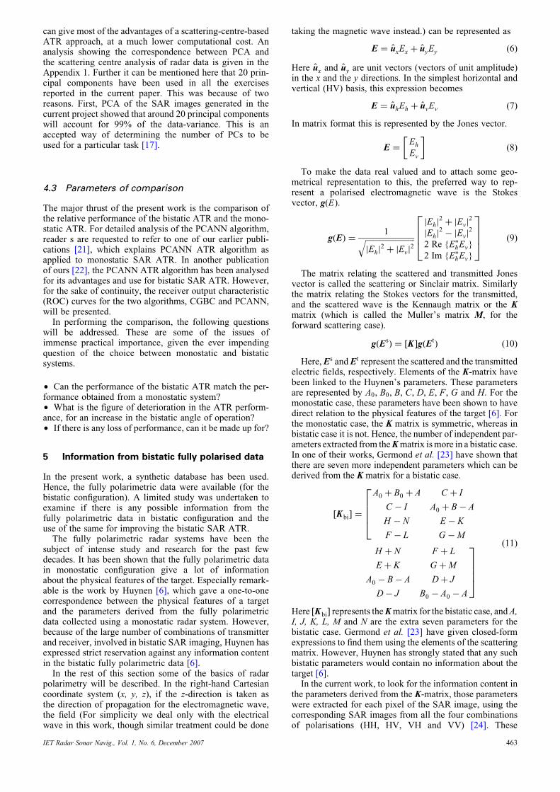
The ROCs for bistatic ATR for the two algorithms are givenin Fig. 4. For the ease of comparison, separate sets of ROCcurves have been drawn for the four types of targets

Fig. 4 ROC curves for different ATR algorithms

464

modelled. It can be observed that the ROC curves are notmuch worse than the ROC curves found for the case ofmonostatic ATR, in the open literature [10]. Hence, bistaticATR can give performance almost as good as a monostaticATR system. As far as comparison of the PCANN ATRalgorithm with the standard CGBC algorithm is concerned,it can be observed that except for the target APC, for allother types of targets, PCANN algorithm outperforms theCGBC algorithm. For the target type APC also, the per-formance of PCANN is not consistently worse than theCGBC algorithm. For the sake of conciseness, the compari-son between the monostatic and bistatic ATR performancewill be done using the PCANN algorithm only.

6.2 Monostatic against Bistatic ATR

The comparison between the monostatic and the bistaticATR is the most important contribution of the presentwork. Hence, care was taken so that the process of databasegeneration is as similar as possible for the two cases. In thebistatic case, if the transmitter is kept fixed and the receiveris moved round the target, then the bistatic angle goes onincreasing, and hence making the product image of increas-ingly course resolution. To overcome this problem, the(simulated) receiver platform was moved keeping thebistatic angle below a certain angle. For example, in oneset of the data collected, the bistatic angle was kept belowa rough value of 608. In this case, the (simulated) transmitterwas kept fixed first at the predecided elevation and at 08azimuth, and the receiver was moved at the same elevationand with the azimuth angle varying from 2608 to þ608.Next set of data was collected by keeping transmitterazimuth at 1208 and moving the receiver platform from608 till 1808. The total three sets of data were collected,so that the final data are again a patch in the k-space, withno major gap or jump. Then this patch of k-space wasused in similar manner as in the monostatic case to forman image clip data base. To see the performance of bistaticATR for different values of bistatic angles, two sets ofbistatic data were collected, one where the bistatic angleis kept less than 308 and the other where the bistatic angleis kept less than 608.The ROC curves for the three cases of monostatic,

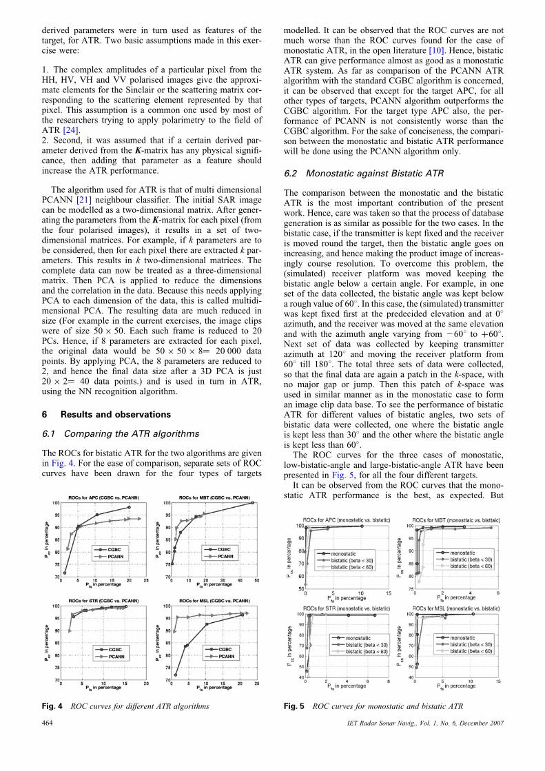
low-bistatic-angle and large-bistatic-angle ATR have beenpresented in Fig. 5, for all the four different targets.It can be observed from the ROC curves that the mono-

static ATR performance is the best, as expected. But

Fig. 5 ROC curves for monostatic and bistatic ATR


contrary to what might be expected, the bistatic ATR per-formance is not drastically worse. Another important obser-vation (again contrary to what might have been expected) isthat with increasing bistatic angle the ATR performancedoes not degrade significantly. Performance seems to bemore or less the same for the two types of bistatic dataused in these experiments. This might be because of the fol-lowing reason.In the present work, the target models used are simple and

have distinct, major physical features. Hence, the courseresolution image clips from even a 608 bistatic angle bistaticconfigurations may have most of the major features neededfor classifying that target type. However, as has been dis-cussed before, the ATR performance should not dependon the detailed features of a target.

6.3 Bistatic ATR with increased bistatic angle

With positive conclusions about the abilities of a bistatic ATRsystem, the next important issue is about the implementationof a bistatic ATR system. It is well known that the image res-olution deteriorates with the increase in the bistatic angle ofimaging. At very high values of bistatic angle, the image res-olution is extremely poor and most of the traditional usages ofa SAR-image are no longer possible. Hence, it was deemedpertinent to look into what might be an upper threshold forthe value of bistatic angle, for practical purposes. Second, isthere any way to make up for the loss of ATR performance,which comes with increasing bistatic angle of imaging?For this, the data collected were was divided into three

sets. The first one consisted of all the image clips formedwith the bistatic angle of imaging less than 608. Thesecond set was formed by those images whose bistaticangle of operation lie between 608 and 808, and the thirdset consisted of those images whose bistatic angle of collec-tion lie between 808 and 1008. Both the training and the testdatasets were divided in this manner.The results for ATR experiments in the individual sets

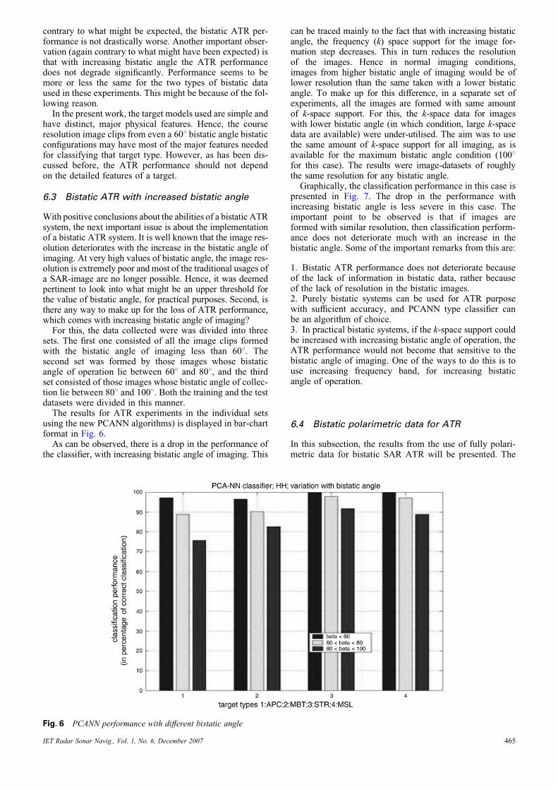
using the new PCANN algorithms) is displayed in bar-chartformat in Fig. 6.As can be observed, there is a drop in the performance of

the classifier, with increasing bistatic angle of imaging. This


can be traced mainly to the fact that with increasing bistaticangle, the frequency (k) space support for the image for-mation step decreases. This in turn reduces the resolutionof the images. Hence in normal imaging conditions,images from higher bistatic angle of imaging would be oflower resolution than the same taken with a lower bistaticangle. To make up for this difference, in a separate set ofexperiments, all the images are formed with same amountof k-space support. For this, the k-space data for imageswith lower bistatic angle (in which condition, large k-spacedata are available) were under-utilised. The aim was to usethe same amount of k-space support for all imaging, as isavailable for the maximum bistatic angle condition (1008for this case). The results were image-datasets of roughlythe same resolution for any bistatic angle.Graphically, the classification performance in this case is

presented in Fig. 7. The drop in the performance withincreasing bistatic angle is less severe in this case. Theimportant point to be observed is that if images areformed with similar resolution, then classification perform-ance does not deteriorate much with an increase in thebistatic angle. Some of the important remarks from this are:

1. Bistatic ATR performance does not deteriorate becauseof the lack of information in bistatic data, rather becauseof the lack of resolution in the bistatic images.2. Purely bistatic systems can be used for ATR purposewith sufficient accuracy, and PCANN type classifier canbe an algorithm of choice.3. In practical bistatic systems, if the k-space support couldbe increased with increasing bistatic angle of operation, theATR performance would not become that sensitive to thebistatic angle of imaging. One of the ways to do this is touse increasing frequency band, for increasing bistaticangle of operation.

6.4 Bistatic polarimetric data for ATR

In this subsection, the results from the use of fully polari-metric data for bistatic SAR ATR will be presented. The

Fig. 6 PCANN performance with different bistatic angle

465

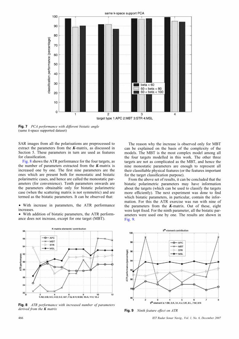
Fig. 7 PCA performance with different bistatic angle(same k-space supported dataset)

SAR images from all the polarisations are preprocessed toextract the parameters from the K-matrix, as discussed inSection 5. These parameters in turn are used as featuresfor classification.Fig. 8 shows the ATR performance for the four targets, as

the number of parameters extracted from the K-matrix isincreased one by one. The first nine parameters are theones which are present both for monostatic and bistaticpolarimetric cases, and hence are called the monostatic par-ameters (for convenience). Tenth parameters onwards arethe parameters obtainable only for bistatic polarimetriccase (when the scattering matrix is not symmetric) and aretermed as the bistatic parameters. It can be observed that:

† With increase in parameters, the ATR performanceincreases.† With addition of bistatic parameters, the ATR perform-ance does not increase, except for one target (MBT).

Fig. 8 ATR performance with increased number of parametersderived from the K matrix

466

The reason why the increase is observed only for MBTcan be explained on the basis of the complexity of themodels. The MBT is the most complex model among allthe four targets modelled in this work. The other threetargets are not as complicated as the MBT, and hence thenine monostatic parameters are enough to represent alltheir classifiable physical features (or the features importantfor the target classification purpose).From the above set of results, it can be concluded that the

bistatic polarimetric parameters may have informationabout the targets (which can be used to classify the targetsmore efficiently). The next experiment was done to findwhich bistatic parameters, in particular, contain the infor-mation. For this the ATR exercise was run with nine ofthe parameters from the K-matrix. Out of these, eightwere kept fixed. For the ninth parameter, all the bistatic par-ameters were used one by one. The results are shown inFig. 9.

Fig. 9 Ninth feature effect on ATR


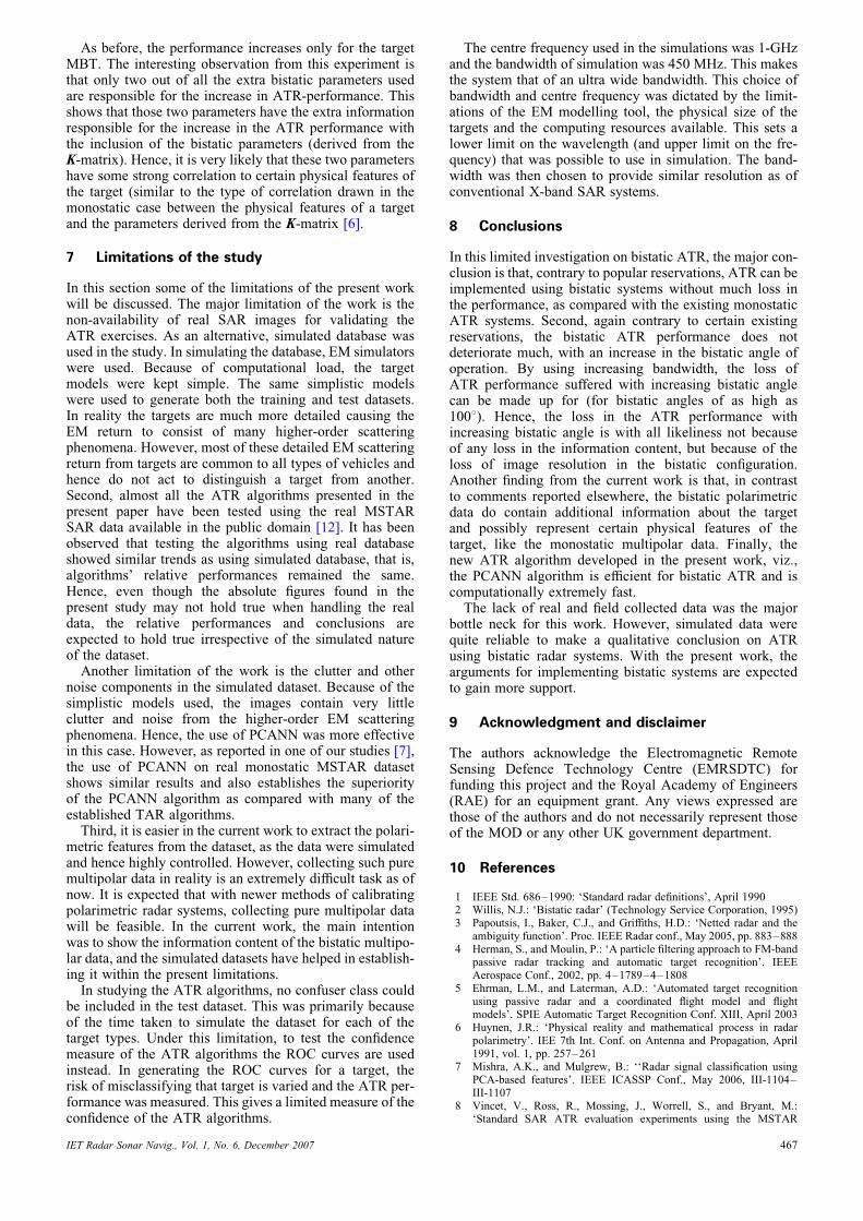
As before, the performance increases only for the targetMBT. The interesting observation from this experiment isthat only two out of all the extra bistatic parameters usedare responsible for the increase in ATR-performance. Thisshows that those two parameters have the extra informationresponsible for the increase in the ATR performance withthe inclusion of the bistatic parameters (derived from theK-matrix). Hence, it is very likely that these two parametershave some strong correlation to certain physical features ofthe target (similar to the type of correlation drawn in themonostatic case between the physical features of a targetand the parameters derived from the K-matrix [6].

7 Limitations of the study

In this section some of the limitations of the present workwill be discussed. The major limitation of the work is thenon-availability of real SAR images for validating theATR exercises. As an alternative, simulated database wasused in the study. In simulating the database, EM simulatorswere used. Because of computational load, the targetmodels were kept simple. The same simplistic modelswere used to generate both the training and test datasets.In reality the targets are much more detailed causing theEM return to consist of many higher-order scatteringphenomena. However, most of these detailed EM scatteringreturn from targets are common to all types of vehicles andhence do not act to distinguish a target from another.Second, almost all the ATR algorithms presented in thepresent paper have been tested using the real MSTARSAR data available in the public domain [12]. It has beenobserved that testing the algorithms using real databaseshowed similar trends as using simulated database, that is,algorithms’ relative performances remained the same.Hence, even though the absolute figures found in thepresent study may not hold true when handling the realdata, the relative performances and conclusions areexpected to hold true irrespective of the simulated natureof the dataset.Another limitation of the work is the clutter and other

noise components in the simulated dataset. Because of thesimplistic models used, the images contain very littleclutter and noise from the higher-order EM scatteringphenomena. Hence, the use of PCANN was more effectivein this case. However, as reported in one of our studies [7],the use of PCANN on real monostatic MSTAR datasetshows similar results and also establishes the superiorityof the PCANN algorithm as compared with many of theestablished TAR algorithms.Third, it is easier in the current work to extract the polari-

metric features from the dataset, as the data were simulatedand hence highly controlled. However, collecting such puremultipolar data in reality is an extremely difficult task as ofnow. It is expected that with newer methods of calibratingpolarimetric radar systems, collecting pure multipolar datawill be feasible. In the current work, the main intentionwas to show the information content of the bistatic multipo-lar data, and the simulated datasets have helped in establish-ing it within the present limitations.In studying the ATR algorithms, no confuser class could

be included in the test dataset. This was primarily becauseof the time taken to simulate the dataset for each of thetarget types. Under this limitation, to test the confidencemeasure of the ATR algorithms the ROC curves are usedinstead. In generating the ROC curves for a target, therisk of misclassifying that target is varied and the ATR per-formance was measured. This gives a limited measure of theconfidence of the ATR algorithms.


The centre frequency used in the simulations was 1-GHzand the bandwidth of simulation was 450 MHz. This makesthe system that of an ultra wide bandwidth. This choice ofbandwidth and centre frequency was dictated by the limit-ations of the EM modelling tool, the physical size of thetargets and the computing resources available. This sets alower limit on the wavelength (and upper limit on the fre-quency) that was possible to use in simulation. The band-width was then chosen to provide similar resolution as ofconventional X-band SAR systems.

8 Conclusions

In this limited investigation on bistatic ATR, the major con-clusion is that, contrary to popular reservations, ATR can beimplemented using bistatic systems without much loss inthe performance, as compared with the existing monostaticATR systems. Second, again contrary to certain existingreservations, the bistatic ATR performance does notdeteriorate much, with an increase in the bistatic angle ofoperation. By using increasing bandwidth, the loss ofATR performance suffered with increasing bistatic anglecan be made up for (for bistatic angles of as high as1008). Hence, the loss in the ATR performance withincreasing bistatic angle is with all likeliness not becauseof any loss in the information content, but because of theloss of image resolution in the bistatic configuration.Another finding from the current work is that, in contrastto comments reported elsewhere, the bistatic polarimetricdata do contain additional information about the targetand possibly represent certain physical features of thetarget, like the monostatic multipolar data. Finally, thenew ATR algorithm developed in the present work, viz.,the PCANN algorithm is efficient for bistatic ATR and iscomputationally extremely fast.The lack of real and field collected data was the major

bottle neck for this work. However, simulated data werequite reliable to make a qualitative conclusion on ATRusing bistatic radar systems. With the present work, thearguments for implementing bistatic systems are expectedto gain more support.

9 Acknowledgment and disclaimer

The authors acknowledge the Electromagnetic RemoteSensing Defence Technology Centre (EMRSDTC) forfunding this project and the Royal Academy of Engineers(RAE) for an equipment grant. Any views expressed arethose of the authors and do not necessarily represent thoseof the MOD or any other UK government department.

10 References

1 IEEE Std. 686–1990: ‘Standard radar definitions’, April 19902 Willis, N.J.: ‘Bistatic radar’ (Technology Service Corporation, 1995)3 Papoutsis, I., Baker, C.J., and Griffiths, H.D.: ‘Netted radar and the

ambiguity function’. Proc. IEEE Radar conf., May 2005, pp. 883–8884 Herman, S., and Moulin, P.: ‘A particle filtering approach to FM-band

passive radar tracking and automatic target recognition’. IEEEAerospace Conf., 2002, pp. 4–1789–4–1808

5 Ehrman, L.M., and Laterman, A.D.: ‘Automated target recognitionusing passive radar and a coordinated flight model and flightmodels’. SPIE Automatic Target Recognition Conf. XIII, April 2003

6 Huynen, J.R.: ‘Physical reality and mathematical process in radarpolarimetry’. IEE 7th Int. Conf. on Antenna and Propagation, April1991, vol. 1, pp. 257–261

7 Mishra, A.K., and Mulgrew, B.: ‘‘Radar signal classification usingPCA-based features’. IEEE ICASSP Conf., May 2006, III-1104–III-1107

8 Vincet, V., Ross, R., Mossing, J., Worrell, S., and Bryant, M.:‘Standard SAR ATR evaluation experiments using the MSTAR

467

public release data set’. Research Report, Wright State University,1998

9 Novak, L.M.: ‘State of the art of SAR ATR’. IEEE RADAR Conf.,May 2000, pp. 836–843

10 De Vore, M.D., and O’Sullivan, J.A.: ‘Performance complexity studyof several approaches to ATR from SAR images’, IEEE Trans.Aerosp. Electron. Sys., 2002, 38, (2), pp. 632–648

11 Zhao, Q., and Principe, J.C.: ‘Support Vector Machines for SARATR’, IEEE Trans. Aerosp. Electron. Syst., 2001, 37, (2),pp. 643–654

12 https://www.sdms.afrl.af.mil, accessed May 200413 ‘EM Software & Systems-SA.: ‘FEKO User’s Manual’ (EM Software

& Systems-S.A. (Pty) Ltd., 2004)14 Mishra, A.K., and Mulgrew, B.: ‘Database generation of bistatic

ground target signatures’. IEEE/ACES Conf. on WirelessCommunication and Applied Computational Electromagnetics, April2005, pp. 523–528

15 Ender, J.H.G.: ‘The meaning of k-space for classical and advancedSAR-techniques’. PSIP’2001, Marseille, January 2001, pp. 60–71

16 Charles, V.J. Jr., Wahl, D.E., Eichel, P.H., Ghiglia, D.C., andThompson, P.A.: ‘Spotlight-mode synthetic aperture radar: a signalprocessing approach’ (Kluwer academic publishers, 1996)

17 Jolliffe, I.T.: ‘Principal component analysis’ (Springer press, 2002,2nd edn.)

18 Dunteman, , and George, H.: ‘Brief description: principal componentsanalysis’ (Newbury Park, Calif. London Sage, 1989)

19 Mishra, A.K., and Mulgrew, B.: ‘Principal component analysis andrelevance to scattering centre model of radar data’. Proc. Int. RadarSymposium (IRS), Berlin, September 2005, pp 161–165

20 Potter, L.C., and Moses, R.L.: ‘Attributed Scattering Centres for SARATR’, IEEE Trans. Image Process., 1997, 6, (1), pp. 79–91

21 Mishra, A.K., and Mulgrew, B.: ‘SAR-ATR using one and 2-D PCA’.Proc. Int. Radar Symposium India, Bangalore, December 2005,pp. 781–185

22 Mishra, A.K., and Mulgrew, B.: ‘Bistatic SAR ATR using PCA-basedfeatures’. Proc. SPIE-ATR XVI, Defence and Security Symposium,Orlando, May 2006

23 Germond, A.L., Pottier, E., and Saillard, J.: ‘Foundations of bistaticradar polarimetry theory’. Proc. IEE Radar Conf., October 1997,pp. 833–837

24 Krogager, E.: ‘Decomposition of the radar target scattering matrixwith application to high resolution target imaging’. Proc.Telesystems Conf., March 1991, pp. 77–82

25 Haykin, S.: ‘Adaptive filter theory’ (Prentice-Hall internationaledition, 1991)

26 Golub, G.H., and Loan, C.F.V.: ‘Matrix computation’ (John HopkinsUniversity Press, 1996)

27 Cui, J., Jon, G., and Brookes, M.: ‘Radar shadow and superresolutionradar imaging using MUSIC algorithm’. Proc. IEEE Radar Conf., May2005, pp. 534–539

28 Radoi, E., Quinquis, A., Totir, F., and Pellen, F.: ‘‘Automatic targetrecognition using super-resolution MUSIC 2D images andself-organising neural netowrks’. Proc. EUSIPCO 2004, September2004, pp. 2139–2142

29 Rihaczek, A.W., and Hershkowitz, S.J.: ‘Man-made targetbackscattering behaviour: applicability of conventional radarresolution theory’, IEEE Trans. Aerosp. Electron. Syst., 1996, 32,(2), pp. 809–824

11 Appendix

In this section the eigenvalue analysis of the radar imagedata is presented to show that within standard SARimaging assumptions, principal components represent thescattering centres from a SAR image. In one of the previouswork [19], the PCA relevance of the scattering centres isshown by analysing the real SAR images of militarytargets. In another work [7], PCANN is applied to ATRusing real SAR image database [12]. These two previouswork show that in spite of the noise present in SARimages, PCA is effective in extracting the scatteringcentre information from the SAR images.Traditionally, radar imaging has depended on the scatter-

ing centre assumption. According to this, if wavelength ofthe illuminating EM wave is smaller than the object dimen-sions, the scattered return could be modelled as comingfrom distinct scattering centres. This model when appliedto radar imaging gives the scattering centre modelling of

468

the radar images, where the radar image is modelled to bethe summation of distinct scattering centres. The theoreticalrepresentation of an ideal scattering centre is the two-dimensional Kronecker’s delta function. Practically, moreapproximate mathematical functions can be used. In thepresent analysis, a two-dimensional sinc function is takenas the model for an ideal scattering centre in a radarimage. Let us analyse a simple radar image, with a singlescattering centre in the scene, at the centre of the scene.Let the size of the scene be N � N pixels. The image canbe represented by a matrix A of pixel amplitudes, whichaccording to the scattering centre model can be modelledwith a two dimensional sinc function.

A ¼ �uS �vH (12)

Here, �u and �v are two one-dimensional sinc vectors(vectors of dimension N � 1) and S a diagonal matrixwith the diagonal set to the value one (Hence S is unitmatrix), and of dimension 1� 1. ()H represents theHermitian operation on a matrix. Two of the importantcharacteristics of a scattering centre are its amplitude andposition. It can be observed from the above equation that:

† To change the intensity of the scattering centre, the valueof the diagonal elements of the S matrix needs to bechanged.† To shift the position of the scattering centre, the sincvectors, viz., �u and �v are to be shifted appropriately.

Similarly, a scene with k scattering centres at differentpositions can be represented as:

A ¼ USVH (13)

Here (Dimension of A is N � N , of U is N � k, of S isk � k, and of VH is k � N .) U ¼ [ �u1 �u2 �u3 . . . �uk], andV ¼ [�v1 �v2 �v3 . . . �vk]. Each element vectors �ui and �viare sinc-function vectors of length N, and appropriatelyshifted to represent the position of the ith scatteringcentre. S is a diagonal matrix of size k � k, with the ithdiagonal element representing the intensity of the ith scat-tering centre.Because the vectors �ui’s and �vi’s are sinc functions, the

matrices U and V are unitary and orthonormal. This con-clusion holds true for most of the mathematical functionswhich could be taken to model an ideal scattering centre.Given these facts, (12) is in the same form as the singularvalue decomposition (SVD) of the image pixel matrix.Hence, it can be observed that radar images can be decom-posed as per SVD (provided the scattering centre assump-tion is true). Few points worth noting are:

† The number of scattering centres determines the numberof elements in S, and hence the rank of the final imagematrix.† The position of the scattering centres is determined bythe elements of U and V matrices.† The strength of the scattering centres is determined by thesingular values (i.e. The elements of the diagonal matrix S)† The ith element of S can be shown to be equal tol

1=2i ,

where li is the ith eigenvalue of the covariance matrix ofAAH [18, 25].† Columns of U are the eigenvectors of AAH, and those ofV are the eigenvectors of AH A [17, 26]. Let it be assumedthat in the image matrix A, the rows represent range andcolumns represent cross-range vectors. Then AAH is thecovariance matrix (assuming the image has been zero-centred) of the cross-range pixel variables, and AHA


represents the covariance matrix (assuming the image hasbeen zero-centred) of the range pixel variables. Hence, pre-multiplication of the image matrix with UH represents thePCA with respect to cross-range pixels and multiplicationof the image matrix with V represents PCA with respectto range pixels [18].

UHAV ¼ U

H(USVH)V (14)

¼ ISI ¼ S (15)

† The second step can be explained as both U and V areunitary, that is, UH ¼ U21 and VH ¼ V21, UH U ¼ VH

V ¼ I. Here I is the identity matrix and U21 representsthe inverse of the matrix U. Hence, applying PCA in onedimension is equivalent to extracting the position of thescattering centres in that dimension. Hence the result ofapplying PCA is a two-dimensional matrix with informationabout the scattering centre intensities.† In real images, there is the presence of noise. Hence, thechoice of the dimension of S, U and V depends on thechoice of k, the number of the largest eigenvalues of AAH

to be taken. This is similar to the super-resolution algor-ithms [25], which have been applied by some researchersin filtering the noise from the radar images [27, 28].† When PCA is performed on a radar image, matrices Uand V are calculated. These matrices not only help toreduce the dimension of the matrix D, but represent the pos-ition of the scattering centres in the image matrix A.† The eigenvectors chosen in forming U and V correspondto the largest eigenvalues, and hence correspond to thebrightest scattering centres in the image matrix A.† Hence, applying PCA is equivalent to extracting the pos-ition and intensity information of the scattering centres.


Use in classification: In training phase, given the images ofthe target of a particular class, the U and V matrices arefound out,

† which in turn correspond to the positions of the scatteringcentres in the target image, and† which, when applied on an image of the target, will givea matrix S, which will be a diagonal matrix with elements indiagonal, corresponding to the intensity of the brightestscattering centres.

Given a test image, applying U and V on that and findingthe distance (Euclidean distance for simplicity) of theresulting matrix from S in essence represents the task ofcomparing the position and intensities of the major scatter-ing centres in the test image with the target class with whosetraining the matrices S, U and V have been found.The above analysis shows the correlation between PCA

of radar images and scattering centre analysis of the radarimages. However, the analysis is limited in a few aspects.First, it does not hold whether the scattering centre modelof the radar image does not hold correct [29]. Second,here the two-dimensional PCA has been presented, wherePCA is applied both to the range and to the cross-rangedimensions of the radar image. In the current project, astacking operation is performed on the radar images toform one-dimensional vectors, and then one-dimensionalPCA is applied. However, the stacking operation is linear.Hence, the results derived in the current analysis wouldstill hold true. Moreover, it has been checked by applyingthe two- and one-dimensional PCA to radar images thatboth ways of applying PCA result in the same ATR per-formance [21].

469

bistatic sar atr

Documents