arX

iv:0

711.

1697

v2 [

hep-

th]

23

Nov

200

7

PUPT-2249

ITEP-TH-16/07

arXiv:0711.1697

Bethe Ansatz Equations

For General Orbifolds of N =4 SYM

Alexander Solovyov a, b

a Physics Department,

Princeton University, Princeton, NJ 08544

b Bogolyubov Institute for Theoretical Physics,

Kiev 03680, Ukraine

Abstract

We consider the Bethe Ansatz Equations for orbifolds of N = 4 SYM w.r.t. an arbitrary discrete

group. Techniques used for the Abelian orbifolds can be extended to the generic non-Abelian case

with minor modifications. We show how to make a transition between the different notations in

the quiver gauge theory.

1. Introduction

For a long time in high energy physics there exists a strong interest in the web of dualities

between gauge theory and closed strings. The relationship essentially started with the

inception of string theory as a dual model of hadronic interactions (for a recent review see,

e.g., [1]). From the point of view of QCD, the modern theory of strong interactions, hadronic

strings would be interpreted as color electric flux tubes between quarks. A concrete version

of gauge/string correspondence was proposed by ’t Hooft in [2] (see also [3],[4],[5]) in the

form of the 1/N -expansion, the central idea of which is that the Feynman graphs of a large

N gauge theory naturally organize themselves as triangulations of a string surface. The rank

of the gauge group N is related to the string coupling via gS = 1/N , and counts the number

of handles of the surface spanned by the non-planar graphs. The gauge theory/closed string

duality is expected to be a limit of a more general open/closed string correspondence, which

should hold at the world sheet level. Open string diagrams are equivalent to closed string

world sheets with holes. The idea behind the open/closed string correspondence is that the

holes can be replaced by closed string vertex operators, and absorbed into an adjustment of

the sigma model that governs the motion of the closed string. From the perspective of the

low energy effective field theory, this relation between open and closed strings gives rise to

the famous duality between gauge theory and gravity, the central example of which is the

celebrated AdS/CFT correspondence [6],[7],[8],[9]. The key physical insight that spurned

this development was the discovery of the D-branes [10], followed by understanding of the

geometrical nature of the non-Abelian Chan-Paton factors in terms of stacks of coincident

branes [11]. On the other side, in terms of the Matrix Theory proposal [12] non-Abelian

gauge degrees of freedom are just a part of a more general theory; and thus they naturally

incorporate into the web of dualities.

However, there are some difficulties in studying the AdS/CFT conjecture. One of them

is the fact that the weak coupling on the gravity side (closed strings) corresponds to the

strong coupling regime on the gauge theory side (open strings); and this prevents one from

performing simple perturbative checks. It was major breakthrough when it was realized

that some integrable structures were present in the scalar subsector of N =4 SYM [13], and

this result was extended to the complete set of operators in [14],[15],[16]. At the same time

there was investigated the integrability of the closed string motion in [17] and the following

works. This opened the new opportunities of understanding the AdS/CFT duality beyond

perturbation theory.

Another idea commonly used in string theory since [18] is that of the orbifold space. An

2

orbifold is a quotient of some manifold w.r.t. a discrete group. The procedure of orbifoldiza-

tion was expected to be useful in particular for model building. A strong motivation for this

is the usage of quotient spaces for (super)symmetry breaking. Another way to use orbifold

construction which was used recently is to embed some models into quiver gauge theories.

Even though there are some works studying these dualities for some special orbifolds or

some special limits [19],[20],[21],[22],[23],[24],[25],[26],[27]; they mainly deal with the Abelian

orbifolds and the corresponding quiver gauge theories. The main goal of this paper is to

extend some of these studies to the generic orbifolds with an arbitrary non-Abelian orbifold

group. Organization of the paper is as follows. In the second Section we summarize the

results regarding the closed string motion on orbifolds. We discuss the subtleties specific

to the general non-Abelian orbifolds. In the third Section we introduce the orbifold gauge

theory which is the low-energy limit of the corresponding open string theory. We introduce

the two different descriptions, the one using the twist fields (and most closely resembling the

original unorbifolded theory) as well as the one using the quiver diagram. Then we develop

the transition formulae between them. In the fourth Section we introduce the Feynman

rules for the quiver gauge theory and study the field theory dynamics. This leads to the

representation of the matrix of anomalous dimensions as a spin chain Hamiltonian. The

Hamiltonian locally coincides with that of the unorbifolded theory. In the fifth Section

we review the Bethe Ansatz Equations (BAE) and generalize them to the generic orbifold

theories. The key ingredients of the construction are essentially the same as those for the

Abelian orbifolds. The idea is that one can diagonalize the twist field in each given twisted

sector, and then the setup reduces to the Abelian case modulo some subtleties. In the sixth

Section we study some applications of the BAE. We find the solutions in the long spin chain

limit and compare them with the closed string energies. We also consider particular quivers

(both Abelian and non-Abelian) and show how the eigenvectors of the matrix of anomalous

dimensions are rewritten in terms of the quiver notation. Appendix A introduces the basic

group theory notations and conventions. Appendix B contains the calculations related to

the conversion between the two descriptions in the orbifold gauge theory as well as the

construction of observables.

2. Orbifold String Theory

Besides exploring the integrability of the orbifold gauge theories, an important mo-

tivation for our study is to test the correspondence between large N gauge theory and

closed string theory. The closed string dual to the orbifold gauge theories follows from the

3

AdS/CFT dictionary. The stack of N D3-branes, located on the fixed point of the orbifold

space C3/Γ, induce via their gravitational backreaction a near-horizon geometry that is given

by

AdS5 × S5/Γ. (1)

The AdS/CFT correspondence states that the planar diagrams of the orbifold gauge theory

span the worldsheet of closed strings propagating on this near-horizon geometry.

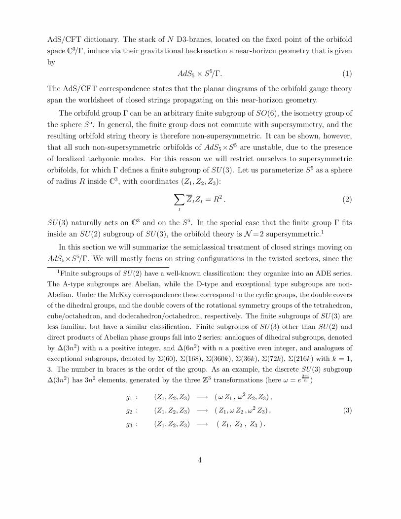
The orbifold group Γ can be an arbitrary finite subgroup of SO(6), the isometry group of

the sphere S5. In general, the finite group does not commute with supersymmetry, and the

resulting orbifold string theory is therefore non-supersymmetric. It can be shown, however,

that all such non-supersymmetric orbifolds of AdS5×S5 are unstable, due to the presence

of localized tachyonic modes. For this reason we will restrict ourselves to supersymmetric

orbifolds, for which Γ defines a finite subgroup of SU(3). Let us parameterize S5 as a sphere

of radius R inside C3, with coordinates (Z1, Z2, Z3):

∑

I

ZIZI = R2 . (2)

SU(3) naturally acts on C3 and on the S5. In the special case that the finite group Γ fits

inside an SU(2) subgroup of SU(3), the orbifold theory is N =2 supersymmetric.1

In this section we will summarize the semiclassical treatment of closed strings moving on

AdS5×S5/Γ. We will mostly focus on string configurations in the twisted sectors, since the

1Finite subgroups of SU(2) have a well-known classification: they organize into an ADE series.

The A-type subgroups are Abelian, while the D-type and exceptional type subgroups are non-

Abelian. Under the McKay correspondence these correspond to the cyclic groups, the double covers

of the dihedral groups, and the double covers of the rotational symmetry groups of the tetrahedron,

cube/octahedron, and dodecahedron/octahedron, respectively. The finite subgroups of SU(3) are

less familiar, but have a similar classification. Finite subgroups of SU(3) other than SU(2) and

direct products of Abelian phase groups fall into 2 series: analogues of dihedral subgroups, denoted

by ∆(3n2) with n a positive integer, and ∆(6n2) with n a positive even integer, and analogues of

exceptional subgroups, denoted by Σ(60), Σ(168), Σ(360k), Σ(36k), Σ(72k), Σ(216k) with k = 1,

3. The number in braces is the order of the group. As an example, the discrete SU(3) subgroup

∆(3n2) has 3n2 elements, generated by the three Z3 transformations (here ω = e2πin )

g1 : (Z1, Z2, Z3) −→ (ω Z1 , ω2 Z2, Z3) ,

g2 : (Z1, Z2, Z3) −→ (Z1, ω Z2 , ω2 Z3) , (3)

g3 : (Z1, Z2, Z3) −→ ( Z1, Z2 , Z3 ) .

4

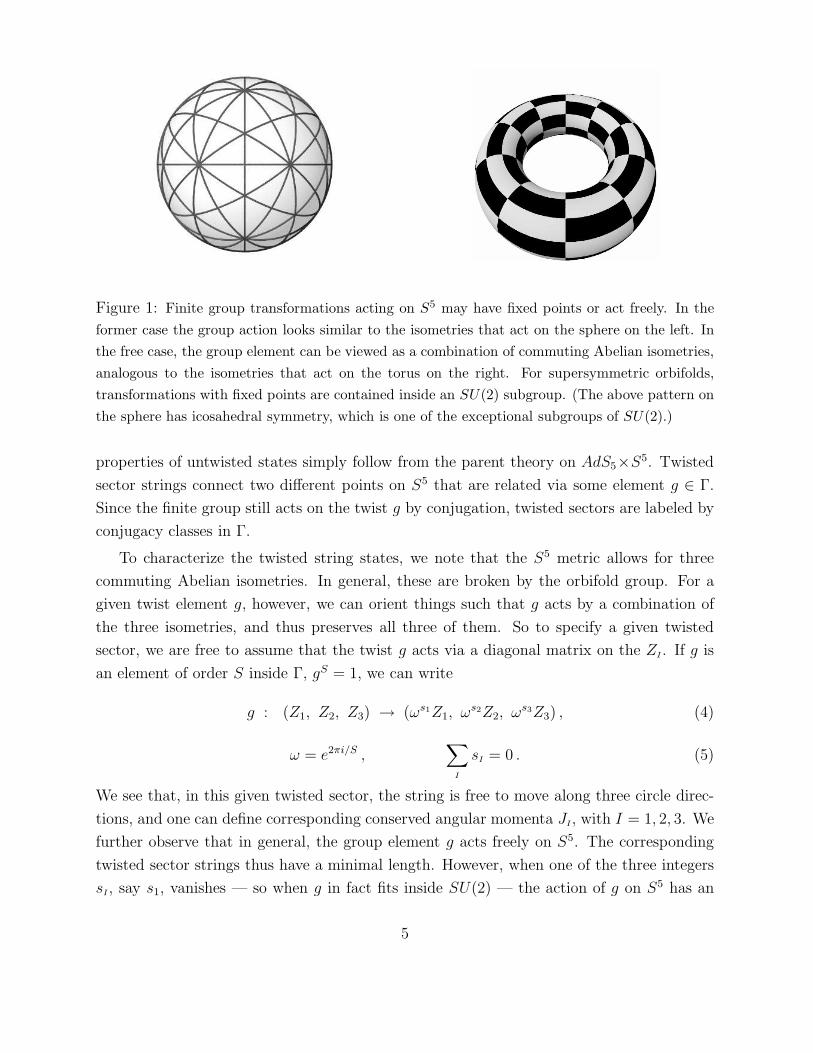
Figure 1: Finite group transformations acting on S5 may have fixed points or act freely. In the

former case the group action looks similar to the isometries that act on the sphere on the left. In

the free case, the group element can be viewed as a combination of commuting Abelian isometries,

analogous to the isometries that act on the torus on the right. For supersymmetric orbifolds,

transformations with fixed points are contained inside an SU(2) subgroup. (The above pattern on

the sphere has icosahedral symmetry, which is one of the exceptional subgroups of SU(2).)

properties of untwisted states simply follow from the parent theory on AdS5×S5. Twisted

sector strings connect two different points on S5 that are related via some element g ∈ Γ.

Since the finite group still acts on the twist g by conjugation, twisted sectors are labeled by

conjugacy classes in Γ.

To characterize the twisted string states, we note that the S5 metric allows for three

commuting Abelian isometries. In general, these are broken by the orbifold group. For a

given twist element g, however, we can orient things such that g acts by a combination of

the three isometries, and thus preserves all three of them. So to specify a given twisted

sector, we are free to assume that the twist g acts via a diagonal matrix on the ZI. If g is

an element of order S inside Γ, gS = 1, we can write

g : (Z1, Z2, Z3) → (ωs1Z1, ωs2Z2, ω

s3Z3) , (4)

ω = e2πi/S ,∑

I

sI = 0 . (5)

We see that, in this given twisted sector, the string is free to move along three circle direc-

tions, and one can define corresponding conserved angular momenta JI, with I = 1, 2, 3. We

further observe that in general, the group element g acts freely on S5. The corresponding

twisted sector strings thus have a minimal length. However, when one of the three integers

sI, say s1, vanishes — so when g in fact fits inside SU(2) — the action of g on S5 has an

5

obvious fixed point at (Z1, Z2, Z3) = (R, 0, 0).

2.1. Classical strings on S5/Γ: Semiclassical Treatment

We now summarize some relevant results on the classical motion of strings along the

S5 having in mind the future comparison with the gauge theory side. The more general

calculations can be found in [28] and references therein; in particular, [29], [30] and [31]. We

restrict ourselves to the strings moving in S5 directions only and trivially embedded into

AdS5. This motion is governed by the sigma model action (restricted to the bosonic string

coordinates)

S ∼∫dτdσ

(1

2∂at ∂at − ∂aZI∂

aZI + Λ(ZIZI −R2)

). (6)

Here t denotes the AdS time coordinate, and Λ is a Lagrange multiplier field. This action

is obtained as a reduction of the string worldsheet action in the conformal gauge; thus the

equations of motion derived from this action must be supplemented by the corresponding

Virasoro constraints:

t2 = ZI˙ZI + Z ′

IZ ′

I, (7)

0 = ZIZ′I. (8)

We want to solve for the motion of the string in the twisted sector defined by the twist

element (4). As it was emphasized in [23], the closedness requirement then allows for the

fractional winding numbers,

ZI(σ + 2π) = e2πimIZ

I(σ) , mI = mI +

sI

S. (9)

The S5 metric has three commuting isometries. In general, these are broken by the orbifold

group. However, from the explicit form of the twist element given in (4), we see that in this

given twisted sector, the string is free to move along three circle directions. It is therefore

natural to choose the following Ansatz,

t = κτ , ZI = zI(σ) eiωIτ . (10)

Inserting this Ansatz, the Lagrangian governing the dependence zI(σ) becomes

L =1

2

∑

I

(z′Iz′

I− ω2

Iz

Iz

I)− 1

2Λ(

∑

I

zIz

I−R2) . (11)

6

The Virasoro constraints simplify to

κ2 =∑

I

(z′Iz′

I+ ω2

Iz

Iz

I) , (12)

0 =∑

I

ωI(z′Iz

I− z′

Iz

I) . (13)

Note that both Lagrangian and Virasoro constraints have a U(1)3-invariance w.r.t. the

multiplication by a phase,

zI → eiαIzI , zI → e−iαI zI . (14)

This invariance leads to the three integrals of motion,

ℓI =i

2(z′

Iz

I− z′

Iz

I) . (15)

This allows us to eliminate the angular variables. Then denoting r2I

= zI zI and substituting

this back into the action we get the following effective Lagrangian:

L =1

2

∑

I

(r′2

I− w2

Ir2

I+ℓ2

I

r2I

)− 1

2Λ

( 3∑

I

r2I− 1

). (16)

This system is called the Neumann-Rosochatius (NR) integrable system (e.g., [32]); and

its detailed analysis in the context of the closed string dynamics is given in [28]. Here we

restrict ourselves to the simplest example, the circular strings. These solutions take the

following forms:

zI = aI eimIσ , Λ = const. (17)

With this ansatz integrals ℓI = mIa2I; while the dynamical equations yield

w2I

= −Λ− m2I,

3∑

I=1

a2I

= 1 ; (18)

κ2 =3∑

I=1

a2I(w2

I+ m2

I) ,

3∑

I=1

a2IwImI = 0 . (19)

The space-time energy for the circular string configuration is

E =√

8π2λ

∫ 2π

0

dσ

2πt =√

8π2λκ ; (20)

while the spins are

JI =√

8π2λwI

∫ 2π

0

dσ

2πr2

I(σ) =

√8π2λwIa

2I. (21)

7

One can define the total spin L =∑3

I=1 |JI|. The relations (18) and (19) can be rewritten

in terms of the energy and the spins. Eqs. (19) read

E2

8π2λ= −Λ ,

3∑

I=1

mIJI = 0 ; (22)

while (18) becomes3∑

I=1

|JI|√−Λ− m2

I

=√

8π2λ . (23)

We will consider the two spin solution with J3 = 0. Then in the large L limit one can

solve these equations and find the following expansion for the energy:

E = L+4π2λ

L|m1| |m2| . (24)

Given that J1, J2 > 0, one must have m1m2 < 0. Recalling the definition of the fractional

winding numbers m2, m2 one can write the string energy as

E = L+4π2λ

L

(m− s1

S

)(m′ +

s2

S

); (25)

m and m′ being some positive integers. In Section 6 we will see that this expression matches

the one-loop anomalous dimensions for the corresponding su2 subsector formed by the two

scalars in the field theory.

3. Orbifold Gauge Theory

We now turn to the study the class of quiver gauge theories obtained by taking an ar-

bitrary (Abelian or non-Abelian) orbifold of N = 4 supersymmetric U(N) gauge theory.

Our motivation is to investigate to what extent the recently uncovered large N integra-

bility of N = 4 SYM can be extended to this general class of orbifold gauge theories. In

this section we will summarize some of their relevant properties. The relevant references

are [33],[34],[35],[36],[37],[38].

3.1. Orbifold Projection

It will be convenient to think of the quiver gauge theory as the low energy limit of the

open string theory on a stack of N D3-branes located near an orbifold singularity. Before

taking the orbifold quotient, the transverse space of the D3-branes is R6 ≃ C

3. The low

8

energy field theory on the D3-branes is N = 4 SYM, with its field content (in N = 1

superfield notation): a vector multiplet A and three chiral multiplets ΦI , with I = 1, 2, 3,

that parameterize the three complex transverse positions of the D3-branes along C3.

Let Γ be some finite group of order |Γ|, that acts on C3. The orbifold space is obtained

by dividing out the action of the discrete group Γ. The transverse space to the D3-branes

thus becomes

C3/Γ .

When viewed from the covering space, the stack of N D3-branes in the orbifold space give

rise to the total of |Γ|N image D3-branes. It is convenient to label the image D3-branes by

a pair of Chan-Paton indices (i, h) with i = 1, . . . , N and h ∈ Γ, so that the brane labeled

by (i, h) is the image of the i-th brane inside the D3-stack under the group element h ∈ Γ.

The group Γ thus acts on the Chan-Paton indices as

g : (i, h) → (i, gh) . (26)

When the N coincident D-branes all approach the orbifold fixed point, the image branes all

coincide and the strings stretched between them have massless ground states. The vector

multiplet A has a separate matrix entry for each open string stretching between two image

branes, and thus defines an |Γ|N×|Γ|N matrix. Before imposing invariance under the orbifold

group Γ, the full collection of image branes thus supports an U(|Γ|N) gauge symmetry. The

orbifold projection, however, selects only those fields that are invariant under the discrete

group Γ. The discrete group acts on the vector multiplet A only via the Chan-Paton indices

and on the chiral multiplets ΦI via both the Chan-Paton and transverse indices.

Although the orbifold theories all have less supersymmetry, their action is assumed to

be identical to that of the parent N =4 theory, which in N =1 superfield notation reads

L =

∫d4θ Tr

(WαWα + eAΦ†

Ie−AΦI

)+

∫d2θ ǫIJK Tr (ΦI [ΦJ ,ΦK ]) + c.c. (27)

Here the trace Tr is over the adjoint representation of the full U(|Γ|N) gauge group of the

N = 4 theory. The fields (A,Φ) of the orbifold theory, however, are special matrices that

are obtained by applying a linear projection PΓ

on the fields of the parent theory

A = PΓAN=4

, Φ = PΓΦ

N=4

. (28)

9

The projection operator PΓ

takes the generic form2

PΓ

=1

|Γ|∑

g

g , (29)

where g acts in an appropriate representation on (A,Φ), that we will specify momentarily.

This projection operator does not commute with the full N =4 superconformal invariance,

but in the special case that Γ forms a subgroup of SU(3), the orbifold quotient preserves

N =1 superconformal invariance. More generally, one could consider orbifolds with Γ some

subgroup of SO(6). However, it has been shown that for non-supersymmetric orbifolds, the

quantum theory has non-zero β-functions for certain double-trace operators and is therefore

not conformally invariant. The renormalized Hamiltonian of non-supersymmetric orbifolds

thus contains extra terms that do not descend from the N = 4 Hamiltonian [40]. For this

reason we will restrict ourselves to the supersymmetric subclass.

Let us specify the action of g in (29) on A and ΦI . First, we recall the definition of the

regular representation of the finite group Γ. The group algebra C[Γ] is the |Γ|-dimensional

vector space of C-valued functions on Γ

C[Γ] =x =

∑

h

x(h) h

(30)

with x(h) ∈ C. The group Γ acts on the group algebra via g : x → ∑h x(h) gh. From this,

we obtain a natural representation of Γ in terms of |Γ|×|Γ| matrices, known as the regular

representation γreg. It acts on the |Γ| dimensional vector space

Vreg ≃ C[Γ] . (31)

The regular representation is directly relevant to our problem. As is evident from our

definition of the Chan-Paton indices, the vector multiplet A is naturally identified as an

element of

A ∈ V ⊕Nreg ⊗V

⊕N

reg . (32)

The finite group Γ acts on A both from the left and from the right, both actions being

implemented via the regular representation. Geometrically, we can think of each as applying

the group element g to the D3-brane at respectively the begin- and end-point of the open

strings. The orbifold symmetry transformation acts simultaneously on both ends, and thus

2Here and in the following, the summation over g runs over the whole finite group Γ, unless

otherwise indicated.

10

acts on A via conjugation. (Note that γreg(g) = γ(g−1).) Similarly, the chiral multiplets Φ

are elements of

Φ ∈ C3 ⊗ V ⊕N

reg ⊗V ⊕N

reg . (33)

To write their transformation rule, we must also account for the action discrete group on

C3, which proceeds via the 3-dimensional defining representation, that we will denote by R.

With these definitions, Γ acts on the fundamental fields as

g : A → γreg(g)A γreg(g) , (34)

g : ΦI → R(g)I

Jγreg(g) ΦJ γreg(g) . (35)

Combined with (28) and (29), this specifies the projection from the N =4 parent theory to

the orbifold gauge theory. Written out explicitly in terms of the group valued Chan-Paton

indices (26), the orbifold projected fields take the form3

A(g) =1

|Γ|

∑

h

Ah,gh (36)

ΦI(g) =1

|Γ|

∑

h

R(h)I

JΦJ

h,gh (37)

We see that after the projection, the Γ valued left and right Chan-Paton indices have

collapsed to a single group valued index. The gauge and matter fields can thus be thought of

as group algebra valued N×N matrices. We will refer to the above basis of orbifold projected

fields as the orbit basis (as distinguished from the quiver basis, that will be introduced later).

Note that, since the orbifold projection (28) does not commute with U(|Γ|N), the gauge

symmetry gets broken to a subgroup. This unbroken gauge group is identified as follows.

The regular representation γreg decomposes into irreducible representations ρλ via

γreg(g) =⊕

λ

ρλ(g)⊕Nλ , Nλ = dim ρλ. (38)

In words, each irreducible representation ρλ occurs Nλ times in the decomposition of the

regular representation. In explicit matrix notation, we have

γreg =

ρ1 ⊗ 1N10 ... 0

0 ρ2 ⊗ 1N2... 0

......

. . ....

0 0 ... ρr ⊗ 1Nr

(39)

3Here we suppress the other U(N) valued Chan-Paton index.

11

where ρλ ⊗ 1Nλis the Nλ ×Nλ matrix

ρλ ⊗ 1Nλ=

ρλ 0 ... 0

0 ρλ ... 0...

.... . .

...

0 0 ... ρλ

. (40)

Here each ρλ denotes an Nλ×Nλ matrix. By inspecting the explicit form (39) of γreg, it

is not difficult to derive that the orbifold gauge group, defined as the subgroup of U(|Γ|N)

transformations that commutes with γ(g) for all g ∈ Γ, takes the product form

⊗

λ

U(NNλ) . (41)

Here the product runs over all representations of Γ and each factor U(NNλ) is the subgroup

that rearranges theNNλ copies of the representation space Vλ of ρλ — it therefore obviously

commutes with Γ. Using Schur’s lemma, one proves that (41) indeed defines the maximal

unbroken gauge group: physical operators need only be gauge invariant under this group.4

3.2. The Untwisted Sector

The untwisted sector states of the orbifold theory have a simple relation to those of

the parent theory: they are obtained by applying the projection operator PΓ

to (every

elementary field inside) gauge invariant single-trace operators of the parent theory of the

form

O = Tr(W

A1W

A2. . .W

AL

). (44)

4In other words, the decomposition (38) of the regular representation shows that the represen-

tation vector space Vreg decomposes as

Vreg =⊕

λ

Vλ ⊗CNλ , (42)

where Vλ denotes the Nλ dimensional representation space of ρλ. Combining (42) with (32) and

the invariance condition (70), we find that

A ∈⊕

λ

(V ⊕NλNλ )⊗ (V ⊕NλN

λ ) =⊕

λ

(Vλ ⊗ Vλ) ⊗ (CNNλ⊗ CNNλ). (43)

This decomposition of A makes manifest that the commutant of Γ within U(|Γ|N) takes the form

(41).

12

HereWA

stands for a multiple covariant derivative of one of the fields of the theory, in N =1

notation:

WA∈

DnΦI , DmWα

(45)

It should be emphasized, however, that not all single trace expressions of the form (44)

lead to non-vanishing operators of the orbifold theory: the orbifold projection, combined

with the cyclicity of the trace, implies that only the Γ-invariant combinations survive. A

complete basis of untwisted operators thus takes the form5

OK = KA1 A2 ˙˙˙AL Tr(W

A1W

A2. . .W

AL

), (46)

where KA1 A2 ˙˙˙AL denotes any Γ-invariant tensor.

In recent years, there has been enormous progress in understanding of the quantum

properties of such single trace operators in the large N limit of N = 4 super Yang-Mills

theory. The central insight that has precipitated this breakthrough development, is that

local operators of the form (44) can be represented as spin chain states

|O〉 = |A1, A2, . . . , AL〉 . (47)

Under this identification, the gauge theory generator of conformal rescalings maps to the

spin chain Hamiltonian H. The energy eigenvalues EO of H are related to the anomalous

dimensions ∆O of local single trace operators O by

∆O = λEO, (48)

with λ =g2

YMN

8π2 the ’t Hooft coupling. Most remarkably, there is a fast growing and con-

vincing body of evidence that the spin chain system defined via this correspondence is

completely integrable, at least at leading order at large N and for large length L of the

spin chain (many operators WA

in (44)). This realization has lead to a flurry of new gauge

theory results and non-trivial quantitative checks of the AdS/CFT correspondence.

In the following, we will investigate how these results can be generalized to the full class

of supersymmetric orbifolds of N = 4 super Yang-Mills theory. Although these orbifolds

all have less supersymmetry and are less special than the parent theory, there are several

direct and indirect arguments to support the conjecture that these orbifold gauge theories

are indeed still integrable. Our goal is to extend the known results ([26] and related works)

to the general orbifold gauge theories.

It is a well known fact that in the large N limit, the planar Feynman diagram expansion

in the untwisted sector coincides with that of the unorbifolded theory modulo the projection

5This obvious calculation is given in Appendix B.3.

13

onto the Γ-invariant states. As a consequence, the Hamiltonian H of the orbifold theory,

when acting on untwisted states, is simply equal to the N =4 Hamiltonian HN=4 acting on

the Γ-invariant subspace of the N = 4 Hilbert space, H = ΠΓHN=4. The original action

being Γ-invariant, the N = 4 Hamiltonian commutes with the projector, [HN=4,ΠΓ] = 0;

and thus the action of H is defined correctly. In particular, the conformal dimensions of the

gauge invariant untwisted sector operators of the orbifold theory are identical to those of

the parent theory. This correspondence extends to arbitrary loop order.

3.3. The Twisted Sectors

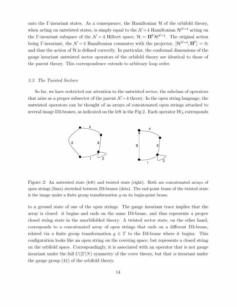
So far, we have restricted our attention to the untwisted sector, the subclass of operators

that arise as a proper subsector of the parent N =4 theory. In the open string language, the

untwisted operators can be thought of as arrays of concatenated open strings attached to

several image D3-branes, as indicated on the left in the Fig 2. Each operatorWA corresponds

Figure 2: An untwisted state (left) and twisted state (right). Both are concatenated arrays of

open strings (lines) stretched between D3-branes (dots). The end-point brane of the twisted state

is the image under a finite group transformation g on its begin-point brane.

to a ground state of one of the open strings. The gauge invariant trace implies that the

array is closed: it begins and ends on the same D3-brane, and thus represents a proper

closed string state in the unorbifolded theory. A twisted sector state, on the other hand,

corresponds to a concatenated array of open strings that ends on a different D3-brane,

related via a finite group transformation g ∈ Γ to the D3-brane where it begins. This

configuration looks like an open string on the covering space, but represents a closed string

on the orbifold space. Correspondingly, it is associated with an operator that is not gauge

invariant under the full U(|Γ|N) symmetry of the cover theory, but that is invariant under

the gauge group (41) of the orbifold theory.

14

In the gauge theory, the twisted states are represented as single trace expressions

O(g) = Tr(γ(g)W

A1W

A1. . .W

AL

), (49)

where we introduced a twist operator γ(g), defined as follows. When γ(g) acts from the

left on a matrix-valued operator WA , it acts via the group action (26) — the regular repre-

sentation γreg(g) — on the left Chan-Paton index. When γ(g) acts from the right, it acts

via the complex conjugate group action γreg(g) on the right Chan-Paton index. The actions

from the left and from the right are not identical; instead, the operatorsWA of the orbifold

theory satisfy a relation of the form

γ(g)WA

= R(g)B

AW

Bγ(g) , (50)

where R(g)B

A denotes a matrix representation of the finite group Γ, acting on the C3 index

of WA.6

As a consequence of the orbifold projection, some of the physical operators (49) vanish

identically. Using equation (50) to commute γ(g) past all the fields in the operator shows

that a necessary condition for non-vanishing operators is that the total single trace operator

must be invariant under the simultaneous action of R(g)B

Aon all the spins. However, while

necessary, this is not sufficient. More generally, physical operators are of the form

OK(g) = K(g)A1 A2 ˙˙˙AL Tr

(γ(g)W

A1W

A1. . .W

AL

), (51)

where K(g) must be an invariant tensor under the complete stabilizer subgroup Sg of g,

defined as the subgroup within Γ of all elements that commute with g.7 In the untwisted

case, where g is the identity element in Γ, the stabilizer subgroup is the whole group Γ

and indeed, as we saw before, untwisted operators are in one-to-one correspondence with

Γ-invariant tensors. For non-trivial twisted sectors, it would be too strong a condition to

impose that K(g) is invariant under the full group Γ, since the group acts non-trivially

on the twist element. Correspondingly, we must define the Sg invariant tensors K(g) to

transform non-trivially under the full group action via

K(g)A1 A2 ˙˙˙AL

R(h)B1

A1

R(h)B2

A2

. . . R(h)BL

AL= K(hgh−1)

B1 B2 ˙˙˙BL (52)

6Here R(g) = 1 in caseWA has no C3 index. Note further that inserting multiple twist operators

in the trace does not introduce a new class of operators, since by using the exchange relation (50)

and the property γ(g1)γ(g2) = γ(g1g2), one can always reduce any number of twist operators to

a single overall twist. This is as one would have expected from the string interpretation.7It can be the case that even for some Sg-invariant tensor K(g) the corresponding operator

OK(g) vanishes identically due to some symmetry reasons — for instance, this is the case in the

Z6 quiver we consider in Section 6.

15

for all h ∈ Γ. We see that, in a given twisted sector, the Γ-invariance is spontaneously

broken to the stabilizer subgroup of the twist element g: the property (52) states the K(g)

is invariant under the simultaneous action of R(h) on all spins, provided that h commutes

with g.

As one could have expected from the string dictionary [39], the twisted operators (51)

depend only on the conjugacy class of the twist element g:

OK(g) = OK(hgh−1) (53)

This result easily follows by combining the property (52) with the transformation rule (50)

of the operators WA.

It is important to note that the basis (51) of operators is really a complete basis, in the

sense that any operator of the seemingly more general class given in (49), that is not of

the form (51), vanishes identically.8 The reason is that the single site operators WA

are all

selected via the orbifold projection (28)-(29) to transform according to (50) under the finite

group Γ. The space of orbifold operators is spanned by the orbit basis, defined by

WA(g) =

1

|Γ|∑

h

R(h)B

AW

B ;h,gh . (54)

This definition combines the two formulas (36) and (37).

Let us now state the main conclusion of the section, that will become important later:

It is possible to define a basis of twisted sector operators (51) such that the single site

operators WA

that contribute in the sum are all eigenstates of the twist matrix R(g)B

A.

To prove this statement, we first note that the invariance condition (52)-(53) allows us to

restrict ourselves to a given representative g in each twisted sector [g]. Let Sk denote the

representation of Sg that acts on the k-th site. Then a single element g can be diagonalized,

and the eigenvalue of the corresponding spin WAk

is given by

Sk(g) = σk(g)1, (55)

If g is an element of order S in Γ, then σk(g) is some phase factor of the form exp(2πisk/S).

This observation will be useful in the later sections, where we will study the classical and

quantum properties of these twisted sector operators. The idea is to diagonalize the action

of a given group element g, and then apply some of the tools used in the studies of the

Abelian orbifolds. This property will be exploited in Section 5 where we study the Bethe

8Detailed construction of twisted operators as well as the proof of their gauge invariance is

given in Appendix B.4.

16

Ansatz Equations for the orbifold gauge theory.

3.4. Quiver Gauge Theory

In this section, we will make a comparison between the above group theoretic description

of the physical operators with the quiver representation of the orbifold gauge theory. The

reader that is mostly interested in the integrability of the orbifold theory may wish to skip

this section at first reading.

The physical field content of orbifold gauge theories is made most manifest via its repre-

sentation as a quiver gauge theory. As discussed, the unbroken gauge group of the orbifold

theory takes the product form ⊗

λ

U(NNλ) , (56)

where the product runs over all representations ρλ of the finite group Γ and Nλ = dimVλ.

Notice that, even in the case that N = 1, that is, for the world-brane theory of a single

D3-brane near an orbifold singularity, this gauge group contains several, in general non-

Abelian, factors. In the string theoretic construction, each gauge factor is associated to a

stack on NNλ so-called fractional D3-branes. There is one type of fractional brane for each

representation ρλ of the finite group.

The vector multiplets A arise as the ground states of open strings attached to a given

fractional brane. Let us denote by Aλ the vector multiplet of the fractional brane associated

to ρλ. Hence Aλ is an U(NNλ) gauge multiplet. In terms of the orbit basis A(g) defined

in (36), the quiver basis Aλ is obtained via the Fourier-like transformation

Aλ =∑

g

ρλ(g)A(g) (57)

Setting up the quiver terminology, we will refer to each gauge factor and its associated stack

of fractional branes, as a node of the quiver diagram. There is one quiver node for each

irreducible representation of Γ.

In a quiver diagram, the nodes are connected by oriented lines: these represent the

chiral matter fields. In the string theory construction, the chiral matter fields ΦI arise

as the ground states of open strings that may have end-points on two different fractional

branes. Correspondingly, they transform as bi-fundamental fields under the product gauge

group (56). More accurately, the chiral matter fields are invariant tensors

Φλµ ∈ Inv(C3 ⊗ Vλ ⊗ V µ). (58)

17

U(Na) U(Nb)

U(Nc)

nab

nbcnca

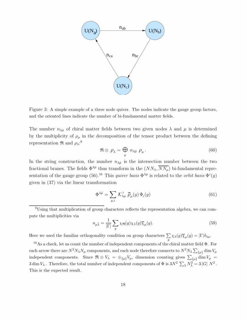
Figure 3: A simple example of a three node quiver. The nodes indicate the gauge group factors,

and the oriented lines indicate the number of bi-fundamental matter fields.

The number nλµ of chiral matter fields between two given nodes λ and µ is determined

by the multiplicity of ρµ in the decomposition of the tensor product between the defining

representation R and ρλ:9

R⊗ ρλ =⊕

µ

nλµ ρµ . (60)

In the string construction, the number nλµ is the intersection number between the two

fractional branes. The fields Φλµ thus transform in the (NNλ, NNµ) bi-fundamental repre-

sentation of the gauge group (56).10 This quiver basis Φλµ is related to the orbit basis ΦI(g)

given in (37) via the linear transformation

Φλµ =∑

g,I

K I

λµ ρµ(g) ΦI(g) (61)

9Using that multiplication of group characters reflects the representation algebra, we can com-

pute the multiplicities via

nµλ =1

|Γ|∑

g

χR(g)χλ(g)χµ(g). (59)

Here we used the familiar orthogonality condition on group characters∑g

χλ(g)χµ(g) = |Γ|δλµ.

10As a check, let us count the number of independent components of the chiral matter field Φ. For

each arrow there are N2NλNµ components, and each node therefore connects to N2Nλ

∑µ dimVµ

independent components. Since R ⊗ Vλ = ⊕µVµ, dimension counting gives∑

µ dim Vµ =

3dim Vλ . Therefore, the total number of independent components of Φ is 3N2∑

λ N2λ = 3 |G| N2 .

This is the expected result.

18

where Kλµ denotes one of the nλµ basis elements that spans the space of invariant tensors

in C3 ⊗ Vλ ⊗ V µ.

In the quiver basis, it is now easy to specify all possible single trace operators of the

orbifold gauge theory. For this, it is useful to introduce the notion of the path algebra of

the quiver diagram. A path is a concatenated array of arrows that connect quiver nodes

connected by oriented lines. The arrows are allowed to point back to the same node. We

can multiply two paths if one ends at the same node as where the other begins. We can

then connect them head to tail to produce a single longer path. In the quiver gauge theory,

each arrow of the path represents a gauge or matter operator WA

of the general form (45),

transforming in the corresponding representation of the quiver gauge group. Connecting two

arrows amounts to taking their gauge invariant product at the corresponding quiver node.

To write gauge invariant operators, we now simply choose arbitrary closed paths along the

quiver, pick a corresponding array of operators, and in the end take the trace.

How does this description of gauge invariant single trace operators compare with that in

terms of twisted sector states (51) given in the previous section? To make this dictionary,

we must first relate the quiver basis of the single site operators WA

to the corresponding

orbit basis (62). This is done via the general formula

Wλµ =∑

g,A

KA

λµ ρµ(g)WA(g) (62)

Here the invariant tensor Kλµ is simply equal to the identity operator when the index A

belongs to the trivial representation and λ = µ; i.e. in case the operator is associated to

an arrow beginning and ending at the same node. (Nevertheless, there can be the scalar

lines beginning and ending at the same node emerging from the fields having indices in a

non-trivial transverse representation.)

Now let us pick some closed path Cλ, that starts and ends at a given node λ but along

the way visits the following sequence of quiver nodes

Cλ : λ ← µ ← ν ← . . . ← σ ← λ . (63)

For each arrow along this path, we pick an operator of the form (62) and multiply them

together, and take the trace at the λ node

OCλ= Trλ

(WλµWµν · · ·Wσλ

). (64)

This a manifestly gauge invariant operator of the quiver gauge theory. The equivalence with

the group algebraic description of the orbifold theory implies that this operator must be a

19

linear combination of twisted state operators OK(g) defined in Eqn. (51). A straightforward

calculation, described in Appendix B, indeed shows that

OCλ= OK(g) , (65)

where the invariant tensor K is given by

K(g)A1A2...AL = Trλ

(ρλ(g)K

A1

λµKA2

µν · · ·KAL

σλ

)(66)

This expression indeed satisfies the relation (52). The class of operators associated to closed

loops on the quiver diagram span a complete basis of twisted sector operators, and vice versa.

4. Field Theory Dynamics

The field theoretic problem we are trying to solve on the gauge theory side is diagonal-

ization of the matrix of anomalous dimensions. Generally if there is a basis in the space of

operators, Oi, the renormalization involves some matrix valued Z-factor. It means that

the renormalized operators are given as

Oi = Z ij Oj . (67)

There exists a distinguished basis in the space of operators such that the correlation functions

become diagonal,⟨Oi(0) Oj(x)

⟩∼ δij

x2(L+∆i). (68)

Here L is the bare dimension of operators and γi is called the anomalous dimension. It can

be found as the corresponding eigenvalue of the matrix of anomalous dimensions

D =dZ

d log ΛZ−1 . (69)

Here Λ is the cutoff scale. These are exactly the eigenvectors of this matrix that make the

correlation functions diagonal as in (68). We will mainly be interested in diagonalization

of the two point correlation functions of single trace operators. We restrict ourselves to the

planar diagrams (the large N expansion).

20

4.1. Feynman Rules

As outlined above, we can think of the fields in the orbifold as a special subset of N =4

fields, defined by the projection (28)-(29), where g acts as given in Eqn. (34). A natural

strategy is to feed theN =4 Feynman rules through this identification. Let us therefore label

the orbifold fields by the inverse image under PΓ. Clearly, this is a redundant representation:

via this labeling, we introduce a |Γ|-fold excess, since the orbifold projection identifies

Afg,f h = Ag,h ,

Φ I

fg,f h = R(f)I

JΦ J

g,h. (70)

This notation, keeping the redundant group indices, proves to be very useful for the com-

parison to the unorbifolded theory. Namely, one now easily verifies that the N =4 Feynman

rules imply the following non-zero Wick contractions for the orbifold theory11 12

⟨Aµ

h,g Aνfh,f g

⟩=

δµν

|Γ| p2, (71)

⟨Φ I

h,g Φ J

fg,f h

⟩=

R(f−1)IJ

|Γ| p2. (72)

The factor of 1/|Γ| compensates for the overcounting of fields. Generally, for elementary

fields (or their derivatives)WA

there takes place the following replacement in the propagator:

〈WAW

B〉N=4 = G(p) δAB → 〈W

AW

B〉 = G(p) R

AB (f) . (73)

We notice the important feature that the propagator is not simply diagonal on the group

valued Chan-Paton indices (g, h), but there can be a twist by some group element f , that

acts simultaneously on both the left and right index. The advantage of this redundant double

line notation is that the interaction vertices coincide with those of the original theory, and

the only modification is the introduction of these twists along the propagators.

Equivalently, we can think of the twist as the assignment of a group element f to each

line of the dual graph to the Feynman diagram. We will call these lines on the dual graph

‘cuts’. When a propagator crosses a cut, the propagator 〈φI φJ〉 is non-diagonal: the con-

ventional factor δIJ gets replaced by the matrix element RIJ(f−1) with f the twist along

11We ignore the ghost fields. Gauge fixing is easy to do via the Feynman gauge. Since the gauge

field A can be treated as a group algebra valued, the gauge fixing and Faddeev-Popov ghosts can

also be treated as group algebra valued.12Detailed derivation of the Feynman rules is given in Appendix C.

21

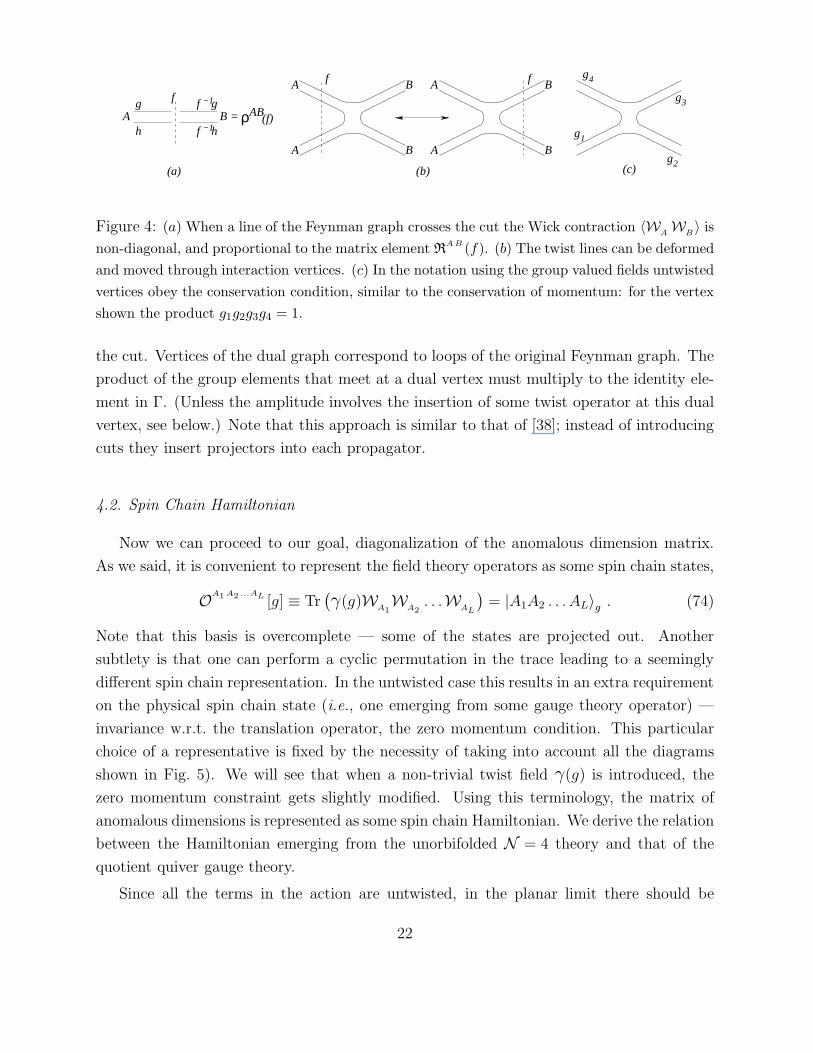
f −1hρAB(f)=

f −1gfgA B

h

A

A

B

B

f A

A

B

B

f

g2

g3

g1

g4

(a) (b) (c)

Figure 4: (a) When a line of the Feynman graph crosses the cut the Wick contraction 〈WAW

B〉 is

non-diagonal, and proportional to the matrix element RA B (f). (b) The twist lines can be deformed

and moved through interaction vertices. (c) In the notation using the group valued fields untwisted

vertices obey the conservation condition, similar to the conservation of momentum: for the vertex

shown the product g1g2g3g4 = 1.

the cut. Vertices of the dual graph correspond to loops of the original Feynman graph. The

product of the group elements that meet at a dual vertex must multiply to the identity ele-

ment in Γ. (Unless the amplitude involves the insertion of some twist operator at this dual

vertex, see below.) Note that this approach is similar to that of [38]; instead of introducing

cuts they insert projectors into each propagator.

4.2. Spin Chain Hamiltonian

Now we can proceed to our goal, diagonalization of the anomalous dimension matrix.

As we said, it is convenient to represent the field theory operators as some spin chain states,

OA1 A2 ...AL [g] ≡ Tr(γ(g)W

A1W

A2. . .W

AL

)= |A1A2 . . . AL〉g . (74)

Note that this basis is overcomplete — some of the states are projected out. Another

subtlety is that one can perform a cyclic permutation in the trace leading to a seemingly

different spin chain representation. In the untwisted case this results in an extra requirement

on the physical spin chain state (i.e., one emerging from some gauge theory operator) —

invariance w.r.t. the translation operator, the zero momentum condition. This particular

choice of a representative is fixed by the necessity of taking into account all the diagrams

shown in Fig. 5). We will see that when a non-trivial twist field γ(g) is introduced, the

zero momentum constraint gets slightly modified. Using this terminology, the matrix of

anomalous dimensions is represented as some spin chain Hamiltonian. We derive the relation

between the Hamiltonian emerging from the unorbifolded N = 4 theory and that of the

quotient quiver gauge theory.

Since all the terms in the action are untwisted, in the planar limit there should be

22

.

.

.

.

.

.

A1 A2 AL A1 A2 AL

B1 B2 BL B1 B2 BL

f f

+ + ...

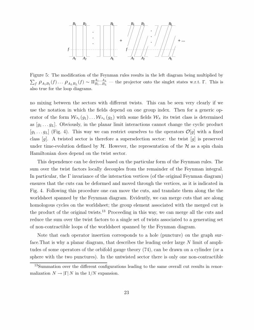
Figure 5: The modification of the Feynman rules results in the left diagram being multiplied by∑

f ρA1B1(f) . . . ρALBL

(f) ∼ ΠA1...AL

B1...BL— the projector onto the singlet states w.r.t. Γ. This is

also true for the loop diagrams.

no mixing between the sectors with different twists. This can be seen very clearly if we

use the notation in which the fields depend on one group index. Then for a generic op-

erator of the form WA1 (g1) . . .WAL (gL) with some fields WA its twist class is determined

as [g1 . . . gL]. Obviously, in the planar limit interactions cannot change the cyclic product

[g1 . . . gL] (Fig. 4). This way we can restrict ourselves to the operators O[g] with a fixed

class [g]. A twisted sector is therefore a superselection sector: the twist [g] is preserved

under time-evolution defined by H. However, the representation of the H as a spin chain

Hamiltonian does depend on the twist sector.

This dependence can be derived based on the particular form of the Feynman rules. The

sum over the twist factors locally decouples from the remainder of the Feynman integral.

In particular, the Γ invariance of the interaction vertices (of the original Feynman diagram)

ensures that the cuts can be deformed and moved through the vertices, as it is indicated in

Fig. 4. Following this procedure one can move the cuts, and translate them along the the

worldsheet spanned by the Feynman diagram. Evidently, we can merge cuts that are along

homologous cycles on the worldsheet; the group element associated with the merged cut is

the product of the original twists.13 Proceeding in this way, we can merge all the cuts and

reduce the sum over the twist factors to a single set of twists associated to a generating set

of non-contractible loops of the worldsheet spanned by the Feynman diagram.

Note that each operator insertion corresponds to a hole (puncture) on the graph sur-

face.That is why a planar diagram, that describes the leading order large N limit of ampli-

tudes of some operators of the orbifold gauge theory (74), can be drawn on a cylinder (or a

sphere with the two punctures). In the untwisted sector there is only one non-contractible

13Summation over the different configurations leading to the same overall cut results in renor-

malization N → |Γ|N in the 1/N expansion.

23

loop wrapping the cylinder. Summation over this twist leads to projection onto the Γ-

invariant states (see Fig. 5). Hence in this case, the amplitudes of the orbifold coincide with

those of the N =4 theory, as advocated. The miraculous integrability of the N =4 theory

therefore directly carries over to the untwisted sector of the orbifold gauge theory, provided

it is supersymmetric.

σB(g)−1σA(g)=

g−1h−1h

A

B

h

g

g−1h−1h

A

B

h

g

g−1h−1h

h

g

( ) ( )

(a) (b)

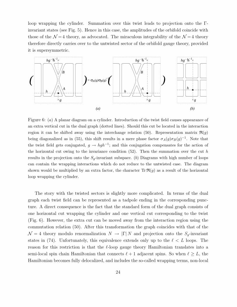
Figure 6: (a) A planar diagram on a cylinder. Introduction of the twist field causes appearance of

an extra vertical cut in the dual graph (dotted lines). Should this cut be located in the interaction

region it can be shifted away using the interchange relation (50). Representation matrix R(g)

being diagonalized as in (55), this shift results in a mere phase factor σA(g)σB(g)−1. Note that

the twist field gets conjugated, g → hgh−1; and this conjugation compensates for the action of

the horizontal cut owing to the invariance condition (52). Then the summation over the cut h

results in the projection onto the Sg-invariant subspace. (b) Diagrams with high number of loops

can contain the wrapping interactions which do not reduce to the untwisted case. The diagram

shown would be multiplied by an extra factor, the character Tr R(g) as a result of the horizontal

loop wrapping the cylinder.

The story with the twisted sectors is slightly more complicated. In terms of the dual

graph each twist field can be represented as a tadpole ending in the corresponding punc-

ture. A direct consequence is the fact that the standard form of the dual graph consists of

one horizontal cut wrapping the cylinder and one vertical cut corresponding to the twist

(Fig. 6). However, the extra cut can be moved away from the interaction region using the

commutation relation (50). After this transformation the graph coincides with that of the

N = 4 theory modulo renormalization N → |Γ|N and projection onto the Sg-invariant

states in (74). Unfortunately, this equivalence extends only up to the ℓ < L loops. The

reason for this restriction is that the ℓ-loop gauge theory Hamiltonian translates into a

semi-local spin chain Hamiltonian that connects ℓ + 1 adjacent spins. So when ℓ ≥ L, the

Hamiltonian becomes fully delocalized, and includes the so-called wrapping terms, non-local

24

interactions that wrap around the full length of the spin chain. When this is the case, the

extra cut emerging from insertion of the twist field γ(g) can no longer be shifted away from

the interaction region, and some propagators inevitably cross it (Fig. 6b).

The conclusion is that locally, on any nearest neighbor set of spins, the interaction terms

in H all act identically to the local interaction terms of the N = 4 Hamiltonian, as long

as the local set of spins does not contain the twist operator γ(g). If the twist generator is

present in the interaction region, one could shift the twist operator to either side, until it is

outside the interaction region. In this way we derive, for example, that the nearest neighbor

interaction term, when acting on two spins separated by a twist γ(g), gets modified via

H[12]WAγ(g)W

B= HCD

ABW

Cγ(g)W

D, (75)

where

HCD

AB= HCD′

AB′R(g)B

′

BR(g)D

D′. (76)

This relation (and analogous relations for the higher order terms) expresses the Γ-invariance

of the local interaction terms of H — the twist field can be moved either to the left or to

the right, which results in the same phase factor.

5. Integrability: Orbifolding the Bethe Ansatz

From the standpoint of the string theory dual it is easy to argue that, in the strong

’t Hooft coupling limit, orbifold field theories of N = 4 SYM are integrable. We shall in-

vestigate the gauge theory Bethe ansatz for the orbifold model. First we explore the su2

subsector consisting of the two scalar fields and explain the derivation of the Bethe equa-

tions [41],[42] as well as their modification for the orbifold theory.14 Then we extend the

complete set of Bethe equations from the N =4 gauge theory to the quotient quiver gauge

theory.

5.1. Bethe Equations: A Brief Introduction

We will start with the simplest example, the periodic Heisenberg su2 spin chain of length

L. Each of the L spins has a two-dimensional space of states C2 with the basis vectors |↓〉14There exists a different approach using theR-matrices; e.g., [43]. However, in our exposition we

mainly restrict ourselves to the concept of BAE emerging from analysis of multiple scattering waves.

The same approach was used in the study of the integrable two-dimensional field theories [44].

25

and |↑〉 corresponding to the spin being oriented downward or upward. (In the field theory

language these correspond to the two scalar fields, Z and W .) Thus for the whole chain the

space of states is C 2L

. Our goal is to diagonalize the Hamiltonian

H =L∑

i=1

(1−Pi,i+1

). (77)

Here Pi,i+1 is the interchange operator acting between the i-th and the i+ 1-th sites. It is

known that the su2 subsector consisting of the two scalar fields is closed in N =4 theory, and

its matrix anomalous dimension is given exactly by the Heisenberg spin chain Hamiltonian.

First, there exists a vacuum state |↓ ↓ . . . ↓〉 with all spins pointing down. (TrZL operator

in field theory.) The next step is to consider states with one excitation,

|n〉 = |↓ ↓ . . . ↓ ↑n ↓ . . . ↓〉 (78)

with the spin up being at the n-th position. Acting with the Hamiltonian we get

H |n〉 = − |n− 1〉+ 2 |n〉 − |n+ 1〉 (79)

with the identification |0〉 ≡ |L〉 and |L+ 1〉 ≡ |1〉. One can try to find a plane wave solution

in the form

|k〉 =

L∑

n=1

eikn |n〉 . (80)

Acting with the Hamiltonian and equating the coefficients before a generic |n〉, we get for

the eigenvalue ǫ(k)

ǫ eikn =(−eik + 2− e−ik

)eikn = 2 (1− cos k) eikn , (81)

thus ǫ(k) = 1− cos k. In order for these equations to hold for |0〉 and |L〉 one has to impose

an extra periodicity condition,

eikL = 1 . (82)

Physically such a solution corresponds to a standing wave.

One can proceed and introduce states with the two excitations located at positions n1

and n2,

|n1, n2〉 = |↓ ↓ . . . ↓ ↑n1↓ . . . ↓ ↑n2

↓ . . . ↓〉 . (83)

26

The solution can now be found in the form of the two scattering waves,

|k1, k2〉 =∑

1≤n1<n2≤L

(ei(k1n1+k2n2) + S(k1, k2) ei(k2n1+k1n2)

)|n1, n2〉 . (84)

Acting with the Hamiltonian and equating the coefficients before generic |n1, n2〉, we get

the two non-interacting waves having the energy

ǫ(k1, k2) = ǫ(k1) + ǫ(k2) . (85)

Coefficients before |n, n+ 1〉 are responsible for the interaction, and the corresponding equa-

tion determines the scattering phase

S(k1, k2) = −ei(k1+k2) + 1− 2eik2

ei(k1+k2) + 1− 2eik1

=λ1 − λ2 − iλ1 − λ2 + i

; (86)

where we have introduced the rapidity λ = 12

cot k2. Note that the momentum and energy

in terms of rapidity are

eik(λ) =λ+ i

2

λ− i2

, ǫ(λ) =1

λ2 + 14

. (87)

A remarkable feature of this system is its integrability. It manifests itself in the fact

that the scattering reduces to the two-particle scattering, and this two-particle scattering is

a mere exchange of quantum numbers. The solution (84) can be generalized to the states

with the l spins up, and it becomes

|k1, k2, . . . kl〉 =∑

1≤n1<...<nl≤L

an1,n2,...nl(k1, k2, . . . kl) |n1, n2, . . . nl〉 . (88)

The corresponding coefficients

an1,n2,...nl(k1, k2, . . . kl) =

∑

σ∈Sl

S(σ, k) exp i[kσ(1)n1 + · · ·+ kσ(l)nl] . (89)

Here Sl is the group of permutations, and the phase factor S(σ, k) obeys the group property

S(σ1σ2, k) = S(σ2, k)S(σ1, σ2k) . (90)

For the interchange of the two neighboring excitations σi,i+1 the phase factor

S(σi,i+1, k) = S(ki, ki+1) (91)

reduces to the two-particle scattering phase (86).

27

Having taken this into account one can easily formulate the periodicity condition for the

standing wave:

an1,n2,...nl(k1, k2, . . . kl) = an2,...nl,n1+L(k2, . . . kl, k1) (92)

(note the order of momenta ki). Using explicit form of the coefficients a(k) in (89) and the

properties of the phase S(σ, k) one finds

eik1L∏

j 6=1

S(k1, kj) = 1 . (93)

(Similar equations hold for the other momenta.) In terms of rapidities λj these periodicity

conditions read

(λj + i2

λj − i2

)L

=∏

k 6=j

λj − λk + i

λj − λk − i, j = 1, 2, . . . l . (94)

The set of equations (94) is known as the Bethe ansatz equations (BAE).

The zero momentum constraint results in the condition

eiP

j kj = 1 ; (95)

equivalently,

∏

j

λj + i2

λj − i2

= 1 . (96)

These results can be generalized to su2-symmetric chains with higher spins. We give

them without derivation. The BAE for a spin s chain read

(λj + is

λj − is)L

=∏

k 6=j

λj − λk + i

λj − λk − i, j = 1, 2, . . . l . (97)

The energy and momentum

eiP =λ+ is

λ− is , ǫ(λ) =2s

λ2 + s2. (98)

28

5.2. Bethe Equations for the Orbifold Gauge Theory: su2 Subsector

The first step towards the construction of the BAE for the orbifold gauge theory would

be to consider a su2 subsector and go through the construction in detail. As it was argued,

interaction terms are unaffected by the orbifoldization procedure except for the interaction

between the first and the L-th site. This means that the bulk solution (88) will remain

unaltered, though the periodicity condition as well as the zero momentum constraint will

get modified.

As it was stated in (55), the action of the twist field γ(g) can be diagonalized for each

given element g. With reference to the su2 subsector it means that the action on the fields

Z and W can be brought to the form

g :

Z

W

→

ωsZ 0

0 ωsW

Z

W

, (99)

where ω = S√

1 = e2πi/S; S being the order of the element g, i.e., gS = 1. The Hamiltonian

H =∑L

i=1Hi,i+1, where Hi = 1 − Pi,i+1 for i = 1, . . . L − 1; while HL,1 gets modified

according to (76). Explicitly it means

HL,1 |Z . . . Z〉g = 0 , (100)

HL,1 |Z . . .W 〉g = |Z . . .W 〉g − ωsW−sZ |W . . . Z〉g , (101)

HL,1 |W . . . Z〉g = |W . . . Z〉g − ωsZ−sW |Z . . .W 〉g , (102)

HL,1 |W . . .W 〉g = 0 . (103)

Note that for almost all the sites the Hamiltonian is unaltered. As it was emphasized in [45],

one can use the same ansatz, and the only novelty is the modification of the periodicity

conditions.

The simplest way to derive the new periodicity condition is to consider a plane wave

solution

|k〉g =L∑

n=1

eikn |n〉g . (104)

Acting with the Hamiltonian and equating the coefficients before a generic |n〉g, we get

ǫeikn |n〉g =(−eik + 2− e−ik

)eikn |n〉g ; (105)

giving the same eigenvalue ǫ(k) = 2(1 − cos k). Equations for |1〉g and |L〉g have to be

29

considered separately because of the modified action of the Hamiltonian

H |1〉g = −ωsZ−sW |L〉g + 2 |1〉g − |2〉g , (106)

H |L〉g = − |L− 1〉g + 2 |L〉g − ωsW−sZ |1〉g . (107)

Then equating the coefficients we get the two equations

|1〉g : ǫ = −eik + 2− eikLωsW−sZe−ik , (108)

|L〉g : ǫ = −e−ikLω−(sW−sZ)eik + 2− e−ik . (109)

The periodicity condition for a single wave solution then reads

eikLωsW−sZ = 1 . (110)

Analogously, for several interacting waves the BAE read

eiPjL ≡(λj + i

2

λj − i2

)L

= ωsZ−sW

∏

k 6=j

λj − λk + i

λj − λk − i. (111)

In order to formulate the “zero momentum constraint” one has to go back to its physical

origin. In the unorbifolded theory the zero momentum condition reflects the cyclicity of the

trace. However, in the twisted sectors the identification (74) suggests a fixed position of the

twist fields γ(g) in the l.h.s. and thus breaks the cyclic invariance. Recall that generally the

cyclicity condition is to fix a spin chain representative of a given field theory operator in

such a way that all the diagrams in Fig. 5 are accounted for. This consideration shows that

the modified zero momentum constraint should be stated as follows: should one perform a

cyclic shift of the fields under the trace (including the twist field) and use the commutation

relation (50) to move the twist back, the corresponding state would remain invariant. Then

the shift operator

U : |A1 . . . AL〉 → |A2 . . . ALA1〉 (112)

in the twisted sector should be modified according to

Ug : |A1 . . . AL〉g → σA1(g) |A2 . . . ALA1〉g . (113)

The zero momentum condition is nothing but the Ug-invariance.

In the su2 subsector the action of the shift operator on a state with l excitations becomes

Ug |n1, n2, . . . nl〉g =

ω−sZ |n1 − 1, n2 − 1, . . . nl − 1〉g , n1 6= 1 ,

ω−sW |n2 − 1, . . . nL − 1, L〉g , n1 = 1 .(114)

30

Thus the action of the shift operator depends on whether the last spin is up or down. We

will see in a moment that this difference is canceled when we take into account the form

of the periodicity condition. Thus taking the solution in the form (88) and acting with the

shift operator we have to analyze the terms with n1 6= 1 and n1 = 1 separately. For n1 6= 1

we get

Ug :∑

1<n1<...<nl≤L

an1,n2,...nl(k1, k2, . . . kl) |n1, n2, . . . nl〉g

→ ω−sZ

∑

1<n1<...<nl≤L

an1,n2,...nl(k1, k2, . . . kl) |n1 − 1, n2 − 1, . . . nl − 1〉g

= ω−sZ

∑

1≤n1<...<nl<L

an1+1,n2+1,...nl+1(k1, k2, . . . kl) |n1, n2, . . . nl〉g

= ω−sZeiP∑

1≤n1<...<nl<L

an1,n2,...nl(k1, k2, . . . kl) |n1, n2, . . . nl〉g ; (115)

where we have used the fact that for nl < L

an1+1,n2+1,...nl+1(k1, k2, . . . kl) = eiPan1,n2,...nl(k1, k2, . . . kl) . (116)

Considering the terms with n1 = 1 gives

Ug :∑

1<n2<...<nl≤L

a1,n2,...nl(k1, k2, . . . kl) |1, n2, . . . nl〉g

→ ω−sW

∑

1<n2<...<nl≤L

a1,n2,...nl(k1, k2, . . . kl) |n2 − 1, . . . nl − 1, L〉g

= ω−sW

∑

1≤n2<...<nl<L

a1,n2+1,...nl+1(k1, k2, . . . kl) |n2, . . . nl, L〉g

= ω−sZeiP∑

1≤n2<...<nl<L

an2,...nl,L(k2, . . . kl, k1) |n2, . . . nl, L〉g . (117)

In the last line we have used the periodicity condition leading to the orbifold BAE (111),

a1,n2+1,...nl+1(k1, k2, . . . kl) = ωsW−sZan2+1,...nl+1,L+1(k2, . . . kl, k1) (118)

= ωsW−sZeiPan2,...nl,L(k2, . . . kl, k1) .

The conclusion is that the action of the shift operator on all the terms is the same, and

U |k1, k2, . . . kl〉g = ω−sZeiP |k1, k2, . . . kl〉g . (119)

Finally, the orbifold zero momentum condition in a given twisted sector is

ω−sZeiP = 1 . (120)

31

5.3. Bethe Equations: Chains with Arbitrary Symmetry Algebrae

Let us first review integrability for the full parent N = 4 supersymmetric model. The

algebra behind the N = 4 supersymmetry is the su2,2|4 superalgebra. Thus generic opera-

tors of the field theory get identified with some states of the su2,2|4-symmetric spin chain.

Provided the spin chain is integrable, there exists a generic formulation of the BAE for an

arbitrary underlying symmetry algebra. These BAE were formulated in [46] for orthogonal

and symplectic algebrae and then generalized to an arbitrary Lie algebrae in [47]. Extension

to the superalgebrae case was given in [48],[49],[50].

Let us introduce the notations regarding generic Lie algebrae. A semisimple Lie algebra

g has the maximal commuting subalgebra h ⊂ g — the Cartan subalgebra. The number

r = dim h = rk g is called the rank of the Lie algebra g. The adjoint action of h on the

complement h⊥ can be diagonalized, so that for any h ∈ h

ad hEα = α(h)Eα , (121)

α ∈ h∗ being the root and Eα the corresponding root vector. It is known that whenever

α is a root, −α is also a root; and that the roots are non-degenerate. The set of roots

R =⋃

α Rα can be split into the opposite positive and negative roots, R = R+ ∪R− such

that the sum of any two positive (negative) roots is again a positive (negative) root. There

exist exactly r simple roots such that any positive root can be obtained as their sum with

the positive integer coefficients. Then in the Chevalley-Serre basis,

[Hi, Hj ] = 0 , [Hi, E±j ] = ±ajiE

±j , [E+

i , E−j ] = Hiδij . (122)

The root vectors are normalized so that the bilinear form B(E+i , E

−i ) = −1; equivalently, it

means that αi(H) = −B(Hi, H) for H ∈ h. The coroots α∨i = 2αi/(αi, αi), and the Cartan

matrix aij = (αi α∨j ) are the elements of the Cartan matrix. Each triple (Hi, E

+i , E

−i ) forms

an su2 subalgebra; though the raising and lowering operators from the r different subalgebrae

do not necessarily commute. Forming all their possible commutators we get the complete

basis in g. There are the additional relations

ad1−aji

E±i

E±j = 0 . (123)

Similarly, any irreducible representation V can be decomposed into a sum of linear

spaces with definite weights; and there exists a unique highest weight for which the sum of

the coefficient in its expansion in simple roots is maximal. (Roots can be viewed as weights

of the adjoint representation.) Given the vector of the highest weight, one can build the

32

space of a unique irreducible representation by acting on it with the lowering operators E−i .

It is convenient to use the basis of the so-called fundamental weights ωi normalized by

(ωi, α∨j ) = δij . (124)

Then any highest weight can be expanded as

Ω =∑

i

Viωi ; (125)

where the coefficients Vi are called the Dynkin labels. Restricting the representation to one of

these su2 subalgebrae (Hi, E±i ), one concludes that the Dynkin labels are to be integer for the

finite dimensional representations. (Note the factor of two in the definition of the coroot.)

There exist the r distinguished representations with the highest weights ωi, i = 1, 2, . . . r,

called the fundamental representations. For the i-th fundamental representation the Dynkin

labels Vj = δij . Since tensoring the two vectors results in addition of their weights, any

irreducible representation can be extracted from the Clebsch-Gordan series of the tensor

product of some fundamental representations. In particular, the representation with the

highest weight nωi can be obtained as the n-th symmetric power of the i-th fundamental

representation.

Now one can formulate the set of the BAE for a generic15 g-symmetric spin chain.

There exist the r types of excitations, corresponding to the r simple roots. Since there

can be multiple excitations of the same type it is convenient to number the corresponding

spectral parameters as λj,k; where j = 1, 2, . . . r and k = 1, 2, . . .Kj, Kj being the number

of excitations of type j. The set of the BAE becomes

eiPj,kL =∏

(j′,k′)6=(j,k)

Sjj′(λj,k, λj′,k′) ; (126)

where the scattering matrix

Sjj′ =λj,k − λj′,k′ + i

2aj,j′

λj,k − λj′,k′ − i2aj,j′

. (127)

Momentum

eiPj,k =λj,k + i

2Vj

λj,k − i2Vj

. (128)

15The word “generic” here refers to the generic symmetry algebra; of course, the integrability

condition fixes the form of the Hamiltonian.

33

(Here Vj are the Dynkin labels of the representation via which the algebra acts on each site

— twice the spin in the su2 case.) The total energy of the corresponding eigenstate

ǫ =r∑

j=1

Kj∑

k=1

ǫj(λj,k) , ǫj(λj,k) =Vj

λ2j,k + 1

4V 2

j

. (129)

The superconformal symmetry algebra of the N = 4 SYM theory is the su2,2|4 superal-

gebra. Its bosonic subalgebrae su2,2 and su4 are nothing but the algebra of the conformal

group in four dimensions and the R-symmetry algebra. Unlike the bosonic semisimple Lie

algebrae, the Dynkin diagram of a superalgebra is not unique. For the su2,2|4 there exist

the two distinguished choices of the root system, the so-called “Beauty” and the “Beast”.

Though the “Beast” is the most obvious system with one fermionic root, the “Beauty” root

system proves useful in the context of N = 4 supersymmetry. Exact embedding of these

root systems into su2,2|4 as well as the corresponding Cartan matrices is shown in Table 1.

More details regarding these root systems are given in Appendix A.2. The whole N = 4

theory was proved to be integrable [14],[15],[16]. Note that the spin chains with the different

representations of su2,2|4 correspond to different subclasses of operators.

5.4. Generalization to General Orbifolds

As it was argued, there is no mixing between the different twisted sectors. Furthermore,

in each given twisted sector [g] one can construct all the states inserting one twist field

γ(g), g being any fixed representative of the conjugacy class [g]. In conjunction with the

result (55) — the fact that one can diagonalize the action of any given element g ∈ Γ —

the problem reduces to the Abelian case modulo some subtleties. In particular, the Sg-

invariance does not completely incorporate into Bethe equations; and it is to be imposed by

hand — that is why some of the Bethe eigenstates may be projected out.

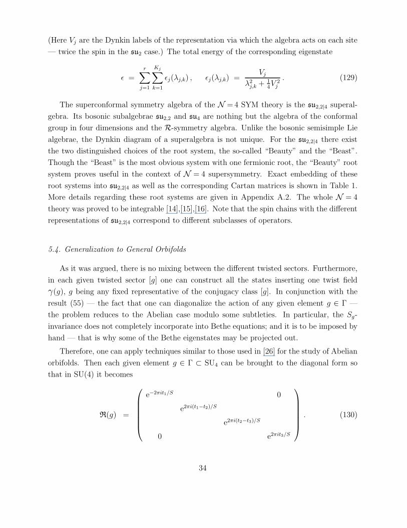
Therefore, one can apply techniques similar to those used in [26] for the study of Abelian

orbifolds. Then each given element g ∈ Γ ⊂ SU4 can be brought to the diagonal form so

that in SU(4) it becomes

R(g) =

e−2πit1/S 0

e2πi(t1−t2)/S

e2πi(t2−t3)/S

0 e2πit3/S

. (130)

34

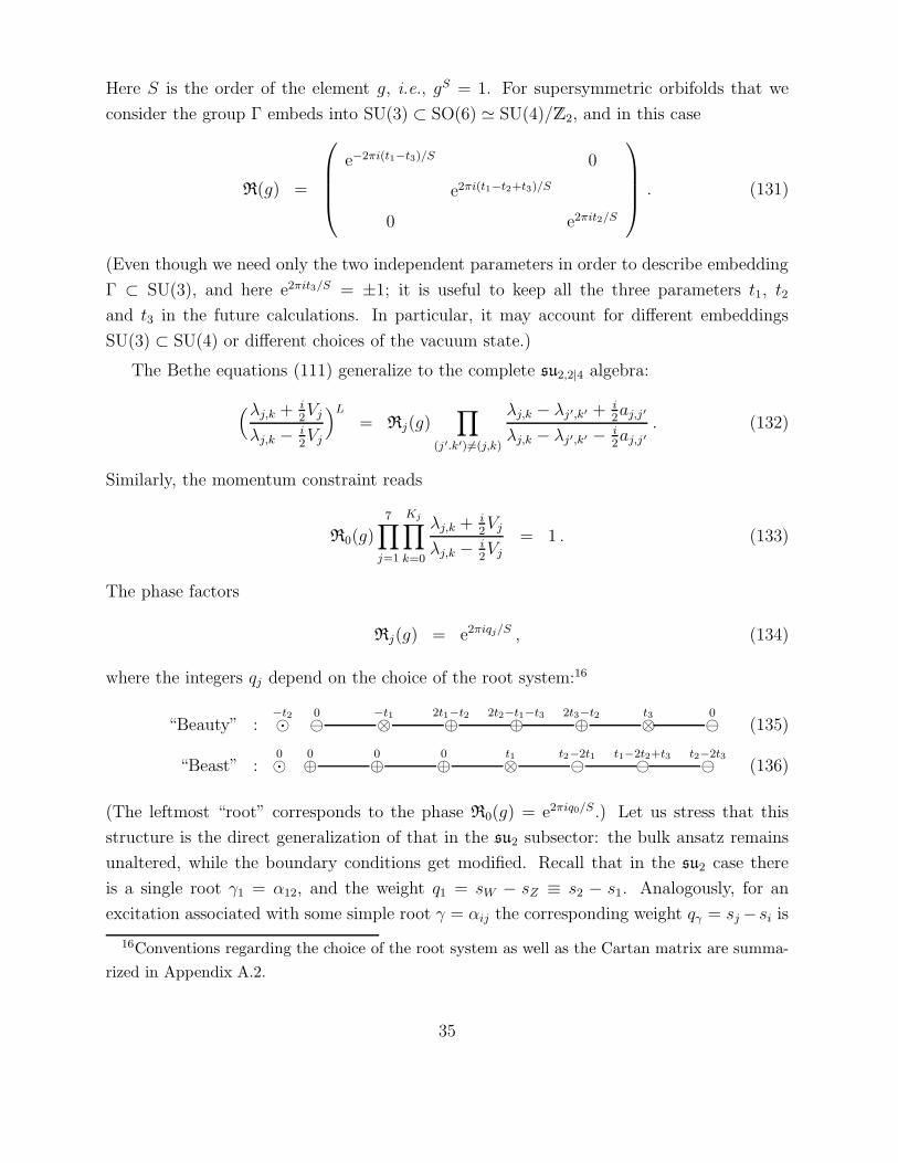
Here S is the order of the element g, i.e., gS = 1. For supersymmetric orbifolds that we

consider the group Γ embeds into SU(3) ⊂ SO(6) ≃ SU(4)/Z2, and in this case

R(g) =

e−2πi(t1−t3)/S 0

e2πi(t1−t2+t3)/S

0 e2πit2/S

. (131)

(Even though we need only the two independent parameters in order to describe embedding

Γ ⊂ SU(3), and here e2πit3/S = ±1; it is useful to keep all the three parameters t1, t2

and t3 in the future calculations. In particular, it may account for different embeddings

SU(3) ⊂ SU(4) or different choices of the vacuum state.)

The Bethe equations (111) generalize to the complete su2,2|4 algebra:

(λj,k + i2Vj

λj,k − i2Vj

)L

= Rj(g)∏

(j′.k′)6=(j,k)

λj,k − λj′,k′ + i2aj,j′

λj,k − λj′,k′ − i2aj,j′

. (132)

Similarly, the momentum constraint reads

R0(g)7∏

j=1

Kj∏

k=0

λj,k + i2Vj

λj,k − i2Vj

= 1 . (133)

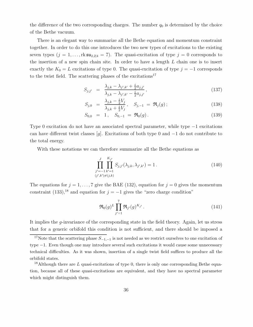
The phase factors

Rj(g) = e2πiqj/S , (134)

where the integers qj depend on the choice of the root system:16

“Beauty” :−t2⊙

0⊖

−t1⊗2t1−t2⊕

2t2−t1−t3⊕2t3−t2⊕

t3⊗0⊖ (135)

“Beast” :0⊙

0⊕

0⊕

0⊕

t1⊗t2−2t1⊖

t1−2t2+t3⊖t2−2t3⊖ (136)

(The leftmost “root” corresponds to the phase R0(g) = e2πiq0/S.) Let us stress that this

structure is the direct generalization of that in the su2 subsector: the bulk ansatz remains

unaltered, while the boundary conditions get modified. Recall that in the su2 case there

is a single root γ1 = α12, and the weight q1 = sW − sZ ≡ s2 − s1. Analogously, for an

excitation associated with some simple root γ = αij the corresponding weight qγ = sj−si is

16Conventions regarding the choice of the root system as well as the Cartan matrix are summa-

rized in Appendix A.2.

35

the difference of the two corresponding charges. The number q0 is determined by the choice

of the Bethe vacuum.

There is an elegant way to summarize all the Bethe equation and momentum constraint

together. In order to do this one introduces the two new types of excitations to the existing

seven types (j = 1, . . . , rk su2,2|4 = 7). The quasi-excitation of type j = 0 corresponds to

the insertion of a new spin chain site. In order to have a length L chain one is to insert

exactly the K0 = L excitations of type 0. The quasi-excitation of type j = −1 corresponds

to the twist field. The scattering phases of the excitations17

Sj,j′ =λj,k − λj′,k′ + i

2aj,j′

λj,k − λj′,k′ − i2aj,j′

, (137)

Sj,0 =λj,k − i

2Vj

λj,k + i2Vj

, Sj,−1 = Rj(g) ; (138)

S0,0 = 1 , S0,−1 = R0(g) . (139)

Type 0 excitation do not have an associated spectral parameter, while type −1 excitations

can have different twist classes [g]. Excitations of both type 0 and −1 do not contribute to

the total energy.

With these notations we can therefore summarize all the Bethe equations as

J∏

j′=−1

Kj′∏

k′=1

(j′,k′)6=(j,k)

Sj,j′(λj,k, λj′,k′) = 1 . (140)

The equations for j = 1, . . . , 7 give the BAE (132), equation for j = 0 gives the momentum

constraint (133),18 and equation for j = −1 gives the “zero charge condition”

R0(g)L

7∏

j′=1

Rj′(g)Kj′ . (141)

It implies the g-invariance of the corresponding state in the field theory. Again, let us stress

that for a generic orbifold this condition is not sufficient, and there should be imposed a

17Note that the scattering phase S−1,−1 is not needed as we restrict ourselves to one excitation of

type −1. Even though one may introduce several such excitations it would cause some unnecessary

technical difficulties. As it was shown, insertion of a single twist field suffices to produce all the

orbifold states.18Although there are L quasi-excitations of type 0, there is only one corresponding Bethe equa-

tion, because all of these quasi-excitations are equivalent, and they have no spectral parameter

which might distinguish them.

36

more restrictive invariance condition w.r.t. the full stabilizer Sg. That is why some of the

Bethe eigenstates may be projected out in field theory.

6. Applications of the BAE

Now we study some application of the Bethe equations. First we show that in the large

L limit one can reproduce the known results for the su2 subsector, which adhere to the

closed string dual. Next we consider particular quivers, ones with both Abelian and non-

Abelian orbifold group. For these simple examples one can easily determine the anomalous

dimensions of operators in the twisted sectors. Then these operators can be recast into the

quiver notation.

6.1. Comparison with the Closed String Sector

It is known that the Bethe equations can be solved in the limit of the long spin chain,

L≫ 1. Another restriction is L≪ N , which prevents the number of the non-planar graphs

from growing. In this limit one can perform a rescaling of the Bethe roots, λj → Lλj [51].

Then the momenta and energies of individual excitations

Pj,k = −i logLλj,k + i

2Vj

Lλj,k − i2Vj

≈ Vj

Lλj,kǫj,k ≈

Vj

L2λ2j,k

. (142)

Using the same approximation, eqs. (132) and (133) after taking the logarithm become19

Vj

λj,k

= 2π(mj +

qjS

)+

1

L

∑

(j′,k′)6=(j,k)

ajj′

λj,k − λj′,k′

, (143)

0 = 2π(m0 +

q0S

)+

1

L

7∑

j=1

Kj∑

k=1

Vj

λj,k

. (144)

It is well known how to solve these equations when there are present excitations of only

one type. It is convenient to define the resolvent (we drop the index j of the eigenvalues

since they are all of the same type)

G(x) =1

L

K∑

k=1

1

x− λk. (145)

19Here we will ignore the possibility of some states being projected out.

37

In terms of the resolvent the total momentum and total energy (anomalous dimension) of

the spin chain are

P = −Vj G(0) , ∆ = −λVj

LG′(0) . (146)

The Bethe equations are

Vj

λk= 2πmj +

2

L

∑

l 6=k

1

λk − λl, (147)

0 = 2πn+1

L

K∑

k=1

Vj

λk; (148)

m = mj + qj/S , n = m+ q0/S . (149)

The standard trick is to multiply the first equation with 1x−λk

and sum over k. After

performing some useful transformations,

∑

k

1

λk(x− λk)=

1

x

∑

k

[ 1

λk+

1

x− λk

]= L

G(0) +G(x)

x= −2πn

x+LG(x)

x,

and∑

k,l

k 6=l

2

(x− λk)(λk − λl)=

∑

k,l

k 6=l

1

λk − λl

( 1

x− λk

− 1

x− λl

)=

∑

k,l

k 6=l

1

(x− λk)(x− λl)

=∑

k,l

1

(x− λk)(x− λl)−

∑

k

1

(x− λk)2= L2G(x)− LG′(x) ;

the Bethe equations take the form

xG2(x) + (2πmx− Vj)G(x) + 2πnVj =x

LG′(x) . (150)

In the large L limit the term in the r.h.s. can be dropped, and there remains a mere quadratic

equation on G(x). The solution is

G(x) =Vj − 2πmx+ sgn m

√(2πmx− Vj)2 − 8πnVjx

2 x. (151)

The choice of the solution is determined by the correct asymptotics at infinity,

G(x) ∼ − nVj

mx=

Kj

Lx, x≫ 1 . (152)

(Recall that Kj is the number of excitations — that is why for large x we write G(x) ∼ Kj

Lx.)

This imposes the requirement mn < 0. In its turn the regularity of G at zero requires

m < 0; then n > 0. Expanding the resolvent at x = 0 yields

G(x) ∼ 2πnx− 4π2

Vj

n(|m| − n)x , x≪ 1 . (153)

38

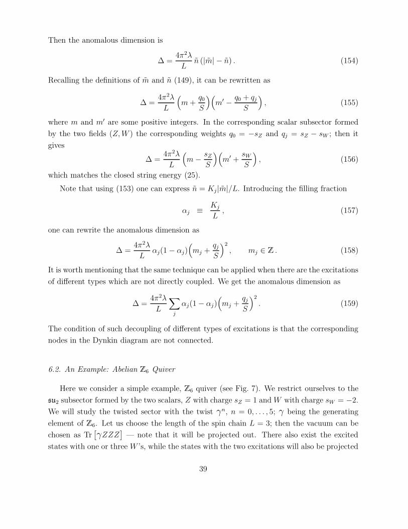
Then the anomalous dimension is

∆ =4π2λ

Ln (|m| − n) . (154)

Recalling the definitions of m and n (149), it can be rewritten as

∆ =4π2λ

L

(m+

q0S

)(m′ − q0 + qj

S

), (155)

where m and m′ are some positive integers. In the corresponding scalar subsector formed

by the two fields (Z,W ) the corresponding weights q0 = −sZ and qj = sZ − sW ; then it

gives

∆ =4π2λ

L

(m− sZ

S

)(m′ +

sW

S

), (156)

which matches the closed string energy (25).

Note that using (153) one can express n = Kj |m|/L. Introducing the filling fraction

αj ≡Kj

L, (157)

one can rewrite the anomalous dimension as

∆ =4π2λ

Lαj(1− αj)

(mj +

qjS

)2

, mj ∈ Z . (158)

It is worth mentioning that the same technique can be applied when there are the excitations

of different types which are not directly coupled. We get the anomalous dimension as

∆ =4π2λ

L

∑

j

αj(1− αj)(mj +

qjS

)2

. (159)

The condition of such decoupling of different types of excitations is that the corresponding

nodes in the Dynkin diagram are not connected.

6.2. An Example: Abelian Z6 Quiver

Here we consider a simple example, Z6 quiver (see Fig. 7). We restrict ourselves to the

su2 subsector formed by the two scalars, Z with charge sZ = 1 and W with charge sW = −2.

We will study the twisted sector with the twist γn, n = 0, . . . , 5; γ being the generating

element of Z6. Let us choose the length of the spin chain L = 3; then the vacuum can be

chosen as Tr[γZZZ

]— note that it will be projected out. There also exist the excited

states with one or three W ’s, while the states with the two excitations will also be projected

39

03

4 5

12

~0

1

2

0

(a) (b)

Figure 7: (a) The Z6 quiver. There are the six nodes corresponding to the six representations

of Z6. We show only the scalar lines corresponding to the fields Z (blue lines) transforming in

RZ ≃ ρ1 and W (red lines) transforming in RW ≃ ρ4 ≃ ρ−2. (b) The D5 quiver with the

two-dimensional defining representation R ≃ ρ1. Note that for these two quivers we show only

the lines corresponding to the su2 subsector; i.e., the two scalar fields.

out. Our goal will be to describe these Bethe vectors in terms of the quiver notation. By

Oijki ≡ Tr ΦijΦ

jkΦ

ki we will denote the quiver gauge theory operator corresponding to the

closed cycle between the three nodes k → j → i in the quiver.

Note that the state with the three excitations is unique in each given twisted sector, and

it corresponds to the field theory operator Tr[γnWWW

]. Commuting the twist field γn

with one of the fields W we find that

Tr[γnWWW

]= e2πinsW /6 Tr

[γnWWW

]; (160)

i.e., this state is projected out in all sectors except for n = 0 and n = 3. The reason for this

is the extra symmetry: it is sufficient to commute the twist field with only one of the three

W fields. Note that the total charge of the three fields W is zero, and normally one would

expect Tr[γWWW

]to be a non-trivial operator.

Using the formula (65) we find that

O0420 = Tr[WWW

]+ Tr

[γ3WWW

], (161)

O1531 = Tr[WWW

]− Tr

[γ3WWW

]; (162)

40

or

Tr[WWW

]=

1

2O0420 +

1

2O1531 , (163)

Tr[γ3WWW

]=

1

2O0420 −

1

2O1531 . (164)

Graphically the operators O042 and O153 correspond to the two closed triangles formed by

the red lines. Applying the Hamiltonian we find the anomalous dimensions

∆Tr [γ3WWW ] = ∆Tr [γ3WWW ] = 0 . (165)

The states with one excitation have the form Tr[γnZZW

], and there is one such state

in each given twisted sector. These operators correspond to the triangles with the two blue

(field Z) and one red (field W ) line. There are six such triangles and there are six different

operators with n = 1, . . . , 5 — these numbers coincide as we expect. The transition formula

between these two descriptions is

Ol, l+1, l+2, l =

5∑

n=0

e−2πi ln6 Tr

[γnZZW

]; (166)

performing the Fourier transform yields

Tr[γnZZW

]=

1

6

5∑

l=0

e2πi ln6 Ol, l+1, l+2, l . (167)

These operators diagonalize the matrix of anomalous dimensions. Direct application of the

Hamiltonian shows that the corresponding eigenvalues are

∆Tr [γnZZW ] = 4λ sin2 πn

6. (168)

This simple example illustrates the interrelation of the two descriptions in the orbifold gauge

theory. First, the quiver description gives a very clear understanding of what the physical

fields and gauge invariant operators are, while in the “orbit” description using the twist

fields some of the operators may be projected out. On the other hand, the description

using the twist fields proves to be more robust for studying the field theory dynamics (the

matrix of anomalous dimensions). In order to illustrate this let us write the part of the

action responsible for the non-trivial part of the interaction Hamiltonian, Tr[ZWZ†W † +

WZW †Z†]. In terms of the quiver notation

Tr[ZWZ†W † +WZW †Z†

]=

∑

l

[Ol,l+1,l−1,l−2,l +Ol,l−2,l−1,l+1,l

](169)

=∑

l

Tr[Z l

l+1Wl+1l−1 Z

l−2 †l−1 W l−2 †

l +W ll−2 Z

l−2l−1 W

l+1 †l−1 Z l †

l+1

].

41

Here Zkl denotes the field corresponding to the quiver arrow going from node l to node k.

Note that the conjugation changes the direction of the corresponding arrow; e.g., Z1 †2 is an

arrow going from node 1 to node 2. Indeed, as we see, studying the matrix of anomalous

dimensions using the quiver notation would have been more complicated.

6.3. An Example: non-Abelian D5 Quiver

Next we consider a simple orbifold with a non-Abelian discrete group D5 (the facts

about the dihedral group DS as well as its representation ring are given in Appendix A.3.)

The corresponding quiver is shown in Fig. 7. Again, we study the su2 sector, and the

scalar field ΦI transforms in the two-dimensional representation R ≃ ρ1. From the quiver

representation it is clear that there are the four different operators of length L = 2; namely,

those are

O010 , O010 , O121 , O222 . (170)

On the other hand, there are the four different twist classes, [e], [r], [r2], [σ]. Applying

the definitions of the operators (240), we see that in each twist class there is exactly one

non-trivial operator; thus there are the total of four operators of length two:

Oe = Tr[ZW

], Or = Tr

[γ(r)ZW

], Or2 = Tr

[γ(r2)ZW

], Oσ = Tr

[γ(σ)ZZ

]. (171)

Here Z andW denote the first and second components of the field ΦI . Note that the product

of the two fields ZZ has transforms non-trivially under the action of r; nevertheless, in the

sector with twist [σ] the operator Oσ = Tr[γ(σ)ZZ

]is non-trivial as r 6∈Sσ. The absence

of mixing between the different twist classes ensures that the set of operators Oe, Or, Or2 ,

Oσ diagonalize the matrix of anomalous dimensions. Acting with the Hamiltonian we find

the corresponding anomalous dimensions as

∆Oe = 0 , ∆Or = 4λ sin2 π

5=

5−√

5

2λ , ∆O

r2= 4λ sin2 2π

5=

5 +√

5

2λ , ∆Oσ = 0 .

(172)

The same eigenvalues can be obtained solving the Bethe equations. The three operators

Oe, Or and Or2 are the states with one excitation. Diagonalizing the twist field as

γ(g) =

eiα 0

0 e−iα

, g = e, r, r2 ; (173)

we find that the Bethe equation and the momentum constraint reduce to

λ+ i2

λ− i2

= eiα , ǫ =1

λ2 + 14

. (174)

42

This gives

λ =1

2cot

α

2, ǫ = 4 sinh2 α

2. (175)

For the twist element g = e, r, r2 we have α = 0, 2π/5, 4π/5 correspondingly. This

reproduces the correct result. The twist field γ(g) is non-diagonal. After the diagonalization

of γ(σ) operator Oσ maps to the vacuum state, and that is why ∆Oσ = 0.

The next step is to find the dictionary between the two notations. In order to do

this one can start with the quiver notation and rewrite the corresponding operators using

the transition rules (230) and (231) from Appendix B.4. The two operators O010 and

O010 correspond to the closed paths ρ0 ← ρ1 ← ρ0 and ρ0 ← ρ1 ← ρ0. Since the

representations ρ0 and ρ0 are one-dimensional, the corresponding invariant tensors

KAB11 = KAB (176)

(the indices A, B belong to the defining representation R ≃ ρ1.) The non-zero components

are

K12 = K21 =1√2

(177)

(note that the normalization respects the unitarity condition.) Then

KAB(g) = KAB ρλ(g) , λ = 0, 0 . (178)

This gives

O010 =√

2Tr[ZW + (1 + ω)γ(r)ZW + (1 + ω2)γ(r2)ZW + 5γ(σ)ZZ

]

=√

2[Oe + (1 + ω)Or + (1 + ω2)Or2 + 5Oσ

]; (179)

O010 =√

2Tr[ZW + (1 + ω)γ(r)ZW + (1 + ω2)γ(r2)ZW − 5γ(σ)ZZ

]

=√

2[Oe + (1 + ω)Or + (1 + ω2)Or2 − 5Oσ

]. (180)

(We have used the permutation relation (243).)

Next, O121 corresponds to the product of the two tensors,

KABkl =

∑

p∈ρ2

KpAlKk

Bp , k, l ∈ ρ1 . (181)

The non-trivial coefficients corresponding to the decomposition R ⊗ ρ1 → ρ2 are K111 =

K222 = 1, while those corresponding to the decomposition R⊗ ρ2 → ρ1 are K1

21 = K212 = 1.

This gives the corresponding invariant tensor in (181):

K1211 = K21

22 = 1 . (182)

43

Therefore, one identifies

O121 = 2[Oe + (ω2 + ω4)Or + (ω3 + ω4)Or2

]. (183)

Similarly, for the operator O222 we need to find the decomposition R ⊗ ρ2 → ρ2. The

non-trivial coefficients are K211 = K1

22 = 1. Consequently,

K1211 = K21

22 = 1 (184)

and

O222 = 2[Oe + 2ω3Or + (1 + ω)Or2

]. (185)

These formulae give the transition between the two bases in the operator space. Again,

the conclusion is that generally operators corresponding to the closed paths in the quiver

are not the eigenvectors of the matrix of anomalous dimensions. In other words, an operator

corresponding to a closed loop in the quiver is typically a mix of operators with different

conformal dimensions; neither does it belong to a given twisted sector.

7. Concluding Remarks

As we have seen, methods of studying the Abelian orbifold gauge theories can be ex-

tended to arbitrary non-Abelian setups with minor modifications. The key argument is that

the diagonalization of the twist field in each given twisted sector allows one to apply the

techniques used for the Abelian case. Indeed, in a given twisted sector [g] the BAE reduce

to those in the Abelian theory; though some of the states may still be projected out. As

a general rule, which states survive the projection is determined by the invariant tensors

of the stabilizer subgroup Sg; although there can be present extra symmetries projecting

out some of the conceivably non-trivial states. A useful feature is that there is no mixing

between the different twisted sectors; and this superselection rule simplifies diagonalization

of the matrix of anomalous dimensions. On the other hand, one can use the quiver gauge

theory notation. In this language the problems with some states being projected out do not

appear, but the matrix of anomalous dimensions becomes more complicated.

It seems that the higher loop techniques described in [26], [52] apply to the non-Abelian

case as well. This would open a possibility of applying the existing powerful integrability

techniques to the quiver gauge theories with reduced supersymmetry. This will be done

elsewhere.

44

Acknowledgements

First of all, I would like to thank my advisor H. Verlinde for the formulation of the

problem and extensive help during the work on the project. I would also like to thank

N. Beisert for his comments on different stages of the project. The work was supported by

the National Science Foundation under grant PHY-0243680. Any opinions, findings, and

conclusions or recommendations expressed in this material are those of the author and do

not necessarily reflect the views of the National Science Foundation.

A. Group Theory Facts

A.1. Basic Notations and Definitions

For a discrete group Γ the group algebra C[Γ] consists of the formal sums of the form

C[Γ] ∋ x =∑

g∈Γ

xg g ,

with xg ∈ C being some numbers. For matrix elements of unitary irreducible representations

Rλ of a discrete group Γ over C there hold the following orthogonality relations,

1

|Γ|∑

g∈Γ

ρλij(g) ρ

µkl(g) =

1

dim Vλ

δλµ δik δjl . (186)

Thus any function on the group can be expanded in Fourier series

x(g) =∑

λ

dim Vλ∑

m,n=1

1

SλXλ

mn ρλmn(g) ; where Sλ =

|Γ|dimVλ

. (187)

Then the orthogonality relation (186), implies the inverse Fourier transform

Xλmn =

∑

g∈Γ

x(g) ρλmn(g) . (188)

In particular, the decomposition (187) provides the famous Peter-Weyl decomposition of

the regular representation Rreg,

Vreg ≃⊕

λ

CNλ ⊗ Vλ , Nλ = dim Vλ . (189)

Tensor product of the two unitary decomposable representations can be decomposed as

a direct sum of irreducible representations,

Vλ ⊗ Vµ =⊕

ν

Vν .

45

(Some representations can enter the sum with multiplicities.) It terms of the basis vectors

this means

eλl ⊗ eµm =∑

νn

Kνnλl,µm eνn ; (190)

and when the representations in the l.h.s. are irreducible the numbers Kνnλl,µm = Cνn

λl; µm are

called the Clebsch-Gordan coefficients. Since all the representations are unitary, Clebsch-

Gordan coefficients must also be unitary; i.e.,

eνn =∑

λl, µm

Cνnλl;µm eλl ⊗ eµm . (191)

A more general expansion is

eλ1l1 ⊗ · · · ⊗ eλklk =∑

µm

Kµmλ1l1,...λklk

eµm . (192)

(The same representation µ can enter the sum more than once.) In particular, acting on

both sides with a group element h one derives the following useful expansion,

ρλ1

l1m1(h) . . . ρλk

lkmk(h) =

∑

µ, pq

ρµpq(h)Kµp

λ1l1,...λklkKµq

λ1m1,...λkmk. (193)

Summation over the group yields

∑

h

ρλ1

l1m1(h) . . . ρλk

lkmk(h) = |Γ|

∑

a

K(a)λ1l1,...λklk

K(a)λ1m1,...λkmk

, (194)

where the invariant tensors

Kλ1l1,...λklk= Ktriv

λ1l1,...λklk

are simply the coefficients projecting onto the trivial representation (there is an extra index

a numbering them if the trivial representation enters the product Vλ1⊗· · ·⊗Vλk

more than

once). They are orthogonal in the sense that

∑

li

K(a)λ1l1,...λklk

K(b)λ1l1,...λklk

= δab . (195)

A.2. Root System of the su2,2|4 Superalgebra

Here we summarize the relevant facts regarding the superconformal algebra su2,2|4 and

its complex form sl2,2|4(C). The corresponding supergroup SU(2, 2|4) is the group of transfor-

mations of the superspace C2,2|4 preserving the corresponding quadratic form η = diag(12,−12|14),

46

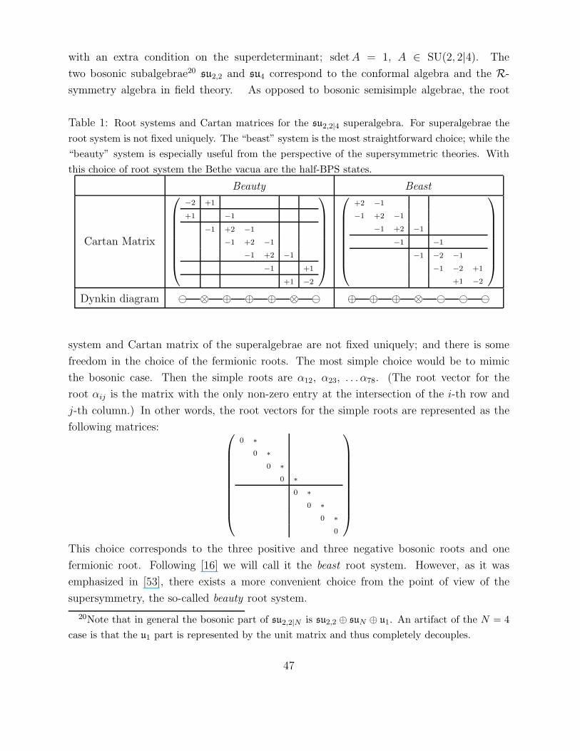
with an extra condition on the superdeterminant; sdetA = 1, A ∈ SU(2, 2|4). The

two bosonic subalgebrae20 su2,2 and su4 correspond to the conformal algebra and the R-

symmetry algebra in field theory. As opposed to bosonic semisimple algebrae, the root

Table 1: Root systems and Cartan matrices for the su2,2|4 superalgebra. For superalgebrae the

root system is not fixed uniquely. The “beast” system is the most straightforward choice; while the

“beauty” system is especially useful from the perspective of the supersymmetric theories. With

this choice of root system the Bethe vacua are the half-BPS states.

Beauty Beast

Cartan Matrix

−2 +1

+1 −1

−1 +2 −1

−1 +2 −1

−1 +2 −1

−1 +1

+1 −2

+2 −1

−1 +2 −1

−1 +2 −1

−1 −1

−1 −2 −1

−1 −2 +1

+1 −2

Dynkin diagram ⊖ ⊗ ⊕ ⊕ ⊕ ⊗ ⊖ ⊕ ⊕ ⊕ ⊗ ⊖ ⊖ ⊖

system and Cartan matrix of the superalgebrae are not fixed uniquely; and there is some

freedom in the choice of the fermionic roots. The most simple choice would be to mimic

the bosonic case. Then the simple roots are α12, α23, . . .α78. (The root vector for the

root αij is the matrix with the only non-zero entry at the intersection of the i-th row and

j-th column.) In other words, the root vectors for the simple roots are represented as the

following matrices:

0 ∗

0 ∗

0 ∗

0 ∗

0 ∗

0 ∗

0 ∗

0

This choice corresponds to the three positive and three negative bosonic roots and one

fermionic root. Following [16] we will call it the beast root system. However, as it was

emphasized in [53], there exists a more convenient choice from the point of view of the

supersymmetry, the so-called beauty root system.

20Note that in general the bosonic part of su2,2|N is su2,2 ⊕ suN ⊕ u1. An artifact of the N = 4

case is that the u1 part is represented by the unit matrix and thus completely decouples.

47

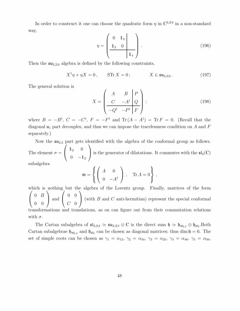
In order to construct it one can choose the quadratic form η in C2,2|4 in a non-standard

way,

η =

0 12

12 0

14

. (196)

Then the su2,2|4 algebra is defined by the following constraints,

X†η + ηX = 0 , STrX = 0 ; X ∈ su2,2|4 . (197)

The general solution is

X =

A B P

C −A† Q

−Q† −P † F

; (198)

where B = −B†, C = −C†, F = −F † and Tr (A − A†) = TrF = 0. (Recall that the

diagonal u1 part decouples, and thus we can impose the tracelessness condition on A and F

separately.)

Now the su2,2 part gets identified with the algebra of the conformal group as follows.

The element σ =

12 0

0 −12

is the generator of dilatations. It commutes with the sl2(C)

subalgebra

m =

A 0

0 −A†

, TrA = 0

,

which is nothing but the algebra of the Lorentz group. Finally, matrices of the form 0 B

0 0

and

0 0

C 0

(with B and C anti-hermitian) represent the special conformal

transformations and translations, as on can figure out from their commutation relations

with σ.

The Cartan subalgebra of sl2,2|4 ≃ su2,2|4 ⊗ C is the direct sum h ≃ hsl2,2⊕ hsl4

.Both

Cartan subalgebrae hsl2,2and hsl4

can be chosen as diagonal matrices; thus dim h = 6. The

set of simple roots can be chosen as γ1 = α12, γ2 = α34, γ3 = α25, γ4 = α48, γ5 = α56,

48

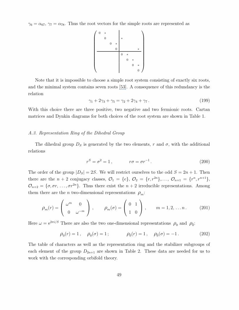
γ6 = α67, γ7 = α78. Thus the root vectors for the simple roots are represented as

0 ∗

0 ∗

0 ∗

0 ∗

0 ∗

0 ∗

0 ∗

0

Note that it is impossible to choose a simple root system consisting of exactly six roots,

and the minimal system contains seven roots [53]. A consequence of this redundancy is the

relation

γ1 + 2γ3 + γ5 = γ2 + 2γ4 + γ7 . (199)

With this choice there are three positive, two negative and two fermionic roots. Cartan

matrices and Dynkin diagrams for both choices of the root system are shown in Table 1.

A.3. Representation Ring of the Dihedral Group

The dihedral group DS is generated by the two elements, r and σ, with the additional

relations

rS = σ2 = 1 , rσ = σr−1 . (200)

The order of the group |DS| = 2S. We will restrict ourselves to the odd S = 2n + 1. Then

there are the n + 2 conjugacy classes, O1 = e, O2 = r, r2n,. . . , On+1 = rn, rn+1,On+2 = σ, σr, . . . , σr2n. Thus there exist the n + 2 irreducible representations. Among

them there are the n two-dimensional representations ρm:

ρm(r) =

ωm 0

0 ω−m

, ρm(σ) =

0 1

1 0

, m = 1, 2, . . . n . (201)

Here ω = e2πi/S There are also the two one-dimensional representations ρ0 and ρ0:

ρ0(r) = 1 , ρ0(σ) = 1 ; ρ0(r) = 1 , ρ0(σ) = −1 . (202)

The table of characters as well as the representation ring and the stabilizer subgroups of

each element of the group D2n+1 are shown in Table 2. These data are needed for us to

work with the corresponding orbifold theory.

49

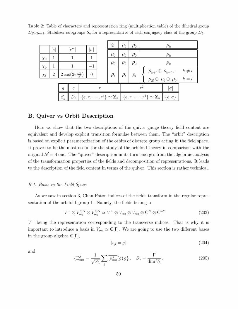
Table 2: Table of characters and representation ring (multiplication table) of the dihedral group

DS=2n+1. Stabilizer subgroups Sg for a representative of each conjugacy class of the group D5.

[e] [rm] [σ]

χ0 1 1 1

χ0 1 1 −1

χl 2 2 cos(2π lm

S

)0

⊗ ρ0 ρ0 ρk

ρ0 ρ0 ρ0 ρk

ρ0 ρ0 ρ0 ρk

ρl ρl ρl

ρk+l ⊕ ρk−l , k 6= l

ρ2l ⊕ ρ0 ⊕ ρ0 , k = l

g e r r2 [σ]

Sg D5 e, r, . . . , r4 ≃ Z5 e, r, . . . , r4 ≃ Z5 e, σ

B. Quiver vs Orbit Description

Here we show that the two descriptions of the quiver gauge theory field content are

equivalent and develop explicit transition formulae between them. The “orbit” description

is based on explicit parameterization of the orbits of discrete group acting in the field space.

It proves to be the most useful for the study of the orbifold theory in comparison with the

original N = 4 one. The “quiver” description in its turn emerges from the algebraic analysis

of the transformation properties of the fields and decomposition of representations. It leads

to the description of the field content in terms of the quiver. This section is rather technical.

B.1. Basis in the Field Space

As we saw in section 3, Chan-Paton indices of the fields transform in the regular repre-

sentation of the orbifold group Γ. Namely, the fields belong to

V ⊥ ⊗ V ⊕Nreg ⊗ V ⊕N

reg ≃ V ⊥ ⊗ Vreg ⊗ Vreg ⊗ CN ⊗ C

∗N (203)

V ⊥ being the representation corresponding to the transverse indices. That is why it is

important to introduce a basis in Vreg ≃ C[Γ]. We are going to use the two different bases

in the group algebra C[Γ],

eg = g (204)

and

Eλmn =

1√Sλ

∑

g

ρλnm(g) g , Sλ =

|Γ|dimVλ

. (205)

50

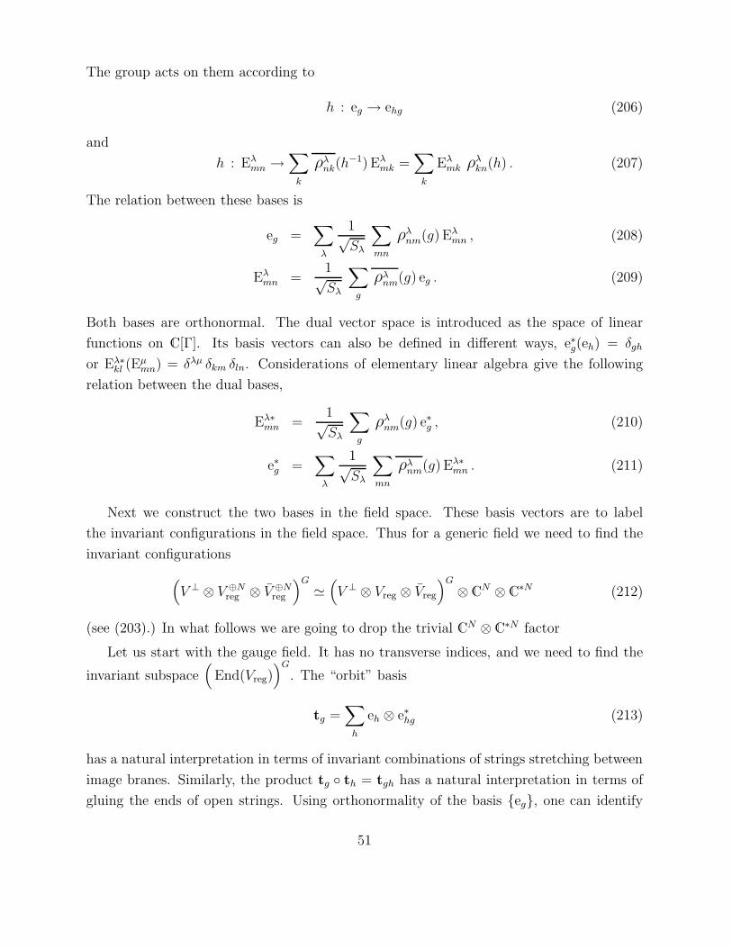
The group acts on them according to

h : eg → ehg (206)

and

h : Eλmn →

∑

k

ρλnk(h

−1) Eλmk =

∑

k

Eλmk ρ

λkn(h) . (207)

The relation between these bases is

eg =∑

λ

1√Sλ

∑

mn

ρλnm(g) Eλ

mn , (208)

Eλmn =

1√Sλ

∑

g

ρλnm(g) eg . (209)

Both bases are orthonormal. The dual vector space is introduced as the space of linear

functions on C[Γ]. Its basis vectors can also be defined in different ways, e∗g(eh) = δgh

or Eλ∗kl (E

µmn) = δλµ δkm δln. Considerations of elementary linear algebra give the following

relation between the dual bases,

Eλ∗mn =

1√Sλ

∑

g

ρλnm(g) e∗g , (210)

e∗g =∑

λ

1√Sλ

∑

mn

ρλnm(g) Eλ∗

mn . (211)

Next we construct the two bases in the field space. These basis vectors are to label

the invariant configurations in the field space. Thus for a generic field we need to find the

invariant configurations

(V ⊥ ⊗ V ⊕N

reg ⊗ V ⊕Nreg

)G

≃(V ⊥ ⊗ Vreg ⊗ Vreg

)G

⊗ CN ⊗ C

∗N (212)

(see (203).) In what follows we are going to drop the trivial CN ⊗ C∗N factor

Let us start with the gauge field. It has no transverse indices, and we need to find the

invariant subspace(

End(Vreg))G

. The “orbit” basis

tg =∑

h

eh ⊗ e∗hg (213)

has a natural interpretation in terms of invariant combinations of strings stretching between

image branes. Similarly, the product tg th = tgh has a natural interpretation in terms of

gluing the ends of open strings. Using orthonormality of the basis eg, one can identify

51

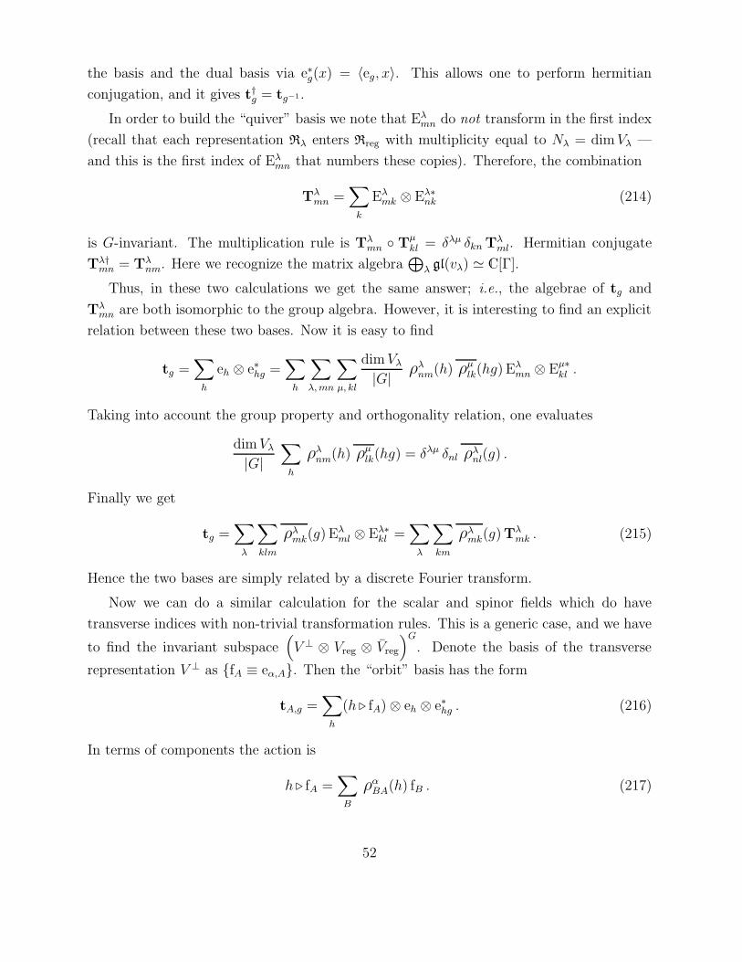
the basis and the dual basis via e∗g(x) = 〈eg, x〉. This allows one to perform hermitian

conjugation, and it gives t†g = tg−1.

In order to build the “quiver” basis we note that Eλmn do not transform in the first index

(recall that each representation Rλ enters Rreg with multiplicity equal to Nλ = dimVλ —

and this is the first index of Eλmn that numbers these copies). Therefore, the combination

Tλmn =

∑

k

Eλmk ⊗ Eλ∗

nk (214)

is G-invariant. The multiplication rule is Tλmn T

µkl = δλµ δkn Tλ

ml. Hermitian conjugate

Tλ†mn = Tλ

nm. Here we recognize the matrix algebra⊕

λ gl(vλ) ≃ C[Γ].

Thus, in these two calculations we get the same answer; i.e., the algebrae of tg and

Tλmn are both isomorphic to the group algebra. However, it is interesting to find an explicit

relation between these two bases. Now it is easy to find

tg =∑

h

eh ⊗ e∗hg =∑

h

∑

λ, mn

∑

µ, kl

dimVλ

|G| ρλnm(h) ρµ

lk(hg) Eλmn ⊗ Eµ∗

kl .

Taking into account the group property and orthogonality relation, one evaluates

dimVλ

|G|∑

h

ρλnm(h) ρµ

lk(hg) = δλµ δnl ρλnl(g) .

Finally we get

tg =∑

λ

∑

klm

ρλmk(g) Eλ

ml ⊗ Eλ∗kl =

∑

λ

∑

km

ρλmk(g)Tλ

mk . (215)

Hence the two bases are simply related by a discrete Fourier transform.

Now we can do a similar calculation for the scalar and spinor fields which do have

transverse indices with non-trivial transformation rules. This is a generic case, and we have

to find the invariant subspace(V ⊥ ⊗ Vreg ⊗ Vreg

)G

. Denote the basis of the transverse

representation V ⊥ as fA ≡ eα,A. Then the “orbit” basis has the form

tA,g =∑

h

(h ⊲ fA)⊗ eh ⊗ e∗hg . (216)

In terms of components the action is

h ⊲ fA =∑

B

ραBA(h) fB . (217)

52

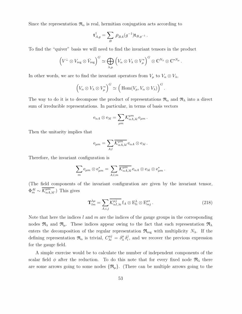
Since the representation Rα is real, hermitian conjugation acts according to

t†A,g =

∑

B

ρBA(g−1)tB,g−1 .

To find the “quiver” basis we will need to find the invariant tensors in the product

(V ⊥ ⊗ Vreg ⊗ Vreg

)G

≃⊕

λ,µ

(Vα ⊗ Vλ ⊗ V ∗

µ

)G

⊗ CNλ ⊗ C

∗Nµ .

In other words, we are to find the invariant operators from Vµ to Vα ⊗ Vλ,

(Vα ⊗ Vλ ⊗ V ∗

µ

)G

≃(

Hom(Vµ, Vα ⊗ Vλ))G

.

The way to do it is to decompose the product of representations Rα and Rλ into a direct

sum of irreducible representations. In particular, in terms of basis vectors

eαA ⊗ eλl =∑

µm

KµmαA,λl eµm .

Then the unitarity implies that

eµm =∑

A,l

KµmαA,λl eαA ⊗ eλl .

Therefore, the invariant configuration is

∑

m

eµm ⊗ e∗µm =∑

A,l,m

KµmαA,λl eαA ⊗ eλl ⊗ e∗µm .

(The field components of the invariant configuration are given by the invariant tensor,

ΦAlm ∼ Kµm

αA,λl.) This gives

Tλµlm =

∑

A,i,j

KµjαI,λi fA ⊗ Eλ

li ⊗ Eµ∗mj . (218)

Note that here the indices l and m are the indices of the gauge groups in the corresponding

nodes Rλ and Rµ. These indices appear owing to the fact that each representation Rλ

enters the decomposition of the regular representation Rreg with multiplicity Nλ. If the

defining representation Rα is trivial, Cµjλi = δµ

λ δji , and we recover the previous expression

for the gauge field.

A simple exercise would be to calculate the number of independent components of the

scalar field φ after the reduction. To do this note that for every fixed node Rλ there

are some arrows going to some nodes Rµ. (There can be multiple arrows going to the

53

same node.) For each arrow there are N2NλNµ components since there are NNλ copies

of Rλ and NNµ copies of Rµ in CN ⊗Rreg. Therefore, to each node Rλ there correspond

N2Nλ

∑µ dimVµ independent components. Since Vα ⊗ Vλ ≃

⊕µ Vµ, the dimension

counting gives∑

µ dim Vµ = (dim Vλ) (dimVα). Therefore, the total number of indepen-

dent components of φ is N2 dimVα

∑λN

2λ = |G| N2 dimVα. This fact is not surprising

since the invariant configurations of the fields are orbits in the field space, and one can

parameterize them in terms of the group algebra valued fields. This way the dimension

counting confirms equivalence of the two descriptions. Furthermore, it is possible to find

an exact transition formula between them. Indeed, substituting for the basis vectors eg via

Eλlm, we get for tA,g

tA,g =∑

B

∑

h

∑

λ, mn

∑

µ, kl

dim Vλ

|G| ραBA(h) ρλ

nm(h) ρµlk(hg) fB ⊗ Eλ

mn ⊗ Eµ∗kl .

Using expansion

ραBA(h) ρλ

nm(h) =∑

ν,pq

KνpB,λnKνq

A,λm ρνpq(h) ,

and orthogonality relation, one can evaluate

∑

h

dimVλ

|G| ραBA(h) ρλ

nm(h) ρµlk(hg) =

∑

i

dimVλ

dimVµKµl

B,λnKµiA,λm ρµ

ik(g) .

Finally, after the use of (218) this gives

tA,g =∑

λ,l

∑

µ,km

dimVλ

dimVµKµk

A,λl ρµkm(g)T

λµlm . (219)

The presence of the factor Kµ·α·,λ· restricts the sum over (λ, µ) only to those pairs which are

connected by a line in the quiver. Again, when the defining representation Rα is trivial, the

correct formula (215) is recovered.

B.2. Relation Between the Field Components

It is very convenient to write the field operators in the quiver notation (then the gauge

invariance is manifest), while the Feynman rules most closely resemble those for the unorb-

ifolded theory in the notation with fields depending on the group index. Here we proceed

to develop the connection between the field components and the algebra of fields in the two

notations. Writing down the gauge field as A =∑

g Ag tg =∑

λ

∑lmA

λlm Tλ

lm and using

(215), we find the relation

Aλlm =

∑

g

ρλlm(g)Ag . (220)

54

Similarly, for the scalar fields we get

φλµlm =

∑

g

∑

k

Nλ

NµKµk

A,λl ρµkm(g)φA

g . (221)

Then to the matrix multiplication of the gauge fields at the same node there corresponds

the convolution product in terms of the group algebra:

∑

l

AλklA

λlm =

∑

g,h

∑

l

ρλkl(g) ρ

λlm(h)Ag Ah =

∑

g

ρλkm(gh)Ag Ah =

∑

g

ρλkm(g) (A A)(g) .

The story with the scalar fields is slightly more complicated. The product of the two fields

φ and ψ with the transverse indices transforming in the representations Rα and Rβ can be

viewed as a field with a transverse index in the product representation Rα⊗Rβ, though the

convolution rule is slightly modified. Particularly,

∑

m

φλµlm ψ

µνmn =

Nλ

Nν

∑

g,h

KµpαA,λlKνq

βB,µm ρµpm(g) ρν

qn(h)φAg ψ

Bh .

Since the decomposition coefficients K ··,· are invariant tensors by construction, we have

ρµpm(g)Kνq

βB,µm = ρβBC(g−1) ρν

qr(g−1)Kνr

βC,µp .

Substituting this and summing over the index q, we get

∑

m

φλµlm ψ

µνmn =

Nλ

Nν

∑

g,h

KνrαA,βB,λl ρν

nr(h−1g−1) ρβ

BC(g)φAg ψ

Ch . (222)

Here KνrαA,βB,λl =

∑pKµp

αA,λlKνrβB,µp is (one of) the invariant tensors corresponding to the

decomposition Rα⊗Rβ⊗Rλ → Rν . Let us stress that generally there can exist a possibility

of decomposing Rα ⊗ Rλ → Rµ and/or Rβ ⊗ Rµ → Rν in multiple ways. In this case we

do not have to sum over these different tensors. Graphically this corresponds to the case

when there are multiple arrows between the same nodes in quiver, and then one is free to

choose between them. Another observation is that (222) has the same structure as (221),

the product φ ψ having the defining representation Rα ⊗ Rβ. The convolution rule is

slightly modified,

(φ ψ)ABg =

∑

h

φAh ρBC(h)ψC

h−1g . (223)

Both formulae (222) and (223) are also valid for the gauge fields which have no transverse in-

dices (trivial representation). In this case some matrix elements and decomposition tensors

55

become degenerate. Recalling the reduction formula (244) one can see that the multiplica-

tion rule (223) naturally corresponds to the standard matrix multiplication in the SU(|Γ|N)

theory. This means that∑

f

φAhf ψ

Bfg = ρα

AA′(h) ρβBB′(h) (φ ψ)A′B′

h−1g .

This way of multiplication is induced from the original theory, and that is why it respects

the gauge transformations. Another nice feature of the formula (222) is that when there

exist several arrows going between different nodes the choice of a given arrow affects only

the choice of the invariant tensors and does not affect the convolution product (223). It

means that all the operators corresponding to the different paths (not necessarily closed) in

the quiver formed by L consequent scalar lines λ1 → λ2 → · · · → λL+1 are contained in the

product φA1 . . . φAL.

We can summarize these results as follows. An operator formed in the quiver notation

as the product φλν1 φν1ν2 . . . φνL−1µ can be recast as

(φ · · · φ

)λµ

lm=

∑

g

∑

k

Nλ

Nµ

KA1 ...AL

µk

λl ρµkm(g)

(φ · · · φ

)A1 ...AL

g; (224)

where the invariant tensor K is the one corresponding to the decomposition Rλ ⊗ Rν1⊗

· · · ⊗RνL−1→ Rµ. The product of fields in the r.h.s. is calculated according to (223). In

its turn it is related to the product of the fields of the original N = 4 theory as

(φ

A1 . . . φAL

)

h,hg=

∑

B1 ,...BL

ρA1 B1(h) . . . ρAL BL

(h)(φ · · · φ

)B1 ...BL

g. (225)

These formulae will be of crucial importance for constructing the gauge invariant observ-

ables.

B.3. Construction of Observables: Untwisted Sector

Let us first study the untwisted observables which are obtained by a reduction — for

instance, TrφL. They can be rewritten in terms of the group valued field φ in the following

way:

OA1...Ak = TrφA1 . . . φAk =∑

h,i

φA1

i1h1,i2h2φA2

i2h2,i3h3. . . φAn

inhn,i1h1. (226)

Using (244), it reduces to

OA1...Ak =∑

h, i, B

ρA1B1(h1) . . . ρAnBn

(hn)φB1

i1i2(h−1

1 h2) . . . φBn

ini1(h−1

n h1) .

56

Introducing the new variables h, pi, i = 1, . . . , n− 1 according to h = h1, hi+1 = hpi, we get

OA1...Ak =∑

h, p, B

ρA1B1(h) ρA2B2

(hp1) . . . ρAnBn(hpn−1)×

×TrφB1(p1)φB2(p−1

1 p2) . . . φBn−1(p−1

n−2pn−1)φBn(p−1

n−1) .

This rewrites as

OA1...Ak =∑

p, B, C

DA1B1, A2C2, ...AnCn ρC2B2(p1) . . . ρCnBn

(pn−1) ×

×TrφB1(p1)φB2(p−1

1 p2) . . . φBn−1(p−1

n−2pn−1)φBn(p−1

n−1) ,

where

DA1B1, ..., AnBn =∑

h

ρA1B1(h) ρA2B2

(h) . . . ρAnBn(h) .

Using (193), it can be evaluated as

DA1B1, ..., AnBn =∑

h

∑

µ, pq

ρµpq(h)Kµp

A1,...AnKµq

B1,...Bn= |G| Ktriv

A1,...AnKtriv

B1,...Bn.

(In case there exist several different invariant tensors, one should sum over them.) Then

OA1...Ak =∑

a

∑

p, B, C

K(a)A1,...An

K(a)B1C2,...Cn

ρC2B2(p1) . . . ρCnBn

(pn−1)×

×|Γ| TrφB1(p1)φB2(p−1

1 p2) . . . φBn−1(p−1

n−2pn−1)φBn(p−1

n−1) . (227)

The presence of invariant tensors implies that only the index combinations which are invari-

ant w.r.t. the orbifold group are able to survive the projection (i.e., the reduction procedure

extracts the invariant part of the operator only). Multiplication in the r.h.s. of (227) cor-

responds exactly to the convolution rule (223). Then orthogonality relation (195) implies

that the operators

O(a) =1

|Γ| K(a)A1,...Ak

OA1...Ak = K(a)A1,...Ak

(φ · · · φ)A1,...Ak(e) (228)

form a basis in the space of untwisted observables obtained by a reduction from the original

theory. In terms of the fields of the parent theory

O(a) = K(a)A1,...AL

Tr(φ

A1 . . . φAL ) . (229)

57

B.4. Construction of Observables: Twisted Sectors

It turns out that the twisted operators are constructed in a similar way. In order to

construct generic observables it is convenient to use the quiver notation. Taking a closed

loop in the quiver and using (224) one can write the corresponding operator as

Tr Rλ1

φλ1λ2 φλ2λ3 . . . φλLλ1 =∑

g

∑

k,l

KA1,...AL

λ1k

λ1lρλ

kl(g)(φ . . . φ

)A1,...AL

g; (230)

where the invariant tensor

KA1,...AL

λ1k

λ1l=

∑

l2,..., lL

Kλ2l2

A1 λ1lKλ3l3

A2 λ2l2. . .KλLlL

AL−1 λL−1lL−1

Kλ1k

AL λLlL. (231)

corresponds to the closed path λ1 → λL → · · · → λ2 → λ1. Note that the l.h.s. is explicitly

symmetric w.r.t. the cyclic permutations of the fields under the trace. It would be interesting

to illustrate that the r.h.s. possesses the same symmetry. For this small digression we

consider the simplest example, the Abelian ZS orbifold. There is one generating element g in

the ZS group, and gS = 1. There are the S one-dimensional representations Rn, ρn(g) =

ǫn, ǫ = e2πi/S , n = 0, . . . S−1. The complex scalar φA decomposes into three representations;

i.e., g : φA → ǫnAφA . The quiver has S nodes corresponding to the S representations of

ZS. In this setup the invariant tensor is simply KA1 ˙˙˙AL= δ(n

A1+ · · ·+n

AL), and it makes

sure that the total charge of the product is zero. Choose a closed loop in the quiver going

between the nodes n → n + nA1→ n + n

A1+ n

A2→ · · · → n +

∑i nAi

= n. (Thus the

closedness of the loop translates into the condition that the operator has zero charge). The

character χn(gm) = ǫmn. Denote n1 = n, ni = n +∑i−1

j=1 nAj, i = 2, . . . L. Then (230)

becomes

On1...nL=

∑

m

ǫ−mn1 TrφA . . . φAL t−m =

∑

m

∑

l1+···+lL≡m

ǫ−mn1 TrφA1

l1 · · · φAL

lL. (232)

Naıvely the formula is not symmetric since it has explicit dependence on n = n1 in the char-

acter. However, using the permutation rule (243) we get TrφA1

l1. . . φ

AL

lL= ǫmnIL Trφ

AL

lLφA1

l1. . . φ

AL−1

lL−1.

This yields

On1...nL=

∑

m

∑

l1+···+lL≡m

ǫ−m(n1−nAL) Trφ

AL

lLφ

A1

l1 . . . φAL−1

lL−1

=∑

m

∑

l1+···+lL≡m

ǫ−mnL TrφAL

lLφ

A1

l1 . . . φAL−1

lL−1= OnLn1...nL−1

.

The form of the formula (230) is indeed invariant w.r.t. the cyclic permutations of the fields.

58

There also exists a different way to construct gauge invariant operators. Namely, let us

start with the ansatz

O[K] =∑

g

∑

A1 ,... AL

KA1 ... AL(g)

(φ . . . φ

)A1,...Ak

g. (233)

Generally such an expression corresponds to a sum of operators corresponding to some paths

in the quiver, not necessarily closed. That is why the gauge invariance condition has to be

imposed separately. In order to do this we can consider a generic group algebra valued

generator of gauge transformations χ =∑

g χgg and require that δχO[K] = 0. Recall that

the gauge transformation rule of the adjoint fields is δχφA = [χ, φA] =

(χ φ − φ χ

)A,

where the convolution product is understood in the sense of (223). This gives

(δχ

(φ . . . φ

))A1...Ak

g=

∑

h

ρA1B1(h) . . . ρALBL

(h)χh

(φ . . . φ

)B1...Bk

h−1g−

−∑

h

(φ . . . φ

)A1...Ak

hχh−1g . (234)

Then

δχO[K] =∑

g,h

∑

B1...BL

[KA1...AL

(hg) ρA1B1(h) . . . ρALBL

(h)−KB1...BL(gh)

]

×χh

(φ . . . φ

)B1...Bk

g. (235)

This condition rewrites as

KB1 ···BL(h−1gh) =

∑

A1 ···AL

KA1 ···AL(g) ρA1 B1

(h) . . . ρAL BL(h) . (236)

A straightforward consequence of this result is that K[g] has to be an invariant tensor w.r.t.

the stabilizer subgroup Sg. Note that in (230) we had

KA1...AL(g) =

∑

k,l

KA1,...AL

λkλl ρλ

kl(g) , (237)

and it obviously satisfies (236). On the other side, tensor K(g) can be expanded in Fourier

series as a function on the group,

KA1...AL(g) =

∑

λ

∑

k,l

K(λ)A1,...AL

λkλl ρλ

kl(g) ; (238)

and then the condition (236) translates into the requirement that the coefficients K(λ)A1,...AL

λkλl

are invariant tensors. These considerations provide a dictionary between the two notations

in the quiver gauge theory.

59

It is very important that the gauge invariance condition (236) relates the values of the

tensor K(g) within the same conjugacy class, and there is no relation between the values of

K on the different conjugacy classes. That is why one can build a gauge invariant operator

with K(g) 6= 0 only on a given conjugacy class [g]. Such operators are said to belong to the

twisted sector with the twist [g] (determined only up to a conjugation). One can choose a

reference element g in the conjugacy class [hgh−1] and set KA1...AL(g) = KA1...AL

, KA1...AL

being some Sg-invariant tensor. Then (236) determines the values of K(h−1gh) on all the

elements of the conjugacy class. The corresponding operator

O[K] =∑

g,h

∑

A1 ···AL

∑

B1 ···BL

KA1 ···ALρA1 B1

(h) . . . ρAL BL(h)

(φ · · ·φ

)B1 ···BL

h−1gh. (239)

It can be rewritten in terms of the fields of the original N = 4 theory in a very simple way,

O[K] =∑

g,h

∑

A1 ···AL

KA1 ···ALTr

[γ(g)φ

A1 . . . φAL

]. (240)

The twist field γ(g) acts on the dynamical fields as follows,

(φA γ(g)

)h1,h2

= φAh1,gh2

, (241)(γ(g)φA

)h1,h2

= φAg−1h1,h2

. (242)

Invariance condition imposed by the orbifold projection on the fields implies that

(γ(g)φA

)= ρAB(g−1)

(φB γ(g)

). (243)

C. Derivation of the Feynman Rules

As an example we go through the derivation for the scalar field ΦI ; the other fields are

treated in a similar way. Then the Γ-invariance condition (70) for the scalar field is solved

by

ΦI

i,h; j,g =∑

J

R(h)I

JφJ

ij(h−1g) . (244)

We can parameterize the invariant configurations of the scalar field ΦI

ig,jh in terms of this

group algebra valued object φI

ij(g), and this group algebra valued field φ is to be integrated

over in the path integral. Using the parameterization (244) and the orthogonality of the

60

defining representation R : Γ → SO(6), we get the kinetic term for the scalar field in the

form

Lφφ =1

2

∑

I

Tr ∂µΦI ∂µΦI =1

2|Γ|

∑

g

∑

I,J

R(g)I

J∂µ TrφI (g) ∂µφJ (g−1) . (245)

Then for the quadratic propagator the only modification compared to the original theory is

“conservation of the group index” and renormalization:

⟨φI

ij,g φJ

kl,h

⟩= |Γ|−1R(g)I

J

p2δgh,e δil δjk , (246)

In terms of the original N = 4 fields (we omit the obvious Latin part of the Chan-Paton

indices)

⟨ΦI

h,g ΦJ

f−1g, f−1h

⟩=

R(f)I

J

|Γ| p2. (247)

61

References

[1] R.C. Brower, “String/Gauge Duality: (re)discovering the QCD string in AdS space,”

Acta Phys. Polon. B 34, 5927 (2003) [hep-th/0508036].

[2] G. ’t Hooft, “A Planar Diagram Theory for Strong Interactions,” Nucl. Phys. B72, 461

(1974).

[3] K. G. Wilson, “Confinement of Quarks,” Phys. Rev. D 10, 2445 (1974).

[4] J. B. Kogut and L. Susskind, “Hamiltonian Formulation Of Wilson’s Lattice Gauge

Theories,” Phys. Rev. D 11, 395 (1975).

[5] A. M. Polyakov, “Gauge Fields As Rings Of Glue,” Nucl. Phys. B 164 (1980) 171.

[6] J. M. Maldacena, “The large N limit of superconformal field theories and supergravity,”

Adv. Theor. Math. Phys. 2, 231 (1998) [Int. J. Theor. Phys. 38, 1113 (1999)] [hep-

th/9711200].

[7] S. S. Gubser, I. R. Klebanov and A. M. Polyakov, “Gauge theory correlators from non-

critical string theory,” Phys. Lett. B 428, 105 (1998) [hep-th/9802109].

[8] E. Witten, “Anti-de Sitter space and holography,” Adv. Theor. Math. Phys. 2, 253

(1998) [arXiv:hep-th/9802150].

[9] O. Aharony, S. S. Gubser, J. M. Maldacena, H. Ooguri and Y. Oz, “Large N Field

Theories, String Theory and Gravity,” Phys. Rept. 323, 183 (2000) [hep-th/9905111].

[10] J. Polchinski, “Dirichlet-Branes and Ramond-Ramond Charges,” Phys. Rev. Lett. 75

(1995) 4724 [hep-th/9510017].

[11] E. Witten, “Bound states of strings and p-branes,” Nucl. Phys. B 460, 335 (1996)

[arXiv:hep-th/9510135].

[12] T. Banks, W. Fischler, S. H. Shenker and L. Susskind, “M theory as a matrix model:

A conjecture,” Phys. Rev. D 55 (1997) 5112 [hep-th/9610043].

[13] J. A. Minahan and K. Zarembo, “The Bethe-ansatz for N =4 super Yang-Mills,” JHEP

0303, 013 (2003) [arXiv:hep-th/0212208].

[14] N. Beisert, C. Kristjansen and M. Staudacher, “The dilatation operator of N =4 super

Yang-Mills theory,” Nucl. Phys. B 664, 131 (2003) [arXiv:hep-th/0303060].

62

[15] N. Beisert, “The complete one-loop dilatation operator of N = 4 super Yang-Mills

theory,” Nucl. Phys. B 676, 3 (2004) [arXiv:hep-th/0307015].

[16] N. Beisert and M. Staudacher, “The N = 4 SYM integrable super spin chain,” Nucl.

Phys. B 670, 439 (2003) [arXiv:hep-th/0307042].

[17] S. S. Gubser, I. R. Klebanov and A. M. Polyakov, “A semi-classical limit of the

gauge/string correspondence,” Nucl. Phys. B 636 (2002) 99 [arXiv:hep-th/0204051].

[18] L. J. Dixon, J. A. Harvey, C. Vafa and E. Witten, “Strings On Orbifolds,” Nucl. Phys.

B 261, 678 (1985).

L. J. Dixon, J. A. Harvey, C. Vafa and E. Witten, “Strings On Orbifolds II,” Nucl. Phys.

B 274, 285 (1986).

[19] M. Alishahiha and M. M. Sheikh-Jabbari, “The pp-wave limits of orbifolded AdS5×S5,”

Phys. Lett. B 535 (2002) 328 [arXiv:hep-th/0203018].

[20] N. W. Kim, A. Pankiewicz, S. J. Rey and S. Theisen, “Superstring on pp-wave orbifold

from large-N quiver gauge theory,” Eur. Phys. J. C 25 (2002) 327 [arXiv:hep-th/0203080].

[21] M. Bertolini, J. de Boer, T. Harmark, E. Imeroni and N. A. Obers, “Gauge theory

description of compactified pp-waves,” JHEP 0301, 016 (2003) [arXiv:hep-th/0209201].

[22] X. J. Wang and Y. S. Wu, “Integrable spin chain and operator mixing in N = 1, 2

supersymmetric theories,” Nucl. Phys. B 683 (2004) 363 [arXiv:hep-th/0311073].

[23] K. Ideguchi, “Semiclassical strings on AdS5×S5/ZM and operators in orbifold field

theories,” JHEP 0409 (2004) 008 [arXiv:hep-th/0408014].

[24] G. De Risi, G. Grignani, M. Orselli and G. W. Semenoff, “DLCQ string spectrum from

N = 2 SYM theory,” JHEP 0411, 053 (2004) [arXiv:hep-th/0409315].

[25] D. Sadri and M. M. Sheikh-Jabbari, “Integrable spin chains on the conformal moose,”

JHEP 0603, 024 (2006) [arXiv:hep-th/0510189].

[26] N. Beisert and R. Roiban, “The Bethe ansatz for ZS orbifolds ofN =4 super Yang-Mills

theory,” JHEP 0511 (2005) 037 [arXiv:hep-th/0510209].

[27] D. Astolfi, V. Forini, G. Grignani and G. W. Semenoff, “Finite size corrections and

integrability of N = 2 SYM and DLCQ strings on a pp-wave,” JHEP 0609, 056 (2006)

[arXiv:hep-th/0606193].

63

[28] G. Arutyunov, J. Russo and A. A. Tseytlin, “Spinning strings in AdS5×S5: New

integrable system relations,” Phys. Rev. D 69 (2004) 086009 [arXiv:hep-th/0311004].

[29] S. Frolov and A. A. Tseytlin, “Multi-spin string solutions in AdS5×S5,” Nucl. Phys.

B 668, 77 (2003) [arXiv:hep-th/0304255].

[30] G. Arutyunov, S. Frolov, J. Russo and A. A. Tseytlin, “Spinning strings in AdS5×S5

and integrable systems,” Nucl. Phys. B 671, 3 (2003) [arXiv:hep-th/0307191].

[31] G. Arutyunov and M. Staudacher, “Matching higher conserved charges for strings and

spins,” JHEP 0403, 004 (2004) [arXiv:hep-th/0310182].

[32] T.S. Ratiu, “The Lie algebraic interpretation of the complete integrability of the

Rosochatius system”, AIP Proceed. 88, Amer. Inst. Physics, New York (1982), pp. 109;

L. Gagnon, J. P. Harnad, J. Hurtubise and P. Winternitz, “Abelian Integrals And The Re-

duction Method For An Integrable Hamiltonian System,” J. Math. Phys. 26, 1605 (1985);

C. Bartocci, G. Falqui and M. Pedroni, “A geometrical approach to the separability of the

Neumann-Rosochatius system”, arXiv:nlin.SI/0307021;

R. Kubo, W. Ogura, T. Saito and Y. Yasui, “Geodesic flows for the Neumann-Rosochatius

systems,” YITP-97-46;

J. Moser, “Geometry of Quadrics”, Chern Symposium, Berkeley (1979), p.147.

[33] S. Kachru and E. Silverstein, “4d conformal theories and strings on orbifolds,” Phys.

Rev. Lett. 80 (1998) 4855 [arXiv:hep-th/9802183].

[34] E.G. Gimon and J. Polchinski, “Consistency Conditions for Orientifolds and D-

Manifolds,” Phys. Rev. D 54, 1667 (1996) [hep-th/9601038].

[35] M.R. Douglas and G.W. Moore, “D-branes, Quivers, and ALE Instantons,” hep-

th/9603167.

[36] A.E. Lawrence, N. Nekrasov and C. Vafa, “On conformal field theories in four dimen-

sions,” Nucl. Phys. B 533, 199 (1998) [hep-th/9803015].

[37] M. Bershadsky, Z. Kakushadze and C. Vafa, “String expansion as large N expansion of

gauge theories,” Nucl. Phys. B 523, 59 (1998) [hep-th/9803076].

[38] M. Bershadsky and A. Johansen, “Large N limit of orbifold field theories,” Nucl. Phys.

B 536 (1998) 141 [hep-th/9803249].

64

[39] R. Dijkgraaf, C. Vafa, E.P. Verlinde and H.L. Verlinde, “The Operator Algebra of

Orbifold Models,” Commun. Math. Phys. 123 (1989) 485.

[40] A. Dymarsky, I. R. Klebanov and R. Roiban, “Perturbative search for fixed lines in

large N gauge theories,” JHEP 0508, 011 (2005) [arXiv:hep-th/0505099].

[41] H. Bethe, “On the theory of metals. 1. Eigenvalues and eigenfunctions for the linear

atomic chain,” Z. Phys. 71 (1931) 205.

[42] R. P. Feynman, Statistical Mechanics, Westview Press, 1998.

[43] L. D. Faddeev, “How Algebraic Bethe Ansatz works for integrable model,” arXiv:hep-

th/9605187.

[44] A. B. Zamolodchikov and A. B. Zamolodchikov, “Factorized S-matrices in two dimen-

sions as the exact solutions of certain relativistic quantum field models,” Annals Phys.

120, 253 (1979).

[45] D. Berenstein and S. A. Cherkis, “Deformations of N = 4 SYM and integrable spin

chain models,” Nucl. Phys. B 702, 49 (2004) [arXiv:hep-th/0405215].

[46] N. Y. Reshetikhin, “A Method Of Functional Equations In The Theory Of Exactly

Solvable Quantum Systems,” Lett. Math. Phys. 7, 205 (1983).

N. Y. Reshetikhin, “Integrable models of quantum one-dimensional magnets with O(n)

and Sp(2k) symmetry, ”Theor. Math. Phys. 63, 555 (1985) [Teor. Mat. Fiz. 63, 347

(1985)].

[47] E. Ogievetsky and P. Wiegmann, “Factorized S Matrix And The Bethe Ansatz For

Simple Lie Groups,” Phys. Lett. B 168, 360 (1986).

[48] P. P. Kulish, “Integrable graded magnets,” J. Sov. Math. 35 (1986) 2648.

[49] M. J. Martins and P. B. Ramos, “The algebraic Bethe ansatz for rational braid-monoid

lattice models,” Nucl. Phys. B 500, 579 (1997) [arXiv:hep-th/9703023].

[50] H. Saleur, “The continuum limit of slN |K integrable super spin chains,” Nucl. Phys. B

578, 552 (2000) [arXiv:solv-int/9905007].

[51] M. Lubcke and K. Zarembo, “Finite-size corrections to anomalous dimensions in N =4

SYM theory,” JHEP 0405, 049 (2004) [arXiv:hep-th/0405055].

65

[52] N. Beisert and R. Roiban, “Beauty and the twist: The Bethe ansatz for twisted N =4

SYM,” JHEP 0508, 039 (2005) [arXiv:hep-th/0505187].

[53] V. K. Dobrev and V. B. Petkova, “Group Theoretical Approach To Extended Confor-

mal Supersymmetry: Function Space Realizations And Invariant Differential Operators,”

Fortsch. Phys. 35, 537 (1987).

66