an improved whale optimization algorithm based on different
TRANSCRIPT
symmetryS S
Article
An Improved Whale Optimization Algorithm Basedon Different Searching Paths andPerceptual Disturbance
Wei-zhen Sun 1,2, Jie-sheng Wang 1,3,* and Xian Wei 2,*1 School of Electronic and Information Engineering, University of Science and Technology Liaoning,
Anshan 114044, China; [email protected] Fujian Institute of Research on the Structure, Fuzhou 350002, China3 National Financial Security and System Equipment Engineering Research Center, University of Science and
Technology Liaoning, Anshan 114044, China* Correspondence: [email protected] (J.-s.W.); [email protected] (X.W.);
Tel.: +86-0412-2538355 (J.-s.W.); +86-15860328381 (X.W.)
Received: 15 April 2018; Accepted: 6 June 2018; Published: 11 June 2018�����������������
Abstract: Whale optimization algorithm (WOA) is a swarm intelligence optimization algorithminspired by humpback whale hunting behavior. WOA has many similarities with other swarmintelligence algorithms (PSO, GWO, etc.). WOA’s unique search mechanism enables it to havea strong global search capability while taking into account the strong global search capabilities.In this work, considering the the deficiency of WOA in local search mechanism, combined with theoptimization methods of other group intelligent algorithms, perceptual perturbation mechanismis introduced, which makes the agent perform more detailed searches near the local extreme point.At the same time, since the WOA uses a logarithmic spiral curve, the agent cannot fully search allthe spaces within its search range, even though the introduction of the perturbation mechanism maystill lead to the algorithm falling into a local optimum. Therefore, the equal pitch Archimedes spiralcurve is chosen to replace the classic logarithmic spiral curve. In order to fully verify the effect ofthe search path on the performance of the algorithm, several other spiral curves have been chosenfor experimental comparison. By utilizing the 23 benchmark test functions, the simulation resultsshow that WOA (PDWOA) with perceptual perturbation significantly outperforms the standardWOA. Then, based on the PDWOA, the effect of the search path on the performance of the algorithmhas been verified. The simulation results show that the equal pitch of the Archimedean spiral curveis best.
Keywords: whale optimization algorithm; searching path; function optimization
1. Introduction
Problems with optimization must find the most optimal solution of the objective function byiteration. Generally, the search target—which can be described by coutinuous, descrete, linear, unlinear,convace, and convex functions—is a function that belongs to optimal objective functions. In order tosolve the problem of function optimization, a heuristic algorithm inspired by natural processes and/orevents has raised concerns. Swarm intelligence optimization algorithms that simulate biologicalpopulation evolution is a random search algorithm. It can solve complex global optimization problemsthrough cooperation and competition among individuals. Swarm intelligence optimization algorithminclude the ant colony optimization (ACO) algorithm [1–3], genetic algorithm (GA) [4,5], particleswarm optimization (PSO) algorithm [6–8], artificial bee colony (ABC) algorithm [9], grey wolfalgorithm (GWO) [10], harmony search (HS) Algorithm [11,12], etc.
Symmetry 2018, 10, 210; doi:10.3390/sym10060210 www.mdpi.com/journal/symmetry
Symmetry 2018, 10, 210 2 of 31
The whale optimization algorithm (WOA) is a biological heuristic algorithm presented by SeyedaliMirjalili and Andrew Lewis in 2016. WOA is a swarm intelligence optimization algorithm inspiredby the unique humpback hunting method. Because of unique optimization mechanism, WOA hasa good global search capability. Therefore, the new algorithm has been widely proposed by theengineering community. As a new type of bionic algorithm with better global search performance,many scholars are interested in it and apply it to a variety of engineering problems. It has been widelyused in the optimization of neural network parameters, allocation, and scheduling. On the allocationand scheduling, the literatures [13–16] use WOA to optimize energy management system (EMS) ofthe Combined Economic Emission Dispatch (CEED) problem for microgrid systems, and MATLABsoftware is used to compared it with GM, ACO, PSO and WOA; the results show that WOA canobtain better results with fewer iterations. The literature [17] applies WOA to the Unit CommitmentProblem of power generation operation scheduling, the experimental results show that the convergencespeed of WOA is obviously faster than PSO, GA, etc. In order to reduce the wire loss of distributionnetwork, the literature [18] uses WOA to optimize the distribution scheme of the capacitors in the grid.The simulation results show that WOA is more effective in reducing operating costs and maintainingbetter voltage distribution. Similarly, the literature [19] uses the WOA to the water resources schedulingproblem. The research results show that WOA has a faster convergence speed.
In terms of parameter optimization, the literature [20] uses WOA to optimize two parametersof a least-squares support vector machine to establish a WOA-LSSVM (WOA-least-squares supportvector machine) model to predict carbon dioxide emissions. Similarly, chaos WOA algorithm (CWOA)is proposed to optimize the parameters of Elman neural network in the literature [21], so as to establisha soft measurement model and predict variables. The literature [22] compares WOA with othermethods for optimizing neural network parameters quantitatively and qualitatively. Simulation resultsshow that the proposed trainer can outperform current algorithms on most data sets in terms of localoptimal avoidance and convergence speed. The literature [23] uses WOA to optimize the parametersof the multilayer perception model, and it uses five standard data sets to verify the validity of themodified model. We compared it with GWO and PSO, and found a high convergence and classificationrate of WOA, and it is possible to avoid local minimums.
In terms of variable prediction, the literature [24] proposes a multi-objective whale optimizationalgorithm (MOWOA) model to predict the wind speed in the power system and thus providea reference for power dispatching. The literature [25] combines the reverse adaptive whale optimizationalgorithm (AWOA) and the fast learning network (FLN) to propose an integrated modeling method(AWOA-FLN) and establishes a 600-MW prediction model for supercritical steam turbine group heatrate. Simulation results show that the AWOA-FLN model has stronger prediction accuracy andstronger generalization ability than the improved PSO algorithm and differential evolution algorithm,and it can more accurate predict the heat rate of the turbine. In image processing, in order to find thebest image segmentation threshold, the literature [26] combines WOA and moth-flame optimization toavoid the problem of determining the optimal threshold spend too much time in the case of multilevelthresholds. The simulation results show that the proposed algorithm has better performance than otherswarm intelligence algorithms. The literature [27] propose a MRI image liver segmentation methodbased on the whale optimization algorithm (WOA). The proposed method uses a set of 70 magneticresonance images (MRI) images for testing. The experimental results show that the method has a highaccuracy overall. In addition, considering WOA optimization and other applications, the literature [28]introduces the nondominated sorting algorithm to obtain the optimal solution of WOA, named thenondominated sorting WOA (NSWOA). The simulation results show that the method is much betterthan multiobjective collision-body optimizer (MOCBO), multi-objective particle swarm optimizer(MOPSO), nondominated sorting genetic algorithm II (NSGA-II) and the multiobjective symbioticorganism search (MOSOS). The literature [29] proposed a chaos WOA (CWOA) algorithm to calculateand automatically adjust the internal parameters of the optimization algorithm through chaoticmapping. This idea is essentially different from the literature [21]. The experimental results show
Symmetry 2018, 10, 210 3 of 31
that CWOA can effectively optimize the parameters of photovoltaic cells and their components.The literature [30] proposes a WOA-based feature selection approach, which is applied to find thelargest subset of features so that it maximizes classification accuracy while retaining the minimumnumber of features.
The essence of a group intelligence algorithm is to find the global optimal value as much aspossible with the help of various mechanisms. The improvement ideas proposed by many scholars areas far as possible to complete the search mechanism of group intelligent algorithm, so that the searchagent traverses the entire search space as much as possible.
In this paper, we analyze the search mechanism of the WOA algorithm and find that its searchmechanism has defects. However, this kind of defect cannot be solved by adjusting the movingstep length. The original WOA uses a logarithmic spiral curve as the search path of the agent.However, the screw pitch of the logarithmic spiral curve is not fixed. Because the screw pitch causesa large amount of agent movements in the early stage, some areas cannot be searched. As a result,the global optimum is ignored. For this problem, this paper proposes a WOA with perceptualperturbation [31–33] so that the agent can perturb near the local extreme points to obtain better optimalvalues as much as possible. The closest to the idea of this paper is the literature [34]. In order toimprove the PSO’s local search ability, literature [34] defines and analyzes the regions with the mostparticles. At the same time, presented a PSO algorithm with intermediate disturbance searchingstrategy (IDPSO), which enhances the global search ability of particles and increases their convergencerates. Introducing the perturbation mechanism into the group intelligent algorithm can effectivelyimprove the performance of the algorithm. The difference between this article and other methods isthat the step length is set to make the search agent’s moving step smaller and smaller, so that the agentcan search more and more carefully. The definition of the minimum step size makes it impossiblefor the agent’s step size to be smaller and smaller, thus ensuring the algorithm’s convergence speedand ability to jump out of the local extreme point. At the same time, for the defects of the searchmechanism, this paper uses the remaining seven spiral curves instead of the original logarithmic spiralcurve to obtain an optimal search path. Finally, we select 23 benchmark test functions to verify theeffectiveness of perceived perturbation and remaining spiral curves.
The structure of this paper is as follows: we have an introduction in the first section. The secondsection introduces the WOA optimization algorithm and analyzes the defects of the algorithm.The third section introduces the idea and method of improving WOA. The fourth section is a simulation,and a summary in the fifth section.
2. Whale Optimization Algorithm
2.1. Inspiration
The whale optimization algorithm (WOA) is inspired by the unique hunting method of thehumpback whale, which is called the bubble-net predation method [35–39]. The humpback whalecan perceive the distance between him and the prey and surround the prey. It is observed that thehumpback whale can move up with a spiral path in about 15 m deep, and spit out a number of differentsizes of bubbles. The last spit out bubble and the first spit out bubble rose to the surface at the sametime so as to form a cylindrical or tubular bubble network. It likes a huge spider knotted web tosurround the prey tightly, and makes the prey toward the center of the net. So the humpback whalesalmost upright open mouth in the bubble circle and swallow the prey in the net. According to theabove descriptions, the hunting behavior of the humpback whale can be divided into three steps:encircling prey, spiral bubble-net feeding maneuver and searching for prey.
2.2. Search for Prey (Exploration Phase)
In order to establish the mathematical model of the humpback whale searching path,each humpback whale is set as a search agent. At the same time, the algorithm is divided into
Symmetry 2018, 10, 210 4 of 31
three steps: the search for prey, encircling prey and spiral bubble-net attacking method (exploitationphase). Then these three kinds of behavioral mathematical model are established. And themathematical model is established for these three behaviors. In the modeling of the spiral bubble-netattacking method, two methods are proposed, which are the shrinking encircling mechanism andthe spiral updating position method. Among them, the searching for prey can be regarded as theexploration stage, whose main purpose is to find a better solution. The bubble-net attacking methodcan also be called the exploitation phase, whose main purpose is to use this better solution more fully.
In the exploration phase (searching for prey), in order to make the search more extensive,
the search agents are pushed away from each other by the positive and negative of a random vector→A.
At the same time, the position of the search agent is replaced by a randomly selected search agent toreplace the current optimal search agent. The mathematical model is described as follows:
→D =
∣∣∣∣→C ·→Xrand −→X∣∣∣∣ (1)
→X(t + 1) =
→Xrand −
→A ·→D (2)
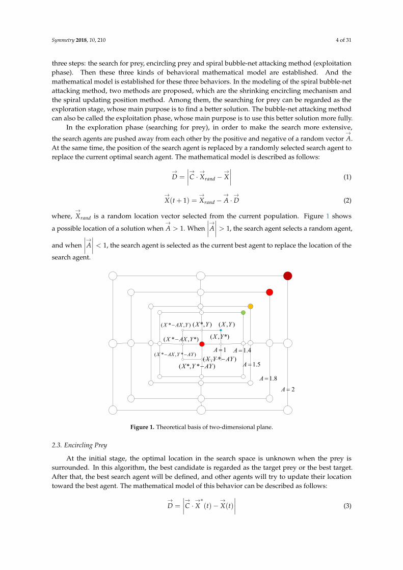
where,→Xrand is a random location vector selected from the current population. Figure 1 shows
a possible location of a solution when→A > 1. When
∣∣∣∣→A∣∣∣∣ > 1, the search agent selects a random agent,
and when∣∣∣∣→A∣∣∣∣ < 1, the search agent is selected as the current best agent to replace the location of the
search agent.
Symmetry 2018, 10, x FOR PEER REVIEW 4 of 31
whose main purpose is to find a better solution. The bubble-net attacking method can also be called the exploitation phase, whose main purpose is to use this better solution more fully.
In the exploration phase (searching for prey), in order to make the search more extensive, the search agents are pushed away from each other by the positive and negative of a random vector A
.
At the same time, the position of the search agent is replaced by a randomly selected search agent to replace the current optimal search agent. The mathematical model is described as follows:
randD C X X
(1)
( 1) randX t X A D (2)
where, randX
is a random location vector selected from the current population. Figure 1 shows a
possible location of a solution when 1A
. When 1A
, the search agent selects a random agent,
and when 1A
, the search agent is selected as the current best agent to replace the location of the
search agent.
( , )X Y( *, )X Y( * , )X AX Y
( * , *)X AX Y
( * , * )X AX Y AY
( *, * )X Y AY( , * )X Y AY
( , *)X Y
1A 1.4A
1.5A
1.8A
2A
Figure 1. Theoretical basis of two-dimensional plane.
2.3. Encircling Prey
At the initial stage, the optimal location in the search space is unknown when the prey is surrounded. In this algorithm, the best candidate is regarded as the target prey or the best target. After that, the best search agent will be defined, and other agents will try to update their location toward the best agent. The mathematical model of this behavior can be described as follows:
*( ) ( )D C X t X t
(3)
*( 1) ( )X t X t A D (4)
where t is the current iteration number, A and C
are the coefficient vector, *X is the known
optimal location vector, X
is the location vector of other search agents. It is proposed that, in each iteration, if a better solution occurs, the *X will be replaced with a better one.
The calculated expressions of A and C
are described follows:
2a r-aA (5)
=2 rC (6)
Figure 1. Theoretical basis of two-dimensional plane.
2.3. Encircling Prey
At the initial stage, the optimal location in the search space is unknown when the prey issurrounded. In this algorithm, the best candidate is regarded as the target prey or the best target.After that, the best search agent will be defined, and other agents will try to update their locationtoward the best agent. The mathematical model of this behavior can be described as follows:
→D =
∣∣∣∣→C ·→X∗(t)−→X(t)∣∣∣∣ (3)
Symmetry 2018, 10, 210 5 of 31
→X(t + 1) =
→X∗(t)−
→A ·→D (4)
where t is the current iteration number,→A and
→C are the coefficient vector, X∗ is the known optimal
location vector,→X is the location vector of other search agents. It is proposed that, in each iteration,
if a better solution occurs, the X∗ will be replaced with a better one.
The calculated expressions of→A and
→C are described follows:
→A = 2a ·→r − a (5)
→C = 2•→r (6)
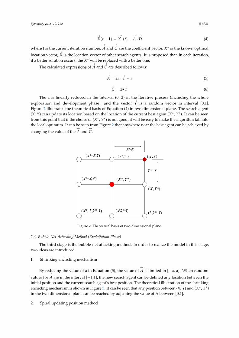
The a is linearly reduced in the interval (0, 2) in the iterative process (including the wholeexploration and development phase), and the vector
→r is a random vector in interval [0,1].
Figure 2 illustrates the theoretical basis of Equation (4) in two dimensional plane. The search agent(X, Y) can update its location based on the location of the current best agent (X∗, Y∗). It can be seenfrom this point that if the choice of (X∗, Y∗) is not good, it will be easy to make the algorithm fall intothe local optimum. It can be seen from Figure 2 that anywhere near the best agent can be achieved by
changing the value of the→A and
→C .
Symmetry 2018, 10, x FOR PEER REVIEW 5 of 31
The a is linearly reduced in the interval (0, 2) in the iterative process (including the whole exploration and development phase), and the vector r
is a random vector in interval [0,1]. Figure 2
illustrates the theoretical basis of Equation (4) in two dimensional plane. The search agent (X, Y) can update its location based on the location of the current best agent ( *X , *Y ). It can be seen from this point that if the choice of ( *X , *Y ) is not good, it will be easy to make the algorithm fall into the local optimum. It can be seen from Figure 2 that anywhere near the best agent can be achieved by changing the value of the A
and C
.
*X X
*Y Y
( , *)X Y
( , * )XY Y
( , )X Y( *, )X Y
( *, *)X Y
( *, * )X Y Y( * , * )X XY Y
( * , *)X X Y
( * , )X X Y
Figure 2. Theoretical basis of two-dimensional plane.
2.4. Bubble-Net Attacking Method (Exploitation Phase)
The third stage is the bubble-net attacking method. In order to realize the model in this stage, two ideas are introduced.
1. Shrinking encircling mechanism
By reducing the value of a in Equation (5), the value of A is limited in [-a, a]. When random
values for A are in the interval [−1,1], the new search agent can be defined any location between the
initial position and the current search agent’s best position. The theoretical illustration of the shrinking encircling mechanism is shown in Figure 3. It can be seen that any position between (X, Y) and ( *X , *Y ) in the two dimensional plane can be reached by adjusting the value of A between [0,1].
2. Spiral updating position method
The sketch map of spiral renewal position method is shown in Figure 4, which is the path of the search agent proposed by the original WOA. It calculates the distance between whale (X, Y) and ( *X
, *Y ) prey. The equation imitating the humpback whales spiral moving mode is described as follows. *( t+1) cos(2 ) ( )blX D e l X t
(7)
where, *( ) ( )D X t X t
represents the distance between the i th whale and the prey, b is used to
define the constant to limit the logarithmic spiral and l is a random number between the interval [−1,1].
Figure 2. Theoretical basis of two-dimensional plane.
2.4. Bubble-Net Attacking Method (Exploitation Phase)
The third stage is the bubble-net attacking method. In order to realize the model in this stage,two ideas are introduced.
1. Shrinking encircling mechanism
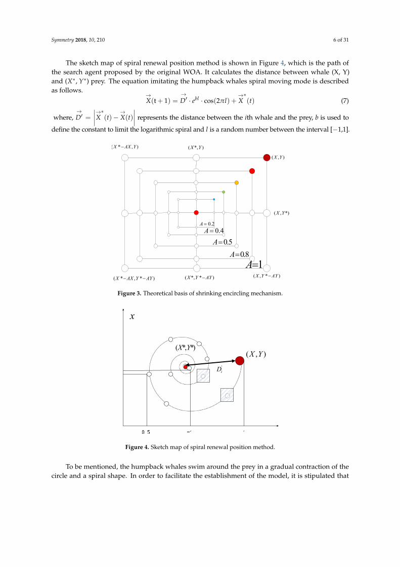
By reducing the value of a in Equation (5), the value of→A is limited in [−a, a]. When random
values for→A are in the interval [−1,1], the new search agent can be defined any location between the
initial position and the current search agent’s best position. The theoretical illustration of the shrinkingencircling mechanism is shown in Figure 3. It can be seen that any position between (X, Y) and (X∗, Y∗)in the two dimensional plane can be reached by adjusting the value of A between [0,1].
2. Spiral updating position method
Symmetry 2018, 10, 210 6 of 31
The sketch map of spiral renewal position method is shown in Figure 4, which is the path ofthe search agent proposed by the original WOA. It calculates the distance between whale (X, Y)and (X∗, Y∗) prey. The equation imitating the humpback whales spiral moving mode is describedas follows.
→X(t + 1) =
→D′ · ebl · cos(2πl) +
→X∗(t) (7)
where,→D′ =
∣∣∣∣→X∗(t)−→X(t)∣∣∣∣ represents the distance between the ith whale and the prey, b is used to
define the constant to limit the logarithmic spiral and l is a random number between the interval [−1,1].Symmetry 2018, 10, x FOR PEER REVIEW 6 of 31
( , )X Y
( , *)X Y
( , * )X Y AY( *, * )X Y AY( * , * )X AX Y AY
( *, )X Y( * , )X AX Y
1A
0.5A
0.8A
0.2A 0.4A
Figure 3. Theoretical basis of shrinking encircling mechanism.
( , )X Y( *, *)X Y
'iD
x
Figure 4. Sketch map of spiral renewal position method.
To be mentioned, the humpback whales swim around the prey in a gradual contraction of the circle and a spiral shape. In order to facilitate the establishment of the model, it is stipulated that each of the fifty percent of the whales may choose to surround the contraction path or spiral model to update their locations. The mathematical model is described as follows.
*
*
( ) 0.5( 1)
cos(2 ) ( ) 0.5bl
X t A D pX t
D e l X t p
(8)
where, p is a random number between [0,1].
2.5. Idea of Improving Whale Optimization Algorithm
Through carrying out the research on the original WOA idea, two improvement ideas are put forward.
(1) It can be seen from the searching path of the whales in Figure 4 and Equation (7), the logarithmic spiral curve adopted as the searching path, but the pitch is not equal seen from the logarithmic helix curve. In other words, when the searching agent carries out the searching process according to the path, it can be seen from the two shaded sections in Figure 2 that any location around the best agent can be changed by changing the values of A
and C
. However, if the pitch of the
Figure 3. Theoretical basis of shrinking encircling mechanism.
Symmetry 2018, 10, x FOR PEER REVIEW 6 of 31
( , )X Y
( , *)X Y
( , * )X Y AY( *, * )X Y AY( * , * )X AX Y AY
( *, )X Y( * , )X AX Y
1A
0.5A
0.8A
0.2A 0.4A
Figure 3. Theoretical basis of shrinking encircling mechanism.
( , )X Y( *, *)X Y
'iD
x
Figure 4. Sketch map of spiral renewal position method.
To be mentioned, the humpback whales swim around the prey in a gradual contraction of the circle and a spiral shape. In order to facilitate the establishment of the model, it is stipulated that each of the fifty percent of the whales may choose to surround the contraction path or spiral model to update their locations. The mathematical model is described as follows.
*
*
( ) 0.5( 1)
cos(2 ) ( ) 0.5bl
X t A D pX t
D e l X t p
(8)
where, p is a random number between [0,1].
2.5. Idea of Improving Whale Optimization Algorithm
Through carrying out the research on the original WOA idea, two improvement ideas are put forward.
(1) It can be seen from the searching path of the whales in Figure 4 and Equation (7), the logarithmic spiral curve adopted as the searching path, but the pitch is not equal seen from the logarithmic helix curve. In other words, when the searching agent carries out the searching process according to the path, it can be seen from the two shaded sections in Figure 2 that any location around the best agent can be changed by changing the values of A
and C
. However, if the pitch of the
Figure 4. Sketch map of spiral renewal position method.
To be mentioned, the humpback whales swim around the prey in a gradual contraction of thecircle and a spiral shape. In order to facilitate the establishment of the model, it is stipulated that
Symmetry 2018, 10, 210 7 of 31
each of the fifty percent of the whales may choose to surround the contraction path or spiral model toupdate their locations. The mathematical model is described as follows.
→X(t + 1) =
→X∗(t)−
→A ·→D p < 0.5
→D′ · ebl · cos(2πl) +
→X∗(t) p ≥ 0.5
(8)
where, p is a random number between [0,1].
2.5. Idea of Improving Whale Optimization Algorithm
Through carrying out the research on the original WOA idea, two improvement ideas areput forward.
(1) It can be seen from the searching path of the whales in Figure 4 and Equation (7), the logarithmicspiral curve adopted as the searching path, but the pitch is not equal seen from the logarithmic helixcurve. In other words, when the searching agent carries out the searching process according to thepath, it can be seen from the two shaded sections in Figure 2 that any location around the best agent
can be changed by changing the values of→A and
→C . However, if the pitch of the spiral curve is larger
than that of the search agent, it will lead to some locations can not be searched so as to reduce theergodicity of the algorithm.
(2) In order to make the algorithm search thoroughly near the location of the search agents,after each iteration of the WOA, a set of more advantageous searched positions X∗(t) are obtained.Then X∗(t) will be no go directly into the next iteration, the disturbance is carried on it so as tosearching the nearby scope of X∗(t). The next iteration will generate a new best searching agent.
3. Complex Path-Perceptual Disturbance WOA
3.1. Selection of Mathematical Model of Searching Path
According to the logarithmic spiral model proposed by the original WOA, seven kinds of spiralsare puts forward as the mathematical models of searching paths [40].
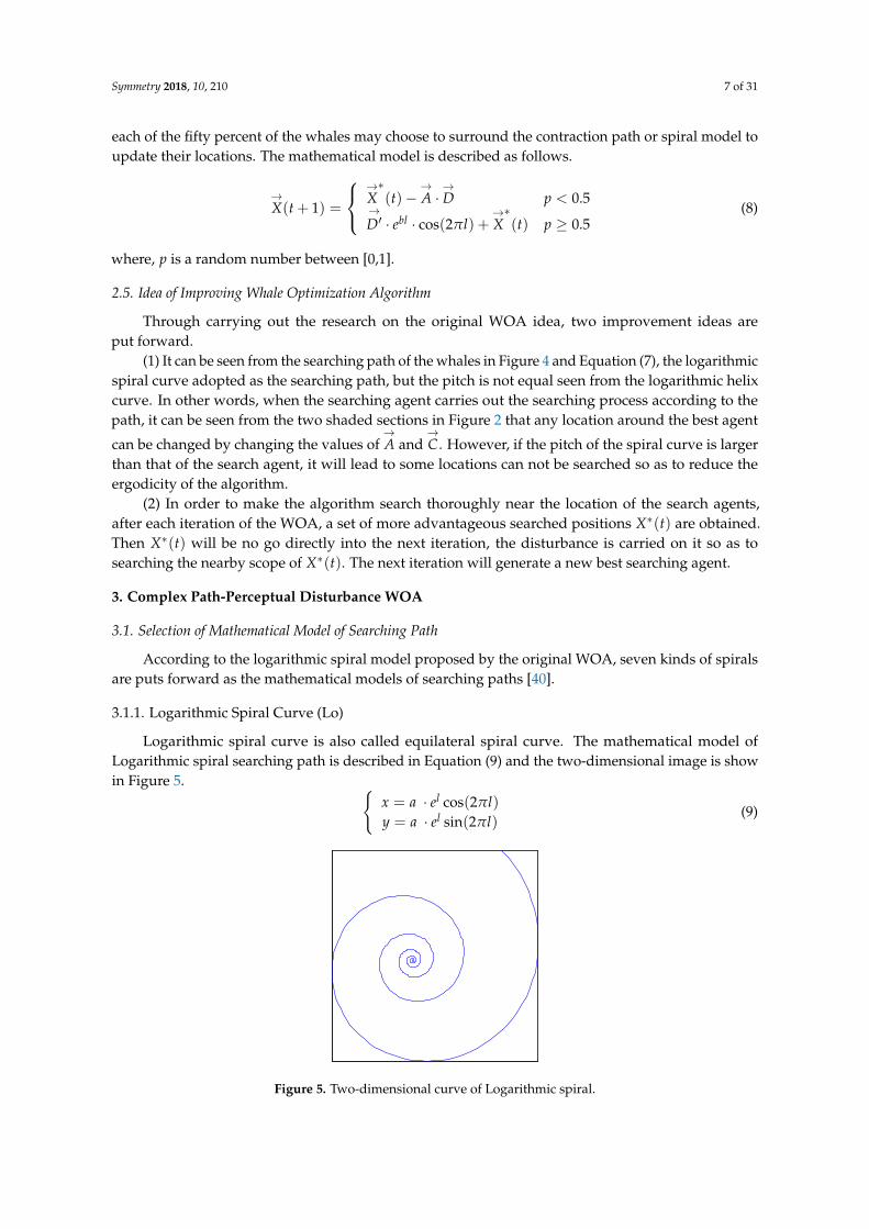
3.1.1. Logarithmic Spiral Curve (Lo)
Logarithmic spiral curve is also called equilateral spiral curve. The mathematical model ofLogarithmic spiral searching path is described in Equation (9) and the two-dimensional image is showin Figure 5. {
x = a · el cos(2πl)y = a · el sin(2πl)
(9)
Symmetry 2018, 10, x FOR PEER REVIEW 7 of 31
spiral curve is larger than that of the search agent, it will lead to some locations can not be searched so as to reduce the ergodicity of the algorithm.
(2) In order to make the algorithm search thoroughly near the location of the search agents, after each iteration of the WOA, a set of more advantageous searched positions * ( )X t are obtained. Then
* ( )X t will be no go directly into the next iteration, the disturbance is carried on it so as to searching the nearby scope of * ( )X t . The next iteration will generate a new best searching agent.
3. Complex Path-Perceptual Disturbance WOA
3.1. Selection of Mathematical Model of Searching Path
According to the logarithmic spiral model proposed by the original WOA, seven kinds of spirals are puts forward as the mathematical models of searching paths [40].
3.1.1. Logarithmic Spiral Curve (Lo)
Logarithmic spiral curve is also called equilateral spiral curve. The mathematical model of Logarithmic spiral searching path is described in Equation (9) and the two-dimensional image is show in Figure 5.
cos(2 )
sin(2 )
l
l
x a e l
y a e l
(9)
Figure 5. Two-dimensional curve of Logarithmic spiral.
3.1.2. Archimedes Spiral Curve (Ar)
The Archimedes spiral curve is a trail generated by a point evenly moving away from a fixed point, while moving at a fixed angular velocity around the fixed point. The equal pitch Archimedes spiral means that the pitch of the spiral curve is a invariant constant shown in Figure 6. The mathematical model of Archimedes spiral searching path is described in Equation (10) and the two-dimensional image is show in Figure 6.
( ) cos(2 )
( ) sin(2 )
x a b l l
y a b l l
(10)
As we put forward, the pitch of the spiral curve gradually changes to affect the convergence performance of the algorithm. Therefore, we first select the Archimedean spiral curve with a constant pitch. Since its pitch is equidistant, we use an algorithm to adjust the parameters of the function so that the algorithm achieves optimal performance.
Figure 5. Two-dimensional curve of Logarithmic spiral.
Symmetry 2018, 10, 210 8 of 31
3.1.2. Archimedes Spiral Curve (Ar)
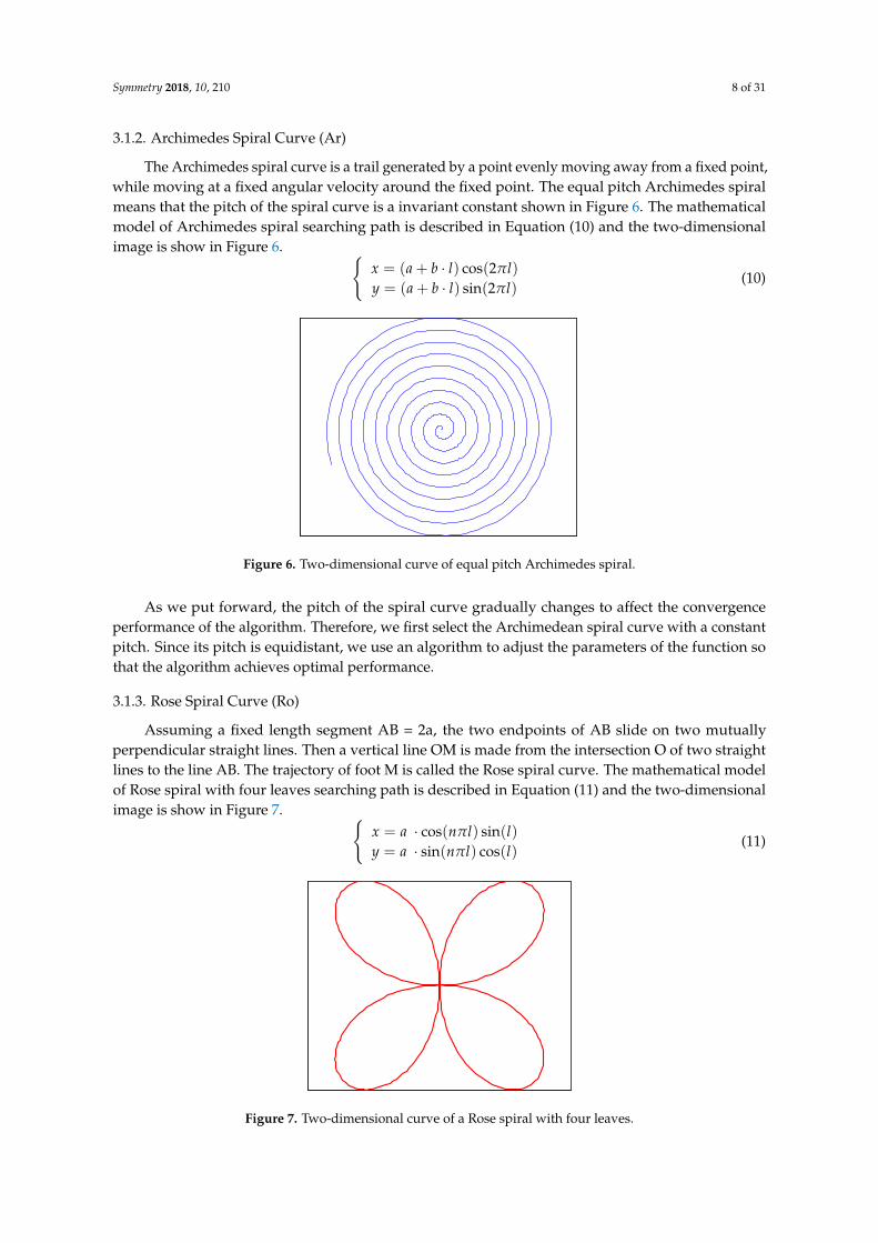
The Archimedes spiral curve is a trail generated by a point evenly moving away from a fixed point,while moving at a fixed angular velocity around the fixed point. The equal pitch Archimedes spiralmeans that the pitch of the spiral curve is a invariant constant shown in Figure 6. The mathematicalmodel of Archimedes spiral searching path is described in Equation (10) and the two-dimensionalimage is show in Figure 6. {
x = (a + b · l) cos(2πl)y = (a + b · l) sin(2πl)
(10)Symmetry 2018, 10, x FOR PEER REVIEW 8 of 31
Figure 6. Two-dimensional curve of equal pitch Archimedes spiral.
3.1.3. Rose Spiral Curve (Ro)
Assuming a fixed length segment AB = 2a, the two endpoints of AB slide on two mutually perpendicular straight lines. Then a vertical line OM is made from the intersection O of two straight lines to the line AB. The trajectory of foot M is called the Rose spiral curve. The mathematical model of Rose spiral with four leaves searching path is described in Equation (11) and the two-dimensional image is show in Figure 7.
cos( ) sin( )
sin( ) cos( )
x a n l l
y a n l l
(11)
Figure 7. Two-dimensional curve of a Rose spiral with four leaves.
Because the path of the function is relatively simple, taking into account the existence of the disturbance, by adjusting the parameters of the function, the spacing between the search paths is as small as possible, and the optimal value may be obtained faster with as few iterations as possible. So we chose this spiral curve.
3.1.4. Epitrochoid-I (Ep-I)
A movable circle is carried out the roll around the externally-tangent of the fixed circle internally, where the radius of the fixed circle is a and the radius of the movable circle is b. In the process of the movable circle rolling, the trajectory is formed by a fixed point P on the movable circle, which is called the Epicycloid-I. The mathematical model of Epitrochoid-I searching path is described in Equation (12) and the two-dimensional image is show in Figure 8.
Figure 6. Two-dimensional curve of equal pitch Archimedes spiral.
As we put forward, the pitch of the spiral curve gradually changes to affect the convergenceperformance of the algorithm. Therefore, we first select the Archimedean spiral curve with a constantpitch. Since its pitch is equidistant, we use an algorithm to adjust the parameters of the function sothat the algorithm achieves optimal performance.
3.1.3. Rose Spiral Curve (Ro)
Assuming a fixed length segment AB = 2a, the two endpoints of AB slide on two mutuallyperpendicular straight lines. Then a vertical line OM is made from the intersection O of two straightlines to the line AB. The trajectory of foot M is called the Rose spiral curve. The mathematical modelof Rose spiral with four leaves searching path is described in Equation (11) and the two-dimensionalimage is show in Figure 7. {
x = a · cos(nπl) sin(l)y = a · sin(nπl) cos(l)
(11)
Symmetry 2018, 10, x FOR PEER REVIEW 8 of 31
Figure 6. Two-dimensional curve of equal pitch Archimedes spiral.
3.1.3. Rose Spiral Curve (Ro)
Assuming a fixed length segment AB = 2a, the two endpoints of AB slide on two mutually perpendicular straight lines. Then a vertical line OM is made from the intersection O of two straight lines to the line AB. The trajectory of foot M is called the Rose spiral curve. The mathematical model of Rose spiral with four leaves searching path is described in Equation (11) and the two-dimensional image is show in Figure 7.
cos( ) sin( )
sin( ) cos( )
x a n l l
y a n l l
(11)
Figure 7. Two-dimensional curve of a Rose spiral with four leaves.
Because the path of the function is relatively simple, taking into account the existence of the disturbance, by adjusting the parameters of the function, the spacing between the search paths is as small as possible, and the optimal value may be obtained faster with as few iterations as possible. So we chose this spiral curve.
3.1.4. Epitrochoid-I (Ep-I)
A movable circle is carried out the roll around the externally-tangent of the fixed circle internally, where the radius of the fixed circle is a and the radius of the movable circle is b. In the process of the movable circle rolling, the trajectory is formed by a fixed point P on the movable circle, which is called the Epicycloid-I. The mathematical model of Epitrochoid-I searching path is described in Equation (12) and the two-dimensional image is show in Figure 8.
Figure 7. Two-dimensional curve of a Rose spiral with four leaves.
Symmetry 2018, 10, 210 9 of 31
Because the path of the function is relatively simple, taking into account the existence of thedisturbance, by adjusting the parameters of the function, the spacing between the search paths is assmall as possible, and the optimal value may be obtained faster with as few iterations as possible.So we chose this spiral curve.
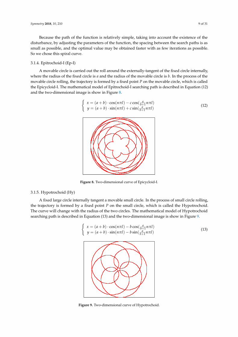
3.1.4. Epitrochoid-I (Ep-I)
A movable circle is carried out the roll around the externally-tangent of the fixed circle internally,where the radius of the fixed circle is a and the radius of the movable circle is b. In the process of themovable circle rolling, the trajectory is formed by a fixed point P on the movable circle, which is calledthe Epicycloid-I. The mathematical model of Epitrochoid-I searching path is described in Equation (12)and the two-dimensional image is show in Figure 8.{
x = (a + b) · cos(nπl)− c cos( ab+1 nπl)
y = (a + b) · sin(nπl) + c sin( ab+1 nπl)
(12)
Symmetry 2018, 10, x FOR PEER REVIEW 9 of 31
( ) cos( ) cos( )1
( ) sin( ) sin( )1
ax a b n l c n l
ba
y a b n l c n lb
(12)
Figure 8. Two-dimensional curve of Epicycloid-I.
3.1.5. Hypotrochoid (Hy)
A fixed large circle internally tangent a movable small circle. In the process of small circle rolling, the trajectory is formed by a fixed point P on the small circle, which is called the Hypotrochoid. The curve will change with the radius of the two circles. The mathematical model of Hypotrochoid searching path is described in Equation (13) and the two-dimensional image is show in Figure 9.
( ) cos( ) cos( )1
( ) sin( ) sin( )1
ax a b n l b n l
ba
y a b n l b n lb
(13)
Figure 9. Two-dimensional curve of Hypotrochoid.
3.1.6. Epitrochoid-II (Ep-II)
The formation principle of the Epicycloid-II and the Epicycloid-I is the same. Just the difference of the radius of the big circle and the small circle produces the different trend. The mathematical model of Epitrochoid-II searching path is described in Equation (14) and the two-dimensional image is show in Figure 10.
Figure 8. Two-dimensional curve of Epicycloid-I.
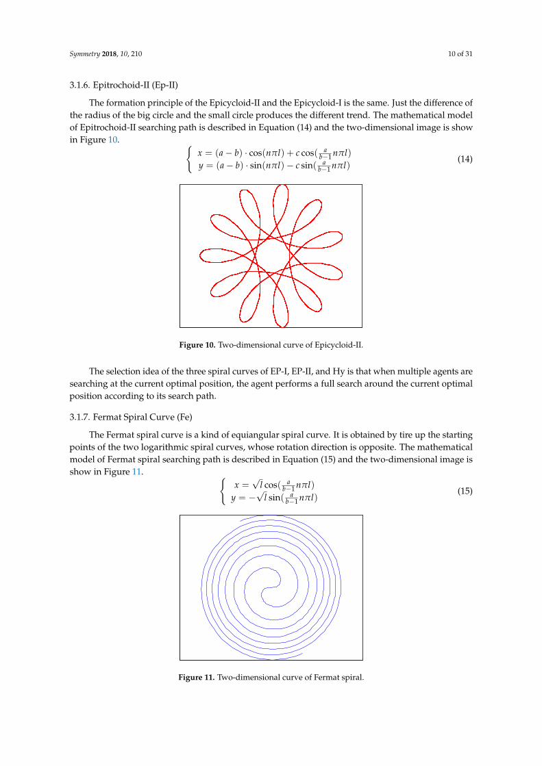
3.1.5. Hypotrochoid (Hy)
A fixed large circle internally tangent a movable small circle. In the process of small circle rolling,the trajectory is formed by a fixed point P on the small circle, which is called the Hypotrochoid.The curve will change with the radius of the two circles. The mathematical model of Hypotrochoidsearching path is described in Equation (13) and the two-dimensional image is show in Figure 9.{
x = (a + b) · cos(nπl)− b cos( ab+1 nπl)
y = (a + b) · sin(nπl)− b sin( ab+1 nπl)
(13)
Symmetry 2018, 10, x FOR PEER REVIEW 9 of 31
( ) cos( ) cos( )1
( ) sin( ) sin( )1
ax a b n l c n l
ba
y a b n l c n lb
(12)
Figure 8. Two-dimensional curve of Epicycloid-I.
3.1.5. Hypotrochoid (Hy)
A fixed large circle internally tangent a movable small circle. In the process of small circle rolling, the trajectory is formed by a fixed point P on the small circle, which is called the Hypotrochoid. The curve will change with the radius of the two circles. The mathematical model of Hypotrochoid searching path is described in Equation (13) and the two-dimensional image is show in Figure 9.
( ) cos( ) cos( )1
( ) sin( ) sin( )1
ax a b n l b n l
ba
y a b n l b n lb
(13)
Figure 9. Two-dimensional curve of Hypotrochoid.
3.1.6. Epitrochoid-II (Ep-II)
The formation principle of the Epicycloid-II and the Epicycloid-I is the same. Just the difference of the radius of the big circle and the small circle produces the different trend. The mathematical model of Epitrochoid-II searching path is described in Equation (14) and the two-dimensional image is show in Figure 10.
Figure 9. Two-dimensional curve of Hypotrochoid.
Symmetry 2018, 10, 210 10 of 31
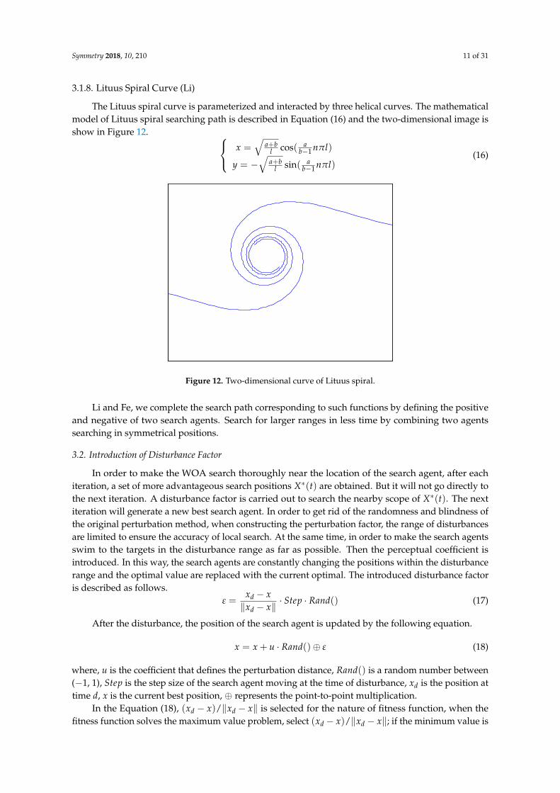
3.1.6. Epitrochoid-II (Ep-II)
The formation principle of the Epicycloid-II and the Epicycloid-I is the same. Just the difference ofthe radius of the big circle and the small circle produces the different trend. The mathematical modelof Epitrochoid-II searching path is described in Equation (14) and the two-dimensional image is showin Figure 10. {
x = (a− b) · cos(nπl) + c cos( ab−1 nπl)
y = (a− b) · sin(nπl)− c sin( ab−1 nπl)
(14)
Symmetry 2018, 10, x FOR PEER REVIEW 10 of 31
( ) cos( ) cos( )1
( ) sin( ) sin( )1
ax a b n l c n l
ba
y a b n l c n lb
(14)
Figure 10. Two-dimensional curve of Epicycloid-II.
The selection idea of the three spiral curves of EP-I, EP-II, and Hy is that when multiple agents are searching at the current optimal position, the agent performs a full search around the current optimal position according to its search path.
3.1.7. Fermat Spiral Curve (Fe)
The Fermat spiral curve is a kind of equiangular spiral curve. It is obtained by tire up the starting points of the two logarithmic spiral curves, whose rotation direction is opposite. The mathematical model of Fermat spiral searching path is described in Equation (15) and the two-dimensional image is show in Figure 11.
cos( )1
sin( )1
ax l n l
ba
y l n lb
(15)
Figure 11. Two-dimensional curve of Fermat spiral.
Figure 10. Two-dimensional curve of Epicycloid-II.
The selection idea of the three spiral curves of EP-I, EP-II, and Hy is that when multiple agents aresearching at the current optimal position, the agent performs a full search around the current optimalposition according to its search path.
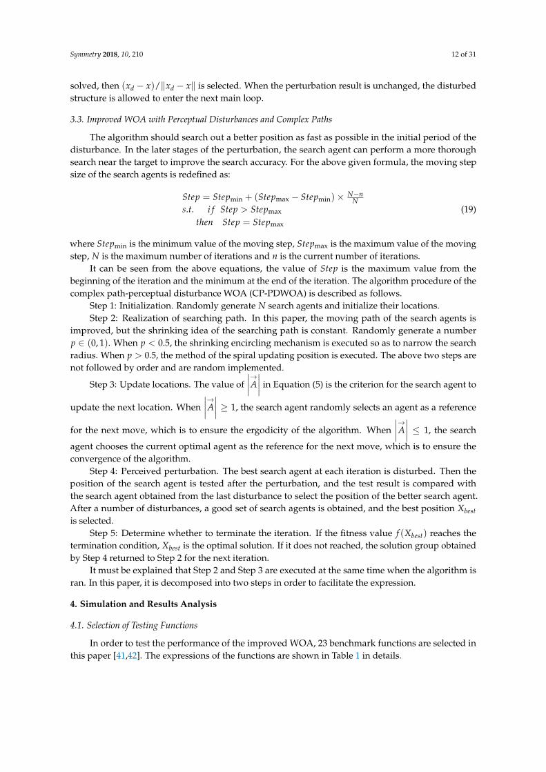
3.1.7. Fermat Spiral Curve (Fe)
The Fermat spiral curve is a kind of equiangular spiral curve. It is obtained by tire up the startingpoints of the two logarithmic spiral curves, whose rotation direction is opposite. The mathematicalmodel of Fermat spiral searching path is described in Equation (15) and the two-dimensional image isshow in Figure 11. {
x =√
l cos( ab−1 nπl)
y = −√
l sin( ab−1 nπl)
(15)
Symmetry 2018, 10, x FOR PEER REVIEW 10 of 31
( ) cos( ) cos( )1
( ) sin( ) sin( )1
ax a b n l c n l
ba
y a b n l c n lb
(14)
Figure 10. Two-dimensional curve of Epicycloid-II.
The selection idea of the three spiral curves of EP-I, EP-II, and Hy is that when multiple agents are searching at the current optimal position, the agent performs a full search around the current optimal position according to its search path.
3.1.7. Fermat Spiral Curve (Fe)
The Fermat spiral curve is a kind of equiangular spiral curve. It is obtained by tire up the starting points of the two logarithmic spiral curves, whose rotation direction is opposite. The mathematical model of Fermat spiral searching path is described in Equation (15) and the two-dimensional image is show in Figure 11.
cos( )1
sin( )1
ax l n l
ba
y l n lb
(15)
Figure 11. Two-dimensional curve of Fermat spiral.
Figure 11. Two-dimensional curve of Fermat spiral.
Symmetry 2018, 10, 210 11 of 31
3.1.8. Lituus Spiral Curve (Li)
The Lituus spiral curve is parameterized and interacted by three helical curves. The mathematicalmodel of Lituus spiral searching path is described in Equation (16) and the two-dimensional image isshow in Figure 12. x =
√a+b
l cos( ab−1 nπl)
y = −√
a+bl sin( a
b−1 nπl)(16)
Symmetry 2018, 10, x FOR PEER REVIEW 11 of 31
3.1.8. Lituus Spiral Curve (Li)
The Lituus spiral curve is parameterized and interacted by three helical curves. The mathematical model of Lituus spiral searching path is described in Equation (16) and the two-dimensional image is show in Figure 12.
cos( )1
sin( )1
a b ax n l
l b
a b ay n l
l b
(16)
Figure 12. Two-dimensional curve of Lituus spiral.
Li and Fe, we complete the search path corresponding to such functions by defining the positive and negative of two search agents. Search for larger ranges in less time by combining two agents searching in symmetrical positions.
3.2. Introduction of Disturbance Factor
In order to make the WOA search thoroughly near the location of the search agent, after each iteration, a set of more advantageous search positions * ( )X t are obtained. But it will not go directly to the next iteration. A disturbance factor is carried out to search the nearby scope of * ( )X t . The next iteration will generate a new best search agent. In order to get rid of the randomness and blindness of the original perturbation method, when constructing the perturbation factor, the range of disturbances are limited to ensure the accuracy of local search. At the same time, in order to make the search agents swim to the targets in the disturbance range as far as possible. Then the perceptual coefficient is introduced. In this way, the search agents are constantly changing the positions within the disturbance range and the optimal value are replaced with the current optimal. The introduced disturbance factor is described as follows.
()d
d
x xStep Rand
x x
(17)
After the disturbance, the position of the search agent is updated by the following equation.
()x x u Rand (18)
where, u is the coefficient that defines the perturbation distance, ()Rand is a random number between (−1, 1), Step is the step size of the search agent moving at the time of disturbance, dx is the position at time d, x is the current best position, represents the point-to-point multiplication.
In the Equation (18), ( ) /d dx x x x is selected for the nature of fitness function, when the fitness function solves the maximum value problem, select ( ) /d dx x x x ; if the minimum value
y
Figure 12. Two-dimensional curve of Lituus spiral.
Li and Fe, we complete the search path corresponding to such functions by defining the positiveand negative of two search agents. Search for larger ranges in less time by combining two agentssearching in symmetrical positions.
3.2. Introduction of Disturbance Factor
In order to make the WOA search thoroughly near the location of the search agent, after eachiteration, a set of more advantageous search positions X∗(t) are obtained. But it will not go directly tothe next iteration. A disturbance factor is carried out to search the nearby scope of X∗(t). The nextiteration will generate a new best search agent. In order to get rid of the randomness and blindness ofthe original perturbation method, when constructing the perturbation factor, the range of disturbancesare limited to ensure the accuracy of local search. At the same time, in order to make the search agentsswim to the targets in the disturbance range as far as possible. Then the perceptual coefficient isintroduced. In this way, the search agents are constantly changing the positions within the disturbancerange and the optimal value are replaced with the current optimal. The introduced disturbance factoris described as follows.
ε =xd − x‖xd − x‖ · Step · Rand() (17)
After the disturbance, the position of the search agent is updated by the following equation.
x = x + u · Rand()⊕ ε (18)
where, u is the coefficient that defines the perturbation distance, Rand() is a random number between(−1, 1), Step is the step size of the search agent moving at the time of disturbance, xd is the position attime d, x is the current best position, ⊕ represents the point-to-point multiplication.
In the Equation (18), (xd − x)/‖xd − x‖ is selected for the nature of fitness function, when thefitness function solves the maximum value problem, select (xd − x)/‖xd − x‖; if the minimum value is
Symmetry 2018, 10, 210 12 of 31
solved, then (xd − x)/‖xd − x‖ is selected. When the perturbation result is unchanged, the disturbedstructure is allowed to enter the next main loop.
3.3. Improved WOA with Perceptual Disturbances and Complex Paths
The algorithm should search out a better position as fast as possible in the initial period of thedisturbance. In the later stages of the perturbation, the search agent can perform a more thoroughsearch near the target to improve the search accuracy. For the above given formula, the moving stepsize of the search agents is redefined as:
Step = Stepmin + (Stepmax − Stepmin)× N−nN
s.t. i f Step > Stepmax
then Step = Stepmax
(19)
where Stepmin is the minimum value of the moving step, Stepmax is the maximum value of the movingstep, N is the maximum number of iterations and n is the current number of iterations.
It can be seen from the above equations, the value of Step is the maximum value from thebeginning of the iteration and the minimum at the end of the iteration. The algorithm procedure of thecomplex path-perceptual disturbance WOA (CP-PDWOA) is described as follows.
Step 1: Initialization. Randomly generate N search agents and initialize their locations.Step 2: Realization of searching path. In this paper, the moving path of the search agents is
improved, but the shrinking idea of the searching path is constant. Randomly generate a numberp ∈ (0, 1). When p < 0.5, the shrinking encircling mechanism is executed so as to narrow the searchradius. When p > 0.5, the method of the spiral updating position is executed. The above two steps arenot followed by order and are random implemented.
Step 3: Update locations. The value of∣∣∣∣→A∣∣∣∣ in Equation (5) is the criterion for the search agent to
update the next location. When∣∣∣∣→A∣∣∣∣ ≥ 1, the search agent randomly selects an agent as a reference
for the next move, which is to ensure the ergodicity of the algorithm. When∣∣∣∣→A∣∣∣∣ ≤ 1, the search
agent chooses the current optimal agent as the reference for the next move, which is to ensure theconvergence of the algorithm.
Step 4: Perceived perturbation. The best search agent at each iteration is disturbed. Then theposition of the search agent is tested after the perturbation, and the test result is compared withthe search agent obtained from the last disturbance to select the position of the better search agent.After a number of disturbances, a good set of search agents is obtained, and the best position Xbestis selected.
Step 5: Determine whether to terminate the iteration. If the fitness value f (Xbest) reaches thetermination condition, Xbest is the optimal solution. If it does not reached, the solution group obtainedby Step 4 returned to Step 2 for the next iteration.
It must be explained that Step 2 and Step 3 are executed at the same time when the algorithm isran. In this paper, it is decomposed into two steps in order to facilitate the expression.
4. Simulation and Results Analysis
4.1. Selection of Testing Functions
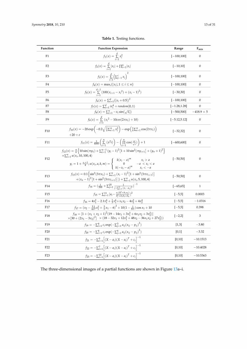
In order to test the performance of the improved WOA, 23 benchmark functions are selected inthis paper [41,42]. The expressions of the functions are shown in Table 1 in details.
Symmetry 2018, 10, 210 13 of 31
Table 1. Testing functions.
Function Function Expression Range Fmin
F1 f1(x) =d∑
i=1x2
i [−100,100] 0
F2 f2(x) =d∑
i=1|xi|+ ∏n
i=1|xi| [−10,10] 0
F3 f3(x) =d∑
i=1
(∑i
j−1 xj
)2[−100,100] 0
F4 f4(x) = maxi{|xi|, 1 ≤ i ≤ n} [−100,100] 0
F5 f5(x) =d−1∑
i=1(100(xi+1 − xi
2) + (xi − 1)2) [−30,30] 0
F6 f6(x) = ∑di=1([xi + 0.5])2 [−100,100] 0
F7 f7(x) = ∑di=1 ix4
i + random[0, 1) [−1.28,1.28] 0
F8 f8(x) = ∑ni=1−xi sin
(√xi)
[−500,500] −418.9 × 5
F9 f9(x) =d∑
i=1(xi
2 − 10cos(2πxi) + 10) [−5.12,5.12] 0
F10 f10(x) = −20 exp(−0.2
√1n ∑n
i=1 x2i
)− exp
(1n ∑n
i=1 cos(2πxi))
+20 + e[−32,32] 0
F11 f11(x) = 14000
(n∑
i=1(x2i)
)−(
n∏i=1
cos( xi√i)
)+ 1 [−600,600] 0
F12
f12(x) = πn
{10 sin(πy1) + ∑n−1
i=1 (yi − 1)2[1 + 10 sin2(πyi+1]+ (yn + 1)2
}+∑n
i=1 u(xi, 10, 100, 4)
yi = 1 + xi+14 ; u(xi, a, k, m) =
k(xi − a)m
0k(−xi − a)m
xi > a−a < xi < a
xi < −a
[−50,50] 0
F13f13(x) = 0.1
{sin2(3πx1) + ∑n
i=1 (xi − 1)2[1 + sin2(3πxi+1)]
+(xn − 1)2[1 + sin2(3πxi+1)]}+ ∑n
i=1 u(xi, 5, 100, 4)[−50,50] 0
F14 f14 = ( 1500 + ∑25
j=11
j+∑2i=1 (xi−aij)
6 )−1
[−65,65] 1
F15 f15 = ∑11i=1 [ai−
x1(b2i +b1x2)
b2i +b1b3+b4
]2 [−5,5] 0.0003
F16 f16 = 4x21 − 2.1x4
1 +13 x6
1+x1x2 − 4x22 + 4x4
2 [−5,5] −1.0316
F17 f17 = (x2 − 5.14π2 x2
1 +5π x1 − 6)
2+ 10(1− 1
8π ) cos x1 + 10 [−5,5] 0.398
F18 f18 = [1 + (x1 + x2 + 1)2(19− 14x1 + 3x21 + 6x1x2 + 3x2
2)]
×[30 + (2x1 − 3x2)2] × (18− 32x1 + 12x2
1 + 48x2 − 36x1x2 + 27x22))
[−2,2] 3
F19 f19 = −∑4i=1 ci exp(−∑3
j=1 aij(xij − pij)2) [1,3] −3.80
F20 f20 = −∑4i=1 ci exp(−∑6
j=1 aij(xij − pij)2) [0,1] −3.32
F21 f21 = −∑5i=1
[(X− ai)(X− ai)
T + ci
]−1[0,10] −10.1513
F22 f22 = −∑7i=1
[(X− ai)(X− ai)
T + ci
]−1[0,10] −10.4028
F23 f23 = −∑10i=1
[(X− ai)(X− ai)
T + ci
]−1[0,10] −10.5363
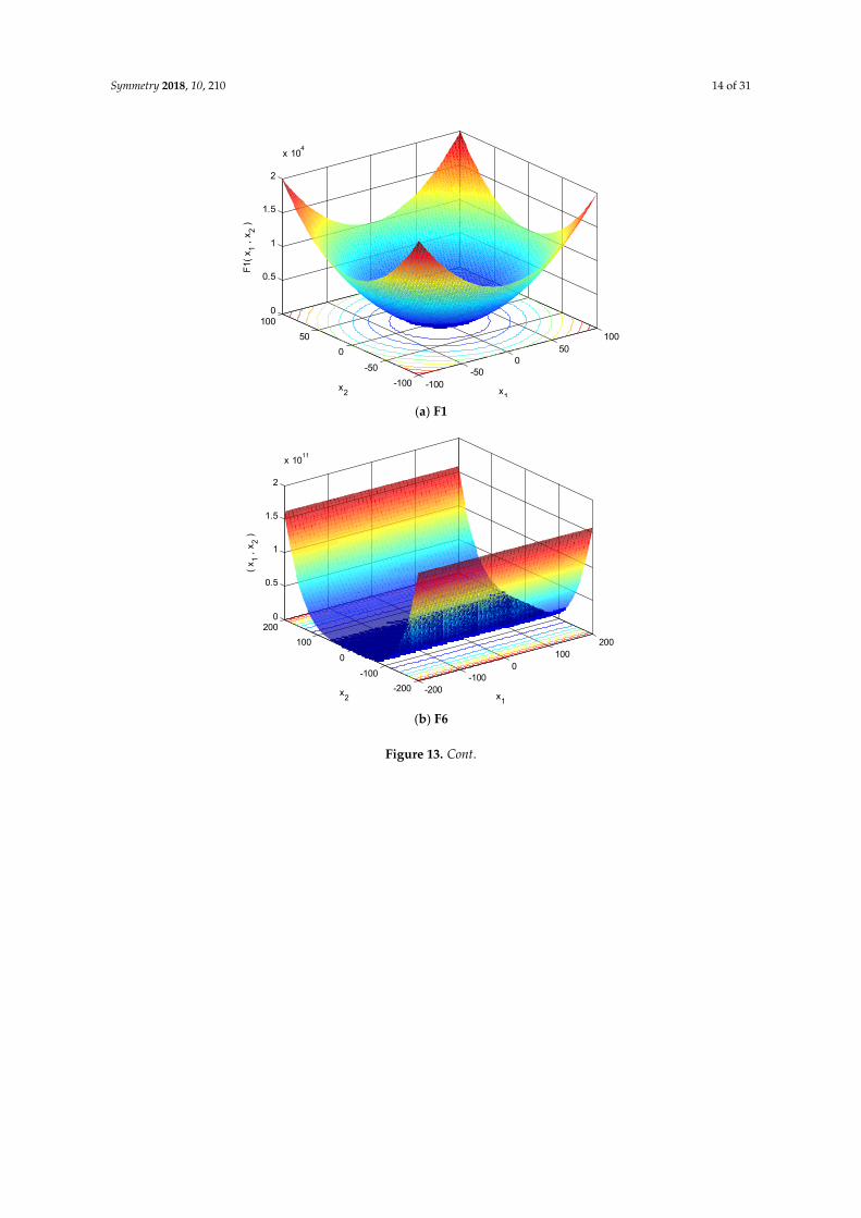
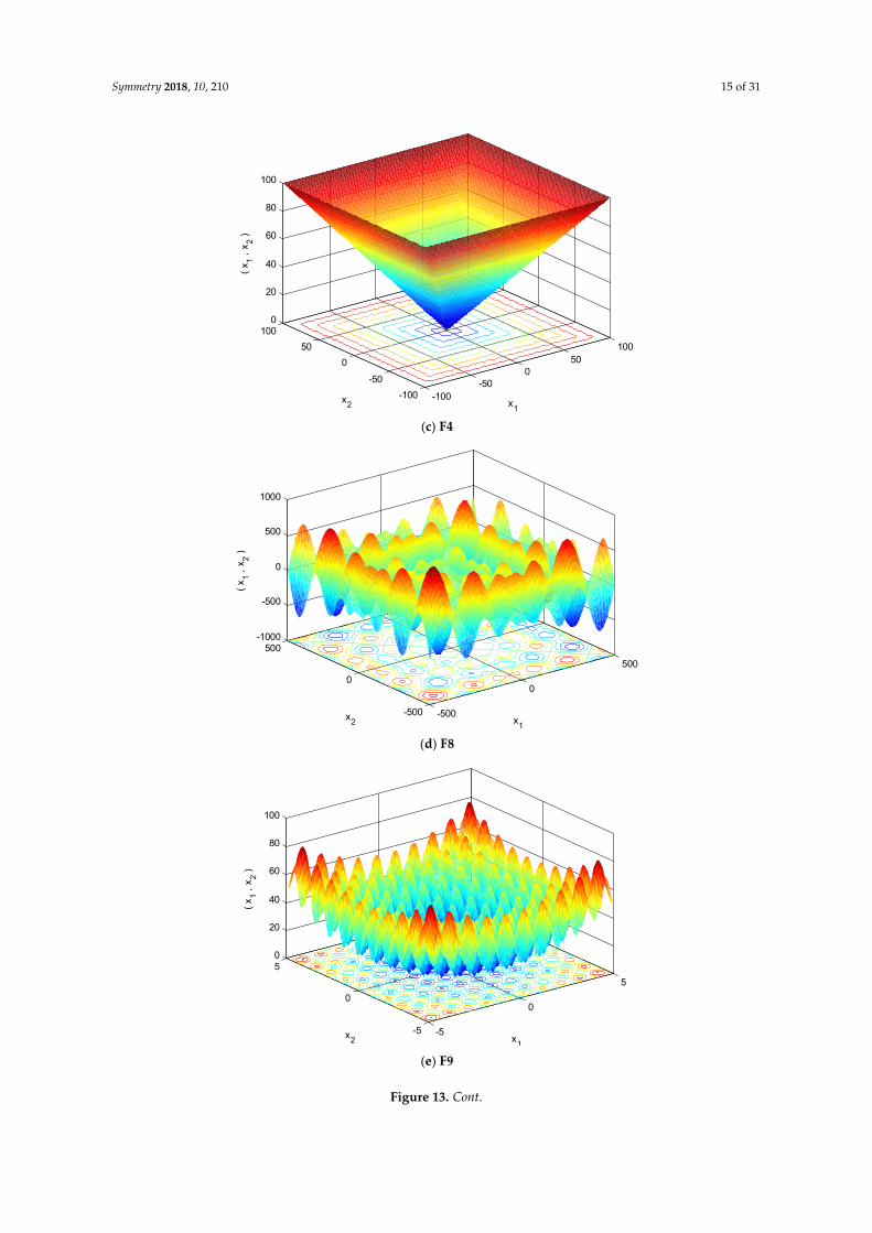
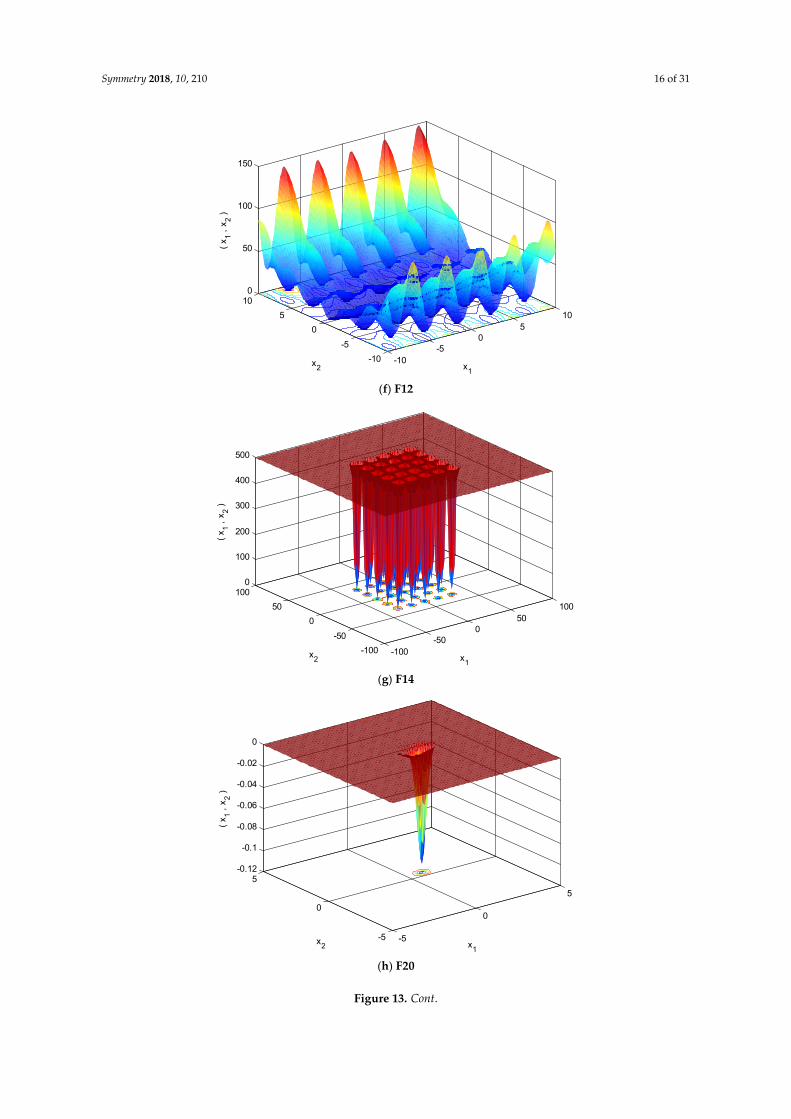
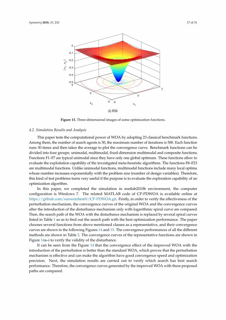
The three-dimensional images of a partial functions are shown in Figure 13a–i.
Symmetry 2018, 10, 210 14 of 31
Symmetry 2018, 10, x FOR PEER REVIEW 14 of 31
F22 17
22 1( )( )Ti i ii
f X a X a c
[0,10] −10.4028
F23 110
23 1( )( )Ti i ii
f X a X a c
[0,10] −10.5363
The three-dimensional images of a partial functions are shown in Figure 13a–i.
(a) F1
(b) F6
-100-50
050
100
-100
-50
0
50
1000
0.5
1
1.5
2
x 104
x1
x2
F1(
x1 ,
x2 )
-200-100
0100
200
-200
-100
0
100
2000
0.5
1
1.5
2
x 1011
x1
x2
( x 1 ,
x2 )
Figure 13. Cont.
Symmetry 2018, 10, 210 15 of 31
Symmetry 2018, 10, x FOR PEER REVIEW 15 of 31
(c) F4
(d) F8
(e) F9
-100-50
050
100
-100
-50
0
50
1000
20
40
60
80
100
x1
x2
( x 1 ,
x2 )
-500
0
500
-500
0
500-1000
-500
0
500
1000
x1
x2
( x 1 ,
x2 )
-5
0
5
-5
0
50
20
40
60
80
100
x1
x2
( x 1 ,
x2 )
Figure 13. Cont.
Symmetry 2018, 10, 210 16 of 31
Symmetry 2018, 10, x FOR PEER REVIEW 16 of 31
(f) F12
(g) F14
(h) F20
-10-5
05
10
-10
-5
0
5
100
50
100
150
x1
x2
( x 1 ,
x2 )
-100-50
050
100
-100
-50
0
50
1000
100
200
300
400
500
x1
x2
( x 1 ,
x2 )
-5
0
5
-5
0
5-0.12
-0.1
-0.08
-0.06
-0.04
-0.02
0
x1
x2
( x 1 ,
x2 )
Figure 13. Cont.
Symmetry 2018, 10, 210 17 of 31
Symmetry 2018, 10, x FOR PEER REVIEW 17 of 31
(i) F21
Figure 13. Three-dimensional images of some optimization functions.
4.2. Simulation Results and Analysis
This paper tests the computational power of WOA by adopting 23 classical benchmark functions. Among them, the number of search agents is 30, the maximum number of iterations is 500. Each function runs 30 times and then takes the average to plot the convergence curve. Benchmark functions can be divided into four groups: unimodal, multimodal, fixed-dimension multimodal and composite functions. Functions F1–F7 are typical unimodal since they have only one global optimum. These functions allow to evaluate the exploitation capability of the investigated meta-heuristic algorithms. The functions F8–F23 are multimodal functions. Unlike unimodal functions, multimodal functions include many local optima whose number increases exponentially with the problem size (number of design variables). Therefore, this kind of test problems turns very useful if the purpose is to evaluate the exploration capability of an optimization algorithm.
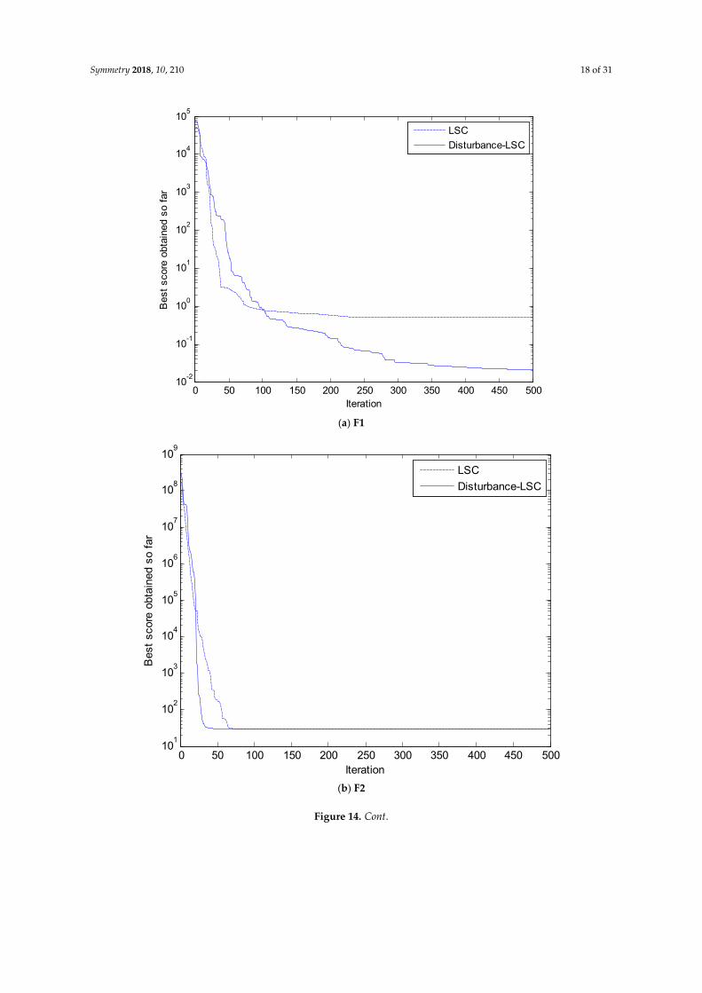
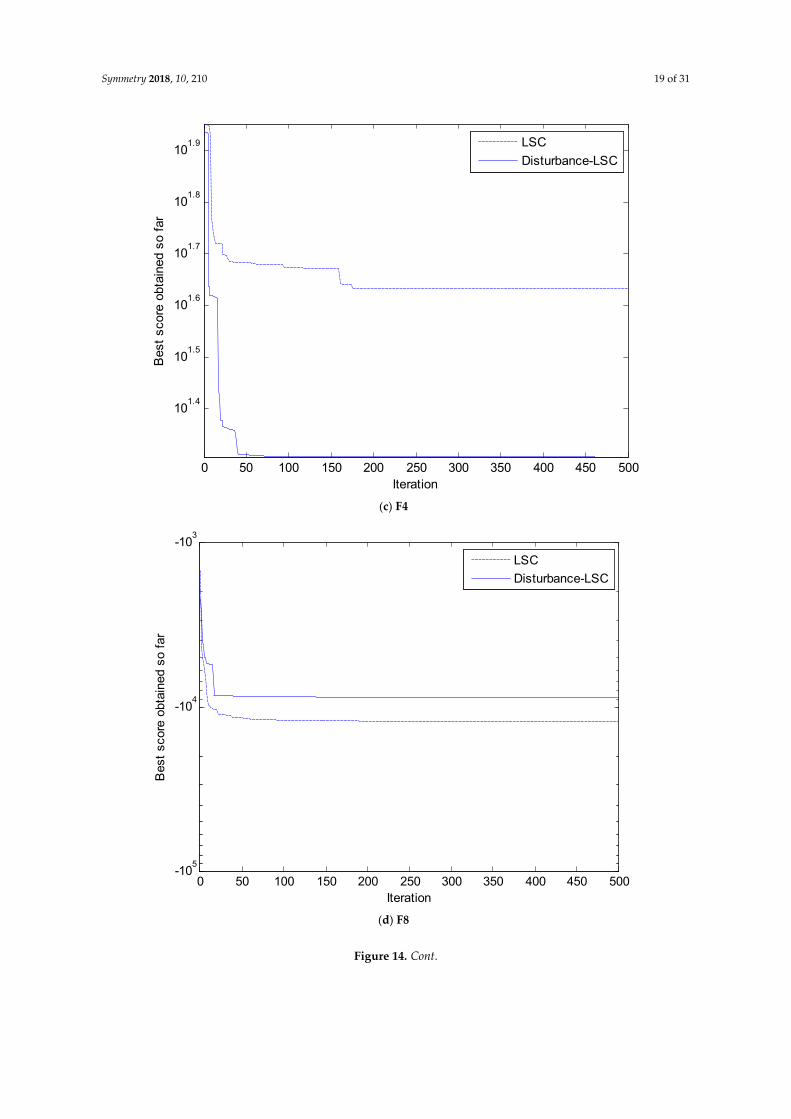
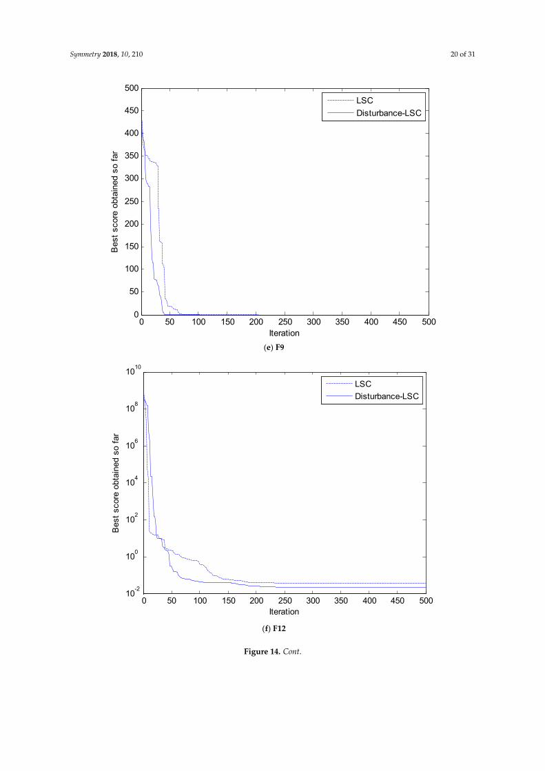
In this paper, we completed the simulation in matlab2010b environment, the computer configuration is Windows 7. The related MATLAB code of CP-PDWOA is available online at https://github.com/sunweizhen01/CP-PDWOA.git. Firstly, in order to verify the effectiveness of the perturbation mechanism, the convergence curves of the original WOA and the convergence curves after the introduction of the disturbance mechanism only with logarithmic spiral curve are compared. Then, the search path of the WOA with the disturbance mechanism is replaced by several spiral curves listed in Table 1 so as to find out the search path with the best optimization performance. The paper chooses several functions from above mentioned classes as a representative, and their convergence curves are shown in the following Figures 14 and 15. The convergence performances of all the different methods are shown in Table 2. The convergence curves of the representative functions are shown in Figure 14a–i to verify the validity of the disturbance.
It can be seen from the Figure 14 that the convergence effect of the improved WOA with the introduction of the perturbation is better than the standard WOA, which proves that the perturbation mechanism is effective and can make the algorithm have good convergence speed and optimization precision. Next, the simulation results are carried out to verify which search has best search performance. Therefore, the convergence curves generated by the improved WOA with these proposed paths are compared.
-5
0
5
-5
0
5-0.5
-0.4
-0.3
-0.2
-0.1
0
x1
x2
( x 1 ,
x2 )
Figure 13. Three-dimensional images of some optimization functions.
4.2. Simulation Results and Analysis
This paper tests the computational power of WOA by adopting 23 classical benchmark functions.Among them, the number of search agents is 30, the maximum number of iterations is 500. Each functionruns 30 times and then takes the average to plot the convergence curve. Benchmark functions can bedivided into four groups: unimodal, multimodal, fixed-dimension multimodal and composite functions.Functions F1–F7 are typical unimodal since they have only one global optimum. These functions allow toevaluate the exploitation capability of the investigated meta-heuristic algorithms. The functions F8–F23are multimodal functions. Unlike unimodal functions, multimodal functions include many local optimawhose number increases exponentially with the problem size (number of design variables). Therefore,this kind of test problems turns very useful if the purpose is to evaluate the exploration capability of anoptimization algorithm.
In this paper, we completed the simulation in matlab2010b environment, the computerconfiguration is Windows 7. The related MATLAB code of CP-PDWOA is available online athttps://github.com/sunweizhen01/CP-PDWOA.git. Firstly, in order to verify the effectiveness of theperturbation mechanism, the convergence curves of the original WOA and the convergence curvesafter the introduction of the disturbance mechanism only with logarithmic spiral curve are compared.Then, the search path of the WOA with the disturbance mechanism is replaced by several spiral curveslisted in Table 1 so as to find out the search path with the best optimization performance. The paperchooses several functions from above mentioned classes as a representative, and their convergencecurves are shown in the following Figures 14 and 15. The convergence performances of all the differentmethods are shown in Table 2. The convergence curves of the representative functions are shown inFigure 14a–i to verify the validity of the disturbance.
It can be seen from the Figure 14 that the convergence effect of the improved WOA with theintroduction of the perturbation is better than the standard WOA, which proves that the perturbationmechanism is effective and can make the algorithm have good convergence speed and optimizationprecision. Next, the simulation results are carried out to verify which search has best searchperformance. Therefore, the convergence curves generated by the improved WOA with these proposedpaths are compared.
Symmetry 2018, 10, 210 18 of 31
Symmetry 2018, 10, x FOR PEER REVIEW 18 of 31
(a) F1
(b) F2
0 50 100 150 200 250 300 350 400 450 50010
-2
10-1
100
101
102
103
104
105
Iteration
Bes
t sc
ore
obta
ined
so
far
LSC
Disturbance-LSC
0 50 100 150 200 250 300 350 400 450 50010
1
102
103
104
105
106
107
108
109
Iteration
Bes
t sc
ore
obta
ined
so
far
LSC
Disturbance-LSC
Figure 14. Cont.
Symmetry 2018, 10, 210 19 of 31
Symmetry 2018, 10, x FOR PEER REVIEW 19 of 31
(c) F4
(d) F8
0 50 100 150 200 250 300 350 400 450 500
101.4
101.5
101.6
101.7
101.8
101.9
Iteration
Bes
t sc
ore
obta
ined
so
far
LSC
Disturbance-LSC
0 50 100 150 200 250 300 350 400 450 500-10
5
-104
-103
Iteration
Bes
t sc
ore
obta
ined
so
far
LSC
Disturbance-LSC
Figure 14. Cont.
Symmetry 2018, 10, 210 20 of 31Symmetry 2018, 10, x FOR PEER REVIEW 20 of 31
(e) F9
(f) F12
0 50 100 150 200 250 300 350 400 450 5000
50
100
150
200
250
300
350
400
450
500
Iteration
Bes
t sc
ore
obta
ined
so
far
LSC
Disturbance-LSC
0 50 100 150 200 250 300 350 400 450 50010
-2
100
102
104
106
108
1010
Iteration
Bes
t sc
ore
obta
ined
so
far
LSC
Disturbance-LSC
Figure 14. Cont.
Symmetry 2018, 10, 210 21 of 31
Symmetry 2018, 10, x FOR PEER REVIEW 21 of 31
(g) F14
(h) F20
0 50 100 150 200 250 300 350 400 450 50010
0
101
102
103
Iteration
Bes
t sc
ore
obta
ined
so
far
LSC
Disturbance-LSC
0 50 100 150 200 250 300 350 400 450 500
-100.1
-100.2
-100.3
-100.4
-100.5
Iteration
Bes
t sc
ore
obta
ined
so
far
LSC
Disturbance-LSC
Figure 14. Cont.
Symmetry 2018, 10, 210 22 of 31
Symmetry 2018, 10, x FOR PEER REVIEW 22 of 31
(i) F21
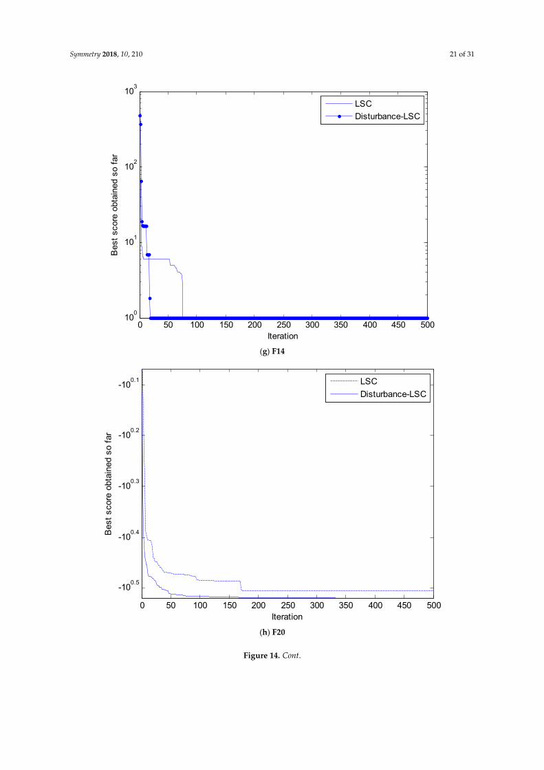
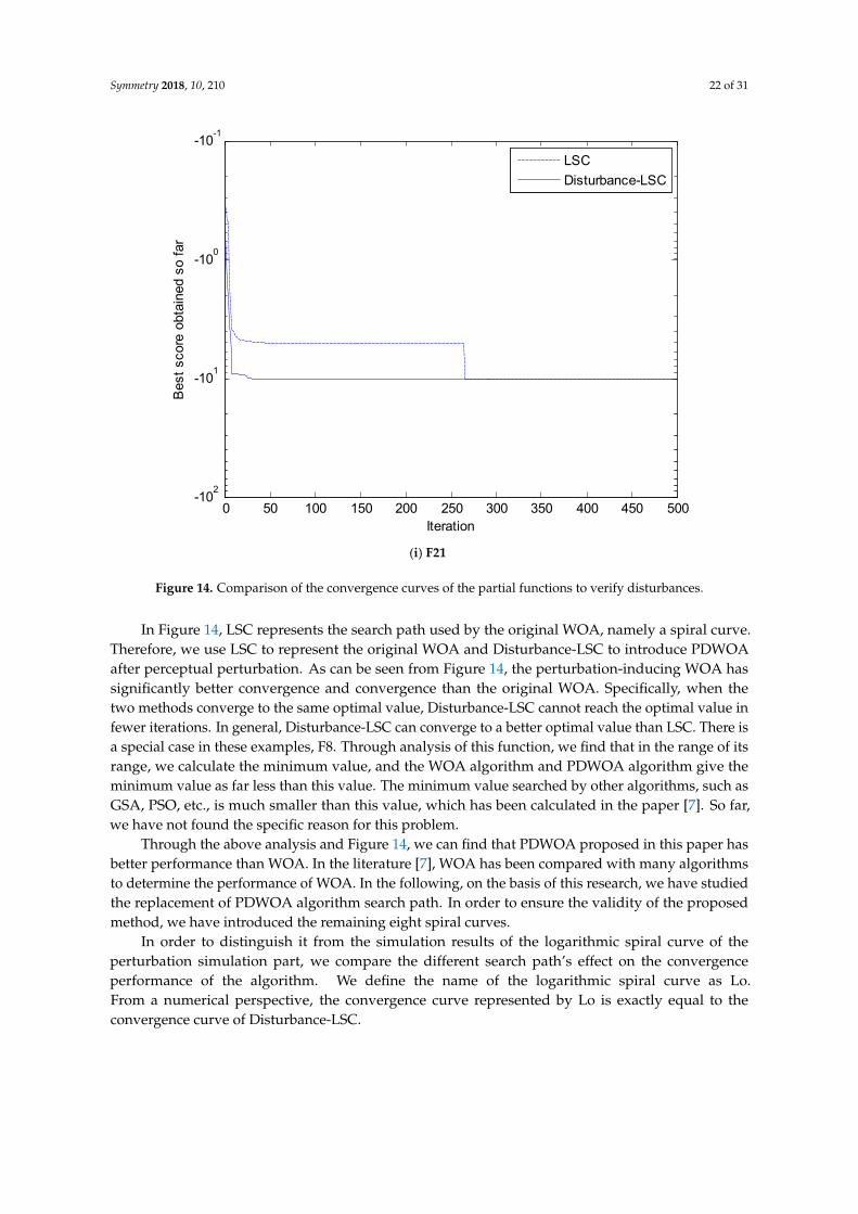
Figure 14. Comparison of the convergence curves of the partial functions to verify disturbances.
In Figure 14, LSC represents the search path used by the original WOA, namely a spiral curve. Therefore, we use LSC to represent the original WOA and Disturbance-LSC to introduce PDWOA after perceptual perturbation. As can be seen from Figure 14, the perturbation-inducing WOA has significantly better convergence and convergence than the original WOA. Specifically, when the two methods converge to the same optimal value, Disturbance-LSC cannot reach the optimal value in fewer iterations. In general, Disturbance-LSC can converge to a better optimal value than LSC. There is a special case in these examples, F8. Through analysis of this function, we find that in the range of its range, we calculate the minimum value, and the WOA algorithm and PDWOA algorithm give the minimum value as far less than this value. The minimum value searched by other algorithms, such as GSA, PSO, etc., is much smaller than this value, which has been calculated in the paper [7]. So far, we have not found the specific reason for this problem.
Through the above analysis and Figure 14, we can find that PDWOA proposed in this paper has better performance than WOA. In the literature [7], WOA has been compared with many algorithms to determine the performance of WOA. In the following, on the basis of this research, we have studied the replacement of PDWOA algorithm search path. In order to ensure the validity of the proposed method, we have introduced the remaining eight spiral curves.
In order to distinguish it from the simulation results of the logarithmic spiral curve of the perturbation simulation part, we compare the different search path’s effect on the convergence performance of the algorithm. We define the name of the logarithmic spiral curve as Lo. From a numerical perspective, the convergence curve represented by Lo is exactly equal to the convergence curve of Disturbance-LSC.
0 50 100 150 200 250 300 350 400 450 500-10
2
-101
-100
-10-1
Iteration
Bes
t sc
ore
obta
ined
so
far
LSC
Disturbance-LSC
Figure 14. Comparison of the convergence curves of the partial functions to verify disturbances.
In Figure 14, LSC represents the search path used by the original WOA, namely a spiral curve.Therefore, we use LSC to represent the original WOA and Disturbance-LSC to introduce PDWOAafter perceptual perturbation. As can be seen from Figure 14, the perturbation-inducing WOA hassignificantly better convergence and convergence than the original WOA. Specifically, when thetwo methods converge to the same optimal value, Disturbance-LSC cannot reach the optimal value infewer iterations. In general, Disturbance-LSC can converge to a better optimal value than LSC. There isa special case in these examples, F8. Through analysis of this function, we find that in the range of itsrange, we calculate the minimum value, and the WOA algorithm and PDWOA algorithm give theminimum value as far less than this value. The minimum value searched by other algorithms, such asGSA, PSO, etc., is much smaller than this value, which has been calculated in the paper [7]. So far,we have not found the specific reason for this problem.
Through the above analysis and Figure 14, we can find that PDWOA proposed in this paper hasbetter performance than WOA. In the literature [7], WOA has been compared with many algorithmsto determine the performance of WOA. In the following, on the basis of this research, we have studiedthe replacement of PDWOA algorithm search path. In order to ensure the validity of the proposedmethod, we have introduced the remaining eight spiral curves.
In order to distinguish it from the simulation results of the logarithmic spiral curve of theperturbation simulation part, we compare the different search path’s effect on the convergenceperformance of the algorithm. We define the name of the logarithmic spiral curve as Lo.From a numerical perspective, the convergence curve represented by Lo is exactly equal to theconvergence curve of Disturbance-LSC.
Symmetry 2018, 10, 210 23 of 31Symmetry 2018, 10, x FOR PEER REVIEW 23 of 31
(a) F1
(b) F2
0 100 200 300 400 50010
-120
10-100
10-80
10-60
10-40
10-20
100
1020
Iteration
Bes
t sc
ore
obta
ined
so
far
Ar
LoEp-II
Hy
Ep-I
R0Fe
Li
0 100 200 300 400 5000
0.5
1
1.5
2
2.5x 10
5
Iteration
Bes
t sc
ore
obta
ined
so
far
Ar
LoEp-II
Hy
Ep-I
R0Fe
Li
Figure 15. Cont.
Symmetry 2018, 10, 210 24 of 31
Symmetry 2018, 10, x FOR PEER REVIEW 24 of 31
(c) F4
(d) F8
0 100 200 300 400 5000
10
20
30
40
50
60
70
80
90
100
Iteration
Bes
t sc
ore
obta
ined
so
far
Ar
LoEp-II
Hy
Ep-I
R0Fe
Li
0 50 100 150 200 250 300 350 400 450 500Iteration
-104
-103
-102
-101
Bes
t sco
re o
btai
ned
so f
ar
ArLoEp-IIHyEp-IRoFeLi
Figure 15. Cont.
Symmetry 2018, 10, 210 25 of 31Symmetry 2018, 10, x FOR PEER REVIEW 25 of 31
(e) F9
(f) F12
0 100 200 300 400 50010
-5
100
105
1010
Iteration
Bes
t sc
ore
obta
ined
so
far
Ar
LoEp-II
Hy
Ep-I
R0Fe
Li
0 100 200 300 400 5000
50
100
150
200
250
300
350
400
450
Iteration
Bes
t sc
ore
obta
ined
so
far
Ar
LoEp-II
Hy
Ep-I
R0Fe
Li
Figure 15. Cont.
Symmetry 2018, 10, 210 26 of 31
Symmetry 2018, 10, x FOR PEER REVIEW 26 of 31
(g) F14
(h) F20
0 100 200 300 400 50010
-1
100
101
102
103
Iteration
Bes
t sc
ore
obta
ined
so
far
Ar
LoEp-II
Hy
Ep-I
R0Fe
Li
0 50 100 150 200-3.5
-3
-2.5
-2
-1.5
-1
Iteration
Bes
t sc
ore
obta
ined
so
far
Ar
LoEp-II
Hy
Ep-I
R0Fe
Li
Figure 15. Cont.
Symmetry 2018, 10, 210 27 of 31Symmetry 2018, 10, x FOR PEER REVIEW 27 of 31
(i) F21
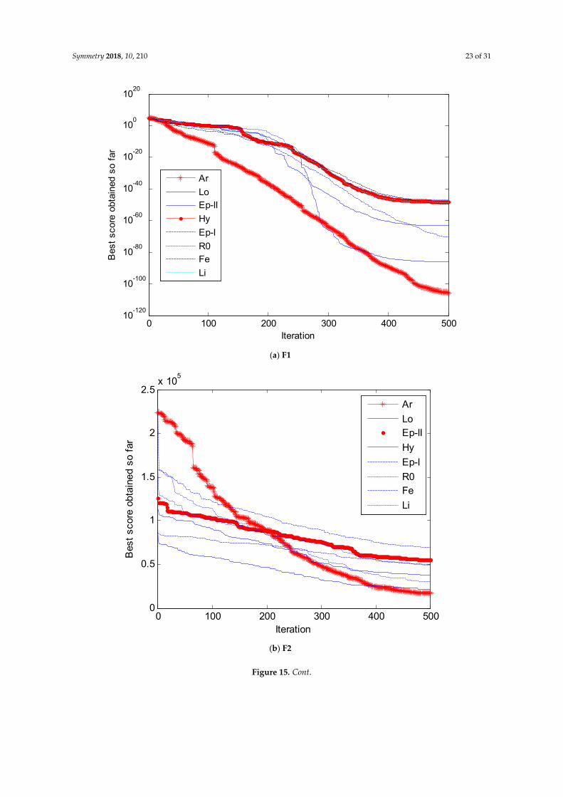
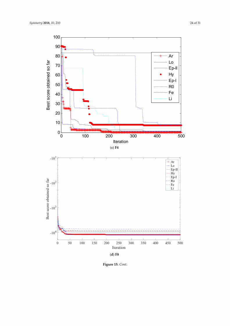
Figure 15. Comparison of the convergence curves of the partial functions.
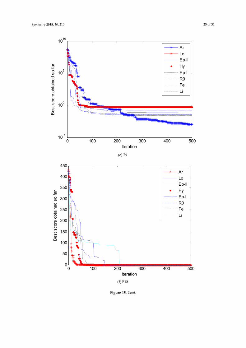
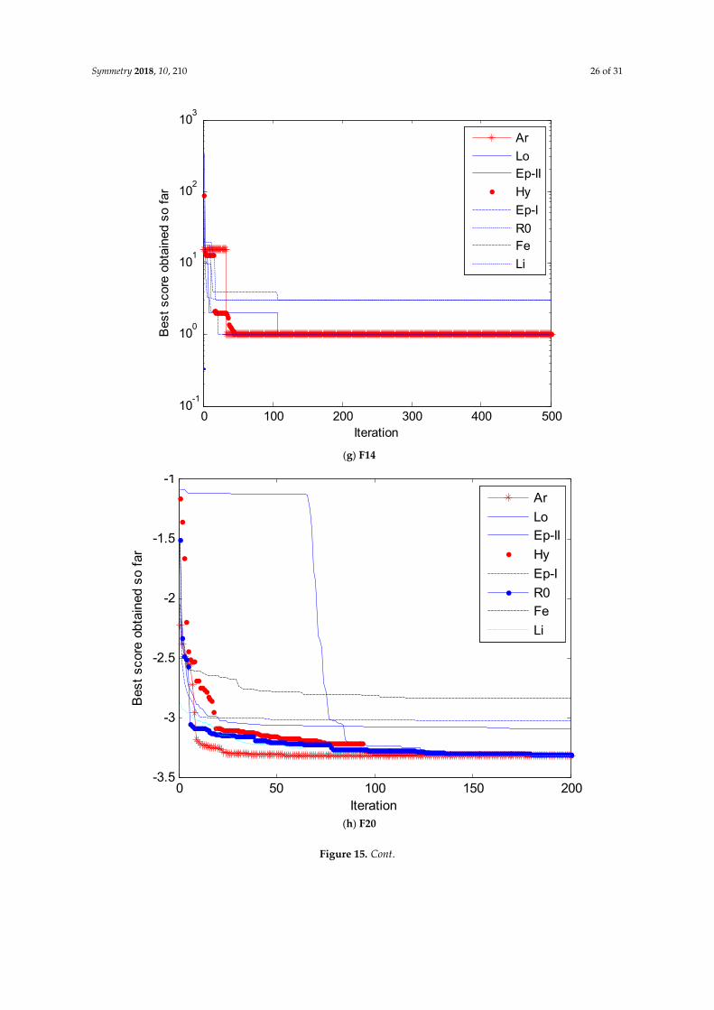
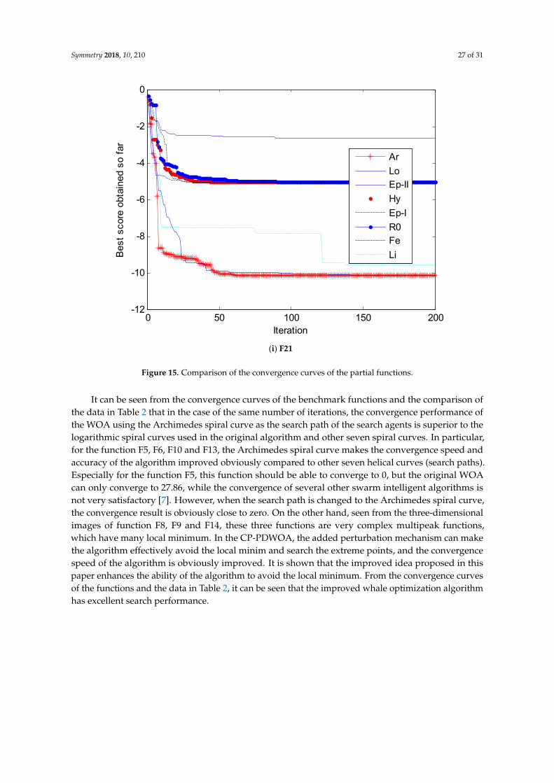
It can be seen from the convergence curves of the benchmark functions and the comparison of the data in Table 2 that in the case of the same number of iterations, the convergence performance of the WOA using the Archimedes spiral curve as the search path of the search agents is superior to the logarithmic spiral curves used in the original algorithm and other seven spiral curves. In particular, for the function F5, F6, F10 and F13, the Archimedes spiral curve makes the convergence speed and accuracy of the algorithm improved obviously compared to other seven helical curves (search paths). Especially for the function F5, this function should be able to converge to 0, but the original WOA can only converge to 27.86, while the convergence of several other swarm intelligent algorithms is not very satisfactory [7]. However, when the search path is changed to the Archimedes spiral curve, the convergence result is obviously close to zero. On the other hand, seen from the three-dimensional images of function F8, F9 and F14, these three functions are very complex multipeak functions, which have many local minimum. In the CP-PDWOA, the added perturbation mechanism can make the algorithm effectively avoid the local minim and search the extreme points, and the convergence speed of the algorithm is obviously improved. It is shown that the improved idea proposed in this paper enhances the ability of the algorithm to avoid the local minimum. From the convergence curves of the functions and the data in Table 2, it can be seen that the improved whale optimization algorithm has excellent search performance.
0 50 100 150 200-12
-10
-8
-6
-4
-2
0
Iteration
Bes
t sc
ore
obta
ined
so
far
Ar
LoEp-II
Hy
Ep-I
R0Fe
Li
Figure 15. Comparison of the convergence curves of the partial functions.
It can be seen from the convergence curves of the benchmark functions and the comparison ofthe data in Table 2 that in the case of the same number of iterations, the convergence performance ofthe WOA using the Archimedes spiral curve as the search path of the search agents is superior to thelogarithmic spiral curves used in the original algorithm and other seven spiral curves. In particular,for the function F5, F6, F10 and F13, the Archimedes spiral curve makes the convergence speed andaccuracy of the algorithm improved obviously compared to other seven helical curves (search paths).Especially for the function F5, this function should be able to converge to 0, but the original WOAcan only converge to 27.86, while the convergence of several other swarm intelligent algorithms isnot very satisfactory [7]. However, when the search path is changed to the Archimedes spiral curve,the convergence result is obviously close to zero. On the other hand, seen from the three-dimensionalimages of function F8, F9 and F14, these three functions are very complex multipeak functions,which have many local minimum. In the CP-PDWOA, the added perturbation mechanism can makethe algorithm effectively avoid the local minim and search the extreme points, and the convergencespeed of the algorithm is obviously improved. It is shown that the improved idea proposed in thispaper enhances the ability of the algorithm to avoid the local minimum. From the convergence curvesof the functions and the data in Table 2, it can be seen that the improved whale optimization algorithmhas excellent search performance.
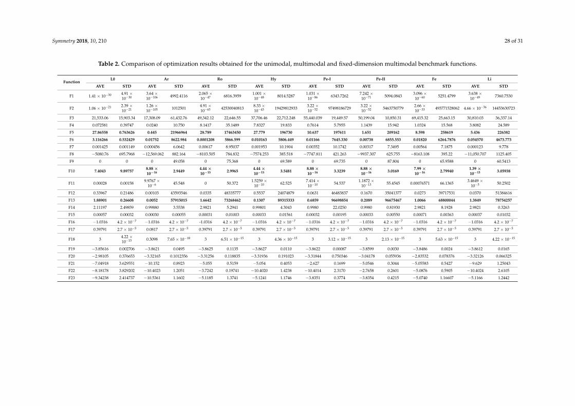
Symmetry 2018, 10, 210 28 of 31
Table 2. Comparison of optimization results obtained for the unimodal, multimodal and fixed-dimension multimodal benchmark functions.
FunctionL0 Ar Ro Hy Pe-I Pe-II Fe Li
AVE STD AVE STD AVE STD AVE STD AVE STD AVE STD AVE STD AVE STD
F1 1.41 × 10⁻³⁰ 4.91 ×10⁻³⁰
3.64 ×10−106 4992.4116 2.065 ×
10−47 6816.3959 1.001 ×10−48 8014.5287 1.031 ×
10−86 6343.7262 7.242 ×10−71 5094.0843 3.096 ×
10−60 5251.4799 3.638 ×10−49 7360.7530
F2 1.06 × 10⁻²¹ 2.39 ×10⁻²¹
1.26 ×10−105 1012501 4.91 ×
10−65 42530040813 8.33 ×10−43 19429812933 3.22 ×
10−52 97498186729 3.22 ×10−52 5463750779 2.66 ×
10−33 493771528062 4.66 × 10−36 14453630723
F3 21,533.06 15,903.34 17,308.09 61,432.76 49,342.12 22,646.55 37,706.46 22,712.248 55,440.039 19,449.57 50,199.04 10,850.31 69,415.32 25,663.15 30,810.03 36,337.14
F4 0.072581 0.39747 0.0240 10.750 8.1417 35.1489 7.8327 19.833 0.7614 5.7955 1.1439 15.942 1.0324 15.568 3.8082 24.589
F5 27.86558 0.763626 0.445 21966964 28.789 17463450 27.779 196730 10.637 197611 1.651 209162 8.598 258619 5.436 226382
F6 3.116266 0.532429 0.01752 8622.984 0.0001208 5866.599 0.010163 5806.449 0.01166 7645.330 0.00738 6855.553 0.01820 6264.7876 0.054570 4673.773
F7 0.001425 0.001149 0.000456 6.0642 0.00617 8.95037 0.001953 10.1904 0.00352 10.1742 0.00317 7.3495 0.00564 7.1875 0.000123 9.778
F8 −5080.76 695.7968 −12,569.062 882.164 −8103.505 784.832 −7574.253 385.518 −7747.811 421.263 −9937.307 625.755 −8163.108 395.22 −11,050.707 1125.405
F9 0 0 0 49.058 0 75.368 0 69.589 0 69.735 0 87.804 0 65.9588 0 60.5413
F10 7.4043 9.89757 8.88 ×10⁻¹⁶ 2.9449 4.44 ×
10−15 2.9965 4.44 ×10⁻¹⁵ 3.5481 8.88 ×
10−16 3.3239 8.88 ×10⁻¹⁶ 3.0169 7.99 ×
10−16 2.79940 1.39 ×10⁻¹³ 3.05938
F11 0.00028 0.00158 9.9767 ×10⁻⁶ 45.548 0 50.372 1.5259 ×
10−10 62.525 7.414 ×10⁻¹⁰ 54.537 1.1872 ×
10−13 55.4545 0.00076571 66.1365 3.4649 ×10⁻⁵ 50.2502
F12 0.33967 0.21486 0.00103 43593546 0.0335 48335777 0.5537 24074879 0.0631 46483837 0.1670 35041377 0.0273 39717531 0.0370 51384616
F13 1.88901 0.26608 0.0052 57915015 1.6642 73268462 0.1307 89315333 0.6859 96698854 0.2089 96675467 1.0066 68800044 1.3849 78754257
F14 2.11197 2.49859 0.99880 3.5538 2.9821 5.2941 0.99801 4.3043 0.9980 22.0250 0.9980 0.81930 2.9821 8.1928 2.9821 0.3263
F15 0.00057 0.00032 0.00030 0.00055 0.00031 0.01003 0.00033 0.01561 0.00032 0.00195 0.00033 0.00550 0.00071 0.00363 0.00037 0.01032
F16 −1.0316 4.2 × 10⁻⁷ −1.0316 4.2 × 10⁻⁷ -1.0316 4.2 × 10⁻⁷ −1.0316 4.2 × 10⁻⁷ −1.0316 4.2 × 10⁻⁷ −1.0316 4.2 × 10⁻⁷ −1.0316 4.2 × 10⁻⁷ −1.0316 4.2 × 10⁻⁷
F17 0.39791 2.7 × 10⁻⁵ 0.0817 2.7 × 10⁻⁵ 0.39791 2.7 × 10⁻⁵ 0.39791 2.7 × 10⁻⁵ 0.39791 2.7 × 10⁻⁵ 0.39791 2.7 × 10⁻⁵ 0.39791 2.7 × 10⁻⁵ 0.39791 2.7 × 10⁻⁵
F18 3 4.22 ×10⁻¹⁵ 0.3098 7.65 × 10⁻¹⁸ 3 6.51 × 10⁻¹⁵ 3 4.36 × 10⁻¹⁵ 3 3.12 × 10⁻¹⁵ 3 2.13 × 10⁻¹⁵ 3 5.63 × 10⁻¹⁵ 3 4.22 × 10⁻¹⁵
F19 −3.85616 0.002706 −3.8621 0.0495 −3.8625 0.1135 −3.8627 0.0110 −3.8622 0.00087 −3.8599 0.0030 −3.8486 0.0024 −3.8612 0.0165
F20 −2.98105 0.376653 −3.32165 0.1012356 −3.31256 0.118835 −3.31936 0.191023 −3.31844 0.750346 −3.04178 0.055936 −2.83532 0.078376 −3.32126 0.066325
F21 −7.04918 3.629551 −10.152 0.8923 −5.055 0.5159 −5.054 0.4053 −2.627 0.1699 −5.0546 0.3044 −5.05583 0.5427 −9.629 1.25043
F22 −8.18178 3.829202 −10.4023 1.2051 −3.7242 0.19741 −10.4020 1.4238 −10.4014 2.3170 −2.7658 0.2601 −5.0876 0.5905 −10.4024 2.6105
F23 −9.34238 2.414737 −10.5361 1.1602 −5.1185 1.3741 −5.1241 1.1746 −3.8351 0.3774 −3.8354 0.4215 −5.0740 1.16607 −5.1166 1.2442
Symmetry 2018, 10, 210 29 of 31
As can be seen from Figure 15f, when the average value of the function F12 is searched, the areasof the convergence curves corresponding to Lo and Hy are equal, and there is only a slight differencein the early stage. This is not surprising, because from the convergence results of all the models, theirconvergence results do not think that there are huge differences in other functions; From the paths ofthe two models, it can be seen that the approximate convergence curve is obtained by adjusting theparameters of the function. The main reason is that these two models fall into the same local extremepoint, so we get the same convergence curve, which is also related to the initialization of the agent.Because in order to ensure the feasibility of the simulation, we chose the pseudo-random number asthe initial position of the agent.
It is concluded that the introduction of perceptual perturbation not only makes the searchingof agents more purposeful, but also makes the location of search agents more diversified andprevents the algorithm from falling into local minim. At the same time, the moving step size ofthe search agent can be adjusted at different simulation phase so as to ensure that the algorithm inthe early search has a strong ability to exploit and in the late search has a stronger explore capability.This ensures the accuracy of the algorithm searching process, but also makes the algorithm havea faster convergence rate.
5. Conclusions
In this paper, we have learned from other scholars’ experience in the improvement of swarmintelligence algorithms, and improved the performance of WOA by introducing disturbance factors.Then the WOA search mechanism is analyzed and the logarithmic spiral curve of equal pitch is used asthe search path of the agent. The simulation results also prove that the performance of the equal-pitchArchimedean spiral curve is superior to other types of spiral curve. When collating simulation andalgorithm, we found that if we randomly define different search paths for different agents in the sameiteration, the resulting convergence performance will be better, but correspondingly, this will alsogive the algorithm parameters. The adjustment brings a certain degree of difficulty. In summary,the proposed complex path-perceptual disturbance WOA (CP-PDWOA) algorithm has a strongersearch performance.
Supplementary Materials: The related MATLAB code of CP-PDWOA is available online at https://github.com/sunweizhen01/CP-PDWOA.git.
Author Contributions: Conceptualization, W.-z.S. and J.-s.W.; Methodology, W.-z.S.; Software, W.-z.S.; Validation,W.-z.S. and J.-s.W.; Formal Analysis, X.W.; Investigation, W.-z.S.; Resources, W.-z.S.; Data Curation, W.-z.S.;Writing-Original Draft Preparation, W.-z.S.; Writing-Review & Editing, X.W.; Visualization, W.-z.S.; Supervision,J.-s.W.; Project Administration, J.-s.W.; Funding Acquisition, J.-s.W.
Funding: This research was funded by the Project by National Natural Science Foundation of China grant number[21576127], the Basic Scientific Research Project of Institution of Higher Learning of Liaoning Province grantnumber [2017FWDF10], and the CAS Pioneer Hundred Talents Program (Type C) grant number [2017-122].
Conflicts of Interest: The authors declare no conflicts of interest.
References
1. Chandra Mohan, B.; Baskaran, R. A survey: Ant Colony Optimization based recent research andimplementation on several engineering domain. Expert Syst. Appl. 2012, 39, 4618–4627. [CrossRef]
2. Yu, Y.; Li, Y.; Li, J. Nonparametric modeling of magnetorheological elastomer base isolator based on artificialneural network optimized by ant colony algorithm. J. Intell. Mater. Syst. Struct. 2015, 26, 1789–1798.[CrossRef]
3. Precup, R.E.; Sabau, M.C.; Petriu, E.M. Nature-inspired optimal tuning of input membership functions ofTakagi-Sugeno-Kang fuzzy models for anti-lock braking systems. Appl. Soft Comput. 2015, 27, 575–589.[CrossRef]
4. Vallada, E.; Ruiz, R. A genetic algorithm for the unrelated parallel machine scheduling problem withsequence dependent setup times. Eur. J. Oper. Res. 2011, 211, 612–622. [CrossRef]
Symmetry 2018, 10, 210 30 of 31
5. Zăvoianu, A.-C.; Bramerdorfer, G.; Lughofer, E.; Silber, S.; Amrhein, W.; Klement, E.P. Hybridization ofmulti-objective evolutionary algorithms and artificial neural networks for optimizing the performance ofelectrical drives. Eng. Appl. Artif. Intell. 2013, 26, 1781–1794. [CrossRef]
6. Kennedy, J. Particle swarm optimization. In Encyclopedia of Machine Learning; Springer: New York, NY, USA,2010; pp. 760–766.
7. Yu, Y.; Li, Y.; Li, J. Parameter identification of a novel strain stiffening model for magnetorheological elastomerbase isolator utilizing enhanced particle swarm optimization. J. Intell. Mater. Syst. Struct. 2015, 26, 2446–2462.[CrossRef]
8. Yu, Y.; Li, Y.; Li, J. Forecasting hysteresis behaviours of magnetorheological elastomer base isolatorutilizing a hybrid model based on support vector regression and improved particle swarm optimization.Smart Mater. Struct. 2015, 24, 035025. [CrossRef]
9. Karaboga, D.; Basturk, B. A powerful and efficient algorithm for numerical function optimization:Artificial bee colony (ABC) algorithm. J. Glob. Optim. 2007, 39, 459–471. [CrossRef]
10. Precup, R.E.; David, R.C.; Petriu, E.M. Grey Wolf Optimizer Algorithm-Based Tuning of Fuzzy ControlSystems with Reduced Parametric Sensitivity. IEEE Trans. Ind. Electron. 2016, 64, 527–534. [CrossRef]
11. Saadat, J.; Moallem, P.; Koofigar, H. Training echo state neural network using harmony search algorithm.Int. J. Artif. Intell. 2017, 15, 163–179.
12. Vrkalovic, S.; Teban, T.A.; Borlea, L.D. Stable Takagi-Sugeno fuzzy control designed by optimization.Int. J. Artif. Intell. 2017, 15, 17–29.
13. Reddy, P.D.P.; Reddy, V.C.V.; Manohar, T.G. Whale optimization algorithm for optimal sizing of renewableresources for loss reduction in distribution systems. Renew. Wind Water Solar 2017, 4, 3. [CrossRef]
14. Trivedi, I.N.; Bhoye, M.; Bhesdadiya, R.H.; Jangir, P.; Jangir, N.; Kumar, A. An emissionconstraint environment dispatch problem solution with microgrid using Whale Optimization Algorithm.In Proceedings of the Power Systems Conference, Bhubaneswar, India, 19–21 December 2016.
15. Rosyadi, A.; Penangsang, O.; Soeprijanto, A. Optimal filter placement and sizing in radial distributionsystem using whale optimization algorithm. In Proceedings of the International Seminar on IntelligentTechnology and ITS Applications, Surabaya, Indonesia, 28–29 August 2017; pp. 87–92.
16. Buch, H.; Jangir, P.; Jangir, N.; Ladumor, D.; Bhesdadiya, R.H. Optimal Placement and Coordination of StaticVAR Compensator with Distributed Generation using Whale Optimization Algorithm. In Proceedings of theIEEE 1st International Conference on Power Electronics, Intelligent Control and Energy Systems (ICPEICES),Delhi, India, 4–6 July 2016.
17. Ladumor, D.P.; Trivedi, I.N.; Jangir, P.; Kumar, A. A Whale Optimization Algorithm approach for UnitCommitment Problem Solution. In Proceedings of the Conference Advancement in Electrical & PowerElectronics Engineering (AEPEE 2016), Morbi, India, 14–17 December 2016.
18. Prakash, D.B.; Lakshminarayana, C. Optimal siting of capacitors in radial distribution network using WhaleOptimization Algorithm. Alex. Eng. J. 2016, 56, 499–509. [CrossRef]
19. Yan, Z.; Sha, J.; Liu, B.; Tian, W.; Lu, J. An Ameliorative Whale Optimization Algorithm for Multi-ObjectiveOptimal Allocation of Water Resources in Handan, China. Water 2018, 10, 87. [CrossRef]
20. Medani, K.B.O.; Sayah, S.; Bekrar, A. Whale optimization algorithm based optimal reactive power dispatch:A case study of the Algerian power system. Electr. Power Syst. Res. 2017. [CrossRef]
21. Sun, W.Z.; Wang, J.S. Elman Neural network Soft-sensor Model of Conversion Velocity in PolymerizationProcess Optimized by Chaos Whale Optimization Algorithm. IEEE Access 2017, 5, 13062–13076. [CrossRef]
22. Aljarah, I.; Faris, H.; Mirjalili, S. Optimizing connection weights in neural networks using the whaleoptimization algorithm. Soft Comput. 2016, 22, 1–15. [CrossRef]
23. Bhesdadiya, R.; Jangir, P.; Jangir, N.; Trivedi, I.N.; Ladumor, D. Training Multi-Layer Perceptron in NeuralNetwork using Whale Optimization Algorithm. Indian J. Sci. Technol. 2016, 9, 28–36.
24. Wang, J.; Du, P.; Niu, T.; Yang, W. A novel hybrid system based on a new proposedalgorithm—Multi-Objective Whale Optimization Algorithm for wind speed forecasting. Appl. Energy2017, 208, 344–360. [CrossRef]
25. Niu, P.F.; Wu, Z.L.; Ma, Y.P.; Shi, C.J.; Li, J.B. Prediction of steam turbine heat consumption rate based onwhale optimization algorithm. CIESC J. 2017, 68, 1049–1057.
26. Aziz, M.A.E.; Ewees, A.A.; Hassanien, A.E. Whale Optimization Algorithm and Moth-Flame Optimizationfor multilevel thresholding image segmentation. Expert Syst. Appl. 2017, 83, 242–256. [CrossRef]
Symmetry 2018, 10, 210 31 of 31
27. Mostafa, A.; Hassanien, A.E.; Houseni, M.; Hefny, H. Liver segmentation in MRI images based on whaleoptimization algorithm. Multimed. Tools Appl. 2017, 76, 24931–24954. [CrossRef]
28. Jangir, P.; Jangir, N. Non-Dominated Sorting Whale Optimization Algorithm (NSWOA): A Multi-ObjectiveOptimization Algorithm for Solving Engineering Design Problems. Glob. J. Res. Eng. 2017, 17, 15–42.
29. Oliva, D.; Aziz, M.A.E.; Hassanien, A.E. Parameter estimation of photovoltaic cells using an improvedchaotic whale optimization algorithm. Appl. Energy 2017, 200, 141–154.
30. Sharawi, M.; Zawbaa, H.M.; Emary, E. Feature selection approach based on whale optimization algorithm.In Proceedings of the Ninth International Conference on Advanced Computational Intelligence, Doha, Qatar,4–6 February 2017; pp. 163–168.
31. Zhao, G.; Zhou, Y.; Ouyang, Z.; Wang, Y. A Novel Disturbance Parameters PSO Algorithm for FunctionsOptimization. Adv. Inf. Sci. Serv. Sci. 2012, 4, 51–57.
32. Jing, Y.E. The Diversity Disturbance PSO Algorithm to Solve TSP Problem. J. Langfang Teach. Coll. 2010, 5, 2.33. Li, D.; Deng, N. An electoral quantum-behaved PSO with simulated annealing and gaussian disturbance for
permutation flow shop scheduling. J. Inf. Comput. Sci. 2012, 9, 2941–2949.34. Gao, H.; Kwong, S.; Yang, J.; Cao, J. Particle swarm optimization based on intermediate disturbance strategy
algorithm and its application in multi-threshold image segmentation. Inf. Sci. 2013, 250, 82–112. [CrossRef]35. Mirjalili, S.; Lewis, A. The Whale Optimization Algorithm. Adv. Eng. Softw. 2016, 95, 51–67. [CrossRef]36. Mafarja, M.M.; Mirjalili, S. Hybrid Whale Optimization Algorithm with simulated annealing for feature
selection. Neurocomputing 2017, 260, 302–312. [CrossRef]37. Ling, Y.; Zhou, Y.; Luo, Q. Lévy Flight Trajectory-Based Whale Optimization Algorithm for Global
Optimization. IEEE Access 2017, 5, 6168–6186. [CrossRef]38. Abdel-Basset, M.; El-Shahat, D.; El-Henawy, I.; Sangaiah, A.K.; Ahmed, S.H. A Novel Whale Optimization
Algorithm for Cryptanalysis in Merkle-Hellman Cryptosystem. Mob. Netw. Appl. 2018, 5, 1–11. [CrossRef]39. Kaveh, A.; Ghazaan, M.I. Enhanced Whale Optimization Algorithm for Sizing Optimization of Skeletal
Structures. Mech. Based Des. Struct. Mach. 2017, 45, 345–362. [CrossRef]40. Spiral Curve. Van Nostrand’s Scientific Encyclopedia; John Wiley & Sons, Inc.: Hoboken, NJ, USA, 2005.41. Ren, Y.; Wu, Y. An efficient algorithm for high-dimensional function optimization. Soft Comput. 2013, 17,
995–1004. [CrossRef]42. Yuan, Z.; de Oca, M.A.M.; Birattari, M.; Stützle, T. Continuous optimization algorithms for tuning real and
integer parameters of swarm intelligence algorithms. Swarm Intell. 2012, 6, 49–75. [CrossRef]
© 2018 by the authors. Licensee MDPI, Basel, Switzerland. This article is an open accessarticle distributed under the terms and conditions of the Creative Commons Attribution(CC BY) license (http://creativecommons.org/licenses/by/4.0/).