fresco+: an improved o2 a-band cloud retrieval algorithm for tropospheric trace gas retrievals

ACPD8, 9697–9729, 2008

FRESCO+ cloudretrieval algorithm

P. Wang et al.

Title Page

Abstract Introduction

Conclusions References

Tables Figures

J I

J I

Back Close

Full Screen / Esc

Printer-friendly Version

Interactive Discussion

Atmos. Chem. Phys. Discuss., 8, 9697–9729, 2008www.atmos-chem-phys-discuss.net/8/9697/2008/© Author(s) 2008. This work is distributed underthe Creative Commons Attribution 3.0 License.

AtmosphericChemistry

and PhysicsDiscussions

FRESCO+: an improved O2 A-band cloudretrieval algorithm for tropospheric tracegas retrievals

P. Wang1, P. Stammes1, R. van der A1, G. Pinardi2, and M. van Roozendael2

1Royal Netherlands Meteorological Institute (KNMI), De Bilt, The Netherlands2BIRA-IASB, Belgian Institute for Space Aeronomy, Brussels, Belgium

Received: 21 February 2008 – Accepted: 21 April 2008 – Published: 27 May 2008

Correspondence to: P. Wang ([email protected])

Published by Copernicus Publications on behalf of the European Geosciences Union.

9697

http://www.atmos-chem-phys-discuss.net

http://www.atmos-chem-phys-discuss.net/8/9697/2008/acpd-8-9697-2008-print.pdf

http://www.atmos-chem-phys-discuss.net/8/9697/2008/acpd-8-9697-2008-discussion.html

http://creativecommons.org/licenses/by/3.0/

ACPD8, 9697–9729, 2008


P. Wang et al.

Title Page



Tables Figures

J I

J I

Back Close

Full Screen / Esc



Abstract

The FRESCO (Fast Retrieval Scheme for Clouds from the Oxygen A-band) algorithmhas been used to retrieve cloud information from measurements of the O2 A-bandaround 760 nm by GOME, SCIAMACHY and GOME-2. The cloud parameters re-trieved by FRESCO are the effective cloud fraction and cloud pressure, which are5

used for cloud correction in the retrieval of trace gases like O3 and NO2. To im-prove the cloud pressure retrieval for partly cloudy scenes, single Rayleigh scatter-ing has been included in an improved version of the algorithm, called FRESCO+.We compared FRESCO+ and FRESCO effective cloud fractions and cloud pressuresusing simulated spectra and one month of GOME measured spectra. As expected,10

FRESCO+ gives more reliable cloud pressures over partly cloudy pixels. Simulationsand comparisons with ground-based radar/lidar measurements of clouds shows thatthe FRESCO+ cloud pressure is about the optical midlevel of the cloud. Globally aver-aged, the FRESCO+ cloud pressure is about 50 hPa higher than the FRESCO cloudpressure, while the FRESCO+ effective cloud fraction is about 0.01 larger.15

The effect of FRESCO+ cloud parameters on O3 and NO2 vertical column den-sities (VCD) is studied using SCIAMACHY data and ground-based DOAS measure-ments. We find that the FRESCO+ algorithm has a significant effect on troposphericNO2 retrievals but a minor effect on total O3 retrievals. The retrieved SCIAMACHYtropospheric NO2 VCDs using FRESCO+ cloud parameters (v1.1) are lower than20

the tropospheric NO2 VCDs which used FRESCO cloud parameters (v1.04), in par-ticular over heavily polluted areas with low clouds. The difference between SCIA-MACHY tropospheric NO2 VCDs v1.1 and ground-based MAXDOAS measurementsperformed in Cabauw, The Netherlands, during the DANDELIONS campaign is about−2.12×1014 molec cm−2.25

9698





ACPD8, 9697–9729, 2008


P. Wang et al.

Title Page



Tables Figures

J I

J I

Back Close

Full Screen / Esc



1 Introduction

Clouds have significant effects on trace gas retrievals from satellite spectrometers op-erating in the UV/visible, such as GOME, SCIAMACHY, OMI and GOME-2. Cloudscan shield trace gases from observation, but they can also enhance the sensitivity totrace gases above the clouds. Because of the relatively coarse spatial resolution of5

the above satellite instruments, only 5–15% of the pixels are cloud-free (Krijger et al.,2007). To correct for cloud effects on trace gas retrievals, the most relevant cloudparameters are the cloud fraction and height (Stammes et al., 2008). There are sev-eral cloud retrieval algorithms that have been developed for GOME and SCIAMACHYusing the O2 A-band (Koelemeijer et al., 2001; Kokhanovsky et al., 2006; van Dieden-10

hoven et al., 2007) or using Polarisation Monitoring Devices (PMDs) (Grzegorski et al.,2006; Loyola, 2004). FRESCO (Koelemeijer et al., 2001) is a simple, fast and robustalgorithm, which is also implemented in GOME-2 level 1 data processor (Munro andEisinger, 2004).

In the FRESCO algorithm, the cloud pressure and the effective cloud fraction are15

retrieved from top-of-atmosphere (TOA) reflectances in three 1-nm wide wavelengthwindows at 758–759, 760–761, and 765–766 nm. The cloud is assumed to be a Lam-bertian surface with albedo 0.8, and only absorption due to O2 above the cloud and theground surface and reflections from the surface and cloud are taken into account. TheFRESCO effective cloud fractions and cloud pressures have been validated globally20

and regionally, and the products have been used in trace gas retrievals (Koelemeijer etal., 2003; Tuinder et al., 2004; Grzegorski et al., 2006; Fournier et al., 2006).

The effective cloud fraction retrieved by FRESCO is the cloud fraction of a Lamber-tian cloud with albedo 0.8 yielding the same TOA radiance as the real cloud in thescene. Generally the effective cloud fraction is smaller than the geometric cloud frac-25

tion. The choice of Lambertian cloud albedo 0.8 and effective cloud fraction concepthave recently been discussed by Stammes et al. (2008). The use of effective cloudfractions for the cloud correction in the O3 and NO2 retrievals has been investigated

9699





ACPD8, 9697–9729, 2008


P. Wang et al.

Title Page



Tables Figures

J I

J I

Back Close

Full Screen / Esc



in several papers (Koelemeijer and Stammes, 1999; Wang et al., 2006; Stammes etal., 2008). The Lambertian cloud is a good approximation for cloud correction of totalO3 column retrievals. For scenes with 50% cloud coverage the error in the total O3column due to the Lambertian cloud assumption instead of a scattering cloud modelis about 0.5% (Stammes et al., 2008). For tropospheric NO2 retrievals, the effective5

cloud fraction assumption leads to errors of about 10% (Wang et al., 2006). Here thecloud height is also important, because the large amount of tropospheric NO2 can beinside the clouds or below the clouds.

Recently, we have found that the FRESCO cloud pressures are often too low (cloudheights are too high) when the effective cloud fractions are less than 0.1. These are10

cases with a relatively large contribution from Rayleigh scattering, which is missing inthe FRESCO algorithm. Apparently, the missing Rayleigh scattering is compensatedby fitting a high cloud. Pixels with small cloud fractions are important for tropospherictrace gas retrievals. For example, in the operational tropospheric NO2 retrievals fromthe TEMIS project the effective cloud fractions are allowed to be less than 0.3 (Eskes15

and Boersma, 2003). Therefore, we improved the FRESCO algorithm by the additionof single Rayleigh scattering in the transmission and reflectance databases (forwardcalculations) and in the retrieval. This improved version is called FRESCO+.

The structure of the paper is as follows. In Sect. 2 we explain the principle ofFRESCO+. The formulas of FRESCO+ are given in the Appendix. The FRESCO+20

results and the comparisons with FRESCO are shown in Sect. 3 for simulations andreal data. In Sect. 4 the effects of FRESCO+ cloud parameters on O3 and NO2 verticalcolumn density (VCD) retrievals are discussed. The SCIAMACHY NO2 VCDs usingFRESCO+ and FRESCO cloud corrections are compared with NO2 VCD from ground-based MAXDOAS measurements. Section 5 contains the conclusions.25

9700





ACPD8, 9697–9729, 2008


P. Wang et al.

Title Page



Tables Figures

J I

J I

Back Close

Full Screen / Esc



2 Principle of FRESCO+

The FRESCO+ algorithm retrieves the effective cloud fraction ceff and cloud pressurePc from the TOA reflectance at three 1-nm wide windows, namely 758–759, 760–761and 765–766 nm. Each of the three windows contains 5 reflectance measurements(spectral data points). Due to the presence of clouds, the reflectance in the continuum5

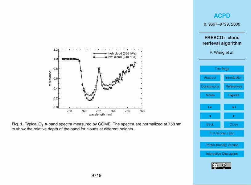
window (758 nm) is larger than for a clear sky scene, whereas the depth of the strongestO2 absorption band at 760 nm and of the weaker O2 absorption band at 765 nm variesaccording to the height and the optical thickness of the cloud. Typical O2 A-bandspectra of scenes with high and low clouds measured by GOME are shown in Fig. 1.

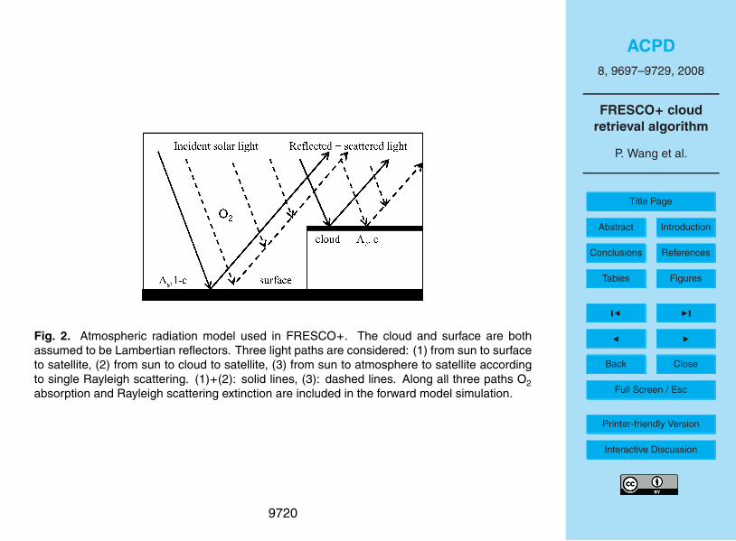
The atmospheric radiation model assumed in the FRESCO+ algorithm is shown in10

Fig. 2. The FRESCO+ algorithm fits a simulated reflectance spectrum to the measuredreflectance spectrum in the three windows, to retrieve the effective cloud fraction andcloud pressure. The simulated reflectance (Rsim) at TOA is written as the sum of thereflectances of the cloud-free and cloudy parts of the pixel:

Rsim = (1 − c)TsAs + (1 − c)Rs + cTcAc + cRc. (1)15

Here Rc, Tc and Rs, Ts are the single Rayleigh scattering reflectance and transmittanceof the cloudy and cloud-free part of the pixel, respectively. Tc and Ts contain O2 ab-sorption and Rayleigh scattering extinction, and are pre-calculated as a function of thesolar zenith angle (SZA), viewing zenith angle (VZA), wavelength, and altitude. Ac isthe cloud albedo, which is assumed to be 0.8, and As is the surface albedo taken from20

a climatology (Koelemeijer et al., 2003; Fournier et al., 2006). The surface pressure iscalculated from surface elevation. The O2 transmission is calculated using a line-by-line method for a 1-pm wavelength grid using the line parameters from HITRAN 2004(Rothman et al., 2005) and then convolved using the instrument response function atthe measurement wavelength grid. Rayleigh scattering is a small but significant contri-25

bution to Rsim in the case of an almost cloud-free pixel. Due to single Rayleigh scat-tering the reflectance at 760 nm is larger than if only surface or cloud reflection wouldtake place, while at 758 nm the reflectance is a bit smaller than without single Rayleigh

9701





ACPD8, 9697–9729, 2008


P. Wang et al.

Title Page



Tables Figures

J I

J I

Back Close

Full Screen / Esc



scattering. The single Rayleigh scattering reflectances are pre-calculated and storedas a look-up-table (LUT) which has the same format as the transmission database. TheRayleigh scattering formulae used in FRESCO+ are given in the Appendix, whereasthe O2 transmission formulae are given in detail by Wang and Stammes (2007).

3 Simulation, application and validation of FRESCO+5

3.1 FRESCO+ and FRESCO cloud retrievals from simulated spectra

To test the FRESCO+ algorithm on simulated spectra of cloudy scenes, O2 A-bandreflectance spectra were simulated with the DAK (Doubling-Adding KNMI) model (DeHaan et al., 1987; Stammes et al., 1989; Stammes, 2001). This is line-by-line radiativetransfer model in which multiple scattering is fully taken into account. The simulations10

are performed for a mid-latitude-summer atmosphere consisting of 32 plane-parallelhomogeneous layers with Rayleigh scattering and oxygen absorption. In this atmo-sphere homogeneous scattering cloud layers are inserted, with varying optical thick-ness and height. The cloud particle scattering phase function is a Henyey-Greensteinfunction with asymmetry parameter 0.85. The cloud scenes are simulated for single-15

layer clouds and two-layer clouds. For the single-layer cloud case, the cloud is at7–8 km, the cloud optical thickness is 7 and the geometric cloud fraction is 0.5 and 1.The two-layer cloud case includes two cloud scenes, namely optically thin and opticallythick clouds. For the optically thin clouds, the first cloud layer is at 9–10 km with opticalthickness 7, and the second cloud layer is at 1–2 km, with optical thickness 14. For20

the optically thick clouds, the cloud layers are at the same altitude as the optically thincloud, but the cloud optical thickness is 14 for the first layer and 21 for the secondlayer. In all the simulations the surface albedo (As) is 0.1, the surface height is 0 kmand no aerosol is included. We also simulated O2 A-band reflectance spectra for acloud-free scene to obtain reflectance spectra for partly cloudy scenes, by using the25

independent-pixel-approximation. The O2 absorption cross-sections were calculated

9702





ACPD8, 9697–9729, 2008


P. Wang et al.

Title Page



Tables Figures

J I

J I

Back Close

Full Screen / Esc



line-by-line using HITRAN 2004 line parameters, which is the same in FRESCO+ andFRESCO. For reason of comparison, the FRESCO algorithm (without Rayleigh scat-tering) was included in the tests. The spectra were calculated from 755 to 772 nm at0.01 nm wavelength grid, and then convoluted with the SCIAMACHY slit function. Thegeometries used in the retrievals are: nadir view, and solar zenith angles (SZA) 0, 30,5

45, 60, 70, and 75 degrees.First we consider cloud-free scenes. The effective cloud fractions retrieved by

FRESCO and FRESCO+ from the simulated clear sky spectra were almost 0 (less than0.01) as expected. However, the cloud height retrieved by FRESCO was close to 8 km.The reason for this large cloud height is that Rayleigh scattering by air molecules is in-10

cluded in the DAK model, but not in FRESCO. So the reflectances inside the O2 A-band(at 760 and 765 nm) are larger than that of a purely absorbing O2 atmosphere. Usingthe same clear sky DAK spectra as input, the cloud heights retrieved by FRESCO+ areabout 0.5 km, which is much more reasonable than the FRESCO cloud height. So wemay expect that FRESCO+ will give better cloud height results for partly cloudy scenes15

than FRESCO. The remaining 0.5 km error in cloud height for the cloud free scene isdue to the contribution of multiple Rayleigh scattering in the simulated spectra, whereasFRESCO+ only includes single Rayleigh scattering.

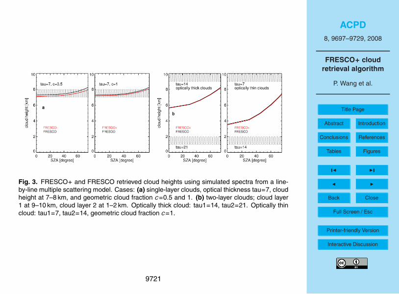
Next we consider scenes with single-layer and two-layer scattering clouds. Figure 3shows the results of the FRESCO and FRESCO+ retrieved cloud heights as a func-20

tion of solar zenith angle. The FRESCO and FRESCO+ retrieved cloud heights areinside the cloud for a single-layer cloud (Fig. 3a). For a two-layer cloud, FRESCOand FRESCO+ cloud heights are between the two layers (Fig. 3b). The FRESCO andFRESCO+ cloud heights generally increase with increasing SZA, because at largeSZA sunlight penetrates less deep into the cloud.25

In the single-layer cloud case, the FRESCO cloud heights are almost the same forthe fully (c=1) and partly cloudy (c=0.5) scenes. The FRESCO+ cloud height for thepartly cloudy scene in Fig. 3a is somewhat lower than for the fully cloudy scene. AtSZA=45◦, the difference between FRESCO+ and FRESCO cloud heights is −0.2 km

9703





ACPD8, 9697–9729, 2008


P. Wang et al.

Title Page



Tables Figures

J I

J I

Back Close

Full Screen / Esc



for c=1 (ceff=0.4) and -0.12 km for c=0.5 (ceff=0.2) scenes. FRESCO+ cloud heightsare lower than FRESCO cloud heights due to inclusion of single Rayleigh scattering,which makes the reflectance of FRESCO+ in the O2 absorption bands larger than thatof FRESCO. To simulate the same reflectance as the scene, FRESCO+ needs moreO2 absorption, therefore the FRESCO+ cloud height is lower than the FRESCO cloud5

height.In the two-layer cloud case, the FRESCO and FRESCO+ cloud heights retrieved

in the optically thick cloud case is higher than that retrieved in the optically thin cloudcase (see Fig. 3b). In the O2 A-band photons can penetrate to some distance into theclouds. Therefore the retrieved cloud height depends on both the cloud height and the10

cloud optical thickness. For the two-layer cloud scenes, the FRESCO and FRESCO+cloud heights are very close because the clouds are optically thicker than that in thesingle-layer cloud scene and therefore the effective cloud fractions are larger (between0.8–1.0). We found that the difference between the FRESCO+ and FRESCO cloudheights decreases with effective cloud fraction.15

3.2 FRESCO+ and FRESCO cloud retrievals from GOME data

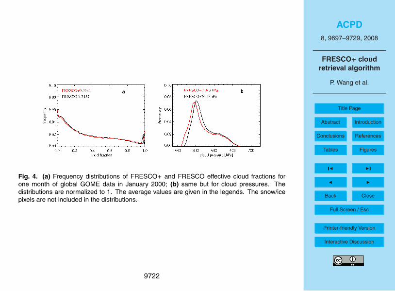
The FRESCO+ and FRESCO cloud retrievals have been compared for one month ofglobal GOME data of January 2000. The effective cloud fraction and cloud pressurefrequency distributions are shown in Fig. 4. The FRESCO+ and FRESCO effectivecloud fraction distributions almost coincide except that FRESCO+ has more clouds at20

effective cloud fractions 1 and 0. The mean effective cloud fractions differ about 0.014,with FRESCO+ being higher, because the inclusion of single Rayleigh scattering inFRESCO+ leads to a simulated continuum reflectance that is smaller than that sim-ulated by FRESCO. If we would exclude cloud fractions larger than 0.95, where thechi-squares of the O2 A-band fit are the largest, the effective cloud fraction difference25

would only be 0.005. In the cloud pressure distributions only pixels with effective cloudfractions larger than 0.1 are selected, and pixels over snow/ice are excluded. TheFRESCO+ cloud pressure distribution is shifted to higher pressures as compared to

9704





ACPD8, 9697–9729, 2008


P. Wang et al.

Title Page



Tables Figures

J I

J I

Back Close

Full Screen / Esc



FRESCO (about 50 hPa), but the shapes of the distributions are similar. The distribu-tions of other months show the same behaviour.

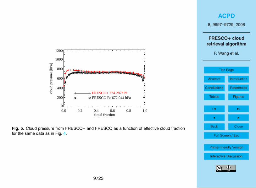
To analyze the difference between the FRESCO+ and FRESCO cloud pressures,we show in Fig. 5 these cloud pressures as a function of effective cloud fraction. Foreffective cloud fractions below 0.01, the cloud pressures retrieved by FRESCO are5

often 130 hPa – the lower limit of the FRESCO retrieval – which is not a realisticvalue. Figure 5 shows that the average cloud pressure retrieved by FRESCO in thesmallest effective cloud fraction bin [0, 0.05] is about 250 hPa. FRESCO+ retrievesmore reasonable cloud pressures than FRESCO, even if the cloud fraction is less than0.01. On average FRESCO+ cloud pressures are about 50 hPa higher than FRESCO10

cloud pressures. The difference in cloud pressure between FRESCO and FRESCO+is larger for the less cloudy pixels than for the fully cloudy pixels, which is due to thelarger relative amount of single Rayleigh scattering in the reflectance. The differencesfound between the FRESCO and FRESCO+ cloud pressures from GOME observa-tions agree with the simulations.15

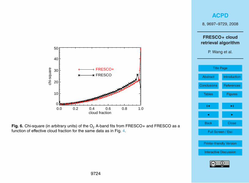
The chi-squares of the FRESCO+ and FRESCO O2 A-band fits as a function of ef-fective cloud fractions are shown in Fig. 6. The chi-squares of FRESCO+ are smallerthan those of FRESCO, which indicates an improvement of the fit in FRESCO+, espe-cially for effective cloud fractions smaller than 0.05. However, when the effective cloudfraction is 1 (i.e. a very bright scene) the chi-squares of FRESCO+ are larger than20

those of FRESCO. The reason is the following. In both retrieval algorithms the proce-dure for very bright scenes is: when the measured reflectance at 758 nm is larger than0.8, the cloud albedo is set to the measured reflectance at 758 nm and the effectivecloud fraction is retrieved. If the retrieved effective cloud fraction is larger than 1, it isset to 1 and the chi-square is calculated for ceff = 1 but not the retrieved value of ceff>1.25

In FRESCO+ the simulated transmission in the continuum (Tc in Eq. 1) is smaller thanthat in FRESCO due to Rayleigh scattering extinction, which is more important at largeSZA and for very bright scenes. Therefore, the simulated reflectance by FRESCO+ issmaller than the measured reflectance, which is the reason for the larger chi-squares

9705





ACPD8, 9697–9729, 2008


P. Wang et al.

Title Page



Tables Figures

J I

J I

Back Close

Full Screen / Esc



at ceff=1.

3.3 Validation of FRESCO+ cloud heights with ground-based data

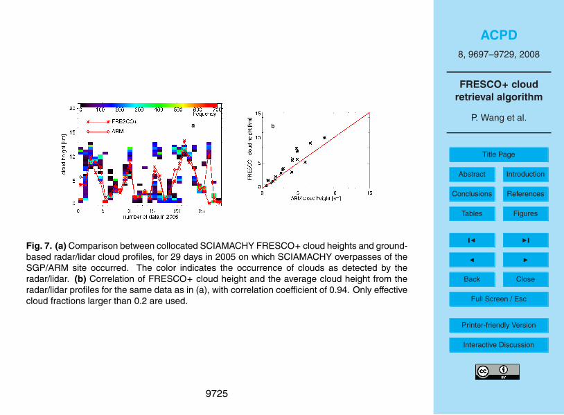
Cloud heights retrieved by FRESCO+ from one year of SCIAMACHY measurementsin 2005 have been compared with collocated ARM (Atmospheric Radiation Measure-ment) active remote sensing cloud boundaries data at SGP (Southern Great Plains)5

in the USA (Clothiaux et al., 2000). The SCIAMACHY pixel size is 30×60 km2, whichis not easy to compare with ground-based radar/lidar measurements. The criteria weused for spatial and temporal collocation were as follows: (1) the SCIAMACHY datawere selected with pixel centers within 60 km of the SGP/ARM site; (2) the SGP/ARMdata were selected within one hour of the SCIAMACHY overpass time (10:00 local10

solar time). The ARM cloud profiles are measured every 10 s with up to 10 cloud lay-ers per measurement. Most measurements have up to 3 cloud layers. The maximumnumber of collocated cloud data points in one hour is thus 3600. From this data set wecalculated the ARM cloud layer height distribution, using the cloud layer heights andtheir frequency of occurrence. The ARM cloud layer height distributions and the collo-15

cated SCIAMACHY FRESCO+ cloud heights are shown in Fig. 7a. In this plot we havefurther limited the FRESCO+ effective cloud fractions to values larger than 0.2 and thetime periods of ARM cloud cover to periods longer than 30 min, which corresponds togeometric cloud fractions larger than 0.5. As shown in Fig. 7a, the FRESCO+ cloudheight is close to the middle of the ARM cloud profiles. This agrees with the results20

of FRESCO+ for simulated spectra (Sect. 3.1). As shown in Fig. 7b, the FRESCO+cloud heights have an excellent correlation with the averaged ARM cloud profiles, witha correlation coefficient of 0.94.

9706





ACPD8, 9697–9729, 2008


P. Wang et al.

Title Page



Tables Figures

J I

J I

Back Close

Full Screen / Esc



4 Impact of FRESCO+ cloud parameters on O3 and NO2 retrievals

The FRESCO+ effective cloud fraction and cloud pressure retrievals are being used inO3 and NO2 total and tropospheric vertical column density (VCD) retrievals performedwithin the DUE TEMIS project (see http://www.temis.nl). To investigate whether theimprovement of the FRESCO+ cloud algorithm also leads to improved trace gas re-5

trievals, we performed the following comparisons: (1) SCIAMACHY total O3 from theTOSOMI product version 0.4, which uses FRESCO, was compared to version 0.42,which uses FRESCO+; (2) SCIAMACHY total and tropospheric NO2 column version1.04, which uses FRESCO, was compared to version 1.1, which uses FRESCO+; (3)a comparison of satellite retrievals using FRESCO+ with ground-based measurements10

of tropospheric NO2 was performed.

4.1 Impact of FRESCO+ cloud parameters on total O3 retrievals

For a partly cloudy pixel the total O3 vertical column density, Nt, is given by (VanRoozendael et al., 2006):

Nt =Ns + wMcloudyNg

M, (2)15

where M is the total air mass factor (AMF) of the partly cloudy pixel, Ns is the mea-sured slant column density, Mcloudy is the AMF for a fully cloudy scene, and Ng is thevertical column density below the cloud, which is also called the “ghost column”. Ng iscomputed by integrating the ozone profile from the surface to the cloud pressure level.M is given by the radiance-weighted sum of the AMFs of the clear and cloudy parts of20

the pixel:

M = wMcloudy + (1 − w)Mclear, (3)

where w is the weighting factor, and Mclear is the AMF for a clear scene. The weightingfactor w is the fraction of the photons that originates from the cloudy part of the pixel,

9707





http://www.temis.nl

ACPD8, 9697–9729, 2008


P. Wang et al.

Title Page



Tables Figures

J I

J I

Back Close

Full Screen / Esc



and can thus be written as (Martin et al., 2002):

w =cRcloudy(Pc)

R. (4)

where c is the (effective) cloud fraction, Rcloudy(Pc) is the average reflectance over thefit window for a scene that is fully covered with a cloud located at pressure Pc, andR is the measured reflectance for the pixel. It is important to mention that in the O35

and NO2 retrieval algorithms of TEMIS, clouds are also assumed to be Lambertianreflectors with albedo of 0.8, like in the FRESCO(+) algorithm.

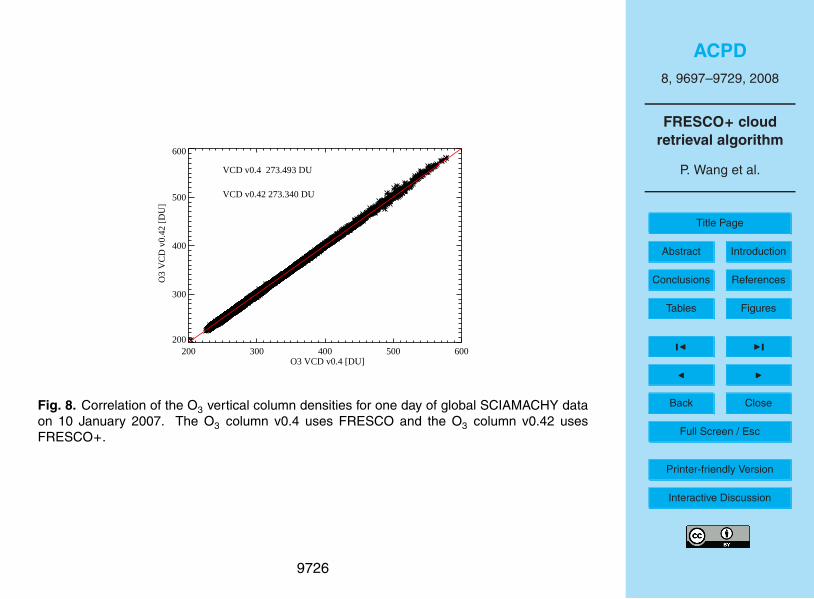
The correlation between the total O3 vertical column densities retrieved usingFRESCO and FRESCO+ cloud products for one day of global SCIAMACHY data isshown in Fig. 8. For this day (10 January 2007) the global averaged difference in O310

total column is only 0.2 DU. Differences for other days are similar. Apparently, theimprovement in the FRESCO+ cloud product has a small effect on total O3 columnretrievals. Since the effective cloud fractions from FRESCO and FRESCO+ are verysimilar, the difference in the O3 vertical column is mainly due to the cloud pressuredifference. The cloud pressure affects the cloud air mass factor Mcloudy and the ghost15

column Ng in Eq. (2). The differences between FRESCO+ and FRESCO cloud heightscause only small differences in the total O3 AMFs and in the ghost columns, becauseof the relatively low tropospheric O3 amount. Because O3 is mainly in stratosphere,the FRESCO+ cloud pressure improvement only weakly affects total O3.

4.2 Impact of FRESCO+ cloud parameters on tropospheric NO2 retrievals20

The cloud correction approaches for the total and tropospheric NO2 vertical columndensity retrievals are similar as for the total O3 retrievals, which are given by Eqs. (2–4). However, the NO2 air mass factor depends on the NO2 profile, because a largefraction of NO2 resides in the troposphere where Rayleigh scattering and scattering byaerosols and clouds is important. Therefore, the tropospheric NO2 air mass factor Mtr25

is obtained by multiplying the elements of the troposphere-only a-priori NO2 profile xa

9708





ACPD8, 9697–9729, 2008


P. Wang et al.

Title Page



Tables Figures

J I

J I

Back Close

Full Screen / Esc



with the elements of the altitude dependent air mass factor ml as follows (Eskes andBoersma, 2003):

Mtr =

∑l ml (b) · xa,l∑

l xa,l, (5)

where the elements of the altitude dependent air mass factor depend on the set ofmodel parameters b including cloud fraction, cloud height and surface albedo. The5

tropospheric NO2 VCD is given by:

Ntr =Ns − Ns,st

Mtr (xa, b). (6)

In the TEMIS processing the a priori NO2 profile is derived from a chemistry-transportmodel.

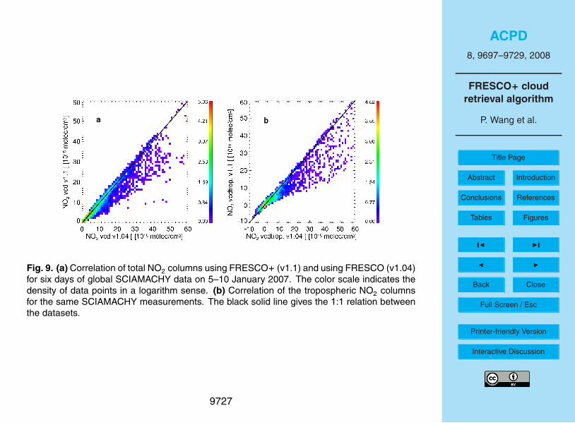
As shown in Fig. 9 both the total NO2 columns and the tropospheric NO2 columns re-10

trieved from SCIAMACHY using the FRESCO+ and FRESCO cloud products correlatewell. Note that the tropospheric NO2 VCDs are only reported for pixels with effectivecloud fractions less than 0.3. For most of the pixels the NO2 columns using FRESCO+and using FRESCO are almost the same, because there is no tropospheric NO2 or noclouds. Therefore, the globally averaged NO2 columns are similar. However the largest15

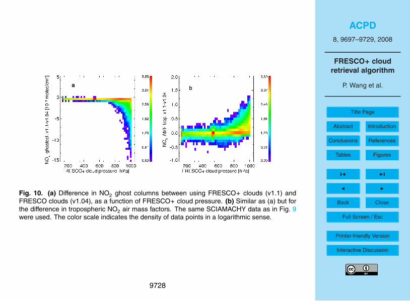
differences occur for the larger tropospheric NO2 columns.The effect of cloud pressure differences on tropospheric NO2 AMFs and NO2

ghost columns is shown in Fig. 10. The difference between the ghost columns us-ing FRESCO+ and using FRESCO increases for cloud pressures larger than about700 hPa; using FRESCO+, the NO2 ghost columns are clearly smaller than using20

FRESCO. The difference in tropospheric NO2 AMFs also increases with cloud pres-sure; the tropospheric NO2 AMFs are larger using FRESCO+ than using FRESCO.According to Eq. (2), the increase of AMF and decrease of ghost column both yield alower tropospheric NO2 VCD, especially for highly polluted scenes.

We can understand the results of Figs. 9 and 10 as follows. High NO2 concentrations25

occur mainly in the boundary layer, roughly below 2 km. For polluted pixels with low9709





ACPD8, 9697–9729, 2008


P. Wang et al.

Title Page



Tables Figures

J I

J I

Back Close

Full Screen / Esc



clouds even small cloud height differences can cause large differences in NO2 ghostcolumns. For polluted pixels with high clouds, when FRESCO and FRESCO+ cloudheights are both above the NO2 layer, differences in ghost column are small, so dif-ferences in NO2 VCD are also small. The global cloud height frequency distributionfrom SCIAMACHY shows that the cloud pressure peaks at about 800 hPa. So, globally5

there are more low clouds than high clouds, and the impact of the FRESCO+ cloudheight on tropospheric NO2 retrievals is significant.

4.3 Comparison with ground-based measurements of tropospheric NO2

To demonstrate that the FRESCO+ cloud parameters are an improvement for tropo-spheric NO2 retrievals from satellite, we compared tropospheric NO2 columns from10

SCIAMACHY (v1.1 and v1.04) with ground-based measurements of tropospheric NO2columns measured with Multi-AXis DOAS (MAXDOAS) instruments.

The ground-based data include results from the three MAXDOAS instruments(BIRA/IASB, Bremen and Heidelberg) operated during the DANDELIONS (DutchAerosol and Nitrogen Dioxide Experiments for vaLIdation of OMI and SCIAMACHY)15

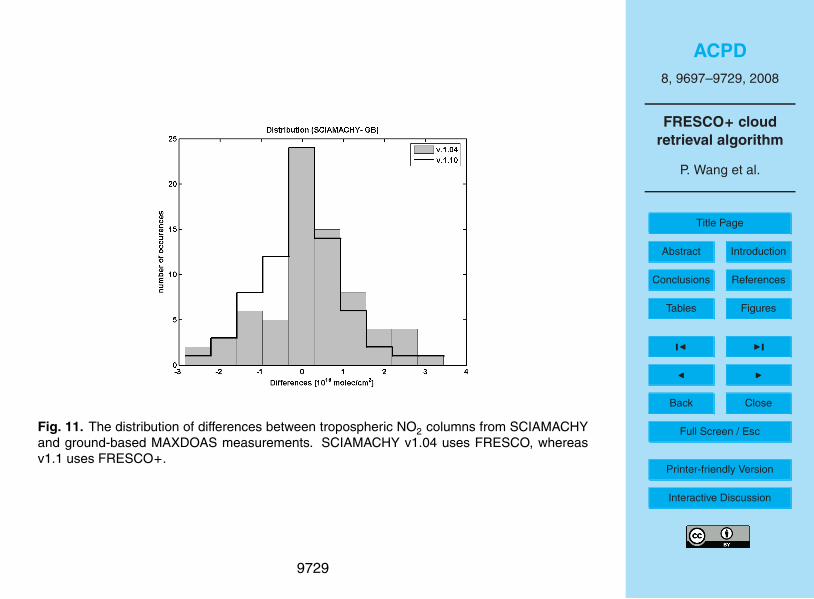
campaigns held at Cabauw (52◦ N, 5◦ E) in May–July 2005 and September 2006.The tropospheric NO2 VCDs are retrieved using a geometrical approximation validfor boundary-layer NO2, as described in Brinksma et al. (2008) and subsequently in-terpolated at the time of the SCIAMACHY overpasses. SCIAMACHY data are se-lected within a 200 km radius around Cabauw, leading to 72 points of comparison with20

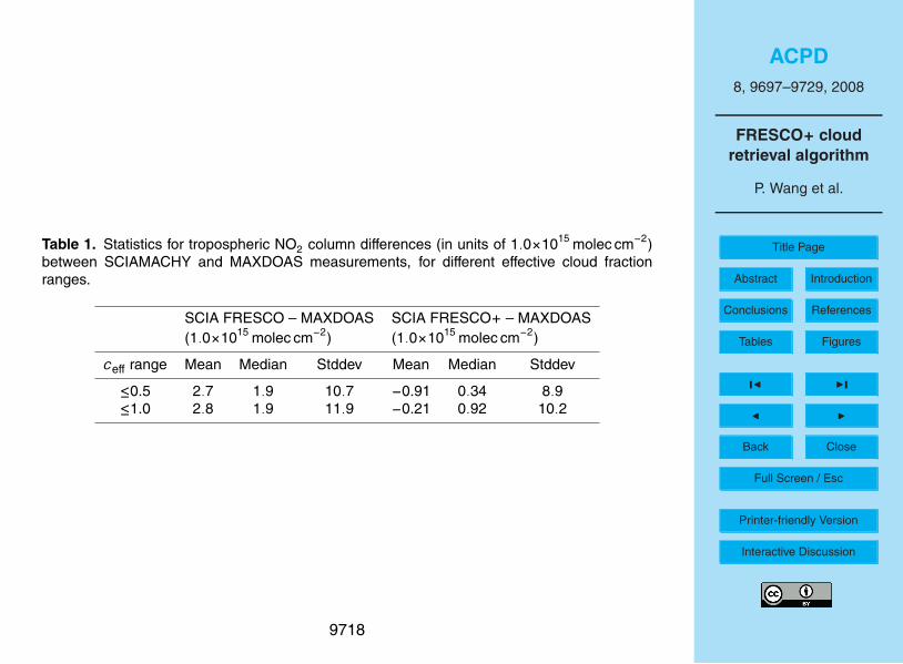
ground-based measurements. As can be seen in Fig. 11, the distribution of the differ-ences between SCIAMACHY NO2 VCD retrievals using FRESCO (v1.04) and ground-based measurements is asymmetric, showing more positive deviations. In contrast,the SCIAMACHY NO2 product using FRESCO+ (v1.1) is closer to the MAXDOASresults, and the differences show a more symmetric distribution. The statistics of25

the tropospheric NO2 column differences (SCIAMACHY minus MAXDOAS) are givenin Table 1. One can see that the mean and median differences are closer to zerowhen the FRESCO+ cloud product is used in the SCIAMACHY retrievals. The overall

9710





ACPD8, 9697–9729, 2008


P. Wang et al.

Title Page



Tables Figures

J I

J I

Back Close

Full Screen / Esc



mean difference between the SCIAMACHY NO2 VCD (v1.1) and ground-based MAX-DOAS NO2 VCD is −2.12×1014 molec cm−2 with a corresponding standard deviationof 1.02×1016 molec cm−2.

5 Conclusions

An improved version of the FRESCO cloud algorithm, FRESCO+, has been presented.5

This version includes Rayleigh scattering which is important for less cloudy scenes.The FRESCO+ algorithm has been applied to simulated O2 A-band spectra and toGOME and SCIAMACHY satellite measurements of the O2 A-band spectra. It ap-pears that FRESCO+ yields more accurate cloud heights in less cloudy scenes. TheFRESCO+ cloud pressure is about 50 hPa higher in the monthly global average than10

the FRESCO cloud pressure due to the addition of single Rayleigh scattering. Theeffective cloud fractions from FRESCO and FRESCO+ differ only by about 0.01 in themonthly global average.

For the first time FRESCO+ cloud height retrievals have been compared to ground-based Lidar/Radar cloud height measurements and a good correlation was found.15

From these measurements and simulations we found that the FRESCO+ and FRESCOcloud heights are closer to the middle of the clouds than to the top of the clouds in thescene. This is important to realize when applying FRESCO+ cloud heights in trace gascorrections and in cloud pressure comparisons.

As a first application we compared the total O3 columns retrieved from SCIAMACHY20

using FRESCO+ and FRESCO data in the cloud correction. It appears that the re-trieved total O3 columns are very similar using FRESCO+ or FRESCO cloud products(0.2 DU difference), because the cloud height improvement of FRESCO+ weakly af-fects stratospheric trace gas retrievals. As a second application, we applied FRESCO+to NO2 retrievals from SCIAMACHY. Here we found a large impact of the FRESCO+25

improvement on tropospheric NO2 retrievals. The cloud height improvement influencesthe ghost column of tropospheric NO2 directly, especially for highly polluted cases. The

9711





ACPD8, 9697–9729, 2008


P. Wang et al.

Title Page



Tables Figures

J I

J I

Back Close

Full Screen / Esc



cloud height improvement also affects the tropospheric NO2 air mass factors, becausethey depend on the NO2 profile and the profile of the scatterers.

Finally, we compared SCIAMACHY tropospheric NO2 column retrievals usingFRESCO+ and FRESCO to ground-based MAX-DOAS measurements performed dur-ing the DANDELIONS campaign in Cabauw. We found that the SCIAMACHY tropo-5

spheric NO2 columns using the FRESCO+ cloud product in the cloud correction, agreebetter with the ground-based data than using the FRESCO cloud product. We concludethat FRESCO+ is an improvement of FRESCO algorithm, not only in the physics of theretrieval algorithm, but also in the application of the cloud product for tropospheric tracegas retrievals.10

Appendix A

In this appendix, the formulae for the FRESCO+ simulations of the O2 A-band re-flectance are given, which is an update of the FRESCO formulae given by Koelemeijeret al. (2001).

A1 Rayleigh scattering cross section and phase function15

The Rayleigh scattering cross section, σR , is calculated with the formula (Bates, 1984):

σR = (32π3/3N2λ4)(nair − 1)2F ′k(air), (A1)

where (nair−1) is the refractive index, and F ′k(air) is the effective King correction factor.

The effective King correction factors and refractive index for air are chosen at 750 and800 nm from Table 1 in Bates (1984), and are linearly interpolated between 750 and20

800 nm.The Rayleigh scattering phase function (without polarization) is given by

FR(Θ) =3(1 − ρn)

4(1 + ρn/2)(cos2 Θ+

1 + ρn

1 − ρn), (A2)

9712





ACPD8, 9697–9729, 2008


P. Wang et al.

Title Page



Tables Figures

J I

J I

Back Close

Full Screen / Esc



with

cosΘ = − cosθ cosθ0 + sinθ sinθ0 cos(ϕ −ϕ0), (A3)

where Θ is the scattering angle, θ is the viewing zenith angle, θ0 is the solar zenithangle, ϕ is the viewing azimuth angle, and ϕ0 is the solar azimuth angle. ρn is thedepolarization factor; at 750 nm ρn=0.02786.5

A2 Atmospheric optical thickness and transmission

The atmospheric optical thickness and transmission is determined by oxygen absorp-tion and Rayleigh scattering. The absorption is calculated from the number density ofO2 molecules (nO2

) and the O2 absorption cross section, σO2(λ), along the light path.

σO2(λ) depends on the atmospheric temperature and pressure but this is omitted from10

the notation. The absorption coefficient (in 1/m) is given by:

kabs(λ, z) = nO2(z)σO2

(λ, z). (A4)

The Rayleigh scattering coefficient is calculated from the air density (nair) and theRayleigh scattering cross section (σR(λ, z)),

ksca(λ, z) = nair(z)σR(λ, z). (A5)15

The total atmospheric optical thickness, τ, is the sum of the absorption and scatteringcontributions:

τ(λ, zr , θ, θ0) =∫ ∞

zr

(kabs(λ, z) + ksca(λ, z))(Ssp(θ0, z − zr ) + (Ssp(θ, z − zr ))dz. (A6)

Here Ssp(θ0, z−zr ) and Ssp(θ, z−zr ) are the spherical light path factors from the sun tothe reflector and from the reflector to the satellite (Koelemeijer et al., 2001). z is height20

in the atmosphere, zr is the altitude of the reflector (surface or clouds). θ0, θ are thesolar zenith angle and viewing zenith angle at surface height.

9713





ACPD8, 9697–9729, 2008


P. Wang et al.

Title Page



Tables Figures

J I

J I

Back Close

Full Screen / Esc



The transmittance from TOA to zr , assuming a reflector at altitude zr , and back fromzr to TOA is now given by:

T (λ, zr , θ, θ0) = e−τ(λ,zr ,θ,θ0). (A7)

The transmittances T are stored in a look-up-table (LUT).

A3 Single Rayleigh scattering reflectance5

The single Rayleigh scattering reflectance, RR , is calculated with the formula (seeFig. 2) (Hovenier et al., 2005),

RR(λ, zr , µ, µ0, ϕ −ϕ0) =FR(µ,µ0, ϕ −ϕ0)

4µ0µ

∫ ∞

zr

ksca(λ, z)T (λ, z, µ, µ0)dz, (A8)

where T (λ, z, µ, µ0) is the transmittance, µ0= cosθ0, µ= cosθ. We have to modifyEq. (A8) for the spherical light path:10

RR(λ, zr , θ, θ0, ϕ −ϕ0) =FR(θ, θ0, ϕ −ϕ0)

4 cosθ0

∫ ∞

zr

ksca(λ, z)T (λ, z, θ, θ0)Ssp(θ, z)dz. (A9)

Since we can neglect the wavelength dependence of the Rayleigh scattering phasefunction FR in the O2 A-band, we can multiply by the phase function in Eq. (A9) afterthe convolution with the slit function. Therefore, the reflectances are stored in a look-up-table (LUT) as:15

R1(λ, zr , θ, θ0) =∫ ∞

zr

ksca(λ, z)T (λ, z, θ, θ0)Ssp(θ, z)dz. (A10)

Another advantage of using Eq. (A10) is that the azimuth is not needed in the re-flectance LUT, which now has the same parameters as the FRESCO+ transmit-tance LUT. The factor FR(θ, θ0, ϕ−ϕ0)/(4 cosθ0) is calculated in the FRESCO+ re-trieval program according to the measurement geometry. In the main text, Rs and20

Rc are RR for clear sky and cloudy cases, respectively. Rc=RR(λ, zc, θ, θ0, ϕ−ϕ0),Rs=RR(λ, zs, θ, θ0, ϕ−ϕ0), where zc is the cloud height, and zs is the surface height.

9714





ACPD8, 9697–9729, 2008


P. Wang et al.

Title Page



Tables Figures

J I

J I

Back Close

Full Screen / Esc



Acknowledgements. Funding was provided by the Netherlands Institute for Space Research(SRON) through the FRESCO+ project (EO-067). SCIAMACHY validation activities at BIRA-IASB are funded by the PRODEX CINAMON project. The MAXDOAS measurements duringthe DANDELIONS campaign were supported by the EU FP6, through the ACCENT NoE. ARMdata is made available through the US Department of Energy as part of the Atmospheric Radi-5

ation Measurement Program.

References

Bates, D. R.: Rayleigh scattering by air, Planet. Space Sci., 32(6), 785–790, 1984. 9712Brinksma, E. J., Pinardi, G., Braak, R., et al.: The 2005 and 2006 DANDELIONS NO2

and Aerosol Intercomparison Campaigns, J. Geophys. Res., doi:10.1029/2007JD008808,10

in press, 2008. 9710Clothiaux, E. E., Ackerman, T. P., Mace, G. G., Moran, K. P., Marchand, R. T., Miller, M. A.,

and Martner, B. E.: Objective determination of cloud heights and radar reflectivities using acombination of active remote sensors at the ARM CART sites, J. Appl. Meteorol., 39, 645–665, 2000. 970615

van Diedenhoven, B., Hasekamp, O. P., and Landgraf, J.: Retrieval of cloud parameters fromsatellite-based reflectance measurements in the ultraviolet and the oxygen A-band, J. Geo-phys. Res., 112, D15208, doi:10.1029/2006JD008155, 2007. 9699

Eskes, H. J. and Boersma, H. F.: Averaging kernels for DOAS total-column satellite retrievals.Atmos. Chem. Phys.. 3, 1285–1291, 2003. 9700, 970920

Fournier, N., Stammes, P., de Graaf, M., van der A, R., Piters, A., Grzegorski, M., andKokhanovsky, A.: Improving cloud information over deserts from SCIAMACHY Oxygen A-band measurements, Atmos. Chem. Phys., 6, 163–172, 2006,http://www.atmos-chem-phys.net/6/163/2006/. 9699, 9701

Grzegorski, M., Wenig, M., Platt, U., Stammes, P., Fournier, N., and Wagner, T.: The Heidelberg25

iterative cloud retrievallll utilities (HICRU) and its application to GOME data, Atmos. Chem.Phys., 6, 4461–4476, 2006,http://www.atmos-chem-phys.net/6/4461/2006/. 9699

de Haan, J. F., Bosma, P. B., and Hovenier, J. W.: The adding method for multiple scatteringcalculations of polarized light, Astron. Astrophys., 183, 371–391, 1987. 970230

9715





http://www.atmos-chem-phys.net/6/163/2006/


ACPD8, 9697–9729, 2008


P. Wang et al.

Title Page



Tables Figures

J I

J I

Back Close

Full Screen / Esc



Hovenier, J. W., Domke, H., and van der Mee, C.: Transfer of Polarized Light in PlanetaryAtmospheres: Basic Concepts and Practical Methods, Kluwer academic publishers, Dor-drecht/Boston/London, 2005.

Koelemeijer, R. B. A. and Stammes, P.: Effects of clouds on the ozone column retrieval fromGOME UV measurements, J. Geophys. Res., D104, 8281–8294, 1999. 97005

Koelemeijer, R. B. A., Stammes, P., Hovenier, J. W., and de Haan, J. F.: A fast method forretrieval of cloud parameters using oxygen A-band measurements from the Global OzoneMonitoring Experiment, J. Geophys. Res., 106, 3475–3490, 2001. 9699, 9712, 9713

Koelemeijer, R. B. A., de Haan, J. F., and Stammes, P.: A database of spectral surface reflec-tivity in the range 335–772 nm derived from 5.5 years of GOME observations, J. Geophys.10

Res., 108(D2), D24070, doi:10.1029/2002JD002429, 2003. 9699, 9701Kokhanovsky, A. A., Rozanov, V. V., Nauss, T., Reudenbach, C., Daniel, J. S., Miller, H. L.,

and Burrows, J. P.: The semianalytical cloud retrieval algorithm for SCIAMACHY – I. Thevalidation, Atmos. Chem. Phys., 6, 1905–1911, 2006,http://www.atmos-chem-phys.net/6/1905/2006/. 969915

Krijger, J., van Weele, M., Aben, I., and Frey, I.: Technical note: The effect of sensor resolutionon the number of cloudfree observations from space, Atmos. Chem. Phys., 7, 2881–2891,2007,http://www.atmos-chem-phys.net/7/2881/2007/. 9699

Loyola, D.: Automatic Cloud Analysis from Polar-Orbiting Satellites Using Neural Network and20

Data Fusion Techniques, in: Proceedings of the IEEE International Geoscience and RemoteSensing Symposium, IGARSS’2004, Anchorage, 4, 2530–2534, 2004. 9699

Martin, R. V., Chance, K., Jacob, D. J., et al.: An improved Retrieval of Tropospheric NitrogenDioxide from GOME, J. Geophys. Res., 107(D20), 4437, doi:10.1029/2001JD001027, 2002.970825

Munro, R. and Eisinger, M.: The Second Global Ozone Monitoring Experiment (GOME-2) AnOverview, Programme Development Department Technical Memorandum No.11, Eumetsat,Darmstadt, October 2004. 9699

Rothman, L. S., Jacquemart, D., Barbe, A., et al.: The HITRAN 2004 molecular spectroscopicdatabase, J. Quant. Spectr. Radiat. Trans., 96, 139–204, 2005. 970130

Stammes, P., de Haan, J., and Hovenier, J.: The polarized internal radiation field of a planetaryatmosphere, Astron. Astrophys., 225, 239–259, 1989. 9702

Stammes, P.: Spectral radiance modeling in the UV-visible range, in: IRS 2000: Current Prob-

9716







ACPD8, 9697–9729, 2008


P. Wang et al.

Title Page



Tables Figures

J I

J I

Back Close

Full Screen / Esc



lems in Atmospheric Radiation, edited by: Smith, W. and Timofeyev, Y., pp. 385–388, A.Deepak, Hampton, Va., 2001. 9702

Stammes, P., Sneep M., de Haan, J. F., Veefkind, J. P., Wang, P., and Levelt, P. F.: Ef-fective cloud fractions from OMI: theoretical framework and validation, J. Geophys. Res.,doi:10.1029/2007JD008820, in press, 2008. 9699, 97005

Tuinder, O. N. E., de Winter-Sorkina, R., and Builtjes, P.: Retrieval methods of effective cloudcover from the GOME instrument: an intercomparison, Atmos. Chem. Phys., 4, 255–273,2004,http://www.atmos-chem-phys.net/4/255/2004/. 9699

Van Roozendael, M., Loyola, D., Spurr, R., Balis, D., Lambert, J-C., Livschitz, Y., Valks, P.,10

Ruppert, T., Kenter, P., Fayt, C., and Zehner, C.: Ten years of GOME/ERS-2 total ozonedata-The new GOME data Processor (GDP) version 4: 1 Algorithm description, J. Geophys.Res., 111, D14311, doi:10.1029/2005JD006375, 2006. 9707

Wang, P., Stammes, P., and Boersma, K. F.: Impact of the effective cloud fraction assumption ontropospheric NO2 retrievals, in Proceedings of the first conference on atmospheric science,15

SP-628, ESA, 2006. 9700Wang, P. and Stammes, P.: FRESCO-GOME2 project, EUM/CO/06/1536/FM, final report, Eu-

metsat, Darmstadt, 14 September, 2007. 9702

9717






ACPD8, 9697–9729, 2008


P. Wang et al.

Title Page



Tables Figures

J I

J I

Back Close

Full Screen / Esc



Table 1. Statistics for tropospheric NO2 column differences (in units of 1.0×1015 molec cm−2)between SCIAMACHY and MAXDOAS measurements, for different effective cloud fractionranges.

SCIA FRESCO – MAXDOAS SCIA FRESCO+ – MAXDOAS(1.0×1015 molec cm−2) (1.0×1015 molec cm−2)

ceff range Mean Median Stddev Mean Median Stddev

≤0.5 2.7 1.9 10.7 −0.91 0.34 8.9≤1.0 2.8 1.9 11.9 −0.21 0.92 10.2

9718





ACPD8, 9697–9729, 2008


P. Wang et al.

Title Page



Tables Figures

J I

J I

Back Close

Full Screen / Esc



758 760 762 764 766 768wavelength [nm]

0.0

0.2

0.4

0.6

0.8

1.0

1.2re

flect

ance

low cloud (948 hPa)high cloud (366 hPa)

Fig. 1. Typical O2 A-band spectra measured by GOME. The spectra are normalized at 758 nmto show the relative depth of the band for clouds at different heights.

9719





ACPD8, 9697–9729, 2008


P. Wang et al.

Title Page



Tables Figures

J I

J I

Back Close

Full Screen / Esc



Fig. 2. Atmospheric radiation model used in FRESCO+. The cloud and surface are bothassumed to be Lambertian reflectors. Three light paths are considered: (1) from sun to surfaceto satellite, (2) from sun to cloud to satellite, (3) from sun to atmosphere to satellite accordingto single Rayleigh scattering. (1)+(2): solid lines, (3): dashed lines. Along all three paths O2absorption and Rayleigh scattering extinction are included in the forward model simulation.

9720





ACPD8, 9697–9729, 2008


P. Wang et al.

Title Page



Tables Figures

J I

J I

Back Close

Full Screen / Esc



Fig. 3. FRESCO+ and FRESCO retrieved cloud heights using simulated spectra from a line-by-line multiple scattering model. Cases: (a) single-layer clouds, optical thickness tau=7, cloudheight at 7–8 km, and geometric cloud fraction c=0.5 and 1. (b) two-layer clouds; cloud layer1 at 9–10 km, cloud layer 2 at 1–2 km. Optically thick cloud: tau1=14, tau2=21. Optically thincloud: tau1=7, tau2=14, geometric cloud fraction c=1.

9721





ACPD8, 9697–9729, 2008


P. Wang et al.

Title Page



Tables Figures

J I

J I

Back Close

Full Screen / Esc



Fig. 4. (a) Frequency distributions of FRESCO+ and FRESCO effective cloud fractions forone month of global GOME data in January 2000; (b) same but for cloud pressures. Thedistributions are normalized to 1. The average values are given in the legends. The snow/icepixels are not included in the distributions.

9722





ACPD8, 9697–9729, 2008


P. Wang et al.

Title Page



Tables Figures

J I

J I

Back Close

Full Screen / Esc



0.0 0.2 0.4 0.6 0.8 1.0cloud fraction

0

200

400

600

800

1000

1200cl

oud

pres

sure

[hP

a]

FRESCO Pc 672.044 hPaFRESCO+ 724.287hPa

Fig. 5. Cloud pressure from FRESCO+ and FRESCO as a function of effective cloud fractionfor the same data as in Fig. 4.

9723





ACPD8, 9697–9729, 2008


P. Wang et al.

Title Page



Tables Figures

J I

J I

Back Close

Full Screen / Esc



0.0 0.2 0.4 0.6 0.8 1.0cloud fraction

0

10

20

30

40

50ch

i-squ

are

FRESCO

FRESCO+

Fig. 6. Chi-square (in arbitrary units) of the O2 A-band fits from FRESCO+ and FRESCO as afunction of effective cloud fraction for the same data as in Fig. 4.

9724





ACPD8, 9697–9729, 2008


P. Wang et al.

Title Page



Tables Figures

J I

J I

Back Close

Full Screen / Esc



Fig. 7. (a) Comparison between collocated SCIAMACHY FRESCO+ cloud heights and ground-based radar/lidar cloud profiles, for 29 days in 2005 on which SCIAMACHY overpasses of theSGP/ARM site occurred. The color indicates the occurrence of clouds as detected by theradar/lidar. (b) Correlation of FRESCO+ cloud height and the average cloud height from theradar/lidar profiles for the same data as in (a), with correlation coefficient of 0.94. Only effectivecloud fractions larger than 0.2 are used.

9725





ACPD8, 9697–9729, 2008


P. Wang et al.

Title Page



Tables Figures

J I

J I

Back Close

Full Screen / Esc



200 300 400 500 600O3 VCD v0.4 [DU]

200

300

400

500

600O

3 V

CD

v0.

42 [

DU

]VCD v0.4 273.493 DU

VCD v0.42 273.340 DU

Fig. 8. Correlation of the O3 vertical column densities for one day of global SCIAMACHY dataon 10 January 2007. The O3 column v0.4 uses FRESCO and the O3 column v0.42 usesFRESCO+.

9726





ACPD8, 9697–9729, 2008


P. Wang et al.

Title Page



Tables Figures

J I

J I

Back Close

Full Screen / Esc



Fig. 9. (a) Correlation of total NO2 columns using FRESCO+ (v1.1) and using FRESCO (v1.04)for six days of global SCIAMACHY data on 5–10 January 2007. The color scale indicates thedensity of data points in a logarithm sense. (b) Correlation of the tropospheric NO2 columnsfor the same SCIAMACHY measurements. The black solid line gives the 1:1 relation betweenthe datasets.

9727





ACPD8, 9697–9729, 2008


P. Wang et al.

Title Page



Tables Figures

J I

J I

Back Close

Full Screen / Esc



Fig. 10. (a) Difference in NO2 ghost columns between using FRESCO+ clouds (v1.1) andFRESCO clouds (v1.04), as a function of FRESCO+ cloud pressure. (b) Similar as (a) but forthe difference in tropospheric NO2 air mass factors. The same SCIAMACHY data as in Fig. 9were used. The color scale indicates the density of data points in a logarithmic sense.

9728





ACPD8, 9697–9729, 2008


P. Wang et al.

Title Page



Tables Figures

J I

J I

Back Close

Full Screen / Esc



Fig. 11. The distribution of differences between tropospheric NO2 columns from SCIAMACHYand ground-based MAXDOAS measurements. SCIAMACHY v1.04 uses FRESCO, whereasv1.1 uses FRESCO+.

9729





fresco+: an improved o2 a-band cloud retrieval algorithm for tropospheric trace gas retrievals

Documents