ray-traced tropospheric delays in vlbi analysis

Ray-traced tropospheric delays in VLBI analysis

Vahab Nafisi,1,2,3 Matthias Madzak,2 Johannes Böhm,2 Alireza A. Ardalan,1

and Harald Schuh2

Received 8 November 2011; revised 7 February 2012; accepted 28 February 2012; published 25 April 2012.

[1] We develop a ray-tracing package for the calculation of path delays of microwavesignals in the troposphere based on numerical weather models which we use for thedetermination of the delays of geodetic Very Long Baseline Interferometry (VLBI)observations. We show results for a two-week campaign of continuous VLBI sessionsin 2008 (CONT08), where we apply those ray-traced delays and analyze therepeatability of baseline lengths in comparison to a standard approach with zenith delaysand mapping functions. We find improvement in baseline length repeatabilities when notropospheric gradients are estimated in the analysis. Furthermore, ray-traced delays areapplied for Intensive sessions containing the stations Tsukuba (Japan) and Wettzell(Germany) for the determination of Universal Time (UT1). We perform an externalvalidation using GPS-derived length-of-day values and find an improvement for UT1with ray-traced delays by up to 4.5%.

Citation: Nafisi, V., M. Madzak, J. Böhm, A. A. Ardalan, and H. Schuh (2012), Ray-traced tropospheric delays in VLBIanalysis, Radio Sci., 47, RS2020, doi:10.1029/2011RS004918.

1. Introduction

[2] The troposphere is a composition of dry gases andwater vapor, both parts imposing a time delay on propagat-ing electromagnetic waves. Furthermore, an inhomogeneousmedium causes an electromagnetic (EM) wave to propagatealong a curved path, which is called the bending effectresulting in the geometric delay. Because of these twoeffects on space geodetic observations, the observed dis-tances are longer than the straight line between the receiverand the transmitter in vacuum. In this paper, the combinationof both effects is called total tropospheric delay or just delay.[3] Tropospheric delay modeling has always been an

important issue in space geodetic data analysis. As describedin the IERS Conventions 2010 [Petit and Luzum, 2010], apriori zenith hydrostatic delays (ZHD) can be estimated fromthe surface pressure at the site as suggested by Saastamoinen[1972]. Considering the elevation angle, the ZHD is mappedto the direction of the specific observation using the hydro-static mapping function [Davis et al., 1985], while zenithwet delays (ZWD) are estimated using the wet mappingfunction as partial derivative. Furthermore, troposphericgradients [Chen and Herring, 1997] are usually estimated toconsider the azimuthal asymmetry of the delays.

[4] Modern mapping functions such as the Vienna Map-ping Functions 1 (VMF1) [Böhm et al., 2006a] and theGlobal Mapping Functions (GMF) [Böhm et al., 2006b] arebased on numerical weather models (NWM), which havebeen continuously improving with regard to their spatial andtemporal resolution as well as with regard to advances in dataassimilation. One can find a comprehensive and widespreadcomparison of the models available up to the last decade inthe work by Mendes [1999]. Ghoddousi-Fard [2009] hasreviewed recent mapping functions based on NWM as wellas commonly used gradient mapping functions.[5] Unlike the mapping function method, ray-tracing

estimates slant delays for each specific direction. Bean andThayer [1959] were one of the early proponents of “ray-tracing” in a spherically stratified atmosphere and somemathematical models for this purpose were presented. Dueto lack of powerful and fast computers and the need of ahuge number of calculations to obtain the results, simplifi-cations were used in the equations.[6] Nowadays many fields of science where the propaga-

tion of an EM wave through a stratified medium has to betraced can benefit from the ray-tracing technique. The mainapplication of this method in tropospheric research is thedetermination of the total delay along the trajectory of asignal, which is transmitted from a source. The geometricaloptics approximation [Born and Wolf, 1999] can be used toobtain the Eikonal equation, which represents the solution ofthe Helmholtz equation for an EM wave propagatingthrough a slowly varying medium [Wheelon, 2001]. TheEikonal equation is used to establish a ray-tracing system todetermine the raypath and the optical path length.[7] Generally speaking, ray-tracing methods can be cate-

gorized in three groups using different assumptions:

1Department of Surveying and Geomatics Engineering, College ofEngineering, University of Tehran, Tehran, Iran.

2Institute of Geodesy and Geophysics, Vienna University ofTechnology, Vienna, Austria.

3Department of Surveying Engineering, Faculty of Engineering,University of Isfahan, Isfahan, Iran.

Copyright 2012 by the American Geophysical Union.0048-6604/12/2011RS004918

RADIO SCIENCE, VOL. 47, RS2020, doi:10.1029/2011RS004918, 2012

RS2020 1 of 17

http://dx.doi.org/10.1029/2011RS004918

[8] Horizontal symmetry: In this case horizontal symmetryof the troposphere is the main assumption. Therefore, the raydirection is sufficiently defined by the elevation angle.Usually, one tropospheric profile, where meteorologicalparameters such as temperature, pressure and humidity areknown, is enough for a specific station. The Vienna Map-ping Functions 1 [Böhm et al., 2006a] are based on thisconcept.[9] Horizontal asymmetry-2D: In this case the azimuth-

dependent behavior of the troposphere is accounted for. Itmeans that in addition to the elevation angle, the azimuth ofthe observation becomes a parameter which must be con-sidered for the raypath. However, the ray is not allowed toleave the constant azimuth plane. In other words, any out-of-plane component is neglected.[10] Horizontal asymmetry-3D: In addition to the above

mentioned azimuth dependency of the troposphere, it ispossible for the raypath to have out-of-plane components.These components are due to horizontal gradients of therefractivity. Obviously this hypothesis is more realistic but,as a drawback, comes along with some difficulties from thecomputational point of view.[11] To illustrate the differences between the three above

mentioned categories of ray-tracers, Figure 1 shows theslant delay variations with respect to azimuth for a sampledata set.[12] This paper discusses the applications of the ray-tracing

method for calculating total tropospheric delays in VeryLong Baseline Interferometry (VLBI) analysis. Section 1introduces the refractivity of moist air. A ray-tracing sys-tem based on Eikonal and Maxwell’s equations for totaldelay computations is developed and presented in section 2.In section 3 we discuss the structure of a typical ray-tracingsystem. Section 4 deals with the most important computa-tional aspects of a ray-tracing system, which must be con-sidered to improve accuracy and efficiency of the system. Insection 5 we show some results for the VLBI campaign

CONT08, a continuous two-week VLBI campaign inAugust 2008. For more information about CONT08 werefer to Teke et al. [2011]. Also some validation resultsfrom Intensive sessions between Tsukuba and Wettzell arepresented in this section. For example, we show the effectof ray-traced delays on baseline length repeatabilities andthe estimation of DUT1 values. Outlook and concludingremarks from this research can be found in section 6.

1.1. Refractive Index of Moist Air

[13] For a medium, the refractive index n is defined as theratio of the velocity of an electromagnetic wave in vacuum tothe speed of propagation in this medium. It can be written as

n ¼ c

vð1Þ

where c and v are the velocities in vacuum and in themedium, respectively.[14] In general this index is complex. The imaginary part

corresponds to the attenuation of the wave, which is nottypically significant for frequencies smaller than 10 GHz[Nilsson, 2008]. Because the refractive index of a signal inmoist air is very close to one, n � 1 will be very small and itis therefore convenient to introduce and use another param-eter, namely refractivity N:

N ¼ n� 1ð Þ � 106: ð2Þ

[15] The total refractivity N of moist air can be expressedas [Davis, 1986]

N ¼ Nd þ Nv ¼ k1Rdrd þ k2Rvrv þ k3RvrvT: ð3Þ

[16] Hereafter k1, k2 and k3 are refractivity coefficientswhich can be determined experimentally. These coefficientsrepresent the induced dipole moment and the polarizationorientation of polar and non-polar molecules that depend onthe frequency of an EM wave. However, for microwavesignals propagating through the neutral atmosphere thecoefficients are practically independent of frequency [Hecht,2001]. These constants have been estimated using directmeasurements made with microwave cavities [Boudouris,1963] and different coefficients are suggested by variousauthors, as summarized in Table 1. For detailed reviews and

Figure 1. Total delays computed by different assumptionsat 5� outgoing elevation angle: Horizontal symmetry (black),horizontal asymmetry-3D (blue) and horizontal asymmetry-2D (red). The sample data set is derived from the epoch0:00 UTC of August 12th 2008 at the station Tsukuba,Japan. 3D results are not necessarily larger than those of2D. The sign of differences between 2D and 3D is dependenton horizontal gradients of the troposphere.

Table 1. Refractivity Coefficients as Realized by DifferentAuthors [Rüeger, 2002a, 2002b]

Coefficientk1

(�10�2 K/Pa)k2

(�10�2 K/Pa)k3

(�103 K2/Pa)

Essen and Froome [1951] 77.68 64.7 372Essen [1953] 77.6654 75.1682 369.226Smith and Weintraub [1953] 77.61 72.0 375Bean [1962] 77.607 71.600 374.700Boudouris [1963] 77.631 72.006 375.031Zhevakin and

Naumov [1967]77.607 71.6 307.658

Thayer [1974] 77.60 64.8 377.6Bevis et al. [1994] 77.60 70.4 373.9Rüeger [2002b] -

best average77.6890 71.2952 375.463

Rüeger [2002b] -best available

77.695 71.97 375.406

IUGG 77.624 64.700 371.897

NAFISI ET AL.: RAY-TRACED TROPOSPHERIC DELAYS RS2020RS2020

2 of 17

discussions of the different values we refer to Rüeger[2002a, 2002b] and Healy [2011].[17] Since NWM provide meteorological parameters, it is

useful to express equation (3) in terms of total pressure (p),water vapor pressure (e) and temperature (T). Using theequation of state for non-ideal gases [Kleijer, 2004]

pi ¼ ZiriRiT ð4Þ

where i = d, v (Rd and Rv denote the gas constant for dry airand water vapor, respectively), we can obtain [Davis, 1986]

N ¼ k1p

Tþ k ′2

e

Tþ k3

e

T2

� �Z�1v ¼Nh þ Nnh ð5Þ

where Nh and Nnh denote the hydrostatic and non-hydrostaticrefractivities, respectively. The separation into these twoparts is possible under the assumption of unsaturated con-ditions for air. In this case the total pressure p can beexpressed as a combination of the partial pressure of dry airpd and water vapor e (=pv) [Stull, 2000; Wallace and Hobbs,2006]. A new refractivity coefficient k ′2 introduced inequation (5) is expressed as

k ′2 ¼ k2 � k1Rd

Rv: ð6Þ

[18] Zv in equation (5) is the water vapor compressibilityfactor, which in normal conditions is close to one [Kleijer,2004]. Ignoring compressibility factors in this equationintroduces errors of 0.1 ppm for wet components [Thayer,1974], which is much lower than the accuracy of this com-ponent [Cucurull, 2010].[19] The water vapor pressure e can be calculated using

the following equation [Wallace and Hobbs, 2006]

e ¼ qp

ɛþ 1� ɛð Þq ð7Þ

where ɛ = Mv/Md is the ratio of the molar masses of watervapor and dry gasses, and the values of the specific humidityq are provided by NWM.

1.2. Total Tropospheric Delay

[20] The total delay can be defined as the differencebetween the propagation time of a specific wave in a realmedium (in our case the troposphere) and in vacuum. Inideal conditions, which means without any dispersion, thepath of the ray between the receiver and the source of thewave (a quasar in VLBI) is a straight line.

S ¼ZV

ds: ð8Þ

[21] On the other hand, due to variations in the tropo-spheric refractive index, the real path of the ray is defined as

L ¼ZT

n r; q;l; tð Þds ð9Þ

where r is the radial distance, q is the co-latitude, and l is thelongitude (0 ≤ q ≤ p, 0 ≤ l ≤ 2p). n(r, q, l, t) denotes the

refractive index at a position defined by r, q and l at time t.Using equations (8) and (9) and refractivity instead ofrefractive index, the total tropospheric delay reads as

Dt ¼ 10�6

ZT

N r; q;l; tð Þ dsþZT

ds� S

0@

1A: ð10Þ

[22] The first term of equation (10) represents the signaldelay along the path which causes the excess of the path.The second term denotes the so-called geometric delay. Thefirst term inside the brackets is the length of the curved pathT. Inserting equation (5) into equation (10), we find

Dt ¼ 10�6ZT

Nh r; q;l; tð Þ dsþ 10�6ZT

Nnh r; q;l; tð Þ ds

þZT

ds� S

0@

1A ð11Þ

or

Dt ¼ Dth þDtnh þDtb: ð12Þ

[23] Equation (12) shows the different components of thesignal delay due to tropospheric propagation effects, i.e., thehydrostatic (Dth) and non-hydrostatic (Dtnh) parts as wellas the geometric delay Dtb which depends on the totalrefractivity.[24] The geometric delay for elevation angles above 57� is

less than 0.1 mm, but it significantly increases withdecreasing elevation angles. At 3, 5, and 10� elevation, theeffect is about 60, 20, and 3 cm, respectively.

2. Maxwell’s Equations and the Eikonal Equationin a Random Media

[25] Combining the four Maxwell equations [Fleisch,2010] allows us to find two important implications. First,we can find the wave equation and an equation for therefractive index can be obtained, which is directly linked tothe physical body of the troposphere. Second, the Eikonalequation is obtained using some assumptions and arrange-ments. This equation plays an important role in the devel-opment of our ray-tracing algorithm. With Maxwell’sequations and considering a medium free of currents andcharges, and a short vacuum wavelength and applying somemathematical operations, we can write the well-knownEikonal equation in vector notation [Born and Wolf, 1999] as

rL 2 ¼ n2 r*ð Þ�� ð13Þ

where rL comprises the components of the ray directions, Lis the optical path length, n is the refractive index of amedium and r* is the position vector. The surfaces L(r) =constant are called geometrical wave surfaces or geometricalwavefronts.

2.1. Hamiltonian Formalism of the Eikonal Equation

[26] Equation (13) is a partial differential equation of thefirst order for n r*ið Þ and it can be expressed in many alter-native forms. In general, we can write the Eikonal equation


3 of 17

in the Hamiltonian canonical formalism as follows [Bornand Wolf, 1999; Cerveny, 2005]:

H r*;rLð Þ ≡ 1

arL:rLð Þa2 � n r*ð Þa

n o¼ 0 ð14Þ

dr*i

du¼ ∂H

∂rLið15Þ

drLidu

¼ � ∂H∂r*i

ð16Þ

dL

du¼ rLi

∂H∂rLi

: ð17Þ

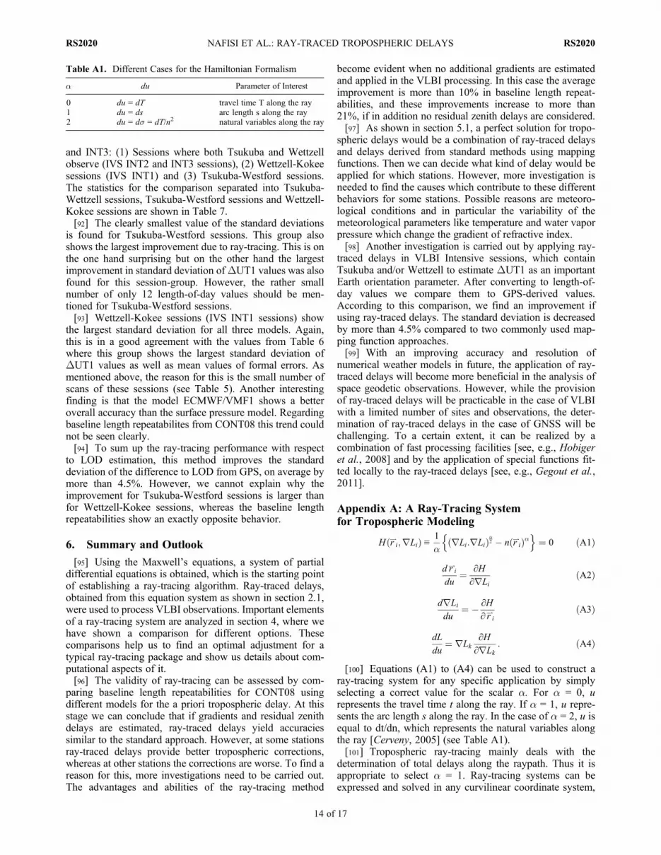
[27] The scalar value a determines the parameter ofinterest u (see Table A1 in Appendix A). In general it is areal number but in applications we must consider it to be aninteger number. H r*i;rLið Þ is called the Hamiltonian func-tion or just Hamiltonian.[28] In a 3D space this system consists of seven equa-

tions. Six equations are obtained from equations (15) and(16) and must be solved altogether. The result of these sixequations is ri = ri(u), which describes the trajectory of a3D curve. The seventh equation, i.e., equation (17), can besolved independently and yields the optical path length.Details of a ray-tracing system for practical purposesbased on the Hamiltonian formalism are presented inAppendix A. In the following section we discuss differentaspects of this problem.

3. Structure of the Ray-Tracing System

[29] If we want to describe our ray-tracing system, we candistinguish four main properties. Since these parts are verygeneral, one can find different realizations.[30] Inputs: Inputs of the system can be divided into three

different groups[31] - Numerical weather model data set, which provides

basic meteorological parameters needed for the estimation ofrefractivity like temperature, water vapor pressure and totalpressure.[32] - Coordinates of the stations (receivers) and time of

observation, which provide basic information for horizontaland temporal interpolation.[33] - Elevation angles and azimuth angles of the raypath,

which provide information for the direction of the ray andalso the stopping criteria for the iterations.[34] Pre-calculations: For speeding up the ray-tracing

calculations, some pre-calculations should be performedbefore the main ray-tracing computations. Outputs of thisstep are vertical inter- and extrapolated refractivity profiles.In addition, we need to set some parameters such as theinterpolation and extrapolation method, transformationbetween geodetic and meteorological systems, auxiliaryatmospheric data sets, height of upper limit of the tropo-sphere and size of increments.[35] Ray-tracing: The solution of the Eikonal equation is

the main result of this part. Based on wave propagationtheory and optics approximation, which is explained in

section 2, we can construct seven partial differential equa-tions for a 3D ray-tracing system. Six of them must besolved simultaneously and the seventh equation yields theoptical path length.[36] Outputs: Important outputs of this partial differential

system are the coordinates of the points along the trajectory.Combining these coordinates and refractivity information,the total delay for our observation is determined. The totaldelay can be converted to a slant factor, which is slant delaydivided by zenith delay. Because the curved raypath is notknown in advance, a few iterations are needed to completethe work, i.e., to find the initial angles corresponding to thefinal ray tangent directions. A criterion for stopping theiterations is when successive outgoing elevation and azimuthangles do not differ by more than 0.1 mm (delay) or 60milliarcseconds. The number of iterations depends mainlyon elevation angle and the meteorological conditions of thetroposphere. A priori bending angle models can help toreduce the number of iterations [Hobiger et al., 2008].

4. Computational Aspects of a Ray-TracingSystem

[37] In the following subsections we discuss the mostimportant details and computational aspects of a tropo-spheric ray-tracing system. Although the effect on the delayof some of them is negligible, it can be useful for drawing ageneral perspective about the ray-tracing package. Theinfluence of errors in the slant delay on station heights isdetermined using a rule of thumb: The error in the stationheight is approximately 1/5 of the delay error for a minimumelevation angle of 5� [MacMillan and Ma, 1994]. Althoughthis rule of thumb has been developed for mapping func-tions which are independent of azimuth, we will also useit for individual azimuths. This is not fully correct, but itprovides the possibility to better understand and assess ourfindings.[38] Different numerical weather models as input for ray-

tracing systems can be used. A direct outcome of differentcharacteristics of these NWM like uppermost pressure level,number of pressure levels, spatial resolution and assimilationmethod, are discrepancies in the final ray-traced results.Some examples are given by Nafisi et al. [2012], whereresults of a comparison campaign are presented andanalyzed.

4.1. Horizontal Resolution and Interpolation

[39] NWM provide data sets with different resolutions.The resolution of a data set can affect the final results in twoways. First, a finer resolution can provide more reasonableand more accurate information for a ray-tracing system. Inother words, we can get a more realistic image of the tro-posphere. Second, to obtain meteorological parameters for aspecific station, it is necessary to interpolate using some gridpoints around the point of interest.[40] On the other hand there are also disadvantages with

finer data sets, e.g., the huge amount of data, which couldreduce the computational efficiency of the software. For anapplication of fine-mesh numerical weather model data inspace geodesy we refer to Hobiger et al. [2010]. As we wantto find the best resolution for our system we have to assessthe size of the differences in total delays due to different


4 of 17

resolutions. Figure 2 shows the differences between ray-traced slant factors computed from two different data setswith a spatial resolution of 0.5� and 1.0�, the latter being adown-sampled version of the high-resolution data set. Dif-ferences reach about 1 dm for lowest elevations. Therefore,we use a spatial resolution of 0.5� in VLBI analysis.[41] The original input of a ray-tracing system based on

numerical weather models is a gridded data set containingmeteorological values for each node point at a vertical layer.To obtain the meteorological parameters for a specific point,i.e., the location of the receiver or an arbitrary integrationpoint, a horizontal interpolation is necessary. For our ray-tracing system, we can consider different methods of hori-zontal interpolations. The influence of spline, arithmeticmean, weighted mean and bilinear interpolation is investi-gated in this study.[42] For an evaluation of the interpolation methods, a

comparison is carried out using gridded refractivity profilesobtained from ECMWF meteorological parameters. Thegoal of this procedure is to retrieve the refractivity for onepoint of interest (Figure 3) by spline and mean interpolation.Three versions of spline interpolation are applied: (1) Spline1:with 16 (green) points around the point of interest, (2) Spline2:with 8 points along the meridian and (3) Spline3: with8 points along the parallel. For the method of mean interpo-lation, we have used all 16 points (mean2) or only the4 nearest points (mean1). These methods are applied for allvertical layers from the station height to about 76 km.ECMWF data are used for five stations (Tsukuba, Medicina,Wettzell, Kokee and HartRAO) at four epochs per day fromAugust 12th – 26th 2008.[43] We can estimate the uncertainty of the total zenith

delay using real and interpolated refractivity profiles. Ourresults are presented in Figure 4, and we use the differentstrategies in VLBI analysis in section 5.1.[44] Another aspect concerning horizontal interpolation is

the map projection used to produce various NWM. If themodel grid is not aligned with the geodetic coordinate sys-tem defined by longitude and latitude, resampling might be

needed, because the horizontal components of the gradientare expressed in spherical coordinates. Hobiger et al. [2008]state that such an irregularity can significantly increase thecomputation time required to solve the Eikonal equation. Ifsuch resampling is necessary, it should be performed in apre-calculation step. For ECMWF data sets, for example, thetransformation is not needed, because the map projection isalready based on a rectangular grid.

4.2. Refractivity Constants

[45] As shown in section 1, the refractivity (or equivalentrefractive index) of the troposphere is a very important input

Figure 2. Differences between ray-traced slant factorsdetermined from data sets with different resolutions (0.5�and 1.0�) for Tsukuba station, August 12th–26th 2008. Slantfactors are multiplied by a nominal total zenith delay of2.5 m.

Figure 3. A method for evaluating various horizontal inter-polation methods, using a real refractivity data set. The pointof interest is the red point in the center. The goal of the pro-cedure is to retrieve the refractivity at the red square fromother grid points (green points) and different interpolationmethods. Brown solid and violet dashed rectangles showthe chosen points for spline2 and spline3, respectively.

Figure 4. Zenith total delay errors for different methods(Spline1: black, Spline2: brown, Spline3: orange, Mean1:yellow, and Mean2: white) and five VLBI stations (Wett:Wettzell, Koke: Kokee Park, Tsuk: Tsukuba, Hart: HartRAO,Medi: Medicina), August 12th – 26th 2008.


5 of 17

for the ray-tracing system. This parameter can be determinedusing meteorological parameters (temperature, pressure, andwater vapor pressure) and refractivity coefficients. Figure 5shows differences in slant factors and slant delays com-puted from some of the refractivity constants tabulated inTable 1. The reference for Figure 5 (Rüeger best average) isused in the VLBI analysis. This model was suggested by theIAG Working Group 4.3.3 for the ray-tracing comparisoncampaign [Nafisi et al., 2012].

4.3. Radius of the Earth

[46] The radius of curvature of the Earth has a significantimpact on slant delays. When using simplified geometricalfigures of the Earth such as a sphere of constant radius, errorsin the delay can be expected which are a function of latitude.Even when adopting a sphere of constant radius, such a spherehas its radial direction aligned with the ellipsoidal normal.Some of the more common representations for computing theradius of the Earth which can be used by ray-tracing methodsare Gaussian curvature or Euler’s formula [Nafisi et al., 2012].Figure 6 shows slant factor differences computed usingGaussian and constant radii with respect to Euler’s formula,the latter radii being azimuth-dependent. Typically, the dif-ferences for the constant Earth radius are larger than for theGaussian radius which is latitude-dependent.[47] The formula for the radius by Euler is more realistic

because the effect of the direction (azimuth) is included. Themaximum difference between Euler and the constant radiusis about 7.5 mm, corresponding to the station height error ofaround 1.5 mm. We use Gaussian curvature in VLBI anal-ysis which can be seen as arithmetic mean of Euler’s formulaover all azimuths. Figure 7 shows the latitude-dependencyof the results. Delays based on the Gaussian radius have nolatitude-dependent errors at azimuths of odd multiples of45� (45�, 135�, 225�, 315�), while a constant radius yieldslatitude-dependent errors.

4.4. Vertical Interpolation

[48] Since NWM are usually based on a geopotentialheight system we need to transform them into a global geo-detic coordinate system, which is defined using geometrical(ellipsoidal) heights [Hobiger et al., 2008]. Thus, in order touse the information from NWM for a ray-tracing calculation,it is necessary to transform heights of the profiles before theycan be introduced in the new reference system. The geopo-tential height (V) is defined as the ratio of the geopotentialvalue F and a constant standard value of the gravity accel-eration g0, which is usually assigned 9.80665 m/s2 in mete-orological applications. In contrast, the orthometric heightH0

is defined as

Ho ¼ F�g q;l;Hoð Þ ¼

V go�g q;l;Hoð Þ ð18Þ

Figure 5. Slant factor differences computed for a 5� eleva-tion angle for different refractivity constants with respect toRüeger best average: Rüeger best available (blue-solid),IUGG (green-solid), Bevis (magenta-solid), Smith andWeintraub (red-bold), Essen (magenta-dashed), and Essenand Froome (black-bold) at station Tsukuba, 18th August2008, 0 h. Slant factors (dimensionless) are multiplied by2500 mm to get the results in mm.

Figure 6. Slant factor differences computed using differentradii with respect to Euler’s formula: Gaussian curvature(red) and constant radius (black). The outgoing elevationangle is equal to 5�. Results are multiplied by 2500 mm toget the results in mm. Values are shown for Tsukuba onAugust 12th 2008.

Figure 7. Slant factor differences computed using differentradii with respect to Euler’s formula: Gaussian curvature(black triangles) and constant radius (red circles). The outgo-ing elevation angle is equal to 5� and the results are for azi-muth equal to 0�. Results are multiplied by 2500 mm to getthe results in mm for all CONT08 stations on August 12th,2008.


6 of 17

where �g q;l;Hoð Þ is the mean acceleration due to gravitybetween the geoid and the point. By introducing the geoidundulation Hu, the ellipsoidal height He can be calculatedusing

He ¼ Ho þ Hu: ð19Þ

[49] Different values of gravity in equation (18) can beused, such as normal gravity, normal gravity without cen-trifugal contribution, or an EGM96 expansion of the actualgravity or the Office of the Federal Coordinator forMeteorology [2007] model value. Investigations show thatthe impact of different gravity values on the total delay isinsignificant if the formula considers the effect of centrif-ugal acceleration due to Earth rotation [Urquhart, 2011;Nievinski, 2009].[50] After the transformation of geopotential heights into

heights above the reference ellipsoid, the meteorologicalparameters (total pressure, water vapor pressure and tem-perature) must be interpolated in order to obtain a finer res-olution for the ray-tracing calculation. Because of thenonlinearity of total pressure, water vapor pressure and tem-perature for the calculation of the refractivity (equation (5)) itis more adequate to interpolate these parameters separately anddetermine the refractivity in a later step. In the case of tem-perature, a simple linear interpolation is sufficient to gain ahigher spatial resolution in the vertical domain. Consideringthe total pressure and water vapor pressure behavior the moststraight forward approach is to use a logarithmic interpolation.To find the interpolated pressure pint at height h, we can use thepressure and height of layer i (hi and pi, respectively) andcalculate pint according to Wallace and Hobbs [2006]

p int ¼ pi exp � h� hið ÞgmRdTv

� �ð20Þ

where Tv is the virtual temperature, which can be obtainedfrom the following equation [Wallace and Hobbs, 2006]

Tv ¼ T :p

p� 1� Mv

Md

� �e: ð21Þ

[51] The virtual temperature is the temperature that dry airat pressure p would have when its density is equal to that ofmoist air at temperature T and pressure p [Haltnier andMartin, 1957; Kleijer, 2004]. Mv and Md represent themolecular weight of water and dry air, respectively. Gravityin equation (20) can be calculated using different formulae.For gm we can use a formula, which is a function of latitudeand height, for more details see Kraus [2004]. The interpo-lation of water vapor pressure is performed using the for-mula [Böhm and Schuh, 2003]

eint ¼ ei exphint � hi

C

� �ð22Þ

where

C ¼ hiþ1 � hi

logeiþ1

ei

� � ð23Þ

and (i+1) and (i) refer to the levels above and below thepoint of interest (int).

[52] NWM can provide data only up to a certain pressurelevel. For ray-tracing computations it is necessary to con-sider refractivity values above this maximum height. For thispurpose standard atmosphere models play an important roleand can be used as reasonable supplementary data sets. Inthis step the accuracy of the results will mainly depend onfour important factors:[53] Extrapolation technique: For the extrapolation the

same methods as those for the interpolation can be applied,but it is worth to mention that in this part of the tropospherethe humidity components of air disappear and thereforewater vapor pressure will be equal to zero. This makes cal-culations simpler for the upper part of the troposphere.[54] Height of the uppermost pressure level: The height of

the uppermost level is dependent on the numerical weathermodel and can vary between e.g., 50 and 0.1 hPa. For acomparison, showing the effect of these different heights onfinal results see Urquhart [2011].[55] Upper limit of the troposphere: The upper limit of the

troposphere defines the end point of the extrapolation. Theselection of this value implicitly can control computationalefficiency and accuracy of the ray-tracing system. An opti-mum selection for this parameter can reduce the number ofvertically interpolated layers, and therefore the computationtime. In theory, this point is defined as where the air densityis practically equal to zero or, in other words, the refractiveindex is approximately equal to one. In this study we haveconsidered three different heights for the upper limit of thetroposphere. The computed slant delays are compared withthose using an upper limit of 100 km. We have used 5� aslowest elevation angle and 86, 76 and 66 km as upper limitsof the troposphere. The maximum differences are 0.09, 0.2and 1.1 mm, respectively. We have chosen 76 km as theupper limit of the troposphere, which can impose a maxi-mum error of 0.04 mm on station height.[56] Optimum number of height levels: The number of

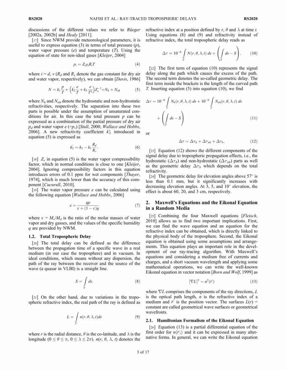
height levels chosen in ray-tracing systems controls both theaccuracy of the ray-traced delay and the computationalspeed. Therefore, a proper choice of the interpolated heightscan significantly impact the overall performance of the ray-tracer. Rocken et al. [2001] suggested an integration stepsize of 10 m between 0 and 2 km, 20 m between 2 and 6 km,50 m between 6 and 16 km, 100 m between 16 and 36 kmand 500 m between 36 and 136 km. They confirmed that thisselection yields nearly identical results (sub-millimeteragreement at 1� elevation) to a 5 m integration for the entireheight range. Urquhart [2011] utilized these integration stepsizes along the raypath, whereas Böhm and Schuh [2003]used them for vertical profiles. Nievinski [2009] employedan adaptive scheme by which the spacing is smaller or largerdepending on the smoothness of the refractivity field.Hobiger et al. [2008] proposed an iterative procedure toestimate the number of height levels. He suggested gener-ating 320 layers from each data set. This enables achievingmillimeter-level accuracy in ray-tracing even at very lowelevation angles.[57] Differences between slant delays using a constant 10-m

step and the one suggested by Rocken et al. [2001] for asample data set are shown in Figure 8. Maximum dis-crepancies are seen as expected for low elevation angles. Forelevation angles above 10�, these differences are practicallyequal to zero. It is important to mention that the number of


7 of 17

vertically interpolated and extrapolated layers using Rockenet al.’s [2001] suggestion is 872 whereas using constantincrements the number increases to 7529. This illustratesthe disadvantages of the constant increments from a com-putational efficiency point of view. In this case both thepre-calculation and the main ray-tracing computations willbe very time consuming without any considerableimprovement of the final results. Maximum absolute andmean values of differences between slant delays of thesetwo selections are 0.7 mm and 0.08 mm respectively for anelevation angle of 5�, which corresponds to a station heighterror of about 0.1 mm.

4.5. Time Interpolation

[58] For geodetic applications we need to compute thetotal delay for each observation epoch. The observation rateis dependent on the space geodetic technique. Since NWMprovide data every 3 or 6 h, time interpolation between twoepochs has to be carried out. Weighted averaging (linearinterpolation) can be used to calculate the meteorologicalparameters for the time of interest.

4.6. Solutions of the Partial Differential Equations

[59] As mentioned before, finding solutions of the partialdifferential equations is an important part of solving theEikonal equation. In fact, the Eikonal equation is nothing buta system of equations containing seven (in 3D case) or five(in 2D case) differential equations.[60] Runge–Kutta methods, as an important family of

implicit and explicit methods for the approximation ofsolutions of ordinary differential equations, can be used forthis task. Equations (A9) to (A14) (see Appendix A) showthe initial values for the unknowns, which are the coordi-nates (r, q, l) of each point along the raypath in a specificcoordinate system (which is in our case a spherical coordi-nate system), and the elements of the ray direction in thesepoints (Lr, Lq, Ll).[61] To find the components of the gradient, which are

needed for the Eikonal equation, different methods may beused. One possibility is presented by Hobiger et al. [2008],where four points around the point of interest in the aboveand below layers are involved and a bilinear interpolation isperformed to find the final result. This method can beimproved if we use more than four points in a layer and a

different interpolation method. In this paper we have used8 points along the meridian and a spline interpolation. Thischoice is based on our investigation shown in the subsectionon horizontal interpolation. However, this part of the workcan be reduced considerably if we restrict our calculationsonly to the 2D case, where the horizontal components of thegradient are set to zero.

4.7. Gradient Components of the Refractive Index

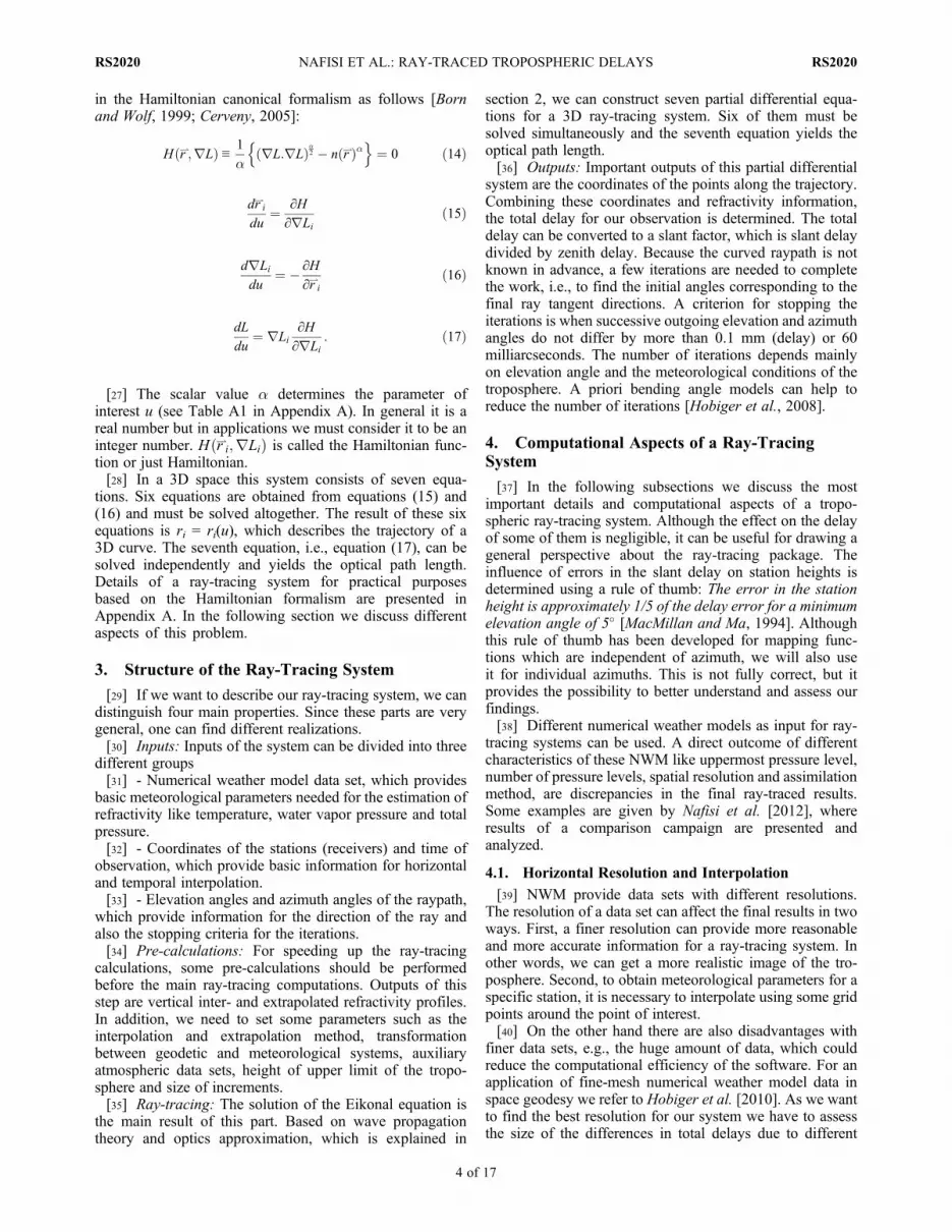
[62] An important question is whether a 2D or 3D ray-tracing algorithm should be used. We know that 2D methodsare faster and therefore more efficient than 3D methods interms of time. In this subsection we discuss this challengefrom different viewpoints and try to quantify these effects.Figure 9 shows horizontal gradient values for stationsWettzell and Tsukuba.[63] The most important difference between a 2D and 3D

ray-tracing method is the negligence of out of plane com-ponents of the trajectory in the 2D case. In other words, inthe 2D case the ray is not allowed to leave the plane ofconstant azimuth. In fact, we have assumed azimuthal

Figure 8. Differences between slant delays using constantstep sizes of 10 m and those suggested by Rocken et al.[2001] for station Tsukuba, August 12th, 2008.

Figure 9. Horizontal gradient values (sum of the two hor-izontal components of the gradient) in mm for stationsWettzell (red) and Tsukuba (black).

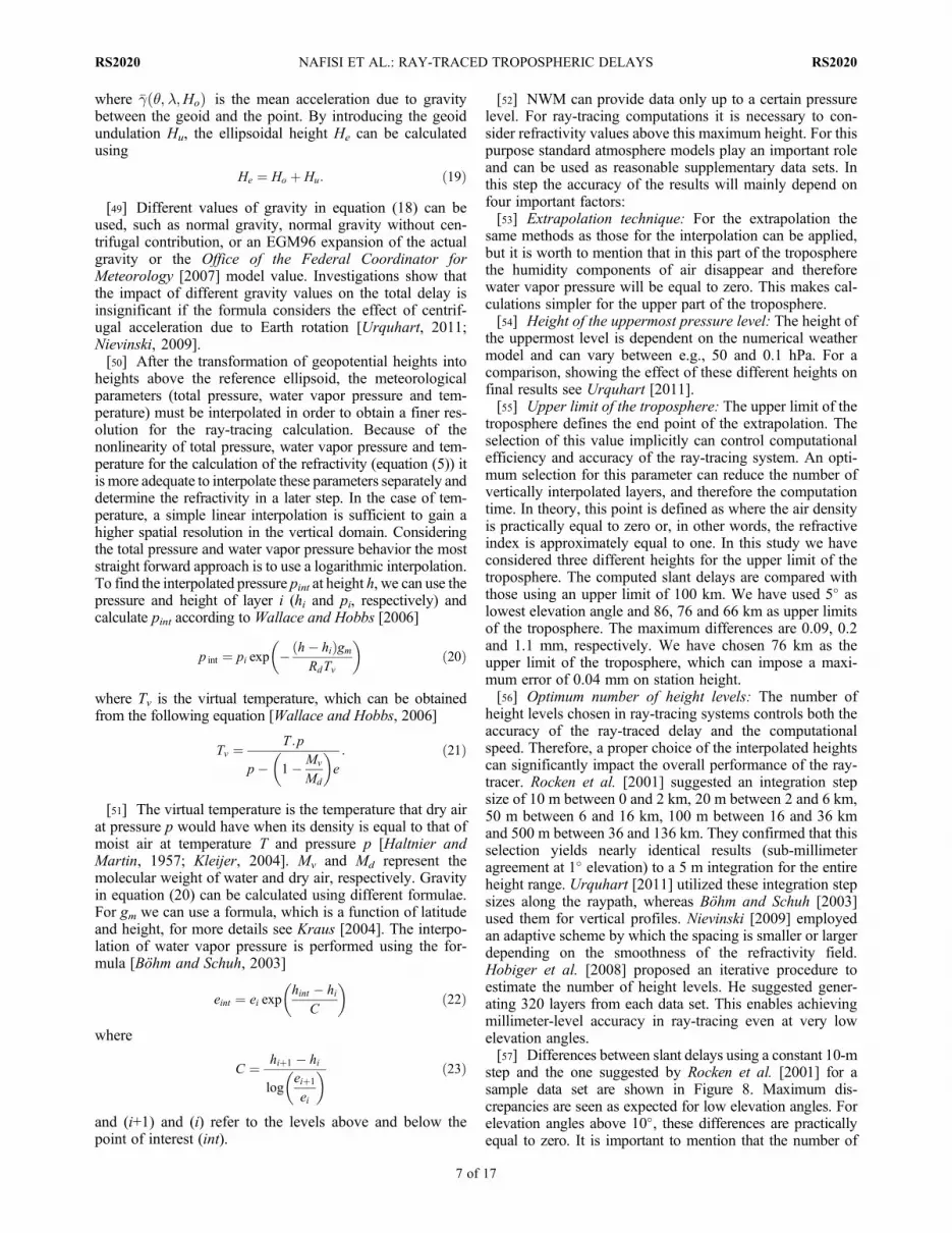
Figure 10. Delay differences between 2D and 3D at 5� ele-vation for station Wettzell at epoch of first availableECMWF data set on August 13th 2008. Red: Difference intotal delay, black: Difference in total delay without geomet-ric delay, blue: Difference in geometric delay.


8 of 17

asymmetry of the troposphere but ignored the effect of gra-dients, which is due to the out of plane components. Figures 10and 11 show the differences between 2D and 3D ray-traceddelays for the VLBI stations Tsukuba and Wettzell, respec-tively. In Table 2, these differences are summarized in terms ofmean and maximum absolute values for nine VLBI stationsparticipating in CONT08.[64] As by-products of our ray-tracing system we can cal-

culate the refractivity gradient components and therefore findthe effect of these components along the raypath (for i = 1 tomvertical layers) as follows

DSr r;l;qð Þ ¼Xmi¼1

∂n r;l; qð Þ∂r i

þ 1

r

∂n r;l; qð Þ∂q i

��

�

þ 1

r sin q∂n r;l; qð Þ

∂l

��i

�dsi: ð24Þ

[65] In Figure 9, the last two terms in equation (24) arereferred to as gradient. We see a very similar pattern for geo-metric delay differences and gradient effects. Gu and Brunner[1990] have developed a formula, which shows analyticallythe dependency of the curvature (geometric delay) on thegradient components. Their original equation is developed forrefractivity in a dispersive medium, which depends on fre-quency in addition to position. For the troposphere, it is

possible to modify this equation to be a function of refractiveindex in a non-dispersive medium [Wijaya, 2010]. Since slantdelays usually increase at lower elevation angles, also thedifference between 2D and 3D ray-traced delays is largestclose to the horizon. To illustrate this difference with respect toelevation angle, we calculated 2D and 3D ray-traced delays forall CONT08 observations, and the difference is shown inFigure 12.

5. Application in VLBI Analysis

[66] The principle observable in geodetic VLBI is thedifference in arrival times at two or more radio telescopes ofsignals emitted by distant extragalactic radio sources. Due tothe very long baselines (up to one diameter of the Earth)between the telescopes, the delay in the neutral atmospherediffers from station to station significantly, and an error inthe modeled delay enters into geodetic parameters likebaseline lengths or Earth orientation parameters. Recentstudies based on turbulence [e.g., Pany et al., 2011; Nilssonand Haas, 2010] have shown that troposphere delay mod-eling is and will continue to be the most critical error sourcein the analysis of VLBI observations. However, compared toobservations with the Global Navigation Satellite Systems(GNSS), VLBI is very well suited for the accuracy assess-ment of ray-traced delays at low elevation angles because itis not subject to effects like phase center variations ormultipath.

Figure 11. Delay differences between 2D and 3D at 5� ele-vation for station Tsukuba at epoch of first availableECMWF data set on August 13th 2008. Red: Difference intotal delay, black: Difference in total delay without geomet-ric delay, blue: Difference in geometric delay.

Table 2. Differences Between 2D and 3D Ray-Traced Delays (2D Minus 3D) in mm for Nine CONT08 StationsComputed From the First Available ECMWF Data Each Day From August 12th – 16th, 2008 at 5� Elevation

VLBI StationMean

(Hyd. + Non-hyd.)Maximum Absolute(Hyd. + Non-hyd.)

Mean(Bending Only)

Maximum Absolute(Bending Only)

Tsukuba 12.8 31.7 �5.1 11.0Wettzell 5.6 13.2 �0.6 2.5HartRAO �1.7 3.2 �0.2 1.2Kokee �0.6 2.5 �0.2 1.4Medicina 10.2 16.5 �1.4 4.9Onsala 8.2 14.6 �0.3 1.4TIGOCONC 3.9 15.2 �1.1 3.3Westford 2.0 6.6 �0.5 1.6Zelenchk 3.6 9.7 �0.7 2.8

Figure 12. Differences between 3D and 2D ray-traceddelays with respect to the elevation angle, calculated for allobservations of CONT08.


9 of 17

5.1. CONT08 Baseline Length Repeatabilities

[67] Ray-traced tropospheric delays are included in theVLBI analysis of the CONT08 experiment.[68] For this validation we used the Vienna VLBI Soft-

ware (VieVS) [Böhm et al., 2011], which has been modifiedto read external ray-traced delays. Station coordinates wereestimated using the No Net Translation (NNT) and the NoNet Rotation (NNR) condition on VTRF2008 [Böckmannet al., 2010]. Atmospheric loading [Petrov and Boy, 2004]and tidal ocean loading [Scherneck, 1991] based on the oceanmodel FES2004 [Lyard et al., 2006] were considered. Sourcecoordinates were fixed to ICRF2. Five constant Earth orien-tation parameters were estimated in addition to IERS EOP 05C04 [Gambis, 2004; Bizouard and Gambis, 2009]. For aquality assessment we use baseline length repeatabilities, i.e.,standard deviations of baseline lengths from the 15 CONT08sessions.[69] The results are compared to those of a standard

approach where a priori total delays are set up as the sum ofhydrostatic and wet slant delays, each of them being theproduct of the zenith delay derived from data of theECMWF and the respective mapping function (VMF1)[Böhm et al., 2006a]. Both models, ray-tracing andECMWF/VMF1, include the wet part, and, if residual zenithdelays are estimated, the wet mapping function is used aspartial derivative.[70] We have analyzed three approaches: (1) Estimating

zenith delays and gradients in the analysis, (2) estimating

zenith delays but not estimating gradients, and (3) estimatingneither zenith delays nor gradients. The setup of the ray-tracing system used in this investigation (called ‘standardversion’) is summarized in Table 3.[71] In general, if gradients and residual zenith delays are

estimated, the application of ray-traced delays yields similar

Table 3. Details of the Standard Ray-Tracing System

Parameter Option

Horizontal interpolation splineNumber of points around 8 points, along the meridianRefractivity constants Rüeger best averageHorizontal resolution

of data set0.5�

Type 2DSupplementary atmosphere U.S.76Radius of curvature

of the EarthGaussian curvature

Gravity National Imagery and MappingAgency [2000]

Vertical interpolation(extrapolation)

temperature and specific humidity:linear, pressure: logarithmically

Height of upper limit of thetroposphere

76 Km

Figure 13. Baseline length repeatabilities using ray-traceddelays (red) and ECMWF/VMF1 (black); gradients andzenith wet delays are estimated in both cases.

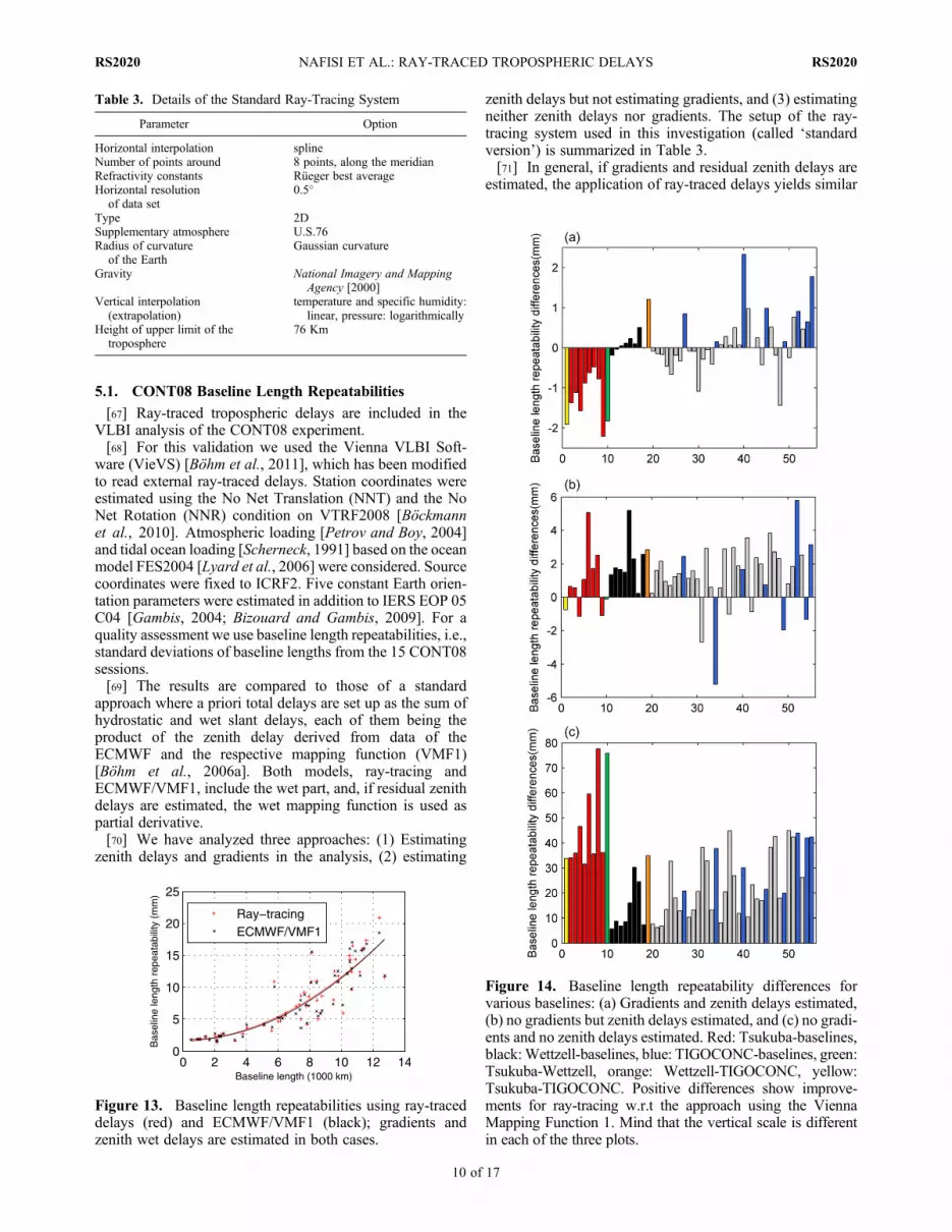
Figure 14. Baseline length repeatability differences forvarious baselines: (a) Gradients and zenith delays estimated,(b) no gradients but zenith delays estimated, and (c) no gradi-ents and no zenith delays estimated. Red: Tsukuba-baselines,black:Wettzell-baselines, blue: TIGOCONC-baselines, green:Tsukuba-Wettzell, orange: Wettzell-TIGOCONC, yellow:Tsukuba-TIGOCONC. Positive differences show improve-ments for ray-tracing w.r.t the approach using the ViennaMapping Function 1. Mind that the vertical scale is differentin each of the three plots.


10 of 17

baseline length repeatabilities as the standard approach withmapping functions (Figure 13). It should be mentioned herethat the estimation of gradients also accounts for other azi-muth-dependent non-tropospheric error sources (e.g., sys-tematic cable stretching in case of VLBI; multipath andunmodeled phase center variations in case of GNSS).[72] However, taking a closer look at the stations, ray-

traced delays provide better tropospheric corrections at somestations, whereas at other stations the corrections are worse.The dependency on particular baselines is shown inFigure 14, where the results for three stations (Tsukuba,Wettzell, and TIGOCONC) are highlighted. According toFigure 14, it can be clearly seen that ray-traced delaysdegrade baseline length repeatabilities for baselines withTsukuba if zenith delays and gradients are estimated. On theother hand, baselines including TIGOCONC are mostlyimproved. Furthermore, for the two other approaches wheregradients and/or zenith delays are not estimated, we can findsimilar clusters of these three stations.

[73] The advantages and possibilities of the ray-tracingmethod can be seen in those cases where no additional gra-dients are estimated. On average we can find an improve-ment of more than 1.2 mm in baseline length repeatabilities,which reaches more than 25 mm if no residual zenith delaysare estimated. For more details, we refer to Nafisi et al.[2011].[74] Next we present statistical values, showing how

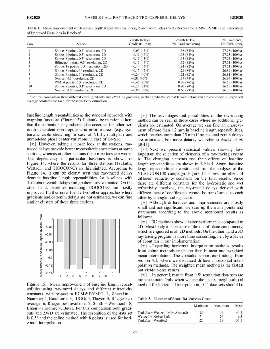
important the selection of elements of a ray-tracing systemis. The changing elements and their effects on baselinelength repeatabilities are shown in Table 4. Again, baselinelength repeatabilities are estimated from the analyses of theVLBI CONT08 campaign. Figure 15 shows the effect ofdifferent refractivity constants on the final results. Sincethere are different constants for the hydrostatic and wetrefractivity involved, the ray-traced delays derived withdifferent sets of coefficients cannot be transformed to eachother by a single scaling factor.[75] Although differences and improvements are mostly

small and not significant, we sum up the main points andstatements according to the above mentioned results asfollows:[76] - 3D methods show a better performance compared to

2D. Most likely it is because of the out of plane components,which are ignored in all 2D methods. On the other hand a 3Dray-tracing program is more time consuming, i.e., by a factorof about ten in our implementation.[77] - Regarding horizontal interpolation methods, results

from spline methods are better than bilinear and weightedmean interpolation. These results support our findings fromsection 4.1, where we discussed different horizontal inter-polation methods. The weighted mean method is the fastestbut yields worse results.[78] - In general, results from 0.5� resolution data sets are

more accurate. Only when we use the nearest neighborhoodmethod for horizontal interpolation, 0.1� data sets should be

Table 4. Mean Improvement of Baseline Length Repeatabilities Using Ray-Traced Delays With Respect to ECMWF/VMF1 and Percentageof Improved Baselines in Bracketsa

Case ModelZenith Delays,Gradients (mm)

Zenith Delays,No Gradients (mm)

No Gradients,No ZWD (mm)

1 Spline, 8 points, 0.5� resolution, 3D �0.07 (45%) 1.38 (84%) 27.08 (100%)2 Spline, 4 points, 0.5� resolution, 2D �0.10 (47%) 1.35 (84%) 27.05 (100%)3 Spline, 8 points, 0.5� resolution, 2D �0.10 (45%) 1.35 (82%) 27.05 (100%)4 Bilinear,4 points, 0.5� resolution, 2D �0.13 (44%) 1.32 (82%) 27.01 (100%)5 Spline, 16 points, 0.5� resolution, 2D �0.14 (45%) 1.31 (82%) 27.01 (100%)6 Spline, 8 points, 1� resolution, 2D �0.17 (45%) 1.29 (84%) 26.99 (100%)7 Spline, 4 points, 1� resolution, 2D �0.24 (40%) 1.21 (82%) 26.91 (100%)8 Nearest, 0.1� resolution, 2D �031 (40%) 1.14 (78%) 26.84 (100%)9 WM, 4 points, 0.5� resolution, 2D �0.47 (20%) 0.98 (76%) 26.68 (100%)10 Spline, 8 points, 0.1� resolution, 2D �0.51 (33%) 0.95 (80%) 26.65 (100%)11 Nearest, 0.5� resolution, 2D �0.80 (29%) 0.65 (78%) 26.35 (100%)

aFor this comparison three different cases (gradients and ZWD, no gradients, neither gradients nor ZWD were estimated) are considered. Rüeger bestaverage constants are used for the refractivity estimation.

Figure 15. Mean improvement of baseline length repeat-abilities using ray-traced delays and different refractivityconstants, with respect to ECMWF/VMF1. 1, Zhevakin –Naumov; 2, Boudouris; 3, IUGG; 4, Thayer; 5, Rüeger bestaverage; 6, Rüeger best available; 7, Smith – Weintraub; 8,Essen – Froome; 9, Bevis. For this comparison both gradi-ents and ZWD are estimated. The resolution of the data setis 0.5� and the spline method with 8 points is used for hori-zontal interpolation.

Table 5. Number of Scans for Various Cases

Minimum Maximum Mean

Tsukuba + Wettzell (+Ny Ålesund) 25 44 41.2Wettzell + Kokee Park 7 24 16.3Tsukuba + Westford 22 39 31.1


11 of 17

used instead of 0.5�. It should be mentioned that the size ofthe data sets also affects the efficiency of processing. Forexample, in a pre-calculation step of our method, meteoro-logical parameters from gridded ECMWF data sets areconverted to refractivity index profiles and saved in a binaryMatlab-internal format. The file size for one epoch is onaverage 6 and 127 MB for resolutions 0.5� and 0.1�,respectively. This means that during the main processingstep more memory is needed for loading the high resolutionprofiles and the computation time increases.[79] - Regarding the “no gradient” case, 76% of all base-

lines are improved when using ray-traced delays instead ofthe standard approach ECMWF/VMF1. The averageimprovement over all baselines is 1.18 mm.[80] - In the “no gradient, no zenith delay” case, improve-

ments compared to ECMWF/VMF1 can be seen for allbaselines, on average by 26.97 mm. However, the repeat-ability for both methods (ECMWF/VMF1 and ray-tracing) issignificantly degraded compared to the “no gradient” case.[81] - Furthermore, we want to mention that even in the

case of applying ray-traced delays and estimating zenithdelays, the additional estimation of gradients improvesbaseline length repeatabilities significantly (not shown here).

5.2. Universal Time (UT1) Estimation From IntensiveSessions

[82] Another test for the validity of ray-traced delays is theestimation of UT1-UTC from VLBI Intensive sessions.Since usually only two or three stations are observing forone hour in these sessions, they are very sensitive to asym-metries in the troposphere delays around the stations,

because those asymmetries are not averaged out over timeand over stations as is the case with 24-h sessions containingfive or more stations. Böhm et al. [2010] found improvementin UT1 values for ray-traced delays at Tsukuba that weredetermined from data of the Japan Meteorological Agency(JMA).[83] The IVS Intensive sessions are usually separated into

three groups: (1) Intensive 1 (INT1) sessions operated fromMonday through Friday at 18:30, where Kokee Park andWettzell are involved. Tsukuba and Wettzell observe togetherin (2) Intensive 2 (INT2) sessions, which run on Saturday andSunday at 7:30. Finally there are (3) Intensive 3 (INT3) ses-sions every Monday at 7:00 containing Tsukuba, Wettzell andNy Ålesund.[84] For our investigation, we used Intensive sessions

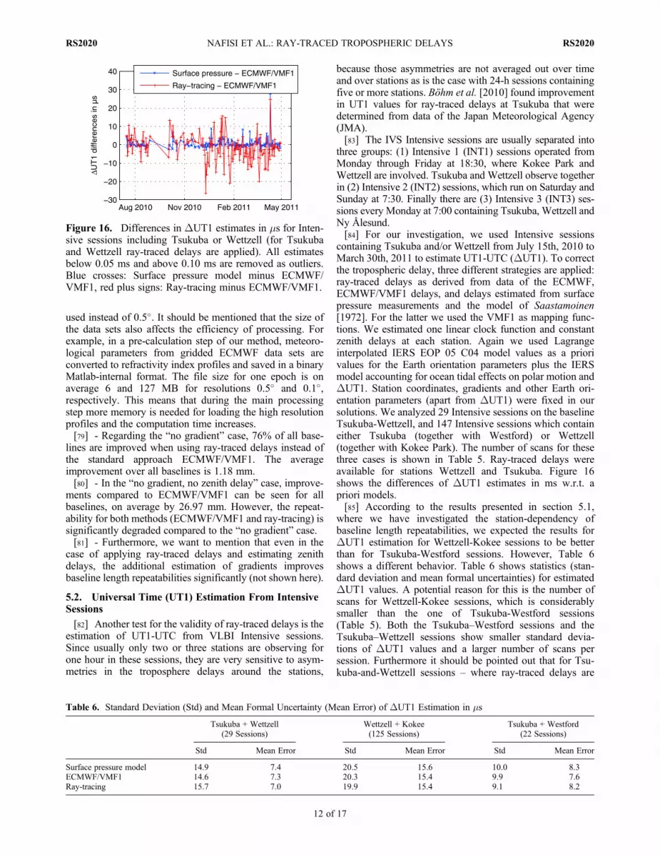
containing Tsukuba and/or Wettzell from July 15th, 2010 toMarch 30th, 2011 to estimate UT1-UTC (DUT1). To correctthe tropospheric delay, three different strategies are applied:ray-traced delays as derived from data of the ECMWF,ECMWF/VMF1 delays, and delays estimated from surfacepressure measurements and the model of Saastamoinen[1972]. For the latter we used the VMF1 as mapping func-tions. We estimated one linear clock function and constantzenith delays at each station. Again we used Lagrangeinterpolated IERS EOP 05 C04 model values as a priorivalues for the Earth orientation parameters plus the IERSmodel accounting for ocean tidal effects on polar motion andDUT1. Station coordinates, gradients and other Earth ori-entation parameters (apart from DUT1) were fixed in oursolutions. We analyzed 29 Intensive sessions on the baselineTsukuba-Wettzell, and 147 Intensive sessions which containeither Tsukuba (together with Westford) or Wettzell(together with Kokee Park). The number of scans for thesethree cases is shown in Table 5. Ray-traced delays wereavailable for stations Wettzell and Tsukuba. Figure 16shows the differences of DUT1 estimates in ms w.r.t. apriori models.[85] According to the results presented in section 5.1,

where we have investigated the station-dependency ofbaseline length repeatabilities, we expected the results forDUT1 estimation for Wettzell-Kokee sessions to be betterthan for Tsukuba-Westford sessions. However, Table 6shows a different behavior. Table 6 shows statistics (stan-dard deviation and mean formal uncertainties) for estimatedDUT1 values. A potential reason for this is the number ofscans for Wettzell-Kokee sessions, which is considerablysmaller than the one of Tsukuba-Westford sessions(Table 5). Both the Tsukuba–Westford sessions and theTsukuba–Wettzell sessions show smaller standard devia-tions of DUT1 values and a larger number of scans persession. Furthermore it should be pointed out that for Tsu-kuba-and-Wettzell sessions – where ray-traced delays are

Table 6. Standard Deviation (Std) and Mean Formal Uncertainty (Mean Error) of DUT1 Estimation in ms

Tsukuba + Wettzell(29 Sessions)

Wettzell + Kokee(125 Sessions)

Tsukuba + Westford(22 Sessions)

Std Mean Error Std Mean Error Std Mean Error

Surface pressure model 14.9 7.4 20.5 15.6 10.0 8.3ECMWF/VMF1 14.6 7.3 20.3 15.4 9.9 7.6Ray-tracing 15.7 7.0 19.9 15.4 9.1 8.2

Figure 16. Differences in DUT1 estimates in ms for Inten-sive sessions including Tsukuba or Wettzell (for Tsukubaand Wettzell ray-traced delays are applied). All estimatesbelow 0.05 ms and above 0.10 ms are removed as outliers.Blue crosses: Surface pressure model minus ECMWF/VMF1, red plus signs: Ray-tracing minus ECMWF/VMF1.


12 of 17

applied for both stations – the standard deviation is largercompared to the mapping function approaches whereas themean of the formal errors is smaller. A reason for this mightbe the fact that the standard deviation shows the agreementof DUT1 values to the a priori EOP model (IERS EOP 05C04). Since the surface pressure and the VMF1 are used forthe determination of the IERS EOP 05 C04 model, thestandard deviation values are smaller although the formalerrors are larger compared to the use of ray-traced delays. Inany case, considering the small differences, a further inves-tigation is strongly desirable.[86] DUT1 values as for example derived from VLBI

Intensive sessions can be converted to length-of-day (LOD)values. Length-of-day is the negative time derivative ofDUT1 = UT1�UTC

LOD ¼ � ∂DUT1

∂t: ð25Þ

[87] These variations can be measured very accurately byGNSS and they are publicly available at the IGS (Interna-tional GNSS Service) webpage at http://igscb.jpl.nasa.gov/.Using GNSS length-of-day (LOD) values allows us to per-form an external validation of the derived DUT1 values,independent of the IERS 05 C04 values. Hence we are able

to give quantitative statements about the different tropo-spheric correction methods.[88] We estimated length-of-day values as shown in

equation (25) for all Intensive sessions from consecutivedays. If we allow the time span of two sessions defining oneLOD value to exceed 24 (�1) hours, we get less accurateresults. The LOD value we calculate is valid between theepochs of the two sessions. These values as well as thosefrom IGS are shown in Figure 17.[89] For the comparison we interpolated the IGS LOD

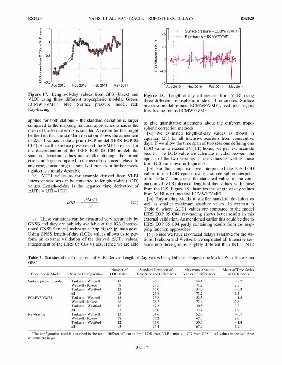
values to our LOD epochs using a simple spline interpola-tion. Table 7 summarizes the statistical values of the com-parison of VLBI derived length-of-day values with thosefrom the IGS. Figure 18 illustrates the length-of-day valuesfrom VLBI w.r.t. method ECMWF/VMF1.[90] Ray-tracing yields a smaller standard deviation as

well as smaller maximum absolute values. In contrast toTable 6, where DUT1 values are compared to the modelIERS EOP 05 C04, ray-tracing shows better results in thisexternal validation. As mentioned earlier this could be due toIERS EOP 05 C04 partly containing results from the map-ping function approaches.[91] Since we have ray-traced delays available for the sta-

tions Tsukuba and Wettzell, we separated all Intensive ses-sions into three groups, slightly different than INT1, INT2

Figure 17. Length-of-day values from GPS (black) andVLBI using three different tropospheric models. Green:ECMWF/VMF1, blue: Surface pressure model, red:Ray-tracing.

Table 7. Statistics of the Comparison of VLBI-Derived Length-of-Day Values Using Different Tropospheric Models With Those FromGPSa

Tropospheric Model Session ConfigurationNumber ofLOD Values

Standard Deviation ofTime Series of Differences

Maximum AbsoluteValues of Differences

Mean of Time Seriesof Differences

Surface pressure model Tsukuba - Wettzell 13 26.5 54.4 �2.2Wettzell - Kokee 68 28.5 71.2 2.5Tsukuba - Westford 12 17.0 34.0 �0.3all 93 26.8 71.2 1.5

ECMWF/VMF1 Tsukuba - Wettzell 13 25.8 52.3 �1.5Wettzell - Kokee 68 28.2 72.4 2.8Tsukuba - Westford 12 17.3 30.5 0.3all 93 26.6 72.4 1.9

Ray-tracing Tsukuba - Wettzell 13 24.6 52.6 �0.7Wettzell - Kokee 68 27.2 67.9 3.0Tsukuba - Westford 12 13.0 30.6 �1.4all 93 25.4 67.9 1.9

aThe configuration used is described in the text. “Difference” stands for “‘LOD from VLBI’ minus ‘LOD from GPS’.” All values in the last threecolumns are in ms.

Figure 18. Length-of-day differences from VLBI usingthree different tropospheric models. Blue crosses: Surfacepressure model minus ECMWF/VMF1, red plus signs:Ray-tracing minus ECMWF/VMF1.


13 of 17

and INT3: (1) Sessions where both Tsukuba and Wettzellobserve (IVS INT2 and INT3 sessions), (2) Wettzell-Kokeesessions (IVS INT1) and (3) Tsukuba-Westford sessions.The statistics for the comparison separated into Tsukuba-Wettzell sessions, Tsukuba-Westford sessions and Wettzell-Kokee sessions are shown in Table 7.[92] The clearly smallest value of the standard deviations

is found for Tsukuba-Westford sessions. This group alsoshows the largest improvement due to ray-tracing. This is onthe one hand surprising but on the other hand the largestimprovement in standard deviation ofDUT1 values was alsofound for this session-group. However, the rather smallnumber of only 12 length-of-day values should be men-tioned for Tsukuba-Westford sessions.[93] Wettzell-Kokee sessions (IVS INT1 sessions) show

the largest standard deviation for all three models. Again,this is in a good agreement with the values from Table 6where this group shows the largest standard deviation ofDUT1 values as well as mean values of formal errors. Asmentioned above, the reason for this is the small number ofscans of these sessions (see Table 5). Another interestingfinding is that the model ECMWF/VMF1 shows a betteroverall accuracy than the surface pressure model. Regardingbaseline length repeatabilites from CONT08 this trend couldnot be seen clearly.[94] To sum up the ray-tracing performance with respect

to LOD estimation, this method improves the standarddeviation of the difference to LOD from GPS, on average bymore than 4.5%. However, we cannot explain why theimprovement for Tsukuba-Westford sessions is larger thanfor Wettzell-Kokee sessions, whereas the baseline lengthrepeatabilities show an exactly opposite behavior.

6. Summary and Outlook

[95] Using the Maxwell’s equations, a system of partialdifferential equations is obtained, which is the starting pointof establishing a ray-tracing algorithm. Ray-traced delays,obtained from this equation system as shown in section 2.1,were used to process VLBI observations. Important elementsof a ray-tracing system are analyzed in section 4, where wehave shown a comparison for different options. Thesecomparisons help us to find an optimal adjustment for atypical ray-tracing package and show us details about com-putational aspects of it.[96] The validity of ray-tracing can be assessed by com-

paring baseline length repeatabilities for CONT08 usingdifferent models for the a priori tropospheric delay. At thisstage we can conclude that if gradients and residual zenithdelays are estimated, ray-traced delays yield accuraciessimilar to the standard approach. However, at some stationsray-traced delays provide better tropospheric corrections,whereas at other stations the corrections are worse. To find areason for this, more investigations need to be carried out.The advantages and abilities of the ray-tracing method

become evident when no additional gradients are estimatedand applied in the VLBI processing. In this case the averageimprovement is more than 10% in baseline length repeat-abilities, and these improvements increase to more than21%, if in addition no residual zenith delays are considered.[97] As shown in section 5.1, a perfect solution for tropo-

spheric delays would be a combination of ray-traced delaysand delays derived from standard methods using mappingfunctions. Then we can decide what kind of delay would beapplied for which stations. However, more investigation isneeded to find the causes which contribute to these differentbehaviors for some stations. Possible reasons are meteoro-logical conditions and in particular the variability of themeteorological parameters like temperature and water vaporpressure which change the gradient of refractive index.[98] Another investigation is carried out by applying ray-

traced delays in VLBI Intensive sessions, which containTsukuba and/or Wettzell to estimate DUT1 as an importantEarth orientation parameter. After converting to length-of-day values we compare them to GPS-derived values.According to this comparison, we find an improvement ifusing ray-traced delays. The standard deviation is decreasedby more than 4.5% compared to two commonly used map-ping function approaches.[99] With an improving accuracy and resolution of

numerical weather models in future, the application of ray-traced delays will become more beneficial in the analysis ofspace geodetic observations. However, while the provisionof ray-traced delays will be practicable in the case of VLBIwith a limited number of sites and observations, the deter-mination of ray-traced delays in the case of GNSS will bechallenging. To a certain extent, it can be realized by acombination of fast processing facilities [see, e.g., Hobigeret al., 2008] and by the application of special functions fit-ted locally to the ray-traced delays [see, e.g., Gegout et al.,2011].

Appendix A: A Ray-Tracing Systemfor Tropospheric Modeling

H r*i;rLið Þ ≡ 1

arLi:rLið Þa2 � n r*ið Þa

n o¼ 0 ðA1Þ

d r*i

du¼ ∂H

∂rLiðA2Þ

drLidu

¼ � ∂H∂ r*i

ðA3Þ

dL

du¼ rLk

∂H∂rLk

: ðA4Þ

[100] Equations (A1) to (A4) can be used to construct aray-tracing system for any specific application by simplyselecting a correct value for the scalar a. For a = 0, urepresents the travel time t along the ray. If a = 1, u repre-sents the arc length s along the ray. In the case of a = 2, u isequal to dt/dn, which represents the natural variables alongthe ray [Cerveny, 2005] (see Table A1).[101] Tropospheric ray-tracing mainly deals with the

determination of total delays along the raypath. Thus it isappropriate to select a = 1. Ray-tracing systems can beexpressed and solved in any curvilinear coordinate system,

Table A1. Different Cases for the Hamiltonian Formalism

a du Parameter of Interest

0 du = dT travel time T along the ray1 du = ds arc length s along the ray2 du = ds = dT/n2 natural variables along the ray


14 of 17

including non-orthogonal systems, which draws consider-able attention to spherical coordinates. By selecting a = 1and representing the function H in a spherical polar coordi-nate system (r, q, l), equation (A1) can be rewritten as

H r; q; l; Lr; Lq; Llð Þ ≡ L2r þ1

r2L2q þ

1

r2 sin2qL2l

� �1=2

� n r; q;l; tð Þ ¼ 0 ðA5Þ

where r is the radial distance, q is the co-latitude and l is thelongitude (0 ≤ q ≤ p, 0 ≤ l ≤ 2p). Lr = ∂L/∂r, Lq = ∂L/∂q, andLl = ∂L/∂l are the elements of the ray directions.[102] Now, by substituting equation (A5) into equations

(A2) and (A3), we obtain a system of equations in a spher-ical coordinate system as follows:

dr

ds¼ 1

BLr ðA6Þ

dqds

¼ 1

B

Lqr2

ðA7Þ

dlds

¼ 1

B

Llr2 sin2q

ðA8Þ

dLrds

¼ ∂n r; q;l; tð Þ∂r

þ 1

Br

L2qr2

þ L2lr2 sin2q

� �ðA9Þ

dLqds

¼ ∂n r; q; l; tð Þ∂q

þ 1

B

L2lr2 sin3q

ðA10Þ

dLlds

¼ ∂n r; q; l; tð Þ∂l

ðA11Þ

where

B ¼ L2r þ1

r2L2q þ

1

r2 sin2qL2l

� �1=2

¼ n r; q;l; tð Þ: ðA12Þ

[103] This system is a direct result of equations (A2) and(A3) in a 3D medium, and obviously all of the six partialdifferential equations must be solved simultaneously. Aknown and standard method for this numerical integration isRunge-Kutta’s method. The final outputs are the positions ofall points along the trajectory of a ray.[104] For solving the above ray-tracing system, the fol-

lowing initial conditions at the starting point (station) can beused [Cerveny, 2005]:

r ¼ r0 ðA13Þ

l ¼ l0 ðA14Þ

q ¼ q0 ðA15Þ

Lr0 ¼ n0 cos z0 ðA16Þ

Lq0 ¼ n0r0 sin z0 cos a0 ðA17Þ

Ll0 ¼ n0r0 sin z0 sin a0 sin q0 ðA18Þ

where a0 and z0 are the initial geodetic azimuth and zenithangle, respectively.[105] In a 3D case, horizontal gradients are important

because they can affect the bending of the raypath andtherefore the total delay. The gradient in a spherical coor-dinate system can be stated as follows:

rn r; l; qð Þ ¼ ∂n r;l; q; tð Þ∂r

þ 1

r

∂n r;l; q; tð Þ∂q

þ 1

r sinq∂n r;l; q; tð Þ

∂l:

ðA19Þ

[106] From a practical point of view, we must find asophisticated way of computing the gradient components ofthe refractive index in equations (A9), (A10) and (A11),which are

rnr ¼ ∂n r; q;l; tð Þ∂r

ðA20Þ

rnq ¼ ∂n r; q; l; tð Þ∂q

ðA21Þ

rnl ¼ ∂n r; q;l; tð Þ∂l

: ðA22Þ

[107] For details we refer to the discussion in section 4.6.Furthermore, it is possible to write the Eikonal equation andthe ray-tracing system in a curvilinear non-orthogonalcoordinate system. This form is more general but far awayfrom our practical computation. For more details andexplanations see Cerveny et al. [1988]. In the special case ofexistence of symmetries, the ray-tracing system in a curvi-linear coordinate system would be more useful. But we mustmention that in general a ray-tracing system in curvilinearcoordinates is more complex and can fail in some regions. Avery common example for singularity is to find a solution forthe ray-tracing system in spherical polar coordinates whenq ≈ 0� or q ≈ 180�. According to Cerveny [2005] a generalsolution for removing singularities such as the abovementioned, can be transformations between ray-tracingsystems in various forms. Using standard transformationrelations, a model in curvilinear coordinates can be trans-formed into a universal model in Cartesian coordinates andvice versa. Another method by Alkhalifah and Fomel[2001] proposes to add a small constant parameter (d) tosinq in the denominator of fractions in the ray-tracingequations. This yields a higher numerical stability. How-ever, this small constant must be selected carefully, other-wise it may lead to unreasonable results.[108] Another important purpose of a ray-tracing system is

to find the optical path length. By substituting equation (A5)into equation (A4) and solving the integration, we can obtainthis important and well-known equation to calculate theoptical path length L.

L ¼Z

n r; q;lð Þ ds: ðA23Þ

[109] Once the position of a point along the raypath hasbeen determined by equations (A6) to (A11), the refractiveindex n and the optical path length L can be calculated usingequation (A23).[110] 3D ray-tracing can be easily reduced to 2D ray-

tracing by setting ∂n/∂q = 0 and ∂n/∂l = 0 in equations(A10) and (A11). In this case, we assume that the ray does


15 of 17

not leave the plane of constant azimuth. For the 2D case, thesystem of six partial differential equations (A6) to (A11) isreduced to four equations:

dr

ds¼ 1

BLr ðA24Þ

dqds

¼ 1

B

Lqr2

ðA25Þ

dLrds

¼ ∂n r; q; lð Þ∂r

þ 1

Br

L2qr2

þ L2lr2 sin2q

� �ðA26Þ

dLqds

¼ 1

B

L2lr2 sin3q

: ðA27Þ

[111] Equation (A23) remains valid also for a 2D ray-tracing system. Further simplification for a horizontallystratified atmosphere can be applied to improve the calcu-lation speed [Thayer, 1967].[112] The Eikonal equation requires, as a validity condi-

tion, that the refractive index does not change significantlyover a distance equal to the wavelength of the radiation[Kravtsov and Orlov, 1990]. If this is the case, the geomet-rical optics approximation is applicable. This conditionstates that the refractive index of a medium for an EM wavevaries only slowly [Wijaya, 2010].[113] It is also possible to discuss another aspect of this

validity condition, when we consider a turbulent conditionfor the troposphere. In this case an important factor, whichimposes limitations to the geometrical optics approximation,is the physics of the turbulence which is characterized byeddies of different size. Also the geometrical opticsapproximation is valid if the wavelength of the interestedsignal is small enough. For more details seeWheelon [2001].

[114] Acknowledgments. We like to thank the International VLBIService for Geodesy and Astrometry (IVS) [Schlüter and Behrend, 2007]for coordinating the CONT08 campaign. J. Böhm thanks the Zentralanstaltfür Meteorologie und Geodynamik (ZAMG) for granting access to dataof the ECMWF. V. Nafisi thanks the Austrian Science Fund (FWF) forsupporting this research under project P20902-N10 (GGOS Atmosphere).V. Nafisi would also like to acknowledge the University of Tehran, the IranMinistry of Science, Research and Technology (MSRT) and the Universityof Isfahan, Iran, for funding part of his research at Vienna University ofTechnology. The authors would like to thank Thomas Hobiger and twoanonymous reviewers for their valuable comments which helped to improvethis paper.

ReferencesAlkhalifah, T., and S. Fomel (2001), Implementing the fast marchingEikonal solver: Spherical versus Cartesian coordinates,Geophys. Prospect.,49, 165–178, doi:10.1046/j.1365-2478.2001.00245.x.

Bean, B. R. (1962), The radio refractive index of air, Proc. IRE, 50(3),260–273, doi:10.1109/JRPROC.1962.288318.

Bean, B. R., and G. D. Thayer (1959), CRPL Exponential ReferenceAtmosphere, Natl. Bur. of Stand. Monogr., vol. 4, U.S. Gov. Print.Off., Washington, D. C. [Available at http://digicoll.manoa.hawaii.edu/techreports/PDF/NBS4.pdf]

Bevis, M., S. Businger, S. Chiswell, T. Herring, R. Anthes, C. Rocken, andR. Ware (1994), GPS meteorology: Mapping zenith wet delays onto pre-cipitable water, J. Appl. Meteorol., 33, 379–386, doi:10.1175/1520-0450(1994)033<0379:GMMZWD>2.0.CO;2.

Bizouard, C., and D. Gambis (2009), The combined solution C04 forEarth orientation parameters consistent with International TerrestrialReference Frame, in Geodetic Reference Frames, edited by H. Drewes,pp. 265–270, Springer, Dordrecht, Netherlands.

Böckmann, S., T. Artz, and A. Nothnagel (2010), VLBI terrestrial referenceframe contributions to ITRF2008, J. Geod., 84, 201–219, doi:10.1007/s00190-009-0357-7.

Böhm, J., and H. Schuh (2003), Vienna mapping functions, in Proceedings ofthe 16th Working Meeting on European VLBI for Geodesy and Astrometry,pp. 131–143, Verlag des Bundesamtes für Kartogr. und Geod., Frankfurt,Germany.

Böhm, J., B. Werl, and H. Schuh (2006a), Tropospheric mapping functionfor GPS and very long baseline interferometry from European Center forMedium-range Weather Forecasts operational analysis data, J. Geophys.Res., 111, B02406, doi:10.1029/2005JB003629.

Böhm, J., A. Niell, P. Tregoning, and H. Schuh (2006b), The Global Map-ping Function (GMF): A new empirical mapping function based on datafrom numerical weather model data, Geophys. Res. Lett., 33, L07304,doi:10.1029/2005GL025546.

Böhm, J., T. Hobiger, R. Ichikawa, T. Kondo, Y. Koyama, A. Pany,H. Schuh, and K. Teke (2010), Asymmetric tropospheric delays fromnumerical weather models for UT1 determination from VLBI intensivesessions on the baseline Wettzell-Tsukuba, J. Geod., 84(5), 319–325,doi:10.1007/s00190-010-0370-x.

Böhm, J., S. Böhm, T. Nilsson, A. Pany, L. Plank, H. Spicakova, K. Teke,and H. Schuh (2011), The new Vienna VLBI software, in IAG Scien-tific Assembly 2009, Int. Assoc. of Geod. Symp., vol. 136, edited byS. Kenyon, M. C. Pacino, and U. Marti, pp. 1007–1012, Springer,Berlin.

Born, M., and E. Wolf (1999), Principles of Optics, 7th ed., 952 pp.,Cambridge Univ. Press, New York.

Boudouris, G. (1963), On the index of refraction of air, the absorption anddispersion of centimetre waves by gases, J. Res. Natl. Bur. Stand., Sect.D, 67D(6), 631–684.

Cerveny, V. (2005), Seismic Ray Theory, 713 pp., Cambridge Univ. Press,New York.

Cerveny, V., L. Klimes, and I. Psencik (1988), Complete seismic-ray trac-ing in three-dimensional structures, in Seismological Algorithms, editedby D. J. Doornbos, pp. 89–168, Academic, San Diego, Calif.

Chen, G., and T. A. Herring (1997), Effects of atmospheric azimuthal asym-metry on the analysis of space geodetic data, J. Geophys. Res., 102(B9),20,489–20,502, doi:10.1029/97JB01739.

Cucurull, L. (2010), Improvement in the use of an operational constellationof GPS radio-occultation receivers in weather forecasting, Weather Fore-cast., 25, 749–767, doi:10.1175/2009WAF2222302.1.

Davis, J. L. (1986), Atmospheric propagation effects on radio interferome-try, PhD thesis, Harvard Coll. Obs., Mass. Inst. of Technol., Cambridge.[Available at http://hdl.handle.net/1721.1/27953]

Davis, J. L., T. A. Herring, I. I. Shapiro, A. E. E. Rogers, and G. Elgered(1985), Geodesy by radio interferometry: Effects of atmospheric model-ing errors on estimates of baseline length, Radio Sci., 20(6), 1593–1607.

Essen, L. (1953), The refractive indices of water vapour, air, oxygen, nitro-gen, hydrogen, deuterium and helium, Proc. Phys. Soc. B, 66, 189–193,doi:10.1088/0370-1301/66/3/306.

Essen, L., and K. D. Froome (1951), The refractive indices and dielectricconstants of air and its principal constituents at 24 GHz, Proc. Phys.Soc., Sect. B, 64, 862–875, doi:10.1088/0370-1301/64/10/303.

Fleisch, D. (2010), A Student’s Guide to Maxwell’s Equations, 134 pp.,Cambridge Univ. Press, Cambridge, U. K.

Gambis, D. (2004), Monitoring Earth orientation using space-geodetic tech-niques: State-of-the-art and prospective, J. Geod., 78(4–5), 295–303,doi:10.1007/s00190-004-0394-1.

Gegout, P., R. Biancale, and L. Soudarin (2011), Adaptive mapping func-tions to the azimuthal anisotropy of the neutral atmosphere, J. Geod.,85(10), 661–677, doi:10.1007/s00190-011-0474-y.

Ghoddousi-Fard, R. (2009), Modelling tropospheric gradients and para-meters from NWP models: Effects on GPS estimates, PhD thesis,216 pp., Dep. of Geod. and Geomatics Eng., Univ. of N. B., Fredericton,N. B., Canada. [Available at http://gge.unb.ca/Pubs/TR264.pdf]

Gu, M., and F. K. Brunner (1990), Theory of the two frequency dispersiverange correction, Manuscr. Geod., 15, 357–361.

Haltnier, G. J., and F. L. Martin (1957), Dynamical and Physical Mete-orology, McGraw-Hill, New York.

Healy, S. B. (2011), Refractivity coefficients used in the assimilation ofGPS radio occultation measurements, J. Geophys. Res., 116, D01106,doi:10.1029/2010JD014013.

Hecht, E. (2001), Optics, 4th ed., 698 pp., Addison-Wesley, Boston, Mass.Hobiger, T., R. Ichikawa, Y. Koyama, and T. Kondo (2008), Fast and accu-rate ray-tracing algorithms for real-time space geodetic applications usingnumerical weather models, J. Geophys. Res., 113, D20302, doi:10.1029/2008JD010503.

Hobiger, T., S. Shimada, S. Shimizu, R. Ichikawa, Y. Koyama, and T.Kondo (2010), Improving GPS positioning estimates during extreme


16 of 17

weather situations by the help of fine-mesh numerical weather models,J. Atmos. Sol. Terr. Phys., 72(2–3), 262–270, doi:10.1016/j.jastp.2009.11.018.

Kleijer, F. (2004), Tropospheric modeling and filtering for precise GPS lev-eling, PhD thesis, 262 pp., TU Delft, Delft, Netherlands. [Available athttp://enterprise.lr.tudelft.nl/publications/files/ae_kleijer_20040413.pdf]

Kraus, H. (2004), Die Atmosphäre der Erde - Eine Einführung in dieMeteorologie, 3rd ed., Springer, Berlin.

Kravtsov, Y. A., and Y. I. Orlov (1990), Geometrical Optics of Inhomoge-neous Media, Springer, Berlin.

Lyard, F., F. Lefèvre, T. Letellier, and O. Francis (2006), Modelling theglobal ocean tides: A modern insight from FES2004, Ocean Dyn., 56,394–415, doi:10.1007/s10236-006-0086-x.

MacMillan, D. S., and C. Ma (1994), Evaluation of very long baselineinterferometry atmospheric modeling improvements, J. Geophys. Res.,99(B1), 637–651, doi:10.1029/93JB02162.

Mendes, V. B. (1999), Modeling the neutral-atmosphere propagationdelay in radiometric space techniques, PhD thesis, 349 pp., Univ. ofN. B., Fredericton, N. B., Canada.

Nafisi, V., M. Madzak, J. Böhm, H. Schuh, and A. A. Ardalan (2011), Ray-traced tropospheric slant delays in VLBI analysis, in Austrian Contribu-tions to the XXV General Assembly of the International Union of Geodesyand Geophysics (IUGG), Oesterreichische Z. fuer Vermessung undGeoinf., vol. 2/2011, pp. 149–153, Österreichische Geod. Komm.,Vienna.

Nafisi, V., et al. (2012), Comparison of ray-tracing packages for tropo-sphere delays, IEEE Trans. Geosci. Remote Sens., 50(2), 469–481,doi:10.1109/TGRS.2011.2160952.

National Imagery and Mapping Agency (2000), Department of DefenseWorld Geodetic System 1984, its definition and relationships with local geo-detic systems, NIMA Tech. Rep., TR8350.2, St. Louis, Mo. [Availableat http://earth-info.nga.mil/GandG/publications/tr8350.2/wgs84fin.pdf]

Nievinski, F. G. (2009), Ray-tracing options to mitigate the neutral atmo-sphere delay in GPS, MScE thesis, 232 pp., Dep. of Geod. and GeomaticsEng., Univ. of N. B., Fredericton, N. B., Canada. [Available at http://hdl.handle.net/1882/1050]

Nilsson, T. (2008), Measuring and modeling variations in the distribution ofatmospheric water vapour using GPS, PhD thesis, Dep. of Radio andSpace Sci., Chalmers Univ. of Technol., Gothenburg, Sweden.

Nilsson, T., and R. Haas (2010), Impact of atmospheric turbulence on geo-detic very long baseline interferometry, J. Geophys. Res., 115, B03407,doi:10.1029/2009JB006579.

Office of the Federal Coordinator for Meteorology (2007), Rawinsonde andPibal Observations, Fed. Meteorol. Handb., vol. 3, Washington, D. C.

Pany, A., J. Böhm, D. MacMillan, H. Schuh, T. Nilsson, and J. Wresnik(2011), Monte Carlo simulations of the impact of troposphere, clockand measurement errors on the repeatability of VLBI positions, J. Geod.,85(1), 39–50, doi:10.1007/s00190-010-0415-1.

Petit, G., and B. Luzum (Eds.) (2010), IERS Conventions 2010, Frankfurtam Main,IERS Tech. Note, 36, 179 pp., Verlag des Bundesamts fürKartogr. und Geod., Frankfurt, Germany.

Petrov, L., and J. P. Boy (2004), Study of the atmospheric pressure loadingsignal in VLBI observations, J. Geophys. Res., 109, B03405, doi:10.1029/2003JB002500.

Rocken, C., S. Sokolovskiy, J. M. Johnson, and D. Hunt (2001),Improved mapping of tropospheric delays, J. Atmos. Oceanic Technol.,

18, 1205–1213, doi:10.1175/1520-0426(2001)018<1205:IMOTD>2.0.CO;2.

Rüeger, J. M. (2002a), Refractive indices of light, infrared and radio wavesin the atmosphere, Tech. Rep., UNISURV S-68, Sch. of Surv. and SpatialInf. Syst., Univ. of N. S. W., Kensington, N. S. W., Australia.

Rüeger, J. M. (2002b), Refractive index formulae for radio waves, paperpresented at FIG XXII International Congress, Int. Fed. of Surv.,Washington, D. C. [Available at http://www.fig.net/pub/fig_2002/js28/js28_rueger.pdf]

Saastamoinen, J. (1972), Atmospheric correction for the troposphere andstratosphere in radio ranging of satellites, in The Use of Artificial Satel-lites for Geodesy, Geophys. Monogr. Ser., vol. 15, edited by S. W.Henriksen, A. Mancini, and B. H. Chovitz, pp. 247–251, AGU,Washington, D. C.

Scherneck, H.-G. (1991), A parametrized solid earth tide model and oceantide loading effects for global geodetic baseline measurements, Geophys.J. Int., 106, 677–694, doi:10.1111/j.1365-246X.1991.tb06339.x.

Schlüter, W., and D. Behrend (2007), The International VLBI Service forGeodesy and Astrometry (IVS): Current capabilities and future prospects,J. Geod., 81(6–8), 379–387, doi:10.1007/s00190-006-0131-z.

Smith, E. K., and S. Weintraub (1953), The constants in the equation foratmospheric refractive index at radio frequencies, J. Res. Natl. Bur.Stand. U.S., 50, 39–41.

Stull, R. B. (2000), Meteorology for Scientists and Engineers, 2nd ed.,Brooks/Cole, Independence, Ky.

Teke, K., et al. (2011), Multi-technique comparison of troposphere zenithdelays and gradients during CONT08, J. Geod., 85(7), 395–413,doi:10.1007/s00190-010-0434-y.

Thayer, G. D. (1967), A rapid and accurate ray tracing algorithm for a hor-izontally stratified atmosphere, Radio Sci., 1(2), 249–252.

Thayer, G. (1974), An improved equation for the refractive index of air,Radio Sci., 9(10), 803–807, doi:10.1029/RS009i010p00803.

Urquhart, L. (2011), Assessment of tropospheric slant factor models: Com-parison with three dimensional ray-tracing and impact on geodetic posi-tioning, MScE thesis, 190 pp., Dep. of Geod. and Geomatics Eng.,Univ. of N. B., Fredericton, N. B., Canada. [Available at http://gge.unb.ca/Pubs/TR275.pdf]

Wallace, J. M., and P. V. Hobbs (2006), Atmospheric Science: An Introduc-tory Survey, 2nd ed., 483 pp., Academic, San Diego, Calif.

Wheelon, A. D. (2001), Electromagnetic Scintillation, vol. 1, GeometricalOptics, 455 pp., Cambridge Univ. Press, Cambridge, U. K.

Wijaya, D. D. (2010), Atmospheric correction formulae for space geodetictechniques, PhD thesis, 163 pp., Inst. of Eng., Geod. and Measur. Syst.,Graz Univ. of Technol., Graz, Austria.

Zhevakin, S. A., and A. P. Naumov (1967), Refraction of millimetre andsubmillimetre radio waves in the lower atmosphere, Radio Eng. Electron.Phys. Engl. Transl., 12(1), 885–894.

A. A. Ardalan and V. Nafisi, Department of Surveying and GeomaticsEngineering, College of Engineering, University of Tehran, PO Box 4563-11365, Tehran, Iran.J. Böhm, M. Madzak, and H. Schuh, Institute of Geodesy and

Geophysics, Vienna University of Technology, A-1040 Vienna, Austria.([email protected])


17 of 17

ray-traced tropospheric delays in vlbi analysis

Documents