low frequency vlbi in space using - "gas-can" satellites
TRANSCRIPT

JPL Publication 87-36
Low Frequency VLBI in Space Using "GAS-Can" Satellites Report on the May 1987 JPL Workshop
M. J. Mahoney D. L. Jones T. B. H. Kuiper R. A. Preston
(HAS&-CR-182362) LOU PBEQUENCY V L B I XN SPaCE U S I N G GAS-CAN SATELLITES: REPORT 3 P T H E HAY 7987 JPL WORKSHOP
L a b . ) 73 p CSCL 228 Unclas
1988- 14904
(Jet Propulsion
G3/90 0115285
November 1,1987
NASA National Aeronautics and Space Administration
Jet Propulsion Laboratory California Institute of Technology Pasadena, California

JPL Publication 87-36
Low Frequency VLBl in Space Using "GAS-Can" Satel I ites Report on the May 1987 JPL Workshop
M. J. Mahoney D. L. Jones T. B. H. Kuiper R. A. Preston
November 1,1987
NASA National Aeronautics and Space Administration
Jet Propulsion Laboratory California Institute of Technology Pasadena, California

The research described in this publication was carried out by the Jet Propulsion Laboratory, California Institute of Technology, under a contract with the National Aeronautics and Space Administration.
Reference herein to any specific commercial product, process, or service by trade name, trademark, manufacturer, or otherwise, does not constitute or imply its endorsement by the United States Government or the Jet Propulsion Laboratory, California Institute of Technology.

ABSTRACT
This report summarizes the results of a workshop held at JPL on May 28 and 29, 1987, to study the feasibility of using small, very inexpensive spacecraft for a low-frequency radio interferometer array. Many technical aspects of a mission to produce high angular resolution images of the entire sky at frequencies from 2 to 20 MHz were discussed. The workshop conclusion was that such a mission was scientifically valuable and technically practical. A useful array could be based on six or more satellites no larger than those launched from Get-Away- Special canisters. The cost of each satellite could be $1-2M, and the mass less than 90 kg. Many details require further study, but as this report shows, there is good reason to proceed with the necessary studies. No fundamental problems with using untraditional, very inexpensive spacecraft for this type of mission have been discovered.
iii
PREFACE
During 1984 and 1985, R. A. Preston and T. B. H. Kuiper had some informal discussions with various people at JPL about a low frequency orbiting VLBI array. In January 1986, Kuiper presented a concept for low frequency receivers on small, inexpensive satellites co-orbiting with Space Station, and forming an aperture synthesis array. A similar concept, sans Space Station, was presented in October 1986 by D. L. Jones, Preston and Kuiper at the Green Bank Workshop on Radio Astronomy from Space.
In the spring of 1987, internal JPL funds were made available for Jones to organize a study of the low frequency space mission concept. It was decided to hold an internal workshop to explore the feasibility of using very inexpensive satellites, patterned on Get-Away Specials. To support the study, a number of outside experts were invited. The participants were:
D. D. W. S. D. D. M. R. T. G. R. M. R. R. R. J. S. J.
Dickinson Durham Erickson Gulkis Gurnett Jones Janssen Jurgens Kuiper Levy Megill Mahoney Preston Peltzer Ridenoure Rose Synnott Wilcher
JPL JPL University of Maryland JPL University of Iowa JPL JPL JPL JPL JPL Globesat, Incorporated Clark Lake Radio Observatory JPL Martin Marietta Aerospace Ecliptic Astronautics Company JPL JPL JPL.
Jones served as the workshop organizer. Kuiper coordinated the technical contributions. Mahoney authored this report.
V

ACKNOWLEDGEMENTS
Those responsible for the Workshop would first like to acknowledge the contributions of the above participants for taking the time, both during and after the Workshop, to share their expertise.
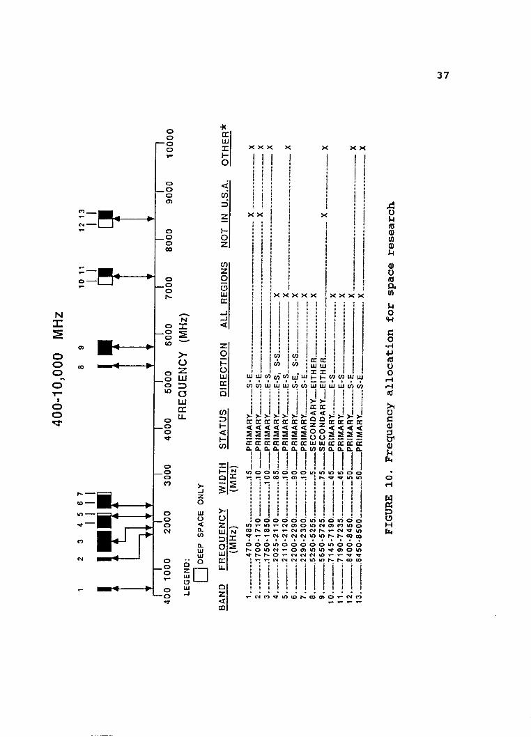
Several individuals receive our thanks for providing art- work incorporated herein: Rex Megill of Globesat and Utah State University for Figures 4 , 5 , and 8 ; Don Gurnett of the University of Iowa for Figures 2 and 7 ; and Jim Wilcher of JPL for Figure 10. Bill Erickson of the University of Maryland provided the confusion limit calculation.
Andrew Sexton of Globesat, Inc. contributed Appendix B, and Ali Siahpush and Roger Hart, graduate students in the Center for Space Engineering at USU wrote Appendices A and C, respectively. We thank them for their contributions.
We would also like to acknowledge correspondence and phone conversations with Kurt Weiler and others of the NRL Low Frequency Space Array group for discussing problems with us and for providing us with their reports.
Finally, we would like to thank JPL Assistant Laboratory Director, Don Rea, of the Office of Technology and Space Program Development for taking an interest in the potential for gas-can satellites, and for providing us with funding to conduct the Workshop and produce this report.
vi

TABLE OF CONTENTS
I . INTRODUCTION . . . . . . . . . . . . . . . . . . . . . 1 A . The Mission Concept . . . . . . . . . . . . . . . . 1 B . The Workshop of May 28.29. 1987 . . . . . . . . . . 3
I1 . SCIENTIFIC MOTIVATION . . . . . . . . . . . . . . . . . 3
I11 . MISSION REQUIREMENTS . . . . 5 A . Scientific . . . . . . . . . . . . . . . . . . . . . 5
1 . Unexplored Radio Spectrum . . . . . . . . . . . 6 a) The critical frequency (f0F2) . . . . . . 6 b) Interstellar scattering (ISS) . . . . . . 6 c) Interplanetary scattering (IPS) . . . . . 7 d) Auroral Kilometric Radiation (AKR) . . . . 7 e) Frequency band conclusions . . . . . . . . 8
2 . Range of Angular Scale Sizes . . . . . . . . . 9 3 . Large Number of Detectable Sources . . . . . . 9
a) Confusion limit . . . . . . . . . . . . . 10 b) Sensitivity limit . . . . . . . . . . . . 11 c) Source count conclusions . . . . . . . . . 11
B.Fisca1 . . . . . . . . . . . . . . . . . . . . . . . 13
IV . THESPACECRAFT . . . . . . . . . . . . . . . . . . . . 13 A . The GAS-Can Concept . . . . . . . . . . . . . . . . 13 B . Standard CANSAT Specification . . . . . . . . . . . 14
1 . Physical Parameters . . . . . . . . . . . . . . 14 2 . Power System . . . . . . . . . . . . . . . . . 16 3 . Stabilization . . . . . . . . . . . . . . . . . 16 4 . Orientation Determination . . . . . . . . . . . 16 5 . Command and Control Computer . . . . . . . . . 17
v . T H E A R R A Y . . . . . . . . . . . . . . . . A . Altitude . . . . . . . . . . . . . . .
1 . Propagation Delay . . . . . . . . 2 . Van Allen Belts . . . . . . . . . 3 . Drag . . . . . . . . . . . . . . 4 . Differential Gravity . . . . . . 5 . Telemetry . . . . . . . . . . . . 6 . Altitude Conclusions . . . . . .
B. Inclination . . . . . . . . . . . . . C . Delivery . . . . . . . . . . . . . . .
1 . Space Transportation System (STS) 2 . American Rocket Company (AMROC) . 3 . Other Delivery Companies . . . .
D . Number of Array Elements . . . . . . . E . Array Geometry Considerations . . . .
1 . Dynamical Disturbances . . . . . a) Gravity effects . . . . . . b) J2 effects . . . . . . . . . c) Solar pressure . . . . . . .
. . . . . . . 17 . . . . . . . 17 . . . . . . . 17 . . . . . . . 18 . . . . . . . 18 . . . . . . . 18 . . . . . . . 19 . . . . . . . 20 . . . . . . . 20 . . . . . . . 21 . . . . . . . 21 . . . . . . . 21 . . . . . . . 22 . . . . . . . 22 . . . . . . . 25 . . . . . . . 25 . . . . . . . 25 . . . . . . . 25 . . . . . . . 26
vii

d) Drag effects . . . . . . . . . . . . . . . 26 e) Attitude control firings (ACF) . . . . . . 26 f) Orbit injection . . . . . . . . . . . . . 27
2 . Position Determination . . . . . . . . . . . . 27 a) Relative positions . . . . . . . . . . . . 27 b) Array Orientation . . . . . . . . . . . . 28 c) VLBI Position Determination . . . . . . . 29
3 . (U.V ).Coverage . . . . . . . . . . . . . . . . 29
VI . SPACECRAFT HARDWARE . . . . . . . . A . The Antenna . . . . . . . . . .
2 . Long Travelling-wave Vees . B . The Receiver . . . . . . . . . .
1 . Reliability Trade-offs . . 2 . Hardware Specification . .
a) Front-end . . . . . . b) Channelizer . . . . . c) Down Converter . . . . d) Crystal Oscillator . . e) Intermediate Frequency
1 . Long dipoles . . . . . . . 3 . Infinitesimal dipoles . . .
f) Digitizer . . . . . .
. . . . . . . . . . . . . . . . . . . . . . . . . . . . . . . . . . . . . . . . . . . . . . . . . . . . . . . . . . . . . . . . . . . . . . . . . . . . . . . . . . . . (IF) Receiver . . . . . . .
. . . 29 . . . 30 . . . 30 . . . 31 . . . 31 . . . 31 . . . 31 . . . 31 . . . 33 . . . 33 . . . 33 . . . 33 . . . 34 . . . 34
VI1 . Telemetry and Ground Support . . . . . . . . . . . . . 35 A . Number of Telemetry Satellites . . . . . . . . . . . 35 B . Telemetry Bandwidth . . . . . . . . . . . . . . . . 35 C . Communications Band . . . . . . . . . . . . . . . . 36 D . Ground Support . . . . . . . . . . . . . . . . . . . 36
VIII.TOPICS REQUIRING FURTHER STUDY . . . . . . . . . . . . 38
IX . CONCLUSIONS . . . . . . . . . . . . . . . . . . . . . . 39
REFERENCES . . . . . . . . . . . . . . . . . . . . . . . . . 40
APPENDIX A Stability and Natural Frequencies of a Radio Interferometer
Satellite in a 10. 000 km Circular Orbit . . . . 41
APPENDIX B Application of Magnetic Torquers for a Radio Interferometer
Satellite in a 10. 000 km Orbit . . . . . . 49
APPENDIX C Separation of High Altitude. Co-orbiting Satellites Due to
Differences in Atmospheric Drag . . . . . . 59
. . . . . . . . . . . . . . . . . . . . . . . . . . . INDEX 67
viii

LIST OF FIGURES
FIGURE 1. The low frequency VLBI GAS-can array in orbit. . . 2
FIGURE 2. The natural radio spectrum below 10 MHz. . . . . . 8
FIGURE 3 . The confusion limit versus angular resolution for confusion criteria of: (a) 100 beam areas per resolved source, and (b) 10 beam areas per resolved source. . . . . . . . . . . . . . . . . . 12
FIGURE 4. Location of GAS-can launchers in Shuttle cargo bay.. . . . . . . . . . . . . . . . . . . . . . . 13
FIGURE 5 . Two possible spacecraft configurations for the low frequency VLBI array: (a) two dipole gravity gradient stabilized, and (b) three dipole unstabilized.. . . . . . . . . . . . . . . . . . . 15
FIGURE 6. Altitude variation of the electron flux with latitude in August 1964, longitudinally averaged (Evans and Hagfors, 1968).. . . . . . . . 19
FIGURE 7. Schematic illustrating the plasmasphere propagation surface for auroral kilometric radiation. . . . . . . . . . . . . . . . . . . . . 21
FIGURE 8. (a) Detail of Globesat CANSAT carrier, and (b) position of carrier in AMROC nose cone.. . . . 23
FIGURE 8. (c) Schematic of AMROC rocket with mechanical details. . . . . . . . . . . . . . . . . . . . . . 24
FIGURE 9. Receiver and computer system schematic.. . . . . . 32
FIGURE 10.Frequency allocation for space research. . . . . . 37
ix
1
I. INTRODUCTION
A. The Mission Concept
A compelling mission opportunity has arisen which promises substantial scientific return. It would involve the deployment of an array of very inexpensive satellites in high earth orbit (FIGURE 1) to do very long baseline interferometry (VLBI) at low radio frequencies (< 25 MHz). Because the array would observe in a new spectral window with good angular resolution, the project can be expected to result in major astronomical discoveries, significant insights into astrophysical processes, and an enrichment of our understanding of the Universe. The recent very successful IRAS mission is an excellent example of what can be accomplished in such circumstances.
Our concept for a low frequency VLBI array in space was initially motivated by the opportunity to deploy small satellites cheaply from 88Get-Away-Specia118 canisters, or GAS-cans, on the Space Transportation System (STS). This mission, however, will require a much higher orbit than can be provided by Shuttle GAS- can deployment, but alternate launch capabilities are becoming available, some of which are designed specifically for GAS-can compatible satellites. Considerable experience has been gained within the aegis of the GAS-can program, both in universities and in private companies, and small satellites are now widely accepted as a viable, inexpensive vehicle for space exploration.
For a number of reasons, a VLBI array in space is an ideal application for small satellites.
0
0
0
0
The mission cost is greatly reduced because the satellites are very inexpensive, lightweight and identical.
A multi-satellite VLBI array is inherently redundant: therefore, its performance is not seriously affected if a small fraction of the array elements fail. This greatly relaxes the flight certification requirements, and hence the cost.
A low frequency VLBI array in space involves no new technology, and could be launched much more quickly than conventional missions.
The entire array can be tracked by small antennas on the ground. This is expected to greatly simplify satellite position determination, and offers an inexpensive opportunity for university involvement.

2

3
B. The Workshop of May 28-29, 1987
To study the technical feasibility of an inexpensive low frequency VLBI mission using small satellites, an informal Work- shop was sponsored by the Jet Propulsion Laboratory (JPL) on May 28-29, 1987. The workshop was attended by eighteen scientists and engineers from JPL and five other institutions. The participants assumed that the scientific justification for such a mission was intact. As a result, science issues were discussed only in the context of how they might impact the mission requirements. With the lowest possible price being the primary constraint, every effort was made to exclude anything which was not absolute-ly essential. Only existing technology was considered, complexity was avoided where possible, and redundancy was allowed only if the cost impact was trivial compared to the total mission cost.
With the exception of the following section, which briefly discusses the scientific objectives of the mission, the remainder of this report attempts to present the technical issues raised during the meeting, the outstanding questions which require further consideration, and the conclusions which were reached. The conclusions, however, are not to be regarded as final; rather, they should form the basis for a more detailed study.
11. SCIENTIFIC MOTIVATION
The purpose of this mission is to map the entire sky at frequencies below 25 MHz with good angular resolution; this part of the radio spectrum is essentially unexplored from the ground because it is either inaccessible (because it is below the ionospheric critical frequency) or extremely difficult to observe (because of man-made interference). It is as far removed from the frequency range normally used for radio astronomy as the infrared region explored by IRAS is from either the radio or optical spectral regions.
The history of astronomy clearly shows the importance of angular resolution for identifying sources of emission and understanding the physical processes involved. Although it is possible to obtain high angular resolution at long wavelengths by using lunar occultation and scintillation measurements, these methods are inappropriate for an all-sky survey. For llconventionalll astronomical observations, angular resolution is proportional to the ratio of the observed wavelength to the size of the telescope aperture; therefore, arc-minute resolution at long radio wavelengths is only possible with apertures of hundreds of kilometers. Such a large aperture can only be realized by employing aperture synthesis or VLBI techniques. By using multiple small spacecraft as elements of a low frequency VLBI array in space, radio sources will be imaged with high

4
angular resolution; this provides a valuable improvement over previous single satellite missions operated at these frequencies, such as the Radio Astronomy Explorers (RAEs), which had only steradian resolution.
The objects which can be studied at low radio frequencies range from solar system objects to distant clusters of galaxies. Within this range are galactic sources such as pulsars and supernova remnants, and extragalactic sources such the radio lobes of active galaxies. The radio emission from many of these objects reaches a maximum at frequencies below 100 MHz, which makes this frequency range unique in its ability to provide information on the total luminosities, magnetic field strengths, and radiative lifetimes. In addition, low frequency measurements of the apparent sizes of compact extragalactic radio sources can tell us about the density irregularities and turbulence in the interstellar and interplanetary media.
The scientific objectives appropriate to a low frequency space array have been addressed at length in an Explorer class proposal prepared by a group at the Naval Research Laboratory (NRL) (see for example, Dennison et al., 1986). Rather than repeat their work, we summarize below (with some additions) their conclusions. The current report will concentrate on the technical feasibility of undertaking a similar mission, but at lower cost and with a larger number of satellites.
1. Do radio source counts differ between very low frequencies and higher frequencies? A survey of the entire sky below 25 MHz should detect several thousand sources; this is a large enough sample for significant statistical studies to be made.
2. What do the radio spectra of various types of sources look like below 25 MHz? Where do these spectra turn over? Measurements of source spectra will allow the importance of physical processes such as synchrotron self-absorption, inverse Compton scattering, HI1 absorption, the Razin-Tystovich effect, and synchrotron losses to be determined. The shape of the low frequency spectral turnovers also provides information on magnetic field strengths, relativistic particle populations, and plasma densities.
3. What are the effects of scattering and refraction by the interstellar and interplanetary media at low frequencies? Are these effects responsible for the low frequency flux density variations seen in some compact extragalactic radio sources?
4 . What is the distribution of low energy cosmic ray electrons within galaxies? Sensitive, high resolution maps of the background non-thermal emission in other galaxies could determine this.
5
5. Are there Btfossilll radio components associated with presently "radio quiet" galaxies and quasars? This would be a sensitive test for earlier epochs of activity, since at these frequencies the electron lifetimes are a significant fraction of the age of the Universe.
6 . What is the galactic distribution of diffuse ionized hydrogen? This can be determined by surveying its absorption effects along lines of sight to a number of discrete galactic and extragalactic radio sources.
7. What is the origin of the known correlation between low frequency steep spectrum radio emission from some clusters of galaxies and their enhanced X-ray emission? Mapping the extended radio halos of these clusters will help in understanding this.
8 . Are there extra-solar system objects (other than pulsars) which radiate by coherent mechanisms? Are they similar to those found in the Sun and Jupiter?
9. What is the volume emissivity distribution in the Galaxy? This can be studied by looking at the foreground emission between the earth and a totally absorbing HI1 region.
10. Is there a population of very steep spectrum radio sources? Some pulsars, for example, are known to have such steep spectra that their pulsed emission is extremely difficult to detect at the higher frequencies normally used for radio astronomy.
11. Are there serendipitous discoveries to be made at long wavelengths with a VLBI space array? Although not justification in itself for exploring a new spectral region, instruments with greatly improved capabilities nearly always make unexpected discoveries.
111. MISSION REQUIREDENTS
A. Scientific
The goals of the proposed mission are to obtain spectral information in a new region of the radio spectrum with resolution appropriate to a wide range of angular scale sizes, and sufficient sensitivity to detect a statistically useful sample of radio sources.

6
1. Unexplored Radio Spectrum
The band of useful frequencies that can be observed at long wavelengths from space is bounded on the high side by radio frequency interference (RFI) from earth, and hence the ionospheric critical frequency, f0F2, and on the low side by interstellar scattering (ISS), interplanetary scattering (IPS), and auroral kilometric radiation (AKR). These constraints are examined in turn.
a) The critical frequency (f0F2)
Radio frequency interference begins to seriously hamper earth-based observations below about 25 MHz. Observations from space will be similarly affected until frequencies below the ionospheric critical frequency, f0F2, are reached. The critical frequency is largest in the daytime during the winter at sunspot maximum, when it has an average value of 11 MHz (Evans and Hagfors, 1968). From daytime to nighttime f0F2 can decrease by a factor of 2.5, while an additional decrease by a factor of 2.0 can occur from solar maximum to solar minimum. The seasonal Variation is less important. Therefore, an upper limit on the frequency spectrum in space which is free from man-made interference is approximately 11 MHZ.
b) Interstellar scattering (ISS)
A soft lower limit on the useful frequency spectrum is dictated by the amount of interstellar scattering which can be tolerated. The table below summarizes the results of Cordes (1984) for the scattering disc size as a function of galactic latitude, b (in degrees) and the frequency, f (in MHz) .
Galactic Latitude Ranae OTSS (FWHM) Scatterins Disc Size
lbl < 0.6 degrees 3.52*104 f-2-2 arc-minutes
2.32*103 f-2-2 Isin(b)l-0*6 arc-minutes
lbl > 3-5 degrees 5.84*101 f-2-2 Isin(b) arc-minutes
0.6 < lbl < 3-5 degrees
It is clear that for galactic latitudes below 5 degrees that the scattering is severe at low frequencies. At higher latitudes and for the lowest frequency considered here (2 MHz), the scattering disc can still be nearly one degree in extent, thus limiting the

7
useful resolution of a VLBI array for studying intrinsic source structure. The array, however, would still be useful for studying the properties of the scattering medium. At 5 MHz, the amount of scattering decreases to a few arc-minutes, a much more reasonable value for radio source work. It should be noted that the measurements of Cordes assume that measured VLBI source sizes are indicative of ISS and not some intrinsic angular size for extragalactic radio sources. This point requires further study because of its effect on the angular resolution of any radio telescope below about 5 MHz.
c) Interplanetary scattering (IPS)
The interplanetary medium will also cause serious scattering in directions toward the sun. Erickson (1964) has shown empirically that the half width of the scattering distribution can be expressed as:
01ps = 45*105 f (MHz)-~ R(So1ar Radii)'2 arc-minutes,
when the angular separation R is less than 60 solar radii. In terms of the solar elongation angle, E, this relationship can be cast in the form:
OIPS - - 100 f (MHz)-~ sin(E)'2 arc-minutes,
for solar elongations less than 17 degrees. This expression extrapolates reasonably well (based on Mariner spacecraft measurements) to the radius of the earth's orbit (E=90 degrees): the behavior at larger angular separations is less certain. Note that the last expression is invalid for elongations over 90 degrees: the original expression should be used in this case. It is clear that IPS is important within 90 degrees of the sun. At 5 MHz and for an elongation angle of less than 90 degrees, the half width of the IPS scattering disc is greater than 4 arc-minutes. During solar maximum, this could increase by a factor of 2. Thus IPS will be an important factor competing against the critical frequency f0F2 in determining an optimum observing frequency.
d) Auroral Kilometric Radiation (AKR)
Another important consideration in the selection of the low frequency limit for a space array is the auroral kilometric radiation. Although AKR peaks near 200 KHz (FIGURE 2), its intensity can be 4 or 5 orders of magnitude above the galactic background and hence still significant above 1 MHz. The AKR is not only highly variable, but also coherent on baselines in excess of 1000 wavelengths, as determined by measurements with ISEE-1 and ISEE-2. Thus both the radio noise and radio signal environment of the space array could be affected. As will be

a
discussed in Section V, the impact of AKR can for the most part be mitigated by a proper choice of orbit.
AURORAL KILOMETRIC RAD1 AT ION
(HIGHLY VARIABLE) fP fP
LOCAL MAGNETOSHEATH
- I I
I o3
CONTINUUM RAD1 AT1 ON
R SPECTRUM
7
FREQUENCY (Hz)
FIGURE 2. The natural radio spectrum below 10 MHz.
e) Frequency band conclusions
In summary, ISS, IPS, and AKR constrain the lowest useful frequency, while the ionospheric critical frequency, f0F2, constrains the highest useful frequency. The following frequency band would therefore appear best suited to low frequency VLBI in space:
2.0 MHz < Frequency < 11.0 MHz,
with the understanding that the upper limit represents ideal ionospheric conditions, while the lower limit may only be useful for studying ISS, IPS, and large scale structure such as the galactic background radiation, the spectrum of which turns over near 2 MHz. It should be noted that both the sensitivity and confusion limits also influence the selection of an optimum frequency (see below) .

9
2. Range of Angular Scale Sizes
A range of angular scale sizes is needed to observe both point sources and extended sources. To be useful the array should be sensitive to structure as small as 1 arc-minute (or less) and as large as 1 degree (or more). The former requirement is needed for good source statistics and to study structural detail, while the latter requirement would allow extended objects such as supernova remnants and giant radio galaxies to be mapped.
To first order, the angular resolution of any telescope is simply the reciprocal baseline (or largest dimension) expressed in wavelengths. Since the space array would dynamically expand from a very compact size at deployment, essentially all baselines up to several earth radii might in principle be measured. Unfortunately, available baselines do not constrain the angular resolution. Interstellar and interplanetary scattering, and not the longest baseline, place strong constraints on the smallest intrinsic scale sizes measurable, while the confusion limit, and not the shortest baseline, constrains the largest angular scale sizes measurable. Both of these restrictions are best mitigated by choosing the highest frequency consistent with the discussion in the previous sub-section. As a minimum requirement, the following range of angular scale sizes should be measurable:
1 arc-minute < Angular Resolution < 60 arc-minutes.
At 5.0 MHz, the corresponding limits for the required baseline lengths are:
3 km < Baseline < 200 km.
3. Large Number of Detectable Sources
The number of sources a telescope can detect is a function of its sensitivity and/or confusion limits. We believe that at least 1000 radio sources should be observable to be useful. This would provide sufficient data for source count studies, give many lines of sight through the galaxy for studies of ISM properties, and allow useful statistics for studying different classes of objects. To determine if this many sources can be detected under the above frequency and angular resolution restrictions, it is necessary to determine whether the system is confusion limited or sensitivity limited. Confusion noise is generated primarily by weak sources in the main beam or sidelobes of a telescope; they behave collectively to impair the detection of stronger sources. The statistical properties of confusion noise are the same as receiver noise, but unlike receiver noise, it cannot be reduced by increasing the integration time. Confusion noise depends strongly on the resolution of a telescope, its beam pattern and its bandwidth.

10
a) Confusion limit
To determine the confusion limit, we follow the procedure of Perley and Erickson (1984), who used the differential source count data of Pearson (1975); these data were based on the Cambridge 5C, Molonglo MC1, and various other surveys at 408 MHz. The count has been normalized by a Euclidean number count of 750 sources/steradian above 1 Jy at 408 MHz. Integrated source counts per steradian, N ( S ) , are then defined for three regions:
i) N ( S ) = 3.45*103 S-2*2 - 0.63 for 50.0 Jy > S > 10.0 Jy,
ii) N ( S ) = l.01*103 S-lo5 - 10.0 for 10.0 Jy > S > 0.8 Jy, and
iii) N ( S ) = 2.20*103 S-Oo8 - 1230 for 0.8 Jy > S > .001 Jy,
corresponding to breaks in the differential source count spectrum at 408 MHz; S is the flux density in Janskys. The extension of region iii) to 0.001 Jy from the lower limit of 0.01 Jy used by Pearson is justified on the basis of more recent Very Large Array (VLA) source counts. These three relationships are scaled to long wavelengths by assuming that the integrated source count spectrum maintains its shape with frequency (i.e. , the number of sources in each interval does not change), and that the sources have a characteristic spectral index a=-0.75 (defined by S=k fa). This should be an excellent approximation since few flat spectrum sources have appreciable flux density at long wavelengths, and the dispersion in spectral index amongst steep-spectrum sources is small. Less certain is the effect of low frequency turnovers.
Confusion limits have been calculated for a range of angular resolutions and frequencies. By assuming a confusion criterion of 100 beam areas per resolved source, the source count per steradian at the confusion limit is easily calculated. If these values are substituted into the appropriate expressions for the integrated source counts at each frequency, flux densities can be derived for the confusion limits. The table below gives the value of the source counts and confusion limits for several angular resolutions at 5 MHz.
Source Counts Der Steradian and Confusion Limits at 5 MHz
Anaular Resolution ( ' 1 1.0 10.0 100.0
Source Count / steradian 118,200 1,182 11.82 Confusion Limit (Jy) 0.166 24.3 350

11
b) Sensitivity limit
To determine the sensitivity limit of the system, a correlation receiver with a 22 KHz bandwidth (see VI.B.2.f) and an integration time of T seconds is assumed. To derive an upper limit, it is also assumed that a minimum array of 6 antennas (see Section V), or 15 simultaneous baselines, would be deployed. Because the system noise will be dominated by the galactic background, the polar cap survey of Cane (1979) can be used to determine appropriate sk brightnesses. Between 1 and 5 MHz the brightness is about l o B Jy/sr, and it decreases towards higher and lower frequencies. With these assumptions and isotropic antennas, the RMS system noise is 7,680 T-Il2 Jy; a five sigma detection would then require a source flux density of 38,340 T-li2 Jy. This is a relatively high limit and may be a strong argument for using as much bandwidth as possible.
c) Source count conclusions
If it is assumed that geometry of the array and its orbital precession rate can be controlled to allow integration times of lo6 seconds (about 2 weeks), then a comparison of the sensitivity limit with the confusion limits in the above table shows that at 5 MHz the array starts to become confusion limited for angular scale sizes around 10 arc-minutes.
To provide a clearer perspective on the impact of confusion noise at large angular scale sizes, FIGURE 3 (a) plots the confusion limit as a function of the angular resolution for frequencies between 1 and 11 MHz. To emphasize the importance of interstellar scattering, the curves have been truncated at the angular resolution for which the scattering disc size is equal to the resolution of the array. This should not be regarded as a hard limit on useful angular resolution since the system could still be used to study the shape and size of scattering discs. Several five sigma sensitivity limits and the IPS sizes at 90 degree solar elongation are also indicated on the plot.
This figure shows clearly that the best dynamic range in angular resolution is obtained at the highest frequency. Daytime observations will therefore be the most useful, and deployment near sunspot maximum would help significantly. (The next solar maximum is in 1992.) There are, of course, many assumptions built into these conclusions. In particular, the confusion criterion of 100 beam areas per resolved source is very conservative. If this is relaxed to 10 beam areas per resolved source, the results presented in Figure 3 (b) are obtained. Further studies of the confusion limit should take into account the actual beam shape of the array, as well as the levels of ISS and IPS, because of their importance in determining the lowest useful frequency for studying radio source structure.

12
104
103 -
' I , , , I
la) CONFUSION LIMIT vs RESOLUTION CONFUSION CRITERION: 100 BEAMS/SOURCE
T = 1O8s
T = 109,
I -I
103 .
102 -
- $ 101 -
z 100 - 0
t I
v)
3 U
z 8 10-1 -
10-2 -
10-3 -
(b) CONFUSION LIMIT vs RESOLUTION CONFUSION CRITERION: 10 BEAMS/SOUACE
(b) CONFUSION LIMIT vs RESOLUTION CONFUSION CRITERION: 10 BEAMS/SOUACE
3 k
1 1 I I , I I 1 I , ( I , I
1000.0 100.0 1 .o 10.0 0.1
ANGULAR RESOLUTION (arc-minutes)
FIGURE 3. The confusion limit versus angular resolution (a) 100 beam areas for confusion criteria of:
per resolved source, and (b) 10 beam areas per resolved source.

13
B. Fiscal
The primary constraint on deploying a low frequency VLBI array in space was assumed to be fiscal. This report will demonstrate that the expense of such a mission may be reduced to levels far below what would have previously been thought possible - a useful array in orbit for millions instead of hundreds of millions of dollars. The use of many identical satellites and the inexpensive GAS-can technology make this possible.
IV. THE SPACECRAFT
A. The GAS-Can Concept
The llGet-Away-Specialll Canister, or GAS-can, was introduced by NASA to allow small (both in size and mass) experiments to be flown cheaply in low earth orbit. The original canister measured 19 inches in diameter and was 28 inches in length. (The length has now been extended to 35 inches.) It could be carried in the shuttle cargo bay in one of two configurations: as a single canister, or as one of twelve canisters on a "GAS bridge" spanning the cargo bay (FIGURE 4 ) . The canisters are interfaced
V I E W FROH TOP OF BAY
BAY 5 M Y 8
FIGURE 4 . Location of GAS-can launchers in Shuttle cargo bay.

14
to a standard NASA control bus, and can contain packages which remain with the shuttle or which are deployed. If the canister is opened in flight, the contents must pass stringent space certification requirements to avoid outgassing problems and the like. The launch cost for a canister is $25K. To date 55 of the standard 28 inch GAS-cans have flown on the shuttle, primarily in orbits under 350 km with inclinations of 28.5 degrees.
Standard GAS-can compatible satellites are now becoming commercially available. Two possible satellite configurations for a low frequency VLBI array are shown in FIGURE 5. FIGURE 5(a) depicts a spacecraft which is an adaptation of a figure provided by Globesat, Inc. of its gravity gradient stabilized CANSAT satellite. To complement the Globesat hardware for the purposes of this mission would require the addition of two orthogonal pairs of observational antennae, a radio astronomy receiver and telemetry hardware. This spacecraft configuration would be used in orbits low enough to allow gravity gradient stabilization.
FIGURE 5(b) depicts a spacecraft with three orthogonal pairs of antennae. This configuration would be used for very high altitude orbits where gravity gradient stabilization would not work effectively. It would, however, require orientation sensing to be useful, but such hardware is now available, and it is inexpensive. In fact, the three antenna system might be superior to the two antenna system in that orbital inclination would not impact the sky coverage.
In order to take advantage of the cheap launch costs for GAS-cans on the STS and to standardize their basic contents, Globesat was incorporated. Its GAS-can compatible satellite, CANSAT, will be used in the subsequent discussion to illustrate the capabilities of these small satellites.
B. Standard CANSAT Specification
The basic CANSAT configuration was shown in FIGURE 5(a). Including a launcher (which is superior to that of the STS) to eject it from the bus, it sells for under $0.5M. A discussion of some of its features follows.
1. Physical Parameters
The CANSAT has been designed to fit in a long GAS-can environment (a cylinder 19 inches in diameter and 35 inches long). It is a right octagonal cylinder constructed of an aluminum alloy, and has a mass of 90 kg. It will accept an experiment weighing 23 kg (50 pounds) with a volume of 56,800 cm3 (2.0 cubic feet).

5 1
15
r 11’
FIGURE 5. Two possible spacecraft configurations for the low frequency VLBI array: (a) two dipole gravity gradient stabilized, and (b) three dipole unstabilized.

16
2. Power System
Power is provided by 0.5 m2 of solar cells mounted around the satellite. The available power is 10 watts averaged over an orbit; the actual average value depends on orbital inclination and day of year. Fifty to eighty percent of this is available for the experiment package. The batteries are able to provide 100 watt-hours of backup power.
3 . Stabilization
For spacecraft not requiring high pointing accuracy, gravity gradient stabilization can be an effective means for maintaining a radially directed orientation. However, because librational motions can result from the orbit insertion process, or from torques exerted by the spacecraft environment, it is necessary to have the means to counteract these disturbances.
The stability and natural frequencies of a small satellite under the force of gravity have been investigated in Appendix A, where appropriate expressions are derived for 2-axis and 3-axis stability. Under 2-axis stability the spacecraft can precess and nutate about the yaw (or radial) axis, while being stable about the roll and pitch axes (i.e., in the direction of the flight path and transverse to the orbital plane). FIGURE 3 of this appendix illustrates the minimum boom length and yaw tip- mass required for stability. For example, a 4 meter boom would gravity gradient stabilize a spacecraft if the tip-mass was 5 kg. These are reasonable values for this mission. For 3-axis stability, short booms must also be added to the roll axis so that the moments of inertia satisfy the appropriate stability criteria.
Gravity, however, is not the only force which produces significant torques on the spacecraft. As is discussed in Appendix B , solar radiation pressure is equally important. Its effect is most easily eliminated by using a pair of radial booms pointing in opposite directions. This is not essential because magnetic torquers can be used to stabilize motion about the yaw axis. Magnetic torquers involve no expendables and are easily implemented for the small satellites discussed here. All that is required is a knowledge of the satellite's attitude, its orbital position relative to the earth's magnetic field, and on/off control of the magnetic torquers.
4 . Orientation Determination
The standard CANSAT satellite will contain four charge coupled device (CCD) arrays with pinhole optics for determining

17
the satellite's orientation. It will do this by means of limb and terminator observations of the Earth, and observations of the Sun. These measurements will be relayed to earth to derive the spacecraft's orientation to at least 1 degree accuracy.
5 . Command and Control Computer
The spacecraft computer system has approximately the power of an IBM XT, and controls all functions on board the satellite. It uses an 80C88 microprocessor, which draws about 0.5 watts, and comes with a custom multitasking interrupt driven operating system. Subroutines for all housekeeping functions, operation of the orientation sensors, controlling the transmitter and receiver, and uploading new programs are provided. The system is supplied with 2 Mbytes of battery backed RAM, but can support up to 30 Mbytes of memory (at 50 milliwatts/Mbyte) for data storage. It has no direct memory access capability but has two analog-to-digital converter (ADC) boards for custom purposes.
v. T H E A R R A Y
A. Altitude
Orbit altitude or height when referred to in this report is the vertical distance above the earth's surface to the spacecraft orbit; orbit radii are obtained by adding the earth's radius (6378 km) to the quoted altitudes. All spacecraft orbits are circular and at the same altitude, since this reduces the dynamical effects which would disperse the array apart too quickly.
Although there was some early discussion at the meeting of a low earth orbit (<lo3 km high) array, a much higher altitude ( l o 4 km) was quickly adopted, primarily because of the large propagation delays at the lower altitude. Discussions subsequent to the meeting now indicate that an even higher orbit (3-4*104 km) is needed to avoid radiation damage. Some of the altitude dependent trade-offs are now discussed.
1. Propagation Delay
The lowered group velocity of a radio wave propagating through the ionospheric plasma produces a propagation delay relative to the corresponding free space propagation time. The propagation delay will be a function of the spacecraft altitude, the frequency of observation, and the angle measured from the zenith, Z. The table below summarizes the expressions appropriate to the two altitudes being considered here.

18
Propaaation Delav as a Function of Orbit Altitude
Orbit Altitude Propacfation Delav
1,000 km 10,000 km
3.00 f (MHz) -2 sec ( Z ) milliseconds 0.03 f (MHz)-~ sec(Z) milliseconds
If the structure of the ionosphere was well known, the geometrical delay, including the propagation delay, between pairs of satellite interferometers could be calculated just as it is for earth-based interferometers. Unfortunately, variations in the geomagnetic field along the different ray paths, as well as small scale structure in the ionospheric plasma, cause unknown path length, or delay, fluctuations. Because the lower altitude produces single path delays which are 100 times larger, the relative delay fluctuations are expected to be much larger. This strongly favors the highest possible orbit.
2 . Van Allen Belts
The electrons and protons trapped in the Van Allen belts present a potentially harmful environment for spacecraft components. As can be seen in FIGURE 6, the Inner Belt lies at approximately 2,200 km, while the Outer Belt is near 22,000 km. Particle densities do not decrease to safe levels until altitudes below about 600 km or above 40,000 km are reached. The electron flux does decrease near lo4 km altitude, but it has limited latitudinal range and is still large. As a result, priority should be given to studying the radiation environment, and the implications of orbit altitudes above 3*104 km.
3 . Drag
Ionospheric drag on the satellites is a strong function of altitude. In particular, it is 5*10-6 times smaller for a lo4 km orbit than for a lo3 km orbit. This affects the lifetime of the satellites, but, more importantly, it has a tremendous impact on the orbital dynamics of the array. This will be discussed in more detail in Section V.E.1.c.
4. Differential Gravity
The gravity gradient for the higher orbit will be about that of the lower orbit. The main impact of differential
gravity is on the performance of the gravity gradient stabilization. It should still be adequate at lo4 km, but could present a problem at higher altitudes.

19
I
102 90"
3 x 10⁵ electrons/crn2-s
A 90"
NORTH GEOGRAPHIC LATITUDE SOUTH
FIGURE 6. Altitude variation of the electron flux with latitude in August 1964, longitudinally averaged (Evans and Hagfors, 1968).
5. Telemetry
The maximum time, tmay, a satellite is above the horizon at a given ground station is:
tma, = 3.16*10-3 RSlo5 arccos(Re/Rs) seconds,
where Rs and Re are spacecraft orbital radius and earth radius,

20
respectively, in km. Thus a ground station would see a satellite in a 1,000 km altitude orbit for less than 17 minutes (0.1 of the orbital period), while a satellite in a 10,000 km orbit would be seen for up to 130 minutes ( 0 . 4 of the orbital period). As a result, the lower orbit satellites would require higher telemetry data rates, and would probably require recorders on each satellite. A separate ground antenna might also be needed to track each satellite. On the other hand, the higher orbit satellites would require lower data rates and no recorders, since three or four ground stations could provide complete orbital coverage. In addition, only one small antenna would be required to cover the entire array, which would subtend an angle of only a few degrees.
6. Altitude Conclusions
From the above discussion it is clear that the propagation delay, radiation environment and ionospheric drag strongly favor a high orbit, while the launch cost per spacecraft and the use of gravity gradient stabilization favor a low orbit. The final altitude chosen will have to be a compromise between these competing factors.
B. Inclination
For an all-sky survey, a high orbital inclination is preferred. For a satellite in polar orbit, precession of the orbital plane would allow the entire sky to be mapped on the peak of the antenna beam pattern with the smallest propagation delays. Lower inclination orbits would require mapping away from the peak antenna gain with increased phase errors due to propagation delays. However, high orbital inclinations have several drawbacks: they are more expensive to achieve, radiation damage is more likely, and the effect of the AKR will be felt more strongly. The latter difficulty is improved significantly for a low inclination orbit.
As can be seen in FIGURE 7, auroral kilometric radiation generated above the geomagnetic pole at about one earth radius is unable to penetrate the plasmasphere because it is - for the most part - below the critical frequency. Because of its tremendous strength, the AKR would ruin observations, as well as put heavy dynamic range requirements on a low frequency receiver front-end. In practice a compromise orbit inclination will have to be settled upon for a fixed mission cost. The variables to be considered are the number of satellites, the sky-coverage, the orbit altitude, and the impact of propagation delays.

AURORAL FIELD
PROPAGAT ION
RAY PATHS
AURORAL FIELD LINE
PROPAGAT ION
RAY PATHS
FIGURE 7. Schematic illustrating the plasmasphere propogation surface for auroral kilometric radiation.
C . Delivery
21
1. Space Transportation System (STS)
For a low orbit (<lo3 km), the STS would have been the primary launch vehicle, especially in view of its $25K price tag per GAS-can. However, for the much higher orbits anticipated by this study, the usefulness of the Shuttle is diminished. It is also uncertain what the status of Shuttle GAS-cans will be in the post-Challenger era. The GAS-can configuration in the shuttle cargo bay was shown in FIGURE 4 for both a single canister and multiple canisters. In the past few years several companies have formed to provide alternative launch vehicles.
2. American Rocket Company (AMROC)
One of the newcomers is the American Rocket Company, located in Camarillo, CA. AMROC has formed a joint venture with Globesat (called Orbital Express) for the purpose of delivering up to 15 GAS-can type satellites per launch. A detail of Globesat's 15 canister supporting structure is shown in FIGURE 8(a), while FIGURE 8(b) illustrates its location in the AMROC nose cone. FIGURE 8(c) shows the nose cone in position on AMROC'S

22
Industrial Launch Vehicle (ILV); mechanical specifications are also provided in the figure. The Orbital Express launch cost for low earth orbit is $l.OM per CANSAT, including the cost of the standard satellite. In the case of a lo4 km orbit, only 6-8 CANSATs could be launched, so the cost could rise to $2.5M per standard satellite. This is a worst case estimate, however, since a lower orbit may be possible, and it may also be possible to reduce the individual spacecraft masses. Both these factors would reduce the launch cost per spacecraft under a fixed budget. At the present time AMROC plans a suborbital test in December 1987 and three orbital launches in 1988. It is also worth noting that Orbital Express guarantees its launches to the extent that it will provide a re-launch in the event of a failure. It also sells insurance to provide additional launches if they are needed.
3 . Other Delivery Companies
Other American companies which should be considered are Space Services Incorporated (SSI) and Pacific American. The SSI rocket is called the Conestoga I11 A; it is built from existing Castor IV and Star motors and will cost about $16M per launch. SSI promises a DARPA launch in 1987. Pacific American's rocket is called the Liberty Vehicle; its stage of development is not known. Neither company has any known plans for accommodating multiple GAS-can launches.
D. Number of Array Elements
The absolute minimum number of array elements can be set at four, since this is the smallest number which will allow closure amplitudes to be calculated. (Only three are needed for closure phases.) The maximum number of array elements is controlled primarily by cost, but it must be large enough to allow failures if the strategy of reducing costs by minimizing hardware certification is to work. Other considerations are the following: more satellites will allow better instantaneous (U,V)-coverage, and provide additional constraints for self-calibration; more satellites will improve the synthesized beam shape and hence help reduce the confusion noise limit; and more satellites allow the performance of the array to degrade gracefully in the event of individual satellite failures.
In summary, as many array elements as possible should be launched, but 6 would be the minimum number consistent with costs, amplitude closure (allowing for failure), and current launch capabilities.

23
k Q)
w 0
0
II) 0 a n a W

24 AMERICAN ROCKET COMPANY
tNOUSTAlAL LAUNCH VEHICLE ONE SPECIFICATIONS
Payload (1 35 mi circular orbit) Polar - 3,000 Ibs. 28.5" inclination - 4,000 Ibs.
Payload Interface 37 in diameter standard per De WPAM-D/Ariane
Nose Fairing Diameter - 90 in. Cylindrical length - 9 ft. Conical-6ft.
Maximum Acceleration (Longitudinal)
Without throttling - 7.2 g With throttling - 5.8 g
FIGURE 8. (c) Schematic of AMROC rocket with mechanical details. (Courtesy of American Rocket Company, Camarillo, CA)

25
E. Array Geometry Considerations
Under ideal circumstances the relative positions of array elements in circular orbits at the same altitude would be stable and well-defined. In practice this is not the case because a number of forces act on the array elements with different and often unpredictable effects. Some preliminary calculations have been made to try to estimate the impact of these differential forces on the relative positions of the array elements, and several different methods for keeping track of the array under these conditions are discussed.
1. Dynamical Disturbances
In order to obtain a crude estimate of what the most important dynamical disturbances might be, the relative positions of two satellites separated by approximately 100 km in orbital longitude were considered. The effect of different forces were determined numerically by comparing their relative positions in the absence of the various forces, and in their presence. An orbital altitude of 10,000 km and an inclination of 30 degrees were assumed. Briefly, the following conclusions were reached for each of the forces.
a) Gravity effects
First order gravity forces include those of the sun and moon. The effects of these forces on the relative positions of two spacecraft were found to be less than one km/month, and therefore not serious. Differences in orbital inclinations were not considered; they may be important.
b) J2 effects
J2 effects are second order gravity forces due to the oblateness of the equipotential force field which a satellite experiences. They arise because satellites at the same altitude, but different latitudes, experience different centrifugal forces. A s a result, satellites with different orbital inclinations will disperse. Specifically, the J2 effect will cause a 2 0 km/month separation in the equatorial crossing position for a pair of satellites with an inclination difference of 0 . 0 0 5 degrees. Because of this, it will be important that the relative orbital inclinations of the satellites be controlled very closely during orbit injection.

26
c) Solar pressure
Although solar radiation pressure is an important consideration for spacecraft stability, its effect on the array is very small (both absolutely and relatively) if the orbits have low eccentricity (e<10-4).
d) Drag effects
The ionospheric drag force depends exponentially on altitude and produces large absolute effects (about 1000 km/month). The differential effects, by comparison, are small, but are accentuated by ionospheric inhomogeneities.
Subsequent to the meeting the problem of differential drag was examined by Globesat personnel, and the results are presented in Appendix C. It is shown that for a lo4 km orbit a one percent mismatch in the drag experienced by two spacecraft will cause a negligible effect on the radius of their orbits, and the longitudinal separation will be less than 1 meter/year.
e) Attitude control firings (ACF)
Micro-thrusters are normally used to control spacecraft attitude. In the case of an array, however, they could also be used to control the mutual spacecraft separations. For this mission magnetic torquers will be used for attitude control, but micro-thrusters may be needed to maintain the array configuration. If further studies indicate that this is the case, then special consideration will have to be given to the problem of leakage, since uncontrolled leakage could disperse the array.
Globesat has suggested an interesting design which would nullify this problem. A single propellant chamber would dispense propellant through a valve to a manifold which would supply six micro-thrusters, each with its own valve. The micro- thrusters would be aligned so that their direction of thrust would be through the center of gravity of the spacecraft. Normally the main chamber valve would be closed and the micro- thruster valves opened. Leakage through the main valve would then have no effect on the spacecraft, as the propellant would exit all the micro-thrusters. When used for maneuvering, all micro- thruster valves, except those being used, would be closed and the main chamber valve would be opened to supply the manifold, and hence the active micro-thruster(s).
During the meeting the use of micro-thrusters was considered unjustified because they would add significantly to the expense of a spacecraft, and because of the potential leakage problem. It was also felt that with a large number of satellites

27
position control would be less critical than with only a few. The possible use of micro-thrusters should be studied further.
f) Orbit injection
Control of the initial state of the array may be the most critical factor affecting the long-term stability of its configuration. For example, a 1 cm/sec velocity difference at deployment (averaged over the orbital period) will result in a 300 km/year separation of two satellites. Clearly deployment is a subject which will require further study to ensure the success of the mission.
The concept of using a tethered satellite system (TSS) was also brought up, and has been discussed previously (e.g., Banks, 1980). The TSS is deployed by Shuttle and can involve either a single satellite or multiple satellites on tethers in excess of 100 km. Such a system might seem ideal for this project in view of the potential orbital dynamics problems, but as yet 100 km tethers have not been demonstrated. Another serious consideration from the perspective of this project is the fact that the tethers must be dynamically controlled. The control mechanism is likely to be expensive, but also much too large to be flown on a CANSAT.
2. Position Determination
There are two aspects to position determination which must be considered: the relative positions of the satellites, and the orientation of the array in space. In practice it may be possible to make both measurements simultaneously using VLBI techniques. The overriding constraint placed on any hardware used f o r position determination is that it be cheap enough to be provided on all the spacecraft in the array. This keeps the spacecraft identical and provides redundancy for the position determination.
a) Relative positions
A number of potential active methods involving inter- satellite radar, or pseudo-radar, techniques such as chirping or frequency counting were discussed. These methods have been used in the past for spacecraft docking manuevers, but would probably require local ranging transponders on all of the satellites. Laser radar might work, but it could become very expensive if extensive optics are needed to direct the beam. One possibility is to simply use passive corner reflectors, but it is not clear whether they can be arranged to always be visible to the ranging satellite if the spacecraft are not adequately stabilized.

28
Both analog and digital transponder techniques were discussed which are inexpensive and likely to work. They both take advantage of the fact that the relative spacecraft positions are essentially stationary. The major difficulty will be in ensuring that each of the ranging satellites can I1seeg1 the transponders on the others.
The analog technique involves a positive feedback loop in which a voltage controlled oscillator (VCO) transmits a swept frequency signal which is either actively or passively returned by the target. This return signal is then detected in the source satellite and applied to the VCO. Because the travel time delay corresponds to a phase shift in the frequency domain, the positive feedback on the VCO will cause it to break into oscillation at a frequency proportional to the spacecraft separation. The hardware for such a system could be quite inexpensive if local transponders are not needed.
The digital technique involves transmitting a pseudo- random square wave at about a 1 MHz baud rate. The return signal is then digitally correlated with a lagged version of itself to measure the triangular response function. The pseudo-random nature of the signal ensures that the response is well defined, but the wave-train must be long enough to avoid ambiguities. An inexpensive 64 lag correlator chip is now being built at JPL which could be clocked at a high enough rate that, in combination with signal averaging and simple fitting in a microprocessor, could provide timing to 10 nanoseconds or better. This corresponds to better than 3 meter range accuracy.
b) Array Orientation
The array orientation can be determined by either ranging or differential Doppler measurements from earth. Differential Doppler measurements with one earth station and three orbits, or three stations on one orbit, are able to determine positions to 10 meter accuracy. This could be accomplished using traditional Deep Space Network (DSN) orbit determination methods, but is probably impractical for all the satellites. Transponders would be required on all of the satellites and they are expensive -- about $100K each. It may be possible to reduce the transponder cost by using the telemetry antennas on the spacecraft.
An alternative option is the Global Positioning Satellite system (GPS); it could provide absolute positions, and hence both relative positions and orientation. GPS transmits its position to a receiver, which is then able to determine its relative position. Typically the receivers cost $100K each, although $20K receivers are becoming available which work if

29
relative velocities are below 1000 km/hr. Besides being expensive, the GPS system would probably have excessive power requirements.
c) VLBI Position Determination
The least expensive option for position determination is VLBI on strong radio sources. Initial impressions are that this might be possible. An alternative option that appears promising takes advantage of the fact that all the satellites are in the beam of a single ground station antenna. The suggestion is to use the uplink communications signal as a coherent signal source which on command is fed into the receiver data stream for subsequent baseline determination. Since the satellite array in the lo4 km orbit is visible over more than 120 degrees on the sky, there should be adequate baseline sampling for position determination. Further study is needed to determine whether the latter technique will work. VLBI on strong radio sources should be possible, but it must yet be determined whether there are enough strong sources available for it to work reliably. There are sufficient sources for self-calibration techniques to work, but this is a distinct problem from baseline determination because it is much more lldeterminedll.
3. (U, V) -Coverage
(U,V) -coverage, that is, sampling in the Fourier Transform, or visibility, plane of the image, has not been discussed since there are clearly a number of other questions which must be answered before such calculations can be made. Among the questions are: the number of satellites and their separations, the observing frequency, the orbital inclination, altitude and precession rate, the primary antenna beam pattern, the receiver bandwidth, and so on. Another important consideration, if fringe searching is required, is the longest integration time consistent with smearing in the visibility plane of the array.
VI. SPACECRAFT HARDWARE
If it is assumed that small satellites of the type which are commercially available are deployed, then only a limited amount of hardware must be added to complete the spacecraft for this mission. This includes the observational antennae, the observational receiver, and telemetry hardware. The spacecraft hardware offers two possibilities for cost reduction over conventional satellite missions: the development costs will be shared by at least six spacecraft, and they will be further reduced because the fault tolerance of an array of satellites

30
reduces the flight certification requirements. When well-tested hardware already exists and costs permit, it will be used. This is expected to be the case for the observational and telemetry antennae, as well as the telemetry receivers and ground station support. The various components of the add-on hardware will now be discussed individually.
A. The Antenna
Considerable discussion during the course of the meeting focussed on the type of antennas to be used. The basic types were long (100 m) dipoles, travelling-wave Vees and infinitesimal dipoles, although occasional "blue skyingtl led to ingenious schemes for deploying helical and rhombic antennas. The latter will not be considered further as they would involve technology development, and hence increase costs. Because of the serious Faraday fading that can occur if only a single linear polarization is measured by an interferometer, it was implicitly assumed that two orthogonal polarizations would be measured and sent to earth for processing. If the spacecraft use gravity gradient stabilization, a pair of orthogonal antennas was deemed adequate, but this might restrict the sky coverage if the orbital inclination is not high enough. If the chosen orbit altitude is too high for gravity gradient stabilization to work effectively, then a third pair of antennas must be considered. They would have the advantages that spacecraft stabilization is not needed (provided orientation sensing is available) and full sky coverage is obtained. The basic antenna options are the following:
1. Long dipoles
Fifty to one hundred meter dipoles present some difficult challenges, although they have been used successfully on spacecraft such as RAE. In the GAS-can environment the physical size of four long dipoles will present a fundamental problem; a single 100 m dipole occupies about one sixth of a cubic foot, and a large part of that is deployment mechanism. The antennas can be either motor loaded or spring loaded; the former is heavy and. expensive, and therefore inappropriate, while the latter presents a control problem and could impact the gravity gradient stabilization. In addition, long antennas require considerable effort in design to control thermal effects, which could cause the satellite to librate at the orbital frequency. Finally, two pairs of long dipoles could cost as much as $800K, which is a prohibitive sum when considered in the context of total spacecraft cost, and when other options are available.
31
2. Long Travelling-wave Vees
Long Vee antennas suffer the same fundamental problems as long dipoles, although they offer higher directivity, have wider bandwidth characteristics, and work better under gravity gradient stabilization.
3. Infinitesimal dipoles
Short (10 m) dipole antennas offer the most collecting area per unit of material used. They also take up little volume, are relatively immune to thermal effects, have well-known impedance characteristics, and cost only tens of thousands of dollars. Short Vee antennas offer little directivity compared to simple dipoles unless they are tip terminated. This, however, would add to the cost and impact the gravity gradient stabilization.
In summary, a pair of 10 meter orthogonal dipole antennas is the preferred antenna design for this mission.
B. The Receiver
1. Reliability Trade-offs
Compromises in the receiver development offer a unique opportunity to reduce the cost of this mission. Although the receivers will be built as high reliability systems (with appropriate components such as burned-in resistors), they will not be certified. To ensure a high success rate, about 30% more receivers will be built than needed. After being burned-in, the most stable will be selected for flight; this is expected to result in a 10-20 percent rejection rate compared to the full flight certification process. Another factor affecting receiver reliability is the effect of radiation damage. This will depend strongly on orbital inclination and altitude, and requires further study.
2. Hardware Specification
A schematic layout of the receiver hardware and control system is shown in FIGURE 9, and should be referenced in the following discussion.

32
I
I MIXER - I
DIPOLE ANTENNA
FREQUENCY SYNTHESIZER
i
aw CRYSTAL
O W L LATO R
I ! - I I I
CLOCK GENERATOR I FILTER
0
I I I I I I I I I I I I I I
- LOCAL
RANGING
f
NARROW PROCESSOR 3 SENSING
I I
--- -- 1 ORIENTATION
4 MICRO
-1 I
MISCELLANEOUS AID
FILTER
MAGNETIC TO ROUE RS
XMlT TOTAL POWER
DETECTOR
SPACECRAFT SYSTEMS
TELEMETRY ANTENNA
J L ------- --- RECEIVER CHAIN
(ONE OF TWO1
FIGURE 9. Receiver and computer system schematic

3 3
a) Front-end
The antenna is followed immediately by a high-pass filter, and then a preamplifier. The high-pass filter should have a sharp cutoff below the lowest observed frequency in order to minimize the effect of the AKR. It is also important that the various receiver components remain linear over a wide dynamic range in order to minimize the impact of natural or man-made interference. Voltages from one microvolt to a tenth of a volt have been measured by previous spacecraft at low frequencies.
b) Channelizer
Band-pass filters are used to reduce amplifier bandwidth requirements by channelizing the broadband amplified input signal at center frequencies appropriate for subsequent detection. In addition, each center frequency might have several bandwidths in order to avoid interference which might tax the dynamic range of the remainder of the receiver. Each channel has its own amplifier; these are then followed by a selector switch which is used to select the actual band passed on to the receiver back-end. The switch avoids the cost of multiple copies of the back-end electronics.
The number of channels and their center frequencies were not finalized, but clearly a decision would have to take into consideration our earlier frequency band conclusions. There
' are obvious advantages to having as many channels as possible. Among them are the ability to avoid narrow band interference, to change spectral or baseline coverage, and to bypass component failures. The major consideration is the cost impact of more receiver channels relative to the total mission cost.
c) Down Converter
A down converter, or mixer, is used to combine the selected band-pass signal with a frequency synthesizer signal (derived from the crystal oscillator) to form an intermediate frequency (IF). It is followed by a filter to stop spectrum foldover, and to reduce the bandwidth.
d) Crystal Oscillator
The crystal oscillator requires special consideration as it provides the fundamental time reference on the spacecraft, and hence is critical to time synchronization between spacecraft. Synchronization will be achieved by accumulating crystal derived clock bits in a counter, which (after a preset number of counts) encodes timing information on the downlink monitor data stream.

34
Comparison of the monitor data from the different satellites with a stable reference on the ground will then allow any clock drifts to be corrected.
It will be important that all digital hardware clocks, including ADC and computer clocks, be derived from the crystal oscillator. In this way problems associated with intermodulation between clocks will be minimized.
It is expected that a crystal clock in an oven will provide coherent integration times of several minutes. To minimize drift between the various spacecraft clocks, it will be important that all the crystals be cut from the same blank. Further investigation of the trade-offs between clock stability (and cost) versus array requirements is needed since crystals good to a part in 1O1O can cost as much as $100K.
e) Intermediate Frequency (IF) Receiver
The IF signal output from the mixer, which has a nominal bandwidth of about 1 MHz, next passes through an IF amplifier, the output of which is tapped by a total power detector. This is followed by a narrow band filter and amplifier with automatic gain control (AGC) ; they determine the detection bandwidth and signal level, respectively.
f) Digitizer
The final stage of the receiver is the digitizer or sampler. Consideration was given at the meeting to sending down an analog signal, but those with experience in this area favored digitization. In fact, the availability of very cheap single-chip 16-bit ADCs with Reed-Solomon encoders and time-tagging built in made this option even more attractive. These chips were developed for commercial compact disc (CD) audio systems and sample at 4 4 KHz; thus, a 22 KHz bandwidth is Nyquist sampled, which is a reasonable bandwidth for this project. The 16 bits of digitization would be useful for detecting a small signal on a slowly varying background, but if RFI and AKR are not serious problems, this level of digitization unnecessarily increases the downlink bandwidth. In practice, one or two bits may be adequate, so the number of bits should be a programmable option. [This topic will be pursued in the following discussion on downlink bandwidth.] The receiver should trade off bits of digitization for bandwidth, but only if this does not push the sensitivity beyond the confusion limit. At this point nothing would be gained. Although extra bits might help, it may be better to simply reduce the downlink bandwidth to the smallest value possible.

35
VII. Telemetry and Ground Support
The questions of telemetry and ground station support were discussed only briefly at the meeting. These topics require much more discussion. Some of the issues raised were the following.
A. Number of Telemetry Satellites
One of the topics discussed at some length was the question of whether only one of the satellites should be involved in the telemetry link, or all of them. Assuming only a single communications band is available, a single telemetry link has the advantage that the available bandwidth is not consumed by guard- bands. If each satellite had its own communications channel, the channels must be separated by about five times the modulation bandwidth, or typically more than 200 KHz. This would unnecessarily waste the limited bandwidth available. A mother satellite downlink also saves some of the expense of multiple copies of the telemetry hardware, but at the same time it reduces the reliability of the system. In any event, the slave satellites would still need to communicate with the mother satellite. This might be easier because there are apparently no standards for spacecraft-spacecraft frequency allocation.
Other factors also play into this topic. Specifically, if the ground station is to be used as a source for VLBI baseline determinations, it would be desirable to use the telemetry hardware in a transponder mode. This being the case, each satellite would require copies of the hardware, and frequency multiplexing would probably be used. The available communications bands will also affect this decision.
B. Telemetry Bandwidth
The total bandwidth required by a single satellite in the space array is primarily a function of the radio astronomy receiver requirements. Relevant factors are the number of receiver channels (2 or 3 ) , the data sampling rate (44 KHz if 22 KHz CD technology is used), and the number of bits sampled (1 to 16 bits). Therefore, a minimum of 88 KHz per spacecraft is required, and this number could go as high as 2.1 MHz. The table below summarizes the total bandwidth requirements for a two channel receiver for various values of the number of bits sampled and the number of array elements.

36
Total Bandwidth Reauirements versus Number of Arrav Elements (N)
N Bits Bandwidth - N Bits Bandwidth - N Bits Bandwidth - 1 704 KHz 15 1 1.3 MHZ 1 1 88 KHz 8
2 176 KHz 2 1408 KHZ 2 2.6 MHz 4 352 KHz 4 2816 KHz 4 5.3 MHZ 8 704 KHz 16 1408 KHz
8 5632 KHZ 8 10.5 MHZ 16 11.3 MHz 16 21.1 MHZ
Note that this table does not include bandwidth needed for monitor and control functions, or bandwidth required for guard- bands if frequency multiplexing is implemented.
c. Communications Band FIGURE 10 summarizes the frequency allocations for space
Spacecraft to Earth only) and the region covered by the allocation. Currently, X-band (8.4 GHz) appears the most promising from the perspective of spacecraft downlink power requirements and ground station antenna size. If it is assumed that the spacecraft is in a lo4 km altitude orbit, that the telemetry antenna has full earth coverage, and that a 250 KHz data rate is needed, then a 5 dB data margin is obtained with only a 2.4 meter ground antenna and a 5 watt transmitter. A 3*104 km orbit under the same conditions would require a 7.2 meter antenna. If in the higher orbit the spacecraft is unstabilized, a cooled receiver may be needed to ensure adequate data margins, because in this case the spacecraft telemetry antenna would have lower gain.
research. Note the direction of the band allocation (e.g., S-E =
D. Ground Support
Very little was said about ground support beyond the basic statement that a small antenna would be used to provide coverage of the entire array. Important questions are how many stations are needed, the antenna size, the cost, and whether the DSN will be used. One attractive feature of the project is the potential for involvement of universities in the ground support. Several universities have been pursuing the development of ground support facilities for small satellites; it is expected that the cost of a ground station might well be within the financial means of a university.
37
N I z 0 0 0 0- r
I 0 0 U
N- 2-u" l-
0- =-w -
QJ-
1 - 7
0 0 -0 0 r
0 -0 0 I-
n N
0 -0 0 c)
0 .o 0 ol
0 .o 0
0 '0 Q
v-
x x x
! I . . . . . . . . . . . . . . . . . . . . . . . . . . . . . . . . . . . . . . . . . . i i
x x . .
U
x x x x
x x x x x I x x
. . . . . . . . . . ~ ~ ~ v ) w l c ~ ~ m o r
I i I i
i I i
[
i i
i i
i
x
i
I ?
! ? ? i i
a 51
c c
c L 1 i i
:
f
3 3 n
7
9 i i i
d
a u k a, m Q) k a, u a u1
k 0 w c 0 -4 +,
0 0 l-l rl
a
a
a h u c
i a,
k ra
0 rl
2 B H ra

38
VIII.TOPICS REQUIRING FURTHER STUDY
The preceding sections have addressed some of the technical questions that might affect the successful deployment of a low frequency VLBI array in space. None of the conclusions should be regarded as final, and some of the topics certainly require follow-up study to determine their impact on the array. A short list of topics follows:
1. What is the importance of the Van Allen Belts in determining the orbit altitude? Which orbits require radiation hardening of spacecraft components and how much does it cost?
2. How will orbit injection be accomplished in order to guarantee the initial and long-term stability of the array?
3. What is the array (U,V)-coverage, and what is its impact on the sensitivity and confusion limits?
4. What is the mass and volume required by the radio astronomy receiver, and will it fit in a CANSAT? Will rigid plumbing be an important factor?
5. What are the best choices for observing frequencies, number of channels, and bandwidth? What receiver calibration techniques will be used?
6. What frequency bands will be used for up and down links?
7. Will VLBI baseline determination be adequate for station keeping? If not, what are the requirements for ground-based ranging, and can the spacecraft telemetry hardware be used in a transponder mode?
8. What are the ground station requirements, and can the DSN be used? Is it efficient to use the DSN?
9. What is the importance of degradation of solar cells by radiation (20% annually) on the longevity of the array?
10. What is the importance of the position in the sunspot cycle on the success of the mission? This will affect both f0F2 and the level of IPS. RAE-1 was in orbit during a sunspot maximum and might provide a good database to help answer this question.
11. Can more be done to quantify the effects of ISS and IPS?
12. What is the optimum altitude consistent with propagation delays, ionospheric drag, the radiation environment, and the launch cost per satellite?

39
13. How accurate must the on-board and ground-based clocks be in order to ensure reasonable coherent integration times?
14. Does the RAE experience provide useful information on the RFI environment, or would it be useful to launch a single satellite to study it in more detail? Has the earth’s RFI environment changed enough in the last two decades to invalidate the use of RAE data for this purpose?
15. If a large number of satellites are to be launched, would it be useful to build and launch a single prototype to test the hardware system before multiple copies are made? The RFI environment could be studied as a spin-off of this activity.
16. Are micro-thrusters needed? Can they be used cost effectively, and in a manner which eliminates problems due to leakage?
17. Are present assumptions about Shuttle-based GAS-can provisions and policies valid in the post-Challenger disaster era?
IX. CONCLUSIONS
This report has presented the topics discussed during a two day workshop held at JPL to study the technical and scientific feasibility of deploying a low frequency VLBI array in space using GAS-can satellites. The conclusion reached is that there are no obvious showstoppers.
As discussed in the previous section, there are many technical questions which require further study. Three of the most important are the following.
1. Beyond the obvious cost savings involved in using inexpensive GAS-can satellites, much of the remaining savings depends on bypassing costly flight certification requirements. This is possible because of the relative immunity of a synthesis array to failure in a few of its components. Whether the certification requirements can be avoided depends in a large part on how damaging the earth’s radiation belts are on spacecraft components. This question must be addressed in detail to determine its impact on orbit altitude, and whether radiation hardening is required.
2. Simultaneous orbit injection of an array of satellites with closely controlled relative inclinations and velocities is crucial to the success of this mission. Tied in with this is the question of optimum orbital parameters such as altitude,

40
inclination, and precession rate. The mission also requires detailed orbital dynamics analysis.
3 . Finally, if orbital periods are too short, there may be insufficient coherent integration time per (U,V) cell to ensure confusion limited performance for the array. This question also requires closer scrutiny.
Once these issues have been addressed, it will be necessary to define more precisely the other parameters discussed in the report for which only limits were given, or no details at all.
There will undoubtably be scientific trade-offs made; these will be driven by the effects of IPS and ISS, man-made and natural interference, and what can be achieved inexpensively. Nevertheless, the Workshop participants are very optimistic that an inexpensive low frequency VLBI array in space is technically feasible. Finally, they are also convinced that, when the low frequency radio spectrum is explored by such a mission, the scientific returns can be as exciting as those that resulted when IRAS first explored the infrared spectrum.
REFERENCES
Alexander, J.K., and Novaco, J.C. (1974), A.J., 7 9 , 777. Banks, P.M. (1980), Tethered Satellite System, Utah State
University. Cane, H.k. (1979), MNRAS, 189, 465. Cordes, J.M. (1984), in R. Fanti et al.(eds.), VLBI and Compact
Radio Sources, IAU Symposium No. 110, p. 303. Dennison, B.K., Weiler, K.W., Johnston, K.J., Simon, R.S.,
Spencer, J.H., Hammarstrom, L.M., Wilhelm, P.G., Erickson, W.C., Kaiser, M.L., Desch, M.D., Fainberg, J., Brown, L.W., and Stone, R.G. (1986), The Low Frequency Space Array, NRL Memorandum Report 5905.
Evans, J.E, and Hagfor, Tor (1968), in Radar Astronomv, p. 82, MacGraw-Hill, Inc.
Pearson, T.J. (1975), MNRAS, 171, 475. Perley, R.A., and Erickson, W.C. (1984), VLA Scientific
Memorandum 146, A Proposal for a Large, Low Frequency Array at the VLA Site.
41
APPENDIX A Stability and Natural Frequencies of a Radio Interferometer
Satellite in a 10,000 km Circular Orbit

43
rad ius (in)
Stability and Natural Frequenciea of a Radio Interferometer Satellite in a 10000 Hm Circular Orbit
0.241 0.45 a t base 0.1 0.025 0.25 a t t i p
S. Ali Siahpush June, 1987
mass (kg)
length dens i ty (kg/rn)
It is desired to determine the stability and natural frequencies of a radio inter- ferometer satellite in a 1OOOOkrncircular orbit. The analysis performed here is based on the following assumptions: (1) the satellite is a rigid body with no moving parts (no structural energy dissipation); (2) the satellite is in a circular orbit; (3) the attitude deviation from the equilibrium positions is small; (4) the only external torque on the satellite is due to the gravity.
50 ... 10 (rnax.) 0.5
. . . 0.134 ... ...
Referring to Fig. 1, the main body yaw:roll:pitch mass moment of inertia is 1.45:4.03:4.03 kg - ma. The satellite haa two, 10-meter long booms in both the roll and pitch directions. The dimension and masspropertiesof the satellite are presented in Table 1. The number of booms (1 or 2) and tip-masses in the yaw direction may be selected to meet specific criteria. In general, to exploit gravity gradient stabilization, the boom(s) in the yaw direction needs to be as long as possible. The satellite configuration in Fig. 1 will provide 2-ax.j~ stability, since the pitch and roll have the same mas8 moment of inertia. Note that 2-axis stability refers to the roll and pitch being stable and yaw nutating and precessing in a constant rate (like a spinning top on a flat surface). In the following paragraphs the stability criteria for 2- or Saxis stability are briefly reviewed.
n b l e 1. Dimension and mass properties.
rnai n body boom( s 1 yaw tip-mass r o l l tip-mass I (cy1 i nder (sphere) (sphere)
2 . 5 t o 10 . . . ...

44 YAW (1) 0
EARTH 0 Fig. 1. Attitude coordinate system.
Define 11, Is, and 13 as the inertia of the yaw, roll, an^ pitch, respectively. In the Lagrange region (13 2 .la > I l ) , the pitch stability condition I2 > I1 is necessary and sufficient. In terms of Ic l , and S, this condition is written as 111
ka 2 kl (1) I -I where h = -9 and kl = t;̂ .
For the yaw/roll stability, the necessary and sufficient conditions are
As mentioned before, the conditions in Fig. 1 provide Z-axis stability. The yaw tipmass is plotted va. yaw boom length for the roll and pitch boom lengths of 10 m (Fig. 2). Figure 2 shows the minimum requirements for 2-axis stability. It is strongly advised that when the minimum requirement is met, either the yaw boom length or the associated tipmass be increased to prevent the satellite from tumbling. If %axis atability is deaired, to satisfy Conditions (Z), adding tip-masses in the roll direction is suggested. A case with the roll tipmasses of 0.5 kg each,

45
and the yaw tip-mass of 10 kg is simulated with the result depicted in Fig. 3. The length of the boom in the yaw direction has a minimal effect on the yaw moment of inertia (assuming a very small boom cross sectional area). This small contribution is ignored in this analysis and the 11 = 298 (kg . ma). This figure shows that the minimum length of the yaw boom should be greater than 4 m. The d u e s less than 4 m will result in tumbling of the satellite. In this case, since 13 is no longer greater than 11, the satellite will attempt to align its minimum inertia axis with the local vertical.
5.5
5.0
4.5 h
v I
I I- o z w J 4 .0 I 0 0 m
z > 3.5
3.0
2.5
2-MIS STAEILIN
3 4 5 6 7 8 9 10 YAW TIP-MASS (KC)
Fig. 2. Z-axis stability minimum requirement.
The aforementioned equations are independent of the satellite altitude and are valid for any circular orbit. The effect of the altitude is briefly explained in the following paragraph.
The orbital frequency (w,) of a satellite in a circular orbit is defined as
w, = /$ (3)
where p is the gravitational constant, and r is the distance from the center of Earth to the satellite position. For a %axis gravity gradient s tab i l id satellite, there

46
exists a good approximated relation between wo and the natural frequencies of the yaw (wi) , roll (wa), and pitch ( ~ 3 ) as [2]
It should be noted that, in the case of 2-axis stability the equations defining wa, and w3 (Eq. (4))are still valid. For the radiointerferometer satellite, in a loo00 km circular orbit (from l3q. (3)), wo = O.OOO301 (z). Substitution of wo into Set (4) will yield
~1 FY 0.000301, W a M 0.000602, ~3 M 0.000521
where the units are in z. Note that the value of w1 is valid if and only if the yaw axis is stable.
The period of the each axis (T) can easily be determined from
W (5)
Substitution of ws into (5) will yield
TI FJ 5.7983, Ta M 2.8984, T3 M 3.3499
where the units are in hrs.
In summary, the basic stability conditions are given in Eqs. (1) and (2) (sum- m a r i d in Figs. 2 and 3). Note that the combination of conditions (1) and (2) will provide Saxis stability. Also, natural frequencies of small librations can be evaluated from Set (4), and the corresponding period can be calculated from Eq. (5).

47
1700
1600
1500
1400
1300
1200
1100
1. y 1000 v
2 900 [L w
800
700
600
500
2 LENGTH OF BOOM IN YAW OIR. (M)
01-r AI -p
Fig. 3. 3-axis stability map.

48
REFERENCES
111. Kaplan, Marahall, Modern Spacecmft Dynamics and Contd, John Wiley, New York, 1976.
(21. Hughes, Peter C., Spacecmfi Attitude Dynamics, John W h y , NewYork, 1986.

49
APPENDIX B Application of Magnetic Torquers for a Radio Interferometer
Satellite in a 10,000 km Orbit

51
Application of Magnetic Torquers for a Radio Interferometer Satellite in a 10,000 km Orbit
Andrew Sexton Globesat, Inc.
June 1987
Abstract
This report examines the potential for using a magnetic torquing system for a radio interferometer satellite in a 10,000 km circular orbit. Gravity gradient stabilization is assumed to be the primary attitude control system. The applicability of using magnetic torquers for supplementary satellite attitude control is examined. The principle of operation for the magnetic torquers is reviewed. Magnitudes of the gravity gradient, solar pressure, and magnetic moment torques are computed and compared.
1.0 Introduction
In principle, there are many means for controlling the attitude of small satellites. Practicality, however, dictates that the systems employed be fairly simple when dealing with small satellites. For satellite missions where pointing accuracy requirements are not too exacting, a gravity gradient stabilization scheme is useful for maintaining an Earth observing orientation. Because of the passive nature of the gravity gradient restoring torques and the fact that gravity gradient forces are conservative, a need exists for dissipating the energy of librational motions. These motions can be a result of the orbit insertion process or the disturbing torques due to the environment.
For the purposes of this report, a particular satellite configuration has been assumed. Figure 1.1 illustrates the basic shape and the desired orientation of the satellite with respect to the Earth. Table 1.1 lists the important characteristics of this assumed configuration.

52
radius ( i n )
YAW ( 1 ) P
0.241 0.45 at base 0.1 0.25 at t i p
Figure 1.1 Satellite Shape and Orientation.
length density (kg/m)
.. . 0.134 . . .
1::;gth 10.89 2.5 to 10 . . . . . .
~~
. . .
Tab1 e 1.1 Sate1 1 i t e Characteristics.
2.0 Application of Magnetic Torquing for Small Satellites
Although the gravity gradient stabilization is assumed to be the primary attitude control system, a need exists for a supplementary, controllable, secondary attitude control system. For example, gravity gradient torques do not favor a right side "up" orientation over inverted orientation. In the event of inverted gravity gradient capture, it would be necessary to apply an impulse to re-invert the satellite. Magnetic torquers could accomplish such a task.
In addition to the possible re-inversion needs, the magnetic torquers could be used for removing the angular momentum and rotational kinetic energy associated with librational motion. With good knowledge of the satellite's attitude, the orbital position, and the Earth's magnetic field, it is a relatively easy task to use the magnetic torquers to supply rotat-ional impulses large enough to damp the librational motions.

53
Magnetic torquers are an attractive alternative to other, more complex attitude control systems. Unlike cold gas or hydrazine thrusters, a magnetic torquing system does not consume onboard expendables. Problems associated with leaking or balky control valves are also circumvented.
For missions where pointing accuracy requirements are not too exacting, the gravity gradient stabilization scheme with a supplementary magnetic torquer is perhaps the least expensive attitude control system to use.
3.0 Principle of Operation
In the presence of a magnetic field, a bar magnet will tend to be forced into alignment with the field. A compass needle is simple example of the phenomena. The torque which acts upon the bar magnet is described by
T m = U x B
where T = torque, Newton-meters 8 = magnetic moment of bar magnet, Ampere-turns B = magnetic induction, Tesla
The magnetic moment may be due to a bar magnet, as in the above example of a compass needle, or it may be produced by a coil of wire which has current passing through it. Unlike the bar magnet, the current through the wire c o i l s may be stopped, quickly destroying the magnetic moment.
The Earth's magnetic field at a 10,000 km orbit can be used for torquing a satellite's structure. Through proper selection and sizing, a simple coil(s) can provide sufficient torquing capability to overcome both gravity gradient and solar pressure torques.
4.0 Comparison of Control and Perturbing Torques
4.1 Gravity Gradient Torques
The magnitude of the gravity gradient torques is a function of the mass distribution on-board the satellite. An I,J,K orbiting reference frame is defined so that I is along the outward local vertical, J is along the velocity vector, and K is normal to the orbit plane. If the i,j,k body-fixed axes of a satellite coincide with the principle axes, the Euler moment equations may be written as [l]

I 54
where 1 / I z are the principal moments of inertia and R , R RIX’aze the components of the satellite position R afonz‘tfie principal body directions.
As can be seen from the Euler moment equations, the gravity gradient torques are dependent upon the differences in moments of inertia as well as the attitude of the satellite with respect to the orbiting I , J , K reference frame. In general, the small i,j,k body-fixed axes will not be a l i g n e d w i t h the I,J,K reference axes and a n e t g rav i ty gradient torque will result. Figure 4.1 depicts the magnitude of the gravity gradient torque as a function of yaw boom length.
2 3 4 5 6 7 8 9 1 0 1 1 1 2
Y A W BOOM LENGTH (in meters)
Figure 4.1 Gravity gradient torques as a function o f yaw boom length for a 10,000 km orbit altitude

55
4.2 Solar Radiation Pressure Torques
The solar radiation forces are due to photons impinging on the satellite surfaces. In general, a fraction of the impinging photons, p I will be specularly deflected, a fraction, p I will b8 diffusely reflected, and a fraction, pa will be abgorbed by the satellite surfaces.
The magnitude of the torques due to solar radiation pressure forces is a function of the satellite's shape. Satellites with large solar arrays are particularly susceptible to this type of perturbing torque. Indeed, for geosynchronous spacecraft, the solar pressure torque is the major long-term disturbance torque.
For the satellite described in this report, no large solar arrays are to be deployed. The extensible booms provided a negligible cross section. The main satellite cylindrical structure and the tip mass provide the two largest surfaces for arresting the incoming photons.
Using the derivation for solar pressure torques found in reference [2] and assuming the worst case conditions of normal photon incidence leads to the following equation describing the solar pressure torques
= 2PAr TS
where P is the solar radiat'on pZessure, assumed constant, having the value 4.644 x 10 N/m , A is the area of one of the satellite's surfaces, and r is the distance from the center of mass to the center of pressure of the given area.
-6
For a 4 meter boom with tip mass ig the2yaw direction, the solar pressure t o r q u e is 2.9 x 10- N/m ; almost equa l in magnitude t o the gravity gradient torque. The effect of the solar pressure torque can be minimized by having a symmetric satellite. Deploying a second boom/tip mass in the opposite yaw direction would accomplish this.
4 . 3 Magnetic Moment Torques
The magnitude of the torques supplied by the magnetic torquers is tailored to be capable of overcoming both the gravity gradient and so lar pressure induced torques. The principal magnetic torquer design factors that can be varied are: the enclosed coil area, the-number of coil turns, and the coil driving current.

56
Fi in the minimum acceptable torquing capability to be 10 N-m allows one to size the coi.ls. As noted in section 3.0, the torque due to a magnetic moment interaction is
-5
= M x B Tm where the magnetic moment, M, for a coil of wi.re, is given by
M = NiAs
with N equaling the number of turns, i the driving current, A the enclosed coil area, and s a unit vector normal to the coil plane.
At a 10,000 km orbit, the Earth's magnetic field is of the order of 2,000 to 3,000 nT [3]. Substituting into the above equations leads to the requirement t5at NiA be greater than or equal to 3.33 Ampere-turns-meter . The upper bound on enclosed area for one of the transvers? satellite axes (pitch or roll) is approximately .4 meter . This, in turn, leads to the requirement that Ni be greater than or equal to 7.77 Ampere-turns. This requirement can be easily met. For example, 16 turns of #20AWG copper wire w i l l easily carry . 5 amperes.
5.0 Conclusions
The use of magnetic torquers for attitude control and adjustment of small gravity gradient stabilized satellites in high Earth orbits is shown to be feasible. A magnetic torquer system has the advantage, over cold gas or hydrazine thruster systems, of not requiring onboard expendables. The lifetime of the magnetic torquing system is not limited to the supply of cold gas or hydrazine. It is relatively easy too design a coil system which will provide torques large enough t-o overcome both the gravity gradient and solar pressure torques. It appears that it would be advantageous to use two booms, one ''up" and one "down", along the satellite yaw axis, in order to mitigate the effect of solar pressure torques, which can be of the same magnitude as the gravity gradient torques.

57
REFERENCES
[ 13 Kaplan, Marshall , Modern Spacecraf t Dynamics and Control , John Wiley, New York, 1976.
[ 2 3 Agrawal , Bri j N . , Design o f Geosychronous Spacecra f t , Prentice-Hall, N e w Jersey, 1986.
[3] Wertz, James, E d . , Spacecraf t A t t i t u d e Determination and Con t ro l , R e i d e l , Boston, 1978.
59
APPENDIX C Separation of High Altitude, Co-orbiting Satellites Due to
Differences in Atmospheric Drag

61
Separation of High Altitude, Cbarbithg Satellitea Due to Ditreresces in Atmoepheric Drag
Roger Hart June, 1887
In an idealited case, aeveral satellites placed in the same circular orbit will remain in the initial configuration indefinitely. In reality, however, the formation will inevitably be disrupted by perturbing forces including the earth’s oblateness, atmospheric drag, solar radiation pmure, and lunar and solar gravitation acting on the satellites. Relative magnitudes of several accelerations acting on a satellite are shown in ?\able 1 (notice that at loo00 km the order of the accelerations with respect to site has changed, and the has greater influence than the oblateness of the earth). The effects of the gravitational perturbatione are predictable while solar radiation pressure and atmoapheric drag are more diflicult to predict and are non- coneemtive, causing changea in the orbit energy and shape. This report considers the magnitude of the change in relative position c a d by atmoepheric drag acting on co-orbiting satellitea in high circular orbits.
The effect of air drag on the orbit of a satellite ie estimated by combining the equation of motion of the satellite subject to atmospheric drag, fa,
with the equation of orbital energy,
to obtain an expression for the decay of the semimajor axis of an orbit [2],
T h e drag force b defined by 6 = -bp6w, where p is the atmospheric denaity at orbital altitude, and 6 is a constant gven by FSCD/m, where F is a correction for the rotation of the atmosphere computed for the orbit’s initial conditions,
F = ( l - - coB(io))’ VO
(4)
S is the (JO%S sectional area of the satellite perpendicular to the velocity vector, Co is the d c i e n t of drag, and i 2 is the angular rotation rate of the earth.

62
If density k taken to be comtant over small rangea at high altitudes and the orbit is w m e d to be circular (u = a, equation (3) can be integrated to yield an equation for the semimajor axis as a function of time,
Substituting equation (5) into the expression for circular orbit velocity and integrating gives the distance travelled along the orbit,
A specific case waa examined for two small, stabilized satellites (S = 0.405 d, rn = 80 kg, Co = 2.2) in a 28.5", loo00 km circular orbit. Equations (5) and (6) were used to determine the separation of two satellites c a d by a 1% difference in the drag force between the two. Atmospheric density at loo00 km is highly variable, so two models for density were used to give a representative range of satellite separation. Figure 1 shows the dmay of the orbit radius over two yeara for both density models. The difference in orbit radius between the two satellites is less than one mil l imeter at the end of this period. Separation of the satellites along the orbit track ia larger than the radial separation but is still less than one meter (Figure 2), indicating that atmoapheric drag forcee do very little to disturb the relative positions of co-orbiting satellites at high altitudes and that corrections for drag induced errors will be small and infrequently necessary.
Table 1. Relative Magnitudes of Accelerations Acting on a Satellite (in G's)
Accelerations 370 km [l] 10000 km
Earth (spherical)
Earth (oblateness)
Sun
Moon
Air drag
.89 .15
10-3 7. ~ x I O - ~
2.6~10'4 6.1~10'~
3.3~10'6 3.4~10'~
1.5~10'8 7x10'14

63
E E Y
15
3
2.5
2
I5
I
0.5
0
0 2m tm
WE (DAYS)
Fignre 1. Decay of orbit radius with time.

64
0 rm
TINE (DAYS)
Figure 2. Along-track separation.

65
REFERENCES
[l]. Bate, R. R., Mneller, D. D., and White J. E., findomentab of Adrodyncrrnice, p. 11. Dover, New York, 1971.
[2]. King-Hele, D. G., Theory of Satellite Orbits in un Atmosphere, p. 33. Butter- worths, London, 1064.

67
INDEX
(U.V ).coverage . . . . . . . . . . . . . . . . . . . . 22. 29. 38
altitude . . . . . . . . 14. 17-20. 25. 26. 29-31. 36. 38. 39. 56 angular resolution . . . . . . . . . . . . . . . 1. 3. 4. 7. 9-12 antenna . . . . . . . . . . . . . . . . . 14. 20. 29-31. 33. 36 attitude . . . . . . . . . . . . . . . . . . . . . . . . . 16. 26 auroral . . . . . . . . . . . . . . . . . . . . . . 6. 7. 20. 21 bandwidth . . . . . . . . . . . . . . . 9. 11, 29. 31. 33-36. 38 baseline . . . . . . . . . . . . . . . . . . 1. 9. 29. 33. 35. 38 battery . . . . . . . . . . . . . . . . . . . . . . . . . . . 17 boom . . . . . . . . . . . . . . . . . . . . . . . . . . . . . 16 CANSAT . . . . . . . . . . . . . . . . . . 14. 16. 22. 23. 27. 38 cargobay . . . . . . . . . . . . . . . . . . . . . . . . 13. 21 certification . . . . . . . . . . . . . . . . 14. 22. 30. 31. 39 clock . . . . . . . . . . . . . . . . . . . . . . . . . . 33. 34 closure . . . . . . . . . . . . . . . . . . . . . . . . . . . 22 computer . . . . . . . . . . . . . . . . . . . . . . . 17. 32. 34 confusion limit . . . . . . . . . . . . . . . . . . . . 9-12. 34 constraints . . . . . . . . . . . . . . . . . . . . . . 6. 9. 22
critical frequency . . . . . . . . . . . . . . . . . . 3. 6-8. 20 delivery . . . . . . . . . . . . . . . . . . . . . . . . . 21. 22 deployment . . . . . . . . . . . . . . . . . 1. 9. 11. 27. 30. 38 differential gravity . . . . . . . . . . . . . . . . . . . . . 18 dipoles . . . . . . . . . . . . . . . . . . . . . . . . . 30. 31 directivity . . . . . . . . . . . . . . . . . . . . . . . . . 31 disturbances . . . . . . . . . . . . . . . . . . . . . . . 16. 25 down1 ink . . . . . . . . . . . . . . . . . . . . . . . . . 3 4-36 drag . . . . . . . . . . . . . . . . . . . . . 18. 20. 26. 38. 56 dynamical . . . . . . . . . . . . . . . . . . . . . . . . 17 . 25 environment . . . . . . . . . . . 7. 14. 16. 18. 20. 30. 38. 39 foF2 . . . . . . . . . . . . . . . . . . . . . . . . . . 6-8. 38 frequency . . . . . . . . . . .l-11. 13-15. 17. 20. 27-30. 33-40 galactic background . . . . . . . . . . . . . . . . . . 7. 8. 11 Globesat . . . . . . . . . . . . . . . . . . . . . 14. 21. 23. 26 GPS . . . . . . . . . . . . . . . . . . . . . . . . . . . 28129 gravity gradient . . . . . . . . . . . . . 14. 16. 18. 20. 30. 31 ground . . . . . . . . . . . 1. 3. 19. 20. 29. 30. 34-36. 38. 39 impedance . . . . . . . . . . . . . . . . . . . . . . . . . . 31 inclination . . . . . . . . . . . . . 14. 16. 20. 25. 29-31. 40 inertia . . . . . . . . . . . . . . . . . . . . . . . . . . . 16 integration . . . . . . . . . . . . . . . 9. 11. 29. 34. 39. 40 interferometer . . . . . . . . . . . . . . . . . . . . 30. 41. 48 ionosphere . . . . . . . . . . . . . . . . . . . . . . . . . . 18
ACF . . . . . . . . . . . . . . . . . . . . . . . . . . . . . 26 AKR . . . . . . . . . . . . . . . . . . . . . . 6-8. 20. 33. 34
AMROC . . . . . . . . . . . . . . . . . . . . . . . . . . 21-24
cost . . . . . . . 1. 3. 4. 14. 20. 22. 28-31. 33. 34. 36. 38. 39
IPS . . . . . . . . . . . . . . . . . . . . . . 6-8. 11. 38. 40 ISS . . . . . . . . . . . . . . . . . . . . 6. 7. 8. 11. 38. 40

68
launch . . . . . . . . . . . . . . . . . . . 1. 14. 20.22. 38. magnetic . . . . . . . . . . . . . . . . . . . . . 4. 16. 26. memory . . . . . . . . . . . . . . . . . . . . . . . . . . . . NASA . . . . . . . . . . . . . . . . . . . . . . . . . . . 13. noise . . . . . . . . . . . . . . . . . . . . . . . 7. 9. 11. orbit . 1. 2. 7. 8. 13. 16-18. 20-22. 25-30. 36. 38. 39. 41. orientation . . . . . . . . . . . . . . . 14. 16. 17. 27. 28. orthogonal . . . . . . . . . . . . . . . . . . . . . . 14. 30. pitch . . . . . . . . . . . . . . . . . . . . . . . . . . . . polar . . . . . . . . . . . . . . . . . . . . . . . . . . 11. power . . . . . . . . . . . . . . . . . . . . 16. 17. 29. 34. pressure . . . . . . . . . . . . . . . . . . . . . . . . . 16. propagation . . . . . . . . . . . . . . . . . 17. 18. 20. 21. radar . . . . . . . . . . . . . . . . . . . . . . . . . . 27. radiation hardening . . . . . . . . . . . . . . . . . . . 38. radiation pressure . . . . . . . . . . . . . . . . . . . . 16. RAE . . . . . . . . . . . . . . . . . . . . . . . 4. 30. 38. receiver . . . . . . . . . . 9. 11. 14. 17. 20. 28. 29. 31-36. roll . . . . . . . . . . . . . . . . . . . . . . . . . . . . . scale . . . . . . . . . . . . . . . . . . . . . 5. 8. 9. 11. scattering . . . . . . . . . . . . . . . . . . . . 4. 6. 7. 9. sensitivity . . . . . . . . . . . . . . . . 5. 8. 9. 11. 34. spectrum . . . . . . . . . . . . . . . . . 3. 5. 6. 8. 10. 33.
stabilization . . . . . . . . . . . . . . 14. 16. 18. 20. 30. station . . . . . . . . . . . . . . 1. 19. 20. 28-30. 35. 36. station keeping . . . . . . . . . . . . . . . . . . . . . 1. sunspot . . . . . . . . . . . . . . . . . . . . . . . 6.11. technology . . . . . . . . . . . . . . . . . . . 1. 3. 13. 30. telemetry . . . . . . . . . . . . 14. 19. 20. 28-30. 35. 36. tethered . . . . . . . . . . . . . . . . . . . . . . . . . 27 . thrusters . . . . . . . . . . . . . . . . . . . . . . . . 26. tip-mass . . . . . . . . . . . . . . . . . . . . . . . . . . . torquers . . . . . . . . . . . . . . . . . . . . . . . 16. 26. transmitter . . . . . . . . . . . . . . . . . . . . . . . 17. transponder . . . . . . . . . . . . . . . . . . . . . 28. 35. travelling-wave . . . . . . . . . . . . . . . . . . . . . 30. TSS . . . . . . . . . . . . . . . . . . . . . . . . . . . . . uplink . . . . . . . . . . . . . . . . . . . . . . . . . . . . vanAllen . . . . . . . . . . . . . . . . . . . . . . . . 18. Vee . . . . . . . . . . . . . . . . . . . . . . . . . . . . . vertical . . . . . . . . . . . . . . . . . . . . . . . . . . . VLBI . . . . . . . . . . . . 1-5. 7. 8. 13-15. 27. 29. 35. 38 workshop . . . . . . . . . . . . . . . . . . . . . . 1. 3. 39.
sourcecounts . . . . . . . . . . . . . . . . . . . . . . 4. SSI . . . . . . . . . . . . . . . . . . . . . . . . . . . . .
yaw . . . . . . . . . . . . . . . . . . . . . . . . . . . . .
39 48 17 14 22 48 30 31 16 20 36 26 38 40 39 26 39 38 16 18 11 38 10 40 22 31 38 38 38 35 38 40 39 16 48 36 38 31 27 29 38 31 17
-40 40 16

.. -. - .. . ... .
A Report on the May 1987 JPL Workshop
7. Autharb)
1. Report No. 87-36 12. Govmnmrrurj Accossion No. I 3. Recipient's Catalog No.
8. Performing Organization Report No,
I I 4. Title and Subtitle I 5. Report Date
'7. Key Mrdr QeIoctmd by Authorb)) Astronaut ics (General) ; '"Astronomy
Low Frequency VLBI i n Space Using "GAS-Can" November 1, 1987 Satel l i tes 6. Performing Organization Code
18. Dirtrlbotbn Statement Unclassif ied; unlimited
9. Security C I a i f , (of this roport) 20. Socwtty Clouif. (of this pago) 21. No. of Pages
Unclassif ied Unclass i f ied
~~ - ~
TECHNICAL REPORT STANDARD TITLE PAGE I
22. Price
9 . Performing Organization Name and Addross
JET PROPULSION LABORATORY Cal i forn ia I n s t i t u t e of Technology 4800 Oak Grove Drive Pasadena, Cal i forn ia 91109
12. Sponsoring Agency Name and Address
NATIONAL AEXONAUTICS AND SPACE ADMINISTRATION Washington, DOC. 20546'
110. Work Unit No.
11. Contract or Grant No.
13. Type of Report and Period Covered NAS 7 -9 I8
-3PL -Publhxtion-- External Report
B-055-10-02-00-96 -
15. Supplementary Notes
16. Abstract
This repor t summarizes t h e r e s u l t s of a workshop held a t JPL on May 28 and 29, 1987, t o study the f e a s i b i l i t y of using s m a l l , very inexpensive space- c r a f t f o r a low-frequency r ad io in te r fe rometer array. of a mission t o produce high angular r e so lu t ion images of the en t i re sky a t f requencies from 2 t o 20 MHz were discussed. such a mission was s c i e n t i f i c a l l y valuable and technica l ly p r a c t i c a l . a r r a y could be based on s ix o r more satell i tes no l a r g e r than those launched from Get-Away-Special canisters. The cos t of each sa te l l i t e could be $1-2M, and the mass less than 90 kg. Many d e t a i l s requi re f u r t h e r study, but as t h i s repor t shows, there is good reason to proceed wi th the necessary s tud ie s . No fundamental problems with using un t r ad i t i ona l , very inexpensive spacecraf t f o r t h i s type of mission-have been discovered.
Many t echn ica l aspec ts
The workshop conclusion w a s t h a t A usefu l