the development of a hybrid optimization algorithm for the
TRANSCRIPT

Florida International UniversityFIU Digital Commons
FIU Electronic Theses and Dissertations University Graduate School
2014
The Development of a Hybrid OptimizationAlgorithm for the Evaluation and Optimization ofthe Asynchronous Pulse UnitEric [email protected]
DOI: 10.25148/etd.FI14110709Follow this and additional works at: https://digitalcommons.fiu.edu/etd
Part of the Computer-Aided Engineering and Design Commons, and the Other MechanicalEngineering Commons
This work is brought to you for free and open access by the University Graduate School at FIU Digital Commons. It has been accepted for inclusion inFIU Electronic Theses and Dissertations by an authorized administrator of FIU Digital Commons. For more information, please contact [email protected].
Recommended CitationInclan, Eric, "The Development of a Hybrid Optimization Algorithm for the Evaluation and Optimization of the Asynchronous PulseUnit" (2014). FIU Electronic Theses and Dissertations. 1582.https://digitalcommons.fiu.edu/etd/1582
FLORIDA INTERNATIONAL UNIVERSITY
Miami, Florida
THE DEVELOPMENT OF A HYBRID OPTIMIZATION ALGORITHM FOR THE
EVALUATION AND OPTIMIZATION OF THE ASYNCHRONOUS PULSE UNIT
A thesis submitted in partial fulfillment of
the requirements for the degree of
MASTER OF SCIENCE
in
MECHANICAL ENGINEERING
by
Eric Inclan
2014

ii
To: Dean Amir Mirmiran College of Engineering and Computing
This thesis, written by Eric Inclan, and entitled The Development of a Hybrid Optimization Algorithm for the Evaluation and Optimization of the Asynchronous Pulse Unit, having been approved in respect to style and intellectual content, is referred to you for judgment.
We have read this thesis and recommend that it be approved.
_______________________________________ Leonel Lagos
_______________________________________ Igor Tsukanov
_______________________________________ George S. Dulikravich, Major Professor
Date of Defense: September 12, 2014
The thesis of Eric Inclan is approved.
_______________________________________ Dean Amir Mirmiran
College of Engineering and Computing
_______________________________________ Dean Lakshmi N. Reddi
University Graduate School
Florida International University, 2014

iii
DEDICATION
This thesis is dedicated to my wife, and my mother, as well as the Blake, Elviro, and
Babyak families.

iv
ACKNOWLEDGMENTS
First, I would like to thank Dr. George S. Dulikravich, my major professor, for
inspiring me, for challenging me to go farther than I have ever gone before, and for
giving me so many opportunities to expand my learning. Also, thank you for guiding me
toward optimization research, and for giving me the tools I needed to succeed.
I would like to thank Dr. Leonel Lagos for extending to me the opportunity to
work at the Applied Research Center, for opening doors for me, and for believing in my
potential. I would like to thank Dr. Seckin Gokaltun for providing me with the resources I
needed to help start my research. I would like to thank Mr. Stephen Wood for helping me
work through his MOC code. I would also like to thank Mr. Amer Awwad, and Mr. Jairo
Crespo for their camaraderie, and guidance with all matters experimental. Finally, I
would like to thank all my friends at the Applied Research Center. It just would not have
been the same without you.
I would like to thank Dr. Igor Tsukanov for his keen instruction and help.
I would also like to thank Dr. Benjamin Wylie for his kindness, patience, and
responsiveness to my questions. Your guidance was invaluable.
I would like to thank Dr. Klaus Schittkowski for his kindness and willingness to
assist me with his computer code.
I would like to thank Dr. Marcelo Colaço for his help with OPTRAN. Muito
obrigado!
v
ABSTRACT OF THE THESIS
THE DEVELOPMENT OF A HYBRID OPTIMIZATION ALGORITHM FOR THE
EVALUATION AND OPTIMIZATION OF THE ASYNCHRONOUS PULSE UNIT
by
Eric Inclan
Florida International University, 2014
Miami, Florida
Professor George S. Dulikravich, Major Professor
The effectiveness of an optimization algorithm can be reduced to its ability to
navigate an objective function’s topology. Hybrid optimization algorithms combine
various optimization algorithms using a single meta-heuristic so that the hybrid algorithm
is more robust, computationally efficient, and/or accurate than the individual algorithms
it is made of. This thesis proposes a novel meta-heuristic that uses search vectors to select
the constituent algorithm that is appropriate for a given objective function. The hybrid is
shown to perform competitively against several existing hybrid and non-hybrid
optimization algorithms over a set of three hundred test cases. This thesis also proposes a
general framework for evaluating the effectiveness of hybrid optimization algorithms.
Finally, this thesis presents an improved Method of Characteristics Code with novel
boundary conditions, which better characterizes pipelines than previous codes. This code
is coupled with the hybrid optimization algorithm in order to optimize the operation of
real-world piston pumps.

vi
TABLE OF CONTENTS CHAPTER PAGE 1. INTRODUCTION .......................................................................................................... 2
1.1. Personal Contributions ............................................................................................. 4 2. LITERATURE REVIEW ............................................................................................... 6
2.1. General Optimization Theory ................................................................................... 6 2.1.1. Designs as Vectors ............................................................................................. 6 2.1.2. Objective Functions............................................................................................ 6 2.1.3. Constraints .......................................................................................................... 7 2.1.4. Performance Benchmarking ............................................................................... 8
2.2. Passive Pure Optimization Algorithms .................................................................... 9 2.2.1. Local Optimization ........................................................................................... 10 2.2.2. Global Optimization ......................................................................................... 10
2.3. Hybrid Optimization Algorithms ........................................................................... 14 2.3.1. No Free Lunch .................................................................................................. 15 2.3.2. Hybrid Algorithm Architectures ...................................................................... 16 2.3.3. Switching Logic ............................................................................................... 17
3. SEARCH VECTOR BASED HYBRID OPTIMIZATION ALGORITHM ................ 21
3.1. A Global-Global Hybrid ......................................................................................... 21 3.1.1. Single Objective – Multiple Topologies .......................................................... 21 3.1.2. Search Vectors .................................................................................................. 23 3.1.3. Constituent Algorithm Search Vector .............................................................. 29
3.2. Search Vector Based Hybrid .................................................................................. 30 3.2.1. Constituent Algorithm Selection Criteria ......................................................... 32 3.2.2. Hybrid Algorithm Architecture ........................................................................ 34 3.2.3. Ramifications of Hybrid Algorithm Architecture ............................................ 39
3.3. Proposed Multi-Objective Extension of Hybrid ..................................................... 42 3.3.1. Multi-Objective Search Vectors ....................................................................... 42
4. HYBRID ALGORITHM BENCHMARKING ............................................................ 45
4.1. Benchmark Case Set Up and Reporting ................................................................. 46 4.1.1. Establishing Statistical Significance ................................................................ 46 4.1.2. Impact of Floating Point Arithmetic ................................................................ 48 4.1.3. Computational Expense .................................................................................... 49
4.2. Comparison of Blind Hybrid Optimization Algorithms ......................................... 50 4.2.1. Comparison of Constituent Algorithm Selection Methods .............................. 50 4.2.2. Constituent Algorithm Selection Preference .................................................... 51 4.2.3. Blind Hybrid Performance ............................................................................... 54
4.3. Comparison of All Search Vector Hybrids............................................................. 57 4.3.1. Revisiting Constituent Algorithm Selection Preference .................................. 58 4.3.2. Search Vector Hybrid Performance ................................................................. 59
vii
4.3.3. Impact of Problem Dimensionality .................................................................. 64 4.4. Comparison of Auto Hybrid to Non-Search Vector Hybrids ................................. 66
4.4.1. Comparison of Execution Times ...................................................................... 74 4.5. Discussion of Results ............................................................................................. 78
4.5.1. Characterizing Hybrid Performance ................................................................. 78 4.5.2. Search Vector Hybrid Characterization ........................................................... 82
5. OPTIMIZATION OF THE ASYNCHRONOUS PULSE UNIT ................................. 86
5.1. Pipeline Simulation Software ................................................................................. 87 5.1.1. Existing Codes.................................................................................................. 87 5.1.2. Updated Method of Characteristics .................................................................. 88
5.2. Verification ............................................................................................................. 97 5.2.1. Steady State Results ......................................................................................... 97 5.2.2. Transient State Results ................................................................................... 108
5.3. Validation ............................................................................................................. 109 5.3.1. Experimental Set Up and Boundary Conditions ............................................ 113 5.3.2. Simulation Results.......................................................................................... 114
5.4. Evaluating and Optimizing the APU .................................................................... 118 5.4.1. Optimization Problem Set Up ........................................................................ 118 5.4.2. Optimization Results ...................................................................................... 120
6. CONCLUSIONS......................................................................................................... 124 REFERENCES ............................................................................................................... 126 APPENDIX ..................................................................................................................... 133
viii
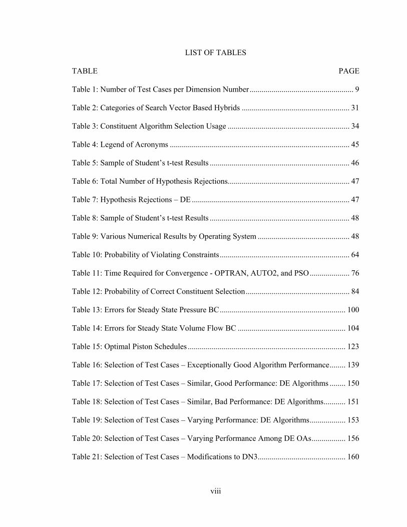
LIST OF TABLES TABLE PAGE Table 1: Number of Test Cases per Dimension Number .................................................... 9 Table 2: Categories of Search Vector Based Hybrids ...................................................... 31 Table 3: Constituent Algorithm Selection Usage ............................................................. 34 Table 4: Legend of Acronyms .......................................................................................... 45 Table 5: Sample of Student’s t-test Results ...................................................................... 46 Table 6: Total Number of Hypothesis Rejections............................................................. 47 Table 7: Hypothesis Rejections – DE ............................................................................... 47 Table 8: Sample of Student’s t-test Results ...................................................................... 48 Table 9: Various Numerical Results by Operating System .............................................. 48 Table 10: Probability of Violating Constraints ................................................................. 64 Table 11: Time Required for Convergence - OPTRAN, AUTO2, and PSO .................... 76 Table 12: Probability of Correct Constituent Selection .................................................... 84 Table 13: Errors for Steady State Pressure BC ............................................................... 100 Table 14: Errors for Steady State Volume Flow BC ...................................................... 104 Table 15: Optimal Piston Schedules ............................................................................... 123 Table 16: Selection of Test Cases – Exceptionally Good Algorithm Performance ........ 139 Table 17: Selection of Test Cases – Similar, Good Performance: DE Algorithms ........ 150 Table 18: Selection of Test Cases – Similar, Bad Performance: DE Algorithms ........... 151 Table 19: Selection of Test Cases – Varying Performance: DE Algorithms .................. 153 Table 20: Selection of Test Cases – Varying Performance Among DE OAs ................. 156 Table 21: Selection of Test Cases – Modifications to DN3 ............................................ 160

ix
Table 22: Selected Test Case – Improvement to STD Due to Modifications ................. 162 Table 23: Relative Performance of Standard and Modified STD ................................... 162 Table 24: Relative Performance of Standard and Modified BST ................................... 162 Table 25: Relative Performance of Standard and Modified DN3 ................................... 162 Table 26: Relative Performance of Standard and Modified TDE ................................... 162 Table 27: Relative Performance of PSO and PRD ......................................................... 163

x
LIST OF FIGURES FIGURE PAGE Figure 1: Various Sections of Rastrigin Function............................................................. 22 Figure 2: Example of Global Best Vector ......................................................................... 24 Figure 3: Example of Population Weighted Average ....................................................... 25 Figure 4: Example of Negative of the Global Worst Vector ............................................ 26 Figure 5: Example of Population Movements and their Accompanying Centroids Using Two Fictitious Algorithms CA1, and CA2 ....................................................................... 29 Figure 6: Utopia vector for two-objective minimization problem .................................... 43 Figure 7: Relative Performance of Blind Hybrids with Different Constituent Selection Methods............................................................................................................................. 51 Figure 8: CKO Selection Preference of PWA Blind hybrid ............................................. 52 Figure 9: CKO & DN3 Selection Preference of IBWA Blind hybrid .............................. 53 Figure 10: Selection Preferences of GB and PGB Blind hybrids ..................................... 53 Figure 11: Selection Preferences of NGW and AV1 Blind hybrids ................................. 54 Figure 12: Relative Performance of Blind hybrids and their Constituent algorithms ...... 55 Figure 13: Convergence Histories for Modified BST on TC 110, and GB Blind hybrid Constituent Algorithm Selection ....................................................................................... 56 Figure 14: Convergence Histories for TC 110 – Blind hybrids ........................................ 56 Figure 15: Relative Performance of Blind hybrids ........................................................... 57 Figure 16: Selection Preferences of AUTO1 and AUTO2 Hybrids ................................. 58 Figure 17: Selection Preferences of DIR Hybrids ............................................................ 58 Figure 18: Best Performance of DIR, AUTO1, AUTO2, and their Constituent Algorithms ........................................................................................................................ 59 Figure 19: Worst Performance of DIR, AUTO1, AUTO2, and their Constituent Algorithms ........................................................................................................................ 60
xi
Figure 20: Best Performance of DIR, AUTO1, AUTO2, and Constituent Algorithms (By Iteration) ..................................................................................................................... 61 Figure 21: Relative Performance of All Search Vector Hybrids ...................................... 61 Figure 22: Relative Performance of DIR, AUTO1, and AUTO2 ..................................... 62 Figure 23: Relative Performance of All Optimization Algorithms .................................. 62 Figure 24: Relative Performance of All Optimization Algorithms (By Iteration) ............ 63 Figure 25: High Dimensional Test Case Convergence Histories – DIR, AUTO1, AUTO2 ............................................................................................................................. 65 Figure 26: Increasing Dimensionality Test Case Convergence Histories – DIR, AUTO1, AUTO2 .............................................................................................................. 66 Figure 27: Convergence History Comparison – Levy9 .................................................... 67 Figure 28: Convergence History Comparison – Griewank ............................................... 68 Figure 29: Griewank – Successful Trials .......................................................................... 68 Figure 30: Convergence History Comparison – Levy ...................................................... 69 Figure 31: Convergence History Comparison – Rosen .................................................... 70 Figure 32: Convergence History Comparison – Schwefel ............................................... 71 Figure 33: Schwefel – Successful Trials ........................................................................... 71 Figure 34: Convergence History Comparison – Schubert ................................................ 72 Figure 35: Best Performance of OPTRAN and AUTO2 (Unconstrained Cases) ............. 73 Figure 36: Convergence Histories over Time (a) AUTO2 (b) OPTRAN ......................... 77 Figure 37: Depiction of Set of Objective Functions A, B, and D ..................................... 80 Figure 38: Example of Possible Worst Case X ................................................................. 80 Figure 39: Example of Typical Performance .................................................................... 80 Figure 40: Ideal Performance ............................................................................................ 81
xii
Figure 41: Relative Performance of Auto2 vs. its Constituents....................................... 83 Figure 44: Comparison of Steady-State Simulations with Pressure BC – Flooded Pipeline ............................................................................................................................. 99 Figure 45: Comparison of Steady-State Simulations with Pressure BC – Flooded Pipeline ........................................................................................................................... 100 Figure 46: Comparison of Steady-State Simulations with Volume Flow BC – Flooded Pipeline ........................................................................................................................... 101 Figure 47: Comparison of Steady-State Simulations with Volume Flow BC, MOC – Flooded Pipeline ............................................................................................................. 103 Figure 48: MOC code with BC computed from Eq. 5.32 – Flooded Pipeline w/ Tees .. 104 Figure 49: Comparison of Steady-State Simulations with Pressure BC – Pipeline with Air ................................................................................................................................... 105 Figure 50: Comparison of Steady-State Simulations with Volume Flow BC – Pipeline with Air ........................................................................................................................... 106 Figure 51: Comparison of Steady-State Simulations with Volume Flow BC – Pipeline with Air ........................................................................................................................... 107 Figure 52: Steady-State MOC Simulation with Volume Flow BC – Pipeline with Air . 108 Figure 53: Comparison of Transient Simulation with Pressure BC – Pipeline with Air 109 Figure 54: Experimental Pipeline Simplified Diagram (Not to Scale) ........................... 110 Figure 55: Photos of Tee Fittings.................................................................................... 110 Figure 56: Photo of Inlet Tee Fitting and Piston Pump .................................................. 111 Figure 57: Photo of Plug ................................................................................................. 111 Figure 58: Validation of MOC code – Volume Flow BC – Fully Flooded Pipeline, 500 mesh elements ................................................................................................................. 114 Figure 59: Validation of MOC code – Pressure BC – Fully Flooded Pipeline, 50 mesh elements .......................................................................................................................... 115 Figure 60: Validation of MOC code – Volume Flow BC – Half Stoke of Air, 50 mesh
xiii
elements .......................................................................................................................... 115 Figure 61: Validation of MOC code – Pressure BC – Half Stoke of Air, 50 mesh elements .......................................................................................................................... 116 Figure 62: Validation of MOC code – Volume Flow BC – Full Stoke of Air, 50 mesh elements .......................................................................................................................... 116 Figure 63: Validation of MOC code – Pressure BC – Full Stoke of Air, 50 mesh elements .......................................................................................................................... 117 Figure 64: Optimization of Piston Operation - Fully Flooded Pipeline .......................... 120 Figure 65: Optimization of Piston Operation – Pipeline with Air on Upstream Side of Plug ................................................................................................................................. 122 Figure 66: Optimization of Piston Operation – Asynchronous (a) Single Phase (b) Pipeline with air on Upstream Side of Plug .................................................................... 122 Figure 67: Best Performance of Unmodified Optimization Algorithms ........................ 138 Figure 68: Convergence Histories, Test Case 4 .............................................................. 141 Figure 69: Convergence Histories, Test Case 45 ............................................................ 141 Figure 70: Convergence Histories, Test Case 220 .......................................................... 142 Figure 71: Convergence Histories, Test Case 234 .......................................................... 143 Figure 72: Convergence Histories, Test Case 236 .......................................................... 144 Figure 73: Convergence Histories, Test Case 238 .......................................................... 145 Figure 74: Convergence Histories, Test Case 239 .......................................................... 146 Figure 75: Convergence Histories, Test Case 242 ......................................................... 147 Figure 76: Convergence Histories, Test Case 331 .......................................................... 148 Figure 77: Convergence Histories, Test Case 378 .......................................................... 149 Figure 78: Convergence Histories - Similar, Good Performance: DE Algorithms ........ 150 Figure 79: Convergence Histories –Curse of Dimensionality Among DE Algorithms.. 152
xiv
Figure 80: Convergence Histories – Varying Performance Among DE Algorithms ..... 154 Figure 81: Convergence Histories – Curse of Dimensionality Among PSO Algorithms155 Figure 82: Convergence Histories – Varying Performance of PSO Algorithms ............ 156 Figure 83: Convergence Histories – Varying Performance of Yang/Simon Algorithms 157 Figure 84: Best Performance of Unmodified vs Modified Optimization Algorithms .... 158 Figure 85: Convergence Histories – Modified DN3 ....................................................... 159 Figure 86: Convergence Histories – PSO and PRD ........................................................ 160 Figure 87: Convergence Histories – Various Improvements Due to Modifications ...... 161

2
CHAPTER 1
1. INTRODUCTION
The past 30 years have seen a wave of novel global optimization algorithms
published. Many of these algorithms draw inspiration from natural processes, while
others combine successful features from different algorithms into a single, more robust
algorithm through a process called hybridization. One powerful approach to hybridization
is to develop a meta-heuristic that performs automatic switching among a collection of
constituent optimization algorithms. This approach is attractive in part because it is
modular. That is, new modular optimization algorithms can be added or removed from
the hybrid algorithm at any time, making it easy to update the hybrid with the latest
methods. Furthermore, the meta-heuristic itself can be modified without making changes
to the constituent algorithms. In essence, this approach is one of the most customizable
approaches to optimization algorithm development. This thesis proposes a new meta-
heuristic scheme for hybridization based on search vectors that serve as guides to aid in
the selection of a constituent algorithm that is appropriate for the given problem.
The selection of an optimization problem for a given problem, however, raises a
variety of concerns regarding the quality of the criteria used. Specifically, there needs to
be a mechanism that relates the topology of an objective function to some feature of the
optimization algorithm such that the algorithm selected for the problem is likely to be the
best performing algorithm of all constituent algorithms available to the hybrid. This
thesis explores some of the theory surrounding this topic, and demonstrates how using
search vectors provides a good first indication about which global search algorithm is
appropriate for a specific problem.

3
In light of the sheer volume of optimization algorithms presented, this thesis also
explores questions relating to how the performance of hybrid optimization algorithms
ought to be evaluated. Many authors select a small set of test cases with which to
benchmark the performance of their algorithms. While this approach is simple, a small
set of test cases is prone to produce misleading results because it is possible to tailor an
optimization algorithm to a class of problems. Specialization is an undesirable quality for
hybrid algorithms, because the primary goal of hybridization is to increase the number
and type of problems that can be solved by the algorithm. This thesis evaluates the
proposed hybrid optimization algorithm using a set of nearly three hundred test cases, so
that any specialization in the algorithm will be revealed. After evaluating the hybrid
optimization algorithm using standard techniques, this thesis proposes a general
framework for evaluating the performance of hybrids that use automatic switching meta-
heuristics.
After benchmarking the hybrid algorithm against other popular algorithms, the
hybrid algorithm is applied to a real-world problem. The Applied Research Center at
Florida International University has been engaged in research for the Department of
Energy including the evaluation of pipeline unplugging technologies. One such
technology proposed by the Applied Research Center is called the Asynchronous Pulse
Unit. The goal of this pipeline pressurization technology is to build up a large enough
pressure to dislodge plugs that form within the pipeline. In order to assist in this effort,
this thesis presents an improved Method of Characteristics code using novel boundary
conditions that accurately model the experimental set ups used by the Applied Research
Center over the past two years. The code models the propagation of pressure transients in
4
black-iron pipelines created by piston pumps connected to their inlet. By coupling the
Method of Characteristics code to the hybrid optimization algorithm, this thesis
demonstrates that the hybrid algorithm can predict optimal piston pump operation
schedules that produce high pressures across the plug while simultaneously operating
within the specified safety limitations of the pipeline. This information, generated
inexpensively using widely available desktop computers, can be used to help guide
experimental efforts in obtaining the best possible piston pump operation schedule for the
pipelines at their disposal.
1.1. Personal Contributions
As a member of the DOE Fellows program at the Applied Research Center, I
assisted in the construction of experimental pipelines, as well as gathering experimental
data. Additionally, I performed computational fluid dynamics simulations of the pipeline
using ANSYS Fluent in addition to writing an updated Method of Characteristics code
based on [1]. As a member of the MAIDROC Laboratory, I proposed the hybrid
presented in this thesis and wrote the computer code for the hybrid using C++ and
OpenMPI. I translated 300 standard optimization test cases (used for benchmarking
optimization algorithm performance) originally written in Fortran 77, into C++. I
benchmarked the performance of the hybrid and other optimization algorithms (listed
below) on MAIDROC’s 240-core cluster named Tesla, as well as a shared-memory
architecture platform, and interfaced the hybrid with Method of Characteristics code for
the optimization of the Asynchronous Pulse Unit. I wrote the post-processing code used
to create most of the figures and tables in this thesis using MATLAB R2010a. I evaluated
optimization algorithms developed by other authors including Biogeography-Based

5
Optimization, five variations of Differential Evolution, Particle Swarm, two variations of
Quantum Particle Swarm, the Firefly Algorithm, Cuckoo Search, and the Bat Algorithm.
I also proposed modifications to Differential Evolution and Particle Swarm that led to
improvements in their performance. Those modified algorithms were subsequently
incorporated into the hybrid optimization algorithm. I also compared the hybrid
developed in this thesis to a hybrid named OPTRAN, which was previously developed by
researchers at MAIDROC.
6
CHAPTER 2
2. LITERATURE REVIEW
2.1. General Optimization Theory
Engineering problems are inherently optimization problems. The task is never
merely to design a product, but to design a product that meets a specific set of goals in
the best possible way. Therefore, it is possible to formulate engineering problems at a
higher level of abstraction so that algorithms can generate a design that satisfies these
goals.
2.1.1. Designs as Vectors
In optimization literature, vectors are often used to represent designs. For
example, the shape of a molecule can be represented by the collection of positions of
each atom in three-dimensional space. For a diatomic molecule, this would require a six-
dimensional vector. The vector representing the design is called the “design vector” [2],
although it can take on names such as “habitat” [3], “individual” [4], “bat” [5], or
“decision variable” [6] depending on the author. The space created by the set of all
possible designs for a given problem is called the design space. This thesis only deals
with designs that can be expressed as vectors, therefore, all design spaces are also
assumed to be vector spaces. The goal is to locate a vector in this space that satisfies the
goals of the design process to the greatest possible extent. This vector is called an
“optimal” solution or design.
2.1.2. Objective Functions
The goal of an engineering problem is associated with a metric (e.g. cost, or
weight). These metrics are functions of the design parameters (e.g. a larger beam will
7
cost and weigh more than a smaller one). Thus, an engineering problem can be
represented by a mathematical function called an “objective function,” that is designed to
reflect the goal of the optimization process (e.g. minimize cost). By convention, the
objective function is written such that the goal is always met by minimizing the function
[7],
)(xUUMinimize
(2.1)
where U is the objective function and x is the design vector.
Although a simple engineering problem may only have a single objective
function, that objective function can have more than one minimum. The lowest possible
value of the objective function is called the global minimum, while other minima with
higher values are called local minima. A function with a single global minimum is called
“unimodal,” while a function with multiple global minima is called “multimodal” [8].
Real-world engineering problems are usually multi-objective. If the objective
functions have distinct global minima (i.e. the objectives are conflicting) the problem has
a cardinality greater than one, and there is no single solution to the problem [8].
Therefore, there exists a set of solutions called the “Pareto optimal set,” or “Pareto Front”
that satisfies each objective such that no improvement can be made in one objective
without diminishing performance in another objective [8].
The optimization algorithms considered in this thesis are designed for a single-
objective optimization problem, but often have multi-objective extensions.
2.1.3. Constraints
Real-world engineering problems also have constraints. These constraints may be
limitations on the value of an objective function (e.g. cost cannot exceed a given value),
8
the value of a design parameter (e.g. wing span must remain below a given value), or
some combination thereof. Constraints can be expressed as inequalities or equalities, as
follows,
0)( xg (2.2)
0)( xh (2.3)
For example, an equality constraint for the composition of a metal alloy would be that the
sum of the percentages of all alloying elements must equal 100%. Due to precision issues
that arise from floating point arithmetic, equality constraints are often recast as,
)(xh
(2.3a)
where ε is a small number (e.g. 10-7).
Many optimization algorithms lack explicit mechanisms for handling constraints.
Therefore, several methods have been developed including the Lagrangian and
Augmented Lagrangian Methods [7], Exterior and Interior Penalty Functions [7], Rosen’s
Projection [9] [10] and others. This thesis utilizes a modified exterior penalty function,
which is discussed in Chapter 3.
2.1.4. Performance Benchmarking
When developing optimization algorithms, it is desirable to compare its
performance to that of other algorithms because this provides an indication of the
algorithm’s relative speed, accuracy, and robustness. It is common practice to use a
handful of standard test cases for performance benchmarking. Some authors have pointed
out that benchmarking in this way can be misleading because many standard functions
contain symmetries or other features (convexity, unimodality, etc.) that can be taken

9
advantage of by a specialized algorithm [11]. Such algorithms perform well for the
problem at hand but poorly for other types of problems. The algorithm presented in this
thesis is intended for simply-connected-domain, black-box problems, and so must not be
specialized.
The Schittkowski & Hock test cases [12] [13] is a set of over 300 test cases
ranging from unconstrained, smooth and continuous objective functions to heavily
constrained, discontinuous objective functions. The dimensionality of the problems
ranges from two to one hundred, as shown in Table 1 below.
Table 1: Number of Test Cases per Dimension Number
Dimension 2 3 4 5 6 7 8 9 10 11
Quantity 89 51 39 27 17 9 6 6 16 1
Dimension 12 13 14 15 16 20 30 48 50 100
Quantity 1 3 1 10 2 6 5 1 5 3
This set is large and diverse enough to be considered useful and representative of a wide
range of real-world problems. Therefore, this set of test cases can reveal when an
optimization algorithm is tailored excessively in favor of one class of problems.
2.2. Passive Pure Optimization Algorithms
Most optimization algorithms converge to a solution in an iterative fashion based
on some mathematical formula. This systematic procedure will be referred to as the
search logic of the algorithm. In this thesis, a passive optimization algorithm denotes an
algorithm whose search logic is static for every iteration. A dynamic algorithm changes
logic based on information from the objective function, or some other scheme. A pure
algorithm (here, a heuristic, and sometimes also referred to as a metaheuristic) will refer
to an algorithm that uses a single logic, while a hybrid combines more than one search

10
logic. Hybrids are classified as metaheuristics.
2.2.1. Local Optimization
For well over 80 years, myriad algorithms have been devised for finding the local
minimum of a function. Most of these methods begin with a point assumed to be near a
minimum (the “initial guess”), formulate a search direction and a step size, and search
along the resulting line toward the minimum. Two of the most widely used methods in
this category, the DFP Conjugate Gradient Method [14] and BFGS Quasi-Newton
Method [15], are called Gradient-Based Methods because they use gradient information
to determine the search direction and step size. Local optimization methods suffer the
drawback that they are only guaranteed to find the global optimum when the objective
function is convex, because in this case the sole local optimum is also the global
optimum. Otherwise, local optimization algorithms simply converge to the nearest
minimum and stop searching once they locate it. Gradient-based methods have the
additional drawback that the function must be differentiable.
2.2.2. Global Optimization
Global optimization algorithms are designed to search large portions of the design
space in order to locate the region containing the global minimum. This is usually
achieved using a set of design vectors (often called a “population” of design vectors).
Many of these algorithms are inspired by observations from biology. One of the first of
these algorithms to be developed, Genetic Algorithms (GA) [16], is inspired by
evolutionary changes in DNA and is a combinatorial algorithm. Other algorithms are
designed for continuous domains and use linear combinations of design vectors in their
search logic. Two very popular methods used in the hybrid developed for this thesis are

11
presented below. The remaining algorithms considered for this thesis are briefly
presented in the Appendix.
2.2.2.1. Particle Swarm Optimization
Particle Swarm Optimization (PSO) has become very popular due to its simplicity
and speed. It is based on the social behavior of various species and uses linear
combination of design vectors to form a new design [17]. Going forward, the equation
used to modify the designs will be referred to as the update equation. The basic PSO
algorithm is given below.
1) Create initial set (population) of design vectors. 2) Evaluate objective function(s) for each design vector. 3) Store copy of initial population to serve as individual best vectors and store the
global best. 4) Begin main loop:
a. For each solution in the population, i. Apply update equation (2.4).
ii. Evaluate objective function(s) using new design vector. iii. Replace individual best with new solution if new solution is superior. b. Replace global best if best new solution is superior to previous global best.
5) End main loop once population converges or maximum number of iterations is reached.
The update equations are,
gi
gi
gi VXX
1 (2.4)
iGbestiibestg
ig
i XXRXXRVV
,2,1
1 (2.5)
where V
is the so-called “velocity vector,” α and β (0.5 and 2, respectively) are user
defined scalars, g is the iteration number, and R1 and R2 are uniformly distributed random
numbers ϵ [0,1]. The vector ibestX ,
corresponds to the best value ever held by the ith

12
design vector (referred to here as the “individual best”, and GbestX ,
is the best solution
ever found (also known as the “global best”). The first term on the right of Eq. 2.5 is the
“inertia,” which is effectively a scalar multiple of the velocity from the previous
iterations. In this thesis, the velocity is initially set to zero.
2.2.2.2. Differential Evolution
Differential Evolution (DE) utilizes an update equation in order to generate a new
design vector, and replaces an existing design vector with the new one if the new design
vector is superior. The standard DE algorithm can be described as follows:
1) Create initial population of candidate design vectors. 2) Evaluate objective function(s) for each design vector. 3) Begin main loop:
a) Copy original population to temporary population. b) For each design vector in the temporary population,
i. Create a new design vector: 1. Randomly select one dimension, j, of design vector and apply update
equation. 2. For each dimension (excluding j) of the current design vector,
a. If R < CR, apply update equation, otherwise, leave unchanged. ii. Evaluate objective function(s) for new design vector.
iii. Compare new design vector to corresponding design vector from original population
iv. If new design vector is superior to original design vector, replace the original with the new design vector.
4) End main loop once population converges or maximum number of iterations is reached.
In the above algorithm, CR is a user-defined scalar ϵ [0,1] known as the “crossover rate,”
and R is a uniformly distributed, random number ϵ [0,1].
There are many forms of DE currently in use, several of which vary only by the
update equation used. Three particularly successful forms are the so-called rand/1/bin,
and best/2/bin proposed in [18] as well as Donor3 proposed in [19]. Their respective
update equations are as follows,
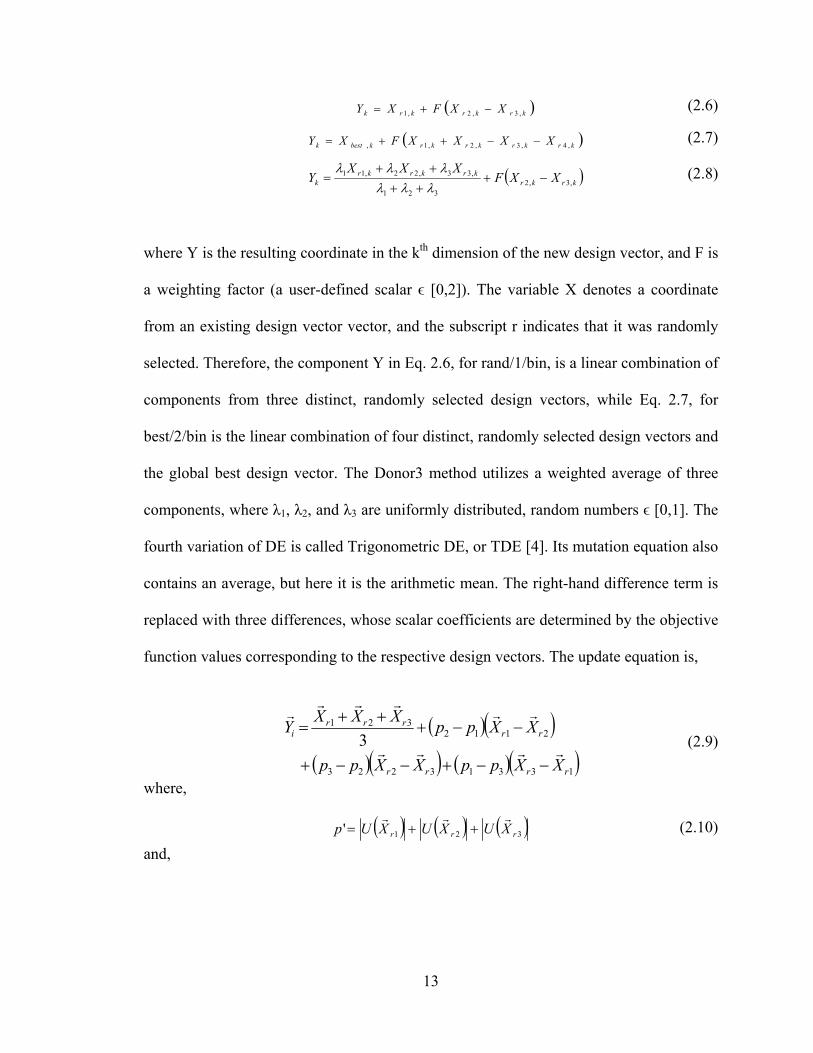
13
krkrkrk XXFXY ,3,2,1 (2.6)
krkrkrkrkbestk XXXXFXY ,4,3,2,1, (2.7)
krkrkrkrkr
k XXFXXX
Y ,3,2321
,33,22,11
(2.8)
where Y is the resulting coordinate in the kth dimension of the new design vector, and F is
a weighting factor (a user-defined scalar ϵ [0,2]). The variable X denotes a coordinate
from an existing design vector vector, and the subscript r indicates that it was randomly
selected. Therefore, the component Y in Eq. 2.6, for rand/1/bin, is a linear combination of
components from three distinct, randomly selected design vectors, while Eq. 2.7, for
best/2/bin is the linear combination of four distinct, randomly selected design vectors and
the global best design vector. The Donor3 method utilizes a weighted average of three
components, where λ1, λ2, and λ3 are uniformly distributed, random numbers ϵ [0,1]. The
fourth variation of DE is called Trigonometric DE, or TDE [4]. Its mutation equation also
contains an average, but here it is the arithmetic mean. The right-hand difference term is
replaced with three differences, whose scalar coefficients are determined by the objective
function values corresponding to the respective design vectors. The update equation is,
13313223
2112321
3
rrrr
rrrrr
i
XXppXXpp
XXppXXX
Y
(2.9)
where,
321' rrr XUXUXUp
(2.10)
and,

14
'
'
'
33
22
11
pXUp
pXUp
pXUp
r
r
r
(2.11)
Clearly, if all three p values equal zero, this method will yield an undefined value.
Therefore, as a precaution, the following condition was added to this algorithm,
4010')0'( ppif (2.12)
This condition was implemented in lieu of the more common practice of adding a small
constant to p’ so that the algorithm’s performance will not be biased when the values of p
are small. Apart from a distinct update equation, this method differs from the previous
method in that it also contains an additional condition,
a) For each dimension (excluding j) of the current design vector, i. If R1 < CR,
1. If R2 < Mt use Eq. 2.9 to create mutant, else use Eq. 2.6 where R1 and R2 are distinct, random numbers ϵ [0,1], and Mt is a user-defined scalar ϵ
[0,1]. The method’s developers suggested that Mt be set to 0.05, because TDE is a
“greedy” search method [4]. Lampinen and Fan also remarked that if Mt were set to zero,
this method would reduce to DE rand/1/bin.
Global optimization algorithms often have the drawback that they require many
function evaluations (sometimes thousands or more) to locate the region containing the
global minimum, and can require just as many evaluations to converge to the solution
itself once within that region.
2.3. Hybrid Optimization Algorithms
Depending on the objective function topology, some algorithms perform better
15
than others. Thus, it is desirable to combine algorithms into a more complex, hybrid
algorithm so that their strengths can be leveraged and their weaknesses mitigated.
Algorithms that make up the hybrid are called “constituent algorithms.” For example,
using a global optimization algorithm to locate the region containing the global minimum
and switching to a local optimization algorithm dramatically improves the likelihood of
reaching the global minimum in a computationally efficient manner. Such a hybrid is
classified as a “global-local” hybrid (for example, see [20]).
2.3.1. No Free Lunch
The question then becomes, is it possible to create a black-box optimization
algorithm (hybrid or not) with competitive or even superior performance against all other
algorithms for all possible optimization problems? In other words, is it possible to create
an effective general-purpose optimization algorithm? Some authors have said no (given
certain assumptions). Wolpert and Macready [21] claim that “the average performance of
any pair of algorithms across all possible problems is identical.” Their “No Free Lunch”
(NFL) theorem indicates that if one algorithm is superior to another for a given set of
optimization problems, it must then be inferior over another set of optimization problems.
Droste, Jansen, and Wegener, [22] show that while this is true under some circumstances,
it is not absolutely applicable because there are instances where an algorithm can perform
in an above-average sense. They propose an “Almost No Free Lunch” (ANFL) theorem,
which states that an algorithm is efficient at solving a certain class of problems because it
implicitly utilizes information about the structure of the function. Therefore, “it is
possible to describe other simple functions which are closely related to functions easy for
[the algorithm] and which, nevertheless, are hard for [the algorithm].” Yang [23] points

16
out that Wolpert and Macready’s NFL theorem is based on assumptions that do not
always apply: (1) the design space is countable and finite, and (2) the algorithm does not
revisit the same region. It has been shown that if the problem domain is continuous
(uncountable), or not closed under permutation (revisiting), that the NFL theorem does
not hold [24] [25] [26]. Therefore, under certain real-world conditions it appears possible
to develop a black-box optimization algorithm with above-average performance.
2.3.2. Hybrid Algorithm Architectures
There currently exist a great many optimization algorithms in literature, and there
are untold thousands of ways to combine them. Talbi [27] developed a taxonomy,
referenced below, to categorize hybrid algorithm architectures, which was later expanded
upon by authors including Raidl [28]. For the purpose of this thesis it suffices to say that,
in general, there are three noteworthy approaches to hybridization, each based on the way
in which the population of design vectors is operated on. A global-local hybrid can be
created from any one of these architectures simply by passing some or all of the
population to a local optimization algorithm at some stage of the optimization process.
2.3.2.1 Competitive
Competitive hybrids (high-level, relay [27]) switch between constituent
algorithms such that only a single constituent algorithm operates on the entire population
at a time. For example, the competitive hybrid might begin with PSO, and then switch to
DE once some criterion is met. The hybrid presented in this thesis is of this type.
Additional examples will be discussed in greater detail below.
2.3.2.2 Cooperative
Cooperative hybrids (high-level teamwork [27]) allow multiple constituent

17
algorithms to operate on subsets of the population simultaneously during each iteration.
Unlike competitive hybrids, the switching logic pertains to the size of the population
passed to each constituent algorithm, which may be constant. An example of such
hybrids can be found in [29].
2.3.2.3 Merged
Merged hybrids (low-level, relay [27]) combine the essential components of
different constituent algorithms into a single algorithm. In this way, the basic operations
of all constituents are executed on the entire population during each iteration of the
hybrid algorithm. Thus, the population is updated multiple times during a single iteration.
This is different from a competitive hybrid in that competitive hybrids may not execute a
given constituent at all, and it is different from the cooperative hybrid in that the entire
population is operated on. Examples of such hybrids can be found in [30] [31] [32].
2.3.3. Switching Logic
Within the scope of a competitive hybrid, the essence of the algorithm is the way
it switches from one constituent algorithm to another. Since each constituent algorithm
has its own search logic, the switching mechanism may override that logic by interrupting
the sequence of events that would naturally follow. Over several years, researchers
affiliated with MAIDROC have developed and tested several hybrid algorithms with
automatic switching that do not override the constituent algorithm’s search logic [33]
[34] [35]. Rather, these hybrids allow the constituent algorithm to proceed until it triggers
some failure mode or convergence criterion, and then switch to another algorithm in
order to perform an efficient local search, or perform a new global search. The interested
18
reader is referred to [36] [37] [38] for a discussion of multi-objective hybrids developed
by MAIDROC.
The first in the series was simply a global-local algorithm made up of GA and
DFP [33]. Once GA’s convergence rated slowed to a certain value, the hybrid would
switch to DFP and converge to the nearest minimum. Once DFP converged, the hybrid
would restart GA and this cycle would repeat a number of times in order to increase the
likelihood of finding the global minimum.
The second in this series [34], combined three local optimization algorithms
[DFP, the Nelder-Mead (NM) simplex method, and simulated annealing (SA)], and used
GA to perform a global search. It enforced constraints using Rosen’s projection, feasible
searching, and random design generation. The additional local search algorithms enabled
the hybrid to switch from GA to NM in the event of a failure (a bad mutation or lost
generation). If the objective function variance was small, the hybrid would switch from
GA to SA. If the design vector variance was small, the hybrid would switch from GA to
DFP. NM and SA would switch to DFP in the event of a stall or insufficient energy,
respectively. SA would switch to NM if it exceeded a predetermined number of
iterations.
The third and fourth hybrids in the series were very similar. They each included
DFP, GA, NM, and sequential quadratic programming (SQP). The fourth generation [39]
added a second global optimization algorithm (DE), and replaced SA with a Quasi-
Newton algorithm by Pshenichny-Danilin (LM). The hybrid would begin with GA and
cycle through NM, or SQP. SQP’s convergence would trigger LM, which would
similarly trigger DFP. DFP’s convergence would trigger the activation of DE. Once DE’s

19
convergence stalled, the algorithm would switch back to GA and repeat for a given
number of loops.
The fifth and sixth hybrids in the series utilized only three constituent algorithms
(PSO, DE, and BFGS), where the sixth included the use of response surfaces (surrogate
models that approximate the value of the objective function but are computationally
faster to execute) in order to improve its overall speed [33]. The global optimization
search would begin with PSO, and would switch to DE once a certain percentage of the
population appeared to converge. If the search executed by DE produced an improvement
in the current minimum, the hybrid would switch back to PSO. Otherwise, it would
switch to BFGS to rapidly locate the nearest minimum. Once BFGS converged, the
hybrid would switch back to PSO and loop as the previous hybrids did.
Each of these hybrids calls their constituent optimization algorithms in a
predetermined sequence based on a set of rules (triggers). This style of hybrid
architecture development uses inductive reasoning that proceeds roughly as follows:
If algorithm X behaves in manner A, this implies B.
Given B, use algorithm Y.
Otherwise, use algorithm Z.
All global-local hybrids are based on this logic (if the global optimization algorithm
appears to converge, the hybrid switches to the local optimization algorithm). In cases
like these, the architect of the hybrid has assumed certain characteristics about the nature
of the design space, the objective function space, and the search logic of the constituent
algorithms, and developed rules intended to capitalize on these characteristics. Thus, it
follows that if any of the assumptions are wrong (A does not imply B), or if the rules are

20
inadequate (e.g. Y should not always be used given B), the hybrid risks converging to a
local minimum. While the additional search logic of hybrid algorithms may increase the
risk of poor convergence beyond those of its constituent algorithms, hybrid algorithms
possess the greatest potential in obtaining as close to a free lunch as possible. The hybrids
discussed above have been shown to outperform their constituent algorithms [33].
Therefore, a properly crafted switching mechanism is the key to a competitive hybrid’s
success.
21
CHAPTER 3
3. SEARCH VECTOR BASED HYBRID OPTIMIZATION ALGORITHM
3.1. A Global-Global Hybrid
The motivation behind the hybrid developed in this thesis is based on two
observations. The first comes from the statement in [22]: “Each search heuristic which is
able to optimize some functions efficiently follows some idea about the structure of the
considered functions.” Therefore, a hybrid that intelligently switches between global
optimization algorithms (a global-global hybrid) can efficiently optimize a wider range of
objective functions without requiring input from the user. That is, it serves as a better
black-box algorithm than its constituent algorithms (in the global optimization sense).
3.1.1. Single Objective – Multiple Topologies
It is easy to read the above statement and mistakenly assume that a single
objective function must have a single structure. While this is true from a strictly
theoretical standpoint, this is not really the case in practice when no a priori knowledge
of the problem is available. Global optimization is an inherently statistical process that
begins with a sample of designs. Determinations regarding the topology of an objective
function depend entirely on the distribution and size of the sample, which can be
misleading because it is incomplete. The second motivation for the hybrid presented here,
and the stronger statement made for it in this thesis is that, from the “perspective” of the
optimization algorithm, the topology of most objective functions appears to change
throughout the optimization process. That is, most objective functions have multiple
“effective” topologies. Therefore, for the broader set of optimization problems there
should be no expectation that any single algorithm will perform in an above-average
22
sense. A hybrid, on the other hand, has the potential to do so (within the scope of real-
world scenarios discussed in Chapter 2).
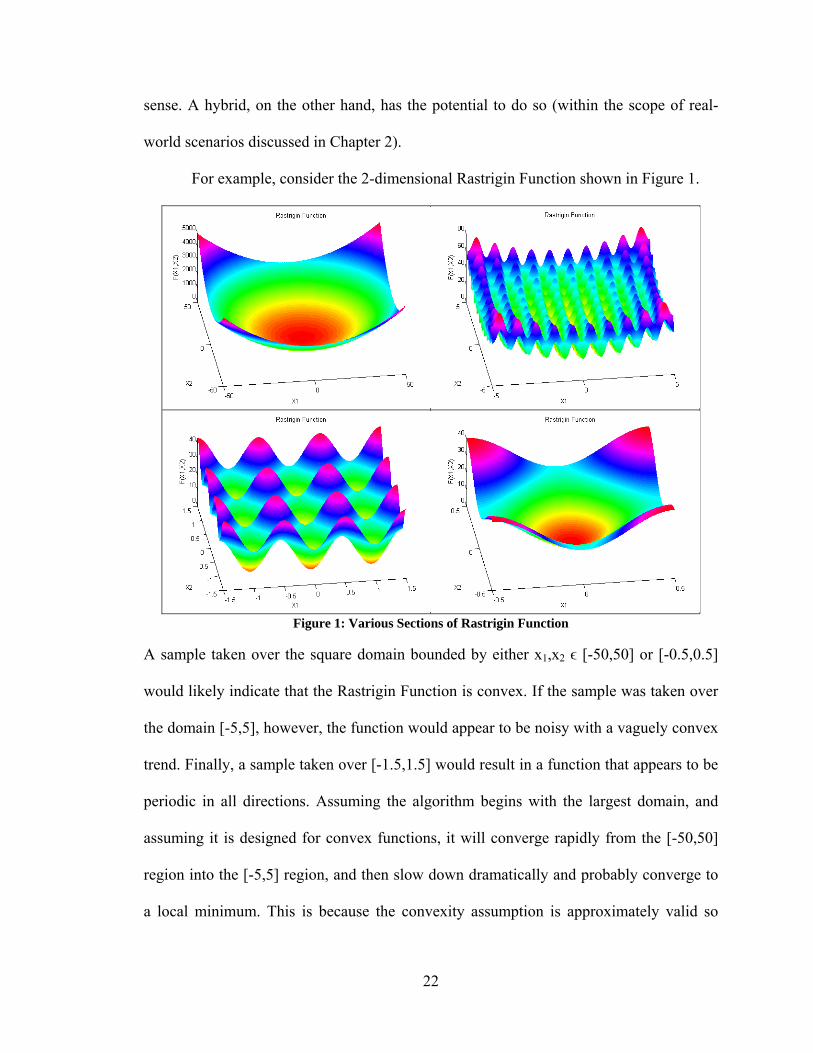
For example, consider the 2-dimensional Rastrigin Function shown in Figure 1.
Figure 1: Various Sections of Rastrigin Function
A sample taken over the square domain bounded by either x1,x2 ϵ [-50,50] or [-0.5,0.5]
would likely indicate that the Rastrigin Function is convex. If the sample was taken over
the domain [-5,5], however, the function would appear to be noisy with a vaguely convex
trend. Finally, a sample taken over [-1.5,1.5] would result in a function that appears to be
periodic in all directions. Assuming the algorithm begins with the largest domain, and
assuming it is designed for convex functions, it will converge rapidly from the [-50,50]
region into the [-5,5] region, and then slow down dramatically and probably converge to
a local minimum. This is because the convexity assumption is approximately valid so

23
long as the population is spaced very far apart. Once the population converges to a
smaller space (i.e. the distribution of the sample decreases), the assumption is no longer
valid and the algorithm becomes ill-suited for the effective topology it is navigating.
Therefore, the hybrid presented here, and previously briefly introduced in [33],
does not wait for a constituent algorithm to converge. Rather, it uses other indicators to
determine if, and when, to use a constituent algorithm.
3.1.2. Search Vectors
In local optimization, many algorithms fall into the category of line search
algorithms, whose basic equation takes the form,
sxx initialfinal
(3.1)
where s
is the search direction, and α is the scalar step size that enables the algorithm to
“step” from the initial design to a final design. The hybrid presented here utilizes a
population-based analogy of the search direction called a “search vector” with the
following general form,
centroidsamplesearch vvv
(3.2)
Where v
search is the search vector, and v
centroid is the arithmetic mean of the population.
The sample point (also a vector), v
sample, is any vector taken from the population or
calculated from some formula that is used to guide the search. In this analogy, rather than
moving a single design from one location to another within the design space, the entire
population is moved from one region in space to another. This movement is represented
by the displacement of the population’s centroid, as follows,
searchinitialcentroidfinalcentroid vvv
,, (3.3)
24
The distribution of the population is not considered in this calculation, indicating that the
population can disperse from or converge toward its centroid without affecting the
hybrid’s switching logic. The following subsections discuss the formulas for the eight
sample points used to create search directions in this thesis:
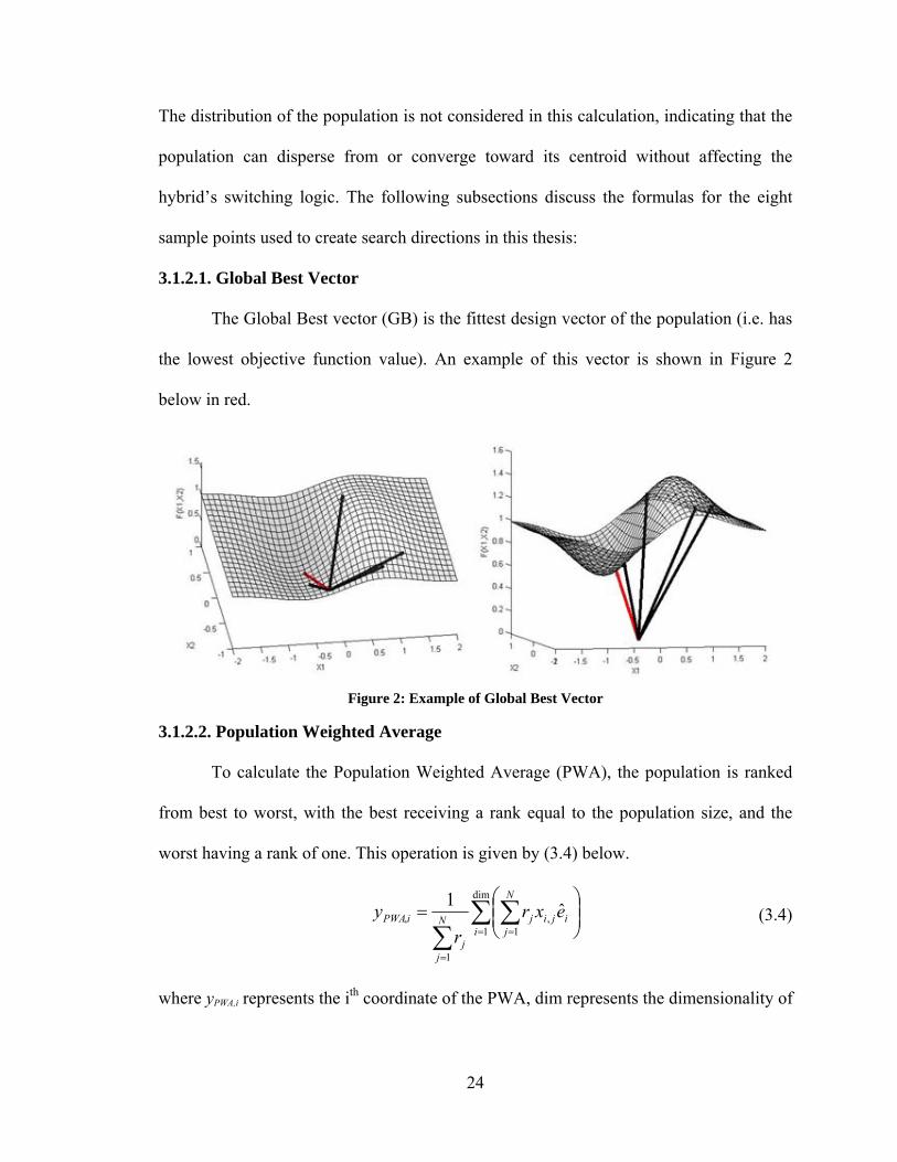
3.1.2.1. Global Best Vector
The Global Best vector (GB) is the fittest design vector of the population (i.e. has
the lowest objective function value). An example of this vector is shown in Figure 2
below in red.
Figure 2: Example of Global Best Vector
3.1.2.2. Population Weighted Average
To calculate the Population Weighted Average (PWA), the population is ranked
from best to worst, with the best receiving a rank equal to the population size, and the
worst having a rank of one. This operation is given by (3.4) below.
dim
1 1,
1
, ˆ1
i
N
jijijN
jj
iPWA exrr
y (3.4)
where yPWA,i represents the ith coordinate of the PWA, dim represents the dimensionality of

25
the design space, N is the population size, rj represents the rank of the jth design vector in
the population, e i is the unit vector in the ith direction, and xi,j is the ith coordinate of the jth
design vector. This vector is not originally a part of the population.
3.1.2.3. Individual Best Weighted Average
Another vector called the Individual Best Weighted Average (IBWA) is
conceptually identical to the PWA but uses the individual best population stored for
Particle Swarm. In the first iteration, this vector is equal to the PWA. An example of the
PWA is shown in Figure 3 below in red. For alternative (conceptually similar)
combinations of individual best vectors, the interested reader is referred to [40].
Figure 3: Example of Population Weighted Average
3.1.2.4. Negative of the Global Worst Vector
The Negative of the Global Worst vector (NGW) is constructed by reflecting the
global worst vector (the design with the highest objective function value) across the
center of the domain, according to the equation below:
GWULNGW xddy
(3.5)
where y
NGW represents the NGW, d
L represents the lower limit of the domain, d
U is
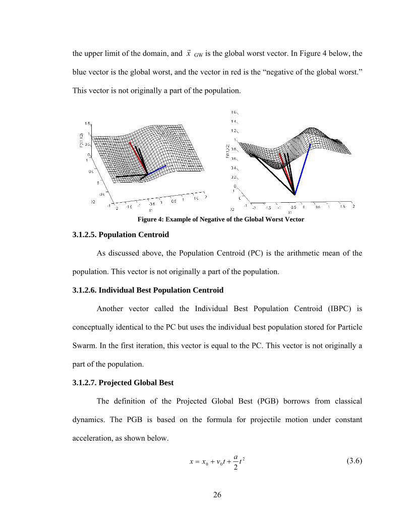
26
the upper limit of the domain, and x
GW is the global worst vector. In Figure 4 below, the
blue vector is the global worst, and the vector in red is the “negative of the global worst.”
This vector is not originally a part of the population.
Figure 4: Example of Negative of the Global Worst Vector
3.1.2.5. Population Centroid
As discussed above, the Population Centroid (PC) is the arithmetic mean of the
population. This vector is not originally a part of the population.
3.1.2.6. Individual Best Population Centroid
Another vector called the Individual Best Population Centroid (IBPC) is
conceptually identical to the PC but uses the individual best population stored for Particle
Swarm. In the first iteration, this vector is equal to the PC. This vector is not originally a
part of the population.
3.1.2.7. Projected Global Best
The definition of the Projected Global Best (PGB) borrows from classical
dynamics. The PGB is based on the formula for projectile motion under constant
acceleration, as shown below.
200 2
ta
tvxx (3.6)
27
where x represents position, x0 is the initial position, v0 is the initial velocity, a is the
acceleration, and t is time. Time, here, is understood to be the number of iterations. This
concept was implemented due to its mathematical simplicity and because it strives to
predict the location of the next GB, rather than relying strictly on population values from
the current iteration. Given the GBs for the previous two iterations and the current
iteration, x0, x1, and x2, respectively, the PGB, represented by x3, can be derived from the
following linear system of equations:
00 xx (3.6a)
2001
avxx (3.6b)
avxx 22 002 (3.6c)
This leads to a system of two equations with two unknowns, namely the initial velocity
and acceleration. Using matrix notation and combining (3.6b) with (3.6c),
02
010
22
5.01
xx
xx
a
v (3.6d)
Inverting the coefficient matrix yields,
02
010
12
5.02
xx
xx
a
v (3.6e)
Thus, v0 and a can be expressed in terms of the previous positions.
0120 5.125.0 xxxv (3.6f)
012 2 xxxa (3.6g)
At the third iteration, the position equation becomes,
28
avxx2
93 003 (3.6h)
Substituting (3.6f) and (3.6g) into (3.6h) and simplifying yields the final result,
0123 33 xxxx (3.6i)
This equation is computed separately for each component of the PGB, as though each
dimension were under its own constant acceleration. This vector is not originally a part of
the population.
3.1.2.8. Average Vector 1
The Average Vector 1 (AV1) is the arithmetic mean of the GB, PWA and NGW,
and was found to be advantageous in certain objective function topologies after some
experimentation.
During early development of this hybrid, only a single sample point was used throughout
the entire optimization process. This way, the sample point could be calculated without
being evaluated (unless it was already part of the population), reducing the total number
of objective function evaluations required by the algorithm. After some experimentation,
it was decided that all sample points should be evaluated and compared. The sample
point with the lowest objective function value was then selected for use by the hybrid. It
is clear from Equation 3.3 that,
samplefinalcentroid vv
, (3.3a)
Therefore, for each iteration, the sample point is the desired final destination for the
population centroid. The sample point is one of the indicators that guides the global
search (during early development, it was the only indicator). Each iteration, the goal of
the hybrid switching mechanism is to shift the population toward the sample point
29
because this point is assumed the correct direction for the population to move to in order
to locate the global minimum. Therefore, the hybrid must select a constituent algorithm
that is most likely to produce this result.
3.1.3. Constituent Algorithm Search Vector
Each constituent algorithm has some mechanism (an equation, etc.) to produce
new candidate design vectors for the next iteration. The set of new candidate designs
shall be called the “temporary population.” The objective function is not executed for
these points (i.e. the temporary population is not evaluated), and contains as many design
vectors as there are in the primary population used by the hybrid. The arithmetic mean of
the temporary population shall be called the “temporary centroid.” In order to select a
constituent algorithm, the hybrid will execute a constituent algorithm ten times, so that
ten temporary populations are created. The temporary centroid for each temporary
population is computed, and then averaged to produce one final vector (a centroid of all
ten temporary populations).
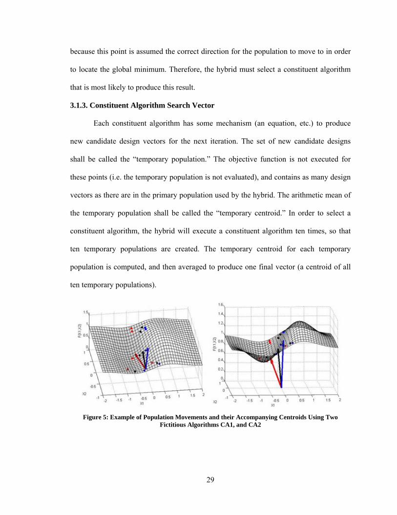
Figure 5: Example of Population Movements and their Accompanying Centroids Using Two
Fictitious Algorithms CA1, and CA2
30
This final result is called the “centroid of the constituent algorithm,” or simply the CCA.
For example, suppose the hybrid has two constituent algorithms called CA1 and CA2
(see Figure 5). It is possible that CA1 will update the current population (black dots) in
one direction (red dots), while CA2 will update the population in another direction (blue
dots). The vectors in Figure 5 represent the centroids of each population. Since each
constituent algorithm contains random parameters, it is executed ten times so that its CCA
has some statistical significance without excessively increasing the method’s
computational cost. The CCA represents the location that the population centroid would be
moved to if that constituent algorithm were used. This process is repeated for every
constituent algorithm so that a CCA is computed for each (e.g. a CPSO, CDE, etc.). During
early stages of development, the CCA’s were compared to the sample point using some
equation (discussed below) in order to determine which constituent algorithm to use, but
never evaluated. Dr. Dulikravich suggested that the CCA’s be evaluated and used as the
sole indicator for constituent algorithm switching. After more experimentation, it was
later decided that both CCA’s and sample points be evaluated and used as indicators, and a
more sophisticated switching logic was devised. In order to facilitate certain
comparisons, the “constituent algorithm search vector” was defined as follows,
centroidCACA vcv
(3.7)
where c
CA is the CCA, and v
CA is the CCA translated so that it originates at the centroid
of the population. When needed, the CCA can be compared directly to the sample point,
and the search vector can be compared directly to the constituent algorithm search vector.
3.2. Search Vector Based Hybrid
One of the goals in developing the Search Vector Based Hybrid was to minimize
31
the number of additional objective function evaluations required by the hybrid beyond
those performed by the constituent algorithms (minimize overhead).
Table 2: Categories of Search Vector Based Hybrids
Category Evaluate & Compare
Search Vector Evaluate &
Compare CCA Blind No No Direct N/A Yes Auto Yes Yes
Therefore, during the early stages of development, none of the search vectors or CCAs
were evaluated unless they were already part of the population. Since these vectors guide
the population without any information about the objective function at that location, this
category of search vector hybrid is called a “Blind Hybrid Optimization Algorithm.” The
“Direct Hybrid Optimization Algorithm” does not compute search vectors at all, but at
the suggestion of Dr. Dulikravich, computes and evaluates the CCAs and uses their values
to compare each constituent algorithm directly. Both the Blind and Direct hybrids have
an automatic constituent algorithm switching mechanism, but do not automatically switch
between search vectors. That is, the Blind and Direct hybrids use a single search vector
throughout the entire optimization process. The “Auto Hybrid Optimization Algorithm”
evaluates the sample points so that it can automatically switch between search vectors
and constituent algorithms each iteration.
In order to achieve this functionality, the search vectors and constituent
algorithms are implemented as modules. This provides the added benefit that the hybrid
can utilize any set of algorithms, whether it is the same algorithm tailored for different
problems (e.g. multiple modules of Differential Evolution with different parameters for

32
different classes of problems), or a variety of different methods including newly
published algorithms.
3.2.1. Constituent Algorithm Selection Criteria
Although the hybrid’s search logic assumes that the sample point is the best
direction to move in, there are several ways to use this information when selecting a
constituent algorithm. The following five selection methods have been developed for this
thesis:
3.2.1.1. Lowest Distance
This method calculates the Euclidean distance between the CCA and the sample
point. This distance is calculated in the design space; therefore, the objective function
value is not taken into consideration.
dim
1
2,,
iiCAisample cvd
(3.8)
The constituent algorithm whose CCA is closest to the sample point will be selected.
3.2.1.2. Highest Dot Product
This method calculates the dot product between the search vector and the
constituent algorithm search vector. That is,
centroidCAcentroidsample
centroidCAcentroidsample
CAsearch
CAsearch
vcvv
vcvv
vv
vv
(3.9)
Again, the objective function value is not taken into consideration. The constituent
algorithm whose centroid is closest to parallel to the search vector will be selected. This
formulation cannot be used when the sample point is the population centroid (the lowest
distance can be used instead).
33
3.2.1.3. Lowest Scaled Distance
Similar to the lowest distance, this method uses the following equation below,
1
2
1^1
pop
temp
pop
temps dd
(3.10)
where ds is the “scaled” distance between the sample point and the CCA, while d is the
Euclidean distance from Eq. 3.8. The term in brackets is the exponent of the d+1 term,
and contains the ratio between the standard deviation of the temporary population, σtemp,
and the current population standard deviation, σpop. The standard deviation are based on
the distances between the populations under consideration and their respective centroids.
The exponent rewards constituent algorithms whose standard deviation is less than the
existing population’s standard deviation, or greater than 50% of that value. This was
developed in an effort to penalize methods that converge too quickly or cause the
population to spread out further. The constituent algorithm with the lowest scaled
distance is selected.
3.2.1.4. Direct CCA Comparison
This method, proposed by Dr. George Dulikravich, ignores the objective function
values of sample points. Instead, it evaluates the CCAs generated by the constituent
algorithms and selects the algorithm with the minimum CCA.
3.2.1.5. Pareto Ranking Method
This method treats the Lowest Distance and Direct Comparison methods as two
distinct objectives. The constituent algorithms are ranked using the Pareto dominance
scheme in [8]. The constituent algorithm is then randomly selected from the Pareto
optimal set (the constituent algorithms that are non-dominated in terms of lowest distance
34
and minimum CCA). Although developed independently, and applied differently, the
concept of using multi-objective processes in a single objective problem appears in [41],
and its references.
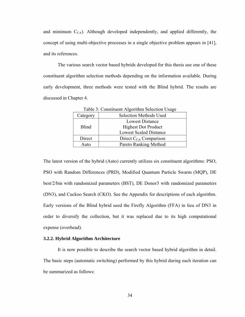
The various search vector based hybrids developed for this thesis use one of these
constituent algorithm selection methods depending on the information available. During
early development, three methods were tested with the Blind hybrid. The results are
discussed in Chapter 4.
Table 3: Constituent Algorithm Selection Usage Category Selection Methods Used
Blind Lowest Distance
Highest Dot Product Lowest Scaled Distance
Direct Direct CCA Comparison Auto Pareto Ranking Method
The latest version of the hybrid (Auto) currently utilizes six constituent algorithms: PSO,
PSO with Random Differences (PRD), Modified Quantum Particle Swarm (MQP), DE
best/2/bin with randomized parameters (BST), DE Donor3 with randomized parameters
(DN3), and Cuckoo Search (CKO). See the Appendix for descriptions of each algorithm.
Early versions of the Blind hybrid used the Firefly Algorithm (FFA) in lieu of DN3 in
order to diversify the collection, but it was replaced due to its high computational
expense (overhead).
3.2.2. Hybrid Algorithm Architecture
It is now possible to describe the search vector based hybrid algorithm in detail.
The basic steps (automatic switching) performed by this hybrid during each iteration can
be summarized as follows:

35
I) Calculate each sample point i) Evaluate each sample point (Auto only)
II) Calculate each CCA i) Evaluate each CCA (Direct and Auto only)
III) Perform constituent algorithm selection IV) Operate on population using constituent algorithm
Therefore, this hybrid does not have any rules or equations enabling it to generate new
designs of its own. Rather, the initial population is created using a random number
generator, and the constituent algorithms generate every subsequent population. The
hybrid architecture “wraps around” the constituent algorithms.
3.2.2.1. Random Number Generator
The hybrid is equipped with two random number generators: the ran2 function
given in [42], as well as Sobol’s Algorithm [43] downloaded from [44]. Ran2 is the
hybrid’s default random number generator due to its speed.
3.2.2.2. Population Size
A typical global optimization algorithm only operates on its population once per
iteration, but the search vector hybrid executes its constituent algorithms a total of 10M +
1 times per iteration, where M is the number of constituent algorithms. This means that
the current version of the hybrid loops over the population 61 times per iteration (the first
60 times are simply to generate temporary populations). For this reason, and due to the
high computational expense typical of objective function evaluations, it is desirable to
reduce the population size.
One popular approach to determining the population size is to vary it linearly with
the dimensionality of the problem. For example, the following might be used,
dim10N (3.11)
36
where dim is the dimensionality of the problem, and N is the population size. In order to
reduce the size of the population for problems with high dimensionality, the following
nonlinear function was developed after several tests,
3
log(dim)5.65dim142.14dim59.12 3/2
ceilN (3.12)
where ceil is a function that rounds a number up to the nearest integer. Both (3.11) and
(3.12) result in a population size of 20 for a 2D problem.
3.2.2.3. Constraint Enforcement
For simplicity, the hybrid uses a modified objective function based on a type of
exterior penalty function. Since the global minima of the Schittkowski and Hock test
cases are published, the objective function is first modified to reflect the error (E), that is
the difference between the current value and the published minimum value (U*), as
follows,
*)()( UxUxE (3.13)
This is then combined with a penalty function. The standard form given for an exterior
penalty function given in [7] is,
l
jj
m
ii xhxgxp
1
2
1
2 )()](,0max[)(
(3.14)
where m is the number of inequality constraints, and l is the number of equality
constraints. This penalty function modifies the objective (error) function as follows,
)()()( xprxExW p
(3.15)
where W is the modified objective function, and rp is a user-defined scaling factor. The
scaling factor serves to increase or decrease the magnitude of the penalty generated by

37
the penalty function. If the penalty is too small relative to the magnitude of the objective
function, this form of constraint enforcement can easily yield infeasible results, but if it is
too large, it may yield suboptimal results. The greater concern, however, is feasibility.
Because the scaling factor is user-defined its value often depends on the user’s intuition,
or is tailored to suit a specific class of problems or algorithms. To alleviate this issue
(letting rp = 1), the following penalty function is used,
l
jj
m
ii xhxgxEnxp
11
)()](,0max[)()(
(3.16)
where n is the total number of constraints violated. This formula ensures that the penalty
function always has a magnitude at least as large as that of the objective function. It is
important to note that this form of constraint enforcement changes the effective topology
of the objective function, often making a function non-differentiable.
3.2.2.4. Blind Hybrid Algorithm Steps
The earliest of the search vector based hybrids developed, this hybrid requires the
fewest additional objective function evaluations. Its primary advantage, however, is not
in its computational cost, but its utility as a research tool. By forcing the search to
proceed in a particular direction, it is possible to gain insights into the relationship
between the effective topology of the objective function and the optimization algorithm
that is ultimately selected. The algorithm is as follows,
I) Initialize population of design vectors II) Evaluate objective function for all design vectors III) Begin Hybrid Loop
i) Calculate sample point ii) Calculate all CCAs iii) Perform constituent algorithm selection iv) Operate on population using constituent algorithm v) If convergence detected, end loop, otherwise return to step i)

38
IV) End algorithm
As demonstrated in the algorithm, the objective function is only evaluated following
initialization and during step (iv).
3.2.2.5. Direct Hybrid Algorithm Steps
The second of the search vector based hybrids presented, this hybrid uses CCAs in
lieu of search vectors and evaluates them. Therefore, it requires additional objective
function evaluations (equal to the number of constituent algorithms used).
I) Initialize population of design vectors II) Evaluate objective function for all design vectors III) Begin Hybrid Loop
i) Calculate all CCAs ii) Evaluate all CCAs iii) Select constituent algorithm with minimum CCA iv) Operate on population using constituent algorithm v) If convergence detected, end loop, otherwise return to step i)
IV) End algorithm
Apart from the direct comparison in step (iii), the CCAs are never used again. Future
versions of the hybrid may incorporate these vectors into the population to improve the
diversity of the population, or to replace inferior design vectors.
3.2.2.6. Auto Hybrid Algorithm Steps
The latest version of the search vector hybrid has the greatest overhead cost, but also
the greatest amount of information with which to make a decision. The algorithm is as
follows,
I) Initialize population of design vectors II) Evaluate objective function for all design vectors III) Begin Hybrid Loop
i) Calculate all sample points ii) Evaluate all sample points iii) Select minimum sample point iv) Calculate all CCAs

39
v) Evaluate all CCAs vi) Select constituent algorithm using Pareto Ranking Method vii) Operate on population using constituent algorithm viii) If convergence detected, end loop, otherwise return to step i)
IV) End algorithm
The first version of the Auto hybrid did not incorporate the sample points or CCAs into
the population. Certain constituent algorithms utilize the “global best” vector in their
search (e.g. DE and PSO). Since the selected sample point may be superior to the best
design vector in the population, the second version of the hybrid passed the sample point
to these constituent algorithms. The results are discussed in Chapter 4.
3.2.3. Ramifications of Hybrid Algorithm Architecture
This section will discuss the implications of the structure of the Auto hybrid
optimization algorithm. The Auto hybrid will simply be referred to as “the hybrid.”
3.2.3.1. Search Logic
The hybrids discussed in Section 2.3.3. allow their global optimization constituent
algorithms to converge, which suggests that these hybrids assume there is a “good match”
between the constituent algorithm and the objective function topology. The search vector
based hybrid switching mechanism often prohibits any one constituent algorithm from
running completely to convergence. Rather, the hybrid compares the constituent
algorithm to the search vector and assumes that a good match between the CCA and the
search vector indicates that the constituent algorithm is a good match for the effective
topology (which changes each iteration). Therefore, the search logic inherent in the
constituent algorithm is overridden by the search logic of the hybrid.
Like all algorithms, the hybrid’s structure is well suited for certain classes of
problems. For example, the hybrid assumes that the sample point with the lowest
40
objective function value is the best. Therefore, if there exists a class of “deceptive”
functions for which this assumption is invalid, this approach may impair the hybrid. An
improvement on this hybrid could include the addition of statistical metrics that could
warn against misleading functions, and give the hybrid a means by which to select other,
more appropriate sample points. For the purpose of this thesis, however, a random
parameter was introduced in the algorithm. Each iteration after the first, there is a 10%
chance that the hybrid will reselect the constituent algorithm used in the previous
iteration. Another way to implement a similar feature could be to introduce a probability
that the hybrid will select a random constituent algorithm rather than the previous one,
but that is beyond the scope of this thesis
3.2.3.2. Constituent Algorithm Implementation
Although the hybrid algorithm is simple, the proper incorporation of constituent
algorithms and maintenance of auxiliary vector populations, such as the velocity of PSO,
is not trivial. Algorithms like BST, DN3, and CKO do not utilize information from
previous iterations and can be treated as independent modules. The PSO and PRD
algorithms, however, utilize a velocity vector population that is a function of the previous
iteration’s velocity. As long as one of these modules is called sequentially, the velocity
vector can be computed normally. However, if the hybrid switches from PSO or PRD to
another method and then back to PSO or PRD, the velocity must be reinitialized. Since
the inertia term is a vital part of PSO, the manner in which this is done dramatically
affects its performance. As a first attempt, the velocity is re-initialized according to the
following equation,
41
jLjUjLgj DDRDV ,,,02.1
2.0 (3.17)
where Vj is the jth coordinate of the velocity vector, DL,j and DU,j are the lower and upper
limits of the search domain in the jth direction respectively, R is a uniformly distributed
random number ϵ [0,1] and g is the generation (iteration) number.
Additionally, algorithms with DE-style comparisons have an implicit form of
elitism. These comparisons prohibit the superior design vectors like the global best
design vector from being replaced by inferior design vectors. This feature is not present
in algorithms like PSO. Therefore, if the hybrid algorithm switches from DE to PSO and
back to DE it is possible to lose superior design vectors. Therefore, the hybrid stores the
global best design vector separately, which partially remedies this problem. Nevertheless,
the hybrid allows the other vectors to be overwritten by constituent algorithms.
3.2.3.3. Computational Expense
Since many real-world problems have objective functions that require hours to
evaluate, generating the search vectors and CCAs is relatively computationally
inexpensive. Evaluating them, in these cases, is not. However, if the objective function is
inexpensive to evaluate (such as when surrogate models are used) the hybrid’s overhead
becomes an important contributor to the overall computational expense. Accordingly, the
hybrid was written using OpenMPI in order to benefit from a parallel computing
environment.
The global optimization algorithms utilized in the hybrid are embarrassingly
parallel. Therefore, in parallel environments, the populations are subdivided among
nodes, reducing the time required for generating temporary populations. For problems of

42
low dimensionality, communication costs between nodes can exceed the costs related to
the population size. When run on Tesla (in serial), the hybrid completes the average 2D
problem (200 iterations) in roughly 2.4 seconds. On Tesla, in parallel (20 nodes), the
communication costs increase this time to 6 seconds. One hundred dimensional problems,
however, take on the order of hours to days in serial, but only minutes to hours in
parallel.
3.3. Proposed Multi-Objective Extension of Hybrid
The notion of a search direction along a given topology is already well
established. When the problem becomes multi-objective, and the objective function space
grows in cardinality, the notion of a single search direction must change to accommodate
the principles of Pareto optimality [8].
3.3.1. Multi-Objective Search Vectors
Some search vectors present in this hybrid, such as the population centroid, can be
used in a multi-objective context without modification. Others, such as the population
weighted average and negative of the global worst, must take on a new meaning and new
formulation. In the context of multi-objective optimization, rankings no longer refer to
single vectors, but rather, refer to sets of vectors. Non-dominated vectors have a rank of
one (the Pareto-optimal set). Vectors dominated only by those in the Pareto Front have a
rank of two, and the ranks increase in a similar fashion for inferior vectors. The negative
of the global worst, therefore, would originate at the centroid of the worst set of vectors
and pass through the centroid of the population. The formula for the population weighted
average could take the form,
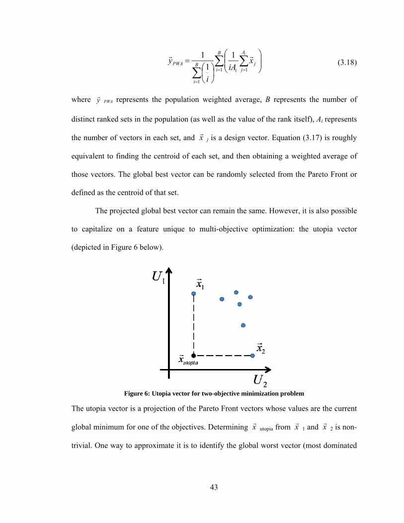
43
B
i
A
jj
iB
i
PWA
i
xiA
i
y1 1
1
1
1
1 (3.18)
where y
PWA represents the population weighted average, B represents the number of
distinct ranked sets in the population (as well as the value of the rank itself), Ai represents
the number of vectors in each set, and x
j is a design vector. Equation (3.17) is roughly
equivalent to finding the centroid of each set, and then obtaining a weighted average of
those vectors. The global best vector can be randomly selected from the Pareto Front or
defined as the centroid of that set.
The projected global best vector can remain the same. However, it is also possible
to capitalize on a feature unique to multi-objective optimization: the utopia vector
(depicted in Figure 6 below).
Figure 6: Utopia vector for two-objective minimization problem
The utopia vector is a projection of the Pareto Front vectors whose values are the current
global minimum for one of the objectives. Determining x
utopia from x
1 and x
2 is non-
trivial. One way to approximate it is to identify the global worst vector (most dominated

44
point), and assume x
utopia is located at the point that forms a parallelogram with the
global worst, x
1, and x
2. Alternatively if a surface is constructed from the Pareto
Front, as in [45], the utopia vector can be projected onto this surface, and that new point
can be used as the projected global best vector.
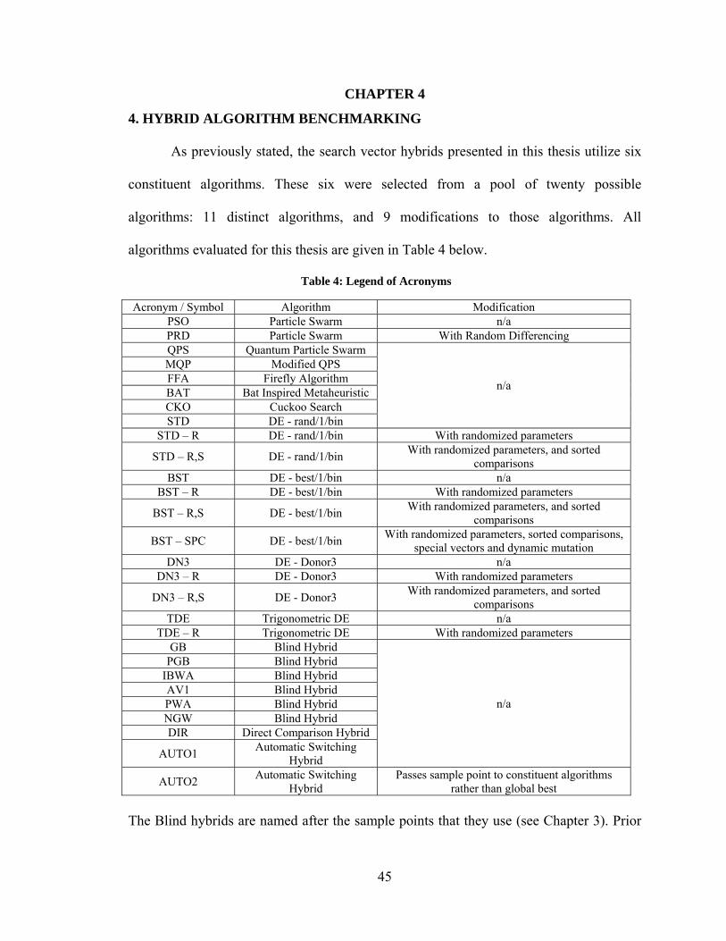
45
CHAPTER 4
4. HYBRID ALGORITHM BENCHMARKING
As previously stated, the search vector hybrids presented in this thesis utilize six
constituent algorithms. These six were selected from a pool of twenty possible
algorithms: 11 distinct algorithms, and 9 modifications to those algorithms. All
algorithms evaluated for this thesis are given in Table 4 below.
Table 4: Legend of Acronyms
Acronym / Symbol Algorithm Modification PSO Particle Swarm n/a PRD Particle Swarm With Random Differencing QPS Quantum Particle Swarm
n/a
MQP Modified QPS FFA Firefly Algorithm BAT Bat Inspired Metaheuristic CKO Cuckoo Search STD DE - rand/1/bin
STD – R DE - rand/1/bin With randomized parameters
STD – R,S DE - rand/1/bin With randomized parameters, and sorted
comparisons BST DE - best/1/bin n/a
BST – R DE - best/1/bin With randomized parameters
BST – R,S DE - best/1/bin With randomized parameters, and sorted
comparisons
BST – SPC DE - best/1/bin With randomized parameters, sorted comparisons,
special vectors and dynamic mutation DN3 DE - Donor3 n/a
DN3 – R DE - Donor3 With randomized parameters
DN3 – R,S DE - Donor3 With randomized parameters, and sorted
comparisons TDE Trigonometric DE n/a
TDE – R Trigonometric DE With randomized parameters GB Blind Hybrid
n/a
PGB Blind Hybrid IBWA Blind Hybrid AV1 Blind Hybrid PWA Blind Hybrid NGW Blind Hybrid DIR Direct Comparison Hybrid
AUTO1 Automatic Switching
Hybrid
AUTO2 Automatic Switching
Hybrid Passes sample point to constituent algorithms
rather than global best The Blind hybrids are named after the sample points that they use (see Chapter 3). Prior

46
to selection, the algorithms listed above were compared, and their relative performance is
reported in the Appendix. Two-hundred and ninety-six of the Schittkowski & Hock test
cases were used to benchmark the candidate algorithms, as well as the hybrids presented
below.
4.1. Benchmark Case Set Up and Reporting
In order to compare the algorithms, each algorithm was executed for a certain
number of iterations, and the final value of the objective function was used as the
measure of performance. In order for this approach to be statistically meaningful, these
numerical experiments must be repeated a certain number of times. Each numerical
experiment is called a “trial.” For each trial, the optimization algorithm was executed for
200 iterations on a given Schittkowski & Hock test case.
4.1.1. Establishing Statistical Significance
The number of trials needed to establish a statistically significant result is not
known a priori. In order to establish a guideline, a search vector hybrid was executed on
the full set of test cases for 50, 60, 70, 80, and 90 trials. The mean accuracy and standard
deviations were calculated and used to perform Student’s t-tests on each pair of trials.
The table below contains a small sample of the data from the Student’s t-tests.
Table 5: Sample of Student’s t-test Results
TC Dim 50 vs. 60 60 vs. 70 70 vs. 80 80 vs. 90
1 2 0 0 0 0
2 2 0 0 0 0
3 2 1 0 0 0
4 2 1 0 0 0
5 2 1 0 0 0
6 2 0 0 0 0
7 2 1 1 0 0
8 2 1 0 0 0
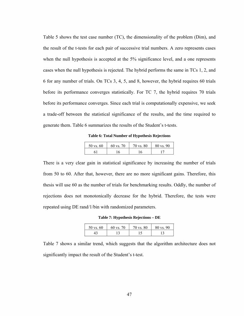
47
Table 5 shows the test case number (TC), the dimensionality of the problem (Dim), and
the result of the t-tests for each pair of successive trial numbers. A zero represents cases
when the null hypothesis is accepted at the 5% significance level, and a one represents
cases when the null hypothesis is rejected. The hybrid performs the same in TCs 1, 2, and
6 for any number of trials. On TCs 3, 4, 5, and 8, however, the hybrid requires 60 trials
before its performance converges statistically. For TC 7, the hybrid requires 70 trials
before its performance converges. Since each trial is computationally expensive, we seek
a trade-off between the statistical significance of the results, and the time required to
generate them. Table 6 summarizes the results of the Student’s t-tests.
Table 6: Total Number of Hypothesis Rejections
50 vs. 60 60 vs. 70 70 vs. 80 80 vs. 90
61 16 16 17 There is a very clear gain in statistical significance by increasing the number of trials
from 50 to 60. After that, however, there are no more significant gains. Therefore, this
thesis will use 60 as the number of trials for benchmarking results. Oddly, the number of
rejections does not monotonically decrease for the hybrid. Therefore, the tests were
repeated using DE rand/1/bin with randomized parameters.
Table 7: Hypothesis Rejections – DE
50 vs. 60 60 vs. 70 70 vs. 80 80 vs. 90 43 13 15 13
Table 7 shows a similar trend, which suggests that the algorithm architecture does not
significantly impact the result of the Student’s t-test.
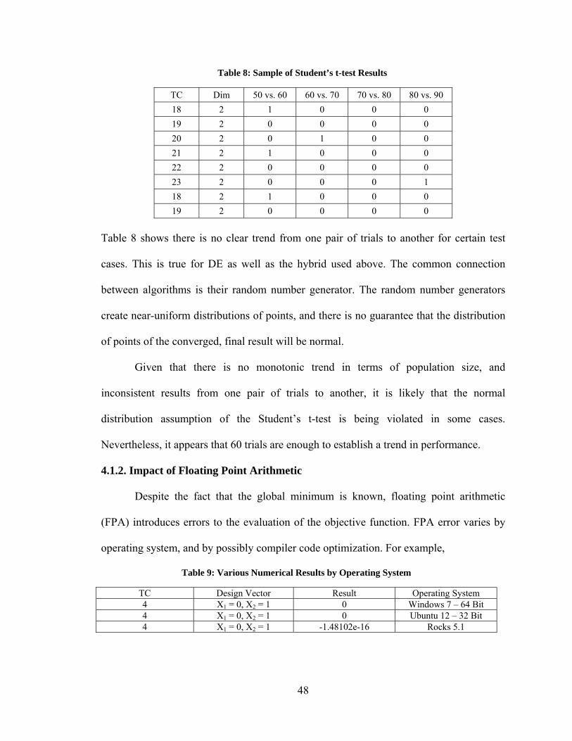
48
Table 8: Sample of Student’s t-test Results
TC Dim 50 vs. 60 60 vs. 70 70 vs. 80 80 vs. 90
18 2 1 0 0 0
19 2 0 0 0 0
20 2 0 1 0 0
21 2 1 0 0 0
22 2 0 0 0 0
23 2 0 0 0 1
18 2 1 0 0 0
19 2 0 0 0 0
Table 8 shows there is no clear trend from one pair of trials to another for certain test
cases. This is true for DE as well as the hybrid used above. The common connection
between algorithms is their random number generator. The random number generators
create near-uniform distributions of points, and there is no guarantee that the distribution
of points of the converged, final result will be normal.
Given that there is no monotonic trend in terms of population size, and
inconsistent results from one pair of trials to another, it is likely that the normal
distribution assumption of the Student’s t-test is being violated in some cases.
Nevertheless, it appears that 60 trials are enough to establish a trend in performance.
4.1.2. Impact of Floating Point Arithmetic
Despite the fact that the global minimum is known, floating point arithmetic
(FPA) introduces errors to the evaluation of the objective function. FPA error varies by
operating system, and by possibly compiler code optimization. For example,
Table 9: Various Numerical Results by Operating System
TC Design Vector Result Operating System 4 X1 = 0, X2 = 1 0 Windows 7 – 64 Bit 4 X1 = 0, X2 = 1 0 Ubuntu 12 – 32 Bit 4 X1 = 0, X2 = 1 -1.48102e-16 Rocks 5.1
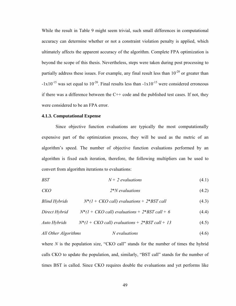
49
While the result in Table 9 might seem trivial, such small differences in computational
accuracy can determine whether or not a constraint violation penalty is applied, which
ultimately affects the apparent accuracy of the algorithm. Complete FPA optimization is
beyond the scope of this thesis. Nevertheless, steps were taken during post processing to
partially address these issues. For example, any final result less than 10-20 or greater than
-1x10-15 was set equal to 10-20. Final results less than -1x10-15 were considered erroneous
if there was a difference between the C++ code and the published test cases. If not, they
were considered to be an FPA error.
4.1.3. Computational Expense
Since objective function evaluations are typically the most computationally
expensive part of the optimization process, they will be used as the metric of an
algorithm’s speed. The number of objective function evaluations performed by an
algorithm is fixed each iteration, therefore, the following multipliers can be used to
convert from algorithm iterations to evaluations:
BST N + 2 evaluations (4.1)
CKO 2*N evaluations (4.2)
Blind Hybrids N*(1 + CKO call) evaluations + 2*BST call (4.3)
Direct Hybrid N*(1 + CKO call) evaluations + 2*BST call + 6 (4.4)
Auto Hybrids N*(1 + CKO call) evaluations + 2*BST call + 13 (4.5)
All Other Algorithms N evaluations (4.6)
where N is the population size, “CKO call” stands for the number of times the hybrid
calls CKO to update the population, and, similarly, “BST call” stands for the number of
times BST is called. Since CKO requires double the evaluations and yet performs like
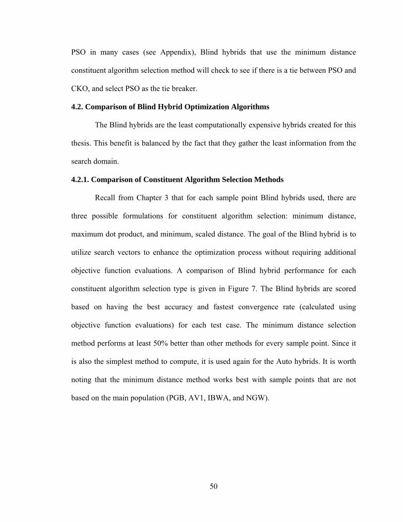
50
PSO in many cases (see Appendix), Blind hybrids that use the minimum distance
constituent algorithm selection method will check to see if there is a tie between PSO and
CKO, and select PSO as the tie breaker.
4.2. Comparison of Blind Hybrid Optimization Algorithms
The Blind hybrids are the least computationally expensive hybrids created for this
thesis. This benefit is balanced by the fact that they gather the least information from the
search domain.
4.2.1. Comparison of Constituent Algorithm Selection Methods
Recall from Chapter 3 that for each sample point Blind hybrids used, there are
three possible formulations for constituent algorithm selection: minimum distance,
maximum dot product, and minimum, scaled distance. The goal of the Blind hybrid is to
utilize search vectors to enhance the optimization process without requiring additional
objective function evaluations. A comparison of Blind hybrid performance for each
constituent algorithm selection type is given in Figure 7. The Blind hybrids are scored
based on having the best accuracy and fastest convergence rate (calculated using
objective function evaluations) for each test case. The minimum distance selection
method performs at least 50% better than other methods for every sample point. Since it
is also the simplest method to compute, it is used again for the Auto hybrids. It is worth
noting that the minimum distance method works best with sample points that are not
based on the main population (PGB, AV1, IBWA, and NGW).

51
Best Speed and Accuracy
(a)
(b)
(c)
(d)
(e)
(f)
Figure 7: Relative Performance of Blind Hybrids with Different Constituent Selection Methods
This suggests that search directions derived directly from the population (using its
members or an average of its members) provide a slightly better indication of the
direction in which to search, whereas the more exotic sample points provide better
information regarding the local neighborhood in which to search, relative to the search
vector in use.
4.2.2. Constituent Algorithm Selection Preference
The Blind hybrid strategy provides useful insight into potential correlations
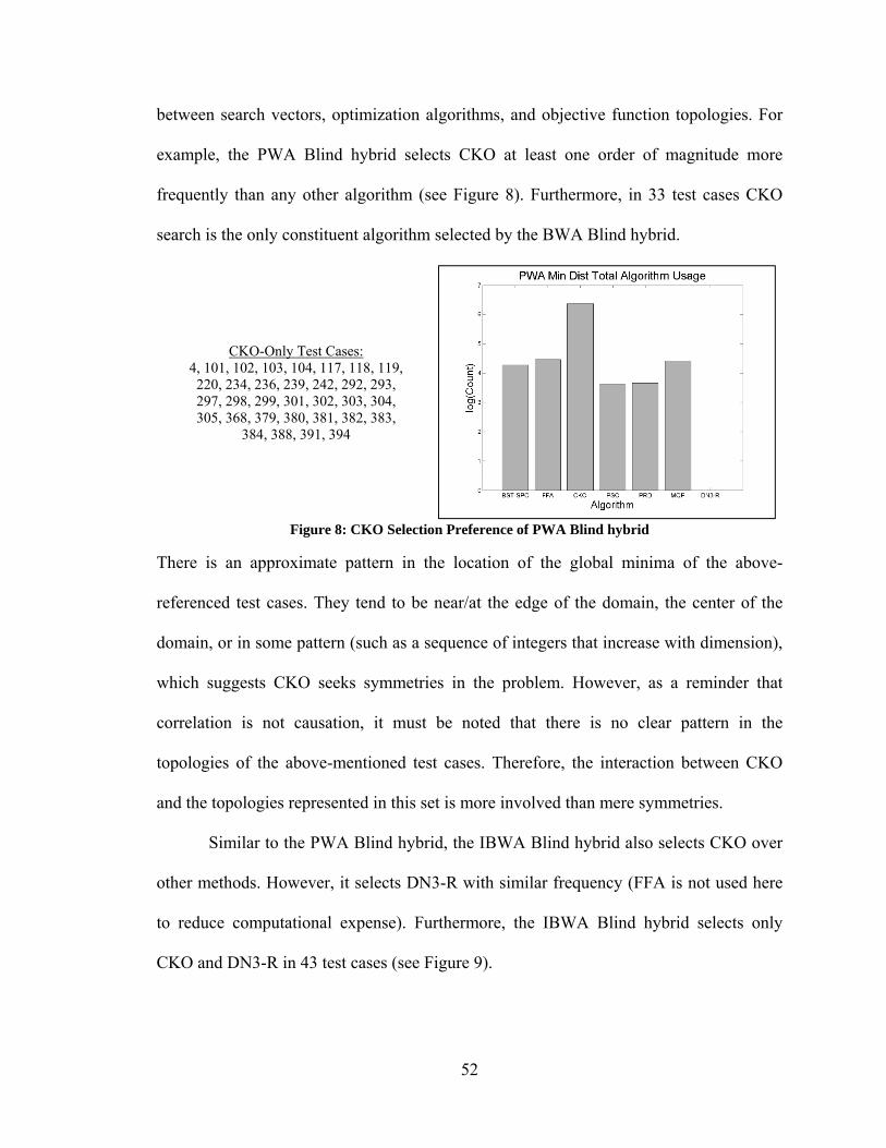
52
between search vectors, optimization algorithms, and objective function topologies. For
example, the PWA Blind hybrid selects CKO at least one order of magnitude more
frequently than any other algorithm (see Figure 8). Furthermore, in 33 test cases CKO
search is the only constituent algorithm selected by the BWA Blind hybrid.
CKO-Only Test Cases: 4, 101, 102, 103, 104, 117, 118, 119, 220, 234, 236, 239, 242, 292, 293, 297, 298, 299, 301, 302, 303, 304, 305, 368, 379, 380, 381, 382, 383,
384, 388, 391, 394
Figure 8: CKO Selection Preference of PWA Blind hybrid
There is an approximate pattern in the location of the global minima of the above-
referenced test cases. They tend to be near/at the edge of the domain, the center of the
domain, or in some pattern (such as a sequence of integers that increase with dimension),
which suggests CKO seeks symmetries in the problem. However, as a reminder that
correlation is not causation, it must be noted that there is no clear pattern in the
topologies of the above-mentioned test cases. Therefore, the interaction between CKO
and the topologies represented in this set is more involved than mere symmetries.
Similar to the PWA Blind hybrid, the IBWA Blind hybrid also selects CKO over
other methods. However, it selects DN3-R with similar frequency (FFA is not used here
to reduce computational expense). Furthermore, the IBWA Blind hybrid selects only
CKO and DN3-R in 43 test cases (see Figure 9).
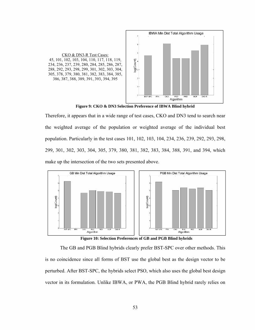
53
CKO & DN3-R Test Cases: 45, 101, 102, 103, 104, 110, 117, 118, 119,
234, 236, 237, 239, 280, 284, 285, 286, 287, 288, 292, 293, 298, 299, 301, 302, 303, 304, 305, 378, 379, 380, 381, 382, 383, 384, 385,
386, 387, 388, 389, 391, 393, 394, 395
Figure 9: CKO & DN3 Selection Preference of IBWA Blind hybrid
Therefore, it appears that in a wide range of test cases, CKO and DN3 tend to search near
the weighted average of the population or weighted average of the individual best
population. Particularly in the test cases 101, 102, 103, 104, 234, 236, 239, 292, 293, 298,
299, 301, 302, 303, 304, 305, 379, 380, 381, 382, 383, 384, 388, 391, and 394, which
make up the intersection of the two sets presented above.
Figure 10: Selection Preferences of GB and PGB Blind hybrids
The GB and PGB Blind hybrids clearly prefer BST-SPC over other methods. This
is no coincidence since all forms of BST use the global best as the design vector to be
perturbed. After BST-SPC, the hybrids select PSO, which also uses the global best design
vector in its formulation. Unlike IBWA, or PWA, the PGB Blind hybrid rarely relies on
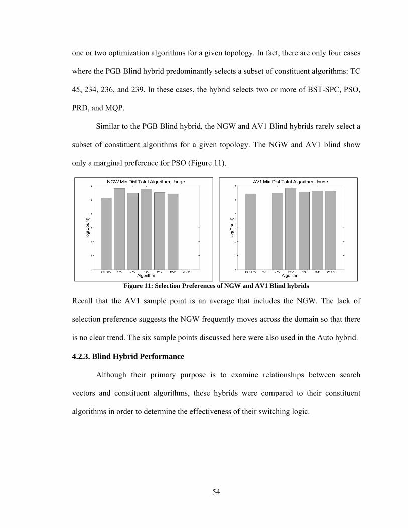
54
one or two optimization algorithms for a given topology. In fact, there are only four cases
where the PGB Blind hybrid predominantly selects a subset of constituent algorithms: TC
45, 234, 236, and 239. In these cases, the hybrid selects two or more of BST-SPC, PSO,
PRD, and MQP.
Similar to the PGB Blind hybrid, the NGW and AV1 Blind hybrids rarely select a
subset of constituent algorithms for a given topology. The NGW and AV1 blind show
only a marginal preference for PSO (Figure 11).
Figure 11: Selection Preferences of NGW and AV1 Blind hybrids
Recall that the AV1 sample point is an average that includes the NGW. The lack of
selection preference suggests the NGW frequently moves across the domain so that there
is no clear trend. The six sample points discussed here were also used in the Auto hybrid.
4.2.3. Blind Hybrid Performance
Although their primary purpose is to examine relationships between search
vectors and constituent algorithms, these hybrids were compared to their constituent
algorithms in order to determine the effectiveness of their switching logic.

55
4.2.3.1. Hybrid vs. Constituent Algorithms
Figure 12 shows the results of comparing Blind hybrids to one-another and their
constituent algorithms. Interestingly, the GB hybrid is the most accurate and fastest in
nearly 18% of the test cases. If speed is not considered, it is as accurate as or better than
other optimization algorithms in over 23% of the test cases. From this, and the
overwhelming success of BST-SPC, it can be concluded that a strategy as simple as
moving the population toward the global best each iteration is enough to perform well in
one-fifth of the Schittkowski & Hock test cases.
Figure 12: Relative Performance of Blind hybrids and their Constituent algorithms
None of the Blind hybrids outperform BST-SPC in any metric (speed, robustness,
etc.) over the set of test cases because the Blind hybrid switching strategy is too
simplistic to be robust. However, there are specific cases, such as TC 110, where the
hybrid outperforms its constituent algorithms.
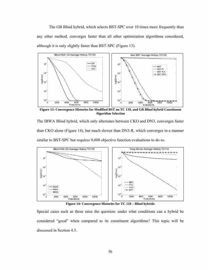
56
The GB Blind hybrid, which selects BST-SPC over 10 times more frequently than
any other method, converges faster than all other optimization algorithms considered,
although it is only slightly faster than BST-SPC (Figure 13).
Figure 13: Convergence Histories for Modified BST on TC 110, and GB Blind hybrid Constituent Algorithm Selection
The IBWA Blind hybrid, which only alternates between CKO and DN3, converges faster
than CKO alone (Figure 14), but much slower than DN3-R, which converges in a manner
similar to BST-SPC but requires 9,000 objective function evaluations to do so.
Figure 14: Convergence Histories for TC 110 – Blind hybrids
Special cases such as these raise the question: under what conditions can a hybrid be
considered “good” when compared to its constituent algorithms? This topic will be
discussed in Section 4.5.

57
4.2.3.2. Hybrid vs. Hybrid
Figure 15 shows the results of comparing Blind hybrids to one-another, using the
minimum distance formulation.
Figure 15: Relative Performance of Blind hybrids
It is clear that the two most computationally efficient search methods, which account for
the best results in roughly 82% of all test cases, are the GB and PGB search vectors.
Once again, the simpler formulations are usually the best. It is worth noting that the class
of test cases for which the PGB Blind hybrid is the best does not intersect with other
hybrids. That is, if speed is not taken into consideration, it will still perform well in
exactly 35.14% of test cases.
4.3. Comparison of All Search Vector Hybrids
The three remaining hybrids are DIR, AUTO1, and AUTO2. Unlike AUTO1, the
AUTO2 hybrid passes the sample point to the constituent algorithm in lieu of the global
best vector (Table 4). These hybrids were designed to improve upon the performance of
the Blind hybrids by using additional information about the objective function topology.
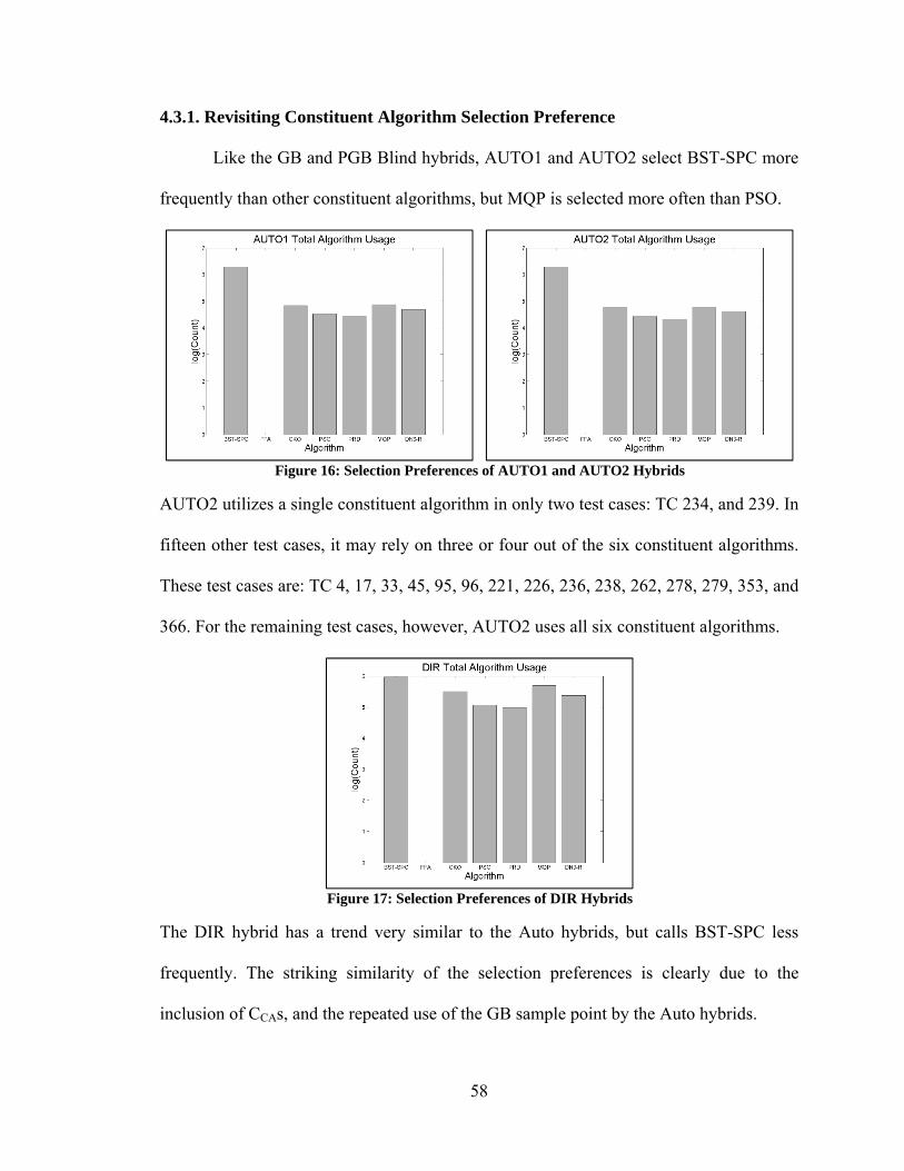
58
4.3.1. Revisiting Constituent Algorithm Selection Preference
Like the GB and PGB Blind hybrids, AUTO1 and AUTO2 select BST-SPC more
frequently than other constituent algorithms, but MQP is selected more often than PSO.
Figure 16: Selection Preferences of AUTO1 and AUTO2 Hybrids
AUTO2 utilizes a single constituent algorithm in only two test cases: TC 234, and 239. In
fifteen other test cases, it may rely on three or four out of the six constituent algorithms.
These test cases are: TC 4, 17, 33, 45, 95, 96, 221, 226, 236, 238, 262, 278, 279, 353, and
366. For the remaining test cases, however, AUTO2 uses all six constituent algorithms.
Figure 17: Selection Preferences of DIR Hybrids
The DIR hybrid has a trend very similar to the Auto hybrids, but calls BST-SPC less
frequently. The striking similarity of the selection preferences is clearly due to the
inclusion of CCAs, and the repeated use of the GB sample point by the Auto hybrids.

59
4.3.2. Search Vector Hybrid Performance
4.3.2.1. Hybrid vs. Constituent Algorithms
Comparing DIR, AUTO1, and AUTO2 against their constituent algorithms,
AUTO2 is clearly the dominant hybrid, but BST-SPC is still the most robust algorithm.
Figure 18: Best Performance of DIR, AUTO1, AUTO2, and their Constituent Algorithms
AUTO2 and BST-SPC could be considered ideal for different classes of test cases,
despite the fact that AUTO2 utilizes BST-SPC. See section 4.5 for a more detailed
discussion of this topic.
In addition to accuracy and speed, another indicator of an algorithms’
performance is the frequency with which it converges to a local minimum. Since all of
the algorithms presented here converge to a local minimum in one problem or another, it
is instructive to count the number of times an algorithm produces the single worst result
for a given test case.

60
Figure 19: Worst Performance of DIR, AUTO1, AUTO2, and their Constituent Algorithms
Figure 19 shows that the AUTO2 hybrid and BST-SPC are least likely to produce the
worst result. Since AUTO2 incorporates constituents including BST-SPC, this
demonstrates that the AUTO2 switching logic dramatically reduces the likelihood of
producing a terrible result in spite of its constituents. On the other hand, the DIR hybrid
still possesses a fairly high likelihood of yielding a poor result, indicating that switching
search directions and constituents is a better strategy than switching based only on CCAs.
If the convergence rate is calculated based on iterations rather than objective
function evaluations, BST-SPC and AUTO2 switch roles. Situations like this might arise
when surrogate models are used in lieu of objective function evaluations, greatly
reducing the computational expense of the optimization process. In these cases, AUTO2
is the more robust algorithm.

61
Figure 20: Best Performance of DIR, AUTO1, AUTO2, and Constituent Algorithms (By Iteration)
4.3.2.2. Hybrid vs. Hybrid
Compared to the Blind hybrids, the DIR, AUTO1, and AUTO2 hybrids converge
faster, are more accurate, and more robust (Figure 21).
Figure 21: Relative Performance of All Search Vector Hybrids
AUTO2, in particular, is faster and more accurate than any other hybrid in over half of
the test cases. AUTO2 obtains the single worst answer in 6.08% of test cases, superseded
only by the AV1 Min Dist hybrid at 4.73%.

62
Figure 22: Relative Performance of DIR, AUTO1, and AUTO2
Comparing DIR, AUTO1, and AUTO2 exclusively, AUTO2 again significantly
outperforms the other hybrids, reinforcing the conclusion that automatically switching
search directions and constituents is better than switching based solely on CCAs.
4.3.2.3. Hybrid vs. All
Figure 23: Relative Performance of All Optimization Algorithms
Figure 23 shows the relative performance of every optimization algorithm used in
this thesis except Blind hybrids using the maximum dot product and minimum scaled

63
distance formulations. The four dominant methods in accuracy and speed are BST-R,
BST-R,S, BST-SPC and AUTO2. AUTO2 obtains the single worst result in only 1.35%
of test cases. The remaining 25 methods are well suited to very small percentages of test
cases.
Figure 24: Relative Performance of All Optimization Algorithms (By Iteration)
If we again relax the assumption that the objective function evaluation dominates the
computational expense of the optimization process, then the AUTO2 hybrid becomes the
most robust algorithm. If speed is not taken into consideration, then within 200 iterations
AUTO2 obtains the best accuracy in 46.6% of test cases.
4.3.2.4. Feasibility of Results
Due to the use of an exterior penalty function, the accuracy of the hybrid includes
the penalty of the constraint violation. Since the penalty function alters the topology of
the objective function, it can mislead the hybrid (as well as the other optimization
algorithms described in this thesis), causing it to converge to a local minimum outside of
the feasible space. The results in Table 10 reflect the probability that the solution will be
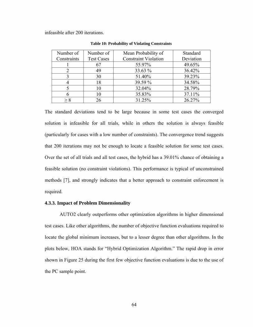
64
infeasible after 200 iterations.
Table 10: Probability of Violating Constraints
Number of Constraints
Number of Test Cases
Mean Probability of Constraint Violation
Standard Deviation
1 67 55.97% 49.65% 2 49 33.63 % 36.42% 3 30 51.40% 39.23% 4 18 39.59 % 34.58% 5 10 32.04% 28.79% 6 10 35.83% 37.11% ≥ 8 26 31.25% 26.27%
The standard deviations tend to be large because in some test cases the converged
solution is infeasible for all trials, while in others the solution is always feasible
(particularly for cases with a low number of constraints). The convergence trend suggests
that 200 iterations may not be enough to locate a feasible solution for some test cases.
Over the set of all trials and all test cases, the hybrid has a 39.01% chance of obtaining a
feasible solution (no constraint violations). This performance is typical of unconstrained
methods [7], and strongly indicates that a better approach to constraint enforcement is
required.
4.3.3. Impact of Problem Dimensionality
AUTO2 clearly outperforms other optimization algorithms in higher dimensional
test cases. Like other algorithms, the number of objective function evaluations required to
locate the global minimum increases, but to a lesser degree than other algorithms. In the
plots below, HOA stands for “Hybrid Optimization Algorithm.” The rapid drop in error
shown in Figure 25 during the first few objective function evaluations is due to the use of
the PC sample point.
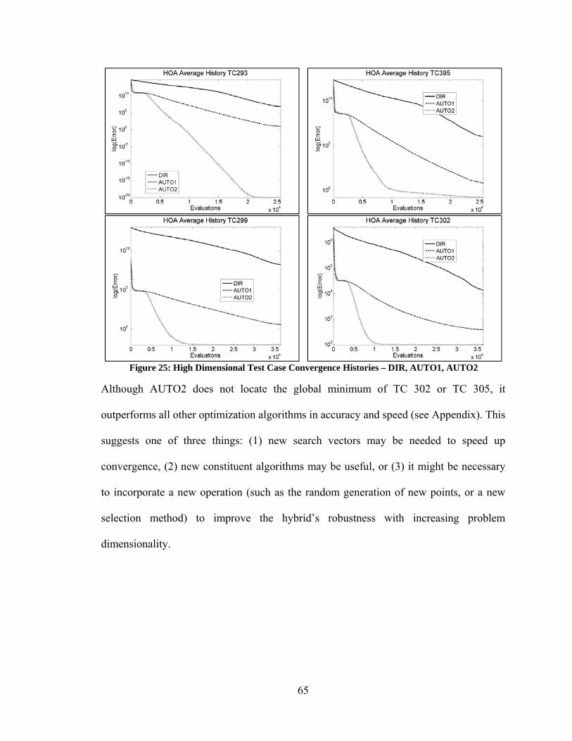
65
Figure 25: High Dimensional Test Case Convergence Histories – DIR, AUTO1, AUTO2
Although AUTO2 does not locate the global minimum of TC 302 or TC 305, it
outperforms all other optimization algorithms in accuracy and speed (see Appendix). This
suggests one of three things: (1) new search vectors may be needed to speed up
convergence, (2) new constituent algorithms may be useful, or (3) it might be necessary
to incorporate a new operation (such as the random generation of new points, or a new
selection method) to improve the hybrid’s robustness with increasing problem
dimensionality.
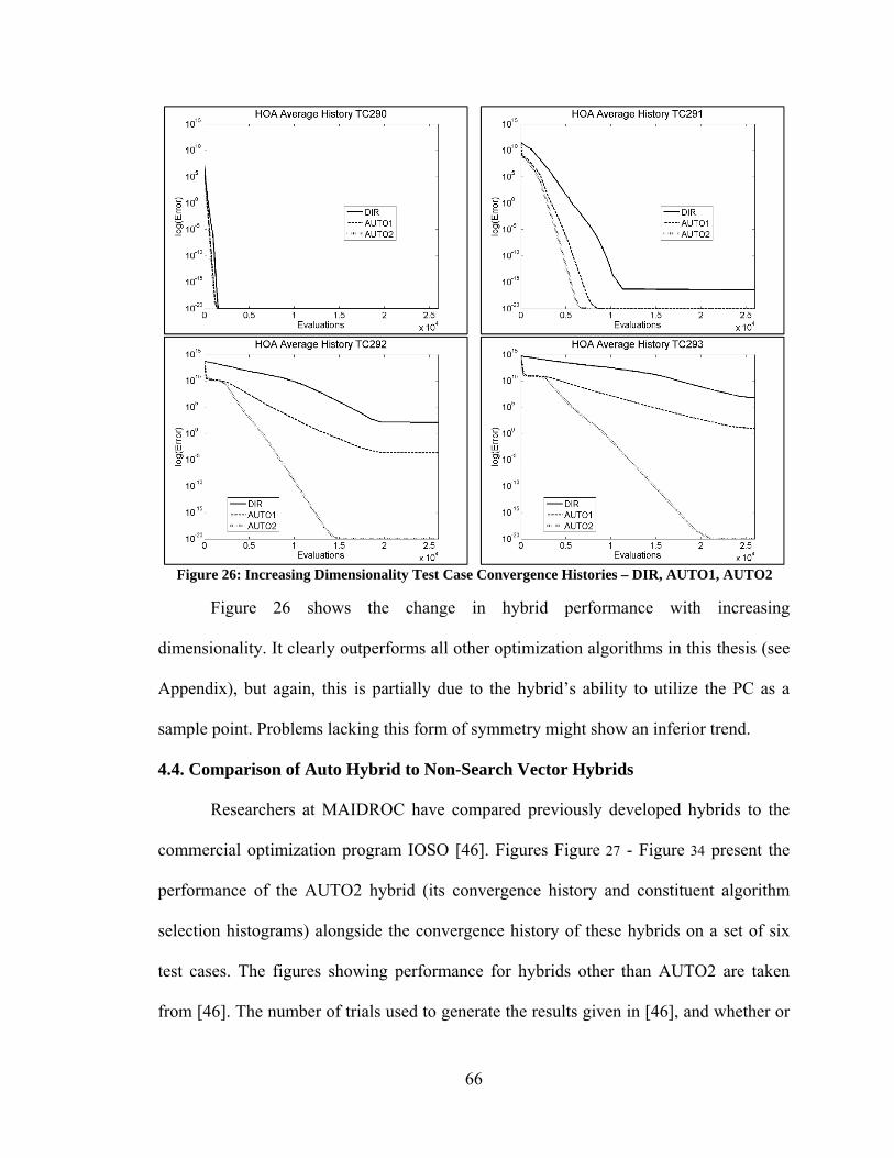
66
Figure 26: Increasing Dimensionality Test Case Convergence Histories – DIR, AUTO1, AUTO2
Figure 26 shows the change in hybrid performance with increasing
dimensionality. It clearly outperforms all other optimization algorithms in this thesis (see
Appendix), but again, this is partially due to the hybrid’s ability to utilize the PC as a
sample point. Problems lacking this form of symmetry might show an inferior trend.
4.4. Comparison of Auto Hybrid to Non-Search Vector Hybrids
Researchers at MAIDROC have compared previously developed hybrids to the
commercial optimization program IOSO [46]. Figures Figure 27 - Figure 34 present the
performance of the AUTO2 hybrid (its convergence history and constituent algorithm
selection histograms) alongside the convergence history of these hybrids on a set of six
test cases. The figures showing performance for hybrids other than AUTO2 are taken
from [46]. The number of trials used to generate the results given in [46], and whether or

67
not these plots are an average of those trials, or simply the best result from all trials is
unknown. The AUTO2 results (excluding Figure 29) are the arithmetic mean of 60
convergence histories.
Figure 27: Convergence History Comparison – Levy9
Results for the 4-dimensional Levy9 test case are shown in Figure 27. The
AUTO2 hybrid roughly matches the Dulikravich, Martin, Colaço (DMC) hybrid’s
performance at the first 2,000 objective function evaluations, and then rapidly surpasses
it. The Colaço BFGS-based optimizer outperforms both in terms of speed, but appears to
converge to a local minimum. IOSO is much more efficient, but also incorporates highly
advanced surrogate modeling techniques. The surrogate model evaluations are not
included in IOSO’s convergence history.
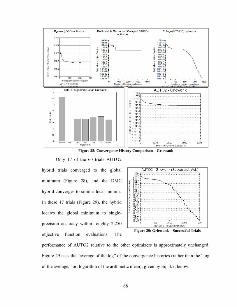
68
Figure 28: Convergence History Comparison – Griewank
Only 17 of the 60 trials AUTO2
hybrid trials converged to the global
minimum (Figure 28), and the DMC
hybrid converges to similar local minima.
In these 17 trials (Figure 29), the hybrid
locates the global minimum to single-
precision accuracy within roughly 2,250
objective function evaluations. The
performance of AUTO2 relative to the other optimizers is approximately unchanged.
Figure 29 uses the “average of the log” of the convergence histories (rather than the “log
of the average,” or, logarithm of the arithmetic mean), given by Eq. 4.7, below.
Figure 29: Griewank – Successful Trials

69
N
ttH
NH
110
* )(log1
(4.7)
where tH
is the vector representing the convergence history for a given trial, t, and *H
is the “average of the log” of the N convergence histories (N trials). This representation
was selected because it reflects the change in order of magnitude of several convergence
histories better than a simple arithmetic mean.
Figure 30: Convergence History Comparison – Levy
The AUTO2 hybrid converges to the global minimum of the Levy function
(Figure 30) in less than 3,000 objective function evaluations. No results were reported for
IOSO. This Levy function is 7-dimensional, and varies slightly in form from the Levy9
function. This is an excellent illustration of the ANFL theorem’s claim that a small
change in an objective function can cause a big change in an algorithm’s performance.
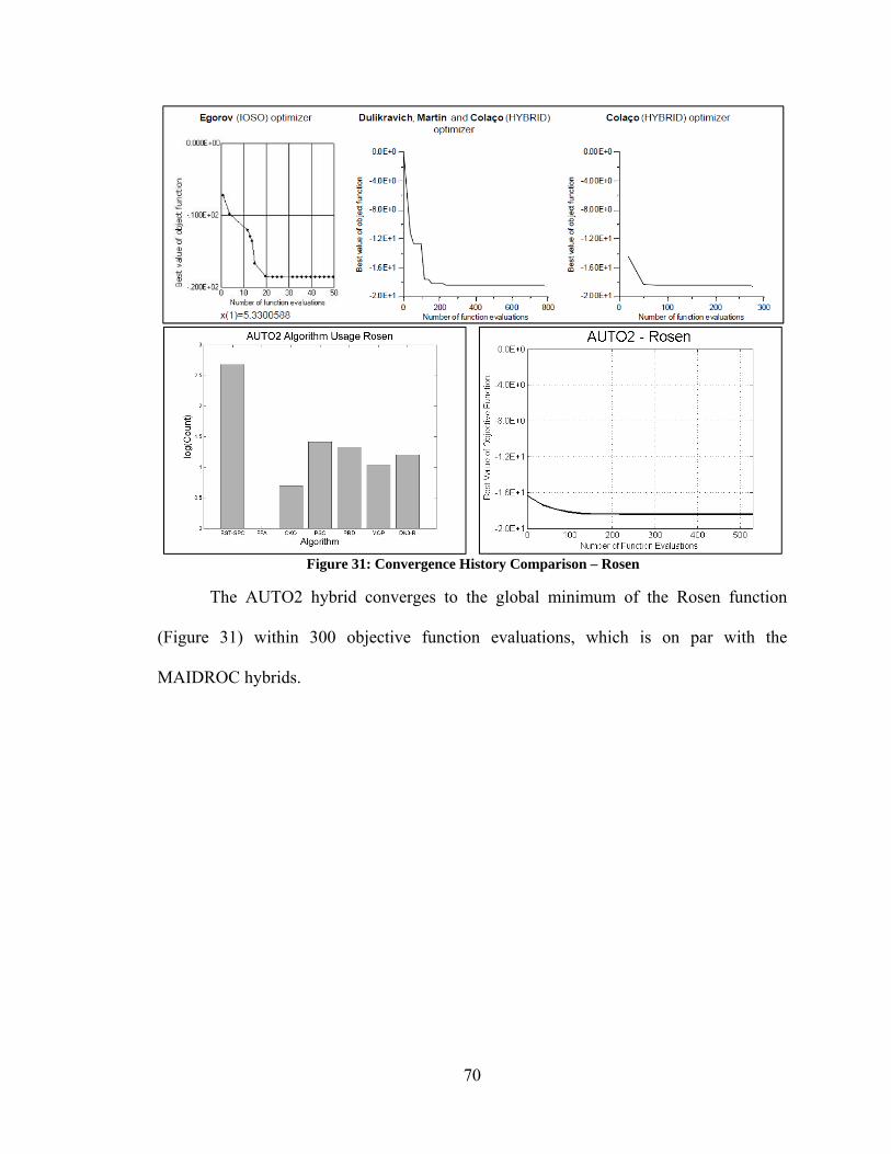
70
Figure 31: Convergence History Comparison – Rosen
The AUTO2 hybrid converges to the global minimum of the Rosen function
(Figure 31) within 300 objective function evaluations, which is on par with the
MAIDROC hybrids.
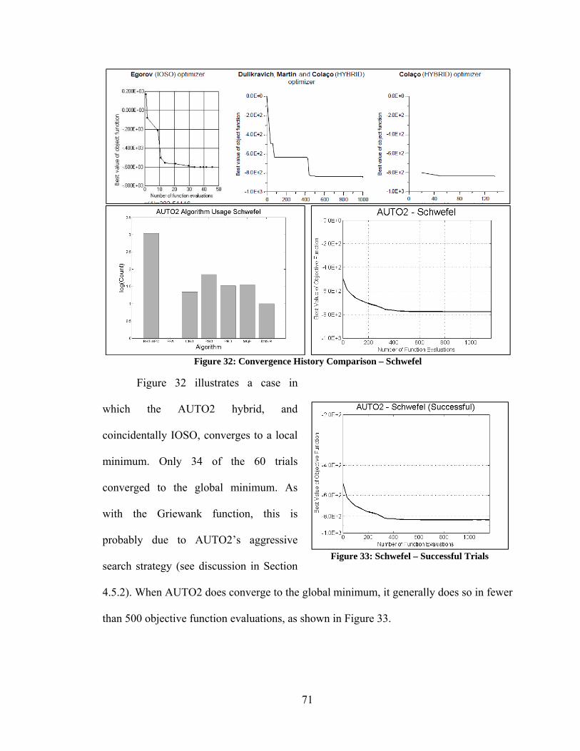
71
Figure 32: Convergence History Comparison – Schwefel
Figure 32 illustrates a case in
which the AUTO2 hybrid, and
coincidentally IOSO, converges to a local
minimum. Only 34 of the 60 trials
converged to the global minimum. As
with the Griewank function, this is
probably due to AUTO2’s aggressive
search strategy (see discussion in Section
4.5.2). When AUTO2 does converge to the global minimum, it generally does so in fewer
than 500 objective function evaluations, as shown in Figure 33.
Figure 33: Schwefel – Successful Trials
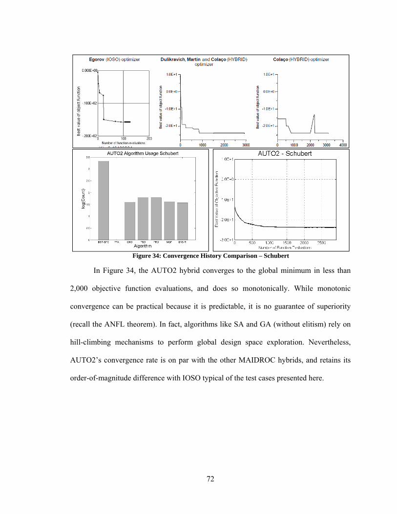
72
Figure 34: Convergence History Comparison – Schubert
In Figure 34, the AUTO2 hybrid converges to the global minimum in less than
2,000 objective function evaluations, and does so monotonically. While monotonic
convergence can be practical because it is predictable, it is no guarantee of superiority
(recall the ANFL theorem). In fact, algorithms like SA and GA (without elitism) rely on
hill-climbing mechanisms to perform global design space exploration. Nevertheless,
AUTO2’s convergence rate is on par with the other MAIDROC hybrids, and retains its
order-of-magnitude difference with IOSO typical of the test cases presented here.

73
Figure 35: Best Performance of OPTRAN and AUTO2 (Unconstrained Cases)
AUTO2 was also compared with a hybrid developed at MAIDROC called
OPTRAN. Different versions of OPTRAN exist. The one used here is the 4th generation
of MAIDROC hybrids discussed in Section 2.3.3. The following steps were taken to
minimize the bias in their comparison:
1. OPTRAN does not use a penalty function for constraint enforcement, therefore,
the unconstrained subset of the Schittkowski & Hock test cases were used.
2. Each optimizer has a different population initialization technique. OPTRAN
possesses the built-in capability to read in a single design, while AUTO2 can read
in an entire population. Therefore, OPTRAN was provided with the global best
design from the same initial population used by AUTO2.
On an objective-function-evaluation basis, AUTO2 dramatically outperforms OPTRAN
(Figure 35). This is important because, unlike AUTO2, OPTRAN is a global-local
hybrid. Therefore, this performance suggests that OPTRAN often converges to local
minima that the AUTO2 hybrid can avoid.
74
4.4.1. Comparison of Execution Times
Although using objective function evaluations is a practical, implementation-
agnostic, platform-agnostic measurement of an algorithm’s speed, another common
practice is to compare their execution times. This method provides some indication of
how an algorithm performs when the computational cost of evaluating the objective
function is relatively low. Unfortunately, this approach can be biased by a large number
of factors. Some biasing factors relevant to this thesis include:
Bias due to the method of implementation
o OPTRAN, and the Auto hybrid have different input/output (I/O)
subroutines. They store different numbers of files, and different amounts of
data within those files. Furthermore, the Auto hybrid performs some basic
file clean up tasks (compressing and deleting files) once the optimization is
complete. Also, OPTRAN prints a substantial amount of text to standard
output, while the Auto hybrid does not. For the purpose of this thesis,
OPTRAN’s standard output was redirected to a file (these files reached
hundreds of megabytes for 100-dimensional problems).
o All search vector hybrids presented in this thesis run in parallel. In order to
minimize bias, the time comparisons are performed using a single processor
which causes the MPI function calls to unnecessarily increase the Auto
hybrid’s computational expense.
o OPTRAN was written in FORTRAN, while the other algorithms were
written in C++. The two languages handle tasks such as file I/O and passing

75
variables to functions in very different manners, all of which impact
performance.
o OPTRAN is used in conjunction with a C++ version of the Schittkowski &
Hock test cases, and so must be cross compiled (FORTRAN and C++).
Furthermore, the Auto hybrid and the PSO implementation used for this
section use a compiler containing wrappers for MPI. Therefore, OPTRAN
uses gfortran and g++, while the Auto hybrid and PSO use mpic++ (a
wrapper for g++).
Bias due to time measurement approach
o In addition to differences between languages, within C++ there are several
ways to measure time, each with significant consequences. For the purpose
of this thesis it suffices to say that each optimization algorithm executable is
timed from the beginning of its execution until the end using the high
resolution clock in the <chrono> library with millisecond accuracy. The
interested reader can learn more about timing from [47] [48] [49].
o Although OPTRAN contains a timing subroutine, it is not active in the
version used for this thesis, therefore, the method stated above is used.
An algorithm’s computational expense also depends on the skill of the programmer, and
the number of processes being executed in the background by the operating system at the
time of testing. Setting all these factors aside, an algorithm’s execution time will also
vary from system to system. In this thesis, the algorithms were executed on an Ubuntu
13.10 virtual machine (Parallels 9) with 8GB of dedicated memory and 4 available cores.
The virtual machine is hosted on a MacBook Pro (OS version 10.8.5) with a 2.8GHz Intel
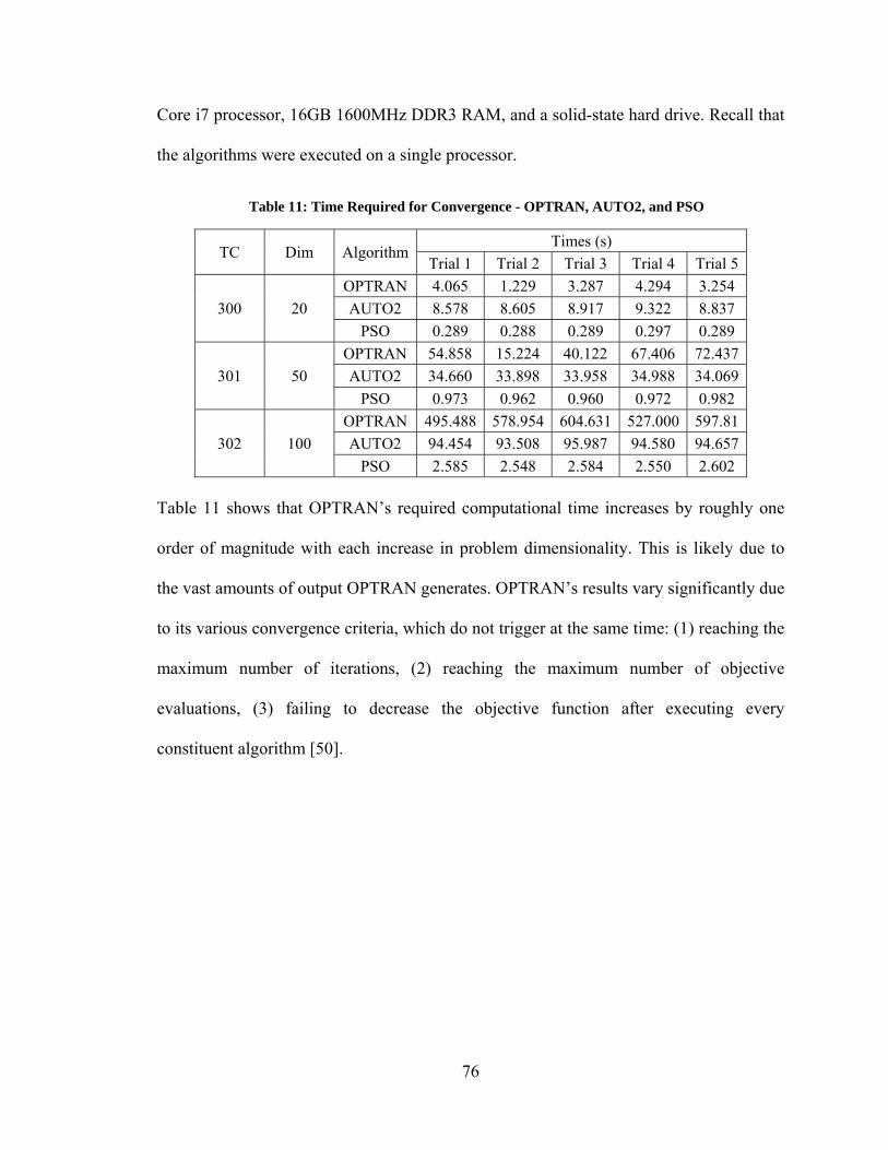
76
Core i7 processor, 16GB 1600MHz DDR3 RAM, and a solid-state hard drive. Recall that
the algorithms were executed on a single processor.
TC Dim AlgorithmTimes (s)
Trial 1 Trial 2 Trial 3 Trial 4 Trial 5
300 20
OPTRAN 4.065 1.229 3.287 4.294 3.254
AUTO2 8.578 8.605 8.917 9.322 8.837
PSO 0.289 0.288 0.289 0.297 0.289
301 50
OPTRAN 54.858 15.224 40.122 67.406 72.437
AUTO2 34.660 33.898 33.958 34.988 34.069
PSO 0.973 0.962 0.960 0.972 0.982
302 100
OPTRAN 495.488 578.954 604.631 527.000 597.81
AUTO2 94.454 93.508 95.987 94.580 94.657
PSO 2.585 2.548 2.584 2.550 2.602 Table 11 shows that OPTRAN’s required computational time increases by roughly one
order of magnitude with each increase in problem dimensionality. This is likely due to
the vast amounts of output OPTRAN generates. OPTRAN’s results vary significantly due
to its various convergence criteria, which do not trigger at the same time: (1) reaching the
maximum number of iterations, (2) reaching the maximum number of objective
evaluations, (3) failing to decrease the objective function after executing every
constituent algorithm [50].
Table 11: Time Required for Convergence - OPTRAN, AUTO2, and PSO

77
(a) (b) Figure 36: Convergence Histories over Time (a) AUTO2 (b) OPTRAN
78
AUTO2, on the other hand, runs for a fixed number of iterations (here, 200).
AUTO2 clearly outperforms OPTRAN for test cases with higher dimensionality in terms
of execution time. The slight variability comes in the number of objective function
evaluations per iteration as discussed in Section 4.1.3, Eq. 4.5. PSO’s computational cost
is roughly one-thirtieth that of AUTO2 due to its simplicity.
Figure 36 shows the convergence history of OPTRAN and AUTO2 over time. In
this test case (as well as TC300 and TC302) OPTRAN converges to a result more
accurate than AUTO2. The smooth convergence profile occurring after the first ten
seconds is probably the result of its use of the DFP constituent algorithm. This is an
example of the advantage of global-local hybridization.
4.5. Discussion of Results
4.5.1. Characterizing Hybrid Performance
Having benchmarked the algorithms, the Auto hybrid is clearly a competitive
alternative to other optimization algorithms. While this may be sufficient to establish a
case for its use, there is one question that benchmarking alone cannot answer:
What makes a hybrid “good”?
Recall from [22] that any algorithm that efficiently solves a problem does so because it
implicitly contains a heuristic that is compatible with the objective function’s topology.
In the case of a pure optimization algorithm, metrics such as speed and accuracy provide
an adequate characterization of this compatibility. Since a single algorithm cannot be
ideally suited for all problems, an implicit goal of hybrids with switching mechanisms is
to correctly match an objective function topology to a compatible constituent algorithm.
Therefore, the true measure of a hybrid’s quality is not merely its speed and accuracy, but

79
also its ability to identify the constituent algorithm required to best solve a problem. In
light of the “effective topology” concept presented earlier, the quality of the search vector
hybrids is determined by its ability to perform this match during each iteration of the
optimization process. Thus, a new metric for quality is introduced: the probability of
selecting the most compatible constituent algorithm for a given objective function.
This new metric naturally raises another question: Over the set of all optimization
problems, what is the upper limit of a hybrid’s performance? In order to answer this
question, let us say that there are two optimization algorithms C1, and C2 that are ideally
suited for two disjoint sets of objective functions A, and B, respectively. The sets of
objective function topologies represented by A, and B are denoted TA and TB
respectively. Let set D be a set of objective functions disjoint with respect to A and B,
containing objective function topologies, TD, that are distinct from, and not reducible to
combinations of TA and TB. An example of a function whose topology is reducible to a
combination of others is the sine function, which can be thought of as an infinite series of
piecewise convex and concave sections. Another (impractical) example would be to
consider all continuous functions to be an infinite series of infinitesimal linear sections.
Let U be the set of all objective functions, as shown in Figure 37 below:

80
Figure 37: Depiction of Set of Objective Functions A, B, and D
Now say there is a hybrid optimization algorithm H that automatically switches between
C1 and C2 and is ideally suited to solve the set of objective functions X. In the worst case
scenario, the set X will be a proper subset of A and/or B (Figure 38). It is likely, however,
that X will be a subset of A, B, and D (Figure 39), as a natural consequence of the ANFL
theorem. This will be referred to as “typical” performance.
Figure 38: Example of Possible Worst Case X Figure 39: Example of “Typical” Performance
The typical case is drawn deliberately to suggest that the hybrid converges as quickly and
accurately as C1 and C2 wherever X intersects A and B respectively, because the term
“ideally suited” should not be construed to mean that an algorithm’s superiority in one
class of problems is mutually exclusive with all other algorithms. In fact, in practice there
would be no guarantee that C1 and C2 are ideally suited for disjoint sets, which could
adversely affect the hybrid’s performance.

81
A hybrid with “satisfactory” performance is one in which X is the union of A and
B. Now, consider a set of objective functions, E, whose topologies can be decomposed
into some combination of topologies in TA and TB. A hybrid is considered to have “ideal”
performance if X is the union of A, B, and E as shown in Figure 40.
Figure 40: “Ideal” Performance
A hybrid with “utopian” performance is one in which X is the union of A, B, D, and E.
Although it is trivial to stipulate that such levels of performance are attainable, in
practice it may not be possible to create an ideal or utopian hybrid. It is obvious that a
simple global-local hybrid, which allows its global algorithm to converge and then passes
the best solution to the local algorithm, can have satisfactory performance. The precise
condition utilized in such hybrids could cause its performance to deviate from
satisfactory, but this is easy to remedy with some experimentation. The higher levels of
performance, however, are more difficult to obtain.
82
4.5.2. Search Vector Hybrid Characterization
The premise of this thesis is that given the existence of a set E (described above),
there exists a hybrid that can match its constituents to a series of effective topologies such
that its performance is ideal. Underlying this statement is the assumption that the
sequence of effective topologies the hybrid encounters during the optimization process
can correctly represent the topologies into which the problem should be decomposed.
Since the quality of the effective topology depends on the population size and
distribution, it is easy to imagine circumstances in which the assumption may be invalid.
Nevertheless, the validity of the premise alone is not sufficient to guarantee that the
hybrid’s performance will be ideal. Consider a case where PSO is the single best
constituent algorithm for a given problem, and the Auto hybrid consistently selects PSO.
Although the hybrid is making the correct decision, it will always converge more slowly
than PSO, on an objective function evaluation basis, due to the additional computational
expense of evaluating the sample points and CCAs.
In this sense, the Auto hybrids have typical performance by definition, except that
here typical performance includes a subset of E. If the Auto hybrid utilized C1 and C2,
one could say it exchanges convergence speed in subsets of A and B for improved overall
robustness (the ability to solve problems in D and E). In order for a hybrid to have ideal
performance, it would have to switch between algorithms without requiring any
additional objective function evaluations. Alternatively, if the hybrid algorithm uses
surrogate models to perform its constituent selection operations, and if the surrogate
model adequately represents the objective function, and if the computational expense of
evaluating the surrogate is negligible compared to that of the objective function, then
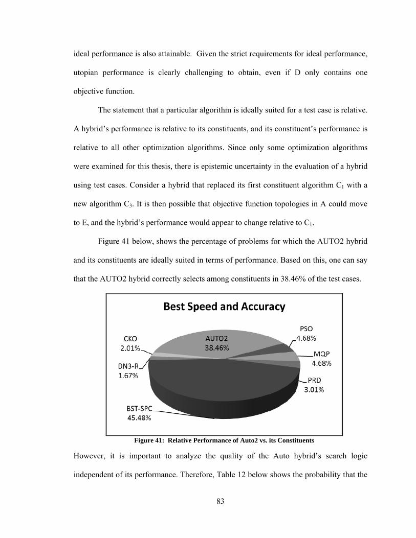
83
ideal performance is also attainable. Given the strict requirements for ideal performance,
utopian performance is clearly challenging to obtain, even if D only contains one
objective function.
The statement that a particular algorithm is ideally suited for a test case is relative.
A hybrid’s performance is relative to its constituents, and its constituent’s performance is
relative to all other optimization algorithms. Since only some optimization algorithms
were examined for this thesis, there is epistemic uncertainty in the evaluation of a hybrid
using test cases. Consider a hybrid that replaced its first constituent algorithm C1 with a
new algorithm C3. It is then possible that objective function topologies in A could move
to E, and the hybrid’s performance would appear to change relative to C1.
Figure 41 below, shows the percentage of problems for which the AUTO2 hybrid
and its constituents are ideally suited in terms of performance. Based on this, one can say
that the AUTO2 hybrid correctly selects among constituents in 38.46% of the test cases.
Figure 41: Relative Performance of Auto2 vs. its Constituents
However, it is important to analyze the quality of the Auto hybrid’s search logic
independent of its performance. Therefore, Table 12 below shows the probability that the
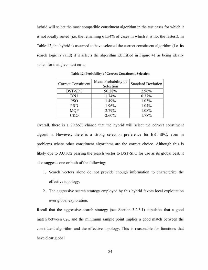
84
hybrid will select the most compatible constituent algorithm in the test cases for which it
is not ideally suited (i.e. the remaining 61.54% of cases in which it is not the fastest). In
Table 12, the hybrid is assumed to have selected the correct constituent algorithm (i.e. its
search logic is valid) if it selects the algorithm identified in Figure 41 as being ideally
suited for that given test case.
Table 12: Probability of Correct Constituent Selection
Correct ConstituentMean Probability of
Selection Standard Deviation
BST-SPC 90.28% 2.96% DN3 1.74% 0.37% PSO 1.49% 1.03% PRD 1.96% 1.04% MQP 2.79% 1.08% CKO 2.60% 1.78%
Overall, there is a 79.86% chance that the hybrid will select the correct constituent
algorithm. However, there is a strong selection preference for BST-SPC, even in
problems where other constituent algorithms are the correct choice. Although this is
likely due to AUTO2 passing the search vector to BST-SPC for use as its global best, it
also suggests one or both of the following:
1. Search vectors alone do not provide enough information to characterize the
effective topology.
2. The aggressive search strategy employed by this hybrid favors local exploitation
over global exploration.
Recall that the aggressive search strategy (see Section 3.2.3.1) stipulates that a good
match between CCA and the minimum sample point implies a good match between the
constituent algorithm and the effective topology. This is reasonable for functions that
have clear global

85
trends, but can be misleading for objective functions that have large, apparently favorable
neighborhoods located far from one another within the design space.
Given the high probability of correct constituent algorithm selection and the hybrid’s
competitive performance, automatic switching between search vectors appears to be the
beginning of a good foundation for the development of a hybrid that operates on
continuous domains. Including statistical measures of the objective function’s
distribution, as well as the population’s distribution over the course of the hybrid’s
convergence, could help it detect the presence of misleading neighborhoods and other
important topology features. This information could be used to probabilistically select
sample points and constituent algorithms. Furthermore, it is possible to stop evaluating
CCAs, and simply use their proximity to the sample point as part of the selection
mechanism. This would reduce the hybrid’s computational expense and bring its
performance closer to ideal.

86
CHAPTER 5
5. OPTIMIZATION OF THE ASYNCHRONOUS PULSE UNIT
During World War II and the Cold War, the United States built a number of
nuclear weapon research and manufacturing facilities across the country. These facilities
produced massive amounts of high-level waste (HLW), which were stored in large single
and double-shelled tanks. One such site, called the Hanford site, [51] contains:
“more than 53 million gallons of radioactive and chemically hazardous
waste in 177 underground storage tanks, 2,300 tons (2,100 metric tons) of
spent nuclear fuel, 9 tons (8 metric tons) of plutonium in various forms,
about 25 million cubic feet (750,000 cubic meters) of buried or stored
solid waste, and groundwater contaminated above drinking water
standards, spread out over about 80 square miles (208 square kilometers),
more than 1,700 waste sites, and about 500 contaminated facilities” [52].
As part of the cleanup process, some of this waste is transported through underground
pipelines that can run over 8 miles in length [53]. Sometimes these pipelines become
clogged, which leads to costly delays in waste removal [54] as well as environmental
concerns.
Since 2007, the Applied Research Center (ARC) at Florida International
University (FIU) has been testing and evaluating the efficacy of several pipeline-
unplugging technologies including an erosive-wave-action technology by NuVision
Engineering, and sonic resonance system by AIMM Technologies [55]. Additionally,
FIU has proposed and developed two technologies: a pneumatic crawler [56], and a
pressure-pulse system called the Asynchronous Pulse Unit (APU) [57].

87
In order to test the APU, the researchers at ARC have constructed a number of
small-scale pipelines, and clogged them using non-radioactive simulant blockages made
from a variety of materials. These experiments are time-consuming to set up, and limited
in the data that can be extrapolated from them. Therefore, ARC has chosen to supplement
these experiments with numerical simulations using software developed in-house [53] as
well as commercially available computational fluid dynamics (CFD) software [58].
Although efforts to simulate the APU using the commercial program ANSYS Fluent at
ARC are ongoing, they are beyond the scope of this thesis.
This chapter briefly reviews one pipeline simulation program developed at ARC,
as well as a similar program presented in [59]. It then presents a new pipeline analysis
program developed for this thesis. The software is verified, and validated. The operation
of the APU is then cast as an optimization problem. Finally, the new software is coupled
to the hybrid optimization algorithm presented in Chapter 3, and the optimization
problem is solved.
5.1. Pipeline Simulation Software
5.1.1. Existing Codes
In 2012, researchers at ARC modified the Method of Characteristics (MOC)
described in [60] to serve as a simplified computer model of the experimental set up. This
method reduces the governing partial differential equations to a set of ordinary
differential equations, whose solution can then be approximated. The interested reader is
referred to [53] and [60] for a complete discussion. The so-called “Modified Method of
Characteristics” (MMOC) is used in [53] to characterize pipelines, model their transient
behavior, and optimize the operation of the piston pumps acting on the pipeline. Going

88
forward, this code will be referred to as “Wood’s code,” after its author. It will be used to
verify the results of the code developed for this thesis.
Recently, Dr. Mambretti of the State University of Campinas in Brazil published a
textbook on the topic of water hammer simulations [59]. The computer codes provided
with this textbook will also be used to verify the code developed for this thesis. Going
forward, this will be referred to as the “WHS code,” which stands for “Water Hammer
Simulation” after the title of the book.
5.1.2. Updated Method of Characteristics
An MOC code based on the updated version of Wylie’s textbook [1] was written
for this thesis. The new textbook contains several changes to the numerical procedure in
[53]. The most notable changes are:
The use of a staggered grid: nodes are now evaluated every other time step,
beginning with odd numbered nodes during the first time step. This requires that
each pipeline have an even number of “reaches” (mesh elements).
The final forms of the equations for various pipeline elements have changed.
Furthermore, the code developed for this thesis differs from the code in [53] in a number
of ways:
It does not use interpolations in the numerical solution.
It automatically adjusts the time step such that the Courant Condition is always
satisfied.
It is capable of modeling tee fittings, with and without air.
It does not utilize geometric friction coefficients.
89
New boundary conditions are proposed (see Section 5.1.2.5). Furthermore, it can
utilize either mass-flow or pressure boundary conditions.
Going forward, the MOC code developed for this thesis will be referred to as “the MOC
code.” The derivations of various equations used in the MOC code are presented in the
subsections that follow.
5.1.2.1. Material Properties
The pipeline is divided into an even number of pipe sections of length dx.
Although the pressurization of the pipeline does cause the pipes to expand/contract
radially, a quick calculation of the hoop stress in the pipeline shows that the deformation
of the pipe wall is negligible. The hoop stress, σθ, for a thin-walled cylinder is given by
the equation in [61],
e
rP (5.1)
where P is the internal pressure, r is the pipe radius, and e is the pipe wall thickness.
Using Hook’s Law, the hoop strain, εθ, for a pipe (open-ended cylinder) is,
eE
rP (5.2)
where E is the Young’s Modulus of the pipe. Given that E = 29,002,666 psi [62], the
internal radius is 1.534 inches (ANSI Sch. 40), the pipe wall thickness is .216 inches
(ANSI Sch. 40), and the maximum allowed internal pressure is 300psi, the maximum
hoop strain is 7.35x10⁻⁵. The maximum change in internal diameter is 7.17x10⁻⁵ inches.
Therefore, the pipe cross-sectional area is assumed constant throughout the simulation.
Pipeline elasticity and the manner in which the pipeline is supported have a
significant impact on the wave speed of a pressure transient. This effect is captured in the

90
modified wave speed equation [1],
eDEKc
Ka
11
(5.3)
where a is the wave speed, ρ is the fluid density, K is the bulk modulus of the fluid, D is
the pipeline inner diameter, and c1 is a scalar that accounts for the effect of the pipeline’s
anchoring. For a pipeline anchored throughout against longitudinal movement [1],
eD
D
D
ec
2
1
11
2 (5.4)
where μ is the Poisson’s Ratio for the black-iron pipe (here assumed to be 0.31).
5.1.2.2. Straight Pipe
Among the equations in [1] that are different than those in [60] are the equations
for a straight section of pipe. The derivation below fills in steps left out from [1]. The
pipeline characteristic impedance, B, is given as,
gA
aB (5.5)
where A is the pipe’s cross-sectional area, and g is the acceleration due to gravity (here,
32.2 ft/s2). The pipeline characteristic resistance, R, is given as,
22gDA
fdxR (5.6)
The C+ and C- characteristic equations are,
ippi QBCH (5.7a)
immi QBCH (5.7b)
where,
91
1 ip QRBB (5.8a)
11 iip BQHC (5.8b)
1 im QRBB (5.8c)
11 iim BQHC (5.8d)
In the above equations, H represents the pressure head, Q represents the volumetric flow
rate, and the subscripts i, i-1, and i+1 refer to the given pipe segment, the upstream pipe
segment, and the downstream pipe segment respectively.
Subtracting equation 5.7a from 5.7b yields,
ipmpm QBBCC 0 (5.9a)
Thus the flow rate can be solved for, resulting in,
mp
mpi BB
CCQ
(5.9b)
Adding equation 5.7a and 5.7b yields,
ipmmpi QBBCCH 2 (5.10a)
Substituting in equation 5.9b yields,
mp
mppmmpi BB
CCBBCCH
2 (5.10b)
which simplifies to,
mp
pmmpi BB
BCBCH
(5.10c)
It is clear from the above equations that flows and pressures in straight pipe sections
depend only on the flow rates of adjacent sections from the previous time step.
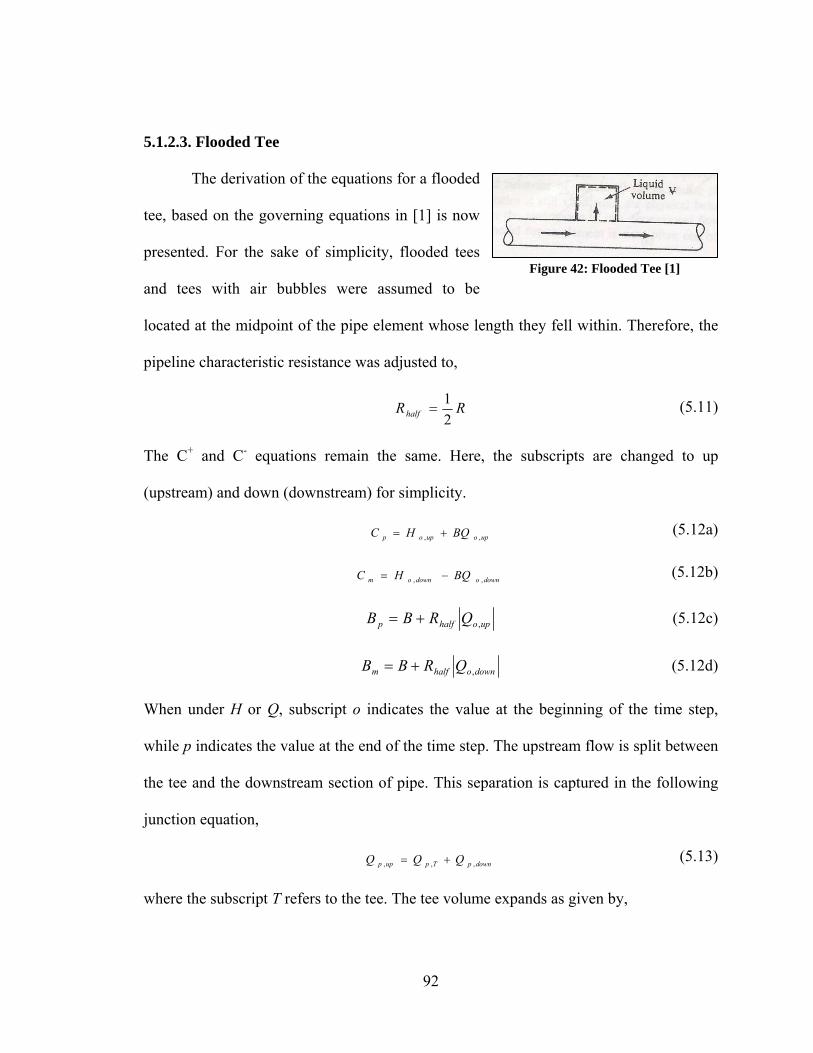
92
5.1.2.3. Flooded Tee
The derivation of the equations for a flooded
tee, based on the governing equations in [1] is now
presented. For the sake of simplicity, flooded tees
and tees with air bubbles were assumed to be
located at the midpoint of the pipe element whose length they fell within. Therefore, the
pipeline characteristic resistance was adjusted to,
RRhalf 2
1 (5.11)
The C+ and C- equations remain the same. Here, the subscripts are changed to up
(upstream) and down (downstream) for simplicity.
upoupop BQHC ,, (5.12a)
downodownom BQHC ,, (5.12b)
upohalfp QRBB , (5.12c)
downohalfm QRBB , (5.12d)
When under H or Q, subscript o indicates the value at the beginning of the time step,
while p indicates the value at the end of the time step. The upstream flow is split between
the tee and the downstream section of pipe. This separation is captured in the following
junction equation,
downpTpupp QQQ ,,, (5.13)
where the subscript T refers to the tee. The tee volume expands as given by,
Figure 42: Flooded Tee [1]
93
dtQQV TpTo ,, (5.14)
where ∆V is the change in volume, and dt is the change in time (size of time step).
Per [1] the tee is modeled as a lumped capacitor, meaning that friction and inertia
effects can be neglected, and elastic effects dominate. Therefore, the liquid and tee wall
elasticity are combined, and the change in pressure within the tee is given by,
TpToT
TToTp QQ
gV
dtKHH ,,,,
(5.15)
where VT is the volume of the tee. The bulk modulus of the tee, KT, is given by,
eDEKc
KK
w
wT
11 (5.16)
where Kw is the bulk modulus of the water in the tee. The pressure in the tee is assumed
equal to that pipe section it is connected to, therefore,
pdownpTpupp HHHH ,,, (5.17)
This results in a system of four equations and four unknowns. The pressure head and
flows at the end of the time step are given by,
dtK
gV
BBQH
dtK
gV
B
C
B
CH
T
T
mpToo
T
T
m
m
p
pp
11, (5.18)
p
upppupp B
HCQ ,
,
(5.19)
m
downpmdownp B
HCQ ,
,
(5.20)
ToToTpT
TTp QHH
dtK
gVQ ,,,,
(5.21)
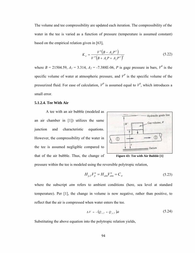
94
The volume and tee compressibility are updated each iteration. The compressibility of the
water in the tee is varied as a function of pressure (temperature is assumed constant)
based on the empirical relation given in [63],
22
21
22
0
PAPABV
PABVK
Pw
(5.22)
where B = 21504.59, A1 = 3.314, A2 = -7.388E-06, P is gage pressure in bars, V0 is the
specific volume of water at atmospheric pressure, and VP is the specific volume of the
pressurized fluid. For ease of calculation, VP is assumed equal to V0, which introduces a
small error.
5.1.2.4. Tee With Air
A tee with an air bubble (modeled as
an air chamber in [1]) utilizes the same
junction and characteristic equations.
However, the compressibility of the water in
the tee is assumed negligible compared to
that of the air bubble. Thus, the change of
pressure within the tee is modeled using the reversible polytropic relation,
An
atmatmnpTp CVHVH , (5.23)
where the subscript atm refers to ambient conditions (here, sea level at standard
temperature). Per [1], the change in volume is now negative, rather than positive, to
reflect that the air is compressed when water enters the tee.
dtQQV TpTo ,, (5.24)
Substituting the above equation into the polytropic relation yields,
Figure 43: Tee with Air Bubble [1]

95
An
ToTpatmTp CQQdtVzHH ,,, (5.25)
where z represents the head of the air bubble above or below the ambient. From the
characteristic equations, the flows in the adjoining pipe sections are given by Eq. 5.19
and 5.20, as before. Using the junction equation (5.13), the flow in the tee is,
m
m
p
pTp
mpTp B
C
B
CH
BBQ
,,
11 (5.26)
Thus the polytropic relation (5.23) can be expressed as,
011
,,,
A
n
Tpmp
Tom
m
p
patmTp CH
BBdtQ
B
C
B
CdtVzHH (5.27)
This equation must be solved iteratively for Hp,T. The method of choice in the textbook is
Newton’s Method. Therefore, the equation is recast as,
A
n
Tpmp
Tom
m
p
patmTp CH
BBdtQ
B
C
B
CdtVzHHF
,,,
11 (5.28)
Collecting terms,
n
Tpmp
Tom
m
p
pnp H
BBdtQ
B
C
B
CdtVV
,,
11 (5.29)
Thus, the derivative can be written as,
mpp
Anp BBV
ndtCV
dH
dF 11 (5.30)
Therefore, the equation,
0 HdH
dFF (5.31)
can now be solved iteratively for the pressure head of the tee. As before, the pressure

96
head is assumed the same in the tee and the pipe section it is connected to. The air
volume and z are updated each iteration.
5.1.2.5. Boundary Condition Equations
For the experiments discussed below, there is only one applicable downstream
boundary condition, while there are two applicable upstream conditions. The downstream
condition is a wall, which mimics the behavior of a rigid plug. In this case, the flow rate
at the wall is zero and the C+ characteristic equation, Eq. 5.7a, reduces to Hp,wall = Cp. If
there is an air pocket at the wall, the reduced C+ characteristic equation is combined with
Eq. 5.23 as shown in [53] and [1].
The first applicable inlet condition is a pressure variation at the inlet, also known
as a “reservoir at upstream end” [1]. Here, the inlet pressure is specified as a function of
time, and the pressure head is solved for using the C- characteristic Eq. 5.7b. Like many
other standard approaches, this formulation is valid for an idealized case. It assumes the
flow rate at the inlet can take on any value resulting from Eq. 5.7b. It will be shown in
Section 5.3, however, this is not the case for the experimental set up. Therefore, the
following pressure inlet boundary condition is proposed for this thesis,
H0 = H(t) (5.32a)
Q0 = 0 (5.32b)
where the 0 subscript represents the inlet. It is shown in Section 5.3 that this boundary
condition provides a good approximation of the flow regime in the experimental pipeline.
The second applicable inlet condition is a volume flow inlet, also known as a
velocity inlet, or “discharge at the upstream end” [1]. In this case, the flow rate is
specified as a function of time, and the pressure head is solved for using the C-
97
characteristic equation 5.7b. Since Eq. 5.7b only uses information at the inlet as well as
downstream information, it does not take the pressure of the incoming fluid into account.
The development of an improved volume-flow inlet condition is a topic of future
research. Nevertheless, a fair approximation of the experimental boundary condition is,
H0 = H1 (5.32c)
Qinlet = Q(t) (5.32d)
where the subscript 1 denotes the next element downstream of the inlet.
5.2. Verification
Since the MOC code is more versatile than Wood’s code and the WHS code, the
performance of each code will first be established by comparing them to steady-state
cases whose results are easy to compute. Afterwards, the MOC code will be compared to
Wood’s code for a transient case, and as well as cases for which Wood’s code had to be
modified. In each case presented in this section, the geometric friction factor in Wood’s
code was set to zero.
5.2.1. Steady State Results
The first two cases are fully flooded pipelines. If the bulk modulus of the fluid in
the pipeline is assumed constant, which is valid for small changes, the change in pressure
due to the injection of a certain volume of fluid is given by the following equation [1],
KV
Vp
(5.33)
Here the change in volume is positive because an inflow (positive flow) of fluid is equal
to a decrease in the total volume of the fluid.

98
It is a little more difficult to relate pressure changes to inflows for multiphase
flows. However, the solution is trivial for steady pressure boundary conditions,
inlett
pp
lim (5.34)
This relation can be used for pipelines with air, as well as fully flooded pipelines.
5.2.1.1 Fully Flooded Straight Pipe
Assume a fully flooded pipeline that is 278ft long, is 3 inches in diameter.
Assume the fluid has a wave speed of 4,512.17ft/s, and the pipeline has a Darcy friction
factor of 0.021. Now apply a constant pressure head of 164.04ft of water. The response of
the pipeline according to each code is shown in Figure 44 below.
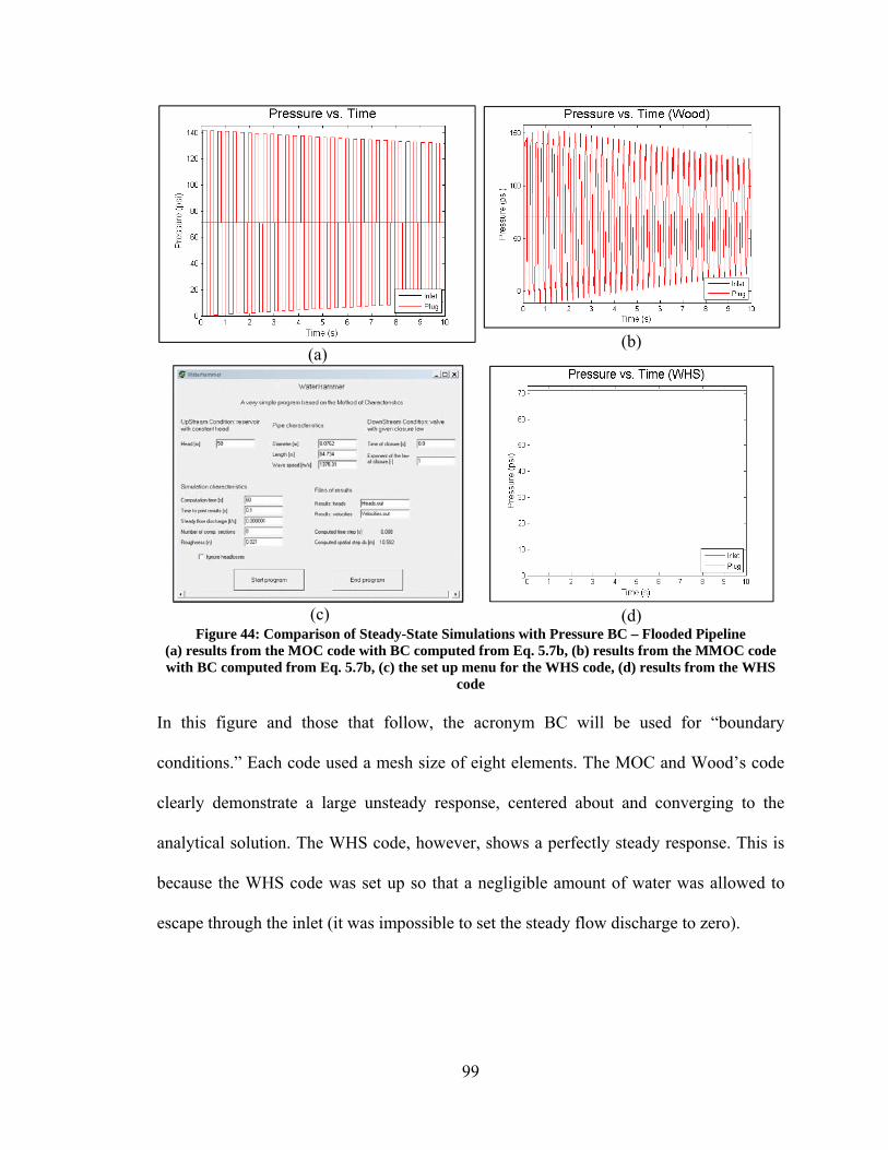
99
(a) (b)
(c)
(d)
Figure 44: Comparison of Steady-State Simulations with Pressure BC – Flooded Pipeline(a) results from the MOC code with BC computed from Eq. 5.7b, (b) results from the MMOC code with BC computed from Eq. 5.7b, (c) the set up menu for the WHS code, (d) results from the WHS
code In this figure and those that follow, the acronym BC will be used for “boundary
conditions.” Each code used a mesh size of eight elements. The MOC and Wood’s code
clearly demonstrate a large unsteady response, centered about and converging to the
analytical solution. The WHS code, however, shows a perfectly steady response. This is
because the WHS code was set up so that a negligible amount of water was allowed to
escape through the inlet (it was impossible to set the steady flow discharge to zero).
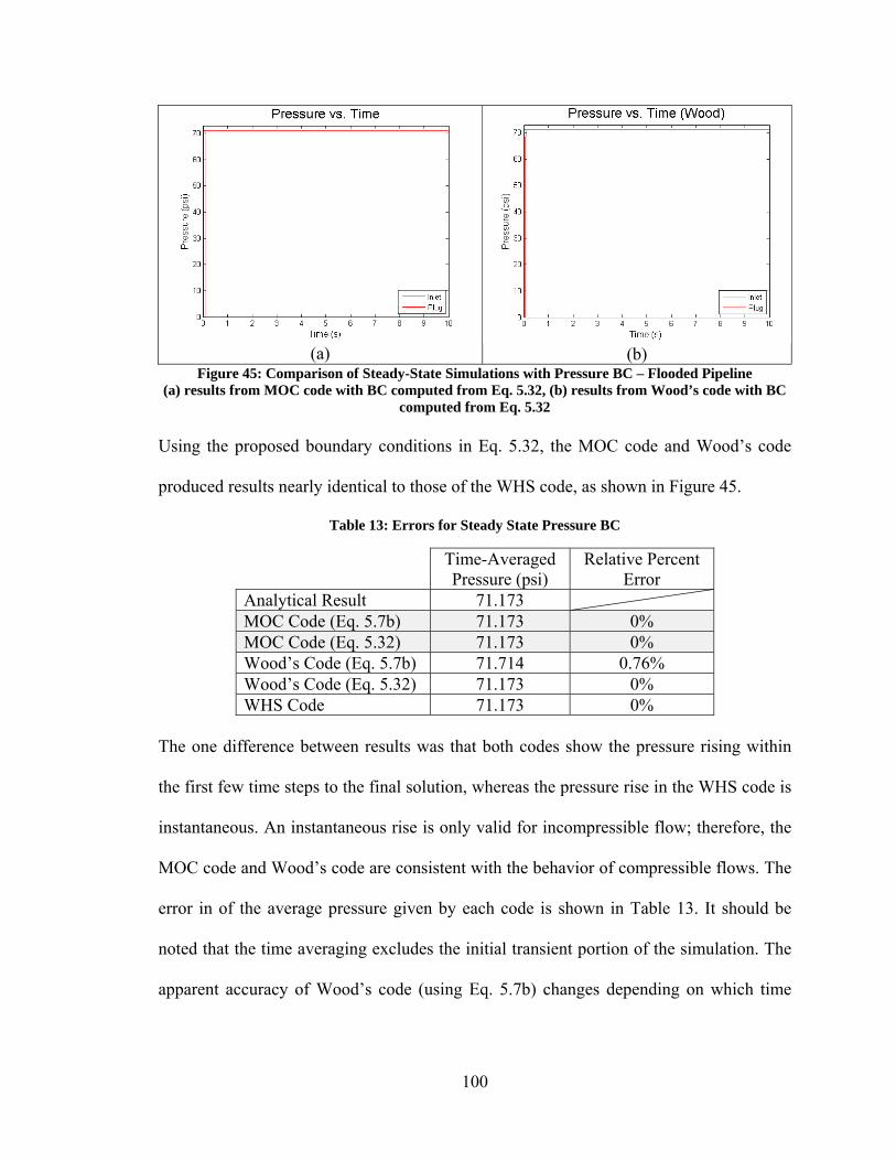
100
(a) (b) Figure 45: Comparison of Steady-State Simulations with Pressure BC – Flooded Pipeline
(a) results from MOC code with BC computed from Eq. 5.32, (b) results from Wood’s code with BC computed from Eq. 5.32
Using the proposed boundary conditions in Eq. 5.32, the MOC code and Wood’s code
produced results nearly identical to those of the WHS code, as shown in Figure 45.
Table 13: Errors for Steady State Pressure BC
Time-Averaged Pressure (psi)
Relative Percent Error
Analytical Result 71.173 MOC Code (Eq. 5.7b) 71.173 0% MOC Code (Eq. 5.32) 71.173 0% Wood’s Code (Eq. 5.7b) 71.714 0.76% Wood’s Code (Eq. 5.32) 71.173 0% WHS Code 71.173 0%
The one difference between results was that both codes show the pressure rising within
the first few time steps to the final solution, whereas the pressure rise in the WHS code is
instantaneous. An instantaneous rise is only valid for incompressible flow; therefore, the
MOC code and Wood’s code are consistent with the behavior of compressible flows. The
error in of the average pressure given by each code is shown in Table 13. It should be
noted that the time averaging excludes the initial transient portion of the simulation. The
apparent accuracy of Wood’s code (using Eq. 5.7b) changes depending on which time
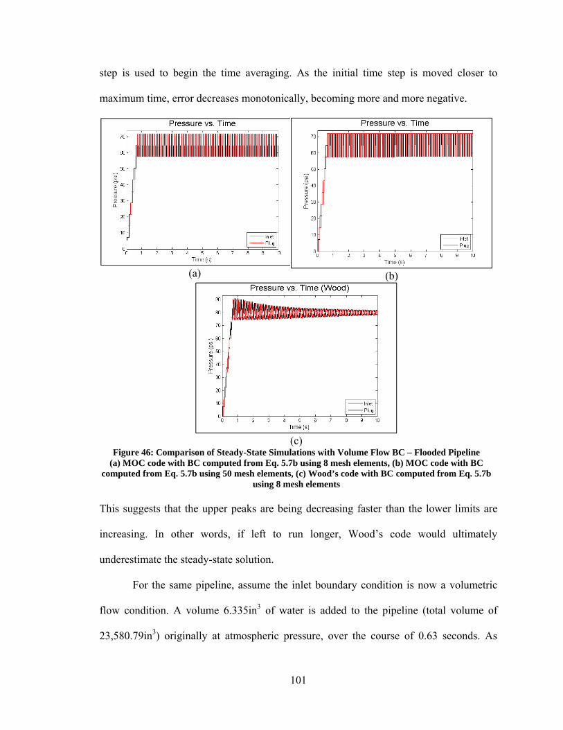
101
step is used to begin the time averaging. As the initial time step is moved closer to
maximum time, error decreases monotonically, becoming more and more negative.
(a) (b)
(c)
Figure 46: Comparison of Steady-State Simulations with Volume Flow BC – Flooded Pipeline(a) MOC code with BC computed from Eq. 5.7b using 8 mesh elements, (b) MOC code with BC
computed from Eq. 5.7b using 50 mesh elements, (c) Wood’s code with BC computed from Eq. 5.7b using 8 mesh elements
This suggests that the upper peaks are being decreasing faster than the lower limits are
increasing. In other words, if left to run longer, Wood’s code would ultimately
underestimate the steady-state solution.
For the same pipeline, assume the inlet boundary condition is now a volumetric
flow condition. A volume 6.335in3 of water is added to the pipeline (total volume of
23,580.79in3) originally at atmospheric pressure, over the course of 0.63 seconds. As

102
shown in Figure 46 (a) and (b), the range of pressures calculated by the MOC code using
the textbook boundary condition formula changes very little with increased mesh size.
The average pressure, however, changes substantially (see Table 14). In addition, it
shows very little dampening of the pressure transient. Wood’s code, on the other hand,
shows relatively significant dampening, and a much higher initial peak pressure.
No results are reported for the WHS code because it does not include a means of
specifying a volume flow inlet boundary condition. Note also that Wood’s code was
modified to use the volume flow inlet boundary condition. Figure 47 shows the results of
the MOC code with the proposed boundary condition (Eq. 5.32). Although the MOC
code consistently underestimates the steady state solution, it converges to it
monotonically with increasing mesh size. The results are very poor when the number of
mesh elements is small because the assumption given in Eq. 5.32a is inaccurate for large
sections of pipe (i.e. large mesh elements).
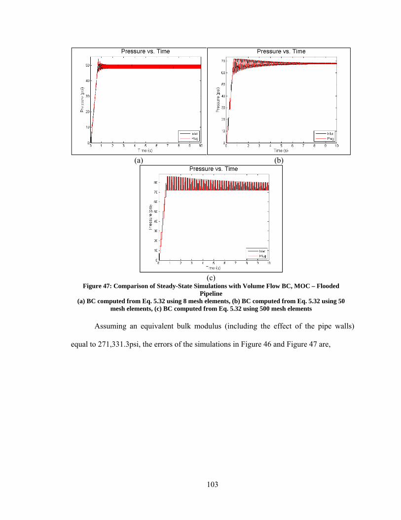
103
(a) (b)
(c)
Figure 47: Comparison of Steady-State Simulations with Volume Flow BC, MOC – Flooded Pipeline
(a) BC computed from Eq. 5.32 using 8 mesh elements, (b) BC computed from Eq. 5.32 using 50 mesh elements, (c) BC computed from Eq. 5.32 using 500 mesh elements
Assuming an equivalent bulk modulus (including the effect of the pipe walls)
equal to 271,331.3psi, the errors of the simulations in Figure 46 and Figure 47 are,
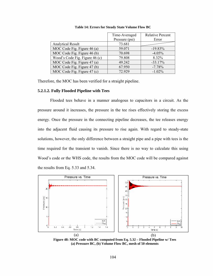
104
Table 14: Errors for Steady State Volume Flow BC
Time-Averaged Pressure (psi)
Relative Percent Error
Analytical Result 73.681 MOC Code Fig. Figure 46 (a) 59.071 -19.83% MOC Code Fig. Figure 46 (b) 70.698 -4.05% Wood’s Code Fig. Figure 46 (c) 79.808 8.32% MOC Code Fig. Figure 47 (a) 49.242 -33.17% MOC Code Fig. Figure 47 (b) 67.950 -7.78% MOC Code Fig. Figure 47 (c) 72.929 -1.02%
Therefore, the MOC has been verified for a straight pipeline.
5.2.1.2. Fully Flooded Pipeline with Tees
Flooded tees behave in a manner analogous to capacitors in a circuit. As the
pressure around it increases, the pressure in the tee rises effectively storing the excess
energy. Once the pressure in the connecting pipeline decreases, the tee releases energy
into the adjacent fluid causing its pressure to rise again. With regard to steady-state
solutions, however, the only difference between a straight pipe and a pipe with tees is the
time required for the transient to vanish. Since there is no way to calculate this using
Wood’s code or the WHS code, the results from the MOC code will be compared against
the results from Eq. 5.33 and 5.34.
(a)
(b) Figure 48: MOC code with BC computed from Eq. 5.32 – Flooded Pipeline w/ Tees
(a) Pressure BC, (b) Volume Flow BC, mesh of 50 elements
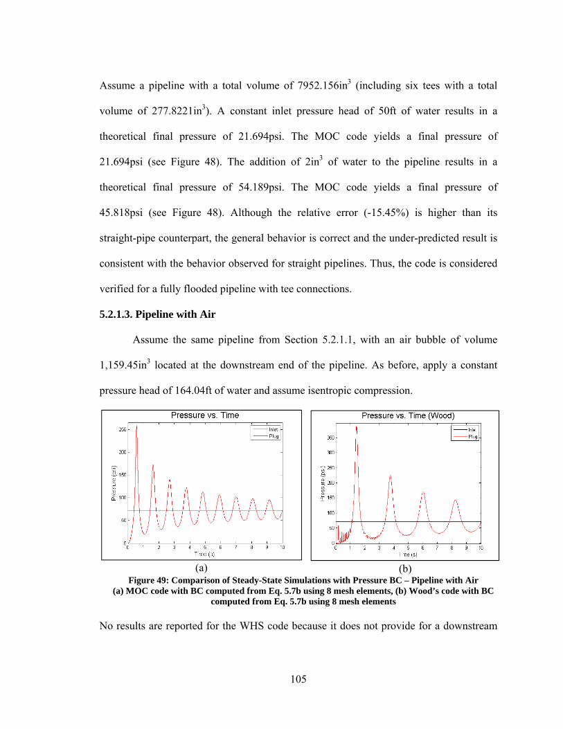
105
Assume a pipeline with a total volume of 7952.156in3 (including six tees with a total
volume of 277.8221in3). A constant inlet pressure head of 50ft of water results in a
theoretical final pressure of 21.694psi. The MOC code yields a final pressure of
21.694psi (see Figure 48). The addition of 2in3 of water to the pipeline results in a
theoretical final pressure of 54.189psi. The MOC code yields a final pressure of
45.818psi (see Figure 48). Although the relative error (-15.45%) is higher than its
straight-pipe counterpart, the general behavior is correct and the under-predicted result is
consistent with the behavior observed for straight pipelines. Thus, the code is considered
verified for a fully flooded pipeline with tee connections.
5.2.1.3. Pipeline with Air
Assume the same pipeline from Section 5.2.1.1, with an air bubble of volume
1,159.45in3 located at the downstream end of the pipeline. As before, apply a constant
pressure head of 164.04ft of water and assume isentropic compression.
(a)
(b) Figure 49: Comparison of Steady-State Simulations with Pressure BC – Pipeline with Air
(a) MOC code with BC computed from Eq. 5.7b using 8 mesh elements, (b) Wood’s code with BC computed from Eq. 5.7b using 8 mesh elements
No results are reported for the WHS code because it does not provide for a downstream
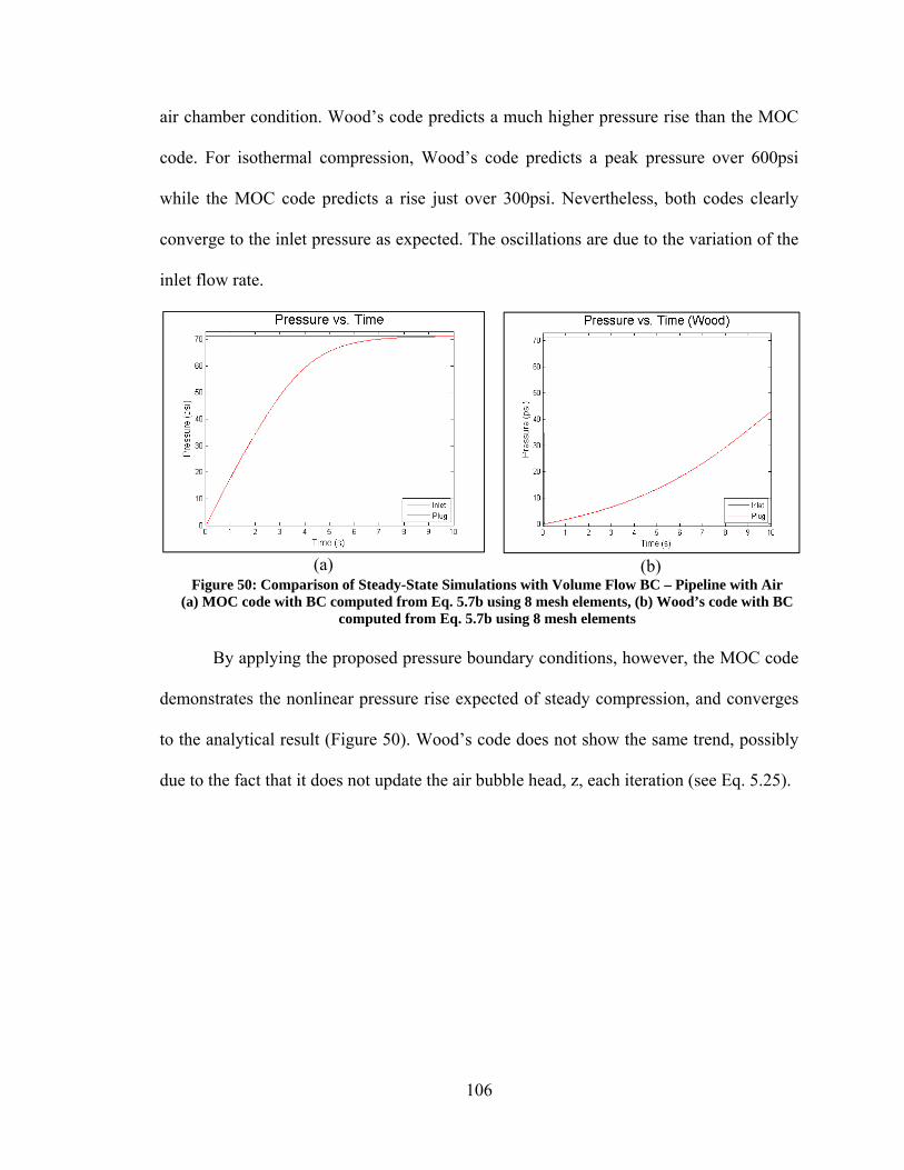
106
air chamber condition. Wood’s code predicts a much higher pressure rise than the MOC
code. For isothermal compression, Wood’s code predicts a peak pressure over 600psi
while the MOC code predicts a rise just over 300psi. Nevertheless, both codes clearly
converge to the inlet pressure as expected. The oscillations are due to the variation of the
inlet flow rate.
(a)
(b) Figure 50: Comparison of Steady-State Simulations with Volume Flow BC – Pipeline with Air
(a) MOC code with BC computed from Eq. 5.7b using 8 mesh elements, (b) Wood’s code with BC computed from Eq. 5.7b using 8 mesh elements
By applying the proposed pressure boundary conditions, however, the MOC code
demonstrates the nonlinear pressure rise expected of steady compression, and converges
to the analytical result (Figure 50). Wood’s code does not show the same trend, possibly
due to the fact that it does not update the air bubble head, z, each iteration (see Eq. 5.25).
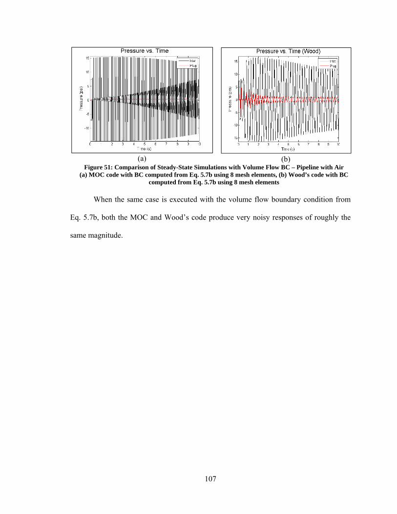
107
(a)
(b) Figure 51: Comparison of Steady-State Simulations with Volume Flow BC – Pipeline with Air
(a) MOC code with BC computed from Eq. 5.7b using 8 mesh elements, (b) Wood’s code with BC computed from Eq. 5.7b using 8 mesh elements
When the same case is executed with the volume flow boundary condition from
Eq. 5.7b, both the MOC and Wood’s code produce very noisy responses of roughly the
same magnitude.
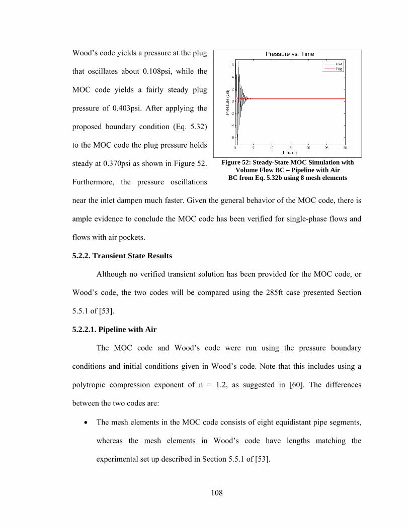
108
Wood’s code yields a pressure at the plug
that oscillates about 0.108psi, while the
MOC code yields a fairly steady plug
pressure of 0.403psi. After applying the
proposed boundary condition (Eq. 5.32)
to the MOC code the plug pressure holds
steady at 0.370psi as shown in Figure 52.
Furthermore, the pressure oscillations
near the inlet dampen much faster. Given the general behavior of the MOC code, there is
ample evidence to conclude the MOC code has been verified for single-phase flows and
flows with air pockets.
5.2.2. Transient State Results
Although no verified transient solution has been provided for the MOC code, or
Wood’s code, the two codes will be compared using the 285ft case presented Section
5.5.1 of [53].
5.2.2.1. Pipeline with Air
The MOC code and Wood’s code were run using the pressure boundary
conditions and initial conditions given in Wood’s code. Note that this includes using a
polytropic compression exponent of n = 1.2, as suggested in [60]. The differences
between the two codes are:
The mesh elements in the MOC code consists of eight equidistant pipe segments,
whereas the mesh elements in Wood’s code have lengths matching the
experimental set up described in Section 5.5.1 of [53].
Figure 52: Steady-State MOC Simulation with Volume Flow BC – Pipeline with Air
BC from Eq. 5.32b using 8 mesh elements
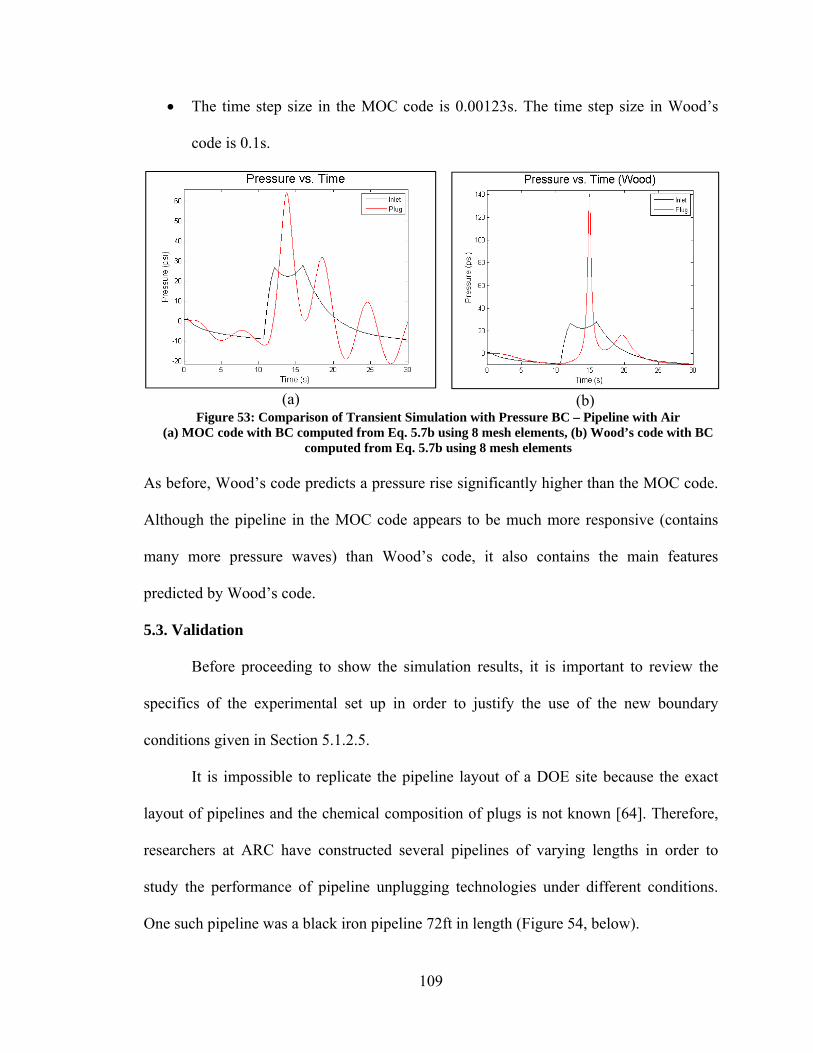
109
The time step size in the MOC code is 0.00123s. The time step size in Wood’s
code is 0.1s.
(a)
(b) Figure 53: Comparison of Transient Simulation with Pressure BC – Pipeline with Air
(a) MOC code with BC computed from Eq. 5.7b using 8 mesh elements, (b) Wood’s code with BC computed from Eq. 5.7b using 8 mesh elements
As before, Wood’s code predicts a pressure rise significantly higher than the MOC code.
Although the pipeline in the MOC code appears to be much more responsive (contains
many more pressure waves) than Wood’s code, it also contains the main features
predicted by Wood’s code.
5.3. Validation
Before proceeding to show the simulation results, it is important to review the
specifics of the experimental set up in order to justify the use of the new boundary
conditions given in Section 5.1.2.5.
It is impossible to replicate the pipeline layout of a DOE site because the exact
layout of pipelines and the chemical composition of plugs is not known [64]. Therefore,
researchers at ARC have constructed several pipelines of varying lengths in order to
study the performance of pipeline unplugging technologies under different conditions.
One such pipeline was a black iron pipeline 72ft in length (Figure 54, below).
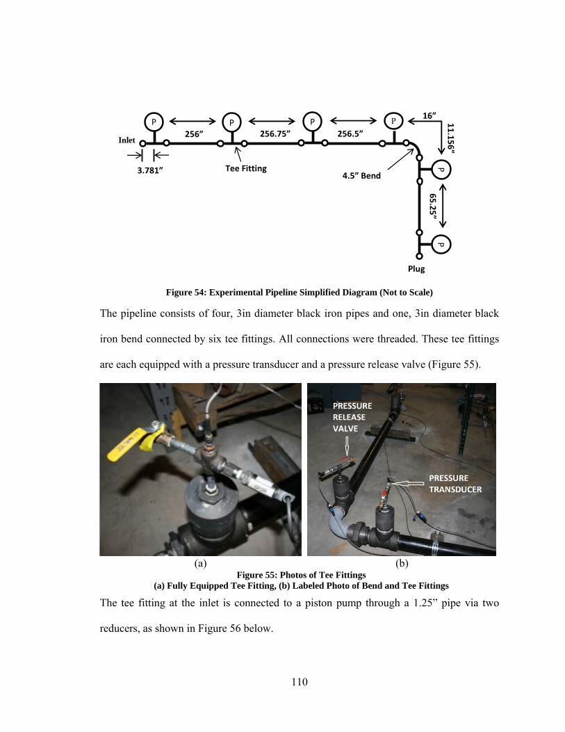
110
Figure 54: Experimental Pipeline Simplified Diagram (Not to Scale)
The pipeline consists of four, 3in diameter black iron pipes and one, 3in diameter black
iron bend connected by six tee fittings. All connections were threaded. These tee fittings
are each equipped with a pressure transducer and a pressure release valve (Figure 55).
(a)
(b) Figure 55: Photos of Tee Fittings
(a) Fully Equipped Tee Fitting, (b) Labeled Photo of Bend and Tee Fittings
The tee fitting at the inlet is connected to a piston pump through a 1.25” pipe via two
reducers, as shown in Figure 56 below.
PPP PP
P
Plug
3.781”
256” 256.75” 256.5”
16” 11.156”
65.25”
4.5” BendTee Fitting
Inlet

111
Figure 56: Photo of "Inlet" Tee Fitting and Piston Pump
Although tests in 2012 incorporated the use of a solid aluminum plug and a potassium-
magnesium-sulfate (K-mag) plug [65], the experimental results will focus on the behavior
of the fluid in the pipeline and disregard any solid-fluid interaction. Therefore, the “plug”
at the end of the pipeline is small extension terminated with a pressure release valve as
shown in Figure 57 below.
Figure 57: Photo of “Plug”
Thus, it is clear that the physical control volume (the geometric shape of the fluid
volume) begins at the face of the piston cylinder and terminates at the closed pressure
release valve. More importantly, the water in the physical experiment is not free to flow.

112
Rather, it is merely compressed and expanded by the piston. Therefore, the physics of
this experimental set up resemble the dynamics of a pressure vessel with a moving
boundary much more than that of a large network of pipes with freely flowing fluid.
The computational domain excludes the volume of fluid just before the “inlet tee”
and just after the last tee before the plug. That is, the computational domain (in the case
of this pipeline) includes roughly 99.754% of the volume of the physical domain. Typical
boundary conditions for a pipeline assume that flows entering the pipeline are fully
developed. Even if the flows are not fully developed, the boundary conditions in [60] and
[1] clearly assume that if one value (inlet pressure or velocity) is specified, the other is
free to take on any value that results from the computation (e.g. the upstream reservoir
can absorb any flow leaving the pipeline). Given the proximity of the computational inlet
to the piston head, it is impossible for the flow rate to assume an arbitrary value when
pressure is specified. When air is present and the wave speed is reduced, this proximity
also means that the unsteady changes in density and pressure occurring at the piston face
cannot be neglected. Furthermore, when the speed of sound is high and the pipeline is
short (as is the case with the fully flooded experimental pipeline) the pressure and density
of the fluid upstream of the inlet cannot be assumed independent of the downstream flow
field. Therefore, typical boundary conditions such as those in [1] are inappropriate for
this experimental set up. Instead, new boundary conditions that mimic the physics of a
pressure vessel must be developed. Although that research is outside the scope of this
thesis, it will be shown in Section 5.3.2 that under the right conditions, the simplified
boundary conditions proposed in Section 5.1.2.5 approximate the behavior of the physical
pipeline with sufficient accuracy.

113
5.3.1. Experimental Set Up and Boundary Conditions
The data used in the following section for validation is based on a pipeline similar
to that of the previous section. In this case, the pipeline is 94ft long. The specified
volume flow, Q(t), will be the time derivative of two third-order polynomials fitted
through the measured piston displacement. The pressure head, H(t), will be created using
a higher-order polynomial fitted through pressure measurements taken by the “inlet”
pressure transducer. The pressure transducers were numbered based on their order
downstream of the piston, therefore, the inlet sensor is “P1.” In these experiments, air
was only added to the fourth tee, therefore, the pressure of the air was measured by
sensor “P4.”
The system described above contains several features that are not modeled by the
MOC code:
Air/water leaks: These can be safely neglected.
Errors in the measurement of the air volume in the pipeline: They are assumed
below the tolerance specified by ARC.
Piston/Pipeline Vibrations
Unsmooth piston movement: While establishing an experimental control case, it
was observed that the piston velocity was not smooth due to an interaction
between the control unit’s signal and the piston. This is assumed negligible.
Heat Transfer: In previous experiments, the temperature variation measured in the
pipeline was less than 1°C and located close to the piston, therefore, the pipeline
can be assumed isothermal.
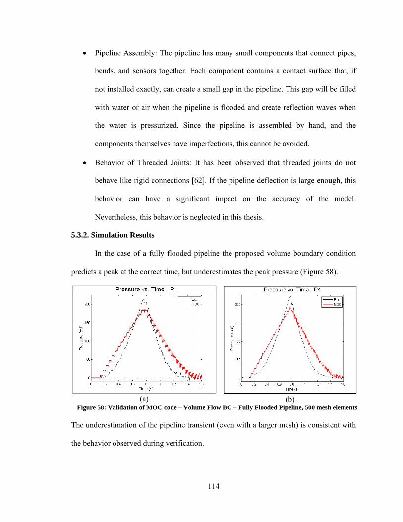
114
Pipeline Assembly: The pipeline has many small components that connect pipes,
bends, and sensors together. Each component contains a contact surface that, if
not installed exactly, can create a small gap in the pipeline. This gap will be filled
with water or air when the pipeline is flooded and create reflection waves when
the water is pressurized. Since the pipeline is assembled by hand, and the
components themselves have imperfections, this cannot be avoided.
Behavior of Threaded Joints: It has been observed that threaded joints do not
behave like rigid connections [62]. If the pipeline deflection is large enough, this
behavior can have a significant impact on the accuracy of the model.
Nevertheless, this behavior is neglected in this thesis.
5.3.2. Simulation Results
In the case of a fully flooded pipeline the proposed volume boundary condition
predicts a peak at the correct time, but underestimates the peak pressure (Figure 58).
(a)
(b) Figure 58: Validation of MOC code – Volume Flow BC – Fully Flooded Pipeline, 500 mesh elements
The underestimation of the pipeline transient (even with a larger mesh) is consistent with
the behavior observed during verification.

115
(a)
(b) Figure 59: Validation of MOC code – Pressure BC – Fully Flooded Pipeline, 50 mesh elements
The proposed pressure boundary condition is much more accurate than the volume flow
boundary condition (Figure 59).
For a pipeline with 0.327in3 of air, a piston “half-stroke,” the volume flow
boundary condition overestimates the peak pressure (Figure 60). Despite this, the
pressure wave noticeably smoothes out as it travels along the pipeline and forms a clear
peak which is consistent with the experimental profile.
(a)
(b) Figure 60: Validation of MOC code – Volume Flow BC – Half Stoke of Air, 50 mesh elements
The pressure boundary condition performs roughly the same in the presence of small
amounts of air. It should be noted that two 6th order polynomials were used to fit the P1
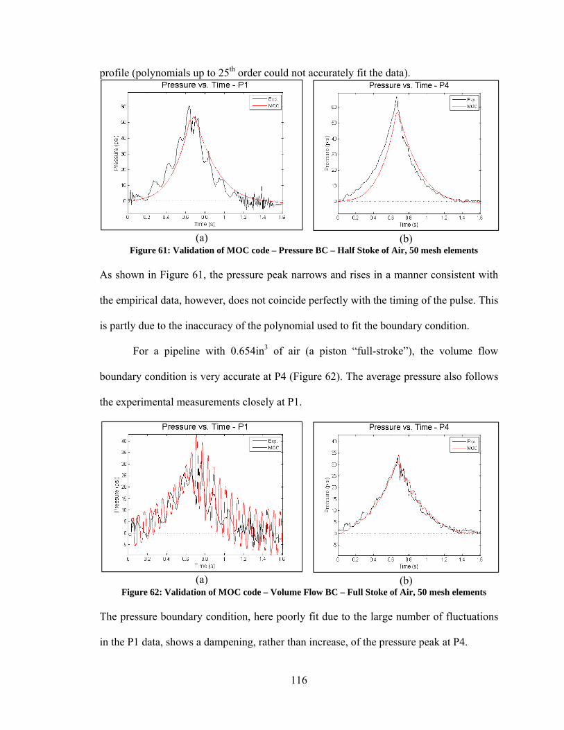
116
profile (polynomials up to 25th order could not accurately fit the data).
(a)
(b) Figure 61: Validation of MOC code – Pressure BC – Half Stoke of Air, 50 mesh elements
As shown in Figure 61, the pressure peak narrows and rises in a manner consistent with
the empirical data, however, does not coincide perfectly with the timing of the pulse. This
is partly due to the inaccuracy of the polynomial used to fit the boundary condition.
For a pipeline with 0.654in3 of air (a piston “full-stroke”), the volume flow
boundary condition is very accurate at P4 (Figure 62). The average pressure also follows
the experimental measurements closely at P1.
(a)
(b) Figure 62: Validation of MOC code – Volume Flow BC – Full Stoke of Air, 50 mesh elements
The pressure boundary condition, here poorly fit due to the large number of fluctuations
in the P1 data, shows a dampening, rather than increase, of the pressure peak at P4.
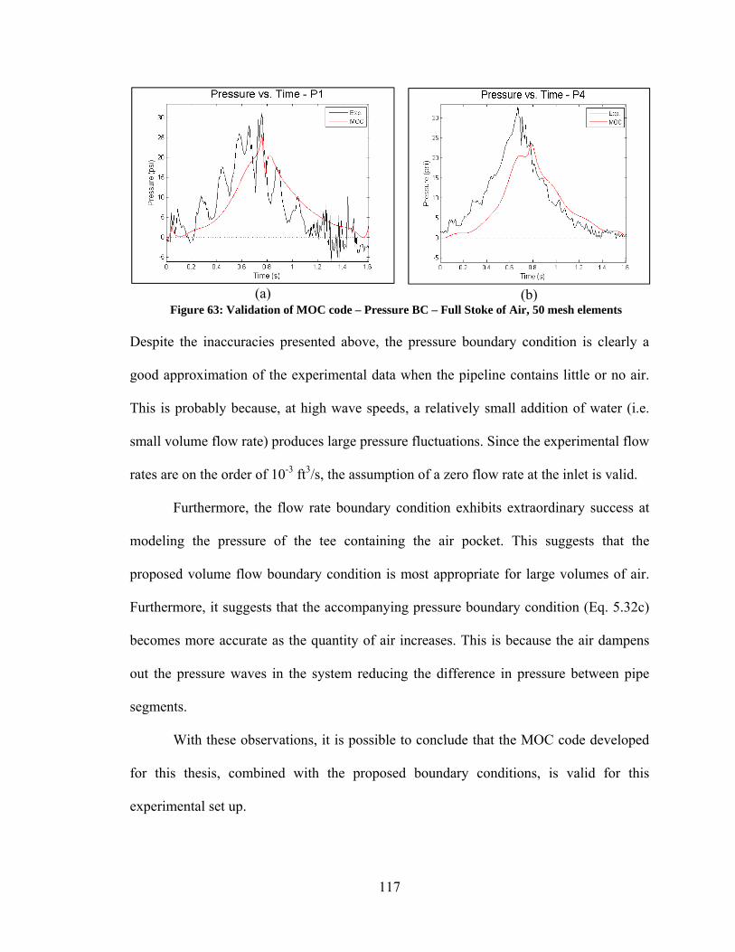
117
(a)
(b) Figure 63: Validation of MOC code – Pressure BC – Full Stoke of Air, 50 mesh elements
Despite the inaccuracies presented above, the pressure boundary condition is clearly a
good approximation of the experimental data when the pipeline contains little or no air.
This is probably because, at high wave speeds, a relatively small addition of water (i.e.
small volume flow rate) produces large pressure fluctuations. Since the experimental flow
rates are on the order of 10-3 ft3/s, the assumption of a zero flow rate at the inlet is valid.
Furthermore, the flow rate boundary condition exhibits extraordinary success at
modeling the pressure of the tee containing the air pocket. This suggests that the
proposed volume flow boundary condition is most appropriate for large volumes of air.
Furthermore, it suggests that the accompanying pressure boundary condition (Eq. 5.32c)
becomes more accurate as the quantity of air increases. This is because the air dampens
out the pressure waves in the system reducing the difference in pressure between pipe
segments.
With these observations, it is possible to conclude that the MOC code developed
for this thesis, combined with the proposed boundary conditions, is valid for this
experimental set up.
118
5.4. Evaluating and Optimizing the APU
In light of the coupling between the piston pump’s movement, and the behavior of
the pipeline, it is clear that the evaluation of a pump’s performance is specific to the
pump and the pipeline. In addition to this, a plugged pipeline has the added complexity of
the solid-fluid interaction between the plug, the pipe walls, and the surrounding fluid. For
short pipelines with large wave speeds in which the flow cannot be reversed (i.e.
pipelines that resemble pressure vessels), the specification of an arbitrary pressure profile
at the inlet is not enough to properly evaluate the pipeline’s performance. In this case,
there is no guarantee than a given piston pump will have the ability to reproduce a given
pressure profile. Therefore, the evaluation of a pipeline will require some
experimentation to determine the maximum and minimum pressures achievable with a
given piston pump, and the frequencies at which those pressures can be generated. Given
the bounds of a pump’s performance, however, an optimization algorithm can be used to
determine the optimal performance of the pump.
During earlier experiments, it was determined that if the pipeline conditions are
right and the timing of the pulses is right, pressure waves reaching the blockage can cause
a buildup of pressure at the surface of the blockage that will ultimately dislodge the plug
[57]. To avoid damaging the pipeline, the DOE designated safety limit for pipeline
pressure is 300 psi [57]. Furthermore, to avoid cavitation the pressure in the pipeline must
remain above -14.447 psi [66]. With this information, it is now possible to formulate the
APU operation process as an optimization process.
5.4.1. Optimization Problem Set Up
The goal of the APU unplugging process is to maximize the difference in
119
pressures at each face of the plug over the period (t_max) of the operation of the APU.
Therefore, the objective function can be written as:
max_)(max_
0
ttPUt
t
(5.35)
where ∆P represents the difference in pressure across the plug. The objective function is
negative because the hybrid optimization algorithm is designed to locate the global
minimum.
The pressure at one surface of the plug is a function of the frequency and peak
pressures produced by the piston. Assuming a sequence of 5 consecutive half-pulses at
the same frequency, the design vector representing the piston’s pulse schedule can be
written as:
2110987654321 ,,,,,,,,,,, ffPPPPPPPPPPx
(5.36)
Where Pi is the amplitude of the pressure of the ith pulse, f1 and f2 are the frequency of the
first and second five pulses, respectively. The first five amplitudes correspond to the
piston acting upstream of the plug; while the second set of five correspond to a second
piston acting downstream of the plug. Here, a “half-pulse” means the pressure generated
during the first half of the period of a sinusoidal pulse.
Given the limitations on the pressure in the pipeline, this optimization problem
contains two constraints:
0448.14
0300
g
g (5.37)
For each constraint violation at any point during the simulation, anywhere in the pipeline,
a penalty of 300psi is added to the objective function value.
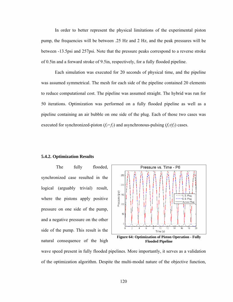
120
In order to better represent the physical limitations of the experimental piston
pump, the frequencies will be between .25 Hz and 2 Hz, and the peak pressures will be
between -13.5psi and 257psi. Note that the pressure peaks correspond to a reverse stroke
of 0.5in and a forward stroke of 9.5in, respectively, for a fully flooded pipeline.
Each simulation was executed for 20 seconds of physical time, and the pipeline
was assumed symmetrical. The mesh for each side of the pipeline contained 20 elements
to reduce computational cost. The pipeline was assumed straight. The hybrid was run for
50 iterations. Optimization was performed on a fully flooded pipeline as well as a
pipeline containing an air bubble on one side of the plug. Each of those two cases was
executed for synchronized-piston (f1=f2) and asynchronous-pulsing (f1≠f2) cases.
5.4.2. Optimization Results
The fully flooded,
synchronized case resulted in the
logical (arguably trivial) result,
where the pistons apply positive
pressure on one side of the pump,
and a negative pressure on the other
side of the pump. This result is the
natural consequence of the high
wave speed present in fully flooded pipelines. More importantly, it serves as a validation
of the optimization algorithm. Despite the multi-modal nature of the objective function,
Figure 64: Optimization of Piston Operation - Fully Flooded Pipeline

121
(the trivial result is not unique) the optimization algorithm converged to the logical
answer given the constraints applied to the pipeline, and the limitations of the piston
pump.
The second case involves a pipeline that is fully flooded on the downstream side
of the plug, but, contains an air bubble (“full-stroke” of air) on the upstream side of the
plug with synchronized pistons. This profile is very similar to the first case, except that
the upstream side of the pipeline displays the slow response time typical of air bubbles.
The solution obtained by the optimization algorithm is clearly the reasonable solution: the
maximum positive pressure is applied on the flooded side of the plug, whereas the
suction is applied on the side with the air. If the positive pressure was applied on the side
with air, the bubble would dramatically reduce the peak pressure, and since the minimum
pressure has a low magnitude compared to the maximum positive pressure, it would be
impossible to maximize the pressure across the plug in this way.
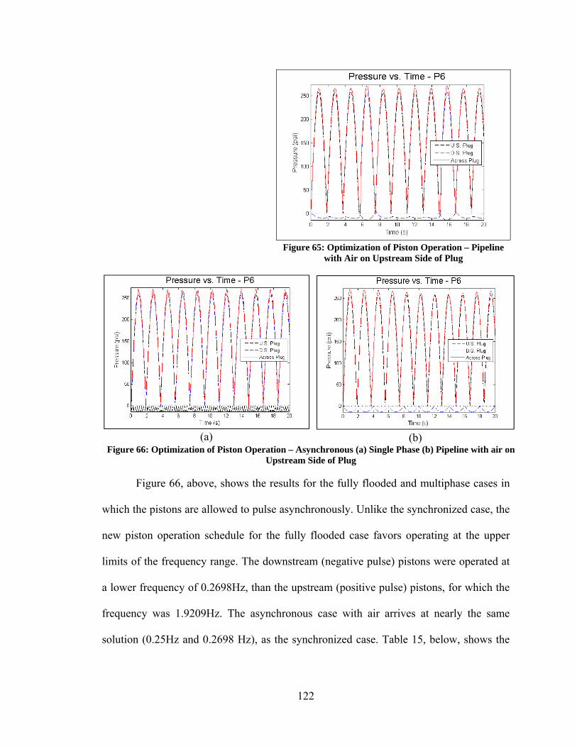
122
(a) (b) Figure 66: Optimization of Piston Operation – Asynchronous (a) Single Phase (b) Pipeline with air on
Upstream Side of Plug
Figure 66, above, shows the results for the fully flooded and multiphase cases in
which the pistons are allowed to pulse asynchronously. Unlike the synchronized case, the
new piston operation schedule for the fully flooded case favors operating at the upper
limits of the frequency range. The downstream (negative pulse) pistons were operated at
a lower frequency of 0.2698Hz, than the upstream (positive pulse) pistons, for which the
frequency was 1.9209Hz. The asynchronous case with air arrives at nearly the same
solution (0.25Hz and 0.2698 Hz), as the synchronized case. Table 15, below, shows the
Figure 65: Optimization of Piston Operation – Pipeline with Air on Upstream Side of Plug
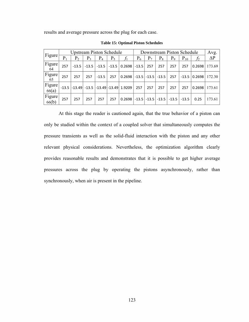
123
results and average pressure across the plug for each case.
Table 15: Optimal Piston Schedules
Figure Upstream Piston Schedule Downstream Piston Schedule Avg.
ΔP P1 P2 P3 P4 P5 f1 P6 P7 P8 P9 P10 f2 Figure
64 257 ‐13.5 ‐13.5 ‐13.5 ‐13.5 0.2698 ‐13.5 257 257 257 257 0.2698 173.69
Figure 65
257 257 257 ‐13.5 257 0.2698 ‐13.5 ‐13.5 ‐13.5 257 ‐13.5 0.2698 172.30
Figure 66(a)
‐13.5 ‐13.49 ‐13.5 ‐13.49 ‐13.49 1.9209 257 257 257 257 257 0.2698 173.61
Figure 66(b)
257 257 257 257 257 0.2698 ‐13.5 ‐13.5 ‐13.5 ‐13.5 ‐13.5 0.25 173.61
At this stage the reader is cautioned again, that the true behavior of a piston can
only be studied within the context of a coupled solver that simultaneously computes the
pressure transients as well as the solid-fluid interaction with the piston and any other
relevant physical considerations. Nevertheless, the optimization algorithm clearly
provides reasonable results and demonstrates that it is possible to get higher average
pressures across the plug by operating the pistons asynchronously, rather than
synchronously, when air is present in the pipeline.
124
CHAPTER 6
6. CONCLUSIONS
This thesis has achieved its primary goals. First, a novel, hybrid optimization
algorithm switching logic was proposed. After being tested against other algorithms using
standard benchmarking techniques, it was found to be superior to many algorithms over a
broad set of test cases. Due to the added overhead, however, the BST-SPC algorithm was
found to be superior to the hybrid in a variety of test cases as well. Nevertheless, the
hybrid is a strong competitor outperforming OPTRAN in the majority of unconstrained
test cases, and performing competitively against other hybrid algorithms in other test
cases.
Second, a general framework for gaging the performance of hybrid optimization
algorithms was proposed. This framework can be applied to any hybrid whose express
aim is to outperform its constituent algorithms. Within this context, the hybrid is found to
perform “typically” suggesting that its extra computational expense prevents it from
maximizing the potential given the constituent algorithms at its disposal. Therefore, in the
future it would be useful to incorporate surrogate models, or improve the search
vector/constituent selection scheme so that the overhead costs of the hybrid are reduced.
Third, a Method of Characteristics code was developed to model the
Asynchronous Pulse Unit. Using an updated version of the text book, and including new
boundary conditions proposed for the purpose of this thesis, the code was found to
accurately model a variety of experimental flows. With this, it became possible to
connect the hybrid optimization algorithm to the MOC code so that the operation of the

125
piston pumps could be performed. Once done, it was found that higher average pressures
across the plug could be achieved by pulsing the pistons asynchronously.
The research performed for this thesis also opened up new topics of study. For
example, the question of how to decompose an objective function’s topology into
effective topologies remains unsolved. For many problems it is clear that this
decomposition is not unique. Therefore, if it is done carelessly, it is possible that an
incorrect set of effective topologies will be selected, which will misguide the
optimization algorithm. Furthermore, the question of how to best identify the iterative
heuristic that solves a problem given this set of effective topologies remains unanswered.
It is clear from the results in this thesis that matching the fittest search vector to the
constituent algorithm centroid is a useful approach, but it is only part of the solution.
Could there be rules, or a probabilistic selection scheme that would improve the hybrid’s
robustness? What additional measurements should the selection criteria be based on (e.g.
standard deviation of the range)?
What is clear from these questions and the effectiveness of the proposed hybrid, is
that this is a fruitful area of research with ample room for continued investigation.
Although it may not be possible to create a single algorithm that solves all problems, a
well-constructed hybrid algorithm has clear advantages over any other kind of
optimization algorithm.
126
REFERENCES
[1] B. E. Wylie and V. L. Streeter, Fluid Transients in Systems, Upper Saddle River, NJ: Prentice-Hall, Inc., 1993.
[2] R. J. Moral, Hybrid Multi-Objective Optimization and Hybridized Self-Organizing Respose Surface Method, Miami: ProQuest Dissertations and Theses; Florida International University, 2008.
[3] D. Simon, "Biogeography-Based Optimization," IEEE TRANSACTIONS ON EVOLUTIONARY COMPUTATION, vol. 12, no. 6, pp. 702-713, December 2008.
[4] J. Lampinen and H.-Y. Fan, "A Trigonometric Mutation Operation to Differential Evolution," Journal of Global Optimization, pp. 105-129, 2003.
[5] X.-S. Yang, "A New Metaheuristic Bat-Inspired Algorithm," Nature Inspired Cooperative Strategies for Optimization (NISCO 2010), vol. 284, pp. 65-74, 2010.
[6] G. Saurav, S. Das, S. Roy, S. M. Islam and P. N. Suganthan, "A Differential Covariance Matrix Adaptation Evolutionary Algorithm for Real Parameter Optimization," Information Sciences, vol. 182, pp. 199-219, 2011.
[7] G. N. Vanderplaats, Multidiscipline Design Optimization, Vanderplaats Research and Development, 2007.
[8] K. Deb, Multi-Objective Optimization using Evolutionary Algorithms, Chichester: Wiley, 2009.
[9] J. B. Rosen, "The Gradient Projection Method for Nonlinear Programming, Part I – Linear Constraints," Journal of the Society for Industrial and Applied Mathematics, vol. 8, no. 1, pp. 181-217, Mar. 1960.
[10]
J. B. Rosen, "The Gradient Projection Method for Nonlinear Programming, Part II – Nonlinear Constraints," Journal of the Society for Industrial and Applied Mathematics, vol. 9, no. 4, pp. 514-532, Dec. 1961.
[11]
A. Ahrari, M. R. Saadatmand, M. Shariat-Panahi and A. A. Atai, "On the limitations of classical benchmark functions for evaluating robustness of evolutionary algorithms," Applied Mathematics and Computation, no. 215, p. 3222–3229, 2010.
[12]
K. Schittkowski and W. Hock, Test Examples for Nonlinear Programming Codes - All Problems from the Hock-Schittkowski-Collection, Bayreuth: Springer, 1981.
127
[13]
K. Schittkowski, More Test Examples for Nonlinear Programming Codes, Berlin: Springer-Verlag, 1987.
[14]
R. Fletcher and M. J. D. Powell, "A Rapidly Convergent Descent Method for Minimization," The Computer Journal, vol. 6, no. 2, pp. 163-168, 1963.
[15]
D. Goldfarb, "Conditioning of Quasi-Newton Methods for Function Minimization," Math. Comput., pp. 647-656, 1970.
[16]
D. E. Goldberg, Genetic Algorithms in Search, Optimization and Machine Learning, Boston: Addison-Wesley Longman Publishing Co., 1989.
[17]
J. Kennedy and R. Eberhart, "Particle Swarm Optimization," Neural Networks, 1995. Proceedings., IEEE International Conference on, pp. 1942-1948, 1995.
[18]
R. Storn and K. Price, "Differential Evolution – A Simple and Efficient Heuristic for Global Optimization over Continuous Spaces," Journal of Global Optimization, p. 341–359, 1997.
[19]
H.-Y. Fan, J. Lampinen and G. S. Dulikravich, "Improvements to Mutation Donor Formulation of Differential Evolution," in EUROGEN2003 - International Congress on Evolutionary Methods for Design, Optimization and Control with Applications to Industrial Problems, (eds: G. Bugeda, J. A- Désidéri, J. Periaux, M. Schoenauer and G. Winter) Barcelona, Spain, September 15-17, 2003.
[20]
J.-R. Zhang, J. Zhang, L. Tat-Ming and M. R. Lyu, "A hybrid particle swarm optimization–back-propagation algorithm for feedforward neural network training," Applied Mathematics and Computation, vol. 185, p. 1026–1037, 2007.
[21]
W. G. MacReady and D. H. Wolpert, "No Free Lunch Theorems for Optimization," IEEE TRANSACTIONS ON EVOLUTIONARY COMPUTATION, vol. 1, no. 1, pp. 67-82, April 1997.
[22]
S. Droste, T. Jansen and I. Wegener, "Optimization with randomized search heuristics—the (A)NFL theorem, realistic scenarios, and diffcult functions," Theoretical Computer Science, vol. 287, p. 131 – 144, 2002.
[23]
X.-S. Yang, "Free Lunch or No Free Lunch: That is not Just a Question?," International Journal on Artificial Intelligence Tools, vol. 21, no. 3, 2012.
[24]
D. Corne and J. Knowles, "Some Multiobjective Optimizers are Better than Others," in The 2003 Congress on Evolutionary Computation, Canberra, 2003.
128
[25]
C. Igel and M. Toussaint, "On Classes of Functions for which No Free Lunch Results Hold," Information Processing Letters, vol. 86, no. 6, pp. 317-321, 2003.
[26]
A. Auger and O. Teytaud, "Continuous Lunches Are Free Plus the Design of Optimal Optimization Algorithms," Algorithmica, vol. 57, p. 121–146, 2010.
[27]
E. Talbi, "A taxonomy of hybrid metaheuristics," J. Heuristics, vol. 8, no. 5, p. 541–564, 2002.
[28]
G. Raidl, "A unified view on hybrid metaheuristics," in Hybrid Metaheuristics, F. Almeida, M. B. Aguilera, C. Blum, J. M. Vega, M. P. Perez, A. Roli and M. Sampels, Eds., Berlin, Springer, 2006, pp. 1-12.
[29]
J. A. Vrugt and B. A. Robinson, "Improved Evolutionary Optimization from Genetically Adaptive Multimethod Search," Proceedings of the National Academy of Sciences (U.S.), vol. 104, no. 3, p. 708–711, 2007.
[30]
W. Gong, Z. Cai and C. X. Ling, "DE/BBO: a hybrid differential evolution with biogeography-based optimization for global numerical optimization," Soft Computing, vol. 15, no. 4, pp. 645-665, 2010.
[31]
P. Sriyanyong, "A Hybrid Particle Swarm Optimization Solution to Ramping Rate Constrained Dynamic Economic Dispatch," Engineering and Technology, vol. 47, 2008.
[32]
M. Løvbjerg, T. K. Rasmussen and T. Krink, "Hybrid Particle Swarm Optimiser with Breeding and Subpopulations," in Proceedings of the Genetic and Evolutionary Computation Conference, 2001.
[33]
G. S. Dulikravich, T. J. Martin, M. J. Colaço and E. J. Inclan, "Automatic Switching Algorithms in Hybrid Single-Objective Optimization," FME Transactions, Vols. 41, No. 3, University of Belgrade Faculty of Mechanical Engineering, 2013, pp. 167-179.
[34]
G. Dulikravich, T. Martin, D. B.H. and N. Foster, "Multidisciplinary Hybrid Constrained GA Optimization," Invited Lecture, Chapter 12 in EUROGEN’99 - Evolutionary Algorithms in Engineering and Computer Science: Recent Advances and Industrial Applications, Jyvaskyla, Finland, May 30-June 3, 1999, pp. 231-260.
[35]
G. S. Dulikravich and M. J. Colaço, "Hybrid Optimization Algorithms and Hybrid Response Surfaces," in Advances in Evolutionary and Deterministic Methods for Design, Optimization and Control in Engineering and Sciences, Springer International Publishing Switzerland, 2015.
129
[36]
R. J. Moral and G. S. Dulikravich, "Multi-Objective Hybrid Evolutionary Optimization with Automatic Switching Among Constituent Algorithms," AIAA Journal, vol. 46, no. 3, pp. 673-700, March 2008.
[37]
G. S. Dulikravich, R. J. Moral and D. Sahoo, "A Multi-Objective Evolutionary Hybrid Optimizer," in EUROGEN 2005 - Evolutionary and Deterministic Methods for Design, Optimization and Control with Applications to Industrial and Societal Problems, Munich, Germany, September 12-14, 2005.
[38]
R. J. Moral, D. Sahoo and G. S. Dulikravich, "Multi-Objective Hybrid Evolutionary Optimization With Automatic Switching," in AIAA-2006-6976, 11th AIAA/ISSMO Multidisciplinary Analysis and Optimization Conference, Portsmouth, VA, September 6-8, 2006.
[39]
M. J. Colaço, G. S. Dulikravich and T. J. Martin, "Control of Unsteady Solidification via Optimized Magnetic Fields," Materials and Manufacturing Processes, vol. 20, no. 3, pp. 435-458, May 2005.
[40]
R. Mendes, J. Kennedy and J. Neves, "The Fully Informed Particle Swarm: Simpler, Maybe Better," IEEE Transactions on Evolutionary Computation, vol. 8, no. 3, pp. 204-210, 3 June 2004.
[41]
M. T. Jensen, "Guiding Single-Objective Optimization Using Multi-objective Methods," in Applications of Evolutionary Computing, vol. 2611, G. C. S. C. J. C. D. G. J. G. A. H. E. J. C. M. E. M. J. M. M. Raidl, Ed., Springer Berlin Heidelberg, 2003, pp. 268-279.
[42]
W. H. Press, S. A. Teukolsky, W. T. Vetterling and B. P. Flannery, Numerical Recipes in C: The Art of Scientific Computing, 2nd ed., New York: Cambridge University Press, 1992.
[43]
P. Bratley and B. L. Fox, "Algorithm 659 Implementing Sobol's Quasirandom Sequence Generator," ACM Transactions on Mathematical Software, vol. 14, no. 1, pp. 88-100, March 1988.
[44]
J. Burkardt, "SOBOL - The Sobol Quasirandom Sequence:," 12 December 2009. [Online]. Available: http://people.sc.fsu.edu/~jburkardt/cpp_src/sobol/sobol.html. [Accessed 1 January 2013].
[45]
T. Goel, R. Vaidyanathan, R. T. Haftka, W. Shyy, N. V. Queipo and K. Tucker, "Response surface approximation of Pareto optimal front in multi-objective optimization," Comput. Methods Appl. Mech. Engrg., vol. 196, p. 879–893, 2007.
[46 G. S. Dulikravich, "Brief comparison among different optimizers," FL, USA, 2011.
130
]
[47]
D. R. Musser, "Measuring Computing Times and Operation Counts of Generic Algorithms," Rensselaer Polytechnic Institute, 19 September 1998. [Online]. Available: http://www.cs.rpi.edu/~musser/gp/timing.html. [Accessed 17 June 2014].
[48]
StackOverflow, "Timing algorithm: clock() vs time() in C++," StackOverflow, 6 July 2013. [Online]. Available: http://stackoverflow.com/questions/12231166/timing-algorithm-clock-vs-time-in-c. [Accessed 17 June 2014].
[49]
StackOverflow, "Easily measure elapsed time," StackOverflow, 28 August 2013. [Online]. Available: http://stackoverflow.com/questions/2808398/easily-measure-elapsed-time. [Accessed 17 June 2014].
[50]
T. J. Martin, M. Colaço and G. S. Dulikravich, "OPTRAN User Manual," Multidisciplinary Analysis, Inverse Design, Robust Optimization and Control Laboratory, 1999.
[51]
State of Oregon, "oregon.gov," 14 July 2009. [Online]. Available: http://web.archive.org/web/20100602110418/http:/www.oregon.gov/ENERGY/NUCSAF/HCleanup.shtml. [Accessed 1 July 2013].
[52]
DOE Richland Operations Office, "Richland Operations Office - About Us," 1 February 2007. [Online]. Available: http://web.archive.org/web/20080516002347/http:/www.hanford.gov/rl/?page=45&parent=0. [Accessed 1 June 2013].
[53]
S. Wood, "Modeling of Pipeline Transients: Modified Method of Characteristics," FIU Electronic Theses and Dissertations., Miami, 2011.
[54]
R. D. Hunt, J. S. Lindner, A. J. Mattus, J. C. Schryver and C. F. Weber, "Waste Preparation and Transport Chemistry: Results of the FY 2002 Studies," Oak Ridge National Laboratory, Oak Ridge, 2003.
[55]
S. Gokaltun, D. McDaniel, D. Roelant, J. Varona, R. Patel and A. Awwad, "Evaluation of Innovative High-Level Waste Pipeline Unplugging Technologies," Phoenix, 2009.
[56]
J. A. Matos, "Development of a Body for a Pneumatic Crawler for Radioactive Waste Pipelines," FIU Electronic Theses and Dissertations, Miami, 2013.
[57]
S. Gokaltun, T. Pribanic, J. Varona, D. McDaniel, A. Awwad and D. Roelant, "Evaluation and Development of Innovative High-Level Waste Pipeline Unplugging Technologies," in WM Symposia 2010, Phoenix, 2010.
131
[58]
T. Pribanic, S. Gokaltun, D. McDaniel, J. Varona, A. Awwad and D. Roelant, "Summary of Conceptual Designs for Two Pipeline Unplugging Methods," Florida International University Applied Research Center, Miami, 2009.
[59]
S. Mambretti, Water Hammer Simulations, Billerica, MA: WIT Press, 2014.
[60]
E. B. Wylie and V. L. Streeter, Fluid Transients, New York: McGraw-Hill, 1978.
[61]
D. Roylance, "Pressure Vessels," Department of Materials Science and Engineering, MIT, Massachusetts, 2001.
[62]
Y. Ryu, A. Behrouzi, T. Melesse and V. C. Matzen, "Inelastic Behavior of Threaded Piping Connections - Reconciliation of Experimental and Analytic Results," in Proceedings of the ASME 2011 Pressure Vessels & Piping Division Conference, Baltimore, 2011.
[63]
R. A. Fine and F. J. Millero, "Compressibility of water as a function of temperature and pressure," The Journal of Chemical Physics, vol. 59, no. 10, pp. 5529-5536, 1973.
[64]
Committee on Long-Term Research Needs for Radioactive High-Level Waste at Department of Energy Sites, Board on Radioactive Waste Management, National Research Council, Research Needs for High-Level Waste Stored in Tanks and Bins at U.S. Department of Energy Sites: Environmental Management Science Program, Washington, D.C.: National Academy Press, 2001.
[65]
T. Pribanic, A. Awwad, J. Crespo, D. McDaniel, J. Varona, S. Gokaltun and D. Roelant, "Design Improvements and Analysis of Innovative High-Level Waste Pipeline Unplugging Technologies," Phoenix, 2012.
[66]
A. Wexler, "Journal of Research of the National Bureau of Standards - A. Physics and Chemistry," vol. 80A, no. 5,6, 1976.
[67]
E. J. Inclan, G. S. Dulikravich and X.-S. Yang, "Modern Optimization Algorithms and Particle Swarm Variations," in 4th Symposium on Inverse Problems, Design and Optimization-IPDO2013, (eds.: Fudym, O., Battaglia, J.L.) Albi, France, June 26-28, 2013.
[68]
E. J. Inclan and G. S. Dulikravich, "Effective Modifications to Differential Evolution Optimization Algorithm," in V International Conference on Computational Methods for Coupled Problem in Science and Engineering, Santa Eulalia, Ibiza, Spain, June 17-19, 2013.
132
[69]
J. Sun, C. H. Lai, W. Xu and Z. Chai, "A Novel and More Efficient Search Strategy of Quantum-Behaved Particle Swarm Optimization," ICANNGA '07 Proceedings of the 8th international conference on Adaptive and Natural Computing Algorithms, pp. 394 - 403, 2007.
[70]
X.-S. Yang, "Firefly Algorithms for Multimodal Optimization," Stochastic Algorithms: Foundations and Applications, SAGA 2009, vol. 5792, pp. 169-178, 2009.
[71]
X.-S. Yang and S. Deb, "Engineering Optimisation by Cuckoo Search," Int. J. Mathematical Modelling and Numerical Optimisation, vol. 1, no. 4, pp. 330-343, 2010.
[72]
H. Ma, "An analysis of the equilibrium of migration models for biogeography-based optimization," Information Sciences, p. 3444–3464, 2010.
[73]
"Particle Swarm Optimization and Differential Evolution Algorithms: Technical Analysis, Applications and Hybridization Perspectives," in Advances of Computational Intelligence in Industrial Systems, vol. 116, Berlin / Heidelberg, Springer, 2008, pp. 1-38.
[74]
H. Iba and N. Noman, "Accelerating Differential Evolution Using an Adaptive Local Search," IEEE Transactions on Evolutionary Computation, vol. 12, no. 1, pp. 107-125, 2008.
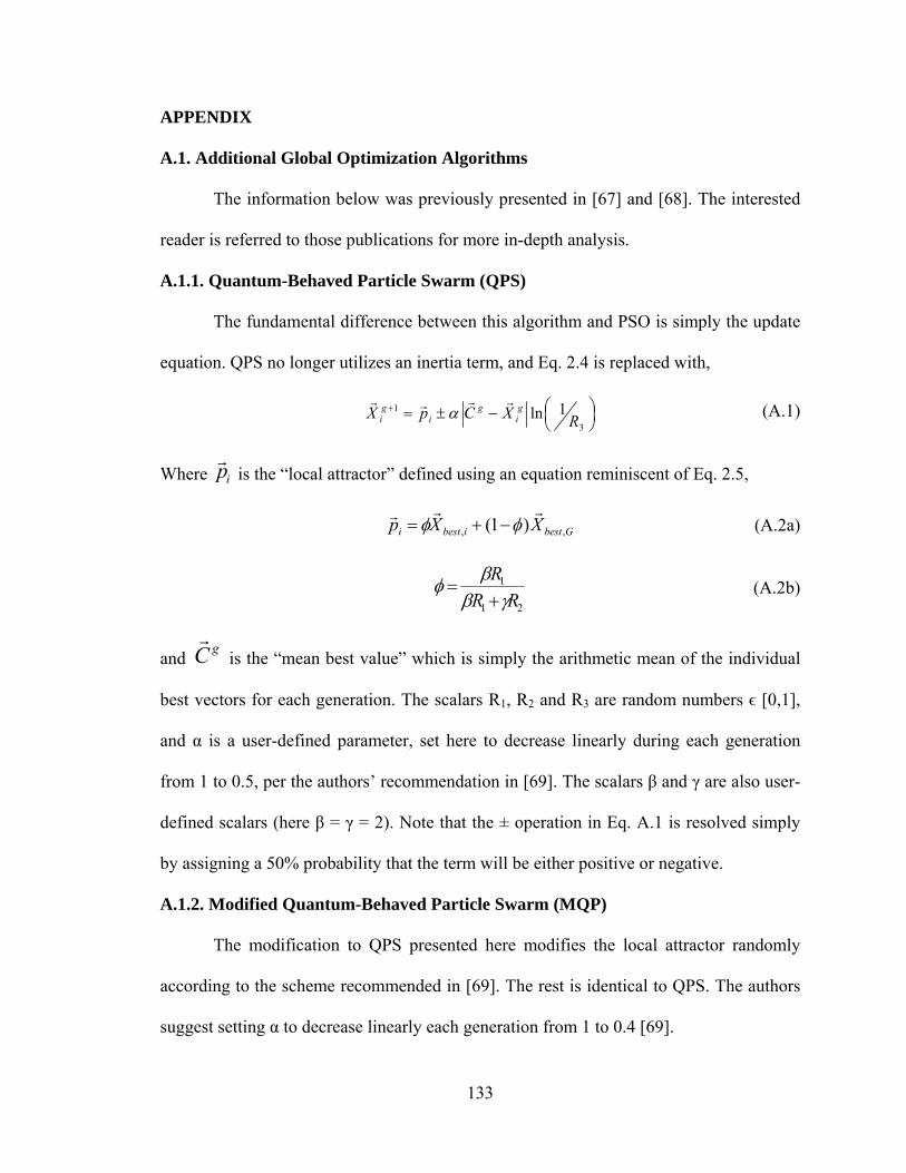
133
APPENDIX
A.1. Additional Global Optimization Algorithms
The information below was previously presented in [67] and [68]. The interested
reader is referred to those publications for more in-depth analysis.
A.1.1. Quantum-Behaved Particle Swarm (QPS)
The fundamental difference between this algorithm and PSO is simply the update
equation. QPS no longer utilizes an inertia term, and Eq. 2.4 is replaced with,
3
1 1ln RXCpX gi
gi
gi
(A.1)
Where ip
is the “local attractor” defined using an equation reminiscent of Eq. 2.5,
Gbestibesti XXp ,, )1( (A.2a)
21
1
RR
R
(A.2b)
and gC
is the “mean best value” which is simply the arithmetic mean of the individual
best vectors for each generation. The scalars R1, R2 and R3 are random numbers ϵ [0,1],
and α is a user-defined parameter, set here to decrease linearly during each generation
from 1 to 0.5, per the authors’ recommendation in [69]. The scalars β and γ are also user-
defined scalars (here β = γ = 2). Note that the ± operation in Eq. A.1 is resolved simply
by assigning a 50% probability that the term will be either positive or negative.
A.1.2. Modified Quantum-Behaved Particle Swarm (MQP)
The modification to QPS presented here modifies the local attractor randomly
according to the scheme recommended in [69]. The rest is identical to QPS. The authors
suggest setting α to decrease linearly each generation from 1 to 0.4 [69].

134
A.1.3. Firefly Algorithm (FFA)
Under certain circumstances, FFA reduces to a special case of PSO [70]. Unlike
any other method presented here, it uses two loops over the population with one loop
nested inside the other. The attractiveness equation used in this thesis is a replica of the
equation provided in Dr. Yang’s MATLAB code, which is,
minmin0
2
re (A.3)
where γ is a user-defined parameter (here set to 1). The scalars β0 and βmin are also user-
defined parameters (here set to 1 and 0.2, respectively). Finally, r is the Euclidean
distance. The small random perturbation vector is generated in the MATLAB code
according to,
dim
1
ˆ)5.0(i
ieLRu (A.4)
where α is a user-defined parameter that decreases linearly with the generation number
from 0.25 to 0, R is a uniformly distributed random number ϵ [0,1], and L is the width of
the search domain in the ie direction. Finally, the update equation is given as,
uXXX gj
gi
gi
11 (A.5)
The resemblance to the velocity equation of PSO is striking.
A.1.4. Bat-Inspired Algorithm (BAT)
This algorithm resembles DE in that it uses comparisons to update each new
generation of candidate solutions. Reminiscent of best/2/bin, it partially incorporates
perturbations of the best design vector into its formulation, and like sociability-only-PSO,
it searches the function space based on a multiple of the difference between the global
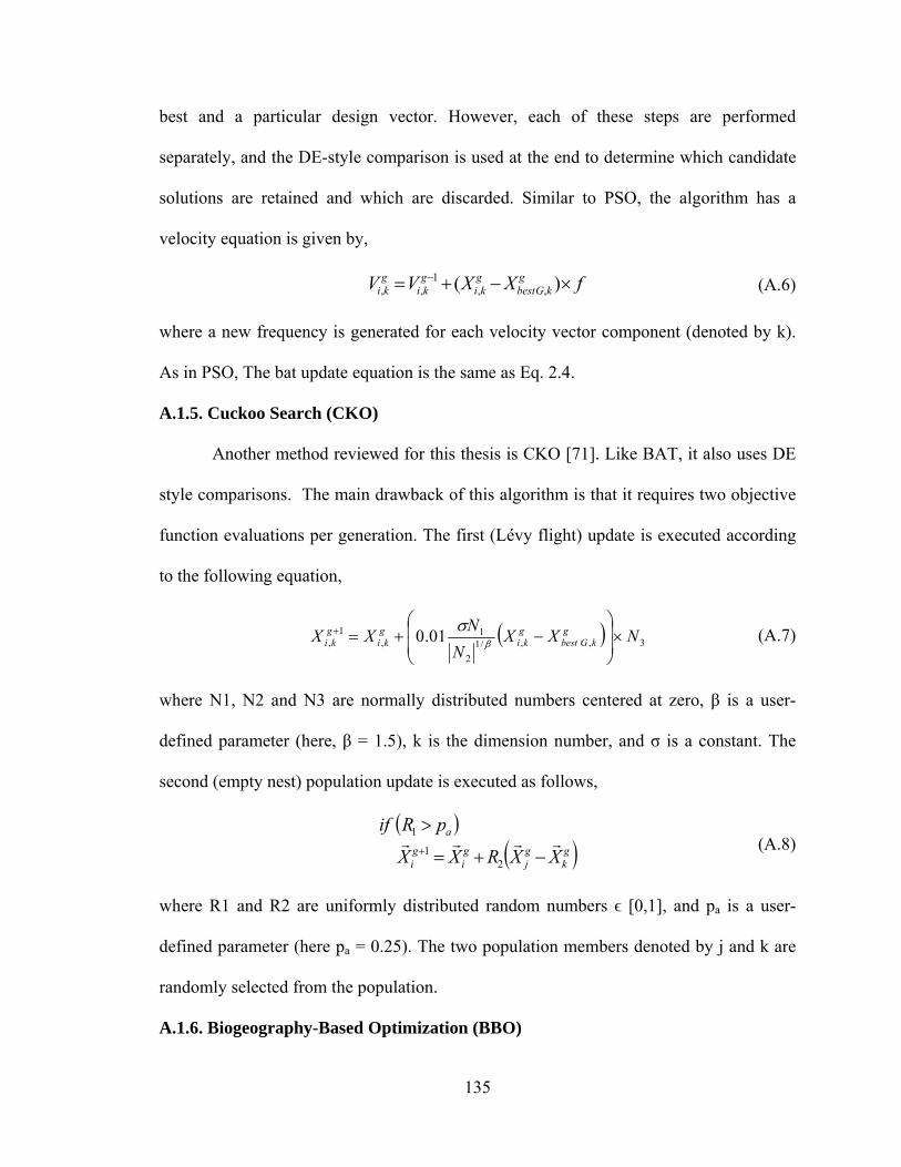
135
best and a particular design vector. However, each of these steps are performed
separately, and the DE-style comparison is used at the end to determine which candidate
solutions are retained and which are discarded. Similar to PSO, the algorithm has a
velocity equation is given by,
fXXVV gkGbest
gki
gki
gki )( ,,
1,, (A.6)
where a new frequency is generated for each velocity vector component (denoted by k).
As in PSO, The bat update equation is the same as Eq. 2.4.
A.1.5. Cuckoo Search (CKO)
Another method reviewed for this thesis is CKO [71]. Like BAT, it also uses DE
style comparisons. The main drawback of this algorithm is that it requires two objective
function evaluations per generation. The first (Lévy flight) update is executed according
to the following equation,
3,,/1
2
1,
1, 01.0 NXX
N
NXX g
kGbestgki
gki
gki
(A.7)
where N1, N2 and N3 are normally distributed numbers centered at zero, β is a user-
defined parameter (here, β = 1.5), k is the dimension number, and σ is a constant. The
second (empty nest) population update is executed as follows,
gk
gj
gi
gi
a
XXRXX
pRif
21
1 (A.8)
where R1 and R2 are uniformly distributed random numbers ϵ [0,1], and pa is a user-
defined parameter (here pa = 0.25). The two population members denoted by j and k are
randomly selected from the population.
A.1.6. Biogeography-Based Optimization (BBO)
136
BBO is modeled after the migration of species from one habitat to another [3].
Unlike the previous methods, BBO does not use an update equation, but rather, creates
new design vectors by creating permutations of existing design vectors based on their
fitness. BBO contains three user-defined parameters: µ, λ and the mutation probability.
Researchers have found that varying the emigration and immigration profiles can
improve the algorithm’s performance [72], but that is outside the scope of this thesis. The
value of µ must be nonnegative, or the algorithm may never perform emigration (the
update). The update condition is given by the following inequality,
emigrationforkindividualselectthenRifpop
ii
k
ii ,
11
(A.9)
where R is a random number between zero and one, and k is the design vector whose µ
value makes the condition statement true.
A.1.7. Particle Swarm With Random Differences (RD)
Inspired by the concept of random walks and the modified local attractor of MQP,
this proposed modification adds versatility to PSO without dramatically changing its
basic procedure. Traditionally, each design vector in PSO is subtracted from its own
individual best vector. This method, proposed in [67], introduces a probability that a
design vector will be subtracted from an individual best other than its own based on the
value Rp, which is the “probability of random differencing,” a user-defined parameter ϵ
[0,1]. The above algorithm is roughly equivalent to rewriting Eq. 2.4 as follows,
jiandpopjiwhere
XXRXXRVV iGbestijbestg
ig
i
],1[,,2,1
1
(A.10)
137
where pop is the number of candidate design vectors in the population. The requirement
that i not equal j is not strictly enforced when the vectors are shuffled.
A.1.8. Modifications to DE
Over the years many modifications to DE have been proposed. Some of these
modifications relate to the update equation [4], while others involve merging DE with
some other technique [73] [74]. Recently, three types of modifications were proposed in
[68] that draw more performance out of DE while minimizing the changes made to the
implementation of DE.
1. Randomly Varying Parameters
Randomly varying both F and CR dramatically improves the convergence speed
and robustness of the DE methods in many test functions.
2. Special Vectors
Since DE involves the weighted average of a collection of vectors, including
special vectors in the population (such as the weighted average) after each iteration has
been shown to improve performance. An average vector, and a weighted average vector
are used for this purpose. This was the precursor to the search vector concept.
3. Sorted Comparisons
This method has been shown to greatly increase convergence speed but reduce
robustness, causing the algorithm to converge to local minima more frequently.

138
A.2. Comparison of Standard Optimization Algorithms
Figure 67, below, compares the relative accuracy and speed of each algorithm.
Although PSO obtained the single best answer in 58.4% of the test cases, STD and DN3
outperformed all other methods in speed and accuracy in nearly half of the test cases.
Second to STD and DN3 in both speed and accuracy were PSO and MQP. These four
methods combined account for nearly 75% of the best-performing algorithms. Although
BST, TDE and QPS have accuracies above 10%, they suffer in the combined speed-
accuracy category due to their lack of speed relative to other methods. BBO rarely
outperforms any of the other algorithms. This may be due to the fact that BBO relies on
two processes in order to produce new designs:
1. Permutations: given an existing population, each new member generated by the
“migration” operation is simply a permutation of existing members.
2. Mutation / Replacement of Duplicates: the random generation of new designs.
Figure 67: Best Performance of Unmodified Optimization Algorithms
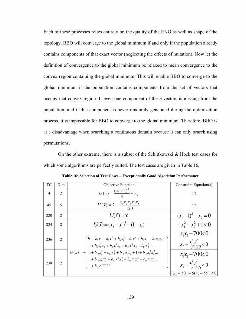
139
Each of these processes relies entirely on the quality of the RNG as well as shape of the
topology. BBO will converge to the global minimum if and only if the population already
contains components of that exact vector (neglecting the effects of mutation). Now let the
definition of convergence to the global minimum be relaxed to mean convergence to the
convex region containing the global minimum. This will enable BBO to converge to the
global minimum if the population contains components from the set of vectors that
occupy that convex region. If even one component of these vectors is missing from the
population, and if this component is never randomly generated during the optimization
process, it is impossible for BBO to converge to the global minimum. Therefore, BBO is
at a disadvantage when searching a continuous domain because it can only search using
permutations.
On the other extreme, there is a subset of the Schittkowski & Hock test cases for
which some algorithms are perfectly suited. The test cases are given in Table 16,
Table 16: Selection of Test Cases – Exceptionally Good Algorithm Performance
TC Dim Objective Function Constraint Equation(s)
4 2 2
31
3
)1()( x
xxU
n/a
45 5 120
2)( 54321 xxxxxxU
n/a
220 2 1)( xxU
0)1( 22
1 xx
234 2 )1()()( 13
12 xxxxU
0122
21 xx
236 2
214520
32119
22118
32
3117
22
3116
22
2115214
4213
3212
22112
41102
3192
218
21726415
314
213121
...
......
...)1/(...
......
...
)(
xxeeb
xxbxxbxxbxxb
xxbxbxbxb
xbxxbxxbxxb
xxbxbxbxbxbxbb
xU
070021 xx
0125
21
2 xx
238 2
070021 xx
0125
21
2 xx
0)55(5)50( 12 xx
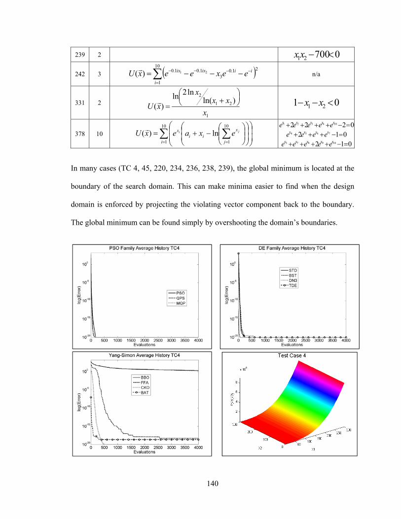
140
239 2 070021 xx
242 3
10
1
21.03
1.01.0 21)(i
iiixix eexeexU
n/a
331 2
1
21
2)ln(
ln2ln)(
x
xxx
xU
01 21 xx
378 10
10
1
10
1
ln)(i j
xii
x ji exaexU
0222 106321 xxxxx eeeee
012 7654 xxxx eeee
012 109873 xxxxx eeeee In many cases (TC 4, 45, 220, 234, 236, 238, 239), the global minimum is located at the
boundary of the search domain. This can make minima easier to find when the design
domain is enforced by projecting the violating vector component back to the boundary.
The global minimum can be found simply by overshooting the domain’s boundaries.
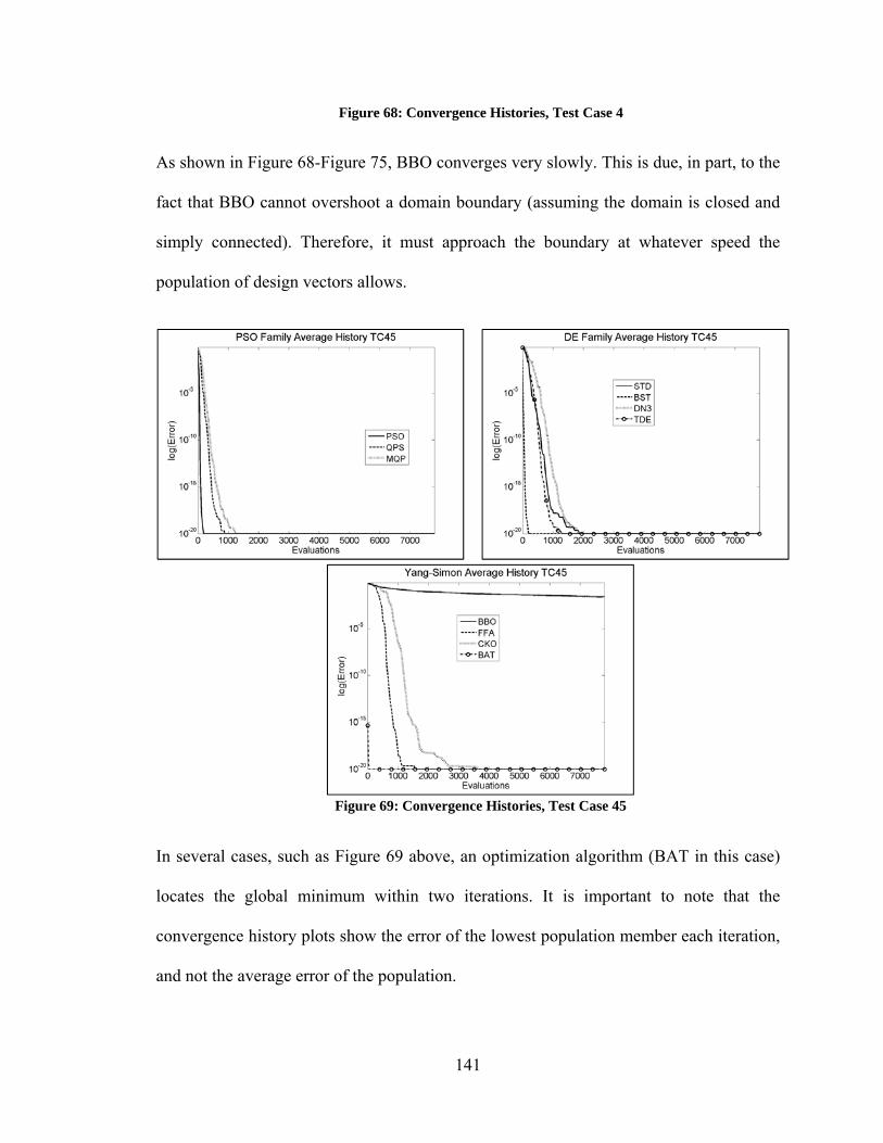
141
Figure 68: Convergence Histories, Test Case 4
As shown in Figure 68-Figure 75, BBO converges very slowly. This is due, in part, to the
fact that BBO cannot overshoot a domain boundary (assuming the domain is closed and
simply connected). Therefore, it must approach the boundary at whatever speed the
population of design vectors allows.
Figure 69: Convergence Histories, Test Case 45
In several cases, such as Figure 69 above, an optimization algorithm (BAT in this case)
locates the global minimum within two iterations. It is important to note that the
convergence history plots show the error of the lowest population member each iteration,
and not the average error of the population.
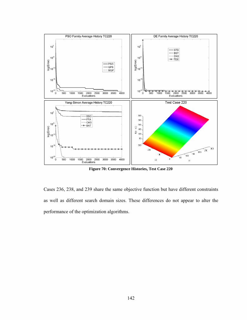
142
Figure 70: Convergence Histories, Test Case 220
Cases 236, 238, and 239 share the same objective function but have different constraints
as well as different search domain sizes. These differences do not appear to alter the
performance of the optimization algorithms.
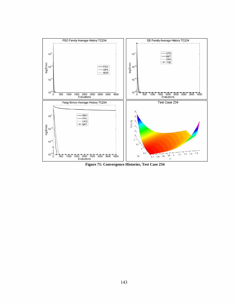
143
Figure 71: Convergence Histories, Test Case 234
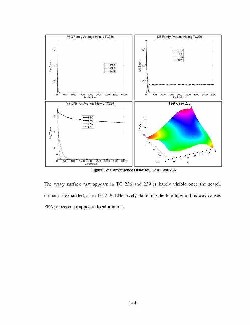
144
Figure 72: Convergence Histories, Test Case 236
The wavy surface that appears in TC 236 and 239 is barely visible once the search
domain is expanded, as in TC 238. Effectively flattening the topology in this way causes
FFA to become trapped in local minima.
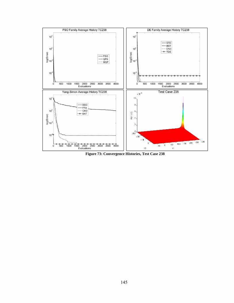
145
Figure 73: Convergence Histories, Test Case 238
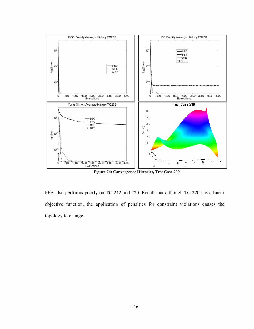
146
Figure 74: Convergence Histories, Test Case 239
FFA also performs poorly on TC 242 and 220. Recall that although TC 220 has a linear
objective function, the application of penalties for constraint violations causes the
topology to change.
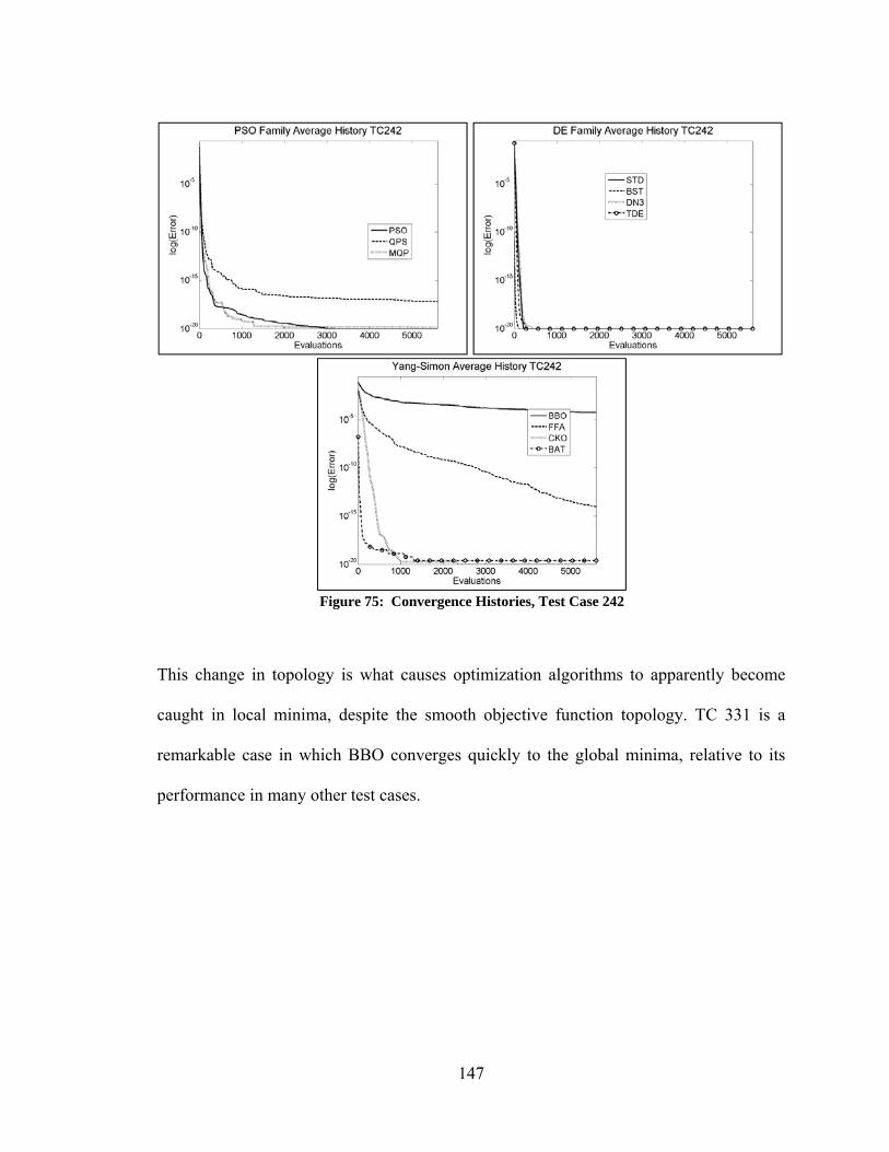
147
Figure 75: Convergence Histories, Test Case 242
This change in topology is what causes optimization algorithms to apparently become
caught in local minima, despite the smooth objective function topology. TC 331 is a
remarkable case in which BBO converges quickly to the global minima, relative to its
performance in many other test cases.
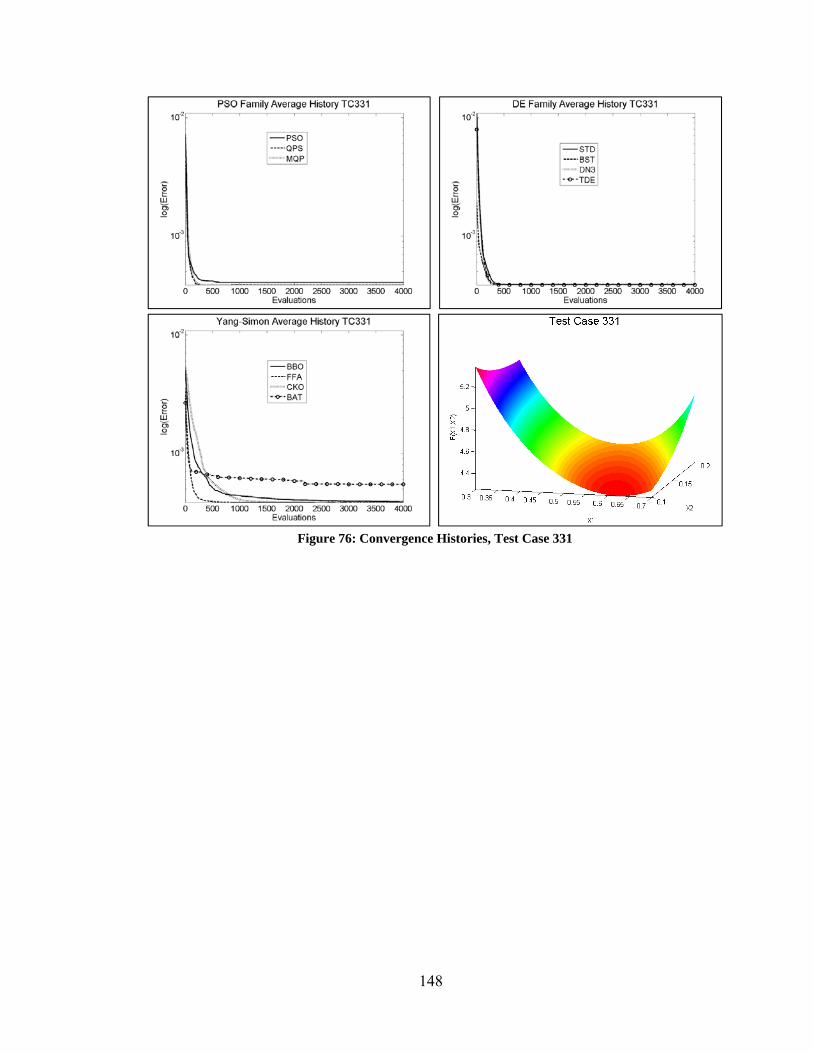
148
Figure 76: Convergence Histories, Test Case 331
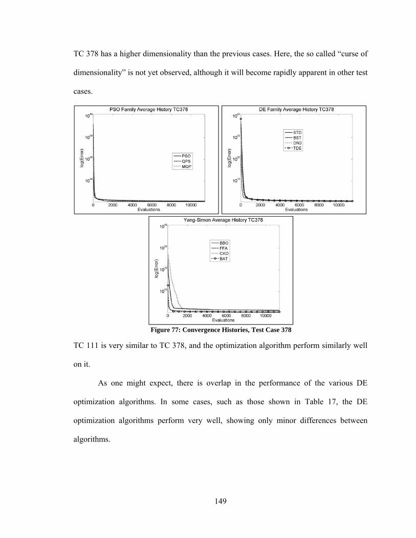
149
TC 378 has a higher dimensionality than the previous cases. Here, the so called “curse of
dimensionality” is not yet observed, although it will become rapidly apparent in other test
cases.
Figure 77: Convergence Histories, Test Case 378
TC 111 is very similar to TC 378, and the optimization algorithm perform similarly well
on it.
As one might expect, there is overlap in the performance of the various DE
optimization algorithms. In some cases, such as those shown in Table 17, the DE
optimization algorithms perform very well, showing only minor differences between
algorithms.
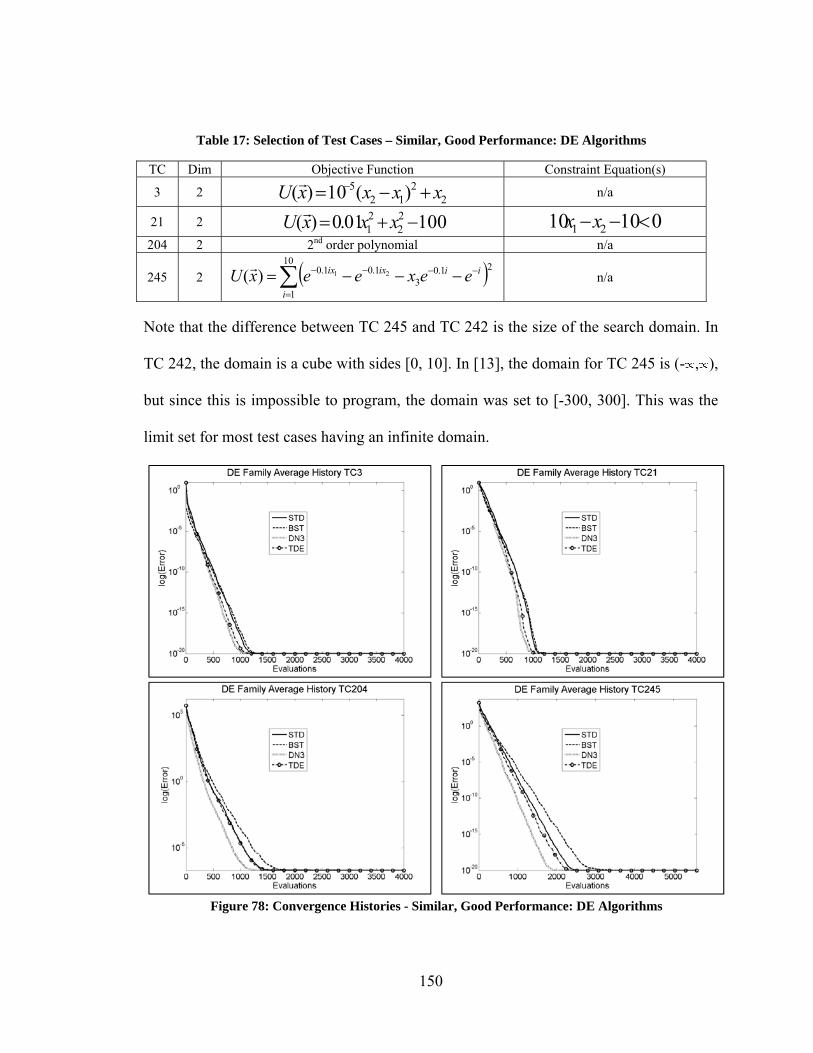
150
Table 17: Selection of Test Cases – Similar, Good Performance: DE Algorithms
TC Dim Objective Function Constraint Equation(s)
3 2 2
212
5 )(10)( xxxxU n/a
21 2 10001.0)( 22
21 xxxU
01010 21 xx
204 2 2nd order polynomial n/a
245 2
10
1
21.03
1.01.0 21)(i
iiixix eexeexU
n/a
Note that the difference between TC 245 and TC 242 is the size of the search domain. In
TC 242, the domain is a cube with sides [0, 10]. In [13], the domain for TC 245 is (- , ),
but since this is impossible to program, the domain was set to [-300, 300]. This was the
limit set for most test cases having an infinite domain.
Figure 78: Convergence Histories - Similar, Good Performance: DE Algorithms
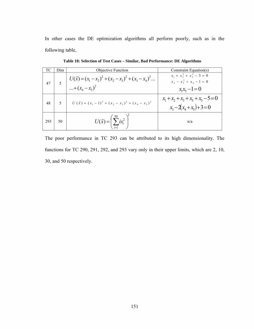
151
In other cases the DE optimization algorithms all perform poorly, such as in the
following table,
Table 18: Selection of Test Cases – Similar, Bad Performance: DE Algorithms
TC Dim Objective Function Constraint Equation(s)
47 5 2
54
243
232
221
)(...
...)()()()(
xx
xxxxxxxU
0323
221 xxx
014232 xxx
0151 xx
48 5 254
232
21 )()()1()( xxxxxxU
0555321 xxxxx
032 543 xxx
293 50
250
1
2)(
iiixxU
n/a
The poor performance in TC 293 can be attributed to its high dimensionality. The
functions for TC 290, 291, 292, and 293 vary only in their upper limits, which are 2, 10,
30, and 50 respectively.
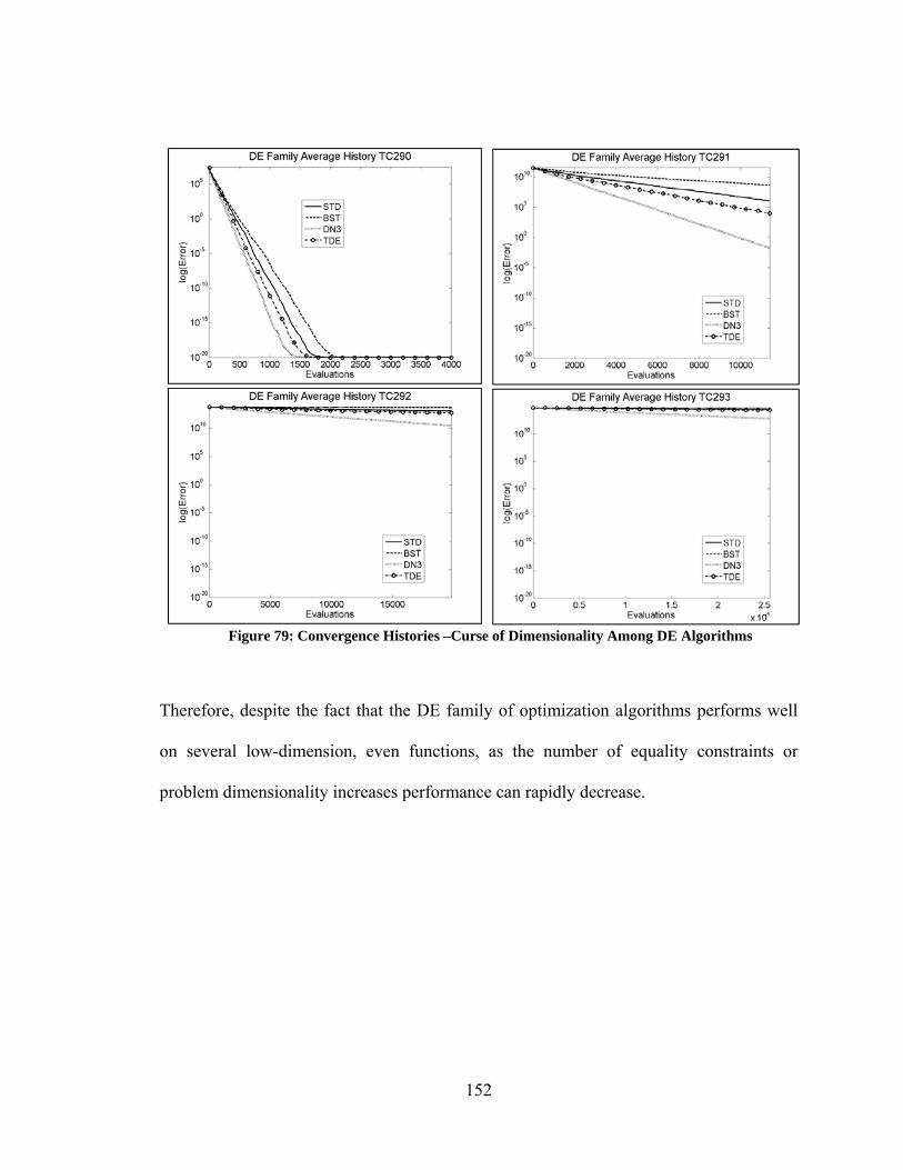
152
Figure 79: Convergence Histories –Curse of Dimensionality Among DE Algorithms
Therefore, despite the fact that the DE family of optimization algorithms performs well
on several low-dimension, even functions, as the number of equality constraints or
problem dimensionality increases performance can rapidly decrease.
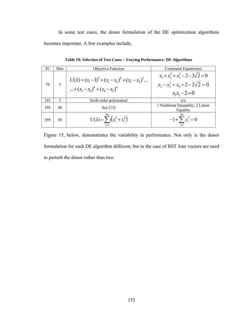
153
In some test cases, the donor formulation of the DE optimization algorithms
becomes important. A few examples include,
Table 19: Selection of Test Cases – Varying Performance: DE Algorithms
TC Dim Objective Function Constraint Equation(s)
79 5 4
544
43
232
221
21
)()(...
...)()()1()(
xxxx
xxxxxxU
023223
221 xxx
02224232 xxx
0251 xx
241 3 Sixth order polynomial n/a
393 48 See [13] 1 Nonlinear Inequality, 2 Linear
Equality
395 50
50
1
42)(i
ii xxixU
0150
1
2 i
ix
Figure 15, below, demonstrates the variability in performance. Not only is the donor
formulation for each DE algorithm different, but in the case of BST four vectors are used
to perturb the donor rather than two.
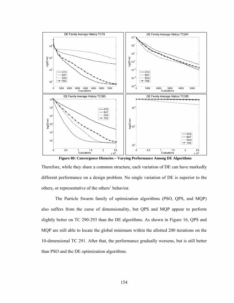
154
Figure 80: Convergence Histories – Varying Performance Among DE Algorithms
Therefore, while they share a common structure, each variation of DE can have markedly
different performance on a design problem. No single variation of DE is superior to the
others, or representative of the others’ behavior.
The Particle Swarm family of optimization algorithms (PSO, QPS, and MQP)
also suffers from the curse of dimensionality, but QPS and MQP appear to perform
slightly better on TC 290-293 than the DE algorithms. As shown in Figure 16, QPS and
MQP are still able to locate the global minimum within the allotted 200 iterations on the
10-dimensional TC 291. After that, the performance gradually worsens, but is still better
than PSO and the DE optimization algorithms.
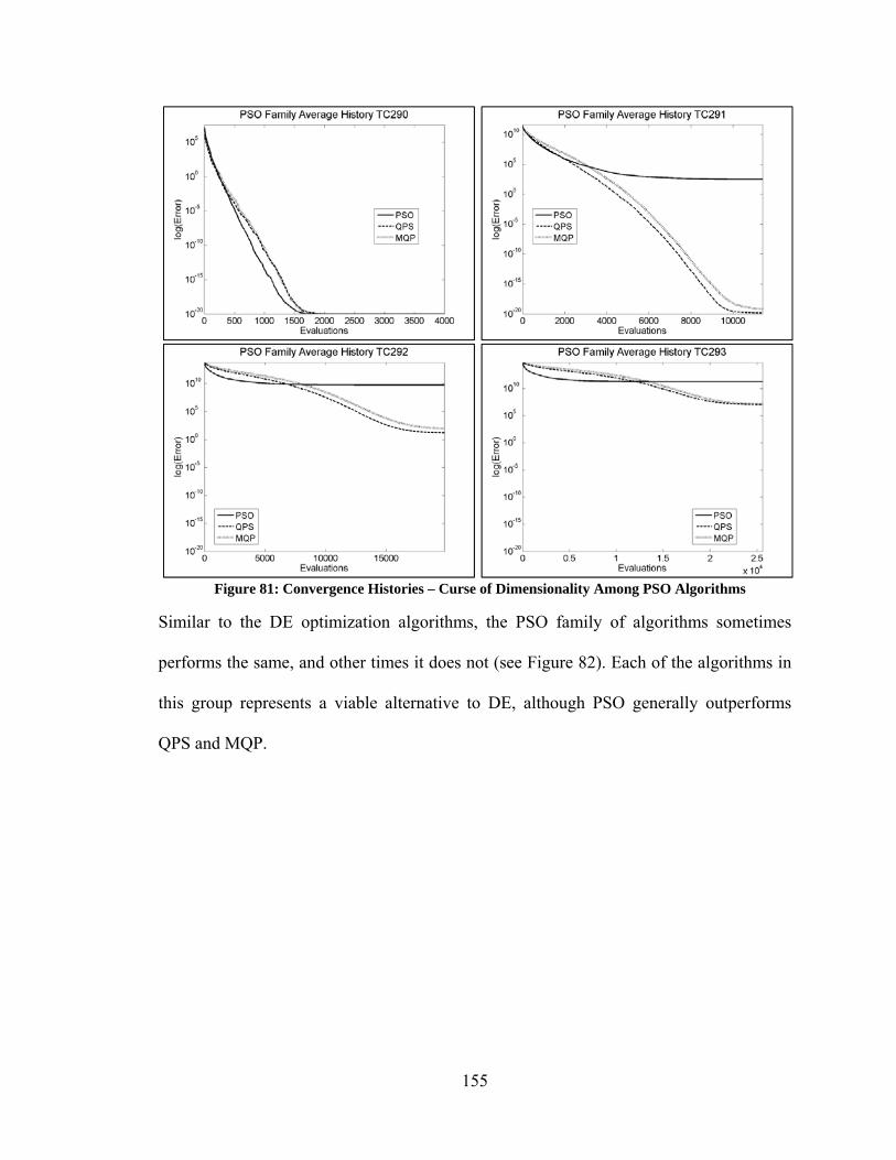
155
Figure 81: Convergence Histories – Curse of Dimensionality Among PSO Algorithms
Similar to the DE optimization algorithms, the PSO family of algorithms sometimes
performs the same, and other times it does not (see Figure 82). Each of the algorithms in
this group represents a viable alternative to DE, although PSO generally outperforms
QPS and MQP.
156
Figure 82: Convergence Histories – Varying Performance of PSO Algorithms
TC 5, 9, and 110 are given in Table 20, below. From this it is clear that PSO, QPS, and
MQP are capable of handling highly nonlinear problems, although problem
dimensionality is still an issue.
Table 20: Selection of Test Cases – Varying Performance Among DE OAs
TC Dim Objective Function Constraint Equation(s)
5 2 15.25.1)()sin()( 112
2121 xxxxxxxU
n/a
9 2 )16/cos()12/sin()( 21 xxxU
034 21 xx
110 10 2.010
1
10
1
22 )10ln()2ln()(
ii
iii xxxxU
n/a
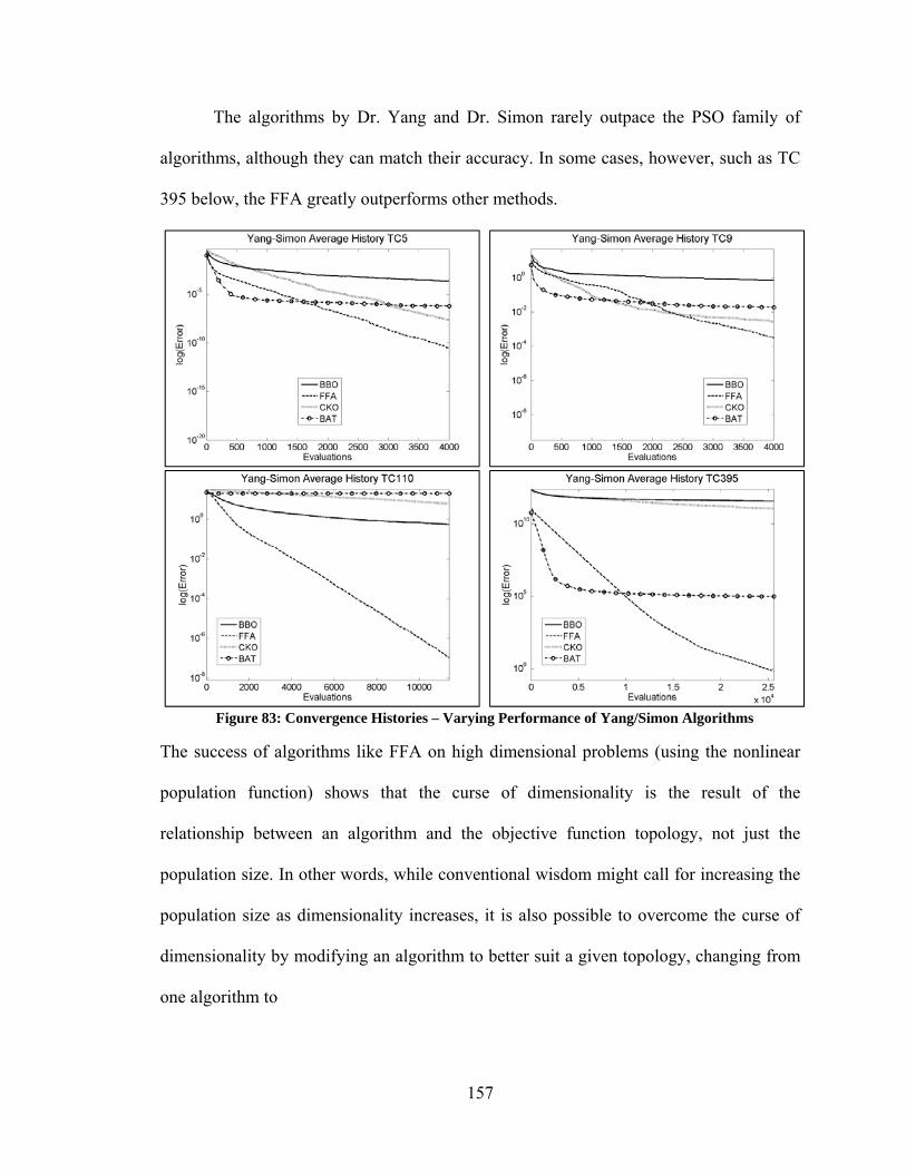
157
The algorithms by Dr. Yang and Dr. Simon rarely outpace the PSO family of
algorithms, although they can match their accuracy. In some cases, however, such as TC
395 below, the FFA greatly outperforms other methods.
Figure 83: Convergence Histories – Varying Performance of Yang/Simon Algorithms
The success of algorithms like FFA on high dimensional problems (using the nonlinear
population function) shows that the curse of dimensionality is the result of the
relationship between an algorithm and the objective function topology, not just the
population size. In other words, while conventional wisdom might call for increasing the
population size as dimensionality increases, it is also possible to overcome the curse of
dimensionality by modifying an algorithm to better suit a given topology, changing from
one algorithm to
158
another, or creating an algorithm capable of adapting on its own. Simply increasing the
population size in hopes of obtaining better results is a merely a brute-force approach.
A.3. Comparison of Modified Optimization Algorithms
The modifications to DE and PSO discussed in [67] and [68] greatly enhance each
algorithm’s performance. Figure 87, below, compares the relative performance of all
modified optimization algorithms, and their standard counterparts. The single greatest
improvement in performance can be seen in the difference between BST and BST-SPC,
as well as BST and BST-R to a lesser degree. The randomization of parameters
dramatically improves the performance of BST because it allows for a wider range of
perturbations to the global best vector. It also improves the performance of STD but
appears to decrease the performance of DN3 as well as TDE.
This apparent decrease, however, is misleading. In fact, it is more appropriate to say that
randomizing the parameters of DN3 as done here shifts the class of functions for which it
Figure 84: Best Performance of Unmodified vs Modified Optimization Algorithms

159
is well suited from one type to another. Consider, for example, the 50-dimensional
problems, TC 293 and 395, as well as the 100-dimensional problems, TC 299, and 302.
Figure 85: Convergence Histories – Modified DN3
In each of the above cases, the algorithm’s accuracy (and speed) is improved by several
orders of magnitude. Therefore, there is a tradeoff between improvement in some
problems and worsening in others. It should be noted that modified DN3’s performance
also improves in the 100-dimensional TC 305, but by less than one order of magnitude.
Therefore, randomization may not lead to performance improvements in all higher
dimension problems.
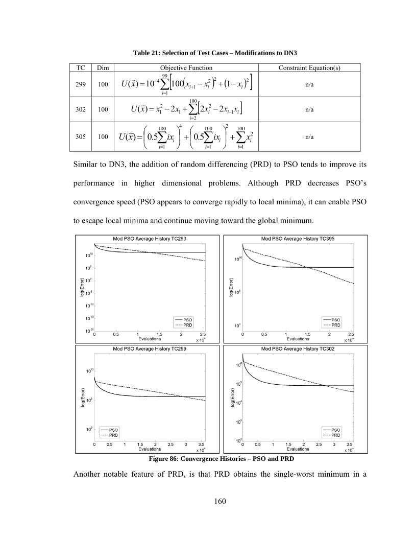
160
Table 21: Selection of Test Cases – Modifications to DN3
TC Dim Objective Function Constraint Equation(s)
299 100
99
1
2221
4 110010)(i
iii xxxxU
n/a
302 100
100
21
21
21 222)(
iiii xxxxxxU
n/a
305 100
100
1
2
2100
1
4100
1
5.05.0)(i
ii
ii
i xixixxU
n/a
Similar to DN3, the addition of random differencing (PRD) to PSO tends to improve its
performance in higher dimensional problems. Although PRD decreases PSO’s
convergence speed (PSO appears to converge rapidly to local minima), it can enable PSO
to escape local minima and continue moving toward the global minimum.
Figure 86: Convergence Histories – PSO and PRD
Another notable feature of PRD, is that PRD obtains the single-worst minimum in a
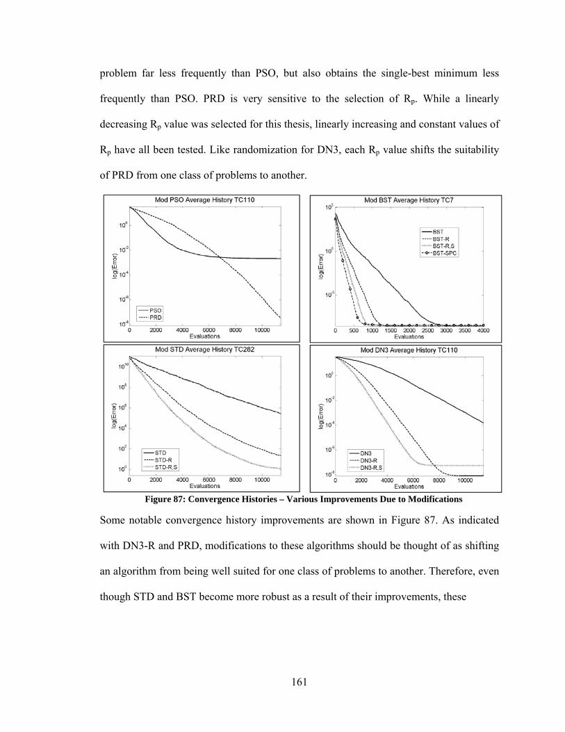
161
problem far less frequently than PSO, but also obtains the single-best minimum less
frequently than PSO. PRD is very sensitive to the selection of Rp. While a linearly
decreasing Rp value was selected for this thesis, linearly increasing and constant values of
Rp have all been tested. Like randomization for DN3, each Rp value shifts the suitability
of PRD from one class of problems to another.
Figure 87: Convergence Histories – Various Improvements Due to Modifications
Some notable convergence history improvements are shown in Figure 87. As indicated
with DN3-R and PRD, modifications to these algorithms should be thought of as shifting
an algorithm from being well suited for one class of problems to another. Therefore, even
though STD and BST become more robust as a result of their improvements, these
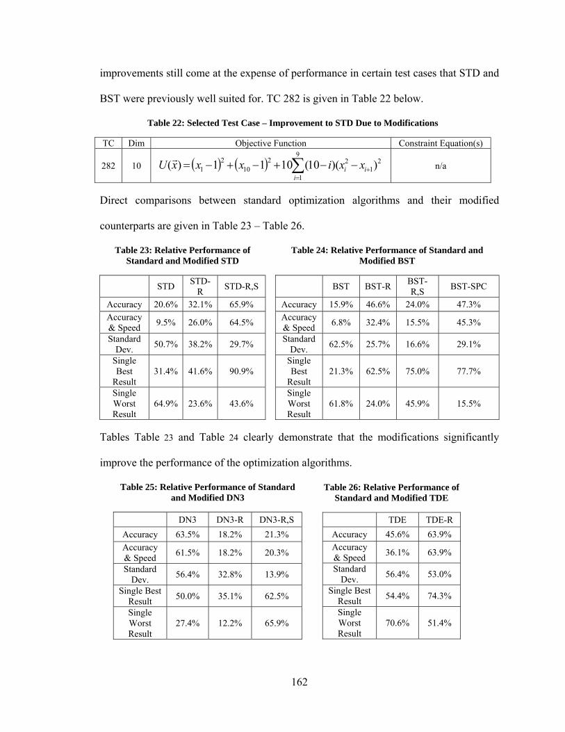
162
improvements still come at the expense of performance in certain test cases that STD and
BST were previously well suited for. TC 282 is given in Table 22 below.
Table 22: Selected Test Case – Improvement to STD Due to Modifications
TC Dim Objective Function Constraint Equation(s)
282 10
9
1
21
2210
21 ))(10(1011)(
iii xxixxxU
n/a
Direct comparisons between standard optimization algorithms and their modified
counterparts are given in Table 23 – Table 26.
Table 23: Relative Performance of Standard and Modified STD
STD
STD-R
STD-R,S
Accuracy 20.6% 32.1% 65.9% Accuracy & Speed
9.5% 26.0% 64.5%
Standard Dev.
50.7% 38.2% 29.7%
Single Best
Result 31.4% 41.6% 90.9%
Single Worst Result
64.9% 23.6% 43.6%
Table 24: Relative Performance of Standard and Modified BST
BST BST-R
BST-R,S
BST-SPC
Accuracy 15.9% 46.6% 24.0% 47.3% Accuracy & Speed
6.8% 32.4% 15.5% 45.3%
Standard Dev.
62.5% 25.7% 16.6% 29.1%
Single Best
Result 21.3% 62.5% 75.0% 77.7%
Single Worst Result
61.8% 24.0% 45.9% 15.5%
Tables Table 23 and Table 24 clearly demonstrate that the modifications significantly
improve the performance of the optimization algorithms.
Table 25: Relative Performance of Standard and Modified DN3
DN3 DN3-R DN3-R,S
Accuracy 63.5% 18.2% 21.3%
Accuracy & Speed
61.5% 18.2% 20.3%
Standard Dev.
56.4% 32.8% 13.9%
Single Best Result
50.0% 35.1% 62.5%
Single Worst Result
27.4% 12.2% 65.9%
Table 26: Relative Performance of Standard and Modified TDE
TDE TDE-R
Accuracy 45.6% 63.9%
Accuracy & Speed
36.1% 63.9%
Standard Dev.
56.4% 53.0%
Single Best Result
54.4% 74.3%
Single Worst Result
70.6% 51.4%
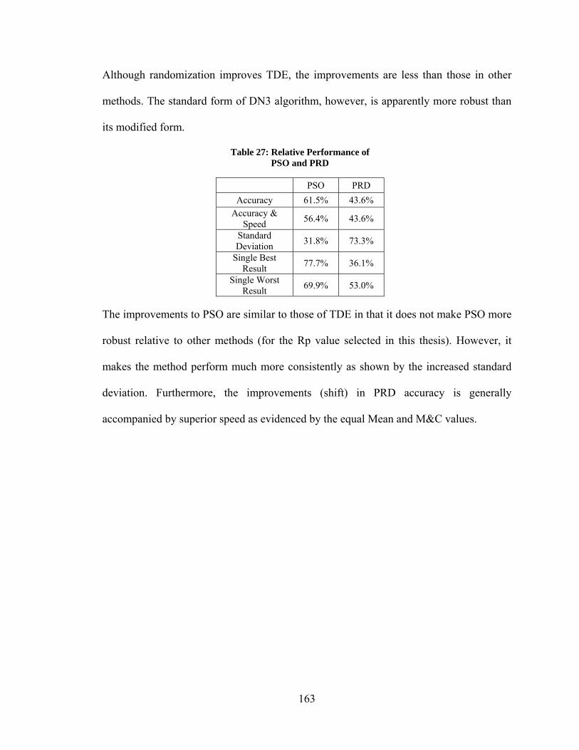
163
Although randomization improves TDE, the improvements are less than those in other
methods. The standard form of DN3 algorithm, however, is apparently more robust than
its modified form.
Table 27: Relative Performance of PSO and PRD
PSO PRD
Accuracy 61.5% 43.6% Accuracy &
Speed 56.4% 43.6%
Standard Deviation
31.8% 73.3%
Single Best Result
77.7% 36.1%
Single Worst Result
69.9% 53.0%
The improvements to PSO are similar to those of TDE in that it does not make PSO more
robust relative to other methods (for the Rp value selected in this thesis). However, it
makes the method perform much more consistently as shown by the increased standard
deviation. Furthermore, the improvements (shift) in PRD accuracy is generally
accompanied by superior speed as evidenced by the equal Mean and M&C values.