�����������������

Citation: Uray, E.; Carbas, S.;

Geem, Z.W.; Kim, S. Parameters

Optimization of Taguchi Method

Integrated Hybrid Harmony Search

Algorithm for Engineering Design

Problems. Mathematics 2022, 10, 327.

https://doi.org/10.3390/

math10030327

Academic Editor: Alfredo Milani

Received: 4 December 2021

Accepted: 14 January 2022

Published: 21 January 2022

Publisher’s Note: MDPI stays neutral

with regard to jurisdictional claims in

published maps and institutional affil-

iations.

Copyright: © 2022 by the authors.

Licensee MDPI, Basel, Switzerland.

This article is an open access article

distributed under the terms and

conditions of the Creative Commons

Attribution (CC BY) license (https://

creativecommons.org/licenses/by/

4.0/).

mathematics

Article

Parameters Optimization of Taguchi Method Integrated HybridHarmony Search Algorithm for Engineering Design ProblemsEsra Uray 1,* , Serdar Carbas 1,2 , Zong Woo Geem 3,* and Sanghun Kim 4

1 Department of Civil Engineering, KTO Karatay University, Konya 42020, Turkey; scarbas@kmu.edu.tr2 Department of Civil Engineering, Karamanoglu Mehmetbey University, Karaman 70200, Turkey3 College of IT Convergence, Gachon University, Seongnam 13120, Korea4 Department of Civil and Environmental Engineering, Temple University, Philadelphia, PA 19122, USA;

sanghun.kim@temple.edu* Correspondence: esra.uray@karatay.edu.tr (E.U.); geem@gachon.ac.kr (Z.W.G.)

Abstract: Performance of convergence to the optimum value is not completely a known process due tocharacteristics of the considered design problem and floating values of optimization algorithm controlparameters. However, increasing robustness and effectiveness of an optimization algorithm maybe possible statistically by estimating proper algorithm parameters values. Not only the algorithmwhich utilizes these estimated-proper algorithm parameter values may enable to find the best fitnessin a shorter time, but also it may supply the optimum searching process with a pragmatical manner.This study focuses on the statistical investigation of the optimum values for the control parameters ofthe harmony search algorithm and their effects on the best solution. For this purpose, the Taguchimethod integrated hybrid harmony search algorithm has been presented as an alternative method foroptimization analyses instead of sensitivity analyses which are generally used for the investigationof the proper algorithm parameters. The harmony memory size, the harmony memory consideringrate, the pitch adjustment rate, the maximum iteration number, and the independent run numberof entire iterations have been debated as the algorithm control parameters of the harmony searchalgorithm. To observe the effects of design problem characteristics on control parameters, the newhybrid method has been applied to different engineering optimization problems including severalengineering-optimization examples and a real-size engineering optimization design. End of extensiveoptimization and statistical analyses to achieve optimum values of control parameters providing rapidconvergence to optimum fitness value and handling constraints have been estimated with reasonablerelative errors. Employing the Taguchi method integrated hybrid harmony search algorithm inparameter optimization has been demonstrated as it is a reliable and efficient manner to obtain theoptimum results with fewer numbers of run and iteration.

Keywords: hybrid harmony search algorithm; Taguchi method; algorithm control parameteroptimization; engineering design problems; reinforced cantilever retaining wall design

1. Introduction

The well-functioning optimum designs, which aim to reach stable and economic orproductive mechanisms in engineering regulation, are based on mathematical theorems andapproaches. While optimization methods were applied by Newton, Lagrange, Cauchyeski,and so on for smaller-sized problems in ancient times, today produce the solutions withimproved or hybrid versions of the optimization algorithms for large-size complex engi-neering designs. In this conjuncture, metaheuristic optimization algorithms that enablethem to achieve reasonable solutions in a shorter time have been commonly employed incomplicated engineering designs, since environmental and global phenomena due to devel-oping technology and increasing population have been raised in the last two decades [1].Although each of them adopts a different process and texture within itself, many effective

Mathematics 2022, 10, 327. https://doi.org/10.3390/math10030327 https://www.mdpi.com/journal/mathematics

Mathematics 2022, 10, 327 2 of 36

and robust metaheuristic optimization algorithms hitherto have been developed dealingwith better optimization processes than previous ones.

Metaheuristic optimization methods are the algorithms that generate solutions to large-scale design optimization problems which are inspired by natural events such as swarms(bird, fish, etc.), physics, evolution, or uniqueness [2]. Major metaheuristic optimizationalgorithms improved by mimicking the characteristics and feeling of swarms that try tosurvive and meet some needs such as nutrition, defense, and migration in nature are the antcolony optimization (ACO) [3], the particle swarm optimization (PSO) [4], the artificial beecolony algorithm (ABC) [5], and the whale optimization algorithm (WOA) [6]. While thegravitational search algorithm (GSA) [7] and big bang-big crunch algorithm (BB-BC) [8] areevaluated as based on physics, optimization methods such as the cuckoo search algorithm(CSA) [9], the firefly algorithm (FA) [10], and the bat algorithm (BA) [11] are inspiredby animals’ nature. The differential evolution (DE) [12] and the biogeography-basedoptimization (BBO) [13] are based on evolution concepts such as the genetic algorithm(GA) [14] and the simulated annealing algorithm (SA) [15].

As different from the other algorithms the harmony search algorithm (HSA) presentedby Geem et al. [16] is based on the music and mimics the process of finding the bestharmony of the notes performed by musicians’ intuition. The HSA, which is a powerfuland effective optimization method because of its simple algorithm scheme, gives fastresults, has an easy-to-apply algorithm, has been exceedingly employed by the researchersfor design optimization analysis. Thanks to the implementation of the algorithm to designoptimization problems effectively and convergence achievement of optimum solutions,hybrid and improved versions of HSA have been employed in the several fields of civil,electrical, industrial, software, mechanical engineering, scheduling, clustering, networking,image processing, and so on [2].

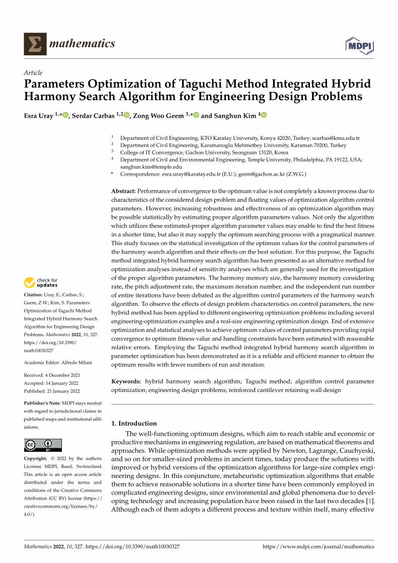
To boost the convergence performance of metaheuristic algorithms and their capacityto produce solutions with fewer iterations, improved versions [17,18] and hybrid versionsof algorithms [19–21] combined each other have been proposed by researchers. In Figure 1a,the number and the percentage of conducted studies considering hybrid optimizationalgorithms in literature [22] are demonstrated as a comparison graph by years. It is seenthat the usage of hybrid metaheuristic optimization algorithms has increased considerablyin the last two decades. The distribution of hybrid optimization studies for the differentfields has been examined by utilizing the Web of Science database and obtained resultsare given in Figure 1b [22]. Although other studies except for the fields given in the figurecorrespond to 78% out of whole fields, it is obvious that the hybrid optimization algorithmstudies have a considerable extent of usage in, especially multidisciplinary engineeringstudies. Hybrid HSA studies included setting algorithm parameters and hybridization ofHSA with other metaheuristic algorithms as well as collocation of the artificial intelligencealgorithms, which are depicted in Figure 1c as the result of a comprehensive literaturesurvey [23]. According to the graph, harmony search hybrid optimization studies carriedout in the last five years being 72% out of all studies published between 2008 and 2021shows that hybrid studies of HSA substantially have been preferred by researchers. Resultsgiven in Figure 1 belong to all types of studies such as research articles, proceeding papers,early access, book chapters, review articles, and so on.

Mathematics 2022, 10, 327 3 of 36

Mathematics 2022, 10, x FOR PEER REVIEW 3 of 37

optimum with fewer computational attempts. To investigate reasonable factors, design comprehensive sensitivity analyses have been performed considering different values of algorithm control parameters [24]. Although sensitivity analyses are employed as a path for the researcher to converge to the optimum result, it takes time because it follows a trial-and-error method. In addition, it can’t guarantee the appropriate value of a parame-ter when it is closest to the optimum solution. In most of the studies using metaheuristic algorithms, the values of the algorithm parameters are chosen by referring to the studies in the literature. As it may vary depending on discrete-continuous design variables, con-straint-unconstrained cases, and the size of the current design problem with the numbers of design variables and constraints and so on in the search for the appropriate value of the metaheuristic algorithm parameter, it would be a better manner to find algorithm param-eter values considering the current handled optimization problem. According to a study presented by Uray et al. [25] which investigated optimum values of the scatter search al-gorithm parameters by the Taguchi method, it has been seen that it is possible to estimate the statistically appropriate values of the algorithm parameters according to a selected objective.

(a)

(b)

(c)

Figure 1. Web of Science citation report studies in literature following: (a) Change between pub-lished years of hybrid optimization studies and numbers with percentages; (b) Distribution of hy-brid optimization studies according to fields; (c) Change between published years of hybrid and based on harmony search optimization studies and numbers.

One of the statistical experimental design methods commonly utilized to investigate the parameter effect on the quality in the manufacturing or design process of goods is the

Figure 1. Web of Science citation report studies in literature following: (a) Change between publishedyears of hybrid optimization studies and numbers with percentages; (b) Distribution of hybridoptimization studies according to fields; (c) Change between published years of hybrid and based onharmony search optimization studies and numbers.

In the literature, the number of optimization studies carried out utilizing metaheuristicalgorithms and their improved or hybrid versions so far is mainly due to the researcher’seffort to reach better convergence to the optimum solution. The literature survey has beendemonstrated the popularity of these algorithms in applying engineering design problemseven for real-size complex ones. While the possibility of finding new solutions has increasedby adding some algorithm parameters to the optimum search process, formed mathematicalexpressions combining two or more optimization algorithms effectively enable to reachoptimum results. Even though new or hybrid versions of metaheuristic algorithms havebeen suggested in this manner, investigating the reasonable values of the current algorithmparameters is an important issue for convergence to the optimum with fewer computationalattempts. To investigate reasonable factors, design comprehensive sensitivity analyseshave been performed considering different values of algorithm control parameters [24].Although sensitivity analyses are employed as a path for the researcher to converge to theoptimum result, it takes time because it follows a trial-and-error method. In addition, itcan’t guarantee the appropriate value of a parameter when it is closest to the optimumsolution. In most of the studies using metaheuristic algorithms, the values of the algorithmparameters are chosen by referring to the studies in the literature. As it may vary dependingon discrete-continuous design variables, constraint-unconstrained cases, and the size ofthe current design problem with the numbers of design variables and constraints andso on in the search for the appropriate value of the metaheuristic algorithm parameter,

Mathematics 2022, 10, 327 4 of 36

it would be a better manner to find algorithm parameter values considering the currenthandled optimization problem. According to a study presented by Uray et al. [25] whichinvestigated optimum values of the scatter search algorithm parameters by the Taguchimethod, it has been seen that it is possible to estimate the statistically appropriate values ofthe algorithm parameters according to a selected objective.

One of the statistical experimental design methods commonly utilized to investigatethe parameter effect on the quality in the manufacturing or design process of goods is theTaguchi method [26,27]. Thanks to this successful and robust design method, it can esti-mate the optimum value of considering effective parameters according to specific responsevalues depending on desired aim. Studies for Taguchi method hybridization of the meta-heuristic optimization algorithms such as the simulated annealing (SA) algorithm [28], thegenetic algorithm (GA) [29,30], and particle swarm optimization (PSO) [31] are instancesto overcome problems encountered in their field and obtained better results. In the study,which is conducted shape optimization design by employing Taguchi method hybrid ver-sion with the HSA, more optimum design variable values have been acquired regardless ofthe investigating for optimum values of the HSA parameters [32]. In the study which usedstatistical mathematical models improved by considering the Taguchi method employed asobjective function and design constraints, the optimum design of the cantilever retainingwall has been investigated via HSA [33]. According to the extensive research results in theliterature, no study has been found in which the optimum values for the number of runsand the number of maximum iterations with optimum HSA control parameters have beeninvestigated based on the Taguchi method with different engineering problems.

Thus, in this study, some of the considered complex benchmark engineering designoptimization problems and a real-size engineering design optimization problem have beenemployed to examine HSA parametric effect and to investigate the optimum values ofalgorithmic parameters. In this scope, statistical and optimization analyses to be presentedin this paper have been conducted as follows:

• The effect of variable run values on finding the optimum solution by employingdifferent complex benchmark engineering design optimization problems and a real-size engineering design problem, frequently considered in optimization analyzes inthe literature has been investigated;

• Taguchi method integrated hybrid harmony search algorithm (TIHHSA) has beengenerated based on the HSA and Taguchi method, namely the proposed hybridizationcan be defined as initial optimization for optimum algorithm parameter values of HSA;

• The effect of HSA parameters on the objective function and the optimum numberof runs and maximum iterations with optimum HSA control parameters have beenexamined for different engineering optimization design problems utilizing TIHHSA;

• Whether the variation of the optimum values of the HSA parameters depending onthe nature of the engineering design optimization problem has been evaluated;

• According to accomplished optimum results for engineering design optimizationproblems, the robustness, and the benefits of TIHHSA presented a new method havebeen interpreted and evaluated with previously reported studies in the literature.

2. Materials and Methods2.1. Complex Benchmark Engineering Design Optimization Problems

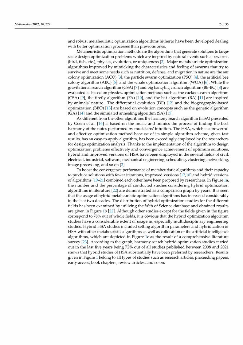
In this section, the welded beam design (WBD), the pressure vessel design (PVD),the gear train design (GTD), and the speed reducer design (SRD) engineering designoptimization problems demonstrated in Figure 2 have been presented with their designvariables, constraints, and objective functions.

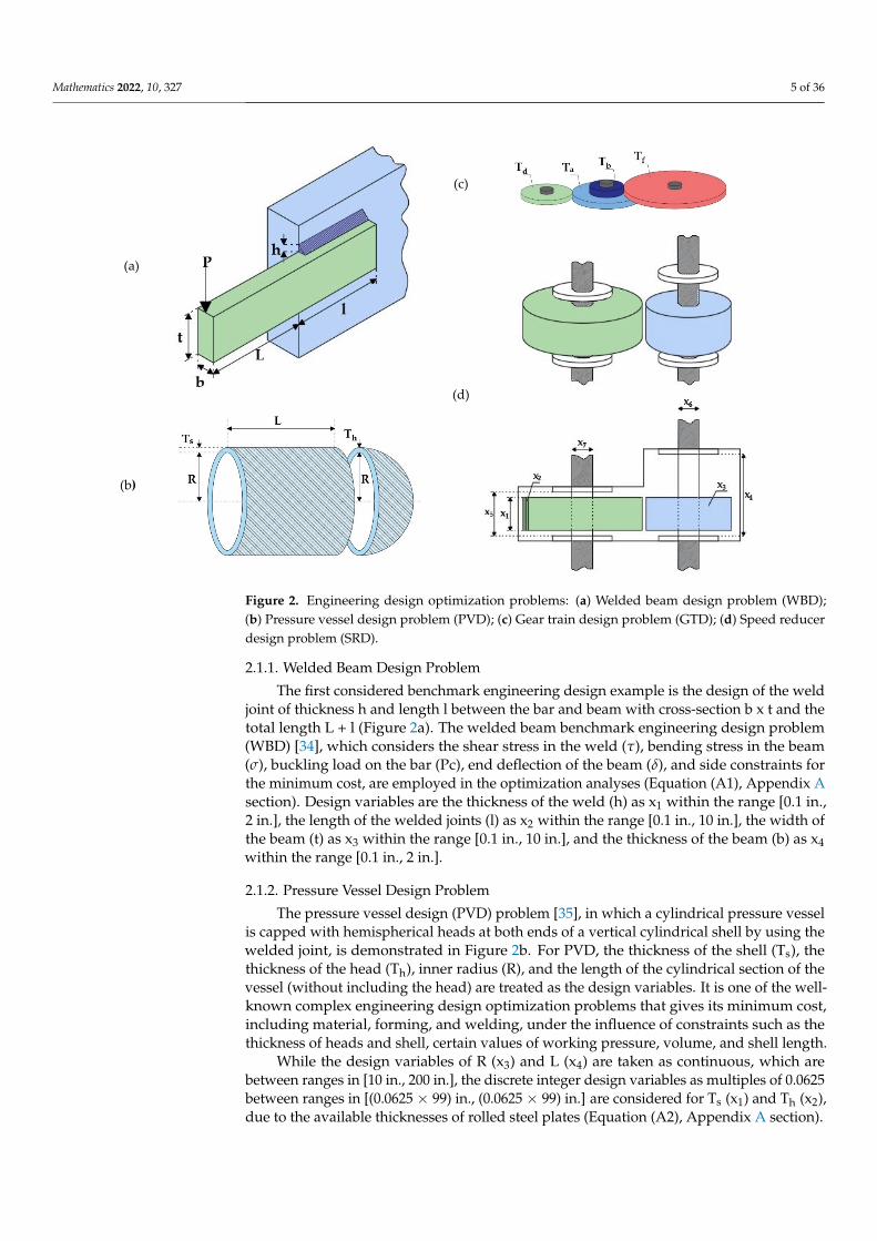
Mathematics 2022, 10, 327 5 of 36

Mathematics 2022, 10, x FOR PEER REVIEW 5 of 37

in., 2 in.], the length of the welded joints (l) as x2 within the range [0.1 in., 10 in.], the width of the beam (t) as x3 within the range [0.1 in., 10 in.], and the thickness of the beam (b) as x4 within the range [0.1 in., 2 in.].

(a)

(c)

(d)

(b)

Figure 2. Engineering design optimization problems: (a) Welded beam design problem (WBD); (b) Pressure vessel design problem (PVD); (c) Gear train design problem (GTD); (d) Speed reducer de-sign problem (SRD).

2.1.2. Pressure Vessel Design Problem The pressure vessel design (PVD) problem [35], in which a cylindrical pressure vessel

is capped with hemispherical heads at both ends of a vertical cylindrical shell by using the welded joint, is demonstrated in Figure 2b. For PVD, the thickness of the shell (Ts), the thickness of the head (Th), inner radius (R), and the length of the cylindrical section of the vessel (without including the head) are treated as the design variables. It is one of the well-known complex engineering design optimization problems that gives its minimum cost, including material, forming, and welding, under the influence of constraints such as the thickness of heads and shell, certain values of working pressure, volume, and shell length.

While the design variables of R (x3) and L (x4) are taken as continuous, which are between ranges in [10 in., 200 in.], the discrete integer design variables as multiples of 0.0625 between ranges in [(0.0625 × 99) in., (0.0625 × 99) in.] are considered for Ts (x1) and Th (x2), due to the available thicknesses of rolled steel plates (Equation (A2), Appendix A section).

2.1.3. Gear Train Design Sandgren [35] introduced the gear train design (GTD) with discrete and integer de-

sign variables, then it has been treated as an engineering design optimization problem to research the numbers of teeth on each gear with the desired gear ratio. The output shaft’s angular velocity ratio to the input shaft’s angular velocity should be close to 1/6.931 for

Figure 2. Engineering design optimization problems: (a) Welded beam design problem (WBD);(b) Pressure vessel design problem (PVD); (c) Gear train design problem (GTD); (d) Speed reducerdesign problem (SRD).

2.1.1. Welded Beam Design Problem

The first considered benchmark engineering design example is the design of the weldjoint of thickness h and length l between the bar and beam with cross-section b x t and thetotal length L + l (Figure 2a). The welded beam benchmark engineering design problem(WBD) [34], which considers the shear stress in the weld (τ), bending stress in the beam(σ), buckling load on the bar (Pc), end deflection of the beam (δ), and side constraints forthe minimum cost, are employed in the optimization analyses (Equation (A1), Appendix Asection). Design variables are the thickness of the weld (h) as x1 within the range [0.1 in.,2 in.], the length of the welded joints (l) as x2 within the range [0.1 in., 10 in.], the width ofthe beam (t) as x3 within the range [0.1 in., 10 in.], and the thickness of the beam (b) as x4within the range [0.1 in., 2 in.].

2.1.2. Pressure Vessel Design Problem

The pressure vessel design (PVD) problem [35], in which a cylindrical pressure vesselis capped with hemispherical heads at both ends of a vertical cylindrical shell by using thewelded joint, is demonstrated in Figure 2b. For PVD, the thickness of the shell (Ts), thethickness of the head (Th), inner radius (R), and the length of the cylindrical section of thevessel (without including the head) are treated as the design variables. It is one of the well-known complex engineering design optimization problems that gives its minimum cost,including material, forming, and welding, under the influence of constraints such as thethickness of heads and shell, certain values of working pressure, volume, and shell length.

While the design variables of R (x3) and L (x4) are taken as continuous, which arebetween ranges in [10 in., 200 in.], the discrete integer design variables as multiples of 0.0625between ranges in [(0.0625 × 99) in., (0.0625 × 99) in.] are considered for Ts (x1) and Th (x2),due to the available thicknesses of rolled steel plates (Equation (A2), Appendix A section).

Mathematics 2022, 10, 327 6 of 36

2.1.3. Gear Train Design

Sandgren [35] introduced the gear train design (GTD) with discrete and integer designvariables, then it has been treated as an engineering design optimization problem to researchthe numbers of teeth on each gear with the desired gear ratio. The output shaft’s angularvelocity ratio to the input shaft’s angular velocity should be close to 1/6.931 for the desiredgear ratio. In the GTD problem, each design variable corresponds to Ta (x1), Tb (x2), Td (x3),and Tf (x4), which takes a value between 12 and 60 as an integer due to considering thenumber of them (Figure 2c).

The objective function without constraints, which aims to minimize the differencebetween desired gear ratio and the current gear ratio, is given by Equation (A3) (Appendix Asection).

2.1.4. Speed Reducer Design

Speed reducer design (SRD), one of the complex benchmark engineering designoptimization problems, was first studied by Golinski [36]. The SRD problem satisfies elevenconstraints at the minimum gear box’s weight and is accepted as a benchmark for the newmetaheuristic optimization methods. The design consists of gears between the engine andpropeller working at its most efficient speed of rotating with seven design variables. Inthe design problem demonstrated in Figure 2d, face width, b (x1), teeth module, m (x2),number of pinion teeth (x3), shaft length 1 (x4), shaft length 2 (x5), shaft diameter 1 (x6),and shaft diameter 2 (x7) are considered as design variables.

Design variables of the design problem are determined following ranges, [2.6 cm, 3.6cm] is for x1, [0.7 cm, 0.8 cm] is for x2, [17 pieces, 28 pieces] is for x3, [7.3 cm, 8.3 cm] is for x4and x5, [2.9 cm, 3.9 cm] is for x6, and [5.0 cm, 5.5 cm] is for x7. Mathematical formulationsfor the objective function and the constraints include the limits on the bending stress of thegear teeth, surface stress, transverse deflections of shafts 1 and 2 due to transmitted force,and stresses in shafts 1 and 2 (Equation (A4), Appendix A section).

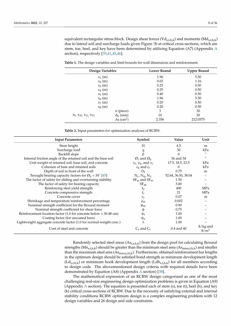
2.2. Real-Size Engineering Design Optimization Problem

In today’s world, where obtaining the most economical designs in a short time gainsimportance, metaheuristic optimization algorithms have become an alternative method.In this context, Afzal et al. [37] have reported that hundreds of retaining wall designoptimization studies for solving such real-life designs were conducted in the literature. Ingeotechnical engineering, the design of a cantilever retaining wall is a complex engineeringproblem used to provide stability against lateral soil loads that happen between twosoil levels. Furthermore, the trial-error method utilized in the traditional wall design ischallenging, and finding the safe design is time-consuming considering many iterationsdue to the existence of various soil and slope properties.

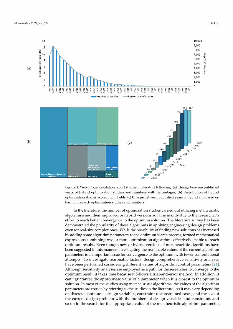
The reinforced concrete cantilever retaining wall design (RCRW) (Figure 3) has beenselected as a real-size engineering design optimization problem because of the abovemen-tioned cases. In investigating optimum RCRW designs, Building Code Requirements forStructural Concrete (ACI 318-05) and commentary (ACI 318R-05) [38] have been consid-ered as design provisions for stable and safe design. Arranged mathematical expressionsby investigating some of the optimum RCRW studies in the literature [39–43] have beenpresented in this section. In the design problem demonstrated in Figure 3a, base width (x1),toe extension, (x2), stem bottom width (x3), stem top width (x4), base thickness (x5), keydistance from toe (x6), key width (x7), key thickness (x8), vertical steel area in the stem perunit length of the wall (x9), horizontal steel area of the toe slab (x10), horizontal steel area ofthe heel slab (x11), and vertical steel area of the shear key per unit length of the wall (x12) areconsidered as design variables in the design optimization of an RCRW. The RCRW designstability conditions taken as design constraints in the optimization process are checkedaccording to acting loads on the wall demonstrated in Figure 3b for geotechnical externaland internal reinforced concrete stability conditions.

Mathematics 2022, 10, 327 7 of 36Mathematics 2022, 10, x FOR PEER REVIEW 7 of 37

(a) (b)

(c)

Figure 3. Reinforced concrete cantilever retaining wall design (RCRW): (a) Design variables; (b) Acting loads on retaining wall; (c) Design details.

By employing the limit bounds of the design variables tabulated in Table 1 the design space has been formed. Input parameters utilized for geotechnical and design as RCRW design problem are demonstrated in Table 2.

Table 1. The design variables and limit bounds for wall dimensions and reinforcement.

Design Variables Lower Bound Upper Bound x1 (m) 1.96 5.50 x2 (m) 0.65 1.16 x3 (m) 0.25 0.50 x4 (m) 0.25 0.50 x5 (m) 0.40 0.50 x6 (m) 1.96 5.50 x7 (m) 0.20 0.50 x8 (m) 0.20 0.50

x9, x10, x11, x12 n (piece) 3 30 db (mm) 10 30 As (cm2) 2.356 212.0575

Figure 3. Reinforced concrete cantilever retaining wall design (RCRW): (a) Design variables;(b) Acting loads on retaining wall; (c) Design details.

The steel areas (As) of x9, x10, x11, and x12 design variables have been determinedwith the number (n) and diameter (db) of the rebar. The steel areas for x9, x10, x11, and x12design variables have been determined by considering together the number and diameterof reinforcement for the stem, toe, heel, and key of the wall, respectively.

By employing the limit bounds of the design variables tabulated in Table 1 the designspace has been formed. Input parameters utilized for geotechnical and design as RCRWdesign problem are demonstrated in Table 2.

Mathematical formulations of sliding, overturning, and bearing capacity safety factorsdetailed given in Equation (A5) (Appendix A section) have been utilized to satisfy ofgeotechnical external stability of the wall [44].

In terms of providing internal reinforced concrete stability, the flexural strengths(Mns,t,h,k) resistance to design moments (Mds,t,h,k) have been examined for four criticalcross-sections; (i) the section linked stem to base slab, (ii) the initial section of the toeextension from the stem, (iii) initial section of heel extension from the stem, (iv) the sectionlinked the key to base slab (Figure 3c). In the same way, the design shear forces (Vds,t,h,k)should be safely fulfilled by nominal shear strength (Vns,t,h,k) at critical cross-sections ofthe wall. The nominal shear and flexural strengths for the critical cross-sections of the wallhave been computed via Equation (A6) (Appendix A section) [38]. In Equation (A6), b isthe width of the section (1000 mm), d is the height of the section, and a is the depth of the

Mathematics 2022, 10, 327 8 of 36

equivalent rectangular stress block. Design shear forces (Vds,t,h,k) and moments (Mds,t,h,k)due to lateral soil and surcharge loads given Figure 3b at critical cross-sections, which arestem, toe, heel, and key have been determined by utilizing Equation (A7) (Appendix Asection), respectively [39,41,45,46].

Table 1. The design variables and limit bounds for wall dimensions and reinforcement.

Design Variables Lower Bound Upper Bound

x1 (m) 1.96 5.50x2 (m) 0.65 1.16x3 (m) 0.25 0.50x4 (m) 0.25 0.50x5 (m) 0.40 0.50x6 (m) 1.96 5.50x7 (m) 0.20 0.50x8 (m) 0.20 0.50

x9, x10, x11, x12

n (piece) 3 30db (mm) 10 30As (cm2) 2.356 212.0575

Table 2. Input parameters for optimization analyses of RCRW.

Input Parameters Symbol Value Unit

Stem height H 4.5 mSurcharge load q 30 kPaBackfill slope β 0 ◦

Internal friction angle of the retained soil and the base soil Ør and Øb 36 and 34 ◦

Unit weight of retained soil, base soil, and concrete γr, γb, and γc 17.5, 18.5, 23.5 kPaCohesion of base and retained soils cb and cr 0 kPa

Depth of soil in front of the wall Df 0.75 mTerzaghi bearing capacity factors for Øb = 34◦ [45] Nc, Nq, Nγ 52.64, 36.50, 38.04 –

The factor of safety for sliding and overturning stability SFss and SFso 1.50 –The factor of safety for bearing capacity SFsb 3.00 –

Reinforcing steel yield strength fy 400 MPaConcrete compressive strength fc 21 MPa

Concrete cover cc 0.07 mShrinkage and temperature reinforcement percentage ρst 0.002 –Nominal strength coefficient for the flexural moment φm 0.90 –

Nominal strength coefficient for shear force φ 0.75 –Reinforcement location factor (1.0 for concrete below < 30.48 cm) ψt 1.00 –

Coating factor (for uncoated bars) ψe 1.00 –Lightweight aggregate concrete factor (1.0 for normal-weight conc.) λ 1.00 –

Cost of steel and concrete Cs and Cc 0.4 and 40 $/kg and$/m3

Randomly selected steel areas (Ass,t,h,k) from the design pool for calculating flexuralstrengths (Mns,t,h,k) should be greater than the minimum steel area (Asmins,t,h,k) and smallerthan the maximum steel area (Asmaxs,t,h,k). Furthermore, obtained reinforcement bar lengthsin the optimum design should be satisfied bond strength as minimum development length(Lds,t,h,k) or minimum hook development length (Ldhs,t,h,k) for all members accordingto design code. The abovementioned design criteria with required details have beendemonstrated by Equation (A8) (Appendix A section) [38].

The mathematical expression of an RCRW design categorized as one of the mostchallenging real-size engineering design optimization problems is given in Equation (A9)(Appendix A section). The equation is presented each of stem (s), toe (t), heel (h), and key(k) critical cross-sections of RCRW. Due to the necessity of satisfying external and internalstability conditions RCRW optimum design is a complex engineering problem with 12design variables and 26 design and side constraints.

Mathematics 2022, 10, 327 9 of 36

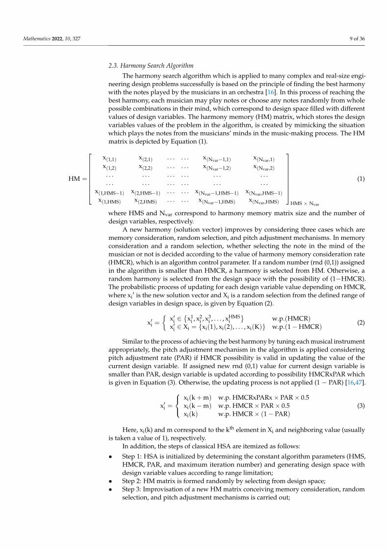
2.3. Harmony Search Algorithm

The harmony search algorithm which is applied to many complex and real-size engi-neering design problems successfully is based on the principle of finding the best harmonywith the notes played by the musicians in an orchestra [16]. In this process of reaching thebest harmony, each musician may play notes or choose any notes randomly from wholepossible combinations in their mind, which correspond to design space filled with differentvalues of design variables. The harmony memory (HM) matrix, which stores the designvariables values of the problem in the algorithm, is created by mimicking the situationwhich plays the notes from the musicians’ minds in the music-making process. The HMmatrix is depicted by Equation (1).

HM =

x(1,1) x(2,1) . . . . . . x(Nvar−1,1) x(Nvar,1)x(1,2) x(2,2) . . . . . . x(Nvar−1,2) x(Nvar,2)

. . . . . . . . . . . . . . . . . .

. . . . . . . . . . . . . . . . . .x(1,HMS−1) x(2,HMS−1) . . . . . . x(Nvar−1,HMS−1) x(Nvar,HMS−1)

x(1,HMS) x(2,HMS) . . . . . . x(Nvar−1,HMS) x(Nvar,HMS)

HMS × Nvar

(1)

where HMS and Nvar correspond to harmony memory matrix size and the number ofdesign variables, respectively.

A new harmony (solution vector) improves by considering three cases which arememory consideration, random selection, and pitch adjustment mechanisms. In memoryconsideration and a random selection, whether selecting the note in the mind of themusician or not is decided according to the value of harmony memory consideration rate(HMCR), which is an algorithm control parameter. If a random number (rnd (0,1)) assignedin the algorithm is smaller than HMCR, a harmony is selected from HM. Otherwise, arandom harmony is selected from the design space with the possibility of (1−HMCR).The probabilistic process of updating for each design variable value depending on HMCR,where xi

′ is the new solution vector and Xi is a random selection from the defined range ofdesign variables in design space, is given by Equation (2).

x′i ={

x′i ∈{

x1i , x2

i , x3i , . . . , xHMS

i}

w.p.(HMCR)x′i ∈ Xi = {xi(1), xi(2), . . . , xi(K)} w.p.(1−HMCR)

(2)

Similar to the process of achieving the best harmony by tuning each musical instrumentappropriately, the pitch adjustment mechanism in the algorithm is applied consideringpitch adjustment rate (PAR) if HMCR possibility is valid in updating the value of thecurrent design variable. If assigned new rnd (0,1) value for current design variable issmaller than PAR, design variable is updated according to possibility HMCRxPAR whichis given in Equation (3). Otherwise, the updating process is not applied (1 − PAR) [16,47].

x′i =

xi(k + m) w.p. HMCRxPARx× PAR× 0.5xi(k−m) w.p. HMCR× PAR× 0.5xi(k) w.p. HMCR× (1− PAR)

(3)

Here, xi(k) and m correspond to the kth element in Xi and neighboring value (usuallyis taken a value of 1), respectively.

In addition, the steps of classical HSA are itemized as follows:

• Step 1: HSA is initialized by determining the constant algorithm parameters (HMS,HMCR, PAR, and maximum iteration number) and generating design space withdesign variable values according to range limitation;

• Step 2: HM matrix is formed randomly by selecting from design space;• Step 3: Improvisation of a new HM matrix conceiving memory consideration, random

selection, and pitch adjustment mechanisms is carried out;

Mathematics 2022, 10, 327 10 of 36

• Step 4: HM matrix is updated depending on whether a better solution is obtained, andthen the worst solution is drawn from HM by replacing the better one;

• Step 5: Until the current iteration is reached the predefined maximum iteration number,Step 3 and Step 4 are repeated. If it is conducted HSA is ended.

2.4. Taguchi Method Background

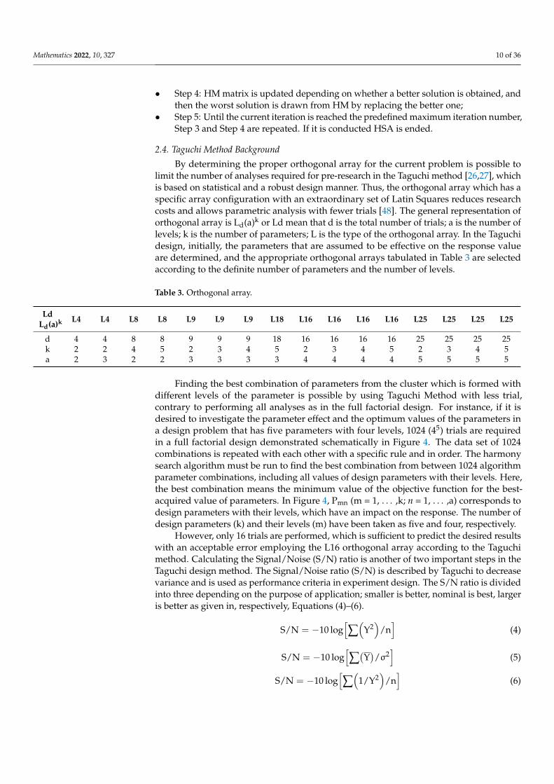
By determining the proper orthogonal array for the current problem is possible tolimit the number of analyses required for pre-research in the Taguchi method [26,27], whichis based on statistical and a robust design manner. Thus, the orthogonal array which has aspecific array configuration with an extraordinary set of Latin Squares reduces researchcosts and allows parametric analysis with fewer trials [48]. The general representation oforthogonal array is Ld(a)k or Ld mean that d is the total number of trials; a is the number oflevels; k is the number of parameters; L is the type of the orthogonal array. In the Taguchidesign, initially, the parameters that are assumed to be effective on the response valueare determined, and the appropriate orthogonal arrays tabulated in Table 3 are selectedaccording to the definite number of parameters and the number of levels.

Table 3. Orthogonal array.

LdLd(a)k L4 L4 L8 L8 L9 L9 L9 L18 L16 L16 L16 L16 L25 L25 L25 L25

d 4 4 8 8 9 9 9 18 16 16 16 16 25 25 25 25k 2 2 4 5 2 3 4 5 2 3 4 5 2 3 4 5a 2 3 2 2 3 3 3 3 4 4 4 4 5 5 5 5

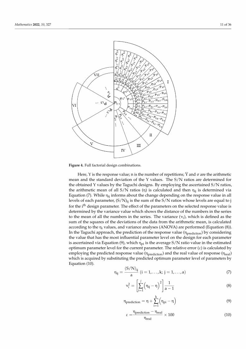
Finding the best combination of parameters from the cluster which is formed withdifferent levels of the parameter is possible by using Taguchi Method with less trial,contrary to performing all analyses as in the full factorial design. For instance, if it isdesired to investigate the parameter effect and the optimum values of the parameters ina design problem that has five parameters with four levels, 1024 (45) trials are requiredin a full factorial design demonstrated schematically in Figure 4. The data set of 1024combinations is repeated with each other with a specific rule and in order. The harmonysearch algorithm must be run to find the best combination from between 1024 algorithmparameter combinations, including all values of design parameters with their levels. Here,the best combination means the minimum value of the objective function for the best-acquired value of parameters. In Figure 4, Pmn (m = 1, . . . ,k; n = 1, . . . ,a) corresponds todesign parameters with their levels, which have an impact on the response. The number ofdesign parameters (k) and their levels (m) have been taken as five and four, respectively.

However, only 16 trials are performed, which is sufficient to predict the desired resultswith an acceptable error employing the L16 orthogonal array according to the Taguchimethod. Calculating the Signal/Noise (S/N) ratio is another of two important steps in theTaguchi design method. The Signal/Noise ratio (S/N) is described by Taguchi to decreasevariance and is used as performance criteria in experiment design. The S/N ratio is dividedinto three depending on the purpose of application; smaller is better, nominal is best, largeris better as given in, respectively, Equations (4)–(6).

S/N = −10 log[∑(

Y2)

/n]

(4)

S/N = −10 log[∑(Y)/σ2

](5)

S/N = −10 log[∑(

1/Y2)

/n]

(6)

Mathematics 2022, 10, 327 11 of 36Mathematics 2022, 10, x FOR PEER REVIEW 11 of 37

Figure 4. Full factorial design combinations.

( )2S / N 10log Y n = − (4)

( ) 2S / N= 10log Y σ − (5)

( )2S / N 10log 1 Y n = − (6)

Here, Y is the response value; n is the number of repetitions; Y and σ are the arith-metic mean and the standard deviation of the Y values. The S/N ratios are determined for the obtained Y values by the Taguchi designs. By employing the ascertained S/N ratios, the arithmetic mean of all S/N ratios (η) is calculated and then ηij is determined via Equa-tion (7). While ηij informs about the change depending on the response value in all levels of each parameter, (S/N)ij is the sum of the S/N ratios whose levels are equal to j for the ith design parameter. The effect of the parameters on the selected response value is deter-mined by the variance value which shows the distance of the numbers in the series to the mean of all the numbers in the series. The variance (νi), which is defined as the sum of the squares of the deviations of the data from the arithmetic mean, is calculated according to the ηi values, and variance analyses (ANOVA) are performed (Equation (8)). In the Taguchi approach, the prediction of the response value (ηprediction) by considering the value that has the most influential parameter level on the design for each parameter is ascer-tained via Equation (9), which ηpi is the average S/N ratio value in the estimated optimum parameter level for the current parameter. The relative error (ε) is calculated by employing the predicted response value (ηprediction) and the real value of response (ηreal) which is ac-quired by substituting the predicted optimum parameter level of parameters by Equation (10).

(S/N)ijη = ( i=1,...,k; j=1,...,a )ij a

(7)

Figure 4. Full factorial design combinations.

Here, Y is the response value; n is the number of repetitions; Y and σ are the arithmeticmean and the standard deviation of the Y values. The S/N ratios are determined forthe obtained Y values by the Taguchi designs. By employing the ascertained S/N ratios,the arithmetic mean of all S/N ratios (η) is calculated and then ηij is determined viaEquation (7). While ηij informs about the change depending on the response value in alllevels of each parameter, (S/N)ij is the sum of the S/N ratios whose levels are equal to jfor the ith design parameter. The effect of the parameters on the selected response value isdetermined by the variance value which shows the distance of the numbers in the seriesto the mean of all the numbers in the series. The variance (νi), which is defined as thesum of the squares of the deviations of the data from the arithmetic mean, is calculatedaccording to the ηi values, and variance analyses (ANOVA) are performed (Equation (8)).In the Taguchi approach, the prediction of the response value (ηprediction) by consideringthe value that has the most influential parameter level on the design for each parameteris ascertained via Equation (9), which ηpi is the average S/N ratio value in the estimatedoptimum parameter level for the current parameter. The relative error (ε) is calculated byemploying the predicted response value (ηprediction) and the real value of response (ηreal)which is acquired by substituting the predicted optimum parameter level of parameters byEquation (10).

ηij =(S/N)ij

a(i = 1, . . . , k; j = 1, . . . , a) (7)

ν2i =

[j

∑i=1

(ηij − η

)2]

1a− 1

(8)

ηprediction = η+k

∑i=1

(ηpi − η

)(9)

ε =ηprediction − ηreal

ηreal× 100 (10)

Mathematics 2022, 10, 327 12 of 36

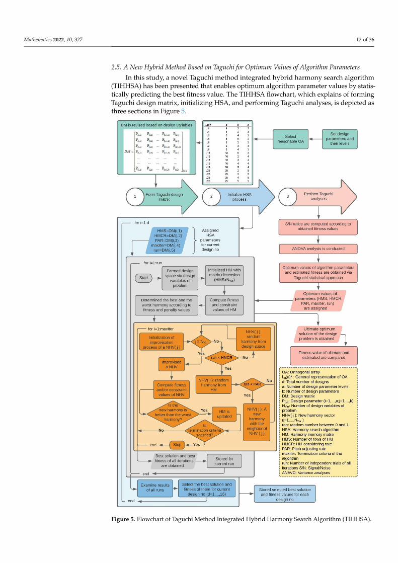
2.5. A New Hybrid Method Based on Taguchi for Optimum Values of Algorithm Parameters

In this study, a novel Taguchi method integrated hybrid harmony search algorithm(TIHHSA) has been presented that enables optimum algorithm parameter values by statis-tically predicting the best fitness value. The TIHHSA flowchart, which explains of formingTaguchi design matrix, initializing HSA, and performing Taguchi analyses, is depicted asthree sections in Figure 5.

Mathematics 2022, 10, x FOR PEER REVIEW 13 of 37

Figure 5. Flowchart of Taguchi Method Integrated Hybrid Harmony Search Algorithm (TIHHSA).

Figure 5. Flowchart of Taguchi Method Integrated Hybrid Harmony Search Algorithm (TIHHSA).

Mathematics 2022, 10, 327 13 of 36

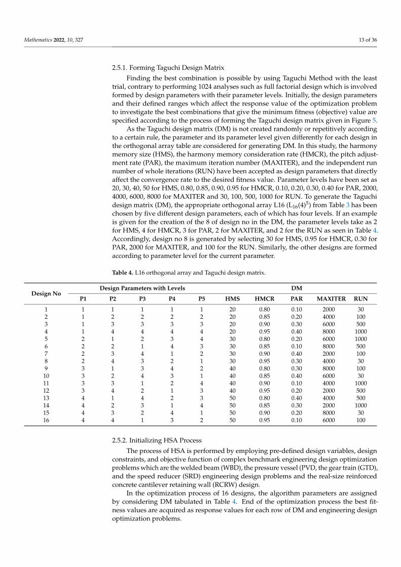
2.5.1. Forming Taguchi Design Matrix

Finding the best combination is possible by using Taguchi Method with the leasttrial, contrary to performing 1024 analyses such as full factorial design which is involvedformed by design parameters with their parameter levels. Initially, the design parametersand their defined ranges which affect the response value of the optimization problemto investigate the best combinations that give the minimum fitness (objective) value arespecified according to the process of forming the Taguchi design matrix given in Figure 5.

As the Taguchi design matrix (DM) is not created randomly or repetitively accordingto a certain rule, the parameter and its parameter level given differently for each design inthe orthogonal array table are considered for generating DM. In this study, the harmonymemory size (HMS), the harmony memory consideration rate (HMCR), the pitch adjust-ment rate (PAR), the maximum iteration number (MAXITER), and the independent runnumber of whole iterations (RUN) have been accepted as design parameters that directlyaffect the convergence rate to the desired fitness value. Parameter levels have been set as20, 30, 40, 50 for HMS, 0.80, 0.85, 0.90, 0.95 for HMCR, 0.10, 0.20, 0.30, 0.40 for PAR, 2000,4000, 6000, 8000 for MAXITER and 30, 100, 500, 1000 for RUN. To generate the Taguchidesign matrix (DM), the appropriate orthogonal array L16 (L16(4)5) from Table 3 has beenchosen by five different design parameters, each of which has four levels. If an exampleis given for the creation of the 8 of design no in the DM, the parameter levels take as 2for HMS, 4 for HMCR, 3 for PAR, 2 for MAXITER, and 2 for the RUN as seen in Table 4.Accordingly, design no 8 is generated by selecting 30 for HMS, 0.95 for HMCR, 0.30 forPAR, 2000 for MAXITER, and 100 for the RUN. Similarly, the other designs are formedaccording to parameter level for the current parameter.

Table 4. L16 orthogonal array and Taguchi design matrix.

Design NoDesign Parameters with Levels DM

P1 P2 P3 P4 P5 HMS HMCR PAR MAXITER RUN

1 1 1 1 1 1 20 0.80 0.10 2000 302 1 2 2 2 2 20 0.85 0.20 4000 1003 1 3 3 3 3 20 0.90 0.30 6000 5004 1 4 4 4 4 20 0.95 0.40 8000 10005 2 1 2 3 4 30 0.80 0.20 6000 10006 2 2 1 4 3 30 0.85 0.10 8000 5007 2 3 4 1 2 30 0.90 0.40 2000 1008 2 4 3 2 1 30 0.95 0.30 4000 309 3 1 3 4 2 40 0.80 0.30 8000 100

10 3 2 4 3 1 40 0.85 0.40 6000 3011 3 3 1 2 4 40 0.90 0.10 4000 100012 3 4 2 1 3 40 0.95 0.20 2000 50013 4 1 4 2 3 50 0.80 0.40 4000 50014 4 2 3 1 4 50 0.85 0.30 2000 100015 4 3 2 4 1 50 0.90 0.20 8000 3016 4 4 1 3 2 50 0.95 0.10 6000 100

2.5.2. Initializing HSA Process

The process of HSA is performed by employing pre-defined design variables, designconstraints, and objective function of complex benchmark engineering design optimizationproblems which are the welded beam (WBD), the pressure vessel (PVD, the gear train (GTD),and the speed reducer (SRD) engineering design problems and the real-size reinforcedconcrete cantilever retaining wall (RCRW) design.

In the optimization process of 16 designs, the algorithm parameters are assignedby considering DM tabulated in Table 4. End of the optimization process the best fit-ness values are acquired as response values for each row of DM and engineering designoptimization problems.

Mathematics 2022, 10, 327 14 of 36

2.5.3. Performing Taguchi Analyses

In this section, the S/N ratios of response value have been calculated via Equation (4),which is given for smaller is the better purpose, for WBD, PVD, GTD, SRD, and RCRWengineering design optimization problems, separately. The graphs that show the variationbetween the determined ηij values via Equation (7) and the design parameter with theirlevels were drawn. The variance (ν) values of design parameters by employing η and ηivalues according to Equation (8) and the parameter effect (PE) on response value based onthe sum of squares for the design parameters are specified.

And then the verification analyses are performed vis a vis estimated optimum valuesof design parameters which are suggested for ηprediction value depicted in Equation (9). Byassigning the HMS, HMCR, PAR, MAXITER, and RUN optimum values that come fromthe Taguchi approach results to HSA, optimization analyses are conducted again for eachdesign optimization problem and ηreal is determined. The relative error (ε) which is areliability criterion of the Taguchi design is calculated by Equation (10).

3. Design Experiments and Results

In this section, the optimization analysis results reached by the HSA and the proposedTIHHSA method have been given with the aim of investigating different engineeringoptimization design problem’s characteristic effect on the fitness value. In the optimizationanalyses performed with HSA, the variation of the fitness values achieved for differentnumbers of run values according to the characteristics of different engineering optimizationproblems has been examined. The robustness of the proposed TIHHSA method has beenevaluated for engineering optimization design problems and the optimum values of thealgorithm parameters have been estimated with the HMS, HMCR, PAR, MAXITER, andRUN effects obtained from the variance analyses (ANOVA).

3.1. Optimization Analyses of Engineering Design Problems and Real-Size Engineering DesignOptimization Problem

In this section, the optimization analyses result of the welded beam (WBD), thepressure vessel (PVD), the gear train (GTD), and the speed reducer (SRD) benchmarkengineering design problems and the real-size reinforced concrete cantilever retaining wall(RCRW) design have been presented. In the optimization analysis through harmony searchalgorithm (HSA) [16], the algorithm parameters are selected as HMS = 20, HMCR = 0.90,and PAR = 0.35 [47]. Deb’s rules [49] are implemented as a constraint-handling strategy. Thebest solution is determined according to penalty values of all constraints with the fitnessvalues. The best solution is evaluated according to the current fitness value if solutionshave the same penalty value or no penalty.

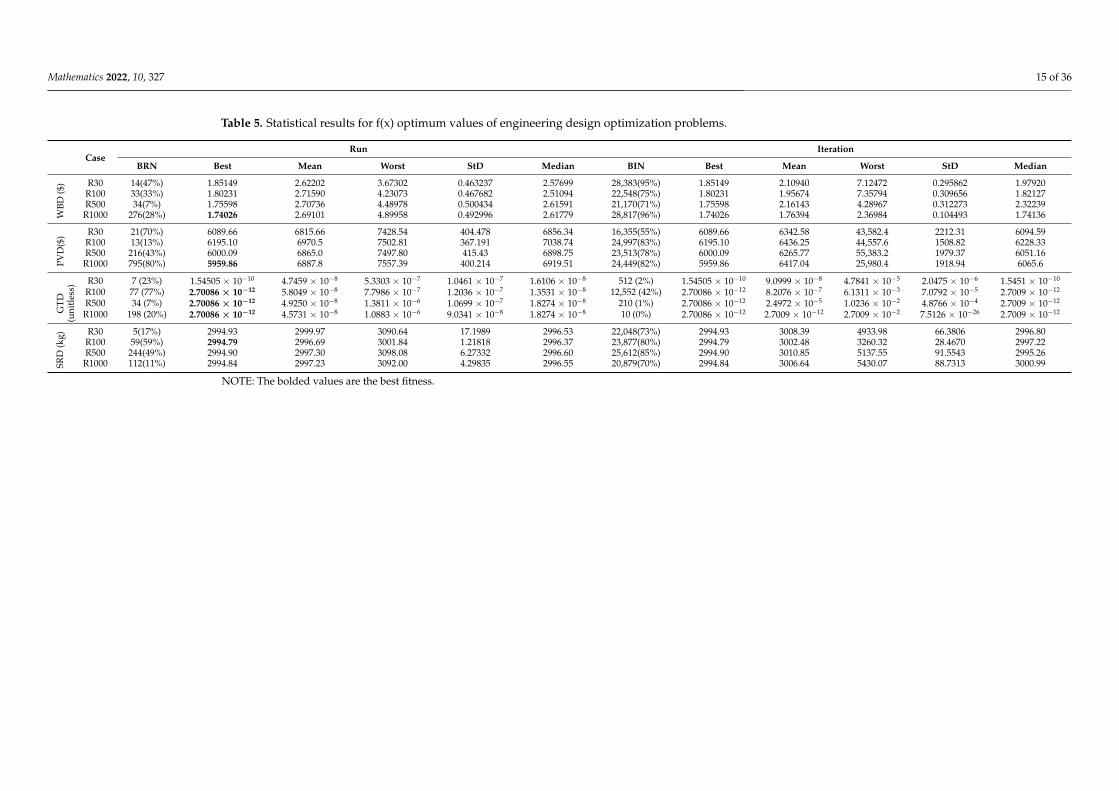
Different run cases (R30, R100, R500, R1000) have been chosen to investigate the effectof variable run values on the minimum objective function, in the optimization analyses. HSalgorithm is performed until maximum iteration numbers reach 30,000. This process hasbeen repeated for different independent runs as 30, 100, 500, and 1000. In the evaluationof the results, while the best iteration number (BIN) corresponds to the iteration in whichno more minimum objective function value is yielded with ongoing analysis, the best runnumber (BRN) is the best-obtained fitness value among all runs for each case. The best,the worst, the mean, the standard deviation (StD), and the median values of the minimumobjective function (fitness value) have been determined for BRN and BIN, separately.

Achieved statistical evaluations of optimization analyses satisfied the constraints aretabulated in Table 5 for WBD, PVD, GTD, and SRD.

Mathematics 2022, 10, 327 15 of 36

Table 5. Statistical results for f(x) optimum values of engineering design optimization problems.

CaseRun Iteration

BRN Best Mean Worst StD Median BIN Best Mean Worst StD Median

WBD

($) R30 14(47%) 1.85149 2.62202 3.67302 0.463237 2.57699 28,383(95%) 1.85149 2.10940 7.12472 0.295862 1.97920

R100 33(33%) 1.80231 2.71590 4.23073 0.467682 2.51094 22,548(75%) 1.80231 1.95674 7.35794 0.309656 1.82127R500 34(7%) 1.75598 2.70736 4.48978 0.500434 2.61591 21,170(71%) 1.75598 2.16143 4.28967 0.312273 2.32239

R1000 276(28%) 1.74026 2.69101 4.89958 0.492996 2.61779 28,817(96%) 1.74026 1.76394 2.36984 0.104493 1.74136

PVD

($) R30 21(70%) 6089.66 6815.66 7428.54 404.478 6856.34 16,355(55%) 6089.66 6342.58 43,582.4 2212.31 6094.59

R100 13(13%) 6195.10 6970.5 7502.81 367.191 7038.74 24,997(83%) 6195.10 6436.25 44,557.6 1508.82 6228.33R500 216(43%) 6000.09 6865.0 7497.80 415.43 6898.75 23,513(78%) 6000.09 6265.77 55,383.2 1979.37 6051.16

R1000 795(80%) 5959.86 6887.8 7557.39 400.214 6919.51 24,449(82%) 5959.86 6417.04 25,980.4 1918.94 6065.6

GTD

(uni

tles

s)

R30 7 (23%) 1.54505 × 10−10 4.7459 × 10−8 5.3303 × 10−7 1.0461 × 10−7 1.6106 × 10−8 512 (2%) 1.54505 × 10−10 9.0999 × 10−8 4.7841 × 10−5 2.0475 × 10−6 1.5451 × 10−10

R100 77 (77%) 2.70086 × 10−12 5.8049 × 10−8 7.7986 × 10−7 1.2036 × 10−7 1.3531 × 10−8 12,552 (42%) 2.70086 × 10−12 8.2076 × 10−7 6.1311 × 10−3 7.0792 × 10−5 2.7009 × 10−12

R500 34 (7%) 2.70086 × 10−12 4.9250 × 10−8 1.3811 × 10−6 1.0699 × 10−7 1.8274 × 10−8 210 (1%) 2.70086 × 10−12 2.4972 × 10−5 1.0236 × 10−2 4.8766 × 10−4 2.7009 × 10−12

R1000 198 (20%) 2.70086 × 10−12 4.5731 × 10−8 1.0883 × 10−6 9.0341 × 10−8 1.8274 × 10−8 10 (0%) 2.70086 × 10−12 2.7009 × 10−12 2.7009 × 10−2 7.5126 × 10−26 2.7009 × 10−12

SRD

(kg) R30 5(17%) 2994.93 2999.97 3090.64 17.1989 2996.53 22,048(73%) 2994.93 3008.39 4933.98 66.3806 2996.80

R100 59(59%) 2994.79 2996.69 3001.84 1.21818 2996.37 23,877(80%) 2994.79 3002.48 3260.32 28.4670 2997.22R500 244(49%) 2994.90 2997.30 3098.08 6.27332 2996.60 25,612(85%) 2994.90 3010.85 5137.55 91.5543 2995.26

R1000 112(11%) 2994.84 2997.23 3092.00 4.29835 2996.55 20,879(70%) 2994.84 3006.64 5430.07 88.7313 3000.99

NOTE: The bolded values are the best fitness.

Mathematics 2022, 10, 327 16 of 36

According to Table 5, the minimum fitness value of the WBD problem has been foundfor the R1000 case as $1.74026 in 28,817 iterations, which corresponds to 96% of the optimumsearch process performed with 30,000 iterations. After this value was accomplished for276 runs out of 1000 (276/1000 × 100 = 28%), no more minimum fitness was not reachedduring continuing runs. For the other run cases (R30, R100, R500), while the optimumvalues have been achieved on the average of 80% of 30,000 iterations, it is seen that theaverage of 38% of all runs is enough for this search process.

It is clearly shown that the minimum fitness value of PVD has been gained for theR1000 case as $5959.86 in 82% out of 30,000 iterations and 795 runs out of 1000 (80%). Whilethe minimum fitness values have been found in an average of 70% of the optimum searchprocess, an average of 42% of independently operated runs has been sufficient to acquirethe minimum objective function value for R30, R100, and R500 cases.

Though increasing the run number has been caused that the algorithm obligates toinvestigate more optimum value, the only best fitness value of GTD problem has revealedas 2.70086 × 10−12 in the case of R100. While the algorithm has been reached the bestfitness value in 210 and 10 trials out of 30,000 iterations, it is seen that 34 and 198 runs areenough to find the optimum solution for R500 and R1000 cases, respectively.

When the values tabulated for the SRD problem are examined, it is observed thatthe best fitness value (2994.79 kg) has been just attained for the R100 case alike for theGTD problem, even though the optimization process for more runs which is ongoing. Thesearching process for the minimum fitness value of the SRD problem has been performedwith 30,000 iterations and the best value has been found in 23,877 iterations out of entireiterations that means 80% of the process. The more minimum fitness value has not beenreached for increasing runs.

Since the algorithm cannot reach a better solution after reaching the best solution, theprocess is conducted again to possibly find a more minimum result with different runs.It is observed that more fitness values have been generally yielded with increasing runsfor different design problems. The fitness values of WBD and PVD design problems havebeen achieved for the R1000 case when given statistical result tables are examined. Thefitness value of GTD and SRD design problems has been obtained for the R100 case inoptimization analyses which are seen that the fitness value is not changing with continuinganalysis any longer.

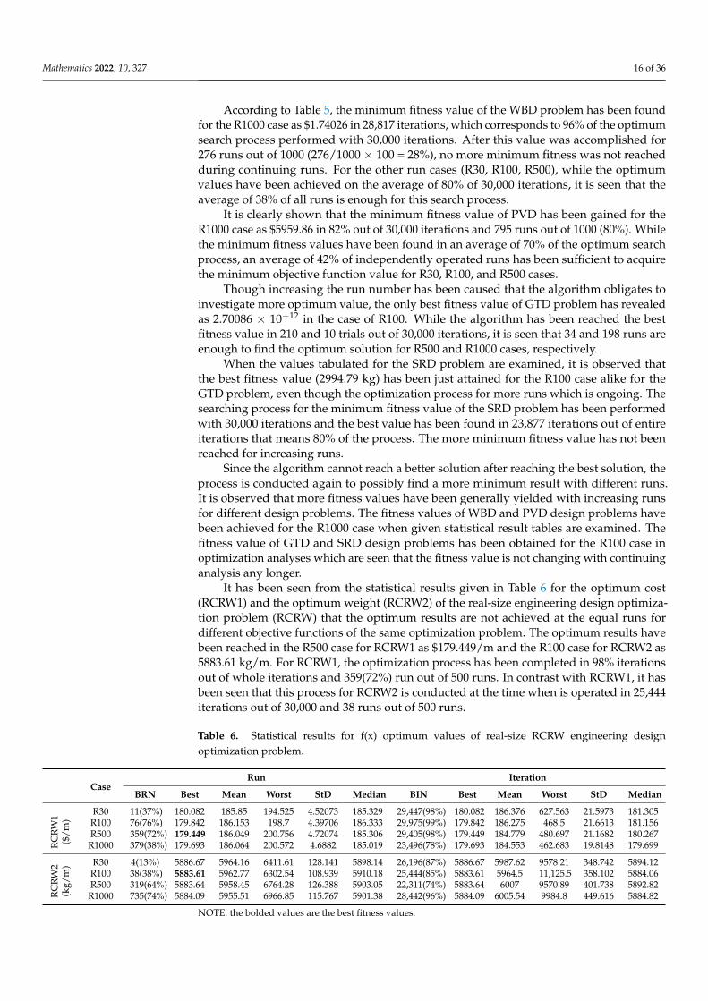
It has been seen from the statistical results given in Table 6 for the optimum cost(RCRW1) and the optimum weight (RCRW2) of the real-size engineering design optimiza-tion problem (RCRW) that the optimum results are not achieved at the equal runs fordifferent objective functions of the same optimization problem. The optimum results havebeen reached in the R500 case for RCRW1 as $179.449/m and the R100 case for RCRW2 as5883.61 kg/m. For RCRW1, the optimization process has been completed in 98% iterationsout of whole iterations and 359(72%) run out of 500 runs. In contrast with RCRW1, it hasbeen seen that this process for RCRW2 is conducted at the time when is operated in 25,444iterations out of 30,000 and 38 runs out of 500 runs.

Table 6. Statistical results for f(x) optimum values of real-size RCRW engineering designoptimization problem.

CaseRun Iteration

BRN Best Mean Worst StD Median BIN Best Mean Worst StD Median

RC

RW

1($

/m)

R30 11(37%) 180.082 185.85 194.525 4.52073 185.329 29,447(98%) 180.082 186.376 627.563 21.5973 181.305R100 76(76%) 179.842 186.153 198.7 4.39706 186.333 29,975(99%) 179.842 186.275 468.5 21.6613 181.156R500 359(72%) 179.449 186.049 200.756 4.72074 185.306 29,405(98%) 179.449 184.779 480.697 21.1682 180.267

R1000 379(38%) 179.693 186.064 200.572 4.6882 185.019 23,496(78%) 179.693 184.553 462.683 19.8148 179.699

RC

RW

2(k

g/m

) R30 4(13%) 5886.67 5964.16 6411.61 128.141 5898.14 26,196(87%) 5886.67 5987.62 9578.21 348.742 5894.12R100 38(38%) 5883.61 5962.77 6302.54 108.939 5910.18 25,444(85%) 5883.61 5964.5 11,125.5 358.102 5884.06R500 319(64%) 5883.64 5958.45 6764.28 126.388 5903.05 22,311(74%) 5883.64 6007 9570.89 401.738 5892.82

R1000 735(74%) 5884.09 5955.51 6966.85 115.767 5901.38 28,442(96%) 5884.09 6005.54 9984.8 449.616 5884.82

NOTE: the bolded values are the best fitness values.

Mathematics 2022, 10, 327 17 of 36

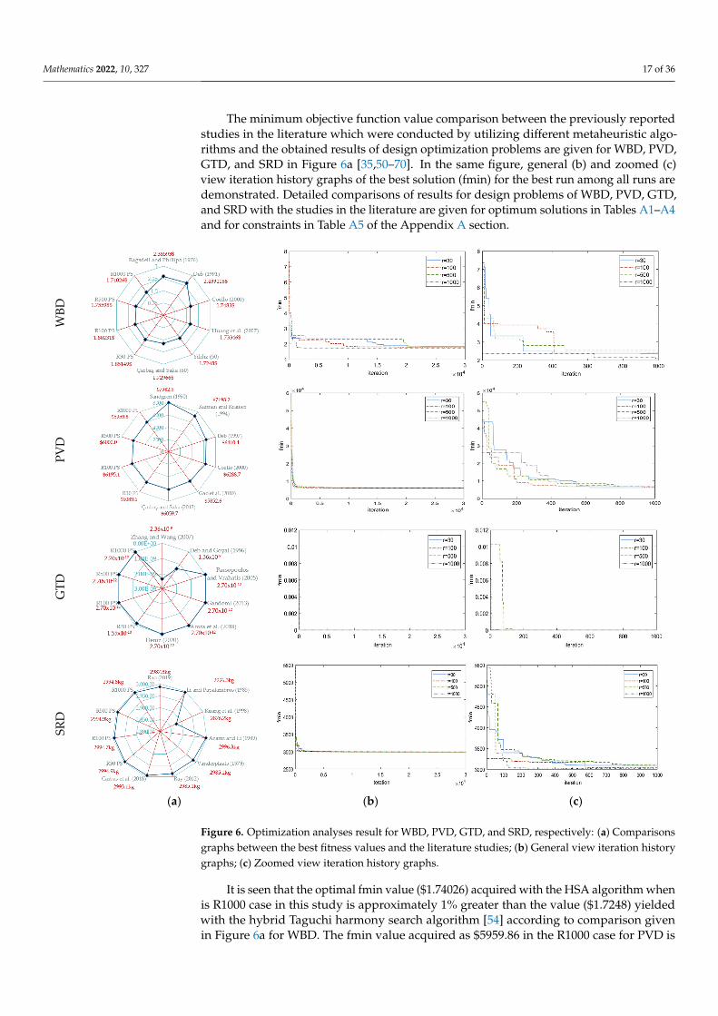
The minimum objective function value comparison between the previously reportedstudies in the literature which were conducted by utilizing different metaheuristic algo-rithms and the obtained results of design optimization problems are given for WBD, PVD,GTD, and SRD in Figure 6a [35,50–70]. In the same figure, general (b) and zoomed (c)view iteration history graphs of the best solution (fmin) for the best run among all runs aredemonstrated. Detailed comparisons of results for design problems of WBD, PVD, GTD,and SRD with the studies in the literature are given for optimum solutions in Tables A1–A4and for constraints in Table A5 of the Appendix A section.

Mathematics 2022, 10, x FOR PEER REVIEW 17 of 37

SRD with the studies in the literature are given for optimum solutions in Tables A1–A4 and for constraints in Table A5 of the Appendix A section.

It is seen that the optimal fmin value ($1.74026) acquired with the HSA algorithm when is R1000 case in this study is approximately 1% greater than the value ($1.7248) yielded with the hybrid Taguchi harmony search algorithm [50] according to comparison given in Figure 6a for WBD. The fmin value acquired as $5959.86 in the R1000 case for PVD is above the best fitness value with 2% ($5852.6394) presented according to the study by Gao et al. [51], which utilized the HSA with the bandwidth improvisation to the pitch adjustment rate. The reached optimum value of GTD in the R30 case which is 2.70086 × 10−12 is the same as the best values presented in the literature. The acquired optimum value (2994.79 kg) for SRD is higher than the best fitness value (2876.22 kg) presented in the literature study [52] with 4% obtained according to the Taguchi-aided optimization search method.

WBD

PVD

GTD

SRD

(a) (b) (c)

Figure 6. Optimization analyses result for WBD, PVD, GTD, and SRD, respectively: (a) Comparisons graphs between the best fitness values and the literature studies; (b) General view iteration history graphs; (c) Zoomed view iteration history graphs.

Figure 6. Optimization analyses result for WBD, PVD, GTD, and SRD, respectively: (a) Comparisonsgraphs between the best fitness values and the literature studies; (b) General view iteration historygraphs; (c) Zoomed view iteration history graphs.

It is seen that the optimal fmin value ($1.74026) acquired with the HSA algorithm whenis R1000 case in this study is approximately 1% greater than the value ($1.7248) yieldedwith the hybrid Taguchi harmony search algorithm [54] according to comparison givenin Figure 6a for WBD. The fmin value acquired as $5959.86 in the R1000 case for PVD is

Mathematics 2022, 10, 327 18 of 36

above the best fitness value with 2% ($5852.6394) presented according to the study by Gaoet al. [58], which utilized the HSA with the bandwidth improvisation to the pitch adjustmentrate. The reached optimum value of GTD in the R30 case which is 2.70086 × 10−12 is thesame as the best values presented in the literature [61–64]. The acquired optimum value(2994.79 kg) for SRD is higher than the best fitness value (2876.22 kg) presented in theliterature study [66] with 4% obtained according to the Taguchi-aided optimization searchmethod.

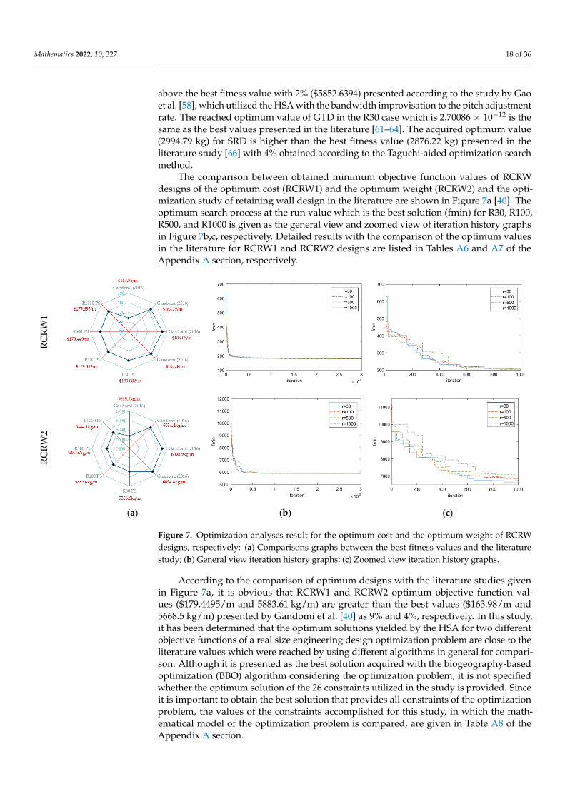
The comparison between obtained minimum objective function values of RCRWdesigns of the optimum cost (RCRW1) and the optimum weight (RCRW2) and the opti-mization study of retaining wall design in the literature are shown in Figure 7a [40]. Theoptimum search process at the run value which is the best solution (fmin) for R30, R100,R500, and R1000 is given as the general view and zoomed view of iteration history graphsin Figure 7b,c, respectively. Detailed results with the comparison of the optimum valuesin the literature for RCRW1 and RCRW2 designs are listed in Tables A6 and A7 of theAppendix A section, respectively.

Mathematics 2022, 10, x FOR PEER REVIEW 18 of 37

The comparison between obtained minimum objective function values of RCRW de-signs of the optimum cost (RCRW1) and the optimum weight (RCRW2) and the optimi-zation study of retaining wall design in the literature are shown in Figure 7a. The opti-mum search process at the run value which is the best solution (fmin) for R30, R100, R500, and R1000 is given as the general view and zoomed view of iteration history graphs in Figure 7b,c, respectively. Detailed results with the comparison of the optimum values in the literature for RCRW1 and RCRW2 designs are listed in Table A6 and Table A7 of the Appendix A section, respectively.

RCRW

1

RCRW

2

(a) (b) (c)

Figure 7. Optimization analyses result for the optimum cost and the optimum weight of RCRW designs, respectively: (a) Comparisons graphs between the best fitness values and the literature study; (b) General view iteration history graphs; (c) Zoomed view iteration history graphs.

According to the comparison of optimum designs with the literature studies given in Figure 7a, it is obvious that RCRW1 and RCRW2 optimum objective function values ($179.4495/m and 5883.61 kg/m) are greater than the best values ($163.98/m and 5668.5 kg/m) presented by Gandomi et al. [40] as 9% and 4%, respectively. In this study, it has been determined that the optimum solutions yielded by the HSA for two different objec-tive functions of a real size engineering design optimization problem are close to the lit-erature values which were reached by using different algorithms in general for compari-son. Although it is presented as the best solution acquired with the biogeography-based optimization (BBO) algorithm considering the optimization problem, it is not specified whether the optimum solution of the 26 constraints utilized in the study is provided. Since it is important to obtain the best solution that provides all constraints of the optimization problem, the values of the constraints accomplished for this study, in which the mathe-matical model of the optimization problem is compared, are given in Table A8 of the Ap-pendix A section.

Conducted analyses have been shown that the appropriate numbers of iteration and the independent run of entire iterations, which formed the extent of the acquiring opti-mum process, are significant to reaching the best fitness value instead of many or fewer numbers of them. The reaching process of the maximum iteration number defined as the run is accepted 30 times in the literature of optimization studies and the most minimum fitness value satisfying the design constraints is presented as the optimum result. The minimum fitness values have been yielded by operating different design problems with

Figure 7. Optimization analyses result for the optimum cost and the optimum weight of RCRWdesigns, respectively: (a) Comparisons graphs between the best fitness values and the literaturestudy; (b) General view iteration history graphs; (c) Zoomed view iteration history graphs.

According to the comparison of optimum designs with the literature studies givenin Figure 7a, it is obvious that RCRW1 and RCRW2 optimum objective function val-ues ($179.4495/m and 5883.61 kg/m) are greater than the best values ($163.98/m and5668.5 kg/m) presented by Gandomi et al. [40] as 9% and 4%, respectively. In this study,it has been determined that the optimum solutions yielded by the HSA for two differentobjective functions of a real size engineering design optimization problem are close to theliterature values which were reached by using different algorithms in general for compari-son. Although it is presented as the best solution acquired with the biogeography-basedoptimization (BBO) algorithm considering the optimization problem, it is not specifiedwhether the optimum solution of the 26 constraints utilized in the study is provided. Sinceit is important to obtain the best solution that provides all constraints of the optimizationproblem, the values of the constraints accomplished for this study, in which the math-ematical model of the optimization problem is compared, are given in Table A8 of theAppendix A section.

Mathematics 2022, 10, 327 19 of 36

Conducted analyses have been shown that the appropriate numbers of iteration andthe independent run of entire iterations, which formed the extent of the acquiring optimumprocess, are significant to reaching the best fitness value instead of many or fewer numbersof them. The reaching process of the maximum iteration number defined as the run isaccepted 30 times in the literature of optimization studies and the most minimum fitnessvalue satisfying the design constraints is presented as the optimum result. The minimumfitness values have been yielded by operating different design problems with different runswhen the number of the runs is greater than 30 according to the results given in the tables.It observed that while the more minimum fitness values generally are obtained with theincreasing runs in some engineering design problems, the minimum result may not befound with larger runs too in some of them. This brings to the fore the necessity that thenumber of executions of the optimization algorithm may have an optimum value.

3.2. Taguchi Analyses

The best combination, which provided the best fitness value for the welded beamdesign (WBD), the pressure vessel design (PVD), the gear tear design (GTD), the speedreducer design (SRD), the reinforced concrete cantilever retaining wall design (RCRW1)optimization problems have been investigated in terms of design parameters effectiveon the searching optimum solutions via the Taguchi method integrated hybrid harmonysearch algorithm (TIHHSA) as visualized in Figure 5.

3.2.1. Part I: Investigation of Five Optimum Design Parameter Values with Effect on theFitness Value

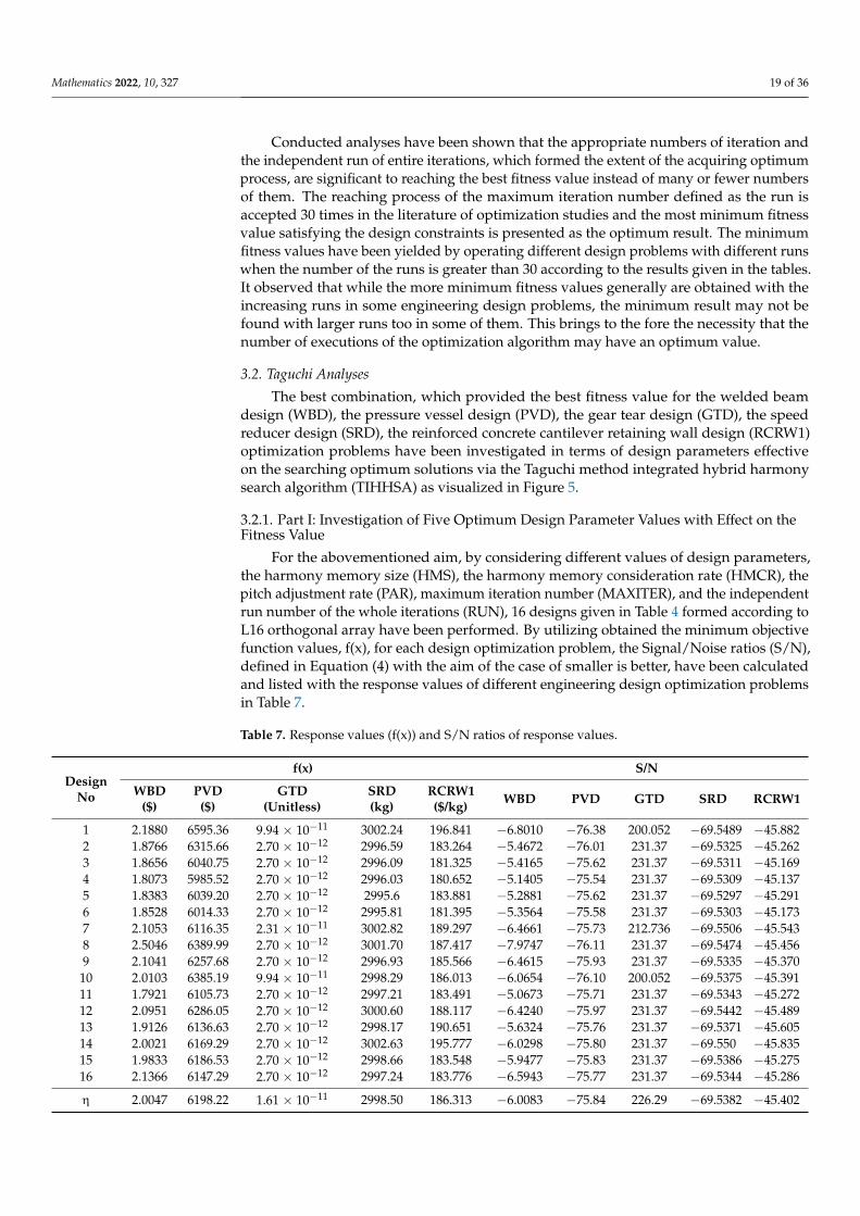
For the abovementioned aim, by considering different values of design parameters,the harmony memory size (HMS), the harmony memory consideration rate (HMCR), thepitch adjustment rate (PAR), maximum iteration number (MAXITER), and the independentrun number of the whole iterations (RUN), 16 designs given in Table 4 formed according toL16 orthogonal array have been performed. By utilizing obtained the minimum objectivefunction values, f(x), for each design optimization problem, the Signal/Noise ratios (S/N),defined in Equation (4) with the aim of the case of smaller is better, have been calculatedand listed with the response values of different engineering design optimization problemsin Table 7.

Table 7. Response values (f(x)) and S/N ratios of response values.

DesignNo

f(x) S/N

WBD($)

PVD($)

GTD(Unitless)

SRD(kg)

RCRW1($/kg) WBD PVD GTD SRD RCRW1

1 2.1880 6595.36 9.94 × 10−11 3002.24 196.841 −6.8010 −76.38 200.052 −69.5489 −45.8822 1.8766 6315.66 2.70 × 10−12 2996.59 183.264 −5.4672 −76.01 231.37 −69.5325 −45.2623 1.8656 6040.75 2.70 × 10−12 2996.09 181.325 −5.4165 −75.62 231.37 −69.5311 −45.1694 1.8073 5985.52 2.70 × 10−12 2996.03 180.652 −5.1405 −75.54 231.37 −69.5309 −45.1375 1.8383 6039.20 2.70 × 10−12 2995.6 183.881 −5.2881 −75.62 231.37 −69.5297 −45.2916 1.8528 6014.33 2.70 × 10−12 2995.81 181.395 −5.3564 −75.58 231.37 −69.5303 −45.1737 2.1053 6116.35 2.31 × 10−11 3002.82 189.297 −6.4661 −75.73 212.736 −69.5506 −45.5438 2.5046 6389.99 2.70 × 10−12 3001.70 187.417 −7.9747 −76.11 231.37 −69.5474 −45.4569 2.1041 6257.68 2.70 × 10−12 2996.93 185.566 −6.4615 −75.93 231.37 −69.5335 −45.370

10 2.0103 6385.19 9.94 × 10−11 2998.29 186.013 −6.0654 −76.10 200.052 −69.5375 −45.39111 1.7921 6105.73 2.70 × 10−12 2997.21 183.491 −5.0673 −75.71 231.37 −69.5343 −45.27212 2.0951 6286.05 2.70 × 10−12 3000.60 188.117 −6.4240 −75.97 231.37 −69.5442 −45.48913 1.9126 6136.63 2.70 × 10−12 2998.17 190.651 −5.6324 −75.76 231.37 −69.5371 −45.60514 2.0021 6169.29 2.70 × 10−12 3002.63 195.777 −6.0298 −75.80 231.37 −69.550 −45.83515 1.9833 6186.53 2.70 × 10−12 2998.66 183.548 −5.9477 −75.83 231.37 −69.5386 −45.27516 2.1366 6147.29 2.70 × 10−12 2997.24 183.776 −6.5943 −75.77 231.37 −69.5344 −45.286

η 2.0047 6198.22 1.61 × 10−11 2998.50 186.313 −6.0083 −75.84 226.29 −69.5382 −45.402

Mathematics 2022, 10, 327 20 of 36

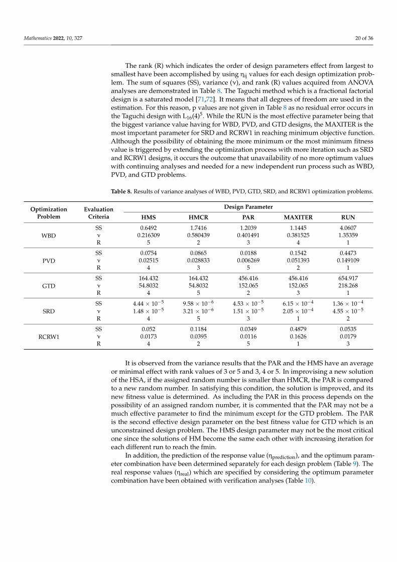
The rank (R) which indicates the order of design parameters effect from largest tosmallest have been accomplished by using ηij values for each design optimization prob-lem. The sum of squares (SS), variance (ν), and rank (R) values acquired from ANOVAanalyses are demonstrated in Table 8. The Taguchi method which is a fractional factorialdesign is a saturated model [71,72]. It means that all degrees of freedom are used in theestimation. For this reason, p values are not given in Table 8 as no residual error occurs inthe Taguchi design with L16(4)5. While the RUN is the most effective parameter being thatthe biggest variance value having for WBD, PVD, and GTD designs, the MAXITER is themost important parameter for SRD and RCRW1 in reaching minimum objective function.Although the possibility of obtaining the more minimum or the most minimum fitnessvalue is triggered by extending the optimization process with more iteration such as SRDand RCRW1 designs, it occurs the outcome that unavailability of no more optimum valueswith continuing analyses and needed for a new independent run process such as WBD,PVD, and GTD problems.

Table 8. Results of variance analyses of WBD, PVD, GTD, SRD, and RCRW1 optimization problems.

OptimizationProblem

EvaluationCriteria

Design Parameter

HMS HMCR PAR MAXITER RUN

WBDSS 0.6492 1.7416 1.2039 1.1445 4.0607ν 0.216309 0.580439 0.401491 0.381525 1.35359R 5 2 3 4 1

PVDSS 0.0754 0.0865 0.0188 0.1542 0.4473ν 0.02515 0.028833 0.006269 0.051393 0.149109R 4 3 5 2 1

GTDSS 164.432 164.432 456.416 456.416 654.917ν 54.8032 54.8032 152.065 152.065 218.268R 4 5 2 3 1

SRDSS 4.44 × 10−5 9.58 × 10−6 4.53 × 10−5 6.15 × 10−4 1.36 × 10−4

ν 1.48 × 10−5 3.21 × 10−6 1.51 × 10−5 2.05 × 10−4 4.55 × 10−5

R 4 5 3 1 2

RCRW1SS 0.052 0.1184 0.0349 0.4879 0.0535ν 0.0173 0.0395 0.0116 0.1626 0.0179R 4 2 5 1 3

It is observed from the variance results that the PAR and the HMS have an averageor minimal effect with rank values of 3 or 5 and 3, 4 or 5. In improvising a new solutionof the HSA, if the assigned random number is smaller than HMCR, the PAR is comparedto a new random number. In satisfying this condition, the solution is improved, and itsnew fitness value is determined. As including the PAR in this process depends on thepossibility of an assigned random number, it is commented that the PAR may not be amuch effective parameter to find the minimum except for the GTD problem. The PARis the second effective design parameter on the best fitness value for GTD which is anunconstrained design problem. The HMS design parameter may not be the most criticalone since the solutions of HM become the same each other with increasing iteration foreach different run to reach the fmin.

In addition, the prediction of the response value (ηprediction), and the optimum param-eter combination have been determined separately for each design problem (Table 9). Thereal response values (ηreal) which are specified by considering the optimum parametercombination have been obtained with verification analyses (Table 10).

Mathematics 2022, 10, 327 21 of 36

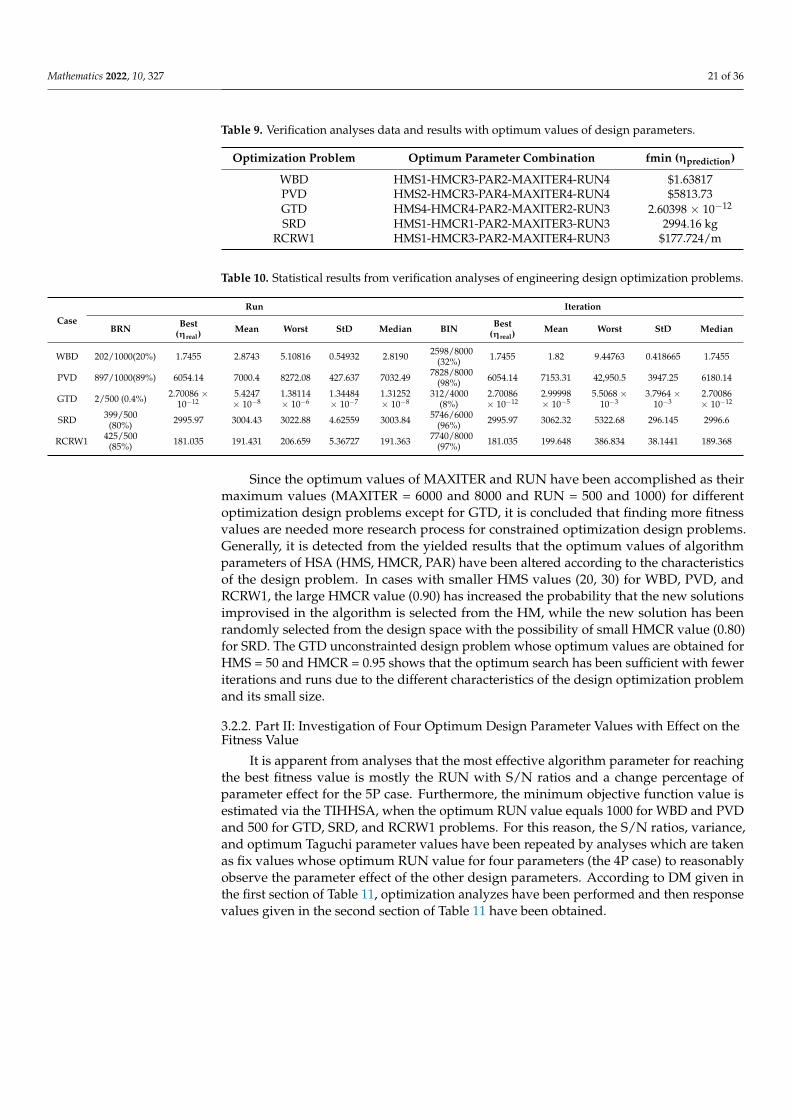
Table 9. Verification analyses data and results with optimum values of design parameters.

Optimization Problem Optimum Parameter Combination fmin (ηprediction)

WBD HMS1-HMCR3-PAR2-MAXITER4-RUN4 $1.63817PVD HMS2-HMCR3-PAR4-MAXITER4-RUN4 $5813.73GTD HMS4-HMCR4-PAR2-MAXITER2-RUN3 2.60398 × 10−12

SRD HMS1-HMCR1-PAR2-MAXITER3-RUN3 2994.16 kgRCRW1 HMS1-HMCR3-PAR2-MAXITER4-RUN3 $177.724/m

Table 10. Statistical results from verification analyses of engineering design optimization problems.

CaseRun Iteration

BRN Best(ηreal)

Mean Worst StD Median BIN Best(ηreal)

Mean Worst StD Median

WBD 202/1000(20%) 1.7455 2.8743 5.10816 0.54932 2.8190 2598/8000(32%) 1.7455 1.82 9.44763 0.418665 1.7455

PVD 897/1000(89%) 6054.14 7000.4 8272.08 427.637 7032.49 7828/8000(98%) 6054.14 7153.31 42,950.5 3947.25 6180.14

GTD 2/500 (0.4%) 2.70086 ×10−12

5.4247× 10−8

1.38114× 10−6

1.34484× 10−7

1.31252× 10−8

312/4000(8%)

2.70086× 10−12

2.99998× 10−5

5.5068 ×10−3

3.7964 ×10−3

2.70086× 10−12

SRD 399/500(80%) 2995.97 3004.43 3022.88 4.62559 3003.84 5746/6000

(96%) 2995.97 3062.32 5322.68 296.145 2996.6

RCRW1 425/500(85%) 181.035 191.431 206.659 5.36727 191.363 7740/8000

(97%) 181.035 199.648 386.834 38.1441 189.368

Since the optimum values of MAXITER and RUN have been accomplished as theirmaximum values (MAXITER = 6000 and 8000 and RUN = 500 and 1000) for differentoptimization design problems except for GTD, it is concluded that finding more fitnessvalues are needed more research process for constrained optimization design problems.Generally, it is detected from the yielded results that the optimum values of algorithmparameters of HSA (HMS, HMCR, PAR) have been altered according to the characteristicsof the design problem. In cases with smaller HMS values (20, 30) for WBD, PVD, andRCRW1, the large HMCR value (0.90) has increased the probability that the new solutionsimprovised in the algorithm is selected from the HM, while the new solution has beenrandomly selected from the design space with the possibility of small HMCR value (0.80)for SRD. The GTD unconstrainted design problem whose optimum values are obtained forHMS = 50 and HMCR = 0.95 shows that the optimum search has been sufficient with feweriterations and runs due to the different characteristics of the design optimization problemand its small size.

3.2.2. Part II: Investigation of Four Optimum Design Parameter Values with Effect on theFitness Value

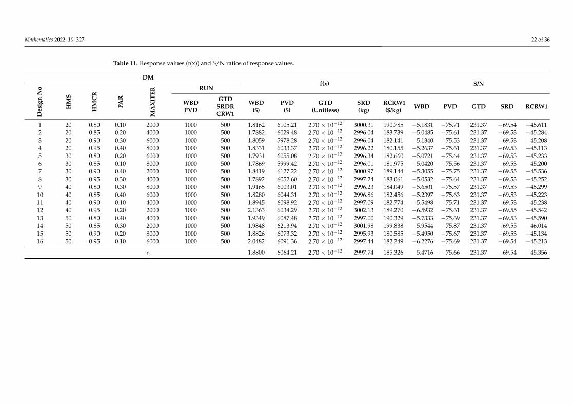
It is apparent from analyses that the most effective algorithm parameter for reachingthe best fitness value is mostly the RUN with S/N ratios and a change percentage ofparameter effect for the 5P case. Furthermore, the minimum objective function value isestimated via the TIHHSA, when the optimum RUN value equals 1000 for WBD and PVDand 500 for GTD, SRD, and RCRW1 problems. For this reason, the S/N ratios, variance,and optimum Taguchi parameter values have been repeated by analyses which are takenas fix values whose optimum RUN value for four parameters (the 4P case) to reasonablyobserve the parameter effect of the other design parameters. According to DM given inthe first section of Table 11, optimization analyzes have been performed and then responsevalues given in the second section of Table 11 have been obtained.

Mathematics 2022, 10, 327 22 of 36

Table 11. Response values (f(x)) and S/N ratios of response values.

DMf(x) S/N

Des

ign

No

HM

S

HM

CR

PAR

MA

XIT

ER

RUN

WBDPVD

GTDSRDRCRW1

WBD($)

PVD($)

GTD(Unitless)

SRD(kg)

RCRW1($/kg) WBD PVD GTD SRD RCRW1

1 20 0.80 0.10 2000 1000 500 1.8162 6105.21 2.70 × 10−12 3000.31 190.785 −5.1831 −75.71 231.37 −69.54 −45.6112 20 0.85 0.20 4000 1000 500 1.7882 6029.48 2.70 × 10−12 2996.04 183.739 −5.0485 −75.61 231.37 −69.53 −45.2843 20 0.90 0.30 6000 1000 500 1.8059 5978.28 2.70 × 10−12 2996.04 182.141 −5.1340 −75.53 231.37 −69.53 −45.2084 20 0.95 0.40 8000 1000 500 1.8331 6033.37 2.70 × 10−12 2996.22 180.155 −5.2637 −75.61 231.37 −69.53 −45.1135 30 0.80 0.20 6000 1000 500 1.7931 6055.08 2.70 × 10−12 2996.34 182.660 −5.0721 −75.64 231.37 −69.53 −45.2336 30 0.85 0.10 8000 1000 500 1.7869 5999.42 2.70 × 10−12 2996.01 181.975 −5.0420 −75.56 231.37 −69.53 −45.2007 30 0.90 0.40 2000 1000 500 1.8419 6127.22 2.70 × 10−12 3000.97 189.144 −5.3055 −75.75 231.37 −69.55 −45.5368 30 0.95 0.30 4000 1000 500 1.7892 6052.60 2.70 × 10−12 2997.24 183.061 −5.0532 −75.64 231.37 −69.53 −45.2529 40 0.80 0.30 8000 1000 500 1.9165 6003.01 2.70 × 10−12 2996.23 184.049 −5.6501 −75.57 231.37 −69.53 −45.29910 40 0.85 0.40 6000 1000 500 1.8280 6044.31 2.70 × 10−12 2996.86 182.456 −5.2397 −75.63 231.37 −69.53 −45.22311 40 0.90 0.10 4000 1000 500 1.8945 6098.92 2.70 × 10−12 2997.09 182.774 −5.5498 −75.71 231.37 −69.53 −45.23812 40 0.95 0.20 2000 1000 500 2.1363 6034.29 2.70 × 10−12 3002.13 189.270 −6.5932 −75.61 231.37 −69.55 −45.54213 50 0.80 0.40 4000 1000 500 1.9349 6087.48 2.70 × 10−12 2997.00 190.329 −5.7333 −75.69 231.37 −69.53 −45.59014 50 0.85 0.30 2000 1000 500 1.9848 6213.94 2.70 × 10−12 3001.98 199.838 −5.9544 −75.87 231.37 −69.55 −46.01415 50 0.90 0.20 8000 1000 500 1.8826 6073.32 2.70 × 10−12 2995.93 180.585 −5.4950 −75.67 231.37 −69.53 −45.13416 50 0.95 0.10 6000 1000 500 2.0482 6091.36 2.70 × 10−12 2997.44 182.249 −6.2276 −75.69 231.37 −69.54 −45.213

η 1.8800 6064.21 2.70 × 10−12 2997.74 185.326 −5.4716 −75.66 231.37 −69.54 −45.356

Mathematics 2022, 10, 327 23 of 36

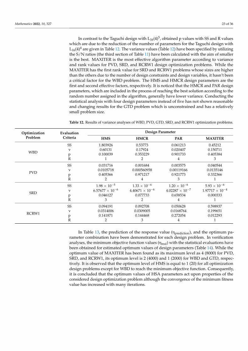
In contrast to the Taguchi design with L16(4)5, obtained p values with SS and R valueswhich are due to the reduction of the number of parameters for the Taguchi design withL16(4)4 are given in Table 12. The variance values (Table 12) have been specified by utilizingthe S/N ratios (the third section of Table 11) have been calculated with the aim of smalleris the best. MAXITER is the most effective algorithm parameter according to varianceand rank values for PVD, SRD, and RCRW1 design optimization problems. While theMAXITER has the first rank value for SRD and RCRW1 problems whose sizes are higherthan the others due to the number of design constraints and design variables, it hasn’t beena critical factor for the WBD problem. The HMS and HMCR design parameters are thefirst and second effective factors, respectively. It is noticed that the HMCR and PAR designparameters, which are included in the process of reaching the best solution according to therandom number assigned in the algorithm, generally have lower variance. Conducting thestatistical analysis with four design parameters instead of five has not shown reasonableand changing results for the GTD problem which is unconstrained and has a relativelysmall problem size.

Table 12. Results of variance analyses of WBD, PVD, GTD, SRD, and RCRW1 optimization problems.

OptimizationProblem

EvaluationCriteria

Design Parameter

HMS HMCR PAR MAXITER

WBD

SS 1.803926 0.53773 0.061213 0.45212ν 0.60131 0.17924 0.020407 0.150711p 0.100039 0.353229 0.901733 0.405384R 1 2 4 3

PVD

SS 0.031716 0.001684 0.003575 0.040544ν 0.0105718 0.000560958 0.00119166 0.0135146p 0.405366 0.971217 0.921773 0.332366R 2 4 3 1

SRD

SS 1.98 × 10−5 1.33 × 10−6 1.20 × 10−6 5.93 × 10−6

ν 6.57677 × 10−6 4.40671 × 10−6 4.02287 × 10−7 1.97717 × 10−4

p 0.046127 0.077733 0.658534 0.000333R 3 2 4 1

RCRW1

SS 0.094191 0.092708 0.050628 0.598937ν 0.0314006 0.0309005 0.0168764 0.199651p 0.141871 0.144468 0.272054 0.012293R 2 3 4 1

In Table 13, the prediction of the response value (ηprediction), and the optimum pa-rameter combination have been demonstrated for each design problem. In verificationanalyses, the minimum objective function values (ηreal) with the statistical evaluations havebeen obtained for estimated optimum values of design parameters (Table 14). While theoptimum value of MAXITER has been found as its maximum level as 4 (8000) for PVD,SRD, and RCRW1, its optimum level is 2 (4000) and 1 (2000) for WBD and GTD, respec-tively. It is observed that the optimum level of HMS is equal to 1 (20) for all optimizationdesign problems except for WBD to reach the minimum objective function. Consequently,it is concluded that the optimum values of HSA parameters act upon properties of theconsidered design optimization problem although the convergence of the minimum fitnessvalue has increased with many iterations.

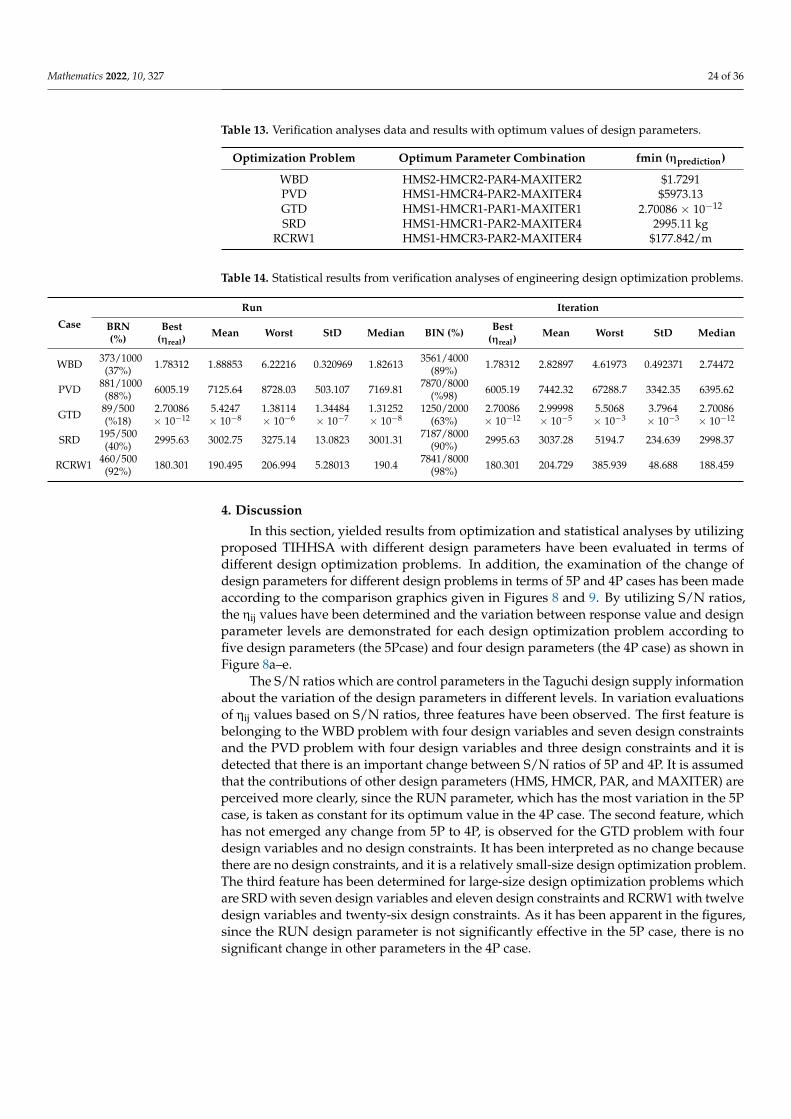
Mathematics 2022, 10, 327 24 of 36

Table 13. Verification analyses data and results with optimum values of design parameters.

Optimization Problem Optimum Parameter Combination fmin (ηprediction)

WBD HMS2-HMCR2-PAR4-MAXITER2 $1.7291PVD HMS1-HMCR4-PAR2-MAXITER4 $5973.13GTD HMS1-HMCR1-PAR1-MAXITER1 2.70086 × 10−12

SRD HMS1-HMCR1-PAR2-MAXITER4 2995.11 kgRCRW1 HMS1-HMCR3-PAR2-MAXITER4 $177.842/m

Table 14. Statistical results from verification analyses of engineering design optimization problems.

Case

Run Iteration

BRN(%)

Best(ηreal)

Mean Worst StD Median BIN (%) Best(ηreal)

Mean Worst StD Median

WBD 373/1000(37%) 1.78312 1.88853 6.22216 0.320969 1.82613 3561/4000

(89%) 1.78312 2.82897 4.61973 0.492371 2.74472

PVD 881/1000(88%) 6005.19 7125.64 8728.03 503.107 7169.81 7870/8000

(%98) 6005.19 7442.32 67288.7 3342.35 6395.62

GTD 89/500(%18)

2.70086× 10−12

5.4247× 10−8

1.38114× 10−6

1.34484× 10−7

1.31252× 10−8

1250/2000(63%)

2.70086× 10−12

2.99998× 10−5

5.5068× 10−3

3.7964× 10−3

2.70086× 10−12

SRD 195/500(40%) 2995.63 3002.75 3275.14 13.0823 3001.31 7187/8000

(90%) 2995.63 3037.28 5194.7 234.639 2998.37

RCRW1 460/500(92%) 180.301 190.495 206.994 5.28013 190.4 7841/8000

(98%) 180.301 204.729 385.939 48.688 188.459

4. Discussion

In this section, yielded results from optimization and statistical analyses by utilizingproposed TIHHSA with different design parameters have been evaluated in terms ofdifferent design optimization problems. In addition, the examination of the change ofdesign parameters for different design problems in terms of 5P and 4P cases has been madeaccording to the comparison graphics given in Figures 8 and 9. By utilizing S/N ratios,the ηij values have been determined and the variation between response value and designparameter levels are demonstrated for each design optimization problem according tofive design parameters (the 5Pcase) and four design parameters (the 4P case) as shown inFigure 8a–e.

The S/N ratios which are control parameters in the Taguchi design supply informationabout the variation of the design parameters in different levels. In variation evaluationsof ηij values based on S/N ratios, three features have been observed. The first feature isbelonging to the WBD problem with four design variables and seven design constraintsand the PVD problem with four design variables and three design constraints and it isdetected that there is an important change between S/N ratios of 5P and 4P. It is assumedthat the contributions of other design parameters (HMS, HMCR, PAR, and MAXITER) areperceived more clearly, since the RUN parameter, which has the most variation in the 5Pcase, is taken as constant for its optimum value in the 4P case. The second feature, whichhas not emerged any change from 5P to 4P, is observed for the GTD problem with fourdesign variables and no design constraints. It has been interpreted as no change becausethere are no design constraints, and it is a relatively small-size design optimization problem.The third feature has been determined for large-size design optimization problems whichare SRD with seven design variables and eleven design constraints and RCRW1 with twelvedesign variables and twenty-six design constraints. As it has been apparent in the figures,since the RUN design parameter is not significantly effective in the 5P case, there is nosignificant change in other parameters in the 4P case.

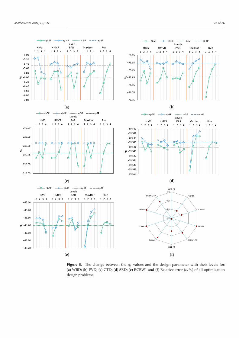
Mathematics 2022, 10, 327 25 of 36

Mathematics 2022, 10, x FOR PEER REVIEW 24 of 37

design parameters (the 5Pcase) and four design parameters (the 4P case) as shown in Fig-ure 8a–e.

(a) (b)

(c) (d)

(e) (f)

Figure 8. The change between the ηij values and the design parameter with their levels for: (a) WBD; (b) PVD; (c) GTD; (d) SRD; (e) RCRW1 and (f) Relative error (ε, %) of all optimization design prob-lems.

Figure 8. The change between the ηij values and the design parameter with their levels for:(a) WBD; (b) PVD; (c) GTD; (d) SRD; (e) RCRW1 and (f) Relative error (ε, %) of all optimizationdesign problems.

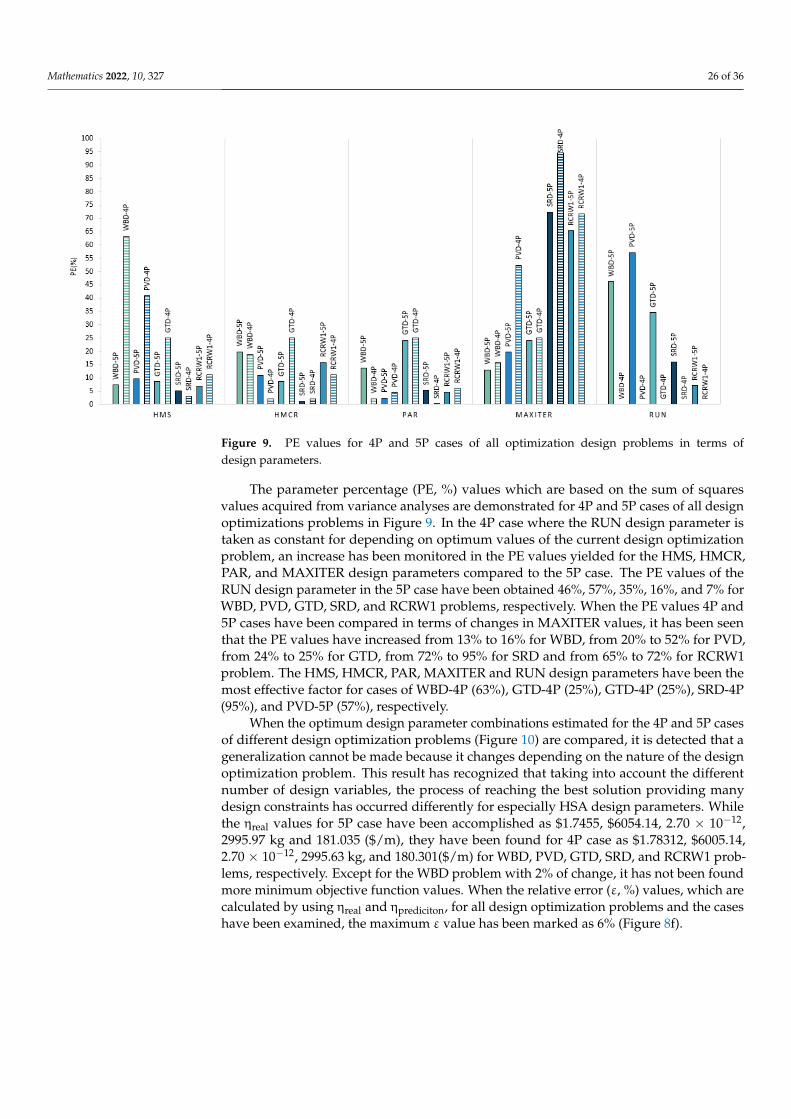
Mathematics 2022, 10, 327 26 of 36Mathematics 2022, 10, x FOR PEER REVIEW 25 of 37

Figure 9. PE values for 4P and 5P cases of all optimization design problems in terms of design pa-rameters.

The S/N ratios which are control parameters in the Taguchi design supply infor-mation about the variation of the design parameters in different levels. In variation eval-uations of ηij values based on S/N ratios, three features have been observed. The first fea-ture is belonging to the WBD problem with four design variables and seven design con-straints and the PVD problem with four design variables and three design constraints and it is detected that there is an important change between S/N ratios of 5P and 4P. It is as-sumed that the contributions of other design parameters (HMS, HMCR, PAR, and MAX-ITER) are perceived more clearly, since the RUN parameter, which has the most variation in the 5P case, is taken as constant for its optimum value in the 4P case. The second feature, which has not emerged any change from 5P to 4P, is observed for the GTD problem with four design variables and no design constraints. It has been interpreted as no change be-cause there are no design constraints, and it is a relatively small-size design optimization problem. The third feature has been determined for large-size design optimization prob-lems which are SRD with seven design variables and eleven design constraints and RCRW1 with twelve design variables and twenty-six design constraints. As it has been apparent in the figures, since the RUN design parameter is not significantly effective in the 5P case, there is no significant change in other parameters in the 4P case.

The parameter percentage (PE, %) values which are based on the sum of squares val-ues acquired from variance analyses are demonstrated for 4P and 5P cases of all design optimizations problems in Figure 9. In the 4P case where the RUN design parameter is taken as constant for depending on optimum values of the current design optimization problem, an increase has been monitored in the PE values yielded for the HMS, HMCR, PAR, and MAXITER design parameters compared to the 5P case. The PE values of the RUN design parameter in the 5P case have been obtained 46%, 57%, 35%, 16%, and 7% for WBD, PVD, GTD, SRD, and RCRW1 problems, respectively. When the PE values 4P and 5P cases have been compared in terms of changes in MAXITER values, it has been seen that the PE values have increased from 13% to 16% for WBD, from 20% to 52% for PVD, from 24% to 25% for GTD, from 72% to 95% for SRD and from 65% to 72% for RCRW1 problem. The HMS, HMCR, PAR, MAXITER and RUN design parameters have been the most effective factor for cases of WBD-4P (63%), GTD-4P (25%), GTD-4P (25%), SRD-4P (95%), and PVD-5P (57%), respectively.

When the optimum design parameter combinations estimated for the 4P and 5P cases of different design optimization problems (Figure 10) are compared, it is detected that a

Figure 9. PE values for 4P and 5P cases of all optimization design problems in terms ofdesign parameters.

The parameter percentage (PE, %) values which are based on the sum of squaresvalues acquired from variance analyses are demonstrated for 4P and 5P cases of all designoptimizations problems in Figure 9. In the 4P case where the RUN design parameter istaken as constant for depending on optimum values of the current design optimizationproblem, an increase has been monitored in the PE values yielded for the HMS, HMCR,PAR, and MAXITER design parameters compared to the 5P case. The PE values of theRUN design parameter in the 5P case have been obtained 46%, 57%, 35%, 16%, and 7% forWBD, PVD, GTD, SRD, and RCRW1 problems, respectively. When the PE values 4P and5P cases have been compared in terms of changes in MAXITER values, it has been seenthat the PE values have increased from 13% to 16% for WBD, from 20% to 52% for PVD,from 24% to 25% for GTD, from 72% to 95% for SRD and from 65% to 72% for RCRW1problem. The HMS, HMCR, PAR, MAXITER and RUN design parameters have been themost effective factor for cases of WBD-4P (63%), GTD-4P (25%), GTD-4P (25%), SRD-4P(95%), and PVD-5P (57%), respectively.

When the optimum design parameter combinations estimated for the 4P and 5P casesof different design optimization problems (Figure 10) are compared, it is detected that ageneralization cannot be made because it changes depending on the nature of the designoptimization problem. This result has recognized that taking into account the differentnumber of design variables, the process of reaching the best solution providing manydesign constraints has occurred differently for especially HSA design parameters. Whilethe ηreal values for 5P case have been accomplished as $1.7455, $6054.14, 2.70 × 10−12,2995.97 kg and 181.035 ($/m), they have been found for 4P case as $1.78312, $6005.14,2.70 × 10−12, 2995.63 kg, and 180.301($/m) for WBD, PVD, GTD, SRD, and RCRW1 prob-lems, respectively. Except for the WBD problem with 2% of change, it has not been foundmore minimum objective function values. When the relative error (ε, %) values, which arecalculated by using ηreal and ηprediciton, for all design optimization problems and the caseshave been examined, the maximum ε value has been marked as 6% (Figure 8f).

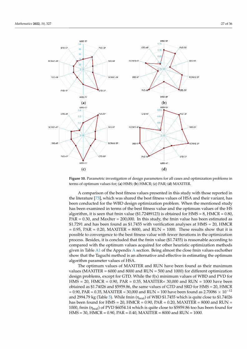
Mathematics 2022, 10, 327 27 of 36

Mathematics 2022, 10, x FOR PEER REVIEW 26 of 37

generalization cannot be made because it changes depending on the nature of the design optimization problem. This result has recognized that taking into account the different number of design variables, the process of reaching the best solution providing many de-sign constraints has occurred differently for especially HSA design parameters. While the ηreal values for 5P case have been accomplished as $1.7455, $6054.14, 2.70 × 10−12, 2995.97 kg and 181.035 ($/m), they have been found for 4P case as $1.78312, $6005.14, 2.70 × 10−12, 2995.63 kg, and 180.301($/m) for WBD, PVD, GTD, SRD, and RCRW1 problems, respec-tively. Except for the WBD problem with 2% of change, it has not been found more mini-mum objective function values. When the relative error (ε, %) values, which are calculated by using ηreal and ηprediciton, for all design optimization problems and the cases have been examined, the maximum ε value has been marked as 6% (Figure 8f).

(a) (b)

(c) (d)

Figure 10. Parametric investigation of design parameters for all cases and optimization problems in terms of optimum values for; (a) HMS; (b) HMCR; (c) PAR; (d) MAXITER.

A comparison of the best fitness values presented in this study with those reported in the literature [55], which was shared the best fitness values of HSA and their variant, has been conducted for the WBD design optimization problem. When the mentioned study has been examined in terms of the best fitness value and the optimum values of the HS algorithm, it is seen that fmin value ($1.72489123) is obtained for HMS = 8, HMCR = 0.80, PAR = 0.30, and MaxIter = 200,000. In this study, the fmin value has been estimated as $1.7291 and has been found as $1.7455 with verification analyses at HMS = 20, HMCR = 0.95, PAR = 0.20, MAXITER = 8000, and RUN = 1000. These results show that it is possible to convergence to the best fitness value with fewer iterations in the optimization process. Besides, it is concluded that the fmin value ($1.7455) is reasonable according to compared with the optimum values acquired for other heuristic optimization methods given in Ta-ble A1 of the Appendix A section. Being almost the close fmin values eachother show that the Taguchi method is an alternative and effective in estimating the optimum algorithm parameter values of HSA.

Figure 10. Parametric investigation of design parameters for all cases and optimization problems interms of optimum values for; (a) HMS; (b) HMCR; (c) PAR; (d) MAXITER.

A comparison of the best fitness values presented in this study with those reported inthe literature [73], which was shared the best fitness values of HSA and their variant, hasbeen conducted for the WBD design optimization problem. When the mentioned studyhas been examined in terms of the best fitness value and the optimum values of the HSalgorithm, it is seen that fmin value ($1.72489123) is obtained for HMS = 8, HMCR = 0.80,PAR = 0.30, and MaxIter = 200,000. In this study, the fmin value has been estimated as$1.7291 and has been found as $1.7455 with verification analyses at HMS = 20, HMCR= 0.95, PAR = 0.20, MAXITER = 8000, and RUN = 1000. These results show that it ispossible to convergence to the best fitness value with fewer iterations in the optimizationprocess. Besides, it is concluded that the fmin value ($1.7455) is reasonable according tocompared with the optimum values acquired for other heuristic optimization methodsgiven in Table A1 of the Appendix A section. Being almost the close fmin values eachothershow that the Taguchi method is an alternative and effective in estimating the optimumalgorithm parameter values of HSA.

The optimum values of MAXITER and RUN have been found as their maximumvalues (MAXITER = 6000 and 8000 and RUN = 500 and 1000) for different optimizationdesign problems, except for GTD. While the f(x) minimum values of WBD and PVD forHMS = 20, HMCR = 0.90, PAR = 0.35, MAXITER= 30,000 and RUN = 1000 have beenobtained as $1.74026 and $5959.86, the same values of GTD and SRD for HMS = 20, HMCR= 0.90, PAR = 0.35, MAXITER = 30,000 and RUN = 100 have been found as 2.70086 × 10−12

and 2994.79 kg (Table 5). While fmin (ηreal) of WBD $1.7455 which is quite close to $1.74026has been found for HMS = 20, HMCR = 0.90, PAR = 0.20, MAXITER = 8000 and RUN =1000, fmin (ηreal) of PVD $6054.14 which is quite close to $5959.86 too has been found forHMS = 30, HMCR = 0.90, PAR = 0.40, MAXITER = 8000 and RUN = 1000.

Mathematics 2022, 10, 327 28 of 36

5. Conclusions

In this study, optimum values of harmony search algorithm (HSA) design parameters,which are the harmony memory size (HMS), the harmony memory consideration rate(HMCR), the pitch adjustment rate (PAR), maximum iteration number (MAXITER), and theindependent run number of whole iterations (RUN), have been investigated for complexbenchmark engineering design problems (the welded beam (WBD), the pressure vessel(PVD), the gear train (GTD), and the speed reducer (SRD)) and complicated real-sizereinforcement cantilever retaining wall (RCRW) design problem. To examine the optimumvalues of algorithm design parameters, the Taguchi method integrated hybrid harmonysearch algorithm (TIHHSA) has been presented as a new hybrid method based on theTaguchi Method which is a statistical-based experiment procedure utilized in boostingalgorithmic quality. In addition, the effect of algorithm design parameters on the best fitnessvalue and characteristics of the optimization problem has been studied. The results yieldedaccording to the optimum algorithm design parameters and the best fitness values, whosevalues do not change with repetitive statistical, and optimization analyzes for differentengineering design optimization problems, are as follows;

Accomplished results from the Taguchi analyses show that converging to the bestfitness value is possible with fewer iteration numbers in a shorter time;

• The obtained estimations have a reasonable relative error in determining optimumvalues of algorithm design parameters without performing many trials;

• It has been seen that the optimum values of the algorithm design parameters vary de-pending on the nature of the design optimization problem, which includes the numberof design variables, the number of design constraints, exposure to the constraints.

• Instead of taking into account the value of the algorithm parameter proposed for char-acteristically different optimization problems in the literature, it has been concludedthat using the optimum values yielded statistically according to the nature of theproblem is an effective and prosperous manner in converging to the optimum.

• Instead of the trial-error method, which is time-consuming and exhaustive, it hasbeen concluded that the newly proposed TIHHSA is a robust and reliable methodfor estimating the optimum algorithm parameter values of the harmony search meta-heuristic optimization technique in a shorter time without conducting sensitivityanalyses which are utilized to increase convergence rate in the solution of the designoptimization problem.

Author Contributions: Conceptualization, E.U.; methodology, E.U. and S.C.; software, E.U.; valida-tion, S.C.; writing—original draft preparation, E.U.; writing—review and editing, E.U, S.C., Z.W.G.and S.K.; supervision, Z.W.G. and S.K.; funding acquisition, Z.W.G. All authors have read and agreedto the published version of the manuscript.

Funding: This work was supported by a National Research Foundation of Korea (NRF) grant fundedby the Korean government (MSIT) (2020R1A2C1A01011131). This research was also supported by theEnergy Cloud R&D Program through the National Research Foundation of Korea (NRF) funded bythe Ministry of Science, ICT (2019M3F2A1073164).

Institutional Review Board Statement: Not applicable.

Informed Consent Statement: Not applicable.

Data Availability Statement: Not applicable.

Conflicts of Interest: The authors declare no conflict of interest.

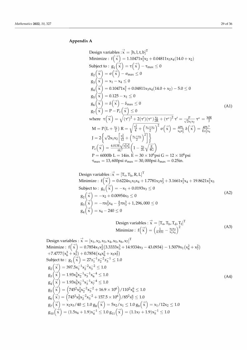
Mathematics 2022, 10, 327 29 of 36

Appendix A

Design variables :→x = [h, l, t, b]T

Minimize : f(→

x)= 1.10471x2

1x2 + 0.04811x3x4(14.0 + x2)

Subject to : g1

(→x)= τ

(→x)− τmax ≤ 0

g2

(→x)= σ

(→x)− σmax ≤ 0

g3

(→x)= x1 − x4 ≤ 0

g4

(→x)= 0.10471x2

1 + 0.04811x3x4(14.0 + x2)− 5.0 ≤ 0

g5

(→x)= 0.125− x1 ≤ 0

g6

(→x)= δ

(→x)− δmax ≤ 0

g7

(→x)= P− Pc

(→x)≤ 0

where τ(→

x)=√(τ′)2 + 2(τ′)(τ′′ ) x2

2R + (τ′′ )2 τ′ = P√2x1x2

τ′′ = MRJ

M = P(L + x2

2)

R =

√x2

24 +

(x1+x3

2

)2σ(→

x)= 6PL

x4x23δ(→

x)= 4PL3

Ex33x4

J = 2{√

2x1x2

[x2

212 +

(x1+x3

2

)2]}

Pc

(→x)=

4.013E√

x23x6

46L2

(1− x3

2L

√E

4G

)P = 6000lb L = 14in. E = 30× 106psi G = 12× 106psiτmax = 13, 600psi σmax = 30, 000psi δmax = 0.25in.

(A1)

Design variables :→x = [Ts, Th, R, L]T

Minimize : f(→

x)= 0.6224x1x3x4 + 1.7781x2x2

3 + 3.1661x21x4 + 19.8621x2

1x3

Subject to : g1

(→x)= −x1 + 0.0193x3 ≤ 0

g2

(→x)= −x2 + 0.00954x3 ≤ 0

g3

(→x)= −πx2

3x4 − 43πx3

3 + 1, 296, 000 ≤ 0

g4

(→x)= x4 − 240 ≤ 0

(A2)

Design variables :→x = [Ta, Tb, Td, Tf]

T

Minimize : f(→

x)=(

16.931 −

x2x3x1x4

)2 (A3)

Design variables :→x = [x1, x2, x3, x4, x5, x6, x7]

T

Minimize : f(→

x)= 0.7854x1x2

2(3.3333x3

3 + 14.9334x3 − 43.0934)− 1.5079x1

(x2

6 + x27)

+7.4777(x3

6 + x37)+ 0.7854

(x4x2

6 + x5x27)

Subject to : g1

(→x)= 27x−1

1 x−22 x−1

3 ≤ 1.0

g2

(→x)= 397.5x−1

1 x−22 x−2

3 ≤ 1.0

g3

(→x)= 1.93x3

4x−12 x−1

3 x−46 ≤ 1.0

g4

(→x)= 1.93x3

5x−12 x−1

3 x−47 ≤ 1.0

g5

(→x)=(

7452x24x−2

2 x−23 + 16.9× 106

)/1102x6

6 ≤ 1.0

g6

(→x ) =

(7452x2

5x−22 x−2

3 + 157.5× 106)

/852x67 ≤ 1.0

g7

(→x)= x2x3/40 ≤ 1.0 g8

(→x)= 5x2/x1 ≤ 1.0 g9

(→x)= x1/12x2 ≤ 1.0

g10

(→x)= (1.5x6 + 1.9)x−1

4 ≤ 1.0 g11

(→x)= (1.1x7 + 1.9)x−1

5 ≤ 1.0

(A4)

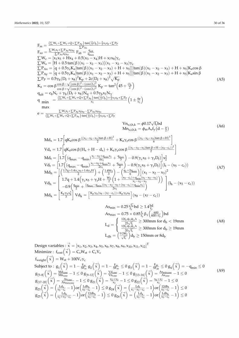
Mathematics 2022, 10, 327 30 of 36

Fss =(∑ Wc+∑ Ws+Q+∑ PAy) tan( 2

3 Ob)+ 23 x1cb+∑ PP

∑ PAx

Fso =∑ Wixi+∑ PAyxPAy

∑ PAxxPAxFsb =

qultqmax

∑ Wc = [x1x5 + Hx4 + 0.5(x3 − x4)H + x7x8]γc∑ Ws = [H + 0.5 tan(β)(x1 − x2 − x3)](x1 − x2 − x3)γr∑ PAx = [q + 0.5γrKa[tan(β)(x1 − x2 − x3) + H + x5]][tan(β)(x1 − x2 − x3) + H + x5]Kacosβ∑ PAy = [q + 0.5γrKa[tan(β)(x1 − x2 − x3) + H + x5]][tan(β)(x1 − x2 − x3) + H + x5]Kasinβ∑ PP = 0.5γb(Df + x8)

2Kp + 2c(Df + x8)2√Kp

Ka = cosβ cosβ−√

(cosβ)2−(cos Or)2

cosβ+√

(cosβ)2−(cos Or)2 Kp = tan2

(45 + Ob

2

)qult = cbNc + γb(Df + x8)Nq + 0.5γbx1Nγ

q minmax

=(∑ Wc+∑ Ws+Q+∑ PAy) tan( 2

3 Ob)+ 23 x1cb+∑ PP

x1

(1± 6e

x1

)e =

∑ Wixi+∑ PAyxPAy−∑ PAxxPAx

(∑ Wc+∑ Ws+Q+∑ PAy) tan( 23 Ob)+ 2

3 x1cb+∑ PP

(A5)

Vns,t,h,k = φ0.17√

fcbdMns,t,h,k = φmAsfy

(d− a

2) (A6)

Mds = 1.7[

qKacosβ ((x1−x2−x3)tanβ+H)2

2 + Kaγrcosβ ((x1−x2−x3)tanβ+H)3

6

]Vds = 1.7

[qKacosβ(Hs + H− ds) + Kaγrcosβ ((x1−x2−x3)tanβ+H−(x5−cc))

2

2

]Mdt =

[1.7((qmax − qmin)

x1−x2+qminx16x1

+qmax

3

)− 0.9(γcx5 + γrDf)

]x2

2

Vdt =[1.7((qmax − qmin)

x1−x2+qminx12x1

+qmax

2

)− 0.9(γcx5 + γrDf)

](lt − (x5 − cc))

Mdh =[(

1.7q+1.4γcx5+1.4γrH2

)+(

1.4W53

)−(

q1+2qmin6

)](x1 − x2 − x3)

2

Vdh =

1.7q + 1.4(γcx5 + γrH + W5

2

(1 + (x5−cc)+qmin(x1−x2−x3)

x1−x2−x3

))−0.9

(qmin

2 +(qmax−qmin)(x1−x2−x3+(x5−cc)+qminx1)

2x1

) (lh − (x5 − cc))

Mdk =

[Kpγbx3

83

]Vdk =

[Kpγb(x8−(x7−cc))+Kpγbx8

2

](x8 − (x7 − cc))

(A7)

Asmin = 0.25√

fcfy

bd ≥ 1.4 bdfy

Asmax = 0.75× 0.85 fcfyβ1

(600

600+fy

)bd

Ld =

12fyψtψeλ

25√

fc≥ 300mm for db < 19mm

12fyψtψeλ

20√

fc≥ 300mm for db ≥ 19mm

Ldh =(

0.24fy√fc

)db ≥ 150mm or 8db

(A8)

Design variables :→x = [x1, x2, x3, x4, x5, x6, x7, x8, x9, x10, x11, x12]

T

Minimize : fcost

(→x)= CsWst + CcVc

fweight

(→x)= Wst + 100Vcγc

Subject to : g1

(→x)= 1− Fss

SFssg2

(→x)= 1− Fso

SFso≤ 0 g3

(→x)= 1− Fsb

SFsb≤ 0 g4

(→x)= −qmin ≤ 0

g[5–8]

(→x)= Mdcase

Mncase− 1 ≤ 0 g[9–12]

(→x)= Vdcase

Vncase− 1 ≤ 0 g[13–16]

(→x)= Asmincase

Ascase− 1 ≤ 0

g[17–20]

(→x)= Ascase

Asmaxcase− 1 ≤ 0 g21

(→x)= x2+x3

x1− 1 ≤ 0 g22

(→x)= x6+x7

x1− 1 ≤ 0

g23

(→x)=(

Ldsx5−cc

− 1)

or(

Ldhsx5−cc

− 1)≤ 0 g24

(→x)=(

Ldtx1−x2−cc

− 1)

or(

12dbtx5−cc

− 1)≤ 0

g25

(→x)=(

Ldhx2+x3−cc

− 1)

or(

12dbhx5−cc

− 1)≤ 0 g26

(→x)=(

Ldkx5−cc

− 1)

or(

Ldhkx5−cc

− 1)≤ 0

(A9)

Mathematics 2022, 10, 327 31 of 36

Table A1. Optimum values and comparison of the best solutions in literature for WBD.

Optimum Solutions x1(h)(in.) x2(l) (in.) x3(t) (in.) x4(b) (in.) f(x) ($)

Lite

ratu

re

Ragsdell and Phillips [50] 0.24550 6.1960 8.2730 0.2455 2.38593Deb [51] 0.2489 6.173 8.1789 0.2533 2.433116

Coello [52] 0.2088 3.4205 8.9975 0.21 1.7483Huang et al. [53] 0.203137 3.542998 9.033498 0.206179 1.73346

Yildiz [54] 0.20573 3.47042 9.03649 0.205735 1.7248Çarbas and Saka [55] 0.203907 3.499898 9.063898 0.205594 1.72966

Cas

ePS

R30 0.206741 3.65285 8.54856 0.231265 1.85149R100 0.171535 4.42418 8.98313 0.208289 1.80231R500 0.198864 3.66442 8.94678 0.209895 1.75598

R1000 0.19823 3.64539 9.02857 0.206407 1.74026WBD-5P 0.195872 3.70387 9.07235 0.205574 1.7455WBD-4P 0.188171 3.95948 8.91723 0.21133 1.78312

PS Present study.

Table A2. Optimum values and comparison of the best solutions in literature for PVD.

Optimum Solutions x1(Ts) (in.) x2(Th)(in.) x3(R) (in.) x4(L) (in.) f(x) ($)

Lite

ratu

re

Sandgren [35] 1.125 0.625 48.97 106.72 7982.5Kannan and Kramer [56] 1.25 0.625 50 120 7198.20

Deb [57] 0.9375 0.50 48.329 112.679 6410.381Coello [52] 0.8125 0.4375 40.3239 200.0 6288.7445

Gao et al. [58] 0.75 0.375 38.8441 221.612 5852.639Çarbas and Saka [55] 0.8125 0.4375 42.09845 176.6366 6059.7143

Cas

ePS

R30 0.876366 0.434563 45.3293 140.344 6089.66R100 0.915835 0.454142 47.2497 121.872 6195.1R500 0.833985 0.413952 43.1577 163.94 6000.09

R1000 0.814181 0.403799 42.1533 176.032 5959.86PVD-5P 0.84119 0.430252 43.5749 159.245 6054.14PVD-4P 0.822121 0.409189 42.367 173.44 6005.19

PS Present study.

Table A3. Optimum values and comparison of the best solutions in literature for GTD.

Optimum Solutions x1(Ta)(piece)

x2(Tb)(piece)

x3(Td)(piece)

x4 (Tf)(piece) Gear ratio f(x) (unitless)

Lite

ratu

re

Zhang and Wang [59] 43 16 19 49 0.1442 2.36 × 10−9

Deb and Goyal [60] 33 14 17 50 0.1442 1.362 × 10−9

Parsopoulos and Vrahatis [61] 43 16 19 49 0.1442 2.701 × 10−12

Gandomi [62] 43 16 19 49 0.1442 2.701 × 10−12

Arora et al. [63] 43 16 19 49 0.1442 2.701 × 10−12

Deniz [64] 43 16 19 49 0.1442 2.701 × 10−12

Cas

ePS

R30 44 13 21 43 0.144292 1.54505 × 10−10

R100 43 16 19 49 0.144281 2.70086 × 10−12

R500 49 16 19 43 0.144281 2.70086 × 10−12

R1000 49 16 19 43 0.144281 2.70086 × 10−12

GTD-5P 49 16 19 43 0.144281 2.70086 × 10−12

GTD-4P 49 16 19 43 0.144281 2.70086 × 10−12

PS Present study.

Mathematics 2022, 10, 327 32 of 36

Table A4. Optimum values and comparison of the best solutions in literature for SRD.

Optimum Solutions x1 (cm) x2 (cm) x3 (piece) x4 (cm) x5 (cm) x6 (cm) x7 (cm) f(x) (kg)

Lite

ratu

re

Li and Papalambros[65] 3.50 0.70 17.00 7.30 7.71 3.3500000 5.2900000 2996.30977

Kuang et al. [66] 3.60 0.70 17.00 7.30 7.80 3.4000000 5.0000000 2876.22Azarm and Li [67] 3.50 0.70 17.00 7.30 7.71 3.3500000 5.2900000 2996.30978Vanderplaats [68] 3.50 0.70 17.00 7.30 7.30 3.3502145 5.2865176 2985.15188

Ray [69] 3.50 0.70 17.00 7.30 7.30 3.3502145 5.2865176 2985.15188Carbas et al. [70] 3.50 0.70 17.00 7.17984 7.70889 3.35009 5.28668 2993.13917

Cas

ePS

R30 3.5001 0.700016 17.0017 7.30052 7.71562 3.35025 5.28667 2994.93R100 3.50014 0.700021 17.0002 7.30117 7.71637 3.35053 5.28667 2994.79R500 3.50029 0.700019 17.0001 7.3009 7.71572 3.35053 5.28681 2994.90

R1000 3.50025 0.700016 17.0004 7.30034 7.71652 3.35036 5.28673 2994.84SRD-5P 3.50184 0.700073 17.0008 7.3036 7.72133 3.35036 5.28679 2995.97SRD-4P 3.50006 0.700006 17.0034 7.30108 7.71868 3.3516 5.28677 2995.63

PS Present study.

Table A5. Constraint values of WBD, PVD, and SRD optimization problems.

R30 R100 R500 R1000 5P 4P R30 R100 R500 R1000 5P 4P

WBD

g1(x) −8.821 −0.086 −7.948 −7.525 −65.745 −32.706

SRD

g1(x) 0.92592 0.92598 0.92595 0.92595 0.92536 0.92587g2(x) −178.142 −14.670 −1.819 −45.079 −213.275 −7.722 g2(x) 0.80178 0.80190 0.80188 0.80187 0.80134 0.80165g3(x) −0.025 −0.037 −0.011 −0.008 −0.010 −0.023 g3(x) 0.50085 0.50086 0.50081 0.50079 0.50141 0.50012g4(x) −3.317 −3.338 −3.400 −3.414 −3.407 −3.368 g4(x) 0.09535 0.09539 0.09536 0.09539 0.09555 0.09545g5(x) −0.082 −0.047 −0.074 −0.073 −0.071 −0.063 g5(x) 0.99994 0.99944 0.99944 0.99974 0.99975 0.99752g6(x) −0.235 −0.235 −0.235 −0.236 −0.236 −0.235 g6(x) 0.99998 0.99998 0.99982 0.99991 0.99985 0.99987g7(x) −2211.802 −202.416 −330.005 −55.908 −1.921 −446.574 g7(x) 0.29754 0.29751 0.29751 0.29751 0.29755 0.29756

PVD

g1(x) −0.002 −0.002 −0.004 −0.001 −0.001 0.000 g8(x) 0.99999 0.99999 0.99994 0.99995 0.99958 0.99999g2(x) −0.002 −0.002 −0.003 −0.002 −0.002 −0.015 g9(x) 0.41667 0.41667 0.41669 0.41669 0.41684 0.41667g3(x) −89.466 −89.466 −636.323 −9.038 −412.835 −498.618 g10(x) 0.94861 0.94859 0.94862 0.94866 0.94824 0.94882g4(x) −99.656 −99.656 −118.128 −76.060 −63.968 −80.755 g11(x) 0.99996 0.99987 0.99997 0.99986 0.99924 0.99958

Table A6. Optimum values of RCRW design for the optimum cost (RCRW1).

OptimumSolutions

x1(m)

x2(m)

x3(m)

x4(m)

x5(m)

x6(m)

x7(m)

x8(cm2)

x9(cm2)

x10(cm2)

x11(cm2)

x12(cm2)

f(x)($/kg)

Lite

ratu

re

Gandomi[40] 2.709 1 0.412 0.25 0.4 2.455 0.2 0.2 21.9911 11.7809 11.7809 4.7124 163.98

Gandomi[40] 2.727 1.035 0.36 0.28 0.401 2.274 0.293 0.296 32.1699 13.3517 13.8544 8.6394 182.79

Gandomi[40] 2.816 0.988 0.447 0.294 0.422 2.223 0.367 0.203 21.9911 15.2681 15.2681 12.7234 185.05

Gandomi[40] 2.694 0.836 0.403 0.27 0.405 2.346 0.227 0.445 23.7504 12.7234 22.6195 26.1380 182.84

Cas

ePS

R30 3.3439 1.1598 0.3526 0.2504 0.4 2.5435 0.2002 0.2 21.2999 14.3212 18.8016 7.1532 180.082R100 3.3431 1.1596 0.3917 0.25 0.4001 2.4623 0.2001 0.2002 18.8963 14.2586 18.9194 9.5172 179.842R500 3.3351 1.1593 0.4418 0.25 0.4001 3.0523 0.2004 0.2002 16.6776 14.3189 16.557 7.2319 179.449R1000 3.3394 1.1593 0.3916 0.2501 0.4 2.7275 0.2004 0.2003 18.691 14.392 18.7638 7.2583 179.693

RCRW1−5P 3.36761 1.15955 0.391877 0.250366 0.400094 2.84595 0.200248 0.201545 18.7689 14.4128 18.7273 10.0995 181.035RCRW1−4P 3.34757 1.15992 0.394711 0.250081 0.400157 2.37294 0.202173 0.201494 18.7718 14.1765 18.7523 9.34978 180.301

PS Present study.

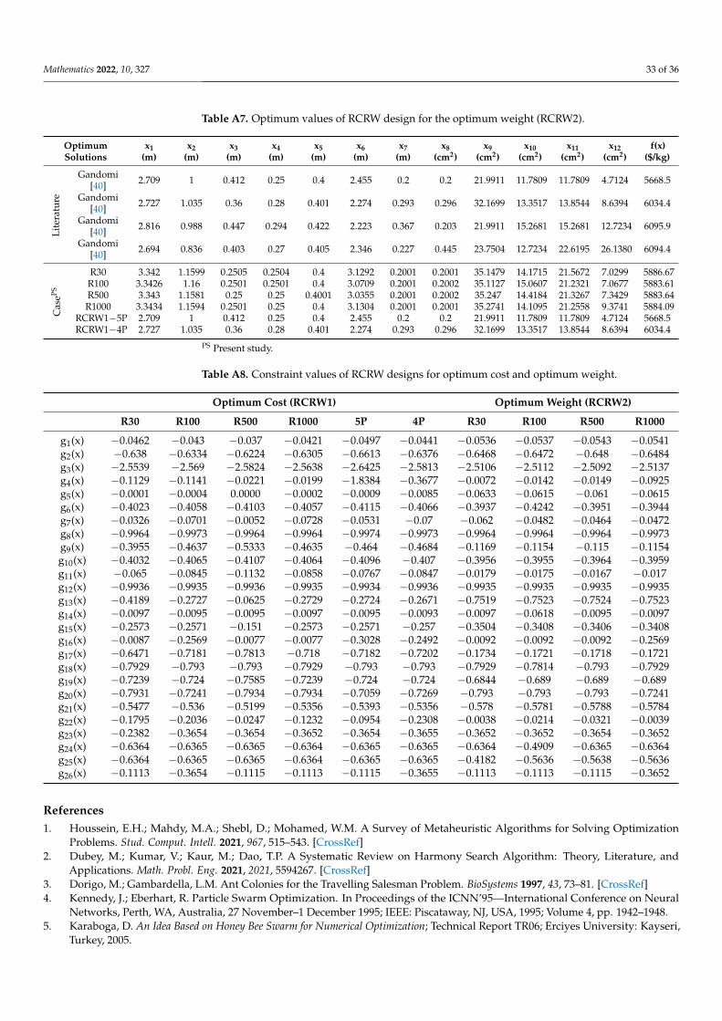
Mathematics 2022, 10, 327 33 of 36

Table A7. Optimum values of RCRW design for the optimum weight (RCRW2).

OptimumSolutions

x1(m)

x2(m)

x3(m)

x4(m)

x5(m)

x6(m)

x7(m)

x8(cm2)

x9(cm2)

x10(cm2)

x11(cm2)

x12(cm2)

f(x)($/kg)

Lite

ratu

re

Gandomi[40] 2.709 1 0.412 0.25 0.4 2.455 0.2 0.2 21.9911 11.7809 11.7809 4.7124 5668.5

Gandomi[40] 2.727 1.035 0.36 0.28 0.401 2.274 0.293 0.296 32.1699 13.3517 13.8544 8.6394 6034.4

Gandomi[40] 2.816 0.988 0.447 0.294 0.422 2.223 0.367 0.203 21.9911 15.2681 15.2681 12.7234 6095.9

Gandomi[40] 2.694 0.836 0.403 0.27 0.405 2.346 0.227 0.445 23.7504 12.7234 22.6195 26.1380 6094.4

Cas

ePS

R30 3.342 1.1599 0.2505 0.2504 0.4 3.1292 0.2001 0.2001 35.1479 14.1715 21.5672 7.0299 5886.67R100 3.3426 1.16 0.2501 0.2501 0.4 3.0709 0.2001 0.2002 35.1127 15.0607 21.2321 7.0677 5883.61R500 3.343 1.1581 0.25 0.25 0.4001 3.0355 0.2001 0.2002 35.247 14.4184 21.3267 7.3429 5883.64R1000 3.3434 1.1594 0.2501 0.25 0.4 3.1304 0.2001 0.2001 35.2741 14.1095 21.2558 9.3741 5884.09

RCRW1−5P 2.709 1 0.412 0.25 0.4 2.455 0.2 0.2 21.9911 11.7809 11.7809 4.7124 5668.5RCRW1−4P 2.727 1.035 0.36 0.28 0.401 2.274 0.293 0.296 32.1699 13.3517 13.8544 8.6394 6034.4

PS Present study.

Table A8. Constraint values of RCRW designs for optimum cost and optimum weight.

Optimum Cost (RCRW1) Optimum Weight (RCRW2)

R30 R100 R500 R1000 5P 4P R30 R100 R500 R1000

g1(x) −0.0462 −0.043 −0.037 −0.0421 −0.0497 −0.0441 −0.0536 −0.0537 −0.0543 −0.0541g2(x) −0.638 −0.6334 −0.6224 −0.6305 −0.6613 −0.6376 −0.6468 −0.6472 −0.648 −0.6484g3(x) −2.5539 −2.569 −2.5824 −2.5638 −2.6425 −2.5813 −2.5106 −2.5112 −2.5092 −2.5137g4(x) −0.1129 −0.1141 −0.0221 −0.0199 −1.8384 −0.3677 −0.0072 −0.0142 −0.0149 −0.0925g5(x) −0.0001 −0.0004 0.0000 −0.0002 −0.0009 −0.0085 −0.0633 −0.0615 −0.061 −0.0615g6(x) −0.4023 −0.4058 −0.4103 −0.4057 −0.4115 −0.4066 −0.3937 −0.4242 −0.3951 −0.3944g7(x) −0.0326 −0.0701 −0.0052 −0.0728 −0.0531 −0.07 −0.062 −0.0482 −0.0464 −0.0472g8(x) −0.9964 −0.9973 −0.9964 −0.9964 −0.9974 −0.9973 −0.9964 −0.9964 −0.9964 −0.9973g9(x) −0.3955 −0.4637 −0.5333 −0.4635 −0.464 −0.4684 −0.1169 −0.1154 −0.115 −0.1154g10(x) −0.4032 −0.4065 −0.4107 −0.4064 −0.4096 −0.407 −0.3956 −0.3955 −0.3964 −0.3959g11(x) −0.065 −0.0845 −0.1132 −0.0858 −0.0767 −0.0847 −0.0179 −0.0175 −0.0167 −0.017g12(x) −0.9936 −0.9935 −0.9936 −0.9935 −0.9934 −0.9936 −0.9935 −0.9935 −0.9935 −0.9935g13(x) −0.4189 −0.2727 −0.0625 −0.2729 −0.2724 −0.2671 −0.7519 −0.7523 −0.7524 −0.7523g14(x) −0.0097 −0.0095 −0.0095 −0.0097 −0.0095 −0.0093 −0.0097 −0.0618 −0.0095 −0.0097g15(x) −0.2573 −0.2571 −0.151 −0.2573 −0.2571 −0.257 −0.3504 −0.3408 −0.3406 −0.3408g16(x) −0.0087 −0.2569 −0.0077 −0.0077 −0.3028 −0.2492 −0.0092 −0.0092 −0.0092 −0.2569g17(x) −0.6471 −0.7181 −0.7813 −0.718 −0.7182 −0.7202 −0.1734 −0.1721 −0.1718 −0.1721g18(x) −0.7929 −0.793 −0.793 −0.7929 −0.793 −0.793 −0.7929 −0.7814 −0.793 −0.7929g19(x) −0.7239 −0.724 −0.7585 −0.7239 −0.724 −0.724 −0.6844 −0.689 −0.689 −0.689g20(x) −0.7931 −0.7241 −0.7934 −0.7934 −0.7059 −0.7269 −0.793 −0.793 −0.793 −0.7241g21(x) −0.5477 −0.536 −0.5199 −0.5356 −0.5393 −0.5356 −0.578 −0.5781 −0.5788 −0.5784g22(x) −0.1795 −0.2036 −0.0247 −0.1232 −0.0954 −0.2308 −0.0038 −0.0214 −0.0321 −0.0039g23(x) −0.2382 −0.3654 −0.3654 −0.3652 −0.3654 −0.3655 −0.3652 −0.3652 −0.3654 −0.3652g24(x) −0.6364 −0.6365 −0.6365 −0.6364 −0.6365 −0.6365 −0.6364 −0.4909 −0.6365 −0.6364g25(x) −0.6364 −0.6365 −0.6365 −0.6364 −0.6365 −0.6365 −0.4182 −0.5636 −0.5638 −0.5636g26(x) −0.1113 −0.3654 −0.1115 −0.1113 −0.1115 −0.3655 −0.1113 −0.1113 −0.1115 −0.3652

References1. Houssein, E.H.; Mahdy, M.A.; Shebl, D.; Mohamed, W.M. A Survey of Metaheuristic Algorithms for Solving Optimization

Problems. Stud. Comput. Intell. 2021, 967, 515–543. [CrossRef]2. Dubey, M.; Kumar, V.; Kaur, M.; Dao, T.P. A Systematic Review on Harmony Search Algorithm: Theory, Literature, and

Applications. Math. Probl. Eng. 2021, 2021, 5594267. [CrossRef]3. Dorigo, M.; Gambardella, L.M. Ant Colonies for the Travelling Salesman Problem. BioSystems 1997, 43, 73–81. [CrossRef]4. Kennedy, J.; Eberhart, R. Particle Swarm Optimization. In Proceedings of the ICNN’95—International Conference on Neural

Networks, Perth, WA, Australia, 27 November–1 December 1995; IEEE: Piscataway, NJ, USA, 1995; Volume 4, pp. 1942–1948.5. Karaboga, D. An Idea Based on Honey Bee Swarm for Numerical Optimization; Technical Report TR06; Erciyes University: Kayseri,

Turkey, 2005.

Mathematics 2022, 10, 327 34 of 36

6. Mirjalili, S.; Lewis, A. The Whale Optimization Algorithm. Adv. Eng. Softw. 2016, 95, 51–67. [CrossRef]7. Rashedi, E.; Nezamabadi-pour, H.; Saryazdi, S. GSA: A Gravitational Search Algorithm. Inf. Sci. 2009, 179, 2232–2248. [CrossRef]8. Erol, O.K.; Eksin, I. A New Optimization Method: Big Bang–Big Crunch. Adv. Eng. Softw. 2006, 37, 106–111. [CrossRef]9. Rajabioun, R. Cuckoo Optimization Algorithm. Appl. Soft Comput. 2011, 11, 5508–5518. [CrossRef]10. Yang, X.S. Firefly Algorithms for Multimodal Optimization. In International Symposium on Stochastic Algorithms. SAGA 2009:

Stochastic Algorithms: Foundations and Applications; Watanabe, O., Zeugmann, T., Eds.; Lecture Notes in Computer Science;Springer: Berlin/Heidelberg, Germany, 2009; Volume 5792, pp. 169–178. ISBN 978-3-642-04943-9. [CrossRef]

11. Yang, X.-S. A New Metaheuristic Bat-Inspired Algorithm. In Nature Inspired Cooperative Strategies for Optimization; González, J.R.,Pelta, D.A., Cruz, C., Terrazas, G., Natalio, K., Eds.; Springer: Berlin/Heidelberg, Germany, 2010; Volume 284, pp. 65–74.

12. Storn, R.; Price, K. Differential Evolution—A Simple and Efficient Heuristic for Global Optimization over Continuous Spaces. J.Glob. Optim. 1997, 11, 341–359. [CrossRef]

13. Simon, D. Biogeography-Based Optimization. IEEE Trans. Evol. Comput. 2008, 12, 702–713. [CrossRef]14. Goldberg, D.E.; Kuo, C.H. Genetic Algorithms in Pipeline Optimization. J. Comput. Civ. Eng. 1987, 1, 128–141. [CrossRef]15. Kirkpatrick, S.; Gelatt, C.D.; Vecchi, M.P. Optimization by Simulated Annealing. Science 1983, 220, 671–680. [CrossRef]16. Geem, Z.W.; Kim, J.H.; Loganathan, G.V. A New Heuristic Optimization Algorithm: Harmony Search. Simulation 2001,

76, 60–68. [CrossRef]17. Hakli, H.; Ortacay, Z. An Improved Scatter Search Algorithm for the Uncapacitated Facility Location Problem. Comput. Ind. Eng.

2019, 135, 855–867. [CrossRef]18. Mahdavi, M.; Fesanghary, M.; Damangir, E. An Improved Harmony Search Algorithm for Solving Optimization Problems. Appl.

Math. Comput. 2007, 188, 1567–1579. [CrossRef]19. Liu, Y. Hybrid Particle Swarm Optimizer for Constrained Optimization Problems. Qinghua Daxue Xuebao/J. Tsinghua Univ. 2013,

53, 242–246.20. Fesanghary, M.; Mahdavi, M.; Minary-Jolandan, M.; Alizadeh, Y. Hybridizing Harmony Search Algorithm with Se-

quential Quadratic Programming for Engineering Optimization Problems. Comput. Methods Appl. Mech. Eng. 2008,197, 3080–3091. [CrossRef]

21. Sheikholeslami, R.; Khalili, B.G.; Sadollah, A.; Kim, J.H. Optimization of Reinforced Concrete Retaining Walls via Hybrid FireflyAlgorithm with Upper Bound Strategy. KSCE J. Civ. Eng. 2016, 20, 2428–2438. [CrossRef]

22. Search for Hybrid Optimization in Web of Science. Available online: https://www.webofscience.com/wos/woscc/summary/19ecf7e7-1092-459a-bc98-e94ff827d659-0de1a535/relevance/1 (accessed on 22 October 2021).

23. Search for Hybrid Harmony Search in Web of Science. Available online: https://www.webofscience.com/wos/woscc/summary/f92b392b-51ef-41e5-9784-2f785de062f3-0f0bc6d0/relevance/1 (accessed on 22 October 2021).

24. Akay, B.; Karaboga, D. A Modified Artificial Bee Colony Algorithm for Real-Parameter Optimization. Inf. Sci. 2012,192, 120–142. [CrossRef]

25. Uray, E.; Hakli, H.; Carbas, S. Statistical Investigation of the Robustness for the Optimization Algorithms. In Nature-InspiredMetaheuristic Algorithms for Engineering Optimization Applications; Carbas, S., Toktas, A., Ustun, D., Eds.; Springer: Singapore, 2021;pp. 201–224.

26. Taguchi, G. Introduction to Quality Engineering: Designing Quality into Products and Processes; The Organization: Tokyo, Japan, 1986;ISBN 9283310837.

27. Taguchi, G.; Chowdhury, S.; Wu, Y. Taguchi’s Quality Engineering Handbook; John Wiley & Sons, Inc.: Hoboken, NJ, USA, 2005;ISBN 9780471413349.

28. Chao, S.-M.; Whang, A.J.-W.; Chou, C.-H.; Su, W.-S.; Hsieh, T.-H. Optimization of a Total Internal Reflection Lens by Using aHybrid Taguchi-Simulated Annealing Algorithm. Opt. Rev. 2014, 21, 153–161. [CrossRef]

29. Tsai, J.; Liu, T.; Chou, J. Hybrid Taguchi-Genetic Algorithm for Global Numerical Optimization. IEEE Trans. Evol. Comput. 2004,8, 365–377. [CrossRef]

30. Cheng, B.W.; Chang, C.L. A Study on Flowshop Scheduling Problem Combining Taguchi Experimental Design and GeneticAlgorithm. Expert Syst. Appl. 2007, 32, 415–421. [CrossRef]

31. Jia, X.; Lu, G. A Hybrid Taguchi Binary Particle Swarm Optimization for Antenna Designs. IEEE Antennas Wirel. Propag. Lett.2019, 18, 1581–1585. [CrossRef]

32. Yildiz, A.R.; Öztürk, F. Hybrid Taguchi-Harmony Search Approach for Shape Optimization. Stud. Comput. Intell. 2010,270, 89–98. [CrossRef]

33. Uray, E.; Tan, Ö.; Çarbas, S.; Erkan, H. Metaheuristics-Based Pre-Design Guide for Cantilever Retaining Walls. Tek. Dergi 2021,32, 10967–10993. [CrossRef]

34. Rao, S. Engineering Optimization: Theory and Practice; John Wiley & Sons: Hoboken, NJ, USA, 1996.35. Sandgren, E. Nonlinear Integer and Discrete Programming in Mechanical Design Optimization. J. Mech. Des. 1990,

112, 223–229. [CrossRef]36. Jan Golinski Optimal Synthesis Problems Solved by Means of Nonlinear Programming and Random Methods. J. Mech. 1970,

5, 287–309. [CrossRef]37. Afzal, M.; Liu, Y.; Cheng, J.C.P.; Gan, V.J.L. Reinforced Concrete Structural Design Optimization: A Critical Review. J. Clean. Prod.

2020, 260, 120623. [CrossRef]

Mathematics 2022, 10, 327 35 of 36

38. ACI Committee. Building Code Requirements for Structural Concrete (ACI 318-05) and Commentary (ACI 318R-05); American ConcreteInstitute: Farmington Hills, MI, USA, 2005.

39. Akin, A.; Saka, M.P. Optimum Design of Concrete Cantilever Retaining Walls Using the Harmony Search Algorithm. Civ. -CompProc. 2010, 93, 1–21. [CrossRef]

40. Gandomi, A.H.; Kashani, A.R.; Roke, D.A.; Mousavi, M. Optimization of Retaining Wall Design Using Evolutionary Algorithms.Struct. Multidiscip. Optim. 2016, 55, 809–825. [CrossRef]

41. Kalemci, E.N.; Ikizler, S.B.; Dede, T.; Angın, Z. Design of Reinforced Concrete Cantilever Retaining Wall Using Grey WolfOptimization Algorithm. Structures 2020, 23, 245–253. [CrossRef]

42. Uray, E.; Çarbas, S.; Erkan, I.H.; Tan, Ö. Parametric Investigation for Discrete Optimal Design of a Cantilever Retaining Wall.Chall. J. Struct. Mech. 2019, 5, 108. [CrossRef]

43. Uray, E.; Çarbas, S.; Erkan, I.H.; Olgun, M. Investigation of Optimal Designs for Concrete Cantilever Retaining Walls in DifferentSoils. Chall. J. Concr. Res. Lett. 2020, 11, 39. [CrossRef]

44. Camp, C.; Akin, A. Design of Retaining Walls Using Big Bang–Big Crunch Optimization. J. Struct. Eng. 2012, 138, 438–448. [CrossRef]45. Das, B.M.; Sivakugan, N. Principles of Foundation Engineering, 9th ed.; Cengage Learning: Boston, MA, USA, 2017;

ISBN 9781305970953.46. Gandomi, A.H.; Kashani, A.R.; Roke, D.A.; Mousavi, M. Optimization of Retaining Wall Design Using Recent Swarm Intelligence

Techniques. Eng. Struct. 2015, 103, 72–84. [CrossRef]47. Lee, K.S.; Geem, Z.W. A New Meta-Heuristic Algorithm for Continuous Engineering Optimization: Harmony Search Theory and

Practice. Comput. Methods Appl. Mech. Eng. 2005, 194, 3902–3933. [CrossRef]48. Rankovic, N.; Rankovic, D.; Ivanovic, M.; Lazic, L. A New Approach to Software Effort Estimation Using Different Artificial

Neural Network Architectures and Taguchi Orthogonal Arrays. IEEE Access 2021, 9, 26926–26936. [CrossRef]49. Deb, K. An Efficient Constraint Handling Method for Genetic Algorithms. Comput. Methods Appl. Mech. Eng. 2000,

186, 311–338. [CrossRef]50. Ragsdell, K.M.; Phillips, D.T. Optimal Design of a Class of Welded Structures Using Geometric Programming. J. Manuf. Sci. Eng.

Trans. ASME 1976, 98, 1021–1025. [CrossRef]51. Deb, K. Optimal Design of a Welded Beam via Genetic Algorithms. AIAA J. 1991, 29, 2013–2015. [CrossRef]52. Coello Coello, C.A. Use of a Self-Adaptive Penalty Approach for Engineering Optimization Problems. Comput. Ind. 2000,

41, 113–127. [CrossRef]53. Huang, F.Z.; Wang, L.; He, Q. An Effective Co-Evolutionary Differential Evolution for Constrained Optimization. Appl. Math.

Comput. 2007, 186, 340–356. [CrossRef]54. Yildiz, A.R. Hybrid Taguchi-Harmony Search Algorithm for Solving Engineering Optimization Problems. Int. J. Ind. Eng. Theory

Appl. Pract. 2008, 15, 286–293.55. Carbas, S.; Saka, M.P. Efficiency of Improved Harmony Search Algorithm for Solving Engineering Optimization Problems. Iran

Univ. Sci. Technol. 2013, 3, 99–114.56. Kannan, B.K.; Kramer, S.N. An Augmented Lagrange Multiplier Based Method for Mixed Integer Discrete Continuous Optimiza-

tion and Its Applications to Mechanical Design. J. Mech. Des. 1994, 116, 405–411. [CrossRef]57. Deb, K. GeneAS: A Robust Optimal Design Technique for Mechanical Component Design. Evol. Algorithms Eng. Appl.

1997, 497–514. [CrossRef]58. Gao, L.; Zou, D.; Ge, Y.; Jin, W. Solving Pressure Vessel Design Problems by an Effective Global Harmony Search Algo-

rithm. In Proceedings of the 2010 Chinese Control and Decision Conference, CCDC 2010, Xuzhou, China, 26–28 May 2010;pp. 4031–4035. [CrossRef]

59. Zhang, C.; Awang, H.-P.(Ben). Mixed-Discrete Nonlinear Optimization with Simulated Annealing. Eng. Optim. 2007,21, 277–291. [CrossRef]

60. Deb, K.; Deb, K.; Goyal, M. A Combined Genetic Adaptive Search (GeneAS) for Engineering Design. Comput. Sci. Inform. 1996,26, 30–45.

61. Parsopoulos, K.E.; Vrahatis, M.N. Unified Particle Swarm Optimization for Solving Constrained Engineering OptimizationProblems. Lect. Notes Comput. Sci. 2005, 3612, 582–591. [CrossRef]

62. Gandomi, A.H.; Yang, X.-S.; Alavi, A.H. Cuckoo Search Algorithm: A Metaheuristic Approach to Solve Structural OptimizationProblems. Eng. Comput. 2013, 29, 17–35. [CrossRef]

63. Arora, S.; Singh, S.; Yetilmezsoy, K. A Modified Butterfly Optimization Algorithm for Mechanical Design Optimization Problems.J. Braz. Soc. Mech. Sci. Eng. 2018, 40, 21. [CrossRef]

64. Ustun, D. An Enhanced Adaptive Butterfly Optimization Algorithm Rigorously Verified on Engineering Problems and Imple-mented to ISAR Image Motion Compensation. Eng. Comput. 2020, 37, 3543–3566. [CrossRef]

65. Li, H.L.; Papalambros, P. A Production System for Use of Global Optimization Knowledge. J. Mech. Transm. Autom. Des. 1985,107, 277–284. [CrossRef]

66. Kuang, J.K.; Rao, S.S.; Chen, L. Taguchi-Aided Search Method for Design Optimization of Engineering Systems. Eng. Optim. 1998,30, 1–23. [CrossRef]

67. Azarm, S.; Li, W.-C. Multi-Level Design Optimization Using Global Monotonicity. J. Mech. Transm. Autom. 1989,111, 259–263. [CrossRef]

Mathematics 2022, 10, 327 36 of 36

68. Vanderplaats, G.N. Conmin, a Fortran Program for Constrained Function Minimization: User’s Manual; Technical Memorandum TMX-62282; NASA Ames Research Center: Moffett Field, CA, USA, 1973.

69. Ray, T. Golinski’s Speed Reducer Problem Revisited. AIAA J. 2012, 41, 556–558. [CrossRef]70. Çarbas, S.; Tunca, O.; Yıldızel, S. Contemporary Optimization Assessment of Complicated Engineering Problems. In Proceedings

of the International Conference on Mathematical Studies and Applications, Karaman, Turkey, 4 October 2018; pp. 61–66.71. Bissell, A.F. Interpreting Mean Squares in Saturated Fractional Designs. J. Appl. Stat. 2006, 16, 7–18. [CrossRef]72. Chen, Y.; Chan, C.K.; Leung, B.P.K. An Analysis of Three-Level Orthogonal Saturated Designs. Comput. Stat. Data Anal. 2010,

54, 1952–1961. [CrossRef]73. Li, H.; Shih, P.C.; Zhou, X.; Ye, C.; Huang, L. An Improved Novel Global Harmony Search Algorithm Based on Selective

Acceptance. Appl. Sci. 2020, 10, 1910. [CrossRef]