genetic algorithm based hyper-parameters optimization for
TRANSCRIPT

Genetic Algorithm based hyper-parameters
optimization for transfer Convolutional Neural
Network Chen Li1,2, JinZhe Jiang1,2, YaQian Zhao1,2, RenGang Li1,2, EnDong Wang1,2, Xin Zhang3,4,5*, Kun Zhao6
1. State Key Laboratory of High-end Server & Storage Technology, Beijing, China, 100085
2. Inspur Group Co., Ltd, Beijing, China, 100085
3. Shandong Hailiang Information Technology Institutes, Jinan, China, 250014
4. State Key Laboratory of High-End Server & Storage Technology, Jinan, China, 250014
5. Inspur Electronic Information Industry Co., Ltd, Jinan, China, 250014
6. Guangdong Inspur Intelligent Computing Technology Co., Ltd, Guangzhou, China, 510000
Abstract
Hyperparameter optimization is a challenging problem in developing deep neural
networks. Decision of transfer layers and trainable layers is a major task for design of
the transfer convolutional neural networks (CNN). Conventional transfer CNN models
are usually manually designed based on intuition. In this paper, a genetic algorithm is
applied to select trainable layers of the transfer model. The filter criterion is constructed
by accuracy and the counts of the trainable layers. The results show that the method is
competent in this task. The system will converge with a precision of 97% in the
classification of Cats and Dogs datasets, in no more than 15 generations. Moreover,
backward inference according the results of the genetic algorithm shows that our
method can capture the gradient features in network layers, which plays a part on
understanding of the transfer AI models.
1. Introduction
Convolutional neural networks (CNN) now is an extensively used artificial
intelligence model in computer vision tasks [1]. However, a great deal of labeled data
is required for training process, which sometimes is not easy to obtain. Also, it is
inefficient to restart training a CNN model from the very beginning on every task.
Transfer learning can be used in these situation to improve a model from one domain

to another related one by transferring information.
Oquab et al. come up with a method to transfer a pre-parameterized CNN model to
a new task [2]. With this pre-trained parameters, they fine-tune the original model to a
target model. The only difference is that an additional network layer is added to the pre-
parameterized model. To adapt the target dataset, the additional layer is fine-tuned from
the new task with small samples.
With lots of refined datasets established, it is reasonable to use ready-made datasets
as a reference and take this advantage to a fresh task. To date, transfer learning has
become a widely used technique in many area successfully, such as text sentiment
classification [3], human activity classification [4], image classification [5]-[7], and
multi-language text classification [8]-[10].
Transfer learning technique has been widely used to solve challenging applications
and has shown its potential, while the mechanism behind is still ambiguous. Just like
the clouds of deep neuron networks, interpretability is one of the challenging questions
for transfer learning. Especially in the case of transfer of CNN, it is difficult to design
the hyper-parameter, for instance, which layers should be trainable and which frozen
because of the interpretability problem. So far, all of these are based on manual design.
However, the parameter space increases exponentially or sub-exponentially with the
NN layers, which makes it difficult to find an optimized solution by trial and error.
In this paper, an automatically learning the hyper-parameters method is proposed
on a transfer CNN model. Only one hyper-parameter, the trainability of parameters in
layers, is considered in this work. Under this condition, the search space has the
exponential relationship with the number of layers. Instead of ergodic search, we adopt
the genetic algorithm (GA) to explore the trainability of CNN layers.
The GA constructs an initial population of individuals, each individual
corresponding to a certain solution. After genetic operations performed, the population
is pushed towards the target we set. In this paper, the state of all the layers are encoded
as a binary string to represent the trainability of networks. And selection, mutation and
crossover are defined to imitate evolution of population, so that individual diversity can
be generated. After a period of time, the excellent individuals will survive, and the weak

ones will be terminated. To quantify the quality of individuals, the accuracy of the CNN
model and the number of trainable layers are adopted, which embodies in the form of
the fitness function. For each individual, we perform a conventional training process,
including the techniques that are widely used in deep learning field. And for the whole
population that is consist of individuals in the same generation, the genetic operations
are performed. The process ends up with the stop criterion reaches.
As it needs to carry through a whole CNN training process in the all population, the
genetic process is computationally expensive. In view of this, several small datasets
(cats_vs_dogs, horses or humans and rock_paper_scissors) [11]-[13] are selected to test
the genetic process. Here, we demonstrate the ability of the GA to search key layers to
be fixed (or to be trained). And then the implication of important layers is analyzed to
make a further understanding of the models. The GA shows a robust result to obtain the
best transfer model.
The following of this paper is organized into 4 sections. First, Section 2 introduces
the related work. And in Section 3, we briefly illustrate the details of the GA to search
the space of the transfer model’s trainability. Section 4 gives the experiment results.
And conclusions are drawn in Section 5.
2. Related Work
Our method is related to the works on CNN, transfer learning, and the GA on hyper-
parameter optimization, which we briefly discuss below.
Convolutional Neural Networks. A neural network is a network connected by
artificial nodes (or neurons). The neurons are connected by tunable weights. And an
activation function controls the amplitude of the output. Neural networks are verified
to be capable of recognition tasks [14]. CNN is a particular neural network with a
hierarchical structure. The convolution operation is carried out in specific neurons that
are adjoining in spatial. In the general model, assume layer p give outputs A, and this
output A will then convoluted with a filter to transport the information to the layer (p+1).
The activation function is performed then to define the outputs. During the training

process, error signals are computed back-propagating the CNN model. Here, error is
calculated by a certain way according to the difference between the supervision and
prediction of the outputs. In the past years, the establishing of large-scale datasets (e.g.,
ImageNet [15]) and the advance of hardware make it possible to train deep CNN
[16][17] which significantly outperform Bag-of-Visual-Words [18]-[20] and
compositional models [21]. Recently, several efficient methods were combined with the
CNN model, such as ReLU activation [16], batch normalization [22], Dropout [23] and
so on. With the assistance of methods mentioned above, the CNNs [16][17] have shown
the state-of-the-art of the performance over the conventional method [18]-[21] in the
area of computer vision.
Transfer learning. Transfer learning is a method that aims to transfer experience or
knowledge from original source to new domains [24]. In computer vision, two
examples of transfer learning attempt to overcome the shortage of samples [25],[26].
They use the classifiers trained for task A as a pre-trained model, to transfer to new
classification task B. Some methods discuss different scene of transfer learning, which
the original domains and target domains can be classified into the same categories
with different sample distributions [27]-[29]. For instance, same objects in different
background, lighting intensity and view-point variations lead to different data
distributions. Oquab et al. [2] propose a method to transfer a pre-parameterized CNN
model. In their work, they show that the pre-trained information can be reused in the
new task with a fairly high precision. This transfer CNN model carry out the new task
successfully, also save the training time passingly. Some other works also propose
transferring image representations to several image recognition tasks, for instance
image classification of the Caltech256 dataset [30], scene classification [31], object
localization [32],[33], etc. Transfer learning is supposed to be a potential approach.
Genetic algorithm on hyper-parameter optimization. The genetic algorithm is a
kind of a heuristic algorithm inspired by the theory of evolution. It is widely used in
search problems and optimization problems [34],[35]. By performing biological
heuristic operators such as selection, mutation and crossover. The GA becomes a useful
tool in many areas [34]-[41].

A standard GA translates the solution of the target problem into codes, then a fitness
function is constructed to evaluate the competitiveness of individuals. A typical
example is the travelling-salesman problem (TSP) [36], which is a classical NP-hard
problem in combinatorial optimization on optimizing the Hamiltonian path in an
undirected weighted graph.
A GA can generate various individual genes, and can make the population evolved
in the genetic process. Selection, mutation and crossover are common methods of
genetic process. The selection process imitate natural selection to select the superior
and eliminate the inferior. Mutation and crossover process makes it possible to produce
new individuals. The specific technical details of mutation and crossover operations are
usually based on the specific tasks. For instance, mutation operation can be designed to
flip a single bit for binary encoding.
Some previous works have already applied the GA to learning the structure [37][38]
or weights [39][40] of artificial neural networks. Xie et al. [41] optimize the
architectures of CNN by using the GA. The idea of their work is that encoding network
state to a fixed-length binary string. Subsequently, populations are generated according
the binary string. And every individual is trained on a reference dataset. Then evaluating
all of them and performing the selection process and so on. They perform the GA on
CIFAR-10 dataset, and find that the generated structures show fairly good performance.
These structures are able to employ for a larger scale image recognition task than
CIFAR-10 such as the ILSVRC2012 dataset.
Suganuma et al. [42] apply Cartesian genetic programming encoding method to
optimize CNN architectures automatically for vision classification. They construct a
node functions in Cartesian genetic programming including tensor concatenation
modules and convolutional blocks. The recognition accuracy is set as the target of
Cartesian genetic programming. The connectivity of the Cartesian genetic
programming and the CNN architecture are optimized. In their work, CNN
architectures are constructed to validate the method using the reference dataset CIFAR-
10. By the validation, their method is proved to be capable to construct a CNN model
that comparable with state-of-the-art models.

The GA is applied to solve the hyper-parameter optimization problem in another
work proposed by Han et al. [43]. In [43], the validation accuracy and the verification
time are combined into the fitness function. The model is simplified to a single
convolution layer and a single fully connected layer. They evaluated their method with
two datasets, the MNIST dataset and the motor fault diagnosis dataset. They show the
method can make the both the accuracy and the efficiency considered.
Young et al. [44] propose a GA based method to select network on multi-node
clusters. They test the GA to optimize the hyper-parameter of a 3-layer CNN. The
distributed GA can speed up the hyper-parameter searching process significantly. Real
et al. [45] come up with a mutation only evolutionary algorithm. The deep learning
model grows gradually to find a satisfactory set of combinations. The evolutionary
process is slow due to the mutation only nature. Xiao et al. propose a variable length
GA to optimize the hyper-parameters in CNNs [46]. In their work, they does not restrain
the depth of the model. Experimental results show they can find satisfactory hyper-
parameter combinations efficiently.
3. Method
In this section, we introduce the method of GA for learning the trainable layers of
transfer CNN. In general, the state of all the layers are encoded as a binary string to
represent the trainability of networks. Following, selection, mutation and crossover are
defined to imitate evolution of population, so that individual diversity can be generated
and excellent characters can be filtrate out.
Throughout this work, the GA is adopted to explore the trainability of the hidden
layers. The network model, optimizer, base learning rate and other hyper-parameters of
each individual are obtained via an empirical selection and are not optimized
specifically.
3.1 Details of Genetic Algorithm
Considering the states of the networks, each layer has two possibilities, trainable or
frozen, so a T layers network will give 2T possible states. Due to the difficulty of

searching an exponential space, we simplify the problem on the case that the labels of
trainable layers are continuous, which means the state of the model should be a
sandwich-shape (Frozen_layers-Trainable_layers-Frozen_layers, shown in Figure 1).
Then the tunable parameters can be set to the label of the start layer 𝐿𝑠 and the label
of the end layer 𝐿𝑒. That makes a bivariate optimization problem, which will change
the 2T space to T×(T-1)/2. The flowchart of the genetic process is shown in Algorithm
1.
Figure 1. Transfer CNN model in sandwich-shape encoding, Ls and Le are tunable
parameters to determine the boundary of trainable layers
The GA is performed by N generations, and very round between generations
consists of selection, mutation and crossover process, respectively.
Initialization. The population is set to M individuals (M=50 in our case). And the
genes for each individual is initialized in a binary string with D bits (In our case, the
bounds of two parameters 𝐿𝑠 and 𝐿𝑒 are 0 and 156, respectively. To represent the
number with the length of 156 by a binary string, 8 bits are needed because 28=256.
And consider that there are two parameters, the total bits of D is then set to 8*2=16).
Here, all the bits are randomized to either 0 or 1, independently.
Mutation and Crossover. As the bits are set to a binary encoding, for each individual
with D bits, the mutation process involves flipping every bit with the probability qM.
The set of qM will affect the exploration breadth and the rate of convergence. Instead of
randomly choosing every bit individually, the crossover process consider exchange
fragments of two individuals. Here the fragments are the subsets in individuals, for

purpose of hold the useful characters in the form of binary schema. Each pair of
corresponding fragments are exchanged with the probability qC (0.2 in our case).
Evaluation and Selection. In this paper, the selection process is performed after
mutation and crossover. A fitness function F is used to identify excellent individuals,
which is defined as the Eq. 1:
Fi,j = 𝑎𝑐𝑐𝑖,𝑗 − γ ∙ (Le − Ls) (Eq. 1)
where 𝑎𝑐𝑐𝑖,𝑗 is the accuracy for the j-th individual in the i-th generation obtained from
testing of the CNN model. γ is the weight of layer number (0.005 in our case). Although
it is not necessary that the more the trainable layers open, the better accuracy the model
will be (details shown in section 4.1), we introduce the number of trainable layers as a
part of component of fitness function.
Fitness impacts the probability that whether the j-th individual is selected to survive.
A Russian roulette process is performed following the Eq. 2 to determine which
individuals to select.
𝑃𝑖,𝑗 =𝐹𝑖,𝑗
∑ 𝐹𝑖,𝑗𝑀𝑗=1
(Eq. 2)
where Pi,j is the probability for j-th individual to survive. According to the Russian
roulette process, the larger the fitness value of individual is, the more probable the
individual will survive.
Algorithm 1 The Genetic Algorithm for Trainable Layers Decision
1. Input: the dataset I, the pre-trained model P, the number of generations N, the
number of individuals in each generation M, the mutation parameter qM, the
crossover parameter qC, and the weight of layer number.
2. Initialization: the genes for each individual is initialized in a binary string with D
bits, all the bits are randomized to either 0 or 1. Performing training process to get
accuracies of each individuals;
3. for t = 1, 2, . . . , N do
4. Crossover: for each pair, performing crossover with probability qC;
5. Mutation: for each individuals, performing mutation with probability qM;

6. Selection: producing a new generation with a Russian roulette process;
7. Evaluation: performing training process to get accuracies of for the new
population. And check the convergence, jump out of the loop if the stopping criterion
is satisfied;
8. end for
9. Output: M individuals in the last generation with their recognition accuracies.
3.2 Details of transfer CNN model
The MobileNetV2 model developed by Google [47],[48] are used as the base model
in our case. This model is pre-trained on the ImageNet dataset [15], which consisting
of 1.4 M images and can be classified into 1000 categories. In this work, this base of
knowledge is used to be transferred to classify specific categories with different datasets.
In the feature extraction experiment, one way to design a transfer CNN model is
adding layers on top of the original model. Then the original model is fixed with the
structure and some of the weights. And the rest part is trained to transfer toward the
specific classification problem. During the process, the generic feature maps is retained,
while the changing weights and the adding layers are optimized to specific features.
Besides the top layers, the performance can be even further improvement by fine-tune
the parameters of other layers of the pre-trained model, which is usually an empirical
process. In most convolutional networks, it is believed that the early layers of the model
learn generic features of images, such as edges, textures, etc. With the layers forward
to the tail layers of the model, the features extracting by CNN become more specific to
the target domain. The goal of transfer learning is to preserve the generic parts of the
model and update the specialized features to adapt with the target domain.
In this work, the task is simplified to transfer the MobileNetV2 pre-trained model
on several classification problems. Instead of manual adjustment, the GA is used to
optimize the trainability of the hidden layers of the transfer model.
4. Experiments
ASIRRA (Animal Species Image Recognition for Restricting Access) is a Human
Interactive Proof that works by asking users to identify photographs of animals. They've
provided by Microsoft Research with over three million images of cats and dogs [11]
(Dataset 1). For transfer learning, we use 0.1% for training and 99.9% for testing.
Horses or Humans is a dataset of 300×300 images in 24-bit color, created by Laurence
Moroney [12] (Dataset 2). The set contains 500 rendered images of various species of
horse and 527 rendered images of humans in various poses and locations. Rock Paper
Scissors is a dataset containing 2,892 images of diverse hands in Rock/Paper/Scissors
poses [13] (Dataset 3). Each image is 300×300 pixels in 24-bit color. We use 10% for
training and 90% for testing.
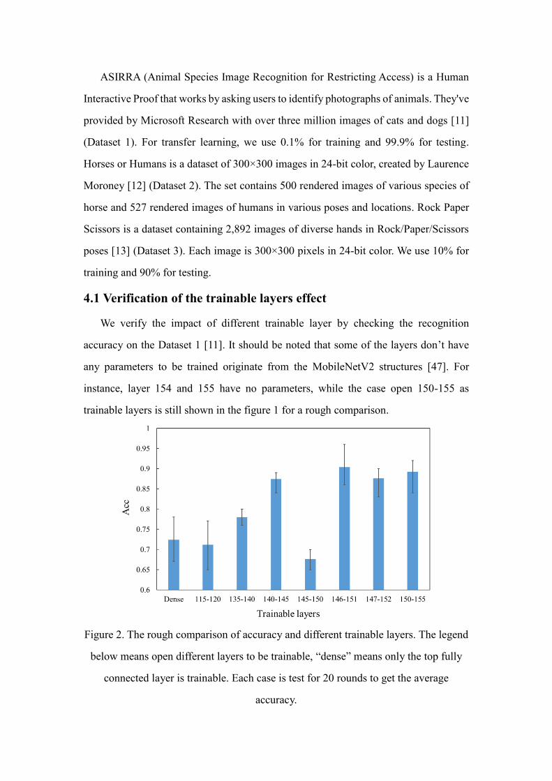
4.1 Verification of the trainable layers effect
We verify the impact of different trainable layer by checking the recognition
accuracy on the Dataset 1 [11]. It should be noted that some of the layers don’t have
any parameters to be trained originate from the MobileNetV2 structures [47]. For
instance, layer 154 and 155 have no parameters, while the case open 150-155 as
trainable layers is still shown in the figure 1 for a rough comparison.
Figure 2. The rough comparison of accuracy and different trainable layers. The legend
below means open different layers to be trainable, “dense” means only the top fully
connected layer is trainable. Each case is test for 20 rounds to get the average
accuracy.

Fig. 2 shows a conflict with the intuition we introduced in Section 3.2. Training the
layers 135-140 makes the accuracy higher than the layers of 115-120, while training the
layers 147-152 decrease the accuracy compared with the case of 146-151. That means
with the layers higher up, the features are not necessary to be more specific to the target
dataset. Also, the result indicates the choice of trainable layers is of vital importance.
4.2 Optimization result from genetic algorithm
To verify the performance of GA on the transfer CNN tasks, three datasets (Dataset
1, 2 and 3) are tested. The result is shown in Fig. 3. With the genetic operations, it shows
a significant improvement in the average accuracy on all the three datasets. Especially
for the Dataset 3, the accuracies in the first generation are barely better than a random
choice. While, after the system converged, the best individual achieves the accuracy of
97%. At around the 14th generation, the system is converged and gives the average
recognition accuracies at 93%, 90% and 87% of the three dataset, respectively.
Figure 3. The average accuracy over all individuals with respect to the generation
number. Blue solid line, red solid line and green dash line correspond to three
datasets, respectively. The bars indicate the highest and lowest accuracies in the
corresponding generation.
The results of Dataset 1 are summarized in Table 1. The average recognition
accuracy is updated from 76% to 88% by generation. The best individuals and the worst

individuals are also improved with the genetic process. Although there is a fortunate
fluke that the best individual gives a fairly high accuracy in the first generation, it still
can be proved that the GA is more efficiency than random search. For the Dataset 2 and
3, see the SI (Supplementary Information, Table 2 and Table 3).
Table 1. The Recognition accuracy on the Cats and Dogs dataset testing set. The
best individual in corresponding generation is translated to trainable layer numbers.
Gen Max Min Avg Start Layers End Layers
1 0.92 0.47 0.76 131 133
2 0.95 0.47 0.81 147 151
3 0.95 0.53 0.85 130 155
4 0.96 0.53 0.86 130 155
5 0.96 0.62 0.86 123 151
6 0.96 0.59 0.87 127 151
7 0.97 0.71 0.86 146 151
8 0.97 0.70 0.87 124 151
9 0.96 0.72 0.88 147 151
10 0.97 0.67 0.87 124 151
11 0.96 0.67 0.88 129 151
12 0.96 0.71 0.90 129 151
13 0.98 0.76 0.91 129 151
14 0.97 0.76 0.91 129 151
4.3 Characterization of neural network layers
After being translated to trainable layer numbers, the best individuals in each
generations are shown in Table 1. For the case of Dataset 1, the result converged to the
129-151 as trainable layers. While different Datasets will give specific selection of
trainable layers (142-151 for Dataset 2, 130-136 for Dataset 3. Shown in SI). It reveals
that even with the same model, the importance of network layers is different for
different tasks. That maybe originates from that the specialized features are composed

of generic features extracting by different network layers. So, different datasets
correspond to specialized features, which corresponding to specific network layers.
To investigate the responding of the network layers, the gradients information is
then analyzed. Figure 4 shows the result of the maximum value of gradients in each
layers activated by dogs images and cats images, respectively. It shows the maximum
gradients of nodes in each layer are not sensitive to different categories in Dataset 1.
Figure 4. The maximum value of gradients in each layer activated by dogs/cats
images
Figure 5(a) shows that it is distinguishable of two categories by the average value
of gradients in the layers, but with a complicated features. It is worth emphasizing that
this comes from an average of the dataset ensemble, which is maybe not necessarily
consistent with a single sample. While summation of gradients reveals some features
are distinctly different between two categories, which is shown in Figure 5(b).
The summation of gradients in the layer 105, 114, 124, 132, 141 and 150 are
significantly higher than others. For the layer 114, 132 and 150, the sign of summation
value of two categories are even opposite on average, which maybe contribute to the
classification as a criterion. It is interesting that the layer 150 is also the boundary of
the optimized trainable layers by GA. That inspires us with an explainable AI
perspective, although it is still superficial. However, the start layers optimized by GA

is converged to 129, which is affected by the weight of layer number γ. It still need
further works on the effect of this factor.
Figure 5. (a) The average gradient of each layers activated by dogs/cats images (b)
Summation of gradients by all the nodes in the same layer
5. Conclusions
In this paper, we apply the GA to learn to decide the trainable layers of transfer
CNN automatically. Our main idea is to encode the trainable layers number as a gene
of individuals, and update the population by genetic operations to obtain the best

transfer CNN networks. We perform the GA on three datasets (cats_vs_dogs, horses or
humans and rock_paper_scissors). The results demonstrate the availability of the GA to
apply to this task.
Moreover, according this GA guided results, we can acquire more information by
analyzing other features such as gradients. This backward inference can help us
understanding the transfer AI models.
Although we find some essential information from the analysis of gradients, it is
challenging to interpret AI models by the information so far, even to give an insight of
design the transfer CNN. However, it’s an open question for the interpretability of AI
model. Our approach may help to this goal. Further analysis can help us learn more
from AI models, help us moving on towards explainable AI models.
DNA computing, as an alternative technique of computing architecture, uses DNA
molecules to store information, and uses molecular interaction to process computing
[49]. The parallelism is the advantage of DNA computing compared with electronic
computer, which can speed up exponentially in some cases. The GA can be
implemented by DNA computing naturally. With the DNA computing based GA, it may
greatly speed up hyper-parameter optimization process in future.
Acknowledgements
This work was supported by National Key R&D Program of China under grant no.
2017YFB1001700, and Natural Science Foundation of Shandong Province of China
under grant no. ZR2018BF011.
Reference
[1] LeCun Y, Bottou L, HuangFu J. Learning methods for generic object recognition
with invariance to pose and lighting. In: Proceedings of the 2004 IEEE computer
society conference on computer vision and pattern recognition, vol. 2. 2004. p. 97–
104.
[2] Oquab M, Bottou L, Laptev I, Sivic J. Learning and transferring mid-level image

representations using convolutional neural networks. In: Proceedings of the 2014
IEEE conference on computer vision and pattern recognition. 2013. p. 1717–24.
[3] Wang C, Mahadevan S. Heterogeneous domain adaptation using manifold
alignment. In: Proceedings of the 22nd international joint conference on artificial
intelligence, vol. 2. 2011. p. 541–46.
[4] Harel M, Mannor S. Learning from multiple outlooks. In: Proceedings of the 28th
international conference on machine learning. 2011. p. 401–8.
[5] Kulis B, Saenko K, Darrell T. What you saw is not what you get: domain adaptation
using asymmetric kernel transforms. In: IEEE 2011 conference on computer vision
and pattern recognition. 2011. p. 1785–92.
[6] Zhu Y, Chen Y, Lu Z, Pan S, Xue G, Yu Y, Yang Q. Heterogeneous transfer learning
for image classification. In: Proceedings of the national conference on artificial
intelligence, vol. 2. 2011. p. 1304–9.
[7] Duan L, Xu D, Tsang IW. Learning with augmented features for heterogeneous
domain adaptation. IEEE Trans Pattern Anal Mach Intell. 2012;36(6):1134–48.
[8] Prettenhofer P, Stein B. (2010) Cross-language text classification using structural
correspondence learning. In: Proceedings of the 48th annual meeting of the
association for computational linguistics. 2010. p. 1118–27.
[9] Zhou JT, Tsang IW, Pan SJ Tan M. Heterogeneous domain adaptation for multiple
classes. In: International conference on artificial intelligence and statistics. 2014. p.
1095–103.
[10] Zhou JT, Pan S, Tsang IW, Yan Y. Hybrid heterogeneous transfer learning through
deep learning. In: Proceedings of the national conference on artificial intelligence,
vol. 3. 2014. p. 2213–20.
[11] E. Jeremy, D. John, H. Jon, S. Jared. Asirra: A CAPTCHA that Exploits Interest-
Aligned Manual Image Categorization. Proceedings of 14th ACM Conference on
Computer and Communications Security (CCS), 2007.
[12] L. Moroney. Horses Or Humans Dataset.
http://www.laurencemoroney.com/horses-or-humans-dataset/, 2019.
[13] L. Moroney. Rock, Paper, Scissors Dataset.
http://www.laurencemoroney.com/rock-paper-scissors-dataset/, 2019.
[14] Y. LeCun, J. Denker, D. Henderson, R. Howard, W. Hubbard, and L. Jackel.
Handwritten Digit Recognition with a Back-Propagation Network. Advances in
Neural Information Processing Systems, 1990.
[15] Olga Russakovsky, Jia Deng, Hao Su, Jonathan Krause, Sanjeev Satheesh, Sean
Ma, Zhiheng Huang, Andrej Karpathy, Aditya Khosla, Michael Bernstein,
Alexander C. Berg, and Li Fei-Fei. Imagenet large scale visual recognition
challenge. Int. J. Comput. Vision, 115(3):211–252, 2015.
[16] Krizhevsky A, Sutskever I, and Hinton G. ImageNet Classification with Deep
Convolutional Neural Networks. Advances in Neural Information Processing
Systems, 2012.
[17] K. Simonyan and A. Zisserman. Very Deep Convolutional Networks for Large-
Scale Image Recognition. International Conference on Learning Representations,
2014.
[18] G. Csurka, C. Dance, L. Fan, J. Willamowski, and C. Bray. Visual Categorization
with Bags of Keypoints. Workshop on Statistical Learning in Computer Vision,
European Conference on Computer Vision, 1(22):1–2, 2004.
[19] J. Wang, J. Yang, K. Yu, F. Lv, T. Huang, and Y. Gong. Locality-Constrained Linear
Coding for Image Classification. Computer Vision and Pattern Recognition, 2010.
[20] F. Perronnin, J. Sanchez, and T. Mensink. Improving the Fisher Kernel for Large-
scale Image Classification. European Conference on Computer Vision, 2010.
[21] P. Felzenszwalb, R. Girshick, D. McAllester, and D. Ramanan. Object Detection
with Discriminatively Trained Part-Based Models. IEEE Transactions on Pattern
Analysis and Machine Intelligence, 32(9):1627–1645, 2010.
[22] S. Ioffe and C. Szegedy. Batch Normalization: Accelerating Deep Network
Training by Reducing Internal Covariate Shift. International Conference on
Machine Learning, 2015.
[23] N. Srivastava, G. Hinton, A. Krizhevsky, I. Sutskever, and R. Salakhutdinov.
Dropout: A SimpleWay to Prevent Neural Networks from Overfitting. Journal of
Machine Learning Research, 15(1):1929–1958, 2014.

[24] S. Pan and Q. Yang. A survey on transfer learning. Knowledge and Data
Engineering, IEEE Transactions on, 22(10):1345–1359, 2010.
[25] Y. Aytar and A. Zisserman. Tabula rasa: Model transfer for object category
detection. In ICCV, 2011.
[26] T. Tommasi, F. Orabona, and B. Caputo. Safety in numbers: Learning categories
from few examples with multi model knowledge transfer. In CVPR, 2010.
[27] A. Farhadi, M. K. Tabrizi, I. Endres, and D. Forsyth. A latent model of
discriminative aspect. In ICCV, 2009.
[28] A. Khosla, T. Zhou, T. Malisiewicz, A. A. Efros, and A. Torralba. Undoing the
damage of dataset bias. In ECCV, 2012.
[29] K. Saenko, B. Kulis, M. Fritz, and T. Darrell. Adapting visual category models to
new domains. In ECCV, 2010.
[30] M. Zeiler and R. Fergus. Visualizing and understanding convolutional networks. In
ECCV, 2014.
[31] J. Donahue, Y. Jia, O. Vinyals, J. Hoffman, N. Zhang, E. Tzeng, and T. Darrell.
Decaf: A deep convolutional activation feature for generic visual recognition. In
CVPR, 2014.
[32] R. Girshick, J. Donahue, T. Darrell, and J. Malik. Rich feature hierarchies for
accurate object detection and semantic segmentation. In CVPR, 2014.
[33] P. Sermanet, D. Eigen, X. Zhang, M. Mathieu, R. Fergus, and Y. LeCun. Overfeat:
Integrated recognition, localization and detection using convolutional networks. In
CVPR, 2013.
[34] C. Reeves. A Genetic Algorithm for Flowshop Sequencing. Computers &
Operations Research, 22(1):5–13, 1995.
[35] C. Houck, J. Joines, and M. Kay. A Genetic Algorithm for Function Optimization:
A Matlab Implementation. Technical Report, North Carolina State University, 2009.
[36] J. Grefenstette, R. Gopal, B. Rosmaita, and D. Van Gucht. Genetic Algorithms for
the Traveling Salesman Problem. International Conference on Genetic Algorithms
and their Applications, 1985.
[37] K. Stanley and R. Miikkulainen. Evolving Neural Networks through Augmenting

Topologies. Evolutionary Computation, 10(2):99–127, 2002.
[38] J. Bayer, D. Wierstra, J. Togelius, and J. Schmidhuber. Evolving Memory Cell
Structures for Sequence Learning. International Conference on Artificial Neural
Networks, 2009.
[39] X. Yao. Evolving Artificial Neural Networks. Proceedings of the IEEE,
87(9):1423–1447, 1999.
[40] S. Ding, H. Li, C. Su, J. Yu, and F. Jin. Evolutionary Artificial Neural Networks: A
Review. Artificial Intelligence Review, 39(3):251–260, 2013.
[41] L. Xie, A. Yuille. Genetic CNN. In: ICCV, 2017, pp. 1379–1388.
[42] M. Suganuma, S. Shirakawa, T. Nagao. A Genetic Programming Approach to
Designing Convolutional Neural Network Architectures. In: GECCO, 2017, pp. 497.
[43] J. Han, D. Choi, S. Park, S. Hong. Hyperparameter Optimization Using a Genetic
Algorithm Considering Verification Time in a Convolutional Neural Network.
Journal of Electrical Engineering & Technology, 15, pp. 721–726, 2020.
[44] Steven R. Young, Derek C. Rose, Thomas P. Karnowski, Seung-Hwan Lim, and
Robert M. Patton. Optimizing deep learning hyper-parameters through an
evolutionary algorithm. In Proceedings of the Workshop on Machine Learning in
High-Performance Computing Environments - MLHPC ’15, pages 1–5, Austin,
Texas, USA, 2015. ACM Press.
[45] Esteban Real, SherryMoore, Andrew Selle, Saurabh Saxena, Yutaka Leon
Suematsu, Jie Tan, Quoc Le, and Alex Kurakin. Large-Scale Evolution of Image
Classifiers. In Proceedings of the 34th International Conference on Machine
Learning - Volume 70, pages 2902–2911, Sydney, NSW, Australia, 2017.
[46] X. Xiao, M. Yan, S. Basodi, C. Ji, Y. Pan. Efficient Hyperparameter Optimization
in Deep Learning Using a Variable Length Genetic Algorithm. arXiv:2006.12703,
2020.
[47] M. Sandler, A. Howard, M. Zhu, A. Zhmoginov, L. Chen. MobileNetV2: Inverted
Residuals and Linear Bottlenecks. The IEEE Conference on Computer Vision and
Pattern Recognition (CVPR), 2018, pp. 4510-4520.
[48] Mobilenet V2 Imagenet Checkpoints from Google.

https://storage.googleapis.com/mobilenet_v2/checkpoints/mobilenet_v2_1.0_160.t
gz
[49] L. M. Adleman. Molecular Computation of Solutions to Combinatorial Problems.
Science, 266:1021, 1994.