adaptive sampling line search for simulation optimization
TRANSCRIPT
Adaptive Sampling Line Search for Simulation Optimization
Prasanna Kumar Ragavan
Dissertation submitted to the Faculty of the
Virginia Polytechnic Institute and State University
in partial fulllment of the requirements for the degree of
Doctor of Philosophy
in
Industrial and Systems Engineering
Michael R. Taae, Co-Chair
Raghu Pasupathy, Co-Chair
Douglas R. Bish
Christian Wernz
February 17, 2017
Blacksburg, Virginia
Keywords: Simulation Optimization, Adaptive Sampling, Line Search, ADALINE
Copyright 2017, Prasanna Kumar Ragavan
Adaptive Sampling Line Search for Simulation Optimization
Prasanna Kumar Ragavan
(ABSTRACT)
This thesis is concerned with the development of algorithms for simulation optimization (SO), a
special case of stochastic optimization where the objective function can only be evaluated through noisy
observations from a simulation. Deterministic techniques, when directly applied to simulation optimization
problems fail to converge due to their inability to handle randomness thus requiring sophisticated algorithms.
However, many existing algorithms dedicated for simulation optimization often show poor performance on
implementation as they require extensive parameter tuning.
To overcome these shortfalls with existing SO algorithms, we develop ADALINE, a line search based
algorithm that minimizes the need for user dened parameter. ADALINE is designed to identify a local
minimum on continuous and integer ordered feasible sets. ADALINE on continuous feasible sets mimics
deterministic line search algorithms, while it iterates between a line search and an enumeration procedure
on integer ordered feasible sets in its quest to identify a local minimum. ADALINE improves upon many of
the existing SO algorithms by determining the sample size adaptively as a trade-o between the error due to
estimation and the optimization error, that is, the algorithm expends simulation eort proportional to the
quality of the incumbent solution. We also show that ADALINE converges almost surely to the set of local
minima on integer ordered feasible sets at an exponentially fast rate. Finally, our numerical results suggest
that ADALINE converges to a local minimum faster than the best available SO algorithm for the purpose.
To demonstrate the performance of our algorithm on a practical problem, we apply ADALINE in
solving a surgery rescheduling problem. In the rescheduling problem, the objective is to minimize the cost of
disruptions to an existing schedule shared between multiple surgical specialties while accommodating semi-
urgent surgeries that require expedited intervention. The disruptions to the schedule are determined using
a threshold based heuristic and ADALINE identies the best threshold levels for various surgical specialties
that minimizes the expected total cost of disruption. A comparison of the solutions obtained using a Sample
Average Approximation (SAA) approach, and ADALINE is provided. We nd that the adaptive sampling
strategy in ADALINE identies a better solution more quickly than SAA.

Adaptive Sampling Line Search for Simulation Optimization
Prasanna Kumar Ragavan
(GENERAL AUDIENCE ABSTRACT)
This thesis is concerned with the development of algorithms for simulation optimization (SO), where
the objective function does not have an analytical form, and can only be estimated through noisy observations
from a simulation. Deterministic techniques, when directly applied to simulation optimization problems fail
to converge due to their inability to handle randomness thus requiring sophisticated algorithms. However,
many existing algorithms dedicated for simulation optimization often show poor performance on implemen-
tation as they require extensive parameter tuning.
To overcome these shortfalls with existing SO algorithms, we develop ADALINE, a line search based
algorithm that minimizes the need for user dened parameter. ADALINE is designed to identify a local
minimum on continuous and integer ordered feasible sets. ADALINE on continuous feasible sets mimics
deterministic line search algorithms, while it iterates between a line search and an enumeration procedure
on integer ordered feasible sets in its quest to identify a local minimum. ADALINE improves upon many of
the existing SO algorithms by determining the sample size adaptively as a trade-o between the error due
to estimation and the optimization error, that is, the algorithm expends simulation eort proportional to
the quality of the incumbent solution. Finally, our numerical results suggest that ADALINE converges to a
local minimum faster than the best available SO algorithm for the purpose.
To demonstrate the performance of our algorithm on a practical problem, we apply ADALINE in
solving a surgery rescheduling problem. In the rescheduling problem, the objective is to minimize the cost
of disruptions to an existing schedule shared between multiple surgical specialties while accommodating
semi-urgent surgeries that require expedited intervention. The disruptions to the schedule are determined
using a threshold based heuristic and ADALINE identies the best threshold levels for various surgical
specialties that minimizes the expected total cost of disruption. A comparison of the solutions obtained
using traditional optimization techniques, and ADALINE is provided. We nd that the adaptive sampling
strategy in ADALINE identies a better solution more quickly than traditional optimization.

To my family, and all my teachers...
iv

Acknowledgments
I would like to express my heartfelt gratitude to Dr. Raghu Pasupathy, and Dr. Michael Taae, for, this
thesis would have been a dream had it not been for their intervention, and persistent support. I am greatly
indebted to Dr. Pasupathy for all his time, and patience in molding me a researcher, and a good human
being. All the courses taught by Dr. Pasupathy were instrumental in me pursuing further research in this
eld. I will always look up to him. I am greatly indebted to Dr. Taae for motivating me, for his guidance
in writing and for his eorts and care in making sure I completed my PhD.
I would like to sincerely thank Dr. Doug Bish for being a part of my committee and for his valu-
able insights and encouragement throughout the course of my graduate program. I would like to thank
Dr. Christian Wernz for being a part of my committee and for providing inputs on healthcare operations
research. I am also thankful to Dr. Ebru Bish for her support during the initial stages of my graduate
study, and for evoking interest in me to solve problems in healthcare. I am thankful to Dr. Don Taylor, Dr.
Maury Nussbaum, and Dr. Jamie Camelio for providing teaching assistantships in the Grado Department
of Industrial and Systems Engineering (ISE). As a teaching assistant at ISE, I enjoyed working with Dr.
Laurel Travis and Dr. Natalie Cherbaka.
I am thankful to my friends Krishnan Gopalan, Niloy Mukherjee for their support in personal and
professional development through my stay in Blacksburg. Thanks to Mahesh Narayanamurthy for all his
help in the nal stages, and for never letting me stranded while in Blacksburg. I also thank Kalyani Nagaraj
for helping me during the initial phases of my research. I would also like to take this opportunity to thank
Vamshi for his valuable insights in clinical scheduling.
I would also like to thank my cousins Raghavendran and Priya for being there for me through the
thick and thin. My brother Guruprasadh has been a great friend and source of support in times of need. I am
blessed to have such a wonderful brother for guidance and advice. Thanks to Jayashree for standing besides
me all the time, and for her unconditional love and support throughout. Finally, my sincerest thanks to my
parents, Sujatha and Ragavan for all their struggles, and sacrices in helping me receive a good education.
v

Contents
1 Introduction 1
1.1 Motivation . . . . . . . . . . . . . . . . . . . . . . . . . . . . . . . . . . . . . . . . . . . . . . 2
1.1.1 Example: Continuous Simulation Optimization . . . . . . . . . . . . . . . . . . . . . . 2
1.1.2 Example: Integer Simulation Optimization . . . . . . . . . . . . . . . . . . . . . . . . 3
1.2 Simulation Optimization . . . . . . . . . . . . . . . . . . . . . . . . . . . . . . . . . . . . . . . 3
1.2.1 Continuous Simulation Optimization . . . . . . . . . . . . . . . . . . . . . . . . . . . . 4
1.2.2 Integer Ordered Simulation Optimization . . . . . . . . . . . . . . . . . . . . . . . . . 6
1.3 Organization of the thesis . . . . . . . . . . . . . . . . . . . . . . . . . . . . . . . . . . . . . . 7
2 ADALINE for Integer-Ordered Simulation Optimization 9
2.1 Competitors . . . . . . . . . . . . . . . . . . . . . . . . . . . . . . . . . . . . . . . . . . . . . . 10
2.2 Algorithm ADALINE - Integer Ordered . . . . . . . . . . . . . . . . . . . . . . . . . . . . . . 11
2.2.1 Adaptive Linear Interpolation and Line Search . . . . . . . . . . . . . . . . . . . . . . 13
2.2.2 Neighborhood Enumeration (NE) . . . . . . . . . . . . . . . . . . . . . . . . . . . . . . 15
2.3 Local Convergence . . . . . . . . . . . . . . . . . . . . . . . . . . . . . . . . . . . . . . . . . . 21
2.4 Numerical Results . . . . . . . . . . . . . . . . . . . . . . . . . . . . . . . . . . . . . . . . . . 23
2.4.1 Inventory Optimization with ADALINE . . . . . . . . . . . . . . . . . . . . . . . . . . 23
2.4.2 Bus Scheduling Problem . . . . . . . . . . . . . . . . . . . . . . . . . . . . . . . . . . . 24
vi

2.4.3 Multi-dimensional Quadratic minimization . . . . . . . . . . . . . . . . . . . . . . . . 27
2.5 Conclusion . . . . . . . . . . . . . . . . . . . . . . . . . . . . . . . . . . . . . . . . . . . . . . 28
3 ADALINE for Continuous Simulation Optimization 29
3.1 Deterministic Line Search Methods . . . . . . . . . . . . . . . . . . . . . . . . . . . . . . . . . 30
3.2 Variable Sampling in Simulation Optimization . . . . . . . . . . . . . . . . . . . . . . . . . . . 31
3.3 ADALINE - Continuous Simulation Optimization . . . . . . . . . . . . . . . . . . . . . . . . . 33
3.3.1 Details of the algorithm & pseudocode . . . . . . . . . . . . . . . . . . . . . . . . . . . 33
3.4 Numerical Results . . . . . . . . . . . . . . . . . . . . . . . . . . . . . . . . . . . . . . . . . . 34
3.4.1 Alu-Pentini Function . . . . . . . . . . . . . . . . . . . . . . . . . . . . . . . . . . . . 36
3.4.2 Rosenbrock Function . . . . . . . . . . . . . . . . . . . . . . . . . . . . . . . . . . . . . 39
3.5 Conclusion . . . . . . . . . . . . . . . . . . . . . . . . . . . . . . . . . . . . . . . . . . . . . . 41
4 Surgery Rescheduling using Simulation Optimization 42
4.1 Literature review . . . . . . . . . . . . . . . . . . . . . . . . . . . . . . . . . . . . . . . . . . . 43
4.2 Problem Statement . . . . . . . . . . . . . . . . . . . . . . . . . . . . . . . . . . . . . . . . . . 45
4.2.1 Random Variables . . . . . . . . . . . . . . . . . . . . . . . . . . . . . . . . . . . . . . 47
4.2.2 Surgery Rescheduling using SAA . . . . . . . . . . . . . . . . . . . . . . . . . . . . . . 48
4.3 Solution Methodology . . . . . . . . . . . . . . . . . . . . . . . . . . . . . . . . . . . . . . . . 52
4.3.1 Scheduling Heuristic . . . . . . . . . . . . . . . . . . . . . . . . . . . . . . . . . . . . . 54
4.3.2 Total Cost of Rescheduling . . . . . . . . . . . . . . . . . . . . . . . . . . . . . . . . . 55
4.4 Threshold Determination . . . . . . . . . . . . . . . . . . . . . . . . . . . . . . . . . . . . . . 57
4.4.1 Optimize threshold using Integer Programming . . . . . . . . . . . . . . . . . . . . . . 58
4.4.2 Optimize threshold using Simulation Optimization - ADALINE . . . . . . . . . . . . . 62
4.5 Numerical Results . . . . . . . . . . . . . . . . . . . . . . . . . . . . . . . . . . . . . . . . . . 64
4.5.1 Threshold Optimization using ADALINE . . . . . . . . . . . . . . . . . . . . . . . . . 65
vii

4.5.2 Threshold Optimization using Integer programming . . . . . . . . . . . . . . . . . . . 66
4.6 Conclusion . . . . . . . . . . . . . . . . . . . . . . . . . . . . . . . . . . . . . . . . . . . . . . 67
5 Concluding Remarks 70
Bibliography 72
Appendix A ADALINE for Continuous Simulation Optimization 78
Appendix B ADALINE for Integer Simulation Optimization 90
Appendix C Surgery Scheduling Problem 103
viii
List of Figures
2.1 Trajectory of ADALINE . . . . . . . . . . . . . . . . . . . . . . . . . . . . . . . . . . . . . . . 12
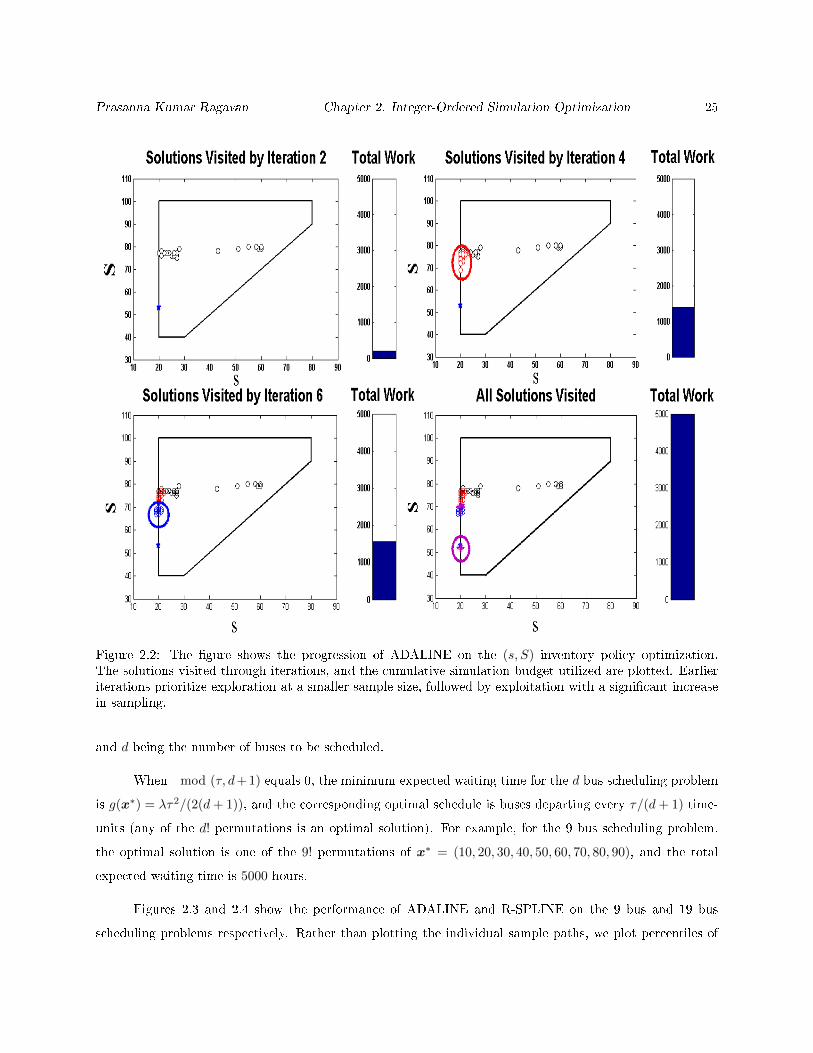
2.2 The gure shows the progression of ADALINE on the (s, S) inventory policy optimization. The
solutions visited through iterations, and the cumulative simulation budget utilized are plotted.
Earlier iterations prioritize exploration at a smaller sample size, followed by exploitation with
a signicant increase in sampling. . . . . . . . . . . . . . . . . . . . . . . . . . . . . . . . . . . 25
2.3 The gure shows percentiles of the expected wait time corresponding to the solution returned
by ADALINE and R-SPLINE at the end of b simulation calls on the nine-bus scheduling
problem. . . . . . . . . . . . . . . . . . . . . . . . . . . . . . . . . . . . . . . . . . . . . . . . . 26
2.4 The gure shows percentiles of the expected wait time corresponding to the solution returned
by ADALINE and R-SPLINE at the end of b simulation calls on the nineteen-bus scheduling
problem. . . . . . . . . . . . . . . . . . . . . . . . . . . . . . . . . . . . . . . . . . . . . . . . . 27
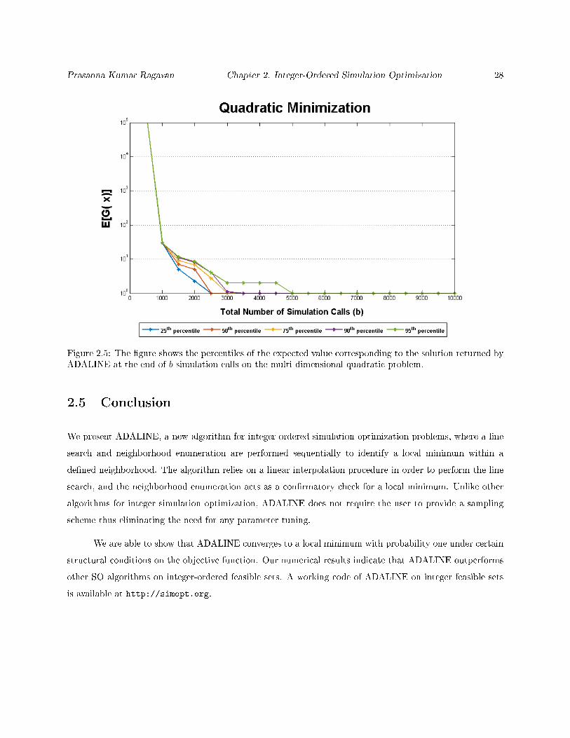
2.5 The gure shows the percentiles of the expected value corresponding to the solution returned
by ADALINE at the end of b simulation calls on the multi-dimensional quadratic problem. . 28
3.1 The gure shows percentiles of the norm of the true gradient corresponding to the solutions
returned by all variations of our algorithm on the Alu-Pentini problem . . . . . . . . . . . . 37
3.2 Performance of the adaptive samplings strategy on the Alu-Pentini problem in comparison
with the sampling strategy in Kreji¢ and Krklec (2013) . . . . . . . . . . . . . . . . . . . . . . 38
3.3 Sample growth in the Alu-Pentini problem for the Stochastic BFGS method . . . . . . . . . 39
3.4 The gure shows percentiles of the norm of the true gradient corresponding to the solutions
returned by all variations of our algorithm on the Rosenbrock problem . . . . . . . . . . . . . 40
ix
3.5 Performance of the adaptive samplings strategy on the Rosenbrock problem in comparison
with the sampling strategy in Kreji¢ and Krklec (2013) . . . . . . . . . . . . . . . . . . . . . . 40
3.6 Sample growth in the Rosenbrock problem for the Stochastic BFGS method . . . . . . . . . . 41
4.1 Realization of Random Variables that represent the requests for Semi-urgent surgeries . . . . 47
4.2 Sequence of Decisions for the Surgical Rescheduling Problem . . . . . . . . . . . . . . . . . . 54
4.3 Figure shows the expected total cost of rescheduling as a function of the total simulation calls
for the solutions identied by ADALINE at specied budget levels . . . . . . . . . . . . . . . 65
4.4 Figure shows the expected total cost of rescheduling as a function of elapsed time for the
solutions identied by ADALINE at specied time limits . . . . . . . . . . . . . . . . . . . . . 66
4.5 Figure shows the expected total cost of rescheduling as a function of elapsed time for the
solutions identied by the integer optimization framework with various sample sizes . . . . . 68
4.6 Figure shows a comparison of the quality of solutions obtained with thresholds determined
through ADALINE and the Integer Optimization framework . . . . . . . . . . . . . . . . . . . 68
x

List of Tables
4.1 Table shows the mean and standard deviation of the negative binomially distributed random
variable indicating the number of semi-urgent cases requested on any particular day. . . . . . 64
4.2 Table shows the parameters of the the distribution of surgery duration . . . . . . . . . . . . . 64
4.3 Average optimality gap of the solutions to the mixed integer programming formulation ob-
tained at various time limits . . . . . . . . . . . . . . . . . . . . . . . . . . . . . . . . . . . . . 67
xi
Chapter 1
Introduction
In this research, we develop algorithms for simulation optimization (SO)a branch of optimization where
the objective function, and possibly the constraints, do not have an analytical form and can only be observed
through a stochastic simulation. Formally, the simulation optimization problem can be stated as follows:
PSO : minimize g(x)
subject to x ∈ X
where, the feasible set X ⊆ Rd is either continuous, or integer-ordered, X ⊆ Zd.
In Problem PSO, the objective function, g : X→ R is real-valued, and in the form of an expectation,
such that, g(x) = Eξ [G(x, ·)]. Further, at any decision point, x, only an estimate of the objective function
can be obtained through random observations, G(x, ξj), from a simulation. We assume that the observations
are independent and identically distributed (i.i.d.), and a point estimator of the objective function, gm(x),
is constructed based on these outcomes. Since g(x) = E [G(x, ·)], the sample mean of the observations,
gm(x) = m−1∑mj=1G(x, ξj), is a suitable estimator. It should be noted that, in SO, obtaining an estimate
of the objective function entails either repeating the simulation multiple times, as in the case of terminating
simulations or longer simulation times (steady state simulation).
1

Prasanna Kumar Ragavan Chapter 1. Introduction 2
1.1 Motivation
To motivate our research, we present an application of SO in operating room (OR) management. OR
management involves three phases of decision making, namely (i) determination of total operating room
capacity (strategic), (ii) allocation of capacity between various specialties (tactical), and (iii) scheduling
individual surgeries to operating rooms (operational). Later, in Chapter 4, we study in detail the problem
of allocating surgical capacity between non-elective and elective surgeries under a constrained operating
room environment. However, for illustrative purposes, let us consider the problem of allocating capacity to
individual specialties when the total available operating room capacity is unconstrained, a simplied version
of the real problem.
1.1.1 Example: Continuous Simulation Optimization
Even when unlimited capacity is available, capacity allocation requires scheduling of OR resources which
incurs a xed cost of cr dollars per unit time. When sucient capacity is not allocated to the specialty,
resources have to be scheduled with overtime to meet the excess demand, costing co dollars for every unit
of overtime incurred. The surgical duration every week for any specialty is a random variable, D, with
cdf, FD(·). Therefore, determining the optimal capacity, x∗ can be formulated as a news vendor problem
(Hosseini and Taae, 2014) as follows:
g(x) = minx
ED[G(x,D)] = ED[cr x+ (co maxD − x, 0)]
It is well known that the optimal solution to the one dimensional news vendor problem is to sta for the(co−crco
)th quantile of the demand distribution. For example, if regular stang cost, cr = $1400/hr, the
overtime cost, co = $1600/hr and the surgical volume, D is a random variable uniformly distributed between
160 and 600 hours, then the optimal solution is to plan for the 0.125th quantile which translates to 215
stang hours with a total expected cost of $570, 500 per week. If the solution were to replace the random
variable D with its expectation, the optimal solution is to sta for the expectation of the random variable,
that is, x, is equal to 380. The total expected cost incurred by using such a solution is $620, 000, an increase
of approximately $50, 000 per week from the optimal cost, thereby justifying the need for sophisticated
techniques that deal with uncertainty.
In the above example, we assume that the distribution of the random quantity (surgical volume) is
known which leads to an analytical solution. Under incomplete information on the demand, a closed form
Prasanna Kumar Ragavan Chapter 1. Introduction 3
solution may be impossible necessitating simulation/black-box based optimization techniques. In this case,
under incomplete information on demand, the optimal solution can be estimated as the(co−crco
)th quantile
by repeatedly drawing samples using a simulation.
A variation of this problem, where allocating labor hours between multiple specialties under a con-
strained environment (with a constraint on the total available capacity), however, requires a dierent solution
technique. Stang for the(co−crco
)th quantile for every specialty may no longer be feasible for the multi-
dimensional news vendor problem, and when the demand distribution is unknown, simulation optimization
methods that exploit the structure of g(x) through random observations, G(x, D) are required (Kim, 2006).
1.1.2 Example: Integer Simulation Optimization
For the multi-dimensional news vendor problem discussed in Section 1.1, when the feasible space is contin-
uous, gradient information observed at any decision point can be directly utilized to guide a SO algorithm.
However, when the feasible space is integer-ordered, gradient based techniques are not directly applicable.
Consider the problem of accommodating surgeries in a hospital where surgical capacity is shared between
non-elective and elective surgeries. Elective surgeries that are scheduled at least a week in advance may
have to be postponed or canceled to accommodate non-elective surgeries which have an uncertain demand
and are realized only a day or two prior to the surgery. A threshold based scheduling policy that exclusively
reserves operating room capacity for non-elective surgeries can be devised to solve this problem, the details
of which can be found in Chapter 4. However, optimizing the threshold levels, that take values in the integer-
ordered space, when the surgical demand can be realized only through a simulation requires sophisticated
SO techniques which are developed as a part of this dissertation.
1.2 Simulation Optimization
Simulation optimization (SO) is concerned with solving problems where the objective function, and (or) the
constraints can only be evaluated through a simulation or as the response of a black-box given an input.
Such problems nd a variety of applications including but not limited to supply chain management (Iravani
et al., 2003; Jung et al., 2004), operations and scheduling (Belyi et al., 2009; Buchholz and Thummler, 2005),
revenue management (Gosavi et al., 2007; Horng and Yang, 2012), public health services (Eubank et al.,
2004; Henderson and Mason, 2005) and hospital operations (Balasubramanian et al., 2007; Lamiri et al.,
2009). For a comprehensive list of applications, along with the detailed problem description, please refer
to Pasupathy and Henderson (2006) and http://www.simopt.org. In addition to classical SO problems,
Prasanna Kumar Ragavan Chapter 1. Introduction 4
the stochastic nature of large scale supervised machine learning models present themselves conducive for
exploitation using SO algorithms (Byrd et al., 2012, 2014).
Several algorithms have been proposed to solve simulation optimization problems and a number of
review articles have been published on this topic. Amaran et al. (2014) provides a comprehensive overview
of the eld starting with applications of simulation optimization, and a taxonomy of the algorithms. In SO,
the algorithms can be classied based on the feasible space they operate on (continuous or discrete decision
variables), cardinality of the feasible set (nite versus uncountable feasible sets), and the search mechanism
(random search or gradient search or derivative free methods). Ranking and Selection procedures are designed
to select the best solution out of a nite set of feasible solutions with a probabilistic guarantee on choosing the
best solution. Conventional ranking and selection methods seek to determine the best solution in a sequential
setting where inferior systems are dropped in each phase, followed by an increase in sample size for further
evaluations of `promising' systems (Kim, 2005; Kim and Nelson, 2007). In ranking and selection, even if the
feasible set is nite, the requirement to completely enumerate the set of all feasible solutions renders them
inecient when evaluating large number of solutions (Fu et al., 2015). Algorithms that iteratively determine
the next solution eliminate the need for enumerating the feasible region, and are applicable even when the
feasible set is uncountable. In this section, we focus on such SO algorithms that determine the subsequent
solutions to evaluate on the y for continuous, and integer-ordered simulation optimization problems.
1.2.1 Continuous Simulation Optimization
Simulation optimization on continuous feasible sets involves visiting a sequence of solutions that are chosen
iteratively from an uncountable number of candidates, often by using the estimated gradient at each iteration.
One of the rst algorithms for continuous simulation optimization is the Stochastic Approximation (SA)
algorithm given by Robbins-Monro (Robbins and Monro, 1951). SA is an iterative method, where starting
with an initial solution, x0, the sequence of iterates, Xk are updated using the equation
Xk+1 := Xk + ak∇G(Xk, ξ), k ≥ 0
This method is the stochastic analogue to Newton type search methods in deterministic optimization, where
∇G(Xk, ξ) denotes an observation of the `noisy' gradient from a simulation, and ak denotes the step length.
Unlike deterministic optimization where ak is determined at every iteration, a decreasing sequence of positive
numbers approaching zero in the limit constitute the step length. For the algorithm to converge, in addition
to limk→∞
ak = 0, the following conditions should also hold: (i)∑∞k=0 ak =∞ and (ii)
∑∞k=0 a
2k <∞.
Although SA attains the canonical rate of convergence, that is, converges at the best possible rate
Prasanna Kumar Ragavan Chapter 1. Introduction 5
for a stochastic algorithm (O(1/√n)), it often performs poorly on implementation due to a pre-specied
step length sequence. Polyak and Juditsky (1992) proposes a variation of the SA algorithm by averaging
the iterates, and that takes a longer step at each iteration to obtain a more robust performance while
not compromising on the rate of convergence. However, the optimal choice of step length is still unknown
for a particular problem, and thus SA requires extensive parameter tuning to achieve better nite time
performance. For a thorough treatment of various SA algorithms in solving unconstrained, and constrained
SO problems along with a discussion of their theoretical convergence, and rates, please refer to Kushner and
Clark (2012).
In order to overcome the issues associated with a pre-specied step length sequence in SA, determin-
istic line search algorithms can be adapted with appropriate sampling techniques to solve a sample path
probleman approximation of the objective function obtained by i.i.d realizations of the random output.
This method, called Sample Average Approximation is appropriate for SO problems where the underlying
structure of the objective function is known. Since, in SAA, an estimate of the objective function obtained
using a xed number of realizations is optimized, it is readily applicable for solving stochastic optimization
problems irrespective of the feasible set, or the constraints. A simple choice on the approximation is to
replace the expectation with its sample average obtained using a nite sample size, M , and with a big-
enough sample size, it can guarantee convergence. Some of the previous work on SAA, and its application
in stochastic optimization along with the convergence theory includes Shapiro (1996), Shapiro and Wardi
(1996), Homem-de Mello and Bayraksan (2014), and Kim et al. (2015).
One of the important components in line search based simulation optimization algorithms is the
estimation of the gradient at any iterate. In order for SA to converge, it requires that the estimator for
the gradient to be unbiased, that is, E[∇G(Xk, ξ)] = ∇E[G(Xk, ξ)]. When the gradient is not directly
observable, procedures like nite dierence methods, or simultaneous perturbations (Spall, 1992) can be used
to estimate the gradient. When nite dierence methods are used for gradient estimation in SA, it is called the
Kiefer-Wolfowitz type algorithm (Kiefer et al., 1952). When nite dierence methods are used for gradient
estimation, the addition of another parameter, ck, further aects the convergence of SA type algorithms.
Glasserman (1991) proposes a specialized gradient estimation procedure for discrete event systems called the
innitesimal perturbation analysis that provides unbiased estimates of the gradient. However, this requires
special conditions on the structure of the problem.
In solving unconstrained SO problems of the form PSO, two important issues arise: (i) a procedure for
estimating the gradient, and (ii) the sample sizes used in the estimation phase. In this thesis, we assume that
an unbiased estimate of the gradient is readily available via a simulation oracle and refer interested readers to
the aforementioned manuscripts for a detailed overview on gradient estimation emphasizing the sample size.

Prasanna Kumar Ragavan Chapter 1. Introduction 6
Notice that both the SA, and SAA described above work within an iterative framework where the number of
realizations remains xed in every iteration. Though, a large simulation eort at any visited solution yields
a better estimate of the objective function, the iterative nature of the optimization, along with a limited
computational budget for functional evaluation means that xed sampling schemes are computationally
inecient options for SO. On the other hand, sample size, m, when too little, may lead to non-convergence
of the algorithm. Later, in Chapter 3, we discuss variable sampling strategies to overcome shortfalls of
xed sample sizes along with the literature, and provide a new adaptive sampling strategy for continuous
simulation optimization.
1.2.2 Integer Ordered Simulation Optimization
In this section, we discuss algorithms for simulation optimization involving integer ordered decision variables.
When only a handful of candidate solutions are available, ranking and selection procedures are often utilized
for selecting the best solution. When it is infeasible to enumerate all candidate solutions, more sophisticated
algorithms are utilized. A majority of the search techniques in integer SO are random search methods,
where as the name suggests, candidate solutions are chosen from the entire feasible space, either uniformly,
oblivious of the solution quality, or based on the quality of the solution in the previous iteration.
One of the rst random search methods for solving SO problems on integer ordered feasible sets is
the Stochastic Ruler Method proposed by Yan and Mukai (1992). In this method, the subsequent solution
to be visited is determined based on the objective function estimate of the current solution and a uniform
random variable. Andradóttir (1999) improves the performance of random search methods with focus on
further exploitation of visited solutions. Prudius (2007) proposes a class of adaptive random search methods
that balance the exploration, and exploitation based on partitioning the feasible set into promising, and not
promising regions, and choosing the subsequent set of solutions to visit by constructing a global, and a local
sampling distribution.
Shi and Ólafsson (2000) propose the nested partitions method where subsequent solutions are chosen
adaptively from nested sets that are pre-determined. Hong and Nelson (2006) propose COMPASS, an
improvement over the nested partitions method to identify a local solution, where the promising region is
updated at the end of every iteration by solving an optimization problem. However, the requirement to
solve an optimization problem increases the computational overhead, and aects scalability of the algorithm
to higher dimensions. The Industrial Strength - COMPASS (ISC) (Xu et al., 2010), an enhancement to
COMPASS, improves the quality of solution obtained by restarting COMPASS multiple times, and returning
the best solution out of the resulting local solutions using a ranking and selection procedure.
Prasanna Kumar Ragavan Chapter 1. Introduction 7
R-SPLINE (Wang, 2012) breaks from the tradition of random search methods, and exploits structure
within the objective function by repeatedly performing a line search, and enumeration procedure to identify
a local solution. R-SPLINE works within a retrospective frameworkan optimization technique where
sample path problems are solved sequentially starting with the optimal solution identied in the previous
iteration. The sample size increases in the number of retrospective iterations so that the resulting sequence
of approximate solutions would eventually converge to a local minimum. However, in R-SPLINE, and the
random search methods discussed above (Yan and Mukai, 1992; Shi and Ólafsson, 2000; Hong and Nelson,
2006), the sampling scheme at any iteration is xed, oblivious of the quality of the visited solution, often
aecting nite time performance. In this thesis, we address this gap on choosing the sample size for integer
ordered simulation optimization by developing ADALINE, an algorithm that adaptively determines the
sample size without the requirement for any parameter tuning.
1.3 Organization of the thesis
The theme of this dissertation centers around developing algorithms for continuous and integer-ordered simu-
lation optimization problems. In Chapter 2, we present ADALINE (Adaptive Piecewise Linear Interpolation
with line search and Neighborhood Enumeration), an iterative method for determining a local minimum
for integer-ordered SO problems. In ADALINE, a linear interpolation phase is rst performed to identify
a descent direction, followed by a neighborhood enumeration procedure to conrm the presence of a local
minimum. As the name suggests, the sample size used for interpolation, and the neighborhood enumeration
are chosen adaptively at every iteration. ADALINE is designed to be a non-terminating algorithm, that is, it
will expend all available simulation budget on convergence to a local minimum. However, numerical results
suggest that ADALINE converges to a local minimum much faster than a competing algorithm, R-SPLINE
(Wang et al., 2013), utilizing only a fraction of the total simulation budget. In Chapter 3, we discuss the
basic principles of line search techniques that are widely used in deterministic optimization, and extend these
algorithms to work within an adaptive sampling framework for simulation optimization on continuous feasi-
ble sets. We present empirical results on the performance of the algorithm on the stochastic Alu Pentini
and Rosenbrock functions.
An application of ADALINE to operating room rescheduling is discussed in Chapter 4. A threshold
based scheduling heuristic is developed to accommodate semi-urgent surgeries, and elective surgeries under
an uncertain operating room environment. The threshold levels are optimized using ADALINE, and a
comparison of the solutions obtained using a Sample Average Approximation (SAA) approach and ADALINE
is provided. We nd that the adaptive sampling strategy in ADALINE converges to a better threshold level,

Prasanna Kumar Ragavan Chapter 1. Introduction 8
and is faster than the traditional SAA approach where the sample size is xed.
Finally, MATLAB codes for the continuous simulation optimization algorithm, followed by Python
implementations of ADALINE and the codes for the surgery rescheduling problem are listed in Appendix A.

Chapter 2
ADALINE for Integer-Ordered
Simulation Optimization
In this chapter, we consider simulation optimization (SO) problems where the decision variables are integer-
ordered, and the objective function is of the form of an expectation that cannot be analytically computed,
but only noisy observations can be observed through simulation experiments. Our objective is to develop
an algorithm that will identify a local minimum for such problems. Formally, the integer-ordered SO problem
can be stated as:
PI : min g(x)
subject to x ∈ X ⊆ Zd
where X denotes the feasible set. The objective function, g : X ⊆ Zd → R, is an expectation, given
by g(x) = Eξ[G(x, ξ)], where ξ is a random vector dened on the probability space (Ω,A, P ). At any
decision point, x, the analytical form of g(x) is unavailable and can only be estimated by using random
observations, G(x, ·), by calling a Monte Carlo simulation oracle. We assume that an unbiased and strongly
consistent estimator of the objective function is available, that is, gm(x) = m−1∑mj=1G(x, ξj) such that
E[gm(x)] = g(x), and limm→∞ gm(x) = g(x), respectively. The feasibility is implicitly determined by the
simulation oracle, that is, in addition to returning the random objective function, the oracle also ags an
infeasible solution.
SO with integer-ordered decision variables nd applications in a variety of settings, including, but not
9
Prasanna Kumar Ragavan Chapter 2. Integer-Ordered Simulation Optimization 10
limited to, inventory replenishment policy optimization (Jalali and Nieuwenhuyse, 2015), revenue manage-
ment (Gosavi et al., 2007), surgery planning and scheduling (Lamiri et al., 2009), and determining vaccine
allocation strategies to prevent an epidemic outbreak (Eubank et al., 2004).
Similar to continuous simulation optimization, the majority of algorithms that have so far been pro-
posed to solve PI (Hong and Nelson, 2006; Wang et al., 2013; Xu et al., 2010) require that the sample size
for estimating the objective function be a parameter specied by the user, and a majority of them operate
on an explicitly dened feasible set. Recall from Chapter 1, that predetermined sample sizes can lead to
ineciency in the SO algorithm by either sampling too little at points close to a locally optimal solution
or too much far away from a locally optimal solution. Thus, our objective in this chapter is to focus on
integer-ordered feasible sets.
In the context of integer-ordered simulation optimization, a feasible solution x∗ is a local minimum if
and only if all other feasible solutions in the N 1 neighborhood are inferior to x∗ as measured by the objective
function g; thus, x∗ is a local minimum if g(x∗) ≤ g(x), ∀x ∈ N 1(x∗)∩X. We dene a N 1 neighborhood as
follows: N 1(x∗) = x : ||x∗−x|| = 1. In this chapter, we propose ADALINE- Integer Ordered (Adaptive
Piecewise Linear Interpolation with line search and Neighborhood Enumeration), an integer-ordered SO
algorithm, that adaptively determines the sample size in a line search framework and that can guarantee
convergence to a local minimum.
2.1 Competitors
Major competitors for ADALINE include the related line search based algorithm, R-SPLINE (Wang et al.,
2013); popular partitioning based algorithms COMPASS (Hong and Nelson, 2006), the enhanced Industrial
Strength COMPASS (ISC) (Xu et al., 2010); and the recent Gaussian Process-based Search (GPS) (Sun
et al., 2014). Operating on an explicitly dened feasible space, COMPASS iteratively partitions and expends
simulation eort to solutions from the promising regions of the feasible space to guarantee convergence to
a local solution. The promising region is updated at the end of every iteration by solving an optimization
problem after identifying and grouping solutions that are close to the best solution. COMPASS implicitly
exploits the structure of the objective function, though the requirement to solve an optimization problem
aects scalability to higher dimensions.
The Industrial Strength COMPASS (ISC), an enhancement over COMPASS, returns a good quality
local solution by restarting COMPASS several times starting with promising initial solutions obtained using
a genetic algorithm (GA). The best solution out of the resulting local solutions is returned by using a ranking
Prasanna Kumar Ragavan Chapter 2. Integer-Ordered Simulation Optimization 11
and selection (R & S) algorithm. However, ISC still suers from the issue of scaling well to higher dimensions.
Both COMPASS and ISC exploit the structure of the objective function implicitly by sampling more at points
which are promising, whereas, R-SPLINE and our adaptive search algorithm rely on phantom gradients,
evaluated by dierencing the objective function values through an interpolation procedure, to exploit the
structure of the objective function. GPS is a random search method that balances the exploration and
exploitation trade-o by generating the sampling distribution that allocates further simulation eort using
a Gaussian process. Of all the above algorithms, GPS guarantees convergence to a global solution as the
sample size, M , goes to innity, whereas, the other algorithms guarantee convergence to a local solution.
R-SPLINE, a line search based algorithm identies a local minimum by operating within a retrospec-
tive framework, where a sequence of sample path problems are solved with increasing sample sizes at each
phase. Each retrospective phase involves an interpolation and a neighborhood enumeration procedure, where
interpolation with line search exploits the structural information on the objective function by estimating a
pseudogradient, and the neighborhood enumeration (NE) acting as a conrmatory procedure for a local
minimum. In addition to acting as a conrmatory test, the NE procedure signals an increase in sample size
for the subsequent sample path problem (Wang et al., 2013).
One of the key dierentiations between R-SPLINE and ADALINE is how the neighborhood enumera-
tion procedure is performed. In R-SPLINE, once a sample path problem is solved to optimality, an increase
in sample size is signaled, making it impossible to revert back to a smaller sample size. Though such a
framework to increase sample size would guarantee convergence to a local minimum, improving nite time
performance may require extensive parameter tuning.
2.2 Algorithm ADALINE - Integer Ordered
We provide a broad outline of the algorithm, ADALINE (Adaptive Piecewise Linear Interpolation with
line search and Neighborhood Enumeration Integer Ordered), which we see as an improvement over an
existing integer-ordered algorithm R-SPLINE. As the name suggests, ADALINE is an iterative procedure
that incorporates an interpolation phase with a gradient based search (LI) and a neighborhood enumeration
(NE) procedure. The choice of sample size for estimating the gradient, performing the line search and
the neighborhood enumeration are determined adaptively at each iteration. Specically, each iteration of
ADALINE performs the following steps.
S.1 Perturb an integer solution and estimate the pseudogradient within an adaptive sampling framework;
S.2 Perform a line search along the negative gradient direction identied in S.1 to identify a better solution;

Prasanna Kumar Ragavan Chapter 2. Integer-Ordered Simulation Optimization 12
S.3 Perform a strategic neighborhood enumeration of the N 1 neighborhood to conrm a local minimum.
At each one of the 2d neighbors in the N 1 neighborhood, an estimate of the objective function is obtained by
expending a simulation eort of M I . If a trivial search in the neighborhood fails to yield a better solution,
it indicates that M I is insucient, and an adaptive neighborhood enumeration is performed. In Section
2.2, we will explain in more detail, the adaptive neighborhood enumeration procedure. The trajectory
of the algorithm is illustrated in Figure 2.1. Starting with an initial solution, X0, ADALINE performs
an adaptive interpolation procedure, followed by a line search that terminates at XNE0 . At XNE
0 , an
adaptive NE procedure is performed such that X1 is deemed the best solution at the end of iteration 1. A
similar sequence of adaptive interpolation, followed by a neighborhood enumeration, results in ADALINE
converging to X∗, a local minimum in the N 1 neighborhood, in the subsequent iterations. ADALINE
Figure 2.1: Trajectory of ADALINE
is a non-terminating algorithm, that is, on convergence to a local minimum, the algorithm is designed to
expend innite simulation eort. For all practical purposes, the algorithm can be stopped upon expending
a maximum simulation budget, denoted by B. In the following section, we provide a detailed description of
the adaptive linear interpolation and the NE procedure.
Prasanna Kumar Ragavan Chapter 2. Integer-Ordered Simulation Optimization 13
Algorithm 1 ADALINE
Require: Initial solution, x0; Minimum sample size, Mmin; Condence level, α; Total simulation budget,B; s0 = 2, c = 2, jmax = 25
Ensure: Solution, X∗ ∈ X such that g(X∗) < g(X),∀X ∈ NR(X∗), R = 11: Set k ← 0; Xk ← x0; ncalls← 02: repeat Piecewise-linear Interpolation (PLI) and Neighborhood Enumeration (NE)3: [XPLI , M
I , γ] = PLI(Xk, Mmin)4: Set Y0 ← XPLI ; j ← 0. Update ncalls after PLI5: repeat Line Search6: j ← j + 1; s = cj−1 × s0; Yj = Y0 − s× γ/||γ||7: Estimate gMI (Yj); ncalls← ncalls+M I
8: until gMI (Yj) > gMI (Yj−1) or Yj is infeasible or j < jmax9: Xbest ← Yj−1
10: [Xbest,ME ] = NE(Xbest,M
I)
11: ncalls← ncalls+2d∑i=1
MEi
12: k ← k + 1; Xk ← Xbest
13: until ncalls > B
2.2.1 Adaptive Linear Interpolation and Line Search
Adaptive piecewise-linear interpolation, LI, marks the beginning of an iteration in ADALINE, where an
interpolation followed by a line search is sequentially employed starting with an initial feasible solution, Xk.
Similar to other line search techniques, it involves two phases, namely, (i) a gradient estimation phase, and
(ii) a line search phase. However, unlike continuous optimization, it should be noted that a gradient based
search strategy in integer-ordered space presents two major challenges, (i) function is not dierentiable, and
hence its gradient and descent direction is undened; and (ii) points visited during the line search may be
infeasible, and additional rules to guarantee feasibility needs to be enforced.
In order to ensure that feasible solutions are returned from a line search, we can project an infeasible
solution onto the convex hull of the feasible set, X, by rounding non-integer points to the closest feasible
integer point. Concerning the descent direction, nite dierence methods are commonly used to approximate
the gradient when it is undened. However, they are computationally intensive and fail to yield a reasonable
approximation under certain scenarios, as observed in Atlason et al. (2003), when all the points are within
unit distance from the current solution. Given the iterative nature of the algorithm, the search procedure
may be performed multiple times, making it imperative that it is computationally ecient. In addition to
the above, the question of, What should be the sample size for simulation?, adds to the complexity of the
problem.
Therefore, the search procedure we utilize should serve two major purposes: (i) provide a reasonable
approximation to the gradient, and the descent direction, and (ii) nd the optimal simulation eort to expend
for gradient estimation, and subsequently the line search. One such technique that is ecient, and that
Prasanna Kumar Ragavan Chapter 2. Integer-Ordered Simulation Optimization 14
provides a good approximation to the gradient is the piecewise-linear interpolation (PLI) procedure utilized
in R-SPLINE (Wang et al., 2013). It involves the approximation of descent direction by systematically
simulating at points that are suciently far apart in the feasible set.
In PLI, otherwise called simplex interpolation, the feasible point is rst extended to the continuous
space, followed by the construction of a d-simplex that encloses the perturbed point. To be more precise,
consider the perturbation of Xk ∈ Zd to the continuous space, such that the resulting point, X ∈ Rd\Zd.
Now, of the 2d vertices that enclose the perturbed point, simplex interpolation requires that d + 1 vertices
be chosen. The objective is to choose the vertices carefully so that the perturbed point, X, lies in the convex
hull of the simplex, and the objective function at the perturbed point, g(X), can be written as a convex
combination of the functional value at each one of the d+ 1 vertices.
We retain the same procedure from R-SPLINE to construct the d-simplex, where the rst vertex of
the simplex is chosen to be the integer oor of all elements in X, denoted by X0. Subsequent vertices,
X1, · · · ,Xd are chosen to be exactly a unit distance from each other in the order of elements of X with the
greatest fractional part. Since this is no dierent than the one described in the PLI phase of R-SPLINE,
we refer to Section 4 of Wang et al. (2013) for further information and only provide an example of how the
simplex is constructed.
Suppose, X = (2.2, 5.1, 8.3), the d + 1 vertices of the simplex would be X0 = (b2.2c, b5.1c, b8.3c) =
(2, 5, 8), X1 = (2, 5, 9), X2 = (3, 5, 9) and X3 = (3, 6, 9), respectively. Once the vertices of the simplex are
identied, functional estimates are obtained to interpolate the objective function and also to estimate the
direction of descent. However, it should be noted, that in R-SPLINE, the sample size at each of these d+ 1
vertices is specied at the beginning of an iteration, whereas in the adaptive version, a sampling rule that
determines the simulation eort to be expended is enforced.
Recall that the estimator of g(X) is strongly consistent, that is, limM→∞ gM (X) = g(X). If the
minimum sample size, Mmin is `big enough,' the obtained estimates and the resulting approximation to
the descent direction would be reliable. However, what constitutes a `big enough' sample size depends on
the problem and a large sample size to estimate the pseudogradient leads to ineciency, necessitating an
optimal allocation rule. We build upon existing sequential sampling schemes described in Hashemi et al.
(2014); Pasupathy and Schmeiser (2010) and allocate simulation eort as a trade-o between the optimization
error (norm of the pseudogradient) and the standard error. Mathematically, the sampling rule can be written
as:
M I = infm : κ(α,m)× sem(γ) ≤ ‖γ‖,
where se denotes the standard error on the estimated pseudogradient, ‖γ‖ is the estimated norm, and κ is
a constant. κ(α,m) can be chosen to be the αth percentile of a Student's t distribution with m− 1 degrees
Prasanna Kumar Ragavan Chapter 2. Integer-Ordered Simulation Optimization 15
of freedom. User specied parameters at the start of an iteration include the minimum sample size, Mmin,
and the condence level, α. The sample size for line search and neighborhood enumeration that follows
the interpolation phase is set to be M I and the best integer solution at the end of interpolation, XPLI , is
updated.
A line search is performed only when all d+ 1 vertices in the simplex interpolation phase are feasible;
otherwise, only the best solution from interpolation, XPLI is updated. Parameters used in the line search
include, (i) the initial step size, s0, and (ii) the step size increment, c. The search identies a sequence of
solutions starting with the initial point, XPLI , and along the descent direction, −γ. If Y denotes a solution
visited during the search, probability of Y being feasible is arbitrarily small. Under such circumstances,
rather than performing an interpolation at every visited solution, we conserve simulation eort by rounding
every element of Y to the nearest integer and estimate gMI (Y ).
The line search is terminated at one of the following events: (i) the line search results in an infeasible
solution, or (ii) the line search results in a solution that is inferior a prior solution in the sequence, or (iii)
the number of simulation calls (ncalls) exceeds the total simulation budget, B. On termination of the line
search, the best available integer solution is updated to be Xbest.
2.2.2 Neighborhood Enumeration (NE)
The NE procedure in ADALINE is a conrmatory test for a local minimum, that is, it veries if any better
solution exists in the neighborhood ofXbest. However, in addition to exploring solutions in the neighborhood,
ADALINE also includes an optional co-ordinate search, when there is sucient condence that a search along
a sub-set of coordinates may improve the objective function. The three critical procedures in NE are given
as follows: (i) Enumeration and initial estimation, (ii) Conrmatory check for a local minimum, (iii a)
Identication of Xbest (iii b) Adaptive sampling. Only on failing to identify a better solution in the
neighborhood, an adaptive neighborhood enumeration is performed.
Enumeration and Initial Estimation
This is the exploratory phase of neighborhood enumeration where all feasible points in the NR neighborhood
of the iterate, Xbest are identied. Let F denote the set of all feasible solutions. An initial estimate obtained
using simulation eort, M I . If R = 1, the total number of neighboring points that are exactly one unit away
from Xbest is 2d. For example, if d = 2 and Xbest = (3, 5), then N 1(Xbest) = (4, 5), (2, 5), (3, 6), (3, 4).
Once all feasible solutions in the neighborhood are identied, at every solution, denoted by Xi, ∀i ∈
N 1(Xbest), and the incumbent solution, Xbest, estimates of the sample mean, gMI (Xi), and the sample
Prasanna Kumar Ragavan Chapter 2. Integer-Ordered Simulation Optimization 16
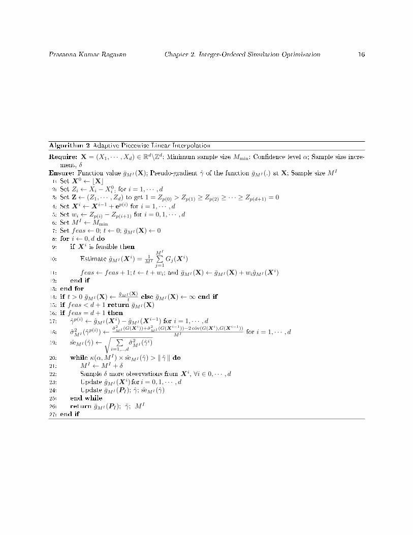
Algorithm 2 Adaptive Piecewise Linear Interpolation
Require: X = (X1, · · · , Xd) ∈ Rd\Zd; Minimum sample size Mmin; Condence level α; Sample size incre-ment, δ
Ensure: Function value gMI (X); Pseudo-gradient γ of the function gMI (.) at X; Sample size M I
1: Set X0 ← bXc2: Set Zi ← Xi −X0
i , for i = 1, · · · , d3: Set Z← (Z1, · · · , Zd) to get 1 = Zp(0) > Zp(1) ≥ Zp(2) ≥ · · · ≥ Zp(d+1) = 0
4: Set Xi ←Xi−1 + ep(i) for i = 1, · · · , d5: Set wi ← Zp(i) − Zp(i+1) for i = 0, 1, · · · , d6: Set M I ←Mmin
7: Set feas← 0; t← 0; gMI (X)← 08: for i← 0, d do9: if Xi is feasible then
10: Estimate gMI (Xi) = 1MI
MI∑j=1
Gj(Xi)
11: feas← feas+ 1; t← t+ wi; and gMI (X)← gMI (X) + wigMI (Xi)12: end if
13: end for
14: if t > 0 gMI (X)← gMI (X)
t else gMI (X)←∞ end if
15: if feas < d+ 1 return gMI (X)16: if feas = d+ 1 then17: γp(i) ← gMI (Xi)− gMI (Xi−1) for i = 1, · · · , d18: σ2
MI (γp(i))← σ2MI (G(Xi))+σ2
MI (G(Xi−1))−2 ˆcov(G(Xi),G(Xi−1))
MI for i = 1, · · · , d19: seMI (γ)←
√ ∑i=1,..,d
σ2MI (γi)
20: while κ(α,M I)× seMI (γ) > ‖ γ ‖ do21: M I ←M I + δ22: Sample δ more observations from Xi, ∀i ∈ 0, · · · , d23: Update gMI (Xi) for i = 0, 1, · · · , d24: Update gMI (PI); γ; seMI (γ)25: end while
26: return gMI (PI); γ; M I
27: end if
Prasanna Kumar Ragavan Chapter 2. Integer-Ordered Simulation Optimization 17
variance, σ2MI (Xi) are obtained. The dierence in sample mean between the incumbent solution and a
neighbor, denoted by µi, is:
µi = gMI (Xbest)− gMI (Xi), ∀i ∈ 1, · · · , 2d,
We write the standard error of the dierence in sample mean as follows:
se(µi) =
√σ2MI (G(Xi)) + σ2
MI (G(Xbest))− 2 ˆcov(G(Xi), G(Xbest))
M I
Conrmatory Check for a local minimum
When µi > 0, ∀i ∈ N 1(Xbest), it indicates that a unit step along that coordinate direction results in a better
solution than Xbest. Let Q denote the set of all neighbors better than the incumbent,
Q = i : i ∈ N 1(Xbest), µi > 0,
and thus QC = F \Q. Conditional on the cardinality of Q, two dierent trajectories for the algorithm are
possible:
CASE A (|Q| > 0) : Update Xbest based on the best solution observed in the neighborhood.
CASE B (|Q| = 0) : If none of the solutions are better than the incumbent solution, either Xbest is a local
minimum or the sample size from interpolation, M I is insucient to distinguish between the neighbors and
the incumbent solution. This condition triggers the adaptive neighborhood enumeration, where the sample
size is strategically increased across solutions in the neighborhood.
Identify a better solution - CASE A
As the name suggests, in this phase, Xbest is updated to be the best solution in Q. However, if the sample
size, M I , is sucient to establish that the dierence in means is signicant, a coordinate search will improve
nite time performance. A neighboring solution is signicantly dierent if the standard error on the dierence
in sample means is less than the absolute value of the dierence. Thus, to establish signicant dierence in
sample mean, following our previous denition of optimal sampling, the condition, κ(α,M I) seMI (µi) ≤ |µi|
should hold, and we let S denote the set of all neighbors satisfying the same:
S = i : i ∈ N 1(Xbest), seMI (µi) ≤ |µi| (2.1)

Prasanna Kumar Ragavan Chapter 2. Integer-Ordered Simulation Optimization 18
Adaptive Neighborhood Enumeration - CASE B
Adaptive neighborhood enumeration forms the exploitative phase of ADALINE, where the objective is to
conrm a local minimum by repeated sampling, when we fail to identify a better solution in the neighborhood
based on the initial estimates. Sampling is strategically repeated across feasible solutions in the neighbor-
hood, and the incumbent solution, Xbest, until the budget is expended, or a signicantly better solution is
identied. Any solution in the set, Q ∩ S should be deemed signicantly better. We follow a three step
procedure described below in allocating simulation eort across all feasible solutions in the neighborhood:
1. Stratify: Based on the initial estimates of µi, se(µi) obtained by expending M I , we classify all feasible
neighbors into one of three categories as follows:
(i) Set Q ∩ S, the set of all neighbors that satisfy sampling criterion in (2.1), and are also promising
enough to be a descent direction; that is,
Q∩ S ← i : i ∈ N 1(X), κ(α,Mi)× se(µi) ≤ |µi|, and µi > 0.
(ii) Set QC ∩ S, the set of all neighbors that satisfy sampling criterion in (2.1), but are not promising
enough to be a descent direction; that is,
QC ∩ S ← i : i ∈ N 1(X), κ(α,Mi)× se(µi) ≤ |µi|, and µi ≤ 0.
(iii) SC, the set of all neighbors that do not satisfy sampling criterion in (2.1).
Note that adaptive neighborhood enumeration is performed only when the set Q = ∅.
2. Prioritize Upon classication of neighbors, the following actions are possible depending on the state of
the neighboring solutions:
(i) When |Q ∩ S| > 0, it indicates that a subset of signicantly better solutions have been identied
and hence the neighborhood enumeration procedure is terminated.
(ii) When |Q ∩ S| = 0, it indicates that further sampling is needed to identify a signicantly better
solution. Instead of allocating eort randomly across the neighbors, we use the following ordering
to determine where further simulation eort should be expended:
SC ≺ QC ∩ S,

Prasanna Kumar Ragavan Chapter 2. Integer-Ordered Simulation Optimization 19
where ≺ indicates the precedence constraint, that is, the non-empty set to the left of ≺ has higher
priority over the set to the right. Thus, sampling eort is uniformly allocated only to neighbors
where the dierence in sample means is not signicant.
3. Simulate and Update: Once the set of neighbors where further simulation eort should be allocated
are identied, we further collect δ independent samples at each of those neighoring solutions. Based
on the new sample information, µi, se(µi) and all other relevant sample statistics are updated and the
stratication rule is applied again to check if the termination criterion for NE is satised. Else, the above
three steps are repeated until |Q ∩ S| > 0.
If Xbest is indeed a local minimum, all the remaining simulation budget is expended between the incum-
bent and its neighbors, increasing the condence on the estimated objective.
Remark. With the availability of new information, a neighboring solution may repeatedly transition
between QC ∩ S, Q ∩ SC, and QC ∩ SC. Under such circumstances, after a set has been chosen for
further simulation, we equalize the sample size at all neighbors before expending δ more simulations.
Coordinate Search
Once the set of all signicantly better solutions are identied, estimates of the partial gradients in the
neighborhood is used to perform a block coordinate search. The gradient direction is a d dimensional vector,
thus we rst resolve the neighbors in A to the corresponding co-ordinate axis (j = 1, · · · , d), and then
estimate the gradient along each coordinate axis as follows:
γj =
(−1)i+1(gMi(Xi)− gM (X)
), j = b i2c and ∀i ∈ A
0, otherwise.
The coordinate search is similar to line search described in Section 2.2.1 and does not require much elabo-
ration. In the coordinate search, instead of searching along the entire decision vector, we restrict our search
to a subspace.
ADALINE continues to alternate between the enumeration procedure and the coordinate search until
all the simulation budget is expended. The solution with the lowest estimated objective function is chosen
to be Xbest and returned to the user as the solution to Problem (1).
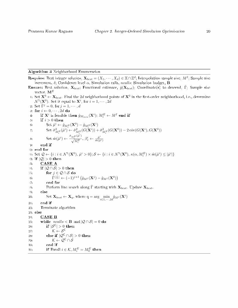
Prasanna Kumar Ragavan Chapter 2. Integer-Ordered Simulation Optimization 20
Algorithm 3 Neighborhood Enumeration
Require: Best integer solution, Xbest = (X1, · · · , Xd) ∈ X∩Zd; Interpolation sample size, M I ; Sample sizeincrement, δ; Condence level α, Simulation calls, ncalls; Simulation budget, B
Ensure: Best solution, Xbest; Functional estimate, g(Xbest); Coordinate(s) to descend, Γ; Sample sizevector, ME
1: Set X0 ← Xbest. Find the 2d neighborhood points of X0 in the rst-order neighborhood, i.e., determineN 1(X0). Set it equal to Xi, for i = 1, · · · , 2d
2: Set Γj = 0, for j = 1, · · · , d3: for i← 0, · · · , 2d do4: if Xi is feasible then gMmin(Xi); ME
i ←M I end if
5: if i > 0 then6: Set µi ← gME
i(X0)− gME
i(Xi)
7: Set σ2ME
i(µi)← σ2
MEi
(G(Xi)) + σ2ME
i(G(X0))− 2 ˆcov(G(Xi), G(X0))
8: Set se(µi)←σME
i(µi)
√ME
i
, βiv ←µi
se(µi)
9: end if
10: end for
11: Set Q ← i : i ∈ N 1(X0), µi > 0;S ← i : i ∈ N 1(X0), κ(α,MEi )× se(µi) ≤ |µi|
12: if |Q| > 0 then13: CASE A
14: if |Q ∩ S| > 0 then15: for j ∈ Q ∩ S do16: Γb
j2 c ← (−1)j+1
(gMI (Xj)− gMI (X0)
)17: end for
18: Perform line search along Γ starting with Xbest. Update Xbest.19: else
20: Set Xbest ← Xq, where q = arg mini∈1,··· ,2d
gMI (Xi)
21: end if
22: Terminate algorithm23: else
24: CASE B
25: while ncalls < B and |Q ∩ S| = 0 do26: if |SC| > 0 then27: K ← SC28: else if |QC ∩ S| > 0 then29: K ← QC ∩ S30: end if
31: if Forall i ∈ K,MEi = ME
0 then

Prasanna Kumar Ragavan Chapter 2. Integer-Ordered Simulation Optimization 21
32: for i ∈ K ∪ 0 do33: ME
i ←MEi + δ
34: Estimate gMEi
(Xi), σ2ME
i(Xi), ˆcov(G(Xi), G(X0))
35: end for
36: else
37: for i = i : i ∈ K, MEi < ME
0 do38: ME
i ←MEi + (ME
0 −MEi )
39: Estimate gMEi
(Xi), σ2ME
i(Xi), ˆcov(G(Xi), G(X0))
40: end for
41: end if
42: Update µi, σ2(µi), se(µi), βiv, ncalls43: Update Q, S using conditions in line 11.44: end while
45: for i ∈ Q ∩ S do46: Γb
i2 c ← (−1)i+1
(gMi
(Xi)− gM (X0))
47: end for
48: Terminate algorithm49: end if
2.3 Local Convergence
Let F denote the set of all feasible points, and L(N 1) denote the set of local minima. Under certain
assumptions on the feasible set, we show that the sequence of points visited by ADALINE, denoted by Xk,
converges with probability one (wp1) to the set of local minima, L(N 1). In order to prove convergence of
ADALINE, we use the following assumptions:
Assumption 1. The set of all feasible points, denoted by F , is nite, that is, |F| <∞.
Assumption 2. The objective function is of the form of an expectation, g(x) = E[G(x, ξ)]. An unbiased,
and strongly consistent estimator of the objective function, gm(x) is available such that, E[gm(x)] = g(x),
and limm→∞
gm(x) = g(x), respectively.
Assumption 3. For each x ∈ F , the objective function is nite, i.e., E[G(x, ξ)] <∞.
Assumption 4. For each x ∈ F , the variance of the random simulation observations is nite, i.e.,
Var(G(x, ξ)) <∞.
Lemma 1. Under Assumptions 1− 4, the following assertions hold:
(i) Suppose x ∈ L(N 1). Then P(Xl = x ∀l > k |Xk = x) > 0.
(ii) Suppose x /∈ L(N 1). Then P(Xl = x ∀l > k |Xk = x) = 0.
Prasanna Kumar Ragavan Chapter 2. Integer-Ordered Simulation Optimization 22
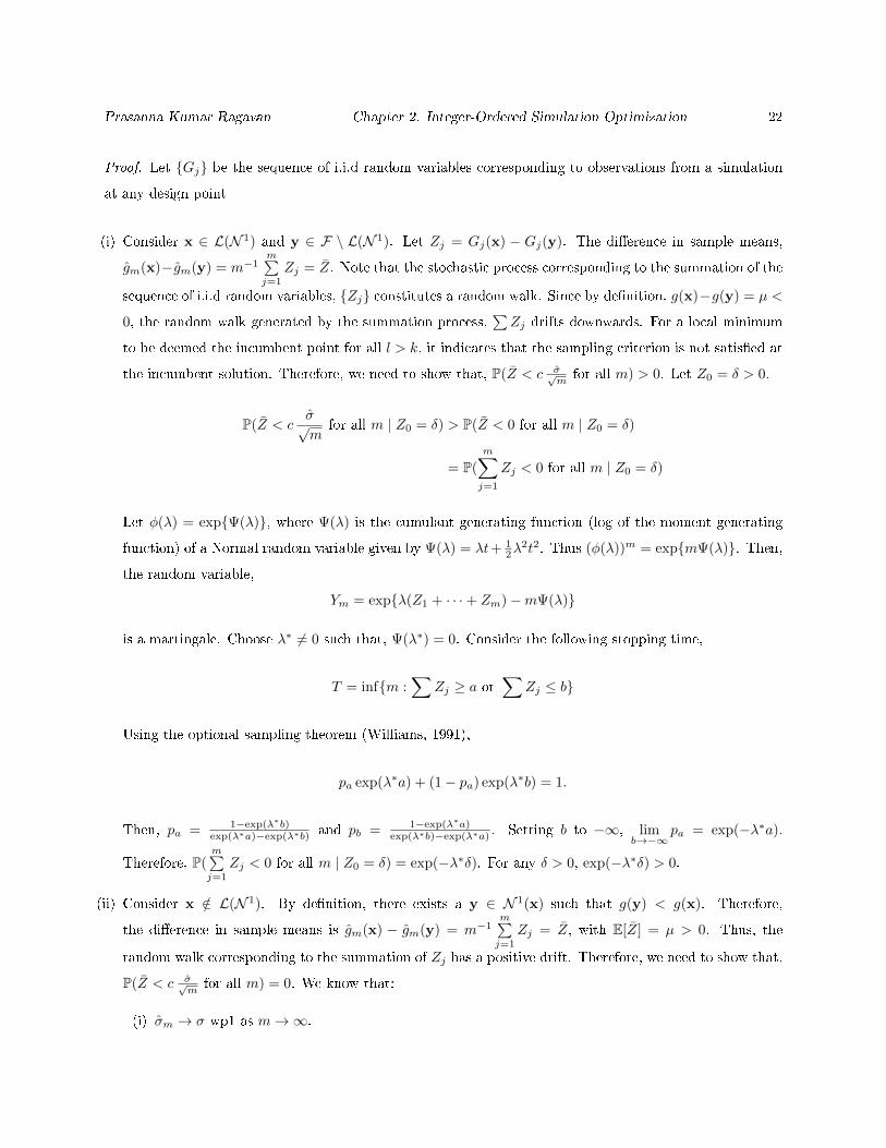
Proof. Let Gj be the sequence of i.i.d random variables corresponding to observations from a simulation
at any design point
(i) Consider x ∈ L(N 1) and y ∈ F \ L(N 1). Let Zj = Gj(x) − Gj(y). The dierence in sample means,
gm(x)−gm(y) = m−1m∑j=1
Zj = Z. Note that the stochastic process corresponding to the summation of the
sequence of i.i.d random variables, Zj constitutes a random walk. Since by denition, g(x)−g(y) = µ <
0, the random walk generated by the summation process,∑Zj drifts downwards. For a local minimum
to be deemed the incumbent point for all l > k, it indicates that the sampling criterion is not satised at
the incumbent solution. Therefore, we need to show that, P(Z < c σ√m
for all m) > 0. Let Z0 = δ > 0.
P(Z < cσ√m
for all m | Z0 = δ) > P(Z < 0 for all m | Z0 = δ)
= P(
m∑j=1
Zj < 0 for all m | Z0 = δ)
Let φ(λ) = expΨ(λ), where Ψ(λ) is the cumulant generating function (log of the moment generating
function) of a Normal random variable given by Ψ(λ) = λt+ 12λ
2t2. Thus (φ(λ))m = expmΨ(λ). Then,
the random variable,
Ym = expλ(Z1 + · · ·+ Zm)−mΨ(λ)
is a martingale. Choose λ∗ 6= 0 such that, Ψ(λ∗) = 0. Consider the following stopping time,
T = infm :∑
Zj ≥ a or∑
Zj ≤ b
Using the optional sampling theorem (Williams, 1991),
pa exp(λ∗a) + (1− pa) exp(λ∗b) = 1.
Then, pa = 1−exp(λ∗b)exp(λ∗a)−exp(λ∗b) and pb = 1−exp(λ∗a)
exp(λ∗b)−exp(λ∗a) . Setting b to −∞, limb→−∞
pa = exp(−λ∗a).
Therefore, P(m∑j=1
Zj < 0 for all m | Z0 = δ) = exp(−λ∗δ). For any δ > 0, exp(−λ∗δ) > 0.
(ii) Consider x /∈ L(N 1). By denition, there exists a y ∈ N 1(x) such that g(y) < g(x). Therefore,
the dierence in sample means is gm(x) − gm(y) = m−1m∑j=1
Zj = Z, with E[Z] = µ > 0. Thus, the
random walk corresponding to the summation of Zj has a positive drift. Therefore, we need to show that,
P(Z < c σ√m
for all m) = 0. We know that:
(i) σm → σ wp1 as m→∞.
Prasanna Kumar Ragavan Chapter 2. Integer-Ordered Simulation Optimization 23
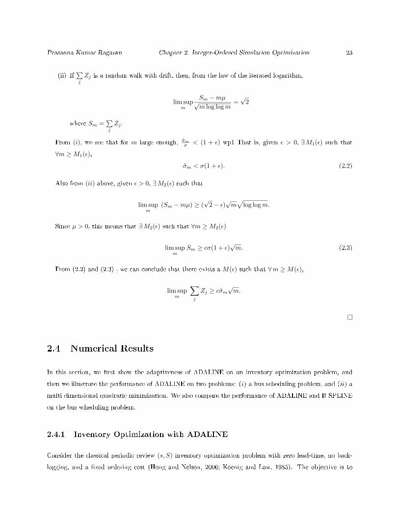
(ii) If∑j
Zj is a random walk with drift, then, from the law of the iterated logarithm,
lim supm
Sm −mµ√m log logm
=√
2
where Sm =∑j
Zj .
From (i), we see that for m large enough, σm
σ < (1 + ε) wp1 That is, given ε > 0, ∃M1(ε) such that
∀m ≥M1(ε),
σm < σ(1 + ε). (2.2)
Also from (ii) above, given ε > 0, ∃M2(ε) such that
lim supm
(Sm −mµ) ≥ (√
2− ε)√m√
log logm.
Since µ > 0, this means that ∃M2(ε) such that ∀m ≥M2(ε)
lim supm
Sm ≥ cσ(1 + ε)√m. (2.3)
From (2.2) and (2.3) , we can conclude that there exists a M(ε) such that ∀m ≥M(ε),
lim supm
∑j
Zj ≥ cσm√m.
2.4 Numerical Results
In this section, we rst show the adaptiveness of ADALINE on an inventory optimization problem, and
then we illustrate the performance of ADALINE on two problems: (i) a bus scheduling problem, and (ii) a
multi-dimensional quadratic minimization. We also compare the performance of ADALINE and R-SPLINE
on the bus scheduling problem.
2.4.1 Inventory Optimization with ADALINE
Consider the classical periodic review (s, S) inventory optimization problem with zero lead-time, no back-
logging, and a xed ordering cost (Hong and Nelson, 2006; Koenig and Law, 1985). The objective is to
Prasanna Kumar Ragavan Chapter 2. Integer-Ordered Simulation Optimization 24
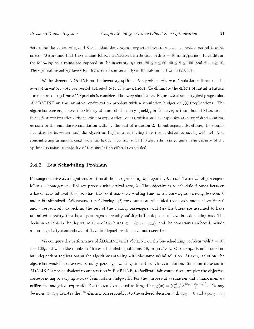
determine the values of s, and S such that the long-run expected inventory cost per review period is mini-
mized. We assume that the demand follows a Poisson distribution with λ = 10 units/period. In addition,
the following constraints are imposed on the inventory system, 20 ≤ s ≤ 80, 40 ≤ S ≤ 100, and S − s ≥ 10.
The optimal inventory levels for this system can be analytically determined to be (20, 53).
We implement ADALINE on the inventory optimization problem where a simulation call returns the
average inventory cost per period averaged over 30 time periods. To eliminate the eects of initial transient
states, a warm-up time of 50 periods is considered in every simulation. Figure 2.2 shows a typical progression
of ADALINE on the inventory optimization problem with a simulation budget of 5000 replications. The
algorithm converges near the vicinity of true solution very quickly, in this case, within about 10 iterations.
In the rst two iterations, the maximum exploration occurs, with a small sample size at every visited solution,
as seen in the cumulative simulation calls by the end of iteration 2. In subsequent iterations, the sample
size steadily increases, and the algorithm begins transitioning into the exploitation mode, with solutions
concentrating around a small neighborhood. Eventually, as the algorithm converges in the vicinity of the
optimal solution, a majority of the simulation eort is expended.
2.4.2 Bus Scheduling Problem
Passengers arrive at a depot and wait until they are picked up by departing buses. The arrival of passengers
follows a homogeneous Poisson process with arrival rate, λ. The objective is to schedule d buses between
a xed time interval [0, τ ] so that the total expected waiting time of all passengers arriving between 0
and τ is minimized. We assume the following: (i) two buses are scheduled to depart, one each at time 0
and τ respectively to pick up the rest of the waiting passengers, and (ii) the buses are assumed to have
unlimited capacity, that is, all passengers currently waiting in the depot can leave in a departing bus. The
decision variable is the departure time of the buses, x = (x1, · · · , xd), and the constraints enforced include
a non-negativity constraint, and that the departure times cannot exceed τ .
We compare the performance of ADALINE and R-SPLINE on the bus scheduling problem with λ = 10,
τ = 100, and when the number of buses scheduled equal 9 and 19, respectively. Our comparison is based on
50 independent replications of the algorithms starting with the same initial solution. At every solution, the
algorithm would have access to noisy passenger-waiting times through a simulation. Since an iteration in
ADALINE is not equivalent to an iteration in R-SPLINE, to facilitate fair comparison, we plot the objective
corresponding to varying levels of simulation budget, B. For the purpose of evaluation and comparison, we
utilize the analytical expression for the total expected waiting time, g(x) =∑d+1i=1 λ
(x(i)−x(i−1))2
2 . For any
decision, x, x(i) denotes the ith element corresponding to the ordered decision with x(0) = 0 and x(d+1) = τ ,
Prasanna Kumar Ragavan Chapter 2. Integer-Ordered Simulation Optimization 25
Figure 2.2: The gure shows the progression of ADALINE on the (s, S) inventory policy optimization.The solutions visited through iterations, and the cumulative simulation budget utilized are plotted. Earlieriterations prioritize exploration at a smaller sample size, followed by exploitation with a signicant increasein sampling.
and d being the number of buses to be scheduled.
When mod (τ, d+ 1) equals 0, the minimum expected waiting time for the d bus scheduling problem
is g(x∗) = λτ2/(2(d+ 1)), and the corresponding optimal schedule is buses departing every τ/(d+ 1) time-
units (any of the d! permutations is an optimal solution). For example, for the 9 bus scheduling problem,
the optimal solution is one of the 9! permutations of x∗ = (10, 20, 30, 40, 50, 60, 70, 80, 90), and the total
expected waiting time is 5000 hours.
Figures 2.3 and 2.4 show the performance of ADALINE and R-SPLINE on the 9 bus and 19 bus
scheduling problems respectively. Rather than plotting the individual sample paths, we plot percentiles of

Prasanna Kumar Ragavan Chapter 2. Integer-Ordered Simulation Optimization 26
Figure 2.3: The gure shows percentiles of the expected wait time corresponding to the solution returnedby ADALINE and R-SPLINE at the end of b simulation calls on the nine-bus scheduling problem.
the true objective corresponding to the random decision at a budget level based on the 50 replications. While
implementing R-SPLINE, the sample growth rate that governs the sample size and the budget within each
retrospective iteration is set to be a geometric series with r = 1.1. Please note that the growth rate governs
two independent parameters in R-SPLINE; namely interpolation sample size,M I ; neighborhood enumeration
sample size, ME . These parameters are adaptively determined in ADALINE without the requirement for
any user input. In Figure 2.3, for the 9 bus scheduling problem, we can clearly see that ADALINE hits a N 1
local minimum in the vicinity of the global minimum by 10,000 simulation calls. In the case of R-SPLINE,
to achieve similar performance, it takes nearly twice the eort. Though ADALINE nds a local minimum
quickly, R-SPLINE with its ability to oscillate between local solutions, eventually achieves a good quality
solution.
For the 19 bus scheduling problem, shown in Figure 2.4, ADALINE performs signicantly better
than R-SPLINE indicating that xed sample growth strategies are not ecient. Almost all replications of
ADALINE reach a local minimum within 30,000 simulation calls, whereas in the case of R-SPLINE, none of
the replications converge to a local minimum even after expending 100,000 simulation calls. Our conjecture
is that the coordinate search phase after neighborhood enumeration helps ADALINE to outperform other
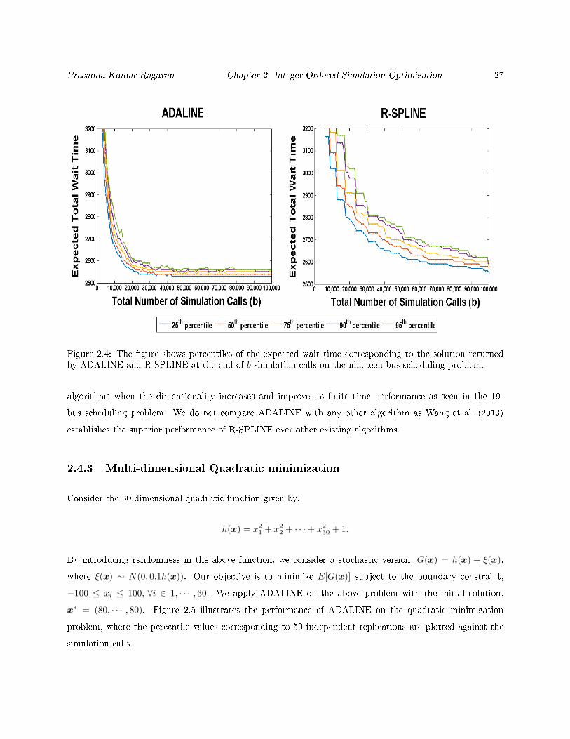
Prasanna Kumar Ragavan Chapter 2. Integer-Ordered Simulation Optimization 27
Figure 2.4: The gure shows percentiles of the expected wait time corresponding to the solution returnedby ADALINE and R-SPLINE at the end of b simulation calls on the nineteen-bus scheduling problem.
algorithms when the dimensionality increases and improve its nite time performance as seen in the 19-
bus scheduling problem. We do not compare ADALINE with any other algorithm as Wang et al. (2013)
establishes the superior performance of R-SPLINE over other existing algorithms.
2.4.3 Multi-dimensional Quadratic minimization
Consider the 30 dimensional quadratic function given by:
h(x) = x21 + x2
2 + · · ·+ x230 + 1.
By introducing randomness in the above function, we consider a stochastic version, G(x) = h(x) + ξ(x),
where ξ(x) ∼ N(0, 0.1h(x)). Our objective is to minimize E[G(x)] subject to the boundary constraint,
−100 ≤ xi ≤ 100, ∀i ∈ 1, · · · , 30. We apply ADALINE on the above problem with the initial solution,
x∗ = (80, · · · , 80). Figure 2.5 illustrates the performance of ADALINE on the quadratic minimization
problem, where the percentile values corresponding to 50 independent replications are plotted against the
simulation calls.
Prasanna Kumar Ragavan Chapter 2. Integer-Ordered Simulation Optimization 28
Figure 2.5: The gure shows the percentiles of the expected value corresponding to the solution returned byADALINE at the end of b simulation calls on the multi-dimensional quadratic problem.
2.5 Conclusion
We present ADALINE, a new algorithm for integer-ordered simulation optimization problems, where a line
search and neighborhood enumeration are performed sequentially to identify a local minimum within a
dened neighborhood. The algorithm relies on a linear interpolation procedure in order to perform the line
search, and the neighborhood enumeration acts as a conrmatory check for a local minimum. Unlike other
algorithms for integer simulation optimization, ADALINE does not require the user to provide a sampling
scheme thus eliminating the need for any parameter tuning.
We are able to show that ADALINE converges to a local minimum with probability one under certain
structural conditions on the objective function. Our numerical results indicate that ADALINE outperforms
other SO algorithms on integer-ordered feasible sets. A working code of ADALINE on integer feasible sets
is available at http://simopt.org.

Chapter 3
ADALINE for Continuous Simulation
Optimization
In this chapter, we consider the unconstrained simulation optimization problem of the form:
PCO : minimize g(x) = Eξ [G(x, ξ)]
subject to x ∈ X
where, the feasible X ⊆ Rd is continuous, and the objective function can be observed only through a stochastic
simulation. We assume that a Monte Carlo simulation provides a point estimate of the unknown objective
function, gm(x) = m−1∑mj=1G(x, ξj), such that limm→∞ gm(x)→ gm(x), where m denotes the simulation
eort. We also assume that an estimate of the gradient, ∇gm(x), is constructed through noisy gradient
observations, ∇G(x, ξj).
In addition to simulation optimization, problems of type PCO are frequently encountered in large scale
machine learning applications, where the parameters of a prediction model are determined by minimizing a
loss function using a small sample of the training data (Byrd et al., 2012). To solve such problems, either the
Stochastic Approximation (SA) technique, or the Sample Average Approximation (SAA) technique discussed
in Chapter 1 are frequently used. Both SA and SAA require the gradient to be estimated using a suitable
procedure (either by directly observing the gradient, or through nite dierence methods), and have analogs
in derivative based deterministic optimization strategies. First, we discuss the fundamentals of deterministic
line search methods, and extend line search techniques to develop ADALINE-Continuous (Adaptive Line
29

Prasanna Kumar Ragavan Chapter 3. Continuous Simulation Optimization 30
Search for Continuous Simulation Optimization) for solving Problem PCO.
3.1 Deterministic Line Search Methods
Deterministic line search algorithms are iterative techniques that seek to identify a local minimum on con-
tinuous feasible sets. Given an initial solution, x0, the algorithm identies a sequence of iterates, xk using
the recursive relation:
xk+1 := xk + skdk,
where dk is the direction of descent, and sk is the step length along the descent direction. The descent
direction is chosen such that it ensures a decrease in objective function for a suitable step length. Thus, a
line search method is a two step procedure, where the rst step is to identify the direction of descent, dk,
followed by determining the step length along that direction.
To build more intuition about line search methods, consider the second order Taylor's expansion of
the function, g at xk+1:
g(xk + skdk) = g(xk) + skdkT∇g(xk) +
1
2s2kdk
T∇2g(xk)dk (3.1)
From (3.1), it should be noted that the condition, dkT∇g(xk) < 0 should hold for the algorithm to guar-
antee a decrease in objective function at the new iterate, xk+1. Writing dkT∇g(xk) as a dot product,
||dk|| ||∇g(xk)|| cos θ, the condition can be further simplied as cos θ < 0. For the descent direction to
guarantee a decrease in objective function, it should be of the form dk = −B−1k ∇g(xk), where B−1
k is a
positive-denite matrix, choices of which lead to many variations in line search methods as seen later.
Once the direction of descent, dk, is determined, the optimal step length is the minimizer of minsg(xk+
sdk). In practice, nding an exact step length at each iteration is computationally intensive, and hence,
the step length is usually determined by an inexact search method. An inexact line search is an iterative
process to determine the step length such that the resulting iterate satises one or more sucient decrease
conditions. Two of the commonly used conditions for determining step length are the Armijo-Goldstein
conditions (Armijo et al., 1966; Nocedal and Wright, 2006), which guarantees a step length that minimizes
the functional value to atleast a fraction attained by a rst order Taylor's expansion while preventing the
step length from becoming too small (Nocedal and Wright, 2006).
g(xk + skdk) ≤ g(xk) + η sk dTk ∇g(xk) (3.2)
g(xk + skdk) ≥ g(xk) + (1− η) sk dTk ∇g(xk) (3.3)

Prasanna Kumar Ragavan Chapter 3. Continuous Simulation Optimization 31
The choice of the descent direction, particularly the choice of Bk leads to dierent variations of line search
methods. When Bk is the Hessian matrix and a unit step length is used, it is the well known Newton's
method, whereas if Bk is the identity matrix, it is the gradient or the steepest descent method. However,
Newton's method has several disadvantages including the expensive computational eort in calculating the
Hessian, and the steepest descent method suers from inferior asymptotic rate of convergence. Quasi-Newton
methods overcome these limitations by approximating the Hessian at each iteration using the gradient from
previous iterate. Depending on the mechanism for updating Bk, many Quasi-Newton algorithms can be
designed, and for a thorough treatment of these methods, and other line search algorithms, we refer readers
to Nocedal and Wright (2006).
3.2 Variable Sampling in Simulation Optimization
From Chapter 1, recall that SA, the analogue of deterministic line search in SO, uses a Newton-type recursion
with a xed step length, and that the SAA can utilize the same algorithms with no modications. However,
these methods are sensitive to the estimation error of the gradient, and the objective function respectively
(Kushner and Clark, 2012). Moreover, the convergence and nite time performance of these algorithms are
highly dependent on the user-specied choice of sample size and the step size (Powell, 2007), often referred
to as the learning rate in machine learning applications.
A poor choice of step length or a large sample size introduces ineciency, whereas insucient sam-
pling leads to non-convergence. Specically, the sampling scheme, which primarily governs the quality of
the estimated objective function and the gradient (the direction of descent) is of particular importance.
Therefore, our focus will be on developing a gradient based line search technique that adaptively determines
the sample size at every iteration. As is the case with other gradient based methods, our algorithm will seek
to determine a local minimum, x∗, of Problem PCO. Recall that, by denition, x∗ ∈ Rd is a local minimum
if and only if any other feasible solution within an ε-neighborhood of x∗ is inferior to x∗.
In SO, several variable sampling schemes have been proposed to work either within a SA or SAA
framework. Recall that, in the SAA procedure, the true objective function in Problem PCO is approximated
with the sample average, gm(x) = m−1∑mj=1G(x, ξj). Then, a sequence of approximate problems are solved
using any deterministic optimization procedure, and for a large enough sample size, SAA converges to an
optimal solution. Since SAA requires the approximate problem to be solved repeatedly starting with the
same initial solution, to conserve simulation eort, Homem-De-Mello (2003) proposed a variable sampling
scheme where the sample size, mk, in iteration k increases at a certain rate such that mk → ∞. However,
the sampling scheme is xed, and non-decreasing irrespective of the problem.
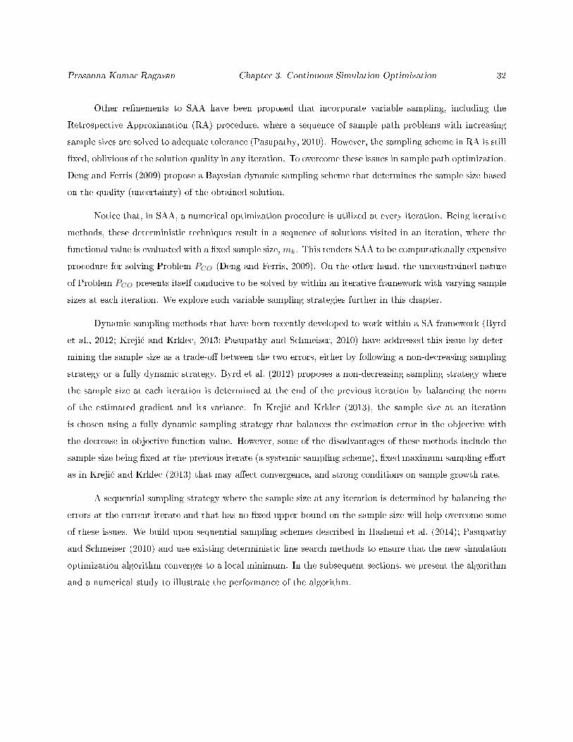
Prasanna Kumar Ragavan Chapter 3. Continuous Simulation Optimization 32
Other renements to SAA have been proposed that incorporate variable sampling, including the
Retrospective Approximation (RA) procedure, where a sequence of sample path problems with increasing
sample sizes are solved to adequate tolerance (Pasupathy, 2010). However, the sampling scheme in RA is still
xed, oblivious of the solution quality in any iteration. To overcome these issues in sample path optimization,
Deng and Ferris (2009) propose a Bayesian dynamic sampling scheme that determines the sample size based
on the quality (uncertainty) of the obtained solution.
Notice that, in SAA, a numerical optimization procedure is utilized at every iteration. Being iterative
methods, these deterministic techniques result in a sequence of solutions visited in an iteration, where the
functional value is evaluated with a xed sample size, mk. This renders SAA to be computationally expensive
procedure for solving Problem PCO (Deng and Ferris, 2009). On the other hand, the unconstrained nature
of Problem PCO presents itself conducive to be solved by within an iterative framework with varying sample
sizes at each iteration. We explore such variable sampling strategies further in this chapter.
Dynamic sampling methods that have been recently developed to work within a SA framework (Byrd
et al., 2012; Kreji¢ and Krklec, 2013; Pasupathy and Schmeiser, 2010) have addressed this issue by deter-
mining the sample size as a trade-o between the two errors, either by following a non-decreasing sampling
strategy or a fully dynamic strategy. Byrd et al. (2012) proposes a non-decreasing sampling strategy where
the sample size at each iteration is determined at the end of the previous iteration by balancing the norm
of the estimated gradient and its variance. In Kreji¢ and Krklec (2013), the sample size at an iteration
is chosen using a fully dynamic sampling strategy that balances the estimation error in the objective with
the decrease in objective function value. However, some of the disadvantages of these methods include the
sample size being xed at the previous iterate (a systemic sampling scheme), xed maximum sampling eort
as in Kreji¢ and Krklec (2013) that may aect convergence, and strong conditions on sample growth rate.
A sequential sampling strategy where the sample size at any iteration is determined by balancing the
errors at the current iterate and that has no xed upper bound on the sample size will help overcome some
of these issues. We build upon sequential sampling schemes described in Hashemi et al. (2014); Pasupathy
and Schmeiser (2010) and use existing deterministic line search methods to ensure that the new simulation
optimization algorithm converges to a local minimum. In the subsequent sections, we present the algorithm
and a numerical study to illustrate the performance of the algorithm.

Prasanna Kumar Ragavan Chapter 3. Continuous Simulation Optimization 33
3.3 ADALINE - Continuous Simulation Optimization
The paradigm of ADALINE on continuous feasible sets is similar to that of deterministic line search methods,
where a direction of descent is identied rst, followed by a search along that direction. However, when noisy
gradients are observed, to estimate the direction of descent with sucient condence, the rst phase of our
algorithm determines the sample size adaptively based on the incumbent solution quality. The following
steps are performed in one iteration of our algorithm:
S.1 An adaptive sampling criterion is employed to determine the sample size, and the gradient is estimated
at each iterate;
S.2 A line search along the negative gradient direction identied in S.1 is employed to identify a better
solution.
As discussed earlier, the sampling scheme we propose allocates simulation eort directly proportional to
the quality of the visited solution. This is achieved by letting the sample size be determined as a trade-o
between the estimation error and the optimization error. By letting the sample size depend only on the
solution quality in a sequential sampling framework, our algorithm also eliminates the need for other user-
dened parameters. To provide some perspective, our adaptive sampling strategy relies on one user-specied
parameter to determine the sample size at any iteration, whereas, a comparable sampling strategy developed
in Kreji¢ and Krklec (2013) requires four user specied parameters just to determine the sample size. Once
the sample size is determined, a line search is performed in S.2 to identify a better solution.
In our algorithm, we let Xk denote the kth visited solution, and Mk the sample size in the kth
iteration. The minimum sample size at any iteration is denoted by Mmin. The estimated gradient, ∇g(Xk),
and the sample variance, σNk
(∇(g(Xk))
)form the basis for the optimization error, and the estimation error
respectively.
3.3.1 Details of the algorithm & pseudocode
Recall that the line search method uses a recursive equation of the form, Xk+1 = Xk + sk dk. The search
direction, dk, is a function of the estimated gradient, and is of the form, dk = −B−1k ∇g(Xk). Based on the
structure of the matrix, Bk, the line search method is classied as follows: (i) Stochastic Gradient Descent,
where Bk is the identity matrix, I; and (ii) Stochastic quasi-Newton method (BFGS method ), where Bk
is an approximation of the Hessian that approaches the true Hessian as the algorithm progresses (Nocedal
Prasanna Kumar Ragavan Chapter 3. Continuous Simulation Optimization 34
and Wright, 2006). In both of the methods, once a directional estimate is available, an inexact line search is
performed to determine the step length, sk along the direction dk using the Armijo-Goldstein conditions (3.2)
and (3.3). Note that the above algorithm is a stochastic counterpart to deterministic line search methods
with the exception that the true gradient/functional values are replaced with their corresponding sample
mean. In the proposed strategy, the sampling eort, Mk, at any iteration is a trade-o between a linear
transformation of the sample covariance matrix that denotes the estimation error, σn(∇g(Xk)), and the
optimization error given by the estimated norm of the gradient, ||∇gMk(Xk)|| (Hashemi et al., 2014)
Mk = infm>dkre
m :
κ(α,Mk)× σm(∇g(Xk))√m
≤ ||∇gm(Xk)||
and r > 1. (3.4)
The constant, κ(α,m), can be chosen to be the αth percentile of a Student's t distribution with m−1 degrees
of freedom. Following the results of Pasupathy et al. (2015), in order to ensure almost sure convergence,
an escort sequence is used to establish a sucient growth in the minimum sampling eort at each iteration.
Since an inexact line search estimates the function at the new iterate, gMk(Xk+1), by imposing a simple
condition onMk+1, we obtain two possible algorithmic variation as follows: (i) a dynamic sampling strategy
that just satises the condition (3.4) at each iteration, and (ii) a non-decreasing sampling strategy where
Mk ≤ Mk+1. In the rst strategy, it should be noted that reduction in sample size is possible between
iterations making it a completely adaptive sampling scheme, whereas in the second strategy, such reduction
is not permitted, and the algorithm only signals when the sample size should be increased.
3.4 Numerical Results
We implement our adaptive sampling line search algorithm on the stochastic counterpart of the following
well known deterministic functions: (i) The Rosenbrock function (Deng and Ferris, 2009), and (ii) the Alu-
Pentini function (Alu Pentini et al., 1985), each with two decision variables. A stochastic counterpart is
generated by multiplying one of the decision variables in each of the above functions with a random variable
with mean 1. In order to illustrate the advantages of our sampling strategy, we also compare our results
with an existing adaptive sampling strategy proposed by Kreji¢ and Krklec (2013).
Despite the sampling strategy in our proposed algorithm being adaptive, that is, automatically signal
an increase or decrease in sample sizes between iterations, we can devise a variation which restricts the
sample sizes to be non-decreasing between iterations. Moreover, the choice of the descent direction in the
line search technique results in two other variations of our algorithm: (i) a stochastic gradient descent
(SGD) method, and (ii) a stochastic BFGS method (Quasi-Newton). Thus, the four possible variations of
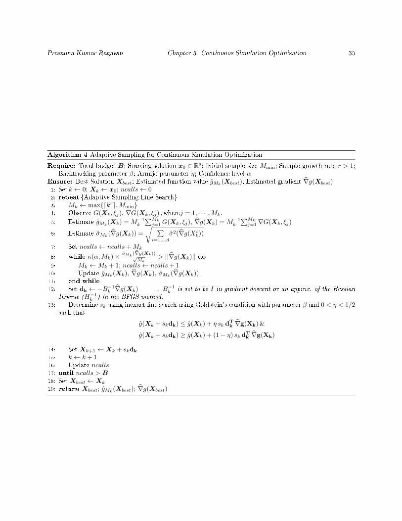
Prasanna Kumar Ragavan Chapter 3. Continuous Simulation Optimization 35
Algorithm 4 Adaptive Sampling for Continuous Simulation Optimization
Require: Total budget B; Starting solution x0 ∈ Rd; Initial sample size Mmin; Sample growth rate r > 1;Backtracking parameter β; Armijo parameter η; Condence level α
Ensure: Best Solution Xbest; Estimated function value gMk(Xbest); Estimated gradient ∇g(Xbest)
1: Set k ← 0; Xk ← x0; ncalls← 02: repeat Adaptive Sampling Line Search3: Mk ← maxdkre,Mmin4: Observe G(Xk, ξj), ∇G(Xk, ξj) ,wherej = 1, · · · ,Mk.5: Estimate gMk
(Xk) = M−1k
∑Mk
j=1G(Xk, ξj), ∇g(Xk) = M−1k
∑Mk
j=1∇G(Xk, ξj)
6: Estimate σMk(∇g(Xk)) =
√ ∑i=1,..,d
σ2(∇g(Xik))
7: Set ncalls← ncalls+Mk
8: while κ(α,Mk)× σMk(∇g(Xk))√Mk
> ||∇g(Xk)|| do9: Mk ←Mk + 1; ncalls← ncalls+ 1
10: Update gMk(Xk), ∇g(Xk), σMk
(∇g(Xk))11: end while
12: Set dk ← −B−1k ∇g(Xk) . B−1
k is set to be I in gradient descent or an approx. of the HessianInverse (H−1
k ) in the BFGS method.13: Determine sk using inexact line search using Goldstein's condition with parameter β and 0 < η < 1/2
such that
g(Xk + skdk) ≤ g(Xk) + η sk dTk ∇g(Xk) &
g(Xk + skdk) ≥ g(Xk) + (1− η) sk dTk ∇g(Xk)
14: Set Xk+1 ←Xk + skdk
15: k ← k + 116: Update ncalls17: until ncalls > B18: Set Xbest ←Xk
19: return Xbest; gMk(Xbest); ∇g(Xbest)

Prasanna Kumar Ragavan Chapter 3. Continuous Simulation Optimization 36
the algorithm based on the sampling strategy, and the line search technique are as follows: (i) SGD with
adaptive sampling, (ii) SGD with non-decreasing sampling, (iii) SBFGS with adaptive sampling, and (iv)
SBFGS with non-decreasing sampling.
Recall that, in the stochastic BFGS update, an approximation of the Hessian matrix is generated
using the estimated gradient, and the step size. In order to avoid frequent noisy updates to the Hessian
approximation, particularly at the initial iterations of the algorithm, we follow the work of Byrd et al. (2014),
and update the approximation of the Hessian matrix only at every Lth iteration. As discussed earlier, an
escort sequence is used to establish a sucient growth in the sample size between iterations, that is, to
provide a lower bound on the sample size every iteration. In our experiments, we set the escort sequence as
a polynomial function, kr, where k denotes the iteration number, and r is a constant.
We run multiple independent replications of the algorithm starting with the same initial solution.
Since the algorithm is designed to expend innite simulation eort on convergence to a local minimum, we
terminate the algorithm on exceeding the simulation budget, B. A call to the simulation oracle, in addition
to providing a realization of the objective function, G(x, ξ), also provides a noisy observation of the gradient,
∇G(x, ξ). The following parameters govern the sample size, and the line search during the optimization:
Algorithm Parameters
Total budget (B) : 3× 10⁵
Initial sample size (Mmin) : 2
Sample growth rate (r) : 1.1
Backtracking parameter (β) : 1/2
Armijo parameter (η) : 1× 10⁻⁴
3.4.1 Alu-Pentini Function
The deterministic Alu-Pentini function in two dimensions is converted to its stochastic counterpart by
multiplying a random component to the rst term, such that, x = (x1ξ, x2). We minimize the expectation
of the resulting stochastic function giving rise to the following unconstrained optimization problem:
minx
g(x) = Eξ[0.25(x1ξ)4 − 0.5(x1ξ)
2 + 0.1(x1ξ) + 0.5x22]
The random variable, ξ, is assumed to follow a normal distribution with mean, µ, equal to 1, and variance,
σ2, equal to 0.1. As an analytical form for the function is available, we determine the set of all local minima
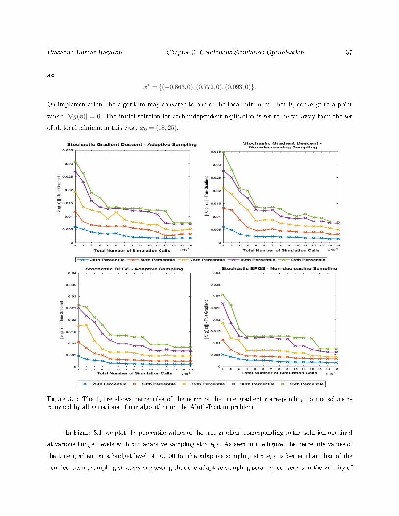
Prasanna Kumar Ragavan Chapter 3. Continuous Simulation Optimization 37
as:
x∗ = (−0.863, 0), (0.772, 0), (0.093, 0).
On implementation, the algorithm may converge to one of the local minimum, that is, converge to a point
where |∇g(x)| = 0. The initial solution for each independent replication is set to be far away from the set
of all local minima, in this case, x0 = (18, 25).
Figure 3.1: The gure shows percentiles of the norm of the true gradient corresponding to the solutionsreturned by all variations of our algorithm on the Alu-Pentini problem
In Figure 3.1, we plot the percentile values of the true gradient corresponding to the solution obtained
at various budget levels with our adaptive sampling strategy. As seen in the gure, the percentile values of
the true gradient at a budget level of 10,000 for the adaptive sampling strategy is better than that of the
non-decreasing sampling strategy suggesting that the adaptive sampling strategy converges in the vicinity of

Prasanna Kumar Ragavan Chapter 3. Continuous Simulation Optimization 38
a local minimum more quickly than the non-decreasing sampling scheme. However, both of these sampling
schemes perform similar with further increase in the total simulation budget.
Figure 3.2: Performance of the adaptive samplings strategy on the Alu-Pentini problem in comparisonwith the sampling strategy in Kreji¢ and Krklec (2013)
In Figure 3.2, we compare the performance of our algorithm with the adaptive sampling strategy
proposed in (Kreji¢ and Krklec, 2013), with a Quasi-Newton update, and a maximum sample size, Mmax =
1500. In this gure, we plot the product of the square root of the cumulative simulation eort and the norm
of true gradient averaged over several independent replications across the iterations. Since, we expect the
algorithm to converge to a stationary point, the closer the product is to zero, the better the quality of the
obtained solution by the algorithm. As it can be clearly seen, our algorithm converges to an iterate that is
at least four times better within about twenty ve iterations, whereas the adaptive strategy in (Kreji¢ and
Krklec, 2013) does not provide a better solution despite expending the entire simulation budget.
Figure 3.3 illustrates the sample size across all indepedent replications as a function of the iteration
for the Alu-Pentini problem. At the initial stages of the algorithm, the impact of the escort sequence is
signicant for at least 50% of the replications, and as the algorithm progresses, the sampling criterion in (3.4)
takes over in determining the sample size. However, for the non-decreasing sampling strategy, the escort
sequence does not seem to show any signicant role in sample size determination.
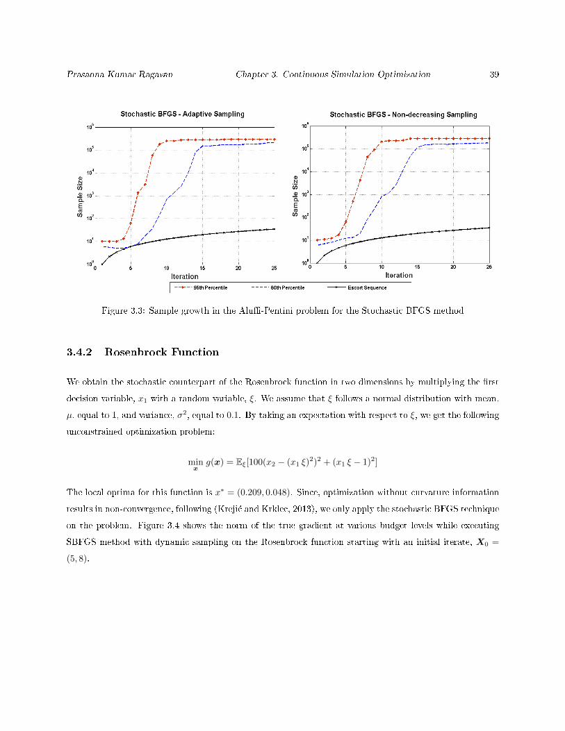
Prasanna Kumar Ragavan Chapter 3. Continuous Simulation Optimization 39
Figure 3.3: Sample growth in the Alu-Pentini problem for the Stochastic BFGS method
3.4.2 Rosenbrock Function
We obtain the stochastic counterpart of the Rosenbrock function in two dimensions by multiplying the rst
decision variable, x1 with a random variable, ξ. We assume that ξ follows a normal distribution with mean,
µ, equal to 1, and variance, σ2, equal to 0.1. By taking an expectation with respect to ξ, we get the following
unconstrained optimization problem:
minx
g(x) = Eξ[100(x2 − (x1 ξ)2)2 + (x1 ξ − 1)2]
The local optima for this function is x∗ = (0.209, 0.048). Since, optimization without curvature information
results in non-convergence, following (Kreji¢ and Krklec, 2013), we only apply the stochastic BFGS technique
on the problem. Figure 3.4 shows the norm of the true gradient at various budget levels while executing
SBFGS method with dynamic sampling on the Rosenbrock function starting with an initial iterate, X0 =
(5, 8).

Prasanna Kumar Ragavan Chapter 3. Continuous Simulation Optimization 40
Figure 3.4: The gure shows percentiles of the norm of the true gradient corresponding to the solutionsreturned by all variations of our algorithm on the Rosenbrock problem
As in the case of the Alu-Pentini function, our sampling strategy yields better results when compared to
the strategy provided in (Kreji¢ and Krklec, 2013), as shown in Figure 3.5
Figure 3.5: Performance of the adaptive samplings strategy on the Rosenbrock problem in comparison withthe sampling strategy in Kreji¢ and Krklec (2013)
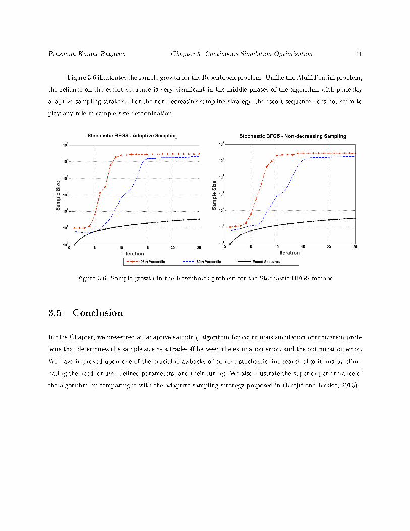
Prasanna Kumar Ragavan Chapter 3. Continuous Simulation Optimization 41
Figure 3.6 illustrates the sample growth for the Rosenbrock problem. Unlike the Alu Pentini problem,
the reliance on the escort sequence is very signicant in the middle phases of the algorithm with perfectly
adaptive sampling strategy. For the non-decreasing sampling strategy, the escort sequence does not seem to
play any role in sample size determination.
Figure 3.6: Sample growth in the Rosenbrock problem for the Stochastic BFGS method
3.5 Conclusion
In this Chapter, we presented an adaptive sampling algorithm for continuous simulation optimization prob-
lems that determines the sample size as a trade-o between the estimation error, and the optimization error.
We have improved upon one of the crucial drawbacks of current stochastic line search algorithms by elimi-
nating the need for user dened parameters, and their tuning. We also illustrate the superior performance of
the algorithm by comparing it with the adaptive sampling strategy proposed in (Kreji¢ and Krklec, 2013).
Chapter 4
Surgery Rescheduling using Simulation
Optimization
In this chapter, we demonstrate the use and superiority of ADALINE over a competing algorithm on a (quasi-
realistic) surgery scheduling problem. The total costs incurred due to assigning and performing surgeries in
an operating room (OR) account for a large percentage of a hospital's operating expenses, in some cases upto
50% of the total operating cost (Elixhauser and Andrews, 2010). Since the number of surgeries performed
varies signicantly between specialties, optimal allocation of capacity and ecient scheduling practices are
critical to improving OR nancial performance. Hospitals typically allocate OR capacity to specialties based
on a variety of factors including the historical volume, priority level of the specialty, as well as to incentivize
surgeons for increasing the overall utilization of the operating rooms (OR) (Hosseini and Taae, 2014).
Surgical specialties compete, not just for the operating rooms, but also for other resources including
equipment and technicians, necessitating the need for a scheduling policy that streamlines the allocation
of these resources. Therefore, a weekly scheduling policy, called Block Scheduling is usually utilized as a
framework where surgeries with similar resource needs are grouped together and then assigned to specic
time blocks in the future (Blake et al., 2002). Block scheduling improves surgeon satisfaction and leads to
better utilization of operating rooms while minimizing the total overhead cost.
In addition to performing elective surgeries that are scheduled in advance, hospitals have to accom-
modate non-elective surgeries that require expedited surgical intervention. These pose signicant challenges
to the scheduler due to the uncertainty in their arrival times and surgical resource needs. Also, the actual
versus planned duration of surgeries vary signicantly and often lead to schedule disruptions. These dis-
42
Prasanna Kumar Ragavan Chapter 5. Surgery Rescheduling using Simulation Optimization 43
ruptions add to the operating cost of a hospital either by forcing the scheduler to reschedule/cancel elective
procedures or accommodate the non-elective surgeries by assigning overtime work.
Every day schedulers have to decide on protocols to accommodate elective and non-elective cases
under a capacity constrained operating room environment. A sub-optimal rescheduling decision leads to
nancial losses due to high overtime costs, postponement costs and cancellation costs (Gul et al., 2015).
Thus, a sophisticated rescheduling policy is required to aid the scheduler in making the following decisions:
(i) the number of elective cases that should be postponed, (ii) the policy for scheduling non-elective cases
that are realized on any given day , and (iii) the overtime hours needed to accommodate all cases planned
for that day. A successful scheduling policy is also one that ts into the block scheduling framework without
perturbing the surgical blocks too much.
Non-elective surgeries, one of the primary causes of uncertainty in the operating room environment,
can further be classied into urgent and semi-urgent surgeries. Urgent surgeries (emergency) require im-
mediate surgical intervention and semi-urgent surgeries require prioritized intervention within a specied
time period. Prior work on urgent surgeries concludes that dedicating specic operating rooms minimizes
disruption to the existing schedule (Heng and Wright, 2013). Therefore, we restrict the scope of our work
to only accommodating elective surgeries and semi-urgent surgeries, particularly on the development and
optimization of a rescheduling policy for operating room resource allocation.
The remainder of this work is organized as follows: in Section 4.1, we discuss relevant work in the
literature on surgical scheduling; in Section 4.2, we introduce the problem statement and develop a mathe-
matical model for nding an optimal solution; in Section 4.3, we discuss characteristics of optimal solution
to the true problem, its advantages and disadvantages, and how the disadvantages can be overcome us-
ing a threshold-based scheduling policy, and describe the heuristic in detail; in Section 4.4, we present an
optimization and simulation optimization based framework for optimizing the threshold levels; and nally
in Section 4.5, we detail the performance of the simulation optimization (SO) framework and the integer
optimization on a synthetic data set, followed by concluding remarks.
4.1 Literature review
Surgery scheduling is an extensively studied problem with prior work categorized into the following three
groups based on the time horizon of decision making: (i) operating room capacity planning (strategic
decisions), (ii) block scheduling, that is, allocation of surgical capacity to specialties (tactical decisions), and
nally (iii) allocation of individual surgeries based on the block schedule to operating rooms (operational

Prasanna Kumar Ragavan Chapter 5. Surgery Rescheduling using Simulation Optimization 44
decisions). A majority of the literature on OR capacity planning and surgical block allocation utilize an
integer programming framework, usually with an objective to increase the long term utilization of operating
rooms (Blake and Donald, 2002; Day et al., 2012; Hosseini and Taae, 2014). While these models account
for the variability in utilization of operating rooms, they do not explicitly consider the impact of scheduling
practices that induce such variability.
To overcome the disadvantages associated with conventional models, Zhang et al. (2009) propose an
integrated framework for capacity allocation and surgery scheduling. The model allocates surgical time
between elective and urgent surgeries with the objective of minimizing the length of stay after a surgical
procedure. However, by failing to account for the uncertainty and replacing the random variables with their
expected value, the solution from the model is rendered inferior. Min and Yih (2010) propose a model for the
scheduling and assignment of elective cases when the duration of surgeries are random, and under constrained
operating room resources. In this case, the assignment of surgeries, and allocation of other resources is guided
by a two stage stochastic programming approach, solved using sample average approximation (SAA)an
approach where the random variables are replaced by their realizations, and solved using deterministic
techniques. If not for the allocation of secondary resources, this work is equivalent to an elective surgery
assignment problem with random surgery durations, where the objective is to minimize the over time cost.
Lamiri et al. (2009) propose a stochastic model for assigning elective cases across the planning horizon
so that the overall cost of accommodating urgent surgeries is minimized. Unlike Zhang et al. (2009), the
random variables in the model are replaced by Monte Carlo realizations resulting in an approximate problem
that is solved using deterministic techniques. Surgeries that exceed the available capacity are accommodated
using overtime, whereas, elective surgeries may often be rescheduled under such circumstances. By failing
to account for the dynamic nature of the decision process, the utility of this model is primarily restricted to
developing an initial schedule for electives.
Herring and Herrmann (2012) study the single day surgery scheduling problem, where a policy is
developed for assigning surgeries to a particular day in the future. By either accommodating the surgeries
immediately or deferring decisions to the future, schedulers can optimize the utilization of surgical blocks
on a dynamic basis until the day of the surgery. However, even for smaller surgical blocks, this problem is
intractable due to the curse of dimensionality in their proposed dynamic programming framework. There-
fore, they propose an optimization based threshold policy that dierentiates between competing specialties
to occupy a surgical block. Note that the similar threshold based approach is applicable for the surgery
rescheduling problem, for we study the allocation of surgical blocks between elective and urgent surgeries
rather than competing specialties.

Prasanna Kumar Ragavan Chapter 5. Surgery Rescheduling using Simulation Optimization 45
Gul et al. (2015) develop a comprehensive optimization framework for dynamic scheduling of elective
surgeries across a planning horizon. Though they do not dierentiate between elective, or urgent surgeries,
their optimization framework is exible enough to accommodate such modications. On a dynamic basis,
surgeries are scheduled and repetitively rescheduled so that the overall cost of performing surgeries is min-
imized. Similar to the work of Lamiri et al. (2009), this model utilizes a Monte Carlo simulation based
optimization approach to represent the uncertainty in the demand, and duration of surgeries. Though the
solution from this model is optimal and provides critical insights on allocating surgical capacity to develop
block schedules, as we later discuss, these solutions are not implementable in real time.
The capacity allocation model developed by Zonderland et al. (2010) is the only work in the surgery
scheduling literature that considers semi-urgent surgeries. Theirs is a queuing model that can be formulated
in a Markov decision process (MDP) framework to optimize the capacity reserved for semi-urgent surgeries
every week. However, they assume that all semi-urgent surgeries are assigned on a weekly basis, and are
realized at the beginning of the week according to a Poisson process. Though these assumptions yield an
analytical expression, they render the model unrealistic, for the OR scheduler often makes adjustments to
the schedule based on individual surgeries, and on a daily basis.
Our problem is very similar to those studied in Gul et al. (2015) and Zonderland et al. (2010). By
considering the preliminary schedule for electives as a model parameter, we dier from Gul et al. (2015)
where electives are also scheduled. Note that the preliminary schedule in our model can be the optimal
solution to the static surgery assignment models from Lamiri et al. (2009); Min and Yih (2010); Zhang
et al. (2009). At the same time, we overcome the drawbacks associated with Zonderland et al. (2010) by
letting semi-urgent surgeries to be scheduled everyday, and by making no assumptions on the distribution
of the random variables that govern the uncertainty. Thus, we believe our work ts seamlessly into exisiting
scheduling practices, for it provides an implementable policy on accommodating semi-urgent surgeries.
4.2 Problem Statement
We consider the problem of accommodating elective and semi-urgent surgeries in a hospital, where the
electives are scheduled in advance and the semi-urgent surgeries have an unknown demand. In general,
elective surgeries of various surgical specialties are assigned at least a week prior to the surgery, based on a
block schedule. The demand for semi-urgent surgeries can only be realized a day or two prior to the surgery,
making it a challenge for the scheduler to accommodate them, given the limitations on available operating
room time. Thus, the objective is to develop a scheduling policy that accommodates elective and semi-urgent
surgeries with minimal disruption to the existing schedule, and that reduces the cost of adding unplanned

Prasanna Kumar Ragavan Chapter 5. Surgery Rescheduling using Simulation Optimization 46
overtime.
A detailed description of the problem is as follows: At the start of a week, information on the exact
number of elective surgeries over the entire coming week is known to the OR scheduler. The capacity allocated
to every surgical specialty is also xed based on the block schedule. Before executing the schedule on any
particular day, requests for semi-urgent surgeries are realized at the start of the day. Upon realization of semi-
urgent surgical requests, the OR scheduler has to accommodate them so that the overall cost of disrupting
the existing schedule is minimized. If sucient slack in the schedule is available, semi-urgent surgeries may
be accommodated without any disruption to the original schedule. In the event of not having any additional
capacity in the existing schedule, semi-urgent surgeries have to be accommodated by one of the following
means: (i) postponing currently scheduled elective surgeries, (ii) cancellation of elective surgical cases, (iii)
accommodating semi-urgent surgeries with overtime.
Each of the above three decisions incur an additional cost that increases the operating cost of the
hospital. For example, a decision to postpone an elective surgery is followed by another decision on xing
the day it should be performed. In general, when the requests for semi-urgent surgeries are realized on any
particular day, the following sequence of decisions are made by the OR scheduler:
(i) A schedule for accommodating semi-urgent surgeries using available capacity.
(ii) A new schedule after postponement and cancellation of elective surgeries that were previously scheduled
for the day.
(iii) Inclusion of additional capacity via overtime, if any, when the original capacity allocated based on the
block schedule is limited.
We assume the following about the semi-urgent surgeries: (i) the requests are made by a surgical specialty
at the start of day; and (ii) the semi-urgent cases should be accommodated within 3 days (including the
day of arrival), failing which, a loss in revenue is incurred by the hospital. Despite the above relaxing
assumptions, the problem is dicult to solve because of the uncertainty in the number of semi-urgent surgeries
requested, and the requirement to make such decisions on a repetitive basis. Thus, a decision framework
to solve the surgery rescheduling problem should incorporate the following features, (i) a mechanism for
generating realizations from the probability distribution of the demand and duration of surgeries, and (ii) an
optimization model that minimizes the total cost of rescheduling for a realization of these random variables.
In the remainder of this section, we discuss the random variables followed by the optimization model that
makes rescheduling decisions for a realization of the random variables across the entire time horizon.
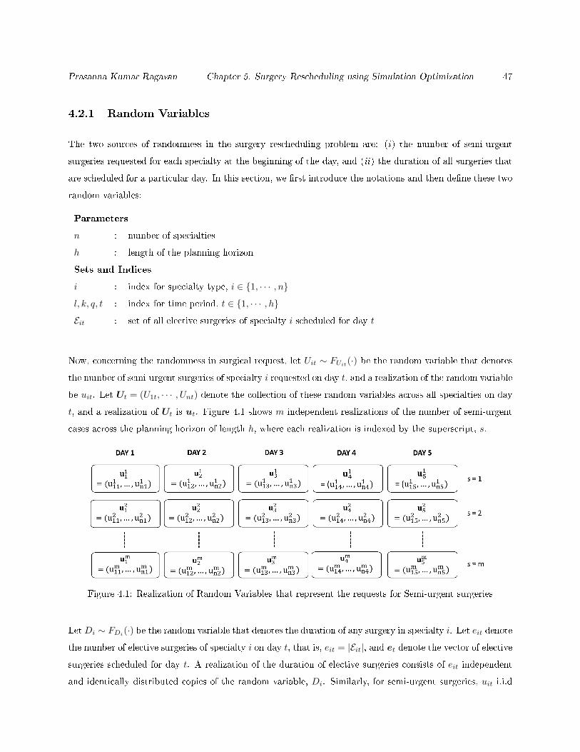
Prasanna Kumar Ragavan Chapter 5. Surgery Rescheduling using Simulation Optimization 47
4.2.1 Random Variables
The two sources of randomness in the surgery rescheduling problem are: (i) the number of semi-urgent
surgeries requested for each specialty at the beginning of the day, and (ii) the duration of all surgeries that
are scheduled for a particular day. In this section, we rst introduce the notations and then dene these two
random variables:
Parameters
n : number of specialties
h : length of the planning horizon
Sets and Indices
i : index for specialty type, i ∈ 1, · · · , n
l, k, q, t : index for time period, t ∈ 1, · · · , h
Eit : set of all elective surgeries of specialty i scheduled for day t
Now, concerning the randomness in surgical request, let Uit ∼ FUit(·) be the random variable that denotes
the number of semi-urgent surgeries of specialty i requested on day t, and a realization of the random variable
be uit. Let Ut = (U1t, · · · , Unt) denote the collection of these random variables across all specialties on day
t, and a realization of Ut is ut. Figure 4.1 shows m independent realizations of the number of semi-urgent
cases across the planning horizon of length h, where each realization is indexed by the superscript, s.
Figure 4.1: Realization of Random Variables that represent the requests for Semi-urgent surgeries
LetDi ∼ FDi(·) be the random variable that denotes the duration of any surgery in specialty i. Let eit denote
the number of elective surgeries of specialty i on day t, that is, eit = |Eit|, and et denote the vector of elective
surgeries scheduled for day t. A realization of the duration of elective surgeries consists of eit independent
and identically distributed copies of the random variable, Di. Similarly, for semi-urgent surgeries, uit i.i.d
Prasanna Kumar Ragavan Chapter 5. Surgery Rescheduling using Simulation Optimization 48
random variables following the distribution, FDi(·), are generated on any particular day.
The set of all surgical durations realized on day t be denoted by Dt. Dt has two elements, each in-turn
is a set corresponding to the duration of semi-urgent and elective surgeries, respectively. Further, each one
of these sets is a collection of random vectors of surgery durations across multiple specialties. For example,
if ut = (u1t, u2t), the duration of these surgeries is a set with two elements, where each element is a vector
of length u1t and u2t respectively. A realization of the number of semi-urgent surgeries and their duration
at any time period t across all surgical specialties is St = ut, Dt. Similarly, we denote a realization across
the entire time horizon by the set, S = ut1≤t≤h, Dt1≤t≤h.
At the start of the day, when the surgical requests are realized, the scheduler has to make decisions so
that the rescheduling cost is minimized. Note that, for stochastic optimization, explicitly incorporating the
probability distribution of the random variables, and analytically determining an optimal solution requires
painstaking eort. Likewise, solving such problems using classical optimization techniques may even be
impossible, particularly when the uncertain variables have an innite support, as in continuous probability
distributions.
Often, to overcome these issues, a nite number of realizations of the random variables are used to
construct a discrete approximation, and the resulting deterministic equivalent of the problem is solved using
existing optimization techniques. This technique is known as the Sample Average Approximation (SAA)
method or the scenario based optimization method. In the following section, we formulate the surgery
rescheduling problem as a deterministic problem where the realizations of the random variables become
input parameters to the mathematical model. For convenience, we denote the set of all such realizations of
these random variables used for SAA by S, with every individual realization indexed by s, ∀s ∈ 1, · · · , |S|.
4.2.2 Surgery Rescheduling using SAA
For the rescheduling problem, decisions are made sequentially everyday with little or no information about the
future. Similar to the other surgery scheduling problems studied in the literature (Gul et al., 2015; Lamiri
et al., 2009), we consider a multi-stage optimization framework where the objective is to minimize total
expected cost of rescheduling across the entire planning horizon. Particularly, we extend the optimization
framework studied in Gul et al. (2015) for formulating the surgery rescheduling problem, with additional
decision variables for semi-urgent surgeries. Before we detail the formulation, we list all notations used in
the optimization model:
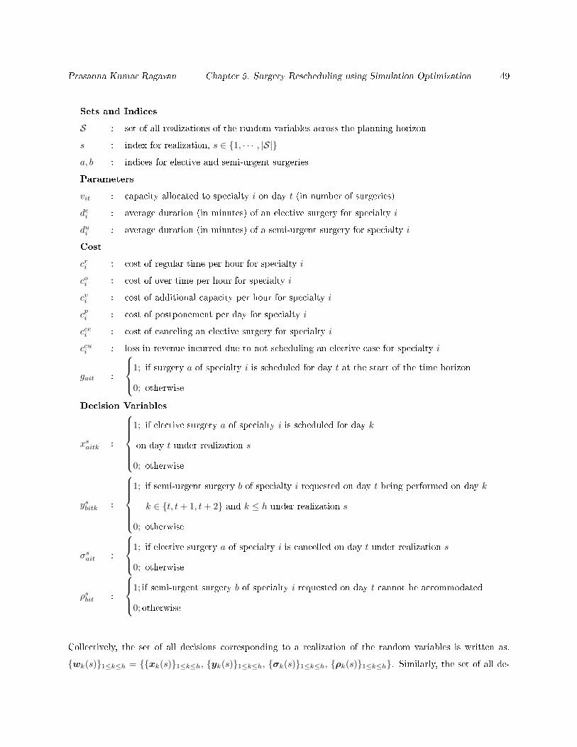
Prasanna Kumar Ragavan Chapter 5. Surgery Rescheduling using Simulation Optimization 49
Sets and Indices
S : set of all realizations of the random variables across the planning horizon
s : index for realization, s ∈ 1, · · · , |S|
a, b : indices for elective and semi-urgent surgeries
Parameters
vit : capacity allocated to specialty i on day t (in number of surgeries)
dei : average duration (in minutes) of an elective surgery for specialty i
dui : average duration (in minutes) of a semi-urgent surgery for specialty i
Cost
cri : cost of regular time per hour for specialty i
coi : cost of over time per hour for specialty i
cvi : cost of additional capacity per hour for specialty i
cpi : cost of postponement per day for specialty i
ccei : cost of canceling an elective surgery for specialty i
ccui : loss in revenue incurred due to not scheduling an elective case for specialty i
gait :
1; if surgery a of specialty i is scheduled for day t at the start of the time horizon
0; otherwise
Decision Variables
xsaitk :
1; if elective surgery a of specialty i is scheduled for day k
on day t under realization s
0; otherwise
ysbitk :
1; if semi-urgent surgery b of specialty i requested on day t being performed on day k
k ∈ t, t+ 1, t+ 2 and k ≤ h under realization s
0; otherwise
σsait :
1; if elective surgery a of specialty i is cancelled on day t under realization s
0; otherwise
ρsbit :
1; if semi-urgent surgery b of specialty i requested on day t cannot be accommodated
0; otherwise
Collectively, the set of all decisions corresponding to a realization of the random variables is written as,
wk(s)1≤k≤h = xk(s)1≤k≤h, yk(s)1≤k≤h, σk(s)1≤k≤h, ρk(s)1≤k≤h. Similarly, the set of all de-
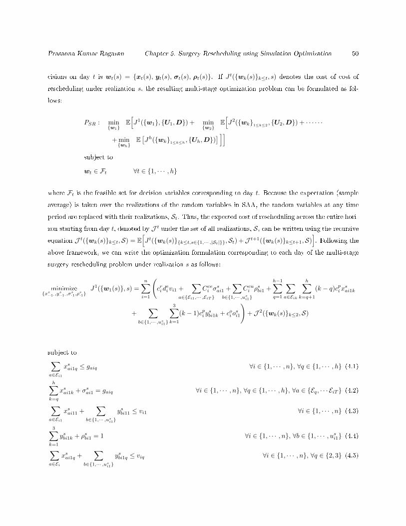
Prasanna Kumar Ragavan Chapter 5. Surgery Rescheduling using Simulation Optimization 50
cisions on day t is wt(s) = xt(s), yt(s), σt(s), ρt(s). If J t(wk(s)k≤t, s) denotes the cost of cost of
rescheduling under realization s, the resulting multi-stage optimization problem can be formulated as fol-
lows:
PSR : minw1
E[J1(w1, U1,D) + min
w2E[J2(wk1≤k≤2
, U2,D) + · · · · · ·
+ minwh
E[Jh(wk1≤k≤h
, Uh,D)] ]]
subject to
wt ∈ Ft ∀t ∈ 1, · · · , h
where Ft is the feasible set for decision variables corresponding to day t. Because the expectation (sample
average) is taken over the realizations of the random variables in SAA, the random variables at any time
period are replaced with their realizations, St. Thus, the expected cost of rescheduling across the entire hori-
zon starting from day t, denoted by J t under the set of all realizations, S, can be written using the recursive
equation J t(wk(s)k≤t,S) = E[J t(wk(s)k≤t,s∈1,··· ,|St|,St) +J t+1(wk(s)k≤t+1,S)
]. Following the
above framework, we can write the optimization formulation corresponding to each day of the multi-stage
surgery rescheduling problem under realization s as follows:
minimizexs
··1·,ys··1·,σ
s·1,ρ
s·1
J1(w1(s), s) =
n∑i=1
(cri d
ei vi1 +
∑a∈Ei1,··· ,EiT
Ccei σsai1 +
∑b∈1,··· ,us
i1
Ccui ρsbi1 +
h−1∑q=1
∑a∈Eik
h∑k=q+1
(k − q)cpi xsai1k
+∑
b∈1,··· ,usi1
3∑k=1
(k − 1)cpi ysbi1k + coi o
si1
)+ J 2(wk(s)k≤2,S)
subject to∑a∈Ei1
xsai1q ≤ gaiq ∀i ∈ 1, · · · , n, ∀q ∈ 1, · · · , h (4.1)
h∑k=q
xsai1k + σsai1 = gaiq ∀i ∈ 1, · · · , n, ∀q ∈ 1, · · · , h, ∀a ∈ Eq, · · · EiT (4.2)
∑a∈Ei1
xsai11 +∑
b∈1,··· ,usi1
ysbi11 ≤ vi1 ∀i ∈ 1, · · · , n (4.3)
3∑k=1
ysbi1k + ρsbi1 = 1 ∀i ∈ 1, · · · , n, ∀b ∈ 1, · · · , usi1 (4.4)
∑a∈Ei
xsai1q +∑
b∈1,··· ,usi1
ysbi1q ≤ viq ∀i ∈ 1, · · · , n, ∀q ∈ 2, 3 (4.5)

Prasanna Kumar Ragavan Chapter 5. Surgery Rescheduling using Simulation Optimization 51
∑a∈Ei1
Dsai xsai11 +∑
b∈1,··· ,usi1
Dsbi ysbi11
− osit − dei vi1 ≤ 0 ∀i ∈ 1, · · · , n (4.6)
xsai1q, ysbi1k, σ
sai1, ρ
sbi1 ∈ 0, 1 ∀i ∈ 1, · · · , n, ∀a ∈ Ei, ∀b ∈ 1, · · · , usi1
∀q ∈ 1, · · · , h,∀k ∈ 1, 2, 3 (4.7)
osi1 ≥ 0 ∀i ∈ 1, · · · , n (4.8)
The above formulation corresponds to the rst day of rescheduling when the random variables realized are
indexed by s. Constraint 4.1 restricts surgeries with an initial assignment in the future from being assigned
on stage 1. Constraint 4.2 ensures that surgeries are either assigned to one of the days across the entire time
horizon where they can be performed or they are canceled. Constraint 4.3 limits the allocation of surgeries
such that the capacity constraint on day 1 is satised. Constraints 4.4 and 4.5 guide the allocation of
semi-urgent surgeries within a span of two days from the day of request such that the capacity constraint is
satised, and nally, Constraint 4.6 calculates the overtime incurred under realization s. For days 2, · · ·h,
the multi-stage optimization problem can be formulated as follows:
minimizexs
··t·,ys··t·,σ
s·t,ρ
s·t
J t(wk(s)k≤t, s) =
n∑i=1
(cri d
ei vit +
∑a∈Ei1,··· ,EiT
Ccei σsait +
∑b∈1,··· ,us
it
Ccui ρsbit +
h−1∑q=t
∑a∈Eik
h∑k=q+1
(k − q)cpi xsaitk
+∑
b∈1,··· ,usit
min(h,t+2)∑k=t
(k − 1)cpi ysbitk + coi o
sit
)+ J t+1(wk(s)k≤t+1,S)
subject to
t−1∑q=1
xsaiqt =
h∑k=t
xsaitk + σsait ∀i ∈ 1, · · · , n, ∀a ∈ Ei1, · · · , Ei(t−1) (4.9)
∑a∈Ei1,··· ,Eit
xsaitt +∑
b∈1,··· ,usit
ysbitt +
t−1∑q=t−2
∑b∈Us
iq
ysbiqt ≤ vit ∀i ∈ 1, · · · , n (4.10)
min(T,t+2)∑k=t
ysbitk + ρsbit = 1 ∀i ∈ 1, · · · , n, ∀b ∈ 1, · · · , usit (4.11)
∑a∈Ei
xsait(t+1) +∑
l∈t−1,t
∑b∈Us
il
ysbil(t+1) ≤ vi(t+1) ∀i ∈ 1, · · · , n (4.12)
∑a∈Ei
xsait(t+2) +∑
b∈1,··· ,usit
ysbit(t+2) ≤ vi(t+2) ∀i ∈ 1, · · · , n (4.13)

Prasanna Kumar Ragavan Chapter 5. Surgery Rescheduling using Simulation Optimization 52
∑a∈Ei1,··· ,Eit
Dsai xsaitt +
t∑l=t−1
∑b∈Us
il
Dsbi ysbilt − osit − dei vit ≤ 0 ∀i ∈ 1, · · · , n (4.14)
xsaitq, ysbitk, σ
sait, ρ
sbit ∈ 0, 1 ∀i ∈ 1, · · · , n, ∀a ∈ Ei, ∀b ∈ 1, · · · , usit
∀q ∈ 1, · · · , h,∀k ∈ t, t+ 1, t+ 2 (4.15)
osit ≥ 0 ∀i ∈ 1, · · · , n (4.16)
We let the total expected cost at stage h + 1, J h+1(wk(s)k≤h,S) = 0. Constraint 4.9, equivalent to
Constraint 4.2, ensures that assignment decisions from the past are either upheld or the schedule is further
modied, where surgeries may be postponed to the future or even canceled. Constraint 4.10 restricts the
total number of surgeries performed on any day, including the surgeries postponed from the past does not
exceed the available capacity. Constraint 4.11, equivalent to Constraint 4.4 schedules semi-urgent surgeries
within a three day limit, failing which they are not performed. Constraints 4.12-4.13 satisfy the capacity
restriction on future days while semi-urgent surgeries are postponed. Constraint 4.14 calculates the overtime
associated with realization s. As in the case of (Gul et al., 2015), the above multi-stage optimization is
NP−hard because it corresponds to the bin packing problem with xed number of bins.
4.3 Solution Methodology
The multi-stage optimization model in Section 4.2.2 minimizes the total expected cost of accommodating
elective and semi-urgent surgeries under an uncertain operating environment. Irrespective of the quality of
approximation, an optimal solution to the multi-stage optimization problem has the following disadvantages:
(i) It is not implementable in real time because the decisions made on a rolling basis vary with the realized
number of semi-urgent surgeries, that is, the scheduling policy is not well dened and varies with each
realization.
(ii) The SAA method only minimizes the expected total cost over a subset of possible realizations.
(iii) The multi-stage optimization model for minimizing the expected total cost is NP-hard and there is
no guarantee that an optimal solution can be found within the limited duration available to make a
decision.
In addition to the solution being impractical to implement, the model has some other drawbacks: (i) given a
very short time horizon during which surgeries are rescheduled, reversing previous decisions based on future
realizations may be impossible on a daily basis, and (ii) introducing a decision variable for every semi-urgent
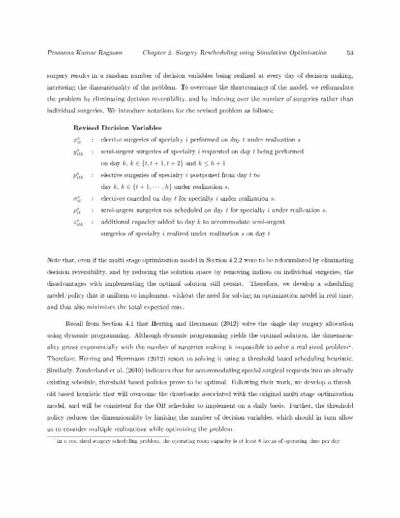
Prasanna Kumar Ragavan Chapter 5. Surgery Rescheduling using Simulation Optimization 53
surgery results in a random number of decision variables being realized at every day of decision making,
increasing the dimensionality of the problem. To overcome the shortcomings of the model, we reformulate
the problem by eliminating decision reversibility, and by indexing over the number of surgeries rather than
individual surgeries. We introduce notations for the revised problem as follows:
Revised Decision Variables
xsit : elective surgeries of specialty i performed on day t under realization s
ysitk : semi-urgent surgeries of specialty i requested on day t being performed
on day k, k ∈ t, t+ 1, t+ 2 and k ≤ h+ 1
psitk : elective surgeries of specialty i postponed from day t to
day k, k ∈ t+ 1, · · · , h under realization s.
σsit : electives canceled on day t for specialty i under realization s.
ρsit : semi-urgent surgeries not scheduled on day t for specialty i under realization s.
zsitk : additional capacity added to day k to accommodate semi-urgent
surgeries of specialty i realized under realization s on day t
Note that, even if the multi-stage optimization model in Section 4.2.2 were to be reformulated by eliminating
decision reversibility, and by reducing the solution space by removing indices on individual surgeries, the
disadvantages with implementing the optimal solution still persist. Therefore, we develop a scheduling
model/policy that is uniform to implement, without the need for solving an optimization model in real time,
and that also minimizes the total expected cost.
Recall from Section 4.1 that Herring and Herrmann (2012) solve the single day surgery allocation
using dynamic programming. Although dynamic programming yields the optimal solution, the dimension-
ality grows exponentially with the number of surgeries making it impossible to solve a real sized problem1.
Therefore, Herring and Herrmann (2012) resort to solving it using a threshold based scheduling heuristic.
Similarly, Zonderland et al. (2010) indicates that for accommodating special surgical requests into an already
existing schedule, threshold based policies prove to be optimal. Following their work, we develop a thresh-
old based heuristic that will overcome the drawbacks associated with the original multi-stage optimization
model, and will be consistent for the OR scheduler to implement on a daily basis. Further, the threshold
policy reduces the dimensionality by limiting the number of decision variables, which should in turn allow
us to consider multiple realizations while optimizing the problem.
1In a real sized surgery scheduling problem, the operating room capacity is at least 6 hours of operating time per day

Prasanna Kumar Ragavan Chapter 5. Surgery Rescheduling using Simulation Optimization 54
Figure 4.2: Sequence of Decisions for the Surgical Rescheduling Problem
4.3.1 Scheduling Heuristic
The heuristic that we propose includes two components: (i) a threshold parameter, and (ii) a scheduling
policy that determines the value of the decision variables. By setting a threshold, a portion of the total
available capacity is reserved only for performing semi-urgent surgeries, and all requests that fall below the
threshold are accommodated within the same day.
If αit denotes the threshold for specialty i on day t, the number of semi-urgent surgeries that can be
accommodated on the same day, ysitt is restricted to αit. However, the scheduler has to not only accommodate
semi-urgent surgeries, but also modify the schedule of electives due to such accommodations. As mentioned
in Section 4.2, rescheduling entails the following decisions: (i) determining when to schedule the postponed
semi-urgent surgeries, that is, determine ysit(t+1) and ysit(t+2); (ii) establish a schedule for the elective cases
to be performed, xsit, and those that need to be postponed, psitk, t < k ≤ h; and nally, (iii) determine
planned overtime in the future, zsit, to perform semi-urgent surgeries. We propose a prioritization based
scheduling policy that will work in tandem with the threshold level, and guide the scheduler through the
above decisions. Figure 4.2 shows the decision making sequence for the surgical rescheduling problem over
a h day horizon.
The scheduling policy we propose determines the above decisions on a repetitive basis in a myopic
way for each specialty, that is, only semi-urgent surgeries realized on a particular day are considered, and
no information from the future is incorporated into decision making. Such myopic policies are often used
as a benchmark while evaluating the performance of numerous scheduling approaches (Gul et al., 2015;
Herring and Herrmann, 2012). In addition, each specialty, with its own surgical block, has an independent
schedule. Though the duration of surgeries is not considered explicitly in decision making, the eects of
random surgical durations are eventually added to the objective function. Note that, given a threshold, any
Prasanna Kumar Ragavan Chapter 5. Surgery Rescheduling using Simulation Optimization 55
scheduling heuristic can be accommodated to t into the existing framework.
Since semi-urgent surgeries require prompt medical attention, and the loss in revenue associated with
not performing a semi-urgent surgery is higher than for electives, a schedule for all semi-urgent surgeries
that are realized on a particular day is rst determined. As mentioned above, the threshold level determines
ysitt, the number of cases that can be accommodated the same day. Surgeries that are to be postponed,
θu = usit − ysitt, are scheduled the following day if any slack is available in the schedule, that is, ysit(t+1) is
determined based on αi(t+1), and any unscheduled surgery is performed on day t+2, satisfying the condition,
usit = ysitt + ysit(t+1) + ysit(t+2) + ρsit.
If sucient capacity is not available in the block schedule to accommodate all surgeries, additional
capacity, in the form of planned overtime, z, is added. Note that, in this policy, even though we consider
specialties to be independent of each other, the additional slots may well be available through release of
unused capacity by other specialties (Block release). Neverthless, we set an upper bound on the planned
overtime capacity to account for the eects of unplanned overtime due to random surgical durations. All
other surgeries that exceed the threshold, are never scheduled, leading to a loss in revenue. Once semi-urgent
surgeries have been accommodated, xing those decisions, the existing schedule for electives is modied.
Out of the eit electives that are pre-scheduled, xsit are performed, where xsit = eit − αit −∑k<t p
sikt, that
is, all available slots after accommodating semi-urgent surgeries are released for electives. Other electives,
θE = eit − xsit, have to be postponed or canceled, and subsequently, a new schedule determined. For this
purpose, we derive a threshold for elective surgeries, γit, by letting all unreserved capacity to be utilized for
scheduling electives, that is, γit = vit − αit. Following a process similar to that of postponing semi-urgent
cases, the schedule for postponed electives, psitk, t < k < h+ 1 is determined by utilizing γit as a threshold,
and all electives that cannot be postponed are canceled. The heuristic is repeatedly applied across the entire
time horizon for any realization, with rescheduling decisions made every day. These decisions are, in turn,
used to evaluate the objective function which includes the cost of postponement, additional capacity, regular
time, and unplanned overtime.
4.3.2 Total Cost of Rescheduling
If H denotes the heuristic, under realization s, the resulting schedule is, (x,y, z,p,σ,ρ) = Hs(α). With α
xed, the total cost of rescheduling under any realization s is:
J(α, s) =
n∑i=1
h∑t=1
(ccei σ
sit + ccui ρ
sit +
h∑k>t
cpi (k − t)psitk+

Prasanna Kumar Ragavan Chapter 5. Surgery Rescheduling using Simulation Optimization 56
Algorithm 5 Threshold based Scheduling Heuristic
Require: Initial capacity allocation, v; Initial schedule of elective surgeries, E ; Threshold level, α; Semi-urgent cases realized under realization s, us.
Ensure: Schedule of semi-urgent surgeries, y; Schedule of elective surgeries, x; Postponed electives, p;Semi-urgent surgeries performed in planned overtime, z
1: for t ∈ 1, · · · , h do2: for i ∈ 1, · · · , n do3: Set βit ← αit; γit ← vit − αit4: Set θu ← 0, θE ← 0Schedule Semi-urgent Surgeries & Electives
5: yitt ← min(Uit, αit − 1t≥2yi(t−1)t + 1t≥3
(zi(t−2)t − yi(t−2)t
) )6: xit ← min
(eit, vit − αit + 1t≥3 zi(t−2)t − 1t≥2
∑k<t
pikt
)7: θu ← Uit − yitt, θE ← eit − xitSchedule Postponed Semi-urgent Surgeries
8: if θu > 0 then9: if 1 ≤ t ≤ h− 2 then
10: yit(t+1) ← min(θu, αi(t+1) − 1t≥2yi(t−1)(t+1) + 1t≥2zi(t−1)(t+1)
)11: yit(t+2) ← min
(θu −
t+1∑q=t
yitq, αi(t+2) + δi(t+2)
)12: zit(t+2) ←
(yit(t+2) − αi(t+2)
)+
13: ρit ← θu −t+2∑q=t
yitq
14: else if t = h− 1 then
15: yit(t+1) ← min(θu, αi(t+1) − 1t≥2yi(t−1)(t+1) + 1t≥2zi(t−1)(t+1)
)16: ρit ← θu −
t+1∑q=t
yitq
17: else
18: ρit ← θu19: end if
20: end if
Schedule Postponed Elective Surgeries
21: if θE > 0 then22: q ← t+ 123: while θE > 0 and q ≤ h do
24: pitq ← min(θE ,
(γiq − niq − 1t≥2
t−1∑l=1
pilq
)+ )25: θE ← θE − pitq26: q ← q + 127: end while
28: σit ← θE29: end if
30: end for
31: end for
max(h,t+2)∑k=t+1
cpi (k − t)ysitk + cvi d
ui zsit + cri d
ei vit + coi o
sit
), (4.17)
Prasanna Kumar Ragavan Chapter 5. Surgery Rescheduling using Simulation Optimization 57
where osit is the overtime incurred under realization s.
4.4 Threshold Determination
In Section 4.3, we elaborated the scheduling heuristic, where, given a threshold, α, and the request for
semi-urgent cases, us, a feasible schedule is determined. The cost of implementing this scheduling policy,
J(α, s), is most sensitive to the choice of threshold, α. Therefore, it is important that the threshold levels are
aligned with other parameters in the model, including the cost, and the distribution of the random variables.
However, nding the best threshold is a non-trivial problem due to the following reasons, (i) the number
of feasible alternatives grows exponentially with the capacity of the operating room, v, and the number of
specialties, n, (ii) the threshold policy induces a non-linear relationship between the threshold levels, α, and
the resulting cost.
The operators that link the threshold, α with the scheduling decisions, (x,y, z,p,ρ, and σ) are clearly
non-linear. With respect to the feasible space, consider the surgical rescheduling problem with n = 1, and
h = 5, and vt = 10,∀t ∈ 1, · · · , h. Though the number of decision variables is ve, a threshold for each day
of the week, nding the best solution requires us to evaluate 100, 000 feasible solutions, and optimization
techniques that do not exploit the structure of the problem may fail in identifying a good solution. Following
is a formulation of the non-linear optimization problem to determine the optimal threshold level.
PT : minimizeα
J (α) = E[J(α, Ut1≤t≤h, Dt1≤t≤h)]
subject to αit ≤ vit ∀i ∈ 1, · · · , n, ∀t ∈ 1, · · · , h
Note that, unlike the multi-stage optimization framework in Section 4.2, the threshold determination
problem, PT is a static optimization problem under uncertainty. As in the case of the multi-stage opti-
mization framework, explicitly incorporating the distribution is still impossible, and we resort to using the
SAA method using realizations of the random variables. Given a threshold level, α, Monte Carlo simulation
generates the realizations, S. For each realization, s ∈ S, the scheduling heuristic, H is applied and the
resulting rescheduling cost, J(α, s), is observed. The reformulated problem with the expected rescheduling
cost replaced by the sample mean is:
PTS : minα
J (α,S) =1
|S|∑s∈S
J(α, s)
subject to αit ≤ vit ∀i ∈ 1, · · · , n, ∀t ∈ 1, · · · , h
Prasanna Kumar Ragavan Chapter 5. Surgery Rescheduling using Simulation Optimization 58
Problem PTS is the deterministic equivalent of the stochastic threshold determination problem and can be
solved using one of the many existing optimization techniques. Let α∗S denote the optimal solution to the
approximation, PTS , and the corresponding expected cost be J (α∗S). If the set of optimal solutions to the
true problem, PT is denoted by π∗, then α∗S converges to an element in π∗, when the number of realizations,
|S|, is large, specically, as |S| → ∞.
Our objective is to identify a solution that is close enough to the set π∗ without sacricing the
nite time performance. Towards this goal, we consider two approaches: (i) a SAA technique, that is,
solving Problem PTS with xed number of realizations, and (ii) a simulation based optimization approach.
By introducing a simulation based approach, we emphasize on quantifying the overwhelming impact of
approximation strategies (uncertainty) on stochastic optimization problems. Further, we restrict the scope
of this work to only comparing the quality of solution obtained using the SAA method and a simulation
optimization method, and exclude studying other advanced decomposition techniques.
4.4.1 Optimize threshold using Integer Programming
In this section, we present an integer programming formulation for optimizing the threshold levels when
heuristic H is utilized for the rescheduling decisions. With uncertainty in surgical requests restricted to a
nite number of realizations, the objective of this formulation is to minimize the sample mean of the total
cost across these realizations. Given the requirement to explicitly formulate the policy in the mathematical
model, individual scheduling rules are linearized using convexication procedures. The resulting linear integer
programming formulation for threshold optimization is as follows:
minimizeα
J (α,S) = cri dei vit +
1
|S|
|S|∑i=1
(n∑i=1
( h∑t=1
Ccei σsit + Ccui ρsit +
h∑k>t
cPi (k − t)psitk
+
max(h,t+2)∑k=t+1
cPi (k − t)ysitk + cvi dui zsit
))(4.18)
subject to
αit ≤ vit ∀i, ∀t ∈ 1, · · · , h (4.19)
γit = vit − αit ∀i, ∀t ∈ 1, · · · , h (4.20)
ysitt ≤ usit ∀s, ∀i, ∀t ∈ 1, · · · , h (4.21)
ysitt ≤ Asit ∀s, ∀i, ∀t ∈ 1, · · · , h (4.22)
Prasanna Kumar Ragavan Chapter 5. Surgery Rescheduling using Simulation Optimization 59
usit ≤ ysitt + (1−G1sit )×M ∀s, ∀i, ∀t ∈ 1, · · · , h (4.23)
Asitt ≤ ysitt + (1−H1sit )×M ∀s, ∀i, ∀t ∈ 1, · · · , h (4.24)
G1sit +H1s
it = 1 ∀s, ∀i, ∀t ∈ 1, · · · , h (4.25)
Asit ≥ αit − 1t≥3
t∑k=t−2
ysikt + 1t≥3zsi(t−2)t ∀s, ∀i, ∀t ∈ 1, · · · , h (4.26)
Asit ≥ vit − αit − 1t≥2
t−1∑k=1
psikt − 1t≥3
t−1∑k=t−2
ysikt
+ 1t≥3zsi(t−2)t ∀s, ∀i, ∀t ∈ 3, · · · , h (4.27)
αit − 1t≥3
t∑k=t−2
ysikt + 1t≥3zsi(t−2)t ≥ Asit − (1−G2s
it )×M ∀s, ∀i, ∀t ∈ 1, · · · , h (4.28)
vit − αit − 1t≥2
t−1∑k=1
psikt − 1t≥3
t−1∑k=t−2
ysikt
+ 1t≥3zsi(t−2)t ≥ Asit − (1−H2s
it )×M ∀s, ∀i, ∀t ∈ 1, · · · , h (4.29)
G2sit +H2s
it = 1 ∀s, ∀i, ∀t ∈ 1, · · · , h (4.30)
xsit ≤ eit ∀s, ∀i, ∀t ∈ 1, · · · , h (4.31)
xsit ≤ vit + 1t≥3zsi(t−2)t − 1t≥2
t−1∑k=1
psikt − 1t≥3
t∑k=t−2
ysikt ∀s, ∀i, ∀t ∈ 1, · · · , h (4.32)
eit ≤ xsit + (1−G3sit )×M ∀s, ∀i, ∀t ∈ 1, · · · , h (4.33)
vit + 1t≥3zsi(t−2)t − 1t≥2
t−1∑k=1
psikt − 1t≥3
t∑k=t−2
ysikt ≤
xsit(1−H3sit )×M ∀s, ∀i, ∀t ∈ 1, · · · , h (4.34)
G3sit +H3s
it = 1 ∀s, ∀i, ∀t ∈ 1, · · · , h (4.35)
ysit(t+1) ≤ usit − ysitt ∀s, ∀i, ∀t ∈ 1, · · · , h− 1 (4.36)
ysit(t+1) ≤ αi(t+1) − 1t≥2ysi(t−1)(t+1) ∀s, ∀i, ∀t ∈ 1, · · · , h− 1 (4.37)
usit − ysitt ≤ ysit(t+1) + (1−G4sit )×M ∀s, ∀i, ∀t ∈ 1, · · · , h− 1 (4.38)
αi(t+1) − 1t≥2ysi(t−1)(t+1) ≤ ysit(t+1) + (1−H4s
it )×M ∀i, ∀t ∈ 1, · · · , h− 1 (4.39)
G4sit +H4s
it = 1 ∀s, ∀i, ∀t ∈ 1, · · · , h− 1 (4.40)
ysit(t+2) ≤ usit − ysitt − ysit(t+1) ∀s, ∀i, ∀t ∈ 1, · · · , h− 2 (4.41)
ysit(t+2) ≤ αi(t+2) + δi(t+2) ∀s, ∀i, ∀t ∈ 1, · · · , h− 2 (4.42)
usit − ysitt − ysit(t+1) ≤ ysit(t+2) + (1−G5sit )×M ∀s, ∀i, ∀t ∈ 1, · · · , h− 2 (4.43)
αi(t+2) + δi(t+2) ≤ ysit(t+2) + (1−H5sit )×M ∀s, ∀i, ∀t ∈ 1, · · · , h− 2 (4.44)
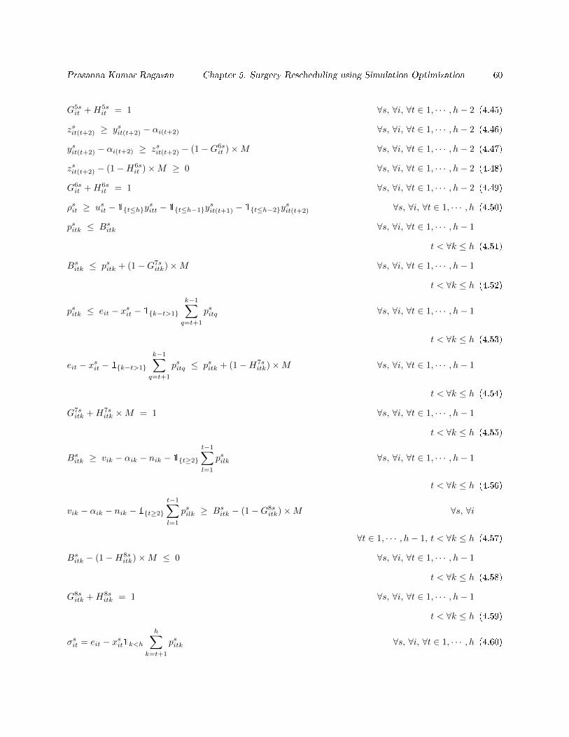
Prasanna Kumar Ragavan Chapter 5. Surgery Rescheduling using Simulation Optimization 60
G5sit +H5s
it = 1 ∀s, ∀i, ∀t ∈ 1, · · · , h− 2 (4.45)
zsit(t+2) ≥ ysit(t+2) − αi(t+2) ∀s, ∀i, ∀t ∈ 1, · · · , h− 2 (4.46)
ysit(t+2) − αi(t+2) ≥ zsit(t+2) − (1−G6sit )×M ∀s, ∀i, ∀t ∈ 1, · · · , h− 2 (4.47)
zsit(t+2) − (1−H6sit )×M ≥ 0 ∀s, ∀i, ∀t ∈ 1, · · · , h− 2 (4.48)
G6sit +H6s
it = 1 ∀s, ∀i, ∀t ∈ 1, · · · , h− 2 (4.49)
ρsit ≥ usit − 1t≤hysitt − 1t≤h−1ysit(t+1) − 1t≤h−2y
sit(t+2) ∀s, ∀i, ∀t ∈ 1, · · · , h (4.50)
psitk ≤ Bsitk ∀s, ∀i, ∀t ∈ 1, · · · , h− 1
t < ∀k ≤ h (4.51)
Bsitk ≤ psitk + (1−G7sitk)×M ∀s, ∀i, ∀t ∈ 1, · · · , h− 1
t < ∀k ≤ h (4.52)
psitk ≤ eit − xsit − 1k−t>1
k−1∑q=t+1
psitq ∀s, ∀i, ∀t ∈ 1, · · · , h− 1
t < ∀k ≤ h (4.53)
eit − xsit − 1k−t>1
k−1∑q=t+1
psitq ≤ psitk + (1−H7sitk)×M ∀s, ∀i, ∀t ∈ 1, · · · , h− 1
t < ∀k ≤ h (4.54)
G7sitk +H7s
itk ×M = 1 ∀s, ∀i, ∀t ∈ 1, · · · , h− 1
t < ∀k ≤ h (4.55)
Bsitk ≥ vik − αik − nik − 1t≥2
t−1∑l=1
psilk ∀s, ∀i, ∀t ∈ 1, · · · , h− 1
t < ∀k ≤ h (4.56)
vik − αik − nik − 1t≥2
t−1∑l=1
psilk ≥ Bsitk − (1−G8sitk)×M ∀s, ∀i
∀t ∈ 1, · · · , h− 1, t < ∀k ≤ h (4.57)
Bsitk − (1−H8sitk)×M ≤ 0 ∀s, ∀i, ∀t ∈ 1, · · · , h− 1
t < ∀k ≤ h (4.58)
G8sitk +H8s
itk = 1 ∀s, ∀i, ∀t ∈ 1, · · · , h− 1
t < ∀k ≤ h (4.59)
σsit = eit − xsit1k<hh∑
k=t+1
psitk ∀s, ∀i, ∀t ∈ 1, · · · , h (4.60)

Prasanna Kumar Ragavan Chapter 5. Surgery Rescheduling using Simulation Optimization 61
Gwsit , Hwsit , G
wsitk, H
wsitk ∈ 0, 1 ∀s, ∀i, ∀t ∈ 1, · · · , h− 1
∀w ∈ 1, · · · , 6, ∀w ∈ 7, 8
t < ∀k ≤ h (4.61)
Asit, Bsitk ∀s, ∀i, ∀t ∈ 1, · · · , h− 1
t < ∀k ≤ h (4.62)
xsit, σsit, ρ
sit, y
sitq ≥ 0 ∀s ∈ S, ∀i, ∀t ∈ 1, · · · , h,
t ≤ q < max(h, t+ 2) (4.63)
zsil(l+2), psitk ≥ 0 ∀s, ∀i, ∀t ∈ 1, · · · , h
t < ∀k ≤ h, ∀l ∈ 1, · · · , h− 2 (4.64)
The objective function, 4.18, is the sum of the regular cost for a xed block schedule, and the cost of
cancellation, postponement, and capacity addition across the time horizon for the individual specialties.
Note that the cost of overtime is ignored, for doing so requires that individual surgeries are indexed often
resulting in an intractable model. To illustrate the linearization of constraints, and thus the rules in the
scheduling heuristic, H, consider the constraint Z = min(A,B). For the min operator, convexication
involves the following:
Z ≤ A
Z ≤ B
A ≤ Z + (1− d1)×MB ≤ Z + (1− d2)×M
d1 + d2 = 1
d1, d2 ∈ 0, 1
Notice that the convexication of the min operator results in addition of two binary variables, d1, and d2,
and four additional constraints. The parameter, M is the big-M variable that is suciently large, set to be
10, 000 throughout the formulation. Using a similar procedure, the max operator can be linearized. Upon
linearization, the scheduling rule that governs the accommodation of semi-urgent surgeries on the same day
of request is represented by constraints 4.19 - 4.30. The binary variables G, andH are the dummy variables
from the linearization procedure throughout this formulation. Constraints 4.31 - 4.35 ensure that the total
number of electives that can be accommodated out of the eit cases pre-scheduled on any day t does not exceed
the capacity available after accommodating semi-urgent surgeries, and previously postponed electives.
Constraints 4.36 - 4.49 correspond to the rules for postponing semi-urgent surgeries, and their accom-

Prasanna Kumar Ragavan Chapter 5. Surgery Rescheduling using Simulation Optimization 62
modation within two days from the day of request, with any additional planned overtime capacity. Note that
for days h−1, and h, any semi-urgent surgery that cannot be accommodated within the last day of the week
are canceled resulting in a loss of revenue, ccui , number of which is denoted by constraint 4.50. Constraints
4.52 - 4.59 correspond to the scheduling rules for postponed electives. Similar to the semi-urgent surgeries,
electives that cannot be accommodated within the end of the week are canceled incurring a cancellation cost
of ccei . Though the class of constraints in the formulation is restricted to four, that is, an individual class of
rules for scheduling semi-urgent surgeries and electives followed by their postponement, the addition of bi-
nary variables adds to the computational complexity of the problem. For example, linearizing the constraints
in the rescheduling problem with n = 2, |S| = 1, and h = 5, results in 80 binary variables being added to
the problem. The threshold determination problem is also an NP-hard because the threshold determination
under one realization is still equivalent to the bin packing problem with constraints on the number of bins.
4.4.2 Optimize threshold using Simulation Optimization - ADALINE
Classical optimization algorithms to solve the threshold optimization model provided above are often iter-
ative, and visit a sequence of solutions which improve the objective function until a termination criterion
is satised. However, due to the stochastic nature of the problem, quality of the resulting solution, α∗S , is
heavily reliant on the number of random realizations.2 Although incorporating a large number of realiza-
tions yields a better approximation, the computational eciency of the algorithm greatly diminishes with
the number of realizations. On the other hand, there is no guarantee on the quality of α∗S when only a
handful of realizations are used. In addition, failure to incorporate the quality of an iterate in choosing the
number of realizations induces ineciency in these algorithms. Therefore, a balance between optimization,
and sampling is often required to nd a good quality solution without compromising on the algorithm's
performance.
Moreover, the optimization approach requires the analytical form of the objective function and con-
straints to be explicitly specied, often rendering it inexible to accommodate even minor modications in
scheduling policy. Likewise, even seemingly simple mathematical models can be hard to solve when non-
convexity is induced in the constraint space due to the scheduling policy. For instance, in the threshold
determination problem, reformulation of the non-convex constraints that govern the scheduling heuristic, H,
results in dummy variables, and reformulation constraints being explicitly added to the model. This signi-
cantly increases the complexity of the model, despite the fact that the total number of decision variables are
only n× h.2On specifying a realization, s, and the threshold level, α, the scheduling policy yields the realized cost of rescheduling,
J s, which is equivalent to the random outcome from a simulation. Therefore, we use the terms realization and sample size
interchangeably throughout this work
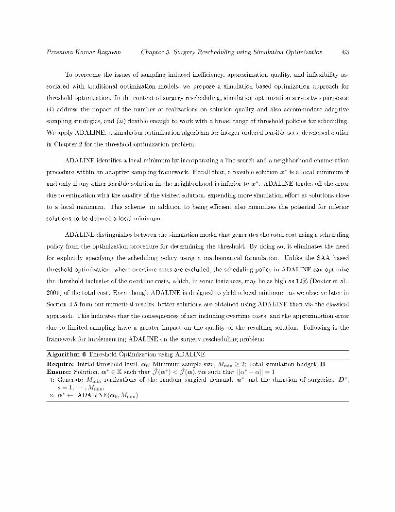
Prasanna Kumar Ragavan Chapter 5. Surgery Rescheduling using Simulation Optimization 63
To overcome the issues of sampling induced ineciency, approximation quality, and inexibility as-
sociated with traditional optimization models, we propose a simulation based optimization approach for
threshold optimization. In the context of surgery rescheduling, simulation optimization serves two purposes:
(i) address the impact of the number of realizations on solution quality and also accommodate adaptive
sampling strategies, and (ii) exible enough to work with a broad range of threshold policies for scheduling.
We apply ADALINE, a simulation optimization algorithm for integer-ordered feasible sets, developed earlier
in Chapter 2 for the threshold optimization problem.
ADALINE identies a local minimum by incorporating a line search and a neighborhood enumeration
procedure within an adaptive sampling framework. Recall that, a feasible solution x∗ is a local minimum if
and only if any other feasible solution in the neighborhood is inferior to x∗. ADALINE trades o the error
due to estimation with the quality of the visited solution, expending more simulation eort at solutions close
to a local minimum. This scheme, in addition to being ecient also minimizes the potential for inferior
solutions to be deemed a local minimum.
ADALINE distinguishes between the simulation model that generates the total cost using a scheduling
policy from the optimization procedure for determining the threshold. By doing so, it eliminates the need
for explicitly specifying the scheduling policy using a mathematical formulation. Unlike the SAA based
threshold optimization, where overtime costs are excluded, the scheduling policy in ADALINE can optimize
the threshold inclusive of the overtime costs, which, in some instances, may be as high as 12% (Dexter et al.,
2001) of the total cost. Even though ADALINE is designed to yield a local minimum, as we observe later in
Section 4.5 from our numerical results, better solutions are obtained using ADALINE than via the classical
approach. This indicates that the consequences of not including overtime costs, and the approximation error
due to limited sampling have a greater impact on the quality of the resulting solution. Following is the
framework for implementing ADALINE on the surgery rescheduling problem:
Algorithm 6 Threshold Optimization using ADALINE
Require: Initial threshold level, α0; Minimum sample size, Mmin ≥ 2; Total simulation budget, BEnsure: Solution, α∗ ∈ X such that J (α∗) < J (α),∀α such that ||α∗ − α|| = 11: Generate Mmin realizations of the random surgical demand, us and the duration of surgeries, Ds,s = 1, · · · ,Mmin.
2: α∗ ← ADALINE(α0,Mmin)
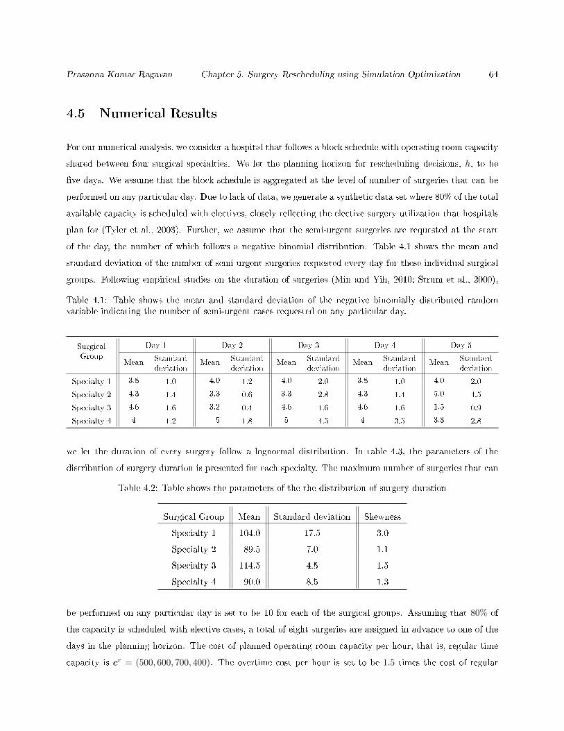
Prasanna Kumar Ragavan Chapter 5. Surgery Rescheduling using Simulation Optimization 64
4.5 Numerical Results
For our numerical analysis, we consider a hospital that follows a block schedule with operating room capacity
shared between four surgical specialties. We let the planning horizon for rescheduling decisions, h, to be
ve days. We assume that the block schedule is aggregated at the level of number of surgeries that can be
performed on any particular day. Due to lack of data, we generate a synthetic data set where 80% of the total
available capacity is scheduled with electives, closely reecting the elective surgery utilization that hospitals
plan for (Tyler et al., 2003). Further, we assume that the semi-urgent surgeries are requested at the start
of the day, the number of which follows a negative binomial distribution. Table 4.1 shows the mean and
standard deviation of the number of semi-urgent surgeries requested every day for these individual surgical
groups. Following empirical studies on the duration of surgeries (Min and Yih, 2010; Strum et al., 2000),
Table 4.1: Table shows the mean and standard deviation of the negative binomially distributed randomvariable indicating the number of semi-urgent cases requested on any particular day.
SurgicalGroup
Day 1 Day 2 Day 3 Day 4 Day 5
Mean Standarddeviation
Mean Standarddeviation
Mean Standarddeviation
Mean Standarddeviation
Mean Standarddeviation
Specialty 1 3.8 1.0 4.0 1.2 4.0 2.0 3.8 1.0 4.0 2.0
Specialty 2 4.3 1.4 3.3 0.6 3.3 2.8 4.3 1.4 5.0 4.5
Specialty 3 4.6 1.6 3.2 0.4 4.6 1.6 4.6 1.6 1.5 0.9
Specialty 4 4 1.2 5 1.8 5 4.5 4 3.5 3.3 2.8
we let the duration of every surgery follow a lognormal distribution. In table 4.3, the parameters of the
distribution of surgery duration is presented for each specialty. The maximum number of surgeries that can
Table 4.2: Table shows the parameters of the the distribution of surgery duration
Surgical Group Mean Standard deviation Skewness
Specialty 1 104.0 17.5 3.0
Specialty 2 89.5 7.0 1.1
Specialty 3 114.5 4.5 1.5
Specialty 4 90.0 8.5 1.3
be performed on any particular day is set to be 10 for each of the surgical groups. Assuming that 80% of
the capacity is scheduled with elective cases, a total of eight surgeries are assigned in advance to one of the
days in the planning horizon. The cost of planned operating room capacity per hour, that is, regular time
capacity is cr = (500, 600, 700, 400). The overtime cost per hour is set to be 1.5 times the cost of regular
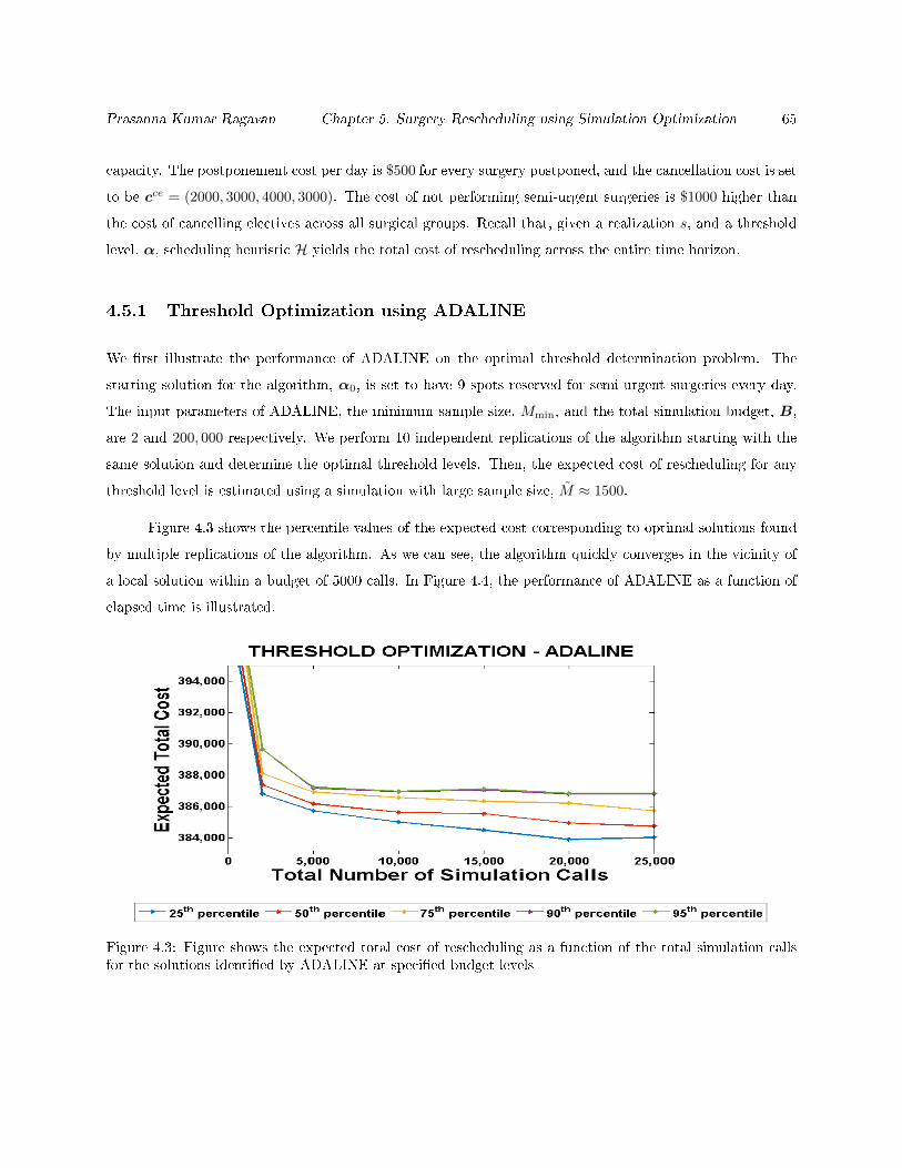
Prasanna Kumar Ragavan Chapter 5. Surgery Rescheduling using Simulation Optimization 65
capacity. The postponement cost per day is $500 for every surgery postponed, and the cancellation cost is set
to be cce = (2000, 3000, 4000, 3000). The cost of not performing semi-urgent surgeries is $1000 higher than
the cost of cancelling electives across all surgical groups. Recall that, given a realization s, and a threshold
level, α, scheduling heuristic H yields the total cost of rescheduling across the entire time horizon.
4.5.1 Threshold Optimization using ADALINE
We rst illustrate the performance of ADALINE on the optimal threshold determination problem. The
starting solution for the algorithm, α0, is set to have 9 spots reserved for semi-urgent surgeries every day.
The input parameters of ADALINE, the minimum sample size, Mmin, and the total simulation budget, B,
are 2 and 200, 000 respectively. We perform 10 independent replications of the algorithm starting with the
same solution and determine the optimal threshold levels. Then, the expected cost of rescheduling for any
threshold level is estimated using a simulation with large sample size, M ≈ 1500.
Figure 4.3 shows the percentile values of the expected cost corresponding to optimal solutions found
by multiple replications of the algorithm. As we can see, the algorithm quickly converges in the vicinity of
a local solution within a budget of 5000 calls. In Figure 4.4, the performance of ADALINE as a function of
elapsed time is illustrated.
Figure 4.3: Figure shows the expected total cost of rescheduling as a function of the total simulation callsfor the solutions identied by ADALINE at specied budget levels

Prasanna Kumar Ragavan Chapter 5. Surgery Rescheduling using Simulation Optimization 66
Figure 4.4: Figure shows the expected total cost of rescheduling as a function of elapsed time for the solutionsidentied by ADALINE at specied time limits
4.5.2 Threshold Optimization using Integer programming
We solve the SAA problem with sample sizes (number of realizations), M = 1, 2, 3, 5, 10, 20 and compare it
with the solution from ADALINE. Corresponding to every value of M , the best solution obtained within a
specied time limit, and its optimality gap is determined. Similar to the implementation of ADALINE, to
account for uncertainty in semi-urgent surgeries, and thus its impact on the obtained solution, we perform
10 independent replications of the algorithm for every value ofM . We implement the threshold optimization
problem using PuLP (Mitchell et al., 2011), a mathematical programming environment in Python. The
resulting integer optimization problem is solved using IBM ILOG CPLEX 12.0 on a PC with 2.40 GHz Intel
Core i7 and 8 GB memory.
The size of the deterministic equivalent increases rapidly with the sample size,M and early termination
of the algorithm results in inferior solutions. For larger instances of the threshold optimization problem, the
optimality gap of the resulting solution may be as high as 35%. Table 4.3 lists the average optimality gap
of the resulting solution corresponding to varying values of M , and at specied time limits.
Even though larger values of M yield solutions that close the optimality gap, guaranteeing such a solution
in nite time may be impossible. We believe that an appropriate sampling based decomposition strategy,
as developed in (Gul et al., 2015), will result in better solutions, while not being computationally intensive.
However, such techniques usually entail more overhead due to time incurred with modeling.

Prasanna Kumar Ragavan Chapter 5. Surgery Rescheduling using Simulation Optimization 67
Table 4.3: Average optimality gap of the solutions to the mixed integer programming formulation obtainedat various time limits
SampleSize
Time (in minutes)
0.5 1.0 2.0 3.0 5.0 10.0 20.0 30.0
1 0.0 0.0 0.0 0.0 0.0 0.0 0.0 0.0
2 0.0 0.0 0.0 0.0 0.0 0.0 0.0 0.0
3 17.2 14.1 11.9 11.3 10.2 8.1 6.9 6.5
5 43.8 38.0 34.2 32.8 32.0 31.1 29.6 29.1
10 56.6 48.4 45.1 44.6 43.3 40.9 35.9 34.2
20 83.4 74.3 53.7 50.3 44.7 44.0 38.8 38.0
Figure 4.5 compares solution quality from ADALINE and by solving the integer optimization problem
as a function of the elapsed time. For every solution obtained by solving the deterministic equivalent, the
expected cost of rescheduling is determined by simulating the rescheduling policy with a large sample size, M .
It can be seen that the average expected cost of the solution obtained using ADALINE across 10 independent
replications of the algorithm is at least 2% better than the average expected solution from CPLEX. When
the xed regular time cost of operating room resources is ignored, ADALINE decreases the rescheduling cost
by close to 4% than the best solution from the SAA technique with xed number of realizations. Note that
ADALINE converges to the vicinity of an optimal solution within half a second, and without the need for any
signicant modeling eort. A simulation optimization framework with ADALINE also provides exibility
in the choice of scheduling policy. In Figure 4.6, expected cost of 100 dierent solutions returned from
ADALINE and solutions obtained by solving the SAA problem with M = 2 are plotted in a histogram. As
clearly seen in the gure, almost 70% of the solutions from ADALINE have an expected cost of $384, 000,
whereas 90% of the solutions from solving the integer optimization problem are worse than $390, 000. Though
ADALINE is designed to nd a local minimum, its ability to adaptively determine the sample size results in
superior performance over the SAA method.
4.6 Conclusion
In this work, we propose a surgery rescheduling policy to accommodate semi-urgent surgeries on a daily
basis under demand uncertainty. To overcome implementation issues associated with solutions from a multi-
stage optimization framework, we propose a threshold based scheduling policy that exclusively reserves a

Prasanna Kumar Ragavan Chapter 5. Surgery Rescheduling using Simulation Optimization 68
Figure 4.5: Figure shows the expected total cost of rescheduling as a function of elapsed time for the solutionsidentied by the integer optimization framework with various sample sizes
Figure 4.6: Figure shows a comparison of the quality of solutions obtained with thresholds determinedthrough ADALINE and the Integer Optimization framework
proportion of the capacity for performing semi-urgent surgeries. In order to determine the optimal threshold
levels, we utilize an integer programming approach, and a simulation optimization method.

Prasanna Kumar Ragavan Chapter 5. Surgery Rescheduling using Simulation Optimization 69
For the integer optimization method, the scheduling policy is formulated as a linear integer program
through convexication of constraints, and solved using CPLEX. This method yields inferior solutions for
they approximate the problem using a limited number of realizations failing to account for the uncertainty
in determining an optimal solution. Furthermore, the size of the problem is large, even with a handful of
realizations, resulting in the integer programming approach often failing to nd an optimal solution within
nite time. On the other hand, ADALINE outperforms the traditional approach in yielding a good solution
without being too computationally intensive. Although ADALINE is designed to yield only a local solution,
by distributing simulation eort in line with the quality of the solution using an adaptive sampling framework,
it quickly converges to the vicinity of a local minimum.
The simulation optimization approach provides exibility in accommodating a variety of threshold
based scheduling policies eliminating the need for formulating and solving an integer programming problem.
The threshold levels are determined through a static optimization framework for the dynamic nature of
decision making is implicitly handled through the scheduling policy. However, the dynamic and stochastic
nature of the surgery rescheduling problem suggests several areas for future research, including, but not
limited to: (i) a simulation optimization framework for dynamic decision making problems in the presence
of uncertainty, particularly if an adaptive sampling framework can be implemented at various stages of the
multi-stage problem, and (ii) a framework for obtaining global optimal solutions to the surgery rescheduling
problem.
Chapter 5
Concluding Remarks
In this thesis, we develop ADALINE, a line search based algorithm to nd a local minimum for continuous,
and integer-ordered simulation optimization (SO). ADALINE addresses one of the important questions in
SO regarding the choice of sample size through an adaptive sampling scheme. It does so by allocating the
simulation eort based on measures of proximity to a local solution. ADALINE on continuous feasible sets
mimics deterministic line search strategies, where the sample size at every iteration is determined based
on sequential sampling schemes developed in Pasupathy et al. (2015). By trading o the estimation error
(standard error on the estimated gradient) with the optimization error (norm of the estimated gradient),
ADALINE eliminates the need for user dened sampling schemes that lead to ineciency in traditional
SO algorithms. Numerical results indicate that it consistently outperforms other adaptive strategies for
continuous simulation optimization.
ADALINE on integer ordered feasible sets, alternates between a line search, and a neighborhood
enumeration procedure to identify a local minimum. The adaptive line search exploits structure in the
objective function whereas the neighborhood enumeration is a conrmatory test for a local minimum. In
addition to the adaptive sample sizes, nite time performance of ADALINE in integer-ordered feasible
regions is improved by a co-ordinate search following the neighborhood enumeration. Under certain structural
conditions on the objective function, and with niteness of the feasible set, we are able to show that ADALINE
converges with probability one to the set of local minima. Extensive numerical implementation shows
that ADALINE has better nite time performance than R-SPLINE that similarly uses a line search, and
enumeration with xed sample sizes at every iteration.
In the nal chapter, we formulate and solve a surgical rescheduling problem to show the perfor-
70
Prasanna Kumar Ragavan Chapter 6. Concluding Remarks 71
mance of ADALINE on an operating room rescheduling problem. We devise a threshold based heuristic for
rescheduling, and determine the optimal threshold levels using ADALINE. Our numerical results suggest
that ADALINE nds threshold levels that result in lower total expected cost of rescheduling in comparison
with Sample Average Approximation (SAA).
Some avenues for future investigation include further improving the nite time performance, and
using ADALINE as the local search procedure of choice in random restart methods. ADALINE is currently
designed to be a non-terminating algorithm, that is, it expends all available simulation budget on convergence
to a local minimum. However, the algorithm can be terminated without expending all simulation eort when
the probability of a solution being deemed a local minimum is at least (1−α), akin to ranking and selection
procedures. In addition, ADALINE, due to its nite time performance, is a good candidate for random
restart methods to identify a global minimum. Extending ADALINE to simulation optimization problems
with an equality constraint presents further challenges due to the requirement to redene the neighborhood
as any feasible solution is a local minimum with equality constrained problems.

Bibliography
Alu Pentini, F.; Parisi, V., and Zirilli, F. Global optimization and stochastic dierential equations. Journal
of Optimization Theory and Applications, 47(1):116, 1985. ISSN 0022-3239. doi: 10.1007/BF00941312.
URL http://dx.doi.org/10.1007/BF00941312.
Amaran, Satyajith; Sahinidis, Nikolaos V; Sharda, Bikram, and Bury, Scott J. Simulation optimization: a
review of algorithms and applications. 4OR, 12(4):301333, 2014.
Andradóttir, Sigrún. Accelerating the convergence of random search methods for discrete stochastic opti-
mization. ACM Transactions on Modeling and Computer Simulation (TOMACS), 9(4):349380, 1999.
Armijo, Larry and others, . Minimization of functions having lipschitz continuous rst partial derivatives.
Pacic Journal of mathematics, 16(1):13, 1966.
Atlason, JÙlíus; Epelman, Marina; Henderson, Shane G, and others, . Using simulation to approximate sub-
gradients of convex performance measures in service systems. In Simulation Conference, 2003. Proceedings
of the 2003 Winter, volume 2, pages 18241832. IEEE, 2003.
Balasubramanian, Hari; Banerjee, Ritesh; Gregg, Melissa, and Denton, Brian T. Improving primary care
access using simulation optimization. In 2007 Winter Simulation Conference, pages 14941500. IEEE,
2007.
Belyi, Dmitriy; Popova, Elmira; Morton, David, and Damien, Paul. Bayesian non-parametric simulation of
hazard functions. In Winter Simulation Conference, pages 475482. Winter Simulation Conference, 2009.
Blake, John T and Donald, Joan. Mount sinai hospital uses integer programming to allocate operating room
time. Interfaces, 32(2):6373, 2002.
Blake, John T; Dexter, Franklin, and Donald, Joan. Operating room managers use of integer programming
for assigning block time to surgical groups: a case study. Anesthesia & Analgesia, 94(1):143148, 2002.
72

Buchholz, Peter and Thummler, Axel. Enhancing evolutionary algorithms with statistical selection pro-
cedures for simulation optimization. In Proceedings of the Winter Simulation Conference, 2005., pages
11pp. IEEE, 2005.
Byrd, Richard H; Chin, Gillian M; Nocedal, Jorge, and Wu, Yuchen. Sample size selection in optimization
methods for machine learning. Mathematical Programming, 134(1):127155, 2012.
Byrd, Richard H; Hansen, SL; Nocedal, Jorge, and Singer, Yoram. A stochastic quasi-newton method for
large-scale optimization. arXiv preprint arXiv:1401.7020, 2014.
Day, Robert; Garnkel, Robert, and Thompson, Steven. Integrated block sharing: a win-win strategy for
hospitals and surgeons. Manufacturing & Service Operations Management, 14(4):567583, 2012.
Deng, Geng and Ferris, Michael C. Variable-number sample-path optimization. Mathematical Programming,
117(1-2):81109, 2009.
Dexter, Franklin; Epstein, Richard H, and Marsh, H Michael. A statistical analysis of weekday operat-
ing room anesthesia group stang costs at nine independently managed surgical suites. Anesthesia &
Analgesia, 92(6):14931498, 2001.
Elixhauser, Anne and Andrews, Roxanne M. Prole of inpatient operating room procedures in us hospitals
in 2007. Archives of surgery, 145(12):12011208, 2010.
Eubank, Stephen; Guclu, Hasan; Kumar, VS Anil; Marathe, Madhav V; Srinivasan, Aravind; Toroczkai,
Zoltan, and Wang, Nan. Modelling disease outbreaks in realistic urban social networks. Nature, 429
(6988):180184, 2004.
Fu, Michael and others, . Handbook of simulation optimization, volume 216. Springer, 2015.
Glasserman, Paul. Gradient estimation via perturbation analysis, volume 116. Springer Science & Business
Media, 1991.
Gosavi, Abhijit; Ozkaya, Emrah, and Kahraman, Aykut F. Simulation optimization for revenue management
of airlines with cancellations and overbooking. OR Spectrum, 29(1):2138, 2007.
Gul, Serhat; Denton, Brian T, and Fowler, John W. A progressive hedging approach for surgery planning
under uncertainty. INFORMS Journal on Computing, 27(4):755772, 2015.
Hashemi, Fatemeh S; Ghosh, Sudip, and Pasupathy, Raghu. On adaptive sampling rules for stochastic
recursions. In Simulation Conference (WSC), 2014 Winter, pages 39593970. IEEE, 2014.
73

Henderson, Shane G and Mason, Andrew J. Ambulance service planning: simulation and data visualisation.
In Operations Research and Health Care, pages 77102. Springer, 2005.
Heng, Marilyn and Wright, James G. Dedicated operating room for emergency surgery improves access and
eciency. Canadian Journal of Surgery, 56(3):167, 2013.
Herring, William L and Herrmann, Jerey W. The single-day surgery scheduling problem: sequential
decision-making and threshold-based heuristics. OR Spectrum, 34(2):429459, 2012.
Homem-De-Mello, Tito. Variable-sample methods for stochastic optimization. ACM Transactions on Mod-
eling and Computer Simulation (TOMACS), 13(2):108133, 2003.
Homem-de Mello, Tito and Bayraksan, Güzin. Monte carlo sampling-based methods for stochastic optimiza-
tion. Surveys in Operations Research and Management Science, 19(1):5685, 2014.
Hong, L Je and Nelson, Barry L. Discrete optimization via simulation using compass. Operations Research,
54(1):115129, 2006.
Horng, Shih-Cheng and Yang, Feng-Yi. Ordinal optimization based algorithm for hotel booking limits
problem. In 2012 International Symposium on Computer, Consumer and Control (IS3C), pages 759762.
IEEE, 2012.
Hosseini, Narges and Taae, Kevin M. Allocating operating room block time using historical caseload
variability. Health Care Management Science, pages 112, 2014.
Iravani, SMR; Luangkesorn, KL, and Simchi-Levi, D. On assemble-to-order systems with exible customers.
IIE Transactions, 35(5):389403, 2003.
Jalali, Hamed and Nieuwenhuyse, Inneke Van. Simulation optimization in inventory replenishment: a clas-
sication. IIE Transactions, 47(11):12171235, 2015.
Jung, June Young; Blau, Gary; Pekny, Joseph F; Reklaitis, Gintaras V, and Eversdyk, David. A simulation
based optimization approach to supply chain management under demand uncertainty. Computers &
chemical engineering, 28(10):20872106, 2004.
Kiefer, Jack; Wolfowitz, Jacob, and others, . Stochastic estimation of the maximum of a regression function.
The Annals of Mathematical Statistics, 23(3):462466, 1952.
Kim, Seong-Hee. Comparison with a standard via fully sequential procedures. ACM Transactions on
Modeling and Computer Simulation (TOMACS), 15(2):155174, 2005.
74

Kim, Seong-Hee and Nelson, Barry L. Recent advances in ranking and selection. In Proceedings of the 39th
conference on Winter simulation: 40 years! The best is yet to come, pages 162172. IEEE Press, 2007.
Kim, Sujin. Gradient-based simulation optimization. In Proceedings of the 38th conference on Winter
simulation, pages 159167. Winter Simulation Conference, 2006.
Kim, Sujin; Pasupathy, Raghu, and Henderson, Shane G. A guide to sample average approximation. In
Handbook of Simulation Optimization, pages 207243. Springer, 2015.
Koenig, Lloyd W and Law, Averill M. A procedure for selecting a subset of size m containing the l best of k
independent normal populations, with applications to simulation. Communications in Statistics-Simulation
and Computation, 14(3):719734, 1985.
Kreji¢, Nata²a and Krklec, Nata²a. Line search methods with variable sample size for unconstrained opti-
mization. Journal of Computational and Applied Mathematics, 245:213231, 2013.
Kushner, Harold Joseph and Clark, Dean S. Stochastic approximation methods for constrained and uncon-
strained systems, volume 26. Springer Science & Business Media, 2012.
Lamiri, Mehdi; Grimaud, Frédéric, and Xie, Xiaolan. Optimization methods for a stochastic surgery planning
problem. International Journal of Production Economics, 120(2):400410, 2009.
Min, Daiki and Yih, Yuehwern. Scheduling elective surgery under uncertainty and downstream capacity
constraints. European Journal of Operational Research, 206(3):642652, 2010.
Mitchell, Stuart; OSullivan, Michael, and Dunning, Iain. Pulp: a linear programming toolkit for
python. The University of Auckland, Auckland, New Zealand, http://www. optimization-online.
org/DB_FILE/2011/09/3178. pdf, 2011.
Nocedal, Jorge and Wright, Stephen. Numerical optimization. Springer Science & Business Media, 2006.
Pasupathy, R.; Glynn, P. W.; Ghosh, S., and Hahemi, F. How much to sample in simulation-based stochastic
recursions. SIAM Journal on Optimization, 2015. Under revision.
Pasupathy, Raghu. On choosing parameters in retrospective-approximation algorithms for stochastic root
nding and simulation optimization. Operations Research, 58(4-part-1):889901, 2010.
Pasupathy, Raghu and Henderson, Shane G. A testbed of simulation-optimization problems. In Proceedings
of the 38th conference on Winter simulation, pages 255263. Winter Simulation Conference, 2006.
Pasupathy, Raghu and Schmeiser, Bruce W. Root nding via darts dynamic adaptive random target shooting.
In Simulation Conference (WSC), Proceedings of the 2010 Winter, pages 12551262. IEEE, 2010.
75
Polyak, Boris T and Juditsky, Anatoli B. Acceleration of stochastic approximation by averaging. SIAM
Journal on Control and Optimization, 30(4):838855, 1992.
Powell, Warren B. Approximate Dynamic Programming: Solving the curses of dimensionality, volume 703.
John Wiley & Sons, 2007.
Prudius, Andrei A. Adaptive random search methods for simulation optimization. PhD thesis, Georgia
Institute of Technology, 2007.
Robbins, Herbert and Monro, Sutton. A stochastic approximation method. The annals of mathematical
statistics, pages 400407, 1951.
Shapiro, Alexander. Simulation based optimization: convergence analysis and statistical inference. Stochastic
Models, 12(3):425454, 1996.
Shapiro, Alexander and Wardi, Yorai. Convergence analysis of stochastic algorithms. Mathematics of Oper-
ations Research, 21(3):615628, 1996.
Shi, Leyuan and Ólafsson, Sigurdur. Nested partitions method for global optimization. Operations Research,
48(3):390407, 2000.
Spall, James C. Multivariate stochastic approximation using a simultaneous perturbation gradient approxi-
mation. IEEE transactions on automatic control, 37(3):332341, 1992.
Strum, David P; May, Jerrold H, and Vargas, Luis G. Modeling the uncertainty of surgical procedure
timescomparison of log-normal and normal models. The Journal of the American Society of Anesthesiol-
ogists, 92(4):11601167, 2000.
Sun, Lihua; Hong, L Je, and Hu, Zhaolin. Balancing exploitation and exploration in discrete optimization
via simulation through a gaussian process-based search. Operations Research, 62(6):14161438, 2014.
Tyler, Donald C; Pasquariello, Caroline A, and Chen, Chun-Hung. Determining optimum operating room
utilization. Anesthesia & Analgesia, 96(4):11141121, 2003.
Wang, Honggang. Retrospective optimization of mixed-integer stochastic systems using dynamic simplex
linear interpolation. European Journal of Operational Research, 217(1):141148, 2012.
Wang, Honggang; Pasupathy, Raghu, and Schmeiser, Bruce W. Integer-ordered simulation optimization
using r-spline: Retrospective search with piecewise-linear interpolation and neighborhood enumeration.
ACM Transactions on Modeling and Computer Simulation (TOMACS), 23(3):17, 2013.
Williams, David. Probability with martingales. Cambridge university press, 1991.
76

Xu, Jie; Nelson, Barry L, and Hong, JEFF. Industrial strength compass: A comprehensive algorithm
and software for optimization via simulation. ACM Transactions on Modeling and Computer Simulation
(TOMACS), 20(1):3, 2010.
Yan, Di and Mukai, H. Stochastic discrete optimization. SIAM Journal on control and optimization, 30(3):
594612, 1992.
Zhang, Bo; Murali, Pavankumar; Dessouky, MM, and Belson, David. A mixed integer programming approach
for allocating operating room capacity. Journal of the Operational Research Society, 60(5):663673, 2009.
Zonderland, Maartje E; Boucherie, Richard J; Litvak, Nelly, and Vleggeert-Lankamp, Carmen LAM. Plan-
ning and scheduling of semi-urgent surgeries. Health Care Management Science, 13(3):256267, 2010.
77
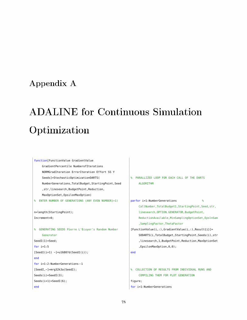
Appendix A
ADALINE for Continuous Simulation
Optimization
function[FunctionValue GradientValue
GradientPercentile NumberofIterations
NORMGradIteration ErrorIteration Effort SS Y
Seeds]=StochasticOptimizationDARTS(
NumberGenerations,TotalBudget,StartingPoint,Seed
,str,linesearch,BudgetPoint,Reduction,
MaxOptionSet,EpsilonMaxOption)
% ENTER NUMBER OF GENERATIONS (ANY EVEN NUMBER>1)
n=length(StartingPoint);
Increment=0;
% GENERATING SEEDS Pierre L'Ecuyer's Random Number
Generator
SeedI(1)=Seed;
for i=1:5
[SeedI(i+1) ~]=u16807d(SeedI(i));
end
for i=1:2:NumberGenerations−1
[SeedI,~]=mrg32k3a(SeedI);
Seeds(i)=SeedI(3);
Seeds(i+1)=SeedI(6);
end
% PARALLIZED LOOP FOR EACH CALL OF THE DARTS
ALGORITHM
parfor i=1:NumberGenerations %
CallNumber,TotalBudget1,StartingPoint,Seed,str,
linesearch,OPTION_GENERATOR,BudgetPoint,
ReductionAvailable,MinSamplingOptionSet,EpslnSam
,SamplingFactor,ThetaFactor
[FunctionValue(i,:),GradientValue(i,:),Resulti]=
SODARTS(i,TotalBudget,StartingPoint,Seeds(i),str
,linesearch,1,BudgetPoint,Reduction,MaxOptionSet
,EpsilonMaxOption,0,0);
end
% COLLECTION OF RESULTS FROM INDIVIDUAL RUNS AND
COMPILING THEM FOR PLOT GENERATION
figure;
for i=1:NumberGenerations
78
NumberofIterations(i)=size(Resulti,1);
for k=1:n
Y(1:NumberofIterations(i),Increment*n+k)=Resulti(:,
k);
end
NORMGradIteration(1:NumberofIterations(i),i)=Resulti
(:,n+2);
LastValue(i)=Resulti(NumberofIterations(i),n+2);
Effort(1:NumberofIterations(i),i)=Resulti(:,n+3);
SS(1:NumberofIterations(i),i)=Resulti(:,n+4);
Increment=Increment+1;
end
for i=1:NumberGenerations
SS(NumberofIterations(i)+1:size(NORMGradIteration,1),
i)=Resulti(NumberofIterations(i),n+4);
NORMGradIteration(NumberofIterations(i)+1:size(
NORMGradIteration,1),i)=LastValue(i);
Effort(NumberofIterations(i)+1:size(NORMGradIteration
,1),i)=TotalBudget;
end
MaxNumber=min(50,floor(max(NumberofIterations)));
for j=1:MaxNumber
ErrorIteration(j)=sum(NORMGradIteration(j,:)*sqrt(
Effort(j,:))')/sum(sum(NORMGradIteration(j,:)
~=0));
AverageSampleSize(j)=mean(SS(j,:));
end
SampleSizeMax=max(AverageSampleSize);
ErrorIteration=ErrorIteration';
PercentileValues=[25,50,75,90,95];
for i=1:length(PercentileValues)
for j=1:length(BudgetPoint)
GradientPercentile(i,j)=prctile(GradientValue(:,j),
PercentileValues(i));
end
subplot(1,2,1);
plot(BudgetPoint,GradientPercentile(i,:),'−x','
linewidth',1.5);
hold all;
end
% GENERATION OF PLOT
grid on;
xlabel('Budget');ylabel('||\nabla f|| at last
iteration');title('Budget Vs ||\nabla f|| at
last iteration');
legend('25th Percentile','50th Percentile','75th
Percentile','90th Percentile','95th Percentile')
;
subplot(1,2,2);
[ax,p1,p2]=plotyy(1:MaxNumber,ErrorIteration,1:
MaxNumber,AverageSampleSize);
set(p1,'LineWidth',2.5);
set(p2,'LineWidth',1.5);
xlabel('Iteration');ylabel(ax(1),'\surd W_k \times
||\nabla f|| at Iteration');
ylabel(ax(2),'M_k');
set(ax(1),'YLim',[0 50]);
set(ax(2),'YLim',[0 SampleSizeMax]);
set(ax(1),'YTick',[0:20:100]);
set(ax(2),'YTick',[0:7500:SampleSizeMax]);
grid on;
title('Iteration Vs \surd W_k \times ||\nabla f||
at Iteration');
annotation('textbox'
,[0.739,0.748,0.14568081991215204,0.111827956989],
'String','X_0:[5,8]','TOTAL BUDGET:200000','
NO. INDEPENDENT RUNS: 50');
hold off;
savefig('OutputFigure.fig');
save('OutputFile.mat','FunctionValue', 'GradientValue
', 'GradientPercentile', 'NumberofIterations', '
NORMGradIteration', 'ErrorIteration', 'Effort',
'Y', 'Seeds');
end
function [OutputFunctionValue,OutputGradientValue,
Result,H] = SODARTS(CallNumber,TotalBudget1,
79

StartingPoint,Seed,str,linesearch,
OPTION_GENERATOR,BudgetPoint,ReductionAvailable,
MinSamplingOptionSet,EpslnSam,SamplingFactor,
ThetaFactor)
global TotalBudget M S fhandle X SampleSize Iteration
Flag EF EGRADF UtilizedBudget H RandomSeed n;
TotalBudget=TotalBudget1;
MaxIterationNumber=1000;
if (MinSamplingOptionSet==0)
EpslnSam=−1;
end
% NUMBER OF DIMENSIONS IN THE PROBLEM
n=length(StartingPoint);
% CHOOSE THE FUNCTION FOR THE ORACLE & DIMENSION OF
PROBLEM
if (strcmp(str,'AluffiPentini'))
M=1;
S=sqrt(0.1);
elseif(strcmp(str,'Rosenbrock'))
% linesearch='Goldstein_BFGS';
M=1;
S=sqrt(0.1);
end
if strcmp(linesearch,'Goldstein_BFGS')
H=eye(n)^−1;
end
fhandle=str2func(str);
fhandleline=str2func(linesearch);
% PARAMETER INITIALIZATION
UtilizedBudget=0;
Iteration=0;
X(1,:)=StartingPoint;
Flag=1;
count=0;
% VECTOR INITIALIZATION
F=zeros(TotalBudget,1);
% Function realization at each sample (budget
point)
GRADF=zeros(TotalBudget,n);
% Gradient realization at each sample (budget
point)
EF=zeros(MaxIterationNumber);
% Estimated functional value at each iterate
EGRADF=zeros(MaxIterationNumber,2);
% Estimated gradient value at each iterate
SampleSize=zeros(MaxIterationNumber);
% Sample size at each iterate
LineSearchSampleSize=zeros(MaxIterationNumber);
% Effort in Line Search
NORMGRADF=zeros(MaxIterationNumber);
% Norm of the gradient at each iteration
CI=zeros(MaxIterationNumber);
% Half−width of the norm of the estimated
gradient at each iteration
CumulativeBudget=zeros(MaxIterationNumber);
% Total effort expended until Iteration k
TotalSampleSize=zeros(MaxIterationNumber);
TrueObjectiveSolution=zeros(MaxIterationNumber);
% True objective function value at kth iterate
TrueGradientSolution=zeros(MaxIterationNumber,n);
% True gradient at kth iterate
StepSize=zeros(MaxIterationNumber);
% Step size in the line search performed at kth
iteration
EnteredSampling=zeros(MaxIterationNumber);
% Indicator variable that more sampling is
performed at the current iteration
RandomSeed(1)=Seed;
Q=0;
CumulativeBudget(1)=0;
FileName=strcat('DARTS_',str,'_',linesearch,'
_ReductionOption=',int2str(ReductionAvailable),'
_Call=',int2str(CallNumber),'.txt');
fileID=fopen(FileName,'w');
fprintf(fileID,'% 3s % 11s % 11s % 11s % 11s % 11s %
80
11s % 11s % 8s % 8s % 8s % 8s\r\n','No.', 'X[1]'
,'X[2]','F−Estimate','F−TrueValue','HW−
Estimate','NG−Estimate','NG−TrueValue','SS−It'
,'SS−LINE','Step Size','Cumulative');
while (UtilizedBudget<TotalBudget && Flag==1)
% COMPUTE THE TRUE FUNCTIONAL VALUE AT EACH ITERATE
[TrueObjectiveSolution(Iteration+1),
TrueGradientSolution(Iteration+1,:)]=
ComputeTrueValue(X(Iteration+1,:),M,S,str);
NORMTRUEGRADIENT(Iteration+1)=norm(
TrueGradientSolution(Iteration+1,:));
% INCREMENT THE ITERATION AND SET THE INITIAL
SAMPLE SIZE TO 0
Iteration=Iteration+1;
LineSearchSampleSize(Iteration)=0;
EnteredSampling(Iteration)=0;
SampleSize(Iteration)=0;
T=0;
% if (Iteration<=2)
% fhandleline=str2func('Goldstein');
% else
% fhandleline=str2func(linesearch);
% end
% INITIATING THE PROCESS FOR EACH ITERATION (MEET
MINIMUM SAMPLE SIZE REQUIREMENT OR USE VALUES
FROM PREVIOUS ITERATE)
if (Iteration==1)
for i=1:2
[F(i),GRADF(i,:),RandomSeed(i+1)]=fhandle(X(Iteration
,:),RandomSeed(i),M,S);
SampleSize(Iteration)=SampleSize(Iteration)+1;
UtilizedBudget=UtilizedBudget+1;
end
EF(Iteration)=mean(F(1:2));
EGRADF(Iteration,:)=sum(GRADF(1:2,:))/2;
NORMGRADF(Iteration)=norm(EGRADF(Iteration,:));
CI(Iteration)=1/sqrt(2)*ThetaFactor+tinv(0.975,1)*
sqrt(norm(var(GRADF(1:2,:)),1))/2^(0.5+
SamplingFactor);
else
SampleSize(Iteration)=SampleSize(Iteration−1);
EF(Iteration)=mean(F(UtilizedBudget−SampleSize(
Iteration)+1:UtilizedBudget));
EGRADF(Iteration,:)=sum(GRADF(UtilizedBudget−
SampleSize(Iteration)+1:UtilizedBudget,:))/
SampleSize(Iteration);
NORMGRADF(Iteration)=norm(EGRADF(Iteration,:));
CI(Iteration)=1/sqrt(SampleSize(Iteration))*
ThetaFactor+tinv(0.975,SampleSize(Iteration)−1)
*sqrt(norm(var(GRADF(UtilizedBudget−SampleSize(
Iteration)+1:UtilizedBudget,:)),1))/(SampleSize(
Iteration))^(0.5+SamplingFactor);
end
% INCREASE SAMPLING UNTIL $C*\frac\hat\sigma_m_k
(X_k)\leq ||\nabla \ha
while (CI(Iteration)>=(NORMGRADF(Iteration)) && Flag
==1)
EnteredSampling(Iteration)=1;
if(UtilizedBudget>=TotalBudget)
Flag=0;
break;
else
SampleSize(Iteration)=SampleSize(Iteration)+1;
UtilizedBudget=UtilizedBudget+1;
[F(UtilizedBudget),GRADF(UtilizedBudget,:),RandomSeed
(SampleSize(Iteration)+1)]=fhandle(X(Iteration
,:),RandomSeed(SampleSize(Iteration)),M,S);
EF(Iteration)=mean(F(UtilizedBudget−SampleSize(
81
Iteration)+1:UtilizedBudget));
EGRADF(Iteration,:)=sum(GRADF(UtilizedBudget−
SampleSize(Iteration)+1:UtilizedBudget,:))/
SampleSize(Iteration);
NORMGRADF(Iteration)=norm(EGRADF(Iteration,:));
CI(Iteration)=1/sqrt(SampleSize(Iteration))*
ThetaFactor+tinv(0.975,SampleSize(Iteration)−1)
*sqrt(norm(var(GRADF(UtilizedBudget−SampleSize(
Iteration)+1:UtilizedBudget,:)),1))/(SampleSize(
Iteration))^(0.5+SamplingFactor);
end
end
% REDUCE SAMPLE SIZE AT CURRENT ITERATION IF
POSSIBLE
if (CI(Iteration)<=(NORMGRADF(Iteration)) &&
ReductionAvailable==1 && SampleSize(Iteration)>2
&& EnteredSampling(Iteration)==0)
while (CI(Iteration)<=(NORMGRADF(Iteration)) &&
SampleSize(Iteration)−T>=2)
T=T+1;
EF(Iteration)=mean(F(UtilizedBudget−SampleSize(
Iteration)+1:UtilizedBudget−T));
EGRADF(Iteration,:)=sum(GRADF(UtilizedBudget−
SampleSize(Iteration)+1:UtilizedBudget−T,:))/(
SampleSize(Iteration)−T);
NORMGRADF(Iteration)=norm(EGRADF(Iteration,:));
% CI(Iteration)=1/sqrt(SampleSize(
Iteration)−T)*ThetaFactor+tinv(0.975,SampleSize
(Iteration)−(T+1))*std(F(UtilizedBudget−
SampleSize(Iteration)+1:UtilizedBudget−T))/(
SampleSize(Iteration)−T)^(0.5+SamplingFactor);
CI(Iteration)=1/sqrt(SampleSize(Iteration)−T)*ThetaFactor+tinv(0.975,SampleSize(Iteration)−(T
+1))*sqrt(norm(var(GRADF(UtilizedBudget−
SampleSize(Iteration)+1:UtilizedBudget−T,:)),1)
)/(SampleSize(Iteration)−T)^(0.5+SamplingFactor
);
end
EF(Iteration)=mean(F(UtilizedBudget−SampleSize(
Iteration)+1:UtilizedBudget+1−T));
EGRADF(Iteration,:)=sum(GRADF(UtilizedBudget−
SampleSize(Iteration)+1:UtilizedBudget+1−T,:))
/(SampleSize(Iteration)+1−T);
NORMGRADF(Iteration)=norm(EGRADF(Iteration,:));
CI(Iteration)=1/sqrt(SampleSize(Iteration)+1−T)*ThetaFactor+tinv(0.975,SampleSize(Iteration)−T)
*sqrt(norm(var(GRADF(UtilizedBudget−SampleSize(
Iteration)+1:UtilizedBudget+1−T,:)),1))/(
SampleSize(Iteration)+1−T)^(0.5+SamplingFactor)
;
if MinSamplingOptionSet==0
SampleSize(Iteration)=SampleSize(Iteration)−T+1;
end
end
% SET THE SAMPLE SIZE TO BE THE MAX (K^(1+EPSILON),
M_K)
if MinSamplingOptionSet==1
if EnteredSampling(Iteration)==1
NewSampleSize=max(floor(Iteration^(1+EpslnSam)),
SampleSize(Iteration));
else
NewSampleSize=max(floor(Iteration^(1+EpslnSam)),
SampleSize(Iteration)+1−T);
end
if (NewSampleSize > SampleSize(Iteration))
count1=0;
for i=1:NewSampleSize−SampleSize(Iteration)
count1=count1+1;
[F(UtilizedBudget+i),GRADF(UtilizedBudget+i,:),
RandomSeed(SampleSize(Iteration)+count1+1)]=
fhandle(X(Iteration,:),RandomSeed(SampleSize(
Iteration)+count1),M,S);
end
end
UtilizedBudget=UtilizedBudget+NewSampleSize−
SampleSize(Iteration);
EF(Iteration)=mean(F(UtilizedBudget−NewSampleSize+1:
UtilizedBudget));
EGRADF(Iteration,:)=sum(GRADF(UtilizedBudget−
82

NewSampleSize+1:UtilizedBudget,:))/(
NewSampleSize);
NORMGRADF(Iteration)=norm(EGRADF(Iteration,:));
CI(Iteration)=1/sqrt(SampleSize(Iteration)+1)*
ThetaFactor+tinv(0.975,NewSampleSize−1)*sqrt(
norm(var(GRADF(UtilizedBudget−NewSampleSize+1:
UtilizedBudget,:)),1))/(NewSampleSize)^(0.5+
SamplingFactor);
SampleSize(Iteration)=NewSampleSize;
end
% LINE SEARCH TO DETERMINE THE NEXT ITERATE
if (Flag==1 && TotalBudget>=UtilizedBudget+SampleSize
(Iteration))
[LF,LGRADF,LineSearchSampleSize(Iteration),StepSize(
Iteration)]=fhandleline(1);
for i=1:LineSearchSampleSize(Iteration)
F(UtilizedBudget+i,1)=LF(i,1);
GRADF(UtilizedBudget+i,:)=LGRADF(i,:);
end
UtilizedBudget=UtilizedBudget+LineSearchSampleSize(
Iteration);
else
LineSearchSampleSize(Iteration)=TotalBudget−
UtilizedBudget;
StepSize(Iteration)=1;
UtilizedBudget=UtilizedBudget+LineSearchSampleSize(
Iteration);
Flag=0;
end
CumulativeBudget(Iteration)=UtilizedBudget;
TotalSampleSize(Iteration)=SampleSize(Iteration)+
LineSearchSampleSize(Iteration);
% PRINT THE RESULTS AT EACH ITERATION
fprintf(fileID,'% 3d % 11.5f % 11.5f % 11.5f % 11.5f
% 11.5f % 11.5f % 11.5f % 8d % 8d % 8.4f % 8d\r\
n',...
Iteration, X(Iteration,1),X(Iteration,2),EF(Iteration
),TrueObjectiveSolution(Iteration),CI(Iteration)
,NORMGRADF(Iteration),NORMTRUEGRADIENT(Iteration
),SampleSize(Iteration),LineSearchSampleSize(
Iteration),StepSize(Iteration),CumulativeBudget(
Iteration));
% PASS THE VALUES TO THE GENERATOR CODE AT VARIOUS
MID−POINTS IF OPTION−GENERATOR IS SET TO 1.
if(OPTION_GENERATOR==1 && CumulativeBudget(Iteration)
>=BudgetPoint(Q+1) && Q<=length(BudgetPoint))
if (Iteration==1)
Y=find(BudgetPoint<=CumulativeBudget(Iteration));
else
Y=find(BudgetPoint<=CumulativeBudget(Iteration) &
BudgetPoint>CumulativeBudget(Iteration−1));
end
count=count+1;
IterationNumber(count)=Iteration;
Points(Iteration)=length(Y);
for L=1:Points(Iteration)
TRUEGRADIENT(Q+L)=NORMTRUEGRADIENT(Iteration);
OPTIMALVALUE(Q+L,:)=X(Iteration,:);
TRUEFUNCTION(Q+L)= TrueObjectiveSolution(Iteration);
end
Q=Q+Points(Iteration);
if (Iteration>1 && Q−Points(Iteration)>0 && any(
BudgetPoint(Q−Points(Iteration))==
CumulativeBudget(1:Iteration−1)))
TRUEGRADIENT(Q−Points(Iteration))=NORMTRUEGRADIENT(
IterationNumber(count−1)+1);
OPTIMALVALUE(Q−Points(Iteration),:)=X(
IterationNumber(count−1)+1,:);
TRUEFUNCTION(Q−Points(Iteration))=
TrueObjectiveSolution(IterationNumber(count−1)
+1);
end
end
end
83
OutputValue=OPTIMALVALUE';
OutputFunctionValue=TRUEFUNCTION;
OutputGradientValue=TRUEGRADIENT;
OutputSeed=RandomSeed(SampleSize(Iteration)+1);
fclose(fileID);
% PLOT THE TRAJECTORY OF THE ALGORITHM OVER A SINGLE
RUN WHEN IT IS NOT CALLED BY A GENERATOR
if OPTION_GENERATOR==0
plottrajectory(str,M,S,X,Iteration,
LineSearchSampleSize(Iteration));
end
Result=[X(1:Iteration,:) TrueObjectiveSolution(1:
Iteration)' NORMTRUEGRADIENT(1:Iteration)'
CumulativeBudget(1:Iteration)' SampleSize(1:
Iteration)'];
end
function[LF,LGRADF,SSL,alphatempout]=Goldstein_BFGS(
YY)
global TotalBudget M S fhandle X SampleSize Iteration
Flag EF EGRADF RandomSeed UtilizedBudget H n;
% INITIALIZE THE ARRAYS THAT COLLECT INFORMATION
FROM EVERY BUDGET POINT
LF=[];
LGRADF=[];
% H=[2*(M^2+S^2)+1200*X(Iteration,1)^2*(M^4+3*S
^4+6*M^2*S^2)−400*X(Iteration,2)*(M^2+S^2)
,−400*X(Iteration,1)*(M^2+S^2);−400*X(Iteration
,1)*(M^2+S^2),200]^−1;
% INITIALIZE THE PARAMETERS
SSL=0;
Flag=1;
I=1;
a(1)=0;
b(1)=10^4;
Condition=0;
bracketingmultiplier=2;
% PARAMETERS FOR THE LINE SEARCH METHOD (GOLDSTEIN
CONDITION PARAMETERS)
alpha=YY;
c=0.0001;
% INITIALIZE THE LINE SEARCH ITERATION AND THE
POINTS
alphatemp(I)=alpha;
% SAMPLE FROM THE INITIAL ALPHA(I) VALUE
LinearModelResult(I)=EF(Iteration)−c*alphatemp(I)*(
EGRADF(Iteration,:)*EGRADF(Iteration,:)');
LinearModelResultNegative(I)=EF(Iteration)−(1−c)*alphatemp(I)*(EGRADF(Iteration,:)*EGRADF(
Iteration,:)');
XL(I,:)=X(Iteration,:)−alphatemp(I)*(H*EGRADF(
Iteration,:)')';
for k=1:SampleSize(Iteration)
SSL=SSL+1;
[FEndingPoint(k,1),GRADFEndingPoint(k,:),~]=fhandle(
XL(I,:),RandomSeed(k),M,S);
if ((UtilizedBudget+SSL)>=TotalBudget)
Flag=0;
break;
end
end
FXL(I)=mean(FEndingPoint);
GRADFLX(I,:)=sum(GRADFEndingPoint)/SampleSize(
Iteration);
LF=[LF;FEndingPoint];
LGRADF=[LGRADF;GRADFEndingPoint];
% Wolfe(I)=
% CHECK IF THE FIRST RULE IS SATISFIED BY THIS POINT
while(Condition==0 && Flag==1 && alphatemp(I)>10^−7)
% && alphatemp(I)>10^−8
if(FXL(I)<=LinearModelResult(I))
if (FXL(I)>=LinearModelResultNegative(I))
Condition=1;
break;
84
else
I=I+1;
a(I)=alphatemp(I−1);
b(I)=b(I−1);
if (b(I)<b(1))
alphatemp(I)=(a(I)+b(I))/2;
else
alphatemp(I)=bracketingmultiplier*alphatemp(I−1);
end
LinearModelResult(I)=EF(Iteration)−c*alphatemp(I)*(
EGRADF(Iteration,:)*EGRADF(Iteration,:)');
LinearModelResultNegative(I)=EF(Iteration)−(1−c)*alphatemp(I)*(EGRADF(Iteration,:)*EGRADF(
Iteration,:)');
XL(I,:)=X(Iteration,:)−alphatemp(I)*(H*EGRADF(
Iteration,:)')';
for k=1:SampleSize(Iteration)
SSL=SSL+1;
[FEndingPoint(k,1),GRADFEndingPoint(k,:),~]=fhandle(
XL(I,:),RandomSeed(k),M,S);
if ((UtilizedBudget+SSL)>=TotalBudget)
Flag=0;
break;
end
end
FXL(I)=mean(FEndingPoint);
GRADFLX(I,:)=sum(GRADFEndingPoint)/SampleSize(
Iteration);
LF=[LF;FEndingPoint];
LGRADF=[LGRADF;GRADFEndingPoint];
end
else
I=I+1;
a(I)=a(I−1);
b(I)=alphatemp(I−1);
alphatemp(I)=(a(I)+b(I))/2;
LinearModelResult(I)=EF(Iteration)−c*alphatemp(I)*(
EGRADF(Iteration,:)*EGRADF(Iteration,:)');
LinearModelResultNegative(I)=EF(Iteration)−(1−c)*alphatemp(I)*(EGRADF(Iteration,:)*EGRADF(
Iteration,:)');
XL(I,:)=X(Iteration,:)−alphatemp(I)*(H*EGRADF(
Iteration,:)')';
for k=1:SampleSize(Iteration)
SSL=SSL+1;
[FEndingPoint(k,1),GRADFEndingPoint(k,:),~]=fhandle(
XL(I,:),RandomSeed(k),M,S);
if ((UtilizedBudget+SSL)>=TotalBudget)
Flag=0;
break;
end
end
FXL(I)=mean(FEndingPoint);
GRADFLX(I,:)=sum(GRADFEndingPoint)/SampleSize(
Iteration);
LF=[LF;FEndingPoint];
LGRADF=[LGRADF;GRADFEndingPoint];
end
end
alphatempout=alphatemp(I);
X(Iteration+1,:)=XL(I,:);
SK=−(alphatempout*H*EGRADF(Iteration,:)');
YK=GRADFLX(I,:)'−EGRADF(Iteration,:)';
RHOK=1/(SK'*YK);
if (Iteration==1)
H=(YK'*SK)/(YK'*YK)*H;
end
if YK'*SK>0
H=(eye(n)−RHOK*SK*YK')*H*(eye(n)−RHOK*YK*SK')+RHOK
*(SK*SK');
end
end
function[LF,LGRADF,SSL,alphatempout]=Goldstein(YY)
global TotalBudget M S fhandle X SampleSize Iteration
Flag EF EGRADF RandomSeed UtilizedBudget;
% INITIALIZE THE ARRAYS THAT COLLECT INFORMATION
FROM EVERY BUDGET POINT
LF=[];
LGRADF=[];
% INITIALIZE THE PARAMETERS
SSL=0;
85
Flag=1;
I=1;
a(1)=0;
b(1)=10^4;
Condition=0;
bracketingmultiplier=2;
% PARAMETERS FOR THE LINE SEARCH METHOD (GOLDSTEIN
CONDITION PARAMETERS)
alpha=YY;
c=0.0001;
% INITIALIZE THE LINE SEARCH ITERATION AND THE
POINTS
alphatemp(I)=alpha;
% SAMPLE FROM THE INITIAL ALPHA(I) VALUE
LinearModelResult(I)=EF(Iteration)−c*alphatemp(I)*(
EGRADF(Iteration,:)*EGRADF(Iteration,:)');
LinearModelResultNegative(I)=EF(Iteration)−(1−c)*alphatemp(I)*(EGRADF(Iteration,:)*EGRADF(
Iteration,:)');
XL(I,:)=X(Iteration,:)−alphatemp(I)*EGRADF(Iteration
,:);
for k=1:SampleSize(Iteration)
SSL=SSL+1;
[FEndingPoint(k,1),GRADFEndingPoint(k,:),~]=fhandle(
XL(I,:),RandomSeed(k),M,S);
if ((UtilizedBudget+SSL)>=TotalBudget)
Flag=0;
break;
end
end
FXL(I)=mean(FEndingPoint);
GRADFLX(I,:)=sum(GRADFEndingPoint)/SampleSize(
Iteration);
LF=[LF;FEndingPoint];
LGRADF=[LGRADF;GRADFEndingPoint];
% CHECK IF THE FIRST RULE IS SATISFIED BY THIS POINT
while(Condition==0 && Flag==1 && alphatemp(I)>10^−7)
if(FXL(I)<=LinearModelResult(I))
if (FXL(I)>=LinearModelResultNegative(I))
Condition=1;
break;
else
I=I+1;
a(I)=alphatemp(I−1);
b(I)=b(I−1);
if (b(I)<b(1))
alphatemp(I)=(a(I)+b(I))/2;
else
alphatemp(I)=bracketingmultiplier*alphatemp(I−1);
end
LinearModelResult(I)=EF(Iteration)−c*alphatemp(I)*(
EGRADF(Iteration,:)*EGRADF(Iteration,:)');
LinearModelResultNegative(I)=EF(Iteration)−(1−c)*alphatemp(I)*(EGRADF(Iteration,:)*EGRADF(
Iteration,:)');
XL(I,:)=X(Iteration,:)−alphatemp(I)*EGRADF(Iteration
,:);
for k=1:SampleSize(Iteration)
SSL=SSL+1;
[FEndingPoint(k,1),GRADFEndingPoint(k,:),~]=fhandle(
XL(I,:),RandomSeed(k),M,S);
if ((UtilizedBudget+SSL)>=TotalBudget)
Flag=0;
break;
end
end
FXL(I)=mean(FEndingPoint);
GRADFLX(I,:)=sum(GRADFEndingPoint)/SampleSize(
Iteration);
LF=[LF;FEndingPoint];
LGRADF=[LGRADF;GRADFEndingPoint];
end
else
I=I+1;
a(I)=a(I−1);
b(I)=alphatemp(I−1);
alphatemp(I)=(a(I)+b(I))/2;
LinearModelResult(I)=EF(Iteration)−c*alphatemp(I)*(
EGRADF(Iteration,:)*EGRADF(Iteration,:)');
LinearModelResultNegative(I)=EF(Iteration)−(1−c)*alphatemp(I)*(EGRADF(Iteration,:)*EGRADF(
Iteration,:)');
86
XL(I,:)=X(Iteration,:)−alphatemp(I)*EGRADF(Iteration
,:);
for k=1:SampleSize(Iteration)
SSL=SSL+1;
[FEndingPoint(k,1),GRADFEndingPoint(k,:),~]=fhandle(
XL(I,:),RandomSeed(k),M,S);
if ((UtilizedBudget+SSL)>=TotalBudget)
Flag=0;
break;
end
end
FXL(I)=mean(FEndingPoint);
GRADFLX(I,:)=sum(GRADFEndingPoint)/SampleSize(
Iteration);
LF=[LF;FEndingPoint];
LGRADF=[LGRADF;GRADFEndingPoint];
end
end
alphatempout=alphatemp(I);
X(Iteration+1,:)=XL(I,:);
end
function[]=plottrajectory(str,M,S,X,Iteration,
LineSearchSample)
if (strcmp(str,'AluffiPentini'))
[A,B]=meshgrid(−1:0.00001:1,−0.1:0.01:0.1);
Value=0.25*A.^4*(M^4+6*M^2*(S)^2+3*(S)^4)−0.5*X(
Iteration,1)^2*(M^2+(S)^2)+0.1*X(Iteration,1)*M
+0.5*B.^2;
elseif(strcmp(str,'Rosenbrock'))
[A,B]=meshgrid(−2:0.1:2,−2:0.1:2);
end
LocalOptima=[−0.863645,0;0.771579,0];
zmin = floor(min(Value(:)));
zmax = ceil(max(Value(:)));
zinc = (zmax − zmin) / 75;
zlevs = zmin:zinc:zmax;
contour(A,B,Value,zlevs);
hold on;
T=1:1:Iteration;
plot(X(:,1),X(:,2),'−rO','linewidth',2.5);
strValues = strtrim(cellstr(num2str(T','%d')));
if LineSearchSample>0
text(X(1:Iteration,1),X(1:Iteration,2),strValues,'
HorizontalAlignment','center','VerticalAlignment
','bottom');
else
text(X(:,1),X(:,2),strValues,'HorizontalAlignment','
center','VerticalAlignment','bottom');
end
plot(LocalOptima(:,1),LocalOptima(:,2),'r*','
MarkerSize',20);
hold off;
end
function[ObjectiveValue,GradientValue]=
ComputeTrueValue(Y,M,S,str)
if (strcmp(str,'AluffiPentini'))
ObjectiveValue=0.25*Y(1)^4*(M^4+6*M^2*(S)^2+3*(S)^4)
−0.5*Y(1)^2*(M^2+(S)^2)+0.1*Y(1)*M+0.5*Y(2)^2;
GradientValue(1)=(Y(1))^(3)*(M^4+6*M^(2)*(S)^2+3*S^4)
−Y(1)*(M^(2)+(S)^(2))+0.1*M;
GradientValue(2)=Y(2);
NormGradientValue=norm(GradientValue);
elseif(strcmp(str,'Rosenbrock'))
ObjectiveValue=Y(1)^2*(M^2+(S)^2)+1−2*Y(1)*M+100*(Y
(2)^2+Y(1)^4*(M^4+6*M^2*(S)^2+3*(S)^4)−2*Y(1)
^2*Y(2)*(M^2+(S)^2));
GradientValue(1)=2*Y(1)*(M^2+(S)^2)−2*M+100*(4*Y(1)
^3*(M^4+6*M^2*(S)^2+3*(S)^4)−4*Y(1)*Y(2)*(M^2+(
S)^2));
GradientValue(2)=200*(Y(2)−Y(1)^2*(M^2+(S)^2));
NormGradientValue=norm(GradientValue);
end
end
function [F1, GRADF1, Seed1] = AluffiPentini(XX,Seed1
87
,M1,Sg1)
% INPUT: X=[X_1,....,X_N] and the Seed from the
Master problem.
% OUTPUT: The functional value and the true gradient
at a realization and the next random seed.
% FUNCTION CALLS: Generate random variates.
% PARAMETERS: a,b,c,d
% Set Parameters
% A) Functional Parameters
a=0.25;b=0.5;c=0.1;d=0.5;
% B) Distributional Paramters for the Noise function
% M is the mean and Sg is the standard deviation of
the normal random variable (When using other
distributions, please change them and alter the
parameters accordingly)
% Generate a random realization for the noise
function
[Seed1 URV]=u16807d(Seed1); % URV= Uniform Random
Variate
R=norminv(URV,M1,Sg1);
% R=1;
F1= a*(XX(1)*R)^4−b*(XX(1)*R)^2+c*XX(1)*R+d*XX(2)^2;
GRADFX1=4*a*(XX(1))^3*R^4−2*b*XX(1)*R^2+c*R;
GRADFX2=2*d*XX(2);
GRADF1=[GRADFX1,GRADFX2];
end
function [F1, GRADF1, Seed1] = Rosenbrock(XX,Seed1,M1
,Sg1)
% INPUT: X=[X_1,....,X_N] and the Seed from the
Master problem.
% OUTPUT: The functional value and the true gradient
at a realization and the next random seed.
% FUNCTION CALLS: Generate random variates.
% PARAMETERS: a,b,c,d
% Set Parameters
% A) Functional Parameters
% a=0.25;b=0.5;c=0.1;d=0.5;
% B) Distributional Paramters for the Noise function
% M is the mean and Sg is the standard deviation of
the normal random variable (When using other
distributions, please change them and alter the
parameters accordingly)
% Generate a random realization for the noise
function
[Seed1 URV]=u16807d(Seed1); % URV= Uniform Random
Variate
R=norminv(URV,M1,Sg1);
% R=1;
F1=(XX(1)*R−1)^2+100*(XX(2)−(XX(1)*R)^2)^2;
GRADFX1=2*(XX(1)*R−1)*R−400*(XX(2)−(XX(1)*R)^2)*(XX
(1)*R^2);
GRADFX2=200*(XX(2)−(XX(1)*R)^2);
GRADF1=[GRADFX1,GRADFX2];
end
function [iseed,u16807d]=u16807d(iseed)
%
..........................................................................
% bruce schmeiser january 1989.
.
% a linear congruential pseudorandom number
generator .
% using constant 16807 and modulus (2**31)−1.
.
% iseed = iseed*16807 (mod 2^31 −1)
.
% for implementations that don't require double
precision, see .
% s.k. park and k.w. miller, "random numbers
generators: good .
% ones are hard to find," cacm, 31, 10 (October
1988), 1192−1201. .
% in correct implementations, starting with a seed
value of 1 will .
% result in a seed value of 1043618065 on call
number 10001. .
%
..........................................................................
% input: iseed. integer.
88
.
% chosen from [1,2147483646] on the
first call. .
% thereafter, the value returned
from the last call.
% output: iseed. integer.
.
% to be used in the next call.
.
% output: u16807d. real.
.
% a pseudorandom number in (0,1).
.
%
..........................................................................
u16807d=0;
while (u16807d<=0 || u16807d>=1)
iseed = mod (iseed * 16807,2147483647);
u16807d = iseed / 2147483648;
end
end
function [seed,u] = mrg32k3a(seed)
%
%
..........................................................................
% Raghu Pasupathy June 2012.
%
% This is an implementation of Pierre L'Ecuyer's
Random Number Generator,
% MRG32K3A. ("Good Parameters and Implementations
for Combined Multiple
% Recursive Random Number Generators", Operations
Research 47, pp.
% 159−164, 1999.)
%
%
%
..........................................................................
% input: seed(1),seed(2),seed(3) positive integers
< m1, not all zero.
% input: seed(4),seed(5),seed(6) positive integers
< m2, not all zero.
%
% output: seed (seeds to be used in
the next call)
% u (a pseudorandom number
in (0,1)
%
..........................................................................
s1 = 1403580;
t1 = 810728;
s2 = 527612;
t2 = 1370589;
m1 = 4294967087;
m2 = 4294944443;
m3 = 4294967088;
p1 = mod( ( s1 * seed(1) ) − ( t1 * seed(2) ), m1);
p2 = mod( ( s2 * seed(4) ) − ( t2 * seed(5) ), m2);
z = mod( ( p1 − p2 ), m1 );
if ( z > 0 )
u = z / m3;
elseif ( z == 0 )
u = m1 / m3;
end
seed(1) = seed(2); seed(2) = seed(3); seed(3) = p1;
seed(4) = seed(5); seed(5) = seed(6); seed(6) = p2;
%
−−−−−−−−−−−−−−−−−−−−−−−−−−−−−−−−−−−−−−−−−−−−−−−−−−−−−−−−−−−−−−−−−−−−−−−−−−
end
89

Appendix B
ADALINE for Integer Simulation
Optimization
1 # DECLARE THE STATIC GLOBAL VARIABLES AND INITIALIZE THE PARAMETERS
2 class G:
3 oracle_parameter = [0,0,0]
4 dimension = 0
5 total_neighbors = 0
6
7 total_budget = 0
8 iseed = 0
9 iseed_perturb = 0
10
11 alpha = 0
12 min_sample = 0
13 delta = 0
14
15 iteration_max = 400
16 imax = 15
17 s = 1
18 c = 2
19
20 @staticmethod
21 def calculate_dimensions ():
22 G.dimension = G.oracle_parameter [0]
23 G.total_neighbors = 2 * G.oracle_parameter [0]
24
25
26 class DecisionVariable:
27 x = [[0 for i in range(G.dimension)] for j in range(G.iteration_max)]
28
29
30 class Dynamic:
31 output_seed = []
32 urv = []
33
34
35 class OracleClass:
36 @staticmethod
90

37 def multi_quadratic(x_input_oracle ,total_sample ,current_sample):
38 feasibility = 1
39 est_value = 0
40 est_var = float('Inf')
41 true_value = 1
42 ind_values = [0] * total_sample
43 rv = [0] * total_sample
44 if all(-100 <= i <= 100 for i in x_input_oracle):
45 for i in range(G.dimension):
46 true_value += x_input_oracle[i] ** 2
47 mu = G.oracle_parameter [1]
48 sigma = G.oracle_parameter [2] * true_value
49 for i in range(total_sample):
50 seed = Dynamic.output_seed[current_sample + i]
51 seed_generator = u16807d_randomnumber(seed)
52 seed = seed_generator [1]
53 u = seed_generator [0]
54 rv[i] = norm.ppf(u, loc=mu , scale=sigma)
55 ind_values[i] = true_value + rv[i]
56 Dynamic.output_seed[current_sample+i+1] = seed
57 est_value = np.mean(ind_values)
58 if not total_sample == 1:
59 est_var = np.var(ind_values ,ddof =1)
60 else:
61 feasibility = 0
62 return feasibility , est_value , est_var , true_value , ind_values
63
64 @staticmethod
65 def bus_scheduling(x_input_oracle , total_sample , current_sample):
66 feasibility = 1
67 est_value = 0
68 est_var = float('Inf')
69 true_value = 1
70 ind_values = [0] * total_sample
71 if all(0 <= i < G.oracle_parameter [2] for i in x_input_oracle):
72 for i in range(total_sample):
73 time_sum = 0
74 time_arrive = 0
75 time_bus = 0
76 seed = Dynamic.output_seed[current_sample + i]
77 while time_arrive <= G.oracle_parameter [2]:
78 seed_generator = u16807d_randomnumber(seed)
79 seed = seed_generator [1]
80 u = seed_generator [0]
81 if(1- u > 0):
82 time_arrive += (-math.log (1.0 - u))/G.oracle_parameter [1]
83 if time_arrive > time_bus:
84 time_bus = G.oracle_parameter [2]
85 for j in range(G.oracle_parameter [0]):
86 if time_arrive <= x_input_oracle[j] < time_bus:
87 time_bus = x_input_oracle[j]
88 time_sum += time_bus - time_arrive
89 ind_values[i] = time_sum
90 Dynamic.output_seed[current_sample+i+1] = seed
91 est_value = np.mean(ind_values)
92 if not total_sample == 1:
93 est_var = np.var(ind_values ,ddof =1)
94 else:
95 feasibility = 0
96 return feasibility , est_value , est_var , true_value , ind_values
97
98 @staticmethod
99 def inventory_optimization(x_input_oracle , total_sample , current_sample):
100 feasibility = 1
91
101 est_value = 0
102 est_var = float('Inf')
103 true_value = 1
104 ind_values = [0] * total_sample
105 no_days = G.oracle_parameter [2]
106 mean_demand = G.oracle_parameter [1]
107 warm_up = 100
108 holding_cost = 1
109 ordering_cost = 32
110 per_unit_cost = 3
111 shortage_cost= 5
112 start_inventory = x_input_oracle [1]
113 initial_inventory = [[0 for i in range(no_days + warm_up + 1)] \
114 for j in range(total_sample)]
115 order_quantity = copy.deepcopy(initial_inventory)
116 order_period = copy.deepcopy(initial_inventory)
117 shortage = copy.deepcopy(initial_inventory)
118 holding = copy.deepcopy(initial_inventory)
119 inventory_position = copy.deepcopy(initial_inventory)
120 if x_input_oracle [1] - x_input_oracle [0] >= 10 and \
121 20 <= x_input_oracle [0] <= 80 and 40 <= x_input_oracle [1] <= 100:
122 for i in range(total_sample):
123 cost = 0
124 np.random.seed(Dynamic.output_seed[current_sample + i])
125 demand = np.random.poisson(mean_demand ,no_days + warm_up)
126 seed_generator = u16807d_randomnumber(Dynamic.output_seed\
127 [current_sample + i])
128 initial_inventory[i][0] = start_inventory
129 for j in range(no_days + warm_up):
130 if initial_inventory[i][j] < x_input_oracle [0]:
131 order_quantity[i][j] = x_input_oracle [1] \
132 - initial_inventory[i][j]
133 order_period[i][j] = 1
134 inventory_position[i][j] = initial_inventory[i][j] \
135 + order_quantity[i][j]
136 shortage[i][j] = max(0,demand[j] - inventory_position[i][j])
137 holding[i][j] = max(0, inventory_position[i][j] - demand[j])
138 initial_inventory[i][j+1] = holding[i][j]
139 if j >= warm_up:
140 cost += shortage[i][j] * shortage_cost + holding[i][j] \
141 * holding_cost + per_unit_cost * order_quantity[i][j] \
142 + order_period[i][j] * ordering_cost
143 ind_values[i] = cost
144 Dynamic.output_seed[current_sample + i + 1] = seed_generator [1]
145 est_value = np.mean(ind_values)
146 if not total_sample == 1:
147 est_var = np.var(ind_values ,ddof =1)
148 else:
149 feasibility = 0
150 return feasibility , est_value , est_var , true_value , ind_values
151
152
153
154 def oracle_call(x_input_oracle ,total_sample ,current_sample ,problem):
155 z = getattr(OracleClass ,problem)(x_input_oracle ,total_sample ,current_sample)
156 return z[0],z[1],z[2],z[3],z[4]
157
158
159 # RANDOM SEED GENERATOR
160 def u16807d ():
161 seed = G.iseed
162 for i in range(G.total_budget +100):
163 urv = 0
164 while urv <= 0 or urv >= 1:
92

165 temp = seed * 16807
166 seed = temp % 2147483647
167 urv = seed / 2147483648
168 Dynamic.output_seed[i] = seed
169 Dynamic.urv.append(urv)
170
171
172 # RANDOM NUMBER GENERATOR
173 def u16807d_randomnumber(seed):
174 urv = 0
175 while urv <= 0 or urv >= 1:
176 temp = seed * 16807
177 seed = temp % 2147483647
178 urv = seed/ 2147483648
179 return urv , seed
180
181
182 # INTEGER ORDERED SIMULATION OPTIMIZATION USING ADAPTIVE SPLINE
183 def stochastic_integer(x_input_opt ,problem ,algorithm_parameters ,run):
184 # INITIALIZE ALL THE SOLVER PARAMETERS
185 budget = G.total_budget
186 escort = algorithm_parameters [0]
187 gradient = algorithm_parameters [1]
188 adaptive_PLI = algorithm_parameters [2]
189 adaptive_NE = algorithm_parameters [3]
190 sol_tolerance = 0
191 min_sample = G.min_sample
192
193 # RUN THE U16807D GENERATOR IF THE PROBLEM TO BE SOLVED IS THE
194 # MULTI DIMENSIONAL QUADRATIC PROBLEM
195 # if problem == 'multi_quadratic ':
196 # u16807d ()
197
198 # CREATE AND NAME THE LOG FILE THAT IS GENERATED
199 filename = "GradientDescent_SeedNO" + str(run+1) + ".txt"
200 f = open(filename ,'w')
201
202 # INITIALIZE ALL THE VARIABLES CORRESPONDING TO ONE RUN OF THE
203 # SIMULATION OPTIMIZATION ALGORITHM
204 true_objective = []
205 iteration_Q = []
206 samplesize = []
207 Work = []
208 Magnitude = []
209 overallsample = []
210 fx_iteration = []
211 search_direction = []
212 out_search_direction = []
213 pli_sample_size = []
214 Q = 0
215 ncalls = 0
216 iteration = 0
217 max_sample = min_sample
218 fx_best = float('inf')
219 DecisionVariable.x[iteration] = x_input_opt
220 x_best = copy.deepcopy(DecisionVariable.x[iteration ])
221 f.write("Iteration\t\t\t\t"+ " " \
222 + "Decision Variable at start\t\t\t\t\t\t\t\t" + " "
223 + "Best at end of iteration\t\t\t" + " " \
224 + "Estimated Total Cost\t" + " "
225 + "Search Direction\t\t" + " " + "Sample Size\t" + " "\
226 + "Work".rjust (15) + " " + "Overall Sample Size".rjust (200) + "\n\n")
227
228 feasibility = oracle_call(x_best , 1, 0, problem)
93
229 if feasibility [0] == 0:
230 print "Enter a feasible solution to start algorithm"
231 return
232
233 if adaptive_PLI == 0:
234 search_sample_size = 0
235
236
237 # PERFORM ADAPTIVE PLI AND NEIGHBORHOOD ENUMERATION UNTIL THE BUDGET GETS EXPENDED
238 while ncalls < G.total_budget:
239 # START THE ADAPTIVE PLI FRAMEWORK
240 if adaptive_PLI == 1 and ncalls + (G.dimension + 1) \
241 * min_sample <= G.total_budget:
242 linear_interpolation = Adaptive_PLI(x_best , \
243 min_sample , ncalls , problem)
244 fx_pli_best = linear_interpolation [1]
245 x_pli_best = linear_interpolation [0]
246 search_gradient = linear_interpolation [2]
247 search_sample_size = linear_interpolation [3]
248 ncalls = linear_interpolation [4]
249 pli_sample_size.append(search_sample_size)
250
251 # MAKE THE SAMPLE SIZES EQUAL FOR COMPARISON PURPOSES
252 estimate_best = oracle_call(x_best ,search_sample_size ,0,problem)
253 fx_best = estimate_best [1]
254 ncalls += search_sample_size
255
256 # UPDATE X_BEST IF PLI RETURNS A BETTER SOLUTION
257 # THAN THE CURRENT BEST
258 if fx_pli_best < fx_best + sol_tolerance:
259 x_best = x_pli_best
260 fx_best = fx_pli_best
261
262 # PERFORM LINE SEARCH AT THE END OF THE ADAPTIVE PLI PROCEDURE
263 x_temp = copy.deepcopy(x_best)
264 xl = copy.deepcopy(x_temp)
265 i = 0
266 while i < G.imax:
267 s = G.s * (G.c ** i)
268 magnitude = np.linalg.norm(np.array(search_gradient))
269 for k in range(len(xl)):
270 xl[k] = x_temp[k] - np.floor(search_gradient[k] / magnitude * s +
271 np.sign(search_gradient[k]) *0.5)
272 feasibility_check = oracle_call(xl, 1, 0, problem)
273 if feasibility_check [0] > 0 and \
274 ncalls + search_sample_size <= G.total_budget:
275 sampling = oracle_call(xl , search_sample_size , 0, problem)
276 ncalls += search_sample_size
277 if sampling [1] < fx_best + sol_tolerance:
278 fx_best = sampling [1]
279 x_best = copy.deepcopy(xl)
280 # print "PLI Line Search yields ", fx_best ," at ", x_best , "\n"
281 else:
282 # print "PLI Line Search failed due to solution being inferior", "\n
"
283 break
284 else:
285 # print "PLI Line Search failed due to infeasibility", "\n"
286 break
287 i += 1
288 elif ncalls + (G.dimension + 1) * min_sample > G.total_budget:
289 # print "Budget Exceeded"
290 break
291
94
292 # PERFORM NEIGHBORHOOD ENUMERATION
293 if adaptive_NE == 1:
294 neighborestimation = neighborhoodsearch(ncalls , iteration , x_best ,
295 min_sample , adaptive_NE , problem)
296 else:
297 neighborestimation = neighborhoodsearch(ncalls , iteration , x_best ,
298 search_sample_size , adaptive_NE , problem
)
299 ncalls = neighborestimation [0]
300 overallsample.append(neighborestimation [1])
301 samplesize.append(neighborestimation [2])
302 search_direction.append(neighborestimation [3])
303 fx_best = neighborestimation [6]
304 linesearch_NE = neighborestimation [10]
305 if neighborestimation [5] < fx_best + sol_tolerance:
306 fx_best = neighborestimation [5]
307 x_best = neighborestimation [4]
308
309 # CONDUCT LINE SEARCH ALONG THE SEARCH DIRECTION AFTER NEIGHBORHOOD
310 # ENUMERATION IF SAMPLING CRITERION IS SATISFIED
311 if ncalls < G.total_budget and search_direction[iteration] >= 0
312 and len(search_direction[iteration ]) >= 0:
313 if len(search_direction[iteration ]) >= 1:
314 max_sample_temp = max(overallsample[iteration ]\
315 [search_direction[iteration ][0]], search_sample_size)
316 x_temp = copy.deepcopy(x_best)
317 xl = copy.deepcopy(x_temp)
318 search_vector = [0] * G.dimension
319 for k in range(len(search_direction[iteration ])):
320 if (search_direction[iteration ][k] % 2) == 0:
321 search_vector [( search_direction[iteration ][k] // 2)] \
322 = neighborestimation [9][ search_direction[iteration ][k]]
323 else:
324 search_vector [( search_direction[iteration ][k] // 2)] = \
325 - neighborestimation [9][ search_direction[iteration ][k]]
326
327 i = 0
328 if adaptive_NE == 1 or linesearch_NE == 1:
329 while i < G.imax:
330 s = G.s * (G.c ** i)
331 if gradient == 0:
332 xl = map(sum ,zip(x_temp ,np.array(search_vector)*s))
333 else:
334 magnitude = np.linalg.norm(np.array(search_vector))
335 for k in range(len(xl)):
336 xl[k] = \
337 x_temp[k] + np.floor(search_vector[k] / magnitude * s
338 + np.sign(search_vector[k])* 0.5)
339 feasibility_check = oracle_call(xl, 1, 0, problem)
340 if feasibility_check [0] > 0 and \
341 ncalls + overallsample[iteration ][ search_direction[iteration ][0]]
342 <= G.total_budget:
343 sampling = \
344 oracle_call(xl, overallsample[iteration ]\
345 [search_direction[iteration ][0]],0, problem)
346 ncalls += overallsample[iteration ][ search_direction\
347 [iteration ][0]]
348 if sampling [1] < fx_best + sol_tolerance:
349 fx_best = sampling [1]
350 x_best = copy.deepcopy(xl)
351 # print "NE Line Search yields ", fx_best , " at ", x_best , "\n
"
352 else:
353 # print "NE Line Search fails due to inferior solution ", "\n"
95

354 break
355 else:
356 # print "NE Line Search fails due to infeasible solution", "\n"
357 break
358 i += 1
359
360 # PRINT THE SEARCH DIRECTION AT THE END OF NEIGHBORHOOD ENUMERATION
361 if search_direction[iteration] != -1000 \
362 and len(search_direction[iteration ]) > 0:
363 out_search_direction.append ([0]* len(search_direction[iteration ]))
364 else:
365 out_search_direction.append ([10001])
366 if search_direction[iteration] > 0:
367 for ii in range(len(out_search_direction[iteration ])):
368 if search_direction[iteration ][ii]%2 == 0:
369 out_search_direction[iteration ][ii] = \
370 search_direction[iteration ][ii]/2 + 1
371 else:
372 out_search_direction[iteration ][ii] = \
373 - (search_direction[iteration ][ii]+1)/2
374 else:
375 out_search_direction[iteration ][0] = -1000
376
377 f.write(str(iteration).rjust (2) + " " +
378 str(DecisionVariable.x[iteration ][:]).rjust (80)
379 + " " + str(x_best).rjust (80) + " " +
380 str(int(fx_best)).rjust (8) + " " + str(out_search_direction[iteration ])
381 + " " + str(samplesize[iteration ]) + " " + str(ncalls) + " "
382 + str(overallsample[iteration ]).rjust (200) + "\n\n")
383 fx_iteration.append(fx_best)
384 iteration += 1
385
386 # DISCARD USED SEEDS AT THE END OF EVERY ITERATION
387 if max_sample_temp <= max_sample:
388 max_sample_generate = u16807d_randomnumber\
389 (Dynamic.output_seed[max_sample ])
390 Dynamic.output_seed[max_sample] = max_sample_generate [1]
391 else:
392 max_sample = max(max_sample ,max_sample_temp)
393 Dynamic.output_seed [0] = Dynamic.output_seed[max_sample]
394
395 # INCREMENT MINIMUM SAMPLE SIZE IF THE ESCORT SEQUENCE IS ACTIVATED
396 if escort == 1: min_sample = max(int(iteration **0.65) ,G.min_sample)
397
398 DecisionVariable.x[iteration ][:] = x_best [:]
399 Work.append(ncalls)
400 Magnitude.append(np.linalg.norm
401 (np.array(DecisionVariable.x[iteration ][:]) -
402 np.array(DecisionVariable.x[iteration -1][:])))
403
404 #TO FIGURE OUT THE TRUE OBJECTIVE FUNCTION AT THE END OF EACH
405 # ITERATION , REPLACE WITH ESTIMATED VALUES IF TRUE FUNCTION IS UNKNOWN
406 if Work[iteration -1] >= G.budget_vector[Q] and Q <= len(G.budget_vector):
407 if iteration == 1:
408 inds = indices(G.budget_vector , lambda x: x <= Work[iteration -1])
409 else:
410 inds = indices(G.budget_vector , lambda x: Work[iteration -2]
411 < x <= Work[iteration -1])
412 Q += len(inds)
413 iteration_Q.append(iteration)
414 if iteration <= 1:
415 for L in range(len(inds)):
416 objective_value = true_objective_quadratic(x_input_opt)
417 true_objective.append(objective_value)
96
418 else:
419 objective_value = true_objective_quadratic(
420 DecisionVariable.x[iteration_Q [-1]-1])
421 for L in range(len(inds)):
422 true_objective.append(objective_value)
423 if Q >= len(G.budget_vector):
424 objective_value = true_objective_quadratic(DecisionVariable.x[iteration -1])
425 true_objective [-1] = objective_value
426
427 f.close()
428 return true_objective , pli_sample_size , overallsample , ncalls , search_direction ,x_best
429
430
431 def indices(a, func):
432 return [i for (i, val) in enumerate(a) if func(val)]
433
434
435 def neighborhoodsearch(ncalls , iteration , x, min_sample , adaptive_NE , problem):
436 linesearch_NE = 0
437 delta = G.delta
438 incumbent_solution = x
439 alpha = 0.85
440 budget_limit = 0
441 diff_zone = 0
442
443 # INITIALIZE THE PARAMETERS FOR THE NEIGHBORHOOD ENUMERATION PROCEDURE
444 neighbor_solution = [[ incumbent_solution[j] for j in range(G.dimension)]
445 for i in range(G.total_neighbors)]
446 individual_incumbent = []
447 samplesize_incumbent = min_sample
448 samplesize = [0] * G.total_neighbors
449 est_value_incumbent = [0] * G.total_neighbors
450 est_value = [0] * G.total_neighbors
451 est_var_incumbent = 1
452 est_var = [1] * G.total_neighbors
453 mean_diff = [0] * G.total_neighbors
454 se_diff = [1] * G.total_neighbors
455 coeff_diff = [-1] * G.total_neighbors
456 norm_diff = [1] * G.total_neighbors
457 sum_xy = [0] * G.total_neighbors
458 sum_xx = [0] * G.total_neighbors
459 cov_xy = [0] * G.total_neighbors
460 sample_reduced = [0] * G.total_neighbors
461 sample_reduced_indices = []
462 sample_only = [0] * G.total_neighbors
463 sample_only_indices = []
464 reduced_only = [0] * G.total_neighbors
465 reduced_only_indices = []
466 secondary_priority = [0] * G.total_neighbors
467 secondary_priority_indices = []
468 indicestosample = []
469 infeasible_index = []
470 x_best = [-1] * G.dimension
471 fx_best = -1000
472
473 # CREATE ALL THE CANDIDATE SOLUTIONS AND SAMPLE A MINIMUM FROM EACH CANDIDATE
474 for i in range(G.total_neighbors):
475 if (i % 2) == 0:
476 neighbor_solution[i][i // 2] += 1
477 else:
478 neighbor_solution[i][(i - 1) // 2] += -1
479 feasibility_check = oracle_call(neighbor_solution[i][:], 1, 0, problem)
480 infeasible_index.append(feasibility_check [0])
481 feasible_set = [i for i in range(G.total_neighbors) if infeasible_index[i] == 1]
97

482 for i in feasible_set:
483 if ncalls + min_sample <= G.total_budget:
484 estimate_neighbor = oracle_call(neighbor_solution[i][:], min_sample , 0, problem)
485 est_value[i] = estimate_neighbor [1]
486 est_var[i] = estimate_neighbor [2]
487 ncalls += min_sample
488 samplesize[i] = min_sample
489 else:
490 indicestosample = [i]
491 ncalls = G.total_budget + 1
492 budget_limit = 1
493 break
494 if i == feasible_set [0]:
495 estimate_incumbent = oracle_call(incumbent_solution , min_sample , 0, problem)
496 est_value_incumbent = [estimate_incumbent [1]] * G.total_neighbors
497 est_var_incumbent = estimate_incumbent [2]
498 individual_incumbent.extend(estimate_incumbent [4])
499 ncalls += min_sample
500 mean_diff[i] = est_value_incumbent[i] - est_value[i]
501 sum_xx[i] = np.dot(np.array(estimate_neighbor [4], dtype=object),
502 np.array(estimate_neighbor [4],dtype=object))
503 sum_xy[i] = np.dot(np.array(individual_incumbent ,dtype=float),
504 np.array(estimate_neighbor [4],dtype=object))
505 cov_xy[i] += (sum_xy[i] - min_sample * est_value_incumbent[i] *
506 est_value[i]) / (min_sample - 1)
507
508 # CATEGORIZE THE FEASIBLE NEIGHBORS INTO 1 OF 4 CATEGORIES BASED ON
509 # THEIR ESTIMATED OBJECTIVE AND STD. ERROR
510 if est_var[i] + est_var_incumbent - 2 * cov_xy[i] > 0:
511 se_diff[i] = math.sqrt(( est_var[i] + est_var_incumbent -
512 2 * cov_xy[i]) / min_sample)
513 coeff_diff[i] = mean_diff[i] / se_diff[i]
514 else:
515 se_diff[i] = 0
516 coeff_diff[i] = mean_diff[i] / (10**( -5))
517
518 norm_diff[i] = 1/stats.t.ppf(alpha , min_sample -1) * abs(mean_diff[i])
519 if se_diff[i] > norm_diff[i] and mean_diff[i] > diff_zone:
520 reduced_only[i] = 1
521 reduced_only_indices.append(i)
522 elif se_diff[i] <= norm_diff[i] and mean_diff[i] > diff_zone:
523 sample_reduced[i] = 1
524 sample_reduced_indices.append(i)
525 elif se_diff[i] <= norm_diff[i] and mean_diff[i] <= diff_zone:
526 sample_only[i] = 1
527 sample_only_indices.append(i)
528 else:
529 secondary_priority[i] = 1
530 secondary_priority_indices.append(i)
531
532 # CHECK IF ADAPTIVE NEIGHBORHOOD ENUMERATION IS REQUIRED?
533 if len(sample_reduced_indices) > 0 and adaptive_NE == 0:
534 linesearch_NE = 1
535 list_direction = [i for i in sample_reduced_indices if mean_diff[i] > diff_zone]
536 elif len(reduced_only_indices) > 0 and adaptive_NE == 0:
537 list_direction = [i for i in reduced_only_indices if mean_diff[i] > diff_zone]
538
539 # PERFORM ADAPTIVE NE PROCEDURE WHEN THERE IS NO DESCENT DIRECTION TO HOP ON TO
540 if len(reduced_only_indices) == 0 or adaptive_NE == 1:
541 linesearch_NE = 1
542
543 # PERFORM ADAPTIVE NE PROCEDURE
544 while ncalls <= G.total_budget and budget_limit == 0
545 and len(sample_reduced_indices) == 0:
98
546 samplefromincumbent = 0
547 extrasample = [0] * G.total_neighbors
548 if len(reduced_only_indices) + len(secondary_priority_indices) > 0:
549 indicestosample = reduced_only_indices [:] + secondary_priority_indices [:]
550 rcondition = 1
551 elif len(sample_only_indices) == len(feasible_set):
552 indicestosample = sample_only_indices [:]
553 rcondition = 3
554 templist = indicestosample [:]
555 for j in templist:
556 extrasample[j] = samplesize_incumbent - samplesize[j]
557 if extrasample[j] == 0:
558 indicestosample.remove(j)
559 if max(extrasample) == 0:
560 indicestosample = templist [:]
561 for k in indicestosample:
562 extrasample[k] = delta
563 samplefromincumbent = 1
564 if samplefromincumbent == 1:
565 new_sample_incumbent = oracle_call(incumbent_solution , delta ,
566 samplesize_incumbent , problem)
567 individual_incumbent.extend(new_sample_incumbent [4])
568 samplesize_incumbent += delta
569 ncalls += delta
570 current_estimate = np.mean(individual_incumbent)
571
572 # SAMPLE ALL THE NEIGHBORS THAT DO NOT SATISFY THE SAMPLING CRITERION
573 for j in indicestosample:
574 if ncalls + extrasample[j] < G.total_budget:
575 new_sample_neighbor = oracle_call(neighbor_solution[j][:],
576 extrasample[j], samplesize[j], problem)
577 else:
578 ncalls = G.total_budget + 1
579 budget_limit = 1
580 break
581 sum_xx[j] += \
582 np.dot(np.array(new_sample_neighbor [4],dtype=object),
583 np.array(new_sample_neighbor [4], dtype=object))
584 sum_xy[j] += \
585 np.dot(np.array(new_sample_neighbor [4],dtype=object),
586 np.array(individual_incumbent[-extrasample[j]:], dtype=float))
587 est_value[j] = (est_value[j] * samplesize[j] + np.mean(new_sample_neighbor
[4])
588 * extrasample[j]) / (samplesize[j] +
extrasample[j])
589 est_var[j] = (sum_xx[j] - (samplesize[j] + extrasample[j]) * est_value[j] **
2) / (
590 (samplesize[j] + extrasample[j]) - 1)
591 ncalls += extrasample[j]
592 samplesize[j] += extrasample[j]
593 est_value_incumbent[j] = np.mean(individual_incumbent [0: samplesize[j]])
594 est_var_incumbent = np.var(individual_incumbent , ddof =1)
595 cov_xy[j] = (sum_xy[j] - samplesize[j] * est_value[j] *
596 est_value_incumbent[j]) / (samplesize[j] - 1)
597 mean_diff[j] = est_value_incumbent[j] - est_value[j]
598 if est_var[j] + est_var_incumbent - 2 * cov_xy[j] > 0:
599 se_diff[j] = math.sqrt(( est_var[j] + est_var_incumbent -
600 2 * cov_xy[j]) / samplesize_incumbent)
601 else:
602 se_diff[j] = 0
603 coeff_diff[j] = mean_diff[j] / se_diff[j]
604 norm_diff[j] = 1/stats.t.ppf(alpha ,samplesize_incumbent -1) * abs(mean_diff[j
])
605
99
606 # UPDATE THE NEIGHBORS BASED ON THE NEW INFORMATION AFTER SAMPLING
607 if se_diff[j] <= norm_diff[j] and mean_diff[j] > diff_zone:
608 sample_reduced[j] = 1
609 sample_reduced_indices.append(j)
610 if se_diff[j] == 0:
611 coeff_diff[j] = mean_diff[j] / (10**( -7))
612 elif se_diff[j] <= norm_diff[j] and mean_diff[j] <= diff_zone and rcondition
!= 3:
613 sample_only[j] = 1
614 sample_only_indices.append(j)
615 elif se_diff[j] > norm_diff[j] and rcondition != 3:
616 if mean_diff[j] <= diff_zone and j in reduced_only_indices:
617 secondary_priority[j] = 1
618 secondary_priority_indices.append(j)
619 reduced_only[j] = 0
620 reduced_only_indices.remove(j)
621 elif mean_diff[j] > diff_zone and j in secondary_priority_indices:
622 reduced_only[j] = 1
623 reduced_only_indices.append(j)
624 secondary_priority[j] = 0
625 secondary_priority_indices.remove(j)
626 if se_diff[j] <= norm_diff[j] and rcondition != 3:
627 if j in reduced_only_indices:
628 reduced_only[j] = 0
629 reduced_only_indices.remove(j)
630 elif j in secondary_priority_indices:
631 secondary_priority[j] = 0
632 secondary_priority_indices.remove(j)
633 if rcondition == 3:
634 if se_diff[j] > norm_diff[j] and mean_diff[j] <= diff_zone:
635 secondary_priority[j] = 1
636 secondary_priority_indices.append(j)
637 sample_only[j] = 0
638 sample_only_indices.remove(j)
639 elif se_diff[j] > norm_diff[j] and mean_diff[j] > diff_zone:
640 reduced_only[j] = 1
641 reduced_only_indices.append(j)
642 sample_only[j] = 0
643 sample_only_indices.remove(j)
644 elif se_diff[j] <= norm_diff[j] and mean_diff[j] > diff_zone:
645 sample_only[j] = 0
646 sample_only_indices.remove(j)
647 #print current_estimate , est_value_incumbent
648 for k in sample_only_indices:
649 if current_estimate - est_value[k] > diff_zone :
650 sample_only[k] = 0
651 sample_only_indices.remove(k)
652 reduced_only[k] = 1
653 reduced_only_indices.append(k)
654 list_direction = [i for i in sample_reduced_indices if coeff_diff[i] > 0]
655 max_sample = np.argmax(samplesize)
656
657 # UPDATE X_BEST AND FX_BEST
658 if len(list_direction) > 0:
659 search_direction = list_direction
660 x_best = neighbor_solution[search_direction[np.argmax ([ mean_diff[i] for i in
list_direction ])]]
661 fx_best = est_value[search_direction[np.argmax ([ mean_diff[i] for i in list_direction
])]]
662 # print fx_best
663 elif ncalls > G.total_budget:
664 budget_limit = 1
665 search_direction = -1000
666 fx_best = min(est_value_incumbent[indicestosample [0]],min(est_value))
100

667 else:
668 search_direction = -1
669 x_best = incumbent_solution
670 # print search_direction , samplesize
671 # print incumbent_solution , x_best , "\n"
672 return ncalls , samplesize , samplesize_incumbent ,
673 search_direction , x_best , fx_best , est_value_incumbent[max_sample],
674 neighbor_solution , budget_limit , mean_diff , linesearch_NE
675
676
677 def Adaptive_PLI(x_in ,sample_size ,ncalls , problem):
678 delta = 1
679 alpha = G.alpha
680 x_best = x_in
681 infeasible_simplex = 0
682 d = G.dimension
683 x = [[0 for i in range(d)] for j in range(d+1)]
684 grad = [0] * d
685 var_grad = [0] * d
686 cov_grad = [0] * d
687 sum_xy = [0] * d
688 sum_xx = [0] * (d+1)
689 w = [0] * (d+1)
690 fnx = [100000000000000] * (d+1)
691 varfnx = [0] * (d+1)
692 npoints = 0
693 fbar = 0
694
695 seed = u16807d_randomnumber(G.iseed_perturb)
696 np.random.seed(G.iseed_perturb)
697 perturb_urv = np.random.uniform(0,1,d)
698 G.iseed_perturb = seed [1]
699
700 pert = [x_in[i] + 0.3*( perturb_urv[i]-0.5) for i in range(d)]
701
702 x[0] = np.floor(pert)
703 z = pert - x[0]
704 z = np.insert(z,0,1)
705 z = np.insert(z,len(z) ,0)
706 p = np.argsort(z)
707 for i in range(1,d+1):
708 x[i][:] = x[i -1][:]
709 x[i][p[len(p)-i-1]-1] += 1
710 w[i-1] = z[p[len(p)-i]] - z[p[len(p)-i-1]]
711 w[d] = z[p[1]] - z[p[0]]
712 if (x_in in x[i] for i in range(d+1)):
713 npoints -= 1
714 # SAMPLE FROM EVERY POINT IN THE (d+1) SIMPLEX
715 for i in range(d+1):
716 feasibility_check = oracle_call(x[i], 1, 0, problem)
717 if feasibility_check [0] == 1:
718 npoints += 1
719 estimate_x = oracle_call(x[i], sample_size , 0, problem)
720 fnx[i] = estimate_x [1]
721 sum_xx[i] = np.dot(np.array(estimate_x [4],dtype=object),
722 np.array(estimate_x [4],dtype=object))
723 varfnx[i] = (sum_xx[i] - (sample_size * fnx[i] ** 2)) / (sample_size - 1)
724 fbar += w[i] * fnx[i]
725 if i > 0:
726 sum_xy[i-1] = np.dot(np.array(estimate_x [4],dtype=object),
727 np.array(old_collection ,dtype=object))
728 cov_grad[i-1] = (sum_xy[i-1] - sample_size * fnx[i] * fnx[i-1])/( sample_size
-1)
729 grad[p[len(p)-i-1]-1] = fnx[i] - ghatold
101

730 var_grad[p[len(p)-i-1]-1] = varfnx[i] + varghatold - 2 * cov_grad[i-1]
731 ghatold = fnx[i]
732 varghatold = varfnx[i]
733 old_collection = estimate_x [4]
734 else:
735 npoints = 0
736 grad = [0] * d
737 fx_pli_best = 1000000000
738 ghatold = 0
739 infeasible_simplex = 1
740 break
741
742 se_grad = math.sqrt(np.linalg.norm(var_grad ,1))/math.sqrt(sample_size)
743 norm_grad = 1/stats.t.ppf(alpha ,sample_size -1) * np.linalg.norm(grad)
744 ncalls += npoints * sample_size
745
746 # ADAPTIVELY SAMPLE UNTIL THE SAMPLING CRITERION IS SATISFIED
747 while se_grad > norm_grad and ncalls <= G.total_budget + 1:
748 for i in range(d+1):
749 new_x = oracle_call(x[i], delta , sample_size , problem)
750 fnx[i] = (fnx[i] * sample_size + np.sum(new_x [4]))
751 / (sample_size + delta)
752 sum_xx[i] += np.dot(np.array(new_x[4], dtype=object),
753 np.array(new_x [4],dtype=object))
754 varfnx[i] = (sum_xx[i] - (( sample_size + delta) * fnx[i] ** 2))
755 / (sample_size + delta - 1)
756 fbar += w[i] * fnx[i]
757 if i > 0:
758 sum_xy[i-1] += np.dot(np.array(new_x [4],dtype=object),
759 np.array(old_collection ,dtype=object))
760 cov_grad[i-1] = (sum_xy[i-1] - (sample_size + delta) *
761 fnx[i] * fnx[i-1])/( sample_size + delta -1)
762 grad[p[len(p)-i-1]-1] = fnx[i] - ghatold
763 var_grad[p[len(p)-i-1]-1] = varfnx[i] + varghatold - 2 * cov_grad[i-1]
764 ghatold = fnx[i]
765 varghatold = varfnx[i]
766 old_collection = new_x [4]
767 sample_size += delta
768 se_grad = math.sqrt(np.linalg.norm(var_grad ,1))/math.sqrt(sample_size)
769 norm_grad = 1/stats.t.ppf(alpha ,sample_size -1) * np.linalg.norm(grad)
770 ncalls += npoints * delta
771
772 if infeasible_simplex == 0:
773 fx_pli_best = np.min(fnx)
774 x_best = x[np.argmin ([fnx[i] for i in range(d+1)])]
775
776 return x_best , fx_pli_best , grad , sample_size , ncalls
777
778
779 # CALCULATE THE TRUE OBJECTIVE SOLUTION FOR THE BUS SCHEDULING PROBLEM
780 def true_objective_bus(x_in):
781 sort_x = np.sort(x_in)
782 true_solution = G.oracle_parameter [1]* (sort_x [0] ** 2)/2
783 for i in range(1,G.oracle_parameter [0]):
784 true_solution += G.oracle_parameter [1] * (( sort_x[i]- sort_x[i-1]) ** 2)/2
785 true_solution += G.oracle_parameter [1] *((G.oracle_parameter [2]-
786 sort_x[G.oracle_parameter [0] -1]) ** 2)/2
787 print true_solution
788 return true_solution
789
790 # CALCULATE THE TRUE OBJECTIVE SOLUTION FOR THE QUADRATIC MINIMIZATION PROBLEM
791 def true_objective_quadratic(x_in):
792 true_solution = np.dot(x_in ,x_in) + 1
793 return true_solution
102
Appendix C
Surgery Scheduling Problem
Scenario Generation for Surgery requests
1 #
---------------------------------------------------------------------------------------------------------------------
2 # PRASANNA RAGAVAN DECEMBER 2015
3 # This code generates the scenarios for surgical requests and their duration across the
entire time horizon.
4 # Surgical requests include tentatively scheduled elective surgeries , realized semi -urgent
surgeries and
5 # emergency surgeries.
6 #
---------------------------------------------------------------------------------------------------------------------
7 # input parameters:
8 # 1. seed = seed (0),seed (1),seed (2) positive integers < m1
, not all zero.
9 # seed (3),seed (4),seed (5) positive integers < m2
, not all zero.
10 # seed for Pierre L'Ecuyer 's Random Number Generator ,
MRG32K3A
11 #
12 # 2. time_horizon = length of the time horizon
13 #
14 # 3. no_specialties = Total number of specialties considered
15 #
16 # 4. elective_surgeries
17 # semi_urgent_surgeries = parameters of the distribution of the
number of elective , semi -urgent
18 # urgent_surgeries and emergency surgeries
19 #
20 # 5. duration = parameters of the distribution of elective , semi -
urgent and emergency case
21 # duration
22 #
---------------------------------------------------------------------------------------------------------------------
23
103
24 from __future__ import division
25 import numpy as np
26 import math
27 import sys
28 from scipy.stats import norm
29 from scipy import stats
30 import pandas as pd
31 import scipy.io
32 import copy
33 import matplotlib.pyplot as plt
34 import seaborn as sns
35
36
37 class parameters:
38 seed = [11232 , 1556, 45673, 6587897 , 5643456 ,
39 35969] # Seed for Pierre L'Ecuyer 's Random Number Generator (MRG32K3A)
40 total_budget = 1000
41 time_horizon = 5
42 no_specialties = 4
43 # dist_semi = 'Poisson '
44 # dist_duration = 'uniform '
45 dist_no_semi = 'negative_binomial '
46 dist_duration = 'log_normal '
47 z0 = [[10 ,10 ,10 ,10] ,[10 ,10 ,10 ,10] ,[10 ,10 ,10 ,10] ,[10 ,10 ,10 ,10] ,[10 ,10 ,10 ,10]]
48 elective_surgeries = [[8,8,8,8], [8,8,8,8], [8,8,8,8], [8,8,8,8], [8,8,8,8]]
49 semi_urgent_poisson = [[3,3,3,3], [5,5,5,5], [3,3,3,3], [2,2,2,2], [3,3,3,3]]
50 semi_urgent_nb = [[[0.8 ,3] ,[0.7 ,3] ,[0.65 ,3] ,[0.75 ,3]] ,
[[0.75 ,3] ,[0.9 ,3] ,[0.95 ,3] ,[0.6 ,3]] , [[0.5 ,2] ,[0.3 ,1] ,[0.65 ,3] ,[0.2 ,1]] , \
51 [[0.8 ,3] ,[0.7 ,3] ,[0.65 ,3] ,[0.25 ,1]] ,
[[0.5 ,2] ,[0.2 ,1] ,[0.65 ,1] ,[0.3 ,1]]] # follows a negative
binomial distribution distribution
52 duration_log_normal = [[0.05 , 1], [0.25 , 0.55], [0.6, 0.3], [0.2 ,0.65]] # follows a
log -normal distribution
53 duration_uniform = [[1, 1.5], [1.3, 1.7], [1.4, 2.0], [1.5, 2.3]] # follows a
log -normal distribution
54
55
56 # store all generated scenarios as a class variable
57 class Scenarios(object):
58 index = 0
59 urgent = []
60 semi_urgent = []
61 time_urgent = []
62 time_semi_urgent = []
63 time_elective = []
64 def __init__(self , urgent , semi_urgent , time_urgent , time_semi_urgent , time_elective):
65 self.urgent.append(urgent)
66 self.semi_urgent.append(semi_urgent)
67 self.time_urgent.append(time_urgent)
68 self.time_semi_urgent.append(time_semi_urgent)
69 self.time_elective.append(time_elective)
70 self.identity = Scenarios.index
71 Scenarios.index += 1
72
73
74 class Dynamic:
75 output_seed = []
76
77
78 # generate 'm' realizations of the number of urgent and
79 # semi -urgent cases across the entire time horizon
80 def generate_surgeries ():
81 mrg32k3a ()
82 for z in range(parameters.total_budget):
104
83 time_urgent = []
84 time_semi_urgent = []
85 time_elective = []
86 semi_urgent = [[0 for j in range(parameters.no_specialties)] for i in range(
parameters.time_horizon)]
87 urgent = [0 for i in range(parameters.time_horizon)]
88 seed = u16807d(Dynamic.output_seed[z])
89 for i in range(parameters.time_horizon):
90 for j in range(parameters.no_specialties):
91 np.random.seed(seed [0])
92 if parameters.dist_no_semi == 'negative_binomial ':
93 semi_urgent[i][j] = int(parameters.semi_urgent_nb[i][j][1]\
94 + np.random.negative_binomial(parameters.
semi_urgent_nb[i][j][1], parameters.
semi_urgent_nb[i][j][0]))
95 elif parameters.dist_no_semi == 'poisson ':
96 semi_urgent[i][j] = int(np.random.poisson(parameters.semi_urgent_poisson
[i][j][0]))
97 dsu = [0] * semi_urgent[i][j]
98 seed = u16807d(seed [0])
99 np.random.seed(seed [0])
100 for l in range(semi_urgent[i][j]):
101 if parameters.dist_duration == 'log_normal ':
102 dsu[l] = round(np.random.lognormal(parameters.duration_log_normal[j
][0], parameters.duration_log_normal[j][1]) ,2)
103 elif parameters.dist_duration == 'uniform ':
104 dsu[l] = round(np.random.uniform(parameters.duration_uniform[j][0],
parameters.duration_uniform[j][1]) ,2)
105 seed = u16807d(seed [0])
106 np.random.seed(seed [0])
107 time_semi_urgent.append(dsu)
108 de = [0] * parameters.elective_surgeries[i][j]
109 for p in range(len(de)):
110 if parameters.dist_duration == 'log_normal ':
111 de[p] = round(np.random.lognormal(parameters.duration_log_normal[j
][0], parameters.duration_log_normal[j][1]) ,0)
112 elif parameters.dist_duration == 'uniform ':
113 de[p] = round(np.random.uniform(parameters.duration_uniform[j][0],
parameters.duration_uniform[j][1]) ,0)
114 seed = u16807d(seed [0])
115 np.random.seed(seed [0])
116 time_elective.append(de)
117 seed = u16807d(seed [0])
118
119 surgery = Scenarios(urgent , semi_urgent , time_urgent , time_semi_urgent ,
time_elective)
120
121 #
----------------------------------------------------------------------------------------------------------------------
122 # Supporting seed generators (MRG32K3A , U16807D) and random variate generators for
generating the scenarios
123 #
----------------------------------------------------------------------------------------------------------------------
124
125
126 # generate a poisson random variate with the given parameter
127 def generate_poisson(cum_probability , mean):
128 x = 0
129 p = math.exp(-mean)
130 s = p
131 while cum_probability > s:
132 x += 1
105

133 p *= mean / x
134 s += p
135 return x
Threshold based Scheduling Heuristic
1 # parameters for the optimization algorithm
2 class G:
3 iseed_perturb = 0
4 total_budget = 0
5 min_sample = 0
6 delta = 0
7 budget_vector = 0
8 iteration_max = 500
9 imax = 400
10 s = 1
11 c = 2
12 dimension = (parameters.threshold_no -2) * parameters.time_horizon * parameters.
no_specialties
13 total_neighbors = 2 * dimension
14
15
16 class Decision:
17 z = []
18 p = []
19 x = []
20 y = []
21 utilization_elective = []
22 utilization_semi_urgent = []
23 time_elective = []
24 time_semi_urgent = []
25
26 # generate decision variables for every iteration and store it as a class variable
27 @staticmethod
28 def generate_decision ():
29 p = [[[0 for j in range(parameters.no_specialties)] for i in
30 range(min(k + 1, parameters.time_horizon - 1), parameters.time_horizon)] for k
in
31 range(parameters.time_horizon)]
32 p.insert(0, [[]])
33 # p.extend ([[0 for i in range(parameters.no_specialties)]])
34 z = [[0 for i in range(parameters.no_specialties)] for j in range(parameters.
time_horizon)]
35 z.insert (0,[])
36 y = [[[0 for j in range(parameters.no_specialties)] for i in range(k, min(parameters
.time_horizon + 1, k + 3))]
37 for k in range(parameters.time_horizon)]
38 y.insert(0, [[]])
39 x = [[0 for i in range(parameters.no_specialties)] for j in range(parameters.
time_horizon)]
40 x.insert(0, [])
41 utilization_elective = [[0 for j in range(parameters.no_specialties)] for i in range
(parameters.time_horizon)]
42 utilization_elective.insert(0, [])
43 time_elective = copy.deepcopy(utilization_elective)
44 utilization_semi_urgent = copy.deepcopy(utilization_elective)
45 time_semi_urgent = copy.deepcopy(utilization_elective)
46 Decision.time_semi_urgent.extend(time_semi_urgent)
47 Decision.time_elective.extend(time_elective)
48 Decision.utilization_elective.extend(utilization_elective)
49 Decision.utilization_semi_urgent.extend(utilization_semi_urgent)
106

50 Decision.p.extend(p)
51 Decision.y.extend(y)
52 Decision.x.extend(x)
53 Decision.z.extend(z)
54
55 @staticmethod
56 def delete_decision ():
57 Decision.z = []
58 Decision.p = []
59 Decision.x = []
60 Decision.y = []
61 Decision.utilization_elective = []
62 Decision.utilization_semi_urgent = []
63 Decision.time_elective = []
64 Decision.time_semi_urgent = []
65
66 class DecisionVariable:
67 x = [[0 for i in range(G.dimension)] for j in range(G.iteration_max)]
68 th_su = [[[0 for j in range(parameters.no_specialties)] for i in range(parameters.
time_horizon)] for k in
69 range(G.iteration_max)]
70 th_su_p = copy.deepcopy(th_su)
71 th_e_p = copy.deepcopy(th_su)
72
73
74 # random number generator for each seed
75 def u16807d_randomnumber(seed):
76 urv = 0
77 while urv <= 0 or urv >= 1:
78 temp = seed * 16807
79 seed = temp % 2147483647
80 urv = seed/ 2147483648
81 return urv , seed
82
83 def surgery_scheduling(number , decision_vector):
84 z = copy.deepcopy(Decision.x)
85 p = copy.deepcopy(Decision.p)
86 y = copy.deepcopy(Decision.y)
87 x = copy.deepcopy(Decision.x)
88 s_cancellation = copy.deepcopy(Decision.x)
89 # number of postponed semi -urgent cases
90 nps = copy.deepcopy(Decision.x)
91 # number of postponed elective cases
92 npe = copy.deepcopy(Decision.x)
93 # duration elective cases
94 elective_scenario_duration = copy.deepcopy(Decision.x)
95 postponed_scenario_duration = copy.deepcopy(Decision.x)
96 semi_urgent_scenario_duration = copy.deepcopy(Decision.x)
97 over_time_scenario = copy.deepcopy(Decision.x)
98
99 cost_postponement = copy.deepcopy(Decision.x)
100 cost_regular = copy.deepcopy(Decision.x)
101 cost_capadd = copy.deepcopy(Decision.x)
102 cost_cancellation = [0 for i in range(parameters.no_specialties)]
103 total_cost = [0 for i in range(parameters.time_horizon)]
104 cum_cost = [0 for i in range(parameters.time_horizon)]
105
106 # calculation of total regular time cost
107 total_capacity = [[0 for j in range(parameters.no_specialties)] for i in range(
parameters.time_horizon)]
108 avg_duration = [0 for j in range(parameters.no_specialties)]
109 if parameters.dist_duration == 'log_normal ':
110 for i in range(parameters.time_horizon):
111 for j in range(parameters.no_specialties):
107
112 total_capacity[i][j] = parameters.z0[i][j] * math.exp(parameters.
duration_log_normal[j][0] + 0.5 * parameters.duration_log_normal[j][1]
** 2)
113 if i == 0:
114 avg_duration[j] = math.exp(parameters.duration_log_normal[j][0] + 0.5 *
parameters.duration_log_normal[j][1] ** 2)
115 elif parameters.dist_duration == 'uniform ':
116 for i in range(parameters.time_horizon):
117 for j in range(parameters.no_specialties):
118 total_capacity[i][j] = parameters.z0[i][j] * 0.5 * (parameters.
duration_uniform[j][0] + parameters.duration_uniform[j][1])
119 if i == 0:
120 avg_duration[j] = 0.5 * (parameters.duration_uniform[j][0] + parameters.
duration_uniform[j][1])
121
122 for j in range(1, parameters.time_horizon +1):
123 cost_regular[j] = np.dot(parameters.regular_cost [: parameters.no_specialties],
total_capacity[j-1])
124
125
126 for j in range(1, parameters.time_horizon + 1):
127 # parameters.time_horizon +1
128 #############################################################
129 # start of module to calculate the utilization at stage 'j'
130 for i in range(parameters.no_specialties):
131 nps[j][i] = 0
132 npe[j][i] = 0
133 if j > 1:
134 for l in range(1, j):
135 npe[j][i] += p[l][j - l - 1][i]
136 if j - l <= 2:
137 nps[j][i] += y[l][j - l][i]
138 # end of module to calculate utilization at stage 'j'
139 #
#########################################################################################
140 # start of module to optimize stage 'j' considering average duration of revealed
scenarios
141 optimal_result = optimization_module(j, x, y, z, p, npe , nps , number ,
decision_vector)
142 z = optimal_result [0]
143 x = optimal_result [1]
144 y = optimal_result [2]
145 p = optimal_result [3]
146 s_cancellation[j] = optimal_result [5]
147 # print "stage =", j
148 # print "capacity allocation to the future = ", z
149 # print "electives to be performed = ", x
150 # print "semi_urgent schedule =", y
151 # print "postponement of electives =", p
152
153 # cost calculation across all stages and specialties
154 for j in range(1, parameters.time_horizon + 1):
155 for i in range(parameters.no_specialties):
156 # cost_over_time[j][i] = max(over_time_scenario[j][i], 0) * parameters.
overtime_cost[i]
157 cost_capadd[j][i] = parameters.capadd_cost[i] * z[j][i]
158 if j < parameters.time_horizon:
159 cost_postponement[j][i] += y[j][1][i] * parameters.postponement_cost[i]
160 if j < parameters.time_horizon - 1:
161 cost_postponement[j][i] += 2 * y[j][2][i] * parameters.postponement_cost
[i]
162 for l in range(parameters.time_horizon - j):
163 cost_postponement[j][i] += (p[j][l][i] * (l+1)) * parameters.
108

postponement_cost[i]
164
165 # cost of cancellation
166 for i in range(parameters.no_specialties):
167 cost_cancellation[i] = p[parameters.time_horizon ][0][i] * parameters.
cancellation_cost[i] \
168 + sum(s_cancellation[j][i] for j in range(1, parameters.
time_horizon +1)) * parameters.s_cancellation_cost[i]
169
170 # calculation of elective , postponed elective and semi -urgent duration across all
scenarios and stages
171 for i in range(parameters.no_specialties):
172 temp = SurgeryGeneration.Scenarios.time_elective[number ][i:: parameters.
no_specialties]
173 temp_semi_urgent = SurgeryGeneration.Scenarios.time_semi_urgent[number ][i::
parameters.no_specialties]
174 for j in range(1, parameters.time_horizon + 1):
175 elective_scenario_duration[j][i] = sum(temp[j - 1][: int(x[j][i])])
176 extra = int(x[j][i])
177 if j < parameters.time_horizon:
178 for k in range(j + 1, parameters.time_horizon + 1):
179 postponed_scenario_duration[k][i] += sum(temp[j - 1][ extra:extra + int(p
[j][k - j - 1][i])])
180 extra += int(p[j][k - j - 1][i])
181 if 2 < j <= parameters.time_horizon:
182 semi_urgent_scenario_duration[j][i] = sum(temp_semi_urgent[j - 1][: int(y[j
][0][i])]) + sum(
183 temp_semi_urgent[j - 2][int(y[j][0][i]):int(y[j][0][i]) + int(y[j -
1][1][i])]) \
184 + sum(temp_semi_urgent[j - 3][
185 int(y[j][0][i]) + int(y[j -
1][1][i]):int(y[j][0][i]) +
int(
186 y[j - 1][1][i]) + int(y[j -
2][2][i])])
187 elif j == 1:
188 semi_urgent_scenario_duration[j][i] = sum(temp_semi_urgent[j - 1][: int(y[j
][0][i])])
189 elif j == 2:
190 semi_urgent_scenario_duration[j][i] = sum(temp_semi_urgent[j - 1][: int(y[j
][0][i])]) + sum(
191 temp_semi_urgent[j - 2][int(y[j - 1][0][i]):int(y[j - 1][0][i]) + int(y[
j - 1][1][i])])
192
193 # calculation of over time across all stages and specialties
194 for i in range(parameters.no_specialties):
195 for j in range(1, parameters.time_horizon + 1):
196 over_time_scenario[j][i] = max(0, semi_urgent_scenario_duration[j][i] +
elective_scenario_duration[j][i] + \
197 postponed_scenario_duration[j][i] - parameters.z0[j
-1][i] * avg_duration[i-1] - z[j][i] *
avg_duration[i-1])
198
199
200 # total cost at various stages
201 for j in range(1, parameters.time_horizon + 1):
202 total_cost[j - 1] = cost_regular[j] + sum(cost_postponement[j]) + sum(cost_capadd[j
])\
203 + np.dot(over_time_scenario[j],parameters.overtime_cost)
204 if j == 1:
205 cum_cost [0] = total_cost [0]
206 else:
207 cum_cost[j - 1] = total_cost[j - 1] + cum_cost[j - 2]
208
109

209 total_cost[parameters.time_horizon - 1] += sum(cost_cancellation)
210 total_cost_regular = sum(cost_regular [1:])
211 total_cost_postponement = sum(sum(cost_postponement ,[]))
212 total_cost_cancellation = sum(cost_cancellation)
213 total_cost_capadd = sum(sum(cost_capadd ,[]))
214 cum_cost[parameters.time_horizon - 1] += sum(cost_cancellation)
215 return cum_cost , total_cost , total_cost_regular , total_cost_postponement ,
total_cost_capadd , total_cost_cancellation
216
217
218 def optimization_module(stage , x, y, z, p, npe , nps , number , decision_vector):
219
220 # DECISION VARIABLES FOR THIS PROBLEM (SEPARATE THEM OUT FROM THE SINGLE LIST
221 # CHANGE THIS EVERY TIME THERE IS AN INCREASE OR DECREASE IN THE NUMBER OF PARAMETERS
222 th_su = copy.deepcopy(decision_vector [0: parameters.time_horizon ])
223 th_su_p = copy.deepcopy(decision_vector [1 * parameters.time_horizon: 2 * parameters.
time_horizon ])
224 th_e_p = copy.deepcopy(decision_vector [2 * parameters.time_horizon: 3 * parameters.
time_horizon ])
225 ######################################################################################
226 ######################################################################################
227
228 # initialize all variables for one stage of the heuristic
229 semi_urgent_to_postpone = [0 for j in range(parameters.no_specialties)]
230 semi_urgent_to_cancel = [0 for j in range(parameters.no_specialties)]
231 electives_to_postpone = [0 for j in range(parameters.no_specialties)]
232 electives_to_cancel = [0 for j in range(parameters.no_specialties)]
233 cap_electives = [0 for j in range(parameters.no_specialties)]
234 cap_semi_urgent = [0 for j in range(parameters.no_specialties)]
235
236 for i in range(parameters.no_specialties):
237 # schedule semi -urgent surgeries for the same day
238 cap_semi_urgent[i] = max(th_su[stage - 1][i] + z[stage][i] - nps[stage][i],
239 parameters.z0[stage -1][i] - parameters.
elective_surgeries[stage -1][i]
240 + z[stage ][i] - npe[stage][i] - nps[stage][i])
241 y[stage ][0][i] = min(SurgeryGeneration.Scenarios.semi_urgent[number ][stage -1][i],
cap_semi_urgent[i])
242
243 # schedule elective surgeries on this stage
244 # cap_electives[i] = max(0, parameters.z0[stage -1][i] + z[stage][i] - npe[stage ][i]
- nps[stage][i] - y[stage ][0][i])
245 cap_electives[i] = max(0, parameters.z0[stage -1][i] + z[stage][i] - npe[stage ][i] -
th_su[stage -1][i])
246 x[stage][i] = min(parameters.elective_surgeries[stage -1][i], cap_electives[i])
247
248 # semi -urgent and elective cases to be postponed
249 semi_urgent_to_postpone[i] = SurgeryGeneration.Scenarios.semi_urgent[number ][stage
-1][i] - y[stage ][0][i]
250 electives_to_postpone[i] = parameters.elective_surgeries[stage -1][i] - x[stage][i]
251
252 if stage == parameters.time_horizon:
253 if electives_to_postpone[i] > 0:
254 electives_to_cancel[i] = copy.deepcopy(electives_to_postpone[i])
255 electives_to_postpone[i] = 0
256 if semi_urgent_to_postpone[i] > 0:
257 y[stage ][1][i] = copy.deepcopy(semi_urgent_to_postpone[i])
258 semi_urgent_to_cancel[i] = copy.deepcopy(semi_urgent_to_postpone[i])
259 semi_urgent_to_postpone[i] = 0
260
261 # schedule the postponed semi -urgent cases
262 if semi_urgent_to_postpone[i] > 0:
263 if stage == 1:
264 y[stage ][1][i] = min(semi_urgent_to_postpone[i], th_su_p[stage ][i])
110

265 semi_urgent_to_postpone[i] -= y[stage ][1][i]
266 y[stage ][2][i] = min(semi_urgent_to_postpone[i],th_su_p[stage +1][i]+
parameters.th_z)
267 z[stage + 2][i] = max(y[stage ][2][i] - th_su_p[stage +1][i], 0)
268 semi_urgent_to_cancel[i] = semi_urgent_to_postpone[i] - y[stage ][2][i]
269 elif 2 <= stage <= parameters.time_horizon - 2:
270 y[stage ][1][i] = min(semi_urgent_to_postpone[i], th_su_p[stage ][i] + z[stage
+1][i] - y[stage -1][2][i])
271 semi_urgent_to_postpone[i] -= y[stage ][1][i]
272 y[stage ][2][i] = min(semi_urgent_to_postpone[i],th_su_p[stage +1][i]+
parameters.th_z)
273 z[stage + 2][i] = max(y[stage ][2][i] - th_su_p[stage +1][i], 0)
274 semi_urgent_to_cancel[i] = semi_urgent_to_postpone[i] - y[stage ][2][i]
275 elif stage == parameters.time_horizon -1:
276 y[stage ][1][i] = min(semi_urgent_to_postpone[i], th_su_p[stage ][i] + z[stage
+1][i] - y[stage -1][2][i])
277 semi_urgent_to_cancel[i] = semi_urgent_to_postpone[i] - y[stage ][1][i]
278 y[stage ][2][i] = semi_urgent_to_cancel[i]
279 semi_urgent_to_postpone[i] = 0
280
281 # schedule the postponed elective cases
282 if electives_to_postpone[i] > 0 and stage < parameters.time_horizon:
283 k = stage + 1
284 while electives_to_postpone[i] > 0:
285 if stage == 1 and k < parameters.time_horizon + 1:
286 p[stage][k-stage -1][i] = min(electives_to_postpone[i], max(0,th_e_p[k
-1][i]
287 - parameters.elective_surgeries[k-1][i]))
288 electives_to_postpone[i] -= p[stage][k-stage -1][i]
289 elif stage > 1 and k < parameters.time_horizon + 1:
290 postponed_electives = 0
291 for l in range(1, stage):
292 postponed_electives += p[l][k-l-1][i]
293 p[stage][k-stage -1][i] = min(electives_to_postpone[i], max(0,th_e_p[k
-1][i]
294 - parameters.elective_surgeries[k-1][i] -
postponed_electives))
295 electives_to_postpone[i] -= p[stage][k-stage -1][i]
296 k += 1
297 if k == parameters.time_horizon + 1:
298 electives_to_cancel[i] = copy.deepcopy(electives_to_postpone[i])
299 electives_to_postpone[i] = 0
300 p[parameters.time_horizon ][0][i] += electives_to_cancel[i]
301 return z, x, y, p, electives_to_cancel ,semi_urgent_to_cancel
302
303 # print semi_urgent_to_postpone
304 # print x
305 # print y
306
307
308 def oracle_surgery_scheduling(x_input_oracle , total_scenarios , current_sample):
309 feasibility = 1
310 est_value = 0
311 est_var = float('Inf')
312 true_value = 0
313 ind_values = np.array ([0] * total_scenarios)
314 ind_regular = np.array ([0] * total_scenarios)
315 ind_overtime = np.array ([0] * total_scenarios)
316 ind_capadd = np.array ([0] * total_scenarios)
317 ind_postponement = np.array ([0] * total_scenarios)
318 ind_cancellation = np.array ([0] * total_scenarios)
319 total_cost_matrix = []
320 cum_cost_matrix = []
321 x_input = copy.deepcopy(x_input_oracle)
111
322 if all(0 <= i <= 10 for i in x_input_oracle):
323 # enforce equality of the postponement of semi -urgent parameter
324 final = [ii-jj for ii, jj in zip(sum(parameters.z0 ,[]),x_input_oracle)]
325 x_input.extend(x_input_oracle)
326 x_input.extend(final)
327 col = parameters.no_specialties
328 row = parameters.time_horizon * parameters.threshold_no
329 x_oracle = [x_input[col * i: col * (i + 1)] for i in range(row)]
330 for i in range(total_scenarios):
331 cost_scenario = surgery_scheduling(i + current_sample , x_oracle)
332 total_cost_matrix.append(cost_scenario [1])
333 cum_cost_matrix.append(cost_scenario [0])
334 ind_values[i] = cum_cost_matrix[i][ parameters.time_horizon - 1]
335 ind_regular[i] = cost_scenario [2]
336 ind_capadd[i] = cost_scenario [4]
337 ind_postponement[i] = cost_scenario [3]
338 ind_cancellation[i] = cost_scenario [5]
339 est_value = np.mean(ind_values)
340 if not total_scenarios == 1:
341 est_var = np.var(ind_values , ddof =1)
342 else:
343 feasibility = 0
344 # print "Estimated Total Cost =",est_value , "Estimated Variance=",est_var
345 return feasibility , est_value , est_var , true_value , ind_values
Threshold Optimization using CPLEX
1 def mip_surgery(total_scenarios ,start):
2 total_capacity = [[0 for j in range(parameters.no_specialties)] for i in range(
parameters.time_horizon)]
3 avg_duration = [0 for j in range(parameters.no_specialties)]
4 if parameters.dist_duration == 'log_normal ':
5 for i in range(parameters.time_horizon):
6 for j in range(parameters.no_specialties):
7 total_capacity[i][j] = parameters.z0[i][j] * math.exp(parameters.
duration_log_normal[j][0] + 0.5 * parameters.duration_log_normal[j][1]
** 2)
8 if i == 0:
9 avg_duration[j] = math.exp(parameters.duration_log_normal[j][0] + 0.5 *
parameters.duration_log_normal[j][1] ** 2)
10 elif parameters.dist_duration == 'uniform ':
11 for i in range(parameters.time_horizon):
12 for j in range(parameters.no_specialties):
13 total_capacity[i][j] = parameters.z0[i][j] * 0.5 * (parameters.
duration_uniform[j][0] + parameters.duration_uniform[j][1])
14 if i == 0:
15 avg_duration[j] = 0.5 * (parameters.duration_uniform[j][0] + parameters.
duration_uniform[j][1])
16 reg_cost = [0] * parameters.time_horizon
17 for j in range(parameters.time_horizon):
18 reg_cost[j] = np.dot(parameters.regular_cost [: parameters.no_specialties],
total_capacity[j])
19 # print reg_cost
20
21 # not releasing unused semi -urgent time
22 assumption = 0
23 # create an LP problem
24 model = pulp.LpProblem("surgery_scheduling", LpMinimize)
25 # total number of scenarios in this problem
26 n = total_scenarios
27 # total number of days in the time horizon
112
28 t = parameters.time_horizon
29 # total number of specialties
30 sp = parameters.no_specialties
31 # tuple of scenarios
32 t_scenarios = [(i,) for i in range(1, n + 1)]
33 # tuple of specialties
34 t_specialties = [(i,) for i in range(1, sp + 1)]
35 # tuple of days
36 t_days = [(i,) for i in range(1, t + 1)]
37 # create all combinations for postponement of elective surgeries
38 p_electives_dummy = [tuple(p) for p in itertools.combinations(range(1, t + 2), 2)]
39 p_electives = []
40 [[[ p_electives.append(t_scenarios[i] + t_specialties[j] + p_electives_dummy[p]) for p in
41 range(len(p_electives_dummy))]
42 for j in range(len(t_specialties))] for i in range(len(t_scenarios))]
43 # create all combinations for scheduling of elective surgeries
44 x_electives = []
45 [[[ x_electives.append(t_scenarios[i] + t_specialties[j] + t_days[p]) for p in range(len(
t_days))]
46 for j in range(len(t_specialties))] for i in range(len(t_scenarios))]
47 # create all combinations for scheduling semi -elective surgeries
48 y_semi_urgent = []
49 y_semi_urgent_dummy = []
50 for i in range(1, t - 1):
51 for j in range(i, i + parameters.min_days + 1):
52 y_semi_urgent_dummy.append ((i, j))
53 y_semi_urgent_dummy.extend ([(t - 1, t - 1), (t - 1, t), (t-1, t+1), (t, t), (t, t + 1)])
54 [[[ y_semi_urgent.append(t_scenarios[i] + t_specialties[j] + y_semi_urgent_dummy[p]) for
p in
55 range(len(y_semi_urgent_dummy))]
56 for j in range(len(t_specialties))] for i in range(len(t_scenarios))]
57 # create all combinations for capacity addition in the hospital
58 z_dummy = []
59 z_capacity = []
60 for i in range(1, t - 1):
61 z_dummy.append ((i, i + 2))
62 [[[ z_capacity.append(t_scenarios[i] + t_specialties[j] + z_dummy[p]) for p in range(len(
z_dummy))]
63 for j in range(len(t_specialties))] for i in range(len(t_scenarios))]
64 # create a tuple for alpha , beta and gamma
65 threshold = []
66 [[ threshold.append(t_specialties[j] + t_days[p]) for p in range(len(t_days))] for j in
range(len(t_specialties))]
67 cost_scenarios = [i for i in range(n+1)]
68
69 # add all the tuples created as variables in the problem
70 x = LpVariable.dicts("X", x_electives , lowBound=0, cat=LpInteger)
71 a = LpVariable.dicts("A", x_electives , lowBound=0, cat=LpInteger)
72 b = LpVariable.dicts("B", p_electives , lowBound=0, cat=LpInteger)
73 sc = LpVariable.dicts("SC",x_electives ,lowBound=0, cat=LpInteger)
74 y = LpVariable.dicts("Y", y_semi_urgent , lowBound=0, cat=LpInteger)
75 p = LpVariable.dicts("P", p_electives , lowBound=0, cat=LpInteger)
76 z = LpVariable.dicts("Z", z_capacity , lowBound=0, cat=LpInteger)
77 # artificial variables added for reformulation of min or max constraints
78 g1 = LpVariable.dicts("G1", x_electives , lowBound=0, cat=LpBinary)
79 h1 = LpVariable.dicts("H1", x_electives , lowBound=0, cat=LpBinary)
80 g2 = LpVariable.dicts("G2", x_electives , lowBound=0, cat=LpBinary)
81 h2 = LpVariable.dicts("H2", x_electives , lowBound=0, cat=LpBinary)
82 g3 = LpVariable.dicts("G3", x_electives , lowBound=0, cat=LpBinary)
83 h3 = LpVariable.dicts("H3", x_electives , lowBound=0, cat=LpBinary)
84 g4 = LpVariable.dicts("G4", x_electives , lowBound=0, cat=LpBinary)
85 h4 = LpVariable.dicts("H4", x_electives , lowBound=0, cat=LpBinary)
86 g5 = LpVariable.dicts("G5", p_electives , lowBound=0, cat=LpBinary)
87 h5 = LpVariable.dicts("H5", p_electives , lowBound=0, cat=LpBinary)
113
88 g6 = LpVariable.dicts("G6", p_electives , lowBound=0, cat=LpBinary)
89 h6 = LpVariable.dicts("H6", p_electives , lowBound=0, cat=LpBinary)
90 g7 = LpVariable.dicts("G7", z_capacity , lowBound=0, cat=LpBinary)
91 h7 = LpVariable.dicts("H7", z_capacity , lowBound=0, cat=LpBinary)
92
93 g8 = LpVariable.dicts("G8", z_capacity , lowBound=0, cat=LpBinary)
94 h8 = LpVariable.dicts("H8", z_capacity , lowBound=0, cat=LpBinary)
95 cost = LpVariable.dicts("C",cost_scenarios ,lowBound=0, cat=LpInteger)
96
97 # decision variables in the formulation
98 alpha_semi_urgent = LpVariable.dicts("TY", threshold , lowBound=0, cat=LpInteger)
99 beta_semi_urgent = LpVariable.dicts("TP", threshold , lowBound=0, cat=LpInteger)
100 gamma_electives = LpVariable.dicts("TPE", threshold , lowBound=0, cat=LpInteger)
101
102 # ADD OBJECTIVE FUNCTION
103 model += lpSum(lpSum(lpSum(parameters.cancellation_cost[i-1]* p[s,i,j,t+1] for j in
range(1,t+1))
104 for i in range(1,len(t_specialties)+1)) for s in range(1,len(
t_scenarios)+1))\
105 + lpSum(lpSum(parameters.s_cancellation_cost[i-1] * (y[s,i,parameters.
time_horizon -1, parameters.time_horizon +1] + \
106 y[s,i,parameters.time_horizon ,parameters.time_horizon +1]) for i in range
(1,len(t_specialties)+1))for s in range(1,len(t_scenarios)+1)) \
107 + lpSum(lpSum(lpSum(lpSum(parameters.postponement_cost[i-1]* (k-j)* p[s,i,j,k]
for k in range(j+1,t+1))
108 for j in range(1,t)) for i in range(1,len(t_specialties)+1)) for s
in range(1,len(t_scenarios)+1))\
109 + lpSum(lpSum(lpSum(parameters.capadd_cost[i-1] * (z[s,i,j,j+2]) for j in range
(1,t-1))
110 for i in range(1,len(t_specialties)+1)) for s in range(1,len(
t_scenarios)+1))\
111 + lpSum(lpSum(parameters.postponement_cost[i -1]*1*y[s,i,k,k+1] for k in range(1,t
) for i in range(1,len(t_specialties)+1)) for s in range(1,len(t_scenarios)
+1)) \
112 + lpSum(lpSum(parameters.postponement_cost[i -1]*2*(y[s,i,k,k+2]) for k in range
(1,t-1) for i in range(1,len(t_specialties)+1)) for s in range(1,len(
t_scenarios)+1))\
113 + lpSum(lpSum(lpSum(parameters.s_cancellation_cost[i-1]* sc[s,i,k] for k in range
(1,t+1)) for i in range(1,len(t_specialties)+1))for s in range(1,len(
t_scenarios)+1))
114
115 # ADD CONSTRAINTS
116
117 # for loop for adding constraints on the decision variables
118 for i in range(1, len(t_specialties) + 1):
119 for j in range(1, len(t_days) + 1):
120 model += alpha_semi_urgent[i, j] <= parameters.z0[j - 1][i - 1]
121 model += beta_semi_urgent[i, j] == alpha_semi_urgent[i, j]
122 model += gamma_electives[i, j] == parameters.z0[j - 1][i - 1] -
alpha_semi_urgent[i, j], "ThPE%s%s" % (i, j)
123
124 for s in range(1, len(t_scenarios) + 1):
125 for i in range(1, len(t_specialties) + 1):
126 for j in range(1, t + 1):
127 # scheduling of semi -urgent surgeries
128 if j < t - 1:
129 model += lpSum(y[s, i, j, k] for k in range(j, j + 3)) + sc[s,i,j] ==
SurgeryGeneration.Scenarios.semi_urgent[s + start - 1][j - 1][i -
1], "TotalY%s%s%s" % (s, i, j)
130 elif j == t - 1:
131 model += lpSum(y[s, i, j, k] for k in range(j, j + 3)) ==
SurgeryGeneration.Scenarios.semi_urgent[s + start - 1][j - 1][i -
1], "TotalY%s%s%s" % (s, i, j)
132 elif j == t:
114

133 model += lpSum(y[s, i, j, k] for k in range(j, j + 2)) ==
SurgeryGeneration.Scenarios.semi_urgent[s + start - 1][j - 1][i -
1], "TotalY%s%s%s" % (s, i, j)
134 # scheduling of same day semi -urgent surgery
135 # y^s_ijj = min(U^s_ij , max(alpha_ij - previous y, capacity - n_ij -
postponed + added capacity))
136
137 model += y[s, i, j, j] <= SurgeryGeneration.Scenarios.semi_urgent[s + start
- 1][j - 1][i - 1]
138 model += y[s, i, j, j] <= a[s, i, j]
139 model += SurgeryGeneration.Scenarios.semi_urgent[s + start - 1][j - 1][i -
1] <= y[s, i, j, j] + (1-g1[s,i,j])*1000
140 model += a[s, i, j] <= y[s, i, j, j] + (1-h1[s,i,j])*1000
141 model += g1[s,i,j] + h1[s,i,j] == 1
142
143 # code module for scheduling elective cases
144 if j >= 3:
145 model += a[s,i,j] >= alpha_semi_urgent[i, j] - lpSum(y[s, i, k, j] for k
in range(j - 2, j)) + z[s, i, j - 2, j]
146 model += a[s,i,j] >= parameters.z0[j - 1][i - 1] - parameters.
elective_surgeries[j-1][i-1] - lpSum(p[s, i, k, j] for k in range(1,
j)) \
147 + z[s, i, j - 2, j] - lpSum(y[s, i, k, j] for k in
range(j - 2, j))
148 model += alpha_semi_urgent[i, j] - lpSum(y[s, i, k, j] for k in range(j
- 2, j)) + z[s, i, j - 2, j] \
149 >= a[s,i,j] - (1-g2[s,i,j])*1000
150 model += parameters.z0[j - 1][i - 1] - parameters.elective_surgeries[j
-1][i-1] - lpSum(p[s, i, k, j] for k in range(1, j)) \
151 + z[s, i, j - 2, j] - lpSum(y[s, i, k, j] for k in range(j - 2,
j)) \
152 >= a[s,i,j] - (1-h2[s,i,j])*1000
153 model += g2[s,i,j] + h2[s,i,j] == 1
154
155 model += x[s,i,j] <= parameters.elective_surgeries[j - 1][i - 1]
156 model += x[s,i,j] <= parameters.z0[j - 1][i - 1] + z[s, i, j - 2, j]\
157 - lpSum(p[s, i, k, j] for k in range(1, j)) -
alpha_semi_urgent[i,j]
158 model += parameters.elective_surgeries[j - 1][i - 1] <= x[s,i,j] + (1-g3
[s,i,j])*1000
159 model += parameters.z0[j - 1][i - 1] + z[s, i, j - 2, j] - lpSum(p[s, i,
k, j] for k in range(1, j)) \
160 - alpha_semi_urgent[i,j] <= x[s,i,j] + (1-h3[s,i,j])*1000
161 model += g3[s,i,j] + h3[s,i,j] == 1
162 elif j == 1:
163 model += a[s,i,j] >= alpha_semi_urgent[i, j]
164 model += a[s,i,j] >= parameters.z0[j - 1][i - 1] - parameters.
elective_surgeries[j-1][i-1]
165 model += alpha_semi_urgent[i, j] >= a[s,i,j] - (1-g2[s,i,j])*1000
166 model += parameters.z0[j - 1][i - 1] - parameters.elective_surgeries[j
-1][i-1] >= a[s,i,j] - (1-h2[s,i,j]) *1000
167 model += g2[s,i,j] + h2[s,i,j] == 1
168
169 model += x[s,i,j] <= parameters.elective_surgeries[j - 1][i - 1]
170 model += x[s,i,j] <= parameters.z0[j - 1][i - 1] - alpha_semi_urgent[i,j
]
171 model += parameters.elective_surgeries[j - 1][i - 1] <= x[s,i,j] + (1-g3
[s,i,j])*1000
172 model += parameters.z0[j - 1][i - 1] - alpha_semi_urgent[i,j] <= x[s,i,j
] + (1-h3[s,i,j])*1000
173 model += g3[s,i,j] + h3[s,i,j] == 1
174 elif j == 2:
175 model += a[s,i,j] >= alpha_semi_urgent[i, j] - lpSum(y[s, i, k, j] for k
in range(1, j))
115
176 model += a[s,i,j] >= parameters.z0[j - 1][i - 1] - parameters.
elective_surgeries[j-1][i-1] - p[s, i, j - 1, j] - y[s, i, j - 1, j]
177 model += alpha_semi_urgent[i, j] - lpSum(y[s, i, k, j] for k in range(1,
j)) >= a[s,i,j] - (1-g2[s,i,j])*1000
178 model += parameters.z0[j - 1][i - 1] - parameters.elective_surgeries[j
-1][i-1] - p[s, i, j - 1, j] - y[s, i, j - 1, j]\
179 >= a[s,i,j] - (1-h2[s,i,j])*1000
180 model += g2[s,i,j] + h2[s,i,j] == 1
181
182 model += x[s,i,j] <= parameters.elective_surgeries[j - 1][i - 1]
183 model += x[s,i,j] <= parameters.z0[j - 1][i - 1] - alpha_semi_urgent[i,j
] - p[s, i, j - 1, j]
184 model += parameters.elective_surgeries[j - 1][i - 1] <= x[s,i,j] + (1-g3
[s,i,j])*1000
185 model += parameters.z0[j - 1][i - 1] - alpha_semi_urgent[i,j] - p[s, i,
j - 1, j] <= x[s,i,j] + (1-h3[s,i,j])*1000
186 model += g3[s,i,j] + h3[s,i,j] == 1
187 # scheduling of elective surgeries
188 model += x[s, i, j] + lpSum(p[s, i, j, k] for k in range(j+1, t + 2)) == \
189 parameters.elective_surgeries[j - 1][i - 1], "XTotal%s%s%s" % (s, i
, j)
190
191 # code module for postponing elective cases
192 if j < t:
193 for k in range(j+1, t+2):
194 if k < t+1:
195 if j == 1 and k-j == 1:
196 model += p[s,i,j,k] <= parameters.elective_surgeries[j-1][i
-1] - x[s,i,j]
197 model += p[s,i,j,k] <= b[s,i,j,k]
198 model += b[s,i,j,k] <= p[s,i,j,k] + (1-h6[s,i,j,k]) *10000
199 model += parameters.elective_surgeries[j-1][i-1] - x[s,i,j]
<= p[s,i,j,k]\
200 + (1-g6[s,i,j,k]) *10000
201 model += g6[s,i,j,k] + h6[s,i,j,k] == 1
202
203 model += b[s,i,j,k] >= gamma_electives[i,k] - parameters.
elective_surgeries[k-1][i-1]
204 model += gamma_electives[i,k] - parameters.
elective_surgeries[k-1][i-1] >= b[s,i,j,k] - (1-g5[s,i,j
,k]) *10000
205 model += 0 >= b[s,i,j,k] - (1-h5[s,i,j,k]) *10000
206 model += g5[s,i,j,k] + h5[s,i,j,k] == 1
207 elif j == 1 and k-j > 1:
208 model += p[s,i,j,k] <= parameters.elective_surgeries[j-1][i
-1] - x[s,i,j] - lpSum(p[s,i,j,l] for l in range(j+1,k))
209 model += p[s,i,j,k] <= b[s,i,j,k]
210 model += b[s,i,j,k] <= p[s,i,j,k] + (1-h6[s,i,j,k]) *10000
211 model += parameters.elective_surgeries[j-1][i-1] - x[s,i,j]
- lpSum(p[s,i,j,l] for l in range(j+1,k)) <= p[s,i,j,k]
+ (1-g6[s,i,j,k]) *10000
212 model += g6[s,i,j,k] + h6[s,i,j,k] == 1
213
214 model += b[s,i,j,k] >= gamma_electives[i,k] - parameters.
elective_surgeries[k-1][i-1]
215 model += gamma_electives[i,k] - parameters.
elective_surgeries[k-1][i-1] >= b[s,i,j,k] - (1-g5[s,i,j
,k]) *10000
216 model += 0 >= b[s,i,j,k] - (1-h5[s,i,j,k]) *10000
217 model += g5[s,i,j,k] + h5[s,i,j,k] == 1
218 elif j > 1 and k - j == 1:
219 model += p[s,i,j,k] <= parameters.elective_surgeries[j-1][i
-1] - x[s,i,j]
220 model += p[s,i,j,k] <= b[s,i,j,k]
116

221 model += b[s,i,j,k] <= p[s,i,j,k] + (1-h6[s,i,j,k]) *10000
222 model += parameters.elective_surgeries[j-1][i-1] - x[s,i,j]
<= p[s,i,j,k] + (1-g6[s,i,j,k]) *10000
223 model += g6[s,i,j,k] + h6[s,i,j,k] == 1
224
225 model += b[s,i,j,k] >= gamma_electives[i,k]- parameters.
elective_surgeries[k-1][i-1] - lpSum(p[s,i,l,k] for l in
range(1,j))
226 model += gamma_electives[i,k]- parameters.elective_surgeries
[k-1][i-1] - lpSum(p[s,i,l,k] for l in range(1,j)) \
227 >= b[s,i,j,k] - (1-g5[s,i,j,k]) *10000
228 model += 0 >= b[s,i,j,k] - (1-h5[s,i,j,k]) *10000
229 model += g5[s,i,j,k] + h5[s,i,j,k] == 1
230 else:
231 model += p[s,i,j,k] <= b[s,i,j,k]
232 model += b[s,i,j,k] <= p[s,i,j,k] + (1-h6[s,i,j,k]) *10000
233 model += p[s,i,j,k] <= parameters.elective_surgeries[j-1][i
-1] - x[s,i,j] - lpSum(p[s,i,j,l] for l in range(j+1,k))
234 model += parameters.elective_surgeries[j-1][i-1] - x[s,i,j]
- lpSum(p[s,i,j,l] for l in range(j+1,k)) <= p[s,i,j,k]
+ (1-g6[s,i,j,k]) *10000
235 model += g6[s,i,j,k] + h6[s,i,j,k] == 1
236
237 model += b[s,i,j,k] >= gamma_electives[i,k] - parameters.
elective_surgeries[k-1][i-1] - lpSum(p[s,i,l,k] for l in
range(1,j))
238 model += gamma_electives[i,k]- parameters.elective_surgeries
[k-1][i-1] - lpSum(p[s,i,l,k] for l in range(1,j)) \
239 >= b[s,i,j,k] - (1-g5[s,i,j,k]) *10000
240 model += 0 >= b[s,i,j,k] - (1-h5[s,i,j,k]) *10000
241 model += g5[s,i,j,k] + h5[s,i,j,k] == 1
242 elif k == t+1:
243 model += p[s,i,j,k] == parameters.elective_surgeries[j-1][i-1] -
x[s,i,j]\
244 - lpSum(p[s,i,j,l] for l in range(j+1, t+1)), "P3%s%s%s
%s" %(s,i,j,k)
245 elif j == t:
246 model += p[s,i,j,j+1] == parameters.elective_surgeries[j-1][i-1] - x[s,i
,j], "P3%s%s%s%s" %(s,i,j,j+1)
247
248
249 # code module for postponing semi -urgent cases
250 if j == 1:
251 model += y[s,i,j,j+1] <= beta_semi_urgent[i,j+1]
252 model += y[s,i,j,j+1] <= SurgeryGeneration.Scenarios.semi_urgent[s+start
-1][j-1][i-1] - y[s,i,j,j]
253 model += beta_semi_urgent[i,j+1] <= y[s,i,j,j+1] + (1-g4[s,i,j]) *1000
254 model += SurgeryGeneration.Scenarios.semi_urgent[s+start -1][j-1][i-1] -
y[s,i,j,j] <= y[s,i,j,j+1] + (1-h4[s,i,j]) *1000
255 model += g4[s,i,j] + h4[s,i,j] == 1
256
257 model += y[s,i,j,j+2] <= SurgeryGeneration.Scenarios.semi_urgent[s+start
-1][j-1][i-1] - y[s,i,j,j] - y[s,i,j,j+1]
258 model += y[s,i,j,j+2] <= beta_semi_urgent[i,j+2] + parameters.th_z
259 model += beta_semi_urgent[i,j+2] + parameters.th_z <= y[s,i,j,j+2] + (1-
g8[s,i,j,j+2]) *10000
260 model += SurgeryGeneration.Scenarios.semi_urgent[s+start -1][j-1][i-1] -
y[s,i,j,j] - y[s,i,j,j+1] <= y[s,i,j,j+2] + (1-h8[s,i,j,j+2]) *10000
261 model += g8[s,i,j,j+2] + h8[s,i,j,j+2] == 1
262
263 model += z[s,i,j,j+2] >= y[s,i,j,j+2] - beta_semi_urgent[i,j+2]
264 model += y[s,i,j,j+2] - beta_semi_urgent[i,j+2] >= z[s,i,j,j+2] - (1-g7[
s,i,j,j+2]) *10000
265 model += 0 >= z[s,i,j,j+2] - (1-h7[s,i,j,j+2]) *10000
117
266 model += g7[s,i,j,j+2] + h7[s,i,j,j+2] == 1
267 model += sc[s,i,j] == SurgeryGeneration.Scenarios.semi_urgent[s+start
-1][j-1][i-1] - y[s,i,j,j] - y[s,i,j,j+1] - y[s,i,j,j+2]
268 elif 1 < j < t-1:
269 model += y[s,i,j,j+1] <= beta_semi_urgent[i,j+1] + z[s,i,j-1,j+1] - y[s,
i,j-1,j+1]
270 model += y[s,i,j,j+1] <= SurgeryGeneration.Scenarios.semi_urgent[s+start
-1][j-1][i-1] - y[s,i,j,j]
271 model += beta_semi_urgent[i,j+1] + z[s,i,j-1,j+1] - y[s,i,j-1,j+1] <= y[
s,i,j,j+1] + (1-g4[s,i,j]) *1000
272 model += SurgeryGeneration.Scenarios.semi_urgent[s+start -1][j-1][i-1] -
y[s,i,j,j] <= y[s,i,j,j+1] + (1-h4[s,i,j]) *1000
273 model += g4[s,i,j] + h4[s,i,j] == 1
274
275 model += y[s,i,j,j+2] <= SurgeryGeneration.Scenarios.semi_urgent[s+start
-1][j-1][i-1] - y[s,i,j,j] - y[s,i,j,j+1]
276 model += y[s,i,j,j+2] <= beta_semi_urgent[i,j+2] + parameters.th_z
277 model += beta_semi_urgent[i,j+2] + parameters.th_z <= y[s,i,j,j+2] + (1-
g8[s,i,j,j+2]) *10000
278 model += SurgeryGeneration.Scenarios.semi_urgent[s+start -1][j-1][i-1] -
y[s,i,j,j] - y[s,i,j,j+1] <= y[s,i,j,j+2] + (1-h8[s,i,j,j+2]) *10000
279 model += g8[s,i,j,j+2] + h8[s,i,j,j+2] == 1
280
281 model += z[s,i,j,j+2] >= y[s,i,j,j+2] - beta_semi_urgent[i,j+2]
282 model += y[s,i,j,j+2] - beta_semi_urgent[i,j+2] >= z[s,i,j,j+2] - (1-g7[
s,i,j,j+2]) *10000
283 model += 0 >= z[s,i,j,j+2] - (1-h7[s,i,j,j+2]) *10000
284 model += g7[s,i,j,j+2] + h7[s,i,j,j+2] == 1
285 model += sc[s,i,j] == SurgeryGeneration.Scenarios.semi_urgent[s+start
-1][j-1][i-1] - y[s,i,j,j] - y[s,i,j,j+1] - y[s,i,j,j+2]
286 elif j == t-1:
287 model += y[s,i,j,j+1] <= beta_semi_urgent[i,j+1] + z[s,i,j-1,j+1] - y[s,
i,j-1,j+1]
288 model += y[s,i,j,j+1] <= SurgeryGeneration.Scenarios.semi_urgent[s+start
-1][j-1][i-1] - y[s,i,j,j]
289 model += beta_semi_urgent[i,j+1] + z[s,i,j-1,j+1] - y[s,i,j-1,j+1] <= y[
s,i,j,j+1] + (1-g4[s,i,j])*1000
290 model += SurgeryGeneration.Scenarios.semi_urgent[s+start -1][j-1][i-1] -
y[s,i,j,j] <= y[s,i,j,j+1] + (1-h4[s,i,j]) *1000
291 model += g4[s,i,j] + h4[s,i,j] == 1
292 model += y[s,i,j,j+2] == SurgeryGeneration.Scenarios.semi_urgent[s+start
-1][j-1][i-1] - y[s,i,j,j] - y[s,i,j,j+1], "Y1%s%s%s%s" % (s,i,j,j
+2)
293 elif j == t:
294 model += y[s,i,j,j+1] == SurgeryGeneration.Scenarios.semi_urgent[s+start
-1][j-1][i-1] - y[s,i,j,j], "Y1%s%s%s%s" % (s,i,j,j+1)
295 # if j <= t-2:
296 # model += z[s,i,j,j+2] <= 3
297 filename = "cplex_"+str(total_scenarios) + str(start //2) + ".lp"
298 model.writeLP(filename)
299 return model.numVariables (), model.numConstraints ()
300
301 def lpinloops(totalscenarios ,time_limit):
302 # samplestart = copy.deepcopy(LCI)
303 NumVars = [0 for i in range(len(totalscenarios))]
304 start = 0
305 NumConstraints = copy.deepcopy(NumVars)
306 optimality_gap = [[0 for j in range(len(time_limit))] for i in range(len(totalscenarios)
)]
307 print optimality_gap
308 output = copy.deepcopy(optimality_gap)
309 filename = "CPLEX_Results.txt"
310 f = open(filename ,'a' ,0)
311 f.write("Sample Size\t"+ " " + "Time Limit\t" + " "
118

312 + "Best Solution at Time Limit\t" + " " + "Optimality Gap\t" + "\n")
313 for i in range(len(totalscenarios)):
314 A = mip_surgery(totalscenarios[i],start *2)
315 NumVars[i] = A[0]
316 NumConstraints[i] = A[1]
317 start += 1
318 start = 0
319 for i in range(len(totalscenarios)):
320 filename = "cplex_" +str(totalscenarios[i]) + str(start) + ".lp"
321 start += 1
322 for j in range(len(time_limit)):
323 parameters.time = time_limit[j]
324 if j>=1 and optimality_gap[i][j-1] <= 0.05:
325 optimality_gap[i][j] = optimality_gap[i][j-1]
326 output[i][j] = output[i][j-1]
327 else:
328 A = solveMIPCplex(filename , parameters.time)
329 optimality_gap[i][j] = A[1]*100
330 output[i][j] = A[0][:20]
331 output[i][j] = [round(x) for x in output[i][j]]
332 f.write( str(totalscenarios[i]) + "\t " +str(time_limit[j]) + "\t " + str(
output[i][j]) + "\t " + str(optimality_gap[i][j]) + "\n")
333 f.write("Solutions for Sample Size = " + str(totalscenarios[i]) + " are " + str(
output[i][:]) + "\n")
334 f.close()
335 return output ,optimality_gap
336
337
338 def solveMIPCplex(filename , time_limit):
339 c = cplex.Cplex(filename)
340 c.parameters.timelimit.set(time_limit)
341 c.parameters.mip.strategy.file.set(2)
342 c.parameters.emphasis.memory.set(1)
343 c.parameters.workmem.set (2500)
344 c.set_results_stream(None)
345 output = [0 for i in range(parameters.no_specialties *parameters.time_horizon)]
346
347 # c.set_results_stream (" CplexTest.txt")
348
349 try:
350 c.solve()
351 except CplexSolverError:
352 print "Exception raised during solve"
353 return
354 # solution status ()
355 gap = c.solution.MIP.get_mip_relative_gap ()
356 # for i in range(len(c.solution.get_values ())):
357 # print c.variables.get_names(i), "=" , c.solution.get_values(i)
358 count = 0
359 for i in range(1, parameters.time_horizon +1):
360 for j in range(1, parameters.no_specialties +1):
361 var_name = 'TY_(' + str(j) +',_' + str(i) + ")"
362 output[count] = c.solution.get_values(var_name)
363 count +=1
364 # print c.solution.get_values(value(alpha_semi_urgent[i,j]) for j in range(1, parameters.
time_horizon +1) for i in range(1, parameters.no_specialties +1))
365 return output , gap
119