Seediscussions,stats,andauthorprofilesforthispublicationat:https://www.researchgate.net/publication/50981205

AdaptiveErrorModellinginMCMCSamplingforLargeScaleInverseProblems

TECHNICALREPORT·DECEMBER2012

Source:OAI

CITATIONS

4

READS

55

3AUTHORS:

TiangangCui

MassachusettsInstituteofTechnology

19PUBLICATIONS77CITATIONS

SEEPROFILE

ColinFox

UniversityofOtago

77PUBLICATIONS865CITATIONS

SEEPROFILE

MichaelO'Sullivan

UniversityofAuckland

198PUBLICATIONS1,208CITATIONS

SEEPROFILE

Allin-textreferencesunderlinedinbluearelinkedtopublicationsonResearchGate,

lettingyouaccessandreadthemimmediately.

Availablefrom:ColinFox

Retrievedon:03February2016

Adaptive Error Modelling in MCMC Sampling for Large Scale Inverse Problems

by

T. Cui, C. Fox and M. J. O'Sullivan

Report, Univeristy of Auckland, Faculty of Engineering, no. 687

ISSN 1178-360

Adaptive Error Modelling in MCMC sampling for LargeScale Inverse Problems

T. Cui

The University of Auckland, Auckland, New Zealand.

C. Fox

University of Otago, Dunedin, New Zealand.

M. J. O’Sullivan

The University of Auckland, Auckland, New Zealand.

Summary. We present a new adaptive delayed-acceptance Metropolis-Hastings algorithm(ADAMH) that adapts to the error in a reduced order model to enable efficient sampling fromthe posterior distribution arising in complex inverse problems. This use of adaptivity differsfrom existing algorithms that tune proposals of the Metropolis-Hastings algorithm (MH), thoughADAMH also implements that strategy. We build on the recent simplified conditions given byRoberts and Rosenthal (2007) to give practical constructions that are provably convergent tothe correct target distribution. The main components of ADAMH are the delayed acceptancescheme of Christen and Fox (2005), the enhanced error model introduced by Kaipio and Som-ersalo (2007) as well as recent advances in adaptive MCMC (Haario et al., 2001; Robertsand Rosenthal, 2007). We developed this algorithm for automatic calibration of large-scalenumerical models of geothermal reservoirs. ADAMH shows good computational and statisticalefficiencies on measured data sets. This algorithm could allow significant improvement in com-putational efficiency when implementing sample-based inference in other large-scale inverseproblems.

Keywords: adaptive MCMC, delayed acceptance, reduced order models, enhanced error model,geothermal reservoir modelling, inverse problem

1. Introduction

1.1. OverviewWe present an adaptive delayed acceptance Metropolis-Hastings algorithm (ADAMH) toenable efficient sampling from the computationally expensive posterior distributions thatoccur in large scale inverse problems. Given a physical system, the inverse problem com-monly arises from reconstructing some quantities of interest from measurable features ofthe system which indirectly relates to the quantities of interest. Formally, a forward modelis used to describe the physical system, and the quantities of interest are parametrized bymodel parameters. Hence the measurable features of the system can be predicted by theforward model given a set of model parameters. The corresponding inverse problem consistsof inferring the model parameters from a set of field measurements of those features.

The unknowns of the interested physical system are usually spatially distributed quanti-ties, e.g. permeability distribution of subsurface fluid transportation model (Higdon et al.,2003; Cui, 2010), resistivity/conductivity field of impedance imaging (Vauhkonen et al.,1999; Andersen et al., 2004; Watzenig and Fox, 2009), and flow field of ocean circula-tion (McKeague et al., 2005). These spatially distributed parameters can be considered

2 T. Cui, C. Fox and M. J. O’Sullivan

in the form of images, and hence techniques developed in statistical image analysis, suchas Grenander (1967, 1976, 1981); Geman and Geman (1984); Besag (1986); Grenanderand Miller (1994); Besag et al. (1995); Hurn et al. (2003), can be applied to solve inverseproblems. In particular, we formulate the inverse problem into the Bayesian inferentialframework, which offers a coherent and rigorous foundation for solving the inverse problemby accounting various sources of uncertainties in the data modelling process, and incor-porating prior information. Based on the posterior distribution, answers to the inverseproblem, such as parameter estimation, uncertainty assessment, and model prediction arecalculated from the mean, modes, or higher oder moments of statistics of interest over theposterior.

Historically, Bayesian image analysis put a great emphasis on prior modelling of theimage, extensive investigations have been carried. These include Gaussian Markov randomfield models (Besag, 1986; Kuensch, 1987; Besag et al., 1991; Besag and Kooperberg, 1995;Higdon, 1998; Rue and Held, 2005) and Gaussian process models (Cressie, 1993) that havebeen developed for low-level pixel based representation, intermediate-level modelling thatbased on continuous random partition of a plane (Arak et al., 1993; Green, 1995; Mollerand Plenge Waagepetersen, 1998; Nicholls, 1998; Moller and Skare, 2001), and object basedhigh-level modelling such as deformable template approaches of Amit et al. (1991); Bad-deley and van Lieshout (1993); Grenander and Miller (1994); Jain et al. (1998); Rue andHurn (1999). In comparison with the effort put into prior modelling, the data modellingis a rather neglected area in Bayesian image analysis. However, this is crucial to the cred-ibility of the inference results in physical applications, because constructing the likelihoodfunction requires a forward model that accurately describes the map from the image to themeasurements. Some works on using physical models in the Bayesian image analysis canbe found in impedance imaging (Nicholls and Fox, 1998; Andersen et al., 2004), ultrasoundimaging (Husby et al., 2001), and emission tomography (Green, 1990; Higdon et al., 1997;Weir, 1997). The resulting high dimensional posterior distribution are sampled by Markovchain Monte Carlo (MCMC), and then the estimations can be calculated by Monte Carlointegration over samples.

In real applications of the inverse problem, the forward model usually consists of a set ofnon-linear governing partial differential equations (PDE) and its numerical implementation.Difficulties on applying MCMC sampling to inverse problems arise from the high dimen-sionality of the model parameters, and computational demands of numerical simulations offorward models. Unlike most of the problems in Bayesian image analysis, where the highdimensionality is not necessarily an issue because the posterior distributions are trivial andmillions of MCMC iterations can be carried out. Each of the forward model simulation ofa typical inverse problem requires the order of minutes to hours of CPU time to evaluate.In practice, it is computationally prohibitive to run MCMC for many number of iterations.Hence the feasibility of applying MCMC to solve inverse problems is greatly constrainedby the computing time of the forward model. Even though there are few comprehensivestudies on posterior sampling of large scale inverse problems, include the work on retrievingocean circulation field (McKeague et al., 2005), retrieving fields of wind vectors (Cornfordet al., 2004), recovering atmosphere gas density (Haario et al., 2004), and characterisingsubsurface properties of aquifers and petroleum reservoirs (Oliver et al., 1997; Higdon et al.,2002, 2003; Mondal et al., 2010).

The massive scale of computation in each of these examples indicate that considerableimprovement of sampling efficiency of MCMC algorithms for inverse problems is necessary.Recently, several investigations on the improvement of sampling efficiency have been carried

ADAMH Algorithm 3

out, includes the adaptive Metropolis algorithm (AM) of Haario et al. (2001), the delayedrejection AM algorithm (DRAM) of Haario et al. (2006), the differential evolution MonteCarlo algorithm (DEMC) developed by Ter Braak (2006), and many other adaptive MCMCalgorithms (e.g., Atchade and Rosenthal, 2005; Andrieu and Moulines, 2006; Roberts andRosenthal, 2009). These algorithms focus on optimizing the proposal distributions of MH toefficiently traverse the parameter space. For computationally fast models that require in theorder of one minute to simulate, the above algorithms can adequately explore the posteriordistribution in the order of one hundred thousands iterations within a week of computingtime. However, it is still computationally prohibitive to apply MCMC for computationallyexpensive models that may requires hours to simulate.

The ADAMH algorithm we presented here employs a computationally fast approximateposterior distribution (also referred to as approximation) to reduce the computing time periteration of the MCMC sampling. The approximation is based on a reduced order model(ROM) that approximates the behavior of the accurate forward model, and adaptively tunedby ADAMH to accommodate the model reduction error. This use of adaptivity improves theaccuracy of the approximation on-line, and differs from existing adaptive MCMC algorithms(Haario et al., 2001; Atchade and Rosenthal, 2005; Andrieu and Moulines, 2006; Robertsand Rosenthal, 2007, 2009) that tune random walk proposals, though this strategy is alsoimplemented by ADAMH.

The ROM plays a central role in numerical analysis on reducing the computational cost ofthe numerical models, while retain the basic features of the original numerical model. Thereare many possible ways to construct a ROM, common approaches include coarsening thegrid structure of the numerical model (e.g., Christie and Blunt, 2001; Kaipio and Somersalo,2007), linearizing the forward model (e.g., Christen and Fox, 2005), and projection methods(e.g., Grimme, 1997; Li, 2002). Computer experimental design community have also appliedGaussian process models to construct emulators of the numerical models (Sacks et al., 1989;Welch et al., 1992; Morris et al., 1993; Kennedy and O’Hagan, 2001; Santner et al., 2003;Bayarri et al., 2007; Higdon et al., 2008; Gramacy and Lee, 2008). However, this approachis constrained by the dimensionality of the parameter space, and usually have difficulties indealing with the extremely high dimensional parameters in inverse problems. In analysingthe geothermal reservoir modelling problem, we construct the ROM by coarsening the gridstructure used by the forward model, see Section 4.

ROM has been employed by several researchers to perform fast MCMC sampling. Forexample, Higdon et al. (2003) developed a Metropolis coupled MCMC scheme that simul-taneously runs chains for models that have different levels of grid resolution. Informationfrom the faster running coarse formulations speed-up the mixing of the finest scale chain,from which samples are taken. Lieberman et al. (2010) employed a projection based ROMto construct an approximate posterior density on a reduced parameter space, and thensamples are drawn from the approximate posterior distribution directly. ADAMH aims atsampling directly from the exact posterior distribution, and uses the ROM in a different way,within the framework of the delayed acceptance Metropolis-Hastings algorithm (DAMH) ofChristen and Fox (2005).

In the first step of DAMH, an approximation is used to pre-compute the acceptanceprobability of proposals as in MH, then a second step evaluation of the exact posteriordensity only occurs for the proposals accepted in the first step. Here, a modified acceptanceprobability is used in the second step for ensuring the ergodicity of the Markov chain. Thistwo step MCMC scheme is very similar to the “surrogate transition” method (e.g., Liu, 2001,Section 9.4.3). However, the “surrogate transition” method only allows the use of a state

4 T. Cui, C. Fox and M. J. O’Sullivan

independent approximate posterior distribution, while one of the most important feature ofDAMH is that it can deal with a more general form of approximation that includes boththe state-dependent and state-independent cases. The extensive numerical experiments inCui (2010) show that using a properly designed state-dependent approximation results in asignificant improvement in the sampling efficiency compared to state-independent approxi-mations.

The main disadvantage of the ROM is that it usually has a non-negligible discrepancywith the accurate model. In building the approximate posterior distribution, ignoranceof the statistics of this model reduction error would result in a biased estimation. InDAMH, this would causes a very low acceptance rate in the second step, and hence apoorly mixed Markov chain. ADAMH implements a modified version of the enhanced errormodel (EEM) of Kaipio and Somersalo (2007) to estimate the model reduction error, andallows for constructing the approximation that adapts to the model reduction error.

We first validate ADAMH on a 1D homogeneous geothermal reservoir model withsynthetic data. Then, ADAMH is applied to the estimation of the heterogeneous andanisotropic permeability distribution and the heterogeneous boundary conditions of a 3Dsteady state model of a two phase geothermal reservoir. There are about 104 parametersin our model, and each model simulation requires about 30 to 50 minutes of CPU time,which makes it virtually impossible for the standard MH algorithm to be applied. ADAMHshows a great enhancement in the sampling efficiency, and achieves a speed-up factor about7.7 compare to the standard MH. We are able to run 11,200 iterations in about 40 days.The sampling results show good agreement between the estimated temperature profiles andthe measured data. We expect that ADAMH will produce significant improvement in com-putational efficiency when applied to sample-based inference in other large scale inverseproblems.

1.2. Outline of this paperSection 2 provides a brief review of the Bayesian inference for inverse problems and the asso-ciated computational issues, including a discussion of DAMH and EEM. Section 3 reviewsadaptive MCMC algorithms of Haario et al. (2001); Roberts and Rosenthal (2009), andpresents the ADAMH algorithm and several adaptive approximations. Section 4 presentstwo case studies of ADAMH on calibrating two geothermal reservoir models. Section 5offers some conclusions and discussions.

2. Bayesian inverse problems and computation

2.1. Bayesian formulation of inverse problemsSuppose a physical system is represented by a forward model F (·), and the unknowns of thephysical system are parameterized by model parameters x. Given a set of model parameters,the forward model produces outputs d = F (x), which represents the measurable features ofthe system. In solving a inverse problem, we wish to recover unknown x from measurementsd, and to make future prediction about the output of the physical system.

Because the parameters of interest such as permeabilities are usually spatially distributedand highly heterogeneous, and field data are only able to be sparely measured, recoveringthe parameters from field data is an ill-posed inverse problem (Hadamard, 1902; Kaipio andSomersalo, 2004). Ill-posedness means that there exist a range of feasible parameters thatare consistent with the measured data, and hence a range of possible model predictions.

ADAMH Algorithm 5

In a Bayesian framework, this consistency is quantified by the posterior distribution whichprovides the relative probability of a set of parameters being correct. Thus, the assessmentof parameters and model predictions can be performed by summarizing information overthe posterior distribution.

In oder to formulate the posterior distribution, it is necessary to build the prior modelof unknown parameters and the likelihood function. Formulating the prior distributionπ(x) requires stochastic modelling of the unknowns. This is typically derived from expertknowledge of allowable parameter values, previous measurements, modelling of processesthat produce the unknowns, or a combination of these. The parametrization of unknownsis a composite part of prior modelling, since expressing certain types of knowledge is simplerin some representations than others, and solutions that cannot be represented are excluded.For inverse problems with spatially distributed parameters, representations and prior dis-tributions are usefully drawn from spatial statistics developed in Bayesian image analysis.Hurn et al. (2003) provides a comprehensive review about this topic.

In the geothermal reservoir modelling problem we presented here, a non-informativeprior is used in the 1D homogeneous model with synthetic data. For the 3D model withheterogeneous and spatially distributed parameters, a low-level pixel based representationand Gaussian Markov random field prior (Rue and Held, 2005) are employed to parametrizethe permeabilities. A separate radial basis function (RBF) model is used to represent theunknown boundary conditions.

The likelihood function L(d | x) is constructed by given the probabilistic model ofvarious uncertainties associated with the data modelling process. The commonly usedstochastic relationship between the measurements and the model parameters is

d = F (x) + e, (1)

where the vector e represents random noise in the data modelling process, and the forwardmodel F (x) is usually deterministic. The noise vector e probes both the measurement noiseand uncertainties that arise from model bias between F (x) and the underlying physicalsystem. Such model bias may be caused by numerical error in computer implementationof the forward model, spatial discretization of the unknown parameters, and inappropriateassumptions in the mathematical model, etc. Many classical literatures of inverse problemsconsider the forward model is perfect in representing the underlying system, and only assumethe existence of the measurement noise. However, when the model bias is more significantthan the measurement noise (which is common in practice), ignorance of such model biaswould results an imprecise likelihood function, and the inversion results often have biasedestimates and over-tighten uncertainty intervals. It is worth mentioning that Kennedy andO’Hagan (2001) offer a framework for analysing the model biases of complex computercode outputs, which requires multiple sets of data are measured from experiments withvarious controllable model inputs. Unfortunately, there is only one set of data comes froma single experiment in most of the inverse problems, and hence it is unclear how to applythe framework of Kennedy and O’Hagan (2001) in such case. As discussed by Higdon et al.(2003), it may not possible to separate the measurement noise and model bias in case thatonly single set of data is available. Thus, it is necessary to incorporate the modeller’sjudgments about the appropriate size and nature of the noise term e.

For the geothermal reservoir models, a Gaussian noise with known variance is used togenerate the synthetic data set in the 1D homogeneous test case. In the 3D problem withmeasured data set, since the data are reasonably sparse and measured in steady state, we

6 T. Cui, C. Fox and M. J. O’Sullivan

assume that the noise e follow a zero mean independent and identically distributed Gaussiandistribution. The value of the variance is suggested by manual calibration results and trialruns of MCMC sampling, and the posterior analysis shows that this simplified assumptionis appropriate. Therefore, the likelihood function used in this research has the form

L(d|x) ∝ exp

−1

2[F (x)− d]TΣ−1

e [F (x)− d]

, (2)

where Σe is the covariance matrix of the noise vector e.Following the Bayes’ rule, the unnormalized posterior distribution is given as the product

of likelihood function and prior distribution:

π(x|d) ∝ L(d|x)π(x). (3)

2.2. ComputationIn principle, the posterior distribution can be explored by MCMC method, the Metropolis-Hastings algorithm (MH) (Metropolis et al., 1953; Hastings, 1970) and its extensions (e.g.,Green, 1995) in particular. Then, robust model predictions and uncertainty quantificationare calculated as expectations of desired quantities over the posterior distribution by MonteCarlo integration. In recent years, this method has been applied to various field of inverseproblems as summarized in Section 1. However, there are several important features aboutthe posterior distribution that would make it difficult to be explored:

(a) The spatially distributed parameters x are usually high dimensional, from the orderof ten to ten thousands, depends on the parametrization and grid resolution.

(b) Evaluation of the posterior distribution is computationally expensive, because simu-lating the forward model F (·) usually involves computationally demanding numericalschemes such as finite element and finite difference methods.

(c) Since the governing equations of the forward map is usually a set of non-linear PDEs,the resulting posterior may be highly non-linear and has strong spatial interactions.

For example, the 3D geothermal reservoir model presented in Section 4 has about tenthousands parameters, each model evaluation takes about 30 to 50 minutes CPU time, andthe governing PDEs is highly non-linear (phase changing and table look-up are involved).

These features render that there are two crucial issues in applying MCMC methodto practical inverse problem, includes: (i) designing proposal distributions that is ableto efficiently traverse the support of the posterior, and (ii) lowering the computationalcost per iteration of MH to make the MCMC sampling being computationally feasible.Formally, the former is a problem on improving the statistical efficiency, i.e., using lessnumber of MCMC iterations to generate statistically independent samples; and the latterrequires enhancement in the computational efficiency, i.e., using less CPU time to generatestatistically independent samples.

By using adaptivity or multiple chains to optimize the scale and orientation of the pro-posal distribution, recent algorithms such as AM, DRAM, the adaptive Metropolis withinGibbs algorithm (AMWG) of Roberts and Rosenthal (2009), and DEMC demonstrate sta-tistical efficiencies in several high dimensional sampling problems (Haario et al., 2004; Turroet al., 2007; Vrugt et al., 2008). Also, these algorithms avoid the expensive (in terms ofcomputing and human input) tuning process by employing adaptivity or multiple chains.

ADAMH Algorithm 7

However it is still infeasible to apply these algorithms directly to computationally demand-ing models that requires hours to simulate. To improve the computational efficiency, theADAMH algorithm we present here uses the idea of delayed acceptance (Christen and Fox,2005) to reduce the computational cost per iteration.

2.3. Delayed acceptance Metropolis-Hastings algorithmSuppose we have a computationally expensive target distribution π(·), and a computation-ally fast approximation π∗

x(·) (can be state dependent or state independent) of π(·). Considera proposal distribution q(x,y). DAMH first “corrects” the proposal with the approximationπ∗x(y) to create a modified proposal distribution q∗(x,y), to be used in a standard MH. If

the modified proposal has a high acceptance rate, DAMH gains computational efficiency byavoiding calculating π(y) when proposals are rejected by π∗

x(y). Following the descriptionof of Christen and Fox (2005), one iteration of the process is given by:

Algorithm 1. Delayed acceptance Metropolis-HastingsAt step n, given Xn = x, then Xn+1 is determined in the following way:

(a) Generate a proposal y from the proposal distribution q(x, ·).(b) Let

α(x,y) = min

[

1,π∗x(y)q(y,x)

π∗x(x)q(x,y)

]

.

With probability α(x,y), accept y to be used as a proposal for the standard Metropolis–Hastings algorithm. Otherwise use y = x as a proposal. The actual proposal distribu-tion used is

q∗(x,y) = α(x,y)q(x,y) + (1− r(x))δx(y)

where r(x) =∫

Xα(x,y)q(x,y)dy and δx(·) denotes the Dirac mass at x.

(c) Let

β(x,y) = min

[

1,π(y)q∗(y,x)

π(x)q∗(x,y)

]

.

With probability β(x,y) accept y setting Xn+1 = y. Otherwise reject y by settingXn+1 = x.

For state dependent approximation, we can assume that the approximate posterior hasthe same density as the exact target distribution at the “current” state of the chain, i.e.,π∗x(x) = π(x). Hence, the second step acceptance probability can be simplified by

β(x,y) = min

[

1,minπ(y)q(y,x), π∗

y(x)q(x,y)

minπ(x)q(x,y), π∗x(y)q(y,x)

]

.

If the approximation is state-independent, π∗(·) is used instead of π∗x(·), and the second

step acceptance probability has the following form

β(x,y) = min

[

1,π(y)

π∗(y)

π∗(x)

π(x)

]

,

which is exactly the “surrogate transition method” (Liu, 2001). However, the surrogatetransition does not include a state-dependent approximation, which is an important aspect

8 T. Cui, C. Fox and M. J. O’Sullivan

of DAMH since that case commonly occurs in efficient construction of ROM to nonlinearproblems.

As cited in Theorem 2 of Christen and Fox (2005), both of statistical and computationalefficiencies of DAMH depend on the quality of the approximate target distribution. A“good” approximation will produce β(x,y) ≈ 1, and hence the transaction probability fromx to y of the delayed acceptance scheme is close to of the standard MH. One obvious wayto construct an approximation is to directly replace the forward model by a ROM in thelikelihood function. Since a state independent coarse model is used as the ROM in thisresearch, we have the following approximation:

Approximation 1. Approximation built by directly using ROM. A state independentROM is used, and the approximate posterior distribution has the form of

π∗(x|d) ∝ exp

−1

2[F ∗(x)− d]TΣ−1

e [F ∗(x)− d]

π(x). (4)

This approximation can be generalized to state dependent case when a state dependentROM F ∗

x (y) is used. To make consistency notations, the terms “coarse model” and “ROM”will be refer to as state independent ROM hereinafter. The state dependent ROM will beaddressed specifically.

The model reduction error of the ROM is usually significant for complex forward models.This has not been counted by the above approximation, and would induces a very lowacceptance rate in the second step of DAMH. Efendiev et al. (2005) and the numericalexperiments in Section 4 show that the second step acceptance rate is only about 20% forapproximation 1, which results in a very poorly mixing chain. It always possible to improvethe accuracy of the ROM by reduce the level of model reduction, e.g., using a coarse modelwith grid resolution close to the forward model. However, this would result in an increasingcomputational cost in evaluating the approximation. The EEM introduced in next sectionprovides an alternative way to improve the accuracy of the approximation by including thestatsitics of the model reduction error. This approach uses the same ROM, and does notincur additional computational cost.

2.4. Enhanced error modelKaipio and Somersalo (2007) suggest that, by employing an estimation of the model reduc-tion error between the low precision ROM and the forward model, it is possible to makean accurate approximate posterior distribution based on a ROM. Suppose that, we have aROM F ∗(·), then Equation (1) can be expressed as

d = F ∗(x) + [F (x)− F ∗(x)] + e

= F ∗(x) +B(x) + e. (5)

Where B(x) is the change in the model reduction error between the forward model and theROM.

The enhanced error model of Kaipio and Somersalo (2007) assumes that the modelreduction error is independent of the model parameters and normally distributed, thenEquation (5) is reduced to

d = F ∗(x) +B + e,

ADAMH Algorithm 9

where B ∼ N(µB ,ΣB). To construct the EEM, a set of L random samples is drawn fromthe prior distribution xi ∼ π(x), i = 1, · · · , L, for each of xi. Then, µB and ΣB areempirically estimated from the differences of the model outputs of the forward model andthe ROM, F (xi)− F ∗(xi)

Li=1.

The EEM and a ROM can be used to give the following approximation to the exactlikelihood function (2), and hence the approximate unnormalized posterior distribution (3),which have the form of:

Approximation 2. EEM built over the prior distribution. A ROM and the EEM areused to construct the following approximate posterior distribution

π∗(x|d) ∝ exp

−1

2[F ∗(x) + µB − d]T (ΣB +Σe)

−1[F ∗(x) + µB − d]

π(x). (6)

This approximation has been employed by Arridge et al. (2006) to analyse an opticaldiffusion problem, and the MAP estimate shows a reliable reconstruction result. Moreinterestingly, the marginal density of the EEM is very close to the exact marginal posteriordensity, while the marginal density of Approximation 1 has almost zero probability in themode of the exact marginal posterior density. This suggest that, the approximate posteriordistribution (6) provides a potential approximation for DAMH.

Note that the EEM is constructed a priori to the parameter reconstruction. Becausethe prior distribution may have a quite different structure compared to the posterior dis-tribution. When the EEM is used to estimate the parameters from a particular measureddata set, it may not be able to accurately capture the differences between the outputs of theforward model outputs and ROM that are compatible with data. To make a more accurateestimation of the EEM and hence a better approximate posterior distribution, we integratethe EEM into ADAMH as an approximation used in the first step of the algorithm. Thisallows for estimating the a posteriori model reduction error adaptively through MCMCsampling.

3. Adaptive delayed acceptance Metropolis-Hastings algorithm

In practice, using a MCMC algorithm usually requires adjusting the variables in the tran-sition kernel to achieve statistical efficiency, e.g. the scale variables in the random walkproposals of MH. If there exists many variables to adjust or the target distribution is com-putationally expensive to evaluate, this tuning process can be very time consuming in termsof human input and computing time. By summarizing the statistical information of the sam-ples previously drawn from a Markov chain, the adaptive MCMC algorithms (Haario et al.,2001; Atchade and Rosenthal, 2005; Andrieu and Moulines, 2006; Roberts and Rosenthal,2007, 2009) provide possibilities for automatically adjusting those variable.

To allow for the construction of adaptive MCMC algorithms under more general andsimpler conditions, Roberts and Rosenthal (2007) proved ergodicity theorems of adaptiveMCMC algorithms under simpler conditions, namely simultaneously ergodicity and dimin-ishing adaptation. Based on these regularity conditions, we design ADAMH that does notonly adaptively adjust the form of the first step proposal distribution, but also uses theempirical estimation of the model reduction error from the sampling history to improve theaccuracy of the approximate posterior distribution. Before discussing ADAMH, we firstreview two adaptive MCMC algorithms: the adaptive Metropolis algorithm (AM) (Haario

10 T. Cui, C. Fox and M. J. O’Sullivan

et al., 2001) and the adaptive Metropolis-within-Gibbs algorithm (AMWG) (Roberts andRosenthal, 2009).

3.1. Examples of adaptive MCMC algorithmsLet x and X denote the current state and parameter space, respectively. Assume that theparameter space X ∈ Rd is a subspace of Rd with compact support. AM is a Metropolisalgorithm with Gaussian proposal q(x, ·) = N(x,Σ), where Σ is estimated adaptively fromthe past history of the chain. Suppose we have a target distribution π(·), AM is given by:

Algorithm 2. Adaptive MetropolisAt step n, given Xn = x, then Xn+1 is determined in the following way:

(a) Propose new state y from the proposal

qn(x, ·) =

N(x, 0.12

d Id) n ≤ 2d

(1− β)N(x, 2.382

d Σn) + βN(x, 0.12

d Id) n > 2d,

where Σn is the empirical estimation of the covariance structure of the target distri-bution up to step n, and β is a small positive constant.

(b) With probability min[

1, π(y)π(x)

]

, set Xn+1 = y, otherwise Xn+1 = x.

The motivation of AM is that the proposal distribution N(x, 2.382

d Σn) is optimal in aparticular large dimensional context (Roberts et al., 1997; Roberts and Rosenthal, 2001).

The mixer with the non-adaptive Gaussian distribution, N(x, 0.12

d Id) is introduced to pre-vent the algorithm from being stuck at problematic value of Σn.

Unlike AM tune the random walk proposal by calculating empirical estimates of pastsamples, AMWG uses a different idea of adaptation by adjusting the proposal variable tomatch the target acceptance rate. This algorithm uses a Gaussian distribution N(xi, γ

2i )

component-wise as the proposal, which is defined as:

Algorithm 3. Adaptive Metropolis-within-GibbsAt step n, given Xn = x, then Xn+1 is determined in the following way:

(a) Initialize y = x, for all i = 1 . . . , d:

• we draw z from the proposal distribution qγi(xi, ·) = N(xi, γ

2i ),

• with probability min[

1, π(y1,...,z,...,yd)π(y)

]

, set yi = z, otherwise yi unchanged.

(b) Then Xn+1 = y after updating all the components of the parameter y.(c) For a pre-specified batch number N , if n mod N = 0, for all i = 1 . . . , d, the acceptance

rate αi from the past N updates on ith component is calculated. Then, if αi > 0.44,γi = γi + exp(δ), otherwise γi = γi − exp(δ). Here δ = min[0.01, ( n

N )−1/2].

AMWG attempts to vary the scale of the proposal to match the acceptance rate of 0.44for all the elements of the parameter, where the acceptance rates of 0.44 is optimal for one-dimensional proposals in certain settings, see Roberts et al. (1997); Roberts and Rosenthal(2001).

ADAMH Algorithm 11

3.2. Adaptive delayed acceptance Metropolis-Hastings algorithmTo allow estimation of the model reduction error from the posterior distribution adaptivelythrough running ADAMH, we have the following adaptive approximation:

Approximation 3. EEM built over the posterior distribution. A ROM is used, and theapproximate posterior distribution at step n has the form of

π∗ξ(x|d) ∝ exp

−1

2[F ∗(x) + µB,n − d]T (ΣB,n +Σe)

−1[F ∗(x) + µB,n − d]

π(x). (7)

Where ξ = (µB,n,ΣB,n) represents the mean and covariance matrix of model reductionerror after n steps of adaptive updating. For an accepted state xn at time n, the differencebetween the forward model and the ROM, Bn = F (xn)−F ∗(xn), can be computed virtuallyno cost compared to the evaluation time of the forward models. Therefore, (µB,n,ΣB,n) isupdated to (µB,n+1,ΣB,n+1) by:

µB,n+1 =1

n+ 1[nµB,n +Bn+1],

ΣB,n+1 =1

n[(n− 1)ΣB,n +Bn+1Bn+1

T − nµB,n+1µB,n+1T ]. (8)

By Combining the adaptive approximation (e.g., Approximation 3), adaptive MCMCalgorithms and DAMH together, we have ADAMH. To simplify the notation, let π(·) =π(·|d) be the exact posterior distribution based on the forward model. To give a moregeneral type of approximation than the state-independent Approximation 3, we let π∗

ξ,x(·) =

π∗ξ,x(·|d) denotes the state dependent approximation to the exact posterior distribution,

where ξ is the variable used in the approximate posterior distribution, e.g., Equation (7) inApproximation 3. Let qγ(x, ·) represents the adaptive proposal distribution used in the firststep, where γ is the variables in the proposals, e.g., the covariance matrix of AM. Thus,ADAMH is given as:

Algorithm 4. Adaptive delayed acceptance Metropolis-HastingsAt step n, suppose we have Xn = x, then Xn+1 is determined in the following way:

(a) Generate a proposal y from the adaptive proposal distribution qγ(x, ·).(b) Let

αγ,ξ(x,y) = min

[

1,π∗ξ,x(y)qγ(y,x)

π∗ξ,x(x)qγ(x,y)

]

.

With probability α(x,y), accept y to be used as a proposal for the standard MH.Otherwise use y = x as a proposal. The actual proposal distribution used is

q∗γ,ξ(x,y) = αγ,ξ(x,y)qγ(x,y) + (1− rγ,ξ(x))δx(y),

where rγ,ξ(x) =∫

Xαγ,ξ(x,y)qγ(x,y)dy and δx(·) denotes the Dirac mass at x.

(c) Let

βγ,ξ(x,y) = min

[

1,π(y)q∗γ,ξ(y,x)

π(x)q∗γ,ξ(x,y)

]

.

With probability βγ,ξ(x,y) accept y setting Xn+1 = y. Otherwise reject y settingXn+1 = x.

12 T. Cui, C. Fox and M. J. O’Sullivan

(d) Update the approximation π∗ξ,x(·).

(e) Update the adaptive proposal qγ(x, ·).

In this algorithm, the proposal qγ(x, ·) in step (a) and its adaptation in step (e) may havethe form of any of the adaptive algorithms such as AM and AMWG. When Approximation3 is used in step (b), for each state Xn = x in the Markov chain, a variable Bn is requiredto represent the difference between the forward model and the ROM, if a candidate statey is accepted in step (c), Bn+1 is updated to F (y)− F ∗(y), otherwise Bn+1 = Bn. Then,the EEM is updated in step (d) as in the updating rule (8).

3.3. Ergodicity conditions and theoremWe follow the notation in Roberts and Rosenthal (2007) to formalise ADAMH. Supposeπ(·) is a fixed target distribution, defined on state space X with σ-algebra B(X ), e.g., theexact posterior distribution. Let Kγγ∈Y be a family of Markov chain kernels (associatedwith standard MH) on X , and each has π(·) as the unique stationary distribution for allγ ∈ Y. Let π∗

ξ,x(·)ξ∈E be a family of state-dependent approximations to the exact targetdistribution π(·) for all ξ ∈ E , e.g., Approximation 3. The variable γ and ξ are referredas adaptation indices, e.g. the ξ = (µB,n,ΣB,n) in Approximation 3 and the proposalvariables γi, i = 1, . . . , d in AMWG.

At each time n, ADAMH updates γ and ξ by Y-valued random variable Γn and E-valued random variable Ξn, respectively. The transition kernel of ADAMH is denoted byKγ,ξγ∈Y,ξ∈E . By using the conditions stated in Theorem 1 and Corollary 5 in Robertsand Rosenthal (2007). We prove the following theorem that, the ergodicity of ADAMH canbe achieved by imposing certain regularity conditions.

Theorem 1. Consider an adaptive delayed acceptance Metropolis-Hastings algorithm,with target distribution π(·) defined on a state space X , with first step proposal adaptationindex Y and approximation adaptation index E.

Suppose for each γ ∈ Y, Kγ represents a standard Metropolis-Hastings algorithm withproposal kernel Qγ(x,dy) = qγ(x,dy)λ(dy) having a density qγ(, ·) with respect to some fi-nite reference measure λ(·), with corresponding density h for π(·) so that π(dy) = h(y)λ(dy).Similarly, for each ξ ∈ E, the state-dependent approximation π∗

ξ,x(·) has density h∗ξ,x(·) such

that, π∗ξ,x(dy) = h∗

ξ,x(y)λ(dy). Let Kγ,ξ denotes the transition kernel of an adaptive de-layed acceptance Metropolis-Hastings algorithm with a given first step transition kernel Kγ

and a given approximation π∗ξ,x(·). Suppose further the following conditions hold:

(a) The state space X is compact with respect to some topology.(b) Each transition kernel Kγ is ergodic for π(·).(c) For all γ ∈ Y, qγ(x, ·) is uniformly bounded. For each fixed y ∈ X , the mapping

(x,γ) → qγ(x,y) is continuous with respect to some product metric space topology,with respect to which X × Y is compact.

(d) For given γ ∈ Y and ξ ∈ E, Kγ(x,y) > 0 implies π∗ξ,x(y) > 0.

(e) For each fixed y ∈ X , the map (x, ξ) → h∗ξ,x(y) is continuous with respect to some

product metric space topology, with respect to which X × E is compact.(f) Diminishing adaptation. The amount of adaptation in the transition kernel van-

ishes as n → ∞, i.e. limn→∞ ‖KΓn+1,Ξn+1(x, ·)−KΓn,Ξn(x, ·)‖TV = 0 in probability,

where ‖µ(·)− ν(·)‖TV = supA∈B(X ) ‖µ(A)− ν(A)‖ is the total variational norm.

ADAMH Algorithm 13

Then ADAMH is ergodic.

Proof: In order to prove this theorem, the elements of Theorem 1 of Roberts and Rosenthal(2007) are used along with the method of proof used in Corollary 5 (ergodicity of thesingle step Metropolis-Hastings algorithm with adaptive proposal) of Roberts and Rosenthal(2007).

By Theorem 1 of Christen and Fox (2005), Condition (b) and (d) imply that the tran-sition kernel Kγ,ξ is ergodic for given γ ∈ Y and ξ ∈ E . The effective proposal density inthe second step of ADAMH can be written as

q∗γ,ξ(x,dy) = αγ,ξ(x,y)qγ(x,y)λ(dy) + [1− rγ,ξ(x)]δx(dy),

where αγ,ξ(x,y) is the first step acceptance probability, in the form

αγ,ξ(x,y) = min

[

1,h∗ξ,x(y)qγ(y,x)

h∗ξ,x(x)qγ(x,y)

]

,

and rγ,ξ(x) is the probability of accepting a proposal from x, which is given by:

rγ,ξ(x) =

∫

X

αγ,ξ(x,y)qγ(x,y)λ(dy).

Since αγ,ξ(x,y) is jointly continuous in x, γ, and ξ by Condition (c) and (d), rγ,ξ(x) is ajointly continuous function of (x,γ, ξ) ∈ X × Y × E by the Bounded Convergence Theorem.We can assume without loss of generality that rγ,ξ(x) = 1 whenever λ(x) > 0, i.e., thatδx(·) and π(·) are orthogonal measures. Furthermore, the probability of being able to accepta proposal in the first step fγ,ξ(x,y) = αγ,ξ(x,y)qγ(x,y) is uniformly bounded and jointlycontinuous in x, γ and ξ.

Therefore, the overall probability of accepting a proposal from x in the an adaptivedelayed acceptance Metropolis-Hastings algorithm is given by:

ργ,ξ(x) =

∫

X

βγ,ξ(x,y)fγ,ξ(x,y)λ(dy),

where βγ,ξ(x,y) is the second step acceptance rate, in the form of

βγ,ξ(x,y) = min

[

1,h(y)fγ,ξ(y,x)

h(x)fγ,ξ(x,y)

]

.

Using a similar argument to that above, ργ,ξ(x) is a jointly continuous function of (x,γ, ξ) ∈X × Y × E , and the transition kernel of the ADAMH can be decomposed as

Kγ,ξ(x,dz) = gγ,ξ(x, z)λ(dz) + [1− ργ,ξ(x)]δx(dz),

where gγ,ξ(x, z) = qγ(x, z)αγ,ξ(x, z)βγ,ξ(x, z) is jointly continuous in x, γ and ξ.Now we can exactly follow the proof of Corollary 5 of Roberts and Rosenthal (2007).

By iterating Kγ,ξ(x,dz), we have the n-step transition law

Knγ,ξ(x,dz) = gnγ,ξ(x, z)λ(dz) + [1− ργ,ξ(x)]

nδx(dz).

14 T. Cui, C. Fox and M. J. O’Sullivan

Again, we can assume without loss of generality that ργ,ξ(x) = 1 whenever λ(x) > 0. Itthen follows that:

‖Knγ,ξ(x, ·)− π(·)‖TV =

1

2

∫

X

|gnγ,ξ(x, z)− h(z)|λ(dz) + [1− ργ,ξ(x)]n.

This quantity is jointly continuous in x, γ and ξ by the Bounded Convergence Theorem.Moreover, it converges to zero as n → ∞ for each fixed x, γ and ξ. Hence, by compact-ness, the convergence is uniform in x, γ and ξ. Thus, the simultaneous uniform ergodicitycondition in Theorem 1 of Roberts and Rosenthal (2007) is satisfied. Then, also the transi-tion kernel Kn

γ,ξ(x, ·) satisfies the diminishing adaptation. Therefore, all the conditions inTheorem 1 of Roberts and Rosenthal (2007) are satisfied, and the result follows.

The strong conditions imposed in Theorem 1 can be relaxed further by using morespecialized arguments for specific algorithms, e.g., Saksman and Vihola (2010); Vihola(2011). However, these conditions are sufficient to design usable adaptive approximations inADAMH for practical purpose. Given an adaptive proposal density qγ(x, ·) satisfies Condi-tion (b) and (c) of Theorem 1, the following corollary prove that Approximation 3 satisfiesCondition (d) and (e) of Theorem 1, and hence ADAMH using Approximation 3 is ergodic.

Corollary 1. Suppose that the class of proposal kernels used in the first step of ADAMH,Qγγ∈Y , satisfy the diminishing adaptation condition and Condition (b) and (c) of Theo-rem 1, ADAMH with Approximation 3 is ergodic.

Proof: Without loss of generality, we assume that the parameter space X is compact, as wecan always define some bounds for the input parameter to the computer model. Since anycontinuous image of a compact set is compact, for any continuous mathematical model, theimage is compact. When the continuous map is solved numerically by finite element methodsor integrated finite difference methods, the computer model is necessarily continuous sincethe stiffness matrix is non-singular. This implies that the outputs of the forward model F (·)and its ROM F ∗(·) are compact, and hence the model reduction error B(·) = F (·)−F ∗(·) iscompact as well. Thus, the mean and covariance of the model reduction error is bounded,i.e., ‖µB,n‖∞ < C1 and 0 ≤ ΣB,n < C2I for some C1, C2 > 0. This guarantees that the Eis compact, and hence X × E is compact.

The approximate posterior distribution (7) is always continuous except when ΣB,n+Σe

is singular. We can show that ΣB,n+Σe is bounded away from zero as follows. The positivedefinite observation noise covariance Σe ensures that, there exists C4 > C3 > 0 such thatC3I ≤ ΣB,n + Σe < C4I, and hence the approximate posterior distribution defined bythe approximate posterior distribution (7) and an appropriate prior distribution has thecontinuous and bounded density mapping (x, ξ) → h∗

ξ,x(y). Therefore, Condition (d) and(e) in Theorem 1 is satisfied.

π∗ξ,x(·) give in the updating rule (8) is easy to satisfy the diminishing adaptation con-

dition. Because the empirical estimates change about O(1/n) at the nth iteration, themean and covariance matrix trend to constant expected values over π(·). Together withthe diminishing adaptation assumed for Qγγ∈Y , the diminishing adaptation condition issatisfied, and thus Theorem 1 applies.

3.4. State dependent approximationsOne significant advantage of Approximation 3 is that it has more accurate mean estimationand smaller variance than Approximation 2. Another advantage is that this adaptive ap-proach does not require any pre-computation to give an estimation of EEM before setting

ADAMH Algorithm 15

up an MCMC simulation. Since the model reduction error commonly has different struc-tures in different regions of the state space, a local estimation of B(x) can be used insteadof the global mean. Suppose that, the model reduction error B(x) is known for some pointx ∈ X . We assume for the points around x, say y ∈ ‖y − x‖ ≤ δ : y ∈ X for given δ > 0,the model reduction error B(y) is close to B(x), i.e., ‖B(y)−B(x)‖ ≤ CδP for some C > 0and P > 1. Let us define a state-dependent ROM based on the zeroth order correction tothe ROM, F ∗

x (y) = F ∗(y) + [F (x) − F ∗(x)], a non-adaptive version of approximation isgiven:

Approximation 4. Local approximation. Suppose at step n, the Markov chain has stateXn = x, a state-dependent ROM F ∗

x (·) can be given as the sum of model reduction error atXn = x and the ROM F ∗(·) to the forward model F (·). For a proposed state y ∼ q(x, ·), itis given by:

F ∗x (y) = F ∗(y) + [F (x)− F ∗(x)]. (9)

The approximate posterior distribution has the form of

π∗x(y|d) ∝ exp

−1

2[F ∗

x (y)− d]TΣ−1e [F ∗

x (y)− d]

π(y). (10)

It is worth mentioning that the above state-dependent ROM is just an example basedsolely on a state independent ROM and a zeroth order local correction. Whenever it is possi-ble, higher oder derivatives can be used to give a more accurate state-dependent ROM. Theerror structure of the above state-dependent ROM can also be estimated by employing theEEM, Approximation 3 and 4 can be combined to give a more sophisticated approximation:

Approximation 5. EEM built over the posterior distribution with state-dependent ROM.Suppose at step n of the Markov chain, we have Xn = x and a proposed state y ∼ q(x, ·).Let ξ = (µB,n,ΣB,n) represents the mean and covariance matrix of EEM of the state-dependent ROM after n steps of adaptively updating. The state-dependent approximateposterior distribution has the form of

π∗ξ,x(y|d) ∝ exp

−1

2[F ∗

x (y) + µB,n − d]T (ΣB,n +Σe)−1[F ∗

x (y) + µB,n − d]

π(y). (11)

When the above zeroth order correction (9) is used, the model reduction error is given byBx(y) = F (y)− F ∗

x (y) for an accepted state y, otherwise Bx(y) = 0.Given a current state x, the mean and covariance are only estimated from the accepted

state y. Hence, the mean and covariance of the EEM in Approximation 5 with ROM (9)are actually estimations of Eπ[

∫

XBx(y)K(x,y)dy] and Covπ[

∫

XBx(y)K(x,y)dy], respec-

tively. Where the transition kernel K(x,y) gives the transaction probability from x toa candidate y. In general, when the distance between two states x and y increases, themodel reduction error Bx(y) increases, while the transaction probability K(x,y) decreases.Eπ[

∫

XBx(y)K(x,y)dy] can be written as:

∫

X

∫

X

[F (y)− F ∗(y)]π(x)K(x,y)dydx−

∫

X

∫

X

[F (x)− F ∗(x)]π(x)K(x,y)dydx.

From the detailed balance condition, π(x)K(x,y) = π(y)K(y,x), we have:∫

X

∫

X

[F (y)− F ∗(y)]π(y)K(y,x)dydx−

∫

X

∫

X

[F (x)− F ∗(x)]π(x)K(x,y)dxdy,

16 T. Cui, C. Fox and M. J. O’Sullivan

which has value zero. However, the covariance of the model reduction error Bx(y) is non-zero, and can be computed adaptively by:

ΣB,n =1

n− 1

[

(n− 2)ΣB,n−1 +Bxn−1(xn)Bxn−1

(xn)T]

(12)

Hence, the approximate posterior distribution (11) can be rewritten in the following form:

π∗ξ,x(y|d) ∝ exp

−1

2[F ∗

x (y)− d]T (ΣB,n +Σe)−1[F ∗

x (y)− d]

π(x). (13)

The Approximation 4 can be considered as a special case of Approximation 5 with zerocovariance. Given an adaptive proposal distribution qγ(x, ·) that satisfies the Condition 2,then following the proof of Corollary 1, the ergodicity of ADAMH with Approximation 5can be shown.

Corollary 2. Suppose that the class of proposal kernels used in the first step of ADAMH,Qγγ∈Y , satisfy the diminishing adaptation condition and Conditions (b) and (c) of The-orem 1, ADAMH with Approximation 5 is ergodic.

Proof: See proof of Corollary 1.

Compare Approximation 5 to Approximation 3, the use of a state dependent approxima-tion is able to give a more accurate approximation is the jump size in the first step proposalis small. However, this may not hold for large jump size. Another practical advantage giveby Approximation 5 with ROM (9) is that it does not require as many burn-in steps asApproximation 3 to achieve good second step acceptance rate. In practice, we found thatApproximation 5 with ROM (9) could archive good second step acceptance rate withoutany burn-in steps, while Approximation 3 need few thousands or even more burn-in stepsto build a reasonably good approximation. This mainly because of the local structure usedin Approximation 5 does not require any computation from the sample history, which iscompulsory for the EEM used in Approximation 3. However, Approximation 5 does requireburn-in steps to build the covariance matrix, which also improves the second step accep-tance rate. This is observed in several computing experiments in Cui (2010), and furtherstudy is necessary to understand how the covariance matrix affect the statistical efficiencyof Approximation 5.

3.5. Performance estimatesTo estimate the speed-up factor of ADAMH, let the computing time of the approximatetarget density and the exact target density be t∗ and t, respectively. Suppose that theaverage first step acceptance rate of ADAMH is about α. Let the integrated autocorrelationtime (IACT) of some statistics h be τ∗. Consider the same target distribution also beingsampled by the standard MH, with the IACT of h denoted by τ . The number of effectivelyindependent samples generated in n iteration by the standard MH and ADAMH are n/(2τ)and n/(2τ∗) respectively. The time required to run n iteration for the standard MH andADAMH are nt and n(1 − α)t∗ + nα(t∗ + t) (or n(1 − α)t∗ + nα(2t∗ + t) if calculatingthe second step acceptance rate requires backward evaluation of the approximation π∗

y(x),e.g. with the linearisation in Christen and Fox (2005)). Hence the speed-up factor of

ADAMH Algorithm 17

ADAMH compared to the standard MH can be estimated as the ratio of computing timeper effectively independent sample, which has the form of

τ

τ∗1

α+ t∗

t

, (14)

orτ

τ∗1

α+ (1 + α) t∗

t

, (15)

for the case which requires backward evaluation of the approximation. Here τ/τ∗ < 1is a measure of the decrease of the statistical efficiency of ADAMH. ADAMH is alwaysstatistically less efficient than the standard MH (Christen and Fox, 2005), because it requiresmore iterations to generate a statistically independent sample than the standard MH. Thisfact follows directly from the condition βn(x,x

′) ≤ 1. This suggest that there are twoimportant issues in implementing ADAMH: (i) designing efficient moves in the first step,which optimize the statistical efficiency in the sense of running a standard MH; and (ii)maintaining the statistical efficiency of ADAMH, which requires a “good” approximateposterior distribution that has transaction probability from x to y close to the standardMH, i.e., βn(x,y) ≈ 1, and hence τ/τ∗ ≈ 1.

The speed-up factor (14) and (15) suggest that we can always lower the first step accep-tance rate in ADAMH, and hence the overall acceptance rate, thus lowering the computingtime per independent sample. However, the statistical efficiency of the algorithm drops asthe acceptance rate approaches 0 (Roberts et al., 1997; Roberts and Rosenthal, 2001). Thereis a trade off in selecting the appropriate acceptance rate. Roberts et al. (1997); Robertsand Rosenthal (2001) suggested an optimal acceptance rate of about 0.23 for high dimen-sional parameters, but they also suggest that any acceptance rate in the rage of [0.1, 0.6]gives good statistical efficiency. The numerical experiments based on geothermal reservoirmodels in (Cui, 2010) shows that an acceptance rate of 0.1 produces optimal statisticalefficiency, and hence we adopt it for the higher dimensional problem in Section 4.

4. Applications in geothermal reservoir models

We apply ADAMH to two sampling problems of geothermal reservoir models here. First,an one dimensional radial symmetry model of the feedzone of a geothermal reservoir withsynthetic data is used to validate the algorithm. Then ADAMH is applied to sample a 3Dmodel with measured data. We start this section by reviewing the governing equations andits numerical simulator of the geothermal reservoir.

4.1. Data simulationMultiphase non-isothermal flow in a geothermal reservoir can be simulated by the numericalpackage TOUGH2 (Pruess, 1991). In TOUGH2, two phase flow (water and vapour) is mod-elled by general mass balance and energy balance equations. For an arbitrary subdomainΩ with bounding surface ∂Ω, the balance equations can be written in the form

d

dt

∫

Ω

Mα dV =

∫

∂Ω

Qα · n dΓ +

∫

Ω

qα dV, (16)

where Ω is the control volume and ∂Ω is the boundary of the control volume. The accumu-lation term qα represents the mass (qm) and heat qe sources or sinks in the control volume,

18 T. Cui, C. Fox and M. J. O’Sullivan

and Qα denotes the mass (Qm) or energy (Qe) flux through the boundary of the controlvolume. The mass and energy within the control volume are represented by Mm and Me,respectively. Here, Mm and Me are defined by

Mm = φ (ρlSl + ρvSv),

Me = (1− φ) ρrcrT + φ (ρlulSl + ρvulSv).

Here φ is porosity, ρ is density, S is saturation, u is specific internal energy, c is specificheat and T is the temperature. The subscripts l, v and r indicate the quantities pertainingto liquid, vapour and rock, respectively. Note that: Sl + Sv = 1.

The mass flux term Qm is given as a sum over liquid and vapour phase:

Qm =∑

β=l,v

kkrβνβ

(p− ρβg). (17)

Here k is a diagonal second order permeability tensor in 3-dimensions, g represents theacceleration due to gravity, p is the pressure gradient acting on the fluid flow, and νβis the kinematic viscosities. Relative permeability krβ is introduced to account for theinterference between liquid and vapour phases as they move through the rock matrix inthe geothermal reservoir. There are several empirically derived curves available to modelkrβ as functions of vapour saturation Sv. We use the van Genuchten-Mualem model (vanGenuchten, 1980):

(krl, krv) = fvGM(m,Srl, Sls)

where m, Srl, and Sls are hyper-parameters. This model has restrictions 0 ≤ krl, krv ≤ 1,Srl + Srv < 1, and Srl < Sls.

Energy is carried by the movement of steam and water, and by thermal conduction.Hence the energy flux Qe is given by

Qe =∑

β=l,v

kkrβνβ

(p− ρβg)hβ −KT. (18)

Here h denotes specific enthalpy and K is the thermal conductivity in a saturated medium.

In the system of equations (16) - (18), pressure p and temperature T (or vapor saturationSv for two phase flow) are spatially distributed quantities that represent the state of thesystem. Permeability k, relative permeabilities krl and krv and porosity φ are the parametersof interest. The thermolphysical properties of liquid water and steam (such as density,viscosity, specific internal energy, specific heat and specific enthalpy) are calculated usingsteam table equations given by the International Formulation Committee (1967).

Spatial discretization of (16) is based on an integrated finite difference or finite volumemethod, which is implemented in the existing Fortran code TOUGH2. To guarantee thenumerical stability of simulation, TOUGH2 uses a fully implicit method for numerical in-tegration in time, and upstream weighting for calculating the velocity of fluid movementbetween adjacent blocks (in (17) and (18)). For each time step, the Newton-Raphsonmethod is used to solve the resulting system of non-linear difference equations. TOUGH2uses a preconditioned iterative sparse matrix solver for solving the linear equations at eachNewton-Raphson iteration (see Pruess, 1991).

ADAMH Algorithm 19

0

100

200

300

−50

0

50

x [km]y [km]

(a)

0

100

200

300

−50

0

50

x [km]y [km]

(b)

0 20 40 60 80−7

−6

−5

−4

Pro

d. R

ate

[kg/s

]

(c)

0 20 40 60 8040

60

80

100

Pre

ssure

[bar]

(d)

0 20 40 60 802000

2200

2400

Enth

alp

y [kJ/k

g]

(e)

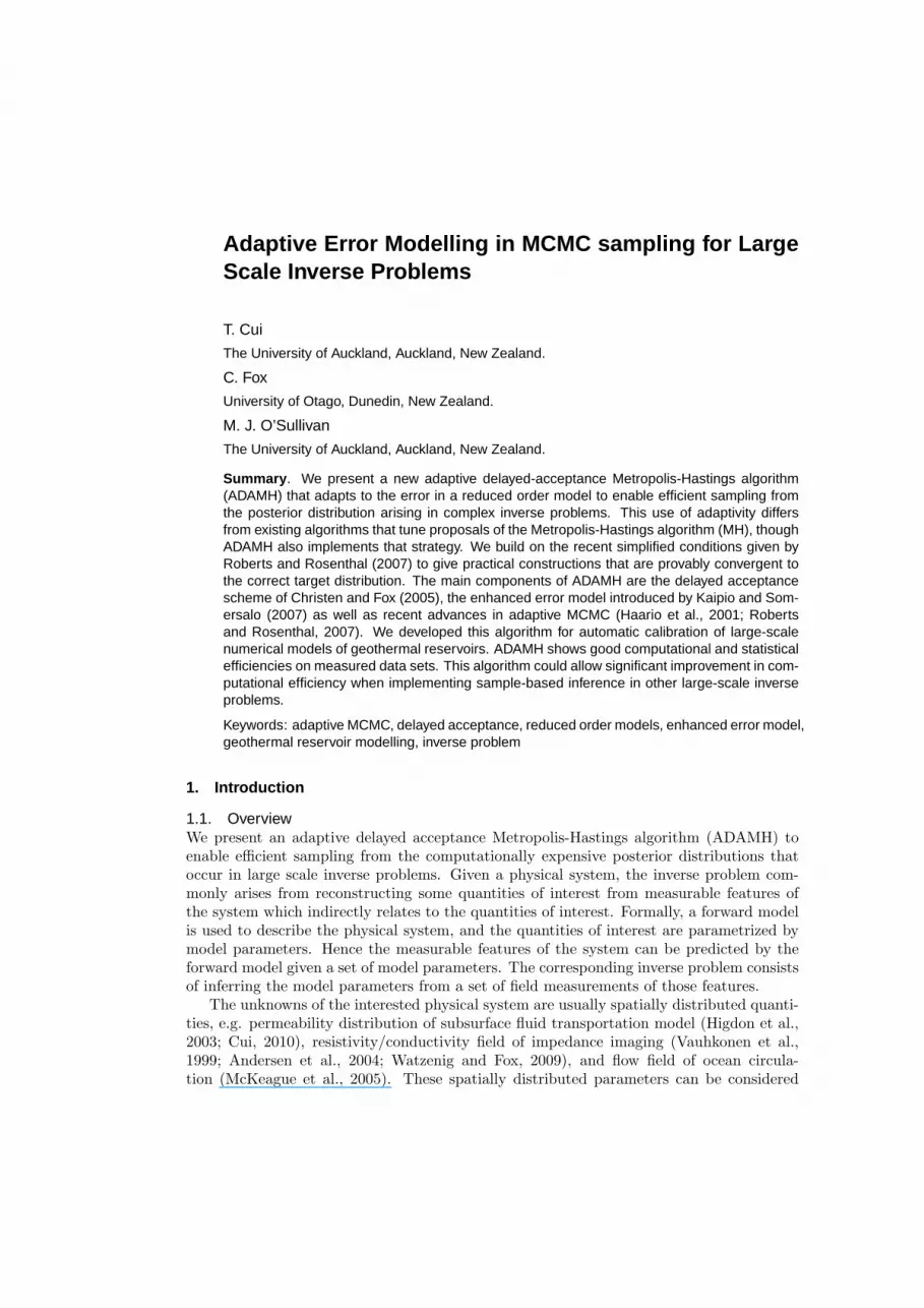
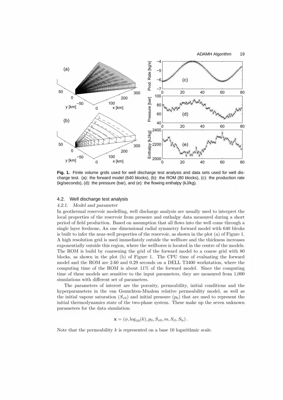
Fig. 1. Finite volume grids used for well discharge test analysis and data sets used for well dis-charge test. (a): the forward model (640 blocks), (b): the ROM (80 blocks), (c): the production rate(kg/seconds), (d): the pressure (bar), and (e): the flowing enthalpy (kJ/kg).

4.2. Well discharge test analysis4.2.1. Model and parameter

In geothermal reservoir modelling, well discharge analysis are usually used to interpret thelocal properties of the reservoir from pressure and enthalpy data measured during a shortperiod of field production. Based on assumption that all flows into the well come through asingle layer feedzone, An one dimensional radial symmetry forward model with 640 blcoksis built to infer the near-well properties of the reservoir, as shown in the plot (a) of Figure 1.A high resolution grid is used immediately outside the wellbore and the thickness increasesexponentially outside this region, where the wellbores is located in the centre of the models.The ROM is build by coarsening the grid of the forward model to a coarse grid with 80blocks, as shown in the plot (b) of Figure 1. The CPU time of evaluating the forwardmodel and the ROM are 2.60 and 0.29 seconds on a DELL T3400 workstation, where thecomputing time of the ROM is about 11% of the forward model. Since the computingtime of these models are sensitive to the input parameters, they are measured from 1,000simulations with different set of parameters.

The parameters of interest are the porosity, permeability, initial conditions and thehyperparameters in the van Genuchten-Mualem relative permeability model, as well asthe initial vapour saturation (Sv0) and initial pressure (p0) that are used to represent theinitial thermodynamics state of the two-phase system. These make up the seven unknownparameters for the data simulation:

x = (φ, log10(k), p0, Sv0,m, Srl, Sls) .

Note that the permeability k is represented on a base 10 logarithmic scale.

20 T. Cui, C. Fox and M. J. O’Sullivan

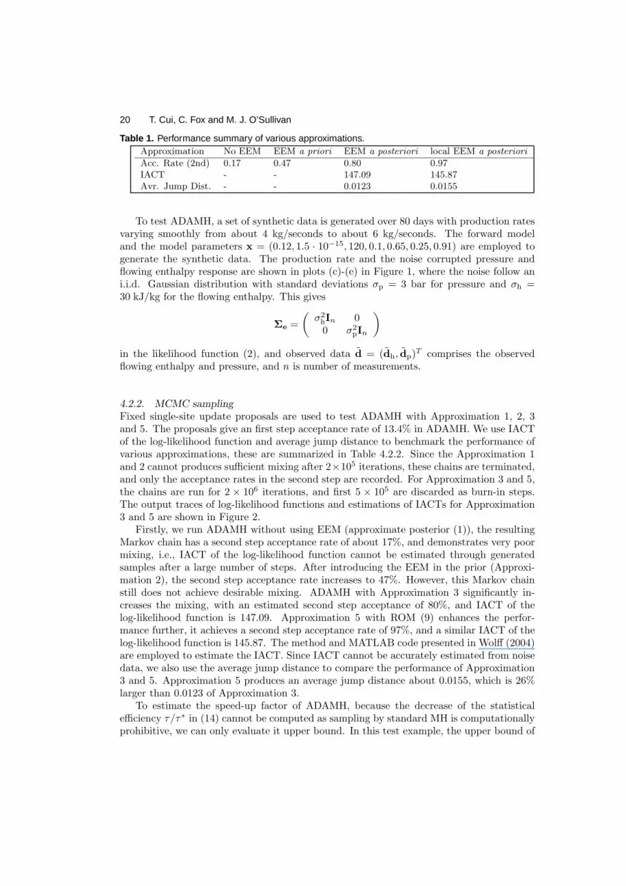
Table 1. Performance summary of various approximations.Approximation No EEM EEM a priori EEM a posteriori local EEM a posteriori

Acc. Rate (2nd) 0.17 0.47 0.80 0.97IACT - - 147.09 145.87Avr. Jump Dist. - - 0.0123 0.0155

To test ADAMH, a set of synthetic data is generated over 80 days with production ratesvarying smoothly from about 4 kg/seconds to about 6 kg/seconds. The forward modeland the model parameters x = (0.12, 1.5 · 10−15, 120, 0.1, 0.65, 0.25, 0.91) are employed togenerate the synthetic data. The production rate and the noise corrupted pressure andflowing enthalpy response are shown in plots (c)-(e) in Figure 1, where the noise follow ani.i.d. Gaussian distribution with standard deviations σp = 3 bar for pressure and σh =30 kJ/kg for the flowing enthalpy. This gives

Σe =

(

σ2hIn 00 σ2

pIn

)

in the likelihood function (2), and observed data d = (dh, dp)T comprises the observed

flowing enthalpy and pressure, and n is number of measurements.

4.2.2. MCMC sampling

Fixed single-site update proposals are used to test ADAMH with Approximation 1, 2, 3and 5. The proposals give an first step acceptance rate of 13.4% in ADAMH. We use IACTof the log-likelihood function and average jump distance to benchmark the performance ofvarious approximations, these are summarized in Table 4.2.2. Since the Approximation 1and 2 cannot produces sufficient mixing after 2×105 iterations, these chains are terminated,and only the acceptance rates in the second step are recorded. For Approximation 3 and 5,the chains are run for 2 × 106 iterations, and first 5 × 105 are discarded as burn-in steps.The output traces of log-likelihood functions and estimations of IACTs for Approximation3 and 5 are shown in Figure 2.

Firstly, we run ADAMH without using EEM (approximate posterior (1)), the resultingMarkov chain has a second step acceptance rate of about 17%, and demonstrates very poormixing, i.e., IACT of the log-likelihood function cannot be estimated through generatedsamples after a large number of steps. After introducing the EEM in the prior (Approxi-mation 2), the second step acceptance rate increases to 47%. However, this Markov chainstill does not achieve desirable mixing. ADAMH with Approximation 3 significantly in-creases the mixing, with an estimated second step acceptance of 80%, and IACT of thelog-likelihood function is 147.09. Approximation 5 with ROM (9) enhances the perfor-mance further, it achieves a second step acceptance rate of 97%, and a similar IACT of thelog-likelihood function is 145.87. The method and MATLAB code presented in Wolff (2004)are employed to estimate the IACT. Since IACT cannot be accurately estimated from noisedata, we also use the average jump distance to compare the performance of Approximation3 and 5. Approximation 5 produces an average jump distance about 0.0155, which is 26%larger than 0.0123 of Approximation 3.

To estimate the speed-up factor of ADAMH, because the decrease of the statisticalefficiency τ/τ∗ in (14) cannot be computed as sampling by standard MH is computationallyprohibitive, we can only evaluate it upper bound. In this test example, the upper bound of

ADAMH Algorithm 21

the speed-up factor is about 4.1. Given the second step acceptance rates of Approximation 3and 5 are more than 80%, the decrease of the statistical efficiency should not be significant.Especially for Approximation 5, the 97% accpetance rate in the second step suggest thatthe statistical efficiency of ADAMH should close to standard MH in this case.

The histograms of the model predictions computed on several different time points aregiven in Figure 3. We can observe that the predictions at these observation times followuni-modal distributions that close to Gaussian. The model predictions and the 95% credibleintervals over an 80-day period are shown in Figure 3, with pressure on the left and enthalpyon the right. For both predictions, the means follow the observed data reasonably well.

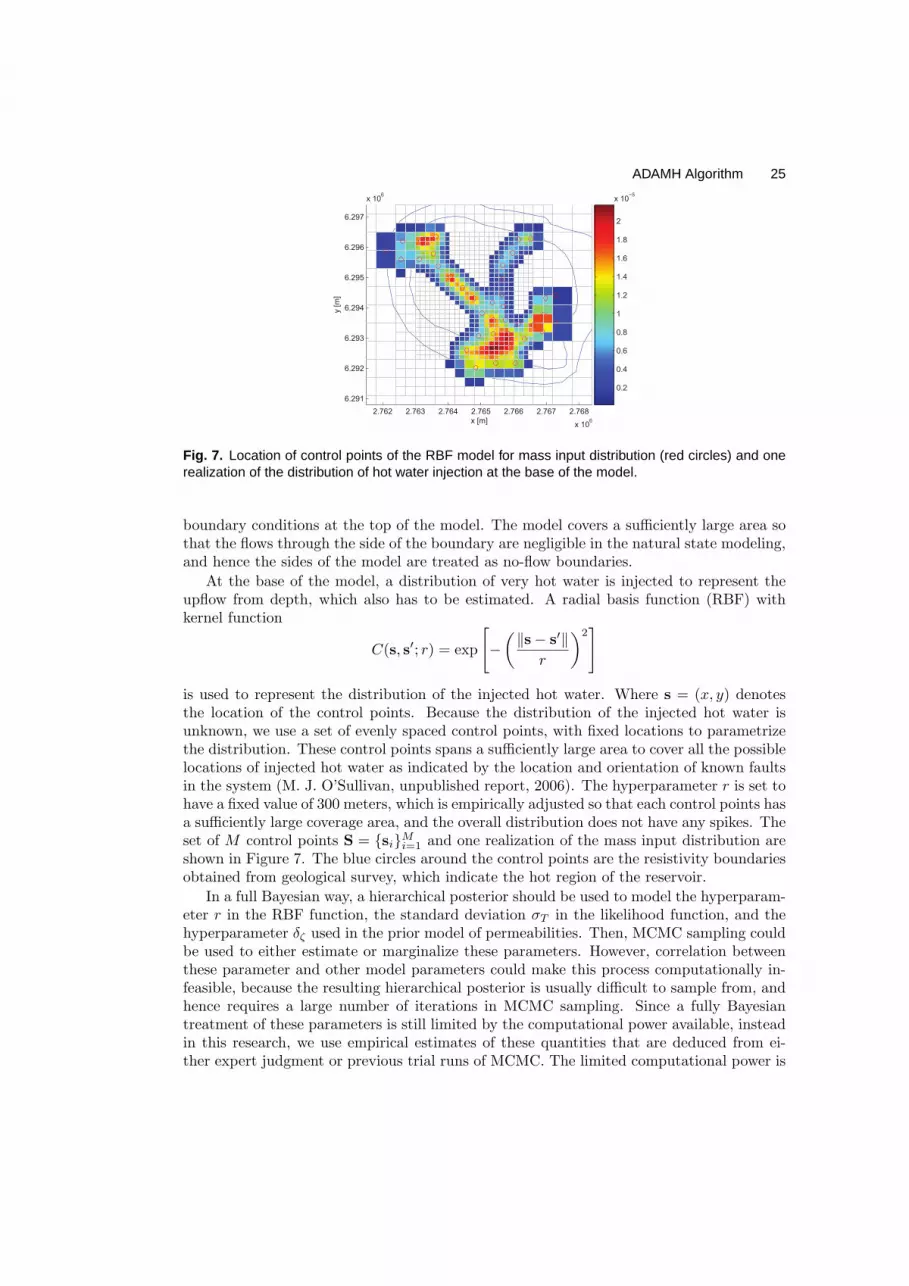
The histograms of the marginal distributions of the parameter x (see first two rows ofFigure 5) show skewness in porosity and two of the hyperparameters of the van Genuchten-Mualem relative permeability model (m and Srl). The number of bins in the histograms arechosen according to the Freedman-Diaconis rule (Freedman and Diaconis, 1981). The scatterplots between parameters show strong negative correlations between the permeability (onbase 10 logarithmic scale) and the initial pressure, see the first plot of last row of Figure5. There also exists strong negative correlations between the initial saturation and one ofthe hyperparameters of the van Genuchten-Mualem (Sls), see the second plot of last row ofFigure 5.

4.3. Natural state modellingOne important step in setting up a large scale geothermal reservoir model is the naturalstate modelling, in which the aim is the estimation of the large scale permeability structureand boundary conditions (Grant et al., 1982; O’Sullivan, 1985). Because the horizontalpermeabilities are only able to be estimated locally by expensive well test analysis (interms of investment on drilling new production/injection wells), and there is no way toinfer the vertical permeability directly. The large scale permeability structure are inferredfrom steady state temperature distributions indicating the movement of hot fluid, whichis directly influenced by the permeability structure and boundary condition. Since theporosities do not affect the solution of the set of equations (16) - (18), and the relativepermeabilities only have minor impact on the solution, these parameters are not consideredin the natural state modelling.

The temperature measurements are presented in Figure 9, manual calibration resultsand trial runs of MCMC sampling suggest that the model mis-fit has standard deviationσT = 7.5 C. Thus, Σe = σ2

TIn is used in the likelihood function (2), where n is the numberof observations.

The geological setting of geothermal reservoir model we demonstrate here is summarizedin Cui (2010). The model covers a volume of 12.0 km by 14.4 km extending down to 3050meters below the sea level. Relatively large blocks were used in the outside of the modeland then they were progressively refined near the wells to achieve a well-by-well allocationto the blocks. The 3D structure of the forward model has 26, 005 blocks, which is shown inplot (a) of Figure 6, where the blue lines in the middle of the grid are wells drilled into thereservoir. To speed up the computation, a ROM based on a coarse grid with 3, 335 blocksis constructed by combining adjacent blocks in the x, y and z directions of the forwardmodel (see plot (b) of Figure 6). A coarser level of grid resolution is not used here becausefurther coarsening of the grid structure would produce a model that cannot reproduce theconvective plume in the reservoir. Each simulation of the forward model takes about 30to 50 minutes CPU time on a DELL T3400 workstation, and the computing time for the

22 T. Cui, C. Fox and M. J. O’Sullivan

0 500 1000 1500−0.5

0

0.5

1Normalized autocorrelation

0 500 1000 15000

100

200IACT with statistical errors

IAC

T

W

2 4 6 8 10 12 14

x 104

−35

−30

−25

log

−lik

elih

oo

d

MCMC iterations

0 500 1000 1500−0.5

0

0.5

1Normalized autocorrelation

0 500 1000 15000

100

200

300IACT with statistical errors

IAC

T

W

2 4 6 8 10 12 14

x 104

−35

−30

−25

log

−lik

elih

oo

d

MCMC iterations

Fig. 2. IACT of the log-likelihood function, ADAMH with Approximation 3 (left column) and 5 (rightcolumn). Top row: Normalized autocorrelation, middle row: estimated IACT, bottom row: traces oflog-likelihood.

75 80 850

50

100

150Pres. Day 40

60 65 700

50

100

150Pres. Day 50

40 60 800

50

100

150Pres. Day 60

50 60 700

50

100

150Pres. Day 70

2100 21500

50

100

150Enth. Day 40

2200 2250 23000

50

100

150Enth. Day 50

2200 2300 24000

50

100

150Enth. Day 60

2200 2250 23000

50

100

150Enth. Day 70

Fig. 3. Histograms of the predictive density, at day 40, 50, 60 and 70. Top row: Pressure, bottomrow: enthalpy.

ADAMH Algorithm 23

10 20 30 40 50 60 70

50

60

70

80

90

Time [day]

Pre

ssu

re [

ba

r]

10 20 30 40 50 60 70

2100

2200

2300

Time [day]

En

tha

lpy [

kJ/k

g]

(a) (b)

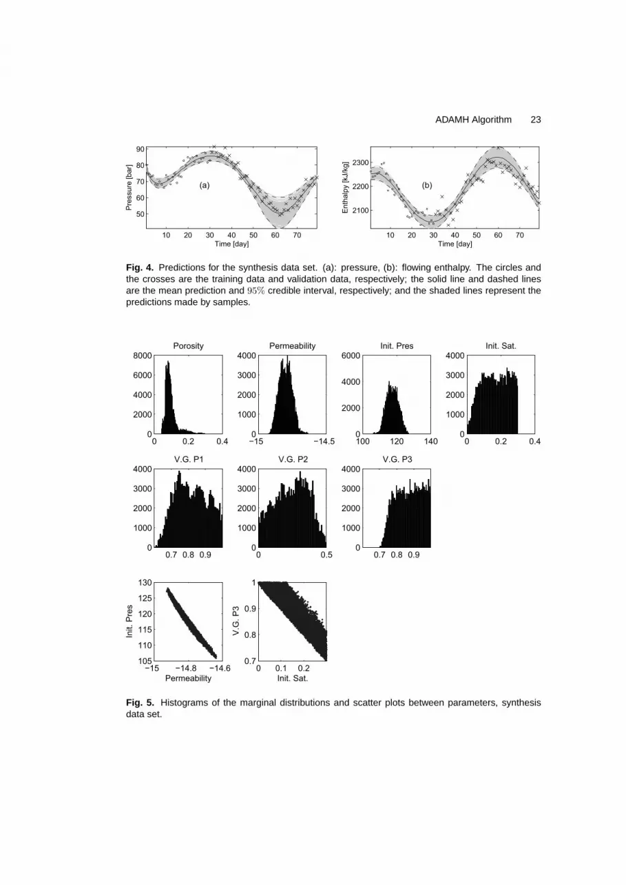
Fig. 4. Predictions for the synthesis data set. (a): pressure, (b): flowing enthalpy. The circles andthe crosses are the training data and validation data, respectively; the solid line and dashed linesare the mean prediction and 95% credible interval, respectively; and the shaded lines represent thepredictions made by samples.

0 0.2 0.40

2000

4000

6000

8000Porosity

−15 −14.50

1000

2000

3000

4000Permeability

100 120 1400

2000

4000

6000Init. Pres

0 0.2 0.40

1000

2000

3000

4000Init. Sat.

0.7 0.8 0.90

1000

2000

3000

4000V.G. P1

0 0.50

1000

2000

3000

4000V.G. P2

0.7 0.8 0.90

1000

2000

3000

4000V.G. P3

−15 −14.8 −14.6105

110

115

120

125

130

Permeability

Init.

Pre

s

0 0.1 0.20.7

0.8

0.9

1

Init. Sat.

V.G

. P

3

Fig. 5. Histograms of the marginal distributions and scatter plots between parameters, synthesisdata set.

24 T. Cui, C. Fox and M. J. O’Sullivan

2.762.762

2.7642.766

2.7682.77

x 106

6.288

6.29

6.292

6.294

6.296

6.298

6.3

x 106

−3000

−2000

−1000

0

x [m]y [m]

z [

m]

2.762.762

2.7642.766

2.7682.77

x 106

6.288

6.29

6.292

6.294

6.296

6.298

6.3

x 106

−3000

−2000

−1000

0

x [m]y [m]

z [

m]

(a) (b)

Fig. 6. The fine grid (left) and the coarse grid (right) used for natural state modelling.

ROM is about 1 to 1.5 minutes (roughly 3% of the forward model). The computing timefor these models is sensitive to the input parameters.

4.3.1. Prior modelling of permeabilities

Previously, the rock structure of the model was pre-assigned by a geologist, and each rocktype covers a range of grid blocks. From manual calibration of the model, we found thatthe permeability may not have a very good correspondence with the type of rock, and ithas a large variation depending on the location. To capture these variabilities, we employ alow-level pixel based representation with the same resolution as the coarse grid used by theROM. Therefore, the permeabilities in x y, and z directions are represented by N = 3, 335

dimensional vectors k(ζ) = [log10(k(ζ)1 ), . . . , log10(k

(ζ)N )], ζ ∈ x, y, z.

Because there is no point measurement and other direct survey (e.g., seismic data) ofthe permeabilities available for this reservoir, we assume the permeabilities in x, y and zdirections are uncorrelated. A first order Gaussian Markov random field (GMRF) model(Rue and Held, 2005) is employed to formulate the prior distribution for each of the x, y,and z direction of permeabilities. Let i ∼ j denote that two blocks i and j are adjacent toeach other. The prior has the form of

π(k(ζ)) ∝ exp

−δζ∑

i∼j

ωij

[

log10(k(ζ)i )− log10(k

(ζ)j )

]2

, (19)

where ωij is the inverse Euclidean distance between the two adjacent block centers, and δζis a hyperparameter controls the smoothing (has different meaning with the δ in Section3). We take the hyperparameter δζ = 0.5 for all ζ ∈ x, y, z, a value suggested by thetrial runs of MCMC. With this setting, the posterior distribution is still dominated by thelikelihood function, and hence the model parameters are determined by the data. The priorprovides a minor constraint to enforce the condition that the permeabilities are smooth.

4.3.2. Prior modelling of boundary conditions

The top of the model is assumed to be “open”, which allows the model to have directconnection with the atmosphere. Atmosphere pressure and temperature are used as the

ADAMH Algorithm 25

2.762 2.763 2.764 2.765 2.766 2.767 2.768

x 106

6.291

6.292

6.293

6.294

6.295

6.296

6.297

x 106

x [m]

y [

m]

0.2

0.4

0.6

0.8

1

1.2

1.4

1.6

1.8

2

x 10−5

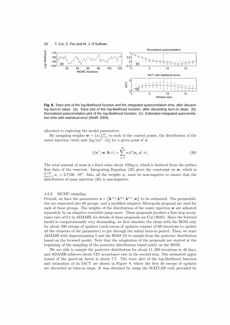
Fig. 7. Location of control points of the RBF model for mass input distribution (red circles) and onerealization of the distribution of hot water injection at the base of the model.

boundary conditions at the top of the model. The model covers a sufficiently large area sothat the flows through the side of the boundary are negligible in the natural state modeling,and hence the sides of the model are treated as no-flow boundaries.

At the base of the model, a distribution of very hot water is injected to represent theupflow from depth, which also has to be estimated. A radial basis function (RBF) withkernel function

C(s, s′; r) = exp

[

−

(

‖s− s′‖

r

)2]

is used to represent the distribution of the injected hot water. Where s = (x, y) denotesthe location of the control points. Because the distribution of the injected hot water isunknown, we use a set of evenly spaced control points, with fixed locations to parametrizethe distribution. These control points spans a sufficiently large area to cover all the possiblelocations of injected hot water as indicated by the location and orientation of known faultsin the system (M. J. O’Sullivan, unpublished report, 2006). The hyperparameter r is set tohave a fixed value of 300 meters, which is empirically adjusted so that each control points hasa sufficiently large coverage area, and the overall distribution does not have any spikes. Theset of M control points S = si

Mi=1 and one realization of the mass input distribution are

shown in Figure 7. The blue circles around the control points are the resistivity boundariesobtained from geological survey, which indicate the hot region of the reservoir.

In a full Bayesian way, a hierarchical posterior should be used to model the hyperparam-eter r in the RBF function, the standard deviation σT in the likelihood function, and thehyperparameter δζ used in the prior model of permeabilities. Then, MCMC sampling couldbe used to either estimate or marginalize these parameters. However, correlation betweenthese parameter and other model parameters could make this process computationally in-feasible, because the resulting hierarchical posterior is usually difficult to sample from, andhence requires a large number of iterations in MCMC sampling. Since a fully Bayesiantreatment of these parameters is still limited by the computational power available, insteadin this research, we use empirical estimates of these quantities that are deduced from ei-ther expert judgment or previous trial runs of MCMC. The limited computational power is

26 T. Cui, C. Fox and M. J. O’Sullivan

20 40 60 80 100 120−100

−90

−80

−70

MCMC iterations

Lo

g−

like

lihoo

d

(a)

0 5 10 15−0.5

0

0.5

1Normalized autocorrelation

(b)

0 5 10 150

5

IACT with statistical errors

(c)

IAC

T

Window size

Fig. 8. Trace plot of the log-likelihood function and the integrated autocorrelation time, after discard-ing burn-in steps. (a): Trace plot of the log-likelihood function, after discarding burn-in steps. (b):Normalized autocorrelation plot of the log-likelihood function. (c): Estimated integrated autocorrela-tion time with statistical error (Wolff, 2004).

allocated to exploring the model parameters.By assigning weights w = wi

Mi=1 to each of the control points, the distribution of the

water injection (with unit [kg/(m2 · s)]) for a given point s′ is

f(s′ | w,S, r) =

M∑

i=1

wiC(si, s′; r). (20)

The total amount of mass is a fixed value about 105kg/s, which is deduced from the surfaceflow data of the reservoir. Integrating Equation (20) gives the constraint on w, which is∑M

i=1 wi = 3.7136 · 104. Also, all the weights wi must be non-negative to ensure that thedistribution of mass injection (20) is non-negative.

4.3.3. MCMC sampling

Overall, we have the parameters x =

k(x),k(y),k(z),w

to be estimated. The permeabili-ties are separated into 68 groups, and a modified adaptive Metropolis proposal are used foreach of these groups. The weights of the distribution of the water injection w are adjustedseparately by an adaptive reversible jump move. These proposals produce a first step accep-tance rate of 0.1 in ADAMH, for details of these proposals see Cui (2010). Since the forwardmodel is computationally very demanding, we first simulate the chain with the ROM onlyfor about 200 sweeps of updates (each sweep of updates consists of 69 iterations to updateall the elements of the parameter) to get through the initial burn-in period. Then, we startADAMH with Approximation 5 and the ROM (9) to sample from the posterior distributionbased on the forward model. Note that the adaptation of the proposals are started at thebeginning of the sampling of the posterior distribution based solely on the ROM.

We are able to sample the posterior distribution for about 11, 200 iterations in 40 days,and ADAMH achieves about 74% accpetance rate in the second step. The estimated upperbound of the speed-up factor is about 7.7. The trace plot of the log-likelihood functionand estimation of its IACT are shown in Figure 8, where the first 40 sweeps of updatesare discarded as burn-in steps. It was obtained by using the MATLAB code provided by

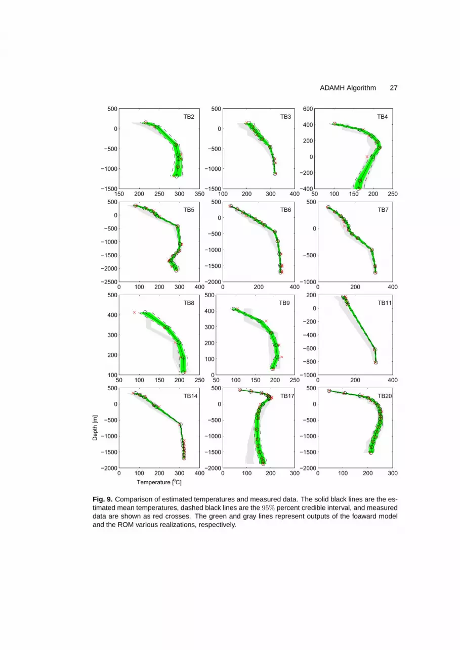
ADAMH Algorithm 27

150 200 250 300 350−1500

−1000

−500

0

500

TB2

100 200 300 400−1500

−1000

−500

0

500

TB3

50 100 150 200 250−400

−200

0

200

400

600

TB4

0 100 200 300 400−2500

−2000

−1500

−1000

−500

0

500

TB5

0 200 400−2000

−1500

−1000

−500

0

500

TB6

0 200 400−1000

−500

0

500

TB7

50 100 150 200 250100

200

300

400

500

TB8

50 100 150 200 2500

100

200

300

400

500

TB9

0 200 400−1000

−800

−600

−400

−200

0

200

TB11

0 100 200 300 400−2000

−1500

−1000

−500

0

500

TB14

Temperature [oC]

De

pth

[m

]

0 100 200 300−2000

−1500

−1000

−500

0

500

TB17

0 100 200 300−2000

−1500

−1000

−500

0

500

TB20

Fig. 9. Comparison of estimated temperatures and measured data. The solid black lines are the es-timated mean temperatures, dashed black lines are the 95% percent credible interval, and measureddata are shown as red crosses. The green and gray lines represent outputs of the foaward modeland the ROM various realizations, respectively.

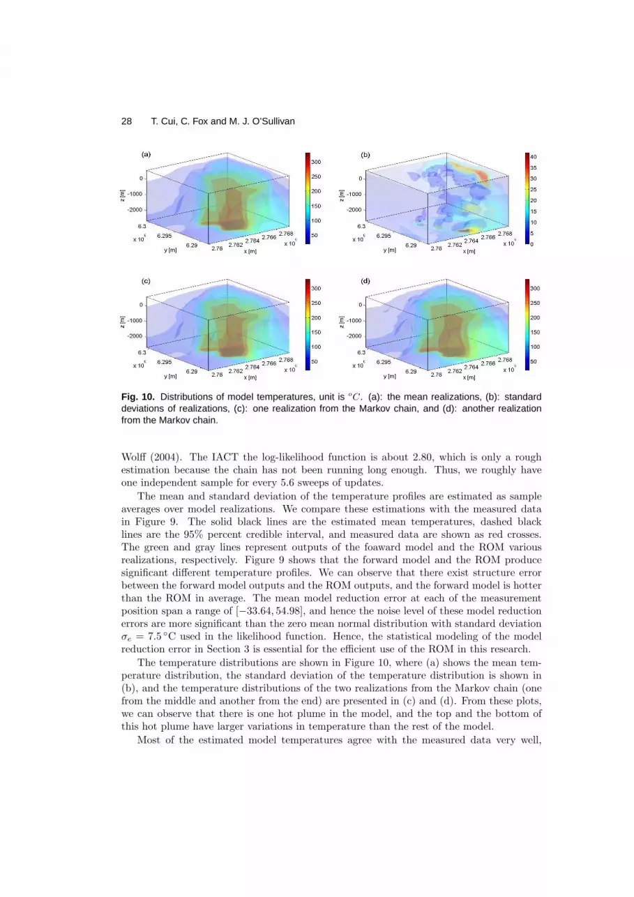
28 T. Cui, C. Fox and M. J. O’Sullivan

Fig. 10. Distributions of model temperatures, unit is o

C. (a): the mean realizations, (b): standarddeviations of realizations, (c): one realization from the Markov chain, and (d): another realizationfrom the Markov chain.

Wolff (2004). The IACT the log-likelihood function is about 2.80, which is only a roughestimation because the chain has not been running long enough. Thus, we roughly haveone independent sample for every 5.6 sweeps of updates.

The mean and standard deviation of the temperature profiles are estimated as sampleaverages over model realizations. We compare these estimations with the measured datain Figure 9. The solid black lines are the estimated mean temperatures, dashed blacklines are the 95% percent credible interval, and measured data are shown as red crosses.The green and gray lines represent outputs of the foaward model and the ROM variousrealizations, respectively. Figure 9 shows that the forward model and the ROM producesignificant different temperature profiles. We can observe that there exist structure errorbetween the forward model outputs and the ROM outputs, and the forward model is hotterthan the ROM in average. The mean model reduction error at each of the measurementposition span a range of [−33.64, 54.98], and hence the noise level of these model reductionerrors are more significant than the zero mean normal distribution with standard deviationσe = 7.5 C used in the likelihood function. Hence, the statistical modeling of the modelreduction error in Section 3 is essential for the efficient use of the ROM in this research.

The temperature distributions are shown in Figure 10, where (a) shows the mean tem-perature distribution, the standard deviation of the temperature distribution is shown in(b), and the temperature distributions of the two realizations from the Markov chain (onefrom the middle and another from the end) are presented in (c) and (d). From these plots,we can observe that there is one hot plume in the model, and the top and the bottom ofthis hot plume have larger variations in temperature than the rest of the model.

Most of the estimated model temperatures agree with the measured data very well,

ADAMH Algorithm 29

the root mean square error is in the range of [7.11, 8.66], with mean value of 7.22. Theassumption that the residuals follow a Gaussian distribution with standard deviation σe =7.5 C is validated by the normal quantile plot and the cumulative density plot of theresiduals (see Figure 11). The normal quantile plot shows that the residuals are symmetricand roughly follow the Gaussian distribution in the interval [−10, 10], where most of themare located. Outside of this range, the residuals are slightly skewed (light tailed below -10and heavy tailed above 10). The same result is suggested by the cumulative density plot.Overall, these plots show that the normality assumption is reasonable.

We also present the mean estimations, standard deviations and two realizations of thedistribution of mass input and permeability distribution in the x, y, and z directions inFigure 12 - 15. In these figures, (a) is the mean estimation, (b) is the standard deviation,and two realizations are shown in (c) and (d).

The mean distribution of the mass input shows that most of the injected hot wateroccurs at the bottom of the inner resistivity boundary. This corresponds to the opinion ofgeologists that the major source of deep hot water occurs at the intersection of two geologicalfaults in this area. The standard deviation and two realizations of this distribution suggestthat the variation among the samples is very small.

The reasonably large variations in the reconstructed permeability distributions suggestthat there exists ambiguities in the permeability distributions, and this may be causedby the sparsely measured data. This effect is more significant in the region close to theboundary of the reservoir, where no measured data are available. We can either give moreaccurate quantifications to these ambiguities by running the chain for a very long time,or remove these ambiguities by imposing a stronger prior distribution or using differentparameterizations of the permeability distributions.

5. Discussion

We developed an adaptive delayed acceptance Metropolis-Hastings algorithm for efficientsampling the computationally demanding posterior distribution occurs in inverse problems.ADAMH improves the computational efficiency of the standard MH algorithm by employingan approximate posterior distribution based on a reduced order model. Components of thedelayed acceptance MH algorithm (Christen and Fox, 2005), the enhanced error modelof Kaipio and Somersalo (2007), and adaptive MCMC (Haario et al., 2001; Roberts andRosenthal, 2007) are used to construct ADAMH. By using the regularity conditions providedin Section 3, several adaptive approximate posterior distributions are designed.

As shown in the first example, ADAMH improves the accuracy of the approximationsignificantly without extra computing time by using EEM and adaptive sampling, and henceimprove the computational efficiency of sampling. The state dependent approximation 5with the ROM (9) have the best performance over all approximations. ADAMH withApproximation 5 is used to sample the posterior distribution of the large scale 3D geothermalreservoir model in the second example. We are able to run the MCMC sampling for about11, 200 iterations in about 40 days, which would takes about 10 months for the standardMH algorithm. The significant speed-up offered by ADAMH would allow MCMC methodto be applied to inverse problems that on the limitation of the computing power.

The ROM we used here is based on coarsening the grid structure of the forward model.Even through the ROM (9) is state dependent by adding a local correction term, the overallstructure of the ROM is fixed during the sampling. Based on the conditions supplied in

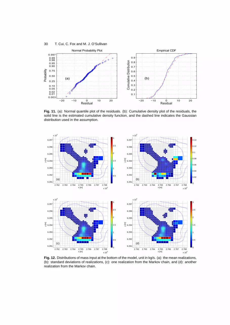
30 T. Cui, C. Fox and M. J. O’Sullivan

−20 −10 0 10 20

0.003

0.010.02

0.05

0.10

0.25

0.50

0.75

0.90

0.95

0.980.99

0.997

Residual

Pro

babili

ty

Normal Probability Plot

(a)

−20 −10 0 10 20

0.1

0.2

0.3

0.4

0.5

0.6

0.7

0.8

0.9

Residual

Co

mu

lativ

e D

istr

ibu

tion

Empirical CDF

(b)

Fig. 11. (a): Normal quantile plot of the residuals. (b): Cumulative density plot of the residuals, thesolid line is the estimated cumulative density function, and the dashed line indicates the Gaussiandistribution used in the assumption.

0.5

1

1.5

2

2.5

3

2.762 2.763 2.764 2.765 2.766 2.767 2.768

x 106

6.291

6.292

6.293

6.294

6.295

6.296

6.297

x 106

x [m]

y [m

]

(a)0

0.02

0.04

0.06

0.08

0.1

0.12

0.14

2.762 2.763 2.764 2.765 2.766 2.767 2.768

x 106

6.291

6.292

6.293

6.294

6.295

6.296

6.297

x 106

x [m]

y [m

]

(b)

0

0.5

1

1.5

2

2.5

3

2.762 2.763 2.764 2.765 2.766 2.767 2.768

x 106

6.291

6.292

6.293

6.294

6.295

6.296

6.297

x 106

x [m]

y [m

]

(c)0

0.5

1

1.5

2

2.5

3

2.762 2.763 2.764 2.765 2.766 2.767 2.768

x 106

6.291

6.292

6.293

6.294

6.295

6.296

6.297

x 106

x [m]

y [m

]

(d)

Fig. 12. Distributions of mass input at the bottom of the model, unit in kg/s. (a): the mean realizations,(b): standard deviations of realizations, (c): one realization from the Markov chain, and (d): anotherrealization from the Markov chain.

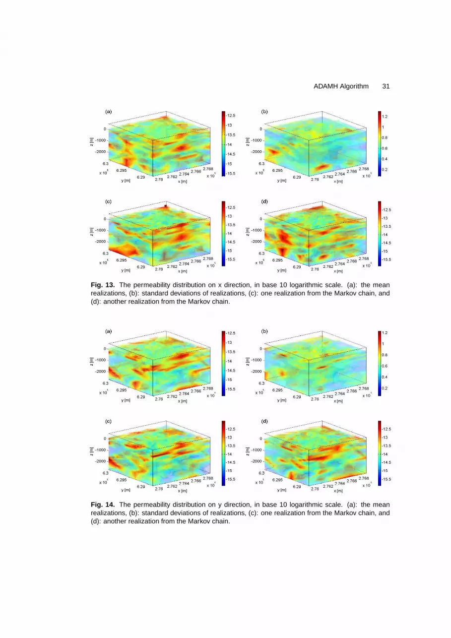
ADAMH Algorithm 31

Fig. 13. The permeability distribution on x direction, in base 10 logarithmic scale. (a): the meanrealizations, (b): standard deviations of realizations, (c): one realization from the Markov chain, and(d): another realization from the Markov chain.

Fig. 14. The permeability distribution on y direction, in base 10 logarithmic scale. (a): the meanrealizations, (b): standard deviations of realizations, (c): one realization from the Markov chain, and(d): another realization from the Markov chain.

32 T. Cui, C. Fox and M. J. O’Sullivan

Fig. 15. The permeability distribution on z direction, in base 10 logarithmic scale. (a): the meanrealizations, (b): standard deviations of realizations, (c): one realization from the Markov chain, and(d): another realization from the Markov chain.

Theorem 1, other more sophisticated model reduction techniques such as projection basedmethods (Grimme, 1997; Li, 2002) can be used to construct ROMs that adapts to the localstructure of the forward model. Further investigations are necessary to integrate thesetechniques into ADAMH.

References

Amit, Y., U. Grenander, and M. Piccioni (1991). Structural image restoration throughdeformable templates. Journal of the American Statistical Association 86(414), 376–387.

Andersen, K. E., S. P. Brooks, and M. B. Hansen (2004). Bayesian inversion of geoelectricalresistivity data. Journal of the Royal Statistical Society: Series B 65, 619–644.

Andrieu, C. and E. Moulines (2006). On the ergodicity properties of some adaptive Markovchain Monte Carlo algorithms. Annals of Applied Probability 16(1), 462–505.

Arak, T., P. Clifford, and D. Surgailis (1993). Point based polygonal models for randomgraphs. Advances in Applied Probabiity 25, 348–372.

Arridge, S. R., J. P. Kaipio, V. Kolehmainen, M. Schweiger, E. Somersalo, T. Tarvainen, andM. Vauhkonen (2006). Approximation errors and model reduction with an application inoptical diffusion tomography. Inverse Problems 22, 175–195.

Atchade, Y. F. and J. S. Rosenthal (2005). On adaptive Markov chain Monte Carlo algo-rithms. Bernoulli 11, 815–828.

ADAMH Algorithm 33

Baddeley, A. J. and M. N. M. van Lieshout (1993). Stochastic geometry models in high-levelvision. In K. V. Mardia (Ed.), Statistics and Images, pp. 233–258. Carfax, Abingdon.

Bayarri, M. J., J. O. Berger, J. Cafeo, G. Garcia-Donato, F. Liu, J. Palomo,R. Parthasarathy, R. Paulo, J. Sacks, and D. Walsh (2007). Computer model valida-tion with function output. Annals of Statistics 35(5), 1874–1906.

Besag, J. E. (1986). On the statistical analysis of dirty pictures. Journal of the RoyalStatistical Society, Series B 48, 259–302.

Besag, J. E. and C. Kooperberg (1995). On conditional and intrinsic autoregressions.Biometrika 82(4), 733–746.

Besag, J. E., J. York, and A. Mollie (1991). Bayesian image restoration, with two ap-plications in spatial statistics (with discussion). Annals of the Institute of StatisticalMathematics 43, 1–59.

Besag, J. E..and Green, P. J., D. Higdon, and K. Mengersen (1995). Bayesian computationand stochastic systems. Statistical Science 10, 3–41.

Christen, J. A. and C. Fox (2005). MCMC using an approximation. Journal of Computa-tional and Graphical Statistics 14(4), 795–810.

Christie, M. A. and M. J. Blunt (2001). Tenth spe comparative solution project: A com-parison of upscaling techniques. SPE Reservoir Engineering and Evaluation 4, 308–317.

Cornford, D., L. Csat, D. J. Evans, and M. Opper (2004). Bayesian analysis of the scat-terometer wind retrieval inverse problem: Some new approaches. Journal of the RoyalStatistical Society. Series B 66(3), 609–652.

Cressie, N. A. C. (1993). Statistics for Spatial Data, Revised Edition. Wiley-Interscience.

Cui, T. (2010). Bayesian Calibration of Geothermal Reservoir Models via Markov ChainMonte Carlo. Ph. D. thesis, The University of Auckland.

Efendiev, Y., A. Datta-Gupta, V. Ginting, X. Ma, and B. Mallick (2005). An efficient two-stage Markov chain Monte Carlo method for dynamic data integration. Water ResourcesResearch 41.

Freedman, D. and P. Diaconis (1981). On the histogram as a density estimator: l2 theory.Probability Theory and Related Fields 57(4), 453–476.

Geman, S. and D. Geman (1984). Stochastic relaxation, Gibbs distributions, and theBayesian restoration of images. IEEE Transactions on Pattern Analysis and MachineIntelligence 6(6), 721–741.

Gramacy, R. B. and H. K. H. Lee (2008). Bayesian treed gaussian process models withan application to computer modeling. Journal of the American Statistical Associa-tion 103(483), 1119–1130.

Grant, M. A., I. G. Donaldson, and P. F. Bixley (1982). Geothermal Reservoir Engineering.Academic Press.

34 T. Cui, C. Fox and M. J. O’Sullivan

Green, P. J. (1990). Bayesian reconstructions from emission tomography data using amodified EM algorithm. IEEE Transactions on Medical Imaging 9(1), 84–93.

Green, P. J. (1995). Reversible jump Markov chain Monte Carlo computation and Bayesianmodel determination. Biometrika 82, 711–732.

Grenander, U. (1967). Lectures in Pattern Theory. Volume 1: Pattern Synthesis, Volume 24of Applied Mathematical Sciences. Berlin: Springer-Verlag.

Grenander, U. (1976). Lectures in Pattern Theory. Volume 2: Pattern Analysis, Volume 24of Applied Mathematical Sciences. Berlin: Springer-Verlag.

Grenander, U. (1981). Lectures in Pattern Theory. Volume 3: Regular Structures, Volume 33of Applied Mathematical Sciences. Berlin: Springer-Verlag.

Grenander, U. and M. I. Miller (1994). Representations of knowledge in complex systems.Journal of the Royal Statistical Society. Series B 56(4), 549–603.

Grimme, E. J. (1997). Krylov projection methods for model. reduction. Ph. D. thesis,University of Illinois Urbana Champaign.

Haario, H., M. Laine, M. Lehtinen, Saksman, E., and J. Tamminen (2004). Markov chainMonte Carlo methods for high dimensional inversion in remote sensing. Journal of theRoyal Statistical Society: Series B 66, 591–608.

Haario, H., M. Laine, M. Lehtinen, E. Saksman, and J. Tamminen (2004). Markov chainMonte Carlo Methods for high dimensional inversion in remote sensing. Journal of theRoyal Statistical Society. Series B 66(3), 591–607.

Haario, H., M. Laine, A. Mira, and E. Saksman (2006). Dram: Efficient adaptive MCMC.Statistics and Computing 16, 339–354.

Haario, H., E. Saksman, and J. Tamminen (2001). An adaptive Metropolis algorithm.Bernoulli 7, 223–242.

Hadamard, J. (1902). Sur les problemes aux derivees partielles et leur signification physique.[on the problems about partial derivatives and their physical significance]. PrincetonUniversity Bulletin 13, 49–52.

Hastings, W. (1970). Monte Carlo sampling using Markov chains and their applications.Biometrika 57, 97–109.

Higdon, D. (1998). A process-convolution approach to modelling temperatures in the northatlantic ocean. Environmental and Ecological Statistics 5(2), 173–190.

Higdon, D., J. E. Bowsher, V. E. Johnson, T. G. Turkington, D. R. Gilland, and R. J.Jaszczak (1997). Fully bayesian estimation of gibbs hyperparameters for emission com-puted tomography data. IEEE Transactions on Medical Imaging 16(5), 516–526.

Higdon, D., J. Gattiker, B. Williams, and M. Rightley (2008). Computer model calibrationusing high dimensional output. Journal of the American Statistical Association 103(482),570–583.

ADAMH Algorithm 35

Higdon, D., H. Lee, and Z. B. (2002). A Bayesian approach to characterizing uncertainty ininverse problems using coarse and fine-scale information. IEEE Transactions on SignalProcessing 50(2), 389–399.

Higdon, D., H. Lee, and C. Holloman (2003). Markov chain Monte Carlo-based approachesfor inference in computationally intensive inverse problems. In J. M. Bernardo, M. J.Bayarri, J. O. Berger, A. P. Dawid, D. Heckerman, A. F. M. Smith, and M. West (Eds.),Bayesian Statistics 7, pp. 181–197. Oxford University Press.

Hurn, M. A., O. Husby, and H. Rue (2003). Advances in Bayesian image analysis. In P. J.Green, N. L. Hjort, and S. Richardson (Eds.), Highly Structured Stochastic Systems, pp.301–322. Oxford University Press.

Husby, O., T. Lie, T. Lango, J. Hokland, and H. Rue (2001). Bayesian 2-D deconvolution: amodel for diffuse ultrasound scattering. IEEE Transactions on Ultrasonics, Ferroelectricsand Frequency Control 48(1), 121–130.

International Formulation Committee (1967). A Formulation of the Thermodynamic Prop-erties of Ordinary Water Substance. IFC Secretariat.

Jain, A. K., Y. Zhong, and M. P. Dubuisson-Jolly (1998). Deformable template models: Areview. Signal Processing 71(2), 109–129.

Kaipio, J. and E. Somersalo (2004). Statistical and Computational Inverse Problems.Springer-Verlag.

Kaipio, J. P. and E. Somersalo (2007). Statistical inverse problems: Discretization, modelreduction and inverse crimes. Journal of Computational and Applied Mathematics 198(2),493–504.

Kennedy, M. C. and A. O’Hagan (2001). Bayesian calibration of computer models (withdiscussion). Journal of the Royal Statistical Society: Series B 63, 425–464.

Kuensch, H. R. (1987). Intrinsic autoregressions and related models on the two-dimensionallattice. Biometrika 74, 517–524.

Li, J. R. (2002). Model reduction of large linear systems via low rank system Gramians. Ph.D. thesis, MIT.

Lieberman, C., K. Willcox, and O. Ghattas (2010). Parameter and state model reductionfor large-scale statistical inverse problems. SIAM Journal on Scientific Computing 32(5),2523–2542.

Liu, J. S. (2001). Monte Carlo Strategies in Scientific Computing. Springer-Verlag.

McKeague, I. W., Nicholls, G. K., K. Speer, and R. Herbei (2005). Statistical inversionof South Atlantic circulation in an abyssal neutral density layer. Journal of MarineResearch 63 (4), in press.

Metropolis, N., A. W. Rosenbluth, M. N. Rosenbluth, A. H. Teller, and E. Teller(1953). Equation of state calculations by fast computing machines. Journal of chem-ical physics 21, 1087–1092.

36 T. Cui, C. Fox and M. J. O’Sullivan

Moller, J. and R. P. Plenge Waagepetersen (1998). Markov connected component fields.Advances in Applied Probabiity 30(1), 1–35.

Moller, J. and O. Skare (2001). Coloured voronoi tessellations for bayesian image analysisand reservoir modelling. Statistical Modelling 1, 213–232.

Mondal, A., Y. Efendiev, B. Mallick, and A. Datta-Gupta (2010). Bayesian uncertaintyquantification for flows in heterogeneous porous media using reversible jump markovchain monte carlo methods. Advances in Water Resources 33(3), 241–256.

Morris, M. D., T. J. Mitchell, and D. Ylvisaker (1993). Bayesian design and analysis ofcomputer experiments: Use of derivatives in surface prediction. Technometrics 35, 243–255.

Nicholls, G. K. (1998). Bayesian image analysis with Markov chain Monte Carlo andcoloured continuum triangulation mosaics. Journal of the Royal Statistical Society: SeriesB 60, 643–659.

Nicholls, G. K. and C. Fox (1998). Prior modelling and posterior sampling in impedanceimaging. In Bayesian Inference for Inverse Problems, Volume 3459, pp. 116–127. SPIE.

Oliver, D. S., L. B. Cunha, and A. C. Reynolds (1997). Markov chain Monte Carlo methodsfor conditioning a permeability field to pressure data. Mathematical Geology 29(1), 61–91.

O’Sullivan, M. J. (1985). Geothermal reservoir simulation. International Journal of EnergyResearch 9(3), 319–332.

Pruess, K. (1991). TOUGH2 - A General-Purpose Numerical Simulator for MultiphaseFluid and Heat Flow. Berkeley, California: Lawrence Berkeley National Laboratory.

Roberts, G. O., A. Gelman, and W. R. Gilks (1997). Weak convergence and optimal scalingof random walk Metropolis algorithms. Annals of Applied Probability 7, 110–120.

Roberts, G. O. and J. S. Rosenthal (2001). Optimal scaling for various Metropolis-Hastingsalgorithms. Statistical Science 16, 351–367.

Roberts, G. O. and J. S. Rosenthal (2007). Coupling and ergodicity of adaptive MCMC.Journal of Applied Probability 44, 458–475.

Roberts, G. O. and J. S. Rosenthal (2009, Jun). Examples of adaptive MCMC. Journal ofComputational and Graphical Statistics 18(2), 349–367.

Rue, H. and L. Held (2005). Gaussian Markov Random Fields: Theory and Applications.Chapman & Hall.

Rue, H. and M. A. Hurn (1999). Bayesian object identification. Biometrika 86(3), 649–660.

Sacks, J., W. J. Welch, T. J. Mitchell, and H. P. Wynn (1989). Design and analysis ofcomputer experiments (c/r: p423-435). Statistical Science 4, 409–423.

Saksman, E. and M. Vihola (2010). On the ergodicity of the adaptive metropolis algorithmon unbounded domains. Annals of Applied Probability 20(6), 2178–2203.

ADAMH Algorithm 37

Santner, T., B. Williams, and W. Notz (2003). The Design and Analysis of ComputerExperiments. Springer-Verlag.

Ter Braak, C. J. F. (2006). A Markov chain Monte Carlo version of the genetic algorithmdifferential evolution: easy Bayesian computing for real parameter spaces. Statistics andComputing 16(3), 239–249.

Turro, E., N. Bochkina, A. M. K. Hein, and S. Richardson (2007). Bgx: a bioconductorpackage for the bayesian integrated analysis of affymetrix genechips. BMC Bioinformat-ics 8(439).

van Genuchten, M. T. (1980). A closed-form equation for predicting the hydraulic conduc-tivity of unsaturated soils. Soil Science Society of America Journal 44, 892–898.

Vauhkonen, P., M. Vauhkonen, T. Savolainen, and J. Kaipio (1999). Three-dimensional elec-trical impedance tomography based on the complete electrode model. IEEE Transactionson Biomedical Engineering 46, 1150–1160.

Vihola, M. (2011). Can the adaptive metropolis algorithm collapse without the covariancelower bound? Electronic Journal of Probability 16, 45–75.

Vrugt, J. A., C. J. F. ter Braak, M. P. Clark, J. M. Hyman, and B. A. Robinson (2008).Treatment of input uncertainty in hydrologic modeling: doing hydrology backward withMarkov chain Monte Carlo simulation. Water Resource Research 44.

Watzenig, D. and C. Fox (2009). A review of statistical modelling and inference for electricalcapacitance tomography. Measurement Science and Technology 20(5).

Weir, I. S. (1997). Fully bayesian reconstructions from single-photon emission computedtomography data. Journal of the American Statistical Association 92, 49–60.

Welch, W. J., R. J. Buck, J. Sacks, H. P. Wynn, T. J. Mitchell, and M. D. Morris (1992).Screening, predicting, and computer experiments. Technometrics 34, 15–25.

Wolff, U. (2004). Monte Carlo errors with less errors. Computer Physics Communica-tions 156(2), 143–153.