inverse laplace
TRANSCRIPT
The Inverse Laplace Transform
The University of TennesseeElectrical and Computer Engineering Department
Knoxville, Tennessee
wlg

Inverse Laplace TransformsBackground:
To find the inverse Laplace transform we use transform pairsalong with partial fraction expansion:
F(s) can be written as;
)()()(
sQsPsF
Where P(s) & Q(s) are polynomials in the Laplace variable, s.We assume the order of Q(s) P(s), in order to be in properform. If F(s) is not in proper form we use long division and divide Q(s) into P(s) until we get a remaining ratio of polynomialsthat are in proper form.
Inverse Laplace TransformsBackground:
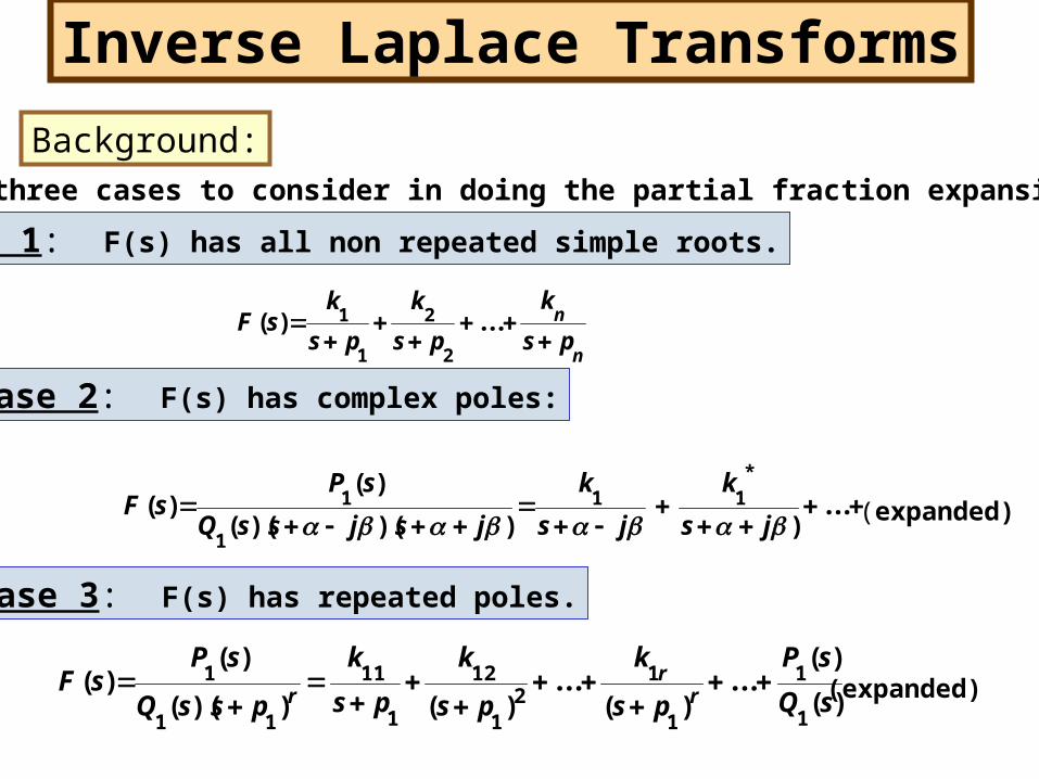
There are three cases to consider in doing the partial fraction expansion of F(s).Case 1: F(s) has all non repeated simple roots.
n
nps
kps
kps
ksF
...)(
2
2
1
1
Case 2: F(s) has complex poles:
...)))()(()(
)(*11
1
1 js
kjs
kjsjssQ
sPsF
Case 3: F(s) has repeated poles.
)()(
...)(
...)())((
)()(
1
1
1
12
1
12
1
11
11
1sQsP
psk
psk
psk
pssQsP
sF rr
r
(expanded)
(expanded)

Inverse Laplace TransformsCase 1: Illustration:
Given:
)10()4()1()10)(4)(1()2(4)( 321
sA
sA
sA
sssssF
274)10)(4)(1()2(4)1( | 11
ssssssA 94)10)(4)(1(
)2(4)4( | 42
ssss
ssA
2716)10)(4)(1()2(4)10( | 103
ssssssA
)()2716()94()274()( 104 tueeetf ttt
Find A1, A2, A3 from Heavyside
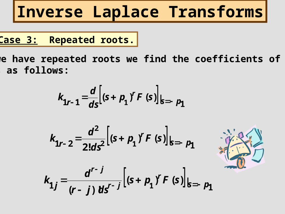
Inverse Laplace TransformsCase 3: Repeated roots.
When we have repeated roots we find the coefficients of the terms as follows:
| 111 )()( 1 psr sFpsdsdk r
| 121 )()(!2 12
2psr sFps
dsdk r
| 11 )()()!( 1 psj sFpsdsjr
dk rjr
jr

Inverse Laplace TransformsCase 3: Repeated roots.Example
2
1
1
2211
2 )3()3()3()1()(
K
K
A
sK
sK
sA
ssssF
)(____________________)( 33 tuteetf tt ? ? ?

Inverse Laplace TransformsCase 2: Complex Roots:
...)))()(()(
)(*11
1
1 js
Kjs
KjsjssQ
sPsF
F(s) is of the form;
K1 is given by,
jeKKK
jsjssQsPjs
K js
||||
))(()()()(
111
1
11 |

Inverse Laplace TransformsCase 2: Complex Roots:
jseK
jseK
jsK
jsK jj
11
*11 |||
tjetejetjetejeK
jseK
jseK
Ljj
1|||||| 111
2)()(
|1|21|| tjetjeateKtjetejetjetejeK
Inverse Laplace Transforms
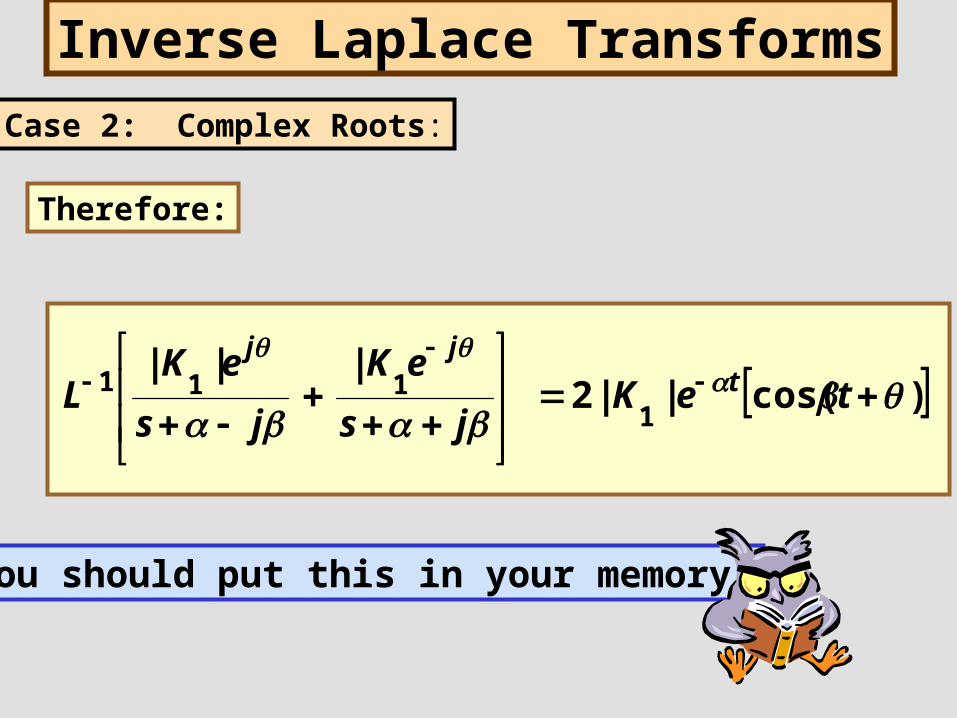
)cos(||2|||
1111
teK
jseK
jseK
L tjj
Case 2: Complex Roots:
Therefore:
You should put this in your memory:

Inverse Laplace TransformsComplex Roots: An Example.
For the given F(s) find f(t)
o
jjj
jsssK
sssA
jsK
jsK
sAsF
jsjsss
sssssF
js
s
10832.0)2)(2(12
)2()1(
51
)54()1(
22)(
)2)(2()1(
)54()1()(
|
|
2|1
0|
11
2
2
*

Inverse Laplace TransformsComplex Roots: An Example.(continued)
We then have;
jsjsssF
oo
210832.0
210832.02.0)(
Recalling the form of the inverse for complex roots;
)(108cos(64.02.0)( 2 tutetf ot

Inverse Laplace TransformsConvolution Integral:
Consider that we have the following situation.
h(t)x(t) y(t)
x(t) is the input to the system.h(t) is the impulse response of the system.y(t) is the output of the system.
System
We will look at how the above is related in the time domainand in the Laplace transform.
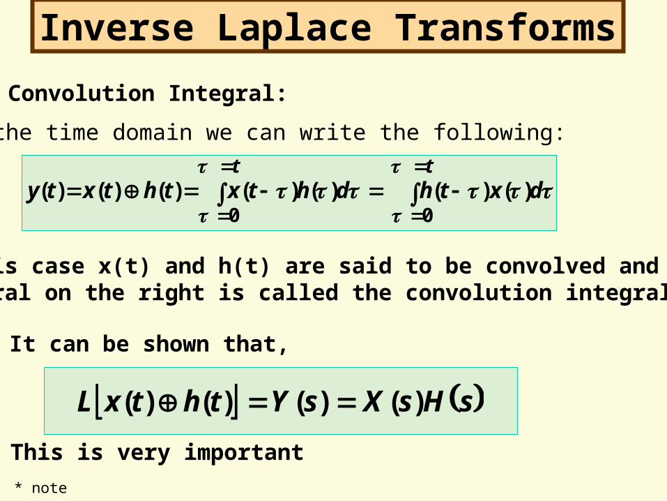
Inverse Laplace TransformsConvolution Integral:
In the time domain we can write the following:
ttdxthdhtxthtxty
00)()()()()()()(
In this case x(t) and h(t) are said to be convolved and theintegral on the right is called the convolution integral.
It can be shown that,
sHsXsYthtxL )()()()(
This is very important* note
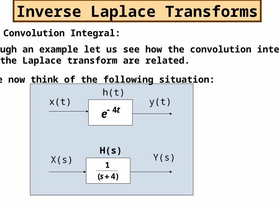
Inverse Laplace TransformsConvolution Integral:
Through an example let us see how the convolution integral and the Laplace transform are related.
We now think of the following situation:
x(t) y(t)
X(s) Y(s)
te 4
h(t)
H(s)
)4(1s
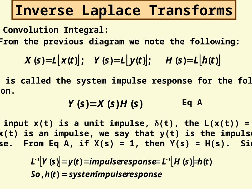
Inverse Laplace TransformsConvolution Integral:From the previous diagram we note the following:
)()(;)()(;)()( thLsHtyLsYtxLsX
h(t) is called the system impulse response for the followingreason.
)()()( sHsXsY
If the input x(t) is a unit impulse, (t), the L(x(t)) = X(s) = 1.Since x(t) is an impulse, we say that y(t) is the impulseresponse. From Eq A, if X(s) = 1, then Y(s) = H(s). Since,
Eq A
.)(,
)()()()( 11
responseimpulsesystemthSothsHLresponseimpulsetysYL

Inverse Laplace TransformsConvolution Integral:
A really important thing here is that anytime you are givena system diagram as follows,
H(s)X(s) Y(s)
the inverse Laplace transform of H(s) is the system’simpulse response.
This is important !!

Inverse Laplace TransformsConvolution Integral:Example using the convolution integral.
e-4t
x(t) y(t) = ?
t
tt tt deededuety
0
44
0
)(4)(4 )()(
)(41
41
41)( 444
0
44 | 0 tueeedeety ttt
t t
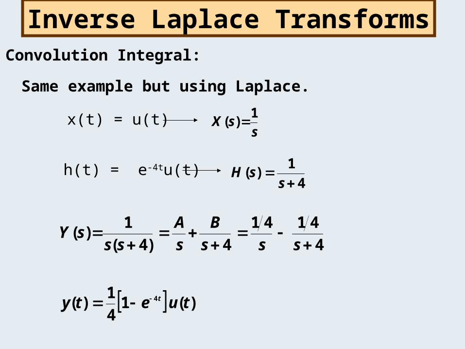
Inverse Laplace TransformsConvolution Integral:Same example but using Laplace.
x(t) = u(t) s
sX 1)(
h(t) = e-4tu(t) 4
1)(
s
sH
)(141)(
44141
4)4(1)(
4 tuety
sssB
sA
sssY
t

Inverse Laplace TransformsConvolution Integral:
Practice problems:
?)(,)2(3)(2)()( thiswhat
ssYand
ssXIfa
).(),()()()()( 6 thfindtutetyandtutxIfb t
).(,)4(
2)()()()( 2 tyfinds
sHandttutxIfc
Answers given on note page
)(2)(5.1)( 2 tuetth t

Inverse Laplace TransformsCircuit theory problem:You are given the circuit shown below.
+_
t = 0 6 k
3 k 100 F
+_
v(t)12 V
Use Laplace transforms to find v(t) for t > 0.
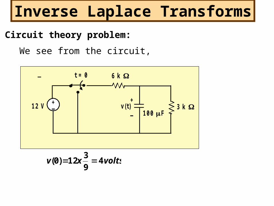
Circuit theory problem:
Inverse Laplace Transforms
We see from the circuit,
+_
t = 0 6 k
3 k 100 F
+_
v(t)12 V
voltsxv 49312)0(

Circuit theory problem:
Inverse Laplace Transforms
+_
vc(t) i( t )3 k
100 F6 k
05)(
0)(
0)()(
tvdt
tdv
RCtv
dttdv
tvdt
tdvRC
cc
cc
cc
Take the Laplace transformof this equations includingthe initial conditions on vc(t)
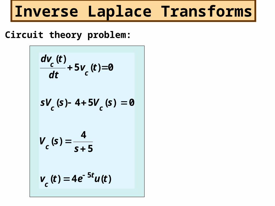
Circuit theory problem:
Inverse Laplace Transforms
)(4)(
54)(
0)(54)(
0)(5)(
5 tuetv
ssV
sVssV
tvdt
tdv
tc
c
cc
cc

Stop